A Numerical Study of Magnetic Reconnection - CSUN

Proceedings of Symposia in Applied Mathematics

A Numerical Study of Magnetic Reconnection: A Central

Scheme for Hall MHD

Xin Qian, Jorge Balbas, Amitava Bhattacharjee, and Hongang Yang

Abstract. Over the past few years, several non-oscillatory central schemesfor hyperbolic conservation laws have been proposed for approximating thesolution of the Ideal MHD equations and similar astrophysical models. Thesimplicity, versatility, and robustness of these black-box type schemes for sim-ulating MHD flows suggest their further development for solving MHD modelswith more complex wave structures. In this work we construct a non-oscillatorycentral scheme for the Hall MHD equations and use it to conduct a study ofthe magnetic reconnection phenomenon in flows governed by this model.

1. Introduction

The successful implementation of non-oscillatory central schemes for the equa-tions of ideal magnetohydrodynamics (MHD) and similar astrophysical models (see,for example, [3, 2, 9]), and the versatility of these balck-box type schemes, suggesttheir further development for computing the approximate solutions of other MHDmodels whose more complex characteristic decomposition makes the utilization ofschemes based on Riemann solvers impractical. In this work, we present a high-resoltuion, non-oscillatory, central scheme for the the Hall MHD model

∂ρ

∂t= −∇ · (ρv)(1.1a)

∂

∂t(ρv) = −∇ ·

{

ρvv⊤ +

(

p+B2

2

)

I3×3 − BB⊤

}

(1.1b)

∂B

∂t= −∇× E(1.1c)

∂U

∂t= −∇ ·

{(

U + p−B2

2

)

v + E× B

}

,(1.1d)

where (1.1a), (1.1b), and (1.1d) express the conservation of mass, momentum andenergy respectively, and equation (1.1c) the evolution of the magnetic field, which

1991 Mathematics Subject Classification. Primary 76W05, 76M12; Secondary 65Z05.Key words and phrases. MHD, Central Schemes, Reconnection.

c©0000 (copyright holder)

1

2 XIN QIAN, JORGE BALBAS, AMITAVA BHATTACHARJEE, AND HONGANG YANG

also implies the solenoidal constraint,

(1.2) ∇ · B = 0.

The total energy, U , momentum, ρv, and magnetic field, B, are coupled throughthe equation of state,

(1.3) U =p

γ − 1+ρv2

2+B2

2.

And the electric field, E, is expressed in the generalized Ohm’s law

E = −v × B + ηj +δiL0

j × B

ρ−δiL0

∇↔

p

ρ+

(

δeL0

)21

ρ

[

∂j

∂t+ (v · ∇)j

]

,(1.4a)

j = ∇× B(1.4b)

where L0 is the normalizing length unit, and δe and δi stand for the electron andion inertia respectively; they are related to the electron-ion mass ratio by (δe/δi)

2 =me/mi. For the simulations considered in this work, the electron pressure tensor,

−(δi/L0)(∇↔

p/ρ) can be ignored.This model follows from the MHD equations after normalizing as the Geospace

Environment Modeling (GEM) challenge, preserving the unit length in the gener-alized Ohm’s law, (1.4), for simplicity.

The scheme we propose below is built upon the semi-discrete formulation ofKurganov and Tadmor, [14], and we employ it to investigate the role that the Hallterm, j × B, and the electron inertia term,

(1.5) Te =

(

δeδi

)21

ρ

{

∂

∂t+ (v · ∇)

}

j,

play in the magnetic reconnection process.Our work is organized as follows: in §2 we briefly describe the physical phe-

nomena under consideration and the physical relevance of the terms on the righthand side of equation (1.4). In §3 we describe the proposed numerical scheme andits properties, and in §4 we present the numerical simulations calculated with thecentral scheme and discuss our findings.

2. Theoretical background: Magnetic Reconnection and Hall MHD

Magnetic reconnection is an irreversible process observed in space and lab-oratory plasma in which magnetic fields with different direction merge togetherand dissipate in the diffusive region breaking the magnetic frozen-in condition andquickly converting magnetic energy into kinetic and thermal energy. It is widelybelieved that the reconnection process is the main energy converting process inspace, and most of the eruptive events are driven or associated with it.

Classic MHD theory –without the Hall term– predicts a much slower reconnec-tion process than direct space observations suggest. Numerical simulations suggestthat the Hall effect [15, 6] –caused by ions being heavier than the electrons, couldenable fast reconnection, and both in-site space observation[10] and laboratoryexperiments[17] provide evidence of the presence of the Hall effect in the reconnec-tion process. In addition, recent particle in cell (PIC) simulations [4, 8, 11] suggestthat electron’s kinetic effect might also be important in the reconnection process.

A NUMERICAL STUDY OF MAGNETIC RECONNECTION: A CENTRAL SCHEME FOR HALL MHD3

In view of these results, we investigate the ability of the model (1.1) – (1.4)to describe the reconnection phenomenon by simulating flows with different typicalscales L0. When this is of the same order as δi, but still much larger than δe, theelectron inertia term, (1.5) in the generalized Ohm law, (1.4a), may be ignored,but not the Hall term, j × B. The magnetic frozen-in condition can no longer besatisfied where the Hall term becomes large. In this region, fluid elements don’tflow along the magnetic field, instead they may move across the field lines. Forthose flows, we write the electric field as

(2.1) E = −v × B +j × B

ρ+ η j + ηj∆ j.

When the typical scale L0 approaches the electron inertia length δe, the electron’sbehavior can no longer be ignored and the electron inertia term in the generalizedOhm’s law, (1.4) should be include in the simulation. The electric field for thisflows reads

(2.2) E = −v × B +j × B

ρ+ η j + ηj ∆ j + Te.

In both cases, the hyperresistivity, ηj∆j –mainly a numerical artifact– helps smooth-ing the structure around the grid scale without strongly diffusing the longer scalelengths.

3. Numerical Scheme

Both Hall and the electron inertia terms in (2.1) and (2.2) pose significantnumerical challenges for simulating MHD flows. Unlike in classical MHD where thecharacteristic speeds remain constant with respect to the wave frequency, the Alvenmode wave in Hall MHD satisfies the dispersion relation v ∼ k (where k is relatedto the wave frequency by ω ∼ k2, [5]). Thus, the Alven wave speed increases whenthe wave length becomes small, v ∼ 1/λ, and the maximum wave speed increasesas the grid is refined, vmax ∼ 1/△x, requiring extremely small time steps that mayresult in too much numerical dissipation.

Results previously obtained with central schemes for Ideal MHD flows, [3, 2],and the minimal characteristic information from the underlying PDE they required,suggest these as the building block for new schemes to solve more complex MHDflows. In particular, we turn our attention to the semi-discrete central formulation ofKurganov and Tadmor, [14], whose numerical viscosity does not increase as the timestep decreases –in contrast with fully-discrete central schemes whose viscosity is oforder O((∆x)2r/∆t), the viscosity of semi-discrete schemes is of order O((∆x)2r−1).

In order to construct our central scheme, we begin by re-writting the system(1.1) in conservation form,

(3.1) ut + f(u)x + g(u)y = 0,


with

u =(ρ, ρvx, ρvy, ρvz, Bx, By, Bz, U)⊤(3.2a)

f(u) =(

ρvx, ρv2x + p+

B2

2−B2

x, ρvxvy −BxBy, ρvxvz −BxBz,(3.2b)

0, −Ez, Ey, U′vx + EyBz − EzBy

)⊤

g(u) =(

ρvy, ρvxvy −ByBx, ρv2y + p+

B2

2−B2

y , ρvyvz −ByBz,(3.2c)

Ez , 0, −Ex, U′vy + EzBx − ExBz

)⊤

,

where

(3.3) U ′ = U + p−B2

2and p = (γ − 1)

(

U −ρv2

2−B2

2

)

,

and the electric field given by (2.1) or (2.2).

3.1. Central Schemes for Hyperbolic Conservation Laws. To approx-imate the solution of the Hall MHD model, we construct a semi-disrete centralscheme based on the formulation of Kurganov and Tadmor for hyperbolic conser-vation laws in 2D, [14]. A formulation that we describe here briefly for the shakeof completeness.

Central schemes realized the solution of the hyperbolic conservation law interms of the cell average of u over the control volume Ii,j = [xi− 1

2, xi+ 1

2]×[yj− 1

2, yj+ 1

2],

(3.4) ui,j(t) =1

∆x∆y

∫ xi+∆x2

xi−∆x2

∫ yj+∆y

2

yj−∆y

2

u(x, y, t) dydx.

Integrating (3.1) over Ii,j and dividing by the space scales ∆x and ∆y, yields theequivalent formulation

(3.5)d

dtui,j(t) = −

1

∆x∆y

∫ yj+ 1

2

yj− 1

2

(

f(u(xi+ 12, y)) − f(u(xi− 1

2, y))

)

dy

+

∫ xi+1

2

xi− 1

2

(

g(u(x, yj+ 12)) − g(u(x, yj− 1

2))

)

dx

,

which we write in the more compact form

(3.6)d

dtuj(t) = −

1

∆x

[

Hxi+ 1

2,j −Hx

i− 12,j

]

−1

∆y

[

Hy

i,j+ 12

−Hy

i,j− 12

]

where the numerical fluxesHxi± 1

2,j

andHy

i,j± 12

approximate the integrals on the right

of (3.5) and are calculated so as to account for the propagation of discontinuitiesat the cell interfaces x = xi± 1

2and y = yj± 1

2. For the results we presented below,

we chose the midpoint rule for approximating the integrals, which results in the


fluxes,

Hxi+ 1

2,j =

f(uWi+1,j) + f(uE

i,j)

2−ax

i+ 12,j

2

(

uWi+1,j − uE

i,j

)

(3.7a)

Hy

i,j+ 12

=g(uS

i,j+1) + g(uNi,j)

2−ay

i,j+ 12

2

(

uSi,j+1 − uN

i,j

)

.(3.7b)

For the actual implementation of the scheme, the values of u(x, y, t) at the cell

interfaces, uN/S,E/Wi,j (t) are recovered via a non-oscillatory, piece-wise polynomial

reconstruction R(x, y;u(t)) =∑

i,j pi,j(x, y) · 1Ii,j(x, y), and defined as

uEi,j := pi,j(xi+ 1

2, yj) uW

i,j := pi,j(xi− 12, yj)(3.8a)

uNi,j := pi,j(xi, yj+ 1

2) uS

i,j := pi,j(xi, yj− 12),(3.8b)

and axi+ 1

2

and ay

i,j+ 12

stand for the maximum speeds of propagation at the cell

interfaces in the x and y directions respectively; we approximate these by

(3.9) axi+ 1

2,j = max

{

ρ(

uWi+1,j

)

, ρ(

uEi,j

)}

, ay

i,j+ 12

= max{

σ(

uSi,j+1

)

, σ(

uNi,j

)}

,

where ρ and σ stand for the spectral radius of the jacobian matrices of f(u) andg(u) respectively. These values will, indeed, be exact if f(u) and g(u) are convex.For the second order scheme that we propose, the interface values are reconstructedfrom the cell averages via the bi-linear functions

(3.10) pi,j(x, y) = ui,j + (ux)i,j(x − xi) + (uy)i,j(y − yj)

with the numerical derivatives of u approximated with the limiter, [19],

(3.11) (ux)i,j = minmod

{

ui+1,j − ui,j

∆x,ui,j − ui−1,j

∆x

}

,

and similarly for (uy)i,j , where minmod{a, b} = (sgn(a)+sgn(b))min{|a|, |b|}. Oncethe point values (3.8) are recovered and the speeds of propagation (3.9) estimatedso as to compute the numerical fluxes (3.7), an evolution routine can be employed toevolve the cell averages of u. We choose a second order SSP Runge-Kutta scheme,[12], for the simulations below,

u(1) = un + ∆t C(un),(3.12a)

un+1 = u(1) +∆t

2

[

C(u(1)) − C(un)]

.(3.12b)

This scheme is provided by CentPack, [1], a software package that implementsseveral central schemes for hyperbolic conservation laws, and we employ it as ourbase scheme to evolve the solution of (1.1).

3.2. Magnetic and Electric Fields. When L0 is sufficiently large to ignorethe effects of the electron inertia term, Te, the scheme described above can be usedto evolve the solution of the system (1.1) – (1.3) provided the electric field, E, isapproximated consistently with (2.1), and the solenoidal constraint ∇ · B = 0 isenforced. In such cases, we approximate the high-order terms in (2.1) with high-order central finite differences. This allows us to feed back the electric field intothe fluxes and evolve the solution of (1.1) with the central scheme described above.


The evolved magnetic field, that we denote by B∗, is then reprojected onto itsdivergence free component by solving the Poisson equation,

(3.13) ∆Φ = −∇ · B∗

and writing the new magnetic field as

(3.14) Bn+1 = B∗ + ∇Φ.

Including the electron inertia term in the description of the electric field posesadditional difficulties as it involves the time derivative of j. For the numericalexperiments requiring the approximation of Te, we have followed two approaches:the finite difference of the the previous two consecutive time values, and the methodsuggested in [13], where the induction equation is re-written in non-conservativeform,

(3.15)∂B′

∂t= −∇×

(

v × B +j × B′

ρ+ η j

)

+ ηj∆j with B′ = B −me

mi∆B.

The first method works only when me/mi is small. For the second method, webuild a linear solver using the numerical package Portable Extensible Toolkit forScientific computation (PETSc).

4. Numerical Result

In order to test the validity of the proposed scheme, we run numerical testsin both linear and non-linear regimes. In the linear regime, we test the dispersionrelationship of the system and quantitatively compare the results with analyticalsolutions. In the non-linear regime, we run a typical reconnection simulation, sothat a qualitative comparison of the results obtained can be compared with previousresults.

4.1. Dispersion Relationship Test. We begin our numerical experimentsby testing the dispersion relation that follows for the linear analysis of the system(1.1) – (1.4) under a small sinusoidal perturbation of wave length λ and amplitudeδ. After launching an oscillation with wave length λ in a periodic simulation box,we measure the frequency of the oscillation, and compare the the computed wavespeed with the linear analytical prediction.

The linear analysis of the model shows that the wave mode corresponding tothe linear polarized Alven wave in MHD is a circularly polarized wave known aswhistle wave (see, for example, [16]). In our numerical test, this wave propagatesin the x direction, and the density, pressure and the x components of the velocityand magnetic field remain unperturbed by the small oscillation in both Hall MHDand classic MHD. So the pure Alven mode wave will be launched in the simula-tion domain, no other MHD waves like sonic wave or magnetosonic wave will betriggered.

We evolve the initial conditions

(4.1)ρ = 1, vx = 0, vy = −δ cos (kx), vz = δ sin (kx)

p = 1, Bx = 1, By = δ vp cos (kx), Bz = −δ vp sin (kx)

over a solution domain of size xL = 9.6 using a uniform mesh of size ∆x = 0.05,and a perturbation amplitude of δ = 10−5, with periodic boundary conditions. Thephase speed vp is calculated from linear analysis.


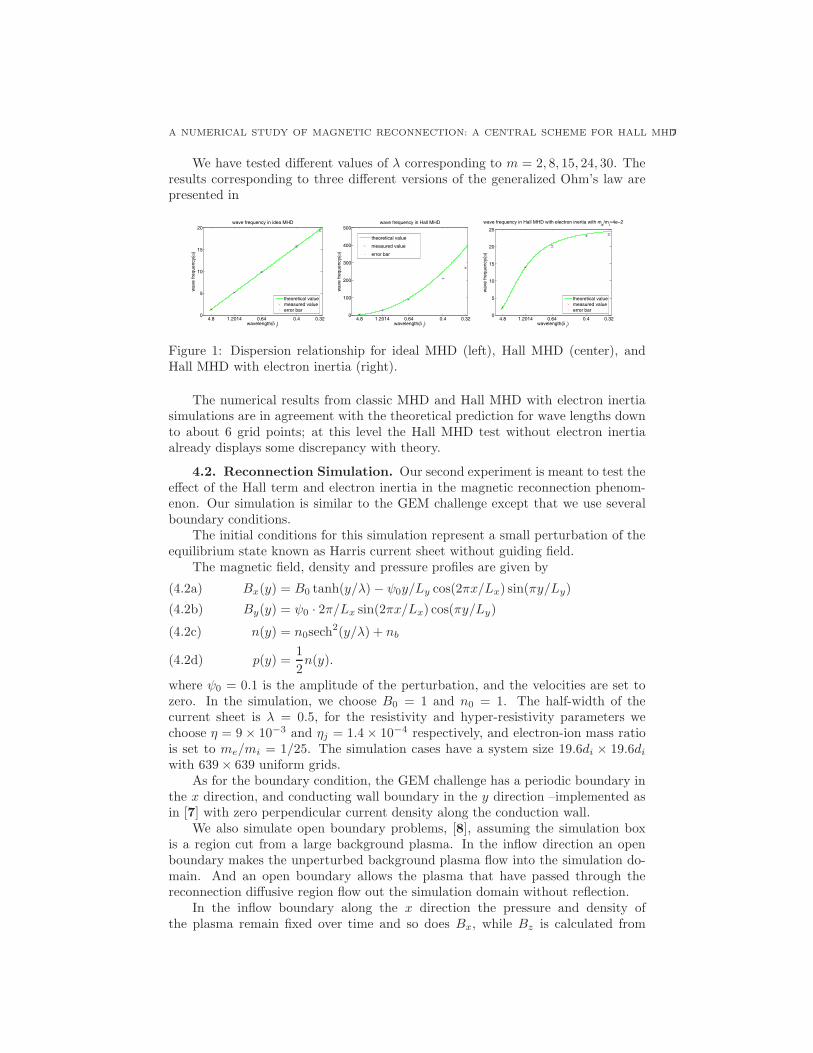
We have tested different values of λ corresponding to m = 2, 8, 15, 24, 30. Theresults corresponding to three different versions of the generalized Ohm’s law arepresented in

4.8 1.2014 0.64 0.4 0.320

5

10

15

20

wave fre

que

ncy(ω

)

wavelength(δ i)

wave frequency in idea MHD

theoretical valuemeasured valueerror bar

4.8 1.2014 0.64 0.4 0.320

100

200

300

400

500

wave fre

que

ncy(ω

)

wavelength(δ i)

wave frequency in Hall MHD

theoretical value

measured value

error bar

4.8 1.2014 0.64 0.4 0.320

5

10

15

20

25

wave fre

que

ncy(ω

)

wavelength(δ i)

wave frequency in Hall MHD with electron inertia with me/m

i=4e−2

theoretical valuemeasured valueerror bar

Figure 1: Dispersion relationship for ideal MHD (left), Hall MHD (center), andHall MHD with electron inertia (right).

The numerical results from classic MHD and Hall MHD with electron inertiasimulations are in agreement with the theoretical prediction for wave lengths downto about 6 grid points; at this level the Hall MHD test without electron inertiaalready displays some discrepancy with theory.

4.2. Reconnection Simulation. Our second experiment is meant to test theeffect of the Hall term and electron inertia in the magnetic reconnection phenom-enon. Our simulation is similar to the GEM challenge except that we use severalboundary conditions.

The initial conditions for this simulation represent a small perturbation of theequilibrium state known as Harris current sheet without guiding field.

The magnetic field, density and pressure profiles are given by

Bx(y) = B0 tanh(y/λ) − ψ0y/Ly cos(2πx/Lx) sin(πy/Ly)(4.2a)

By(y) = ψ0 · 2π/Lx sin(2πx/Lx) cos(πy/Ly)(4.2b)

n(y) = n0sech2(y/λ) + nb(4.2c)

p(y) =1

2n(y).(4.2d)

where ψ0 = 0.1 is the amplitude of the perturbation, and the velocities are set tozero. In the simulation, we choose B0 = 1 and n0 = 1. The half-width of thecurrent sheet is λ = 0.5, for the resistivity and hyper-resistivity parameters wechoose η = 9 × 10−3 and ηj = 1.4 × 10−4 respectively, and electron-ion mass ratiois set to me/mi = 1/25. The simulation cases have a system size 19.6di × 19.6di

with 639 × 639 uniform grids.As for the boundary condition, the GEM challenge has a periodic boundary in

the x direction, and conducting wall boundary in the y direction –implemented asin [7] with zero perpendicular current density along the conduction wall.

We also simulate open boundary problems, [8], assuming the simulation boxis a region cut from a large background plasma. In the inflow direction an openboundary makes the unperturbed background plasma flow into the simulation do-main. And an open boundary allows the plasma that have passed through thereconnection diffusive region flow out the simulation domain without reflection.

In the inflow boundary along the x direction the pressure and density ofthe plasma remain fixed over time and so does Bx, while Bz is calculated from


∂Bz/∂y = 0, and By from the ∇ · B = 0 condition. The velocity components vx

and vz are set to zero and vy is calculated from ∂vy/∂y = 0. And for the out flowboundary, the pressure, density and vx are interpolated as uj+1 = 1.3uj − 0.3uj−1,Bx is calculated from ∇ ·B = 0 condition and Bz, By and vy, vz obey ∂u/∂x = 0.When electron inertia is included, B′ is assigned according to the same methodthat is applied on B. Figure 2 left shows some reflections from the boundary atthe beginning of the simulation.

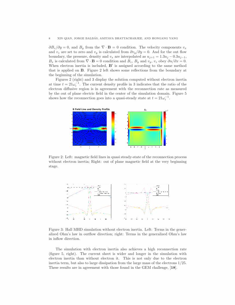
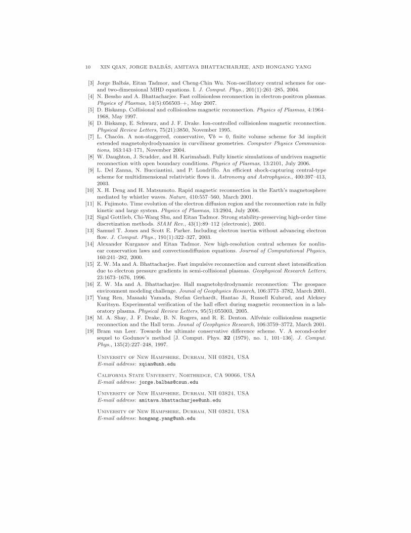
Figures 2 (right) and 3 display the solution computed without electron inertiaat time t = 21ω−1

i . The current density profile in 3 indicates that the ratio of theelectron diffusive region is in agreement with the reconnection rate as measuredby the out of plane electric field in the center of the simulation domain. Figure 5shows how the reconnection goes into a quasi-steady state at t = 21ω−1

i .

B Field Line and Density Profile 3Bz

Figure 2: Left: magnetic field lines in quasi steady-state of the reconnection processwithout electron inertia; Right: out of plane magnetic field at the very beginningstage.

Figure 3: Hall MHD simulation without electron inertia. Left: Terms in the gener-alized Ohm’s law in outflow direction; right: Terms in the generalized Ohm’s lawin inflow direction.

The simulation with electron inertia also achieves a high reconnection rate(figure 5, right). The current sheet is wider and longer in the simulation withelectron inertia than without electron it. This is not only due to the electroninertia term, but also to large dissipation from the large mass of the electrons 1/25.These results are in agreement with those found in the GEM challenge, [18].


Also, we note that in the center of the diffusive region, we can appreciate adensity depletion region, also found in space observations. This suggests that thelongitudinal wave might also be important in the Hall MHD simulation, and thatit should be included in the Hall MHD simulation both with and without electroninertia.

Our results indicate that central schemes provide a simple, yet robust approachfor approximating the solutions of non-classical MHD models with complex wavestructures. In the linear regime, the dispersion relationship test shows agreementwith the theoretical result. In the nonlinear regime, the reconnection simulationagrees with the previously published result. The numerical package CentPack,[1], allows us to reliably investigate different non-classical MHD models into onenumerical code.

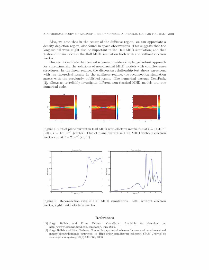
Figure 4: Out of plane current in Hall MHD with electron inertia run at t = 14.4ω−1

(left), t = 16.1ω−1 (center); Out of plane current in Hall MHD without electroninertia run at t = 21ω−1(right).

0 5 10 15 20 250

0.05

0.1

0.15

0.2

0.25

0.3

0.35Reconnection Rate

time (ωi

−1)

Ez a

t X

poin

t

0 2 4 6 8 10 12 14 16 180

0.02

0.04

0.06

0.08

0.1

0.12

0.14Reconnection Rate

time (ωi

−1)

Ez a

t X

poin

t

Figure 5: Reconnection rate in Hall MHD simulations. Left: without electroninertia, right: with electron inertia

References

[1] Jorge Balbas and Eitan Tadmor. CentPack. Available for download at

http://www.cscamm.umd.edu/centpack/, July 2006.[2] Jorge Balbas and Eitan Tadmor. Nonoscillatory central schemes for one- and two-dimensional

magnetohydrodynamics equations. ii: High-order semidiscrete schemes. SIAM Journal on

Scientific Computing, 28(2):533–560, 2006.


[3] Jorge Balbas, Eitan Tadmor, and Cheng-Chin Wu. Non-oscillatory central schemes for one-and two-dimensional MHD equations. I. J. Comput. Phys., 201(1):261–285, 2004.

[4] N. Bessho and A. Bhattacharjee. Fast collisionless reconnection in electron-positron plasmas.Physics of Plasmas, 14(5):056503–+, May 2007.

[5] D. Biskamp. Collisional and collisionless magnetic reconnection. Physics of Plasmas, 4:1964–1968, May 1997.

[6] D. Biskamp, E. Schwarz, and J. F. Drake. Ion-controlled collisionless magnetic reconnection.Physical Review Letters, 75(21):3850, November 1995.

[7] L. Chacon. A non-staggered, conservative, ∇b = 0, finite volume scheme for 3d implicitextended magnetohydrodynamics in curvilinear geometries. Computer Physics Communica-

tions, 163:143–171, November 2004.[8] W. Daughton, J. Scudder, and H. Karimabadi. Fully kinetic simulations of undriven magnetic

reconnection with open boundary conditions. Physics of Plasmas, 13:2101, July 2006.[9] L. Del Zanna, N. Bucciantini, and P. Londrillo. An efficient shock-capturing central-type

scheme for multidimensional relativistic flows ii. Astronomy and Astrophysics., 400:397–413,2003.

[10] X. H. Deng and H. Matsumoto. Rapid magnetic reconnection in the Earth’s magnetospheremediated by whistler waves. Nature, 410:557–560, March 2001.

[11] K. Fujimoto. Time evolution of the electron diffusion region and the reconnection rate in fully

kinetic and large system. Physics of Plasmas, 13:2904, July 2006.[12] Sigal Gottlieb, Chi-Wang Shu, and Eitan Tadmor. Strong stability-preserving high-order time

discretization methods. SIAM Rev., 43(1):89–112 (electronic), 2001.[13] Samuel T. Jones and Scott E. Parker. Including electron inertia without advancing electron

flow. J. Comput. Phys., 191(1):322–327, 2003.[14] Alexander Kurganov and Eitan Tadmor. New high-resolution central schemes for nonlin-

ear conservation laws and convectiondiffusion equations. Journal of Computational Physics,160:241–282, 2000.

[15] Z. W. Ma and A. Bhattacharjee. Fast impulsive reconnection and current sheet intensificationdue to electron pressure gradients in semi-collisional plasmas. Geophysical Research Letters,23:1673–1676, 1996.

[16] Z. W. Ma and A. Bhattacharjee. Hall magnetohydrodynamic reconnection: The geospaceenvironment modeling challenge. Jounal of Geophysics Research, 106:3773–3782, March 2001.

[17] Yang Ren, Masaaki Yamada, Stefan Gerhardt, Hantao Ji, Russell Kulsrud, and AlekseyKuritsyn. Experimental verification of the hall effect during magnetic reconnection in a lab-oratory plasma. Physical Review Letters, 95(5):055003, 2005.

[18] M. A. Shay, J. F. Drake, B. N. Rogers, and R. E. Denton. Alfvenic collisionless magneticreconnection and the Hall term. Jounal of Geophysics Research, 106:3759–3772, March 2001.

[19] Bram van Leer. Towards the ultimate conservative difference scheme. V. A second-ordersequel to Godunov’s method [J. Comput. Phys. 32 (1979), no. 1, 101–136]. J. Comput.

Phys., 135(2):227–248, 1997.

University of New Hampshire, Durham, NH 03824, USA

E-mail address: [email protected]

California State University, Northridge, CA 90066, USA






Documents

A Numerical Study of Magnetic Reconnection - CSUN