Nonlinear mechanics of the heart's swinging during

Nonlinear mechanics of the heart’s swinging during pericardial effusion

DAVID R. RIGNEY AND ARY L. GOLDBERGER Cardiovascular Division, Department of Medicine, Beth Israel Hospital and Harvard Medical School, Boston, Massachusetts 02215

RIGNEY, DAVID R., AND ARY L. GOLDBERGER. NonLinear mechanics of the heart’s swinging during pericardial effusion. Am. J. Physiol. 257 (Heart Circ. Physiol. 26): H1292-H1305, 1989.-When excessive fluid accumulates in the pericardial space, the heart, suspended by the great vessels, is then free to swing as a pendulum. The swinging may occur at either the same frequency as the heart rate (1:1 oscillation) or at half the heart rate (2:1 oscillation), the latter frequency often arising during cardiac tamponade. We show that these two frequencies of oscillation may be explained by the nonlinearity of Newton’s equation of motion as applied to the heart. Terms in the equation correspond to gravitational and buoyancy forces, forces due to ejection of blood into the great vessels, and damping forces. A transition between the 1:l and 2:l swinging is found to occur when particular parameters of the model are changed, notably when there is an increase of heart rate. This finding is compatible with previous clinical reports.

electrical alternans; echocardiography; electrocardiography; equation of motion; hemodynamics; nonlinear dynamics

THE LOCATION OF THE HEART within the thorax does not ordinarily vary by more than a few centimeters, since the heart is constrained by the pericardium. But when excessive fluid accumulates in the pericardial space, the heart, suspended by the great vessels, is then free to swing as a pendulum within the pericardial fluid. Two frequencies of pendular movement have been observed by echocardiography (6, 11, 12, 29, 33, 38). In cases of uncomplicated pericardial effusion, the swinging is usually observed to have the same frequency as the heart rate (1:l swinging). In other cases, the heart is observed to swing at half the heart rate (2:l swinging), notably when the pericardial pressure is large enough to impair the heart’s filling during diastole, i.e., when tamponade is present. The 2:l oscillation is of particular interest to electrocardiographers because it provides a straightfor- ward explanation for the observation of an electrocardi- ogram (ECG) waveform that repeats itself every other beat (total electrical alternans). Whereas the heart’s electrical vector is the same during successive systoles of the simple 1:l swinging, during the 2:l swinging the position of the heart alternates on successive systoles so the heart’s electrical vector will also alternate.

Several questions arise when considering the pendular movement of the heart during pericardial effusion and tamponade. What are the forces that drive the swinging? Why does the swinging occur at either the heart rate or

at half that frequency but not at other frequencies? What anatomical and physiological factors influence the amplitude and frequency of the oscillation? Recently, Gold- berger et al. (14,15) argued that the swinging heart could best be understood as a system for which the response to a perturbation of position is nonlinearly proportional to the magnitude of the perturbation. The observation that guided their reasoning is the fact that the period of oscillation is either 1:l or 2:l. Because period doubling of this sort is understood to be diagnostic for events known as subharmonic bifurcations, they inferred that the equation of motion for the swinging heart contains nonlinear terms. However, the actual equation was not provided in the initial analysis.

The aim of this article is, therefore, to analyze the factors responsible for the period doubling, by construct- ing and integrating Newton’s equation of motion, as applied to swinging movement of the heart. We show that the existence of two frequencies of oscillation is a consequence of the nonlinear forces involved. We also show that certain physiological changes accompanying tamponade, notably a reflex increase in the heart rate, have a greater influence than others on initiating the period doubling.

Alternation phenomena (alternans) are not uncom- mon in cardiovascular physiology (e.g., Refs. 1, 6, 12-15, 21,23,29,35,38), and the transition between alternating (2:l) and nonalternating (1:l) states is often seen to occur abruptly. The type of model that is presented here for swinging of the heart, a nonlinear parametric oscillator model, predicts the change between alternating and nonalternating states. The model might, therefore, serve as a prototype for analyzing other systems that exhibit alternans.

METHODS

Formulation of the model. Although 2:l swinging movement of the heart is often exhibited by patients with a pericardial pressure that is large enough to impair diastolic filling of the heart (tamponade), the 2:1 swinging and associated electrical alternans are also seen in patients with large effusions without tamponade (11, 33). Furthermore, 2:l pendular movement may be demonstrated with isolated, perfused animal hearts, suspended in a solution whose pressure does not impair diastolic filling (6). Consequently, it is not necessary to model tamponade explicitly to explain the pendular movements

H1292 0363-6135/89 $1.50 Copyright 0 1989 the American Physiological Society

NONLINEAR MECHANICS OF THE SWINGING HEART H1293

of the heart. Instead, the problem is to model the normal forces that would cause the heart to swing when it is free of pericardial constraints and to treat tamponade as a case with a special set of parameter values. Note too that 2:l swinging is different from mechanical alternans (l), even though the name might imply that they are the same. Mechanical alternans, also known as pulsus alternans, describes a beat-to-beat alternation in pulse pressure (among other variables) and may occasionally be observed in patients with 2:l swinging of the heart (13, 29, 34). However, because they do not always occur together, the two types of alternans must have different mechanisms.

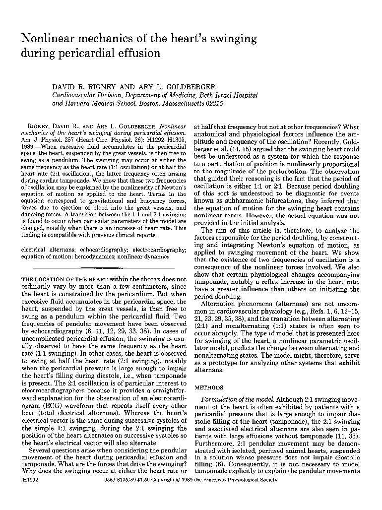
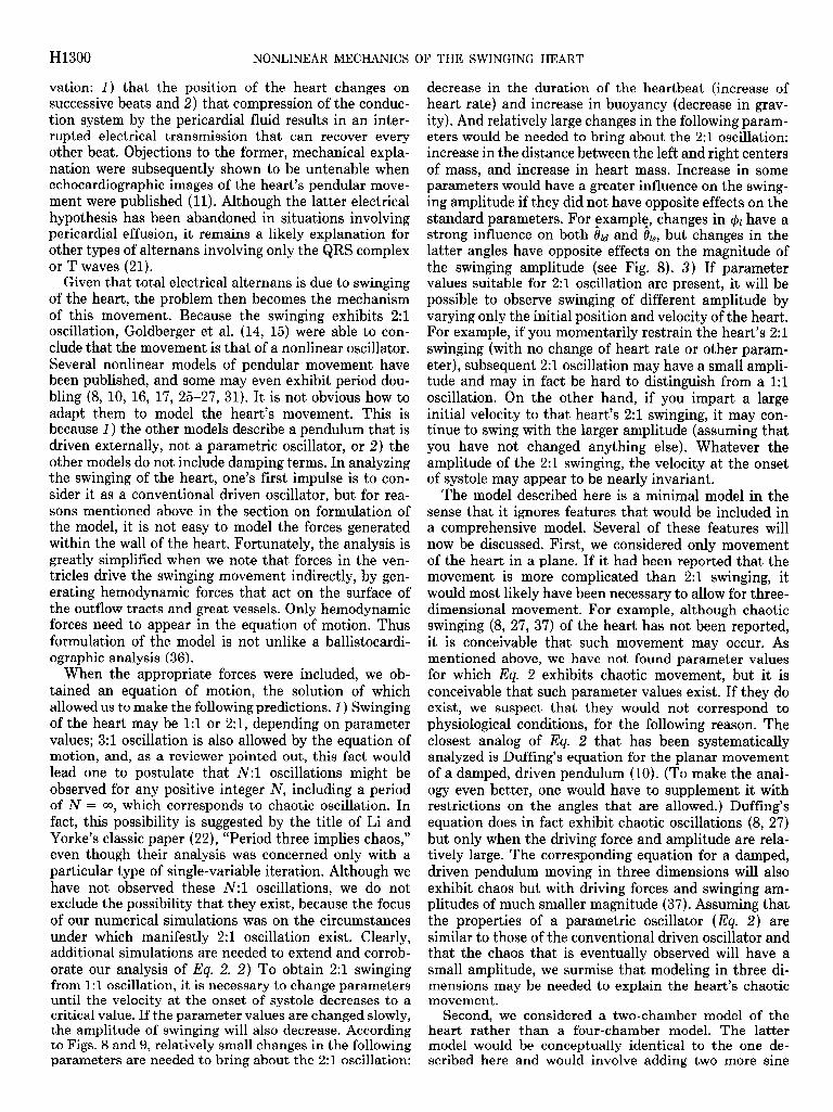
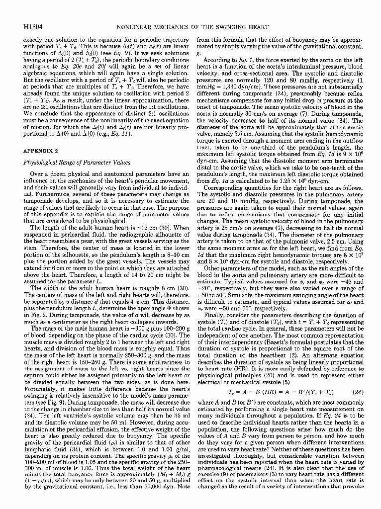
The primary mechanism thought to drive the heart’s swinging (6) is illustrated by Fig. 1, which represents the heart as two chambers, each of which ejects blood into its respective vessel. The fluid leaving a chamber will change direction (momentum) in the outflow tract and in the vessel, as it flows to the point where the vessel wall is fixed to the surrounding structures. As a result of the curved flow, momentum of the ejected blood will be transferred to the vessel and outflow tract, which will then straighten by lifting the chamber. Thus the situa- tion is similar to a curved garden hose that straightens itself when water is passed through it. Note that the force of the water on such a hose depends on the degree to which it is curved. As fluid strikes the inner wall of the hose, the curvature will decrease as the hose straightens in response to force from the fluid. Eventually it is either perfectly straight (zero fluid force perpendicular to the hose’s long axis) or force from the fluid on the curved hose is counterbalanced by other forces, e.g., gravity. The important point is that the magnitude of the force producing the movement depends on the vari-

Pivot of the heart’s pendular movement

Blood changes direction in the outflow tract and

great vessel, causing the vessel to straighten

and lift the heart.

Direction of flow as , blood leaves the

heart chamber

FIG. 1. Two-chamber model of heart and great vessels, showing direction of blood as it leaves each chamber during systole and as it enters the point at which vessels are anatomically fixed. Change in direction of flow between these points will cause rotation of heart about pivot.

able hose curvature, not simply on the magnitude of the fluid pressure and flow. Consequently, the swinging heart is not a conventional driven oscillator, the driving force for which would be independent of the oscillator’s angle. Instead, the driving force is explicitly a function of position (i.e., angular displacement or curvature). As discussed below, the fluid pressure alone will cause a curved vessel to straighten even in the absence of flow, for the same reason that a cylindrical balloon will resist bending at its waist. In either case, the torques exerted on the left and right heart chambers by their respective vessels will not generally cancel, so there will be a tend- ency for the heart to swing around its point of suspen- sion.

Ordinarily, this swinging would be resisted by the pericardium and the structures that support it. Further- more, the weight of the heart would ordinarily prevent large-amplitude oscillations. But when the heart is suspended in fluid, its effective weight is reduced by buoyancy, and the only resistance to oscillation is that from the pericardial fluid plus perhaps the restricted angle of movement that may be imposed by the thoracic walls. Newton’s equation of motion as applied to the heart is constructed below by representing these hemodynamic, gravitational, and damping forces by particular functions. The equation is then integrated assuming a physiological range of values for the model’s parameters. Finally, the properties predicted by the integrations are compared with what has been observed clinically.

Note that it will not be necessary to explicitly include contractile forces in the equation of motion, even though contractile forces within the heart’s wall are ultimately responsible for driving the heart’s pendular movement. This is because the ventricular forces drive the movement indirectly, by generating a variation in blood pressure and flow, which is transmitted away from the sites of contraction (see Fig. 1). That is to say, hemodynamic forces are produced by the contractile forces, but only the former forces need to be included in the model. If we wanted to explicitly include the contractile forces in the equation of motion, we might do so by expressing the ventricular compliance in terms of them. For example, the blood pressure (P) in a chamber of the heart may be regarded as a function of the volume of the chamber (V) and the elastic compliance of the ventricular wall (C), e.g., P = (V - &J/C, where V. is a parameter. As the heart contracts, the ventricular wall stiffens so that C decreases, and consequently the pressure P increases. Thus the consumption of chemical energy during the cardiac cycle allows the force vs. distension characteris- tics of the ventricular wall to vary periodically, which may be interpreted as a time-varying ventricular compliance. The modeling of such ventricular mechanics is not easy (32), and fortunately we may simplify the analysis by assuming that the blood pressure and flow are given, rather than attempting to explain them in terms of the heart’s contractile forces.

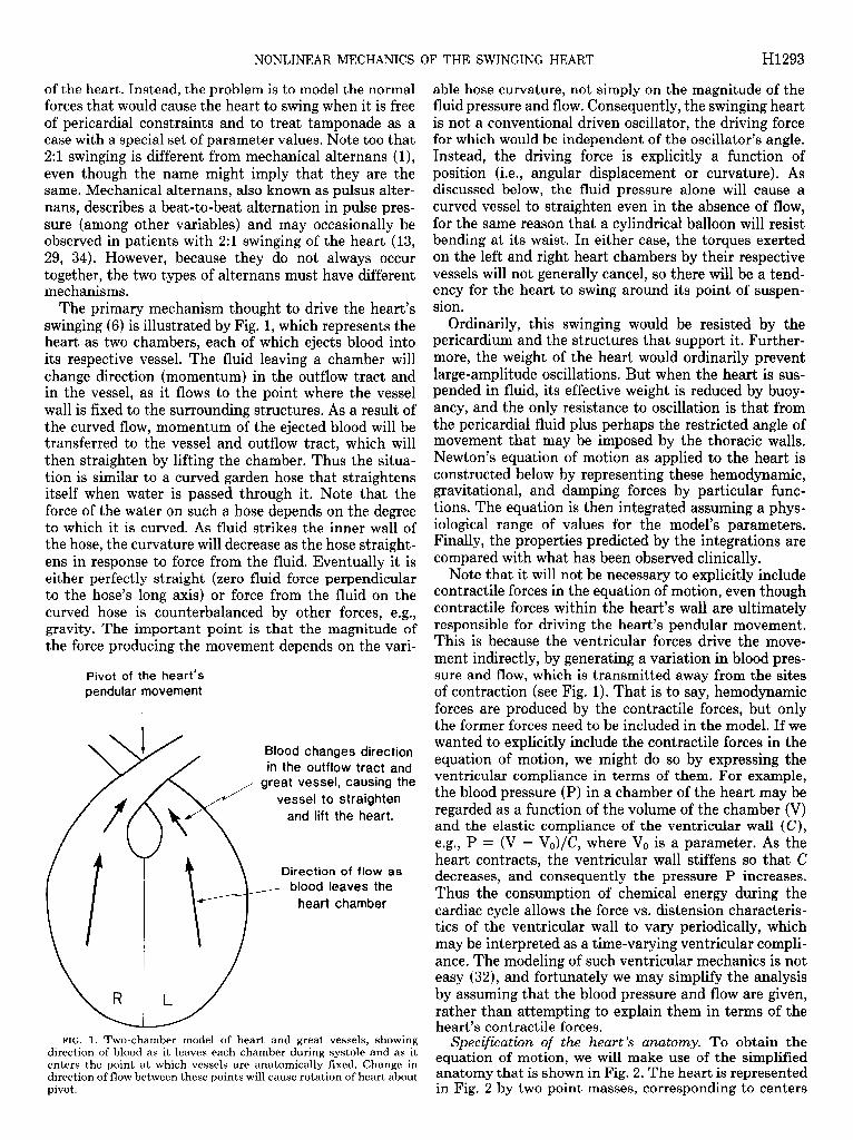
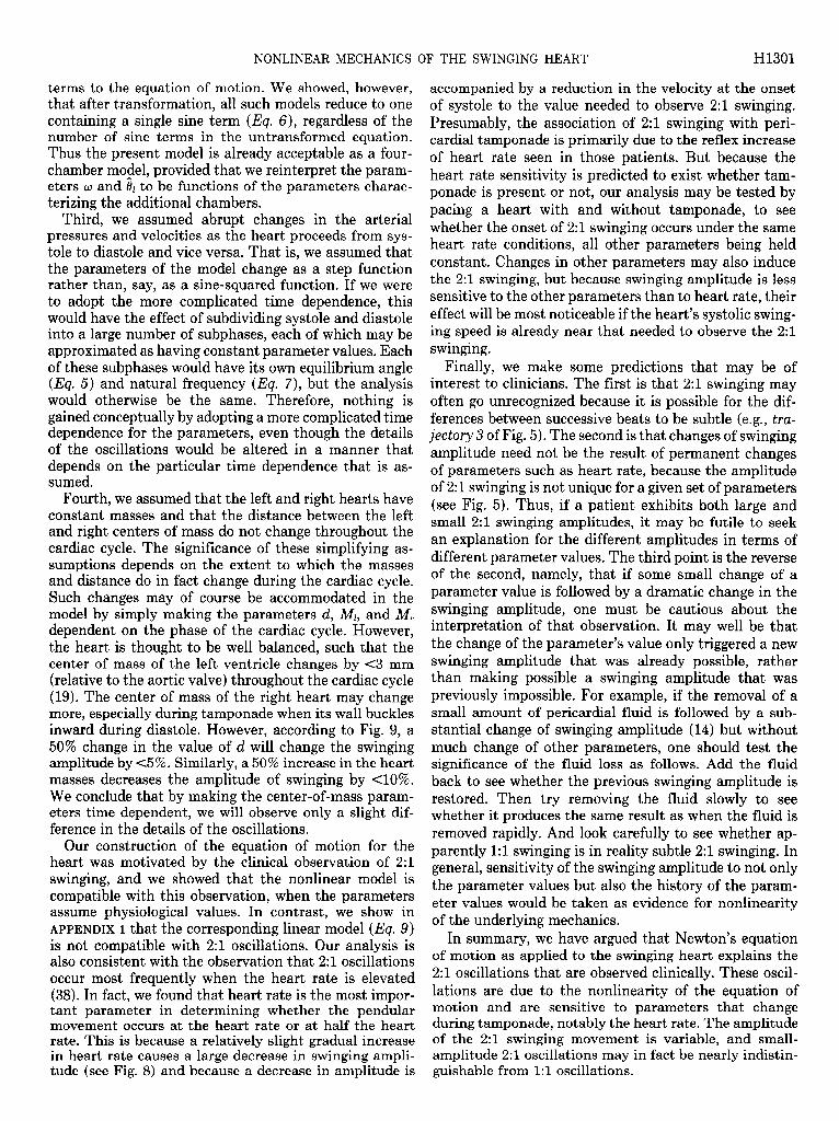
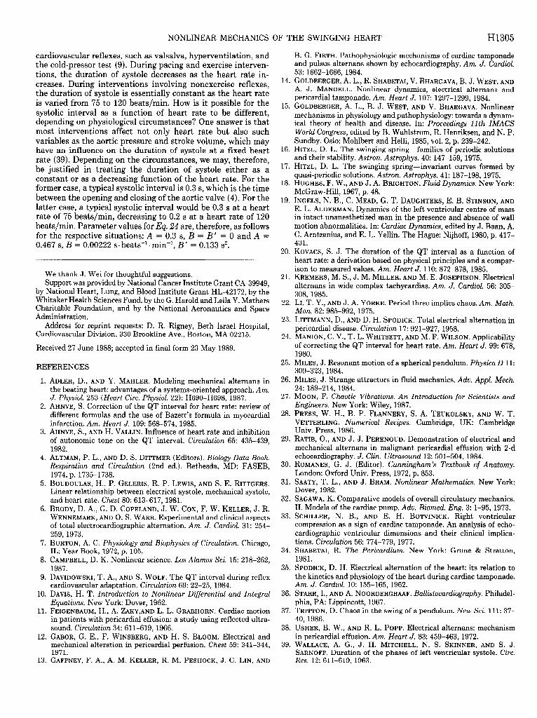
Specification of the heart’s anatomy. To obtain the equation of motion, we will make use of the simplified anatomy that is shown in Fig. 2. The heart is represented in Fig. 2 by two point masses, corresponding to centers

H1294 NONLINEAR MECHANICS OF THE SWINGING HEART

direction of f hid movement

pivot of heart’s pendular movement

+ angles - angles

direction of gravity

FIG. 2. Simplified anatomy of heart. L, distance between heart- chamber center of mass and point where great vessels are fixed in place; Ml and M,, masses of left and right hearts; 8l and 8,, (variable) angles of masses with respect to direction of gravity; & and &, (constant) angles of aorta and pulmonary artery, respectively, at their point of attachment. Differences between fixed angles q$ and @r and variable angles & and 8, are used to represent change in direction of flow as blood leaves heart chambers and enters great vessels. Apex of heart is assumed to have a fixed angle a. CY~ and CY~, maximum angles that or and 8, can exhibit before encountering wall of pericardium.

of mass of its right and left sides (M, and Ml, respectively). 2M, and Ml are joined by a rigid, massless bar of length d. They are also connected to a pivot where the great vessels are attached at the superior pericardial reflection. The pivotal sides of the triangle are considered to be rigid, massless bars of equal length L.

The anatomy of the heart and vessels is then specified by several angles, and in the minimal model that is presented here, all of the angles are assumed to lie in the same plane. The (constant) angle of the triangle’s apex is denoted by <P, i.e., half of + equals the angle whose sine is d/(2L). The remaining angles are defined clockwise with respect to a line in the direction of gravity, drawn through the pendulum’s pivot. 0, and 01 represent the angles of the right and left heart centers, respectively, and will change as the heart swings. (Only one of those angles is independent because 8, = & + a.) Let & and & denote the time-invariant angles at which blood flows through the great vessels at the pivot (see also Fig. 1). Finally, let a, and cyl denote the greatest angles that 0, and 81 may exhibit, respectively, before the heart encoun- ters the pericardial wall.

Torques acting on the swinging heart. Three types of external torques are considered to act on the heart: 1) torques due to gravity and buoyancy, 2) torques due to lifting by the great vessels, resulting from curvature of the vessels and outflow tract, and 3) torques due to

damping forces. Internal torques caused by one part of the heart acting on another need not be considered because they will cancel one another.

The torque due to gravity is the product of the moment arm calculated about the pivot and the component of the force perpendicular to the arm. For the left heart, this torque equals -L(Mlg - bl) sin& where L is the length of the pendulum, g is the gravitational constant, and bl is the buoyancy force (volume of the left heart times the specific weight of the pericardial fluid). This torque may be expressed entirely in terms of volumes, using the expressions Ml = h&n + h&b and bl = [hnPf + hbpflg, where Vl, and Va are the muscle and blood volumes of the left heart, respectively, and where pm, pb, and pf are the densities of muscle, blood, and pericardial fluid, respectively. Because the blood volume changes from systole to diastole, the gravitational torque is a function of the position in the cardiac cycle. However, for reasons explained later, the magnitude of the change is small compared with other torques that change during the cardiac cycle, so the masses and volumes may be treated as constants. If 01 is positive, this torque causes rotation in the counterclockwise (negative) direction, so the torque has the opposite sign as the angle. The gravitational torque on the right heart has the same form as that on the left heart and is obtained by simply changing the subscripts from Z to r.

The torque exerted by the blood on the left heart will be of the form -LiFl(t), where Fl(t) is a time-dependent force perpendicular to the moment arm Ll. The length of the moment arm Ll will be less than the length of the pendulum L because the force is exerted on the outflow tract and vessel, rather than at the left heart’s center of mass. An estimate for the force of the blood on the left heart is provided by an expression representing the force of fluid on a pipe that is bent (derived in Ref. 12). If we consi.der the aortic pressure and flow to be approximately constant during systole, the left systolic (Is) force is

F l(systole)(t) = f%tpLs- + pb&in[h(t) - $11 (I ) a

where Al is taken to be the cross-sectional area of the aortic valve, pk is the average systolic pressure in the aorta, VI is the systolic velocity of blood in the aorta, and 81 - 41 is the angle of the left heart minus the one at which blood would be ejected straight into the aorta.

The aorta’s force on the left heart during diastole is assumed to have the same form, with the pressure given by the average diastolic pressure (pu) and with the blood’s velocity set equal to zero

FI( diastole) ( t ) = Ap&@dt) - 411 (lb)

The moment arm Ll during diastole will be even shorter than during systole because the pressure causing rotation about the pivot is maintained only beyond the aortic valve. Analogous systolic and diastolic forces on the right heart [ F+stole) and Fr(~as~O~e)] involve the corresponding quantities for the pulmonary artery.

Thus the torques Tl= -LlFl(t) and T, = -L,F,(t) are time dependent for two reasons: 1) the angles 81 and 8, are changing and 2) pressure, flow, and moment arms change as the heart proceeds from systole to diastole and


vice versa. For simplicity of notation, we will use primes to indicate the portions of the torques that are independent of the angles 81 and 8,

Z(t) = -T[( t)sin(& - @I) (1 ) C

Z(t) = -TF(t)sin(B, - &.)

In the minimal model that is presented here, we treat expressions of the form T’ = LA(p + pu2) as constants that change discontinuously as the heart progresses from diastole to systole. Thus

1 = Ldl(pk + pu;) during systole Tf(t) = $ = L A p 1 during’ diastole (14

Id 1 Id,

T’(t) = I 1

= &A,( prs + pu”) during systole gi = L A p d during diastole rd r r-9

The duration of systole and of diastole are also parameters of the model, the relative lengths of which are made to change as the heart rate is changed.

A damping torque opposes the swinging of the left heart and is assumed to be of the form --Lv&, where 8, is the time derivative of 01 and the damping constant vl is proportional to the viscosity of the pericardial fluid. The damping torque for the right heart is assumed to have the same form as that for the left heart and may be obtained by changing the subscript from I to r.

Equation of motion. The angular momentum of the left mass about the pivot is A4J,201, and the angular momentum of the right mass is the same, provided that we change the subscript from I to r. The total angular momentum of the heart is the sum of that for the left and right masses, and because 6, = 81 + a, the total angular momentum is simply (A4l + M,)L281. The equation of motion for a pendulum states that the time derivative of the total angular momentum is equal to the sum of torques acting on the system. That is to say (A4l + Mr)L28, is equal to the sum of the external torques mentioned above for the left and right hearts

(Ml + Mr)L2#l = -L(Mig - bJsin 81

-L(Mrg - b,)sin 8,

-T[( t)sin(& - &)

-T:(t)sin(& - $r)

-UVl + Vr)fjl

(2 ) a

By replacing 0, by 81 + a, we obtain a second-order differential equation in terms of 01 alone

til + alsin el + a2sin(& + a) + a3sin(& - 41) (2b)

+ a*sin(& + + - 4r) + t&/7 = 0

where the coefficients al to a4 and 7 are

al = UQ - bl)/(M + 2M,)L

a2 = (M-g - b-)/CM + 2M,)L

as(t) = Tl’(t)I(Ml + Mr)L2

a4(t) = Ti(t)I(M + Mr)L2

and

l/ 7 = (?I1 + rlr)l(Ml + IM,)L

Because coefficients in the sine terms are time dependent and because the right-hand side of Eq. 2b equals zero rather than some external driving force, the swinging heart is modeled here as a parametric oscillator rather than as a conventional driven oscillator.

To complete the model, it is necessary to indicate what happens if the left heart’s center of mass reaches its limit (0 = ~1) or if the right heart’s center of mass reaches its limit (0, = CYr or el = Cyr - @). In those cases, we simulate the restraining forces of the pericardial wall by simply setting 81 equal to zero until the total torque changes direction and causes the heart to move back into the pericardial fluid.

Because the equation of motion contains four sine terms, it is not obvious that it describes a simple pendulum. As shown in APPENDIX 1, however, that is in fact the case (see Eq. 6). Equations for the equilibrium angle and for the small-amplitude natural frequency of oscillation of the pendulum are given in APPENDIX I, Eqs. 5, 7, and 9. Because large-amplitude oscillations are allowed by the model, there is no single frequency of oscillation: the greater the swinging amplitude, the greater the period of oscillation.

The equilibrium angle and the small-amplitude natural frequency are functions of the model’s parameters, some of which change as the heart proceeds from systole to diastole and vice versa. Therefore, each cardiac phase has its own natural frequency and equilibrium angle. During a particular phase, the heart is attracted to that phase’s equilibrium angle, but before it can come to rest at that angle, the cardiac phase changes and the heart is attracted to the other equilibrium angle. Thus the model attributes the heart’s sustained swinging motion to a periodic alternation in the equilibrium angle, resulting from periodic changes of pressure and flow (see Eq. Id). With each change of the equilibrium angle, the potential energy of the movement is altered, which makes it possible to replenish energy that has been dissipated by the damping forces. The magnitude of the energy supplied (or removed) during a change of the cardiac phase is given by Eq. 21 of APPENDIX I.

Numerical simulations. Equation 2 does not admit a simple analytical solution. Consequently, many of the results presented below were obtained by integrating it numerically, using either the IMSL subroutine DGEAR or by using the fourth-order Runge-Kutta method (28). For the simulations, initial conditions for the pendulum’s angle and angular velocity were usually either set to analytical approximations for the asymptotic solution (see APPENDIX 1) or were set to the terminal values of a previous simulation. The equation of motion was then integrated numerically until the motion became periodic. The amplitude and frequency of movement for that particular set of parameter values was then recorded, and the procedure was repeated for additional sets of parameter values.

Physiologic range of parameter values. Over a dozen physical and anatomical parameters were noted above as having an influence on the mechanics of the heart’s


pendular movement: masses of the left and right hearts, buoyancy of the left and right heart (volume of left and right heart, specific gravity of the pericardial fluid, heart muscle and blood), distance between the centers of mass of the left and right hearts, distance between attachment of the great vessels and either the left or right center of mass, angles of the aorta and pulmonary artery, systolic and diastolic pressure in the aorta, systolic and diastolic pressure in the pulmonary artery, velocities of blood flow in the aorta and pulmonary artery during systole, cross- sectional areas of the aorta and pulmonary arteries, gravitational constant, durations of systole and diastole, and damping constant for the pericardial fluid (viscosity of pericardial fluid, surface area of the heart). Most of these parameters vary from person to person. Several of the parameters may also change during tamponade. Con- sequently, it is necessary to establish the range of acceptable parameter values under different physiological circumstances, to evaluate their effect on the heart’s mechanics. The range of values that were considered physiological is discussed in APPENDIX 2.

RESULTS

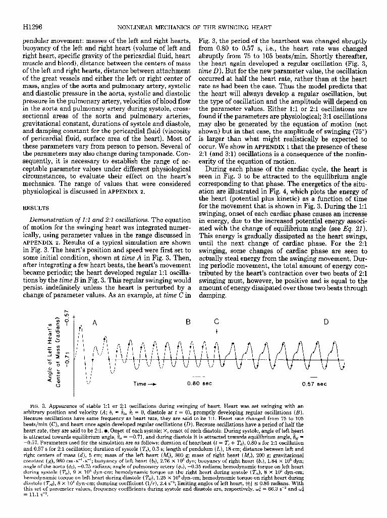
Demonstration of 1:l and 2:l oscillations. The equation of motion for the swinging heart was integrated numerically, using parameter values in the range discussed in APPENDIX 2. Results of a typical simulation are shown in Fig. 3. The heart’s position and speed were first set to some initial condition, shown at time A in Fig. 3. Then, after integrating a few heart beats, the heart’s movement became periodic; the heart developed regular 1:l oscillations by the time B in Fig. 3. This regular swinging would persist indefinitely unless the heart is perturbed by a change of parameter values. As an example, at time C in

Fig. 3, the period of the heartbeat was changed abruptly from 0.80 to 0.57 s, i.e., the heart rate was changed abruptly from 75 to 105 beats/min. Shortly thereafter, the heart again developed a regular oscillation (Fig. 3, time 0). But for the new parameter value, the oscillation occurred at half the heart rate, rather than at the heart rate as had been the case. Thus the model predicts that the heart will always develop a regular oscillation, but the type of oscillation and the amplitude will depend on the parameter values. Either 1:l or 21 oscillations are found if the parameters are physiological; 3:l oscillations may also be generated by the equation of motion (not shown) but in that case, the amplitude of swinging (75”) is larger than what might realistically be expected to occur. We show in APPENDIX 1 that the presence of these 21 (and 3:l) oscillations is a consequence of the nonlinearity of the equation of motion.

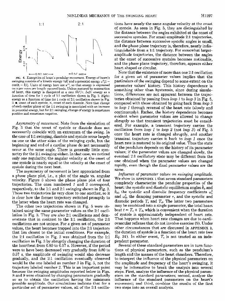
During each phase of the cardiac cycle, the heart is seen in Fig. 3 to be attracted to the equilibrium angle corresponding to that phase. The energetics of the situ- ation are illustrated in Fig. 4, which plots the energy of the heart (potential plus kinetic) as a function of time for the movement that is shown in Fig. 3. During the 1:l swinging, onset of each cardiac phase causes an increase in energy, due to the increased potential energy associated with the change of equilibrium angle (see Eq. 21). This energy is gradually dissipated as the heart swings, until the next change of cardiac phase. For the 2:l swinging, some changes of cardiac phase are seen to actually steal energy from the swinging movement. Dur- ing periodic movement, the total amount of energy con- tributed by the heart’s contraction over two beats of 2:l swinging must, however, be positive and is equal to the amount of energy dissipated over those two beats through damping.

C D +

Time e 0.80 set 0.57 8ec

FIG. 3. Appearance of stable 1:l or !$l oscillations during swinging of heart. Heart was set swinging with an arbitrary position and velocity (A; 8l = I!& 81 = 0, diastole at t = 0), promptly developing regular oscillations (B ) . Because oscillations have same frequency as heart rate, they are said to be l:l. Heart rate changed from 75 to 105 beats/min (C), and heart once again developed regular oscillations (D). Because oscillations have a period of half the heart rate, they are said to be 2:l. l , On_set of each systole; X, onset of each diastole. During systole, angle of left h_eart is attracted towards equilibrium angle, I& = -0.71, and during diastole it is attracted towards equilibrium angle, 6u = -0.57. Parameters used for the simulation are as follows: duration of heartbeat (t = T, + Td), 0.80 s for 1:l oscillation and 0.57 s for 2:l oscillation; duration of systole (T,), 0.3 s; length of pendulum (L), 18 cm; distance between left and right centers of mass (d), 5 cm; mass of the left heart (Ml), 300 g; mass of right heart (M,), 200 g; gravitational constant (g), 980 cm. s-l. s-l; buoyancy of left heart (bl), 2.76 X lo5 dyn; buoyancy of right heart (b,), 1.84 X 10’ dyn; angle of the aorta (@J, -0.75 radians; angle of pulmonary artery (&), -0.35 radians; hemodynamic torque on left heart during systole (Th), 9 x lo6 dyn-cm; hemodynamic torque on the right heart during systole (T,,), 8 X lo5 dyn-cm; hemodynamic torque on left heart during diastole (Tu), 1.25 x 10” dyn-cm; hemodynamic torque on right heart during diastole (TJ, 8 X lo4 dyn-cm; damping coefficient (l/7), 2.4 s-‘; limiting angles of left heart, 1 &I 5 0.85 radians. With this set of parameter values, frequency coefficients during systole and diastole are, respectively, wf = 66.3 sB2 and wz = 11.1 s-2.


1:l 23

1 -0.80 sec- co.57 set- FIG. 4. Energetics of heart’s pendular movement. Energy of heart’s

swinging_consists of a kinetic energy l/z@ and a potential energy w2[1 - cos(& - I&)]. Units of energy here are sV2, so that energy is expressed on a per mass per length-squared basis. Unless restored by contraction of heart, this energy is dissipated at a rate (&)“/T. Left: energy as a function of time for 1 cycle of 1:l oscillation shown in Fig. 3. Right: energy as a function of time for 1 cycle of 2:l oscillation shown in Fig. 3. l , onset of each systole, X, onset of each diastole. Note that change of each cardiac phase of the 1:l swinging is associated with an increase in potential energy, but for 2:l swinging, change of energy is sometimes positive and sometimes negative.

Asymmetry of nzouenzent. Note from the simulation of Fig. 3 that the onset of systole or diastole does not necessarily coincide with an extremum of the swing. In the case of 1:l swingi .ng, di .astole and systole occu r largely on one or the other sides of the swi nging cycle, but the beginning and end of a cardiac phase do not necessarily occur at the same angle. There is generally little sym- metry for the 2:l swinging either. In that case, we noticed only one regularity; one systole is nearly

the angular velocity at the onset of equal to the velocity at the onset of

systole during the next beat. The asymmetry of movement is best appreciated from

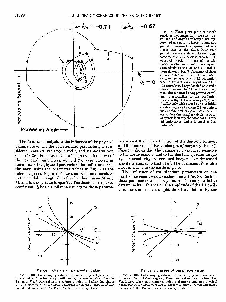
a phase plane plot, i.e., a plot of the angle vs. angular velocity. Figure 5 shows the phase plane plot of-four trajectori .es. The ones numbered 1 and 2 correspond, respectively, to the 1:l and 2:l swinging shown in Fig. 3. Those two trajectories lie very close to one another, so it is clear how the former trajectory switched promptly to the latter when the heart rate was changed.

The other two trajectories shown in Fig. 5 were obtained using the same parameter values as the 2:l oscillation in Fig. 3. They are also 2:l oscillations and dem- onstrate that in contrast to the 1:l oscillation, the 2:l oscillations are not unique. For a given set of parameter values, the heart becomes trapped into the 2:l trajectory that lies closest to the initial conditions. For example, the 2:l oscillation in Fig. 3 was obtained from the 1:l oscillation in Fig. 3 by abruptly changing the duration of the heartbeat from 0.80 to 0.57 s. However, if the period were to have been decreased very gradually from 0.80 to 0.57 s, the amplitude of swinging would also decrease gradually, and the 2:l oscillation eventually observed would be the one labeled as number 3 in Fig. 5, not the trajectory labeled number 2. This is an important point because the swinging amplitudes reported below in Figs. 8 and 9 were obtained by changing parameters gradually so as to obtain the oscillation having the minimum possible amplitude. Our simulations indicate that for a particular set of parameter values, all of the 2:l oscilla-

tions have nearly the same angular velocity at the onset of systole. As seen in Fig. 5, they are distinguished by the distance between the angles exhibited at the onset of successive systoles. For small-amplitude 2:l trajectories, the distance between successive systolic angles is small, and the phase plane trajectory is, therefore, nearly indis- tinguishable from a 1:l trajectory. For somewhat larger- amplitude trajectories, the distance between the angles at the onset of successive systoles becomes noticeable, and the phase plane trajectory, therefore, appears either heart shaped or circular.

Note that the existence of more than one 2:l oscillation for a given set of parameter values implies that the particulars of the swinging depend to some extent on the parameter values’ history. This history dependence is something other than hysteresis, since during simulations, differences are not apparent between the trajectories obtained by passing from loop 1 to loop 3 in Fig. 5, compared with those obtained by going back from loop 3 to loop 1 through reversal of the heart rate (slowly and continuously). Rather, the history dependence becomes evident when parameter values are allowed to change abruptly so that transient trajectories must be considered. For example, a transient trajectory carries the oscillation from loop 1 to loop 2 (not loop 3) of Fig. 5 once the heart rate is changed abruptly, and another transient trajectory carries it back to loop 1 once the heart rate is restored to its original value. Thus the state of the pendulum depends on the history of its parameter values; if the parameter values are changed slowly, the eventual 2:l oscillatory state may be different from the one obtained when the parameter values are changed rapidly, even though the final parameter values are the same.

Influence of parameter vaZues on swinging amplitude. We show in APPENDIX 1 that seven standard parameters completely characterize the pendular properties of the heart: the systolic and diastolic equilibrium angles & and fiti, the systolic and diastolic frequency coefficients 0,” and w:, the damping parameter 7, and the systolic and diastolic periods T, and Td. The latter two parameters may be combined into a single parameter, the total heart beat t = T, + Td, which is convenient when the duration of systole is approximately independent of heart rate. That happens when heart rate changes are due to cardiovascular reflexes that do not involve exercise (9). Under other circumstances that are discussed in APPENDIX 2, the duration of systole is a function of the heart rate (see EQ. 24). In either event, T, is not treated as an independent parameter.

Several of these standard parameters are in turn functions of physical parameters, such as the pendulum’s length and the masses of the heart chambers. Therefore, to interpret the influence of the physical parameters on the amplitude and frequency of the heart’s swinging, it may be informative to break the analysis into several steps. First, analyze the influence of the physical parameters on the standard parameters; second, analyze the influence of the standard parameters on the heart’s movement; and third, combine the results of the first two steps into an overall analysis.


Increasing Angle -

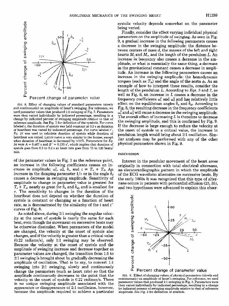
The first step, analysis of the influence of the physical parameters on the derived standard parameters, is considered in APPENDIX 1 (Eqs. 5 and 7) and in the definition of 7 (Eq. Zb). For illustration of tho_se equations, two of the standard parameters, oz and Ou, were plotted as functions of the physical parameters that influence them the most, using the parameter values in Fig. 3 as the reference point. Figure 6 shows that of is most sensitive to the pendulum length L, to the chamber masses Ml and M, and to the systolic torque TL. The diastolic frequency coefficient U: has a similar sensitivity to those parame-

L

FIG. 5. Phase plane plots of heart’s pendular movement. In these plots, position 81 and angular velocity 81 are represented as a point in the x-y plane, and periodic movement is represented as a closed loop in the plane. Four such periodic loops are shown. In each case, movement is in clockwise direction. l , onset of systole; X, onset of diastole. Loops labeled as 1 and 2 correspond respectively to the 1:l and 2:l oscillations shown in Fig. 3. Proximity of those curves explains why 1:l oscillation switched so promptly to 2:l oscillation when heart rate was changed from 75 to 105 beats/min. Loops labeled as 3 and 4 also correspond to 2:l oscillations and were also generated using parameter values corresponding to 2:l oscillation shown in Fig. 3. Because loops 2, 3, and 4 differ only with regard to their initial conditions, more than one 2:l oscillation may be obtained for a given set of parameters. Note that angular velocity at onset of systole is nearly the same for all three 2:l trajectories, and it is equal to 0.21 radians/s.

ters except that it is a function of the diastolic torques, and it is more sensitive to changes o,f buoyancy than OZ. Figure 7 shows that the parameter Ou is most sensitive to the aortic angle 41 and to the diastolic ejection torque Tu. Its sensitivity to increased buoyancy or decreased gravity is similar to that of & The coefficient & is also most sensitive to the aortic angle 41.

The influence of the standard parameters on the heart’s movement was considered next (Fig. 8). Each of those parameters was slowly and continuously varied to determine its influence on the amplitude of the 1:l oscillation or the smallest-amplitude 2:l oscillation. By use

t 50

$1

I/ 25

Percent change of parameter value Percent change of parameter value FIG. 6. Effect of changing values of indicated physical parameters

on the value of the frequency coefficient wz. Parameter values given in FIG. 7. Effect of changing yalues of indicated physical parameters

on value of equilibrium angle &+ Parameter values given in legend to legend to Fig. 3 were taken as a reference point, and after changing a physical parameter by indicated percentage, percent change in wf was

Fig. 3 were taken as a reference point, and after changing a physical parameter by indicated percentage, percent change in 8u was calculated

calculated using Eq. 7. See Fig. 3 for definition of symbols. using Eq. 5. See Fig. 3 for definition of symbols.


a> 3

3 cn “0 aJ : c 0 z \ ti

4 I t I

t &

t -50

iii

(L Percent change of parameter value

FIG. 8. Effect of changing values of standard parameters (slowly and continuously) on amplitude of heart’s swinging. For reference, we used parameter values that produced 1:l swinging of Fig. 3. Parameters were then varied individually by indicated percentage, resulting in a change by indicated percent of swinging amplitude relative to that of reference amplitude. See Fig. 3 for definition of the symbols. For curve labeled t, the duration of systole was held constant at 0.3 s as duration of heartbeat was varied by indicated percentage. For curve labeled t ‘, Eq. 24 was used to calculate duration of systole while duration of heartbeat was varied. Latter curve is very similar to the former, except when duration of heartbeat is decreased by X0%. Parameters for Eq. 24 were A = 0.467 s and B’ = 0.133 s*, which implies that duration of systole goes from 0.3 to 0.2 s as heart rate goes from 75 to 120 beats/ min.

of the parameter values in Fig. 3 as the reference point, an increase in the following coefficients causes an increase in amplitude: o:, o:, 8,, and t = T, + Td. A,n increase in the damping parameter l/7 or in the angle 0d causes a decrease in swinging amplitude. Sensitivity of amplitude to change in parameterAvalue is greatest for T, + Td, nearly as great for 81, and old, and is smallest for 7. The sensitivity to changes in the duration of the heartbeat does not depend on whether the duration of systole is constant or changing as a function of heart rate, as is demonstrated by the similarity of the t and t’ curves of Fig. 8.

As noted above, during 2:l swinging the angular velocity at the onset of systole is nearly the same for each beat, even though the movement on successive beats may be otherwise dissimilar. When parameters of the model are changed, the velocity at the onset of systole also changes, and if the velocity is greater than a critical value (0.22 radians/s), only 1:l swinging may be observed. Because the velocity at the onset of systole and the amplitude of swinging increase and decrease together as parameter values are changed, the transition from 1:l to 2:l swinging is brought about by gradually decreasing the amplitude of oscillation. That is to say, to convert 1:l swinging into 2:l swinging, slowly and continuously change the parameters (such as heart rate) so that the amplitude continuously decreases to the point that the velocity at the onset of systole is 0.22 radians/s. There is no unique swinging amplitude associated with the appearance or disappearance of 2: 1 oscillation, however, because the amnlitude reauired to achieve a particular

systolic velocity depends somewhat on the parameter being varied.

Finally, consider the effect varying individual physical parameters on the amplitude of swinging. As seen in Fig. 9, a gradual increase in the following parameters causes a decrease in the swinging amplitude: the distance between centers of mass d, the masses of the left and right hearts Ml and A& and the length of the pendulum L. An increase in buoyancy also causes a decrease in the amplitude, or what is essentially the same thing, a decrease in the gravitational constant causes a decrease in amplitude. An increase in the following parameters causes an increase in the swinging amplitude: the hemodynamic torques (such as TJ and the angle of the aorta 41. As an example of how to interpret these results, consider the length of the pendulum L. According to Eas. 5 and 7, as well as Fig. 6, an increase in L causes a decrease in the frequency coefficients U: and & and has relatively little effect on the equilibrium angles & and &. According to Fig. 8, the resulting decrease in the frequency coefficients O: and O: will cause a decrease in the swinging amplitude. The overall effect of increasing L is therefore to decrease the swinging amplitude, and this is confirmed by Fig. 9. If the decrease is large enough to reduce the velocity at the onset of systole to a critical value, the increase in pendulum length would bring about 2:l oscillation. Sim- ilar analyses may be performed with any of the other physical parameters shown in Fig. 9.

DISCUSSION

Interest in the pendular movement of the heart arose originally in connection with total electrical alternans, an electrocardiographic pattern in which the amplitude of the ECG waveform alternates on successive beats. By the early 1960s it was recognized that this type of alternans occurs in patients with pericardial effusion (23,35), and two hypotheses were advanced to explain this obser-

a E

a Percent change of parameter value FIG. 9. Effect of changing values of physical parameters (slowly and

continuously) on amplitude of heart’s swinging. For reference, we used parameter values that produced 1:l swinging in Fig. 3. Parameters were then varied individually by indicated percentage, resulting in a change by indicated percent of swinging amplitude relative to that of reference amplitude. See Fig. 3 for definition of symbols.


vation: 1) that the position of the heart changes on successive beats and 2) that compression of the conduc- tion system by the pericardial fluid results in an inter- rupted electrical transmission that can recover every other beat. Objections to the former, mechanical explanation were subsequently shown to be untenable when echocardiographic images of the heart’s pendular movement were published (11). Although the latter electrical hypothesis has been abandoned in situations involving pericardial effusion, it remains a likely explanation for other types of alternans involving only the QRS complex or T waves (21).

Given that total electrical alternans is due to swinging of the heart, the problem then becomes the mechanism of this movement. Because the swinging exhibits 2:l oscillation, Goldberger et al. (14, 15) were able to conclude that the movement is that of a nonlinear oscillator. Several nonlinear models of pendular movement have been published, and some may even exhibit period doubling (8, 10, 16, 17, 25-27, 31). It is not obvious how to adapt them to model the heart’s movement. This is because 1) the other models describe a pendulum that is driven externally, not a parametric oscillator, or 2) the other models do not include damping terms. In analyzing the swinging of the heart, one’s first impulse is to consider it as a conventional driven oscillator, but for reasons mentioned above in the section on formulation of the model, it is not easy to model the forces generated within the wall of the heart. Fortunately, the analysis is greatly simplified when we note that forces in the ven- tricles drive the swinging movement indirectly, by generating hemodynamic forces that act on the surface of the outflow tracts and great vessels. Only hemodynamic forces need to appear in the equation of motion. Thus formulation of the model is not unlike a ballistocardi- ographic analysis (36).

When the appropriate forces were included, we obtained an equation of motion, the solution of which allowed us to make the following predictions. 1) Swinging of the heart may be 1:l or 2:1, depending on parameter values; 3:l oscillation is also allowed by the equation of motion, and, as a reviewer pointed out, this fact would lead one to postulate that N:l oscillations might be observed for any positive integer N, including a period of N = 00, which corresponds to chaotic oscillation. In fact, this possibility is suggested by the title of Li and Yorke’s classic paper (22), “Period three implies chaos,” even though their analysis was concerned only with a particular type of single-variable iteration. Although we have not observed these N:l oscillations, we do not exclude the possibility that they exist, because the focus of our numerical simulations was on the circumstances under which manifestly 2:1 oscillation exist. Clearly, additional simulations are needed to extend and corrob- orate our analysis of Eq. 2. 2) To obtain 2:l swinging from 1:l oscillation, it is necessary to change parameters until the velocity at the onset of systole decreases to a critical value. If the parameter values are changed slowly, the amplitude of swinging will also decrease. According to Figs. 8 and 9, relatively small changes in the following parameters are needed to bring about the 2:l oscillation:

decrease in the duration of the heartbeat (increase of heart rate) and increase in buoyancy (decrease in gravity). And relatively large changes in the following parameters would be needed to bring about the 2:l oscillation: increase in the distance between the left and right centers of mass, and increase in heart mass. Increase in some parameters would have a greater influence on the swinging amplitude if they did not have opposite effects on the standard parameters. For exampl:, changes in 41 have a strong influence on both 0u and 8h, but changes in the latter angles have opposite effects on the magnitude of the swinging amplitude (see Fig. 8). 3) If parameter values suitable for 2:l oscillation are present, it will be possible to observe swinging of different amplitude by varying only the initial position and velocity of the heart. For example, if you momentarily restrain the heart’s 2:l swinging (with no change of heart rate or other parameter), subsequent 2:l oscillation may have a small amplitude and may in fact be hard to distinguish from a 1:l oscillation. On the other hand, if you impart a large initial velocity to that heart’s 2:l swinging, it may con- tinue to swing with the larger amplitude (assuming that you have not changed anything else). Whatever the amplitude of the 2:l swinging, the velocity at the onset of systole may appear to be nearly invariant.

The model described here is a minimal model in the sense that it ignores features that would be included in a comprehensive model. Several of these features will now be discussed. First, we considered only movement of the heart in a plane. If it had been reported that the movement is more complicated than 2:l swinging, it would most likely have been necessary to allow for three- dimensional movement. For example, although chaotic swinging (8, 27, 37) of the heart has not been reported, it is conceivable that such movement may occur. As mentioned above, we have not found parameter values for which Eq. 2 exhibits chaotic movement, but it is conceivable that such parameter values exist. If they do exist, we suspect that they would not correspond to physiological conditions, for the following reason. The closest analog of Eq. 2 that has been systematically analyzed is Duffing’s equation for the planar movement of a damped, driven pendulum (10). (To make the anal- ogy even better, one would have to supplement it with restrictions on the angles that are allowed.) Duffing’s equation does in fact exhibit chaotic oscillations (8, 27) but only when the driving force and amplitude are relatively large. The corresponding equation for a damped, driven pendulum moving in three dimensions will also exhibit chaos but with driving forces and swinging amplitudes of much smaller magnitude (37). Assuming that the properties of a parametric oscillator (Eq. 2) are similar to those of the conventional driven oscillator and that the chaos that is eventually observed will have a small amplitude, we surmise that modeling in three dimensions may be needed to explain the heart’s chaotic movement.

Second, we considered a two-chamber model of the heart rather than a four-chamber model. The latter model would be conceptually identical to the one described here and would involve adding two more sine


terms to the equation of motion. We showed, however, that after transformation, all such models reduce to one containing a single sine term (Eq. 6), regardless of the number of sine terms in the untransformed equation. Thus the present model is already acceptable as a four- chamber model, provided that we reinterpret the parameters o and 81 to be functions of the parameters charac- terizing the additional chambers.

Third, we assumed abrupt changes in the arterial pressures and velocities as the heart proceeds from systole to diastole and vice versa. That is, we assumed that the parameters of the model change as a step function rather than, say, as a sine-squared function. If we were to adopt the more complicated time dependence, this would have the effect of subdividing systole and diastole into a large number of subphases, each of which may be approximated as having constant parameter values. Each of these subphases would have its own equilibrium angle (Eq. 5) and natural frequency (Ea. 7), but the analysis would otherwise be the same. Therefore, nothing is gained conceptually by adopting a more complicated time dependence for the parameters, even though the details of the oscillations would be altered in a manner that depends on the particular time dependence that is assumed.

Fourth, we assumed that the left and right hearts have constant masses and that the distance between the left and right centers of mass do not change throughout the cardiac cycle. The significance of these simplifying as- sumptions depends on the extent to which the masses and distance do in fact change during the cardiac cycle. Such changes may of course be accommodated in the model by simply making the parameters d, Ml, and M, dependent on the phase of the cardiac cycle. However, the heart is thought to be well balanced, such that the center of mass of the left ventricle changes by <3 mm (relative to the aortic valve) throughout the cardiac cycle (19). The center of mass of the right heart may change more, especially during tamponade when its wall buckles inward during diastole. However, according to Fig. 9, a 50% change in the value of d will change the swinging amplitude by 4%. Similarly, a 50% increase in the heart masses decreases the amplitude of swinging by <lo%. We conclude that by making the center-of-mass parameters time dependent, we will observe only a slight difference in the details of the oscillations.

Our construction of the equation of motion for the heart was motivated by the clinical observation of 21 swinging, and we showed that the nonlinear model is compatible with this observation, when the parameters assume physiological values. In contrast, we show in APPENDIX 1 that the corresponding linear model (Eq. 9) is not compatible with 2:l oscillations. Our analysis is also consistent with the observation that 2:l oscillations occur most frequently when the heart rate is elevated (38). In fact, we found that heart rate is the most important parameter in determining whether the pendular movement occurs at the heart rate or at half the heart rate. This is because a relatively slight gradual increase in heart rate causes a large decrease in swi nging ampli- tu .de (see Fig 8) and becaus le a decre ase in ampli .tude is

accompanied by a reduction in the velocity at the onset of systole to the value needed to observe 2:l swinging. Presumably, the association of 2:l swinging with pericardial tamponade is primarily due to the reflex increase of heart rate seen in those patients. But because the heart rate sensitivity is predicted to exist whether tamponade is present or not, our analysis may be tested by pacing a heart with and without tamponade, to see whether the onset of 2:l swinging occurs under the same heart rate conditions, all other parameters being held constant. Changes in other parameters may also induce the 2:l swinging, but because swinging amplitude is less sensitive to the other parameters than to heart rate, their effect will be most noticeable if the heart’s systolic swinging speed is already near that needed to observe the 2:l swinging.

Finally, we make some predictions that may be of interest to clinicians. The first is that 2:l swinging may often go unrecognized because it is possible for the differences between successive beats to be subtle (e.g., trajectory 3 of Fig. 5). The second is that changes of swinging amplitude need not be the result of permanent changes of parameters such as heart rate, because the amplitude of 2:l swinging is not unique for a given set of parameters (see Fig. 5). Thus, if a patient exhibits both large and small 2:l swinging amplitudes, it may be futile to seek an explanation for the different amplitudes in terms of different parameter values. The third point is the reverse of the second, namely, that if some small change of a parameter value is followed by a dramatic change in the swinging amplitude, one must be cautious about the interpretation of that observation. It may well be that the change of the parameter’s value only triggered a new swinging amplitude that was already possible, rather than making possible a swinging amplitude that was previously impossible. For example, if the removal of a small amount of pericardial fluid is followed by a sub- stantial change of swinging amplitude (14) but without much change significance 0

of other param .eters, one should test the f the flu id loss as follows. Add the fluid

back to see whether the previous swinging amplitude is restored. Then try removing the fluid slowly to see whether it produces the same result as when the fluid is removed rapidly. And look carefully to see whether ap- parently 1:l swinging is in reality subtle 2:l swinging. In general, sensitivity of the swinging amplitude to not only the parameter values but also the history of the parameter values would be taken as evidence for nonlinearity of the underlying mechanics.

In summary, we have argued that Newton’s equation of motion as applied to the swinging heart explains the 2:l oscillations that are observed clinically. These oscillations are due to the nonlinearity of the equation of motion and are sensitive to parameters that change during tamponade, notably the heart rate. The amplitude of the 2:l swinging movement is variable, and small- amplitude 2:l oscillations may in fact be nearly indistin- guishable from 1: 1 oscillations.


APPENDIX 1

Analysis of the Equation of Motion for the Heart’s Swinging

The following equation of motion was derived above for the swinging movement of the heart

& + alsin 61 + agin (0, + a) + assin (0,

- @J + adsin (e, + @ - &.) + &/T = 0 (2b)

where t9/ refers to the center of mass of the left heart, and where al to a4, 7, a, $1, and & are parameters of the model, some of which are in turn functions of other parameters such as the systolic blood pressure. This equation does not admit a simple analytical solution. Sources of difficulty are 1) nonlinearity of the terms involving sine functions and 2) the time dependence of parameters a3 and a 4, which have different values during systole and diastole. However, approximate analytical solutions to the equation of motion may be derived by procedures that are outlined in this appendix.

Motion of the Heart During a Single Cardiac Phase

Equilibrium solution. Note that the coefficients as(t) and a4(t) of Eq. 2b are assumed to be constant during diastole and systole, described by steady torques 2’; and 7’: that are different for the two periods (see Eq. Id). That is, we may consider as(t) and a4(t) to be the constants ass and a4S, or &d and a4& when we restrict the solution to a particular phase of the cardiac cycle. If either phase of the cardiac cycle were of infinite duration, the heart’s movement would eventually damp itself out, and the left heart would assume an equilibrium angle, which we denote by 0u and 81, for diastole and systole, respectively. The values of 01 are found by solving the algebraic equation obtained by setting & = t$ = 0 in Eq. 2

alsin i?l + a2sin (& + @) + assin (&

- 41) + a4sin (& + + - &) = 0 (3)

The following formula may then be substituted into Eq. 3 to solve for the equilibrium angles

sin(A + B) = sin A cos B + cos A sin B (4)

with A = & and B = the remaining terms of each argument. The equilibrium angle & is then found to satisfy the expression

tan& = -[azsin @ + assin (-@I) + a4sin (a - &)I

al + a2cos @ + a3cos (-$I) + a4cos (a - $J (5)

where the coefficients a3 and a4, and therefore the angle &, are different for systole and diastole.

Equation of motion in standard form. Let A,(t) = e,(t) - &, and A,(t) = 0,(t) - & denote the difference between the angle of the left heart and the systolic and diastolic equilibrium angles, respectively. When we replace 01 in Eq. 2 by either of the A, + 81 and expand the sine terms of Eq. 2 using Eq. 4 (with A= A, and B = & + remaining terms), Eq. 2 is transformed into a form that is more easily recognized to represent a damped, simple pendulum

where

& + &/T + 02sin A, = 0 (6)

u2 = altos i9~ + a2cos (8, + 5P) + a3cos (&

- $1) + a4cos 6 + @ - db) (7)

and where A, and 61 may refer to either A, and &, or to Ati and old. The coefficient w times 27~ is the natural oscillation frequency for the pendulum, which is observed when the amplitude

of swinging is small and there is no damping. Note that because a3 and a4 are different for systole and diastole, each cardiac phase has its own natural swinging frequency. Note too that the right hand side of Eq. 6 equals zero, not some external driving force. That is to say, this is the equation of motion for a parametric oscillator, not Duffing’s equation for a driven oscillator (10). Finally, note that in deriving Eq. 6, we have made use of Eq. 3 to eliminate the terms involving cos (A,).

Energy equation. When Eq. 6 is integrated once, we find that

(AJ2dt’ + w2[1 - cos(A,)] = E (8)

where E is a constant of integration representing the total energy that is present initially. In a phase space plot of Al vs. A,, this equation describes a spiral inwards towards the origin, the pitch of which increases as 7 is decreased. Terms on the left-hand side of Eq. 8 correspond respectively to the kinetic energy, to the energy that has been dissipated through damping by time t and to the potential energy. At t + 00, & = Ai = 0, so the first and third terms vanish. The initial energy E will therefore eventually be dissipated and will be accounted for by the second term.

Approximations. Equation 6 has been the subject of much analysis, and unfortunately, it does not admit a simple analytical solution. However, limiting cases may be treated analyti- cally, expressions for which may be used to test the accuracy of numerical solutions.

1) If the amplitude of oscillation is small (sin A, = A,), Eq. 6 becomes linear and A,(t) may be found exactly under that approximation. The solution is then substituted into 81 = & + Al and & = & to obtain the linearized solution to Eq. 2

6,(t) = il + A(t)[&(O) - &] + B(t)&(O) (9 ) a

&(t) = C( t)[&(O) - &] + D(t)&(O) (W

where

A(t) =

-t - e2T cos

[

1 Kt + - sin

2K7 Kt 1

21 B(t) = e27 - sin td [ 1 K

C(t) = e Z[-(&+ ,),i,.tl

D(t) = ,f I 2 sin Kt + cos Kt 1

K=W j/h(&)

and where 0,(O) and &O) refer to the angle of the left heart and its time derivative at t = 0. The expression for K provides the small-amplitude natural swinging frequency when damping is present. Again, we must add a subscript to indicate whether each coefficient refers to diastole or sys_tole: Ad, &, Cd9 Dd, wd, Old, b(t), and &(t) or A,, Bs, C,, Ds, W, &, &At), ad &At).

2) If damping is very small (7 = m), the solution for A,(t) may be expressed in terms of elliptic functions (10). Note that if the damping term is negligible, Eq. 8 implies that

l l 2

2 1 (A) - w2[1 - cos A,] = E (10)

where the integration constant E is determined by the initial


conditions, so that

Al(t) = d[~&(o)]~ + 202[cos A,(t) - cos AdO)

The maximum angle that A, will achieve is also determined by the initial conditions

[MN2 cos(AltMAxj) = cos A,(O) - -

2u2 (12)

Integrating Eq. 11, we find that time may be expressed as an integral of the angle A,

JA,(O) A/[&(O)]” + 202[cos A; - cos A,(O)] \-- I

This integral may be rewritten as elliptic integrals of the first kind. Let F&k) be the elliptic integral, and let

k = sin 1

( ) sA l(MAX) (14)

Then, Eq. 13 may be rewritten as r I r I \ -I \

t = $‘(arcsin [sin ($)/k], k)

- F arcsin sin ( l [ l ($ylk]‘k)] (15)

This equation may then be inverted to express A, as a function of time, using Jacobi’s elliptic sine function sn( u,k), which is the inverse of the elliptic integral F(u,k)

A,(t) = wt

L ’ + F( arcsin[ sin(F)/k],k),k)] (16)

Series expansions may then be used to obtain numerical values

sin u cos u

where

I (18)

and

sn(u,k) = u - (1 + k2)$ + (1 + 14k2 + k4)$ - l . l (19)

. .

Periodic Solutions to the Equation of Motion

The previous section dealt only with movement of the heart during a single cardiac phase. Here we consider the heart’s movement over many cardiac cycles, allowing the parameters a3 and a4 to change discontinuously at the onset of each cardiac phase. Let T, and Td denote the durations of systole and diastole, respectively, and define the start of each beat to be the onset of systole. Because the angle and angular velocity do not change when the cardiac phase changes

t&j’(O) = 6&p(T) s w-d

&j’(O) = 8p(Ts) mm ejj”‘(0) = I#‘( Td) m)

&j"'(O) = &j’( Td) (204

where the arguments refer to the time elapsed since the onset of the indicated cardiac phase, and where the superscript j denotes the number of beats that have elapsed. The angles are periodic with a period of 2v beats if

So’“’ = sp(0) (204

and the angular velocity is periodic with a period of M beats if

fjg+“‘(()) = (Q’(O) @Of) For periodic trajectories, the energy dissipated per cycle must

equal the potential energy supplied by the heart’s contraction. The supply or removal of potential energy occurs at the onset of each cardiac phase and is due to theAchange of angle towards which the heart is being attracted (0, or 0,). The potential energy change at the start of diastole (end of systole) is

Ed = wd[l - cos a,(O)] - w,[l - cos Ah( (Zla)

Alternatively, we may express the energy change Ed as a function of the angle 81 at which systole turns to diastole

Ed = (od - 0,) + [oscos i& - ~~~0s iu] sin e1 - [o,sin &. - odsin P,]cos e1 @lb)

The expression for the potential energy change when diastole turns to systole, Es, is the same provided that we interchange the subscripts s and d. Note that each energy change may be either positive or negative, but their sum must be positive since for a periodic solution, it will equal the energy dissipated per cardiac cycle (which is necessarily positive). Thus for a cycle of period 1

s 0 Ts

P I l 7 2

Es + Ed = ‘“dt’ + s

Td

‘ddt’ >O P 3

l 7 2

(22) 0

An analytical solution of Eqs. 20e and 2Of for the periodic trajectory is difficult to obtain except in the linear approximation. Substituting Eq. 9 into Eq. 20, the initial conditions that reproduce themselves after one beat are found to satisfy an algebraic equation whose solution is

e,(o) = b.422 - v~u~~VDET (234

e,(O) = b2Ull - w21JIDET (23b)

where

DET = ~11~22 - ~21~12

with

ull = Ad( TcdAs( T,) + Bd T&U3 - 1

~12 = Ad(Td)BsU’s) + &U’cdDsU’s)

~21 = c,( T,dAs( Ts) + Dd Td)cs(Ts)

~22 = c,( Td)Bs( T,) + Dd( Td)Ds( T,) - 1

-V1 = 8~ + &(T&&

- iu) - [Ad(T&4,(T,) + &(Td)Cs(T,)1&

An approximate asymptotic solution to Eq. 2 is, therefore, given by Eq. 9, with the initial conditions during systole given by Eq. 23. The values of til and & at the end of systole are then used as the initial conditions during diastole, as required by Eq. 20.

Note that under the linear approximation, there is always


exactly one solution to the equation for a periodic trajectory with period T, + & This is because A,(t) and A,(t) are linear functions of A,(O) and &(O) (see Eq. 9). If we seek solutions having a period of 2 (T, + Td), the periodic boundary conditions analogous to Eq. 2Oe and 2Of will again be a set of linear algebraic equations, which will again have a single solution. But the oscillator with a period of T, + Td will also be periodic at periods that are multiples of T, + Td. Therefore, we have already found the unique solution to oscillation with period 2 (T, + Td). As a result, under the linear approximation, there are no 2:1 oscillations that are distinct from the 1:l oscillations. We conclude that the appearance of distinct 2:1 oscillations must be a consequence of the nonlinearity of the exact equation of motion, for which the A,(t) and A,(t) are not linearly proportional to A,(O) and A,(O) (e.g., Eq. 11).

APPENDIX 2

Physiological Range of Parameter Values

Over a dozen physical and anatomical parameters have an influence on the mechanics of the heart’s pendular movement, and their values will generally vary from individual to individual. Furthermore, several of these parameters may change as tamponade develops, and so it is necessary to estimate the range of values that are likely to occur in that case. The purpose of this appendix is to explain the range of parameter values that are considered to be physiological.

The length of the adult human heart is -12 cm (30). When suspended in pericardial fluid, the radiographic silhouette of the heart resembles a pear, with the great vessels serving as the stem. Therefore, the center of mass is located in the lower portion of the silhouette, so the pendulum’s length is 8-10 cm plus the portion added by the great vessels. The vessels may extend for 6 cm or more to the point at which they are attached above the heart. Therefore, a length of 14 to 20 cm might be assumed for the parameter L.

The width of the adult human heart is roughly 8 cm (30). The centers of mass of the left and right hearts will, therefore, be separated by a distance d that equals 4-5 cm. This distance, plus the pendulum length L, determine the apex angle @ shown in Fig. 2. During tamponade, the value of d will decrease by as much as a centimeter as the right heart collapses inwards.

The mass of the male human heart is -300 g plus 100-200 g of blood, depending on the phase of the cardiac cycle (30). The muscle mass is divided roughly 2 to 1 between the left and right hearts, and division of the blood mass is roughly equal. Thus the mass of the left heart is normally 250-300 g, and the mass of the right heart is 150-250 g. There is some arbitrariness to the assignment of mass to the left vs. right hearts since the septum could either be assigned primarily to the left heart or be divided equally between the two sides, as is done here. Fortunately, it makes little difference because the heart’s swinging is relatively insensitive to the model’s mass parameters (see Fig. 9). During tamponade, the mass will decrease due to the change in chamber size to less than half its normal value (34). The left ventricle’s systolic volume may then be 35 ml and its diastolic volume may be 50 ml. However, during accu- mulation of the pericardial effusion, the effective weight of the heart is also greatly reduced due to buoyancy. The specific gravity of the pericardial fluid (pf) is similar to that of other lymphatic fluid (34), which is between 1.0 and 1.01 g/ml, depending on its protein content. The specific gravity ~b of the 100-200 ml of blood is 1.05 and the specific gravity of the 250- 300 ml of muscle is 1.06. Thus the total weight of the heart minus the total buoyancy force is approximately (Ml + MJ g (1 - pfIpb), which may be only between 20 and 50 g, multiplied by the gravitational constant, i.e., less than 50,000 dyn. Note

from this formula that the effect of buoyancy may be approximated by simply varying the value of the gravitational constant, 65

According to Eq. 1, the force exerted by the aorta on the left heart is a function of the aorta’s intraluminal pressure, blood velocity, and cross-sectional area. The systolic and diastolic pressures are normally 120 and 80 mmHg, respectively (1 mmHg = 1,330 dyn/cm). These pressures are not substantially different during tamponade (34)) presumably because reflex mechanisms compensate for any initial drop in pressure at the onset of tamponade. The mean systolic velocity of blood in the aorta is normally 30 cm/s on average (7). During tamponade, the velocity decreases to half of its normal value (34). The diameter of the aorta will be approximately that of the aortic valve, namely 3.5 cm. Assuming that the systolic hemodynamic torque is exerted through a moment arm ending in the outflow tract, taken to be one-third of the pendulum’s length, the maximum left systolic torque obtained from Eq. ld is 9 x lo6 dyn-cm. Assuming that the diastolic moment arm terminates distal to the aortic valve, which we take to be one-tenth of the pendulum’s length, the maximum left diastolic torque obtained from Eq. ld is calculated to be 1.25 X lo6 dyn-cm.

Corresponding quantities for the right heart are as follows. The systolic and diastolic pressures in the pulmonary artery are 20 and 10 mmHg, respectively. During tamponade, the pressures are again taken to equal their normal values, again due to reflex mechanisms that compensate for any initial changes. The mean systolic velocity of blood in the pulmonary artery is 25 cm/s on average (7), decreasing to half its normal value during tamponade (34). The diameter of the pulmonary artery is taken to be that of the pulmonic valve, 2.5 cm. Using the same moment arms as for the left heart, we find from EQ. Id that the maximum right hemodynamic torques are 8 x lo5 and 8 x lo4 dyn-cm for systole and diastole, respectively.

Other parameters of the model, such as the exit angles of the blood in the aorta and pulmonary artery are more difficult to estimate. Typical values assumed for & and & were -45 and -2O”, respectively, but they were also varied over a range of -50 to 50°. Similarly, the maximum swinging angle of the heart is difficult to estimate, and typical values assumed for cyl and a, were -50 and 50”, respectively.

Finally, consider the parameters describing the duration of systole (T,) and of diastole (?‘J, with t = T, + Td representing the total cardiac cycle. In general, these parameters will not be independent of one another. The most common representation of their interdependency (Bazett’s formula) postulates that the duration of systole is proportional to the square root of the total duration of the heartbeat (2). An alternate equation describes the duration of systole as being linearly proportional to heart rate (HR). It is more easily defended by reference to physiological principles (20) and is used to represent either electrical or mechanical systole (5)

T, = A - B (HR) = A - B’/(T, + Td) (24

where A and B (or B ‘) are constants, which are most commonly estimated by performing a single heart rate measurement on many individuals throughout a population. If Ea. 24 is to be used to describe individual hearts rather than the hearts in a population, the following questions arise: how much do the values of A and B vary from person to person, and how much do they vary for a given person when different interventions are used to vary heart rate? Neither of these questions has been investigated thoroughly, but considerable variation between individuals has been reported when the heart rate is varied by pharmacological means (24). It is also clear that the use of exercise (9) or pacemakers (3) to vary heart rate has a different effect on the systolic interval than when the heart rate is changed as the result of a variety of interventions that provoke


cardiovascular reflexes, such as valsalva, hyperventilation, and the cold-pressor test (9). During pacing and exercise interventions, the duration of systole decreases as the heart rate increases. During interventions involving nonexercise reflexes, the duration of systole is essentially constant as the heart rate is varied from 75 to 120 beats/min. How is it possible for the systolic interval as a function of heart rate to be different, depending on physiological circumstances? One answer is that most interventions affect not only heart rate but also such variables as the aortic pressure and stroke volume, which may have an influence on the duration of systole at a fixed heart rate (39). Depending on the circumstances, we may, therefore, be justified in treating the duration of systole either as a constant or as a decreasing function of the heart rate. For the former case, a typical systolic interval is 0.3 s, which is the time between the opening and closing of the aortic valve (4). For the latter case, a typical systolic interval would be 0.3 s at a heart rate of 75 beats/min, decreasing to 0.2 s at a heart rate of 120 beats/min. Parameter values for Eq. 24 are, therefore, as follows for the respective situations: A = 0.3 s, B = B’ = 0 and A = 0.467 s, B = 0.00222 sbeats-l l rein-1, B’ = 0.133 s2.

14.

15.

16.

17.

18.

19.

B. G. FIRTH. Pathophysiologic mechanisms of cardiac tamponade and pulsus alternans shown by echocardiography. Am. J. Curdiol. 53: 1662-1666,1984. GOLDBERGER, A. L., R. SHABETAI, V. BHARGAVA, B. J. WEST, AND A. J. MANDELL. Nonlinear dynamics, electrical alternans and pericardial tamponade. Am. Heart J. 107: 1297-1299,1984. GOLDBERGER, A. L., B. J. WEST, AND V. BHARGAVA. Nonlinear mechanisms in physiology and pathophysiology: towards a dynam- ical theory of health and disease. In: Proceedings II th IMACS World Congress, edited by B. Wahlstrom, R. Henriksen, and N. P. Sundby. Oslo: Mohlbert and Helli, 1985, vol. 2, p. 239-242. HITZL, D. L. The swinging spring-families of periodic solutions and their stability. Astron. Astrophys. 40: 147-159, 1975. HITZL, D. L. The swinging spring-invariant curves formed by quasi-periodic solutions. Astron. Astrophys. 41: 187-198, 1975. HUGHES, F. W., AND J. A. BRIGHTON. Fluid Dynamics. New York: McGraw-Hill, 1967, p. 48. INGELS, N. B., C. MEAD, G. T. DAUGHTERS, E. B. STINSON, AND E. L. ALDERMAN. Dynamics of the left ventricular centre of mass in intact unanesthetized man in the presence and absence of wall motion abnormalities. In: Cardiac Dynamics, edited by J. Baan, A. C. Arntzenius, and E. L. Yellin. The Hague: Nijhoff, 1980, p. 417- 431.

20.

We thank J. Wei for thoughtful suggestions. Support was provided by National Cancer Institute Grant CA-39949,

by National Heart, Lung, and Blood Institute Grant I-K-42172, by the Whitaker Health Sciences Fund, by the G. Harold and Leila Y. Mathers Charitable Foundation, and by the National Aeronautics and Space Administration.

21.

Address for reprint requests: D. R. Rigney, Beth Israel Hospital, Cardiovascular Division, 330 Brookline Ave., Boston, MA 02215.

22.

23.

24.

Received 27 June 1988; accepted in final form 23 May 1989.

KOVACS, S. J. The duration of the QT interval as a function of heart rate: a derivation based on physical principles and a compar- ison to measured values. Am. Heart J. 110: 872-878, 1985. KREMERS, M. S., J. M. MILLER, AND M. E. JOSEPHSON. Electrical alternans in wide complex tachycardias. Am. J. Curdiol. 56: 305- 308,1985. LI, T. Y., AND J. A. YORKE. Period three implies chaos. Am. Math. Mon. 82: 985-992,1975. LITTMANN, D., AND D. H. SPODICK. Total electrical alternation in pericardial disease. Circulation 17: 921-927, 1958. MANION, C. V., T. L. WHITSETT, AND M. F. WILSON. Applicability of correcting the QT interval for heart rate. Am. Heart J. 99: 678, 1980.

REFERENCES

1. ADLER, D., AND Y. MAHLER. Modeling mechanical alternans in the beating heart: advantages of a systems-oriented approach. Am. J. Physiol. 253 (Heart Circ. Physiol. 22): H690-H698, 1987.

2. AHNVE, S. Correction of the QT interval for heart rate: review of different formulas and the use of Bazett’s formula in myocardial infarction. Am. Heart J. 109: 568-574, 1985.

3. AHNVE, S., AND H. VALLIN. Influence of heart rate and inhibition of autonomic tone on the QT interval. Circulation 65: 435-439, 1982.

25.

26.

27.

28.

29.

4. ALTMAN, P. L., AND D. S. DITTMER (Editors). Biology Data Book. Respiration and Circulation (2nd ed.). Bethesda, MD: FASEB, 1974, p. 1735-1738.

5. BOUDOULAS, H., P. GELERIS, R. P. LEWIS, AND S. E. RITTGERS. Linear relationship between electrical systole, mechanical systole, and heart rate. Chest 80: 613-617, 1981.

6. BRODY, D. A., G. D. COPELAND, J. W. Cox, F. W. KELLER, J. R. WENNEMARK, AND 0. S. WARR. Experimental and clinical aspects of total electrocardiographic alternation. Am. J. Curdiol. 31: 254- 259,1973.

30.

31.

32.

33.

7. BURTON, A. C. Physiology and Biophysics of Circulation. Chicago, IL: Year Book, 1972, p. 105.

8. CAMPBELL, D. K. Nonlinear science. Los Alumos Sci. 15: 218-262, 1987.

34.

35.

MILES, J. Resonant motion of a spherical pendulum. Physicu D 11: 309-323,1984. MILES, J. Strange attractors in fluid mechanics. Adu. Appl. Mech. 24: 189-214,1984. MOON, F. Chaotic Vibrations. An Introduction for Scientists and Engineers. New York: Wiley, 1987. PRESS, W. H., B. P. FLANNERY, S. A. TEUKOLSKY, AND W. T. VETTERLING. Numerical Recipes. Cambridge, UK: Cambridge Univ. Press, 1986. RATIB, O., AND J. J. PERENOUD. Demonstration of electrical and mechanical alternans in malignant pericardial effusion with 2-d echocardiography. J. Clin. Ultrasound 12: 501-504, 1984. ROMANES, G. J. (Editor). Cunningham’s Textbook of Anatomy. London: Oxford Univ. Press, 1972, p. 853. SAATY, T. L., AND J. BRAM. Nonlinear Mathematics. New York: Dover, 1982. SAGAWA, K. Comparative models of overall circulatory mechanics. II. Models of the cardiac pump. Adu. Biomed. Eng. 3: l-95, 1973. SCHILLER, N. B., AND E. H. BOTVINICK. Right ventricular compression as a sign of cardiac tamponade. An analysis of echocardiographic ventricular dimensions and their clinical implica- tions. Circulation 56: 774-779, 1977. SHABETAI, R. The Pericardium. New York: Grune & Stratton, 1981.

9. DAVIDOWSKI, T. A., AND S. WOLF. The QT interval during reflex cardiovascular adaptation. Circulation 69: 22-25, 1984.

10. DAVIS, H. T. Introduction to Nonlinear Differential and Integral Equations. New York: Dover, 1962.

11. FEIGENBAUM, H., A. ZAKY,AND L. L. GRABHORN. Cardiac motion in patients with pericardial effusion: a study using reflected ultrasound. Circulation 34: 611-619, 1966.

12. GABOR, G. E., F. WINSBERG, AND H. S. BLOOM. Electrical and mechanical alteration in pericardial perfusion. Chest 59: 341-344, 1971.

36.

37.

38.

39.

13. GAFFNEY, F. A., A. M. KELLER, R. M. PESHOCK, J. C. LIN, AND

SPODICK, D. H. Electrical alternation of the heart: its relation to the kinetics and physiology of the heart during cardiac tamponade. Am. J. Curdiol. 10: 155-165,1962. STARR, I., AND A. NOORDERGRAAF. Bullistocurdiogruphy. Philadel- phia, PA: Lippincott, 1967. TRITTON, D. Chaos in the swing of a pendulum. New Sci. 111: 37- 40, 1986. USHER, B. W., AND R. L. POPP. Electrical alternans: mechanism in pericardial effusion. Am. Heart J. 83: 459-463, 1972. WALLACE, A. G., J. H. MITCHELL, N. S. SKINNER, AND S. J. SARNOFF. Duration of the phases of left ventricular systole. Circ. Res. 12: 611-619, 1963.

Documents

Nonlinear mechanics of the heart's swinging during