CELESTIAL MECHANICS

Jeff Kaplan, Jennifer Mitchel, D. Martin Ma, Knicole Colon, Kirsten Ruch, Parker Meares,

Brandon Levan, Joe Kowalski, Deepali Dhar, Tyler Patla

Advisor: Professor Steve Surace Teaching Assistant: Sally Warner

ABSTRACT Celestial Mechanics is the study of the motion of heavenly bodies such as stars, the planets, the sun, and the moon. The practice of searching the skies for both philosophical and mathematical answers has been with humans since time immemorial. Some of the first mathematics ever to be derived and utilized by the ancients was directly influenced by the cosmos; the skies above have posed mysteries and questions, since man first learned to ask. INTRODUCTION In our team project, we used the concepts of celestial mechanics to derive laws pertaining to planetary motion. By studying the apparent motion of the sun through the sky, we were able to predict the sunrise, calculate the latitude of the artic circle, and construct a sundial. We also devised a relationship between time of sunrise and latitude. Given the latitude and date, we can find the time of the sunrise; conversely, if given the date and a specific time for the sunrise, we can find the corresponding latitude. The mathematics to accomplish these tasks can be put into two main categories: calculus coupled with geometry, and spherical trigonometry. Calculus and geometry allow us to prove that planets move around the sun in elliptical orbits, and they aid us in measuring angles around the sun, as they pertain to certain dates on earth. Spherical trigonometry is important when we turn our gaze to sky; this is because the sky can be viewed as a giant celestial sphere around our planet. Therefore we must work with spherical trigonometry in order to predict when the sun will rise. This trigonometry was also important as we constructed our sundial, which uses the position of the sun to track the time of day. SPHERICAL TRIGONOMETRY: CURVED TRIANGLES AND THE DERIVATION OF NEW LAWS Spherical trigonometry is defined as being “the math of triangles,” but instead of the usual two dimensional reference frame, the triangles are applied onto the surface of a sphere. The three points of the triangle on the sphere’s surface are equidistant from the center of the sphere. The most obvious application for spherical trigonometric laws is in the field of celestial mechanics—we must use these particular laws, because from the vantage point of an observer, the movements of the heavenly bodies are all in the context of an infinite sphere. No mere triangles relate the distances between the sun and the earth at any given time; rather, celestial motion follows different laws which must be derived from the previous ones (i.e., the classical

8-1

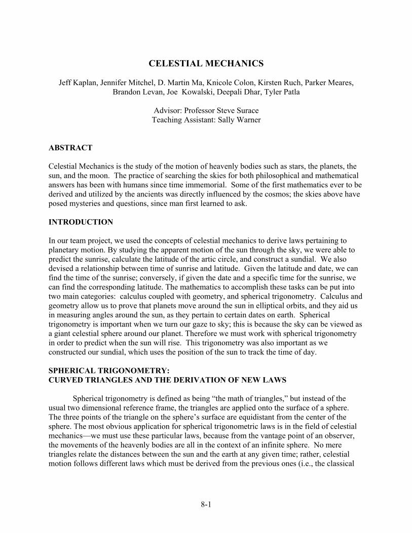
trigonometric laws). In Figure 1, ABC is an example of a spherical triangle; all points are equidistant from the center of the sphere.

Fig.1: Representation for Law of Cosines derivation.

Law of Cosines In Figure 1, the sphere with center O is resting on a flat surface, with tangent point C; points A and B are arbitrary. A line is projected out from O through points A and B, and extended out to the flat surface to create points A’ and B’. The object is now to solved for side lengths A’O and B’O, which will allow us to relate a set of two equations formed from the Law of Cosines ((because this projected triangle is not spherical, so we can use this law).

The Law of Cosines is one of the basic laws used in trigonometry; it follows that a similarly structured law should be utilized for spherical triangles, i.e. a law which maintains the relationship between the arc lengths and an angle. Following is the derivation of the of the Law of Cosines from the above picture. When in polar form, the length of an arc s = rθ. Therefore:

rbOCA =′∠

=′

rb

rAOcos

=′

rbrCA tan

raOCB =′∠

=′

ra

rBOcos

=′

rarCB tan

rcBOA =′′∠

Using the law of cosines twice, we set up two equations with (A’B’)2

8-2

( ) ( ) ( )( ) ( ) ( ) ( ) ( )( ) CCBCACBCABABOABOAOBOAO ∠′′−′+′==′′∠′′−′+′ cos2)''(cos2 22222 ( ) ( ) ( )( ) ( ) ( ) ( ) ( )( ) CCBCACBCABOABOAOBOAO ∠′′−′+′=′′∠′′−′+′ cos2cos2 2222 Plugging in:

( )Cra

rbr

rar

rbr

rc

ra

rbr

ra

r

rb

r costantan2tantancoscoscos

2coscos

222222

2

2

2

2

−+=−+

Simplify the equation

Cra

rb

ra

rb

rc

ra

rbr

arb costantan2tantancos

coscos

12secsec 2222

−+=−+

C

ra

rb

ra

rb

rc

rc

ra

rbr

arb costantan2tantancoscos

coscos

122tantan 2222

−

+

=

−++

Cra

rb

ra

rb

rc

costantan2coscos

cos22 −=−

(Eqn.1) C

ra

rb

ra

rb

rc cossinsincoscos +=cos

This is the formula for the Law of Cosines as applied to spherically curved triangles. Law of Sines derived from Law of Cosines:

After one has access to the Law of Cosines, it is merely a matter of clever substitutions and algebraic/trigonometric manipulations to derive the Law of Sines used for spherical triangles. Analogous to its two dimensional counterpart, it relates arc lengths and angles.

Crb

ra

rb

ra

rc cossinsincoscoscos +=

rb

ra

rb

ra

rc

Csinsin

coscoscoscos

−=

which simplifies algebraically to:

rc

rb

ra

rc

rb

ra

rc

rb

ra

rcC

222

222

2

2

sinsinsin

coscoscos2coscoscos1

sin

sin +−−−=

In the equation, the variables a, b, and c can be interchanged and the same equation will result for each value on the left. Therefore, we can conclude that:

8-3

rcC

rbB

raA

2

2

2

2

2

2

sin

sin

sin

sin

sin

sin== ,

which can also be written as:

(Eqn.2) cC

bB

aA

′=

′=

′ 2

2

2

2

2

2

sinsin

sinsin

sinsin where:

rcc

rbb

raa === ',','

Distance Between Two Points on a Sphere

This is one practical and very important application of spherical trigonometry. Our goal here is to find the distance between any two points on Earth (or any other sphere) when given the points’ locations in terms of latitude and longitude (Figure 2).

Note: angle C = La – Lb

(90-φa)r (90-φb)r X φbLb φaLa r

∠AOB La-Lb ∠BOC 90-φb ∠AOC 90-φa

Fig.3: Enlargement of spherical triangle ABC (where O is the center, and AO & BO are radii)

Fig.2:Example of any two points given in terms of latitude and longitude (φ and L) Where:

La= latitude of point A Lb= latitude of point B φa= longitude of point A φb= longitude of point B

Next we can apply the Law of Cosines again on triangle ABC (Figure 3):

x=distance between the points r=Earth radius = 6371km

8-4

( )ba

baba

LLr

r

r

r

r

r

r

r

rx

−

−

−

+

−

−

= cos2sin2sin2cos2coscosφπφπφπφπ

( )bababa LLrx

−+= coscoscossinsincos φφφφ

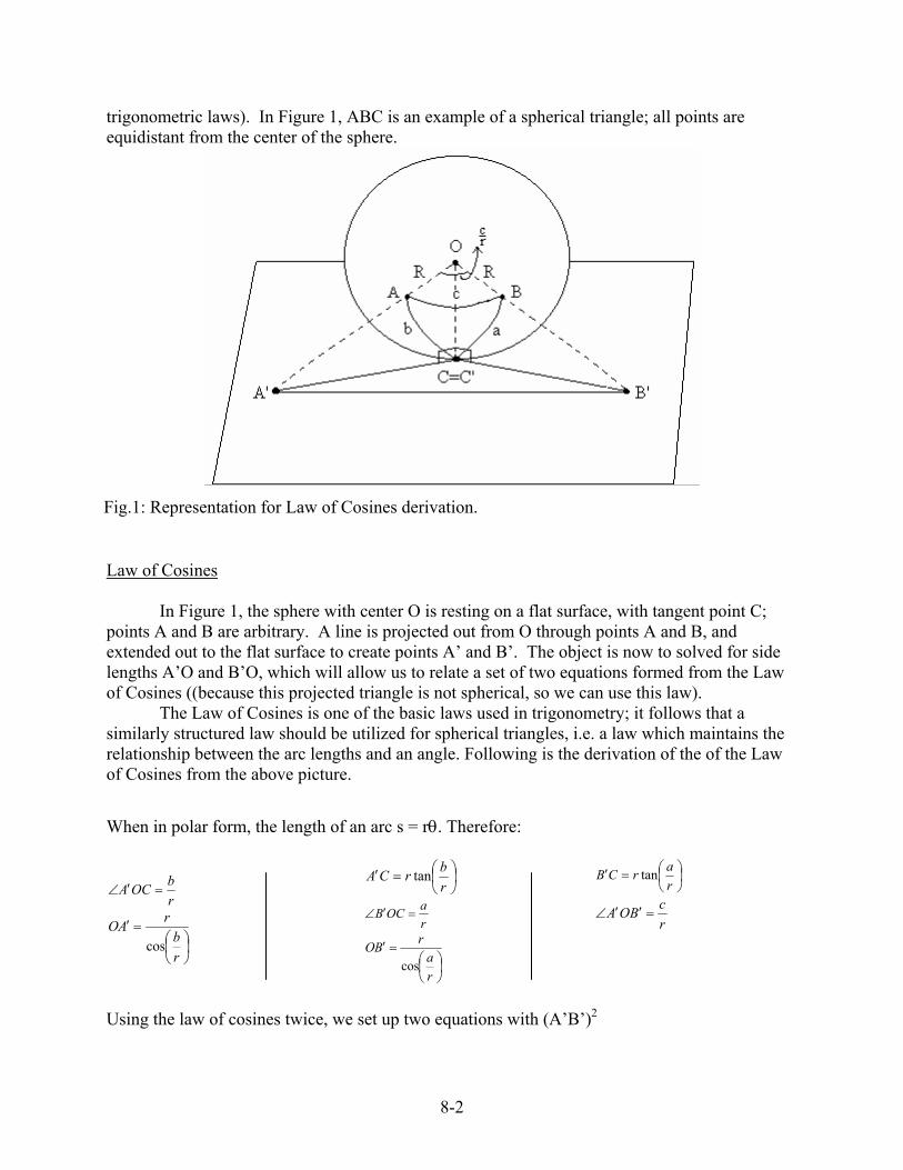
This formula can be used to calculate the distance between any two points on a spherically curved triangle. DERIVING THE PATH OF A PLANET: ELLIPTICAL GEOMETRY AND HARDCORE SUBSTITUTIONS

All the planets in our solar system take an elliptical path around the sun. First, we needed to transform the function equation for an ellipse centered on the origin into a polar equation in which the sun resides at one of the focus points. This representation mirrors what is occurring in the heavens, in that the sun is not in the center of the ellipse, but rather at the focus point. This equation in terms of the radius, r, is useful because it allows us to find the distance between the sun and the earth (or any given planet) at any given time.

θ

θθθθθθ

θθθθθ

θθθ

θθθ

cos1)1( (Eqn.3)

)cos1(2)2)(cos1(4)cos2cos2(cos2cos2

)2()cos2cos2()sincos(cos0

sincos2cos

1sincos2cos1)(

)(

2

22

2422222233

24222322222

222

22222

2

2222

222

22

2

2222

22

2

2

2

eear

eaeaeaeaeaeaeae

r

aeaeaaeaerereaa

reaaa

eaaerreaa

ra

eaaerraea

ya

aex

+−

=

−

−−−−−±−=

−−+−++−=−

−−=

++

=−

+++

⇒=−

++

θθ sincos)(

1

2222

2

2

2

2

ryrxaeabab

aecace

by

ax

==

+=−=

=⇒=

=+

Fig.4

8-5

Note.: In the above equations, r is the radius, a is the length of the semi-major axis, and e is the eccentricity (which basically measures how close to being circular the ellipse is). θ is our independent variable, whereas a and e are fixed constants for any given planet.

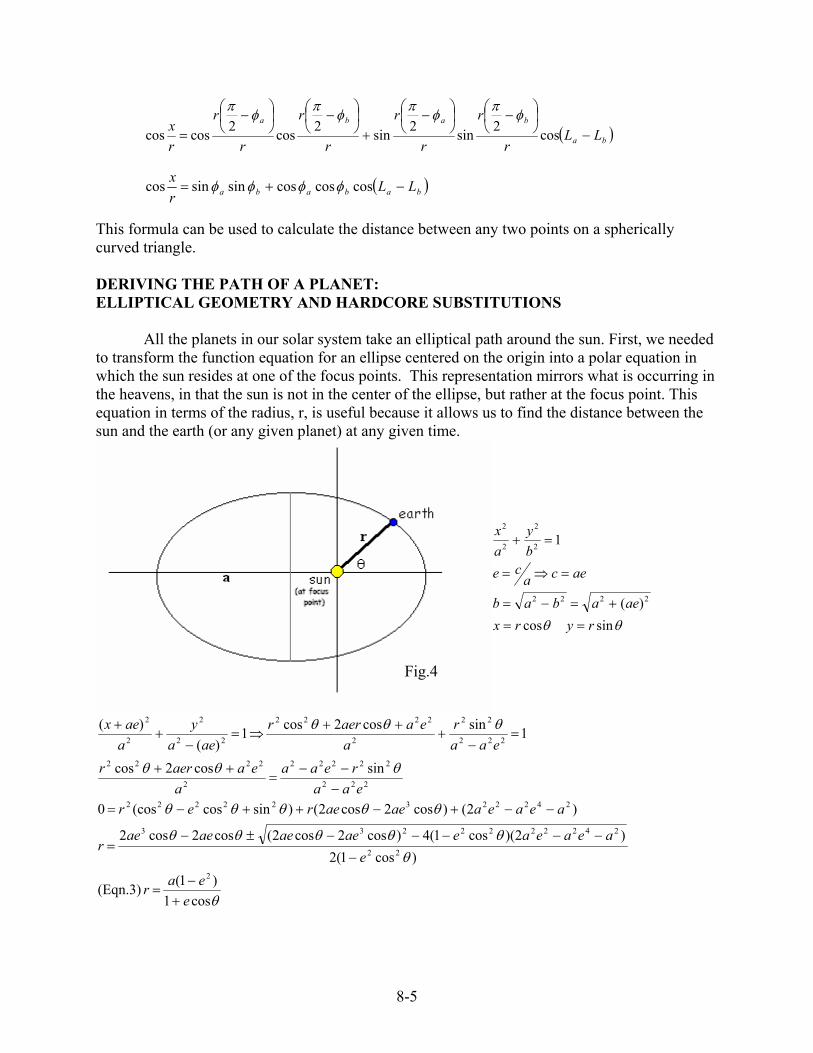
Now that we have the ability to calculate position coordinates for any given angle, we have to put our equations into more workable forms. We used a relationship between a circle and an ellipse, because it is easier to work with a central angle of a circle. This required deriving a consistent relationship between our elliptical angle, θ, and the central angle E. We began this process by writing a half angle formula for tangents, which allows us to then derive a relationship between E and θ. We are allowed to do this because the cosine of E can be written in terms of θ.

1coscoscos

++

=θ

θeeE

EEE

cos1cos1

2tan

+−

=

( )( )( )( 11cos

11cos2

tan++−−

=

eeE

θθ

)

( )( )

+−

=

2tan

11

2tan θ

eeE

(Eqn.4)

Fig.5: Relationship of E and θ

This provides us with a direct relation between θ and the central angle E. This

relationship becomes vital later, after Kepler’s laws are derived, because they prove that the planets revolve around the sun in an elliptical orbit, with the sun at a focus point (the equation for which was derived earlier).

8-6

CALCULUS AND CELESTIAL MOTION: PLANETARY LAWS IN A COHERENT FRAMEWORK Deriving Kepler’s Laws From Newton’s Laws

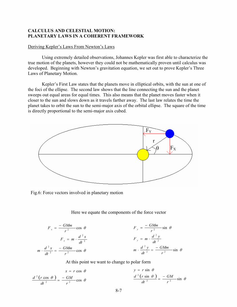
Using extremely detailed observations, Johannes Kepler was first able to characterize the true motion of the planets, however they could not be mathematically proven until calculus was developed. Beginning with Newton’s gravitation equation, we set out to prove Kepler’s Three Laws of Planetary Motion. Kepler’s First Law states that the planets move in elliptical orbits, with the sun at one of the foci of the ellipse. The second law shows that the line connecting the sun and the planet sweeps out equal areas for equal times. This also means that the planet moves faster when it closer to the sun and slows down as it travels farther away. The last law relates the time the planet takes to orbit the sun to the semi-major axis of the orbital ellipse. The square of the time is directly proportional to the semi-major axis cubed.

θ r

FY

FX

Fig.6: Force vectors involved in planetary motion

Here we equate the components of the force vector

2

( ) θθ

θ

θ

θ

coscoscos

cos

cos

22

2

22

2

2

2

rGM

dtrd

rx

rGMm

dtxdm

dtxdmF

rGMmF

x

x

−=

=

−=⋅

⋅=

−=

( ) θθ

θ

θ

θ

sinsinsin

sin

sin

22

2

22

2

2

2

2

rGM

dtrdry

rGMm

dtydm

dtydmF

rGMmF

y

y

−=

=

−=⋅

⋅=

−=

At this point we want to change to polar form

8-7

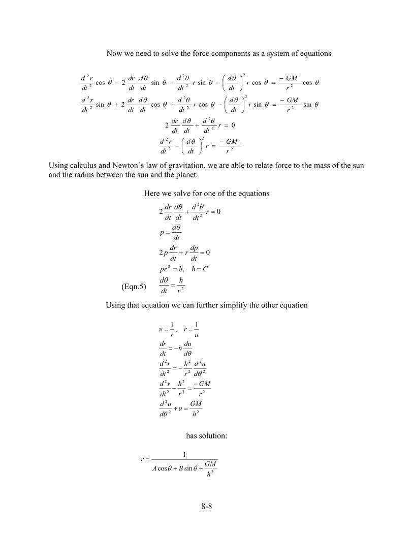
Now we need to solve the force components as a system of equations

2

2

2

2

2

2

2

2

2

2

2

2

2

2

2

2

2

2

02

sinsincoscos2sin

coscossinsin2cos

rGMr

dtd

dtrd

rdtd

dtd

dtdr

rGMr

dtdr

dtd

dtd

dtdr

dtrd

rGMr

dtdr

dtd

dtd

dtdr

dtrd

−=

−

=+

−=

−++

−=

−−−

θ

θθ

θθθθθθθθ

θθθθθθθθ

Using calculus and Newton’s law of gravitation, we are able to relate force to the mass of the sun and the radius between the sun and the planet.

Here we solve for one of the equations

2

2

2

2

,

02

02

rh

dtd

Chhprdtdpr

dtdrp

dtdp

rdtd

dtd

dtdr

=

==

=+

=

=+

θ

θ

θθ (Eqn.5)

Using that equation we can further simplify the other equation

22

2

23

2

2

2

2

2

2

2

2

2

1,1

hGMu

dud

rGM

rh

dtrd

dud

rh

dtrd

dduh

dtdr

ur

ru

=+

−=−

−=

−=

==

θ

θ

θ

has solution:

2sincos

1

hGMBA

r++

=θθ

8-8

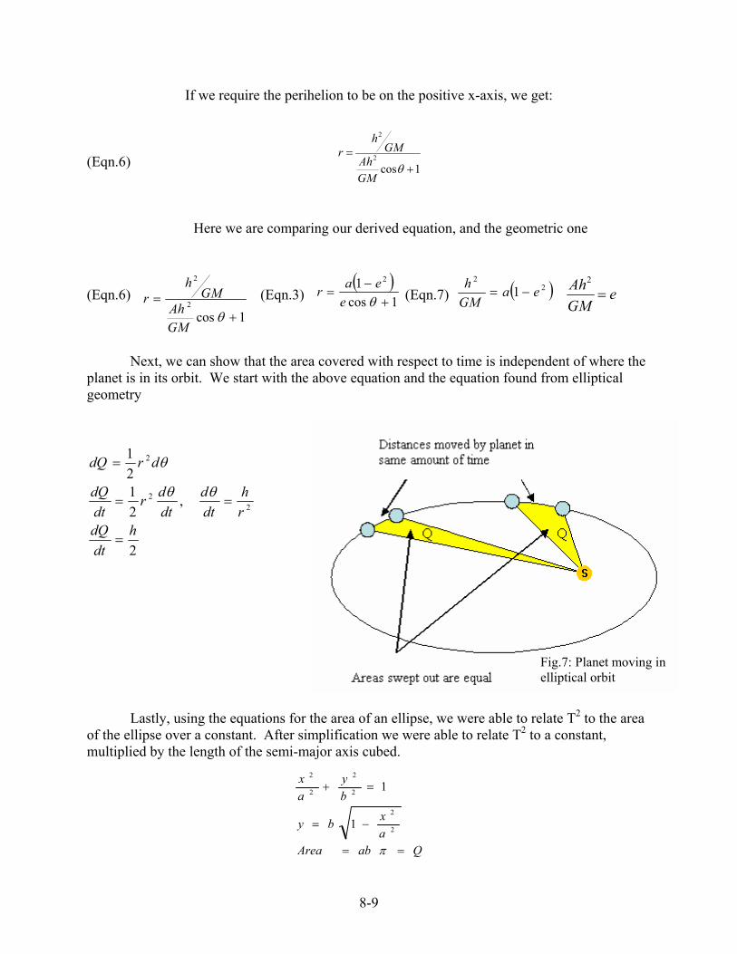
If we require the perihelion to be on the positive x-axis, we get:

1cos2

2

+=

θGMAh

GMh

r (Eqn.6)

Here we are comparing our derived equation, and the geometric one

2

,2121

22

2

hdtdQ

rh

dtd

dtdr

dtdQ

drdQ

=

==

=

θθ

θ

(Eqn.6) (Eqn.3) (Eqn.7) 2= GMr 1cos +

=θe

r ( )1 2− ea

1cos

2

+θGMAh

h ( )22

1 eaGMh

−= eGMAh

=2

Next, we can show that the area covered with respect to time is independent of where the planet is in its orbit. We start with the above equation and the equation found from elliptical geometry

Fig.7: Planet moving in elliptical orbit

Lastly, using the equations for the area of an ellipse, we were able to relate T2 to the area

of the ellipse over a constant. After simplification we were able to relate T2 to a constant, multiplied by the length of the semi-major axis cubed.

QabAreaaxby

by

ax

==

−=

=+

π

2

2

2

2

2

2

1

1

8-9

Equating the area formulas:

( )222222 1,

,2

,2

,2

eabcab

ceaace

habT

abQhTQhdtdQ

−=−=

===

===

π

π

Finishing the proportion

after further manipulation we get:

( ) ( )

( )( )3

22

2

2242

2

2222

2222

41

14

4

1,1

aGM

T

eGMaeaT

hbaT

eGMaheaGMh

π

π

π

=

−−

=

=

−=−=

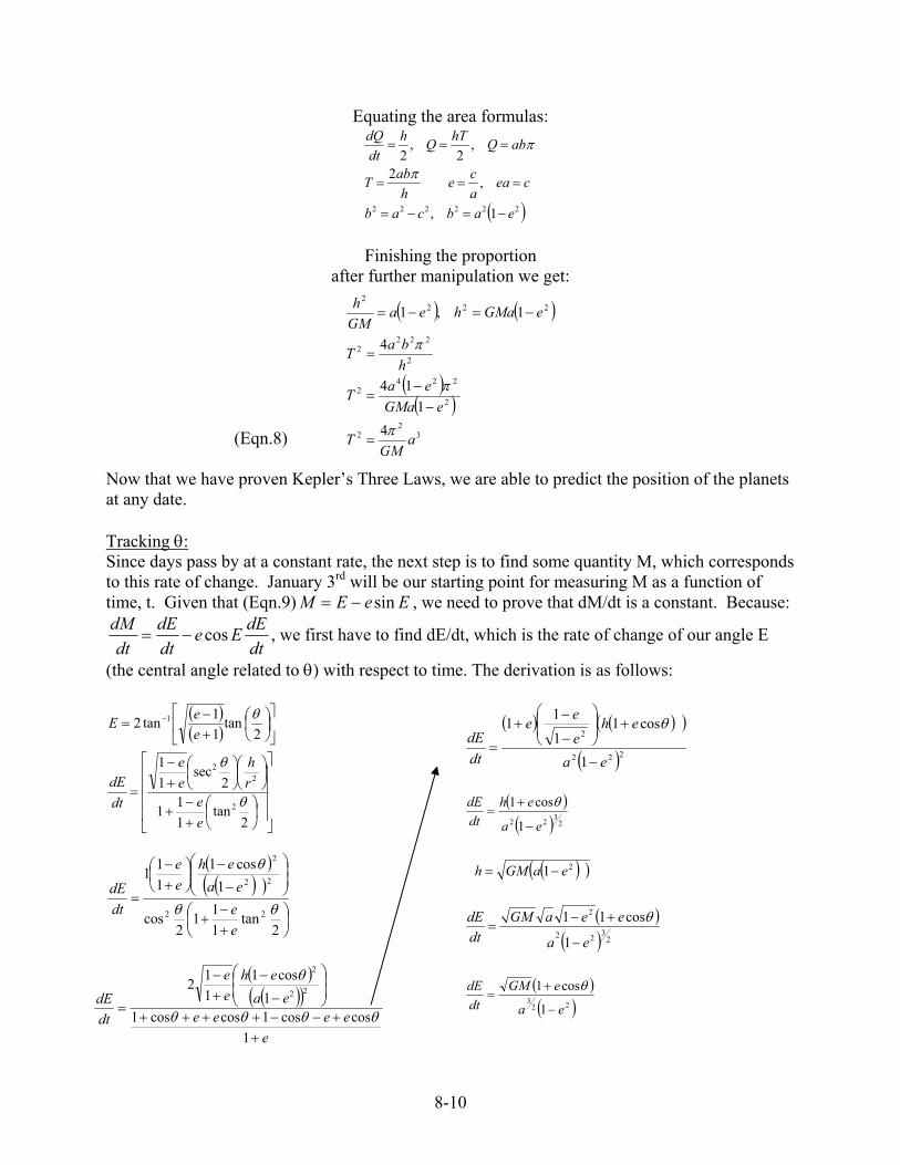
(Eqn.8) Now that we have proven Kepler’s Three Laws, we are able to predict the position of the planets at any date. Tracking θ: Since days pass by at a constant rate, the next step is to find some quantity M, which corresponds to this rate of change. January 3rd will be our starting point for measuring M as a function of time, t. Given that (Eqn.9) , we need to prove that dM/dt is a constant. Because: EeEM sin−=

dtdEEe

dtdE

dtdM cos−= , we first have to find dE/dt, which is the rate of change of our angle E

(the central angle related to θ) with respect to time. The derivation is as follows:

( )( )

+−

= −

2tan

11tan2 1 θ

eeE ( ) ( )(

( )

)222

2

1

cos11

11

ea

ehe

ee

dtdE

−

+

−

−+

=

θ

+−

+

+−

=

2tan

111

2sec

11

2

22

θ

θ

ee

rh

ee

dtdE

( )( ) )(

+−

+

−

−

+−

=

2tan

111

2cos

1cos1

111

22

22

2

θθ

θ

eeea

ehee

dtdE

( )

( )( )

eeeee

eaeh

ee

dtdE

++−−++++

−

−+−

=

1coscos1coscos1

1cos1

112 22

2

θθθθ

θ

( )

( ) 2322 1

cos1

ea

ehdtdE

−

+=

θ

( ) )( 21 eaGM −=h

( )( ) 2

322

2

1

cos11

ea

eeaGMdtdE

−

+−=

θ

( )( )22

31

cos1

ea

eGMdtdE

−

+=

θ

8-10

Using this formula, we can now solve the equation for dM/dt.

dtdEEe

dtdE

dtdM cos−=

[ ]EedtdE cos1−=

( )( )

++

−−

+=

θθθ

cos1cos1

1

cos1

23

22 eee

ea

eh

( )( )

( )( )( ) ( )( )2

322

2

23

22 1cos1

coscos1

1

cos1

eae

eeh

ea

eh

−+

++−

−

+=

θ

θθθ

( ) ( )( )2

322

2

1

coscos1

ea

eeheh

−

+−+=

θθ

( )( )2

322 1

coscos1

ea

eeeh

−

−−+=

θθ

( )( )2

322

2

1

1

ea

eh

−

−=

22 1 ea

hdt

dM

−=

Now, using previous formulas derived from Newton’s Gravitational Laws, we can find that:

Teah

22 12 −=

π , which, when substituted into our equation for dM/dt, yields: Tdt

dM π2=

Integrating yields: (Eqn.10) tT

M π2= , where t is the number of days since January 3.

CALCULATING THE SUNRISE: FINDING λ, THE DECLINATION, AND H

To calculate the sunrise on any given day, it is necessary to find the declination of the sun on that day. The declination, δ, of the sun is the angle deviation in the sun’s path from a path directly overhead. A larger declination results when the sun to travel higher in the sky, resulting in a longer path and a longer day. The sun takes its shortest path overhead on March 21, when the declination is zero. An angle λ can be found, having the function of keeping track of the earth’s position relative to the vernal equinox, because this is where the declination is zero. (Eqn.11) λ = θ + ω − 180

Set the date equal to March 21; on this date we defined λ to equal zero, so set theta equal to the time between Jan 3 and March 21. In solving for ω in this equation with these values, we find ω to be equal to 102.89 degrees.

Now that we can keep track of the sun’s angle relative to March 21, using λ, we can find

the declination of the sun. We also know the maximum declination of the sun, ε = 23.43975°. Using spherical trig we can find δ. Knowing epsilon and lambda we can solve for delta in terms

8-11

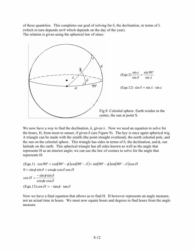
of these quantities. This completes our goal of solving for δ, the declination, in terms of λ (which in turn depends on θ which depends on the day of the year). The relation is given using the spherical law of sines:

εS S

ελδ

λδε

sinsinsin (Eqn.12)

sin90sin

sinsin(Eqn.2)

⋅=

°=

λδ

°90α

Fig.8: Celestial sphere. Earth resides in the center, the sun at point S.

We now have a way to find the declination, δ, given λ. Now we need an equation to solve for the hours, H, from noon to sunset, if given δ (see Figure 9). The key is once again spherical trig. A triangle can be made with the zenith (the point straight overhead), the north celestial pole, and the sun on the celestial sphere. This triangle has sides in terms of δ, the declination, and φ, our latitude on the earth. This spherical triangle has all sides known as well as the angle that represents H as an interior angle; we can use the law of cosines to solve for the angle that represents H:

( ) ( ) ( ) ( )

δφδφδφ

δφδφδφδφ

tantancos (Eqn.13)coscossinsincos

coscoscossinsin0cos90sin90sin90cos90cos90cos (Eqn.1)

⋅−=

−=

+=−°−°+−°−°=°

Hc

H

HcH

Now we have a final equation that allows us to find H. H however represents an angle measure, not an actual time in hours. We must now equate hours and degrees to find hours from the angle measure

8-12

.

°90φ−°90

δ−°90

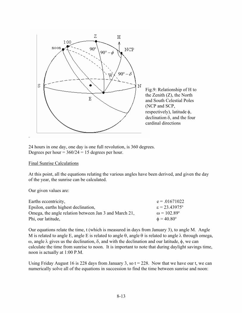
Fig.9: Relationship of H to the Zenith (Z), the North and South Celestial Poles (NCP and SCP, respectively), latitude φ, declination δ, and the four cardinal directions

24 hours in one day, one day is one full revolution, is 360 degrees. Degrees per hour = 360/24 = 15 degrees per hour. Final Sunrise Calculations At this point, all the equations relating the various angles have been derived, and given the day of the year, the sunrise can be calculated. Our given values are: Earths eccentricity, e = .01671022 Epsilon, earths highest declination, ε = 23.43975° Omega, the angle relation between Jan 3 and March 21, ω = 102.89° Phi, our latitude, φ = 40.80° Our equations relate the time, t (which is measured in days from January 3), to angle M. Angle M is related to angle E, angle E is related to angle θ, angle θ is related to angle λ through omega, ω, angle λ gives us the declination, δ, and with the declination and our latitude, φ, we can calculate the time from sunrise to noon. It is important to note that during daylight savings time, noon is actually at 1:00 P.M. Using Friday August 16 is 228 days from January 3, so t = 228. Now that we have our t, we can numerically solve all of the equations in succession to find the time between sunrise and noon:

8-13

7566335.615/3495.101,tantancos

75581.12,sinsinsin28451.146,180

39451.2238989697.3,2

tan11

2tan

9105328.3,sin

9221526.3,228,2

=°°=−=

==°=−+=

°==+−

=

=⋅−=

===

HHH

eeE

EEeEM

MtatT

tM

δφδελδ

λωθλ

θθ

π(Eqn.10) (Eqn.9) (Eqn.4) (Eqn.11) (Eqn.12) (Eqn.13) A time of 6.7566 hours between noon and sunrise yields a sunrise time of 6:15 A.M. When compared to 3 researched values (6:09, 6:09, and 6:07), this time is accurate within 8 minutes or .56%. Using this information, we can also calculate the latitude at which, on the longest day of summer, the sun never sets. This latitude is called the artic circle. We simply have to solve for the latitude, φ, given that sunrise is 12 hours from noon. If the sunrise is 12 hours from noon, the sunrise and sunset times are the same, resulting the sun rising when it sets, so in other words, the sun never sets. The longest day of summer is on June 21, or the summer solstice. We can actually skip much of the calculations because we know that the earth’s declination is the greatest on this day, which means that δ = ε. (Eqn.12) cos °=−=

=°=°=

5603.66,tantan18012

23.43975

φδφ

δ

HHhours

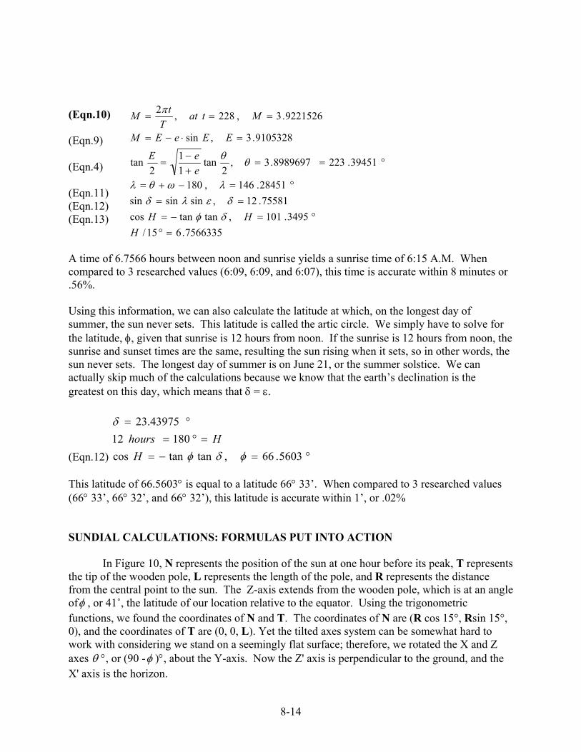
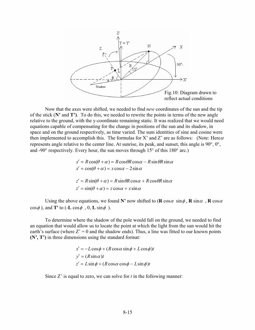
This latitude of 66.5603° is equal to a latitude 66° 33’. When compared to 3 researched values (66° 33’, 66° 32’, and 66° 32’), this latitude is accurate within 1’, or .02% SUNDIAL CALCULATIONS: FORMULAS PUT INTO ACTION In Figure 10, N represents the position of the sun at one hour before its peak, T represents the tip of the wooden pole, L represents the length of the pole, and R represents the distance from the central point to the sun. The Z-axis extends from the wooden pole, which is at an angle of , or 41˚, the latitude of our location relative to the equator. Using the trigonometric functions, we found the coordinates of N and T. The coordinates of N are (R cos 15°, Rsin 15°, 0), and the coordinates of T are (0, 0, L). Yet the tilted axes system can be somewhat hard to work with considering we stand on a seemingly flat surface; therefore, we rotated the X and Z axes °, or (90 - )°, about the Y-axis. Now the Z' axis is perpendicular to the ground, and the X' axis is the horizon.

φ

θ φ

8-14

φ

Fig.10: Diagram drawn to reflect actual conditions

Now that the axes were shifted, we needed to find new coordinates of the sun and the tip

of the stick (N’ and T’). To do this, we needed to rewrite the points in terms of the new angle relative to the ground, with the y-coordinate remaining static. It was realized that we would need equations capable of compensating for the change in positions of the sun and its shadow, in space and on the ground respectively, as time varied. The sum identities of sine and cosine were then implemented to accomplish this. The formulas for X’ and Z’ are as follows: (Note: Here represents angle relative to the center line. At sunrise, its peak, and sunset, this angle is 90°, 0°, and -90° respectively. Every hour, the sun moves through 15° of this 180° arc.)

α

αθαθαθ sinsincoscos)cos( RRRRRx −=+=′

αααθ sin2cos)cos( −=+=′ xx

αααθαθαθαθ

sincos)sin(sincoscossin)sin(

xzzRRRRRz

+=+=′+=+=′

Using the above equations, we found N’ now shifted to (R cos sin , R sin , R cos

cos ), and T' to (-L cos , 0, L sin ). α φ α α

φ φ φ To determine where the shadow of the pole would fall on the ground, we needed to find

an equation that would allow us to locate the point at which the light from the sun would hit the earth’s surface (where Z’ = 0 and the shadow ends). Thus, a line was fitted to our known points (N’, T’) in three dimensions using the standard format:

tLRLztRy

tLRLx

)sincoscos(sin)sin(

)cossincos(cos

φφαφα

φφαφ

−+=′=′

++−=′

Since Z’ is equal to zero, we can solve for t in the following manner:

8-15

tLR

LtLRL

tLRLz

=−

−−=−

−+==′

φφαφ

φφαφφφαφ

sincoscossin

)sincoscos(sin)sincoscos(sin0

0

We can then substitute the value for t back into the equations for x’ and y’ to obtain the formulas to give us the ∆y and ∆x of the shadow as time progresses. Following some house cleaning and simplification, the following equations for the point of contact for the light and ground were obtained:

)sincoscos

sin)(cossincos(cosφφα

φφφαφLR

LLRLx−

−++−=′

φφαα

sincoscoscos

LRLRx

−−

=′

)sincoscos

sin(sinφφα

φαLR

LRy−

−=′

φφαφαsincoscos

sinsinLR

LRy−

−=′

After obtaining the equations necessary for calculating the x’ and y’ coordinates, given that z’ = 0, we then were forced to devise a method of calculating the angle on the ground as changed in terms of x’ and y’. In order to do this, we turned to the trig function tangent. The angle found by using the inverse tangent function is the angle through which the pole’s shadow moved away from the 1:00 PM line.

α

xy′−′−

=θtan

xy′′

= −1tanθ

)cos

sincoscos)(sincoscos

sinsin(tan 1

αφφα

φφαφαθ

RLLR

LRRL

−−

−−

= −

)cos

sinsin(tan 1

αφαθ −=

CONSTRUCTION OF THE SUNDIAL Once the calculations were complete, it was time to apply them by constructing the sundial. The materials needed included nails, a hammer, string, a meter stick, a wooden pole, a 2’ X 4’, a shovel, and a T-square. At precisely 1:00 PM, which is noon during Daylight Savings

8-16

8-17

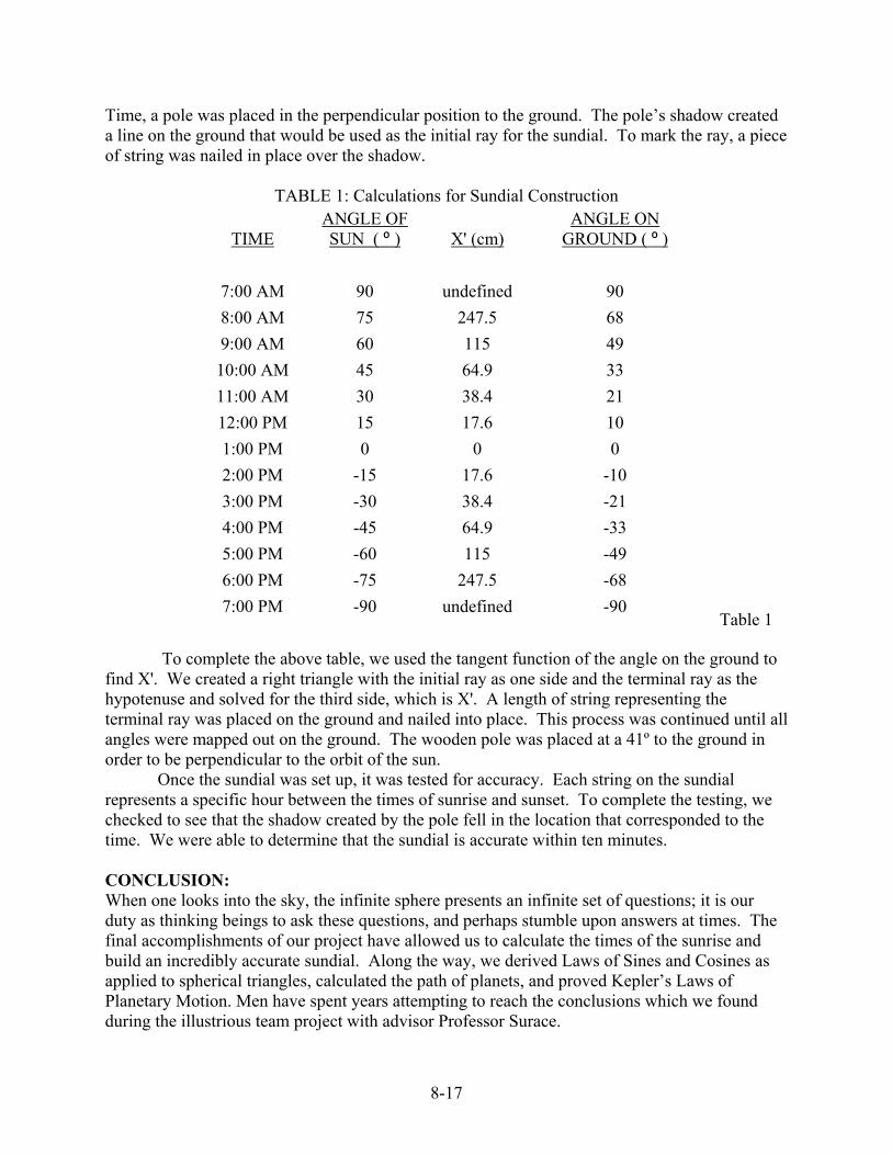
Time, a pole was placed in the perpendicular position to the ground. The pole’s shadow created a line on the ground that would be used as the initial ray for the sundial. To mark the ray, a piece of string was nailed in place over the shadow.

TABLE 1: Calculations for Sundial Construction

TIME

ANGLE OF SUN ( º ) X' (cm)

ANGLE ON GROUND ( º )

7:00 AM 90 undefined 90 8:00 AM 75 247.5 68 9:00 AM 60 115 49 10:00 AM 45 64.9 33 11:00 AM 30 38.4 21 12:00 PM 15 17.6 10 1:00 PM 0 0 0 2:00 PM -15 17.6 -10 3:00 PM -30 38.4 -21 4:00 PM -45 64.9 -33 5:00 PM -60 115 -49 6:00 PM -75 247.5 -68 7:00 PM -90 undefined -90

Table 1

To complete the above table, we used the tangent function of the angle on the ground to find X'. We created a right triangle with the initial ray as one side and the terminal ray as the hypotenuse and solved for the third side, which is X'. A length of string representing the terminal ray was placed on the ground and nailed into place. This process was continued until all angles were mapped out on the ground. The wooden pole was placed at a 41º to the ground in order to be perpendicular to the orbit of the sun.

Once the sundial was set up, it was tested for accuracy. Each string on the sundial represents a specific hour between the times of sunrise and sunset. To complete the testing, we checked to see that the shadow created by the pole fell in the location that corresponded to the time. We were able to determine that the sundial is accurate within ten minutes.

CONCLUSION: When one looks into the sky, the infinite sphere presents an infinite set of questions; it is our duty as thinking beings to ask these questions, and perhaps stumble upon answers at times. The final accomplishments of our project have allowed us to calculate the times of the sunrise and build an incredibly accurate sundial. Along the way, we derived Laws of Sines and Cosines as applied to spherical triangles, calculated the path of planets, and proved Kepler’s Laws of Planetary Motion. Men have spent years attempting to reach the conclusions which we found during the illustrious team project with advisor Professor Surace.