Embed Size (px)
Citation preview

Quantum Mechanics
Second Edition


Quantum MechanicsConcepts and Applications
Second Edition
Nouredine ZettiliJacksonville State University, Jacksonville, USA
A John Wiley and Sons, Ltd., Publication

Copyright 2009 John Wiley & Sons, Ltd
Registered office
John Wiley & Sons Ltd, The Atrium, Southern Gate, Chichester, West Sussex, PO19 8SQ, United Kingdom
For details of our global editorial offices, for customer services and for information about how to apply for
permission to reuse the copyright material in this book please see our website at www.wiley.com.
The right of the author to be identified as the author of this work has been asserted in accordance with the
Copyright, Designs and Patents Act 1988.
All rights reserved. No part of this publication may be reproduced, stored in a retrieval system, or transmitted,
in any form or by any means, electronic, mechanical, photocopying, recording or otherwise, except as
permitted by the UK Copyright, Designs and Patents Act 1988, without the prior permission of the publisher.
Wiley also publishes its books in a variety of electronic formats. Some content that appears in print may not
be available in electronic books.
Designations used by companies to distinguish their products are often claimed as trademarks. All brand
names and product names used in this book are trade names, service marks, trademarks or registered
trademarks of their respective owners. The publisher is not associated with any product or vendor mentioned
in this book. This publication is designed to provide accurate and authoritative information in regard to the
subject matter covered. It is sold on the understanding that the publisher is not engaged in rendering
professional services. If professional advice or other expert assistance is required, the services of a competent
professional should be sought.
Library of Congress Cataloging-in-Publication Data
Zettili, Nouredine.
Quantum Mechanics: concepts and applications / Nouredine Zettili. – 2nd ed.
p. cm.
Includes bibliographical references and index.
ISBN 978-0-470-02678-6 (cloth: alk. paper) – ISBN 978-0-470-02679-3 (pbk.: alk. paper)
1. Quantum theory. I. Title
QC174.12.Z47 2009
530.12 – dc22
2008045022
A catalogue record for this book is available from the British Library
Produced from LaTeX files supplied by the author
Printed and bound in Great Britain by CPI Antony Rowe Ltd, Chippenham, Wiltshire
ISBN: 978-0-470-02678-6 (H/B)
978-0-470-02679-3 (P/B)
Contents
Preface to the Second Edition xiii
Preface to the First Edition xv
Note to the Student xvi
1 Origins of Quantum Physics 1
1.1 Historical Note . . . . . . . . . . . . . . . . . . . . . . . . . . . . . . . . . . 1
1.2 Particle Aspect of Radiation . . . . . . . . . . . . . . . . . . . . . . . . . . . 4
1.2.1 Blackbody Radiation . . . . . . . . . . . . . . . . . . . . . . . . . . . 4
1.2.2 Photoelectric Effect . . . . . . . . . . . . . . . . . . . . . . . . . . . . 10
1.2.3 Compton Effect . . . . . . . . . . . . . . . . . . . . . . . . . . . . . . 13
1.2.4 Pair Production . . . . . . . . . . . . . . . . . . . . . . . . . . . . . . 16
1.3 Wave Aspect of Particles . . . . . . . . . . . . . . . . . . . . . . . . . . . . . 18
1.3.1 de Broglie’s Hypothesis: Matter Waves . . . . . . . . . . . . . . . . . 18
1.3.2 Experimental Confirmation of de Broglie’s Hypothesis . . . . . . . . . 18
1.3.3 Matter Waves for Macroscopic Objects . . . . . . . . . . . . . . . . . 20
1.4 Particles versus Waves . . . . . . . . . . . . . . . . . . . . . . . . . . . . . . 22
1.4.1 Classical View of Particles and Waves . . . . . . . . . . . . . . . . . . 22
1.4.2 Quantum View of Particles and Waves . . . . . . . . . . . . . . . . . . 23
1.4.3 Wave–Particle Duality: Complementarity . . . . . . . . . . . . . . . . 26
1.4.4 Principle of Linear Superposition . . . . . . . . . . . . . . . . . . . . 27
1.5 Indeterministic Nature of the Microphysical World . . . . . . . . . . . . . . . 27
1.5.1 Heisenberg’s Uncertainty Principle . . . . . . . . . . . . . . . . . . . 28
1.5.2 Probabilistic Interpretation . . . . . . . . . . . . . . . . . . . . . . . . 30
1.6 Atomic Transitions and Spectroscopy . . . . . . . . . . . . . . . . . . . . . . 30
1.6.1 Rutherford Planetary Model of the Atom . . . . . . . . . . . . . . . . 30
1.6.2 Bohr Model of the Hydrogen Atom . . . . . . . . . . . . . . . . . . . 31
1.7 Quantization Rules . . . . . . . . . . . . . . . . . . . . . . . . . . . . . . . . 36
1.8 Wave Packets . . . . . . . . . . . . . . . . . . . . . . . . . . . . . . . . . . . 38
1.8.1 Localized Wave Packets . . . . . . . . . . . . . . . . . . . . . . . . . 39
1.8.2 Wave Packets and the Uncertainty Relations . . . . . . . . . . . . . . . 42
1.8.3 Motion of Wave Packets . . . . . . . . . . . . . . . . . . . . . . . . . 43
1.9 Concluding Remarks . . . . . . . . . . . . . . . . . . . . . . . . . . . . . . . 54
1.10 Solved Problems . . . . . . . . . . . . . . . . . . . . . . . . . . . . . . . . . 54
1.11 Exercises . . . . . . . . . . . . . . . . . . . . . . . . . . . . . . . . . . . . . 71
v
vi CONTENTS
2 Mathematical Tools of Quantum Mechanics 79
2.1 Introduction . . . . . . . . . . . . . . . . . . . . . . . . . . . . . . . . . . . . 79
2.2 The Hilbert Space and Wave Functions . . . . . . . . . . . . . . . . . . . . . . 79
2.2.1 The Linear Vector Space . . . . . . . . . . . . . . . . . . . . . . . . . 79
2.2.2 The Hilbert Space . . . . . . . . . . . . . . . . . . . . . . . . . . . . 80
2.2.3 Dimension and Basis of a Vector Space . . . . . . . . . . . . . . . . . 81
2.2.4 Square-Integrable Functions: Wave Functions . . . . . . . . . . . . . . 84
2.3 Dirac Notation . . . . . . . . . . . . . . . . . . . . . . . . . . . . . . . . . . 84
2.4 Operators . . . . . . . . . . . . . . . . . . . . . . . . . . . . . . . . . . . . . 89
2.4.1 General Definitions . . . . . . . . . . . . . . . . . . . . . . . . . . . . 89
2.4.2 Hermitian Adjoint . . . . . . . . . . . . . . . . . . . . . . . . . . . . 91
2.4.3 Projection Operators . . . . . . . . . . . . . . . . . . . . . . . . . . . 92
2.4.4 Commutator Algebra . . . . . . . . . . . . . . . . . . . . . . . . . . . 93
2.4.5 Uncertainty Relation between Two Operators . . . . . . . . . . . . . . 95
2.4.6 Functions of Operators . . . . . . . . . . . . . . . . . . . . . . . . . . 97
2.4.7 Inverse and Unitary Operators . . . . . . . . . . . . . . . . . . . . . . 98
2.4.8 Eigenvalues and Eigenvectors of an Operator . . . . . . . . . . . . . . 99
2.4.9 Infinitesimal and Finite Unitary Transformations . . . . . . . . . . . . 101
2.5 Representation in Discrete Bases . . . . . . . . . . . . . . . . . . . . . . . . . 104
2.5.1 Matrix Representation of Kets, Bras, and Operators . . . . . . . . . . . 105
2.5.2 Change of Bases and Unitary Transformations . . . . . . . . . . . . . 114
2.5.3 Matrix Representation of the Eigenvalue Problem . . . . . . . . . . . . 117
2.6 Representation in Continuous Bases . . . . . . . . . . . . . . . . . . . . . . . 121
2.6.1 General Treatment . . . . . . . . . . . . . . . . . . . . . . . . . . . . 121
2.6.2 Position Representation . . . . . . . . . . . . . . . . . . . . . . . . . 123
2.6.3 Momentum Representation . . . . . . . . . . . . . . . . . . . . . . . . 124
2.6.4 Connecting the Position and Momentum Representations . . . . . . . . 124
2.6.5 Parity Operator . . . . . . . . . . . . . . . . . . . . . . . . . . . . . . 128
2.7 Matrix and Wave Mechanics . . . . . . . . . . . . . . . . . . . . . . . . . . . 130
2.7.1 Matrix Mechanics . . . . . . . . . . . . . . . . . . . . . . . . . . . . 130
2.7.2 Wave Mechanics . . . . . . . . . . . . . . . . . . . . . . . . . . . . . 131
2.8 Concluding Remarks . . . . . . . . . . . . . . . . . . . . . . . . . . . . . . . 132
2.9 Solved Problems . . . . . . . . . . . . . . . . . . . . . . . . . . . . . . . . . 133
2.10 Exercises . . . . . . . . . . . . . . . . . . . . . . . . . . . . . . . . . . . . . 155
3 Postulates of Quantum Mechanics 165
3.1 Introduction . . . . . . . . . . . . . . . . . . . . . . . . . . . . . . . . . . . . 165
3.2 The Basic Postulates of Quantum Mechanics . . . . . . . . . . . . . . . . . . 165
3.3 The State of a System . . . . . . . . . . . . . . . . . . . . . . . . . . . . . . . 167
3.3.1 Probability Density . . . . . . . . . . . . . . . . . . . . . . . . . . . . 167
3.3.2 The Superposition Principle . . . . . . . . . . . . . . . . . . . . . . . 168
3.4 Observables and Operators . . . . . . . . . . . . . . . . . . . . . . . . . . . . 170
3.5 Measurement in Quantum Mechanics . . . . . . . . . . . . . . . . . . . . . . 172
3.5.1 How Measurements Disturb Systems . . . . . . . . . . . . . . . . . . 172
3.5.2 Expectation Values . . . . . . . . . . . . . . . . . . . . . . . . . . . . 173
3.5.3 Complete Sets of Commuting Operators (CSCO) . . . . . . . . . . . . 175
3.5.4 Measurement and the Uncertainty Relations . . . . . . . . . . . . . . . 177
CONTENTS vii
3.6 Time Evolution of the System’s State . . . . . . . . . . . . . . . . . . . . . . . 178
3.6.1 Time Evolution Operator . . . . . . . . . . . . . . . . . . . . . . . . . 178
3.6.2 Stationary States: Time-Independent Potentials . . . . . . . . . . . . . 179
3.6.3 Schrödinger Equation and Wave Packets . . . . . . . . . . . . . . . . . 180
3.6.4 The Conservation of Probability . . . . . . . . . . . . . . . . . . . . . 181
3.6.5 Time Evolution of Expectation Values . . . . . . . . . . . . . . . . . . 182
3.7 Symmetries and Conservation Laws . . . . . . . . . . . . . . . . . . . . . . . 183
3.7.1 Infinitesimal Unitary Transformations . . . . . . . . . . . . . . . . . . 184
3.7.2 Finite Unitary Transformations . . . . . . . . . . . . . . . . . . . . . . 185
3.7.3 Symmetries and Conservation Laws . . . . . . . . . . . . . . . . . . . 185
3.8 Connecting Quantum to Classical Mechanics . . . . . . . . . . . . . . . . . . 187
3.8.1 Poisson Brackets and Commutators . . . . . . . . . . . . . . . . . . . 187
3.8.2 The Ehrenfest Theorem . . . . . . . . . . . . . . . . . . . . . . . . . . 189
3.8.3 Quantum Mechanics and Classical Mechanics . . . . . . . . . . . . . . 190
3.9 Solved Problems . . . . . . . . . . . . . . . . . . . . . . . . . . . . . . . . . 191
3.10 Exercises . . . . . . . . . . . . . . . . . . . . . . . . . . . . . . . . . . . . . 209
4 One-Dimensional Problems 215
4.1 Introduction . . . . . . . . . . . . . . . . . . . . . . . . . . . . . . . . . . . . 215
4.2 Properties of One-Dimensional Motion . . . . . . . . . . . . . . . . . . . . . . 216
4.2.1 Discrete Spectrum (Bound States) . . . . . . . . . . . . . . . . . . . . 216
4.2.2 Continuous Spectrum (Unbound States) . . . . . . . . . . . . . . . . . 217
4.2.3 Mixed Spectrum . . . . . . . . . . . . . . . . . . . . . . . . . . . . . 217
4.2.4 Symmetric Potentials and Parity . . . . . . . . . . . . . . . . . . . . . 218
4.3 The Free Particle: Continuous States . . . . . . . . . . . . . . . . . . . . . . . 218
4.4 The Potential Step . . . . . . . . . . . . . . . . . . . . . . . . . . . . . . . . . 220
4.5 The Potential Barrier and Well . . . . . . . . . . . . . . . . . . . . . . . . . . 224
4.5.1 The Case E V0 . . . . . . . . . . . . . . . . . . . . . . . . . . . . . 2244.5.2 The Case E V0: Tunneling . . . . . . . . . . . . . . . . . . . . . . 227
4.5.3 The Tunneling Effect . . . . . . . . . . . . . . . . . . . . . . . . . . . 229
4.6 The Infinite Square Well Potential . . . . . . . . . . . . . . . . . . . . . . . . 231
4.6.1 The Asymmetric Square Well . . . . . . . . . . . . . . . . . . . . . . 231
4.6.2 The Symmetric Potential Well . . . . . . . . . . . . . . . . . . . . . . 234
4.7 The Finite Square Well Potential . . . . . . . . . . . . . . . . . . . . . . . . . 234
4.7.1 The Scattering Solutions (E V0) . . . . . . . . . . . . . . . . . . . . 2354.7.2 The Bound State Solutions (0 E V0) . . . . . . . . . . . . . . . . 235
4.8 The Harmonic Oscillator . . . . . . . . . . . . . . . . . . . . . . . . . . . . . 239
4.8.1 Energy Eigenvalues . . . . . . . . . . . . . . . . . . . . . . . . . . . . 241
4.8.2 Energy Eigenstates . . . . . . . . . . . . . . . . . . . . . . . . . . . . 243
4.8.3 Energy Eigenstates in Position Space . . . . . . . . . . . . . . . . . . 244
4.8.4 The Matrix Representation of Various Operators . . . . . . . . . . . . 247
4.8.5 Expectation Values of Various Operators . . . . . . . . . . . . . . . . 248
4.9 Numerical Solution of the Schrödinger Equation . . . . . . . . . . . . . . . . . 249
4.9.1 Numerical Procedure . . . . . . . . . . . . . . . . . . . . . . . . . . . 249
4.9.2 Algorithm . . . . . . . . . . . . . . . . . . . . . . . . . . . . . . . . . 251
4.10 Solved Problems . . . . . . . . . . . . . . . . . . . . . . . . . . . . . . . . . 252
4.11 Exercises . . . . . . . . . . . . . . . . . . . . . . . . . . . . . . . . . . . . . 276
viii CONTENTS
5 Angular Momentum 283
5.1 Introduction . . . . . . . . . . . . . . . . . . . . . . . . . . . . . . . . . . . . 283
5.2 Orbital Angular Momentum . . . . . . . . . . . . . . . . . . . . . . . . . . . 283
5.3 General Formalism of Angular Momentum . . . . . . . . . . . . . . . . . . . 285
5.4 Matrix Representation of Angular Momentum . . . . . . . . . . . . . . . . . . 290
5.5 Geometrical Representation of Angular Momentum . . . . . . . . . . . . . . . 293
5.6 Spin Angular Momentum . . . . . . . . . . . . . . . . . . . . . . . . . . . . . 295
5.6.1 Experimental Evidence of the Spin . . . . . . . . . . . . . . . . . . . . 295
5.6.2 General Theory of Spin . . . . . . . . . . . . . . . . . . . . . . . . . . 297
5.6.3 Spin 1 2 and the Pauli Matrices . . . . . . . . . . . . . . . . . . . . . 298
5.7 Eigenfunctions of Orbital Angular Momentum . . . . . . . . . . . . . . . . . . 301
5.7.1 Eigenfunctions and Eigenvalues of Lz . . . . . . . . . . . . . . . . . . 302
5.7.2 Eigenfunctions of L2 . . . . . . . . . . . . . . . . . . . . . . . . . . . 3035.7.3 Properties of the Spherical Harmonics . . . . . . . . . . . . . . . . . . 307
5.8 Solved Problems . . . . . . . . . . . . . . . . . . . . . . . . . . . . . . . . . 310
5.9 Exercises . . . . . . . . . . . . . . . . . . . . . . . . . . . . . . . . . . . . . 325
6 Three-Dimensional Problems 333
6.1 Introduction . . . . . . . . . . . . . . . . . . . . . . . . . . . . . . . . . . . . 333
6.2 3D Problems in Cartesian Coordinates . . . . . . . . . . . . . . . . . . . . . . 333
6.2.1 General Treatment: Separation of Variables . . . . . . . . . . . . . . . 333
6.2.2 The Free Particle . . . . . . . . . . . . . . . . . . . . . . . . . . . . . 335
6.2.3 The Box Potential . . . . . . . . . . . . . . . . . . . . . . . . . . . . 336
6.2.4 The Harmonic Oscillator . . . . . . . . . . . . . . . . . . . . . . . . . 338
6.3 3D Problems in Spherical Coordinates . . . . . . . . . . . . . . . . . . . . . . 340
6.3.1 Central Potential: General Treatment . . . . . . . . . . . . . . . . . . 340
6.3.2 The Free Particle in Spherical Coordinates . . . . . . . . . . . . . . . 343
6.3.3 The Spherical Square Well Potential . . . . . . . . . . . . . . . . . . . 346
6.3.4 The Isotropic Harmonic Oscillator . . . . . . . . . . . . . . . . . . . . 347
6.3.5 The Hydrogen Atom . . . . . . . . . . . . . . . . . . . . . . . . . . . 351
6.3.6 Effect of Magnetic Fields on Central Potentials . . . . . . . . . . . . . 365
6.4 Concluding Remarks . . . . . . . . . . . . . . . . . . . . . . . . . . . . . . . 368
6.5 Solved Problems . . . . . . . . . . . . . . . . . . . . . . . . . . . . . . . . . 368
6.6 Exercises . . . . . . . . . . . . . . . . . . . . . . . . . . . . . . . . . . . . . 385
7 Rotations and Addition of Angular Momenta 391
7.1 Rotations in Classical Physics . . . . . . . . . . . . . . . . . . . . . . . . . . 391
7.2 Rotations in Quantum Mechanics . . . . . . . . . . . . . . . . . . . . . . . . . 393
7.2.1 Infinitesimal Rotations . . . . . . . . . . . . . . . . . . . . . . . . . . 393
7.2.2 Finite Rotations . . . . . . . . . . . . . . . . . . . . . . . . . . . . . . 395
7.2.3 Properties of the Rotation Operator . . . . . . . . . . . . . . . . . . . 396
7.2.4 Euler Rotations . . . . . . . . . . . . . . . . . . . . . . . . . . . . . . 397
7.2.5 Representation of the Rotation Operator . . . . . . . . . . . . . . . . . 398
7.2.6 Rotation Matrices and the Spherical Harmonics . . . . . . . . . . . . . 400
7.3 Addition of Angular Momenta . . . . . . . . . . . . . . . . . . . . . . . . . . 403
7.3.1 Addition of Two Angular Momenta: General Formalism . . . . . . . . 403
7.3.2 Calculation of the Clebsch–Gordan Coefficients . . . . . . . . . . . . . 409
CONTENTS ix
7.3.3 Coupling of Orbital and Spin Angular Momenta . . . . . . . . . . . . 415
7.3.4 Addition of More Than Two Angular Momenta . . . . . . . . . . . . . 419
7.3.5 Rotation Matrices for Coupling Two Angular Momenta . . . . . . . . . 420
7.3.6 Isospin . . . . . . . . . . . . . . . . . . . . . . . . . . . . . . . . . . 422
7.4 Scalar, Vector, and Tensor Operators . . . . . . . . . . . . . . . . . . . . . . . 425
7.4.1 Scalar Operators . . . . . . . . . . . . . . . . . . . . . . . . . . . . . 426
7.4.2 Vector Operators . . . . . . . . . . . . . . . . . . . . . . . . . . . . . 426
7.4.3 Tensor Operators: Reducible and Irreducible Tensors . . . . . . . . . . 428
7.4.4 Wigner–Eckart Theorem for Spherical Tensor Operators . . . . . . . . 430
7.5 Solved Problems . . . . . . . . . . . . . . . . . . . . . . . . . . . . . . . . . 434
7.6 Exercises . . . . . . . . . . . . . . . . . . . . . . . . . . . . . . . . . . . . . 450
8 Identical Particles 455
8.1 Many-Particle Systems . . . . . . . . . . . . . . . . . . . . . . . . . . . . . . 455
8.1.1 Schrödinger Equation . . . . . . . . . . . . . . . . . . . . . . . . . . . 455
8.1.2 Interchange Symmetry . . . . . . . . . . . . . . . . . . . . . . . . . . 457
8.1.3 Systems of Distinguishable Noninteracting Particles . . . . . . . . . . 458
8.2 Systems of Identical Particles . . . . . . . . . . . . . . . . . . . . . . . . . . . 460
8.2.1 Identical Particles in Classical and Quantum Mechanics . . . . . . . . 460
8.2.2 Exchange Degeneracy . . . . . . . . . . . . . . . . . . . . . . . . . . 462
8.2.3 Symmetrization Postulate . . . . . . . . . . . . . . . . . . . . . . . . 463
8.2.4 Constructing Symmetric and Antisymmetric Functions . . . . . . . . . 464
8.2.5 Systems of Identical Noninteracting Particles . . . . . . . . . . . . . . 464
8.3 The Pauli Exclusion Principle . . . . . . . . . . . . . . . . . . . . . . . . . . 467
8.4 The Exclusion Principle and the Periodic Table . . . . . . . . . . . . . . . . . 469
8.5 Solved Problems . . . . . . . . . . . . . . . . . . . . . . . . . . . . . . . . . 475
8.6 Exercises . . . . . . . . . . . . . . . . . . . . . . . . . . . . . . . . . . . . . 484
9 Approximation Methods for Stationary States 489
9.1 Introduction . . . . . . . . . . . . . . . . . . . . . . . . . . . . . . . . . . . . 489
9.2 Time-Independent Perturbation Theory . . . . . . . . . . . . . . . . . . . . . . 490
9.2.1 Nondegenerate Perturbation Theory . . . . . . . . . . . . . . . . . . . 490
9.2.2 Degenerate Perturbation Theory . . . . . . . . . . . . . . . . . . . . . 496
9.2.3 Fine Structure and the Anomalous Zeeman Effect . . . . . . . . . . . . 499
9.3 The Variational Method . . . . . . . . . . . . . . . . . . . . . . . . . . . . . . 507
9.4 The Wentzel–Kramers–Brillouin Method . . . . . . . . . . . . . . . . . . . . 515
9.4.1 General Formalism . . . . . . . . . . . . . . . . . . . . . . . . . . . . 515
9.4.2 Bound States for Potential Wells with No Rigid Walls . . . . . . . . . 518
9.4.3 Bound States for Potential Wells with One Rigid Wall . . . . . . . . . 524
9.4.4 Bound States for Potential Wells with Two Rigid Walls . . . . . . . . . 525
9.4.5 Tunneling through a Potential Barrier . . . . . . . . . . . . . . . . . . 528
9.5 Concluding Remarks . . . . . . . . . . . . . . . . . . . . . . . . . . . . . . . 530
9.6 Solved Problems . . . . . . . . . . . . . . . . . . . . . . . . . . . . . . . . . 531
9.7 Exercises . . . . . . . . . . . . . . . . . . . . . . . . . . . . . . . . . . . . . 562
x CONTENTS
10 Time-Dependent Perturbation Theory 571
10.1 Introduction . . . . . . . . . . . . . . . . . . . . . . . . . . . . . . . . . . . . 571
10.2 The Pictures of Quantum Mechanics . . . . . . . . . . . . . . . . . . . . . . . 571
10.2.1 The Schrödinger Picture . . . . . . . . . . . . . . . . . . . . . . . . . 572
10.2.2 The Heisenberg Picture . . . . . . . . . . . . . . . . . . . . . . . . . . 572
10.2.3 The Interaction Picture . . . . . . . . . . . . . . . . . . . . . . . . . . 573
10.3 Time-Dependent Perturbation Theory . . . . . . . . . . . . . . . . . . . . . . 574
10.3.1 Transition Probability . . . . . . . . . . . . . . . . . . . . . . . . . . 576
10.3.2 Transition Probability for a Constant Perturbation . . . . . . . . . . . . 577
10.3.3 Transition Probability for a Harmonic Perturbation . . . . . . . . . . . 579
10.4 Adiabatic and Sudden Approximations . . . . . . . . . . . . . . . . . . . . . . 582
10.4.1 Adiabatic Approximation . . . . . . . . . . . . . . . . . . . . . . . . . 582
10.4.2 Sudden Approximation . . . . . . . . . . . . . . . . . . . . . . . . . . 583
10.5 Interaction of Atoms with Radiation . . . . . . . . . . . . . . . . . . . . . . . 586
10.5.1 Classical Treatment of the Incident Radiation . . . . . . . . . . . . . . 587
10.5.2 Quantization of the Electromagnetic Field . . . . . . . . . . . . . . . . 588
10.5.3 Transition Rates for Absorption and Emission of Radiation . . . . . . . 591
10.5.4 Transition Rates within the Dipole Approximation . . . . . . . . . . . 592
10.5.5 The Electric Dipole Selection Rules . . . . . . . . . . . . . . . . . . . 593
10.5.6 Spontaneous Emission . . . . . . . . . . . . . . . . . . . . . . . . . . 594
10.6 Solved Problems . . . . . . . . . . . . . . . . . . . . . . . . . . . . . . . . . 597
10.7 Exercises . . . . . . . . . . . . . . . . . . . . . . . . . . . . . . . . . . . . . 613
11 Scattering Theory 617
11.1 Scattering and Cross Section . . . . . . . . . . . . . . . . . . . . . . . . . . . 617
11.1.1 Connecting the Angles in the Lab and CM frames . . . . . . . . . . . . 618
11.1.2 Connecting the Lab and CM Cross Sections . . . . . . . . . . . . . . . 620
11.2 Scattering Amplitude of Spinless Particles . . . . . . . . . . . . . . . . . . . . 621
11.2.1 Scattering Amplitude and Differential Cross Section . . . . . . . . . . 623
11.2.2 Scattering Amplitude . . . . . . . . . . . . . . . . . . . . . . . . . . . 624
11.3 The Born Approximation . . . . . . . . . . . . . . . . . . . . . . . . . . . . . 628
11.3.1 The First Born Approximation . . . . . . . . . . . . . . . . . . . . . . 628
11.3.2 Validity of the First Born Approximation . . . . . . . . . . . . . . . . 629
11.4 Partial Wave Analysis . . . . . . . . . . . . . . . . . . . . . . . . . . . . . . . 631
11.4.1 Partial Wave Analysis for Elastic Scattering . . . . . . . . . . . . . . . 631
11.4.2 Partial Wave Analysis for Inelastic Scattering . . . . . . . . . . . . . . 635
11.5 Scattering of Identical Particles . . . . . . . . . . . . . . . . . . . . . . . . . . 636
11.6 Solved Problems . . . . . . . . . . . . . . . . . . . . . . . . . . . . . . . . . 639
11.7 Exercises . . . . . . . . . . . . . . . . . . . . . . . . . . . . . . . . . . . . . 650
A The Delta Function 653
A.1 One-Dimensional Delta Function . . . . . . . . . . . . . . . . . . . . . . . . . 653
A.1.1 Various Definitions of the Delta Function . . . . . . . . . . . . . . . . 653
A.1.2 Properties of the Delta Function . . . . . . . . . . . . . . . . . . . . . 654
A.1.3 Derivative of the Delta Function . . . . . . . . . . . . . . . . . . . . . 655
A.2 Three-Dimensional Delta Function . . . . . . . . . . . . . . . . . . . . . . . . 656

CONTENTS xi
B Angular Momentum in Spherical Coordinates 657
B.1 Derivation of Some General Relations . . . . . . . . . . . . . . . . . . . . . . 657
B.2 Gradient and Laplacian in Spherical Coordinates . . . . . . . . . . . . . . . . 658
B.3 Angular Momentum in Spherical Coordinates . . . . . . . . . . . . . . . . . . 659
C C++ Code for Solving the Schrödinger Equation 661
Index 665

xii CONTENTS

Preface
Preface to the Second Edition
It has been eight years now since the appearance of the first edition of this book in 2001. During
this time, many courteous users—professors who have been adopting the book, researchers, and
students—have taken the time and care to provide me with valuable feedback about the book.
In preparing the second edition, I have taken into consideration the generous feedback I have
received from these users. To them, and from the very outset, I want to express my deep sense
of gratitude and appreciation.
The underlying focus of the book has remained the same: to provide a well-structured and
self-contained, yet concise, text that is backed by a rich collection of fully solved examples
and problems illustrating various aspects of nonrelativistic quantum mechanics. The book is
intended to achieve a double aim: on the one hand, to provide instructors with a pedagogically
suitable teaching tool and, on the other, to help students not only master the underpinnings of
the theory but also become effective practitioners of quantum mechanics.
Although the overall structure and contents of the book have remained the same upon the
insistence of numerous users, I have carried out a number of streamlining, surgical type changes
in the second edition. These changes were aimed at fixing the weaknesses (such as typos)
detected in the first edition while reinforcing and improving on its strengths. I have introduced a
number of sections, new examples and problems, and newmaterial; these are spread throughout
the text. Additionally, I have operated substantive revisions of the exercises at the end of the
chapters; I have added a number of new exercises, jettisoned some, and streamlined the rest.
I may underscore the fact that the collection of end-of-chapter exercises has been thoroughly
classroom tested for a number of years now.
The book has now a collection of almost six hundred examples, problems, and exercises.
Every chapter contains: (a) a number of solved examples each of which is designed to illustrate
a specific concept pertaining to a particular section within the chapter, (b) plenty of fully solved
problems (which come at the end of every chapter) that are generally comprehensive and, hence,
cover several concepts at once, and (c) an abundance of unsolved exercises intended for home-
work assignments. Through this rich collection of examples, problems, and exercises, I want
to empower the student to become an independent learner and an adept practitioner of quantum
mechanics. Being able to solve problems is an unfailing evidence of a real understanding of the
subject.
The second edition is backed by useful resources designed for instructors adopting the book
(please contact the author or Wiley to receive these free resources).
The material in this book is suitable for three semesters—a two-semester undergraduate
course and a one-semester graduate course. A pertinent question arises: How to actually use
xiii
xiv PREFACE
the book in an undergraduate or graduate course(s)? There is no simple answer to this ques-
tion as this depends on the background of the students and on the nature of the course(s) at
hand. First, I want to underscore this important observation: As the book offers an abundance
of information, every instructor should certainly select the topics that will be most relevant
to her/his students; going systematically over all the sections of a particular chapter (notably
Chapter 2), one might run the risk of getting bogged down and, hence, ending up spending too
much time on technical topics. Instead, one should be highly selective. For instance, for a one-
semester course where the students have not taken modern physics before, I would recommend
to cover these topics: Sections 1.1–1.6; 2.2.2, 2.2.4, 2.3, 2.4.1–2.4.8, 2.5.1, 2.5.3, 2.6.1–2.6.2,
2.7; 3.2–3.6; 4.3–4.8; 5.2–5.4, 5.6–5.7; and 6.2–6.4. However, if the students have taken mod-
ern physics before, I would skip Chapter 1 altogether and would deal with these sections: 2.2.2,
2.2.4, 2.3, 2.4.1–2.4.8, 2.5.1, 2.5.3, 2.6.1–2.6.2, 2.7; 3.2–3.6; 4.3–4.8; 5.2–5.4, 5.6–5.7; 6.2–
6.4; 9.2.1–9.2.2, 9.3, and 9.4. For a two-semester course, I think the instructor has plenty of
time and flexibility to maneuver and select the topics that would be most suitable for her/his
students; in this case, I would certainly include some topics from Chapters 7–11 as well (but
not all sections of these chapters as this would be unrealistically time demanding). On the other
hand, for a one-semester graduate course, I would cover topics such as Sections 1.7–1.8; 2.4.9,
2.6.3–2.6.5; 3.7–3.8; 4.9; and most topics of Chapters 7–11.
AcknowledgmentsI have received very useful feedback from many users of the first edition; I am deeply grateful
and thankful to everyone of them. I would like to thank in particular Richard Lebed (Ari-
zona State University) who has worked selflessly and tirelessly to provide me with valuable
comments, corrections, and suggestions. I want also to thank Jearl Walker (Cleveland State
University)—the author of The Flying Circus of Physics and of the Halliday–Resnick–Walkerclassics, Fundamentals of Physics—for having read the manuscript and for his wise sugges-tions; Milton Cha (University of Hawaii System) for having proofread the entire book; Felix
Chen (Powerwave Technologies, Santa Ana) for his reading of the first 6 chapters. My special
thanks are also due to the following courteous users/readers who have provided me with lists of
typos/errors they have detected in the first edition: Thomas Sayetta (East Carolina University),
Moritz Braun (University of South Africa, Pretoria), David Berkowitz (California State Univer-
sity at Northridge), John Douglas Hey (University of KwaZulu-Natal, Durban, South Africa),
Richard Arthur Dudley (University of Calgary, Canada), Andrea Durlo (founder of the A.I.F.
(Italian Association for Physics Teaching), Ferrara, Italy), and RickMiranda (Netherlands). My
deep sense of gratitude goes to M. Bulut (University of Alabama at Birmingham) and to Heiner
Mueller-Krumbhaar (Forschungszentrum Juelich, Germany) and his Ph.D. student C. Gugen-
berger for having written and tested the C++ code listed in Appendix C, which is designed to
solve the Schrödinger equation for a one-dimensional harmonic oscillator and for an infinite
square-well potential.
Finally, I want to thank my editors, Dr. Andy Slade, Celia Carden, and Alexandra Carrick,
for their consistent hard work and friendly support throughout the course of this project.
N. ZettiliJacksonville State University, USAJanuary 2009
xv
Preface to the First Edition
Books on quantum mechanics can be grouped into two main categories: textbooks, where
the focus is on the formalism, and purely problem-solving books, where the emphasis is on
applications. While many fine textbooks on quantum mechanics exist, problem-solving books
are far fewer. It is not my intention to merely add a text to either of these two lists. My intention
is to combine the two formats into a single text which includes the ingredients of both a textbook
and a problem-solving book. Books in this format are practically nonexistent. I have found this
idea particularly useful, for it gives the student easy and quick access not only to the essential
elements of the theory but also to its practical aspects in a unified setting.
During many years of teaching quantum mechanics, I have noticed that students generally
find it easier to learn its underlying ideas than to handle the practical aspects of the formalism.
Not knowing how to calculate and extract numbers out of the formalism, one misses the full
power and utility of the theory. Mastering the techniques of problem-solving is an essential part
of learning physics. To address this issue, the problems solved in this text are designed to teach
the student how to calculate. No real mastery of quantum mechanics can be achieved without
learning how to derive and calculate quantities.
In this book I want to achieve a double aim: to give a self-contained, yet concise, presenta-
tion of most issues of nonrelativistic quantum mechanics, and to offer a rich collection of fully
solved examples and problems. This unified format is not without cost. Size! Judicious care
has been exercised to achieve conciseness without compromising coherence and completeness.
This book is an outgrowth of undergraduate and graduate lecture notes I have been sup-
plying to my students for about one decade; the problems included have been culled from a
large collection of homework and exam exercises I have been assigning to the students. It is
intended for senior undergraduate and first-year graduate students. The material in this book
could be covered in three semesters: Chapters 1 to 5 (excluding Section 3.7) in a one-semester
undergraduate course; Chapter 6, Section 7.3, Chapter 8, Section 9.2 (excluding fine structure
and the anomalous Zeeman effect), and Sections 11.1 to 11.3 in the second semester; and the
rest of the book in a one-semester graduate course.
The book begins with the experimental basis of quantum mechanics, where we look at
those atomic and subatomic phenomena which confirm the failure of classical physics at the
microscopic scale and establish the need for a new approach. Then come the mathematical
tools of quantum mechanics such as linear spaces, operator algebra, matrix mechanics, and
eigenvalue problems; all these are treated by means of Dirac’s bra-ket notation. After that we
discuss the formal foundations of quantum mechanics and then deal with the exact solutions
of the Schrödinger equation when applied to one-dimensional and three-dimensional problems.
We then look at the stationary and the time-dependent approximation methods and, finally,
present the theory of scattering.
I would like to thank Professors Ismail Zahed (University of New York at Stony Brook)
and Gerry O. Sullivan (University College Dublin, Ireland) for their meticulous reading and
comments on an early draft of the manuscript. I am grateful to the four anonymous reviewers
who provided insightful comments and suggestions. Special thanks go to my editor, Dr Andy
Slade, for his constant support, encouragement, and efficient supervision of this project.
I want to acknowledge the hospitality of the Center for Theoretical Physics of MIT, Cam-
bridge, for the two years I spent there as a visitor. I would like to thank in particular Professors
Alan Guth, Robert Jaffee, and John Negele for their support.
xvi PREFACE
Note to the student
We are what we repeatedly do. Excellence, then, is not an act, but a habit.
Aristotle
No one expects to learn swimming without getting wet. Nor does anyone expect to learn
it by merely reading books or by watching others swim. Swimming cannot be learned without
practice. There is absolutely no substitute for throwing yourself into water and training for
weeks, or even months, till the exercise becomes a smooth reflex.
Similarly, physics cannot be learned passively. Without tackling various challenging prob-lems, the student has no other way of testing the quality of his or her understanding of the
subject. Here is where the student gains the sense of satisfaction and involvement produced by
a genuine understanding of the underlying principles. The ability to solve problems is the bestproof of mastering the subject. As in swimming, the more you solve problems, the more yousharpen and fine-tune your problem-solving skills.
To derive full benefit from the examples and problems solved in the text, avoid consulting
the solution too early. If you cannot solve the problem after your first attempt, try again! If
you look up the solution only after several attempts, it will remain etched in your mind for a
long time. But if you manage to solve the problem on your own, you should still compare your
solution with the book’s solution. You might find a shorter or more elegant approach.
One important observation: as the book is laden with a rich collection of fully solved ex-
amples and problems, one should absolutely avoid the temptation of memorizing the various
techniques and solutions; instead, one should focus on understanding the concepts and the un-
derpinnings of the formalism involved. It is not my intention in this book to teach the student a
number of tricks or techniques for acquiring good grades in quantummechanics classes without
genuine understanding or mastery of the subject; that is, I didn’t mean to teach the student how
to pass quantum mechanics exams without a deep and lasting understanding. However, the stu-
dent who focuses on understanding the underlying foundations of the subject and on reinforcing
that by solving numerous problems and thoroughly understanding themwill doubtlessly achieve
a double aim: reaping good grades as well as obtaining a sound and long-lasting education.
N. Zettili
Chapter 1
Origins of Quantum Physics
In this chapter we are going to review the main physical ideas and experimental facts that
defied classical physics and led to the birth of quantum mechanics. The introduction of quan-
tum mechanics was prompted by the failure of classical physics in explaining a number of
microphysical phenomena that were observed at the end of the nineteenth and early twentieth
centuries.
1.1 Historical Note
At the end of the nineteenth century, physics consisted essentially of classical mechanics, the
theory of electromagnetism1, and thermodynamics. Classical mechanics was used to predict
the dynamics of material bodies, and Maxwell’s electromagnetism provided the proper frame-work to study radiation; matter and radiation were described in terms of particles and waves,respectively. As for the interactions between matter and radiation, they were well explained
by the Lorentz force or by thermodynamics. The overwhelming success of classical physics—
classical mechanics, classical theory of electromagnetism, and thermodynamics—made people
believe that the ultimate description of nature had been achieved. It seemed that all known
physical phenomena could be explained within the framework of the general theories of matter
and radiation.
At the turn of the twentieth century, however, classical physics, which had been quite unas-
sailable, was seriously challenged on two major fronts:
Relativistic domain: Einstein’s 1905 theory of relativity showed that the validity of
Newtonian mechanics ceases at very high speeds (i.e., at speeds comparable to that of
light).
Microscopic domain: As soon as new experimental techniques were developed to the
point of probing atomic and subatomic structures, it turned out that classical physics fails
miserably in providing the proper explanation for several newly discovered phenomena.
It thus became evident that the validity of classical physics ceases at the microscopic
level and that new concepts had to be invoked to describe, for instance, the structure ofatoms and molecules and how light interacts with them.
1Maxwell’s theory of electromagnetism had unified the, then ostensibly different, three branches of physics: elec-
tricity, magnetism, and optics.
1
2 CHAPTER 1. ORIGINS OF QUANTUM PHYSICS
The failure of classical physics to explain several microscopic phenomena—such as black-
body radiation, the photoelectric effect, atomic stability, and atomic spectroscopy—had cleared
the way for seeking new ideas outside its purview.
The first real breakthrough came in 1900 when Max Planck introduced the concept of the
quantum of energy. In his efforts to explain the phenomenon of blackbody radiation, he suc-ceeded in reproducing the experimental results only after postulating that the energy exchange
between radiation and its surroundings takes place in discrete, or quantized, amounts. He ar-gued that the energy exchange between an electromagnetic wave of frequency and matter
occurs only in integer multiples of h , which he called the energy of a quantum, where h is afundamental constant called Planck’s constant. The quantization of electromagnetic radiationturned out to be an idea with far-reaching consequences.
Planck’s idea, which gave an accurate explanation of blackbody radiation, prompted new
thinking and triggered an avalanche of new discoveries that yielded solutions to the most out-
standing problems of the time.
In 1905 Einstein provided a powerful consolidation to Planck’s quantum concept. In trying
to understand the photoelectric effect, Einstein recognized that Planck’s idea of the quantization
of the electromagnetic waves must be valid for light as well. So, following Planck’s approach,he posited that light itself is made of discrete bits of energy (or tiny particles), called photons,each of energy h , being the frequency of the light. The introduction of the photon concept
enabled Einstein to give an elegantly accurate explanation to the photoelectric problem, which
had been waiting for a solution ever since its first experimental observation by Hertz in 1887.
Another seminal breakthrough was due to Niels Bohr. Right after Rutherford’s experimental
discovery of the atomic nucleus in 1911, and combining Rutherford’s atomic model, Planck’s
quantum concept, and Einstein’s photons, Bohr introduced in 1913 his model of the hydrogen
atom. In this work, he argued that atoms can be found only in discrete states of energy andthat the interaction of atoms with radiation, i.e., the emission or absorption of radiation by
atoms, takes place only in discrete amounts of h because it results from transitions of the atom
between its various discrete energy states. This work provided a satisfactory explanation to
several outstanding problems such as atomic stability and atomic spectroscopy.
Then in 1923 Compton made an important discovery that gave the most conclusive confir-
mation for the corpuscular aspect of light. By scattering X-rays with electrons, he confirmed
that the X-ray photons behave like particles with momenta h c; is the frequency of the
X-rays.
This series of breakthroughs—due to Planck, Einstein, Bohr, and Compton—gave both
the theoretical foundations as well as the conclusive experimental confirmation for the particle
aspect of waves; that is, the concept that waves exhibit particle behavior at the microscopic
scale. At this scale, classical physics fails not only quantitatively but even qualitatively and
conceptually.
As if things were not bad enough for classical physics, de Broglie introduced in 1923 an-
other powerful new concept that classical physics could not reconcile: he postulated that not
only does radiation exhibit particle-like behavior but, conversely, material particles themselvesdisplay wave-like behavior. This concept was confirmed experimentally in 1927 by Davissonand Germer; they showed that interference patterns, a property of waves, can be obtained with
material particles such as electrons.
Although Bohr’s model for the atom produced results that agree well with experimental
spectroscopy, it was criticized for lacking the ingredients of a theory. Like the “quantization”
scheme introduced by Planck in 1900, the postulates and assumptions adopted by Bohr in 1913
1.1. HISTORICAL NOTE 3
were quite arbitrary and do not follow from the first principles of a theory. It was the dissatis-
faction with the arbitrary nature of Planck’s idea and Bohr’s postulates as well as the need to fit
them within the context of a consistent theory that had prompted Heisenberg and Schrödinger
to search for the theoretical foundation underlying these new ideas. By 1925 their efforts paid
off: they skillfully welded the various experimental findings as well as Bohr’s postulates into
a refined theory: quantum mechanics. In addition to providing an accurate reproduction of theexisting experimental data, this theory turned out to possess an astonishingly reliable predic-
tion power which enabled it to explore and unravel many uncharted areas of the microphysical
world. This new theory had put an end to twenty five years (1900–1925) of patchwork which
was dominated by the ideas of Planck and Bohr and which later became known as the old
quantum theory.
Historically, there were two independent formulations of quantum mechanics. The first
formulation, called matrix mechanics, was developed by Heisenberg (1925) to describe atomicstructure starting from the observed spectral lines. Inspired by Planck’s quantization of waves
and by Bohr’s model of the hydrogen atom, Heisenberg founded his theory on the notion that
the only allowed values of energy exchange between microphysical systems are those that are
discrete: quanta. Expressing dynamical quantities such as energy, position, momentum and
angular momentum in terms of matrices, he obtained an eigenvalue problem that describes the
dynamics of microscopic systems; the diagonalization of the Hamiltonian matrix yields the
energy spectrum and the state vectors of the system. Matrix mechanics was very successful in
accounting for the discrete quanta of light emitted and absorbed by atoms.
The second formulation, called wave mechanics, was due to Schrödinger (1926); it is ageneralization of the de Broglie postulate. This method, more intuitive than matrix mechan-
ics, describes the dynamics of microscopic matter by means of a wave equation, called theSchrödinger equation; instead of the matrix eigenvalue problem of Heisenberg, Schrödingerobtained a differential equation. The solutions of this equation yield the energy spectrum and
the wave function of the system under consideration. In 1927 Max Born proposed his proba-bilistic interpretation of wave mechanics: he took the square moduli of the wave functions thatare solutions to the Schrödinger equation and he interpreted them as probability densities.
These two ostensibly different formulations—Schrödinger’s wave formulation and Heisen-berg’s matrix approach—were shown to be equivalent. Dirac then suggested a more generalformulation of quantum mechanics which deals with abstract objects such as kets (state vec-
tors), bras, and operators. The representation of Dirac’s formalism in a continuous basis—theposition or momentum representations—gives back Schrödinger’s wave mechanics. As for
Heisenberg’s matrix formulation, it can be obtained by representing Dirac’s formalism in a
discrete basis. In this context, the approaches of Schrödinger and Heisenberg represent, re-spectively, the wave formulation and the matrix formulation of the general theory of quantummechanics.
Combining special relativity with quantum mechanics, Dirac derived in 1928 an equation
which describes the motion of electrons. This equation, known as Dirac’s equation, predicted
the existence of an antiparticle, the positron, which has similar properties, but opposite charge,
with the electron; the positron was discovered in 1932, four years after its prediction by quan-
tum mechanics.
In summary, quantum mechanics is the theory that describes the dynamics of matter at the
microscopic scale. Fine! But is it that important to learn? This is no less than an otiose question,
for quantum mechanics is the only valid framework for describing the microphysical world.It is vital for understanding the physics of solids, lasers, semiconductor and superconductor
4 CHAPTER 1. ORIGINS OF QUANTUM PHYSICS
devices, plasmas, etc. In short, quantum mechanics is the founding basis of all modern physics:
solid state, molecular, atomic, nuclear, and particle physics, optics, thermodynamics, statistical
mechanics, and so on. Not only that, it is also considered to be the foundation of chemistry and
biology.
1.2 Particle Aspect of Radiation
According to classical physics, a particle is characterized by an energy E and a momentump, whereas a wave is characterized by an amplitude and a wave vector k ( k 2 ) that
specifies the direction of propagation of the wave. Particles and waves exhibit entirely different
behaviors; for instance, the “particle” and “wave” properties are mutually exclusive. We should
note that waves can exchange any (continuous) amount of energy with particles.
In this section we are going to see how these rigid concepts of classical physics led to its
failure in explaining a number of microscopic phenomena such as blackbody radiation, the
photoelectric effect, and the Compton effect. As it turned out, these phenomena could only be
explained by abandoning the rigid concepts of classical physics and introducing a new concept:
the particle aspect of radiation.
1.2.1 Blackbody Radiation
At issue here is how radiation interacts with matter. When heated, a solid object glows and
emits thermal radiation. As the temperature increases, the object becomes red, then yellow,
then white. The thermal radiation emitted by glowing solid objects consists of a continuousdistribution of frequencies ranging from infrared to ultraviolet. The continuous pattern of the
distribution spectrum is in sharp contrast to the radiation emitted by heated gases; the radiation
emitted by gases has a discrete distribution spectrum: a few sharp (narrow), colored lines with
no light (i.e., darkness) in between.
Understanding the continuous character of the radiation emitted by a glowing solid object
constituted one of the major unsolved problems during the second half of the nineteenth century.
All attempts to explain this phenomenon by means of the available theories of classical physics
(statistical thermodynamics and classical electromagnetic theory) ended up in miserable failure.
This problem consisted in essence of specifying the proper theory of thermodynamics that
describes how energy gets exchanged between radiation and matter.
When radiation falls on an object, some of it might be absorbed and some reflected. An
idealized “blackbody” is a material object that absorbs all of the radiation falling on it, and
hence appears as black under reflection when illuminated from outside. When an object is
heated, it radiates electromagnetic energy as a result of the thermal agitation of the electrons
in its surface. The intensity of this radiation depends on its frequency and on the temperature;
the light it emits ranges over the entire spectrum. An object in thermal equilibrium with its
surroundings radiates as much energy as it absorbs. It thus follows that a blackbody is a perfect
absorber as well as a perfect emitter of radiation.
A practical blackbody can be constructed by taking a hollow cavity whose internal walls
perfectly reflect electromagnetic radiation (e.g., metallic walls) and which has a very small
hole on its surface. Radiation that enters through the hole will be trapped inside the cavity and
gets completely absorbed after successive reflections on the inner surfaces of the cavity. The

1.2. PARTICLE ASPECT OF RADIATION 5
T=5000 K
T=4000 K
T=3000 K
T=2000 K
u (10 J m Hz )-16 -3 -1
� (10 Hz)14
Figure 1.1 Spectral energy density u T of blackbody radiation at different temperatures as
a function of the frequency .
hole thus absorbs radiation like a black body. On the other hand, when this cavity is heated2 to
a temperature T , the radiation that leaves the hole is blackbody radiation, for the hole behavesas a perfect emitter; as the temperature increases, the hole will eventually begin to glow. To
understand the radiation inside the cavity, one needs simply to analyze the spectral distribution
of the radiation coming out of the hole. In what follows, the term blackbody radiation willthen refer to the radiation leaving the hole of a heated hollow cavity; the radiation emitted by a
blackbody when hot is called blackbody radiation.
By the mid-1800s, a wealth of experimental data about blackbody radiation was obtained
for various objects. All these results show that, at equilibrium, the radiation emitted has a well-
defined, continuous energy distribution: to each frequency there corresponds an energy density
which depends neither on the chemical composition of the object nor on its shape, but only
on the temperature of the cavity’s walls (Figure 1.1). The energy density shows a pronounced
maximum at a given frequency, which increases with temperature; that is, the peak of the radi-ation spectrum occurs at a frequency that is proportional to the temperature (1.16). This is theunderlying reason behind the change in color of a heated object as its temperature increases, no-
tably from red to yellow to white. It turned out that the explanation of the blackbody spectrum
was not so easy.
A number of attempts aimed at explaining the origin of the continuous character of this
radiation were carried out. The most serious among such attempts, and which made use of
classical physics, were due to Wilhelm Wien in 1889 and Rayleigh in 1900. In 1879 J. Stefan
found experimentally that the total intensity (or the total power per unit surface area) radiatedby a glowing object of temperature T is given by
P a T 4 (1.1)
which is known as the Stefan–Boltzmann law, where 5 67 10 8 Wm 2K 4 is the
2When the walls are heated uniformly to a temperature T , they emit radiation (due to thermal agitation or vibrationsof the electrons in the metallic walls).
6 CHAPTER 1. ORIGINS OF QUANTUM PHYSICS
T=4000 K
u (10 J m Hz )-16 -3 -1
� (10 Hz)14
Wien’s Law
Rayleigh-JeansLaw
Planck’s Law
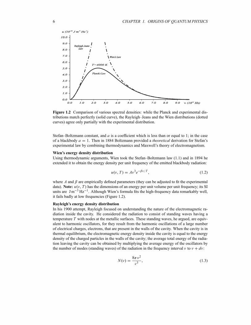
Figure 1.2 Comparison of various spectral densities: while the Planck and experimental dis-
tributions match perfectly (solid curve), the Rayleigh–Jeans and the Wien distributions (dotted
curves) agree only partially with the experimental distribution.
Stefan–Boltzmann constant, and a is a coefficient which is less than or equal to 1; in the caseof a blackbody a 1. Then in 1884 Boltzmann provided a theoretical derivation for Stefan’sexperimental law by combining thermodynamics and Maxwell’s theory of electromagnetism.
Wien’s energy density distribution
Using thermodynamic arguments, Wien took the Stefan–Boltzmann law (1.1) and in 1894 he
extended it to obtain the energy density per unit frequency of the emitted blackbody radiation:
u T A 3e T (1.2)
where A and are empirically defined parameters (they can be adjusted to fit the experimental
data). Note: u T has the dimensions of an energy per unit volume per unit frequency; its SI
units are Jm 3Hz 1. Although Wien’s formula fits the high-frequency data remarkably well,
it fails badly at low frequencies (Figure 1.2).
Rayleigh’s energy density distribution
In his 1900 attempt, Rayleigh focused on understanding the nature of the electromagnetic ra-
diation inside the cavity. He considered the radiation to consist of standing waves having a
temperature T with nodes at the metallic surfaces. These standing waves, he argued, are equiv-alent to harmonic oscillators, for they result from the harmonic oscillations of a large number
of electrical charges, electrons, that are present in the walls of the cavity. When the cavity is in
thermal equilibrium, the electromagnetic energy density inside the cavity is equal to the energy
density of the charged particles in the walls of the cavity; the average total energy of the radia-
tion leaving the cavity can be obtained by multiplying the average energy of the oscillators by
the number of modes (standing waves) of the radiation in the frequency interval to d :
N8 2
c3(1.3)
1.2. PARTICLE ASPECT OF RADIATION 7
where c 3 108 ms 1 is the speed of light; the quantity 8 2 c3 d gives the number of
modes of oscillation per unit volume in the frequency range to d . So the electromagneticenergy density in the frequency range to d is given by
u T N E8 2
c3E (1.4)
where E is the average energy of the oscillators present on the walls of the cavity (or of the
electromagnetic radiation in that frequency interval); the temperature dependence of u T is
buried in E .How does one calculate E ? According to the equipartition theorem of classical thermo-
dynamics, all oscillators in the cavity have the same mean energy, irrespective of their frequen-
cies3:
E 0 Ee E kT dE
0 e E kT dEkT (1.5)
where k 1 3807 10 23 JK 1 is the Boltzmann constant. An insertion of (1.5) into (1.4)
leads to the Rayleigh–Jeans formula:
u T8 2
c3kT (1.6)
Except for low frequencies, this law is in complete disagreement with experimental data: u Tas given by (1.6) diverges for high values of , whereas experimentally it must be finite (Fig-ure 1.2). Moreover, if we integrate (1.6) over all frequencies, the integral diverges. This impliesthat the cavity contains an infinite amount of energy. This result is absurd. Historically, this wascalled the ultraviolet catastrophe, for (1.6) diverges for high frequencies (i.e., in the ultravioletrange)—a real catastrophical failure of classical physics indeed! The origin of this failure can
be traced to the derivation of the average energy (1.5). It was founded on an erroneous premise:
the energy exchange between radiation and matter is continuous; any amount of energy can beexchanged.
Planck’s energy density distribution
By devising an ingenious scheme—interpolation between Wien’s rule and the Rayleigh–Jeans
rule—Planck succeeded in 1900 in avoiding the ultraviolet catastrophe and proposed an ac-
curate description of blackbody radiation. In sharp contrast to Rayleigh’s assumption that a
standing wave can exchange any amount (continuum) of energy with matter, Planck consideredthat the energy exchange between radiation and matter must be discrete. He then postulatedthat the energy of the radiation (of frequency ) emitted by the oscillating charges (from the
walls of the cavity) must come only in integer multiples of h :
E nh n 0 1 2 3 (1.7)
where h is a universal constant and h is the energy of a “quantum” of radiation ( representsthe frequency of the oscillating charge in the cavity’s walls as well as the frequency of the
radiation emitted from the walls, because the frequency of the radiation emitted by an oscil-
lating charged particle is equal to the frequency of oscillation of the particle itself). That is,
the energy of an oscillator of natural frequency (which corresponds to the energy of a charge
3Using a variable change 1 kT , we have E ln 0 e EdE ln 1 1 kT .
8 CHAPTER 1. ORIGINS OF QUANTUM PHYSICS
oscillating with a frequency ) must be an integral multiple of h ; note that h is not the same
for all oscillators, because it depends on the frequency of each oscillator. Classical mechanics,
however, puts no restrictions whatsoever on the frequency, and hence on the energy, an oscilla-
tor can have. The energy of oscillators, such as pendulums, mass–spring systems, and electric
oscillators, varies continuously in terms of the frequency. Equation (1.7) is known as Planck’squantization rule for energy or Planck’s postulate.So, assuming that the energy of an oscillator is quantized, Planck showed that the cor-
rect thermodynamic relation for the average energy can be obtained by merely replacing theintegration of (1.5)—that corresponds to an energy continuum—by a discrete summation cor-responding to the discreteness of the oscillators’ energies4:
E n 0 nh enh kT
n 0 enh kT
h
eh kT 1(1.8)
and hence, by inserting (1.8) into (1.4), the energy density per unit frequency of the radiation
emitted from the hole of a cavity is given by
u T8 2
c3h
eh kT 1(1.9)
This is known as Planck’s distribution. It gives an exact fit to the various experimental radiationdistributions, as displayed in Figure 1.2. The numerical value of h obtained by fitting (1.9) withthe experimental data is h 6 626 10 34 J s. We should note that, as shown in (1.12), we
can rewrite Planck’s energy density (1.9) to obtain the energy density per unit wavelength
u T8 hc5
1
ehc kT 1(1.10)
Let us now look at the behavior of Planck’s distribution (1.9) in the limits of both low and
high frequencies, and then try to establish its connection to the relations of Rayleigh–Jeans,
Stefan–Boltzmann, and Wien. First, in the case of very low frequencies h kT , we canshow that (1.9) reduces to the Rayleigh–Jeans law (1.6), since exp h kT 1 h kT .Moreover, if we integrate Planck’s distribution (1.9) over the whole spectrum (where we use a
change of variable x h kT and make use of a special integral5), we obtain the total energydensity which is expressed in terms of Stefan–Boltzmann’s total power per unit surface area
(1.1) as follows:
0
u T d8 h
c3 0
3
eh kT 1d
8 k4T 4
h3c3 0
x3
ex 1dx
8 5k4
15h3c3T 4
4
cT 4
(1.11)
where 2 5k4 15h3c2 5 67 10 8 Wm 2K 4 is the Stefan–Boltzmann constant. In
this way, Planck’s relation (1.9) leads to a finite total energy density of the radiation emittedfrom a blackbody, and hence avoids the ultraviolet catastrophe. Second, in the limit of highfrequencies, we can easily ascertain that Planck’s distribution (1.9) yields Wien’s rule (1.2).
In summary, the spectrum of the blackbody radiation reveals the quantization of radiation,
notably the particle behavior of electromagnetic waves.
4To derive (1.8) one needs: 1 1 x n 0 xn and x 1 x 2 n 0 nx
n with x e h kT .
5In integrating (1.11), we need to make use of this integral: 0x3ex 1
dx4
15.
1.2. PARTICLE ASPECT OF RADIATION 9
The introduction of the constant h had indeed heralded the end of classical physics and thedawn of a new era: physics of the microphysical world. Stimulated by the success of Planck’s
quantization of radiation, other physicists, notably Einstein, Compton, de Broglie, and Bohr,
skillfully adapted it to explain a host of other outstanding problems that had been unanswered
for decades.
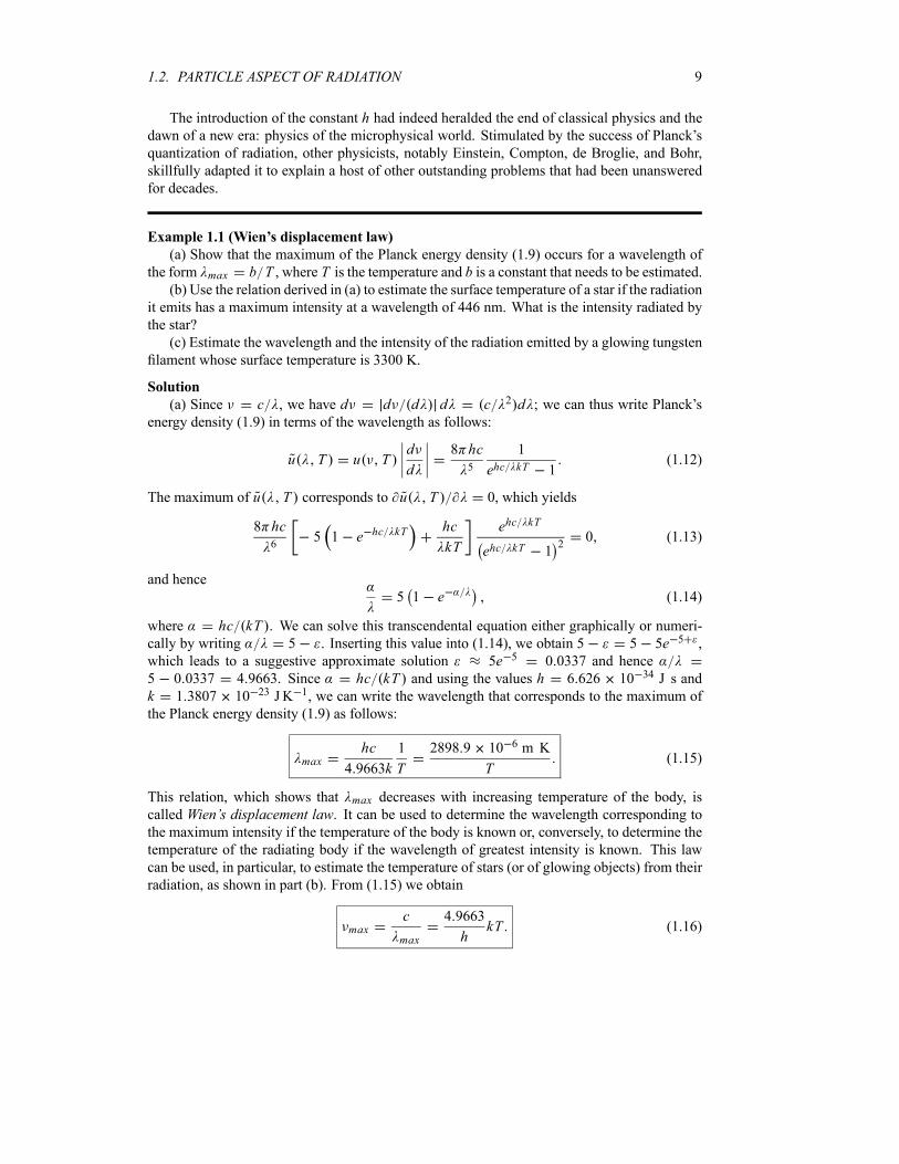
Example 1.1 (Wien’s displacement law)
(a) Show that the maximum of the Planck energy density (1.9) occurs for a wavelength of
the form max b T , where T is the temperature and b is a constant that needs to be estimated.(b) Use the relation derived in (a) to estimate the surface temperature of a star if the radiation
it emits has a maximum intensity at a wavelength of 446 nm. What is the intensity radiated by
the star?
(c) Estimate the wavelength and the intensity of the radiation emitted by a glowing tungsten
filament whose surface temperature is 3300 K.
Solution
(a) Since c , we have d d d d c 2 d ; we can thus write Planck’senergy density (1.9) in terms of the wavelength as follows:
u T u Td
d
8 hc5
1
ehc kT 1(1.12)
The maximum of u T corresponds to u T 0, which yields
8 hc6
5 1 e hc kT hc
kT
ehc kT
ehc kT 12
0 (1.13)
and hence
5 1 e (1.14)
where hc kT . We can solve this transcendental equation either graphically or numeri-cally by writing 5 . Inserting this value into (1.14), we obtain 5 5 5e 5 ,
which leads to a suggestive approximate solution 5e 5 0 0337 and hence
5 0 0337 4 9663. Since hc kT and using the values h 6 626 10 34 J s and
k 1 3807 10 23 J K 1, we can write the wavelength that corresponds to the maximum of
the Planck energy density (1.9) as follows:
maxhc
4 9663k
1
T
2898 9 10 6 m K
T(1.15)
This relation, which shows that max decreases with increasing temperature of the body, is
called Wien’s displacement law. It can be used to determine the wavelength corresponding tothe maximum intensity if the temperature of the body is known or, conversely, to determine the
temperature of the radiating body if the wavelength of greatest intensity is known. This law
can be used, in particular, to estimate the temperature of stars (or of glowing objects) from their
radiation, as shown in part (b). From (1.15) we obtain
maxc
max
4 9663
hkT (1.16)
10 CHAPTER 1. ORIGINS OF QUANTUM PHYSICS
This relation shows that the peak of the radiation spectrum occurs at a frequency that is propor-
tional to the temperature.
(b) If the radiation emitted by the star has a maximum intensity at a wavelength of max
446 nm, its surface temperature is given by
T2898 9 10 6 m K
446 10 9 m6500 K (1.17)
Using Stefan–Boltzmann’s law (1.1), and assuming the star to radiate like a blackbody, we can
estimate the total power per unit surface area emitted at the surface of the star:
P T 4 5 67 10 8 Wm 2K 4 6500 K 4 101 2 106 Wm 2 (1.18)
This is an enormous intensity which will decrease as it spreads over space.
(c) The wavelength of greatest intensity of the radiation emitted by a glowing tungsten
filament of temperature 3300 K is
max2898 9 10 6 m K
3300 K878 45 nm (1.19)
The intensity (or total power per unit surface area) radiated by the filament is given by
P T 4 5 67 10 8 Wm 2K 4 3300 K 4 6 7 106 Wm 2 (1.20)
1.2.2 Photoelectric Effect
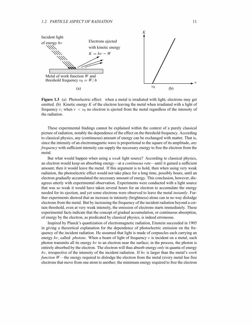
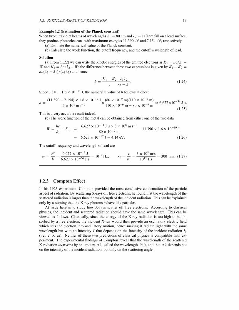
The photoelectric effect provides a direct confirmation for the energy quantization of light. In
1887 Hertz discovered the photoelectric effect: electrons6 were observed to be ejected from
metals when irradiated with light (Figure 1.3a). Moreover, the following experimental laws
were discovered prior to 1905:
If the frequency of the incident radiation is smaller than the metal’s threshold frequency—
a frequency that depends on the properties of the metal—no electron can be emitted
regardless of the radiation’s intensity (Philip Lenard, 1902).
No matter how low the intensity of the incident radiation, electrons will be ejected in-stantly the moment the frequency of the radiation exceeds the threshold frequency 0.
At any frequency above 0, the number of electrons ejected increases with the intensity
of the light but does not depend on the light’s frequency.
The kinetic energy of the ejected electrons depends on the frequency but not on the in-
tensity of the beam; the kinetic energy of the ejected electron increases linearly with theincident frequency.
6In 1899 J. J. Thomson confirmed that the particles giving rise to the photoelectric effect (i.e., the particles ejected
from the metals) are electrons.
1.2. PARTICLE ASPECT OF RADIATION 11
Incident light
of energy h@@@@
@@@@
@@@@
@@@@@R@R@R@R ©©
©©©*
³³³³
³1»»»
»:
Electrons ejected
with kinetic energy
K h W
Metal of work function W andthreshold frequency 0 W h
(a)
-
6K
¢¢¢¢¢¢¢¢¢¢¢
¢¢¢¢¢¢¢¢¢¢¢
0 (b)
Figure 1.3 (a) Photoelectric effect: when a metal is irradiated with light, electrons may get
emitted. (b) Kinetic energy K of the electron leaving the metal when irradiated with a light offrequency ; when 0 no electron is ejected from the metal regardless of the intensity of
the radiation.
These experimental findings cannot be explained within the context of a purely classical
picture of radiation, notably the dependence of the effect on the threshold frequency. According
to classical physics, any (continuous) amount of energy can be exchanged with matter. That is,
since the intensity of an electromagnetic wave is proportional to the square of its amplitude, anyfrequency with sufficient intensity can supply the necessary energy to free the electron from themetal.
But what would happen when using a weak light source? According to classical physics,an electron would keep on absorbing energy—at a continuous rate—until it gained a sufficientamount; then it would leave the metal. If this argument is to hold, then when using very weak
radiation, the photoelectric effect would not take place for a long time, possibly hours, until an
electron gradually accumulated the necessary amount of energy. This conclusion, however, dis-
agrees utterly with experimental observation. Experiments were conducted with a light source
that was so weak it would have taken several hours for an electron to accumulate the energy
needed for its ejection, and yet some electrons were observed to leave the metal instantly. Fur-ther experiments showed that an increase in intensity (brightness) alone can in no way dislodge
electrons from the metal. But by increasing the frequency of the incident radiation beyond a cer-
tain threshold, even at very weak intensity, the emission of electrons starts immediately. These
experimental facts indicate that the concept of gradual accumulation, or continuous absorption,
of energy by the electron, as predicated by classical physics, is indeed erroneous.
Inspired by Planck’s quantization of electromagnetic radiation, Einstein succeeded in 1905
in giving a theoretical explanation for the dependence of photoelectric emission on the fre-
quency of the incident radiation. He assumed that light is made of corpuscles each carrying an
energy h , called photons. When a beam of light of frequency is incident on a metal, each
photon transmits all its energy h to an electron near the surface; in the process, the photon is
entirely absorbed by the electron. The electron will thus absorb energy only in quanta of energyh , irrespective of the intensity of the incident radiation. If h is larger than the metal’s workfunction W—the energy required to dislodge the electron from the metal (every metal has freeelectrons that move from one atom to another; the minimum energy required to free the electron
12 CHAPTER 1. ORIGINS OF QUANTUM PHYSICS
from the metal is called the work function of that metal)—the electron will then be knocked out
of the metal. Hence no electron can be emitted from the metal’s surface unless h W :
h W K (1.21)
where K represents the kinetic energy of the electron leaving the material.Equation (1.21), which was derived by Einstein, gives the proper explanation to the exper-
imental observation that the kinetic energy of the ejected electron increases linearly with theincident frequency , as shown in Figure 1.3b:
K h W h 0 (1.22)
where 0 W h is called the threshold or cutoff frequency of the metal. Moreover, thisrelation shows clearly why no electron can be ejected from the metal unless 0: since the
kinetic energy cannot be negative, the photoelectric effect cannot occur when 0 regardless
of the intensity of the radiation. The ejected electrons acquire their kinetic energy from the
excess energy h 0 supplied by the incident radiation.
The kinetic energy of the emitted electrons can be experimentally determined as follows.
The setup, which was devised by Lenard, consists of the photoelectric metal (cathode) that is
placed next to an anode inside an evacuated glass tube. When light strikes the cathode’s surface,
the electrons ejected will be attracted to the anode, thereby generating a photoelectric current.
It was found that the magnitude of the photoelectric current thus generated is proportional tothe intensity of the incident radiation, yet the speed of the electrons does not depend on theradiation’s intensity, but on its frequency. To measure the kinetic energy of the electrons, wesimply need to use a varying voltage source and reverse the terminals. When the potential Vacross the tube is reversed, the liberated electrons will be prevented from reaching the anode;
only those electrons with kinetic energy larger than e V will make it to the negative plate and
contribute to the current. We vary V until it reaches a value Vs , called the stopping potential,at which all of the electrons, even the most energetic ones, will be turned back before reaching
the collector; hence the flow of photoelectric current ceases completely. The stopping potential
Vs is connected to the electrons’ kinetic energy by e Vs12me 2 K (in what follows, Vs
will implicitly denote Vs ). Thus, the relation (1.22) becomes eVs h W or
Vsh
e
W
e
hc
e
W
e(1.23)
The shape of the plot of Vs against frequency is a straight line, much like Figure 1.3b withthe slope now given by h e. This shows that the stopping potential depends linearly on thefrequency of the incident radiation.
It was Millikan who, in 1916, gave a systematic experimental confirmation to Einstein’s
photoelectric theory. He produced an extensive collection of photoelectric data using various
metals. He verified that Einstein’s relation (1.23) reproduced his data exactly. In addition,
Millikan found that his empirical value for h, which he obtained by measuring the slope h e of(1.23) (Figure 1.3b), is equal to Planck’s constant to within a 0 5% experimental error.
In summary, the photoelectric effect does provide compelling evidence for the corpuscular
nature of the electromagnetic radiation.
1.2. PARTICLE ASPECT OF RADIATION 13
Example 1.2 (Estimation of the Planck constant)
When two ultraviolet beams of wavelengths 1 80 nm and 2 110 nm fall on a lead surface,
they produce photoelectrons with maximum energies 11 390 eV and 7 154 eV, respectively.
(a) Estimate the numerical value of the Planck constant.
(b) Calculate the work function, the cutoff frequency, and the cutoff wavelength of lead.
Solution
(a) From (1.22) we can write the kinetic energies of the emitted electrons as K1 hc 1
W and K2 hc 2 W ; the difference between these two expressions is given by K1 K2hc 2 1 1 2 and hence
hK1 K2c
1 2
2 1(1.24)
Since 1 eV 1 6 10 19 J, the numerical value of h follows at once:
h11 390 7 154 1 6 10 19 J
3 108 ms 1
80 10 9 m 110 10 9 m
110 10 9 m 80 10 9 m6 627 10 34 J s
(1.25)
This is a very accurate result indeed.
(b) The work function of the metal can be obtained from either one of the two data
Whc
1K1
6 627 10 34 J s 3 108 ms 1
80 10 9 m11 390 1 6 10 19 J
6 627 10 19 J 4 14 eV (1.26)
The cutoff frequency and wavelength of lead are
0W
h
6 627 10 19 J
6 627 10 34 J s1015 Hz 0
c
0
3 108 m/s
1015 Hz300 nm (1.27)
1.2.3 Compton Effect
In his 1923 experiment, Compton provided the most conclusive confirmation of the particle
aspect of radiation. By scattering X-rays off free electrons, he found that the wavelength of the
scattered radiation is larger than the wavelength of the incident radiation. This can be explained
only by assuming that the X-ray photons behave like particles.
At issue here is to study how X-rays scatter off free electrons. According to classical
physics, the incident and scattered radiation should have the same wavelength. This can be
viewed as follows. Classically, since the energy of the X-ray radiation is too high to be ab-
sorbed by a free electron, the incident X-ray would then provide an oscillatory electric field
which sets the electron into oscillatory motion, hence making it radiate light with the same
wavelength but with an intensity I that depends on the intensity of the incident radiation I0(i.e., I I0). Neither of these two predictions of classical physics is compatible with ex-periment. The experimental findings of Compton reveal that the wavelength of the scattered
X-radiation increases by an amount , called the wavelength shift, and that depends not
on the intensity of the incident radiation, but only on the scattering angle.
14 CHAPTER 1. ORIGINS OF QUANTUM PHYSICS
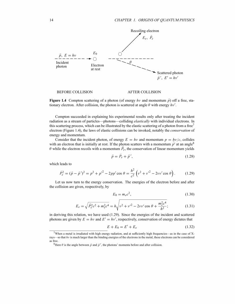
-
Electronat rest
Incidentphoton
p E h
BEFORE COLLISION
E0¡¡¡¡¡µ
PPPPPPPPq
Recoiling electron
Ee Pe
Scattered photon
p E h
AFTER COLLISION
Figure 1.4 Compton scattering of a photon (of energy h and momentum p) off a free, sta-tionary electron. After collision, the photon is scattered at angle with energy h .
Compton succeeded in explaining his experimental results only after treating the incident
radiation as a stream of particles—photons—colliding elastically with individual electrons. Inthis scattering process, which can be illustrated by the elastic scattering of a photon from a free7
electron (Figure 1.4), the laws of elastic collisions can be invoked, notably the conservation ofenergy and momentum.
Consider that the incident photon, of energy E h and momentum p h c, collideswith an electron that is initially at rest. If the photon scatters with a momentum p at an angle8
while the electron recoils with a momentum Pe, the conservation of linear momentum yields
p Pe p (1.28)
which leads to
P2e p p 2 p2 p2
2pp cosh2
c22 2
2 cos (1.29)
Let us now turn to the energy conservation. The energies of the electron before and after
the collision are given, respectively, by
E0 mec2 (1.30)
Ee P2e c2 m2ec
4 h 2 2 2 cosm2ec
4
h2(1.31)
in deriving this relation, we have used (1.29). Since the energies of the incident and scattered
photons are given by E h and E h , respectively, conservation of energy dictates that
E E0 E Ee (1.32)
7When a metal is irradiated with high energy radiation, and at sufficiently high frequencies—as in the case of X-
rays—so that h is much larger than the binding energies of the electrons in the metal, these electrons can be considered
as free.8Here is the angle between p and p , the photons’ momenta before and after collision.
1.2. PARTICLE ASPECT OF RADIATION 15
or
h mec2 h h 2 2 2 cos
m2ec4
h2(1.33)
which in turn leads to
mec2
h2 2 2 cos
m2ec4
h2(1.34)
Squaring both sides of (1.34) and simplifying, we end up with
1 1 h
mec21 cos
2h
mec2sin 2
2(1.35)
Hence the wavelength shift is given by
h
mec1 cos 2 C sin
2
2(1.36)
where C h mec 2 426 10 12 m is called the Compton wavelength of the electron.
This relation, which connects the initial and final wavelengths to the scattering angle, confirms
Compton’s experimental observation: the wavelength shift of the X-rays depends only on the
angle at which they are scattered and not on the frequency (or wavelength) of the incident
photons.
In summary, the Compton effect confirms that photons behave like particles: they collide
with electrons like material particles.
Example 1.3 (Compton effect)
High energy photons ( -rays) are scattered from electrons initially at rest. Assume the photons
are backscatterred and their energies are much larger than the electron’s rest-mass energy, Emec2.(a) Calculate the wavelength shift.
(b) Show that the energy of the scattered photons is half the rest mass energy of the electron,
regardless of the energy of the incident photons.
(c) Calculate the electron’s recoil kinetic energy if the energy of the incident photons is
150 MeV.
Solution
(a) In the case where the photons backscatter (i.e., ), the wavelength shift (1.36)
becomes
2 C sin2
22 C 4 86 10 12 m (1.37)
since C h mec 2 426 10 12 m.
(b) Since the energy of the scattered photons E is related to the wavelength by Ehc , equation (1.37) yields
Ehc hc
2h mec
mec2
mec2 hc 2
mec2
mec2 E 2(1.38)
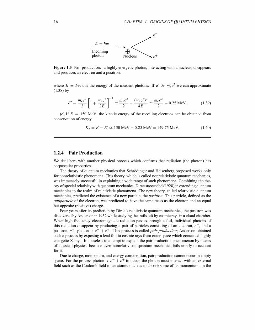
16 CHAPTER 1. ORIGINS OF QUANTUM PHYSICS
-
Nucleus
Incomingphoton
E h ©©©©
©*
HHHHHj
e
e
Figure 1.5 Pair production: a highly energetic photon, interacting with a nucleus, disappears
and produces an electron and a positron.
where E hc is the energy of the incident photons. If E mec2 we can approximate(1.38) by
Emec2
21
mec2
2E
1mec2
2
mec2 2
4E
mec2
20 25 MeV (1.39)
(c) If E 150 MeV, the kinetic energy of the recoiling electrons can be obtained from
conservation of energy
Ke E E 150 MeV 0 25 MeV 149 75 MeV (1.40)
1.2.4 Pair Production
We deal here with another physical process which confirms that radiation (the photon) has
corpuscular properties.
The theory of quantum mechanics that Schrödinger and Heisenberg proposed works only
for nonrelativistic phenomena. This theory, which is called nonrelativistic quantum mechanics,
was immensely successful in explaining a wide range of such phenomena. Combining the the-
ory of special relativity with quantummechanics, Dirac succeeded (1928) in extending quantum
mechanics to the realm of relativistic phenomena. The new theory, called relativistic quantum
mechanics, predicted the existence of a new particle, the positron. This particle, defined as theantiparticle of the electron, was predicted to have the same mass as the electron and an equalbut opposite (positive) charge.
Four years after its prediction by Dirac’s relativistic quantum mechanics, the positron was
discovered by Anderson in 1932while studying the trails left by cosmic rays in a cloud chamber.
When high-frequency electromagnetic radiation passes through a foil, individual photons of
this radiation disappear by producing a pair of particles consisting of an electron, e , and apositron, e : photon e e . This process is called pair production; Anderson obtainedsuch a process by exposing a lead foil to cosmic rays from outer space which contained highly
energetic X-rays. It is useless to attempt to explain the pair production phenomenon by means
of classical physics, because even nonrelativistic quantum mechanics fails utterly to account
for it.
Due to charge, momentum, and energy conservation, pair production cannot occur in empty
space. For the process photon e e to occur, the photon must interact with an external
field such as the Coulomb field of an atomic nucleus to absorb some of its momentum. In the
1.2. PARTICLE ASPECT OF RADIATION 17
reaction depicted in Figure 1.5, an electron–positron pair is produced when the photon comes
near (interacts with) a nucleus at rest; energy conservation dictates that
h Ee Ee EN mec2 ke mec
2 ke KN
2mec2 ke ke (1.41)
where h is the energy of the incident photon, 2mec2 is the sum of the rest masses of theelectron and positron, and ke and ke are the kinetic energies of the electron and positron,
respectively. As for EN KN , it represents the recoil energy of the nucleus which is purelykinetic. Since the nucleus is very massive compared to the electron and the positron, KN canbe neglected to a good approximation. Note that the photon cannot produce an electron or a
positron alone, for electric charge would not be conserved. Also, a massive object, such as the
nucleus, must participate in the process to take away some of the photon’s momentum.
The inverse of pair production, called pair annihilation, also occurs. For instance, when
an electron and a positron collide, they annihilate each other and give rise to electromagneticradiation9: e e photon. This process explains why positrons do not last long in nature.
When a positron is generated in a pair production process, its passage through matter will make
it lose some of its energy and it eventually gets annihilated after colliding with an electron.
The collision of a positron with an electron produces a hydrogen-like atom, called positronium,with a mean lifetime of about 10 10 s; positronium is like the hydrogen atom where the proton
is replaced by the positron. Note that, unlike pair production, energy and momentum can
simultaneously be conserved in pair annihilation processes without any additional (external)
field or mass such as the nucleus.
The pair production process is a direct consequence of the mass–energy equation of Einstein
E mc2, which states that pure energy can be converted into mass and vice versa. Conversely,pair annihilation occurs as a result of mass being converted into pure energy. All subatomic
particles also have antiparticles (e.g., antiproton). Even neutral particles have antiparticles;
for instance, the antineutron is the neutron’s antiparticle. Although this text deals only with
nonrelativistic quantum mechanics, we have included pair production and pair annihilation,
which are relativistic processes, merely to illustrate how radiation interacts with matter, and
also to underscore the fact that the quantum theory of Schrödinger and Heisenberg is limited to
nonrelativistic phenomena only.
Example 1.4 (Minimum energy for pair production)
Calculate the minimum energy of a photon so that it converts into an electron–positron pair.
Find the photon’s frequency and wavelength.
Solution
The minimum energy Emin of a photon required to produce an electron–positron pair must beequal to the sum of rest mass energies of the electron and positron; this corresponds to the case
where the kinetic energies of the electron and positron are zero. Equation (1.41) yields
Emin 2mec2 2 0 511 MeV 1 02 MeV (1.42)
9When an electron–positron pair annihilate, they produce at least two photons each having an energy mec2
0 511 MeV.
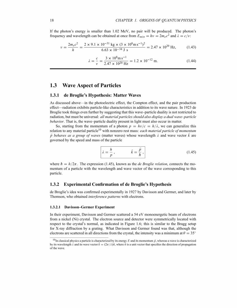
18 CHAPTER 1. ORIGINS OF QUANTUM PHYSICS
If the photon’s energy is smaller than 1 02 MeV, no pair will be produced. The photon’s
frequency and wavelength can be obtained at once from Emin h 2mec2 and c :
2mec2
h
2 9 1 10 31 kg 3 108ms 1 2
6 63 10 34 J s2 47 1020 Hz (1.43)
c 3 108ms 1
2 47 1020 Hz1 2 10 12 m (1.44)
1.3 Wave Aspect of Particles
1.3.1 de Broglie’s Hypothesis: Matter Waves
As discussed above—in the photoelectric effect, the Compton effect, and the pair production
effect—radiation exhibits particle-like characteristics in addition to its wave nature. In 1923 de
Broglie took things even further by suggesting that this wave–particle duality is not restricted to
radiation, but must be universal: all material particles should also display a dual wave–particlebehavior. That is, the wave–particle duality present in light must also occur in matter.So, starting from the momentum of a photon p h c h , we can generalize this
relation to any material particle10 with nonzero rest mass: each material particle of momentump behaves as a group of waves (matter waves) whose wavelength and wave vector k aregoverned by the speed and mass of the particle
h
pk
p
h(1.45)
where h h 2 . The expression (1.45), known as the de Broglie relation, connects the mo-mentum of a particle with the wavelength and wave vector of the wave corresponding to this
particle.
1.3.2 Experimental Confirmation of de Broglie’s Hypothesis
de Broglie’s idea was confirmed experimentally in 1927 by Davisson and Germer, and later by
Thomson, who obtained interference patterns with electrons.
1.3.2.1 Davisson–Germer Experiment
In their experiment, Davisson and Germer scattered a 54 eV monoenergetic beam of electrons
from a nickel (Ni) crystal. The electron source and detector were symmetrically located with
respect to the crystal’s normal, as indicated in Figure 1.6; this is similar to the Bragg setup
for X-ray diffraction by a grating. What Davisson and Germer found was that, although the
electrons are scattered in all directions from the crystal, the intensity was a minimum at 35
10In classical physics a particle is characterized by its energy E and its momentum p, whereas a wave is characterizedby its wavelength and its wave vector k 2 n, where n is a unit vector that specifies the direction of propagationof the wave.
1.3. WAVE ASPECT OF PARTICLES 19
@@@@@R¡
¡¡¡¡µ
Electron
source
@¡
¡@ Electron
detector¡@
@¡2 2
Ni crystal
Figure 1.6 Davisson–Germer experiment: electrons strike the crystal’s surface at an angle ;
the detector, symmetrically located from the electron source, measures the number of electrons
scattered at an angle , where is the angle between the incident and scattered electron beams.
and a maximum at 50 ; that is, the bulk of the electrons scatter only in well-specified
directions. They showed that the pattern persisted even when the intensity of the beam was so
low that the incident electrons were sent one at a time. This can only result from a constructive
interference of the scattered electrons. So, instead of the diffuse distribution pattern that results
from material particles, the reflected electrons formed diffraction patterns that were identical
with Bragg’s X-ray diffraction by a grating. In fact, the intensity maximum of the scatteredelectrons in the Davisson–Germer experiment corresponds to the first maximum (n 1) of
the Bragg formula,
n 2d sin (1.46)
where d is the spacing between the Bragg planes, is the angle between the incident ray and the
crystal’s reflecting planes, is the angle between the incident and scattered beams (d is givenin terms of the separation D between successive atomic layers in the crystal by d D sin ).
For an Ni crystal, we have d 0 091 nm, since D 0 215 nm. Since only one maximum
is seen at 50 for a mono-energetic beam of electrons of kinetic energy 54 eV, and since
2 and hence sin cos 2 (Figure 1.6), we can obtain from (1.46) the
wavelength associated with the scattered electrons:
2d
nsin
2d
ncos
1
2
2 0 091 nm
1cos 25 0 165 nm (1.47)
Now, let us look for the numerical value of that results from de Broglie’s relation. Since the
kinetic energy of the electrons is K 54 eV, and since the momentum is p 2meK withmec2 0 511 MeV (the rest mass energy of the electron) and hc 197 33 eV nm, we can
show that the de Broglie wavelength is
h
p
h
2meK
2 hc
2mec2K0 167 nm (1.48)
which is in excellent agreement with the experimental value (1.47).
We have seen that the scattered electrons in the Davisson–Germer experiment produced
interference fringes that were identical to those of Bragg’s X-ray diffraction. Since the Bragg
formula provided an accurate prediction of the electrons’ interference fringes, the motion of an
electron of momentum p must be described by means of a plane wave
r t Aei k r t Aei p r Et h (1.49)

20 CHAPTER 1. ORIGINS OF QUANTUM PHYSICS
Incident
electron
beam-------HH
HHHHHHHHHHHH
Thin film
Photographic plateHHHHHHHH
HHHHHHHH
XXXXXXXXXXXXXXXXXXXX
XXXXXXXXXXz
»»»»»»
»»»»»»
»»»»»»
»»»
»»»»»»
»»»»:
hhhhhhhhhhhhhhhhhhhh
((((((((
((((((((
((((
Diffraction rings
Figure 1.7 Thomson experiment: diffraction of electrons through a thin film of polycrystalline
material yields fringes that usually result from light diffraction.
where A is a constant, k is the wave vector of the plane wave, and is its angular frequency;
the wave’s parameters, k and , are related to the electron’s momentum p and energy E bymeans of de Broglie’s relations: k p h, E h.We should note that, inspired by de Broglie’s hypothesis, Schrödinger constructed the the-
ory of wave mechanics which deals with the dynamics of microscopic particles. He described
the motion of particles by means of awave function r t which corresponds to the de Brogliewave of the particle. We will deal with the physical interpretation of r t in the followingsection.
1.3.2.2 Thomson Experiment
In the Thomson experiment (Figure 1.7), electrons were diffracted through a polycrystalline
thin film. Diffraction fringes were also observed. This result confirmed again the wave behavior
of electrons.
The Davisson–Germer experiment has inspired others to obtain diffraction patterns with a
large variety of particles. Interference patterns were obtained with bigger and bigger particles
such as neutrons, protons, helium atoms, and hydrogen molecules. de Broglie wave interference
of carbon 60 (C60) molecules were recently11 observed by diffraction at a material absorption
grating; these observations supported the view that each C60 molecule interferes only with
itself (a C60 molecule is nearly a classical object).
1.3.3 Matter Waves for Macroscopic Objects
We have seen that microscopic particles, such as electrons, display wave behavior. What about
macroscopic objects? Do they also display wave features? They surely do. Although macro-
11Markus Arndt, et al., "Wave–Particle Duality of C60 Molecules", Nature, V401, n6754, 680 (Oct. 14, 1999).
1.3. WAVE ASPECT OF PARTICLES 21
scopic material particles display wave properties, the corresponding wavelengths are too small
to detect; being very massive12, macroscopic objects have extremely small wavelengths. At the
microscopic level, however, the waves associated with material particles are of the same size
or exceed the size of the system. Microscopic particles therefore exhibit clearly discernible
wave-like aspects.
The general rule is: whenever the de Broglie wavelength of an object is in the range of, or
exceeds, its size, the wave nature of the object is detectable and hence cannot be neglected. But
if its de Broglie wavelength is much too small compared to its size, the wave behavior of this
object is undetectable. For a quantitative illustration of this general rule, let us calculate in the
following example the wavelengths corresponding to two particles, one microscopic and the
other macroscopic.
Example 1.5 (Matter waves for microscopic and macroscopic systems)
Calculate the de Broglie wavelength for
(a) a proton of kinetic energy 70 MeV kinetic energy and
(b) a 100 g bullet moving at 900 m s 1.
Solution
(a) Since the kinetic energy of the proton is T p2 2m p , its momentum is p 2Tm p.
The de Broglie wavelength is p h p h 2Tm p. To calculate this quantity numerically,it is more efficient to introduce the well-known quantity hc 197 MeV fm and the rest mass
of the proton m pc2 938 3 MeV, where c is the speed of light:
p 2hc
pc2
hc
2Tm pc22
197 MeV fm
2 938 3 70 MeV23 4 10 15 m (1.50)
(b) As for the bullet, its de Broglie wavelength is b h p h m and since h6 626 10 34 J s, we have
bh
m
6 626 10 34 J s
0 1 kg 900 m s 17 4 10 36 m (1.51)
The ratio of the two wavelengths is b p 2 2 10 21. Clearly, the wave aspect of this
bullet lies beyond human observational abilities. As for the wave aspect of the proton, it cannot
be neglected; its de Broglie wavelength of 3 4 10 15 m has the same order of magnitude as
the size of a typical atomic nucleus.
We may conclude that, whereas the wavelengths associated with microscopic systems arefinite and display easily detectable wave-like patterns, the wavelengths associated with macro-scopic systems are infinitesimally small and display no discernible wave-like behavior. So,when the wavelength approaches zero, the wave-like properties of the system disappear. In
such cases of infinitesimally small wavelengths, geometrical optics should be used to describethe motion of the object, for the wave associated with it behaves as a ray.
12Very massive compared to microscopic particles. For instance, the ratio between the mass of an electron and a
100 g bullet is infinitesimal: me mb 10 29.
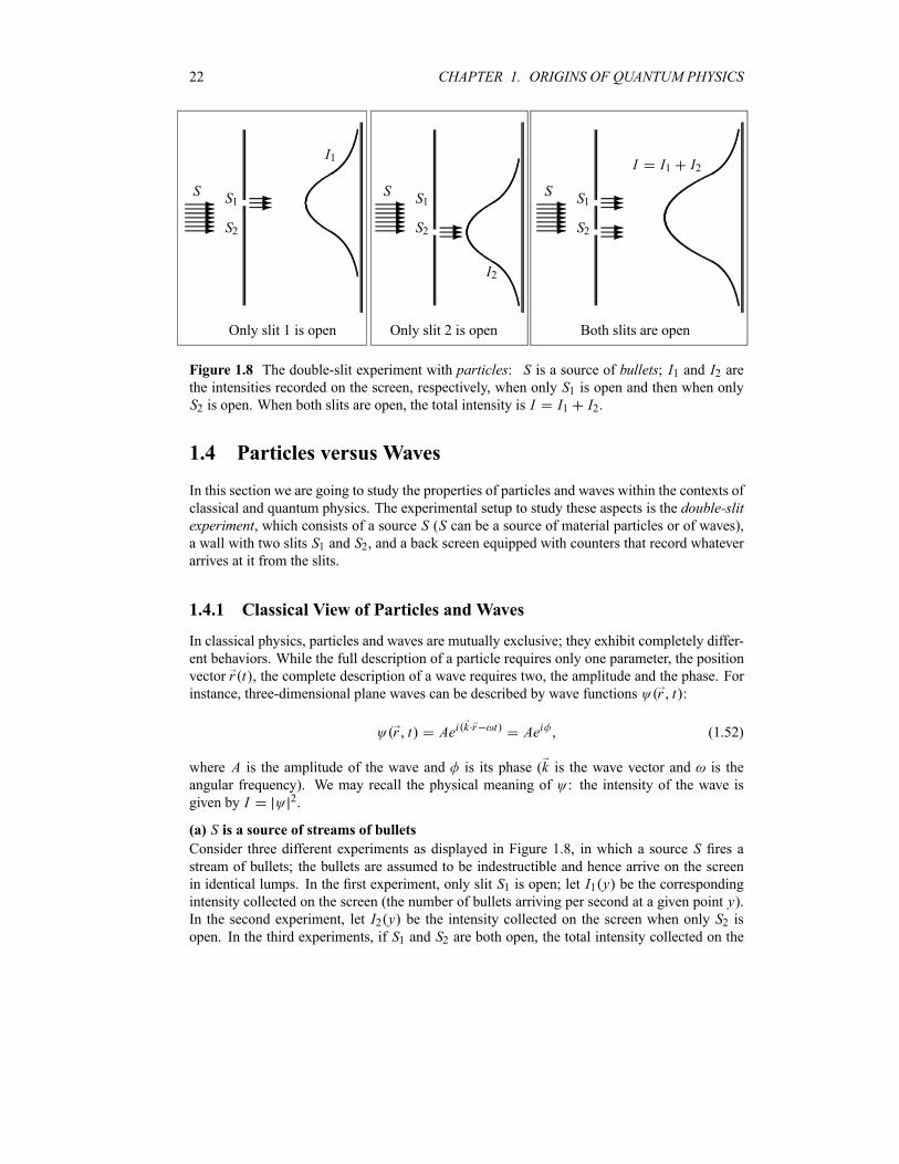
22 CHAPTER 1. ORIGINS OF QUANTUM PHYSICS
-------
S S1
S2
---
I1
Only slit 1 is open
-------
S S1
S2 ---
I2
Only slit 2 is open
-------
S S1
S2
------
Both slits are open
I I1 I2
Figure 1.8 The double-slit experiment with particles: S is a source of bullets; I1 and I2 arethe intensities recorded on the screen, respectively, when only S1 is open and then when onlyS2 is open. When both slits are open, the total intensity is I I1 I2.
1.4 Particles versus Waves
In this section we are going to study the properties of particles and waves within the contexts of
classical and quantum physics. The experimental setup to study these aspects is the double-slitexperiment, which consists of a source S (S can be a source of material particles or of waves),a wall with two slits S1 and S2, and a back screen equipped with counters that record whateverarrives at it from the slits.
1.4.1 Classical View of Particles and Waves
In classical physics, particles and waves are mutually exclusive; they exhibit completely differ-
ent behaviors. While the full description of a particle requires only one parameter, the position
vector r t , the complete description of a wave requires two, the amplitude and the phase. Forinstance, three-dimensional plane waves can be described by wave functions r t :
r t Aei k r t Aei (1.52)
where A is the amplitude of the wave and is its phase (k is the wave vector and is the
angular frequency). We may recall the physical meaning of : the intensity of the wave is
given by I 2.
(a) S is a source of streams of bulletsConsider three different experiments as displayed in Figure 1.8, in which a source S fires astream of bullets; the bullets are assumed to be indestructible and hence arrive on the screen
in identical lumps. In the first experiment, only slit S1 is open; let I1 y be the correspondingintensity collected on the screen (the number of bullets arriving per second at a given point y).In the second experiment, let I2 y be the intensity collected on the screen when only S2 isopen. In the third experiments, if S1 and S2 are both open, the total intensity collected on the
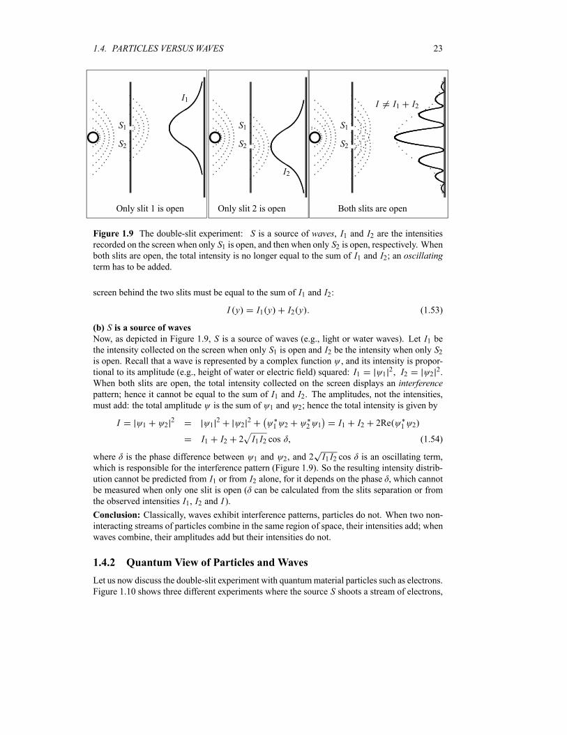
1.4. PARTICLES VERSUS WAVES 23
ijk S1
S2
I1
Only slit 1 is open
ijk S1
S2
I2
Only slit 2 is open
ijk S1
S2
Both slits are open
I I1 I2
Figure 1.9 The double-slit experiment: S is a source of waves, I1 and I2 are the intensitiesrecorded on the screen when only S1 is open, and then when only S2 is open, respectively. Whenboth slits are open, the total intensity is no longer equal to the sum of I1 and I2; an oscillatingterm has to be added.
screen behind the two slits must be equal to the sum of I1 and I2:
I y I1 y I2 y (1.53)
(b) S is a source of wavesNow, as depicted in Figure 1.9, S is a source of waves (e.g., light or water waves). Let I1 bethe intensity collected on the screen when only S1 is open and I2 be the intensity when only S2is open. Recall that a wave is represented by a complex function , and its intensity is propor-
tional to its amplitude (e.g., height of water or electric field) squared: I1 12 I2 2
2.
When both slits are open, the total intensity collected on the screen displays an interferencepattern; hence it cannot be equal to the sum of I1 and I2. The amplitudes, not the intensities,must add: the total amplitude is the sum of 1 and 2; hence the total intensity is given by
I 1 22
12
22
1 2 2 1 I1 I2 2Re 1 2
I1 I2 2 I1 I2 cos (1.54)
where is the phase difference between 1 and 2, and 2 I1 I2 cos is an oscillating term,
which is responsible for the interference pattern (Figure 1.9). So the resulting intensity distrib-
ution cannot be predicted from I1 or from I2 alone, for it depends on the phase , which cannotbe measured when only one slit is open ( can be calculated from the slits separation or from
the observed intensities I1, I2 and I ).
Conclusion: Classically, waves exhibit interference patterns, particles do not. When two non-
interacting streams of particles combine in the same region of space, their intensities add; when
waves combine, their amplitudes add but their intensities do not.
1.4.2 Quantum View of Particles and Waves
Let us now discuss the double-slit experiment with quantummaterial particles such as electrons.
Figure 1.10 shows three different experiments where the source S shoots a stream of electrons,
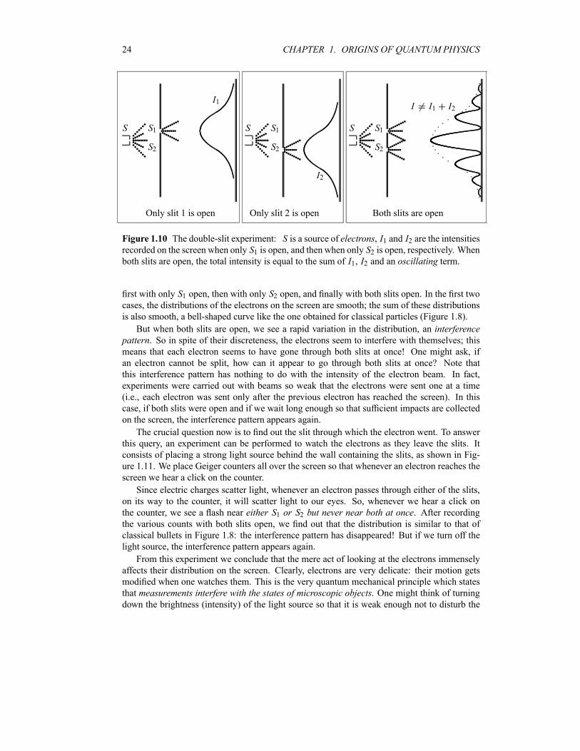
24 CHAPTER 1. ORIGINS OF QUANTUM PHYSICS
S qqqqqqqqqqqqqqqqqqqqqqqqqqqqqqqqqqS1
S2
qqqqqqqqqqqqqqqqqqqqqqqqqqI1
Only slit 1 is open
S qqqqqqqqqqqqqqqqqqqqqqqqqqqqqqqqqS1
S2 qqqqqqqqqqqqqqqqqqqqqqqqqI2
Only slit 2 is open
S qqqqqqqqqqqqqqqqqqqqqqqqqqqqqqqqqqS1
S2
Both slits are open
qqqqqqqqqqqqqqqqqqqqqqqqqqqqqqqqqqqqqqqqqqqqqqqqqqq
I I1 I2
Figure 1.10 The double-slit experiment: S is a source of electrons, I1 and I2 are the intensitiesrecorded on the screen when only S1 is open, and then when only S2 is open, respectively. Whenboth slits are open, the total intensity is equal to the sum of I1, I2 and an oscillating term.
first with only S1 open, then with only S2 open, and finally with both slits open. In the first twocases, the distributions of the electrons on the screen are smooth; the sum of these distributions
is also smooth, a bell-shaped curve like the one obtained for classical particles (Figure 1.8).
But when both slits are open, we see a rapid variation in the distribution, an interferencepattern. So in spite of their discreteness, the electrons seem to interfere with themselves; thismeans that each electron seems to have gone through both slits at once! One might ask, if
an electron cannot be split, how can it appear to go through both slits at once? Note that
this interference pattern has nothing to do with the intensity of the electron beam. In fact,
experiments were carried out with beams so weak that the electrons were sent one at a time
(i.e., each electron was sent only after the previous electron has reached the screen). In this
case, if both slits were open and if we wait long enough so that sufficient impacts are collected
on the screen, the interference pattern appears again.
The crucial question now is to find out the slit through which the electron went. To answer
this query, an experiment can be performed to watch the electrons as they leave the slits. It
consists of placing a strong light source behind the wall containing the slits, as shown in Fig-
ure 1.11. We place Geiger counters all over the screen so that whenever an electron reaches the
screen we hear a click on the counter.
Since electric charges scatter light, whenever an electron passes through either of the slits,
on its way to the counter, it will scatter light to our eyes. So, whenever we hear a click on
the counter, we see a flash near either S1 or S2 but never near both at once. After recordingthe various counts with both slits open, we find out that the distribution is similar to that of
classical bullets in Figure 1.8: the interference pattern has disappeared! But if we turn off the
light source, the interference pattern appears again.
From this experiment we conclude that the mere act of looking at the electrons immensely
affects their distribution on the screen. Clearly, electrons are very delicate: their motion gets
modified when one watches them. This is the very quantum mechanical principle which states
that measurements interfere with the states of microscopic objects. One might think of turningdown the brightness (intensity) of the light source so that it is weak enough not to disturb the
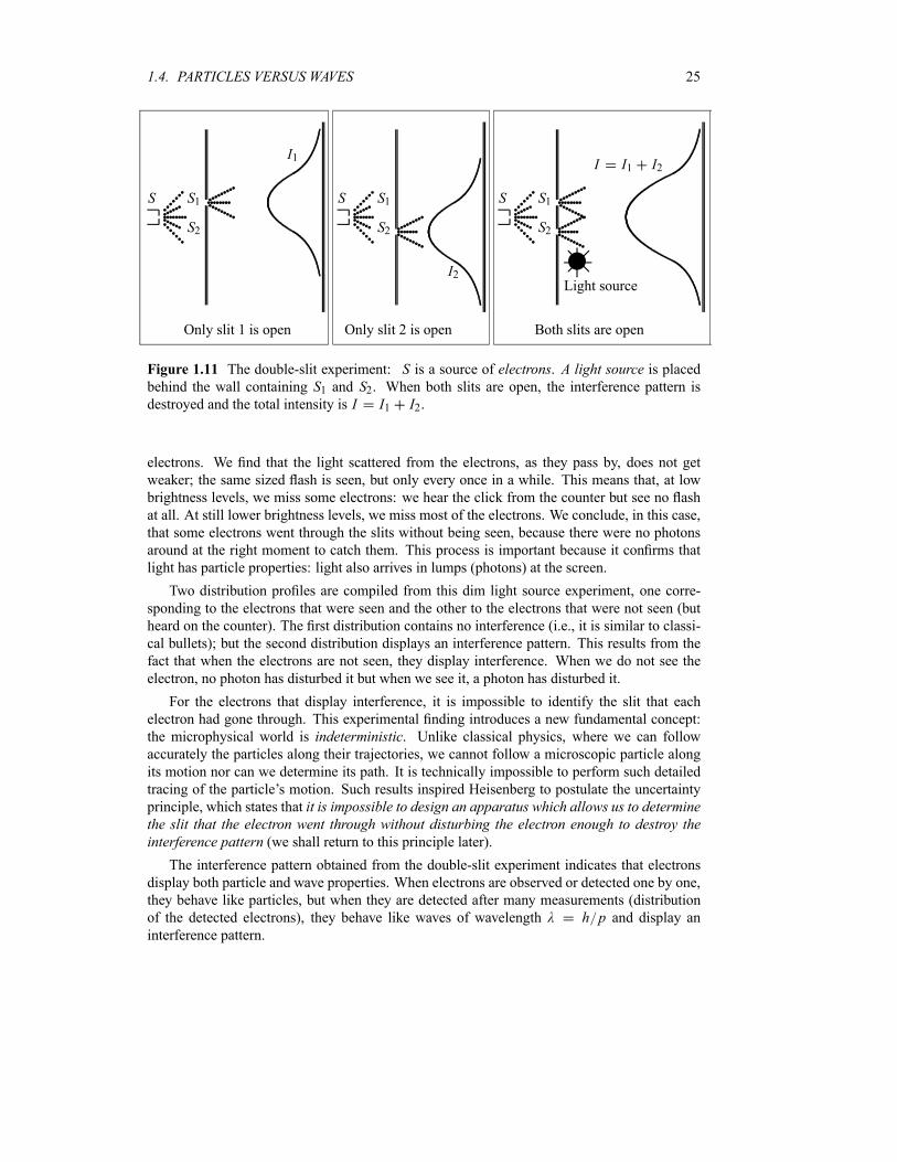
1.4. PARTICLES VERSUS WAVES 25
S qqqqqqqqqqqqqqqqqqqqqqqqqqqqqqqqqqS1
S2
qqqqqqqqqqqqqqqqqqqqqqqqqqI1
Only slit 1 is open
S qqqqqqqqqqqqqqqqqqqqqqqqqqqqqqqqqS1
S2 qqqqqqqqqqqqqqqqqqqqqqqqqI2
Only slit 2 is open
S qqqqqqqqqqqqqqqqqqqqqqqqqqqqqqqqqqS1
S2
Both slits are open
qqqqqqqqqqqqqqqqqqqqqqqqqqqqqqqqqqqqqqqqqqqqqqqqqqq{Light source
¡¡@@
I I1 I2
Figure 1.11 The double-slit experiment: S is a source of electrons. A light source is placedbehind the wall containing S1 and S2. When both slits are open, the interference pattern isdestroyed and the total intensity is I I1 I2.
electrons. We find that the light scattered from the electrons, as they pass by, does not get
weaker; the same sized flash is seen, but only every once in a while. This means that, at low
brightness levels, we miss some electrons: we hear the click from the counter but see no flash
at all. At still lower brightness levels, we miss most of the electrons. We conclude, in this case,
that some electrons went through the slits without being seen, because there were no photons
around at the right moment to catch them. This process is important because it confirms that
light has particle properties: light also arrives in lumps (photons) at the screen.
Two distribution profiles are compiled from this dim light source experiment, one corre-
sponding to the electrons that were seen and the other to the electrons that were not seen (but
heard on the counter). The first distribution contains no interference (i.e., it is similar to classi-
cal bullets); but the second distribution displays an interference pattern. This results from the
fact that when the electrons are not seen, they display interference. When we do not see the
electron, no photon has disturbed it but when we see it, a photon has disturbed it.
For the electrons that display interference, it is impossible to identify the slit that each
electron had gone through. This experimental finding introduces a new fundamental concept:
the microphysical world is indeterministic. Unlike classical physics, where we can followaccurately the particles along their trajectories, we cannot follow a microscopic particle along
its motion nor can we determine its path. It is technically impossible to perform such detailed
tracing of the particle’s motion. Such results inspired Heisenberg to postulate the uncertainty
principle, which states that it is impossible to design an apparatus which allows us to determinethe slit that the electron went through without disturbing the electron enough to destroy theinterference pattern (we shall return to this principle later).
The interference pattern obtained from the double-slit experiment indicates that electrons
display both particle and wave properties. When electrons are observed or detected one by one,
they behave like particles, but when they are detected after many measurements (distribution
of the detected electrons), they behave like waves of wavelength h p and display aninterference pattern.
26 CHAPTER 1. ORIGINS OF QUANTUM PHYSICS
1.4.3 Wave–Particle Duality: Complementarity
The various experimental findings discussed so far—blackbody radiation, photoelectric and
Compton effect, pair production, Davisson–Germer, Thomson, and the double-slit experiments—
reveal that photons, electrons, and any other microscopic particles behave unlike classical par-
ticles and unlike classical waves. These findings indicate that, at the microscopic scale, nature
can display particle behavior as well as wave behavior. The question now is, how can something
behave as a particle and as a wave at the same time? Aren’t these notions mutually exclusive?
In the realm of classical physics the answer is yes, but not in quantum mechanics. This dualbehavior can in no way be reconciled within the context of classical physics, for particles and
waves are mutually exclusive entities.
The theory of quantum mechanics, however, provides the proper framework for reconcil-
ing the particle and wave aspects of matter. By using a wave function r t (see (1.49))to describe material particles such as electrons, quantum mechanics can simultaneously make
statements about the particle behavior and the wave behavior of microscopic systems. It com-
bines the quantization of energy or intensity with a wave description of matter. That is, it uses
both particle and wave pictures to describe the same material particle.
Our ordinary concepts of particles or waves are thus inadequate when applied to micro-
scopic systems. These two concepts, which preclude each other in the macroscopic realm, do
not strictly apply to the microphysical world. No longer valid at the microscopic scale is the
notion that a wave cannot behave as a particle and vice versa. The true reality of a quantum
system is that it is neither a pure particle nor a pure wave. The particle and wave aspects of
a quantum system manifest themselves only when subjected to, or intruded on by, penetrating
means of observation (any procedure of penetrating observation would destroy the initial state
of the quantum system; for instance, the mere act of looking at an electron will knock it out
of its orbit). Depending on the type of equipment used to observe an electron, the electron
has the capacity to display either “grain” or wave features. As illustrated by the double-slit
experiment, if we wanted to look at the particle aspect of the electron, we would need only to
block one slit (or leave both slits open but introduce an observational apparatus), but if we were
interested only in its wave features, we would have to leave both slits open and not intrude on
it by observational tools. This means that both the “grain” and “wave” features are embedded
into the electron, and by modifying the probing tool, we can suppress one aspect of the electron
and keep the other. An experiment designed to isolate the particle features of a quantum system
gives no information about its wave features, and vice versa. When we subject an electron to
Compton scattering, we observe only its particle aspects, but when we involve it in a diffraction
experiment (as in Davisson–Germer, Thomson, or the double-slit experiment), we observe its
wave behavior only. So if we measure the particle properties of a quantum system, this will
destroy its wave properties, and vice versa. Any measurement gives either one property or the
other, but never both at once. We can get either the wave property or the particle but not both
of them together.
Microscopic systems, therefore, are neither pure particles nor pure waves, they are both.
The particle and wave manifestations do not contradict or preclude one another, but, as sug-
gested by Bohr, they are just complementary. Both concepts are complementary in describingthe true nature of microscopic systems. Being complementary features of microscopic matter,
particles and waves are equally important for a complete description of quantum systems. From
here comes the essence of the complementarity principle.We have seen that when the rigid concept of either/or (i.e., either a particle or a wave)
is indiscriminately applied or imposed on quantum systems, we get into trouble with reality.
1.5. INDETERMINISTIC NATURE OF THE MICROPHYSICAL WORLD 27
Without the complementarity principle, quantum mechanics would not have been in a position
to produce the accurate results it does.
1.4.4 Principle of Linear Superposition
How do we account mathematically for the existence of the interference pattern in the double-
slit experiment with material particles such as electrons? An answer is offered by the superpo-sition principle. The interference results from the superposition of the waves emitted by slits1 and 2. If the functions 1 r t and 2 r t , which denote the waves reaching the screenemitted respectively by slits 1 and 2, represent two physically possible states of the system,
then any linear superposition
r t 1 1 r t 2 2 r t (1.55)
also represents a physically possible outcome of the system; 1 and 2 are complex constants.
This is the superposition principle. The intensity produced on the screen by opening only slit
1 is 1 r t2 and it is 2 r t
2 when only slit 2 is open. When both slits are open, the
intensity is
r t 21 r t 2 r t
2
1 r t2
2 r t2
1 r t 2 r t 1 r t 2 r t
(1.56)
where the asterisk denotes the complex conjugate. Note that (1.56) is not equal to the sum of
1 r t2 and 2 r t
2; it contains an additional term 1 r t 2 r t 1 r t 2 r t .This is the very term which gives rise in the case of electrons to an interference pattern similar
to light waves. The interference pattern therefore results from the existence of a phase shift
between 1 r t and 2 r t . We can measure this phase shift from the interference pattern,but we can in no way measure the phases of 1 and 2 separately.
We can summarize the double-slit results in three principles:
Intensities add for classical particles: I I1 I2.
Amplitudes, not intensities, add for quantum particles: r t 1 r t 2 r t ;this gives rise to interference.
Whenever one attempts to determine experimentally the outcome of individual events
for microscopic material particles (such as trying to specify the slit through which an
electron has gone), the interference pattern gets destroyed. In this case the intensities add
in much the same way as for classical particles: I I1 I2.
1.5 Indeterministic Nature of the Microphysical World
Let us first mention two important experimental findings that were outlined above. On the one
hand, the Davisson–Germer and the double-slit experiments have shown that microscopic ma-
terial particles do give rise to interference patterns. To account for the interference pattern, we
have seen that it is imperative to describe microscopic particles by means of waves. Waves are
28 CHAPTER 1. ORIGINS OF QUANTUM PHYSICS
not localized in space. As a result, we have to give up on accuracy to describe microscopic
particles, for waves give at best a probabilistic account. On the other hand, we have seen in the
double-slit experiment that it is impossible to trace the motion of individual electrons; there is
no experimental device that would determine the slit through which a given electron has gone.
Not being able to predict single events is a stark violation of a founding principle of classi-
cal physics: predictability or determinacy. These experimental findings inspired Heisenberg
to postulate the indeterministic nature of the microphysical world and Born to introduce the
probabilistic interpretation of quantum mechanics.
1.5.1 Heisenberg’s Uncertainty Principle
According to classical physics, given the initial conditions and the forces acting on a system,
the future behavior (unique path) of this physical system can be determined exactly. That is,
if the initial coordinates r0, velocity 0, and all the forces acting on the particle are known,
the position r t and velocity t are uniquely determined by means of Newton’s second law.Classical physics is thus completely deterministic.Does this deterministic view hold also for the microphysical world? Since a particle is rep-
resented within the context of quantum mechanics by means of a wave function corresponding
to the particle’s wave, and since wave functions cannot be localized, then a microscopic particle
is somewhat spread over space and, unlike classical particles, cannot be localized in space. In
addition, we have seen in the double-slit experiment that it is impossible to determine the slit
that the electron went through without disturbing it. The classical concepts of exact position,
exact momentum, and unique path of a particle therefore make no sense at the microscopic
scale. This is the essence of Heisenberg’s uncertainty principle.
In its original form, Heisenberg’s uncertainty principle states that: If the x-component ofthe momentum of a particle is measured with an uncertainty px , then its x-position cannot,at the same time, be measured more accurately than x h 2 px . The three-dimensionalform of the uncertainty relations for position and momentum can be written as follows:
x pxh
2y py
h
2z pz
h
2(1.57)
This principle indicates that, although it is possible to measure the momentum or position
of a particle accurately, it is not possible to measure these two observables simultaneously toan arbitrary accuracy. That is, we cannot localize a microscopic particle without giving to ita rather large momentum. We cannot measure the position without disturbing it; there is no
way to carry out such a measurement passively as it is bound to change the momentum. To
understand this, consider measuring the position of a macroscopic object (e.g., a car) and the
position of a microscopic system (e.g., an electron in an atom). On the one hand, to locate the
position of a macroscopic object, you need simply to observe it; the light that strikes it and gets
reflected to the detector (your eyes or a measuring device) can in no measurable way affect the
motion of the object. On the other hand, to measure the position of an electron in an atom, you
must use radiation of very short wavelength (the size of the atom). The energy of this radiation
is high enough to change tremendously the momentum of the electron; the mere observation
of the electron affects its motion so much that it can knock it entirely out of its orbit. It is
therefore impossible to determine the position and the momentum simultaneously to arbitrary
accuracy. If a particle were localized, its wave function would become zero everywhere else and
its wave would then have a very short wavelength. According to de Broglie’s relation p h ,
1.5. INDETERMINISTIC NATURE OF THE MICROPHYSICAL WORLD 29
the momentum of this particle will be rather high. Formally, this means that if a particle isaccurately localized (i.e., x 0), there will be total uncertainty about its momentum (i.e.,
px ). To summarize, since all quantum phenomena are described by waves, we have no
choice but to accept limits on our ability to measure simultaneously any two complementary
variables.
Heisenberg’s uncertainty principle can be generalized to any pair of complementary, or
canonically conjugate, dynamical variables: it is impossible to devise an experiment that canmeasure simultaneously two complementary variables to arbitrary accuracy (if this were everachieved, the theory of quantum mechanics would collapse).
Energy and time, for instance, form a pair of complementary variables. Their simultaneous
measurement must obey the time–energy uncertainty relation:
E th
2(1.58)
This relation states that if we make two measurements of the energy of a system and if these
measurements are separated by a time interval t , the measured energies will differ by anamount E which can in no way be smaller than h t . If the time interval between the twomeasurements is large, the energy difference will be small. This can be attributed to the fact
that, when the first measurement is carried out, the system becomes perturbed and it takes it
a long time to return to its initial, unperturbed state. This expression is particularly useful in
the study of decay processes, for it specifies the relationship between the mean lifetime and the
energy width of the excited states.
We see that, in sharp contrast to classical physics, quantum mechanics is a completelyindeterministic theory. Asking about the position or momentum of an electron, one cannotget a definite answer; only a probabilistic answer is possible. According to the uncertaintyprinciple, if the position of a quantum system is well defined, its momentum will be totally
undefined. In this context, the uncertainty principle has clearly brought down one of the most
sacrosanct concepts of classical physics: the deterministic nature of Newtonian mechanics.
Example 1.6 (Uncertainties for microscopic and macroscopic systems)
Estimate the uncertainty in the position of (a) a neutron moving at 5 106ms 1 and (b) a 50 kg
person moving at 2m s 1.
Solution
(a) Using (1.57), we can write the position uncertainty as
xh
2 p
h
2mn
1 05 10 34 J s
2 1 65 10 27 kg 5 106 ms 16 4 10 15 m (1.59)
This distance is comparable to the size of a nucleus.
(b) The position uncertainty for the person is
xh
2 p
h
2m
1 05 10 34 J s
2 50 kg 2 m s 10 5 10 36 m (1.60)
An uncertainty of this magnitude is beyond human detection; therefore, it can be neglected. The
accuracy of the person’s position is limited only by the uncertainties induced by the device used
30 CHAPTER 1. ORIGINS OF QUANTUM PHYSICS
in the measurement. So the position and momentum uncertainties are important for microscopic
systems, but negligible for macroscopic systems.
1.5.2 Probabilistic Interpretation
In quantum mechanics the state (or one of the states) of a particle is described by a wavefunction r t corresponding to the de Broglie wave of this particle; so r t describes thewave properties of a particle. As a result, when discussing quantum effects, it is suitable to
use the amplitude function, , whose square modulus, 2, is equal to the intensity of the
wave associated with this quantum effect. The intensity of a wave at a given point in space is
proportional to the probability of finding, at that point, the material particle that corresponds to
the wave.
In 1927 Born interpreted 2 as the probability density and r t 2d3r as the probability,dP r t , of finding a particle at time t in the volume element d3r located between r and r dr :
r t 2d3r d P r t (1.61)
where 2 has the dimensions of [Length] 3. If we integrate over the entire space, we are
certain that the particle is somewhere in it. Thus, the total probability of finding the particle
somewhere in space must be equal to one:
all spacer t 2d3r 1 (1.62)
The main question now is, how does one determine the wave function of a particle? The
answer to this question is given by the theory of quantum mechanics, where is determined
by the Schrödinger equation (Chapters 3 and 4).
1.6 Atomic Transitions and Spectroscopy
Besides failing to explain blackbody radiation, the Compton, photoelectric, and pair production
effects and the wave–particle duality, classical physics also fails to account for many other
phenomena at the microscopic scale. In this section we consider another area where classical
physics breaks down—the atom. Experimental observations reveal that atoms exist as stable,
bound systems that have discrete numbers of energy levels. Classical physics, however, statesthat any such bound system must have a continuum of energy levels.
1.6.1 Rutherford Planetary Model of the Atom
After his experimental discovery of the atomic nucleus in 1911, Rutherford proposed a model
in an attempt to explain the properties of the atom. Inspired by the orbiting motion of the
planets around the sun, Rutherford considered the atom to consist of electrons orbiting around
a positively charged massive center, the nucleus. It was soon recognized that, within the context
of classical physics, this model suffers from two serious deficiencies: (a) atoms are unstableand (b) atoms radiate energy over a continuous range of frequencies.The first deficiency results from the application of Maxwell’s electromagnetic theory to
Rutherford’s model: as the electron orbits around the nucleus, it accelerates and hence radiates

1.6. ATOMIC TRANSITIONS AND SPECTROSCOPY 31
energy. It must therefore lose energy. The radius of the orbit should then decrease continuously
(spiral motion) until the electron collapses onto the nucleus; the typical time for such a collapse
is about 10 8 s. Second, since the frequency of the radiated energy is the same as the orbiting
frequency, and as the electron orbit collapses, its orbiting frequency increases continuously.Thus, the spectrum of the radiation emitted by the atom should be continuous. These two
conclusions completely disagree with experiment, since atoms are stable and radiate energyover discrete frequency ranges.
1.6.2 Bohr Model of the Hydrogen Atom
Combining Rutherford’s planetary model, Planck’s quantum hypothesis, and Einstein’s pho-
ton concept, Bohr proposed in 1913 a model that gives an accurate account of the observed
spectrum of the hydrogen atom as well as a convincing explanation for its stability.
Bohr assumed, as in Rutherford’s model, that each atom’s electron moves in an orbit around
the nucleus under the influence of the electrostatic attraction of the nucleus; circular or elliptic
orbits are allowed by classical mechanics. For simplicity, Bohr considered only circular orbits,
and introduced several, rather arbitrary assumptions which violate classical physics but which
are immensely successful in explaining many properties of the hydrogen atom:
Instead of a continuum of orbits, which are possible in classical mechanics, only a dis-crete set of circular stable orbits, called stationary states, are allowed. Atoms can existonly in certain stable states with definite energies: E1, E2, E3, etc.
The allowed (stationary) orbits correspond to those for which the orbital angular momen-
tum of the electron is an integer multiple of h (h h 2 ):
L nh (1.63)
This relation is known as the Bohr quantization rule of the angular momentum.
As long as an electron remains in a stationary orbit, it does not radiate electromagnetic
energy. Emission or absorption of radiation can take place only when an electron jumps
from one allowed orbit to another. The radiation corresponding to the electron’s transition
from an orbit of energy En to another Em is carried out by a photon of energy
h En Em (1.64)
So an atom may emit (or absorb) radiation by having the electron jump to a lower (or
higher) orbit.
In what follows we are going to apply Bohr’s assumptions to the hydrogen atom. We want to
provide a quantitative description of its energy levels and its spectroscopy.
1.6.2.1 Energy Levels of the Hydrogen Atom
Let us see how Bohr’s quantization condition (1.63) leads to a discrete set of energies En andradii rn . When the electron of the hydrogen atom moves in a circular orbit, the applicationof Newton’s second law to the electron yields F mear me 2 r . Since the only force13
13At the atomic scale, gravity has no measurable effect. The gravitational force between the hydrogen’s proton and
electron, FG Gmem p r2, is negligible compared to the electrostatic force Fe e2 4 0r2 , since FG Fe
4 0 Gmem p e2 10 40.
32 CHAPTER 1. ORIGINS OF QUANTUM PHYSICS
acting on the electron is the electrostatic force applied on it by the proton, we can equate the
electrostatic force to the centripetal force and obtain
e2
4 0r2me
2
r(1.65)
Now, assumption (1.63) yields
L me r nh (1.66)
hence me 2 r n2h2 mer3 , which when combined with (1.65) yields e2 4 0r2
n2h2 mer3 ; this relation in turn leads to a quantized expression for the radius:
rn4 0h
2
mee2n2 n2a0 (1.67)
where
a04 0h
2
mee2(1.68)
is the Bohr radius, a0 0 053 nm. The speed of the orbiting electron can be obtained from
(1.66) and (1.67):
nnh
mern
e2
4 0
1
nh(1.69)
Note that the ratio between the speed of the electron in the first Bohr orbit, 1, and the speed of
light is equal to a dimensionless constant , known as the fine structure constant:
1
c
1
4 0
e2
hc
1
1371 c
3 108 ms 1
1372 19 106 ms 1 (1.70)
As for the total energy of the electron, it is given by
E1
2me
2 1
4 0
e2
r(1.71)
in deriving this relation, we have assumed that the nucleus, i.e., the proton, is infinitely heavy
compared with the electron and hence it can be considered at rest; that is, the energy of the
electron–proton system consists of the kinetic energy of the electron plus the electrostatic po-
tential energy. From (1.65) we see that the kinetic energy, 12me 2, is equal to 1
2e2 4 0r ,
which when inserted into (1.71) leads to
E1
2
e2
4 0r(1.72)
This equation shows that the electron circulates in an orbit of radius r with a kinetic energyequal to minus one half the potential energy (this result is the well known Virial theorem of
classical mechanics). Substituting rn of (1.67) into (1.72), we obtain
Ene2
8 0
1
rn
me
2h2e2
4 0
21
n2R
n2(1.73)
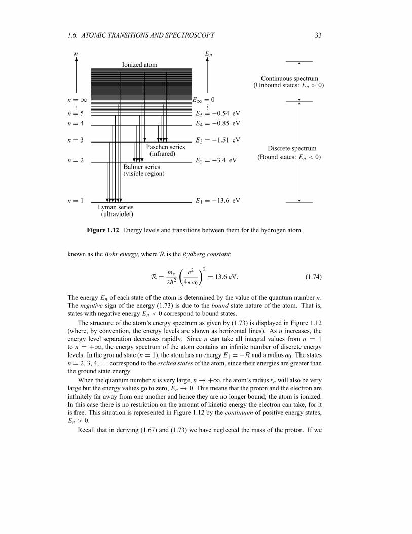
1.6. ATOMIC TRANSITIONS AND SPECTROSCOPY 33
Ionized atom
n 1
n 2
n 3
n 4
n 5
n
6n
E1 13 6 eV
E2 3 4 eV
E3 1 51 eV
E4 0 85 eV
E5 0 54 eV
E 0
6En
??????Lyman series(ultraviolet)
????
?
Balmer series(visible region)
????Paschen series(infrared)
Discrete spectrum
(Bound states: En 0)
Continuous spectrum(Unbound states: En 0)
?
6?
6
Figure 1.12 Energy levels and transitions between them for the hydrogen atom.
known as the Bohr energy, whereR is the Rydberg constant:
Rme
2h2e2
4 0
2
13 6 eV (1.74)
The energy En of each state of the atom is determined by the value of the quantum number n.The negative sign of the energy (1.73) is due to the bound state nature of the atom. That is,states with negative energy En 0 correspond to bound states.
The structure of the atom’s energy spectrum as given by (1.73) is displayed in Figure 1.12
(where, by convention, the energy levels are shown as horizontal lines). As n increases, theenergy level separation decreases rapidly. Since n can take all integral values from n 1
to n , the energy spectrum of the atom contains an infinite number of discrete energy
levels. In the ground state (n 1), the atom has an energy E1 R and a radius a0. The statesn 2 3 4 correspond to the excited states of the atom, since their energies are greater thanthe ground state energy.
When the quantum number n is very large, n , the atom’s radius rn will also be verylarge but the energy values go to zero, En 0. This means that the proton and the electron are
infinitely far away from one another and hence they are no longer bound; the atom is ionized.
In this case there is no restriction on the amount of kinetic energy the electron can take, for it
is free. This situation is represented in Figure 1.12 by the continuum of positive energy states,En 0.
Recall that in deriving (1.67) and (1.73) we have neglected the mass of the proton. If we
34 CHAPTER 1. ORIGINS OF QUANTUM PHYSICS
include it, the expressions (1.67) and (1.73) become
rn4 0h2
e2n2 1
mem p
a0n2 En
2h2e2
4 0
21
n21
1 me m p
R
n2
(1.75)
where m pme m p me me 1 me m p is the reduced mass of the proton–electronsystem.
We should note that rn and En of (1.75), which were derived for the hydrogen atom, canbe generalized to hydrogen-like ions where all electrons save one are removed. To obtain the
radius and energy of a single electron orbiting a fixed nucleus of Z protons, we need simply toreplace e2 in (1.75) by Ze2,
rn 1meM
a0Zn2 En
Z2
1 me M
R
n2(1.76)
where M is the mass of the nucleus; when me M 1 we can just drop the term me M .
de Broglie’s hypothesis and Bohr’s quantization condition
The Bohr quantization condition (1.63) can be viewed as a manifestation of de Broglie’s hypoth-
esis. For the wave associated with the atom’s electron to be a standing wave, the circumference
of the electron’s orbit must be equal to an integral multiple of the electron’s wavelength:
2 r n n 1 2 3 (1.77)
This relation can be reduced to (1.63) or to (1.66), provided that we make use of de Broglie’s
relation, h p h me . That is, inserting h me into (1.77) and using the fact
that the electron’s orbital angular momentum is L me r , we have
2 r n nh
meme r n
h
2L nh (1.78)
which is identical with Bohr’s quantization condition (1.63). In essence, this condition states
that the only allowed orbits for the electron are those whose circumferences are equal to integral
multiples of the de Broglie wavelength. For example, in the hydrogen atom, the circumference
of the electron’s orbit is equal to when the atom is in its ground state (n 1); it is equal to
2 when the atom is in its first excited state (n 2); equal to 3 when the atom is in its second
excited state (n 3); and so on.
1.6.2.2 Spectroscopy of the Hydrogen Atom
Having specified the energy spectrum of the hydrogen atom, let us now study its spectroscopy.
In sharp contrast to the continuous nature of the spectral distribution of the radiation emitted by
glowing solid objects, the radiation emitted or absorbed by a gas displays a discrete spectrumdistribution. When subjecting a gas to an electric discharge (or to a flame), the radiation emitted
from the excited atoms of the gas discharge consists of a few sharp lines (bright lines of pure
color, with darkness in between). A major success of Bohr’s model lies in its ability to predict
accurately the sharpness of the spectral lines emitted or absorbed by the atom. The modelshows clearly that these discrete lines correspond to the sharply defined energy levels of the
1.6. ATOMIC TRANSITIONS AND SPECTROSCOPY 35
atom. The radiation emitted from the atom results from the transition of the electron from an
allowed state n to another m; this radiation has a well defined (sharp) frequency :
h En Em R1
m21
n2(1.79)
For instance, the Lyman series, which corresponds to the emission of ultraviolet radiation, isdue to transitions from excited states n 2 3 4 5 to the ground state n 1 (Figure 1.12):
h L En E1 R1
121
n2n 1 (1.80)
Another transition series, the Balmer series, is due to transitions to the first excited state (n2):
h B En E2 R1
221
n2n 2 (1.81)
The atom emits visible radiation as a result of the Balmer transitions. Other series are Paschen,n 3 with n 3; Brackett, n 4 with n 4; Pfund, n 5 with n 5; and so on. They
correspond to the emission of infrared radiation. Note that the results obtained from (1.79) arein spectacular agreement with those of experimental spectroscopy.
So far in this chapter, we have seen that when a photon passes through matter, it interacts
as follows:
If it comes in contact with an electron that is at rest, it will scatter from it like a corpus-
cular particle: it will impart a momentum to the electron, it will scatter and continue its
travel with the speed of light but with a lower frequency (or higher wavelength). This is
the Compton effect.
If it comes into contact with an atom’s electron, it will interact according to one of the
following scenarios:
– If it has enough energy, it will knock the electron completely out of the atom and
then vanish, for it transmits all its energy to the electron. This is the photoelectric
effect.
– If its energy h is not sufficient to knock out the electron altogether, it will kick the
electron to a higher orbit, provided h is equal to the energy difference between the
initial and final orbits: h En Em . In the process it will transmit all its energyto the electron and then vanish. The atom will be left in an excited state. However,
if h En Em , nothing will happen (the photon simply scatters away).
If it comes in contact with an atomic nucleus and if its energy is sufficiently high (h2mec2), it will vanish by creating matter: an electron–positron pair will be produced.This is pair production.
Example 1.7 (Positronium’s radius and energy spectrum)
Positronium is the bound state of an electron and a positron; it is a short-lived, hydrogen-like
atom where the proton is replaced by a positron.
36 CHAPTER 1. ORIGINS OF QUANTUM PHYSICS
(a) Calculate the energy and radius expressions, En and rn .(b) Estimate the values of the energies and radii of the three lowest states.
(c) Calculate the frequency and wavelength of the electromagnetic radiation that will just
ionize the positronium atom when it is in its first excited state.
Solution
(a) The radius and energy expressions of the positronium can be obtained at once from
(1.75) by simply replacing the reduced mass with that of the electron–positron system
meme me me12me:
rn8 0h2
mee2n2 En
me
4h2e2
4 0
21
n2(1.82)
We can rewrite rn and En in terms of the Bohr radius, a0 4 0h2 mee2 0 053 nm, and
the Rydberg constant,R me2h2
e2
4 0
213 6 eV, as follows:
rn 2a0n2 En
R
2n2(1.83)
These are related to the expressions for the hydrogen by rn pos 2rnH and En pos12EnH .
(b) The radii of the three lowest states of the positronium are given by r1 2a0 0 106 nm,
r2 8a0 0 424 nm, and r3 18a0 0 954 nm. The corresponding energies are E112R 6 8 eV, E2
18R 1 7 eV, and E3
118R 0 756 eV.
(c) Since the energy of the first excited state of the positronium is E2 1 7 eV 1 7
1 6 10 19 J 2 72 10 19 J, the energy of the electromagnetic radiation that will just ionize
the positronium is equal to h E E2 0 2 72 10 19 J 2 72 10 19 J Eion;hence the frequency and wavelength of the ionizing radiation are given by
Eionh
2 72 10 19 J
6 6 10 34 J s4 12 1014 Hz (1.84)
c 3 108 ms 1
4 12 1014 Hz7 28 10 7 m (1.85)
1.7 Quantization Rules
The ideas that led to successful explanations of blackbody radiation, the photoelectric effect,
and the hydrogen’s energy levels rest on two quantization rules: (a) the relation (1.7) that Planck
postulated to explain the quantization of energy, E nh , and (b) the condition (1.63) thatBohr postulated to account for the quantization of the electron’s orbital angular momentum,
L nh. A number of attempts were undertaken to understand or interpret these rules. In 1916Wilson and Sommerfeld offered a scheme that included both quantization rules as special cases.
In essence, their scheme, which applies only to systems with coordinates that are periodic in
time, consists in quantizing the action variable, J p dq, of classical mechanics:
p dq nh n 0 1 2 3 (1.86)
1.7. QUANTIZATION RULES 37
where n is a quantum number, p is the momentum conjugate associated with the coordinateq; the closed integral is taken over one period of q. This relation is known as the Wilson–Sommerfeld quantization rule.
Wilson–Sommerfeld quantization rule and Planck’s quantization relation
In what follows we are going to show how theWilson–Sommerfeld rule (1.86) leads to Planck’s
quantization relation E nh . For an illustration, consider a one-dimensional harmonic os-cillator where a particle of mass m oscillates harmonically between a x a; its classicalenergy is given by
E x pp2
2m
1
2m 2x2 (1.87)
hence p E x 2mE m2 2x2. At the turning points, xmin a and xmax a,the energy is purely potential: E V a 1
2m 2a2; hence a 2E m 2 . Using
p E x 2mE m2 2x2 and from symmetry considerations, we can write the action as
p dx 2a
a2mE m2 2x2dx 4m
a
0
a2 x2dx (1.88)
The change of variables x a sin leads to
a
0
a2 x2dx a22
0
cos2 da2
2
2
0
1 cos 2 da2
4
E
2m 2(1.89)
Since 2 , where is the frequency of oscillations, we have
p dx2 E E
(1.90)
Inserting (1.90) into (1.86), we end up with the Planck quantization rule E nh , i.e.,
p dx nhE
nh En nh (1.91)
We can interpret this relation as follows. From classical mechanics, we know that the motion of
a mass subject to harmonic oscillations is represented in the xp phase space by a continuum ofellipses whose areas are given by p dx E , because the integral p x dx gives the areaenclosed by the closed trajectory of the particle in the xp phase space. The condition (1.86) or(1.91) provides a mechanism for selecting, from the continuum of the oscillator’s energy values,
only those energies En for which the areas of the contours p x En 2m En V x are
equal to nh with n 0, 1, 2, 3, . That is, the only allowed states of oscillation are those
represented in the phase space by a series of ellipses with “quantized” areas p dx nh. Notethat the area between two successive states is equal to h: p x En 1 dx p x En dx h.This simple calculation shows that the Planck rule for energy quantization is equivalent to
the quantization of action.
Wilson–Sommerfeld quantization rule and Bohr’s quantization condition
Let us now show how the Wilson–Sommerfeld rule (1.86) leads to Bohr’s quantization condi-
tion (1.63). For an electron moving in a circular orbit of radius r , it is suitable to use polarcoordinates r . The action J p dq, which is expressed in Cartesian coordinates by thelinear momentum p and its conjugate variable x , is characterized in polar coordinates by the
38 CHAPTER 1. ORIGINS OF QUANTUM PHYSICS
orbital angular momentum L and its conjugate variable , the polar angle, where is periodic
in time. That is, J p dq is given in polar coordinates by 20 L d . In this case (1.86)
becomes2
0
L d nh (1.92)
For spherically symmetric potentials—as it is the case here where the electron experiences the
proton’s Coulomb potential—the angular momentum L is a constant of the motion. Hence(1.92) shows that angular momentum can change only in integral units of h:
L2
0
d nh L nh
2nh (1.93)
which is identical with the Bohr quantization condition (1.63). This calculation also shows
that the Bohr quantization is equivalent to the quantization of action. As stated above (1.78),the Bohr quantization condition (1.63) has the following physical meaning: while orbiting the
nucleus, the electron moves only in well specified orbits, orbits with circumferences equal to
integral multiples of the de Broglie wavelength.
Note that the Wilson–Sommerfeld quantization rule (1.86) does not tell us how to calculate
the energy levels of non-periodic systems; it applies only to systems which are periodic. On a
historical note, the quantization rules of Planck and Bohr have dominated quantum physics from
1900 to 1925; the quantum physics of this period is known as the “old quantum theory.” The
success of these quantization rules, as measured by the striking agreement of their results with
experiment, gave irrefutable evidence for the quantization hypothesis of all material systems
and constituted a triumph of the “old quantum theory.” In spite of their quantitative success,
these quantization conditions suffer from a serious inconsistency: they do not originate from a
theory, they were postulated rather arbitrarily.
1.8 Wave Packets
At issue here is how to describe a particle within the context of quantum mechanics. As quan-
tum particles jointly display particle and wave features, we need to look for a mathematical
scheme that can embody them simultaneously.
In classical physics, a particle is well localized in space, for its position and velocity canbe calculated simultaneously to arbitrary precision. As for quantum mechanics, it describes
a material particle by a wave function corresponding to the matter wave associated with theparticle (de Broglie’s conjecture). Wave functions, however, depend on the whole space; hencethey cannot be localized. If the wave function is made to vanish everywhere except in theneighborhood of the particle or the neighborhood of the “classical trajectory,” it can then be
used to describe the dynamics of the particle. That is, a particle which is localized within a
certain region of space can be described by a matter wave whose amplitude is large in that
region and zero outside it. This matter wave must then be localized around the region of spacewithin which the particle is confined.
A localized wave function is called a wave packet. A wave packet therefore consists of agroup of waves of slightly different wavelengths, with phases and amplitudes so chosen that
they interfere constructively over a small region of space and destructively elsewhere. Not only
are wave packets useful in the description of “isolated” particles that are confined to a certain
spatial region, they also play a key role in understanding the connection between quantum
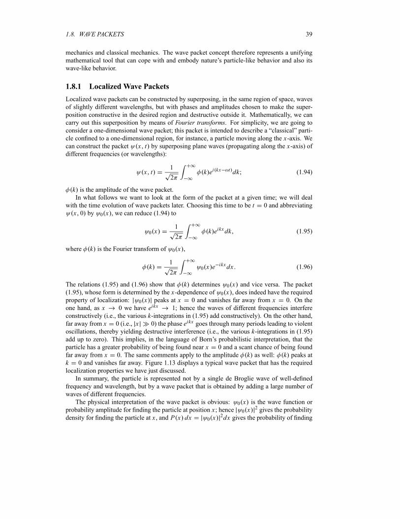
1.8. WAVE PACKETS 39
mechanics and classical mechanics. The wave packet concept therefore represents a unifying
mathematical tool that can cope with and embody nature’s particle-like behavior and also its
wave-like behavior.
1.8.1 Localized Wave Packets
Localized wave packets can be constructed by superposing, in the same region of space, waves
of slightly different wavelengths, but with phases and amplitudes chosen to make the super-
position constructive in the desired region and destructive outside it. Mathematically, we can
carry out this superposition by means of Fourier transforms. For simplicity, we are going toconsider a one-dimensional wave packet; this packet is intended to describe a “classical” parti-
cle confined to a one-dimensional region, for instance, a particle moving along the x-axis. Wecan construct the packet x t by superposing plane waves (propagating along the x-axis) ofdifferent frequencies (or wavelengths):
x t1
2k ei kx t dk (1.94)
k is the amplitude of the wave packet.In what follows we want to look at the form of the packet at a given time; we will deal
with the time evolution of wave packets later. Choosing this time to be t 0 and abbreviating
x 0 by 0 x , we can reduce (1.94) to
0 x1
2k eikxdk (1.95)
where k is the Fourier transform of 0 x ,
k1
20 x e
ikxdx (1.96)
The relations (1.95) and (1.96) show that k determines 0 x and vice versa. The packet
(1.95), whose form is determined by the x-dependence of 0 x , does indeed have the requiredproperty of localization: 0 x peaks at x 0 and vanishes far away from x 0. On the
one hand, as x 0 we have eikx 1; hence the waves of different frequencies interfere
constructively (i.e., the various k-integrations in (1.95) add constructively). On the other hand,far away from x 0 (i.e., x 0) the phase eikx goes through many periods leading to violentoscillations, thereby yielding destructive interference (i.e., the various k-integrations in (1.95)add up to zero). This implies, in the language of Born’s probabilistic interpretation, that the
particle has a greater probability of being found near x 0 and a scant chance of being found
far away from x 0. The same comments apply to the amplitude k as well: k peaks atk 0 and vanishes far away. Figure 1.13 displays a typical wave packet that has the required
localization properties we have just discussed.
In summary, the particle is represented not by a single de Broglie wave of well-defined
frequency and wavelength, but by a wave packet that is obtained by adding a large number of
waves of different frequencies.
The physical interpretation of the wave packet is obvious: 0 x is the wave function or
probability amplitude for finding the particle at position x ; hence 0 x2 gives the probability
density for finding the particle at x , and P x dx 0 x2dx gives the probability of finding
40 CHAPTER 1. ORIGINS OF QUANTUM PHYSICS
-
6
x0
0 x2
x
-
6
k
k0 k0
k 2
Figure 1.13 Two localized wave packets: 0 x 2 a2 1 4e x2 a2eik0x and k
a2 2 1 4e a2 k k02 4; they peak at x 0 and k k0, respectively, and vanish far away.
the particle between x and x dx . What about the physical interpretation of k ? From (1.95)and (1.96) it follows that
0 x2dx k 2dk (1.97)
then if x is normalized so is k , and vice versa. Thus, the function k can be interpretedmost naturally, like 0 x , as a probability amplitude for measuring a wave vector k for a parti-cle in the state k . Moreover, while k 2 represents the probability density for measuring kas the particle’s wave vector, the quantity P k dk k 2dk gives the probability of findingthe particle’s wave vector between k and k dk.We can extract information about the particle’s motion by simply expressing its correspond-
ing matter wave in terms of the particle’s energy, E , and momentum, p. Using k p h,dk dp h, E h and redefining p k h, we can rewrite (1.94) to (1.96) asfollows:
x t1
2 hp ei px Et hdp (1.98)
0 x1
2 hp eipx hdp (1.99)
p1
2 h0 x e
ipx hdx (1.100)
where E p is the total energy of the particle described by the wave packet x t and p isthe momentum amplitude of the packet.
In what follows we are going to illustrate the basic ideas of wave packets on a simple,
instructive example: the Gaussian and square wave packets.
Example 1.8 (Gaussian and square wave packets)
(a) Find x 0 for a Gaussian wave packet k A exp a2 k k0 2 4 , where A isa normalization factor to be found. Calculate the probability of finding the particle in the region
a 2 x a 2.
1.8. WAVE PACKETS 41
(b) Find k for a square wave packet 0 xAeik0x x a0 x a
Find the factor A so that x is normalized.
Solution
(a) The normalization factor A is easy to obtain:
1 k 2dk A 2 expa2
2k k0
2 dk (1.101)
which, by using a change of variable z k k0 and using the integral e a2z2 2dz
2 a, leads at once to A a 2 [a2 2 ]1 4. Now, the wave packet corresponding
to
ka2
2
1 4
expa2
4k k0
2 (1.102)
is
0 x1
2k eikxdk
1
2
a2
2
1 4
e a2 k k02 4 ikxdk (1.103)
To carry out the integration, we need simply to rearrange the exponent’s argument as follows:
a2
4k k0
2 ikxa
2k k0
i x
a
2 x2
a2ik0x (1.104)
The introduction of a new variable y a k k0 2 i x a yields dk 2dy a, and whencombined with (1.103) and (1.104), this leads to
0 x1
2
a2
2
1 4
e x2 a2eik0xe y2 2
ady
1 2
a2
1 4
e x2 a2eik0x e y2dy (1.105)
Since e y2dy , this expression becomes
0 x2
a2
1 4
e x2 a2eik0x (1.106)
where eik0x is the phase of 0 x ; 0 x is an oscillating wave with wave number k0 modulatedby a Gaussian envelope centered at the origin. We will see later that the phase factor eik0x hasreal physical significance. The wave function 0 x is complex, as necessitated by quantum
mechanics. Note that 0 x , like k , is normalized. Moreover, equations (1.102) and (1.106)show that the Fourier transform of a Gaussian wave packet is also a Gaussian wave packet.
The probability of finding the particle in the region a 2 x a 2 can be obtained atonce from (1.106):
Pa 2
a 20 x
2dx2
a2
a 2
a 2e 2x2 a2dx
1
2
1
1
e z2 2dz2
3(1.107)
42 CHAPTER 1. ORIGINS OF QUANTUM PHYSICS
where we have used the change of variable z 2x a.(b) The normalization of 0 x is straightforward:
1 0 x2dx A 2
a
ae ik0xeik0xdx A 2
a
adx 2a A 2 (1.108)
hence A 1 2a. The Fourier transform of 0 x is
k1
20 x e
ikxdx1
2 a
a
aeik0xe ikxdx
1
a
sin [ k k0 a]
k k0(1.109)
1.8.2 Wave Packets and the Uncertainty Relations
We want to show here that the width of a wave packet 0 x and the width of its amplitude
k are not independent; they are correlated by a reciprocal relationship. As it turns out, thereciprocal relationship between the widths in the x and k spaces has a direct connection toHeisenberg’s uncertainty relation.
For simplicity, let us illustrate the main ideas on the Gaussian wave packet treated in the
previous example (see (1.102) and (1.106)):
0 x2
a2
1 4
e x2 a2eik0x ka2
2
1 4
e a2 k k0 2 4 (1.110)
As displayed in Figure 1.13, 0 x2 and k 2 are centered at x 0 and k k0, respec-
tively. It is convenient to define the half-widths x and k as corresponding to the half-maximaof 0 x
2 and k 2. In this way, when x varies from 0 to x and k from k0 to k0 k,the functions 0 x
2 and k 2 drop to e 1 2:
x 0 2
0 0 2e 1 2 k0 k 2
k02
e 1 2 (1.111)
These equations, combined with (1.110), lead to e 2 x2 a2 e 1 2 and e a2 k2 2 e 1 2,
respectively, or to
xa
2k
1
a(1.112)
hence
x k1
2(1.113)
Since k p h we have
x ph
2(1.114)
This relation shows that if the packet’s width is narrow in x-space, its width in momentumspace must be very broad, and vice versa.
A comparison of (1.114) with Heisenberg’s uncertainty relations (1.57) reveals that the
Gaussian wave packet yields an equality, not an inequality relation. In fact, equation (1.114) is
1.8. WAVE PACKETS 43
the lowest limit of Heisenberg’s inequality. As a result, the Gaussian wave packet is called theminimum uncertainty wave packet. All other wave packets yield higher values for the productof the x and p uncertainties: x p h 2; for an illustration see Problem 1.11. In conclusion,the value of the uncertainties product x p varies with the choice of , but the lowest bound,
h 2, is provided by a Gaussian wave function. We have now seen how the wave packet conceptoffers a heuristic way of deriving Heisenberg’s uncertainty relations; a more rigorous derivation
is given in Chapter 2.
1.8.3 Motion of Wave Packets
How do wave packets evolve in time? The answer is important, for it gives an idea not only
about the motion of a quantum particle in space but also about the connection between classical
and quantum mechanics. Besides studying how wave packets propagate in space, we will also
examine the conditions under which packets may or may not spread.
At issue here is, knowing the initial wave packet 0 x or the amplitude k , how do wefind x t at any later time t? This issue reduces to calculating the integral k ei kx t dkin (1.94). To calculate this integral, we need to specify the angular frequency and the ampli-
tude k . We will see that the spreading or nonspreading of the packet is dictated by the formof the function k .
1.8.3.1 Propagation of a Wave Packet without Distortion
The simplest form of the angular frequency is when it is proportional to the wave number k;this case corresponds to a nondispersive propagation. Since the constant of proportionality hasthe dimension of a velocity14, which we denote by 0 (i.e., 0k), the wave packet (1.94)becomes
x t1
2k eik x 0t dk (1.115)
This relation has the same structure as (1.95), which suggests that x t is identical with
0 x 0t :x t 0 x 0t (1.116)
the form of the wave packet at time t is identical with the initial form. Therefore, when is
proportional to k, so that 0k, the wave packet travels to the right with constant velocity
0 without distortion.However, since we are interested in wave packets that describe particles, we need to con-
sider the more general case of dispersive media which transmit harmonic waves of differentfrequencies at different velocities. This means that is a function of k: k . The formof k is determined by the requirement that the wave packet x t describes the particle.Assuming that the amplitude k peaks at k k0, then k g k k0 is appreciably
different from zero only in a narrow range k k k0, and we can Taylor expand k aboutk0:
k k0 k k0d k
dk k k0
1
2k k0
2 d2 k
dk2 k k0
k0 k k0 g k k02 (1.117)
14For propagation of light in a vacuum this constant is equal to c, the speed of light.

44 CHAPTER 1. ORIGINS OF QUANTUM PHYSICS
- x
6Re x t
- g
- ph
Figure 1.14 The function Re x t of the wave packet (1.118), represented here by the solidcurve contained in the dashed-curve envelope, propagates with the group velocity g along the
x axis; the individual waves (not drawn here), which add up to make the solid curve, move withdifferent phase velocities ph .
where gd kdk k k0
and 12d2 kdk2 k k0
.
Now, to determine x t we need simply to substitute (1.117) into (1.94) with kg k k0 . This leads to
x t1
2eik0 x ph t g k k0 e
i k k0 x g t e i k k02 t dk (1.118)
where15
gd k
dkph
k
k(1.119)
ph and g are respectively the phase velocity and the group velocity. The phase velocitydenotes the velocity of propagation for the phase of a single harmonic wave, eik0 x ph t , and
the group velocity represents the velocity of motion for the group of waves that make up the
packet. One should not confuse the phase velocity and the group velocity; in general they are
different. Only when is proportional to k will they be equal, as can be inferred from (1.119).
Group and phase velocities
Let us take a short detour to explain the meanings of ph and g. As mentioned above, when
we superimpose many waves of different amplitudes and frequencies, we can obtain a wave
packet or pulse which travels at the group velocity g; the individual waves that constitute thepacket, however, move with different speeds; each wave moves with its own phase velocity
ph . Figure 1.14 gives a qualitative illustration: the group velocity represents the velocity with
which the wave packet propagates as a whole, where the individual waves (located inside thepacket’s envelope) that add up to make the packet move with different phase velocities. As
shown in Figure 1.14, the wave packet has an appreciable magnitude only over a small region
and falls rapidly outside this region.
The difference between the group velocity and the phase velocity can be understood quan-
titatively by deriving a relationship between them. A differentiation of k ph (see (1.119))
with respect to k yields d dk ph k d ph dk , and since k 2 , we have d ph dk
15In these equations we have omitted k0 since they are valid for any choice of k0.
1.8. WAVE PACKETS 45
d ph d d dk 2 k2 d ph d or k d ph dk d ph d ; combining these
relations, we obtain
gd
dkph k
d ph
dkph
d ph
d(1.120)
which we can also write as
g ph pd ph
dp(1.121)
since k d ph dk p h d ph dp dp dk p d ph dp because k p h. Equations(1.120) and (1.121) show that the group velocity may be larger or smaller than the phase veloc-
ity; it may also be equal to the phase velocity depending on the medium. If the phase velocity
does not depend on the wavelength—this occurs in nondispersive media—the group and phase
velocities are equal, since d ph d 0. But if ph depends on the wavelength—this occurs in
dispersive media—then d ph d 0; hence the group velocity may be smaller or larger than
the phase velocity. An example of a nondispersive medium is an inextensible string; we would
expect g ph . Water waves offer a typical dispersive medium; in Problem 1.13 we show
that for deepwater waves we have g12 ph and for surface waves we have g
32 ph ; see
(1.212) and (1.214).
Consider the case of a particle traveling in a constant potential V ; its total energy isE p p2 2m V . Since the corpuscular features (energy and momentum) of a particle areconnected to its wave characteristics (wave frequency and number) by the relations E hand p hk, we can rewrite (1.119) as follows:
gdE p
dpph
E p
p(1.122)
which, when combined with E p p2
2m V , yield
gd
dp
p2
2mV
p
mparticle ph
1
p
p2
2mV
p
2m
V
p(1.123)
The group velocity of the wave packet is thus equal to the classical velocity of the particle,
g particle. This suggests we should view the “center” of the wave packet as traveling like
a classical particle that obeys the laws of classical mechanics: the center would then follow
the “classical trajectory” of the particle. We now see how the wave packet concept offers a
clear connection between the classical description of a particle and its quantum mechanical
description. In the case of a free particle, an insertion of V 0 into (1.123) yields
gp
mph
p
2m
1
2g (1.124)
This shows that, while the group velocity of the wave packet corresponding to a free particle
is equal to the particle’s velocity, p m, the phase velocity is half the group velocity. Theexpression ph
12 g is meaningless, for it states that the wave function travels at half the
speed of the particle it is intended to represent. This is unphysical indeed. The phase velocity
has in general no meaningful physical significance.
46 CHAPTER 1. ORIGINS OF QUANTUM PHYSICS
Time-evolution of the packet
Having taken a short detour to discuss the phase and group velocities, let us now return to our
main task of calculating the packet x t as listed in (1.118). For this, we need to decide onwhere to terminate the expansion (1.117) or the exponent in the integrand of (1.118). We are
going to consider two separate cases corresponding to whether we terminate the exponent in
(1.118) at the linear term, k k0 gt , or at the quadratic term, k k0 2 t . These two casesare respectively known as the linear approximation and the quadratic approximation.In the linear approximation, which is justified when g k k0 is narrow enough to neglect
the quadratic k2 term, k k0 2 t 1, the wave packet (1.118) becomes
x t1
2eik0 x ph t g k k0 e
i k k0 x g t dk (1.125)
This relation can be rewritten as
x t eik0 x ph t0 x gt e
ik0 x g t (1.126)
where 0 is the initial wave packet (see (1.95))
0 x gt1
2g q ei x g t q ik0 x g t dq (1.127)
the new variable q stands for q k k0. Equation (1.126) leads to
x t 20 x gt
2(1.128)
Equation (1.126) represents a wave packet whose amplitude is modulated. As depicted in Fig-
ure 1.14, the modulating wave, 0 x gt , propagates to the right with the group velocity g;
the modulated wave, eik0 x ph t , represents a pure harmonic wave of constant wave number k0that also travels to the right with the phase velocity ph . That is, (1.126) and (1.128) represent
a wave packet whose peak travels as a whole with the velocity g, while the individual wave
propagates inside the envelope with the velocity ph . The group velocity, which gives the ve-
locity of the packet’s peak, clearly represents the velocity of the particle, since the chance of
finding the particle around the packet’s peak is much higher than finding it in any other region
of space; the wave packet is highly localized in the neighborhood of the particle’s position and
vanishes elsewhere. It is therefore the group velocity, not the phase velocity, that is equal to the
velocity of the particle represented by the packet. This suggests that the motion of a material
particle can be described well by wave packets. By establishing a correspondence between
the particle’s velocity and the velocity of the wave packet’s peak, we see that the wave packet
concept jointly embodies the particle aspect and the wave aspect of material particles.
Now, what about the size of the wave packet in the linear approximation? Is it affected
by the particle’s propagation? Clearly not. This can be inferred immediately from (1.126):
0 x gt represents, mathematically speaking, a curve that travels to the right with a velocity
g without deformation. This means that if the packet is initially Gaussian, it will remain
Gaussian as it propagates in space without any change in its size.
To summarize, we have shown that, in the linear approximation, the wave packet propagates
undistorted and undergoes a uniform translational motion. Next we are going to study the
conditions under which the packet experiences deformation.
1.8. WAVE PACKETS 47
1.8.3.2 Propagation of a Wave Packet with Distortion
Let us now include the quadratic k2 term, k k0 2 t , in the integrand’s exponent of (1.118)and drop the higher terms. This leads to
x t eik0 x ph t f x t (1.129)
where f x t , which represents the envelope of the packet, is given by
f x t1
2g q eiq x g t e iq2 tdq (1.130)
with q k k0. Were it not for the quadratic q2 correction, iq2 t , the wave packet wouldmove uniformly without any change of shape, since similarly to (1.116), f x t would be givenby f x t 0 x gt .To show how affects the width of the packet, let us consider the Gaussian packet (1.102)
whose amplitude is given by k a2 2 1 4 exp a2 k k0 2 4 and whose initial widthis x0 a 2 and k h a. Substituting k into (1.129), we obtain
x t1
2
a2
2
1 4
eik0 x ph t exp iq x gta2
4i t q2 dq
(1.131)
Evaluating the integral (the calculations are detailed in the following example, see Eq. (1.145)),
we can show that the packet’s density distribution is given by
x t 2 1
2 x texp
x gt2
2 [ x t ]2(1.132)
where x t is the width of the packet at time t :
x ta
21
16 2
a4t2 x0 1
2t2
x0 4(1.133)
We see that the packet’s width, which was initially given by x0 a 2, has grown by a factorof 1 2t2 x0 4 after time t . Hence the wave packet is spreading; the spreading is dueto the inclusion of the quadratic q2 term, iq2 t . Should we drop this term, the packet’s widthx t would then remain constant, equal to x0.The density distribution (1.132) displays two results: (1) the center of the packet moves
with the group velocity; (2) the packet’s width increases linearly with time. From (1.133) we
see that the packet begins to spread appreciably only when 2t2 x0 4 1 or t x0 2 .
In fact, if t x0 2 the packet’s spread will be negligible, whereas if t x02
the
packet’s spread will be significant.
To be able to make concrete statements about the growth of the packet, as displayed in
(1.133), we need to specify ; this reduces to determining the function k , since12d2
dk2 k k0. For this, let us invoke an example that yields itself to explicit calculation. In
fact, the example we are going to consider—a free particle with a Gaussian amplitude—allowsthe calculations to be performed exactly; hence there is no need to expand k .
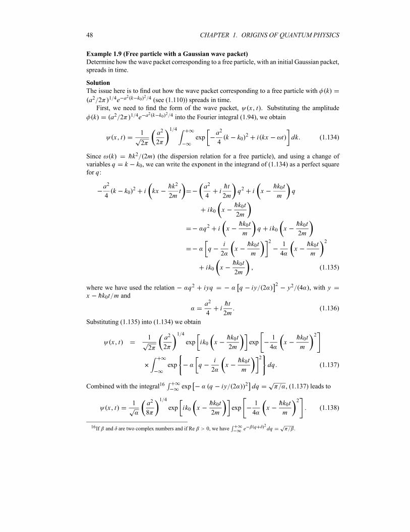
48 CHAPTER 1. ORIGINS OF QUANTUM PHYSICS
Example 1.9 (Free particle with a Gaussian wave packet)
Determine how the wave packet corresponding to a free particle, with an initial Gaussian packet,
spreads in time.
Solution
The issue here is to find out how the wave packet corresponding to a free particle with k
a2 2 1 4e a2 k k02 4 (see (1.110)) spreads in time.
First, we need to find the form of the wave packet, x t . Substituting the amplitude
k a2 2 1 4e a2 k k02 4 into the Fourier integral (1.94), we obtain
x t1
2
a2
2
1 4
expa2
4k k0
2 i kx t dk (1.134)
Since k hk2 2m (the dispersion relation for a free particle), and using a change of
variables q k k0, we can write the exponent in the integrand of (1.134) as a perfect squarefor q:
a2
4k k0
2 i kxhk2
2mt
a2
4iht
2mq2 i x
hk0t
mq
ik0 xhk0t
2m
q2 i xhk0t
mq ik0 x
hk0t
2m
qi
2x
hk0t
m
21
4x
hk0t
m
2
ik0 xhk0t
2m(1.135)
where we have used the relation q2 iyq q iy 22
y2 4 , with yx hk0t m and
a2
4iht
2m(1.136)
Substituting (1.135) into (1.134) we obtain
x t1
2
a2
2
1 4
exp ik0 xhk0t
2mexp
1
4x
hk0t
m
2
exp qi
2x
hk0t
m
2
dq (1.137)
Combined with the integral16 exp q iy 2 2 dq , (1.137) leads to
x t1 a2
8
1 4
exp ik0 xhk0t
2mexp
1
4x
hk0t
m
2
(1.138)
16If and are two complex numbers and if Re 0, we have e q 2dq .
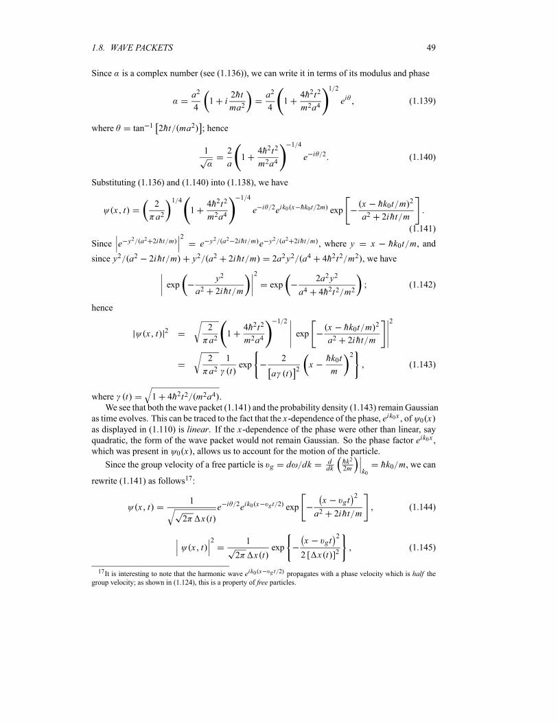
1.8. WAVE PACKETS 49
Since is a complex number (see (1.136)), we can write it in terms of its modulus and phase
a2
41 i
2ht
ma2a2
41
4h2t2
m2a4
1 2
ei (1.139)
where tan 1 2ht ma2 ; hence
1 2
a1
4h2t2
m2a4
1 4
e i 2 (1.140)
Substituting (1.136) and (1.140) into (1.138), we have
x t2
a2
1 4
14h2t2
m2a4
1 4
e i 2eik0 x hk0t 2m expx hk0t m
2
a2 2iht m(1.141)
Since e y2 a2 2iht m2
e y2 a2 2iht m e y2 a2 2iht m , where y x hk0t m, and
since y2 a2 2iht m y2 a2 2iht m 2a2y2 a4 4h2t2 m2 , we have
expy2
a2 2iht m
2
exp2a2y2
a4 4h2t2 m2(1.142)
hence
x t 2 2
a21
4h2t2
m2a4
1 2
expx hk0t m
2
a2 2iht m
2
2
a21
texp
2
a t2x
hk0t
m
2
(1.143)
where t 1 4h2t2 m2a4 .We see that both the wave packet (1.141) and the probability density (1.143) remain Gaussian
as time evolves. This can be traced to the fact that the x-dependence of the phase, eik0x , of 0 xas displayed in (1.110) is linear. If the x-dependence of the phase were other than linear, sayquadratic, the form of the wave packet would not remain Gaussian. So the phase factor eik0x ,which was present in 0 x , allows us to account for the motion of the particle.
Since the group velocity of a free particle is g d dk ddk
hk2
2m k0hk0 m, we can
rewrite (1.141) as follows17:
x t1
2 x te i 2eik0 x g t 2 exp
x gt2
a2 2iht m(1.144)
x t2 1
2 x texp
x gt2
2 [ x t ]2(1.145)
17It is interesting to note that the harmonic wave eik0 x g t 2 propagates with a phase velocity which is half thegroup velocity; as shown in (1.124), this is a property of free particles.

50 CHAPTER 1. ORIGINS OF QUANTUM PHYSICS
-
6
1
2 x0 1 t 2-
t 0
t t1
t t2
2 a2
x t 2
gt2 gt1 0 gt1 gt2x
- g
Figure 1.15 Time evolution of x t 2: the peak of the packet, which is centered at x
gt , moves with the speed g from left to right. The height of the packet, represented here
by the dotted envelope, is modulated by the function 1 2 x t , which goes to zero att and is equal to 2 a2 at t 0. The width of the packet x t x0 1 t 2
increases linearly with time.
where18
x ta
2t
a
21
4h2t2
m2a4(1.146)
represents the width of the wave packet at time t . Equations (1.144) and (1.145) describe aGaussian wave packet that is centered at x gt whose peak travels with the group speed g
hk0 m and whose width x t increases linearly with time. So, during time t , the packet’scenter has moved from x 0 to x gt and its width has expanded from x0 a 2 to
x t x0 1 4h2t2 m2a4 . The wave packet therefore undergoes a distortion; although
it remains Gaussian, its width broadens linearly with time whereas its height, 1 2 x t ,decreases with time. As depicted in Figure 1.15, the wave packet, which had a very broad width
and a very small amplitude at t , becomes narrower and narrower and its amplitude
larger and larger as time increases towards t 0; at t 0 the packet is very localized, its width
and amplitude being given by x0 a 2 and 2 a2, respectively. Then, as time increases(t 0), the width of the packet becomes broader and broader, and its amplitude becomes
smaller and smaller.
In the rest of this section we are going to comment on several features that are relevant not
only to the Gaussian packet considered above but also to more general wave packets. First, let
us begin by estimating the time at which the wave packet starts to spread out appreciably. The
packet, which is initially narrow, begins to grow out noticeably only when the second term,
2ht ma2 , under the square root sign of (1.146) is of order unity. For convenience, let us write
18We can derive (1.146) also from (1.111): a combination of the half-width x t 2 0 0 2 e 1 2
with (1.143) yields e 2[ x a t ]2 e 1 2, which in turn leads to (1.146).
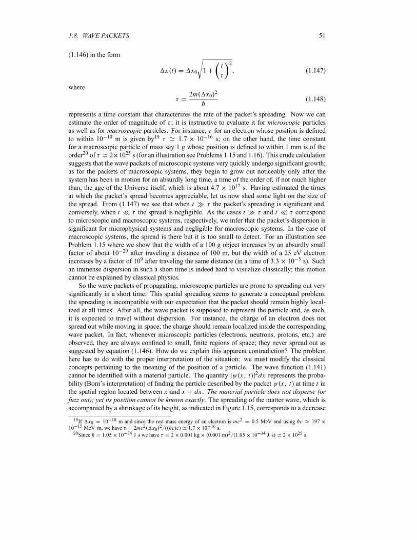
1.8. WAVE PACKETS 51
(1.146) in the form
x t x0 1t 2
(1.147)
where2m x0 2
h(1.148)
represents a time constant that characterizes the rate of the packet’s spreading. Now we can
estimate the order of magnitude of ; it is instructive to evaluate it for microscopic particlesas well as for macroscopic particles. For instance, for an electron whose position is defined
to within 10 10 m is given by19 1 7 10 16 s; on the other hand, the time constant
for a macroscopic particle of mass say 1 g whose position is defined to within 1 mm is of the
order20 of 2 1025 s (for an illustration see Problems 1.15 and 1.16). This crude calculation
suggests that the wave packets of microscopic systems very quickly undergo significant growth;
as for the packets of macroscopic systems, they begin to grow out noticeably only after the
system has been in motion for an absurdly long time, a time of the order of, if not much higher
than, the age of the Universe itself, which is about 4 7 1017 s. Having estimated the times
at which the packet’s spread becomes appreciable, let us now shed some light on the size of
the spread. From (1.147) we see that when t the packet’s spreading is significant and,
conversely, when t the spread is negligible. As the cases t and t correspond
to microscopic and macroscopic systems, respectively, we infer that the packet’s dispersion is
significant for microphysical systems and negligible for macroscopic systems. In the case of
macroscopic systems, the spread is there but it is too small to detect. For an illustration see
Problem 1.15 where we show that the width of a 100 g object increases by an absurdly small
factor of about 10 29 after traveling a distance of 100 m, but the width of a 25 eV electron
increases by a factor of 109 after traveling the same distance (in a time of 3 3 10 5 s). Such
an immense dispersion in such a short time is indeed hard to visualize classically; this motion
cannot be explained by classical physics.
So the wave packets of propagating, microscopic particles are prone to spreading out very
significantly in a short time. This spatial spreading seems to generate a conceptual problem:
the spreading is incompatible with our expectation that the packet should remain highly local-
ized at all times. After all, the wave packet is supposed to represent the particle and, as such,
it is expected to travel without dispersion. For instance, the charge of an electron does not
spread out while moving in space; the charge should remain localized inside the corresponding
wave packet. In fact, whenever microscopic particles (electrons, neutrons, protons, etc.) are
observed, they are always confined to small, finite regions of space; they never spread out as
suggested by equation (1.146). How do we explain this apparent contradiction? The problem
here has to do with the proper interpretation of the situation: we must modify the classical
concepts pertaining to the meaning of the position of a particle. The wave function (1.141)
cannot be identified with a material particle. The quantity x t 2dx represents the proba-bility (Born’s interpretation) of finding the particle described by the packet x t at time t inthe spatial region located between x and x dx . The material particle does not disperse (orfuzz out); yet its position cannot be known exactly. The spreading of the matter wave, which isaccompanied by a shrinkage of its height, as indicated in Figure 1.15, corresponds to a decrease
19If x0 10 10 m and since the rest mass energy of an electron is mc2 0 5 MeV and using hc 197
10 15 MeV m, we have 2mc2 x02 hc c 1 7 10 16 s.
20Since h 1 05 10 34 J s we have 2 0 001 kg 0 001 m 2 1 05 10 34 J s 2 1025 s.
52 CHAPTER 1. ORIGINS OF QUANTUM PHYSICS
of the probability density x t 2 and implies in no way a growth in the size of the particle.
So the wave packet gives only the probability that the particle it represents will be found at a
given position. No matter how broad the packet becomes, we can show that its norm is always
conserved, for it does not depend on time. In fact, as can be inferred from (1.143), the norm of
the packet is equal to one:
x t 2 dx2
a21
exp2 x hk0t m
2
a 2dx
2
a21 a2 2
21
(1.149)
since e x2dx . This is expected, since the probability of finding the particle
somewhere along the x-axis must be equal to one. The important issue here is that the normof the packet is time independent and that its spread does not imply that the material particle
becomes bloated during its motion, but simply implies a redistribution of the probability density.
So, in spite of the significant spread of the packets of microscopic particles, the norms of these
packets are always conserved—normalized to unity.
Besides, we should note that the example considered here is an idealized case, for we aredealing with a free particle. If the particle is subject to a potential, as in the general case, itswave packet will not spread as dramatically as that of a free particle. In fact, a varying potential
can cause the wave packet to become narrow. This is indeed what happens when a measurement
is performed on a microscopic system; the interaction of the system with the measuring device
makes the packet very narrow, as will be seen in Chapter 3.
Let us now study how the spreading of the wave packet affects the uncertainties product
x t p t . First, we should point out that the average momentum of the packet hk0 and itsuncertainty h k do not change in time. This can be easily inferred as follows. Rewriting (1.94)in the form
x t1
2k 0 ei kx t dk
1
2k t eikxdk (1.150)
we have
k t e i k t k 0 (1.151)
where k 0 a2 2 1 4e a2 k k02 4; hence
k t 2 k 0 2 (1.152)
This suggests that the widths of k t and k 0 are equal; hence k remains constant andso must the momentum dispersion p (this is expected because the momentum of a free particleis a constant of the motion). Since the width of k 0 is given by k 1 a (see (1.112)), wehave
p h kh
a(1.153)
Multiplying this relation by (1.146), we have
x t ph
21
4h2
m2a4t2 (1.154)
which shows that x t p h 2 is satisfied at all times. Notably, when t 0 we obtain
the lower bound limit x0 p h 2; this is the uncertainty relation for a stationary Gaussianpacket (see (1.114)). As t increases, however, we obtain an inequality, x t p h 2.

1.8. WAVE PACKETS 53
-
6x t
©©©©
©©©©
©©©
HHHH
HHHH
HHH
t0
xcl ht maxcl ht ma
Figure 1.16 Time evolutions of the packet’s width x t x0 1 xcl t x02 (dotted
curve) and of the classical dispersion xcl t ht ma (solid lines). For large values of t ,x t approaches xcl t and at t 0, x 0 x0 a 2.
Having shown that the width of the packet does not disperse in momentum space, let us now
study the dispersion of the packet’s width in x-space. Since x0 a 2 we can write (1.146)as
x ta
21
4h2t2
m2a4x0 1
xcl t
x0
2
(1.155)
where the dispersion factor xcl t x0 is given by
xcl t
x0
2h
ma2t
h
2m x20t (1.156)
As shown in Figure 1.16, when t is large (i.e., t ), we have x t xcl t with
xcl tht
ma
p
mt t (1.157)
where h ma represents the dispersion in velocity. This means that if a particle starts
initially (t 0) at x 0 with a velocity dispersion equal to , then will remain constant
but the dispersion of the particle’s position will increase linearly with time: xcl t h t ma(Figure 1.16). We see from (1.155) that if xcl t x0 1, the spreading of the wave packet
is negligible, but if xcl t x0 1, the wave packet will spread out without bound.
We should highlight at this level the importance of the classical limit of (1.154): in the limit
h 0, the product x t p goes to zero. This means that the x and p uncertainties becomenegligible; that is, in the classical limit, the wave packet will propagate without spreading. In
this case the center of the wave packet moves like a free particle that obeys the laws of classical
mechanics. The spread of wave packets is thus a purely quantum effect. So when h 0 all
quantum effects, the spread of the packet, disappear.
We may conclude this study of wave packets by highlighting their importance:
They provide a linkage with the Heisenberg uncertainty principle.
They embody and unify the particle and wave features of matter waves.
They provide a linkage between wave intensities and probabilities.
They provide a connection between classical and quantum mechanics.
54 CHAPTER 1. ORIGINS OF QUANTUM PHYSICS
1.9 Concluding Remarks
Despite its striking success in predicting the hydrogen’s energy levels and transition rates, the
Bohr model suffers from a number of limitations:
It works only for hydrogen and hydrogen-like ions such as He and Li2 .
It provides no explanation for the origin of its various assumptions. For instance, it gives
no theoretical justification for the quantization condition (1.63) nor does it explain why
stationary states radiate no energy.
It fails to explain why, instead of moving continuously from one energy level to another,the electrons jump from one level to the other.
The model therefore requires considerable extension to account for the electronic properties
and spectra of a wide range of atoms. Even in its present limited form, Bohr’s model represents
a bold and major departure from classical physics: classical physics offers no justification for
the existence of discrete energy states in a system such as a hydrogen atom and no justification
for the quantization of the angular momentum.
In its present form, the model not only suffers from incompleteness but also lacks the ingre-
dients of a consistent theory. It was built upon a series of ad hoc, piecemeal assumptions. These
assumptions were not derived from the first principles of a more general theory, but postulated
rather arbitrarily.
The formulation of the theory of quantum mechanics was largely precipitated by the need
to find a theoretical foundation for Bohr’s ideas as well as to explain, from first principles, a
wide variety of other microphysical phenomena such as the puzzling processes discussed in
this chapter. It is indeed surprising that a single theory, quantum mechanics, is powerful and
rich enough to explain accurately a wide variety of phenomena taking place at the molecular,
atomic, and subatomic levels.
In this chapter we have dealt with the most important experimental facts which confirmed
the failure of classical physics and subsequently led to the birth of quantum mechanics. In the
rest of this text we will focus on the formalism of quantum mechanics and on its application to
various microphysical processes. To prepare for this task, we need first to study the mathemat-
ical tools necessary for understanding the formalism of quantum mechanics; this is taken up in
Chapter 2.
1.10 Solved Problems
Numerical calculations in quantum physics can be made simpler by using the following units.
First, it is convenient to express energies in units of electronvolt ( eV): one eV is defined as
the energy acquired by an electron passing through a potential difference of one Volt. The
electronvolt unit can be expressed in terms of joules and vice versa: 1 eV 1 6 10 19 C
1 V 1 6 10 19 J and 1 J 0 625 1019 eV.
It is also convenient to express the masses of subatomic particles, such as the electron,
proton, and neutron, in terms of their rest mass energies: mec2 0 511 MeV, m pc2
938 27 MeV, and mnc2 939 56 MeV.
In addition, the quantities hc 197 33 MeV fm 197 33 10 15 MeV m or hc1242 37 10 10 eV m are sometimes more convenient to use than h 1 05 10 34 J s.
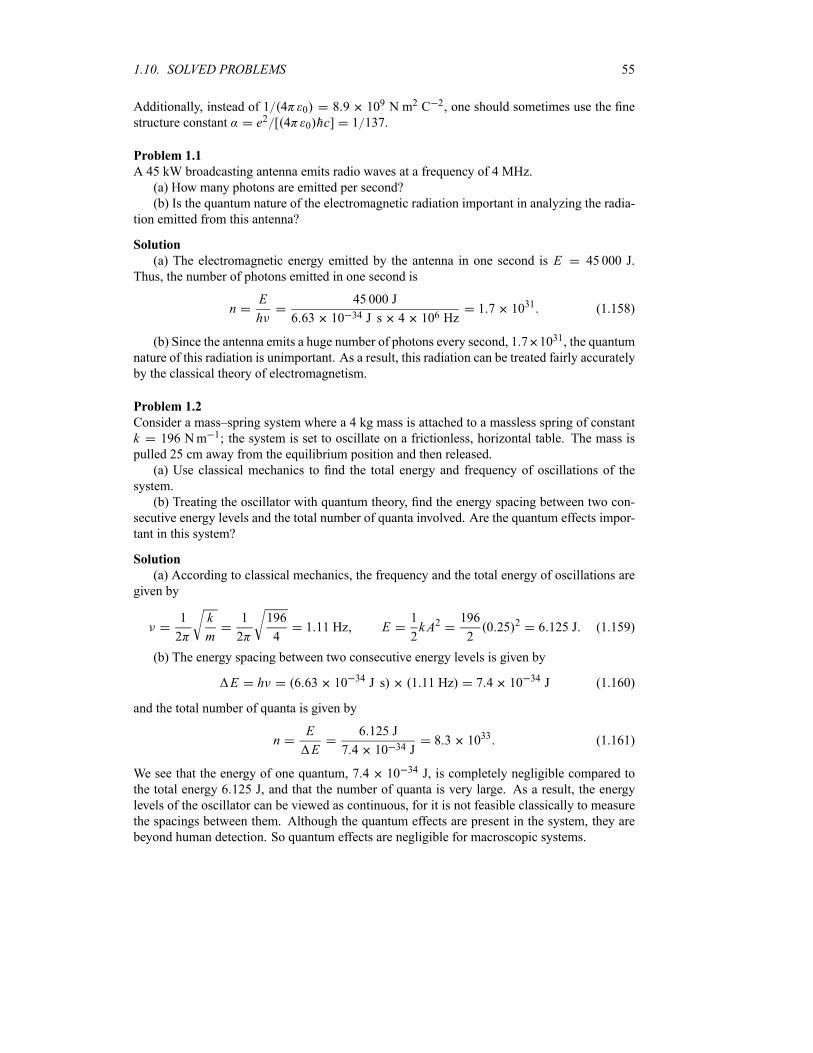
1.10. SOLVED PROBLEMS 55
Additionally, instead of 1 4 0 8 9 109 N m2 C 2, one should sometimes use the fine
structure constant e2 [ 4 0 hc] 1 137.
Problem 1.1
A 45 kW broadcasting antenna emits radio waves at a frequency of 4 MHz.
(a) How many photons are emitted per second?
(b) Is the quantum nature of the electromagnetic radiation important in analyzing the radia-
tion emitted from this antenna?
Solution
(a) The electromagnetic energy emitted by the antenna in one second is E 45 000 J.
Thus, the number of photons emitted in one second is
nE
h
45 000 J
6 63 10 34 J s 4 106 Hz1 7 1031 (1.158)
(b) Since the antenna emits a huge number of photons every second, 1 7 1031, the quantum
nature of this radiation is unimportant. As a result, this radiation can be treated fairly accurately
by the classical theory of electromagnetism.
Problem 1.2
Consider a mass–spring system where a 4 kg mass is attached to a massless spring of constant
k 196 Nm 1; the system is set to oscillate on a frictionless, horizontal table. The mass is
pulled 25 cm away from the equilibrium position and then released.
(a) Use classical mechanics to find the total energy and frequency of oscillations of the
system.
(b) Treating the oscillator with quantum theory, find the energy spacing between two con-
secutive energy levels and the total number of quanta involved. Are the quantum effects impor-
tant in this system?
Solution
(a) According to classical mechanics, the frequency and the total energy of oscillations are
given by
1
2
k
m
1
2
196
41 11 Hz E
1
2kA2
196
20 25 2 6 125 J (1.159)
(b) The energy spacing between two consecutive energy levels is given by
E h 6 63 10 34 J s 1 11 Hz 7 4 10 34 J (1.160)
and the total number of quanta is given by
nE
E
6 125 J
7 4 10 34 J8 3 1033 (1.161)
We see that the energy of one quantum, 7 4 10 34 J, is completely negligible compared to
the total energy 6 125 J, and that the number of quanta is very large. As a result, the energy
levels of the oscillator can be viewed as continuous, for it is not feasible classically to measure
the spacings between them. Although the quantum effects are present in the system, they are
beyond human detection. So quantum effects are negligible for macroscopic systems.
56 CHAPTER 1. ORIGINS OF QUANTUM PHYSICS
Problem 1.3
When light of a given wavelength is incident on a metallic surface, the stopping potential for
the photoelectrons is 3 2 V. If a second light source whose wavelength is double that of the first
is used, the stopping potential drops to 0 8 V. From these data, calculate
(a) the wavelength of the first radiation and
(b) the work function and the cutoff frequency of the metal.
Solution
(a) Using (1.23) and since the wavelength of the second radiation is double that of the first
one, 2 2 1, we can write
Vs1hc
e 1
W
e(1.162)
Vs2hc
e 2
W
e
hc
2e 1
W
e(1.163)
To obtain 1 we have only to subtract (1.163) from (1.162):
Vs1 Vs2hc
e 11
1
2
hc
2e 1(1.164)
The wavelength is thus given by
1hc
2e Vs1 Vs2
6 6 10 34 J s 3 108ms 1
2 1 6 10 19 C 3 2 V 0 8 V2 6 10 7 m (1.165)
(b) To obtain the work function, we simply need to multiply (1.163) by 2 and subtract the
result from (1.162), Vs1 2Vs2 W e, which leads to
W e Vs1 2Vs2 1 6 eV 1 6 1 6 10 19 2 56 10 19 J (1.166)
The cutoff frequency is
W
h
2 56 10 19 J
6 6 10 34 J s3 9 1014 Hz (1.167)
Problem 1.4
(a) Estimate the energy of the electrons that we need to use in an electron microscope to
resolve a separation of 0 27 nm.
(b) In a scattering of 2 eV protons from a crystal, the fifth maximum of the intensity is
observed at an angle of 30 . Estimate the crystal’s planar separation.
Solution
(a) Since the electron’s momentum is p 2 h , its kinetic energy is given by
Ep2
2me
2 2h2
me 2(1.168)
Since mec2 0 511 MeV, hc 197 33 10 15 MeV m, and 0 27 10 9 m, we have
E2 2 hc 2
mec2 2
2 2 197 33 10 15 MeV m 2
0 511 MeV 0 27 10 9 m 220 6 eV (1.169)
1.10. SOLVED PROBLEMS 57
(b) Using Bragg’s relation (1.46), 2d n sin , where d is the crystal’s planar separa-tion, we can infer the proton’s kinetic energy from (1.168):
Ep2
2m p
2 2h2
m p 2
n2 2h2
2m pd2 sin 2(1.170)
which leads to
dn h
sin 2m pE
n hc
sin 2m pc2E(1.171)
Since n 5 (the fifth maximum), 30 , E 2 eV, and m pc2 938 27 MeV, we have
d5 197 33 10 15 MeV m
sin 30 2 938 27 MeV 2 10 6 MeV0 101 nm (1.172)
Problem 1.5
A photon of energy 3 keV collides elastically with an electron initially at rest. If the photon
emerges at an angle of 60 , calculate
(a) the kinetic energy of the recoiling electron and
(b) the angle at which the electron recoils.
Solution
(a) From energy conservation, we have
h mec2 h Ke mec
2 (1.173)
where h and h are the energies of the initial and scattered photons, respectively, mec2 is therest mass energy of the initial electron, Ke mec2 is the total energy of the recoiling electron,and Ke is its recoil kinetic energy. The expression for Ke can immediately be inferred from(1.173):
Ke h hc1 1 hc
h (1.174)
where the wave shift is given by (1.36):
h
mec1 cos
2 hc
mec21 cos
2 197 33 10 15 MeV m
0 511 MeV1 cos 60
0 0012 nm (1.175)
Since the wavelength of the incident photon is 2 hc h , we have 2 197 33
10 15 MeV m 0 003 MeV 0 414 nm; the wavelength of the scattered photon is given by
0 4152 nm (1.176)
Now, substituting the numerical values of and into (1.174), we obtain the kinetic energy
of the recoiling electron
Ke h 3 keV0 0012 nm
0 4152 nm8 671 eV (1.177)
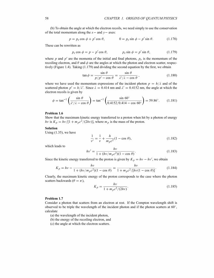
58 CHAPTER 1. ORIGINS OF QUANTUM PHYSICS
(b) To obtain the angle at which the electron recoils, we need simply to use the conservation
of the total momentum along the x and y axes:
p pe cos p cos 0 pe sin p sin (1.178)
These can be rewritten as
pe cos p p cos pe sin p sin (1.179)
where p and p are the momenta of the initial and final photons, pe is the momentum of therecoiling electron, and and are the angles at which the photon and electron scatter, respec-
tively (Figure 1.4). Taking (1.179) and dividing the second equation by the first, we obtain
tansin
p p cos
sin
cos(1.180)
where we have used the momentum expressions of the incident photon p h and of the
scattered photon p h . Since 0 414 nm and 0 4152 nm, the angle at which the
electron recoils is given by
tan 1 sin
costan 1 sin 60
0 4152 0 414 cos 6059 86 (1.181)
Problem 1.6
Show that the maximum kinetic energy transferred to a proton when hit by a photon of energy
h is K p h [1 m pc2 2h ], where m p is the mass of the proton.
Solution
Using (1.35), we have1 1 h
m pc21 cos (1.182)
which leads to
hh
1 h m pc2 1 cos(1.183)
Since the kinetic energy transferred to the proton is given by K p h h , we obtain
K p hh
1 h m pc2 1 cos
h
1 m pc2 [h 1 cos ](1.184)
Clearly, the maximum kinetic energy of the proton corresponds to the case where the photon
scatters backwards ( ),
K ph
1 m pc2 2h(1.185)
Problem 1.7
Consider a photon that scatters from an electron at rest. If the Compton wavelength shift is
observed to be triple the wavelength of the incident photon and if the photon scatters at 60 ,
calculate
(a) the wavelength of the incident photon,
(b) the energy of the recoiling electron, and
(c) the angle at which the electron scatters.
1.10. SOLVED PROBLEMS 59
Solution
(a) In the case where the photons scatter at 60 and since 3 , the wave shift
relation (1.36) yields
3h
mec1 cos 60 (1.186)
which in turn leads to
h
6mec
hc
3mec23 14 197 33 10 15 MeV m
3 0 511 MeV4 04 10 13 m (1.187)
(b) The energy of the recoiling electron can be obtained from the conservation of energy:
Ke hc1 1 3hc
4
3 hc
2
3 3 14 197 33 10 15 MeV m
2 4 04 10 13 m2 3 MeV
(1.188)
In deriving this relation, we have used the fact that 4 .
(c) Since 4 the angle at which the electron recoils can be inferred from (1.181)
tan 1 sin
costan 1 sin 60
4 cos 6013 9 (1.189)
Problem 1.8
In a double-slit experiment with a source of monoenergetic electrons, detectors are placed along
a vertical screen parallel to the y-axis to monitor the diffraction pattern of the electrons emittedfrom the two slits. When only one slit is open, the amplitude of the electrons detected on the
screen is 1 y t A1e i ky t 1 y2, and when only the other is open the amplitude is
2 y t A2e i ky y t 1 y2, where A1 and A2 are normalization constants that needto be found. Calculate the intensity detected on the screen when
(a) both slits are open and a light source is used to determine which of the slits the electron
went through and
(b) both slits are open and no light source is used.
Plot the intensity registered on the screen as a function of y for cases (a) and (b).
Solution
Using the integral dy 1 y2 , we can obtain the normalization constants at once:
A1 A2 1 ; hence 1 and 2 become 1 y t e i ky t 1 y2 , 2 y t
e i ky y t 1 y2 .(a) When we use a light source to observe the electrons as they exit from the two slits on
their way to the vertical screen, the total intensity recorded on the screen will be determined by
a simple addition of the probability densities (or of the separate intensities):
I y 1 y t2
2 y t2 2
1 y2(1.190)
As depicted in Figure 1.17a, the shape of the total intensity displays no interference pattern.
Intruding on the electrons with the light source, we distort their motion.

60 CHAPTER 1. ORIGINS OF QUANTUM PHYSICS
-
6I y
y0
(a)
-
6I y
y0
(b)
Figure 1.17 Shape of the total intensity generated in a double slit experiment when both slits
are open and (a) a light source is used to observe the electrons’ motion, I y 2 1 y2 ,and no interference is registered; (b) no light source is used, I y 4 [ 1 y2 ] cos2 y 2 ,and an interference pattern occurs.
(b) When no light source is used to observe the electrons, the motion will not be distorted
and the total intensity will be determined by an addition of the amplitudes, not the intensities:
I y 1 y t 2 y t2 1
1 y2e i ky t e i ky y t
2
1
1 y21 ei y 1 e i y
4
1 y2cos 2
2y (1.191)
The shape of this intensity does display an interference pattern which, as shown in Figure 1.17b,
results from an oscillating function, cos2 y 2 , modulated by 4 [ 1 y2 ].
Problem 1.9
Consider a head-on collision between an -particle and a lead nucleus. Neglecting the recoil
of the lead nucleus, calculate the distance of closest approach of a 9 0 MeV -particle to the
nucleus.
Solution
In this head-on collision the distance of closest approach r0 can be obtained from the conserva-tion of energy Ei E f , where Ei is the initial energy of the system, -particle plus the leadnucleus, when the particle and the nucleus are far from each other and thus feel no electrostatic
potential between them. Assuming the lead nucleus to be at rest, Ei is simply the energy of the-particle: Ei 9 0 MeV 9 106 1 6 10 19 J.
As for E f , it represents the energy of the system when the -particle is at its closest distance
from the nucleus. At this position, the -particle is at rest and hence has no kinetic energy.
The only energy the system has is the electrostatic potential energy between the -particle
and the lead nucleus, which has a positive charge of 82e. Neglecting the recoil of the lead
1.10. SOLVED PROBLEMS 61
nucleus and since the charge of the -particle is positive and equal to 2e, we have E f2e 82e 4 0r0 . The energy conservation Ei E f or 2e 82e 4 0r0 Ei leads atonce to
r02e 82e
4 0Ei2 62 10 14 m (1.192)
where we used the values e 1 6 10 19 C and 1 4 0 8 9 109 N m2 C 2.
Problem 1.10
Considering that a quintuply ionized carbon ion, C5 , behaves like a hydrogen atom, calculate
(a) the radius rn and energy En for a given state n and compare them with the correspondingexpressions for hydrogen,
(b) the ionization energy of C5 when it is in its first excited state and compare it with the
corresponding value for hydrogen, and
(c) the wavelength corresponding to the transition from state n 3 to state n 1; compare
it with the corresponding value for hydrogen.
Solution
(a) The C5 ion is generated by removing five electrons from the carbon atom. To find the
expressions for rnC and EnC for the C5 ion (which has 6 protons), we need simply to insert
Z 6 into (1.76):
rnCa06n2 EnC
36R
n2(1.193)
where we have dropped the term me M , since it is too small compared to one. Clearly, theseexpressions are related to their hydrogen counterparts by
rnCa06n2
rnH6
EnC36R
n236EnH (1.194)
(b) The ionization energy is the one needed to remove the only remaining electron of the
C5 ion. When the C5 ion is in its first excited state, the ionization energy is
E2C36R
49 13 6 eV 122 4 eV (1.195)
which is equal to 36 times the energy needed to ionize the hydrogen atom in its first excited
state: E2H 3 4 eV (note that we have taken n 2 to correspond to the first excited state;
as a result, the cases n 1 and n 3 will correspond to the ground and second excited states,
respectively).
(c) The wavelength corresponding to the transition from state n 3 to state n 1 can be
inferred from the relation hc E3C E1C which, when combined with E1C 489 6 eV
and E3C 54 4 eV, leads to
hc
E3C E1C
2 hc
E3C E1C
2 197 33 10 9 eV m
54 4 eV 489 6 eV2 85 nm (1.196)
Problem 1.11
(a) Find the Fourier transform for kA a k k a0 k a
where a is a positive parameter and A is a normalization factor to be found.(b) Calculate the uncertainties x and p and check whether they satisfy the uncertainty
principle.
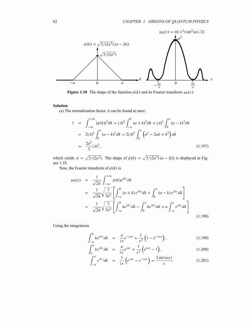
62 CHAPTER 1. ORIGINS OF QUANTUM PHYSICS
-
6
¡¡¡¡¡¡@
@@@@@
k 3 2a3 a k
k0a a
3 2a3
-
60 x 4 x2 sin2 ax 2
x0
a2
2a
2a
Figure 1.18 The shape of the function k and its Fourier transform 0 x .
Solution
(a) The normalization factor A can be found at once:
1 k 2dk A 20
aa k 2dk A 2
a
0
a k 2dk
2 A 2a
0
a k 2dk 2 A 2a
0
a2 2ak k2 dk
2a3
3A 2 (1.197)
which yields A 3 2a3 . The shape of k 3 2a3 a k is displayed in Fig-
ure 1.18.
Now, the Fourier transform of k is
0 x1
2k eikxdk
1
2
3
2a3
0
aa k eikxdk
a
0
a k eikxdk
1
2
3
2a3
0
akeikxdk
a
0
keikxdk aa
aeikxdk
(1.198)
Using the integrations
0
akeikxdk
a
ixe iax 1
x21 e iax (1.199)
a
0
keikxdka
ixeiax
1
x2eiax 1 (1.200)
a
aeikxdk
1
i xeiax e iax 2 sin ax
x(1.201)
1.10. SOLVED PROBLEMS 63
and after some straightforward calculations, we end up with
0 x4
x2sin 2
ax
2(1.202)
As shown in Figure 1.18, this wave packet is localized: it peaks at x 0 and decreases gradu-
ally as x increases. We can verify that the maximum of 0 x occurs at x 0; writing 0 xas a2 ax 2 2 sin2 ax 2 and since limx 0 sin bx bx 1, we obtain 0 0 a2.(b) Figure 1.18a is quite suggestive in defining the half-width of k : k a (hence
the momentum uncertainty is p ha). By defining the width as k a, we know withfull certainty that the particle is located between a k a; according to Figure 1.18a, theprobability of finding the particle outside this interval is zero, for k vanishes when k a.Now, let us find the width x of 0 x . Since sin a 2a 1, 0 a 4a2 2, and
that 0 0 a2, we can obtain from (1.202) that 0 a 4a2 2 4 20 0 , or
0 a
0 0
42
(1.203)
This suggests that x a: when x x a the wave packet 0 x drops to 4 2
from its maximum value 0 0 a2. In sum, we have x a and k a; hence
x k (1.204)
or
x p h (1.205)
since k p h. In addition to satisfying Heisenberg’s uncertainty principle (1.57), thisrelation shows that the product x p is higher than h 2: x p h 2. The wave packet(1.202) therefore offers a clear illustration of the general statement outlined above; namely, only
Gaussian wave packets yield the lowest limit to Heisenberg’s uncertainty principle x ph 2 (see (1.114)). All other wave packets, such as (1.202), yield higher values for the productx p.
Problem 1.12
Calculate the group and phase velocities for the wave packet corresponding to a relativistic
particle.
Solution
Recall that the energy and momentum of a relativistic particle are given by
E mc2m0c2
1 2 c2p m
m0
1 2 c2(1.206)
where m0 is the rest mass of the particle and c is the speed of light in a vacuum. Squaring andadding the expressions of E and p, we obtain E2 p2c2 m20c
4; hence
E c p2 m20c2 (1.207)

64 CHAPTER 1. ORIGINS OF QUANTUM PHYSICS
Using this relation along with p2 m20c2 m20c
2 1 2 c2 and (1.122), we can show thatthe group velocity is given as follows:
gdE
dp
d
dpc p2 m20c
2pc
p2 m20c2
(1.208)
The group velocity is thus equal to the speed of the particle, g .
The phase velocity can be found from (1.122) and (1.207): ph E p c 1 m20c2 p2
which, when combined with p m0 1 2 c2, leads to 1 m20c2 p2 c ; hence
phE
pc 1
m20c2
p2c2
(1.209)
This shows that the phase velocity of the wave corresponding to a relativistic particle with
m0 0 is larger than the speed of light, ph c2 c. This is indeed unphysical. Theresult ph c seems to violate the special theory of relativity, which states that the speedof material particles cannot exceed c. In fact, this principle is not violated because ph does
not represent the velocity of the particle; the velocity of the particle is represented by the group
velocity (1.208). As a result, the phase speed of a relativistic particle has nomeaningful physical
significance.
Finally, the product of the group and phase velocities is equal to c2, i.e., g ph c2.
Problem 1.13
The angular frequency of the surface waves in a liquid is given in terms of the wave number kby gk T k3 , where g is the acceleration due to gravity, is the density of the liquid,
and T is the surface tension (which gives an upward force on an element of the surface liquid).Find the phase and group velocities for the limiting cases when the surface waves have: (a) very
large wavelengths and (b) very small wavelengths.
Solution
The phase velocity can be found at once from (1.119):
phk
g
k
Tk
g
2
2 T(1.210)
where we have used the fact that k 2 , being the wavelength of the surface waves.
(a) If is very large, we can neglect the second term in (1.210); hence
phg
2
g
k(1.211)
In this approximation the phase velocity does not depend on the nature of the liquid, since it
depends on no parameter pertaining to the liquid such as its density or surface tension. This
case corresponds, for instance, to deepwater waves, called gravity waves.
1.10. SOLVED PROBLEMS 65
To obtain the group velocity, let us differentiate (1.211) with respect to k: d ph dk1 2k g k ph 2k. A substitution of this relation into (1.120) shows that the group
velocity is half the phase velocity:
gd
dkph k
d ph
dkph
1
2ph
1
2ph
1
2
g
2(1.212)
The longer the wavelength, the faster the group velocity. This explains why a strong, steady
wind will produce waves of longer wavelength than those produced by a swift wind.
(b) If is very small, the second term in (1.210) becomes the dominant one. So, retaining
only the second term, we have
ph2 T T
k (1.213)
which leads to d ph dk T k 2k ph 2k. Inserting this expression into (1.120), weobtain the group velocity
g ph kd ph
dkph
1
2ph
3
2ph (1.214)
hence the smaller the wavelength, the faster the group velocity. These are called ripple waves;
they occur, for instance, when a container is subject to vibrations of high frequency and small
amplitude or when a gentle wind blows on the surface of a fluid.
Problem 1.14
This problem is designed to illustrate the superposition principle and the concepts of modulated
and modulating functions in a wave packet. Consider two wave functions 1 y t 5y cos 7tand 2 y t 5y cos 9t , where y and t are in meters and seconds, respectively. Show thattheir superposition generates a wave packet. Plot it and identify the modulated and modulating
functions.
Solution
Using the relation cos cos cos sin sin , we can write the superposition of
1 y t and 2 y t as follows:
y t 1 y t 2 y t 5y cos 7t 5y cos 9t
5y cos 8t cos t sin 8t sin t 5y cos 8t cos t sin 8t sin t
10y sin t sin 8t (1.215)
The periods of 10y sin t and sin 8t are given by 2 and 2 8, respectively. Since the period of
10y sin t is larger than that of sin 8t , 10y sin t must be the modulating function and sin 8t themodulated function. As depicted in Figure 1.19, we see that sin 8t is modulated by 10y sin t .
Problem 1.15
(a) Calculate the final size of the wave packet representing a free particle after traveling a
distance of 100 m for the following four cases where the particle is
(i) a 25 eV electron whose wave packet has an initial width of 10 6 m,
66 CHAPTER 1. ORIGINS OF QUANTUM PHYSICS
-
6 ¾ 10y sin t
¾ sin 8t
t
Figure 1.19 Shape of the wave packet y t 10y sin t sin 8t . The function sin 8t , thesolid curve, is modulated by 10y sin t , the dashed curve.
(ii) a 25 eV electron whose wave packet has an initial width of 10 8 m,
(iii) a 100 MeV electron whose wave packet has an initial width of 1 mm, and
(iv) a 100 g object of size 1 cm moving at a speed of 50 m s 1.
(b) Estimate the times required for the wave packets of the electron in (i) and the object in
(iv) to spread to 10 mm and 10 cm, respectively. Discuss the results obtained.
Solution
(a) If the initial width of the wave packet of the particle is x0, the width at time t is givenby
x t x0 1x
x0
2
(1.216)
where the dispersion factor is given by
x
x0
2ht
ma2ht
2m a 2 2ht
2m x02
(1.217)
(i) For the 25 eV electron, which is clearly not relativistic, the time to travel the L 100 m
distance is given by t L L mc2 2E c, since E 12m 2 1
2mc2 2 c2 or
c 2E mc2 . We can therefore write the dispersion factor as
x
x0
h
2m x20t
h
2m x20
L
c
mc2
2E
hcL
2mc2 x20
mc2
2E(1.218)
The numerics of this expression can be made easy by using the following quantities: hc197 10 15 MeV m, the rest mass energy of an electron is mc2 0 5 MeV, x0 10 6 m,
E 25 eV 25 10 6 MeV, and L 100 m. Inserting these quantities into (1.218), we
obtain
x
x0
197 10 15 MeV m 100 m
2 0 5 MeV 10 12 m20 5 MeV
2 25 10 6 MeV2 103 (1.219)
the time it takes the electron to travel the 100 m distance is given, as shown above, by
tL
c
mc2
2E
100 m
3 108 ms 1
0 5 MeV
2 25 10 6 MeV3 3 10 5 s (1.220)
1.10. SOLVED PROBLEMS 67
Using t 3 3 10 5 s and substituting (1.219) into (1.216), we obtain
x t 3 3 10 5 s 10 6 m 1 4 106 2 10 3 m 2 mm (1.221)
The width of the wave packet representing the electron has increased from an initial value of
10 6 m to 2 10 3 m, i.e., by a factor of about 103. The spread of the electron’s wave packet
is thus quite large.
(ii) The calculation needed here is identical to that of part (i), except the value of x0 isnow 10 8 m instead of 10 6 m. This leads to x x0 2 107 and hence the width is
x t 20 cm; the width has therefore increased by a factor of about 107. This calculation is
intended to show that the narrower the initial wave packet, the larger the final spread. In fact,starting in part (i) with an initial width of 10 6 m, the final width has increased to 2 10 3 m
by a factor of about 103; but in part (ii) we started with an initial width of 10 8 m, and the final
width has increased to 20 cm by a factor of about 107.
(iii) The motion of a 100 MeV electron is relativistic; hence to good approximation, its
speed is equal to the speed of light, c. Therefore the time it takes the electron to travel adistance of L 100 m is t L c 3 3 10 7 s. The dispersion factor for this electron can
be obtained from (1.217) where x0 10 3 m:
x
x0
hL
2mc x20
hcL
2mc2 x20
197 10 15 MeV m 100 m
2 0 5 MeV 10 6 m22 10 5 (1.222)
The increase in the width of the wave packet is relatively small:
x t 3 3 10 7 s 10 3 m 1 4 10 10 10 3 m x0 (1.223)
So the width did not increase appreciably. We can conclude from this calculation that, when
the motion of a microscopic particle is relativistic, the width of the corresponding wave packet
increases by a relatively small amount.
(iv) In the case of a macroscopic object of mass m 0 1 kg, the time to travel the distance
L 100 m is t L 100 m 50 ms 1 2 s. Since the size of the system is about
x0 1 cm 0 01 m and h 1 05 10 34 J s, the dispersion factor for the object can be
obtained from (1.217):
x
x0
ht
2m x20
1 05 10 34 J s 2 s
2 0 1 kg 10 4 m210 29 (1.224)
Since x x0 10 29 1, the increase in the width of the wave packet is utterly unde-
tectable:
x 2s 10 2 m 1 10 58 10 2 m x0 (1.225)
(b) Using (1.216) and (1.217) we obtain the expression for the time t in which the wavepacket spreads to x t :
tx t
x0
2
1 (1.226)
where represents a time constant 2m x0 2 h (see (1.148)). The time constant for theelectron of part (i) is given by
2mc2 x0 2
hc22 0 5 MeV 10 12 m2
197 10 15 MeV m 3 108ms 11 7 10 8 s (1.227)
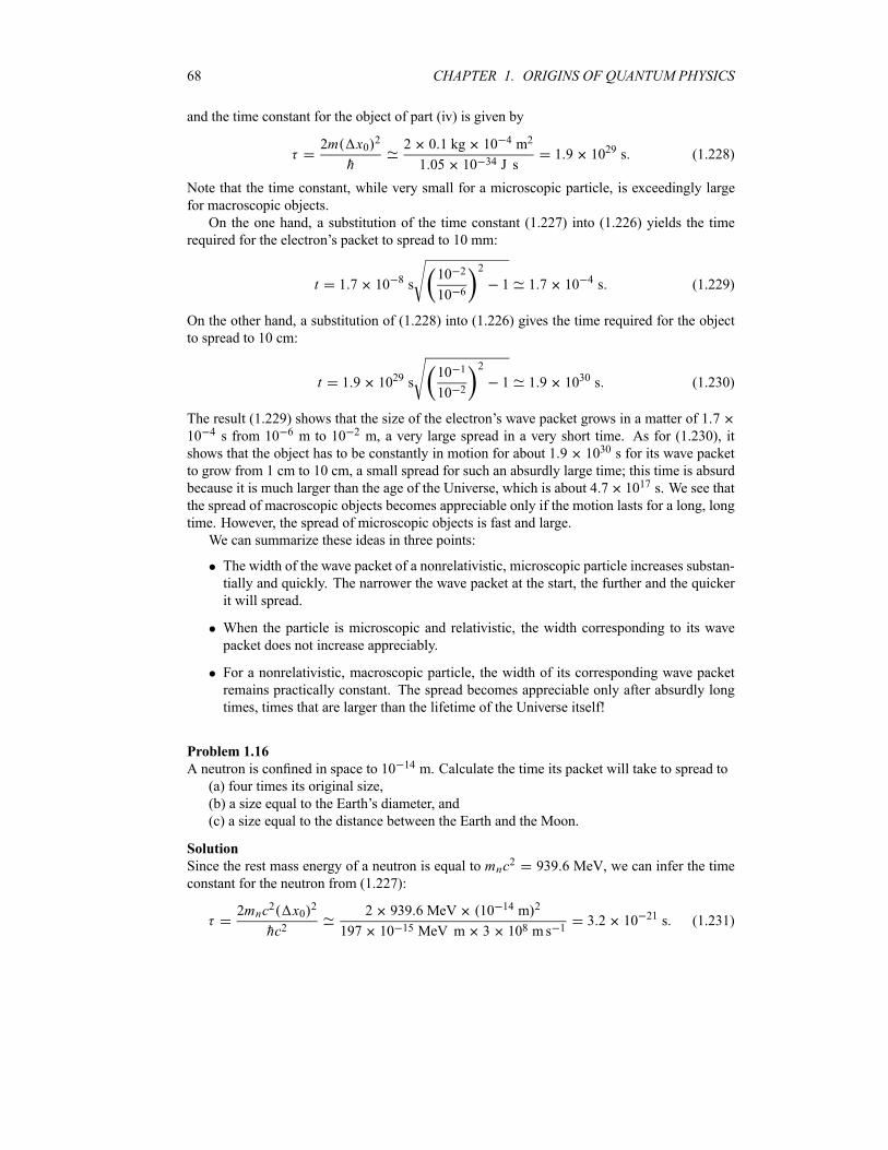
68 CHAPTER 1. ORIGINS OF QUANTUM PHYSICS
and the time constant for the object of part (iv) is given by
2m x0 2
h
2 0 1 kg 10 4 m2
1 05 10 34 J s1 9 1029 s (1.228)
Note that the time constant, while very small for a microscopic particle, is exceedingly large
for macroscopic objects.
On the one hand, a substitution of the time constant (1.227) into (1.226) yields the time
required for the electron’s packet to spread to 10 mm:
t 1 7 10 8 s10 2
10 6
2
1 1 7 10 4 s (1.229)
On the other hand, a substitution of (1.228) into (1.226) gives the time required for the object
to spread to 10 cm:
t 1 9 1029 s10 1
10 2
2
1 1 9 1030 s (1.230)
The result (1.229) shows that the size of the electron’s wave packet grows in a matter of 1 7
10 4 s from 10 6 m to 10 2 m, a very large spread in a very short time. As for (1.230), it
shows that the object has to be constantly in motion for about 1 9 1030 s for its wave packet
to grow from 1 cm to 10 cm, a small spread for such an absurdly large time; this time is absurd
because it is much larger than the age of the Universe, which is about 4 7 1017 s. We see that
the spread of macroscopic objects becomes appreciable only if the motion lasts for a long, long
time. However, the spread of microscopic objects is fast and large.
We can summarize these ideas in three points:
The width of the wave packet of a nonrelativistic, microscopic particle increases substan-
tially and quickly. The narrower the wave packet at the start, the further and the quicker
it will spread.
When the particle is microscopic and relativistic, the width corresponding to its wave
packet does not increase appreciably.
For a nonrelativistic, macroscopic particle, the width of its corresponding wave packet
remains practically constant. The spread becomes appreciable only after absurdly long
times, times that are larger than the lifetime of the Universe itself!
Problem 1.16
A neutron is confined in space to 10 14 m. Calculate the time its packet will take to spread to
(a) four times its original size,
(b) a size equal to the Earth’s diameter, and
(c) a size equal to the distance between the Earth and the Moon.
Solution
Since the rest mass energy of a neutron is equal to mnc2 939 6 MeV, we can infer the time
constant for the neutron from (1.227):
2mnc2 x0 2
hc22 939 6 MeV 10 14 m 2
197 10 15 MeV m 3 108 ms 13 2 10 21 s (1.231)
1.10. SOLVED PROBLEMS 69
Inserting this value in (1.226) we obtain the time it takes for the neutron’s packet to grow from
an initial width x0 to a final size x t :
tx t
x0
2
1 3 2 10 21 sx t
x0
2
1 (1.232)
The calculation of t reduces to simple substitutions.(a) Substituting x t 4 x0 into (1.232), we obtain the time needed for the neutron’s
packet to expand to four times its original size:
t 3 2 10 21 s 16 1 1 2 10 20 s (1.233)
(b) The neutron’s packet will expand from an initial size of 10 14 m to 12 7 106 m (the
diameter of the Earth) in a time of
t 3 2 10 21 s12 7 106 m
10 14 m
2
1 4 1 s (1.234)
(c) The time needed for the neutron’s packet to spread from 10 14 m to 3 84 108 m (the
distance between the Earth and the Moon) is
t 3 2 10 21 s3 84 108 m
10 14 m
2
1 12 3 s (1.235)
The calculations carried out in this problem show that the spread of the packets of micro-
scopic particles is significant and occurs very fast: the size of the packet for an earthly neutron
can expand to reach the Moon in a mere 12 3 s! Such an immense expansion in such a short
time is indeed hard to visualize classically. One should not confuse the packet’s expansion with
a growth in the size of the system. As mentioned above, the spread of the wave packet does
not mean that the material particle becomes bloated. It simply implies a redistribution of the
probability density. In spite of the significant spread of the wave packet, the packet’s norm is
always conserved; as shown in (1.149) it is equal to 1.
Problem 1.17
Use the uncertainty principle to estimate: (a) the ground state radius of the hydrogen atom and
(b) the ground state energy of the hydrogen atom.
Solution
(a) According to the uncertainty principle, the electron’s momentum and the radius of its
orbit are related by rp h; hence p h r . To find the ground state radius, we simply need tominimize the electron–proton energy
E rp2
2me
e2
4 0r
h2
2mer2e2
4 0r(1.236)
with respect to r :
0dE
dr
h2
mer30
e2
4 0r20(1.237)
70 CHAPTER 1. ORIGINS OF QUANTUM PHYSICS
This leads to the Bohr radius
r04 0h
2
mee20 053 nm (1.238)
(b) Inserting (1.238) into (1.236), we obtain the Bohr energy:
E r0h2
2mr20
e2
4 0r0
me
2h2e2
4 0
2
13 6 eV (1.239)
The results obtained for r0 and E r0 , as shown in (1.238) and (1.239), are indeed impressivelyaccurate given the crudeness of the approximation.
Problem 1.18
Consider the bound state of two quarks having the same mass m and interacting via a potentialenergy V r kr where k is a constant.(a) Using the Bohr model, find the speed, the radius, and the energy of the system in the
case of circular orbits. Determine also the angular frequency of the radiation generated by a
transition of the system from energy state n to energy state m.(b) Obtain numerical values for the speed, the radius, and the energy for the case of the
ground state, n 1, by taking a quark mass of mc2 2 GeV and k 0 5 GeV fm 1.
Solution
(a) Consider the two quarks to move circularly, much like the electron and proton in a
hydrogen atom; then we can write the force between them as
2
r
dV r
drk (1.240)
where m 2 is the reduced mass and V r is the potential. From the Bohr quantization
condition of the orbital angular momentum, we have
L r nh (1.241)
Multiplying (1.240) by (1.241), we end up with 2 3 nhk, which yields the (quantized)speed of the relative motion for the two-quark system:
nhk2
1 3
n1 3 (1.242)
The radius can be obtained from (1.241), rn nh n ; using (1.242), this leads to
rnh2
k
1 3
n2 3 (1.243)
We can obtain the total energy of the relative motion by adding the kinetic and potential
energies:
En1
22n krn
3
2
h2k21 3
n2 3 (1.244)
1.11. EXERCISES 71
In deriving this relation, we have used the relations for n and rn as given by (1.242) by (1.243),respectively.
The angular frequency of the radiation generated by a transition from n to m is given by
nmEn Emh
3
2
k2
h
1 3
n2 3 m2 3 (1.245)
(b) Inserting n 1, hc 0 197 GeV fm, c2 mc2 2 1 GeV, and k 0 5 GeV fm 1
into (1.242) to (1.244), we have
1hck
c2 2
1 3
c0 197 GeV fm 0 5 GeV fm 1
1 GeV 2
1 3
c 0 46c (1.246)
where c is the speed of light and
r1hc 2
c2k
1 30 197 GeV fm 2
1 GeV 0 5 GeV fm 1
1 3
0 427 fm (1.247)
E13
2
hc 2k2
c2
1 33
2
0 197 GeV fm 2 0 5 GeV fm 1 2
1 GeV
1 3
0 32 GeV (1.248)
1.11 Exercises
Exercise 1.1
Consider a metal that is being welded.
(a) How hot is the metal when it radiates most strongly at 490 nm?
(b) Assuming that it radiates like a blackbody, calculate the intensity of its radiation.
Exercise 1.2
Consider a star, a light bulb, and a slab of ice; their respective temperatures are 8500K, 850K,
and 273 15K.
(a) Estimate the wavelength at which their radiated energies peak.
(b) Estimate the intensities of their radiation.
Exercise 1.3
Consider a 75W light bulb and an 850W microwave oven. If the wavelengths of the radiation
they emit are 500 nm and 150mm, respectively, estimate the number of photons they emit per
second. Are the quantum effects important in them?
Exercise 1.4
Assuming that a given star radiates like a blackbody, estimate
(a) the temperature at its surface and
(b) the wavelength of its strongest radiation,
when it emits a total intensity of 575MWm 2.
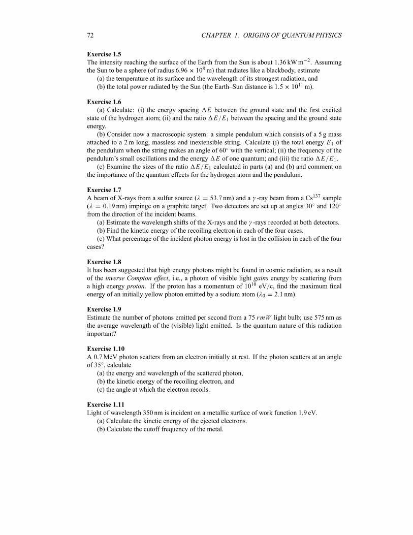
72 CHAPTER 1. ORIGINS OF QUANTUM PHYSICS
Exercise 1.5
The intensity reaching the surface of the Earth from the Sun is about 1 36 kWm 2. Assuming
the Sun to be a sphere (of radius 6 96 108m) that radiates like a blackbody, estimate
(a) the temperature at its surface and the wavelength of its strongest radiation, and
(b) the total power radiated by the Sun (the Earth–Sun distance is 1 5 1011m).
Exercise 1.6
(a) Calculate: (i) the energy spacing E between the ground state and the first excitedstate of the hydrogen atom; (ii) and the ratio E E1 between the spacing and the ground stateenergy.
(b) Consider now a macroscopic system: a simple pendulum which consists of a 5 g mass
attached to a 2m long, massless and inextensible string. Calculate (i) the total energy E1 ofthe pendulum when the string makes an angle of 60 with the vertical; (ii) the frequency of the
pendulum’s small oscillations and the energy E of one quantum; and (iii) the ratio E E1.(c) Examine the sizes of the ratio E E1 calculated in parts (a) and (b) and comment on
the importance of the quantum effects for the hydrogen atom and the pendulum.
Exercise 1.7
A beam of X-rays from a sulfur source 53 7 nm and a -ray beam from a Cs137 sample
( 0 19 nm) impinge on a graphite target. Two detectors are set up at angles 30 and 120
from the direction of the incident beams.
(a) Estimate the wavelength shifts of the X-rays and the -rays recorded at both detectors.
(b) Find the kinetic energy of the recoiling electron in each of the four cases.
(c) What percentage of the incident photon energy is lost in the collision in each of the four
cases?
Exercise 1.8
It has been suggested that high energy photons might be found in cosmic radiation, as a result
of the inverse Compton effect, i.e., a photon of visible light gains energy by scattering froma high energy proton. If the proton has a momentum of 1010 eV c, find the maximum final
energy of an initially yellow photon emitted by a sodium atom ( 0 2 1 nm).
Exercise 1.9
Estimate the number of photons emitted per second from a 75 rmW light bulb; use 575 nm as
the average wavelength of the (visible) light emitted. Is the quantum nature of this radiation
important?
Exercise 1.10
A 0 7MeV photon scatters from an electron initially at rest. If the photon scatters at an angle
of 35 , calculate
(a) the energy and wavelength of the scattered photon,
(b) the kinetic energy of the recoiling electron, and
(c) the angle at which the electron recoils.
Exercise 1.11
Light of wavelength 350 nm is incident on a metallic surface of work function 1 9 eV.
(a) Calculate the kinetic energy of the ejected electrons.
(b) Calculate the cutoff frequency of the metal.
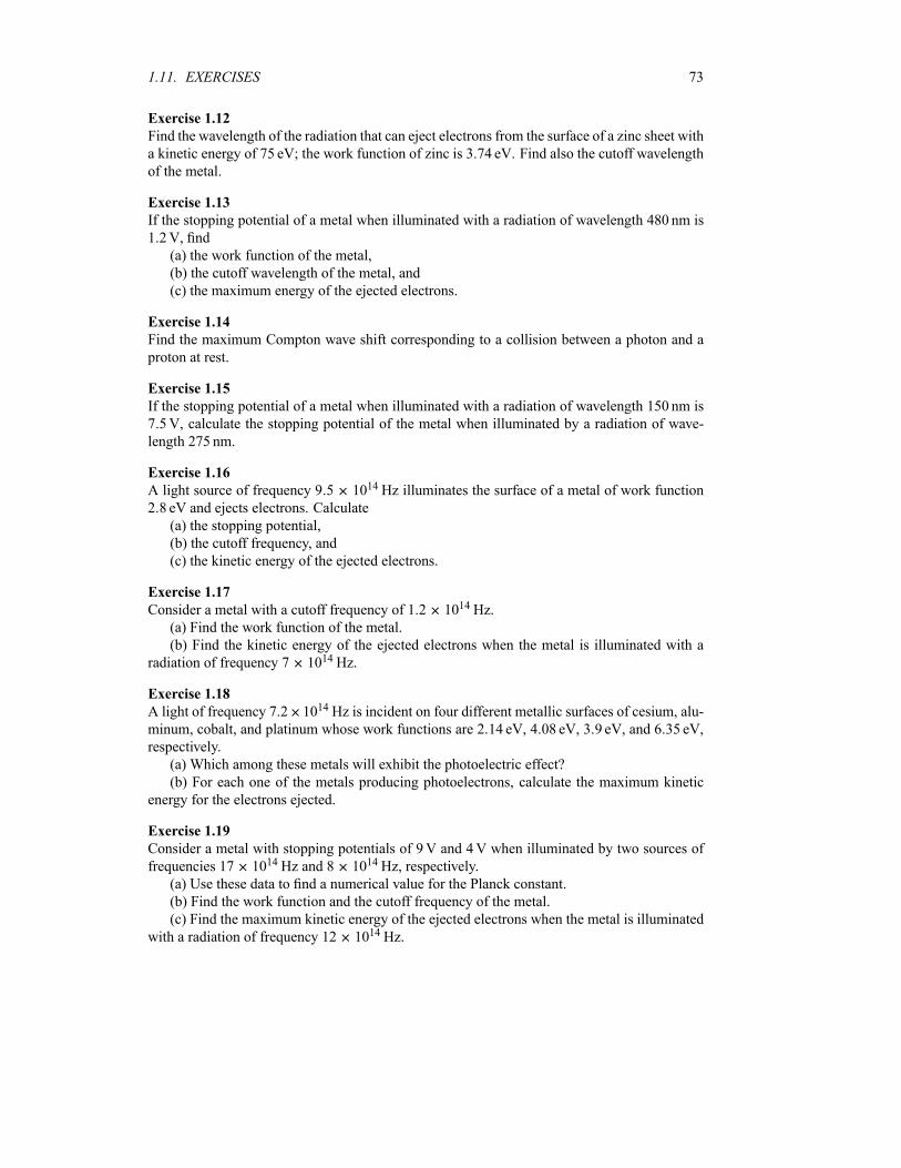
1.11. EXERCISES 73
Exercise 1.12
Find the wavelength of the radiation that can eject electrons from the surface of a zinc sheet with
a kinetic energy of 75 eV; the work function of zinc is 3 74 eV. Find also the cutoff wavelength
of the metal.
Exercise 1.13
If the stopping potential of a metal when illuminated with a radiation of wavelength 480 nm is
1 2V, find
(a) the work function of the metal,
(b) the cutoff wavelength of the metal, and
(c) the maximum energy of the ejected electrons.
Exercise 1.14
Find the maximum Compton wave shift corresponding to a collision between a photon and a
proton at rest.
Exercise 1.15
If the stopping potential of a metal when illuminated with a radiation of wavelength 150 nm is
7 5V, calculate the stopping potential of the metal when illuminated by a radiation of wave-
length 275 nm.
Exercise 1.16
A light source of frequency 9 5 1014Hz illuminates the surface of a metal of work function
2 8 eV and ejects electrons. Calculate
(a) the stopping potential,
(b) the cutoff frequency, and
(c) the kinetic energy of the ejected electrons.
Exercise 1.17
Consider a metal with a cutoff frequency of 1 2 1014Hz.
(a) Find the work function of the metal.
(b) Find the kinetic energy of the ejected electrons when the metal is illuminated with a
radiation of frequency 7 1014Hz.
Exercise 1.18
A light of frequency 7 2 1014Hz is incident on four different metallic surfaces of cesium, alu-
minum, cobalt, and platinum whose work functions are 2 14 eV, 4 08 eV, 3 9 eV, and 6 35 eV,
respectively.
(a) Which among these metals will exhibit the photoelectric effect?
(b) For each one of the metals producing photoelectrons, calculate the maximum kinetic
energy for the electrons ejected.
Exercise 1.19
Consider a metal with stopping potentials of 9V and 4V when illuminated by two sources of
frequencies 17 1014Hz and 8 1014Hz, respectively.
(a) Use these data to find a numerical value for the Planck constant.
(b) Find the work function and the cutoff frequency of the metal.
(c) Find the maximum kinetic energy of the ejected electrons when the metal is illuminated
with a radiation of frequency 12 1014Hz.
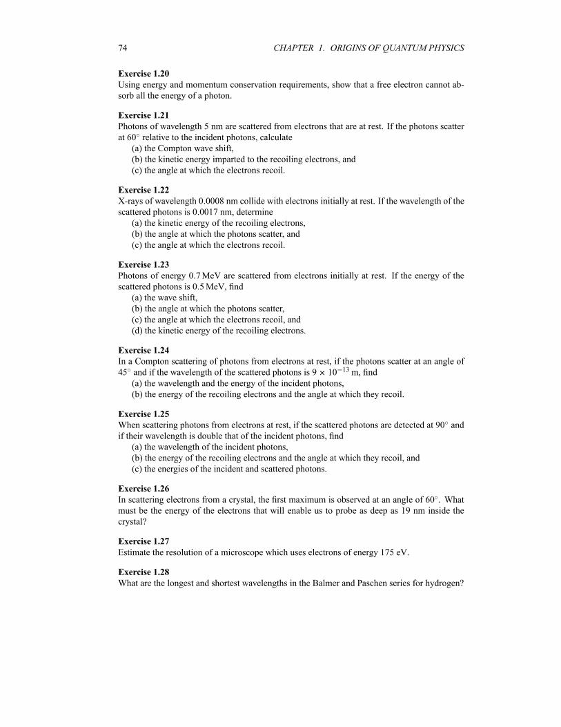
74 CHAPTER 1. ORIGINS OF QUANTUM PHYSICS
Exercise 1.20
Using energy and momentum conservation requirements, show that a free electron cannot ab-
sorb all the energy of a photon.
Exercise 1.21
Photons of wavelength 5 nm are scattered from electrons that are at rest. If the photons scatter
at 60 relative to the incident photons, calculate
(a) the Compton wave shift,
(b) the kinetic energy imparted to the recoiling electrons, and
(c) the angle at which the electrons recoil.
Exercise 1.22
X-rays of wavelength 0 0008 nm collide with electrons initially at rest. If the wavelength of the
scattered photons is 0 0017 nm, determine
(a) the kinetic energy of the recoiling electrons,
(b) the angle at which the photons scatter, and
(c) the angle at which the electrons recoil.
Exercise 1.23
Photons of energy 0 7MeV are scattered from electrons initially at rest. If the energy of the
scattered photons is 0 5MeV, find
(a) the wave shift,
(b) the angle at which the photons scatter,
(c) the angle at which the electrons recoil, and
(d) the kinetic energy of the recoiling electrons.
Exercise 1.24
In a Compton scattering of photons from electrons at rest, if the photons scatter at an angle of
45 and if the wavelength of the scattered photons is 9 10 13m, find
(a) the wavelength and the energy of the incident photons,
(b) the energy of the recoiling electrons and the angle at which they recoil.
Exercise 1.25
When scattering photons from electrons at rest, if the scattered photons are detected at 90 and
if their wavelength is double that of the incident photons, find
(a) the wavelength of the incident photons,
(b) the energy of the recoiling electrons and the angle at which they recoil, and
(c) the energies of the incident and scattered photons.
Exercise 1.26
In scattering electrons from a crystal, the first maximum is observed at an angle of 60 . What
must be the energy of the electrons that will enable us to probe as deep as 19 nm inside the
crystal?
Exercise 1.27
Estimate the resolution of a microscope which uses electrons of energy 175 eV.
Exercise 1.28
What are the longest and shortest wavelengths in the Balmer and Paschen series for hydrogen?
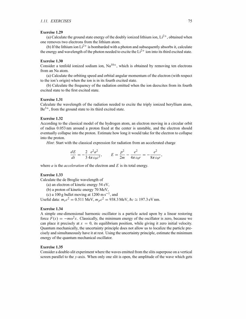
1.11. EXERCISES 75
Exercise 1.29
(a) Calculate the ground state energy of the doubly ionized lithium ion, Li2 , obtained when
one removes two electrons from the lithium atom.
(b) If the lithium ion Li2 is bombarded with a photon and subsequently absorbs it, calculate
the energy and wavelength of the photon needed to excite the Li2 ion into its third excited state.
Exercise 1.30
Consider a tenfold ionized sodium ion, Na10 , which is obtained by removing ten electrons
from an Na atom.
(a) Calculate the orbiting speed and orbital angular momentum of the electron (with respect
to the ion’s origin) when the ion is in its fourth excited state.
(b) Calculate the frequency of the radiation emitted when the ion deexcites from its fourth
excited state to the first excited state.
Exercise 1.31
Calculate the wavelength of the radiation needed to excite the triply ionized beryllium atom,
Be3 , from the ground state to its third excited state.
Exercise 1.32
According to the classical model of the hydrogen atom, an electron moving in a circular orbit
of radius 0 053 nm around a proton fixed at the center is unstable, and the electron should
eventually collapse into the proton. Estimate how long it would take for the electron to collapse
into the proton.
Hint: Start with the classical expression for radiation from an accelerated charge
dE
dt
2
3
e2a2
4 0c3E
p2
2m
e2
4 0r
e2
8 0r
where a is the acceleration of the electron and E is its total energy.
Exercise 1.33
Calculate the de Broglie wavelength of
(a) an electron of kinetic energy 54 eV,
(b) a proton of kinetic energy 70 MeV,
(c) a 100 g bullet moving at 1200 m s 1, and
Useful data: mec2 0 511 MeV, m pc2 938 3MeV, hc 197 3 eVnm.
Exercise 1.34
A simple one-dimensional harmonic oscillator is a particle acted upon by a linear restoring
force F x m 2x . Classically, the minimum energy of the oscillator is zero, because wecan place it precisely at x 0, its equilibrium position, while giving it zero initial velocity.
Quantum mechanically, the uncertainty principle does not allow us to localize the particle pre-
cisely and simultaneously have it at rest. Using the uncertainty principle, estimate the minimum
energy of the quantum mechanical oscillator.
Exercise 1.35
Consider a double-slit experiment where the waves emitted from the slits superpose on a vertical
screen parallel to the y-axis. When only one slit is open, the amplitude of the wave which gets
76 CHAPTER 1. ORIGINS OF QUANTUM PHYSICS
through is 1 y t e y2 32ei t ay and when only the other slit is open, the amplitude is
2 y t e y2 32ei t ay y .
(a) What is the interference pattern along the y-axis with both slits open? Plot the intensityof the wave as a function of y.(b) What would be the intensity if we put a light source behind the screen to measure which
of the slits the light went through? Plot the intensity of the wave as a function of y.
Exercise 1.36
Consider the following three wave functions:
1 y A1ey2
2 y A2ey2 2
3 y A3 ey2 ye y2 2
where A1, A2, and A3 are normalization constants.(a) Find the constants A1, A2, and A3 so that 1, 2, and 3 are normalized.
(b) Find the probability that each one of the states will be in the interval 1 y 1.
Exercise 1.37
Find the Fourier transform p of the following function and plot it:
x1 x x 1
0 x 1
Exercise 1.38
(a) Find the Fourier transform of k Ae a k ibk , where a and b are real numbers, buta is positive.(b) Find A so that x is normalized.(c) Find the x and k uncertainties and calculate the uncertainty product x p. Does it
satisfy Heisenberg’s uncertainty principle?
Exercise 1.39
(a) Find the Fourier transform x of
p0 p p0A p0 p p00 p0 p
where A is a real constant.(b) Find A so that x is normalized and plot p and x . Hint: The following integral
might be needed: dx sin2 ax x2 a.(c) Estimate the uncertainties p and x and then verify that x p satisfies Heisenberg’s
uncertainty relation.
Exercise 1.40
Estimate the lifetime of the excited state of an atom whose natural width is 3 10 4 eV; you
may need the value h 6 626 10 34J s 4 14 10 15 eV s.
Exercise 1.41
Calculate the final width of the wave packet corresponding to an 80 g bullet after traveling for
20 s; the size of the bullet is 2 cm.
1.11. EXERCISES 77
Exercise 1.42
A 100 g arrow travels with a speed of 30 m s 1 over a distance of 50m. If the initial size of the
wave packet is 5 cm, what will be its final size?
Exercise 1.43
A 50MeV beam of protons is fired over a distance of 10 km. If the initial size of the wave
packet is 1 5 10 6m, what will be the final size upon arrival?
Exercise 1.44
A 250GeV beam of protons is fired over a distance of 1 km. If the initial size of the wave packet
is 1mm, find its final size.
Exercise 1.45
Consider an inextensible string of linear density (mass per unit length). If the string is subject
to a tension T , the angular frequency of the string waves is given in terms of the wave numberk by k T . Find the phase and group velocities.
Exercise 1.46
The angular frequency for a wave propagating inside a waveguide is given in terms of the wave
number k and the width b of the guide by kc 1 2 b2k21 2. Find the phase and
group velocities of the wave.
Exercise 1.47
Show that for those waves whose angular frequency and wave number k obey the dispersionrelation k2c2 2 constant , the product of the phase and group velocities is equal to c2,
g ph c2, where c is the speed of light.
Exercise 1.48
How long will the wave packet of a 10 g object, initially confined to 1mm, take to quadruple
its size?
Exercise 1.49
How long will it take for the wave packet of a proton confined to 10 15m to grow to a size
equal to the distance between the Earth and the Sun? This distance is equal to 1 5 108 km.
Exercise 1.50
Assuming the wave packet representing the Moon to be confined to 1m, how long will the
packet take to reach a size triple that of the Sun? The Sun’s radius is 6 96 105 km.

78 CHAPTER 1. ORIGINS OF QUANTUM PHYSICS
Chapter 2
Mathematical Tools of Quantum
Mechanics
2.1 Introduction
We deal here with the mathematical machinery needed to study quantum mechanics. Although
this chapter is mathematical in scope, no attempt is made to be mathematically complete or
rigorous. We limit ourselves to those practical issues that are relevant to the formalism of
quantum mechanics.
The Schrödinger equation is one of the cornerstones of the theory of quantum mechan-
ics; it has the structure of a linear equation. The formalism of quantum mechanics deals withoperators that are linear and wave functions that belong to an abstract Hilbert space. The math-
ematical properties and structure of Hilbert spaces are essential for a proper understanding of
the formalism of quantum mechanics. For this, we are going to review briefly the properties of
Hilbert spaces and those of linear operators. We will then consider Dirac’s bra-ket notation.Quantum mechanics was formulated in two different ways by Schrödinger and Heisenberg.
Schrödinger’s wave mechanics and Heisenberg’s matrix mechanics are the representations of
the general formalism of quantum mechanics in continuous and discrete basis systems, respec-tively. For this, we will also examine the mathematics involved in representing kets, bras,
bra-kets, and operators in discrete and continuous bases.
2.2 The Hilbert Space and Wave Functions
2.2.1 The Linear Vector Space
A linear vector space consists of two sets of elements and two algebraic rules:
a set of vectors and a set of scalars a, b, c, ;
a rule for vector addition and a rule for scalar multiplication.
(a) Addition rule
The addition rule has the properties and structure of an abelian group:
79
80 CHAPTER 2. MATHEMATICAL TOOLS OF QUANTUM MECHANICS
If and are vectors (elements) of a space, their sum, , is also a vector of the
same space.
Commutativity: .
Associativity: .
Existence of a zero or neutral vector: for each vector , there must exist a zero vector
O such that: O O .
Existence of a symmetric or inverse vector: each vector must have a symmetric vector
such that O.
(b) Multiplication rule
The multiplication of vectors by scalars (scalars can be real or complex numbers) has these
properties:
The product of a scalar with a vector gives another vector. In general, if and are two
vectors of the space, any linear combination a b is also a vector of the space, a andb being scalars.
Distributivity with respect to addition:
a a a a b a b (2.1)
Associativity with respect to multiplication of scalars:
a b ab (2.2)
For each element there must exist a unitary scalar I and a zero scalar "o" such that
I I and o o o (2.3)
2.2.2 The Hilbert Space
A Hilbert spaceH consists of a set of vectors , , , and a set of scalars a, b, c, which
satisfy the following four properties:
(a) H is a linear space
The properties of a linear space were considered in the previous section.
(b) H has a defined scalar product that is strictly positive
The scalar product of an element with another element is in general a complex
number, denoted by , where complex number. Note: Watch out for the
order! Since the scalar product is a complex number, the quantity is generally not
equal to : while . The scalar product satisfies the
following properties:
The scalar product of with is equal to the complex conjugate of the scalar
product of with :
(2.4)
2.2. THE HILBERT SPACE AND WAVE FUNCTIONS 81
The scalar product of with is linear with respect to the second factor if
a 1 b 2:
a 1 b 2 a 1 b 2 (2.5)
and antilinear with respect to the first factor if a 1 b 2:
a 1 b 2 a 1 b 2 (2.6)
The scalar product of a vector with itself is a positive real number:
2 0 (2.7)
where the equality holds only for O.
(c) H is separable
There exists a Cauchy sequence n H n 1 2 such that for every of H and
0, there exists at least one n of the sequence for which
n (2.8)
(d) H is complete
Every Cauchy sequence n H converges to an element of H . That is, for any n , the
relation
limn m
n m 0 (2.9)
defines a unique limit ofH such that
limn
n 0 (2.10)
Remark
We should note that in a scalar product , the second factor, , belongs to the Hilbert
spaceH, while the first factor, , belongs to its dual Hilbert spaceHd . The distinction between
H and Hd is due to the fact that, as mentioned above, the scalar product is not commutative:
; the order matters! From linear algebra, we know that every vector space can
be associated with a dual vector space.
2.2.3 Dimension and Basis of a Vector Space
A set of N nonzero vectors 1, 2, , N is said to be linearly independent if and only if thesolution of the equation
N
i 1
ai i 0 (2.11)
is a1 a2 aN 0. But if there exists a set of scalars, which are not all zero, so that
one of the vectors (say n) can be expressed as a linear combination of the others,
n
n 1
i 1
ai i
N
i n 1
ai i (2.12)
82 CHAPTER 2. MATHEMATICAL TOOLS OF QUANTUM MECHANICS
the set i is said to be linearly dependent.Dimension: The dimension of a vector space is given by the maximum number of linearlyindependent vectors the space can have. For instance, if the maximum number of linearly inde-
pendent vectors a space has is N (i.e., 1, 2, , N ), this space is said to be N -dimensional.In this N -dimensional vector space, any vector can be expanded as a linear combination:
N
i 1
ai i (2.13)
Basis: The basis of a vector space consists of a set of the maximum possible number of linearlyindependent vectors belonging to that space. This set of vectors, 1, 2, , N , to be denoted
in short by i , is called the basis of the vector space, while the vectors 1, 2, , N are
called the base vectors. Although the set of these linearly independent vectors is arbitrary,
it is convenient to choose them orthonormal; that is, their scalar products satisfy the relation
i j i j (we may recall that i j 1 whenever i j and zero otherwise). The basis issaid to be orthonormal if it consists of a set of orthonormal vectors. Moreover, the basis is saidto be complete if it spans the entire space; that is, there is no need to introduce any additionalbase vector. The expansion coefficients ai in (2.13) are called the components of the vectorin the basis. Each component is given by the scalar product of with the corresponding base
vector, a j j .
Examples of linear vector spaces
Let us give two examples of linear spaces that are Hilbert spaces: one having a finite (discrete)set of base vectors, the other an infinite (continuous) basis.
The first one is the three-dimensional Euclidean vector space; the basis of this space
consists of three linearly independent vectors, usually denoted by i , j , k. Any vector ofthe Euclidean space can be written in terms of the base vectors as A a1i a2 j a3k,where a1, a2, and a3 are the components of A in the basis; each component can bedetermined by taking the scalar product of A with the corresponding base vector: a1i A, a2 j A, and a3 k A. Note that the scalar product in the Euclidean space is realand hence symmetric. The norm in this space is the usual length of vectors A A.Note also that whenever a1i a2 j a3k 0 we have a1 a2 a3 0 and that none
of the unit vectors i , j , k can be expressed as a linear combination of the other two.
The second example is the space of the entire complex functions x ; the dimension ofthis space is infinite for it has an infinite number of linearly independent basis vectors.
Example 2.1
Check whether the following sets of functions are linearly independent or dependent on the real
x-axis.(a) f x 4, g x x2, h x e2x
(b) f x x , g x x2, h x x3
(c) f x x , g x 5x , h x x2
(d) f x 2 x2, g x 3 x 4x3, h x 2x 3x2 8x3
Solution
2.2. THE HILBERT SPACE AND WAVE FUNCTIONS 83
(a) The first set is clearly linearly independent since a1 f x a2g x a3h x 4a1a2x2 a3e2x 0 implies that a1 a2 a3 0 for any value of x .(b) The functions f x x , g x x2, h x x3 are also linearly independent since
a1x a2x2 a3x3 0 implies that a1 a2 a3 0 no matter what the value of x . Forinstance, taking x 1 1 3, the following system of three equations
a1 a2 a3 0 a1 a2 a3 0 3a1 9a2 27a3 0 (2.14)
yields a1 a2 a3 0.
(c) The functions f x x , g x 5x , h x x2 are not linearly independent, sinceg x 5 f x 0 h x .(d) The functions f x 2 x2, g x 3 x 4x3, h x 2x 3x2 8x3 are not
linearly independent since h x 3 f x 2g x .
Example 2.2
Are the following sets of vectors (in the three-dimensional Euclidean space) linearly indepen-
dent or dependent?
(a) A 3 0 0 , B 0 2 0 , C 0 0 1
(b) A 6 9 0 , B 2 3 0
(c) A 2 3 1 , B 0 1 2 , C 0 0 5
(d) A 1 2 3 , B 4 1 7 , C 0 10 11 , and D 14 3 4
Solution
(a) The three vectors A 3 0 0 , B 0 2 0 , C 0 0 1 are linearly indepen-
dent, since
a1A a2B a3C 0 3a1i 2a2 j a3k 0 (2.15)
leads to
3a1 0 2a2 0 a3 0 (2.16)
which yields a1 a2 a3 0.
(b) The vectors A 6 9 0 , B 2 3 0 are linearly dependent, since the solution
to
a1A a2B 0 6a1 2a2 i 9a1 3a2 j 0 (2.17)
is a1 a2 3. The first vector is equal to 3 times the second one: A 3B.(c) The vectors A 2 3 1 , B 0 1 2 , C 0 0 5 are linearly independent,
since
a1A a2B a3C 0 2a1i 3a1 a2 j a1 2a2 5a3 k 0 (2.18)
leads to
2a1 0 3a1 a2 0 a1 2a2 5a3 0 (2.19)
The only solution of this system is a1 a2 a3 0.
(d) The vectors A 1 2 3 , B 4 1 7 , C 0 10 11 , and D 14 3 4 are
not linearly independent, because D can be expressed in terms of the other vectors:
D 2A 3B C (2.20)
84 CHAPTER 2. MATHEMATICAL TOOLS OF QUANTUM MECHANICS
2.2.4 Square-Integrable Functions: Wave Functions
In the case of function spaces, a “vector” element is given by a complex function and the scalarproduct by integrals. That is, the scalar product of two functions x and x is given by
x x dx (2.21)
If this integral diverges, the scalar product does not exist. As a result, if we want the functionspace to possess a scalar product, we must select only those functions for which is finite.In particular, a function x is said to be square integrable if the scalar product of with
itself,
x 2 dx (2.22)
is finite.It is easy to verify that the space of square-integrable functions possesses the properties of
a Hilbert space. For instance, any linear combination of square-integrable functions is also a
square-integrable function and (2.21) satisfies all the properties of the scalar product of a Hilbert
space.
Note that the dimension of the Hilbert space of square-integrable functions is infinite, since
each wave function can be expanded in terms of an infinite number of linearly independent
functions. The dimension of a space is given by the maximum number of linearly independent
basis vectors required to span that space.
A good example of square-integrable functions is the wave function of quantum mechanics,r t . We have seen in Chapter 1 that, according to Born’s probabilistic interpretation ofr t , the quantity r t 2 d3r represents the probability of finding, at time t , the particle
in a volume d3r , centered around the point r . The probability of finding the particle somewherein space must then be equal to 1:
r t 2 d3r dx dy r t 2 dz 1 (2.23)
hence the wave functions of quantum mechanics are square-integrable. Wave functions sat-
isfying (2.23) are said to be normalized or square-integrable. As wave mechanics deals with
square-integrable functions, any wave function which is not square-integrable has no physical
meaning in quantum mechanics.
2.3 Dirac Notation
The physical state of a system is represented in quantum mechanics by elements of a Hilbert
space; these elements are called state vectors. We can represent the state vectors in different
bases by means of function expansions. This is analogous to specifying an ordinary (Euclid-
ean) vector by its components in various coordinate systems. For instance, we can represent
equivalently a vector by its components in a Cartesian coordinate system, in a spherical coor-
dinate system, or in a cylindrical coordinate system. The meaning of a vector is, of course,independent of the coordinate system chosen to represent its components. Similarly, the stateof a microscopic system has a meaning independent of the basis in which it is expanded.
To free state vectors from coordinate meaning, Dirac introduced what was to become an in-
valuable notation in quantum mechanics; it allows one to manipulate the formalism of quantum
2.3. DIRAC NOTATION 85
mechanics with ease and clarity. He introduced the concepts of kets, bras, and bra-kets, which
will be explained below.
Kets: elements of a vector space
Dirac denoted the state vector by the symbol , which he called a ket vector, or simply aket. Kets belong to the Hilbert (vector) spaceH, or, in short, to the ket-space.
Bras: elements of a dual space
As mentioned above, we know from linear algebra that a dual space can be associated with
every vector space. Dirac denoted the elements of a dual space by the symbol , which he
called a bra vector, or simply a bra; for instance, the element represents a bra. Note: Forevery ket there exists a unique bra and vice versa. Again, while kets belong to theHilbert spaceH, the corresponding bras belong to its dual (Hilbert) spaceHd .
Bra-ket: Dirac notation for the scalar product
Dirac denoted the scalar (inner) product by the symbol , which he called a a bra-ket. Forinstance, the scalar product ( ) is denoted by the bra-ket :
(2.24)
Note: When a ket (or bra) is multiplied by a complex number, we also get a ket (or bra).
Remark: In wave mechanics we deal with wave functions r t , but in the more generalformalism of quantum mechanics we deal with abstract kets . Wave functions, like kets,
are elements of a Hilbert space. We should note that, like a wave function, a ket represents the
system completely, and hence knowing means knowing all its amplitudes in all possible
representations. As mentioned above, kets are independent of any particular representation.
There is no reason to single out a particular representation basis such as the representation in
the position space. Of course, if we want to know the probability of finding the particle at some
position in space, we need to work out the formalism within the coordinate representation. The
state vector of this particle at time t will be given by the spatial wave function r tr t . In the coordinate representation, the scalar product is given by
r t r t d3r (2.25)
Similarly, if we are considering the three-dimensional momentum of a particle, the ket will
have to be expressed in momentum space. In this case the state of the particle will be described
by a wave function p t , where p is the momentum of the particle.
Properties of kets, bras, and bra-kets
Every ket has a corresponding bra
To every ket , there corresponds a unique bra and vice versa:
(2.26)
There is a one-to-one correspondence between bras and kets:
a b a b (2.27)
where a and b are complex numbers. The following is a common notation:
a a a a (2.28)
86 CHAPTER 2. MATHEMATICAL TOOLS OF QUANTUM MECHANICS
Properties of the scalar product
In quantummechanics, since the scalar product is a complex number, the ordering matters
a lot. We must be careful to distinguish a scalar product from its complex conjugate;
is not the same thing as :
(2.29)
This property becomes clearer if we apply it to (2.21):
r t r t d3r r t r t d3r (2.30)
When and are real, we would have . Let us list some
additional properties of the scalar product:
a1 1 a2 2 a1 1 a2 2 (2.31)
a1 1 a2 2 a1 1 a2 2 (2.32)
a1 1 a2 2 b1 1 b2 2 a1b1 1 1 a1b2 1 2
a2b1 2 1 a2b2 2 2
(2.33)
The norm is real and positive
For any state vector of the Hilbert space H, the norm is real and positive;
is equal to zero only for the case where O, where O is the zero vector.If the state is normalized then 1.
Schwarz inequality
For any two states and of the Hilbert space, we can show that
2 (2.34)
If and are linearly dependent (i.e., proportional: , where is a
scalar), this relation becomes an equality. The Schwarz inequality (2.34) is analogous to
the following relation of the real Euclidean space
A B 2 A 2 B 2 (2.35)
Triangle inequality
(2.36)
If and are linearly dependent, , and if the proportionality scalar
is real and positive, the triangle inequality becomes an equality. The counterpart of this
inequality in Euclidean space is given by A B A B .
Orthogonal states
Two kets, and , are said to be orthogonal if they have a vanishing scalar product:
0 (2.37)
2.3. DIRAC NOTATION 87
Orthonormal states
Two kets, and , are said to be orthonormal if they are orthogonal and if each one
of them has a unit norm:
0 1 1 (2.38)
Forbidden quantities
If and belong to the same vector (Hilbert) space, products of the type
and are forbidden. They are nonsensical, since and are
neither kets nor bras (an explicit illustration of this will be carried out in the example
below and later on when we discuss the representation in a discrete basis). If and
belong, however, to different vector spaces (e.g., belongs to a spin space and
to an orbital angular momentum space), then the product , written as
, represents a tensor product of and . Only in these typical cases are
such products meaningful.
Example 2.3
(Note: We will see later in this chapter that kets are represented by column matrices and bras
by row matrices; this example is offered earlier than it should because we need to show some
concrete illustrations of the formalism.) Consider the following two kets:
3i2 i4
2
i2 3i
(a) Find the bra .
(b) Evaluate the scalar product .
(c) Examine why the products and do not make sense.
Solution
(a) As will be explained later when we introduce the Hermitian adjoint of kets and bras, we
want to mention that the bra can be obtained by simply taking the complex conjugate of
the transpose of the ket :
2 i 2 3i (2.39)
(b) The scalar product can be calculated as follows:
2 i 2 3i3i
2 i4
2 3i i 2 i 4 2 3i
7 8i (2.40)
(c) First, the product cannot be performed because, from linear algebra, the
product of two column matrices cannot be performed. Similarly, since two row matrices cannot
be multiplied, the product is meaningless.
88 CHAPTER 2. MATHEMATICAL TOOLS OF QUANTUM MECHANICS
Physical meaning of the scalar product
The scalar product can be interpreted in two ways. First, by analogy with the scalar product
of ordinary vectors in the Euclidean space, where A B represents the projection of B on A,the product also represents the projection of onto . Second, in the case of
normalized states and according to Born’s probabilistic interpretation, the quantity
represents the probability amplitude that the system’s state will, after a measurement is
performed on the system, be found to be in another state .
Example 2.4 (Bra-ket algebra)
Consider the states 3i 1 7i 2 and 1 2i 2 , where 1 and
2 are orthonormal.
(a) Calculate and .
(b) Calculate the scalar products and . Are they equal?
(c) Show that the states and satisfy the Schwarz inequality.
(d) Show that the states and satisfy the triangle inequality.
Solution
(a) The calculation of is straightforward:
3i 1 7i 2 1 2i 2
1 3i 1 5i 2 (2.41)
This leads at once to the expression of :
1 3i 1 5i 2 1 3i 1 5i 2 (2.42)
(b) Since 1 1 2 2 1, 1 2 2 1 0, and since the bras
corresponding to the kets 3i 1 7i 2 and 1 2i 2 are given by
3i 1 7i 2 and 1 2i 2 , the scalar products are
3i 1 7i 2 1 2i 2
3i 1 1 1 7i 2i 2 2
14 3i (2.43)
1 2i 2 3i 1 7i 2
1 3i 1 1 2i 7i 2 2
14 3i (2.44)
We see that is equal to the complex conjugate of .
(c) Let us first calculate and :
3i 1 7i 2 3i 1 7i 2 3i 3i 7i 7i 58 (2.45)
1 2i 2 1 2i 2 1 1 2i 2i 5 (2.46)
Since 14 3i we have 2 142 32 205. Combining the values of2, , and , we see that the Schwarz inequality (2.34) is satisfied:
205 58 5 2 (2.47)
2.4. OPERATORS 89
(d) First, let us use (2.41) and (2.42) to calculate :
[ 1 3i 1 5i 2 ] [ 1 3i 1 5i 2 ]
1 3i 1 3i 5i 5i
35 (2.48)
Since 58 and 5, we infer that the triangle inequality (2.36) is satisfied:
35 58 5 (2.49)
Example 2.5
Consider two states 1 2i 1 2 a 3 4 4 and 2 3 1 i 2 5 3 4 ,
where 1 , 2 , 3 , and 4 are orthonormal kets, and where a is a constant. Find the valueof a so that 1 and 2 are orthogonal.
Solution
For the states 1 and 2 to be orthogonal, the scalar product 2 1 must be zero. Using
the relation 2 3 1 i 2 5 3 4 , we can easily find the scalar product
2 1 3 1 i 2 5 3 4 2i 1 2 a 3 4 4
7i 5a 4 (2.50)
Since 2 1 7i 5a 4 0, the value of a is a 7i 4 5.
2.4 Operators
2.4.1 General Definitions
Definition of an operator: An operator1 A is a mathematical rule that when applied to a kettransforms it into another ket of the same space and when it acts on a bra
transforms it into another bra :
A A (2.51)
A similar definition applies to wave functions:
A r r r A r (2.52)
Examples of operators
Here are some of the operators that we will use in this text:
Unity operator: it leaves any ket unchanged, I .
The gradient operator: r r x i r y j r z k.
1The hat on A will be used throughout this text to distinguish an operator A from a complex number or a matrix A.

90 CHAPTER 2. MATHEMATICAL TOOLS OF QUANTUM MECHANICS
The linear momentum operator: P r ih r .
The Laplacian operator: 2 r 2 r x2 2 r y2 2 r z2.
The parity operator: P r r .
Products of operators
The product of two operators is generally not commutative:
AB BA (2.53)
The product of operators is, however, associative:
ABC A BC AB C (2.54)
We may also write AnAm
An m
. When the product AB operates on a ket (the order
of application is important), the operator B acts first on and then A acts on the new ketB :
AB A B (2.55)
Similarly, when ABCD operates on a ket , D acts first, then C , then B, and then A.When an operator A is sandwiched between a bra and a ket , it yields in general
a complex number: A complex number. The quantity A can also be a
purely real or a purely imaginary number. Note: In evaluating A it does not matter if
one first applies A to the ket and then takes the bra-ket or one first applies A to the bra and thentakes the bra-ket; that is A A .
Linear operators
An operator A is said to be linear if it obeys the distributive law and, like all operators, itcommutes with constants. That is, an operator A is linear if, for any vectors 1 and 2 and
any complex numbers a1 and a2, we have
A a1 1 a2 2 a1A 1 a2A 2 (2.56)
and
1 a1 2 a2 A a1 1 A a2 2 A (2.57)
Remarks
The expectation or mean value A of an operator A with respect to a state is defined
by
AA
(2.58)
The quantity (i.e., the product of a ket with a bra) is a linear operator in Dirac’s
notation. To see this, when is applied to a ket , we obtain another ket:
(2.59)
since is a complex number.
Products of the type A and A (i.e., when an operator stands on the right of a ket
or on the left of a bra) are forbidden. They are not operators, or kets, or bras; they have
no mathematical or physical meanings (see equation (2.219) for an illustration).
2.4. OPERATORS 91
2.4.2 Hermitian Adjoint
The Hermitian adjoint or conjugate2, †, of a complex number is the complex conjugate of
this number: † . The Hermitian adjoint, or simply the adjoint, A†, of an operator A is
defined by this relation:
A†
A (2.60)
Properties of the Hermitian conjugate rule
To obtain the Hermitian adjoint of any expression, we must cyclically reverse the order of the
factors and make three replacements:
Replace constants by their complex conjugates: † .
Replace kets (bras) by the corresponding bras (kets): † and † .
Replace operators by their adjoints.
Following these rules, we can write
A† † A (2.61)
aA † a A†
(2.62)
An † A
† n (2.63)
A B C D † A†
B† C† D† (2.64)
ABCD † D†C†B†A†
(2.65)
ABCD † D†C†B†A† (2.66)
The Hermitian adjoint of the operator is given by
† (2.67)
Operators act inside kets and bras, respectively, as follows:
A A A A†
(2.68)
Note also that A†
A† † A. Hence, we can also write:
A A†
A (2.69)
Hermitian and skew-Hermitian operators
An operator A is said to be Hermitian if it is equal to its adjoint A†:
A A†
or A A (2.70)
2The terms “adjoint” and “conjugate” are used indiscriminately.
92 CHAPTER 2. MATHEMATICAL TOOLS OF QUANTUM MECHANICS
On the other hand, an operator B is said to be skew-Hermitian or anti-Hermitian if
B† B or B B (2.71)
Remark
The Hermitian adjoint of an operator is not, in general, equal to its complex conjugate: A†
A .
Example 2.6
(a) Discuss the hermiticity of the operators A A†, i A A
†, and i A A
†.
(b) Find the Hermitian adjoint of f A 1 i A 3A21 2i A 9A
25 7A .
(c) Show that the expectation value of a Hermitian operator is real and that of an anti-
Hermitian operator is imaginary.
Solution
(a) The operator B A A†is Hermitian regardless of whether or not A is Hermitian,
since
B† A A† † A
†A B (2.72)
Similarly, the operator i A A†is also Hermitian; but i A A
†is anti-Hermitian, since
[i A A†]† i A A
†.
(b) Since the Hermitian adjoint of an operator function f A is given by f † A f A†,
we can write
1 i A 3A21 2i A 9A
2
5 7A
†1 2i A
†9A†
2
1 i A†
3A†2
5 7A†
(2.73)
(c) From (2.70) we immediately infer that the expectation value of a Hermitian operator is
real, for it satisfies the following property:
A A (2.74)
that is, if A†
A then A is real. Similarly, for an anti-Hermitian operator, B† B,we have
B B (2.75)
which means that B is a purely imaginary number.
2.4.3 Projection Operators
An operator P is said to be a projection operator if it is Hermitian and equal to its own square:
P† P P2 P (2.76)
The unit operator I is a simple example of a projection operator, since I† I I 2 I .

2.4. OPERATORS 93
Properties of projection operators
The product of two commuting projection operators, P1 and P2, is also a projectionoperator, since
P1P2† P
†2 P†1 P2P1 P1P2 and P1P2
2 P1P2P1P2 P21 P22 P1P2
(2.77)
The sum of two projection operators is generally not a projection operator.
Two projection operators are said to be orthogonal if their product is zero.
For a sum of projection operators P1 P2 P3 to be a projection operator, it is
necessary and sufficient that these projection operators be mutually orthogonal (i.e., the
cross-product terms must vanish).
Example 2.7
Show that the operator is a projection operator only when is normalized.
Solution
It is easy to ascertain that the operator is Hermitian, since † . As
for the square of this operator, it is given by
2 (2.78)
Thus, if is normalized, we have 2 . In sum, if the state is
normalized, the product of the ket with the bra is a projection operator.
2.4.4 Commutator Algebra
The commutator of two operators A and B, denoted by [A B], is defined by
[A B] AB BA (2.79)
and the anticommutator A B is defined by
A B AB BA (2.80)
Two operators are said to commute if their commutator is equal to zero and hence AB BA.Any operator commutes with itself:
[A A] 0 (2.81)
Note that if two operators are Hermitian and their product is also Hermitian, these operators
commute:
AB † B†A†
BA (2.82)
and since AB † AB we have AB BA.
94 CHAPTER 2. MATHEMATICAL TOOLS OF QUANTUM MECHANICS
As an example, we may mention the commutators involving the x-position operator, X ,and the x-component of the momentum operator, Px ih x , as well as the y and the zcomponents
[X Px ] ih I [Y Py] ih I [Z Pz] ih I (2.83)
where I is the unit operator.
Properties of commutators
Using the commutator relation (2.79), we can establish the following properties:
Antisymmetry:
[A B] [B A] (2.84)
Linearity:
[A B C D ] [A B] [A C] [A D] (2.85)
Hermitian conjugate of a commutator:
[A B]† [B† A†] (2.86)
Distributivity:
[A BC] [A B]C B[A C] (2.87)
[AB C] A[B C] [A C]B (2.88)
Jacobi identity:
[A [B C]] [B [C A]] [C [A B]] 0 (2.89)
By repeated applications of (2.87), we can show that
[A Bn]n 1
j 0
B j [A B]Bn j 1 (2.90)
[AnB]
n 1
j 0
An j 1
[A B]Aj
(2.91)
Operators commute with scalars: an operator A commutes with any scalar b:
[A b] 0 (2.92)
Example 2.8
(a) Show that the commutator of two Hermitian operators is anti-Hermitian.
(b) Evaluate the commutator [A [B C]D].
2.4. OPERATORS 95
Solution
(a) If A and B are Hermitian, we can write
[A B]† AB BA † B†A†
A†B† BA AB [A B] (2.93)
that is, the commutator of A and B is anti-Hermitian: [A B]† [A B].(b) Using the distributivity relation (2.87), we have
[A [B C]D] [B C][A D] [A [B C]]D
BC CB AD DA A BC CB D BC CB AD
CBDA BCDA ABCD ACBD (2.94)
2.4.5 Uncertainty Relation between Two Operators
An interesting application of the commutator algebra is to derive a general relation giving the
uncertainties product of two operators, A and B. In particular, we want to give a formal deriva-tion of Heisenberg’s uncertainty relations.
Let A and B denote the expectation values of two Hermitian operators A and B withrespect to a normalized state vector : A A and B B .
Introducing the operators A and B,
A A A B B B (2.95)
we have A 2 A2
2A A A 2 and B 2 B2 2B B B 2, and hence
A 2 A 2 A2
A 2 B 2 B2 B 2 (2.96)
where A2
A2
and B2 B2 . The uncertainties A and B aredefined by
A A 2 A2
A 2 B B 2 B2 B 2 (2.97)
Let us write the action of the operators (2.95) on any state as follows:
A A A B B B (2.98)
The Schwarz inequality for the states and is given by
2 (2.99)
Since A and B are Hermitian, A and B must also be Hermitian: A†
A†
A
A A A and B† B B B. Thus, we can show the following three relations:
A 2 B 2 A B(2.100)
96 CHAPTER 2. MATHEMATICAL TOOLS OF QUANTUM MECHANICS
For instance, since A†
A we have A†A A 2
A 2 . Hence, the Schwarz inequality (2.99) becomes
A 2 B 2 A B2
(2.101)
Notice that the last term A B of this equation can be written as
A B1
2[ A B]
1
2A B
1
2[A B]
1
2A B (2.102)
where we have used the fact that [ A B] [A B]. Since [A B] is anti-Hermitian andA B is Hermitian and since the expectation value of a Hermitian operator is real and
that the expectation value of an anti-Hermitian operator is imaginary (see Example 2.6), the
expectation value A B of (2.102) becomes equal to the sum of a real part A B 2
and an imaginary part [A B] 2; hence
A B2 1
4[A B]
2 1
4A B
2(2.103)
Since the last term is a positive real number, we can infer the following relation:
A B2 1
4[A B]
2(2.104)
Comparing equations (2.101) and (2.104), we conclude that
A 2 B 2 1
4[A B]
2(2.105)
which (by taking its square root) can be reduced to
A B1
2[A B] (2.106)
This uncertainty relation plays an important role in the formalism of quantum mechanics. Its
application to position and momentum operators leads to the Heisenberg uncertainty relations,
which represent one of the cornerstones of quantum mechanics; see the next example.
Example 2.9 (Heisenberg uncertainty relations)
Find the uncertainty relations between the components of the position and the momentum op-
erators.
Solution
By applying (2.106) to the x-components of the position operator X , and the momentum op-erator Px , we obtain x px
12
[X Px ] . But since [X Px ] ih I , we havex px h 2; the uncertainty relations for the y and z components follow immediately:
x pxh
2y py
h
2z pz
h
2(2.107)
These are the Heisenberg uncertainty relations.
2.4. OPERATORS 97
2.4.6 Functions of Operators
Let F A be a function of an operator A. If A is a linear operator, we can Taylor expand F Ain a power series of A:
F An 0
anAn
(2.108)
where an is just an expansion coefficient. As an illustration of an operator function, consider
eaA, where a is a scalar which can be complex or real. We can expand it as follows:
eaA
n 0
an
n!An
I aAa2
2!A2 a3
3!A3
(2.109)
Commutators involving function operators
If A commutes with another operator B, then B commutes with any operator function thatdepends on A:
[A B] 0 [B F A ] 0 (2.110)
in particular, F A commutes with A and with any other function, G A , of A:
[A F A ] 0 [AnF A ] 0 [F A G A ] 0 (2.111)
Hermitian adjoint of function operators
The adjoint of F A is given by
[F A ]† F A†
(2.112)
Note that if A is Hermitian, F A is not necessarily Hermitian; F A will be Hermitian only if
F is a real function and A is Hermitian. An example is
eA † eA†
ei A † e i A† ei A † e i A† (2.113)
where is a complex number. So if A is Hermitian, an operator function which can be ex-
panded as F A n 0 anAnwill be Hermitian only if the expansion coefficients an are real
numbers. But in general, F A is not Hermitian even if A is Hermitian, since
F A†
n 0
an A† n (2.114)
Relations involving function operators
Note that
[A B] 0 [B F A ] 0 (2.115)
in particular, eAeB eA B . Using (2.109) we can ascertain that
eAeB eA Be[A B] 2 (2.116)
eABe A B [A B]1
2![A [A B]]
1
3![A [A [A B]]] (2.117)
98 CHAPTER 2. MATHEMATICAL TOOLS OF QUANTUM MECHANICS
2.4.7 Inverse and Unitary Operators
Inverse of an operator: Assuming it exists3 the inverse A1of a linear operator A is defined
by the relation
A1A AA
1I (2.118)
where I is the unit operator, the operator that leaves any state unchanged.
Quotient of two operators: Dividing an operator A by another operator B (provided that theinverse B 1 exists) is equivalent to multiplying A by B 1:
A
BAB 1 (2.119)
The side on which the quotient is taken matters:
A
BAI
BAB 1 and
I
BA B 1A (2.120)
In general, we have AB 1 B 1A. For an illustration of these ideas, see Problem 2.12. Wemay mention here the following properties about the inverse of operators:
ABCD1
D 1C 1B 1A1
An 1
A1 n
(2.121)
Unitary operators: A linear operator U is said to be unitary if its inverse U 1 is equal to its
adjoint U†:
U† U 1 or UU† U†U I (2.122)
The product of two unitary operators is also unitary, since
UV UV † UV V †U† U VV † U† UU† I (2.123)
or UV † UV 1. This result can be generalized to any number of operators; the product
of a number of unitary operators is also unitary, since
ABCD ABCD † ABCD D†C†B†A†
ABC DD† C†B†A†
AB CC† B†A†
A BB† A†
AA†
I (2.124)
or ABCD † ABCD 1.
Example 2.10 (Unitary operator)
What conditions must the parameter and the operator G satisfy so that the operatorU ei G
is unitary?
3Not every operator has an inverse, just as in the case of matrices. The inverse of a matrix exists only when its
determinant is nonzero.
2.4. OPERATORS 99
Solution
Clearly, if is real and G is Hermitian, the operator ei G would be unitary. Using the property
[F A ]† F A†, we see that
ei G † e i G ei G 1 (2.125)
that is, U† U 1.
2.4.8 Eigenvalues and Eigenvectors of an Operator
Having studied the properties of operators and states, we are now ready to discuss how to find
the eigenvalues and eigenvectors of an operator.
A state vector is said to be an eigenvector (also called an eigenket or eigenstate) of anoperator A if the application of A to gives
A a (2.126)
where a is a complex number, called an eigenvalue of A. This equation is known as the eigen-value equation, or eigenvalue problem, of the operator A. Its solutions yield the eigenvaluesand eigenvectors of A. In Section 2.5.3 we will see how to solve the eigenvalue problem in adiscrete basis.
A simple example is the eigenvalue problem for the unity operator I :
I (2.127)
This means that all vectors are eigenvectors of I with one eigenvalue, 1. Note that
A a An an and F A F a (2.128)
For instance, we have
A a ei A eia (2.129)
Example 2.11 (Eigenvalues of the inverse of an operator)
Show that if A1exists, the eigenvalues of A
1are just the inverses of those of A.
Solution
Since A1A I we have on the one hand
A1A (2.130)
and on the other hand
A1A A
1A aA
1(2.131)
Combining the previous two equations, we obtain
aA1
(2.132)
100 CHAPTER 2. MATHEMATICAL TOOLS OF QUANTUM MECHANICS
hence
A1 1
a(2.133)
This means that is also an eigenvector of A1with eigenvalue 1 a. That is, if A
1exists,
then
A a A1 1
a(2.134)
Some useful theorems pertaining to the eigenvalue problem
Theorem 2.1 For a Hermitian operator, all of its eigenvalues are real and the eigenvectorscorresponding to different eigenvalues are orthogonal.
If A†
A A n an n an real number, and m n mn
(2.135)
Proof of Theorem 2.1
Note that
A n an n m A n an m n (2.136)
and
m A† am m m A† n am m n (2.137)
Subtracting (2.137) from (2.136) and using the fact that A is Hermitian, A A†, we have
an am m n 0 (2.138)
Two cases must be considered separately:
Case m n: since n n 0, we must have an an ; hence the eigenvalues an mustbe real.
Case m n: since in general an am , we must have m n 0; that is, m and
n must be orthogonal.
Theorem 2.2 The eigenstates of a Hermitian operator define a complete set of mutually or-thonormal basis states. The operator is diagonal in this eigenbasis with its diagonal elementsequal to the eigenvalues. This basis set is unique if the operator has no degenerate eigenvaluesand not unique (in fact it is infinite) if there is any degeneracy.
Theorem 2.3 If two Hermitian operators, A and B, commute and if A has no degenerate eigen-value, then each eigenvector of A is also an eigenvector of B. In addition, we can construct acommon orthonormal basis that is made of the joint eigenvectors of A and B.
Proof of Theorem 2.3
Since A is Hermitian with no degenerate eigenvalue, to each eigenvalue of A there correspondsonly one eigenvector. Consider the equation
A n an n (2.139)
2.4. OPERATORS 101
Since A commutes with B we can write
BA n AB n or A B n an B n (2.140)
that is, B n is an eigenvector of A with eigenvalue an . But since this eigenvector is unique(apart from an arbitrary phase constant), the ket n must also be an eigenvector of B:
B n bn n (2.141)
Since each eigenvector of A is also an eigenvector of B (and vice versa), both of these operatorsmust have a common basis. This basis is unique; it is made of the joint eigenvectors of A andB. This theorem also holds for any number of mutually commuting Hermitian operators.Now, if an is a degenerate eigenvalue, we can only say that B n is an eigenvector of
A with eigenvalue an; n is not necessarily an eigenvector of B. If one of the operators isdegenerate, there exist an infinite number of orthonormal basis sets that are common to these
two operators; that is, the joint basis does exist and it is not unique.
Theorem 2.4 The eigenvalues of an anti-Hermitian operator are either purely imaginary orequal to zero.
Theorem 2.5 The eigenvalues of a unitary operator are complex numbers of moduli equal toone; the eigenvectors of a unitary operator that has no degenerate eigenvalues are mutuallyorthogonal.
Proof of Theorem 2.5
Let n and m be eigenvectors to the unitary operator U with eigenvalues an and am ,respectively. We can write
m U† U n aman m n (2.142)
Since U†U I this equation can be rewritten as
aman 1 m n 0 (2.143)
which in turn leads to the following two cases:
Case n m: since n n 0 then anan an 2 1, and hence an 1.
Case n m: the only possibility for this case is that m and n are orthogonal,
m n 0.
2.4.9 Infinitesimal and Finite Unitary Transformations
We want to study here how quantities such as kets, bras, operators, and scalars transform under
unitary transformations. A unitary transformation is the application of a unitary operator U toone of these quantities.
102 CHAPTER 2. MATHEMATICAL TOOLS OF QUANTUM MECHANICS
2.4.9.1 Unitary Transformations
Kets and bras transform as follows:
U U† (2.144)
Let us now find out how operators transform under unitary transformations. Since the transform
of A is A , we can rewrite A as A U U
U A which, in turn, leads to A U U A. Multiplying both sides of A U U A byU† and
since UU† U†U I , we have
A U AU† A U†A U (2.145)
The results reached in (2.144) and (2.145) may be summarized as follows:
U U† A U AU† (2.146)
U† U A U†A U (2.147)
Properties of unitary transformations
If an operator A is Hermitian, its transformed A is also Hermitian, since
A † U AU† † U A†U† U AU† A (2.148)
The eigenvalues of A and those of its transformed A are the same:
A n an n A n an n (2.149)
since
A n U AU† U n U A U†U n
U A n an U n an n (2.150)
Commutators that are equal to (complex) numbers remain unchanged under unitary trans-
formations, since the transformation of [A B] a, where a is a complex number, isgiven by
[A B ] [U AU† UBU†] U AU† UBU† UBU† U AU†
U [A B]U† UaU† aUU† a
[A B] (2.151)
We can also verify the following general relations:
A B C A B C (2.152)
A BCD A B C D (2.153)
where A , B , C , and D are the transforms of A, B, C , and D, respectively.
2.4. OPERATORS 103
Since the result (2.151) is valid for any complex number, we can state that complex
numbers, such as A , remain unchanged under unitary transformations, since
A U† U AU† U U†U A U†U A(2.154)
Taking A I we see that scalar products of the type
(2.155)
are invariant under unitary transformations; notably, the norm of a state vector is con-
served:
(2.156)
We can also verify that UAU†n
UAnU† since
UAU†n
UAU† UAU† UAU† UA U†U A U†U U†U AU†
UAnU† (2.157)
We can generalize the previous result to obtain the transformation of any operator func-
tion f A :
U f A U† f U AU† f A (2.158)
or more generally
U f A B C U† f U AU† UBU† UCU† f A B C (2.159)
A unitary transformation does not change the physics of a system; it merely transforms one
description of the system to another physically equivalent description.
In what follows we want to consider two types of unitary transformations: infinitesimal
transformations and finite transformations.
2.4.9.2 Infinitesimal Unitary Transformations
Consider an operator U which depends on an infinitesimally small real parameter and which
varies only slightly from the unity operator I :
U G I i G (2.160)
where G is called the generator of the infinitesimal transformation. Clearly, U is a unitary
transformation only when the parameter is real and G is Hermitian, since
U U†
I i G I i G† I i G G† I (2.161)
where we have neglected the quadratic terms in .
The transformation of a state vector is
I i G (2.162)
104 CHAPTER 2. MATHEMATICAL TOOLS OF QUANTUM MECHANICS
where
i G (2.163)
The transformation of an operator A is given by
A I i G A I i G A i [G A] (2.164)
If G commutes with A, the unitary transformation will leave A unchanged, A A:
[G A] 0 A I i G A I i G A (2.165)
2.4.9.3 Finite Unitary Transformations
We can construct a finite unitary transformation from (2.160) by performing a succession ofinfinitesimal transformations in steps of ; the application of a series of successive unitary
transformations is equivalent to the application of a single unitary transformation. Denoting
N , where N is an integer and is a finite parameter, we can apply the same unitary
transformation N times; in the limit N we obtain
U G limN
N
k 1
1 iNG lim
N1 i
NG
Nei G (2.166)
where G is now the generator of the finite transformation and is its parameter.
As shown in (2.125), U is unitary only when the parameter is real and G is Hermitian,since
ei G † e i G ei G 1 (2.167)
Using the commutation relation (2.117), we can write the transformation A of an operator Aas follows:
ei G Ae i G A i [G A]i 2
2!G [G A]
i 3
3!G [G [G A]]
(2.168)
If G commutes with A, the unitary transformation will leave A unchanged, A A:
[G A] 0 A ei G Ae i G A (2.169)
In Chapter 3, we will consider some important applications of infinitesimal unitary transfor-
mations to study time translations, space translations, space rotations, and conservation laws.
2.5 Representation in Discrete Bases
By analogy with the expansion of Euclidean space vectors in terms of the basis vectors, we need
to express any ket of the Hilbert space in terms of a complete set of mutually orthonormal
base kets. State vectors are then represented by their components in this basis.
2.5. REPRESENTATION IN DISCRETE BASES 105
2.5.1 Matrix Representation of Kets, Bras, and Operators
Consider a discrete, complete, and orthonormal basis which is made of an infinite4 set of kets
1 , 2 , 3 , , n and denote it by n . Note that the basis n is discrete, yet
it has an infinite number of unit vectors. In the limit n , the ordering index n of the unitvectors n is discrete or countable; that is, the sequence 1 , 2 , 3 , is countably
infinite. As an illustration, consider the special functions, such as the Hermite, Legendre, or
Laguerre polynomials, Hn x , Pn x , and Ln x . These polynomials are identified by a discreteindex n and by a continuous variable x ; although n varies discretely, it can be infinite.In Section 2.6, we will consider bases that have a continuous and infinite number of base
vectors; in these bases the index n increases continuously. Thus, each basis has a continuum ofbase vectors.
In this section the notation n will be used to abbreviate an infinitely countable set of
vectors (i.e., 1 , 2 , 3 , ) of the Hilbert space H. The orthonormality condition of
the base kets is expressed by
n m nm (2.170)
where nm is the Kronecker delta symbol defined by
nm1 n m0 n m
(2.171)
The completeness, or closure, relation for this basis is given by
n 1
n n I (2.172)
where I is the unit operator; when the unit operator acts on any ket, it leaves the ket unchanged.
2.5.1.1 Matrix Representation of Kets and Bras
Let us now examine how to represent the vector within the context of the basis n .
The completeness property of this basis enables us to expand any state vector in terms of
the base kets n :
In 1
n nn 1
an n (2.173)
where the coefficient an , which is equal to n , represents the projection of onto n ;
an is the component of along the vector n . Recall that the coefficients an are complexnumbers. So, within the basis n , the ket is represented by the set of its components,
a1, a2, a3, along 1 , 2 , 3 , , respectively. Hence can be represented by a
column vector which has a countably infinite number of components:
1
2
n
a1a2
an
(2.174)
4Kets are elements of the Hilbert space, and the dimension of a Hilbert space is infinite.
106 CHAPTER 2. MATHEMATICAL TOOLS OF QUANTUM MECHANICS
The bra can be represented by a row vector:
1 2 n
1 2 n
a1 a2 an (2.175)
Using this representation, we see that a bra-ket is a complex number equal to the matrix
product of the row matrix corresponding to the bra with the column matrix corresponding
to the ket :
a1 a2 an
b1b2
bn n
anbn (2.176)
where bn n . We see that, within this representation, the matrices representing
and are Hermitian adjoints of each other.
Remark
A ket is normalized if n an2 1. If is not normalized and we want
to normalized it, we need simply to multiply it by a constant so that 2
1, and hence 1 .
Example 2.12
Consider the following two kets:
5i2
i
3
8i9i
(a) Find and .
(b) Is normalized? If not, normalize it.
(c) Are and orthogonal?
Solution
(a) The expressions of and are given by
5i2
i5i 2 i (2.177)
where we have used the fact that is equal to the complex conjugate of the transpose of the
ket . Hence, we should reiterate the important fact that .
(b) The norm of is given by
5i 2 i5i2
i5i 5i 2 2 i i 30 (2.178)
2.5. REPRESENTATION IN DISCRETE BASES 107
Thus, is not normalized. By multiplying it with 1 30, it becomes normalized:
1
30
1
30
5i2
i1 (2.179)
(c) The kets and are not orthogonal since their scalar product is not zero:
5i 2 i3
8i9i
5i 3 2 8i i 9i 9 i (2.180)
2.5.1.2 Matrix Representation of Operators
For each linear operator A, we can write
A I AIn 1
n n Am 1
m mnm
Anm n m (2.181)
where Anm is the nm matrix element of the operator A:
Anm n A m (2.182)
We see that the operator A is represented, within the basis n , by a square matrix A (Awithout a hat designates a matrix), which has a countably infinite number of columns and a
countably infinite number of rows:
A
A11 A12 A13A21 A22 A23A31 A32 A33 (2.183)
For instance, the unit operator I is represented by the unit matrix; when the unit matrix ismultiplied with another matrix, it leaves that unchanged:
I
1 0 0
0 1 0
0 0 1 (2.184)
In summary, kets are represented by column vectors, bras by row vectors, and operators bysquare matrices.
108 CHAPTER 2. MATHEMATICAL TOOLS OF QUANTUM MECHANICS
2.5.1.3 Matrix Representation of Some Other Operators
(a) Hermitian adjoint operation
Let us now look at the matrix representation of the Hermitian adjoint operation of an operator.
First, recall that the transpose of a matrix A, denoted by AT , is obtained by interchanging therows with the columns:
AT nm Amn or
A11 A12 A13A21 A22 A23A31 A32 A33
TA11 A21 A31A12 A22 A32A13 A23 A33
(2.185)
Similarly, the transpose of a column matrix is a row matrix, and the transpose of a row matrix
is a column matrix:
a1a2
an
T
a1 a2 an and a1 a2 anT
a1a2
an
(2.186)
So a square matrix A is symmetric if it is equal to its transpose, AT A. A skew-symmetricmatrix is a square matrix whose transpose equals the negative of the matrix, AT A.The complex conjugate of a matrix is obtained by simply taking the complex conjugate of
all its elements: A nm Anm .
The matrix which represents the operator A†is obtained by taking the complex conjugate
of the matrix transpose of A:
A† AT or A†nm n A
†m m A n Amn (2.187)
that is,
A11 A12 A13A21 A22 A23A31 A32 A33
†A11 A21 A31A12 A22 A32A13 A23 A33
(2.188)
If an operator A is Hermitian, its matrix satisfies this condition:
AT A or Amn Anm (2.189)
The diagonal elements of a Hermitian matrix therefore must be real numbers. Note that aHermitian matrix must be square.
(b) Inverse and unitary operators
A matrix has an inverse only if it is square and its determinant is nonzero; a matrix that has
an inverse is called a nonsingular matrix and a matrix that has no inverse is called a singular
2.5. REPRESENTATION IN DISCRETE BASES 109
matrix. The elements A 1nm of the inverse matrix A
1, representing an operator A1, are given
by the relation
A 1nm
cofactor of Amndeterminant of A
or A 1 BT
determinant of A(2.190)
where B is the matrix of cofactors (also called the minor); the cofactor of element Amn is equalto 1 m n times the determinant of the submatrix obtained from A by removing the mth rowand the nth column. Note that when the matrix, representing an operator, has a determinantequal to zero, this operator does not possess an inverse. Note that A 1A AA 1 I where Iis the unit matrix.
The inverse of a product of matrices is obtained as follows:
ABC PQ 1 Q 1P 1 C 1B 1A 1 (2.191)
The inverse of the inverse of a matrix is equal to the matrix itself, A 1 1A.
A unitary operator U is represented by a unitary matrix. A matrix U is said to be unitary ifits inverse is equal to its adjoint:
U 1 U† or U†U I (2.192)
where I is the unit matrix.
Example 2.13 (Inverse of a matrix)
Calculate the inverse of the matrix A2 i 0
3 1 5
0 i 2
. Is this matrix unitary?
Solution
Since the determinant of A is det A 4 16i , we have A 1 BT 4 16i , where theelements of the cofactor matrix B are given by Bnm 1 n m times the determinant of the
submatrix obtained from A by removing the nth row and the mth column. In this way, we have
B11 1 1 1 A22 A23A32 A33
1 21 5
i 22 5i (2.193)
B12 1 1 2 A21 A23A31 A33
1 33 5
0 26 (2.194)
B13 1 1 3 A21 A22A31 A32
1 43 1
0 i3i (2.195)
B21 1 3i 0
i 22i B22 1 4
2 0
0 24 (2.196)
B23 1 52 i0 i
2i B31 1 4i 0
1 55i (2.197)
B32 1 52 0
3 510 B33 1 6
2 i3 1
2 3i (2.198)
110 CHAPTER 2. MATHEMATICAL TOOLS OF QUANTUM MECHANICS
and hence
B2 5i 6 3i2i 4 2i5i 10 2 3i
(2.199)
Taking the transpose of B, we obtain
A 1 1
4 16iBT
1 4i
68
2 5i 2i 5i6 4 10
3i 2i 2 3i
1
68
22 3i 8 2i 20 5i6 24i 4 16i 10 40i12 3i 8 2i 14 5i
(2.200)
Clearly, this matrix is not unitary since its inverse is not equal to its Hermitian adjoint:
A 1 A†.
(c) Matrix representation of
It is now easy to see that the product is indeed an operator, since its representation
within n is a square matrix:
a1a2a3 a1 a2 a3
a1a1 a1a2 a1a3a2a1 a2a2 a2a3a3a1 a3a2 a3a3
(2.201)
(d) Trace of an operator
The trace Tr A of an operator A is given, within an orthonormal basis n , by the expression
Tr An
n A nn
Ann (2.202)
we will see later that the trace of an operator does not depend on the basis. The trace of a matrix
is equal to the sum of its diagonal elements:
Tr
A11 A12 A13A21 A22 A23A31 A32 A33 A11 A22 A33 (2.203)
Properties of the trace
We can ascertain that
Tr A†
Tr A (2.204)
Tr A B C Tr A Tr B Tr C (2.205)
and the trace of a product of operators is invariant under the cyclic permutations of these oper-
ators:
Tr ABCDE Tr E ABCD Tr DEABC Tr CDEAB (2.206)
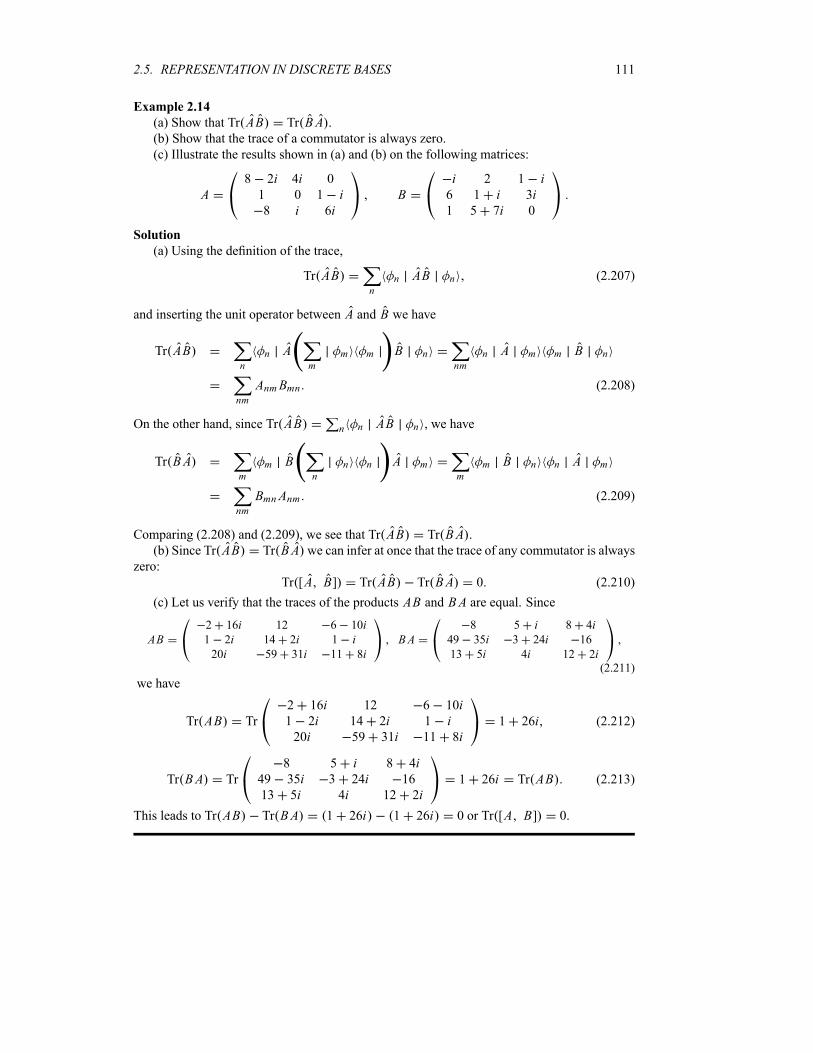
2.5. REPRESENTATION IN DISCRETE BASES 111
Example 2.14
(a) Show that Tr AB Tr BA .(b) Show that the trace of a commutator is always zero.
(c) Illustrate the results shown in (a) and (b) on the following matrices:
A8 2i 4i 0
1 0 1 i8 i 6i
Bi 2 1 i6 1 i 3i1 5 7i 0
Solution
(a) Using the definition of the trace,
Tr ABn
n AB n (2.207)
and inserting the unit operator between A and B we have
Tr ABn
n Am
m m B nnm
n A m m B n
nm
AnmBmn (2.208)
On the other hand, since Tr AB n n AB n , we have
Tr BAm
m Bn
n n A mm
m B n n A m
nm
BmnAnm (2.209)
Comparing (2.208) and (2.209), we see that Tr AB Tr BA .(b) Since Tr AB Tr BA we can infer at once that the trace of any commutator is always
zero:
Tr [A B] Tr AB Tr BA 0 (2.210)
(c) Let us verify that the traces of the products AB and BA are equal. Since
AB2 16i 12 6 10i1 2i 14 2i 1 i20i 59 31i 11 8i
BA8 5 i 8 4i
49 35i 3 24i 16
13 5i 4i 12 2i(2.211)
we have
Tr AB Tr
2 16i 12 6 10i1 2i 14 2i 1 i20i 59 31i 11 8i
1 26i (2.212)
Tr BA Tr
8 5 i 8 4i49 35i 3 24i 16
13 5i 4i 12 2i1 26i Tr AB (2.213)
This leads to Tr AB Tr BA 1 26i 1 26i 0 or Tr [A B] 0.
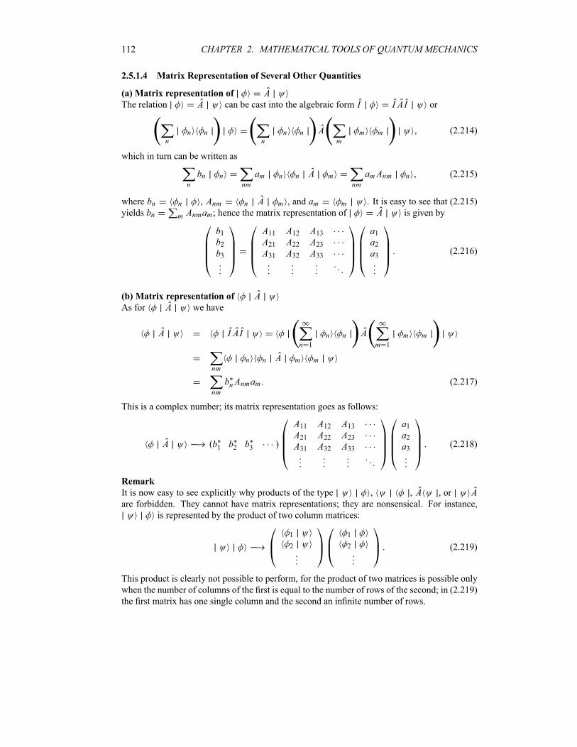
112 CHAPTER 2. MATHEMATICAL TOOLS OF QUANTUM MECHANICS
2.5.1.4 Matrix Representation of Several Other Quantities
(a) Matrix representation of AThe relation A can be cast into the algebraic form I I AI or
nn n
nn n A
mm m (2.214)
which in turn can be written as
n
bn nnm
am n n A mnm
am Anm n (2.215)
where bn n , Anm n A m , and am m . It is easy to see that (2.215)
yields bn m Anmam ; hence the matrix representation of A is given by
b1b2b3
A11 A12 A13A21 A22 A23A31 A32 A33
a1a2a3 (2.216)
(b) Matrix representation of AAs for A we have
A I AIn 1
n n Am 1
m m
nmn n A m m
nm
bnAnmam (2.217)
This is a complex number; its matrix representation goes as follows:
A b1 b2 b3
A11 A12 A13A21 A22 A23A31 A32 A33
a1a2a3 (2.218)
Remark
It is now easy to see explicitly why products of the type , , A , or Aare forbidden. They cannot have matrix representations; they are nonsensical. For instance,
is represented by the product of two column matrices:
1
2
1
2 (2.219)
This product is clearly not possible to perform, for the product of two matrices is possible only
when the number of columns of the first is equal to the number of rows of the second; in (2.219)
the first matrix has one single column and the second an infinite number of rows.
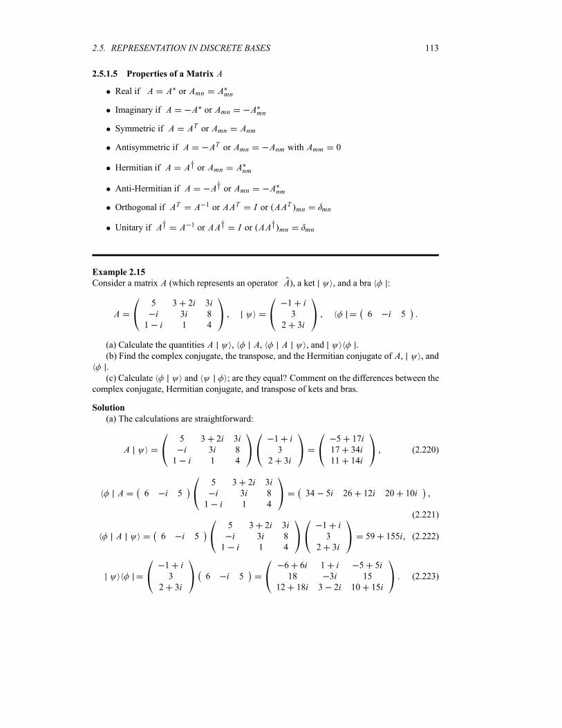
2.5. REPRESENTATION IN DISCRETE BASES 113
2.5.1.5 Properties of a Matrix A
Real if A A or Amn Amn
Imaginary if A A or Amn Amn
Symmetric if A AT or Amn Anm
Antisymmetric if A AT or Amn Anm with Amm 0
Hermitian if A A† or Amn Anm
Anti-Hermitian if A A† or Amn Anm
Orthogonal if AT A 1 or AAT I or AAT mn mn
Unitary if A† A 1 or AA† I or AA† mn mn
Example 2.15
Consider a matrix A (which represents an operator A), a ket , and a bra :
A5 3 2i 3ii 3i 8
1 i 1 4
1 i3
2 3i6 i 5
(a) Calculate the quantities A , A, A , and .
(b) Find the complex conjugate, the transpose, and the Hermitian conjugate of A, , and
.
(c) Calculate and ; are they equal? Comment on the differences between the
complex conjugate, Hermitian conjugate, and transpose of kets and bras.
Solution
(a) The calculations are straightforward:
A5 3 2i 3ii 3i 8
1 i 1 4
1 i3
2 3i
5 17i17 34i11 14i
(2.220)
A 6 i 5
5 3 2i 3ii 3i 8
1 i 1 4
34 5i 26 12i 20 10i
(2.221)
A 6 i 5
5 3 2i 3ii 3i 8
1 i 1 4
1 i3
2 3i59 155i (2.222)
1 i3
2 3i6 i 5
6 6i 1 i 5 5i18 3i 15
12 18i 3 2i 10 15i(2.223)
114 CHAPTER 2. MATHEMATICAL TOOLS OF QUANTUM MECHANICS
(b) To obtain the complex conjugate of A, , and , we need simply to take the
complex conjugate of their elements:
A5 3 2i 3ii 3i 8
1 i 1 4
1 i3
2 3i6 i 5
(2.224)
For the transpose of A, , and , we simply interchange columns with rows:
AT5 i 1 i
3 2i 3i 1
3i 8 4
T 1 i 3 2 3i T6
i5(2.225)
The Hermitian conjugate can be obtained by taking the complex conjugates of the transpose
expressions calculated above: A† AT , † T , † T :
A†5 i 1 i
3 2i 3i 1
3i 8 4
1 i 3 2 3i6
i5(2.226)
(c) Using the kets and bras above, we can easily calculate the needed scalar products:
6 i 5
1 i3
2 3i6 1 i i 3 5 2 3i 4 18i (2.227)
1 i 3 2 3i6
i5
6 1 i i 3 5 2 3i 4 18i (2.228)
We see that and are not equal; they are complex conjugates of each other:
4 18i (2.229)
Remark
We should underscore the importance of the differences between , T , and †. Most
notably, we should note (from equations (2.224)–(2.226)) that is a ket, while T and† are bras. Additionally, we should note that is a bra, while T and † are kets.
2.5.2 Change of Bases and Unitary Transformations
In a Euclidean space, a vector A may be represented by its components in different coordinatesystems or in different bases. The transformation from one basis to the other is called a change
of basis. The components of A in a given basis can be expressed in terms of the components ofA in another basis by means of a transformation matrix.Similarly, state vectors and operators of quantum mechanics may also be represented in
different bases. In this section we are going to study how to transform from one basis to
another. That is, knowing the components of kets, bras, and operators in a basis n , how
2.5. REPRESENTATION IN DISCRETE BASES 115
does one determine the corresponding components in a different basis n ? Assuming that
n and n are two different bases, we can expand each ket n of the old basis in
terms of the new basis n as follows:
nm
m m nm
Umn m (2.230)
where
Umn m n (2.231)
The matrix U , providing the transformation from the old basis n to the new basis n ,
is given by
U1 1 1 2 1 3
2 1 2 2 2 3
3 1 3 2 3 3
(2.232)
Example 2.16 (Unitarity of the transformation matrix)
Let U be a transformation matrix which connects two complete and orthonormal bases n
and n . Show that U is unitary.
Solution
For this we need to prove that UU† I , which reduces to showing that m UU† n
mn . This goes as follows:
m UU† n m Ul
l l U† nl
UmlUnl (2.233)
where Uml m U l and Unl l U† n n U l . According to
(2.231), Uml m l and Unl l n ; we can thus rewrite (2.233) as
l
UmlUnll
m l l n m n mn (2.234)
Combining (2.233) and (2.234), we infer m UU† n mn , or UU† I .
2.5.2.1 Transformations of Kets, Bras, and Operators
The components n of a state vector in a new basis n can be expressed in terms
of the components n of in an old basis n as follows:
m m I mn
n nn
Umn n (2.235)
This relation, along with its complex conjugate, can be generalized into
ne U old ne old U† (2.236)
116 CHAPTER 2. MATHEMATICAL TOOLS OF QUANTUM MECHANICS
Let us now examine how operators transform when we change from one basis to another. The
matrix elements Amn m A n of an operator A in the new basis can be expressed in
terms of the old matrix elements, A jl j A l , as follows:
Amn mj
j j Al
l l njl
Umj A jlUnl (2.237)
that is,
Ane U AoldU† or Aold U†Ane U (2.238)
We may summarize the results of the change of basis in the following relations:
ne U old ne old U† Ane U AoldU† (2.239)
or
old U† ne old ne U Aold U†Ane U (2.240)
These relations are similar to the ones we derived when we studied unitary transformations; see
(2.146) and (2.147).
Example 2.17
Show that the operator U n n n satisfies all the properties discussed above.
Solution
First, note that U is unitary:
UU†
nln n l l
nln l nl
nn n I (2.241)
Second, the action ofU on a ket of the old basis gives the corresponding ket from the new basis:
U mn
n n mn
n nm m (2.242)
We can also verify that the actionU† on a ket of the new basis gives the corresponding ket fromthe old basis:
U† ml
l l ml
l lm m (2.243)
How does a trace transform under unitary transformations? Using the cyclic property of the
trace, Tr ABC Tr CAB Tr BCA , we can ascertain that
Tr A Tr U AU† Tr U†U A Tr A (2.244)
2.5. REPRESENTATION IN DISCRETE BASES 117
Tr n ml
l n m ll
m l l n
ml
l l n m n mn (2.245)
Tr m n n m (2.246)
Example 2.18 (The trace is base independent)
Show that the trace of an operator does not depend on the basis in which it is expressed.
Solution
Let us show that the trace of an operator A in a basis n is equal to its trace in another basis
n . First, the trace of A in the basis n is given by
Tr An
n A n (2.247)
and in n by
Tr An
n A n (2.248)
Starting from (2.247) and using the completeness of the other basis, n , we have
Tr An
n A nn
nm
m m A n
nmn m m A n (2.249)
All we need to do now is simply to interchange the positions of the numbers (scalars) n m
and m A n :
Tr Am
m An
n n mm
m A m (2.250)
From (2.249) and (2.250) we see that
Tr An
n A nn
n A n (2.251)
2.5.3 Matrix Representation of the Eigenvalue Problem
At issue here is to work out the matrix representation of the eigenvalue problem (2.126) and
then solve it. That is, we want to find the eigenvalues a and the eigenvectors of an operator
A such thatA a (2.252)
118 CHAPTER 2. MATHEMATICAL TOOLS OF QUANTUM MECHANICS
where a is a complex number. Inserting the unit operator between A and and multiplying
by m , we can cast the eigenvalue equation in the form
m An
n n a mn
n n (2.253)
or
n
Amn n an
n nm (2.254)
which can be rewritten as
n
[Amn a nm] n 0 (2.255)
with Amn m A n .
This equation represents an infinite, homogeneous system of equations for the coefficients
n , since the basis n is made of an infinite number of base kets. This system of
equations can have nonzero solutions only if its determinant vanishes:
det Amn a nm 0 (2.256)
The problem that arises here is that this determinant corresponds to a matrix with an infinite
number of columns and rows. To solve (2.256) we need to truncate the basis n and assume
that it contains only N terms, where N must be large enough to guarantee convergence. In thiscase we can reduce (2.256) to the following N th degree determinant:
A11 a A12 A13 A1NA21 A22 a A23 A2NA31 A32 A33 a A3N
AN1 AN2 AN3 ANN a
0 (2.257)
This is known as the secular or characteristic equation. The solutions of this equation yieldthe N eigenvalues a1, a2, a3, , aN , since it is an N th order equation in a. The set of theseN eigenvalues is called the spectrum of A. Knowing the set of eigenvalues a1, a2, a3, , aN ,we can easily determine the corresponding set of eigenvectors 1 , 2 , , N . For
each eigenvalue am of A, we can obtain from the “secular” equation (2.257) the N components
1 , 2 , 3 , , N of the corresponding eigenvector m .
If a number of different eigenvectors (two or more) have the same eigenvalue, this eigen-
value is said to be degenerate. The order of degeneracy is determined by the number of linearlyindependent eigenvectors that have the same eigenvalue. For instance, if an eigenvalue has five
different eigenvectors, it is said to be fivefold degenerate.
In the case where the set of eigenvectors n of A is complete and orthonormal, this setcan be used as a basis. In this basis the matrix representing the operator A is diagonal,
A
a1 0 0
0 a2 0
0 0 a3 (2.258)
2.5. REPRESENTATION IN DISCRETE BASES 119
the diagonal elements being the eigenvalues an of A, since
m A n an m n an mn (2.259)
Note that the trace and determinant of a matrix are given, respectively, by the sum and product
of the eigenvalues:
Tr An
an a1 a2 a3 (2.260)
det An
an a1a2a3 (2.261)
Properties of determinants
Let us mention several useful properties that pertain to determinants. The determinant of a
product of matrices is equal to the product of their determinants:
det ABCD det A det B det C det D (2.262)
det A det A det A† det A (2.263)
det AT det A det A eTr ln A (2.264)
Some theorems pertaining to the eigenvalue problem
Here is a list of useful theorems (the proofs are left as exercises):
The eigenvalues of a symmetric matrix are real; the eigenvectors form an orthonormal
basis.
The eigenvalues of an antisymmetric matrix are purely imaginary or zero.
The eigenvalues of a Hermitian matrix are real; the eigenvectors form an orthonormal
basis.
The eigenvalues of a skew-Hermitian matrix are purely imaginary or zero.
The eigenvalues of a unitary matrix have absolute value equal to one.
If the eigenvalues of a square matrix are not degenerate (distinct), the corresponding
eigenvectors form a basis (i.e., they form a linearly independent set).
Example 2.19 (Eigenvalues and eigenvectors of a matrix)
Find the eigenvalues and the normalized eigenvectors of the matrix
A7 0 0
0 1 i0 i 1
120 CHAPTER 2. MATHEMATICAL TOOLS OF QUANTUM MECHANICS
Solution
To find the eigenvalues of A, we simply need to solve the secular equation det A aI 0:
0
7 a 0 0
0 1 a i0 i 1 a
7 a 1 a 1 a i2 7 a a2 2
(2.265)
The eigenvalues of A are thus given by
a1 7 a2 2 a3 2 (2.266)
Let us now calculate the eigenvectors of A. To find the eigenvector corresponding to the firsteigenvalue, a1 7, we need to solve the matrix equation
7 0 0
0 1 i0 i 1
xyz
7
xyz
7x 7xy iz 7yiy z 7z
(2.267)
this yields x 1 (because the eigenvector is normalized) and y z 0. So the eigenvector
corresponding to a1 7 is given by the column matrix
a1
1
0
0
(2.268)
This eigenvector is normalized since a1 a1 1.
The eigenvector corresponding to the second eigenvalue, a2 2, can be obtained from
the matrix equation
7 0 0
0 1 i0 i 1
xyz
2
xyz
7 2 x 0
1 2 y i z 0
iy 1 2 z 0
(2.269)
this yields x 0 and z i 2 1 y. So the eigenvector corresponding to a2 2 is given
by the column matrix
a2
0
yi 2 1 y
(2.270)
The value of the variable y can be obtained from the normalization condition of a2 :
1 a2 a2 0 y i 2 1 y0
yi 2 1 y
2 2 2 y 2
(2.271)
Taking only the positive value of y (a similar calculation can be performed easily if one is
interested in the negative value of y), we have y 1 2 2 2 ; hence the eigenvector
(2.270) becomes
a2
01
2 2 2
i 2 1
2 2 2
(2.272)
2.6. REPRESENTATION IN CONTINUOUS BASES 121
Following the same procedure that led to (2.272), we can show that the third eigenvector is
given by
a3
0
yi 1 2 y
(2.273)
its normalization leads to y 1 2 2 2 (we have considered only the positive value of
y); hence
a3
01
2 2 2
i 1 2
2 2 2
(2.274)
2.6 Representation in Continuous Bases
In this section we are going to consider the representation of state vectors, bras, and operators
in continuous bases. After presenting the general formalism, we will consider two importantapplications: representations in the position and momentum spaces.In the previous section we saw that the representations of kets, bras, and operators in a
discrete basis are given by discrete matrices. We will show here that these quantities are repre-
sented in a continuous basis by continuous matrices, that is, by noncountable infinite matrices.
2.6.1 General Treatment
The orthonormality condition of the base kets of the continuous basis k is expressed not by
the usual discrete Kronecker delta as in (2.170) but by Dirac’s continuous delta function:
k k k k (2.275)
where k and k are continuous parameters and where k k is the Dirac delta function (seeAppendix A), which is defined by
x1
2eikxdk (2.276)
As for the completeness condition of this continuous basis, it is not given by a discrete sum as
in (2.172), but by an integral over the continuous variable
dk k k I (2.277)
where I is the unit operator.Every state vector can be expanded in terms of the complete set of basis kets k :
I dk k k dk b k k (2.278)
122 CHAPTER 2. MATHEMATICAL TOOLS OF QUANTUM MECHANICS
where b k , which is equal to k , represents the projection of on k .
The norm of the discrete base kets is finite ( n n 1), but the norm of the continuous
base kets is infinite; a combination of (2.275) and (2.276) leads to
k k 01
2dk (2.279)
This implies that the kets k are not square integrable and hence are not elements of the
Hilbert space; recall that the space spanned by square-integrable functions is a Hilbert space.
Despite the divergence of the norm of k , the set k does constitute a valid basis of vectors
that span the Hilbert space, since for any state vector , the scalar product k is finite.
The Dirac delta function
Before dealing with the representation of kets, bras, and operators, let us make a short detour
to list some of the most important properties of the Dirac delta function (for a more detailed
presentation, see Appendix A):
x 0 for x 0 (2.280)
b
af x x x0 dx
f x0 if a x0 b0 elsewhere
(2.281)
f xdn x a
dxndx 1 n
dn f x
dxn x a(2.282)
r r x x y y z z1
r2 sinr r (2.283)
Representation of kets, bras, and operators
The representation of kets, bras, and operators can be easily inferred from the study that was
carried out in the previous section, for the case of a discrete basis. For instance, the ket
is represented by a single column matrix which has a continuous (noncountable) and infinite
number of components (rows) b k :
k (2.284)
The bra is represented by a single row matrix which has a continuous (noncountable)
and infinite number of components (columns):
k (2.285)
Operators are represented by square continuous matrices whose rows and columns have
continuous and infinite numbers of components:
AA k k
(2.286)
As an application, we are going to consider the representations in the position and momentum
bases.

2.6. REPRESENTATION IN CONTINUOUS BASES 123
2.6.2 Position Representation
In the position representation, the basis consists of an infinite set of vectors r which are
eigenkets to the position operator R:
R r r r (2.287)
where r (without a hat), the position vector, is the eigenvalue of the operator R. The orthonor-mality and completeness conditions are respectively given by
r r r r x x y y z z (2.288)
d3 r r r I (2.289)
since, as discussed in Appendix A, the three-dimensional delta function is given by
r r1
2 3d3k eik r r (2.290)
So every state vector can be expanded as follows:
d3 r r r d3r r r (2.291)
where r denotes the components of in the r basis:
r r (2.292)
This is known as the wave function for the state vector . Recall that, according to the
probabilistic interpretation of Born, the quantity r 2 d3r represents the probability offinding the system in the volume element d3r .The scalar product between two state vectors, and , can be expressed in this form:
d3r r r d3r r r (2.293)
Since R r r r we have
r R n r r n r r (2.294)
Note that the operator R is Hermitian, since
R d3r r r r d3r r r r
R (2.295)
124 CHAPTER 2. MATHEMATICAL TOOLS OF QUANTUM MECHANICS
2.6.3 Momentum Representation
The basis p of the momentum representation is obtained from the eigenkets of the momen-
tum operator P:
P p p p (2.296)
where p is the momentum vector. The algebra relevant to this representation can be easilyinferred from the position representation. The orthonormality and completeness conditions of
the momentum space basis p are given by
p p p p and d3p p p I (2.297)
Expanding in this basis, we obtain
d3 p p p d3 p p p (2.298)
where the expansion coefficient p represents the momentum space wave function. Thequantity p 2 d3 p is the probability of finding the system’s momentum in the volumeelement d3 p located between p and p d p.By analogy with (2.293) the scalar product between two states is given in the momentum
space by
d3 p p p d3 p p p (2.299)
Since P p p p we have
p P n p p n p p (2.300)
2.6.4 Connecting the Position and Momentum Representations
Let us now study how to establish a connection between the position and the momentum rep-
resentations. By analogy with the foregoing study, when changing from the r basis to the
p basis, we encounter the transformation function r p .To find the expression for the transformation function r p , let us establish a connection
between the position and momentum representations of the state vector :
r r d3 p p p d3 p r p p (2.301)
that is,
r d3 p r p p (2.302)
Similarly, we can write
p p p d3r r r d3r p r r (2.303)
2.6. REPRESENTATION IN CONTINUOUS BASES 125
The last two relations imply that r and p are to be viewed as Fourier transforms of eachother. In quantum mechanics the Fourier transform of a function f r is given by
f r1
2 h 3 2d3 p ei p r hg p (2.304)
notice the presence of Planck’s constant. Hence the function r p is given by
r p1
2 h 3 2ei p r h (2.305)
This function transforms from the momentum to the position representation. The function
corresponding to the inverse transformation, p r , is given by
p r r p1
2 h 3 2e i p r h (2.306)
The quantity r p 2 represents the probability density of finding the particle in a region
around r where its momentum is equal to p.
Remark
If the position wave function
r1
2 h 3 2d3 p ei p r h p (2.307)
is normalized (i.e., d3r r r 1), its Fourier transform
p1
2 h 3 2d3r e i p r h r (2.308)
must also be normalized, since
d3 p p p d3 p p1
2 h 3 2d3r e i p r h r
d3r r1
2 h 3 2d3 p p e i p r h
d3r r r
1 (2.309)
This result is known as Parseval’s theorem.
2.6.4.1 Momentum Operator in the Position Representation
To determine the form of the momentum operator P in the position representation, let us cal-
culate r P :
r P r P p p d3 p p r p p d3 p
1
2 h 3 2p ei p r h p d3 p (2.310)
126 CHAPTER 2. MATHEMATICAL TOOLS OF QUANTUM MECHANICS
where we have used the relation p p d3 p I along with Eq. (2.305). Now, since
p ei p r h ih ei p r h , and using Eq. (2.305) again, we can rewrite (2.310) as
r P ih1
2 h 3 2ei p r h p d3 p
ih r p p d3 p
ih r (2.311)
Thus, P is given in the position representation by
P ih (2.312)
Its Cartesian components are
Px ihx
Py ihy
Pz ihz
(2.313)
Note that the form of the momentum operator (2.312) can be derived by simply applying the
gradient operator on a plane wave function r t Aei p r Et h :
ih r t p r t P r t (2.314)
It is easy to verify that P is Hermitian (see equation (2.378)).
Now, since P ih , we can write the Hamiltonian operator H P 2 2m V in theposition representation as follows:
Hh2
2m2 V r
h2
2m
2
x2
2
y2
2
z2V r (2.315)
where 2 is the Laplacian operator; it is given in Cartesian coordinates by 2 2 x22 y2 2 z2.
2.6.4.2 Position Operator in the Momentum Representation
The form of the position operator R in the momentum representation can be easily inferred
from the representation of P in the position space. In momentum space the position operatorcan be written as follows:
R j ihp j
j x y z (2.316)
or
X ihpx
Y ihpy
Z ihpz
(2.317)
2.6. REPRESENTATION IN CONTINUOUS BASES 127
2.6.4.3 Important Commutation Relations
Let us now calculate the commutator [R j Pk] in the position representation. As the separate
actions of X Px and Px X on the wave function r are given by
X Px r ihxr
x(2.318)
Px X r ihxx r ih r ihx
r
x(2.319)
we have
[X Px ] r X Px r Px X r ihxr
xih r ihx
r
xih r (2.320)
or
[X Px ] ih (2.321)
Similar relations can be derived at once for the y and the z components:
[X Px ] ih [Y PY ] ih [Z PZ ] ih (2.322)
We can verify that
[X Py] [X Pz] [Y Px ] [Y Pz] [Z Px ] [Z Py] 0 (2.323)
since the x , y, z degrees of freedom are independent; the previous two relations can be groupedinto
[R j Pk] ih jk [R j Rk] 0 [Pj Pk] 0 j k x y z (2.324)
These relations are often called the canonical commutation relations.Now, from (2.321) we can show that (for the proof see Problem 2.8 on page 139)
[Xn Px ] ihnXn 1 [X Pnx ] ihnPn 1x (2.325)
Following the same procedure that led to (2.320), we can obtain a more general commutation
relation of Px with an arbitrary function f X :
[ f X Px ] ihd f X
dXP F R ih F R (2.326)
where F is a function of the operator R.The explicit form of operators thus depends on the representation adopted. We have seen,
however, that the commutation relations for operators are representation independent. In par-ticular, the commutator [R j Pk] is given by ih jk in the position and the momentum represen-
tations; see the next example.
128 CHAPTER 2. MATHEMATICAL TOOLS OF QUANTUM MECHANICS
Example 2.20 (Commutators are representation independent)
Calculate the commutator [X P] in the momentum representation and verify that it is equal toih.
Solution
As the operator X is given in the momentum representation by X ih p, we have
[X P] p X P p PX p ihpp p ih p
p
p
ih p ih pp
pih p
p
pih p (2.327)
Thus, the commutator [X P] is given in the momentum representation by
[X P] ihpP ih (2.328)
The commutator [X P] was also shown to be equal to ih in the position representation (seeequation (2.321):
[X P] X ihpx
ih (2.329)
2.6.5 Parity Operator
The space reflection about the origin of the coordinate system is called an inversion or a parityoperation. This transformation is discrete. The parity operator P is defined by its action on thekets r of the position space:
P r r r P† r (2.330)
such that
P r r (2.331)
The parity operator is Hermitian, P† P , since
d3r r P r d3r r r d3r r r
d3r P r r (2.332)
From the definition (2.331), we have
P2 r P r r (2.333)
hence P2 is equal to the unity operator:
P2 I or P P 1 (2.334)
2.6. REPRESENTATION IN CONTINUOUS BASES 129
The parity operator is therefore unitary, since its Hermitian adjoint is equal to its inverse:
P† P 1 (2.335)
Now, since P2 I , the eigenvalues of P are 1 or 1 with the corresponding eigenstates
P r r r P r r r (2.336)
The eigenstate is said to be even and is odd. Therefore, the eigenfunctions of theparity operator have definite parity: they are either even or odd.Since and are joint eigenstates of the same Hermitian operator P but with
different eigenvalues, these eigenstates must be orthogonal:
d3r r r d3r r r (2.337)
hence is zero. The states and form a complete set since any function
can be written as r r r , which leads to
r1
2r r r
1
2r r (2.338)
Since P2 I we have
PnP when n is oddI when n is even
(2.339)
Even and odd operators
An operator A is said to be even if it obeys the condition
PAP A (2.340)
and an operator B is odd ifPBP B (2.341)
We can easily verify that even operators commute with the parity operator P and that odd
operators anticommute with P:
AP PAP P PAP2 PA (2.342)
BP PBP P PBP2 PB (2.343)
The fact that even operators commute with the parity operator has very useful consequences.
Let us examine the following two important cases depending on whether an even operator has
nondegenerate or degenerate eigenvalues:
If an even operator is Hermitian and none of its eigenvalues is degenerate, then this oper-
ator has the same eigenvectors as those of the parity operator. And since the eigenvectors
of the parity operator are either even or odd, the eigenvectors of an even, Hermitian, and
nondegenerate operator must also be either even or odd; they are said to have a defi-nite parity. This property will have useful applications when we solve the Schrödingerequation for even Hamiltonians.
130 CHAPTER 2. MATHEMATICAL TOOLS OF QUANTUM MECHANICS
If the even operator has a degenerate spectrum, its eigenvectors do not necessarily have a
definite parity.
What about the parity of the position and momentum operators, R and P? We can easily showthat both of them are odd, since they anticommute with the parity operator:
PR RP PP PP (2.344)
hence
PRP† R PPP† P (2.345)
since PP† 1. For instance, to show that R anticommutes with P , we need simply to look atthe following relations:
PR r rP r r r (2.346)
RP r R r r r (2.347)
If the operators A and B are even and odd, respectively, we can verify that
PAnP A
nPBnP 1 nBn (2.348)
These relations can be shown as follows:
PAnP PAP PAP PAP A
n(2.349)
PBnP PBP PBP PBP 1 nBn (2.350)
2.7 Matrix and Wave Mechanics
In this chapter we have so far worked out the mathematics pertaining to quantum mechanics in
two different representations: discrete basis systems and continuous basis systems. The theoryof quantum mechanics deals in essence with solving the following eigenvalue problem:
H E (2.351)
where H is the Hamiltonian of the system. This equation is general and does not depend onany coordinate system or representation. But to solve it, we need to represent it in a given basis
system. The complexity associated with solving this eigenvalue equation will then vary from
one basis to another.
In what follows we are going to examine the representation of this eigenvalue equation in a
discrete basis and then in a continuous basis.
2.7.1 Matrix Mechanics
The representation of quantum mechanics in a discrete basis yields a matrix eigenvalue prob-lem. That is, the representation of (2.351) in a discrete basis n yields the following matrix
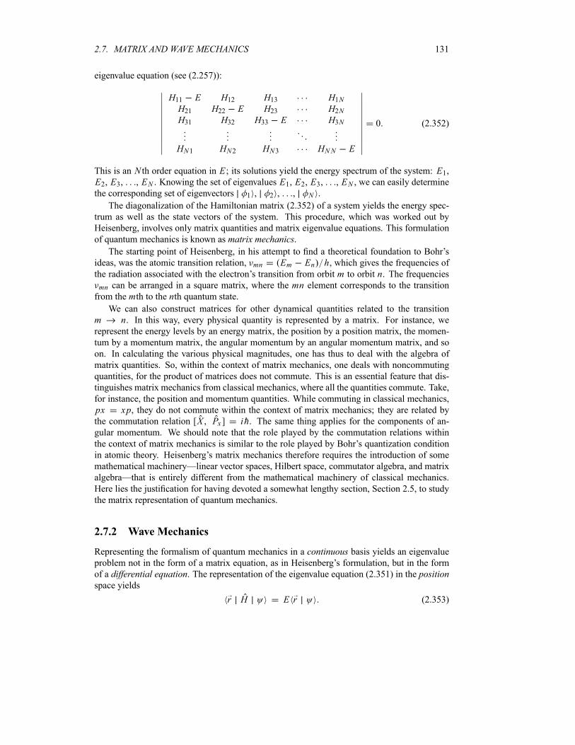
2.7. MATRIX AND WAVE MECHANICS 131
eigenvalue equation (see (2.257)):
H11 E H12 H13 H1NH21 H22 E H23 H2NH31 H32 H33 E H3N
HN1 HN2 HN3 HNN E
0 (2.352)
This is an N th order equation in E ; its solutions yield the energy spectrum of the system: E1,E2, E3, , EN . Knowing the set of eigenvalues E1, E2, E3, , EN , we can easily determinethe corresponding set of eigenvectors 1 , 2 , , N .
The diagonalization of the Hamiltonian matrix (2.352) of a system yields the energy spec-
trum as well as the state vectors of the system. This procedure, which was worked out by
Heisenberg, involves only matrix quantities and matrix eigenvalue equations. This formulation
of quantum mechanics is known as matrix mechanics.The starting point of Heisenberg, in his attempt to find a theoretical foundation to Bohr’s
ideas, was the atomic transition relation, mn Em En h, which gives the frequencies ofthe radiation associated with the electron’s transition from orbit m to orbit n. The frequencies
mn can be arranged in a square matrix, where the mn element corresponds to the transitionfrom the mth to the nth quantum state.We can also construct matrices for other dynamical quantities related to the transition
m n. In this way, every physical quantity is represented by a matrix. For instance, werepresent the energy levels by an energy matrix, the position by a position matrix, the momen-
tum by a momentum matrix, the angular momentum by an angular momentum matrix, and so
on. In calculating the various physical magnitudes, one has thus to deal with the algebra of
matrix quantities. So, within the context of matrix mechanics, one deals with noncommuting
quantities, for the product of matrices does not commute. This is an essential feature that dis-
tinguishes matrix mechanics from classical mechanics, where all the quantities commute. Take,
for instance, the position and momentum quantities. While commuting in classical mechanics,
px xp, they do not commute within the context of matrix mechanics; they are related bythe commutation relation [X Px ] ih. The same thing applies for the components of an-gular momentum. We should note that the role played by the commutation relations within
the context of matrix mechanics is similar to the role played by Bohr’s quantization condition
in atomic theory. Heisenberg’s matrix mechanics therefore requires the introduction of some
mathematical machinery—linear vector spaces, Hilbert space, commutator algebra, and matrix
algebra—that is entirely different from the mathematical machinery of classical mechanics.
Here lies the justification for having devoted a somewhat lengthy section, Section 2.5, to study
the matrix representation of quantum mechanics.
2.7.2 Wave Mechanics
Representing the formalism of quantum mechanics in a continuous basis yields an eigenvalueproblem not in the form of a matrix equation, as in Heisenberg’s formulation, but in the form
of a differential equation. The representation of the eigenvalue equation (2.351) in the positionspace yields
r H E r (2.353)
132 CHAPTER 2. MATHEMATICAL TOOLS OF QUANTUM MECHANICS
As shown in (2.315), the Hamiltonian is given in the position representation by h2 2 2mV r , so we can rewrite (2.353) in a more familiar form:
h2
2m2 r V r r E r (2.354)
where r r is the wave function of the system. This differential equation is knownas the Schrödinger equation (its origin will be discussed in Chapter 3). Its solutions yieldthe energy spectrum of the system as well as its wave function. This formulation of quantum
mechanics in the position representation is called wave mechanics.Unlike Heisenberg, Schödinger took an entirely different starting point in his quest to find
a theoretical justification for Bohr’s ideas. He started from the de Broglie particle–wave hy-
pothesis and extended it to the electrons orbiting around the nucleus. Schrödinger aimed at
finding an equation that describes the motion of the electron within an atom. Here the focus
is on the wave aspect of the electron. We can show, as we did in Chapter 1, that the Bohrquantization condition, L nh, is equivalent to the de Broglie relation, 2 h p. To es-tablish this connection, we need simply to make three assumptions: (a) the wavelength of the
wave associated with the orbiting electron is connected to the electron’s linear momentum pby 2 h p, (b) the electron’s orbit is circular, and (c) the circumference of the electron’sorbit is an integer multiple of the electron’s wavelength, i.e., 2 r n . This leads at onceto 2 r n 2 h p or nh rp L. This means that, for every orbit, there is only onewavelength (or one wave) associated with the electron while revolving in that orbit. This wave
can be described by means of a wave function. So Bohr’s quantization condition implies, inessence, a uniqueness of the wave function for each orbit of the electron. In Chapter 3 we will
show how Schrödinger obtained his differential equation (2.354) to describe the motion of an
electron in an atom.
2.8 Concluding Remarks
Historically, the matrix formulation of quantum mechanics was worked out by Heisenberg
shortly before Schrödinger introduced his wave theory. The equivalence between the matrix
and wave formulations was proved a few years later by using the theory of unitary transfor-
mations. Different in form, yet identical in contents, wave mechanics and matrix mechanics
achieve the same goal: finding the energy spectrum and the states of quantum systems.
The matrix formulation has the advantage of greater (formal) generality, yet it suffers from
a number of disadvantages. On the conceptual side, it offers no visual idea about the structure
of the atom; it is less intuitive than wave mechanics. On the technical side, it is difficult to
use in some problems of relative ease such as finding the stationary states of atoms. Matrix
mechanics, however, becomes powerful and practical in solving problems such as the harmonic
oscillator or in treating the formalism of angular momentum.
But most of the efforts of quantum mechanics focus on solving the Schrödinger equation,
not the Heisenberg matrix eigenvalue problem. So in the rest of this text we deal mostly with
wave mechanics. Matrix mechanics is used only in a few problems, such as the harmonic
oscillator, where it is more suitable than Schrödinger’s wave mechanics.
In wave mechanics we need only to specify the potential in which the particle moves; the
Schrödinger equation takes care of the rest. That is, knowing V r , we can in principle solveequation (2.354) to obtain the various energy levels of the particle and their corresponding wave
2.9. SOLVED PROBLEMS 133
functions. The complexity we encounter in solving the differential equation depends entirely on
the form of the potential; the simpler the potential the easier the solution. Exact solutions of the
Schrödinger equation are possible only for a few idealized systems; we deal with such systems
in Chapters 4 and 6. However, exact solutions are generally not possible, for real systems do not
yield themselves to exact solutions. In such cases one has to resort to approximate solutions.
We deal with such approximate treatments in Chapters 9 and 10; Chapter 9 deals with time-
independent potentials and Chapter 10 with time-dependent potentials.
Before embarking on the applications of the Schrödinger equation, we need first to lay down
the theoretical foundations of quantum mechanics. We take up this task in Chapter 3, where
we deal with the postulates of the theory as well as their implications; the postulates are the
bedrock on which the theory is built.
2.9 Solved Problems
Problem 2.1
Consider the states 9i 1 2 2 andi2
11
22 , where the two
vectors 1 and 2 form a complete and orthonormal basis.
(a) Calculate the operators and . Are they equal?
(b) Find the Hermitian conjugates of , , , and .
(c) Calculate Tr and Tr . Are they equal?
(d) Calculate and and the traces Tr and Tr . Are they
projection operators?
Solution
(a) The bras corresponding to 9i 1 2 2 and i 1 2 2 2
are given by 9i 1 2 2 and i2
11
22 , respectively. Hence we
have
1
29i 1 2 2 i 1 2
1
29 1 1 9i 1 2 2i 2 1 2 2 2
(2.355)
1
29 1 1 2i 1 2 9i 2 1 2 2 2 (2.356)
As expected, and are not equal; they would be equal only if the states
and were proportional and the proportionality constant real.
(b) To find the Hermitian conjugates of , , , and , we need simply
to replace the factors with their respective complex conjugates, the bras with kets, and the kets
with bras:
† 9i 1 2 2† 1
2i 1 2 (2.357)
134 CHAPTER 2. MATHEMATICAL TOOLS OF QUANTUM MECHANICS
† 1
29 1 1 2i 1 2
9i 2 1 2 2 2 (2.358)
† 1
29 1 1 9i 1 2
2i 2 1 2 2 2 (2.359)
(c) Using the property Tr AB Tr BA and since 1 1 2 2 1 and
1 2 2 1 0, we obtain
Tr Tr
i
21
1
22 9i 1 2 2
7
2(2.360)
Tr Tr
9i 1 2 2i
21
1
22
7
2
Tr (2.361)
The traces Tr and Tr are equal only because the scalar product of and
is a real number. Were this product a complex number, the traces would be different; in
fact, they would be the complex conjugate of one another.
(d) The expressions and are
9i 1 2 2 9i 1 2 2
81 1 1 18i 1 2 18i 2 1 4 2 2
(2.362)
1
21 1 i 1 2 i 2 1 2 2
1
21 i 1 2 i 2 1 (2.363)
In deriving (2.363) we have used the fact that the basis is complete, 1 1 2 2 1.
The traces Tr and Tr can then be calculated immediately:
Tr 9i 1 2 2 9i 1 2 2 85 (2.364)
Tr1
2i 1 2 i 1 2 1 (2.365)
So is normalized but is not. Since is normalized, we can easily ascertain that
is a projection operator, because it is Hermitian, † , and equal to
its own square:
2 (2.366)
As for , although it is Hermitian, it cannot be a projection operator since is not
normalized. That is, is not equal to its own square:
2 85 (2.367)
2.9. SOLVED PROBLEMS 135
Problem 2.2
(a) Find a complete and orthonormal basis for a space of the trigonometric functions of the
form Nn 0 an cos n .
(b) Illustrate the results derived in (a) for the case N 5; find the basis vectors.
Solution
(a) Since cos n 12ein e in , we can write
Nn 0 an cos n as
1
2
N
n 0
an ein e in 1
2
N
n 0
anein
0
n N
a nein
N
n N
Cnein (2.368)
where Cn an 2 for n 0, Cn a n 2 for n 0, and C0 a0. Since any trigonometricfunction of the form x N
n 0 an cos n can be expressed in terms of the functions
n ein 2 , we can try to take the set n as a basis. As this set is complete, let us
see if it is orthonormal. The various functions n are indeed orthonormal, since their scalar
products are given by
m n m n d1
2ei n m d nm (2.369)
In deriving this result, we have considered two cases: n m and n m. First, the case n mis obvious, since n n
12
d 1. On the other hand, when n m we have
m n1
2ei n m d
1
2
ei n m e i n m
i n m
2i sin n m
2i n m0
(2.370)
since sin n m 0. So the functions n ein 2 form a complete and orthonor-
mal basis. From (2.368) we see that the basis has 2N 1 functions n ; hence the dimension
of this space of functions is equal to 2N 1.
(b) In the case where N 5, the dimension of the space is equal to 11, for the basis
has 11 vectors: 5 e 5i 2 , 4 e 4i 2 , , 0 1 2 , ,
4 e4i 2 , 5 e5i 2 .
Problem 2.3
(a) Show that the sum of two projection operators cannot be a projection operator unless
their product is zero.
(b) Show that the product of two projection operators cannot be a projection operator unless
they commute.
Solution
Recall that an operator P is a projection operator if it satisfies P† P and P2 P .(a) If two operators A and B are projection operators and if AB BA, we want to show
that A B † A B and that A B 2 A B. First, the hermiticity is easy to ascertain
since A and B are both Hermitian: A B † A B. Let us now look at the square of
A B ; since A2
A and B2 B, we can write
A B 2 A2
B2 AB BA A B AB BA (2.371)
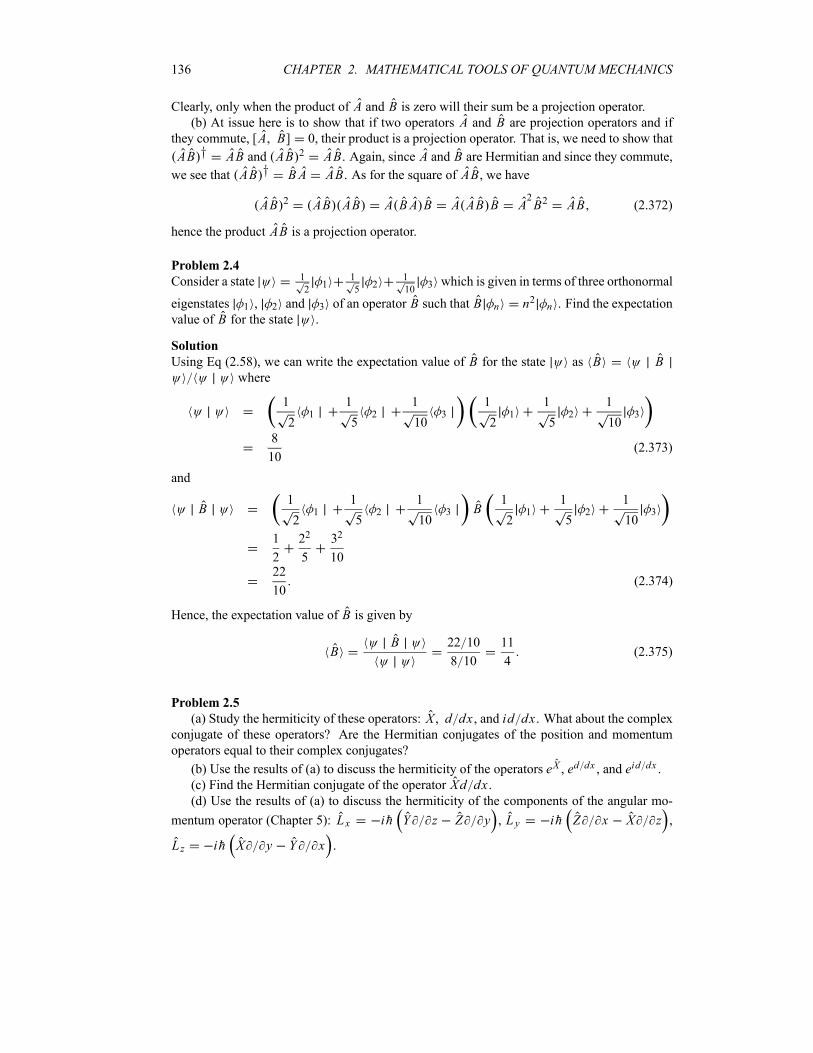
136 CHAPTER 2. MATHEMATICAL TOOLS OF QUANTUM MECHANICS
Clearly, only when the product of A and B is zero will their sum be a projection operator.(b) At issue here is to show that if two operators A and B are projection operators and if
they commute, [A B] 0, their product is a projection operator. That is, we need to show that
AB † AB and AB 2 AB. Again, since A and B are Hermitian and since they commute,
we see that AB † BA AB. As for the square of AB, we have
AB 2 AB AB A BA B A AB B A2B2 AB (2.372)
hence the product AB is a projection operator.
Problem 2.4
Consider a state 1
21
1
52
1
103 which is given in terms of three orthonormal
eigenstates 1 , 2 and 3 of an operator B such that B n n2 n . Find the expectation
value of B for the state .
Solution
Using Eq (2.58), we can write the expectation value of B for the state as B Bwhere
1
21
1
52
1
103
1
21
1
52
1
103
8
10(2.373)
and
B1
21
1
52
1
103 B
1
21
1
52
1
103
1
2
22
5
32
1022
10(2.374)
Hence, the expectation value of B is given by
BB 22 10
8 10
11
4(2.375)
Problem 2.5
(a) Study the hermiticity of these operators: X , d dx , and id dx . What about the complexconjugate of these operators? Are the Hermitian conjugates of the position and momentum
operators equal to their complex conjugates?
(b) Use the results of (a) to discuss the hermiticity of the operators eX , ed dx , and eid dx .(c) Find the Hermitian conjugate of the operator Xd dx .(d) Use the results of (a) to discuss the hermiticity of the components of the angular mo-
mentum operator (Chapter 5): Lx ih Y z Z y , L y ih Z x X z ,
L z ih X y Y x .
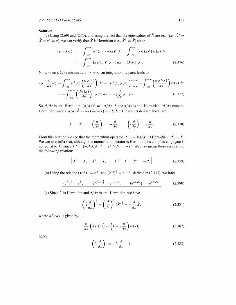
2.9. SOLVED PROBLEMS 137
Solution
(a) Using (2.69) and (2.70), and using the fact that the eigenvalues of X are real (i.e., X
X or x x), we can verify that X is Hermitian (i.e., X† X) since
X x x x dx x x x dx
x x x dx X (2.376)
Now, since x vanishes as x , an integration by parts leads to
d
dxx
d x
dxdx x x
x
x
d x
dxx dx
d x
dxx dx
d
dx(2.377)
So, d dx is anti-Hermitian: d dx † d dx . Since d dx is anti-Hermitian, id dx must be
Hermitian, since id dx † i d dx id dx . The results derived above are
X† Xd
dx
† d
dxid
dx
†
id
dx(2.378)
From this relation we see that the momentum operator P ihd dx is Hermitian: P† P .We can also infer that, although the momentum operator is Hermitian, its complex conjugate is
not equal to P , since P ihd dx ihd dx P . We may group these results intothe following relation:
X† X X X P† P P P (2.379)
(b) Using the relations eA † eA†and ei A † e i A
†derived in (2.113), we infer
eX † eX ed dx † e d dx eid dx † eid dx (2.380)
(c) Since X is Hermitian and d dx is anti-Hermitian, we have
Xd
dx
† d
dx
†X †
d
dxX (2.381)
where dX dx is given by
d
dxX x 1 x
d
dxx (2.382)
hence
Xd
dx
†Xd
dx1 (2.383)
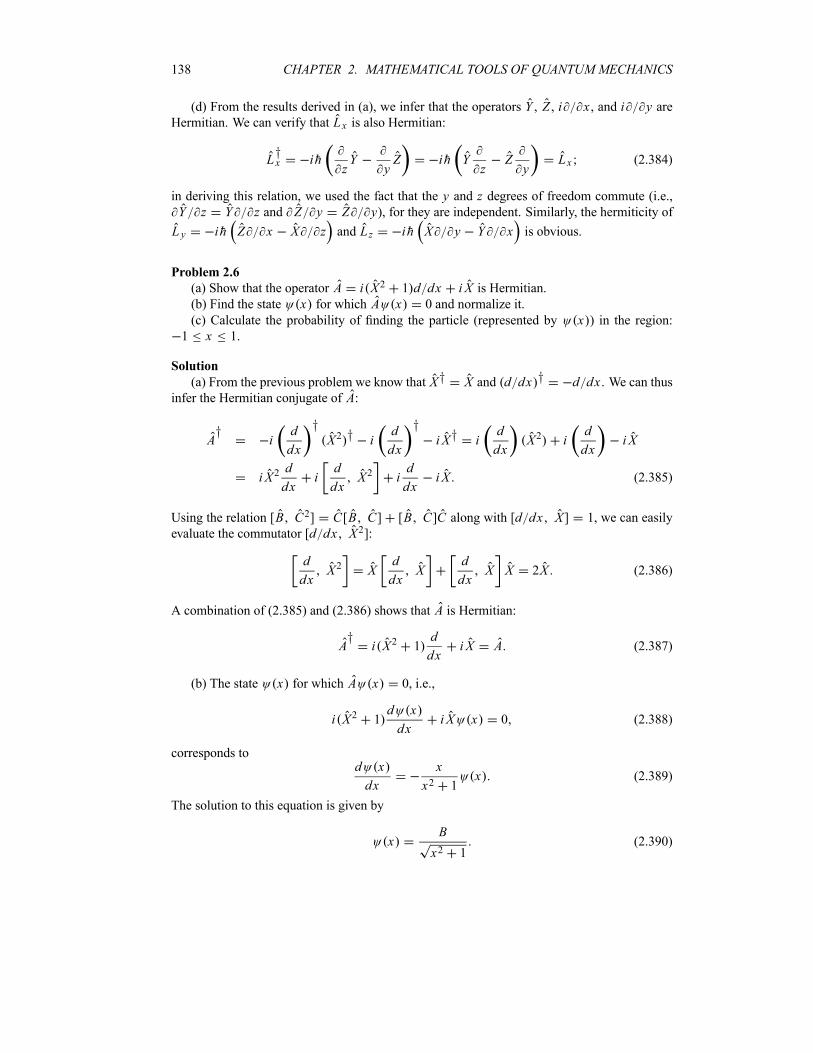
138 CHAPTER 2. MATHEMATICAL TOOLS OF QUANTUM MECHANICS
(d) From the results derived in (a), we infer that the operators Y , Z , i x , and i y areHermitian. We can verify that Lx is also Hermitian:
L†x ih
zY
yZ ih Y
zZy
Lx (2.384)
in deriving this relation, we used the fact that the y and z degrees of freedom commute (i.e.,Y z Y z and Z y Z y), for they are independent. Similarly, the hermiticity of
L y ih Z x X z and L z ih X y Y x is obvious.
Problem 2.6
(a) Show that the operator A i X2 1 d dx i X is Hermitian.(b) Find the state x for which A x 0 and normalize it.
(c) Calculate the probability of finding the particle (represented by x ) in the region:1 x 1.
Solution
(a) From the previous problem we know that X† X and d dx † d dx . We can thusinfer the Hermitian conjugate of A:
A†
id
dx
†X2 † i
d
dx
†i X† i
d
dxX2 i
d
dxi X
i X2d
dxid
dxX2 i
d
dxi X (2.385)
Using the relation [B C2] C[B C] [B C]C along with [d dx X] 1, we can easily
evaluate the commutator [d dx X2]:
d
dxX2 X
d
dxX
d
dxX X 2X (2.386)
A combination of (2.385) and (2.386) shows that A is Hermitian:
A†
i X2 1d
dxi X A (2.387)
(b) The state x for which A x 0, i.e.,
i X2 1d x
dxi X x 0 (2.388)
corresponds tod x
dx
x
x2 1x (2.389)
The solution to this equation is given by
xB
x2 1(2.390)
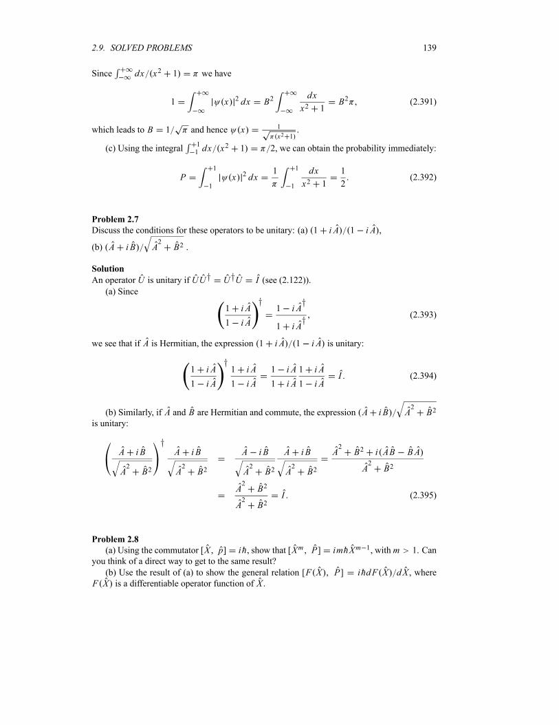
2.9. SOLVED PROBLEMS 139
Since dx x2 1 we have
1 x 2 dx B2dx
x2 1B2 (2.391)
which leads to B 1 and hence x 1
x2 1.
(c) Using the integral11 dx x2 1 2, we can obtain the probability immediately:
P1
1
x 2 dx1 1
1
dx
x2 1
1
2(2.392)
Problem 2.7
Discuss the conditions for these operators to be unitary: (a) 1 i A 1 i A ,
(b) A i B A2
B2 .
Solution
An operator U is unitary if UU† U†U I (see (2.122)).(a) Since
1 i A
1 i A
†1 i A
†
1 i A†
(2.393)
we see that if A is Hermitian, the expression 1 i A 1 i A is unitary:
1 i A
1 i A
†1 i A
1 i A
1 i A
1 i A
1 i A
1 i AI (2.394)
(b) Similarly, if A and B are Hermitian and commute, the expression A i B A2
B2
is unitary:
A i B
A2
B2
†A i B
A2
B2
A i B
A2
B2
A i B
A2
B2
A2
B2 i AB BA
A2
B2
A2
B2
A2
B2I (2.395)
Problem 2.8
(a) Using the commutator [X p] ih, show that [Xm P] imhXm 1, with m 1. Can
you think of a direct way to get to the same result?
(b) Use the result of (a) to show the general relation [F X P] ihdF X dX , whereF X is a differentiable operator function of X .
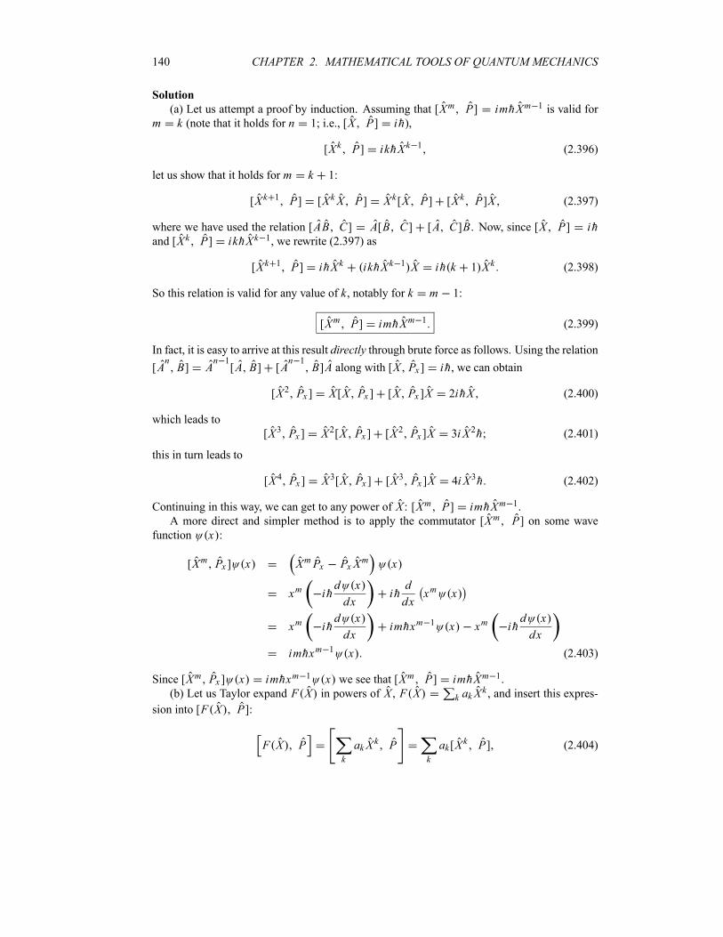
140 CHAPTER 2. MATHEMATICAL TOOLS OF QUANTUM MECHANICS
Solution
(a) Let us attempt a proof by induction. Assuming that [Xm P] imhXm 1 is valid for
m k (note that it holds for n 1; i.e., [X P] ih),
[Xk P] ikhXk 1 (2.396)
let us show that it holds for m k 1:
[X k 1 P] [XkX P] X k[X P] [X k P]X (2.397)
where we have used the relation [AB C] A[B C] [A C]B. Now, since [X P] ihand [X k P] ikhX k 1, we rewrite (2.397) as
[Xk 1 P] ihXk ikhXk 1 X ih k 1 X k (2.398)
So this relation is valid for any value of k, notably for k m 1:
[Xm P] imhXm 1 (2.399)
In fact, it is easy to arrive at this result directly through brute force as follows. Using the relation
[AnB] A
n 1[A B] [A
n 1B]A along with [X Px ] ih, we can obtain
[X2 Px ] X[X Px ] [X Px ]X 2ihX (2.400)
which leads to
[X3 Px ] X2[X Px ] [X2 Px ]X 3i X2h (2.401)
this in turn leads to
[X4 Px ] X3[X Px ] [X3 Px ]X 4i X3h (2.402)
Continuing in this way, we can get to any power of X : [Xm P] imhXm 1.
A more direct and simpler method is to apply the commutator [Xm P] on some wavefunction x :
[Xm Px ] x XmPx Px Xm x
xm ihd x
dxihd
dxxm x
xm ihd x
dximhxm 1 x xm ih
d x
dx
imhxm 1 x (2.403)
Since [Xm Px ] x imhxm 1 x we see that [Xm P] imhXm 1.
(b) Let us Taylor expand F X in powers of X , F X k akXk , and insert this expres-
sion into [F X P]:
F X Pk
akXk P
k
ak[Xk P] (2.404)
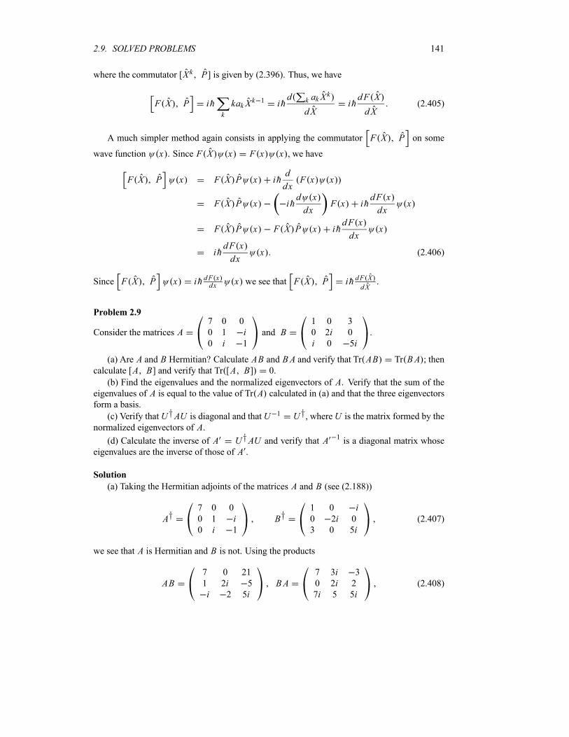
2.9. SOLVED PROBLEMS 141
where the commutator [Xk P] is given by (2.396). Thus, we have
F X P ihk
kakXk 1 ih
d k akXk
dXihdF X
dX(2.405)
A much simpler method again consists in applying the commutator F X P on some
wave function x . Since F X x F x x , we have
F X P x F X P x ihd
dxF x x
F X P x ihd x
dxF x ih
dF x
dxx
F X P x F X P x ihdF x
dxx
ihdF x
dxx (2.406)
Since F X P x ih dF xdx x we see that F X P ih dF XdX
.
Problem 2.9
Consider the matrices A7 0 0
0 1 i0 i 1
and B1 0 3
0 2i 0
i 0 5i.
(a) Are A and B Hermitian? Calculate AB and BA and verify that Tr AB Tr BA ; thencalculate [A B] and verify that Tr [A B] 0.
(b) Find the eigenvalues and the normalized eigenvectors of A. Verify that the sum of theeigenvalues of A is equal to the value of Tr A calculated in (a) and that the three eigenvectors
form a basis.
(c) Verify thatU†AU is diagonal and thatU 1 U†, whereU is the matrix formed by thenormalized eigenvectors of A.
(d) Calculate the inverse of A U†AU and verify that A 1is a diagonal matrix whose
eigenvalues are the inverse of those of A .
Solution
(a) Taking the Hermitian adjoints of the matrices A and B (see (2.188))
A†7 0 0
0 1 i0 i 1
B†1 0 i0 2i 0
3 0 5i(2.407)
we see that A is Hermitian and B is not. Using the products
AB7 0 21
1 2i 5
i 2 5iBA
7 3i 3
0 2i 2
7i 5 5i(2.408)
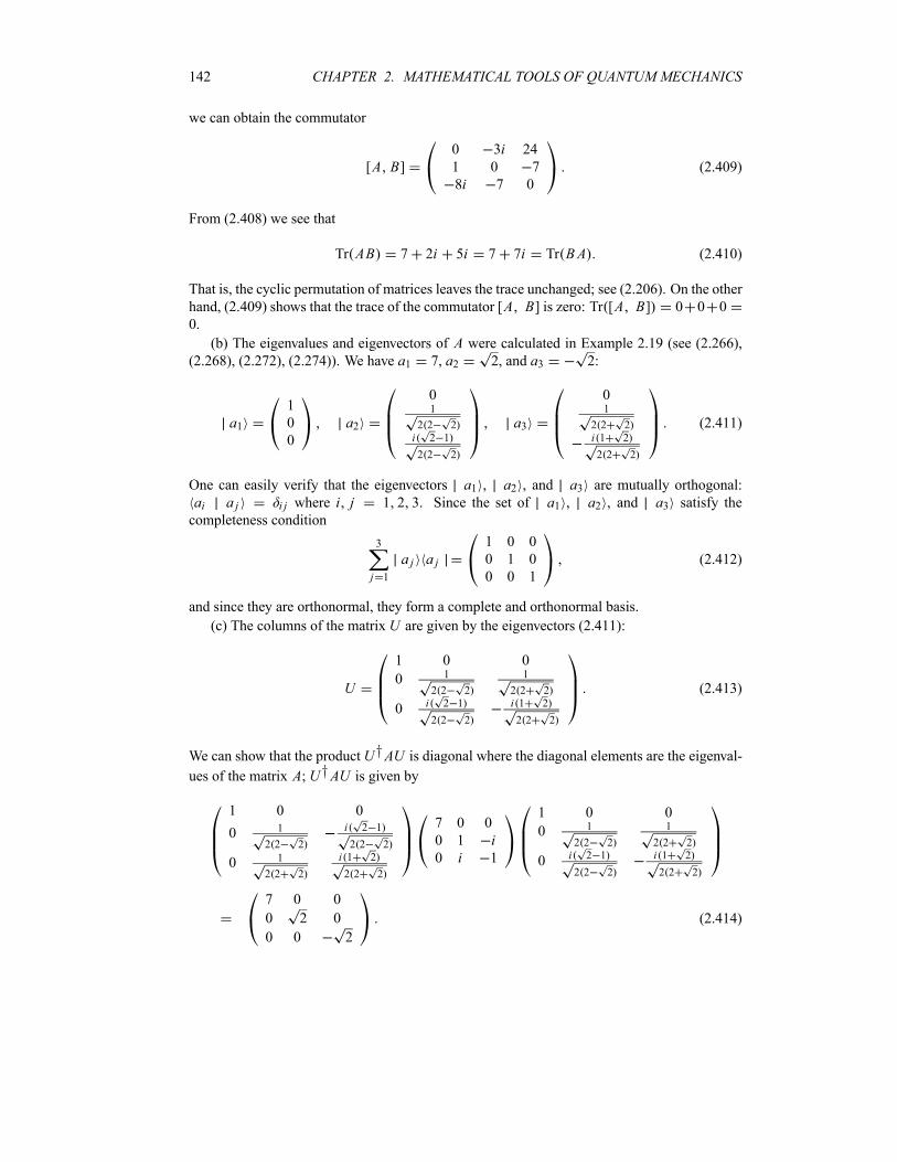
142 CHAPTER 2. MATHEMATICAL TOOLS OF QUANTUM MECHANICS
we can obtain the commutator
[A B]0 3i 24
1 0 7
8i 7 0
(2.409)
From (2.408) we see that
Tr AB 7 2i 5i 7 7i Tr BA (2.410)
That is, the cyclic permutation of matrices leaves the trace unchanged; see (2.206). On the other
hand, (2.409) shows that the trace of the commutator [A B] is zero: Tr [A B] 0 0 0
0.
(b) The eigenvalues and eigenvectors of A were calculated in Example 2.19 (see (2.266),(2.268), (2.272), (2.274)). We have a1 7, a2 2, and a3 2:
a1
1
0
0
a2
01
2 2 2
i 2 1
2 2 2
a3
01
2 2 2
i 1 2
2 2 2
(2.411)
One can easily verify that the eigenvectors a1 , a2 , and a3 are mutually orthogonal:
ai a j i j where i j 1 2 3. Since the set of a1 , a2 , and a3 satisfy the
completeness condition
3
j 1
a j a j
1 0 0
0 1 0
0 0 1
(2.412)
and since they are orthonormal, they form a complete and orthonormal basis.
(c) The columns of the matrix U are given by the eigenvectors (2.411):
U
1 0 0
0 1
2 2 2
1
2 2 2
0 i 2 1
2 2 2
i 1 2
2 2 2
(2.413)
We can show that the productU†AU is diagonal where the diagonal elements are the eigenval-
ues of the matrix A; U†AU is given by
1 0 0
0 1
2 2 2
i 2 1
2 2 2
0 1
2 2 2
i 1 2
2 2 2
7 0 0
0 1 i0 i 1
1 0 0
0 1
2 2 2
1
2 2 2
0 i 2 1
2 2 2
i 1 2
2 2 2
7 0 0
0 2 0
0 0 2
(2.414)
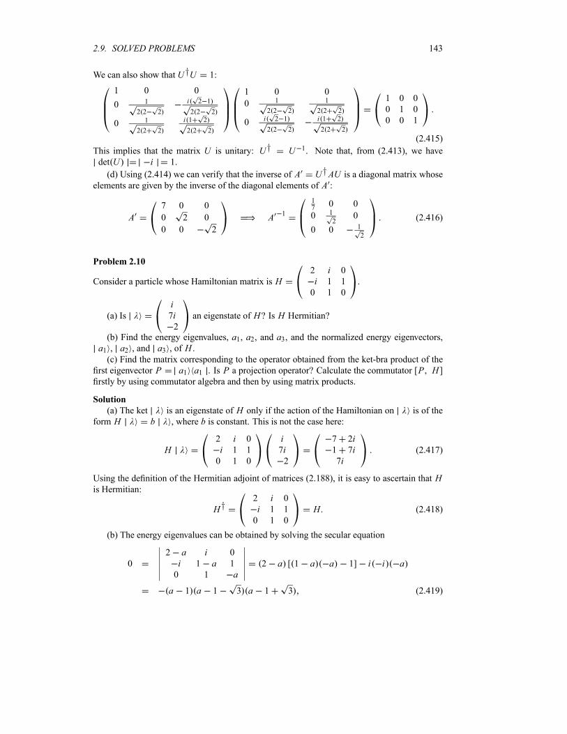
2.9. SOLVED PROBLEMS 143
We can also show that U†U 1:
1 0 0
0 1
2 2 2
i 2 1
2 2 2
0 1
2 2 2
i 1 2
2 2 2
1 0 0
0 1
2 2 2
1
2 2 2
0 i 2 1
2 2 2
i 1 2
2 2 2
1 0 0
0 1 0
0 0 1
(2.415)
This implies that the matrix U is unitary: U† U 1. Note that, from (2.413), we have
det U i 1.
(d) Using (2.414) we can verify that the inverse of A U†AU is a diagonal matrix whoseelements are given by the inverse of the diagonal elements of A :
A7 0 0
0 2 0
0 0 2
A 1
17
0 0
0 1
20
0 0 1
2
(2.416)
Problem 2.10
Consider a particle whose Hamiltonian matrix is H2 i 0
i 1 1
0 1 0
.
(a) Is
i7i2
an eigenstate of H? Is H Hermitian?
(b) Find the energy eigenvalues, a1, a2, and a3, and the normalized energy eigenvectors,a1 , a2 , and a3 , of H .(c) Find the matrix corresponding to the operator obtained from the ket-bra product of the
first eigenvector P a1 a1 . Is P a projection operator? Calculate the commutator [P H ]firstly by using commutator algebra and then by using matrix products.
Solution
(a) The ket is an eigenstate of H only if the action of the Hamiltonian on is of the
form H b , where b is constant. This is not the case here:
H2 i 0
i 1 1
0 1 0
i7i2
7 2i1 7i7i
(2.417)
Using the definition of the Hermitian adjoint of matrices (2.188), it is easy to ascertain that His Hermitian:
H†2 i 0
i 1 1
0 1 0
H (2.418)
(b) The energy eigenvalues can be obtained by solving the secular equation
0
2 a i 0
i 1 a 1
0 1 a2 a [ 1 a a 1] i i a
a 1 a 1 3 a 1 3 (2.419)
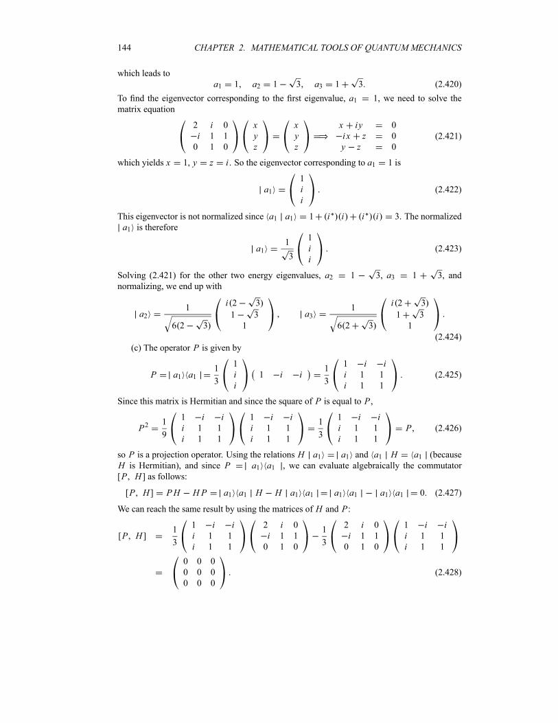
144 CHAPTER 2. MATHEMATICAL TOOLS OF QUANTUM MECHANICS
which leads to
a1 1 a2 1 3 a3 1 3 (2.420)
To find the eigenvector corresponding to the first eigenvalue, a1 1, we need to solve the
matrix equation
2 i 0
i 1 1
0 1 0
xyz
xyz
x iy 0
i x z 0
y z 0
(2.421)
which yields x 1, y z i . So the eigenvector corresponding to a1 1 is
a1
1
ii
(2.422)
This eigenvector is not normalized since a1 a1 1 i i i i 3. The normalized
a1 is therefore
a11
3
1
ii
(2.423)
Solving (2.421) for the other two energy eigenvalues, a2 1 3, a3 1 3, and
normalizing, we end up with
a21
6 2 3
i 2 3
1 3
1
a31
6 2 3
i 2 3
1 3
1
(2.424)
(c) The operator P is given by
P a1 a11
3
1
ii
1 i i1
3
1 i ii 1 1
i 1 1
(2.425)
Since this matrix is Hermitian and since the square of P is equal to P ,
P21
9
1 i ii 1 1
i 1 1
1 i ii 1 1
i 1 1
1
3
1 i ii 1 1
i 1 1
P (2.426)
so P is a projection operator. Using the relations H a1 a1 and a1 H a1 (because
H is Hermitian), and since P a1 a1 , we can evaluate algebraically the commutator
[P H ] as follows:
[P H ] PH HP a1 a1 H H a1 a1 a1 a1 a1 a1 0 (2.427)
We can reach the same result by using the matrices of H and P:
[P H ]1
3
1 i ii 1 1
i 1 1
2 i 0
i 1 1
0 1 0
1
3
2 i 0
i 1 1
0 1 0
1 i ii 1 1
i 1 1
0 0 0
0 0 0
0 0 0
(2.428)
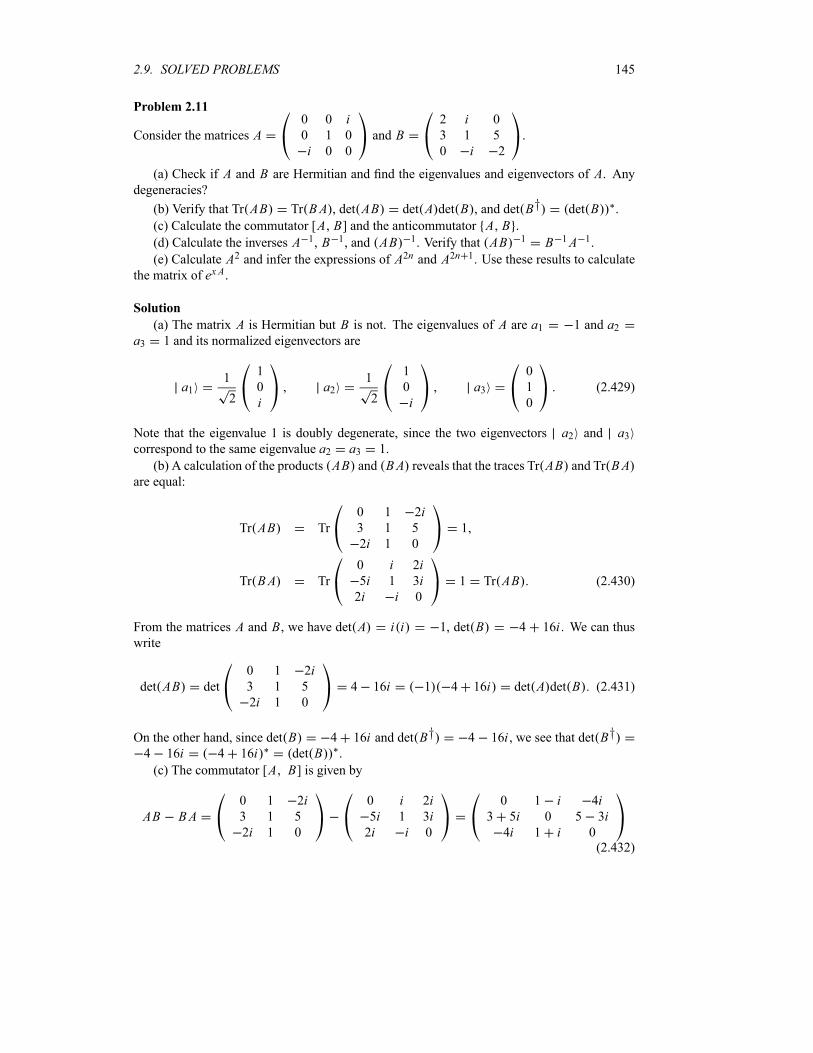
2.9. SOLVED PROBLEMS 145
Problem 2.11
Consider the matrices A0 0 i0 1 0
i 0 0
and B2 i 0
3 1 5
0 i 2
.
(a) Check if A and B are Hermitian and find the eigenvalues and eigenvectors of A. Anydegeneracies?
(b) Verify that Tr AB Tr BA , det AB det A det B , and det B† det B .
(c) Calculate the commutator [A B] and the anticommutator A B .(d) Calculate the inverses A 1, B 1, and AB 1. Verify that AB 1 B 1A 1.
(e) Calculate A2 and infer the expressions of A2n and A2n 1. Use these results to calculate
the matrix of ex A.
Solution
(a) The matrix A is Hermitian but B is not. The eigenvalues of A are a1 1 and a2a3 1 and its normalized eigenvectors are
a11
2
1
0
ia2
1
2
1
0
ia3
0
1
0
(2.429)
Note that the eigenvalue 1 is doubly degenerate, since the two eigenvectors a2 and a3correspond to the same eigenvalue a2 a3 1.
(b) A calculation of the products AB and BA reveals that the traces Tr AB and Tr BAare equal:
Tr AB Tr
0 1 2i3 1 5
2i 1 0
1
Tr BA Tr
0 i 2i5i 1 3i2i i 0
1 Tr AB (2.430)
From the matrices A and B, we have det A i i 1, det B 4 16i . We can thuswrite
det AB det
0 1 2i3 1 5
2i 1 0
4 16i 1 4 16i det A det B (2.431)
On the other hand, since det B 4 16i and det B† 4 16i , we see that det B†
4 16i 4 16i det B .
(c) The commutator [A B] is given by
AB BA0 1 2i3 1 5
2i 1 0
0 i 2i5i 1 3i2i i 0
0 1 i 4i3 5i 0 5 3i4i 1 i 0
(2.432)
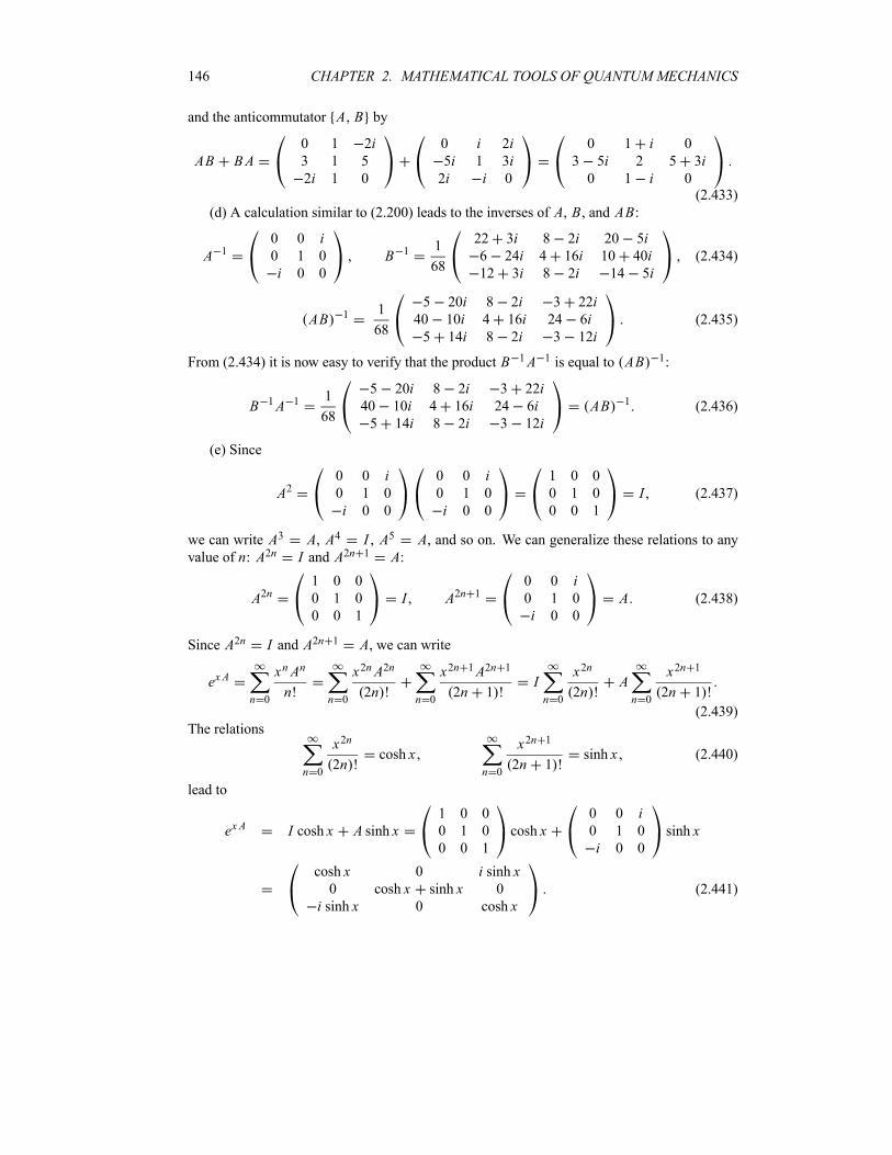
146 CHAPTER 2. MATHEMATICAL TOOLS OF QUANTUM MECHANICS
and the anticommutator A B by
AB BA0 1 2i3 1 5
2i 1 0
0 i 2i5i 1 3i2i i 0
0 1 i 0
3 5i 2 5 3i0 1 i 0
(2.433)
(d) A calculation similar to (2.200) leads to the inverses of A, B, and AB:
A 10 0 i0 1 0
i 0 0
B 1 1
68
22 3i 8 2i 20 5i6 24i 4 16i 10 40i12 3i 8 2i 14 5i
(2.434)
AB 1 1
68
5 20i 8 2i 3 22i40 10i 4 16i 24 6i5 14i 8 2i 3 12i
(2.435)
From (2.434) it is now easy to verify that the product B 1A 1 is equal to AB 1:
B 1A 1 1
68
5 20i 8 2i 3 22i40 10i 4 16i 24 6i5 14i 8 2i 3 12i
AB 1 (2.436)
(e) Since
A20 0 i0 1 0
i 0 0
0 0 i0 1 0
i 0 0
1 0 0
0 1 0
0 0 1
I (2.437)
we can write A3 A, A4 I , A5 A, and so on. We can generalize these relations to anyvalue of n: A2n I and A2n 1 A:
A2n1 0 0
0 1 0
0 0 1
I A2n 10 0 i0 1 0
i 0 0
A (2.438)
Since A2n I and A2n 1 A, we can write
ex A
n 0
xnAn
n!n 0
x2nA2n
2n !n 0
x2n 1A2n 1
2n 1 !In 0
x2n
2n !An 0
x2n 1
2n 1 !
(2.439)
The relations
n 0
x2n
2n !cosh x
n 0
x2n 1
2n 1 !sinh x (2.440)
lead to
ex A I cosh x A sinh x1 0 0
0 1 0
0 0 1
cosh x0 0 i0 1 0
i 0 0
sinh x
cosh x 0 i sinh x0 cosh x sinh x 0
i sinh x 0 cosh x(2.441)
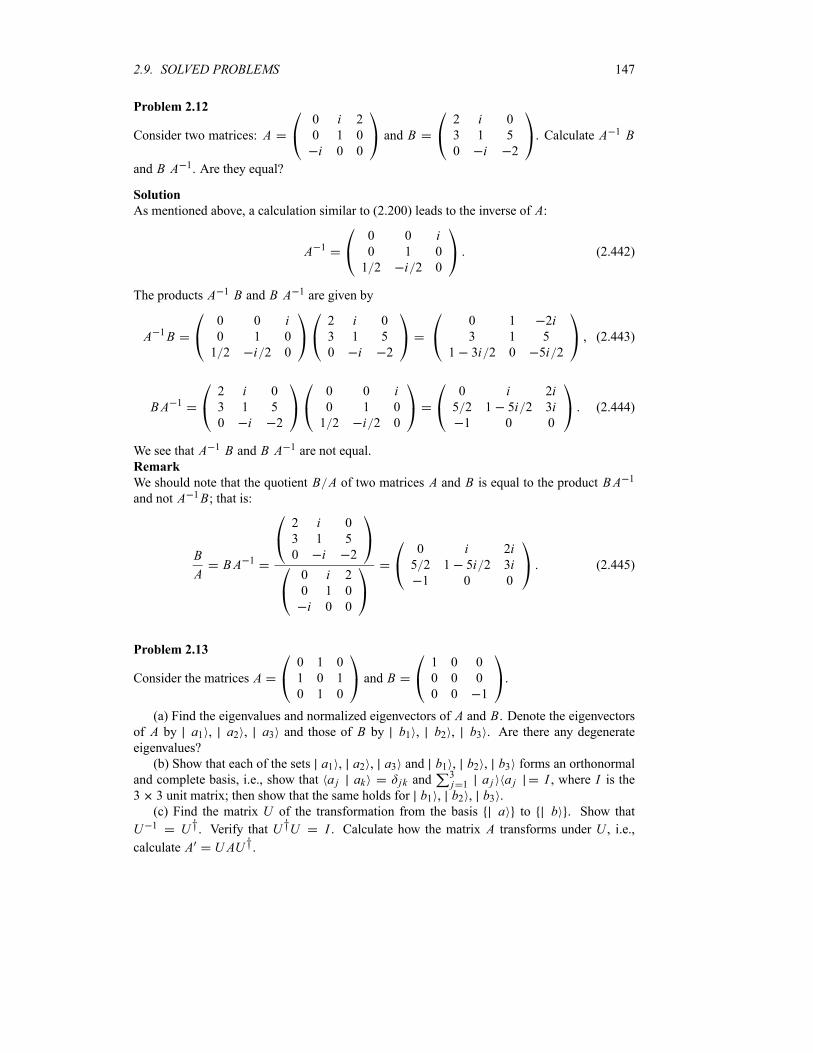
2.9. SOLVED PROBLEMS 147
Problem 2.12
Consider two matrices: A0 i 2
0 1 0
i 0 0
and B2 i 0
3 1 5
0 i 2
. Calculate A 1 B
and B A 1. Are they equal?
Solution
As mentioned above, a calculation similar to (2.200) leads to the inverse of A:
A 10 0 i0 1 0
1 2 i 2 0
(2.442)
The products A 1 B and B A 1 are given by
A 1B0 0 i0 1 0
1 2 i 2 0
2 i 0
3 1 5
0 i 2
0 1 2i3 1 5
1 3i 2 0 5i 2(2.443)
BA 12 i 0
3 1 5
0 i 2
0 0 i0 1 0
1 2 i 2 0
0 i 2i5 2 1 5i 2 3i1 0 0
(2.444)
We see that A 1 B and B A 1 are not equal.
Remark
We should note that the quotient B A of two matrices A and B is equal to the product BA 1
and not A 1B; that is:
B
ABA 1
2 i 0
3 1 5
0 i 2
0 i 2
0 1 0
i 0 0
0 i 2i5 2 1 5i 2 3i1 0 0
(2.445)
Problem 2.13
Consider the matrices A0 1 0
1 0 1
0 1 0
and B1 0 0
0 0 0
0 0 1
.
(a) Find the eigenvalues and normalized eigenvectors of A and B. Denote the eigenvectorsof A by a1 , a2 , a3 and those of B by b1 , b2 , b3 . Are there any degenerateeigenvalues?
(b) Show that each of the sets a1 , a2 , a3 and b1 , b2 , b3 forms an orthonormaland complete basis, i.e., show that a j ak jk and
3j 1 a j a j I , where I is the
3 3 unit matrix; then show that the same holds for b1 , b2 , b3 .(c) Find the matrix U of the transformation from the basis a to b . Show that
U 1 U†. Verify that U†U I . Calculate how the matrix A transforms under U , i.e.,
calculate A U AU†.
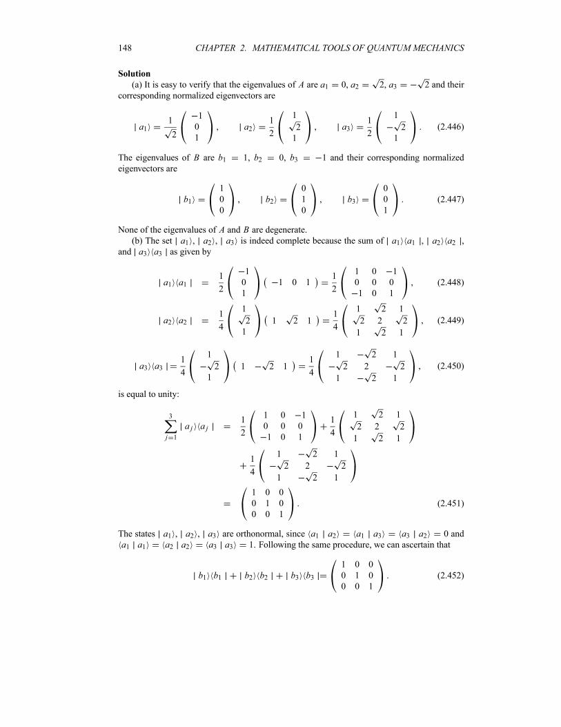
148 CHAPTER 2. MATHEMATICAL TOOLS OF QUANTUM MECHANICS
Solution
(a) It is easy to verify that the eigenvalues of A are a1 0, a2 2, a3 2 and their
corresponding normalized eigenvectors are
a11
2
1
0
1
a21
2
1
2
1
a31
2
1
2
1
(2.446)
The eigenvalues of B are b1 1, b2 0, b3 1 and their corresponding normalized
eigenvectors are
b1
1
0
0
b2
0
1
0
b3
0
0
1
(2.447)
None of the eigenvalues of A and B are degenerate.(b) The set a1 , a2 , a3 is indeed complete because the sum of a1 a1 , a2 a2 ,
and a3 a3 as given by
a1 a11
2
1
0
1
1 0 11
2
1 0 1
0 0 0
1 0 1
(2.448)
a2 a21
4
1
2
1
1 2 11
4
1 2 1
2 2 2
1 2 1
(2.449)
a3 a31
4
1
2
1
1 2 11
4
1 2 1
2 2 2
1 2 1
(2.450)
is equal to unity:
3
j 1
a j a j1
2
1 0 1
0 0 0
1 0 1
1
4
1 2 1
2 2 2
1 2 1
1
4
1 2 1
2 2 2
1 2 1
1 0 0
0 1 0
0 0 1
(2.451)
The states a1 , a2 , a3 are orthonormal, since a1 a2 a1 a3 a3 a2 0 and
a1 a1 a2 a2 a3 a3 1. Following the same procedure, we can ascertain that
b1 b1 b2 b2 b3 b3
1 0 0
0 1 0
0 0 1
(2.452)
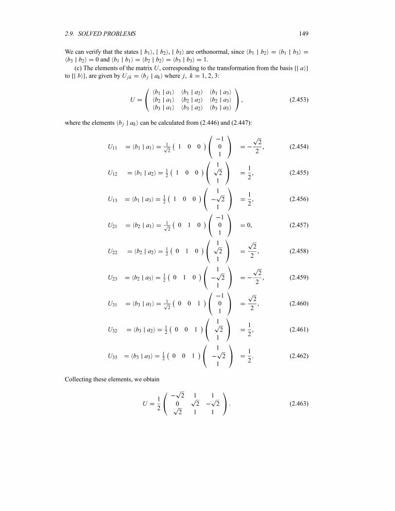
2.9. SOLVED PROBLEMS 149
We can verify that the states b1 , b2 , b3 are orthonormal, since b1 b2 b1 b3b3 b2 0 and b1 b1 b2 b2 b3 b3 1.
(c) The elements of the matrix U , corresponding to the transformation from the basis ato b , are given by U jk b j ak where j k 1 2 3:
Ub1 a1 b1 a2 b1 a3b2 a1 b2 a2 b2 a3b3 a1 b3 a2 b3 a3
(2.453)
where the elements b j ak can be calculated from (2.446) and (2.447):
U11 b1 a11
21 0 0
1
0
1
2
2(2.454)
U12 b1 a212
1 0 0
1
2
1
1
2(2.455)
U13 b1 a312
1 0 0
1
2
1
1
2(2.456)
U21 b2 a11
20 1 0
1
0
1
0 (2.457)
U22 b2 a212
0 1 0
1
2
1
2
2(2.458)
U23 b2 a312
0 1 0
1
2
1
2
2(2.459)
U31 b3 a11
20 0 1
1
0
1
2
2(2.460)
U32 b3 a212
0 0 1
1
2
1
1
2(2.461)
U33 b3 a312
0 0 1
1
2
1
1
2(2.462)
Collecting these elements, we obtain
U1
2
2 1 1
0 2 2
2 1 1
(2.463)

150 CHAPTER 2. MATHEMATICAL TOOLS OF QUANTUM MECHANICS
Calculating the inverse ofU as we did in (2.200), we see that it is equal to its Hermitian adjoint:
U 1 1
2
2 0 2
1 2 1
1 2 1
U† (2.464)
This implies that the matrix U is unitary. The matrix A transforms as follows:
A U AU†1
4
2 1 1
0 2 2
2 1 1
0 1 0
1 0 1
0 1 0
2 0 2
1 2 1
1 2 1
1
2
1 2 1 1
1 2 1
1 1 1 2
(2.465)
Problem 2.14
Calculate the following expressions involving Dirac’s delta function:
(a)55 cos 3x x 3 dx
(b)100 e2x 7 4 x 3 dx
(c) 2 cos2 3x sin x 2 x(d) 0 cos 3 2 d
(e)92 x2 5x 2 [2 x 4 ] dx .
Solution
(a) Since x 3 lies within the interval ( 5 5), equation (2.281) yields
5
5
cos 3x x 3 dx cos 33
1 (2.466)
(b) Since x 3 lies outside the interval (0 10), Eq (2.281) yields at once
10
0
e2x 7 4 x 3 dx 0 (2.467)
(c) Using the relation f x x a f a x a which is listed in Appendix A, we
have
2 cos2 3x sin x 2 x 2 cos2 3 sin 2 x
3 x (2.468)
(d) Inserting n 3 into Eq (2.282) and since cos 3 27 sin 3 , we obtain
0
cos 3 2 d 1 3 cos 3 2 1 3 27 sin 3 2
27 (2.469)
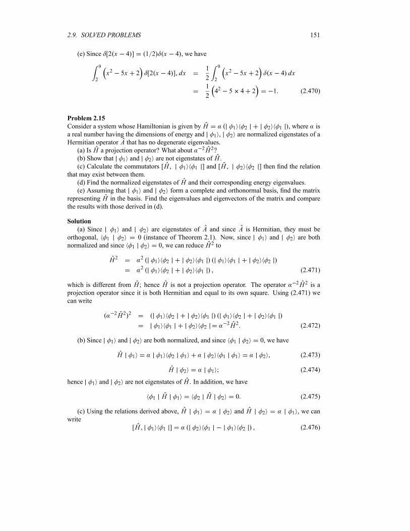
2.9. SOLVED PROBLEMS 151
(e) Since [2 x 4 ] 1 2 x 4 , we have
9
2
x2 5x 2 [2 x 4 ] dx1
2
9
2
x2 5x 2 x 4 dx
1
242 5 4 2 1 (2.470)
Problem 2.15
Consider a system whose Hamiltonian is given by H 1 2 2 1 , where is
a real number having the dimensions of energy and 1 , 2 are normalized eigenstates of a
Hermitian operator A that has no degenerate eigenvalues.(a) Is H a projection operator? What about 2H2?(b) Show that 1 and 2 are not eigenstates of H .(c) Calculate the commutators [H 1 1 ] and [H 2 2 ] then find the relation
that may exist between them.
(d) Find the normalized eigenstates of H and their corresponding energy eigenvalues.(e) Assuming that 1 and 2 form a complete and orthonormal basis, find the matrix
representing H in the basis. Find the eigenvalues and eigenvectors of the matrix and comparethe results with those derived in (d).
Solution
(a) Since 1 and 2 are eigenstates of A and since A is Hermitian, they must beorthogonal, 1 2 0 (instance of Theorem 2.1). Now, since 1 and 2 are both
normalized and since 1 2 0, we can reduce H2 to
H2 21 2 2 1 1 1 2 2
21 2 2 1 (2.471)
which is different from H ; hence H is not a projection operator. The operator 2H2 is aprojection operator since it is both Hermitian and equal to its own square. Using (2.471) we
can write
2H2 2 1 2 2 1 1 2 2 1
1 1 2 22H2 (2.472)
(b) Since 1 and 2 are both normalized, and since 1 2 0, we have
H 1 1 2 1 2 1 1 2 (2.473)
H 2 1 (2.474)
hence 1 and 2 are not eigenstates of H . In addition, we have
1 H 1 2 H 2 0 (2.475)
(c) Using the relations derived above, H 1 2 and H 2 1 , we can
write
[H 1 1 ] 2 1 1 2 (2.476)
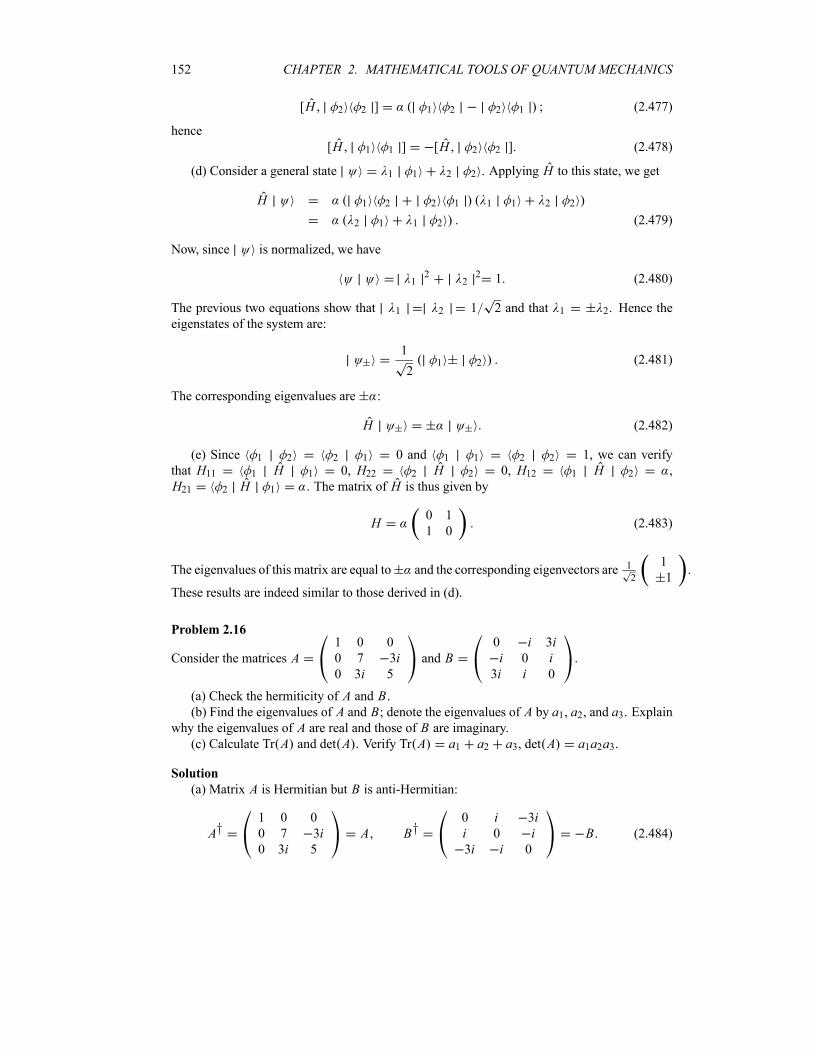
152 CHAPTER 2. MATHEMATICAL TOOLS OF QUANTUM MECHANICS
[H 2 2 ] 1 2 2 1 (2.477)
hence
[H 1 1 ] [H 2 2 ] (2.478)
(d) Consider a general state 1 1 2 2 . Applying H to this state, we get
H 1 2 2 1 1 1 2 2
2 1 1 2 (2.479)
Now, since is normalized, we have
12
22 1 (2.480)
The previous two equations show that 1 2 1 2 and that 1 2. Hence the
eigenstates of the system are:
1
21 2 (2.481)
The corresponding eigenvalues are :
H (2.482)
(e) Since 1 2 2 1 0 and 1 1 2 2 1, we can verify
that H11 1 H 1 0, H22 2 H 2 0, H12 1 H 2 ,
H21 2 H 1 . The matrix of H is thus given by
H0 1
1 0(2.483)
The eigenvalues of this matrix are equal to and the corresponding eigenvectors are 1
2
1
1.
These results are indeed similar to those derived in (d).
Problem 2.16
Consider the matrices A1 0 0
0 7 3i0 3i 5
and B0 i 3ii 0 i3i i 0
.
(a) Check the hermiticity of A and B.(b) Find the eigenvalues of A and B; denote the eigenvalues of A by a1, a2, and a3. Explain
why the eigenvalues of A are real and those of B are imaginary.(c) Calculate Tr A and det A . Verify Tr A a1 a2 a3, det A a1a2a3.
Solution
(a) Matrix A is Hermitian but B is anti-Hermitian:
A†1 0 0
0 7 3i0 3i 5
A B†0 i 3ii 0 i3i i 0
B (2.484)
2.9. SOLVED PROBLEMS 153
(b) The eigenvalues of A are a1 6 10, a2 1, and a3 6 10 and those of B
are b1 i 3 17 2, b2 3i , and b3 i 3 17 2. The eigenvalues of A are
real and those of B are imaginary. This is expected since, as shown in (2.74) and (2.75), theexpectation values of Hermitian operators are real and those of anti-Hermitian operators are
imaginary.
(c) A direct calculation of the trace and the determinant of A yields Tr A 1 7 5 13
and det A 7 5 3i 3i 26. Adding and multiplying the eigenvalues a1 6 10,
a2 1, a3 6 10, we have a1 a2 a3 6 10 1 6 10 13 and
a1a2a3 6 10 1 6 10 26. This confirms the results (2.260) and (2.261):
Tr A a1 a2 a3 13 det A a1a2a3 26 (2.485)
Problem 2.17
Consider a one-dimensional particle which moves along the x-axis and whose Hamiltonian isH Ed2 dx2 16EX2, where E is a real constant having the dimensions of energy.
(a) Is x Ae 2x2 , where A is a normalization constant that needs to be found, aneigenfunction of H? If yes, find the energy eigenvalue.(b) Calculate the probability of finding the particle anywhere along the negative x-axis.(c) Find the energy eigenvalue corresponding to the wave function x 2x x .(d) Specify the parities of x and x . Are x and x orthogonal?
Solution
(a) The integral e 4x2dx 2 allows us to find the normalization constant:
1 x 2 dx A2 e 4x2dx A22
(2.486)
this leads to A 2 and hence x 2 e 2x2 . Since the first and second
derivatives of x are given by
xd x
dx4x x x
d2 x
dx216x2 4 x (2.487)
we see that x is an eigenfunction of H with an energy eigenvalue equal to 4E :
H x Ed2 x
dx216Ex2 x E 16x2 4 x 16Ex2 x 4E x (2.488)
(b) Since0 e 4x2dx 4, the probability of finding the particle anywhere along the
negative x-axis is equal to 12:
0
x 2 dx2 0
e 4x2dx1
2(2.489)
This is expected, since this probability is half the total probability, which in turn is equal to one.
154 CHAPTER 2. MATHEMATICAL TOOLS OF QUANTUM MECHANICS
(c) Since the second derivative of x 2x x is x 4 x 2x x8x 3 4x2 x 4 3 4x2 x , we see that x is an eigenfunction of H with anenergy eigenvalue equal to 12E :
H x Ed2 x
dx216Ex2 x 4E 3 4x2 x 16Ex2 x 12E x
(2.490)
(d) The wave functions x and x are even and odd, respectively, since x xand x x ; hence their product is an odd function. Therefore, they are orthogonal,since the symmetric integration of an odd function is zero:
x x dx x x dx x x dx
x x dx 0 (2.491)
Problem 2.18
(a) Find the eigenvalues and the eigenfunctions of the operator A d2 dx2; restrict thesearch for the eigenfunctions to those complex functions that vanish everywhere except in the
region 0 x a.(b) Normalize the eigenfunction and find the probability in the region 0 x a 2.
Solution
(a) The eigenvalue problem for d2 dx2 consists of solving the differential equation
d2 x
dx2x (2.492)
and finding the eigenvalues and the eigenfunction x . The most general solution to thisequation is
x Aeibx Be ibx (2.493)
with b2. Using the boundary conditions of x at x 0 and x a, we have
0 A B 0 B A a Aeiba Be iba 0 (2.494)
A substitution of B A into the second equation leads to A eiba e iba 0 or eiba
e iba which leads to e2iba 1. Thus, we have sin 2ba 0 and cos 2ba 1, so ba n . The
eigenvalues are then given by n n2 2 a2 and the corresponding eigenvectors by n xA ein x a e in x a ; that is,
nn2 2
a2n x Cn sin
n x
a(2.495)
So the eigenvalue spectrum of the operator A d2 dx2 is discrete, because the eigenvaluesand eigenfunctions depend on a discrete number n.(b) The normalization of n x ,
1 C2n
a
0
sin2n x
adx
C2n2
a
0
1 cos2n x
adx
C2n2a (2.496)
2.10. EXERCISES 155
yields Cn 2 a and hence n x 2 a sin n x a . The probability in the region0 x a 2 is given by
2
a
a 2
0
sin2n x
adx
1
a
a 2
0
1 cos2n x
adx
1
2(2.497)
This is expected since the total probability is 1:a0 n x 2 dx 1.
2.10 Exercises
Exercise 2.1
Consider the two states i 1 3i 2 3 and 1 i 2 5i 3 ,
where 1 , 2 and 3 are orthonormal.
(a) Calculate , , , , and infer . Are the scalar
products and equal?
(b) Calculate and . Are they equal? Calculate their traces and compare
them.
(c) Find the Hermitian conjugates of , , , and .
Exercise 2.2
Consider two states 1 1 4i 2 5 3 and 2 b 1 4 2 3i 3 , where
1 , 2 , and 3 are orthonormal kets, and where b is a constant. Find the value of b so that
1 and 2 are orthogonal.
Exercise 2.3
If 1 , 2 , and 3 are orthonormal, show that the states i 1 3i 2 3
and 1 i 2 5i 3 satisfy
(a) the triangle inequality and
(b) the Schwarz inequality.
Exercise 2.4
Find the constant so that the states 1 5 2 and 3 1 4 2
are orthogonal; consider 1 and 2 to be orthonormal.
Exercise 2.5
If 1 2 and 1 2 , prove the following relations (note that 1
and 2 are not orthonormal):
(a) 2 1 1 2 2 2 ,
(b) 2 1 2 2 2 1 .
Exercise 2.6
Consider a state which is given in terms of three orthonormal vectors 1 , 2 , and 3 as
follows:1
151
1
32
1
53
where n are eigenstates to an operator B such that: B n 3n2 1 n with n 1 2 3.
(a) Find the norm of the state .
(b) Find the expectation value of B for the state .
(c) Find the expectation value of B2 for the state .
156 CHAPTER 2. MATHEMATICAL TOOLS OF QUANTUM MECHANICS
Exercise 2.7
Are the following sets of functions linearly independent or dependent?
(a) 4ex , ex , 5ex
(b) cos x , ei x , 3 sin x(c) 7, x2, 9x4, e x
Exercise 2.8
Are the following sets of functions linearly independent or dependent on the positive x-axis?(a) x , x 2, x 5
(b) cos x , cos 2x , cos 3x(c) sin2 x , cos2 x , sin 2x(d) x , x 1 2, x 1 2
(e) sinh2 x , cosh2 x , 1
Exercise 2.9
Are the following sets of vectors linearly independent or dependent over the complex field?
(a) 2 3 0 , 0 0 1 , 2i i i(b) 0 4 0 , i 3i i , 2 0 1(c) i 1 2 , 3 i 1 , i 3i 5i
Exercise 2.10
Are the following sets of vectors (in the three-dimensional Euclidean space) linearly indepen-
dent or dependent?
(a) 4 5 6 , 1 2 3 , 7 8 9
(b) 1 0 0 , 0 5 0 , 0 0 7
(c) 5 4 1 , 2 0 2 , 0 6 1
Exercise 2.11
Show that if A is a projection operator, the operator 1 A is also a projection operator.
Exercise 2.12
Show that is a projection operator, regardless of whether is normalized
or not.
Exercise 2.13
In the following expressions, where A is an operator, specify the nature of each expression (i.e.,specify whether it is an operator, a bra, or a ket); then find its Hermitian conjugate.
(a) A(b) A(c) A A(d) A i A
(e) A i A
Exercise 2.14
Consider a two-dimensional space where a Hermitian operator A is defined by A 1 1
and A 2 2 ; 1 and 2 are orthonormal.
(a) Do the states 1 and 2 form a basis?
(b) Consider the operator B 1 2 . Is B Hermitian? Show that B2 0.

2.10. EXERCISES 157
(c) Show that the products BB† and B†B are projection operators.
(d) Show that the operator BB† B†B is unitary.
(e) Consider C BB† B†B. Show that C 1 1 and C 2 2 .
Exercise 2.15
Prove the following two relations:
(a) eAeB eA Be[A B] 2,
(b) eABe A B [A B] 12![A [A B]] 1
3![A [A [A B]]] .
Hint: To prove the first relation, you may consider defining an operator function F t eAteBt ,where t is a parameter, A and B are t-independent operators, and then make use of [A G B ][A B]dG B dB, where G B is a function depending on the operator B.
Exercise 2.16
(a) Verify that the matrix
cos sin
sin cos
is unitary.
(b) Find its eigenvalues and the corresponding normalized eigenvectors.
Exercise 2.17
Consider the following three matrices:
A0 1 0
1 0 1
0 1 0
B0 i 0
i 0 i0 i 0
C1 0 0
0 0 0
0 0 1
(a) Calculate the commutators [A B], [B C], and [C A].(b) Show that A2 B2 2C2 4I , where I is the unity matrix.(c) Verify that Tr ABC Tr BCA Tr CAB .
Exercise 2.18
Consider the following two matrices:
A3 i 1
1 i 2
4 3i 1
B2i 5 3
i 3 0
7i 1 i
Verify the following relations:
(a) det AB det A det B ,(b) det AT det A ,
(c) det A† det A , and
(d) det A det A .
Exercise 2.19
Consider the matrix
A0 ii 0
(a) Find the eigenvalues and the normalized eigenvectors for the matrix A.
158 CHAPTER 2. MATHEMATICAL TOOLS OF QUANTUM MECHANICS
(b) Do these eigenvectors form a basis (i.e., is this basis complete and orthonormal)?
(c) Consider the matrix U which is formed from the normalized eigenvectors of A. Verifythat U is unitary and that it satisfies
U†AU 1 0
0 2
where 1 and 2 are the eigenvalues of A.(d) Show that ex A cosh x A sinh x .
Exercise 2.20
Using the bra-ket algebra, show that Tr ABC Tr CAB Tr BCA where A B C areoperators.
Exercise 2.21
For any two kets and that have finite norm, show that Tr .
Exercise 2.22
Consider the matrix A0 0 1 i0 3 0
1 i 0 0
.
(a) Find the eigenvalues and normalized eigenvectors of A. Denote the eigenvectors of Aby a1 , a2 , a3 . Any degenerate eigenvalues?(b) Show that the eigenvectors a1 , a2 , a3 form an orthonormal and complete basis,
i.e., show that3j 1 a j a j I , where I is the 3 3 unit matrix, and that a j ak jk .
(c) Find the matrix corresponding to the operator obtained from the ket-bra product of the
first eigenvector P a1 a1 . Is P a projection operator?
Exercise 2.23
In a three-dimensional vector space, consider the operator whose matrix, in an orthonormal
basis 1 2 3 , is
A0 0 1
0 1 0
1 0 0
(a) Is A Hermitian? Calculate its eigenvalues and the corresponding normalized eigen-vectors. Verify that the eigenvectors corresponding to the two nondegenerate eigenvalues are
orthonormal.
(b) Calculate the matrices representing the projection operators for the two nondegenerate
eigenvectors found in part (a).
Exercise 2.24
Consider two operators A and B whose matrices are
A1 3 0
1 0 1
0 1 1
B1 0 2
0 0 0
2 0 4
(a) Are A and B Hermitian?(b) Do A and B commute?
2.10. EXERCISES 159
(c) Find the eigenvalues and eigenvectors of A and B.(d) Are the eigenvectors of each operator orthonormal?
(e) Verify that U†BU is diagonal, U being the matrix of the normalized eigenvectors of B.
(f) Verify that U 1 U†.
Exercise 2.25
Consider an operator A so that [A A†] 1.
(a) Evaluate the commutators [A†A A] and [A
†A A
†].
(b) If the actions of A and A†on the states a are given by A a a a 1 and
A†a a 1 a 1 and if a a a a , calculate a A a 1 , a 1 A
†a
and a A†A a and a AA
†a .
(c) Calculate a A A† 2 a and a A A
† 2 a .
Exercise 2.26
Consider a 4 4 matrix
A
0 1 0 0
0 0 2 0
0 0 0 3
0 0 0 0
(a) Find the matrices of A†, N A†A, H N 12I (where I is the unit matrix), B
A A†, and C i A A† .
(b) Find the matrices corresponding to the commutators [A† A], [B C], [N B], and[N C].(c) Find the matrices corresponding to B2, C2, [N B2 C2], [H A†], [H A], and
[H N ].(d) Verify that det ABC det A det B det C and det C† det C .
Exercise 2.27
If A and B commute, and if 1 and 2 are two eigenvectors of A with different eigenvalues(A is Hermitian), show that(a) 1 B 2 is zero and
(b) B 1 is also an eigenvector to A with the same eigenvalue as 1 ; i.e., if A 1
a1 1 , show that A B 1 a1B 1 .
Exercise 2.28
Let A and B be two n n matrices. Assuming that B 1 exists, show that [A B 1]
B 1[A B]B 1.
Exercise 2.29
Consider a physical system whose Hamiltonian H and an operator A are given, in a three-dimensional space, by the matrices
H h1 0 0
0 1 0
0 0 1
A a1 0 0
0 0 1
0 1 0

160 CHAPTER 2. MATHEMATICAL TOOLS OF QUANTUM MECHANICS
(a) Are H and A Hermitian?(b) Show that H and A commute. Give a basis of eigenvectors common to H and A.
Exercise 2.30
(a) Using [X P] ih, show that [X2 P] 2ihX and [X P2] 2ihP .(b) Show that [X2 P2] 2ih ih 2PX .(c) Calculate the commutator [X2 P3].
Exercise 2.31
Discuss the hermiticity of the commutators [X P], [X2 P] and [X P2].
Exercise 2.32
(a) Evaluate the commutator [X2 d dx] by operating it on a wave function.(b) Using [X P] ih, evaluate the commutator [X P2 PX2] in terms of a linear combi-
nation of X2P2 and X P .
Exercise 2.33
Show that [X Pn] ihX Pn 1.
Exercise 2.34
Evaluate the commutators [ei X P], [ei X2P], and [ei X P2].
Exercise 2.35
Consider the matrix
A0 0 1
0 1 0
1 0 0
(a) Find the eigenvalues and the normalized eigenvectors of A.(b) Do these eigenvectors form a basis (i.e., is this basis complete and orthonormal)?
(c) Consider the matrix U which is formed from the normalized eigenvectors of A. Verifythat U is unitary and that it satisfies the relation
U†AU1 0 0
0 2 0
0 0 3
where 1, 2, and 3 are the eigenvalues of A.(d) Show that ex A cosh x A sinh x .Hint: cosh x n 0 x
2n 2n ! and sinh x n 0 x2n 1 2n 1 !.
Exercise 2.36
(a) If [A B] c, where c is a number, prove the following two relations: eABe A B c
and eA B eAeBe c 2.
(b) Now if [A B] cB, where c is again a number, show that eABe A ecB.
Exercise 2.37
Consider the matrix
A1
2
2 0 0
0 3 1
0 1 3
2.10. EXERCISES 161
(a) Find the eigenvalues of A and their corresponding eigenvectors.(b) Consider the basis which is constructed from the three eigenvectors of A. Using matrix
algebra, verify that this basis is both orthonormal and complete.
Exercise 2.38
(a) Specify the condition that must be satisfied by a matrix A so that it is both unitary andHermitian.
(b) Consider the three matrices
M10 1
1 0M2
0 ii 0
M31 0
0 1
Calculate the inverse of each matrix. Do they satisfy the condition derived in (a)?
Exercise 2.39
Consider the two matrices
A1
2
1 ii 1
B1
2
1 i 1 i1 i 1 i
(a) Are these matrices Hermitian?
(b) Calculate the inverses of these matrices.
(c) Are these matrices unitary?
(d) Verify that the determinants of A and B are of the form ei . Find the correspondingvalues of .
Exercise 2.40
Show that the transformation matrix representing a 90 counterclockwise rotation about the
z-axis of the basis vectors i j k is given by
U0 1 0
1 0 0
0 0 1
Exercise 2.41
Show that the transformation matrix representing a 90 clockwise rotation about the y-axis ofthe basis vectors i j k is given by
U0 0 1
0 1 0
1 0 0
Exercise 2.42
Show that the operator X P PX 2 is equal to X2P2 P2X2 plus a term of the order of h2.
Exercise 2.43
Consider the two matrices A4 i 7
1 0 1
0 1 iand B
1 1 1
0 i 0
i 0 i. Calculate the
products B 1 A and A B 1. Are they equal? What is the significance of this result?
162 CHAPTER 2. MATHEMATICAL TOOLS OF QUANTUM MECHANICS
Exercise 2.44
Use the relations listed in Appendix A to evaluate the following integrals involving Dirac’s
delta function:
(a) 0 sin 3x cos2 4x x 2 dx .
(b)22 e7x 2 5x dx .
(c)22 sin 2 d .
(d)20 cos2 [ 4] d .
Exercise 2.45
Use the relations listed in Appendix A to evaluate the following expressions:
(a)50 3x
2 2 x 1 dx .
(b) 2x5 4x3 1 x 2 .
(c) 0 5x3 7x2 3 x2 4 dx .
Exercise 2.46
Use the relations listed in Appendix A to evaluate the following expressions:
(a)73 e
6x 2 4x dx .
(b) cos 2 sin 2 2 4 .
(c)11 e5x 1 x dx .
Exercise 2.47
If the position and momentum operators are denoted by R and P , respectively, show that
P†R nP 1 nR n and P†P nP 1 nP n , where P is the parity operator and n isan integer.
Exercise 2.48
Consider an operator
A 1 1 2 2 3 3 i 1 2
1 3 i 2 1 3 1
where 1 , 2 , and 3 form a complete and orthonormal basis.
(a) Is A Hermitian? Calculate A2; is it a projection operator?
(b) Find the 3 3 matrix representing A in the 1 , 2 , 3 basis.
(c) Find the eigenvalues and the eigenvectors of the matrix.
Exercise 2.49
The Hamiltonian of a two-state system is given by
H E 1 1 2 2 i 1 2 i 2 1
where 1 , 2 form a complete and orthonormal basis; E is a real constant having thedimensions of energy.
(a) Is H Hermitian? Calculate the trace of H .(b) Find the matrix representing H in the 1 , 2 basis and calculate the eigenvalues
and the eigenvectors of the matrix. Calculate the trace of the matrix and compare it with the
result you obtained in (a).
(c) Calculate [H 1 1 ], [H 2 2 ], and [H 1 2 ].
2.10. EXERCISES 163
Exercise 2.50
Consider a particle which is confined to move along the positive x-axis and whose Hamiltonianis H Ed2 dx2, where E is a positive real constant having the dimensions of energy.(a) Find the wave function that corresponds to an energy eigenvalue of 9E (make sure that
the function you find is finite everywhere along the positive x-axis and is square integrable).Normalize this wave function.
(b) Calculate the probability of finding the particle in the region 0 x 15.
(c) Is the wave function derived in (a) an eigenfunction of the operator A d dx 7?
(d) Calculate the commutator [H A].
Exercise 2.51
Consider the wave functions:
x y sin 2x cos 5x x y e 2 x2 y2 x y e i x y
(a) Verify if any of the wave functions is an eigenfunction of A x y.(b) Find out if any of the wave functions is an eigenfunction of B 2 x2 2 y2 1.
(c) Calculate the actions of AB and BA on each one of the wave functions and infer [A B].
Exercise 2.52
(a) Is the state e 3i cos an eigenfunction of A or of B ?
(b) Are A and B Hermitian?
(c) Evaluate the expressions A and B .
(d) Find the commutator [A B ].
Exercise 2.53
Consider an operator A Xd dx 2 .
(a) Find the eigenfunction of A corresponding to a zero eigenvalue. Is this function normal-izable?
(b) Is the operator A Hermitian?(c) Calculate [A X ], [A d dx], [A d2 dx2], [X [A X]], and [d dx [A d dx]].
Exercise 2.54
If A and B are two Hermitian operators, find their respective eigenvalues such that A2
2Iand B4 I , where I is the unit operator.
Exercise 2.55
Consider the Hilbert space of two-variable complex functions x y . A permutation operatoris defined by its action on x y as follows: x y y x .(a) Verify that the operator is linear and Hermitian.
(b) Show that 2 I . Find the eigenvalues and show that the eigenfunctions of are given
by
x y1
2x y y x and x y
1
2x y y x

164 CHAPTER 2. MATHEMATICAL TOOLS OF QUANTUM MECHANICS
Chapter 3
Postulates of Quantum Mechanics
3.1 Introduction
The formalism of quantum mechanics is based on a number of postulates. These postulates are
in turn based on a wide range of experimental observations; the underlying physical ideas of
these experimental observations have been briefly mentioned in Chapter 1. In this chapter we
present a formal discussion of these postulates, and how they can be used to extract quantitative
information about microphysical systems.
These postulates cannot be derived; they result from experiment. They represent the mini-
mal set of assumptions needed to develop the theory of quantum mechanics. But how does one
find out about the validity of these postulates? Their validity cannot be determined directly;
only an indirect inferential statement is possible. For this, one has to turn to the theory built
upon these postulates: if the theory works, the postulates will be valid; otherwise they will
make no sense. Quantum theory not only works, but works extremely well, and this represents
its experimental justification. It has a very penetrating qualitative as well as quantitative pre-
diction power; this prediction power has been verified by a rich collection of experiments. So
the accurate prediction power of quantum theory gives irrefutable evidence to the validity of
the postulates upon which the theory is built.
3.2 The Basic Postulates of Quantum Mechanics
According to classical mechanics, the state of a particle is specified, at any time t , by two fun-damental dynamical variables: the position r t and the momentum p t . Any other physicalquantity, relevant to the system, can be calculated in terms of these two dynamical variables.
In addition, knowing these variables at a time t , we can predict, using for instance Hamilton’sequations dx dt H p and dp dt H x , the values of these variables at any latertime t .The quantum mechanical counterparts to these ideas are specified by postulates, which
enable us to understand:
how a quantum state is described mathematically at a given time t ,
how to calculate the various physical quantities from this quantum state, and
165
166 CHAPTER 3. POSTULATES OF QUANTUM MECHANICS
knowing the system’s state at a time t , how to find the state at any later time t ; that is,how to describe the time evolution of a system.
The answers to these questions are provided by the following set of five postulates.
Postulate 1: State of a system
The state of any physical system is specified, at each time t , by a state vector t in a Hilbert
space H; t contains (and serves as the basis to extract) all the needed information about
the system. Any superposition of state vectors is also a state vector.
Postulate 2: Observables and operators
To every physically measurable quantity A, called an observable or dynamical variable, therecorresponds a linear Hermitian operator A whose eigenvectors form a complete basis.
Postulate 3: Measurements and eigenvalues of operators
The measurement of an observable A may be represented formally by the action of A on a statevector t . The only possible result of such a measurement is one of the eigenvalues an(which are real) of the operator A. If the result of a measurement of A on a state t is an ,the state of the system immediately after the measurement changes to n :
A t an n (3.1)
where an n t . Note: an is the component of t when projected1 onto the eigen-
vector n .
Postulate 4: Probabilistic outcome of measurements
Discrete spectra: When measuring an observable A of a system in a state , the proba-
bility of obtaining one of the nondegenerate eigenvalues an of the corresponding operatorA is given by
Pn ann
2 an 2(3.2)
where n is the eigenstate of Awith eigenvalue an . If the eigenvalue an ism-degenerate,Pn becomes
Pn an
mj 1
jn
2 mj 1 a
jn
2
(3.3)
The act of measurement changes the state of the system from to n . If the sys-
tem is already in an eigenstate n of A, a measurement of A yields with certainty thecorresponding eigenvalue an : A n an n .
Continuous spectra: The relation (3.2), which is valid for discrete spectra, can be ex-
tended to determine the probability density that a measurement of A yields a value be-tween a and a da on a system which is initially in a state :
dP a
da
a 2 a 2
a 2da(3.4)
for instance, the probability density for finding a particle between x and x dx is givenby dP x dx x 2 .
1To see this, we need only to expand t in terms of the eigenvectors of A which form a complete basis: t
n n n t n an n .
3.3. THE STATE OF A SYSTEM 167
Postulate 5: Time evolution of a system
The time evolution of the state vector t of a system is governed by the time-dependent
Schrödinger equation
iht
tH t (3.5)
where H is the Hamiltonian operator corresponding to the total energy of the system.
Remark
These postulates fall into two categories:
The first four describe the system at a given time.
The fifth shows how this description evolves in time.
In the rest of this chapter we are going to consider the physical implications of each one of the
four postulates. Namely, we shall look at the state of a quantum system and its interpretation,
the physical observables, measurements in quantum mechanics, and finally the time evolution
of quantum systems.
3.3 The State of a System
To describe a system in quantum mechanics, we use a mathematical entity (a complex function)
belonging to a Hilbert space, the state vector t , which contains all the information we needto know about the system and from which all needed physical quantities can be computed. As
discussed in Chapter 2, the state vector t may be represented in two ways:
A wave function r t in the position space: r t r t .
A momentum wave function p t in the momentum space: p t p t .
So, for instance, to describe the state of a one-dimensional particle in quantum mechanics we
use a complex function x t instead of two real real numbers x p in classical physics.The wave functions to be used are only those that correspond to physical systems. What
are the mathematical requirements that a wave function must satisfy to represent a physical
system? Wave functions x that are physically acceptable must, along with their first deriv-
atives d x dx , be finite, continuous, and single-valued everywhere. As will be discussed inChapter 4, we will examine the underlying physics behind the continuity conditions of xand d x dx (we will see that x and d x dx must be be continuous because the prob-ability density and the linear momentum are continuous functions of x).
3.3.1 Probability Density
What about the physical meaning of a wave function? Only the square of its norm, r t 2,
has meaning. According to Born’s probabilistic interpretation, the square of the norm of
r t ,
P r t r t 2 (3.6)
168 CHAPTER 3. POSTULATES OF QUANTUM MECHANICS
represents a position probability density; that is, the quantity r t 2d3r represents the prob-ability of finding the particle at time t in a volume element d3r located between r and r dr .Therefore, the total probability of finding the system somewhere in space is equal to 1:
r t 2d3r dx dy r t 2dz 1 (3.7)
A wave function r t satisfying this relation is said to be normalized. We may mentionthat r has the physical dimensions of 1 L3, where L is a length. Hence, the physicaldimensions of r 2 is 1 L3: r 2 1 L3.
Note that the wave functions r t and ei r t , where is a real number, represent the
same state.
Example 3.1 (Physical and unphysical wave functions)
Which among the following functions represent physically acceptable wave functions: f x3 sin x , g x 4 x , h2 x 5x , and e x x2.
Solution
Among these functions only f x 3 sin x represents a physically acceptable wave function,since f x and its derivative are finite, continuous, single-valued everywhere, and integrable.The other functions cannot be wave functions, since g x 4 x is not continuous,
not finite, and not square integrable; h2 x 5x is neither finite nor square integrable; ande x x2 is neither finite nor square integrable.
3.3.2 The Superposition Principle
The state of a system does not have to be represented by a single wave function; it can be rep-resented by a superposition of two or more wave functions. An example from the macroscopicworld is a vibrating string; its state can be represented by a single wave or by the superposition
(linear combination) of many waves.
If 1 r t and 2 r t separately satisfy the Schrödinger equation, then the wave functionr t 1 1 r t 2 2 r t also satisfies the Schrödinger equation, where 1 and 2 are
complex numbers. The Schrödinger equation is a linear equation. So in general, according to
the superposition principle, the linear superposition of many wave functions (which describe
the various permissible physical states of a system) gives a new wave function which represents
a possible physical state of the system:
ii i (3.8)
where the i are complex numbers. The quantity
Pi
i i
2
(3.9)
3.3. THE STATE OF A SYSTEM 169
represents the probability for this superposition. If the states i are mutually orthonormal,the probability will be equal to the sum of the individual probabilities:
Pi
i i
2
ii2 P1 P2 P3 (3.10)
where Pi i2; Pi is the probability of finding the system in the state i .
Example 3.2
Consider a system whose state is given in terms of an orthonormal set of three vectors: 1 ,
2 , 3 as
3
31
2
32
2
33
(a) Verify that is normalized. Then, calculate the probability of finding the system in
any one of the states 1 , 2 , and 3 . Verify that the total probability is equal to one.
(b) Consider now an ensemble of 810 identical systems, each one of them in the state .
If measurements are done on all of them, how many systems will be found in each of the states
1 , 2 , and 3 ?
Solution
(a) Using the orthonormality condition j k jk where j , k 1 2 3, we can verify
that is normalized:
1
31 1
4
92 2
2
93 3
1
3
4
9
2
91 (3.11)
Since is normalized, the probability of finding the system in 1 is given by
P1 12 3
31 1
2
31 2
2
31 3
21
3(3.12)
since 1 1 1 and 1 2 1 3 0.
Similarly, from the relations 2 2 1 and 2 1 2 3 0, we obtain the
probability of finding the system in 2 :
P2 22 2
32 2
24
9(3.13)
As for 3 3 1 and 3 1 3 2 0, they lead to the probability of finding the
system in 3 :
P3 32 2
33 3
22
9(3.14)
As expected, the total probability is equal to one:
P P1 P2 P31
3
4
9
2
91 (3.15)
170 CHAPTER 3. POSTULATES OF QUANTUM MECHANICS
(b) The number of systems that will be found in the state 1 is
N1 810 P1810
3270 (3.16)
Likewise, the number of systems that will be found in states 2 and 3 are given, respec-
tively, by
N2 810 P2810 4
9360 N3 810 P3
810 2
9180 (3.17)
3.4 Observables and Operators
An observable is a dynamical variable that can be measured; the dynamical variables encoun-
tered most in classical mechanics are the position, linear momentum, angular momentum, and
energy. How do we mathematically represent these and other variables in quantum mechanics?
According to the second postulate, a Hermitian operator is associated with every physicalobservable. In the preceding chapter, we have seen that the position representation of thelinear momentum operator is given in one-dimensional space by P ih x and in three-
dimensional space by P ih .
In general, any function, f r p , which depends on the position and momentum variables,r and p, can be "quantized" or made into a function of operators by replacing r and p with theircorresponding operators:
f r p F R P f R ih (3.18)
or f x p F X ih x . For instance, the operator corresponding to the Hamiltonian
H1
2mp 2 V r t (3.19)
is given in the position representation by
Hh2
2m2 V R t (3.20)
where 2 is the Laplacian operator; it is given in Cartesian coordinates by: 2 2 x22 y2 2 z2.
Since the momentum operator P is Hermitian, and if the potential V R t is a real function,the Hamiltonian (3.19) is Hermitian. We saw in Chapter 2 that the eigenvalues of Hermitian
operators are real. Hence, the spectrum of the Hamiltonian, which consists of the entire set
of its eigenvalues, is real. This spectrum can be discrete, continuous, or a mixture of both. In
the case of bound states, the Hamiltonian has a discrete spectrum of values and a continuousspectrum for unbound states. In general, an operator will have bound or unbound spectra in the
same manner that the corresponding classical variable has bound or unbound orbits. As for R
and P , they have continuous spectra, since r and p may take a continuum of values.

3.4. OBSERVABLES AND OPERATORS 171
Table 3.1 Some observables and their corresponding operators.
Observable Corresponding operator
r R
p P ih
T p2
2m T h2
2m2
E p2
2m V r t H h2
2m2 V R t
L r p L ihR
According to Postulate 5, the total energy E for time-dependent systems is associated to theoperator
H iht
(3.21)
This can be seen as follows. The wave function of a free particle of momentum p and totalenergy E is given by r t Aei p r Et h , where A is a constant. The time derivative ofr t yields
ihr t
tE r t (3.22)
Let us look at the eigenfunctions and eigenvalues of the momentum operator P . The eigen-value equation
ih r p r (3.23)
yields the eigenfunction r corresponding to the eigenvalue p such that r 2d3r is theprobability of finding the particle with a momentum p in the volume element d3r centeredabout r . The solution to the eigenvalue equation (3.23) is
r Aei p r h (3.24)
where A is a normalization constant. Since p hk is the eigenvalue of the operator P , the
eigenfunction (3.24) reduces to r Aeik r ; hence the eigenvalue equation (3.23) becomes
P r hk r (3.25)
To summarize, there is a one-to-one correspondence between observables and operators
(Table 3.1).
Example 3.3 (Orbital angular momentum)
Find the operator representing the classical orbital angular momentum.
Solution
The classical expression for the orbital angular momentum of a particle whose position and
linear momentum are r and p is given by L r p lx i ly j lzk, where lx ypz zpy ,ly zpx xpz , lz xpy ypx .
172 CHAPTER 3. POSTULATES OF QUANTUM MECHANICS
To find the operator representing the classical angular momentum, we need simply to re-
place r and p with their corresponding operators R and P ih : L ihR . This
leads to
Lx Y Pz Z Py ih Yz
Zy
(3.26)
L y Z Px X Pz ih Zx
XZ
(3.27)
L z X Py Y Px ih Xy
Yx
(3.28)
Recall that in classical mechanics the position and momentum components commute, xpxpx x , and so do the components of the angular momentum, lx ly lylx . In quantum mechanics,
however, this is not the case, since X Px Px X ih and, as will be shown in Chapter 5,Lx L y L yLx ihL z , and so on.
3.5 Measurement in Quantum Mechanics
Quantum theory is about the results of measurement; it says nothing about what might happen
in the physical world outside the context of measurement. So the emphasis is on measurement.
3.5.1 How Measurements Disturb Systems
In classical physics it is possible to perform measurements on a system without disturbing it
significantly. In quantum mechanics, however, the measurement process perturbs the system
significantly. While carrying out measurements on classical systems, this perturbation does
exist, but it is small enough that it can be neglected. In atomic and subatomic systems, however,
the act of measurement induces nonnegligible or significant disturbances.
As an illustration, consider an experiment that measures the position of a hydrogenic elec-
tron. For this, we need to bombard the electron with electromagnetic radiation (photons). If we
want to determine the position accurately, the wavelength of the radiation must be sufficiently
short. Since the electronic orbit is of the order of 10 10m, we must use a radiation whose
wavelength is smaller than 10 10m. That is, we need to bombard the electron with photons of
energies higher than
h hc
h3 108
10 10104 eV (3.29)
When such photons strike the electron, not only will they perturb it, they will knock it com-
pletely off its orbit; recall that the ionization energy of the hydrogen atom is about 13 5 eV.
Thus, the mere act of measuring the position of the electron disturbs it appreciably.
Let us now discuss the general concept of measurement in quantum mechanics. The act ofmeasurement generally changes the state of the system. In theory we can represent the measur-ing device by an operator so that, after carrying out the measurement, the system will be in one
of the eigenstates of the operator. Consider a system which is in a state . Before measuring
an observable A, the state can be represented by a linear superposition of eigenstates n
3.5. MEASUREMENT IN QUANTUM MECHANICS 173
of the corresponding operator A:
nn n
n
an n (3.30)
According to Postulate 4, the act of measuring A changes the state of the system from to one
of the eigenstates n of the operator A, and the result obtained is the eigenvalue an . The onlyexception to this rule is when the system is already in one of the eigenstates of the observablebeing measured. For instance, if the system is in the eigenstate n , a measurement of the
observable A yields with certainty (i.e., with probability = 1) the value an without changing thestate n .
Before a measurement, we do not know in advance with certainty in which eigenstate,
among the various states n , a system will be after the measurement; only a probabilistic
outcome is possible. Postulate 4 states that the probability of finding the system in one particular
nondegenerate eigenstate n is given by
Pnn
2
(3.31)
Note that the wave function does not predict the results of individual measurements; it instead
determines the probability distribution, P 2, over measurements on many identical sys-
tems in the same state.
Finally, we may state that quantum mechanics is the mechanics applicable to objects for
which measurements necessarily interfere with the state of the system. Quantum mechanically,
we cannot ignore the effects of the measuring equipment on the system, for they are important.
In general, certain measurements cannot be performed without major disturbances to other
properties of the quantum system. In conclusion, it is the effects of the interference by theequipment on the system which is the essence of quantum mechanics.
3.5.2 Expectation Values
The expectation value A of A with respect to a state is defined by
AA
(3.32)
For instance, the energy of a system is given by the expectation value of the Hamiltonian:
E H H .
In essence, the expectation value A represents the average result of measuring A on thestate . To see this, using the complete set of eigenvectors n of A as a basis (i.e., A isdiagonal in n), we can rewrite A as follows:
A1
nmm m A n n
n
ann
2
(3.33)
where we have used m A n an nm . Since the quantity n2 gives the
probability Pn of finding the value an after measuring the observable A, we can indeed interpretA as an average of a series of measurements of A:
An
ann
2
n
anPn (3.34)
174 CHAPTER 3. POSTULATES OF QUANTUM MECHANICS
That is, the expectation value of an observable is obtained by adding all permissible eigenvalues
an , with each an multiplied by the corresponding probability Pn .The relation (3.34), which is valid for discrete spectra, can be extended to a continuous
distribution of probabilities P a as follows:
Aa a 2da
a 2daa dP a (3.35)
The expectation value of an observable can be obtained physically as follows: prepare a very
large number of identical systems each in the same state . The observable A is then mea-sured on all these identical systems; the results of these measurements are a1, a2, , an , ;
the corresponding probabilities of occurrence are P1, P2, , Pn , . The average value of all
these repeated measurements is called the expectation value of A with respect to the state .
Note that the process of obtaining different results when measuring the same observable
on many identically prepared systems is contrary to classical physics, where these measure-
ments must give the same outcome. In quantum mechanics, however, we can predict only the
probability of obtaining a certain value for an observable.
Example 3.4
Consider a system whose state is given in terms of a complete and orthonormal set of five
vectors 1 , 2 , 3 , 4 , 5 as follows:
1
191
2
192
2
193
3
194
5
195
where n are eigenstates to the system’s Hamiltonian, H n n 0 n with n 1 2 3 4 5,
and where 0 has the dimensions of energy.
(a) If the energy is measured on a large number of identical systems that are all initially in
the same state , what values would one obtain and with what probabilities?
(b) Find the average energy of one such system.
Solution
First, note that is not normalized:
5
n 1
a2n n n
5
n 1
a2n1
19
4
19
2
19
3
19
5
19
15
19(3.36)
since j k jk with j , k 1 2 3 4 5.
(a) Since En n H n n 0 (n 1 2 3 4 5), the various measurements of the
energy of the system yield the values E1 0, E2 2 0, E3 3 0, E4 4 0, E5 5 0 with
the following probabilities:
P1 E11
2 1
191 1
2 19
15
1
15(3.37)
P2 E22
2 2
192 2
2 19
15
4
15(3.38)
3.5. MEASUREMENT IN QUANTUM MECHANICS 175
P3 E33
2 2
193 3
219
15
2
15(3.39)
P4 E44
2 3
194 4
219
15
3
15(3.40)
and
P5 E55
2 5
195 5
219
15
5
15(3.41)
(b) The average energy of a system is given by
E5
j 1
Pj E j1
150
8
150
6
150
12
150
25
150
52
150 (3.42)
This energy can also be obtained from the expectation value of the Hamiltonian:
EH 19
15
5
n 1
a2n n H n19
15
1
19
8
19
6
19
12
19
25
190
52
150 (3.43)
where the values of the coefficients a2n are listed in (3.36).
3.5.3 Complete Sets of Commuting Operators (CSCO)
Two observables A and B are said to be compatible when their corresponding operators com-mute, [A B] 0; observables corresponding to noncommuting operators are said to be non-compatible.In what follows we are going to consider the task of measuring two observables A and B
on a given system. Since the act of measurement generally perturbs the system, the result ofmeasuring A and B therefore depends on the order in which they are carried out. Measuring Afirst and then B leads2 in general to results that are different from those obtained by measuringB first and then A. How does this take place?
If A and B do not commute and if the system is in an eigenstate an of A, a measurement
of A yields with certainty a value an , since Aan an
an . Then, when we measure B, the
state of the system will be left in one of the eigenstates of B. If we measure A again, we willfind a value which will be different from an . What is this new value? We cannot answer thisquestion with certainty: only a probabilistic outcome is possible. For this, we need to expand
the eigenstates of B in terms of those of A, and thus provide a probabilistic answer as to thevalue of measuring A. So if A and B do not commute, they cannot be measured simultaneously;the order in which they are measured matters.
2The act of measuring A first and then B is represented by the action of product BA of their corresponding operatorson the state vector.
176 CHAPTER 3. POSTULATES OF QUANTUM MECHANICS
What happens when A and B commute? We can show that the results of their measurementswill not depend on the order in which they are carried out. Before showing this, let us mention
a useful theorem.
Theorem 3.1 If two observables are compatible, their corresponding operators possess a setof common (or simultaneous) eigenstates (this theorem holds for both degenerate and nonde-generate eigenstates).
Proof
We provide here a proof for the nondegenerate case only. If n is a nondegenerate eigenstate
of A, A n an n , we have
m [A B] n am an m B n 0 (3.44)
since A and B commute. So m B n must vanish unless an am . That is,
m B n n B n nm (3.45)
Hence the n are joint or simultaneous eigenstates of A and B (this completes the proof).
Denoting the simultaneous eigenstate of A and B by an1
bn2 , we have
A an1
bn2 an1
an1
bn2 (3.46)
B an1
bn2 bn2
an1
bn2 (3.47)
Theorem 3.1 can be generalized to the case of many mutually compatible observables A,B, C , . These compatible observables possess a complete set of joint eigenstates
nan1
bn2
cn3 (3.48)
The completeness and orthonormality conditions of this set are
n1 n2 n3
an1
bn2
cn3
an1
bn2
cn3 1 (3.49)
n n n n n1 n1 n2 n2 n3 n3 (3.50)
Let us now show why, when two observables A and B are compatible, the order in whichwe carry out their measurements is irrelevant. Measuring A first, we would find a value anand would leave the system in an eigenstate of A. According to Theorem 3.1, this eigenstate isalso an eigenstate of B. Thus a measurement of B yields with certainty bn without affecting thestate of the system. In this way, if we measure A again, we obtain with certainty the same initialvalue an . Similarly, another measurement of B will yield bn and will leave the system in thesame joint eigenstate of A and B. Thus, if two observables A and B are compatible, and if thesystem is initially in an eigenstate of one of their operators, their measurements not only yield
precise values (eigenvalues) but they will not depend on the order in which the measurements
were performed. In this case, A and B are said to be simultaneously measurable. So com-patible observables can be measured simultaneously with arbitrary accuracy; noncompatibleobservables cannot.What happens if an operator, say A, has degenerate eigenvalues? The specification of
one eigenvalue does not uniquely determine the state of the system. Among the degenerate
3.5. MEASUREMENT IN QUANTUM MECHANICS 177
eigenstates of A, only a subset of them are also eigenstates of B. Thus, the set of states thatare joint eigenstates of both A and B is not complete. To resolve the degeneracy, we canintroduce a third operator C which commutes with both A and B; then we can construct a set ofjoint eigenstates of A, B, and C that is complete. If the degeneracy persists, we may introduce afourth operator D that commutes with the previous three and then look for their joint eigenstateswhich form a complete set. Continuing in this way, we will ultimately exhaust all the operators
(that is, there are no more independent operators) which commute with each other. When that
happens, we have then obtained a complete set of commuting operators (CSCO). Only then willthe state of the system be specified unambiguously, for the joint eigenstates of the CSCO are
determined uniquely and will form a complete set (recall that a complete set of eigenvectors of
an operator is called a basis). We should, at this level, state the following definition.
Definition: A set of Hermitian operators, A, B, C , , is called a CSCO if the operators
mutually commute and if the set of their common eigenstates is complete and not degenerate
(i.e., unique).
The complete commuting set may sometimes consist of only one operator. Any operatorwith nondegenerate eigenvalues constitutes, all by itself, a CSCO. For instance, the positionoperator X of a one-dimensional, spinless particle provides a complete set. Its momentumoperator P is also a complete set; together, however, X and P cannot form a CSCO, for theydo not commute. In three-dimensional problems, the three-coordinate position operators X , Y ,and Z form a CSCO; similarly, the components of the momentum operator Px , Py , and Pz also
form a CSCO. In the case of spherically symmetric three-dimensional potentials, the set H ,
L 2, L z forms a CSCO. Note that in this case of spherical symmetry, we need three operators
to form a CSCO because H , L 2, and L z are all degenerate; hence the complete and uniquedetermination of the wave function cannot be achieved with one operator or with two.
In summary, when a given operator, say A, is degenerate, the wave function cannot bedetermined uniquely unless we introduce one or more additional operators so as to form a
complete commuting set.
3.5.4 Measurement and the Uncertainty Relations
We have seen in Chapter 2 that the uncertainty condition pertaining to the measurement of any
two observables A and B is given by
A B1
2[A B] (3.51)
where A A2
A 2.
Let us illustrate this on the joint measurement of the position and momentum observables.
Since these observables are not compatible, their simultaneous measurement with infinite ac-
curacy is not possible; that is, since [X P] ih there exists no state which is a simultaneouseigenstate of X and P . For the case of the position and momentum operators, the relation (3.51)yields
x ph
2(3.52)
This condition shows that the position and momentum of a microscopic system cannot be mea-
sured with infinite accuracy both at once. If the position is measured with an uncertainty x ,
178 CHAPTER 3. POSTULATES OF QUANTUM MECHANICS
the uncertainty associated with its momentum measurement cannot be smaller than h 2 x .This is due to the interference between the two measurements. If we measure the position first,we perturb the system by changing its state to an eigenstate of the position operator; then the
measurement of the momentum throws the system into an eigenstate of the momentum operator.
Another interesting application of the uncertainty relation (3.51) is to the orbital angular
momentum of a particle. Since its components satisfy the commutator [Lx L y] ihLz , weobtain
Lx L y1
2h L z (3.53)
We can obtain the other two inequalities by means of a cyclic permutation of x , y, and z. IfL z 0, Lx and L y will have sharp values simultaneously. This occurs when the particle is in
an s state. In fact, when a particle is in an s state, we have Lx L y Lz 0; hence all
the components of orbital angular momentum will have sharp values simultaneously.
3.6 Time Evolution of the System’s State
3.6.1 Time Evolution Operator
We want to examine here how quantum states evolve in time. That is, given the initial state
t0 , how does one find the state t at any later time t? The two states can be related bymeans of a linear operator U t t0 such that
t U t t0 t0 t t0 (3.54)
U t t0 is known as the time evolution operator or propagator. From (3.54), we infer that
U t0 t0 I (3.55)
where I is the unit (identity) operator.The issue now is to find U t t0 . For this, we need simply to substitute (3.54) into the
time-dependent Schrödinger equation (3.5):
ihtU t t0 t0 H U t t0 t0 (3.56)
orU t t0t
i
hHU t t0 (3.57)
The integration of this differential equation depends on whether or not the Hamiltonian depends
on time. If it does not depend on time, and taking into account the initial condition (3.55), we
can easily ascertain that the integration of (3.57) leads to
U t t0 e i t t0 H h and t e i t t0 H h t0 (3.58)
We will show in Section 3.7 that the operator U t t0 e i t t0 H h represents a finite time
translation.
If, on the other hand, H depends on time the integration of (3.57) becomes less trivial. Wewill deal with this issue in Chapter 10 when we look at time-dependent potentials or at the
3.6. TIME EVOLUTION OF THE SYSTEM’S STATE 179
time-dependent perturbation theory. In this chapter, and in all chapters up to Chapter 10, we
will consider only Hamiltonians that do not depend on time.
Note that U t t0 is a unitary operator, since
U t t0 U† t t0 U t t0 U
1 t t0 e i t t0 H hei t t0 H h I (3.59)
or U† U 1.
3.6.2 Stationary States: Time-Independent Potentials
In the position representation, the time-dependent Schrödinger equation (3.5) for a particle of
mass m moving in a time-dependent potential V r t can be written as follows:
ihr t
t
h2
2m2 r t V r t r t (3.60)
Now, let us consider the particular case of time-independent potentials: V r t V r . Inthis case the Hamiltonian operator will also be time independent, and hence the Schrödinger
equation will have solutions that are separable, i.e., solutions that consist of a product of twofunctions, one depending only on r and the other only on time:
r t r f t (3.61)
Substituting (3.61) into (3.60) and dividing both sides by r f t , we obtain
ih1
f t
d f t
dt
1
r
h2
2m2 r V r r (3.62)
Since the left-hand side depends only on time and the right-hand side depends only on r , bothsides must be equal to a constant; this constant, which we denote by E , has the dimensions ofenergy. We can therefore break (3.62) into two separate differential equations, one depending
on time only,
ihd f t
dtE f t (3.63)
and the other on the space variable r ,
h2
2m2 V r r E r (3.64)
This equation is known as the time-independent Schrödinger equation for a particle of mass mmoving in a time-independent potential V r .The solutions to (3.63) can be written as f t e i Et h ; hence the state (3.61) becomes
r t r e i Et h (3.65)
This particular solution of the Schrödinger equation (3.60) for a time-independent potentialis called a stationary state. Why is this state called stationary? The reason is obvious: theprobability density is stationary, i.e., it does not depend on time:
r t 2 r e i Et h 2 r 2 (3.66)
180 CHAPTER 3. POSTULATES OF QUANTUM MECHANICS
Note that such a state has a precise value for the energy, E h .
In summary, stationary states, which are given by the solutions of (3.64), exist only for
time-independent potentials. The set of energy levels that are solutions to this equation are
called the energy spectrum of the system. The states corresponding to discrete and continuousspectra are called bound and unbound states, respectively. We will consider these questions indetail in Chapter 4.
The most general solution to the time-dependent Schrödinger equation (3.60) can be written
as an expansion in terms of the stationary states n r exp i Ent h :
r tn
cn n r expi Ent
h(3.67)
where cn n t 0 n r r d3r . The general solution (3.67) is not a stationarystate, because a linear superposition of stationary states is not necessarily a stationary state.
Remark
The time-dependent and time-independent Schrödinger equations are given in one dimension
by (see (3.60) and (3.64))
ihx t
t
h2
2m
2 x t
x2V x t x t (3.68)
h2
2m
d2 x
dx2V x x E x (3.69)
3.6.3 Schrödinger Equation and Wave Packets
Can we derive the Schrödinger equation (3.5) formally from first principles? No, we cannot;
we can only postulate it. What we can do, however, is to provide an educated guess on the
formal steps leading to it. Wave packets offer the formal tool to achieve that. We are going toshow how to start from a wave packet and end up with the Schrödinger equation.
As seen in Chapter 1, the wave packet representing a particle of energy E and momentump moving in a potential V is given by
x t1
2 hp exp
i
hpx Et dp
1
2 hp exp
i
hpx
p2
2mV t dp (3.70)
recall that wave packets unify the corpuscular (E and p) and the wave (k and ) features of
particles: k p h, h E p2 2m V . A partial time derivative of (3.70) yields
iht
x t1
2 hp
p2
2mV exp
i
hpx
p2
2mV t dp (3.71)
3.6. TIME EVOLUTION OF THE SYSTEM’S STATE 181
Since p2 2m h2 2m 2 x2 and assuming that V is constant, we can take the termh2 2m 2 x2 V outside the integral sign, for it does not depend on p:
iht
x th2
2m
2
x2V
1
2 hp exp
i
hpx
p2
2mV t dp
(3.72)
This can be written as
iht
x th2
2m
2
x2V x t (3.73)
Now, since this equation is valid for spatially varying potentials V V x , we see that we haveended up with the Schrödinger equation (3.68).
3.6.4 The Conservation of Probability
Since the Hamiltonian operator is Hermitian, we can show that the norm t t , which isgiven by
t t r t 2 d3r (3.74)
is time independent. This means, if t is normalized, it stays normalized for all subsequent
times. This is a direct consequence of the hermiticity of H .To prove that t t is constant, we need simply to show that its time derivative is
zero. First, the time derivative of t t is
d
dtt t
d
dtt t t
d t
dt(3.75)
where d t dt and d t dt can be obtained from (3.5):
d
dtt
i
hH t (3.76)
d
dtt
i
ht H†
i
ht H (3.77)
Inserting these two equations into (3.75), we end up with
d
dtt t
i
h
i
ht H t 0 (3.78)
Thus, the probability density does not evolve in time.
In what follows we are going to calculate the probability density in the position representa-
tion. For this, we need to invoke the time-dependent Schrödinger equation
ihr t
t
h2
2m2 r t V r t r t (3.79)
and its complex conjugate
ihr t
t
h2
2m2 r t V r t r t (3.80)
182 CHAPTER 3. POSTULATES OF QUANTUM MECHANICS
Multiplying both sides of (3.79) by r t and both sides of (3.80) by r t , and subtractingthe two resulting equations, we obtain
iht
r t r th2
2mr t 2 r t 2 (3.81)
We can rewrite this equation as
r t
tJ 0 (3.82)
where r t and J are given by
r t r t r t J r tih
2m(3.83)
r t is called the probability density, while J r t is the probability current density, or sim-ply the current density, or even the particle density flux. By analogy with charge conservationin electrodynamics, equation (3.82) is interpreted as the conservation of probability.Let us find the relationship between the density operators t and t0 . Since t
U t t0 t0 and t t0 U† t t0 , we have
t t t U t t0 0 0 U† t t0 (3.84)
This is known as the density operator for the state t . Hence knowing t0 we can calcu-late t as follows:
t U t t0 t0 U† t t0 (3.85)
3.6.5 Time Evolution of Expectation Values
We want to look here at the time dependence of the expectation value of a linear operator; if the
state t is normalized, the expectation value is given by
A t A t (3.86)
Using (3.76) and (3.77), we can write d A dt as follows:
d
dtA
1
iht AH H A t t
A
tt (3.87)
or
d
dtA
1
ih[A H ]
A
t(3.88)
Two important results stem from this relation. First, if the observable A does not depend ex-plicitly on time, the term A t will vanish, so the rate of change of the expectation value of Ais given by [A H ] ih. Second, besides not depending explicitly on time, if the observable Acommutes with the Hamiltonian, the quantity d A dt will then be zero; hence the expectation
3.7. SYMMETRIES AND CONSERVATION LAWS 183
value A will be constant in time. So if A commutes with the Hamiltonian and is not dependenton time, the observable A is said to be a constant of the motion; that is, the expectation value ofan operator that does not depend on time and that commutes with the Hamiltonian is constantin time:
If [H A] 0 andA
t0
d A
dt0 A constant (3.89)
For instance, we can verify that the energy, the linear momentum, and the angular momentum
of an isolated system are conserved: d H dt 0, d P dt 0, and d L dt 0. This
implies that the expectation values of H , P , and L are constant. Recall from classical physicsthat the conservation of energy, linear momentum, and angular momentum are consequences
of the following symmetries, respectively: homogeneity of time, homogeneity of space, and
isotropy of space. We will show in the following section that these symmetries are associated,
respectively, with invariances in time translation, space translation, and space rotation.
As an example, let us consider the time evolution of the expectation value of the den-
sity operator t t t ; see (3.84). From (3.5), which leads to t t1 ih H t and t t 1 ih t H , we have
t
t
1
ihH t t
1
iht t H
1
ih[ t H ] (3.90)
A substitution of this relation into (3.88) leads to
d
dtt
1
ih[ t H ]
t
t
1
ih[ t H ]
1
ih[ t H ] 0 (3.91)
So the density operator is a constant of the motion. In fact, we can easily show that
[ t H ] t [ t t H ] t
t t t H t t H t t t
0 (3.92)
which, when combined with (3.90), yields t t 0.
Finally, we should note that the constants of motion are nothing but observables that can be
measured simultaneously with the energy to arbitrary accuracy. If a system has a complete set
of commuting operators (CSCO), the number of these operators is given by the total number of
constants of the motion.
3.7 Symmetries and Conservation Laws
We are interested here in symmetries that leave the Hamiltonian of an isolated system invariant.We will show that for each such symmetry there corresponds an observable which is a constant
of the motion. The invariance principles relevant to our study are the time translation invariance
and the space translation invariance. We may recall from classical physics that whenever a
system is invariant under space translations, its total momentum is conserved; and whenever it
is invariant under rotations, its total angular momentum is also conserved.
To prepare the stage for symmetries and conservation laws in quantum mechanics, we are
going to examine the properties of infinitesimal and finite unitary transformations that are most
essential to these invariance principles.
184 CHAPTER 3. POSTULATES OF QUANTUM MECHANICS
3.7.1 Infinitesimal Unitary Transformations
In Chapter 2 we saw that the transformations of a state vector and an operator A under aninfinitesimal unitary transformation U G I i G are given by
I i G (3.93)
A I i G A I i G A i [G A] (3.94)
where and G are called the parameter and the generator of the transformation, respectively.Let us consider two important applications of infinitesimal unitary transformations: time
and space translations.
3.7.1.1 Time Translations: G H h
The application of U t H I i h t H on a state t gives
Ii
ht H t t
i
ht H t (3.95)
Since H t ih t t we have
Ii
ht H t t t
t
tt t (3.96)
because t t t t is nothing but the first-order Taylor expansion of t t . Weconclude from (3.96) that the application ofU t H to t generates a state t t which
consists simply of a time translation of t by an amount equal to t . The Hamiltonian inI i h t H is thus the generator of infinitesimal time translations. Note that this translationpreserves the shape of the state t , for its overall shape is merely translated in time by t .
3.7.1.2 Spatial Translations: G Px h
The application of U Px I i h Px to x gives
Ii
hPx x x
i
hPx x (3.97)
Since Px ih x and since the first-order Taylor expansion of x is given by
x x x x , we have
Ii
hPx x x
x
xx (3.98)
So, when U Px acts on a wave function, it translates it spatially by an amount equal to .
Using [X Px ] ih we infer from (3.94) that the position operator X transforms as follows:
X Ii
hPx X I
i
hPx X
i
h[Px X] X (3.99)
The relations (3.98) and (3.99) show that the linear momentum operator in I i h Px is agenerator of infinitesimal spatial translations.
3.7. SYMMETRIES AND CONSERVATION LAWS 185
3.7.2 Finite Unitary Transformations
In Chapter 2 we saw that a finite unitary transformation can be constructed by performing asuccession of infinitesimal transformations. For instance, by applying a single infinitesimal
time translation N times in steps of N , we can generate a finite time translation
U H limN
N
k 1
Ii
h NH lim
NI
i
hH
N
expi
hH (3.100)
where the Hamiltonian is the generator of finite time translations. We should note that the
time evolution operator U t t0 e i t t0 H h , displayed in (3.58), represents a finite unitary
transformation where H is the generator of the time translation.By analogy with (3.96) we can show that the application of U H to t yields
U H t expi
hH t t (3.101)
where t is merely a time translation of t .
Similarly, we can infer from (3.98) that the application ofUa P exp ia P h to a wavefunction causes it to be translated in space by a vector a:
Ua P r expi
ha P r r a (3.102)
To calculate the transformed position vector operator R , let us invoke a relation we derivedin Chapter 2:
A ei G Ae i G A i [G A]i 2
2![G [G A]]
i 3
3![G [G [G A]]]
(3.103)
An application of this relation to the spatial translation operator Ua P yields
R expi
ha P R exp
i
ha P R
i
h[a P R] R a (3.104)
In deriving this, we have used the fact that [a P R] iha and that the other commutators
are zero, notably [a P [a P R]] 0. From (3.102) and (3.104), we see that the linear
momentum in exp ia P h is a generator of finite spatial translations.
3.7.3 Symmetries and Conservation Laws
We want to show here that every invariance principle of H is connected with a conservationlaw.
The Hamiltonian of a system transforms under a unitary transformation ei G as follows;see (3.103):
H ei GHe i G H i [G H ]i 2
2![G [G H ]]
i 3
3![G [G [G H ]]]
(3.105)
186 CHAPTER 3. POSTULATES OF QUANTUM MECHANICS
If H commutes with G, it also commutes with the unitary transformation U G ei G .In this case we may infer two important conclusions. On the one hand, there is an invarianceprinciple: the Hamiltonian is invariant under the transformation U G , since
H ei GHe i G ei Ge i GH H (3.106)
On the other hand, if in addition to [G H ] 0, the operator G does not depend on timeexplicitly, there is a conservation law: equation (3.88) shows that G is a constant of the motion,since
d
dtG
1
ih[G H]
G
t0 (3.107)
We say that G is conserved.So whenever the Hamiltonian is invariant under a unitary transformation, the generator of
the transformation is conserved. We may say, in general, that for every invariance symmetry ofthe Hamiltonian, there corresponds a conservation law.
3.7.3.1 Conservation of Energy and Linear Momentum
Let us consider two interesting applications pertaining to the invariance of the Hamiltonian
of an isolated system with respect to time translations and to space translations. First, let usconsider time translations. As shown in (3.58), time translations are generated in the case of
time-independent Hamiltonians by the evolution operator U t t0 e i t t0 H h . Since Hcommutes with the generator of the time translation (which is given by H itself), it is invariantunder time translations. As H is invariant under time translations, the energy of an isolatedsystem is conserved. We should note that if the system is invariant under time translations,this means there is a symmetry of time homogeneity. Time homogeneity implies that the time-
displaced state t , like t , satisfies the Schrödinger equation.The second application pertains to the spatial translations, or to transformations under
Ua P exp ia P h , of an isolated system. The linear momentum is invariant underUa Pand the position operator transforms according to (3.104):
P P R R a (3.108)
For instance, since the Hamiltonian of a free particle does not depend on the coordinates, it
commutes with the linear momentum [H P] 0. The Hamiltonian is then invariant under
spatial translations, since
H expi
ha P H exp
i
ha P exp
i
ha P exp
i
ha P H H (3.109)
Since [H P] 0 and since the linear momentum operator does not depend explicitly on time,
we infer from (3.88) that P is a constant of the motion, since
d
dtP
1
ih[P H ]
P
t0 (3.110)
So if [H P] 0 the Hamiltonian will be invariant under spatial translations and the linearmomentum will be conserved. A more general case where the linear momentum is a constant
3.8. CONNECTING QUANTUM TO CLASSICAL MECHANICS 187
of the motion is provided by an isolated system, for its total linear momentum is conserved.
Note that the invariance of the system under spatial translations means there is a symmetry of
spatial homogeneity. The requirement for the homogeneity of space implies that the spatially
displaced wave function r a , much like r , satisfies the Schrödinger equation.In summary, the symmetry of time homogeneity gives rise to the conservation of energy,
whereas the symmetry of space homogeneity gives rise to the conservation of linear momentum.
In Chapter 7 we will see that the symmetry of space isotropy, or the invariance of the
Hamiltonian with respect to space rotations, leads to conservation of the angular momentum.
Parity operator
The unitary transformations we have considered so far, time translations and space translations,
are continuous. We may consider now a discrete unitary transformation, the parity. As seen inChapter 2, the parity transformation consists of an inversion or reflection through the origin of
the coordinate system:
P r r (3.111)
If the parity operator commutes with the system’s Hamiltonian,
[H P] 0 (3.112)
the parity will be conserved, and hence a constant of the motion. In this case the Hamiltonianand the parity operator have simultaneous eigenstates. For instance, we will see in Chapter 4
that the wave functions of a particle moving in a symmetric potential, V r V r , havedefinite parities: they can be only even or odd. Similarly, we can ascertain that the parity of an
isolated system is a constant of the motion.
3.8 Connecting Quantum to Classical Mechanics
3.8.1 Poisson Brackets and Commutators
To establish a connection between quantum mechanics and classical mechanics, we may look
at the time evolution of observables.
Before describing the time evolution of a dynamical variable within the context of classical
mechanics, let us review the main ideas of the mathematical tool relevant to this description,
the Poisson bracket. The Poisson bracket between two dynamical variables A and B is definedin terms of the generalized coordinates qi and the momenta pi of the system:
A Bj
A
q j
B
p j
A
p j
B
q j(3.113)
Since the variables qi are independent of pi , we have q j pk 0, p j qk 0; thus we can
show that
q j qk p j pk 0 q j pk jk (3.114)
Using (3.113) we can easily infer the following properties of the Poisson brackets:
Antisymmetry
A B B A (3.115)
188 CHAPTER 3. POSTULATES OF QUANTUM MECHANICS
Linearity
A B C D A B A C A D (3.116)
Complex conjugate
A B A B (3.117)
Distributivity
A BC A B C B A C AB C A B C A C B (3.118)
Jacobi identity
A B C B C A C A B 0 (3.119)
Using d f n x dx n f n 1 x d f x dx , we can show that
A Bn nBn 1 A B An B nAn 1 A B (3.120)
These properties are similar to the properties of the quantum mechanical commutators seen in
Chapter 2.
The total time derivative of a dynamical variable A is given by
d A
dtj
A
q j
q jt
A
p j
p jt
A
tj
A
q j
H
p j
A
p j
H
p j
A
t(3.121)
in deriving this relation we have used the Hamilton equations of classical mechanics:
dq jdt
H
p j
dp jdt
H
q j(3.122)
where H is the Hamiltonian of the system. The total time evolution of a dynamical variable Ais thus given by the following equation of motion:
d A
dtA H
A
t(3.123)
Note that if A does not depend explicitly on time, its time evolution is given simply by d A dtA H . If d A dt 0 or A H 0, A is said to be a constant of the motion.Comparing the classical relation (3.123) with its quantum mechanical counterpart (3.88),
d
dtA
1
ih[A H ]
A
t(3.124)
we see that they are identical only if we identify the Poisson bracket A H with the commuta-
tor [A H ] ih . We may thus infer the following general rule. The Poisson bracket of any pairof classical variables can be obtained from the commutator between the corresponding pair of
quantum operators by dividing it by ih:
1
ih[A B] A B classical (3.125)
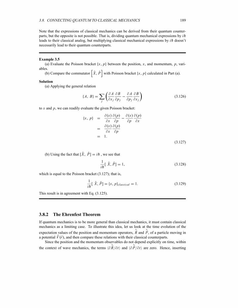
3.8. CONNECTING QUANTUM TO CLASSICAL MECHANICS 189
Note that the expressions of classical mechanics can be derived from their quantum counter-
parts, but the opposite is not possible. That is, dividing quantum mechanical expressions by ihleads to their classical analog, but multiplying classical mechanical expressions by ih doesn’tnecessarily lead to their quantum counterparts.
Example 3.5
(a) Evaluate the Poisson bracket x p between the position, x , and momentum, p, vari-ables.
(b) Compare the commutator X P with Poisson bracket x p calculated in Part (a).
Solution
(a) Applying the general relation
A Bj
A
x j
B
p j
A
p j
B
x j(3.126)
to x and p, we can readily evaluate the given Poisson bracket:
x px
x
p
p
x
p
p
xx
x
p
p1
(3.127)
(b) Using the fact that [X P] ih , we see that
1
ih[ X P] 1 (3.128)
which is equal to the Poisson bracket (3.127); that is,
1
ih[ X P] x p classical 1 (3.129)
This result is in agreement with Eq. (3.125).
3.8.2 The Ehrenfest Theorem
If quantum mechanics is to be more general than classical mechanics, it must contain classical
mechanics as a limiting case. To illustrate this idea, let us look at the time evolution of the
expectation values of the position and momentum operators, R and P , of a particle moving ina potential V r , and then compare these relations with their classical counterparts.Since the position and the momentum observables do not depend explicitly on time, within
the context of wave mechanics, the terms R t and P t are zero. Hence, inserting
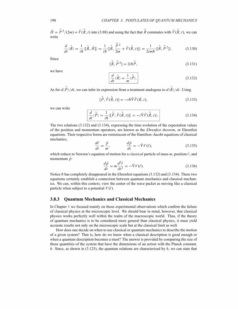
190 CHAPTER 3. POSTULATES OF QUANTUM MECHANICS
H P 2 2m V R t into (3.88) and using the fact that R commutes with V R t , we canwrite
d
dtR
1
ih[R H ]
1
ih[R
P 2
2mV R t ]
1
2imh[R P 2] (3.130)
Since
[R P 2] 2ihP (3.131)
we haved
dtR
1
mP (3.132)
As for d P dt , we can infer its expression from a treatment analogous to d R dt . Using
[P V R t ] ih V R t (3.133)
we can writed
dtP
1
ih[P V R t ] V R t (3.134)
The two relations (3.132) and (3.134), expressing the time evolution of the expectation values
of the position and momentum operators, are known as the Ehrenfest theorem, or Ehrenfestequations. Their respective forms are reminiscent of the Hamilton–Jacobi equations of classical
mechanics,dr
dt
p
m
d p
dtV r (3.135)
which reduce to Newton’s equation of motion for a classical particle of mass m, position r , andmomentum p:
d p
dtmd2r
dt2V r (3.136)
Notice h has completely disappeared in the Ehrenfest equations (3.132) and (3.134). These twoequations certainly establish a connection between quantum mechanics and classical mechan-
ics. We can, within this context, view the center of the wave packet as moving like a classical
particle when subject to a potential V r .
3.8.3 Quantum Mechanics and Classical Mechanics
In Chapter 1 we focused mainly on those experimental observations which confirm the failure
of classical physics at the microscopic level. We should bear in mind, however, that classical
physics works perfectly well within the realm of the macroscopic world. Thus, if the theory
of quantum mechanics is to be considered more general than classical physics, it must yield
accurate results not only on the microscopic scale but at the classical limit as well.
How does one decide on when to use classical or quantummechanics to describe the motion
of a given system? That is, how do we know when a classical description is good enough or
when a quantum description becomes a must? The answer is provided by comparing the size of
those quantities of the system that have the dimensions of an action with the Planck constant,
h. Since, as shown in (3.125), the quantum relations are characterized by h, we can state that
3.9. SOLVED PROBLEMS 191
if the value of the action of a system is too large compared to h, this system can be accuratelydescribed by means of classical physics. Otherwise, the use of a quantal description becomes
unavoidable. One should recall that, for microscopic systems, the size of action variables is of
the order of h; for instance, the angular momentum of the hydrogen atom is L nh, where nis finite.
Another equivalent way of defining the classical limit is by means of "length." Sinceh p the classical domain can be specified by the limit 0. This means that, when the de
Broglie wavelength of a system is too small compared to its size, the system can be described
accurately by means of classical physics.
In summary, the classical limit can be described as the limit h 0 or, equivalently, as the
limit 0. In these limits the results of quantum mechanics should be similar to those of
classical physics:
limh 0
Quantum Mechanics Classical Mechanics (3.137)
lim0Quantum Mechanics Classical Mechanics (3.138)
Classical mechanics can thus be regarded as the short wavelength limit of quantum mechanics.
In this way, quantum mechanics contains classical mechanics as a limiting case. So, in the limit
of h 0 or 0, quantum dynamical quantities should have, as proposed by Bohr, a one-to-
one correspondence with their classical counterparts. This is the essence of the correspondenceprinciple.But how does one reconcile, in the classical limit, the probabilistic nature of quantum me-
chanics with the determinism of classical physics? The answer is quite straightforward: quan-
tum fluctuations must become negligible or even vanish when h 0, for Heisenberg’s un-
certainty principle would acquire the status of certainty; when h 0, the fluctuations in the
position and momentum will vanish, x 0 and p 0. Thus, the position and momentum
can be measured simultaneously with arbitrary accuracy. This implies that the probabilistic as-
sessments of dynamical quantities by quantum mechanics must give way to exact calculations
(these ideas will be discussed further when we study the WKB method in Chapter 9).
So, for those cases where the action variables of a system are too large compared to h(or, equivalently, when the lengths of this system are too large compared to its de Broglie
wavelength), quantum mechanics gives the same results as classical mechanics.
In the rest of this text, we will deal with the various applications of the Schrödinger equation.
We start, in Chapter 4, with the simple case of one-dimensional systems and later on consider
more realistic systems.
3.9 Solved Problems
Problem 3.1
A particle of mass m, which moves freely inside an infinite potential well of length a, has thefollowing initial wave function at t 0:
x 0A
asin
x
a
3
5asin
3 x
a
1
5asin
5 x
a
192 CHAPTER 3. POSTULATES OF QUANTUM MECHANICS
where A is a real constant.(a) Find A so that x 0 is normalized.(b) If measurements of the energy are carried out, what are the values that will be found and
what are the corresponding probabilities? Calculate the average energy.
(c) Find the wave function x t at any later time t .(d) Determine the probability of finding the system at a time t in the state x t2 a sin 5 x a exp i E5t h ; then determine the probability of finding it in the statex t 2 a sin 2 x a exp i E2t h .
Solution
Since the functions
n x2
asin
n x
a(3.139)
are orthonormal,
n m
a
0n x m x dx
2
a
a
0
sinn x
asin
m x
adx nm (3.140)
it is more convenient to write x 0 in terms of n x :
x 0A
asin
x
a
3
5asin
3 x
a
1
5asin
5 x
a
A
21 x
3
103 x
1
105 x (3.141)
(a) Since n m nm the normalization of x 0 yields
1A2
2
3
10
1
10(3.142)
or A 6 5; hence
x 03
51 x
3
103 x
1
105 x (3.143)
(b) Since the second derivative of (3.139) is given by d2 n x dx2 n2 2 a2 n x ,and since the Hamiltonian of a free particle is H h2 2m d2 dx2, the expectation value ofH with respect to n x is
En n H nh2
2m
a
0n x
d2 n x
dx2dx
n2 2h2
2ma2(3.144)
If a measurement is carried out on the system, we would obtain En n2 2h2 2ma2 witha corresponding probability of Pn En n
2. Since the initial wave function (3.143)
contains only three eigenstates of H , 1 x , 3 x , and 5 x , the results of the energy mea-surements along with the corresponding probabilities are
E1 1 H 1
2h2
2ma2P1 E1 1
2 3
5(3.145)
E3 3 H 39 2h2
2ma2P3 E3 3
2 3
10(3.146)
E5 5 H 525 2h2
2ma2P5 E5 5
2 1
10(3.147)
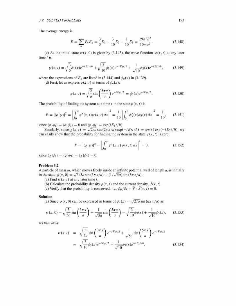
3.9. SOLVED PROBLEMS 193
The average energy is
En
PnEn3
5E1
3
10E3
1
10E5
29 2h2
10ma2(3.148)
(c) As the initial state x 0 is given by (3.143), the wave function x t at any latertime t is
x t3
51 x e
i E1t h3
103 x e
i E3t h1
105 x e
i E5t h (3.149)
where the expressions of En are listed in (3.144) and n x in (3.139).(d) First, let us express x t in terms of n x :
x t2
asin
5 x
ae i E5t h
5 x ei E5t h (3.150)
The probability of finding the system at a time t in the state x t is
P 2a
0
x t x t dx2 1
10
a
05 x 5 x dx
2 1
10(3.151)
since 1 3 0 and 5 exp i E5t h .Similarly, since x t 2 a sin 2 x a exp i E2t h 2 x exp i E2t h , we
can easily show that the probability for finding the system in the state x t is zero:
P 2a
0
x t x t dx2
0 (3.152)
since 1 3 5 0.
Problem 3.2
A particle of massm, which moves freely inside an infinite potential well of length a, is initiallyin the state x 0 3 5a sin 3 x a 1 5a sin 5 x a .(a) Find x t at any later time t .(b) Calculate the probability density x t and the current density, J x t .(c) Verify that the probability is conserved, i.e., t J x t 0.
Solution
(a) Since x 0 can be expressed in terms of n x 2 a sin n x a as
x 03
5asin
3 x
a
1
5asin
5 x
a
3
103 x
1
105 x (3.153)
we can write
x t3
5asin
3 x
ae i E3t h
1
5asin
5 x
ae i E5t h
3
103 x e
i E3t h1
105 x e
i E5t h (3.154)

194 CHAPTER 3. POSTULATES OF QUANTUM MECHANICS
where the expressions for En are listed in (3.144): En n2 2h2 2ma2 .(b) Since x t x t x t , where x t is given by (3.154), we can write
x t3
1023 x
3
103 x 5 x ei E3 E5 t h e i E3 E5 t h
1
1025 x (3.155)
From (3.144) we have E3 E5 9E1 25E1 16E1 8 2h2 ma2 . Thus, x tbecomes
x t3
1023 x
3
53 x 5 x cos
16E1t
h
1
1025 x
3
5asin2
3 x
a
2 3
5asin
3 x
asin
5 x
acos
16E1t
h
1
5asin2
5 x
a(3.156)
Since the system is one-dimensional, the action of the gradient operator on x t and x tis given by x t d x t dx i and x t d x t dx i . We can thus write
the current density J x t ih 2m x t x t x t x t as
J x tih
2mx t
d x t
dxx t
d x t
dxi (3.157)
Using (3.154) we have
d x t
dx
3
a
3
5acos
3 x
ae i E3t h
5
a
1
5acos
5 x
ae i E5t h (3.158)
d x t
dx
3
a
3
5acos
3 x
aei E3t h
5
a
1
5acos
5 x
aei E5t h (3.159)
A straightforward calculation yields
d
dx
d
dx2i
3
5a25 sin
3 x
acos
5 x
a3 sin
5 x
acos
3 x
a
sinE3 E5h
t (3.160)
Inserting this into (3.157) and using E3 E5 16E1, we have
J x th
m
3
5a25 sin
3 x
acos
5 x
a3 sin
5 x
acos
3 x
asin
16E1t
hi
(3.161)
(c) Performing the time derivative of (3.156) and using the expression 32 3E1 5ah16 2h 3 5ma3 , since E1 2h2 2ma2 , we obtain
t
32 3E15ah
sin3 x
asin
5 x
asin
16E1t
h
16 2h 3
5ma3sin
3 x
asin
5 x
asin
16E1t
h(3.162)
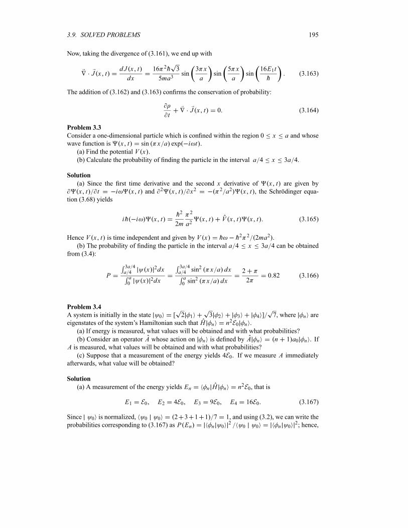
3.9. SOLVED PROBLEMS 195
Now, taking the divergence of (3.161), we end up with
J x td J x t
dx
16 2h 3
5ma3sin
3 x
asin
5 x
asin
16E1t
h(3.163)
The addition of (3.162) and (3.163) confirms the conservation of probability:
tJ x t 0 (3.164)
Problem 3.3
Consider a one-dimensional particle which is confined within the region 0 x a and whosewave function is x t sin x a exp i t .(a) Find the potential V x .(b) Calculate the probability of finding the particle in the interval a 4 x 3a 4.
Solution
(a) Since the first time derivative and the second x derivative of x t are given byx t t i x t and 2 x t x2 2 a2 x t , the Schrödinger equa-
tion (3.68) yields
ih i x th2
2m
2
a2x t V x t x t (3.165)
Hence V x t is time independent and given by V x h h2 2 2ma2 .(b) The probability of finding the particle in the interval a 4 x 3a 4 can be obtained
from (3.4):
P
3a 4a 4 x 2dxa0 x 2dx
3a 4a 4 sin2 x a dxa0 sin
2 x a dx
2
20 82 (3.166)
Problem 3.4
A system is initially in the state 0 [ 2 1 3 2 3 4 ] 7, where n are
eigenstates of the system’s Hamiltonian such that H n n2E0 n .
(a) If energy is measured, what values will be obtained and with what probabilities?
(b) Consider an operator A whose action on n is defined by A n n 1 a0 n . If
A is measured, what values will be obtained and with what probabilities?(c) Suppose that a measurement of the energy yields 4E0. If we measure A immediately
afterwards, what value will be obtained?
Solution
(a) A measurement of the energy yields En n H n n2E0, that is
E1 E0 E2 4E0 E3 9E0 E4 16E0 (3.167)
Since 0 is normalized, 0 0 2 3 1 1 7 1, and using (3.2), we can write the
probabilities corresponding to (3.167) as P En n 02
0 0 n 02; hence,
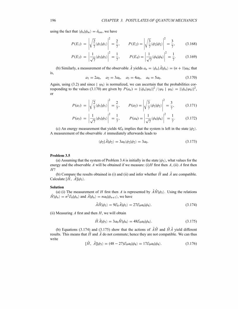
196 CHAPTER 3. POSTULATES OF QUANTUM MECHANICS
using the fact that n m nm , we have
P E12
71 1
22
7P E2
3
72 2
23
7(3.168)
P E31
73 3
21
7P E4
1
74 4
21
7(3.169)
(b) Similarly, a measurement of the observable A yields an n A n n 1 a0; thatis,
a1 2a0 a2 3a0 a3 4a0 a4 5a0 (3.170)
Again, using (3.2) and since 0 is normalized, we can ascertain that the probabilities cor-
responding to the values (3.170) are given by P an n 02
0 0 n 02,
or
P a12
71 1
22
7P a2
3
72 2
23
7(3.171)
P a31
73 3
21
7P a4
1
74 4
21
7(3.172)
(c) An energy measurement that yields 4E0 implies that the system is left in the state 2 .
A measurement of the observable A immediately afterwards leads to
2 A 2 3a0 2 2 3a0 (3.173)
Problem 3.5
(a) Assuming that the system of Problem 3.4 is initially in the state 3 , what values for the
energy and the observable A will be obtained if we measure: (i)H first then A, (ii) A first thenH?(b) Compare the results obtained in (i) and (ii) and infer whether H and A are compatible.
Calculate [H A] 3 .
Solution
(a) (i) The measurement of H first then A is represented by AH 3 . Using the relations
H n n2E0 n and A n na0 n 1 , we have
AH 3 9E0A 3 27E0a0 4 (3.174)
(ii) Measuring A first and then H , we will obtain
H A 3 3a0H 4 48E0a0 4 (3.175)
(b) Equations (3.174) and (3.175) show that the actions of AH and H A yield differentresults. This means that H and A do not commute; hence they are not compatible. We can thuswrite
[H A] 3 48 27 E0a0 4 17E0a0 4 (3.176)
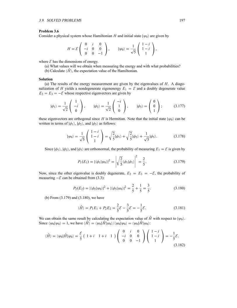
3.9. SOLVED PROBLEMS 197
Problem 3.6
Consider a physical system whose Hamiltonian H and initial state 0 are given by
H E
0 i 0
i 0 0
0 0 10
1
5
1 i1 i1
where E has the dimensions of energy.
(a) What values will we obtain when measuring the energy and with what probabilities?
(b) Calculate H , the expectation value of the Hamiltonian.
Solution
(a) The results of the energy measurement are given by the eigenvalues of H . A diago-nalization of H yields a nondegenerate eigenenergy E1 E and a doubly degenerate value
E2 E3 E whose respective eigenvectors are given by
11
2
1
i0
21
2
i1
03
0
0
1
(3.177)
these eigenvectors are orthogonal since H is Hermitian. Note that the initial state 0 can be
written in terms of 1 , 2 , and 3 as follows:
01
5
1 i1 i1
2
51
2
52
1
53 (3.178)
Since 1 , 2 , and 3 are orthonormal, the probability of measuring E1 E is given by
P1 E1 1 02 2
51 1
22
5(3.179)
Now, since the other eigenvalue is doubly degenerate, E2 E3 E , the probability of
measuring E can be obtained from (3.3):
P2 E2 2 02
3 02 2
5
1
5
3
5(3.180)
(b) From (3.179) and (3.180), we have
H P1E1 P2E22
5E
3
5E
1
5E (3.181)
We can obtain the same result by calculating the expectation value of H with respect to 0 .
Since 0 0 1, we have H 0 H 0 0 0 0 H 0 :
H 0 H 0E
51 i 1 i 1
0 i 0
i 0 0
0 0 1
1 i1 i1
1
5E
(3.182)
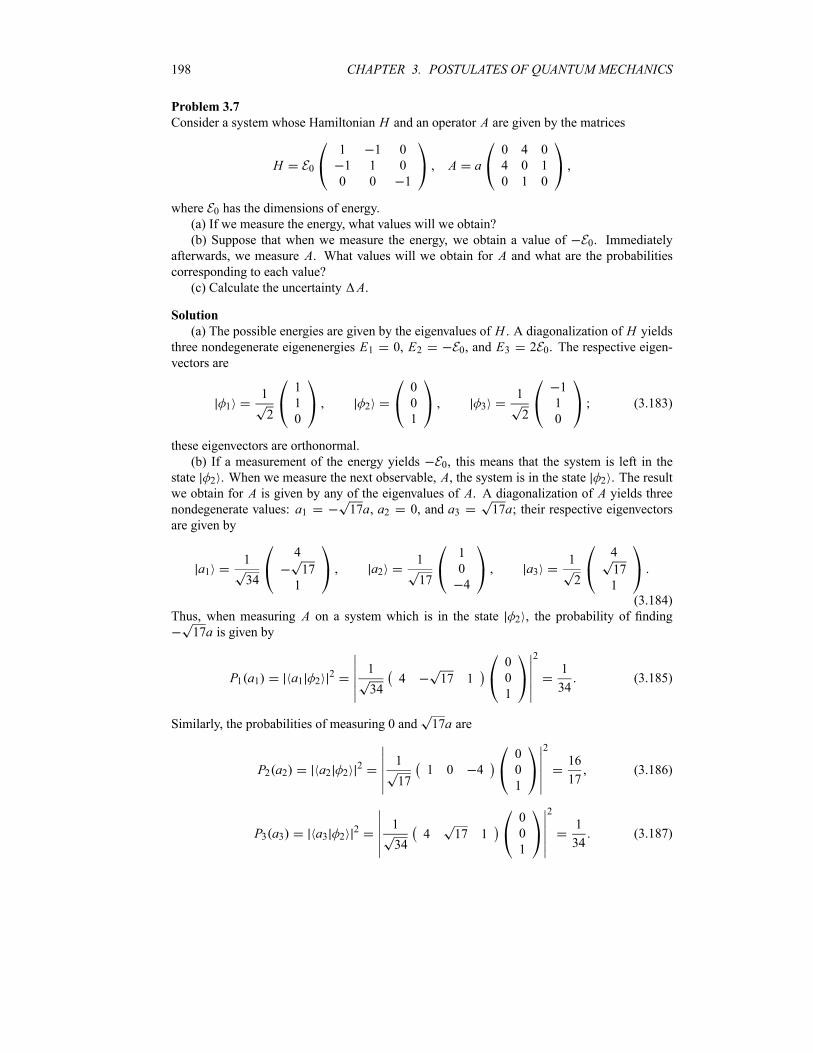
198 CHAPTER 3. POSTULATES OF QUANTUM MECHANICS
Problem 3.7
Consider a system whose Hamiltonian H and an operator A are given by the matrices
H E0
1 1 0
1 1 0
0 0 1
A a0 4 0
4 0 1
0 1 0
where E0 has the dimensions of energy.
(a) If we measure the energy, what values will we obtain?
(b) Suppose that when we measure the energy, we obtain a value of E0. Immediately
afterwards, we measure A. What values will we obtain for A and what are the probabilitiescorresponding to each value?
(c) Calculate the uncertainty A.
Solution
(a) The possible energies are given by the eigenvalues of H . A diagonalization of H yieldsthree nondegenerate eigenenergies E1 0, E2 E0, and E3 2E0. The respective eigen-
vectors are
11
2
1
1
02
0
0
13
1
2
1
1
0
(3.183)
these eigenvectors are orthonormal.
(b) If a measurement of the energy yields E0, this means that the system is left in the
state 2 . When we measure the next observable, A, the system is in the state 2 . The result
we obtain for A is given by any of the eigenvalues of A. A diagonalization of A yields threenondegenerate values: a1 17a, a2 0, and a3 17a; their respective eigenvectorsare given by
a11
34
4
17
1
a21
17
1
0
4
a31
2
4
17
1(3.184)
Thus, when measuring A on a system which is in the state 2 , the probability of finding
17a is given by
P1 a1 a1 22 1
344 17 1
0
0
1
2
1
34(3.185)
Similarly, the probabilities of measuring 0 and 17a are
P2 a2 a2 22 1
171 0 4
0
0
1
2
16
17(3.186)
P3 a3 a3 22 1
344 17 1
0
0
1
2
1
34(3.187)
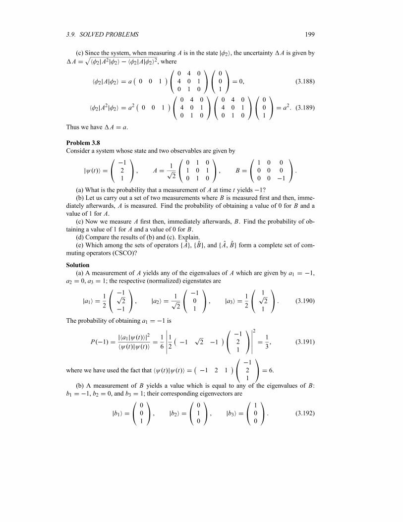
3.9. SOLVED PROBLEMS 199
(c) Since the system, when measuring A is in the state 2 , the uncertainty A is given byA 2 A2 2 2 A 2
2, where
2 A 2 a 0 0 1
0 4 0
4 0 1
0 1 0
0
0
1
0 (3.188)
2 A2
2 a2 0 0 1
0 4 0
4 0 1
0 1 0
0 4 0
4 0 1
0 1 0
0
0
1
a2 (3.189)
Thus we have A a.
Problem 3.8
Consider a system whose state and two observables are given by
t1
2
1
A1
2
0 1 0
1 0 1
0 1 0
B1 0 0
0 0 0
0 0 1
(a) What is the probability that a measurement of A at time t yields 1?
(b) Let us carry out a set of two measurements where B is measured first and then, imme-diately afterwards, A is measured. Find the probability of obtaining a value of 0 for B and avalue of 1 for A.(c) Now we measure A first then, immediately afterwards, B. Find the probability of ob-
taining a value of 1 for A and a value of 0 for B.(d) Compare the results of (b) and (c). Explain.
(e) Which among the sets of operators A , B , and A B form a complete set of com-
muting operators (CSCO)?
Solution
(a) A measurement of A yields any of the eigenvalues of A which are given by a1 1,
a2 0, a3 1; the respective (normalized) eigenstates are
a11
2
1
2
1
a21
2
1
0
1
a31
2
1
2
1
(3.190)
The probability of obtaining a1 1 is
P 1a1 t 2
t t
1
6
1
21 2 1
1
2
1
2
1
3(3.191)
where we have used the fact that t t 1 2 1
1
2
1
6.
(b) A measurement of B yields a value which is equal to any of the eigenvalues of B:b1 1, b2 0, and b3 1; their corresponding eigenvectors are
b1
0
0
1
b2
0
1
0
b3
1
0
0
(3.192)

200 CHAPTER 3. POSTULATES OF QUANTUM MECHANICS
Since the system was in the state t , the probability of obtaining the value b2 0 for B is
P b2b2 t 2
t t
1
60 1 0
1
2
1
2
2
3(3.193)
We deal now with the measurement of the other observable, A. The observables A and B donot have common eigenstates, since they do not commute. After measuring B (the result isb2 0), the system is left, according to Postulate 3, in a state which can be found by
projecting t onto b2 :
b2 b2 t0
1
0
0 1 0
1
2
1
0
2
0
(3.194)
The probability of finding 1 when we measure A is given by
P a3a3
2 1
4
1
21 2 1
0
2
0
2
1
2(3.195)
since 4. In summary, when measuring B then A, the probability of finding a value of0 for B and 1 for A is given by the product of the probabilities (3.193) and (3.195):
P b2 a3 P b2 P a32
3
1
2
1
3(3.196)
(c) Next we measure A first then B. Since the system is in the state t , the probabilityof measuring a3 1 for A is given by
P a3a3 t 2
t t
1
6
1
21 2 1
1
2
1
2
1
3(3.197)
where we have used the expression (3.190) for a3 .We then proceed to the measurement of B. The state of the system just after measuring A
(with a value a3 1) is given by a projection of t onto a3 :
a3 a3 t1
4
1
2
1
1 2 1
1
2
1
2
2
1
2
1
(3.198)
So the probability of finding a value of b2 0 when measuring B is given by
P b2b2
2 1
2
2
20 1 0
1
2
1
2
1
2(3.199)
since 2.
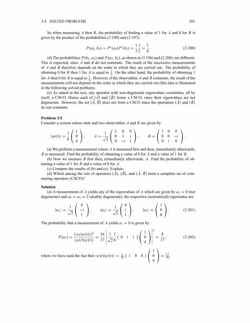
3.9. SOLVED PROBLEMS 201
So when measuring A then B, the probability of finding a value of 1 for A and 0 for B isgiven by the product of the probabilities (3.199) and (3.197):
P a3 b2 P a3 P b21
3
1
2
1
6(3.200)
(d) The probabilities P b2 a3 and P a3 b2 , as shown in (3.196) and (3.200), are different.This is expected, since A and B do not commute. The result of the successive measurementsof A and B therefore depends on the order in which they are carried out. The probability ofobtaining 0 for B then 1 for A is equal to 1
3. On the other hand, the probability of obtaining 1
for A then 0 for B is equal to 16. However, if the observables A and B commute, the result of the
measurements will not depend on the order in which they are carried out (this idea is illustrated
in the following solved problem).
(e) As stated in the text, any operator with non-degenerate eigenvalues constitutes, all by
itself, a CSCO. Hence each of A and B forms a CSCO, since their eigenvalues are not
degenerate. However, the set A B does not form a CSCO since the opertators A and Bdo not commute.
Problem 3.9
Consider a system whose state and two observables A and B are given by
t1
6
1
0
4
A1
2
2 0 0
0 1 i0 i 1
B1 0 0
0 0 i0 i 0
(a) We perform a measurement where A is measured first and then, immediately afterwards,B is measured. Find the probability of obtaining a value of 0 for A and a value of 1 for B.(b) Now we measure B first then, immediately afterwards, A. Find the probability of ob-
taining a value of 1 for B and a value of 0 for A.(c) Compare the results of (b) and (c). Explain.
(d) Which among the sets of operators A , B , and A B form a complete set of com-
muting operators (CSCO)?
Solution
(a) A measurement of A yields any of the eigenvalues of A which are given by a1 0 (not
degenerate) and a2 a3 2 (doubly degenerate); the respective (normalized) eigenstates are
a11
2
0
i1
a21
2
0
i1
a3
1
0
0
(3.201)
The probability that a measurement of A yields a1 0 is given by
P a1a1 t 2
t t
36
17
1
2
1
60 i 1
1
0
4
2
8
17(3.202)
where we have used the fact that t t 136
1 0 4
1
0
4
1736.
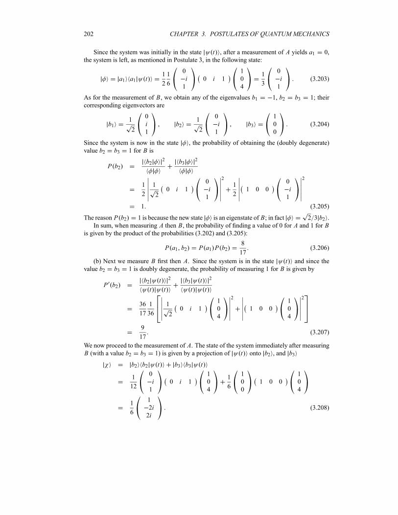
202 CHAPTER 3. POSTULATES OF QUANTUM MECHANICS
Since the system was initially in the state t , after a measurement of A yields a1 0,
the system is left, as mentioned in Postulate 3, in the following state:
a1 a1 t1
2
1
6
0
i1
0 i 1
1
0
4
1
3
0
i1
(3.203)
As for the measurement of B, we obtain any of the eigenvalues b1 1, b2 b3 1; their
corresponding eigenvectors are
b11
2
0
i1
b21
2
0
i1
b3
1
0
0
(3.204)
Since the system is now in the state , the probability of obtaining the (doubly degenerate)
value b2 b3 1 for B is
P b2b2
2 b32
1
2
1
20 i 1
0
i1
2
1
21 0 0
0
i1
2
1 (3.205)
The reason P b2 1 is because the new state is an eigenstate of B; in fact 2 3 b2 .In sum, when measuring A then B, the probability of finding a value of 0 for A and 1 for B
is given by the product of the probabilities (3.202) and (3.205):
P a1 b2 P a1 P b28
17(3.206)
(b) Next we measure B first then A. Since the system is in the state t and since the
value b2 b3 1 is doubly degenerate, the probability of measuring 1 for B is given by
P b2b2 t 2
t t
b3 t 2
t t
36
17
1
36
1
20 i 1
1
0
4
2
1 0 0
1
0
4
2
9
17(3.207)
We now proceed to the measurement of A. The state of the system immediately after measuringB (with a value b2 b3 1) is given by a projection of t onto b2 , and b3
b2 b2 t b3 b3 t
1
12
0
i1
0 i 1
1
0
4
1
6
1
0
0
1 0 0
1
0
4
1
6
1
2i2i
(3.208)
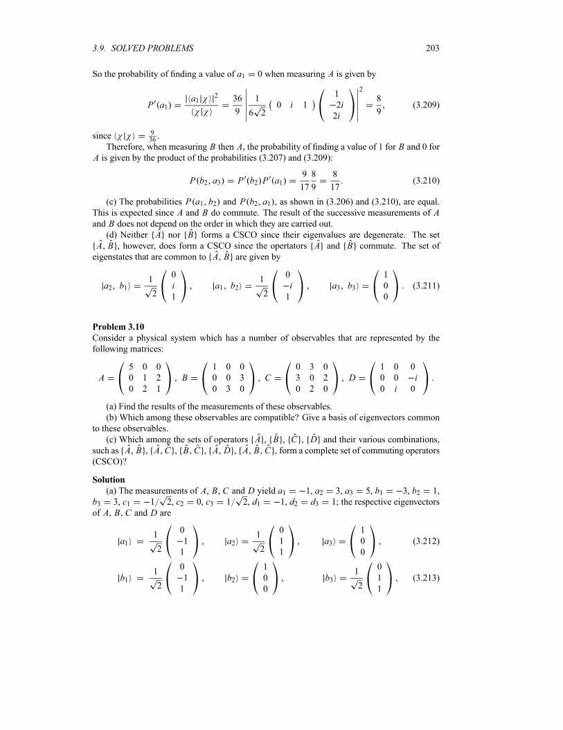
3.9. SOLVED PROBLEMS 203
So the probability of finding a value of a1 0 when measuring A is given by
P a1a1
2 36
9
1
6 20 i 1
1
2i2i
2
8
9(3.209)
since 936.
Therefore, when measuring B then A, the probability of finding a value of 1 for B and 0 forA is given by the product of the probabilities (3.207) and (3.209):
P b2 a3 P b2 P a19
17
8
9
8
17(3.210)
(c) The probabilities P a1 b2 and P b2 a1 , as shown in (3.206) and (3.210), are equal.This is expected since A and B do commute. The result of the successive measurements of Aand B does not depend on the order in which they are carried out.(d) Neither A nor B forms a CSCO since their eigenvalues are degenerate. The set
A B , however, does form a CSCO since the opertators A and B commute. The set of
eigenstates that are common to A B are given by
a2 b11
2
0
i1
a1 b21
2
0
i1
a3 b3
1
0
0
(3.211)
Problem 3.10
Consider a physical system which has a number of observables that are represented by the
following matrices:
A5 0 0
0 1 2
0 2 1
B1 0 0
0 0 3
0 3 0
C0 3 0
3 0 2
0 2 0
D1 0 0
0 0 i0 i 0
(a) Find the results of the measurements of these observables.
(b) Which among these observables are compatible? Give a basis of eigenvectors common
to these observables.
(c) Which among the sets of operators A , B , C , D and their various combinations,
such as A B , A C , B C , A D , A B C , form a complete set of commuting operators(CSCO)?
Solution
(a) The measurements of A, B, C and D yield a1 1, a2 3, a3 5, b1 3, b2 1,
b3 3, c1 1 2, c2 0, c3 1 2, d1 1, d2 d3 1; the respective eigenvectors
of A, B, C and D are
a11
2
0
1
1
a21
2
0
1
1
a3
1
0
0
(3.212)
b11
2
0
1
1
b2
1
0
0
b31
2
0
1
1
(3.213)
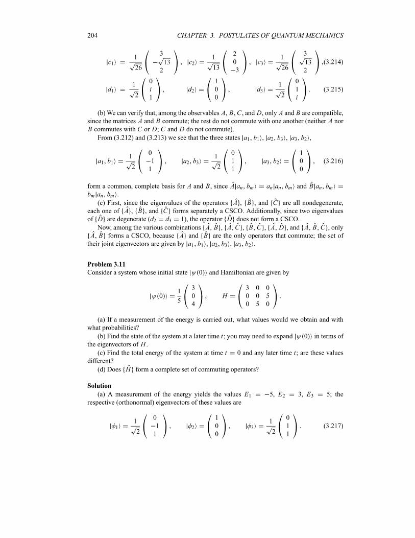
204 CHAPTER 3. POSTULATES OF QUANTUM MECHANICS
c11
26
3
13
2
c21
13
2
0
3
c31
26
3
13
2
(3.214)
d11
2
0
i1
d2
1
0
0
d31
2
0
1
i(3.215)
(b)We can verify that, among the observables A, B,C , and D, only A and B are compatible,since the matrices A and B commute; the rest do not commute with one another (neither A norB commutes with C or D; C and D do not commute).From (3.212) and (3.213) we see that the three states a1 b1 , a2 b3 , a3 b2 ,
a1 b11
2
0
1
1
a2 b31
2
0
1
1
a3 b2
1
0
0
(3.216)
form a common, complete basis for A and B, since A an bm an an bm and B an bmbm an bm .(c) First, since the eigenvalues of the operators A , B , and C are all nondegenerate,
each one of A , B , and C forms separately a CSCO. Additionally, since two eigenvalues
of D are degenerate (d2 d3 1), the operator D does not form a CSCO.
Now, among the various combinations A B , A C , B C , A D , and A B C , onlyA B forms a CSCO, because A and B are the only operators that commute; the set of
their joint eigenvectors are given by a1 b1 , a2 b3 , a3 b2 .
Problem 3.11
Consider a system whose initial state 0 and Hamiltonian are given by
01
5
3
0
4
H3 0 0
0 0 5
0 5 0
(a) If a measurement of the energy is carried out, what values would we obtain and with
what probabilities?
(b) Find the state of the system at a later time t ; you may need to expand 0 in terms of
the eigenvectors of H .(c) Find the total energy of the system at time t 0 and any later time t ; are these values
different?
(d) Does H form a complete set of commuting operators?
Solution
(a) A measurement of the energy yields the values E1 5, E2 3, E3 5; the
respective (orthonormal) eigenvectors of these values are
11
2
0
1
12
1
0
03
1
2
0
1
1
(3.217)
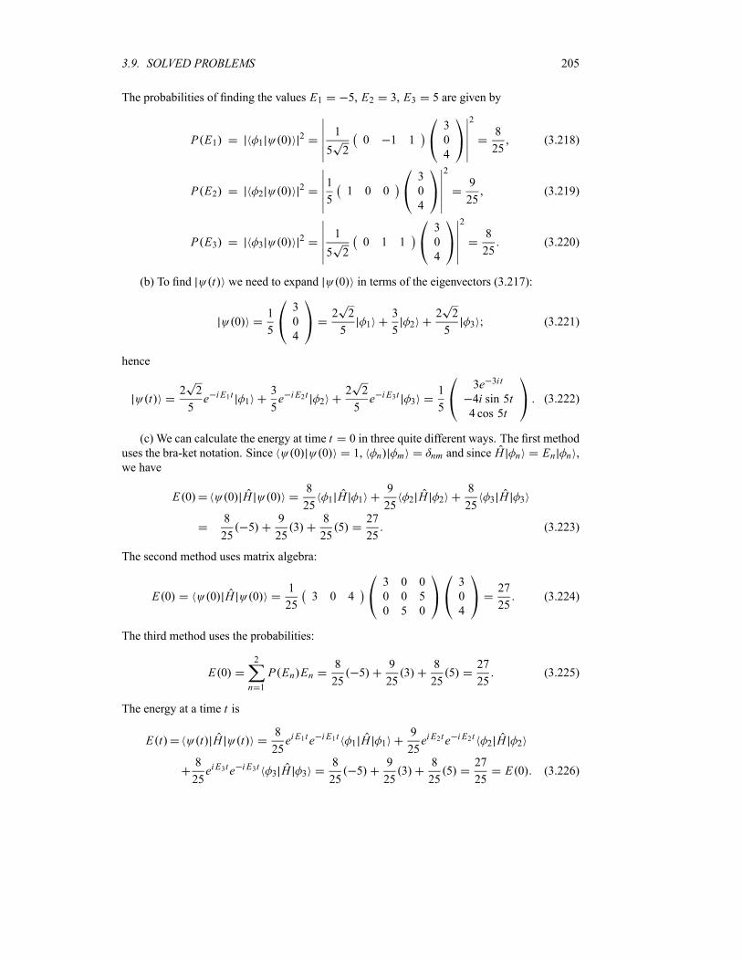
3.9. SOLVED PROBLEMS 205
The probabilities of finding the values E1 5, E2 3, E3 5 are given by
P E1 1 0 2 1
5 20 1 1
3
0
4
2
8
25(3.218)
P E2 2 0 2 1
51 0 0
3
0
4
2
9
25(3.219)
P E3 3 0 2 1
5 20 1 1
3
0
4
2
8
25(3.220)
(b) To find t we need to expand 0 in terms of the eigenvectors (3.217):
01
5
3
0
4
2 2
51
3
52
2 2
53 (3.221)
hence
t2 2
5e i E1t
13
5e i E2t
22 2
5e i E3t
31
5
3e 3i t
4i sin 5t4 cos 5t
(3.222)
(c) We can calculate the energy at time t 0 in three quite different ways. The first method
uses the bra-ket notation. Since 0 0 1, n m nm and since H n En n ,
we have
E 0 0 H 08
251 H 1
9
252 H 2
8
253 H 3
8
255
9
253
8
255
27
25(3.223)
The second method uses matrix algebra:
E 0 0 H 01
253 0 4
3 0 0
0 0 5
0 5 0
3
0
4
27
25(3.224)
The third method uses the probabilities:
E 02
n 1
P En En8
255
9
253
8
255
27
25(3.225)
The energy at a time t is
E t t H t8
25ei E1te i E1t
1 H 19
25ei E2te i E2t
2 H 2
8
25ei E3te i E3t
3 H 38
255
9
253
8
255
27
25E 0 (3.226)
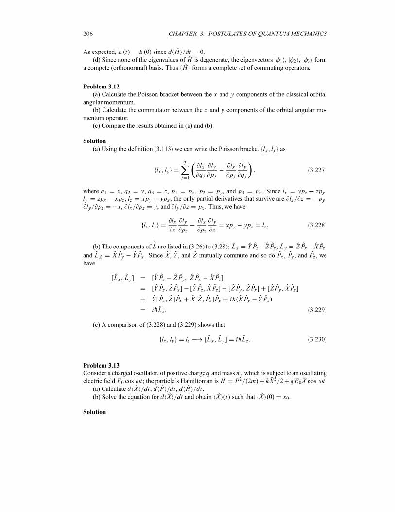
206 CHAPTER 3. POSTULATES OF QUANTUM MECHANICS
As expected, E t E 0 since d H dt 0.
(d) Since none of the eigenvalues of H is degenerate, the eigenvectors 1 , 2 , 3 form
a compete (orthonormal) basis. Thus H forms a complete set of commuting operators.
Problem 3.12
(a) Calculate the Poisson bracket between the x and y components of the classical orbitalangular momentum.
(b) Calculate the commutator between the x and y components of the orbital angular mo-mentum operator.
(c) Compare the results obtained in (a) and (b).
Solution
(a) Using the definition (3.113) we can write the Poisson bracket lx ly as
lx ly3
j 1
lxq j
lyp j
lxp j
lyq j
(3.227)
where q1 x , q2 y, q3 z, p1 px , p2 py , and p3 pz . Since lx ypz zpy ,ly zpx xpz , lz xpy ypx , the only partial derivatives that survive are lx z py ,ly pz x , lx pz y, and ly z px . Thus, we have
lx lylxz
lypz
lxpz
lyz
xpy ypx lz (3.228)
(b) The components of L are listed in (3.26) to (3.28): Lx Y Pz Z Py , L y Z Px X Pz ,
and LZ X Py Y Px . Since X , Y , and Z mutually commute and so do Px , Py , and Pz , wehave
[Lx L y] [Y Pz Z Py Z Px X Pz]
[Y Pz Z Px ] [Y Pz X Pz] [Z Py Z Px ] [Z Py X Pz]
Y [Pz Z ]Px X [Z Pz]Py ih X Py Y Px
ihLz (3.229)
(c) A comparison of (3.228) and (3.229) shows that
lx ly lz [Lx L y] ihLz (3.230)
Problem 3.13
Consider a charged oscillator, of positive charge q and massm, which is subject to an oscillatingelectric field E0 cos t ; the particle’s Hamiltonian is H P2 2m kX2 2 qE0X cos t .(a) Calculate d X dt , d P dt , d H dt .(b) Solve the equation for d X dt and obtain X t such that X 0 x0.
Solution
3.9. SOLVED PROBLEMS 207
(a) Since the position operator X does not depend explicitly on time (i.e., X t 0),
equation (3.88) yields
d
dtX
1
ih[X H ]
1
ihXP2
2m
P
m(3.231)
Now, since [P X ] ih, [P X2] 2ihX and P t 0, we have
d
dtP
1
ih[P H ]
1
ihP1
2kX2 qE0X cos t k X qE0 cos t
(3.232)
d
dtH
1
ih[H H ]
H
t
H
tqE0 X sin t (3.233)
(b) To find X we need to take a time derivative of (3.231) and then make use of (3.232):
d2
dt2X
1
m
d
dtP
k
mX
qE0mcos t (3.234)
The solution of this equation is
X t X 0 cosk
mt
qE0m
sin t A (3.235)
where A is a constant which can be determined from the initial conditions; since X 0 x0we have A 0, and hence
X t x0 cosk
mt
qE0m
sin t (3.236)
Problem 3.14
Consider a one-dimensional free particle of mass m whose position and momentum at timet 0 are given by x0 and p0, respectively.(a) Calculate P t and show that X t p0t2 m x0.(b) Show that d X2 dt 2 PX m ih m and d P2 dt 0.
(c) Show that the position and momentum fluctuations are related by d2 x 2 dt2
2 p 2 m2 and that the solution to this equation is given by x 2 p 20t2 m2 x 20
where x 0 and p 0 are the initial fluctuations.
Solution
(a) From the Ehrenfest equations d P dt [P V x t ] ih as shown in (3.134), andsince for a free particle V x t 0, we see that d P dt 0. As expected this leads to
P t p0, since the linear momentum of a free particle is conserved. Inserting P p0into Ehrenfest’s other equation d X dt P m (see (3.132)), we obtain
d X
dt
1
mp0 (3.237)
208 CHAPTER 3. POSTULATES OF QUANTUM MECHANICS
The solution of this equation with the initial condition X 0 x0 is
X tp0mt x0 (3.238)
(b) First, the proof of d P2 dt 0 is straightforward. Since [P2 H ] [P2 P2 2m] 0
and P2 t 0 (the momentum operator does not depend on time), (3.124) yields
d
dtP2
1
ih[P2 H ]
P2
t0 (3.239)
For d X2 dt we have
d
dtX2
1
ih[X2 H ]
1
2imh[X2 P2] (3.240)
since X2 t 0. Using [X P] ih, we obtain
[X2 P2] P[X2 P] [X2 P]P
PX [X P] P[X P]X X [X P]P [X P]X P
2ih PX X P 2ih 2PX ih (3.241)
henced
dtX2
2
mPX
ih
m(3.242)
(c) As the position fluctuation is given by x 2 X2 X 2, we have
d x 2
dt
d X2
dt2 X
d X
dt
2
mPX
ih
m
2
mX P (3.243)
In deriving this expression we have used (3.242) and d X dt P m. Now, sinced X P dt P d X dt P 2 m and
d PX
dt
1
ih[PX H ]
1
2imh[PX P2]
1
mP2 (3.244)
we can write the second time derivative of (3.243) as follows:
d2 x 2
dt22
m
d PX
dt
d X P
dt
2
m2P2 P 2 2
m2p 20 (3.245)
where p 20 P2 P 2 P2 0 P 20; the momentum of the free particle is a constant
of the motion. We can verify that the solution of the differential equation (3.245) is given by
x 21
m2p 20t
2 x 20 (3.246)
This fluctuation is similar to the spreading of a Gaussian wave packet we derived in Chapter 1.
3.10. EXERCISES 209
3.10 Exercises
Exercise 3.1
A particle in an infinite potential box with walls at x 0 and x a (i.e., the potential is infinitefor x 0 and x a and zero in between) has the following wave function at some initial time:
x1
5asin
x
a
2
5asin
3 x
a
(a) Find the possible results of the measurement of the system’s energy and the correspond-
ing probabilities.
(b) Find the form of the wave function after such a measurement.
(c) If the energy is measured again immediately afterwards, what are the relative probabili-
ties of the possible outcomes?
Exercise 3.2
Let n x denote the orthonormal stationary states of a system corresponding to the energy En .Suppose that the normalized wave function of the system at time t 0 is x 0 and supposethat a measurement of the energy yields the value E1 with probability 1/2, E2 with probability3/8, and E3 with probability 1/8.(a) Write the most general expansion for x 0 consistent with this information.(b) What is the expansion for the wave function of the system at time t , x t ?(c) Show that the expectation value of the Hamiltonian does not change with time.
Exercise 3.3
Consider a neutron which is confined to an infinite potential well of width a 8 fm. At time
t 0 the neutron is assumed to be in the state
x 04
7asin
x
a
2
7asin
2 x
a
8
7asin
3 x
a
(a) If an energy measurement is carried out on the system, what are the values that will be
found for the energy and with what probabilities? Express your answer in MeV (the mass of
the neutron is mc2 939MeV, hc 197MeV fm).
(b) If this measurement is repeated on many identical systems, what is the average value of
the energy that will be found? Again, express your answer in MeV.
(c) Using the uncertainty principle, estimate the order of magnitude of the neutron’s speed
in this well as a function of the speed of light c.
Exercise 3.4
Consider the dimensionless harmonic oscillator Hamiltonian
H1
2P2
1
2X2 with P i
d
dx
(a) Show that the two wave functions 0 x e x2 2 and 1 x xe x2 2 are eigenfunc-
tions of H with eigenvalues 1 2 and 3 2, respectively.
(b) Find the value of the coefficient such that 2 x 1 x2 e x2 2 is orthogonal to
0 x . Then show that 2 x is an eigenfunction of H with eigenvalue 5 2.
210 CHAPTER 3. POSTULATES OF QUANTUM MECHANICS
Exercise 3.5
Consider that the wave function of a dimensionless harmonic oscillator, whose Hamiltonian is
H 12P2 1
2X2, is given at time t 0 by
x 01
80 x
1
182 x
1
8e x2 2 1
181 2x2 e x2 2
(a) Find the expression of the oscillator’s wave function at any later time t .(b) Calculate the probability P0 to find the system in an eigenstate of energy 1 2 and the
probability P2 of finding the system in an eigenstate of energy 5 2.(c) Calculate the probability density, x t , and the current density, J x t .(d) Verify that the probability is conserved; that is, show that t J x t 0.
Exercise 3.6
A particle of mass m, in an infinite potential well of length a, has the following initial wavefunction at t 0:
x 03
5asin
3 x
a
1
5asin
5 x
a(3.247)
and an energy spectrum En h2 2n2 2ma2 .Find x t at any later time t , then calculate t and the probability current density vector
J x t and verify that t J x t 0. Recall that x t x t and J x tih2m x t x t x t x t .
Exercise 3.7
Consider a system whose initial state at t 0 is given in terms of a complete and orthonormal
set of three vectors: 1 , 2 , 3 as follows: 0 1 3 1 A 2 1 6 3 ,
where A is a real constant.(a) Find A so that 0 is normalized.
(b) If the energies corresponding to 1 , 2 , 3 are given by E1, E2, and E3, respec-tively, write down the state of the system t at any later time t .(c) Determine the probability of finding the system at a time t in the state 3 .
Exercise 3.8
The components of the initial state i of a quantum system are given in a complete and
orthonormal basis of three states 1 , 2 , 3 by
1 ii
32 i
2
33 i 0
Calculate the probability of finding the system in a state f whose components are given in
the same basis by
1 f1 i
32 f
1
63 f
1
6
3.10. EXERCISES 211
Exercise 3.9
(a) Evaluate the Poisson bracket x2 p2 .
(b) Express the commutator X2 P2 in terms of X P plus a constant in h2.
(c) Find the classical limit of x2 p2 for this expression and then compare it with the resultof part (a).
Exercise 3.10
A particle bound in a one-dimensional potential has a wave function
xAe5ikx cos 3 x a a 2 x a 20 x a 2
(a) Calculate the constant A so that x is normalized.(b) Calculate the probability of finding the particle between x 0 and x a 4.
Exercise 3.11
(a) Show that any component of the momentum operator of a particle is compatible with its
kinetic energy operator.
(b) Show that the momentum operator is compatible with the Hamiltonian operator only if
the potential operator is constant in space coordinates.
Exercise 3.12
Consider a physical system whose Hamiltonian H and an operator A are given by
H E0
2 0 0
0 1 0
0 0 1
A a0
5 0 0
0 0 2
0 2 0
where E0 has the dimensions of energy.
(a) Do H and A commute? If yes, give a basis of eigenvectors common to H and A.(b) Which among the sets of operators H , A , H A , H2 A form a complete set of
commuting operators (CSCO)?
Exercise 3.13
Show that the momentum and the total energy can be measured simultaneously only when the
potential is constant everywhere.
Exercise 3.14
The initial state of a system is given in terms of four orthonormal energy eigenfunctions 1 ,
2 , 3 , and 4 as follows:
0 t 01
31
1
22
1
63
1
24
(a) If the four kets 1 , 2 , 3 , and 4 are eigenvectors to the Hamiltonian H withenergies E1, E2, E3, and E4, respectively, find the state t at any later time t .(b) What are the possible results of measuring the energy of this system and with what
probability will they occur?
(c) Find the expectation value of the system’s Hamiltonian at t 0 and t 10 s.

212 CHAPTER 3. POSTULATES OF QUANTUM MECHANICS
Exercise 3.15
The complete set expansion of an initial wave function x 0 of a system in terms of orthonor-mal energy eigenfunctions n x of the system has three terms, n 1 2 3. The measurement
of energy on the system represented by x 0 gives three values, E1 and E2 with probability1 4 and E3 with probability 1 2.(a) Write down x 0 in terms of 1 x , 2 x , and 3 x .(b) Find x 0 at any later time t , i.e., find x t .
Exercise 3.16
Consider a system whose Hamiltonian H and an operator A are given by the matrices
H E0
0 i 0
i 0 2i0 2i 0
A a0
0 i 0
i 1 1
0 1 0
(a) If we measure energy, what values will we obtain?
(b) Suppose that when we measure energy, we obtain a value of 5E0. Immediately af-
terwards, we measure A. What values will we obtain for A and what are the probabilitiescorresponding to each value?
(c) Calculate the expectation value A .
Exercise 3.17
Consider a physical system whose Hamiltonian and initial state are given by
H E0
1 1 0
1 1 0
0 0 10
1
6
1
1
2
where E0 has the dimensions of energy.
(a) What values will we obtain when measuring the energy and with what probabilities?
(b) Calculate the expectation value of the Hamiltonian H .
Exercise 3.18
Consider a system whose state t and two observables A and B are given by
t5
1
3
A1
2
2 0 0
0 1 1
0 1 1
B1 0 0
0 0 1
0 1 0
(a) We perform a measurement where A is measured first and then B immediately after-wards. Find the probability of obtaining a value of 2 for A and a value of 1 for B.(b) Now we measure B first and then A immediately afterwards. Find the probability of
obtaining a value of 1 for B and a value of 2 for A.(c) Compare the results of (a) and (b). Explain.
Exercise 3.19
Consider a system whose state t and two observables A and B are given by
t1
3
i2
0
A1
2
1 i 1
i 0 0
1 0 0
B3 0 0
0 1 i0 i 0
3.10. EXERCISES 213
(a) Are A and B compatible? Which among the sets of operators A , B , and A B form
a complete set of commuting operators?
(b) Measuring A first and then B immediately afterwards, find the probability of obtaininga value of 1 for A and a value of 3 for B.(c) Now, measuring B first then A immediately afterwards, find the probability of obtaining
3 for B and 1 for A. Compare this result with the probability obtained in (b).
Exercise 3.20
Consider a physical system which has a number of observables that are represented by the
following matrices:
A1 0 0
0 0 1
0 1 0
B0 0 1
0 0 i1 i 4
C2 0 0
0 1 3
0 3 1
(a) Find the results of the measurements of the compatible observables.
(b) Which among these observables are compatible? Give a basis of eigenvectors common
to these observables.
(c) Which among the sets of operators A , B , C , A B , A C , B C form a com-
plete set of commuting operators?
Exercise 3.21
Consider a system which is initially in a state 0 and having a Hamiltonian H , where
0
4 i2 5i3 2i
H1
2
0 i 0
i 3 3
0 3 0
(a) If a measurement of H is carried out, what values will we obtain and with what proba-bilities?
(b) Find the state of the system at a later time t ; you may need to expand 0 in terms of
the eigenvectors of H .(c) Find the total energy of the system at time t 0 and any later time t ; are these values
different?
(d) Does H form a complete set of commuting operators?
Exercise 3.22
Consider a particle which moves in a scalar potential V r Vx x Vy y Vz z .
(a) Show that the Hamiltonian of this particle can be written as H Hx Hy Hz , where
Hx p2x 2m Vx x , and so on.
(b) Do Hx , Hy , and Hz form a complete set of commuting operators?
Exercise 3.23
Consider a system whose Hamiltonian is H E0 ii 0
, where E is a real constant with
the dimensions of energy.
(a) Find the eigenenergies, E1 and E2, of H .
(b) If the system is initially (i.e., t 0) in the state 01
0, find the probability so
that a measurement of energy at t 0 yields: (i) E1, and (ii) E2.

214 CHAPTER 3. POSTULATES OF QUANTUM MECHANICS
(c) Find the average value of the energy H and the energy uncertainty H2 H 2.
(d) Find the state t .
Exercise 3.24
Prove the relation
d
dtAB
A
tB A
B
t
1
ih[A H ]B
1
ihA[B H ]
Exercise 3.25
Consider a particle of mass m which moves under the influence of gravity; the particle’s Hamil-tonian is H P2z 2m mgZ , where g is the acceleration due to gravity, g 9 8m s 2.
(a) Calculate d Z dt , d Pz dt , d H dt .(b) Solve the equation d Z dt and obtain Z t , such that Z 0 h and Pz 0 0.
Compare the result with the classical relation z t 12gt2 h.
Exercise 3.26
Calculate d X dt , d Px dt , d H dt for a particle with H P2x 2m 12m 2X2 V0X3.
Exercise 3.27
Consider a system whose initial state at t 0 is given in terms of a complete and orthonormal
set of four vectors 1 , 2 , 3 , 4 as follows:
0A
121
1
62
2
123
1
24
where A is a real constant.(a) Find A so that 0 is normalized.
(b) If the energies corresponding to 1 , 2 , 3 , 4 are given by E1, E2, E3, and E4,respectively, write down the state of the system t at any later time t .(c) Determine the probability of finding the system at a time t in the state 2 .
Chapter 4
One-Dimensional Problems
4.1 Introduction
After presenting the formalism of quantum mechanics in the previous two chapters, we are now
well equipped to apply it to the study of physical problems. Here we apply the Schrödinger
equation to one-dimensional problems. These problems are interesting since there exist manyphysical phenomena whose motion is one-dimensional. The application of the Schrödinger
equation to one-dimensional problems enables us to compare the predictions of classical andquantum mechanics in a simple setting. In addition to being simple to solve, one-dimensional
problems will be used to illustrate some nonclassical effects.
The Schrödinger equation describing the dynamics of a microscopic particle of mass m ina one-dimensional time-independent potential V x is given by
h2
2m
d2 x
dx2V x x E x (4.1)
where E is the total energy of the particle. The solutions of this equation yield the allowedenergy eigenvalues En and the corresponding wave functions n x . To solve this partial dif-ferential equation, we need to specify the potential V x as well as the boundary conditions;
the boundary conditions can be obtained from the physical requirements of the system.
We have seen in the previous chapter that the solutions of the Schrödinger equation for
time-independent potentials are stationary,
x t x e i Et h (4.2)
for the probability density does not depend on time. Recall that the state x has the physicaldimensions of 1 L, where L is a length. Hence, the physical dimension of x 2 is 1 L:
x 2 1 L .We begin by examining some general properties of one-dimensional motion and discussing
the symmetry character of the solutions. Then, in the rest of the chapter, we apply the Schrödinger
equation to various one-dimensional potentials: the free particle, the potential step, the finite
and infinite potential wells, and the harmonic oscillator. We conclude by showing how to solve
the Schrödinger equation numerically.
215
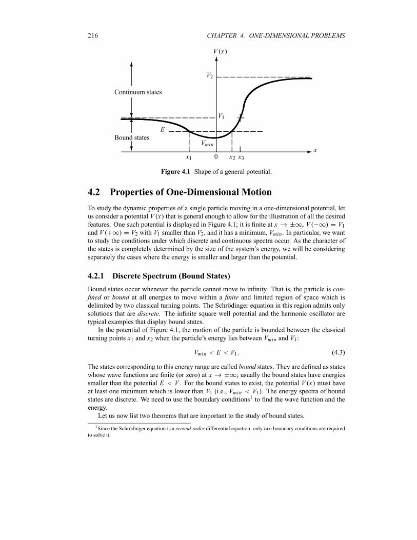
216 CHAPTER 4. ONE-DIMENSIONAL PROBLEMS
-
6
V2
V1
VminBound states
?
6
Continuum states
?
6
E
x1 x2 x30x
V x
Figure 4.1 Shape of a general potential.
4.2 Properties of One-Dimensional Motion
To study the dynamic properties of a single particle moving in a one-dimensional potential, let
us consider a potential V x that is general enough to allow for the illustration of all the desiredfeatures. One such potential is displayed in Figure 4.1; it is finite at x , V V1and V V2 with V1 smaller than V2, and it has a minimum, Vmin . In particular, we wantto study the conditions under which discrete and continuous spectra occur. As the character of
the states is completely determined by the size of the system’s energy, we will be considering
separately the cases where the energy is smaller and larger than the potential.
4.2.1 Discrete Spectrum (Bound States)
Bound states occur whenever the particle cannot move to infinity. That is, the particle is con-fined or bound at all energies to move within a finite and limited region of space which isdelimited by two classical turning points. The Schrödinger equation in this region admits only
solutions that are discrete. The infinite square well potential and the harmonic oscillator aretypical examples that display bound states.
In the potential of Figure 4.1, the motion of the particle is bounded between the classical
turning points x1 and x2 when the particle’s energy lies between Vmin and V1:
Vmin E V1 (4.3)
The states corresponding to this energy range are called bound states. They are defined as stateswhose wave functions are finite (or zero) at x ; usually the bound states have energies
smaller than the potential E V . For the bound states to exist, the potential V x must have
at least one minimum which is lower than V1 (i.e., Vmin V1). The energy spectra of boundstates are discrete. We need to use the boundary conditions1 to find the wave function and the
energy.
Let us now list two theorems that are important to the study of bound states.
1Since the Schrödinger equation is a second-order differential equation, only two boundary conditions are requiredto solve it.
4.2. PROPERTIES OF ONE-DIMENSIONAL MOTION 217
Theorem 4.1 In a one-dimensional problem the energy levels of a bound state system are dis-crete and not degenerate.
Theorem 4.2 The wave function n x of a one-dimensional bound state system has n nodes(i.e., n x vanishes n times) if n 0 corresponds to the ground state and n 1 nodes ifn 1 corresponds to the ground state.
4.2.2 Continuous Spectrum (Unbound States)
Unbound states occur in those cases where the motion of the system is not confined; a typical
example is the free particle. For the potential displayed in Figure 4.1 there are two energyranges where the particle’s motion is infinite: V1 E V2 and E V2.
Case V1 E V2
In this case the particle’s motion is infinite only towards x ; that is, the particle
can move between x x3 and x , x3 being a classical turning point. Theenergy spectrum is continuous and none of the energy eigenvalues is degenerate. The
nondegeneracy can be shown to result as follows. Since the Schrödinger equation (4.1)
is a second-order differential equation, it has, for this case, two linearly independent
solutions, but only one is physically acceptable. The solution is oscillatory for x x3and rapidly decaying for x x3 so that it is finite (zero) at x , since divergent
solutions are unphysical.
Case E V2
The energy spectrum is continuous and the particle’s motion is infinite in both directions
of x (i.e., towards x ). All the energy levels of this spectrum are doubly degen-
erate. To see this, note that the general solution to (4.1) is a linear combination of two
independent oscillatory solutions, one moving to the left and the other to the right. In the
previous nondegenerate case only one solution is retained, since the other one diverges
as x and it has to be rejected.
In contrast to bound states, unbound states cannot be normalized and we cannot use boundary
conditions.
4.2.3 Mixed Spectrum
Potentials that confine the particle for only some energies give rise to mixed spectra; the motion
of the particle for such potentials is confined for some energy values only. For instance, for
the potential displayed in Figure 4.1, if the energy of the particle is between Vmin E V1,the motion of the particle is confined (bound) and its spectrum is discrete, but if E V2, theparticle’s motion is unbound and its spectrum is continuous (if V1 E V2, the motion isunbound only along the x direction). Other typical examples where mixed spectra are
encountered are the finite square well potential and the Coulomb or molecular potential.
218 CHAPTER 4. ONE-DIMENSIONAL PROBLEMS
4.2.4 Symmetric Potentials and Parity
Most of the potentials that are encountered at the microscopic level are symmetric (or even)
with respect to space inversion, V x V x . This symmetry introduces considerable sim-plifications in the calculations.
When V x is even, the corresponding Hamiltonian, H x h2 2m d2 dx2 V x , isalso even. We saw in Chapter 2 that even operators commute with the parity operator; hence
they can have a common eigenbasis.
Let us consider the following two cases pertaining to degenerate and nondegenerate spectra
of this Hamiltonian:
Nondegenerate spectrum
First we consider the particular case where the eigenvalues of the Hamiltonian corre-
sponding to this symmetric potential are not degenerate. According to Theorem 4.1,
this Hamiltonian describes bound states. We saw in Chapter 2 that a nondegenerate,
even operator has the same eigenstates as the parity operator. Since the eigenstates of
the parity operator have definite parity, the bound eigenstates of a particle moving in aone-dimensional symmetric potential have definite parity; they are either even or odd:
V x V x x x (4.4)
Degenerate spectrum
If the spectrum of the Hamiltonian corresponding to a symmetric potential is degenerate,
the eigenstates are expressed only in terms of even and odd states. That is, the eigenstates
do not have definite parity.
Summary: The various properties of the one-dimensional motion discussed in this section can
be summarized as follows:
The energy spectrum of a bound state system is discrete and nondegenerate.
The bound state wave function n x has: (a) n nodes if n 0 corresponds to the ground
state and (b) n 1 nodes if n 1 corresponds to the ground state.
The bound state eigenfunctions in an even potential have definite parity.
The eigenfunctions of a degenerate spectrum in an even potential do not have definite
parity.
4.3 The Free Particle: Continuous States
This is the simplest one-dimensional problem; it corresponds to V x 0 for any value of x .In this case the Schrödinger equation is given by
h2
2m
d2 x
dx2E x
d2
dx2k2 x 0 (4.5)
where k2 2mE h2, k being the wave number. The most general solution to (4.5) is a combi-nation of two linearly independent plane waves x eikx and x e ikx :
k x A eikx A e ikx (4.6)
4.3. THE FREE PARTICLE: CONTINUOUS STATES 219
where A and A are two arbitrary constants. The complete wave function is thus given by the
stationary state
k x t A ei kx t A e i kx t A ei kx hk2t 2m A e i kx hk2t 2m (4.7)
since E h hk2 2m. The first term, x t A ei kx t , represents a wave
traveling to the right, while the second term, x t A e i kx t , represents a wave
traveling to the left. The intensities of these waves are given by A 2 and A 2, respectively.
We should note that the waves x t and x t are associated, respectively, with a freeparticle traveling to the right and to the left with well-defined momenta and energy: p hk,E h2k2 2m. We will comment on the physical implications of this in a moment. Since thereare no boundary conditions, there are no restrictions on k or on E ; all values yield solutions tothe equation.
The free particle problem is simple to solve mathematically, yet it presents a number of
physical subtleties. Let us discuss briefly three of these subtleties. First, the probability densi-
ties corresponding to either solutions
P x t x t 2 A 2 (4.8)
are constant, for they depend neither on x nor on t . This is due to the complete loss of informa-tion about the position and time for a state with definite values of momentum, p hk, andenergy, E h2k2 2m. This is a consequence of Heisenberg’s uncertainty principle: whenthe momentum and energy of a particle are known exactly, p 0 and E 0, there must be
total uncertainty about its position and time: x and t . The second subtlety
pertains to an apparent discrepancy between the speed of the wave and the speed of the particle
it is supposed to represent. The speed of the plane waves x t is given by
a ek
E
hk
h2k2 2m
hk
hk
2m(4.9)
On the other hand, the classical speed of the particle2 is given by
classicalp
m
hk
m2 a e (4.10)
This means that the particle travels twice as fast as the wave that represents it! Third, the wave
function is not normalizable:
x t x t dx A 2 dx (4.11)
The solutions x t are thus unphysical; physical wave functions must be square integrable.The problem can be traced to this: a free particle cannot have sharply defined momenta and
energy.
In view of the three subtleties outlined above, the solutions of the Schrödinger equation
(4.5) that are physically acceptable cannot be plane waves. Instead, we can construct physical
2The classical speed can be associated with the flux (or current density) which, as shown in Chapter 3, is J
ih 12m x x
hkm
pm , where use was made of A 1.
220 CHAPTER 4. ONE-DIMENSIONAL PROBLEMS
solutions by means of a linear superposition of plane waves. The answer is provided by wavepackets, which we have seen in Chapter 1:
x t1
2k ei kx t dk (4.12)
where k , the amplitude of the wave packet, is given by the Fourier transform of x 0 as
k1
2x 0 e ikxdx (4.13)
The wave packet solution cures and avoids all the subtleties raised above. First, the momentum,
the position and the energy of the particle are no longer known exactly; only probabilistic
outcomes are possible. Second, as shown in Chapter 1, the wave packet (4.12) and the particle
travel with the same speed g p m, called the group speed or the speed of the whole packet.Third, the wave packet (4.12) is normalizable.
To summarize, a free particle cannot be represented by a single (monochromatic) plane
wave; it has to be represented by a wave packet. The physical solutions of the Schrödinger
equation are thus given by wave packets, not by stationary solutions.
4.4 The Potential Step
Another simple problem consists of a particle that is free everywhere, but beyond a particular
point, say x 0, the potential increases sharply (i.e., it becomes repulsive or attractive). A
potential of this type is called a potential step (see Figure 4.2):
V x0 x 0
V0 x 0(4.14)
In this problem we try to analyze the dynamics of a flux of particles (all having the same mass
m and moving with the same velocity) moving from left to the right. We are going to considertwo cases, depending on whether the energy of the particles is larger or smaller than V0.
(a) Case E V0The particles are free for x 0 and feel a repulsive potential V0 that starts at x 0 and stays
flat (constant) for x 0. Let us analyze the dynamics of this flux of particles classically and
then quantum mechanically.
Classically, the particles approach the potential step or barrier from the left with a constant
momentum 2mE . As the particles enter the region x 0, where the potential now is V V0,they slow down to a momentum 2m E V0 ; they will then conserve this momentum as theytravel to the right. Since the particles have sufficient energy to penetrate into the region x 0,
there will be total transmission: all the particles will emerge to the right with a smaller kineticenergy E V0. This is then a simple scattering problem in one dimension.Quantum mechanically, the dynamics of the particle is regulated by the Schrödinger equa-
tion, which is given in these two regions by
d2
dx2k21 1 x 0 x 0 (4.15)
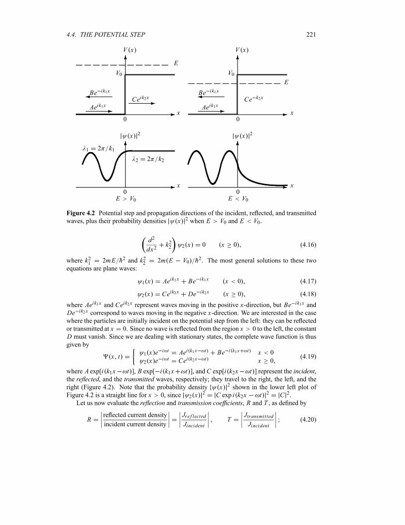
4.4. THE POTENTIAL STEP 221
-
6
0x
x 2
-
6
0x
x 2
-
6
0x
V x
V0
E
Aeik1x-
Be ik1x¾Ceik2x-
-
6
0x
V x
V0
Aeik1x-
Be ik1x¾Ce k2x
E
1 2 k1
2 2 k2
E V0 E V0
Figure 4.2 Potential step and propagation directions of the incident, reflected, and transmitted
waves, plus their probability densities x 2 when E V0 and E V0.
d2
dx2k22 2 x 0 x 0 (4.16)
where k21 2mE h2 and k22 2m E V0 h2. The most general solutions to these twoequations are plane waves:
1 x Aeik1x Be ik1x x 0 (4.17)
2 x Ceik2x De ik2x x 0 (4.18)
where Aeik1x and Ceik2x represent waves moving in the positive x-direction, but Be ik1x and
De ik2x correspond to waves moving in the negative x-direction. We are interested in the casewhere the particles are initially incident on the potential step from the left: they can be reflected
or transmitted at x 0. Since no wave is reflected from the region x 0 to the left, the constant
D must vanish. Since we are dealing with stationary states, the complete wave function is thusgiven by
x t 1 x e i t Aei k1x t Be i k1x t x 0
2 x e i t Cei k2x t x 0(4.19)
where A exp[i k1x t ], B exp[ i k1x t ], and C exp[i k2x t ] represent the incident,the reflected, and the transmitted waves, respectively; they travel to the right, the left, and theright (Figure 4.2). Note that the probability density x 2 shown in the lower left plot of
Figure 4.2 is a straight line for x 0, since 2 x2 C exp i k2x t 2 C 2.
Let us now evaluate the reflection and transmission coefficients, R and T , as defined by
Rreflected current density
incident current density
Jre f lectedJincident
TJtransmittedJincident
(4.20)
222 CHAPTER 4. ONE-DIMENSIONAL PROBLEMS
R represents the ratio of the reflected to the incident beams and T the ratio of the transmitted tothe incident beams. To calculate R and T , we need to find Jincident , Jre f lected , and Jtransmitted .Since the incident wave is i x Aeik1x , the incident current density (or incident flux) isgiven by
Jincidentih
2mi x
d i x
dx i xd i x
dx
hk1m
A 2 (4.21)
Similarly, since the reflected and transmitted waves are r x Be ik1x and t x Ceik2x ,we can verify that the reflected and transmitted fluxes are
Jre f lectedhk1m
B 2 Jtransmittedhk2mC 2 (4.22)
A combination of (4.20) to (4.22) yields
RB 2
A 2T
k2k1
C 2
A 2(4.23)
Thus, the calculation of R and T is reduced to determining the constants B and C . For this,we need to use the boundary conditions of the wave function at x 0. Since both the wave
function and its first derivative are continuous at x 0,
1 0 2 0d 1 0
dx
d 2 0
dx(4.24)
equations (4.17) and (4.18) yield
A B C k1 A B k2C (4.25)
hence
Bk1 k2k1 k2
A C2k1
k1 k2A (4.26)
As for the constant A, it can be determined from the normalization condition of the wave func-tion, but we don’t need it here, since R and T are expressed in terms of ratios. A combinationof (4.23) with (4.26) leads to
Rk1 k2 2
k1 k2 21 K 2
1 K 2T
4k1k2k1 k2 2
4K
1 K 2(4.27)
where K k2 k1 1 V0 E . The sum of R and T is equal to 1, as it should be.In contrast to classical mechanics, which states that none of the particles get reflected,
equation (4.27) shows that the quantum mechanical reflection coefficient R is not zero: thereare particles that get reflected in spite of their energies being higher than the step V0. This effectmust be attributed to the wavelike behavior of the particles.From (4.27) we see that as E gets smaller and smaller, T also gets smaller and smaller so
that when E V0 the transmission coefficient T becomes zero and R 1. On the other hand,
when E V0, we have K 1 V0 E 1; hence R 0 and T 1. This is expected
since, when the incident particles have very high energies, the potential step is so weak that it
produces no noticeable effect on their motion.
Remark: physical meaning of the boundary conditions
Throughout this chapter, we will encounter at numerous times the use of the boundary condi-
tions of the wave function and its first derivative as in Eq (4.24). What is the underlying physics
behind these continuity conditions? We can make two observations:
4.4. THE POTENTIAL STEP 223
Since the probability density x 2 of finding the particle in any small region varies
continuously from one point to another, the wave function x must, therefore, be a
continuous function of x ; thus, as shown in (4.24), we must have 1 0 2 0 .
Since the linear momentum of the particle, P x ihd x dx , must be a continu-ous function of x as the particle moves from left to right, the first derivative of the wavefunction, d x dx , must also be a continuous function of x , notably at x 0. Hence,
as shown in (4.24), we must have d 1 0 dx d 2 0 dx .
(b) Case E V0Classically, the particles arriving at the potential step from the left (with momenta p 2mE)will come to a stop at x 0 and then all will bounce back to the left with the magnitudes of
their momenta unchanged. None of the particles will make it into the right side of the barrier
x 0; there is total reflection of the particles. So the motion of the particles is reversed by the
potential barrier.
Quantummechanically, the picture will be somewhat different. In this case, the Schrödinger
equation and the wave function in the region x 0 are given by (4.15) and (4.17), respectively.
But for x 0 the Schrödinger equation is given by
d2
dx2k22
2 x 0 x 0 (4.28)
where k22
2m V0 E h2. This equation’s solution is
2 x Ce k2x Dek2x x 0 (4.29)
Since the wave function must be finite everywhere, and since the term ek2x diverges whenx , the constant D has to be zero. Thus, the complete wave function is
x tAei k1x t Be i k1x t x 0
Ce k2xe i t x 0(4.30)
Let us now evaluate, as we did in the previous case, the reflected and the transmitted
coefficients. First we should note that the transmitted coefficient, which corresponds to the
transmitted wave function t x Ce k2x , is zero since t x is a purely real function( t x t x ) and therefore
Jtransmittedh
2imt x
d t x
dxt x
d t x
dx0 (4.31)
Hence, the reflected coefficient R must be equal to 1. We can obtain this result by applying thecontinuity conditions at x 0 for (4.17) and (4.29):
Bk1 ik2k1 ik2
A C2k1
k1 ik2A (4.32)
Thus, the reflected coefficient is given by
RB 2
A 2k21 k 22k21 k 22
1 (4.33)

224 CHAPTER 4. ONE-DIMENSIONAL PROBLEMS
We therefore have total reflection, as in the classical case.
There is, however, a difference with the classical case: while none of the particles can be
found classically in the region x 0, quantum mechanically there is a nonzero probability thatthe wave function penetrates this classically forbidden region. To see this, note that the relativeprobability density
P x t x2 C 2e 2k2x
4k21 A2
k21 k 22e 2k2x (4.34)
is appreciable near x 0 and falls exponentially to small values as x becomes large; thebehavior of the probability density is shown in Figure 4.2.
4.5 The Potential Barrier and Well
Consider a beam of particles of mass m that are sent from the left on a potential barrier
V x0 x 0
V0 0 x a0 x a
(4.35)
This potential, which is repulsive, supports no bound states (Figure 4.3). We are dealing here,
as in the case of the potential step, with a one-dimensional scattering problem.Again, let us consider the following two cases which correspond to the particle energies
being respectively larger and smaller than the potential barrier.
4.5.1 The Case E V0
Classically, the particles that approach the barrier from the left at constant momentum, p12mE , as they enter the region 0 x a will slow down to a momentum p2 2m E V0 .
They will maintain the momentum p2 until they reach the point x a. Then, as soon as theypass beyond the point x a, they will accelerate to a momentum p3 2mE and maintainthis value in the entire region x a. Since the particles have enough energy to cross the bar-rier, none of the particles will be reflected back; all the particles will emerge on the right side
of x a: total transmission.It is easy to infer the quantum mechanical study from the treatment of the potential step
presented in the previous section. We need only to mention that the wave function will display
an oscillatory pattern in all three regions; its amplitude reduces every time the particle enters a
new region (see Figure 4.3):
x1 x Aeik1x Be ik1x x 0
2 x Ceik2x De ik2x 0 x a
3 x Eeik1x x a(4.36)
where k1 2mE h2 and k2 2m E V0 h2. The constants B, C , D, and E can beobtained in terms of A from the boundary conditions: x and d dx must be continuous atx 0 and x a, respectively:
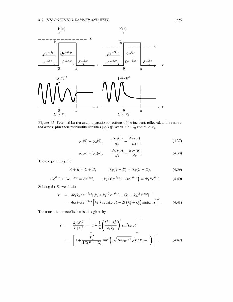
4.5. THE POTENTIAL BARRIER AND WELL 225
-
6
0 ax
x 2
E V0
-
6
0 ax
x 2
E V0
-
6
0 ax
V x
V0
Aeik1x-
Be ik1x¾
Ceik2x-
De ik2x¾
Eeik1x-
E
-
6
0 ax
V x
V0
Aeik1x-
Be ik1x¾
De k2x
Cek2x
Eeik1x-
E
Figure 4.3 Potential barrier and propagation directions of the incident, reflected, and transmit-
ted waves, plus their probability densities x 2 when E V0 and E V0.
1 0 2 0d 1 0
dx
d 2 0
dx(4.37)
2 a 3 ad 2 a
dx
d 3 a
dx(4.38)
These equations yield
A B C D ik1 A B ik2 C D (4.39)
Ceik2a De ik2a Eeik1a ik2 Ceik2a De ik2a ik1Eeik1a (4.40)
Solving for E , we obtain
E 4k1k2Aeik1a[ k1 k2
2 e ik2a k1 k22 eik2a] 1
4k1k2Aeik1a 4k1k2 cos k2a 2i k21 k22 sin k2a
1(4.41)
The transmission coefficient is thus given by
Tk1 E 2
k1 A 21
1
4
k21 k22k1k2
2
sin2 k2a
1
1V 20
4E E V0sin2 a 2mV0 h2 E V0 1
1
(4.42)
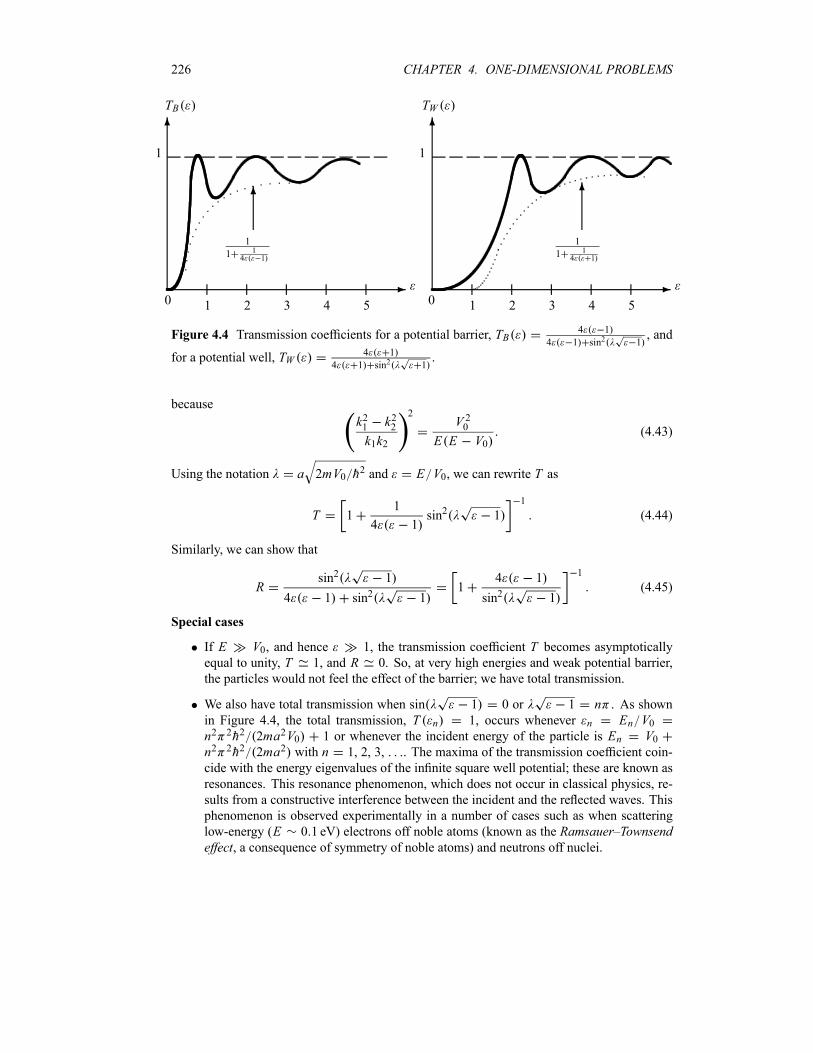
226 CHAPTER 4. ONE-DIMENSIONAL PROBLEMS
-
6
1
0
TB
1 2 3 4 5
1
1 14 1
6
-
6
1
0
TW
1 2 3 4 5
1
1 14 1
6
Figure 4.4 Transmission coefficients for a potential barrier, TB4 1
4 1 sin2 1, and
for a potential well, TW4 1
4 1 sin2 1.
because
k21 k22k1k2
2V 20
E E V0(4.43)
Using the notation a 2mV0 h2 and E V0, we can rewrite T as
T 11
4 1sin2 1
1
(4.44)
Similarly, we can show that
Rsin2 1
4 1 sin2 11
4 1
sin2 1
1
(4.45)
Special cases
If E V0, and hence 1, the transmission coefficient T becomes asymptoticallyequal to unity, T 1, and R 0. So, at very high energies and weak potential barrier,
the particles would not feel the effect of the barrier; we have total transmission.
We also have total transmission when sin 1 0 or 1 n . As shown
in Figure 4.4, the total transmission, T n 1, occurs whenever n En V0n2 2h2 2ma2V0 1 or whenever the incident energy of the particle is En V0n2 2h2 2ma2 with n 1, 2, 3, . The maxima of the transmission coefficient coin-
cide with the energy eigenvalues of the infinite square well potential; these are known as
resonances. This resonance phenomenon, which does not occur in classical physics, re-
sults from a constructive interference between the incident and the reflected waves. This
phenomenon is observed experimentally in a number of cases such as when scattering
low-energy (E 0 1 eV) electrons off noble atoms (known as the Ramsauer–Townsendeffect, a consequence of symmetry of noble atoms) and neutrons off nuclei.
4.5. THE POTENTIAL BARRIER AND WELL 227
In the limit 1 we have sin 1 1, hence (4.44) and (4.45) become
T 1ma2V0
2h2
1
R 12h2
ma2V0
1
(4.46)
The potential well (V0 0)
The transmission coefficient (4.44) was derived for the case where V0 0, i.e., for a barrierpotential. Following the same procedure that led to (4.44), we can show that the transmissioncoefficient for a finite potential well, V0 0, is given by
TW 11
4 1sin2 1
1
(4.47)
where E V0 and a 2m V0 h2. Notice that there is total transmission whenever
sin 1 0 or 1 n . As shown in Figure 4.4, the total transmission, TW n
1, occurs whenever n En V0 n2 2h2 2ma2V0 1 or whenever the incident energy
of the particle is En n2 2h2 2ma2 V0 with n 1 2 3 . We will study in more
detail the symmetric potential well in Section 4.7.
4.5.2 The Case E V0: Tunneling
Classically, we would expect total reflection: every particle that arrives at the barrier (x 0)
will be reflected back; no particle can penetrate the barrier, where it would have a negative
kinetic energy.
We are now going to show that the quantummechanical predictions differ sharply from their
classical counterparts, for the wave function is not zero beyond the barrier. The solutions of the
Schrödinger equation in the three regions yield expressions that are similar to (4.36) except that
2 x Ceik2x De ik2x should be replaced with 2 x Cek2x De k2x :
x1 x Aeik1x Be ik1x x 0
2 x Cek2x De k2x 0 x a
3 x Eeik1x x a(4.48)
where k21 2mE h2 and k22 2m V0 E h2. The behavior of the probability densitycorresponding to this wave function is expected, as displayed in Figure 4.3, to be oscillatory in
the regions x 0 and x a, and exponentially decaying for 0 x a.To find the reflection and transmission coefficients,
RB 2
A 2T
E 2
A 2(4.49)
we need only to calculate B and E in terms of A. The continuity conditions of the wave functionand its derivative at x 0 and x a yield
A B C D (4.50)
ik1 A B k2 C D (4.51)
Cek2a De k2a Eeik1a (4.52)
k2 Cek2a De k2a ik1Eeik1a (4.53)
228 CHAPTER 4. ONE-DIMENSIONAL PROBLEMS
The last two equations lead to the following expressions for C and D:
CE
21 i
k1k2
e ik1 k2 a DE
21 i
k1k2
e ik1 k2 a (4.54)
Inserting these two expressions into the two equations (4.50) and (4.51) and dividing by A, wecan show that these two equations reduce, respectively, to
1B
A
E
Aeik1a cosh k2a i
k1k2sinh k2a (4.55)
1B
A
E
Aeik1a cosh k2a i
k2k1sinh k2a (4.56)
Solving these two equations for B A and E A, we obtain
B
Aik21 k22k1k2
sinh k2a 2 cosh k2a ik22 k21k1k2
sinh k2a
1
(4.57)
E
A2e ik1a 2 cosh k2a i
k22 k21k1k2
sinh k2a
1
(4.58)
Thus, the coefficients R and T become
Rk21 k22k1k2
2
sinh2 k2a 4 cosh2 k2ak22 k21k1k2
2
sinh2 k2a
1
(4.59)
TE 2
A 24 4 cosh2 k2a
k22 k21k1k2
2
sinh2 k2a
1
(4.60)
We can rewrite R in terms of T as
R1
4T
k21 k22k1k2
2
sinh2 k2a (4.61)
Since cosh2 k2a 1 sinh2 k2a we can reduce (4.60) to
T 11
4
k21 k22k1k2
2
sinh2 k2a
1
(4.62)
Note that T is finite. This means that the probability for the transmission of the particles into theregion x a is not zero (in classical physics, however, the particle can in no way make it intothe x 0 region). This is a purely quantum mechanical effect which is due to the wave aspectof microscopic objects; it is known as the tunneling effect: quantum mechanical objects cantunnel through classically impenetrable barriers. This barrier penetration effect has importantapplications in various branches of modern physics ranging from particle and nuclear physics
4.5. THE POTENTIAL BARRIER AND WELL 229
to semiconductor devices. For instance, radioactive decays and charge transport in electronic
devices are typical examples of the tunneling effect.
Now since
k21 k22k1k2
2V0
E V0 E
2 V 20E V0 E
(4.63)
we can rewrite (4.61) and (4.62) as follows:
R1
4
V 20 T
E V0 Esinh2
a
h2m V0 E (4.64)
T 11
4
V 20E V0 E
sinh2a
h2m V0 E
1
(4.65)
or
RT
4 1sinh2 1 (4.66)
T 11
4 1sinh2 1
1
(4.67)
where a 2mV0 h2 and E V0.
Special cases
If E V0, hence 1 or 1 1, we may approximate sinh 112exp 1 . We can thus show that the transmission coefficient (4.67) becomes
asymptotically equal to
T1
4 1
1
2e 1
2 1
16 1 e 2 1
16E
V01
E
V0e 2a h 2m V0 E (4.68)
This shows that the transmission coefficient is not zero, as it would be classically, but has
a finite value. So, quantum mechanically, there is a finite tunneling beyond the barrier,
x a.
When E V0, hence 1, we can verify that (4.66) and (4.67) lead to the relations
(4.46).
Taking the classical limit h 0, the coefficients (4.66) and (4.67) reduce to the classical
result: R 1 and T 0.
4.5.3 The Tunneling Effect
In general, the tunneling effect consists of the propagation of a particle through a region where
the particle’s energy is smaller than the potential energy E V x . Classically this region,defined by x1 x x2 (Figure 4.5a), is forbidden to the particle where its kinetic energy
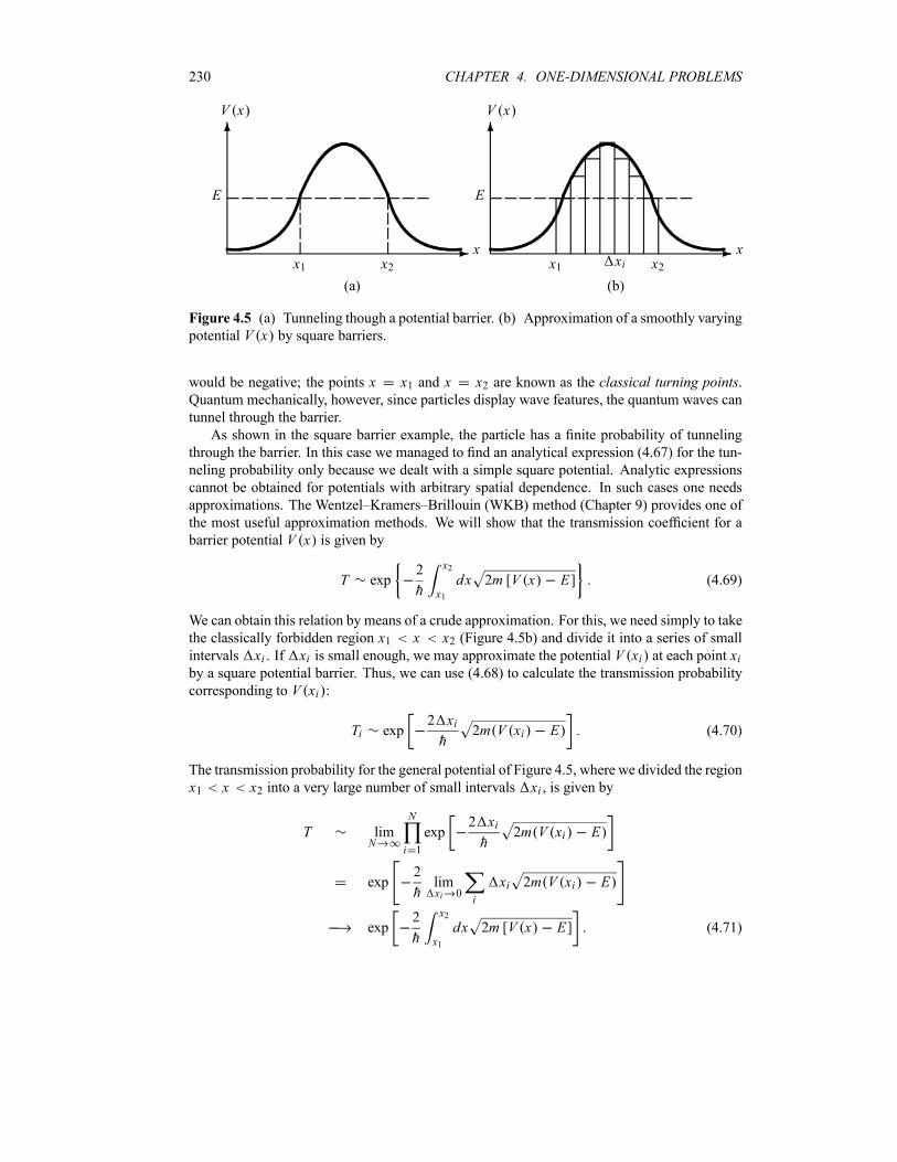
230 CHAPTER 4. ONE-DIMENSIONAL PROBLEMS
-
6
x1 x2
E
x
V x
(a)
-
6
x
V x
E
x1 x2xi
(b)
Figure 4.5 (a) Tunneling though a potential barrier. (b) Approximation of a smoothly varying
potential V x by square barriers.
would be negative; the points x x1 and x x2 are known as the classical turning points.Quantum mechanically, however, since particles display wave features, the quantum waves can
tunnel through the barrier.
As shown in the square barrier example, the particle has a finite probability of tunneling
through the barrier. In this case we managed to find an analytical expression (4.67) for the tun-
neling probability only because we dealt with a simple square potential. Analytic expressions
cannot be obtained for potentials with arbitrary spatial dependence. In such cases one needs
approximations. The Wentzel–Kramers–Brillouin (WKB) method (Chapter 9) provides one of
the most useful approximation methods. We will show that the transmission coefficient for a
barrier potential V x is given by
T exp2
h
x2
x1
dx 2m [V x E] (4.69)
We can obtain this relation by means of a crude approximation. For this, we need simply to take
the classically forbidden region x1 x x2 (Figure 4.5b) and divide it into a series of smallintervals xi . If xi is small enough, we may approximate the potential V xi at each point xiby a square potential barrier. Thus, we can use (4.68) to calculate the transmission probability
corresponding to V xi :
Ti exp2 xih
2m V xi E (4.70)
The transmission probability for the general potential of Figure 4.5, where we divided the region
x1 x x2 into a very large number of small intervals xi , is given by
T limN
N
i 1
exp2 xih
2m V xi E
exp2
hlimxi 0
i
xi 2m V xi E
exp2
h
x2
x1
dx 2m [V x E] (4.71)
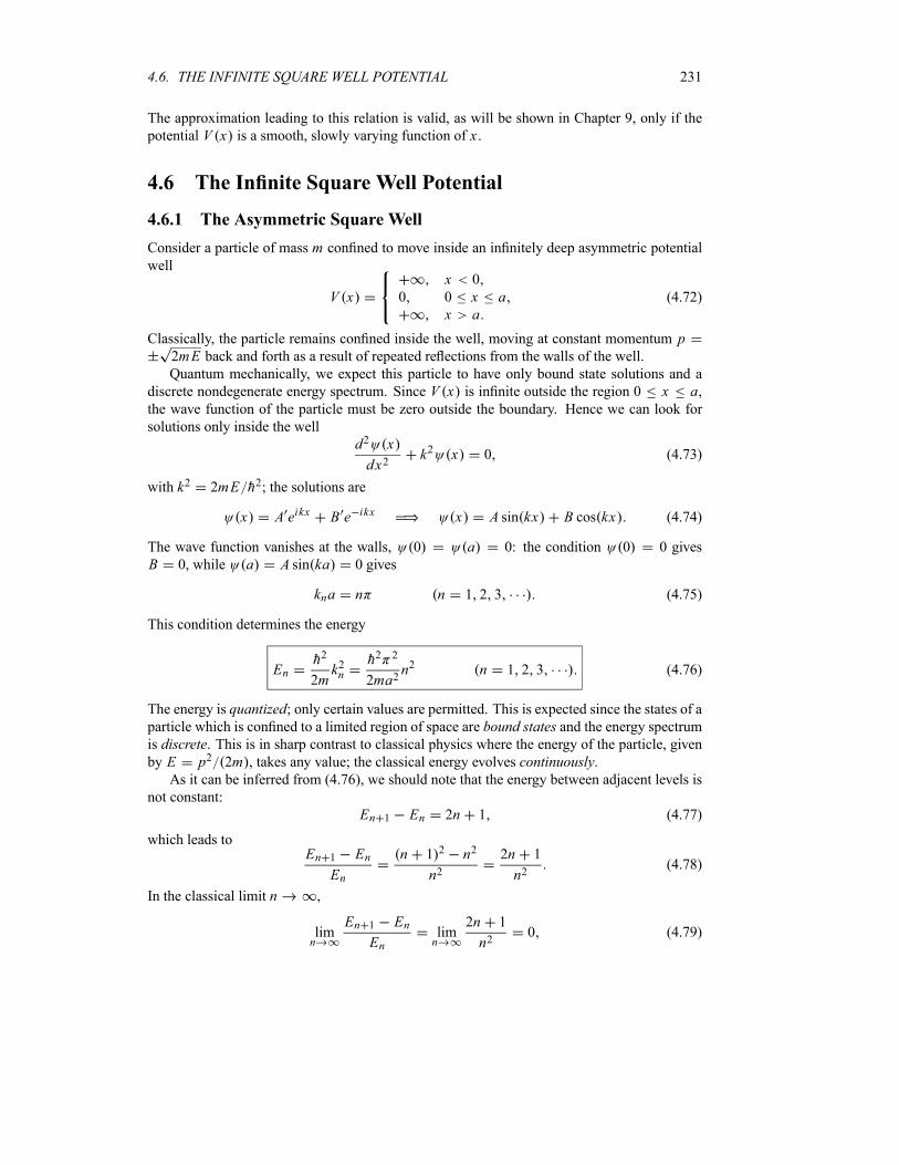
4.6. THE INFINITE SQUARE WELL POTENTIAL 231
The approximation leading to this relation is valid, as will be shown in Chapter 9, only if the
potential V x is a smooth, slowly varying function of x .
4.6 The Infinite Square Well Potential
4.6.1 The Asymmetric Square Well
Consider a particle of mass m confined to move inside an infinitely deep asymmetric potentialwell
V xx 0
0 0 x ax a
(4.72)
Classically, the particle remains confined inside the well, moving at constant momentum p2mE back and forth as a result of repeated reflections from the walls of the well.Quantum mechanically, we expect this particle to have only bound state solutions and a
discrete nondegenerate energy spectrum. Since V x is infinite outside the region 0 x a,the wave function of the particle must be zero outside the boundary. Hence we can look for
solutions only inside the well
d2 x
dx2k2 x 0 (4.73)
with k2 2mE h2; the solutions are
x A eikx B e ikx x A sin kx B cos kx (4.74)
The wave function vanishes at the walls, 0 a 0: the condition 0 0 gives
B 0, while a A sin ka 0 gives
kna n n 1 2 3 (4.75)
This condition determines the energy
Enh2
2mk2n
h2 2
2ma2n2 n 1 2 3 (4.76)
The energy is quantized; only certain values are permitted. This is expected since the states of aparticle which is confined to a limited region of space are bound states and the energy spectrumis discrete. This is in sharp contrast to classical physics where the energy of the particle, givenby E p2 2m , takes any value; the classical energy evolves continuously.As it can be inferred from (4.76), we should note that the energy between adjacent levels is
not constant:
En 1 En 2n 1 (4.77)
which leads toEn 1 En
En
n 1 2 n2
n22n 1
n2(4.78)
In the classical limit n ,
limn
En 1 EnEn
limn
2n 1
n20 (4.79)
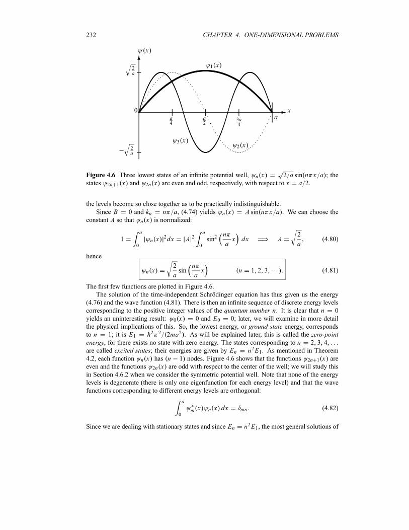
232 CHAPTER 4. ONE-DIMENSIONAL PROBLEMS
-
6
0aa
2
x
x
1 x2a
2a
2 x
a4
3a4
3 x
Figure 4.6 Three lowest states of an infinite potential well, n x 2 a sin n x a ; thestates 2n 1 x and 2n x are even and odd, respectively, with respect to x a 2.
the levels become so close together as to be practically indistinguishable.
Since B 0 and kn n a, (4.74) yields n x A sin n x a . We can choose theconstant A so that n x is normalized:
1a
0n x
2dx A 2a
0
sin2n
ax dx A
2
a(4.80)
hence
n x2
asin
n
ax n 1 2 3 (4.81)
The first few functions are plotted in Figure 4.6.
The solution of the time-independent Schrödinger equation has thus given us the energy
(4.76) and the wave function (4.81). There is then an infinite sequence of discrete energy levels
corresponding to the positive integer values of the quantum number n. It is clear that n 0
yields an uninteresting result: 0 x 0 and E0 0; later, we will examine in more detail
the physical implications of this. So, the lowest energy, or ground state energy, correspondsto n 1; it is E1 h2 2 2ma2 . As will be explained later, this is called the zero-pointenergy, for there exists no state with zero energy. The states corresponding to n 2 3 4
are called excited states; their energies are given by En n2E1. As mentioned in Theorem4.2, each function n x has n 1 nodes. Figure 4.6 shows that the functions 2n 1 x are
even and the functions 2n x are odd with respect to the center of the well; we will study thisin Section 4.6.2 when we consider the symmetric potential well. Note that none of the energy
levels is degenerate (there is only one eigenfunction for each energy level) and that the wave
functions corresponding to different energy levels are orthogonal:
a
0m x n x dx mn (4.82)
Since we are dealing with stationary states and since En n2E1, the most general solutions of
4.6. THE INFINITE SQUARE WELL POTENTIAL 233
the time-dependent Schrödinger equation are given by
x tn 1
n x ei En t h 2
an 1
sinn x
ae in2E1t h (4.83)
Zero-point energy
Let us examine why there is no state with zero energy for a square well potential. If the particle
has zero energy, it will be at rest inside the well, and this violates Heisenberg’s uncertainty
principle. By localizing or confining the particle to a limited region in space, it will acquire afinitemomentum leading to a minimum kinetic energy. That is, the localization of the particle’smotion to 0 x a implies a position uncertainty of order x a which, according to theuncertainty principle, leads to a minimum momentum uncertainty p h a and this in turnleads to a minimum kinetic energy of order h2 2ma2 . This is in qualitative agreement withthe exact value E1 2h2 2ma2 . In fact, as will be shown in (4.216), an accurate evaluationof p1 leads to a zero-point energy which is equal to E1.Note that, as the momentum uncertainty is inversely proportional to the width of the well,
p h a, if the width decreases (i.e., the particle’s position is confined further and further),the uncertainty on P will increase. This makes the particle move faster and faster, so the zero-point energy will also increase. Conversely, if the width of the well increases, the zero-point
energy decreases, but it will never vanish.
The zero-point energy therefore reflects the necessity of a minimum motion of a particledue to localization. The zero-point energy occurs in all bound state potentials. In the case of
binding potentials, the lowest energy state has an energy which is higher than the minimum
of the potential energy. This is in sharp contrast to classical mechanics, where the lowest
possible energy is equal to the minimum value of the potential energy, with zero kinetic energy.
In quantum mechanics, however, the lowest state does not minimize the potential alone, but
applies to the sum of the kinetic and potential energies, and this leads to a finite ground state
or zero-point energy. This concept has far-reaching physical consequences in the realm of the
microscopic world. For instance, without the zero-point motion, atoms would not be stable, for
the electrons would fall into the nuclei. Also, it is the zero-point energy which prevents helium
from freezing at very low temperatures.
The following example shows that the zero-point energy is also present in macroscopic
systems, but it is infinitesimally small. In the case of microscopic systems, however, it has a
nonnegligible size.
Example 4.1 (Zero-point energy)
To illustrate the idea that the zero-point energy gets larger by going from macroscopic to mi-
croscopic systems, calculate the zero-point energy for a particle in an infinite potential well for
the following three cases:
(a) a 100 g ball confined on a 5m long line,
(b) an oxygen atom confined to a 2 10 10m lattice, and
(c) an electron confined to a 10 10m atom.
Solution
(a) The zero-point energy of a 100 g ball that is confined to a 5m long line is
Eh2 2
2ma210 10 68 J
2 0 1 252 10 68 J 1 25 10 49 eV (4.84)
234 CHAPTER 4. ONE-DIMENSIONAL PROBLEMS
This energy is too small to be detected, much less measured, by any known experimental tech-
nique.
(b) For the zero-point energy of an oxygen atom confined to a 2 10 10m lattice, since
the oxygen atom has 16 nucleons, its mass is of the order of m 16 1 6 10 27 kg
26 10 27 kg, so we have
E10 67 J
2 26 10 27 4 10 200 5 10 22 J 3 10 4 eV (4.85)
(c) The zero-point energy of an electron m 10 30 kg that is confined to an atom (a 1
10 10m ) is
E10 67 J
2 10 30 10 205 10 18 J 30 eV (4.86)
This energy is important at the atomic scale, for the binding energy of a hydrogen electron is
about 14 eV. So the zero-point energy is negligible for macroscopic objects, but important for
microscopic systems.
4.6.2 The Symmetric Potential Well
What happens if the potential (4.72) is translated to the left by a distance of a 2 to becomesymmetric?
V xx a 2
0 a 2 x a 2x a 2
(4.87)
First, we would expect the energy spectrum (4.76) to remain unaffected by this translation,
since the Hamiltonian is invariant under spatial translations; as it contains only a kinetic part,
it commutes with the particle’s momentum, [H P] 0. The energy spectrum is discrete and
nondegenerate.
Second, earlier in this chapter we saw that for symmetric potentials, V x V x , thewave function of bound states must be either even or odd. The wave function corresponding to
the potential (4.87) can be written as follows:
n x2
asin
n
ax
a
2
2a cos
na x n 1 3 5 7
2a sin
na x n 2 4 6 8
(4.88)
That is, the wave functions corresponding to odd quantum numbers n 1 3 5 are sym-
metric, x x , and those corresponding to even numbers n 2 4 6 are antisym-
metric, x x .
4.7 The Finite Square Well Potential
Consider a particle of mass m moving in the following symmetric potential:
V xV0 x a 20 a 2 x a 2V0 x a 2
(4.89)
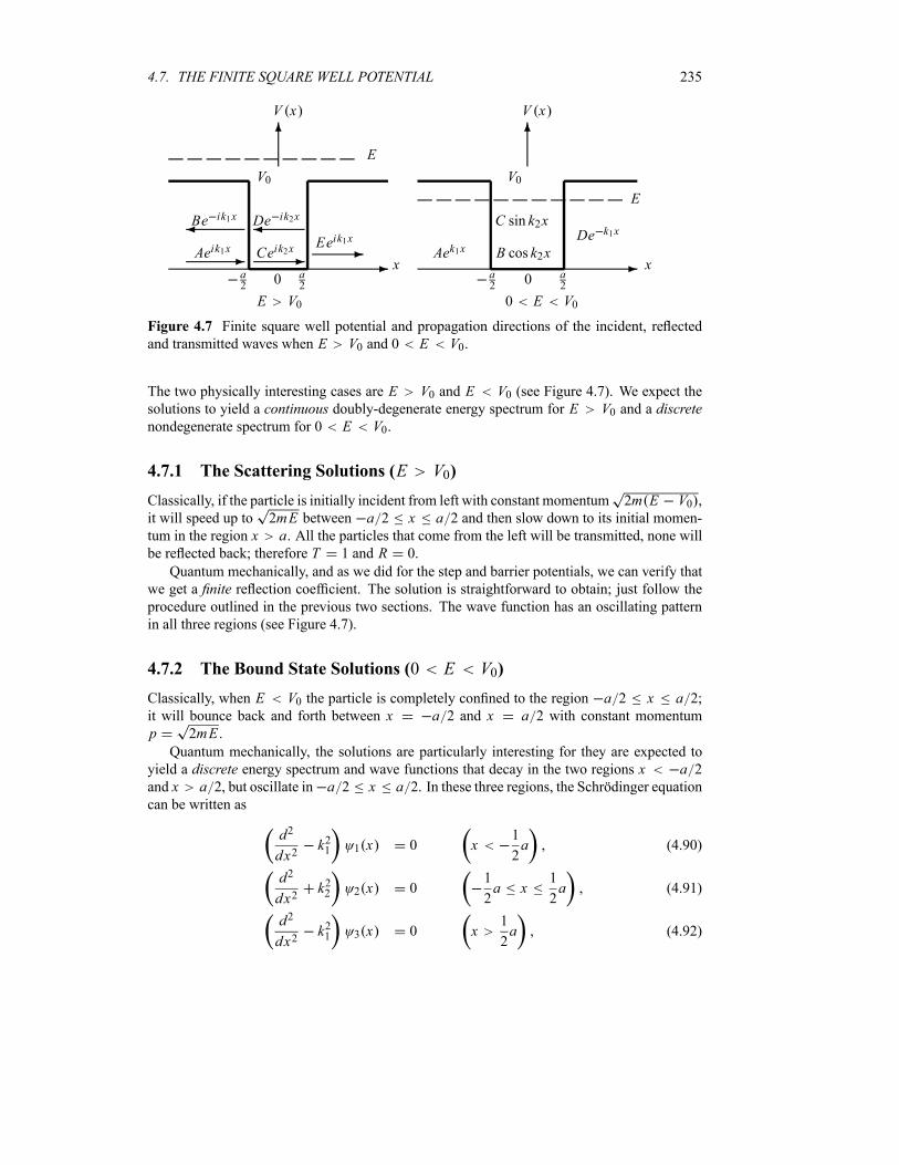
4.7. THE FINITE SQUARE WELL POTENTIAL 235
-
6
0x
V x
V0
E V0
a2
a2
Aeik1x-
Be ik1x¾
Ceik2x-
De ik2x¾Eeik1x-
E
-
6
0x
V x
V0
0 E V0
a2
a2
Aek1x B cos k2x
C sin k2xDe k1x
E
Figure 4.7 Finite square well potential and propagation directions of the incident, reflected
and transmitted waves when E V0 and 0 E V0.
The two physically interesting cases are E V0 and E V0 (see Figure 4.7). We expect thesolutions to yield a continuous doubly-degenerate energy spectrum for E V0 and a discretenondegenerate spectrum for 0 E V0.
4.7.1 The Scattering Solutions (E V0)
Classically, if the particle is initially incident from left with constant momentum 2m E V0 ,it will speed up to 2mE between a 2 x a 2 and then slow down to its initial momen-tum in the region x a. All the particles that come from the left will be transmitted, none willbe reflected back; therefore T 1 and R 0.
Quantum mechanically, and as we did for the step and barrier potentials, we can verify that
we get a finite reflection coefficient. The solution is straightforward to obtain; just follow theprocedure outlined in the previous two sections. The wave function has an oscillating pattern
in all three regions (see Figure 4.7).
4.7.2 The Bound State Solutions (0 E V0)
Classically, when E V0 the particle is completely confined to the region a 2 x a 2;it will bounce back and forth between x a 2 and x a 2 with constant momentump 2mE .Quantum mechanically, the solutions are particularly interesting for they are expected to
yield a discrete energy spectrum and wave functions that decay in the two regions x a 2and x a 2, but oscillate in a 2 x a 2. In these three regions, the Schrödinger equationcan be written as
d2
dx2k21 1 x 0 x
1
2a (4.90)
d2
dx2k22 2 x 0
1
2a x
1
2a (4.91)
d2
dx2k21 3 x 0 x
1
2a (4.92)
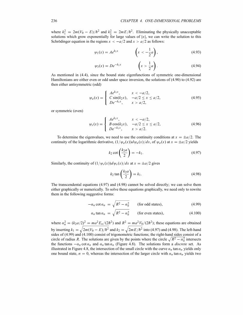
236 CHAPTER 4. ONE-DIMENSIONAL PROBLEMS
where k21 2m V0 E h2 and k22 2mE h2. Eliminating the physically unacceptablesolutions which grow exponentially for large values of x , we can write the solution to thisSchrödinger equation in the regions x a 2 and x a 2 as follows:
1 x Aek1x x1
2a (4.93)
3 x De k1x x1
2a (4.94)
As mentioned in (4.4), since the bound state eigenfunctions of symmetric one-dimensional
Hamiltonians are either even or odd under space inversion, the solutions of (4.90) to (4.92) are
then either antisymmetric (odd)
a xAek1x x a 2C sin k2x a 2 x a 2De k1x x a 2
(4.95)
or symmetric (even)
s xAek1x x a 2B cos k2x a 2 x a 2De k1x x a 2
(4.96)
To determine the eigenvalues, we need to use the continuity conditions at x a 2. Thecontinuity of the logarithmic derivative, 1 a x d a x dx , of a x at x a 2 yields
k2 cotk2a
2k1 (4.97)
Similarly, the continuity of 1 s x d s x dx at x a 2 gives
k2 tank2a
2k1 (4.98)
The transcendental equations (4.97) and (4.98) cannot be solved directly; we can solve them
either graphically or numerically. To solve these equations graphically, we need only to rewrite
them in the following suggestive forms:
n cot n R2 2n for odd states (4.99)
n tan n R2 2n for even states (4.100)
where 2n k2a 2
2 ma2En 2h2 and R2 ma2V0 2h2 ; these equations are obtained
by inserting k1 2m V0 E h2 and k2 2mE h2 into (4.97) and (4.98). The left-handsides of (4.99) and (4.100) consist of trigonometric functions; the right-hand sides consist of a
circle of radius R. The solutions are given by the points where the circle R2 2n intersects
the functions n cot n and n tan n (Figure 4.8). The solutions form a discrete set. Asillustrated in Figure 4.8, the intersection of the small circle with the curve n tan n yields only
one bound state, n 0, whereas the intersection of the larger circle with n tan n yields two

4.7. THE FINITE SQUARE WELL POTENTIAL 237
bound states, n 0 2, and its intersection with n cot n yields two other bound states,
n 1 3.
The number of solutions depends on the size of R, which in turn depends on the depth V0
and the width a of the well, since R ma2V0 2h2 . The deeper and broader the well,the larger the value of R, and hence the greater the number of bound states. Note that there isalways at least one bound state (i.e., one intersection) no matter how small V0 is. When
0 R2
or 0 V02
2 2h2
ma2(4.101)
there is only one bound state corresponding to n 0 (see Figure 4.8); this state—the ground
state—is even. Then, and when
2R or
2
2 2h2
ma2V0
2 2h2
ma2(4.102)
there are two bound states: an even state (the ground state) corresponding to n 0 and the first
odd state corresponding to n 1. Now, if
R3
2or 2 2h
2
ma2V0
3
2
2 2h2
ma2(4.103)
there exist three bound states: the ground state (even state), n 0, the first excited state (odd
state), corresponding to n 1, and the second excited state (even state), which corresponds to
n 2. In general, the well width at which n states are allowed is given by
Rn
2or V0
2
2 2h2
ma2n2 (4.104)
The spectrum, therefore, consists of a set of alternating even and odd states: the lowest state,
the ground state, is even, the next state (first excited sate) is odd, and so on.
In the limiting case V0 , the circle’s radius R also becomes infinite, and hence thefunction R2 2
n will cross n cot n and n tan n at the asymptotes n n 2, because
when V0 both tan n and cot n become infinite:
tan n n2n 1
2n 0 1 2 3 (4.105)
cot n n n n 1 2 3 (4.106)
Combining these two cases, we obtain
nn
21 2 3 (4.107)
Since 2n ma2En 2h2 we see that we recover the energy expression for the infinite well:
nn
2En
2h2
2ma2n2 (4.108)
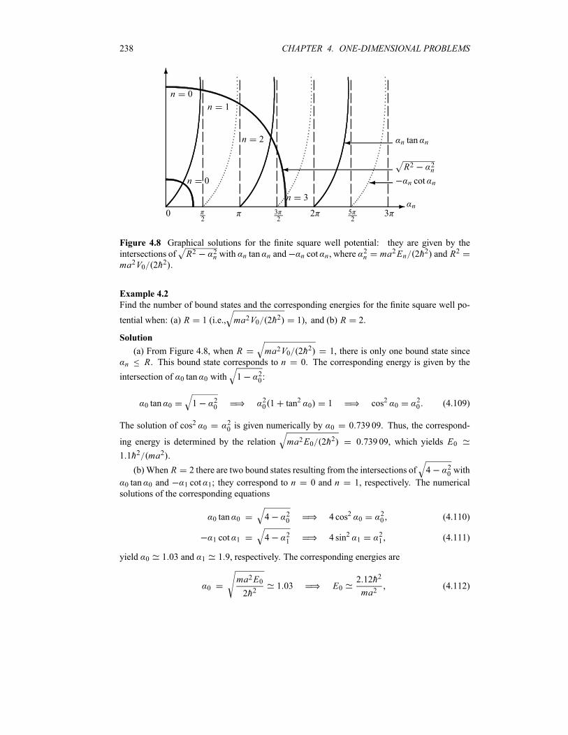
238 CHAPTER 4. ONE-DIMENSIONAL PROBLEMS
-
6
¾ n cot n
¾ R2 2n
¾ n tan n
n 0
n 0
n 1
n 2
n 3
0n
232
2 52
3
Figure 4.8 Graphical solutions for the finite square well potential: they are given by the
intersections of R2 2n with n tan n and n cot n , where
2n ma2En 2h2 and R2
ma2V0 2h2 .
Example 4.2
Find the number of bound states and the corresponding energies for the finite square well po-
tential when: (a) R 1 (i.e., ma2V0 2h2 1), and (b) R 2.
Solution
(a) From Figure 4.8, when R ma2V0 2h2 1, there is only one bound state since
n R. This bound state corresponds to n 0. The corresponding energy is given by the
intersection of 0 tan 0 with 1 20 :
0 tan 0 1 20
20 1 tan2 0 1 cos2 0
20 (4.109)
The solution of cos2 020 is given numerically by 0 0 739 09. Thus, the correspond-
ing energy is determined by the relation ma2E0 2h2 0 739 09, which yields E0
1 1h2 ma2 .
(b) When R 2 there are two bound states resulting from the intersections of 4 20 with
0 tan 0 and 1 cot 1; they correspond to n 0 and n 1, respectively. The numerical
solutions of the corresponding equations
0 tan 0 4 20 4 cos2 0
20 (4.110)
1 cot 1 4 21 4 sin2 1
21 (4.111)
yield 0 1 03 and 1 1 9, respectively. The corresponding energies are
0ma2E0
2h21 03 E0
2 12h2
ma2(4.112)
4.8. THE HARMONIC OSCILLATOR 239
1ma2E1
2h21 9 E1
7 22h2
ma2(4.113)
4.8 The Harmonic Oscillator
The harmonic oscillator is one of those few problems that are important to all branches of
physics. It provides a useful model for a variety of vibrational phenomena that are encountered,
for instance, in classical mechanics, electrodynamics, statistical mechanics, solid state, atomic,
nuclear, and particle physics. In quantum mechanics, it serves as an invaluable tool to illustrate
the basic concepts and the formalism.
The Hamiltonian of a particle of massm which oscillates with an angular frequency under
the influence of a one-dimensional harmonic potential is
HP2
2m
1
2m 2X2 (4.114)
The problem is how to find the energy eigenvalues and eigenstates of this Hamiltonian. This
problem can be studied by means of two separate methods. The first method, called the an-alytic method, consists in solving the time-independent Schrödinger equation (TISE) for theHamiltonian (4.114). The second method, called the ladder or algebraic method, does not dealwith solving the Schrödinger equation, but deals instead with operator algebra involving op-
erators known as the creation and annihilation or ladder operators; this method is in essencea matrix formulation, because it expresses the various quantities in terms of matrices. In our
presentation, we are going to adopt the second method, for it is more straightforward, more el-
egant and much simpler than solving the Schrödinger equation. Unlike the examples seen up to
now, solving the Schrödinger equation for the potential V x 12m x2 is no easy job. Before
embarking on the second method, let us highlight the main steps involved in the first method.
Brief outline of the analytic method
This approach consists in using the power series method to solve the following differential
(Schrödinger) equation:
h2
2m
d2 x
dx21
2m 2x2 x E x (4.115)
which can be reduced to
d2 x
dx22mE
h2x2
x40x 0 (4.116)
where x0 h m is a constant that has the dimensions of length; it sets the length scale
of the oscillator, as will be seen later. The solutions of differential equations like (4.116) have
been worked out by our mathematician colleagues well before the arrival of quantummechanics
(the solutions are expressed in terms of some special functions, the Hermite polynomials). The
occurrence of the term x2 x in (4.116) suggests trying a Gaussian type solution3: x
3Solutions of the type x f x exp x2 2x20are physically unacceptable, for they diverge when x .
240 CHAPTER 4. ONE-DIMENSIONAL PROBLEMS
f x exp x2 2x20 , where f x is a function of x . Inserting this trial function into (4.116),we obtain a differential equation for f x . This new differential equation can be solved byexpanding f x out in a power series (i.e., f x n 0 anx
n , where an is just a coefficient),which when inserted into the differential equation leads to a recursion relation. By demanding
the power series of f x to terminate at some finite value of n (because the wave functionx has to be finite everywhere, notably when x ), the recursion relation yields an
expression for the energy eigenvalues which are discrete or quantized:
En n1
2h n 0 1 2 3 (4.117)
After some calculations, we can show that the wave functions that are physically acceptable
and that satisfy (4.116) are given by
n x1
2nn!x0e x2 2x20Hn
x
x0(4.118)
where Hn y are nth order polynomials called Hermite polynomials:
Hn y 1 ney2 dn
dyne y2 (4.119)
From this relation it is easy to calculate the first few polynomials:
H0 y 1 H1 y 2y
H2 y 4y2 2 H3 y 8y3 12y (4.120)
H4 y 16y4 48y2 12 H5 y 32y5 160y3 120y
We will deal with the physical interpretations of the harmonic oscillator results when we study
the second method.
Algebraic method
Let us now show how to solve the harmonic oscillator eigenvalue problem using the algebraic
method. For this, we need to rewrite the Hamiltonian (4.114) in terms of the two Hermitian,
dimensionless operators p P mh and q X m h:
Hh
2p2 q2 (4.121)
and then introduce two non-Hermitian, dimensionless operators:
a1
2q i p a†
1
2q i p (4.122)
The physical meaning of the operators a and a† will be examined later. Note that
a†a1
2q i p q i p
1
2q2 p2 iq p i pq
1
2q2 p2
i
2[q p] (4.123)
where, using [X P] ih, we can verify that the commutator between q and p is
q pm
hX
1
hmP
1
hX P i (4.124)
4.8. THE HARMONIC OSCILLATOR 241
hence
a†a1
2q2 p2
1
2(4.125)
or1
2q2 p2 a†a
1
2(4.126)
Inserting (4.126) into (4.121) we obtain
H h a†a1
2h N
1
2with N a†a (4.127)
where N is known as the number operator or occupation number operator, which is clearlyHermitian.
Let us now derive the commutator [a a†]. Since [X P] ih we have [q p] 1h [X P]
i ; hence
[a a†]1
2q i p q i p i q p 1 (4.128)
or
[a a†] 1 (4.129)
4.8.1 Energy Eigenvalues
Note that H as given by (4.127) commutes with N , since H is linear in N . Thus, H and N canhave a set of joint eigenstates, to be denoted by n :
N n n n (4.130)
and
H n En n (4.131)
the states n are called energy eigenstates. Combining (4.127) and (4.131), we obtain the
energy eigenvalues at once:
En n1
2h (4.132)
We will show later that n is a positive integer; it cannot have negative values.
The physical meaning of the operators a, a†, and N can now be clarified. First, we need thefollowing two commutators that can be extracted from (4.129) and (4.127):
[a H ] h a [a† H ] h a† (4.133)
These commutation relations along with (4.131) lead to
H a n aH h a n En h a n (4.134)
H a† n a†H h a† n En h a† n (4.135)
Thus, a n and a† n are eigenstates of H with eigenvalues En h and En h ,
respectively. So the actions of a and a† on n generate new energy states that are lower and
242 CHAPTER 4. ONE-DIMENSIONAL PROBLEMS
higher by one unit of h , respectively. As a result, a and a† are respectively known as thelowering and raising operators, or the annihilation and creation operators; they are also knownas the ladder operators.
Let us now find out how the operators a and a† act on the energy eigenstates n . Since
a and a† do not commute with N , the states n are eigenstates neither to a nor to a†. Using(4.129) along with [AB C] A[B C] [A C]B, we can show that
[N a] a [N a†] a† (4.136)
hence Na a N 1 and Na† a† N 1 . Combining these relations with (4.130), we
obtain
N a n a N 1 n n 1 a n (4.137)
N a† n a† N 1 n n 1 a† n (4.138)
These relations reveal that a n and a† n are eigenstates of N with eigenvalues n 1
and n 1 , respectively. This implies that when a and a† operate on n , respectively, theydecrease and increase n by one unit. That is, while the action of a on n generates a new state
n 1 (i.e., a n n 1 ), the action of a† on n generates n 1 . Hence from (4.137)
we can write
a n cn n 1 (4.139)
where cn is a constant to be determined from the requirement that the states n be normalizedfor all values of n. On the one hand, (4.139) yields
n a† a n n a†a n cn2 n 1 n 1 cn
2 (4.140)
and, on the other hand, (4.130) gives
n a† a n n a†a n n n n n (4.141)
When combined, the last two equations yield
cn2 n (4.142)
This implies that n, which is equal to the norm of a n (see (4.141)), cannot be negative,n 0, since the norm is a positive quantity. Substituting (4.142) into (4.139) we end up with
a n n n 1 (4.143)
This equation shows that repeated applications of the operator a on n generate a sequence ofeigenvectors n 1 n 2 n 3 . Since n 0 and since a 0 0, this sequence
has to terminate at n 0; this is true if we start with an integer value of n. But if we start witha noninteger n, the sequence will not terminate; hence it leads to eigenvectors with negativevalues of n. But as shown above, since n cannot be negative, we conclude that n has to be anonnegative integer.
4.8. THE HARMONIC OSCILLATOR 243
Now, we can easily show, as we did for (4.143), that
a† n n 1 n 1 (4.144)
This implies that repeated applications of a† on n generate an infinite sequence of eigenvec-tors n 1 n 2 n 3 . Since n is a positive integer, the energy spectrum of aharmonic oscillator as specified by (4.132) is therefore discrete:
En n1
2h n 0 1 2 3 (4.145)
This expression is similar to the one obtained from the first method (see Eq. (4.117)). The
energy spectrum of the harmonic oscillator consists of energy levels that are equally spaced:
En 1 En h . This is Planck’s famous equidistant energy idea—the energy of the radiation
emitted by the oscillating charges (from the inside walls of the cavity) must come only in
bundles (quanta) that are integral multiples of h —which, as mentioned in Chapter 1, led to
the birth of quantum mechanics.
As expected for bound states of one-dimensional potentials, the energy spectrum is both
discrete and nondegenerate. Once again, as in the case of the infinite square well potential, we
encounter the zero-point energy phenomenon: the lowest energy eigenvalue of the oscillator is
not zero but is instead equal to E0 h 2. It is called the zero-point energy of the oscillator,for it corresponds to n 0. The zero-point energy of bound state systems cannot be zero,
otherwise it would violate the uncertainty principle. For the harmonic oscillator, for instance,
the classical minimum energy corresponds to x 0 and p 0; there would be no oscillations
in this case. This would imply that we know simultaneously and with absolute precision both
the position and the momentum of the system. This would contradict the uncertainty principle.
4.8.2 Energy Eigenstates
The algebraic or operator method can also be used to determine the energy eigenvectors. First,
using (4.144), we see that the various eigenvectors can be written in terms of the ground state
0 as follows:
1 a† 0 (4.146)
21
2a† 1
1
2!a†
20 (4.147)
31
3a† 2
1
3!a†
30 (4.148)
n1
na† n 1
1
n!a†
n0 (4.149)
So, to find any excited eigenstate n , we need simply to operate a† on 0 n successive times.Note that any set of kets n and n , corresponding to different eigenvalues, must be
orthogonal, n n n n , since H is Hermitian and none of its eigenstates is degenerate.

244 CHAPTER 4. ONE-DIMENSIONAL PROBLEMS
Moreover, the states 0 , 1 , 2 , 3 , , n , are simultaneous eigenstates of H and N ;the set n constitutes an orthonormal and complete basis:
n n n nn 0
n n 1 (4.150)
4.8.3 Energy Eigenstates in Position Space
Let us now determine the harmonic oscillator wave function in the position representation.
Equations (4.146) to (4.149) show that, knowing the ground state wave function, we can
determine any other eigenstate by successive applications of the operator a† on the groundstate. So let us first determine the ground state wave function in the position representation.
The operator p, defined by p P mh , is given in the position space by
pih
mh
d
dxi x0
d
dx(4.151)
where, as mentioned above, x0 h m is a constant that has the dimensions of length;
it sets the length scale of the oscillator. We can easily show that the annihilation and creation
operators a and a†, defined in (4.122), can be written in the position representation as
a1
2
X
x0x0d
dx
1
2x0X x20
d
dx(4.152)
a†1
2
X
x0x0d
dx
1
2x0X x20
d
dx(4.153)
Using (4.152) we can write the equation a 0 0 in the position space as
x a 01
2x0x X x20
d
dx0
1
2x0x 0 x x20
d 0 x
dx0 (4.154)
henced 0 x
dx
x
x200 x (4.155)
where 0 x x 0 represents the ground state wave function. The solution of this differ-
ential equation is
0 x A expx2
2x20(4.156)
where A is a constant that can be determined from the normalization condition
1 dx 0 x2 A2 dx exp
x2
x20A2 x0 (4.157)
4.8. THE HARMONIC OSCILLATOR 245
hence A m h 1 4 1 x0. The normalized ground state wave function is thengiven by
0 x1
x0exp
x2
2x20(4.158)
This is a Gaussian function.
We can then obtain the wave function of any excited state by a series of applications of a†
on the ground state. For instance, the first excited state is obtained by one single application of
the operator a† of (4.153) on the ground state:
x 1 x a† 01
2x0x x20
d
dxx 0
1
2x0x x20
x
x200 x
2
x0x 0 x (4.159)
or
1 x2
x0x 0 x
2
x30x exp
x2
2x20(4.160)
As for the eigenstates of the second and third excited states, we can obtain them by applying
a† on the ground state twice and three times, respectively:
x 21
2!x a†
20
1
2!
1
2x0
2
x x20d
dx
2
0 x (4.161)
x 31
3!x a†
30
1
3!
1
2x0
3
x x20d
dx
3
0 x (4.162)
or
2 x1
2 x0
2x2
x201 exp
x2
2x203 x
1
3 x0
2x3
x30
3x
x0exp
x2
2x20(4.163)
Similarly, using (4.149), (4.153), and (4.158), we can easily infer the energy eigenstate for the
nth excited state:
x n1
n!x a†
n0
1
n!
1
2x0
n
x x20d
dx
n
0 x (4.164)
which in turn can be rewritten as
n x1
2nn!
1
xn 1 20
x x20d
dx
n
expx2
2x20(4.165)
In summary, by successive applications of a† X x20d dx 2x0 on 0 x , we canfind the wave function of any excited state n x .

246 CHAPTER 4. ONE-DIMENSIONAL PROBLEMS
Oscillator wave functions and the Hermite polynomials
At this level, we can show that the wave function (4.165) derived from the algebraic method is
similar to the one obtained from the first method (4.118). To see this, we simply need to use the
following operator identity:
e x2 2 xd
dxex2 2 d
dxor e x2 2x20 x x20
d
dxex2 2x20 x20
d
dx(4.166)
An application of this operator n times leads at once to
e x2 2x20 x x20d
dx
n
ex2 2x20 1 n x20
n dn
dxn(4.167)
which can be shown to yield
x x20d
dx
n
e x2 2x20 1 n x20nex
2 2x20dn
dxne x2 x20 (4.168)
We can now rewrite the right-hand side of this equation as follows:
1 n x20nex
2 2x20dn
dxne x2 x20 xn0 e
x2 2x20 1 nex2 x20
dn
d x x0 ne x2 x20
xn0 ex2 2x20 1 ney
2 dn
dyne y2
xn0 ex2 2x20 Hn y (4.169)
where y x x0 and where Hn y are the Hermite polynomials listed in (4.119):
Hn y 1 ney2 dn
dyne y2 (4.170)
Note that the polynomials H2n y are even and H2n 1 y are odd, since Hn y 1 nHn y .Inserting (4.169) into (4.168), we obtain
x x20d
dx
n
e x2 2x20 xn0 ex2 2x20Hn
x
x0(4.171)
substituting this equation into (4.165), we can write the oscillator wave function in terms of the
Hermite polynomials as follows:
n x1
2nn!x0e x2 2x20 Hn
x
x0(4.172)
This wave function is identical with the one obtained from the first method (see Eq. (4.118)).
Remark
This wave function is either even or odd depending on n; in fact, the functions 2n x are even(i.e., 2n x 2n x ) and 2n 1 x are odd (i.e., 2n x 2n x ) since, as can beinferred from Eq (4.120), the Hermite polynomials H2n x are even and H2n 1 x are odd. Thisis expected because, as mentioned in Section 4.2.4, the wave functions of even one-dimensional
potentials have definite parity. Figure 4.9 displays the shapes of the first few wave functions.
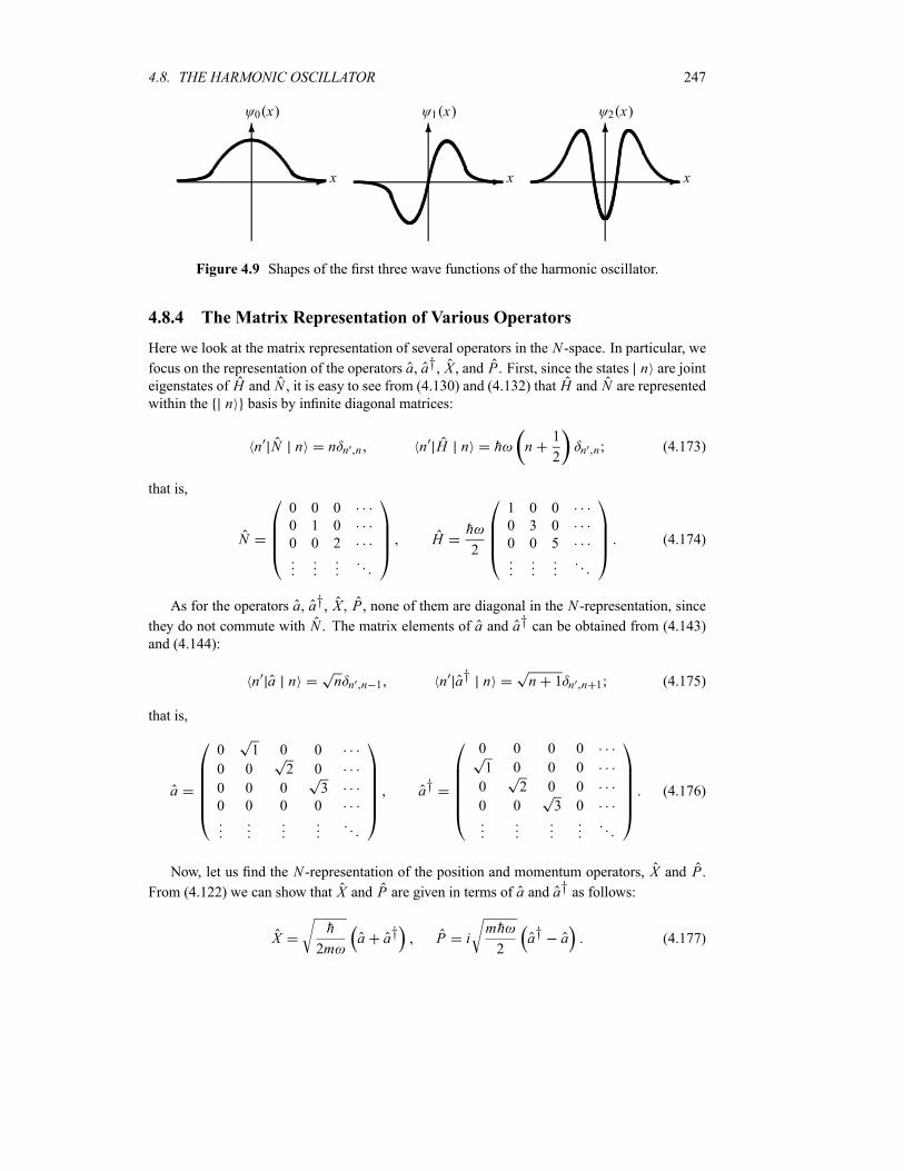
4.8. THE HARMONIC OSCILLATOR 247
-
60 x
x -
61 x
x -
62 x
x
Figure 4.9 Shapes of the first three wave functions of the harmonic oscillator.
4.8.4 The Matrix Representation of Various Operators
Here we look at the matrix representation of several operators in the N -space. In particular, we
focus on the representation of the operators a, a†, X , and P . First, since the states n are jointeigenstates of H and N , it is easy to see from (4.130) and (4.132) that H and N are representedwithin the n basis by infinite diagonal matrices:
n N n n n n n H n h n1
2n n (4.173)
that is,
N
0 0 0
0 1 0
0 0 2 Hh
2
1 0 0
0 3 0
0 0 5 (4.174)
As for the operators a, a†, X , P , none of them are diagonal in the N -representation, since
they do not commute with N . The matrix elements of a and a† can be obtained from (4.143)and (4.144):
n a n n n n 1 n a† n n 1 n n 1 (4.175)
that is,
a
0 1 0 0
0 0 2 0
0 0 0 3
0 0 0 0a†
0 0 0 0
1 0 0 0
0 2 0 0
0 0 3 0(4.176)
Now, let us find the N -representation of the position and momentum operators, X and P .
From (4.122) we can show that X and P are given in terms of a and a† as follows:
Xh
2ma a† P i
mh
2a† a (4.177)
248 CHAPTER 4. ONE-DIMENSIONAL PROBLEMS
Their matrix elements are given by
n X nh
2mn n n 1 n 1 n n 1 (4.178)
n P n imh
2n n n 1 n 1 n n 1 (4.179)
in particular
n X n n P n 0 (4.180)
The matrices corresponding to X and P are thus given by
Xh
2m
0 1 0 0
1 0 2 0
0 2 0 3
0 0 3 0(4.181)
P imh
2
0 1 0 0
1 0 2 0
0 2 0 3
0 0 3 0(4.182)
As mentioned in Chapter 2, the momentum operator is Hermitian, but not equal to its own
complex conjugate: (4.182) shows that P† P and P P . As for X , however, it is both
Hermitian and equal to its complex conjugate: from (4.181) we have that X† X X .Finally, we should mention that the eigenstates n are represented by infinite column ma-
trices; the first few states can be written as
0
1
0
0
01
0
1
0
02
0
0
1
03
0
0
0
1(4.183)
The set of states n forms indeed a complete and orthonormal basis.
4.8.5 Expectation Values of Various Operators
Let us evaluate the expectation values for X2 and P2 in the N -representation:
X2h
2ma2 a†2 aa† a†a
h
2ma2 a†2 2a†a 1 (4.184)
P2mh
2a2 a†2 aa† a†a
mh
2a2 a†2 2a†a 1 (4.185)
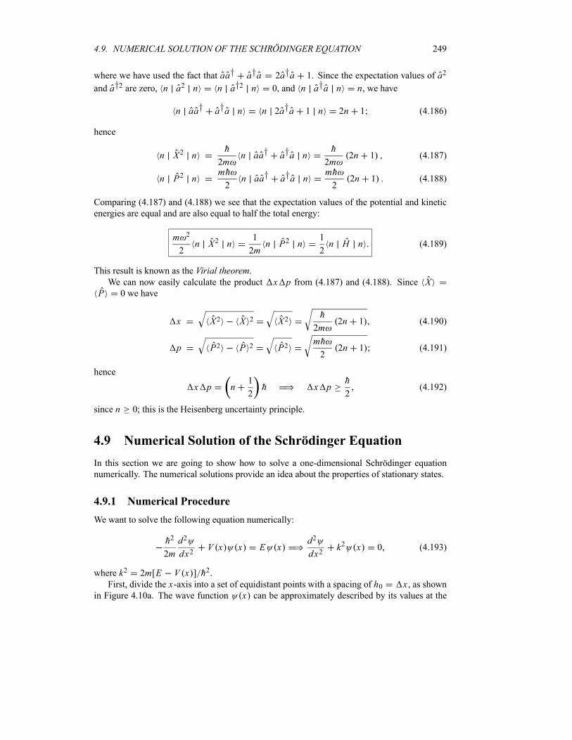
4.9. NUMERICAL SOLUTION OF THE SCHRÖDINGER EQUATION 249
where we have used the fact that aa† a†a 2a†a 1. Since the expectation values of a2
and a†2 are zero, n a2 n n a†2 n 0, and n a†a n n, we have
n aa† a†a n n 2a†a 1 n 2n 1 (4.186)
hence
n X2 nh
2mn aa† a†a n
h
2m2n 1 (4.187)
n P2 nmh
2n aa† a†a n
mh
22n 1 (4.188)
Comparing (4.187) and (4.188) we see that the expectation values of the potential and kinetic
energies are equal and are also equal to half the total energy:
m 2
2n X2 n
1
2mn P2 n
1
2n H n (4.189)
This result is known as the Virial theorem.We can now easily calculate the product x p from (4.187) and (4.188). Since X
P 0 we have
x X2 X 2 X2h
2m2n 1 (4.190)
p P2 P 2 P2mh
22n 1 (4.191)
hence
x p n1
2h x p
h
2(4.192)
since n 0; this is the Heisenberg uncertainty principle.
4.9 Numerical Solution of the Schrödinger Equation
In this section we are going to show how to solve a one-dimensional Schrödinger equation
numerically. The numerical solutions provide an idea about the properties of stationary states.
4.9.1 Numerical Procedure
We want to solve the following equation numerically:
h2
2m
d2
dx2V x x E x
d2
dx2k2 x 0 (4.193)
where k2 2m[E V x ] h2.First, divide the x-axis into a set of equidistant points with a spacing of h0 x , as shown
in Figure 4.10a. The wave function x can be approximately described by its values at the
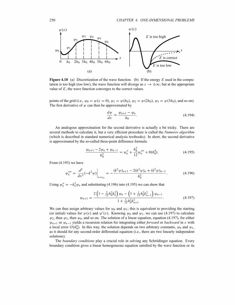
250 CHAPTER 4. ONE-DIMENSIONAL PROBLEMS
-
6
0
0 h0
1
2h0
2
3h0
3
4h0
4
5h0
5
6h0
6
x
x
(a)
-
6
x
x
E is too high
E is correct
E is too low
(b)
Figure 4.10 (a) Discretization of the wave function. (b) If the energy E used in the compu-tation is too high (too low), the wave function will diverge as x ; but at the appropriate
value of E , the wave function converges to the correct values.
points of the grid (i.e., 0 x 0 , 1 h0 , 2 2h0 , 3 3h0 , and so on).The first derivative of can then be approximated by
d
dxn 1 n
h0(4.194)
An analogous approximation for the second derivative is actually a bit tricky. There are
several methods to calculate it, but a very efficient procedure is called the Numerov algorithm(which is described in standard numerical analysis textbooks). In short, the second derivative
is approximated by the so-called three-point difference formula:
n 1 2 n n 1
h20n
h2012 n 0 h40 (4.195)
From (4.193) we have
nd2
dx2k2
x xn
k2 n 1 2 k2 n k2 n 1
h20(4.196)
Using n k2n n and substituting (4.196) into (4.195) we can show that
n 1
2 1 512h20k
2n n 1 1
12h20k
2n 1 n 1
1 112h20k
2n 1
(4.197)
We can thus assign arbitrary values for 0 and 1; this is equivalent to providing the starting
(or initial) values for x and x . Knowing 0 and 1, we can use (4.197) to calculate
2, then 3, then 4, and so on. The solution of a linear equation, equation (4.197), for either
n 1 or n 1 yields a recursion relation for integrating either forward or backward in x witha local error O h60 . In this way, the solution depends on two arbitrary constants, 0 and 1,
as it should for any second-order differential equation (i.e., there are two linearly independent
solutions).
The boundary conditions play a crucial role in solving any Schrödinger equation. Everyboundary condition gives a linear homogeneous equation satisfied by the wave function or its
4.9. NUMERICAL SOLUTION OF THE SCHRÖDINGER EQUATION 251
derivative. For example, in the case of the infinite square well potential and the harmonic
oscillator, the conditions xmin 0, xmax 0 are satisfied as follows:
Infinite square well: a 2 a 2 0
Harmonic oscillator: 0
4.9.2 Algorithm
To solve the Schrödinger equation with the boundary conditions xmin xmax 0, you
may proceed as follows. Suppose you want to find the wave function, n x , and the energyEn for the nth excited4 state of a system:
Take 0 0 and choose 1 (any small number you like), because the value of 1 must
be very close to that of 0.
Choose a trial energy En .
With this value of the energy, En , together with 0 and 1, you can calculate iteratively
the wave function at different values of x ; that is, you can calculate 2, 3, 4, . How?
You need simply to inject 0 0, 1, and En into (4.197) and proceed incrementally tocalculate 2; then use 1 and 2 to calculate 3; then use 2 and 3 to calculate 4;
and so on till you end up with the value of the wave function at xn nh0, n nh0 .
Next, you need to check whether the n you obtained is zero or not. If n is zero, this
means that you have made the right choice for the trial energy. This value En can thenbe taken as a possible eigenenergy for the system; at this value of En , the wave functionconverges to the correct value (dotted curve in Figure 4.10b). Of course, it is highly
unlikely to have chosen the correct energy from a first trial. In this case you need to
proceed as follows. If the value of n obtained is a nonzero positive number or if it
diverges, this means that the trial En you started with is larger than the correct eigenvalue(Figure 4.10b); on the other hand, if n is a negative nonzero number, this means that the
En you started with is less than the true energy. If the n you end up with is a positive
nonzero number, you need to start all over again with a smaller value of the energy. But
if the n you end up with is negative, you need to start again with a larger value of E .You can continue in this way, improving every time, till you end up with a zero value for
n . Note that in practice there is no way to get n exactly equal to zero. You may stop
the procedure the moment n is sufficiently small; that is, you stop the iteration at the
desired accuracy, say at 10 8 of its maximum value.
Example 4.3 (Numerical solution of the Schrödinger equation)
A proton is subject to a harmonic oscillator potential V x m 2x2 2, 5 34 1021s 1.
(a) Find the exact energies of the five lowest states (express them in MeV).
(b) Solve the Schrödinger equation numerically and find the energies of the five lowest statesand compare them with the exact results obtained in (a). Note: You may use these quantities:
rest mass energy of the proton mc2 103MeV, hc 200MeV fm, and h 3 5MeV.
4We have denoted here the wave function of the nth excited state by n x to distinguish it from the value of thewave function at xn nh0, n nh0 .
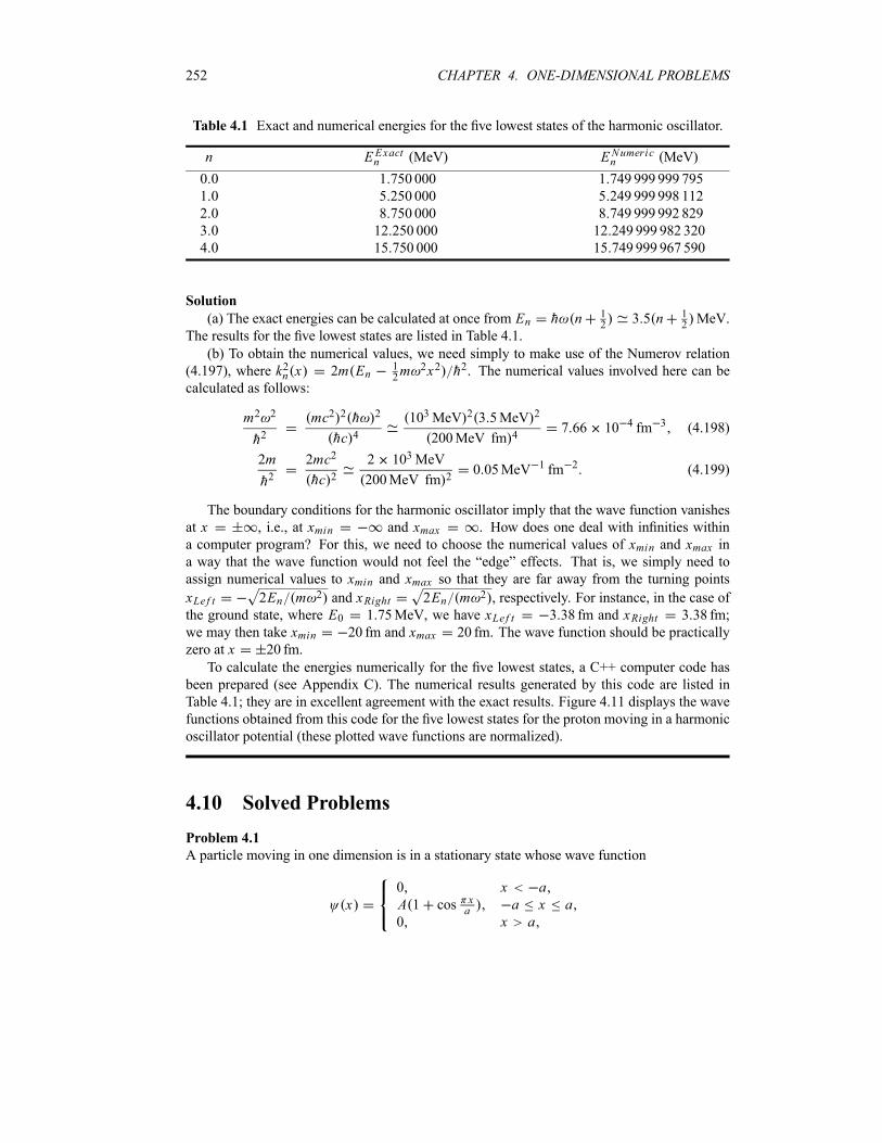
252 CHAPTER 4. ONE-DIMENSIONAL PROBLEMS
Table 4.1 Exact and numerical energies for the five lowest states of the harmonic oscillator.
n EExactn MeV ENumericn MeV
0 0 1 750 000 1 749 999 999 795
1 0 5 250 000 5 249 999 998 112
2 0 8 750 000 8 749 999 992 829
3 0 12 250 000 12 249 999 982 320
4 0 15 750 000 15 749 999 967 590
Solution
(a) The exact energies can be calculated at once from En h n 12
3 5 n 12MeV.
The results for the five lowest states are listed in Table 4.1.
(b) To obtain the numerical values, we need simply to make use of the Numerov relation
(4.197), where k2n x 2m En12m 2x2 h2. The numerical values involved here can be
calculated as follows:
m2 2
h2mc2 2 h 2
hc 4103MeV 2 3 5MeV 2
200MeV fm 47 66 10 4 fm 3 (4.198)
2m
h22mc2
hc 22 103MeV
200MeV fm 20 05MeV 1 fm 2 (4.199)
The boundary conditions for the harmonic oscillator imply that the wave function vanishes
at x , i.e., at xmin and xmax . How does one deal with infinities within
a computer program? For this, we need to choose the numerical values of xmin and xmax ina way that the wave function would not feel the “edge” effects. That is, we simply need to
assign numerical values to xmin and xmax so that they are far away from the turning pointsxLef t 2En m 2 and xRight 2En m 2 , respectively. For instance, in the case of
the ground state, where E0 1 75MeV, we have xLef t 3 38 fm and xRight 3 38 fm;
we may then take xmin 20 fm and xmax 20 fm. The wave function should be practically
zero at x 20 fm.
To calculate the energies numerically for the five lowest states, a C++ computer code has
been prepared (see Appendix C). The numerical results generated by this code are listed in
Table 4.1; they are in excellent agreement with the exact results. Figure 4.11 displays the wave
functions obtained from this code for the five lowest states for the proton moving in a harmonic
oscillator potential (these plotted wave functions are normalized).
4.10 Solved Problems
Problem 4.1
A particle moving in one dimension is in a stationary state whose wave function
x0 x aA 1 cos x
a a x a0 x a
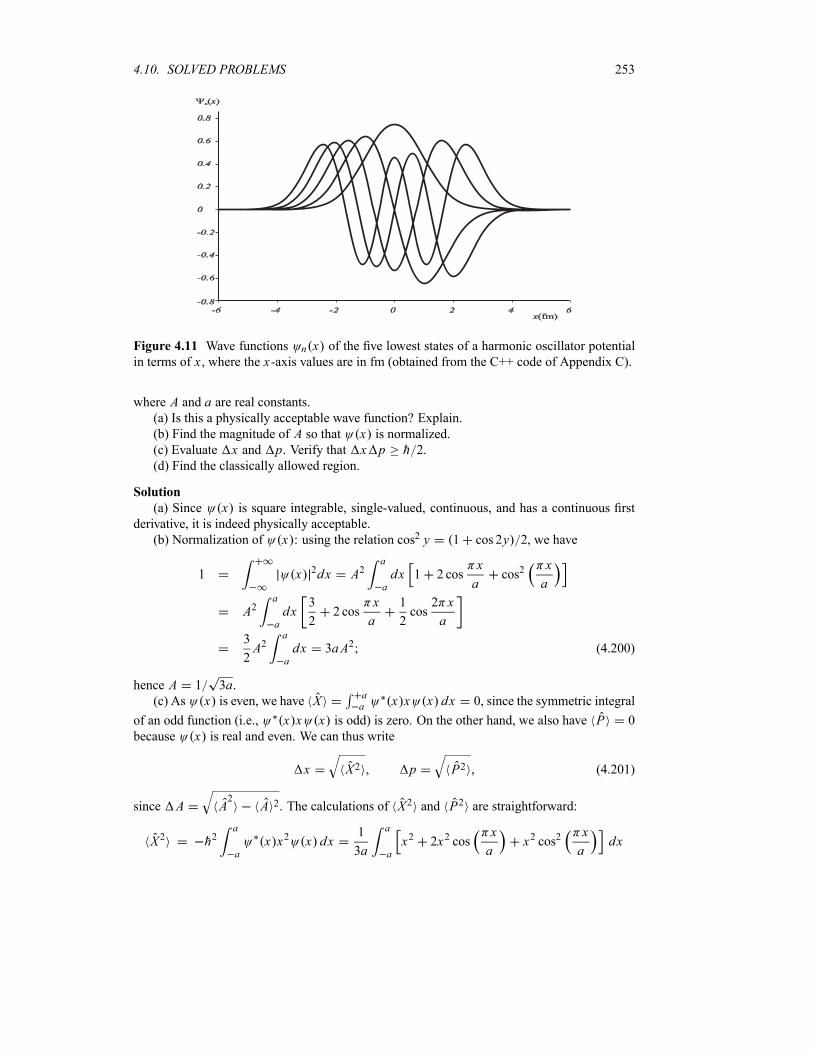
4.10. SOLVED PROBLEMS 253
�n( )x
x(fm)
Figure 4.11 Wave functions n x of the five lowest states of a harmonic oscillator potential
in terms of x , where the x-axis values are in fm (obtained from the C++ code of Appendix C).
where A and a are real constants.(a) Is this a physically acceptable wave function? Explain.
(b) Find the magnitude of A so that x is normalized.(c) Evaluate x and p. Verify that x p h 2.(d) Find the classically allowed region.
Solution
(a) Since x is square integrable, single-valued, continuous, and has a continuous first
derivative, it is indeed physically acceptable.
(b) Normalization of x : using the relation cos2 y 1 cos 2y 2, we have
1 x 2dx A2a
adx 1 2 cos
x
acos2
x
a
A2a
adx
3
22 cos
x
a
1
2cos
2 x
a
3
2A2
a
adx 3aA2 (4.200)
hence A 1 3a.(c) As x is even, we have X a
a x x x dx 0, since the symmetric integral
of an odd function (i.e., x x x is odd) is zero. On the other hand, we also have P 0
because x is real and even. We can thus write
x X2 p P2 (4.201)
since A A2
A 2. The calculations of X2 and P2 are straightforward:
X2 h2a
ax x2 x dx
1
3a
a
ax2 2x2 cos
x
ax2 cos2
x
adx
254 CHAPTER 4. ONE-DIMENSIONAL PROBLEMS
a2
6 22 2 15 (4.202)
P2 h2a
axd2 x
dx2dx
2h2
a2A2
a
acos
x
acos2
x
adx
2h2
3a3
a
a
1
2cos
x
a
1
2cos
2 x
adx
2h2
3a2(4.203)
hence x a 1 3 5 2 2 and p h 3a . We see that the uncertainties product
x ph
31
15
2 2(4.204)
satisfies Heisenberg’s uncertainty principle, x p h 2.(d) Since d 2 dx2 is zero at the inflection points, we have
d2
dx2
2
a2A cos
x
a0 (4.205)
This relation holds when x a 2; hence the classically allowed region is defined by the in-terval between the inflection points a 2 x a 2. That is, since x decays exponentiallyfor x a 2 and for x a 2, the energy of the system must be smaller than the potential.Classically, the system cannot be found in this region.
Problem 4.2
Consider a particle of massm moving freely between x 0 and x a inside an infinite squarewell potential.
(a) Calculate the expectation values X n , P n , X2 n , and P2 n , and compare them withtheir classical counterparts.
(b) Calculate the uncertainties product xn pn .(c) Use the result of (b) to estimate the zero-point energy.
Solution
(a) Since n x 2 a sin n x a and since it is a real function, we have n P n 0
because for any real function x the integral P ih x d x dx dx is imaginary
and this contradicts the fact that P has to be real. On the other hand, the expectation values
of X , X2, and P2 are
n X n
a
0n x x n x dx
2
a
a
0
x sin2n x
adx
1
a
a
0
x 1 cos2n x
adx
a
2(4.206)
n X2
n2
a
a
0
x2 sin2n x
adx
1
a
a
0
x2 1 cos2n x
adx
a2
3
1
a
a
0
x2 cos2n x
adx
4.10. SOLVED PROBLEMS 255
a2
3
1
2nx2 sin
2n x
a
x a
x 0
1
n
a
0
x sin2n x
adx
a2
3
a2
2n2 2(4.207)
n P2
n h2a
0n x
d2 n x
dx2dx
n2 2h2
a2
a
0n x
2dxn2 2h2
a2(4.208)
In deriving the previous three expressions, we have used integrations by parts. Since Enn2 2h2 2ma2 , we may write
n P2
nn2 2h2
a22mEn (4.209)
To calculate the classical average values xa , pa , x2a , p2a , it is easy first to infer that pa 0
and p2a 2mE , since the particle moves to the right with constant momentum p m and to
the left with p m . As the particle moves at constant speed, we have x t , hence
xa1
T
T
0
x t dtT
T
0
t dtT
2
a
2(4.210)
x2a1
T
T
0
x2 t dt2
T
T
0
t2dt1
32T 2
a2
3(4.211)
where T is half 5 of the period of the motion, with a T .We conclude that, while the average classical and quantum expressions for x , p and p2 are
identical, a comparison of (4.207) and (4.211) yields
n X2
na2
3
a2
2n2 2x2a
a2
2n2 2(4.212)
so that in the limit of large quantum numbers, the quantum expression n X2 n matches
with its classical counterpart x2a : limn n X2 n a2 3 x2a .(b) The position and the momentum uncertainties can be calculated from (4.206) to (4.208):
xn n X2 n n X n2
a2
3
a2
2n2 2
a2
4a
1
12
1
2n2 2
(4.213)
pn n P2 n n P n2
n P2 nn h
a(4.214)
hence
xn pn n h1
12
1
2n2 2(4.215)
(c) Equation (4.214) shows that the momentum uncertainty for the ground state is not zero,
but
p1h
a(4.216)
5We may parameterize the other half of the motion by x t , which when inserted in (4.210) and (4.211), wherethe variable t varies between T and 0, the integrals would yield the same results, namely xa a 2 and x2a a2 3,respectively.
256 CHAPTER 4. ONE-DIMENSIONAL PROBLEMS
This leads to a nonzero kinetic energy. Therefore, the lowest value of the particle’s kinetic
energy is of the order of Emin p1 2 2m 2h2 2ma2 . This value, which is in fullagreement with the ground state energy, E1 2h2 2ma2 , is the zero-point energy of theparticle.
Problem 4.3
An electron is moving freely inside a one-dimensional infinite potential box with walls at x 0
and x a. If the electron is initially in the ground state (n 1) of the box and if we suddenlyquadruple the size of the box (i.e., the right-hand side wall is moved instantaneously from x ato x 4a), calculate the probability of finding the electron in:(a) the ground state of the new box and
(b) the first excited state of the new box.
Solution
Initially, the electron is in the ground state of the box x 0 and x a; its energy and wavefunction are
E12h2
2ma21 x
2
asin
x
a(4.217)
(a) Once in the new box, x 0 and x 4a, the ground state energy and wave function ofthe electron are
E1
2h2
2m 4a 2
2h2
32ma21 x
1
2asin
x
4a(4.218)
The probability of finding the electron in 1 x is
P E1 1 12
a
01 x 1 x dx
2 1
a2
a
0
sinx
4asin
x
adx
2
(4.219)
the upper limit of the integral sign is a (and not 4a) because 1 x is limited to the region
between 0 and a. Using the relation sin a sin b 12cos a b 1
2cos a b , we have
sin x 4a sin x a 12cos 3 x 4a 1
2cos 5 x 4a ; hence
P E11
a21
2
a
0
cos3 x
4adx
1
2
a
0
cos5 x
4adx
2
128
152 20 058 5 8% (4.220)
(b) If the electron is in the first excited state of the new box, its energy and wave function
are
E2
2h2
8ma22 x
1
2asin
x
2a(4.221)
The corresponding probability is
P E2 2 12
a
02 x 1 x dx
2 1
a2
a
0
sinx
2asin
x
adx
2
16
9 20 18 18% (4.222)
4.10. SOLVED PROBLEMS 257
Problem 4.4
Consider a particle of mass m subject to an attractive delta potential V x V0 x , whereV0 0 (V0 has the dimensions of Energy Distance).
(a) In the case of negative energies, show that this particle has only one bound state; find
the binding energy and the wave function.
(b) Calculate the probability of finding the particle in the interval a x a.(c) What is the probability that the particle remains bound when V0 is (i) halved suddenly,
(ii) quadrupled suddenly?
(d) Study the scattering case (i.e., E 0) and calculate the reflection and transmission
coefficients as a function of the wave number k.
Solution
(a) Let us consider first the bound state case E 0. We can write the Schrödinger equation
as follows:d2 x
dx22mV0
h2x x
2mE
h2x 0 (4.223)
Since x vanishes for x 0, this equation becomes
d2 x
dx22mE
h2x 0 (4.224)
The bound solutions require that x vanishes at x ; these bound solutions are given
by
xx Aekx x 0
x Be kx x 0(4.225)
where k 2m E h. Since x is continuous at x 0, 0 0 , we have A B.Thus, the wave function is given by x Ae k x ; note that x is even.The energy can be obtained from the discontinuity condition of the first derivative of the
wave function, which in turn can be obtained by integrating (4.223) from to ,
dxd2 x
dx22mV0
h2x x dx
2mE
h2x dx 0 (4.226)
and then letting 0. Using the facts that
dxd2 x
dx2d x
dx x
d x
dx x
d x
dx x
d x
dx x(4.227)
and that x dx 0 (because x is even), we can rewrite (4.226) as follows:
lim0
d x
dx x
d x
dx x 0
2mV0
h20 0 (4.228)
since the wave function is continuous at x 0, but its first derivative is not. Substituting (4.225)
into (4.228) and using A B, we obtain
2kA2mV0
h2A 0 (4.229)
258 CHAPTER 4. ONE-DIMENSIONAL PROBLEMS
or k mV0 h2. But since k 2m E h2, we have mV0 h
2 2m E h2, and since the
energy is negative, we conclude that E mV 20 2h2 . There is, therefore, only one boundstate solution. As for the excited states, all of them are unbound. We may normalize x ,
1 x x dx A20
exp 2kx dx A20
exp 2kx dx
2A20
exp 2kx dxA2
k(4.230)
hence A k. The normalized wave function is thus given by x ke k x . So the
energy and normalized wave function of the bound state are given by
EmV 202h2
xmV0
h2exp
mV0
h2x (4.231)
(b) Since the wave function x ke k x is normalized, the probability of finding the
particle in the interval a x a is given by
P
aa x 2 dx
x 2 dx
a
ax 2 dx k
a
ae 2k x dx
k0
ae2kxdx k
a
0
e 2kxdx 2ka
0
e 2kxdx
1 e 2ka 1 e 2mV0a h2
(4.232)
(c) If the strength of the potential changed suddenly from V0 to V1, the wave function will
be given by 1 x mV1 h2 exp mV1 x h2 . The probability that the particle remains inthe bound state 1 x is
P 12
1 x x dx2
m
h2V0V1 exp
m V0 V1
h2x dx
2
2m
h2V0V1
0
expm V0 V1
h2x dx
2 4V0V1V0 V1 2
(4.233)
(i) In the case where the strength of the potential is halved, V112V0, the probability that the
particle remains bound is
P2V 20
V012V0 2
8
989% (4.234)
(ii) When the strength is quadrupled, V1 4V0, the probability is given by
P16V 205V0 2
16
2564% (4.235)
4.10. SOLVED PROBLEMS 259
(d) The case E 0 corresponds to a free motion and the energy levels represent a contin-
uum. The solution of the Schrödinger equation for E 0 is given by
xx Aeikx Be ikx x 0
x Ceikx x 0(4.236)
where k 2mE h; this corresponds to a plane wave incident from the left together with areflected wave in the region x 0, and only a transmitted wave for x 0.
The values of the constants A and B are to be found from the continuity relations. On theone hand, the continuity of x at x 0 yields
A B C (4.237)
and, on the other hand, substituting (4.236) into (4.228), we end up with
ik C A B2mV0
h2C 0 (4.238)
Solving (4.237) and (4.238) for B A and C A, we find
B
A
1
1 ikh2
mV0
C
A
1
1 imV0h2k
(4.239)
Thus, the reflection and transmission coefficients are
RB
A
21
1 h4k2
m2V 20
1
1 2h2EmV 20
TC
A
21
1m2V 20h4k2
1
1mV 202h2E
(4.240)
with R T 1.
Problem 4.5
A particle of mass m is subject to an attractive double-delta potential V x V0 x aV0 x a , where V0 0. Consider only the case of negative energies.
(a) Obtain the wave functions of the bound states.
(b) Derive the eigenvalue equations.
(c) Specify the number of bound states and the limit on their energies. Is the ground state
an even state or an odd state?
(d) Estimate the ground state energy for the limits a 0 and a .
Solution
(a) The Schrödinger equation for this problem is
d2 x
dx22mV0
h2[ x a x a ] x
2mE
h2x 0 (4.241)
For x a this equation becomes
d2 x
dx22mE
h2x 0 or
d2 x
dx2k2 x 0 (4.242)
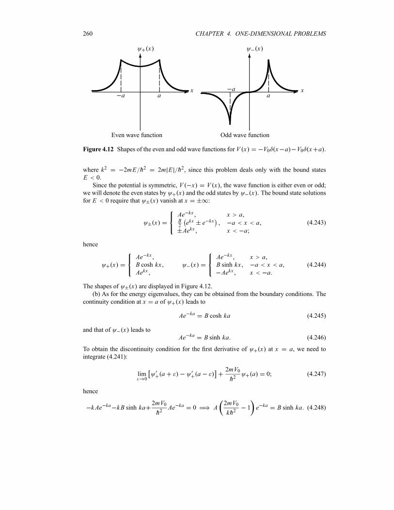
260 CHAPTER 4. ONE-DIMENSIONAL PROBLEMS
-
6
x
x
Even wave function
a a-
6
x
x
Odd wave function
aa
Figure 4.12 Shapes of the even and odd wave functions for V x V0 x a V0 x a .
where k2 2mE h2 2m E h2, since this problem deals only with the bound statesE 0.
Since the potential is symmetric, V x V x , the wave function is either even or odd;we will denote the even states by x and the odd states by x . The bound state solutionsfor E 0 require that x vanish at x :
xAe kx x aB2ekx e kx a x aAekx x a
(4.243)
hence
xAe kx
B cosh kxAekx
xAe kx x aB sinh kx a x aAekx x a
(4.244)
The shapes of x are displayed in Figure 4.12.(b) As for the energy eigenvalues, they can be obtained from the boundary conditions. The
continuity condition at x a of x leads to
Ae ka B cosh ka (4.245)
and that of x leads toAe ka B sinh ka (4.246)
To obtain the discontinuity condition for the first derivative of x at x a, we need tointegrate (4.241):
lim0
a a2mV0
h2a 0 (4.247)
hence
k Ae ka kB sinh ka2mV0
h2Ae ka 0 A
2mV0
kh21 e ka B sinh ka (4.248)

4.10. SOLVED PROBLEMS 261
-
6
0y
1
yy0
y 1¾
tanh y
6
(a) Eigenvalues for even states
-
6
0y
1
y 11-
tanh y
6
largesmall
(b) Eigenvalues for odd states
Figure 4.13 Graphical solutions of the eigenvalue equations for the even states and the odd
states for the double-delta potential V x V0 x a V0 x a .
Similarly, the continuity of the first derivative of x at x a yields
kAe ka kB cosh ka2mV0
h2Ae ka 0 A
2mV0
kh21 e ka B cosh ka
(4.249)
Dividing (4.248) by (4.245) we obtain the eigenvalue equation for the even solutions:
2mV0
kh21 tanh ka tanh y
y1 (4.250)
where y ka and 2maV0 h2. The eigenvalue equation for the odd solutions can beobtained by dividing (4.249) by (4.246):
2mV0
kh21 coth ka coth y
y1 tanh y
y1
1
(4.251)
because coth y 1 tanh y.To obtain the energy eigenvalues for the even and odd solutions, we need to solve the
transcendental equations (4.250) and (4.251). These equations can be solved graphically. In
what follows, let us determine the upper and lower limits of the energy for both the even and
odd solutions.
(c) To find the number of bound states and the limits on the energy, let us consider the even
and odd states separately.
Energies corresponding to the even solutions
There is only one bound state, since the curves tanh y and y 1 intersect only once (Fig-
ure 4.13a); we call this point y y0. When y we have y 1 0, while tanh 0.
Therefore y0 . On the other hand, since tanh y0 1 we have y0 1 1 or y0 2.
We conclude then that 2 y0 or
2y0
2mV 20h2
Ee enmV 202h2
(4.252)
In deriving this relation, we have used the fact that 2 4 y202 where 2maV0 h2
and y20 k20a2 2ma2Ee en h2. So there is always one even bound state, the ground state,
whose energy lies within the range specified by (4.252).
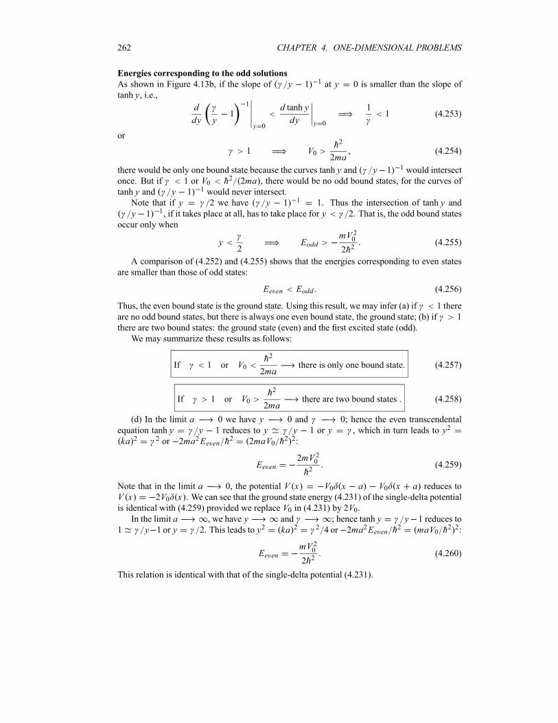
262 CHAPTER 4. ONE-DIMENSIONAL PROBLEMS
Energies corresponding to the odd solutions
As shown in Figure 4.13b, if the slope of y 1 1 at y 0 is smaller than the slope of
tanh y, i.e.,
d
dy y1
1
y 0
d tanh y
dy y 0
11 (4.253)
or
1 V0h2
2ma(4.254)
there would be only one bound state because the curves tanh y and y 1 1 would intersect
once. But if 1 or V0 h2 2ma , there would be no odd bound states, for the curves oftanh y and y 1 1 would never intersect.
Note that if y 2 we have y 1 1 1. Thus the intersection of tanh y andy 1 1, if it takes place at all, has to take place for y 2. That is, the odd bound states
occur only when
y2
EoddmV 202h2
(4.255)
A comparison of (4.252) and (4.255) shows that the energies corresponding to even states
are smaller than those of odd states:
Ee en Eodd (4.256)
Thus, the even bound state is the ground state. Using this result, we may infer (a) if 1 there
are no odd bound states, but there is always one even bound state, the ground state; (b) if 1
there are two bound states: the ground state (even) and the first excited state (odd).
We may summarize these results as follows:
If 1 or V0h2
2mathere is only one bound state (4.257)
If 1 or V0h2
2mathere are two bound states (4.258)
(d) In the limit a 0 we have y 0 and 0; hence the even transcendental
equation tanh y y 1 reduces to y y 1 or y , which in turn leads to y2
ka 2 2 or 2ma2Ee en h2 2maV0 h
2 2:
Ee en2mV 20h2
(4.259)
Note that in the limit a 0, the potential V x V0 x a V0 x a reduces to
V x 2V0 x . We can see that the ground state energy (4.231) of the single-delta potentialis identical with (4.259) provided we replace V0 in (4.231) by 2V0.In the limit a , we have y and ; hence tanh y y 1 reduces to
1 y 1 or y 2. This leads to y2 ka 2 2 4 or 2ma2Ee en h2 maV0 h
2 2:
Ee enmV 202h2
(4.260)
This relation is identical with that of the single-delta potential (4.231).
4.10. SOLVED PROBLEMS 263
Problem 4.6
Consider a particle of mass m subject to the potential
V xx 0
V0 x a x 0
where V0 0. Discuss the existence of bound states in terms of the size of a.
Solution
The Schrödinger equation for x 0 is
d2 x
dx22mV0
h2x a k2 x 0 (4.261)
where k2 2mE h2, since we are looking here at the bound states only, E 0. The
solutions of this equation are
x 1 x Aekx Be kx 0 x a
2 x Ce kx x a(4.262)
The energy eigenvalues can be obtained from the boundary conditions. As the wave func-
tion vanishes at x 0, we have
1 0 0 A B 0 B A (4.263)
The continuity condition at x a of x , 1 a 2 a , leads to
Aeka Ae ka Ce ka (4.264)
To obtain the discontinuity condition for the first derivative of x at x a, we need tointegrate (4.261):
lima 2 a 1 a
2mV0
h22 a 0 (4.265)
or
kCe ka kAeka kAe ka 2mV0
h2Ce ka 0 (4.266)
Substituting Ce ka Aeka Ae ka or (4.264) into (4.266) we have
k Aeka k Ae ka kAeka kAe ka 2mV0
h2Aeka Ae ka 0 (4.267)
From this point on, we can proceed in two different, yet equivalent, ways. These two methods
differ merely in the way we exploit (4.267). For completeness of the presentation, let us discuss
both methods.
First method
The second and fourth terms of (4.267) cancel each other, so we can reduce it to
kAeka kAeka2mV0
h2Aeka Ae ka 0 (4.268)
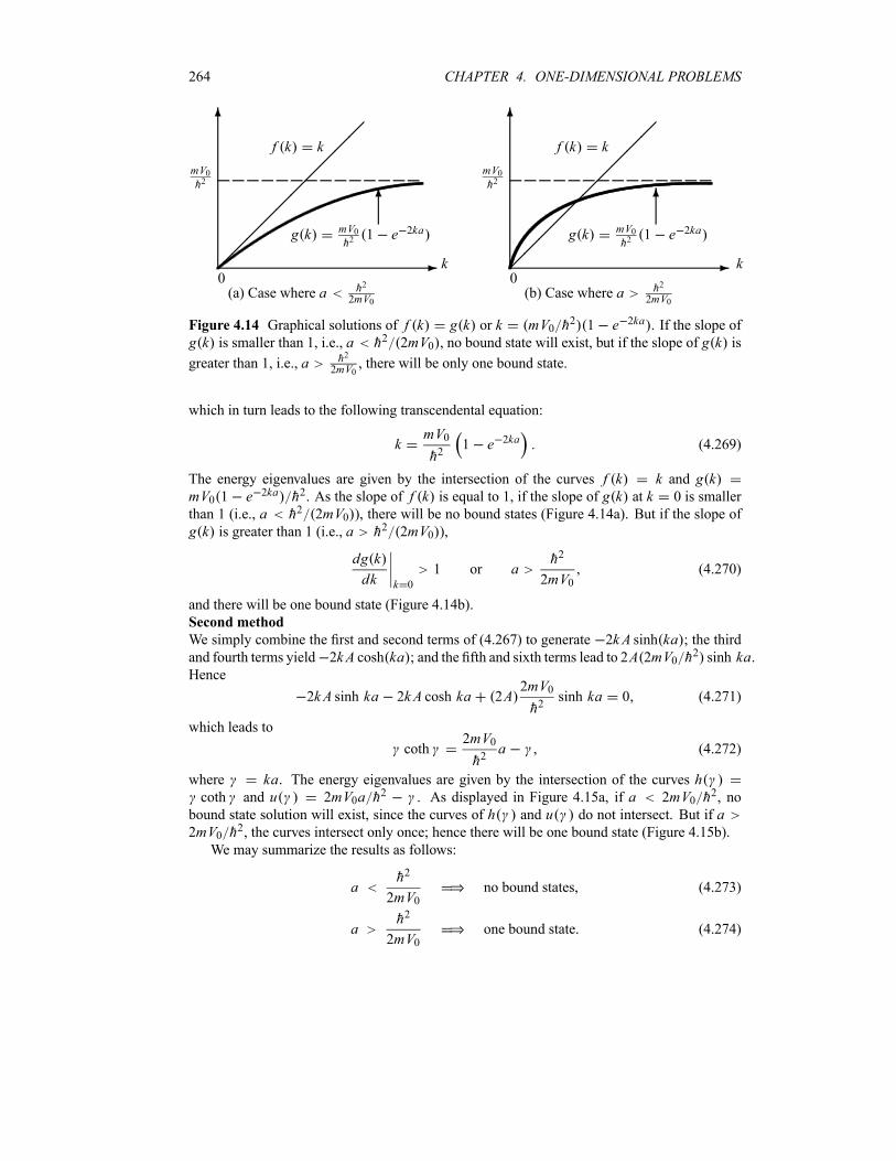
264 CHAPTER 4. ONE-DIMENSIONAL PROBLEMS
-
6
0k
mV0h2
¡¡¡¡¡¡¡¡¡¡
g k mV0h2
1 e 2ka
f k k
6
(a) Case where a h2
2mV0
-
6
0k
mV0h2
¡¡¡¡¡¡¡¡¡¡
f k k
g k mV0h2
1 e 2ka
6
(b) Case where a h2
2mV0
Figure 4.14 Graphical solutions of f k g k or k mV0 h2 1 e 2ka . If the slope of
g k is smaller than 1, i.e., a h2 2mV0 , no bound state will exist, but if the slope of g k is
greater than 1, i.e., a h2
2mV0, there will be only one bound state.
which in turn leads to the following transcendental equation:
kmV0
h21 e 2ka (4.269)
The energy eigenvalues are given by the intersection of the curves f k k and g kmV0 1 e 2ka h2. As the slope of f k is equal to 1, if the slope of g k at k 0 is smaller
than 1 (i.e., a h2 2mV0 ), there will be no bound states (Figure 4.14a). But if the slope ofg k is greater than 1 (i.e., a h2 2mV0 ),
dg k
dk k 0
1 or ah2
2mV0(4.270)
and there will be one bound state (Figure 4.14b).
Second method
We simply combine the first and second terms of (4.267) to generate 2k A sinh ka ; the thirdand fourth terms yield 2kA cosh ka ; and the fifth and sixth terms lead to 2A 2mV0 h
2 sinh ka.Hence
2kA sinh ka 2kA cosh ka 2A2mV0
h2sinh ka 0 (4.271)
which leads to
coth2mV0
h2a (4.272)
where ka. The energy eigenvalues are given by the intersection of the curves hcoth and u 2mV0a h
2 . As displayed in Figure 4.15a, if a 2mV0 h2, no
bound state solution will exist, since the curves of h and u do not intersect. But if a2mV0 h2, the curves intersect only once; hence there will be one bound state (Figure 4.15b).We may summarize the results as follows:
ah2
2mV0no bound states, (4.273)
ah2
2mV0one bound state. (4.274)
4.10. SOLVED PROBLEMS 265
-
6
0
@@@@@@@
1
2maV0h2
coth
2maV0h2
(a) Case where a h2
2mV0
-
6
0
@@@@@@@@@
1
2maV0h2 coth
2maV0h2
(b) Case where a h2
2mV0
Figure 4.15 Graphical solutions of h u , with ka, h coth , and u2mV0a h2 . If a 2mV0 h2 there is no bound state. If a 2mV0 h2 there is one boundstate.
Problem 4.7
A particle of mass m, besides being confined to move inside an infinite square well potential ofsize a with walls at x 0 and x a, is subject to a delta potential of strength V0
V xV0 x a 2 0 x a
elsewhere
where V0 0. Show how to calculate the energy levels of the system in terms of V0 and a.
Solution
The Schrödinger equation
d2 x
dx22mV0
h2x
a
2x
2mE
h2x 0 (4.275)
can be written for x a 2 as
d2 x
dx22mE
h2x 0 (4.276)
The solutions of this equation must vanish at x 0 and x a:
x L x A sin kx 0 x a 2
R x B sin k x a a 2 x a(4.277)
where k 2m E h. The continuity of x at x a 2, L a 2 R a 2 , leads toA sin a 2 B sin a 2 ; hence B A. The wave function is thus given by
x L x A sin kx 0 x a 2
R x A sin k x a a 2 x a(4.278)
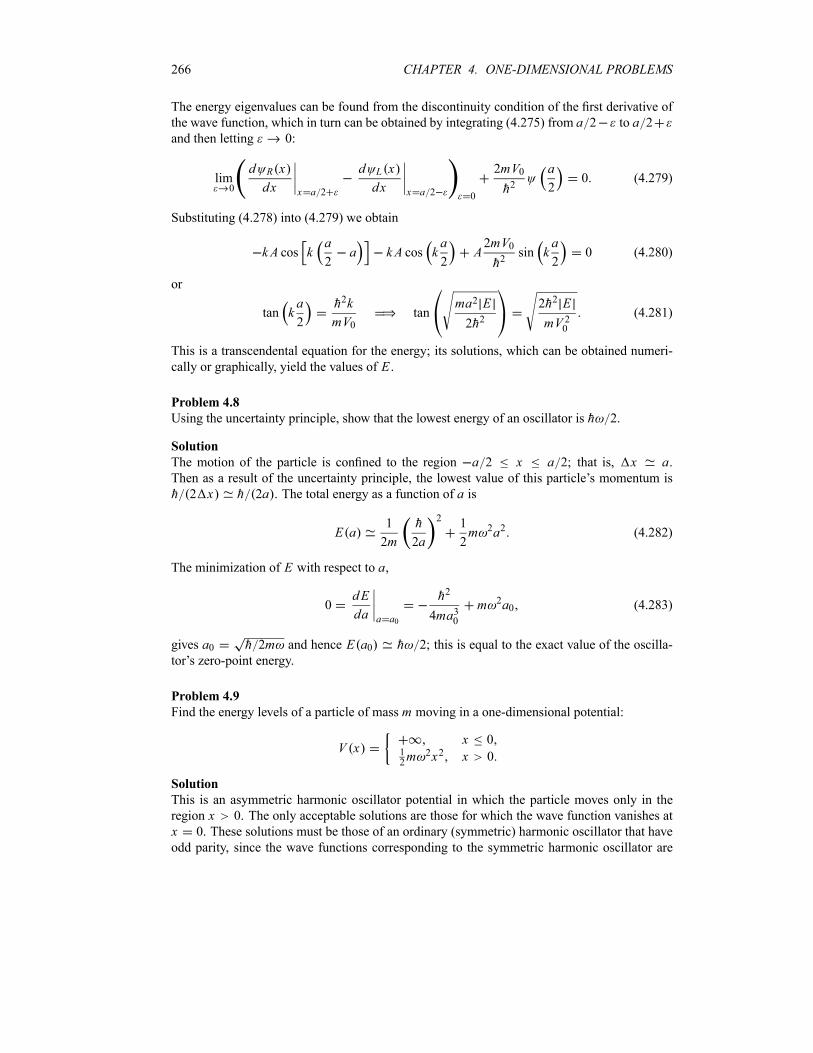
266 CHAPTER 4. ONE-DIMENSIONAL PROBLEMS
The energy eigenvalues can be found from the discontinuity condition of the first derivative of
the wave function, which in turn can be obtained by integrating (4.275) from a 2 to a 2and then letting 0:
lim0
d R x
dx x a 2
d L x
dx x a 2 0
2mV0
h2a
20 (4.279)
Substituting (4.278) into (4.279) we obtain
kA cos ka
2a kA cos k
a
2A2mV0
h2sin k
a
20 (4.280)
or
tan ka
2
h2k
mV0tan
ma2 E
2h22h2 E
mV 20(4.281)
This is a transcendental equation for the energy; its solutions, which can be obtained numeri-
cally or graphically, yield the values of E .
Problem 4.8
Using the uncertainty principle, show that the lowest energy of an oscillator is h 2.
Solution
The motion of the particle is confined to the region a 2 x a 2; that is, x a.Then as a result of the uncertainty principle, the lowest value of this particle’s momentum is
h 2 x h 2a . The total energy as a function of a is
E a1
2m
h
2a
21
2m 2a2 (4.282)
The minimization of E with respect to a,
0dE
da a a0
h2
4ma30m 2a0 (4.283)
gives a0 h 2m and hence E a0 h 2; this is equal to the exact value of the oscilla-
tor’s zero-point energy.
Problem 4.9
Find the energy levels of a particle of mass m moving in a one-dimensional potential:
V xx 0
12m 2x2 x 0
Solution
This is an asymmetric harmonic oscillator potential in which the particle moves only in the
region x 0. The only acceptable solutions are those for which the wave function vanishes at
x 0. These solutions must be those of an ordinary (symmetric) harmonic oscillator that have
odd parity, since the wave functions corresponding to the symmetric harmonic oscillator are
4.10. SOLVED PROBLEMS 267
either even (n even) or odd (n odd), and only the odd solutions vanish at the origin, 2n 1 0
0 n 0 1 2 3 . Therefore, the energy levels of this asymmetric potential must be
given by those corresponding to the odd n energy levels of the symmetric potential, i.e.,
En 2n 11
2h 2n
3
2h n 0 1 2 3 (4.284)
Problem 4.10
Consider the box potential
V x0 0 x a
elsewhere
(a) Estimate the energies of the ground state as well as those of the first and the second
excited states for (i) an electron enclosed in a box of size a 10 10m (express your answer
in electron volts; you may use these values: hc 200MeV fm, mec2 0 5MeV); (ii) a 1 g
metallic sphere which is moving in a box of size a 10 cm (express your answer in joules).
(b) Discuss the importance of the quantum effects for both of these two systems.
(c) Use the uncertainty principle to estimate the velocities of the electron and the metallic
sphere.
Solution
The energy of a particle of mass m in a box having perfectly rigid walls is given by
Enn2h2
8ma2n 1 2 3 (4.285)
where a is the size of the box.(a) (i) For the electron in the box of size 10 10m, we have
Enh2c2
mec2a24 2n2
8
4 104 MeV fm 2
0 5MeV 1010 fm2
2
2n2
4 2n2 eV 39n2 eV (4.286)
Hence E1 39 eV, E2 156 eV, and E3 351 eV.
(ii) For the sphere in the box of side 10 cm we have
En6 6 10 34 J s 2
10 3 kg 10 2m2n2 43 6 10 63n2 J (4.287)
Hence E1 43 6 10 63 J, E2 174 4 10 63 J, and E3 392 4 10 63 J.
(b) The differences between the energy levels are
E2 E1 electron 117 eV E3 E2 electron 195 eV (4.288)
E2 E1 sphere 130 8 10 63 J E3 E2 sphere 218 10 63 J (4.289)
These results show that:
The spacings between the energy levels of the electron are quite large; the levels are far
apart from each other. Thus, the quantum effects are important.

268 CHAPTER 4. ONE-DIMENSIONAL PROBLEMS
The energy levels of the sphere are practically indistinguishable; the spacings between
the levels are negligible. The energy spectrum therefore forms a continuum; hence the
quantum effects are not noticeable for the sphere.
(c) According to the uncertainty principle, the speed is proportional to h ma . For theelectron, the typical distances are atomic, a 10 10m; hence
hc
mc2ac
200MeV fm
0 5MeV 105 fmc 4 10 3c 1 2 106ms 1 (4.290)
where c is the speed of light. The electron therefore moves quite fast; this is expected since wehave confined the electron to move within a small region.
For the sphere, the typical distances are in the range of 1 cm:
h
ma
6 6 10 34 J s
10 3 kg 10 2m6 6 10 29ms 1 (4.291)
At this speed the sphere is practically at rest.
Problem 4.11
(a) Verify that the matrices representing the operators X and P in the N -space for a har-monic oscillator obey the correct commutation relation [X P] ih.(b) Show that the energy levels of the harmonic oscillator can be obtained by inserting the
matrices of X and P into the Hamiltonian H P2 2m 12m 2X2.
Solution
(a) Using the matrices of X and P in (4.181) and (4.182), we obtain
X P ih
2
1 0 2
0 1 0
2 0 1 PX ih
2
1 0 2
0 1 0
2 0 1 (4.292)
hence
X P PX ih
1 0 0
0 1 0
0 0 1 (4.293)
or [X P] ih I , where I is the unit matrix.(b) Again, using the matrices of X and P in (4.181) and (4.182), we can verify that
X2h
2m
1 0 2
0 3 0
2 0 5 P2mh
2
1 0 2
0 3 0
2 0 5
(4.294)
4.10. SOLVED PROBLEMS 269
hence
P2
2m
1
2m 2X2
h
2
1 0 0
0 3 0
0 0 5 (4.295)
The form of this matrix is similar to the result we obtain from an analytical treatment, Enh 2n 1 2, since
Hn n n H nh
22n 1 n n (4.296)
Problem 4.12
Calculate the probability of finding a particle in the classically forbidden region of a harmonic
oscillator for the states n 0 1 2 3 4. Are these results compatible with their classical
counterparts?
Solution
The classical turning points are defined by En V xn or by h n 12
12m 2x2n ; that
is, xn h m 2n 1. Thus, the probability of finding a particle in the classically
forbidden region for a state n x is
Pnxn
n x2 dx
xnn x
2 dx 2xn
n x2 dx (4.297)
where n x is given in (4.172), n x 1 2nn!x0ex2 2x20 Hn x x0 , where x0 is given
by x0 h m . Using the change of variable y x x0, we can rewrite Pn as
Pn2
2nn! 2n 1
e y2H2n y dy (4.298)
where the Hermite polynomials Hn y are listed in (4.120). The integral in (4.298) can be
evaluated only numerically. Using the numerical values
1
e y2dy 0 13943
y2e y2dy 0 0495 (4.299)
5
4y2 22e y2dy 0 6740
7
8y3 12y2e y2dy 3 6363 (4.300)
9
16y4 48y2 122e y2dx 26 86 (4.301)
we obtain
P0 0 1573 P1 0 1116 P2 0 095 069 (4.302)
P3 0 085 48 P4 0 078 93 (4.303)
This shows that the probability decreases as n increases, so it would be very small for verylarge values of n. It is therefore unlikely to find the particle in the classically forbidden regionwhen the particle is in a very highly excited state. This is what we expect, since the classical
approximation is recovered in the limit of high values of n.

270 CHAPTER 4. ONE-DIMENSIONAL PROBLEMS
Problem 4.13
Consider a particle of mass m moving in the following potential
V xx 0
V0 0 x a0 x a
where V0 0.
(a) Find the wave function.
(b) Show how to obtain the energy eigenvalues from a graph.
(c) Calculate the minimum value of V0 (in terms ofm, a, and h) so that the particle will haveone bound state; then calculate it for two bound states. From these two results, try to obtain the
lowest value of V0 so that the system has n bound states.
Solution
(a) As shown in Figure 4.16, the wave function in the region x 0 is zero, x 0. In
the region x 0 the Schrödinger equation for the bound state solutions, V0 E 0, is
given by
d2
dx2k21 1 x 0 0 x a (4.304)
d2
dx2k22 2 x 0 x a (4.305)
where k21 2m V0 E h2 and k22 2mE h2. On one hand, the solution of (4.304) isoscillatory, 1 x A sin k1x B cos k1x , but since 1 0 0 we must have B 0. On
the other hand, eliminating the physically unacceptable solutions which grow exponentially for
large values of x , the solution of (4.305) is 2 x Ce k2x . Thus, the wave function is given
by
x0 x 0
1 x A sin k1x 0 x 0
2 x Ce k2x x a(4.306)
(b) To determine the eigenvalues, we need to use the boundary conditions at x a. Thecondition 1 a 2 a yields
A sin k1a Ce k2a (4.307)
while the continuity of the first derivative, 1 a 2 a , leads to
Ak1 cos k1a Ck2ek2a (4.308)
Dividing (4.308) by (4.307) we obtain
k1a cot k1a k2a (4.309)
Since k21 2m V0 E h2 and k22 2mE h2, we have
k1a2 k2a
2 2 (4.310)
4.10. SOLVED PROBLEMS 271
-
6
E
0
V0
xa
V x
-
6
¾ k1a cot k1a
¾ k1a 2 k2a 2
n 1
n 1
n 2
0k1a
k2a
232
2
Figure 4.16 Potential V x (left curve); the energy levels of V x are given graphically by theintersection of the circular curve k1a 2 k2a 2 with k1a cot k1a (right curve).
where 2mV0a h.The transcendental equations (4.309) and (4.310) can be solved graphically. As shown
in Figure 4.16, the energy levels are given by the intersection of the circular curve k1a 2
k2a 2 2 with k1a cot k1a k2a.(c) If 2 3 2 there will be only one bound state, the ground state n 1, for
there is only one crossing between the curves k1a 2 k2a 2 2 and k1a cot k1a k2a.The lowest value of V0 that yields a single bound state is given by the relation 2, which
leads to 2ma2V0 h2 2 4 or to
V02h2
8ma2(4.311)
Similarly, if 3 2 5 2 there will be two crossings between k1a 2 k2a 2 2 and
k1a cot k1a k2a. Thus, there will be two bound states: the ground state, n 1, and the
first excited state, n 2. The lowest value of V0 that yields two bound states corresponds to2ma2V0 h
2 9 2 4 or to
V09 2h2
8ma2(4.312)
We may thus infer the following general result. If n 2 n 2, there will
be n crossings and hence n bound states:
n2
2mV0h
a n2
there are n bound states (4.313)
The lowest value of V0 giving n bound states is
V02h2
8ma22n 1 2 (4.314)
272 CHAPTER 4. ONE-DIMENSIONAL PROBLEMS
Problem 4.14
(a) Assuming the potential seen by a neutron in a nucleus to be schematically represented by
a one-dimensional, infinite rigid walls potential of length 10 fm, estimate the minimum kinetic
energy of the neutron.
(b) Estimate the minimum kinetic energy of an electron bound within the nucleus described
in (a). Can an electron be confined in a nucleus? Explain.
Solution
The energy of a particle of mass m in a one-dimensional box potential having perfectly rigidwalls is given by
En2h2
2ma2n2 n 1 2 3 (4.315)
where a is the size of the box.(a) Assuming the neutron to be nonrelativistic (i.e., its energy E mnc2), the lowest
energy the neutron can have in a box of size a 10 fm is
Emin2h2
2mna2
2 h2c2
2 mnc2 a22 04MeV (4.316)
where we have used the fact that the rest mass energy of a neutron is mnc2 939 57MeV and
hc 197 3MeV fm. Indeed, we see that Emin mnc2.(b) The minimum energy of a (nonrelativistic) electron moving in a box of size a 10 fm
is given by
Emin2h2
2mea2
2 h2c2
2 mec2 a23755 45MeV (4.317)
The rest mass energy of an electron is mec2 0 511MeV, so this electron is ultra-relativistic
since Emin mec2. It implies that an electron with this energy cannot be confined within sucha nucleus.
Problem 4.15
(a) Calculate the expectation value of the operator X4 in the N -representation with respectto the state n (i.e., n X4 n ).(b) Use the result of (a) to calculate the energy En for a particle whose Hamiltonian is
H P2 2m 12m 2X2 X4.
Solution
(a) Since m 0 m m 1 we can write the expectation value of X4 as
n X4 nm 0
n X2 m m X2 nm 0
m X2 n2
(4.318)
Now since
X2h
2ma2 a†2 aa† a†a
h
2ma2 a†2 2a†a 1 (4.319)
4.10. SOLVED PROBLEMS 273
the only terms m X2 n that survive are
n X2 nh
2mn 2a†a 1 n
h
2m2n 1 (4.320)
n 2 X2 nh
2mn 2 a2 n
h
2mn n 1 (4.321)
n 2 X2 nh
2mn 2 a†2 n
h
2mn 1 n 2 (4.322)
Thus
n X4 n n X2 n2
n 2 X2 n2
n 2 X2 n2
h2
4m2 22n 1 2 n n 1 n 1 n 2
h2
4m2 26n2 6n 3 (4.323)
(b) Using (4.323), and since the Hamiltonian can be expressed in terms of the harmonic
oscillator, H HHO X4, we immediately obtain the particle energy:
En n HHO n n X4 n h n1
2
h2
4m2 26n2 6n 3 (4.324)
Problem 4.16
Find the energy levels and the wave functions of two harmonic oscillators of masses m1 andm2, having identical frequencies , and coupled by the interaction 1
2k X1 X2 2.
Solution
This problem reduces to finding the eigenvalues for the Hamiltonian
H H1 H21
2K X1 X2
2
1
2m1P21
1
2m1
2X211
2m2P22
1
2m2
2X221
2K X1 X2
2 (4.325)
This is a two-particle problem. As in classical mechanics, it is more convenient to describe the
dynamics of a two-particle system in terms of the center of mass (CM) and relative motions.
For this, let us introduce the following operators:
P p1 p2 Xm1x1 m2x2
M(4.326)
pm2 p1 m1 p2
Mx x1 x2 (4.327)
where M m1 m2 and m1m2 m1 m2 is the reduced mass; P and X pertain to theCM; p and x pertain to the relative motion. These relations lead to
p1m1MP p p2
m2MP p (4.328)
x1m2Mx X x2
m1Mx X (4.329)
274 CHAPTER 4. ONE-DIMENSIONAL PROBLEMS
Note that the sets X P and x p are conjugate variables separately: [X P] ih, [x p]ih, [X p] [x P] 0. Taking p1, p2, x1, and x2 of (4.328) and (4.329) and inserting theminto (4.325), we obtain
H1
2m1
m1MP p
2 1
2m1
2 m2Mx X
2
1
2m2
m2MP p
2 1
2m2
2 m1Mx X
2 1
2Kx2
HCM Hrel (4.330)
where
HCM1
2MP2
1
2M 2X2 Hrel
1
2p2
1
22x2 (4.331)
with 2 2 k . We have thus reduced the Hamiltonian of these two coupled harmonic
oscillators to the sum of two independent harmonic oscillators, one with frequency and mass
M and the other of mass and frequency 2 k . That is, by introducing the
CM and relative motion variables, we have managed to eliminate the coupled term from the
Hamiltonian.
The energy levels of this two-oscillator system can be inferred at once from the suggestive
Hamiltonians of (4.331):
En1n2 h n11
2h n2
1
2(4.332)
The states of this two-particle system are given by the product of the two states N n1 n2 ;hence the total wave function, n X x , is equal to the product of the center of mass wave func-tion, n1 X , and the wave function of the relative motion, n2 x : n X x n1 X n2 x .Note that both of these wave functions are harmonic oscillator functions whose forms can be
found in (4.172):
n X x1
2n12n2n1!n2!x01x02eX2 2x201 e
x2 2x202 Hn1X
x01Hn2
x
x02(4.333)
where n n1 n2 , x01 h M , and x02 h .
Problem 4.17
Consider a particle of mass m and charge q moving under the influence of a one-dimensionalharmonic oscillator potential. Assume it is placed in a constant electric field E . The Hamil-
tonian of this particle is therefore given by H P2 2m 12m 2X2 qEX . Derive the
energy expression and the wave function of the nth excited state.
Solution
To find the eigenenergies of the Hamiltonian
H1
2mP2
1
2m 2X2 qEX (4.334)
it is convenient to use the change of variable y X qE m 2 . Thus the Hamiltonian
becomes
H1
2mP2
1
2m 2y2
q2E2
2m 2(4.335)
4.10. SOLVED PROBLEMS 275
Since the term q2E2 2m 2 is a mere constant and P2 2m 12m 2y2 HHO has the
structure of a harmonic oscillator Hamiltonian, we can easily infer the energy levels:
En n H n h n1
2
q2E2
2m 2(4.336)
The wave function is given by n y n x qE m 2 , where n y is given in (4.172):
n y1
2nn!x0e y2 2x20Hn
y
x0(4.337)
Problem 4.18
Consider a particle of mass m that is bouncing vertically and elastically on a smooth reflectingfloor in the Earth’s gravitational field
V zmgz z 0
z 0
where g is a constant (the acceleration due to gravity). Find the energy levels and wave functionof this particle.
Solution
We need to solve the Schrödinger equation with the boundary conditions 0 0 and
0:
h2
2m
d2 z
dz2mgz z E z
d2 z
dz22m
h2mgz E z 0 (4.338)
With the change of variable x h2 2m2g 2 3 2m h2 mgz E , we can reduce this equa-tion to
d2 x
dx2x x 0 (4.339)
This is a standard differential equation; its solution (which vanishes at x , i.e.,
0) is given by
x BAi x where Ai x1
0
cos1
3t3 xt dt (4.340)
where Ai x is called the Airy function.When z 0 we have x 2 mg2h2 1 3E . The boundary condition 0 0 yields
[ 2 mg2h2 1 3E] 0 or Ai[ 2 mg2h2 1 3E] 0. The Airy function has zeros
only at certain values of Rn: Ai Rn 0 with n 0 1 2 3 . The roots Rn of the Airyfunction can be found in standard tables. For instance, the first few roots are R0 2 338,
R1 4 088, R2 5 521, R3 6 787.
The boundary condition 0 0 therefore gives a discrete set of energy levels which canbe expressed in terms of the roots of the Airy function:
Ai2
mg2h2
1 3
E 02
mg2h2
1 3
En Rn (4.341)
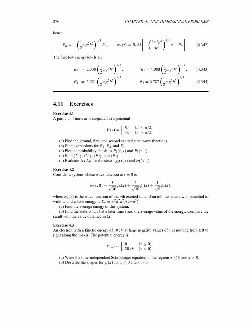
276 CHAPTER 4. ONE-DIMENSIONAL PROBLEMS
hence
En1
2mg2h2
1 3
Rn n z BnAi2m2g2
h2
1 3
z Rn (4.342)
The first few energy levels are
E0 2 3381
2mg2h2
1 3
E1 4 0881
2mg2h2
1 3
(4.343)
E2 5 5211
2mg2h2
1 3
E3 6 7871
2mg2h2
1 3
(4.344)
4.11 Exercises
Exercise 4.1
A particle of mass m is subjected to a potential
V x0 x a 2
x a 2
(a) Find the ground, first, and second excited state wave functions.
(b) Find expressions for E1, E2, and E3.(c) Plot the probability densities P2 x t and P3 x t .(d) Find X 2 X 3 P 2, and P 3.
(e) Evaluate x p for the states 2 x t and 3 x t .
Exercise 4.2
Consider a system whose wave function at t 0 is
x 03
300 x
4
301 x
1
64 x
where n x is the wave function of the nth excited state of an infinite square well potential ofwidth a and whose energy is En 2h2n2 2ma2 .(a) Find the average energy of this system.
(b) Find the state x t at a later time t and the average value of the energy. Compare theresult with the value obtained in (a).
Exercise 4.3
An electron with a kinetic energy of 10 eV at large negative values of x is moving from left toright along the x-axis. The potential energy is
V x0 x 0
20 eV x 0
(a) Write the time-independent Schrödinger equation in the regions x 0 and x 0.
(b) Describe the shapes for x for x 0 and x 0.
4.11. EXERCISES 277
(c) Calculate the electron wavelength (in meters) in 20m x 10m and x 10m.
(d) Write down the boundary conditions at x 0.
(e) Calculate the ratio of the probabilities for finding the electron near x 10 10m and
x 0.
Exercise 4.4
A particle is moving in the potential well
V x
0 a x bV0 b x b0 b x a
elsewhere
where V0 is positive. In this problem consider E V0. Let 1 x and 2 x represent the twolowest energy solutions of the Schrödinger equation; call their energies E1 and E2, respectively.(a) Calculate E1 and E2 in units of eV for the case where mc2 1GeV, a 10 14m, and
b 0 4 10 14m; take hc 200MeV fm.
(b) A particular solution of the Schrödinger equation can be constructed by superposing
1 x ei E1t h and 2 x ei E2t h . Construct a wave packet which at t 0 is (almost) entirely
to the left-hand side of the well and describe its motion in time; find the period of oscillations
between the two terms of .
Exercise 4.5
A particle moves in the potential
V xh2
2m
4
225sinh2 x
2
5cosh x
(a) Sketch V x and locate the position of the two minima.
(b) Show that x 1 4 cosh x exp 215cosh x is a solution of the time-independent
Schrödinger equation for the particle. Find the corresponding energy level and indicate its
position on the sketch of V x .(c) Sketch x and show that it has the proper behavior at the classical turning points and
in the classically forbidden regions.
Exercise 4.6
Show that for a particle of mass m which moves in a one-dimensional infinite potential well oflength a, the uncertainties product xn pn is given by xn pn n h 12.
Exercise 4.7
A particle of mass m is moving in an infinite potential well
V xV0 0 x a
elsewhere
(a) Solve the Schrödinger equation and find the energy levels and the corresponding nor-
malized wave functions.
(b) Calculate X 5, P 5, X2 5, and P2 5 for the fourth excited state and infer the valueof x p.
278 CHAPTER 4. ONE-DIMENSIONAL PROBLEMS
Exercise 4.8
Consider the potential step
V x6 eV x 0
0 x 0
(a) An electron of energy 8 eV is moving from left to right in this potential. Calculate the
probability that the electron will (i) continue moving along its initial direction after reaching
the step and (ii) get reflected at the potential step.
(b) Now suppose the electron is moving from right to left with an energy 3 eV. (i) Estimate
the order of magnitude of the distance the electron can penetrate the barrier. (ii) Repeat part (i)
for a 70 kg person initially moving at 4m s 1 and running into a wall which can be represented
by a potential step of height equal to four times this person’s energy before reaching the step.
Exercise 4.9
Consider a system whose wave function at time t 0 is given by
x 05
500 x
4
501 x
3
502 x
where n x is the wave function of the nth excited state for a harmonic oscillator of energyEn h n 1 2 .
(a) Find the average energy of this system.
(b) Find the state x t at a later time t and the average value of the energy; compare theresult with the value obtained in (a).
(c)Find the expectation value of the operator X with respect to the state x t (i.e., findx t X x t ).
Exercise 4.10
Calculate n X2 m and m X4 n in the N -representation; n and m are harmonic
oscillator states.
Exercise 4.11
Consider the dimensionless Hamiltonian H 12P2 1
2X2, with P id dx .
(a) Show that the wave functions 0 x e x2 2 and 1 x 2 xe x2 2 are
eigenfunctions of H with eigenvalues 1 2 and 3 2, respectively.(b) Find the values of the coefficients and such that
2 x1
2x2 1 e x2 2 and 3 x
1
6x 1 x2 e x2 2
are orthogonal to 0 x and 1 x , respectively. Then show that 2 x and 3 x are eigen-
functions of H with eigenvalues 5 2 and 7 2, respectively.
Exercise 4.12
Consider the dimensionless Hamiltonian H 12P2 1
2X2 (with P id dx) whose wave
function at time t 0 is given by
x 01
20 x
1
81 x
1
102 x
4.11. EXERCISES 279
where 0 x1 e x2 2, 1 x
2 xe x2 2, and 2 x1
22x2 1 e x2 2.
(a) Calculate xn pn for n 0 1 where xn n X2 n n X n2.
(b) Calculate a† 0 x , a 0 x , a† 1 x , a 1 x , and a 2 x , where the operators a† and
a are defined by a X d dx 2 and a† X d dx 2.
Exercise 4.13
Consider a particle of mass m that is moving in a one-dimensional infinite potential well withwalls at x 0 and x a which is initially (i.e., at t 0) in the state
x 01
2[ 1 x 3 x ]
where 1 x and 3 x are the ground and second excited states, respectively.(a) What is the state vector x t for t 0 in the Schrödinger picture.
(b) Find the expectation values X , P , X2 , and P2 with respect to .
(c) Evaluate x p and verify that it satisfies the uncertainty principle.
Exercise 4.14
If the state of a particle moving in a one-dimensional harmonic oscillator is given by
1
170
3
171
2
172
3
173
where n represents the normalized nth energy eigenstate, find the expectation values of thenumber operator, N , and of the Hamiltonian operator.
Exercise 4.15
Find the number of bound states and the corresponding energies for the finite square well po-
tential when (a) R 7 (i.e., ma2V0 2h2 7) and (b) R 3 .
Exercise 4.16
A ball of mass m 0 2 kg bouncing on a table located at z 0 is subject to the potential
V zV0 z 0
mgz z 0
where V0 3 J and g is the acceleration due to gravity.(a) Describe the spectrum of possible energies (i.e., continuous, discrete, or nonexistent) as
E increases from large negative values to large positive values.(b) Estimate the order of magnitude for the lowest energy state.
(c) Describe the general shapes of the wave functions 0 z and 1 z corresponding to thelowest two energy states and sketch the corresponding probability densities.
Exercise 4.17
Consider a particle of mass m moving in a one-dimensional harmonic oscillator potential, with
X h 2m a a† and P i mh 2 a† a .(a) Calculate the product of the uncertainties in position and momentum for the particle in
the fifth excited state, i.e., X P 5.
(b) Compare the result of (a) with the uncertainty product when the particle is in its lowest
energy state. Explain why the two uncertainty products are different.
280 CHAPTER 4. ONE-DIMENSIONAL PROBLEMS
Exercise 4.18
A particle of mass m in an infinite potential well of length a has the following initial wavefunction at t 0:
x 02
7asin
x
a
6
7asin
2 x
a
2
7asin
3 x
a
(a) If we measure energy, what values will we find and with what probabilities? Calculate
the average energy.
(b) Find the wave function x t at any later time t . Determine the probability of findingthe particle at a time t in the state x t 1 a sin 3 x a exp i E3t h .(c) Calculate the probability density x t and the current density J x t . Verify thatt J x t 0.
Exercise 4.19
Consider a particle in an infinite square well whose wave function is given by
xAx a2 x2 0 x a0 elsewhere
where A is a real constant.(a) Find A so that x is normalized.(b) Calculate the position andmomentum uncertainties, x and p, and the product x p.(c) Calculate the probability of finding 52 2h2 2ma2 for a measurement of the energy.
Exercise 4.20
The relativistic expression for the energy of a free particle is E2 m20 c4 p2 c2.
(a) Write down the corresponding relativistic Schrödinger equation, by quantizing this en-
ergy expression (i.e., replacing E and p with their corresponding operators). This equation iscalled the Klein–Gordon equation.
(b) Find the solutions corresponding to a free particle moving along the x-axis.
Exercise 4.21
(a) Write down the classical (gravitational) energy Ec of a particle of massm at rest a heighth0 above the ground (take the zero potential energy to be located at the ground level).(b) Use the uncertainty principle to estimate the ground state energy E0 of the particle
introduced in (a); note that the particle is subject to gravity. Compare E0 to Ec.(c) If h0 3m obtain the numerical values of Ec and the quantum mechanical correc-
tion E0 Ec for a neutron and then for a particle of mass m 0 01 kg. Comment on the
importance of the quantum correction in both cases.
Exercise 4.22
Find the energy levels and the wave functions of two noninteracting particles of masses m1 andm2 that are moving in a common infinite square well potential
V xi0 0 xi a
elsewhere
where xi is the position of the ith particle (i.e., xi denotes x x1 or x2).
4.11. EXERCISES 281
Exercise 4.23
A particle of mass m is subject to a repulsive delta potential V x V0 x , where V0 0 (V0has the dimensions of Energy Distance). Find the reflection and transmission coefficients, Rand T .
Exercise 4.24
A particle of mass m is scattered by a double-delta potential V x V0 x a V0 x a ,where V0 0.
(a) Find the transmission coefficient for the particle at an energy E 0.
(b) When V0 is very large (i.e., V0 ), find the energies corresponding to the resonance
case (i.e., T 1) and compare themwith the energies of an infinite square well potential having
a width of 2a.
Exercise 4.25
A particle of mass m is subject to an antisymmetric delta potential V x V0 x aV0 x a , where V0 0.
(a) Show that there is always one and only one bound state, and find the expression that
gives its energy.
(b) Find the transmission coefficient T .
Exercise 4.26
A particle of mass m is subject to a delta potential
V xx 0
V0 x a x 0
where V0 0.
(a) Find the wave functions corresponding to the cases 0 x a and x a.(b) Find the transmission coefficient.
Exercise 4.27
A particle of mass m, besides being confined to move in an infinite square well potential of size2a with walls at x a and x a, is subject to an attractive delta potential
V xV0 x a x a
elsewhere
where V0 0.
(a) Find the particle’s wave function corresponding to even solutions when E 0.
(b) Find the energy levels corresponding to even solutions.
Exercise 4.28
A particle of mass m, besides being confined to move in an infinite square well potential of size2a with walls at x a and x a, is subject to an attractive delta potential
V xV0 x a x a
elsewhere
where V0 0.
(a) Find the particle’s wave function corresponding to odd solutions when E 0.
(b) Find the energy levels corresponding to odd solutions.
282 CHAPTER 4. ONE-DIMENSIONAL PROBLEMS
Exercise 4.29
Consider a particle of mass m that is moving under the influence of an attractive delta potential
V xV0 x x a
x a
where V0 0. Discuss the existence of bound states in terms of V0 and a.
Exercise 4.30
Consider a system of two identical harmonic oscillators (with an angular frequency ).
(a) Find the energy levels when the oscillators are independent (non-interacting).
(b) Find the energy levels when the oscillators are coupled by an interaction X1X2,where is a constant.
(c) Assuming that m 2 (weak coupling limit), find an approximate value to first order
in m 2 for the energy expression derived in part (b).
Exercise 4.31
A particle is initially in its ground state in an infinite one-dimensional potential box with sides
at x 0 and x a. If the wall of the box at x a is suddenly moved to x 3a, calculate theprobability of finding the particle in
(a) the ground state of the new box and
(b) the first excited state of the new box.
(c) Now, calculate the probability of finding the particle in the first excited state of the new
box, assuming the particle was initially in the first excited state of the old box.
Exercise 4.32
A particle is initially in its ground state in a one-dimensional harmonic oscillator potential,
V x 12kx2. If the spring constant is suddenly doubled, calculate the probability of finding
the particle in the ground state of the new potential.
Exercise 4.33
Consider an electron in an infinite potential well
V x0 0 x a
elsewhere
where a 10 10m.
(a) Calculate the energy levels of the three lowest states (the results should be expressed in
eV) and the corresponding wavelengths of the electron.
(b) Calculate the frequency of the radiation that would cause the electron to jump from the
ground to the third excited energy level.
(c) When the electron de-excites, what are the frequencies of the emitted photons?
(d) Specify the probability densities for all these three states and plot them.
Exercise 4.34
Consider an electron which is confined to move in an infinite square well of width a 10 10m.(a) Find the exact energies of the 11 lowest states (express them in eV).
(b) Solve the Schrödinger equation numerically and find the energies of the 11 lowest statesand compare them with the exact results obtained in (a). Plot the wave functions of the five
lowest states.
Chapter 5
Angular Momentum
5.1 Introduction
After treating one-dimensional problems in Chapter 4, we now should deal with three-dimensional
problems. However, the study of three-dimensional systems such as atoms cannot be under-
taken unless we first cover the formalism of angular momentum. The current chapter, therefore,
serves as an essential prelude to Chapter 6.
Angular momentum is as important in classical mechanics as in quantum mechanics. It
is particularly useful for studying the dynamics of systems that move under the influence of
spherically symmetric, or central, potentials, V r V r , for the orbital angular momenta ofthese systems are conserved. For instance, as mentioned in Chapter 1, one of the cornerstonesof Bohr’s model of the hydrogen atom (where the electron moves in the proton’s Coulomb
potential, a central potential) is based on the quantization of angular momentum. Additionally,
angular momentum plays a critical role in the description of molecular rotations, the motion
of electrons in atoms, and the motion of nucleons in nuclei. The quantum theory of angular
momentum is thus a prerequisite for studying molecular, atomic, and nuclear systems.
In this chapter we are going to consider the general formalism of angular momentum. We
will examine the various properties of the angular momentum operator, and then focus on de-
termining its eigenvalues and eigenstates. Finally, we will apply this formalism to the determi-
nation of the eigenvalues and eigenvectors of the spin and orbital angular momenta.
5.2 Orbital Angular Momentum
In classical physics the angular momentum of a particle with momentum p and position r isdefined by
L r p ypz zpy i zpx xpz j xpy ypx k (5.1)
The orbital angular momentum operator L can be obtained at once by replacing r and p by the
corresponding operators in the position representation, R and P ih :
L R P ihR (5.2)
283
284 CHAPTER 5. ANGULAR MOMENTUM
The Cartesian components of L are
Lx Y Pz Z Py ih Yz
Zy
(5.3)
L y Z Px X Pz ih Zx
Xz
(5.4)
L z X Py Y Px ih Xy
Yx
(5.5)
Clearly, angular momentum does not exist in a one-dimensional space. We should mention that
the components Lx , L y , Lz , and the square of L ,
L2
L2x L2y L2z (5.6)
are all Hermitian.
Commutation relations
Since X , Y , and Z mutually commute and so do Px , Py , and Pz , and since [X Px ] ih,
[Y Py] ih, [Z Pz] ih, we have
[Lx L y] [Y Pz Z Py Z Px X Pz]
[Y Pz Z Px ] [Y Pz X Pz] [Z Py Z Px ] [Z Py X Pz]
Y [Pz Z ]Px X [Z Pz]Py ih X Py Y Px
ihLz (5.7)
A similar calculation yields the other two commutation relations; but it is much simpler to infer
them from (5.7) by means of a cyclic permutation of the xyz components, x y z x :
[Lx L y] ihL z [L y Lz] ihLx [L z Lx ] ihL y (5.8)
As mentioned in Chapter 3, since Lx , L y , and Lz do not commute, we cannot measure themsimultaneously to arbitrary accuracy.
Note that the commutation relations (5.8) were derived by expressing the orbital angular
momentum in the position representation, but since these are operator relations, they mustbe valid in any representation. In the following section we are going to consider the general
formalism of angular momentum, a formalism that is restricted to no particular representation.
Example 5.1
(a) Calculate the commutators [X Lx ], [X L y], and [X Lz].
(b) Calculate the commutators: [Px Lx ], [Px L y], and [Px Lz].
(c) Use the results of (a) and (b) to calculate [X L2] and [Px L2].
5.3. GENERAL FORMALISM OF ANGULAR MOMENTUM 285
Solution
(a) The only nonzero commutator which involves X and the various components of Lx , L y ,
Lz is [X Px ] ih. Having stated this result, we can easily evaluate the needed commutators.First, since Lx Y Pz Z Py involves no Px , the operator X commutes separately with Y , Pz ,
Z , and Py ; hence
[X Lx ] [X Y Pz Z Py] 0 (5.9)
The evaluation of the other two commutators is straightforward:
[X L y] [X Z Px X Pz] [X Z Px ] Z [X Px ] ihZ (5.10)
[X L z] [X X Py Y Px ] [X Y Px ] Y [X Px ] ihY (5.11)
(b) The only commutator between Px and the components of Lx , L y , L z that survives is
again [Px X] ih. We may thus infer
[Px Lx ] [Px Y Pz Z Py] 0 (5.12)
[Px L y] [Px Z Px X Pz] [Px X Pz] [Px X ]Pz ihPz (5.13)
[Px Lz] [Px X Py Y Px ] [Px X Py] [Px X]Py ihPy (5.14)
(c) Using the commutators derived in (a) and (b), we infer
[X L2] [X L2x ] [X L2y] [X L2z ]
0 L y[X L y] [X L y]L y Lz[X Lz] [X L z]Lz
ih L yZ ZL y LzY Y L y (5.15)
[Px L2] [Px L2x ] [Px L2y] [Px L2z ]
0 L y[Px L y] [Px L y]L y Lz[Px L z] [Px L z]Lz
ih L yPz PzL y LzPy PyL y (5.16)
5.3 General Formalism of Angular Momentum
Let us now introduce a more general angular momentum operator J that is defined by its threecomponents Jx Jy and Jz , which satisfy the following commutation relations:
[Jx Jy] ih Jz [Jy Jz] ih Jx [Jz Jx ] ih Jy (5.17)
or equivalently by
J J ih J (5.18)
Since Jx , Jy , and Jz do not mutually commute, they cannot be simultaneously diagonalized;that is, they do not possess common eigenstates. The square of the angular momentum,
J2 J 2x J 2y J 2z (5.19)
286 CHAPTER 5. ANGULAR MOMENTUM
is a scalar operator; hence it commutes with Jx Jy and Jz:
[J2 Jk] 0 (5.20)
where k stands for x y, and z. For instance, in the the case k x we have
[J 2 Jx ] [J 2x Jx ] Jy[Jy Jx ] [Jy Jx ]Jy Jz[Jz Jx ] [Jz Jx ]Jz
Jy ih Jz ih Jz Jy Jz ih Jy ih Jy Jz
0 (5.21)
because [J2x Jx ] 0, [Jy Jx ] ih Jz , and [Jz Jx ] ih Jy . We should note that the
operators Jx , Jy , Jz , and J 2 are all Hermitian; their eigenvalues are real.
Eigenstates and eigenvalues of the angular momentum operator
Since J 2 commutes with Jx , Jy and Jz , each component of J can be separately diagonalized
(hence it has simultaneous eigenfunctions) with J 2. But since the components Jx , Jy and Jzdo not mutually commute, we can choose only one of them to be simultaneously diagonalized
with J2. By convention we choose Jz . There is nothing special about the z-direction; we can
just as well take J2 and Jx or J 2 and Jy .
Let us now look for the joint eigenstates of J 2 and Jz and their corresponding eigenvalues.
Denoting the joint eigenstates by and the eigenvalues of J 2 and Jz by h2 and h ,
respectively, we have
J 2 h2 (5.22)
Jz h (5.23)
The factor h is introduced so that and are dimensionless; recall that the angular momentum
has the dimensions of h and that the physical dimensions of h are: [h] energy time. For
simplicity, we will assume that these eigenstates are orthonormal:
(5.24)
Now we need to introduce raising and lowering operators J and J , just as we did whenwe studied the harmonic oscillator in Chapter 4:
J Jx i Jy (5.25)
This leads to
Jx1
2J J Jy
1
2iJ J (5.26)
hence
J 2x1
4J 2 J J J J J 2 J 2y
1
4J 2 J J J J J2 (5.27)
Using (5.17) we can easily obtain the following commutation relations:
[J 2 J ] 0 [J J ] 2hJz [Jz J ] hJ (5.28)
5.3. GENERAL FORMALISM OF ANGULAR MOMENTUM 287
In addition, J and J satisfy
J J J 2x J 2y hJz J2 J2z hJz (5.29)
J J J2x J2y hJz J 2 J 2z hJz (5.30)
These relations lead to
J2 J J J2z hJz (5.31)
which in turn yield
J 21
2J J J J J 2z (5.32)
Let us see how J operate on . First, since J do not commute with Jz , the ketsare not eigenstates of J . Using the relations (5.28) we have
Jz J J Jz hJ h 1 J (5.33)
hence the ket (J ) is an eigenstate of Jz with eigenvalues h 1 . Now since Jz and
J2 commute, (J ) must also be an eigenstate of J 2. The eigenvalue of J 2 when acting
on J can be determined by making use of the commutator [J2 J ] 0. The state
(J is also an eigenstate of J 2 with eigenvalue h2 :
J2 J J J 2 h2 J (5.34)
From (5.33) and (5.34) we infer that when J acts on , it does not affect the first quantum
number , but it raises or lowers the second quantum number by one unit. That is, Jis proportional to 1 :
J C 1 (5.35)
We will determine the constant C later on.
Note that, for a given eigenvalue of J 2, there exists an upper limit for the quantum number
. This is due to the fact that the operator J 2 J2z is positive, since the matrix elements of
J2 J2z J 2x J 2y are 0; we can therefore write
J 2 J 2z h2 2 0 2 (5.36)
Since has an upper limit max , there must exist a state max which cannot be raised
further:
J max 0 (5.37)
Using this relation along with J J J 2 J2z hJz , we see that J J max 0 or
J2 J2z hJz max h2 2max max max (5.38)

288 CHAPTER 5. ANGULAR MOMENTUM
hence
max max 1 (5.39)
After n successive applications of J on max , we must be able to reach a state min
which cannot be lowered further:
J min 0 (5.40)
Using J J J 2 J 2z hJz , and by analogy with (5.38) and (5.39), we infer that
min min 1 (5.41)
Comparing (5.39) and (5.41) we obtain
max min (5.42)
Since min was reached by n applications of J on max , it follows that
max min n (5.43)
and since min max we conclude that
maxn
2(5.44)
Hence max can be integer or half-odd-integer, depending on n being even or odd.It is now appropriate to introduce the notation j and m to denote max and , respectively:
j maxn
2m (5.45)
hence the eigenvalue of J 2 is given by
j j 1 (5.46)
Now since min max , and with n positive, we infer that the allowed values of m liebetween j and j :
j m j (5.47)
The results obtained thus far can be summarized as follows: the eigenvalues of J 2 and Jzcorresponding to the joint eigenvectors j m are given, respectively, by h2 j j 1 and hm:
J2 j m h2 j j 1 j m and Jz j m hm j m (5.48)
where j 0, 1 2, 1, 3 2 andm j , j 1 , , j 1, j . So for each j there are 2 j 1
values of m. For example, if j 1 then m takes the three values 1, 0, 1; and if j 5 2 then
m takes the six values 5 2, 3 2, 1 2, 1 2, 3 2, 5 2. The values of j are either integer or
half-integer. We see that the spectra of the angular momentum operators J 2 and Jz are discrete.Since the eigenstates corresponding to different angular momenta are orthogonal, and since the
angular momentum spectra are discrete, the orthonormality condition is
j m j m j j m m (5.49)
5.3. GENERAL FORMALISM OF ANGULAR MOMENTUM 289
Let us now determine the eigenvalues of J within the j m basis; j m is not an
eigenstate of J . We can rewrite equation (5.35) as
J j m C jm j m 1 (5.50)
We are going to derive C j m and then infer C j m . Since j m is normalized, we can use (5.50)
to obtain the following two expressions:
J j m † J j m C jm2 j m 1 j m 1 C j m
2 (5.51)
C jm2
j m J J j m (5.52)
But since J J is equal to J2 J 2z h Jz , and assuming the arbitrary phase of C j m to bezero, we conclude that
C jm j m J2 J2z hJz j m h j j 1 m m 1 (5.53)
By analogy with C j m we can easily infer the expression for C j m :
C jm h j j 1 m m 1 (5.54)
Thus, the eigenvalue equations for J and J are given by
J j m h j j 1 m m 1 j m 1 (5.55)
or
J j m h j m j m 1 j m 1 (5.56)
which in turn leads to the two relations:
Jx j m1
2J J j m
h
2j m j m 1 j m 1 j m j m 1 j m 1
(5.57)
Jy j m1
2iJ J j m
h
2ij m j m 1 j m 1 j m j m 1 j m 1
(5.58)
The expectation values of Jx and Jy are therefore zero:
j m Jx j m j m Jy j m 0 (5.59)
We will show later in (5.208) that the expectation values j m J2x j m and j m J 2yj m are equal and given by
J2x J2y1
2j m J2 j m j m J2z j m
h2
2j j 1 m2
(5.60)
290 CHAPTER 5. ANGULAR MOMENTUM
Example 5.2
Calculate [J2x Jy], [J 2z Jy], and [J 2 Jy]; then show j m J2x j m j m J 2yj m .
Solution
Since [Jx Jy] ih Jz and [Jz Jx ] ih Jy , we have
[J 2x Jy] Jx [Jx Jy] [Jx Jy]Jx ih Jx Jz Jz Jx ih 2Jx Jz ih Jy (5.61)
Similarly, since [Jz Jy] ih Jx and [Jz Jx ] ih Jy , we have
[J 2z Jy] Jz[Jz Jy] [Jz Jy]Jz ih Jz Jx Jx Jz ih 2Jx Jz ih Jy (5.62)
The previous two expressions yield
[J2 Jy] [J2x J 2y J 2z Jy] [J2x Jy] [J 2z Jy]
ih 2Jx Jz ih Jy ih 2Jx Jz ih Jy 0 (5.63)
Since we have
J 2x1
4J2 J J J J J 2 J2y
1
4J2 J J J J J 2 (5.64)
and since j m J2 j m j m J 2 j m 0, we can write
j m J2x j m1
4j m J J J J j m j m J 2y j m (5.65)
5.4 Matrix Representation of Angular Momentum
The formalism of the previous section is general and independent of any particular representa-
tion. There are many ways to represent the angular momentum operators and their eigenstates.
In this section we are going to discuss the matrix representation of angular momentum where
eigenkets and operators will be represented by column vectors and square matrices, respec-
tively. This is achieved by expanding states and operators in a discrete basis. We will see later
how to represent the orbital angular momentum in the position representation.
Since J 2 and Jz commute, the set of their common eigenstates j m can be chosen as a
basis; this basis is discrete, orthonormal, and complete. For a given value of j , the orthonormal-ization condition for this base is given by (5.49), and the completeness condition is expressed
byj
m j
j m j m I (5.66)
where I is the unit matrix. The operators J2 and Jz are diagonal in the basis given by their jointeigenstates
j m J2 j m h2 j j 1 j j m m (5.67)
j m Jz j m hm j j m m (5.68)
5.4. MATRIX REPRESENTATION OF ANGULAR MOMENTUM 291
Thus, the matrices representing J 2 and Jz in the j m eigenbasis are diagonal, their diago-
nal elements being equal to h2 j j 1 and hm, respectively.Now since the operators J do not commute with Jz , they are represented in the j m
basis by matrices that are not diagonal:
j m J j m h j j 1 m m 1 j j m m 1 (5.69)
We can infer the matrices of Jx and Jy from (5.57) and (5.58):
j m Jx j mh
2j j 1 m m 1 m m 1
j j 1 m m 1 m m 1 j j (5.70)
j m Jy j mh
2ij j 1 m m 1 m m 1
j j 1 m m 1 m m 1 j j (5.71)
Example 5.3 (Angular momentum j 1)
Consider the case where j 1.
(a) Find the matrices representing the operators J 2, Jz , J , Jx , and Jy .
(b) Find the joint eigenstates of J2 and Jz and verify that they form an orthonormal andcomplete basis.
(c) Use the matrices of Jx , Jy and Jz to calculate [Jx Jy], [Jy Jz], and [Jz Jx ].
(d) Verify that J 3z h2 Jz and J 3 0.
Solution
(a) For j 1 the allowed values of m are 1, 0, 1. The joint eigenstates of J 2 and Jz are
1 1 , 1 0 , and 1 1 . The matrix representations of the operators J 2 and Jz can beinferred from (5.67) and (5.68):
J 21 1 J2 1 1 1 1 J 2 1 0 1 1 J2 1 1
1 0 J2 1 1 1 0 J 2 1 0 1 0 J2 1 1
1 1 J2 1 1 1 1 J 2 1 0 1 1 J 2 1 1
2h21 0 0
0 1 0
0 0 1
(5.72)
Jz h1 0 0
0 0 0
0 0 1
(5.73)
Similarly, using (5.69), we can ascertain that the matrices of J and J are given by
J h 2
0 0 0
1 0 0
0 1 0
J h 2
0 1 0
0 0 1
0 0 0
(5.74)

292 CHAPTER 5. ANGULAR MOMENTUM
The matrices for Jx and Jy in the j m basis result immediately from the relations JxJ J 2 and Jy i J J 2:
Jxh
2
0 1 0
1 0 1
0 1 0
Jyh
2
0 i 0
i 0 i0 i 0
(5.75)
(b) The joint eigenvectors of J2 and Jz can be obtained as follows. The matrix equation ofJz j m mh j m is
h1 0 0
0 0 0
0 0 1
abc
mhabc
ha mha0 mhbhc mhc
(5.76)
The normalized solutions to these equations for m 1, 0, 1 are respectively given by a 1,
b c 0; a 0, b 1, c 0; and a b 0, c 1; that is,
1 1
1
0
0
1 0
0
1
0
1 1
0
0
1
(5.77)
We can verify that these vectors are orthonormal:
1 m 1 m m m m m 1 0 1 (5.78)
We can also verify that they are complete:
1
m 1
1 m 1 m0
0
1
0 0 1
0
1
0
0 1 0
1
0
0
1 0 0
1 0 0
0 1 0
0 0 1
(5.79)
(c) Using the matrices (5.75) we have
Jx Jyh2
2
0 1 0
1 0 1
0 1 0
0 i 0
i 0 i0 i 0
h2
2
i 0 i0 0 0
i 0 i(5.80)
Jy Jxh2
2
0 i 0
i 0 i0 i 0
0 1 0
1 0 1
0 1 0
h2
2
i 0 i0 0 0
i 0 i(5.81)
hence
Jx Jy Jy Jxh2
2
2i 0 0
0 0 0
0 0 2iih2
1 0 0
0 0 0
0 0 1
ih Jz (5.82)
where the matrix of Jz is given by (5.73). A similar calculation leads to [Jy Jz] ih Jx and
[Jz Jx ] ih Jy .
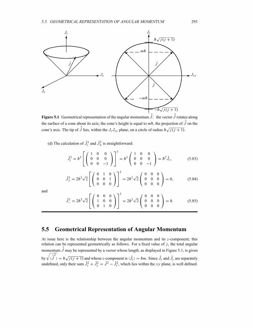
5.5. GEOMETRICAL REPRESENTATION OF ANGULAR MOMENTUM 293
-©©©©©©¼
6Jz
Jy
Jx
J
¡¡¡¡¡¡
@@
@@
@@
¢¢¢¢¢̧
-
6
¡¡¡¡¡¡µ
J
mh
@@@@@@R
J
mh
@@
@@
@@I
¡¡
¡¡
¡¡ª
Jz
Jxy
h j j 1
h j j 1
Figure 5.1 Geometrical representation of the angular momentum J : the vector J rotates along
the surface of a cone about its axis; the cone’s height is equal to mh, the projection of J on the
cone’s axis. The tip of J lies, within the Jz Jxy plane, on a circle of radius h j j 1 .
(d) The calculation of J 3z and J3 is straightforward:
J 3z h31 0 0
0 0 0
0 0 1
3
h31 0 0
0 0 0
0 0 1
h2 Jz (5.83)
J 3 2h3 2
0 1 0
0 0 1
0 0 0
3
2h3 2
0 0 0
0 0 0
0 0 0
0 (5.84)
and
J 3 2h3 2
0 0 0
1 0 0
0 1 0
3
2h3 2
0 0 0
0 0 0
0 0 0
0 (5.85)
5.5 Geometrical Representation of Angular Momentum
At issue here is the relationship between the angular momentum and its z-component; thisrelation can be represented geometrically as follows. For a fixed value of j , the total angular
momentum J may be represented by a vector whose length, as displayed in Figure 5.1, is given
by J2
h j j 1 and whose z-component is Jz hm. Since Jx and Jy are separately
undefined, only their sum J 2x J 2y J2 J 2z , which lies within the xy plane, is well defined.
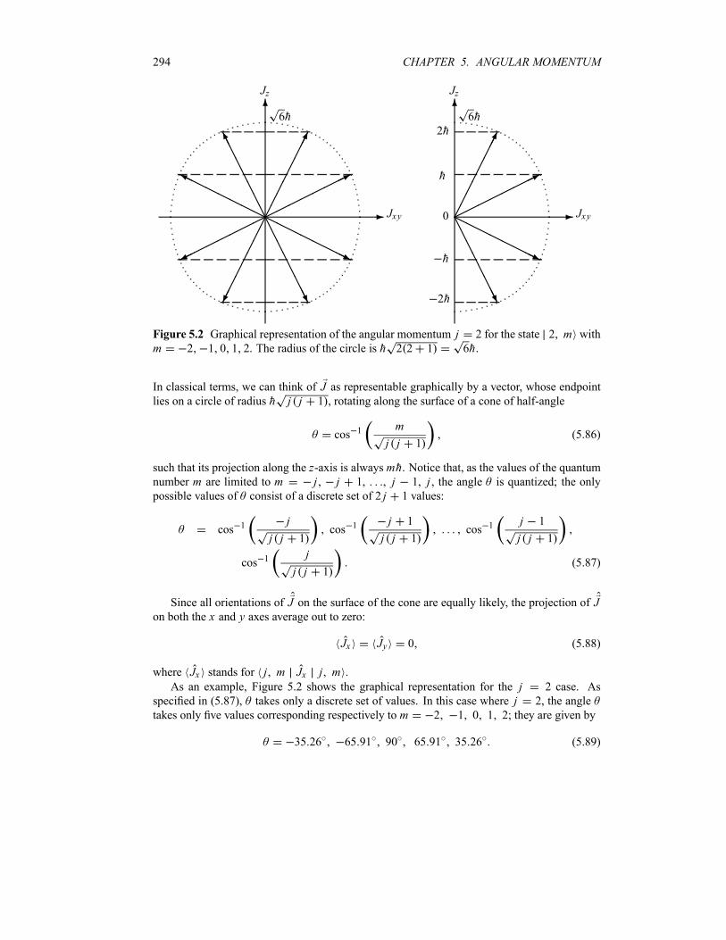
294 CHAPTER 5. ANGULAR MOMENTUM
-
6
AAAAAAAAU
¢¢¢¢¢¢¢¢®
HHHHHHHHj
©©©©©©©©¼
©©©©
©©©©*
HHHH
HHHHY
¢¢¢¢¢¢¢¢̧
AAAAAAAAK
Jz
Jxy
6h
-
6
0
6h
AAAAAAAAU2h
HHHHHHHHjh
©©©©
©©©©*h
¢¢¢¢¢¢¢¢̧
2h
Jz
Jxy
Figure 5.2 Graphical representation of the angular momentum j 2 for the state 2 m with
m 2 1 0 1 2. The radius of the circle is h 2 2 1 6h.
In classical terms, we can think of J as representable graphically by a vector, whose endpointlies on a circle of radius h j j 1 , rotating along the surface of a cone of half-angle
cos 1 m
j j 1(5.86)
such that its projection along the z-axis is always mh. Notice that, as the values of the quantumnumber m are limited to m j , j 1, , j 1, j , the angle is quantized; the only
possible values of consist of a discrete set of 2 j 1 values:
cos 1 j
j j 1cos 1 j 1
j j 1cos 1 j 1
j j 1
cos 1 j
j j 1(5.87)
Since all orientations of J on the surface of the cone are equally likely, the projection of Jon both the x and y axes average out to zero:
Jx Jy 0 (5.88)
where Jx stands for j m Jx j m .As an example, Figure 5.2 shows the graphical representation for the j 2 case. As
specified in (5.87), takes only a discrete set of values. In this case where j 2, the angle
takes only five values corresponding respectively to m 2 1 0 1 2; they are given by
35 26 65 91 90 65 91 35 26 (5.89)
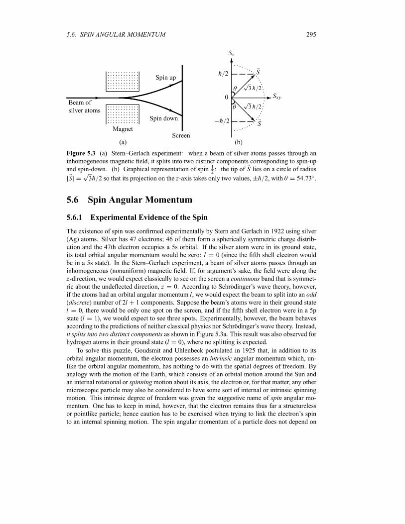
5.6. SPIN ANGULAR MOMENTUM 295
Beam of
silver atoms
MagnetScreen
Spin up
Spin down
-©©*
HHj
-
6
0@@@@R
Sh 2
¡¡¡¡µ
Sh 2
3 h 2
3 h 2
Sz
Sxy
(a) (b)
Figure 5.3 (a) Stern–Gerlach experiment: when a beam of silver atoms passes through an
inhomogeneous magnetic field, it splits into two distinct components corresponding to spin-up
and spin-down. (b) Graphical representation of spin 12: the tip of S lies on a circle of radius
S 3h 2 so that its projection on the z-axis takes only two values, h 2, with 54 73 .
5.6 Spin Angular Momentum
5.6.1 Experimental Evidence of the Spin
The existence of spin was confirmed experimentally by Stern and Gerlach in 1922 using silver
(Ag) atoms. Silver has 47 electrons; 46 of them form a spherically symmetric charge distrib-
ution and the 47th electron occupies a 5s orbital. If the silver atom were in its ground state,
its total orbital angular momentum would be zero: l 0 (since the fifth shell electron would
be in a 5s state). In the Stern–Gerlach experiment, a beam of silver atoms passes through an
inhomogeneous (nonuniform) magnetic field. If, for argument’s sake, the field were along the
z-direction, we would expect classically to see on the screen a continuous band that is symmet-ric about the undeflected direction, z 0. According to Schrödinger’s wave theory, however,
if the atoms had an orbital angular momentum l, we would expect the beam to split into an odd(discrete) number of 2l 1 components. Suppose the beam’s atoms were in their ground state
l 0, there would be only one spot on the screen, and if the fifth shell electron were in a 5p
state (l 1), we would expect to see three spots. Experimentally, however, the beam behaves
according to the predictions of neither classical physics nor Schrödinger’s wave theory. Instead,
it splits into two distinct components as shown in Figure 5.3a. This result was also observed forhydrogen atoms in their ground state (l 0), where no splitting is expected.
To solve this puzzle, Goudsmit and Uhlenbeck postulated in 1925 that, in addition to its
orbital angular momentum, the electron possesses an intrinsic angular momentum which, un-like the orbital angular momentum, has nothing to do with the spatial degrees of freedom. By
analogy with the motion of the Earth, which consists of an orbital motion around the Sun and
an internal rotational or spinningmotion about its axis, the electron or, for that matter, any othermicroscopic particle may also be considered to have some sort of internal or intrinsic spinning
motion. This intrinsic degree of freedom was given the suggestive name of spin angular mo-mentum. One has to keep in mind, however, that the electron remains thus far a structureless
or pointlike particle; hence caution has to be exercised when trying to link the electron’s spin
to an internal spinning motion. The spin angular momentum of a particle does not depend on
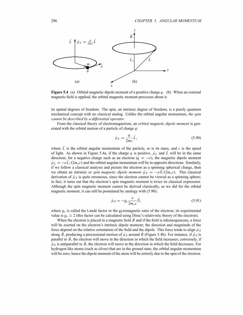
296 CHAPTER 5. ANGULAR MOMENTUM
PPPq
6L Lq2mc L
wq
m³³³1
-©©©©©©¼
6z
B
y
x
LLz
¡¡¡¡¡¡µ
(a) (b)
Figure 5.4 (a) Orbital magnetic dipole moment of a positive charge q. (b) When an externalmagnetic field is applied, the orbital magnetic moment precesses about it.
its spatial degrees of freedom. The spin, an intrinsic degree of freedom, is a purely quantum
mechanical concept with no classical analog. Unlike the orbital angular momentum, the spincannot be described by a differential operator.From the classical theory of electromagnetism, an orbital magnetic dipole moment is gen-
erated with the orbital motion of a particle of charge q:
Lq
2mcL (5.90)
where L is the orbital angular momentum of the particle, m is its mass, and c is the speedof light. As shown in Figure 5.4a, if the charge q is positive, L and L will be in the samedirection; for a negative charge such as an electron (q e), the magnetic dipole moment
L eL 2mec and the orbital angular momentum will be in opposite directions. Similarly,if we follow a classical analysis and picture the electron as a spinning spherical charge, then
we obtain an intrinsic or spin magnetic dipole moment S eS 2mec . This classicalderivation of S is quite erroneous, since the electron cannot be viewed as a spinning sphere;
in fact, it turns out that the electron’s spin magnetic moment is twice its classical expression.
Although the spin magnetic moment cannot be derived classically, as we did for the orbital
magnetic moment, it can still be postulated by analogy with (5.90):
S gse
2mecS (5.91)
where gs is called the Landé factor or the gyromagnetic ratio of the electron; its experimentalvalue is gs 2 (this factor can be calculated using Dirac’s relativistic theory of the electron).
When the electron is placed in a magnetic field B and if the field is inhomogeneous, a forcewill be exerted on the electron’s intrinsic dipole moment; the direction and magnitude of the
force depend on the relative orientation of the field and the dipole. This force tends to align S
along B, producing a precessional motion of S around B (Figure 5.4b). For instance, if S is
parallel to B, the electron will move in the direction in which the field increases; conversely, if
S is antiparallel to B, the electron will move in the direction in which the field decreases. Forhydrogen-like atoms (such as silver) that are in the ground state, the orbital angular momentum
will be zero; hence the dipole moment of the atomwill be entirely due to the spin of the electron.
5.6. SPIN ANGULAR MOMENTUM 297
The atomic beamwill therefore deflect according to the orientation of the electron’s spin. Since,
experimentally, the beam splits into two components, the electron’s spin must have only two
possible orientations relative to the magnetic field, either parallel or antiparallel.
By analogy with the orbital angular momentum of a particle, which is characterized by two
quantum numbers—the orbital number l and the azimuthal number ml (with ml l, l 1,
, l 1, l)—the spin angular momentum is also characterized by two quantum numbers, thespin s and its projection ms on the z-axis (the direction of the magnetic field), where ms s,s 1, , s 1, s. Since only two components were observed in the Stern–Gerlach experiment,
we must have 2s 1 2. The quantum numbers for the electron must then be given by s 12
and ms12.
In nature it turns out that every fundamental particle has a specific spin. Some particles
have integer spins s 0, 1, 2 (the pi mesons have spin s 0, the photons have spin s 1,
and so on) and others have half-odd-integer spins s 12, 32, 52
(the electrons, protons, and
neutrons have spin s 12, the deltas have spin s 3
2, and so on). We will see in Chapter 8 that
particles with half-odd-integer spins are called fermions (quarks, electrons, protons, neutrons,etc.) and those with integer spins are called bosons (pions, photons, gravitons, etc.).Besides confirming the existence of spin and measuring it, the Stern–Gerlach experiment
offers a number of other important uses to quantum mechanics. First, by showing that a beam
splits into a discrete set of components rather than a continuous band, it provides additionalconfirmation for the quantum hypothesis on the discrete character of the microphysical world.
The Stern–Gerlach experiment also turns out to be an invaluable technique for preparing a
quantum state. Suppose we want to prepare a beam of spin-up atoms; we simply pass an
unpolarized beam through an inhomogeneous magnet, then collect the desired component and
discard (or block) the other. The Stern–Gerlach experiment can also be used to determine the
total angular momentum of an atom which, in the case where l 0, is given by the sum of the
orbital and spin angular momenta: J L S. The addition of angular momenta is covered inChapter 7.
5.6.2 General Theory of Spin
The theory of spin is identical to the general theory of angular momentum (Section 5.3). By
analogy with the vector angular momentum J , the spin is also represented by a vector operator
S whose components Sx , Sy , Sz obey the same commutation relations as Jx , Jy , Jz:
[Sx Sy] ihSz [Sy Sz] ihSx [Sz Sx ] ihSy (5.92)
In addition, S2 and Sz commute; hence they have common eigenvectors:
S 2 s ms h2s s 1 s ms Sz s ms hms s ms (5.93)
where ms s, s 1, , s 1, s. Similarly, we have
S s ms h s s 1 ms ms 1 s ms 1 (5.94)
where S Sx i Sy , and
S2x S2y1
2S2 S2z
h2
2s s 1 m2s (5.95)
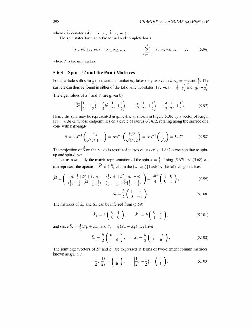
298 CHAPTER 5. ANGULAR MOMENTUM
where A denotes A s ms A s ms .The spin states form an orthonormal and complete basis
s ms s ms s s ms ms
s
ms s
s ms s ms I (5.96)
where I is the unit matrix.
5.6.3 Spin 1 2 and the Pauli Matrices
For a particle with spin 12the quantum number ms takes only two values: ms
12and 1
2. The
particle can thus be found in either of the following two states: s ms12
12and 1
212.
The eigenvalues of S 2 and Sz are given by
S21
2
1
2
3
4h2
1
2
1
2Sz1
2
1
2
h
2
1
2
1
2(5.97)
Hence the spin may be represented graphically, as shown in Figure 5.3b, by a vector of length
S 3h 2, whose endpoint lies on a circle of radius 3h 2, rotating along the surface of acone with half-angle
cos 1 mss s 1
cos 1 h 2
3h 2cos 1 1
354 73 (5.98)
The projection of S on the z-axis is restricted to two values only: h 2 corresponding to spin-up and spin-down.
Let us now study the matrix representation of the spin s 12. Using (5.67) and (5.68) we
can represent the operators S2 and Sz within the s ms basis by the following matrices:
S212
12S2 1
212
12
12
S2 12
12
12
12S2 1
212
12
12
S2 12
12
3h2
4
1 0
0 1(5.99)
Szh
2
1 0
0 1(5.100)
The matrices of S and S can be inferred from (5.69):
S h0 1
0 0S h
0 0
1 0(5.101)
and since Sx12S S and Sy
i2S S , we have
Sxh
2
0 1
1 0Sy
h
2
0 ii 0
(5.102)
The joint eigenvectors of S2 and Sz are expressed in terms of two-element column matrices,known as spinors:
1
2
1
2
1
0
1
2
1
2
0
1(5.103)
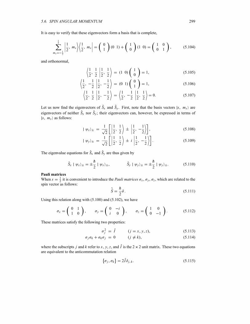
5.6. SPIN ANGULAR MOMENTUM 299
It is easy to verify that these eigenvectors form a basis that is complete,
12
ms12
1
2ms
1
2ms
0
10 1
1
01 0
1 0
0 1(5.104)
and orthonormal,
1
2
1
2
1
2
1
21 0
1
01 (5.105)
1
2
1
2
1
2
1
20 1
0
11 (5.106)
1
2
1
2
1
2
1
2
1
2
1
2
1
2
1
20 (5.107)
Let us now find the eigenvectors of Sx and Sy . First, note that the basis vectors s ms are
eigenvectors of neither Sx nor Sy ; their eigenvectors can, however, be expressed in terms ofs ms as follows:
x1
2
1
2
1
2
1
2
1
2(5.108)
y1
2
1
2
1
2i1
2
1
2(5.109)
The eigenvalue equations for Sx and Sy are thus given by
Sx xh
2x Sy y
h
2y (5.110)
Pauli matrices
When s 12it is convenient to introduce the Pauli matrices x , y , z , which are related to the
spin vector as follows:
Sh
2(5.111)
Using this relation along with (5.100) and (5.102), we have
x0 1
1 0 y0 ii 0 z
1 0
0 1(5.112)
These matrices satisfy the following two properties:
2j I j x y z (5.113)
j k k j 0 j k (5.114)
where the subscripts j and k refer to x y, z, and I is the 2 2 unit matrix. These two equations
are equivalent to the anticommutation relation
j k 2I j k (5.115)
300 CHAPTER 5. ANGULAR MOMENTUM
We can verify that the Pauli matrices satisfy the commutation relations
[ j k] 2i jkl l (5.116)
where jkl is the antisymmetric tensor (also known as the Levi–Civita tensor)
jkl
1 if jkl is an even permutation of x y z1 if jkl is an odd permutation of x y z0 if any two indices among j k l are equal.
(5.117)
We can condense the relations (5.113), (5.114), and (5.116) into
j k j k il
jkl l (5.118)
Using this relation we can verify that, for any two vectors A and B which commute with , we
have
A B A B I i A B (5.119)
where I is the unit matrix. The Pauli matrices are Hermitian, traceless, and have determinantsequal to 1:
†j j Tr j 0 det j 1 j x y z (5.120)
Using the relation x y i z along with 2z I , we obtain
x y z i I (5.121)
From the commutation relations (5.116) we can show that
ei j I cos i j sin j x y z (5.122)
where I is the unit matrix and is an arbitrary real constant.
Remarks
Since the spin does not depend on the spatial degrees of freedom, the components Sx , Sy ,
Sz of the spin operator commute with all the spatial operators, notably the orbital angular
momentum L , the position and the momentum operators R and P:
[S j Lk] 0 [S j Rk] 0 [S j Pk] 0 j k x y z (5.123)
The total wave function of a system with spin consists of a product of two parts: a
spatial part r and a spin part s ms :
s ms (5.124)
This product of the space and spin degrees of freedom is not a product in the usual sense,
but a direct or tensor product as discussed in Chapter 7. We will show in Chapter 6 that
the four quantum numbers n, l, ml , and ms are required to completely describe the stateof an electron moving in a central field; its wave function is
nlmlms r nlml r s ms (5.125)
5.7. EIGENFUNCTIONS OF ORBITAL ANGULAR MOMENTUM 301
Since the spin operator does not depend on the spatial degrees of freedom, it acts only
on the spin part s ms and leaves the spatial wave function, nlml r , unchanged;
conversely, the spatial operators L, R, and P act on the spatial part and not on the spinpart. For spin 1
2particles, the total wave function corresponding to spin-up and spin-down
cases are respectively expressed in terms of the spinors:
nlml12r nlml r
1
0nlml r0
(5.126)
nlml12r nlml r
0
1
0
nlml r(5.127)
Example 5.4
Find the energy levels of a spin s 32particle whose Hamiltonian is given by
Hh2S2x S2y 2S2z h
Sz
and are constants. Are these levels degenerate?
Solution
Rewriting H in the form,
Hh2
S2 3S2z hSz (5.128)
we see that H is diagonal in the s m basis:
Em s m H s mh2
h2s s 1 3h2m2hhm
15
4m 3 m (5.129)
where the quantum number m takes any of the four values m 32, 1
2, 12, 32. Since Em
depends on m, the energy levels of this particle are nondegenerate.
5.7 Eigenfunctions of Orbital Angular Momentum
We now turn to the coordinate representation of the angular momentum. In this section, we are
going to work within the spherical coordinate system. Let us denote the joint eigenstates of L2
and L z by l m :
L2 l m h2l l 1 l m (5.130)
Lz l m hm l m (5.131)
302 CHAPTER 5. ANGULAR MOMENTUM
The operators L z , L2, L , whose Cartesian components are listed in Eqs (5.3) to (5.5), can be
expressed in terms of spherical coordinates (Appendix B) as follows:
Lz ih (5.132)
L2 h21
sinsin
1
sin2
2
2(5.133)
L Lx i L y he i icos
sin(5.134)
Since the operators L z and L depend only on the angles and , their eigenstates depend only
on and . Denoting their joint eigenstates by
l m Ylm (5.135)
where1 Ylm are continuous functions of and , we can rewrite the eigenvalue equations
(5.130) and (5.131) as follows:
L2Ylm h2l l 1 Ylm (5.136)
LzYlm mhYlm (5.137)
Since L z depends only on , as shown in (5.132), the previous two equations suggest that the
eigenfunctions Ylm are separable:
Ylm lm m (5.138)
We ascertain that
L Ylm h l l 1 m m 1 Yl m 1 (5.139)
5.7.1 Eigenfunctions and Eigenvalues of Lz
Inserting (5.138) into (5.137) we obtain L z lm m mh lm m . Now since
L z ih , we have
ih lmm
mh lm m (5.140)
which reduces to
im
m m (5.141)
The normalized solutions of this equation are given by
m1
2eim (5.142)
1For notational consistency throughout this text, we will insert a comma between l and m in Ylm whenever mis negative.
5.7. EIGENFUNCTIONS OF ORBITAL ANGULAR MOMENTUM 303
where 1 2 is the normalization constant,
2
0
d m m m m (5.143)
For m to be single-valued, it must be periodic in with period 2 , m 2 m ;
hence
eim 2 eim (5.144)
This relation shows that the expectation value of L z , lz l m Lz l m , is restricted to adiscrete set of values
lz mh m 0 1 2 3 (5.145)
Thus, the values of m vary from l to l:
m l l 1 l 2 0 1 2 l 2 l 1 l (5.146)
Hence the quantum number l must also be an integer. This is expected since the orbital angularmomentum must have integer values.
5.7.2 Eigenfunctions of L2
Let us now focus on determining the eigenfunctions lm of L2. We are going to followtwo methods. The first method involves differential equations and gives lm in terms of the
well-known associated Legendre functions. The second method is algebraic; it deals with the
operators L and enables an explicit construction of Ylm , the spherical harmonics.
5.7.2.1 First Method for Determining the Eigenfunctions of L2
We begin by applying L2 of (5.133) to the eigenfunctions
Ylm1
2lm eim (5.147)
This gives
L2Ylmh2
2
1
sinsin
1
sin2
2
2 lm eim
h2l l 1
2lm eim (5.148)
which, after eliminating the -dependence, reduces to
1
sin
d
dsin
d lm
dl l 1
m2
sin2lm 0 (5.149)
This equation is known as the Legendre differential equation. Its solutions can be expressed interms of the associated Legendre functions Pml cos :
lm ClmPml cos (5.150)
304 CHAPTER 5. ANGULAR MOMENTUM
which are defined by
Pml x 1 x2 m 2 dm
dx mPl x (5.151)
This shows that
P ml x Pml x (5.152)
where Pl x is the lth Legendre polynomial which is defined by the Rodrigues formula
Pl x1
2ll!
dl
dx lx2 1 l (5.153)
We can obtain at once the first few Legendre polynomials:
P0 x 1 P1 x1
2
d x2 1
dxx (5.154)
P2 x1
8
d2 x2 1 2
dx21
23x2 1 P3 x
1
48
d3 x2 1 3
dx31
25x3 3x
(5.155)
P4 x1
835x4 30x2 3 P5 x
1
863x5 70x3 15x (5.156)
The Legendre polynomials satisfy the following closure or completeness relation:
1
2l 0
2l 1 Pl x Pl x x x (5.157)
From (5.153) we can infer at once
Pl x 1 l Pl x (5.158)
A similar calculation leads to the first few associated Legendre functions:
P11 x 1 x2 (5.159)
P12 x 3x 1 x2 P22 x 3 1 x2 (5.160)
P13 x3
25x2 1 1 x2 P23 x 15x 1 x2 P33 x 15 1 x2 3 2 (5.161)
where P0l x Pl x , with l 0 1 2 3 . The first few expressions for the associated
Legendre functions and the Legendre polynomials are listed in Table 5.1. Note that
Pml x 1 l mPml x (5.162)
The constant Clm of (5.150) can be determined from the orthonormalization condition
l m l m2
0
d0
d sin l m l m l l m m (5.163)
which can be written as
2
0
d0
d sin Yl m Ylm l l m m (5.164)

5.7. EIGENFUNCTIONS OF ORBITAL ANGULAR MOMENTUM 305
Table 5.1 First few Legendre polynomials and associated Legendre functions.
Legendre polynomials Associated Legendre functions
P0 cos 1 P11 cos sin
P1 cos cos P12 cos 3 cos sin
P2 cos123 cos2 1 P22 cos 3 sin2
P3 cos125 cos3 3 cos P13 cos
32sin 5 cos2 1
P4 cos1835 cos4 30 cos2 3 P23 cos 15 sin2 cos
P5 cos1863 cos5 70 cos3 15 cos P33 cos 15 sin3
This relation is known as the normalization condition of spherical harmonics. Using the form
(5.147) for Ylm , we obtain
2
0
d0
d sin Ylm2 Clm 2
2
2
0
d0
d sin Pml cos 2 1 (5.165)
From the theory of associated Legendre functions, we have
0
d sin Pml cos Pml cos2
2l 1
l m !
l m !l l (5.166)
which is known as the normalization condition of associated Legendre functions. A combina-
tion of the previous two relations leads to an expression for the coefficient Clm :
Clm 1 m2l 1
2
l m !
l m !m 0 (5.167)
Inserting this equation into (5.150), we obtain the eigenfunctions of L2:
lm 1 m2l 1
2
l m !
l m !Pml cos (5.168)
Finally, the joint eigenfunctions, Ylm , of L2 and Jz can be obtained by substituting (5.142)and (5.168) into (5.138):
Ylm 1 m2l 1
4
l m !
l m !Pml cos eim m 0 (5.169)
These are called the normalized spherical harmonics.
5.7.2.2 Second Method for Determining the Eigenfunctions of L2
The second method deals with a direct construction of Ylm ; it starts with the case m l(this is the maximum value of m). By analogy with the general angular momentum algebradeveloped in the previous section, the action of L on Yll gives zero,
L l l L Yll 0 (5.170)
306 CHAPTER 5. ANGULAR MOMENTUM
since Yll cannot be raised further as Yll Ylmmax .
Using the expression (5.134) for L in the spherical coordinates, we can rewrite (5.170) as
follows:hei
2i cot ll ei l 0 (5.171)
which leads to1
ll
lll cot (5.172)
The solution to this differential equation is of the form
ll Cl sinl (5.173)
where Cl is a constant to be determined from the normalization condition (5.164) of Yll :
YllCl
2eil sinl (5.174)
We can ascertain that Cl is given by
Cl1 l
2ll!
2l 1 !
2(5.175)
The action of L on Yll is given, on the one hand, by
L Yll h 2lYl l 1 (5.176)
and, on the other hand, by
L Yll h1 l
2l l!
2l 1 !
4ei l 1 sin 1 l d
d cos[ sin 2l ] (5.177)
where we have used the spherical coordinate form (5.134).
Similarly, we can show that the action of Ll m on Yll is given, on the one hand, by
Ll mYll hl m2l ! l m !
l m !Ylm (5.178)
and, on the other hand, by
Ll mYll hl m1 l
2ll!
2l ! 2l 1 !
4eim
1
sinmdl m
d cos l msin 2l (5.179)
where m 0. Equating the previous two relations, we obtain the expression of the spherical
harmonic Ylm for m 0:
Ylm1 l
2ll!
2l 1
4
l m !
l m !eim
1
sinmdl m
d cos l msin 2l (5.180)
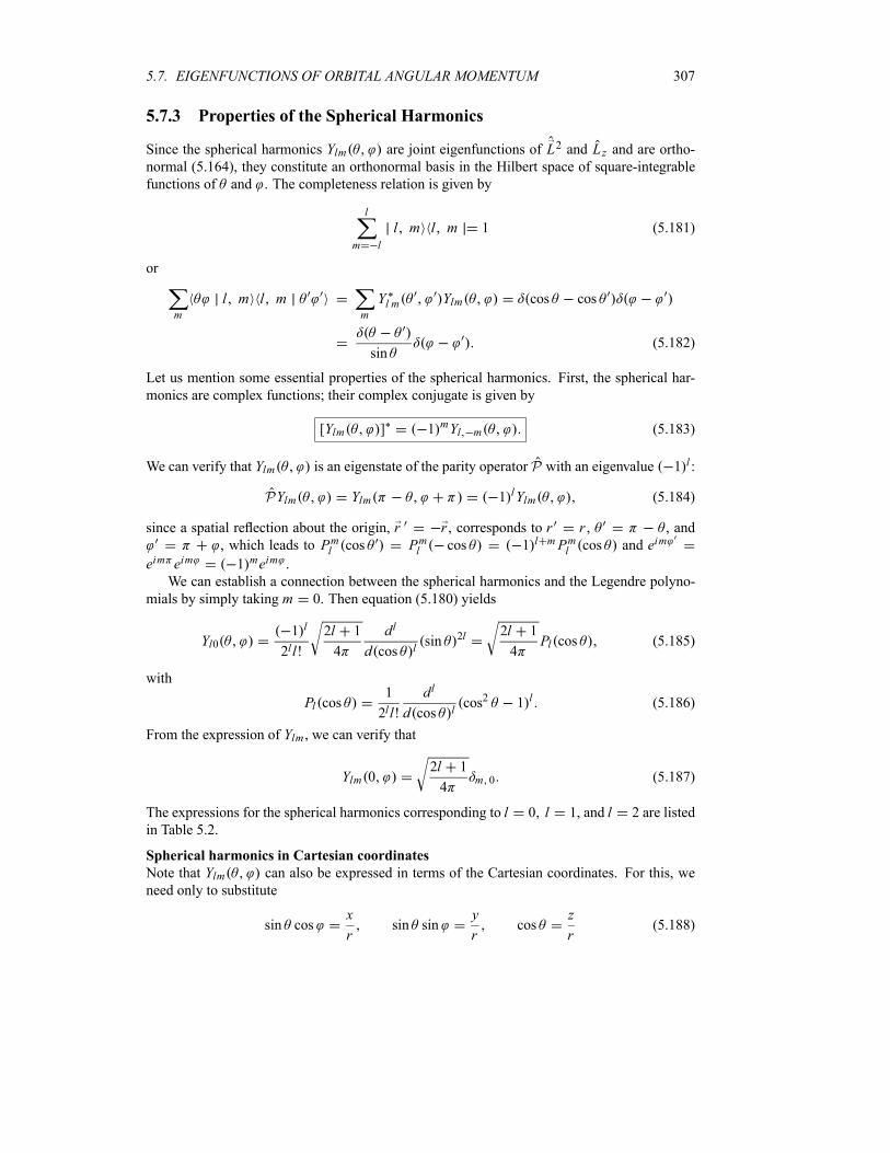
5.7. EIGENFUNCTIONS OF ORBITAL ANGULAR MOMENTUM 307
5.7.3 Properties of the Spherical Harmonics
Since the spherical harmonics Ylm are joint eigenfunctions of L2 and L z and are ortho-normal (5.164), they constitute an orthonormal basis in the Hilbert space of square-integrable
functions of and . The completeness relation is given by
l
m l
l m l m 1 (5.181)
or
m
l m l mm
Yl m Ylm cos cos
sin(5.182)
Let us mention some essential properties of the spherical harmonics. First, the spherical har-
monics are complex functions; their complex conjugate is given by
[Ylm ] 1 mYl m (5.183)
We can verify that Ylm is an eigenstate of the parity operator P with an eigenvalue 1 l :
PYlm Ylm 1 lYlm (5.184)
since a spatial reflection about the origin, r r , corresponds to r r , , and
, which leads to Pml cos Pml cos 1 l mPml cos and eim
eim eim 1 meim .We can establish a connection between the spherical harmonics and the Legendre polyno-
mials by simply taking m 0. Then equation (5.180) yields
Yl01 l
2ll!
2l 1
4
dl
d cos lsin 2l 2l 1
4Pl cos (5.185)
with
Pl cos1
2ll!
dl
d cos lcos2 1 l (5.186)
From the expression of Ylm , we can verify that
Ylm 02l 1
4m 0 (5.187)
The expressions for the spherical harmonics corresponding to l 0 l 1, and l 2 are listed
in Table 5.2.
Spherical harmonics in Cartesian coordinates
Note that Ylm can also be expressed in terms of the Cartesian coordinates. For this, we
need only to substitute
sin cosx
rsin sin
y
rcos
z
r(5.188)
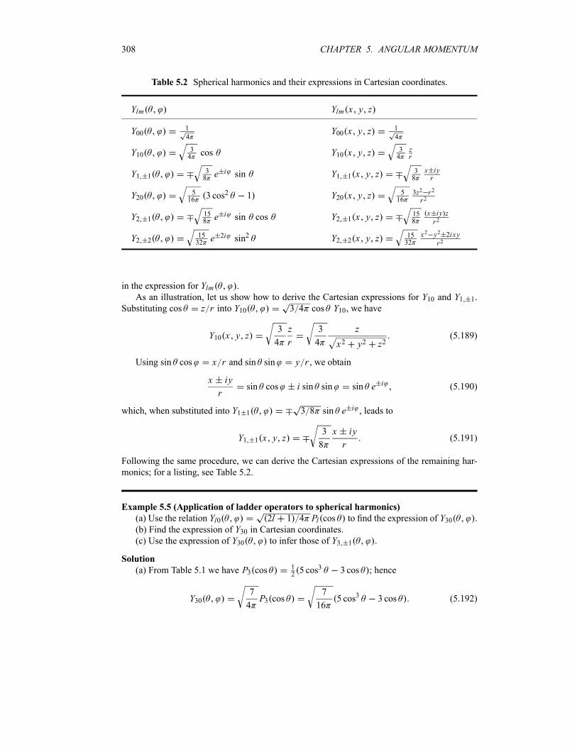
308 CHAPTER 5. ANGULAR MOMENTUM
Table 5.2 Spherical harmonics and their expressions in Cartesian coordinates.
Ylm Ylm x y z
Y001
4Y00 x y z
1
4
Y1034cos Y10 x y z
34
zr
Y1 138e i sin Y1 1 x y z
38
x iyr
Y20516
3 cos2 1 Y20 x y z516
3z2 r2
r2
Y2 1158e i sin cos Y2 1 x y z
158
x iy zr2
Y2 21532
e 2i sin2 Y2 2 x y z1532
x2 y2 2i xyr2
in the expression for Ylm .
As an illustration, let us show how to derive the Cartesian expressions for Y10 and Y1 1.
Substituting cos z r into Y10 3 4 cos Y10, we have
Y10 x y z3
4
z
r
3
4
z
x2 y2 z2(5.189)
Using sin cos x r and sin sin y r , we obtain
x iy
rsin cos i sin sin sin e i (5.190)
which, when substituted into Y1 1 3 8 sin e i , leads to
Y1 1 x y z3
8
x iy
r(5.191)
Following the same procedure, we can derive the Cartesian expressions of the remaining har-
monics; for a listing, see Table 5.2.
Example 5.5 (Application of ladder operators to spherical harmonics)
(a) Use the relation Yl0 2l 1 4 Pl cos to find the expression of Y30 .
(b) Find the expression of Y30 in Cartesian coordinates.(c) Use the expression of Y30 to infer those of Y3 1 .
Solution
(a) From Table 5.1 we have P3 cos125 cos3 3 cos ; hence
Y307
4P3 cos
7
165 cos3 3 cos (5.192)

5.7. EIGENFUNCTIONS OF ORBITAL ANGULAR MOMENTUM 309
(b) Since cos z r , we have 5 cos3 3 cos 5 cos 5 cos2 3 z 5z2 3r2 r3;hence
Y30 x y z7
16
z
r35z2 3r2 (5.193)
(c) To find Y31 from Y30, we need to apply the ladder operator L on Y30 in two ways: first,algebraically
L Y30 h 3 3 1 0Y31 2h 3Y31 (5.194)
and hence
Y311
2h 3L Y30 (5.195)
then we use the differential form (5.134) of L :
L Y30 hei icos
sinY30
h7
16ei i
cos
sin5 cos3 3 cos
3h7
16sin 5 cos2 1 ei (5.196)
Inserting (5.196) into (5.195) we end up with
Y311
2h 3L Y30
21
64sin 5 cos2 1 ei (5.197)
Now, to find Y3 1 from Y30, we also need to apply L on Y30 in two ways:
L Y30 h 3 3 1 0Y3 1 2h 3Y3 1 (5.198)
and hence
Y3 11
2h 3L Y30 (5.199)
then we use the differential form (5.134) of L :
L Y30 he i icos
sinY30
h7
16e i i
cos
sin5 cos3 3 cos
3h7
16sin 5 cos2 1 e i (5.200)
Inserting (5.200) into (5.199), we obtain
Y3 11
2h 3L Y30
21
64sin 5 cos2 1 e i (5.201)

310 CHAPTER 5. ANGULAR MOMENTUM
5.8 Solved Problems
Problem 5.1
(a) Show that Jx Jy h2[ j j 1 m2] 2, where Jx J 2x Jx 2 and the samefor Jy .
(b) Show that this relation is consistent with Jx Jy h 2 Jz h2m 2.
Solution
(a) First, note that Jx and Jy are zero, since
Jx1
2j m J j m
1
2j m J j m 0 (5.202)
As for J2x and J2y , they are given by
J2x1
4J J 2 1
4J 2 J J J J J 2 (5.203)
J2y1
4J J 2 1
4J2 J J J J J 2 (5.204)
Since J 2 J 2 0, we see that
J2x1
4J J J J J2y (5.205)
Using the fact that
J 2x J2y J 2 J 2z (5.206)
along with J2x J 2y , we see that
J 2x J 2y1
2[ J 2 J2z ] (5.207)
Now, since j m is a joint eigenstate of J 2 and Jz with eigenvalues j j 1 h2 and mh, wecan easily see that the expressions of J 2x and J2y are given by
J2x J2y1
2[ J 2 J 2z ]
h2
2j j 1 m2 (5.208)
Hence Jx Jy is given by
Jx Jy J2x J 2yh2
2[ j j 1 m2] (5.209)
(b) Since j m (because m j j 1 j 1 j), we have
j j 1 m2 m m 1 m2 m (5.210)
from which we infer that Jx Jy h2m 2, or
Jx Jyh
2Jz (5.211)
5.8. SOLVED PROBLEMS 311
Problem 5.2
Find the energy levels of a particle which is free except that it is constrained to move on the
surface of a sphere of radius r .
Solution
This system consists of a particle that is constrained to move on the surface of a sphere but free
from the influence of any other potential; it is called a rigid rotator. Since V 0 the energy of
this system is purely kinetic; the Hamiltonian of the rotator is
HL2
2I(5.212)
where I mr2 is the moment of inertia of the particle with respect to the origin. In derivingthis relation, we have used the fact that H p2 2m rp 2 2mr2 L2 2I , since Lr p rp.The wave function of the system is clearly independent of the radial degree of freedom, for
it is constant. The Schrödinger equation is thus given by
HL2
2IE (5.213)
Since the eigenstates of L2 are the spherical harmonics Ylm , the corresponding energy
eigenvalues are given by
Elh2
2Il l 1 l 0 1 2 3 (5.214)
and the Schrödinger equation by
L2
2IYlm
h2
2Il l 1 Ylm (5.215)
Note that the energy levels do not depend on the azimuthal quantum number m. This meansthat there are 2l 1 eigenfunctions Yl l , Yl l 1, , Yl l 1, Yll corresponding to the sameenergy. Thus, every energy level El is 2l 1 -fold degenerate. This is due to the fact that the
rotator’s Hamiltonian, L2 2I , commutes with L . That is, the Hamiltonian is independent of
the orientation of L in space; hence the energy spectrum does not depend on the component of
L in any particular direction.
Problem 5.3
Find the rotational energy levels of a diatomic molecule.
Solution
Consider two molecules of masses m1 and m2 separated by a constant distance r . Let r1 andr2 be their distances from the center of mass, i.e., m1r1 m2r2. The moment of inertia of thediatomic molecule is
I m1r21 m2r
22 r2 (5.216)
312 CHAPTER 5. ANGULAR MOMENTUM
where r r1 r2 and where is their reduced mass, m1m2 m1 m2 . The totalangular momentum is given by
L m1r1r1 m2r2r2 I r2 (5.217)
and the Hamiltonian by
HL2
2I
L2
2 r2(5.218)
The corresponding eigenvalue equation
H l mL2
2 r2l m
l l 1 h2
2 r2l m (5.219)
shows that the eigenenergies are 2l 1 -fold degenerate and given by
Ell l 1 h2
2 r2(5.220)
Problem 5.4
(a) Find the eigenvalues and eigenstates of the spin operator S of an electron in the directionof a unit vector n; assume that n lies in the xz plane.(b) Find the probability of measuring Sz h 2.
Solution
(a) In this question we want to solve
n Sh
2(5.221)
where n is given by n sin i cos k , because it lies in the xz plane, with 0 . We
can thus write
n S sin i cos k Sx i Sy j Szk Sx sin Sz cos (5.222)
Using the spin matrices
Sxh
2
0 1
1 0Sy
h
2
0 ii 0
Szh
2
1 0
0 1(5.223)
we can write (5.222) in the following matrix form:
n Sh
2
0 1
1 0sin
h
2
1 0
0 1cos
h
2
cos sin
sin cos(5.224)
The diagonalization of this matrix leads to the following secular equation:
h2
4cos cos
h2
4sin2 0 (5.225)
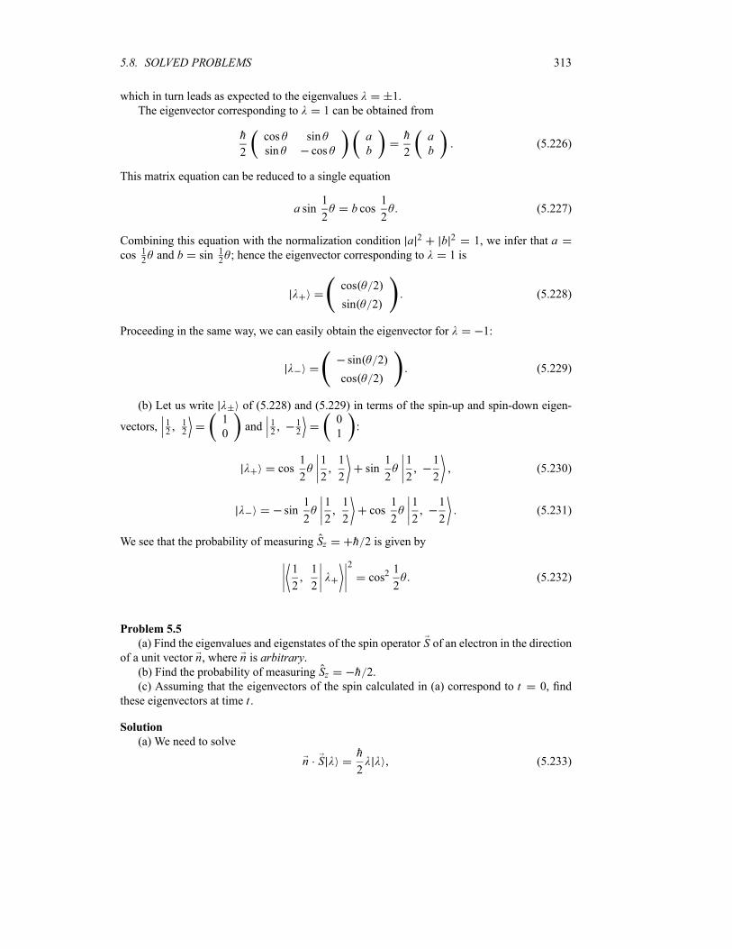
5.8. SOLVED PROBLEMS 313
which in turn leads as expected to the eigenvalues 1.
The eigenvector corresponding to 1 can be obtained from
h
2
cos sin
sin cos
ab
h
2
ab
(5.226)
This matrix equation can be reduced to a single equation
a sin1
2b cos
1
2(5.227)
Combining this equation with the normalization condition a 2 b 2 1, we infer that acos 1
2and b sin 1
2; hence the eigenvector corresponding to 1 is
cos 2
sin 2(5.228)
Proceeding in the same way, we can easily obtain the eigenvector for 1:
sin 2
cos 2(5.229)
(b) Let us write of (5.228) and (5.229) in terms of the spin-up and spin-down eigen-
vectors, 12
12
1
0and 1
212
0
1:
cos1
2
1
2
1
2sin
1
2
1
2
1
2(5.230)
sin1
2
1
2
1
2cos
1
2
1
2
1
2(5.231)
We see that the probability of measuring Sz h 2 is given by
1
2
1
2
2
cos21
2(5.232)
Problem 5.5
(a) Find the eigenvalues and eigenstates of the spin operator S of an electron in the directionof a unit vector n, where n is arbitrary.(b) Find the probability of measuring Sz h 2.(c) Assuming that the eigenvectors of the spin calculated in (a) correspond to t 0, find
these eigenvectors at time t .
Solution
(a) We need to solve
n Sh
2(5.233)
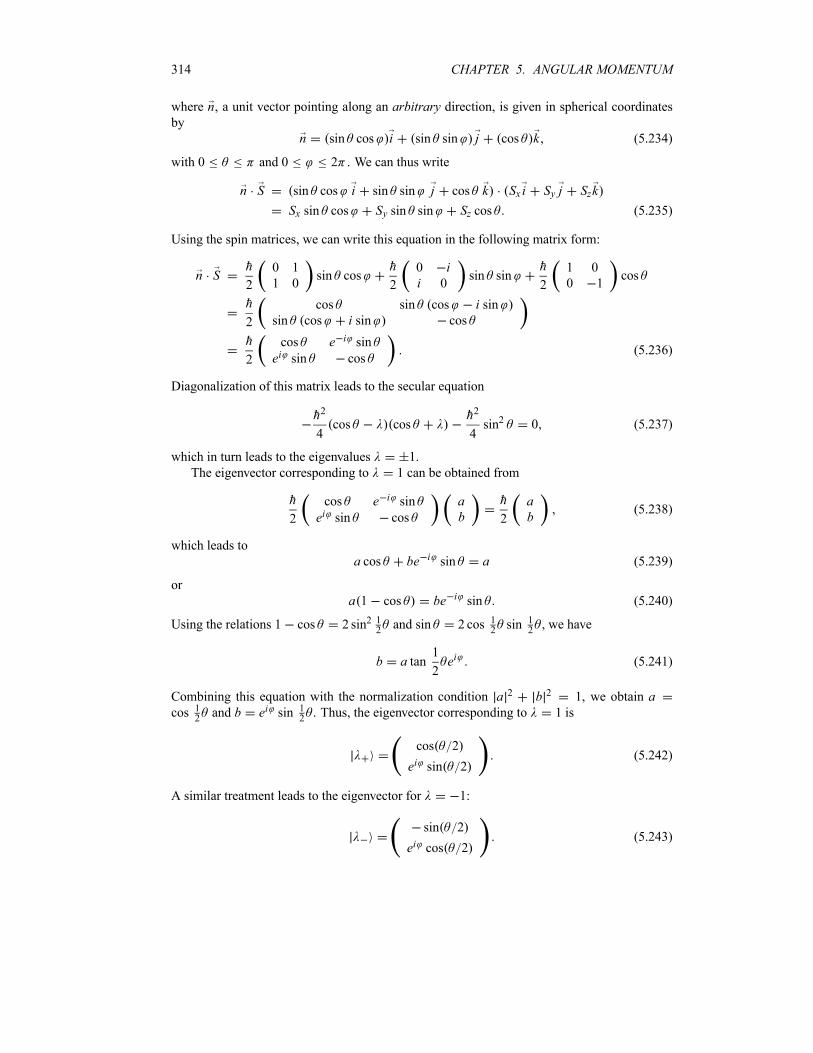
314 CHAPTER 5. ANGULAR MOMENTUM
where n, a unit vector pointing along an arbitrary direction, is given in spherical coordinatesby
n sin cos i sin sin j cos k (5.234)
with 0 and 0 2 . We can thus write
n S sin cos i sin sin j cos k Sx i Sy j Szk
Sx sin cos Sy sin sin Sz cos (5.235)
Using the spin matrices, we can write this equation in the following matrix form:
n Sh
2
0 1
1 0sin cos
h
2
0 ii 0
sin sinh
2
1 0
0 1cos
h
2
cos sin cos i sinsin cos i sin cos
h
2
cos e i sin
ei sin cos(5.236)
Diagonalization of this matrix leads to the secular equation
h2
4cos cos
h2
4sin2 0 (5.237)
which in turn leads to the eigenvalues 1.
The eigenvector corresponding to 1 can be obtained from
h
2
cos e i sin
ei sin cos
ab
h
2
ab
(5.238)
which leads to
a cos be i sin a (5.239)
or
a 1 cos be i sin (5.240)
Using the relations 1 cos 2 sin2 12and sin 2 cos 1
2sin 1
2, we have
b a tan1
2ei (5.241)
Combining this equation with the normalization condition a 2 b 2 1, we obtain acos 1
2and b ei sin 1
2. Thus, the eigenvector corresponding to 1 is
cos 2
ei sin 2(5.242)
A similar treatment leads to the eigenvector for 1:
sin 2
ei cos 2(5.243)
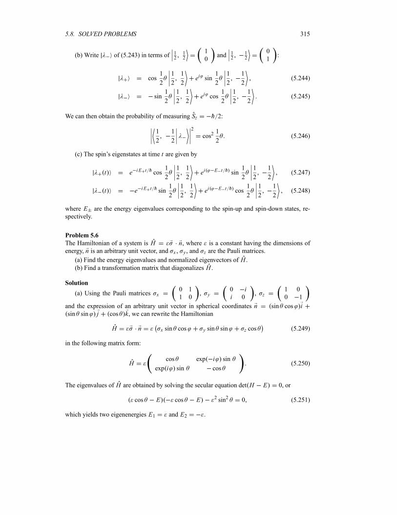
5.8. SOLVED PROBLEMS 315
(b) Write of (5.243) in terms of 12
12
1
0and 1
212
0
1:
cos1
2
1
2
1
2ei sin
1
2
1
2
1
2(5.244)
sin1
2
1
2
1
2ei cos
1
2
1
2
1
2(5.245)
We can then obtain the probability of measuring Sz h 2:
1
2
1
2
2
cos21
2(5.246)
(c) The spin’s eigenstates at time t are given by
t e i E t h cos1
2
1
2
1
2ei E t h sin
1
2
1
2
1
2(5.247)
t e i E t h sin1
2
1
2
1
2ei E t h cos
1
2
1
2
1
2(5.248)
where E are the energy eigenvalues corresponding to the spin-up and spin-down states, re-
spectively.
Problem 5.6
The Hamiltonian of a system is H n, where is a constant having the dimensions of
energy, n is an arbitrary unit vector, and x , y , and z are the Pauli matrices.
(a) Find the energy eigenvalues and normalized eigenvectors of H .(b) Find a transformation matrix that diagonalizes H .
Solution
(a) Using the Pauli matrices x0 1
1 0, y
0 ii 0
, z1 0
0 1
and the expression of an arbitrary unit vector in spherical coordinates n sin cos isin sin j cos k, we can rewrite the Hamiltonian
H n x sin cos y sin sin z cos (5.249)
in the following matrix form:
Hcos exp i sin
exp i sin cos(5.250)
The eigenvalues of H are obtained by solving the secular equation det H E 0, or
cos E cos E 2 sin2 0 (5.251)
which yields two eigenenergies E1 and E2 .
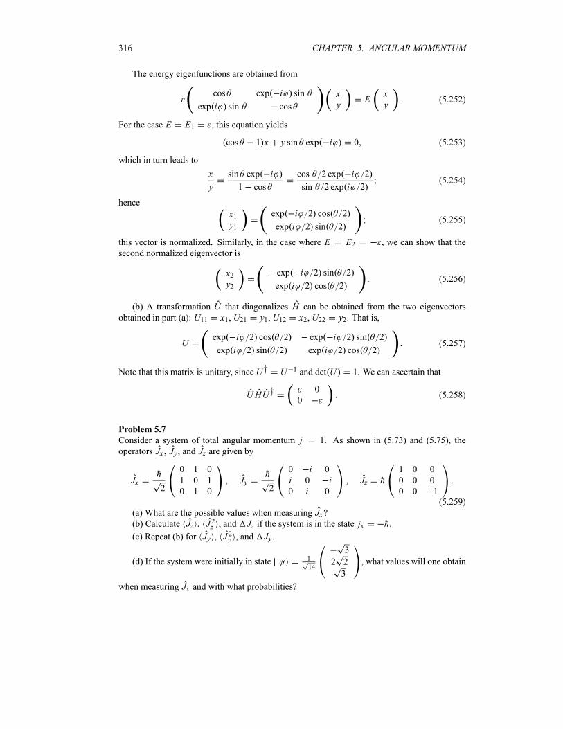
316 CHAPTER 5. ANGULAR MOMENTUM
The energy eigenfunctions are obtained from
cos exp i sin
exp i sin cos
xy
Exy
(5.252)
For the case E E1 , this equation yields
cos 1 x y sin exp i 0 (5.253)
which in turn leads to
x
y
sin exp i
1 cos
cos 2 exp i 2
sin 2 exp i 2(5.254)
hence
x1y1
exp i 2 cos 2
exp i 2 sin 2(5.255)
this vector is normalized. Similarly, in the case where E E2 , we can show that the
second normalized eigenvector is
x2y2
exp i 2 sin 2
exp i 2 cos 2(5.256)
(b) A transformation U that diagonalizes H can be obtained from the two eigenvectors
obtained in part (a): U11 x1, U21 y1, U12 x2, U22 y2. That is,
Uexp i 2 cos 2 exp i 2 sin 2
exp i 2 sin 2 exp i 2 cos 2(5.257)
Note that this matrix is unitary, since U† U 1 and det U 1. We can ascertain that
UHU†0
0(5.258)
Problem 5.7
Consider a system of total angular momentum j 1. As shown in (5.73) and (5.75), the
operators Jx , Jy , and Jz are given by
Jxh
2
0 1 0
1 0 1
0 1 0
Jyh
2
0 i 0
i 0 i0 i 0
Jz h1 0 0
0 0 0
0 0 1(5.259)
(a) What are the possible values when measuring Jx?(b) Calculate Jz , J 2z , and Jz if the system is in the state jx h.
(c) Repeat (b) for Jy , J 2y , and Jy .
(d) If the system were initially in state 1
14
3
2 2
3
, what values will one obtain
when measuring Jx and with what probabilities?
5.8. SOLVED PROBLEMS 317
Solution
(a) According to Postulate 2 of Chapter 3, the results of the measurements are given by
the eigenvalues of the measured quantity. Here the eigenvalues of Jx , which are obtained bydiagonalizing the matrix Jx , are jx h, 0, and h; the respective (normalized) eigenstates are
11
2
1
2
1
01
2
1
0
1
11
2
1
2
1
(5.260)
(b) If the system is in the state jx h, its eigenstate is given by 1 . In this case Jzand J 2z are given by
1 Jz 1h
41 2 1
1 0 0
0 0 0
0 0 1
1
2
1
0 (5.261)
1 J2z 1h2
41 2 1
1 0 0
0 0 0
0 0 1
1
2
1
h2
2(5.262)
Thus, the uncertainty Jz is given by
Jz 1 J2z 1 1 Jz 1 2h2
2
h
2(5.263)
(c) Following the same procedure in (b), we have
1 Jy 1h
4 21 2 1
0 i 0
i 0 i0 i 0
1
2
1
0 (5.264)
1 J2y 1h2
81 2 1
1 0 1
0 2 0
1 0 1
1
2
1
h2
2(5.265)
hence
Jy 1 J 2y 1 1 Jy 1 2h
2(5.266)
(d) We can express 1
14
3
2 2
3
in terms of the eigenstates (5.260) as
1
14
3
2 2
3
2
7
1
2
1
2
1
3
7
1
2
1
0
1
2
7
1
2
1
2
1
(5.267)
or2
71
3
70
2
71 (5.268)
318 CHAPTER 5. ANGULAR MOMENTUM
A measurement of Jx on a system initially in the state (5.268) yields a value jx h withprobability
P 1 1 2 2
71 1
3
71 0
2
71 1
22
7(5.269)
since 1 0 1 1 0 and 1 1 1, and the values jx 0 and jx h with therespective probabilities
P0 0 2 3
70 0
23
7P1 1 2 2
71 1
22
7(5.270)
Problem 5.8
Consider a particle of total angular momentum j 1. Find the matrix for the component of Jalong a unit vector with arbitrary direction n. Find its eigenvalues and eigenvectors.
Solution
Since J Jx i Jy j Jzk and n sin cos i sin sin j cos k, the component
of J along n isn J Jx sin cos Jy sin sin Jz cos (5.271)
with 0 and 0 2 ; the matrices of Jx , Jy , and Jz are given by (5.259). We cantherefore write this equation in the following matrix form:
n Jh
2
0 1 0
1 0 1
0 1 0
sin cosh
2
0 i 0
i 0 i0 i 0
sin sin
h1 0 0
0 0 0
0 0 1
cosh
2
2 cos e i sin 0
ei sin 0 e i sin
0 ei sin 2 cos
(5.272)
The diagonalization of this matrix leads to the eigenvalues 1 h, 2 0, and 3 h; thecorresponding eigenvectors are given by
11
2
1 cos e i
2
2sin
1 cos ei2
1
2
e i sin
2 cos
ei sin
(5.273)
31
2
1 cos e i
2
2sin
1 cos ei
(5.274)
Problem 5.9
Consider a system which is initially in the state
1
5Y1 1
3
5Y10
1
5Y11
5.8. SOLVED PROBLEMS 319
(a) Find L .
(b) If L z were measured what values will one obtain and with what probabilities?(c) If after measuring Lz we find lz h, calculate the uncertainties Lx and L y and
their product Lx L y .
Solution
(a) Let us use a lighter notation for : 1
51 1 3
51 0 1
51 1 .
From (5.56) we can write L l m h l l 1 m m 1 l m 1 ; hence the only
terms that survive in L are
L3
51 0 L 1 1
3
51 1 L 1 0
2 6
5h (5.275)
since 1 0 L 1 1 1 1 L 1 0 2h.(b) If L z were measured, we will find three values lz h, 0, and h. The probability of
finding the value lz h is
P 1 1 1 2 1
51 1 1 1
3
51 1 1 0
1
51 1 1 1
2
1
5(5.276)
since 1 1 1 0 1 1 1 1 0 and 1 1 1 1 1. Similarly, we can verify
that the probabilities of measuring lz 0 and h are respectively given by
P0 1 0 2 3
51 0 1 0
23
5(5.277)
P1 1 1 2 1
51 1 1 1
21
5(5.278)
(c) After measuring lz h, the system will be in the eigenstate lm 1 1 , that is,
Y1 1 . We need first to calculate the expectation values of Lx , L y , L2x , and
L2y using 1 1 . Symmetry requires that 1 1 Lx 1 1 1 1 L y 1 1 0.
The expectation values of L2x and L2y are equal, as shown in (5.60); they are given by
L2x L2y1
2[ L2 L2z ]
h2
2l l 1 m2
h2
2(5.279)
in this relation, we have used the fact that l 1 and m 1. Hence
Lx L2xh
2L y (5.280)
and the uncertainties product Lx L y is given by
Lx L y L2x L2yh2
2(5.281)
320 CHAPTER 5. ANGULAR MOMENTUM
Problem 5.10
Find the angle between the angular momentum l 4 and the z-axis for all possible orientations.
Solution
Since ml 0 1 2 l and the angle between the orbital angular momentum l and thez-axis is cos ml ml l l 1 we have
ml cos 1 mll l 1
cos 1 ml
2 5(5.282)
hence
0 cos 1 0 90 (5.283)
1 cos 1 1
2 577 08 2 cos 1 2
2 563 43 (5.284)
3 cos 1 3
2 547 87 4 cos 1 4
2 526 57 (5.285)
The angles for the remaining quantum numbers m4 1 2 3 4 can be inferred at once
from the relation
ml 180 ml (5.286)
hence
1 180 77 08 102 92 2 180 63 43 116 57 (5.287)
3 180 47 87 132 13 4 180 26 57 153 43 (5.288)
Problem 5.11
Using [X P] ih, calculate the various commutation relations between the following opera-tors2
T11
4P2 X2 T2
1
4X P PX T3
1
4P2 X2
Solution
The operators T1, T2, and T3 can be viewed as describing some sort of collective vibrations; T3has the structure of a harmonic oscillator Hamiltonian. The first commutator can be calculated
as follows:
[T1 T2]1
4[P2 X2 T2]
1
4[P2 T2]
1
4[X2 T2] (5.289)
where, using the commutation relation [X P] ih, we have
[P2 T2]1
4[P2 X P]
1
4[P2 PX]
1
4P[P X P]
1
4[P X P]P
1
4P[P PX ]
1
4[P PX]P
1
4P[P X ]P
1
4[P X]P2
1
4P2[P X]
1
4P[P X ]P
2N. Zettili and F. Villars, Nucl. Phys., A469, 77 (1987).
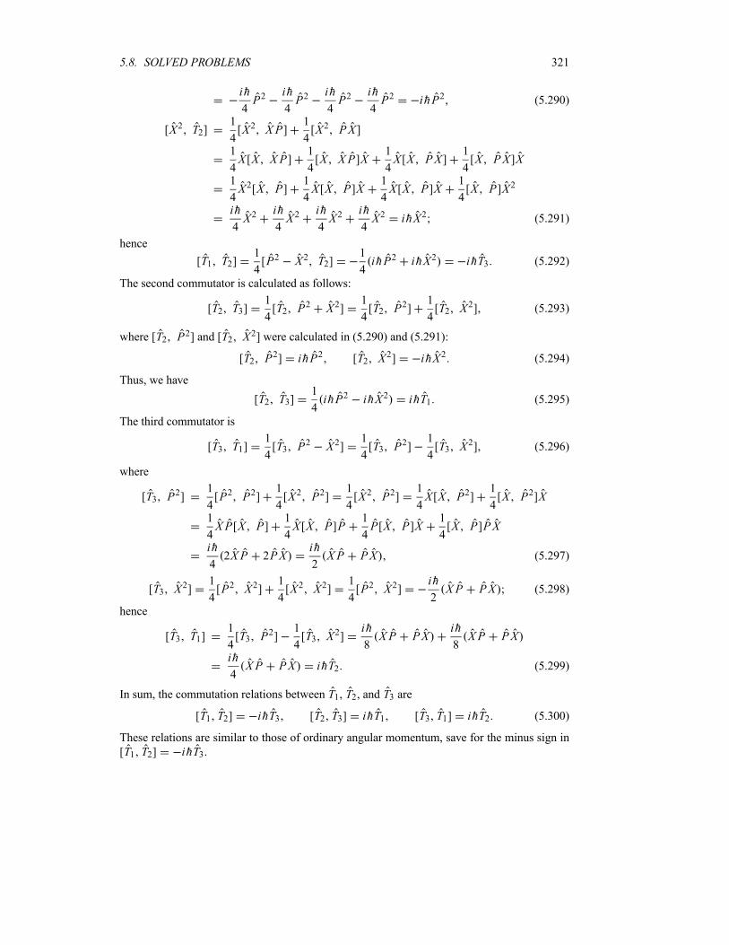
5.8. SOLVED PROBLEMS 321
ih
4P2
ih
4P2
ih
4P2
ih
4P2 ihP2 (5.290)
[X2 T2]1
4[X2 X P]
1
4[X2 PX ]
1
4X [X X P]
1
4[X X P]X
1
4X [X PX]
1
4[X PX]X
1
4X2[X P]
1
4X[X P]X
1
4X[X P]X
1
4[X P]X2
ih
4X2
ih
4X2
ih
4X2
ih
4X2 ihX2 (5.291)
hence
[T1 T2]1
4[P2 X2 T2]
1
4ihP2 ihX2 ihT3 (5.292)
The second commutator is calculated as follows:
[T2 T3]1
4[T2 P2 X2]
1
4[T2 P2]
1
4[T2 X2] (5.293)
where [T2 P2] and [T2 X2] were calculated in (5.290) and (5.291):
[T2 P2] ihP2 [T2 X2] ihX2 (5.294)
Thus, we have
[T2 T3]1
4ihP2 ihX2 ihT1 (5.295)
The third commutator is
[T3 T1]1
4[T3 P2 X2]
1
4[T3 P2]
1
4[T3 X2] (5.296)
where
[T3 P2]1
4[P2 P2]
1
4[X2 P2]
1
4[X2 P2]
1
4X[X P2]
1
4[X P2]X
1
4X P[X P]
1
4X [X P]P
1
4P[X P]X
1
4[X P]PX
ih
42X P 2PX
ih
2X P PX (5.297)
[T3 X2]1
4[P2 X2]
1
4[X2 X2]
1
4[P2 X2]
ih
2X P PX (5.298)
hence
[T3 T1]1
4[T3 P2]
1
4[T3 X2]
ih
8X P PX
ih
8X P PX
ih
4X P PX ihT2 (5.299)
In sum, the commutation relations between T1, T2, and T3 are
[T1 T2] ihT3 [T2 T3] ihT1 [T3 T1] ihT2 (5.300)
These relations are similar to those of ordinary angular momentum, save for the minus sign in
[T1 T2] ihT3.
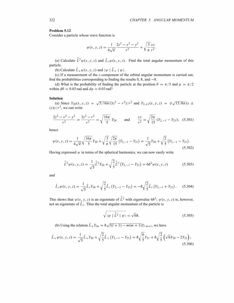
322 CHAPTER 5. ANGULAR MOMENTUM
Problem 5.12
Consider a particle whose wave function is
x y z1
4
2z2 x2 y2
r23 xz
r2
(a) Calculate L2 x y z and Lz x y z . Find the total angular momentum of this
particle.
(b) Calculate L x y z and L .
(c) If a measurement of the z-component of the orbital angular momentum is carried out,find the probabilities corresponding to finding the results 0, h, and h.(d) What is the probability of finding the particle at the position 3 and 2
within d 0 03 rad and d 0 03 rad?
Solution
(a) Since Y20 x y z 5 16 3z2 r2 r2 and Y2 1 x y z 15 8 xiy z r2, we can write
2z2 x2 y2
r23z2 r2
r216
5Y20 and
xz
r22
15Y2 1 Y21 (5.301)
hence
x y z1
4
16
5Y20
3 2
15Y2 1 Y21
1
5Y20
2
5Y2 1 Y21
(5.302)
Having expressed in terms of the spherical harmonics, we can now easily write
L2 x y z1
5L2Y20
2
5L2 Y2 1 Y21 6h2 x y z (5.303)
and
L z x y z1
5L zY20
2
5L z Y2 1 Y21 h
2
5Lz Y2 1 Y21 (5.304)
This shows that x y z is an eigenstate of L2 with eigenvalue 6h2; x y z is, however,not an eigenstate of L z . Thus the total angular momentum of the particle is
L2 6h (5.305)
(b) Using the relation L Ylm h l l 1 m m 1 Yl m 1, we have
L x y z1
5L Y20
2
5L Y2 1 Y21 h
6
5Y21 h
2
56Y20 2Y22
(5.306)
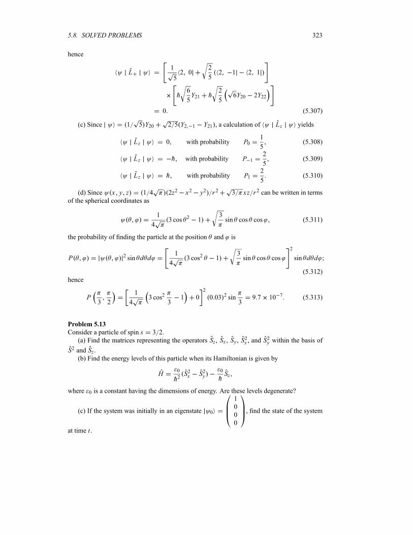
5.8. SOLVED PROBLEMS 323
hence
L1
52 0
2
52 1 2 1
h6
5Y21 h
2
56Y20 2Y22
0 (5.307)
(c) Since 1 5 Y20 2 5 Y2 1 Y21 , a calculation of Lz yields
L z 0 with probability P01
5(5.308)
L z h with probability P 12
5(5.309)
L z h with probability P12
5(5.310)
(d) Since x y z 1 4 2z2 x2 y2 r2 3 xz r2 can be written in termsof the spherical coordinates as
1
43 cos 2 1
3sin cos cos (5.311)
the probability of finding the particle at the position and is
P 2 sin d d1
43 cos2 1
3sin cos cos
2
sin d d
(5.312)
hence
P3 2
1
43 cos2
31 0
2
0 03 2 sin3
9 7 10 7 (5.313)
Problem 5.13
Consider a particle of spin s 3 2.
(a) Find the matrices representing the operators Sz , Sx , Sy , S2x , and S2y within the basis of
S2 and Sz .(b) Find the energy levels of this particle when its Hamiltonian is given by
H0
h2S2x S2y
0
hSz
where 0 is a constant having the dimensions of energy. Are these levels degenerate?
(c) If the system was initially in an eigenstate 0
1
0
0
0
, find the state of the system
at time t .
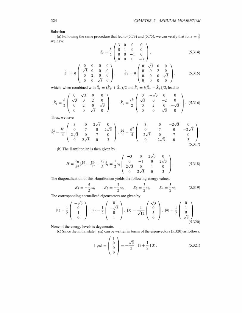
324 CHAPTER 5. ANGULAR MOMENTUM
Solution
(a) Following the same procedure that led to (5.73) and (5.75), we can verify that for s 32
we have
Szh
2
3 0 0 0
0 1 0 0
0 0 1 0
0 0 0 3
(5.314)
S h
0 0 0 0
3 0 0 0
0 2 0 0
0 0 3 0
S h
0 3 0 0
0 0 2 0
0 0 0 3
0 0 0 0
(5.315)
which, when combined with Sx S S 2 and Sy i S S 2, lead to
Sxh
2
0 3 0 0
3 0 2 0
0 2 0 3
0 0 3 0
Syih
2
0 3 0 0
3 0 2 0
0 2 0 3
0 0 3 0
(5.316)
Thus, we have
S2xh2
4
3 0 2 3 0
0 7 0 2 3
2 3 0 7 0
0 2 3 0 3
S2yh2
4
3 0 2 3 0
0 7 0 2 3
2 3 0 7 0
0 2 3 0 3(5.317)
(b) The Hamiltonian is then given by
H0
h2S2x S2y
0
hSz
1
20
3 0 2 3 0
0 1 0 2 3
2 3 0 1 0
0 2 3 0 3
(5.318)
The diagonalization of this Hamiltonian yields the following energy values:
E15
20 E2
3
20 E3
3
20 E4
5
20 (5.319)
The corresponding normalized eigenvectors are given by
11
2
3
0
1
0
21
2
0
3
0
1
31
12
3
0
3
0
41
2
0
1
0
3(5.320)
None of the energy levels is degenerate.
(c) Since the initial state 0 can be written in terms of the eigenvectors (5.320) as follows:
0
1
0
0
0
3
21
1
23 (5.321)
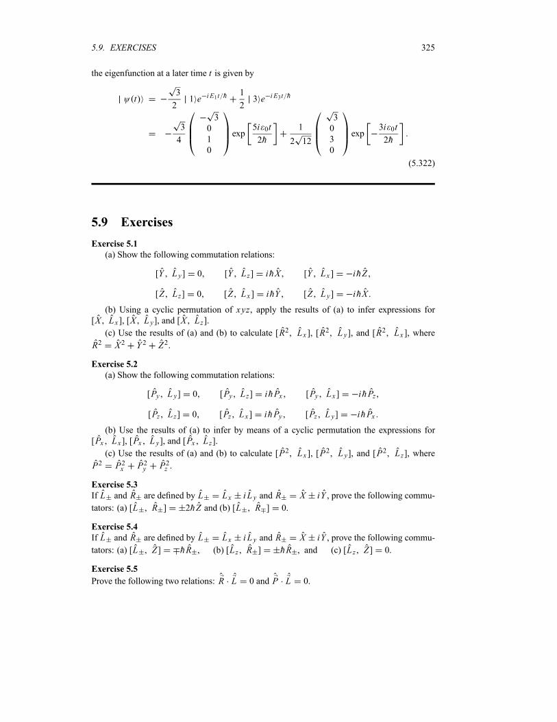
5.9. EXERCISES 325
the eigenfunction at a later time t is given by
t3
21 e i E1t h
1
23 e i E3t h
3
4
3
0
1
0
exp5i 0t
2h
1
2 12
3
0
3
0
exp3i 0t
2h
(5.322)
5.9 Exercises
Exercise 5.1
(a) Show the following commutation relations:
[Y L y] 0 [Y Lz] ihX [Y Lx ] ihZ
[Z Lz] 0 [Z Lx ] ihY [Z L y] ihX
(b) Using a cyclic permutation of xyz, apply the results of (a) to infer expressions for[X Lx ], [X L y], and [X Lz].
(c) Use the results of (a) and (b) to calculate [R2 Lx ], [R2 L y], and [R2 Lx ], where
R2 X2 Y 2 Z2.
Exercise 5.2
(a) Show the following commutation relations:
[Py L y] 0 [Py Lz] ihPx [Py Lx ] ihPz
[Pz L z] 0 [Pz Lx ] ihPy [Pz L y] ihPx
(b) Use the results of (a) to infer by means of a cyclic permutation the expressions for
[Px Lx ], [Px L y], and [Px L z].
(c) Use the results of (a) and (b) to calculate [P2 Lx ], [P2 L y], and [P2 L z], where
P2 P2x P2y P2z .
Exercise 5.3
If L and R are defined by L Lx i L y and R X iY , prove the following commu-
tators: (a) [L R ] 2hZ and (b) [L R ] 0.
Exercise 5.4
If L and R are defined by L Lx i L y and R X iY , prove the following commu-
tators: (a) [L Z] hR , (b) [Lz R ] hR , and (c) [L z Z] 0.
Exercise 5.5
Prove the following two relations: R L 0 and P L 0.
326 CHAPTER 5. ANGULAR MOMENTUM
Exercise 5.6
The Hamiltonian due to the interaction of a particle of spin S with a magnetic field B is givenby H S B where S is the spin. Calculate the commutator [S H ].
Exercise 5.7
Prove the following relation:
[Lz cos ] ih sin
where is the azimuthal angle.
Exercise 5.8
Prove the following relation:
[Lz sin 2 ] 2ih sin2 cos2
where is the azimuthal angle. Hint: [A BC] B[A C] [A B]C .
Exercise 5.9
Using the properties of J and J , calculate j j and j m as functions of the action of
J on the states j m and j j , respectively.
Exercise 5.10
Consider the operator A 12Jx Jy Jy Jx .
(a) Calculate the expectation value of A and A2with respect to the state j m .
(b) Use the result of (a) to find an expression for A2in terms of: J 4, J2, J 2z , J
4 , J4 .
Exercise 5.11
Consider the wave function
3 sin cos ei 2 1 cos2 e2i
(a) Write in terms of the spherical harmonics.
(b) Write the expression found in (a) in terms of the Cartesian coordinates.
(c) Is an eigenstate of L2 or L z?(d) Find the probability of measuring 2h for the z-component of the orbital angular momen-
tum.
Exercise 5.12
Show that L z cos2 sin2 2i sin cos 2h2i , where is the azimuthal angle.
Exercise 5.13
Find the expressions for the spherical harmonics Y30 and Y3 1 ,
Y30 7 16 5 cos3 3 cos Y3 1 21 64 sin 5 cos2 1 e i
in terms of the Cartesian coordinates x y z.
Exercise 5.14
(a) Show that the following expectation values between lm states satisfy the relations
Lx L y 0 and L2x L2y12l l 1 h2 m2h2 .
(b) Verify the inequality Lx L y h2m 2, where Lx L2x Lx 2.
5.9. EXERCISES 327
Exercise 5.15
A particle of mass m is fixed at one end of a rigid rod of negligible mass and length R. Theother end of the rod rotates in the xy plane about a bearing located at the origin, whose axis isin the z-direction.(a) Write the system’s total energy in terms of its angular momentum L.(b)Write down the time-independent Schrödinger equation of the system. Hint: In spherical
coordinates, only varies.
(c) Solve for the possible energy levels of the system, in terms of m and the moment ofinertia I mR2.(d) Explain why there is no zero-point energy.
Exercise 5.16
Consider a system which is described by the state
3
8Y11
1
8Y10 AY1 1
where A is a real constant(a) Calculate A so that is normalized.
(b) Find L .
(c) Calculate the expectation values of Lx and L2 in the state .
(d) Find the probability associated with a measurement that gives zero for the z-componentof the angular momentum.
(e) Calculate Lz and L where
8
15Y11
4
15Y10
3
15Y2 1
Exercise 5.17
(a) Using the commutation relations of angular momentum, verify the validity of the (Ja-
cobi) identity: [Jx [Jy Jz]] [Jy [Jz Jx ]] [Jz [Jx Jy]] 0.
(b)Prove the following identity: [J 2x J 2y ] [J 2y J 2z ] [J 2z J 2x ].
(c) Calculate the expressions of L L Ylm and L L Ylm , and then infer the
commutator [L L L L ]Ylm .
Exercise 5.18
Consider a particle whose wave function is given by x y z A[ x z y z2] r2 A 3,where A is a constant.
(a) Is an eigenstate of L 2? If yes, what is the corresponding eigenvalue? Is it also aneigenstate of L z?(b) Find the constant A so that is normalized.
(c) Find the relative probabilities for measuring the various values of Lz and L 2, and then
calculate the expectation values of Lz and L 2.(d) Calculate L and then infer L .
Exercise 5.19
Consider a system which is in the state
2
13Y3 3
3
13Y3 2
3
13Y30
3
13Y3 2
2
13Y33
328 CHAPTER 5. ANGULAR MOMENTUM
(a) If L z were measured, what values will one obtain and with what probabilities?(b) If after a measurement of L z we find lz 2h, calculate the uncertainties Lx and L y
and their product Lx L y .
(c) Find Lx and L y .
Exercise 5.20
(a) Calculate the energy eigenvalues of an axially symmetric rotator and find the degeneracy
of each energy level (i.e., for each value of the azimuthal quantum number m, find how manystates l m correspond to the same energy). We may recall that the Hamiltonian of an axially
symmetric rotator is given by
HL2x L2y2I1
L2z2I2
where I1 and I2 are the moments of inertia.(b) From part (a) infer the energy eigenvalues for the various levels of l 3.
(c) In the case of a rigid rotator (i.e., I1 I2 I ), find the energy expression and thecorresponding degeneracy relation.
(d) Calculate the orbital quantum number l and the corresponding energy degeneracy for arigid rotator where the magnitude of the total angular momentum is 56h.
Exercise 5.21
Consider a system of total angular momentum j 1. We are interested here in the measure-
ment of Jy ; its matrix is given by
Jyh
2
0 i 0
i 0 i0 i 0
(a) What are the possible values will we obtain when measuring Jy?
(b) Calculate Jz , J 2z , and Jz if the system is in the state jy h.
(c) Repeat (b) for Jx , J 2x , and Jx .
Exercise 5.22
Calculate Y3 2 by applying the ladder operators L on Y3 1 .
Exercise 5.23
Consider a system of total angular momentum j 1. We want to carry out measurements on
Jz h1 0 0
0 0 0
0 0 1
(a) What are the possible values will we obtain when measuring Jz?(b) Calculate Jx , J 2x , and Jx if the system is in the state jz h.
(c) Repeat (b) for Jy , J 2y , and Jy .
Exercise 5.24
Consider a system which is in the state
x y z1
4
z
r
1
3
x
r
5.9. EXERCISES 329
(a) Express x y z in terms of the spherical harmonics then calculate L2 x y z and
Lz x y z . Is x y z an eigenstate of L2 or Lz?(b) Calculate L x y z and L .
(c) If a measurement of the z-component of the orbital angular momentum is carried out,find the probabilities corresponding to finding the results 0, h, and h.
Exercise 5.25
Consider a system whose wave function is given by
1
2Y00
1
3Y11
1
2Y1 1
1
6Y22
(a) Is normalized?
(b) Is an eigenstate of L2 or L z?(c) Calculate L and L .
(d) If a measurement of the z-component of the orbital angular momentum is carried out,find the probabilities corresponding to finding the results 0, h, h, and 2h.
Exercise 5.26
Using the expression of L in spherical coordinates, prove the following two commutators:
[L e i sin ] 0 and [L cos ] he i sin .
Exercise 5.27
Consider a particle whose angular momentum is l 1.
(a) Find the eigenvalues and eigenvectors, 1 mx , of Lx .(b) Express the state 1 mx 1 as a linear superposition of the eigenstates of Lz . Hint:
you need first to find the eigenstates of Lx and find which of them corresponds to the eigenvaluemx 1; this eigenvector will be expanded in the z basis.(c) What is the probability of measuring mz 1 when the particle is in the eigenstate
1 mx 1 ? What about the probability corresponding to measuring mz 0?
(d) Suppose that a measurement of the z-component of angular momentum is performed andthat the result mz 1 is obtained. Now we measure the x-component of angular momentum.What are the possible results and with what probabilities?
Exercise 5.28
Consider a system which is given in the following angular momentum eigenstates l m :
1
71 1 A 1 0
2
71 1
where A is a real constant(a) Calculate A so that is normalized.
(b) Calculate the expectation values of Lx , L y , L z , and L2 in the state .
(c) Find the probability associated with a measurement that gives 1h for the z-componentof the angular momentum.
(d) Calculate 1 m L2 and 1 m L2 .
330 CHAPTER 5. ANGULAR MOMENTUM
Exercise 5.29
Consider a particle of angular momentum j 3 2.
(a) Find the matrices representing the operators J 2, Jx , Jy , and Jz in the32m basis.
(b) Using these matrices, show that Jx , Jy , Jz satisfy the commutator [Jx Jy] ih Jz .
(c) Calculate the mean values of Jx and J2x with respect to the state
0
0
1
0
.
(d) Calculate Jx Jy with respect to the state
0
0
1
0
and verify that this product satisfies Heisenberg’s uncertainty principle.
Exercise 5.30
Consider the Pauli matrices
x0 1
1 0 y0 ii 0 z
1 0
0 1
(a) Verify that 2x
2y
2z I , where I is the unit matrix
I1 0
0 1
(b) Calculate the commutators [ x y], [ x z], and [ y z].
(c) Calculate the anticommutator x y y x .
(d) Show that ei y I cos i y sin , where I is the unit matrix.(e) Derive an expression for ei z by analogy with the one for y .
Exercise 5.31
Consider a spin 32particle whose Hamiltonian is given by
H0
h2S2x S2y
0
h2S2z
where 0 is a constant having the dimensions of energy.
(a) Find the matrix of the Hamiltonian and diagonalize it to find the energy levels.
(b) Find the eigenvectors and verify that the energy levels are doubly degenerate.
Exercise 5.32
Find the energy levels of a spin 52particle whose Hamiltonian is given by
H0
h2S2x S2y
0
hSz
where 0 is a constant having the dimensions of energy. Are the energy levels degenerate?
5.9. EXERCISES 331
Exercise 5.33
Consider an electron whose spin direction is located in the xy plane.(a) Find the eigenvalues (call them 1, 2) and eigenstates ( 1 , 2 ) of the electron’s
spin operator S.(b) Assuming that the initial state of the electron is given by
01
31
2 2
32
find the probability of obtaining a value of S h 2 after measuring the spin of the electron.
Exercise 5.34
(a) Find the eigenvalues (call them 1, 2) and eigenstates ( 1 , 2 ) of the spin operator
S of an electron when S is pointing along an arbitrary unit vector n that lies within the yz plane.(b) Assuming that the initial state of the electron is given by
01
21
3
22
find the probability of obtaining a value of S h 2 after measuring the spin of the electron.
Exercise 5.35
Consider a particle of spin 32. Find the matrix for the component of the spin along a unit vector
with arbitrary direction n. Find its eigenvalues and eigenvectors. Hint:
n sin cos i sin sin j cos k
Exercise 5.36
Show that [Jx Jy Jz] [Jx Jy Jz] ih J 2x 2J 2y J2z .
Exercise 5.37
Find the eigenvalues of the operators L2
and L z for each of the following states:(a) Y21 ,
(b) Y3 2 ,
(c) 1
2Y33 Y3 3 , and
(d) Y40 .
Exercise 5.38
Use the following general relations:
x1
2
1
2
1
2
1
2
1
2y
1
2
1
2
1
2i1
2
1
2
to verify the following eigenvalue equations:
Sx xh
2x and Sy y
h
2y

332 CHAPTER 5. ANGULAR MOMENTUM
Chapter 6
Three-Dimensional Problems
6.1 Introduction
In this chapter we examine how to solve the Schrödinger equation for spinless particles moving
in three-dimensional potentials. We carry out this study in two different coordinate systems:
the Cartesian system and the spherical system.
First, working within the context of Cartesian coordinates, we study the motion of a particle
in different potentials: the free particle, a particle in a (three-dimensional) rectangular potential,
and a particle in a harmonic oscillator potential. This study is going to be a simple generaliza-
tion of the one-dimensional problems presented in Chapter 4. Unlike the one-dimensional case,
three-dimensional problems often exhibit degeneracy, which occurs whenever the potential dis-
plays symmetry.
Second, using spherical coordinates, we describe the motion of a particle in spherically
symmetric potentials. After presenting a general treatment, we consider several applications
ranging from the free particle and the isotropic harmonic oscillator to the hydrogen atom. We
conclude the chapter by calculating the energy levels of a hydrogen atom when placed in a
constant magnetic field; this gives rise to the Zeeman effect.
6.2 3D Problems in Cartesian Coordinates
We examine here how to extend Schrödinger’s theory of one-dimensional problems (Chapter
4) to three dimensions.
6.2.1 General Treatment: Separation of Variables
The time-dependent Schrödinger equation for a spinless particle of mass m moving under theinfluence of a three-dimensional potential is
h2
2m2 x y z t V x y z t x y z ih
x y z t
t(6.1)
where 2 is the Laplacian, 2 2 x2 2 y2 2 z2. As seen in Chapter 4, the wavefunction of a particle moving in a time-independent potential can be written as a product of
333
334 CHAPTER 6. THREE-DIMENSIONAL PROBLEMS
spatial and time components:
x y z t x y z e i Et h (6.2)
where x y z is the solution to the time-independent Schrödinger equation:
h2
2m2 x y z V x y z x y z E x y z (6.3)
which is of the form H E .
This partial differential equation is generally difficult to solve. But, for those cases where
the potential V x y z separates into the sum of three independent, one-dimensional terms
(which should not be confused with a vector)
V x y z Vx x Vy y Vz z (6.4)
we can solve (6.3) by means of the technique of separation of variables. This technique consistsof separating the three-dimensional Schrödinger equation (6.3) into three independent one-
dimensional Schrödinger equations. Let us examine how to achieve this. Note that (6.3), in
conjunction with (6.4), can be written as
Hx Hy Hz x y z E x y z (6.5)
where Hx is given by
Hxh2
2m
2
x2Vx x (6.6)
the expressions for Hy and Hz are analogous.
As V x y z separates into three independent terms, we can also write x y z as a
product of three functions of a single variable each:
x y z X x Y y Z z (6.7)
Substituting (6.7) into (6.5) and dividing by X x Y y Z z , we obtain
h2
2m
1
X
d2X
dx2Vx x
h2
2m
1
Y
d2Y
dy2Vy y
h2
2m
1
Z
d2Z
dz2Vz z E (6.8)
Since each expression in the square brackets depends on only one of the variables x y z, andsince the sum of these three expressions is equal to a constant, E , each separate expressionmust then be equal to a constant such that the sum of these three constants is equal to E . Forinstance, the x-dependent expression is given by
h2
2m
d2
dx2Vx x X x Ex X x (6.9)
Similar equations hold for the y and z coordinates, with
Ex Ey Ez E (6.10)
The separation of variables technique consists in essence of reducing the three-dimensionalSchrödinger equation (6.3) into three separate one-dimensional equations (6.9).
6.2. 3D PROBLEMS IN CARTESIAN COORDINATES 335
6.2.2 The Free Particle
In the simple case of a free particle, the Schrödinger equation (6.3) reduces to three equations
similar to (6.9) with Vx 0, Vy 0, and Vz 0. The x-equation can be obtained from (6.9):
d2X x
dx2k2x X x (6.11)
where k2x 2mEx h2, and hence Ex h2k2x 2m . As shown in Chapter 4, the normalizedsolutions to (6.11) are plane waves
X x1
2eikx x (6.12)
Thus, the solution to the three-dimensional Schrödinger equation (6.3) is given by
k x y z 2 3 2eikx xeiky yeikz z 2 3 2eik r (6.13)
where k and r are the wave and position vectors of the particle, respectively. As for the totalenergy E , it is equal to the sum of the eigenvalues of the three one-dimensional equations(6.11):
E Ex Ey Ezh2
2mk2x k2y k2z
h2
2mk2 (6.14)
Note that, since the energy (6.14) depends only on the magnitude of k, all different orientationsof k (obtained by varying kx ky kz) subject to the condition
k k2x k2y k2z constant (6.15)
generate different eigenfunctions (6.13) without a change in the energy. As the total number
of orientations of k which preserve its magnitude is infinite, the energy of a free particle isinfinitely degenerate.Note that the solutions to the time-dependent Schrödinger equation (6.1) are obtained by
substituting (6.13) into (6.2):
k r t r e i t 2 3 2ei k r t (6.16)
where E h; this represents a propagating wave with wave vector k. The orthonormalitycondition of this wave function is expressed by
kr t k r t d
3rkr k r d
3r 2 3 ei k k rd3r k k (6.17)
which can be written in Dirac’s notation as
k t k t k k k k (6.18)
The free particle can be represented, as seen in Chapter 3, by a wave packet (a superposition of
wave functions corresponding to the various wave vectors):
r t 2 3 2 A k t k r t d3k 2 3 2 A k t ei k r t d3k (6.19)
336 CHAPTER 6. THREE-DIMENSIONAL PROBLEMS
where A k t is the Fourier transform of r t :
A k t 2 3 2 r t e i k r t d3r (6.20)
As seen in Chapters 1 and 4, the position of the particle can be represented classically by the
center of the wave packet.
6.2.3 The Box Potential
We are going to begin with the rectangular box potential, which has no symmetry, and then
consider the cubic potential, which displays a great deal of symmetry, since the xyz axes areequivalent.
6.2.3.1 The Rectangular Box Potential
Consider first the case of a spinless particle of mass m confined in a rectangular box of sidesa b c:
V x y z0 0 x a 0 y b 0 z c
elsewhere(6.21)
which can be written as V x y z Vx x Vy y Vz z , with
Vx x0 0 x a
elsewhere(6.22)
the potentials Vy y and Vz z have similar forms.The wave function x y z must vanish at the walls of the box. We have seen in Chapter
4 that the solutions for this potential are of the form
X x2
asin
nxax nx 1 2 3 (6.23)
and the corresponding energy eigenvalues are
Enxh2 2
2ma2n2x (6.24)
From these expressions we can write the normalized three-dimensional eigenfunctions and their
corresponding energies:
nxnynz x y z8
abcsin
nxax sin
nyby sin
nzcz (6.25)
Enxnynzh2 2
2m
n2xa2
n2yb2
n2zc2
(6.26)
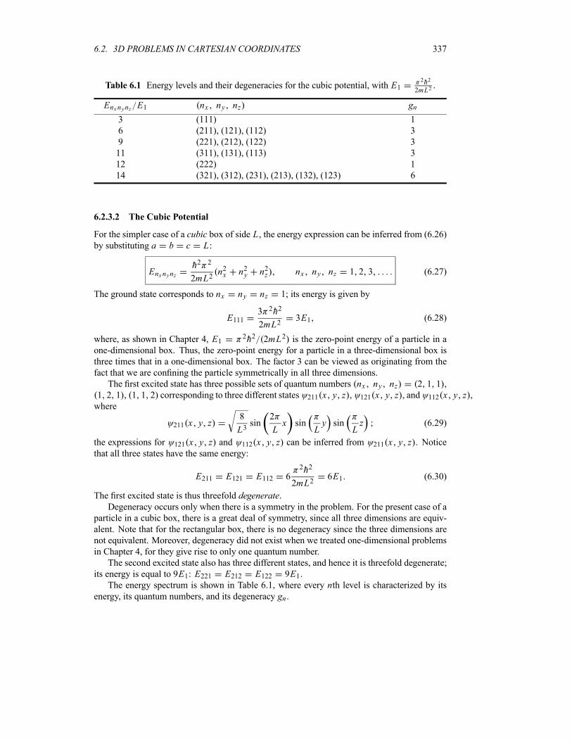
6.2. 3D PROBLEMS IN CARTESIAN COORDINATES 337
Table 6.1 Energy levels and their degeneracies for the cubic potential, with E12h2
2mL2.
Enxnynz E1 nx ny nz gn
3 (111) 1
6 (211), (121), (112) 3
9 (221), (212), (122) 3
11 (311), (131), (113) 3
12 (222) 1
14 (321), (312), (231), (213), (132), (123) 6
6.2.3.2 The Cubic Potential
For the simpler case of a cubic box of side L, the energy expression can be inferred from (6.26)by substituting a b c L:
Enxnynzh2 2
2mL2n2x n2y n2z nx ny nz 1 2 3 (6.27)
The ground state corresponds to nx ny nz 1; its energy is given by
E1113 2h2
2mL23E1 (6.28)
where, as shown in Chapter 4, E1 2h2 2mL2 is the zero-point energy of a particle in aone-dimensional box. Thus, the zero-point energy for a particle in a three-dimensional box is
three times that in a one-dimensional box. The factor 3 can be viewed as originating from the
fact that we are confining the particle symmetrically in all three dimensions.
The first excited state has three possible sets of quantum numbers nx ny nz 2 1 1 ,
1 2 1 , 1 1 2 corresponding to three different states 211 x y z , 121 x y z , and 112 x y z ,where
211 x y z8
L3sin
2
Lx sin
Ly sin
Lz (6.29)
the expressions for 121 x y z and 112 x y z can be inferred from 211 x y z . Noticethat all three states have the same energy:
E211 E121 E112 62h2
2mL26E1 (6.30)
The first excited state is thus threefold degenerate.Degeneracy occurs only when there is a symmetry in the problem. For the present case of a
particle in a cubic box, there is a great deal of symmetry, since all three dimensions are equiv-
alent. Note that for the rectangular box, there is no degeneracy since the three dimensions are
not equivalent. Moreover, degeneracy did not exist when we treated one-dimensional problems
in Chapter 4, for they give rise to only one quantum number.
The second excited state also has three different states, and hence it is threefold degenerate;
its energy is equal to 9E1: E221 E212 E122 9E1.The energy spectrum is shown in Table 6.1, where every nth level is characterized by its
energy, its quantum numbers, and its degeneracy gn .
338 CHAPTER 6. THREE-DIMENSIONAL PROBLEMS
6.2.4 The Harmonic Oscillator
We are going to begin with the anisotropic oscillator, which displays no symmetry, and then
consider the isotropic oscillator where the xyz axes are all equivalent.
6.2.4.1 The Anisotropic Oscillator
Consider a particle of mass m moving in a three-dimensional anisotropic oscillator potential
V x y z1
2m 2
x X2 1
2m 2
yY2 1
2m 2
z Z2 (6.31)
Its Schrödinger equation separates into three equations similar to (6.9):
h2
2m
d2X x
dx21
2m x x
2X x Ex X x (6.32)
with similar equations for Y y and Z z . The eigenenergies corresponding to the potential(6.31) can be expressed as
Enxnynz Enx Eny Enz nx1
2h x ny
1
2h y nz
1
2h z
(6.33)
with nx ny nz 0 1 2 3 . The corresponding stationary states are
nxnynz x y z Xnx x Yny y Znz z (6.34)
where Xnx x , Yny y and Znz z are one-dimensional harmonic oscillator wave functions.These states are not degenerate, because the potential (6.31) has no symmetry (it is anisotropic).
6.2.4.2 The Isotropic Harmonic Oscillator
Consider now an isotropic harmonic oscillator potential. Its energy eigenvalues can be inferredfrom (6.33) by substituting x y z ,
Enxnynz nx ny nz3
2h (6.35)
Since the energy depends on the sum of nx , ny , nz , any set of quantum numbers having thesame sum will represent states of equal energy.
The ground state, whose energy is E000 3h 2, is not degenerate. The first excited state
is threefold degenerate, since there are three different states, 100, 010, 001, that correspond
to the same energy 5h 2. The second excited state is sixfold degenerate; its energy is 7h 2.
In general, we can show that the degeneracy gn of the nth excited state, which is equal tothe number of ways the nonnegative integers nx ny nz may be chosen to total to n, is given by
gn1
2n 1 n 2 (6.36)
where n nx ny nz . Table 6.2 displays the first few energy levels along with theirdegeneracies.

6.2. 3D PROBLEMS IN CARTESIAN COORDINATES 339
Table 6.2 Energy levels and their degeneracies for an isotropic harmonic oscillator.
n 2En h nxnynz gn
0 3 (000) 1
1 5 (100), (010), (001) 3
2 7 (200), (020), (002) 6
(110), (101), (011)
3 9 (300), (030), (003) 10
(210), (201), (021)
(120), (102), (012)
(111)
Example 6.1 (Degeneracy of a harmonic oscillator)
Show how to derive the degeneracy relation (6.36).
Solution
For a fixed value of n, the degeneracy gn is given by the number of ways of choosing nx , ny ,and nz so that n nx ny nz .For a fixed value of nx , the number of ways of choosing ny and nz so that ny nz n nx
is given by n nx 1 ; this can be shown as follows. For a given value of nx , the variouspermissible values of ny nz are given by ny nz 0 n nx , 1 n nx 1 , 2 n nx 2 ,
3 n nx 3 , , n nx 3 3 , n nx 2 2 , n nx 1 1 , and n nx 0 . In all,there are n nx 1 sets of ny nz so that ny nz n nx . Now, since the values of nxcan vary from 0 to n, the degeneracy is then given by
gnn
nx 0
n nx 1 n 1
n
nx 0
1
n
nx 0
nx n 1 21
2n n 1
1
2n 1 n 2
(6.37)
A more primitive way of calculating this series is to use Gauss’s method: simply write the seriesnnx 0 n nx 1 in the following two equivalent forms:
gn n 1 n n 1 n 2 4 3 2 1 (6.38)
gn 1 2 3 4 n 2 n 1 n n 1 (6.39)
Since both of these two series contain n 1 terms each, a term by term addition of these
relations yields
2gn n 2 n 2 n 2 n 2 n 2 n 2
n 1 n 2 (6.40)
hence gn12n 1 n 2 .
340 CHAPTER 6. THREE-DIMENSIONAL PROBLEMS
6.3 3D Problems in Spherical Coordinates
6.3.1 Central Potential: General Treatment
In this section we study the structure of the Schrödinger equation for a particle of mass1 Mmoving in a spherically symmetric potential
V r V r (6.41)
which is also known as the central potential.The time-independent Schrödinger equation for this particle, of momentum ih and po-
sition vector r , ish2
2M2 V r r E r (6.42)
Since the Hamiltonian is spherically symmetric, we are going to use the spherical coordinates
r which are related to their Cartesian counterparts by
x r sin cos y r sin sin z r cos (6.43)
The Laplacian 2 separates into a radial part 2r and an angular part
2 as follows (see Chapter
5):
2 2r
1
h2r22 1
r2 rr2r
1
h2r2L2 1
r
2
r2r
1
h2r2L2
(6.44)
where L is the orbital angular momentum with
L2 h21
sinsin
1
sin2
2
2(6.45)
In spherical coordinates the Schrödinger equation therefore takes the form
h2
2M
1
r
2
r2r
1
2Mr2L2 V r r E r (6.46)
The first term of this equation can be viewed as the radial kinetic energy
h2
2M
1
r
2
r2r
P2r2M
(6.47)
since the radial momentum operator is given by the Hermitian form2
Pr1
2
r
rP P
r
rih
r
1
rih1
r rr (6.48)
1Throughout this section we will designate the mass of the particle by a capital M to avoid any confusion with the
azimuthal quantum number m.2Note that we can show that the commutator between the position operator, r , and the radial momentum operator,
pr , is given by: [r pr ] ih (the proof is left as an exercise).
6.3. 3D PROBLEMS IN SPHERICAL COORDINATES 341
The second term L2 2Mr2 of (6.46) can be identified with the rotational kinetic energy, forthis term is generated from a “pure” rotation of the particle about the origin (i.e., no change in
the radial variable r , where Mr2 is its moment of inertia with respect to the origin).
Now, since L2 as shown in (6.45) does not depend on r , it commutes with both V r andthe radial kinetic energy; hence it also commutes with the Hamiltonian H . In addition, since
Lz commutes with L2, the three operators H , L2, and L z mutually commute:
[H L2] [H L z] 0 (6.49)
Thus H , L2, and L z have common eigenfunctions. We have seen in Chapter 5 that the simulta-
neous eigenfunctions of L2 and L z are given by the spherical harmonics Ylm :
L2Ylm l l 1 h2Ylm (6.50)
L zYlm mhYlm (6.51)
Since the Hamiltonian in (6.46) is a sum of a radial part and an angular part, we can look for
solutions that are products of a radial part and an angular part, where the angular part is simply
the spherical harmonic Ylm :
r r nlm nlm r Rnl r Ylm (6.52)
Note that the orbital angular momentum of a system moving in a central potential is conserved,
since, as shown in (6.49), it commutes with the Hamiltonian.
The radial wave function Rnl r has yet to be found. The quantum number n is introducedto identify the eigenvalues of H :
H nlm En nlm (6.53)
Substituting (6.52) into (6.46) and using the fact that nlm r is an eigenfunction of L2
with eigenvalue l l 1 h2, then dividing through by Rnl r Ylm and multiplying by 2Mr2,we end up with an equation where the radial and angular degrees of freedom are separated:
h2r
Rnl
2
r2r Rnl 2Mr2 V r E
L2YlmYlm
0 (6.54)
The terms inside the first square bracket are independent of and and those of the second
are independent of r . They must then be separately equal to constants and their sum equal to
zero. The second square bracket is nothing but (6.50), the eigenvalue equation of L2; hence itis equal to l l 1 h2. As for the first bracket, it must be equal to l l 1 h2; this leads to anequation known as the radial equation for a central potential:
h2
2M
d2
dr2r Rnl r V r
l l 1 h2
2Mr2r Rnl r En r Rnl r (6.55)
Note that (6.55), which gives the energy levels of the system, does not depend on the azimuthal
quantum numberm. Thus, the energy En is 2l 1 -fold degenerate. This is due to the fact that,
342 CHAPTER 6. THREE-DIMENSIONAL PROBLEMS
for a given l, there are 2l 1 different eigenfunctions nlm (i.e., nl l , nl l 1, , nl l 1,
nl l) which correspond to the same eigenenergy En . This degeneracy property is peculiar tocentral potentials.
Note that (6.55) has the structure of a one-dimensional equation in r ,
h2
2M
d2Unl r
dr2V r
l l 1 h2
2Mr2Unl r EnUnl r (6.56)
or
h2
2M
d2Unl r
dr2Veff r Unl r EnUnl r (6.57)
whose solutions give the energy levels of the system. The wave function Unl r is given by
Unl r r Rnl r (6.58)
and the potential by
Veff r V rl l 1 h2
2Mr2(6.59)
which is known as the effective or centrifugal potential, where V r is the central potential
and l l 1 h2 2Mr2 is a repulsive or centrifugal potential, associated with the orbital angularmomentum, which tends to repel the particle away from the center. As will be seen later, in the
case of atoms, V r is the Coulomb potential resulting from the attractive forces between theelectrons and the nucleus. Notice that although (6.57) has the structure of a one-dimensional
eigenvalue equation, it differs from the one-dimensional Schrödinger equation in one major
aspect: the variable r cannot have negative values, for it varies from r 0 to r . We
must therefore require the wave function nlm r to be finite for all values of r between 0and , notably for r 0. But if Rnl 0 is finite, r Rnl r must vanish at r 0, i.e.,
limr 0
[r Rnl r ] Unl 0 0 (6.60)
Thus, to make the radial equation (6.57) equivalent to a one-dimensional eigenvalue problem,
we need to assume that the particle’s potential is given by the effective potential Veff r for
r 0 and by an infinite potential for r 0.
For the eigenvalue equation (6.57) to describe bound states, the potential V r must be
attractive (i.e., negative) because l l 1 h2 2Mr2 is repulsive. Figure 6.1 shows that, as lincreases, the depth of Veff r decreases and its minimum moves farther away from the origin.The farther the particle from the origin, the less bound it will be. This is due to the fact that as
the particle’s angular momentum increases, the particle becomes less and less bound.
In summary, we want to emphasize the fact that, for spherically symmetric potentials, the
Schrödinger equation (6.46) reduces to a trivial angular equation (6.50) for L2 and to a one-dimensional radial equation (6.57).
Remark
When a particle has orbital and spin degrees of freedom, its total wave function consists
of a product of two parts: a spatial part, r , and a spin part, s ms ; that is,s ms . In the case of an electron moving in a central field, besides the quantum numbers
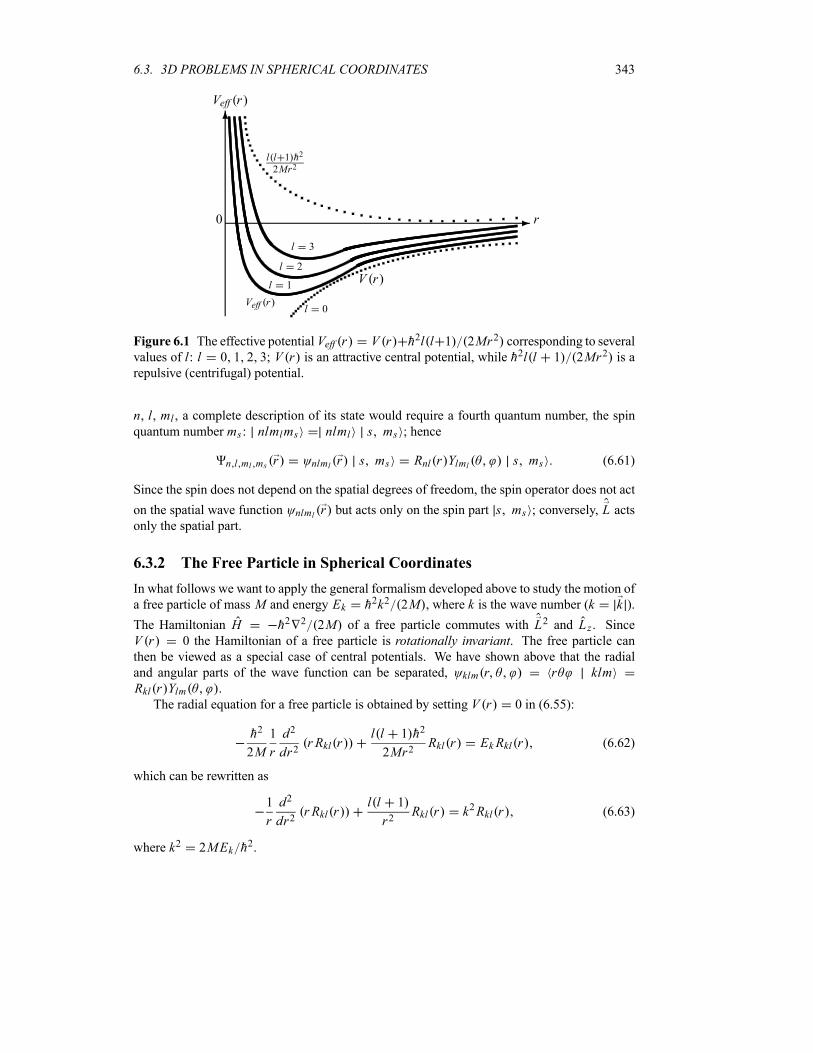
6.3. 3D PROBLEMS IN SPHERICAL COORDINATES 343
-
6
0 r
Veff r
l 1
Veff r
l 2
l 3
l l 1 h2
2Mr2
V r
l 0
Figure 6.1 The effective potential Veff r V r h2l l 1 2Mr2 corresponding to severalvalues of l: l 0 1 2 3; V r is an attractive central potential, while h2l l 1 2Mr2 is arepulsive (centrifugal) potential.
n, l, ml , a complete description of its state would require a fourth quantum number, the spinquantum number ms : nlmlms nlml s ms ; hence
n l ml ms r nlml r s ms Rnl r Ylml s ms (6.61)
Since the spin does not depend on the spatial degrees of freedom, the spin operator does not act
on the spatial wave function nlml r but acts only on the spin part s ms ; conversely, L actsonly the spatial part.
6.3.2 The Free Particle in Spherical Coordinates
In what follows we want to apply the general formalism developed above to study the motion of
a free particle of mass M and energy Ek h2k2 2M , where k is the wave number (k k ).
The Hamiltonian H h2 2 2M of a free particle commutes with L2 and L z . SinceV r 0 the Hamiltonian of a free particle is rotationally invariant. The free particle canthen be viewed as a special case of central potentials. We have shown above that the radial
and angular parts of the wave function can be separated, klm r r klmRkl r Ylm .
The radial equation for a free particle is obtained by setting V r 0 in (6.55):
h2
2M
1
r
d2
dr2r Rkl r
l l 1 h2
2Mr2Rkl r EkRkl r (6.62)
which can be rewritten as
1
r
d2
dr2r Rkl r
l l 1
r2Rkl r k2Rkl r (6.63)
where k2 2MEk h2.
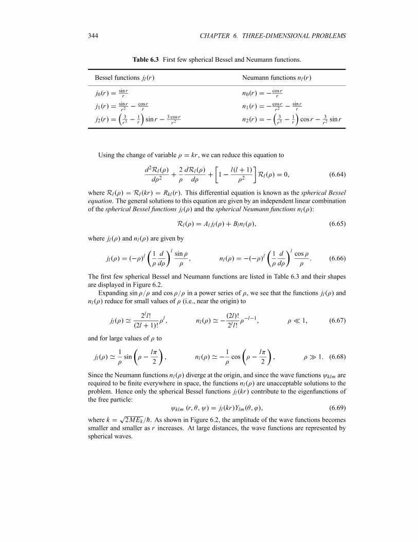
344 CHAPTER 6. THREE-DIMENSIONAL PROBLEMS
Table 6.3 First few spherical Bessel and Neumann functions.
Bessel functions jl r Neumann functions nl r
j0 rsin rr n0 r
cos rr
j1 rsin rr2
cos rr n1 r
cos rr2
sin rr
j2 r3r3
1r sin r 3 cos r
r2n2 r
3r3
1r cos r 3
r2sin r
Using the change of variable kr , we can reduce this equation to
d2Rld 2
2 dRld
1l l 1
2Rl 0 (6.64)
where Rl Rl kr Rkl r . This differential equation is known as the spherical Besselequation. The general solutions to this equation are given by an independent linear combinationof the spherical Bessel functions jl and the spherical Neumann functions nl :
Rl Al jl Blnl (6.65)
where jl and nl are given by
jll 1 d
d
lsin
nll 1 d
d
lcos
(6.66)
The first few spherical Bessel and Neumann functions are listed in Table 6.3 and their shapes
are displayed in Figure 6.2.
Expanding sin and cos in a power series of , we see that the functions jl and
nl reduce for small values of (i.e., near the origin) to
jl2ll!
2l 1 !l nl
2l !
2ll!l 1 1 (6.67)
and for large values of to
jl1sin
l
2nl
1cos
l
21 (6.68)
Since the Neumann functions nl diverge at the origin, and since the wave functions klm are
required to be finite everywhere in space, the functions nl are unacceptable solutions to the
problem. Hence only the spherical Bessel functions jl kr contribute to the eigenfunctions ofthe free particle:
klm r jl kr Ylm (6.69)
where k 2MEk h. As shown in Figure 6.2, the amplitude of the wave functions becomessmaller and smaller as r increases. At large distances, the wave functions are represented byspherical waves.
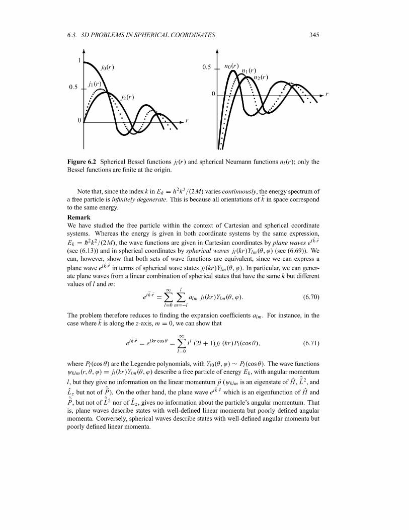
6.3. 3D PROBLEMS IN SPHERICAL COORDINATES 345
-
6
0 r
j0 r1
0 5j1 r
j2 r-
6
0 r
0 5 n0 rn1 r
n2 r
Figure 6.2 Spherical Bessel functions jl r and spherical Neumann functions nl r ; only theBessel functions are finite at the origin.
Note that, since the index k in Ek h2k2 2M varies continuously, the energy spectrum ofa free particle is infinitely degenerate. This is because all orientations of k in space correspondto the same energy.
Remark
We have studied the free particle within the context of Cartesian and spherical coordinate
systems. Whereas the energy is given in both coordinate systems by the same expression,
Ek h2k2 2M , the wave functions are given in Cartesian coordinates by plane waves eik r
(see (6.13)) and in spherical coordinates by spherical waves jl kr Ylm (see (6.69)). We
can, however, show that both sets of wave functions are equivalent, since we can express a
plane wave eik r in terms of spherical wave states jl kr Ylm . In particular, we can gener-
ate plane waves from a linear combination of spherical states that have the same k but differentvalues of l and m:
eik r
l 0
l
m l
alm jl kr Ylm (6.70)
The problem therefore reduces to finding the expansion coefficients alm . For instance, in thecase where k is along the z-axis, m 0, we can show that
eik r eikr cos
l 0
i l 2l 1 jl kr Pl cos (6.71)
where Pl cos are the Legendre polynomials, with Yl0 Pl cos . The wave functions
klm r jl kr Ylm describe a free particle of energy Ek , with angular momentum
l, but they give no information on the linear momentum p ( klm is an eigenstate of H , L2, and
Lz but not of P). On the other hand, the plane wave eik r which is an eigenfunction of H and
P , but not of L2 nor of Lz , gives no information about the particle’s angular momentum. Thatis, plane waves describe states with well-defined linear momenta but poorly defined angular
momenta. Conversely, spherical waves describe states with well-defined angular momenta but
poorly defined linear momenta.
346 CHAPTER 6. THREE-DIMENSIONAL PROBLEMS
6.3.3 The Spherical Square Well Potential
Consider now the problem of a particle of mass M in an attractive square well potential
V rV0 r a
0 r a(6.72)
Let us consider the cases 0 r a and r a separately.
6.3.3.1 Case where 0 r a
Inside the well, 0 r a, the time-independent Schrödinger equation for this particle can beobtained from (6.55):
h2
2M
1
r
d2
dr2r Rl r
l l 1 h2
2Mr2Rl r E V0 Rl r (6.73)
Using the change of variable k1r , where k1 is now given by k1 2M E V0 h, wesee that (6.73) reduces to the spherical Bessel differential equation (6.64). As in the case of
a free particle, the radial wave function must be finite everywhere, and is given as follows in
terms of the spherical Bessel functions jl k1r :
Rl r A jl k1r A jl2M E V0
hr for r a (6.74)
where A is a normalization constant.
6.3.3.2 Case where r a
Outside the well, r a, the particle moves freely; its Schrödinger equation is (6.62):
h2
2M
1
r
d2
dr2r Rkl r
l l 1 h2
2Mr2Rkl r EkRkl r r a (6.75)
Two possibilities arise here, depending on whether the energy is negative or positive.
The negative energy case corresponds to bound states (i.e., to a discrete energy spectrum).
The general solutions of (6.75) are similar to those of (6.63), but k is now an imaginarynumber; that is, we must replace k by ik2 and, hence, the solutions are given by linearcombinations of jl ik2r and nl ik2r :
Rl ik2r B jl ik2r nl ik2r (6.76)
where B is a normalization constant, with k2 2ME h. Note: Linear combinationsof jl and nl can be expressed in terms of the spherical Hankel functions of the first
kind, h 1l , and the second kind, h 2l , as follows:
h 1l jl inl (6.77)
h 2l jl inl h 1l (6.78)
6.3. 3D PROBLEMS IN SPHERICAL COORDINATES 347
The first few spherical Hankel functions of the first kind are
h 10 iei
h 111 i
2ei h 12
i 32
3i3ei
(6.79)
The asymptotic behavior of the Hankel functions when can be inferred from
(6.68):
h 1liei l 2 h 2l
ie i l 2 (6.80)
The solutions that need to be retained in (6.76) must be finite everywhere. As can be
inferred from Eq (6.80), only the Hankel functions of the first kind h 1l ik2r are finite at
large values of r (the functions h 2l ik2r diverge for large values of r). Thus, the wavefunctions outside the well that are physically meaningful are those expressed in terms of
the Hankel functions of the first kind (see (6.76)):
Rl ik2r Bh 1l i2ME
hr B jl i
2ME
hr i Bnl i
2ME
hr
(6.81)
The continuity of the radial function and its derivative at r a yields
1
h 1l ik2r
dh 1l ik2r
drr a
1
jl k1r
d jl k1r
dr r a(6.82)
For the l 0 states, this equation reduces to
k2 k1 cot k1a (6.83)
This continuity condition is analogous to the transcendental equation we obtained in
Chapter 4 when we studied the one-dimensional finite square well potential.
The positive energy case corresponds to the continuous spectrum (unbound or scattering
states), where the solution is asymptotically oscillatory. The solution consists of a linear
combination of jl k r and nl k r , where k 2ME h. Since the solution must befinite everywhere, the continuity condition at r a determines the coefficients of thelinear combination. The particle can move freely to infinity with a finite kinetic energy
E h2k 2 2M .
6.3.4 The Isotropic Harmonic Oscillator
The radial Schrödinger equation for a particle of mass M in an isotropic harmonic oscillator
potential
V r1
2M 2r2 (6.84)
is obtained from (6.57):
h2
2M
d2Unl r
dr21
2M 2r2
l l 1 h2
2Mr2Unl r EUnl r (6.85)
348 CHAPTER 6. THREE-DIMENSIONAL PROBLEMS
We are going to solve this equation by examining the behavior of the solutions at the asymptotic
limits (at very small and very large values of r ). On the one hand, when r 0, the E andM 2r2 2 terms become too small compared to the l l 1 h2 2Mr2 term. Hence, when r 0,
Eq. (6.85) reduces to
h2
2M
d2U r
dr2l l 1 h2
2Mr2U r 0 (6.86)
the solutions of this equation are of the form U r r l 1. On the other hand,when r ,
the E and l l 1 h2 2Mr2 terms become too small compared to the M 2r2 2 term; hence,the asymptotic form of (6.85) when r is
h2
2M
d2U r
dr21
2M 2r2U r 0 (6.87)
which admits solutions of type U r e M r2 2h . Combining (6.86) and (6.87), we can write
the solutions of (6.85) as
U r f r r l 1e M r2 2h (6.88)
where f r is a function of r . Substituting this expression into (6.85), we obtain an equationfor f r :
d2 f r
dr22l 1
r
M
hrd f r
dr
2ME
h22l 3
M
hf r 0 (6.89)
Let us try a power series solution
f rn 0
anrn a0 a1r a2r
2 anrn (6.90)
Substituting this function into (6.89), we obtain
n 0
n n 1 anrn 2 2
l 1
r
M
hr nanr
n 1
2ME
h22l 3
M
hanr
n 0
(6.91)
which in turn reduces to
n 0
n n 2l 1 anrn 2 2M
hn
2ME
h22l 3
M
hanr
n 0 (6.92)
For this equation to hold, the coefficients of the various powers of r must vanish separately. Forinstance, when n 0 the coefficient of r 2 is indeed zero:
0 2l 1 a0 0 (6.93)
Note that a0 need not be zero for this equation to hold. The coefficient of r 1 corresponds to
n 1 in (6.92); for this coefficient to vanish, we must have
1 2l 2 a1 0 (6.94)
6.3. 3D PROBLEMS IN SPHERICAL COORDINATES 349
Since 2l 2 cannot be zero, because the quantum number l is a positive integer, a1 mustvanish.
The coefficient of rn results from the relation
n 0
n 2 n 2l 3 an 22ME
h2M
h2n 2l 3 an rn 0 (6.95)
which leads to the recurrence formula
n 2 n 2l 3 an 22ME
h2M
h2n 2l 3 an (6.96)
This recurrence formula shows that all coefficients an corresponding to odd values of n arezero, since a1 0 (see (6.94)). The function f r must therefore contain only even powers ofr :
f rn 0
a2nr2n
n 0 2 4
an rn (6.97)
where all coefficients a2n , with n 1, are proportional to a0.Now note that when n the function f r diverges, for it behaves asymptotically like
er2. To obtain a finite solution, we must require the series (6.97) to stop at a maximum power
rn ; hence it must be polynomial. For this, we require an 2 to be zero. Thus, setting an 2
0 into the recurrence formula (6.96) and since an 0, we obtain at once the quantizationcondition
2M
h2En l
M
h2n 2l 3 0 (6.98)
or
En l n l3
2h (6.99)
where n is even (see (6.97)). Denoting n by 2N , where N 0 1 2 3 , we rewrite this
energy expression as
En n3
2h n 0 1 2 3 (6.100)
where n n l 2N l.The ground state, whose energy is E0
32h , is not degenerate; the first excited state, E1
52h , is threefold degenerate; and the second excited state, E2
72h , is sixfold degenerate
(Table 6.4). As shown in the following example, the degeneracy relation for the nth level isgiven by
gn1
2n 1 n 2 (6.101)
This expression is in agreement with (6.36) obtained for an isotropic harmonic oscillator in
Cartesian coordinates.
Finally, since the radial wave function is given by Rnl r Unl r r , whereUnl r is listedin (6.88) with f r being a polynomial in r2l of degree n l 2, the total wave function for
the isotropic harmonic oscillator is
nlm r Rnl r YlmUnl r
rYlm r l f r Ylm e M r2 2h (6.102)
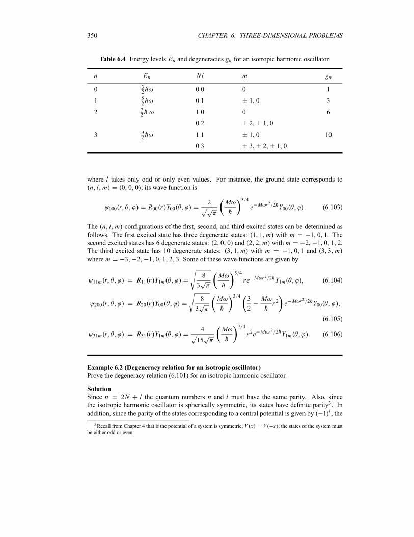
350 CHAPTER 6. THREE-DIMENSIONAL PROBLEMS
Table 6.4 Energy levels En and degeneracies gn for an isotropic harmonic oscillator.
n En Nl m gn
0 32h 0 0 0 1
1 52h 0 1 1, 0 3
2 72h 1 0 0 6
0 2 2, 1, 0
3 92h 1 1 1, 0 10
0 3 3, 2, 1, 0
where l takes only odd or only even values. For instance, the ground state corresponds ton l m 0 0 0 ; its wave function is
000 r R00 r Y002 M
h
3 4
e M r2 2hY00 (6.103)
The n l m configurations of the first, second, and third excited states can be determined as
follows. The first excited state has three degenerate states: 1 1 m with m 1 0 1. The
second excited states has 6 degenerate states: 2 0 0 and 2 2 m with m 2 1 0 1 2.
The third excited state has 10 degenerate states: 3 1 m with m 1 0 1 and 3 3 mwhere m 3 2 1 0 1 2 3. Some of these wave functions are given by
11m r R11 r Y1m8
3
M
h
5 4
re M r2 2hY1m (6.104)
200 r R20 r Y008
3
M
h
3 43
2
M
hr2 e M r2 2hY00
(6.105)
31m r R31 r Y1m4
15
M
h
7 4
r2e M r2 2hY1m (6.106)
Example 6.2 (Degeneracy relation for an isotropic oscillator)
Prove the degeneracy relation (6.101) for an isotropic harmonic oscillator.
Solution
Since n 2N l the quantum numbers n and l must have the same parity. Also, sincethe isotropic harmonic oscillator is spherically symmetric, its states have definite parity3. In
addition, since the parity of the states corresponding to a central potential is given by 1 l , the
3Recall from Chapter 4 that if the potential of a system is symmetric, V x V x , the states of the system mustbe either odd or even.
6.3. 3D PROBLEMS IN SPHERICAL COORDINATES 351
quantum number l ( hence n) can take only even or only odd values. Let us consider separatelythe cases when n is even or odd.First, when n is even the degeneracy gn of the nth excited state is given by
gnn
l 0 2 4
2l 1
n
l 0 2 4
1 2
n
l 0 2 4
l1
2n 2
n n 2
2
1
2n 1 n 2 (6.107)
Amore explicit way of obtaining this series consists of writing it in the following two equivalent
forms:
gn 1 5 9 13 2n 7 2n 3 2n 1 (6.108)
gn 2n 1 2n 3 2n 7 2n 11 13 9 5 1 (6.109)
We then add them, term by term, to get
2gn 2n 2 2n 2 2n 2 2n 2 2n 2 2n 2n
21 (6.110)
This relation yields gn12n 1 n 2 , which proves (6.101) when n is even.
Second, when n is odd, a similar treatment leads to
gnn
l 1 3 5 7
2l 1
n
l 1 3 5 7
1 2
n
l 1 3 5 7
l1
2n 1
1
2n 1 2
1
2n 1 n 2 (6.111)
which proves (6.101) when n is odd. Note that this degeneracy relation is, as expected, identicalwith the degeneracy expression (6.36) obtained for a harmonic oscillator in Cartesian coordi-
nates.
6.3.5 The Hydrogen Atom
The hydrogen atom consists of an electron and a proton. For simplicity, we will ignore their
spins. The wave function then depends on six coordinates re xe ye ze and rp xp yp z p ,where re and rp are the electron and proton position vectors, respectively. According to theprobabilistic interpretation of the wave function, the quantity re rp t 2d3re d3rp repre-sents the probability that a simultaneous measurement of the electron and proton positions at
time t will result in the electron being in the volume element d3re and the proton in d3rp.The time-dependent Schrödinger equation for the hydrogen atom is given by
h2
2m p2p
h2
2me2e V r re rp t ih
tre rp t (6.112)
where 2p and
2e are the Laplacians with respect to the proton and the electron degrees of
freedom, with 2p
2 x2p2 y2p
2 z2p and2e
2 x2e2 y2e
2 z2e , andwhere V r is the potential (interaction) between the electron and the proton. This interaction,which depends only on the distance that separates the electron and the proton r re rp, isgiven by the Coulomb potential:
V re2
r(6.113)
352 CHAPTER 6. THREE-DIMENSIONAL PROBLEMS
Note: Throughout this text, we will be using the CGS units for the Coulomb potential where it
is given by V r e2 r (in the MKS units, however, it is given by V r e2 4 0r ).Since V does not depend on time, the solutions of (6.112) are stationary; hence, they can
be written as follows:
re rp t re rp ei Et h (6.114)
where E is the total energy of the electron–proton system. Substituting this into (6.112), weobtain the time-independent Schrödinger equation for the hydrogen atom:
h2
2m p2p
h2
2me2e
e2
re rpre rp E re rp (6.115)
6.3.5.1 Separation of the Center of Mass Motion
Since V depends only on the relative distance r between the electron and proton, instead of thecoordinates re and rp (position vectors of the electron and proton), it is more appropriate to use
the coordinates of the center of mass, R Xi Y j Zk, and the relative coordinates of theelectron with respect to the proton, r xi y j zk. The transformation from re, rp to R, ris given by
Rmere m prpme m p
r re rp (6.116)
We can verify that the Laplacians 2e and
2p are related to
2R
2
X2
2
Y 2
2
Z22r
2
x2
2
y2
2
z2(6.117)
as follows:1
me2e
1
m p2p
1
M2R
1 2r (6.118)
where
M me m pmem pme m p
(6.119)
are the total and reduced masses, respectively The time-independent Schrödinger equation
(6.115) then becomes
h2
2M2R
h2
22r V r E R r E E R r (6.120)
where E R r re rp . Let us now solve this equation by the separation of variables;that is, we look for solutions of the form
E R r R r (6.121)
where R and r are the wave functions of the CM and of the relative motions, respec-
tively. Substituting this wave function into (6.120) and dividing by R r , we obtain
h2
2M
1
R2R R
h2
2
1
r2r r V r E (6.122)
6.3. 3D PROBLEMS IN SPHERICAL COORDINATES 353
The first bracket depends only on R whereas the second bracket depends only on r . Since Rand r are independent vectors, the two expressions of the left hand side of (6.122) must beseparately constant. Thus, we can reduce (6.122) to the following two separate equations:
h2
2M2R R ER R (6.123)
h2
22r r V r r Er r (6.124)
with the condition
ER Er E (6.125)
We have thus reduced the Schrödinger equation (6.120), which involves two variables R andr , into two separate equations (6.123) and (6.124) each involving a single variable. Note thatequation (6.123) shows that the center of mass moves like a free particle of mass M . Thesolution to this kind of equation was examined earlier in this chapter; it has the form
R 2 3 2eik R (6.126)
where k is the wave vector associated with the center of mass. The constant ER h2k2 2Mgives the kinetic energy of the center of mass in the lab system (the total mass M is located at
the origin of the center of mass coordinate system).
The second equation (6.124) represents the Schrödinger equation of a fictitious particle of
mass moving in the central potential e2 r .We should note that the total wave function E R r R r is seldom used. When
the hydrogen problem is mentioned, this implicitly refers to r and Er . That is, the hydrogenwave function and energy are taken to be given by r and Er , not by E and E .
6.3.5.2 Solution of the Radial Equation for the Hydrogen Atom
The Schrödinger equation (6.124) for the relative motion has the form of an equation for a
central potential. The wave function r that is a solution to this equation is a product of anangular part and a radial part. The angular part is given by the spherical harmonic Ylm .
The radial part R r can be obtained by solving the following radial equation:
h2
2
d2U r
dr2l l 1 h2
2 r2e2
rU r EU r (6.127)
whereU r r R r . To solve this radial equation, we are going to consider first its asymptoticsolutions and then attempt a power series solution.
(a) Asymptotic behavior of the radial wave function
For very small values of r , (6.127) reduces to
d2U r
dr2l l 1
r2U r 0 (6.128)
whose solutions are of the form
U r Ar l 1 Br l (6.129)
354 CHAPTER 6. THREE-DIMENSIONAL PROBLEMS
where A and B are constants. Since U r vanishes at r 0, the second term r l , which
diverges at r 0, must be discarded. Thus, for small r , the solution is
U r r l 1 (6.130)
Now, in the limit of very large values of r , we can approximate (6.127) by
d2U r
dr22 E
h2U r 0 (6.131)
Note that, for bound state solutions, which correspond to the states where the electron and
the proton are bound together, the energy E must be negative. Hence the solutions to thisequation are of the form U r e r where 2 E h. Only the minus sign solutionis physically acceptable, since e r diverges for large values of r . So, for large values of r , U rbehaves like
U r e r (6.132)
The solutions to (6.127) can be obtained by combining (6.130) and (6.132):
U r r l 1 f r e r (6.133)
where f r is an r -dependent function. Substituting (6.133) into (6.127) we end up with adifferential equation that determines the form of f r :
d2 f
dr22l 1
r
d f
dr2
l 1 e2 h2
rf r 0 (6.134)
(b) Power series solutions for the radial equation
As in the case of the three-dimensional harmonic oscillator, let us try a power series solution
for (6.134):
f rk 0
bkrk (6.135)
which, when inserted into (6.134), yields
k 0
k k 2l 1 bkrk 2 2 k l 1
e2
h2bkr
k 1 0 (6.136)
This equation leads to the following recurrence relation (by changing k to k 1 in the last term):
k k 2l 1 bk 2 k le2
h2bk 1 (6.137)
In the limit of large values of k, the ratio of successive coefficients,
bkbk 1
2 k l e2 h2
k k 2l 1(6.138)
is of the order ofbkbk 1
2
k(6.139)
6.3. 3D PROBLEMS IN SPHERICAL COORDINATES 355
This is the behavior of an exponential series, since the ratio of successive coefficients of the
relation e2x k 0 2xk k! is given by
2k
k!
k 1 !
2k 1
2
k(6.140)
That is, the asymptotic behavior of (6.135) is
f rk 0
bkrk e2 r (6.141)
hence the radial solution (6.133) becomes
U r r l 1e2 re r r l 1e r (6.142)
But this contradicts (6.133): for large values of r , the asymptotic behavior of the physicallyacceptable radial function (6.133) is given by e r while that of (6.142) by e r ; the form (6.142)is thus physically unacceptable.
(c) Energy quantization
To obtain physically acceptable solutions, the series (6.135) must terminate at a certain powerN ; hence the function f r becomes a polynomial of order N :
f rN
k 0
bkrk (6.143)
This requires that all coefficients bN 1, bN 2, bN 3, have to vanish. When bN 1 0 the
recurrence formula (6.137) yields
N l 1e2
h20 (6.144)
Since 2 E h2 and using the notation
n N l 1 (6.145)
where n is known as the principal quantum number and N as the radial quantum number, wecan infer the energy
Ene4
2h21
n2(6.146)
which in turn can be written as
Ene4
2h21
n2e2
2a0
1
n2(6.147)
because (from Bohr theory of the hydrogen atom) the Bohr radius is given by a0 h2 e2
and hence h2 1 e2a0 . Note that we can write in terms of a0 as follows:
2h2En 2
1
e2a0
e2
2a0n21
na0(6.148)
356 CHAPTER 6. THREE-DIMENSIONAL PROBLEMS
Since N 0 1 2 3 , the allowed values of n are nonzero integers, n l 1, l 2, l 3,
. For a given value of n, the orbital quantum number l can have values only between 0 andn 1 (i.e., l 0 1 2 n 1).
Remarks
Note that (6.147) is similar to the energy expression obtained from the Bohr quantization
condition, discussed in Chapter 1. It can be rewritten in terms of the Rydberg constant
R mee4 2h2 as follows:
Enm p
m p me
R
n2(6.149)
where R 13 6 eV. Since the ratio me m p is very small (me m p 1), we can
approximate this expression by
En 1mem p
1 R
n21
mem p
R
n2(6.150)
So, if we consider the proton to be infinitely more massive than the electron, we recover
the energy expression as derived by Bohr: En R n2.
Energy of hydrogen-like atoms: How does one obtain the energy of an atom or ion with
a nuclear charge Ze but which has only one electron4? Since the Coulomb potential feltby the single electron due to the charge Ze is given by V r Ze2 r , the energy ofthe electron can be inferred from (6.147) by simply replacing e2 with Ze2:
Enme Ze2 2
2h21
n2Z2E0n2
(6.151)
where E0 e2 2a0 13 6 eV; in deriving this relation, we have assumed that the
mass of the nucleus is infinitely large compared to the electronic mass.
(d) Radial wave functions of the hydrogen atom
The radial wave function Rnl r can be obtained by inserting (6.143) into (6.133),
Rnl r1
rUnl r Anlr
le rN
k 0
bkrk Anlr
le r na0N
k 0
bkrk (6.152)
since, as shown in (6.148), 1 na0 ; Anl is a normalization constant.How does one determine the expression of Rnl r ? This issue reduces to obtaining the form
of the polynomial r l Nk 0 bkr
k and the normalization constant Anl . For this, we are going toexplore two methods: the first approach follows a straightforward calculation and the second
makes use of special functions.
4For instance, Z 1 refers to H, Z 2 to He , Z 3 to Li2 , Z 4 to Be3 , Z 5 to B4 , Z 6 to C5 ,
and so on.
6.3. 3D PROBLEMS IN SPHERICAL COORDINATES 357
(i) First approach: straightforward calculation of Rnl rThis approach consists of a straightforward construction of Rnl r ; we are going to show howto construct only the first few expressions. For instance, if n 1 and l 0 then N 0. Since
N n l 1 and 1 na0 we can write (6.152) as
R10 r A10er a0
0
k 0
bkrk A10b0e
r a0 (6.153)
where A10b0 can be obtained from the normalization of R10 r : using 0 xne ax dx n! an 1,
we have
10
r2 R10 r2 dr A210b
200
r2e 2r a0dr A210b20
a304
(6.154)
hence A10 1 and b0 2 a03 2. Thus, R10 r is given by
R10 r 2 a03 2 e r a0 (6.155)
Next, let us find R20 r . Since n 2, l 0 we have N 2 0 1 1 and
R20 r A20er 2a0
1
k 0
bkrk A20 b0 b1r e
r 2a0 (6.156)
From (6.138) we can express b1 in terms of b0 as
b12 k l 2 a0k k 2l 1
b01
2a0b0
1
a0 a30
(6.157)
because 1 2a0 , k 1, and l 0. So, substituting (6.157) into (6.156) and normalizing,
we get A20 1 2 2 ; hence
R20 r1
2a30
1r
2a0e r 2a0 (6.158)
Continuing in this way, we can obtain the expression of any radial wave function Rnl r ; notethat, knowing b0 2 a0
3 2, we can use the recursion relation (6.138) to obtain all other
coefficients b2, b3, .
(ii) Second approach: determination of Rnl r by means of special functionsThe polynomial r l N
k 0 bkrk present in (6.152) is a polynomial of degree N l or n 1 since
n N l 1. This polynomial, which is denoted by LNk r , is known as the associatedLaguerre polynomial; it is a solution to the Schrödinger equation (6.134). The solutions todifferential equations of the form (6.134) were studied by Laguerre long before the birth of
quantum mechanics. The associated Laguerre polynomial is defined, in terms of the Laguerrepolynomials of order k, Lk r , by
LNk rdN
drNLk r (6.159)
where
Lk r erdk
drkr ke r (6.160)
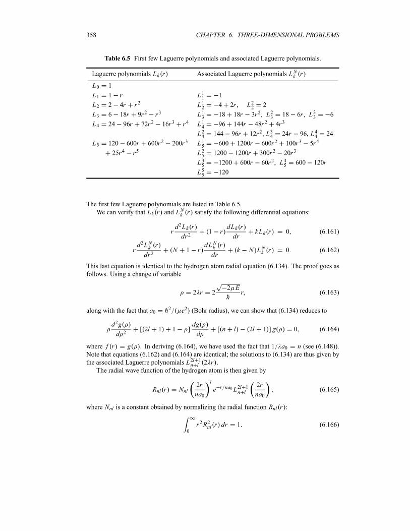
358 CHAPTER 6. THREE-DIMENSIONAL PROBLEMS
Table 6.5 First few Laguerre polynomials and associated Laguerre polynomials.
Laguerre polynomials Lk r Associated Laguerre polynomials LNk r
L0 1
L1 1 r L11 1
L2 2 4r r2 L12 4 2r , L22 2
L3 6 18r 9r2 r3 L13 18 18r 3r2, L23 18 6r , L33 6
L4 24 96r 72r2 16r3 r4 L14 96 144r 48r2 4r3
L24 144 96r 12r2, L34 24r 96, L44 24
L5 120 600r 600r2 200r3 L15 600 1200r 600r2 100r3 5r4
25r4 r5 L25 1200 1200r 300r2 20r3
L35 1200 600r 60r2, L45 600 120r
L55 120
The first few Laguerre polynomials are listed in Table 6.5.
We can verify that Lk r and LNk r satisfy the following differential equations:
rd2Lk r
dr21 r
dLk r
drkLk r 0 (6.161)
rd2LNk r
dr2N 1 r
dLNk r
drk N LNk r 0 (6.162)
This last equation is identical to the hydrogen atom radial equation (6.134). The proof goes as
follows. Using a change of variable
2 r 22 E
hr (6.163)
along with the fact that a0 h2 e2 (Bohr radius), we can show that (6.134) reduces to
d2g
d 2[ 2l 1 1 ]
dg
d[ n l 2l 1 ] g 0 (6.164)
where f r g . In deriving (6.164), we have used the fact that 1 a0 n (see (6.148)).Note that equations (6.162) and (6.164) are identical; the solutions to (6.134) are thus given by
the associated Laguerre polynomials L2l 1n l 2 r .The radial wave function of the hydrogen atom is then given by
Rnl r Nnl2r
na0
l
e r na0L2l 1n l
2r
na0(6.165)
where Nnl is a constant obtained by normalizing the radial function Rnl r :
0
r2R2nl r dr 1 (6.166)

6.3. 3D PROBLEMS IN SPHERICAL COORDINATES 359
Table 6.6 The first few radial wave functions Rnl r of the hydrogen atom.
R10 r 2a 3 20 e r a0 R21 r
1
6a30
r2a0e r 2a0
R20 r1
2a30
1 r2a0
e r 2a0 R31 r8
9 6a30
1 r6a0
r3a0
e r 3a0
R30 r2
3 3a30
1 2r3a0
2r2
27a20e r 3a0 R32 r
4
9 30a30
r3a0
2e r 3a0
Using the normalization condition of the associated Laguerre functions
0
e 2l L2l 1n l
22d
2n [ n l !]3
n l 1 !(6.167)
where 2 r 2r na0 , we can show that Nnl is given by
Nnl2
na0
3 2 n l 1 !
2n[ n l !]3(6.168)
The wave functions of the hydrogen atom are given by
nlm r Rnl r Ylm (6.169)
where the radial functions Rnl r are
Rnl r2
na0
3 2 n l 1 !
2n[ n l !]32r
na0
l
e r na0L2l 1n l
2r
na0(6.170)
The first few radial wave functions are listed in Table 6.6; as shown in (6.155) and (6.158),
they are identical with those obtained from a straightforward construction of Rnl r . The shapesof some of these radial functions are plotted in Figure 6.3.
(e) Properties of the radial wave functions of hydrogen
The radial wave functions of the hydrogen atom behave as follows (see Figure 6.3):
They behave like r l for small r .
They decrease exponentially at large r , since L2l 1n l is dominated by the highest power,
rn l 1.
Each function Rnl r has n l 1 radial nodes, since L2l 1n l is a polynomial of degree
n l 1.
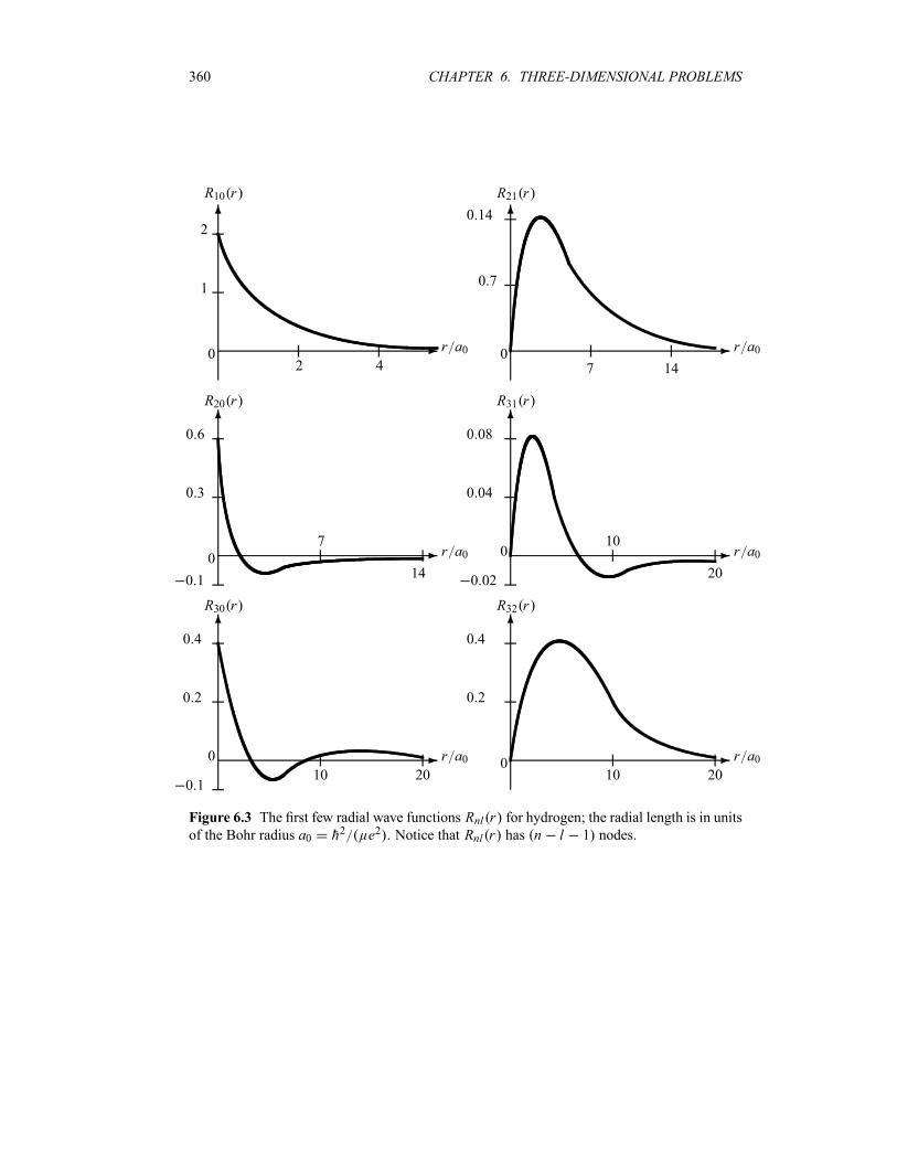
360 CHAPTER 6. THREE-DIMENSIONAL PROBLEMS
-
6
0r a0
R10 r
2
1
42
-
6
0r a0
R21 r
0 14
0 7
147
-
6
0r a0
R20 r
0 6
0 3
0 114
7-
6
0 r a0
R31 r
0 08
0 04
0 0220
10
-
6
0 r a0
R30 r
0 4
0 2
0 12010
-
6
0r a0
R32 r
0 4
0 2
2010
Figure 6.3 The first few radial wave functions Rnl r for hydrogen; the radial length is in unitsof the Bohr radius a0 h2 e2 . Notice that Rnl r has n l 1 nodes.
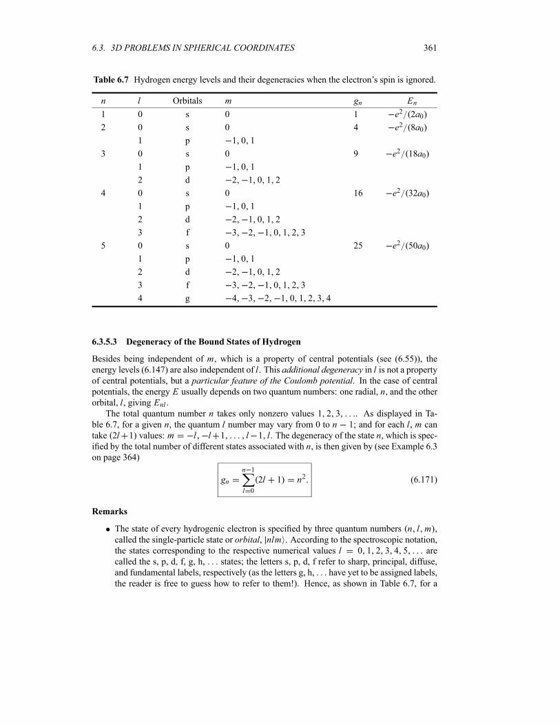
6.3. 3D PROBLEMS IN SPHERICAL COORDINATES 361
Table 6.7 Hydrogen energy levels and their degeneracies when the electron’s spin is ignored.
n l Orbitals m gn En
1 0 s 0 1 e2 2a02 0 s 0 4 e2 8a0
1 p 1 0 1
3 0 s 0 9 e2 18a01 p 1 0 1
2 d 2 1 0 1 2
4 0 s 0 16 e2 32a01 p 1 0 1
2 d 2 1 0 1 2
3 f 3 2 1 0 1 2 3
5 0 s 0 25 e2 50a01 p 1 0 1
2 d 2 1 0 1 2
3 f 3 2 1 0 1 2 3
4 g 4 3 2 1 0 1 2 3 4
6.3.5.3 Degeneracy of the Bound States of Hydrogen
Besides being independent of m, which is a property of central potentials (see (6.55)), theenergy levels (6.147) are also independent of l. This additional degeneracy in l is not a propertyof central potentials, but a particular feature of the Coulomb potential. In the case of centralpotentials, the energy E usually depends on two quantum numbers: one radial, n, and the otherorbital, l, giving Enl .The total quantum number n takes only nonzero values 1 2 3 . As displayed in Ta-
ble 6.7, for a given n, the quantum l number may vary from 0 to n 1; and for each l, m cantake 2l 1 values: m l l 1 l 1 l. The degeneracy of the state n, which is spec-ified by the total number of different states associated with n, is then given by (see Example 6.3on page 364)
gnn 1
l 0
2l 1 n2 (6.171)
Remarks
The state of every hydrogenic electron is specified by three quantum numbers n l m ,called the single-particle state or orbital, nlm . According to the spectroscopic notation,the states corresponding to the respective numerical values l 0 1 2 3 4 5 are
called the s, p, d, f, g, h, states; the letters s, p, d, f refer to sharp, principal, diffuse,
and fundamental labels, respectively (as the letters g, h, have yet to be assigned labels,
the reader is free to guess how to refer to them!). Hence, as shown in Table 6.7, for a
362 CHAPTER 6. THREE-DIMENSIONAL PROBLEMS
given n an s-state has 1 orbital n00 , a p-state has 3 orbitals n1m corresponding to
m 1 0 1, a d-state has 5 orbitals n2m corresponding to m 2 1 0 1 2, and
so on.
If we take into account the spin of the electron, the state of every electron will be specified
by four quantum numbers n l ml ms , where ms12is the z-component of the spin
of the electron. Hence the complete wave function of the hydrogen atom must be equal
to the product of a space part or orbital nlml r Rnl r Ylml , and a spin part12ms :
nlmlms r nlml r1
2
1
2Rnl r Ylml
1
2
1
2(6.172)
Using the spinors from Chapter 5 we can write the spin-up wave function as
nlml12r nlml r
1
2
1
2nlml
1
0nlml0
(6.173)
and the spin-down wave function as
nlml12r nlml r
1
2
1
2nlml
0
1
0
nlml(6.174)
For instance, the spin-up and spin-down ground state wave functions of hydrogen aregiven by
100 12r 100
01 a 3 2
0 e r a0
0(6.175)
100 12r
0
100
0
1 a 3 20 e r a0
(6.176)
When spin is included the degeneracy of the hydrogen’s energy levels is given by
2
n 1
l 0
2l 1 2n2 (6.177)
since, in addition to the degeneracy (6.171), each level is doubly degenerate with respect
to the spin degree of freedom. For instance, the ground state of hydrogen is doubly
degenerate since100 1
2r and
100 12r correspond to the same energy 13 6 eV.
Similarly, the first excited state is eightfold degenerate (2 2 2 8) because the eight
states200 1
2r ,
211 12r ,
210 12r , and
21 1 12r correspond to the same
energy 13 6 4 eV 3 4 eV.
6.3.5.4 Probabilities and Averages
When a hydrogen atom is in the stationary state nlm r , the quantity nlm r 2 d3rrepresents the probability of finding the electron in the volume element d3r , where
6.3. 3D PROBLEMS IN SPHERICAL COORDINATES 363
d3r r2 sin dr d d . The probability of finding the electron in a spherical shell located
between r and r dr (i.e., a shell of thickness dr) is given by
Pnl r dr0
sin d2
0
d nlm r2 r2dr
Rnl r2r2dr
0
sin d2
0
Ylm Ylm d
Rnl r2r2dr (6.178)
If we integrate this quantity between r 0 and r a, we obtain the probability of finding theelectron in a sphere of radius a centered about the origin. Hence integrating between r 0
and r , we would obtain 1, which is the probability of finding the electron somewhere in
space.
Let us now specify the average values of the various powers of r . Since nlm rRnl r Ylm , we can see that the average of rk is independent of the azimuthal quantumnumber m:
nlm rk nlm rk nlm r2r2 sin dr d d
0
rk 2 Rnl r2dr
0
sin d2
0
Ylm Ylm d
0
rk 2 Rnl r2dr
nl rk nl (6.179)
Using the properties of Laguerre polynomials, we can show that (Problem 6.2, page 370)
nl r nl1
23n2 l l 1 a0 (6.180)
nl r2 nl1
2n2 5n2 1 3l l 1 a20 (6.181)
nl r 1 nl1
n2 a0(6.182)
nl r 2 nl2
n3 2l 1 a20(6.183)
where a0 is the Bohr radius, a0 h2 e2 . The averages (6.180) to (6.183) can be easilyderived from Kramers’ recursion relation (Problem 6.3, page 371):
k 1
n2nl r k nl 2k 1 a0 nl r
k 1 nlka204
2l 1 2 k2 nl rk 2 nl 0 (6.184)
Equations (6.180) and (6.182) reveal that 1 r and 1 r are not equal, but are of the sameorder of magnitude:
r n2a0 (6.185)
This relation is in agreement with the expression obtained from the Bohr theory of hydrogen:
the quantized radii of circular orbits for the hydrogen atom are given by rn n2a0. We will

364 CHAPTER 6. THREE-DIMENSIONAL PROBLEMS
show in Problem 6.6 page 375 that the Bohr radii for circular orbits give the locations where
the probability density of finding the electron reaches its maximum.
Next, using the expression (6.182) for r 1 , we can obtain the average value of the Coulomb
potential
V r e21
r
e2
a0
1
n2(6.186)
which, as specified by (6.147), is equal to twice the total energy:
En1
2V r
e2
2a0
1
n2(6.187)
This is known as the Virial theorem, which states that if V r nV r , the average expres-sions of the kinetic and potential energies are related by
Tn
2V r (6.188)
For instance, in the case of a Coulomb potential V r 1V r , we have T 12V ;
hence E 12V V 1
2V .
Example 6.3 (Degeneracy relation for the hydrogen atom)
Prove the degeneracy relation (6.171) for the hydrogen atom.
Solution
The energy En e2 2a0n2 of the hydrogen atom (6.147) does not depend on the orbitalquantum number l or on the azimuthal number m; it depends only on the principal quantumnumber n. For a given n, the orbital number l can take n 1 values: l 0 1 2 3 n 1;
while for each l, the azimuthal number m takes 2l 1 values: m l l 1 l 1 l.Thus, for each n, there exist gn different wave functions nlm r , which correspond to the sameenergy En , with
gnn 1
l 0
2l 1 2
n 1
l 0
ln 1
l 0
1 n n 1 n n2 (6.189)
Another way of finding this result consists of writingn 1l 0 2l 1 in the following two equiv-
alent forms:
gn 1 3 5 7 2n 7 2n 5 2n 3 2n 1 (6.190)
gn 2n 1 2n 3 2n 5 2n 7 7 5 3 1 (6.191)
and then add them, term by term:
2gn 2n 2n 2n 2n 2n 2n 2n 2n (6.192)
Since there are n terms (because l can take n values: l 0 1 2 3 n 1), we have
2gn n 2n ; hence gn n2.
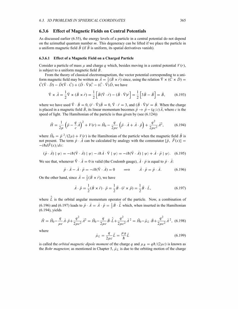
6.3. 3D PROBLEMS IN SPHERICAL COORDINATES 365
6.3.6 Effect of Magnetic Fields on Central Potentials
As discussed earlier (6.55), the energy levels of a particle in a central potential do not depend
on the azimuthal quantum number m. This degeneracy can be lifted if we place the particle ina uniform magnetic field B (if B is uniform, its spatial derivatives vanish).
6.3.6.1 Effect of a Magnetic Field on a Charged Particle
Consider a particle of mass and charge q which, besides moving in a central potential V r ,is subject to a uniform magnetic field B.From the theory of classical electromagnetism, the vector potential corresponding to a uni-
form magnetic field may be written as A 12B r since, using the relation C D
C D D C D C C D, we have
A1
2B r
1
2B r B r
1
23B B B (6.193)
where we have used B 0, r B 0, r 3, and B r B. When the chargeis placed in a magnetic field B, its linear momentum becomes p p q c A, where c is thespeed of light. The Hamiltonian of the particle is thus given by (see (6.124))
H1
2p
q
cA2
V r H0q
2 cp A A p
q2
2 c2A2 (6.194)
where H0 p 2 2 V r is the Hamiltonian of the particle when the magnetic field B isnot present. The term p A can be calculated by analogy with the commutator [p F x ]ihdF x dx :
p A ih A ihA ih A A p (6.195)
We see that, whenever A 0 is valid (the Coulomb gauge), A p is equal to p A:
p A A p ih A 0 A p p A (6.196)
On the other hand, since A 12B r , we have
A p1
2B r p
1
2B r p
1
2B L (6.197)
where L is the orbital angular momentum operator of the particle. Now, a combination of
(6.196) and (6.197) leads to p A A p 12B L which, when inserted in the Hamiltonian
(6.194), yields
H H0q
cA p
q2
2 c2A2 H0
q
2 cB L
q2
2 c2A 2 H0 L B
q2
2 c2A 2 (6.198)
where
Lq
2 cL
B
hL (6.199)
is called the orbital magnetic dipole moment of the charge q and B qh 2 c is known asthe Bohr magneton; as mentioned in Chapter 5, L is due to the orbiting motion of the charge
366 CHAPTER 6. THREE-DIMENSIONAL PROBLEMS
about the center of the potential. The term L B in (6.198) represents the energy resultingfrom the interaction between the particle’s orbital magnetic dipole moment L qL 2 cand the magnetic field B. We should note that if the charge q had an intrinsic spin S, its spinningmotion would give rise to a magnetic dipole moment S qS 2 c which, when interactingwith an external magnetic field B, would in turn generate an energy term S B that must beadded to the Hamiltonian. This issue will be discussed further in Chapter 7.
Finally, using the relation C D E F C E D F C F D E , and sinceA 1
2B r , we have
A 21
4B r B r
1
4B2r2 B r 2 (6.200)
We can thus write (6.198) as
H1
2p 2 V r
q
2 cB L
q2
8 c2B2r2 B r 2 (6.201)
This is the Hamiltonian of a particle of mass and charge q moving in a central potential V runder the influence of a uniform magnetic field B.
6.3.6.2 The Normal Zeeman Effect (S 0)
When a hydrogen atom is placed in an external uniform magnetic field, its energy levels get
shifted. This energy shift is known as the Zeeman effect.In this study we ignore the spin of the hydrogen’s electron. The Zeeman effect without
the spin of the electron is called the normal Zeeman effect. When the spin of the electron isconsidered, we get what is called the anomalous Zeeman effect, to be examined in Chapter9 since its study requires familiarity with the formalisms of addition of angular momenta and
perturbation theory, which will be studied in Chapters 7 and 9, respectively.
For simplicity, we take B along the z-direction: B Bz. The Hamiltonian of the hydrogenatom when subject to such a magnetic field can be obtained from (6.201) by replacing q withthe electron’s charge q e,
H1
2p 2
e2
r
e
2 cBL z
e2B2
8 c2x2 y2 H0
e
2 cBLz
e2B2
8 c2x2 y2
(6.202)
where H0 p2 2 e2 r is the atom’s Hamiltonian in the absence of a magnetic field. Wecan ignore the quadratic term e2B2 x2 y2 8 c2 ; it is too small for a one-electron atomeven when the field B is strong; then (6.202) reduces to
H H0B B
hLz (6.203)
where B eh 2 c 9 2740 10 24 J T 1 5 7884 10 5 eVT 1 is the Bohr magneton;
the electron’s orbital magnetic dipole moment, which results from the orbiting motion of the
electron about the proton, would be given by L eB 2 c . Since H0 commutes withL z , the operators H , L z , and H0 mutually commute; hence they possess a set of commoneigenfunctions: nlm r Rnl r Ylm . The eigenvalues of (6.203) are
Enlm nlm H nlm nlm H0 nlmB B
hnlm L z nlm (6.204)
6.3. 3D PROBLEMS IN SPHERICAL COORDINATES 367
n l 1 0
gl g1 2
2 0 2 1
g2 3
3 0 3 1 3 2
E01
B 0
l 0
l 1
l 2
n l m 1 0 0
2 1 1
2 0 0 2 1 0
2 1 1
E02 B B
E02E02 B B
B 0
3 2 2
3 2 1 3 1 1
3 0 0 3 1 0 3 2 0
3 2 1 3 1 1
3 2 2
E03 2B B
E03 B B
E03E03 B B
E03 2B B
ÃÃÃÃÃÃ
ÃÃ```````̀
!!!!
!!!!
ÃÃÃÃÃÃ
ÃÃ```````̀aaaaaaaa
Figure 6.4 Normal Zeeman effect in hydrogen. (Left) When B 0 the energy levels are
degenerate with respect to l and m. (Right) When B 0 the degeneracy with respect to m isremoved, but the degeneracy with respect to l persists; B eh 2 c .
or
Enlm E0n m BB E0n mh L (6.205)
where E0n are the hydrogen’s energy levels E0n e4 2h2n2 (6.147) and L is called the
Larmor frequency:
LeB
2 c(6.206)
So when a hydrogen atom is placed in a uniform magnetic field, and if we ignore the spin of
the electron, the atom’s spherical symmetry will be broken: each level with angular momentum
l will split into 2l 1 equally spaced levels (Figure 6.4), where the spacing is given by
E h L B B ; the spacing is independent of l. This equidistant splitting of the levels isknown as the normal Zeeman effect. The splitting leads to transitions which are restricted bythe selection rule: m 1 0 1. Transitions m 0 m 0 are not allowed.
The normal Zeeman effect has removed the degeneracy of the levels only partially; the
degeneracy with respect to l remains. For instance, as shown in Figure 6.4, the following levelsare still degenerate: Enlm E200 E210, E32 1 E31 1, E300 E310 E320, andE321 E311. That is, the degeneracies of the levels corresponding to the same n and m butdifferent values of l are not removed by the normal Zeeman effect: Enl m Enlm with l l.The results of the normal Zeeman effect, which show that each energy level splits into an
odd number of 2l 1 equally spaced levels, disagree with the experimental observations. For
instance, every level in the hydrogen atom actually splits into an even number of levels. Thissuggests that the angular momentum is not integer but half-integer. This disagreement is due
to the simplifying assumption where the spin of the electron was ignored. A proper treatment,
which includes the electron spin, confirms that the angular momentum is not purely orbital but
368 CHAPTER 6. THREE-DIMENSIONAL PROBLEMS
includes a spin component as well. This leads to the splitting of each level into an even5 numberof 2 j 1 unequally spaced energy levels. This effect, known as the anomalous Zeeman effect,is in full agreement with experimental findings.
6.4 Concluding Remarks
An important result that needs to be highlighted in this chapter is the solution of the Schrödinger
equation for the hydrogen atom. Unlike Bohr’s semiclassical model, which is founded on
piecemeal assumptions, we have seen how the Schrödinger equation yields the energy levels
systematically and without ad hoc arguments, the quantization of the energy levels comes out
naturally as a by-product of the formalism, not as an unjustified assumption: it is a conse-
quence of the boundary conditions which require the wave function to be finite as r ;
see (6.144) and (6.147). So we have seen that by solving a single differential equation—the
Schrödinger equation—we obtain all that we need to know about the hydrogen atom. As such,
the Schrödinger equation has delivered on the promise made in Chapter 1: namely, a theory
that avoids the undesired aspects of Bohr’s model—its hand-waving, ad hoc assumptions—
while preserving its good points (i.e., the expressions for the energy levels, the radii, and the
transition relations).
6.5 Solved Problems
Problem 6.1
Consider a spinless particle of mass m which is moving in a three-dimensional potential
V x y z12m 2z2 0 x a 0 y a
elsewhere
(a) Write down the total energy and the total wave function of this particle.
(b) Assuming that h 3 2h2 2ma2 , find the energies and the corresponding degenera-cies for the ground state and first excited state.
(c) Assume now that, in addition to the potential V x y z , this particle also has a negativeelectric charge q and that it is subjected to a constant electric field directed along the z-axis.The Hamiltonian along the z-axis is thus given by
Hzh2
2m
2
z21
2m 2z2 q z
Derive the energy expression Enz for this particle and also its total energy Enxnynz . Then findthe energies and the corresponding degeneracies for the ground state and first excited state.
Solution
(a) This three-dimensional potential consists of three independent one-dimensional poten-
tials: (i) a potential well along the x-axis, (ii) a potential well along the y-axis, and (iii) a
5When spin is included, the electron’s total angular momentum j would be half-integer; 2 j 1 is then an even
number.
6.5. SOLVED PROBLEMS 369
harmonic oscillator along the z-axis. The energy must then be given by
Enxnynz
2h2
2ma2n2x n2y h nz
1
2(6.207)
and the wave function by
nxnynz x y z Xnx x Yny y Znz z2
asin
nxax sin
nyay Znz (6.208)
where Znz z is the wave function of a harmonic oscillator which, as shown in Chapter 4, is
given in terms of the Hermite polynomial Hnzzz0
by
Znz z1
2nznz!z0e z2 2z20Hnz
z
z0(6.209)
with z0 h m .
(b) The energy of the ground state is given by
E1102h2
ma2h
2(6.210)
and the energy of the first excited state is given by
E120 E2105 2h2
2ma2h
2(6.211)
Note that, while the ground state is not degenerate, the first excited state is twofold degenerate.
We should also mention that, since h 3 2h2 2ma2 , we have E120 E111, or
E1112h2
ma23h
2E120 h
3 2h2
2ma2(6.212)
and hence the first excited state is given by E120 and not by E111.(c) To obtain the energies for
Hzh2
2m
2
z21
2m 2z2 q z (6.213)
we need simply to make the change of variable z q m 2 ; hence dz d . TheHamiltonian Hz then reduces to
Hzh2
2m
2
2
1
2m 2 2 q2 2
2m 2(6.214)
This suggestive form implies that the energy eigenvalues of Hz are those of a harmonic oscilla-tor that are shifted downwards by an amount equal to q2 2 2m 2 :
Enz nz Hz nz h nz1
2
q2 2
2m 2(6.215)
370 CHAPTER 6. THREE-DIMENSIONAL PROBLEMS
As a result, the total energy is now given by
Enxnynz
2h2
2ma2n2x n2y h nz
1
2
q2 2
2m 2(6.216)
The energies of the ground and first excited states are
E1102h2
ma2h
2
q2 2
2m 2E120 E210
5 2h2
2ma2h
2
q2 2
2m 2(6.217)
Problem 6.2
Show how to obtain the expressions of: (a) nl r 2 nl and (b) nl r 1 nl ; that is, prove(6.183) and (6.182).
Solution
The starting point is the radial equation (6.127),
h2
2
d2Unl r
dr2l l 1 h2
2 r2e2
rUnl r EnUnl r (6.218)
which can be rewritten as
Unl r
Unl r
l l 1
r22 e2
h21
r
2e4
h4n2(6.219)
where Unl r r Rnl r , Unl r d2Unl r dr2, and En e4 2h2n2 .(a) To find r 2
nl , let us treat the orbital quantum number l as a continuous variable andtake the first l derivative of (6.219):
l
Unl r
Unl r
2l 1
r22 2e4
h4n3(6.220)
where we have the fact that n depends on l since, as shown in (6.145), n N l 1; thus
n l 1. Now since 0 U2nl r dr 0 r2R2nl r dr 1, multiplying both sides of (6.220)
by U2nl r and integrating over r we get
0
U2nl r l
Unl r
Unl rdr 2l 1
0
U2nl r1
r2dr
2 2e4
h4n3 0
U2nl r dr (6.221)
or
0
U2nl r l
Unl r
Unl rdr 2l 1 nl
1
r2nl
2 2e4
h4n3(6.222)
The left-hand side of this relation is equal to zero, since
0
U2nl r l
Unl r
Unl rdr
0
Unl rUnl r
ldr
0
Unl rUnl r
ldr 0 (6.223)
We may therefore rewrite (6.222) as
2l 1 nl1
r2nl
2 2e4
h4n3(6.224)
6.5. SOLVED PROBLEMS 371
hence
nl1
r2nl
2
n3 2l 1 a20(6.225)
since a0 h2 e2 .(b) To find r 1
nl we need now to treat the electron’s charge e as a continuous variable in(6.219). The first e-derivative of (6.219) yields
e
Unl r
Unl r
4 e
h21
r
4 2e3
h4n2(6.226)
Again, since 0 U2nl r dr 1, multiplying both sides of (6.226) by U2nl r and integrating
over r we obtain
0
U2nl r e
Unl r
Unl rdr
4 e
h2 0
U2nl r1
rdr
4 2e3
h4n2 0
U2nl r dr (6.227)
or
0
U2nl r e
Unl r
Unl rdr
4 e
h2nl1
rnl
4 2e3
h4n2(6.228)
As shown in (6.223), the left-hand side of this is equal to zero. Thus, we have
4 e
h2nl1
rnl
4 2e3
h4n2nl1
rnl
1
n2a0(6.229)
since a0 h2 e2 .
Problem 6.3
(a) Use Kramers’ recursion rule (6.184) to obtain expressions (6.180) to (6.182) for nl r 1 nl ,nl r nl , and nl r2 nl .(b) Using (6.225) for nl r 2 nl and combining it with Kramers’ rule, obtain the expression
for nl r 3 nl .(c) Repeat (b) to obtain the expression for nl r 4 nl .
Solution
(a) First, to obtain nl r 1 nl , we need simply to insert k 0 into Kramers’ recursion rule
(6.184):1
n2nl r0 nl a0 nl r
1 nl 0 (6.230)
hence
nl1
rnl
1
n2a0(6.231)
Second, an insertion of k 1 into (6.184) leads to the relation for nl r nl :
2
n2nl r nl 3a0 nl r
0 nla204
2l 1 2 1 nl r 1 nl 0 (6.232)
and since nl r 1 nl 1 n2a0 , we have
nl r nl1
23n2 l l 1 a0 (6.233)
372 CHAPTER 6. THREE-DIMENSIONAL PROBLEMS
Third, substituting k 2 into (6.184) we get
3
n2nl r2 nl 5a0 nl r nl
a202
2l 1 2 4 nl r0 nl 0 (6.234)
which when combined with nl r nl 123n2 l l 1 a0 yields
nl r2 nl1
2n2 5n2 1 3l l 1 a20 (6.235)
We can continue in this way to obtain any positive power of r : nl rk nl .(b) Inserting k 1 into Kramers’ rule,
0 a0 nl r2 nl
1
42l 1 2 1 a20 nl r
3 nl (6.236)
we obtain
nl1
r3nl
1
l l 1 a0nl
1
r2nl (6.237)
where the expression for nl r 2 nl is given by (6.225); thus, we have
nl1
r3nl
2
n3l l 1 2l 1 a30(6.238)
(c) To obtain the expression for nl r 4 nl we need to substitute k 2 into Kramers’
rule:
1
n2nl r 2 nl 3a0 nl r
3 nla202
2l 1 2 4 nl r 4 nl 0 (6.239)
Inserting (6.225) and (6.238) for nl r 2 nl and nl r 3 nl , we obtain
nl1
r4nl
4 3n2 l l 1
n5l l 1 2l 1 2l 1 2 4 a40(6.240)
We can continue in this way to obtain any negative power of r : nl r k nl .
Problem 6.4
An electron is trapped inside an infinite spherical well V r0 r a
r a(a) Using the radial Schrödinger equation, determine the bound eigenenergies and the cor-
responding normalized radial wave functions for the case where the orbital angular momentum
of the electron is zero (i.e., l 0).
(b) Show that the lowest energy state for l 7 lies above the second lowest energy state for
l 0.
(c) Calculate the probability of finding the electron in a sphere of radius a 2, and then in aspherical shell of thickness a 2 situated between r a and r 3a 2.
6.5. SOLVED PROBLEMS 373
Solution
(a) Since V r 0 in the region r a, the radial Schrödinger equation (6.57) becomes
h2
2m
d2Unl r
dr2l l 1
r2Unl r EUnl r (6.241)
where Unl r r Rnl r . For the case where l 0, this equation reduces to
d2Un0 r
dr2k2nUn0 r (6.242)
where k2n 2mEn h2. The general solution to this differential equation is given by
Un0 r A cos knr B sin knr (6.243)
or
Rn0 r1
rA cos knr B sin knr (6.244)
Since Rn0 r is finite at the origin or Un0 0 0, the coefficient A must be zero. In addition,since the potential is infinite at r a (rigid wall), the radial function Rn0 a must vanish:
Rn0 a Bsin kna
a0 (6.245)
hence ka n , n 1 2 3 . This relation leads to
Enh2 2
2ma2n2 (6.246)
The normalization of the radial wave function R r , a0 Rn0 r 2r2dr 1, leads to
1 B 2a
0
1
r2sin2 knr r
2drB 2
kn
kna
0
sin2 dB 2
kn 2
sin 2
4
kna
0
1
2B 2a (6.247)
hence B 2 a. The normalized radial wave function is thus given by
Rn0 r2
a
1
rsin
2mEn
h2r (6.248)
(b) For l 7 we have
E1 l 7 Veff l 756h2
2ma228h2
ma2(6.249)
The second lowest state for l 0 is given by the 3s state; its energy is
E2 l 02 2h2
ma2(6.250)
374 CHAPTER 6. THREE-DIMENSIONAL PROBLEMS
since n 2. We see that
E1 l 7 E2 l 0 (6.251)
(c) Since the probability of finding the electron in the sphere of radius a is equal to 1, theprobability of finding it in a sphere of radius a 2 is equal to 1 2.As for the probability of finding the electron in the spherical shell between r a and
r 3a 2, it is equal to zero, since the electron cannot tunnel through the infinite potential fromr a to r a.
Problem 6.5
Find the l 0 energy and wave function of a particle of mass m that is subject to the following
central potential V r0 a r b
elsewhere
Solution
This particle moves between two concentric, hard spheres of radii r a and r b. The l 0
radial equation between a r b can be obtained from (6.57):
d2Un0 r
dr2k2Un0 r 0 (6.252)
where Un0 r r Rn0 r and k2 2mE h2. Since the solutions of this equation must satisfythe condition Un0 a 0, we may write
Un0 r A sin[k r a ] (6.253)
the radial wave function is zero elsewhere, i.e., Un0 r 0 for 0 r a and r b.Moreover, since the radial function must vanish at r b, Un0 b 0, we have
A sin[k b a ] 0 k b a n n 1 2 3 (6.254)
Coupled with the fact that k2 2mE h2 , this condition leads to the energy
Enh2k2
2m
2h2
2m a b 2n 1 2 3 (6.255)
We can normalize the radial function (6.253) to obtain the constant A:
1b
ar2R2n0 r dr
b
aU2n0 r dr A2
b
asin2[k r a ] dr
A2
2
b
a1 cos[2k r a ] dr
b a
2A2 (6.256)
hence A 2 b a . Since kn n b a the normalized radial function is given by
Rn0 r1
rUn0 r
2b a
1r sin[
n r ab a ] a r b
0 elsewhere(6.257)
6.5. SOLVED PROBLEMS 375
To obtain the total wave function nlm r , we need simply to divide the radial function by a1 4 factor, because in this case of l 0 the wave function n00 r depends on no angulardegrees of freedom, it depends only on the radius:
n00 r1
4Rn0 r
24 b a
1r sin[
n r ab a ] a r b
0 elsewhere(6.258)
Problem 6.6
(a) For the following cases, calculate the value of r at which the radial probability densityof the hydrogen atom reaches its maximum: (i) n 1, l 0, m 0; (ii) n 2, l 1, m 0;
(iii) l n 1, m 0.
(b) Compare the values obtained with the Bohr radius for circular orbits.
Solution
(a) Since the radial wave function for n 1 and l 0 is R10 r 2a 3 20 e r a0 , the
probability density is given by
P10 r r2 R10 r2 4
a30r2e 2r a0 (6.259)
(i) The maximum of P10 r occurs at r1:
dP10 r
dr r r1
0 2r12r21a0
0 r1 a0 (6.260)
(ii) Similarly, since R21 r 1 2 6a5 20 re r 2a0 , we have
P21 r r2 R21 r2 1
24a50r4e r a0 (6.261)
The maximum of the probability density is given by
dP21 r
dr r r2
0 4r32r42a0
0 r2 4a0 (6.262)
(iii) The radial function for l n 1 can be obtained from (6.170):
Rn n 1 r2
na0
3 21
2n[ 2n 1 !]3
2r
na0
n 1
e r na0L2n 12n 1
2r
na0(6.263)
From (6.159) and (6.160) we can verify that the associated Laguerre polynomial L2n 12n 1 is a con-
stant, L2n 12n 1 y 2n 1 !. We can thus write Rn n 1 r as Rn n 1 r Anrn 1e r na0 ,
where An is a constant. Hence the probability density is given by
Pn n 1 r r2 Rn n 1 r2 A2nr
2ne 2r na0 (6.264)
The maximum of the probability density is given by
dPn n 1 r
dr r rn
0 2nr2n 1n
2r2nnna0
0 rn n2a0 (6.265)
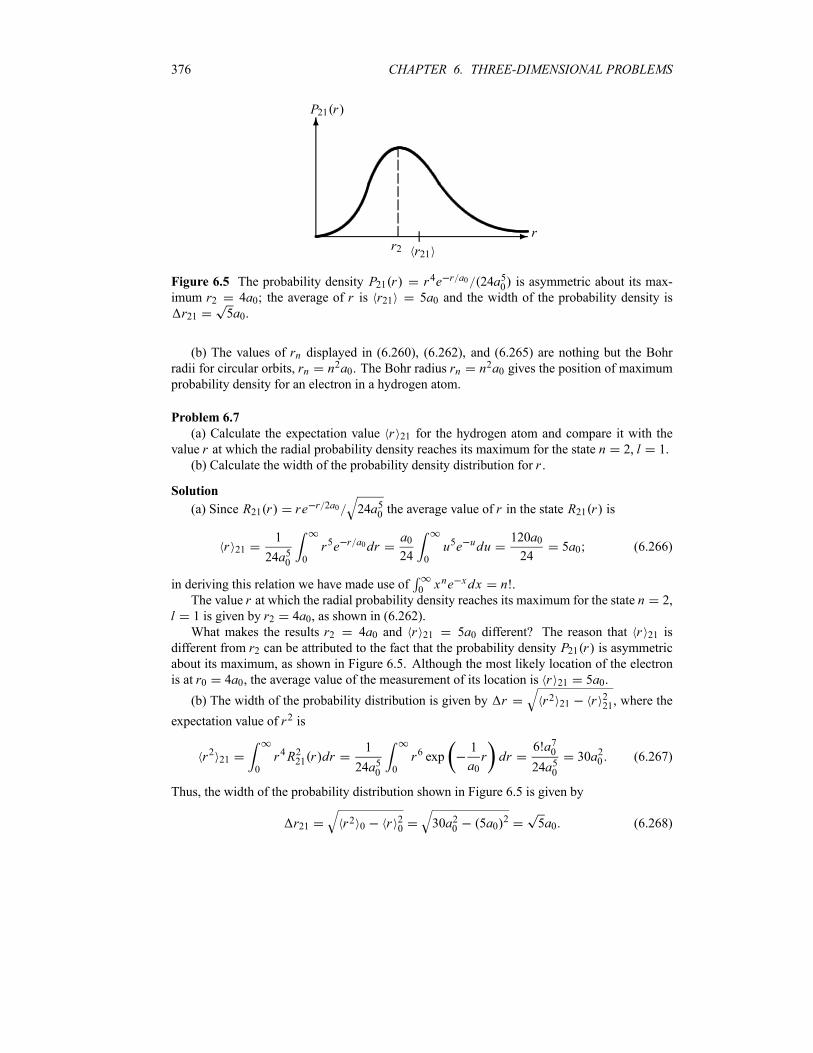
376 CHAPTER 6. THREE-DIMENSIONAL PROBLEMS
-
6
r
P21 r
r2 r21
Figure 6.5 The probability density P21 r r4e r a0 24a50 is asymmetric about its max-
imum r2 4a0; the average of r is r21 5a0 and the width of the probability density isr21 5a0.
(b) The values of rn displayed in (6.260), (6.262), and (6.265) are nothing but the Bohrradii for circular orbits, rn n2a0. The Bohr radius rn n2a0 gives the position of maximumprobability density for an electron in a hydrogen atom.
Problem 6.7
(a) Calculate the expectation value r 21 for the hydrogen atom and compare it with thevalue r at which the radial probability density reaches its maximum for the state n 2, l 1.
(b) Calculate the width of the probability density distribution for r .
Solution
(a) Since R21 r re r 2a0 24a50 the average value of r in the state R21 r is
r 211
24a50 0
r5e r a0dra024 0
u5e udu120a024
5a0 (6.266)
in deriving this relation we have made use of 0 xne xdx n!.The value r at which the radial probability density reaches its maximum for the state n 2,
l 1 is given by r2 4a0, as shown in (6.262).What makes the results r2 4a0 and r 21 5a0 different? The reason that r 21 is
different from r2 can be attributed to the fact that the probability density P21 r is asymmetricabout its maximum, as shown in Figure 6.5. Although the most likely location of the electron
is at r0 4a0, the average value of the measurement of its location is r 21 5a0.
(b) The width of the probability distribution is given by r r2 21 r 221, where the
expectation value of r2 is
r2 210
r4R221 r dr1
24a50 0
r6 exp1
a0r dr
6!a7024a50
30a20 (6.267)
Thus, the width of the probability distribution shown in Figure 6.5 is given by
r21 r2 0 r 20 30a20 5a02 5a0 (6.268)
6.5. SOLVED PROBLEMS 377
Problem 6.8
The operators associated with the radial component of the momentum pr and the radial coordi-nate r are denoted by Pr and R, respectively. Their actions on a radial wave function r are
given by Pr r ih 1 r r r r and R r r r .
(a) Find the commutator [Pr R] and Pr r , where r R2 R 2 and
Pr P2r Pr 2.
(b) Show that P2r h2 r 2 r2 r .
Solution
(a) Since R r r r and
Pr r ih1
r rr r ih
1
rr ih
r
r(6.269)
and since
Pr R r ih1
r rr2 r 2ih r ihr
r
r(6.270)
the action of the commutator [Pr R] on a function r is given by
[Pr R] r ih1
r rr R r ih
1
r rr2 r ih
rr r
2ih r ihrr
rih r ihr
r
rih r (6.271)
Thus, we have
[Pr R] ih (6.272)
Using the uncertainty relation for a pair of operators A and B, A B 12[A B] , we can
write
Pr r1
2[Pr R] (6.273)
or
Pr rh
2(6.274)
(b) The action of P2r on r gives
P2r r h21
r rr1
r rr h2
1
r
2
r2r r (6.275)
hence
P2r h21
r
2
r2r (6.276)
Problem 6.9
Find the number of s bound states for a particle of mass m moving in a delta potential V rV0 r a where V0 0. Discuss the existence of bound states in terms of the size of a.
Find the normalized wave function of the bound state(s).
378 CHAPTER 6. THREE-DIMENSIONAL PROBLEMS
Solution
The l 0 radial equation can be obtained from (6.57):
d2Un0 r
dr22mV0
h2r a k2 Un0 r 0 (6.277)
where Unl r Un0 r r Rn0 r and k2 2mE h2, since we are looking here at thebound states only, E 0. The solutions of this equation are
Un0 rUn01 r Aekr Be kr 0 r aUn02 r Ce kr r a
(6.278)
The energy eigenvalues can be obtained from the boundary conditions. As the wave function
vanishes at r 0, Un0 0 0, we have A B 0 or B A; hence Un01 r D sinh kr :
Un0 r D sinh kr 0 r a (6.279)
with D 2A. The continuity condition at r a of Un0 r , Un01 a Un02 a , leads to
D sinh ka Ce ka (6.280)
To obtain the discontinuity condition for the first derivative of Un0 r at r a, we need tointegrate (6.277):
limaUn02 a Un01 a
2mV0
h2Un02 a 0 (6.281)
or
kCe ka kD cosh ka2mV0
h2Ce ka 0 (6.282)
Taking Ce ka D sinh ka, as given by (6.280), and substituting it into (6.282), we get
k sinh ka k cosh ka2mV0
h2sinh ka 0 (6.283)
hence
coth2mV0
h2a (6.284)
where ka.The energy eigenvalues are given by the intersection of the curves f coth and
g 2mV0a h2 . As shown in Figure 6.6, if a h2 2mV0 then no bound state
solution can exist, since the curves of f and g do not intersect. But if a h2 2mV0the curves intersect only once; hence there is one bound state. We can summarize these results
as follows:
ah2
2mV0no bound states (6.285)
ah2
2mV0only one bound state. (6.286)
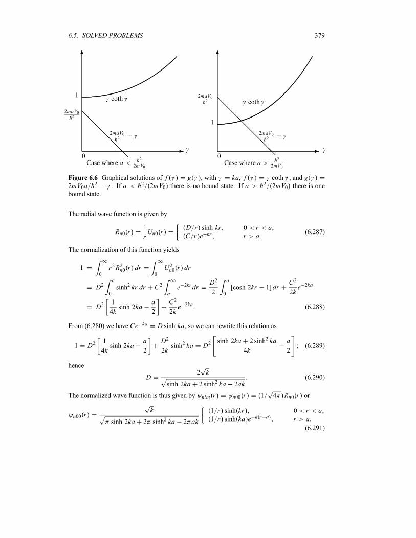
6.5. SOLVED PROBLEMS 379
-
6
0
1
2maV0h2 @
@@@@@@
coth
2maV0h2
Case where a h2
2mV0
-
6
0
1
2maV0h2 @
@@@@@@@@
coth
2maV0h2
Case where a h2
2mV0
Figure 6.6 Graphical solutions of f g , with ka, f coth , and g2mV0a h2 . If a h2 2mV0 there is no bound state. If a h2 2mV0 there is one
bound state.
The radial wave function is given by
Rn0 r1
rUn0 r
D r sinh kr 0 r aC r e kr r a
(6.287)
The normalization of this function yields
10
r2R2n0 r dr0
U2n0 r dr
D2a
0
sinh2 kr dr C2ae 2krdr
D2
2
a
0
[cosh 2kr 1] drC2
2ke 2ka
D21
4ksinh 2ka
a
2
C2
2ke 2ka (6.288)
From (6.280) we have Ce ka D sinh ka, so we can rewrite this relation as
1 D21
4ksinh 2ka
a
2
D2
2ksinh2 ka D2
sinh 2ka 2 sinh2 ka
4k
a
2(6.289)
hence
D2 k
sinh 2ka 2 sinh2 ka 2ak(6.290)
The normalized wave function is thus given by nlm r n00 r 1 4 Rn0 r or
n00 rk
sinh 2ka 2 sinh2 ka 2 ak
1 r sinh kr 0 r a1 r sinh ka e k r a r a
(6.291)

380 CHAPTER 6. THREE-DIMENSIONAL PROBLEMS
Problem 6.10
Consider the l 0 states of a bound system of two quarks having the same mass m and
interacting via V r kr .(a) Using the Bohr model, find the speed, the radius, and the energy of the system in the
case of circular orbits. Determine also the angular frequency of the radiation generated by a
transition of the system from an energy state n to m.(b) Solve the Schrödinger equation for the central potential V r kr for the two-quark
system and find the expressions for the energy and the radial function Rnl r . Compare theenergy with the value obtained in (a).
(c) Use the expressions derived in (a) and (b) to calculate the four lowest energy levels of a
bottom–antibottom (bottomonium) quark system with k 15GeV fm 1; the mass–energy of a
bottom quark is mc2 4 4GeV.
Solution
(a) Consider the two quarks to move circularly, much like the electron and proton in a
hydrogen atom; we can write the force between them as
2
r
dV r
drk (6.292)
where m 2 is the reduced mass. From the Bohr quantization condition of the orbital
angular momentum, we have
L r nh (6.293)
Multiplying (6.292) by (6.293), we end up with 2 3 nhk which yields the speed of therelative motion of the two-quark system:
nnhk2
1 3
(6.294)
The radius can be obtained from (6.293), rn nh n ; using (6.294) this leads to
rnn2h2
k
1 3
(6.295)
We can obtain the total energy of the relative motion by adding the kinetic and potential ener-
gies:
En1
22n krn
3
2
n2h2k21 3
(6.296)
In deriving this we have used the relations for n and rn as given by (6.294) and (6.295),respectively. The angular frequency of the radiation generated by a transition from n to m isgiven by
nmEn Emh
3
2h
k2
h
1 3
n2 3 m2 3 (6.297)
(b) The radial equation is given by (6.57):
h2
2
d2Unl r
dr2kr
l l 1 h2
2Mr2Unl r EnUnl r (6.298)
6.5. SOLVED PROBLEMS 381
where Unl r r Rnl r . Since we are dealing with l 0, we have
h2
2
d2Un0 r
dr2krUn0 r EnUn0 r (6.299)
which can be reduced to
d2Un0 r
dr22 k
h2r
E
kUn0 r 0 (6.300)
Making the change of variable x 2 k h2 1 3 r E k , we can rewrite (6.300) as
d2 n x
dx2x n x 0 (6.301)
We have already studied the solutions of this equation in Chapter 4; they are given by the Airy
functions Ai x : x BAi x . The bound state energies result from the zeros of Ai x .The boundary conditions on Unl of (6.301) are Unl r 0 0 and Unl r 0. The
second condition is satisfied by the Airy functions, since Ai x 0. The first condition
corresponds to [ 2 k h2 1 3E k] 0 or to Ai[ 2 k h2 1 3E k] Ai Rn 0, where
Rn are the zeros of the Airy function.The boundary condition Unl r 0 0 then yields a discrete set of energy levels which
can be expressed in terms of the Airy roots as follows:
Ai2 k
h2
1 3 E
k0
2 k
h2
1 3 Enk
Rn (6.302)
hence
Enh2k2
2
1 3
Rn (6.303)
The radial function of the system is given by Rn0 r 1 r Un0 r Bn r Ai x or
Rn0 rBnrAi x
BnrAi
2 k
h2
1 3
r Rn (6.304)
The energy expression (6.303) has the same structure as the energy (6.296) derived from the
Bohr model E Bn32n2h2k2 1 3; the ratio of the two expressions is
EnE Bn
2
3
Rn2n2 1 3
(6.305)
(c) In the following calculations we will be using k 15GeV fm 1, c2 mc2 22 2GeV, and hc 197 3MeV fm. The values of the four lowest energy levels corresponding
to the expression E Bn32n2h2k2 1 3, derived from the Bohr model, are
E B13
2
h2k21 3
2 38GeV E B2 22 3E B1 3 77GeV (6.306)
E B3 32 3E B1 4 95GeV E B4 42 3E B1 5 99GeV (6.307)
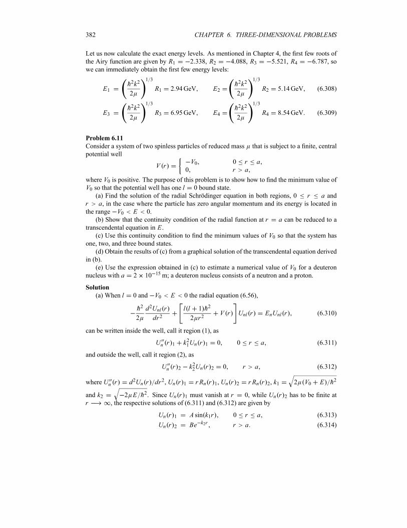
382 CHAPTER 6. THREE-DIMENSIONAL PROBLEMS
Let us now calculate the exact energy levels. As mentioned in Chapter 4, the first few roots of
the Airy function are given by R1 2 338, R2 4 088, R3 5 521, R4 6 787, so
we can immediately obtain the first few energy levels:
E1h2k2
2
1 3
R1 2 94GeV E2h2k2
2
1 3
R2 5 14GeV (6.308)
E3h2k2
2
1 3
R3 6 95GeV E4h2k2
2
1 3
R4 8 54GeV (6.309)
Problem 6.11
Consider a system of two spinless particles of reduced mass that is subject to a finite, central
potential well
V rV0 0 r a
0 r a
where V0 is positive. The purpose of this problem is to show how to find the minimum value ofV0 so that the potential well has one l 0 bound state.
(a) Find the solution of the radial Schrödinger equation in both regions, 0 r a andr a, in the case where the particle has zero angular momentum and its energy is located inthe range V0 E 0.
(b) Show that the continuity condition of the radial function at r a can be reduced to atranscendental equation in E .(c) Use this continuity condition to find the minimum values of V0 so that the system has
one, two, and three bound states.
(d) Obtain the results of (c) from a graphical solution of the transcendental equation derived
in (b).
(e) Use the expression obtained in (c) to estimate a numerical value of V0 for a deuteronnucleus with a 2 10 15m; a deuteron nucleus consists of a neutron and a proton.
Solution
(a) When l 0 and V0 E 0 the radial equation (6.56),
h2
2
d2Unl r
dr2l l 1 h2
2 r2V r Unl r EnUnl r (6.310)
can be written inside the well, call it region (1), as
Un r 1 k21Un r 1 0 0 r a (6.311)
and outside the well, call it region (2), as
Un r 2 k22Un r 2 0 r a (6.312)
where Un r d2Un r dr2, Un r 1 r Rn r 1, Un r 2 r Rn r 2, k1 2 V0 E h2
and k2 2 E h2. Since Un r 1 must vanish at r 0, while Un r 2 has to be finite atr , the respective solutions of (6.311) and (6.312) are given by
Un r 1 A sin k1r 0 r a (6.313)
Un r 2 Be k2r r a (6.314)
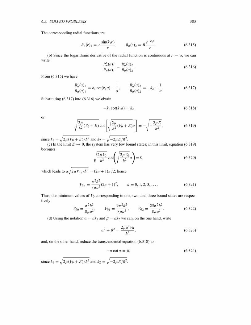
6.5. SOLVED PROBLEMS 383
The corresponding radial functions are
Rn r 1 Asin k1r
rRn r 2 B
e k2r
r(6.315)
(b) Since the logarithmic derivative of the radial function is continuous at r a, we canwrite
Rn a 1Rn a 1
Rn a 2Rn a 2
(6.316)
From (6.315) we have
Rn a 1Rn a 1
k1 cot k1a1
a
Rn a 2Rn a 2
k21
a(6.317)
Substituting (6.317) into (6.316) we obtain
k1 cot k1a k2 (6.318)
or
2
h2V0 E cot
2
h2V0 E a
2 E
h2(6.319)
since k1 2 V0 E h2 and k2 2 E h2.(c) In the limit E 0, the system has very few bound states; in this limit, equation (6.319)
becomes
2 V0
h2cot
2 V0
h2a 0 (6.320)
which leads to a 2 V0n h2 2n 1 2; hence
V0n2h2
8 a22n 1 2 n 0 1 2 3 (6.321)
Thus, the minimum values of V0 corresponding to one, two, and three bound states are respec-tively
V002h2
8 a2V01
9 2h2
8 a2V02
25 2h2
8 a2(6.322)
(d) Using the notation ak1 and ak2 we can, on the one hand, write
2 2 2 a2V0
h2(6.323)
and, on the other hand, reduce the transcendental equation (6.318) to
cot (6.324)
since k1 2 V0 E h2 and k2 2 E h2.
384 CHAPTER 6. THREE-DIMENSIONAL PROBLEMS
-
6
02
32
52
¾ 2 a2V0 h2 2
¾ cot
Figure 6.7 Graphical solutions for the finite, spherical square well potential: they are given
by the intersection of the circle 2 2 2 a2V0 h2 with the curve of cot , where
2 2 a2 V0 E h2 and 2 2 a2E h2, with V0 E 0.
As shown in Figure 6.7, when 2 3 2, which in the limit of E 0 leads to
2h2
8 a2V0
9 2h2
8 a2(6.325)
there exists only one bound state, since the circle intersects only once with the curve cot .
Similarly, there are two bound states if 3 2 5 2 or
9 2h2
8 a2V0
25 2h2
8 a2(6.326)
and three bound states if 5 2 7 2:
25 2h2
8 a2V0
49 2h2
8 a2(6.327)
(e) Since m pc2 938MeV and mnc2 940MeV, the reduced mass of the deuteron is
given by c2 m pc2 mnc2 m pc2 mnc2 469 5MeV. Since a 2 10 15m the
minimum value of V0 corresponding to one bound state is
V02h2
8 a2
2 hc 2
8 c2 a2
2 197MeV fm 2
8 469 5MeV 2 10 15m 225 5MeV (6.328)
Problem 6.12
Calculate nl P4 nl in a stationary state nl of the hydrogen atom.
Solution
6.6. EXERCISES 385
To calculate nl P4 nl we may consider expressing P4 in terms of the hydrogen’s Hamil-tonian. Since H P2 2me e2 r we have P2 2me H e2 r ; hence
nl P4 nl 2me2 nl H
e2
r
2
nl
2me2 nl H2 H
e2
r
e2
rH
e4
r2nl
2me2 E2n En nl
e2
rnl nl
e2
rnl En nl
e4
r2nl
(6.329)
where we have used the fact that nl is an eigenstate of H : H nl En nl withEn e2 2a0n2 13 6 eV n2. The expectation values of 1 r and 1 r2 are given by(6.182) and (6.183), nl r 1 nl 1 n2a0 and nl r 2 nl 2 [n3 2l 1 a20]; we can thusrewrite (6.329) as
nl P4 nl 2me2 E2n 2En nl
e2
rnl nl
e4
r2nl
2meEn2 1
2e2
En
1
n2 a0
e4
E2n
2
n3 2l 1 a20
2meEn2 1 4
8n
2l 1(6.330)
in deriving the last relation we have used En e2 2a0n2 . Now, since a0 h2 mee2 , theenergy En becomes En e2 2a0n2 mee4 2h2n2 which, when inserted into (6.330),leads to
nl P4 nlm4ee
8
h4n48n
2l 13 (6.331)
6.6 Exercises
Exercise 6.1
A spinless particle of mass m is confined to move in the xy plane under the influence of aharmonic oscillator potential V x y 1
2m 2 x2 y2 for all values of x and y.
(a) Show that the Hamiltonian H of this particle can be written as a sum of two familiar one-dimensional Hamiltonians, Hx and Hy . Then show that H commutes with Lz X Py Y Px .(b) Find the expression for the energy levels Enxny .(c) Find the energies of the four lowest states and their corresponding degeneracies.
(d) Find the degeneracy gn of the nth excited state as a function of the quantum number n(n nx ny).(e) If the state vector of the nth excited state is n nx ny or
xy n x nx y ny nx x ny y
386 CHAPTER 6. THREE-DIMENSIONAL PROBLEMS
calculate the expectation value of the operator A x4 y2 in the state n as a function of thequantum numbers nx and ny .
Exercise 6.2
A particle of mass m moves in the xy plane in the potential
V x y12m 2y2 for all y and 0 x a
elsewhere
(a) Write down the time-independent Schrödinger equation for this particle and reduce it to
a set of familiar one-dimensional equations.
(b) Find the normalized eigenfunctions and the eigenenergies.
Exercise 6.3
A particle of mass m moves in the xy plane in a two-dimensional rectangular well
V x y0 0 x a 0 y b
elsewhere
By reducing the time-independent Schrödinger equation to a set of more familiar one-dimensional
equations, find the normalized wave functions and the energy levels of this particle.
Exercise 6.4
Consider an anisotropic three-dimensional harmonic oscillator potential
V x y z1
2m 2
x x2 2
y y2 2
z z2
(a) Evaluate the energy levels in terms of x , y , and z .
(b) Calculate [H L z]. Do you expect the wave functions to be eigenfunctions of L2?(c) Find the three lowest levels for the case x y 2 z 3, and determine the degener-
acy of each level.
Exercise 6.5
Consider a spinless particle of mass m which is confined to move under the influence of athree-dimensional potential
V x y z0 for 0 x a 0 y a 0 z b
elsewhere
(a) Find the expression for the energy levels Enxnynz and their corresponding wave func-tions.
(b) If a 2b find the energies of the five lowest states and their degeneracies.
Exercise 6.6
A particle of mass m moves in the three-dimensional potential
V x y z12m 2z2 for 0 x a 0 y a and z 0
elsewhere
6.6. EXERCISES 387
(a) Write down the time-independent Schrödinger equation for this particle and reduce
it to a set of familiar one-dimensional equations; then find the normalized wave function
nxnynz x y z .(b) Find the allowed eigenenergies of this particle and show that they can be written as:
Enxnynz Enxny Enz .(c) Find the four lowest energy levels in the xy plane (i.e., Enxny ) and their corresponding
degeneracies.
Exercise 6.7
A particle of mass m moves in the potential V x y z V1 x y V2 z where
V1 x y1
2m 2 x2 y2 V2 z
0 0 z aelsewhere
(a) Calculate the energy levels and the wave function of this particle.
(b) Let us now turn off V2 z (i.e., m is subject only to V1 x y ). Calculate the degeneracygn of the nth energy level (note that n nx ny).
Exercise 6.8
Consider a muonic atom which consists of a nucleus that has Z protons (no neutrons) and anegative muon moving around it; the muon’s charge is e and its mass is 207 times the massof the electron, m 207me. For a muonic atom with Z 6, calculate
(a) the radius of the first Bohr orbit,
(b) the energy of the ground, first, and second excited states, and
(c) the frequency associated with the transitions ni 2 n f 1, ni 3 n f 1, and
ni 3 n f 2.
Exercise 6.9
A hydrogen atom has the wave function nlm r , where n 4 l 3 m 3.
(a) What is the magnitude of the orbital angular momentum of the electron around the
proton?
(b) What is the angle between the orbital angular momentum vector and the z-axis? Canthis angle be reduced by changing n or m if l is held constant? What is the physical significanceof this result?
(c) Sketch the shapes of the radial function and of the probability of finding the electron a
distance r from the proton.
Exercise 6.10
An electron in a hydrogen atom is in the energy eigenstate
2 1 1 r Nre r 2a0Y1 1
(a) Find the normalization constant, N .(b) What is the probability per unit volume of finding the electron at r a0, 45 ,
60 ?
(c) What is the probability per unit radial interval (dr ) of finding the electron at r 2a0?(One must take an integral over and at r 2a0.)(d) If the measurements of L2 and L z were carried out, what will be the results?
388 CHAPTER 6. THREE-DIMENSIONAL PROBLEMS
Exercise 6.11
Consider a hydrogen atom which is in its ground state; the ground state wave function is given
by
r1
a30
e r a0
where a0 is the Bohr radius.(a) Find the most probable distance between the electron and the proton when the hydrogen
atom is in its ground state.
(b) Find the average distance between the electron and the proton.
Exercise 6.12
Consider a hydrogen atom whose state at time t 0 is given by
r 01
2300 r
1
3311 r
1
6322 r
(a) What is the time-dependent wave function?
(b) If a measurement of the energy were carried out, what values could be found and with
what probabilities?
(c) Repeat part (b) for L2 and Lz . That is, if a measurement of L2 and Lz were carried out,what values could be found and with what probabilities?
Exercise 6.13
The wave function of an electron in a hydrogen atom is given by
21mlms r R21 r1
3Y10
1
2
1
2
2
3Y11
1
2
1
2
where 12
12are the spin state vectors.
(a) Is this wave function an eigenfunction of Jz , the z-component of the electron’s total an-gular momentum? If yes, find the eigenvalue. (Hint: For this, you need to calculate Jz 21mlms .)
(b) If you measure the z-component of the electron’s spin angular momentum, what valueswill you obtain? What are the corresponding probabilities?
(c) If you measure J 2, what values will you obtain? What are the corresponding probabili-ties?
Exercise 6.14
Consider a hydrogen atom whose state at time t 0 is given by
r 0 A 200 r1
5311 r
1
3422 r
where A is a normalization constant.(a) Find A so that the state is normalized.(b) Find the state of this atom at any later time t .(c) If a measurement of the energy were carried out, what values would be found and with
what probabilities?
(d) Find the mean energy of the atom.
6.6. EXERCISES 389
Exercise 6.15
Calculate the width of the probability density distribution for r for the hydrogen atom in its
ground state: r r2 10 r 210.
Exercise 6.16
Consider a hydrogen atom whose wave function is given at time t 0 by
r 0A 1
a0
3 2
e r a01
2
z 2x
rR21 r
where A is a real constant, a0 is the Bohr radius, and R21 r is the radial wave function:
R21 r 1 6 1 a0 3 2 r 2a0 e r 2a0 .
(a) Write down r 0 in terms of nlm nlm r where nlm r is the hydrogen wave
function nlm r Rnl r Ylm .
(b) Find A so that r 0 is normalized. (Recall that n l m r nlm r d3r n n l l m m .)
(c) Write down the wave function r t at any later time t .
(d) Is r 0 an eigenfunction of L2 and L2? If yes, what are the eigenvalues?(e) If a measurement of the energy is made, what value could be found and with what
probability?
(f) What is the probability that a measurement of Lz yields 1h?(g) Find the mean value of r in the state r 0 .
Exercise 6.17
Consider a pendulum undergoing small harmonic oscillations (with angular frequency
g l, where g is the acceleration due to gravity and l is the length of the pendulum). Showthat the quantum energy levels and the corresponding degeneracies of the pendulum are given
by En n 1 h and gn n 1, respectively.
Exercise 6.18
Consider a proton that is trapped inside an infinite central potential well
V rV0 0 r a
r a
where V0 5104 34 MeV and a 10 fm.
(a) Find the energy and the (normalized) radial wave function of this particle for the s states
(i.e., l 0).
(b) Find the number of bound states that have energies lower than zero; you may use the
values mc2 938 MeV and hc 197MeV fm.
(c) Calculate the energies of the levels that lie just below and just above the zero-energy
level; express your answer in MeV.
Exercise 6.19
Consider the function r A x iy e r 2a0 , where a0 is the Bohr radius and A is a realconstant.
(a) Is r an eigenfunction to L2 and L z? If yes, write r in terms of Rnl r Ylmand find the values of the quantum numbers n m l; Rnl r are the radial wave functions of thehydrogen atom.
(b) Find the constant A so that r is normalized.(c) Find the mean value of r and the most probable value of r in this state.
390 CHAPTER 6. THREE-DIMENSIONAL PROBLEMS
Exercise 6.20
The wave function of a hydrogen-like atom at time t 0 is
r 01
113 2 1 1 r 2 1 0 r 5 2 1 1 r 2 3 1 1 r
where nlm r is a normalized eigenfunction (i.e., nlm r Rnl r Ylm ).
(a) What is the time-dependent wave function?
(b) If a measurement of energy is made, what values could be found and with what proba-
bilities?
(c) What is the probability for a measurement of L z which yields 1h?
Exercise 6.21
Using the fact that the radial momentum operator is given by pr ih 1r r r , calculate thecommutator [r pr ] between the position operator, r , and the radial momentum operator.
Exercise 6.22
Calculate r pr with respect to the state
2 1 0 r1
6
1
a0
3 2 r
2a0e r 2a0 Y1 0
and verify that r pr satisfies the Heisenberg uncertainty principle.

Chapter 7
Rotations and Addition of Angular
Momenta
In this chapter we deal with rotations, the properties of addition of angular momenta, and the
properties of tensor operators.
7.1 Rotations in Classical Physics
A rotation is defined by an angle of rotation and an axis about which the rotation is performed.
Knowing the rotation matrix R, we can determine how vectors transform under rotations; ina three-dimensional space, a vector A becomes A when rotated: A RA. For instance, arotation over an angle about the z-axis transforms the components Ax , Ay , Az of the vector
A into Ax , Ay , Az:
AxAyAz
cos sin 0
sin cos 0
0 0 1
AxAyAz
(7.1)
or
A Rz A (7.2)
where
Rz
cos sin 0
sin cos 0
0 0 1
(7.3)
Similarly, the rotation matrices about the x and y axes are given by
Rx
1 0 0
0 cos sin
0 sin cos
Ry
cos 0 sin
0 1 0
sin 0 cos
(7.4)
From classical physics we know that while rotations about the same axis commute, rotations
about different axes do not. From (7.4) we can verify that Rx Ry Ry Rx . In fact,
391
392 CHAPTER 7. ROTATIONS AND ADDITION OF ANGULAR MOMENTA
using (7.4) we can have
Rx Ry
cos 0 sin
sin2 cos cos sin
cos sin sin cos2(7.5)
Ry Rx
cos sin2 cos sin
0 cos sin
sin sin cos cos2(7.6)
hence Rx Ry Ry Rx is given by
0 sin2 sin cos sin
sin2 0 cos sin sin
sin cos sin cos sin sin 0
(7.7)
In the case of infinitesimal rotations of angle about the x y , z axes, and using cos
1 2 2 and sin , we can reduce (7.7) to
Rx Ry Ry Rx
0 2 02 0 0
0 0 0
(7.8)
which, when combined with Rz 2 of (7.3),
Rz
12
20
12
20
0 0 1
Rz2
1 2 02 1 0
0 0 1
(7.9)
leads to
Rx Ry Ry Rx Rz2 1
1 2 02 1 0
0 0 1
1 0 0
0 1 0
0 0 1
(7.10)
We will show later that this relation can be used to derive the commutation relations between
the components of the angular momentum (7.26).
The rotation matrices R are orthogonal, i.e.,
RRT RT R 1 (7.11)
where RT is the transpose of the matrix R. In addition, the orthogonal matrices conserve themagnitude of vectors:
A A (7.12)
since A RA yields A 2 A2 or A 2x A 2y A 2z A2x A2y A2z .It is easy to show that the matrices of orthogonal rotations form a (nonabelian) group and
that they satisfy this relation
det R 1 (7.13)

7.2. ROTATIONS IN QUANTUM MECHANICS 393
This group is called the special three-dimensional orthogonal group, SO 3 , because the rota-
tion group is a special case of a more general group, the group of three-dimensional orthogonal
transformations, O 3 , which consist of both rotations and reflections and for which
det R 1 (7.14)
The group SO 3 transforms a vector A into another vector A while conserving the size of itslength.
7.2 Rotations in Quantum Mechanics
In this section we study the relationship between the angular momentum and the rotation op-
erator and then study the properties as well as the representation of the rotation operator. The
connection is analogous to that between the linear momentum operator and translations. We
will see that the angular momentum operator acts as a generator for rotations.
A rotation is specified by an angle and by a unit vector n about which the rotation is per-formed. Knowing the rotation operator R, we can determine how state vectors and operatorstransform under rotations; as shown in Chapter 2, a state and an operator A transformaccording to
R A RAR† (7.15)
The problem reduces then to finding R. We may now consider infinitesimal as well as finiterotations.
7.2.1 Infinitesimal Rotations
Consider a rotation of the coordinates of a spinless particle over an infinitesimal angle about
the z-axis. Denoting this rotation by the operator Rz , we have
Rz r r (7.16)
Taylor expanding the wave function to the first order in , we obtain
r r 1 r (7.17)
Comparing (7.16) and (7.17) we see that Rz is given by
Rz 1 (7.18)
Since the z-component of the orbital angular momentum is
L z ih (7.19)
we can rewrite (7.18) as
Rz 1i
hLz (7.20)
394 CHAPTER 7. ROTATIONS AND ADDITION OF ANGULAR MOMENTA
Wemay generalize this relation to a rotation of angle about an arbitrary axis whose direction
is given by the unit vector n:
R 1i
hn L (7.21)
This is the operator corresponding to an infinitesimal rotation of angle about n for a spinlesssystem. The orbital angular momentum is thus the generator of infinitesimal spatial rotations.
Rotations and the commutation relations
We can show that the relation (7.10) leads to the commutation relations of angular momentum
[Lx L y] ihL z . The operators corresponding to infinitesimal rotations of angle about the
x and y axes can be inferred from (7.20):
Rx 1i
hLx
2
2h2L2x Ry 1
i
hL y
2
2h2L2y (7.22)
where we have extended the expansions to the second power in . On the one hand, the follow-
ing useful relation can be obtained from (7.22):
Rx Ry Ry Rx 1i
hLx
2
2h2L2x 1
i
hL y
2
2h2L2y
1i
hL y
2
2h2L2y 1
i
hLx
2
2h2L2x
2
h2Lx L y L yLx
2
h2[Lx L y] (7.23)
where we have kept only terms up to the second power in ; the terms in cancel out automat-
ically.
On the other hand, according to (7.10), we have
Rx Ry Ry Rx Rz2 1 (7.24)
Since Rz 2 1 i 2 h L z this relations leads to
Rx Ry Ry Rx Rz2 1
i 2
hLz (7.25)
Finally, equating (7.23) and (7.25), we end up with
[Lx L y] ihLz (7.26)
Similar calculations for Ry Rz Rz Ry and Rz Rx Rx Rz lead to the
other two commutation relations [L y L z] ihLx and [Lz Lx ] ihL y .
7.2. ROTATIONS IN QUANTUM MECHANICS 395
7.2.2 Finite Rotations
The operator Rz corresponding to a rotation (of the coordinates of a spinless particle) over a
finite angle about the z-axis can be constructed in terms of the infinitesimal rotation operator(7.20) as follows. We divide the angle into N infinitesimal angles : N . The
rotation over the finite angle can thus be viewed as a series of N consecutive infinitesimalrotations, each over the angle , about the z-axis, applied consecutively one after the other:
Rz Rz N RzN 1 i
hLz
N
(7.27)
Since N , and if is infinitesimally small, we have
Rz limN
N
k 1
1i
h Nn L lim
N1
i
h NL z
N
(7.28)
or
Rz e i Lz h (7.29)
We can generalize this result to infer the rotation operator Rn corresponding to a rotation
over a finite angle around an axis n:
Rn e i n L h (7.30)
where L is the orbital angular momentum. This operator represents the rotation of the coordi-nates of a spinless particle over an angle about an axis n.The discussion that led to (7.30) was carried out for a spinless system. A more general
study for a system with spin would lead to a relation similar to (7.30):
Rn eih n J
(7.31)
where J is the total angular momentum operator; this is known as the rotation operator. Forinstance, the rotation operator Rx of a rotation through an angle about the x-axis is givenby
Rx e i Jx h (7.32)
The properties of Rn are determined by those of the operators Jx Jy Jz .
Remark
The Hamiltonian of a particle in a central potential, H P2 2m V r , is invariant underspatial rotations since, as shown in Chapter 6, it commutes with the orbital angular momentum:
[H L] 0 H e i n L h 0 (7.33)
Due to this symmetry of space isotropy or rotational invariance, the orbital angular momentumis conserved1. So, in the case of particles moving in central potentials, the orbital angularmomentum is a constant of the motion.
1In classical physics when a system is invariant under rotations, its total angular momentum is also conserved.
396 CHAPTER 7. ROTATIONS AND ADDITION OF ANGULAR MOMENTA
7.2.3 Properties of the Rotation Operator
The rotation operators constitute a representation of the rotation group and satisfy the following
properties:
The product of any two rotation operators is another rotation operator:
Rn1Rn2 Rn3 (7.34)
The associative law holds for rotation operators:
Rn1Rn2 Rn3 Rn1 Rn2Rn3 (7.35)
The identity operator (corresponding to no rotation) satisfies the relation
I Rn Rn I Rn (7.36)
From (7.31) we see that for each rotation operator Rn , there exists an inverse operatorR 1n so that
RnR1
n R 1n Rn I (7.37)
The operator R n , which is equal to R 1n , corresponds to a rotation in the opposite sense
to Rn .
In sharp contrast to the translation group2 in three dimensions, the rotation group is not com-
mutative (nonabelian). The product of two rotation operators depends on the order in whichthey are performed:
Rn1 Rn2 Rn2 Rn1 (7.38)
this is due to the fact that the commutator [n1 J n2 J ] is not zero. In this way, the rotationgroup is in general nonabelian.
But if the two rotations were performed about the same axis, the corresponding operatorswould commute:
Rn Rn Rn Rn Rn (7.39)
Note that, since the angular momentum operator J is Hermitian, equation (7.31) yields
R†n R 1
n Rn ei n J h (7.40)
hence the rotation operator (7.31) is unitary:
R†n R 1
n R†n Rn I (7.41)
The operator Rn therefore conserves the scalar product of kets, notably the norm of vectors.
For instance, using
Rn Rn (7.42)
along with (7.41), we can show that , since
R†n Rn (7.43)
2The linear momenta Pi and Pj—which are the generators of translation—commute even when i j ; hence thetranslation group is said to be abelian.
7.2. ROTATIONS IN QUANTUM MECHANICS 397
7.2.4 Euler Rotations
It is known from classical mechanics that an arbitrary rotation of a rigid body can be expressed
in terms of three consecutive rotations, called the Euler rotations. In quantum mechanics, in-
stead of expressing the rotation operator Rn e i n J h in terms of a rotation through an
angle about an arbitrary axis n, it is more convenient to parameterize it, as in classical me-chanics, in terms of the three Euler angles where 0 2 , 0 , and
0 2 . The Euler rotations transform the space-fixed set of axes xyz into a new setx y z , having the same origin O, by means of three consecutive counterclockwise rotations:
First, rotate the space-fixed Oxyz system through an angle about the z-axis; this rota-tion transforms the Oxyz system into Ou z: Oxyz Ou z.
Second, rotate the u z system through an angle about the -axis; this rotation trans-
forms the Ou z system into O z : Ou z O z .
Third, rotate the z system through an angle about the z -axis; this rotation trans-forms the O z system into Ox y z : O z Ox y z .
The operators representing these three rotations are given by Rz , R , and Rz , respec-
tively. Using (7.31) we can represent these three rotations by
R Rz R Rz exp i Jz h exp i J h exp i Jz h (7.44)
The form of this operator is rather inconvenient, for it includes rotations about axes belonging
to different systems (i.e., z , , and z); this form would be most convenient were we to express(7.44) as a product of three rotations about the space-fixed axes x , y, z. So let us express Rzand R in terms of rotations about the x y z axes. Since the first Euler rotation describedabove, Rz , transforms the operator Jy into J , i.e., J Rz JyRz by (7.15), we have
R Rz Ry Rz e i Jz he i Jy hei Jz h (7.45)
Here Jz is obtained from Jz by the consecutive application of the second and third Euler rota-tions, Jz R Rz JzRz R ; hence
Rz R Rz Rz Rz R (7.46)
Since R Rz Ry Rz , substituting (7.45) into (7.46) we obtain
Rz Rz Ry Rz Rz Rz Rz Rz Ry Rz
Rz Ry Rz Ry Rz
e i Jz he i Jy he i Jz hei Jy hei Jz h (7.47)
where we used the fact that Rz Rz e i Jz hei Jz h 1.
Finally, inserting (7.45) and (7.47) into (7.44) and simplifying (i.e., using Rz Rz1 and Ry Ry 1), we end up with a product of three rotations about the space-fixed
axes y and z:
R Rz Ry Rz e i Jz he i Jy he i Jz h (7.48)
398 CHAPTER 7. ROTATIONS AND ADDITION OF ANGULAR MOMENTA
The inverse transformation of (7.48) is obtained by taking three rotations in reverse order over
the angles :
R 1 Rz Ry Rz R† ei Jz hei Jy hei Jz h (7.49)
7.2.5 Representation of the Rotation Operator
The rotation operator R as given by (7.48) implies that its properties are determined
by the algebraic properties of the angular momentum operators Jx , Jy , Jz . Since R
commutes with J2, we may look for a representation of R in the basis spanned by the
eigenvectors of J 2 and Jz , i.e., the j m states.
From (7.48), we see thatJ2 commutes with the rotation operator, [J 2 R ] 0;
thus, the total angular momentum is conserved under rotations
J2R j m R J 2 j m j j 1 R j m (7.50)
However, the z-component of the angular momentum changes under rotations, unless the axisof rotation is along the z-axis. That is, when R acts on the state j m , we end upwith a new state having the same j but with a different value of m:
R j mj
m j
j m j m R j m
j
m j
D jm m j m (7.51)
where
D jm m j m R j m (7.52)
These are the matrix elements of R for the j m states; D jm m is the am-
plitude of j m when j m is rotated. The rotation operator is thus represented by a
2 j 1 2 j 1 square matrix in the j m basis. The matrix of D j is known
as the Wigner D-matrix and its elements D jm m as the Wigner functions. This matrix
representation is often referred to as the 2 j 1 -dimensional irreducible representation of therotation operator R .
Since j m is an eigenstate of Jz , it is also an eigenstate of the rotation operator ei Jz h ,because
ei Jz h j m ei m j m (7.53)
We may thus rewrite (7.52) as
D jm m e i m m d j
m m (7.54)
where
d jm m j m e i Jy h j m (7.55)
7.2. ROTATIONS IN QUANTUM MECHANICS 399
This shows that only the middle rotation operator, e i Jy h , mixes states with different values
of m. Determining the matrix elements D jm m therefore reduces to evaluation of the
quantities d jm m .
A general expression of d jm m , called the Wigner formula, is given by the following
explicit expression:
d jm m
k
1 k m m j m ! j m ! j m ! j m !
j m k ! j m k ! k m m !k!
cos2
2 j m m 2k
sin2
m m 2k
(7.56)
The summation over k is taken such that none of the arguments of factorials in the denominatorare negative.
We should note that, since the D-function D jm m is a joint eigenfunction of J 2 and
Jz , we have
J 2D jm m j j 1 h2D j
m m (7.57)
JzDjm m hmD j
m m (7.58)
J D jm m h j m j m 1 D j
m m 1(7.59)
Properties of the D-functionsWe now list some of the most useful properties of the rotation matrices. The complex conjugate
of the D-functions can be expressed as
D jm m j m R j m j m R† j m
j m R 1 j m
D jmm (7.60)
We can easily show that
D jm m 1 m mD j
m m D jmm (7.61)
The D-functions satisfy the following unitary relations:
m
D jkm D j
k m k k (7.62)
m
D jmk D j
mk k k (7.63)
400 CHAPTER 7. ROTATIONS AND ADDITION OF ANGULAR MOMENTA
since
m
D jmk D j
mkm
j k R 1 j m j m R j k
j k R 1 R j k
j k j k
k k (7.64)
From (7.55) we can show that the d-functions satisfy the following relations:
d jm m 1 j m
m m d jm m 0 m m (7.65)
Since d jm m are elements of a unitary real matrix, the matrix dj must be orthogonal. We
may thus write
d jm m d j
m m
1d jmm (7.66)
and
d jm m 1 m md j
mm 1 m md jm m (7.67)
The unitary matrices D j form a 2 j 1 dimensional irreducible representation of the SO 3group.
7.2.6 Rotation Matrices and the Spherical Harmonics
In the case where the angular momentum operator J is purely orbital (i.e., the values of j areinteger, j l), there exists a connection between the D-functions and the spherical harmonicsYlm . The operator R when applied to a vector r pointing in the directionwould generate a vector r along a new direction :
r R r (7.68)
An expansion in terms of l m and a multiplication by l m leads to
l m rm
l m R l m l m r (7.69)
or to
Ylmm
D lm m Ylm (7.70)
since l m r Ylm and l m r Ylm .
In the case where the vector r is along the z-axis, we have 0; hence m 0. From
Chapter 5, Yl0 0 is given by
Ylm 02l 1
4m 0 (7.71)
We can thus reduce (7.70) to
Ylm D lm 0 Yl0 0
2l 1
4D lm 0 (7.72)
7.2. ROTATIONS IN QUANTUM MECHANICS 401
or to
D lm0
4
2l 1Ylm (7.73)
This means that a rotation through the Euler angles of the vector r , when it is alongthe z-axis, produces a vector r whose azimuthal and polar angles are given by and ,
respectively. Similarly, we can show that
D l0m
4
2l 1Ylm (7.74)
and
D l00 0 0 Pl cos (7.75)
where Pl cos is the Legendre polynomial.
We are now well equipped to derive the theorem for the addition of spherical harmonics.
Let be the polar coordinates of the vector r with respect to the space-fixed x y z systemand let be its polar coordinates with respect to the rotated system x y z ; taking thecomplex conjugate of (7.70) we obtain
Ylmm
D lm m Ylm (7.76)
For the case m 0, since (from Chapter 5)
Yl02l 1
4Pl cos (7.77)
and since from (7.74)
D l0m
4
2l 1Ylm (7.78)
we can reduce (7.76) to
2l 1
4Pl cos
m
4
2l 1Ylm Ylm (7.79)
or to
Pl cos4
2l 1m
Ylm Ylm (7.80)
Integrals involving the D-functionsLet denote the Euler angles; hence
d0
sin d2
0
d2
0
d (7.81)
Using the relation
D jm m d
0
d jm m sin d
2
0
e im d2
0
e im d
8 2j 0 m 0 m 0 (7.82)
402 CHAPTER 7. ROTATIONS AND ADDITION OF ANGULAR MOMENTA
we may write
D jmk D j
m k d 1 m k D jm k D j
m k d
1 m k
0
d jm k d j
m k sin d
2
0
e i m m d2
0
e i k k d
8 2
2 j 1j j m m k k (7.83)
Example 7.1
Find the rotation matrices d 1 2 and D 1 2 corresponding to j 12.
Solution
On the one hand, since the matrix of Jy for j12(Chapter 5) is given by
Jyh
2
0 ii 0
h
2y (7.84)
and since the square of the Pauli matrix y is equal to the unit matrix,2y 1, the even and odd
powers of y are given by
2ny
1 0
0 12n 1y
0 ii 0 y (7.85)
On the other hand, since the rotation operator
Ry e i Jy h e i y 2 (7.86)
can be written as
e i y 2
n 0
i 2n
2n ! 2
2n2n
n 0
i 2n 1
2n 1 ! 2
2n 12n 1y (7.87)
a substitution of (7.85) into (7.87) yields
e i y 2 1 0
0 1n 0
1 n
2n ! 2
2n
i yn 0
1 n
2n 1 ! 2
2n 1
1 0
0 1cos
2
0 1
1 0sin
2(7.88)
hence
d 1 2 e i Jy hd 1 21212
d 1 212
12
d 1 21212
d 1 212
12
cos 2 sin 2
sin 2 cos 2
(7.89)
7.3. ADDITION OF ANGULAR MOMENTA 403
Since as shown in (7.54) D jm m e i m m d j
m m , we have
D 1 2e i 2 cos 2 e i 2 sin 2
ei 2 sin 2 ei 2 cos 2(7.90)
7.3 Addition of Angular Momenta
The addition of angular momenta is encountered in all areas of modern physics. Mastering its
techniques is essential for an understanding of the various subatomic phenomena. For instance,
the total angular momentum of the electron in a hydrogen atom consists of two parts, an orbital
part L, which is due to the orbiting motion of the electron around the proton, and a spin part S,which is due to the spinning motion of the electron about itself. The properties of the hydrogen
atom cannot be properly discussed without knowing how to add the orbital and spin parts of the
electron’s total angular momentum.
In what follows we are going to present the formalism of angular momentum addition and
then consider some of its most essential applications.
7.3.1 Addition of Two Angular Momenta: General Formalism
In this section we present the general formalism corresponding to the problem of adding two
commuting angular momenta.
Consider two angular momenta J 1 and J 2 which belong to different subspaces 1 and 2; J 1
and J2 may refer to two distinct particles or to two different properties of the same particle3.The latter case may refer to the orbital and spin angular momenta of the same particle. Assum-
ing that the spin–orbit coupling is sufficiently weak, then the space and spin degrees of freedom
of the electron evolve independently of each other.
The components of J1 and J 2 satisfy the usual commutation relations of angular momen-tum:
J1x J1y ih J1z J1y J1z ih J1x J1z J1x ih J1y (7.91)
J2x J2y ih J2z J2y J2z ih J2x J2z J2x ih J2y (7.92)
Since J1, and J 2 belong to different spaces, their components commute:
J1 j J2k 0 j k x y z (7.93)
3Throughout this section we shall use the labels 1 and 2 to refer to quantities relevant to the two particles or the two
subspaces.
404 CHAPTER 7. ROTATIONS AND ADDITION OF ANGULAR MOMENTA
Now, denoting the joint eigenstates of J 21 and J1z by j1 m1 and those of J 22 and J2z byj2 m2 , we have
J 21 j1 m1 j1 j1 1 h2 j1 m1 (7.94)
J1z j1 m1 m1h j1 m1 (7.95)
J 22 j2 m2 j2 j2 1 h2 j2 m2 (7.96)
J2z j2 m2 m2h j2 m2 (7.97)
The dimensions of the spaces to which J1 and J 2 belong are given by 2 j1 1 and 2 j2 1 ,
respectively4. The operators J 21 and J1z are represented within the j1 m1 basis by square
matrices of dimension 2 j1 1 2 j1 1 , while J 22 and J2z are representation by squarematrices of dimension 2 j2 1 2 j2 1 within the j2 m2 basis.
Consider now the two particles (or two subspaces) 1 and 2 together. The four operators J21,
J 22, J1z , J2z form a complete set of commuting operators; they can thus be jointly diagonalizedby the same states. Denoting their joint eigenstates by j1 j2 m1 m2 , we can write them asdirect products of j1 m1 , and j2 m2
j1 j2 m1 m2 j1 m1 j2 m2 (7.98)
because the coordinates of J1 and J 2 are independent. We can thus rewrite (7.94)–(7.97) as
J 21 j1 j2 m1 m2 j1 j1 1 h2 j1 j2 m1 m2 (7.99)
J1z j1 j2 m1 m2 m1h j1 j2 m1 m2 (7.100)
J 22 j1 j2 m1 m2 j2 j2 1 h2 j1 j2 m1 m2 (7.101)
J2z j1 j2 m1 m2 m2h j1 j2 m1 m2 (7.102)
The kets j1 j2 m1 m2 form a complete and orthonormal basis. Using
m1m2
j1 j2 m1 m2 j1 j2 m1 m2m1
j1 m1 j1 m1m2
j2 m2 j2 m2
(7.103)
and since j1 m1 and j2 m2 are complete (i.e., m1j1 m1 j1 m1 1) and
orthonormal (i.e., j1 m1 j1 m1 j1 j1 m1 m1and similarly for j2 m2 ), we see that
the basis j1 j2 m1 m2 is complete,
j1
m1 j1
j2
m2 j2
j1 j2 m1 m2 j1 j2 m1 m2 1 (7.104)
and orthonormal,
j1 j2 m1 m2 j1 j2 m1 m2 j1 m1 j1 m1 j2 m2 j2 m2
j1 j1 j2 j2 m1 m1 m2 m2(7.105)
4This is due to the fact that the number of basis vectors spanning the spaces to which J1 and J2 belong are equalto 2 j1 1 and 2 j2 1 , respectively; these vectors are j1 j1 , j1 j1 1 , , j1 j1 1 , j1 j1 and
j2 j2 , j2 j2 1 , , j2 j2 1 , j2 j2 .
7.3. ADDITION OF ANGULAR MOMENTA 405
The basis j1 j2 m1 m2 clearly spans the total space which is made of subspaces 1 and 2.
From (7.98) we see that the dimension N of this space is equal to the product of the dimensionsof the two subspaces spanned by j1 m1 and j2 m2 :
N 2 j1 1 2 j2 1 (7.106)
We can now introduce the step operators J1 J1x i J1y and J2 J2x i J2y ; theiractions on j1 j2 m1m2 are given by
J1 j1 j2 m1 m2 h j1 m1 j1 m1 1 j1 j2 m1 1 m2 (7.107)
J2 j1 j2 m1 m2 h j2 m2 j2 m2 1 j1 j2 m1 m2 1 (7.108)
The problem of adding two angular momenta, J 1 and J 2,
J J 1 J 2 (7.109)
consists of finding the eigenvalues and eigenvectors of J 2 and Jz in terms of the eigenvalues and
eigenvectors of J21, J22, J1z , and J2z . Since the matrices of J 1 and J 2 have in general different
dimensions, the addition specified by (7.109) is not an addition of matrices; it is a symbolic
addition.
By adding (7.91) and (7.92), we can easily ascertain that the components of J satisfy thecommutation relations of angular momentum:
Jx Jy ih Jz Jy Jz ih Jx Jz Jx ih Jy (7.110)
Note that J 21, J22, J
2, Jz jointly commute; this can be ascertained from the relation:
J2 J 21 J 22 2J1z J2z J1 J2 J1 J2 (7.111)
which leads to
J2 J21 J2 J 22 0 (7.112)
and to
J 2 Jz J 21 Jz J 22 Jz 0 (7.113)
But in spite of the fact that J2 Jz 0, the operators J1z and J2z do not commute separately
with J2:
J 2 J1z 0 J 2 J2z 0 (7.114)
Now, since J21, J22, J
2, Jz form a complete set of commuting operators, they can be diago-nalized simultaneously by the same states; designating these joint eigenstates by j1 j2 j m ,we have
J21 j1 j2 j m j1 j1 1 h2 j1 j2 j m (7.115)
J22 j1 j2 j m j2 j2 1 h2 j1 j2 j m (7.116)
J2 j1 j2 j m j j 1 h2 j1 j2 j m (7.117)
Jz j1 j2 j m mh j1 j2 j m (7.118)

406 CHAPTER 7. ROTATIONS AND ADDITION OF ANGULAR MOMENTA
For every j , the number m has 2 j 1 allowed values: m j , j 1, , j 1, j .Since j1 and j2 are usually fixed, we will be using, throughout the rest of this chapter, the
shorthand notation j m to abbreviate j1 j2 j m . The set of vectors j m form a
complete and orthonormal basis:
j
j
m j
j m j m 1 (7.119)
j m j m j j m m (7.120)
The space where the total angular momentum J operates is spanned by the basis j m ;
this space is known as a product space. It is important to know that this space is the sameas the one spanned by j1 j2 m1 m2 ; that is, the space which includes both subspaces 1
and 2. So the dimension of the space which is spanned by the basis j m is also equal to
N 2 j1 1 2 j2 1 as specified by (7.106).
The issue now is to find the transformation that connects the bases j1 j2 m1 m2 and
j m .
7.3.1.1 Transformation between Bases: Clebsch–Gordan Coefficients
Let us now return to the addition of J1 and J 2. This problem consists in essence of obtaining the
eigenvalues of J2 and Jz and of expressing the states j m in terms of j1 j2 m1 m2 . We
should mention that j m is the state in which J 2 and J z have fixed values, j j 1 and m,
but in general not a state in which the values of J 1z and J 2z are fixed; as for j1 j2 m1 m2 ,
it is the state in which J 21, J22, J 1z , and J2z have fixed values.
The j1 j2 m1 m2 and j m bases can be connected by means of a transformation
as follows. Inserting the identity operator as a sum over the complete basis j1 j2 m1 m2 ,we can write
j mj1
m1 j1
j2
m2 j2
j1 j2 m1 m2 j1 j2 m1 m2 j m
m1m2
j1 j2 m1 m2 j m j1 j2 m1 m2 (7.121)
where we have used the normalization condition (7.104); since the bases j1 j2 m1 m2and j m are both normalized, this transformation must be unitary. The coefficientsj1 j2 m1 m2 j m , which depend only on the quantities j1, j2, j , m1, m2, and m,are the matrix elements of the unitary transformation which connects the j m and
j1 j2 m1 m2 bases. These coefficients are called the Clebsch–Gordan coefficients.The problem of angular momentum addition reduces then to finding the Clebsch–Gordan
coefficients j1 j2 m1 m2 j m . These coefficients are taken to be real by convention;hence
j1 j2 m1 m2 j m j m j1 j2 m1 m2 (7.122)
Using (7.104) and (7.120) we can infer the orthonormalization relation for the Clebsch–Gordan
coefficients:
m1m2
j m j1 j2 m1 m2 j1 j2 m1 m2 j m j j m m (7.123)
7.3. ADDITION OF ANGULAR MOMENTA 407
and since the Clebsch–Gordan coefficients are real, this relation can be rewritten as
m1m2
j1 j2 m1 m2 j m j1 j2 m1 m2 j m j j m m (7.124)
which leads to
m1m2
j1 j2 m1 m2 j m 2 1 (7.125)
Likewise, we have
j
j
m j
j1 j2 m1 m2 j m j1 j2 m1 m2 j m m1 m1 m2 m2(7.126)
and, in particular,
j m
j1 j2 m1 m2 j m 2 1 (7.127)
7.3.1.2 Eigenvalues of J2 and Jz
Let us study how to find the eigenvalues of J 2 and Jz in terms of those of J 21, J22, J1z , and J2z ;
that is, obtain j and m in terms of j1, j2, m1 and m2. First, since Jz J1z J2z , we havem m1 m2. Now, to find j in terms of j1 and j2, we proceed as follows. Since the maximumvalues of m1 and m2 are m1max j1 and m2max j2, we have mmax m1max m2maxj1 j2; but since m j , then jmax j1 j2.Next, to find the minimum value jmin of j , we need to use the fact that there are a total of
2 j1 1 2 j2 1 eigenkets j m . To each value of j there correspond 2 j 1 eigenstates
j m , so we havejmax
j jmin
2 j 1 2 j1 1 2 j2 1 (7.128)
which leads to (see Example 7.2, page 408, for the proof)
j2min j1 j22 jmin j1 j2 (7.129)
Hence the allowed values of j are located within the range
j1 j2 j j1 j2 (7.130)
This expression can also be inferred from the well-known triangle relation5. So the allowed
values of j proceed in integer steps according to
j j1 j2 j1 j2 1 j1 j2 1 j1 j2 (7.131)
5The length of the sum of two classical vectors, A B, must be located between the sum and the difference of thelengths of the two vectors, A B and A B , i.e., A B A B A B.
408 CHAPTER 7. ROTATIONS AND ADDITION OF ANGULAR MOMENTA
Thus, for every j the allowed values of m are located within the range j m j .Note that the coefficient j1 j2 m1 m2 j m vanishes unless m1 m2 m. This can
be seen as follows: since Jz J1z J2z , we have
j1 j2 m1 m2 Jz J1z J2z j m 0 (7.132)
and since Jz j m mh j m , j1 j2 m1 m2 J1z m1h j1 j2 m1 m2 , and
j1 j2 m1 m2 J2z m2h j1 j2 m1 m2 we can write
m m1 m2 j1 j2 m1 m2 j m 0 (7.133)
which shows that j1 j2 m1 m2 j m is not zero only when m m1 m2 0.
If m1 m2 m j1 j2 m1 m2 j m 0 (7.134)
So, for the Clebsch–Gordan coefficient j1 j2 m1 m2 j m not to be zero, we must simul-
taneously have
m1 m2 m and j1 j2 j j1 j2 (7.135)
These are known as the selection rules for the Clebsch–Gordan coefficients.
Example 7.2
Starting fromjmaxj jmin
2 j 1 2 j1 1 2 j2 1 , prove (7.129).
Solution
Let us first work on the left-hand side of
jmax
j jmin
2 j 1 2 j1 1 2 j2 1 (7.136)
Since jmax j1 j2 we can write the left-hand side of this equation as an arithmetic sumwhich has jmax jmin 1 [ j1 j2 1 jmin] terms:
jmax
j jmin
2 j 1 2 jmin 1 2 jmin 3 2 jmin 5 2 j1 j2 1 (7.137)
To calculate this sum, we simply write it in the following two equivalent ways:
S 2 jmin 1 2 jmin 3 2 jmin 5 [2 j1 j2 1] (7.138)
S [2 j1 j2 1] [2 j1 j2 1] [2 j1 j2 3] 2 jmin 1 (7.139)
Adding these two series term by term, we obtain
2S 2[ j1 j2 1 jmin] 2[ j1 j2 1 jmin] 2[ j1 j2 1 jmin] (7.140)
Since this expression has jmax jmin 1 [ j1 j2 1 jmin] terms, we have
2S 2[ j1 j2 1 jmin][ j1 j2 1 jmin] (7.141)
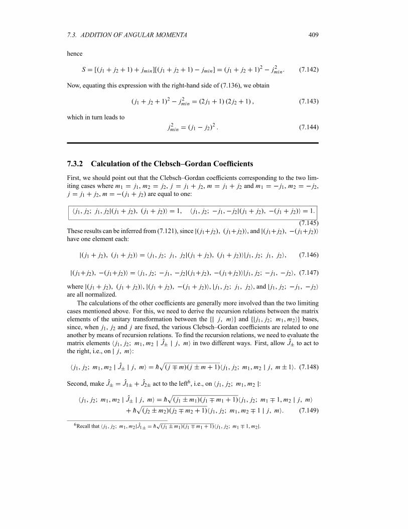
7.3. ADDITION OF ANGULAR MOMENTA 409
hence
S [ j1 j2 1 jmin][ j1 j2 1 jmin] j1 j2 1 2 j2min (7.142)
Now, equating this expression with the right-hand side of (7.136), we obtain
j1 j2 1 2 j2min 2 j1 1 2 j2 1 (7.143)
which in turn leads to
j2min j1 j22 (7.144)
7.3.2 Calculation of the Clebsch–Gordan Coefficients
First, we should point out that the Clebsch–Gordan coefficients corresponding to the two lim-
iting cases where m1 j1, m2 j2, j j1 j2, m j1 j2 and m1 j1, m2 j2,j j1 j2, m j1 j2 are equal to one:
j1 j2 j1 j2 j1 j2 j1 j2 1 j1 j2 j1 j2 j1 j2 j1 j2 1
(7.145)
These results can be inferred from (7.121), since j1 j2 j1 j2 , and j1 j2 j1 j2have one element each:
j1 j2 j1 j2 j1 j2 j1 j2 j1 j2 j1 j2 j1 j2 j1 j2 (7.146)
j1 j2 j1 j2 j1 j2 j1 j2 j1 j2 j1 j2 j1 j2 j1 j2 (7.147)
where j1 j2 j1 j2 , j1 j2 j1 j2 , j1 j2 j1 j2 , and j1 j2 j1 j2are all normalized.
The calculations of the other coefficients are generally more involved than the two limiting
cases mentioned above. For this, we need to derive the recursion relations between the matrix
elements of the unitary transformation between the j m and j1 j2 m1 m2 bases,
since, when j1, j2 and j are fixed, the various Clebsch–Gordan coefficients are related to oneanother by means of recursion relations. To find the recursion relations, we need to evaluate the
matrix elements j1 j2 m1 m2 J j m in two different ways. First, allow J to act to
the right, i.e., on j m :
j1 j2 m1 m2 J j m h j m j m 1 j1 j2 m1 m2 j m 1 (7.148)
Second, make J J1 J2 act to the left6, i.e., on j1 j2 m1 m2 :
j1 j2 m1 m2 J j m h j1 m1 j1 m1 1 j1 j2 m1 1 m2 j m
h j2 m2 j2 m2 1 j1 j2 m1 m2 1 j m (7.149)
6Recall that j1 j2 m1 m2 J1 h j1 m1 j1 m1 1 j1 j2 m1 1 m2 .
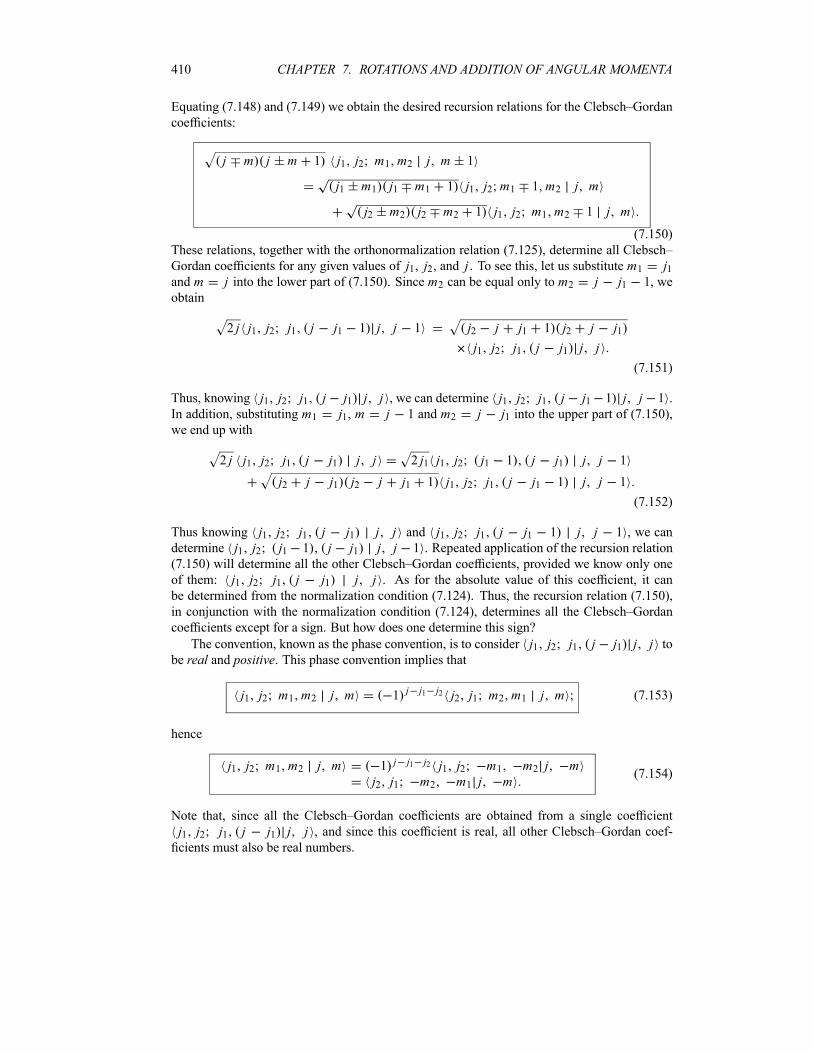
410 CHAPTER 7. ROTATIONS AND ADDITION OF ANGULAR MOMENTA
Equating (7.148) and (7.149) we obtain the desired recursion relations for the Clebsch–Gordan
coefficients:
j m j m 1 j1 j2 m1 m2 j m 1
j1 m1 j1 m1 1 j1 j2 m1 1 m2 j m
j2 m2 j2 m2 1 j1 j2 m1 m2 1 j m
(7.150)
These relations, together with the orthonormalization relation (7.125), determine all Clebsch–
Gordan coefficients for any given values of j1, j2, and j . To see this, let us substitute m1 j1and m j into the lower part of (7.150). Since m2 can be equal only to m2 j j1 1, we
obtain
2 j j1 j2 j1 j j1 1 j j 1 j2 j j1 1 j2 j j1
j1 j2 j1 j j1 j j
(7.151)
Thus, knowing j1 j2 j1 j j1 j j , we can determine j1 j2 j1 j j1 1 j j 1 .
In addition, substituting m1 j1, m j 1 and m2 j j1 into the upper part of (7.150),we end up with
2 j j1 j2 j1 j j1 j j 2 j1 j1 j2 j1 1 j j1 j j 1
j2 j j1 j2 j j1 1 j1 j2 j1 j j1 1 j j 1
(7.152)
Thus knowing j1 j2 j1 j j1 j j and j1 j2 j1 j j1 1 j j 1 , we can
determine j1 j2 j1 1 j j1 j j 1 . Repeated application of the recursion relation
(7.150) will determine all the other Clebsch–Gordan coefficients, provided we know only one
of them: j1 j2 j1 j j1 j j . As for the absolute value of this coefficient, it canbe determined from the normalization condition (7.124). Thus, the recursion relation (7.150),
in conjunction with the normalization condition (7.124), determines all the Clebsch–Gordan
coefficients except for a sign. But how does one determine this sign?
The convention, known as the phase convention, is to consider j1 j2 j1 j j1 j j tobe real and positive. This phase convention implies that
j1 j2 m1 m2 j m 1 j j1 j2 j2 j1 m2 m1 j m (7.153)
hence
j1 j2 m1 m2 j m 1 j j1 j2 j1 j2 m1 m2 j mj2 j1 m2 m1 j m
(7.154)
Note that, since all the Clebsch–Gordan coefficients are obtained from a single coefficient
j1 j2 j1 j j1 j j , and since this coefficient is real, all other Clebsch–Gordan coef-ficients must also be real numbers.
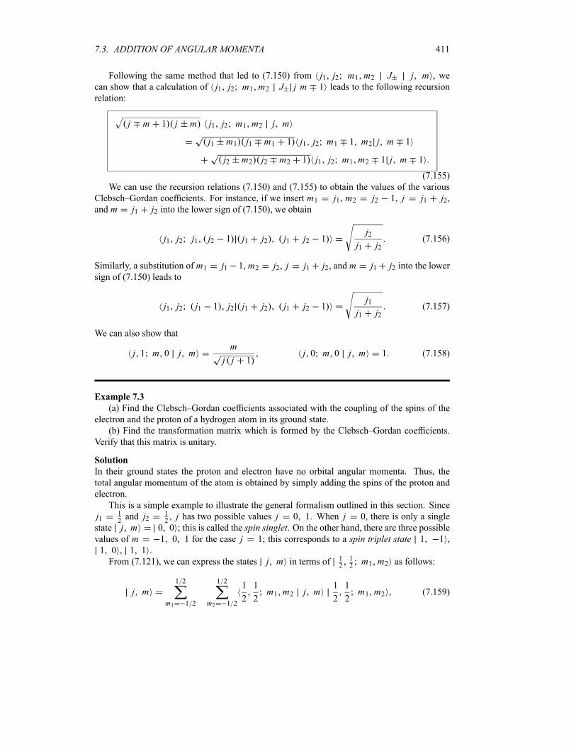
7.3. ADDITION OF ANGULAR MOMENTA 411
Following the same method that led to (7.150) from j1 j2 m1 m2 J j m , wecan show that a calculation of j1 j2 m1 m2 J j m 1 leads to the following recursion
relation:
j m 1 j m j1 j2 m1 m2 j m
j1 m1 j1 m1 1 j1 j2 m1 1 m2 j m 1
j2 m2 j2 m2 1 j1 j2 m1 m2 1 j m 1
(7.155)
We can use the recursion relations (7.150) and (7.155) to obtain the values of the various
Clebsch–Gordan coefficients. For instance, if we insert m1 j1, m2 j2 1, j j1 j2,and m j1 j2 into the lower sign of (7.150), we obtain
j1 j2 j1 j2 1 j1 j2 j1 j2 1j2
j1 j2(7.156)
Similarly, a substitution of m1 j1 1, m2 j2, j j1 j2, and m j1 j2 into the lowersign of (7.150) leads to
j1 j2 j1 1 j2 j1 j2 j1 j2 1j1
j1 j2(7.157)
We can also show that
j 1 m 0 j mm
j j 1j 0 m 0 j m 1 (7.158)
Example 7.3
(a) Find the Clebsch–Gordan coefficients associated with the coupling of the spins of the
electron and the proton of a hydrogen atom in its ground state.
(b) Find the transformation matrix which is formed by the Clebsch–Gordan coefficients.
Verify that this matrix is unitary.
Solution
In their ground states the proton and electron have no orbital angular momenta. Thus, the
total angular momentum of the atom is obtained by simply adding the spins of the proton and
electron.
This is a simple example to illustrate the general formalism outlined in this section. Since
j112and j2
12, j has two possible values j 0 1. When j 0, there is only a single
state j m 0 0 ; this is called the spin singlet. On the other hand, there are three possiblevalues of m 1 0 1 for the case j 1; this corresponds to a spin triplet state 1 1 ,
1 0 , 1 1 .
From (7.121), we can express the states j m in terms of 1212m1 m2 as follows:
j m1 2
m1 1 2
1 2
m2 1 2
1
2
1
2m1 m2 j m
1
2
1
2m1 m2 (7.159)
412 CHAPTER 7. ROTATIONS AND ADDITION OF ANGULAR MOMENTA
which, when applied to the two cases j 0 and j 1, leads to
0 01
2
1
2
1
2
1
20 0
1
2
1
2
1
2
1
2
1
2
1
2
1
2
1
20 0
1
2
1
2
1
2
1
2
(7.160)
1 11
2
1
2
1
2
1
21 1
1
2
1
2
1
2
1
2(7.161)
1 01
2
1
2
1
2
1
21 0
1
2
1
2
1
2
1
2
1
2
1
2
1
2
1
21 0
1
2
1
2
1
2
1
2
(7.162)
1 11
2
1
2
1
2
1
21 1
1
2
1
2
1
2
1
2(7.163)
To calculate the Clebsch–Gordan coefficients involved in (7.160)–(7.163), we are going
to adopt two separate approaches: the first approach uses the recursion relations (7.150) and
(7.155), while the second uses the algebra of angular momentum.
First approach: using the recursion relations
First, to calculate the two coefficients 1212
12
120 0 involved in (7.160), we need, on
the one hand, to substitute j 0 m 0 m1 m212into the upper sign relation of (7.150):
1
2
1
2
1
2
1
20 0
1
2
1
2
1
2
1
20 0 (7.164)
On the other hand, the substitution of j 0 and m 0 into (7.125) yields
1
2
1
2
1
2
1
20 0 2
1
2
1
2
1
2
1
20 0 2 1 (7.165)
Combining (7.164) and (7.165) we end up with
1
2
1
2
1
2
1
20 0
1
2(7.166)
The sign of 1212
12
120 0 has to be positive because, according to the phase convention,
the coefficient j1 j2 j1 j j1 j j is positive; hence
1
2
1
2
1
2
1
20 0
1
2(7.167)
As for 1212
12120 0 , its value can be inferred from (7.164) and (7.167):
1
2
1
2
1
2
1
20 0
1
2(7.168)
Second, the calculation of the coefficients involved in (7.161) to (7.163) goes as follows. The
orthonormalization relation (7.125) leads to
1
2
1
2
1
2
1
21 1 2 1
1
2
1
2
1
2
1
21 1 2 1 (7.169)
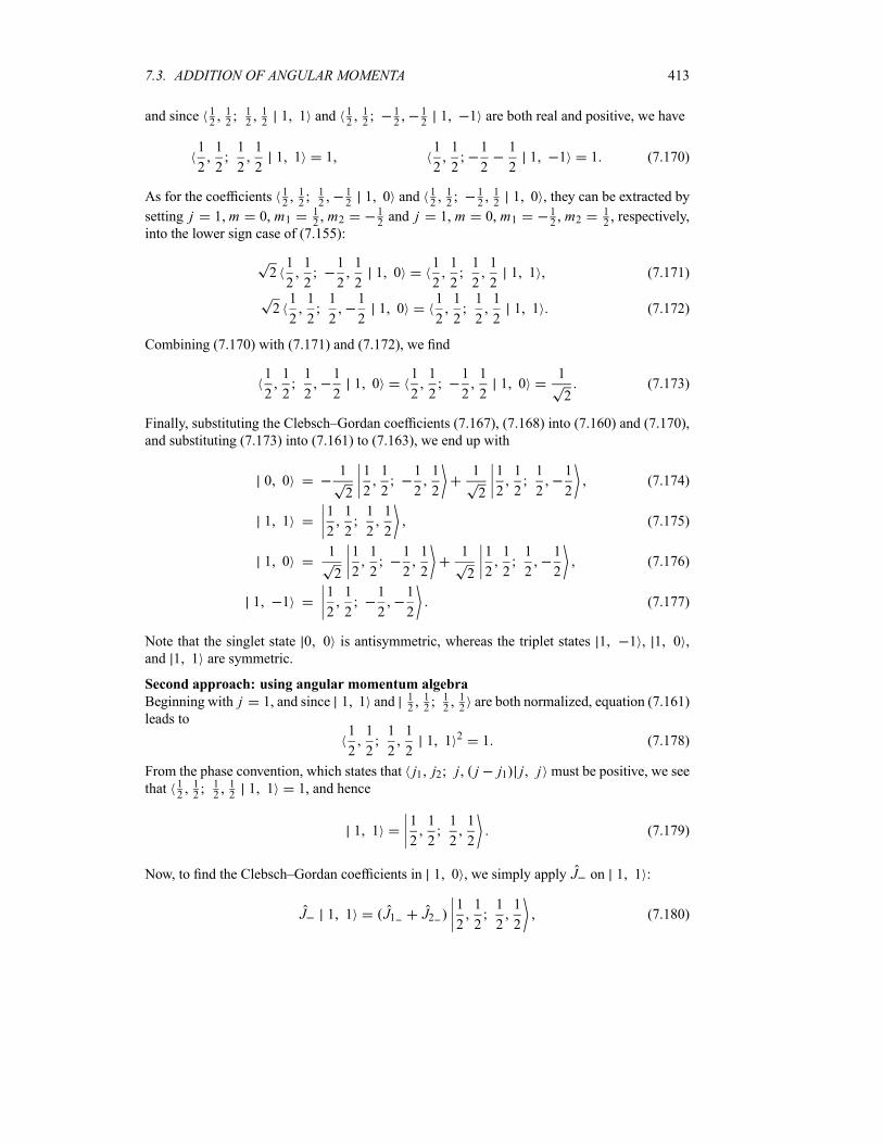
7.3. ADDITION OF ANGULAR MOMENTA 413
and since 1212
12121 1 and 1
212
12
121 1 are both real and positive, we have
1
2
1
2
1
2
1
21 1 1
1
2
1
2
1
2
1
21 1 1 (7.170)
As for the coefficients 1212
12
121 0 and 1
212
12121 0 , they can be extracted by
setting j 1 m 0, m112, m2
12and j 1, m 0, m1
12, m2
12, respectively,
into the lower sign case of (7.155):
21
2
1
2
1
2
1
21 0
1
2
1
2
1
2
1
21 1 (7.171)
21
2
1
2
1
2
1
21 0
1
2
1
2
1
2
1
21 1 (7.172)
Combining (7.170) with (7.171) and (7.172), we find
1
2
1
2
1
2
1
21 0
1
2
1
2
1
2
1
21 0
1
2(7.173)
Finally, substituting the Clebsch–Gordan coefficients (7.167), (7.168) into (7.160) and (7.170),
and substituting (7.173) into (7.161) to (7.163), we end up with
0 01
2
1
2
1
2
1
2
1
2
1
2
1
2
1
2
1
2
1
2(7.174)
1 11
2
1
2
1
2
1
2(7.175)
1 01
2
1
2
1
2
1
2
1
2
1
2
1
2
1
2
1
2
1
2(7.176)
1 11
2
1
2
1
2
1
2(7.177)
Note that the singlet state 0 0 is antisymmetric, whereas the triplet states 1 1 , 1 0 ,
and 1 1 are symmetric.
Second approach: using angular momentum algebra
Beginning with j 1, and since 1 1 and 1212
1212are both normalized, equation (7.161)
leads to1
2
1
2
1
2
1
21 1 2 1 (7.178)
From the phase convention, which states that j1 j2 j j j1 j j must be positive, we seethat 1
212
12121 1 1, and hence
1 11
2
1
2
1
2
1
2(7.179)
Now, to find the Clebsch–Gordan coefficients in 1 0 , we simply apply J on 1 1 :
J 1 1 J1 J21
2
1
2
1
2
1
2(7.180)
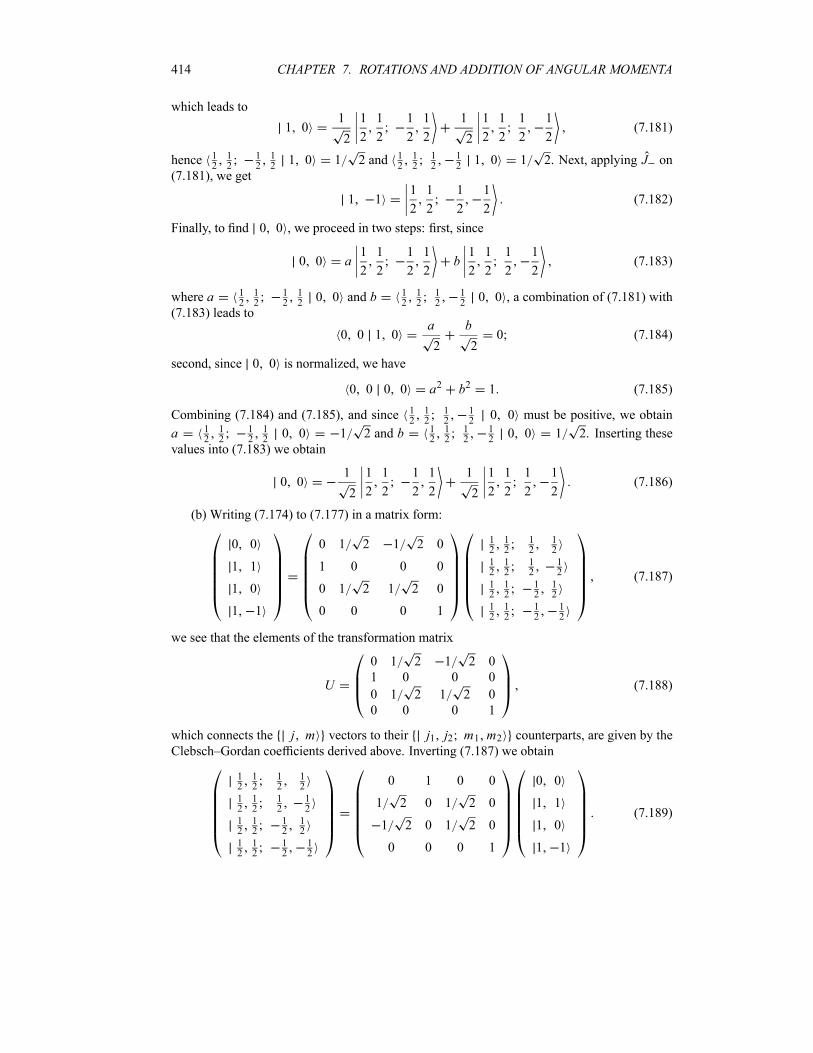
414 CHAPTER 7. ROTATIONS AND ADDITION OF ANGULAR MOMENTA
which leads to
1 01
2
1
2
1
2
1
2
1
2
1
2
1
2
1
2
1
2
1
2(7.181)
hence 1212
12121 0 1 2 and 1
212
12
121 0 1 2. Next, applying J on
(7.181), we get
1 11
2
1
2
1
2
1
2(7.182)
Finally, to find 0 0 , we proceed in two steps: first, since
0 0 a1
2
1
2
1
2
1
2b1
2
1
2
1
2
1
2(7.183)
where a 1212
12120 0 and b 1
212
12
120 0 , a combination of (7.181) with
(7.183) leads to
0 0 1 0a
2
b
20 (7.184)
second, since 0 0 is normalized, we have
0 0 0 0 a2 b2 1 (7.185)
Combining (7.184) and (7.185), and since 1212
12
12
0 0 must be positive, we obtain
a 1212
12120 0 1 2 and b 1
212
12
120 0 1 2. Inserting these
values into (7.183) we obtain
0 01
2
1
2
1
2
1
2
1
2
1
2
1
2
1
2
1
2
1
2(7.186)
(b) Writing (7.174) to (7.177) in a matrix form:
0 0
1 1
1 0
1 1
0 1 2 1 2 0
1 0 0 0
0 1 2 1 2 0
0 0 0 1
1212
12
12
1212
12
12
1212
12
12
1212
12
12
(7.187)
we see that the elements of the transformation matrix
U
0 1 2 1 2 0
1 0 0 0
0 1 2 1 2 0
0 0 0 1
(7.188)
which connects the j m vectors to their j1 j2 m1 m2 counterparts, are given by the
Clebsch–Gordan coefficients derived above. Inverting (7.187) we obtain
1212
12
12
1212
12
12
1212
12
12
1212
12
12
0 1 0 0
1 2 0 1 2 0
1 2 0 1 2 0
0 0 0 1
0 0
1 1
1 0
1 1
(7.189)
7.3. ADDITION OF ANGULAR MOMENTA 415
From (7.187) and (7.189) we see that the transformation matrix U is unitary; this is expected
since U 1 U†.
7.3.3 Coupling of Orbital and Spin Angular Momenta
We consider here an important application of the formalism of angular momenta addition to
the coupling of an orbital and a spin angular momentum: J L S. In particular, we wantto find Clebsch–Gordan coefficients associated with this coupling for a spin s 1
2particle.
In this case we have: j1 l (integer), m1 ml , j2 s 12, and m2 ms
12. The
allowed values of j as given by (7.130) are located within the interval l 12
j l 12. If
l 0 the problem would be obvious: the particle would have only spin and no orbital angular
momentum. But if l 0 then j can take only two possible values j l 12. There are
2 l 1 states l 12m corresponding to the case j l 1 2 and 2l states l 1
2m
corresponding to j l 12. Let us study in detail each one of these two cases.
Case j l 1 2
Applying the relation (7.121) to the case where j l 12, we have
l1
2m
l
ml l
1 2
m2 1 2
l1
2ml m2 l
1
2m l
1
2ml m2
ml
l1
2ml
1
2l
1
2m l
1
2ml
1
2
ml
l1
2ml
1
2l
1
2m l
1
2ml
1
2(7.190)
Using the selection rule ml m2 m or ml m m2, we can rewrite (7.190) as follows:
l1
2m l
1
2m
1
2
1
2l
1
2m l
1
2m
1
2
1
2
l1
2m
1
2
1
2l
1
2m l
1
2m
1
2
1
2(7.191)
We need now to calculate l 12m 1
212l 1
2m and l 1
2m 1
212l 1
2m . We begin
with the calculation of l 12m 1
212l 1
2m . Substituting j l 1
2, j1 l j2
12,
m1 m 12, m2
12into the upper sign case of (7.155), we obtain
l m3
2l m
1
2l1
2m
1
2
1
2l
1
2m
l m1
2l m
1
2l1
2m
1
2
1
2l
1
2m 1
(7.192)
or
l1
2m
1
2
1
2l
1
2m
l m 1 2
l m 3 2l1
2m
1
2
1
2l
1
2m 1 (7.193)
416 CHAPTER 7. ROTATIONS AND ADDITION OF ANGULAR MOMENTA
By analogy with l 12m 1
212l 1
2m we can express the Clebsch–Gordan coefficient
l 12m 1
212l 1
2m 1 in terms of l 1
2m 3
212l 1
2m 2 :
l1
2m
1
2
1
2l
1
2m
l m 1 2
l m 3 2
l m 3 2
l m 5 2
l1
2m
3
2
1
2l
1
2m 2 (7.194)
We can continue this procedure until m reaches its lowest values, l 12:
l1
2m
1
2
1
2l
1
2m
l m 1 2
l m 3 2
l m 3 2
l m 5 2
2l
2l 1l1
2l
1
2
1
2l
1
2
(7.195)
or
l1
2m
1
2
1
2l
1
2m
l m 1 2
2l 1l1
2l
1
2l
1
2l
1
2(7.196)
From (7.125) we can easily obtain l 12
l 12l 1
2l 1
2
21, and since this
coefficient is real we have l 12
l 12l 1
2l 1
21. Inserting this value into
(7.196) we end up with
l1
2m
1
2
1
2l
1
2m
l m 1 2
2l 1(7.197)
Now we turn to the calculation of the second coefficient, l 12m 1
212l 1
2m , involved
in (7.191). We can perform this calculation in two different ways. The first method consists of
following the same procedure adopted above to find l 12m 1
212l 1
2m . For this, we
need only to substitute j l 12j1 l j2
12m1 m 1
2m2
12in the lower sign
case of (7.155) and work our way through. A second, simpler method consists of substituting
(7.197) into (7.191) and then calculating the norm of the resulting equation:
1l m 1 2
2l 1l1
2m
1
2
1
2l
1
2m
2
(7.198)
where we have used the facts that the three kets l 12m and l 1
2m 1
212are normal-
ized. Again, since l 12m 1
212l 1
2m is real, (7.198) leads to
l1
2m
1
2
1
2l
1
2m
l m 1 2
2l 1(7.199)
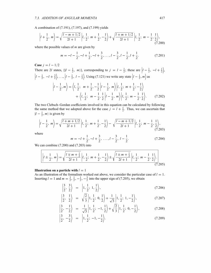
7.3. ADDITION OF ANGULAR MOMENTA 417
A combination of (7.191), (7.197), and (7.199) yields
l1
2m
l m 1 2
2l 1l1
2m
1
2
1
2
l m 1 2
2l 1l1
2m
1
2
1
2(7.200)
where the possible values of m are given by
m l1
2l
1
2l
3
2l
3
2l
1
2l
1
2(7.201)
Case j l 1 2
There are 2l states, l 12m , corresponding to j l 1
2; these are l 1
2l 1
2,
l 12
l 32, , l 1
2l 1
2. Using (7.121) we write any state l 1
2m as
l1
2m l
1
2m
1
2
1
2l
1
2m l
1
2m
1
2
1
2
l1
2m
1
2
1
2l
1
2m l
1
2m
1
2
1
2(7.202)
The two Clebsch–Gordan coefficients involved in this equation can be calculated by following
the same method that we adopted above for the case j l 12. Thus, we can ascertain that
l 12m is given by
l1
2m
l m 1 2
2l 1l1
2m
1
2
1
2
l m 1 2
2l 1l1
2m
1
2
1
2(7.203)
where
m l1
2l
3
2l
3
2l
1
2(7.204)
We can combine (7.200) and (7.203) into
l1
2m
l m 12
2l 1l1
2m
1
2
1
2
l m 12
2l 1l1
2m
1
2
1
2
(7.205)
Illustration on a particle with l 1
As an illustration of the formalism worked out above, we consider the particular case of l 1.
Inserting l 1 and m 32, 12, 1
2, 3
2into the upper sign of (7.205), we obtain
3
2
3
211
211
2(7.206)
3
2
1
2
2
311
201
2
1
311
21
1
2(7.207)
3
2
1
2
1
311
211
2
2
311
20
1
2(7.208)
3
2
3
211
21
1
2(7.209)
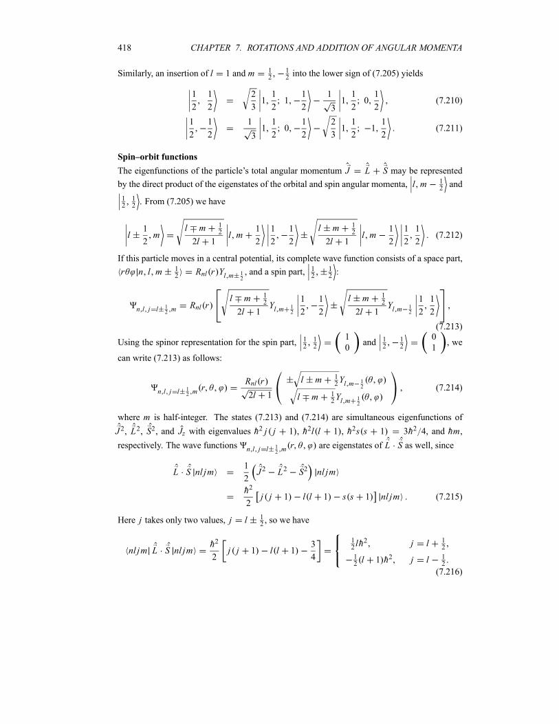
418 CHAPTER 7. ROTATIONS AND ADDITION OF ANGULAR MOMENTA
Similarly, an insertion of l 1 and m 12, 1
2into the lower sign of (7.205) yields
1
2
1
2
2
311
21
1
2
1
311
201
2(7.210)
1
2
1
2
1
311
20
1
2
2
311
211
2(7.211)
Spin–orbit functions
The eigenfunctions of the particle’s total angular momentum J L S may be represented
by the direct product of the eigenstates of the orbital and spin angular momenta, l m 12and
1212. From (7.205) we have
l1
2m
l m 12
2l 1l m
1
2
1
2
1
2
l m 12
2l 1l m
1
2
1
2
1
2(7.212)
If this particle moves in a central potential, its complete wave function consists of a space part,
r n l m 12
Rnl r Yl m 12, and a spin part, 1
212:
n l j l 12 m
Rnl rl m 1
2
2l 1Yl m 1
2
1
2
1
2
l m 12
2l 1Yl m 1
2
1
2
1
2
(7.213)
Using the spinor representation for the spin part, 1212
1
0and 1
212
0
1, we
can write (7.213) as follows:
n l j l 12 m
rRnl r
2l 1
l m 12Yl m 1
2
l m 12Yl m 1
2
(7.214)
where m is half-integer. The states (7.213) and (7.214) are simultaneous eigenfunctions of
J 2, L2, S2, and Jz with eigenvalues h2 j j 1 , h2l l 1 , h2s s 1 3h2 4, and hm,
respectively. The wave functions n l j l 12 m
r are eigenstates of L S as well, since
L S nl jm1
2J 2 L2 S2 nl jm
h2
2j j 1 l l 1 s s 1 nl jm (7.215)
Here j takes only two values, j l 12, so we have
nl jm L S nl jmh2
2j j 1 l l 1
3
4
12lh2 j l 1
2
12l 1 h2 j l 1
2
(7.216)
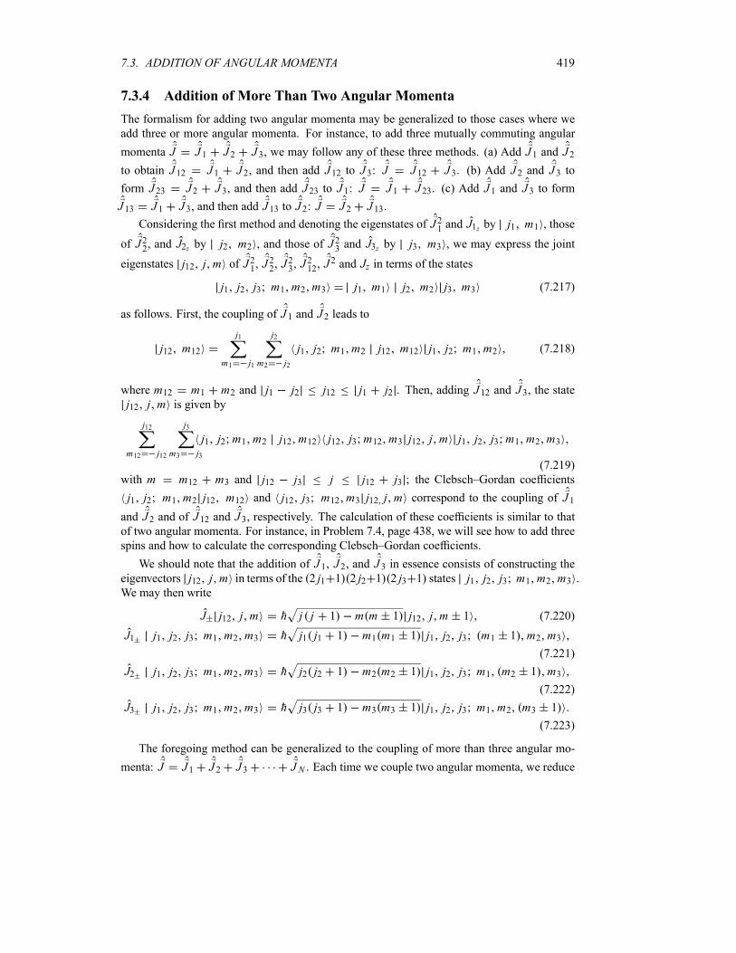
7.3. ADDITION OF ANGULAR MOMENTA 419
7.3.4 Addition of More Than Two Angular Momenta
The formalism for adding two angular momenta may be generalized to those cases where we
add three or more angular momenta. For instance, to add three mutually commuting angular
momenta J J 1 J 2 J3, we may follow any of these three methods. (a) Add J 1 and J 2
to obtain J12 J 1 J2, and then add J 12 to J3: J J 12 J3. (b) Add J2 and J 3 to
form J23 J2 J 3, and then add J 23 to J 1: J J 1 J 23. (c) Add J 1 and J 3 to form
J13 J 1 J 3, and then add J13 to J2: J J 2 J 13.
Considering the first method and denoting the eigenstates of J 21 and J1z by j1 m1 , those
of J 22, and J2z by j2 m2 , and those of J 23 and J3z by j3 m3 , we may express the joint
eigenstates j12 j m of J 21, J22, J
23, J
212, J
2 and Jz in terms of the states
j1 j2 j3 m1 m2 m3 j1 m1 j2 m2 j3 m3 (7.217)
as follows. First, the coupling of J 1 and J2 leads to
j12 m12
j1
m1 j1
j2
m2 j2
j1 j2 m1 m2 j12 m12 j1 j2 m1 m2 (7.218)
where m12 m1 m2 and j1 j2 j12 j1 j2 . Then, adding J12 and J 3, the statej12 j m is given by
j12
m12 j12
j3
m3 j3
j1 j2 m1 m2 j12 m12 j12 j3 m12 m3 j12 j m j1 j2 j3 m1 m2 m3
(7.219)
with m m12 m3 and j12 j3 j j12 j3 ; the Clebsch–Gordan coefficients
j1 j2 m1 m2 j12 m12 and j12 j3 m12 m3 j12 j m correspond to the coupling of J 1
and J 2 and of J12 and J 3, respectively. The calculation of these coefficients is similar to thatof two angular momenta. For instance, in Problem 7.4, page 438, we will see how to add three
spins and how to calculate the corresponding Clebsch–Gordan coefficients.
We should note that the addition of J 1, J 2, and J 3 in essence consists of constructing theeigenvectors j12 j m in terms of the 2 j1 1 2 j2 1 2 j3 1 states j1 j2 j3 m1 m2 m3 .We may then write
J j12 j m h j j 1 m m 1 j12 j m 1 (7.220)
J1 j1 j2 j3 m1 m2 m3 h j1 j1 1 m1 m1 1 j1 j2 j3 m1 1 m2 m3
(7.221)
J2 j1 j2 j3 m1 m2 m3 h j2 j2 1 m2 m2 1 j1 j2 j3 m1 m2 1 m3
(7.222)
J3 j1 j2 j3 m1 m2 m3 h j3 j3 1 m3 m3 1 j1 j2 j3 m1 m2 m3 1
(7.223)
The foregoing method can be generalized to the coupling of more than three angular mo-
menta: J J1 J 2 J3 J N . Each time we couple two angular momenta, we reduce

420 CHAPTER 7. ROTATIONS AND ADDITION OF ANGULAR MOMENTA
the problem to the coupling of N 1 angular momenta. For instance, we may start by adding
J 1 and J 2 to generate J12; we are then left with N 1 angular momenta. Second, by adding
J 12 and J 3 to form J123, we are left with N 2 angular momenta. Third, an addition of J 123
and J 4 leaves us with N 3 angular momenta, and so on. We may continue in this way till
we add all given angular momenta.
7.3.5 Rotation Matrices for Coupling Two Angular Momenta
We want to find out how to express the rotation matrix associated with an angular momentum
J in terms of the rotation matrices corresponding to J 1 and J2 such that J J 1 J2. That is,
knowing the rotation matrices d j1 and d j2 , how does one calculate d jmm ?
Since
d jm m j m Ry j m (7.224)
where
j mm1m2
j1 j2 m1 m2 j m j1 j2 m1 m2 (7.225)
j mm1m2
j1 j2 m1 m2 j m j1 j2 m1 m2 (7.226)
and since the Clebsch–Gordan coefficients are real,
j mm1m2
j1 j2 m1 m2 j m j1 j2 m1 m2 (7.227)
we can rewrite (7.224) as
d jm m
m1m2 m1m2
j1 j2 m1 m2 j m j1 j2 m1 m2 j m
j1 j2 m1 m2 Ry j1 j2 m1 m2 (7.228)
Since Ry exp[ Jy h] exp[ J1y h] exp[ J2y h], because Jy J1y J2y , andsince j1 j2 m1 m2 j1 m1 j2 m2 and j1 j2 m1 m2 j1 m1 j2 m2 , wehave
d jm m
m1m2 m1m2
j1 j2 m1 m2 j m j1 j2 m1 m2 j m
j1 m1 expi
hJ1y j1 m1 j2 m2 exp
i
hJ2y j2 m2
(7.229)
or
d jm m
m1m2 m1m2
j1 j2 m1 m2 j m j1 j2 m1 m2 j m d j1m1m1
d j2m2m2
(7.230)
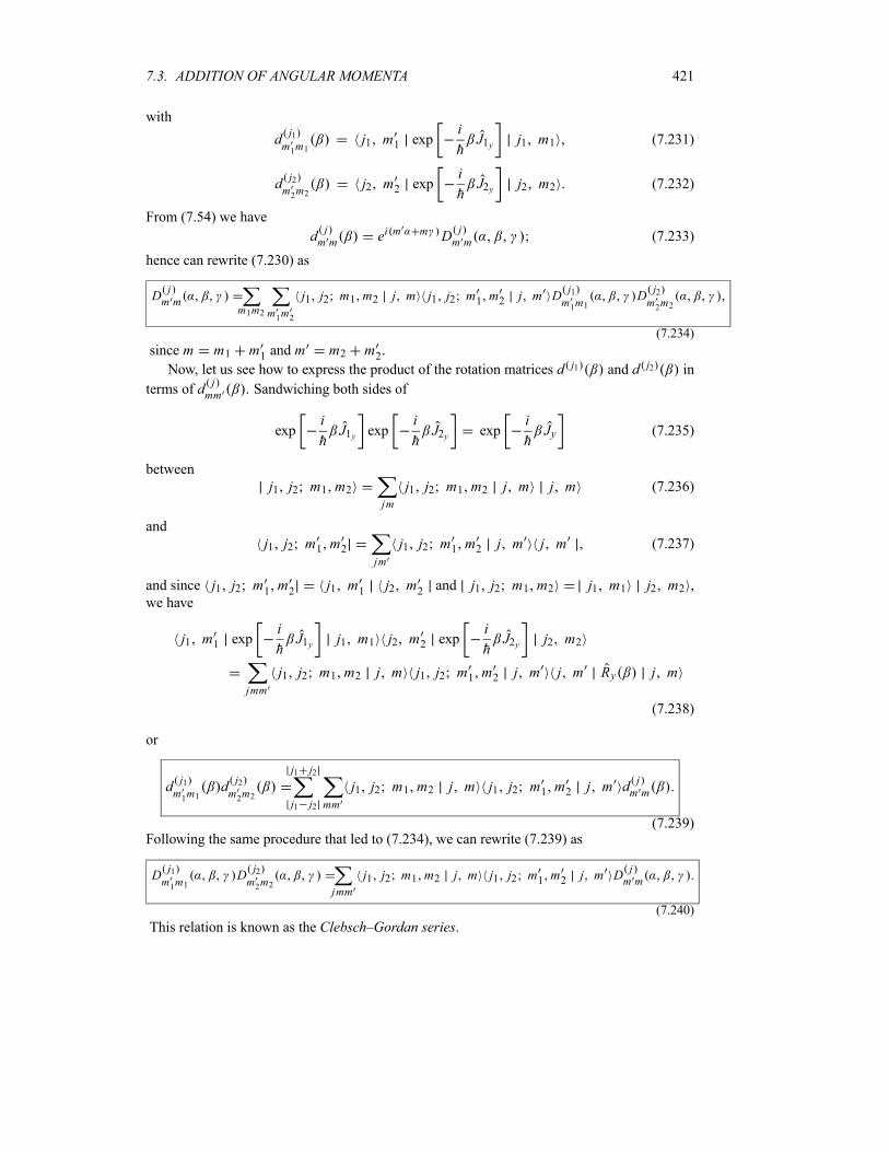
7.3. ADDITION OF ANGULAR MOMENTA 421
with
d j1m1m1
j1 m1 expi
hJ1y j1 m1 (7.231)
d j2m2m2
j2 m2 expi
hJ2y j2 m2 (7.232)
From (7.54) we have
d jm m ei m m D j
m m (7.233)
hence can rewrite (7.230) as
Djm m
m1m2 m1m2
j1 j2 m1 m2 j m j1 j2 m1 m2 j m Dj1m1m1
Dj2m2m2
(7.234)
since m m1 m1 and m m2 m2.Now, let us see how to express the product of the rotation matrices d j1 and d j2 in
terms of d jmm . Sandwiching both sides of
expi
hJ1y exp
i
hJ2y exp
i
hJy (7.235)
between
j1 j2 m1 m2jm
j1 j2 m1 m2 j m j m (7.236)
and
j1 j2 m1 m2jm
j1 j2 m1 m2 j m j m (7.237)
and since j1 j2 m1 m2 j1 m1 j2 m2 and j1 j2 m1 m2 j1 m1 j2 m2 ,we have
j1 m1 expi
hJ1y j1 m1 j2 m2 exp
i
hJ2y j2 m2
jmm
j1 j2 m1 m2 j m j1 j2 m1 m2 j m j m Ry j m
(7.238)
or
d j1m1m1
d j2m2m2
j1 j2
j1 j2 mm
j1 j2 m1 m2 j m j1 j2 m1 m2 j m d jm m
(7.239)Following the same procedure that led to (7.234), we can rewrite (7.239) as
Dj1m1m1
Dj2m2m2
jmm
j1 j2 m1 m2 j m j1 j2 m1 m2 j m Djm m
(7.240)
This relation is known as the Clebsch–Gordan series.

422 CHAPTER 7. ROTATIONS AND ADDITION OF ANGULAR MOMENTA
The relation (7.240) has an important application: the derivation of an integral involving
three spherical harmonics. When j1 and j2 are both integers (i.e., j1 l1 and j2 l2) and m1and m2 are both zero (hence m 0), equation (7.240) finds a useful application:
D l1m10
D l2m20
lm
l1 l2 0 0 l 0 l1 l2 m1 m2 l m D lm 0
(7.241)
Since the expressions of D l1m10, D l2
m20, and D l
m 0 can be inferred from (7.73), notably
D lm 0 0
4
2l 1Ylm (7.242)
we can reduce (7.241) to
Yl1m1 Yl2m2lm
2l1 1 2l2 1
4 2l 1l1 l2 0 0 l 0 l1 l2 m1 m2 l m Ylm
(7.243)
where we have removed the primes and taken the complex conjugate. Multiplying both sides
by Ylm and integrating over and , we obtain the following frequently used integral:
2
0
d0
Ylm Yl1m1 Yl2m2 sin d 2l1 1 2l2 14 2l 1 l1 l2 0 0 l 0
l1 l2 m1 m2 l m
(7.244)
7.3.6 Isospin
The ideas presented above—spin and the addition of angular momenta—find some interesting
applications to other physical quantities. For instance, in the field of nuclear physics, the quan-
tity known as isotopic spin can be represented by a set of operators which not only obey thesame algebra as the components of angular momentum, but also couple in the same way as
ordinary angular momenta.
Since the nuclear force does not depend on the electric charge, we can consider the proton
and the neutron to be separate manifestations (states) of the same particle, the nucleon. Thenucleon may thus be found in two different states: a proton and a neutron. In this way, as the
protons and neutrons are identical particles with respect to the nuclear force, we will need an
additional quantum number (or label) to indicate whether the nucleon is a proton or a neutron.
Due to its formal analogy with ordinary spin, this label is called the isotopic spin or, in short,the isospin. If we take the isospin quantum number to be 1
2, its z-component will then be
represented by a quantum number having the values 12and 1
2. The difference between a
proton and a neutron then becomes analogous to the difference between spin-up and spin-down
particles.
The fundamental difference between ordinary spin and the isospin is that, unlike the spin,
the isospin has nothing to do with rotations or spinning in the coordinate space, it hence cannot
be coupled with the angular momenta of the nucleons. Nucleons can thus be distinguished by
t312, where t3 is the third or z-component of the isospin vector operator t .
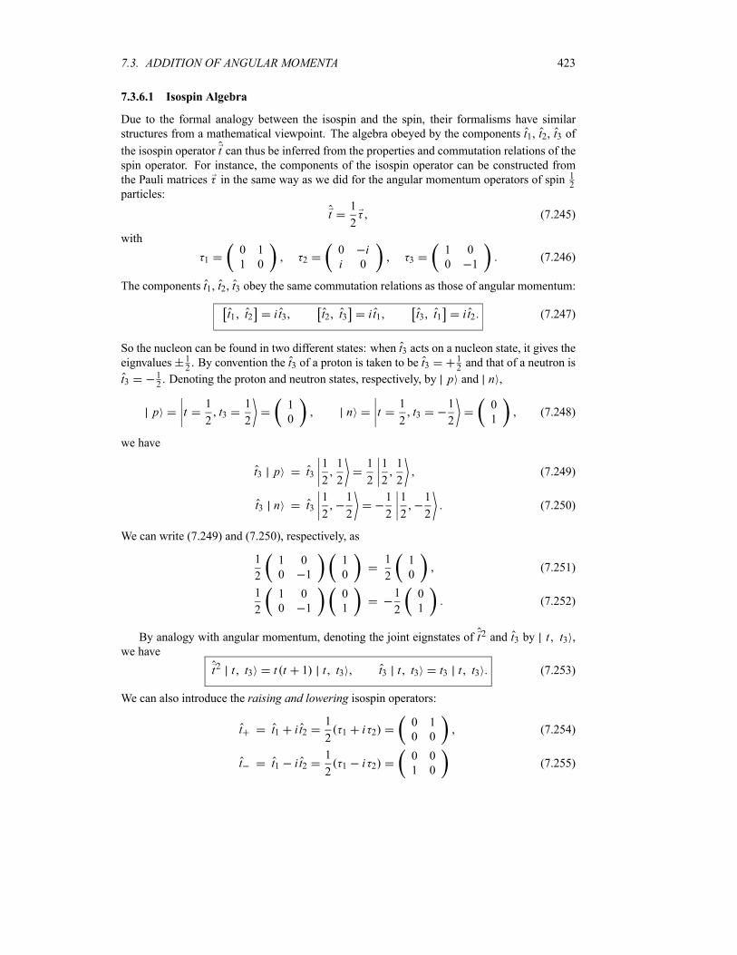
7.3. ADDITION OF ANGULAR MOMENTA 423
7.3.6.1 Isospin Algebra
Due to the formal analogy between the isospin and the spin, their formalisms have similar
structures from a mathematical viewpoint. The algebra obeyed by the components t1, t2, t3 of
the isospin operator t can thus be inferred from the properties and commutation relations of thespin operator. For instance, the components of the isospin operator can be constructed from
the Pauli matrices in the same way as we did for the angular momentum operators of spin 12
particles:
t1
2(7.245)
with
10 1
1 0 20 ii 0 3
1 0
0 1(7.246)
The components t1, t2, t3 obey the same commutation relations as those of angular momentum:
t1 t2 i t3 t2 t3 i t1 t3 t1 i t2 (7.247)
So the nucleon can be found in two different states: when t3 acts on a nucleon state, it gives theeignvalues 1
2. By convention the t3 of a proton is taken to be t3
12and that of a neutron is
t312. Denoting the proton and neutron states, respectively, by p and n ,
p t1
2t3
1
2
1
0n t
1
2t3
1
2
0
1(7.248)
we have
t3 p t31
2
1
2
1
2
1
2
1
2(7.249)
t3 n t31
2
1
2
1
2
1
2
1
2(7.250)
We can write (7.249) and (7.250), respectively, as
1
2
1 0
0 1
1
0
1
2
1
0(7.251)
1
2
1 0
0 1
0
1
1
2
0
1(7.252)
By analogy with angular momentum, denoting the joint eignstates of t2 and t3 by t t3 ,we have
t2 t t3 t t 1 t t3 t3 t t3 t3 t t3 (7.253)
We can also introduce the raising and lowering isospin operators:
t t1 i t21
21 i 2
0 1
0 0(7.254)
t t1 i t21
21 i 2
0 0
1 0(7.255)
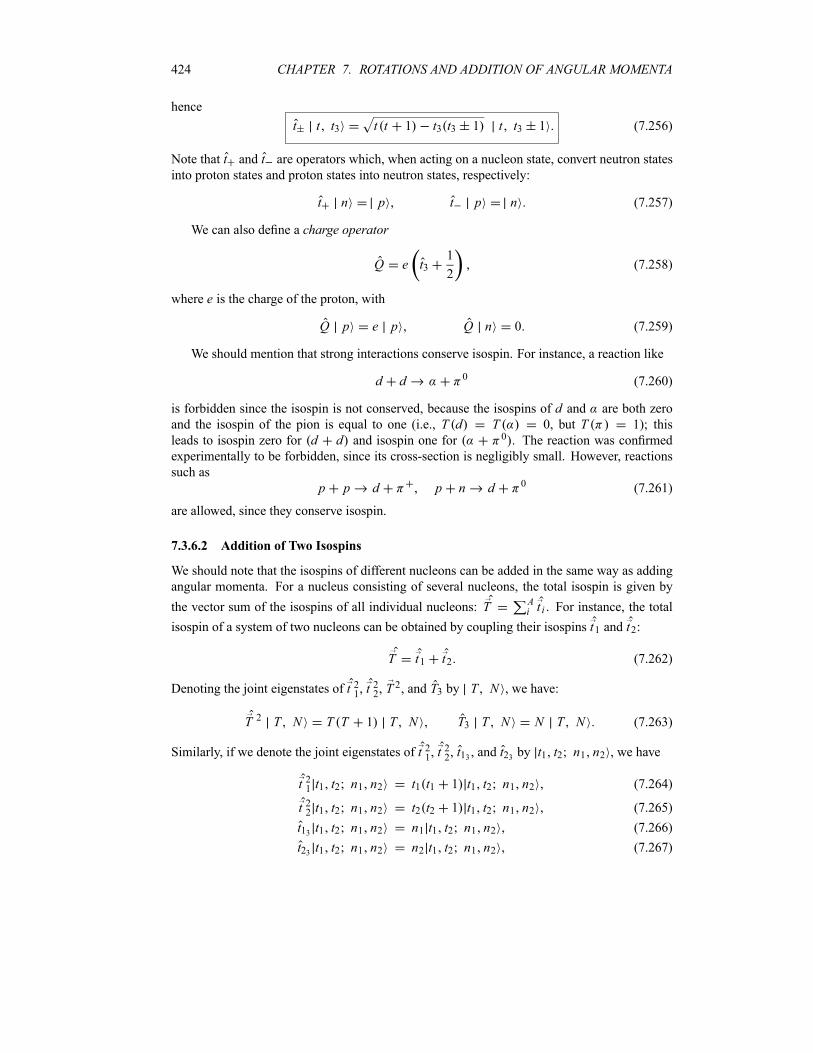
424 CHAPTER 7. ROTATIONS AND ADDITION OF ANGULAR MOMENTA
hence
t t t3 t t 1 t3 t3 1 t t3 1 (7.256)
Note that t and t are operators which, when acting on a nucleon state, convert neutron statesinto proton states and proton states into neutron states, respectively:
t n p t p n (7.257)
We can also define a charge operator
Q e t31
2(7.258)
where e is the charge of the proton, with
Q p e p Q n 0 (7.259)
We should mention that strong interactions conserve isospin. For instance, a reaction like
d d 0 (7.260)
is forbidden since the isospin is not conserved, because the isospins of d and are both zero
and the isospin of the pion is equal to one (i.e., T d T 0, but T 1); this
leads to isospin zero for d d and isospin one for 0 . The reaction was confirmed
experimentally to be forbidden, since its cross-section is negligibly small. However, reactions
such as
p p d p n d 0 (7.261)
are allowed, since they conserve isospin.
7.3.6.2 Addition of Two Isospins
We should note that the isospins of different nucleons can be added in the same way as adding
angular momenta. For a nucleus consisting of several nucleons, the total isospin is given by
the vector sum of the isospins of all individual nucleons: T Ai t i . For instance, the total
isospin of a system of two nucleons can be obtained by coupling their isospins t1 and t2:
T t1 t2 (7.262)
Denoting the joint eigenstates of t 21, t22, T
2, and T3 by T N , we have:
T 2 T N T T 1 T N T3 T N N T N (7.263)
Similarly, if we denote the joint eigenstates of t 21, t22, t13 , and t23 by t1 t2 n1 n2 , we have
t 21 t1 t2 n1 n2 t1 t1 1 t1 t2 n1 n2 (7.264)
t 22 t1 t2 n1 n2 t2 t2 1 t1 t2 n1 n2 (7.265)
t13 t1 t2 n1 n2 n1 t1 t2 n1 n2 (7.266)
t23 t1 t2 n1 n2 n2 t1 t2 n1 n2 (7.267)
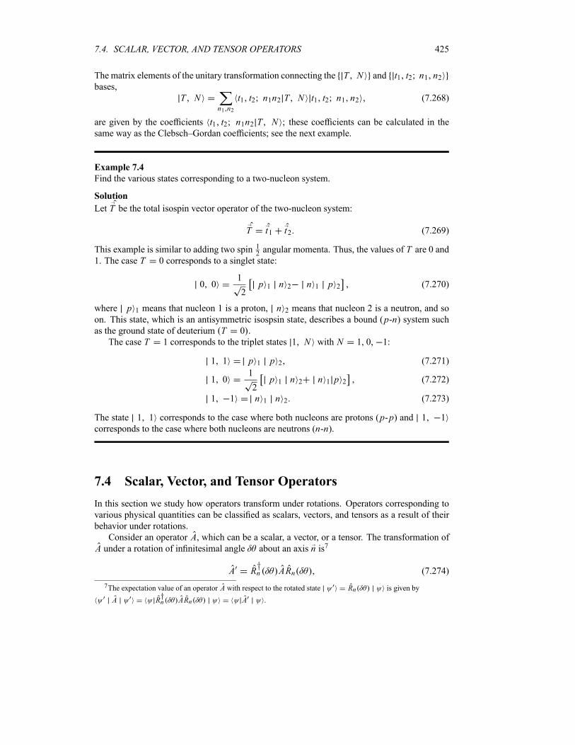
7.4. SCALAR, VECTOR, AND TENSOR OPERATORS 425
The matrix elements of the unitary transformation connecting the T N and t1 t2 n1 n2bases,
T Nn1 n2
t1 t2 n1n2 T N t1 t2 n1 n2 (7.268)
are given by the coefficients t1 t2 n1n2 T N ; these coefficients can be calculated in thesame way as the Clebsch–Gordan coefficients; see the next example.
Example 7.4
Find the various states corresponding to a two-nucleon system.
Solution
Let T be the total isospin vector operator of the two-nucleon system:
T t1 t2 (7.269)
This example is similar to adding two spin 12angular momenta. Thus, the values of T are 0 and
1. The case T 0 corresponds to a singlet state:
0 01
2p 1 n 2 n 1 p 2 (7.270)
where p 1 means that nucleon 1 is a proton, n 2 means that nucleon 2 is a neutron, and soon. This state, which is an antisymmetric isospsin state, describes a bound (p-n) system suchas the ground state of deuterium T 0 .
The case T 1 corresponds to the triplet states 1 N with N 1, 0, 1:
1 1 p 1 p 2 (7.271)
1 01
2p 1 n 2 n 1 p 2 (7.272)
1 1 n 1 n 2 (7.273)
The state 1 1 corresponds to the case where both nucleons are protons (p-p) and 1 1
corresponds to the case where both nucleons are neutrons (n-n).
7.4 Scalar, Vector, and Tensor Operators
In this section we study how operators transform under rotations. Operators corresponding to
various physical quantities can be classified as scalars, vectors, and tensors as a result of their
behavior under rotations.
Consider an operator A, which can be a scalar, a vector, or a tensor. The transformation ofA under a rotation of infinitesimal angle about an axis n is7
A R†n ARn (7.274)
7The expectation value of an operator A with respect to the rotated state Rn is given by
A R†n ARn A .
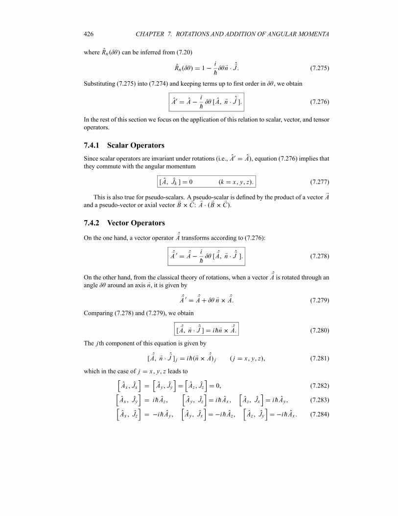
426 CHAPTER 7. ROTATIONS AND ADDITION OF ANGULAR MOMENTA
where Rn can be inferred from (7.20)
Rn 1i
hn J (7.275)
Substituting (7.275) into (7.274) and keeping terms up to first order in , we obtain
A Ai
h[A n J ] (7.276)
In the rest of this section we focus on the application of this relation to scalar, vector, and tensor
operators.
7.4.1 Scalar Operators
Since scalar operators are invariant under rotations (i.e., A A , equation (7.276) implies thatthey commute with the angular momentum
[A Jk ] 0 k x y z (7.277)
This is also true for pseudo-scalars. A pseudo-scalar is defined by the product of a vector Aand a pseudo-vector or axial vector B C: A B C .
7.4.2 Vector Operators
On the one hand, a vector operator A transforms according to (7.276):
A Ai
h[A n J ] (7.278)
On the other hand, from the classical theory of rotations, when a vector A is rotated through anangle around an axis n, it is given by
A A n A (7.279)
Comparing (7.278) and (7.279), we obtain
[A n J ] ihn A (7.280)
The j th component of this equation is given by
[A n J ] j ih n A j j x y z (7.281)
which in the case of j x y z leads to
Ax Jx Ay Jy Az Jz 0 (7.282)
Ax Jy ihAz Ay Jz ihAx Az Jx ihAy (7.283)
Ax Jz ihAy Ay Jx ihAz Az Jy ih Ax (7.284)
7.4. SCALAR, VECTOR, AND TENSOR OPERATORS 427
Some interesting applications of (7.280) correspond to the cases where the vector operator Ais either the angular momentum, the position, or the linear momentum operator. Let us consider
these three cases separately. First, substituting A J into (7.280), we recover the usual angularmomentum commutation relations:
[Jx Jy] ih Jz [Jy Jz] ih Jx [Jz Jx ] ih Jy (7.285)
Second, in the case of a spinless particle (i.e., J L), and if A is equal to the position operator,
A R, then (7.280) will yield the following relations:
x Lx 0 x L y ihz x L z ihy (7.286)
y L y 0 y Lz ihx y Lx ihz (7.287)
z Lz 0 z Lx ihy z L y ihx (7.288)
Third, if J L and if A is equal to the momentum operator, A P , then (7.280) will lead to
Px Lx 0 Px L y ihPz Px L z ihPy (7.289)
Py L y 0 Py L z ihPx Py Lx ihPz (7.290)
Pz Lz 0 Pz Lx ihPy Pz L y ihPx (7.291)
Now, introducing the operators
A Ax i Ay (7.292)
and using the relations (7.282) to (7.284), we can show that
Jx A hAz Jy A ihAz Jz A hA (7.293)
These relations in turn can be shown to lead to
J A 0 J A 2hAz (7.294)
Let us introduce the spherical components A 1, A0, A1 of the vector operator A; they aredefined in terms of the Cartesian coordinates Ax Ay Az as follows:
A 11
2Ax Ay A0 Az (7.295)
For the particular case where A is equal to the position vector R, we can express the componentsRq (where q 1 0 1),
R 11
2x y R0 z (7.296)
428 CHAPTER 7. ROTATIONS AND ADDITION OF ANGULAR MOMENTA
in terms of the spherical coordinates (recall that R1 x r sin cos , R2 y r sin sin ,
and R3 z r cos ) as follows:
R 11
2re i sin R0 r cos (7.297)
Using the relations (7.282) to (7.284) and (7.292) to (7.294), we can ascertain that
Jz Aq hq Aq q 1 0 1 (7.298)
J Aq h 2 q q 1 Aq 1 q 1 0 1 (7.299)
7.4.3 Tensor Operators: Reducible and Irreducible Tensors
In general, a tensor of rank k has 3k components, where 3 denotes the dimension of the space.For instance, a tensor such as
Ti j Ai B j i j x y z (7.300)
which is equal to the product of the components of two vectors A and B, is a second-ranktensor; this tensor has 32 components.
7.4.3.1 Reducible Tensors
A Cartesian tensor Ti j can be decomposed into three parts:
Ti j T 0i j T 1
i j T 2i j (7.301)
with
T 0i j
1
3i j
3
i 1
Ti i (7.302)
T 1i j
1
2Ti j T j i i j (7.303)
T 2i j
1
2Ti j T j i T 0
i j (7.304)
Notice that if we add equations (7.302), (7.303), and (7.304), we end up with an identity rela-
tion: Ti j Ti j .
The term T 0i j has only one component and transforms like a scalar under rotations. The
second term T 1i j is an antisymmetric tensor of rank 1 which has three independent components;
it transforms like a vector. The third term T 2i j is a symmetric second-rank tensor with zero
trace, and hence has five independent components; T 2i j cannot be reduced further to tensors of
lower rank. These five components define an irreducible second-rank tensor.
In general, any tensor of rank k can be decomposed into tensors of lower rank that areexpressed in terms of linear combinations of its 3k components. However, there always remain
7.4. SCALAR, VECTOR, AND TENSOR OPERATORS 429
2k 1 components that behave as a tensor of rank k which cannot be reduced further. These2k 1 components are symmetric and traceless with respect to any two indices; they form
the components of an irreducible tensor of rank k.Equations (7.301) to (7.304) show how to decompose a Cartesian tensor operator, Ti j , into
a sum of irreducible spherical tensor operators T 0i j T 1
i j T 2i j . Cartesian tensors are not very
suitable for studying transformations under rotations, because they are reducible whenever their
rank exceeds 1. In problems that display spherical symmetry, such as those encountered in
subatomic physics, spherical tensors are very useful simplifying tools. It is therefore interesting
to consider irreducible spherical tensor operators.
7.4.3.2 Irreducible Spherical Tensors
Let us now focus only on the representation of irreducible tensor operators in spherical coor-
dinates. An irreducible spherical tensor operator of rank k (k is integer) is a set of 2k 1
operators T kq , with q k k, which transform in the same way as angular momentum
under a rotation of axes. For example, the case k 1 corresponds to a vector. The quantities
T 1q are related to the components of the vector A as follows (see (7.295)):
T 11
1
2Ax Ay T 1
0 Az (7.305)
In what follows we are going to study some properties of spherical tensor operators and
then determine how they transform under rotations.
First, let us look at the various commutation relations of spherical tensors with the angular
momentum operator. Since a vector operator is a tensor of rank 1, we can rewrite equations
(7.298) to (7.299), respectively, as follows:
Jz T 1q hqT 1
q q 1 0 1 (7.306)
J T 1q h 1 1 1 q q 1 T 1
q 1 (7.307)
where we have adopted the notation Aq T 1q . We can easily generalize these two relations
to any spherical tensor of rank k, T kq , and obtain these commutators:
Jz T kq hqT k
q q k k 1 k 1 k (7.308)
J T kq h k k 1 q q 1 T k
q 1 (7.309)
Using the relations
k q Jz k q hq k q k q hq q q (7.310)
k q J k q h k k 1 q q 1 q q 1 (7.311)
along with (7.308) and (7.309), we can write
k
q k
T kq k q Jz k q hqT k
q Jz T kq (7.312)
430 CHAPTER 7. ROTATIONS AND ADDITION OF ANGULAR MOMENTA
k
q k
T kq k q J k q h k k 1 q q 1 T k
q 1 J T kq (7.313)
The previous two relations can be combined into
J T kq
k
q k
T kq k q J k q (7.314)
or
n J T kq
k
q k
T kq k q n J k q (7.315)
Having determined the commutation relations of the tensor operators with the angular mo-
mentum (7.315), we are now well equipped to study how irreducible spherical tensor operators
transform under rotations. Using (7.276) we can write the transformation relation of a spherical
tensor T kq under an infinitesimal rotation as follows:
R†n T k
q Rn T kq
i
hn J T k
q (7.316)
Inserting (7.315) into (7.316), we obtain
R† T kq R
k
q k
T kq k q 1
i
hn J k q
q
T kq k q ei n J h k q
(7.317)
This result also holds for finite rotations
R† T kq R
k
q k
T kq k q R† k q
q
T kq D k
q q
(7.318)
7.4.4 Wigner–Eckart Theorem for Spherical Tensor Operators
Taking the matrix elements of (7.308) between eigenstates of J2 and Jz , we find
j m Jz T kq hqT k
q j m 0 (7.319)
or
m m q j m T kq j m 0 (7.320)
This implies that j m T kq j m vanishes unless m m q. This property suggests
that the quantity j m T kq j m must be proportional to the Clebsch–Gordan coefficient
j m j k m q ; hence (7.320) leads to
m m q j m j k m q 0 (7.321)
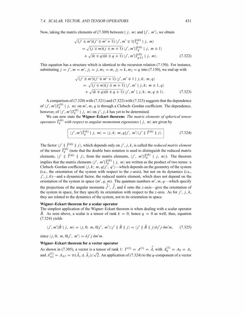
7.4. SCALAR, VECTOR, AND TENSOR OPERATORS 431
Now, taking the matrix elements of (7.309) between j m and j m , we obtain
j m j m 1 j m 1 T kq j m
j m j m 1 j m T kq j m 1
k q k q 1 j m T kq 1 j m (7.322)
This equation has a structure which is identical to the recursion relation (7.150). For instance,
substituting j j m m j1 j m1 m j2 k m2 q into (7.150), we end up with
j m j m 1 j m 1 j k m q
j m j m 1 j m j k m 1 q
k q k q 1 j m j k m q 1 (7.323)
A comparison of (7.320) with (7.321) and (7.322) with (7.323) suggests that the dependence
of j m T kq j m on m , m, q is through a Clebsch–Gordan coefficient. The dependence,
however, of j m T kq j m on j j k has yet to be determined.
We can now state theWigner–Eckart theorem: The matrix elements of spherical tensor
operators T kq with respect to angular momentum eigenstates j m are given by
j m T kq j m j k m q j m j T k j (7.324)
The factor j T k j , which depends only on j j k, is called the reduced matrix element
of the tensor T kq (note that the double bars notation is used to distinguish the reduced matrix
elements, j T k j , from the matrix elements, j m T kq j m ). The theorem
implies that the matrix elements j m T kq j m are written as the product of two terms: a
Clebsch–Gordan coefficient j k m q j q —which depends on the geometry of the system
(i.e., the orientation of the system with respect to the z-axis), but not on its dynamics (i.e.,j j k)—and a dynamical factor, the reduced matrix element, which does not depend on theorientation of the system in space m q m . The quantum numbers m m q—which specify
the projections of the angular momenta J , J , and k onto the z-axis—give the orientation ofthe system in space, for they specify its orientation with respect to the z-axis. As for j , j , k,they are related to the dynamics of the system, not to its orientation in space.
Wigner–Eckart theorem for a scalar operator
The simplest application of the Wigner–Eckart theorem is when dealing with a scalar operator
B. As seen above, a scalar is a tensor of rank k 0; hence q 0 as well; thus, equation
(7.324) yields
j m B j m j 0 m 0 j m j B j j B j j j m m (7.325)
since j 0 m 0 j m j j m m.
Wigner–Eckart theorem for a vector operator
As shown in (7.305), a vector is a tensor of rank 1: T 1 A 1 A, with A 10 A0 Azand A 11 A 1 Ax Ay 2. An application of (7.324) to the q-component of a vector
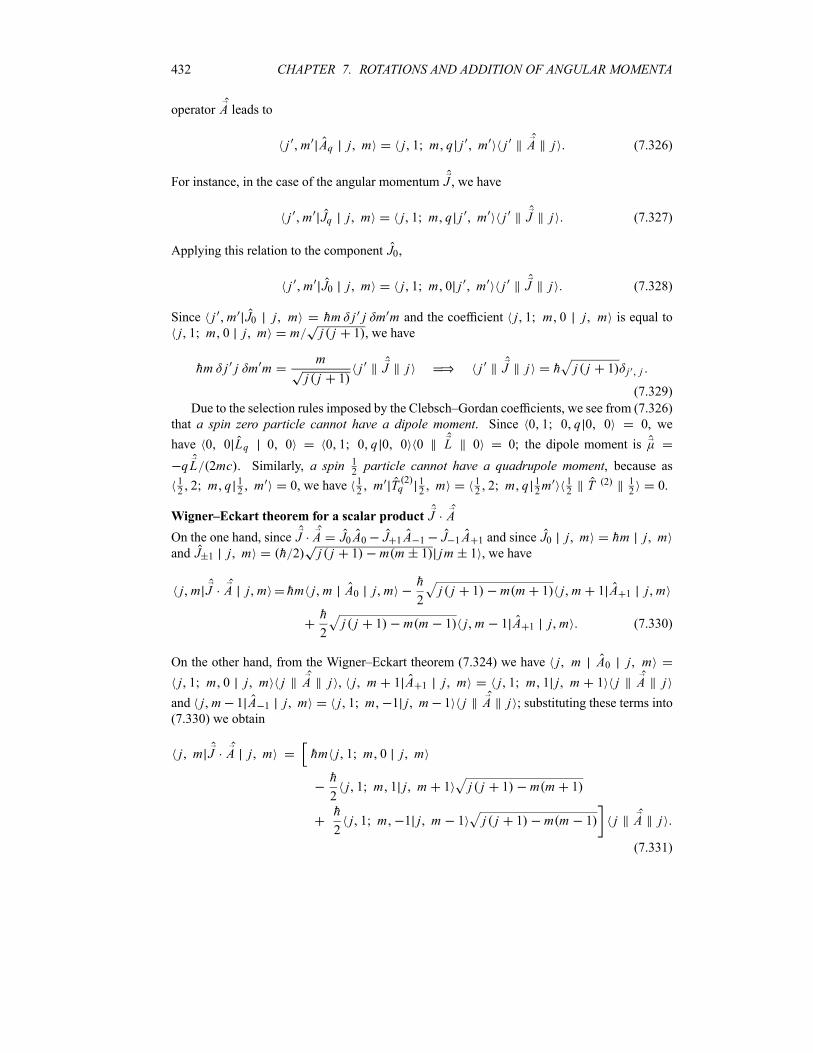
432 CHAPTER 7. ROTATIONS AND ADDITION OF ANGULAR MOMENTA
operator A leads to
j m Aq j m j 1 m q j m j A j (7.326)
For instance, in the case of the angular momentum J , we have
j m Jq j m j 1 m q j m j J j (7.327)
Applying this relation to the component J0,
j m J0 j m j 1 m 0 j m j J j (7.328)
Since j m J0 j m hm j j m m and the coefficient j 1 m 0 j m is equal to
j 1 m 0 j m m j j 1 , we have
hm j j m mm
j j 1j J j j J j h j j 1 j j
(7.329)
Due to the selection rules imposed by the Clebsch–Gordan coefficients, we see from (7.326)
that a spin zero particle cannot have a dipole moment. Since 0 1 0 q 0 0 0, we
have 0 0 Lq 0 0 0 1 0 q 0 0 0 L 0 0; the dipole moment is
qL 2mc . Similarly, a spin 12particle cannot have a quadrupole moment, because as
122 m q 1
2m 0, we have 1
2m T 2
q12m 1
22 m q 1
2m 1
2T 2 1
20.
Wigner–Eckart theorem for a scalar product J A
On the one hand, since J A J0A0 J 1A 1 J 1A 1 and since J0 j m hm j mand J 1 j m h 2 j j 1 m m 1 jm 1 , we have
j m J A j m hm j m A0 j mh
2j j 1 m m 1 j m 1 A 1 j m
h
2j j 1 m m 1 j m 1 A 1 j m (7.330)
On the other hand, from the Wigner–Eckart theorem (7.324) we have j m A0 j m
j 1 m 0 j m j A j , j m 1 A 1 j m j 1 m 1 j m 1 j A j
and j m 1 A 1 j m j 1 m 1 j m 1 j A j ; substituting these terms into(7.330) we obtain
j m J A j m hm j 1 m 0 j m
h
2j 1 m 1 j m 1 j j 1 m m 1
h
2j 1 m 1 j m 1 j j 1 m m 1 j A j
(7.331)

7.4. SCALAR, VECTOR, AND TENSOR OPERATORS 433
When A J this relation leads to
j m J 2 j m hm j 1 m 0 j m
h
2j 1 m 1 j m 1 j j 1 m m 1
h
2j 1 m 1 j m 1 j j 1 m m 1 j J j
(7.332)
We are now equipped to obtain a relation between the matrix elements of a vector operator
A and the matrix elements of the scalar operator J A; this relation is useful in the calculationof the hydrogen’s energy corrections due to the Zeeman effect (see Chapter 9). For this, we
need to calculate two ratios: the first is between (7.326) and (7.327)
j m Aq j m
j m Jq j m
j A j
j J j(7.333)
and the second is between (7.331) and (7.332)
j m J A j m
j m J 2 j m
j A j
j J j
j m J A j m
h2 j j 1 2
j A j
j J j(7.334)
since j m J 2 j m h2 j j 1 . Equating (7.333) and (7.334) we obtain
j m Aq j mj m J A j m
h2 j j 1j m Jq j m (7.335)
An important application of this relation pertains to the case where the vector operator A is a
spin angular momentum S. Since
J S L S S L S S2L S 2 L2 S2
2S2
J 2 L2 S2
2S2
J2 L2 S2
2(7.336)
and since j m is a joint eigenstate of J 2, L2, S2 and Jz with eigenvalues h2 j j 1 ,
h2l l 1 , h2s s 1 , and hm, respectively, the matrix element of Sz then becomes easy tocalculate from (7.335):
j m Sz j mj m J S j m
h2 j j 1j m Jz j m
j j 1 l l 1 s s 1
2 j j 1hm
(7.337)
434 CHAPTER 7. ROTATIONS AND ADDITION OF ANGULAR MOMENTA
7.5 Solved Problems
Problem 7.1
(a) Show how Jx and Jy transform under a rotation of (finite) angle about the z-axis.
Using these results, determine how the angular momentum operator J transform under therotation.
(b) Show how a vector operator A transforms under a rotation of angle about the y-axis.
(c) Show that ei Jz hei Jy he i Jz h e i Jy h .
Solution
(a) The operator corresponding to a rotation of angle about the z-axis is given by Rz
e i Jz h . Under this rotation, an operator B transforms like B R†z BRz ei Jz hBe i Jz h .
Using the relation
eABe A B A B1
2!A A B
1
3!A A A B (7.338)
along with the commutation relations Jz Jy ih Jx and Jz Jx ih Jy , we have
ei Jz h Jxei Jz h Jx
i
hJz Jx
2
2!h2Jz Jz Jx
i 3
3!h3Jz Jz Jz Jx
Jx Jy2
2!Jx
3
3!Jy
4
4!Jx
5
5!Jy
Jx 12
2!
4
4!Jy
3
3!
5
5!
Jx cos Jy sin (7.339)
Similarly, we can show that
ei Jz h Jyei Jz h Jy cos Jx sin (7.340)
As Jz is invariant under an arbitrary rotation about the z-axis (ei Jz h Jze i Jz h Jz), we cancondense equations (7.339) and (7.340) into a single matrix relation:
ei Jz h Je i Jz hcos sin 0
sin cos 0
0 0 1
JxJyJz
(7.341)
(b) Using the commutation relations Jy Ax ihAz and Jy Az ihAx (see
(7.282) to (7.284)) along with (7.338), we have
ei Jy h Axei Jy h Ax
i
hJy Ax
2
2!h2Jy Jy Ax
7.5. SOLVED PROBLEMS 435
i 3
3!h3Jy Jy Jy Ax
Ax Az2
2!Ax
3
3!Az
4
4!Ax
5
5!Jz
Ax 12
2!
4
4!Az
3
3!
5
5!
Ax cos Az sin (7.342)
Similarly, we can show that
Az ei Jy h Azei Jy h Ax sin Az cos (7.343)
Also, since Ay is invariant under an arbitrary rotation about the y-axis, we may combine equa-
tions (7.342) and (7.343) to find the vector operator A obtained by rotating A through an angleabout the y-axis:
A ei Jy h Ae i Jy hcos 0 sin
0 1 0
sin 0 cos
AxAyAz
(7.344)
(c) Expanding ei Jy h and then using (7.340), we obtain
ei Jz hei Jy he i Jz h
n 0
i h n
n!ei Jz h Jy
ne i Jz h
n 0
i h n
n!Jy cos Jx sin
n
n 0
i h n
n!Jy
n
e i Jy h (7.345)
Problem 7.2
Use the Pauli matrices x0 1
1 0, y
0 ii 0
, and z1 0
0 1, to show
that
(a) e i x I cos i x sin , where I is the unit matrix,(b) ei x ze i x z cos 2 y sin 2 .
Solution
(a) Using the expansion
e i x
n 0
i 2n
2n !2n 2n
xn 0
i 2n 1
2n 1 !2n 1 2n 1
x (7.346)
and since 2x 1, 2n
x I , and 2n 1x x , where I is the unit matrix, we have
e i x 1 0
0 1n 0
1 n
2n !2n i x
n 0
1 n
2n 1 !2n 1
I cos i x sin (7.347)
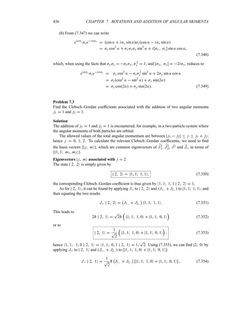
436 CHAPTER 7. ROTATIONS AND ADDITION OF ANGULAR MOMENTA
(b) From (7.347) we can write
ei xze
i x cos i x sin z cos i x sin
z cos2
x z x sin2 i[ x z] sin cos
(7.348)
which, when using the facts that x z z x ,2x I , and [ x z] 2i y , reduces to
ei xze
i xz cos
2z2x sin
2 2 y sin cos
z cos2 sin2 y sin 2
z cos 2 y sin 2 (7.349)
Problem 7.3
Find the Clebsch–Gordan coefficients associated with the addition of two angular momenta
j1 1 and j2 1.
Solution
The addition of j1 1 and j2 1 is encountered, for example, in a two-particle system where
the angular momenta of both particles are orbital.
The allowed values of the total angular momentum are between j1 j2 j j1 j2;hence j 0, 1, 2. To calculate the relevant Clebsch–Gordan coefficients, we need to find
the basis vectors j m , which are common eigenvectors of J 21, J22, J
2 and Jz , in terms of1 1 m1 m2 .
Eigenvectors j m associated with j 2
The state 2 2 is simply given by
2 2 1 1 1 1 (7.350)
the corresponding Clebsch–Gordan coefficient is thus given by 1 1 1 1 2 2 1.
As for 2 1 , it can be found by applying J to 2 2 and J1 J2 to 1 1 1 1 , and
then equating the two results
J 2 2 J1 J2 1 1 1 1 (7.351)
This leads to
2h 2 1 2h 1 1 1 0 1 1 0 1 (7.352)
or to
2 11
21 1 1 0 1 1 0 1 (7.353)
hence 1 1 1 0 2 1 1 1 0 1 2 1 1 2. Using (7.353), we can find 2 0 by
applying J to 2 1 and J1 J2 to [ 1 1 1 0 1 1 0 1 ]:
J 2 11
2h J1 J2 [ 1 1 1 0 1 1 0 1 ] (7.354)
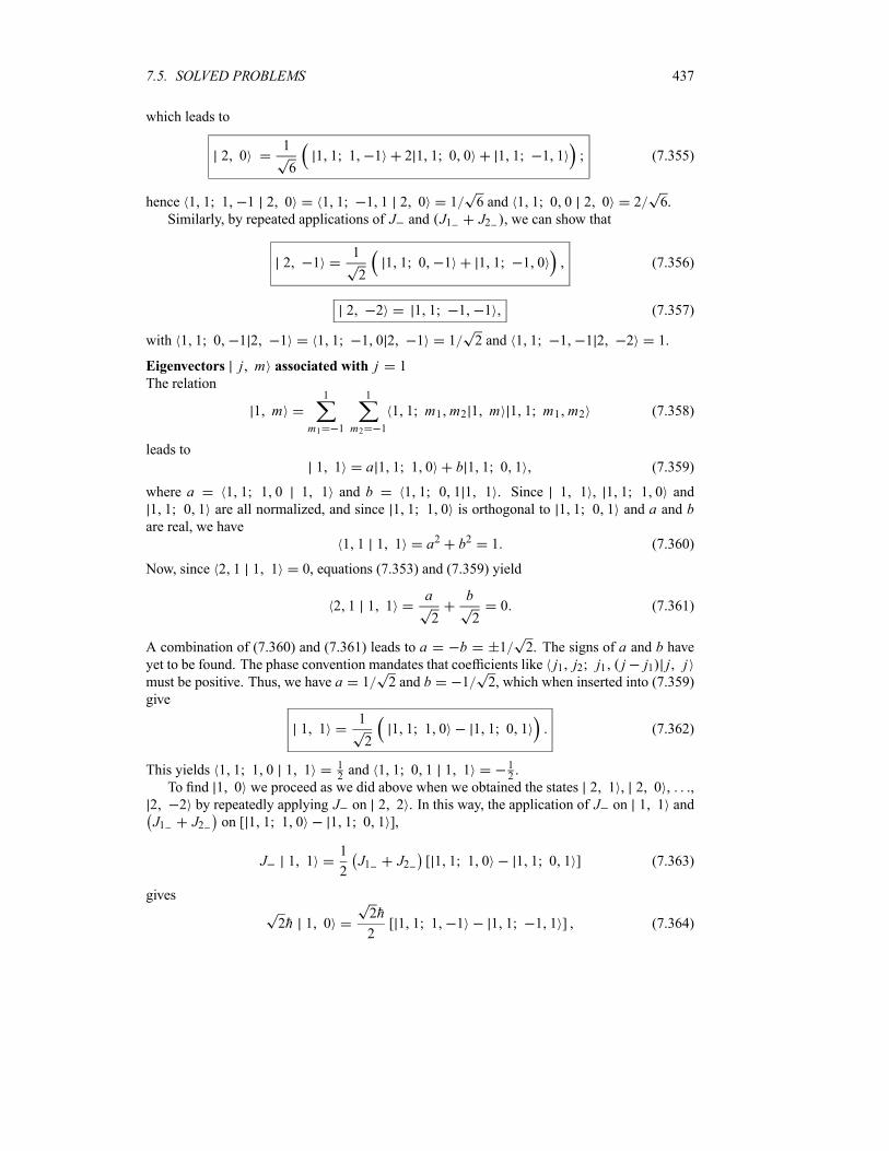
7.5. SOLVED PROBLEMS 437
which leads to
2 01
61 1 1 1 2 1 1 0 0 1 1 1 1 (7.355)
hence 1 1 1 1 2 0 1 1 1 1 2 0 1 6 and 1 1 0 0 2 0 2 6.
Similarly, by repeated applications of J and J1 J2 , we can show that
2 11
21 1 0 1 1 1 1 0 (7.356)
2 2 1 1 1 1 (7.357)
with 1 1 0 1 2 1 1 1 1 0 2 1 1 2 and 1 1 1 1 2 2 1.
Eigenvectors j m associated with j 1
The relation
1 m1
m1 1
1
m2 1
1 1 m1 m2 1 m 1 1 m1 m2 (7.358)
leads to
1 1 a 1 1 1 0 b 1 1 0 1 (7.359)
where a 1 1 1 0 1 1 and b 1 1 0 1 1 1 . Since 1 1 , 1 1 1 0 and
1 1 0 1 are all normalized, and since 1 1 1 0 is orthogonal to 1 1 0 1 and a and bare real, we have
1 1 1 1 a2 b2 1 (7.360)
Now, since 2 1 1 1 0, equations (7.353) and (7.359) yield
2 1 1 1a
2
b
20 (7.361)
A combination of (7.360) and (7.361) leads to a b 1 2. The signs of a and b haveyet to be found. The phase convention mandates that coefficients like j1 j2 j1 j j1 j jmust be positive. Thus, we have a 1 2 and b 1 2, which when inserted into (7.359)
give
1 11
21 1 1 0 1 1 0 1 (7.362)
This yields 1 1 1 0 1 1 12and 1 1 0 1 1 1 1
2.
To find 1 0 we proceed as we did above when we obtained the states 2 1 , 2 0 , ,
2 2 by repeatedly applying J on 2 2 . In this way, the application of J on 1 1 and
J1 J2 on [ 1 1 1 0 1 1 0 1 ],
J 1 11
2J1 J2 [ 1 1 1 0 1 1 0 1 ] (7.363)
gives
2h 1 02h
2[ 1 1 1 1 1 1 1 1 ] (7.364)
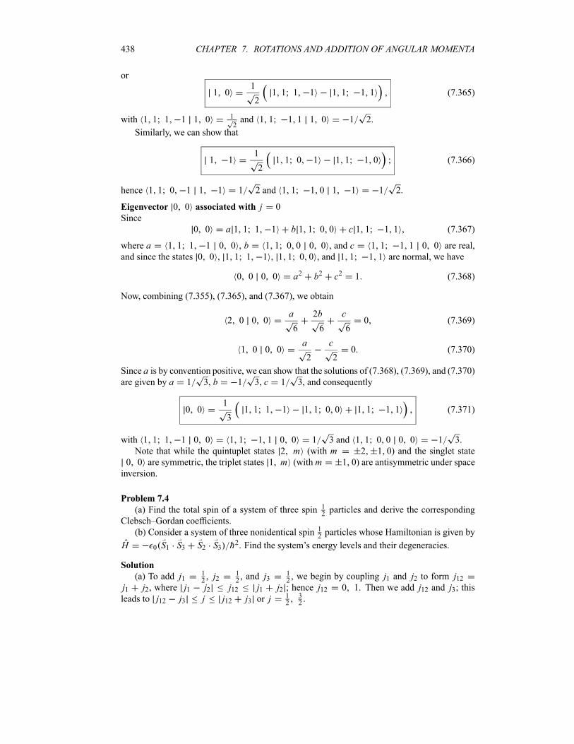
438 CHAPTER 7. ROTATIONS AND ADDITION OF ANGULAR MOMENTA
or
1 01
21 1 1 1 1 1 1 1 (7.365)
with 1 1 1 1 1 0 1
2and 1 1 1 1 1 0 1 2.
Similarly, we can show that
1 11
21 1 0 1 1 1 1 0 (7.366)
hence 1 1 0 1 1 1 1 2 and 1 1 1 0 1 1 1 2.
Eigenvector 0 0 associated with j 0
Since
0 0 a 1 1 1 1 b 1 1 0 0 c 1 1 1 1 (7.367)
where a 1 1 1 1 0 0 , b 1 1 0 0 0 0 , and c 1 1 1 1 0 0 are real,
and since the states 0 0 , 1 1 1 1 , 1 1 0 0 , and 1 1 1 1 are normal, we have
0 0 0 0 a2 b2 c2 1 (7.368)
Now, combining (7.355), (7.365), and (7.367), we obtain
2 0 0 0a
6
2b
6
c
60 (7.369)
1 0 0 0a
2
c
20 (7.370)
Since a is by convention positive, we can show that the solutions of (7.368), (7.369), and (7.370)are given by a 1 3, b 1 3, c 1 3, and consequently
0 01
31 1 1 1 1 1 0 0 1 1 1 1 (7.371)
with 1 1 1 1 0 0 1 1 1 1 0 0 1 3 and 1 1 0 0 0 0 1 3.
Note that while the quintuplet states 2 m (with m 2 1 0) and the singlet state
0 0 are symmetric, the triplet states 1 m (with m 1 0) are antisymmetric under space
inversion.
Problem 7.4
(a) Find the total spin of a system of three spin 12particles and derive the corresponding
Clebsch–Gordan coefficients.
(b) Consider a system of three nonidentical spin 12particles whose Hamiltonian is given by
H 0 S1 S3 S2 S3 h2. Find the system’s energy levels and their degeneracies.
Solution
(a) To add j112, j2
12, and j3
12, we begin by coupling j1 and j2 to form j12
j1 j2, where j1 j2 j12 j1 j2 ; hence j12 0 1. Then we add j12 and j3; thisleads to j12 j3 j j12 j3 or j
12
32.

7.5. SOLVED PROBLEMS 439
We are going to denote the joint eigenstates of J 21, J22, J
23, J
212, J
2, and Jz by j12 j m
and the joint eigenstates of J21, J22, J
23, J1z , J2z , and J3z by j1 j2 j3 m1 m2 m3 ; since
j1 j2 j312and m1
12, m2
12, m3
12, we will be using throughout this
problem the lighter notation j1 j2 j3 to abbreviate 121212
12
12
12.
In total there are eight states j12 j m since 2 j1 1 2 j2 1 2 j3 1 8. Four of
these correspond to the subspace j 32: 1 3
232, 1 3
212, 1 3
212, and 1 3
232.
The remaining four belong to the subspace j 12: 0 1
212, 0 1
212, 1 1
212, and
1 12
12. To construct the states j12 j m in terms of j1 j2 j3 , we are going
to consider the two subspaces j 32and j 1
2separately.
Subspace j 32
First, the states 1 3232and 1 3
232are clearly given by
13
2
3
2j1 j2 j3 1
3
2
3
2j1 j2 j3 (7.372)
To obtain 1 3212, we need to apply, on the one hand, J on 1 3
232(see (7.220)),
J 13
2
3
2h3
2
3
21
3
2
3
21 1
3
2
1
2h 3 1
3
2
1
2(7.373)
and, on the other hand, apply J1 J2 J3 on j1 j2 j3 (see (7.221) to (7.223)).
This yields
J1 J2 J3 j1 j2 j3 h j1 j2 j3 j1 j2 j3
j1 j2 j3 (7.374)
since 1212
1 1212
1 1. Equating (7.373) and (7.374) we infer
13
2
1
2
1
3j1 j2 j3 j1 j2 j3 j1 j2 j3
(7.375)
Following the same method—applying J on 1 3212and J1 J2 J3 on the right-hand
side of (7.375) and then equating the two results—we find
13
2
1
2
1
3j1 j2 j3 j1 j2 j3 j1 j2 j3
(7.376)
Subspace j 12
We can write 0 1212as a linear combination of j1 j2 j3 and j1 j2 j3 :
01
2
1
2j1 j2 j3 j1 j2 j3 (7.377)
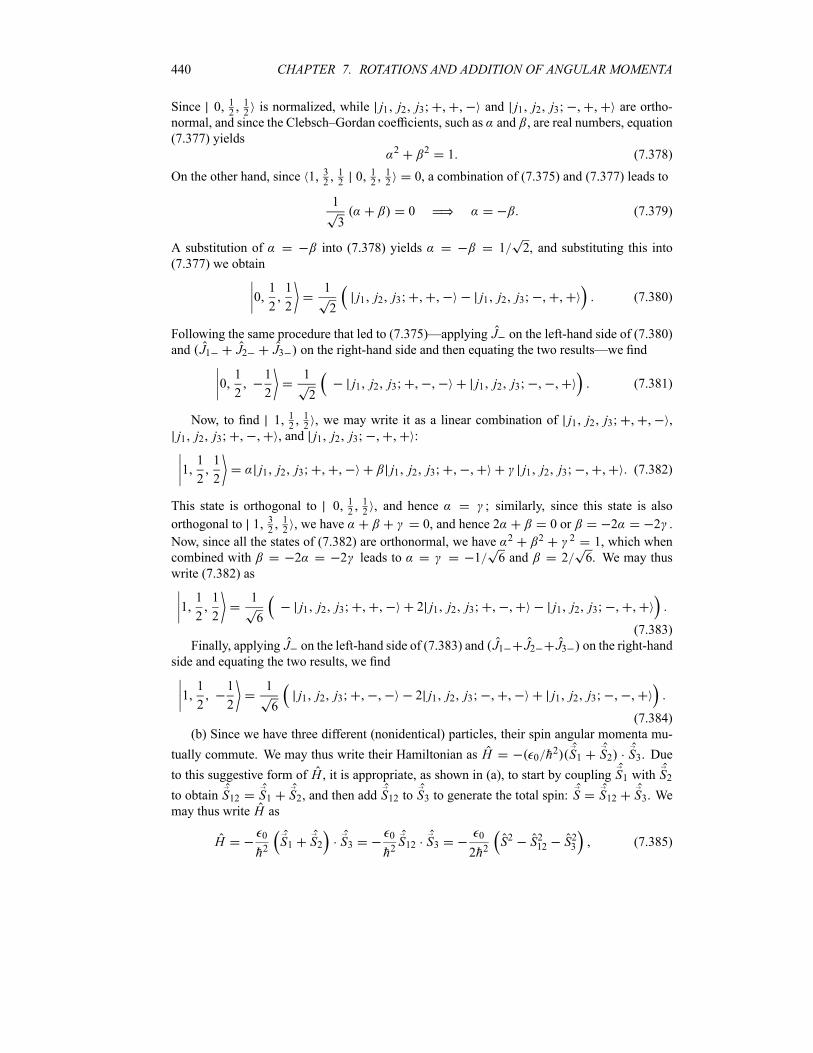
440 CHAPTER 7. ROTATIONS AND ADDITION OF ANGULAR MOMENTA
Since 0 1212is normalized, while j1 j2 j3 and j1 j2 j3 are ortho-
normal, and since the Clebsch–Gordan coefficients, such as and , are real numbers, equation
(7.377) yields2 2 1 (7.378)
On the other hand, since 1 32120 1212
0, a combination of (7.375) and (7.377) leads to
1
30 (7.379)
A substitution of into (7.378) yields 1 2, and substituting this into
(7.377) we obtain
01
2
1
2
1
2j1 j2 j3 j1 j2 j3 (7.380)
Following the same procedure that led to (7.375)—applying J on the left-hand side of (7.380)
and J1 J2 J3 on the right-hand side and then equating the two results—we find
01
2
1
2
1
2j1 j2 j3 j1 j2 j3 (7.381)
Now, to find 1 1212, we may write it as a linear combination of j1 j2 j3 ,
j1 j2 j3 , and j1 j2 j3 :
11
2
1
2j1 j2 j3 j1 j2 j3 j1 j2 j3 (7.382)
This state is orthogonal to 0 1212, and hence ; similarly, since this state is also
orthogonal to 1 3212, we have 0, and hence 2 0 or 2 2 .
Now, since all the states of (7.382) are orthonormal, we have 2 2 2 1, which when
combined with 2 2 leads to 1 6 and 2 6. We may thus
write (7.382) as
11
2
1
2
1
6j1 j2 j3 2 j1 j2 j3 j1 j2 j3
(7.383)
Finally, applying J on the left-hand side of (7.383) and J1 J2 J3 on the right-hand
side and equating the two results, we find
11
2
1
2
1
6j1 j2 j3 2 j1 j2 j3 j1 j2 j3
(7.384)
(b) Since we have three different (nonidentical) particles, their spin angular momenta mu-
tually commute. We may thus write their Hamiltonian as H 0 h2 S1 S2 S3. Due
to this suggestive form of H , it is appropriate, as shown in (a), to start by coupling S1 with S2
to obtain S12 S1 S2, and then add S12 to S3 to generate the total spin: S S12 S3. Wemay thus write H as
H0
h2S1 S2 S3
0
h2S12 S3
0
2h2S2 S212 S23 (7.385)
7.5. SOLVED PROBLEMS 441
since S12 S312[ S12 S3 2 S212 S23 ]. Since the operators H , S
2, S212, and S23 mutually
commute, we may select as their joint eigenstates the kets s12 s m ; we have seen in (a) howto construct these states. The eigenvalues of H are thus given by
H s12 s m0
2h2S2 S212 S23 s12 s m
0
2s s 1 s12 s12 1
3
4s12 s m (7.386)
since s312and S23 s12 s m h2s3 s3 1 s12 s m 3h2 4 s12 s m .
As shown in (7.386), the energy levels of this system are degenerate with respect tom, sincethey depend on the quantum numbers s and s12 but not on m:
Es12 s0
2s s 1 s12 s12 1
3
4(7.387)
For instance, the energy Es12 s E1 3 2 0 2 is fourfold degenerate, since it corresponds
to four different states: s12 s m 1 32
32and 1 3
212. Similarly, the energy
E0 1 2 0 is twofold degenerate; the corresponding states are 0 12
12. Finally, the energy
E1 1 2 0 is also twofold degenerate since it corresponds to 1 12
12.
Problem 7.5
Consider a system of four nonidentical spin 12particles. Find the possible values of the total
spin S of this system and specify the number of angular momentum eigenstates, correspondingto each value of S.
Solution
First, we need to couple two spins at a time: S12 S1 S2 and S34 S3 S4. Then we couple
S12 and S34: S S12 S34. From Problem 7.4, page 438, we have s12 0 1 and s34 0 1.
In total there are 16 states sm since 2s1 1 2s2 1 2s3 1 2s4 1 24 16.
Since s12 0 1 and s34 0 1, the coupling of S12 and S34 yields the following values forthe total spin s:
When s12 0 and s34 0 we have only one possible value, s 0, and hence only one
eigenstate, sm 0 0 .
When s12 1 and s34 0, we have s 1; there are three eigenstates: s m 1 1 ,
and 1 0 .
When s12 0 and s34 1, we have s 1; there are three eigenstates: sm 1 1 ,
and 1 0 .
When s12 1 and s34 1 we have s 0 1 2; we have here nine eigenstates (see
Problem 7.3, page 436): 0 0 , 1 1 , 1 0 , 2 2 , 2 1 , and 2 0 .
In conclusion, the possible values of the total spin when coupling four 12spins are s 0 1 2;
the value s 0 occurs twice, s 1 three times, and s 2 only once.
442 CHAPTER 7. ROTATIONS AND ADDITION OF ANGULAR MOMENTA
Problem 7.6
Work out the coupling of the isospins of a pion–nucleon system and infer the various states of
this system.
Solution
Since the isospin of a pion meson is 1 and that of a nucleon is 12, the total isospin of a pion–
nucleon system can be obtained by coupling the isospins t1 1 and t212. The various values
of the total isospin lie in the range t1 t2 T t1 t2; hence they are given by T32, 12.
The coupling of the isospins t1 1 and t212is analogous to the addition of an orbital
angular momentum l 1 and a spin 12; the expressions pertaining to this coupling are listed in
(7.206) to (7.211). Note that there are three different -mesons:
1 1 1 0 0 1 1 (7.388)
and two nucleons, a proton and a neutron:
1
2
1
2p
1
2
1
2n (7.389)
By analogy with (7.206) to (7.211) we can write the states corresponding to T 32as
3
2
3
21 1
1
2
1
2p (7.390)
3
2
1
2
2
31 0
1
2
1
2
1
31 1
1
2
1
2
2
30 p
1
3n
(7.391)
3
2
1
2
1
31 1
1
2
1
2
2
31 0
1
2
1
2
1
3p
2
30 n
(7.392)
3
2
3
21 1
1
2
1
2n (7.393)
and those corresponding to T 12as
1
2
1
2
2
31 1
1
2
1
2
1
31 0
1
2
1
2
2
3n
1
3
0 p
(7.394)
1
2
1
2
1
31 0
1
2
1
2
2
31 1
1
2
1
2
1
3
0 n2
3p
(7.395)
Problem 7.7
(a) Calculate the expression of 2 0 Y10 1 0 .
(b) Use the result of (a) along with the Wigner–Eckart theorem to calculate the reduced
matrix element 2 Y1 1 .
7.5. SOLVED PROBLEMS 443
Solution
(a) Since
2 0 Y10 1 00
sin d2
0
Y20 Y10 Y10 d (7.396)
and using the relations Y20 5 16 3 cos2 1 and Y10 3 4 cos ,
we have
2 0 Y10 1 03
4
5
16 0
cos2 3 cos2 1 sin d2
0
d
3
2
5
16 0
cos2 3 cos2 1 sin d (7.397)
The change of variables x cos leads to
2 0 Y10 1 03
2
5
16 0
cos2 3 cos3 1 sin d
3
2
5
16
1
1
x2 3x2 1 dx1
5(7.398)
(b) Applying the Wigner–Eckart theorem to 2 0 Y10 1 0 and using the Clebsch–
Gordan coefficient 1 1 0 0 2 0 2 6, we have
2 0 Y10 1 0 1 1 0 0 2 0 2 Y1 12
62 Y1 1 (7.399)
Finally, we may obtain 2 Y1 1 from (7.398) and (7.399):
2 Y1 13
10(7.400)
Problem 7.8
(a) Find the reduced matrix elements associated with the spherical harmonic Ykq .
(b) Calculate the dipole transitions n l m r nlm .
Solution
On the one hand, an application of the Wigner–Eckart theorem to Ykq yields
l m Ykq l m l k m q l m l Y k l (7.401)
and, on the other hand, a straightforward evaluation of
l m Ykq l m2
0
d0
sin d l m Ykq l m
2
0
d0
sin d Yl m Ykq Ylm (7.402)
444 CHAPTER 7. ROTATIONS AND ADDITION OF ANGULAR MOMENTA
can be inferred from the triple integral relation (7.244):
l m Ykq l m2l 1 2k 1
4 2l 1l k 0 0 l 0 l k m q l m (7.403)
We can then combine (7.401) and (7.403) to obtain the reduced matrix element
l Y k l2l 1 2k 1
4 2l 1l k 0 0 l 0 (7.404)
(b) To calculate n l m r nlm it is more convenient to express the vector r in terms ofthe spherical components r r 1 r0 r1 , which are given in terms of the Cartesian coordi-nates x , y, z as follows:
r1x iy
2
r
2ei sin r0 z r cos r 1
x iy
2
r
2e i sin
(7.405)
which in turn may be condensed into a single relation
rq4
3rY1q q 1 0 1 (7.406)
Next we may write n l m rq nlm in terms of a radial part and an angular part:
n l m rq nlm4
3n l rq nl l m Y1q l m (7.407)
The calculation of the radial part, n l rq nl 0 r3Rn l r Rnl r dr , is straightforwardand is of no concern to us here; see Chapter 6 for its calculation. As for the angular part
l m Y1q l m , we can infer its expression from (7.403)
l m Y1q l m3 2l 1
4 2l 1l 1 0 0 l 0 l 1 m q l m (7.408)
The Clebsch–Gordan coefficients l 1 m q l m vanish unless m m q and l 1
l l 1 or m m m q 1 0 1 and l l l 1 0 1. Notice that the case
l 0 is ruled out from the parity selection rule; so, the only permissible values of l and l arethose for which l l l 1. Obtaining the various relevant Clebsch–Gordan coefficients
from standard tables, we can ascertain that the only terms of (7.408) that survive are
l 1 m 1 Y11 l m3 l m 1 l m 2
8 2l 1 2l 3(7.409)
l 1 m 1 Y11 l m3 l m 1 l m
8 2l 1 2l 3(7.410)
l 1 m Y10 l m3[ l 1 2 m2]
4 2l 1 2l 3(7.411)

7.5. SOLVED PROBLEMS 445
l 1 m Y10 l m3 l2 m2
4 2l 1 2l 1(7.412)
l 1 m 1 Y1 1 l m3 l m 1 l m 2
8 2l 1 2l 3(7.413)
l 1 m 1 Y1 1 l m3 l m l m 1
8 2l 1 2l 1(7.414)
Problem 7.9
Find the rotation matrix d 1 corresponding to j 1.
Solution
To find the matrix of d 1 e i Jy h for j 1, we need first to find the matrix representa-
tion of Jy within the joint eigenstates j m of J2 and Jz . Since the basis of j 1 consists
of three states 1 1 , 1 0 , 1 1 , the matrix representing Jy within this basis is given by
Jyh
2
1 1 Jy 1 1 1 1 Jy 1 0 1 1 Jy 1 1
1 0 Jy 1 1 1 0 Jy 1 0 1 0 Jy 1 1
1 1 Jy 1 1 1 1 Jy 1 0 1 1 Jy 1 1
ih
2
0 1 0
1 0 1
0 1 0
(7.415)
We can easily verify that J3y Jy:
J 2yh2
2
1 0 1
0 2 0
1 0 1
J 3yih3
2
0 1 0
1 0 1
0 1 0
h2 Jy (7.416)
We can thus infer
J2ny h2n 2 J 2y n 0 J2n 1y h2n Jy (7.417)
Combining these two relations with
e i Jy h
n 0
1
n!
i
h
n
Jny
n 0
1
2n !
i
h
2n
J2nyn 0
1
2n 1 !
i
h
2n 1
J 2n 1y
(7.418)
we obtain
e i Jy h IJyh
2
n 1
1 n
2n !2n i
Jyhn 0
1 n
2n 1 !2n 1
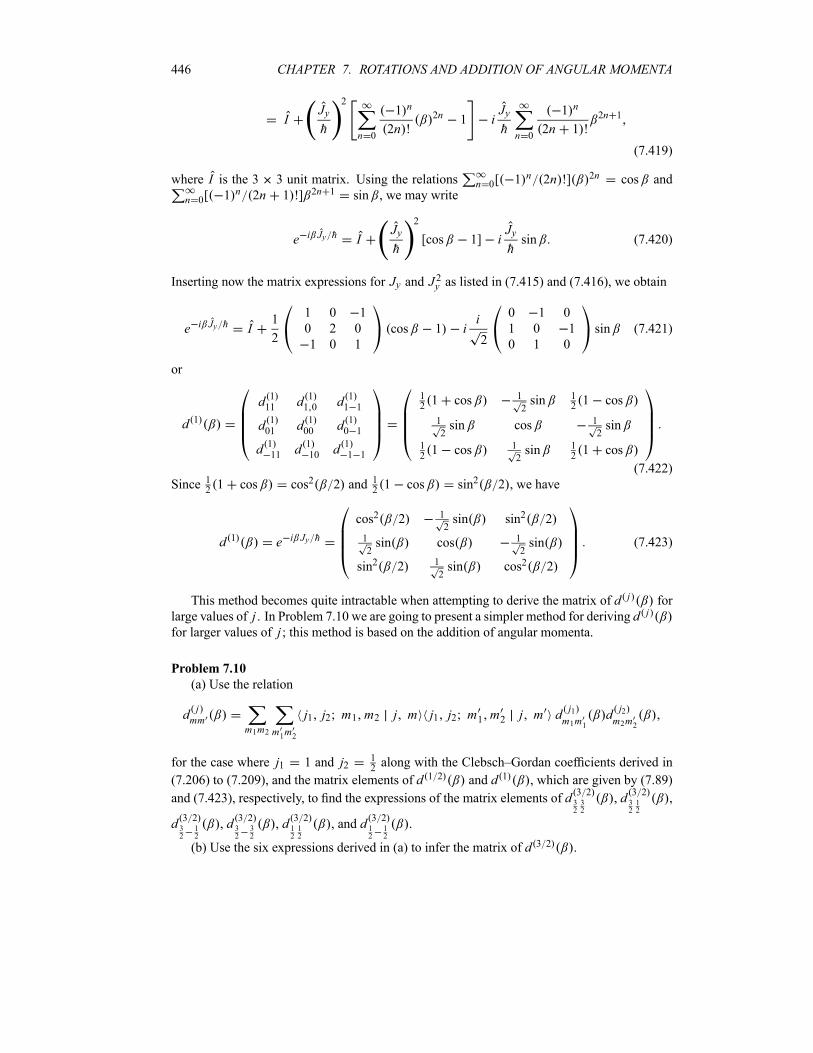
446 CHAPTER 7. ROTATIONS AND ADDITION OF ANGULAR MOMENTA
IJyh
2
n 0
1 n
2n !2n 1 i
Jyhn 0
1 n
2n 1 !2n 1
(7.419)
where I is the 3 3 unit matrix. Using the relations n 0[ 1 n 2n !] 2n cos and
n 0[ 1 n 2n 1 !] 2n 1 sin , we may write
e i Jy h IJyh
2
[cos 1] iJyhsin (7.420)
Inserting now the matrix expressions for Jy and J2y as listed in (7.415) and (7.416), we obtain
e i Jy h I1
2
1 0 1
0 2 0
1 0 1
cos 1 ii
2
0 1 0
1 0 1
0 1 0
sin (7.421)
or
d 1d 111 d 11 0 d 11 1
d 101 d 100 d 10 1
d 111 d 110 d 11 1
121 cos 1
2sin 1
21 cos
1
2sin cos 1
2sin
121 cos 1
2sin 1
21 cos
(7.422)
Since 121 cos cos2 2 and 1
21 cos sin2 2 , we have
d 1 e i Jy h
cos2 2 1
2sin sin2 2
1
2sin cos 1
2sin
sin2 2 1
2sin cos2 2
(7.423)
This method becomes quite intractable when attempting to derive the matrix of d j for
large values of j . In Problem 7.10 we are going to present a simpler method for deriving d j
for larger values of j ; this method is based on the addition of angular momenta.
Problem 7.10
(a) Use the relation
d jmm
m1m2 m1m2
j1 j2 m1 m2 j m j1 j2 m1 m2 j m d j1m1m1
d j2m2m2
for the case where j1 1 and j212along with the Clebsch–Gordan coefficients derived in
(7.206) to (7.209), and the matrix elements of d 1 2 and d 1 , which are given by (7.89)
and (7.423), respectively, to find the expressions of the matrix elements of d 3 23232
, d 3 23212
,
d 3 232
12
, d 3 232
32
, d 3 21212
, and d 3 212
12
.
(b) Use the six expressions derived in (a) to infer the matrix of d 3 2 .

7.5. SOLVED PROBLEMS 447
Solution
(a) Using 1 121 12
32
32
1, d 111 cos2 2 and d 1 21212
cos 2 , we
have
d 3 23232
11
211
2
3
2
3
211
211
2
3
2
3
2d 111 d 1 21
212
cos32
(7.424)
Similarly, since 1 120 12
32
12
2 3, 1 121 1
232
12
1 3, and since
d 110 1 2 sin and d 1 212
12
sin 2 , we have
d 3 23212
11
211
2
3
2
3
211
201
2
3
2
1
2d 110 d 1 21
212
11
211
2
3
2
3
211
21
1
2
3
2
1
2d 111 d 1 21
212
1
3sin cos
2
1
3cos2
2sin
2
3 sin2cos2
2(7.425)
To calculate d 3 232
12
, we need to use the coefficients 1 120 1
232
12
2 3 and
1 12
1 12
32
12
1 3 along with d 11 1 sin2 2 :
d 3 232
12
11
211
2
3
2
3
211
211
2
3
2
1
2d 11 1 d 1 21
212
11
211
2
3
2
3
211
20
1
2
3
2
1
2d 110 d 1 21
212
1
3sin2
2cos
2
1
3sin sin
2
3 sin22cos
2(7.426)
For d 3 232
32
we have
d 3 232
32
11
211
2
3
2
3
211
21
1
2
3
2
3
2d 11 1 d 1 21
212
sin32(7.427)
because 1 12
1 12
32
32
1, d 11 1 sin2 2 , and d 1 212
12
sin 2 .
To calculate d 3 21212
, we need to use the coefficients 1 120 12
32
12
2 3 and
1 121 1
232
12
1 3 along with d 11 1 sin2 2 :
d 3 21212
11
21
1
2
3
2
1
211
21
1
2
3
2
1
2d 111 d 1 21
212
11
201
2
3
2
1
211
21
1
2
3
2
1
2d 101 d 1 21
212
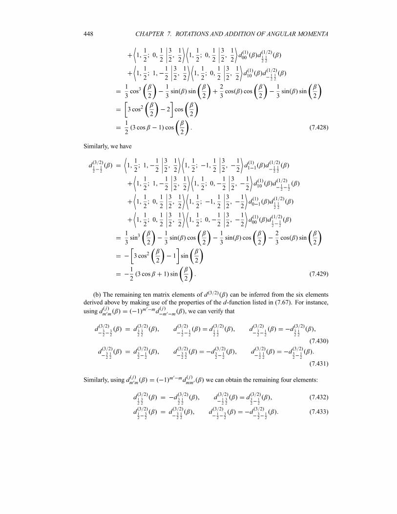
448 CHAPTER 7. ROTATIONS AND ADDITION OF ANGULAR MOMENTA
11
201
2
3
2
1
211
201
2
3
2
1
2d 100 d 1 21
212
11
21
1
2
3
2
1
211
201
2
3
2
1
2d 110 d 1 21
212
1
3cos3
2
1
3sin sin
2
2
3cos cos
2
1
3sin sin
2
3 cos22
2 cos2
1
23 cos 1 cos
2(7.428)
Similarly, we have
d 3 212
12
11
21
1
2
3
2
1
211
211
2
3
2
1
2d 11 1 d 1 21
212
11
21
1
2
3
2
1
211
20
1
2
3
2
1
2d 110 d 1 21
212
11
201
2
3
2
1
211
211
2
3
2
1
2d 10 1 d 1 21
212
11
201
2
3
2
1
211
20
1
2
3
2
1
2d 100 d 1 21
212
1
3sin3
2
1
3sin cos
2
1
3sin cos
2
2
3cos sin
2
3 cos22
1 sin2
1
23 cos 1 sin
2(7.429)
(b) The remaining ten matrix elements of d 3 2 can be inferred from the six elements
derived above by making use of the properties of the d-function listed in (7.67). For instance,
using d jm m 1 m md j
m m , we can verify that
d 3 232
32
d 3 23232
d 3 212
12
d 3 21212
d 3 232
12
d 3 23212
(7.430)
d 3 23212
d 3 232
12
d 3 23232
d 3 232
12
d 3 21212
d 3 232
12
(7.431)
Similarly, using d jm m 1 m md j
mm we can obtain the remaining four elements:
d 3 21232
d 3 23212
d 3 21232
d 3 232
12
(7.432)
d 3 212
32
d 3 23212
d 3 212
32
d 3 232
12
(7.433)
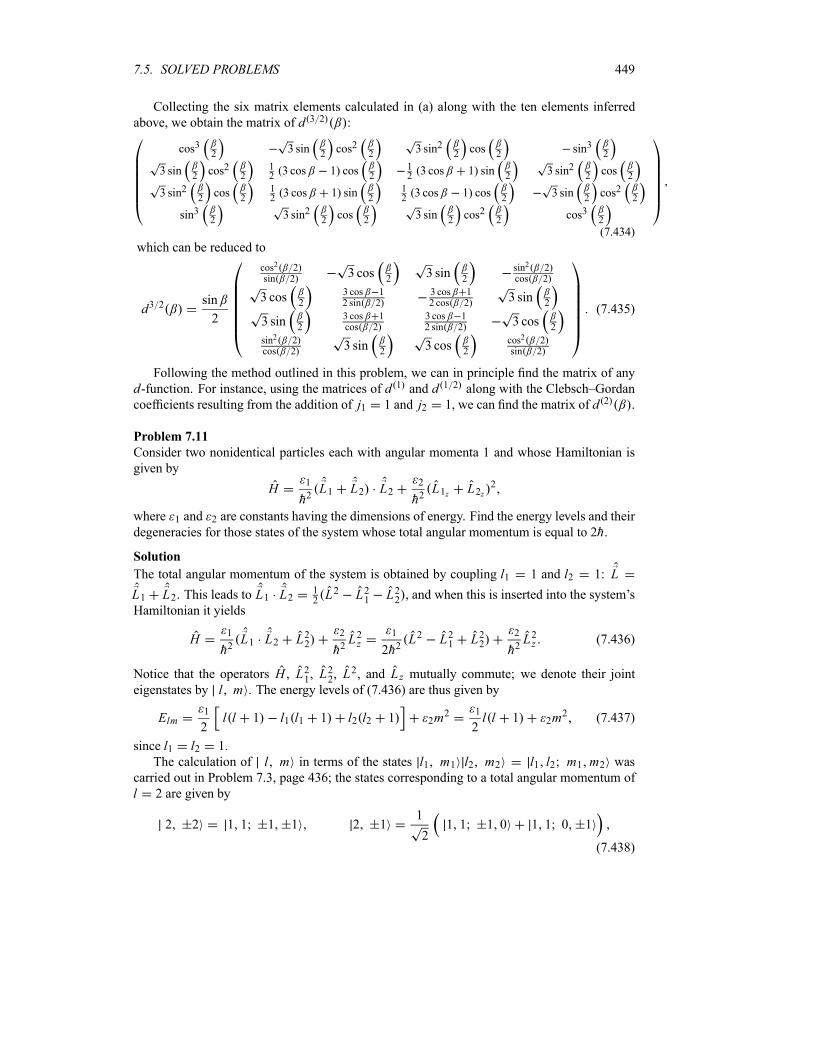
7.5. SOLVED PROBLEMS 449
Collecting the six matrix elements calculated in (a) along with the ten elements inferred
above, we obtain the matrix of d 3 2 :
cos32
3 sin2cos2
23 sin2
2cos
2sin3
2
3 sin2cos2
2123 cos 1 cos
2123 cos 1 sin
23 sin2
2cos
2
3 sin22cos
2123 cos 1 sin
2123 cos 1 cos
23 sin
2cos2
2
sin32
3 sin22cos
23 sin
2cos2
2cos3
2
(7.434)
which can be reduced to
d3 2sin
2
cos2 2sin 2
3 cos2
3 sin2
sin2 2cos 2
3 cos2
3 cos 12 sin 2
3 cos 12 cos 2
3 sin2
3 sin2
3 cos 1cos 2
3 cos 12 sin 2
3 cos2
sin2 2cos 2
3 sin2
3 cos2
cos2 2sin 2
(7.435)
Following the method outlined in this problem, we can in principle find the matrix of any
d-function. For instance, using the matrices of d 1 and d 1 2 along with the Clebsch–Gordancoefficients resulting from the addition of j1 1 and j2 1, we can find the matrix of d 2 .
Problem 7.11
Consider two nonidentical particles each with angular momenta 1 and whose Hamiltonian is
given by
H1
h2L1 L2 L2
2
h2L1z L2z
2
where 1 and 2 are constants having the dimensions of energy. Find the energy levels and their
degeneracies for those states of the system whose total angular momentum is equal to 2h.
Solution
The total angular momentum of the system is obtained by coupling l1 1 and l2 1: L
L1 L2. This leads to L1 L212L2 L21 L22 , and when this is inserted into the system’s
Hamiltonian it yields
H1
h2L1 L2 L22
2
h2L2z
1
2h2L2 L21 L22
2
h2L2z (7.436)
Notice that the operators H , L21, L22, L
2, and Lz mutually commute; we denote their jointeigenstates by l m . The energy levels of (7.436) are thus given by
Elm1
2l l 1 l1 l1 1 l2 l2 1 2m
2 1
2l l 1 2m
2 (7.437)
since l1 l2 1.
The calculation of l m in terms of the states l1 m1 l2 m2 l1 l2 m1 m2 wascarried out in Problem 7.3, page 436; the states corresponding to a total angular momentum of
l 2 are given by
2 2 1 1 1 1 2 11
21 1 1 0 1 1 0 1
(7.438)
450 CHAPTER 7. ROTATIONS AND ADDITION OF ANGULAR MOMENTA
2 01
61 1 1 1 2 1 1 0 0 1 1 1 1 (7.439)
From (7.437) we see that the energy corresponding to l 2 and m 2 is doubly degenerate,
because the states 2 2 have the same energy E2 2 3 1 4 2. The two states 2 1
are also degenerate, for they correspond to the same energy E2 1 3 1 2. The energy
corresponding to 2 0 is not degenerate: E20 3 1.
7.6 Exercises
Exercise 7.1
Show that the linear transformation y Rx where
Rcos sin
sin cosy
y1y2
xx1x2
is a counterclockwise rotation of the Cartesian x1x2 coordinate system in the plane about theorigin with an angle .
Exercise 7.2
Show that the nth power of the rotation matrix
Rcos sin
sin cos
is equal to
Rncos n sin nsin n cos n
What is the geometrical meaning of this result?
Exercise 7.3
Using the space displacement operator U A e i A P h , where P is the linear momentum
operator, show that ei A P h R e i A P h R A.
Exercise 7.4
The components A j (with j x y z) of a vector A transform under space rotations as AiRi j A j , where R is the rotation matrix.
(a) Using the invariance of the scalar product of any two vectors (e.g., A B) under rotations,show that the rows and columns of the rotation matrix R are orthonormal to each other (i.e.,show that Rl j Rlk j k).
(b) Show that the transpose of R is equal to the inverse of R and that the determinant of Ris equal to 1.
Exercise 7.5
The operator corresponding to a rotation of angle about an axis n is given by
Un e i n J h

7.6. EXERCISES 451
Show that the matrix elements of the position operator R are rotated through an infinitesimal
rotation like R R n R. (i.e., in the case where is infinitesimal, show that
Un R jUn R j n R j .
Exercise 7.6
Consider the wave function of a particle r 2x 2y z f r , where f r is a
spherically symmetric function.
(a) Is r an eigenfunction of L2? If so, what is the eigenvalue?(b) What are the probabilities for the particle to be found in the state ml 1, ml 0, and
ml 1?
(c) If r is an energy eigenfunction with eigenvalues E and if f r 3r2, find theexpression of the potential V r to which this particle is subjected.
Exercise 7.7
Consider a particle whose wave function is given by
r1
5Y11
1
5Y1 1
1
2Y10 f r
where f r is a normalized radial function, i.e., 0 r2 f 2 r dr 1.
(a) Calculate the expectation values of L2, Lz , and Lx in this state.(b) Calculate the expectation value of V 2 cos2 in this state.
(c) Find the probability that the particle will be found in the state ml 0.
Exercise 7.8
A particle of spin 12is in a d state of orbital angular momentum (i.e., l 2). Work out the
coupling of the spin and orbital angular momenta of this particle, and find all the states and the
corresponding Clebsch–Gordan coefficients.
Exercise 7.9
The spin-dependent Hamiltonian of an electron–positron system in the presence of a uniform
magnetic field in the z-direction (B Bk) can be written as
H S1 S2eB
mcS1z S2z
where is a real number and S1 and S2 are the spin operators for the electron and the positron,respectively.
(a) If the spin function of the system is given by 12
12, find the energy eigenvalues and
their corresponding eigenvectors.
(b) Repeat (a) in the case where 0, but B 0.
(c) Repeat (a) in the case where B 0, but 0.
Exercise 7.10
(a) Show that e i Jz 2 e i Jx ei Jz 2 e i Jy .
(b) Prove J e i Jx e i Jx J and then show that e i Jx j m e i j j m .
(c) Using (a) and (b), show that e i J y j m 1 j m j m .
452 CHAPTER 7. ROTATIONS AND ADDITION OF ANGULAR MOMENTA
Exercise 7.11
Using the commutation relations between the Pauli matrices, show that:
(a) ei yxe i y
x cos 2 z sin 2 ,
(b) ei z xe i z x cos 2 y sin 2 ,
(c) ei x ye i x y cos 2 z sin 2 .
Exercise 7.12
(a) Show how Jx , Jy , and Jz transform under a rotation of (finite) angle about the x-axis.
(b) Using the results of part (a), determine how the angular momentum operator J trans-forms under the rotation.
Exercise 7.13
(a) Show how the operator J transforms under a rotation of angle about the x-axis.
(b) Use the result of part (a) to show that J e i Jx h e i Jx h J .
Exercise 7.14
Consider a rotation of finite angle about an axis n which transforms unit vector a into another
unit vector b. Show that e i Jb h ei Jn he i Ja he i Jn h .
Exercise 7.15
(a) Show that ei Jy 2h Jxe i Jy 2h Jz .
(b) Show also that ei Jy 2hei Jx he i Jy 2h ei Jz h .
(c) For any vector operator A, show that ei Jz h Axe i Jz h Ax cos Ay sin .
Exercise 7.16
Using J J1 J2 show that
d jmm
m1m2 m1m2
j1 j2 m1 m2 j m j1 j2 m1m2 j m d j1m1m1
d j2m2m2
Exercise 7.17
Consider the tensor A cos sin cos .
(a) Calculate all the matrix elements Am m l m A l m for l 1.
(b) Express A in terms of the components of a spherical tensor of rank 2 (i.e., in terms
of Y2m ).
(c) Calculate again all the matrix elements Am m , but this time using the Wigner–Eckarttheorem. Compare these results with those obtained in (a). (The Clebsch–Gordan coefficients
may be obtained from tables.)
Exercise 7.18
(a) Express xz r2 and x2 y2 r2 in terms of the components of a spherical tensor ofrank 2.
(b) Using the Wigner–Eckart theorem, calculate the values of 1 0 xz r2 1 1 and
1 1 x2 y2 r2 1 1 .
Exercise 7.19
Show that j m e i Jy h J2z ei Jy h j m m j
m j m2 d j
m m2.
7.6. EXERCISES 453
Exercise 7.20
Calculate the trace of the rotation matrix D 1 2 for (a) and (b) and
2 .
Exercise 7.21
The quadrupole moment operator of a charge q is given by Q20 q 3z2 r2 . Write Q20 interms of an irreducible spherical tensor of rank 2 and then express j j Q20 j j in termsof j and the reduced matrix element j r2Y 2 j . Hint: You may use the coefficientj 2 m 0 j m 1 j m[3m2 j j 1 ] 2 j 1 j j 1 2 j 3 .
Exercise 7.22
Prove the following commutation relations:
(a) Jx [Jx Tkq ] q T
kq k q J 2x k q ,
(b) Jx [Jx Tkq ] Jy [Jy T
kq ] Jz [Jz T
kq ] k k 1 h2T k
q .
Exercise 7.23
Consider a spin 12particle which has an orbital angular momentum l 1. Find all the Clebsch–
Gordan coefficients involved in the addition of the orbital and spin angular momenta of this
particle. Hint: The Clebsch–Gordan coefficient j1 j2 j1 j2 j1 j2 j2 is real and
positive.
Exercise 7.24
This problem deals with another derivation of the matrix elements of d 1 . Use the relation
d jmm
m1m2 m1m2
j1 j2 m1 m2 j m j1 j2 m1 m2 j m d j1m1m1
d j2m2m2
for the case where j1 j212along with the matrix elements of d 1 2 , which are given
by (7.89), to derive all the matrix elements of d 1 .
Exercise 7.25
Consider the tensor A sin2 cos 2 .
(a) Calculate the reduced matrix element 2 Y2 2 . Hint: You may calculate explicitly2 1 Y20 2 1 and then use the Wigner–Eckart theorem to calculate it again.
(b) Express A in terms of the components of a spherical tensor of rank 2 (i.e., in terms
of Y2m ).
(c) Calculate Am 1 2 m A 2 1 for m 2, 1, 0. You may need this Clebsch–
Gordan coefficient: j 2 m 0 j m [3m2 j j 1 ] 2 j 1 j j 1 2 j 3 .
Exercise 7.26
(a) Calculate the reduced matrix element 1 Y1 2 . Hint: For this, you may need tocalculate 1 0 Y10 2 0 directly and then from the Wigner–Eckart theorem.
(b) Using the Wigner–Eckart theorem and the relevant Clebsch–Gordan coefficients from
the table, calculate 1 m Y1m 2 m for all possible values of m, m , and m . Hint: You may
find the integral 0 r3R21 r R32 r dr64a015 5
65
5and the following coefficients useful:
j 1 m 0 j 1 m j m j m [ j 2 j 1 ],
j 1 m 1 1 j 1 m j m j m 1 [2 j 2 j 1 ], and
j 1 m 1 1 j 1 m j m j m 1 [2 j 2 j 1 ].
454 CHAPTER 7. ROTATIONS AND ADDITION OF ANGULAR MOMENTA
Exercise 7.27
A particle of spin 12is in a d state of orbital angular momentum (i.e., l 2).
(a) What are its possible states of total angular momentum.
(b) If its Hamiltonian is given by H a bL S cL2, where a, b, and c are numbers, findthe values of the energy for each of the different states of total angular momentum. Express
your answer in terms of a, b, c.
Exercise 7.28
Consider an h-state electron. Calculate the Clebsch–Gordan coefficients involved in the fol-lowing j m states of the electron: 11
292, 11
272, 92
92, 92
72.
Exercise 7.29
Let the Hamiltonian of two nonidentical spin 12particles be
H1
h2S1 S2 S1
2
hS1z S2z
where 1 and 2 are constants having the dimensions of energy. Find the energy levels and their
degeneracies.
Exercise 7.30
Find the energy levels and their degeneracies for a system of two nonidentical spin 12particles
with Hamiltonian
H0
h2S21 S22
0
hS1z S2z
where 0 is a constant having the dimensions of energy.
Exercise 7.31
Consider two nonidentical spin s 12particles with Hamiltonian
H0
h2S1 S2
2 0
h2S1z S2z
2
where 0 is a constant having the dimensions of energy. Find the energy levels and their degen-
eracies.
Exercise 7.32
Consider a system of three nonidentical particles, each of spin s 12, whose Hamiltonian is
given by
H1
h2S1 S3 S2
2
h2S1z S2z S3z
2
where 1 and 2 are constants having the dimensions of energy. Find the system’s energy levels
and their degeneracies.
Exercise 7.33
Consider a system of three nonidentical particles, each with angular momentum 32. Find the
possible values of the total spin S of this system and specify the number of angular momentumeigenstates corresponding to each value of S.
Chapter 8
Identical Particles
Up to this point, we have dealt mainly with the motion of a single particle. Now we want to
examine how to describe systems with many particles. We shall focus on systems of identicalparticles and examine how to construct their wave functions.
8.1 Many-Particle Systems
Most physical systems—nucleons, nuclei, atoms, molecules, solids, fluids, gases, etc.—involve
many particles. They are known as many-particle or many-body systems. While atomic, nu-clear, and subnuclear systems involve intermediate numbers of particles ( 2 to 300), solids,
fluids, and gases are truly many-body systems, since they involve very large numbers of parti-
cles ( 1023).
8.1.1 Schrödinger Equation
How does one describe the dynamics of a system of N particles? This description can beobtained from a generalization of the dynamics of a single particle. The state of a system of
N spinless particles (we ignore their spin for the moment) is described by a wave functionr1 r2 rN t , where r1 r2 rN t 2d3r1 d3r2 d3rN represents the probability
at time t of finding particle 1 in the volume element d3r1 centered about r1, particle 2 in thevolume d3r2 about r2, . . . , and particle N in the volume d3rN about rN . The normalizationcondition of the state is given by
d3r1 d3r2 r1 r2 rN t 2d3rN 1 (8.1)
The wave function evolves in time according to the time-dependent Schrödinger equation
iht
r1 r2 rN t H r1 r2 rN t (8.2)
The form of H is obtained by generalizing the one-particle Hamiltonian P2 2m V r to N
455
456 CHAPTER 8. IDENTICAL PARTICLES
particles:
HN
j 1
P2j2m j
V r1 r2 rN tN
j 1
h2
2m j2j V r1 r2 rN t (8.3)
where m j and P j are the mass and the momentum of the j th particle and V is the operator
corresponding to the total potential energy (V accounts for all forms of interactions—internaland external—the mutual interactions between the various particles of the system and for the
interactions of the particles with the outside world).
The formalism of quantummechanics for an N -particle system can be, in principle, inferredfrom that of a single particle. Operators corresponding to different particles commute; for
instance, the commutation relations between the position and momentum operators are
[X j Pxk ] ih j k [X j Xk] [Px j Pxk ] 0 j k 1 2 3 N (8.4)
where X j is the x-position operator of the j th particle, and Pxk the x-momentum operator ofthe kth particle; similar relations can be obtained for the y and z components.
Stationary states
In the case where the potential V is time independent, the solutions of (8.2) are given by sta-tionary states
r1 r2 rN t r1 r2 rN e i Et h (8.5)
where E is the total energy of the system and is the solution to the time-independent Schrödinger
equation H E , i.e.,
N
j 1
h2
2m j2j V r1 rN r1 r2 rN E r1 r2 rN (8.6)
The properties of stationary states for a single particle also apply to N -particle systems. Forinstance, the probability density , the probability current density j , and the expectationvalues of time-independent operators are conserved, since they do not depend on time:
A A d3r1 d3r2 r1 r2 rN A r1 r2 rN d3rN
(8.7)
In particular, the energy of a stationary state is conserved.
Multielectron atoms
As an illustration, let us consider an atom with Z electrons. If R is used to represent the posi-tion of the center of mass of the nucleus, the wave function of the atom depends on 3 Z 1
coordinates r1 r2 rZ R , where r1 r2 rZ are the position vectors of the Z elec-trons. The time-independent Schrödinger equation for this atom, neglecting contributions from
the spin–orbit correction, the relativistic correction, and similar terms, is given by
h2
2me
Z
i 1
2ri
h2
2M2R
Z
i 1
Z e2
ri R i j
e2
ri r jr1 r2 rZ R
E r1 r2 rZ R (8.8)
8.1. MANY-PARTICLE SYSTEMS 457
where M is the mass of the nucleus and h2 2R 2M is its kinetic energy operator. The term
Zi 1 Ze
2 ri R represents the attractive Coulomb interaction of each electron with the
nucleus and i j e2 ri r j is the repulsive Coulomb interaction between the i th and the
j th electrons; ri r j is the distance separating them. As these (Coulomb) interactions areindependent of time, the states of atoms are stationary.
We should note that the Schrödinger equations (8.3), (8.6), and (8.8) are all many-particle
differential equations. As these equations cannot be separated into one-body equations, it is
difficult, if not impossible, to solve them. For the important case where the N particles of thesystem do not interact—this is referred to as an independent particle system—the Schrödingerequation can be trivially reduced to N one-particle equations (Section 8.1.3); we have seen howto solve these equations exactly (Chapters 4 and 6) and approximately (Chapters 9 and 10).
8.1.2 Interchange Symmetry
Although the exact eigenstates of the many-body Hamiltonian (8.3) are generally impossible
to obtain, we can still infer some of their properties by means of symmetry schemes. Let i
represent the coordinates (position ri , spin si , and any other internal degrees of freedom such asisospin, color, flavor) of the i th particle and let 1 2 N designate the wave function
of the N -particle system.We define a permutation operator (also called exchange operator) Pi j as an operator that,
when acting on an N -particle wave function 1 i j N , interchanges the
i th and the j th particles
Pi j 1 i j N 1 j i N (8.9)
i and j are arbitrary (i j 1, 2, , N ). Since
Pj i 1 i j N 1 j i N
Pi j 1 i j N (8.10)
we have Pi j Pj i . In general, permutation operators do not commute:
Pi j Pkl Pkl Pi j or [Pi j Pkl] 0 i j kl (8.11)
For instance, in the case of a four-particle state 1 2 3 4 3 4 2 3 e i 1 , we have
P12P14 1 2 3 4 P12 4 2 3 1 2 4 3 13 1
4 3e i 2 (8.12)
P14P12 1 2 3 4 P14 2 1 3 4 4 1 3 23 2
1 3e i 4 (8.13)
Since two successive applications of Pi j leave the wave function unchanged,
P2i j 1 i j N Pi j 1 j i N
1 i j N (8.14)
we have P2i j 1; hence Pi j has two eigenvalues 1:
Pi j 1 i j N 1 i j N (8.15)
458 CHAPTER 8. IDENTICAL PARTICLES
The wave functions corresponding to the eigenvalue 1 are symmetric and those correspondingto 1 are antisymmetric with respect to the interchange of the pair i j . Denoting thesefunctions by s and a , respectively, we have
s 1 i j N s 1 j i N (8.16)
a 1 i j N a 1 j i N (8.17)
Example 8.1
Specify the symmetry of the following functions:
(a) x1 x2 4 x1 x2 210
x21 x22,
(b) x1 x23 x1 x2
2 x1 x2 2 7,
(c) x1 x2 x3 6x1x2x3x21 x22 x23 1
2x31 2x32 2x33 5,
(d) x1 x21
x2 3e x1 .
Solution
(a) The function x1 x2 is symmetric, since x2 x1 x1 x2 .(b) The function x1 x2 is antisymmetric, since x2 x1 x1 x2 , and is zero
when x1 x2: x1 x1 0.
(c) The function x1 x2 x3 is symmetric because
x1 x2 x3 x1 x3 x2 x2 x1 x3 x2 x3 x1
x3 x1 x2 x3 x2 x1 (8.18)
(d) The function x2 x1 is neither symmetric nor antisymmetric, sincex2 x1
1x1 3
e x2 x1 x2 .
8.1.3 Systems of Distinguishable Noninteracting Particles
For a system of N noninteracting particles that are distinguishable—each particle has a differentmass mi and experiences a different potential Vi i —the potential V is given by
V 1 2 N
N
i 1
Vi i (8.19)
and the Hamiltonian of this system of N independent particles by
HN
i 1
HiN
i 1
h2
2mi2i Vi i (8.20)
where Hi h2 2i 2mi Vi i is the Hamiltonian of the i th particle, known as the single
particle Hamiltonian. The Hamiltonians of different particles commute [Hi H j ] 0, since
[Xi X j ] [Pi Pj ] 0.
8.1. MANY-PARTICLE SYSTEMS 459
The Schrödinger equation of the N -particle system
H n1 n2 nN 1 2 N En1 n2 nN n1 n2 nN 1 2 N (8.21)
separates into N one-particle equations
h2
2mi2i Vi i ni i ni ni i (8.22)
with
En1 n2 nN n1 n2 nN
N
i 1ni (8.23)
and
n1 n2 nN 1 2 N n1 1 n2 2 nN N
N
i 1ni i (8.24)
We see that, when the interactions are neglected, the N -particle Schrödinger equation separatesinto N one-particle Schrödinger equations. The solutions of these equations yield the single-particle energies ni and states ni i ; the single-particle states are also known as the orbitals.The total energy is the sum of the single-particle energies and the total wave function is the
product of the orbitals. The number ni designates the set of all quantum numbers of the i thparticle. Obviously, each particle requires one, two, or three quantum numbers for its full de-
scription, depending on whether the particles are moving in a one-, two-, or three-dimensional
space; if the spin were considered, we would need to add another quantum number. For in-
stance, if the particles moved in a one-dimensional harmonic oscillator, ni would designatethe occupation number of the i th particle. But if the particles were the electrons of an atom,then ni would stand for four quantum numbers: the radial, orbital, magnetic, and spin quantumnumbers Ni limlimsi .
Example 8.2
Find the energy levels and wave functions of a system of four distinguishable spinless particles
placed in an infinite potential well of size a. Use this result to infer the energy and the wavefunction of the ground state and the first excited state.
Solution
Each particle moves in a potential which is defined by Vi xi 0 for 0 xi a and Vi xifor the other values of xi . In this case the Schrödinger equation of the four-particle system:
4
i 1
h2
2mi
d2
dx2in1 n2 n3 n4 x1 x2 x3 x4 En1 n2 n3 n4 n1 n2 n3 n4 x1 x2 x3 x4
(8.25)
separates into four one-particle equations
h2
2mi
d2 ni xi
dx2ini ni xi i 1 2 3 4 (8.26)

460 CHAPTER 8. IDENTICAL PARTICLES
with
ni
h2 2n2i2mia2
ni xi2
asin
niaxi (8.27)
The total energy and wave function are given by
En1 n2 n3 n4h2 2
2a2n21m1
n22m2
n23m3
n24m4
(8.28)
n1 n2 n3 n4 x1 x2 x3 x44
a2sin
n1ax1 sin
n2ax2 sin
n3ax3 sin
n4ax4
(8.29)
The ground state corresponds to the case where all four particles occupy their respective
ground state orbitals, n1 n2 n3 n4 1. The ground state energy and wave function are
thus given by
E1 1 1 1h2 2
2a21
m1
1
m2
1
m3
1
m4(8.30)
1 1 1 1 x1 x2 x3 x44
a2sin
ax1 sin
ax2 sin
ax3 sin
ax4 (8.31)
The first excited state is somewhat tricky. Since it corresponds to the next higher energy
level of the system, it must correspond to the case where the particle having the largest mass
occupies its first excited state while the other three particles remain in their respective ground
states. For argument’s sake, if the third particle were the most massive, the first excited state
would correspond to the configuration n1 n2 n4 1 and n3 2; the energy and wave
function of the first excited state would then be given by
E1 1 2 1h2 2
2a21
m1
1
m2
4
m3
1
m4(8.32)
1 1 2 1 x1 x2 x3 x44
a2sin
ax1 sin
ax2 sin
2
ax3 sin
ax4 (8.33)
Continuing in this way, we can obtain the entire energy spectrum of this system.
8.2 Systems of Identical Particles
8.2.1 Identical Particles in Classical and Quantum Mechanics
In classical mechanics, when a system is made of identical particles, it is possible to identify
and distinguish each particle from the others. That is, although all particles have the same
physical properties, we can “tag” each classical particle and follow its motion along a path.
For instance, each particle can be colored differently from the rest; hence we can follow the
trajectory of each particle separately at each time. Identical classical particles, therefore, donot lose their identity; they are distinguishable.In quantum mechanics, however, identical particles are truly indistinguishable. The un-
derlying basis for this is twofold. First, to describe a particle, we cannot specify more than
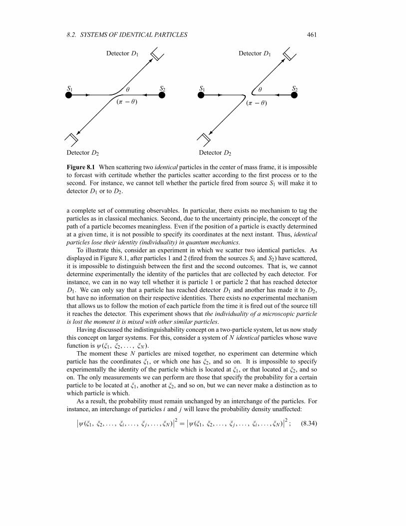
8.2. SYSTEMS OF IDENTICAL PARTICLES 461
¡@¡Detector D2
@
¡¡
¡¡
¡ª
¾ yS2yS1 -¡¡¡¡¡µ@¡¡
Detector D1 @
¡@¡Detector D2
@
¡¡
¡¡
¡ª
¾ yS2yS1 -¡¡¡¡¡µ@¡¡
Detector D1 @
Figure 8.1 When scattering two identical particles in the center of mass frame, it is impossibleto forcast with certitude whether the particles scatter according to the first process or to the
second. For instance, we cannot tell whether the particle fired from source S1 will make it todetector D1 or to D2.
a complete set of commuting observables. In particular, there exists no mechanism to tag the
particles as in classical mechanics. Second, due to the uncertainty principle, the concept of the
path of a particle becomes meaningless. Even if the position of a particle is exactly determined
at a given time, it is not possible to specify its coordinates at the next instant. Thus, identicalparticles lose their identity (individuality) in quantum mechanics.To illustrate this, consider an experiment in which we scatter two identical particles. As
displayed in Figure 8.1, after particles 1 and 2 (fired from the sources S1 and S2) have scattered,it is impossible to distinguish between the first and the second outcomes. That is, we cannot
determine experimentally the identity of the particles that are collected by each detector. For
instance, we can in no way tell whether it is particle 1 or particle 2 that has reached detector
D1. We can only say that a particle has reached detector D1 and another has made it to D2,but have no information on their respective identities. There exists no experimental mechanism
that allows us to follow the motion of each particle from the time it is fired out of the source till
it reaches the detector. This experiment shows that the individuality of a microscopic particleis lost the moment it is mixed with other similar particles.Having discussed the indistinguishability concept on a two-particle system, let us now study
this concept on larger systems. For this, consider a system of N identical particles whose wavefunction is 1 2 N .
The moment these N particles are mixed together, no experiment can determine which
particle has the coordinates 1, or which one has 2, and so on. It is impossible to specify
experimentally the identity of the particle which is located at 1, or that located at 2, and so
on. The only measurements we can perform are those that specify the probability for a certain
particle to be located at 1, another at 2, and so on, but we can never make a distinction as to
which particle is which.
As a result, the probability must remain unchanged by an interchange of the particles. For
instance, an interchange of particles i and j will leave the probability density unaffected:
1 2 i j N2
1 2 j i N2
(8.34)
462 CHAPTER 8. IDENTICAL PARTICLES
hence we have
1 2 i j N 1 2 j i N (8.35)
This means that the wave function of a system of N identical particles is either symmetric orantisymmetric under the interchange of a pair of particles. We will deal with the implications
of this result in Section 8.2.3. We will see that the sign in (8.35) is related to the spin of the
particles: the negative sign corresponds to particles with half-odd-integral spin and the positive
sign corresponds to particles with integral spin; that is, the wave functions of particles with
integral spins are symmetric and the wave functions of particles with half-odd-integral spins
are antisymmetric. In fact, experimental observations show that, in nature, particles come in
two classes:
Particles with integral spin, Si 0 1h 2h 3h , such as photons, pions, alpha
particles. These particles are called bosons.
Particles with half-odd-integral spin, Si h 2, 3h 2, 5h 2, 7h 2, , such as quarks,
electrons, positrons, protons, neutrons. These particles are called fermions.
That is, particles occurring in nature are either bosons or fermions.
Before elaborating more on the properties of bosons and fermions, let us present a brief
outline on the interchange (permutation) symmetry.
8.2.2 Exchange Degeneracy
How does the interchange symmetry affect operators such as the Hamiltonian? Since the
Coulomb potential, which results from electron–electron and electron–nucleus interactions,
V r1 r2 r3 rZZ
i 1
Z e2
ri R i j
e2
ri r j(8.36)
is invariant under the permutation of any pair of electrons, the Hamiltonian (8.8) is also invariant
under such permutations. This symmetry also applies to the orbital, spin, and angular momenta
of an atom. We may thus use this symmetry to introduce another definition of the identicalnessof particles. The N particles of a system are said to be identical if the various observablesof the system (such as the Hamiltonian H , the angular momenta, and so on) are symmetricalwhen any two particles are interchanged. If these operators were not symmetric under particleinterchange, the particles would be distinguishable.
The invariance of the Hamiltonian under particle interchanges is not without physical impli-
cations: the eigenvalues of H are degenerate. The wave functions corresponding to all possibleelectron permutations have the same energy E : H E . This is known as the exchangedegeneracy. For instance, the degeneracy associated with a system of two identical particles isequal to 2, since 1 2 and 2 1 correspond to the same energy E .So the Hamiltonian of a system of N identical particles (mi m) is completely symmetric
with respect to the coordinates of the particles:
H 1 i j N
N
k 1
P2k2m
V 1 i j N
H 1 j i N (8.37)
8.2. SYSTEMS OF IDENTICAL PARTICLES 463
because V is invariant under the permutation of any pair of particles i j :
V 1 i j N V 1 j i N (8.38)
This property can also be ascertained by showing that H commutes with the particle inter-change operator Pi j . If is eigenstate to H with eigenvalue E , we can write
HPi j 1 i j N H 1 j i N
E 1 j i N EPi j 1 i j N
Pi j E 1 i j N Pi jH 1 i j N
(8.39)
or
[H Pi j ] 0 (8.40)
Therefore, Pi j is a constant of the motion. That is, if we start with a wave function that is sym-
metric (antisymmetric), it will remain so for all subsequent times. Moreover, since Pi j and Hcommute, they possess a complete set of functions that are joint eigenstates of both. As shown
in (8.15) to (8.17), these eigenstates have definite parity, either symmetric or antisymmetric.
8.2.3 Symmetrization Postulate
We have shown in (8.35) that the wave function of a system of N identical particles is eithersymmetric or antisymmetric under the interchange of any pair of particles:
1 2 i j N 1 2 j i N (8.41)
This result, which turns out to be supported by experimental evidence, is the very essence of
the symmetrization postulate which stipulates that, in nature, the states of systems containingN identical particles are either totally symmetric or totally antisymmetric under the interchangeof any pair of particles and that states with mixed symmetry do not exist. Besides that, this
postulate states two more things:
Particles with integral spins, or bosons, have symmetric states.
Particles with half-odd-integral spins, or fermions, have antisymmetric states.
Fermions are said to obey Fermi–Dirac statistics and bosons to obey Bose–Einstein statistics.So the wave function of a system of identical bosons is totally symmetric and the wave function
of a system of identical fermions is totally antisymmetric.
Composite particles
The foregoing discussion pertains to identical particles that are “simple” or elementary such as
quarks, electrons, positrons, muons, and so on. Let us now discuss the symmetry of systems
of identical composite “particles” where each particle is composed of two or more identicalelementary particles. For instance, alpha particles, which consist of nuclei that are composed
of two neutrons and two protons each, are a typical example of composite particles. A system
of N hydrogen atoms can also be viewed as a system of identical composite particles whereeach “particle” (atom) consists of a proton and an electron. Protons, neutrons, pions, etc., are
464 CHAPTER 8. IDENTICAL PARTICLES
themselves composite particles, because protons and neutrons consist of three quarks and pions
consist of two. Quarks are elementary spin 12particles.
Composite particles have spin. The spin of each composite particle can be obtained by
adding the spins of its constituents. If the total spin of the composite particle is half-odd-integer,
this particle behaves like a fermion, and hence it obeys Fermi–Dirac statistics. If, on the other
hand, its resultant spin is integer, it behaves like a boson and obeys Bose–Einstein statistics. In
general, if the composite particle has an odd number of fermions; it is then a fermion, otherwise
it is a boson. For instance, nucleons are fermions because they consist of three quarks; mesons
are bosons because they consist of two quarks. For another illustrative example, let us consider
the isotopes 4He and 3He of the helium atom: 4He, which is called an alpha particle, is a boson
for it consists of four nucleons (two protons and two neutrons), while 3He is a fermion since it
consists of three nucleons (one neutron and two protons). The hydrogen atom consists of two
fermions (an electron and a proton), so it is a boson.
8.2.4 Constructing Symmetric and Antisymmetric Functions
Since the wave functions of systems of identical particles are either totally symmetric or totally
antisymmetric, it is appropriate to study the formalism of how to construct wave functions
that are totally symmetric or totally antisymmetric starting from asymmetric functions. For
simplicity, consider first a system of two identical particles. Starting from any normalized
asymmetric wave function 1 2 , we can construct symmetric wave functions s 1 2 as
s 1 21
21 2 2 1 (8.42)
and antisymmetric wave functions a 1 2 as
a 1 21
21 2 2 1 (8.43)
where 1 2 is a normalization factor.
Similarly, for a system of three identical particles, we can construct s and a from an
asymmetric function as follows:
s 1 2 31
61 2 3 1 3 2 2 3 1
2 1 3 3 1 2 3 2 1 (8.44)
a 1 2 31
61 2 3 1 3 2 2 3 1
2 1 3 3 1 2 3 2 1 (8.45)
Continuing in this way, we can in principle construct symmetric and antisymmetric wave
functions for any system of N identical particles.
8.2.5 Systems of Identical Noninteracting Particles
In the case of a system of N noninteracting identical particles, where all particles have equalmass mi m and experience the same potential Vi i V i , the Schrödinger equation of
8.2. SYSTEMS OF IDENTICAL PARTICLES 465
the system separates into N identical one-particle equations
h2
2m2i V i ni i ni ni i (8.46)
Whereas the energy is given, like the case of a system of N distinguishable particles, by a sum ofthe single-particle energies En1 n2 nN
Ni 1 ni , the wave function can no longer be given
by a simple product n1 n2 nN 1 2 NNi 1 ni i for at least two reasons. First,
if the wave function is given by such a product, it would imply that particle 1 is in the state n1 ,
particle 2 in the state n2 , . . . , and particle N in the state nN . This, of course, makes no sense
since all we know is that one of the particles is in the state n1 , another in n2 , and so on; since
the particles are identical, there is no way to tell which particle is in which state. If, however, the
particles were distinguishable, then their total wave function would be given by such a product,
as shown in (8.24). The second reason why the wave function of a system of identical particles
cannot be given byNi 1 ni i has to do with the fact that such a product has, in general,
no definite symmetry—a mandatory requirement for systems of N identical particles whosewave functions are either symmetric or antisymmetric. We can, however, extend the method
of Section 8.2.4 to construct totally symmetric and totally antisymmetric wave functions from
the single-particle states ni i . For this, we are going to show how to construct symmetrized
and antisymmetrized wave functions for systems of two, three, and N noninteracting identicalparticles.
8.2.5.1 Wave Function of Two-Particle Systems
By analogy with (8.42) and (8.43), we can construct the symmetric and antisymmetric wave
functions for a system of two identical, noninteracting particles in terms of the single-particle
wave functions as follows:
s 1 21
2n1 1 n2 2 n1 2 n2 1 (8.47)
a 1 21
2n1 1 n2 2 n1 2 n2 1 (8.48)
where we have supposed that n1 n2. When n1 n2 n the symmetric wave function isgiven by s 1 2 n 1 n 2 and the antisymmetric wave function is zero; we will deal
later with the reason why a 1 2 0 whenever n1 n2.Note that we can rewrite s as
s 1 21
2! P
P n1 1 n2 2 (8.49)
where P is the permutation operator and where the sum is over all possible permutations (herewe have only two possible ones). Similarly, we can write a as
a 1 21
2! P
1 P P n1 1 n2 2 (8.50)

466 CHAPTER 8. IDENTICAL PARTICLES
where 1 P is equal to +1 for an even permutation (i.e., when we interchange both 1 and 2
and also n1 and n2) and equal to 1 for an odd permutation (i.e., when we permute 1 and 2 but
not n1, n2, and vice versa). Note that we can rewrite a of (8.48) in the form of a determinant
a 1 21
2!
n1 1 n1 2
n2 1 n2 2(8.51)
8.2.5.2 Wave Function of Three-Particle Systems
For a system of three noninteracting identical particles, the symmetric wave function is given
by
s 1 2 31
3! P
P n1 1 n2 2 n3 3 (8.52)
or by
s 1 2 31
3!n1 1 n2 2 n3 3 n1 1 n2 3 n3 2
n1 2 n2 1 n3 3 n1 2 n2 3 n3 1
n1 3 n2 1 n3 2 n1 3 n2 2 n3 1 (8.53)
and, when n1 n2 n3, the antisymmetric wave function is given by
a 1 2 31
3! P
1 P P n1 1 n2 2 n3 3 (8.54)
or, in the form of a determinant, by
a 1 2 31
3!
n1 1 n1 2 n1 3
n2 1 n2 2 n2 3
n3 1 n3 2 n3 3
(8.55)
If n1 n2 n3 n we have s 1 2 3 n 1 n 2 n 3 and a 1 2 3 0.
8.2.5.3 Wave Function of Many-Particle Systems
We can generalize (8.52) and (8.55) and write the symmetric and antisymmetric wave functions
for a system of N noninteracting identical particles as follows:
s 1 2 N1
N ! P
P n1 1 n2 2 nN N (8.56)
a 1 2 N1
N ! P
1 Pn1 1 n2 2 nN N (8.57)
or
a 1 2 N1
N !
n1 1 n1 2 n1 N
n2 1 n2 2 n2 N
nN 1 nN 2 nN N
(8.58)

8.3. THE PAULI EXCLUSION PRINCIPLE 467
This N N determinant, which involves one-particle states only, is known as the Slater deter-minant. An interchange of any pair of particles corresponds to an interchange of two columnsof the determinant; this interchange introduces a change in the sign of the determinant. For
even permutations we have 1 P 1, and for odd permutations we have 1 P 1.
The relations (8.56) and (8.58) are valid for the case where the numbers n1, n2, , nN areall different from one another. What happens if some, or all, of these numbers are equal? In the
symmetric case, if n1 n2 nN then s is given by
s 1 2 N
N
i 1n i n 1 n 2 n N (8.59)
When there is a multiplicity in the numbers n1, n2, , nN (i.e., when some of the numbers nioccur more than once), we have to be careful and avoid double counting. For instance, if n1occurs N1 times in the sequence n1, n2, , nN , if n2 occurs N2 times, and so on, the symmetricwave function will be given by
s 1 2 NN1!N2! NN !
N !P
P n1 1 n2 2 nN N (8.60)
the summation P is taken only over permutations which lead to distinct terms and includesN ! N1!N2! Nn! different terms. For example, in the case of a system of three independent,identical bosons where n1 n2 n and n3 n, the multiplicity of n1 is N1 2; hence s is
given by
s 1 2 32!
3!P
P n 1 n 2 n3 31
3n 1 n 2 n3 3
n 1 n3 2 n 3 n3 1 n 2 n 3 (8.61)
Unlike the symmetric case, the antisymmetric case is quite straightforward: if, among the
numbers n1, n2, , nN , only two are equal, the antisymmetric wave function vanishes. Forinstance, if ni n j , the i th and j th rows of the determinant (8.58) will be identical; hence thedeterminant vanishes identically. Antisymmetric wave functions, therefore, are nonzero only
for those cases where all the numbers n1, n2, , nN are different.
8.3 The Pauli Exclusion Principle
As mentioned above, if any two particles occupy the same single-particle state, the determinant
(8.58), and hence the total wave function, will vanish since two rows of the determinant will
be identical. We can thus infer that in a system of N identical particles, no two fermions canoccupy the same single-particle state at a time; every single-particle state can be occupied byat most one fermion. This is the Pauli exclusion principle, which was first postulated in 1925to explain the periodic table. It states that no two electrons can occupy simultaneously thesame (single-particle) quantum state on the same atom; there can be only one (or at most one)electron occupying a state of quantum numbers ni limlimsi : ni limlimsi
ri Si . The exclusionprinciple plays an important role in the structure of atoms. It has a direct effect on the spatialdistribution of fermions.
468 CHAPTER 8. IDENTICAL PARTICLES
Boson condensation
What about bosons? Do they have any restriction like fermions? Not at all. There is no
restriction on the number of bosons that can occupy a single state. Instead of the exclusion
principle of fermions, bosons tend to condense all in the same state, the ground state; this
is called boson condensation. For instance, all the particles of liquid 4He (a boson system)occupy the same ground state. This phenomenon is known as Bose–Einstein condensation. Theproperties of liquid 3He are, however, completely different from those of liquid 4He, because3He is a fermion system.
Remark
We have seen that when the Schrödinger equation involves the spin, the wave function of a
single particle is equal to the product of the spatial part and the spin part: r S r S .The wave function of a system of N particles, which have spins, is the product of the spatialpart and the spin part:
r1 S1 r2 S2 rN SN r1 r2 rN S1 S2 SN (8.62)
This wave function must satisfy the appropriate symmetry requirements when the N particlesare identical. In the case of a system of N identical bosons, the wave function must be symmet-ric; hence the spatial and spin parts must have the same parity:
s r1 S1 r2 S2 rN SNa r1 r2 rN a S1 S2 SNs r1 r2 rN s S1 S2 SN
(8.63)
In the case of a system of N identical fermions, however, the space and spin parts must havedifferent parities, leading to an overall wave function that is antisymmetric:
a r1 S1 r2 S2 rN SNa r1 r2 rN s S1 S2 SNs r1 r2 rN a S1 S2 SN
(8.64)
Example 8.3 (Wave function of two identical, noninteracting particles)
Find the wave functions of two systems of identical, noninteracting particles: the first consists
of two bosons and the second of two spin 12fermions.
Solution
For a system of two identical, noninteracting bosons, (8.47) and (8.48) yield
s r1 S1 r2 S21
2
n1 r1 n2 r2 n1 r2 n2 r1 a S1 S2
n1 r1 n2 r2 n1 r2 n2 r1 s S1 S2(8.65)
and for a system of two spin 12fermions
a r1 S1 r2 S21
2
n1 r1 n2 r2 n1 r2 n2 r1 s S1 S2
n1 r1 n2 r2 n1 r2 n2 r1 a S1 S2(8.66)

8.4. THE EXCLUSION PRINCIPLE AND THE PERIODIC TABLE 469
where, from the formalism of angular momentum addition, there are three states (a triplet) that
are symmetric, s S1 S2 :
triplet S1 S2
1212 1
1212 2
1
2
1212 1
12
12 2
12
12 1
1212 2
12
12 1
12
12 2
(8.67)
and one state (a singlet) that is antisymmetric, a S1 S2 :
singlet S1 S21
2
1
2
1
2 1
1
2
1
2 2
1
2
1
2 1
1
2
1
2 2
(8.68)
8.4 The Exclusion Principle and the Periodic Table
Explaining the periodic table is one of the most striking successes of the Schrödinger equation.
When combined with the Pauli exclusion principle, the equation offers insightful information
on the structure of multielectron atoms.
In Chapter 6, we saw that the state of the hydrogen’s electron, which moves in the spher-
ically symmetric Coulomb potential of the nucleus, is described by four quantum numbers n,l, ml , and ms : nlmlms r nlml r ms , where nlml r Rnl r Ylml is the elec-
tron’s wave function when the spin is ignored and ms12
12is the spin’s state. This
representation turns out to be suitable for any atom as well.
In a multielectron atom, the average potential in which every electron moves is different
from the Coulomb potential of the nucleus; yet, to a good approximation, it can be assumed
to be spherically symmetric. We can therefore, as in hydrogen, characterize the electronic
states by the four quantum numbers n, l, ml , and ms , which respectively represent the principalquantum number, the orbital quantum number, the magnetic (or azimuthal) quantum number,
and the spin quantum number; ml represents the z-component of the electron orbital angularmomentum and ms the z-component of its spin.Atoms have a shell structure. Each atom has a number of major shells that are specified
by the radial or principal quantum number n. Shells have subshells which are specified by theorbital quantum number l. Subshells in turn have subsubshells, called orbitals, specified by ml ;so an orbital is fully specified by three quantum numbers n, l, ml ; i.e., it is defined by nlml .Each shell n therefore has n subshells corresponding to l 0, 1, 2, 3, , n 1, and in turn
each subshell has 2l 1 orbitals (or subsubshells), since to ml l, l 1, l 2, ,
l 2, l 1, l. As in hydrogen, individual electrons occupy single-particle states or orbitals;the states corresponding to the respective numerical values l 0 1 2 3 4 5 are called s,
p, d, f, g, h, states. Hence for a given n an s-state has 1 orbital (ml 0), a p-state has 3
orbitals (ml 1 0 1), a d-state has 5 orbitals (ml 2 1 0 1 2), and so on (Chapter
6). We will label the electronic states by nl where, as before, l refers to s, p, d, f, etc.; forexample 1s corresponds to n l 1 0 , 2s corresponds to n l 2 0 , 2p corresponds ton l 2 1 , 3s corresponds to n l 3 0 , and so on.
How do electrons fill the various shells and subshells in an atom? If electrons were bosons,
they would all group in the ground state nlml 100 ; we wouldn’t then have the rich di-
versity of elements that exist in nature. But since electrons are identical fermions, they are

470 CHAPTER 8. IDENTICAL PARTICLES
6 6? ?
6 6 6? ? ?
6
6
6
6
6
6
6
6
6
6
6
6
6
6
6
6
?
?
?
?
?
?
?
?
?
?
?
?
?
?
6
6
6
6
6
6
6
6
6
6
6
6
?
?
?
Ne
F
O
N
C
B
Be
Li
He
H
1s 2 2s 2 2p 6
1s 2 2s 2 2p 5
1s 2 2s 2 2p 4
1s 2 2s 2 2p 3
1s 2 2s 2 2p 2
1s 2 2s 2 2p 1
1s 2 2s 2
1s 2 2s 1
1s 2
1s 1
Element 1s 2s 2p Configuration
Figure 8.2 Filling orbitals according to the Pauli exclusion principle.
8.4. THE EXCLUSION PRINCIPLE AND THE PERIODIC TABLE 471
governed by the Pauli exclusion principle, which states that no two electrons can occupy simul-taneously the same quantum state nlmlms on the same atom. Hence each orbital state nlmlcan be occupied by two electrons at most: one having spin-up ms
12, the other spin-down
ms12. Hence, each state nl can accommodate 2 2l 1 electrons. So an s-state (i.e., n00 )
can at most hold 2 electrons, a p-state (i.e., n1ml ) at most 6 electrons, a d-state (i.e., n2ml )at most 10 electrons, an f-state (i.e., n3ml ) at most 14 electrons, and so on (Figure 8.2).For an atom in the ground state, the electrons fill the orbitals in order of increasing energy;
once a subshell is filled, the next electron goes into the vacant subshell whose energy is just
above the previous subshell. When all orbitals in a major electronic shell are filled up, we get
a closed shell; the next electron goes into the next major shell, and so on. By filling the atomicorbitals one after the other in order of increasing energy, one obtains all the elements of the
periodic table (Table 8.1).
Elements 1 Z 18
As shown in Table 8.1, the first period (or first horizontal row) of the periodic table has two
elements, hydrogen H and helium He; the second period has 8 elements, lithium Li to neon
Ne; the third period also has 8 elements, sodium Na to argon Ar; and so on. The orbitals of
the 18 lightest elements, 1 Z 18, are filled in order of increasing energy according to the
sequence: 1s, 2s, 2p, 3s, 3p. The electronic state of an atom is determined by specifying the
occupied orbitals or by what is called the electronic configuration. For example, hydrogen hasone electron, its ground state configuration is 1s 1; helium He has two electrons: 1s 2; lithium
Li has three electrons: 1s 2 2s 1; beryllium Be has four: 1s 2 2s 2, and so on.
Now let us see how to determine the total angular momentum of an atom. For this, we need
to calculate the total orbital angular momentum L Zi 1 li , the total spin S
Zi 1 si , and
then obtain total angular momentum by coupling L and S, i.e., J L S, where li and siare the orbital and spin angular momenta of individual electrons. As will be seen in Chapter
9, when the spin–orbit coupling is considered, the degeneracy of the atom’s energy levels is
partially lifted, introducing a splitting of the levels. The four numbers L, S, J , and M are goodquantum numbers, where L S J L S and J M J . So there are 2S 1 values
of J when L S and 2L 1 values when L S. Since the energy depends on J , the levelscorresponding to an L and S split into a 2J 1 -multiplet. The issue now is to determine
which one of these states has the lowest energy. Before studying this issue, let us introduce the
spectroscopic notation according to which the state of an atom is labeled by
2S 1L J (8.69)
where, as before, the numbers L 0 1 2 3 are designated by S, P, D, F, , respectively
(we should mention here that the capital letters S, P, D, F, refer to the total orbital angular
momentum of an atom, while the small letters s, p, d, f, refer to individual electrons; that
is, s, p, d, f, describe the angular momentum states of individual electrons). For example,
since the total angular momentum of a beryllium atom is J 0, because L 0 (all electrons
are in s-states, li 0) and S 0 (both electrons in the 1s 2 state are paired and so are the two
electrons in the 2s 2 state), the ground state of beryllium can be written as 1S0. This applies
actually to all other closed shell atoms such as helium He, neon Ne, argon Ar, and so on; their
ground states are all specified by 1S0 (Table 8.1).
Let us now consider boron B: the closed shells 1s and 2s have L S J 0. Thus the
angular momentum of boron is determined by the 1p electron which has S 1 2 and L 1.
A coupling of S 1 2 and L 1 yields J 1 2 or 3 2, leading therefore to two possible

472 CHAPTER 8. IDENTICAL PARTICLES
Table 8.1 Ground state electron configurations, spectroscopic description, and ionization en-
ergies for the first four rows of the periodic table. The brackets designate closed-shell elements.
Ground state Spectroscopic Ionization
Shell Z Element configuration description energy eV
1 1 H 1s 1 2S1 2 13.60
2 He 1s 2 1S0 24.58
2 3 Li [He] 2s 1 1s 2 2s 1 2S1 2 5.39
4 Be [He] 2s 2 1S0 9.32
5 B [He] 2s 2 2p 1 2P1 2 8.30
6 C [He] 2s 2 2p 2 3P0 11.26
7 N [He] 2s 2 2p 3 4S3 2 14.55
8 O [He] 2s 2 2p 4 3P2 13.61
9 F [He] 2s 2 2p 5 2P3 2 17.42
10 Ne [He] 2s 2 2p 6 1S0 21.56
3 11 Na [Ne] 3s 1 2S1 2 5.14
12 Mg [Ne] 3s 2 1S0 7.64
13 Al [Ne] 3s 2 3p 1 2P1 2 5.94
14 Si [Ne] 3s 2 3p 2 3P0 8.15
15 P [Ne] 3s 2 3p 3 4S3 2 10.48
16 S [Ne] 3s 2 3p 4 3P2 10.36
17 Cl [Ne] 3s 2 3p 5 2P3 2 13.01
18 Ar [Ne] 3s 2 3p 6 1S0 15.76
4 19 K [Ar] 4s 1 2S1 2 4.34
20 Ca [Ar] 4s 2 1S0 6.11
21 Sc [Ar] 3d 1 4s 2 2D3 2 6.54
22 Ti [Ar] 3d 2 4s 2 3F2 6.83
23 V [Ar] 3d 3 4s 2 4F3 2 6.74
24 Cr [Ar] 3d 4 4s 2 7S3 6.76
25 Mn [Ar] 3d 5 4s 2 6S3 2 7.43
26 Fe [Ar] 3d 6 4s 2 5D4 7.87
27 Co [Ar] 3d 7 4s 2 4F9 2 7.86
28 Ni [Ar] 3d 8 4s 2 3F4 7.63
29 Cu [Ar] 3d 10 4s 1 2S1 2 7.72
30 Zn [Ar] 3d 10 4s 2 1S0 9.39
31 Ga [Ar] 3d 10 4s 2 4p 1 2P1 2 6.00
32 Ge [Ar] 3d 10 4s 2 4p 2 3P0 7.88
33 As [Ar] 3d 10 4s 2 4p 3 4S3 2 9.81
34 Se [Ar] 3d 10 4s 2 4p 4 3P2 9.75
35 Br [Ar] 3d 10 4s 2 4p 5 2P3 2 11.84
36 Kr [Ar] 3d 10 4s 2 4p 6 1S0 9.81
8.4. THE EXCLUSION PRINCIPLE AND THE PERIODIC TABLE 473
states:2P1 2 or 2P3 2 (8.70)
Which one has a lower energy? Before answering this question, let us consider another exam-
ple, the carbon atom.
The ground state configuration of the carbon atom, as given by 1s 2 2s 2 2p 2, implies
that its total angular momentum is determined by the two 2p electrons. The coupling of the two
spins s 1 2, as shown in equations (7.174) to (7.177), yields two values for their total spin
S 0 or S 1; and, as shown in Problem 7.3, page 436, a coupling of two individual orbital
angular momenta l 1 yields three values for the total angular momenta L 0, 1, or 2. But
the exclusion principle dictates that the total wave function has to be antisymmetric, i.e., the
spin and orbital parts of the wave function must have opposite symmetries. Since the singlet
spin state S 0 is antisymmetric, the spin triplet S 1 is symmetric, the orbital triplet L 1
is antisymmetric, the orbital quintuplet L 2 is symmetric, and the orbital singlet L 0 is
symmetric, the following states are antisymmetric:
1S03P0
3P13P2 or 1D2 (8.71)
hence any one of these states can be the ground state of carbon. Again, which one of them has
the lowest energy?
To answer this question and the question pertaining to (8.70), we may invoke Hund’s rules:(a) the lowest energy level corresponds to the state with the largest spin S (i.e., the maximumnumber of electrons have unpaired spins); (b) among the states with a given value of S, thelowest energy level corresponds to the state with the largest value of L; (c) for a subshell thatis less than half full the lowest energy state corresponds to J L S , and for a subshell thatis more than half full the lowest energy state corresponds to J L S.Hund’s third rule answers the question pertaining to (8.70): since the 2p shell of boron is
less than half full, the value of J corresponding to the lowest energy is given by J L S1 1 2 1 2; hence 2P1 2 is the lower energy state.
To find which one of the states (8.71) has the lowest energy, Hund’s first rule dictates that
S 1. Since the triplet S 1 is symmetric, we need an antisymmetric spatial wave function;
this is given by the spatial triplet L 1. We are thus left with three possible choices: J 0, 1,
or 2. Hund’s third rule precludes the values J 1 and 2. Since the 2p shell of carbon is less than
half full, the value of J corresponding to the lowest energy is given by J L S 1 1 0;
hence 3P0 is the lower energy state (Table 8.1). That is, the two electrons are in different spatial
states or different orbitals (Figure 8.2). Actually, we could have guessed this result: since the
Coulomb repulsion between the two electrons when they are paired together is much larger
than when they are unpaired, the lower energy configuration corresponds to the case where
the electrons are in different spatial states. The ground state configurations of the remaining
elements, oxygen to argon, can be inferred in a similar way (Table 8.1).
Elements Z 18
When the 3p shell is filled, one would expect to place the next electron in a 3d shell. But this
doesn’t take place due to the occurrence of an interesting effect: the 4s states have lower energy
than the 3d states. Why? In a hydrogen atom the states 3s, 3p, and 3d have the same energy
(E 03 R 32 1 51 eV, since R 13 6 eV). But in multielectron atoms, these states
have different energy values. As l increases, the effective repulsive potential h2l l 1 2mr2
causes the d-state electrons to be thrown outward and the s-state electrons to remain closer to
the nucleus. Being closer to the nucleus, the s-state electrons therefore feel the full attraction of
474 CHAPTER 8. IDENTICAL PARTICLES
the nucleus, whereas the d-state electrons experience a much weaker attraction. This is known
as the screening effect, because the inner electrons, i.e., the s-state electrons, screen the nucleus;hence the outward electrons (the d-state electrons) do not experience the full attraction of the
nucleus, but instead feel a weak effective potential. As a result, the energy of the 3d-state is
larger than that of the 4s-state. The screening effect also causes the energy of the 5s-state to
have a lower energy than the 4d-state, and so on. So for a given n, the energies Enl increase asl increases; in fact, neglecting the spin–orbit interaction and considering relativistic correctionswe will show in Chapter 9 (9.90) that the ground state energy depends on the principal and
orbital quantum numbers n and l as E 0nl Z2E 0
n 1 2Z2[2 2l 1 3 4n] n , where
1 137 is the fine structure constant and E 0n R n2 13 6 eV n2.
In conclusion, the periodic table can be obtained by filling the orbitals in order of increasing
energy Enl as follows (Table 8.1):
1s2 2s2 2p6 3s2 3p6 4s2 3d10 4p6 5s2 4d10 5p6 6s2 4f14
5d10 6p6 7s2 5f14 6d10 7p6
(8.72)
Remarks
The chemical properties of an element is mostly determined by the outermost shell. Hence
elements with similar electron configurations for the outside shell have similar chemical prop-
erties. This is the idea behind the structure of the periodic table: it is arranged in a way that
all elements in a column have similar chemical properties. For example, the elements in the
last column, helium, neon, argon, krypton, and so on, have the outer p-shell completely filled
(except for helium whose outside shell is 1s). These atoms, which are formed when a shell or
a subshell is filled, are very stable, interact very weakly with one another, and do not combine
with other elements to form molecules or new compounds; that is, they are chemically inert.
They are very reluctant to give up or to accept an electron. Due to these properties, they are
called noble gases. They have a very low boiling point (around 200 C). Note that each row
of the periodic table corresponds to filling out a shell or subshell of the atom, up to the next
noble gas. Also, there is a significant energy gap before the next level is encountered after each
of these elements. As shown in Table 8.1, a large energy is required to ionize these elements;
for instance, 24 58 eV is needed to ionize a helium atom.
Atoms consisting of a closed shell (or a noble gas configuration) plus an s-electron (or a va-
lence electron), such as Li, Na, K, and so on, have the lowest binding energy; these elements are
known as the alkali metals. In elements consisting of an alkali configuration plus an electron,
the second s-electron is more bound than the valence electron of the alkali atom because of the
higher nuclear charge. As the p-shell is gradually filled (beyond the noble gas configuration),
the binding energy increases initially (as in boron, carbon, and nitrogen) till the fourth electron,
then it begins to drop (Table 8.1). This is due to the fact that when the p-shell is less than half
full all spins are parallel; hence all three spatial wave functions are antisymmetric. With the
fourth electron (as in oxygen), two spins will be antiparallel or paired; hence the spatial wave
function is not totally antisymmetric, causing a drop in the energy. Note that elements with
one electron more than or one electron less than noble gas configurations are the most active
chemically, because they tend to easily give up or easily accept one electron.
Example 8.4
(a) Specify the total angular momenta corresponding to 4G, 3H, and 1D.
8.5. SOLVED PROBLEMS 475
(b) Find the spectroscopic notation for the ground state configurations of aluminum Al
(Z 13) and scandium Sc (Z 21).
Solution
(a) For the term 4G the orbital angular momentum is L 4 and the spin is S 3 2, since
2S 1 4. The values of the total angular momentum corresponding to the coupling of L 4
and S 3 2 are given by 4 3 2 J 4 3 2. Hence we have J 5 2, 7 2, 9 2, 11 2.
Similarly, for 3H we have S 1 and L 5. Therefore, we have 5 1 J 5 1, or
J 4, 5, 6.
For 1D we have S 0 and L 2. Therefore, we have 2 0 J 2 0, or J 2.
(b) The ground state configuration of Al is [Ne] 3s 2 3p 1. The total angular momentum
of this element is determined by the 3p electron, because S 0 and L 0 for both [Ne] and
3s 2. Since the 3p electron has S 1 2 and L 1, the total angular momentum is given by
1 1 2 J 1 1 2. Hence we have J 1 2, 3 2. Which of the values J 1 2 and
J 3 2 has a lower energy? According to Hund’s third rule, since the 3p shell is less than half
full, the state J L S 1 2 has the lower energy. Hence the ground state configuration
of Al corresponds to 2P1 2 (Table 8.1), where we have used the spectroscopic notation2S 1L J .
Since the ground state configuration of Sc is [Ar] 4s 2 3d 1, the angular momentum is given
by that of the 3d electron. Since S 1 2 and L 2, and since the 3d shell is less than half
full, Hund’s third rule dictates that the total angular momentum is given by J L S2 1 2 3 2. Hence we have 2D3 2.
8.5 Solved Problems
Problem 8.1
Consider a system of three noninteracting particles that are confined to move in a one-dimensional
infinite potential well of length a: V x 0 for 0 x a and V x for other values of
x . Determine the energy and wave function of the ground state and the first and second excitedstates when the three particles are (a) spinless and distinguishable with m1 m2 m3; (b)identical bosons; (c) identical spin 1
2particles; and (d) distinguishable spin 1
2particles.
Solution
(a) As shown in Example 8.2 on page 459, the total energy and wave function are given by
En1 n2 n3h2 2
2a2n21m1
n22m2
n23m3
(8.73)
n1 n2 n3 x1 x2 x38
a3sin
n1ax1 sin
n2ax2 sin
n3ax3 (8.74)
The ground state of the system corresponds to the case where all three particles occupy their
respective ground state orbitals, n1 n2 n3 1; hence
E 0 E1 1 1h2 2
2a21
m1
1
m2
1
m3(8.75)
0 x1 x2 x3 1 1 1 x1 x2 x38
a3sin
ax1 sin
ax2 sin
ax3 (8.76)
476 CHAPTER 8. IDENTICAL PARTICLES
Since particle 3 has the highest mass, the first excited state corresponds to the case where
particle 3 is in n3 2, while particles 1 and 2 remain in n1 n2 1:
E 1 E1 1 2h2 2
2a21
m1
1
m2
4
m3(8.77)
1 x1 x2 x3 1 1 2 x1 x2 x38
a3sin
ax1 sin
ax2 sin
2
ax3 (8.78)
Similarly, the second excited state corresponds to the case where particles 2 and 3 are in n2n3 2, while particle 1 remains in n1 1:
E 2 E1 2 2h2 2
2a21
m1
4
m2
4
m3(8.79)
2 x1 x2 x3 1 2 2 x1 x2 x38
a3sin
ax1 sin
2
ax2 sin
2
ax3 (8.80)
(b) If all three particles were identical bosons, the ground state will correspond to all parti-
cles in the lowest state n1 n2 n3 1 (Figure 8.3):
E 0 E1 1 1 3 13h2 2
2ma2(8.81)
01 x1 1 x2 1 x3
8
a3sin
ax1 sin
ax2 sin
ax3 (8.82)
since n xi 2 a sin n xi a .In the first excited state we have two particles in 1 (each with energy 1 h2 2 2ma2 )
and one in 2 (with energy 2 4h2 2 2ma2 4 1):
E 1 2 1 2 2 1 4 1 6 13 2h2
ma2(8.83)
The wave function is somewhat tricky again. Since the particles are identical, we can no longer
say which particle is in which state; all we can say is that two particles are in 1 and one in 2.
Since the value n 1 occurs twice (two particles are in 1), we infer from (8.60) and (8.61)
that
1 x1 x2 x32!
3!1 x1 1 x2 2 x3 1 x1 2 x2 1 x3
2 x1 1 x2 1 x3 (8.84)
In the second excited state we have one particle in 1 and two in 2:
E 21 2 2 1 8 2 9 1
9 2h2
2ma2(8.85)
Now, since the value n 2 occurs twice (two particles are in 2) and n 1 only once, (8.60)
and (8.61) yield
2 x1 x2 x32!
3!1 x1 2 x2 2 x3 2 x1 1 x2 2 x3
2 x1 2 x2 1 x3 (8.86)
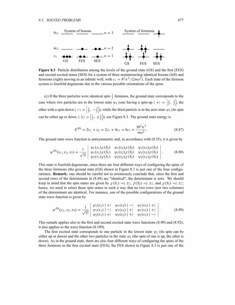
8.5. SOLVED PROBLEMS 477
1
4 1
9 1System of bosons
n 1
n 2
n 3
u uuGS
u uuFES
uu uSES
System of fermions
u6u?
u6GS
u6u6u?
FES
u6u?
u6
SES
Figure 8.3 Particle distribution among the levels of the ground state (GS) and the first (FES)
and second excited states (SES) for a system of three noninteracting identical bosons (left) and
fermions (right) moving in an infinite well, with 1 h2 2 2ma2 . Each state of the fermionsystem is fourfold degenerate due to the various possible orientations of the spins.
(c) If the three particles were identical spin 12fermions, the ground state corresponds to the
case where two particles are in the lowest state 1 (one having a spin-up12
12, the
other with a spin-down 12
12), while the third particle is in the next state 2 (its spin
can be either up or down, 12
12); see Figure 8.3. The ground state energy is
E 0 2 1 2 2 1 4 1 6 13h2 2
ma2(8.87)
The ground state wave function is antisymmetric and, in accordance with (8.55), it is given by
0 x1 x2 x31
3!
1 x1 S1 1 x2 S2 1 x3 S31 x1 S1 1 x2 S2 1 x3 S32 x1 S1 2 x2 S2 2 x3 S3
(8.88)
This state is fourfold degenerate, since there are four different ways of configuring the spins of
the three fermions (the ground state (GS) shown in Figure 8.3 is just one of the four configu-
rations). Remark: one should be careful not to erroneously conclude that, since the first and
second rows of the determinant in (8.88) are "identical", the determinant is zero. We should
keep in mind that the spin states are given by S1 , S2 , and S3 ;
hence, we need to select these spin states in such a way that no two rows (nor two columns)
of the determinant are identical. For instance, one of the possible configurations of the ground
state wave function is given by
0 x1 x2 x31
3!
1 x1 1 x2 1 x31 x1 1 x2 1 x32 x1 2 x2 2 x3
(8.89)
This remark applies also to the first and second excited state wave functions (8.90) and (8.92);
it also applies to the wave function (8.109).
The first excited state corresponds to one particle in the lowest state 1 (its spin can be
either up or down) and the other two particles in the state 2 (the spin of one is up, the other is
down). As in the ground state, there are also four different ways of configuring the spins of the
three fermions in the first excited state (FES); the FES shown in Figure 8.3 is just one of the
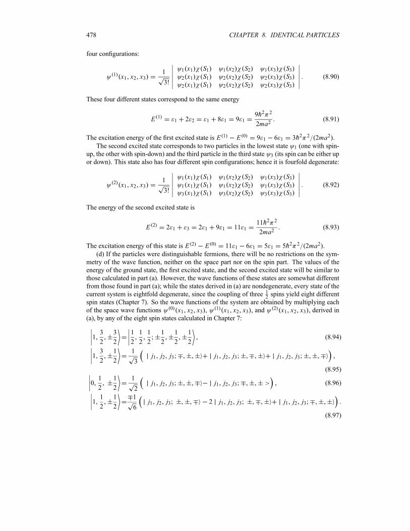
478 CHAPTER 8. IDENTICAL PARTICLES
four configurations:
1 x1 x2 x31
3!
1 x1 S1 1 x2 S2 1 x3 S32 x1 S1 2 x2 S2 2 x3 S32 x1 S1 2 x2 S2 2 x3 S3
(8.90)
These four different states correspond to the same energy
E 11 2 2 1 8 1 9 1
9h2 2
2ma2(8.91)
The excitation energy of the first excited state is E 1 E 0 9 1 6 1 3h2 2 2ma2 .The second excited state corresponds to two particles in the lowest state 1 (one with spin-
up, the other with spin-down) and the third particle in the third state 3 (its spin can be either up
or down). This state also has four different spin configurations; hence it is fourfold degenerate:
2 x1 x2 x31
3!
1 x1 S1 1 x2 S2 1 x3 S31 x1 S1 1 x2 S2 1 x3 S33 x1 S1 3 x2 S2 3 x3 S3
(8.92)
The energy of the second excited state is
E 2 2 1 3 2 1 9 1 11 111h2 2
2ma2(8.93)
The excitation energy of this state is E 2 E 0 11 1 6 1 5 1 5h2 2 2ma2 .(d) If the particles were distinguishable fermions, there will be no restrictions on the sym-
metry of the wave function, neither on the space part nor on the spin part. The values of the
energy of the ground state, the first excited state, and the second excited state will be similar to
those calculated in part (a). However, the wave functions of these states are somewhat different
from those found in part (a); while the states derived in (a) are nondegenerate, every state of the
current system is eightfold degenerate, since the coupling of three 12spins yield eight different
spin states (Chapter 7). So the wave functions of the system are obtained by multiplying each
of the space wave functions 0 x1 x2 x3 , 1 x1 x2 x3 , and 2 x1 x2 x3 , derived in(a), by any of the eight spin states calculated in Chapter 7:
13
2
3
2
1
2
1
2
1
2
1
2
1
2
1
2(8.94)
13
2
1
2
1
3j1 j2 j3 j1 j2 j3 j1 j2 j3
(8.95)
01
2
1
2
1
2j1 j2 j3 j1 j2 j3 (8.96)
11
2
1
2
1
6j1 j2 j3 2 j1 j2 j3 j1 j2 j3
(8.97)
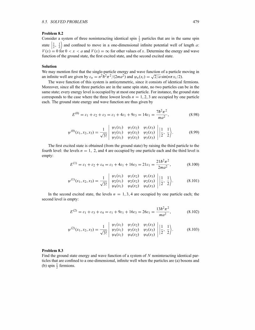
8.5. SOLVED PROBLEMS 479
Problem 8.2
Consider a system of three noninteracting identical spin 12particles that are in the same spin
state 12
12and confined to move in a one-dimensional infinite potential well of length a:
V x 0 for 0 x a and V x for other values of x . Determine the energy and wavefunction of the ground state, the first excited state, and the second excited state.
Solution
We may mention first that the single-particle energy and wave function of a particle moving in
an infinite well are given by n n2h2 2 2ma2 and n xi 2 a sin n xi 2 .The wave function of this system is antisymmetric, since it consists of identical fermions.
Moreover, since all the three particles are in the same spin state, no two particles can be in the
same state; every energy level is occupied by at most one particle. For instance, the ground state
corresponds to the case where the three lowest levels n 1 2 3 are occupied by one particle
each. The ground state energy and wave function are thus given by
E 01 2 3 1 4 1 9 3 14 1
7h2 2
ma2(8.98)
0 x1 x2 x31
3!
1 x1 1 x2 1 x32 x1 2 x2 2 x33 x1 3 x2 3 x3
1
2
1
2(8.99)
The first excited state is obtained (from the ground state) by raising the third particle to the
fourth level: the levels n 1 2, and 4 are occupied by one particle each and the third level is
empty:
E 11 2 4 1 4 1 16 3 21 1
21h2 2
2ma2(8.100)
1 x1 x2 x31
3!
1 x1 1 x2 1 x32 x1 2 x2 2 x34 x1 4 x2 4 x3
1
2
1
2(8.101)
In the second excited state, the levels n 1 3 4 are occupied by one particle each; the
second level is empty:
E 21 3 4 1 9 1 16 3 26 1
13h2 2
ma2(8.102)
2 x1 x2 x31
3!
1 x1 1 x2 1 x33 x1 3 x2 3 x34 x1 4 x2 4 x3
1
2
1
2(8.103)
Problem 8.3
Find the ground state energy and wave function of a system of N noninteracting identical par-ticles that are confined to a one-dimensional, infinite well when the particles are (a) bosons and
(b) spin 12fermions.

480 CHAPTER 8. IDENTICAL PARTICLES
Solution
In the case of a particle moving in an infinite well, its energy and wave function are n
n2h2 2 2ma2 and n xi 2 a sin n xi 2 .(a) In the case where the N particles are bosons, the ground state is obtained by putting all
the particles in the state n 1; the energy and wave function are then given by
E 01 1 1 1 N 1
Nh2 2
2ma2(8.104)
0 x1 x2 xNN
i 1
2
asin
2xi
2N
aNsin
2x1 sin
2x2 sin
2xN
(8.105)
(b) In the case where the N particles are spin 12fermions, each level can be occupied by at
most two particles having different spin states 12
12. The ground state is thus obtained by
distributing the N particles among the N 2 lowest levels at a rate of two particles per level:
E 0 2 1 2 2 2 3 2 N 2 2
N 2
n 1
n2h2 2
2ma2h2 2
ma2
N 2
n 1
n2 (8.106)
If N is large we may calculate N 2n 1 n
2 by using the approximation
N 2
n 1
n2N 2
1
n2dn1
3
N
2
3
(8.107)
hence the ground state energy will be given by
E 0 N3h2 2
24ma2(8.108)
The average energy per particle is E 0 N N2h2 2 24ma2 . In the case where N is even,a possible configuration of the ground state wave function 0 x1 x2 xN is given as
follows:
1
N !
1 x1 S1 1 x2 S2 1 xN SN1 x1 S1 1 x2 S2 1 xN SN2 x1 S1 2 x2 S2 2 xN SN2 x1 S1 2 x2 S2 2 xN SN3 x1 S1 3 x2 S2 3 xN SN3 x1 S1 3 x2 S2 3 xN SN
N 2 x1 S1 N 2 x2 S2 N 2 xN SNN 2 x1 S1 N 2 x2 S2 N 2 xN SN
(8.109)
where Si12
12is the spin state of the i th particle, with i 1, 2, 3, . . . , N . If N is
odd then we need to remove the last row of the determinant.
8.5. SOLVED PROBLEMS 481
Problem 8.4
Neglecting the spin–orbit interaction and the interaction between the electrons, find the energy
levels and the wave functions of the three lowest states for a two-electron atom.
Solution
Examples of such a system are the helium atom (Z 2), the singly ionized Li ion (Z 3),
the doubly ionized Be2 ion (Z 4), and so on. Neglecting the spin–orbit interaction and the
interaction between the electrons, V12 e2 r12 e2 r1 r2 , we can view each electron asmoving in the Coulomb field of the Ze nucleus. The Hamiltonian of this system is thereforeequal to the sum of the Hamiltonians of the two electrons:
H H 10 H 2
0
h2
221
Ze2
r1
h2
222
Ze2
r2(8.110)
where Mme M me , M is the mass of the nucleus, and me is the mass of the electron.We have considered here that the nucleus is placed at the origin and that the electrons are located
at r1 and r2. The Schrödinger equation of the system is given by
H 10 H 2
0 r1 S1 r2 S2 En1n2 r1 S1 r2 S2 (8.111)
where the energy En1n2 is equal to the sum of the energies of the electrons:
En1n2 E 0n1 E 0
n2
Z2e2
2a0
1
n21
Z2e2
2a0
1
n22(8.112)
where a0 h2 me2 is the Bohr radius. The wave function is equal to the product of the
spatial and spin parts:
r1 S1 r2 S2 r1 r2 S1 S2 (8.113)
S1 and S2 are the spin vectors of the electrons.Since this system consists of two identical fermions (electrons), its wave function has to be
antisymmetric. So either the spatial part is antisymmetric and the spin part is symmetric,
r1 S1 r2 S21
2n1l1m1 r1 n2l2m2 r2 n2l2m2 r1 n1l1m1 r2 tri plet S1 S2
(8.114)
or the spatial part is symmetric and the spin part is antisymmetric,
r1 S1 r2 S2 n1l1m1 r1 n2l2m2 r2 singlet S1 S2 (8.115)
where triplet and singlet , which result from the coupling of two spins12, are given by (8.67)
and (8.68).
Let us now specify the energy levels and wave functions of the three lowest states. The
ground state corresponds to both electrons occupying the lowest state nlm 100 (i.e.,
n1 n2 1); its energy and wave function can be inferred from (8.112) and (8.115):
E 0 E11 2E 01 2
Z2e2
2a027 2Z2 eV (8.116)
482 CHAPTER 8. IDENTICAL PARTICLES
0 r1 S1 r2 S2 100 r1 100 r2 singlet S1 S2 (8.117)
where 100 r R10 r Y00 1 Z a0 3 2e Zr a0 .
In the first excited state, one electron occupies the lowest level nlm 100 and the other
electron occupies the level nlm 200 ; this corresponds either to n1 1, n2 2 or to
n1 2, n2 1. The energy and the wave function can thus be inferred from (8.112) and
(8.114):
E 1 E12 E 01 E 0
2
Z2e2
2a0
1
4
Z2e2
2a0
5
413 6Z2 eV 17 0Z2 eV (8.118)
1 r1 S1 r2 S21
2100 r1 200 r2 200 r1 100 r2 triplet S1 S2 (8.119)
where 200 r R20 r Y00 1 8 Z a0 3 2 1 Zr 2a0 e Zr 2a0 .
Finally, the energy and wave function of the second excited state, which correspond to both
electrons occupying the second level nlm 200 (i.e., n1 n2 2), can be inferred from
(8.112) and (8.115):
E 2 E22 E 02 E 0
2 2E 02
1
2
Z2e2
2a0
1
213 6Z2 eV 6 8Z2 eV (8.120)
2 r1 S1 r2 S2 200 r1 200 r2 singlet S1 S2 (8.121)
These results are obviously not expected to be accurate because, by neglecting the Coulomb
interaction between the electrons, we have made a grossly inaccurate approximation. For in-
stance, the numerical value for the ground state energy obtained from (8.112) for the helium
atom is E 0theory 108 8 eV whereas the experimental value is E 0
exp 78 975 eV; that is,
the theoretical value is 37 8% lower than the experimental value.
In Chapter 9 we will show how to use perturbation theory and the variational method to
obtain very accurate theoretical values for the energy levels of two-electron atoms.
Problem 8.5
Find the energy levels and the wave functions of the ground state and the first excited state
for a system of two noninteracting identical particles moving in a common external harmonic
oscillator potential for (a) two spin 1 particles with no orbital angular momentum and (b) two
spin 12particles.
Solution
Since the particles are noninteracting and identical, their Hamiltonian is H H1 H2, whereH1 and H2 are the Hamiltonians of particles 1 and 2: H j h2 2m d2 dx2j m x2j 2 with
j 1 2. The total energy of the system is En1n2 n1 n2 , where n j n j12h .
(a) When the system consists of two identical spin 1 particles, the total wave function of
this system must be symmetric. Thus, the space and spin parts must be both symmetric or both
antisymmetric:
x1 S1 x2 S21
2s x1 x2 s S1 S2 a x1 x2 a S1 S2 (8.122)
8.5. SOLVED PROBLEMS 483
where
s x1 x21
2n1 x1 n2 x2 n1 x2 n2 x1 (8.123)
a x1 x21
2n1 x1 n2 x2 n1 x2 n2 x1 (8.124)
where n x is a harmonic oscillator wave function for the state n; for instance, the groundstate and first excited state are
0 x1
x0exp
x2
2x201 x
2
x30x exp
x2
2x20(8.125)
with x0 h m .
The spin states S1 S2 can be obtained by coupling the spins of the two particles, S1 1
and S2 1: S S1 S2. As shown in Chapter 7, the spin states corresponding to S 2 are
given by
2 2 11 1 1 2 11
21 1 1 0 1 1 0 1 (8.126)
2 01
61 1 1 1 2 1 1 0 0 1 1 1 1 (8.127)
those corresponding to S 1 by
1 11
21 1 1 0 1 1 0 1 (8.128)
1 01
21 1 1 1 1 1 1 1 (8.129)
and the one corresponding to S 0 by
0 01
31 1 1 1 1 1 0 0 1 1 1 1 (8.130)
Obviously, the five states 2 ms , corresponding to S 2 and 00 , are symmetric, whereas
the three states 1 ms are antisymmetric. Thus, s S1 S2 is given by any one of the six states2 2 , 2 1 , 2 0 , and 0 0 ; as for a S1 S2 , it is given by any one of the three states2 1 , and 1 0 .
The ground state corresponds to the case where both particles are in their respective ground
states n1 n2 0. The energy is then given by E 00 0
12h 1
2h h . Since
a x1 x2 , as given by (8.124), vanishes for n1 n2 0, the ground state wave function
(8.122) reduces to
0 x1 S1 x2 S2 0 x1 0 x2 s S1 S21
x0exp
x21 x222x20
s S1 S2
(8.131)
where 0 x is given by (8.125). The ground state is thus sixfold degenerate, since there are
six spin states s S1 S2 that are symmetric.
484 CHAPTER 8. IDENTICAL PARTICLES
In the first excited state, one particle occupies the ground state level n 0 and the other in
the first excited state n 1; this corresponds to two possible configurations: either n1 0 and
n2 1 or n1 1 and n2 0. The energy is then given by E 10 1
12h 3
2h 2h .
The first excited state can be inferred from (8.122) to (8.124):
1 x1 S1 x2 S21
20 x1 1 x2 0 x2 1 x1 s S1 S2
1
20 x1 1 x2 0 x2 1 x1 a S1 S2 (8.132)
where 0 x and 1 x are listed in (8.125). The first excited state is ninefold degenerate
since there are six spin states, s S1 S2 , that are symmetric and three, a S1 S2 , that areantisymmetric.
(b) For a system of two identical fermions, the wave function must be antisymmetric and
the space and spin parts must have opposite symmetries:
x1 S1 x2 S21
2s x1 x2 singlet S1 S2 a x1 x2 tri plet S1 S2 (8.133)
where the symmetric spin state, tri plet S1 S2 , is given by the triplet states listed in (8.67); theantisymmetric spin state, singlet S1 S2 , is given by the (singlet) state (8.68).
The ground state for the two spin 12particles corresponds to the case where both particles
occupy the lowest level, n1 n2 0, and have different spin states. The energy is then given
by E 00 0 h and the wave function by
0 x1 S1 x2 S2 0 x1 0 x2 singlet S1 S2
1
x0exp
x21 x222x20
singlet S1 S2 (8.134)
since a x1 x2 vanishes for n1 n2 0. The ground state is not degenerate, since there is
only one spin state which is antisymmetric, singlet S1 S2 .The first excited state corresponds also to n1 0 and n2 1 or n1 1 and n2 0. The
energy is then given by E 10 1 2h and the wave function by
1 x1 S1 x2 S21
20 x1 1 x2 0 x2 1 x1 singlet S1 S2
1
20 x1 1 x2 0 x2 1 x1 tri plet S1 S2 (8.135)
This state is fourfold degenerate since there are three spin states, triplet S1 S2 , that are sym-metric and one, singlet S1 S2 , that is antisymmetric.
8.6 Exercises
Exercise 8.1
Consider a system of three noninteracting identical bosons that move in a common external
one-dimensional harmonic oscillator potential. Find the energy levels and wave functions of
the ground state, the first excited state, and the second excited state of the system.
8.6. EXERCISES 485
Exercise 8.2
Consider two identical particles of spin 12that are confined in a cubical box of side L . Find the
energy and the wave function of this system in the case of no interaction between the particles.
Exercise 8.3
(a) Consider a system of two nonidentical particles, each of spin 1 and having no orbital
angular momentum (i.e., both particles are in s states). Write down all possible states for this
system.
(b) What restrictions do we get if the two particles are identical? Write down all possible
states for this system of two spin 1 identical particles.
Exercise 8.4
Two identical particles of spin 12are enclosed in a one-dimensional box potential of length L
with rigid walls at x 0 and x L . Assuming that the two-particle system is in a tripletspin state, find the energy levels, the wave functions, and the degeneracies corresponding to thethree lowest states.
Exercise 8.5
Two identical particles of spin 12are enclosed in a one-dimensional box potential of length L
with rigid walls at x 0 and x L. Assuming that the two-particle system is in a singletspin state, find the energy levels, the wave functions, and the degeneracies corresponding to thethree lowest states.
Exercise 8.6
Two identical particles of spin 12are moving under the influence of a one-dimensional harmonic
oscillator potential. Assuming that the two-particle system is in a triplet spin state, find theenergy levels, the wave functions, and the degeneracies corresponding to the three lowest states.
Exercise 8.7
Find the ground state energy, the average ground state energy per particle, and the ground state
wave function of a system of N noninteracting, identical bosons moving under the influence ofa one-dimensional harmonic oscillator potential.
Exercise 8.8
Find the ground state energy, the average ground state energy per particle, and the ground state
wave function of a system of N noninteracting identical spin 12particles moving under the
influence of a one-dimensional harmonic oscillator potential for the following two cases:
(a) when N is even and(b) when N is odd.
Exercise 8.9
Consider a system of four noninteracting particles that are confined to move in a one-dimensional
infinite potential well of length a: V x 0 for 0 x a and V x for other values
of x . Determine the energies and wave functions of the ground state, the first excited state, andthe second excited state when the four particles are
(a) distinguishable bosons such that their respective masses satisfy this relation: m1m2 m3 m4, and(b) identical bosons (each of mass m).
486 CHAPTER 8. IDENTICAL PARTICLES
Exercise 8.10
Consider a system of four noninteracting identical spin 1 2 particles (each of mass m) thatare confined to move in a one-dimensional infinite potential well of length a: V x 0 for
0 x a and V x for other values of x . Determine the energies and wave functions ofthe ground state and the first three excited states. Draw a figure showing how the particles are
distributed among the levels.
Exercise 8.11
Consider a system of four noninteracting identical spin 12particles that are in the same spin state
12
12and confined to move in a one-dimensional infinite potential well of length a: V x 0
for 0 x a and V x for other values of x . Determine the energies and wave functionsof the ground state, the first excited state, and the second excited state.
Exercise 8.12
Assuming the electrons in the helium atom to be spinless bosons and neglecting the interactions
between them, find the energy and the wave function of the ground state and the first excited
state of this (hypothetical) system.
Exercise 8.13
Assuming the electrons in the lithium atom to be spinless bosons and neglecting the interactions
between them, find the energy and the wave function of the ground state and the first excited
state of this (hypothetical) system.
Exercise 8.14
Consider a system of two noninteracting identical spin 1 2 particles (with mass m) that areconfined to move in a one-dimensional infinite potential well of length L: V x 0 for 0
x L and V x for other values of x . Assume that the particles are in a state with thewave function
x1 x22
Lsin
2 x1L
sin5 x2L
sin5 x1L
sin 2x2L
s1 s2
where x1 and x2 are the positions of particles 1 and 2, respectively, and s1 s2 is the spin
state of the two particles.
(a) Is s1 s2 going to be a singlet or triplet state?(b) Find the energy of this system.
Exercise 8.15
Consider a system of two noninteracting identical spin 1 2 particles (with mass m) that areconfined to move in a common one-dimensional harmonic oscillator potential. Assume that the
particles are in a state with the wave function
x1 x22
x20x2 x1 exp
x21 x222x20
s1 s2
where x1 and x2 are the positions of particles 1 and 2, respectively, and s1 s2 is the spin
state of the two particles.
(a) Is s1 s2 going to be a singlet or triplet state?(b) Find the energy of this system.
8.6. EXERCISES 487
Exercise 8.16
Consider a system of five noninteracting electrons (in the approximation where the Coulomb
interaction between the electrons is neglected) that are confined to move in a common one-
dimensional infinite potential well of length L 0 5 nm: V x 0 for 0 x L andV x for other values of x .(a) Find the ground state energy of the system.
(b) Find the energy of the first state of the system.
(c) Find the excitation energy of the first excited state.
Exercise 8.17
Determine the ground state electron configurations for the atoms having Z 40, 53, 70, and
82 electrons.
Exercise 8.18
Specify the possible J values (i.e., total angular momenta) associated with each of the followingstates: 1P , 4F , 2G, and 1H .
Exercise 8.19
Find the spectroscopic notation 2S 1L J (i.e., find the L, S, and J ) for the ground state config-urations of
(a) Sc (Z 21) and
(b) Cu (Z 29).

488 CHAPTER 8. IDENTICAL PARTICLES
Chapter 9
Approximation Methods for
Stationary States
9.1 Introduction
Most problems encountered in quantum mechanics cannot be solved exactly. Exact solutions ofthe Schrödinger equation exist only for a few idealized systems. To solve general problems, onemust resort to approximation methods. A variety of such methods have been developed, and
each has its own area of applicability. In this chapter we consider approximation methods that
deal with stationary states corresponding to time-independent Hamiltonians. In the followingchapter we will deal with approximation methods for explicitly time-dependent Hamiltonians.
To study problems of stationary states, we focus on three approximation methods: pertur-bation theory, the variational method, and the WKB method.Perturbation theory is based on the assumption that the problem we wish to solve is, in
some sense, only slightly different from a problem that can be solved exactly. In the case wherethe deviation between the two problems is small, perturbation theory is suitable for calculatingthe contribution associated with this deviation; this contribution is then added as a correction to
the energy and the wave function of the exactly solvable Hamiltonian. So perturbation theory
builds on the known exact solutions to obtain approximate solutions.
What about those systems whose Hamiltonians cannot be reduced to an exactly solvable
part plus a small correction? For these, we may consider the variational method or the WKB
approximation. The variational method is particularly useful in estimating the energy eigen-
values of the ground state and the first few excited states of a system for which one has only a
qualitative idea about the form of the wave function.
The WKB method is useful for finding the energy eigenvalues and wave functions of sys-
tems for which the classical limit is valid. Unlike perturbation theory, the variational and WKBmethods do not require the existence of a closely related Hamiltonian that can be solved exactly.
The application of the approximation methods to the study of stationary states consists of
finding the energy eigenvalues En and the eigenfunctions n of a time-independent Hamil-
tonian H that does not have exact solutions:
H n En n (9.1)
489
490 CHAPTER 9. APPROXIMATION METHODS FOR STATIONARY STATES
Depending on the structure of H , we can use any of the three methods mentioned above to findthe approximate solutions to this eigenvalue problem.
9.2 Time-Independent Perturbation Theory
This method is most suitable when H is very close to a Hamiltonian H0 that can be solvedexactly. In this case, H can be split into two time-independent parts
H H0 Hp (9.2)
where Hp is very small compared to H0 (H0 is known as the Hamiltonian of the unperturbed
system). As a result, Hp is called the perturbation, for its effects on the energy spectrum andeigenfunctions will be small; such perturbation is encountered, for instance, in systems subject
to weak electric or magnetic fields. We can make this idea more explicit by writing Hp in termsof a dimensionless real parameter which is very small compared to 1:
Hp W 1 (9.3)
Thus the eigenvalue problem (9.1) becomes
H0 W n En n (9.4)
In what follows we are going to consider two separate cases depending on whether the
exact solutions of H0 are nondegenerate or degenerate. Each of these two cases requires itsown approximation scheme.
9.2.1 Nondegenerate Perturbation Theory
In this section we limit our study to the case where H0 has no degenerate eigenvalues; that is,
for every energy E 0n there corresponds only one eigenstate n :
H0 n E 0n n (9.5)
where the exact eigenvalues E 0n and exact eigenfunctions n are known.
The main idea of perturbation theory consists in assuming that the perturbed eigenvalues
and eigenstates can both be expanded in power series in the parameter :
En E 0n E 1
n2E 2n (9.6)
n n1n
2 2n (9.7)
We need to make two remarks. First, one might think that whenever the perturbation is suffi-
ciently weak, the expansions (9.6) and (9.7) always exist. Unfortunately, this is not always the
case. There are cases where the perturbation is small, yet En and n are not expandable in
powers of . Second, the series (9.6) and (9.7) are frequently not convergent. However, when
is small, the first few terms do provide a reliable description of the system. So in practice, we
keep only one or two terms in these expansions; hence the problem of nonconvergence of these
series is avoided (we will deal later with the problem of convergence). Note that when 0
the expressions (9.6) and (9.7) yield the unperturbed solutions: En E 0n and n n .
9.2. TIME-INDEPENDENT PERTURBATION THEORY 491
The parameters E kn and the kets
kn represent the kth corrections to the eigenenergies and
eigenvectors, respectively.
The job of perturbation theory reduces then to the calculation of E 1n , E
2n , and
1n ,
2n , . In this section we shall be concerned only with the determination of E 1
n , E2n ,
and1n . Assuming that the unperturbed states n are nondegenerate, and substituting (9.6)
and (9.7) into (9.4), we obtain
H0 W n1n
2 2n
E 0n E 1
n2E 2n n
1n
2 2n
(9.8)
The coefficients of successive powers of on both sides of this equation must be equal. Equat-
ing the coefficients of the first three powers of , we obtain these results:
Zero order in :
H0 n E 0n n (9.9)
First order in :
H01n W n E 0
n1n E 1
n n (9.10)
Second order in :
H02n W 1
n E 0n
2n E 1
n1n E 2
n n (9.11)
We now proceed to determine the eigenvalues E 1n , E
2n and the eigenvector
1n from
(9.9) to (9.11). For this, we need to specify how the states n and n overlap. Since n
is considered not to be very different from n , we have n n 1. We can, however,
normalize n so that its overlap with n is exactly equal to one:
n n 1 (9.12)
Substituting (9.7) into (9.12) we get
n1n
2n
2n 0 (9.13)
hence the coefficients of the various powers of must vanish separately:
n1n n
2n 0 (9.14)
First-order correction
To determine the first-order correction, E 1n , to En we need simply to multiply both sides of
(9.10) by n :
E 1n n W n (9.15)
where we have used the facts that n H01n and n
1n are both equal to zero
and n n 1. The insertion of (9.15) into (9.6) thus yields the energy to first-order
perturbation:
En E 0n n Hp n (9.16)
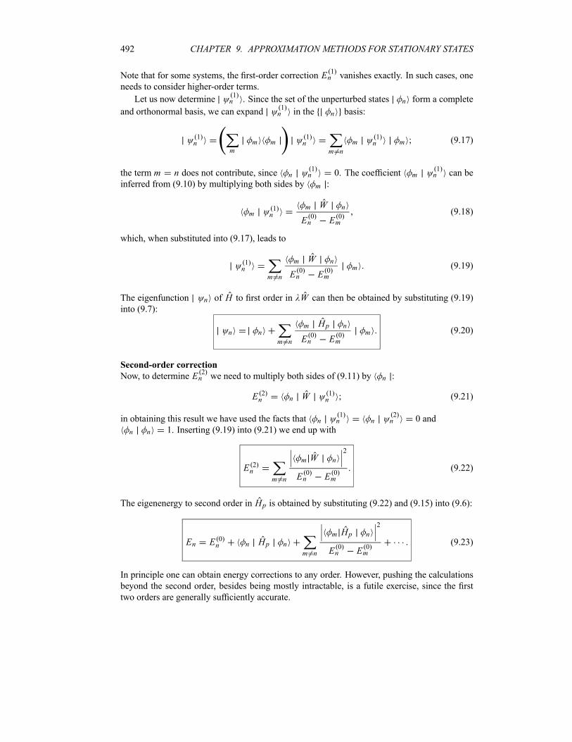
492 CHAPTER 9. APPROXIMATION METHODS FOR STATIONARY STATES
Note that for some systems, the first-order correction E 1n vanishes exactly. In such cases, one
needs to consider higher-order terms.
Let us now determine1n . Since the set of the unperturbed states n form a complete
and orthonormal basis, we can expand1n in the n basis:
1n
mm m
1n
m nm
1n m (9.17)
the term m n does not contribute, since n1n 0. The coefficient m
1n can be
inferred from (9.10) by multiplying both sides by m :
m1n
m W n
E 0n E 0
m
(9.18)
which, when substituted into (9.17), leads to
1n
m n
m W n
E 0n E 0
mm (9.19)
The eigenfunction n of H to first order in W can then be obtained by substituting (9.19)
into (9.7):
n nm n
m Hp n
E 0n E 0
mm (9.20)
Second-order correction
Now, to determine E 2n we need to multiply both sides of (9.11) by n :
E 2n n W 1
n (9.21)
in obtaining this result we have used the facts that n1n n
2n 0 and
n n 1. Inserting (9.19) into (9.21) we end up with
E 2n
m n
m W n
2
E 0n E 0
m
(9.22)
The eigenenergy to second order in Hp is obtained by substituting (9.22) and (9.15) into (9.6):
En E 0n n Hp n
m n
m Hp n
2
E 0n E 0
m
(9.23)
In principle one can obtain energy corrections to any order. However, pushing the calculations
beyond the second order, besides being mostly intractable, is a futile exercise, since the first
two orders are generally sufficiently accurate.
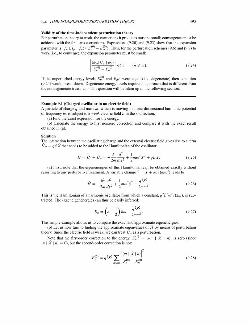
9.2. TIME-INDEPENDENT PERTURBATION THEORY 493
Validity of the time-independent perturbation theory
For perturbation theory to work, the corrections it produces must be small; convergence must be
achieved with the first two corrections. Expressions (9.20) and (9.23) show that the expansion
parameter is m Hp n E 0n E 0
m . Thus, for the perturbation schemes (9.6) and (9.7) to
work (i.e., to converge), the expansion parameter must be small:
m Hp n
E 0n E 0
m
1 n m (9.24)
If the unperturbed energy levels E 0n and E 0
m were equal (i.e., degenerate) then condition
(9.24) would break down. Degenerate energy levels require an approach that is different from
the nondegenerate treatment. This question will be taken up in the following section.
Example 9.1 (Charged oscillator in an electric field)
A particle of charge q and mass m, which is moving in a one-dimensional harmonic potentialof frequency , is subject to a weak electric field E in the x-direction.(a) Find the exact expression for the energy.
(b) Calculate the energy to first nonzero correction and compare it with the exact result
obtained in (a).
Solution
The interaction between the oscillating charge and the external electric field gives rise to a term
HP qEX that needs to be added to the Hamiltonian of the oscillator:
H H0 Hph
2m
d2
dX21
2m 2X2 qEX (9.25)
(a) First, note that the eigenenergies of this Hamiltonian can be obtained exactly without
resorting to any perturbative treatment. A variable change y X qE m 2 leads to
Hh2
2m
d2
dy21
2m 2y2
q2E2
2m 2(9.26)
This is the Hamiltonian of a harmonic oscillator from which a constant, q2E2 2 2m , is sub-tracted. The exact eigenenergies can thus be easily inferred:
En n1
2h
q2E2
2m 2(9.27)
This simple example allows us to compare the exact and approximate eigenenergies.
(b) Let us now turn to finding the approximate eigenvalues of H by means of perturbationtheory. Since the electric field is weak, we can treat Hp as a perturbation.
Note that the first-order correction to the energy, E 1n a n X n , is zero (since
n X n 0), but the second-order correction is not:
E 2n q2E2
m n
m X n2
E 0n E 0
m
(9.28)

494 CHAPTER 9. APPROXIMATION METHODS FOR STATIONARY STATES
Since E 0n n 1
2h , and using the relations
n 1 X n n 1h
2mn 1 X n n
h
2m(9.29)
E 0n E 0
n 1 h E 0n E 0
n 1 h (9.30)
we can reduce (9.28) to
E 2n q2E2
n 1 X n 2
E 0n E 0
n 1
n 1 X n 2
E 0n E 0
n 1
q2E2
2m 2(9.31)
hence the energy is given to second order by
En E 0n E 1
n E 2n n
1
2h
q2E2
2m 2(9.32)
This agrees fully with the exact energy found in (9.27).
Similarly, using (9.19) along with (9.29) and (9.30), we can easily ascertain that1n is
given by
1n
qE
h
h
2mn n 1 n 1 n 1 (9.33)
hence the state n is given to first order by
n nqE
h
h
2mn n 1 n 1 n 1 (9.34)
where n is the exact eigenstate of the nth excited state of a one-dimensional harmonic oscil-lator.
Example 9.2 (The Stark effect)
(a) Study the effect of an external uniform weak electric field, which is directed along the
positive z-axis, E Ek, on the ground state of a hydrogen atom; ignore the spin degrees offreedom.
(b) Find an approximate value for the polarizability of the hydrogen atom.
Solution
(a) The effect that an external electric field has on the energy levels of an atom is called the
Stark effect. In the absence of an electric field, the (unperturbed) Hamiltonian of the hydrogen
atom (in CGS units) is:
H0p 2
2
e2
r(9.35)
The eigenfunctions of this Hamiltonian, nlm r , were obtained in Chapter 6; they are given by
r nlm nlm r Rnl r Ylm (9.36)
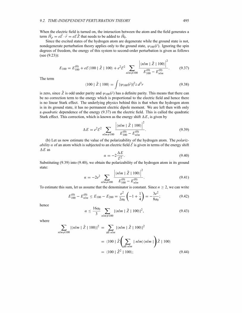
9.2. TIME-INDEPENDENT PERTURBATION THEORY 495
When the electric field is turned on, the interaction between the atom and the field generates a
term Hp eE r eEZ that needs to be added to H0.Since the excited states of the hydrogen atom are degenerate while the ground state is not,
nondegenerate perturbation theory applies only to the ground state, 100 r . Ignoring the spindegrees of freedom, the energy of this system to second-order perturbation is given as follows
(see (9.23)):
E100 E 0100 eE 100 Z 100 e2E2
nlm 100
nlm Z 1002
E 0100 E 0
nlm
(9.37)
The term
100 Z 100 100 r2z d3r (9.38)
is zero, since Z is odd under parity and 100 r has a definite parity. This means that there canbe no correction term to the energy which is proportional to the electric field and hence there
is no linear Stark effect. The underlying physics behind this is that when the hydrogen atom
is in its ground state, it has no permanent electric dipole moment. We are left then with only
a quadratic dependence of the energy (9.37) on the electric field. This is called the quadraticStark effect. This correction, which is known as the energy shift E , is given by
E e2E2
nlm 100
nlm Z 1002
E 0100 E 0
nlm
(9.39)
(b) Let us now estimate the value of the polarizability of the hydrogen atom. The polariz-ability of an atom which is subjected to an electric field E is given in terms of the energy shift
E as
2E
E2(9.40)
Substituting (9.39) into (9.40), we obtain the polarizability of the hydrogen atom in its ground
state:
2e2
nlm 100
nlm Z 1002
E 0100 E 0
nlm
(9.41)
To estimate this sum, let us assume that the denominator is constant. Since n 2, we can write
E 0100 E 0
nlm E100 E200e2
2a01
1
4
3e2
8a0(9.42)
hence16a03
nlm 100
nlm Z 100 2 (9.43)
where
nlm 100
nlm Z 100 2
all nlm
nlm Z 100 2
100 Zall nlm
nlm nlm Z 100
100 Z2 100 (9.44)
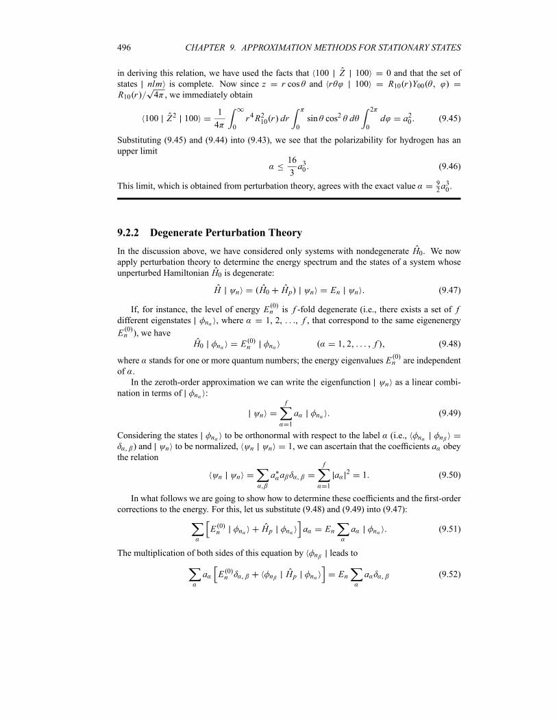
496 CHAPTER 9. APPROXIMATION METHODS FOR STATIONARY STATES
in deriving this relation, we have used the facts that 100 Z 100 0 and that the set of
states nlm is complete. Now since z r cos and r 100 R10 r Y00R10 r 4 , we immediately obtain
100 Z2 1001
4 0
r4R210 r dr0
sin cos2 d2
0
d a20 (9.45)
Substituting (9.45) and (9.44) into (9.43), we see that the polarizability for hydrogen has an
upper limit16
3a30 (9.46)
This limit, which is obtained from perturbation theory, agrees with the exact value 92a30 .
9.2.2 Degenerate Perturbation Theory
In the discussion above, we have considered only systems with nondegenerate H0. We nowapply perturbation theory to determine the energy spectrum and the states of a system whose
unperturbed Hamiltonian H0 is degenerate:
H n H0 Hp n En n (9.47)
If, for instance, the level of energy E 0n is f -fold degenerate (i.e., there exists a set of f
different eigenstates n , where 1, 2, , f , that correspond to the same eigenenergy
E 0n ), we have
H0 n E 0n n 1 2 f (9.48)
where stands for one or more quantum numbers; the energy eigenvalues E 0n are independent
of .
In the zeroth-order approximation we can write the eigenfunction n as a linear combi-
nation in terms of n :
n
f
1
a n (9.49)
Considering the states n to be orthonormal with respect to the label (i.e., n n
) and n to be normalized, n n 1, we can ascertain that the coefficients a obey
the relation
n n a af
1
a 2 1 (9.50)
In what follows we are going to show how to determine these coefficients and the first-order
corrections to the energy. For this, let us substitute (9.48) and (9.49) into (9.47):
E 0n n Hp n a En a n (9.51)
The multiplication of both sides of this equation by n leads to
a E 0n n Hp n En a (9.52)
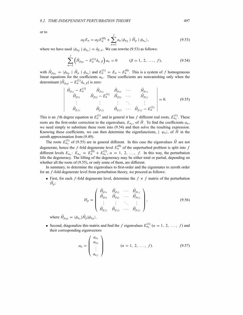
9.2. TIME-INDEPENDENT PERTURBATION THEORY 497
or to
a En a E 0n
f
1
a n Hp n (9.53)
where we have used n n . We can rewrite (9.53) as follows:
f
1
Hp E 1n a 0 1 2 f (9.54)
with Hp n Hp n and E 1n En E 0
n . This is a system of f homogeneouslinear equations for the coefficients a . These coefficients are nonvanishing only when the
determinant Hp E 1n is zero:
Hp11 E 1n Hp12 Hp13 Hp1 f
Hp21 Hp22 E 1n Hp23 Hp2 f
Hp f 1 Hp f 2 Hp f 3 Hp f f E 1n
0 (9.55)
This is an f th degree equation in E 1n and in general it has f different real roots, E 1
n . These
roots are the first-order correction to the eigenvalues, En , of H . To find the coefficients a ,we need simply to substitute these roots into (9.54) and then solve the resulting expression.
Knowing these coefficients, we can then determine the eigenfunctions, n , of H in the
zeroth approximation from (9.49).
The roots E 1n of (9.55) are in general different. In this case the eigenvalues H are not
degenerate, hence the f -fold degenerate level E 0n of the unperturbed problem is split into f
different levels En : En E 0n E 1
n , 1 2 f . In this way, the perturbationlifts the degeneracy. The lifting of the degeneracy may be either total or partial, depending on
whether all the roots of (9.55), or only some of them, are different.
In summary, to determine the eigenvalues to first-order and the eigenstates to zeroth order
for an f -fold degenerate level from perturbation theory, we proceed as follows:
First, for each f -fold degenerate level, determine the f f matrix of the perturbationHp:
Hp
Hp11 Hp12 Hp1 fHp21 Hp22 Hp2 f
Hp f 1 Hp f 2 Hp f f
(9.56)
where Hp n Hp n .
Second, diagonalize this matrix and find the f eigenvalues E 1n 1 2 f and
their corresponding eigenvectors
a
a1
a2
a f
1 2 f (9.57)
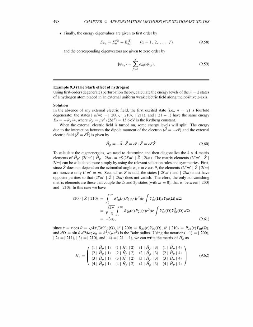
498 CHAPTER 9. APPROXIMATION METHODS FOR STATIONARY STATES
Finally, the energy eigenvalues are given to first order by
En E 0n E 1
n 1 2 f (9.58)
and the corresponding eigenvectors are given to zero order by
n
f
1
a n (9.59)
Example 9.3 (The Stark effect of hydrogen)
Using first-order (degenerate) perturbation theory, calculate the energy levels of the n 2 states
of a hydrogen atom placed in an external uniform weak electric field along the positive z-axis.
Solution
In the absence of any external electric field, the first excited state (i.e., n 2) is fourfold
degenerate: the states nlm 200 , 210 , 211 , and 21 1 have the same energy
E2 Ry 4, where Ry e4 2h2 13 6 eV is the Rydberg constant.
When the external electric field is turned on, some energy levels will split. The energy
due to the interaction between the dipole moment of the electron d er and the externalelectric field (E Ek) is given by
Hp d E er E eEZ (9.60)
To calculate the eigenenergies, we need to determine and then diagonalize the 4 4 matrix
elements of Hp: 2l m Hp 2lm eE 2l m Z 2lm . The matrix elements 2l m Z2lm can be calculated more simply by using the relevant selection rules and symmetries. First,
since Z does not depend on the azimuthal angle , z r cos , the elements 2l m Z 2lmare nonzero only if m m. Second, as Z is odd, the states 2l m and 2lm must have
opposite parities so that 2l m Z 2lm does not vanish. Therefore, the only nonvanishing
matrix elements are those that couple the 2s and 2p states (with m 0); that is, between 200
and 210 . In this case we have
200 Z 2100
R20 r R21 r r2dr Y00 zY10 d
4
3 0
R20 r R21 r r3dr Y00 Y 210 d
3a0 (9.61)
since z r cos 4 3rY10 , r 200 R20 r Y00 , r 210 R21 r Y10 ,
and d sin d d ; a0 h2 e2 is the Bohr radius. Using the notations 1 200 ,
2 211 , 3 210 , and 4 21 1 , we can write the matrix of Hp as
Hp
1 Hp 1 1 Hp 2 1 Hp 3 1 Hp 4
2 Hp 1 2 Hp 2 2 Hp 3 2 Hp 4
3 Hp 1 3 Hp 2 3 Hp 3 3 Hp 4
4 Hp 1 4 Hp 2 4 Hp 3 4 Hp 4
(9.62)

9.2. TIME-INDEPENDENT PERTURBATION THEORY 499
or as
Hp 3eEa0
0 0 1 0
0 0 0 0
1 0 0 0
0 0 0 0
(9.63)
The diagonalization of this matrix leads to the following eigenvalues:
E 12 1
3eEa0 E 12 2
E 12 3
0 E 12 4
3eEa0 (9.64)
Thus, the energy levels of the n 2 states are given to first order by
E21Ry4
3eEa0 E22 E23Ry4
E24Ry4
3eEa0 (9.65)
The corresponding eigenvectors to zeroth order are
2 11
2200 210 2 2 211 (9.66)
2 3 21 1 2 41
2200 210 (9.67)
This perturbation has only partially removed the degeneracy of the n 2 level; the states 211
and 21 1 still have the same energy E3 E4 Ry 4.
9.2.3 Fine Structure and the Anomalous Zeeman Effect
One of the most useful applications of perturbation theory is to calculate the energy correc-
tions for the hydrogen atom, notably the corrections due to the fine structure and the Zeeman
effect. The fine structure is in turn due to two effects: spin–orbit coupling and the relativistic
correction. Let us look at these corrections separately.
9.2.3.1 Spin–Orbit Coupling
The spin–orbit coupling in hydrogen arises from the interaction between the electron’s spin
magnetic moment, S eS mec , and the proton’s orbital magnetic field B.The origin of the magnetic field experienced by the electron moving at in a circular orbit
around the proton can be explained classically as follows. The electron, within its rest frame,
sees the proton moving at in a circular orbit around it (Figure 9.1). From classical electro-
dynamics, the magnetic field experienced by the electron is
B1
cE
1
mecp E
1
mecE p (9.68)
where p me is the linear momentum of the electron and E is the electric field generatedby the proton’s Coulomb’s field: E r e r2 r r er r3. For a more general problemof hydrogen-like atoms—atoms with one valence electron outside a closed shell—where an
electron moves in the (central) Coulomb potential of a nucleus V r e r , the electricfield is
E r r1
eV r
1
e
r
r
dV
dr(9.69)

500 CHAPTER 9. APPROXIMATION METHODS FOR STATIONARY STATES
PPPq
6L
wZe r te
me³³³1 PP
Pi
6
teL B
r wZe
m p³³³1
Figure 9.1 (Left) An electron moving in a circular orbit as seen by the nucleus. (Right) The
same motion as seen by the electron within its rest frame; the electron sees the nucleus moving
in a circular orbit around it.
So the magnetic field of the nucleus calculated in the rest frame of the electron is obtained by
inserting (9.69) into (9.68):
B1
mecE p
1
emec
1
r
dV
drr p
1
emec
1
r
dV
drL (9.70)
where L r p is the orbital angular momentum of the electron.The interaction of the electron’s spin dipole moment S with the orbital magnetic field B
of the nucleus gives rise to the following interaction energy:
HSO S Be
mecS B
1
m2ec2
1
r
dV
drS L (9.71)
This energy turns out to be twice the observed spin–orbit interaction. This is due to the fact that
(9.71) was calculated within the rest frame of the electron. This frame is not inertial, for the
electron accelerates while moving in a circular orbit around the nucleus. For a correct treatment,
we must transform to the rest frame of the nucleus (i.e., the lab frame). This transformation,
which involves a relativistic transformation of velocities, gives rise to an additional motion
resulting from the precession of S; this is known as the Thomas precession. The precessionof the electron’s spin moment is a relativistic effect which occurs even in the absence of an
external magnetic field. The transformation back to the rest frame of the nucleus leads to a
reduction of the interaction energy (9.71) by a factor of 2:
HSO1
2m2ec2
1
r
dV
drS L (9.72)
As this relation was derived from a classical treatment, we can now obtain the corresponding
quantum mechanical expression by replacing the dynamical variables with the corresponding
operators:
HSO1
2m2ec2
1
r
dV
drS L (9.73)
This is the spin–orbit energy. For a hydrogen’s electron, V r e2 r and dV dr e2 r2,equation (9.73) reduces to
HSOe2
2m2ec2
1
r3S L (9.74)
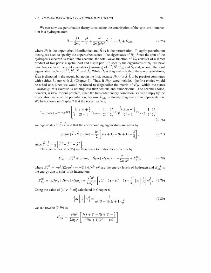
9.2. TIME-INDEPENDENT PERTURBATION THEORY 501
We can now use perturbation theory to calculate the contribution of the spin–orbit interac-
tion in a hydrogen atom:
Hp2
2me
e2
r
e2
2m2ec2r3S L H0 HSO (9.75)
where H0 is the unperturbed Hamiltonian and HSO is the perturbation. To apply perturbationtheory, we need to specify the unperturbed states—the eigenstates of H0. Since the spin of thehydrogen’s electron is taken into account, the total wave function of H0 consists of a directproduct of two parts: a spatial part and a spin part. To specify the eigenstates of H0, we havetwo choices: first, the joint eigenstates nlmlms of L2, S2, Lz , and Sz and, second, the jointeigenstates nl jm of L2, S2, J2, and Jz . While H0 is diagonal in both of these representations,
HSO is diagonal in the second but not in the first, because HSO (or S L to be precise) commuteswith neither Lz nor with Sz (Chapter 7). Thus, if HSO were included, the first choice wouldbe a bad one, since we would be forced to diagonalize the matrix of HSO within the statesnlmlms ; this exercise is nothing less than tedious and cumbersome. The second choice,
however, is ideal for our problem, since the first-order energy correction is given simply by the
expectation value of the perturbation, because HSO is already diagonal in this representation.We have shown in Chapter 7 that the states nl jm ,
n l j l 12 m
Rnl rl m 1
2
2l 1Yl m 1
2
1
2
1
2
l m 12
2l 1Yl m 1
2
1
2
1
2
(9.76)
are eigenstates of S L and that the corresponding eigenvalues are given by
nl jm L S nl jmh2
2j j 1 l l 1
3
4(9.77)
since S L 12J 2 L 2 S 2 .
The eigenvalues of (9.75) are then given to first-order correction by
Enl j E 0n nl jm j HSO nl jm j
e2
2a0
1
n2E 1SO (9.78)
where E 0n e2 2a0n2 13 6 n2 eV are the energy levels of hydrogen and E 1
SO is
the energy due to spin–orbit interaction:
E 1SO nl jm j HSO nl jm j
e2h2
4m2ec2j j 1 l l 1
3
4nl
1
r3nl (9.79)
Using the value of nl r 3 nl calculated in Chapter 6,
nl1
r3nl
2
n3l l 1 2l 1 a30(9.80)
we can rewrite (9.79) as
E 1SO
e2h2
2m2ec2
j j 1 l l 1 34
n3l l 1 2l 1 a30
502 CHAPTER 9. APPROXIMATION METHODS FOR STATIONARY STATES
e2
2a0
1
n2h
meca0
21
n
j j 1 l l 1 34
l l 1 2l 1(9.81)
or
E 1SO
E 0n
2
n
j j 1 l l 1 34
l l 1 2l 1(9.82)
where is a dimensionless constant called the fine structure constant:
h
meca0
e2
hc
1
137(9.83)
Since a0 h2 mee2 and hence E 0n e2 2a0n2 2mec2 2n2 , we can express
(9.82) in terms of as
E 1SO
4mec2
2n3j j 1 l l 1 3
4
l l 1 2l 1(9.84)
9.2.3.2 Relativistic Correction
Although the relativistic effect in hydrogen due to the motion of the electron is small, it can
still be detected by spectroscopic techniques. The relativistic kinetic energy of the electron is
given by T p2c2 m2ec4 mec2, where mec2 is the rest mass energy of the electron; an
expansion of this relation to p4 yields
p2c2 m2ec4 mec
2 p2
2me
p4
8m3ec2
(9.85)
When this term is included, the hydrogen’s Hamiltonian becomes
Hp2
2me
e2
r
p4
8m3ec2
H0 HR (9.86)
where H0 p2 2me e2 r is the unperturbed Hamiltonian and HR p 4 8m3ec2 is the
relativistic mass correction which can be treated by first-order perturbation theory:
E 1R nl jm j HR nl jm j
1
8m3ec2nl jm j p
4 nl jm j (9.87)
The value of nl jm j p 4 nl jm j was calculated in the last solved problem of Chapter 6 (seeequation (6.331)):
nl jm j p4 nl jm j
m4ee8
h4n48n
2l 13
4m4ec4
n48n
2l 13 (9.88)
An insertion of this value in (9.87) leads to
E 1R
4mec2
8n48n
2l 13
2 E 0n
4n28n
2l 13 (9.89)
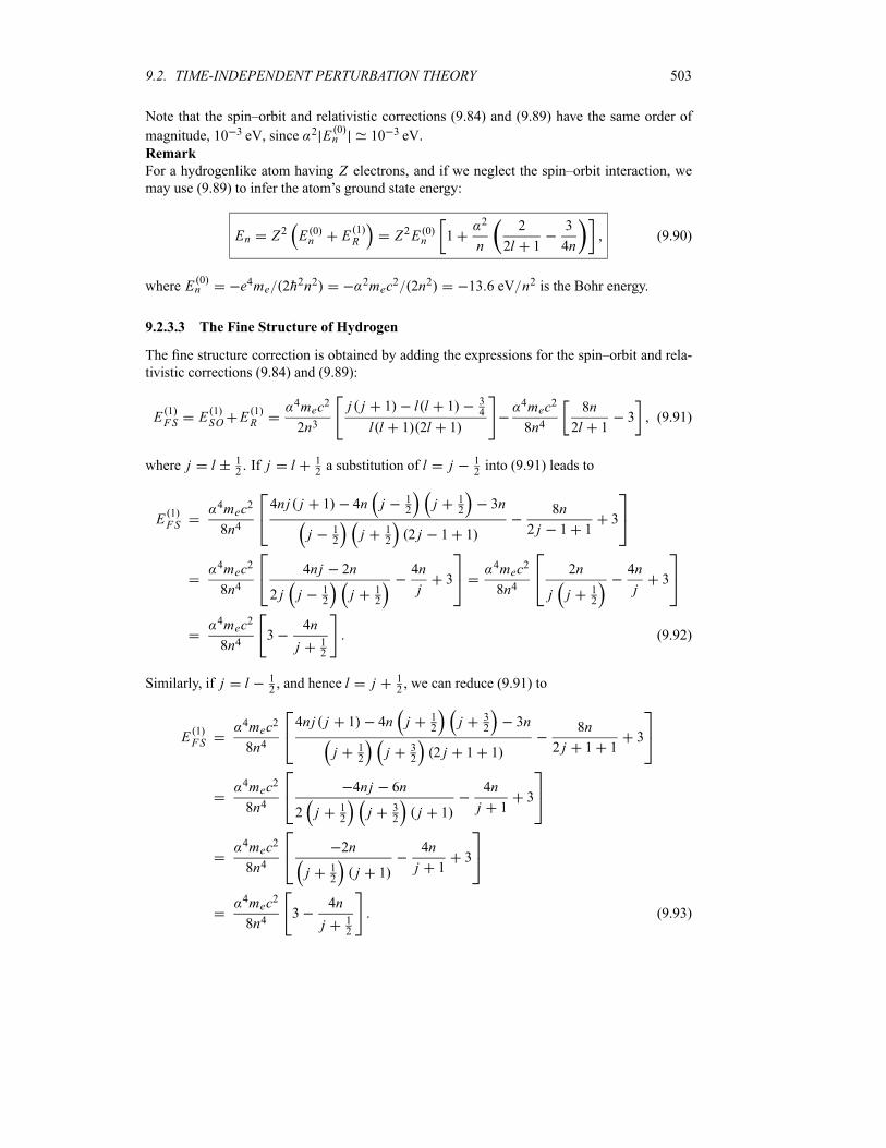
9.2. TIME-INDEPENDENT PERTURBATION THEORY 503
Note that the spin–orbit and relativistic corrections (9.84) and (9.89) have the same order of
magnitude, 10 3 eV, since 2 E 0n 10 3 eV.
Remark
For a hydrogenlike atom having Z electrons, and if we neglect the spin–orbit interaction, wemay use (9.89) to infer the atom’s ground state energy:
En Z2 E 0n E 1
R Z2E 0n 1
2
n
2
2l 1
3
4n(9.90)
where E 0n e4me 2h2n2 2mec2 2n2 13 6 eV n2 is the Bohr energy.
9.2.3.3 The Fine Structure of Hydrogen
The fine structure correction is obtained by adding the expressions for the spin–orbit and rela-
tivistic corrections (9.84) and (9.89):
E 1FS E 1
SO E 1R
4mec2
2n3j j 1 l l 1 3
4
l l 1 2l 1
4mec2
8n48n
2l 13 (9.91)
where j l 12. If j l 1
2a substitution of l j 1
2into (9.91) leads to
E 1FS
4mec2
8n4
4nj j 1 4n j 12
j 12
3n
j 12
j 12
2 j 1 1
8n
2 j 1 13
4mec2
8n44nj 2n
2 j j 12
j 12
4n
j3
4mec2
8n42n
j j 12
4n
j3
4mec2
8n43
4n
j 12
(9.92)
Similarly, if j l 12, and hence l j 1
2, we can reduce (9.91) to
E 1FS
4mec2
8n4
4nj j 1 4n j 12
j 32
3n
j 12
j 32
2 j 1 1
8n
2 j 1 13
4mec2
8n44nj 6n
2 j 12
j 32
j 1
4n
j 13
4mec2
8n42n
j 12
j 1
4n
j 13
4mec2
8n43
4n
j 12
(9.93)

504 CHAPTER 9. APPROXIMATION METHODS FOR STATIONARY STATES
As equations (9.92) and (9.93) show, the expressions for the fine structure correction corre-
sponding to j l 12and j l 1
2are the same:
E 1FS E 1
SO E 1R
4mec2
8n43
4n
j 12
2E 0n
4n24n
j 12
3 (9.94)
where E 0n
2mec2 2n2 and j l 12.
Since the bracket-terms in (9.82), (9.89), and (9.94) are of the order of unity, the ratios of
the spin–orbit, relativistic, and fine structure corrections to the energy of the hydrogen atom are
of the order of 2:
E 1SO
E 0n
2 E 1R
E 0n
2 E 1FS
E 0n
2 (9.95)
All these terms are of the order of 10 4 since 2 1 137 2 10 4.
In sum, the hydrogen’s Hamiltonian, when including the fine structure, is given by
H H0 HFS H0 HSO HRp2
2me
e2
r
e2
2m2ec2r3S L
p4
8m3ec2
(9.96)
A first-order perturbation calculation of the energy levels of hydrogen, when including the fine
structure, yields
Enj E 0n E 1
FS E 0n 1
2
4n24n
j 12
3 (9.97)
where E 0n 13 6 eV n2. Unlike E 0
n , which is degenerate in l, each energy level Enj is
split into two levels En l 12, since for a given value of l there are two values of j : j l 1
2.
In addition to the fine structure, there is still another (smaller) effect which is known as
the hyperfine structure. The hydrogen’s hyperfine structure results from the interaction of thespin of the electron with the spin of the nucleus. When the hyperfine corrections are included,
they would split each of the fine structure levels into a series of hyperfine levels. For instance,
when the hyperfine coupling is taken into account in the ground state of hydrogen, it would
split the 1S1 2 level into two hyperfine levels separated by an energy of 5 89 10 6 eV. This
corresponds, when the atom makes a spontaneous transition from the higher hyperfine level to
the lower one, to a radiation of 1 42 109Hz frequency and 21 cm wavelength. We should note
that most of the information we possess about interstellar hydrogen clouds had its origin in the
radioastronomy study of this 21 cm line.
9.2.3.4 The Anomalous Zeeman Effect
We now consider a hydrogen atom that is placed in an external uniform magnetic field B. Theeffect of an external magnetic field on the atom is to cause a shift of its energy levels; this
is called the Zeeman effect. In Chapter 6 we studied the Zeeman effect, but with one majoromission: we ignored the spin of the electron. In this section we are going to take it into
account. The interaction of the magnetic field with the electron’s orbital and spin magnetic

9.2. TIME-INDEPENDENT PERTURBATION THEORY 505
dipole moments, L and S , gives rise to two energy terms, L B and S B, whose sumwe call the Zeeman energy:
HZ L B S Be
2mecL B
e
mecS B
e
2mecL 2S B
eB
2mecLz 2Sz
(9.98)
with L eL 2mec and S S mec ; for simplicity, we have taken B along thez-axis: B Bz.When a hydrogen atom is placed in an external magnetic field, its Hamiltonian is given by
H H0 HFS HZ (9.99)
Like HFS , the correction due to HZ of (9.99) is expected to be small compared to H0; henceit can be treated perturbatively. We may now consider separately the cases where the magnetic
field B is strong or weak. Strong or weak compared to what? Since HSO and HZ can be writtenas HSO WL S (9.74) and since HZ B B L z 2Sz h, we have HZ HSO B B W ,where B is the Bohr magneton, B eh 2mec . Thus, the cases B W B and BW B would correspond to the weak and strong magnetic fields, respectively.
The strong-field Zeeman effect
The effect of a strong external magnetic field on the hydrogen atom is called the Paschen–Backeffect. If B is strong, B W B , the term eB L z 2Sz 2mec will be much greater thanthe fine structure. Neglecting HFS , we can reduce (9.99) to
H H0 HZ H0eB
2mecLz 2Sz (9.100)
Since H commutes with H0 (because H0 commutes with L z and Sz), they can be diagonalizedby a common set of states, nlmlms :
H nlmlms H0eB
2mecL z 2Sz nlmlms Enlmlms nlmlms (9.101)
where
Enlmlms E 0n
eBh
2mecml 2ms
e2
2a0n2eBh
2mecml 2ms (9.102)
The energy levels E 0n are thus shifted by an amount equal to E B B ml 2ms with
B eh 2mec , known as the Paschen–Back shift (Figure 9.2). When B 0 the degeneracy
of each level of hydrogen is given by gn 2 n 1l 0 2l 1 2n2; when B 0 states with the
same value of ml 2ms are still degenerate.
The weak-field Zeeman effect
If B is weak, B W B , we need to consider all the terms in the Hamiltonian (9.99); the
fine structure term HFS will be the dominant perturbation. In the case where the Hamiltoniancontains several perturbations at once, we should treat them individually starting with the most
dominant, then the next, and so on. In this case the eigenstate should be selected to be one that
diagonalizes the unperturbed Hamiltonian and the dominant perturbation1. In the weak-field
1When the various perturbations are of approximately equal size, a state that is a joint eigenstate of H0 and anyperturbation would be an acceptable choice.
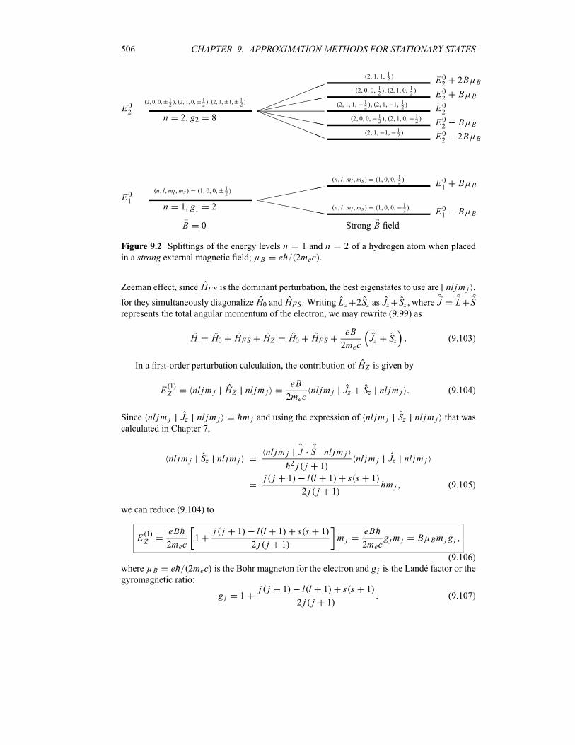
506 CHAPTER 9. APPROXIMATION METHODS FOR STATIONARY STATES
n 1, g1 2
n l ml ms 1 0 0 12
n 2, g2 8
2 0 0 12
2 1 0 12
2 1 1 12
B 0
E01
E02
n l ml ms 1 0 0 12
n l ml ms 1 0 0 12
E01 B B
E01 B B
Strong B field
2 1 1 12
2 0 0 12
2 1 0 12
2 1 1 12
2 1 1 12
2 0 0 12
2 1 0 12
2 1 1 12
E02 2B B
E02 B B
E02E02 B B
E02 2B B
ÃÃÃÃÃÃ
ÃÃ```````̀
!!!!
!!!!
ÃÃÃÃÃÃ
ÃÃ```````̀aaaaaaaa
Figure 9.2 Splittings of the energy levels n 1 and n 2 of a hydrogen atom when placed
in a strong external magnetic field; B eh 2mec .
Zeeman effect, since HFS is the dominant perturbation, the best eigenstates to use are nl jm j ,
for they simultaneously diagonalize H0 and HFS . Writing Lz 2Sz as Jz Sz , where J L Srepresents the total angular momentum of the electron, we may rewrite (9.99) as
H H0 HFS HZ H0 HFSeB
2mecJz Sz (9.103)
In a first-order perturbation calculation, the contribution of HZ is given by
E 1Z nl jm j HZ nl jm j
eB
2mecnl jm j Jz Sz nl jm j (9.104)
Since nl jm j Jz nl jm j hm j and using the expression of nl jm j Sz nl jm j that wascalculated in Chapter 7,
nl jm j Sz nl jm jnl jm j J S nl jm j
h2 j j 1nl jm j Jz nl jm j
j j 1 l l 1 s s 1
2 j j 1hm j (9.105)
we can reduce (9.104) to
E 1Z
eBh
2mec1
j j 1 l l 1 s s 1
2 j j 1m j
eBh
2mecg jm j B Bm jg j
(9.106)
where B eh 2mec is the Bohr magneton for the electron and g j is the Landé factor or thegyromagnetic ratio:
g j 1j j 1 l l 1 s s 1
2 j j 1(9.107)
9.3. THE VARIATIONAL METHOD 507
This shows that when l 0 and j s we have gs 2 and when s 0 and j l we havegl 1. For instance, for an atomic state2 such as 2P3 2, (9.107) shows that its factor is given
by g j 3 243, since j l s 1 1
232; this is how we infer the factor of any state:
State 2S1 22P1 2
2P3 22D3 2
2D5 22F5 2
2F7 2
g j 2 23
43
45
65
67
87
(9.108)
From (9.107), we see that the Landé factors corresponding to the same l but different valuesof j (due to spin) are not equal, since for s 1
2and j l 1
2we have
g j l 12
11
2l 1
2l 22l 1 for j l 1
2
2l2l 1 for j l 1
2
(9.109)
Combining (9.97), (9.103), and (9.106), we can write the energy of a hydrogen atom in a
weak external magnetic field as follows:
Enj E 0n E 1
FS E 1Z E 0
n
2E 0n
4n24n
j 12
3eBh
2mecm jg j (9.110)
The effect of the magnetic field on the atom is thus to split the energy levels with a spacing
E B Bm jg j . Unlike the energy levels obtained in Chapter 6, where we ignored theelectron’s spin, the energy levels (9.110) are not degenerate in l. Each energy level j is splitinto an even number of 2 j 1 sublevels corresponding to the 2 j 1 values of m j : m jj , j 1, , j 1, j . As displayed in Figure 9.3, the splittings between the sublevels
corresponding to the same j are constant: the spacings between the sublevels corresponding toj l 1 2 are all equal to 1 B B 2l 2l 1 , and the spacings between the j l 1 2
sublevels are equal to 2 B B 2l 2 2l 1 . In contrast to the normal Zeeman effect,
however, the spacings between the split levels of the same l (and different values of j) are nolonger constant, 1 2, since they depend on the Landé factor g j ; for a given value of j ,
there are two different values of g j corresponding to l j 12: g j l 1 2 2l 2 2l 1
and g j l 1 2 2l 2l 1 ; see (9.109). This unequal spacing between the split levels iscalled the anomalous Zeeman effect.
9.3 The Variational Method
There exist systems whose Hamiltonians are known, but they cannot be solved exactly or by a
perturbative treatment. That is, there is no closely related Hamiltonian that can be solved ex-
actly or approximately by perturbation theory because the first order is not sufficiently accurate.
One of the approximation methods that is suitable for solving such problems is the variationalmethod, which is also called the Rayleigh–Ritz method. This method does not require knowl-edge of simpler Hamiltonians that can be solved exactly. The variational method is useful for
determining upper bound values for the eigenenergies of a system whose Hamiltonian is known
2We use here the spectroscopic notation where 2s 1 L j designates an atomic state whose spin is s, its total angularmomentum is j , and whose orbital angular momentum is L where the values L 0 1 2 3 4 5 are designated,
respectively, by the capital letters S, P, D, F, G, H, (see Chapter 8).
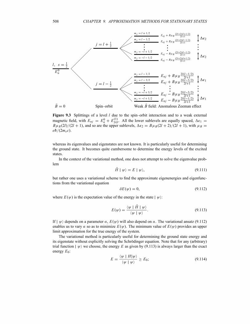
508 CHAPTER 9. APPROXIMATION METHODS FOR STATIONARY STATES
l s 12
E0n
B 0
j l 12
j l 12
Spin–orbit
m j l 1 2
m j l 3 2qqq
m j l 3 2
m j l 1 2 Enj B B2l l 1 22l 1
Enj B B2l l 3 22l 1qqq
Enj B B2l l 3 22l 1
Enj B B2l l 1 22l 1
Weak B field: Anomalous Zeeman effect
1
1
qqq
m j l 1 2
m j l 1 2
qqqm j l 1 2
m j l 1 2
Enj B B2l 2 l 1 2
2l 1
Enj B B2l 2 l 1 2
2l 1qqqEnj B B
2l 2 l 1 22l 1
Enj B B2l 2 l 1 2
2l 1
2
2
qqq
¡¡¡¡¡
@@@@@ ¡
¡¡
©©©
HHH@@@
¡¡¡
©©©
HHH@@@
6?
6?
6?
6?
Figure 9.3 Splittings of a level l due to the spin–orbit interaction and to a weak external
magnetic field, with Enj E0n E 1SO . All the lower sublevels are equally spaced, 1
B B 2l 2l 1 , and so are the upper sublevels, 2 B B 2l 2 2l 1 , with B
eh 2mec .
whereas its eigenvalues and eigenstates are not known. It is particularly useful for determining
the ground state. It becomes quite cumbersome to determine the energy levels of the excited
states.
In the context of the variational method, one does not attempt to solve the eigenvalue prob-
lem
H E (9.111)
but rather one uses a variational scheme to find the approximate eigenenergies and eigenfunc-
tions from the variational equation
E 0 (9.112)
where E is the expectation value of the energy in the state :
EH
(9.113)
If depends on a parameter , E will also depend on . The variational ansatz (9.112)
enables us to vary so as to minimize E . The minimum value of E provides an upper
limit approximation for the true energy of the system.
The variational method is particularly useful for determining the ground state energy and
its eigenstate without explicitly solving the Schrödinger equation. Note that for any (arbitrary)
trial function we choose, the energy E as given by (9.113) is always larger than the exactenergy E0:
EH
E0 (9.114)
9.3. THE VARIATIONAL METHOD 509
the equality condition occurs only when is proportional to the true ground state 0 . To
prove this, we simply expand the trial function in terms of the exact eigenstates of H :
n
an n (9.115)
with
H n En n (9.116)
and since E0 En for nondegenerate one-dimensional bound systems, we have
EH n an
2En
n an2
E0 n an2
n an2
E0 (9.117)
which proves (9.114).
To calculate the ground state energy, we need to carry out the following four steps:
First, based on physical intuition, make an educated guess of a trial function that takes
into account all the physical properties of the ground state (symmetries, number of nodes,
smoothness, behavior at infinity, etc.). For the properties you are not sure about, include
in the trial function adjustable parameters 1, 2, (i.e., 0 0 1 2 )
which will account for the various possibilities of these unknown properties.
Second, using (9.113), calculate the energy; this yields an expression which depends on
the parameters 1, 2, :
E0 1 20 1 2 H 0 1 2
0 1 2 0 1 2(9.118)
In most cases 0 1 2 will be assumed to be normalized; hence the denominator
of this expression is equal to 1.
Third, using (9.118) search for the minimum of E0 1 2 by varying the adjustable
parameters i until E0 is minimized. That is, minimize E 1 2 with respect to
1, 2 :
E0 1 2
i i
0 1 2 H 0 1 2
0 1 2 0 1 20 (9.119)
with i 1 2 . This gives the values of 10 20 that minimize E0.
Fourth, substitute these values of 10 20 into (9.118) to obtain the approximate
value of the energy. The value E0 10 20 thus obtained provides an upper bound
for the exact ground state energy E0. The exact ground state eigenstate 0 will then be
approximated by the state 0 10 20 .
What about the energies of the excited states? The variational method can also be used to find
the approximate values for the energies of the first few excited states. For instance, to find the
energy and eigenstate of the first excited state that will approximate E1 and 1 , we need to
choose a trial function 1 that must be orthogonal to 0 :
1 0 0 (9.120)
510 CHAPTER 9. APPROXIMATION METHODS FOR STATIONARY STATES
Then proceed as we did in the case of the ground state. That is, solve the variational equation
(9.112) for 1 :
i
1 1 2 H 1 1 2
1 1 2 1 1 20 i 1 2 (9.121)
Similarly, to evaluate the second excited state, we solve (9.112) for 2 and take into
account the following two conditions:
2 0 0 2 1 0 (9.122)
These conditions can be included in the variational problem by means of Lagrange multipliers,that is, by means of a constrained variational principle.
In this way, we can in principle evaluate any other excited state. However, the variational
procedure becomes increasingly complicated as we deal with higher excited states. As a result,
the method is mainly used to determine the ground state.
Remark
In those problems where the first derivative of the wave function is discontinuous at a given
value of x , one has to be careful when using the expression
h2
2m
d2
dx2h2
2mxd2 x
dx2dx (9.123)
A straightforward, careless use of this expression sometimes leads to a negative kinetic energy
term (Problem 9.6 on page 541). One might instead consider using the following form:
h2
2m
d2
dx2h2
2m
d x
dx
2
dx (9.124)
Note that (9.123) and (9.124) are identical; an integration by parts leads to
d x
dx
2
dx xd x
dxxd2 x
dx2dx x
d2 x
dx2dx
(9.125)
since x d x dx goes to zero as x (this is the case whenever x is a bound
state, but not so when x is a plane wave).What about the calculation of h2 2m in three dimensions? We might con-
sider generalizing (9.124). For this, we need simply to invoke Gauss’s theorem3 to show that
r r d3r r r d3r (9.126)
To see this, an integration by parts leads to the following relation:
Sr r d A
Vr r r r d3r (9.127)
3Gauss’s theorem states that the surface integral of a vector B over a closed surface S is equal to the volume integralof the divergence of that vector integrated over the volume V enclosed by the surface S: S B dS V B dV .
9.3. THE VARIATIONAL METHOD 511
and since, as S , the surface integral S r r dS vanishes if r is a boundstate, we recover (9.126). So the kinetic energy term (9.124) is given in three dimensions by
h2
2m
h2
2mr r d3r (9.128)
Example 9.4
Show that (9.112) is equivalent to the Schrödinger equation (9.111) .
Solution
Using (9.113), we can rewrite (9.112) as
H E 0 (9.129)
Since is a complex function, we can view and as two independent functions;
hence we can carry out the variations over and independently. Varying first over
, equation (9.129) yields
H E 0 (9.130)
Since is arbitrary, then (9.130) is equivalent to H E . The variation over
leads to the same result. Namely, varying (9.129) over , we get
H E 0 (9.131)
from which we obtain the complex conjugate equation H E , since H is Hermitian.
Example 9.5
Consider a one-dimensional harmonic oscillator. Use the variational method to estimate the
energies of (a) the ground state, (b) the first excited state, and (c) the second excited state.
Solution
This simple problem enables us to illustrate the various aspects of the variational method within
a predictable setting, because the exact solutions are known: E0 h 2, E1 3h 2,
E2 5h 2.
(a) The trial function we choose for the ground state has to be even and smooth everywhere,
it must vanish as x , and it must have no nodes. A Gaussian function satisfies these
requirements. But what we are not sure about is its width. To account for this, we include in
the trial function an adjustable scale parameter :
0 x Ae x2 (9.132)
A is a normalization constant. Using x2ne ax2dx a 1 3 5 2n 1 2a n , we
can show that A is given by A 2 1 4. The expression for E0 is thus given by
0 H 0 A2 e x2 h2
2m
d2
dx21
2m 2x2 e x2dx
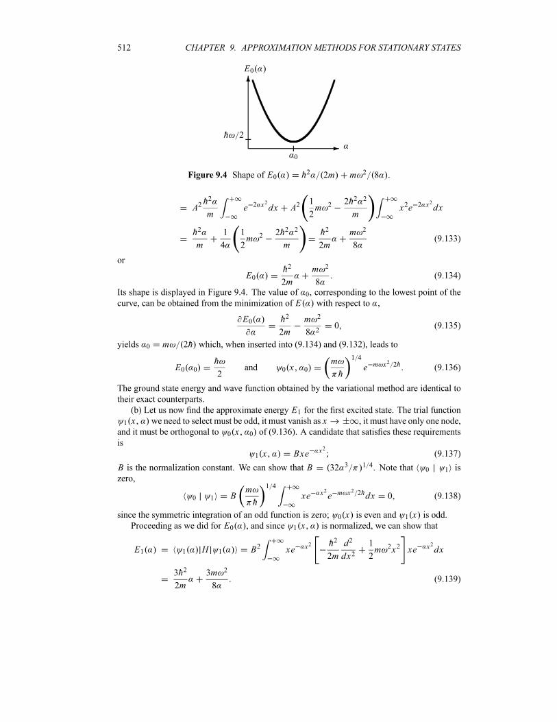
512 CHAPTER 9. APPROXIMATION METHODS FOR STATIONARY STATES
-
6
0
h 2
E0
Figure 9.4 Shape of E0 h2 2m m 2 8 .
A2h2
me 2 x2dx A2
1
2m 2 2h2 2
mx2e 2 x2dx
h2
m
1
4
1
2m 2 2h2 2
m
h2
2m
m 2
8(9.133)
or
E0h2
2m
m 2
8(9.134)
Its shape is displayed in Figure 9.4. The value of 0, corresponding to the lowest point of the
curve, can be obtained from the minimization of E with respect to ,
E0 h2
2m
m 2
8 20 (9.135)
yields 0 m 2h which, when inserted into (9.134) and (9.132), leads to
E0 0h
2and 0 x 0
m
h
1 4
e m x2 2h (9.136)
The ground state energy and wave function obtained by the variational method are identical to
their exact counterparts.
(b) Let us now find the approximate energy E1 for the first excited state. The trial function
1 x we need to select must be odd, it must vanish as x , it must have only one node,
and it must be orthogonal to 0 x 0 of (9.136). A candidate that satisfies these requirements
is
1 x Bxe x2 (9.137)
B is the normalization constant. We can show that B 32 3 1 4. Note that 0 1 is
zero,
0 1 Bm
h
1 4
xe x2e m x2 2hdx 0 (9.138)
since the symmetric integration of an odd function is zero; 0 x is even and 1 x is odd.Proceeding as we did for E0 , and since 1 x is normalized, we can show that
E1 1 H 1 B2 xe x2 h2
2m
d2
dx21
2m 2x2 xe x2dx
3h2
2m
3m 2
8(9.139)
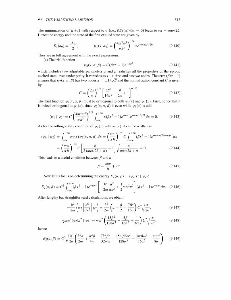
9.3. THE VARIATIONAL METHOD 513
The minimization of E1 with respect to (i.e., E1 0) leads to 0 m 2h.Hence the energy and the state of the first excited state are given by
E1 03h
21 x 0
4m3 3
h3
1 4
xe m x2 2h (9.140)
They are in full agreement with the exact expressions.
(c) The trial function
2 x C x2 1 e x2 (9.141)
which includes two adjustable parameters and , satisfies all the properties of the second
excited state: even under parity, it vanishes as x and has two nodes. The term x2 1
ensures that 2 x has two nodes x 1 and the normalization constant C is givenby
C2
1 43 2
16 2 21
1 2
(9.142)
The trial function 2 x must be orthogonal to both 0 x and 1 x . First, notice that itis indeed orthogonal to 1 x , since 2 x is even while 1 x is odd:
1 2 C4m3 3
h3
1 4
x x2 1 e x2e m x2 2hdx 0 (9.143)
As for the orthogonality condition of 2 x with 0 x , it can be written as
0 2 0 x 2 x dxm
h
1 4
C x2 1 e m 2h x2dx
m
h
1 4
C2 m 2h
1m 2h
0 (9.144)
This leads to a useful condition between and :
m
h2 (9.145)
Now let us focus on determining the energy E2 2 H 2 :
E2 C2 x2 1 e x2 h2
2m
d2
dx21
2m 2x2 x2 1 e x2dx (9.146)
After lengthy but straightforward calculations, we obtain
h2
2m2d2
dx22
h2
2m 2
7 2
16C2
2(9.147)
1
2m 2
2 x2
2 m 2 15 2
128 3
3
16 2
1
8C2
2(9.148)
hence
E2 C22
h2
2m
h2
4m
7h2 2
32m
15m 2 2
128 3
3m 2
16 2
m 2
8(9.149)

514 CHAPTER 9. APPROXIMATION METHODS FOR STATIONARY STATES
To extract the approximate value of E2, we need to minimize E2 with respect to and
to : E2 0 and E2 0. The two expressions we obtain will enable
us to extract (by solving a system of two linear equations with two unknowns) the values of
0 and 0 that minimize E2 . This method is lengthy and quite cumbersome; 0 and 0
have to satisfy the condition (9.145). We can, however, exploit this condition to come up with
a much shorter approach: it consists of replacing the value of as displayed in (9.145) into the
energy relation (9.149), thereby yielding an expression that depends on a single parameter :
E215h2
18m
9h
8
7m 2
16
15m3 4
128h2 3
9m2 3
32h 2
3m2 2
16h2 2
m
4h
3
4
1
(9.150)
in deriving this relation, we have substituted (9.145) into the expression for C as given by(9.142), which in turn is inserted into (9.149). In this way, we need to minimize E2 withrespect to one parameter only, . This yields 0 m 2h which, when inserted into (9.145)leads to 0 2m h. Thus, the energy and wave function are given by
E2 0 05
2h 2 x 0 0
m
4 h
1 42m
hx2 1 e
m2h x
2
(9.151)
These are identical with the exact expressions for the energy and the wave function.
Example 9.6
Use the variational method to estimate the ground state energy of the hydrogen atom.
Solution
The ground state wave function has no nodes and vanishes at infinity. Let us try
r e r (9.152)
where is a scale parameter; there is no angular dependence of r since the ground state
function is spherically symmetric. The energy is given by
EH h2 2m 2 e2 r
(9.153)
where
0
r2e 2r dr0
sin d2
0
d 3 (9.154)
ande2
r4 e2
0
re 2r dr e2 2 (9.155)
To calculate the kinetic energy term, we may use (9.128)
h2
2m2 h2
2mr r d3r (9.156)
where
r rd r
drr
1e r r (9.157)
9.4. THE WENTZEL–KRAMERS–BRILLOUIN METHOD 515
hence
h2
2m2 4
2
h2
2m 0
r2e 2r drh2
2m(9.158)
Inserting (9.154), (9.155), and (9.158) into (9.153), we obtain
Eh2
2m 2
e2(9.159)
Minimizing this relation with respect to , dE d h2 m 30 e2 2
0 0, we obtain
0 h2 me2 which, when inserted into (9.159), leads to the ground state energy
E 0me4
2h2(9.160)
This is the correct ground state energy for the hydrogen atom. The variational method has given
back the correct energy because the trial function (9.152) happens to be identical with the exact
ground state wave function. Note that the scale parameter 0 h2 me2 has the dimensionsof length; it is equal to the Bohr radius.
9.4 The Wentzel–Kramers–Brillouin Method
The Wentzel–Kramers–Brillouin (WKB) method is useful for approximate treatments of sys-
tems with slowly varying potentials; that is, potentials which remain almost constant over aregion of the order of the de Broglie wavelength. In the case of classical systems, this prop-
erty is always satisfied since the wavelength of a classical system approaches zero. The WKB
method can thus be viewed as a semiclassical approximation.
9.4.1 General Formalism
Consider the motion of a particle in a time-independent potential V r ; the Schrödinger equa-tion for the corresponding stationary state is
h2
2m2 r V r r E r (9.161)
or2 r
1
h2p2 r r 0 (9.162)
where p r is the classical momentum at r : p r 2m E V r . If the particle is moving
in a region where V r is constant, the solution of (9.162) is of the form r Ae i p r h . But
how does one deal with those cases where V r is not constant? The WKB method providesan approximate treatment for systems whose potentials, while not constant, are slowly varyingfunctions of r . That is, V r is almost constant in a region which extends over several de
Broglie wavelengths; we may recall that the de Broglie wavelength of a particle of mass m andenergy E that is moving in a potential V r is given by h p h 2m E V r .
516 CHAPTER 9. APPROXIMATION METHODS FOR STATIONARY STATES
In essence, the WKB method consists of trying a solution to (9.162) in the following form:
r A r ei S r h (9.163)
where the amplitude A r and the phase S r , which are real functions, are yet to be determined.Substituting (9.163) into (9.162) we obtain
Ah2
A2A S 2 p2 r ih 2 A S A 2S 0 (9.164)
The real and imaginary parts of this equation must vanish separately:
S 2 p2 r 2m E V r (9.165)
2 A S A 2S 0 (9.166)
In deriving (9.165) we have neglected the term that contains h (i.e., h2 A 2A), since it issmall compared to S 2 and to p2 r ; h is considered to be very small for classical systems.To illustrate the various aspects of the WKB method, let us consider the simple case of the
one-dimensional motion of a single particle. We can thus reduce (9.165) and (9.166), respec-tively, to
dS
dx2m E V p x (9.167)
2d
dxln A p x
d
dxp x 0 (9.168)
Let us find the solutions of (9.167) and (9.168). Integration of (9.167) yields
S x dx 2m E V x p x dx (9.169)
We can reduce (9.168) tod
dx2 ln A ln p x 0 (9.170)
which in turn leads to
A xC
p x(9.171)
where C is an arbitrary constant. So (9.169) and (9.171) give, respectively, the phase S x andamplitude A x of the WKB wave function (9.163).Inserting (9.171) and (9.169) into (9.163), we obtain two approximate solutions to equation
(9.162):
xC
p xexp
i
h
x
p x dx (9.172)
The amplitude of this wave function is proportional to 1 p x ; hence the probability of find-ing the particle between x and x dx is proportional to 1 p x . This is what we expect fora “classical” particle because the time it will take to travel a distance dx is proportional to theinverse of its speed (or its momentum).
9.4. THE WENTZEL–KRAMERS–BRILLOUIN METHOD 517
We can now examine two separate cases corresponding to E V x and E V x . First,let us consider the case E V x , which is called the classically allowed region. Here p x isa real function; the most general solution of (9.162) is a combination of x and x :
xC
p xexp
i
h
x
p x dxC
p xexp
i
h
x
p x dx (9.173)
Second, in the case where E V x , which is known as the classically forbidden region,the momentum p x is imaginary and the exponents of (9.172) become real:
xC
p xexp
1
h xp x dx
C
p xexp
1
h
x
p x dx (9.174)
Equations (9.173) and (9.174) give the system’s wave function in the allowed and forbidden
regions, respectively. But what about the structure of the wave function near the regions EV x ? At the points xi , we have E V xi ; hence the momentum (9.167) vanishes, p xi 0.
These points are called the classical turning points, because classically the particle stops at xiand then turns back to resume its motion in the opposite direction. At these points the wave
function (9.172) becomes infinite since p xi 0. One then needs to examine how to find the
wave function at the turning points. Before looking into that, let us first study the condition of
validity for the WKB approximation.
Validity of the WKB approximation
To obtain the condition of validity for the WKB method, let us examine the size of the various
terms in (9.164), notably A S 2 and ihA 2S. Since quantities of the order of h are too smallin the classical limit, the quasi-classical region is expected to be given by the condition4
h 2S S 2 (9.175)
which can be written in one dimension as
hS
S 21 (9.176)
ord
dx
h
S1 (9.177)
since 2S d2S dx2 S and S dS x dx S . In what follows we are going toverify that this relation yields the condition of validity for the WKB approximation.
Since S p x (see (9.167)), we can reduce (9.177) to
d x
dx1 (9.178)
where x x 2 and x is the de Broglie wavelength of the particle:
xh
p x
h
2m E V x(9.179)
4The condition (9.175) can be found as follows. Substituting r ei S r h into (9.162) and multiplying by h2,we get ih 2S r S 2 p2 r 0. In the classical limit, the term containing h, ih 2S r , must be smallcompared to the terms that do not, S 2; i.e., h 2S r S 2.
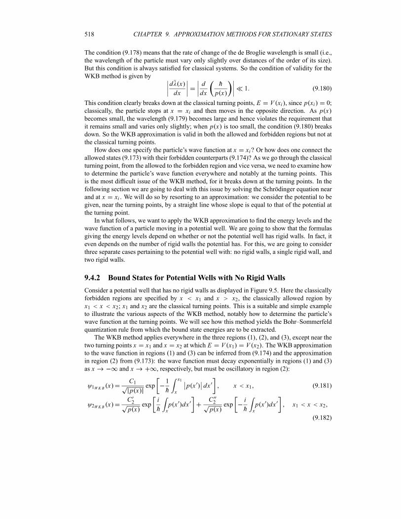
518 CHAPTER 9. APPROXIMATION METHODS FOR STATIONARY STATES
The condition (9.178) means that the rate of change of the de Broglie wavelength is small (i.e.,
the wavelength of the particle must vary only slightly over distances of the order of its size).
But this condition is always satisfied for classical systems. So the condition of validity for the
WKB method is given by
d x
dx
d
dx
h
p x1 (9.180)
This condition clearly breaks down at the classical turning points, E V xi , since p xi 0;
classically, the particle stops at x xi and then moves in the opposite direction. As p xbecomes small, the wavelength (9.179) becomes large and hence violates the requirement that
it remains small and varies only slightly; when p x is too small, the condition (9.180) breaks
down. So the WKB approximation is valid in both the allowed and forbidden regions but not at
the classical turning points.
How does one specify the particle’s wave function at x xi? Or how does one connect theallowed states (9.173) with their forbidden counterparts (9.174)? As we go through the classical
turning point, from the allowed to the forbidden region and vice versa, we need to examine how
to determine the particle’s wave function everywhere and notably at the turning points. This
is the most difficult issue of the WKB method, for it breaks down at the turning points. In the
following section we are going to deal with this issue by solving the Schrödinger equation near
and at x xi . We will do so by resorting to an approximation: we consider the potential to begiven, near the turning points, by a straight line whose slope is equal to that of the potential at
the turning point.
In what follows, we want to apply the WKB approximation to find the energy levels and the
wave function of a particle moving in a potential well. We are going to show that the formulas
giving the energy levels depend on whether or not the potential well has rigid walls. In fact, it
even depends on the number of rigid walls the potential has. For this, we are going to consider
three separate cases pertaining to the potential well with: no rigid walls, a single rigid wall, and
two rigid walls.
9.4.2 Bound States for Potential Wells with No Rigid Walls
Consider a potential well that has no rigid walls as displayed in Figure 9.5. Here the classically
forbidden regions are specified by x x1 and x x2, the classically allowed region byx1 x x2; x1 and x2 are the classical turning points. This is a suitable and simple exampleto illustrate the various aspects of the WKB method, notably how to determine the particle’s
wave function at the turning points. We will see how this method yields the Bohr–Sommerfeld
quantization rule from which the bound state energies are to be extracted.
The WKB method applies everywhere in the three regions 1 , 2 , and 3 , except near the
two turning points x x1 and x x2 at which E V x1 V x2 . TheWKB approximationto the wave function in regions 1 and 3 can be inferred from (9.174) and the approximation
in region 2 from (9.173): the wave function must decay exponentially in regions (1) and (3)
as x and x , respectively, but must be oscillatory in region (2):
1WK B xC1p x
exp1
h
x1
xp x dx x x1 (9.181)
2WK B xC2p x
expi
h xp x dx
C2p x
expi
h xp x dx x1 x x2
(9.182)
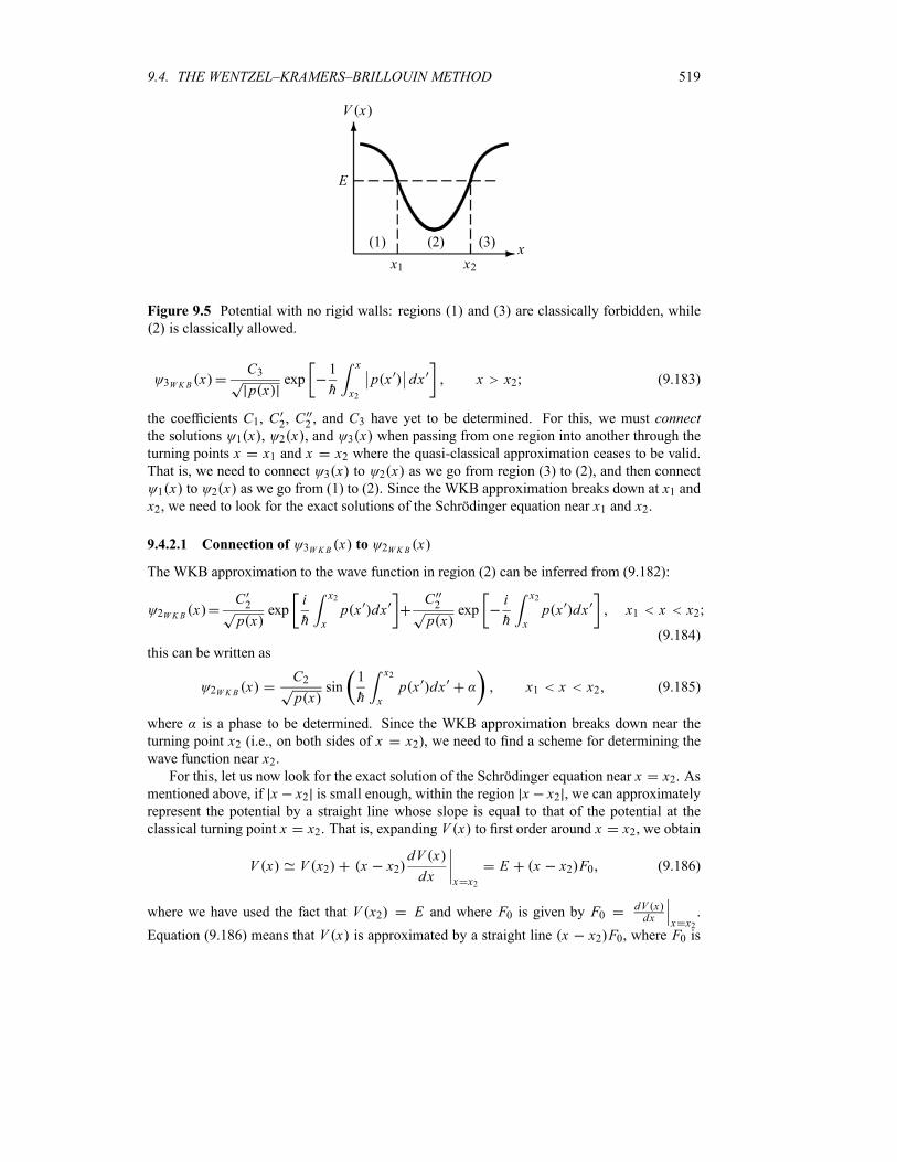
9.4. THE WENTZEL–KRAMERS–BRILLOUIN METHOD 519
-
6
1 2 3
x1 x2
E
x
V x
Figure 9.5 Potential with no rigid walls: regions 1 and 3 are classically forbidden, while
2 is classically allowed.
3WKB xC3p x
exp1
h
x
x2
p x dx x x2 (9.183)
the coefficients C1, C2, C2 , and C3 have yet to be determined. For this, we must connectthe solutions 1 x , 2 x , and 3 x when passing from one region into another through the
turning points x x1 and x x2 where the quasi-classical approximation ceases to be valid.That is, we need to connect 3 x to 2 x as we go from region (3) to (2), and then connect
1 x to 2 x as we go from (1) to (2). Since the WKB approximation breaks down at x1 andx2, we need to look for the exact solutions of the Schrödinger equation near x1 and x2.
9.4.2.1 Connection of 3WKB x to 2WK B x
The WKB approximation to the wave function in region (2) can be inferred from (9.182):
2WKB xC2p x
expi
h
x2
xp x dx
C2p x
expi
h
x2
xp x dx x1 x x2
(9.184)
this can be written as
2WKB xC2p x
sin1
h
x2
xp x dx x1 x x2 (9.185)
where is a phase to be determined. Since the WKB approximation breaks down near the
turning point x2 (i.e., on both sides of x x2), we need to find a scheme for determining thewave function near x2.For this, let us now look for the exact solution of the Schrödinger equation near x x2. As
mentioned above, if x x2 is small enough, within the region x x2 , we can approximatelyrepresent the potential by a straight line whose slope is equal to that of the potential at the
classical turning point x x2. That is, expanding V x to first order around x x2, we obtain
V x V x2 x x2dV x
dx x x2
E x x2 F0 (9.186)
where we have used the fact that V x2 E and where F0 is given by F0dV xdx x x2
.
Equation (9.186) means that V x is approximated by a straight line x x2 F0, where F0 is

520 CHAPTER 9. APPROXIMATION METHODS FOR STATIONARY STATES
the slope of V x at x x2. The Schrödinger equation for the potential (9.186) can be writtenas
d2 x
dx22mF0
h2x x2 x 0 (9.187)
Using the change of variable
y2mF0
h2
1 3
x x2 (9.188)
we can transform (9.187) into
2mF0
h2
2 3 d2 y
dy2y y 0 (9.189)
ord2 y
dy2y y 0 (9.190)
This is a well-known differential equation whose solutions are usually expressed in terms of the
Airy functions5 Ai y :
y A Ai yA
0
cosz3
3yz dz (9.191)
where A is a normalization constant.From the properties of the Airy function Ai y 1 0 cos z3 3 yz dz, the asymptotic
behavior of Ai y is given for large positive and large negative values of y by
Ai y1y 1 4
sin 23
y 3 24
y 0
12 y1 4
exp 23y3 2 y 0
(9.192)
The asymptotic expression of (9.191) is therefore given for large positive and large negative
values of y by
yAy 1 4
sin 23
y 3 24
y 0
A2 y1 4
exp 23y3 2 y 0
(9.193)
Since F0 0 equation (9.188) implies that the cases y 0 and y 0 correspond to x x2and x x2, respectively.Now near the turning point x x2, (9.186) shows that E V x x x2 F0; hence
the square of the classical momentum p2 x is given by
p2 x 2m E V x 2m x x2 F0 (9.194)
which is negative for x x2 and positive for x x2. Combining equations (9.188) and (9.194),we obtain
p2 x 2mhF02 3 y (9.195)
5The solution to the differential equation d2 y dy y y is given by the Airy function y Ai y10 cos z3 3 yz dz.
9.4. THE WENTZEL–KRAMERS–BRILLOUIN METHOD 521
Now since dx h2 2mF0 1 3dy (see (9.188)), we use (9.195) to infer the following expres-sion:
1
h
x2
xp x dx
1
h2mhF0
1 3 h2
2mF0
1 30
yy dy
0
yy dy
2
3y 3 2
(9.196)
Inserting this into (9.193), we obtain
xAp x
sin 1h
x2x p x dx
4x x2
A2 p x
exp 1h
x2x p x dx x x2
(9.197)
where A 2mhF0 1 6A . A comparison of (9.197a) with (9.185) and (9.197b) with
(9.183) reveals that
A 2C3 C2 A4
(9.198)
these expressions are known as the connection formulas, for they connect the WKB solutionsat either side of a turning point. Since 4, 2WK B x of (9.185) becomes
2WK B xC2p x
sin1
h
x2
xp x dx
4(9.199)
9.4.2.2 Connection of 1WKB x to 2WK B x
The WKB wave function for x x1 is given by (9.181); the WKB solution for x x1 can beinferred from (9.182):
2WK B xC2p x
expi
h
x
x1
p x dxC2p x
expi
h
x1
xp x dx x1 x x2
(9.200)
which can be written as
2WK B xD
psin
1
h
x
x1
p x dx (9.201)
Recall that near x x1 the WKB approximation breaks down.The shape of the wave function near x x1 can, however, be found from an exact solution
of the Schrödinger equation. For this, we proceed as we did for x x2. That is, we look forthe exact solution of the Schrödinger equation for small values of x x1 . Expanding V xnear x x1, we obtain a Schrödinger equation similar to (9.190). Its solutions for x x1 andx x1 are given by expressions that are similar to (9.197b) and (9.197a) respectively:
xE
2 p xexp 1
hxx1p x dx x x1
Ep x
sin 1h
xx1p x dx
4x x1
(9.202)
Again, comparing (9.202a) with (9.181) and (9.202b) with (9.201), we obtain the other set of
connection formulas:
E 2C1 E D4
(9.203)
522 CHAPTER 9. APPROXIMATION METHODS FOR STATIONARY STATES
hence 2 x of (9.201) becomes
2WK B xD
p xsin
1
h
x
x1
p x dx4
(9.204)
9.4.2.3 Quantization of the Energy Levels of the Bound States
Since the two solutions (9.199) and (9.204) represent the same wave function in the same re-
gion, they must be equal:
2WK B xD
p xsin
1
h
x
x1
p x dx4
C2p x
sin1
h
x2
xp x dx
4(9.205)
This is an equation of the form D sin 1 C2 sin 2. Its solutions must satisfy the following
two relations. The first is 1 2 n 1 , i.e.,
1
h
x
x1
p x dx4
1
h
x2
xp x dx
4n 1 (9.206)
or1
h
x2
x1
p x dx n1
2n 0 1 2 3 (9.207)
and the second is
D 1 nC2 (9.208)
Since the integral between the turning pointsx2x1p x dx is equal to half the integral over a
complete period of the quasi-classical motion of the particle, i.e.,x2x1p x dx 1
2p x dx ,
we can reduce (9.207) to
p x dx 2x2
x1
p x dx n1
2h n 0 1 2 3 (9.209)
This relation determines the quantized (WKB) energy levels En of the bound states of a semi-classical system. It is similar to the Bohr–Sommerfeld quantization rule, which in turn is knownto represent an improved version of the Wilson–Sommerfeld rule p x dx nh, because theWilson–Sommerfeld rule does not include the zero-point energy term h 2 (in the case of largevalues of n, where the classical approximation becomes reliable, we have n 1 2 n; hence(9.209) reduces to p x dx nh). We can interpret this relation as follows: since the integralp x dx gives the area enclosed by the closed trajectory of the particle in the xp phase space,
the condition (9.209) provides the mechanism for selecting, from the continuum of energy val-
ues of the semiclassical system, only those energies En for which the areas of the contoursp x En 2m En V x are equal to n 1
2h:
p x En dx 2x2
x1
2m En V x dx n1
2h (9.210)
with n 0, 1, 2, 3, . So in the xp phase space, the area between two successive bound statesis equal to h: p x En 1 dx p x En dx h. Each single state therefore corresponds
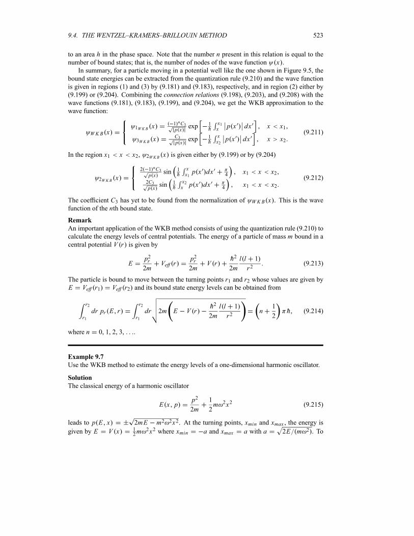
9.4. THE WENTZEL–KRAMERS–BRILLOUIN METHOD 523
to an area h in the phase space. Note that the number n present in this relation is equal to thenumber of bound states; that is, the number of nodes of the wave function x .In summary, for a particle moving in a potential well like the one shown in Figure 9.5, the
bound state energies can be extracted from the quantization rule (9.210) and the wave function
is given in regions (1) and (3) by (9.181) and (9.183), respectively, and in region (2) either by
(9.199) or (9.204). Combining the connection relations (9.198), (9.203), and (9.208) with thewave functions (9.181), (9.183), (9.199), and (9.204), we get the WKB approximation to the
wave function:
WK B x1WK B x
1 nC3p x
exp 1h
x1x p x dx x x1
3WK B xC3p x
exp 1h
xx2p x dx x x2
(9.211)
In the region x1 x x2, 2WKB x is given either by (9.199) or by (9.204)
2WK B x
2 1 nC3p x
sin 1h
xx1p x dx
4x1 x x2
2C3p x
sin 1h
x2x p x dx
4x1 x x2
(9.212)
The coefficient C3 has yet to be found from the normalization of WK B x . This is the wavefunction of the nth bound state.
Remark
An important application of the WKB method consists of using the quantization rule (9.210) to
calculate the energy levels of central potentials. The energy of a particle of mass m bound in acentral potential V r is given by
Ep2r2m
Veff rp2r2m
V rh2
2m
l l 1
r2(9.213)
The particle is bound to move between the turning points r1 and r2 whose values are given byE Veff r1 Veff r2 and its bound state energy levels can be obtained from
r2
r1
dr pr E rr2
r1
dr 2m E V rh2
2m
l l 1
r2n
1
2h (9.214)
where n 0, 1, 2, 3, .
Example 9.7
Use the WKB method to estimate the energy levels of a one-dimensional harmonic oscillator.
Solution
The classical energy of a harmonic oscillator
E x pp2
2m
1
2m 2x2 (9.215)
leads to p E x 2mE m2 2x2. At the turning points, xmin and xmax , the energy isgiven by E V x 1
2m 2x2 where xmin a and xmax a with a 2E m 2 . To
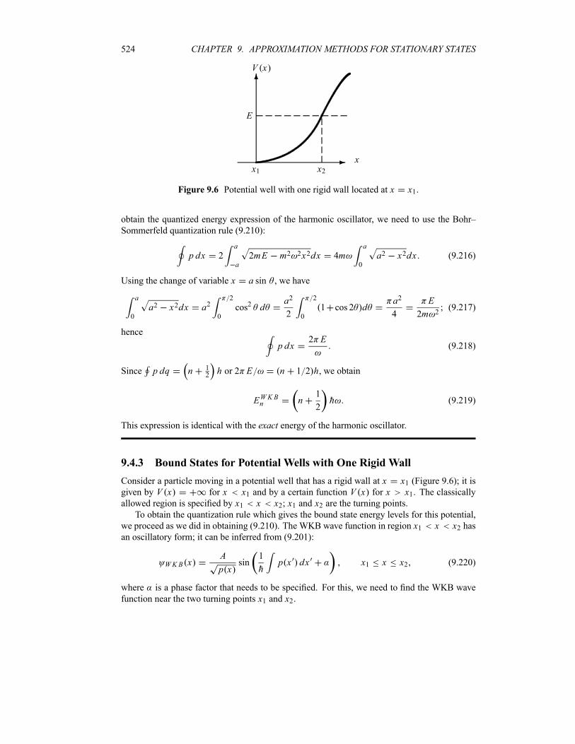
524 CHAPTER 9. APPROXIMATION METHODS FOR STATIONARY STATES
-
6
x1 x2
E
x
V x
Figure 9.6 Potential well with one rigid wall located at x x1.
obtain the quantized energy expression of the harmonic oscillator, we need to use the Bohr–
Sommerfeld quantization rule (9.210):
p dx 2a
a2mE m2 2x2dx 4m
a
0
a2 x2dx (9.216)
Using the change of variable x a sin , we have
a
0
a2 x2dx a22
0
cos2 da2
2
2
0
1 cos 2 da2
4
E
2m 2(9.217)
hence
p dx2 E
(9.218)
Since p dq n 12h or 2 E n 1 2 h, we obtain
EWK Bn n1
2h (9.219)
This expression is identical with the exact energy of the harmonic oscillator.
9.4.3 Bound States for Potential Wells with One Rigid Wall
Consider a particle moving in a potential well that has a rigid wall at x x1 (Figure 9.6); it isgiven by V x for x x1 and by a certain function V x for x x1. The classicallyallowed region is specified by x1 x x2; x1 and x2 are the turning points.To obtain the quantization rule which gives the bound state energy levels for this potential,
we proceed as we did in obtaining (9.210). The WKB wave function in region x1 x x2 hasan oscillatory form; it can be inferred from (9.201):
WK B xA
p xsin
1
hp x dx x1 x x2 (9.220)
where is a phase factor that needs to be specified. For this, we need to find the WKB wave
function near the two turning points x1 and x2.
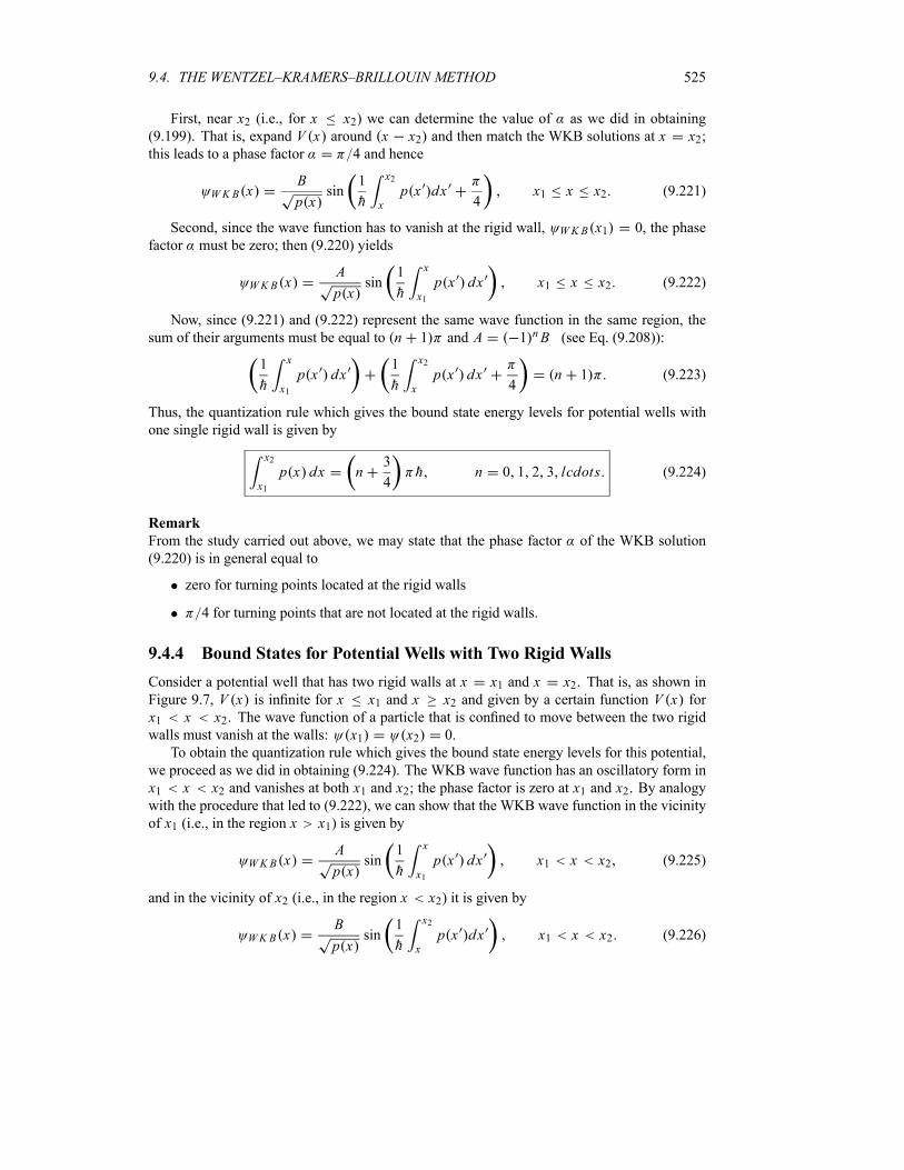
9.4. THE WENTZEL–KRAMERS–BRILLOUIN METHOD 525
First, near x2 (i.e., for x x2) we can determine the value of as we did in obtaining
(9.199). That is, expand V x around x x2 and then match the WKB solutions at x x2;this leads to a phase factor 4 and hence
WK B xB
p xsin
1
h
x2
xp x dx
4x1 x x2 (9.221)
Second, since the wave function has to vanish at the rigid wall, WK B x1 0, the phase
factor must be zero; then (9.220) yields
WK B xA
p xsin
1
h
x
x1
p x dx x1 x x2 (9.222)
Now, since (9.221) and (9.222) represent the same wave function in the same region, the
sum of their arguments must be equal to n 1 and A 1 nB (see Eq. (9.208)):
1
h
x
x1
p x dx1
h
x2
xp x dx
4n 1 (9.223)
Thus, the quantization rule which gives the bound state energy levels for potential wells with
one single rigid wall is given by
x2
x1
p x dx n3
4h n 0 1 2 3 lcdots (9.224)
Remark
From the study carried out above, we may state that the phase factor of the WKB solution
(9.220) is in general equal to
zero for turning points located at the rigid walls
4 for turning points that are not located at the rigid walls.
9.4.4 Bound States for Potential Wells with Two Rigid Walls
Consider a potential well that has two rigid walls at x x1 and x x2. That is, as shown inFigure 9.7, V x is infinite for x x1 and x x2 and given by a certain function V x for
x1 x x2. The wave function of a particle that is confined to move between the two rigidwalls must vanish at the walls: x1 x2 0.
To obtain the quantization rule which gives the bound state energy levels for this potential,
we proceed as we did in obtaining (9.224). The WKB wave function has an oscillatory form in
x1 x x2 and vanishes at both x1 and x2; the phase factor is zero at x1 and x2. By analogywith the procedure that led to (9.222), we can show that the WKB wave function in the vicinity
of x1 (i.e., in the region x x1) is given by
WK B xA
p xsin
1
h
x
x1
p x dx x1 x x2 (9.225)
and in the vicinity of x2 (i.e., in the region x x2) it is given by
WK B xB
p xsin
1
h
x2
xp x dx x1 x x2 (9.226)
526 CHAPTER 9. APPROXIMATION METHODS FOR STATIONARY STATES
-x1 x2
E
x
V x
Figure 9.7 Potential well with two rigid walls located at x1 and x2.
Note that the last two wave functions satisfy the correct boundary conditions at x1 and x2:
WK B x1 WK B x2 0.
Since equations (9.225) and (9.226) represent the same wave function in the same region,
the sum of the arguments must then be equal to n 1 and A 1 nB (see Eq. (9.208)):
1
h
x
x1
p x dx1
h
x2
xp x dx n 1 (9.227)
hence the quantization rule for potential wells with two rigid walls is given by
x2
x1
p x dx n 1 h n 0 1 2 3 (9.228)
or byx2
x1
p x dx n h n 1 2 3 (9.229)
The only difference between (9.228) and (9.229) is in the minimum value of the quantum num-
ber n: the lowest value of n is n 0 in (9.228) and n 1 in (9.229).
Remark
In this section we have derived three quantization rules (9.210), (9.224), and (9.229); they
provide the proper prescriptions for specifying the energy levels for potential wells with zero,
one, and two rigid walls, respectively. These rules differ only in the numbers 12, 34, and 0 that are
added to n. In the cases where n is large, which correspond to the semiclassical domain, thesethree quantization rules become identical; the semiclassical approximation is most accurate for
large values of n.
Example 9.8
Use the WKB approximation to calculate the energy levels of a spinless particle of mass mmoving in a one-dimensional box with walls at x 0 and x L .
Solution
This potential has two rigid walls, one at x 0 and the other at x L. To find the energylevels, we make use of the quantization rule (9.229). Since the momentum is constant within
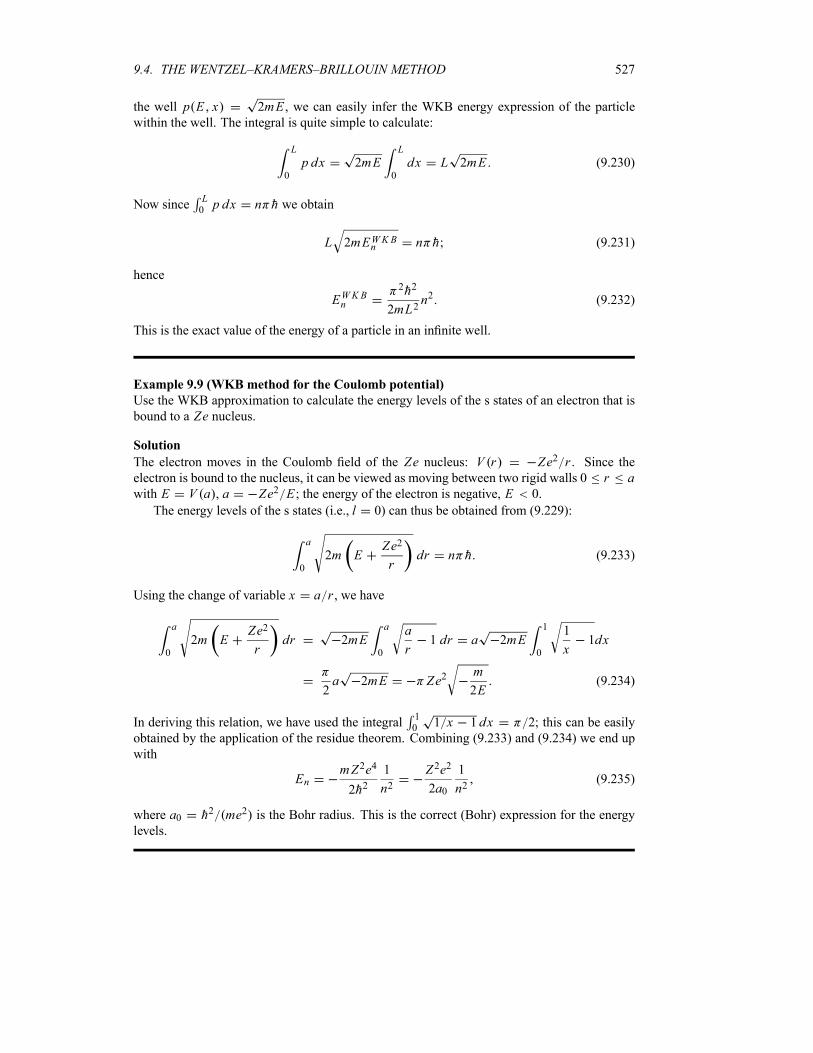
9.4. THE WENTZEL–KRAMERS–BRILLOUIN METHOD 527
the well p E x 2mE , we can easily infer the WKB energy expression of the particlewithin the well. The integral is quite simple to calculate:
L
0
p dx 2mEL
0
dx L 2mE (9.230)
Now sinceL0 p dx n h we obtain
L 2mEWK Bn n h (9.231)
hence
EWK Bn
2h2
2mL2n2 (9.232)
This is the exact value of the energy of a particle in an infinite well.
Example 9.9 (WKB method for the Coulomb potential)
Use the WKB approximation to calculate the energy levels of the s states of an electron that is
bound to a Ze nucleus.
Solution
The electron moves in the Coulomb field of the Ze nucleus: V r Ze2 r . Since theelectron is bound to the nucleus, it can be viewed as moving between two rigid walls 0 r awith E V a , a Ze2 E ; the energy of the electron is negative, E 0.
The energy levels of the s states (i.e., l 0) can thus be obtained from (9.229):
a
0
2m EZe2
rdr n h (9.233)
Using the change of variable x a r , we have
a
0
2m EZe2
rdr 2mE
a
0
a
r1 dr a 2mE
1
0
1
x1dx
2a 2mE Ze2
m
2E(9.234)
In deriving this relation, we have used the integral10 1 x 1 dx 2; this can be easily
obtained by the application of the residue theorem. Combining (9.233) and (9.234) we end up
with
EnmZ2e4
2h21
n2Z2e2
2a0
1
n2(9.235)
where a0 h2 me2 is the Bohr radius. This is the correct (Bohr) expression for the energylevels.
528 CHAPTER 9. APPROXIMATION METHODS FOR STATIONARY STATES
-
6
1 2 3
x1 x2
E
x
V x
Figure 9.8 A potential barrier whose classically allowed regions are specified by x x1 andx x2 and the forbidden region by x1 x x2.
9.4.5 Tunneling through a Potential Barrier
Consider the motion of a particle of momentum p0 2mE incident from left onto a po-tential barrier V x , shown in Figure 9.8, with an energy E that is smaller than the potential’smaximum value Vmax .Classically, the particle can in no way penetrate inside the barrier; hence it will get reflected
backwards. Quantum mechanically, however, the probability corresponding to the particle’s
tunneling through the barrier and “emerging” to the right of the barrier is not zero. In what
follows we want to use the WKB approximation to estimate the particle’s probability of passing
through the barrier.
In regions (1) and (3) of Figure 9.8 the particle is free:
1 x incident x re f lected x Aei p0x h Be i p0x h (9.236)
3 x transmitted x Eei p0x h (9.237)
where A, B, and E are the amplitudes of the incident, reflected, and transmitted waves, respec-tively; in region (3) we have outgoing waves only.
What about the wave function in the classically forbidden region (2)? The WKB method
provides the answer. Since the particle energy is smaller than Vmax , i.e., E Vmax , and if thepotential V x is a slowly varying function of x , the wave function in region (2) is given by theWKB approximation (see (9.174))
2 xC
p xexp
1
h
x
x1
p x dxD
p xexp
1
h
x
x1
p x dx (9.238)
where p x i 2m V x E . The term D p x exp 1 h xx1p x dx increases
exponentially when the barrier is very wide and is therefore unphysical. We shall be considering
the case where the barrier is wide enough so that the approximation D 0 is valid; hence 2 xbecomes
2 xC
p xexp
1
h
x
x1
p x dx (9.239)
The probability corresponding to the particle’s passage through the barrier is given by the
9.4. THE WENTZEL–KRAMERS–BRILLOUIN METHOD 529
transmission coefficient
Ttrans
inc
trans x 2
inc x 2
E 2
A 2(9.240)
since trans inc (the speeds of the incident and transmitted particles are equal). In what
follows we are going to calculate the coefficient E in terms of A. For this, we need to use thecontinuity of the wave function and its derivative at x1 and x2. First, using (9.236) and (9.239),the continuity relations 1 x1 2 x1 and 1 x1 2 x1 lead, respectively, to
Aeip0x1 h Be i p0x1 hC
a1(9.241)
i
hp0 Ae
i p0x1 h Be i p0x1 ha1h a1
C (9.242)
where a1 i 2m V x1 E . The continuity of the wave function and its derivative at x2,
2 x2 3 x2 , and 2 x2 3 x2 lead to
C
a2exp
1
h
x2
x1
p x dx Eeip0x2 h (9.243)
a2h a2
C exp1
h
x2
x1
p x dxip0hEei p0x2 h (9.244)
where a2 i 2m V x2 E .Adding (9.241) and (9.242) we get C 2A a1eip0x1 h 1 a1 i p0 which, when inserted
into (9.243), yields
E
A
2
1 a1 i p0
a1a2eip0 x1 x2 h exp
1
h
x2
x1
p x dx (9.245)
which in turn leads to
E 2
A 24
a2 a1 a1a2 p20exp
2
h
x2
x1
p x dx (9.246)
The substitution of this expression into (9.240) finally yields an approximate value for the
transmission coefficient through a potential barrier V x :
T e 2 1
h
x2
x1
2m V x E dx (9.247)
Tunneling phenomena are common at the microscopic scale; they occur within nuclei,
within atoms, and within solids. In nuclear physics, for instance, there are nuclei that decay
into an -particle (helium nucleus with Z 2) and a daughter nucleus. This process can be
viewed as the tunneling of an -particle through the potential (Coulomb) barrier between the
-particle and the daughter nucleus; once formed inside the nucleus, the -particle cannot es-
cape unless it tunnels through (penetrates) the Coulomb barrier surrounding it. Tunneling also
occurs within metals; when a metal is subject to an external electric field, electrons can be
emitted from the metal. This is known as cold emission; we will study it in Example 9.10.
530 CHAPTER 9. APPROXIMATION METHODS FOR STATIONARY STATES
Example 9.10
Use the WKB approximation to estimate the transmission coefficient of a particle of mass mand energy E moving in the following potential barrier:
V x0 x 0
V0 x x 0
Solution
The transmission coefficient is given by (9.247), where x1 0 and the value of x2, which canbe obtained from the relation V0 x2 E , is given by x2 V0 E . Setting the values
of x1 and x2 into (9.247), and since V x E V0 E x , we get
1
h
x2
x1
2m V x E dx2m
h
V0 E
0
V0 E x dx
2 2m
3hV0 E 3 2 (9.248)
The transmission coefficient is thus given by
T e 2 exp4 2m
3hV0 E 3 2 (9.249)
This problem is useful for the study of cold emission of electrons from metals. In theabsence of any external electric field, the electrons are bound by a potential of the type V xV0 for x 0, known as the work function of the metal. When we turn on an external electric
field E , the potential seen by the electron is no longer V0 but V x V0 eEx . This potentialbarrier has a width through which the electrons can escape: every electron of energy E eExcan escape. The quantity eEx2, where x2 V0 E , is known as the work function of the
metal; the width of the potential barrier of the metal is given by 0 x x2.
9.5 Concluding Remarks
In this chapter we have studied three approximation methods that apply to stationary Hamilto-
nians. As we saw, approximation methods offer efficient, short ways for obtaining energy levels
that are, at times, identical with the exact results. For instance, in the calculation of the energy
levels of the harmonic oscillator and the hydrogen atom, we have seen in a number of solved
examples how the variational method and the WKB method lead to the correct energies withoutresorting to solve the Schrödinger equation; the approximation methods deal merely with the
solution of a few simple integrals. In Chapters 4 and 7, however, we have seen that, to solve the
Schrödinger equation for the harmonic oscillator and for the hydrogen atom, one has to carry
out lengthy, laborious calculations.
Approximation methods offer, in general, powerful economical prescriptions for determin-
ing reliable results for systems that cannot be solved exactly. In the next chapter we are going
to study approximation methods that apply to time-dependent processes such as atomic transi-
tions, decays, and so on.
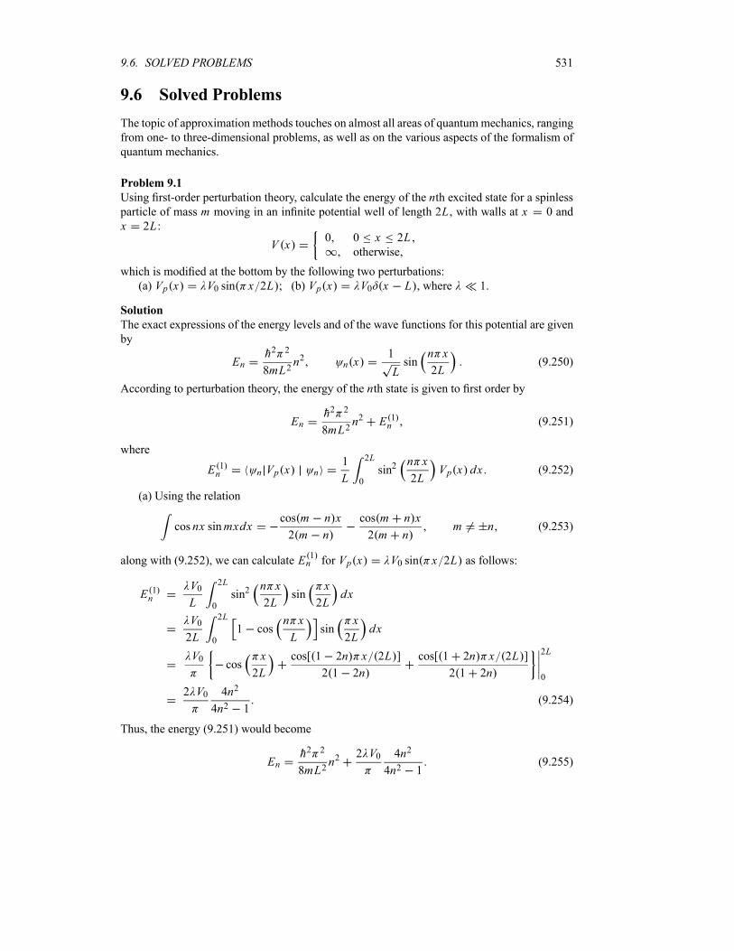
9.6. SOLVED PROBLEMS 531
9.6 Solved Problems
The topic of approximation methods touches on almost all areas of quantummechanics, ranging
from one- to three-dimensional problems, as well as on the various aspects of the formalism of
quantum mechanics.
Problem 9.1
Using first-order perturbation theory, calculate the energy of the nth excited state for a spinlessparticle of mass m moving in an infinite potential well of length 2L, with walls at x 0 and
x 2L:
V x0 0 x 2L
otherwise
which is modified at the bottom by the following two perturbations:
(a) Vp x V0 sin x 2L ; (b) Vp x V0 x L , where 1.
Solution
The exact expressions of the energy levels and of the wave functions for this potential are given
by
Enh2 2
8mL2n2 n x
1
Lsin
n x
2L(9.250)
According to perturbation theory, the energy of the nth state is given to first order by
Enh2 2
8mL2n2 E 1
n (9.251)
where
E 1n n Vp x n
1
L
2L
0
sin2n x
2LVp x dx (9.252)
(a) Using the relation
cos nx sinmxdxcos m n x
2 m n
cos m n x
2 m nm n (9.253)
along with (9.252), we can calculate E 1n for Vp x V0 sin x 2L as follows:
E 1n
V0L
2L
0
sin2n x
2Lsin
x
2Ldx
V02L
2L
0
1 cosn x
Lsin
x
2Ldx
V0cos
x
2L
cos[ 1 2n x 2L ]
2 1 2n
cos[ 1 2n x 2L ]
2 1 2n
2L
0
2 V0 4n2
4n2 1(9.254)
Thus, the energy (9.251) would become
Enh2 2
8mL2n2
2 V0 4n2
4n2 1(9.255)
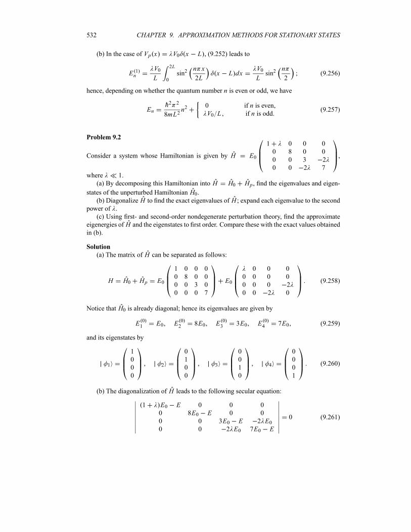
532 CHAPTER 9. APPROXIMATION METHODS FOR STATIONARY STATES
(b) In the case of Vp x V0 x L , (9.252) leads to
E 1n
V0L
2L
0
sin2n x
2Lx L dx
V0Lsin2
n
2(9.256)
hence, depending on whether the quantum number n is even or odd, we have
Enh2 2
8mL2n2
0 if n is evenV0 L if n is odd
(9.257)
Problem 9.2
Consider a system whose Hamiltonian is given by H E0
1 0 0 0
0 8 0 0
0 0 3 2
0 0 2 7
,
where 1.
(a) By decomposing this Hamiltonian into H H0 Hp, find the eigenvalues and eigen-
states of the unperturbed Hamiltonian H0.(b) Diagonalize H to find the exact eigenvalues of H ; expand each eigenvalue to the second
power of .
(c) Using first- and second-order nondegenerate perturbation theory, find the approximate
eigenergies of H and the eigenstates to first order. Compare these with the exact values obtainedin (b).
Solution
(a) The matrix of H can be separated as follows:
H H0 Hp E0
1 0 0 0
0 8 0 0
0 0 3 0
0 0 0 7
E0
0 0 0
0 0 0 0
0 0 0 2
0 0 2 0
(9.258)
Notice that H0 is already diagonal; hence its eigenvalues are given by
E 01 E0 E 0
2 8E0 E 03 3E0 E 0
4 7E0 (9.259)
and its eigenstates by
1
1
0
0
0
2
0
1
0
0
3
0
0
1
0
4
0
0
0
1
(9.260)
(b) The diagonalization of H leads to the following secular equation:
1 E0 E 0 0 0
0 8E0 E 0 0
0 0 3E0 E 2 E00 0 2 E0 7E0 E
0 (9.261)
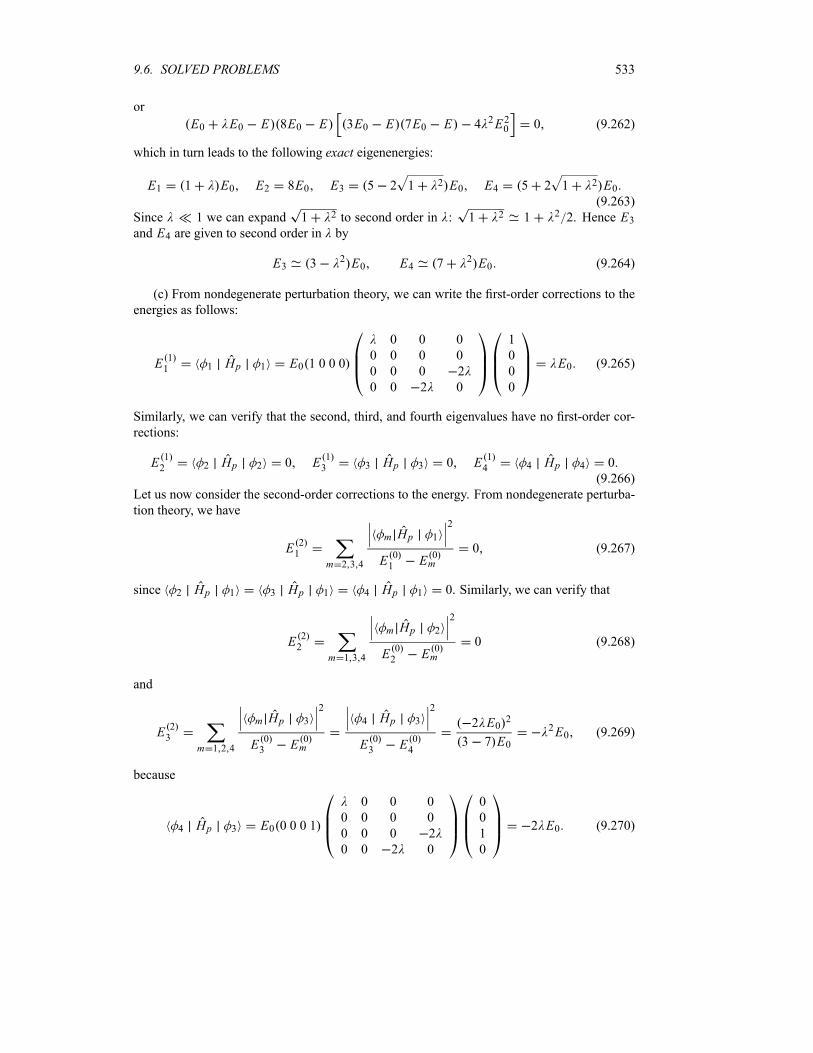
9.6. SOLVED PROBLEMS 533
or
E0 E0 E 8E0 E 3E0 E 7E0 E 4 2E20 0 (9.262)
which in turn leads to the following exact eigenenergies:
E1 1 E0 E2 8E0 E3 5 2 1 2 E0 E4 5 2 1 2 E0(9.263)
Since 1 we can expand 1 2 to second order in : 1 2 1 2 2. Hence E3and E4 are given to second order in by
E3 3 2 E0 E4 7 2 E0 (9.264)
(c) From nondegenerate perturbation theory, we can write the first-order corrections to the
energies as follows:
E 11 1 Hp 1 E0 1 0 0 0
0 0 0
0 0 0 0
0 0 0 2
0 0 2 0
1
0
0
0
E0 (9.265)
Similarly, we can verify that the second, third, and fourth eigenvalues have no first-order cor-
rections:
E 12 2 Hp 2 0 E 1
3 3 Hp 3 0 E 14 4 Hp 4 0
(9.266)
Let us now consider the second-order corrections to the energy. From nondegenerate perturba-
tion theory, we have
E 21
m 2 3 4
m Hp 1
2
E 01 E 0
m
0 (9.267)
since 2 Hp 1 3 Hp 1 4 Hp 1 0. Similarly, we can verify that
E 22
m 1 3 4
m Hp 2
2
E 02 E 0
m
0 (9.268)
and
E 23
m 1 2 4
m Hp 3
2
E 03 E 0
m
4 Hp 3
2
E 03 E 0
4
2 E0 2
3 7 E02E0 (9.269)
because
4 Hp 3 E0 0 0 0 1
0 0 0
0 0 0 0
0 0 0 2
0 0 2 0
0
0
1
0
2 E0 (9.270)
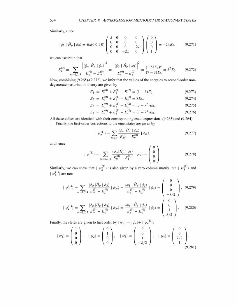
534 CHAPTER 9. APPROXIMATION METHODS FOR STATIONARY STATES
Similarly, since
3 Hp 4 E0 0 0 1 0
0 0 0
0 0 0 0
0 0 0 2
0 0 2 0
0
0
0
1
2 E0 (9.271)
we can ascertain that
E 24
m 1 2 3
m Hp 4
2
E 04 E 0
m
3 Hp 4
2
E 04 E 0
3
2 E0 2
7 3 E02E0 (9.272)
Now, combining (9.265)-(9.272), we infer that the values of the energies to second-order non-
degenerate perturbation theory are given by
E1 E 01 E 1
1 E 21 1 E0 (9.273)
E2 E 02 E 1
2 E 22 8E0 (9.274)
E3 E 03 E 1
3 E 23 3 2 E0 (9.275)
E4 E 04 E 1
4 E 24 7 2 E0 (9.276)
All these values are identical with their corresponding exact expressions (9.263) and (9.264).
Finally, the first-order corrections to the eigenstates are given by
1n
m n
m Hp n
E 0m E 0
nm (9.277)
and hence
11
m 2 3 4
m Hp 1
E 0m E 0
1
m
0
0
0
0
(9.278)
Similarly, we can show that12 is also given by a zero column matrix, but
13 and
14 are not:
13
m 1 2 4
m Hp 3
E 0m E 0
3
m4 Hp 3
E 04 E 0
3
4
0
0
0
2
(9.279)
14
m 1 2 3
m Hp 4
E 0m E 0
4
m3 Hp 4
E 03 E 0
4
3
0
0
1
2
(9.280)
Finally, the states are given to first order by n n1n :
1
1
0
0
0
2
0
1
0
0
3
0
0
1
2
4
0
0
2
1(9.281)
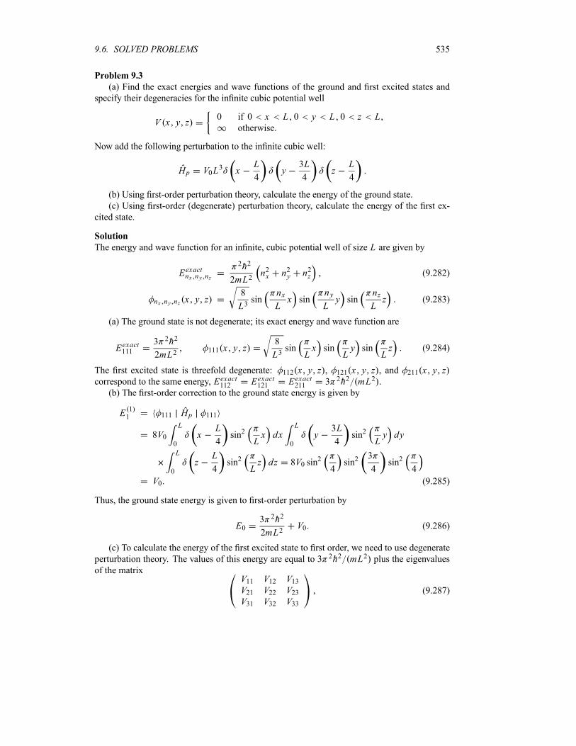
9.6. SOLVED PROBLEMS 535
Problem 9.3
(a) Find the exact energies and wave functions of the ground and first excited states and
specify their degeneracies for the infinite cubic potential well
V x y z0 if 0 x L 0 y L 0 z L,
otherwise.
Now add the following perturbation to the infinite cubic well:
Hp V0L3 x
L
4y
3L
4z
L
4
(b) Using first-order perturbation theory, calculate the energy of the ground state.
(c) Using first-order (degenerate) perturbation theory, calculate the energy of the first ex-
cited state.
Solution
The energy and wave function for an infinite, cubic potential well of size L are given by
Eexactnx ny nz
2h2
2mL2n2x n2y n2z (9.282)
nx ny nz x y z8
L3sin
nxLx sin
nyLy sin
nzLz (9.283)
(a) The ground state is not degenerate; its exact energy and wave function are
Eexact111
3 2h2
2mL2111 x y z
8
L3sin
Lx sin
Ly sin
Lz (9.284)
The first excited state is threefold degenerate: 112 x y z , 121 x y z , and 211 x y zcorrespond to the same energy, Eexact112 Eexact121 Eexact211 3 2h2 mL2 .(b) The first-order correction to the ground state energy is given by
E 11 111 Hp 111
8V0L
0
xL
4sin2
Lx dx
L
0
y3L
4sin2
Ly dy
L
0
zL
4sin2
Lz dz 8V0 sin
2
4sin2
3
4sin2
4
V0 (9.285)
Thus, the ground state energy is given to first-order perturbation by
E03 2h2
2mL2V0 (9.286)
(c) To calculate the energy of the first excited state to first order, we need to use degenerate
perturbation theory. The values of this energy are equal to 3 2h2 mL2 plus the eigenvaluesof the matrix
V11 V12 V13V21 V22 V23V31 V32 V33
(9.287)
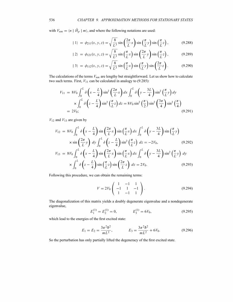
536 CHAPTER 9. APPROXIMATION METHODS FOR STATIONARY STATES
with Vnm n Hp m , and where the following notations are used:
1 211 x y z8
L3sin
2
Lx sin
Ly sin
Lz (9.288)
2 121 x y z8
L3sin
Lx sin
2
Ly sin
Lz (9.289)
3 112 x y z8
L3sin
Lx sin
Ly sin
2
Lz (9.290)
The calculations of the terms Vnm are lengthy but straightforward. Let us show how to calculatetwo such terms. First, V11 can be calculated in analogy to (9.285):
V11 8V0L
0
xL
4sin2
2
Lx dx
L
0
y3L
4sin2
Ly dy
L
0
zL
4sin2
Lz dz 8V0 sin
2
2sin2
3
4sin2
4
2V0 (9.291)
V12 and V13 are given by
V12 8V0L
0
xL
4sin
2
Lx sin
Lx dx
L
0
y3L
4sin
Ly
sin2
Ly dy
L
0
zL
4sin2
Lz dz 2V0 (9.292)
V13 8V0L
0
xL
4sin
2
Lx sin
Lx dx
L
0
y3L
4sin2
Ly dy
L
0
zL
4sin
Lz sin
2
Lz dz 2V0 (9.293)
Following this procedure, we can obtain the remaining terms:
V 2V0
1 1 1
1 1 1
1 1 1
(9.294)
The diagonalization of this matrix yields a doubly degenerate eigenvalue and a nondegenerate
eigenvalue,
E 11 E 1
2 0 E 13 6V0 (9.295)
which lead to the energies of the first excited state:
E1 E23 2h2
mL2E3
3 2h2
mL26V0 (9.296)
So the perturbation has only partially lifted the degeneracy of the first excited state.
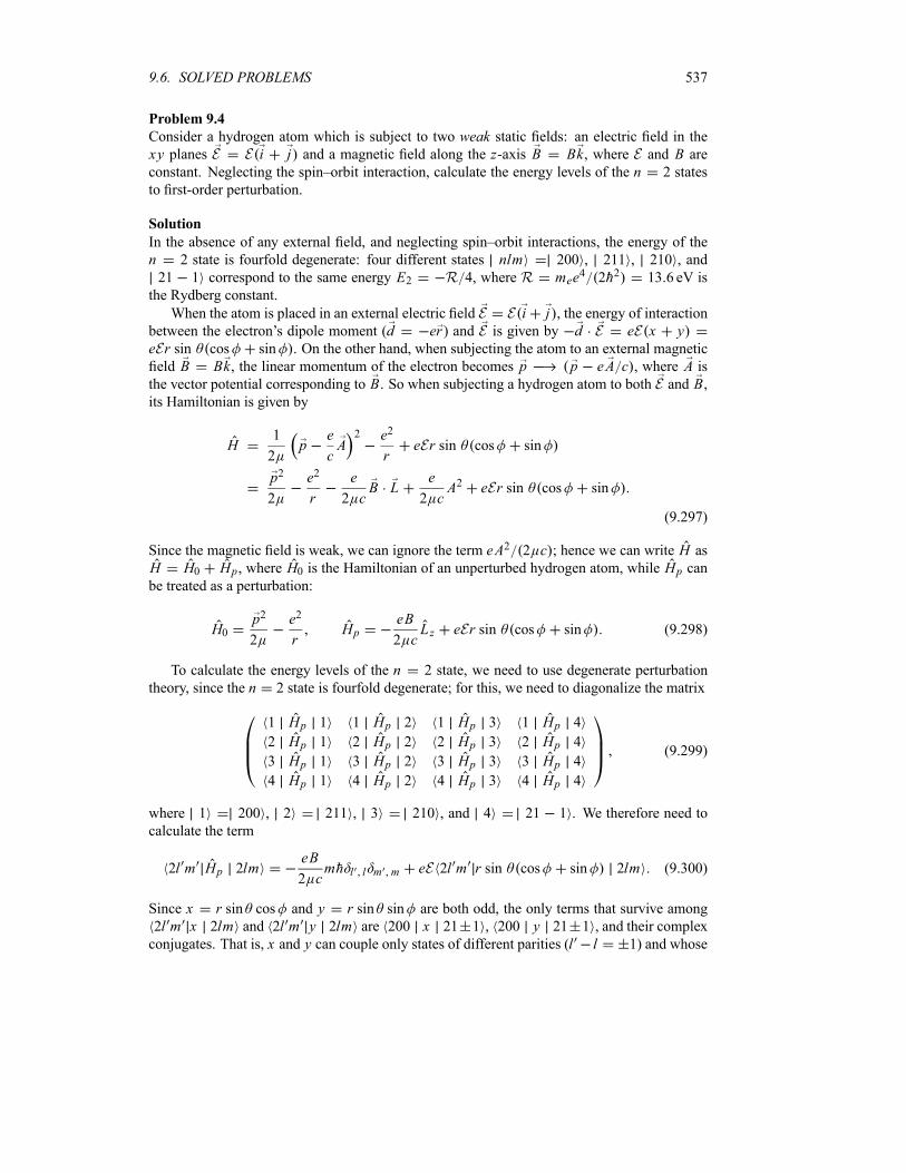
9.6. SOLVED PROBLEMS 537
Problem 9.4
Consider a hydrogen atom which is subject to two weak static fields: an electric field in thexy planes E E i j and a magnetic field along the z-axis B Bk, where E and B areconstant. Neglecting the spin–orbit interaction, calculate the energy levels of the n 2 states
to first-order perturbation.
Solution
In the absence of any external field, and neglecting spin–orbit interactions, the energy of the
n 2 state is fourfold degenerate: four different states nlm 200 , 211 , 210 , and
21 1 correspond to the same energy E2 R 4, where R mee4 2h2 13 6 eV is
the Rydberg constant.
When the atom is placed in an external electric field E E i j , the energy of interactionbetween the electron’s dipole moment (d er) and E is given by d E eE x yeEr sin cos sin . On the other hand, when subjecting the atom to an external magnetic
field B Bk, the linear momentum of the electron becomes p p eA c , where A isthe vector potential corresponding to B. So when subjecting a hydrogen atom to both E and B,its Hamiltonian is given by
H1
2p
e
cA2 e2
reEr sin cos sin
p2
2
e2
r
e
2 cB L
e
2 cA2 eEr sin cos sin
(9.297)
Since the magnetic field is weak, we can ignore the term eA2 2 c ; hence we can write H asH H0 Hp, where H0 is the Hamiltonian of an unperturbed hydrogen atom, while Hp canbe treated as a perturbation:
H0p2
2
e2
rHp
eB
2 cLz eEr sin cos sin (9.298)
To calculate the energy levels of the n 2 state, we need to use degenerate perturbation
theory, since the n 2 state is fourfold degenerate; for this, we need to diagonalize the matrix
1 Hp 1 1 Hp 2 1 Hp 3 1 Hp 4
2 Hp 1 2 Hp 2 2 Hp 3 2 Hp 4
3 Hp 1 3 Hp 2 3 Hp 3 3 Hp 4
4 Hp 1 4 Hp 2 4 Hp 3 4 Hp 4
(9.299)
where 1 200 , 2 211 , 3 210 , and 4 21 1 . We therefore need to
calculate the term
2l m Hp 2lmeB
2 cmh l l m m eE 2l m r sin cos sin 2lm (9.300)
Since x r sin cos and y r sin sin are both odd, the only terms that survive among
2l m x 2lm and 2l m y 2lm are 200 x 21 1 , 200 y 21 1 , and their complex
conjugates. That is, x and y can couple only states of different parities (l l 1) and whose
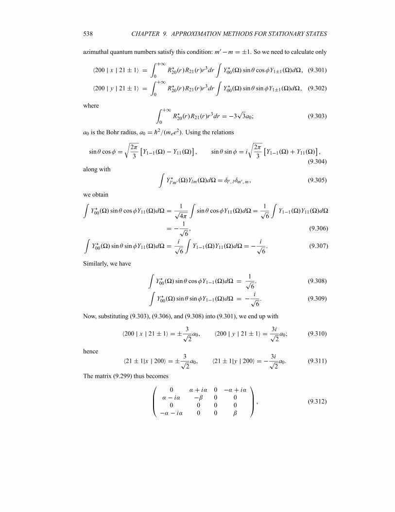
538 CHAPTER 9. APPROXIMATION METHODS FOR STATIONARY STATES
azimuthal quantum numbers satisfy this condition: m m 1. So we need to calculate only
200 x 21 10
R20 r R21 r r3dr Y00 sin cos Y1 1 d (9.301)
200 y 21 10
R20 r R21 r r3dr Y00 sin sin Y1 1 d (9.302)
where
0
R20 r R21 r r3dr 3 3a0 (9.303)
a0 is the Bohr radius, a0 h2 mee2 . Using the relations
sin cos2
3Y1 1 Y11 sin sin i
2
3Y1 1 Y11
(9.304)
along with
Yl m Ylm d l l m m (9.305)
we obtain
Y00 sin cos Y11 d1
4sin cos Y11 d
1
6Y1 1 Y11 d
1
6(9.306)
Y00 sin sin Y11 di
6Y1 1 Y11 d
i
6(9.307)
Similarly, we have
Y00 sin cos Y1 1 d1
6(9.308)
Y00 sin sin Y1 1 di
6(9.309)
Now, substituting (9.303), (9.306), and (9.308) into (9.301), we end up with
200 x 21 13
2a0 200 y 21 1
3i
2a0 (9.310)
hence
21 1 x 2003
2a0 21 1 y 200
3i
2a0 (9.311)
The matrix (9.299) thus becomes
0 i 0 ii 0 0
0 0 0 0
i 0 0
(9.312)
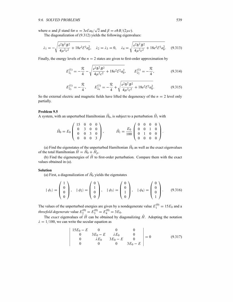
9.6. SOLVED PROBLEMS 539
where and stand for 3eEa0 2 and ehB 2 c .The diagonalization of (9.312) yields the following eigenvalues:
1e2h2B2
4 2c218e2E2a20 2 3 0 4
e2h2B2
4 2c218e2E2a20 (9.313)
Finally, the energy levels of the n 2 states are given to first-order approximation by
E 121
R
4
e2h2B2
4 2c218e2E2a20 E 1
22
R
4(9.314)
E 123
R
4E 124
R
4
e2h2B2
4 2c218e2E2a20 (9.315)
So the external electric and magnetic fields have lifted the degeneracy of the n 2 level only
partially.
Problem 9.5
A system, with an unperturbed Hamiltonian H0, is subject to a perturbation H1 with
H0 E0
15 0 0 0
0 3 0 0
0 0 3 0
0 0 0 3
H1E0100
0 0 0 0
0 0 1 0
0 1 0 0
0 0 0 0
(a) Find the eigenstates of the unperturbed Hamiltonian H0 as well as the exact eigenvaluesof the total Hamiltonian H H0 Hp.
(b) Find the eigenenergies of H to first-order perturbation. Compare them with the exactvalues obtained in (a).
Solution
(a) First, a diagonalization of H0 yields the eigenstates
1
1
0
0
0
2
0
1
0
0
3
0
0
1
0
4
0
0
0
1
(9.316)
The values of the unperturbed energies are given by a nondegenerate value E 01 15E0 and a
threefold degenerate value E 02 E 0
3 E 04 3E0.
The exact eigenvalues of H can be obtained by diagonalizing H . Adopting the notation1 100, we can write the secular equation as
15E0 E 0 0 0
0 3E0 E E0 0
0 E0 3E0 E 0
0 0 0 3E0 E
0 (9.317)
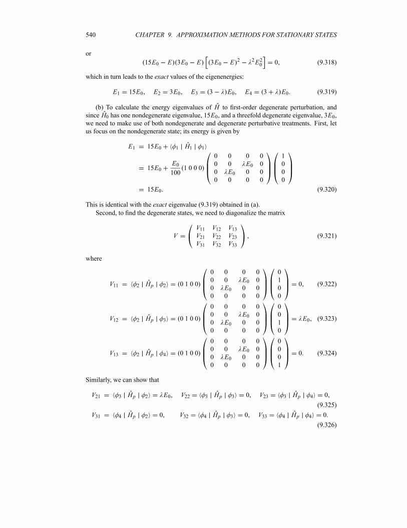
540 CHAPTER 9. APPROXIMATION METHODS FOR STATIONARY STATES
or
15E0 E 3E0 E 3E0 E 2 2E20 0 (9.318)
which in turn leads to the exact values of the eigenenergies:
E1 15E0 E2 3E0 E3 3 E0 E4 3 E0 (9.319)
(b) To calculate the energy eigenvalues of H to first-order degenerate perturbation, and
since H0 has one nondegenerate eigenvalue, 15E0, and a threefold degenerate eigenvalue, 3E0,we need to make use of both nondegenerate and degenerate perturbative treatments. First, let
us focus on the nondegenerate state; its energy is given by
E1 15E0 1 H1 1
15E0E0100
1 0 0 0
0 0 0 0
0 0 E0 0
0 E0 0 0
0 0 0 0
1
0
0
0
15E0 (9.320)
This is identical with the exact eigenvalue (9.319) obtained in (a).Second, to find the degenerate states, we need to diagonalize the matrix
VV11 V12 V13V21 V22 V23V31 V32 V33
(9.321)
where
V11 2 Hp 2 0 1 0 0
0 0 0 0
0 0 E0 0
0 E0 0 0
0 0 0 0
0
1
0
0
0 (9.322)
V12 2 Hp 3 0 1 0 0
0 0 0 0
0 0 E0 0
0 E0 0 0
0 0 0 0
0
0
1
0
E0 (9.323)
V13 2 Hp 4 0 1 0 0
0 0 0 0
0 0 E0 0
0 E0 0 0
0 0 0 0
0
0
0
1
0 (9.324)
Similarly, we can show that
V21 3 Hp 2 E0 V22 3 Hp 3 0 V23 3 Hp 4 0
(9.325)
V31 4 Hp 2 0 V32 4 Hp 3 0 V33 4 Hp 4 0
(9.326)
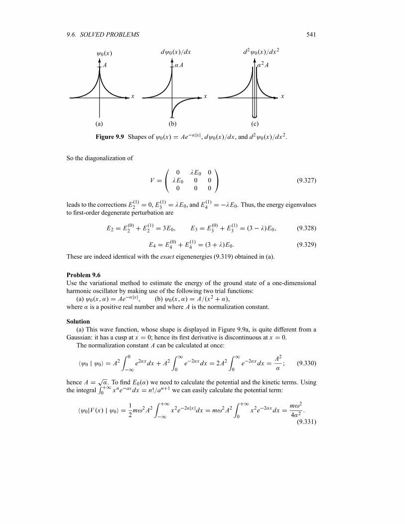
9.6. SOLVED PROBLEMS 541
-
60 x
x
(a)
A
-
6
(b)
d 0 x dx
x
A
-
6
(c)
d2 0 x dx2
x
2A
Figure 9.9 Shapes of 0 x Ae x , d 0 x dx , and d2 0 x dx2.
So the diagonalization of
V0 E0 0
E0 0 0
0 0 0
(9.327)
leads to the corrections E 12 0, E 1
3 E0, and E14 E0. Thus, the energy eigenvalues
to first-order degenerate perturbation are
E2 E 02 E 1
2 3E0 E3 E 03 E 1
3 3 E0 (9.328)
E4 E 04 E 1
4 3 E0 (9.329)
These are indeed identical with the exact eigenenergies (9.319) obtained in (a).
Problem 9.6
Use the variational method to estimate the energy of the ground state of a one-dimensional
harmonic oscillator by making use of the following two trial functions:
(a) 0 x Ae x , (b) 0 x A x2 ,
where is a positive real number and where A is the normalization constant.
Solution
(a) This wave function, whose shape is displayed in Figure 9.9a, is quite different from a
Gaussian: it has a cusp at x 0; hence its first derivative is discontinuous at x 0.
The normalization constant A can be calculated at once:
0 0 A20
e2 xdx A20
e 2 xdx 2A20
e 2 xdxA2
(9.330)
hence A . To find E0 we need to calculate the potential and the kinetic terms. Using
the integral 0 xne axdx n! an 1 we can easily calculate the potential term:
0 V x 01
2m 2A2 x2e 2 x dx m 2A2
0
x2e 2 xdxm 2
4 2
(9.331)
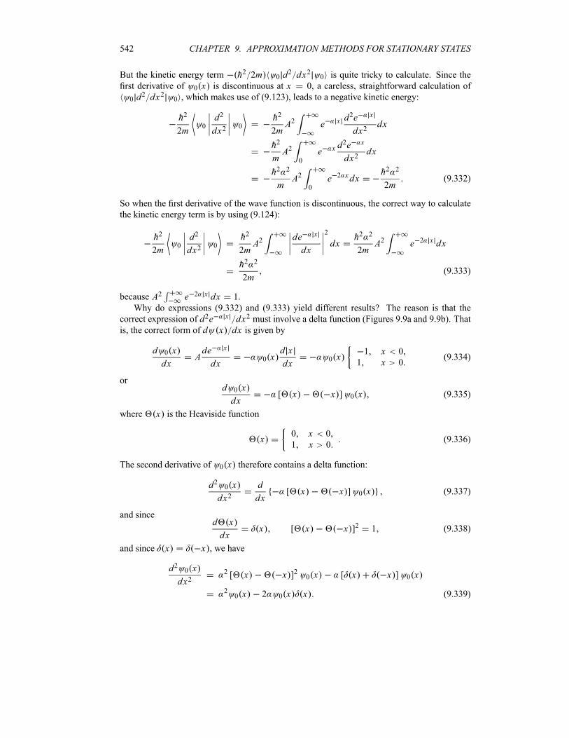
542 CHAPTER 9. APPROXIMATION METHODS FOR STATIONARY STATES
But the kinetic energy term h2 2m 0 d2 dx2 0 is quite tricky to calculate. Since the
first derivative of 0 x is discontinuous at x 0, a careless, straightforward calculation of
0 d2 dx2 0 , which makes use of (9.123), leads to a negative kinetic energy:
h2
2m0d2
dx20
h2
2mA2 e x d
2e x
dx2dx
h2
mA2
0
e x d2e x
dx2dx
h2 2
mA2
0
e 2 xdxh2 2
2m(9.332)
So when the first derivative of the wave function is discontinuous, the correct way to calculate
the kinetic energy term is by using (9.124):
h2
2m0d2
dx20
h2
2mA2
de x
dx
2
dxh2 2
2mA2 e 2 x dx
h2 2
2m(9.333)
because A2 e 2 x dx 1.
Why do expressions (9.332) and (9.333) yield different results? The reason is that the
correct expression of d2e x dx2 must involve a delta function (Figures 9.9a and 9.9b). Thatis, the correct form of d x dx is given by
d 0 x
dxAde x
dx0 x
d x
dx0 x
1 x 0
1 x 0(9.334)
ord 0 x
dx[ x x ] 0 x (9.335)
where x is the Heaviside function
x0 x 0
1 x 0(9.336)
The second derivative of 0 x therefore contains a delta function:
d2 0 x
dx2d
dx[ x x ] 0 x (9.337)
and sinced x
dxx [ x x ]2 1 (9.338)
and since x x , we have
d2 0 x
dx22 [ x x ]2 0 x [ x x ] 0 x
20 x 2 0 x x (9.339)
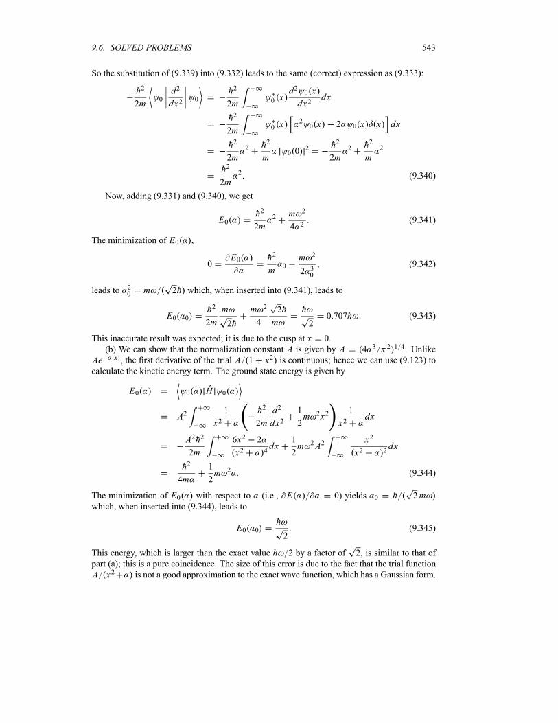
9.6. SOLVED PROBLEMS 543
So the substitution of (9.339) into (9.332) leads to the same (correct) expression as (9.333):
h2
2m0d2
dx20
h2
2m 0 xd2 0 x
dx2dx
h2
2m 0 x20 x 2 0 x x dx
h2
2m2 h2
m0 0
2 h2
2m2 h2
m2
h2
2m2 (9.340)
Now, adding (9.331) and (9.340), we get
E0h2
2m2 m 2
4 2(9.341)
The minimization of E0 ,
0E0 h2
m0
m 2
2 30
(9.342)
leads to 20 m 2h which, when inserted into (9.341), leads to
E0 0h2
2m
m
2h
m 2
4
2h
m
h
20 707h (9.343)
This inaccurate result was expected; it is due to the cusp at x 0.
(b) We can show that the normalization constant A is given by A 4 3 2 1 4. Unlike
Ae x , the first derivative of the trial A 1 x2 is continuous; hence we can use (9.123) tocalculate the kinetic energy term. The ground state energy is given by
E0 0 H 0
A21
x2h2
2m
d2
dx21
2m 2x2
1
x2dx
A2h2
2m
6x2 2
x2 4dx
1
2m 2A2
x2
x2 2dx
h2
4m
1
2m 2 (9.344)
The minimization of E0 with respect to (i.e., E 0) yields 0 h 2mwhich, when inserted into (9.344), leads to
E0 0h
2(9.345)
This energy, which is larger than the exact value h 2 by a factor of 2, is similar to that of
part (a); this is a pure coincidence. The size of this error is due to the fact that the trial function
A x2 is not a good approximation to the exact wave function, which has a Gaussian form.
544 CHAPTER 9. APPROXIMATION METHODS FOR STATIONARY STATES
Problem 9.7
For a particle of mass m moving in a one-dimensional box with walls at x 0 and x L, usethe variational method to estimate
(a) its ground state energy and
(b) its first excited state energy.
Solution
The exact solutions of this problem are known: Eexactn2h2n2 2mL2 .
(a) The trial function for the ground state must vanish at the walls, it must have no nodes,
and must be symmetric (i.e., even) with respect to x L 2. These three requirements can besatisfied by the following parabolic trial function:
0 x x L x (9.346)
no scale parameter is needed here. Since no parameter is involved, we can calculate the energy
directly (no variation is required): E0 0 H 0 0 0 , where
0 0
L
0
20 x dx
L
0
x2 L2 2Lx x2 dx1
30L5 (9.347)
and
0 H 0h2
2m
L
0
d 0 x
dx
2
dxh2
2m
L
0
L2 4Lx 4x2 dxh2L3
6m(9.348)
Thus, the ground state energy is given by
EVM00 H 0
0 010
h2
2mL2(9.349)
This is a very accurate result, for it is higher than the exact result by a mere 1%:
EVM0102Eexact (9.350)
(b) The properties of the exact wave function of the first excited state are known: it has
one node at x L 2 and must be odd with respect to x L 2; this last property makesit orthogonal to the ground state which is even about L 2. Let us try a polynomial function.Since the wave function vanishes at x 0, L 2, and L, the trial function must be at least cubic.The following polynomial function satisfies all these conditions:
1 x x xL
2x L (9.351)
Again, no scale parameter is needed.
To calculate EVM1 , we need to find
1 1
L
0
21 x dx
L
0
x2 xL
2
2
x L 2dx1
840L7 (9.352)
9.6. SOLVED PROBLEMS 545
and
1 H 1h2
2m
L
0
d 1 x
dx
2
dxh2
2m
L
0
3x2 3LxL2
2
2
dx
h2L5
40m(9.353)
Dividing the previous two expressions, we obtain the energy of the first excited state:
EVM11 H 1
1 142
h2
2mL2(9.354)
This too is a very accurate result; since Eexact1 2 2h2 2mL2 we can write EVM1 as
EVM1 42Eexact1 2 2; hence EVM1 is higher than Eexact1 by 6%.
Problem 9.8
Consider an infinite, one-dimensional potential well of length L, with walls at x 0 and x L,that is modified at the bottom by a perturbation Vp x :
V x0 0 x L
elsewhereVp x
V0 0 x L 20 elsewhere
where V0 1.
(a) Using first-order perturbation theory, calculate the energy En .(b) Calculate the energy En in the WKB approximation. Compare this energy with the
expression obtained in (a).
Solution
The exact energy Eexactn and wave function n x for a potential well are given by
Eexactn
2h2
2mL2n2 n x
2
Lsin
n x
L
(a) Since the first-order correction to the energy caused by the perturbation Vp x is given
by
E 1n n Vp n
2
LV0
L 2
0
sin2n x
Ldx
1
LV0
L 2
0
1 cos2n x
Ldx
V02
(9.355)
hence the energy is given to first-order perturbation by
E PTn
2h2
2mL2n2
V02
(9.356)
(b) Since this potential has two rigid walls, the energy within theWKB approximation needs
to be extracted from the quantization conditionL0 p En x dx n h, where
L
0
p En x dx 2m En V0L 2
0
dx 2mEnL
L 2dx
L
22m En V0 En (9.357)

546 CHAPTER 9. APPROXIMATION METHODS FOR STATIONARY STATES
hence L 2m En V0 En 2n h or
En V0 En2n h
L 2m(9.358)
Squaring both sides of this equation and using the notation n 2n2 2h2 mL2 , we have
2 En En V0 n 2En V0 (9.359)
Squaring both sides of this equation, we obtain
4E2n 4EnV02n 4E2n V 20 4 nEn 2 nV0 4EnV0 (9.360)
which, solving for En , leads to
Enn
4
V02
V 204 n
(9.361)
or
EWK Bn
2h2
2mL2n2
V02
mL2V 208 2h2
1
n2(9.362)
When n 1, and since V0 is very small, the WKB energy relation (9.362) gives back theexpression (9.356) that was derived from a first-order perturbative treatment:
EWK Bn E PTn
2h2
2mL2n2
V02
Problem 9.9
Consider a particle of mass m that is bouncing vertically and elastically on a reflecting hard
floor where V zmgz z 0
z 0and g is the gravitational constant.
(a) Use the variational method to estimate the ground state energy of this particle.
(b) Use the WKB method to estimate the ground state energy of this particle.
(c) Compare the results of (a) and (b) with the exact ground state energy.
Solution
(a) The ground state wave function of this particle has no nodes and must vanish at z 0
and be finite as z . The following trial function satisfies these conditions:
0 z Aze z (9.363)
where is a parameter and A is the normalization constant. We can show that A 2 3 2 and
hence
0 z 2 3ze z (9.364)
The energy is given by
EVM0 4 3
0
ze z h2
2m
d2
dz2mgz ze z dz
4 3 h2
2m 0
2 z 2z2 e 2 z dz 4 3mg0
z3e 2 z dz
2 3 h2
m
1
2
1
44mg 3 3
8 4(9.365)
9.6. SOLVED PROBLEMS 547
or
EVM0h2
2m2 3
2mg (9.366)
The minimization of E0 yields 0 3m2g 2h2 1 3 and hence
EVM0 03
2
9
2
1 31
2mg2h2
1 3
(9.367)
(b) Since this potential has one rigid wall at x 0, the correct quantization rule is given by
(9.224):E mg0 p dz n 3
4h; the turning point occurs at E mgz and hence z E mg.
Now, since E p2 2m mgz we have p E z 2mE 1 mgz E , and therefore
E mg
0
p En z dz 2mEE mg
0
1mg
Ez dz 2mE
2E
3mg
8E3
9mg2(9.368)
Inserting this relation into the quantization conditionE mg0 p dz n 3
4h gives
8E3
9mg2n
3
4h (9.369)
and we obtain the WKB approximation for the energy:
EWK Bn9 2
8mg2 2h2 n
3
4
2 1 3
(9.370)
Hence the ground state energy is given by
EWK B0
3
43 2
1 3 1
2mg2h2
1 3
(9.371)
(c) Recall that the exact ground state energy, calculated in Problem 4.18, page 275, for aparticle of mass m moving in the potential V z mgz is given by
Eexact0 2 3381
2mg2h2
1 3
(9.372)
Combining this relation with (9.367) and (9.371), we see that the variational method overesti-
mates the energy by a 5 9% error, while the WKB method underestimates it by a 0 8% error:
EVM03
2
9
2
1 3 Eexact0
2 3381 059Eexact0 (9.373)
EWK B0
3
43 2
1 3 Eexact0
2 3380 992Eexact0 (9.374)
The variational method has given a reasonably accurate result because we succeeded quite well
in selecting the trial function. As for the WKB method, it has given a very accurate result
because we have used the correct quantization rule (9.224). Had we used the quantization rule
(9.210), which contains a factor of 12instead of 1
4in (9.224), the WKB method would have
given a very inaccurate result with a 24 3% error, i.e., EWK B0 0 757Eexact0 .
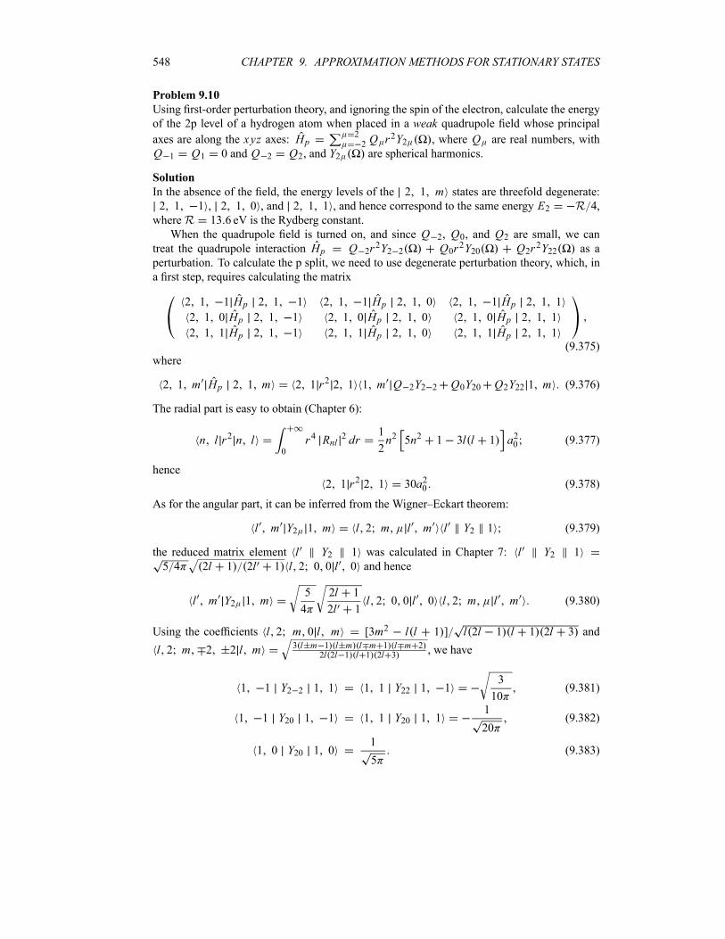
548 CHAPTER 9. APPROXIMATION METHODS FOR STATIONARY STATES
Problem 9.10
Using first-order perturbation theory, and ignoring the spin of the electron, calculate the energy
of the 2p level of a hydrogen atom when placed in a weak quadrupole field whose principal
axes are along the xyz axes: Hp22 Q r2Y2 , where Q are real numbers, with
Q 1 Q1 0 and Q 2 Q2, and Y2 are spherical harmonics.
Solution
In the absence of the field, the energy levels of the 2 1 m states are threefold degenerate:
2 1 1 , 2 1 0 , and 2 1 1 , and hence correspond to the same energy E2 R 4,
whereR 13 6 eV is the Rydberg constant.
When the quadrupole field is turned on, and since Q 2, Q0, and Q2 are small, we cantreat the quadrupole interaction Hp Q 2r2Y2 2 Q0r2Y20 Q2r2Y22 as a
perturbation. To calculate the p split, we need to use degenerate perturbation theory, which, in
a first step, requires calculating the matrix
2 1 1 Hp 2 1 1 2 1 1 Hp 2 1 0 2 1 1 Hp 2 1 1
2 1 0 Hp 2 1 1 2 1 0 Hp 2 1 0 2 1 0 Hp 2 1 1
2 1 1 Hp 2 1 1 2 1 1 Hp 2 1 0 2 1 1 Hp 2 1 1(9.375)
where
2 1 m Hp 2 1 m 2 1 r2 2 1 1 m Q 2Y2 2 Q0Y20 Q2Y22 1 m (9.376)
The radial part is easy to obtain (Chapter 6):
n l r2 n l0
r4 Rnl2 dr
1
2n2 5n2 1 3l l 1 a20 (9.377)
hence
2 1 r2 2 1 30a20 (9.378)
As for the angular part, it can be inferred from the Wigner–Eckart theorem:
l m Y2 1 m l 2 m l m l Y2 1 (9.379)
the reduced matrix element l Y2 1 was calculated in Chapter 7: l Y2 1
5 4 2l 1 2l 1 l 2 0 0 l 0 and hence
l m Y2 1 m5
4
2l 1
2l 1l 2 0 0 l 0 l 2 m l m (9.380)
Using the coefficients l 2 m 0 l m [3m2 l l 1 ] l 2l 1 l 1 2l 3 and
l 2 m 2 2 l m 3 l m 1 l m l m 1 l m 22l 2l 1 l 1 2l 3 , we have
1 1 Y2 2 1 1 1 1 Y22 1 13
10(9.381)
1 1 Y20 1 1 1 1 Y20 1 11
20(9.382)
1 0 Y20 1 01
5(9.383)
9.6. SOLVED PROBLEMS 549
These expressions can also be obtained from the following relations:
Ylm Y20 Ylm d5
4
l l 1 3m2
2l 1 2l 3(9.384)
Ylm 2 Y22 Ylm d Ylm Y2 2 Ylm 2 d
15
8
l m 1 l m l m 1 l m 2
2l 1 2l 3
(9.385)
Combining (9.376) to (9.383) we can write the matrix (9.375) as
30a20
Q020
0 Q2310
0 Q05
0
Q2310
0 Q020
(9.386)
The diagonalization of this matrix leads to the following eigenvalues:
E 11 30
a2010
Q0
2Q2 3 (9.387)
E 12 30
Q0a205
(9.388)
E 13 30
a2010
Q0
2Q2 3 (9.389)
Thus, to first-order perturbation theory, the energies of the p level are given by
E21R
430
a2010
Q0
2Q2 3 (9.390)
E22R
430Q0a205
(9.391)
E23R
430
a2010
Q0
2Q2 3 (9.392)
So the quadrupole interaction has lifted all the degeneracies of the p level.
Problem 9.11
Two protons, located on the z-axis and separated by a distance d (i.e., r dk), are subject to az-oriented magnetic field B Bk.(a) Ignoring all interactions between the two protons, find the energy levels and stationary
states of this system.
(b) Treating the dipole–dipole magnetic interaction energy between the protons,
Hp1
r31 2 3
1 r 2 r
r2
as a perturbation, calculate the energy using first-order perturbation theory.

550 CHAPTER 9. APPROXIMATION METHODS FOR STATIONARY STATES
Solution
(a) Since the magnetic moments of the protons are 1 2 0S1 h and 2 2 0S2 hwhere 0 he 2Mpc is the proton magnetic moment, the Hamiltonian of the two-protonsystem, ignoring all the interactions between the two protons, is due to the interaction of the
magnetic moments of the protons with the external magnetic field:
H0 1 2 B2 0
hS1 S2 B
2 0B
hSz (9.393)
As shown in Chapter 7, the eigenstates of a system consisting of two spin 12particles are a
triplet state and singlet state; the stationary eigenstates of H0 are therefore given by
1 1 11
2
1
2
1
2
1
2(9.394)
2 1 11
2
1
2
1
2
1
2(9.395)
3 1 01
2
1
2
1
2
1
2
1
2
1
2
1
2
1
2
1
2(9.396)
4 0 01
2
1
2
1
2
1
2
1
2
1
2
1
2
1
2
1
2(9.397)
The eigenenergies of 1 , 2 , 3 , and 4 are respectively
E 01 2 0B E 0
2 2 0B E 03 E 0
4 0 (9.398)
So 3 and 4 are (doubly) degenerate, whereas 1 and 2 are not.
(b) To calculate the energy to first order, we need to calculate the matrix elements of Hp:
HPi j i Hp j , with i j 1 2 3 4. For this, since r dk, we have 1 r 2 0dS1z h
and 2 r 2 0dS2z h. Thus, we can write Hp as
Hp1
r31 2 3
1 r 2 r
r24 20
d3h2S1 S2 3S1z S2z (9.399)
Using the relations
2S1 S2 S Sz S1 S22
S21 S21 S Sz
h2 [S S 1 S1 S1 1 S2 S2 1 ] S Sz
h2 S S 13
2S Sz (9.400)
2S1z S2z S Sz Sz2 S1z
2S2z2 S Sz h2 S2z
1
2S Sz (9.401)
along with (9.399), we can rewrite
Hp S Sz2 20
d3S S 1
3
23 S2z
1
2S Sz
2 20
d3S S 1 3S2z S Sz (9.402)
9.6. SOLVED PROBLEMS 551
Since the values of S and Sz are given for the triplet state by S 1, Sz 1, 0, 1, and by
S 0 Sz 0 for the singlet, the matrix elements of Hp are
E 11 1 Hp 1
2 20
d3E 12 2 Hp 2
2 20
d3(9.403)
E 13 3 Hp 3
4 20
d3E 14 4 Hp 4 0 (9.404)
All the other matrix elements of Hp are zero: i Hp j 0 for i j .Finally, the energy levels of the two-proton system can be obtained at once from (9.398)
along with (9.403) and (9.404):
E1 E 01 E 1
1 2 0B2 20
d3(9.405)
E2 E 02 E 1
2 2 0B2 20
d3(9.406)
E3 E 03 E 1
3
4 20
d3(9.407)
E4 E 04 E 1
4 0 (9.408)
So the dipole–dipole magnetic interaction has lifted the degeneracy of the energy levels in the
two-proton system.
Problem 9.12
A spin 12particle of mass m, which is moving in an infinite, symmetric potential well V x of
length 2L , is placed in an external weak magnetic field B with
V x0 L x L
otherwiseB
Bz L x 0
Bx 0 x L
Using first-order perturbation theory, calculate the energy of the nth excited state of this particle.
Solution
First, let us discuss the physics of this particle before placing it in a magnetic field. As seen in
Chapter 4, the energy and wave function of a spinless particle of massm moving in a symmetricpotential well of length 2L are
Enh2 2
8mL2n2 n x
1
L
cos n x2L n 1 3 5
sin n x2L n 2 4 6
(9.409)
When the spin of the particle is considered, its wave function is the product of a spacial part
n x and a spin part :
n x n x1
Lcos n x
2L n 1 3 5
1
Lsin n x
2L n 2 4 6(9.410)
552 CHAPTER 9. APPROXIMATION METHODS FOR STATIONARY STATES
where represent the spinor fields corresponding to the spin-up and spin-down states, re-
spectively:1
2
1
2
1
0
1
2
1
2
0
1(9.411)
Each energy level, En h2 2n2 8mL2 , of this particle is doubly degenerate, for it corre-sponds to two different states.
Let us now consider the case where the particle is placed in the magnetic field B. Theinteraction between the external magnetic field and the particle’s magnetic moment is given
by
Hp B B 0z L x 0
x 0 x L(9.412)
where we have made use of 2 0S h 0 ; recall that the matrices of x and z are
x0 1
1 0 z1 0
0 1(9.413)
To estimate the energy of this particle by means of the degenerate perturbation theory, we
need to calculate first the matrix
n Hp n n Hp n
n Hp n n Hp n(9.414)
where
n Hp n
0
Ln x
2 Hp dxL
0n x
2 Hp dx
0B z
0
Ln x
2 dx x
L
0n x
2 dx
(9.415)
Using0L n x
2 dx L0 n x
2 dx 12and since
z 0 11 0
0 1
0
11
x 0 10 1
1 0
0
10 (9.416)
we have
n Hp n0B
2(9.417)
Following this procedure, we can obtain the remaining matrix elements of (9.414):
0B
2
1 1
1 1(9.418)
The diagonalization of this matrix leads to
0B
2E 1 0B
2E 1 0B
2
2
0 (9.419)
9.6. SOLVED PROBLEMS 553
or E 10B 2. Thus, the energy of the nth excited state to first-order degenerate pertur-
bation theory is given by
Enh2 2
8mL2n2
0B
2(9.420)
The magnetic field has completely removed the degeneracy of the energy spectrum of this
particle.
Problem 9.13
Consider a particle of mass m moving in the potential V xx 0
12m 2x2 x 0
Estimate the ground state energy of this particle using
(a) the variational method and (b) the WKB method.
Solution
(a) As seen in Problem 4.9, page 266, the ground state wave function of this potential must
be selected from the harmonic oscillator wave functions that vanish at x 0. Only the oddwave functions vanish at x 0. So a trial function that, besides being zero at x 0, is finite as
x is given by
0 x xe x2 (9.421)
Using the results
0 00
x2e 2 x2 dx1
8 2(9.422)
01
2m 2x2 0
1
2m 2
0
x4e 2 x2 dx3m 2
64 2 2(9.423)
0h2
2m
d2
dx20
h2
2m 0
3 x2 2 2x4 e 2 x2 dx3h2
16m 2(9.424)
we obtain the ground state energy
E00 H 0
0 0
3h2
2m
3m 2
8(9.425)
The minimization of E0 with respect to yields 0 m 2h and hence E0 032h .
This energy is identical to the exact value obtained in Chapter 4.
(b) This potential contains a single rigid wall at x 0. Thus the proper quantization rule
for this potential is given by (9.224):a0 p dx n 3
4h; the turning point occurs at x a
with E 12m 2a2 and hence a 2E m 2 .
The calculation ofa0 p dx goes as follows:
a
0
p dxa
0
2mE m2 2x2dx ma
0
a2 x2dx (9.426)
The change of variable x a sin leads to
a
0
a2 x2 dx a22
0
cos2 da2
2
2
0
1 cos 2 da2
4(9.427)
554 CHAPTER 9. APPROXIMATION METHODS FOR STATIONARY STATES
hencea
0
p dx ma2
4
E
2(9.428)
Sincea0 p dx n 3
4h, that is, E 2 n 3
4h, we obtain
EWK Bn 2n3
2h n 0 1 2 3 (9.429)
This relation is identical with the exact expression obtained in Chapter 4. The WKB groundstate energy is thus given by EWK B0
32h .
Problem 9.14
Consider an H2 molecule where the protons are separated by a wide distance R and both arelocated on the z-axis. Ignoring the spin degrees of freedom and treating the dipole–dipoleinteraction as a perturbation, use perturbation theory to estimate an upper limit for the ground
state energy of this molecule.
Solution
Assuming the protons are fixed in space and separated by a distance R, we can write the Hamil-tonian of this molecule as follows:
H H0 Hp H A0 H B0 Hp (9.430)
where H A0 and HB0 are the unperturbed Hamiltonians of atoms A and B, and Hp is
Hpe2
R
e2
R rA rB
e2
R rA
e2
R rB(9.431)
where rA and rB are the position vectors of the electrons of atoms A and B as measured fromthe protons. If R a0, where a0 h2 e2 is the Bohr radius, an expansion of (9.431)
in powers of rA R and rB R yields, to first nonvanishing terms, an expression of the order of1 R3:
Hpe2
R3rA rB 3
rA R rB R
R2(9.432)
This is the dipole–dipole interaction energy between the dipole moments of the two atoms.
Since R Rz we can write (9.432) as
Hpe2
R3X AXB YAYB 2ZAZB (9.433)
The ground state energy and wave function of the (unperturbed) molecule are
E0 E A0 E B0 2E100e2
a00
A0
B0 100 A 100 B (9.434)
The first-order correction to the molecule’s energy, E 10 Hp 0 , is given by
E 1 e2
R3A0 X A
A0
B0 XB
B0
A0 YA
A0
B0 YB
B0
2 A0 ZA
A0
B0 ZB
B0 (9.435)
9.6. SOLVED PROBLEMS 555
Since the operators X , Y , and Z are odd and the states A0 and B
0 are spherically symmetric,
then all the terms in (9.435) are zero; hence E 1 0.
Let us now calculate the second-order correction:
E 2
n l m n l m 1 0 0
n l m n l m Hp 0
2
2E100 En En(9.436)
where
n l m n l m Hp 0e2
R3n l m X A 1 0 0 A n l m XB 1 0 0 B
n l m YA 1 0 0 A n l m YB 1 0 0 B
2 n l m ZA 1 0 0 A n l m ZB 1 0 0 B
(9.437)
The terms of this expression are nonzero only if l l 1, since the X , Y , and Z operatorsare proportional to Y1m . We can evaluate E 2 using a crude approximation where we assume
the denominator of (9.436) is constant and we take En En . Note that, for n 2, we have
Enlm E200. In this case we can rewrite (9.436) as
E 2 1
2 E100 E200 n l m n l m 1 0 0
n l m n l m Hp 0
2(9.438)
since the diagonal term is zero (i.e., 1 0 0 1 0 0 Hp 1 0 0 1 0 0 0), we have
n l m n l m
n l m n l m Hp 0
2
n l m n l m
1 0 0 1 0 0 Hp n l m n l m n l m n l m Hp 1 0 0 1 0 0
1 0 0 1 0 0 Hp2 1 0 0 1 0 0
e4
R61 0 0 1 0 0 X AXB YAYB 2ZAZB
2 1 0 0 1 0 0
(9.439)
The calculation of 1 0 0 1 0 0 XAXB YAYB 2ZAZB2 1 0 0 1 0 0 can be made
easier by the use of symmetry. Due to spherical symmetry, the cross terms are zero:
X AYA A X AZA A YAZA A XBYB B YBZB B 0 (9.440)
while the others are given as follows (see (9.45)):
X2A A Y 2A A Z2A A X2B B Y 2B B Z2B B a20 (9.441)
where C AA0 C
A0 and D B
B0 D
B0 . We can thus obtain
1 0 0 1 0 0 X AXB YAYB 2ZAZB2 1 0 0 1 0 0 6a40 (9.442)
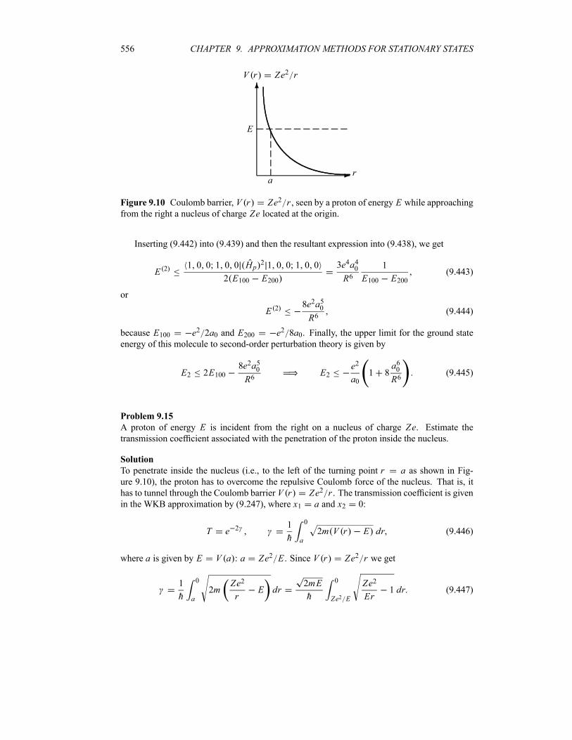
556 CHAPTER 9. APPROXIMATION METHODS FOR STATIONARY STATES
-
6
a
E
r
V r Ze2 r
Figure 9.10 Coulomb barrier, V r Ze2 r , seen by a proton of energy E while approachingfrom the right a nucleus of charge Ze located at the origin.
Inserting (9.442) into (9.439) and then the resultant expression into (9.438), we get
E 2 1 0 0 1 0 0 Hp 2 1 0 0 1 0 0
2 E100 E200
3e4a40R6
1
E100 E200(9.443)
or
E 2 8e2a50R6
(9.444)
because E100 e2 2a0 and E200 e2 8a0. Finally, the upper limit for the ground stateenergy of this molecule to second-order perturbation theory is given by
E2 2E1008e2a50R6
E2e2
a01 8
a60R6
(9.445)
Problem 9.15
A proton of energy E is incident from the right on a nucleus of charge Ze. Estimate thetransmission coefficient associated with the penetration of the proton inside the nucleus.
Solution
To penetrate inside the nucleus (i.e., to the left of the turning point r a as shown in Fig-ure 9.10), the proton has to overcome the repulsive Coulomb force of the nucleus. That is, it
has to tunnel through the Coulomb barrier V r Ze2 r . The transmission coefficient is givenin the WKB approximation by (9.247), where x1 a and x2 0:
T e 2 1
h
0
a2m V r E dr (9.446)
where a is given by E V a : a Ze2 E . Since V r Ze2 r we get
1
h
0
a2m
Ze2
rE dr
2mE
h
0
Ze2 E
Ze2
Er1 dr (9.447)
9.6. SOLVED PROBLEMS 557
The change of variable x Er Ze2 gives
Ze2
h
2m
E
1
0
1
x1 dx
Ze2
h
m
2E(9.448)
in deriving this relation, we have used the integral10 1 x 1dx 2.
The transmission coefficient is thus given by
T e 2 expZe2
h
2m
E(9.449)
The value of this coefficient describes how difficult it is for a positively charged particle, such
as a proton, to approach a nucleus.
Problem 9.16
Two identical particles of spin 12are enclosed in a one-dimensional box potential of length L
with walls at x 0 and x L.(a) Find the energies of the three lowest states.
(b) Then, subjecting the particles to a perturbation
Hp x1 x2 V0L2 x1
L
2x2
L
3
calculate its ground state energy using first-order time-independent perturbation theory.
Solution
Since the two particles have the same spin, the spin wave function of the system, s s1 s2 ,must be symmetric, so s is any one of the triplet states:
s
1 1 12
12 1
12
12 2
1 0 1
2
12
12 1
12
12 2
12
12 1
12
12 2
1 1 12
12 1
12
12 2
(9.450)
In addition, since this two-particle system is a system of identical fermions, its wave functionmust be antisymmetric. Since the spin part is symmetric, the spatial part of the wave functionhas to be antisymmetric:
x1 x2 A x1 x2 s s1 s2 (9.451)
that is,
A x1 x21
2n1 x1 n2 x2 n2 x1 n1 x2
1
Lsin
n1 x1L
sinn2 x2L
sinn2hx1L
sinn1 x2L
(9.452)
The energy levels of this two-particle system are
E2h2
2mL2n21 n22 E0 n
21 n22 (9.453)
558 CHAPTER 9. APPROXIMATION METHODS FOR STATIONARY STATES
where E0 2h2 2mL2 . Note that these energy levels are threefold degenerate because ofthe spin part of the wave function; that is, there are three different spin states that correspond to
the same energy level 2h2 n21 n22 2mL2 .(a) Having written the general expressions for the energies and the wave functions, it is now
easy to infer the energy levels and wave functions of the three lowest states. First, we should
note that the ground state cannot correspond to n1 n2 1, for the spatial wave function
would be zero. The ground state corresponds then to n1 1, n2 2; its energy follows from
(9.453),
E 0 E0 12 22 5E0
5 2h2
2mL2(9.454)
and the wave function 0 x1 x2 follows from (9.452).The first excited state corresponds to n1 1, n2 3. So the wave function 1 x1 x2 can
be inferred from (9.452) and the energy from (9.453):
E 1 E0 12 32 10E0
5 2h2
mL2(9.455)
The second excited state corresponds to n1 2, n2 3; hence the energy is given by
E 2 13E013 2h2
2mL2(9.456)
(b) Introducing the perturbation Hp V0L2 x1 L 2 x2 L 3 , and since Hp isdiagonal in the spin space, the ground state energy to first-order perturbation theory is given by
E5 2h2
2mL20 Hp 0 (9.457)
where
0 Hp 0
L
0
dx1L
0
dx2 0 x1 x2 Hp x1 x2 0 x1 x2 (9.458)
Since
0 x1 x2 0 x1 x21
Lsin
x1L
sin2 x2L
sin2 x1L
sinx2L(9.459)
we have
0 Hp 0V0L2
L2
L
0
dx1 x1L
2
L
0
dx2 x2L
3
sinx1L
sin2 x2L
sin2 x1L
sinx2L
2
V0 sin2sin
2
3sin sin
3
2
3
4V0 (9.460)
9.6. SOLVED PROBLEMS 559
hence
E5 2h2
2mL23
4V0 (9.461)
Problem 9.17
Neglecting the spin–orbit interaction, find the ground state energy of a two-electron atom in
these two ways:
(a) Use a first-order perturbation calculation; treat the Coulomb interaction between the two
electrons as a perturbation.
(b) Use the variational method.
Compare the results and discuss the merits of the two approximation methods.
Solution
Examples of such a system are the helium atom (Z 2), the singly ionized Li ion (Z 3),
the doubly ionized Be2 ion (Z 4), and so on. Each electron of these systems feels the
effects of two Coulomb fields: one from the Ze nucleus, V r Ze2 r , and the other fromthe other electron, V12 e2 r12 e2 r1 r2 ; here we consider the nucleus to be located atthe origin and the electrons at r1 and r2. Neglecting the spin–orbit interaction, we can write theHamiltonian of the two-electron system as
H H0 V12 H0e2
r1 r2(9.462)
where
H0h2
221
22 Ze2
1
r1
1
r2(9.463)
is the Hamiltonian of the atom when the interaction between the two electrons is neglected.
We have seen in Chapter 8 that, when the interaction between the two electrons is neglected,
the ground state energy and wave function are given by
E0 2Z2e2
2a27 2Z2 eV (9.464)
0 r1 S1 r2 S2 0 r1 r2 singlet S1 S2 (9.465)
where the spin part is antisymmetric,
singlet S1 S21
2
1
2
1
2 1
1
2
1
2 2
1
2
1
2 1
1
2
1
2 2
(9.466)
and the spatial part is symmetric, 0 r1 r2 100 r1 100 r2 , with
100 r R10 r Y001 Z
a
3 2
e Zr1 a (9.467)
that is,
0 r1 r21 Z
a
3
e Z r1 r2 a (9.468)
560 CHAPTER 9. APPROXIMATION METHODS FOR STATIONARY STATES
(a) To calculate the ground state energy using first-order perturbation theory, we have to
treat V12 as a perturbation. A first-order treatment yields
E E0 0 V12 0 2Z2e2
2a0 V12 0 (9.469)
where
0 V12 0 d3r1 d3r2 0 r1 r2 V12 0 r1 r2
d3r1 d3r2 100 r12 e2
r1 r2100 r2
2
(9.470)
The calculation of this integral is quite involved (I left it as an exercise); the result is
0 V12 05
8
Ze2
a(9.471)
which, when combined with (9.469), leads to
EZe2
aZ
5
8(9.472)
In the case of helium, Z 2, we have
E 108 8 eV 34 eV 74 8 eV (9.473)
this result disagrees with the experimental value, Eexp 78 975 eV, by 4 eV or by a 5 3%
relative error. Physically, this may be attributed to the fact that, in our calculation, we have not
taken into account the “screening” effect: the presence of one electron tends to decrease the net
charge “seen” by the other electron. Suppose electron 1 is “between” the nucleus and electron
2; then electron 2 will not “see” Z protons but Z 1 protons (i.e., electron 2 feels an effective
charge Z 1 e coming from the nucleus).(b) By analogy with the exact form of the ground state function (9.468), we can choose a
trial function that takes into account the screening effect. For this, we need simply to replace Zin (9.468) by a variational parameter :
0 r1 r2 Ae r1 r2 a (9.474)
where A is a normalization. Using the integral 0 xne bxdx n! bn 1, we can show that
A a 3 ; hence
r1 r21
a
3e r1 r2 a (9.475)
A combination of this relation with (9.471) leads to
E H0 V12 H05
8
e2
a(9.476)
9.6. SOLVED PROBLEMS 561
The calculation of H0 can be simplified by writing it as
H0h2
221
22 Ze2
1
r1
1
r2
h2
221
22 e2
1
r1
1
r2
Z e21
r1
1
r2(9.477)
This form is quite suggestive; since h2 0 0 2 Ze2 0 1 r 0 Z2e2 2awe can write
h2
221
22 e2
1
r1
1
r22
2e2
2a(9.478)
Now since1
r1
1
r24a
3
0
re 2 r adra
(9.479)
we can reduce (9.477) to
H0 22e2
2a2 Z e2
a(9.480)
which, when combined with (9.476), leads to
E 22e2
2a2 Z e2
a
5
8
e2
a2 2 Z
5
16
e2
a(9.481)
The minimization of E , dE d 0, yields
0 Z5
16(9.482)
hence the ground state energy is
E 0 15
8Z
5
16Z
2 Z2e2
a(9.483)
and
r1 r21 Z
a
5
16a
3
expZ
a
5
16ar1 r2 (9.484)
As a numerical illustration, the ground state energy of a helium atom is obtained by sub-
stituting Z 2 into (9.483). This yields E0 77 456 eV, in excellent agreement with the
experimental value Eexp 78 975 eV. The variational method, which overestimates the cor-
rect result by a mere 1 9%, is significantly more accurate than first-order perturbation theory.
The reason is quite obvious; while the perturbation treatment does not account for the screening
effect, the variational method includes it quite accurately. The wave function (9.484) shows that
the second electron does not see a charge Ze, but a lower charge Z 5 16 e.
562 CHAPTER 9. APPROXIMATION METHODS FOR STATIONARY STATES
9.7 Exercises
Exercise 9.1
Calculate the energy of the nth excited state to first-order perturbation for a one-dimensionalbox potential of length 2L , with walls at x L and x L, which is modified at the bottomby the following perturbations with V0 1:
(a) Vp xV0 L x L
0 elsewhere,
(b) Vp xV0 L 2 x L 2
0 elsewhere,
Exercise 9.2
Calculate the energy of the nth excited state to first-order perturbation for a one-dimensionalbox potential of length 2L , with walls at x L and x L, which is modified at the bottomby the following perturbations with V0 1:
(a) Vp xV0 L 2 x 0
0 elsewhere
(b) Vp xV0 0 x L 20 elsewhere
(c) Vp xV0 L 2 x 0
V0 0 x L 20 elsewhere
Exercise 9.3
Calculate the energy of the nth excited state to second-order perturbation and the wave functionto first-order perturbation for a one-dimensional box potential of length 2L, with walls at xL and x L, which is modified at the bottom by the following perturbations with V0 1:
(a) Vp x0 L x 0
V0 0 x L(b) Vp x
V0 1 x2 L2 x L0 elsewhere
Exercise 9.4
Consider a system whose Hamiltonian is given by H E0
3 2 0 0
2 3 0 0
0 0 7 2
0 0 2 7
,
where 1.
(a) Calculate the exact eigenvalues of H ; expand each of these eigenvalues to the secondpower of .
(b) Calculate the energy eigenvalues to second-order perturbation theory and compare them
with the exact results obtained in (a).
(c) Calculate the eigenstates of H up to the first-order correction.
Exercise 9.5
Consider a particle of mass m that moves in a three-dimensional potential V r kr , wherek is a constant having the dimensions of a force. Use the variational method to estimate its
ground state energy; you may take R r e r2 2 2as the trial radial function where is an
adjustable parameter.
9.7. EXERCISES 563
Exercise 9.6
Use the WKB method to estimate the ground state energy of a particle of mass m that movesin a three-dimensional potential V r kr , where k is a constant having the dimensions of aforce.
Exercise 9.7
Consider a two-dimensional harmonic oscillator Hamiltonian:
H1
2mP2x P2y
1
2m 2 X2 Y 2 1 XY
where 1.
(a) Give the wave functions for the three lowest energy levels when 0.
(b) Using perturbation theory, evaluate the first-order corrections of these energy levels
when 0.
Exercise 9.8
Consider a particle that has the Hamiltonian H H0 h a2 a†2
, where H0 is the
Hamiltonian of a simple one-dimensional harmonic oscillator, and where a and a† are the usual
annihilation and creation operators which obey [a a†] 1; is a very small real number.
(a) Calculate the ground state energy to second order in .
(b) Find the energy of the nth excited state, En , to second order in and the corresponding
eigenstate n to first order in .
Exercise 9.9
Consider two identical particles of spin 12that are confined in an isotropic three-dimensional
harmonic oscillator potential of frequency .
(a) Find the ground state energy and the corresponding wave function of this system when
the two particles do not interact.
(b) Consider now that there exists a weakly attractive spin-dependent potential between
the two particles, V r1 r2 kr1r2 S1zS2z , where k and are two small positive real
numbers. Find the ground state to first-order time-independent perturbation theory.
(c) Use the variational method to estimate the ground state energy of this system of two
noninteracting spin 12particles confined to an isotropic three-dimensional harmonic oscillator.
How does your result compare with that obtained in (a).
Exercise 9.10
Two identical spin 12particles are confined to a one-dimensional box potential of size L with
walls at x 0 and x L.(a) Find the ground state energy and the first excited state energy and their respective wave
functions for this system when the two particles do not interact.
(b) Consider now that there exists a weakly attractive potential between the two particles:
Vp xV0 0 x L 2
0 L 2 x L
Find the ground state and first excited state energies to first-order perturbation theory.
(c) Find numerical values for the ground state and first excited state energies calculated in
(a) in the case where L 10 10m, V0 2 eV, and the mass of each individual particle is to be
564 CHAPTER 9. APPROXIMATION METHODS FOR STATIONARY STATES
taken equal to the electron mass. Compare the sizes of the first order energy corrections with
the ground state energy and the first excited state energy (you may simply calculate the ratios
between the first-order corrections with the ground state and first excited state energies).
Exercise 9.11
Consider an isotropic three-dimensional harmonic oscillator.
(a) Find the energy of the first excited state and the different states corresponding to this
energy.
(b) If we now subject this oscillator to a perturbation Vp x y x y, where is a small
real number, find the energy of the first excited state to first-order degenerate time-independent
perturbation theory. Hint: You may use x h2m ax a
†x , y h
2m ay a†y ,
z h2m az a
†z , with ax nx nx nx 1 , and a
†x nx nx 1 nx 1 .
Exercise 9.12
Use the variational method to estimate the ground state energy of the spherical harmonic oscil-
lator by means of the following radial trial functions:
(a) R r Ae r2 and
(b) R r Ae r , where A is a normalization constant that needs to be found in each caseand is an adjustable parameter.
(c) Using the fact that the exact ground state energy is Eexact0 3h 2, find the relative
errors corresponding to the energies derived in (a) and (b).
Exercise 9.13
Consider a particle of mass m that is bouncing vertically and elastically on a smooth reflectingfloor in the Earth’s gravitational field
V zmgz z 0
z 0
where g is a constant (the acceleration due to gravity). Use the variational method to esti-mate the ground state energy of this particle by means of the trial wave function, zz exp z4 , where is an adjustable parameter that needs to be determined. Compare your
result with the exact value Eexact0 2 338 12mg2h2
1 3by calculating the relative error.
Exercise 9.14
Calculate the energy of the ground state to first-order perturbation for a particle which is moving
in a one-dimensional box potential of length L , with walls at x 0 and x L, when a weakpotential Hp x2 is added, where 1.
Exercise 9.15
Consider a semiclassical system whose energy is given by
E a21
2
b2
4a2 p2
1
2
4a2
b2 4 a2q2
where a and b are positive, real constants. Use the Bohr–Sommerfeld quantization rule toextract the expression of the bound state energy En for the nth excited state in terms of a.
9.7. EXERCISES 565
Exercise 9.16
Use the variational method to estimate the ground state energy of a particle of mass m that ismoving in a one-dimensional potential V x V0x4; you may use the trial function 0 x
Ae x2 2, where A is the normalization constant and is an adjustable parameter that needs to
be determined.
Exercise 9.17
Consider a particle of mass m which is moving in a one-dimensional potential V x V0x4.Estimate the ground state energy of this particle by means of the WKB method.
Exercise 9.18
Using 100 r 1 Z a 3 2e Zr a , show that
2100 r1
1
r1 r22100 r2 d
3r1d3r2
5Z
8a
Exercise 9.19
Calculate the ground state energy of the doubly ionized beryllium atom Be2 by means of the
following two methods and then compare the two results:
(a) a first-order perturbation theory treatment,
(b) the variational method with a trial function r1 r2 A exp[ r1 r2 a], whereA is the normalization constant, is an adjusted parameter, and a is the Bohr radius.
Exercise 9.20
Use the variational method to estimate the energy of the second excited state of a particle of
mass m moving in a one-dimensional infinite well with walls at x 0 and x L. Calculatethe relative error between your result and the exact value (recall that the energy of the second
excited state is given by Eexact3 9 2h2 2mL2 ).
Exercise 9.21
Consider a spinless particle of orbital angular momentum l 1 whose Hamiltonian is
H0E
h2L2x L2y
where E is a constant having the dimensions of energy.
(a) Calculate the exact energy levels and the corresponding eigenstates of this particle.
(b) We now add a perturbation Hp L z h, where is a small constant (small compared
to E) having the dimensions of energy. Calculate the energy levels of this particle to second-
order perturbation theory.
(c) Diagonalize the matrix of H H0 Hp and find the exact energy eigenvalues. Thenexpand each eigenvalue to second power in and compare them with the results derived from
perturbation theory in (b).
Exercise 9.22
Consider a system whose Hamiltonian is given by H E0
5 3 0 0
3 5 0 0
0 0 8
0 0 8
, where
1.
566 CHAPTER 9. APPROXIMATION METHODS FOR STATIONARY STATES
(a) By decomposing this Hamiltonian into H H0 Hp, find the eigenvalues and eigen-
states of the unperturbed Hamiltonian H0.(b) Diagonalize H to find the exact eigenvalues of H ; expand each eigenvalue to the second
power of .
(c) Using first- and second-order nondegenerate perturbation theory, find the approximate
eigenergies of H . Compare these with the exact values obtained in (b).
Exercise 9.23
Estimate the ground state energy of the hydrogen atom by means of the variational method
using the following two trial functions, find the relative errors, compare the two results, and
discuss the merit of each trial function.
(a) r1 r r0 r
where is an adjustable parameter. Find a relation between min and the Bohr radius.
(b) r Ae r2 .
Exercise 9.24
(a) Calculate to first-order perturbation theory the energy of the nth excited state of a one-dimensional harmonic oscillator which is subject to the following small perturbation: HpV0x3 V1x4 , where V0, V1, and a are constants and 1.
(b) Use the relation derived in (a) to find the energies of the three lowest states (i.e., n0 1 2) to first-order perturbation theory.
Exercise 9.25
Use the trial function 0 xA 2 x2 2 x0 x
to estimate the ground state energy of a one-dimensional harmonic oscillator by means of the
variational method; is an adjustable parameter and A is the normalization constant. Calculatethe relative error and assess the accuracy of the result.
Exercise 9.26
Use the WKB approximation to estimate the transmission coefficient of a particle of mass mand energy E moving in the following potential barrier:
V xV0 x a 1 a x 0
V0 1 x a 0 x a0 elsewhere
with 0 E V0; sketch this potential.
Exercise 9.27
Use the variational method to estimate the energy of the ground state of a one-dimensional
harmonic oscillator taking the following trial function:
0 x A 1 x e x
where is an adjustable parameter and A is the normalization constant.
9.7. EXERCISES 567
Exercise 9.28
Use the WKB approximation to estimate the transmission coefficient of a particle of mass mand energy E moving in the following potential barrier:
V xV0 1 x2 a2 x a0 x a
where 0 E V0.
Exercise 9.29
Use the WKB approximation to find the energy levels of a particle of mass m moving in thefollowing potential:
V xV0 x2 a2 1 x a0 x a
Exercise 9.30
A particle of mass m is moving in a one-dimensional harmonic oscillator potential, V xm 2x2 2. Calculate(a) the ground state energy, and
(b) the first excited state energy
to first-order perturbation theory when a small perturbation Hp x is added to the poten-tial, with 1.
Exercise 9.31
A particle of mass m is moving in a one-dimensional harmonic oscillator potential, V xm 2x2 2. Calculate(a) the ground state energy and
(b) the first excited state energy
to first-order perturbation theory when a small perturbation Hp x6 is added to the potential,with 1.
Exercise 9.32
A particle of mass m is moving in a three-dimensional harmonic oscillator potential, V xm 2 x2 y2 z2 2. Calculate the energy of the nth excited state to first-order perturbationtheory when a small perturbation Hp X2Y 4Z2 is added to the potential, with 1.
Exercise 9.33
Use the following two trial functions:
(a) Ae x (b) A 1 x e x
to estimate, by means of the variational method, the ground state energy of a particle of mass
m moving in a one-dimensional potential V x x ; is a scale parameter, is a constant,
and A is the normalization constant. Compare the results obtained.
Exercise 9.34
Three distinguishable particles of equal massm are enclosed in a one-dimensional box potentialwith rigid walls at x 0 and x L. If the three particles are subject to a weak, short-rangeattractive potential
Hp V0 [ x1 x2 x2 x3 x3 x1 ]
568 CHAPTER 9. APPROXIMATION METHODS FOR STATIONARY STATES
use first-order perturbation theory to calculate the system’s energy levels of
(a) the ground state, and
(b) the first excited state.
Exercise 9.35
Three distinguishable particles of equal mass m are in a one-dimensional harmonic oscillatorpotential H0
3i 1 p
2i 2m
12m 2x2i . If the three particles are subject to a weak, short-
range attractive potential
Hp V0 [ x1 x2 x2 x3 x3 x1 ]
use first-order perturbation theory to calculate the system’s energy levels of
(a) the ground state and
(b) the first-excited state.
Exercise 9.36
Consider a positronium which is subject to a weak static magnetic field in the xz-plane, BB i k , where B is a small constant. Neglecting the spin–orbit interaction, calculate theenergy levels of the n 2 states to first-order perturbation.
Exercise 9.37
Consider a spherically symmetric top with principal moments of inertia I .(a) Find the energy levels of the top.
(b) Assuming that the top is in the l 1 angular momentum state, find its energy to first-
order perturbation theory when a weak perturbation, HpEI L
2x L2y , is added where E 1.
Exercise 9.38
Estimate the approximate values of the ground state energy of a particle of mass m moving inthe potential V x V0 x , where V0 0, by means of: (a) the variational method and (b)
the WKB approximation. Compare the two results.
Exercise 9.39
Calculate to first-order perturbation theory the relativistic correction to the ground state of a
spinless particle of mass m moving in a one-dimensional harmonic oscillator potential. Hint:You need first to show that the Hamiltonian can be written as H H0 Hp, where H0P2 2m m 2X2 2 and Hp P4 8m3c2 is the leading relativistic correction term whichcan be treated as a perturbation.
Exercise 9.40
Consider a hydrogen atom which is subject to a small perturbation Hp r2. Use a first-orderperturbation theory to calculate the energy corrections to
(a) the ground state and
(b) the 2p state.
Exercise 9.41
(a) Calculate to first-order perturbation theory the contribution due to the spin–orbit inter-
action for the nth excited state for a positronium atom.(b) Use the result of part (a) to obtain numerical values for the spin–orbit correction terms
for the 2p level and compare them to the energy of n 2.
9.7. EXERCISES 569
Exercise 9.42
Ignoring the spin of the electron, calculate to first-order perturbation theory the energy of the
n 2 level of a hydrogen atom when subject to a weak quadrupole field Hp i Q y2 x2 ,where Q is a small, real number Q 1.
Exercise 9.43
Calculate the energy levels of the n 2 states of positronium in a weak external electrical field
E along the z-axis: E Ek; positronium consists of an electron and a positron bound by theelectric interaction.
Exercise 9.44
(a) Calculate to first-order perturbation theory the contributions due to the spin–orbit inter-
action for a hydrogen-like ion having Z protons.(b) Use the result of part (a) to find the spin-orbit correction for the 2p state of a C5 carbon
ion and compare it with the energy of the n 2 level.
Exercise 9.45
Two identical particles of spin 12are enclosed in a cubical box of side L.
(a) Calculate to first-order perturbation theory the ground state energy when the two parti-
cles are subject to weak short-range, attractive interaction:
V r1 r24
3a3V0 r1 r2
(b) Find a numerical value for the energy derived in (a) for L 10 10m, a 10 12m,
V0 10 3 eV, and the mass of each individual particle is to be taken to be the mass of the
electron.

570 CHAPTER 9. APPROXIMATION METHODS FOR STATIONARY STATES
Chapter 10
Time-Dependent Perturbation
Theory
10.1 Introduction
We have dealt so far with Hamiltonians that do not depend explicitly on time. In nature, how-
ever, most quantum phenomena are governed by time-dependent Hamiltonians. In this chapter
we are going to consider approximation methods treating Hamiltonians that depend explicitly
on time.
To study the structure of molecular and atomic systems, we need to know how electro-
magnetic radiation interacts with these systems. Molecular and atomic spectroscopy deals in
essence with the absorption and emission of electromagnetic radiation by molecules and atoms.
As a system absorbs or emits radiation, it undergoes transitions from one state to another.
Time-dependent perturbation theory is most useful for studying processes of absorption
and emission of radiation by atoms or, more generally, for treating the transitions of quantum
systems from one energy level to another.
10.2 The Pictures of Quantum Mechanics
As seen in Chapter 2, there are many representations of wave functions and operators in quan-
tum mechanics. The connection between the various representations is provided by unitary
transformations. Each class of representation, also called a picture, differs from others in theway it treats the time evolution of the system.
In this section we look at the pictures encountered most frequently in quantum mechanics:
the Schrödinger picture, the Heisenberg picture, and the interaction picture. The Schrödinger
picture is useful when describing phenomena with time-independent Hamiltonians, whereas
the interaction and Heisenberg pictures are useful when describing phenomena with time-
dependent Hamiltonians.
571
572 CHAPTER 10. TIME-DEPENDENT PERTURBATION THEORY
10.2.1 The Schrödinger Picture
In describing quantum dynamics, we have been using so far the Schrödinger picture in which
state vectors depend explicitly on time, but operators do not:
ihd
dtt H t (10.1)
where t denotes the state of the system in the Schrödinger picture. We have seen in
Chapter 3 that the time evolution of a state t can be expressed by means of the propagator,
or time-evolution operator, U t t0 , as follows:
t U t t0 t0 (10.2)
with
U t t0 e i t t0 H h (10.3)
The operator U t t0 is unitary,
U† t t0 U t t0 I (10.4)
and satisfies these properties:
U t t I (10.5)
U† t t0 U 1 t t0 U t0 t (10.6)
U t1 t2 U t2 t3 U t1 t3 (10.7)
10.2.2 The Heisenberg Picture
In this picture the time dependence of the state vectors is completely frozen. The Heisenberg
picture is obtained from the Schrödinger picture by applying U on t H :
t H U† t t 0 (10.8)
where t andU† t can be obtained from (10.2) and (10.3), respectively, by setting t0 0:
U† t U† t t0 0 ei t H h and t U t 0 , with U t e i t H h . Thus, we
can rewrite (10.8) as
t H ei t H h t (10.9)
As H is frozen in time we have: d H dt 0. Let us see how the expectation value of
an operator A in the state t evolves in time:
t A t 0 ei t H h Ae i t H h 0 0 AH t 0 H AH t H
(10.10)
where AH t is given by
AH t U† t AU t ei t H hAe i t H h (10.11)
Equation (10.10) shows that the expectation value of an operator is the same in both the
Schrödinger and the Heisenberg pictures. From (10.10) and (10.11) we see that both the
Schrödinger and the Heisenberg pictures coincide at t 0, since 0 H 0 and
AH 0 A.
10.2. THE PICTURES OF QUANTUM MECHANICS 573
10.2.2.1 The Heisenberg Equation of Motion
Let us now derive the equation of motion that regulates the time evolution of operators within
the Heisenberg picture. Assuming that A does not depend explicitly on time (i.e., A t 0)
and since U t is unitary, we have
d AH t
dt
U† t
dtAU t U† t A
U t
t
1
ihU†HUU†AU
1
ihU†AUU†HU
1
ihAH U†HU (10.12)
where we have used (10.3) to write U t t HU ih and U† t t U†H ih. Since
U t and H commute, we have U† t HU t H ; hence we can rewrite (10.12) as
d AHdt
1
ihAH H (10.13)
This is the Heisenberg equation of motion. It plays the role of the Schrödinger equation withinthe Heisenberg picture. Since the Schrödinger and Heisenberg pictures are equivalent, we can
use either picture to describe the quantum system under consideration. The Heisenberg equation
(10.13), however, is in general difficult to solve.
Note that the structure of the Heisenberg equation (10.13) is similar to the classical equation
of motion of a variable A that does not depend explicitly on time d A dt A H , where
A H is the Poisson bracket between A and H (see Chapter 3).
10.2.3 The Interaction Picture
The interaction picture, also called the Dirac picture, is useful to describe quantum phenomenawith Hamiltonians that depend explicitly on time. In this picture both state vectors and opera-tors evolve in time. We need, therefore, to find the equation of motion for the state vectors andfor the operators.
10.2.3.1 Equation of Motion for the State Vectors
State vectors in the interaction picture are defined in terms of the Schrödinger states t by
t I ei t H0 h t (10.14)
If t 0 we have 0 I 0 . The time evolution of t is governed by the
Schrödinger equation (10.1) with H H0 V where H0 is time independent, but V maydepend on time.
To find the time evolution of t I , we need the time derivative of (10.14):
ihd t I
dtH0e
i t H0 h t ei t H0 h ihd t
dt
H0 t I ei t H0 hH t (10.15)

574 CHAPTER 10. TIME-DEPENDENT PERTURBATION THEORY
where we have used (10.1). Since H H0 V and
ei H0t hV ei t H0 hVe i t H0 h ei t H0 h VI t ei t H0 h (10.16)
with
VI t ei t H0 hVe i t H0 h (10.17)
we can rewrite (10.15) as
ihd t I
dtH0 t I H0e
i t H0 h t VI t ei t H0 h t (10.18)
or
ihd t I
dtVI t t I (10.19)
This is the Schrödinger equation in the interaction picture. It shows that the time evolution of
the state vector is governed by the interaction VI t .
10.2.3.2 Equation of Motion for the Operators
The interaction representation of an operator AI t is given, as shown in (10.17), in terms of itsSchrödinger representation by
AI t ei H0t hAe i H0t h (10.20)
Calculating the time derivative of AI t and since A t 0, we can show the time evolution
of AI t is governed by H0:
d AI t
dt
1
ihAI t H0 (10.21)
This equation is similar to the Heisenberg equation of motion (10.13), except that H is replacedby H0. The basic difference between the Heisenberg and interaction pictures can be inferredfrom a comparison of (10.9) with (10.14), and (10.11) with (10.20): in the Heisenberg picture
it is H that appears in the exponents, whereas in the interaction picture it is H0 that appears.In conclusion, we have seen that, within the Schrödinger picture, the states depend on time
but not the operators; in the Heisenberg picture, only operators depend explicitly on time,
state vectors are frozen in time. The interaction picture, however, is intermediate between
the Schrödinger and the Heisenberg pictures, since both state vectors and operators evolve with
time.
10.3 Time-Dependent Perturbation Theory
We consider here only those phenomena that are described by Hamiltonians which can be split
into two parts, a time-independent part H0 and a time-dependent part V t that is small com-pared to H0:
H t H0 V t (10.22)
10.3. TIME-DEPENDENT PERTURBATION THEORY 575
where H0, which describes the system when unperturbed, is assumed to have exact solutionsthat are known. Such splitting of the Hamiltonian is encountered in the following typical
problem. Consider a system which, when unperturbed, is described by a time-independent
Hamilonian H0 whose solutions—the eigenvalues En and eigenstates n —are known,
H0 n En n (10.23)
and whose most general state vectors are given by stationary states
n t e i t H0 hn e i En t h
n (10.24)
In the time interval 0 t we subject the system to an external time-dependent perturbation,
V t , that is small compared to H0:
V tV t 0 t0 t 0 t
(10.25)
During the time interval 0 t , the Hamiltonian of the system is H H0 V t and thecorresponding Schrödinger equation is
ihd t
dtH0 V t t (10.26)
where V t characterizes the interaction of the system with the external source of perturbation.How does V t affect the system? When the system interacts with V t , it either absorbs
or emits energy. This process inevitably causes the system to undergo transitions from one
unperturbed eigenstate to another. Themain task of time-dependent perturbation theory consists
of answering this question: If the system is initially in an (unperturbed) eigenstate i of H0,what is the probability that the system will be found at a later time in another unperturbed
eigenstate f ?
To prepare the ground for answering this question, we need to look for the solutions of the
Schrödinger equation (10.26). The standard method to solve (10.26) is to expand t in
terms of an expansion coefficient cn t :
tn
cn t ei En t
n (10.27)
and then insert this into (10.26) to find cn t to various orders in the approximation. Instead offollowing this procedure, and since we are dealing with time-dependent potentials, it is more
convenient to solve (10.26) in the interaction picture (10.19):
ihd t I
dtVI t t I (10.28)
where t I ei t H0 h t and VI t ei t H0 hV t e i t H0 h . The time evolution
equation t U t ti ti may be written in the interaction picture as
t I ei t H0 h t ei t H0 hU t ti ti ei t H0 hU t ti ei H0ti h ti I
(10.29)

576 CHAPTER 10. TIME-DEPENDENT PERTURBATION THEORY
or as
t I UI t ti ti I (10.30)
where the time evolution operator is given in the interaction picture by
UI t ti ei t H0 hU t ti ei H0ti h (10.31)
Inserting (10.30) into (10.28) we end up with
ihdUI t tidt
VI t UI t ti (10.32)
The solutions of this equation, with the initial conditionUI ti ti I , are given by the integralequation
UI t ti 1i
h
t
ti
VI t UI t ti dt (10.33)
Time-dependent perturbation theory provides approximate solutions to this integral equation.This consists in assuming that VI t is small and then proceeding iteratively. The first-orderapproximation is obtained by inserting UI t ti 1 in the integral sign of (10.33), leading to
U 1I t ti 1 i h t
tiVI t dt . SubstitutingUI t ti U 1
I t ti in the integral sign of(10.33) we get the second-order approximation:
U 2I t ti 1
i
h
t
ti
VI t dti
h
2 t
ti
VI t1 dt1t1
ti
VI t2 dt2 (10.34)
The third-order approximation is obtained by substituting U 2I t ti into (10.33), and so on. A
repetition of this iterative process yields
UI t ti 1i
h
t
ti
VI t dti
h
2 t
ti
VI t1 dt1t1
ti
VI t2 dt2
i
h
n t
ti
VI t1 dt1t1
ti
VI t2 dt2t2
ti
VI t3 dt3tn 1
ti
VI tn dtn
(10.35)
This series, known as the Dyson series, allows for the calculation of the state vector up to thedesired order in the perturbation.
We are now equipped to calculate the transition probability. It may be obtained by taking the
matrix elements of (10.35) between the eigenstates of H0. Time-dependent perturbation theory,where one assumes knowledge of the solutions of the unperturbed eigenvalue problem (10.23),
deals in essence with the calculation of the transition probabilities between the unperturbed
eigenstates n of the system.
10.3.1 Transition Probability
The transition probability corresponding to a transition from an initial unperturbed state i
to another unperturbed state f is obtained from (10.35):
Pi f t f UI t ti i
2
f ii
h
t
0
ei f i tf V t i dt
10.3. TIME-DEPENDENT PERTURBATION THEORY 577
i
h
2
n
t
0
ei f n t1f V t1 n dt1
t1
0
ei ni t2n V t2 i dt2
2
(10.36)
where we have used the fact that
f VI t i f ei H0t hV t e i H0t hi f V t i exp i f i t
(10.37)
where f i is the transition frequency between the initial and final levels i and f :
f iE f Eih
1
hf H0 f i H0 i (10.38)
The transition probability (10.36) can be written in terms of the expansion coefficients cn tintroduced in (10.27) as
Pi f t c 0f c 1f t c 2f t2
(10.39)
where
c 0f f i f i c 1f ti
h
t
0f V t i e
i f i t dt (10.40)
The first-order transition probability for i f with i f (and hence f i
0) is obtained by terminating (10.36) at the first order in VI t :
Pi f ti
h
t
0f V t i e
i f i t dt2
(10.41)
In principle we can use (10.36) to calculate the transition probability to any order in VI t .However, terms higher than the first order become rapidly intractable. For most problems of
atomic and nuclear physics, the first order (10.41) is usually sufficient. In what follows, we are
going to apply (10.41) to calculate the transition probability for two cases, which will have later
usefulness when we deal with the interaction of atoms with radiation: a constant perturbationand a harmonic perturbation.
10.3.2 Transition Probability for a Constant Perturbation
In the case where V does not depend on time, (10.41) leads to
Pi f t1
h2f V i
t
0
ei f i t dt2
1
h2f V i
2 ei f i t 1
f i
2
(10.42)
which, using ei 1 2 4 sin2 2 , reduces to
Pi f t4 f V i
2
h2 2f i
sin2f i t
2(10.43)

578 CHAPTER 10. TIME-DEPENDENT PERTURBATION THEORY
-
6
[sin2 f i t 2 ] 2f i
t2 4
f i6t
4t
2t0 2
t4t
6t
Figure 10.1 Plot of [sin2 f i t 2 ] 2f i versus f i for a fixed value of t ; f i E f Ei 2.
As a function of time, this transition probability is an oscillating sinusoidal function with a
period of 2 f i . As a function of f i , however, the transition probability, as shown in Fig-
ure 10.1, has an interference pattern: it is appreciable only near f i 0 and decays rapidly
as f i moves away from zero (here, for a fixed t , we have assumed that f i is a continuous
variable; that is, we have considered a continuum of final states; we will deal with this in more
detail in a moment). This means that the transition probability of finding the system in a state
f of energy E f is greatest only when Ei E f or when f i 0. The height and the width
of the main peak, centered around f i 0, are proportional to t2 and 1 t , respectively, so thearea under the curve is proportional to t ; since most of the area is under the central peak, thetransition probability is proportional to t . The transition probability therefore grows linearlywith time. The central peak becomes narrower and higher as time increases; this is exactly the
property of a delta function. Thus, in the limit t the transition probability takes the shape
of a delta function, as we are going to see.
As t we can use the asymptotic relation (Appendix A)
limt
sin2 yt
y2ty (10.44)
to write the following expression:
112 f i
2sin2
f i t
22 th h f i (10.45)
because f i 2 2h h f i . Now since h f i E f Ei and hence h f i E f Ei ,we can reduce (10.43) in the limit of long times to
Pi f t2 t
hf V i
2E f Ei (10.46)
The transition rate, which is defined as a transition probability per unit time, is thus given by
i fPi f t
t
2
hf V i
2E f Ei (10.47)
10.3. TIME-DEPENDENT PERTURBATION THEORY 579
The delta term E f Ei guarantees the conservation of energy: in the limit t , the
transition rate is nonvanishing only between states of equal energy. Hence a constant (time-
independent) perturbation neither removes energy from the system nor supplies energy to it. It
simply causes energy-conserving transitions.
Transition into a continuum of final states
Let us now calculate the total transition rate associated with a transition from an initial state
i into a continuum of final states f . If E f is the density of final states—the numberof states per unit energy interval—the number of final states within the energy interval E f andE f dE f is equal to E f dE f . The total transition rate Wi f can then be obtained from(10.47):
Wi fPi f t
tE f dE f
2
hf V i
2 E f E f Ei dE f (10.48)
or
Wi f2
hf V i
2Ei (10.49)
This relation is called the Fermi golden rule. It implies that, in the case of a constant perturba-tion, if we wait long enough, the total transition rate becomes constant (time independent).
10.3.3 Transition Probability for a Harmonic Perturbation
Consider now a perturbation which depends harmonically on time (i.e., the time between the
moments of turning the perturbation on and off):
V t ei t †e i t (10.50)
where is a time-independent operator. Such a perturbation is encountered, for instance, when
charged particles (e.g., electrons) interact with an electromagnetic field. This perturbation pro-
vokes transitions of the system from one stationary state to another.
The transition probability corresponding to this perturbation can be obtained from (10.41):
Pi f t1
h2f i
t
0
ei f i t dt f†
i
t
0
ei f i t dt2
(10.51)
Neglecting the cross terms, for they are negligible compared with the other two (because they
induce no lasting transitions), we can rewrite this expression as
Pi f t1
h2f i
2 ei f i t 1
f i
21
h2f
†i
2 ei f i t 1
f i
2
(10.52)
which, using ei 1 2 4 sin2 2 , reduces to
Pi f t4
h2f i
2 sin2 f i t 2
f i2 f
†i
2 sin2 f i t 2
f i2
(10.53)
As displayed in Figure 10.2, the transition probability peaks either at f i , where its
maximum value is Pi f t t2 4h2 f i2, or at f i , where its maximum
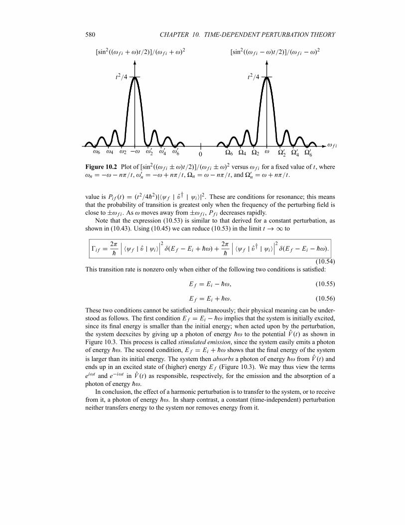
580 CHAPTER 10. TIME-DEPENDENT PERTURBATION THEORY
- f i
6
[sin2 f i t 2 ] f i2
t2 4
6 4 2 2 4 6 0
6
[sin2 f i t 2 ] f i2
t2 4
6 4 2 2 4 6
Figure 10.2 Plot of [sin2 f i t 2 ] f i2 versus f i for a fixed value of t , where
n n t , n n t , n n t , and n n t .
value is Pi f t t2 4h2 f†
i2. These are conditions for resonance; this means
that the probability of transition is greatest only when the frequency of the perturbing field is
close to f i . As moves away from f i , P f i decreases rapidly.Note that the expression (10.53) is similar to that derived for a constant perturbation, as
shown in (10.43). Using (10.45) we can reduce (10.53) in the limit t to
i f2
hf i
2E f Ei h
2
hf
†i
2E f Ei h
(10.54)
This transition rate is nonzero only when either of the following two conditions is satisfied:
E f Ei h (10.55)
E f Ei h (10.56)
These two conditions cannot be satisfied simultaneously; their physical meaning can be under-
stood as follows. The first condition E f Ei h implies that the system is initially excited,
since its final energy is smaller than the initial energy; when acted upon by the perturbation,
the system deexcites by giving up a photon of energy h to the potential V t as shown inFigure 10.3. This process is called stimulated emission, since the system easily emits a photonof energy h . The second condition, E f Ei h shows that the final energy of the system
is larger than its initial energy. The system then absorbs a photon of energy h from V t andends up in an excited state of (higher) energy E f (Figure 10.3). We may thus view the terms
ei t and e i t in V t as responsible, respectively, for the emission and the absorption of aphoton of energy h .
In conclusion, the effect of a harmonic perturbation is to transfer to the system, or to receive
from it, a photon of energy h . In sharp contrast, a constant (time-independent) perturbation
neither transfers energy to the system nor removes energy from it.
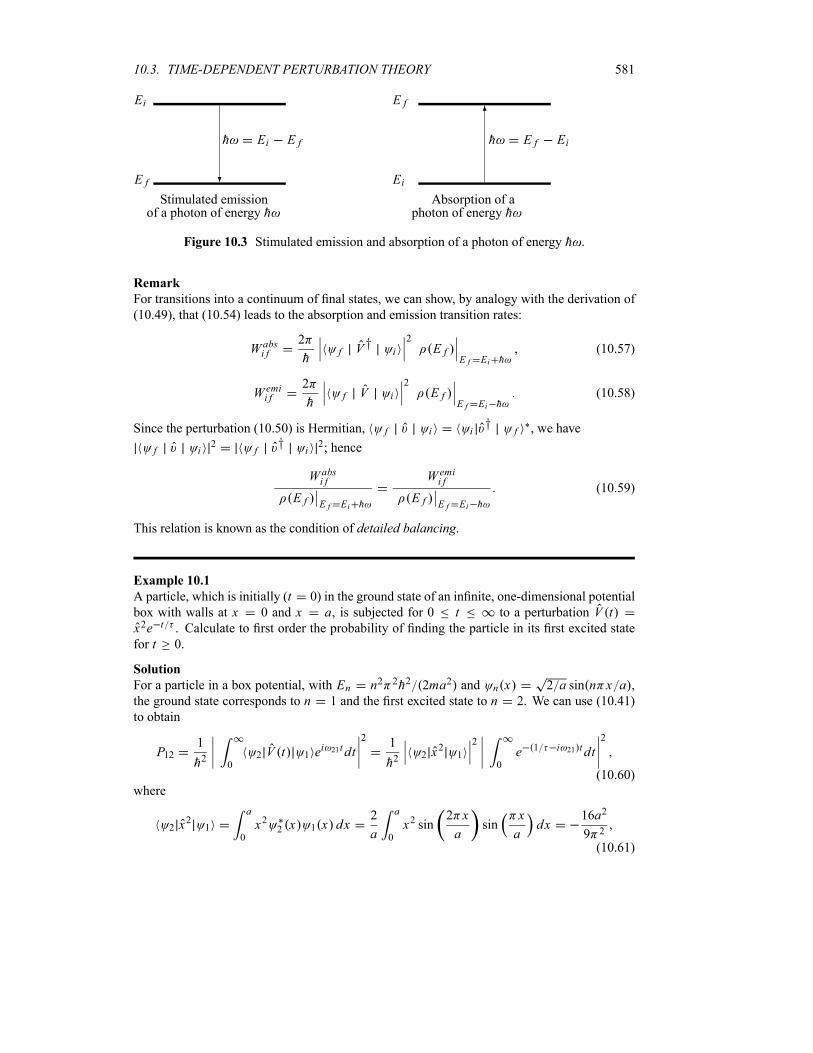
10.3. TIME-DEPENDENT PERTURBATION THEORY 581
E f
Ei
h Ei E f
Stimulated emissionof a photon of energy h
?
6
Ei
E f
h E f Ei
Absorption of aphoton of energy h
Figure 10.3 Stimulated emission and absorption of a photon of energy h .
Remark
For transitions into a continuum of final states, we can show, by analogy with the derivation of
(10.49), that (10.54) leads to the absorption and emission transition rates:
W absi f
2
hf V † i
2E f
E f Ei h(10.57)
W emii f
2
hf V i
2E f
E f Ei h(10.58)
Since the perturbation (10.50) is Hermitian, f i i†
f , we have
f i2
f†
i2; hence
W absi f
E f E f Ei h
W emii f
E f E f Ei h
(10.59)
This relation is known as the condition of detailed balancing.
Example 10.1
A particle, which is initially (t 0) in the ground state of an infinite, one-dimensional potential
box with walls at x 0 and x a, is subjected for 0 t to a perturbation V tx2e t . Calculate to first order the probability of finding the particle in its first excited state
for t 0.
Solution
For a particle in a box potential, with En n2 2h2 2ma2 and n x 2 a sin n x a ,the ground state corresponds to n 1 and the first excited state to n 2. We can use (10.41)
to obtain
P121
h2 02 V t 1 e
i 21tdt2 1
h22 x
21
2
0
e 1 i 21 tdt2
(10.60)
where
2 x2
1
a
0
x2 2 x 1 x dx2
a
a
0
x2 sin2 x
asin
x
adx
16a2
9 2
(10.61)
582 CHAPTER 10. TIME-DEPENDENT PERTURBATION THEORY
t
0
e 1 i 21 tdt2 e 1 i 21 t 1
1 i 21
21 e 2t 2e t cos 21t
221 1 2
(10.62)
which, in the limit t , reduces to
0
e 1 i 21 tdt2
221
12
1 9 4h2
4m2a412
1
(10.63)
since 21 E2 E1 h 3 2h 2ma2 . A substitution of (10.61) and (10.63) into (10.60)leads to
P1216a2
9 2h
29 4h2
4m2a412
1
(10.64)
10.4 Adiabatic and Sudden Approximations
In discussing the time-dependent perturbation theory, we have dealt with phenomena where the
perturbation V t is small, but we have paid no attention to the rate of change of the pertur-bation. In this section we want to discuss approximation methods treating phenomena where
V t is not only small but also switched on either adiabatically (slowly) or suddenly (rapidly).We assume here that V t is switched on at t 0 and off at a later time t (the turning on andoff may be smooth or abrupt).
Since ei f i t 1 i f i ei f i t t an integration by parts yields
i
h
t
0f V t i e
i f i t dt1
h f i
t
0f V t i
tei f i t dt
1
h f if V t i e
i f i tt
t 0
1
h f i
t
0
ei f i t
tf V t i dt
1
h f i
t
0
ei f i t
tf V t i dt (10.65)
where we have used the fact that V t vanishes at the limits (when it is switched on at t 0
and off at time t). The calculation of the integral depends on the rate of change of V t . Inwhat follows we are going to consider the cases where the interaction is switched on slowly or
rapidly.
10.4.1 Adiabatic Approximation
First, let us discuss briefly the adiabatic approximation without combining it with perturbation
theory. This approximation applies to phenomena whose Hamiltonians evolve slowlywith time;we should highlight the fact that the adiabatic approximation does not require the Hamiltonian
to split into an unperturbed part H0 and a weak time-dependent perturbation V t . Essentially,it consists in approximating the solutions of the Schrödinger equation at every time by the sta-
tionary states (energy En and wave functions n) of the instantaneous Hamiltonian in such

10.4. ADIABATIC AND SUDDEN APPROXIMATIONS 583
a way that the wave function at a given time is continuously and smoothly converted into an
eigenstate of the corresponding Hamiltonian at a later time. This result is the basis of an im-
portant theorem of quantum mechanics, known as the adiabatic theorem, which states that: ifa system is initially in the nth state and if its Hamiltonian evolves slowly with time, it will befound at a later time in the nth state of the new (instantaneous) Hamiltonian. That is, the systemwill make no transitions; it simply remains in the nth state of the new Hamiltonian.Let us now discuss the adiabatic approximation for those cases where the Hamiltonian splits
into a time-independent part H0 and a time-dependent part V t , which is small enough so thatperturbation theory applies and which is turned on and off very slowly. If V t is turned on att 0 and off at time t in a slow and smooth way, it will change very little in the time interval0 t t . The term f V t i t will be almost constant, so we can take it outsidethe integral sign in (10.65):
Pi f t1
h2 2f i
tf V t i
2 t
0
ei f i t dt2
(10.66)
or
Pi f t4
h2 4f i
tf V t i
2
sin2f i t
2(10.67)
The adiabatic approximation is valid only when the time change in the energy of the perturba-
tion during one period of oscillation is very small compared with the energy difference E f Eibetween the initial and final states:
1
f i tf V t i E f Ei (10.68)
Since sin2 1 we see from (10.67) that, in the adiabatic approximation, the transition prob-
ability is very small, Pi f 1. In fact, if the rate of change of V t , and hence of H t , is
very small, we will have f V t i t 0, which in turn implies that the transition
probability is practically zero: Pi f 0. Once more, we see that no transition occurs when theperturbation is turned on and off adiabatically. That is, if a system is initially (at t 0) in the
nth state n 0 of H0 with energy En 0 , then at the end (at time t) of an adiabatic pertur-bation V t , it will be found in the nth state n t of the new Hamiltonian (H H0 V t )with energy En t . As an illustrative example, consider a particle in a harmonic oscillator po-tential whose constant is being changed very slowly from k to, say, 3k; if the particle is initiallyin the second excited state, it will remain in the second excited state of the new oscillator.
Note that the transition probability (10.67) was derived by making use of two approxima-
tions: the perturbation theory approximation and the adiabatic approximation. It should be
stressed, however, that when the perturbation is not weak, but switched on adiabatically, we
can still use the adiabatic approximation but no longer in conjunction with perturbation theory.
10.4.2 Sudden Approximation
Again, let us start with a brief discussion of the sudden approximation without invoking pertur-
bation theory. If the Hamiltonian of a system changes abruptly (over a very short time interval)
from one form to another, we would expect the wave function not to change much, yet its
584 CHAPTER 10. TIME-DEPENDENT PERTURBATION THEORY
expansion in terms of the eigenfunctions of the initial and final Hamiltonians may be differ-
ent. Consider, for instance, a system which is initially (t 0) in an eigenstate n of the
Hamiltonian H0:
H0 n E 0n n n t ei E
0n t h
n (10.69)
At time t 0 we assume that the Hamiltonian is suddenly changed from H0 to H and that itpreserves this new form (i.e., H ) for t 0; it should be stressed that the difference between the
two Hamiltonians H H0 does not need to be small. Let n be the eigenfunctions of H :
H n En n n t ei En t h n (10.70)
The state of the system is given for t 0 by
tn
cnei En t h
n (10.71)
If the system is initially in an eigenstate m of H0, the continuity condition at t 0 dictates
that the system remains in this state just after the change takes place:
0n
cn n m cn n m (10.72)
The probability that a sudden change in the system’s Hamiltonian from H0 to H causes a
transition from the mth state of H0 to the nth state of H is
Pmn n m2 (10.73)
We should note that the sudden approximation is applicable only for transitions between dis-
crete states.
Let us now look at the sudden approximation within the context of perturbation theory.
Consider a system which is subjected to a perturbation that is small and switched on suddenly.
When V t is instantaneously turned on, the term ei f i t in (10.65) does not change much
during the switching-on time. We can therefore take ei f i t outside the integral sign,
Pi f1
h2 2f i
ei f i t2 t
0 tf V t i dt
2
(10.74)
hence the transition probability is given within the sudden approximation by
Pi f tf V t i
2
h2 2f i
(10.75)
To conclude, notice that both (10.73) and (10.75) give the transition probability within the
sudden approximation. Equation (10.73) represents the exact formula, where the change in the
Hamiltonians, H H0, may be large, but equation (10.75) gives only an approximate result,for it was derived from a first-order perturbative treatment, where we assumed that the change
H H0 is small, yet sudden.
10.4. ADIABATIC AND SUDDEN APPROXIMATIONS 585
Example 10.2
A particle is initially (t 0) in the ground state of an infinite, one-dimensional potential well
with walls at x 0 and x a.(a) If the wall at x a is moved slowly to x 8a, find the energy and wave function of the
particle in the new well. Calculate the work done in this process.
(b) If the wall at x a is now suddenly moved (at t 0) to x 8a, calculate theprobability of finding the particle in (i) the ground state, (ii) the first excited state, and (iii) the
second excited state of the new potential well.
Solution
For t 0 the particle was in a potential well with walls at x 0 and x a, and hence
Enn2 2h2
2ma2n x
2
asin
n x
a0 x a (10.76)
(a) When the wall is moved slowly, the adiabatic theorem dictates that the particle will make
no transitions; it will be found at time t in the ground state of the new potential well (the wellwith walls at x 0 and x 8a). Thus, we have
E1 t2h2
2m 8a 2
2h2
128ma2 1 x2
8asin
x
8a0 x a
(10.77)
The work needed to move the wall is
W E1 t E12h2
m 8a 2
2h2
2ma263 2h2
128ma2(10.78)
(b) When the wall is moved rapidly, the particle will find itself instantly (at t 0) in the
new potential well; its energy levels and wave function are now given by
Enn2 2h2
2m 8a 2n2 2h2
128ma2 n x2
8asin
n x
8a0 x 8a (10.79)
The probability of finding the particle in the ground state of the new box potential can be
obtained from (10.73): P11 1 12, where
1 1
a
01 x 1 x dx
2
8a
a
0
sinx
8asin
x
adx
16
634 2 2
(10.80)
hence
P11 1 12 16
63
2
4 2 2 0 0077 0 7% (10.81)
The probability of finding the particle in the first excited state of the new box potential is given
by P12 2 12, where
2 1
a
02 x 1 x dx
2
8a
a
0
sinx
4asin
x
adx
8
15(10.82)
hence
P12 2 12 8
15
2
0 1699 17% (10.83)

586 CHAPTER 10. TIME-DEPENDENT PERTURBATION THEORY
A similar calculation leads to
P13 3 12 2
8a
a
0
sin3 x
8asin
x
adx
216
554 2 2
2
24 2%
(10.84)
These calculations show that the particle is most likely to be found in higher excited states; the
probability of finding it in the ground state is very small.
10.5 Interaction of Atoms with Radiation
One of the most important applications of time-dependent perturbation theory is to study the
interaction of atomic electrons with an external electromagnetic radiation. Such an application
reveals a great deal about the structure of atoms. For simplicity, we assume that only one atomic
electron is involved in the interaction and that the electron spin is neglected. We also assume
that the nucleus is infinitely heavy.
In the absence of an external perturbation, the Hamiltonian of the atomic electron is H0P2 2me V0 r , where me is the mass of the electron and V0 r is the static potential due tothe interaction of the electron with the other electrons and with the nucleus.
Now, if electromagnetic radiation of vector potential A r t and electric potential r t isapplied on the atom, the Hamiltonian due to the interaction of the electron (of charge e) withthe radiation is given by
H1
2meP
e
cA r t
2e r t V0 r
H0 e r te
2mec2A P ih A
e2A2
2mec2(10.85)
where we have used the relation P A A P ih A. Since r t 0 for radiation with
no electrostatic source and since A 0 (Coulomb gauge), and neglecting the term in A2,we may write (10.85) as
H H0e
mecA P H0 V t (10.86)
where
V te
mecA r t P (10.87)
This term, which gives the interaction between the electron and the radiation, is small enough
(compared to H0) to be treated by perturbation theory. We are going to use perturbation theoryto study the effect of V t on the atom. In particular, we will focus on the transitions that areinduced as a result of this perturbation.
At this level, we cannot proceed further without calculating A r t . In what follows, weare going to show that, using A r t for an electromagnetic radiation, we obtain a V t which
has the structure of a harmonic perturbation: V t e i t †ei t . Therefore, by analogywith a harmonic perturbation, we would expect the atom to emit or absorb photons and then
undergo transitions from one state to another. For the sake of completeness, we are going to
determine A r t in two different ways: by treating the radiation classically and then quantum
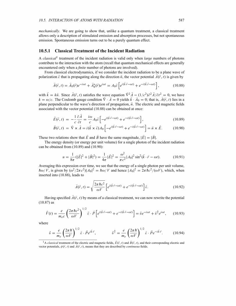
10.5. INTERACTION OF ATOMS WITH RADIATION 587
mechanically. We are going to show that, unlike a quantum treatment, a classical treatmentallows only a description of stimulated emission and absorption processes, but not spontaneous
emission. Spontaneous emission turns out to be a purely quantum effect.
10.5.1 Classical Treatment of the Incident Radiation
A classical1 treatment of the incident radiation is valid only when large numbers of photonscontribute to the interaction with the atom (recall that quantum mechanical effects are generally
encountered only when a finite number of photons are involved).From classical electrodynamics, if we consider the incident radiation to be a plane wave of
polarization that is propagating along the direction n, the vector potential A r t is given by
A r t A0 r ei t A0 r e
i t A0 ei k r t e i k r t (10.88)
with k kn. Since A r t satisfies the wave equation 2A 1 c2 2A t2 0, we have
k c. The Coulomb gauge condition A 0 yields k A0 0; that is, A r t lies in aplane perpendicular to the wave’s direction of propagation, n. The electric and magnetic fieldsassociated with the vector potential (10.88) can be obtained at once:
E r t1
c
A
t
i
cA0 ei k r t e i k r t (10.89)
B r t A i k A0 ei k r t e i k r t n E (10.90)
These two relations show that E and B have the same magnitude, E B .The energy density (or energy per unit volume) for a single photon of the incident radiation
can be obtained from (10.89) and (10.90):
u1
8E 2 B 2 1
4E 2
2
c2A0
2 sin2 k r t (10.91)
Averaging this expression over time, we see that the energy of a single photon per unit volume,
h V , is given by 2 2 c2 A0 2 h V and hence A0 2 2 hc2 V , which, wheninserted into (10.88), leads to
A r t2 hc2
Vei k r t e i k r t (10.92)
Having specified A r t by means of a classical treatment, we can now rewrite the potential(10.87) as
V te
mec
2 hc2
V
1 2
P ei k r t e i k r t e i t †ei t (10.93)
where
e
me
2 h
V
1 2
Peik r † e
me
2 h
V
1 2
Pe ik r (10.94)
1A classical treatment of the electric and magnetic fields, E r t and B r t , and their corresponding electric andvector potentials, r t and A r t , means that they are described by continuous fields.
588 CHAPTER 10. TIME-DEPENDENT PERTURBATION THEORY
The structure of (10.93) is identical with (10.50); that is, the interaction of an atomic electronwith radiation has the structure of a harmonic perturbation. By analogy with (10.50) we canstate that the term e i t in (10.93) gives rise to the absorption of the incident photon of energyh by the atom, and ei t to the stimulated emission of a photon of energy h by the atom. That
is, the absorption process occurs when the atom receives a photon from the radiation, and the
stimulated emission when the radiation receives or gains a photon from the decaying atom. At
this level, we cannot afford not to mention an important application of stimulated emission. In
this process we start with one (incident) photon and end up with two: the incident photon plus
the photon given by the atom resulting from its transition to a lower energy level. What would
happen if we had a large number of atoms in the same excited state? A single external photon
would trigger an avalanche, or chain reaction, of photons released by these atoms in a very short
time and all having the same frequency. This would lead to an amplification of the electromag-netic field. How does this take place? When the incident photon interacts with the first atom, it
will produce two photons, which in turn produce four photons; these four photons then produce
eight photons (after they interact with four different atoms), and so on. This process is known
as the amplification by stimulated emission of the (incident) radiation. Two such radiation am-plifications have been achieved experimentally and have led to enormous applications: one in
the microwave domain, known as maser (microwave amplification by stimulated emission ofradiation); the other in the domain of light waves, called laser (light amplification by stimulatedemission of radiation).
Following the approach that led to the transition rates (10.54) from (10.50), we can eas-
ily show that the transition rates for the stimulated emission and absorption corresponding to
(10.93) are given by
emii f
4 2e2
m2e Vf e ik r P i
2E f Ei h (10.95)
absi f
4 2e2
m2e Vf eik r P i
2E f Ei h (10.96)
These relations represent the expressions for the transition rates when the radiation is treated
classically.
What would happen when there is no radiation? If A 0 (i.e., the atom is placed in a
vacuum), equations (10.95) and (10.96) imply that no transition will occur since, as equation
(10.87) shows, if A 0 the perturbation will be zero; hence emii f 0 and abs
i f 0. As
a result, the classical treatment cannot account for spontaneous emission which occurs even inthe absence of an external perturbing field. This implies, for instance, that a hydrogen atom in
an n 2 energy eigenstate remains in this eigenstate unless it is perturbed by an external field.
This is in complete disagreement with experimental observations, which show that atoms in the
n 2 states undergo spontaneous emissions; they emit electromagnetic radiation even when noexternal perturbation is present. The spontaneous emission is a purely quantum effect.
10.5.2 Quantization of the Electromagnetic Field
We have seen that a classical treatment of radiation leads to transition rates that account only
for the processes of absorption and stimulated emission; spontaneous emission of photons by
atoms is a typical phenomenon that a classical treatment fails to explain, let alone predict. The
10.5. INTERACTION OF ATOMS WITH RADIATION 589
classical treatment is valid only when very large numbers of photons contribute to the radiation;
that is, when the intensity of the radiation is so high that only its wave aspect is important. At
very low intensities, however, the particle nature of the radiation becomes nonnegligible. In this
case we have to consider a quantum mechanical treatment of the electromagnetic radiation. To
obtain a quantum description of the radiation, we would necessarily need to replace the various
fields (such as E r t , B r t , and the potential vector A r t ) with operators.In the absence of charges and currents, the electric and magnetic fields are fully specified
by the vector potential A r t . Since A r t is transverse (perpendicular to the wave vector k),it has only two nonzero components along the directions of two polarization (unit) vectors, 1
and 2, which lie in a plane perpendicular to k. We can thus expand A r t in a Fourier seriesas follows:
A r t1
Vk
2
1
A k ei k r k t Ake i k r k t (10.97)
where we have assumed that the electromagnetic field is confined to a large volume V withperiodic boundary conditions. We are going to see that, by analogy with the quantization of
a classical harmonic oscillator, the quantization of radiation can be achieved by writing theelectromagnetic field in terms of creation and annihilation operators.The Hamiltonian of the complete system (atom and the external radiation) is H H0
Hr V t , where H0 is the Hamiltonian of the unperturbed atom, Hr is the Hamiltonian of theelectromagnetic field, and V t is the interaction of the atom with the radiation. To find Hr weneed to quantize the energy of the electromagnetic field which can be obtained from (10.97):
Hr1
8d3r E2 r t B2 r t
V
8 c2k
2
1
hk 2AkA k (10.98)
with 2 1, where we have used k ck, E r t 1 c A t , and B r t A.Instead of the two variables A k and A k
, we can introduce a new set of two canonically
conjugate variables:
Q k
1
4 c2A
kA k P k
i k
4 c2A
kA k (10.99)
Combining (10.98) and (10.99) we can write
Hrk
2
1
1
2P2
k
2k
2Q2
k(10.100)
This expression has the structure of a Hamiltonian of a collection of independent harmonic
oscillators. This is compatible with the fact that electromagnetic waves in a vacuum result
from the (harmonic) oscillations of the electromagnetic field; hence they can be described by
means of a linear superposition of independent vibrational modes. To quantize (10.100) we
simply need to find the operators Q k and P k that correspond to the variables Q k and P k ,
respectively, such that they obey the canonical commutation relations:
Q1k1
P2k2
ih1 2 k1 k2
(10.101)
590 CHAPTER 10. TIME-DEPENDENT PERTURBATION THEORY
Following the same quantization procedure of a classical harmonic oscillator, and introducing
the lowering and raising operators
a kk
2hQ k
i
2h kP k a
†k
k
2hQ k
i
2h kP k (10.102)
which lead to Q k h 2 k a†k
a k and P k i h k 2 a†k
a k , we can show
that the Hamiltonian operator corresponding to (10.100) is given by
Hrk
2
1
h k N k
1
2(10.103)
with N k a†ka k .
By analogy to the harmonic oscillator, the operators a k and a†kobey the following com-
mutation relations:
a1 k1
a†
2 k2 1 2 k1 k2a1 k1
a2 k2
a†
1 k1a†
2 k20 (10.104)
and serve respectively to annihilate and create a photon of wave number k and polarization .
The eigenvalues of N k are n k 0 1 2 ; by analogy with the harmonic oscillator, its
eigenvectors are
n k
1
n k!a†k
n k
0 (10.105)
where 0 is the state with no photons, the vacuum state, and n k is a state of the elec-
tromagnetic field with n k photons with wave vector k and polarization . The number n k
therefore represents the occupation number mode. The actions of a k and a†kon n k are
given by
a k n k n k n k 1 a†kn k k 1 n k 1 (10.106)
The eigenstates of the Hamiltonian (10.103) can be inferred from (10.105):
n1k1
n2k2
n3k3
j
nj k j
(10.107)
with the energy eigenvalues (of the radiation)
Erk
h k n k
1
2(10.108)
The state n1k1
n2k2
n3k3
describes an electromagnetic field with n1k1photons in the
mode 1 k1 (i.e., n1k1photons with wave vector k1 and polarization 1), n
2k2photons in the

10.5. INTERACTION OF ATOMS WITH RADIATION 591
mode 2 k2 , and so on. Substituting (10.99) into (10.102), we get a k k 2 hc2 A k
and a†k k 2 hc2 A
†k; hence
A k
2 hc2
ka k A
†k
2 hc2
ka†k
(10.109)
An insertion of these two relations into (10.97) gives the vector potential operator:
A r t
k
2
1
2 hc2
kVa ke
i k r k t a†ke i k r k t (10.110)
The interaction V t as given by (10.87) reduces to V t e mec A r t P or
V te
mek
2 h
kVa ke
ik r Pei k t a†keik r Pe i k t (10.111)
or
V t
k
2
1kei k t †
ke i k t (10.112)
where
k
e
me
2 h
kVa ke
ik r P†k
e
me
2 h
kVa†ke ik r P (10.113)
The terms k and†kcorrespond to the absorption (annihilation) and emission (creation) of
a photon by the atom, respectively. As in the classical case, the interaction (10.112) has the
structure of a harmonic perturbation.
Remark
The quantization of the radiation is achieved by writing the electromagnetic field in terms of cre-
ation and annihilation operators, by analogy with the harmonic oscillator. This process, which
is called second quantization, leads to the replacement of the various fields (such as the vectorpotential A r t , the electric field E r t , and the magnetic field B r t ) by operator quanti-ties, which in turn are expressed in terms of creation and annihilation operators. For instance,
the Hamiltonian and the vector potential of the radiation are given in the second quantization
representation by equations (10.103) and (10.110), respectively.
10.5.3 Transition Rates for Absorption and Emission of Radiation
Before the atom and the radiation interact, their initial state is given by i i n k ,
where i is the state of the unperturbed atom and n k is the state vector of the radiation.
After the interaction takes place, the state of the system is given by f f n k f .
Let us look first at the case of emission of a photon. If after interaction the atom emits
a photon, the final state of the system will be given by f f n k 1 , since
the electromagnetic field gains a photon; hence its state changes from n k n k 1 .
592 CHAPTER 10. TIME-DEPENDENT PERTURBATION THEORY
Formally, this process can be achieved by creating a photon, that is, by applying†kor a
†kon
the photonic state n k :
f†k i
e
me
2 h
kVf e ik r P i n k 1 a
†kn k
e
me
2 h
kVn k 1 f e ik r P i (10.114)
When n k 0 (i.e., no radiation), equation (10.114) shows that even in the absence of anexternal radiation, the theory can describe events where there is emission of a photon. This iscalled spontaneous emission. This phenomenon cannot be described by means of a classicaltreatment of radiation. But if n k 0, then n k is responsible for induced or stimulatedemissions; the bigger n k , the bigger the emission probability.
In the case of a photon absorption, the system undergoes a transition from an initial state
i i n k to the final state f f n k 1 . This can be achieved formally
by applying the annihilation operator a k on n k :
f k ie
me
2 h
kVf eik r P i n k 1 a k n k
e
me
2 h
kVn k f eik r P i (10.115)
The transition rates corresponding to the emission or absorption of a photon of energy
h k hck, wave number k, and polarization can be obtained, by analogy with (10.95) and
(10.96), from (10.114) and (10.115):
emii f
4 2e2
m2e kVn k 1 f e ik r P i
2E f Ei h k (10.116)
absi f
4 2e2
m2e kVn k f eik r P i
2E f Ei h k (10.117)
10.5.4 Transition Rates within the Dipole Approximation
Approximate expressions of the transition rates (10.116) and (10.117) can be obtained by ex-
panding e ik r :
e ik r 1 ik r1
2k r 1 i
cn r
1
2
2
c2n r 2 (10.118)
This expansion finds its justification in the fact that k r is a small quantity, since the wave-length of the radiation (visible or ultraviolet) is very large compared to the atomic size: kr2 a0 2 10 10m 10 6m 10 3. In the case of nuclear radiation (such as radia-
tion), kr is also in the range of 10 3, with rnucleus 10 15m.
10.5. INTERACTION OF ATOMS WITH RADIATION 593
The electric dipole approximation corresponds to keeping only the leading term in the ex-
pansion (10.118): e ik r 1; hence
f e ik r P i f P i (10.119)
This term gives rise to electric dipole or E1 transitions. To calculate this term, we need to usethe relation
X H0 XP 2
2meV r X
P2x2me
ih
mePx (10.120)
which can be generalized to [r H0] ihP me. Hence, inserting P me ih [r H0] into(10.119) and using H0 i Ei i and H0 f E f f , we have
f P imeih
f [r H0] im
ihEi E f f r i
ime f i f r i (10.121)
The substitution of this term into (10.119) leads to
f eik r P i ime f i f r i (10.122)
Inserting (10.122) into (10.116) and (10.117), we obtain the transition rates, within the dipoleapproximation, for the emission and absorption of a photon of energy h k by the atom:
emii f
4 2e2 2f i
kVn k 1 f r i
2E f Ei h k (10.123)
absi f
4 2e2 2f i
kVn k f r i
2E f Ei h k (10.124)
10.5.5 The Electric Dipole Selection Rules
Since r is given in spherical coordinates by r r sin cos i r sin sin j r cos k,we can write
r r x sin cos y sin sin z cos (10.125)
Using the relations sin cos 2 3 Y11 Y1 1 , sin sin i 2 3 Y11 Y1 1 ,
and cos 4 3Y10, we may rewrite (10.125) as
r4
3r
x i y
2Y11
x i y
2Y1 1 zY10 (10.126)
which in turn leads to
f r i4
3 0
r3Rn f l f r Rni li r dr
Yl f m fx i y
2Y11
x i y
2Y1 1 zY10 Ylimi d
(10.127)
594 CHAPTER 10. TIME-DEPENDENT PERTURBATION THEORY
where we have used r i Rni li r Ylimi and r f Rn f l f r Yl f m f .
The integration over the angular degrees of freedom can be calculated by means of the
Wigner–Eckart theorem; we have shown in Chapter 7 that
d Yl f m f Y1m Ylimi l f m f Y1m li mi
3 2li 1
4 2l f 1li 1 0 0 l f 0 li 1 mi m l f m f (10.128)
Inserting (10.128) into (10.123) and (10.124), we obtain emii f li 1 mi m l f m f
2
and absi f li 1 mi m l f m f
2. Thus the dipole selection rules are specified by the
selection rules of the Clebsch–Gordan coefficient li 1 mi m l f m f :
The transition rates are zero unless the values of m f and mi satisfy the condition mim m f or m f mi m . But since m takes only three values, m 1, 0, 1, we
have
m f mi 1 0 1 (10.129)
The permissible values of l f must lie between li 1 and li 1 (i.e., li 1 l f li 1),
so we have 1 l f li 1 or
l f li 1 0 1 (10.130)
Note that, since the Clebsch–Gordan coefficient li 1 mi m l f m f vanishes for
li l f 0, no transition between li 0 and l f 0 is allowed.
Finally, since the coefficient li 1 0 0 l f 0 vanishes unless 1 li 1 l f 1 or
1 li l f 1, then li l f must be an odd integer:
l f li odd integer (10.131)
This means that, in the case of electric dipole transitions, the final and initial states must
have different parities. As a result, electric dipole transitions like 1s 2s, 2p 3p, etc.,
are forbidden, while transitions like 1s 2p, 2p 3s, etc., are allowed.
10.5.6 Spontaneous Emission
It is clear from (10.123) that the rate of emission of a photon from an atom is not zero even
in the absence of an external radiation field (n k 0). This corresponds to the spontaneousemission of a photon. The total transition rate corresponding to spontaneous emission can beinferred from (10.123) by taking n k 0:
emii f
4 2 2f i
Vd f i
2 E f Ei h (10.132)
where d f i is the matrix element for the electron’s electric dipole moment d er :
d f i f d i e f r i (10.133)
10.5. INTERACTION OF ATOMS WITH RADIATION 595
The relation (10.132) gives the transition probability per unit time corresponding to the transi-
tion of the atom from the initial state i to the final state f as a result of its spontaneous
emission of a photon of energy h . Thus the final states of the system consist of products
of discrete atomic states and a continuum of photonic states. The photon emitted will be de-
tected in general as having a momentum in the momentum interval p p dp located aroundp hk h c. The transition rate (10.132) needs then to be summed over the continuum ofthe final photonic states. The number of final photonic states within the unit volume V , whosemomenta are within the interval p p dp , is given by
d3nVd3 p
2 h 3V p2dp d
2 h 3Vh3 2
2 h 3c3d d
V 2
2 c 3d d (10.134)
Thus, the transition rate corresponding to the emission of a photon in the solid angle d is
obtained by integrating (10.132) over d :
dW emii f
V
2 3c3d 2 emi
i f d1
2 c3d f i
2d 2f i E f Ei h d
1
2 hc3d f i
2d 2f i i f d (10.135)
where we have used the fact E f Ei h 1 h i f with i f Ei E f h.Carrying out the integration, we can reduce (10.135) to
dW emii f
3
2 hc3d f i
2d (10.136)
The transition rate (10.136) corresponds to a specific polarization; that is, the photon emitted
travels along the direction n (since k kn), which is normal to . To find the transition rate
corresponding to any polarization, we need to sum over the two polarizations of the photon:
2
1
d f i2
1 d f i 12
2 d f i 22 d f i
2 d f i 32 (10.137)
Since the three directions of d f i are equivalent, we have
d f i 12 d f i 2
2 d f i 32 1
3d f i
2 (10.138)
Thus, an average over polarization yields
2
1
d f i2 d f i
2 1
3d f i
2 2
3d f i
2 (10.139)
Substituting (10.139) into (10.136), we obtain the average transition rate corresponding to the
emission of the photon into the solid angle d :
dW emii f
3
3 hc3d f i
2d (10.140)
An integration over all possible (photonic) directions ( d f i 2 is not included in the integrationsince we are integrating over the angular part of the photonic degrees of freedom only and not
596 CHAPTER 10. TIME-DEPENDENT PERTURBATION THEORY
over the electron’s) yields d 4 . Thus, the transition rate associated with the emission
of the photon is
W emii f
4
3
3
hc3d f i
2 4
3
3e2
hc3f r i
2(10.141)
where E f Ei h.The total power (or intensity) radiated by the electron is obtained by multiplying the total
rates (10.141) by h :
Ii f h W emii f
4
3
4
c3d f i
2 4
3
4e2
c3f r i
2(10.142)
The transition rates derived above, (10.141) and (10.142), were obtained for single-electron
atoms. For atoms that have Z electrons, we must replace the dipole moment d er with thedipole moment of all Z electrons: d e Z
j 1 r j .The mean lifetime of an excited state can be obtained by adding together the total transi-
tion probabilities per unit time (10.141) for all possible final states:
1
W
1
f Wi f(10.143)
Example 10.3
A particle of charge q and massm is moving in a one-dimensional harmonic oscillator potentialof frequency 0.
(a) Find the rate of spontaneous emission for a transition from an excited state n to the
ground state.
(b) Obtain an estimate for the rate calculated in (a) and the lifetime of the state n when
the particle is an electron and 0 3 1014 rad s 1.
(c) Find the condition under which the dipole approximation is valid for the particle of (b).
Solution
(a) The spontaneous emission rate for a transition from an excited state n to 0 is given
by (10.141):
W emin 0
4
3
3q2
hc30 X n
2(10.144)
where En E0 h n 12 0
12 0 n 0. Since a n n n 1 and
a† n n 1 n 1 , and since X h 2m 0 a† a , we have
0 X nh
2m 00 a† a n
h
2m 0n 1 0 n 1 n 0 n 1 (10.145)
Thus only a transition from 1 to 0 is possible; hence n 1, 0, and 0 X 1
h 2m 0 . The emission rate (10.144) then becomes
W emi1 0
4
3
3q2
hc30 X 1
2 4
3
30q2
hc3h
2m 0
2
3
20q2
mc3(10.146)

10.6. SOLVED PROBLEMS 597
(b) If the particle is an electron, we have q e:
W emi1 0
2
3
20e2
mec32
3
20h
mec22
3
hc
mec2
20
c(10.147)
Using mec2 0 511MeV, hc 197 33MeV fm, we have
W emi1 0
2
3
hc
mec2
20
c
2
3 137
197 33MeV fm
0 511MeV
9 1028 s 2
3 108ms 15 6 105 s 1 (10.148)
The lifetime of the 1 state is
1
W emi1 0
3
2
mec3
20e2
1
5 6 105sec 20 18 10 5 s (10.149)
(c) For the dipole approximation to be valid, we need kx 1, where x was calculatedin (10.145) for n 1: x h 2me 0 . As for k, a crude estimate yields k cE1 E0 hc 0 c. Thus, we have
kx0
c
h
2me 0
h 0
2mec21 h 0 2mec
2 (10.150)
This is indeed the case since 2mec2 1 022MeV is very large compared to
h 0 hc0
c197 33MeV fm
3 1014 s 1
3 108ms 12 0 10 7MeV (10.151)
10.6 Solved Problems
Problem 10.1
(a) Calculate the position and the momentum operators, XH t and PH t , in the Heisen-berg picture for a one-dimensional harmonic oscillator.
(b) Find the Heisenberg equations of motion for XH t and PH t .
Solution
In the Schrödinger picture, where the operators do not depend explicitly on time, the Hamil-
tonian of a one-dimensional harmonic oscillator is given by
HP2
2m
1
2m 2X2 (10.152)
(a) Using the commutation relations
[H X ]1
2m[P2 X ]
ih
mP (10.153)
[H P]1
2m 2[X2 P] ihm 2X (10.154)

598 CHAPTER 10. TIME-DEPENDENT PERTURBATION THEORY
along with
eABe A B [A B]1
2![A [A B]]
1
3![A [A [A B]]] (10.155)
we may write (see Eq. (10.11))
XH t ei t H hXe i t H h Xit
h[H X]
1
2!
i t
h
2
[H [H X]]
Xt
mP
t 2
2!X
t 3
3!
1
mP
t 4
4!X
t 5
5!
1
mP
X 1t 2
2!
t 4
4!
1
mP t
t 3
3!
t 5
5!
(10.156)
or
XH t X cos t1
mP sin t (10.157)
A similar calculation yields (see Eq. (10.11))
PH t ei t H hPe i t H h Pit
h[H P]
1
2!
i t
h
2
[H [H P]]
P 1t 2
2!
t 4
4!m X t
t 3
3!
t 5
5!
(10.158)
or
PH t P cos t m X sin t (10.159)
(b) To find the equations of motion of XH t and PH t , we need to use the Heisenbergequation d AH t dt 1 ih [AH t H ] which, along with (10.153) and (10.154), leads to
dXH t
dt
1
ih[XH t H ]
1
ihei t H h[X H ]e i t H h 1
ih
ih
mei t H hPe i t H h
(10.160)
dPH t
dt
1
ih[PH t H]
1
ihei t H h[P H ]e i t H h ihm 2
ihei t H hXe i t H h
(10.161)
or
dXH t
dt
1
mPH t
d PH t
dtm 2XH t (10.162)
Problem 10.2
Using the expressions derived in Problem 10.1 for XH t and PH t , evaluate the followingcommutators for a harmonic oscillator:
XH t1 PH t2 XH t1 XH t2 PH t1 PH t2
10.6. SOLVED PROBLEMS 599
Solution
Using (10.157) and (10.159) along with the commutation relations [X P] ih and [X X][P P] 0, we have
[XH t1 PH t2 ] X cos t11
mP sin t1 P cos t2 m X sin t2
[X P] cos t1 cos t2 [P X] sin t1 sin t2
ih [cos t1 cos t2 sin t1 sin t2 ] (10.163)
or
[XH t1 PH t2 ] ih cos [ t1 t2 ] (10.164)
A similar calculation yields
[XH t1 XH t2 ] X cos t11
mP sin t1 X cos t2
1
mP sin t2
1
m[X P] cos t1 sin t2
1
m[P X] sin t1 cos t2
ih
m[cos t1 sin t2 sin t1 cos t2 ] (10.165)
or
[XH t1 XH t2 ]ih
msin [ t1 t2 ] (10.166)
Similarly, we have
[PH t1 PH t2 ] P cos t1 m X sin t1 P cos t2 m X sin t2
m [P X ] cos t1 sin t2 m [X P] sin t1 cos t2
ihm [sin t1 cos t2 cos t1 sin t2 ] (10.167)
or
[PH t1 PH t2 ] ihm sin [ t1 t2 ] (10.168)
Problem 10.3
Evaluate the quantity n XH t X n for the nth excited state of a one-dimensional harmonicoscillator, where XH t and X designate the position operators in the Heisenberg picture andthe Schrödinger picture.
Solution
Using the expression of XH t calculated in (10.157), we have
n XH t X n n X2 n cos t1
mn PX n sin t (10.169)
Since, for a harmonic oscillator, X and P are given by
Xh
2ma† a P i
mh
2a† a (10.170)
600 CHAPTER 10. TIME-DEPENDENT PERTURBATION THEORY
and a† n n 1 n 1 and a n n n 1 , we have
n X2 nh
2mn a† 2 a2 aa† a†a n
h
2m2n 1 (10.171)
n PX nih
2n a† 2 a2 aa† a†a n
ih
2(10.172)
since n a† 2 n n a2 n 0, n a†a n n and n aa† n n 1. Inserting
(10.171) and (10.172) into (10.169), we obtain
n XH t X nh
2m2n 1 cos t i sin t (10.173)
Problem 10.4
The Hamiltonian due to the interaction of a particle of mass m, charge q, and spin S with amagnetic field pointing along the z-axis is H qB mc Sz . Write the Heisenberg equationsof motion for the time-dependent spin operators Sx t , Sy t , and Sz t , and solve them toobtain the operators as functions of time.
Solution
Let us write H in a lighter form H Sz where qB mc. The commutation of Hwith the components of the spin operator can be inferred at once from [Sx Sz] ihSy and
[Sy Sz] ihSx :
[Sx H ] ih Sy [Sy H ] ih Sx [Sz H ] 0 (10.174)
The Heisenberg equations of motion for Sx t , Sy t , and Sz t can be obtained from
d AH t dt 1 ih [AH t H ] 1 ih ei t H h[A 0 H ]e i t H h which, using (10.174),
leads to
dSx t
dt
1
ih[Sx t H ]
1
ihei t H h[Sx 0 H ]e i t H h
ih
ihei t H hSy 0 e
i t H h Sy t (10.175)
Similarly, we have
dSy t
dt
1
ihei t H h[Sy 0 H ]e i t H h ih
ihei t H hSx 0 e
i t H h Sx t (10.176)
dSz t
dt
1
ihei t H h[Sz 0 H ]e i t H h 0 (10.177)
To solve (10.175) and (10.176), we may combine them into two more conducive equations:
dS t
dti S t (10.178)
10.6. SOLVED PROBLEMS 601
where S t Sx t i Sy t . The solutions of (10.178) are S t S 0 e i t which, when
combined with Sx t12[S t S t ] and Sy t
12i [S t S t ], lead to
Sx t Sx 0 cos t Sy 0 sin t (10.179)
Sy t Sy 0 cos t Sx 0 sin t (10.180)
The solution of (10.177) is obvious:
dSz t
dt0 Sz t Sz 0 (10.181)
Problem 10.5
Consider a spinless particle of mass m, which is moving in a one-dimensional infinite potentialwell with walls at x 0 and x a.(a) Find XH t and PH t in the Heisenberg picture.(b) If at t 0 the particle is in the state x 0 [ 1 x 2 x ] 2, where 1 x and
2 x are the ground and first excited states, respectively, with n x 2 a sin n x a , findthe state vector x t for t 0 in the Schrödinger picture.
(c) Evaluate x t X x t and x t P x t as a function of time in the
Schrödinger picture.
(d) Evaluate x t XH t x t and x t PH t x t as a function of
time in the Schrödinger picture.
Solution
(a) Since the particle’s Hamiltonian is purely kinetic, H P2 2m, we have [H P] 0
and
[H X]1
2m[P2 X ]
ih
mP (10.182)
Using these relations along with (10.155), we obtain
XH t ei t H hXe i t H h Xit
h[H X ]
1
2!
i t
h
2
[H [H X ]] (10.183)
and since [H [H X ]] ih m [H P] 0, we end up with
XH t Xt
mP (10.184)
On the other hand, since [H P] 0, we have
P PH t (10.185)
(b) Since the energy of the nth level is given by En n2 2h2 2ma2 , we have
x t1
21 x e
i E1t h2 x e
i E2t h
1
ae i E1t h sin
x
ae i E2t h sin
2 x
a(10.186)

602 CHAPTER 10. TIME-DEPENDENT PERTURBATION THEORY
(c) Using (10.186) we can write
x t X x t1
21 X 1 2 X 2 1 X 2 e
i E2 E1 t h
2 X 1 ei E2 E1 t h (10.187)
Since n X n a 2 (Chapter 4) and
1 X 2 2 X 12
a
a
0
x sinx
asin
2 x
adx
16a
9 2(10.188)
we can rewrite (10.187) as
x t X x t1
2
a
2
a
2
16a
9 2e i E2 E1 t h ei E2 E1 t h
a
2
16a
9 2cos
3 2ht
2ma2(10.189)
since E2 E1 3 2h2 2ma2 .A similar calculation which uses n P n 0 and
1 P 2 ih4
a
a
0
sinx
acos
2 x
adx
8ih
3a2 P 1 (10.190)
leads to
x t P x t1
21 P 1 2 P 2 1 P 2 e
i E2 E1 t h
2 P 1 ei E2 E1 t h (10.191)
or to
x t P x t1
2
8ih
3ae i E2 E1 t h
8ih
3aei E2 E1 t h
8h
3asin
3 2ht
2ma2(10.192)
(d) From (10.184) we have
x t XH t x t x t X x tt
mx t P x t (10.193)
Inserting the expressions for x t X x t and x t P x t calculated in
(10.189) and (10.192), we obtain
x t XH t x ta
2
16a
9 2cos
3 2ht
2ma28ht
3masin
3 2ht
2ma2(10.194)
and x t PH t x t is given by (10.192):
x t PH t x t x t P x t8h
3asin
3 2ht
2ma2(10.195)
since, as shown in (10.185), we have PH t P .
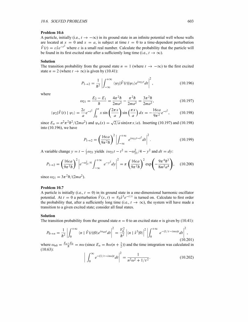
10.6. SOLVED PROBLEMS 603
Problem 10.6
A particle, initially (i.e., t ) in its ground state in an infinite potential well whose walls
are located at x 0 and x a, is subject at time t 0 to a time-dependent perturbation
V t xe t2 where is a small real number. Calculate the probability that the particle will
be found in its first excited state after a sufficiently long time (i.e., t ).
Solution
The transition probability from the ground state n 1 (where t ) to the first excited
state n 2 (where t ) is given by (10.41):
P1 21
h22 V t 1 e
i 21tdt2
(10.196)
where
21E2 E1h
4 2h
2ma2
2h
2ma23 2h
2ma2(10.197)
2 V t 12
ae t2
a
0
x sin2 x
asin
x
adx
16 a
9 2e t2 (10.198)
since En n2 2h2 2ma2 and n x 2 a sin n x a . Inserting (10.197) and (10.198)into (10.196), we have
P1 216 a
9 2h
2
ei 21t t2dt2
(10.199)
A variable change y t i2 21 yields i 21t t2 2
21 4 y2 and dt dy:
P1 216 a
9 2h
2
e221 4 e y2dy
216 a
9 2h
2
exp9 4h2
8m2a4(10.200)
since 21 3 2h 2ma2 .
Problem 10.7
A particle is initially (i.e., t 0) in its ground state in a one-dimensional harmonic oscillator
potential. At t 0 a perturbation V x t V0x3e t is turned on. Calculate to first order
the probability that, after a sufficiently long time (i.e., t ), the system will have made a
transition to a given excited state; consider all final states.
Solution
The transition probability from the ground state n 0 to an excited state n is given by (10.41):
P0 n1
h2 0
n V t 0 ei n0tdt2 V 20
h2n x3 0
2
0
e 1 in tdt2
(10.201)
where n0En E0h n (since En h n 1
2) and the time integration was calculated in
(10.63):
0
e 1 in tdt2
1
n2 2 1 2(10.202)
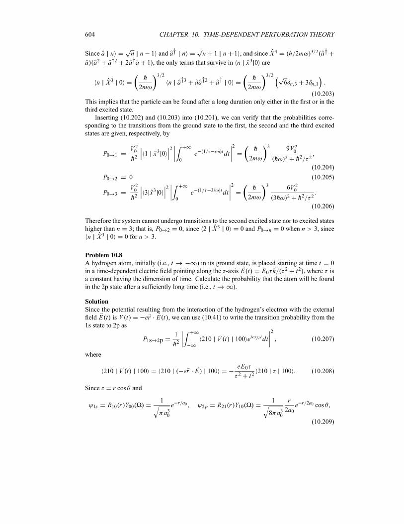
604 CHAPTER 10. TIME-DEPENDENT PERTURBATION THEORY
Since a n n n 1 and a† n n 1 n 1 , and since X3 h 2m 3 2 a†
a a2 a†2 2a†a 1 , the only terms that survive in n x3 0 are
n X3 0h
2m
3 2
n a†3 aa†2 a† 0h
2m
3 2
6 n 3 3 n 1
(10.203)
This implies that the particle can be found after a long duration only either in the first or in the
third excited state.
Inserting (10.202) and (10.203) into (10.201), we can verify that the probabilities corre-
sponding to the transitions from the ground state to the first, the second and the third excited
states are given, respectively, by
P0 1
V 20h2
1 x3 02
0
e 1 i tdt2 h
2m
3 9V 20h 2 h2 2
(10.204)
P0 2 0 (10.205)
P0 3
V 20h2
3 x3 02
0
e 1 3i tdt2 h
2m
3 6V 203h 2 h2 2
(10.206)
Therefore the system cannot undergo transitions to the second excited state nor to excited states
higher than n 3; that is, P0 2 0, since 2 X3 0 0 and P0 n 0 when n 3, since
n X3 0 0 for n 3.
Problem 10.8
A hydrogen atom, initially (i.e., t ) in its ground state, is placed starting at time t 0
in a time-dependent electric field pointing along the z-axis E t E0 k 2 t2 , where is
a constant having the dimension of time. Calculate the probability that the atom will be found
in the 2p state after a sufficiently long time (i.e., t ).
Solution
Since the potential resulting from the interaction of the hydrogen’s electron with the external
field E t is V t er E t , we can use (10.41) to write the transition probability from the1s state to 2p as
P1s 2p1
h2210 V t 100 ei f i tdt
2
(10.207)
where
210 V t 100 210 er E 100eE02 t2
210 z 100 (10.208)
Since z r cos and
1s R10 r Y001
a30
e r a02p R21 r Y10
1
8 a30
r
2a0e r 2a0 cos
(10.209)
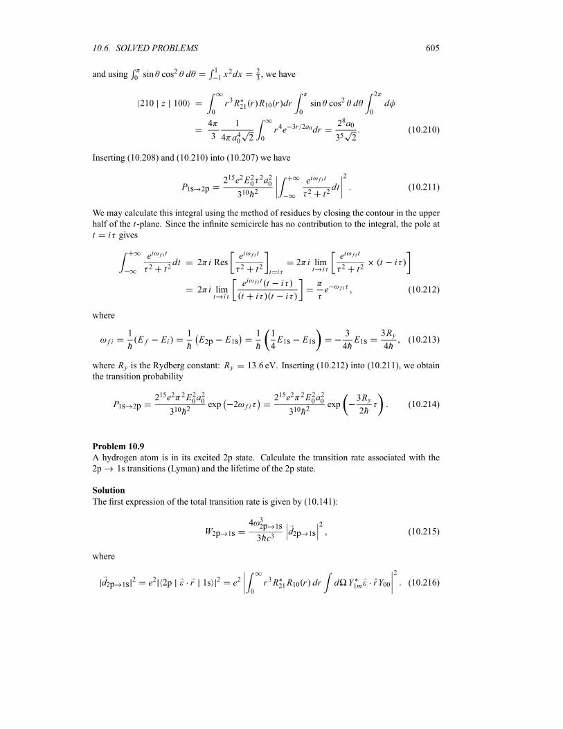
10.6. SOLVED PROBLEMS 605
and using 0 sin cos2 d 11 x2dx 2
3, we have
210 z 1000
r3R21 r R10 r dr0
sin cos2 d2
0
d
4
3
1
4 a40 2 0
r4e 3r 2a0dr28a0
35 2(10.210)
Inserting (10.208) and (10.210) into (10.207) we have
P1s 2p215e2E20
2a20310h2
ei f i t
2 t2dt
2
(10.211)
We may calculate this integral using the method of residues by closing the contour in the upper
half of the t-plane. Since the infinite semicircle has no contribution to the integral, the pole att i gives
ei f i t
2 t2dt 2 i Res
ei f i t
2 t2 t i2 i lim
t i
ei f i t
2 t2t i
2 i limt i
ei f i t t i
t i t ie f i (10.212)
where
f i1
hE f Ei
1
hE2p E1s
1
h
1
4E1s E1s
3
4hE1s
3Ry4h
(10.213)
where Ry is the Rydberg constant: Ry 13 6 eV. Inserting (10.212) into (10.211), we obtain
the transition probability
P1s 2p215e2 2E20a
20
310h2exp 2 f i
215e2 2E20a20
310h2exp
3Ry2h
(10.214)
Problem 10.9
A hydrogen atom is in its excited 2p state. Calculate the transition rate associated with the
2p 1s transitions (Lyman) and the lifetime of the 2p state.
Solution
The first expression of the total transition rate is given by (10.141):
W2p 1s4 32p 1s
3hc3d2p 1s
2(10.215)
where
d2p 1s2 e2 2p r 1s 2 e2
0
r3R21R10 r dr d Y1m rY002
(10.216)
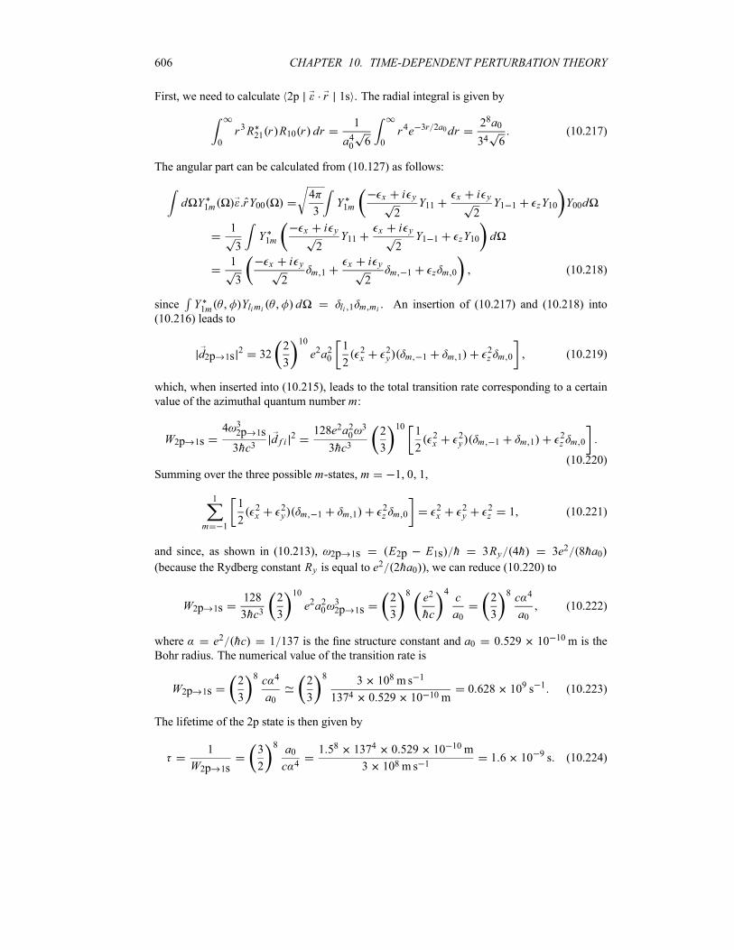
606 CHAPTER 10. TIME-DEPENDENT PERTURBATION THEORY
First, we need to calculate 2p r 1s . The radial integral is given by
0
r3R21 r R10 r dr1
a40 6 0
r4e 3r 2a0dr28a0
34 6(10.217)
The angular part can be calculated from (10.127) as follows:
d Y1m rY004
3Y1m
x i y
2Y11
x i y
2Y1 1 zY10 Y00d
1
3Y1m
x i y
2Y11
x i y
2Y1 1 zY10 d
1
3
x i y
2m 1
x i y
2m 1 z m 0 (10.218)
since Y1m Ylimi d li 1 m mi . An insertion of (10.217) and (10.218) into
(10.216) leads to
d2p 1s2 32
2
3
10
e2a201
22x
2y m 1 m 1
2z m 0 (10.219)
which, when inserted into (10.215), leads to the total transition rate corresponding to a certain
value of the azimuthal quantum number m:
W2p 1s4 32p 1s
3hc3d f i
2 128e2a203
3hc32
3
101
22x
2y m 1 m 1
2z m 0
(10.220)
Summing over the three possible m-states, m 1 0 1,
1
m 1
1
22x
2y m 1 m 1
2z m 0
2x
2y
2z 1 (10.221)
and since, as shown in (10.213), 2p 1s E2p E1s h 3Ry 4h 3e2 8ha0(because the Rydberg constant Ry is equal to e2 2ha0 ), we can reduce (10.220) to
W2p 1s128
3hc32
3
10
e2a2032p 1s
2
3
8 e2
hc
4c
a0
2
3
8 c 4
a0(10.222)
where e2 hc 1 137 is the fine structure constant and a0 0 529 10 10m is the
Bohr radius. The numerical value of the transition rate is
W2p 1s2
3
8 c 4
a0
2
3
8 3 108ms 1
1374 0 529 10 10m0 628 109 s 1 (10.223)
The lifetime of the 2p state is then given by
1
W2p 1s
3
2
8 a0c 4
1 58 1374 0 529 10 10m
3 108ms 11 6 10 9 s (10.224)
10.6. SOLVED PROBLEMS 607
This value is in very good agreement with experimental data.
Remark
Another way of obtaining (10.222) is to use the relation
W2p 1s4e2 3
2p 1s
3hc31
3
1
m 1
21m r 100 2
4e2 32p 1s
9hc3
1
m 1
21m x 100 2 21m y 100 2 21m z 100 2
(10.225)
where we have averaged over the various transitions. Using the relations x r sin cos
2 3 r Y11 Y1 1 , y r sin sin i 2 3 r Y11 Y1 1 , and z r cos4 3 rY10, we can show that
21m x 1001
4
2
3 0
r3R21 r R10 r dr Y1m Y11 Y1 1 d
1
6
24
6
2
3
5
a0 m 1 m 1 (10.226)
21m y 100i
4
2
3 0
r3R21 r R10 r dr Y1m Y11 Y1 1 d
i
6
24
6
2
3
5
a0 m 1 m 1 (10.227)
21m z 1001
4
4
3 0
r3R21 r R10 r dr Y1mY10d
1
3
24
6
2
3
5
a0 m 0 (10.228)
A combination of the previous three relations leads to
1
m 1
21m r 100 2 96a202
3
10
m
1
6m 1 m 1
2 1
6m 1 m 1
2 1
32m 0
96a202
3
10
m
1
6m 1 m 1
1
6m 1 m 1
1
3m 0
96a203
2
3
10 1
m 1
m 1 m 1 m 0 962
3
10
a20
(10.229)
Finally, substituting (10.229) into (10.225) and using 2p 1s 3e2 8ha0 , we obtain
W2p 1s128e2a203hc3
3 2
3
102
3
8 e2
hc
4c
a0
2
3
8 c 4
a0(10.230)
608 CHAPTER 10. TIME-DEPENDENT PERTURBATION THEORY
Problem 10.10
(a) Calculate the transition rate from the first excited state to the ground state for an isotropic
(three-dimensional) harmonic oscillator of charge q.(b) Find a numerical value for the rate calculated in (a) as well as the lifetime of the first
excited state for the case of an electron (i.e., mec2 0 511MeV) oscillating with a frequency
of an optical radiation 1015 rad s 1.
Solution
As mentioned in Chapter 6, the ground state of an isotropic harmonic oscillator is a 1s state,
n l m 0 0 0 , whose energy and wave function are E0 3h 2 and
000 r R00 r Y002 m
h
3 4
e m r2 2hY00 (10.231)
and the first excited state is a 1p state n l m 1 1 m whose energy and wave function
are E1 5h 2 and
11m r R11 r Y1m8
3
m
h
5 4
re m r2 2hY1m (10.232)
Using 0 x4e x2dx 38
along with a change of variable x m h r , we have
0
r3R11 r R10 r dr 42
3
m
h
2
0
r4e m r2 h dr3h
2m(10.233)
(a) The transition rate for a 1p 1s transition is given by
W1p 1s4q2 3
1p 1s
3hc31
3
1
m 1
11m r 000 2
4q2 31p 1s
9hc3
1
m 1
11m x 000 2 11m y 000 2 21m z 000 2
(10.234)
Since x r sin cos 2 3 r Y11 Y1 1 , y r sin sin i 2 3 r Y11 Y1 1 ,
and z r cos 4 3 rY10, and using (10.233), we can show by analogy with (10.226) to(10.228) that
11m x 0001
4
2
3 0
r3R11 r R00 r dr Y1m Y11 Y1 1 d
1
6
3h
2mm 1 m 1 (10.235)
11m y 000i
4
2
3 0
r3R11 r R00 r dr Y1m Y11 Y1 1 d
i
6
3h
2mm 1 m 1 (10.236)

10.6. SOLVED PROBLEMS 609
11m z 0001
4
4
3 0
r3R11 r R00 r dr Y1mY10 d1
3
3h
2mm 0
(10.237)
A combination of the previous three relations leads to
1
m 1
11m r 000 2 3h
2m m
1
6m 1 m 1
2 1
6m 1 m 1
2 1
32m 0
h
2m
1
m 1
m 1 m 1 m 03h
2m(10.238)
Substituting (10.238) into (10.234), and using 1p 1s E1 E0 h 52
32
, we
obtain
W1p 1s4q2 3
1p 1s
9hc33h
2m
2q2 2
3mc3(10.239)
(b) In the case of an electron (q e and mec2 0 511MeV) which is oscillating with a
frequency of 1015 s 1, the transition rate is
W1p 1s2e2 2
3mec32
3
hc
mec2
2
c
2
3
1
137
197MeV fm
0 511MeV
1030 s 2
3 108ms 10 64 107 s 1 (10.240)
where e2 hc 1 137 is the fine structure constant. The lifetime of the 1p state for the
oscillator is given by
1
W1p 1s
3mec3
2e2 2
1
0 64 107 s 11 56 10 7 s (10.241)
Problem 10.11
Show that free electrons can neither emit nor absorb photons.
Solution
If the electron is free both before and after it interacts with the photon, its initial and final wave
functions are given by plane waves: i r 2 3 2eiki r and f r 2 3 2eik f r . Letus assume, for argument sake, that a free electron can absorb and emit a photon; the corre-
sponding absorption and emission transition rates would be given as follows (see (10.95) and
(10.96)):
absi f
4 2e2
m2e Vki f eik r i
2E f Ei h (10.242)
emii f
4 2e2
m2e Vki f e ik r
i
2E f Ei h (10.243)
610 CHAPTER 10. TIME-DEPENDENT PERTURBATION THEORY
where we have used P i r ki i r . Since
f e ik ri
1
2 2d3r ei ki k f k r ki k f k (10.244)
the delta functions ki k f k give the conservation laws of the linear momentum for boththe absorption and emission processes.
Let us show first that a free electron cannot absorb a photon. For this, we are going to
show that the momentum conservation condition ki k f k is incompatible with the energyconservation condition E f Ei h . Combining equations (10.242) and (10.244), we
see that the absorption rate is proportional to the product of two delta functions: absi f
ki k f k E f Ei h , one pertaining to the conservation of momentum
ki k f k pi p f pphoton 0 (10.245)
the other dealing with the conservation of energy
E f Ei h E f Ei cpphoton 0 (10.246)
where pi hki and Ei are the initial momentum and energy of the electron, p f hk f and E fare its final momentum and energy, and pphoton hk and cpphoton are the linear momentumand energy of the absorbed photon. We are now ready to show that the condition (10.245) is
incompatible with (10.246). If we work within the rest frame of the initial electron, we have
pi 0. Thus, on the one hand, (10.245) leads to pphoton p f and, on the other hand,(10.246) leads to E f cpphoton or p2f 2me cpphoton . Indeed, conditions (10.245) and(10.246) are contradictory since, inserting pi 0 and pphoton p f into (10.246), we end upwith p2f 2me cp f or p f 2mec. This suggests either that f 0 and this is meaningless
since, as pphoton p f , the speed of the photon would also be zero; or that f 2c and this isimpossible. So both results are impossible. In summary, having started with the assumption that
a free electron can absorb a photon (10.242), we have ended up with a momentum conservation
law and an energy conservation law that are contradictory. Thus, a free electron cannot absorb
a photon.
Following the same procedure, we can also show that the assumption of a free electron
emitting a photon leads to a momentum conservation law and an energy conservation law that
are incompatible; thus, a free electron cannot emit a photon.
Problem 10.12
A hydrogen atom in its ground state is placed in an oscillating electric field E t E0 sin tof angular frequency with h mee4 2h2 .(a) Find the transition rate (probability per unit time) that the atom will be ionized.
(b) Use the expression derived in (a) to find the maximum transition rate.
Solution
After ionization we assume the electron to be in free motion: its energy is purely kinetic Ekh2k2 2me and its wave function is a plane wave k r 2 3 2eik r . Since the perturbationresulting from the interaction of the hydrogen’s electron with the external field E t is harmonic,
V t er E t er E0 sin te
2ir E0e
i t e
2ir E0e
i t (10.247)
10.6. SOLVED PROBLEMS 611
we can infer, by analogy with the method that led to (10.54) from (10.50), the transition rate
for the ionization of the hydrogen atom:
0k2
h
e
2ik r E0 100
2Ek E0 h
2
h
e
2ik r E0 100
2Ek E0 h (10.248)
where E0 mee4 2h2 13 6 eV is the ground state energy and Ek h2k 2me is the final
energy of the electron. The first delta term, Ek E0 h , in (10.248) does not contribute,
since if h E0 Ek the ionization could not take place because the electric field would notbe strong enough to ionize the atom. The transition rate (10.248) then becomes
0ke2
2hk r E0 100
2Ek E0 h (10.249)
To calculate k r E0 100 , let us take k along the z-axis and hence k r kr cos and
k r 2 3 2eikr cos . Taking and as the respective polar angles of r and E0,we have r r sin cos i sin sin j cos k and E0 E0 sin cos i sin sin jcos k ; hence
r E0 rE0 sin cos sin cos sin sin sin sin cos cos
rE0 sin sin cos cos cos (10.250)
Since 1s a301 2e r a0 and d3r r2dr sin cos d d , we have
k r E0 1001
2 3 2
1
a30
d3r r E0 eikr cos r a0
E0
8 4a300
r3e r a0dr0
sin e ikr cos d2
0
sin sin cos cos cos d
2 E0 cos
8 4a300
r3e r a0 dr0
sin cos e ikr cos d (10.251)
where we have used20 cos d 0, since
20 cos d 0 and
20 sin d 0. A
change of variable x cos and an integration by parts leads to
0
sin cos e ikr cos d1
1
xe ikrxdx1
ikrxe ikrx
1
1
1
ikr 2e ikrx
1
1
i
kre ikr eikr
1
k2r2e ikr eikr (10.252)
When we insert this integral into (10.251), we still need to calculate four radial integrals which
can be carried out by parts:
0
re ikr r a0dr1
ik 1 a0re ikr r a0
0
1
ik 1 a0 2e ikr r a0
0
a20ia0k 1 2
(10.253)
612 CHAPTER 10. TIME-DEPENDENT PERTURBATION THEORY
0
r2e ikr r a0dr1
ik 1 a0r2e ikr r a0
0
2
ik 1 a0 0
re ikr r a0dr
2
ik 1 a0 2re ikr r a0
0
2
ik 1 a0 3e ikr r a0
0
2a30ia0k 1 3
(10.254)
Inserting (10.252) to (10.254) into (10.251), we obtain
k r E0 1002 E0 cos
8 4a30
a20k2 ia0k 1 2
a20k2 ia0k 1 2
2ia30k ia0k 1 3
2ia30k ia0k 1 3
16E0 cos
2a50
ia60k
a20k2 1 3
(10.255)
A substitution of this expression into (10.249) leads to
0ke2
2h
128E20 cos2
2a50
k2a120a20k
2 1 6Ek E0 h (10.256)
This relation gives the transition rate for a single final state k corresponding to a given k. Weneed to sum over all final states of the electron. These represent a continuum; we must then
integrate over all directions of emission and over all possible momenta:
0 0k d3k k2dk
00k sin d
2
0
d
264e2E20a
70
h
k4 Ek E0 h
a20k2 1 6
dk0
sin cos2 d
256e2E20a70
3h
k4 Ek E0 h
a20k2 1 6
dk (10.257)
where we have used 0 sin cos2 d 11 x3dx 2
3. The integration over k can be
converted into an integration over the final energy Ek : since Ek h2k2 2me , a change of
variable k 2meEk h2, and hence k dk me h2 dEk , reduces (10.257) to
0
256e2E20a70
3h
k3 Ek E0 h
a20k2 1 6
k dk
me
h2256e2E20a
70
3h
2meEk h2 3 2 Ek E0 h
2mea20Ek h2 1
6dEk
256e2meE20a70
3h32me h
2 3 2 E0 h 3 2
2mea20 E0 h h2 16
(10.258)
10.7. EXERCISES 613
This relation can be simplified if we use E0 mee4 2h2 h 0, which gives E0 hh 0 h 0 0 1 . Since a0 h2 mee2 , we have h 0a20 mee4h4 2h2m2ee
4
h2 2me and hence 2mea20 E0 h h2 2meh 0a20 0 1 h2 0 1. Thus,
inserting the expressions E0 h h 0 0 1 and 2mea20 E0 h h2 1 0
into (10.258), we obtain
0
256e2meE20a70
3h32me h2 3 2 h 0
3 20 1 3 2
06
(10.259)
Finally, since 2me h2 3 2 h 0
3 2 2me h2 3 2 mee4 2h
2 3 2 m3ee6 h6 and using a40
h8 m4e8 , we can write (10.259) as
0
256E20a30
3h0 6
01
3 2
(10.260)
If the frequency of the oscillating electric field is smaller than or equal to 0, the atom will not
be ionized; at 0 the probability of ionization will be zero.
(b) The maximum transition rate is obtained by taking the derivative of (10.260):
d 0
d0
2
01
1
2 0
4
30 (10.261)
Inserting 43 0 into (10.260) we obtain the maximum transition rate
0max256E20a
30
3h
3
4
64
31
3 2 E20a30
h
37 2
24(10.262)
10.7 Exercises
Exercise 10.1
Consider a spinless particle of mass m in a one-dimensional infinite potential well with walls atx 0 and x a which is initially (i.e., at t 0) in the state x 0 [ 1 x 3 x ] 2,
where 1 x and 3 x are the ground and second excited states, respectively, with n x2 a sin n x a .(a) What is the state vector x t for t 0 in the Schrödinger picture.
(b) Evaluate X , P , X2 , and P2 as functions of time for t 0 in the Schrödinger
picture.
(c) Repeat part (b) in the Heisenberg picture: i.e., evaluate X H , P H , X2 H , and P2 Has functions of time for t 0.
Exercise 10.2
Evaluate the expectation value XH t P 3 for the third excited state of a one-dimensional har-
monic oscillator.
Exercise 10.3
Evaluate the expectation value X PH t n for the nth excited state of a one-dimensional har-monic oscillator.
614 CHAPTER 10. TIME-DEPENDENT PERTURBATION THEORY
Exercise 10.4
Consider a one-dimensional harmonic oscillator which is initially (i.e., at t 0) in the state
0 0 1 2, where 0 and 1 are the ground and first excited states,
respectively.
(a) What is the state vector t for t 0 in the Schrödinger picture?
(b) Evaluate X , P , X2 , and P2 as functions of time for t 0 in the Schrödinger
picture.
(c) Repeat part (b) in the Heisenberg picture.
Exercise 10.5
(a) Calculate the coordinate operator XH t for a free particle in one dimension in theHeisenberg picture.
(b) Evaluate the commutator [XH t XH 0 ].
Exercise 10.6
Consider the Hamiltonian H eB mc Sx Sx .(a)Write down the Heisenberg equations of motion for the time-dependent operators Sx t Sy t ,
and Sz t .(b) Solve these equations to obtain Sx Sy Sz as functions of time.
Exercise 10.7
Evaluate the quantity n PH t P n for the nth excited state of a one-dimensional harmonicoscillator, where PH t and P designate the momentum operators in the Heisenberg pictureand the Schrödinger picture, respectively.
Exercise 10.8
The Hamiltonian due to the interaction of a particle of massm, charge q (the charge is negative),and spin S with a magnetic field pointing along the y-axis is H qB mc Sy .
(a) Use the Heisenberg equation to calculate dSx dt , dSy dt , and dSz dt .(b) Solve these equations to obtain the components of the spin operator as functions of time.
Exercise 10.9
A particle is initially (i.e., when t 0) in its ground state in a one-dimensional harmonic
oscillator potential. At t 0 a perturbation V x t V0x2e t is turned on. Calculate to
first order the probability that, after a sufficiently long time (i.e., t ), the system will have
made a transition to a given excited state; consider all final states.
Exercise 10.10
A particle, initially (i.e., when t 0) in its ground state in an infinite potential well whose
walls are located at x 0 and x a, is subject, starting at time t 0, to a time-dependent
perturbation V t V0x2e t2 where V0 is a small parameter. Calculate the probability that theparticle will be found in its second excited state at t .
Exercise 10.11
Find the intensity associated with the transition 3s 2p in the hydrogen atom.
10.7. EXERCISES 615
Exercise 10.12
A hydrogen atom in its ground state is placed in a region where, at t 0, a time-dependent
electric field is turned on:
E t E0 i j k e t
where is a positive real number. Using first-order time-dependent perturbation theory, calcu-
late the probability that, after a sufficiently long time (i.e., t ), the atom is to be found in
each of the n 2 states (i.e., consider the transitions to all the states in the n 2 level). Hint:
You may use: 0 r3R21 r R10 r dr 24a0 6 23
5.
Exercise 10.13
(a) Calculate the reduced matrix element 1 Y1 2 . Hint: For this, you may need tocalculate 1 0 Y10 2 0 directly and then from the Wigner–Eckart theorem.
(b) Using the Wigner–Eckart theorem and the relevant Clebsch–Gordan coefficients from
tables, calculate 1 m Y1m 2 m for all possible values of m, m , and m .
(c) Using the results of part (b), calculate the 3d 2p transition rate for the hydrogen
atom in the dipole approximation; give a numerical value. Hint: You may use the integral
0 r3R21 r R32 r dr 64a0 15 5 65
5and the following Clebsch–Gordan coefficients:
j 1 m 0 j 1 m j m j m [ j 2 j 1 ],
j 1 m 1 1 j 1 m j m j m 1 [2 j 2 j 1 ], and
j 1 m 1 1 j 1 m j m j m 1 [2 j 2 j 1 ].
Exercise 10.14
A particle is initially in its ground state in an infinite one-dimensional potential box with sides
at x 0 and x a. If the wall of the box at x a is suddenly moved to x 10a, calculatethe probability of finding the particle in
(a) the fourth excited (n 5) state of the new box and
(b) the ninth (n 10) excited state of the new box.
Exercise 10.15
A particle of mass m in the ground state of a one-dimensional harmonic oscillator is placed ina perturbation V t V0xe t . Calculate to first-order perturbation theory the probability
of finding the particle in its first excited state after a long time.
Exercise 10.16
A particle, initially (i.e., when t 0) in its first excited state in an infinite potential well whose
walls are located at x 0 and x a, is subject, starting at time t 0, to a time-dependent
perturbation V t V0 x t2 2 where V0 is a small real number. Calculate the probabilitythat the particle will be found in its second excited state at t .
Exercise 10.17
A one-dimensional harmonic oscillator has its spring constant suddenly reduced by half.
(a) If the oscillator is initially in its ground state, find the probability that the oscillator
remains in the ground state.
(b) Find the work associated with this process.
Exercise 10.18
(a) Find the total transition rate associated with the decay of a harmonic oscillator, of charge
q and mass m, from the nth excited state to the state just below.

616 CHAPTER 10. TIME-DEPENDENT PERTURBATION THEORY
(b) Find the power radiated by this oscillator as a result of its decay.
(c) Find the lifetime of the nth excited state.(d) Estimate the order of magnitudes for the transition rate, the power, and the lifetime of
the fifth excited state (n 5) in the case of a harmonically oscillating electron (i.e., q e) forthe case of an optical radiation 1015 rad s 1.
Exercise 10.19
Assuming that f r i is roughly equal to the size of the system under study, use a crude
calculation to estimate the mean lifetime of
(a) an electric dipole transition in an atom where h 10 eV and
(b) an electric dipole transition in a nucleus where h 1MeV.
Exercise 10.20
A particle is initially (i.e., when t 0) in its ground state in the potential V x V0 xwith V0 0.
(a) If the strength of the potential is changed slowly to 3V0, find the energy and wave func-tion of the particle in the new potential.
(b) Calculate the work done with this process. Find a numerical value for this work in MeV
if this particle were an electron and V0 200 MeV fm.
(c) If the strength of the potential is changed suddenly to 3V0, calculate the probability offinding the particle in the ground state of the new potential.
Exercise 10.21
A hydrogen atom in its ground state is placed at time t 0 in a uniform electric field in the
y-direction, E t E0 je t2 2. Calculate to first-order perturbation theory the probability that
the atom will be found in any of the n 2 states after a sufficiently long time (t ).
Exercise 10.22
A particle, initially (i.e., when t 0) in its ground state in an infinite potential well with its
walls at x 0 and x a, is subject, starting at time t 0, to a time-dependent perturbation
V t V0x x 3a 4 e t where V0 is a small parameter. Calculate the probability that theparticle will be found in its first excited state (n 2) at t .
Exercise 10.23
Consider an isotropic (three-dimensional) harmonic oscillator which undergoes a transition
from the second to the first excited state (i.e., 2s 1p).
(a) Calculate the transition rate corresponding to 2s 1p.
(b) Find the intensity associate with the 2s 1p transition.
Exercise 10.24
Consider a particle which is initially (i.e., when t 0) in its ground state in a three-dimensional
box potential
V x y z0 0 x a 0 y 2a 0 z 4a
elsewhere
(a) Find the energies and wave functions of the ground state and first excited state.
(b) This particle is then subject, starting at time t 0, to a time-dependent perturbation
V t V0xze t2 where V0 is a small parameter. Calculate the probability that the particle willbe found in the first excited state after a long time t .
Chapter 11
Scattering Theory
Much of our understanding about the structure of matter is extracted from the scattering of
particles. Had it not been for scattering, the structure of the microphysical world would have
remained inaccessible to humans. It is through scattering experiments that important building
blocks of matter, such as the atomic nucleus, the nucleons, and the various quarks, have been
discovered.
11.1 Scattering and Cross Section
In a scattering experiment, one observes the collisions between a beam of incident particles and
a target material. The total number of collisions over the duration of the experiment is pro-
portional to the total number of incident particles and to the number of target particles per unit
area in the path of the beam. In these experiments, one counts the collision products that come
out of the target. After scattering, those particles that do not interact with the target continue
their motion (undisturbed) in the forward direction, but those that interact with the target get
scattered (deflected) at some angle as depicted in Figure 11.1. The number of particles coming
out varies from one direction to the other. The number of particles scattered into an element
of solid angle d ( d sin d d ) is proportional to a quantity that plays a central role in
the physics of scattering: the differential cross section. The differential cross section, whichis denoted by d d , is defined as the number of particles scattered into an element of
solid angle d in the direction per unit time and incident flux:
d
d
1
Jinc
dN
d(11.1)
where Jinc is the incident flux (or incident current density); it is equal to the number of incidentparticles per area per unit time. We can verify that d d has the dimensions of an area; hence
it is appropriate to call it a differential cross section.
The relationship between d d and the total cross section is obvious:
d
dd
0
sin d2
0
d
dd (11.2)
617
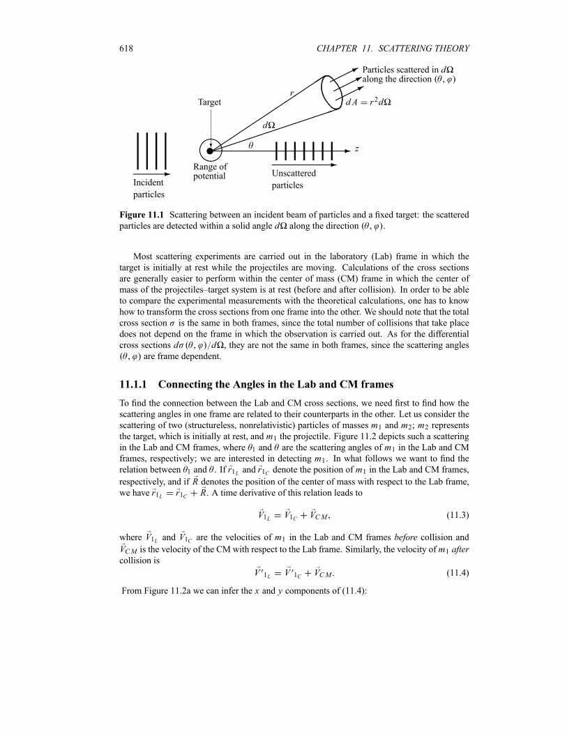
618 CHAPTER 11. SCATTERING THEORY
¹¸º
- z
Range ofpotential
©©©*
©©©*
©©©*
Particles scattered in dalong the direction
vTarget d A r2d
?³³³³
³³³³
³³³³
³³
´´´´´´´´´´´´́
d
r
--
Incident
particles
Unscattered
particles
Figure 11.1 Scattering between an incident beam of particles and a fixed target: the scattered
particles are detected within a solid angle d along the direction .
Most scattering experiments are carried out in the laboratory (Lab) frame in which the
target is initially at rest while the projectiles are moving. Calculations of the cross sections
are generally easier to perform within the center of mass (CM) frame in which the center of
mass of the projectiles–target system is at rest (before and after collision). In order to be able
to compare the experimental measurements with the theoretical calculations, one has to know
how to transform the cross sections from one frame into the other. We should note that the total
cross section is the same in both frames, since the total number of collisions that take place
does not depend on the frame in which the observation is carried out. As for the differential
cross sections d d , they are not the same in both frames, since the scattering angles
are frame dependent.
11.1.1 Connecting the Angles in the Lab and CM frames
To find the connection between the Lab and CM cross sections, we need first to find how the
scattering angles in one frame are related to their counterparts in the other. Let us consider the
scattering of two (structureless, nonrelativistic) particles of masses m1 and m2; m2 representsthe target, which is initially at rest, and m1 the projectile. Figure 11.2 depicts such a scatteringin the Lab and CM frames, where 1 and are the scattering angles of m1 in the Lab and CMframes, respectively; we are interested in detecting m1. In what follows we want to find therelation between 1 and . If r1L and r1C denote the position of m1 in the Lab and CM frames,respectively, and if R denotes the position of the center of mass with respect to the Lab frame,we have r1L r1C R. A time derivative of this relation leads to
V1L V1C VCM (11.3)
where V1L and V1C are the velocities of m1 in the Lab and CM frames before collision andVCM is the velocity of the CM with respect to the Lab frame. Similarly, the velocity ofm1 aftercollision is
V 1L V 1C VCM (11.4)
From Figure 11.2a we can infer the x and y components of (11.4):
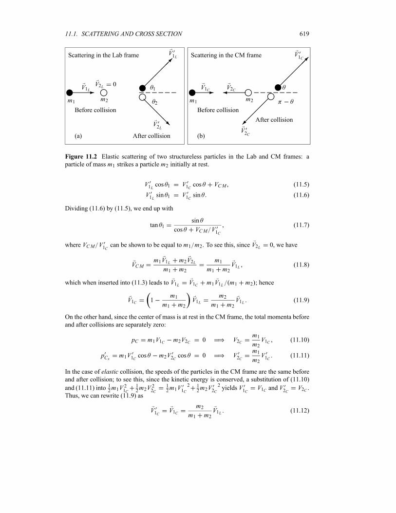
11.1. SCATTERING AND CROSS SECTION 619
-ym1
im2
V1LV2L 0
V1L
V2L
yi 1
2
¡¡¡¡¡µ
@@@@R
Scattering in the Lab frame
Before collision
After collision(a)
- ¾ym1
im2
V1C V2C
V1C
V2C
yi¡¡¡¡¡µ
¡¡
¡¡ª
Scattering in the CM frame
Before collision
After collision
(b)
Figure 11.2 Elastic scattering of two structureless particles in the Lab and CM frames: a
particle of mass m1 strikes a particle m2 initially at rest.
V1L cos 1 V1C cos VCM (11.5)
V1L sin 1 V1C sin (11.6)
Dividing (11.6) by (11.5), we end up with
tan 1sin
cos VCM V1C(11.7)
where VCM V1C can be shown to be equal to m1 m2. To see this, since V2L 0, we have
VCMm1V1L m2V2Lm1 m2
m1m1 m2
V1L (11.8)
which when inserted into (11.3) leads to V1L V1C m1V1L m1 m2 ; hence
V1C 1m1
m1 m2V1L
m2m1 m2
V1L (11.9)
On the other hand, since the center of mass is at rest in the CM frame, the total momenta before
and after collisions are separately zero:
pC m1V1C m2V2C 0 V2Cm1m2V1C (11.10)
pCx m1V1C cos m2V2C cos 0 V2Cm1m2V1C (11.11)
In the case of elastic collision, the speeds of the particles in the CM frame are the same beforeand after collision; to see this, since the kinetic energy is conserved, a substitution of (11.10)
and (11.11) into 12m1V 21C
12m2V 22C
12m1V1C
2 12m2V2C
2yields V1C V1C and V2C V2C .
Thus, we can rewrite (11.9) as
V1C V1Cm2
m1 m2V1L (11.12)
620 CHAPTER 11. SCATTERING THEORY
Dividing (11.8) by (11.12) we obtain
VCMV1C
m1m2
(11.13)
Finally, a substitution of (11.13) into (11.7) yields
tan 1sin
cos V2C V1C
sin
cos m1 m2(11.14)
which, using cos 1 1 tan2 1 1, becomes
cos 1
cos m1m2
1m21m22
2m1m2cos
(11.15)
Remark
By analogy with the foregoing analysis, we can establish a connection between 2 and . From
(11.4) we have V2L V2C VCM . The x and y components of this relation are
V2L cos 2 V2C cos VCM cos 1 V2C (11.16)
V2L sin 2 V2C sin (11.17)
in deriving (11.16), we have used VCM V2C V2C . A combination of (11.16) and (11.17)leads to
tan 2sin
cos VCM V2C
sin
1 coscot
22
2(11.18)
11.1.2 Connecting the Lab and CM Cross Sections
The connection between the differential cross sections in the Lab and CM frames can be ob-
tained from the fact that the number of scattered particles passing through an infinitesimal cross
section d is the same in both frames: d 1 1 d . What differs is the solid an-
gle d , since it is given in the Lab frame by d 1 sin 1d 1d 1 and in the CM frame by
d sin d d . Thus, we have
d
d 1 Labd 1
d
d CMd
d
d 1 Lab
d
d CM
sin
sin 1
d
d 1
d
d 1(11.19)
where 1 1 are the scattering angles of particle m1 in the Lab frame and are its angles
in the CM frame. Since there is cylindrical symmetry around the direction of the incident beam,
we have 1 and hence
d
d 1 Lab
d
d CM
d cos
d cos 1(11.20)
From (11.15) we have
d cos 1
d cos
1 m1m2cos
1m21m22
2m1m2cos
3 2(11.21)
11.2. SCATTERING AMPLITUDE OF SPINLESS PARTICLES 621
which when substituted into (11.20) leads to
d
d 1 Lab
1m21m22
2m1m2cos 3 2
1 m1m2cos
d
d CM(11.22)
Similarly, we can show that (11.20) and (11.18) yield
d
d 2 Lab4 cos 2
d
d 2 CM4 sin
2
d
d 2 CM(11.23)
Limiting cases: (a) If m2 m1, or whenm1m2
0, the Lab and CM results are the same,
since (11.15) leads to 1 and (11.22) to dd 1 Lab
dd CM
. (b) If m2 m1 then
(11.15) leads to tan 1 tan 2 or to 1 2; in this case (11.22) yields dd 1 Lab
4 dd CM
cos 2 .
Example 11.1
In an elastic collision between two particles of equal mass, show that the two particles come
out at right angles with respect to each other in the Lab frame.
Solution
In the special case m1 m2, equations (11.14) and (11.18) respectively become
tan 1 tan2
tan 2 cot2
tan2 2
(11.24)
These two equations yield
12
22 2 2
1 (11.25)
hence 1 2 2. In these cases, (11.22) and (11.23) yield
d
d 1 Lab4d
d CMcos 1 4
d
d CMcos
2(11.26)
d
d 2 Lab4
d
d 2 CMcos 2 4
d
d CMsin
2(11.27)
11.2 Scattering Amplitude of Spinless Particles
The foregoing discussion dealt with definitions of the cross section and how to transform it
from the Lab to the CM frame; the conclusions reached apply to classical as well as to quantum
mechanics. In this section we deal with the quantum description of scattering. For simplicity,
622 CHAPTER 11. SCATTERING THEORY
we consider the case of elastic1 scattering between two spinless, nonrelativistic particles of
masses m1 and m2. During the scattering process, the particles interact with one another. If theinteraction is time independent, we can describe the two-particle system with stationary states
r1 r2 t r1 r2 ei ET t h (11.28)
where ET is the total energy and r1 r2 is a solution of the time-independent Schrödinger
equation:
h2
2m121
h2
2m222 V r1 r2 r1 r2 ET r1 r2 (11.29)
V r1 r2 is the potential representing the interaction between the two particles.In the case where the interaction betweenm1 and m2 depends only on their relative distance
r r1 r2 (i.e., V r1 r2 V r ), we can, as seen in Chapter 6, reduce the eigenvalueproblem (11.29) to two decoupled eigenvalue problems: one for the center of mass (CM),
which moves like a free particle of mass M m1 m2 and which is of no concern to us here,and another for a fictitious particle with a reduced mass m1m2 m1 m2 which movesin the potential V r :
h2
22 r V r r E r (11.30)
The problem of scattering between two particles is thus reduced to solving this equation. We
are going to show that the differential cross section in the CM frame can be obtained from
an asymptotic form of the solution of (11.30). Its solutions can then be used to calculate the
probability per unit solid angle per unit time that the particle is scattered into a solid angle
d in the direction ; this probability is given by the differential cross section d d . In
quantum mechanics the incident particle is described by means of a wave packet that interacts
with the target. The incident wave packet must be spatially large so that spreading during the
experiment is not appreciable. It must be large compared to the target’s size and yet small
compared to the size of the Lab so that it does not overlap simultaneously with the target and
detector. After scattering, the wave function consists of an unscattered part propagating in the
forward direction and a scattered part that propagates along some direction .
We can view (11.30) as representing the scattering of a particle of mass from a fixed
scattering center that is described by V r , where r is the distance from the particle to the
center of V r . We assume that V r has a finite range a. Thus the interaction between theparticle and the potential occurs only in a limited region of space r a, which is called therange of V r , or the scattering region. Outside the range, r a, the potential vanishes,V r 0; the eigenvalue problem (11.30) then becomes
2 k20 inc r 0 (11.31)
where k20 2 E h2. In this case behaves as a free particle before collision and hence canbe described by a plane wave
inc r Aeik0 r (11.32)
where k0 is the wave vector associated with the incident particle and A is a normalization factor.Thus, prior to the interaction with the target, the particles of the incident beam are independent
of each other; they move like free particles, each with a momentum p hk0.
1In elastic scattering, the internal states and the structure of the colliding particles do not change.

11.2. SCATTERING AMPLITUDE OF SPINLESS PARTICLES 623
-k0
¡¡¡¡¡µk
Target
n¹¸º
&%'$
Incidentwave
Scatteredwave (outgoing)
Unscatteredwave
(a) (b)
z-6
@@R
6 6
©©©*
©©©*
©©©*
Waves scattered in dalong the direction
³³³³
³³³³
³³³³
³³
´´´´´´´´´´´´́
d
rd Ar2d
Figure 11.3 (a) Angle between the incident and scattered wave vectors k0 and k. (b) Incident
and scattered waves: the incident wave is a plane wave, inc r Aeik0 r , and the scattered
wave, sc r A f eik r
r , is an outgoing wave.
When the incident wave (11.32) collides or interacts with the target, an outgoing wave
sc r is scattered out. In the case of an isotropic scattering, the scattered wave is spherically
symmetric, having the form eik r r . In general, however, the scattered wave is not sphericallysymmetric; its amplitude depends on the direction along which it is detected and hence
sc r A feik r
r(11.33)
where f is called the scattering amplitude, k is the wave vector associated with the scat-tered particle, and is the angle between k0 and k as displayed in Figure 11.3a. After thescattering has taken place (Figure 11.3b), the total wave consists of a superposition of the inci-
dent plane wave (11.32) and the scattered wave (11.33):
r inc r sc r A eik0 r feik r
r(11.34)
where A is a normalization factor; since A has no effect on the cross section, as will be shownin (11.40), we will take it equal to one throughout the rest of the chapter. We now need to de-
termine f and d d . In the following section we are going to show that the differential
cross section is given in terms of the scattering amplitude by d d f 2.
11.2.1 Scattering Amplitude and Differential Cross Section
The scattering amplitude f plays a central role in the theory of scattering, since it deter-
mines the differential cross section. To see this, let us first introduce the incident and scattered
624 CHAPTER 11. SCATTERING THEORY
flux densities:
Jincih
2inc inc inc inc (11.35)
Jscih
2sc sc sc sc (11.36)
Inserting (11.32) into (11.35) and (11.33) into (11.36) and taking the magnitudes of the expres-
sions thus obtained, we end up with
Jinc A 2hk0
Jsc A 2hk
r2f
2(11.37)
Now, we may recall that the number dN of particles scattered into an element of solid
angle d in the direction and passing through a surface element d A r2d per unit
time is given as follows (see (11.1)):
dN Jscr2d (11.38)
When combined with (11.37) this relation yields
dN
dJscr
2 A 2hk
f2
(11.39)
Now, inserting (11.39) and Jinc A 2hk0 into (11.1), we end up with
d
d
1
Jinc
dN
d
k
k0f
2(11.40)
Since the normalization factor A does not contribute to the differential cross section, we will betaking it equal to one. For elastic scattering k0 is equal to k; hence (11.40) reduces to
d
df
2(11.41)
The problem of determining the differential cross section d d therefore reduces to that of
obtaining the scattering amplitude f .
11.2.2 Scattering Amplitude
We are going to show here that we can obtain the differential cross section in the CM frame
from an asymptotic form of the solution of the Schrödinger equation (11.30). Let us first focus
on the determination of f ; it can be obtained from the solutions of (11.30), which in turn
can be rewritten as2 k2 r
2
h2V r r (11.42)
The general solution to this equation consists of a sum of two components: a general solution
to the homogeneous equation:
2 k20 homo r 0 (11.43)
11.2. SCATTERING AMPLITUDE OF SPINLESS PARTICLES 625
and a particular solution to (11.42). First, note that homo r is nothing but the incident planewave (11.32). As for the particular solution to (11.42), we can express it in terms of Green’sfunction. Thus, the general solution of (11.42) is given by
r inc r2
h2G r r V r r d3r (11.44)
where inc r eik0 r and G r r is Green’s function corresponding to the operator on
the left-hand side of (11.43). The function G r r is obtained by solving the point source
equation2 k2 G r r r r (11.45)
where G r r and r r are given by their Fourier transforms as follows:
G r r1
2 3eiq r r G q d3q (11.46)
r r1
2 3eiq r r d3q (11.47)
A substitution of (11.46) and (11.47) into (11.45) leads to
q 2 k 2 G q 1 G q1
k 2 q 2(11.48)
The expression for G r r is obtained by inserting (11.48) into (11.46):
G r r1
2 3
eiq r r
k2 q2d3q (11.49)
To integrate over the angles in
G r r1
2 30
q2dq
k2 q2 0
eiq r r cos sin d2
0
d (11.50)
we need simply to make the variables change x cos :
0
eiq r r cos sin d1
1
eiq r r xdx1
iq r reiq r r e iq r r (11.51)
Hence (11.50) becomes
G r r1
4 2i r r 0
q
k2 q2eiq r r e iq r r dq (11.52)
or
G r r1
4 2i r r
qeiq r r
q2 k2dq (11.53)
We may evaluate this integral by the method of residues by closing the contour in the upper
half of the q-plane: it is equal to 2 i times the residue of the integrand at the poles. Since there
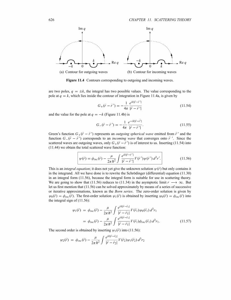
626 CHAPTER 11. SCATTERING THEORY
- -
6 6
Re q Re q
Im q Im q
0 0k
k k
k- - - -
(a) Contour for outgoing waves
¾ ¾
CCO¤¤²CCO¤¤²
- -- - -
(b) Contour for incoming waves
Figure 11.4 Contours corresponding to outgoing and incoming waves.
are two poles, q k, the integral has two possible values. The value corresponding to thepole at q k, which lies inside the contour of integration in Figure 11.4a, is given by
G r r1
4
eik r r
r r(11.54)
and the value for the pole at q k (Figure 11.4b) is
G r r1
4
e ik r r
r r(11.55)
Green’s function G r r represents an outgoing spherical wave emitted from r and the
function G r r corresponds to an incoming wave that converges onto r . Since thescattered waves are outgoing waves, only G r r is of interest to us. Inserting (11.54) into
(11.44) we obtain the total scattered wave function:
r inc r2 h2
eik r r
r rV r r d3r (11.56)
This is an integral equation; it does not yet give the unknown solution r but only contains itin the integrand. All we have done is to rewrite the Schrödinger (differential) equation (11.30)
in an integral form (11.56), because the integral form is suitable for use in scattering theory.
We are going to show that (11.56) reduces to (11.34) in the asymptotic limit r . But
let us first mention that (11.56) can be solved approximately by means of a series of successive
or iterative approximations, known as the Born series. The zero-order solution is given by
0 r inc r . The first-order solution 1 r is obtained by inserting 0 r inc r intothe integral sign of (11.56):
1 r inc r2 h2
eik r r1
r r1V r1 0 r1 d
3r1
inc r2 h2
eik r r1
r r1V r1 inc r1 d
3r1 (11.57)
The second order is obtained by inserting 1 r into (11.56):
2 r inc r2 h2
eik r r2
r r2V r2 1 r2 d
3r2
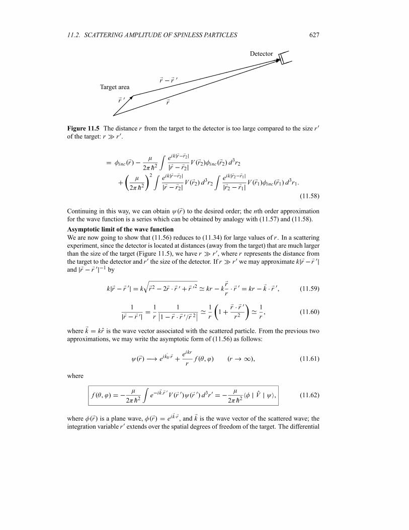
11.2. SCATTERING AMPLITUDE OF SPINLESS PARTICLES 627
¡¡¡µ»»»
»»»»»»
»»»»»»
»»»»»»
»»:
³³³³
³³³³
³³³³
³³³³
³³³³
³³³³
³1
rr
r rTarget area
DetectorBBBB³³
³³
Figure 11.5 The distance r from the target to the detector is too large compared to the size rof the target: r r .
inc r2 h2
eik r r2
r r2V r2 inc r2 d
3r2
2 h2
2 eik r r2
r r2V r2 d
3r2eik r2 r1
r2 r1V r1 inc r1 d
3r1
(11.58)
Continuing in this way, we can obtain r to the desired order; the nth order approximationfor the wave function is a series which can be obtained by analogy with (11.57) and (11.58).
Asymptotic limit of the wave function
We are now going to show that (11.56) reduces to (11.34) for large values of r . In a scatteringexperiment, since the detector is located at distances (away from the target) that are much larger
than the size of the target (Figure 11.5), we have r r , where r represents the distance fromthe target to the detector and r the size of the detector. If r r we may approximate k r rand r r 1 by
k r r k r2 2r r r 2 kr kr
rr kr k r (11.59)
1
r r
1
r
1
1 r r r 21
r1
r r
r21
r(11.60)
where k kr is the wave vector associated with the scattered particle. From the previous twoapproximations, we may write the asymptotic form of (11.56) as follows:
r eik0 reikr
rf r (11.61)
where
f2 h2
e ik r V r r d3r2 h2
V (11.62)
where r is a plane wave, r eik r , and k is the wave vector of the scattered wave; theintegration variable r extends over the spatial degrees of freedom of the target. The differential
628 CHAPTER 11. SCATTERING THEORY
cross section is then given by
d
df 2
2
4 2h4e ik r V r r d3r
2 2
4 2h4V
2
(11.63)
11.3 The Born Approximation
11.3.1 The First Born Approximation
If the potential V r is weak enough, it will distort only slightly the incident plane wave. Thefirst Born approximation consists then of approximating the scattered wave function r bya plane wave. This approximation corresponds to the first iteration of (11.56); that is, r isgiven by (11.57):
r inc r2 h2
eik r r
r rV r inc r d3r (11.64)
Thus, using (11.62) and (11.63), we can write the scattering amplitude and the differential cross
section in the first Born approximation as follows:
f2 h2
e ik r V r inc r d3r2 h2
eiq r V r d3r (11.65)
d
df
2 2
4 2h4eiq r V r d3r
2
(11.66)
where q k0 k and hq is the momentum transfer; hk0 and hk are the linear momenta of theincident and scattered particles, respectively.
In elastic scattering, the magnitudes of k0 and k are equal (Figure 11.6); hence
q k0 k k20 k2 2kk0 cos k 2 1 cos2 2k sin2
(11.67)
If the potential V r is spherically symmetric, V r V r , and choosing the z-axis alongq (Figure 11.6), then q r qr cos and therefore
eiq r V r d3r0
r 2V r dr0
eiqr cos sin d2
0
d
20
r 2V r dr1
1
eiqr xdx4
q 0
r V r sin qr dr
(11.68)
Inserting (11.68) into (11.65) and (11.66) we obtain
f2
h2q 0
r V r sin qr dr (11.69)
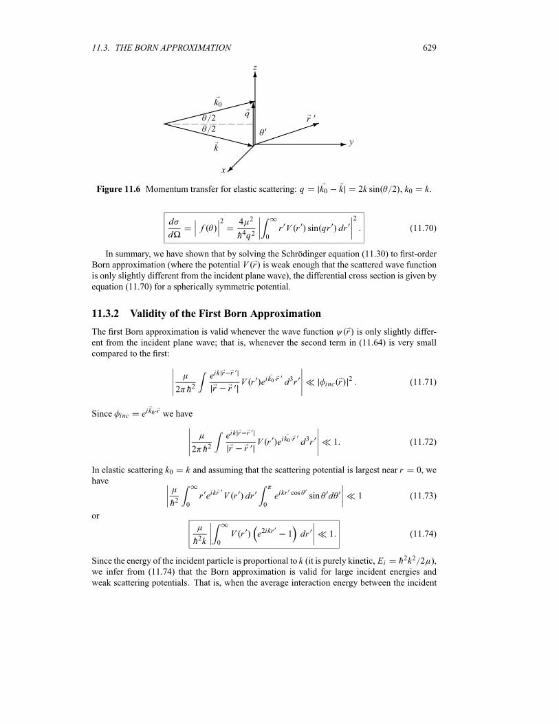
11.3. THE BORN APPROXIMATION 629
- y
6z
¡¡
¡ªx
»»»»»»
»»»»:
XXXXXXXXXXz
6
k
k0
³³³³
³³³1r2
2
q
Figure 11.6 Momentum transfer for elastic scattering: q k0 k 2k sin 2 , k0 k.
d
df
2 4 2
h4q2 0
r V r sin qr dr2
(11.70)
In summary, we have shown that by solving the Schrödinger equation (11.30) to first-order
Born approximation (where the potential V r is weak enough that the scattered wave functionis only slightly different from the incident plane wave), the differential cross section is given by
equation (11.70) for a spherically symmetric potential.
11.3.2 Validity of the First Born Approximation
The first Born approximation is valid whenever the wave function r is only slightly differ-ent from the incident plane wave; that is, whenever the second term in (11.64) is very small
compared to the first:
2 h2eik r r
r rV r eik0 r d3r inc r
2 (11.71)
Since inc eik0 r we have
2 h2eik r r
r rV r eik0 r d3r 1 (11.72)
In elastic scattering k0 k and assuming that the scattering potential is largest near r 0, we
have
h2 0
r eikr V r dr0
eikr cos sin d 1 (11.73)
or
h2k 0
V r e2ikr 1 dr 1 (11.74)
Since the energy of the incident particle is proportional to k (it is purely kinetic, Ei h2k2 2 ),
we infer from (11.74) that the Born approximation is valid for large incident energies and
weak scattering potentials. That is, when the average interaction energy between the incident
630 CHAPTER 11. SCATTERING THEORY
particle and the scattering potential is much smaller than the particle’s incident kinetic energy,
the scattered wave can be considered to be a plane wave.
Example 11.2
(a) Calculate the differential cross section in the first Born approximation for a Coulomb
potential V r Z1Z2e2 r , where Z1e and Z1e are the charges of the projectile and targetparticles, respectively.
(b) To have a quantitative idea about the cross section derived in (a), consider the scattering
of an alpha particle (i.e., a helium nucleus with Z1 2 and A1 4) from a gold nucleus
(Z2 79 and A2 197). (i) If the scattering angle of the alpha particle in the Lab frame is
1 60 , find its scattering angle in the CM frame. (ii) If the incident energy of the alpha
particle is 8MeV, find a numerical estimate for the cross section derived in (a).
Solution
In the case of a Coulomb potential, V r Z1Z2e2 r , equation (11.70) becomes
d
d
4Z21Z22e4 2
h4q2 0
sin qr dr2
(11.75)
where
0
sin qr dr lim0 0
e r sin qr dr1
2ilim0 0
e iq r dr0
e iq r dr
1
2ilim0
1
iq
1
iq
1
q(11.76)
Now, since q 2k sin 2 , an insertion of (11.76) into (11.75) leads to
d
d
2Z1 Z2e2
h2q2
2Z1Z2 e2
2h2k2
2
sin 4
2
Z21Z22e4
16E2sin 4
2(11.77)
where E h2k2 2 is the kinetic energy of the incident particle. This relation is known as the
Rutherford formula or the Coulomb cross section.(b) (i) Since the mass ratio of the alpha particle to the gold nucleus is roughly equal to the
ratio of their atomic masses, m1 m2 A1 A24197
0 0203, and since 1 60 , equation
(11.14) yields the value of the scattering angle in the CM frame:
tan 60sin
cos 0 020361 (11.78)
(ii) The numerical estimate of the cross section can be made easier by rewriting (11.77) in terms
of the fine structure constant e2 hc 1137and hc 197 33MeV fm:
d
d
Z21Z22
16E2e2
hc
2
hc 2 sin 4
2
Z1Z24
2 hc
E
2
sin 4
2(11.79)
Since Z1 2, Z2 79, 61 , 1137, hc 197 33MeV fm, and E 8MeV, we have
d
d
2 79
4 137
2197 33MeV fm
8MeV
2
sin 4 30 5
30 87 fm2 0 31 10 28m2 0 31 barn (11.80)
11.4. PARTIAL WAVE ANALYSIS 631
where 1 barn 10 28m2.
11.4 Partial Wave Analysis
So far we have considered only an approximate calculation of the differential cross section
where the interaction between the projectile particle and the scattering potential V r is con-
sidered small compared with the energy of the incident particle. In this section we are going to
calculate the cross section without placing any limitation on the strength of V r .
11.4.1 Partial Wave Analysis for Elastic Scattering
We assume here the potential to be spherically symmetric. The angular momentum of theincident particle will therefore be conserved; a particle scattering from a central potential will
have the same angular momentum before and after collision. Assuming that the incident plane
wave is in the z-direction and hence inc r exp ikr cos , we may express it in terms
of a superposition of angular momentum eigenstates, each with a definite angular momentum
number l (Chapter 6):
eik r eikr cos
l 0
i l 2l 1 jl kr Pl cos (11.81)
We can then examine how each of the partial waves is distorted by V r after the particle
scatters from the potential. The most general solution of the Schrödinger equation (11.30) is
rlm
ClmRkl r Ylm (11.82)
Since V r is central, the system is symmetrical (rotationally invariant) about the z-axis. Thescattered wave function must not then depend on the azimuthal angle ; hence m 0. Thus,
as Yl0 Pl cos , the scattered wave function (11.82) becomes
rl 0
al Rkl r Pl cos (11.83)
where Rkl r obeys the following radial equation (Chapter 6):
d2
dr2k2
l l 1
r2r Rkl r
2m
h2V r r Rkl r (11.84)
Each term of (11.83), which is known as a partial wave, is a joint eigenfunction of L 2 and L z .A substitution of (11.81) into (11.34) with 0 gives
rl 0
i l 2l 1 jl kr Pl cos feikr
r(11.85)
The scattered wave function is given, on the one hand, by (11.83) and, on the other hand, by
(11.85).

632 CHAPTER 11. SCATTERING THEORY
In almost all scattering experiments, detectors are located at distances from the target that
are much larger than the size of the target itself; thus, the measurements taken by detectors
pertain to scattered wave functions at large values of r . In what follows we are going to showthat, by establishing a connection between the asymptotic forms of (11.83) and (11.85), we can
determine the scattering amplitude and hence the differential cross section.
First, since the limit of the Bessel function jl kr for large values of r (Chapter 6) is givenby
jl krsin kr l 2
krr (11.86)
the asymptotic form of (11.85) is
rl 0
i l 2l 1 Pl cossin kr l 2
krf
eikr
r(11.87)
and since sin kr l 2 [ i leikr i le ikr ] 2i , because e il 2 e i 2 l i l , wecan write (11.87) as
re ikr
2ikrl 0
i2l 2l 1 Pl coseikr
rf
1
2ikl 0
i l i l 2l 1 Pl cos
(11.88)
Second, to find the asymptotic form of (11.83), we need first to determine the asymptotic
form of the radial function Rkl r . At large values of r , the scattering potential is effectivelyzero, for it is short range. In this case (11.84) becomes
d2
dr2k2 r Rkl r 0 (11.89)
As seen in Chapter 6, the general solution of this equation is given by a linear combination of
the spherical Bessel and Neumann functions
Rkl r Al jl kr Blnl kr (11.90)
where the asymptotic form of the Neumann function is
nl krcos kr l 2
krr (11.91)
Inserting of (11.86) and (11.91) into (11.90), we obtain the asymptotic form of the radial func-
tion:
Rkl r Alsin kr l 2
krBlcos kr l 2
krr (11.92)
If V r 0 for all r (free particle), the solution of (11.84), r Rkl r , must vanish at r 0;
thus Rkl r must be finite at the origin. Since the Neumann function diverges at r 0, the
cosine term in (11.92) does not represent a physically acceptable solution; hence, it needs to be
discarded near the origin. By rewriting (11.92) in the form
Rkl r Clsin kr l 2 l
krr (11.93)
11.4. PARTIAL WAVE ANALYSIS 633
we have Al Cl cos l and Bl Cl sin l , hence Cl A2l B2l and
tan lBlAl
l tan 1 BlAl
(11.94)
We see that, with l 0, the radial function Rkl r of (11.93) is finite at r 0, since (11.93)
reduces to jl kr . So l is a real angle which vanishes for all values of l in the absence of thescattering potential (i.e., V 0); l is called the phase shift. It measures, at large values ofr , the degree to which Rkl r differs from jl kr (recall that jl kr is the radial function whenthere is no scattering). Since this “distortion,” or the difference between Rkl r and jl kr , isdue to the potential V r , we would expect the cross section to depend on l . Using (11.93) we
can write the asymptotic limit of (11.83) as
rl 0
al Pl cossin kr l 2 l
krr (11.95)
This wave function is known as a distorted plane wave, for it differs from a plane wave byhaving phase shifts l . Since sin kr l 2 l [ i leikrei l i le ikre i l ] 2i , we canrewrite (11.95) as
re ikr
2ikrl 0
al ile i l Pl cos
eikr
2ikrl 0
al i lei l Pl cos (11.96)
Up to now we have shown that the asymptotic forms of (11.83) and (11.85) are given by
(11.96) and (11.88), respectively. Equating the coefficients of e ikr r in (11.88) and (11.96),we obtain 2l 1 i2l al i le i l and hence
al 2l 1 i lei l (11.97)
Substituting (11.97) into (11.96) and this time equating the coefficient of eikr r in the resultingexpression with that of (11.88), we have
f1
2ikl 0
i l i l 2l 1 Pl cos1
2ikl 0
2l 1 i l i le2i l Pl cos (11.98)
which, when combined with e2i l 1 2i ei l sin l and i l i l 1, leads to
fl 0
fl1
2ikl 0
2l 1 Pl cos e2i l 11
kl 0
2l 1 ei l sin l Pl cos
(11.99)
where fl is known as the partial wave amplitude.
From (11.99) we can obtain the differential and the total cross sections
d
df
2 1
k2l 0 l 0
2l 1 2l 1 ei l l sin l sin l Pl cos Pl cos
(11.100)
634 CHAPTER 11. SCATTERING THEORY
d
dd
0
f 2 sin d2
0
d 20
f 2 sin d
2
k2l 0 l 0
2l 1 2l 1 ei l l sin l sin l0
Pl cos Pl cos sin d
(11.101)
Using the relation0Pl cos Pl cos sin d [2 2l 1 ] ll , we can reduce (11.101) to
l 0l
4
k2l 0
2l 1 sin2 l (11.102)
where l are called the partial cross sections corresponding to the scattering of particles in var-ious angular momentum states. The differential cross section (11.100) consists of a superposi-
tion of terms with different angular momenta; this gives rise to interference patterns betweendifferent partial waves corresponding to different values of l. The interference terms go awayin the total cross section when the integral over is carried out. Note that when V 0 every-
where, all the phase shifts l vanish, and hence the partial and total cross sections, as indicated
by (11.100) and (11.102), are zero. Note that, as shown in equations (11.99) and (11.102), fand are given as infinite series over the angular momentum l. We may recall that, for cases ofpractical importance with the exception of the Coulomb potential, these series converge after a
finite number of terms.
We should note that in the case where we have a scattering between particles that are in
their respective s states, l 0, the scattering amplitude (11.99) becomes
f01
kei 0 sin 0 l 0 (11.103)
where we have used P0 cos 1. Since f0 does not depend on , the differential and total
cross sections are given by the following simple relations:
d
df02 1
k2sin2 0 4 f0
2 4
k2sin2 0 l 0 (11.104)
An important issue here is the fact that the total cross section can be related to the forwardscattering amplitude f 0 . Since Pl cos Pl 1 1 when 0, equation (11.99) leads to
f 01
kl 0
2l 1 sin l cos l i sin2 l (11.105)
which when combined with (11.102) yields the connection between f 0 and :
4
kIm f 0
4
kl 0
2l 1 sin2 l (11.106)
This is known as the optical theorem (it is reminiscent of a similar theorem in optics which dealswith the scattering of light). The physical origin of this theorem is the conservation of particles
(or probability). The beam emerging (after scattering) along the incidence direction ( 0)
11.4. PARTIAL WAVE ANALYSIS 635
contains fewer particles than the incident beam, since a number of particles have scattered in
various directions. This decrease in the number of particles is measured by the total cross
section ; that is, the number of particles removed from the incident beam along the incidence
direction is proportional to or, equivalently, to the imaginary part of f 0 . We should notethat, although (11.106) was derived for elastic scattering, the optical theorem, as will be shown
later, is also valid for inelastic scattering.
11.4.2 Partial Wave Analysis for Inelastic Scattering
The scattering amplitude (11.99) can be rewritten as
fl 0
2l 1 fl k Pl cos (11.107)
where
fl k1
kei l sin l
1
2ike2i l 1
1
2ikSl k 1 (11.108)
with
Sl k e2i l (11.109)
In the case where there is no flux loss, we must have Sl k 1. However, this requirement is
not valid whenever there is absorption of the incident beam. In this case of flux loss, Sl k isredefined by
Sl k l k e2i l (11.110)
with 0 l k 1; hence (11.108) and (11.107) become
fl kle2i l 1
2ik
1
2k[ l sin 2 l i 1 l cos 2 l ] (11.111)
f1
2kl 0
2l 1 [ l sin 2 l i 1 l cos 2 l ] Pl cos (11.112)
The total elastic scattering cross section is given by
el 4
l 0
2l 1 fl2
k2l
2l 1 1 2l 2 l cos 2 l (11.113)
The total inelastic scattering cross section, which describes the loss of flux, is given by
inelk2
l 0
2l 1 1 2l k (11.114)
Thus, if l k 1 there is no inelastic scattering, but if l 0 we have total absorption,
although there is still elastic scattering in this partial wave. The sum of (11.113) and (11.114)
gives the total cross section:
tot el inel2
k2l 0
2l 1 1 l cos 2 l (11.115)
636 CHAPTER 11. SCATTERING THEORY
Next, using (11.107) and (11.111), we infer
Im f 0l 0
2l 1 Im fl1
2kl 0
2l 1 1 l cos 2 l (11.116)
A comparison of (11.115) and (11.116) gives the optical theorem relation, Im f 0 k tot 4 ;
hence the optical theorem is also valid for inelastic scattering.
Example 11.3 (High-energy scattering from a black disk)
Discuss the scattering from a black disk at high energies.
Solution
A black disk is totally absorbing (i.e., l k 0). Assuming the values of l do not exceed amaximum value lmax (l lmax ) and that k is large (high-energy scattering), we have lmax kawhere a is the radius of the disk. Since l 0, equations (11.113) and (11.114) lead to
inel elk2
ka
l 0
2l 1k2ka 1 2 a2 (11.117)
hence the total cross section is given by
inel el inel 2 a2 (11.118)
Classically, the total cross section of a disk is equal to a2. The factor 2 in (11.118) is dueto purely quantum effects, since in the high-energy limit there are two kinds of scattering: one
corresponding to waves that hit the disk, where the cross section is equal to the classical cross
section a2, and the other to waves that are diffracted. According to Babinet’s principle, thecross section for the waves diffracted by a disk is also equal to a2.
11.5 Scattering of Identical Particles
First, let us consider the scattering of two identical bosons in their center of mass frame (we willconsider the scattering of two identical fermions in a moment). Classically, the cross sectionfor the scattering of two identical particles whose interaction potential is central is given by
cl (11.119)
In quantum mechanics there is no way of distinguishing, as indicated in Figure 11.7, between
the particle that scatters at an angle from the one that scatters at . Thus, the scattered
wave function must be symmetric:
sym r eik0 r e ik0 r fsymeikr
r(11.120)
and so must also be the scattering amplitude:
fboson f f (11.121)
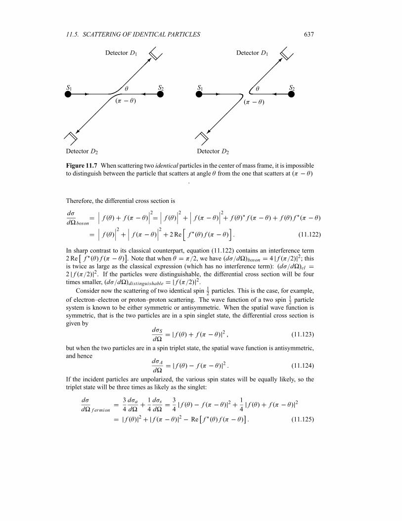
11.5. SCATTERING OF IDENTICAL PARTICLES 637
¡@¡Detector D2
@
¡¡
¡¡
¡ª
¾ yS2yS1 -¡¡¡¡¡µ@¡¡
Detector D1 @
¡@¡Detector D2
@
¡¡
¡¡
¡ª
¾ yS2yS1 -¡¡¡¡¡µ@¡¡
Detector D1 @
Figure 11.7 When scattering two identical particles in the center of mass frame, it is impossibleto distinguish between the particle that scatters at angle from the one that scatters at
.
Therefore, the differential cross section is
d
d bosonf f
2f
2f
2f f f f
f2
f2
2Re f f (11.122)
In sharp contrast to its classical counterpart, equation (11.122) contains an interference term
2Re f f . Note that when 2, we have d d boson 4 f 2 2; this
is twice as large as the classical expression (which has no interference term): d d cl
2 f 2 2. If the particles were distinguishable, the differential cross section will be four
times smaller, d d distinguishable f 2 2.
Consider now the scattering of two identical spin 12particles. This is the case, for example,
of electron–electron or proton–proton scattering. The wave function of a two spin 12particle
system is known to be either symmetric or antisymmetric. When the spatial wave function is
symmetric, that is the two particles are in a spin singlet state, the differential cross section is
given byd S
df f 2 (11.123)
but when the two particles are in a spin triplet state, the spatial wave function is antisymmetric,
and henced A
df f 2 (11.124)
If the incident particles are unpolarized, the various spin states will be equally likely, so the
triplet state will be three times as likely as the singlet:
d
d f ermion
3
4
d a
d
1
4
d s
d
3
4f f 2 1
4f f 2
f 2 f 2 Re f f (11.125)
638 CHAPTER 11. SCATTERING THEORY
When 2, we have d d f ermion f 2 2; this quantum differential cross section
is half the classical expression, d d cl 2 f 2 2, and four times smaller than the ex-
pression corresponding to the scattering of two identical bosons, d d boson 4 f 2 2.
We should note that, in the case of partial wave analysis for elastic scattering, using the
relations cos cos and Pl cos Pl cos 1 l Pl cos and
inserting them into (11.99), we can write
f1
kl 0
2l 1 ei l sin l Pl cos
1
kl 0
1 l 2l 1 ei l sin l Pl cos (11.126)
and hence
f f1
kl 0
1 1 l 2l 1 ei l sin l Pl cos (11.127)
Example 11.4
Calculate the differential cross section in the first Born approximation for the scattering between
two identical particles having spin 1, mass m, and interacting through a potential V rV0e ar .
Solution
As seen in Chapter 7, the spin states of two identical particles with spin s1 s2 1 consist of
a total of nine states: a quintuplet 2 m (i.e., 2 2 , 2 1 , 2 0 ) and a singlet 0 0 ,
which are symmetric, and a triplet 1 m (i.e., 1 1 , 1 0 ), which are antisymmetric under
particle permutation. That is, while the six spin states corresponding to S 2 and S 0
are symmetric, the three S 1 states are antisymmetric. Thus, if the scattering particles are
unpolarized, the differential cross section is
d
d
5
9
d S
d
1
9
d S
d
3
9
d A
d
2
3
d S
d
1
3
d A
d(11.128)
where
d S
df f
2 d A
df f
2(11.129)
The scattering amplitude is given in the Born approximation by (11.69):
f2V0
h2q 0
re ar sin qr drV0
ih2q 0
re a iq r drV0
ih2q 0
re a iq r dr
V0
h2q q 0
e a iq r drV0
h2q q 0
e a iq r dr
V0
h2q q
1
a iq
V0
h2q q
1
a iq
V0
h2q
i
a iq 2
i
a iq 2
4V0 a
h21
a2 q2 24V0 a
h21
a2 4k2 sin2 22
(11.130)
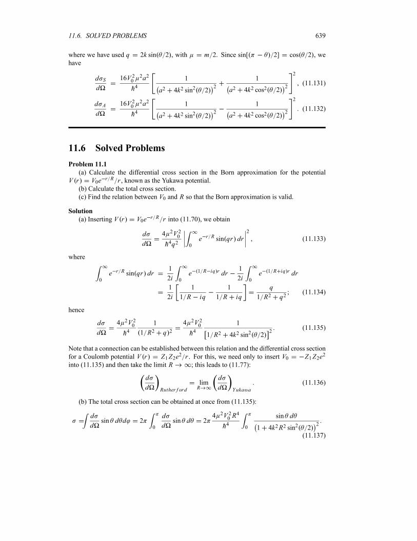
11.6. SOLVED PROBLEMS 639
where we have used q 2k sin 2 , with m 2. Since sin[ 2] cos 2 , we
have
d S
d
16V 202a2
h41
a2 4k2 sin2 22
1
a2 4k2 cos2 22
2
(11.131)
d A
d
16V 202a2
h41
a2 4k2 sin2 22
1
a2 4k2 cos2 22
2
(11.132)
11.6 Solved Problems
Problem 11.1
(a) Calculate the differential cross section in the Born approximation for the potential
V r V0e r R r , known as the Yukawa potential.(b) Calculate the total cross section.
(c) Find the relation between V0 and R so that the Born approximation is valid.
Solution
(a) Inserting V r V0e r R r into (11.70), we obtain
d
d
4 2V 20h4q2 0
e r R sin qr dr2
(11.133)
where
0
e r R sin qr dr1
2i 0
e 1 R iq r dr1
2i 0
e 1 R iq r dr
1
2i
1
1 R iq
1
1 R iq
q
1 R2 q2(11.134)
hence
d
d
4 2V 20h4
1
1 R2 q 2
4 2V 20h4
1
1 R2 4k2 sin2 22
(11.135)
Note that a connection can be established between this relation and the differential cross section
for a Coulomb potential V r Z1Z2e2 r . For this, we need only to insert V0 Z1Z2e2
into (11.135) and then take the limit R ; this leads to (11.77):
d
d Ruther f ordlimR
d
d Yuka a(11.136)
(b) The total cross section can be obtained at once from (11.135):
d
dsin d d 2
0
d
dsin d 2
4 2V 20 R4
h4 0
sin d
1 4k2R2 sin2 22
(11.137)
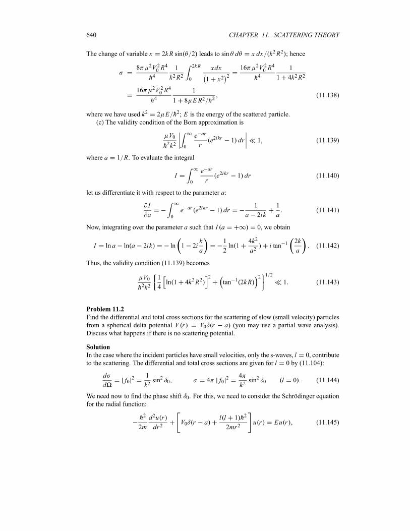
640 CHAPTER 11. SCATTERING THEORY
The change of variable x 2kR sin 2 leads to sin d x dx k2R2 ; hence
8 2V 20 R4
h41
k2R2
2kR
0
xdx
1 x22
16 2V 20 R4
h41
1 4k2R2
16 2V 20 R4
h41
1 8 ER2 h2(11.138)
where we have used k2 2 E h2; E is the energy of the scattered particle.(c) The validity condition of the Born approximation is
V0
h2k2 0
e ar
re2ikr 1 dr 1 (11.139)
where a 1 R. To evaluate the integral
I0
e ar
re2ikr 1 dr (11.140)
let us differentiate it with respect to the parameter a:
I
a 0
e ar e2ikr 1 dr1
a 2ik
1
a(11.141)
Now, integrating over the parameter a such that I a 0, we obtain
I ln a ln a 2ik ln 1 2ik
a
1
2ln 1
4k2
a2i tan 1 2k
a(11.142)
Thus, the validity condition (11.139) becomes
V0
h2k21
4ln 1 4k2R2
2tan 1 2kR
2 1 2
1 (11.143)
Problem 11.2
Find the differential and total cross sections for the scattering of slow (small velocity) particles
from a spherical delta potential V r V0 r a (you may use a partial wave analysis).
Discuss what happens if there is no scattering potential.
Solution
In the case where the incident particles have small velocities, only the s-waves, l 0, contribute
to the scattering. The differential and total cross sections are given for l 0 by (11.104):
d
df02 1
k2sin2 0 4 f0
2 4
k2sin2 0 l 0 (11.144)
We need now to find the phase shift 0. For this, we need to consider the Schrödinger equation
for the radial function:
h2
2m
d2u r
dr2V0 r a
l l 1 h2
2mr2u r Eu r (11.145)
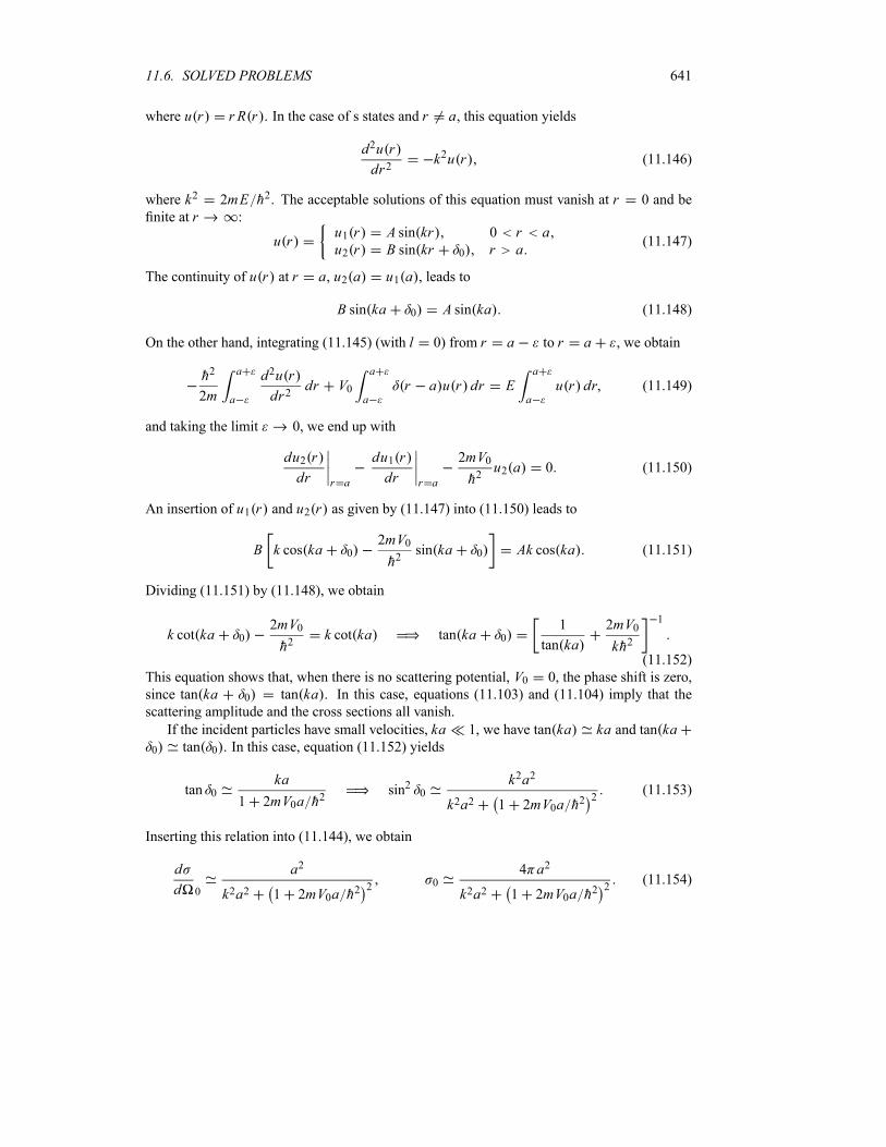
11.6. SOLVED PROBLEMS 641
where u r r R r . In the case of s states and r a, this equation yields
d2u r
dr2k2u r (11.146)
where k2 2mE h2. The acceptable solutions of this equation must vanish at r 0 and be
finite at r :
u ru1 r A sin kr 0 r au2 r B sin kr 0 r a
(11.147)
The continuity of u r at r a, u2 a u1 a , leads to
B sin ka 0 A sin ka (11.148)
On the other hand, integrating (11.145) (with l 0) from r a to r a , we obtain
h2
2m
a
a
d2u r
dr2dr V0
a
ar a u r dr E
a
au r dr (11.149)
and taking the limit 0, we end up with
du2 r
dr r a
du1 r
dr r a
2mV0
h2u2 a 0 (11.150)
An insertion of u1 r and u2 r as given by (11.147) into (11.150) leads to
B k cos ka 02mV0
h2sin ka 0 Ak cos ka (11.151)
Dividing (11.151) by (11.148), we obtain
k cot ka 02mV0
h2k cot ka tan ka 0
1
tan ka
2mV0
kh2
1
(11.152)
This equation shows that, when there is no scattering potential, V0 0, the phase shift is zero,
since tan ka 0 tan ka . In this case, equations (11.103) and (11.104) imply that thescattering amplitude and the cross sections all vanish.
If the incident particles have small velocities, ka 1, we have tan ka ka and tan ka
0 tan 0 . In this case, equation (11.152) yields
tan 0ka
1 2mV0a h2
sin2 0k2a2
k2a2 1 2mV0a h22
(11.153)
Inserting this relation into (11.144), we obtain
d
d 0
a2
k2a2 1 2mV0a h2 2
04 a2
k2a2 1 2mV0a h2 2
(11.154)
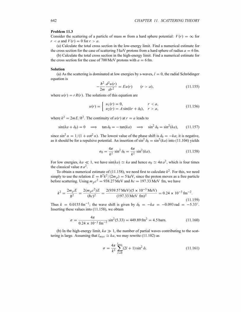
642 CHAPTER 11. SCATTERING THEORY
Problem 11.3
Consider the scattering of a particle of mass m from a hard sphere potential: V r for
r a and V r 0 for r a.(a) Calculate the total cross section in the low-energy limit. Find a numerical estimate for
the cross section for the case of scattering 5 keV protons from a hard sphere of radius a 6 fm.
(b) Calculate the total cross section in the high-energy limit. Find a numerical estimate for
the cross section for the case of 700MeV protons with a 6 fm.
Solution
(a) As the scattering is dominated at low energies by s-waves, l 0, the radial Schrödinger
equation is
h2
2m
d2u r
dr2Eu r r a (11.155)
where u r r R r . The solutions of this equation are
u ru1 r 0 r au2 r A sin kr 0 r a
(11.156)
where k2 2mE h2. The continuity of u r at r a leads to
sin ka 0 0 tan 0 tan ka sin2 0 sin2 ka (11.157)
since sin2 1 1 cot2 . The lowest value of the phase shift is 0 ka; it is negative,as it should be for a repulsive potential. An insertion of sin2 0 sin2 ka into (11.104) yields
04
k2sin2 0
4
k2sin2 ka (11.158)
For low energies, ka 1, we have sin ka ka and hence 0 4 a2, which is four timesthe classical value a2.To obtain a numerical estimate of (11.158), we need first to calculate k2. For this, we need
simply to use the relation E h2k2 2m p 5 keV, since the proton moves as a free particle
before scattering. Using m pc2 938 27MeV and hc 197 33MeV fm, we have
k22m pE
h22 m pc2 E
hc 22 939 57MeV 5 10 3MeV
197 33MeV fm 20 24 10 3 fm 2
(11.159)
Thus k 0 0155 fm 1; the wave shift is given by 0 ka 0 093 rad 5 33 .
Inserting these values into (11.158), we obtain
4
0 24 10 3 fm 2sin2 5 33 449 89 fm2 4 5 barn (11.160)
(b) In the high-energy limit, ka 1, the number of partial waves contributing to the scat-
tering is large. Assuming that lmax ka, we may rewrite (11.102) as
4
k2
lmax
l 0
2l 1 sin2 l (11.161)
11.6. SOLVED PROBLEMS 643
Since so many values of l contribute in this relation, we may replace sin2 l by its average value,12; hence
4
k21
2
lmax
l 0
2l 12
k2lmax 1 2 (11.162)
where we have used nl 0 2l 1 n 1 2. Since lmax 1 we have
2
k2l2max
2
k2ka 2 2 a2 (11.163)
Since a 6 fm, we have 2 6 fm 2 226 1 fm2 2 26 barn. This is almost half the
value obtained in (11.160).
In conclusion, the cross section from a hard sphere potential is (a) four times the classical
value, a2, for low-energy scattering and (b) twice the classical value for high-energy scatter-ing.
Problem 11.4
Calculate the total cross section for the low-energy scattering of a particle of mass m from anattractive square well potential V r V0 for r a and V r 0 for r a, with V0 0.
Solution
Since the scattering is dominated at low energies by the s partial waves, l 0, the Schrödinger
equation for the radial function is given by
h2
2m
d2u r
dr2V0u r Eu r r a (11.164)
h2
2m
d2u r
dr2Eu r r a (11.165)
where u r r R r . The solutions of these equations for positive energy states are
u ru1 r A sin k1r r au2 r B sin k2r 0 r a
(11.166)
where k21 2m E V0 h2 and k22 2mE h2. The continuity of u r and its first derivative,u r du r dr , at r a yield
u2 r
u2 r r a
u1 r
u1 r r a
1
k2tan k2a 0
1
k1tan k1a (11.167)
which yields
0 k2a tan 1 k2k1tan k1a (11.168)
Since
tan k2a 0sin k2a cos 0 cos k2a sin 0
cos k2a cos 0 sin k2a sin 0
tan k2a tan 0
1 tan k2a tan 0(11.169)
644 CHAPTER 11. SCATTERING THEORY
we can reduce Eq. (11.167) to
tan 0k2 tan k1a k1 tan k2a
k1 k2 tan k1a tan k2a(11.170)
Using the relation sin2 0 1 1 1 tan2 0 , we can write
sin2 0 1k1 k2 tan k1a tan k2a
k2 tan k1a k1 tan k2a
2 1
(11.171)
which, when inserted into (11.104), leads to
04
k21sin2 0
4
k211
k1 k2 tan k1a tan k2a
k2 tan k1a k1 tan k2a
2 1
(11.172)
If k2a 1 then (11.170) becomes tan 0tan k1a k1a
k1 k2 k2a tan k1a, since tan k2a k2a. Thus, if
k2a 1 and if E (the scattering energy) is such that tan k1a k1a, we have tan 0 0; hence
there will be no s-wave scattering and the cross section vanishes. Note that if the square well
potential is extended to a hard sphere potential, i.e., E 0 and V0 , equation (11.168)
yields the phase shift of scattering from a hard sphere 0 ka, since k2 k1 tan k1a 0.
Problem 11.5
Find the differential and total cross sections in the first Born approximation for the elastic scat-
tering of a particle of mass m, which is initially traveling along the z-axis, from a nonspherical,double-delta potential V r V0 r ak V0 r ak , where k is the unit vector along thez-axis.
Solution
Since V r is not spherically symmetric, the differential cross section can be obtained from
(11.66):
d
d
m2
4 2h4V0 r ak r ak eiq r d3r
2 m2V0
4 2h4I 2 (11.173)
Since r ak x y z a we can write the integral I as
I x ei xqx dx y eiyqy dy [ z a z a ] ei zqz dz
eiaqz e iaqz 2 cos aqz (11.174)
The calculation of qz is somewhat different from that shown in (11.67). Since the incidentparticle is initially traveling along the z-axis, and since it scatters elastically from the potentialV r , the magnitudes of its momenta before and after collision are equal. So, as shown inFigure 11.8, we have qz q sin 2 2k sin2 2 , since q k0 k 2k sin 2 . Thus,
inserting I 2 cos aqz 2 cos 2ak sin2 2 into (11.173), we obtain
d
d
m2V02h4
cos2 2ak sin22
(11.175)
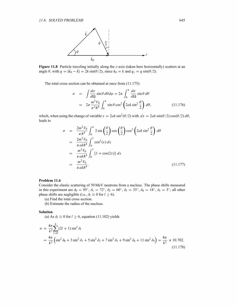
11.6. SOLVED PROBLEMS 645
- z-k0
¡¡¡¡¡¡¡¡µ
kAAAAAAAU
q2
Figure 11.8 Particle traveling initially along the z-axis (taken here horizontally) scatters at anangle , with q k0 k 2k sin 2 , since k0 k and qz q sin 2 .
The total cross section can be obtained at once from (11.175):
d
dsin d d 2
0
d
dsin d
2m2V02h4 0
sin cos2 2ak sin22
d (11.176)
which, when using the change of variable x 2ak sin2 2 with dx 2ak sin 2 cos 2 d ,leads to
2m2V0
h4 0
2 sin2cos
2cos2 2ak sin2
2d
2m2V0
akh4
1
0
cos2 x dx
m2V0
akh4
1
0
[1 cos 2x ] dx
m2V0
akh4(11.177)
Problem 11.6
Consider the elastic scattering of 50MeV neutrons from a nucleus. The phase shifts measured
in this experiment are 0 95 , 1 72 , 2 60 , 3 35 , 4 18 , 5 5 ; all other
phase shifts are negligible (i.e., l 0 for l 6).
(a) Find the total cross section.
(b) Estimate the radius of the nucleus.
Solution
(a) As l 0 for l 6, equation (11.102) yields
4
k2
6
l 0
2l 1 sin2 l
4
k2sin2 0 3 sin2 1 5 sin2 2 7 sin2 3 9 sin2 4 11 sin2 5
4
k210 702
(11.178)
646 CHAPTER 11. SCATTERING THEORY
To calculate k2, we need simply to use the relation E h2k2 2mn 50MeV, since the
neutrons move as free particles before scattering. Using mnc2 939 57MeV and hc197 33MeV fm, we have
k22mnE
h22 mnc2 E
hc 22 939 57MeV 50MeV
197 33MeV fm 22 41 fm 2 (11.179)
An insertion of (11.179) into (11.178) leads to
4
2 41 fm 210 702 55 78 fm2 0 558 barn (11.180)
(b) At large values of l, when the neutron is at its closest approach to the nucleus, it feelsmainly the effect of the centrifugal potential l l 1 h2 2mnr2 ; the effect of the nuclearpotential is negligible. We may thus use the approximations E l l 1 h2 2mnr2c42h2 2mnr2c where we have taken l 6, since l 0 for l 6. A crude value of the radius
of the nucleus is then given by
rc21h2
mnE
21 hc 2
mnc2 E
21 197 33MeV fm 2
939 57MeV 50MeV4 17 fm (11.181)
Problem 11.7
Consider the elastic scattering of an electron from a hydrogen atom in its ground state. If the
atom is assumed to remain in its ground state after scattering, calculate the differential cross
section in the case where the effects resulting from the identical nature of the electrons (a) are
ignored and (b) are taken into account (in part (b), discuss the three cases when the electrons
are in (i) a spin singlet state, (ii) a spin triplet state, or (iii) an unpolarized state).
Solution
(a) By analogy with (11.63) we may write the differential cross section for this process as
d
df 2
2 h2f V i
2
(11.182)
where me 2, since this problem can be viewed as the scattering of a particle whose reducedmass is half that of the electron. Assuming the atom to be very massive and that it remains in
its ground state after scattering, the initial and final states of the system (incident electron plus
the atom) are given by i r k0 r eik0 r 0 r and f r k r eik r 0 r , where
eik0 r and eik r are the states of the incident electron before and after scattering, and 0 r
a301 2e r a0 is the atom’s wave function. We have assumed here that the nucleus is located
at the origin and that the position vectors of the incident electron and the atom’s electron are
given by r and r , respectively. Since the incident electron experiences an attractive Coulombinteraction e2 r with the nucleus and a repulsive interaction e2 r r with the hydrogen’s
electron, we have
f2 h2
d3reiq r d3r 0 re2
r
e2
r r0 r (11.183)
11.6. SOLVED PROBLEMS 647
with q k0 k 2k sin 2 , since k k0 (elastic scattering). Using 0 sin qr dr 1 q
(see (11.76)), and since 0 eiqr cos sin d 1
1 eiqr xdx 2 qr sin qr , we obtain the
following relation:
d3reiq r
r 0
r dr0
eiqr cos sin d2
0
d4
q 0
dr sin qr4
q2(11.184)
which, when inserted into (11.183) and since d3r 0 r 0 r 1, leads to
f2 h2
4 e2
q2d3reiq r d3r 0 r
e2
r r0 r (11.185)
By analogy with (11.184), we have d3reiq r r r r 4 q2; hence we can reduce theintegral in (11.185) to
d3r eiq r d3r 0 re2
r r0 r e2 d3r 0 r eiq r 0 r d3r
eiq r r
r r
4 e2
q2d3r 0 r eiq r 0 r (11.186)
The remaining integral of (11.186) can, in turn, be written as
d3r 0 r eiq r 0 r1
a30 0
r 2e 2r a0 dr0
eiqr cos sin d2
0
d
4
qa30 0
r e 2r a0 sin qr dr 1a20q
2
4
2
(11.187)
where we have used the expression for 0 re ar sin qr dr calculated in (11.130). Inserting(11.187) into (11.186), and the resulting expression into (11.185), we obtain
f2 e2
h2q21 1
a20q2
4
2e2
2k2h2 sin2 21 1 a20k
2 sin22
2
(11.188)
We can thus reduce (11.182) to
d
d
4 2e4
h4q41 1
a20q2
4
2 22e4
4k4h4 sin42
1 1 a20k2 sin2 2
2 2
(11.189)
with q 2k sin 2 .
(b) (i) If the electrons are in their spin singlet state (antisymmetric), the spatial wave function
must be symmetric; hence the differential cross section is
d S
df f
2(11.190)
648 CHAPTER 11. SCATTERING THEORY
where f is given by (11.188) and
f2 e2
h2q21 1
a20q2
4
2e2
2k2h2 cos22
1 1 a20k2 cos2 2
2
(11.191)
since sin 2 cos 2 .
(ii) If, however, the electrons are in their spin triplet state, the spatial wave function must be
antisymmetric; henced A
df f
2(11.192)
(iii) Finally, if the electrons are unpolarized, the differential cross section must be a mixture of
(11.191) and (11.192):
d
d
1
4
d S
d
3
4
d A
d
1
4f f 2 3
4f f 2 (11.193)
Problem 11.8
In an experiment, 650MeV 0 pions are scattered from a heavy, totally absorbing nucleus of
radius 1 4 fm.
(a) Estimate the total elastic and total inelastic cross sections.
(b) Calculate the scattering amplitude and check the validity of the optical theorem.
(c) Using the scattering amplitude found in (b), calculate and plot the differential cross
section for elastic scattering. Calculate the total elastic cross section and verify that it agrees
with the expression found in (a).
Solution
(a) In the case of a totally absorbing nucleus, l k 0, the total elastic and inelastic cross
sections, which are given by (11.113) and (11.114), become equal:
elk2
lmax
l 0
2l 1 inel (11.194)
This experiment can be viewed as a scattering of high-energy pions, E 650MeV, from a
black “disk” of radius a 1 4 fm; thus, the number of partial waves involved in this scattering
can be obtained from lmax ka, where k 2m 0E h2. Since the rest mass energy of a 0
pion is m 0c2 135MeV and since hc 197 33MeV fm, we have
k2m 0E
h22 m 0c2 E
hc 22 135MeV 650MeV
197 33MeV fm 22 12 fm 1 (11.195)
hence lmax ka 2 12 fm 1 1 4 fm 2 97 3. We can thus reduce (11.194) to
el inelk2
3
l 0
2l 116
k216
2 12 fm 1 240 1 fm2 0 40 barn (11.196)
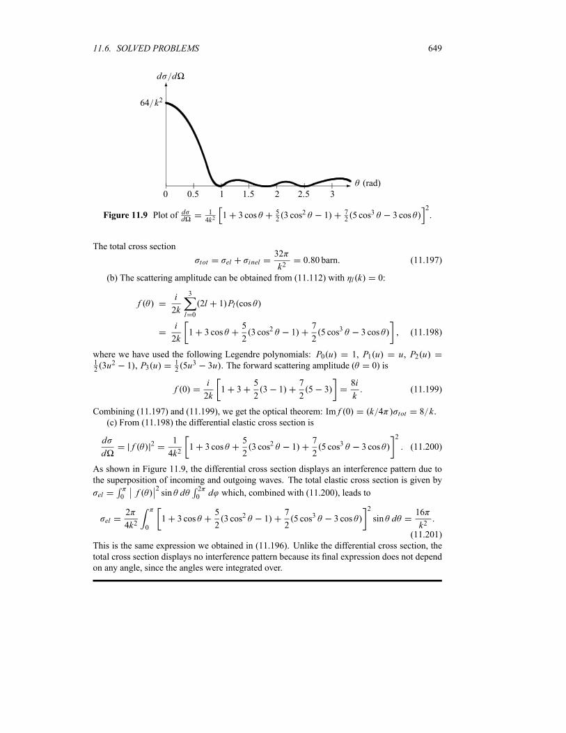
11.6. SOLVED PROBLEMS 649
-
6d d
rad
64 k2
0 0 5 1 1 5 2 2 5 3
Figure 11.9 Plot of dd14k2
1 3 cos 523 cos2 1 7
25 cos3 3 cos
2.
The total cross section
tot el inel32
k20 80 barn (11.197)
(b) The scattering amplitude can be obtained from (11.112) with l k 0:
fi
2k
3
l 0
2l 1 Pl cos
i
2k1 3 cos
5
23 cos2 1
7
25 cos3 3 cos (11.198)
where we have used the following Legendre polynomials: P0 u 1, P1 u u, P2 u123u2 1 , P3 u
125u3 3u . The forward scattering amplitude ( 0) is
f 0i
2k1 3
5
23 1
7
25 3
8i
k(11.199)
Combining (11.197) and (11.199), we get the optical theorem: Im f 0 k 4 tot 8 k.(c) From (11.198) the differential elastic cross section is
d
df 2 1
4k21 3 cos
5
23 cos2 1
7
25 cos3 3 cos
2
(11.200)
As shown in Figure 11.9, the differential cross section displays an interference pattern due to
the superposition of incoming and outgoing waves. The total elastic cross section is given by
el 0f
2sin d 2
0d which, combined with (11.200), leads to
el2
4k2 0
1 3 cos5
23 cos2 1
7
25 cos3 3 cos
2
sin d16
k2(11.201)
This is the same expression we obtained in (11.196). Unlike the differential cross section, the
total cross section displays no interference pattern because its final expression does not depend
on any angle, since the angles were integrated over.

650 CHAPTER 11. SCATTERING THEORY
11.7 Exercises
Exercise 11.1
Consider the scattering of a 5MeV alpha particle (i.e., a helium nucleus with Z1 2 and
A1 4) from an aluminum nucleus (Z2 13 and A2 27). If the scattering angle of the
alpha particle in the Lab frame is 1 30 ,
(a) find its scattering angle in the CM frame and
(b) give a numerical estimate of the Rutherford cross section.
Exercise 11.2
(a) Find the differential and total cross sections for the classical collision of two hard spheres
of radius r and R, where R is the radius of the larger sphere; the larger sphere is considered tobe stationary.
(b) From the results of (a) find the differential and total cross sections for the scattering of
pointlike particles from a hard stationary sphere of radius R. Hint: You may use the classicalrelation d d [b sin ]db d , where b is the impact parameter.
Exercise 11.3
Consider the scattering from the potential V r V0e r2 a2 . Find
(a) the differential cross section in the first Born approximation and
(b) the total cross section.
Exercise 11.4
Calculate the differential cross section in the first Born approximation for the scattering of a
particle by an attractive square well potential: V r V0 for r a and V r 0 for r a,with V0 0.
Exercise 11.5
Consider the elastic scattering from the delta potential V r V0 r a .(a) Calculate the differential cross section in the first Born approximation.
(b) Find an expression between V0, a, , and k so the Born approximation is valid.
Exercise 11.6
Consider the elastic scattering from the potential V r V0e r a , where V0 and a are constant.(a) Calculate the differential cross section in the first Born approximation.
(b) Find an expression between V0, a, , and k so the Born approximation is valid.(c) Find the total cross section using the Born approximation.
Exercise 11.7
Find the differential cross section in the first Born approximation for the elastic scattering of a
particle of mass m, which is initially traveling along the z-axis, from a nonspherical, double-delta potential:
V r V0 r ak V0 r ak
where k is the unit vector along the z-axis.
Exercise 11.8
Find the differential cross section in the first Born approximation for neutron–neutron scattering
in the case where the potential is approximated by V r V0e r a .
11.7. EXERCISES 651
Exercise 11.9
Consider the elastic scattering of a particle of mass m and initial momentum hk off a deltapotential V r V0 x y z a , where V0 is a constant.(a) What is the physical dimensions of the constant V0?(b) Calculate the differential cross sections in the first Born approximation.
(c) Repeat (b) for the case where the potential is now given by
V r V0 x y b z y z a
Exercise 11.10
Consider the S-wave (l 0) scattering of a particle of mass m from a repulsive sphericalpotential V r V0 for r a and V r 0 for r a, with V0 0.
(a) Calculate S wave (l 0) phase shift and the total cross section.
(b) Show that in the limit V0 , the phase shift is given by 0 ka. Find the totalcross section.
Exercise 11.11
Consider the S-wave neutron–neutron scattering where the interaction potential is approximatedby V r V0S1 S2e r a , where S1 and S2 are the spin vector operators of the two neutrons,and V0 0. Find the differential cross section in the first Born approximation.
Exercise 11.12
Consider the S-partial wave scattering (l 0) between two identical spin 1 2 particles where
the interaction potential is given approximately by
V r V0S1 S2 r a
where S1 and S2 are the spin vector operators of the two particles, and V0 0. Assuming that
the incident and target particles are unpolarized, find the differential and total cross sections.
Exercise 11.13
Consider the elastic scattering of 170MeV neutrons from a nucleus or radius a 1 05 fm.
Consider the hypothetical case where the phase shifts measured in this experiment are given by
l180l 2 .
(a) Estimate the maximum angular momentum lmax .(b) Find the total cross section.

652 CHAPTER 11. SCATTERING THEORY
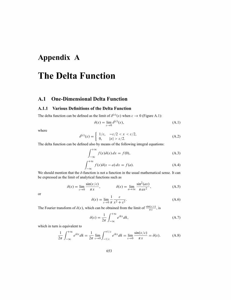
Appendix A
The Delta Function
A.1 One-Dimensional Delta Function
A.1.1 Various Definitions of the Delta Function
The delta function can be defined as the limit of x when 0 (Figure A.1):
x lim0
x (A.1)
where
x1 2 x 2
0 x 2(A.2)
The delta function can be defined also by means of the following integral equations:
f x x dx f 0 (A.3)
f x x a dx f a (A.4)
We should mention that the -function is not a function in the usual mathematical sense. It can
be expressed as the limit of analytical functions such as
x lim0
sin x
xx lim
a
sin2 ax
ax2(A.5)
or
x lim0
1
x2 2(A.6)
The Fourier transform of x , which can be obtained from the limit of sin xx , is
x1
2eikxdk (A.7)
which in turn is equivalent to
1
2eikxdk
1
2lim0
1
1
eikxdk lim0
sin x
xx (A.8)
653
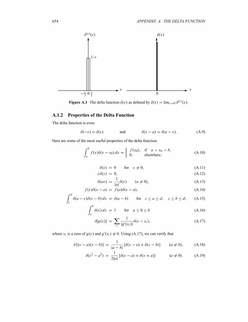
654 APPENDIX A. THE DELTA FUNCTION
-
6
0x
x
1
2 2
-
6
0x
x
Figure A.1 The delta function x as defined by x lim 0 x
A.1.2 Properties of the Delta Function
The delta function is even:
x x and x a a x (A.9)
Here are some of the most useful properties of the delta function:
b
af x x x0 dx
f x0 if a x0 b0 elsewhere
(A.10)
x 0 for x 0 (A.11)
x x 0 (A.12)
ax1
ax a 0 (A.13)
f x x a f a x a (A.14)d
ca x x b dx a b for c a d c b d (A.15)
b
ax dx 1 for a 0 b (A.16)
[g x ]i
1
g xix xi (A.17)
where xi is a zero of g x and g xi 0. Using (A.17), we can verify that
[ x a x b ]1
a b[ x a x b ] a b (A.18)
x2 a21
2 a[ x a x a ] a 0 (A.19)
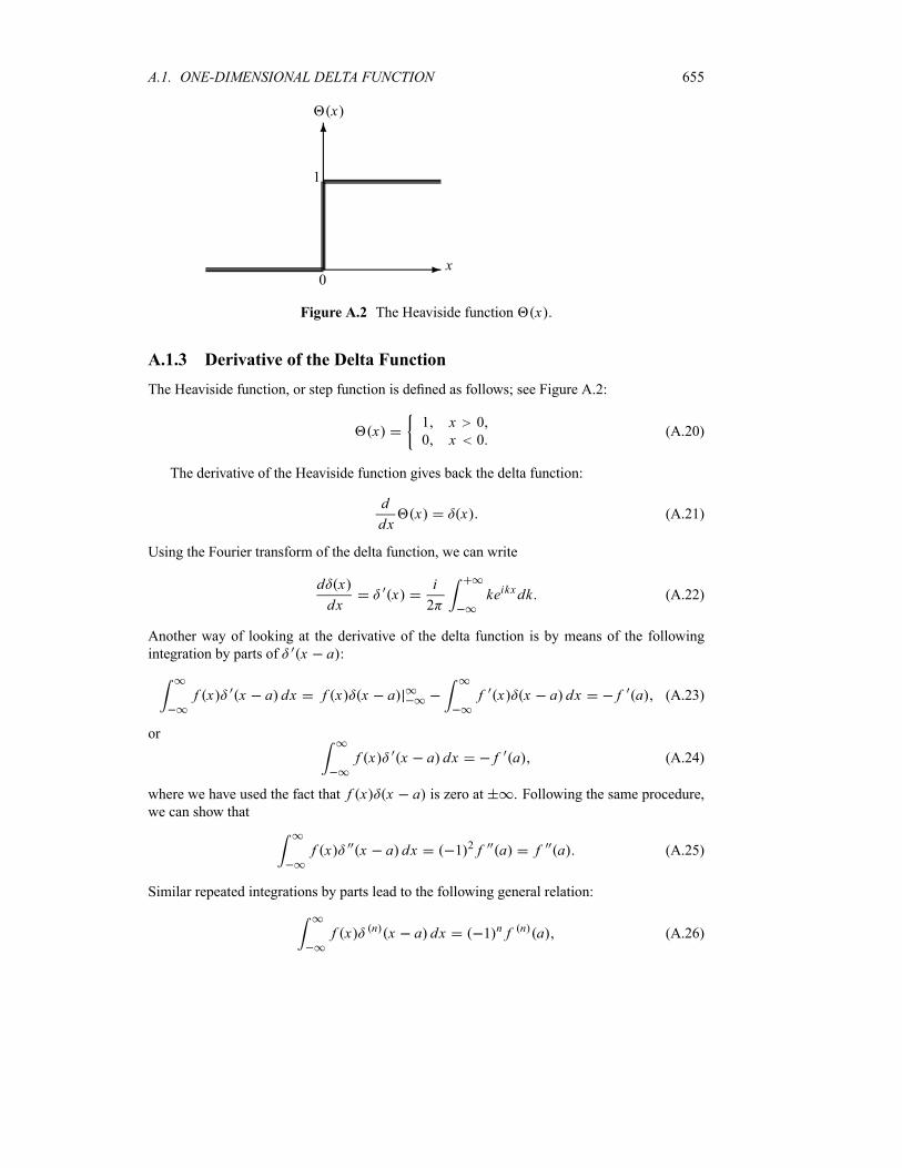
A.1. ONE-DIMENSIONAL DELTA FUNCTION 655
-
6
0x
x
1
Figure A.2 The Heaviside function x .
A.1.3 Derivative of the Delta Function
The Heaviside function, or step function is defined as follows; see Figure A.2:
x1 x 0
0 x 0(A.20)
The derivative of the Heaviside function gives back the delta function:
d
dxx x (A.21)
Using the Fourier transform of the delta function, we can write
d x
dxx
i
2keikxdk (A.22)
Another way of looking at the derivative of the delta function is by means of the following
integration by parts of x a :
f x x a dx f x x a f x x a dx f a (A.23)
or
f x x a dx f a (A.24)
where we have used the fact that f x x a is zero at . Following the same procedure,
we can show that
f x x a dx 1 2 f a f a (A.25)
Similar repeated integrations by parts lead to the following general relation:
f x n x a dx 1 n f n a (A.26)

656 APPENDIX A. THE DELTA FUNCTION
where n x a d n[ x a ] dxn and f n a d n f x dxn x a . In particular, if
f x 1 and n 1, we have
x a dx 0 (A.27)
Here is a list of useful properties of the derivative of the delta function:
x x (A.28)
x x x (A.29)
x2 x 0 (A.30)
x2 x 2 x (A.31)
A.2 Three-Dimensional Delta Function
The three-dimensional form of the delta function is given in Cartesian coordinates by
r r x x y y z z (A.32)
and in spherical coordinates by
r r1
r2r r cos cos
1
r2 sinr r (A.33)
since, according to (A.17), we have cos cos sin .
The Fourier transform of the three-dimensional delta function is
r r1
2 3d3k eik r r (A.34)
and
d3r f r r f 0 d3r f r r r0 f r0 (A.35)
The following relations are often encountered:
r
r24 r 2 1
r4 r (A.36)
where r the unit vector along r .We should mention that the physical dimension of the delta function is one over the di-
mensions of its argument. Thus, if x is a distance, the physical dimension of x is given by
[ x ] 1 [x] 1 L, where L is a length. Similarly, the physical dimensions of r is 1 L3,since
r x y z1
[x]
1
[y]
1
[z]
1
L3(A.37)
Appendix B
Angular Momentum in Spherical
Coordinates
In this appendix, we will show how to derive the expressions of the gradient , the Laplacian2, and the components of the orbital angular momentum in spherical coordinates.
B.1 Derivation of Some General Relations
The Cartesian coordinates x y z of a vector r are related to its spherical polar coordinatesr by
x r sin cos y r sin sin z r cos (B.1)
The orthonormal Cartesian basis x y z is related to its spherical counterpart (r ) by
x r sin cos cos cos sin (B.2)
y r sin sin cos sin cos (B.3)
z r cos sin (B.4)
Differentiating (B.1), we obtain
dx sin cos dr r cos cos d r sin sin d (B.5)
dy sin sin dr r cos sin d r sin cos d (B.6)
dz cos dr r sin d (B.7)
Solving these equations for dr , d , and d , we obtain
dr sin cos dx sin sin dy cos dz (B.8)
d1
rcos cos dx
1
rcos sin dy
1
rsin dz (B.9)
dsin
r sindx
cos
r sindy (B.10)
657
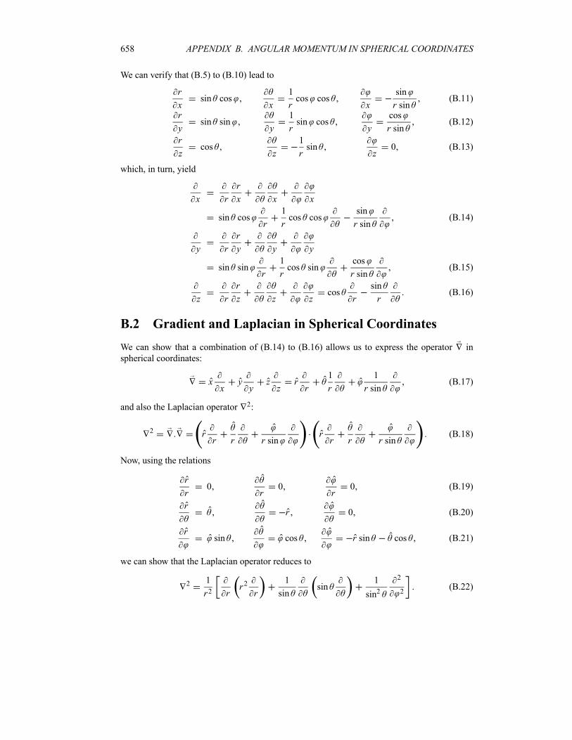
658 APPENDIX B. ANGULAR MOMENTUM IN SPHERICAL COORDINATES
We can verify that (B.5) to (B.10) lead to
r
xsin cos
x
1
rcos cos
x
sin
r sin(B.11)
r
ysin sin
y
1
rsin cos
y
cos
r sin(B.12)
r
zcos
z
1
rsin
z0 (B.13)
which, in turn, yield
x r
r
x x x
sin cosr
1
rcos cos
sin
r sin(B.14)
y r
r
y y y
sin sinr
1
rcos sin
cos
r sin(B.15)
z r
r
z z zcos
r
sin
r(B.16)
B.2 Gradient and Laplacian in Spherical Coordinates
We can show that a combination of (B.14) to (B.16) allows us to express the operator in
spherical coordinates:
xx
yy
zz
rr
1
r
1
r sin(B.17)
and also the Laplacian operator 2:
2 rr r r sin
rr r r sin
(B.18)
Now, using the relations
r
r0
r0
r0 (B.19)
rr 0 (B.20)
rsin cos r sin cos (B.21)
we can show that the Laplacian operator reduces to
2 1
r2 rr2r
1
sinsin
1
sin2
2
2(B.22)
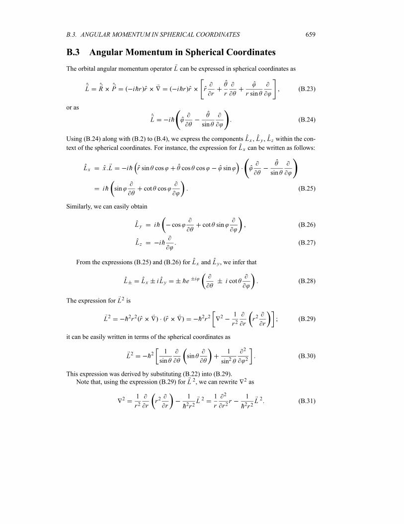
B.3. ANGULAR MOMENTUM IN SPHERICAL COORDINATES 659
B.3 Angular Momentum in Spherical Coordinates
The orbital angular momentum operator L can be expressed in spherical coordinates as
L R P ihr r ihr r rr r r sin
(B.23)
or as
L ihsin
(B.24)
Using (B.24) along with (B.2) to (B.4), we express the components Lx L y Lz within the con-
text of the spherical coordinates. For instance, the expression for Lx can be written as follows:
Lx x L ih r sin cos cos cos sinsin
ih sin cot cos (B.25)
Similarly, we can easily obtain
L y ih cos cot sin (B.26)
L z ih (B.27)
From the expressions (B.25) and (B.26) for Lx and L y , we infer that
L Lx i L y he i i cot (B.28)
The expression for L2 is
L2 h2r2 r r h2r2 2 1
r2 rr2r
(B.29)
it can be easily written in terms of the spherical coordinates as
L2 h21
sinsin
1
sin2
2
2(B.30)
This expression was derived by substituting (B.22) into (B.29).
Note that, using the expression (B.29) for L 2, we can rewrite 2 as
2 1
r2 rr2r
1
h2r2L 2
1
r
2
r2r
1
h2r2L 2 (B.31)

660 APPENDIX B. ANGULAR MOMENTUM IN SPHERICAL COORDINATES
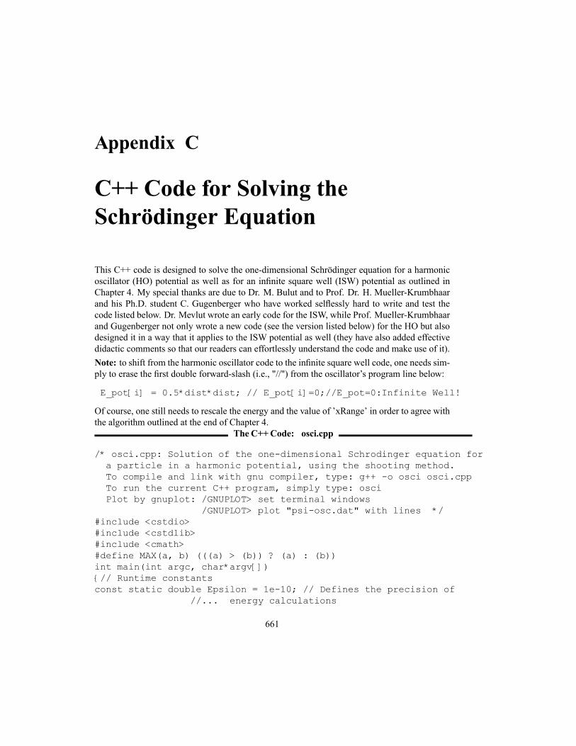
Appendix C
C++ Code for Solving the
Schrödinger Equation
This C++ code is designed to solve the one-dimensional Schrödinger equation for a harmonic
oscillator (HO) potential as well as for an infinite square well (ISW) potential as outlined in
Chapter 4. My special thanks are due to Dr. M. Bulut and to Prof. Dr. H. Mueller-Krumbhaar
and his Ph.D. student C. Gugenberger who have worked selflessly hard to write and test the
code listed below. Dr. Mevlut wrote an early code for the ISW, while Prof. Mueller-Krumbhaar
and Gugenberger not only wrote a new code (see the version listed below) for the HO but also
designed it in a way that it applies to the ISW potential as well (they have also added effective
didactic comments so that our readers can effortlessly understand the code and make use of it).
Note: to shift from the harmonic oscillator code to the infinite square well code, one needs sim-
ply to erase the first double forward-slash (i.e., "//") from the oscillator’s program line below:
E_pot[i] = 0.5*dist*dist; // E_pot[i]=0;//E_pot=0:Infinite Well!
Of course, one still needs to rescale the energy and the value of ’xRange’ in order to agree with
the algorithm outlined at the end of Chapter 4.
The C++Code: osci.cpp
/* osci.cpp: Solution of the one-dimensional Schrodinger equation for
a particle in a harmonic potential, using the shooting method.
To compile and link with gnu compiler, type: g++ -o osci osci.cpp
To run the current C++ program, simply type: osci
Plot by gnuplot: /GNUPLOT> set terminal windows
/GNUPLOT> plot "psi-osc.dat" with lines */
#include <cstdio>
#include <cstdlib>
#include <cmath>
#define MAX(a, b) (((a) > (b)) ? (a) : (b))
int main(int argc, char*argv[])
{// Runtime constants
const static double Epsilon = 1e-10; // Defines the precision of
//... energy calculations
661
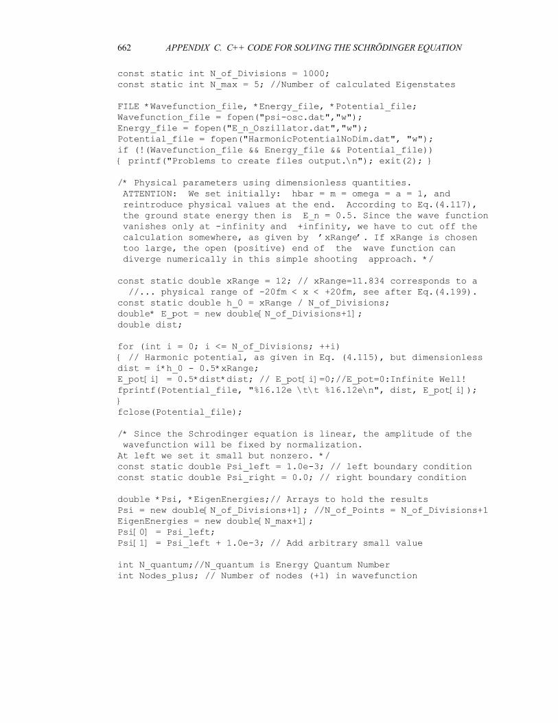
662 APPENDIX C. C++ CODE FOR SOLVING THE SCHRÖDINGER EQUATION
const static int N_of_Divisions = 1000;
const static int N_max = 5; //Number of calculated Eigenstates
FILE *Wavefunction_file, *Energy_file, *Potential_file;
Wavefunction_file = fopen("psi-osc.dat","w");
Energy_file = fopen("E_n_Oszillator.dat","w");
Potential_file = fopen("HarmonicPotentialNoDim.dat", "w");
if (!(Wavefunction_file && Energy_file && Potential_file))
{ printf("Problems to create files output.\n"); exit(2); }
/* Physical parameters using dimensionless quantities.
ATTENTION: We set initially: hbar = m = omega = a = 1, and
reintroduce physical values at the end. According to Eq.(4.117),
the ground state energy then is E_n = 0.5. Since the wave function
vanishes only at -infinity and +infinity, we have to cut off the
calculation somewhere, as given by ’xRange’. If xRange is chosen
too large, the open (positive) end of the wave function can
diverge numerically in this simple shooting approach. */
const static double xRange = 12; // xRange=11.834 corresponds to a
//... physical range of -20fm < x < +20fm, see after Eq.(4.199).
const static double h_0 = xRange / N_of_Divisions;
double* E_pot = new double[N_of_Divisions+1];
double dist;
for (int i = 0; i <= N_of_Divisions; ++i)
{ // Harmonic potential, as given in Eq. (4.115), but dimensionless
dist = i*h_0 - 0.5*xRange;
E_pot[i] = 0.5*dist*dist; // E_pot[i]=0;//E_pot=0:Infinite Well!
fprintf(Potential_file, "%16.12e \t\t %16.12e\n", dist, E_pot[i]);
}
fclose(Potential_file);
/* Since the Schrodinger equation is linear, the amplitude of the
wavefunction will be fixed by normalization.
At left we set it small but nonzero. */
const static double Psi_left = 1.0e-3; // left boundary condition
const static double Psi_right = 0.0; // right boundary condition
double *Psi, *EigenEnergies;// Arrays to hold the results
Psi = new double[N_of_Divisions+1]; //N_of_Points = N_of_Divisions+1
EigenEnergies = new double[N_max+1];
Psi[0] = Psi_left;
Psi[1] = Psi_left + 1.0e-3; // Add arbitrary small value
int N_quantum;//N_quantum is Energy Quantum Number
int Nodes_plus; // Number of nodes (+1) in wavefunction
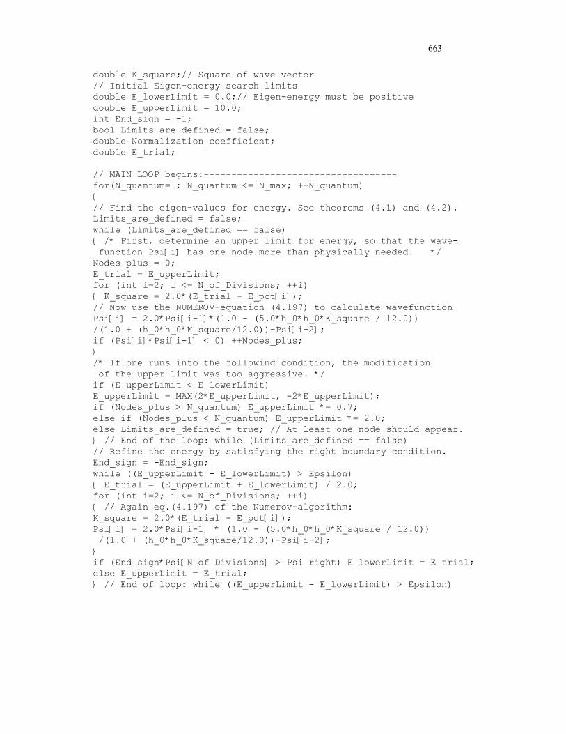
663
double K_square;// Square of wave vector
// Initial Eigen-energy search limits
double E_lowerLimit = 0.0;// Eigen-energy must be positive
double E_upperLimit = 10.0;
int End_sign = -1;
bool Limits_are_defined = false;
double Normalization_coefficient;
double E_trial;
// MAIN LOOP begins:-----------------------------------
for(N_quantum=1; N_quantum <= N_max; ++N_quantum)
{
// Find the eigen-values for energy. See theorems (4.1) and (4.2).
Limits_are_defined = false;
while (Limits_are_defined == false)
{ /* First, determine an upper limit for energy, so that the wave-
function Psi[i] has one node more than physically needed. */
Nodes_plus = 0;
E_trial = E_upperLimit;
for (int i=2; i <= N_of_Divisions; ++i)
{ K_square = 2.0*(E_trial - E_pot[i]);
// Now use the NUMEROV-equation (4.197) to calculate wavefunction
Psi[i] = 2.0*Psi[i-1]*(1.0 - (5.0*h_0*h_0*K_square / 12.0))
/(1.0 + (h_0*h_0*K_square/12.0))-Psi[i-2];
if (Psi[i]*Psi[i-1] < 0) ++Nodes_plus;
}
/* If one runs into the following condition, the modification
of the upper limit was too aggressive. */
if (E_upperLimit < E_lowerLimit)
E_upperLimit = MAX(2*E_upperLimit, -2*E_upperLimit);
if (Nodes_plus > N_quantum) E_upperLimit *= 0.7;
else if (Nodes_plus < N_quantum) E_upperLimit *= 2.0;
else Limits_are_defined = true; // At least one node should appear.
} // End of the loop: while (Limits_are_defined == false)
// Refine the energy by satisfying the right boundary condition.
End_sign = -End_sign;
while ((E_upperLimit - E_lowerLimit) > Epsilon)
{ E_trial = (E_upperLimit + E_lowerLimit) / 2.0;
for (int i=2; i <= N_of_Divisions; ++i)
{ // Again eq.(4.197) of the Numerov-algorithm:
K_square = 2.0*(E_trial - E_pot[i]);
Psi[i] = 2.0*Psi[i-1] * (1.0 - (5.0*h_0*h_0*K_square / 12.0))
/(1.0 + (h_0*h_0*K_square/12.0))-Psi[i-2];
}
if (End_sign*Psi[N_of_Divisions] > Psi_right) E_lowerLimit = E_trial;
else E_upperLimit = E_trial;
} // End of loop: while ((E_upperLimit - E_lowerLimit) > Epsilon)

664 APPENDIX C. C++ CODE FOR SOLVING THE SCHRÖDINGER EQUATION
// Initialization for the next iteration in main loop
E_trial = (E_upperLimit+E_lowerLimit)/2;
EigenEnergies[N_quantum] = E_trial;
E_upperLimit = E_trial;
E_lowerLimit = E_trial;
// Now find the normalization coefficient
double Integral = 0.0;
for (int i=1; i <= N_of_Divisions; ++i)
{ // Simple integration
Integral += 0.5*h_0*(Psi[i-1]*Psi[i-1]+Psi[i]*Psi[i]);
}
Normalization_coefficient = sqrt(1.0/Integral);
// Output of normalized dimensionless wave function
for (int i=0; i <=N_of_Divisions; ++i)
{ fprintf(Wavefunction_file, "%16.12e \t\t %16.12e\n",
i*h_0 - 0.5*xRange, Normalization_coefficient*Psi[i]);
}
fprintf(Wavefunction_file,"\n");
} // End of MAIN LOOP. --------------------------------
fclose(Wavefunction_file);
/*Finally convert dimensionless units in real units. Note that
energy does not depend explicitly on the particle’s mass anymore:
hbar = 1.05457e-34;// Planck constant/2pi
omega = 5.34e21; // Frequency in 1/s
MeV = 1.602176487e-13; // in J
The correct normalization would be hbar*omega/MeV = 3.5148461144,
but we use the approximation 3.5 for energy-scale as in chap. 4.9 */
const static double Energyscale = 3.5;// in MeV
// Output with rescaled dimensions; assign Energy_file
printf("Quantum Harmonic Oscillator, program osci.cpp\n");
printf("Energies in MeV:\n");
printf("n \t\t E_n\n");
for (N_quantum=1; N_quantum <= N_max; ++N_quantum)
{ fprintf(Energy_file,"%d \t\t %16.12e\n", N_quantum-1,
Energyscale*EigenEnergies[N_quantum]);
printf("%d \t\t %16.12e\n", N_quantum-1,
Energyscale*EigenEnergies[N_quantum]);
}
fprintf(Energy_file,"\n");
fclose(Energy_file);
printf("Wave-Functions in File: psi_osc.dat \n");
printf("\n");
return 0;
}

Index
Abelian group, 79, 396
Absorption of a photon, 580
Action quantization, 36
Addition of
three angular momenta, 419–420
two angular momenta, 403–418
Addition of angular momenta, 403–425
Addition of isospins, 424
Adiabatic approximation, 582
Adiabatic theorem, 583
Adjoint of an operator, 91
Airy functions, 275, 520
Algebraic method for
harmonic oscillator, 239
Allowed transitions, 594
Alpha decay, 529
Angular momentum
addition of three, 419–420
addition of two, 403–418
commutation relations, 284, 285
conservation of, 187, 283, 341, 395
eigenfunctions, 301–309
general formalism, 285–290
generator of infinitesimal rotations, 394
geometrical representation, 293–294
matrix representation, 290–293
orbital, 283–285
raising and lowering operators, 286
spin, 295–301
Anisotropic harmonic oscillator, 338
Annihilation operator, 239–243
Anomalous Zeeman effect, 507
Anti-Hermitian operator, 92
Anticommutator, 93
Antiparticle, 16
Antisymmetric state, 458, 463, 464
Associated Laguerre polynomials, 357
Associated Legendre functions, 303
Atomic shell structure, 469
Axial vector, 426
Balmer series, 35
Barrier penetration, 227–231
Basis
complete, 105
continuous, 121–128
discrete, 104–121
of a vector space, 82
orthonormal, 82, 105, 121
Bessel equation, 344
Bessel functions, spherical, 344
Blackbody radiation, 4–10
Bohr atomic model, 31
Bohr energy, 33
Bohr magneton, 365
Bohr quantization rule, 31
Bohr radius, 32
Bohr’s postulates, 31
Bohr–Sommerfeld quantization rule, 522
Boltzmann constant, 7
Born approximation, first, 628
Born approximation, validity, 629
Born series, 626
Bose–Einstein condensation, 468
Bose–Einstein statistics, 463
Boson condensation, 468
Bosons, 462
Bound states, 216–217, 231–239
Boundary conditions, 222
Box potential, 231
Bra-ket
matrix representation of, 105
notation, 84–89
properties, 85
Canonical commutation relations, 127
Center of mass motion, 273, 352
665

666 INDEX
Central potential, 340–343
Centrifugal potential, 342
Characteristic equation, 118
Classical limit, 190–191
Classical turning points, 216, 230, 517
Classically allowed region, 517
Classically forbidden region, 517
Clebsch–Gordan coefficients, 406
orthonormalization relation, 406
recursion relations, 410
Clebsch–Gordan series, 420–421
Closed shell, 471
Closure relation, 105
Cofactor of a matrix, 109
Commutator
algebra, 93–95
anticommutator, 93
definition, 93
Jacobi identity, 94
properties of a, 94
Compatible observables, 175
Complementarity principle, 26
Composite particles, 463
Compton effect, 13–16
Compton wavelength, 15
Configuration, 471
Connection formulas, 519–522
Conservation laws, 183–187
Conservation of
energy, 186–187
linear momentum, 186–187
parity, 187
probability, 181–182
Constant of the motion, 186, 187, 395
Constrained variational principle, 510
Continuity of x , 222Continuity of d x dx , 222Continuous spectrum, 217
Correspondence principle, 191
Coulomb gauge, 365, 586, 587
Coulomb potential, 351, 630, 639, 646
Coulomb scattering, 630
Creation operator, 239–243
Cross section
Coulomb, 630
differential, 617, 623, 624, 628
partial wave, 634
total, 617, 633–635
total elastic, 635
total inelastic, 635
Current density, 182, 194, 222
Davisson–Germer experiment, 18
de Broglie relation, 18
de Broglie wavelength, 19
Degeneracy
definition, 118
exchange, 462–463
for central potentials, 341
for Coulomb potential, 361
for cubical potential, 337
for free particle, 335, 345
for isotropic oscillator, 338, 349
for symmetric potentials, 218
of hydrogen levels, 361, 362
partial lifting of, 365
Degenerate perturbation theory, 496–499
Delta function, 121, 122, 653
Delta potential, 257, 259
Density operator, 182
Detailed balancing, 581
Differential cross section, 617, 623, 624,
628
Dipole moment, 432
Dipole selection rules, 594
Dipole–dipole interaction, 554
Dirac delta function, 121, 122, 653
Dirac picture, 573
Discrete spectrum, 216–217
Distorted plane wave, 633
Double-slit experiment, 22–27
Dual vector space, 81, 85
Dyson series, 576
Effective potential, 342
Ehrenfest theorem, 189–190
Eigenstate, 99
Eigenvalue, 118
Eigenvalue problem, 117–121
Eigenvalues and eigenvectors of an
operator, 99–101
Eigenvectors, 118
Einstein, photoelectic effect, 11
Elastic scattering
partial wave analysis, 631–635

INDEX 667
total cross section, 635
Electric dipole approximation, 593
Electric dipole moment, 498, 594
Electric dipole transition, 593
Electromagnetic field quantization, 588–591
Electronic configuration, 471
Energy conservation, 186
Equation
Klein–Gordon, 280
Equation of motion
density operator, 183
dynamical variable, 188
for expectation value, 182
for operators, 574
Hamilton–Jacobi, 190
Heisenberg, 573
interaction picture, 574
Euler angles, 397
Exchange degeneracy, 462–463
Exchange operator, 457
Exclusion principle, 467, 469
Expectation value, 173
time evolution, 182
Exponential decay, 227, 518
Fermi golden rule, 579
Fermi–Dirac statistics, 463
Fermions, 462
Fine structure constant, 32, 502
Fine structure of hydrogen, 503
Flux, 182, 219, 222
Forbidden transitions, 594
Forward scattering amplitude, 634
Fourier transforms, 39, 625
Free particle motion
one dimensional, 218–220
three dimensional, 335–336, 343–345
Gauss’s theorem, 510
Generator of
finite translations, 185
finite translations, 185
infinitesimal translations, 184
infinitesimal rotations, 394
infinitesimal transformation, 184
Golden rule, 579
Goudsmit, Samuel, 295
Green’s function, 625
Group velocity, 44–45
Gyromagnetic ratio, 296, 506
Hamilton–Jacobi equation, 190
Hankel functions, spherical, 346
Harmonic oscillator, 239–249
anisotropic, 338
energy eigenstates, 243–244
energy eigenvalues, 241–243
isotropic, 338
matrix representation, 247–248
wave function, 245
zero-point energy, 243
Heaviside function, 542
Heisenberg
equation of motion, 573
picture, 572–573
uncertainty principle, 28
uncertainty relations, 28, 96
Helium atom, energy levels, 481, 559, 560
Hermite polynomials, 240
Hermitian adjoint of an operator, 91–92
Hermitian operator, 91
Hund’s rules, 473
Hydrogen atom, 351–364
anomalous Zeeman effect, 504–507
Bohr model, 31–36
degeneracy of energy levels, 361
energy levels, 355–356
fine structure, 503–504
normal Zeeman effect, 366–368
polarizability, 495
probabilities and averages, 362
radial functions, 356–359
radius quantization, 363
relativistic corrections, 502–503
spin–orbit coupling, 499–502
Stark effect, 494, 498
wave function, 359
Hyperfine structure, 504
Identical particles
indistinguishability of, 460–462
systems of, 460–467
Inelastic scattering
partial wave analysis, 635–636
total cross section, 635
Infinitesimal

668 INDEX
rotations, 393
spatial translations, 184
time translations, 184
unitary transformations, 184
Interaction picture, 573–574
Interchange symmetry, 457
Invariance principle, 186
Invariance under
spatial rotation, 395
spatial translation, 186
time translation, 186
Inverse of a matrix, 108
Inverse of an operator, 98
Irreducible tensors, 429
Isospin, 422–425
Ket vector, 85
Klein–Gordon equation, 280
Kronecker delta, 105
Ladder method for
angular momentum, 286–290
harmonic oscillator, 239–243
Ladder operators, 242
Lagrange multipliers, 510
Laguerre polynomials, 357
Landé factor, 296, 506
Laplacian operator, 90
Larmor frequency, 367
Laser, 588
Legendre
associated functions, 303
differential equation, 303
polynomials, 304
polynomials, completeness, 304
Levi–Civita tensor, 300
Lifetime, 596
Linear operators, 90
Linear Stark effect, 495
Linear vector space, 79
Linearly independent vectors, 81
Lowering operator, 242
Lyman series, 35
Magnetic dipole moment, 505
Many-particle systems, 455–460
Maser, 588
Matrix
cofactor of a, 109
inverse of a, 108
properties of a, 113
skew-symmetric, 108
symmetric, 108
trace of a, 110
transpose of a, 108
unitary, 109
Matrix mechanics, 130
Matter waves, 20–21
Mean lifetime, 596
Measurement, 172–178
Mixed spectrum, 217
Momentum conservation, 186
Momentum representation, 124
Neumann functions, spherical, 344
Noble gases, 474
Nodes
of a wave function, 217, 218, 232
of hydrogen radial functions, 359
of variational method wave
function, 509
of WKB wave function, 523
Normalization
of associated Laguerre functions, 359
of associated Legendre functions, 305
of Gaussian wave packet, 42
of radial functions, 358
of spherical harmonics, 305
of WKB wave function, 523
Numerov algorithm, 250
Observables, 170–172
Occupation number, 241
Occupation number, 590
Old quantum theory, 3
Operator density, 182
Operators, 89–104
angular momentum, 285
charge, 424
complete set of commuting, 175–177
definitions, 89
eigenvalues of, 99
even and odd, 129
exchange, 457
functions of, 97
Hermitian adjoint, 91–92

INDEX 669
Inverse of, 98
Laplacian, 90
linear, 90
matrix representation of, 107–111
parity, 128
permutation, 457
products of, 90
projection, 92
rotation, 395
scalar, 426
skew-Hermitian, 92
tensor, 428–430
trace of, 110
uncertainty of, 95
unitary, 98
vector, 426–428
Optical theorem, 634
Orbital
angular momentum, 283–285
magnetic dipole moment, 296, 365
Orbitals, 362, 459, 469
Orthonormality condition, 105, 121
Pair production, 16–18
Parity conservation, 187
Parity operator, 128–130, 187
Parseval’s theorem, 125
Partial wave analysis, 631
Paschen–Back effect, 505
Paschen–Back shift, 505
Pauli exclusion principle, 467–469
Pauli matrices, 299
Periodic table, 469–474
Perturbation theory
time-dependent, 574–582
time-independent, 490–507
degenerate, 496–499
nondegenerate, 490–496
Phase shift, 633
Phase velocity, 44–45
Photoelectric effect, 10–13
Picture
Heisenberg, 572–573
interaction, 573–574
Schrödinger, 572
Pictures of quantum mechanics, 571–574
Pion, 424, 442, 462, 463, 648
Planck’s constant, 13
Planck’s constant, 2
Planck’s distribution, 8
Planck’s postulate, 8
Poisson brackets, 187–189
Polarizability, hydrogen atom, 495
Polynomials
associated Laguerre, 357
Hermite, 246
Laguerre, 357
Legendre, 304, 345
Position representation, 123
Positron, 16
Positronium, 17
Postulates of quantummechanics, 165–167
Potential
barrier and well, 224–231
central, 340–343
centrifugal or effective, 342
Coulomb, 351
delta, 257
double-delta, 259
finite square well, 234–239
harmonic oscillator, 239–249
infinite square well, 231–234
spherical square well, 346
step, 220–224
Yukawa, 639
Power radiated, 596
Probabilistic interpretation, 30
Probability
current, 182
density, 30, 182
Propagation of wave packets, 43–53
Pseudo-scalar, 426
Pseudo-vector, 426
Quadratic Stark effect, 495
Quadrupole interaction, 548, 549
Quantization of action, 36
Quantization of electromagnetic
field, 588–591
Quantization rule
Bohr, 31
Bohr–Sommerfeld, 522
Planck, 8
Wilson–Sommerfeld, 37

670 INDEX
Quantization Rules, 36–38
Quantum number, 232, 234
Quantum theory of radiation, 588–591
Quarks, 464
Radial equation for
a central potential, 341
a free particle, 343
a hydrogen atom, 353
an isotropic oscillator, 347
Raising operator, 242
Ramsauer–Townsend effect, 226
Rayleigh–Jeans formula, 7
Rayleigh–Ritz method, 507
Reduced mass, 622
Reduced matrix element, 431
Reducible tensors, 428
Reflection coefficient, 221
Relativistic corrections, 502
Residue theorem, 527
Rigid rotator, 311
Rodrigues formula, 304
Rotation group, 396
Rotation operator, 395
Rotations
and spherical harmonics, 400–403
classical, 391–393
Euler, 397–398
finite, 395
in quantum mechanics, 393–403
infinitesimal, 393–394
Rutherford model, 30
Rutherford scattering formula, 630
Rydberg constant, 33, 356
Scalar operator, 426
Scalar product, 80, 84–86, 123, 124
Scattering
amplitude, 621–628
cross section, 617–621
of identical particles, 636–639
Rutherford, 630
Schrödinger equation
numerical solution of, 249
time-dependent, 167, 179, 180, 572
time-independent, 179, 180, 215
Schrödinger picture, 572
Schwarz inequality, 86
Screening effect, 474
Second quantization, 591
Secular equation, 118
Selection rules
Clebsch–Gordan coefficients, 408
dipole transitions, 444, 593–594
Semiclassical approximation, 515
Separation of variables, 333–334, 340, 341
Shell structure, 469
Simultaneous eigenstates, 176
Simultaneous measurements, 176, 183
Simultaneous observables, 176
Singlet state, 411, 425, 469, 481, 550, 637,
638
Slater determinant, 467
Space
dimension of a, 82
Euclidean, 82
Hilbert, 80
linear vector, 79
phase, 37, 522
Special SO 3 group, 393, 400
Spectroscopic notation, 471
Spherical Hankel functions, 346
Spherical harmonics, 305, 307–309
Spin
angular momentum, 295–301
experimental evidence, 295
general theory, 297–298
magnetic dipole moment, 296
Singlet state, 411
Triplet state, 411
Spin–orbit coupling, 499
Spin–orbit functions, 418
Spin–orbit interaction, 500
Spinor, 298
Spontaneous emission, 592, 594–597
Square-integrable functions, 84
Stark effect, 494, 498
linear, 495
quadratic, 495
States
orthogonal, 86
orthonormal, 87
Stationary states, 31, 179–180, 215
Stefan–Boltzmann constant, 6
Stefan–Boltzmann law, 5

INDEX 671
Stern–Gerlach experiment, 295–297
Stimulated emission, 580, 592
Sudden approximation, 583–586
Superposition principle, 27, 168
Symmetric state, 458, 462–464
Symmetrization postulate, 463
Tensor operators, 425–433
Thomas precession, 500
Thomson experiment, 20
Time evolution operator, 178
Time–energy uncertainty relation, 29
Time-dependent perturbation theory,
574–582
Time-independent perturbation theory,
490–507
Transition rate, 578, 588
Transmission coefficient, 221
Triangle inequality, 86
Triplet state, 411, 425, 469, 481, 550, 637,
638
Tunneling, 227–231, 528–530
Uhlenbeck, George, 295
Ultraviolet catastrophe, 7
Uncertainty relations, 28, 29, 96
Unit matrix, 107
Unitary matrix, 109
Unitary operators, 98
Unitary transformations, 102–104
finite, 104, 185
infinitesimal, 103, 184
properties, 102
Variational method, 507–515
Vector operator, 426
Vectors
linearly dependent, 82
linearly independent, 81
Velocity
group, 44, 45
phase, 44
Virial theorem, 32, 249, 364
Wave function
antisymmetric, 464
Continuity condition, 222
of many-particle systems, 466
of three-particle systems, 466
of two-particle systems, 465
symmetric, 464
Wave mechanics, 131
Wave packet, 38–53
distorted, 47–52
Gaussian, 40, 42
group velocity, 45
localized, 39
minimum uncertainty, 43
motion of a, 43
Schrödinger equation and, 180
spreading of a, 47
time evolution, 46
undistorted, 43
Wave vector, 4
Wave–particle duality, 26–27
Wavelength, de Broglie, 19
Wien’s displacement law, 9
Wien’s formula, 6
Wigner D-matrix, 398Wigner formula, 399
Wigner functions, 398
Wigner–Eckart theorem, 431
Wilson–Sommerfeld quantization rule, 37
WKB method, 515–530
applied to tunneling, 528
connection formulas, 521
for bound states, 518–526
for central potentials, 523
for Coulomb potentials, 527
quantization condition, 522
Work function, 11
Yukawa potential, 639
Zeeman effect
anomalous, 504–507
normal, 366–368
strong-field, 505
weak-field, 505–507
Zero-point energy, 233, 243, 522
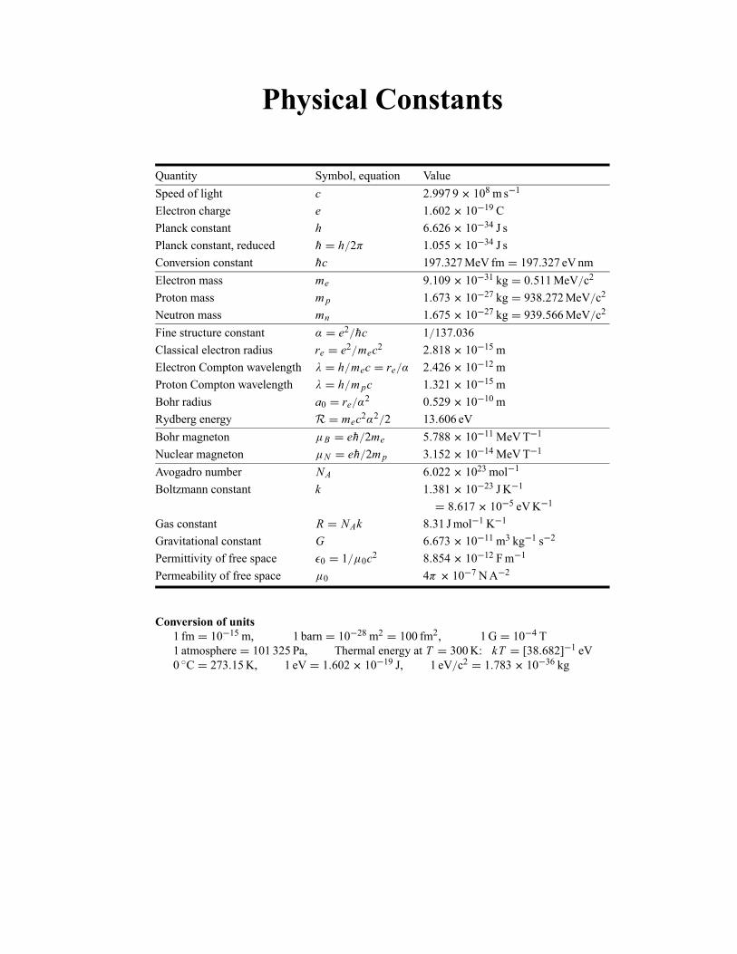
Physical Constants
Quantity Symbol, equation Value
Speed of light c 2 997 9 108ms 1
Electron charge e 1 602 10 19 C
Planck constant h 6 626 10 34 J s
Planck constant, reduced h h 2 1 055 10 34 J s
Conversion constant hc 197 327MeV fm 197 327 eVnm
Electron mass me 9 109 10 31 kg 0 511MeV c2
Proton mass m p 1 673 10 27 kg 938 272MeV c2
Neutron mass mn 1 675 10 27 kg 939 566MeV c2
Fine structure constant e2 hc 1 137 036
Classical electron radius re e2 mec2 2 818 10 15m
Electron Compton wavelength h mec re 2 426 10 12m
Proton Compton wavelength h m pc 1 321 10 15m
Bohr radius a0 re 2 0 529 10 10m
Rydberg energy R mec2 2 2 13 606 eV
Bohr magneton B eh 2me 5 788 10 11MeVT 1
Nuclear magneton N eh 2m p 3 152 10 14MeVT 1
Avogadro number NA 6 022 1023mol 1
Boltzmann constant k 1 381 10 23 J K 1
8 617 10 5 eVK 1
Gas constant R NAk 8 31 Jmol 1K 1
Gravitational constant G 6 673 10 11m3 kg 1 s 2
Permittivity of free space 0 1 0c2 8 854 10 12 Fm 1
Permeability of free space 0 4 10 7NA 2
Conversion of units
1 fm 10 15m, 1 barn 10 28m2 100 fm2, 1 G 10 4 T
1 atmosphere 101 325 Pa, Thermal energy at T 300K: kT [38 682] 1 eV
0 C 273 15K, 1 eV 1 602 10 19 J, 1 eV c2 1 783 10 36 kg
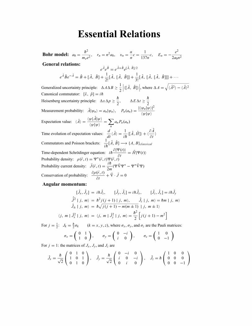
Essential Relations
Bohr model: a0h2
mee2rn n2a0 n
nc
1
137nc En
e2
2a0n2
General relations:eAeB eA Be[A B] 2
eABe A B [A B]1
2![A [A B]]
1
3![A [A [A B]]]
Generalized uncertainty principle: A B1
2[A B] , where A A2 A 2
Canonical commutator: [x p] ih
Heisenberg uncertainty principle: x ph
2E t
h
2
Measurement probability: A n an n Pn ann
2
Expectation value: AA
n
anPn an
Time evolution of expectation values:d
dtA
1
ih[A H ]
A
t
Commutators and Poisson brackets:1
ih[A B] A B classical
Time-dependent Schrödinger equation: iht
tH t
Probability density: r t r t r t
Probability current density: J r tih
2m
Conservation of probability:r t
tJ 0
Angular momentum:
[Jx Jy] ih Jz [Jy Jz] ih Jx [Jz Jx ] ih Jy
J 2 j m h2 j j 1 j m Jz j m hm j m
J j m h j j 1 m m 1 j m 1
j m J 2x j m j m J 2y j mh2
2j j 1 m2
For j 12: Jk
h2 k k x y z , where x , y , and z are the Pauli matrices:
x0 1
1 0 y0 ii 0 z
1 0
0 1
For j 1: the matrices of Jx , Jy , and Jz are
Jxh
2
0 1 0
1 0 1
0 1 0
Jyh
2
0 i 0
i 0 i0 i 0
Jz h1 0 0
0 0 0
0 0 1
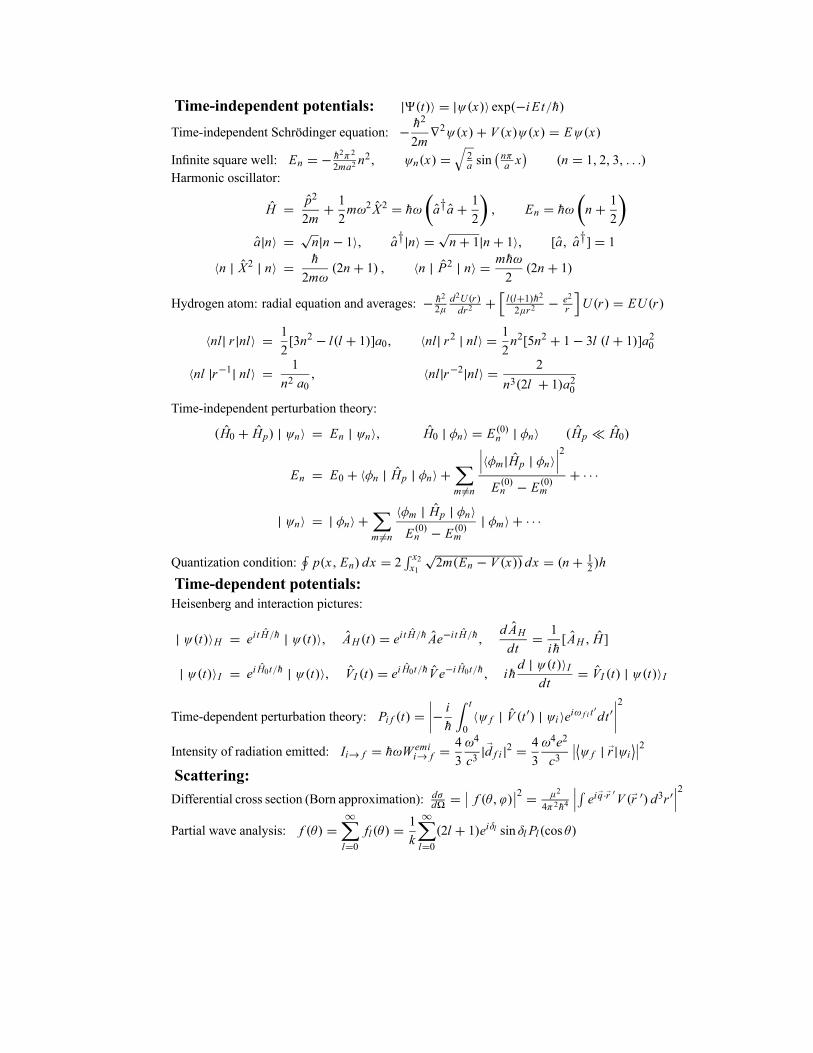
Time-independent potentials: t x exp i Et h
Time-independent Schrödinger equation:h2
2m2 x V x x E x
Infinite square well: Enh2 2
2ma2n2 n x
2a sin
na x n 1 2 3
Harmonic oscillator:
Hp2
2m
1
2m 2X2 h a†a
1
2En h n
1
2
a n n n 1 a† n n 1 n 1 [a a†] 1
n X2 nh
2m2n 1 n P2 n
mh
22n 1
Hydrogen atom: radial equation and averages: h2
2d2U rdr2
l l 1 h2
2 r2e2
r U r EU r
nl r nl1
2[3n2 l l 1 ]a0 nl r2 nl
1
2n2[5n2 1 3l l 1 ]a20
nl r 1 nl1
n2 a0nl r 2 nl
2
n3 2l 1 a20
Time-independent perturbation theory:
H0 Hp n En n H0 n E 0n n Hp H0
En E0 n Hp nm n
m Hp n
2
E 0n E 0
m
n nm n
m Hp n
E 0n E 0
mm
Quantization condition: p x En dx 2x2x1
2m En V x dx n 12h
Time-dependent potentials:
Heisenberg and interaction pictures:
t H ei t H h t AH t ei t H hAe i t H h d AHdt
1
ih[AH H ]
t I ei H0t h t VI t ei H0t hVe i H0t h ihd t I
dtVI t t I
Time-dependent perturbation theory: Pi f ti
h
t
0f V t i e
i f i t dt2
Intensity of radiation emitted: Ii f h W emii f
4
3
4
c3d f i
2 4
3
4e2
c3f r i
2
Scattering:
Differential cross section (Born approximation): dd f2 2
4 2h4eiq r V r d3r
2
Partial wave analysis: fl 0
fl1
kl 0
2l 1 ei l sin l Pl cos


![[Griffiths D.J.] Introduction to quantum mechanics(BookZZ.org)](https://img.dokumen.tips/doc/110x75/6353b1081dfa94ebec0f1318/griffiths-dj-introduction-to-quantum-mechanicsbookzzorg.jpg)


