Quantum Mechanics in Phase Space

May 2012, Volume 1 No 1 37

ARTICLES

Quantum Mechanics in Phase SpaceThomas L. CurtrightDepartment of Physics, University of MiamiCoral Gables, FL 33124-8046, USA

Cosmas K. ZachosHigh Energy Physics Division, Argonne National LaboratoryArgonne, IL 60439-4815, USA

1

Quantum Mech–anics in Ph–ase SpaceThomas L. CurtrightDepartment of Physics, University of Miami

Coral Gables, FL 33124-8046, USA

Cosmas K. ZachosHigh Energy Physics Division, Argonne National Laboratory

Argonne, IL 60439-4815, USA

DOI: 10.1142/S2251159812500030

Abstract: Ever since Werner Heisenberg’s 1927 paper on uncer-

tainty, there has been considerable hesitancy in simultaneously

considering positions and momenta in quantum contexts, since

these are incompatible observables. But this persistent discomfort

with addressing positions and momenta jointly in the quantum

world is not really warranted, as was first fully appreciated by

Hilbrand Groenewold and Jose Moyal in the 1940s. While the

formalism for quantum mechanics in phase space was wholly cast

at that time, it was not completely understood nor widely known

— much less generally accepted — until the late 20th century.

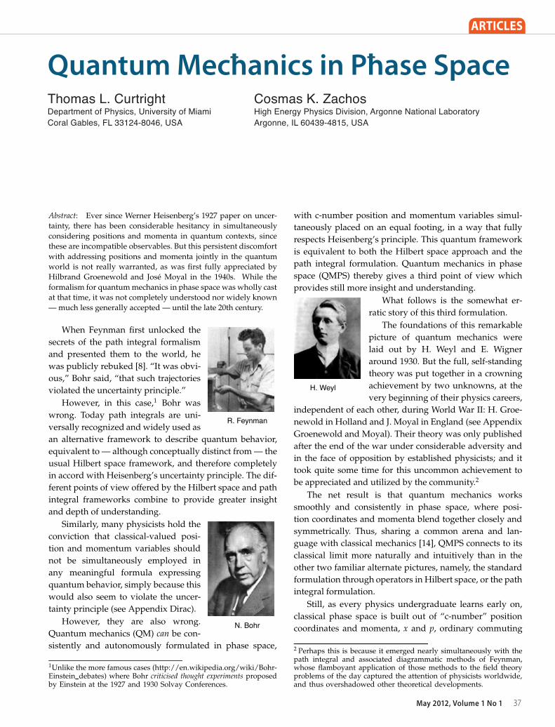
R. Feynman

When Feynman first unlocked the

secrets of the path integral formalism

and presented them to the world, he

was publicly rebuked [8]. “It was obvi-

ous,” Bohr said, “that such trajectories

violated the uncertainty principle.”

However, in this case,1 Bohr was

wrong. Today path integrals are uni-

versally recognized and widely used as

an alternative framework to describe quantum behavior,

equivalent to — although conceptually distinct from — the

usual Hilbert space framework, and therefore completely

in accord with Heisenberg’s uncertainty principle. The dif-

ferent points of view offered by the Hilbert space and path

integral frameworks combine to provide greater insight

and depth of understanding.

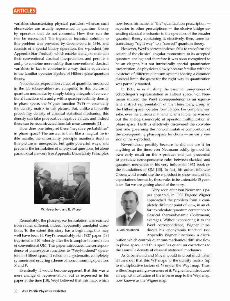
N. Bohr

Similarly, many physicists hold the

conviction that classical-valued posi-

tion and momentum variables should

not be simultaneously employed in

any meaningful formula expressing

quantum behavior, simply because this

would also seem to violate the uncer-

tainty principle (see Appendix Dirac).

However, they are also wrong.

Quantum mechanics (QM) can be con-

sistently and autonomously formulated in phase space,

1Unlike the more famous cases (http://en.wikipedia.org/wiki/Bohr-Einstein debates) where Bohr criticised thought experiments proposedby Einstein at the 1927 and 1930 Solvay Conferences.

with c-number position and momentum variables simul-

taneously placed on an equal footing, in a way that fully

respects Heisenberg’s principle. This quantum framework

is equivalent to both the Hilbert space approach and the

path integral formulation. Quantum mechanics in phase

space (QMPS) thereby gives a third point of view which

provides still more insight and understanding.

H. Weyl

What follows is the somewhat er-

ratic story of this third formulation.

The foundations of this remarkable

picture of quantum mechanics were

laid out by H. Weyl and E. Wigner

around 1930. But the full, self-standing

theory was put together in a crowning

achievement by two unknowns, at the

very beginning of their physics careers,

independent of each other, during World War II: H. Groe-

newold in Holland and J. Moyal in England (see Appendix

Groenewold and Moyal). Their theory was only published

after the end of the war under considerable adversity and

in the face of opposition by established physicists; and it

took quite some time for this uncommon achievement to

be appreciated and utilized by the community.2

The net result is that quantum mechanics works

smoothly and consistently in phase space, where posi-

tion coordinates and momenta blend together closely and

symmetrically. Thus, sharing a common arena and lan-

guage with classical mechanics [14], QMPS connects to its

classical limit more naturally and intuitively than in the

other two familiar alternate pictures, namely, the standard

formulation through operators in Hilbert space, or the path

integral formulation.

Still, as every physics undergraduate learns early on,

classical phase space is built out of “c-number” position

coordinates and momenta, x and p, ordinary commuting

2 Perhaps this is because it emerged nearly simultaneously with thepath integral and associated diagrammatic methods of Feynman,whose flamboyant application of those methods to the field theoryproblems of the day captured the attention of physicists worldwide,and thus overshadowed other theoretical developments.

Asia Pacific Physics Newsletter38

ARTICLES 2

variables characterizing physical particles; whereas such

observables are usually represented in quantum theory

by operators that do not commute. How then can the

two be reconciled? The ingenious technical solution to

this problem was provided by Groenewold in 1946, and

consists of a special binary operation, the ⋆-product (see

Appendix Star Product), which enables x and p to maintain

their conventional classical interpretation, and permits x

and p to combine more subtly than conventional classical

variables; in fact to combine in a way that is equivalent

to the familiar operator algebra of Hilbert space quantum

theory.

Nonetheless, expectation values of quantities measured

in the lab (observables) are computed in this picture of

quantum mechanics by simply taking integrals of conven-

tional functions of x and p with a quasi-probability density

in phase space, the Wigner function (WF) — essentially

the density matrix in this picture. But, unlike a Liouville

probability density of classical statistical mechanics, this

density can take provocative negative values, and indeed

these can be reconstructed from lab measurements [11].

How does one interpret these “negative probabilities”

in phase space? The answer is that, like a magical invis-

ible mantle, the uncertainty principle manifests itself in

this picture in unexpected but quite powerful ways, and

prevents the formulation of unphysical questions, let alone

paradoxical answers (see Appendix Uncertainty Principle).

W. Heisenberg and E. Wigner

Remarkably, the phase-space formulation was reached

from rather different, indeed, apparently unrelated direc-

tions. To the extent this story has a beginning, this may

well have been H. Weyl’s remarkably rich 1927 paper [18]

(reprinted in [20]) shortly after the triumphant formulation

of conventional QM. This paper introduced the correspon-

dence of phase-space functions to “Weyl-ordered” opera-

tors in Hilbert space. It relied on a systematic, completely

symmetrized ordering scheme of noncommuting operators

X and P.

Eventually it would become apparent that this was a

mere change of representation. But as expressed in his

paper at the time [18], Weyl believed that this map, which

now bears his name, is “the” quantization prescription —

superior to other prescriptions — the elusive bridge ex-

tending classical mechanics to the operators of the broader

quantum theory containing it; effectively, then, some ex-

traordinary “right way” to a “correct” quantum theory.

However, Weyl’s correspondence fails to transform the

square of the classical angular momentum to its accepted

quantum analog; and therefore it was soon recognized to

be an elegant, but not intrinsically special quantization

prescription. As physicists slowly became familiar with the

existence of different quantum systems sharing a common

classical limit, the quest for the right way to quantization

was partially mooted.

In 1931, in establishing the essential uniqueness of

Schrodinger’s representation in Hilbert space, von Neu-

mann utilized the Weyl correspondence as an equiva-

lent abstract representation of the Heisenberg group in

the Hilbert space operator formulation. For completeness’

sake, ever the curious mathematician’s foible, he worked

out the analog (isomorph) of operator multiplication in

phase space. He thus effectively discovered the convolu-

tion rule governing the noncommutative composition of

the corresponding phase-space functions — an early ver-

sion of the ⋆-product.

Nevertheless, possibly because he did not use it for

anything at the time, von Neumann oddly ignored his

own early result on the ⋆-product and just proceeded

to postulate correspondence rules between classical and

quantum mechanics in his very influential 1932 book on

the foundations of QM [13]. In fact, his ardent follower,

Groenewold would use the ⋆-product to show some of the

expectations formed by these rules to be untenable 15 years

later. But we are getting ahead of the story.

J. von Neumann

Very soon after von Neumann’s pa-

per appeared, in 1932 Eugene Wigner

approached the problem from a com-

pletely different point of view, in an ef-

fort to calculate quantum corrections to

classical thermodynamic (Boltzmann)

averages. Without connecting it to the

Weyl correspondence, Wigner intro-

duced his eponymous function (see

Appendix Wigner Functions), a distri-

bution which controls quantum-mechanical diffusive flow

in phase space, and thus specifies quantum corrections to

the Liouville density of classical statistical mechanics.

As Groenewold and Moyal would find out much later,

it turns out that this WF maps to the density matrix (up

to multiplicative factors of �) under the Weyl map. Thus,

without expressing awareness of it, Wigner had introduced

an explicit illustration of the inverse map to the Weyl map,

now known as the Wigner map.


ARTICLES3

Wigner also noticed the WF would assume negative

values, which complicated its conventional interpretation

as a probability density function. However, perhaps unlike

his sister’s husband, in time Wigner grew to appreciate that

the negative values of his function were an asset, and not

a liability, in ensuring the orthogonality properties of the

formulation’s building blocks, the “stargenfunctions” (see

Appendix Simple Harmonic Oscillator).

Wigner further worked out the dynamical evolution

law of the WF, which exhibited the nonlocal convolu-

tion features of ⋆-product operations, and violations of

Liouville’s theorem. But, perhaps motivated by practical

considerations, he did not pursue the formal and physical

implications of such operations, at least not at the time.

Those and other decisive steps in the formulation were

taken by two young novices independently during World

War II.

In 1946, based on his wartime PhD thesis work, much

of it carried out in hiding, Hip Groenewold published a

decisive paper, in which he explored the consistency of

the classical-quantum correspondences envisioned by von

Neumann. His tool was a fully mastered formulation of

the Weyl correspondence as an invertible transform, rather

than as a consistent quantization rule. The crux of this

isomorphism is the celebrated ⋆-product in its modern

form.

Use of this product helped Groenewold demonstrate

how Poisson brackets contrast crucially to quantum com-

mutators (“Groenewold’s Theorem”). In effect, the Wigner

map of quantum commutators is a generalization of Pois-

son brackets, today called Moyal brackets (perhaps un-

fairly, given that Groenewold’s work appeared first), which

contains Poisson brackets as their classical limit (techni-

cally, a Wigner-Inonu Lie-algebra contraction). By way

of illustration, Groenewold further worked out the har-

monic oscillator WFs. Remarkably, the basic polynomials

involved turned out to be those of Laguerre, and not the

Hermite polynomials utilized in the standard Schrodinger

formulation! Groenewold had crossed over to a different

continent.

At the very same time, in England, Joe Moyal was

developing effectively the same theory from a yet different

point of view, landing at virtually the opposite coast of

the same continent. He argued with Dirac on its validity

(see Appendix Dirac) and only succeeded in publishing

it, much delayed, in 1949. With his strong statistics back-

ground, Moyal focused on all expectation values of quan-

tum operator monomials, XnPm, symmetrized by Weyl or-

dering, expectations which are themselves the numerically

valued (c-number) building blocks of every quantum ob-

servable measurement.

Moyal saw that these expectation values could be gen-

erated out of a classical-valued characteristic function in

phase space, which he only much later identified with the

Fourier transform of the very function introduced previ-

ously by Wigner. He then appreciated that many familiar

operations of standard quantum mechanics could be ap-

parently bypassed. He reassured himself the uncertainty

principle was incorporated in the structure of this charac-

teristic function, and that it indeed constrained expectation

values of “incompatible observables”. He interpreted sub-

tleties in the diffusion of the probability fluid and the “neg-

ative probability” aspects of it, appreciating that negative

probability is a microscopic phenomenon.

Today, students of QMPS routinely demonstrate as

an exercise that, in 2n-dimensional phase space, domains

where the WF is solidly negative cannot be significantly

larger than the minimum uncertainty volume, (�/2)n, and

are thus not amenable to direct observation — only indirect

inference [11].

Less systematically than Groenewold, Moyal also recast

the quantum time evolution of the WF through a deforma-

tion of the Poisson bracket into the Moyal bracket, and thus

opened up the way for a direct study of the semiclassical

limit � → 0 as an asymptotic expansion in powers of �

— “direct” in contrast to the methods of taking the limit

of large occupation numbers, or of computing expecta-

tions of coherent states (see Appendix Classical Limit). The

subsequent applications paper of Moyal with the eminent

statistician Maurice Bartlett also appeared in 1949, almost

simultaneously with Moyal’s fundamental general paper.

There, Moyal and Bartlett calculated propagators and

transition probabilities for oscillators perturbed by time-

dependent potentials, to demonstrate the power of the

phase-space picture.

M. Bartlett

By 1949 the formulation had been

completed, although few took note of

Moyal’s and especially Groenewold’s

work. And in fact, at the end of the

war in 1945, a number of researchers

in Paris, such as J. Yvon and J. Bass,

were also rediscovering the Weyl corre-

spondence and converging towards the

same picture, albeit in smaller, hesitant,

discursive, and considerably less explicit steps (see [20] for

a guide to this and related literature).

Important additional steps were subsequently carried

out by T. Takabayasi (1954), G. Baker (1958, his thesis),

D. Fairlie (1964), and R. Kubo (1964) (again, see [20]).

These researchers provided imaginative applications and

filled-in the logical autonomy of the picture — the op-

tion, in principle, to derive the Hilbert-space picture from

it, and not vice versa. The completeness and orthog-

onality structure of the eigenfunctions in standard QM


ARTICLES 4

is paralleled in a delightful shadow-dance, by QMPS ⋆-

operations (see Appendix Pure States and Star Products,

and Simple Harmonic Oscillator).

D. Fairlie

QMPS can obviously shed light on

subtle quantization problems as the

comparison with classical theories is

more systematic and natural. Since

the variables involved are the same

in both classical and quantum cases,

the connection to the classical limit as

� → 0 is more readily apparent (see

Appendix Classical Limit). But beyond

this and self-evident pedagogical intu-

ition, what is this alternate formulation of QM and its

panoply of satisfying mathematical structures good for?

It is the natural language to describe quantum trans-

port, and to monitor decoherence of macroscopic quantum

states, in interaction with the environment, a pressing cen-

tral concern of quantum computing [15]. It can also serve

to analyze and quantize physics phenomena unfolding

in a hypothesized noncommutative spacetime with var-

ious noncommutative geometries [17]. Such phenomena

are most naturally described in Groenewold’s and Moyal’s

language.

However, it may be fair to say that, as was true for the

path integral formulation during the first few decades of its

existence, the best QMPS “killer apps” are yet to come.

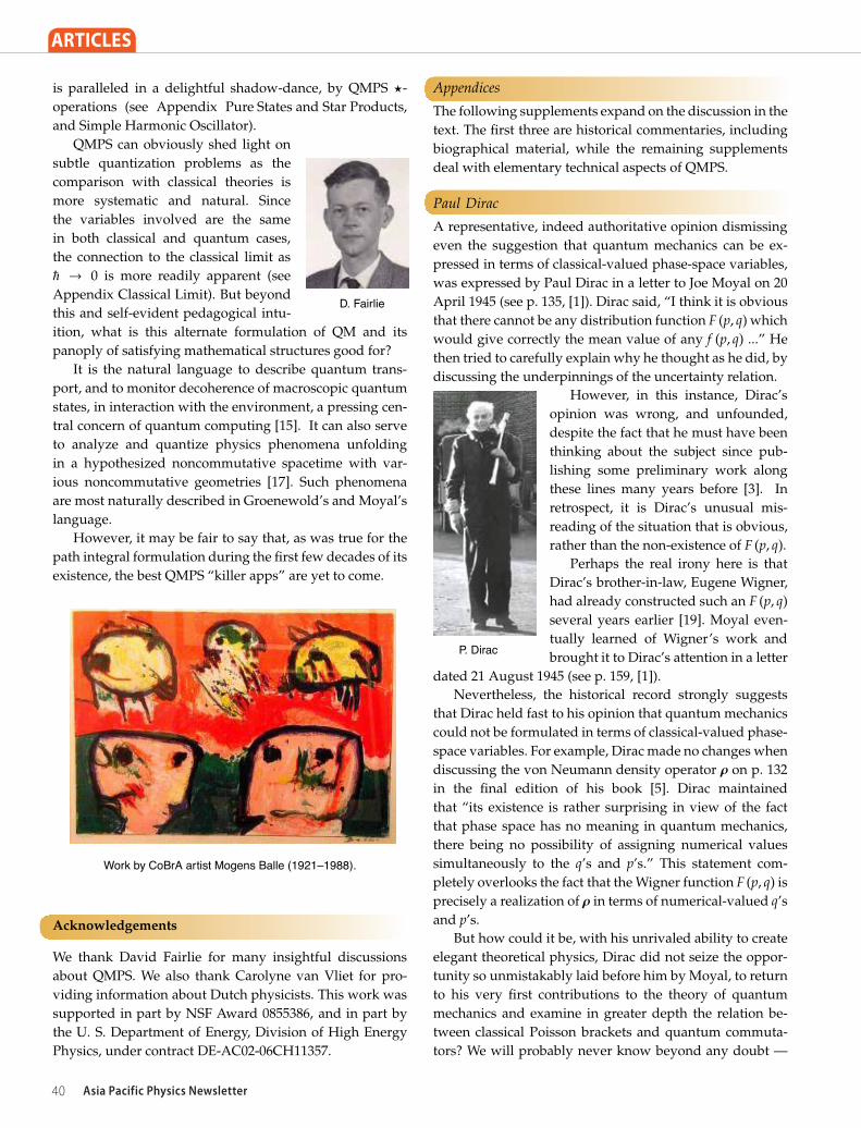
Work by CoBrA artist Mogens Balle (1921–1988).

Acknowledgements

We thank David Fairlie for many insightful discussions

about QMPS. We also thank Carolyne van Vliet for pro-

viding information about Dutch physicists. This work was

supported in part by NSF Award 0855386, and in part by

the U. S. Department of Energy, Division of High Energy

Physics, under contract DE-AC02-06CH11357.

Appendices

The following supplements expand on the discussion in the

text. The first three are historical commentaries, including

biographical material, while the remaining supplements

deal with elementary technical aspects of QMPS.

Paul Dirac

A representative, indeed authoritative opinion dismissing

even the suggestion that quantum mechanics can be ex-

pressed in terms of classical-valued phase-space variables,

was expressed by Paul Dirac in a letter to Joe Moyal on 20

April 1945 (see p. 135, [1]). Dirac said, “I think it is obvious

that there cannot be any distribution function F(

p, q)

which

would give correctly the mean value of any f(

p, q)

...” He

then tried to carefully explain why he thought as he did, by

discussing the underpinnings of the uncertainty relation.

P. Dirac

However, in this instance, Dirac’s

opinion was wrong, and unfounded,

despite the fact that he must have been

thinking about the subject since pub-

lishing some preliminary work along

these lines many years before [3]. In

retrospect, it is Dirac’s unusual mis-

reading of the situation that is obvious,

rather than the non-existence of F(

p, q)

.

Perhaps the real irony here is that

Dirac’s brother-in-law, Eugene Wigner,

had already constructed such an F(

p, q)

several years earlier [19]. Moyal even-

tually learned of Wigner’s work and

brought it to Dirac’s attention in a letter

dated 21 August 1945 (see p. 159, [1]).

Nevertheless, the historical record strongly suggests

that Dirac held fast to his opinion that quantum mechanics

could not be formulated in terms of classical-valued phase-

space variables. For example, Dirac made no changes when

discussing the von Neumann density operator ρ on p. 132

in the final edition of his book [5]. Dirac maintained

that “its existence is rather surprising in view of the fact

that phase space has no meaning in quantum mechanics,

there being no possibility of assigning numerical values

simultaneously to the q’s and p’s.” This statement com-

pletely overlooks the fact that the Wigner function F(

p, q)

is

precisely a realization of ρ in terms of numerical-valued q’s

and p’s.

But how could it be, with his unrivaled ability to create

elegant theoretical physics, Dirac did not seize the oppor-

tunity so unmistakably laid before him by Moyal, to return

to his very first contributions to the theory of quantum

mechanics and examine in greater depth the relation be-

tween classical Poisson brackets and quantum commuta-

tors? We will probably never know beyond any doubt —


ARTICLES5

yet another sort of uncertainty principle — but we are led

to wonder if it had to do with some key features of Moyal’s

theory at that time. First, in sharp contrast to Dirac’s own

operator methods, in its initial stages QMPS theory was

definitely not a pretty formalism! And, as is well known,

beauty was one of Dirac’s guiding principles in theoretical

physics.

Moreover, the logic of the early formalism was not easy

to penetrate. It is clear from his correspondence with Moyal

that Dirac did not succeed in cutting away the formal

undergrowth to clear a precise conceptual path through the

theory behind QMPS, or at least not one that he was eager

to travel again.3

One of the main reasons the early formalism was not

pleasing to the eye, and nearly impenetrable, may have had

to do with another key aspect of Moyal’s 1945 theory: Two

constructs may have been missing. Again, while we cannot

be absolutely certain, we suspect the star product and the

related bracket were both absent from Moyal’s theory at

that time. So far as we can tell, neither of these constructs

appears in any of the correspondence between Moyal and

Dirac.

In fact, the product itself is not even contained in the

published form of Moyal’s work that appeared four years

later [12], although the antisymmetrized version of the

product — the so-called Moyal bracket — is articulated in

that work as a generalization of the Poisson bracket,4 after

first being used by Moyal to express the time evolution

of F(

p, q; t)

.5 Even so, we are not aware of any historical

evidence that Moyal specifically brought his bracket to

Dirac’s attention.

Thus, we can hardly avoid speculating, had Moyal

communicated only the contents of his single paragraph

about the generalized bracket6 to Dirac, the latter would

have recognized its importance, as well as its beauty, and

the discussion between the two men would have acquired

an altogether different tone. As Dirac wrote to Moyal on 31

October 1945 (see p. 160, [1]), “I think your kind of work

would be valuable only if you can put it in a very neat

form.” The Groenewold product and the Moyal bracket did

just that.6

3 Although Dirac did pursue closely related ideas, at least once [4],in his contribution to Bohr’s festschrift.4 See Eqn (7.10) and the associated comments in the last paragraphof §7, p. 106, [12].5 See Eqn (7.8), [12]. Granted, the equivalent of that equation wasalready available in [19], but Wigner did not make the sweepinggeneralization offered by Moyal’s Eqn (7.10).6 In any case, by then Groenewold had already found the starproduct, as well as the related bracket, by taking Weyl’s and vonNeumann’s ideas to their logical conclusion, and had it all published[9] in the time between Moyal’s and Dirac’s last correspondence andthe appearance of [12, 2], wherein discussions with Groenewold areacknowledged by Moyal.

Hilbrand Johannes Groenewold

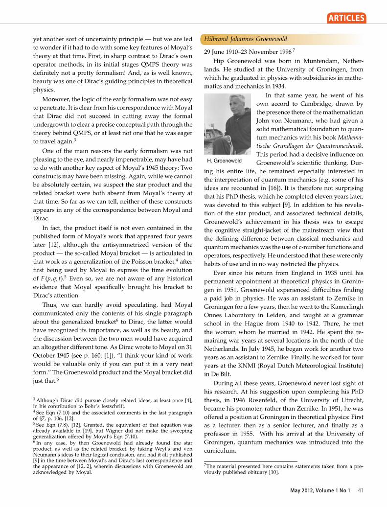
29 June 1910–23 November 1996 7

Hip Groenewold was born in Muntendam, Nether-

lands. He studied at the University of Groningen, from

which he graduated in physics with subsidiaries in mathe-

matics and mechanics in 1934.

H. Groenewold

In that same year, he went of his

own accord to Cambridge, drawn by

the presence there of the mathematician

John von Neumann, who had given a

solid mathematical foundation to quan-

tum mechanics with his book Mathema-

tische Grundlagen der Quantenmechanik.

This period had a decisive influence on

Groenewold’s scientific thinking. Dur-

ing his entire life, he remained especially interested in

the interpretation of quantum mechanics (e.g. some of his

ideas are recounted in [16]). It is therefore not surprising

that his PhD thesis, which he completed eleven years later,

was devoted to this subject [9]. In addition to his revela-

tion of the star product, and associated technical details,

Groenewold’s achievement in his thesis was to escape

the cognitive straight-jacket of the mainstream view that

the defining difference between classical mechanics and

quantum mechanics was the use of c-number functions and

operators, respectively. He understood that these were only

habits of use and in no way restricted the physics.

Ever since his return from England in 1935 until his

permanent appointment at theoretical physics in Gronin-

gen in 1951, Groenewold experienced difficulties finding

a paid job in physics. He was an assistant to Zernike in

Groningen for a few years, then he went to the Kamerlingh

Onnes Laboratory in Leiden, and taught at a grammar

school in the Hague from 1940 to 1942. There, he met

the woman whom he married in 1942. He spent the re-

maining war years at several locations in the north of the

Netherlands. In July 1945, he began work for another two

years as an assistant to Zernike. Finally, he worked for four

years at the KNMI (Royal Dutch Meteorological Institute)

in De Bilt.

During all these years, Groenewold never lost sight of

his research. At his suggestion upon completing his PhD

thesis, in 1946 Rosenfeld, of the University of Utrecht,

became his promoter, rather than Zernike. In 1951, he was

offered a position at Groningen in theoretical physics: First

as a lecturer, then as a senior lecturer, and finally as a

professor in 1955. With his arrival at the University of

Groningen, quantum mechanics was introduced into the

curriculum.

7The material presented here contains statements taken from a pre-viously published obituary [10].


ARTICLES 6

In 1971 Groenewold decided to resign as a professor in

theoretical physics in order to accept a position in the Cen-

tral Interfaculty for teaching Science and Society. However,

he remained affiliated with the theoretical institute as an

extraordinary professor. In 1975 he retired.

In his younger years, Hip was a passionate pup-

pet player, having brought happiness to many children’s

hearts with beautiful puppets he made himself. Later, he

was especially interested in painting. He personally knew

several painters, and owned many of their works. He was

a great lover of the after-war CoBrA art. This love gave him

much comfort during his last years.

Jose Enrique Moyal

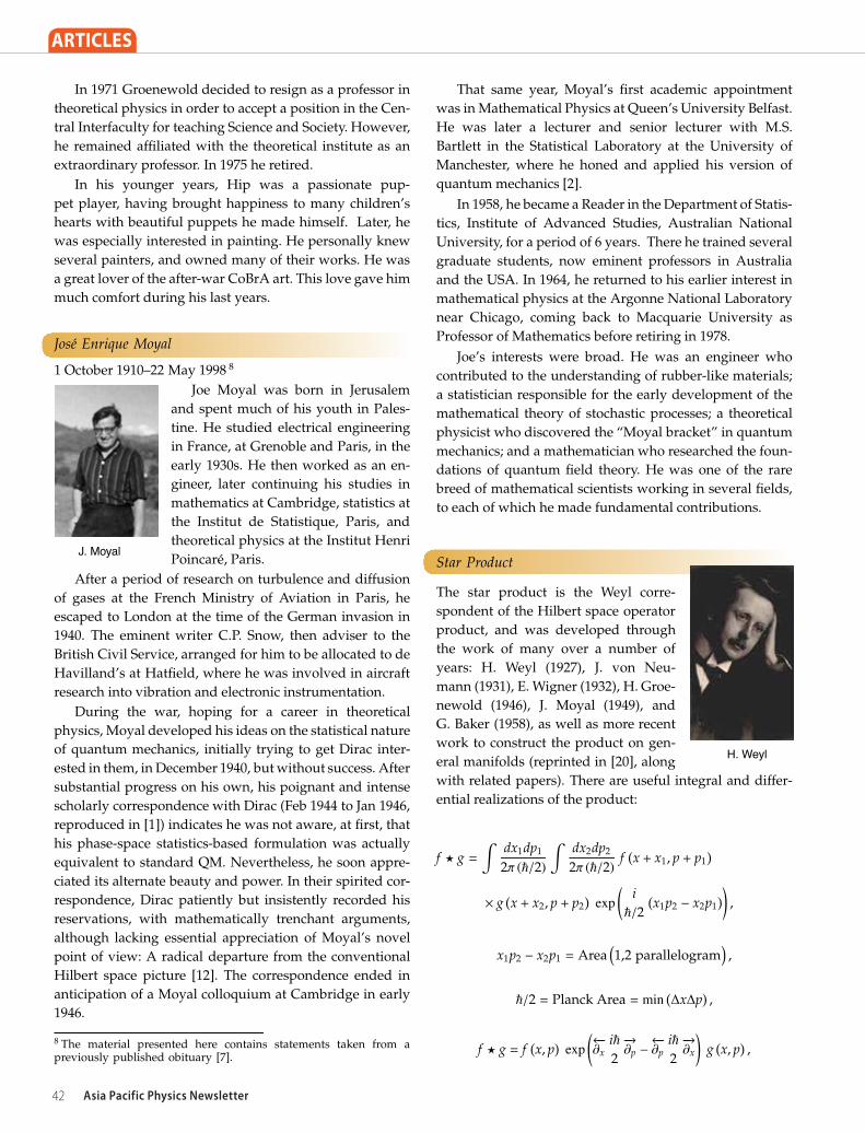
1 October 1910–22 May 1998 8

J. Moyal

Joe Moyal was born in Jerusalem

and spent much of his youth in Pales-

tine. He studied electrical engineering

in France, at Grenoble and Paris, in the

early 1930s. He then worked as an en-

gineer, later continuing his studies in

mathematics at Cambridge, statistics at

the Institut de Statistique, Paris, and

theoretical physics at the Institut Henri

Poincare, Paris.

After a period of research on turbulence and diffusion

of gases at the French Ministry of Aviation in Paris, he

escaped to London at the time of the German invasion in

1940. The eminent writer C.P. Snow, then adviser to the

British Civil Service, arranged for him to be allocated to de

Havilland’s at Hatfield, where he was involved in aircraft

research into vibration and electronic instrumentation.

During the war, hoping for a career in theoretical

physics, Moyal developed his ideas on the statistical nature

of quantum mechanics, initially trying to get Dirac inter-

ested in them, in December 1940, but without success. After

substantial progress on his own, his poignant and intense

scholarly correspondence with Dirac (Feb 1944 to Jan 1946,

reproduced in [1]) indicates he was not aware, at first, that

his phase-space statistics-based formulation was actually

equivalent to standard QM. Nevertheless, he soon appre-

ciated its alternate beauty and power. In their spirited cor-

respondence, Dirac patiently but insistently recorded his

reservations, with mathematically trenchant arguments,

although lacking essential appreciation of Moyal’s novel

point of view: A radical departure from the conventional

Hilbert space picture [12]. The correspondence ended in

anticipation of a Moyal colloquium at Cambridge in early

1946.

8 The material presented here contains statements taken from apreviously published obituary [7].

That same year, Moyal’s first academic appointment

was in Mathematical Physics at Queen’s University Belfast.

He was later a lecturer and senior lecturer with M.S.

Bartlett in the Statistical Laboratory at the University of

Manchester, where he honed and applied his version of

quantum mechanics [2].

In 1958, he became a Reader in the Department of Statis-

tics, Institute of Advanced Studies, Australian National

University, for a period of 6 years. There he trained several

graduate students, now eminent professors in Australia

and the USA. In 1964, he returned to his earlier interest in

mathematical physics at the Argonne National Laboratory

near Chicago, coming back to Macquarie University as

Professor of Mathematics before retiring in 1978.

Joe’s interests were broad. He was an engineer who

contributed to the understanding of rubber-like materials;

a statistician responsible for the early development of the

mathematical theory of stochastic processes; a theoretical

physicist who discovered the “Moyal bracket” in quantum

mechanics; and a mathematician who researched the foun-

dations of quantum field theory. He was one of the rare

breed of mathematical scientists working in several fields,

to each of which he made fundamental contributions.

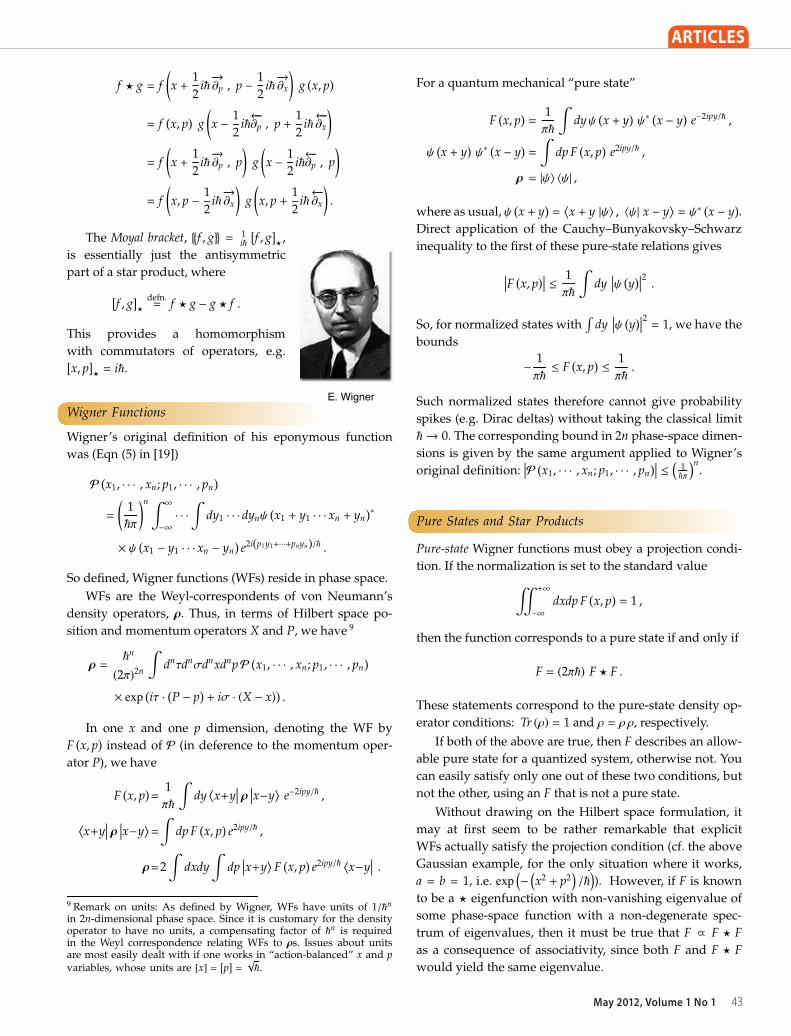
H. Weyl

Star Product

The star product is the Weyl corre-

spondent of the Hilbert space operator

product, and was developed through

the work of many over a number of

years: H. Weyl (1927), J. von Neu-

mann (1931), E. Wigner (1932), H. Groe-

newold (1946), J. Moyal (1949), and

G. Baker (1958), as well as more recent

work to construct the product on gen-

eral manifolds (reprinted in [20], along

with related papers). There are useful integral and differ-

ential realizations of the product:

f ⋆ g =

∫

dx1dp1

2π (�/2)

∫

dx2dp2

2π (�/2)f(

x + x1, p + p1)

× g(

x + x2, p + p2)

exp(

i

�/2

(

x1p2 − x2p1)

)

,

x1p2 − x2p1 = Area(

1,2 parallelogram)

,

�/2 = Planck Area = min(

∆x∆p)

,

f ⋆ g = f(

x, p)

exp(

←−∂x

i�

2

−→∂p −

←−∂p

i�

2

−→∂x

)

g(

x, p)

,


ARTICLES7

f ⋆ g = f

(

x +1

2i�−→∂p , p −

1

2i�−→∂x

)

g(

x, p)

= f(

x, p)

g

(

x − 1

2i�←−∂p , p +

1

2i�←−∂x

)

= f

(

x +1

2i�−→∂p , p

)

g

(

x −1

2i�←−∂p , p

)

= f

(

x, p −1

2i�−→∂x

)

g

(

x, p +1

2i�←−∂x

)

.

E. Wigner

The Moyal bracket,{{

f , g}}

=1i�

[

f , g]

⋆,

is essentially just the antisymmetric

part of a star product, where

[

f , g]

⋆

defn.= f ⋆ g − g ⋆ f .

This provides a homomorphism

with commutators of operators, e.g.[

x, p]

⋆ = i�.

Wigner Functions

Wigner’s original definition of his eponymous function

was (Eqn (5) in [19])

P(

x1, · · · , xn; p1, · · · , pn)

=

(

1

�π

)n ∫ ∞

−∞· · ·∫

dy1 · · · dynψ(

x1 + y1 · · · xn + yn)∗

× ψ(

x1 − y1 · · · xn − yn)

e2i(p1y1+···+pnyn)/� .

So defined, Wigner functions (WFs) reside in phase space.

WFs are the Weyl-correspondents of von Neumann’s

density operators, ρ. Thus, in terms of Hilbert space po-

sition and momentum operators X and P, we have 9

ρ =�

n

(2π)2n

∫

dnτdnσdnxdnpP(

x1, · · · , xn; p1, · · · , pn)

× exp(

iτ ·(

P − p)

+ iσ · (X − x))

.

In one x and one p dimension, denoting the WF by

F(

x, p)

instead of P (in deference to the momentum oper-

ator P), we have

F(

x, p)

=1

π�

∫

dy⟨

x+y∣

∣

∣ ρ

∣

∣

∣x−y⟩

e−2ipy/� ,

⟨

x+y∣

∣

∣ ρ

∣

∣

∣x−y⟩

=

∫

dp F(

x, p)

e2ipy/� ,

ρ=2

∫

dxdy

∫

dp∣

∣

∣x+y⟩

F(

x, p)

e2ipy/� ⟨x−y∣

∣

∣ .

9 Remark on units: As defined by Wigner, WFs have units of 1/�n

in 2n-dimensional phase space. Since it is customary for the densityoperator to have no units, a compensating factor of �n is requiredin the Weyl correspondence relating WFs to ρs. Issues about unitsare most easily dealt with if one works in “action-balanced” x and pvariables, whose units are [x] =

[

p]

=√�.

For a quantum mechanical “pure state”

F(

x, p)

=1

π�

∫

dyψ(

x + y)

ψ∗(

x − y)

e−2ipy/� ,

ψ(

x + y)

ψ∗(

x − y)

=

∫

dp F(

x, p)

e2ipy/� ,

ρ = |ψ� �ψ| ,

where as usual, ψ(

x + y)

=⟨

x + y |ψ� , �ψ| x − y⟩

= ψ∗(

x − y)

.

Direct application of the Cauchy–Bunyakovsky–Schwarz

inequality to the first of these pure-state relations gives

∣

∣

∣F(

x, p)

∣

∣

∣ ≤1

π�

∫

dy∣

∣

∣ψ(

y)

∣

∣

∣

2.

So, for normalized states with∫

dy∣

∣

∣ψ(

y)

∣

∣

∣

2= 1, we have the

bounds

−1

π�≤ F(

x, p)

≤1

π�.

Such normalized states therefore cannot give probability

spikes (e.g. Dirac deltas) without taking the classical limit

�→ 0. The corresponding bound in 2n phase-space dimen-

sions is given by the same argument applied to Wigner’s

original definition:∣

∣

∣P(

x1, · · · , xn; p1, · · · , pn)

∣

∣

∣ ≤(

1�π

)n.

Pure States and Star Products

Pure-state Wigner functions must obey a projection condi-

tion. If the normalization is set to the standard value

�+∞

−∞dxdp F

(

x, p)

= 1 ,

then the function corresponds to a pure state if and only if

F = (2π�) F ⋆ F .

These statements correspond to the pure-state density op-

erator conditions: Tr (ρ) = 1 and ρ = ρ ρ, respectively.

If both of the above are true, then F describes an allow-

able pure state for a quantized system, otherwise not. You

can easily satisfy only one out of these two conditions, but

not the other, using an F that is not a pure state.

Without drawing on the Hilbert space formulation, it

may at first seem to be rather remarkable that explicit

WFs actually satisfy the projection condition (cf. the above

Gaussian example, for the only situation where it works,

a = b = 1, i.e. exp(

−(

x2+ p2)

/�)

). However, if F is known

to be a ⋆ eigenfunction with non-vanishing eigenvalue of

some phase-space function with a non-degenerate spec-

trum of eigenvalues, then it must be true that F ∝ F ⋆ F

as a consequence of associativity, since both F and F ⋆ F

would yield the same eigenvalue.


ARTICLES 8

−0.1

0.0

0.1

0.2

F(x,p)

0.3

−2

0.4

p0 −2

x0

22

n = 0

−0.3

−0.2

−0.1

0.0

F(x,p)

0.1

−2

0.2

p0 −2

x0

22

n = 1

Exercises

Some simple exercises for students to sharpen their QMPS

skills. Show the following.

Exercise 1 Non-commutativity.

eax+bp ⋆ eAx+Bp= e(a+A)x+(b+B)p e(aB−bA)i�/2

�

eAx+Bp ⋆ eax+bp= e(a+A)x+(b+B)p e(Ab−Ba)i�/2

Exercise 2 Associativity.�

eax+bp ⋆ eAx+Bp�

⋆ eαx+βp

= e(a+A+α)x+(b+B+β)p e(aB−bA+aβ−bα+Aβ−Bα)i�/2

= eax+bp ⋆�

eAx+Bp ⋆ eαx+βp�

Exercise 3 Trace properties. (a.k.a. “Lone Star Lemma”)�

dxdp f ⋆ g =

�

dxdp f g =

�

dxdp g f =

�

dxdp g ⋆ f

Exercise 4 Gaussians. For a, b ≥ 0,

exp�

−a

�

�

x2+ p2�

�

⋆ exp�

−b

�

�

x2+ p2�

�

=1

1 + abexp�

−a + b�

1 + ab�

�

�

x2+ p2�

�

.

−0.2

−0.1

0.0

0.1F(x,p)

0.2

−2

0.3

p0 −2

x0

22

n = 2

−0.3

−0.2

−0.1

0.0

0.1

F(x,p)

0.2

−2

p0 −2

x0

22

n = 3

Additional exercises may be culled from the first

chapter of [20].

The Simple Harmonic Oscillator

There is no need to deal with wave functions or Hilbert

space states. The WFs may be constructed directly on the

phase space [9, 2]. Energy eigenstates are obtained as (real)

solutions of the ⋆-genvalue equations [6, 20]:

H ⋆ F = E F = F ⋆H .

To illustrate this, consider the simple harmonic oscillator

(SHO) with (m = 1, ω = 1)

H =1

2

�

p2+ x2�

.

The above equations are now second-order partial differ-

ential equations,

H ⋆ F =1

2

�

p −1

2i� ∂x

�2

+

�

x +1

2i� ∂p

�2

F = EF ,

F ⋆H =1

2

�

p +1

2i� ∂x

�2

+

�

x − 1

2i� ∂p

�2

F = EF .

But if we subtract (or take the imaginary part),

�

p∂x − x∂p

�

F = 0 ⇒ F�

x, p�

= F�

x2+ p2�

.


ARTICLES9

So H⋆F = EF = F⋆H reduces to a single ordinary differential

equation (Laguerre, not Hermite!), namely, the real part of

either of the previous second-order equations.

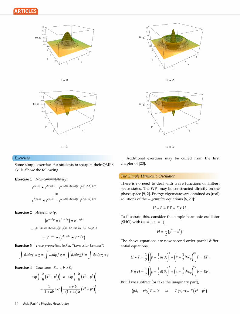
There are integrable solutions if and only if E =

(n + 1/2) �, n = 0, 1, · · · for which

Fn�

x, p�

=(−1)n

π�Ln

�

x2+ p2

�/2

�

e−(x2+p2)/� ,

Ln (z) =1

n!ez dn

dzn

�

zne−z� .

The normalization is chosen to be the standard one�+∞−∞ dxdp Fn

�

x, p�

= 1. Except for the n = 0 ground state

(Gaussian) WF, these F’s change sign on the xp-plane. For

example: L0 (z) = 1, L1 (z) = 1 − z, L2 (z) = 1 − 2z + 12z2, etc.

Using the integral form of the ⋆ product, it is now easy

to check these pure states are ⋆ orthogonal:

(2π�) Fn ⋆ Fk = δnk Fn .

This becomes more transparent by using ⋆

raising/lowering operations to write 10

Fn =1

n!(a∗⋆)n F0 (⋆a)n

=1

π�n!(a∗⋆)n e−(x2

+p2)/� (⋆a)n ,

where a is the usual linear combination a ≡ 1√2�

(x+ ip), and

a∗ is just its complex conjugate a∗ ≡ 1√2�

(x− ip), with a⋆ a∗ −a∗ ⋆ a = 1, and a⋆F0 = 0 = F0 ⋆ a∗ (cf. coherent state density

operators).

The Uncertainty Principle

Expectation values of all phase-space functions, say G�

x, p�

,

for a system described by F�

x, p�

(a real WF, normalized

to 1) are just integrals of ordinary products (cf. Lone Star

Lemma)

�G� =�

dxdp G�

x, p�

F�

x, p�

.

These can be negative, even though G is positive, if the WF

flips sign. So how do we directly establish simple correct

statements such as�

�

x + p�2�

≥ 0 without using marginal

probabilities or invoking Hilbert space results?

The roles of positive-definite Hilbert space operators

are played on phase space by real star-squares:

G�

x, p�

= g∗�

x, p�

⋆ g�

x, p�

.

These always have non-negative expectation values for any

g and any WF,

�g∗ ⋆ g� ≥ 0 ,

10 Note that the earlier exercise giving the star composition law ofGaussians immediately yields the projection property of the SHOground state WF, F0 = (2π�) F0 ⋆ F0.

even if F becomes negative. (Note this is not true if the ⋆

is removed! If g∗ ⋆ g is supplanted by�

�

�g�

�

�

2, then integrated

with a WF, the result could be negative.)

To show this, first suppose the system is in a

pure state. Then use F = (2π�) F ⋆ F (see Appendix

Pure States and Star Products), and the associativity and

trace properties (see Appendix Exercises), to write 11:�

dxdp�

g∗ ⋆ g�

F = (2π�)�

dxdp�

g∗ ⋆ g�

(F ⋆ F)

= (2π�)�

dxdp�

g∗ ⋆ g�

⋆ (F ⋆ F)

= (2π�)�

dxdp�

g∗ ⋆ g ⋆ F�

⋆ F

= (2π�)�

dxdp F ⋆�

g∗ ⋆ g ⋆ F�

= (2π�)�

dxdp�

F ⋆ g∗�

⋆�

g ⋆ F�

= (2π�)�

dxdp�

F ⋆ g∗� �

g ⋆ F�

= (2π�)�

dxdp |g ⋆ F|2

≥ 0 .

In the next to last step we also used the elementary prop-

erty (g ⋆ F)∗ = F ⋆ g∗.

More generally, if the system is in a mixed state, as

defined by a normalized probabilistic sum of pure states,

F =�

j PjFj, with probabilities Pj ≥ 0 satisfying�

j Pj = 1,

then the same inequality holds.

W. Heisenberg

Correlations of observables follow

conventionally from specific choices of

g(x, p). For example, to produce Heisen-

berg’s uncertainty relation, take

g�

x, p�

= a + bx + cp ,

for arbitrary complex coefficients a, b, c.

The resulting positive semi-definite

quadratic form is then

�g∗ ⋆ g� =�

a∗ b∗ c∗�

1 �x� �p��x� �x ⋆ x� �x ⋆ p��p� �p ⋆ x� �p ⋆ p�

ab

c

≥ 0 ,

for any a, b, c. All eigenvalues of the above 3 × 3 hermi-

tian matrix are therefore non-negative, and thus so is its

determinant,

det

1 �x� �p��x� �x ⋆ x� �x ⋆ p��p� �p ⋆ x� �p ⋆ p�

≥ 0 .

11 By essentially the same argument, if F1 and F2 are two distinctpure state WFs, the phase-space overlap integral between the two isalso manifestly non-negative and thus admits interpretation as thetransition probability between the respective states:

�

dxdp F1F2 = (2π�)2

�

dxdp |F1 ⋆ F2 |2 ≥ 0 .


ARTICLES 10

But

x ⋆ x = x2 , p ⋆ p = p2 ,

x ⋆ p = xp + i�/2 , p ⋆ x = xp − i�/2 ,

and with the usual definitions of the variances

(∆x)2 ≡ �(x − �x�)2� , (∆p)2 ≡ �(p − �p�)2� ,

the positivity condition on the above determinant amounts

to

(∆x)2(∆p)2 ≥1

4�

2+(⟨

xp⟩

− �x��p�)2 .

Hence Heisenberg’s relation

(∆x)(

∆p)

≥ �/2 .

The inequality is saturated for a vanishing original inte-

grand g⋆F = 0, for suitable a, b, c, when the⟨

xp⟩

−�x��p� term

vanishes (i.e. x and p statistically independent, as happens

for a Gaussian pure state, F = 1π�

exp(

−(

x2+ p2)

/�)

).

A Classical Limit

The simplest illustration of the classical limit, by far, is

provided by the SHO ground state WF. In the limit �→ 0, a

completely localized phase-space distribution is obtained,

namely, a Dirac delta at the origin of the phase space:

lim�→0

1

π�exp(

−(

x2+ p2)

/�)

= δ (x) δ(

p)

.

Moreover, if the ground state Gaussian is uniformly dis-

placed from the origin by an amount(

x0, p0)

and then

allowed to evolve in time, its peak follows a classical

trajectory (see Movies12 ... this simple behavior does not

hold for less trivial potentials). The classical limit of this

evolving WF is therefore just a Dirac delta whose spike

follows the trajectory of a classical point particle moving

in the harmonic potential:

lim�→0

1

π�exp(

−(

(

x − x0 cos t − p0 sin t)2

+(

p − p0 cos t + x0 sin t)2)

/�)

= δ(

x − x0 cos t − p0 sin t)

δ(

p − p0 cos t + x0 sin t)

.

12http://server.physics.miami.edu/curtright/TimeDependentWignerFunctions.html

References

[1] A. Moyal, Maverick Mathematician, ANU E Press (2006) (onlineat http://epress.anu.edu.au/maverick/mobile devices/).

[2] M. Bartlett and J. Moyal, “The Exact Transition Probabilities ofQuantum-Mechanical Oscillators Calculated by the Phase-SpaceMethod”, Proc. Camb. Phil. Soc. 45, 545–553 (1949).

[3] P. A. M. Dirac, “Note on Exchange Phenomena in the ThomasAtom”, Proc. Camb. Phil. Soc. 26, 376–385 (1930).

[4] P. A. M. Dirac, “On the Analogy Between Classical and Quan-tum Mechanics”, Rev. Mod. Phys. 17, 195–199 (1945).

[5] P. A. M. Dirac, The Principles of Quantum Mechanics, 4th edition,last revised in 1967, (1958).

[6] D. Fairlie, “The Formulation of Quantum Mechanics in Terms ofPhase Space Functions”, Proc. Camb. Phil. Soc. 60 581–586 (1964).Also see T. Curtright, D. Fairlie, and C. Zachos, “Features ofTime Independent Wigner Functions”, Phys. Rev. D 58, 025002(1998).

[7] J. Gani, “Obituary: Jose Enrique Moyal”, J. Appl. Probab. 35,1012–1017 (1998).

[8] J. Gleick, Genius, Pantheon Books, 258 (1992).[9] H. J. Groenewold, “On the Principles of Elementary Quantum

Mechanics”, Physica, 12, 405–460 (1946).[10] N. Hugenholtz, “Hip Groenewold, 29 juni 1910-23 november

1996”, Nederlands Tijdschrift voor Natuurkunde, 2, 31 (1997).[11] D. Leibfried, T. Pfau, and C. Monroe, “Shadows and Mirrors:

Reconstructing Quantum States of Atom Motion”, Physics Today,22–28 (April 1998).

[12] J. E. Moyal, “Quantum Mechanics as a Statistical Theory”, Proc.Camb. Phil. Soc. 45, 99-124 (1949).

[13] J. v. Neumann, Mathematical Foundations of Quantum Mechanics,Princeton University Press, (1955, 1983).

[14] D. Nolte, “The tangled tale of phase space”, Physics Today, 33–38(April 2010).

[15] J. Preskill, “Battling Decoherence: The Fault-Tolerant QuantumComputer”, Physics Today, (June 1999).

[16] S. Saunders, J. Barrett, A. Kent, and D. Wallace, Many Worlds?Oxford University Press, (2010).

[17] R. J. Szabo, “Quantum field theory on noncommutative spaces”,Physics Reports, 378, 207–299 (2003).

[18] H. Weyl, “Quantenmechanik und Gruppentheorie”, Z. Phys. 46,1–33 (1927).

[19] E. Wigner, “Quantum Corrections for Thermodynamic Equilib-rium”, Phys. Rev. 40, 749–759 (1932).

[20] C. Zachos, D. Fairlie, and T. Curtright, Quantum Mechanicsin Phase Space: An Overview with Selected Papers, World Scien-tific, 2005. (A revised and updated first chapter is online athttp://gate.hep.anl.gov/czachos/a.pdf).

10

But

x ⋆ x = x2 , p ⋆ p = p2 ,

x ⋆ p = xp + i�/2 , p ⋆ x = xp − i�/2 ,

and with the usual definitions of the variances

(∆x)2 ≡ �(x − �x�)2� , (∆p)2 ≡ �(p − �p�)2� ,

the positivity condition on the above determinant amounts

to

(∆x)2(∆p)2 ≥1

4�

2+(⟨

xp⟩

− �x��p�)2 .

Hence Heisenberg’s relation

(∆x)(

∆p)

≥ �/2 .

The inequality is saturated for a vanishing original inte-

grand g⋆F = 0, for suitable a, b, c, when the⟨

xp⟩

−�x��p� term

vanishes (i.e. x and p statistically independent, as happens

for a Gaussian pure state, F = 1π�

exp(

−(

x2+ p2)

/�)

).

A Classical Limit

The simplest illustration of the classical limit, by far, is

provided by the SHO ground state WF. In the limit �→ 0, a

completely localized phase-space distribution is obtained,

namely, a Dirac delta at the origin of the phase space:

lim�→0

1

π�exp(

−(

x2+ p2)

/�)

= δ (x) δ(

p)

.

Moreover, if the ground state Gaussian is uniformly dis-

placed from the origin by an amount(

x0, p0)

and then

allowed to evolve in time, its peak follows a classical

trajectory (see Movies12 ... this simple behavior does not

hold for less trivial potentials). The classical limit of this

evolving WF is therefore just a Dirac delta whose spike

follows the trajectory of a classical point particle moving

in the harmonic potential:

lim�→0

1

π�exp(

−(

(

x − x0 cos t − p0 sin t)2

+(

p − p0 cos t + x0 sin t)2)

/�)

= δ(

x − x0 cos t − p0 sin t)

δ(

p − p0 cos t + x0 sin t)

.

12http://server.physics.miami.edu/curtright/TimeDependentWignerFunctions.html

References

[1] A. Moyal, Maverick Mathematician, ANU E Press (2006) (onlineat http://epress.anu.edu.au/maverick/mobile devices/).

[2] M. Bartlett and J. Moyal, “The Exact Transition Probabilities ofQuantum-Mechanical Oscillators Calculated by the Phase-SpaceMethod”, Proc. Camb. Phil. Soc. 45, 545–553 (1949).

[3] P. A. M. Dirac, “Note on Exchange Phenomena in the ThomasAtom”, Proc. Camb. Phil. Soc. 26, 376–385 (1930).

[4] P. A. M. Dirac, “On the Analogy Between Classical and Quan-tum Mechanics”, Rev. Mod. Phys. 17, 195–199 (1945).

[5] P. A. M. Dirac, The Principles of Quantum Mechanics, 4th edition,last revised in 1967, (1958).

[6] D. Fairlie, “The Formulation of Quantum Mechanics in Terms ofPhase Space Functions”, Proc. Camb. Phil. Soc. 60 581–586 (1964).Also see T. Curtright, D. Fairlie, and C. Zachos, “Features ofTime Independent Wigner Functions”, Phys. Rev. D 58, 025002(1998).

[7] J. Gani, “Obituary: Jose Enrique Moyal”, J. Appl. Probab. 35,1012–1017 (1998).

[8] J. Gleick, Genius, Pantheon Books, 258 (1992).[9] H. J. Groenewold, “On the Principles of Elementary Quantum

Mechanics”, Physica, 12, 405–460 (1946).[10] N. Hugenholtz, “Hip Groenewold, 29 juni 1910-23 november

1996”, Nederlands Tijdschrift voor Natuurkunde, 2, 31 (1997).[11] D. Leibfried, T. Pfau, and C. Monroe, “Shadows and Mirrors:

Reconstructing Quantum States of Atom Motion”, Physics Today,22–28 (April 1998).

[12] J. E. Moyal, “Quantum Mechanics as a Statistical Theory”, Proc.Camb. Phil. Soc. 45, 99-124 (1949).

[13] J. v. Neumann, Mathematical Foundations of Quantum Mechanics,Princeton University Press, (1955, 1983).

[14] D. Nolte, “The tangled tale of phase space”, Physics Today, 33–38(April 2010).

[15] J. Preskill, “Battling Decoherence: The Fault-Tolerant QuantumComputer”, Physics Today, (June 1999).

[16] S. Saunders, J. Barrett, A. Kent, and D. Wallace, Many Worlds?Oxford University Press, (2010).

[17] R. J. Szabo, “Quantum field theory on noncommutative spaces”,Physics Reports, 378, 207–299 (2003).

[18] H. Weyl, “Quantenmechanik und Gruppentheorie”, Z. Phys. 46,1–33 (1927).

[19] E. Wigner, “Quantum Corrections for Thermodynamic Equilib-rium”, Phys. Rev. 40, 749–759 (1932).

[20] C. Zachos, D. Fairlie, and T. Curtright, Quantum Mechanicsin Phase Space: An Overview with Selected Papers, World Scien-tific, 2005. (A revised and updated first chapter is online athttp://gate.hep.anl.gov/czachos/a.pdf).

World Scientific Series in 20th Century Physics - Vol. 34

QUANTUM MECHANICS IN PHASE SPACEAn Overview with Selected Papersedited by Cosmas K Zachos (Argonne National Laboratory, USA), David B Fairlie (University of Durham, UK), & Thomas L Curtright (University of Miami, USA)

Wigner's quasi-probability distribution function in phase space is a special (Weyl) representation of the density matrix. In this logically complete and self-standing formulation, one need not choose sides — coordinate or momentum space. It works in full phase space, accom-modating the uncertainty principle, and it offers unique insights into the classical limit of quantum theory. This invaluable book is a collection of the seminal papers on the formulation, with an introductory overview which provides a trail map for those papers; an extensive bibliography; and simple illustrations, suitable for applications to a broad range of physics problems.

560pp Dec 2005978-981-238-384-6 US$180 £119

Documents

Quantum Mechanics in Phase Space