Non-stationary Communication Delays in Failure Detectors

Raul Ceretta Nunes‡†‡ E-mail: ceretta@inf.ufsm.br

Federal University of Santa MariaDepartment of Electronic and Computation

Av. Roraima S/N - Camobi97105-900 - Santa Maria-RS - Brazil

Ingrid Jansch-Porto†† E-mail: ingrid@inf.ufrgs.br

Federal University of Rio Grande do SulInstitute of Computer Science

Caixa Postal 1506491501-970 - Porto Alegre - RS - Brazil

Abstract

The abstraction of failure detectors came as an aid tothe designers and programmers of dependable distributedapplications. However, all implementations of failure detec-tors can make mistakes. In practice, timeout-based failuredetector implementations improve their accuracy by adapt-ing their timeout according to a stationary behavior as-sumption.

This paper analyzes the stationarity behavior of the com-munication delay, observed on a pull-style failure detector,by exploring the time series mathematical model. As a re-sult, this paper shows that the behavior of the time series,instead of stationary, is non-stationary. From this result, wesuggest the use of prediction models based on time series toimprove the accuracy of failure detectors.

1. Introduction

The design and validation of dependable distributed appli-cations over an unreliable asynchronous distributed system,where the communication delays1 are unbounded and faultscan occur, are not trivial tasks [1]. The reason is the im-possibility of distinguishing a slow process/object from acrashed or disconnected one [9]. Consequently, ensuringthe correct state of the distributed application is a challenge.

Despite this problem, the unreliable failure detector ab-straction [5] allows to deterministically specify and provedistributed agreement protocols, like consensus and atomicbroadcast. A failure detector (FD) provides some (unreli-able) information on which processes have crashed. Themost common way to implement this abstraction is makinguse of a maximum waiting time (a timeout).

Although all timeout-based implementations of failuredetectors can make mistakes [5], choosing an accurate time-out is an important task. An inadequate timeout should beavoided because it can decrease the accuracy (increase thenumber of wrong suspicions) and can also decrease the per-formance of the failure detector (time to detect a failure).

Self-tuned failure detectors work adapting (at runtime)their timeouts according to the observed system behavior

1In the context of thios article, communication delay corresponds totime spent on process end-to-end communication.

[12, 11, 6]. However, to the best of our knowledge, with ba-sis on the idea that the observations present a stationary be-havior, the smartest detector, developed by Chen [6], adaptsits timeout according to the sample mean and sample vari-ance of the failure detection observations.

We model the observations of a pull failure detector [8]by using a time series model [3], which is a mathematicalmodel used to describe a sequence of observations of a sto-chastic process taken sequentially in time. In a pull-stylefailure detector, the stochastic process variable is the com-munication delay observed by the failure detector. Moredetails about modeling its observations using time series arebeyond the scope of this paper and are given in [13].

In this paper, we analyze the stationarity behavior of thecommunication delay time series and show that its behav-ior is non-stationary instead of stationary. As consequence,we suggest the use of prediction models based on the timeseries theory to improve the accuracy of self-tuned failuredetectors. This paper is organized as follows: section 2 and3 present the basic concepts of the failure detector abstrac-tion and of the time series theory, respectively; section 4presents the method we have used to build our time series;section 5 details our stationary analysis; and, finally, section6 presents our conclusions.

2. Unreliable Failure Detector

From [5], in a distributed system with Ω processes, a failuredetector is defined as a set of n distributed modules fd1 tofdn, where fdi is attached to process pi ∈ Ω. Each fail-ure detector module fdi maintains a list of processes thatit currently suspects to have crashed. Thus, we say that aprocess pi suspects process pj at some local instant t, if atlocal time t, process pj is in the list of suspected processesmaintained by fdi. A failure detector module makes mis-takes by incorrectly suspecting a process. In our context,the suspicion decision (decision of including a process inthe local suspect list) is based only on a timeout for someevent, i.e., our detector is a timeout-based failure detector.Suspicions are not necessarily stable: after pi has suspectedpj , it can learn that the suspicion was incorrect. Process pj

is then removed by fdi from its list of suspected processes.

A failure detector is specified in terms of two properties:completeness, which specifyes the capability of suspectingevery crashed process; and accuracy, which specifyes thecapability of avoiding the suspition of correct processes.Defining two different levels for the completeness property(strong and weak) and four levels for the accuracy prop-erty (strong, weak, eventually strong and eventually weak),Chandra and Toueg have classified failure detectors into eightclasses (P ,Q,S ,W , ¦P ,¦Q,¦S , ¦W) [5]. Among them,eventually weak (¦W) is the weakest failure detector classthat solves consensus in asynchronous systems with a ma-jority of correct processes [4]. Furthermore, [5] has provedthat the eventually strong class (¦S) can be built from class¦W by using a reduction algorithm that merges all suspectlists of the fd modules.

In practice, none of the Chandra and Toueg failure de-tector classes can be implemented in a pure asynchronoussystem without the possibility of making mistakes. Thus,to ensure application consistency, most of failure detectorimplementations first ensure the completeness property in-stead of the accuracy property. The accuracy property de-pends on the correct choice of the timeout, that is a hardtask. In this context, our approach is to investigate the be-havior of the communication history observed by a failuredetector and efficient model it. From results we will designa consistent timeout value prediction mechanism which canimprove the failure detector accuracy.

2.1. The pull-style failure detector

According to Felber and Guerraoui [8] there are two basicstrategies for implementing timeout-based failure detectors:push (based on ”I’m alive!” messages) and pull (based on”Are you alive?” and ”Yes I am!” messages). In this paperwe explore the pull strategy (or style).

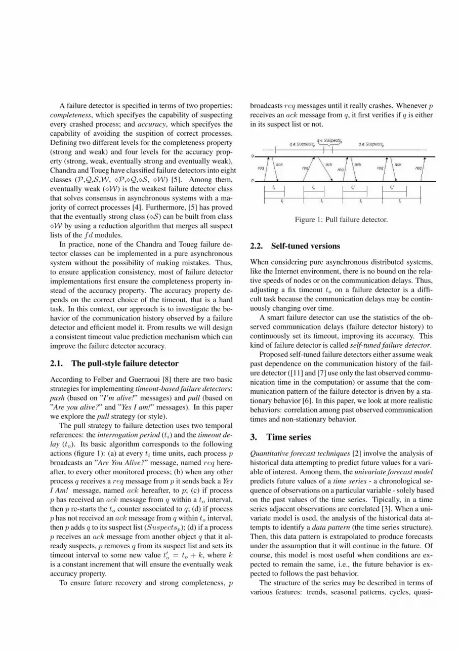
The pull strategy to failure detection uses two temporalreferences: the interrogation period (ti) and the timeout de-lay (to). Its basic algorithm corresponds to the followingactions (figure 1): (a) at every ti time units, each process pbroadcasts an ”Are You Alive?” message, named req here-after, to every other monitored process; (b) when any otherprocess q receives a req message from p it sends back a YesI Am! message, named ack hereafter, to p; (c) if processp has received an ack message from q within a to interval,then p re-starts the to counter associated to q; (d) if processp has not received an ack message from q within to interval,then p adds q to its suspect list (Suspectsp); (d) if a processp receives an ack message from another object q that it al-ready suspects, p removes q from its suspect list and sets itstimeout interval to some new value t′o = to + k, where kis a constant increment that will ensure the eventually weakaccuracy property.

To ensure future recovery and strong completeness, p

broadcasts req messages until it really crashes. Whenever preceives an ack message from q, it first verifies if q is eitherin its suspect list or not.

Figure 1: Pull failure detector.

2.2. Self-tuned versions

When considering pure asynchronous distributed systems,like the Internet environment, there is no bound on the rela-tive speeds of nodes or on the communication delays. Thus,adjusting a fix timeout to on a failure detector is a diffi-cult task because the communication delays may be contin-uously changing over time.

A smart failure detector can use the statistics of the ob-served communication delays (failure detector history) tocontinuously set its timeout, improving its accuracy. Thiskind of failure detector is called self-tuned failure detector.

Proposed self-tuned failure detectors either assume weakpast dependence on the communication history of the fail-ure detector ([11] and [7] use only the last observed commu-nication time in the computation) or assume that the com-munication pattern of the failure detector is driven by a sta-tionary behavior [6]. In this paper, we look at more realisticbehaviors: correlation among past observed communicationtimes and non-stationary behavior.

3. Time series

Quantitative forecast techniques [2] involve the analysis ofhistorical data attempting to predict future values for a vari-able of interest. Among them, the univariate forecast modelpredicts future values of a time series - a chronological se-quence of observations on a particular variable - solely basedon the past values of the time series. Tipically, in a timeseries adjacent observations are correlated [3]. When a uni-variate model is used, the analysis of the historical data at-tempts to identify a data pattern (the time series structure).Then, this data pattern is extrapolated to produce forecastsunder the assumption that it will continue in the future. Ofcourse, this model is most useful when conditions are ex-pected to remain the same, i.e., the future behavior is ex-pected to follows the past behavior.

The structure of the series may be described in terms ofvarious features: trends, seasonal patterns, cycles, quasi-

cycles, and noise. The autoregressive integrated moving-average (ARIMA) models [3] correspond to a widely usedclass to describe the time series structure; these models arein the form of difference equations relating past and presentvalues of the time series [2].

According to Box & Jenkins [3], typically the structureof a stationary time series can be described by: i) an au-toregressive model of order p - AR(p); ii) a moving averagemodel of order q - MA(q); or iii) an autoregressive-movingaverage model of order p and q - ARMA(p,q). Additionally,the behavior of the stationary time series can be usefully de-scribed by its mean, variance and autocorrelation function.When a time series has a non-stationary behavior, it can bedescribed as an autoregressive integrated moving averagemodel of order p, d and q - ARIMA(p,d,q), where d rep-resents the number of differences2 needed to transform thenon-stationary series to stationary.

For a mathematical description of models that representthe time series values zt, zt−1, ..., zn, where zt denote thevalue of a data point at period t, Box & Jenkins define twooperators: the backward shift operator B, defined by Bzt =zt−1, and the backward difference operator ∇, defined by∇zt = zt − zt−1 = (1 − B)zt. From these operators,the AR(p) model has zt = 1

φ(B)at + µ, where at is thenoise at period t, µ is the series mean, and φ(B) is a Bpolynomial with p coefficients. The MA(q) model has zt =θ(B)at, where θ(B) has q coefficients. The ARMA(p, q)model has zt = θ(B)

φ(B)at + µ, where φ(B) and θ(B) has p

and q coefficients, respectively. The (ARIMA(p,q,d)) haszt = θ(B)

φ(B)∇d at + µ.

4. FD observations as a time series

From section 2., we know that at each time interval ti, themonitor of a pull-style failure detector sends a req mes-sage and waits for the corresponding ack on a time smallerthan to, where to < ti. Thus, in a stable period (where noprocess crashes and no timing failures occur), the expectedround-trip-time rtt is less than to and we observe only onertt measure at each interval ti (see figure 2).

Figure 2: A pull failure detector on a stable period.

2From the original time series values zt, zt−1, ..., zn, we produce thefirst difference by taking z1

t = zt − zt−1, where t = 2, ..., n.

Knowing that a time series is a chronological sequenceof observations on a particular variable (section 3.) and thatin a pull-style failure detector the observed variable is thertt, we can make each observed rtt in a stable period cor-respond to one time series sample (see figure 2). Conse-quently, we have a time series rtt1, rtt2, ..., rttn of lengthn built from the previous n round-trip-time observations.

In an unstable period (where crash and timing failuresare allowed), a pull-style failure detector reports us to oneof the four scenarios illustrated on figure 3, where we eitherhave the occurrence of gaps or have multiple measurementsin the same period. As result, the making of a time series inan unstable period needs some kind of fill policy.

In our experiments, we have dealt ignored the gaps andhave handled multiple values using the one which presentsthe highest sequence number (last message sent by the fail-ure detector monitor). More details about modeling thecommunication delays of the failure detectors using timeseries are described in [13].

Figure 3: Possible scenarios on an unstable period.

5. Analysis of the time series stationarity

One of the most important problems in the theory of non-stationary processes (ARIMA processes) is the determina-tion of the order of integration d. In Box & Jenkins’ termi-nology, this order corresponds to the number of differencesneeded to transform the non-stationary series to stationary(see section 3.). However, an exact solution to determinethis order does not exist [10]. On the other hand, there aresome empirical methods that obtain an approximate solu-tion. Our analysis follows the empirical method describedin [2] and is done by empirically examining the behavior ofthe sample autocorrelation function (acf ) for the values ofthe time series rttt, rttt−1, ..., rttt−n+1.

5.1. Determining the order of integration

For most nonseasonal time series, the next rules hold [2]:(i) if the acf of the time series values either cuts off fairlyquickly or dies down fairly quickly then the time series val-ues should be considered stationary; and (ii) if the acf ofthe time series values dies down extremely slowly, then thetime series values should be considered non-stationary.

If the original time series is considered non-stationary,we determine the number of differences (d) needed to trans-form a non-stationary time series to stationary, by differen-tiating the time series until its acf dies down fairly quickly.According to [3], the number d corresponds to the integra-tion order of the time series. In practice, we have a threadwhose basic tasks are as follows:

The empirical characteristic comes from the identifica-tion of the acf behavior. A rule to determine this behavioris to look at the t statistic related to the autocorrelation oflag k, rk, and verify if there is a spike at lag k in the acf ,i.e, to verify if rk is statistically large (significant) at lag k.For a time series rtt1, rtt2, ..., rttn, the t statistic to sam-ple autocorrelation rk is computed by trk

= rk/Srk, where

Srk= (1 + 2

∑k−1j=1 r2

j )1/2/n1/2. By experience [2], forlow lags (k ≤ 3), rk is considered to be statistically largeif the absolute value of the t statistic is greater than 1.6. Ifk > 3, the absolute value of the t statistic must be greaterthan 2 to be considered significant. In this context, we clas-sify the behavior of acf as dying down extremely slowly ifrk is significant on all lags k < 20.

5.2. Our time series

We have collected the measurements of rtt during the courseof a week by monitoring three Internet connections (UFRGS-UFPB with ∼5000 km, UFRGS-POP/PA with ∼8000 km,and UFRGS-UFSM with ∼300 km). Our monitoring pro-gram (pull-style failure detector), written in the Java pro-gramming language, sends one req message per second tothe remote host and observes the round-trip-time of the re-ceived ack messages.

The time series was built following two policies: (a) ig-noring the gaps in periods that resulted from missed mea-surements, and (b) choosing the most recent ack message(with highest sequence number) when we observed more

than one ack message in the same period.Although we have collected large time series (up to 86400

values), for a discrete analysis, we have limited our history(time series) to one hour worth of observed values (maxi-mum of 3600 observations for each analyzed time series).

5.3. Analysis results

Looking at the rtt daily patterns (∼86400 values), like theone of June 27th (figure 4), we clearly see that the observa-tions do not present a stationary behavior during the 24-hourinterval (one day). The patterns in figure 4 are similar toothers found in other days, excluding the weekends. Addi-tionally, daily patterns show us a possible stationary behav-ior during the nights and a possible non-stationary behaviorduring the day time.

Observing the midday period (from 12:00 to 1:00 p.m.)(figure 5), we can see that each connection presents a dif-ferent behavior. On the connections between UFRGS andPOA-PA, and between UFRGS and UFSM, the behavioris clearly non-stationary. However, on the connection be-tween UFRGS and UFPB, the behavior is not clear. Fromthe analysis of the autocorrelation functions (figures 6, 7and 8), however, we clearly notice that, in the three cases,rk is significant (is out of the plotted confidence interval) toall the 32 plotted lags. Therefore, we can conclude that wehave a non-stationary time series in all three cases.

In a similar analysis of all collected time series, we haveobserved that, in a set of 552 cases, the time series is non-stationary in 69,9% of them. We have also observed that,during the night (from 0h to 6h), most time series do notpresent significant autocorrelation and can be classified asstationary. During the day (mainly from 12:00 to 4:00 p.m.),the acf presents a non-stationary behavior in most cases.

By differentiating the original time series values onceand computing the new autocorrelations to the differenti-ated time series, we may observe a stationary behavior (theacf does not die down extremely slowly) in 62,92% of thecases. Thus, we can conclude that, in most cases, the rtttime series is a non-stationary stochastic process that can bedescribed by ARIMA models.

6. Conclusion

A self-tuned failure detector uses its observed communica-tion delay statistics to dynamically set its timeout. The ba-sic idea behind self-tuned versions is to improve the failuredetector accuracy by dynamically setting the timeout withbasis on predicted values. However, all papers found in theliterature have used stationary behavior as an assumption.

In this paper we have shown that during most of the daytime, the observations of the communication delays in apull-style failure detector present a non-stationary behaviorinstead of stationary.

0

500

1000

1500

2000

0 10000 20000 30000 40000 50000 60000 70000 80000

rtt (

ms)

observation

(UFRGS/UFPB) Jun 27 2001

0

500

1000

1500

2000

0 10000 20000 30000 40000 50000 60000 70000 80000

rtt (

ms)

observation

(UFRGS/POP-PA) Jun 27 2001

0

500

1000

1500

2000

0 10000 20000 30000 40000 50000 60000 70000 80000

rtt (

ms)

observation

(UFRGS/UFSM) Jun 27 2001

Figure 4: Three typical rtt daily pattern.

Consequently, we suggest that the self-tuned failure de-tectors should reconfigure their functional parameters byusing time series prediction models that describe non-statio-nary behaviors (for example, ARIMA models). We are cur-rently designing a self-tuned failure detection service, basedon our results. The service models rtt measurements be-tween hosts as time series and dynamically tries to predict

0

500

1000

1500

2000

0 500 1000 1500 2000 2500 3000 3500

rtt (

ms)

observation

(UFRGS/POP-PA) Jun 27 (12:00 to 1:00 p.m.)

0

500

1000

1500

2000

0 500 1000 1500 2000 2500 3000 3500

rtt (

ms)

observation

(UFRGS/UFPB) Jun 27 (12:00 to 1:00 p.m.)

0

500

1000

1500

2000

0 500 1000 1500 2000 2500 3000 3500

rtt (

ms)

observation

(UFRGS/UFSM) Jun 27 (12:00 to 1:00 p.m.)

Figure 5: The rtt pattern on three connections.

an accurate timeout to our failure detector.

References

[1] K. P. Birman. Building Secure and Reliable NetworkApplications. Manning Pub. Co., Greenwich, 1996.

[2] B. L. Bowerman and R. T. O’Connel. Forecasting and

Figure 6: Autocorrelations to UFRGS/POP-PA connection.

Figure 7: Autocorrelations to UFRGS/UFPB connection.

Time Series: an Applied Approach. Duxbury Press,Belmont, CA, 3 edition, 1993.

[3] G. E. P. Box, G. M. Jenkins, and G. C. Reinsel. TimeSeries Analysis: Forecasting and Control. PrenticeHall, New Jersey, 1994.

[4] T. D. Chandra, V. Hadzilacos, and S. Toueg. Theweakest failure detector for solving consensus. Jour-

Figure 8: Autocorrelations to UFRGS/UFSM connection.

nal of the ACM, 43(4):685–722, 1996.[5] T. D. Chandra and S. Toueg. Unreliable failure de-

tectors for reliable distributed systems. Journal of theACM, 43(2):225–267, March 1996.

[6] W. Chen. On the Quality of Service of Failure Detec-tors. PhD thesis, Dept. of Computer Science, CornellUniv., May 2000.

[7] P. Felber. The CORBA Object Group Service - A Ser-vice Approach to Object Groups in CORBA. PhD the-sis, Dpt. d’Informatique, EPFL, Lausanne, 1998.

[8] P. Felber, X. Defago, R. Guerraoui, and P. Oser. Fail-ure detectors as first class objects. In Intl. Symp. onDistributed Objects and Applications - DOA’99. IEEEComputer Society Press, 1999.

[9] M. Fischer, N. Lynch, and M. Paterson. Impossibil-ity of distributed consensus with one faulty process.Journal of the ACM, 32:374–382, April 1985.

[10] C. Gourieroux and A. Monfort. Time Series and Dy-namic Models. Cambridge University Press, 1990.

[11] R. Macedo. Implementing failure detection throughthe use of a self-tuned time connectivity indicator.Tech. Rep. RT008/98, LaSiD, Salvador, Aug. 1998.

[12] A. Montresor. System Support for ProgrammingObject-Oriented Dependable Applications in Parti-tionable Systems. PhD thesis, Department of Com-puter Science, University of Bologna, Bologna, 2000.

[13] R. C. Nunes and I. Jansch-Porto. Modeling commu-nication delays in failure detectors using time series.2002. (in preparation).