Embed Size (px)
Citation preview
arX
iv:1
404.
5590
v1 [
hep-
ph]
22
Apr
201
4
May 6, 2014
Prepared for submission to JHEP
Non-planar master integrals for the production of two
off-shell vector bosons in collisions of massless partons
Fabrizio Caola,1 Johannes M. Henn,2 Kirill Melnikov1 and Vladimir A. Smirnov4
1Department of Physics and Astronomy, Johns Hopkins University, Baltimore, USA2Institute for Advanced Study, Princeton, NJ 08540, USA, USA4Skobeltsyn Institute of Nuclear Physics of Moscow State University, 119991 Moscow, Russia
E-mail: [email protected], [email protected], [email protected],
Abstract: We present the calculation of all non-planar master integrals that are needed to
describe production of two off-shell vector bosons in collisions of two massless partons through
NNLO in perturbative QCD. The integrals are computed analytically using differential equa-
tions in external kinematic variables and expressed in terms of Goncharov polylogarithms.
These results provide the last missing ingredient needed for the computation of two-loop am-
plitudes that describe the production of two gauge bosons with different invariant masses in
hadron collisions.

Contents
1 Introduction 1
2 Notation 2
3 Differential equations 4
4 Solution in terms of multiple polylogarithms 5
5 Master integrals 7
6 Conclusions 15
1 Introduction
Perturbative QCD provides a viable framework to understand physics of hadron collisions.
Continuous progress with perturbative QCD computations was instrumental for the success
of the LHC physics program, crowned with the celebrated discovery of the Higgs boson. It is
expected that a higher collision energy and the higher luminosity that will be reached when
the LHC will resume its operations next year, will enable detailed studies of the multitude
of various processes that involve elementary particles. It is therefore important to continue
pushing frontiers of perturbative QCD in order to provide the best-possible theoretical pre-
dictions for relevant physics observables. A point in case is the production of two vector
bosons, both on- and off-shell, in hadron collisions, pp → V ∗1 V
∗2 . This process is interesting
for a variety of physics reasons that we recently summarized in [1]. Considerations presented
in [1] strongly motivate the extension of existing theoretical predictions for this process [2–7]
to NNLO QCD. First and foremost, such an extension requires the scattering amplitude for
a partonic processes ij → V ∗
1 V∗
2 computed through two loops in perturbative QCD.
In Ref. [1] we made a step towards the computation of this amplitude by calculating all
two-loop planar integrals that contribute to these processes. The goal of the current paper is to
complete the computation of the necessary ingredients for the two-loop amplitude calculation
by providing explicit results for all relevant non-planar integrals. To compute them, we
use the method of differential equations as suggested in Ref. [8]. This allows us to choose
the master integrals in such a way that iterative solution in the dimensional regularization
parameter ǫ = (4− d)/2 becomes straightforward.
The remainder of the paper is organized as follows. In the next Section, we introduce
our notation and explain the basic strategy. In Section 3 we discuss the differential equations
and point out their general properties that are used later. In Section 4 we explain how
– 1 –
we constructed the analytic solutions of these differential equations in terms of multiple
polylogarithms in the physical region. We also discuss how boundary conditions are computed.
In Section 5, we list non-planar master integrals and give their boundary asymptotic behavior
in the physical region; we also present explicit results for divergences of some integrals and
describe checks of our results. We conclude in Section 6. Finally, in attached files, we give
matrices that are needed to construct the differential equations for our basis of master integrals
and the analytic results for all the non-planar two-loop three- and four-point integrals in terms
of Goncharov polylogarithms.
2 Notation
We consider two-loop QCD corrections to the process q(q1)q(q2) → V ∗(q3)V∗(q4). The four-
momenta of external particles satisfy q21 = 0, q22 = 0 and q23 = M23 , q
24 = M2
4 . The Mandelstam
invariants are1
S = (q1+ q2)2 = (q3+ q4)
2, T = (q1− q3)2 = (q2− q4)
2, U = (q1− q4)2 = (q2− q3)
2; (2.1)
they satisfy the standard constraint S + T + U = M23 + M2
4 . The physical values of these
kinematic variables are M23 > 0,M2
4 > 0, S > (M3 + M4)2, T < 0 and U < 0. Further
constraints on these variables can be derived by considering the center-of-mass frame of
colliding partons and expressing the transverse momentum of each of the vector bosons ~q⊥through T and U variables. We find
~q 2⊥ =
(TU −M23M
24 )
S. (2.2)
In addition, the square of the three-momentum of each of the vector bosons in the center-of-
mass frame reads
~q 2 =S2 − 2S(M2
3 +M24 ) + (M2
3 −M24 )
2
4S. (2.3)
The constraints on T and U for given S,M23 ,M
24 follow from obvious inequalities
0 ≤ ~q 2⊥
≤ ~q 2. (2.4)
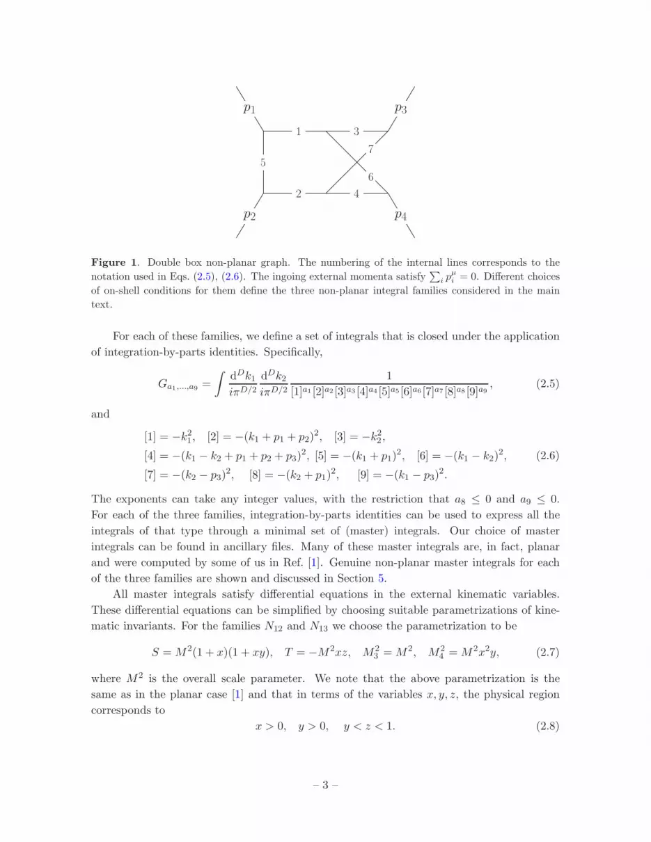
All non-planar two-loop diagrams that are required for the production of two off-shell
vector bosons can be described by a single meta-graph shown in Figure 1. Three mappings,
that define three distinct families of integrals, need to be considered:
1. family N12: p1 = −q4, p2 = −q3, p3 = q2, p4 = q1;
2. family N13: p1 = −q4, p2 = q2, p3 = −q3, p4 = q1;
3. family N34: p1 = q1, p2 = q2, p3 = −q3, p4 = −q4.
1We use Mandelstam variables written with capital letters to refer to the physical process. Later, we will
use Mandelstam variables for families of integrals; those we will write with lower case letters.
– 2 –
1
42
3
6
7
5
p1
p2 p4
p3
Figure 1. Double box non-planar graph. The numbering of the internal lines corresponds to the
notation used in Eqs. (2.5), (2.6). The ingoing external momenta satisfy∑
i pµi = 0. Different choices
of on-shell conditions for them define the three non-planar integral families considered in the main
text.
For each of these families, we define a set of integrals that is closed under the application
of integration-by-parts identities. Specifically,
Ga1,...,a9 =
∫
dDk1iπD/2
dDk2iπD/2
1
[1]a1 [2]a2 [3]a3 [4]a4 [5]a5 [6]a6 [7]a7 [8]a8 [9]a9, (2.5)
and
[1] = −k21, [2] = −(k1 + p1 + p2)2, [3] = −k22 ,
[4] = −(k1 − k2 + p1 + p2 + p3)2, [5] = −(k1 + p1)
2, [6] = −(k1 − k2)2,
[7] = −(k2 − p3)2, [8] = −(k2 + p1)
2, [9] = −(k1 − p3)2.
(2.6)
The exponents can take any integer values, with the restriction that a8 ≤ 0 and a9 ≤ 0.
For each of the three families, integration-by-parts identities can be used to express all the
integrals of that type through a minimal set of (master) integrals. Our choice of master
integrals can be found in ancillary files. Many of these master integrals are, in fact, planar
and were computed by some of us in Ref. [1]. Genuine non-planar master integrals for each
of the three families are shown and discussed in Section 5.
All master integrals satisfy differential equations in the external kinematic variables.
These differential equations can be simplified by choosing suitable parametrizations of kine-
matic invariants. For the families N12 and N13 we choose the parametrization to be
S = M2(1 + x)(1 + xy), T = −M2xz, M23 = M2, M2
4 = M2x2y, (2.7)
where M2 is the overall scale parameter. We note that the above parametrization is the
same as in the planar case [1] and that in terms of the variables x, y, z, the physical region
corresponds to
x > 0, y > 0, y < z < 1. (2.8)
– 3 –
For the family N34, the above parametrization can also be used but it is not optimal since
it leads to the appearance of multiple letters in an alphabet that are quadratic in x, y and z
which is problematic for the construction of an analytic solution that is based on Goncharov
polylogarithms. Instead, we find it useful to choose the following parametrization
S = M2(1 + x)2, T = −M2x ((1 + y)(1 + xy)− 2zy(1 + x)) ,
M23 = M2x2(1− y2), M2
4 = M2(1− x2y2).(2.9)
While the above parametrization also does not lead to a linear alphabet, it allows us to
construct solutions in terms of Goncharov polylogarithms, as we explain below.2
3 Differential equations
In this Section we describe a procedure [8] that allows us to compute the master integrals
and comment on some aspects that arise when this procedure is applied to the calculation of
non-planar integrals. We begin by deriving systems of differential equations for each of the
above families. This is a relatively standard procedure, see e.g. Refs. [9, 10], and we do not
discuss it further. When deriving differential equations we performed a reduction to master
integrals using the c++ version of program FIRE [11, 12]. We choose all master integrals to
be dimensionless, such that they depend only on the three variables x, y, z and find
∂ξ ~f = ǫAξ~f , (3.1)
where ξ = x, y, z and ~f is a vector of master integrals. The master integrals for all the three
families can be found in ancillary files; some examples of master integrals are discussed in
Section 5.
The matrices Aξ contain simple rational functions. They satisfy the integrability condi-
tions
(∂ξ∂η − ∂η∂ξ) ~f = 0 ⇒ ∂ξAη − ∂ηAξ = 0 , [Aη, Aξ ] = 0 , (3.2)
for ξ, η ∈ {x, y, z}. The structure of the equations can be further clarified by writing them in
the combined form
d ~f(x, y, z; ǫ) = ǫ d A(x, y, z) ~f (x, y, z; ǫ) , (3.3)
where the differential d acts on x, y and z. Matrices A for each of the three families can be
found in the ancillary files as well. For our choice of master integrals, the matrix A can be
written in the following way
A =
Nmax∑
i=1
Aαilog(αi) , (3.4)
2We note that it is possible to obtain a linear alphabet for the N34 family by changing variables x → x/y
in Eq.(2.9).
– 4 –
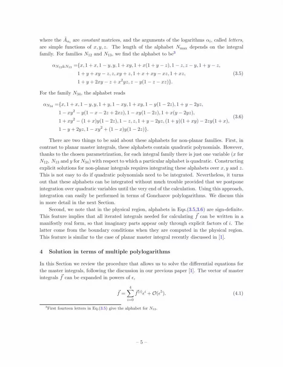
where the Aαiare constant matrices, and the arguments of the logarithms αi, called letters,
are simple functions of x, y, z. The length of the alphabet Nmax depends on the integral
family. For families N12 and N13, we find the alphabet to be3
αN12&N13={x, 1 + x, 1− y, y, 1 + xy, 1 + x(1 + y − z), 1 − z, z − y, 1 + y − z,
1 + y + xy − z, z, xy + z, 1 + x+ xy − xz, 1 + xz,
1 + y + 2xy − z + x2yz, z − y(1− z − xz)}.
(3.5)
For the family N34, the alphabet reads
αN34={x, 1 + x, 1− y, y, 1 + y, 1− xy, 1 + xy, 1− y(1− 2z), 1 + y − 2yz,
1− xy2 − y(1− x− 2z + 2xz), 1 − xy(1− 2z), 1 + x(y − 2yz),
1 + xy2 − (1 + x)y(1− 2z), 1 − z, z, 1 + y − 2yz, (1 + y)(1 + xy)− 2zy(1 + x),
1− y + 2yz, 1− xy2 + (1− x)y(1 − 2z)}.
(3.6)
There are two things to be said about these alphabets for non-planar families. First, in
contrast to planar master integrals, these alphabets contain quadratic polynomials. However,
thanks to the chosen parametrization, for each integral family there is just one variable (x for
N12, N13 and y forN34) with respect to which a particular alphabet is quadratic. Constructing
explicit solutions for non-planar integrals requires integrating these alphabets over x, y and z.
This is not easy to do if quadratic polynomials need to be integrated. Nevertheless, it turns
out that these alphabets can be integrated without much trouble provided that we postpone
integration over quadratic variables until the very end of the calculation. Using this approach,
integration can easily be performed in terms of Goncharov polylogarithms. We discuss this
in more detail in the next Section.
Second, we note that in the physical region, alphabets in Eqs.(3.5,3.6) are sign-definite.
This feature implies that all iterated integrals needed for calculating ~f can be written in a
manifestly real form, so that imaginary parts appear only through explicit factors of i. The
latter come from the boundary conditions when they are computed in the physical region.
This feature is similar to the case of planar master integral recently discussed in [1].
4 Solution in terms of multiple polylogarithms
In this Section we review the procedure that allows us to solve the differential equations for
the master integrals, following the discussion in our previous paper [1]. The vector of master
integrals ~f can be expanded in powers of ǫ,
~f =
4∑
i=0
~f (i)ǫi +O(ǫ5). (4.1)
3First fourteen letters in Eq.(3.5) give the alphabet for N12.
– 5 –
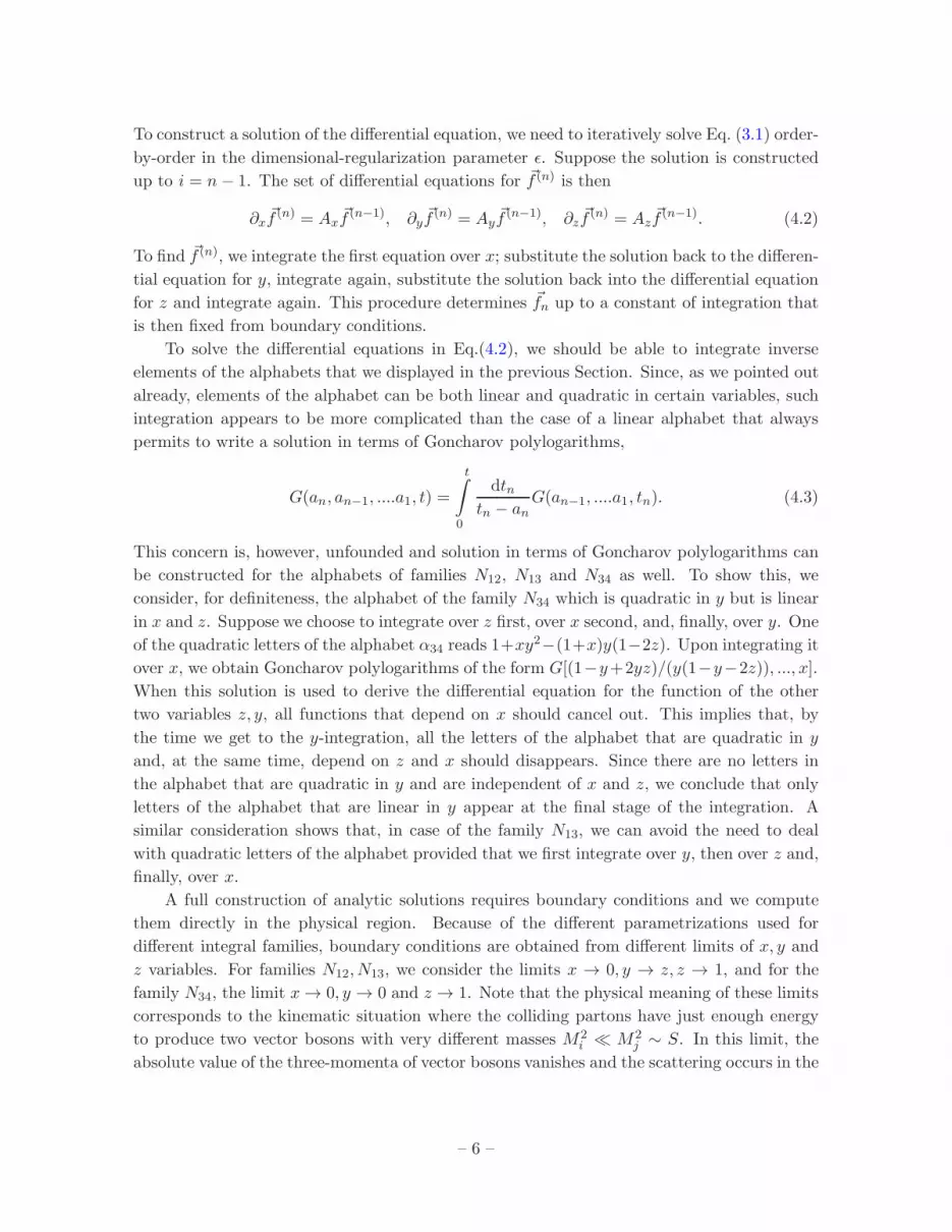
To construct a solution of the differential equation, we need to iteratively solve Eq. (3.1) order-
by-order in the dimensional-regularization parameter ǫ. Suppose the solution is constructed
up to i = n− 1. The set of differential equations for ~f (n) is then
∂x ~f(n) = Ax
~f (n−1), ∂y ~f(n) = Ay
~f (n−1), ∂z ~f(n) = Az
~f (n−1). (4.2)
To find ~f (n), we integrate the first equation over x; substitute the solution back to the differen-
tial equation for y, integrate again, substitute the solution back into the differential equation
for z and integrate again. This procedure determines ~fn up to a constant of integration that
is then fixed from boundary conditions.
To solve the differential equations in Eq.(4.2), we should be able to integrate inverse
elements of the alphabets that we displayed in the previous Section. Since, as we pointed out
already, elements of the alphabet can be both linear and quadratic in certain variables, such
integration appears to be more complicated than the case of a linear alphabet that always
permits to write a solution in terms of Goncharov polylogarithms,
G(an, an−1, ....a1, t) =
t∫
0
dtntn − an
G(an−1, ....a1, tn). (4.3)
This concern is, however, unfounded and solution in terms of Goncharov polylogarithms can
be constructed for the alphabets of families N12, N13 and N34 as well. To show this, we
consider, for definiteness, the alphabet of the family N34 which is quadratic in y but is linear
in x and z. Suppose we choose to integrate over z first, over x second, and, finally, over y. One
of the quadratic letters of the alphabet α34 reads 1+xy2−(1+x)y(1−2z). Upon integrating it
over x, we obtain Goncharov polylogarithms of the form G[(1−y+2yz)/(y(1−y−2z)), ..., x].
When this solution is used to derive the differential equation for the function of the other
two variables z, y, all functions that depend on x should cancel out. This implies that, by
the time we get to the y-integration, all the letters of the alphabet that are quadratic in y
and, at the same time, depend on z and x should disappears. Since there are no letters in
the alphabet that are quadratic in y and are independent of x and z, we conclude that only
letters of the alphabet that are linear in y appear at the final stage of the integration. A
similar consideration shows that, in case of the family N13, we can avoid the need to deal
with quadratic letters of the alphabet provided that we first integrate over y, then over z and,
finally, over x.
A full construction of analytic solutions requires boundary conditions and we compute
them directly in the physical region. Because of the different parametrizations used for
different integral families, boundary conditions are obtained from different limits of x, y and
z variables. For families N12, N13, we consider the limits x → 0, y → z, z → 1, and for the
family N34, the limit x → 0, y → 0 and z → 1. Note that the physical meaning of these limits
corresponds to the kinematic situation where the colliding partons have just enough energy
to produce two vector bosons with very different masses M2i ≪ M2
j ∼ S. In this limit, the
absolute value of the three-momenta of vector bosons vanishes and the scattering occurs in the
– 6 –
forward direction. This is the same kinematics that we used in our previous paper on planar
master integrals [1] and, since many planar integrals appear in the current computation as
non-homogeneous terms in the differential equations, the boundary conditions computed in
[1] can be recycled for a large number of required integrals.
The boundary conditions are a priori unknown for genuine non-planar integrals and we
compute them in two different ways. One possibility is to study consistency conditions of
differential equations in three variables; this procedure is discussed in Ref. [1] and it is often
sufficient to fix the required boundary behavior of non-planar integrals. Another possibility
is to compute the relevant limits directly, expanding Feynman integrals in small kinematic
variables. To accomplish this, we used the strategy of expansion by regions [13, 14] (for a
recent review see Chapter 9 of Ref. [15]) and its implementation in the public computer code
asy.m [16, 17] which is now included into FIESTA [18].
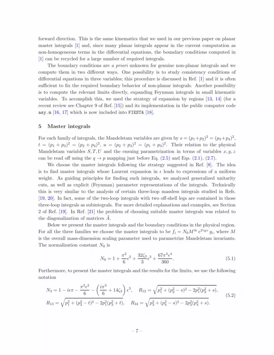
5 Master integrals
For each family of integrals, the Mandelstam variables are given by s = (p1+p2)2 = (p3+p4)
2,
t = (p1 + p3)2 = (p2 + p4)
2, u = (p2 + p3)2 = (p1 + p3)
2. Their relation to the physical
Mandelstam variables S, T, U and the ensuing parametrization in terms of variables x, y, z
can be read off using the q → p mapping just before Eq. (2.5) and Eqs. (2.1), (2.7).
We choose the master integrals following the strategy suggested in Ref. [8]. The idea
is to find master integrals whose Laurent expansion in ǫ leads to expressions of a uniform
weight. As guiding principles for finding such integrals, we analyzed generalized unitarity
cuts, as well as explicit (Feynman) parameter representations of the integrals. Technically
this is very similar to the analysis of certain three-loop massless integrals studied in Refs.
[19, 20]. In fact, some of the two-loop integrals with two off-shell legs are contained in those
three-loop integrals as subintegrals. For more detailed explanations and examples, see Section
2 of Ref. [19]. In Ref. [21] the problem of choosing suitable master integrals was related to
the diagonalization of matrices A.
Below we present the master integrals and the boundary conditions in the physical region.
For all the three families we choose the master integrals to be fi = N0M4ǫ e2γEǫ gi, where M
is the overall mass-dimension scaling parameter used to parametrize Mandelstam invariants.
The normalization constant N0 is
N0 = 1 +π2
6ǫ2 +
32ζ33
ǫ3 +67π4ǫ4
360. (5.1)
Furthermore, to present the master integrals and the results for the limits, we use the following
notation
N3 = 1− iǫπ −π2ǫ2
6−
(
iπ3
6+ 14ζ3
)
ǫ3, R12 =√
p21 + (p22 − s)2 − 2p21(p22 + s),
R13 =√
p21 + (p23 − t)2 − 2p21(p23 + t), R34 =
√
p23 + (p24 − s)2 − 2p23(p24 + s).
(5.2)
– 7 –

In contrast to our previous paper [1], we will not present results for all integrals that
are needed to construct the non-planar master integrals. The reason is that many of these
integrals are the planar ones; they were computed in Ref. [1]. For the family N34, some of
the planar integrals need to be re-expressed in new variables, since the parametrization of the
family N34 differs from the parametrization used for all other families. This is straightforward
to do, at least in principle. Therefore, below we present our choices of the genuine non-planar
integrals and the boundary conditions for them. However, we note that a complete set of all
master integrals for the three integral families can be found in the ancillary files.
Finally, we note that the pictures of master integrals shown below are intended to give a
general idea of how the corresponding master integrals look like, but they do not show squared
propagators, numerators and prefactors. Also, in some cases we chose linear combinations of
integrals as master integrals, and in those cases only one representative figure is given.
For the family N12, there are eight genuine non-planar master integrals. The boundary
conditions are evaluated at the point x → 0, y → 1, z → 1.
p1
p2
p3
p4
gN12
28 = ǫ4 s2 G1,1,1,1,0,1,1,0,0 , (5.3)
fN12
28∼ e2iπǫ
(
1−5π2ǫ2
6− 17ζ3ǫ
3 −17π4ǫ4
36
)
,
p3
p2
p1
p4
gN12
29= ǫ2 p2
1s G1,0,1,1,1,1,1,0,0 , (5.4)
fN12
29 ∼x−4ǫ
4
[
1 + 10iπǫ−46π2ǫ2
3−(
12iπ3 − 16ζ3)
ǫ3
+
(
386π4
45− 32iπζ3
)
ǫ4
]
− iπǫx−4ǫ [(z − y)(1− z)]−2ǫ
,
p3
p2
p1
p4
gN12
30 = ǫ4(
(−p22 + t)G0,0,1,1,1,1,1,0,0 + (u − p21)G1,0,1,1,1,1,1,0,−1
)
, (5.5)
fN12
30∼
1
4e2iπǫ −
1
4x−2ǫ + x−4ǫ
[
− iπǫ+10π2ǫ2
6
+
(
4iπ3
3− 2ζ3
)
ǫ3 −
(
89π4
90− 4iπζ3
)
ǫ4
]
,
p3
p2
p1
p4
gN12
31 = ǫ4p22sG0,1,1,1,1,1,1,0,0 , (5.6)
fN12
31 ∼ 1 + 2iπǫ−17π2ǫ2
6−(
3iπ3 + 17ζ3)
ǫ3 +
(
67π4
36− 34iπζ3
)
ǫ4
− x−2ǫ
(
1−π2ǫ2
6− 7ζ3ǫ
3 −π4ǫ4
3
)
+1
4e2iπǫx−4ǫ
− iπǫx−4ǫ [(z − y)(1 − z)]−2ǫ
,
– 8 –

p3
p2
p1
p4
gN12
32= ǫ4
(
(t− p21)G0,0,1,1,1,1,1,0,0 + (p2
1− s− t)G0,1,1,1,1,1,1,0,−1
)
, (5.7)
fN12
32∼ −
1
4−
iπǫ
2+
11π2ǫ2
12+
(
7iπ3
6+
17ζ32
)
ǫ3 −
(
55π4
72− 17iπζ3
)
ǫ4
+ x−2ǫ
(
1
4−
π2ǫ2
12−
7ζ3ǫ3
2−
π4ǫ4
6
)
,
p3
p2
p1
p4
gN12
33 = ǫ4st[
G0,1,1,1,1,1,1,0,0 +G1,0,1,1,1,1,1,0,0
− G1,1,1,1,1,1,1,−1,0 + sG1,1,1,1,1,1,1,0,0
]
, (5.8)
fN12
33∼ −
x−2ǫ
2
(
1−π2ǫ2
6− 7ζ3ǫ
3 −π4ǫ4
3
)
+x−4ǫ
4
(
1 + 6iπǫ−26π2ǫ2
3+ (8ζ3 −
20iπ3
3)ǫ3 +
(
208π4
45− 16iπζ3
)
ǫ4)
− iπǫx−4ǫ [(z − y)(1 − z)]−2ǫ ,
p3
p2
p1
p4
gN12
34 = −ǫ4suG1,1,1,1,1,1,1,−1,0 , (5.9)
fN12
34 ∼x−2ǫ
2
(
1−π2ǫ2
6− 7ζ3ǫ
3 −π4ǫ4
3
)
−x−4ǫ
4
(
1 + 6iπǫ−26π2ǫ2
3+ (8ζ3 −
20iπ3
3)ǫ3 +
(
208π4
45− 16iπζ3
)
ǫ4)
+ iπǫx−4ǫ [(z − y)(1− z)]−2ǫ
,
p3
p2
p1
p4
gN12
35= ǫ4R12
[
G0,0,1,1,1,1,1,0,0 −G0,1,1,1,1,1,1,0,−1
− G1,0,1,1,1,1,1,0,−1 − sG1,1,1,1,1,1,1,−1,0 +G1,1,1,1,1,1,1,0,−2
]
, (5.10)
fN12
35∼ 0,
There are nine non-planar master integrals in the family N13. These integrals, togetherwith their limits in the kinematic point x → 0, y → 1, z → 1 are
p3
p2
p1
p4
gN13
33= ǫ4p2
3tG0,1,1,1,1,1,1,0,0 , (5.11)
fN13
33∼ 1 + 2iπǫ−
17π2ǫ2
6− (3iπ3 + 17ζ3)ǫ
3 +
(
67π4
36− 34iπζ3
)
ǫ4
− x−2ǫ(
1−π2ǫ2
6− 7ζ3ǫ
3 −π4ǫ4
3
)
+e2iπǫ
4x−4ǫ
− iπǫx−4ǫ [(z − y)(1− z)]−2ǫ ,
– 9 –

p3
p2
p1
p4
gN13
34 = ǫ4((t− p21 + p23)G0,0,1,1,1,1,1,0,0 + (u− p23)G0,1,1,1,1,1,1,0,−1) , (5.12)
fN13
34∼
1
2+ iπǫ−
3π2ǫ2
2−
(
5iπ3
3+ 9ζ3
)
ǫ3 +
(
193π4
180− 18iπζ3
)
ǫ4
− x−2ǫ
(
3
4−
π2ǫ2
4−
21ζ3ǫ3
2−
π4ǫ4
2
)
+ x−4ǫ
(
1
4+
iπǫ
2−
π2ǫ2
2−
iπ3ǫ3
3+
π4ǫ4
6
)
− iπǫx−4ǫ [(z − y)(1− z)]−2ǫ ,
p3
p2
p1
p4
gN13
35 = ǫ4(
p21(p2
3 − s) + p23(−p23 + s+ t))
G1,0,1,1,1,1,1,0,0 , (5.13)
fN13
35 ∼ −x−2ǫ
(
1
2−
π2ǫ2
12−
7
2ζ3ǫ
3 −π4ǫ4
6
)
+ x−3ǫ
(
1 + iǫπ −2π2ǫ2
3−
(
iπ3
3− 2ζ3
)
ǫ3 +
(
π4
10+ 2iπζ3
)
ǫ4)
− x−4ǫ
(
1
2+
2iπǫ
3−
5π2ǫ2
12−
(
5iπ3
18+
ζ32
)
ǫ3 +
(
53π4
360−
iπζ33
)
ǫ4)
−iπǫ
3x−4ǫ [(z − y)(1− z)]
−3ǫN3,
p3
p2
p1
p4
gN13
36= ǫ4R13
(
G1,−1,1,1,1,1,1,0,0 −G1,0,1,1,1,1,1,0,−1
+ (s− p23)G1,0,1,1,1,1,1,0,0
)
, (5.14)
fN13
36∼ 0,
p3
p2
p1
p4
gN13
37= ǫ4
(
tG1,0,0,1,1,1,1,0,0 + (−p23+ s)G1,0,1,1,1,1,1,−1,0
)
, (5.15)
fN13
37∼ −x−4ǫ
[1
4+
iπǫ
6+
π2ǫ2
12−
(
ζ32
−iπ3
18
)
ǫ3 −
(
7π4
360+
iπζ33
)
ǫ4]
+ x−3ǫ[1
2+
iπǫ
2−
π2ǫ2
3+
(
ζ3 −iπ3
6
)
ǫ3 +
(
π4
20+ iπζ3
)
ǫ4]
− x−2ǫ[1
4−
π2ǫ2
12−
7ζ3ǫ3
2−
π4ǫ4
6
]
−iǫπ
3x−4ǫ [(z − y)(1− z)]
−3ǫN3,
– 10 –
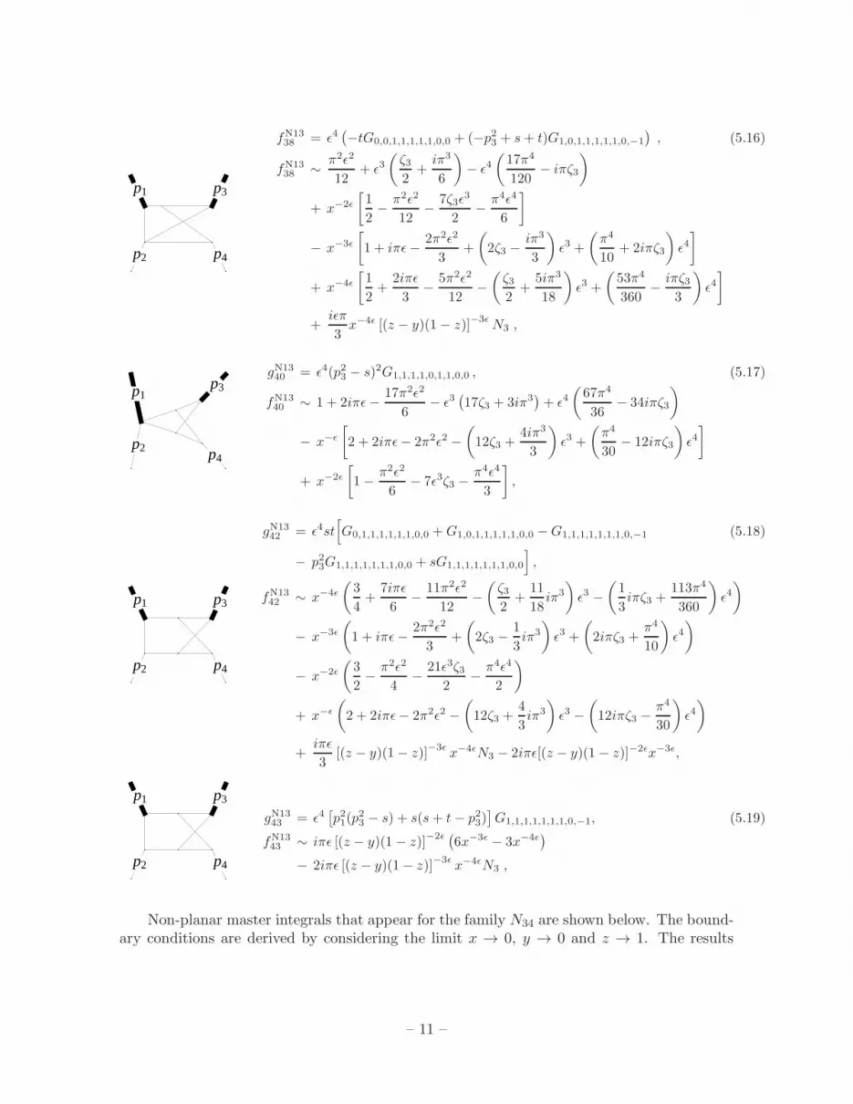
p3
p2
p1
p4
fN13
38 = ǫ4(
−tG0,0,1,1,1,1,1,0,0 + (−p23 + s+ t)G1,0,1,1,1,1,1,0,−1
)
, (5.16)
fN13
38 ∼π2ǫ2
12+ ǫ3
(
ζ32
+iπ3
6
)
− ǫ4(
17π4
120− iπζ3
)
+ x−2ǫ
[
1
2−
π2ǫ2
12−
7ζ3ǫ3
2−
π4ǫ4
6
]
− x−3ǫ
[
1 + iπǫ−2π2ǫ2
3+
(
2ζ3 −iπ3
3
)
ǫ3 +
(
π4
10+ 2iπζ3
)
ǫ4]
+ x−4ǫ
[
1
2+
2iπǫ
3−
5π2ǫ2
12−
(
ζ32
+5iπ3
18
)
ǫ3 +
(
53π4
360−
iπζ33
)
ǫ4]
+iǫπ
3x−4ǫ [(z − y)(1 − z)]
−3ǫN3 ,
p1
p2
p3
p4
gN13
40 = ǫ4(p23 − s)2G1,1,1,1,0,1,1,0,0 , (5.17)
fN13
40 ∼ 1 + 2iπǫ−17π2ǫ2
6− ǫ3
(
17ζ3 + 3iπ3)
+ ǫ4(
67π4
36− 34iπζ3
)
− x−ǫ
[
2 + 2iπǫ− 2π2ǫ2 −
(
12ζ3 +4iπ3
3
)
ǫ3 +
(
π4
30− 12iπζ3
)
ǫ4]
+ x−2ǫ
[
1−π2ǫ2
6− 7ǫ3ζ3 −
π4ǫ4
3
]
,
p3
p2
p1
p4
gN13
42= ǫ4st
[
G0,1,1,1,1,1,1,0,0 +G1,0,1,1,1,1,1,0,0 −G1,1,1,1,1,1,1,0,−1 (5.18)
− p23G1,1,1,1,1,1,1,0,0 + sG1,1,1,1,1,1,1,0,0
]
,
fN13
42 ∼ x−4ǫ
(
3
4+
7iπǫ
6−
11π2ǫ2
12−
(
ζ32
+11
18iπ3
)
ǫ3 −
(
1
3iπζ3 +
113π4
360
)
ǫ4)
− x−3ǫ
(
1 + iπǫ−2π2ǫ2
3+
(
2ζ3 −1
3iπ3
)
ǫ3 +
(
2iπζ3 +π4
10
)
ǫ4)
− x−2ǫ
(
3
2−
π2ǫ2
4−
21ǫ3ζ32
−π4ǫ4
2
)
+ x−ǫ
(
2 + 2iπǫ− 2π2ǫ2 −
(
12ζ3 +4
3iπ3
)
ǫ3 −
(
12iπζ3 −π4
30
)
ǫ4)
+iπǫ
3[(z − y)(1− z)]
−3ǫx−4ǫN3 − 2iπǫ[(z − y)(1 − z)]−2ǫx−3ǫ,
p3
p2
p1
p4
gN13
43= ǫ4
[
p21(p2
3− s) + s(s+ t− p2
3)]
G1,1,1,1,1,1,1,0,−1, (5.19)
fN13
43 ∼ iπǫ [(z − y)(1− z)]−2ǫ(
6x−3ǫ − 3x−4ǫ)
− 2iπǫ [(z − y)(1− z)]−3ǫ
x−4ǫN3 ,
Non-planar master integrals that appear for the family N34 are shown below. The bound-ary conditions are derived by considering the limit x → 0, y → 0 and z → 1. The results
– 11 –
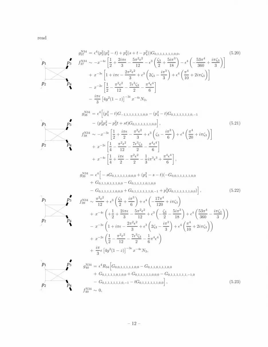
read
p3
p2
p1
p4
gN34
37= ǫ4(p2
3(p2
4− t) + p2
4(s+ t− p2
4))G0,1,1,1,1,1,1,0,0, (5.20)
fN34
37∼ −x−4ǫ
[
1
2+
2iπǫ
3−
5π2ǫ2
12− ǫ3
(
ζ32
+5iπ3
18
)
− ǫ4(
−53π4
360+
iπζ33
)]
+ x−3ǫ
[
1 + iπǫ−2π2ǫ2
3+ ǫ3
(
2ζ3 −iπ3
3
)
+ ǫ4(
π4
10+ 2iπζ3
)]
− x−2ǫ
[
1
2−
π2ǫ2
12−
7ǫ3ζ32
−π4ǫ4
6
]
−iπǫ
3
[
4y2(1− z)]
−3ǫx−4ǫN3,
p3
p2
p1
p4
gN34
38 = ǫ4[
(p24 − t)G−1,1,1,1,1,1,1,0,0 − (p24 − t)G0,1,1,1,1,1,1,0,−1
− (p23p24− p2
3t+ st)G0,1,1,1,1,1,1,0,0
]
, (5.21)
fN34
38∼ −x−3ǫ
[
1
2+
iπǫ
2−
π2ǫ2
3+ ǫ3
(
ζ3 −iπ3
6
)
+ ǫ4(
π4
20+ iπζ3
)]
+ x−2ǫ
[
1
4−
π2ǫ2
12−
7ǫ3ζ32
−π4ǫ4
6
]
+ x−4ǫ
[
1
4+
iπǫ
2−
π2ǫ2
2−
1
3iπ3ǫ3 +
π4ǫ4
6
]
,
p3
p2
p1
p4
gN34
39 = ǫ4[
− sG0,1,1,1,1,1,0,0,0 + (p24 − s− t)(−G0,0,1,1,1,1,1,0,0
+ G0,1,1,0,1,1,1,0,0 −G0,1,1,1,1,0,1,0,0
− G0,1,1,1,1,1,0,0,0 +G0,1,1,1,1,1,1,0,−1 + p24G0,1,1,1,1,1,1,0,0)
]
, (5.22)
fN34
39∼
π2ǫ2
12+ ǫ3
(
ζ32
+iπ3
6
)
+ ǫ4(
−17π4
120+ iπζ3
)
+ x−4ǫ
(
+1
2+
2iπǫ
3−
5π2ǫ2
12+ ǫ3
(
−ζ32
−5iπ3
18
)
+ ǫ4(
53π4
360−
iπζ33
))
− x−3ǫ
(
1 + iπǫ−2π2ǫ2
3+ ǫ3
(
2ζ3 −iπ3
3
)
+ ǫ4(
π4
10+ 2iπζ3
))
+ x−2ǫ
(
1
2−
π2ǫ2
12−
7ǫ3ζ32
−1
6π4ǫ4
)
+iπ
3ǫ[
4y2(1 − z)]
−3ǫx−4ǫN3,
p3
p2
p1
p4
gN34
40= ǫ4R34
[
G0,0,1,1,1,1,1,0,0 −G0,1,1,0,1,1,1,0,0
+ G0,1,1,1,1,0,1,0,0 +G0,1,1,1,1,1,0,0,0 −G0,1,1,1,1,1,1,−1,0
− G0,1,1,1,1,1,1,0,−1 − tG0,1,1,1,1,1,1,0,0
]
, (5.23)
fN34
40 ∼ 0,
– 12 –

p1
p2
p3
p4
gN34
47 = ǫ4(p23 + (p24 − s)2 − 2p23(p2
4 + s))G1,1,1,1,0,1,1,0,0 , (5.24)
fN34
47 ∼ 0
p3
p2
p1
p4
gN34
50 =[
2(p23 + p24 − s)]
−1
ǫ4s[
− 2p23p2
4G0,1,1,1,1,1,1,0,0 − 2p23p2
4G1,0,1,1,1,1,1,0,0
− (p43 + (p24 − s)(p24 − s− t)− p23(2s+ t))G1,1,1,1,1,1,1,0,−1
+ (2p23p24− p2
3t− p2
4t+ st)(G0,1,1,1,1,1,1,0,0 +G1,0,1,1,1,1,1,0,0 (5.25)
− G1,1,1,1,1,1,1,0,−1 − (p23 + p24 − s)G1,1,1,1,1,1,1,0,0)]
,
fN34
50 ∼ −x−4ǫ
(
1
2+
2iπǫ
3−
5π2ǫ2
12−
(
ζ32
+5iπ3
18
)
ǫ3 +
(
+53π4
360−
iπζ33
)
ǫ4)
+ x−3ǫ
(
1 + iπǫ−2π2ǫ2
3+
(
2ζ3 −iπ3
3
)
ǫ3 +
(
π4
10+ 2iπζ3
)
ǫ4)
− x−2ǫ
(
1
2−
π2ǫ2
12−
7ǫ3ζ32
−π4ǫ4
6
)
+5iπǫ
3
[
4y2(1 − z)]
−3ǫx−4ǫN3 ,
p3
p2
p1
p4
gN34
51 = −[
p23 + p24 − s]
−1
ǫ4R34
[
(t− p24)(s− p23 − p24)G0,1,1,1,1,1,1,0,0
+ (t− p23)(s− p23 − p24)G1,0,1,1,1,1,1,0,0
− (p23+ p2
4− s)s(G1,1,1,1,1,1,1,0,−1 + tG1,1,1,1,1,1,1,0,0)
]
, (5.26)
fN34
51∼ 0,
To illustrate how analytic results look like, we provide contributions through O(ǫ2) for
three different master integrals. We introduce the following notation
a1 = z − 1, a2 = (1 + x)/x, a3 = (1 + x(1− z))/x,
a4 =1 + y + xy + xy2
2(1 + x)y, a5 =
1− y − xy + xy2
2(1 + x)y, a6 =
1 + xy
2xy.
(5.27)
For the three integrals that we show below, we separate real and imaginary parts and
write
fNIJi = RefNIJ
i + iImfNIJi , (5.28)
– 13 –
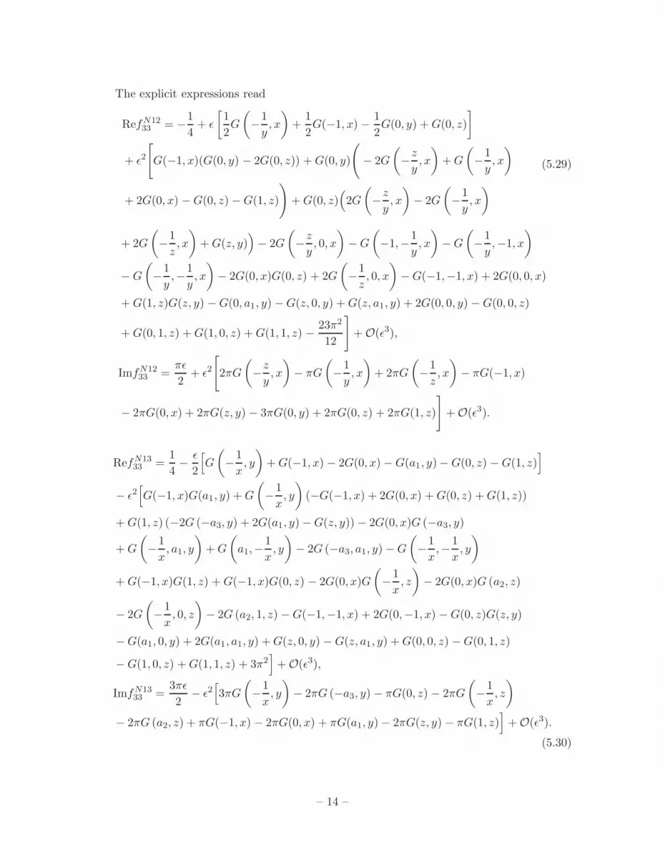
The explicit expressions read
RefN1233 = −
1
4+ ǫ
[
1
2G
(
−1
y, x
)
+1
2G(−1, x) −
1
2G(0, y) +G(0, z)
]
+ ǫ2
[
G(−1, x)(G(0, y) − 2G(0, z)) +G(0, y)
(
− 2G
(
−z
y, x
)
+G
(
−1
y, x
)
+ 2G(0, x) −G(0, z) −G(1, z)
)
+G(0, z)(
2G
(
−z
y, x
)
− 2G
(
−1
y, x
)
(5.29)
+ 2G
(
−1
z, x
)
+G(z, y))
− 2G
(
−z
y, 0, x
)
−G
(
−1,−1
y, x
)
−G
(
−1
y,−1, x
)
−G
(
−1
y,−
1
y, x
)
− 2G(0, x)G(0, z) + 2G
(
−1
z, 0, x
)
−G(−1,−1, x) + 2G(0, 0, x)
+G(1, z)G(z, y) −G(0, a1, y)−G(z, 0, y) +G(z, a1, y) + 2G(0, 0, y) −G(0, 0, z)
+G(0, 1, z) +G(1, 0, z) +G(1, 1, z) −23π2
12
]
+O(ǫ3),
ImfN1233 =
πǫ
2+ ǫ2
[
2πG
(
−z
y, x
)
− πG
(
−1
y, x
)
+ 2πG
(
−1
z, x
)
− πG(−1, x)
− 2πG(0, x) + 2πG(z, y) − 3πG(0, y) + 2πG(0, z) + 2πG(1, z)
]
+O(ǫ3).
RefN1333 =
1
4−
ǫ
2
[
G
(
−1
x, y
)
+G(−1, x) − 2G(0, x) −G(a1, y)−G(0, z) −G(1, z)]
− ǫ2[
G(−1, x)G(a1, y) +G
(
−1
x, y
)
(−G(−1, x) + 2G(0, x) +G(0, z) +G(1, z))
+G(1, z) (−2G (−a3, y) + 2G(a1, y)−G(z, y)) − 2G(0, x)G (−a3, y)
+G
(
−1
x, a1, y
)
+G
(
a1,−1
x, y
)
− 2G (−a3, a1, y)−G
(
−1
x,−
1
x, y
)
+G(−1, x)G(1, z) +G(−1, x)G(0, z) − 2G(0, x)G
(
−1
x, z
)
− 2G(0, x)G (a2, z)
− 2G
(
−1
x, 0, z
)
− 2G (a2, 1, z) −G(−1,−1, x) + 2G(0,−1, x) −G(0, z)G(z, y)
−G(a1, 0, y) + 2G(a1, a1, y) +G(z, 0, y) −G(z, a1, y) +G(0, 0, z) −G(0, 1, z)
−G(1, 0, z) +G(1, 1, z) + 3π2]
+O(ǫ3),
ImfN1333 =
3πǫ
2− ǫ2
[
3πG
(
−1
x, y
)
− 2πG (−a3, y)− πG(0, z) − 2πG
(
−1
x, z
)
− 2πG (a2, z) + πG(−1, x) − 2πG(0, x) + πG(a1, y)− 2πG(z, y) − πG(1, z)]
+O(ǫ3).
(5.30)
– 14 –
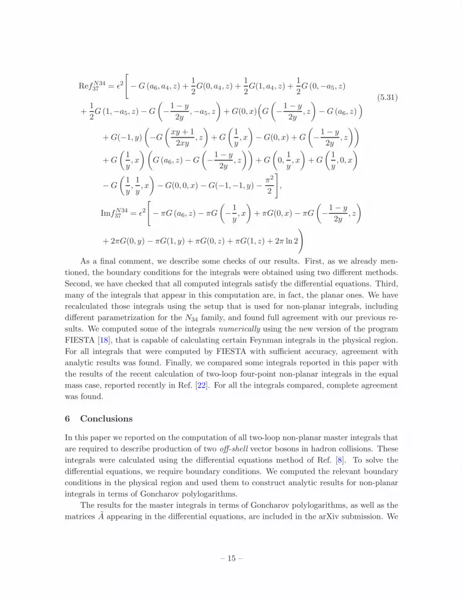
RefN3437 = ǫ2
[
−G (a6, a4, z) +1
2G(0, a4, z) +
1
2G(1, a4, z) +
1
2G (0,−a5, z)
+1
2G (1,−a5, z) −G
(
−1− y
2y,−a5, z
)
+G(0, x)(
G
(
−1− y
2y, z
)
−G (a6, z))
(5.31)
+G(−1, y)
(
−G
(
xy + 1
2xy, z
)
+G
(
1
y, x
)
−G(0, x) +G
(
−1− y
2y, z
))
+G
(
1
y, x
)(
G (a6, z)−G
(
−1− y
2y, z
))
+G
(
0,1
y, x
)
+G
(
1
y, 0, x
)
−G
(
1
y,1
y, x
)
−G(0, 0, x) −G(−1,−1, y) −π2
2
]
,
ImfN3437 = ǫ2
[
− πG (a6, z) − πG
(
−1
y, x
)
+ πG(0, x) − πG
(
−1− y
2y, z
)
+ 2πG(0, y) − πG(1, y) + πG(0, z) + πG(1, z) + 2π ln 2
)
As a final comment, we describe some checks of our results. First, as we already men-
tioned, the boundary conditions for the integrals were obtained using two different methods.
Second, we have checked that all computed integrals satisfy the differential equations. Third,
many of the integrals that appear in this computation are, in fact, the planar ones. We have
recalculated those integrals using the setup that is used for non-planar integrals, including
different parametrization for the N34 family, and found full agreement with our previous re-
sults. We computed some of the integrals numerically using the new version of the program
FIESTA [18], that is capable of calculating certain Feynman integrals in the physical region.
For all integrals that were computed by FIESTA with sufficient accuracy, agreement with
analytic results was found. Finally, we compared some integrals reported in this paper with
the results of the recent calculation of two-loop four-point non-planar integrals in the equal
mass case, reported recently in Ref. [22]. For all the integrals compared, complete agreement
was found.
6 Conclusions
In this paper we reported on the computation of all two-loop non-planar master integrals that
are required to describe production of two off-shell vector bosons in hadron collisions. These
integrals were calculated using the differential equations method of Ref. [8]. To solve the
differential equations, we require boundary conditions. We computed the relevant boundary
conditions in the physical region and used them to construct analytic results for non-planar
integrals in terms of Goncharov polylogarithms.
The results for the master integrals in terms of Goncharov polylogarithms, as well as the
matrices A appearing in the differential equations, are included in the arXiv submission. We
– 15 –
note that representation of master integrals in terms of Goncharov polylogarithms may not
be the most compact one but it has the advantage that these functions are by now standard
and dedicated numerical implementations exist [23, 24]. Also, this representation manifestly
separates real and imaginary parts. We did not try to simplify these results, although such
simplifications should be possible. Probably the most compact and flexible form can be
achieved in terms of Chen iterated integrals [25], at the cost of giving up the feature of a
linear parametrization. In this spirit, in the recent paper [26] dealing with similar multi-scale
integrals, it was shown how a one-dimensional integral representations can be obtained that
gives fast and reliable numerical results. Another possibility is to rewrite the results in terms
of a minimal function basis (but allowing for more complicated arguments of those functions),
which up to weight four consists of classical polylogarithms and one other function, which
may be chosen to be Li2,2 [27, 28].
Finally, we note that the results presented in this paper provide the last missing ingredient
– the non-planar master integrals – for the computation of two-loop amplitudes that describe
annihilation of two massless partons into two off-shell gauge bosons. Once these amplitudes
become available, theoretical predictions for the production of electroweak gauge bosons at
the LHC will be substantially improved.
Acknowledgments
We would like thank L. Tancredi for providing numerical cross-checks for some of the results
reported in this paper. J.M.H. is supported in part by the DOE grant DE-SC0009988 and
by the Marvin L. Goldberger fund. The work of F.C. and K.M. is partially supported by US
NSF under grant PHY-1214000. K.M. is also supported by Karlsruhe Institute of Technology
through its distinguished researcher fellowship program. The work of V.S. was supported
by the Alexander von Humboldt Foundation (Humboldt Forschungspreis). We are grateful
to the Institute for Theoretical Particle Physics (TTP) at Karlsruhe Institute of Technology
where some of the results were obtained. We are indebted to A. Smirnov for the possibility
to use his c++ version of FIRE.
References
[1] J. M. Henn, K. Melnikov and V. A. Smirnov, arXiv:1402.7078 [hep-ph].
[2] L. Dixon, Z. Kunszt and A. Signer, Nucl. Phys. B531 (1998), 3.
[3] L. Dixon, Z. Kunszt and A. Signer, Phys. Rev. D60 (1999), 114037.
[4] A. Bierweiler, T. Kasprzik and J. H. Kuhn, JHEP 1312, 071 (2013).
[5] J. Baglio, L.D. Ninh and M.M. Weber, Phys.Rev. D88 (2013), 113005.
[6] S. Dawson, I.M. Lewis and M. Zeng, Phys. Rev. D88 (2013), 054028.
[7] P. Nason and G. Zanderighi, arXiv:1311.1365.
[8] J. M. Henn, Phys. Rev. Lett. 110 (2013) 25, 251601.
– 16 –
[9] A. Kotikov, Phys. Lett. B254 (1991), 158.
[10] E. Remiddi, Nuovo Cimento A110 (1997), 1435.
[11] A. V. Smirnov, JHEP 0810 (2008), 107.
[12] A. V. Smirnov and V. A. Smirnov, Comput. Phys. Commun. 184 (2013), 2820.
[13] M. Beneke and V. A. Smirnov, Nucl. Phys. B 522 (1998), 321.
[14] V. A. Smirnov, Springer Tracts Mod. Phys. 177 (2002), 1.
[15] V. A. Smirnov, Springer Tracts Mod. Phys. 250 (2012), 1.
[16] A. Pak and A.V. Smirnov, Eur. Phys. J. C 71 (2011) 1626
[17] B. Jantzen, A. V. Smirnov and V. A. Smirnov, Eur. Phys. J. C 72 (2012), 2139.
[18] A. V. Smirnov, arXiv:1312.3186 [hep-ph].
[19] J. M. Henn, A. V. Smirnov and V. A. Smirnov, JHEP 1307 (2013), 128.
[20] J. M. Henn, A. V. Smirnov and V. A. Smirnov, JHEP 1403 (2014), 088.
[21] M. Argeri, S. Di Vita, P. Mastrolia, E. Mirabella, J. Schlenk, U. Schubert, L. Tancredi,
arXiv:1401.2979.
[22] T. Gehrmann, A. von Manteuffel, L. Tancredi and E. Weihs, arXiv:1404.4853 [hep-ph].
[23] C. W. Bauer, A. Frink and R. Kreckel, cs/0004015 [cs-sc].
[24] J. Vollinga and S. Weinzierl, Comput. Phys. Commun. 167, 177 (2005).
[25] K. -T. Chen, Bull. Am. Math. Soc. 83, 831 (1977).
[26] S. Caron-Huot and J. M. Henn, arXiv:1404.2922 [hep-th].
[27] A. B. Goncharov, M. Spradlin, C. Vergu and A. Volovich, Phys. Rev. Lett. 105 (2010), 151605.
[28] C. Duhr, H. Gangl and J. R. Rhodes, JHEP 1210, 075 (2012).
– 17 –


