Embed Size (px)
Citation preview
arX
iv:h
ep-t
h/98
1118
3v3
15
Apr
199
9
MIT-CTP-2803hep-th/9811183
Non-Abelian Finite Gauge Theories
Amihay Hanany and Yang-Hui Hehanany, [email protected]
Center for Theoretical Physics,
Massachusetts Institute of Technology
Cambridge, Massachusetts 02139, U.S.A.
November, 1998
Abstract
We study orbifolds of N = 4 U(n) super-Yang-Mills theory given by discrete sub-groups of SU(2) and SU(3). We have reached many interesting observations that havegraph-theoretic interpretations. For the subgroups of SU(2), we have shown how thematter content agrees with current quiver theories and have offered a possible expla-nation. In the case of SU(3) we have constructed a catalogue of candidates for finite(chiral) N = 1 theories, giving the gauge group and matter content. Finally, we con-jecture a McKay-type correspondence for Gorenstein singularities in dimension 3 withmodular invariants of WZW conformal models. This implies a connection betweena class of finite N = 1 supersymmetric gauge theories in four dimensions and theclassification of affine SU(3) modular invariant partition functions in two dimensions.
1 Introduction
Recent advances on finite four dimensional gauge theories from string theory construc-tions have been dichotomous: either from the geometrical perspective of studying algebro-geometric singularities such as orbifolds [4] [5] [6], or from the intuitive perspective of study-ing various configurations of branes such as the so-called brane-box models [7]. (See [8] andreferences therein for a detailed description of these models. A recent paper discusses thebending of non-finite models in this context [9].) The two approaches lead to the realisationof finite, possibly chiral, N = 1 supersymmetric gauge theories, such as those discussed in[10]. Our ultimate dream is of course to have the flexbility of the equivalence and comple-tion of these approaches, allowing us to compute say, the duality group acting on the moduli
space of marginal gauge couplings [11]. (The duality groups for the N = 2 supersymmetrictheories were discussed in the context of these two approaches in [12] and [13].) The brane-box method has met great success in providing the intuitive picture for orbifolds by Abeliangroups: the elliptic model consisting of k×k′ branes conveniently reproduces the theories onorbifolds by ZZk × ZZk′ [8]. Orbifolds by ZZk subgroups of SU(3) are given by Brane Box Mod-els with non-trivial identification on the torus [11] [8]. Since by the structure theorem thatall finite Abelian groups are direct sums of cyclic ones, this procedure can be presumablyextended to all Abelian quotient singularities. The non-Abelian groups however, presentdifficulties. By adding orientifold planes, the dihedral groups have also been successfullyattacked for theories with N = 2 supersymmetry [14]. The question still remains as to whatcould be done for the myriad of finite groups, and thus to general Gorenstein singularities.
In this paper we shall present a catalogue of these Gorenstein singularities in dimensions2 and 3, i.e., orbifolds constructed from discrete subgroups of SU(2) and SU(3) whoseclassification are complete. In particular we shall concentrate on the gauge group, thefermionic and bosonic matter content resulting from the orbifolding of an N = 4 U(n)super-Yang-Mills theory. In Section 2, we present the general arguments that dictate thematter content for arbitrary finite group Γ. Then in Section 3, we study the case of Γ ⊂SU(2) where we notice interesting graph-theoretic descriptions of the matter matrices. Weanalogously analyse case by case, the discrete subgroups of SU(3) in Section 4, followed bya brief digression of possible mathematical interest in Section 5. This leads to a Mckay-typeconnection between the classification of two dimensional SU(3)k modular invariant partitionfunctions and the class of finite N = 1 supersymmetric gauge theories calculated in thispaper. Finally we tabulate possible chiral theories obtainable by such orbifolding techniquesfor these SU(3) subgroups.
2 The Orbifolding Technique
Prompted by works by Douglas, Greene, Moore and Morrison on gauge theories which ariseby placing D3 branes on orbifold singularities [1] [2], [3], Kachru and Silverstein [4] andsubsequently Lawrence, Nekrasov and Vafa [5] noted that an orbifold theory involving theprojection of a supersymmetric N = 4 gauge theory on some discrete subgroup Γ ⊂ SU(4)leads to a conformal field theory with N ≤ 4 supersymmetry. We shall first briefly summarisetheir results here.
We begin with a U(n) N = 4 super-Yang-Mills theory which has an R-symmetry ofSpin(6) ≃ SU(4). There are gauge bosons AIJ (I, J = 1, ..., n) being singlets of Spin(6),along with adjoint Weyl fermions Ψ4
IJ in the fundamental 4 of SU(4) and adjoint scalars Φ6
IJ
in the antisymmetric 6 of SU(4). Then we choose a discrete (finite) subgroup Γ ⊂ SU(4) withthe set of irreducible representations {ri} acting on the gauge group by breaking the I-indicesup according to {ri}, i.e., by
⊕i
ri =⊕i
CNiri such that CNi accounts for the multiplicity of
each ri and n =∑i=1
Nidim(ri). In the string theory picture, this decomposition of the
gauge group corresponds to permuting n D3-branes and hence their Chan-Paton factors
2
which contain the IJ indices, on orbifolds of IR6. Subsequently by the Maldecena large Nconjecture [15], we have an orbifold theory on AdS5 ×S5, with the R-symmetry manifestingas the SO(6) symmetry group of S5 in which the branes now live [4]. The string perturbativecalculation in this context, especially with respect to vanishing theorems for β-functions, hasbeen performed [6].
Having decomposed the gauge group, we must likewise do so for the matter fields: sincean orbifold is invariant under the Γ-action, we perform the so-called projection on the fieldsby keeping only the Γ-invariant fields in the theory. Subsequently we arrive at a (supercon-formal) field theory with gauge group G =
⊗i
SU(Ni) and Yukawa and quartic interaction
respectively as (in the notation of [5]):
Y =∑
ijk γfij ,fjk,fki
ijk TrΨijfij
Φjkfjk
Ψkifki
V =∑
ijkl ηijklfij ,fjk,fkl,fli
TrΦijfij
Φjkfjk
Φklfkl
Φlifli
,
whereγ
fij ,fjk,fki
ijk = Γαβ,m
(Yfij
)α
vivj
(Yfjk
)m
vj vk
(Yfki)β
vk vi
ηijklfij ,fjk,fkl,fli
=(Yfij
)[m
vivj
(Yfjk
)n]
vj vk
(Yfkl)[mvkvl
(Yfli)n]vlvi
,
such that(Yfij
)α
vivj
,(Yfij
)m
vivj
are the fij ’th Clebsch-Gordan coefficients corresponding to the
projection of 4 ⊗ ri and 6 ⊗ ri onto rj, and Γαβ,m is the invariant in 4 ⊗ 4 ⊗ 6.Furthermore, the matter content is as follows:
1. Gauge bosons transforming as
hom (Cn,Cn)Γ =⊕
i
CNi⊗(CNi
)∗,
which simply means that the original (R-singlet) adjoint U(n) fields now break upaccording to the action of Γ to become the adjoints of the various SU(Ni);
2. a4
ij Weyl fermions Ψijfij
(fij = 1, ..., a4
ij )
(4 ⊗ hom (Cn,Cn))Γ =⊕
ij
a4
ijCNi⊗
(CNj
)∗,
which means that these fermions in the fundamental 4 of the original R-symmetry nowbecome
(Ni, N j
)bi-fundamentals of G and there are a4
ij copies of them;
3. a6
ij scalars Φijfij
(fij = 1, ..., a6
ij ) as
(6 ⊗ hom (Cn,Cn))Γ =⊕
ij
a6
ijCNi⊗
(CNj
)∗,
similarly, these are G bi-fundamental bosons, inherited from the 6 of the original R-symmetry.
3
For the above, we define aRij (R = 4 or 6 for fermions and bosons respectively) as the
composition coefficientsR⊗ ri =
⊕
j
aR
ijrj (1)
Moreover, the supersymmetry of the projected theory must have its R-symmetry in thecommutant of Γ ⊂ SU(4), which is U(2) for SU(2), U(1) for SU(3) and trivial for SU(4),which means: if Γ ⊂ SU(2), we have an N = 2 theory, if Γ ⊂ SU(3), we have N = 1, andfinally for Γ ⊂ the full SU(4), we have a non-supersymmetric theory.
Taking the character χ for element γ ∈ Γ on both sides of (1) and recalling that χ is a(⊗,⊕)-ring homomorphism, we have
χR
γ χ(i)γ =
r∑
j=1
aR
ijχ(j)γ (2)
where r = |{ri}|, the number of irreducible representations, which by an elementary theoremon finite characters, is equal to the number of inequivalent conjugacy classes of Γ. We furtherrecall the orthogonality theorem of finite characters,
r∑
γ=1
rγχ(i)∗γ χ(j)
γ = gδij, (3)
where g = |Γ| is the order of the group and rγ is the order of the conjugacy class containingγ. Indeed, χ is a class function and is hence constant for each conjugacy class; moreover,
r∑γ=1
rγ = g is the class equation for Γ. This orthogonality allows us to invert (2) to finally
give the matrix aij for the matter content
aR
ij =1
g
r∑
γ=1
rγχR
γ χ(i)γ χ(j)∗
γ (4)
where R = 4 for Weyl fermions and 6 for adjoint scalars and the sum is effectively that overthe columns of the Character Table of Γ. Thus equipped, let us specialise to Γ being finitediscrete subgroups of SU(2) and SU((3).
3 Checks for SU(2)
The subgroups of SU(2) have long been classified [19]; discussions and applications thereofcan be found in [16] [17] [18] [22]. To algebraic geometers they give rise to the so-calledKlein singularities and are labeled by the first affine extension of the simply-laced simple Liegroups ADE (whose associated Dynkin diagrams are those of ADE adjointed by an extranode), i.e., there are two infinite series and 3 exceptional cases:
1. An = ZZn+1, the cyclic group of order n + 1;
4
2. Dn, the binary lift of the ordinary dihedral group dn;
3. the three exceptional cases, E6, E7 and E8, the so-called binary or double1 tetrahedral,octahedral and icosahedral groups T ,O, I.
The character tables for these groups are known [25] [26] [28] and are included in Ap-pendix I for reference. Therefore to obtain (4) the only difficulty remains in the choice of R.We know that whatever R is, it must be 4 dimensional for the fermions and 6 dimensionalfor the bosons inherited from the fundamental 4 and antisymmetric 6 of SU(4). Such an Rmust therefore be a 4 (or 6) dimensional irrep of Γ, or be the tensor sum of lower dimen-sional irreps (and hence be reducible); for the character table, this means that the row ofcharacters for R (extending over the conjugacy classes of Γ) must be an existing row or thesum of existing rows. Now since the first column of the character table of any finite groupprecisely gives the dimension of the corresponding representation, it must therefore be thatdim(R) = 4, 6 should be partitioned into these numbers. Out of these possibilities we mustselect the one(s) consistent with the decomposition of the 4 and 6 of SU(4) into the SU(2)subgroup2, namely:
SU(4) → SU(2) × SU(2) × U(1)4 → (2, 1)+1
⊕(1, 2)−1
6 → (1, 1)+2⊕
(1, 1)−2⊕
(2, 2)0
(5)
where the subscripts correspond to the U(1) factors (i.e., the trace) and in particularthe ± forces the overall traceless condition. From (5) we know that Γ ⊂ SU(2) inherits a 2while the complement is trivial. This means that the 4 dimensional represention of Γ mustbe decomposable into a nontrivial 2 dimensional one with a trivial 2 dimensional one. In thecharacter language, this means that R = 4 = 2trivial ⊕ 2 where 2trivial = 1trivial ⊕ 1trivial,the tensor sum of two copies of the (trivial) principal representation where all group elementsare mapped to the identity, i.e., corresponding to the first row in the character table. Whereasfor the bosonic case we have R = 6 = 2trivial ⊕ 2 ⊕ 2
′. We have denoted 2
′to signify that the
two 2’s may not be the same, and correspond to inequivalent representations of Γ with thesame dimension. However we can restrict this further by recalling that the antisymmetrisedtensor product [4 ⊗ 4]A → 1 ⊕ 2 ⊕ 2 ⊕ [2 ⊗ 2]A must in fact contain the 6. Whence weconclude that 2 = 2
′. Now let us again exploit the additive property of the group character,
1 For SO(3) ∼= SU(2)/ZZ2 these would be the familiar symmetry groups of the respective regular solidsin IR3: the dihedron, tetrahedron, octahedron/cube and icosahedron/dodecahedron. However since we arein the double cover SU(2), there is a non-trivial ZZ2- lifting,0 → ZZ2 → SU(2) → SO(3) → 0,⋃ ⋃
D, T ,O, I → d, T, O, Ihence the modifier “binary”. Of course, the A-series, being abelian, receives no lifting. Later on we shallbriefly touch upon the ordinary d, T, I, O groups as well.
2We note that even though this decomposition is that into irreducibles for the full continuous Lie groups,such irreducibility may not be inherited by the discrete subgroup, i.e., the 2’s may not be irreduciblerepresentations of the finite Γ.
5
i.e., a homomorphism from a ⊕-ring to a +-subring of a number field (and indeed much workhas been done for the subgroups in the case of number fields of various characteristics); thismeans that we can simplify χR=x⊕y as χx + χy. Consequently, our matter matrices become:
a4
ij = 1g
r∑γ=1
rγ
(2χ1
γ + χ2
γ
)χ(i)
γ χ(j)∗γ = 2δij + 1
g
r∑γ=1
rγχ2
γχ(i)γ χ(j)∗
γ
a6
ij = 1g
r∑γ=1
rγ
(2χ1
γ + χ2⊕2
γ
)χ(i)
γ χ(j)∗γ = 2δij + 2
g
r∑γ=1
rγχ2
γχ(i)γ χ(j)∗
γ
where we have used the fact that χ of the trivial representation are all equal to 1, thusgiving by (3), the δij ’s. This simplification thus limits our attention to only 2 dimensionalrepresentations of Γ; however there still may remain many possibilities since the 2 may bedecomposed into nontrivial 1’s or there may exist many inequivalent irreducible 2’s.
We now appeal to physics for further restriction. We know that the N = 2 theory (whichwe recall is the resulting case when Γ ⊂ SU(2)) is a non-chiral supersymmetric theory; thismeans our bifundamental fields should not distinguish the left and right indices, i.e., thematter matrix aij must be symmetric. Also we know that in the N = 2 vector multipletthere are 2 Weyl fermions and 2 real scalars, thus the fermionic and bosonic matter matriceshave the same entries on the diagonal. Furthermore the hypermultiplet has 2 scalars and 1Weyl fermion in (Ni, Nj) and another 2 scalars and 1 Weyl fermion in the complex conjugaterepresentation, whence we can restrict the off-diagonals as well, viz., 2a4
ij −a6
ij must be somemultiple of the identity. This supersymmetry matching is of course consistent with (2).
Enough said on generalities. Let us analyse the groups case by case. For the cyclicgroup, the 2 must come from the tensor sum of two 1’s. Of all the possibilities, only thepairing of dual representations gives symmetric aij. By dual we mean the two 1’s whichare complex conjugates of each other (this of course includes when 2 = 12
trivial, which exist
for all groups and gives us merely δij ’s and can henceforth be eliminated as uninteresting).We denote the nontrivial pairs as 1
′and 1
′′. In this case we can easily perform yet another
consistency check. From (5), we have a traceless condition seen as the cancelation of theU(1) factors. That was on the Lie algebra level; as groups, this is our familiar determinantunity condition. Since in the block decomposition (5) the 2trivial ⊂ the complement SU(4)\Γclearly has determinant 1, this forces our 2 matrix to have determinant 1 as well. Howeverin this cyclic case, Γ is abelian, whence the characters are simply presentations of the group,making the 2 to be in fact diagonal. Thus the determinant is simply the product of theentries of the two rows in the character table. And indeed we see for dual representations,being complex conjugate roots of unity, the two rows do multiply to 1 for all members.Furthermore we note that different dual pairs give aij ’s that are mere permutations of eachother. We conclude that the fermion matrix arises from 12⊕1
′⊕1
′′. For the bosonic matrix,
by (2), we have 6 = (1 ⊕ 1′⊕ 1
′′)2. These and ensuing aij ’s are included in Appendix II.
For the dihedral case, the 1’s are all dual to the principal, corresponding to some ZZ2 innerautomorphism among the conjugacy classes and the characters consist no more than ±1’s,giving us aij ’s which are block diagonal in ((1, 0), (0, 1)) or ((0, 1), (1, 0)) and are not terriblyinteresting. Let us rigorise this statement. Whenever we have the character table consistingof a row that is composed of cycles of roots of unity, which is a persistent theme for 1 irreps,
6
this corresponds in general to some ZZk action on the conjugacy classes. This implies thatour aij for this choice of 1 will be the Kronecker product of matrices obtained from the cyclicgroups which offer us nothing new. We shall refer to these cases as “blocks”; they offer usanother condition of elimination whose virtues we shall exploit much. In light of this, forthe dihedral the choice of the 2 comes from the irreducible 2’s which again give symmetricaij ’s that are permutations among themselves. Hence R = 4 = 12⊕2 and R = 6 = 12⊕22.For reference we have done likewise for the dihedral series not in the full SU(2), the choicefor R is the same for them.
Finally for the exceptionals T ,O, I, the 1’s again give uninteresting block diagonals andout choice of 2 is again unique up to permutation. Whence still R = 4 = 12 ⊕ 2 andR = 6 = 12 ⊕ 22. For reference we have computed the ordinary exceptionals T, O, I whichlive in SU(2) with its center removed, i.e., in SU(2)/ZZ2
∼= SO(3). For them the 2 comesfrom the 1
′⊕ 1
′′, the 2, and the trivial 12 respectively.
Of course we can perform an a posteriori check. In this case of SU(2) we already knowthe matter content due to the works on quiver diagrams [1] [17] [14]. The theory dictatesthat the matter content aij can be obtained by looking at the Dynkin diagram of the ADEgroup associated to Γ whereby one assigns 2 for aij on the diagonal as well as 1 for everypair of connected nodes i → j and 0 otherwise, i.e., aij is essentially the adjacency matrixfor the Dynkin diagrams treated as unoriented graphs. Of course adjacency matrices forunoriented graphs are symmetric; this is consistent with our nonchiral supersymmetry argu-ment. Furthermore, the dimension of a4
ij is required to be equal to the number of nodes inthe associated affine Dynkin diagram (i.e., the rank). This property is immediately seen tobe satisfied by examining the character tables in Appendix I where we note that the numberof conjugacy classes of the respective finite groups (which we recall is equal to the numberof irreducible representations) and hence the dimension of aij is indeed that for the ranks of
the associated affine algebras, namely n + 1 for An and Dn and 7,8,9 for E6,7,8 respectively.We note in passing that the conformality condition Nf = 2Nc for this N = 2 [4] [5] nicelytranslates to the graph language: it demands that for the one loop β-function to vanishthe label of each node (the gauge fields) must be 1
2that of those connected thereto (the
bi-fundamentals).Our results for aij computed using (4), Appendix I, and the aforementioned decompo-
sition of R are tabulated in Appendix II. They are precisely in accordance with the quivertheory and present themselves as the relevant adjacency matrices. One interesting point tonote is that for the dihedral series, the ordinary dn (which are in SO(3) and not SU(2)) foreven n also gave the binary Dn′= n+6
2Dynkin diagram while the odd n case always gave the
ordinary Dn′= n+32
diagram.
These results should be of no surprise to us, since a similar calculation was in fact done byJ. Mckay when he first noted his famous correspondence [16]. In the paper he computed thecomposition coefficients mij in R
⊗Rj =
⊕k
mjkRk for Γ ⊂ SU(2) with R being a faithful
representation thereof. He further noted that for all these Γ’s there exists (unique up toautomorphism) such R, which is precisely the 2 dimensional irreducible representation for
7
D and E whereas for A it is the direct sum of a pair of dual 1 dimensional representations.Indeed this is exactly the decomposition of R which we have argued above from supersym-metry. His Theorema Egregium was then
Theorem: The matrix mij is 2I minus the cartan matrix, and is thus the adjacency ma-trix for the associated affine Dynkin diagram treated as undirected C2-graphs (i.e., maximaleigenvalue is 2).
Whence mij has 0 on the diagonal and 1 for connected nodes. Now we note from ourdiscussions above and results in Appendix II, that our R is precisely Mckay’s R (which wehenceforth denote as RM) plus two copies of the trivial representation for the 4 and RM plusthe two dimensional irreps in addition to the two copies of the trivial for the 6. Thereforewe conclude from (4):
a4
ij = 1g
r∑γ=1
rγχRM⊕12
γ χ(i)γ χ(j)∗
γ
a6
ij = 1g
r∑γ=1
rγχRM⊕RM⊕1
2
γ χ(i)γ χ(j)∗
γ
which implies of course, that our matter matrices should be
a4
ij = 2δij + mij
a6
ij = 2δij + 2mij
with Mckay’s mij matrices. This is exactly the results we have in Appendix II. Having ob-tained such an elegant graph-theoretic interpretation to our results, we remark that from thispoint of view, oriented graphs means chiral gauge theory and connected means interactinggauge theory. Hence we have the foresight that the N = 1 case which we shall explore nextwill involve oriented graphs.
Now Mckay’s theorem explains why the discrete subgroups of SU(2) and hence Kleinsingularities of algebraic surfaces (which our orbifolds essentially are) as well as subsequentgauge theories thereupon afford this correspondence with the affine simply-laced Lie groups.However they were originally proven on a case by case basis, and we would like to know adeeper connection, especially in light of quiver theories. We can partially answer this questionby noting a beautiful theorem due to Gabriel [20] [21] which forces the quiver considerationsby Douglas et al. [1] to have the ADE results of Mckay.
It turns out to be convenient to formulate the theory axiomatically. We define L(γ, Λ),for a finite connected graph γ with orientation Λ, vertices γ0 and edges γ1, to be the categoryof quivers whose objects are any collection (V, f) of spaces Vα∈γ0 and mappings fl∈γ1 andwhose morphisms are φ : (V, f) → (V ′, f ′) a collection of linear mappings φα∈Γ0 : Vα → V ′
α
compatible with f by φe(l)fl = f ′lφb(l) where b(l) and e(l) are the beginning and end of the
directed edge l. Then we have
Theorem: If in the quiver category L(γ, Λ) there are only finitely many non-isomorphicindecomposable objects, then γ coincides with one of the graphs An, Dn, E6,7,8.
8
This theorem essentially compels any finite quiver theory to be constructible only ongraphs which are of the type of the Dynkin diagrams of ADE. And indeed, the theoriesof Douglas, Moore et al. [1] [14] have explicitly made the physical realisations of theseconstructions. We therefore see how Mckay’s calculations, quiver theory and our presentcalculations nicely fit together for the case of Γ ⊂ SU(2).
4 The case for SU(3)
We repeat the above analysis for Γ = SU(3), though now we have no quiver-type theoriesto aid us. The discrete subgroups of SU(3) have also been long classified [22]. They include(the order of these groups are given by the subscript), other than all those of SU(2) sinceSU(2) ⊂ SU(3), the following new cases. We point out that in addition to the cyclic groupin SU(2), there is now in fact another Abelian case ZZk × ZZk′ for SU(3) generated by the
matrix ((e2πik , 0, 0), (0, e
2πik′ , 0), (0, 0, e−
2πik
−2πik′ )) much in the spirit that ((e
2πin , 0), (0, e−
2πin ))
generates the ZZn for SU(2). Much work has been done for this ZZk × ZZk′ case, q. v. [8] andreferences therein.
1. Two infinite series ∆3n2 and ∆6n2 for n ∈ ZZ, which are analogues of the dihedral seriesin SU(2):
(a) ∆ ⊂ only the full SU(3): when n = 0 mod 3 where the number of classes for∆(3n2) is (8 + 1
3n2) and for ∆(6n2), 1
6(24 + 9n + n2);
(b) ∆ ⊂ both the full SU(3) and SU(3)/ZZ3: when n 6= 0 mod 3 where the numberof classes for ∆(3n2) is 1
3(8 + n2) and for ∆(6n2), 1
6(8 + 9n + n2);
2. Analogues of the exceptional subgroups of SU(2), and indeed like the later, there aretwo series depending on whether the ZZ3-center of SU(3) has been modded out (werecall that the binary T ,O, I are subgroups of SU(2), while the ordinary T, O, I aresubgroups of the center-removed SU(2), i.e., SO(3), and not the full SU(2)):
(a) For SU(3)/ZZ3:Σ36, Σ60
∼= A5, the alternating symmetric-5 group, which incidentally is preciselythe ordinary icosahedral group I, Σ72, Σ168 ⊂ S7, the symmetric-7 group, Σ216 ⊃Σ72 ⊃ Σ36, and Σ360
∼= A6, the alternating symmetric-6 group;
(b) For the full3 SU(3):Σ36×3, Σ60×3
∼= Σ60 × ZZ3, Σ168×3∼= Σ168 × ZZ3, Σ216×3, and Σ360×3.
3In his work on Gorenstein singularities [23], Yau points out that since the cases of Σ60×3 and Σ168×3
are simply direct products of the respective cases in SU(3)/ZZ3 with ZZ3, they are usually left out by mostauthors. The direct product simply extends the class equation of these groups by 3 copies and acts as aninner automorphism on each conjugacy class. Therefore the character table is that of the respective center-removed cases, but with the entries each multiplied by the matrix ((1, 1, 1), (1, w, w2), (1, w2, w)) wherew = exp(2πi/3), i.e., the full character table is the Kronecker product of that of the corresponding center-removed group with that of ZZ3. Subsequently, the matter matrices aij become the Kronecker product of aij
for the center-removed groups with that for Γ = ZZ3 and gives no interesting new results. In light of this,
9
Up-to-date presentations of these groups and some character tables may be found in[23] [24]. The rest have been computed with [27]. These are included in Appendix III forreference. As before we must narrow down our choices for R. First we note that it must beconsistent with the decomposition:
SU(4) → SU(3) × U(1)4 → 3−1
⊕13
6 → 32⊕
3−2
(6)
This decomposition (6), as in the comments for (5), forces us to consider only 3 dimen-sionals (possibly reducible) and for the fermion case the remaining 1 must in fact be thetrivial, giving us a δij in a4
ij.Now as far as the symmetry of aij is concerned, since SU(3) gives rise to an N = 1 chiral
theory, the matter matrices are no longer necessarily symmetric and we can no longer relyupon this property to guide us. However we still have a matching condition between thebosons and the fermions. In this N = 1 chiral theory we have 2 scalars and a Weyl fermionin the chiral multiplet as well as a gauge field and a Weyl fermion in the vector multiplet. Ifwe denote the chiral and vector matrices as Cij and Vij , and recalling that there is only oneadjoint field in the vector multiplet, then we should have:
a4
ij = Vij + Cij = δij + Cij
a6
ij = Cij + Cji.(7)
This decomposition is indeed consistent with (6); where the δij comes from the principal1 and the Cij and Cji, from dual pairs of 3; incidentally it also implies that the bosonicmatrix should be symmetric and that dual 3’s should give matrices that are mutual trans-poses. Finally as we have discussed in the An case of SU(2), if one is to compose onlyfrom 1 dimensional representations, then the rows of characters for these 1’s must multiplyidentically to 1 over all conjugacy classes. Our choices for R should thus be restricted bythese general properties.
Once again, let us analyse the groups case by case. First the Σ series. For the memberswhich belong to the center-removed SU(2), as with the ordinary T, O, I of SU(2)/ZZ2, weexpect nothing particularly interesting (since these do not have non-trivial 3 dimensionalrepresentations which in analogy to the non-trivial 2 dimensional irreps of Dn and E6,7,8
should be the ones to give interesting results). However, for completeness, we shall touchupon these groups, namely, Σ36,72,216,360. Now the 3 in (6) must be composed of 1 and 2.The obvious choice is of course again the trivial one where we compose everything from onlythe principal 1 giving 4δij and 6δij for the fermionic and bosonic aij respectively. We atonce note that this is the only possibility for Σ360, since its first non-trivial representationis 5 dimensional. Hence this group is trivial for our purposes. For Σ36, the 3 can comeonly from 1’s for which case our condition that the rows must multiply to 1 implies that
we shall adhere to convention and call Σ60 and Σ168 subgroups of both SU(3)/ZZ3 and the full SU(3) andignore Σ60×3 and Σ168×3.
10
3 = Γ1 ⊕ Γ3 ⊕ Γ4, or Γ1 ⊕ Γ22, both of which give uninteresting blocks, in the sense of what
we have discussed in Section 2. For Σ72, we similarly must have 3 = Γ2 ⊕ Γ3 ⊕ Γ4 or 1⊕ theself-dual 2, both of which again give trivial blocks. Finally for Σ216, whose conjugacy classesconsist essentially of ZZ3-cycles in the 1 and 2 dimensional representations, the 3 comes from1 ⊕ 2 and the dual 3, from 1 ⊕ 2
′.
For the groups belonging to the full SU(3), namely Σ168,60,36×3,216×3,360×3, the situation isclear: as to be expected in analogy to the SU(2) case, there always exist dual pairs of 3 rep-resentations. The fermionic matrix is thus obtained by tensoring the trivial representationswith one member from a pair selected in turn out of the various pairs, i.e., 1⊕3; and indeedwe have explicitly checked that the others (i.e., 1 ⊕ 3
′) are permutations thereof. On the
other hand, the bosonic matrix is obtained from tensoring any choice of a dual pair 3 ⊕ 3′
and again we have explicitly checked that other dual pairs give rise to permutations. We maybe tempted to construct the 3 out of the 1’s and 2’s which do exist for Σ36×3,216×3, howeverwe note that in these cases the 1 and 2 characters are all cycles of ZZ3’s which would againgive uninteresting blocks. Thus we conclude still that for all these groups, 4 = 1 ⊕ 3 while6 = 3⊕ dual 3. These choices are of course obviously in accordance with the decomposition(6) above. Furthermore, for the Σ groups that belong solely to the full SU(3), the dual pairof 3’s always gives matrices that are mutual transposes, consistent with the requirement in(7) that the bosonic matrix be symmetric.
Moving on to the two ∆ series. We note4, that for n = 1, ∆3∼= ZZ3 and ∆6
∼= d6 while forn = 2, ∆12
∼= T := E6 and ∆24∼= O := E7. Again we note that for all n > 1 (we have already
analysed the n = 1 case5 for Γ ⊂ SU(2)), there exist the dual 3 and 3′representations as in
the Σ ⊂ full SU(3) above; this is expected of course since as noted before, all the ∆ groupsat least belong to the full SU(3). Whence we again form the fermionic aij from 1⊕3
′, giving
a generically nonsymmetric matrix (and hence a good chiral theory), and the bosonic, from3 ⊕ 3
′, giving us always a symmetric matrix as required. We note in passing that when
n = 0 mod 3, i.e,. when the group belongs to both the full and the center-removed SU(3),the ∆3n2 matrices consist of a trivial diagonal block and an L-shaped block. Moreover, all the∆6n2 matrices are block decomposable. We shall discuss the significances of this observationin the next section. Our analysis of the discrete subgroups of SU(3) is now complete; theresults are tabulated in Appendix IV.
5 Quiver Theory? Chiral Gauge Theories?
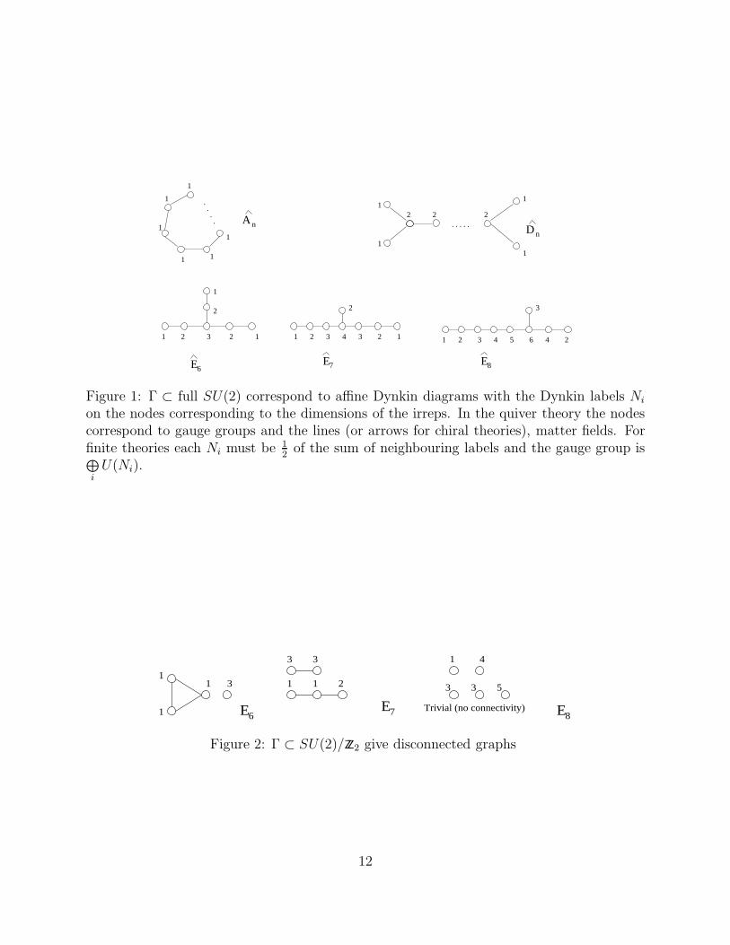
Let us digress briefly to make some mathematical observations. We recall that in the SU(2)case the matter matrices aij , due to Mckay’s theorem and Moore-Douglas quiver theories, areencoded as adjacency matrices of affine Dynkin diagrams considered as unoriented graphsas given by Figures 1 and 2.
4 Though congruence in this case really means group isomorphisms, for our purposes since only the groupcharacters concern us, in what follows we might use the term loosely to mean identical character tables.
5Of course for ZZ3, we must have a different choice for R, in particular to get a good chiral model, wetake the 3 = 1
′ ⊕ 1′′ ⊕ 1
′′′
11
7
2
2 11 3 34 2
E 8E
3
1 2 2453 64
n
1
1 1
2
2 23
6E
....
1
1
1
1 1
1
A n . . . . .
1
1
1
1
2 2 2
D
Figure 1: Γ ⊂ full SU(2) correspond to affine Dynkin diagrams with the Dynkin labels Ni
on the nodes corresponding to the dimensions of the irreps. In the quiver theory the nodescorrespond to gauge groups and the lines (or arrows for chiral theories), matter fields. Forfinite theories each Ni must be 1
2of the sum of neighbouring labels and the gauge group is⊕
iU(Ni).
7
211
33
E8E
3
Trivial (no connectivity)
1
3 3
4
5
E6
1
1
1
Figure 2: Γ ⊂ SU(2)/ZZ2 give disconnected graphs
12
3
1
1
1
3
3
3
3
3
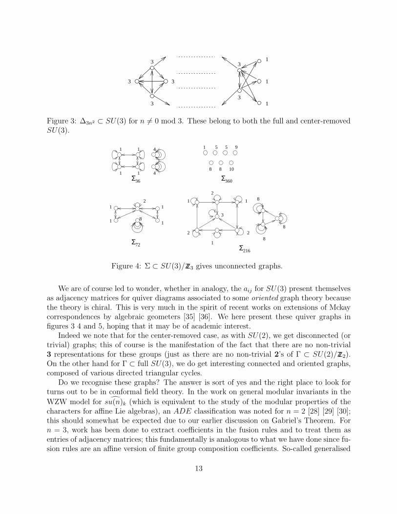
Figure 3: ∆3n2 ⊂ SU(3) for n 6= 0 mod 3. These belong to both the full and center-removedSU(3).
1 1
1 1 4
4
Σ36 Σ360
1 5 5
8
9
108
2
1
1
1
18
2
Σ72 Σ216
3
2
1 1
2
18
8
8
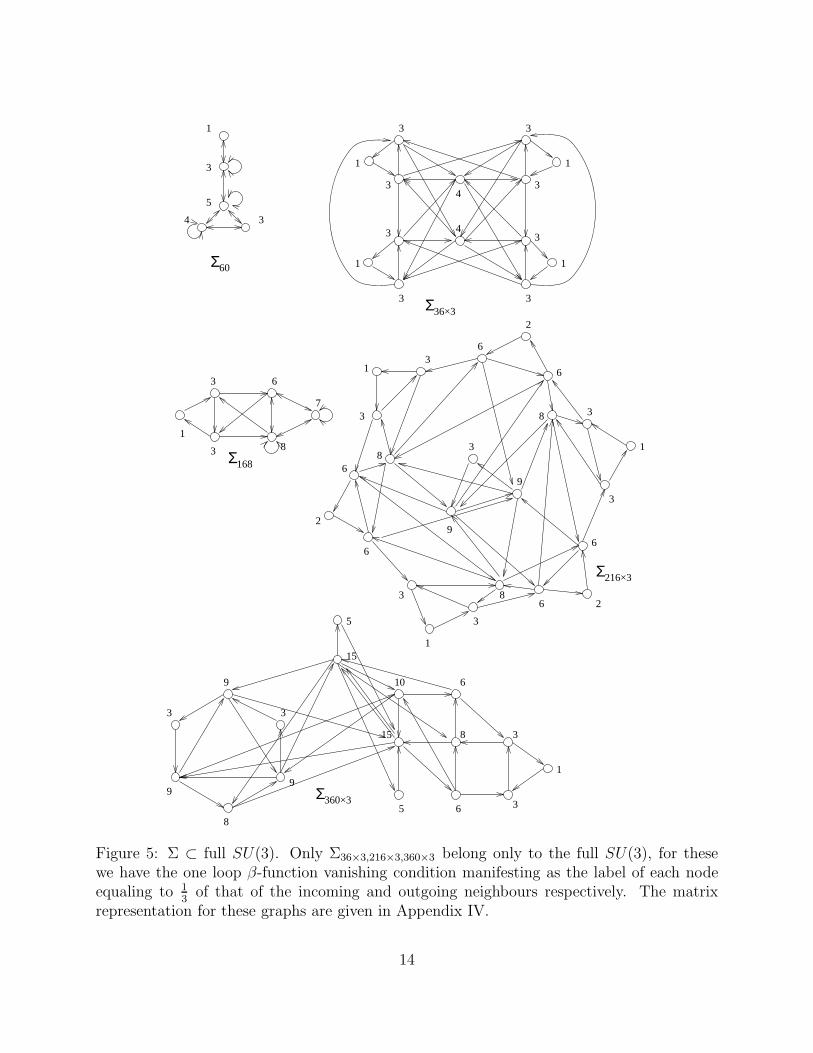
Figure 4: Σ ⊂ SU(3)/ZZ3 gives unconnected graphs.
We are of course led to wonder, whether in analogy, the aij for SU(3) present themselvesas adjacency matrices for quiver diagrams associated to some oriented graph theory becausethe theory is chiral. This is very much in the spirit of recent works on extensions of Mckaycorrespondences by algebraic geometers [35] [36]. We here present these quiver graphs infigures 3 4 and 5, hoping that it may be of academic interest.
Indeed we note that for the center-removed case, as with SU(2), we get disconnected (ortrivial) graphs; this of course is the manifestation of the fact that there are no non-trivial3 representations for these groups (just as there are no non-trivial 2’s of Γ ⊂ SU(2)/ZZ2).On the other hand for Γ ⊂ full SU(3), we do get interesting connected and oriented graphs,composed of various directed triangular cycles.
Do we recognise these graphs? The answer is sort of yes and the right place to look forturns out to be in conformal field theory. In the work on general modular invariants in the
WZW model for su(n)k (which is equivalent to the study of the modular properties of thecharacters for affine Lie algebras), an ADE classification was noted for n = 2 [28] [29] [30];this should somewhat be expected due to our earlier discussion on Gabriel’s Theorem. Forn = 3, work has been done to extract coefficients in the fusion rules and to treat them asentries of adjacency matrices; this fundamentally is analogous to what we have done since fu-sion rules are an affine version of finite group composition coefficients. So-called generalised
13
216×3
2
1
1
1
2
2
3
3
3
3
3
3
3
6
6
6
6
6
6
8
8
8
9
9
Σ
360×3
Σ36×3
1
11
1
3 3
3 3
3
3
3
3
4
4
1
3
3
6
Σ168
8
7
Σ60
1
4 3
3
5
1
3
3
3
9
9
8
9
3
5
15
15
10
6
6
8
5Σ
Figure 5: Σ ⊂ full SU(3). Only Σ36×3,216×3,360×3 belong only to the full SU(3), for thesewe have the one loop β-function vanishing condition manifesting as the label of each nodeequaling to 1
3of that of the incoming and outgoing neighbours respectively. The matrix
representation for these graphs are given in Appendix IV.
14
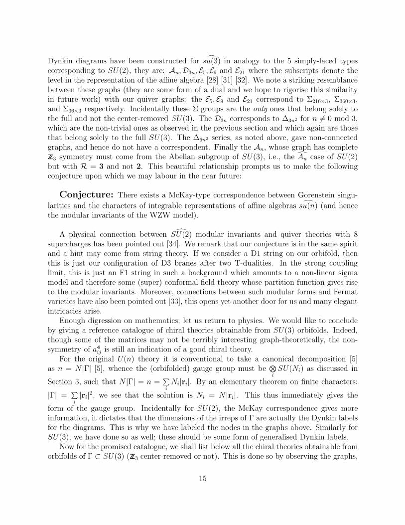
Dynkin diagrams have been constructed for su(3) in analogy to the 5 simply-laced typescorresponding to SU(2), they are: An,D3n, E5, E9 and E21 where the subscripts denote thelevel in the representation of the affine algebra [28] [31] [32]. We note a striking resemblancebetween these graphs (they are some form of a dual and we hope to rigorise this similarityin future work) with our quiver graphs: the E5, E9 and E21 correspond to Σ216×3, Σ360×3,and Σ36×3 respectively. Incidentally these Σ groups are the only ones that belong solely tothe full and not the center-removed SU(3). The D3n corresponds to ∆3n2 for n 6= 0 mod 3,which are the non-trivial ones as observed in the previous section and which again are thosethat belong solely to the full SU(3). The ∆6n2 series, as noted above, gave non-connectedgraphs, and hence do not have a correspondent. Finally the An, whose graph has completeZZ3 symmetry must come from the Abelian subgroup of SU(3), i.e., the An case of SU(2)but with R = 3 and not 2. This beautiful relationship prompts us to make the followingconjecture upon which we may labour in the near future:
Conjecture: There exists a McKay-type correspondence between Gorenstein singu-
larities and the characters of integrable representations of affine algebras su(n) (and hencethe modular invariants of the WZW model).
A physical connection between SU(2) modular invariants and quiver theories with 8supercharges has been pointed out [34]. We remark that our conjecture is in the same spiritand a hint may come from string theory. If we consider a D1 string on our orbifold, thenthis is just our configuration of D3 branes after two T-dualities. In the strong couplinglimit, this is just an F1 string in such a background which amounts to a non-linear sigmamodel and therefore some (super) conformal field theory whose partition function gives riseto the modular invariants. Moreover, connections between such modular forms and Fermatvarieties have also been pointed out [33], this opens yet another door for us and many elegantintricacies arise.
Enough digression on mathematics; let us return to physics. We would like to concludeby giving a reference catalogue of chiral theories obtainable from SU(3) orbifolds. Indeed,though some of the matrices may not be terribly interesting graph-theoretically, the non-symmetry of a4
ij is still an indication of a good chiral theory.For the original U(n) theory it is conventional to take a canonical decomposition [5]
as n = N |Γ| [5], whence the (orbifolded) gauge group must be⊗i
SU(Ni) as discussed in
Section 3, such that N |Γ| = n =∑i
Ni|ri|. By an elementary theorem on finite characters:
|Γ| =∑i|ri|
2, we see that the solution is Ni = N |ri|. This thus immediately gives the
form of the gauge group. Incidentally for SU(2), the McKay correspondence gives moreinformation, it dictates that the dimensions of the irreps of Γ are actually the Dynkin labelsfor the diagrams. This is why we have labeled the nodes in the graphs above. Similarly forSU(3), we have done so as well; these should be some form of generalised Dynkin labels.
Now for the promised catalogue, we shall list below all the chiral theories obtainable fromorbifolds of Γ ⊂ SU(3) (ZZ3 center-removed or not). This is done so by observing the graphs,
15
connected or not, that contain unidirectional arrows. For completeness, we also include thesubgroups of SU(2), which are of course also in SU(3), and which do give non-symmetricmatter matrices (which we eliminated in the N = 2 case) if we judiciously choose the 3 fromtheir representations. We use the short hand (nk1
1 , nk22 , ..., nki
i ) to denote the gauge groupk1⊕
SU(n1)...ki⊕
SU(ni). Analogous to the discussion in Section 3, the conformality conditionto one loop order in this N = 1 case, viz., Nf = 3Nc translates to the requirement that thelabel of each node must be 1
3of the sum of incoming and the sum of outgoing neighbours
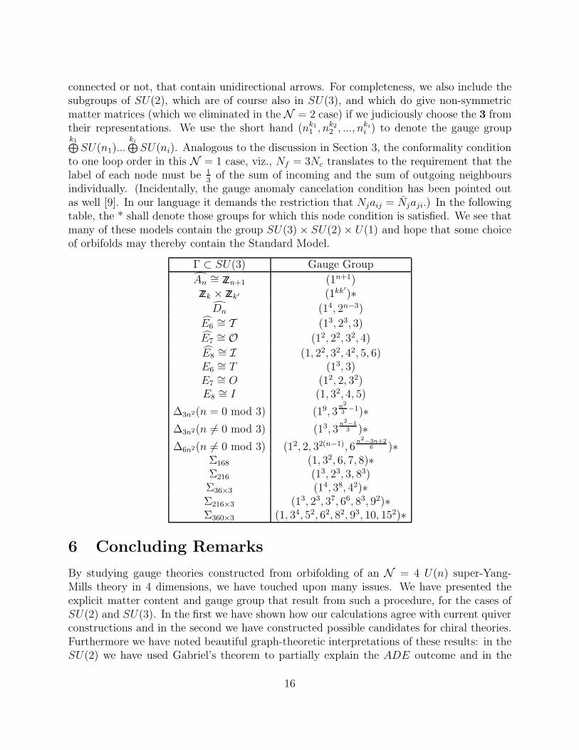
individually. (Incidentally, the gauge anomaly cancelation condition has been pointed outas well [9]. In our language it demands the restriction that Njaij = Njaji.) In the followingtable, the * shall denote those groups for which this node condition is satisfied. We see thatmany of these models contain the group SU(3) × SU(2) × U(1) and hope that some choiceof orbifolds may thereby contain the Standard Model.
Γ ⊂ SU(3) Gauge Group
An∼= ZZn+1 (1n+1)
ZZk × ZZk′ (1kk′)∗
Dn (14, 2n−3)
E6∼= T (13, 23, 3)
E7∼= O (12, 22, 32, 4)
E8∼= I (1, 22, 32, 42, 5, 6)
E6∼= T (13, 3)
E7∼= O (12, 2, 32)
E8∼= I (1, 32, 4, 5)
∆3n2(n = 0 mod 3) (19, 3n2
3−1)∗
∆3n2(n 6= 0 mod 3) (13, 3n2−1
3 )∗
∆6n2(n 6= 0 mod 3) (12, 2, 32(n−1), 6n2−3n+2
6 )∗Σ168 (1, 32, 6, 7, 8)∗Σ216 (13, 23, 3, 83)Σ36×3 (14, 38, 42)∗Σ216×3 (13, 23, 37, 66, 83, 92)∗Σ360×3 (1, 34, 52, 62, 82, 93, 10, 152)∗
6 Concluding Remarks
By studying gauge theories constructed from orbifolding of an N = 4 U(n) super-Yang-Mills theory in 4 dimensions, we have touched upon many issues. We have presented theexplicit matter content and gauge group that result from such a procedure, for the cases ofSU(2) and SU(3). In the first we have shown how our calculations agree with current quiverconstructions and in the second we have constructed possible candidates for chiral theories.Furthermore we have noted beautiful graph-theoretic interpretations of these results: in theSU(2) we have used Gabriel’s theorem to partially explain the ADE outcome and in the
16
SU(3) we have noted connections with generalised Dynkin diagrams and have conjecturedthe existence of a McKay-type correspondence between these orbifold theories and modularinvariants of WZW conformal models.
Much work of course remains. In addition to proving this conjecture, we also havenumerous questions in physics. What about SU(4), the full group? These would giveinteresting non-supersymmetric theories. How do we construct the brane box version of thesetheories? Roan has shown how the Euler character of these orbifolds correspond to the classnumbers [36]; we know the blow-up of these singularities correspond to marginal operators.Can we extract the marginal couplings and thus the duality group this way? We shall hopeto address these problems in forth-coming work. Perhaps after all, string orbifolds, gaugetheories, modular invariants of conformal field theories as well as Gorenstein singularitiesand representations of affine Lie algebras, are all manifestations of a fundamental truism.
Acknowledgements
Ad Catharinae Sanctae Alexandriae et Ad Majorem Dei Gloriam...
We like to extend our sincere gratitude to Prof. M. Artin of the Dept. of Mathematics,M.I.T., for his suggestions and especially to Prof. W. Klink of the University of Iowa forhis kind comments and input on the characters of the SU(3) subgroups. YH would alsolike to thank his collegues K. Bering, B. Feng, J. S. Song and M. B. Spradlin for valuablediscussions, M. Serna and L. Williamson for charming diversions, as well as the NSF for hergracious patronage.This work was supported by the U.S. Department of Energy under contract #DE-FC02-94ER40818.
17
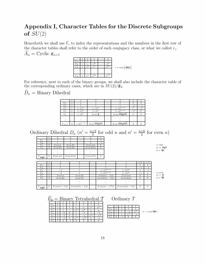
Appendix I, Character Tables for the Discrete Subgroups
of SU(2)
Henceforth we shall use Γi to index the representations and the numbers in the first row ofthe character tables shall refer to the order of each conjugacy class, or what we called rγ.
An = Cyclic ZZn+11 1 1 · · · 1
Γ1 1 1 1 · · · 1
Γ2 1 ǫ ǫ2 · · · ǫn
Γ3 1 ǫ2 ǫ4 · · · ǫ2n
.
.
.
.
.
.
.
.
.
.
.
. · · ·...
Γn 1 ǫn ǫ2n · · · ǫn2
ǫ = exp(
2πi
n+1
)
For reference, next to each of the binary groups, we shall also include the character table ofthe corresponding ordinary cases, which are in SU(2)/ZZ2.
Dn = Binary Dihedral
1 1 2 · · · 2 n nΓ1 1 1 1 · · · 1 1 1Γ2 1 1 1 · · · 1 −1 −1
Γ3 1 (−1)n (−1)1 · · · (−1)n−1 in −in
Γ4 1 (−1)n (−1)1 · · · (−1)n−1 −in in
Γ5 2 (−2)1 2 cos π
n· · · 2 cos
π(n−1)n
0 0
.
.
.
.
.
.
.
.
. · · ·...
.
.
.
.
.
.
.
.
.
Γn+1 2 (−2)n−1 2 cosπ(n−1)
n· · · 2 cos
π(n−1)2
n0 0
Ordinary Dihedral Dn (n′ = n+32 for odd n and n′ = n+6
2 for even n)1 2 2 · · · 2 n
Γ1 1 1 1 · · · 1 1Γ2 1 1 1 · · · 1 −1Γ3 2 2 cos φ 2 cos 2φ · · · 2 cos mφ 0Γ4 2 2 cos 2φ 2 cos 4φ · · · 2 cos 2mφ 0
.
.
.
.
.
.
.
.
.
.
.
. · · ·...
.
.
.
Γ n+32
2 2 cos mφ 2 cos 2mφ · · · 2 cos m2φ 0
n odd
m = n−12
φ = 2π
n
1 2 2 · · · 2 1 n/2 n/2Γ1 1 1 1 · · · 1 1 1 1Γ2 1 1 1 · · · 1 1 −1 −1
Γ3 1 −1 1 · · · (−1)m−1 (−1)m 1 −1
Γ4 1 −1 1 · · · (−1)m−1 (−1)m −1 1Γ5 2 2 cos φ 2 cos 2φ · · · 2 cos(m − 1)φ 2 cos mφ 0 0Γ6 2 2 cos 2φ 2 cos 4φ · · · 2 cos 2(m − 1)φ 2 cos 2mφ 0 0
.
.
.
.
.
.
.
.
.
.
.
. · · ·...
.
.
.
.
.
.
.
.
.
Γ n+62
2 2 cos(m − 1)φ 2 cos 2(m − 1)φ · · · 2 cos(m − 1)2φ 2 cos m(m − 1)φ 0 0
n evenm = n
2φ = 2π
n
E6 = Binary Tetrahedral T Ordinary T1 1 6 4 4 4 4
Γ1 1 1 1 1 1 1 1
Γ2 1 1 1 w w w2 w2
Γ3 1 1 1 w2 w2 w wΓ4 2 −2 0 1 −1 1 −1
Γ5 2 −2 0 w −w w2 −w2
Γ6 2 −2 0 w2 −w2 w −wΓ7 3 3 −1 0 0 0 0
1 3 4 4Γ1 1 1 1 1
Γ2 1 1 −w w2
Γ3 1 1 w2 −wΓ4 3 −1 0 0
w = exp( 2πi
3)
18
E7 = Binary Octahedral O Ordinary O1 1 2 6 6 8 8 16
Γ1 1 1 1 1 1 1 1 1Γ2 1 1 −3 −1 −1 1 1 0
Γ3 2 −2 0√
2 −√
2 1 −1 0
Γ4 2 −2 0 −√
2√
2 1 −1 0Γ5 2 2 −2 0 0 −1 −1 1Γ6 3 3 −1 1 1 0 0 −1Γ7 3 3 −3 −1 −1 0 0 0Γ8 4 −4 0 0 0 −1 1 0
1 3 6 6 8Γ1 1 1 1 1 1Γ2 1 1 −1 −1 1Γ3 2 2 0 0 −1Γ4 3 −1 −1 1 0Γ5 3 −1 1 −1 0
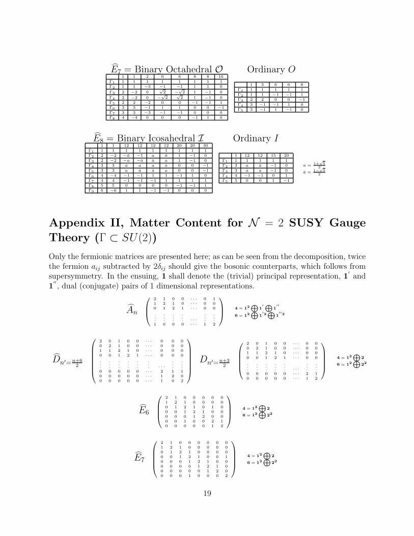
E8 = Binary Icosahedral I Ordinary I1 1 12 12 12 12 20 20 30
Γ1 1 1 1 1 1 1 1 1 1Γ2 2 −2 −a −1 a a 1 −1 0Γ3 2 −2 −a −a a a 1 −1 0Γ4 3 3 a a a a 0 0 −1Γ5 3 3 a a a a 0 0 −1Γ6 4 −4 −1 −1 1 1 −1 1 0Γ7 4 4 −1 −1 −1 1 1 1 1Γ8 5 5 0 0 0 0 −1 −1 1Γ9 6 −6 1 1 −1 −1 0 0 0
1 12 12 15 20Γ1 1 1 1 1 1Γ2 3 a a −1 0Γ3 3 a a −1 0Γ4 4 −1 −1 0 1Γ5 5 0 0 1 −1
a = 1+√
52
a = 1−√
52
Appendix II, Matter Content for N = 2 SUSY Gauge
Theory (Γ ⊂ SU(2))
Only the fermionic matrices are presented here; as can be seen from the decomposition, twicethe fermion aij subtracted by 2δij should give the bosonic counterparts, which follows fromsupersymmetry. In the ensuing, 1 shall denote the (trivial) principal representation, 1
′and
1′′, dual (conjugate) pairs of 1 dimensional representations.
An
2 1 0 0 · · · 0 11 2 1 0 · · · 0 00 1 2 1 · · · 0 0
.
.
.
.
.
.
.
.
.
.
.
. · · ·...
.
.
.1 0 0 0 · · · 1 2
4 = 1
2⊕
1′⊕
1′′
6 = 12⊕
1′2⊕
1′′2
Dn′=n+6
2
2 0 1 0 0 · · · 0 0 00 2 1 0 0 · · · 0 0 01 1 2 1 0 · · · 0 0 00 0 1 2 1 · · · 0 0 0
.
.
.
.
.
.
.
.
.
.
.
.
.
.
.
.
.
. · · ·...
.
.
.0 0 0 0 0 · · · 2 1 10 0 0 0 0 · · · 1 2 00 0 0 0 0 · · · 1 0 2
Dn′=n+3
2
2 0 1 0 0 · · · 0 00 2 1 0 0 · · · 0 01 1 2 1 0 · · · 0 00 0 1 2 1 · · · 0 0
.
.
.
.
.
.
.
.
.
.
.
.
.
.
. · · ·...
.
.
.0 0 0 0 0 · · · 2 10 0 0 0 0 · · · 1 2
4 = 12⊕
2
6 = 12⊕
22
E6
2 1 0 0 0 0 01 2 1 0 0 0 00 1 2 1 0 1 00 0 1 2 1 0 00 0 0 1 2 0 00 0 1 0 0 2 10 0 0 0 0 1 2
4 = 12⊕
2
6 = 12⊕
22
E7
2 1 0 0 0 0 0 01 2 1 0 0 0 0 00 1 2 1 0 0 0 00 0 1 2 1 0 0 10 0 0 1 2 1 0 00 0 0 0 1 2 1 00 0 0 0 0 1 2 00 0 0 1 0 0 0 2
4 = 12⊕
2
6 = 12⊕
22
19
E8
2 1 0 0 0 0 0 0 01 2 1 0 0 0 0 0 00 1 2 1 0 0 0 0 00 0 1 2 1 0 0 0 00 0 0 1 2 1 0 0 00 0 0 0 1 2 1 0 10 0 0 0 0 1 2 1 00 0 0 0 0 0 1 2 00 0 0 0 0 1 0 0 2
4 = 12⊕
2
6 = 12⊕
22
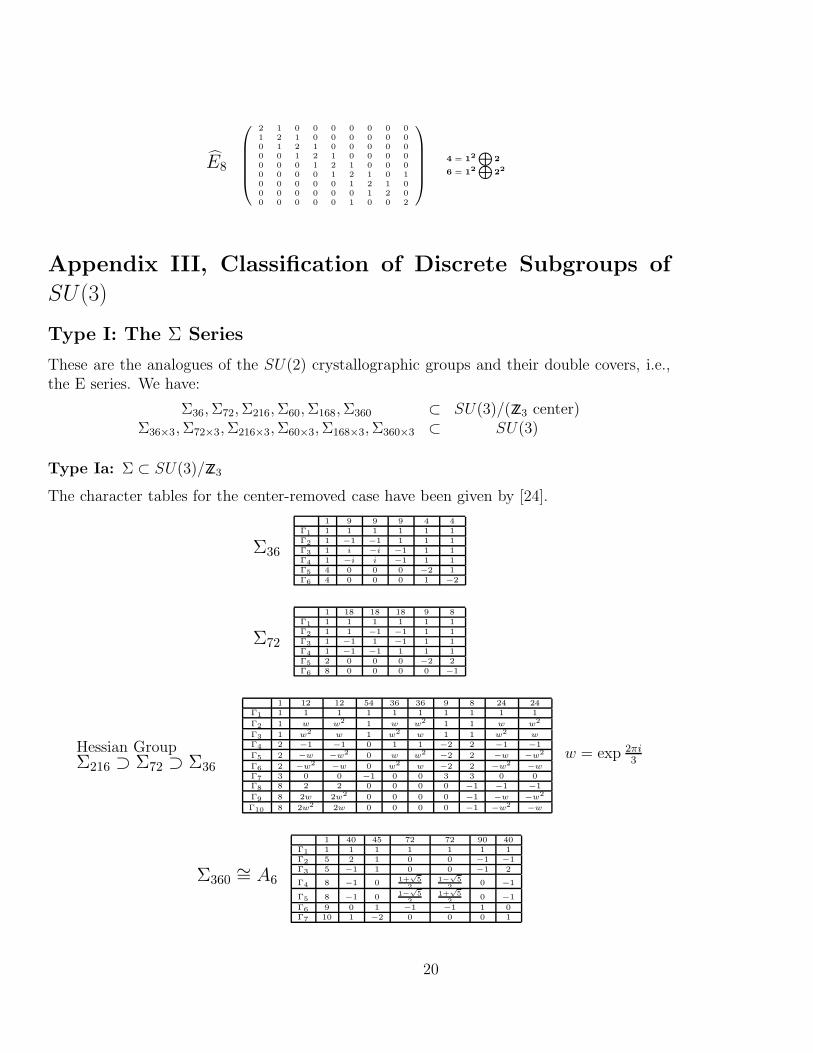
Appendix III, Classification of Discrete Subgroups of
SU(3)
Type I: The Σ Series
These are the analogues of the SU(2) crystallographic groups and their double covers, i.e.,the E series. We have:
Σ36, Σ72, Σ216, Σ60, Σ168, Σ360 ⊂ SU(3)/(ZZ3 center)Σ36×3, Σ72×3, Σ216×3, Σ60×3, Σ168×3, Σ360×3 ⊂ SU(3)
Type Ia: Σ ⊂ SU(3)/ZZ3
The character tables for the center-removed case have been given by [24].
Σ36
1 9 9 9 4 4Γ1 1 1 1 1 1 1Γ2 1 −1 −1 1 1 1Γ3 1 i −i −1 1 1Γ4 1 −i i −1 1 1Γ5 4 0 0 0 −2 1Γ6 4 0 0 0 1 −2
Σ72
1 18 18 18 9 8Γ1 1 1 1 1 1 1Γ2 1 1 −1 −1 1 1Γ3 1 −1 1 −1 1 1Γ4 1 −1 −1 1 1 1Γ5 2 0 0 0 −2 2Γ6 8 0 0 0 0 −1
Hessian GroupΣ216 ⊃ Σ72 ⊃ Σ36
1 12 12 54 36 36 9 8 24 24Γ1 1 1 1 1 1 1 1 1 1 1
Γ2 1 w w2 1 w w2 1 1 w w2
Γ3 1 w2 w 1 w2 w 1 1 w2 wΓ4 2 −1 −1 0 1 1 −2 2 −1 −1
Γ5 2 −w −w2 0 w w2 −2 2 −w −w2
Γ6 2 −w2 −w 0 w2 w −2 2 −w2 −wΓ7 3 0 0 −1 0 0 3 3 0 0Γ8 8 2 2 0 0 0 0 −1 −1 −1
Γ9 8 2w 2w2 0 0 0 0 −1 −w −w2
Γ10 8 2w2 2w 0 0 0 0 −1 −w2 −w
w = exp 2πi3
Σ360∼= A6
1 40 45 72 72 90 40Γ1 1 1 1 1 1 1 1Γ2 5 2 1 0 0 −1 −1Γ3 5 −1 1 0 0 −1 2
Γ4 8 −1 0 1+√
52
1−√
52
0 −1
Γ5 8 −1 0 1−√
52
1+√
52
0 −1
Γ6 9 0 1 −1 −1 1 0Γ7 10 1 −2 0 0 0 1
20
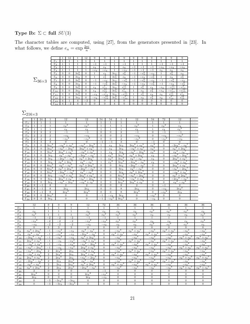
Type Ib: Σ ⊂ full SU(3)
The character tables are computed, using [27], from the generators presented in [23]. Inwhat follows, we define en = exp 2πi
n.
Σ36×3
1 12 1 12 9 9 1 9 9 9 9 9 9 9Γ1 1 1 1 1 1 1 1 1 1 1 1 1 1 1Γ2 1 1 1 1 −1 −1 1 −1 1 1 1 −1 −1 −1Γ3 1 1 1 1 e4 e4 1 e4 −1 −1 −1 −e4 −e4 −e4Γ4 1 1 1 1 −e4 −e4 1 −e4 −1 −1 −1 e4 e4 e4
Γ5 3 0 3e23 0 1 e3 3e3 e2
3 −1 −e23 −e3 1 e2
3 e3
Γ6 3 0 3e3 0 1 e23 3e2
3 e3 −1 −e3 −e23 1 e3 e2
3Γ7 3 0 3e2
3 0 −1 −e3 3e3 −e23 −1 −e2
3 −e3 −1 −e23 −e3
Γ8 3 0 3e3 0 −1 −e23 3e2
3 −e3 −1 −e3 −e23 −1 −e3 −e2
3Γ9 3 0 3e2
3 0 e4 e712 3e3 e11
12 1 e23 e3 −e4 −e11
12 −e712
Γ10 3 0 3e3 0 e4 e1112 3e2
3 e712 1 e3 e2
3 −e4 −e712 −e11
12Γ11 3 0 3e2
3 0 −e4 −e712 3e3 −e11
12 1 e23 e3 e4 e11
12 e712
Γ12 3 0 3e3 0 −e4 −e1112 3e2
3 −e712 1 e3 e2
3 e4 e712 e11
12Γ13 4 1 4 −2 0 0 4 0 0 0 0 0 0 0Γ14 4 −2 4 1 0 0 4 0 0 0 0 0 0 0
Σ216×31 24 1 12 12 54 54 1 12 54 72 12 · · ·
Γ1 1 1 1 1 1 1 1 1 1 1 1 1 · · ·Γ2 1 1 1 e3
2 e32 1 1 1 e3
2 1 e32 e3 · · ·
Γ3 1 1 1 e3 e3 1 1 1 e3 1 e3 e32 · · ·
Γ4 2 2 2 −1 −1 0 0 2 −1 0 −1 −1 · · ·Γ5 2 2 2 −e3 −e3 0 0 2 −e3 0 −e3 −e3
2 · · ·Γ6 2 2 2 −e3
2 −e32 0 0 2 −e3
2 0 −e32 −e3 · · ·
Γ7 3 3 3 0 0 −1 −1 3 0 −1 0 0 · · ·Γ8 3 0 3e3
2 −e92 + e9
5 −e92 − 2e9
5 1 e3 3e3 2e92 + e9
5 e32 0 −2e9
4 − e97 · · ·
Γ9 3 0 3e32 −e9
2 − 2e95 2e9
2 + e95 1 e3 3e3 −e9
2 + e95 e3
2 0 e94 + 2e9
7 · · ·Γ10 3 0 3e3
2 2e92 + e9
5 −e92 + e9
5 1 e3 3e3 −e92 − 2e9
5 e32 0 e9
4 − e97 · · ·
Γ11 3 0 3e3 e94 − e9
7 −2e94 − e9
7 1 e32 3e3
2 e94 + 2e9
7 e3 0 −e92 − 2e9
5 · · ·Γ12 3 0 3e3 −2e9
4 − e97 e9
4 + 2e97 1 e3
2 3e32 e9
4 − e97 e3 0 2e9
2 + e95 · · ·
Γ13 3 0 3e3 e94 + 2e9
7 e94 − e9
7 1 e32 3e3
2 −2e94 − e9
7 e3 0 −e92 + e9
5 · · ·Γ14 6 0 6e3
2 e92 − e9
5 e92 + 2e9
5 0 0 6e3 −2e92 − e9
5 0 0 2e94 + e9
7 · · ·Γ15 6 0 6e3
2 e92 + 2e9
5 −2e92 − e9
5 0 0 6e3 e92 − e9
5 0 0 −e94 − 2e9
7 · · ·Γ16 6 0 6e3
2 −2e92 − e9
5 e92 − e9
5 0 0 6e3 e92 + 2e9
5 0 0 −e94 + e9
7 · · ·Γ17 6 0 6e3 −e9
4 + e97 2e9
4 + e97 0 0 6e3
2 −e94 − 2e9
7 0 0 e92 + 2e9
5 · · ·Γ18 6 0 6e3 2e9
4 + e97 −e9
4 − 2e97 0 0 6e3
2 −e94 + e9
7 0 0 −2e92 − e9
5 · · ·Γ19 6 0 6e3 −e9
4 − 2e97 −e9
4 + e97 0 0 6e3
2 2e94 + e9
7 0 0 e92 − e9
5 · · ·Γ20 8 −1 8 2 2 0 0 8 2 0 −1 2 · · ·Γ21 8 −1 8 2e3 2e3 0 0 8 2e3 0 −e3 2e3
2 · · ·Γ22 8 −1 8 2e3
2 2e32 0 0 8 2e3
2 0 −e32 2e3 · · ·
Γ23 9 0 9e32 0 0 −1 −e3 9e3 0 −e3
2 0 0 · · ·Γ24 9 0 9e3 0 0 −1 −e3
2 9e32 0 −e3 0 0 · · ·
12 9 9 9 12 72 36 36 36 36 36 36Γ1 1 1 1 1 1 1 1 1 1 1 1 1
Γ2 e3 1 1 1 e3 e3 e3 e3 e32 e3
2 e32 e3
Γ3 e32 1 1 1 e3
2 e32 e3
2 e32 e3 e3 e3 e3
2
Γ4 −1 −2 −2 −2 −1 −1 1 1 1 1 1 1
Γ5 −e32 −2 −2 −2 −e3
2 −e32 e3
2 e32 e3 e3 e3 e3
2
Γ6 −e3 −2 −2 −2 −e3 −e3 e3 e3 e32 e3
2 e32 e3
Γ7 0 3 3 3 0 0 0 0 0 0 0 0
Γ8 e94 + 2e9
7 −1 −e32 −e3 e9
4 − e97 0 −e9
4 e94 + e9
7 −e95 e9
2 + e95 −e9
2 −e97
Γ9 e94 − e9
7 −1 −e32 −e3 −2e9
4 − e97 0 e9
4 + e97 −e9
7 e92 + e9
5 −e92 −e9
5 −e94
Γ10 −2e94 − e9
7 −1 −e32 −e3 e9
4 + 2e97 0 −e9
7 −e94 −e9
2 −e95 e9
2 + e95 e9
4 + e97
Γ11 2e92 + e9
5 −1 −e3 −e32 −e9
2 + e95 0 −e9
5 e92 + e9
5 −e94 e9
4 + e97 −e9
7 −e92
Γ12 −e92 + e9
5 −1 −e3 −e32 −e9
2 − 2e95 0 e9
2 + e95 −e9
2 e94 + e9
7 −e97 −e9
4 −e95
Γ13 −e92 − 2e9
5 −1 −e3 −e32 2e9
2 + e95 0 −e9
2 −e95 −e9
7 −e94 e9
4 + e97 e9
2 + e95
Γ14 −e94 − 2e9
7 2 2e32 2e3 −e9
4 + e97 0 −e9
4 e94 + e9
7 −e95 e9
2 + e95 −e9
2 −e97
Γ15 −e94 + e9
7 2 2e32 2e3 2e9
4 + e97 0 e9
4 + e97 −e9
7 e92 + e9
5 −e92 −e9
5 −e94
Γ16 2e94 + e9
7 2 2e32 2e3 −e9
4 − 2e97 0 −e9
7 −e94 −e9
2 −e95 e9
2 + e95 e9
4 + e97
Γ17 −2e92 − e9
5 2 2e3 2e32 e9
2 − e95 0 −e9
5 e92 + e9
5 −e94 e9
4 + e97 −e9
7 −e92
Γ18 e92 − e9
5 2 2e3 2e32 e9
2 + 2e95 0 e9
2 + e95 −e9
2 e94 + e9
7 −e97 −e9
4 −e95
Γ19 e92 + 2e9
5 2 2e3 2e32 −2e9
2 − e95 0 −e9
2 −e95 −e9
7 −e94 e9
4 + e97 e9
2 + e95
Γ20 2 0 0 0 2 −1 0 0 0 0 0 0
Γ21 2e32 0 0 0 2e3
2 −e32 0 0 0 0 0 0
Γ22 2e3 0 0 0 2e3 −e3 0 0 0 0 0 0
Γ23 0 −3 −3e32 −3e3 0 0 0 0 0 0 0 0
Γ24 0 −3 −3e3 −3e32 0 0 0 0 0 0 0 0
21
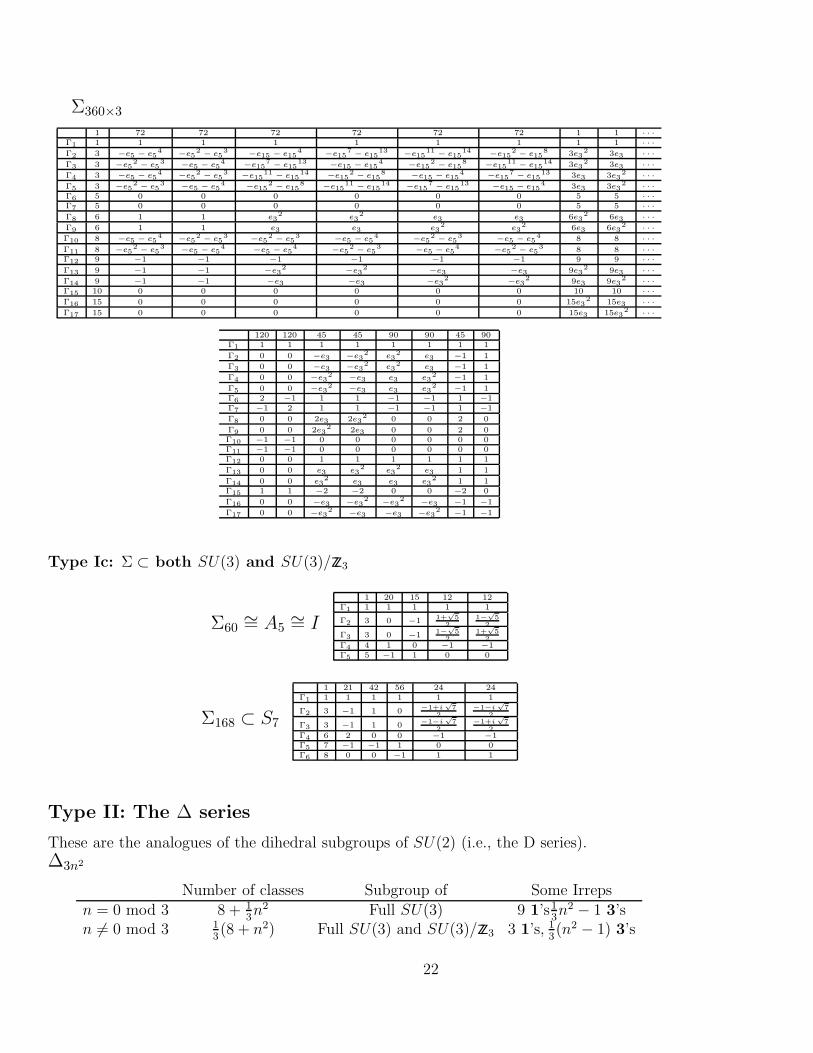
Σ360×3
1 72 72 72 72 72 72 1 1 · · ·Γ1 1 1 1 1 1 1 1 1 1 · · ·Γ2 3 −e5 − e5
4 −e52 − e5
3 −e15 − e154 −e15
7 − e1513 −e15
11 − e1514 −e15
2 − e158 3e3
2 3e3 · · ·Γ3 3 −e5
2 − e53 −e5 − e5
4 −e157 − e15
13 −e15 − e154 −e15
2 − e158 −e15
11 − e1514 3e3
2 3e3 · · ·Γ4 3 −e5 − e5
4 −e52 − e5
3 −e1511 − e15
14 −e152 − e15
8 −e15 − e154 −e15
7 − e1513 3e3 3e3
2 · · ·Γ5 3 −e5
2 − e53 −e5 − e5
4 −e152 − e15
8 −e1511 − e15
14 −e157 − e15
13 −e15 − e154 3e3 3e3
2 · · ·Γ6 5 0 0 0 0 0 0 5 5 · · ·Γ7 5 0 0 0 0 0 0 5 5 · · ·Γ8 6 1 1 e3
2 e32 e3 e3 6e3
2 6e3 · · ·Γ9 6 1 1 e3 e3 e3
2 e32 6e3 6e3
2 · · ·Γ10 8 −e5 − e5
4 −e52 − e5
3 −e52 − e5
3 −e5 − e54 −e5
2 − e53 −e5 − e5
4 8 8 · · ·Γ11 8 −e5
2 − e53 −e5 − e5
4 −e5 − e54 −e5
2 − e53 −e5 − e5
4 −e52 − e5
3 8 8 · · ·Γ12 9 −1 −1 −1 −1 −1 −1 9 9 · · ·Γ13 9 −1 −1 −e3
2 −e32 −e3 −e3 9e3
2 9e3 · · ·Γ14 9 −1 −1 −e3 −e3 −e3
2 −e32 9e3 9e3
2 · · ·Γ15 10 0 0 0 0 0 0 10 10 · · ·Γ16 15 0 0 0 0 0 0 15e3
2 15e3 · · ·Γ17 15 0 0 0 0 0 0 15e3 15e3
2 · · ·
120 120 45 45 90 90 45 90Γ1 1 1 1 1 1 1 1 1
Γ2 0 0 −e3 −e32 e3
2 e3 −1 1
Γ3 0 0 −e3 −e32 e3
2 e3 −1 1
Γ4 0 0 −e32 −e3 e3 e3
2 −1 1
Γ5 0 0 −e32 −e3 e3 e3
2 −1 1Γ6 2 −1 1 1 −1 −1 1 −1Γ7 −1 2 1 1 −1 −1 1 −1
Γ8 0 0 2e3 2e32 0 0 2 0
Γ9 0 0 2e32 2e3 0 0 2 0
Γ10 −1 −1 0 0 0 0 0 0Γ11 −1 −1 0 0 0 0 0 0Γ12 0 0 1 1 1 1 1 1
Γ13 0 0 e3 e32 e3
2 e3 1 1
Γ14 0 0 e32 e3 e3 e3
2 1 1Γ15 1 1 −2 −2 0 0 −2 0
Γ16 0 0 −e3 −e32 −e3
2 −e3 −1 −1
Γ17 0 0 −e32 −e3 −e3 −e3
2 −1 −1
Type Ic: Σ ⊂ both SU(3) and SU(3)/ZZ3
Σ60∼= A5
∼= I
1 20 15 12 12Γ1 1 1 1 1 1
Γ2 3 0 −1 1+√
52
1−√
52
Γ3 3 0 −1 1−√
52
1+√
52
Γ4 4 1 0 −1 −1Γ5 5 −1 1 0 0
Σ168 ⊂ S7
1 21 42 56 24 24Γ1 1 1 1 1 1 1
Γ2 3 −1 1 0−1+i
√7
2−1−i
√7
2
Γ3 3 −1 1 0 −1−i√
72
−1+i√
72
Γ4 6 2 0 0 −1 −1Γ5 7 −1 −1 1 0 0Γ6 8 0 0 −1 1 1
Type II: The ∆ series
These are the analogues of the dihedral subgroups of SU(2) (i.e., the D series).∆3n2
Number of classes Subgroup of Some Irrepsn = 0 mod 3 8 + 1
3n2 Full SU(3) 9 1’s1
3n2 − 1 3’s
n 6= 0 mod 3 13(8 + n2) Full SU(3) and SU(3)/ZZ3 3 1’s, 1
3(n2 − 1) 3’s
22
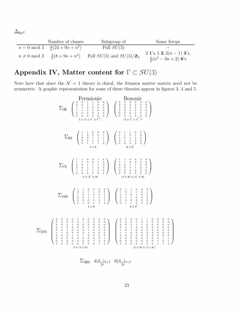
∆6n2
Number of classes Subgroup of Some Irrepsn = 0 mod 3 1
6(24 + 9n + n2) Full SU(3) −
n 6= 0 mod 3 16(8 + 9n + n2) Full SU(3) and SU(3)/ZZ3
2 1’s, 1 2, 2(n − 1) 3’s,16(n2 − 3n + 2) 6’s
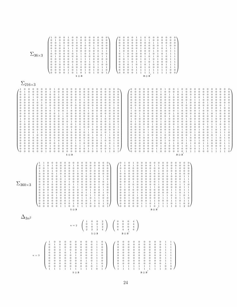
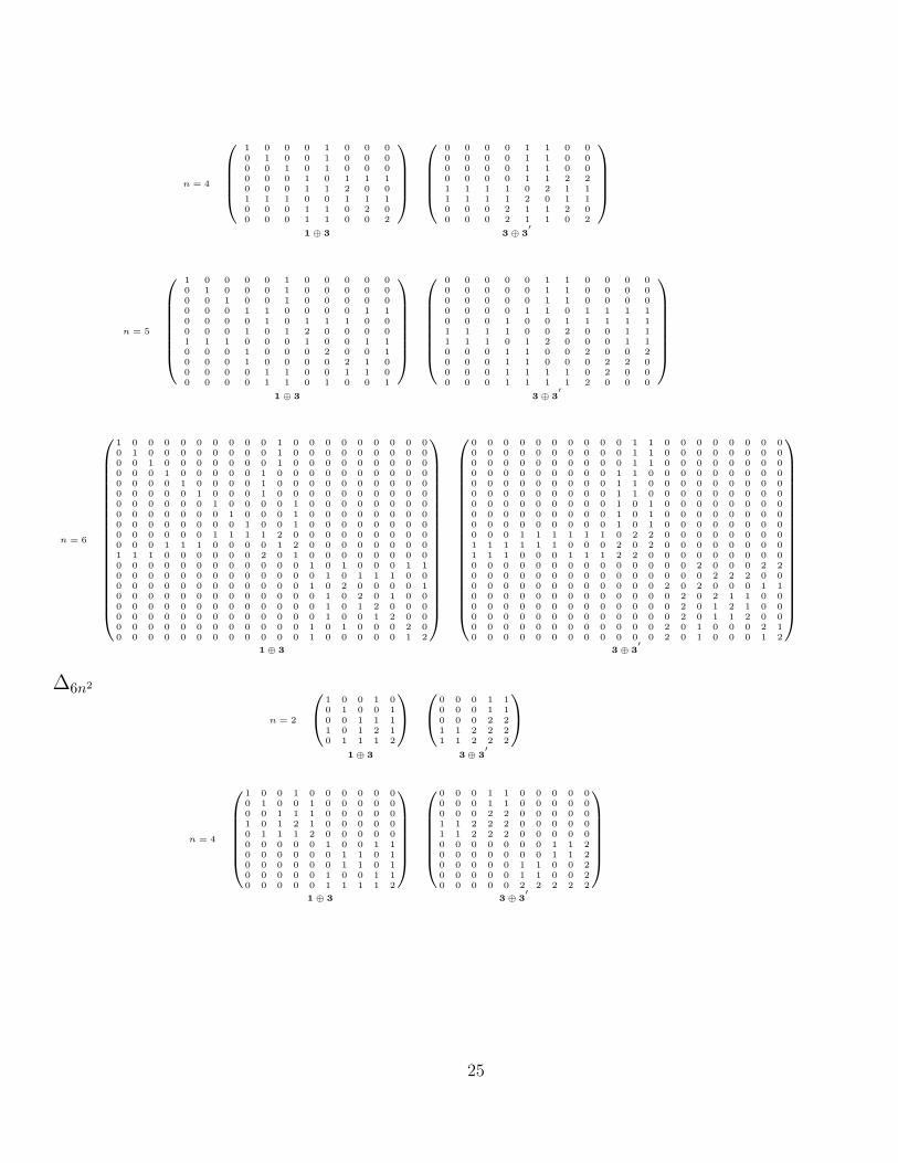
Appendix IV, Matter content for Γ ⊂ SU(3)
Note here that since the N = 1 theory is chiral, the fermion matter matrix need not besymmetric. A graphic representation for some of these theories appear in figures 3, 4 and 5.
Fermionic Bosonic
Σ36
2 0 1 1 0 00 2 1 1 0 01 1 2 0 0 01 1 0 2 0 00 0 0 0 4 00 0 0 0 0 4
2 0 2 2 0 00 2 2 2 0 02 2 2 0 0 02 2 0 2 0 00 0 0 0 6 00 0 0 0 0 6
1 ⊕ (1 ⊕ 1′⊕ 1
′′) (1 ⊕ 1
′⊕ 1
′′)2
Σ60
1 1 0 0 01 2 0 0 10 0 1 1 10 0 1 2 10 1 1 1 2
0 1 1 0 01 1 0 1 21 0 1 1 20 1 1 2 20 2 2 2 2
1 ⊕ 3 3 ⊕ 3′
Σ72
1 1 0 0 1 01 1 0 0 1 00 0 1 1 1 00 0 1 1 1 01 1 1 1 2 00 0 0 0 0 4
1 1 0 0 2 01 1 0 0 2 00 0 1 1 2 00 0 1 1 2 02 2 2 2 2 00 0 0 0 0 6
1 ⊕ (1′⊕ 2) (1 ⊕ 2) ⊕ (1
′⊕ 2)
Σ168
1 1 0 0 0 00 1 1 1 0 01 0 1 0 0 10 0 1 1 1 10 0 0 1 2 10 1 0 1 1 2
0 1 1 0 0 01 0 1 1 0 11 1 0 1 0 10 1 1 0 2 20 0 0 2 2 20 1 1 2 2 2
1 ⊕ 3 3 ⊕ 3′
Σ216
2 0 0 0 1 0 0 0 0 00 2 0 0 0 1 0 0 0 00 0 2 1 0 0 0 0 0 00 1 0 2 0 0 1 0 0 00 0 1 0 2 0 1 0 0 01 1 0 0 0 2 1 0 0 00 0 0 1 1 1 2 0 0 00 0 0 0 0 0 0 3 0 10 0 0 0 0 0 0 1 3 00 0 0 0 0 0 0 0 1 3
2 0 0 0 1 1 0 0 0 00 2 0 1 0 1 0 0 0 00 0 2 1 1 0 0 0 0 00 1 1 2 0 0 2 0 0 01 0 1 0 2 0 2 0 0 01 1 0 0 0 2 2 0 0 00 0 0 2 2 2 2 0 0 00 0 0 0 0 0 0 4 1 10 0 0 0 0 0 0 1 4 10 0 0 0 0 0 0 1 1 4
1 ⊕ (1 ⊕ 2) (1 ⊕ 2) ⊕ (1 ⊕ 2′)
Σ360 4(δij)7×7 6(δij)7×714
16
23
Σ36×3
1 0 0 0 1 0 0 0 0 0 0 0 0 00 1 0 0 0 0 1 0 0 0 0 0 0 00 0 1 0 0 0 0 0 1 0 0 0 0 00 0 0 1 0 0 0 0 0 0 1 0 0 00 0 0 0 1 1 0 0 0 1 0 1 0 01 0 0 0 0 1 0 0 0 0 0 0 1 10 0 0 0 0 0 1 1 0 1 0 1 0 00 1 0 0 0 0 0 1 0 0 0 0 1 10 0 0 0 0 1 0 1 1 1 0 0 0 00 0 1 0 0 0 0 0 0 1 0 0 1 10 0 0 0 0 1 0 1 0 0 1 1 0 00 0 0 1 0 0 0 0 0 0 0 1 1 10 0 0 0 1 0 1 0 1 0 1 0 1 00 0 0 0 1 0 1 0 1 0 1 0 0 1
0 0 0 0 1 1 0 0 0 0 0 0 0 00 0 0 0 0 0 1 1 0 0 0 0 0 00 0 0 0 0 0 0 0 1 1 0 0 0 00 0 0 0 0 0 0 0 0 0 1 1 0 01 0 0 0 0 1 0 0 0 1 0 1 1 11 0 0 0 1 0 0 0 1 0 1 0 1 10 1 0 0 0 0 0 1 0 1 0 1 1 10 1 0 0 0 0 1 0 1 0 1 0 1 10 0 1 0 0 1 0 1 0 1 0 0 1 10 0 1 0 1 0 1 0 1 0 0 0 1 10 0 0 1 0 1 0 1 0 0 0 1 1 10 0 0 1 1 0 1 0 0 0 1 0 1 10 0 0 0 1 1 1 1 1 1 1 1 0 00 0 0 0 1 1 1 1 1 1 1 1 0 0
1 ⊕ 3 3 ⊕ 3′
Σ216×3
1 0 0 0 0 0 0 0 1 0 0 0 0 0 0 0 0 0 0 0 0 0 0 00 1 0 0 0 0 0 1 0 0 0 0 0 0 0 0 0 0 0 0 0 0 0 00 0 1 0 0 0 0 0 0 1 0 0 0 0 0 0 0 0 0 0 0 0 0 00 0 0 1 0 0 0 0 0 0 0 0 0 0 1 0 0 0 0 0 0 0 0 00 0 0 0 1 0 0 0 0 0 0 0 0 0 0 1 0 0 0 0 0 0 0 00 0 0 0 0 1 0 0 0 0 0 0 0 1 0 0 0 0 0 0 0 0 0 00 0 0 0 0 0 1 0 0 0 0 0 0 0 0 0 0 0 0 0 0 0 1 00 0 0 0 0 0 0 1 0 0 0 0 1 0 0 0 0 1 0 0 0 0 0 00 0 0 0 0 0 0 0 1 0 0 1 0 0 0 0 1 0 0 0 0 0 0 00 0 0 0 0 0 0 0 0 1 1 0 0 0 0 0 0 0 1 0 0 0 0 00 0 1 0 0 0 0 0 0 0 1 0 0 0 0 0 0 0 0 0 1 0 0 01 0 0 0 0 0 0 0 0 0 0 1 0 0 0 0 0 0 0 1 0 0 0 00 1 0 0 0 0 0 0 0 0 0 0 1 0 0 0 0 0 0 0 0 1 0 00 0 0 0 0 0 0 0 0 0 0 1 0 1 0 0 0 0 1 0 0 0 0 10 0 0 0 0 0 0 0 0 0 1 0 0 0 1 0 0 1 0 0 0 0 0 10 0 0 0 0 0 0 0 0 0 0 0 1 0 0 1 1 0 0 0 0 0 0 10 0 0 0 1 0 0 0 0 0 0 0 0 0 0 0 1 0 0 1 0 1 0 00 0 0 1 0 0 0 0 0 0 0 0 0 0 0 0 0 1 0 0 1 1 0 00 0 0 0 0 1 0 0 0 0 0 0 0 0 0 0 0 0 1 1 1 0 0 00 0 0 0 0 0 0 0 1 0 0 0 0 1 0 1 0 0 0 1 0 0 1 00 0 0 0 0 0 0 0 0 1 0 0 0 1 1 0 0 0 0 0 1 0 1 00 0 0 0 0 0 0 1 0 0 0 0 0 0 1 1 0 0 0 0 0 1 1 00 0 0 0 0 0 0 0 0 0 0 0 0 0 0 0 1 1 1 0 0 0 1 10 0 0 0 0 0 1 0 0 0 0 0 0 0 0 0 0 0 0 1 1 1 0 1
0 0 0 0 0 0 0 0 1 0 0 1 0 0 0 0 0 0 0 0 0 0 0 00 0 0 0 0 0 0 1 0 0 0 0 1 0 0 0 0 0 0 0 0 0 0 00 0 0 0 0 0 0 0 0 1 1 0 0 0 0 0 0 0 0 0 0 0 0 00 0 0 0 0 0 0 0 0 0 0 0 0 0 1 0 0 1 0 0 0 0 0 00 0 0 0 0 0 0 0 0 0 0 0 0 0 0 1 1 0 0 0 0 0 0 00 0 0 0 0 0 0 0 0 0 0 0 0 1 0 0 0 0 1 0 0 0 0 00 0 0 0 0 0 0 0 0 0 0 0 0 0 0 0 0 0 0 0 0 0 1 10 1 0 0 0 0 0 0 0 0 0 0 1 0 0 0 0 1 0 0 0 1 0 01 0 0 0 0 0 0 0 0 0 0 1 0 0 0 0 1 0 0 1 0 0 0 00 0 1 0 0 0 0 0 0 0 1 0 0 0 0 0 0 0 1 0 1 0 0 00 0 1 0 0 0 0 0 0 1 0 0 0 0 1 0 0 0 0 0 1 0 0 01 0 0 0 0 0 0 0 1 0 0 0 0 1 0 0 0 0 0 1 0 0 0 00 1 0 0 0 0 0 1 0 0 0 0 0 0 0 1 0 0 0 0 0 1 0 00 0 0 0 0 1 0 0 0 0 0 1 0 0 0 0 0 0 1 1 1 0 0 10 0 0 1 0 0 0 0 0 0 1 0 0 0 0 0 0 1 0 0 1 1 0 10 0 0 0 1 0 0 0 0 0 0 0 1 0 0 0 1 0 0 1 0 1 0 10 0 0 0 1 0 0 0 1 0 0 0 0 0 0 1 0 0 0 1 0 1 1 00 0 0 1 0 0 0 1 0 0 0 0 0 0 1 0 0 0 0 0 1 1 1 00 0 0 0 0 1 0 0 0 1 0 0 0 1 0 0 0 0 0 1 1 0 1 00 0 0 0 0 0 0 0 1 0 0 1 0 1 0 1 1 0 1 0 0 0 1 10 0 0 0 0 0 0 0 0 1 1 0 0 1 1 0 0 1 1 0 0 0 1 10 0 0 0 0 0 0 1 0 0 0 0 1 0 1 1 1 1 0 0 0 0 1 10 0 0 0 0 0 1 0 0 0 0 0 0 0 0 0 1 1 1 1 1 1 0 10 0 0 0 0 0 1 0 0 0 0 0 0 1 1 1 0 0 0 1 1 1 1 0
1 ⊕ 3 3 ⊕ 3′
Σ360×3
1 1 0 0 0 0 0 0 0 0 0 0 0 0 0 0 00 1 0 1 0 0 0 0 1 0 0 0 0 0 0 0 00 0 1 0 0 0 0 0 0 0 0 0 0 1 0 0 01 0 0 1 0 0 0 0 0 1 0 0 0 0 0 0 00 0 0 0 1 0 0 0 0 0 0 1 0 0 0 0 00 0 0 0 0 1 0 0 0 0 0 0 0 0 0 1 00 0 0 0 0 0 1 0 0 0 0 0 0 0 0 1 00 0 0 1 0 0 0 1 0 0 0 0 0 0 0 0 10 0 0 0 0 0 0 0 1 1 0 0 0 0 1 0 00 1 0 0 0 0 0 1 0 1 0 0 0 0 0 1 00 0 0 0 0 0 0 0 0 0 1 0 1 0 0 1 00 0 1 0 0 0 0 0 0 0 0 1 1 0 0 1 00 0 0 0 1 0 0 0 0 0 0 0 1 1 0 0 10 0 0 0 0 0 0 0 0 0 1 1 0 1 1 0 00 0 0 0 0 0 0 1 0 0 0 0 1 0 1 1 00 0 0 0 0 0 0 0 1 0 0 0 0 1 0 1 20 0 0 0 0 1 1 0 0 1 1 1 0 0 1 0 1
0 1 0 1 0 0 0 0 0 0 0 0 0 0 0 0 01 0 0 1 0 0 0 0 1 1 0 0 0 0 0 0 00 0 0 0 0 0 0 0 0 0 0 1 0 1 0 0 01 1 0 0 0 0 0 1 0 1 0 0 0 0 0 0 00 0 0 0 0 0 0 0 0 0 0 1 1 0 0 0 00 0 0 0 0 0 0 0 0 0 0 0 0 0 0 1 10 0 0 0 0 0 0 0 0 0 0 0 0 0 0 1 10 0 0 1 0 0 0 0 0 1 0 0 0 0 1 0 10 1 0 0 0 0 0 0 0 1 0 0 0 0 1 1 00 1 0 1 0 0 0 1 1 0 0 0 0 0 0 1 10 0 0 0 0 0 0 0 0 0 0 0 1 1 0 1 10 0 1 0 1 0 0 0 0 0 0 0 1 1 0 1 10 0 0 0 1 0 0 0 0 0 1 1 0 1 1 0 10 0 1 0 0 0 0 0 0 0 1 1 1 0 1 1 00 0 0 0 0 0 0 1 1 0 0 0 1 1 0 1 10 0 0 0 0 1 1 0 1 1 1 1 0 1 1 0 20 0 0 0 0 1 1 1 0 1 1 1 1 0 1 2 0
1 ⊕ 3 3 ⊕ 3′
∆3n2
n = 2
(1 0 0 20 1 0 20 0 1 22 2 2 4
) (0 0 0 40 0 0 40 0 0 44 4 4 6
)
1 ⊕ 3 3 ⊕ 3′
n = 3
1 0 0 0 0 0 0 0 0 1 00 1 0 0 0 0 0 0 0 1 00 0 1 0 0 0 0 0 0 1 00 0 0 1 0 0 0 0 0 1 00 0 0 0 1 0 0 0 0 1 00 0 0 0 0 1 0 0 0 1 00 0 0 0 0 0 1 0 0 1 00 0 0 0 0 0 0 1 0 1 00 0 0 0 0 0 0 0 1 1 00 0 0 0 0 0 0 0 0 1 31 1 1 1 1 1 1 1 1 0 1
0 0 0 0 0 0 0 0 0 1 10 0 0 0 0 0 0 0 0 1 10 0 0 0 0 0 0 0 0 1 10 0 0 0 0 0 0 0 0 1 10 0 0 0 0 0 0 0 0 1 10 0 0 0 0 0 0 0 0 1 10 0 0 0 0 0 0 0 0 1 10 0 0 0 0 0 0 0 0 1 10 0 0 0 0 0 0 0 0 1 11 1 1 1 1 1 1 1 1 0 31 1 1 1 1 1 1 1 1 3 0
1 ⊕ 3 3 ⊕ 3′
24
n = 4
1 0 0 0 1 0 0 00 1 0 0 1 0 0 00 0 1 0 1 0 0 00 0 0 1 0 1 1 10 0 0 1 1 2 0 01 1 1 0 0 1 1 10 0 0 1 1 0 2 00 0 0 1 1 0 0 2
0 0 0 0 1 1 0 00 0 0 0 1 1 0 00 0 0 0 1 1 0 00 0 0 0 1 1 2 21 1 1 1 0 2 1 11 1 1 1 2 0 1 10 0 0 2 1 1 2 00 0 0 2 1 1 0 2
1 ⊕ 3 3 ⊕ 3′
n = 5
1 0 0 0 0 1 0 0 0 0 00 1 0 0 0 1 0 0 0 0 00 0 1 0 0 1 0 0 0 0 00 0 0 1 1 0 0 0 0 1 10 0 0 0 1 0 1 1 1 0 00 0 0 1 0 1 2 0 0 0 01 1 1 0 0 0 1 0 0 1 10 0 0 1 0 0 0 2 0 0 10 0 0 1 0 0 0 0 2 1 00 0 0 0 1 1 0 0 1 1 00 0 0 0 1 1 0 1 0 0 1
0 0 0 0 0 1 1 0 0 0 00 0 0 0 0 1 1 0 0 0 00 0 0 0 0 1 1 0 0 0 00 0 0 0 1 1 0 1 1 1 10 0 0 1 0 0 1 1 1 1 11 1 1 1 0 0 2 0 0 1 11 1 1 0 1 2 0 0 0 1 10 0 0 1 1 0 0 2 0 0 20 0 0 1 1 0 0 0 2 2 00 0 0 1 1 1 1 0 2 0 00 0 0 1 1 1 1 2 0 0 0
1 ⊕ 3 3 ⊕ 3′
n = 6
1 0 0 0 0 0 0 0 0 0 1 0 0 0 0 0 0 0 0 00 1 0 0 0 0 0 0 0 0 1 0 0 0 0 0 0 0 0 00 0 1 0 0 0 0 0 0 0 1 0 0 0 0 0 0 0 0 00 0 0 1 0 0 0 0 0 1 0 0 0 0 0 0 0 0 0 00 0 0 0 1 0 0 0 0 1 0 0 0 0 0 0 0 0 0 00 0 0 0 0 1 0 0 0 1 0 0 0 0 0 0 0 0 0 00 0 0 0 0 0 1 0 0 0 0 1 0 0 0 0 0 0 0 00 0 0 0 0 0 0 1 0 0 0 1 0 0 0 0 0 0 0 00 0 0 0 0 0 0 0 1 0 0 1 0 0 0 0 0 0 0 00 0 0 0 0 0 1 1 1 1 2 0 0 0 0 0 0 0 0 00 0 0 1 1 1 0 0 0 0 1 2 0 0 0 0 0 0 0 01 1 1 0 0 0 0 0 0 2 0 1 0 0 0 0 0 0 0 00 0 0 0 0 0 0 0 0 0 0 0 1 0 1 0 0 0 1 10 0 0 0 0 0 0 0 0 0 0 0 0 1 0 1 1 1 0 00 0 0 0 0 0 0 0 0 0 0 0 1 0 2 0 0 0 0 10 0 0 0 0 0 0 0 0 0 0 0 0 1 0 2 0 1 0 00 0 0 0 0 0 0 0 0 0 0 0 0 1 0 1 2 0 0 00 0 0 0 0 0 0 0 0 0 0 0 0 1 0 0 1 2 0 00 0 0 0 0 0 0 0 0 0 0 0 1 0 1 0 0 0 2 00 0 0 0 0 0 0 0 0 0 0 0 1 0 0 0 0 0 1 2
0 0 0 0 0 0 0 0 0 0 1 1 0 0 0 0 0 0 0 00 0 0 0 0 0 0 0 0 0 1 1 0 0 0 0 0 0 0 00 0 0 0 0 0 0 0 0 0 1 1 0 0 0 0 0 0 0 00 0 0 0 0 0 0 0 0 1 1 0 0 0 0 0 0 0 0 00 0 0 0 0 0 0 0 0 1 1 0 0 0 0 0 0 0 0 00 0 0 0 0 0 0 0 0 1 1 0 0 0 0 0 0 0 0 00 0 0 0 0 0 0 0 0 1 0 1 0 0 0 0 0 0 0 00 0 0 0 0 0 0 0 0 1 0 1 0 0 0 0 0 0 0 00 0 0 0 0 0 0 0 0 1 0 1 0 0 0 0 0 0 0 00 0 0 1 1 1 1 1 1 0 2 2 0 0 0 0 0 0 0 01 1 1 1 1 1 0 0 0 2 0 2 0 0 0 0 0 0 0 01 1 1 0 0 0 1 1 1 2 2 0 0 0 0 0 0 0 0 00 0 0 0 0 0 0 0 0 0 0 0 0 0 2 0 0 0 2 20 0 0 0 0 0 0 0 0 0 0 0 0 0 0 2 2 2 0 00 0 0 0 0 0 0 0 0 0 0 0 2 0 2 0 0 0 1 10 0 0 0 0 0 0 0 0 0 0 0 0 2 0 2 1 1 0 00 0 0 0 0 0 0 0 0 0 0 0 0 2 0 1 2 1 0 00 0 0 0 0 0 0 0 0 0 0 0 0 2 0 1 1 2 0 00 0 0 0 0 0 0 0 0 0 0 0 2 0 1 0 0 0 2 10 0 0 0 0 0 0 0 0 0 0 0 2 0 1 0 0 0 1 2
1 ⊕ 3 3 ⊕ 3′
∆6n2
n = 2
1 0 0 1 00 1 0 0 10 0 1 1 11 0 1 2 10 1 1 1 2
0 0 0 1 10 0 0 1 10 0 0 2 21 1 2 2 21 1 2 2 2
1 ⊕ 3 3 ⊕ 3′
n = 4
1 0 0 1 0 0 0 0 0 00 1 0 0 1 0 0 0 0 00 0 1 1 1 0 0 0 0 01 0 1 2 1 0 0 0 0 00 1 1 1 2 0 0 0 0 00 0 0 0 0 1 0 0 1 10 0 0 0 0 0 1 1 0 10 0 0 0 0 0 1 1 0 10 0 0 0 0 1 0 0 1 10 0 0 0 0 1 1 1 1 2
0 0 0 1 1 0 0 0 0 00 0 0 1 1 0 0 0 0 00 0 0 2 2 0 0 0 0 01 1 2 2 2 0 0 0 0 01 1 2 2 2 0 0 0 0 00 0 0 0 0 0 0 1 1 20 0 0 0 0 0 0 1 1 20 0 0 0 0 1 1 0 0 20 0 0 0 0 1 1 0 0 20 0 0 0 0 2 2 2 2 2
1 ⊕ 3 3 ⊕ 3′
25
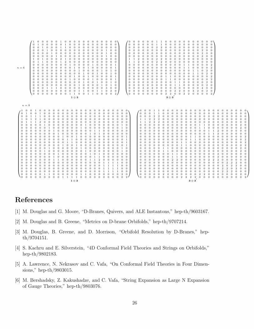
n = 6
1 0 0 0 0 0 1 0 0 0 0 0 0 0 0 0 0 0 00 1 0 0 0 0 0 1 0 0 0 0 0 0 0 0 0 0 00 0 1 0 0 0 1 1 0 0 0 0 0 0 0 0 0 0 00 0 0 1 0 0 0 0 0 0 0 0 0 0 0 0 1 0 00 0 0 0 1 0 0 0 0 0 0 0 0 0 0 0 1 0 00 0 0 0 0 1 0 0 0 0 0 0 0 0 0 0 1 0 01 0 1 0 0 0 2 1 0 0 0 0 0 0 0 0 0 0 00 1 1 0 0 0 1 2 0 0 0 0 0 0 0 0 0 0 00 0 0 0 0 0 0 0 1 0 0 0 0 1 0 0 0 0 10 0 0 0 0 0 0 0 0 1 0 0 1 0 0 0 0 0 10 0 0 0 0 0 0 0 0 0 1 0 0 0 0 1 0 1 00 0 0 0 0 0 0 0 0 0 0 1 0 0 1 0 0 1 00 0 0 0 0 0 0 0 0 1 0 0 1 0 0 0 0 0 10 0 0 0 0 0 0 0 1 0 0 0 0 1 0 0 0 0 10 0 0 0 0 0 0 0 0 0 0 1 0 0 1 0 0 1 00 0 0 0 0 0 0 0 0 0 1 0 0 0 0 1 0 1 00 0 0 1 1 1 0 0 0 0 0 0 0 0 0 0 3 0 00 0 0 0 0 0 0 0 0 0 1 1 0 0 1 1 0 2 00 0 0 0 0 0 0 0 1 1 0 0 1 1 0 0 0 0 2
0 0 0 0 0 0 1 1 0 0 0 0 0 0 0 0 0 0 00 0 0 0 0 0 1 1 0 0 0 0 0 0 0 0 0 0 00 0 0 0 0 0 2 2 0 0 0 0 0 0 0 0 0 0 00 0 0 0 0 0 0 0 0 0 0 0 0 0 0 0 2 0 00 0 0 0 0 0 0 0 0 0 0 0 0 0 0 0 2 0 00 0 0 0 0 0 0 0 0 0 0 0 0 0 0 0 2 0 01 1 2 0 0 0 2 2 0 0 0 0 0 0 0 0 0 0 01 1 2 0 0 0 2 2 0 0 0 0 0 0 0 0 0 0 00 0 0 0 0 0 0 0 0 0 0 0 1 1 0 0 0 0 20 0 0 0 0 0 0 0 0 0 0 0 1 1 0 0 0 0 20 0 0 0 0 0 0 0 0 0 0 0 0 0 1 1 0 2 00 0 0 0 0 0 0 0 0 0 0 0 0 0 1 1 0 2 00 0 0 0 0 0 0 0 1 1 0 0 0 0 0 0 0 0 20 0 0 0 0 0 0 0 1 1 0 0 0 0 0 0 0 0 20 0 0 0 0 0 0 0 0 0 1 1 0 0 0 0 0 2 00 0 0 0 0 0 0 0 0 0 1 1 0 0 0 0 0 2 00 0 0 2 2 2 0 0 0 0 0 0 0 0 0 0 4 0 00 0 0 0 0 0 0 0 0 0 2 2 0 0 2 2 0 2 00 0 0 0 0 0 0 0 2 2 0 0 2 2 0 0 0 0 2
1 ⊕ 3 3 ⊕ 3′
n = 8
1 0 0 1 0 0 0 0 0 0 0 0 0 0 0 0 0 0 0 0 0 0 0 00 1 0 0 1 0 0 0 0 0 0 0 0 0 0 0 0 0 0 0 0 0 0 00 0 1 1 1 0 0 0 0 0 0 0 0 0 0 0 0 0 0 0 0 0 0 01 0 1 2 1 0 0 0 0 0 0 0 0 0 0 0 0 0 0 0 0 0 0 00 1 1 1 2 0 0 0 0 0 0 0 0 0 0 0 0 0 0 0 0 0 0 00 0 0 0 0 1 0 0 0 0 0 0 0 0 1 0 0 0 0 0 0 0 1 00 0 0 0 0 0 1 0 0 0 0 0 0 1 0 0 0 0 0 0 0 0 1 00 0 0 0 0 0 0 1 0 0 0 0 0 0 0 0 1 1 0 0 0 0 0 00 0 0 0 0 0 0 0 1 0 0 0 0 0 0 1 0 1 0 0 0 0 0 00 0 0 0 0 0 0 0 0 1 0 0 1 0 0 0 0 0 0 0 0 0 0 10 0 0 0 0 0 0 0 0 0 1 1 0 0 0 0 0 0 0 0 0 0 0 10 0 0 0 0 0 0 0 0 0 1 1 0 0 0 0 0 0 0 0 0 0 0 10 0 0 0 0 0 0 0 0 1 0 0 1 0 0 0 0 0 0 0 0 0 0 10 0 0 0 0 0 1 0 0 0 0 0 0 1 0 0 0 0 0 0 0 0 1 00 0 0 0 0 1 0 0 0 0 0 0 0 0 1 0 0 0 0 0 0 0 1 00 0 0 0 0 0 0 0 1 0 0 0 0 0 0 1 0 1 0 0 0 0 0 00 0 0 0 0 0 0 1 0 0 0 0 0 0 0 0 1 1 0 0 0 0 0 00 0 0 0 0 0 0 1 1 0 0 0 0 0 0 1 1 2 0 0 0 0 0 00 0 0 0 0 0 0 0 0 0 0 0 0 0 0 0 0 0 1 1 1 1 0 00 0 0 0 0 0 0 0 0 0 0 0 0 0 0 0 0 0 1 1 1 1 0 00 0 0 0 0 0 0 0 0 0 0 0 0 0 0 0 0 0 1 1 1 1 0 00 0 0 0 0 0 0 0 0 0 0 0 0 0 0 0 0 0 1 1 1 1 0 00 0 0 0 0 1 1 0 0 0 0 0 0 1 1 0 0 0 0 0 0 0 2 00 0 0 0 0 0 0 0 0 1 1 1 1 0 0 0 0 0 0 0 0 0 0 2
0 0 0 1 1 0 0 0 0 0 0 0 0 0 0 0 0 0 0 0 0 0 0 00 0 0 1 1 0 0 0 0 0 0 0 0 0 0 0 0 0 0 0 0 0 0 00 0 0 2 2 0 0 0 0 0 0 0 0 0 0 0 0 0 0 0 0 0 0 01 1 2 2 2 0 0 0 0 0 0 0 0 0 0 0 0 0 0 0 0 0 0 01 1 2 2 2 0 0 0 0 0 0 0 0 0 0 0 0 0 0 0 0 0 0 00 0 0 0 0 0 0 0 0 0 0 0 0 1 1 0 0 0 0 0 0 0 2 00 0 0 0 0 0 0 0 0 0 0 0 0 1 1 0 0 0 0 0 0 0 2 00 0 0 0 0 0 0 0 0 0 0 0 0 0 0 1 1 2 0 0 0 0 0 00 0 0 0 0 0 0 0 0 0 0 0 0 0 0 1 1 2 0 0 0 0 0 00 0 0 0 0 0 0 0 0 0 0 1 1 0 0 0 0 0 0 0 0 0 0 20 0 0 0 0 0 0 0 0 0 0 1 1 0 0 0 0 0 0 0 0 0 0 20 0 0 0 0 0 0 0 0 1 1 0 0 0 0 0 0 0 0 0 0 0 0 20 0 0 0 0 0 0 0 0 1 1 0 0 0 0 0 0 0 0 0 0 0 0 20 0 0 0 0 1 1 0 0 0 0 0 0 0 0 0 0 0 0 0 0 0 2 00 0 0 0 0 1 1 0 0 0 0 0 0 0 0 0 0 0 0 0 0 0 2 00 0 0 0 0 0 0 1 1 0 0 0 0 0 0 0 0 2 0 0 0 0 0 00 0 0 0 0 0 0 1 1 0 0 0 0 0 0 0 0 2 0 0 0 0 0 00 0 0 0 0 0 0 2 2 0 0 0 0 0 0 2 2 2 0 0 0 0 0 00 0 0 0 0 0 0 0 0 0 0 0 0 0 0 0 0 0 0 2 2 2 0 00 0 0 0 0 0 0 0 0 0 0 0 0 0 0 0 0 0 2 0 2 2 0 00 0 0 0 0 0 0 0 0 0 0 0 0 0 0 0 0 0 2 2 0 2 0 00 0 0 0 0 0 0 0 0 0 0 0 0 0 0 0 0 0 2 2 2 0 0 00 0 0 0 0 2 2 0 0 0 0 0 0 2 2 0 0 0 0 0 0 0 2 00 0 0 0 0 0 0 0 0 2 2 2 2 0 0 0 0 0 0 0 0 0 0 2
1 ⊕ 3 3 ⊕ 3′
References
[1] M. Douglas and G. Moore, “D-Branes, Quivers, and ALE Instantons,” hep-th/9603167.
[2] M. Douglas and B. Greene, “Metrics on D-brane Orbifolds,” hep-th/9707214.
[3] M. Douglas, B. Greene, and D. Morrison, “Orbifold Resolution by D-Branes,” hep-th/9704151.
[4] S. Kachru and E. Silverstein, “4D Conformal Field Theories and Strings on Orbifolds,”hep-th/9802183.
[5] A. Lawrence, N. Nekrasov and C. Vafa, “On Conformal Field Theories in Four Dimen-sions,” hep-th/9803015.
[6] M. Bershadsky, Z. Kakushadze, and C. Vafa, “String Expansion as Large N Expansionof Gauge Theories,” hep-th/9803076.
26
[7] A. Hanany and A. Zaffaroni,“On the Realization of Chiral Four-Dimensional Gauge The-ories using Branes,” hep-th/9801134.
[8] A. Hanany and A. Uranga, “Brane Boxes and Branes on Singularities,” hep-th/9805139.
[9] R. Leigh and M. Rozali, “Brane Boxes, Anomalies, Bending and Tadpoles,” hep-th/9807082.
[10] R. Leigh and M. Strassler, “Exactly Marginal Operators and Duality in Four Dimen-sional N=1 Supersymmetric Gauge Theories,” hep-th/9503121.
[11] A. Hanany, M. Strassler and A. Uranga, “Finite Theories and Marginal Operators onthe Brane,” hep-th/9803086.
[12] S. Katz, P. Mayr and C. Vafa, “Mirror symmetry and Exact Solution of 4D N=2 GaugeTheories I,” hep-th/9706110.
[13] E. Witten, “Solutions of Four-Dimensional Field Theories via M-Theory,” hep-th/9703166
[14] A. Kapustin, “Dn Quivers from Branes,” hep-th/9806238.
[15] J. Maldecena, “The Large-N Limit of Superconformal Field Theories and Supergravity,”hep-th/9712200.
[16] J. Mckay, “Graphs, Singularities, and Finite Groups,” Proc. Symp. Pure Math. 37,183-186 (1980).
[17] K. Intrilligator and N. Seiberg, “Mirror symmertry in 3D gauge theories,” hep-th/9607207.
[18] P. Kronheimer, “The Construction of ALE Spaces as Hyper -Kahler Quotients,” J. Diff.Geometry, 29 (1989) 665.
[19] F. Klein, “Vorlesungen uber das Ikosaeder und die Auflosung der Gleichungen vomfunften Grade,” Teubner, Leipzig, 1884.
[20] P. Gabriel, “Unzerlegbare Darstellugen I,” Manuscripta Math. 6 (1972) 71-103.
[21] I. N. Bernstein, I. M. Gel’fand, V. A. Ponomarev, “Coxeter Functors and Gabriel’sTheorem,” Russian Math. Surveys, 28, (1973) II.
[22] H. F. Blichfeldt, “Finite Collineation Groups”. The Univ. Chicago Press, Chicago, 1917.
[23] S.-T. Yau and Y. Yu, “Gorenstein Quotients Singularities in Dimension Three,” Mem-oirs of the AMS, 505, 1993.
[24] W. M. Fairbairn, T. Fulton and W. Klink, “Finite and Disconnected Subgroups of SU3
and their Applications to The Elementary Particle Spectrum,” J. Math. Physics, vol 5,Number 8, 1964, pp1038 - 1051.
27
[25] J. Lomont, “Applications of Finite Groups,” Academic Press NY 1959.
[26] D. Anselmi, M. Billo, P. Fre, L. Girardello, A. Zaffaroni, “ALE Manifolds and ConformalField Theories,” hep-th/9304135.
[27] GAP 3.4.3 Lehrstuhl D fur Mathematik,http://www.math.rwth-aachen.de∼GAP/WWW/gap.html; Mathematica 2.0.
[28] P. di Francesco, P. Mathieu, D. Senechal, “Conformal Field Theory,” Springer-Verlag,NY 1997.
[29] D. Gepner and E. Witten, “String Theory on Group Manifold,” Nuc. Phys. B278, 493(1986).
[30] D. Bernard and J. Thierry-Mieg, “Bosonic Kac-Moody String Theories,” Phys. Lett.185B, 65 (1987).
[31] P. di Francesco and J.-B. Zuber, “SU(N) Lattice Integrable Models Associated withGraphs,” Nuclear Physics B, 338, 1990, pp602-646.
[32] T. Gannon, “The Classification of SU(m)k Automorphism Invariants,” hep-th/9408119.
[33] M. Bauer, A. Coste, C. Itzykson, and P. Ruelle, “Comments on the Links betweensu(3) Modular Invariants, Simple Factors in the Jacobian of Fermat Curves, and RationalTriangular Billiards,” hep-th/9604104.
[34] D.-E. Diaconescu and N. Seiberg, “The Coulomb Branch of (4,4) Supersymmetric FieldTheories in 2 Dimensions,” hep-th/9707158.
[35] Y. Ito and M. Reid, “The McKay Correspondence for Finite Subgroups of SL(3,C),”alg-geo/9411010.
[36] S.-S. Roan, “Minimal Resolutions of Gorenstein Orbifolds in Dimension Three,” Topol-
ogy, Vol 35, pp489-508, 1996.
28


