arX

iv:h

ep-t

h/98

0406

9v1

9 A

pr 1

998

IASSNS-HEP-98/34

Solution of N=2 Gauge Theories via

Compactification to Three Dimensions

Anton Kapustin∗

School of Natural Sciences, Institute for Advanced Study

Olden Lane, Princeton, NJ 08540

Abstract

A number of N = 2 gauge theories can be realized by brane config-urations in Type IIA string theory. One way of solving them involveslifting the brane configuration to M-theory. In this paper we presentan alternative way of analyzing a subclass of these theories (ellipticmodels). We observe that upon compactification on a circle one canuse a version of mirror symmetry to map the original brane configura-tion into one containing only D-branes. Simultaneously the Coulombbranch of the four-dimensional theory is mapped to the Higgs branchof a five-dimensional theory with three-dimensional impurities. Thelatter does not receive quantum corrections and can be analyzed ex-actly. The solution is naturally formulated in terms of an integrablesystem, which is a version of a Hitchin system on a punctured torus.

∗Research supported in part by DOE grant DE-FG02-90-ER40542

1 Introduction

In the last few years a lot of effort has been invested into studying modulispaces of vacua of supersymmetric gauge theories. This problem is quitenontrivial when the theory in question is strongly coupled in the infrared. Itis remarkable that nevertheless a complete solution has been found for a largenumber of N = 2 gauge theories using various techniques. In particular, inRef. [1] the structure of the Coulomb branch of theories with product gaugegroups SU(n1)×SU(n2)× . . .×SU(nk−1) has been analyzed. The idea is torealize the gauge theory as a low-energy theory on a configuration of branesin IIA string theory. To this end one considers an array of k parallel NS5-branes extending in the x0, x1, x2, x3, x4, x5 directions and having coincidentpositions in the x7, x8, x9 directions. Then one suspends nα parallel D4-branes between the αth and α+1st 5-branes, so that the world-volume of D4-branes is extended in the x0, x1, x2, x3, x6 directions. (One can also includeD6-branes, but we do not consider this possibility here). Since the extentof this configuration in the x6 direction is finite, the low-energy theory isa four-dimensional gauge theory living in the x0, x1, x2, x3 plane. It canbe checked that this arrangement of branes leaves eight supersymmetriesunbroken, so we get at least N = 2 supersymmetry in d = 4. Naively,the gauge group appears to be U(n1) × U(n2) × · · · × U(nk−1) with matterhypermultiplets in the bifundamental representation (i.e. the hypermultipletstransform as (n1, n2) ⊕ (n2, n3) ⊕ · · · ⊕ (nk−2, nk−1).) The hypermultipletscome from open strings connecting neighboring stacks of D4-branes. A moredetailed analysis [1] shows that the center-of-mass motion of these stacks is“frozen out”, in the sense that the x4, x5 positions of the centers-of-mass areparameters of the Lagrangian rather than dynamical fields. As a consequencethe gauge group is actually SU(n1)×SU(n2)×· · ·×SU(nk−1). It is convenientto combine the x4, x5 coordinates of the center-of-mass of the αth stack into acomplex number vα = x4

α+ix5α. Then the bare mass of the αth hypermultiplet

is given by vα+1 − vα.In order to solve for the Coulomb branch of this theory, one lifts the brane

configuration to M-theory. If the IIA string theory is strongly coupled, theradius of the M-theory circle (whose coordinate we will call x10) is large. Inthis case the IIA brane configuration lifts to a single large smooth 5-branewith worldvolume R1,3 × C. Here R1,3 has coordinates x0, x1, x2, x3, and Cis a Riemann surface holomorphically embedded in C×C∗ with coordinatesv = x4 + ix5, t = exp(x6 + ix10). The moduli of the field theory translate into

1

the moduli of the embedding C → C×C∗. Of course, the embedding is notarbitrary: one must require that upon forgetting x10 the M-theory 5-braneproject back to the correct IIA configuration. To solve the model one hasto find a holomorphic family of embeddings satisfying this constraint anddepending on the right number of parameters.

Another way of solving N = 2 gauge theories is based on their relation tocomplex integrable system [2, 3, 4]. We will explain the precise meaning ofthis statement in the next section. For now it suffices to say that a complexintegrable system can be thought of as a complexification of an integrablesystem of classical mechanics, and that the solution of every N = 2 gaugetheory is encoded in some complex integrable system. Therefore one can tryto match the known integrable models with particular N = 2 gauge theories.The first success of this approach was the observation of Ref. [3] that anaffine Toda chain associated with a simple group G provides a solution forthe N = 2 gauge theory with gauge group G (the Langlands dual of G)and no hypermultiplets. Soon after that the SU(n) Hitchin system [5] on atorus with a single puncture was shown to give a solution of the SU(n) gaugetheory with a massive adjoint hypermultiplet [4]. Some other matches weresuggested in Ref. [6].

It is natural to ask about the relation between the two approaches. Ananswer suggested in Ref. [1] is that a family of embeddings of a Riemannsurface C into C×C∗ can be thought of as an integrable system too, namelythe integrable system of Donagi-Markman type [7]. Thus every model solvedin Ref. [1] is matched to an integrable system.

We do not consider this a completely satisfactory answer, however. In-deed, in the cases where both approaches are applicable, the solutions seemtotally different, and some effort is required to see that they are equivalent.For example, the fact that the solution of the SU(n) theory with a massiveadjoint hypermultiplet can be represented by a Hitchin-type system lookslike a miracle from the point of view of M-theory.

In this paper we would like to address this problem by suggesting a newmethod of solving N = 2 gauge theories.1 The starting point is again thebrane configuration of Ref. [1], but with x3 compactified on a circle. Thus wewill be studying N = 2 gauge theories on R1,2×S1. For technical reasons wewill consider only elliptic models, i.e. those with x6 direction compactifiedas well. However, it will be clear from the derivation that the method can be

1Similar ideas were considered in Ref. [8].

2

applied more generally. Thus the gauge theories we are solving are finite andhave gauge group SU(n)1 ×SU(n)2 ×· · ·×SU(n)k ×U(1) and matter in thebifundamental. The gauge group and the matter content of this theory canbe encoded in an affine Ak−1 quiver. It turns out there is a version of mirrorsymmetry (in the sense of Ref. [9]) which maps the Coulomb branch of theoriginal (“electric”) theory to the Higgs branch of a certain five-dimensional“magnetic” theory on R1,2 × T 2, with three-dimensional impurities localizedat points on T 2. The Higgs branch does not receive quantum corrections andcan be analyzed exactly. This yields a solution of the original problem, for anycompactification radius. An interesting feature of this approach is that thesolution is automatically encoded in a Hitchin-type integrable system. Thus,at least for the class of models considered in this paper (elliptic models), thecorresponding Donagi-Markman systems arise from Hitchin-type systems.In particular, we rederive the fact noticed in Ref. [4] that the SU(n) gaugetheory with a massive adjoint is solved by an SU(n) Hitchin system on apunctured torus. Another spin-off of our approach is a new explanation ofthe “freezing” of U(1) factors in the d=4 gauge theories noticed in Ref. [1].

In the next section we give a very brief summary of the relation betweenN = 2 gauge theories and integrable systems. In this we follow Ref. [4]. Insection 3 we discuss the mirror transform alluded to above. The analysis ofthe Higgs branch of the “magnetic” theory is presented in section 4. There wealso compare our solution with that obtained in Ref. [1]. Some idiosyncraticremarks are collected in section 5.

2 N=2 Gauge Theories and Integrable Mod-

els

In this section we remind the reader the relation between low-energy La-grangians of N = 2 gauge theories and integrable models of classical me-chanics [4]. Consider an N = 2 gauge theory with gauge group G of rankr and matter hypermultiplets. The Coulomb branch of the theory U is aspecial Kahler manifold of complex dimension r. As a complex manifold,U is a copy of Cr. The special Kahler metric is encoded in a holomorphicfunction F on X, the prepotential. This function is multi-valued, however,so it is desirable to give a description of the metric in more invariant terms.To this end one considers a fibration π : X → U , where X is a complex

3

manifold of dimension 2r and the fibers of π are Abelian varieties Ar of di-mension r. (In other words, Ar is a complex torus together with a (1, 1)-formt (polarization) which is positive and has integral periods). We will call thefibration π : X → U the Seiberg-Witten fibration. One also needs a closedholomorphic (2, 0)-form ω on X whose restriction to the fibers of π is zero.Together these data define a metric on U in the following manner: one takesthe (r+1, r+1)-form tr−1∧ω∧ω and integrates over the fibers of π; this yieldsa (1, 1)-form on U which is the Kahler form of the metric we are after. Anadditional physical requirement is that this metric be nondegenerate awayfrom singular fibers of π. This is achieved by asking that ω be nondegenerateaway from the singular fibers.

So far we described how the fibration π : X → U together with ω definea Kahler metric on U and therefore the low-energy effective action for mass-less scalars. The low-energy theory of the Coulomb branch also contains rphotons. To define their action one needs to specify the “τ -parameter”, i.e.an r × r matrix which is a holomorphic function on U whose imaginary partis positive-definite (away from singular fibers). The “τ -parameter” encodesthe gauge couplings and theta-angles of the photons, and because of electric-magnetic duality it is defined up to Sp(2r,Z) transformations. Given theSeiberg-Witten fibration it is very easy to read off τ : at a point u ∈ U it isthe complex structure of the fiber π−1(u).

One can think of X together with ω as a complex symplectic manifold,i.e. as a complexification of the phase space of some mechanical system withr degrees of freedom. Moreover, since the restriction of ω to the fibers ofπ is zero, any two functions on U Poisson-commute. Therefore the coordi-nates on U form a maximal set of commuting integrals of motion, and thecorresponding mechanical system is integrable (it fulfills the conditions ofLiouville’s theorem). In other words, the coordinates on U are action vari-ables, while the coordinates on the fiber Ar are the canonically conjugateangle variables. Thus any N = 2 gauge theory corresponds to a certaincomplex integrable system of classical mechanics.

4

3 Compactification to Three Dimensions and

the Mirror Transform

We start with the brane configuration considered in Ref. [1]: k NS5-braneslocated at x7 = x8 = x9 = 0 and at x6 = s1, . . . , sk and n D4-branes locatedat x7 = x8 = x9 = 0 and worldvolume parametrized by x0, x1, x2, x3, x6.The x6 coordinate is taken to be periodic with period 2πL. Thus D4-branesare wrapped on a circle of radius L. Since D4-branes can end on NS5-branes, a stack of n parallel D4-branes can split at NS5-branes, producingk independent stacks of D4-branes. They can move in the (x4, x5) plane,which we regard as a copy of C parametrized by v = x4 + ix5. This isthe Coulomb branch of the theory. (There is also a mixed Higgs-Coulombbranch corresponding to the situation when some or all D4-branes move offthe x7 = x8 = x9 = 0 plane, but we will not consider it here.) Let us denotethe center-of-mass coordinate of the αth stack by vα. It was shown in Ref. [1]that moving the center-of-mass of any stack in the x4, x5 directions relativeto other stacks costs an infinite amount of energy, therefore the relativecenter-of-mass coordinates mα = vα+1 − vα, α = 1, . . . , k are parameters ofthe theory rather than moduli. Consequently the low-energy theory on D4-branes is a d = 4, N = 2 theory with gauge group SU(n)1 × · · · × SU(n)k ×U(1). There are also k bifundamental hypermultiplets Qα, α = 1, . . . , k; Qα

transforms as n with respect to SU(n)α and as n with respect to SU(n)α+1.They are not charged with respect to U(1). These hypermultiplets arise fromopen strings connecting the adjacent stacks of D4-branes, therefore the baremass of Qα is mα.

We now compactify x3 on a circle of radius R. The theory becomes effec-tively 2+1-dimensional at energies lower than 1/R. Its Coulomb branch is ahyperkahler manifold X of dimension 4r = 4(kn−k+1) with a distinguishedcomplex structure in which it looks like a fibration π : X → Cr with fibersbeing abelian varieties Ar of complex dimension r [10]. Let us remind howthis comes about. The picture is most clear when R is large compared toall field theory scales. One can then go to a low-energy limit in d = 4 andthen compactify to d = 3. The r photons of the Coulomb branch in d = 4reduce to r photons plus r scalars in d = 3. The scalars live in a torus whosesize scales as 1/

√R, as they originate from Wilson lines around the compact

direction. Furthemore, r photons in d = 3 are dual to r compact scalars.Thus we get r more scalars also living on a torus of size of order 1/

√R. If

5

one uses the distinguished complex structure, these 2r real scalars can bethought of as r complex scalars taking values in a complex torus Ar. Onecan show that in this distingushed complex structure the total space of thefibration X → Cr is the same as the Seiberg-Witten fibration of the parenttheory in d = 4. This result is most easily derived for large R; it is then truefor any R, because the complex structure of X does not depend on R [10].

Since X is hyperkahler, it also carries a complex symplectic (2, 0)-formω2 + iω3 and a (1, 1) Kahler form ω1. For large R the periods of ω1 evaluatedon the 2-cycles of Ar are proportional to 1/R, since the linear size of Ar

scales as 1/√

R. Furthemore, the form ω2 + iω3 coincides with the form ωwhich was a part of the four-dimensional data [10] (see section 2).

We now wish to identify the Coulomb branch of our d = 3 theory with theHiggs branch of some “magnetic” theory. To this end we perform T-dualityon x3, then IIB S-duality, and then again T-duality on x3. As a result thestring coupling λ is mapped to λ = R3/2λ−1/2, and R → R = (Rλ)1/2, L →L = L(R/λ)1/2.2 Notice also that after the dualities the modular parameterof the torus in the x3, x6 directions becomes τ ≡ L/R = L/λ.

After the first T-duality NS5-branes become IIB NS5-branes. S-dualityturns them into IIB D5-branes, and the second T-duality turns them intoIIA D4-branes located at fixed x3, x6, x7, x8, x9. We will refer to them asD4′-branes. To understand what happens with D4-branes, we consider thesituation when D4-branes are not broken at the NS5-branes. This corre-sponds to the origin of the classical moduli space in the original (“electric”)theory, where the Coulomb and Higgs branches meet. In this case it is easyto see that D4-branes are left unchanged by this sequence of dualities, i.e.they remain D4-branes wrapped around the T 2 parametrized by x3, x6. TheD4′-branes are localized at points of this T 2. Thus the “magnetic” theoryis a d = 5 theory on R1,2 × T 2 with impurities localized at points on T 2.At energies much lower than min(1/R, 1/L) it becomes a d = 3 theory. Thegauge group of the “magnetic” theory is U(n), and, if not for the impurities,it would have sixteen unbroken supercharges. The impurites break half ofsupersymmetries and give rise to k fundamental hypermultiplets localized atpoints on T 2. The hypermultiplets come from open strings connecting D4and D4′-branes.

Now we can understand how the flat directions in the “electric” and“magnetic” theories are matched. In the “electric” picture the Coulomb

2We set α′ = 1.

6

�

q

x10

x6s

s

s s

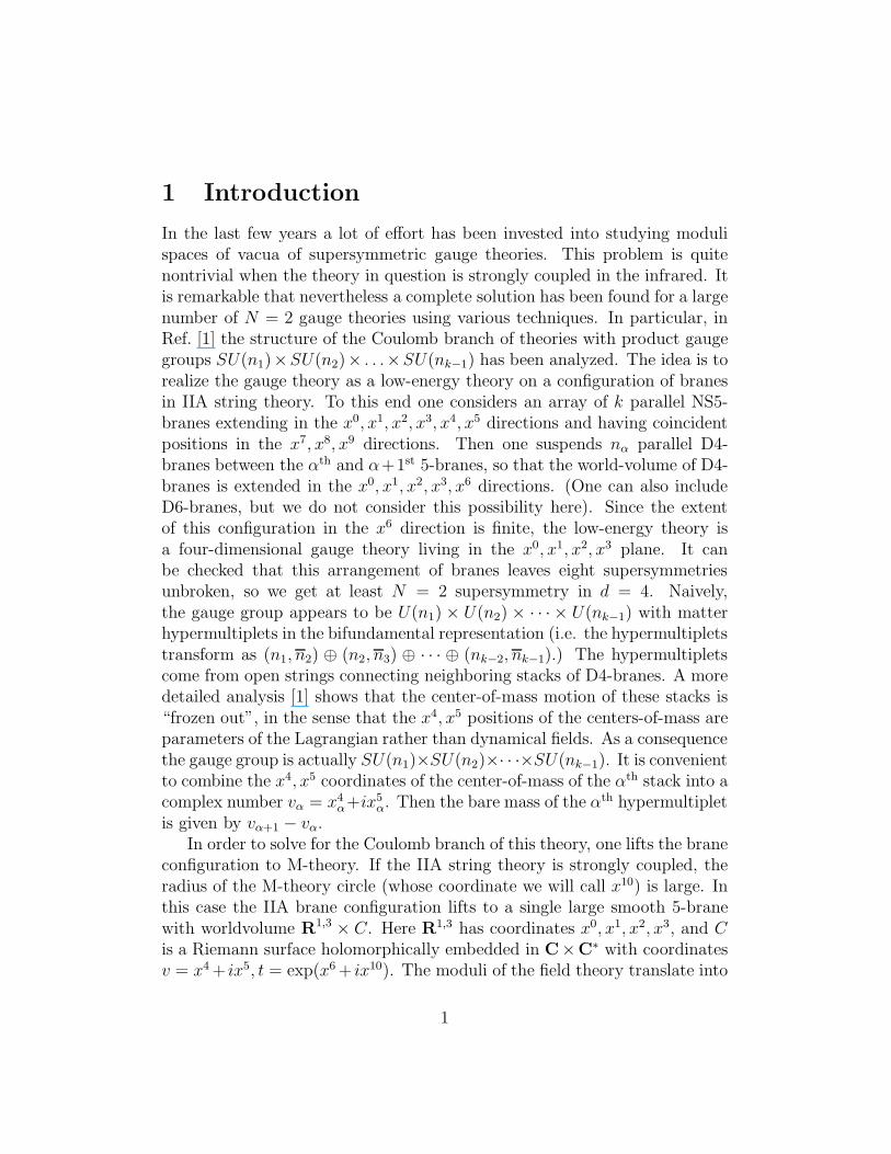
Figure 1: After x3 is reinterpreted as the M-theory circle, the “electric”D4-branes become D4-branes wrapped around x6 and x10, while NS5-branesbecome D4′-branes localized in the x6, x10 directions. Here the positions ofthe D4′-branes are shown as punctures on the T 2 parametrized by x6, x10.

branch was characterized by the fact that D4-branes could not move off in thex7, x8, x9 directions. In the “magnetic” picture this occurs when fundamentalhypermultiplets have VEVs, higgsing the gauge group. Thus the mirrortransform maps the Coulomb branch of the “electric” theory to the Higgsbranch of the “magnetic” theory. Conversely, the “electric” Higgs branchcorresponds to the “magnetic” Coulomb branch.

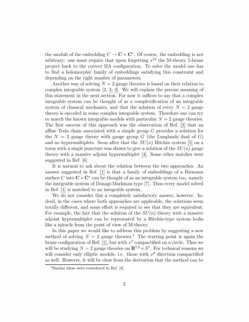
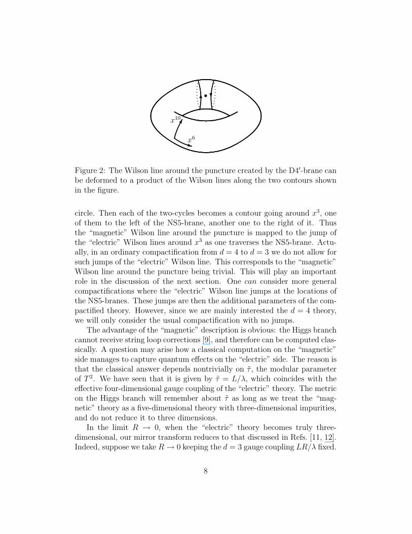
Here is another way to describe this “mirror transform.” We reinter-pret the “electric” IIA brane configuration as an arrangement of branes inM-theory compactified on T 3 with coordinates x3, x6, x10. D4-branes areinterpreted as M5-branes wrapped around T 3, while NS5-branes lift to M5-branes wrapped around x3 and localized in x6, x10. The mirror transformamounts to reinterpreting x3 as the M-theory circle. The “magnetic” IIApicture involves n D4-branes wrapped around a T 2 with coordinates x6, x10,and k D4′-branes localized at points of this T 2 (see Figure 1). This wayof thinking about the mirror transform allows one to see some facts aboutthe “magnetic” theory more easily. For example, consider the “magnetic”Wilson line on the worldvolume of D4-branes around a puncture created bya D4′-brane. What is its analogue in the “electric” theory? The Wilson linearound the puncture can be alternatively computed as the holonomy aroundthe composite contour shown in Figure 2. In the M-theory language, theWilson line on the D4-brane along each component of this contour is inter-preted as a flux of B-field through an appropriate two-cycle. In the case ofthe contours shown in Figure 2 each two-cycle is a T 2 parametrized by x3, x10.Now to go back to the “electric” picture we reinterpret x10 as the M-theory

7

�

q

x10

x6

s

6?

Figure 2: The Wilson line around the puncture created by the D4′-brane canbe deformed to a product of the Wilson lines along the two contours shownin the figure.

circle. Then each of the two-cycles becomes a contour going around x3, oneof them to the left of the NS5-brane, another one to the right of it. Thusthe “magnetic” Wilson line around the puncture is mapped to the jump ofthe “electric” Wilson lines around x3 as one traverses the NS5-brane. Actu-ally, in an ordinary compactification from d = 4 to d = 3 we do not allow forsuch jumps of the “electric” Wilson line. This corresponds to the “magnetic”Wilson line around the puncture being trivial. This will play an importantrole in the discussion of the next section. One can consider more generalcompactifications where the “electric” Wilson line jumps at the locations ofthe NS5-branes. These jumps are then the additional parameters of the com-pactified theory. However, since we are mainly interested the d = 4 theory,we will only consider the usual compactification with no jumps.

The advantage of the “magnetic” description is obvious: the Higgs branchcannot receive string loop corrections [9], and therefore can be computed clas-sically. A question may arise how a classical computation on the “magnetic”side manages to capture quantum effects on the “electric” side. The reason isthat the classical answer depends nontrivially on τ , the modular parameterof T 2. We have seen that it is given by τ = L/λ, which coincides with theeffective four-dimensional gauge coupling of the “electric” theory. The metricon the Higgs branch will remember about τ as long as we treat the “mag-netic” theory as a five-dimensional theory with three-dimensional impurities,and do not reduce it to three dimensions.

In the limit R → 0, when the “electric” theory becomes truly three-dimensional, our mirror transform reduces to that discussed in Refs. [11, 12].Indeed, suppose we take R → 0 keeping the d = 3 gauge coupling LR/λ fixed.

8

The “electric” theory reduces in this limit to a d = 3, N = 4 theory withthe same gauge group and matter content as in d = 4. To see what happenson the “magnetic” side, notice that R/L = λ/L → 0. This means that theT 2 of the impurity theory becomes very “thin” in the x3 direction. Thenit is helpful to perform T-duality on x3. The resulting brane configurationconsists of n D3-branes parallel to x0, x1, x2, x6 and k D5-branes parallel tox0, x1, x2, x3, x4, x5. According to Refs. [11, 12] this setup produces the right“magnetic” theory.

4 Solution of the Models

4.1 The Higgs Branch of the Impurity Theory

In this section we analyze the Higgs branch of the “magnetic” theory. TheD-flatness conditions for an equivalent impurity model have been derived inRef. [13]. (Our model is related to that considered in section 2.3 of Ref. [13]by T-duality on x1, x2.) The result is that the Higgs branch is given by themoduli space of solutions of the following partial differential equations on T 2:

Fzz − [Φz, Φ†z] =

π

RL

k∑

α=1

δ2(z − zα) (Qα ⊗ Q†α − Q†

α ⊗ Qα),

DΦz ≡ ∂Φz − [Az, Φz] = − π

RL

k∑

α=1

δ2(z − zα) Qα ⊗ Qα. (1)

Here Azdz + Azdz is a U(n) connection on T 2, Fzz = ∂Az − ∂Az − [Az, Az],Φz is a complex adjoint-valued 1-form, and Qα, Qα, α = 1, . . . , k are complexvariables. It is understood that Az = −A†

z. The objects appearing in theseequations have a transparent meaning: A is part of the gauge field livingon the worldvolume of D4-branes, Φz is the adjoint field parametrizing themotion of the D4-branes in the directions parallel to D4′-branes (x4 andx5), while (Qα, Qα) make up the fundamental hypermultiplet localized atthe αth impurity. In the absence of impurity terms, Eqs. (1) are known asHitchin equations. Hitchin equations are self-duality equations reduced totwo dimensions. The effect of the impurity terms is to introduce poles for Φz

and Az at z = zα, α = 1, . . . , k. The residues are not fixed; rather they aredetermined by the VEVs of the fundamentals.

As usual in N = 2 theories, D-flatness conditions can be thought of asmoment map equations for a hyperkahler quotient [13]. In this case the group

9

G is infinite-dimensional: it is a group of smooth maps T 2 → U(n). It acts ona space Y consisting of all sets of the form (Az, Φz, Q1, Q1, . . . , Qk, Qk). Thespace Y is an infinite-dimensional affine space with a natural hyperkahlerstructure. An element g(z) ∈ G acts on Y in the following manner:

Az(z) → g(z)(z)Az(z)g−1(z) + g(z)∂g−1(z), Φz → g(z)Φz(z)g−1(z),

Qα → g(zα)Qα, Qα → Qαg(zα)−1, α = 1, . . . , k. (2)

A short computation reveals that the submanifold in Y defined by Eqs. (1)is precisely the zero level of the moment map for G. Thus the moduli spaceof Eqs. (1) is the hyperkahler quotient of Y with respect to G at zero level.A formal application of the theorem of Hitchin, Karlhede, Lindstrom andRocek [14] tells us that X has a natural hyperkahler metric inherited fromthat on Y . This is a formal statement, because Y is infinite-dimensional,and the questions of existence of various objects needed in the constructionof Ref. [14] are nontrivial.

As a matter of fact, one immediately sees two problems with our definitionof X, due precisely to the formal character of our manipulations. First, noticethat Eqs. (1) imply that Φz and Az have simple poles at z = zα, α = 1, . . . , k,with variable residues. Therefore the variations of Φz and Az genericallyhave simple poles as well, and their norm is logarithmically divergent. As aconsequence, some of the tangent vectors to X have infinite norm, since theycorrespond to zero modes of Eqs. (1) which are not normalizable on T 2. Thismeans that it costs an infinite amount of energy to move in these directionson X. Second, we saw in the previous section that the Wilson lines aroundthe punctures at z = zα must be trivial. Then Az must be nonsingular atz = zα, and the first equation in Eq. (1) implies that

Qα ⊗ Q†α − Q†

α ⊗ Qα = 0, α = 1, . . . , k. (3)

But this restriction is incompatible with the hyperkahler structure of X.It is clear what the resolution should be. The residues of Φz and Az

are parameters of the theory rather than dynamical fields. The true modulicorrespond to those variations which have finite norm. To identify the truemoduli space one has to freeze the residues of Az and Φz at some values, sothat variations of Φz and Az are nonsingular. Then the remaining tangentvectors will have finite norm, and the metric will be well-defined. In fact,the constraint Eq. (3) does just this, freezing the residue of Az at zero value.This eliminates some of the tangent vectors with infinite norm (the ones

10

corresponding to variations of Az alone). Further constraints are necessaryto kill the nonnormalizable tangent vectors associated with variations of Φz .To figure out the precise form of these constraints, let us use the U(n) gaugetransformations to bring all Q’s and Q′s to the form

Qα = (aα, bα, 0, . . . , 0), Qα = (aα, 0, 0, . . . , 0), α = 1, . . . , k. (4)

Eq. (3) implies that bα = 0, |aα| = |aα|, α = 1, . . . , k. According to the secondof Eqs. (1), for the residues of Φz to be fixed one has to impose an additionalconstraint

aαaα = mα, α = 1, . . . , k, (5)

where mα are complex constants. These constraints are still invariant withrespect to U(n) gauge transformations which reduce to U(1) × U(n − 1) atz = zα. One can use the U(1) part of these gauge transformations to makeall aα real. Then the degrees of freedom corresponding to Q’s and Q’s arecompletely frozen, and we are left with Hitchin equations for Az and Φz withfixed residues for Φz.

To summarize, the slice of X which does have a well-defined metric con-sists of solutions of the Hitchin equations

Fzz − [Φz , Φ†z] = 0,

DΦz = − π

RL

k∑

α=1

δ2(z − zα) diag(mα, 0, . . . , 0), (6)

modulo the gauge group G0 of U(n) gauge transformations which reduce toU(n − 1) at z = zα. Let us call this moduli space X0. The preceedingdiscussion shows that X0 has a good metric, unlike X. Moreover, Eqs. (6)have the form of moment map equations for G0, hence the metric on X0 ishyperkahler. Thus both problems mentioned above have been resolved.

It will be shown in section 4.3 that dim X0 = 4(kn − k + 1). This is theright dimension for the Coulomb branch of the SU(n)k ×U(1) gauge theory.Recall that the gauge group is SU(n)k × U(1) and not U(n)k because, asobserved in Ref. [1], it costs an infinite amount of energy to excite the k − 1would-be moduli corresponding to the missing U(1)’s. Consequently, theVEVs of these moduli are actually parameters of the theory, the bare massesof the bifundamentals. There is a total of k bifundamentals, but the k massparameters satisfy a constraint

k∑

α=1

mα = 0. (7)

11

Where are these parameters in the “magnetic” description? Since we cun-ningly denoted the parameters in Eq. (6) with the same symbol mα, theanswer should be obvious.3 As a simple check of this identification note thatthe trace of the second of Eqs. (6) implies that Tr Φ is a meromorphic func-tion with simple poles at z = zα and residues imα/2RL. Hence

∑α mα = 0.

Another check is that the U(1)R symmetry of the N = 2, d = 4 theory is real-ized geometrically in the brane configuration as a rotation in the x4, x5 plane.Consequently, a U(1)R transformation acts on Φ by Φ → eiφ Φ, and thereforeby virtue of Eqs. (6) mα → eiφ mα. This is indeed the right transformationlaw for hypermultiplet masses.

It remains to understand how to introduce a nonzero “global mass”∑α mα. On the “electric” side one needs to consider brane configurations

in a nontrivial background geometry [1]. This should correspond to a certaindeformation of Eqs. (6). In fact, there is one obvious deformation: one mayintroduce FI terms for the gauge group G0 on the right-hand-side of Eqs. (6),deforming them to

Fzz − [Φz, Φ†z] = 0,

DΦz = − π

RL

k∑

α=1

δ2(z − zα) diag(mα,−M, . . . ,−M). (8)

Here M is a complex parameter. Note that we did not introduce an FIdeformation into the the first of Eqs. (8), in agreement with our requirementthat the Wilson lines around the punctures be trivial. Thus, although the FIparameter is three-component in general, in our case it has only two nonzerocomponents (which we combined into a complex parameter M). Furthemore,we took all k FI terms to be the same; allowing them to be different doesnot give anything new, as one can make a change of variables in Eqs. (8)which will make them all equal [13]. Therefore we have just one complexdeformation parameter M . It is natural to assume that it corresponds to the“global mass” on the “electric” side. It certainly has the right transformationproperties with respect to U(1)R. The identification of M with the “globalmass” is also in agreement with the general correspondence between masses inthe “electric” theory and FI terms in the “magnetic” theory [9, 11, 12]. Notealso that although in d = 3 the mass parameter has three real components,

3Of course, what we really claim is that such identification holds up to an overallmultiplicative factor. But since the “electric” theory is finite, one can set this factor toone by a choice of scale.

12

in a theory obtained by a straigtforward compactification from d = 4 oneof the components (the so-called real mass) is zero. This agrees with thefact that our FI deformation has only two real components. But the mostdirect way to see how M is related to the “global mass” is to consider thetrace part of Eqs. (8), and use the fact that the sum of the residues of ameromorphic function Tr Φ on a torus must be zero. Then we see that thecondition

∑kα=1 mα = 0 must be replaced by

∑kα=1 mα = k(n − 1)M.

4.2 The Decompactification Limit

So far we discussed the Coulomb branch X0 of the SU(n)k × U(1) theorycompactified on R3 × S1. We showed that X0 is given by the moduli spaceof U(n) Hitchin equations on a torus with k punctures with residues for Φz

of a particular kind. We now wish to decompactify S1, i.e. take R → ∞.The main idea here is that in the limit R → ∞ we no longer think of X0 asthe moduli space of the Coulomb branch endowed with a hyperkahler metric,but rather as the total space of the Seiberg-Witten fibration (see section 2).This amounts to picking a complex structure on X0 in which it looks likea bundle over Cr with fibers being abelian varieties of complex dimensionr.4 Once the complex structure is fixed, the three Kahler forms of X, ω1, ω2,and ω3, can be thought of as a (1, 1) Kahler form ωr = ω1 and a complexsymplectic form ω = ω2 + iω3. Taking R → ∞ is achieved by forgetting ωr.Then X0 becomes a complex manifold fibered by Ar over Cr and equippedwith ω. This data provides a solution of the d = 4 theory in the mannerexplained in section 2. In effect, the solution of the four-dimensional theoryis obtained by forgetting part of the solution of its compactified version.

The distinguished complex structure on Y is easily identified in our case:it is the complex structure which acts on z, Az, Φz, and all Q’s and Q’s bymultiplication by i. This follows from considering which U(1) subgroup of thethree-dimensional SU(2)R symmetry survives the limit R → ∞. The corre-sponding complex structure on X0 can be computed in the following (ratherstandard) manner: using the distingusihed complex structure on Y one cannaturally split the hyperkahler moment map equations into “complex” and“real” equations, discard the real ones, and consider the solutions of the com-plex equations modulo the complexified gauge group. The new moduli spaceis identical to X0 as a complex manifold. In mathematical terms, one sub-

4In our case r = kn − k + 1.

13

stitutes the holomorphic symplectic quotient for the hyperkahler quotient.This procedure is quite common in field theory: there one often treats anN = 2 theory as an N = 1 theory and uses the fact that the classical modulispace of an N = 1 theory is the space of solutions of the F-flatness condi-tions modulo the complexified gauge group. This allows one to avoid solvingN = 1 D-flatness conditions. Of course, the remaining F-flatness conditionsare nothing but the “complex” part of the N = 2 D-flatness conditions. Inour case the complex equations are

DΦz = − π

RL

k∑

α=1

δ2(z − zα) diag(mα,−M, . . . ,−M). (9)

As a complex manifold X0 is the space of solutions of this equation mod-ulo the complexified gauge group GL(n,C). More precisely, the complex-fied gauge group Gc

0 consists of GL(n,C) gauge transformations reducing toGL(n − 1,C) at z = zα, α = 1, . . . , k.

Eq. (9) describes a complex integrable system, just as ordinary Hitchinequations without punctures. Indeed, consider the phase space Y which isT ∗M, the holomorphic cotangent bundle of the space of GL(n,C) connec-tions on T 2. This space is parametrized by all pairs (Az, Φz). T ∗M hasa natural (complex) symplectic structure, as any cotangent bundle. Thismakes Y a complex integrable system. The set of all Φz’s can be thoughtof as the space of action variables. Then Eq. (9) says that X0 is a symplec-tic reduction of Y with respect to Gc

0. Hence X0 has a complex symplecticstructure and is also integrable.

If we set k = 1, we get the system discussed in Ref. [4], with precisely theright residue for Φz, except that in Ref. [4] the gauge group was restricted tobe SL(n,C). This slight difference is due to the fact that we are solving aU(n) gauge theory rather than SU(n). Thus we finally see why this particularHitchin system gives the solution of the N = 2 U(n) gauge theory with amassive adjoint hypermultiplet.

4.3 Comparison with M-theory Curves

In this section we show that for any k ≥ 1 our solution is equivalent tothat obtained in Ref. [1]. We regard the T 2 of the impurity theory as anelliptic curve Σ. It was shown in section 3 that its modular parameter is themicroscopic gauge coupling of the “electric” theory. Recall that a point in

14

X0 can be thought of as a holomorphic GL(n,C)-bundle E over Σ togetherwith Φ, a section of KΣ ⊗ EndE, where KΣ is the canonical bundle of Σ [4].(Simply put, Φz is an adjoint-valued (1, 0) form). For any point (E, Φ) ∈ X0

we consider an n-fold cover of Σ given by

det(t − Φ) = 0, (10)

where t takes values in KΣ. This gives a Riemann surface C. In our case Σ isan elliptic curve, so KΣ is trivial, and one can think of t and Φ as a complexfunction and an adjoint-valued field, respectively. The coefficients of the poly-nomial det(t−Φ) are gauge-invariant polynomials in Φ. By virtue of Hitchinequations, they are meromorphic differentials on Σ. They Poisson-commuteand therefore are the action variables of the integrable system representedby X0. Thus we have a projection X0 → Cr, where r is the number of actionvariables. It will be shown in end of this section that r = kn−k+1. The an-gle variables parametrize the fiber of this projection. As a matter of fact, thefiber is the Jacobian of C [4]. Indeed, given (E, Φ) and the curve C we havea natural holomorphic line bundle over C whose fiber over (t(z), z), z ∈ Σ,consists of the eigenvectors of Φ(z) with eigenvalue t(z). Conversely, givena line bundle L over C we can “project it down” to Σ and obtain a rank nholomorphic vector bundle E on Σ (in mathematical terminology, E is thedirect image sheaf of L). Thus a point in X0 can also be thought of as acurve C together with a point in the Jacobian of C. Recalling the discussionof section 2, we conclude that C is the Seiberg-Witten curve for the gaugesystem in question. So all we have to do is to compare C with the curvederived for the same gauge theory in Ref. [1]. This is very easy to do. Thecurve C is explicitly given by the equation of degree n in t:

tn − f1tn−1 + f2t

n−2 − · · ·+ (−1)nfn = 0, (11)

where fi are invariant polynomials of Φ. As a consequence of Hitchin equa-tions, fi are meromorphic functions on Σ with poles at z = pα, α = 1, . . . , k.Near z = pα Φ has a pole with residue proportional to

diag(mα,−M, . . . ,−M),

therefore fi has a pole of degree i there. Let r(z) be a meromorphic functionon Σ with a simple pole with residue iM/(2RL) at each of pα and a simplepole with residue −ikM/(2RL) at some other point of Σ which we call p∞.

15

Let us define a new variable t = t − r(z), and rewrite Eq. (11) in terms of t:

tn − f1tn−1 + f2t

n−2 − · · ·+ (−1)nfn = 0, (12)

It follows from the form of the residues of Φ that at z = pα precisely one rootof this equation has a simple pole, hence the new coefficients fi have simplepoles at z = pα, α = 1, . . . , k. Also, since fi, i = 1, . . . , n were nonsingular atp∞, inevitably fi has a pole of degree i at p∞. Now in Ref. [1] the curve for theSU(n)k×U(1) gauge theory was specified by the following two requirements:

(1) It is an n-fold cover of Σ given by Eq. (12) where fi are meromorphicfunctions with simple poles at pα, α = 1, . . . , k and poles of order i at somefixed p∞.

(2) There is a change of variables t = t−r(z), with r being a meromorphicfunction with a simple pole at p∞, such that when the curve is expressed interms of t, as in Eq. (11), the coefficients fi are nonsingular at p∞.

We see that our solution agrees with that found in Ref. [1].This description of the complex structure of the moduli space of Hitchin

equations makes it easy to show that X0 has complex dimension 2(kn−k+1).It is sufficient to show that the space of curves C satisfying conditions (1),(2)has complex dimension kn−k+1, since the total space X0 has dimension twicethat. Since the residues of r(z) are fixed in terms of M , r(z) it determinedup to an additive constant. Furthemore, the coefficient fi is a meromorphicfunction with k simple poles at z = pα and a pole of order i at z = p∞. Thesingular part of the Laurent expansion of fi at z = p∞ is determined by r(z),while the residues at k simple poles are free to vary. Thus fi depends on kfree parameters. One exception is f1, since its residues are expressed in termsof mass parameters mα, while its constant part can be removed by a shift oft. Thus there is a total of k(n − 1) parameters in fi, i = 1, . . . , n. Adding asingle parameter in r(z), we get a grand total of kn − k + 1 parameters, asclaimed.

5 Discussion

In this paper we solved some finite N = 2, d = 4 theories compactified on acircle of radius R using a version of mirror symmetry. The Coulomb branchX0 is hyperkahler manifold given by the moduli space of solutions of Hitchinequations on a torus with punctures. The modular parameter of the torusis the gauge coupling of the four-dimensional theory. Remarkably one can

16

determine [13] the precise behavior of the Higgs field Φ at the puncturesusing only the familiar D-brane technology. For a gauge group of rank rX0 looks like a 2r-dimensional torus Ar of size 1/

√R fibered over R2r. The

reason that the size of Ar scales as 1/√

R is due to the fact that the size ofT 2 on which the Hitchin system lives is of order

√R, and the moduli living in

Ar essentially come from Wilson lines around T 2. In the decompactificationlimit R → ∞ the torus Ar of the Coulomb branch shrinks to zero size, andone is only interested in its complex structure, as it gives the Seiberg-Wittensolution of the four-dimensional gauge theory. The complex structure iseasily computed, as it is encoded in the spectral curve of the Hitchin system.This spectral curve is precisely the curve describing the geometry of the M5-brane in the approach of Ref. [1]. Thus we may say that we have a “matrix”description of these M5-brane configurations.

In this paper we only discussed elliptic models, but extension to the caseof noncompact x6 should be straightforward, provided all the beta-functionsare zero. Presumably, one will obtain a Hitchin system on a cylinder with ap-popriate boundary conditions at infinity. Inclusion of orientifold four-planesparallel to D4-branes can also be easily accomplished. A more challengingtask is to extend the method to asymptotically free theories. If the numberof D4-branes jumps as one crosses the NS5-branes, the results of Ref. [13]are not directly applicable. Furthemore, although the number of D4-branesjumps, the M5-brane is still described by a single curve C which covers the(x6, x10) cylinder a fixed number of times which is independent of x6 [1].From the “electric” point of view, this is explained by the bending of theNS5-branes, which provide the missing sheets of the cover. It is not clearhow to incorporate this effect on the “magnetic” side.

Finally, we would like to comment on the relation of our approach tothat of Ref. [15]. On the one hand, in Ref. [15] the Coulomb branch of the(compactified) U(n)k gauge theory with matter content described by the Ak−1

quiver was argued to coincide with the moduli space of n U(k) instantons onR2 × T 2. On the other hand, we showed that this same Coulomb branch isgiven by the moduli space of Eqs. (1) (more precisely, the moduli space ofEqs. (6)). The two statements are equivalent, because Eqs. (1) are the Nahmtransform of instanton equations on R2 ×T 2 [13]. Recall also that in Ref. [1]D4-branes suspended between NS5-branes were described macroscopically asvortices in the worldvolume theory of NS5-branes. It is hard to make senseof this picture on the “microscopic” level, as there is no sensible theory ofa nonabelian two-form potential which supposedly should describe parallel

17

NS5-branes. Morally speaking, we showed that after a mirror transform thesevortices admit a microscopic description as instantons on R2 × T 2.

Acknowledgements

I would like to thank S. Cherkis, A. Hanany, S. Sethi, A. Uranga, and E.Witten for useful discussions. I am also grateful to E. Witten for reading apreliminary draft of this paper.

References

[1] E. Witten, “Solutions Of Four-Dimensional Field Theories Via M The-ory,” Nucl. Phys. B500, 3-42 (1997).

[2] A. Gorskii et al., “Integrability And Seiberg-Witten Exact Solution,”Phys. Lett. B355, 466 (1995).

[3] E. Martinec and N. Warner, “Integrable Systems And SupersymmetricGauge Theory,” Nucl. Phys. B459, 97-112 (1996).

[4] R. Donagi and E. Witten, “Supersymmetric Yang-Mills Theory AndIntegrable Systems,” Nucl. Phys. B460, 299-334 (1996).

[5] N. Hitchin, “Stable Bundles And Integrable Systems,” Duke Math. J.54, 91 (1987).

[6] A. Gorskii et al., “N=2 Supersymmetric QCD And Integrable SpinChains: Rational Case Nf < 2Nc,” Phys. Lett. B380, 75-80 (1996);A. Gorsky, S. Gukov, and A. Mironov., “Multiscale N=2 SUSY FieldTheories, Integrable Systems, And Their Stringy/Brane Origin – I,”hep-th/9707120.

[7] E. Markman, “Spectral Curves And Integrable Systems,” Comp. Math.93, 255 (1994); R. Donagi, L. Ein, and R. Lazarsfeld, “A Non-LinearDeformation Of The Hitchin Dynamical System,” alg-geom/9504017.

[8] S. Gukov, “Seiberg-Witten Solution From Matrix Theory,” hep-th/9709138.

18

[9] K. Intriligator and N. Seiberg, “Mirror Symmetry In Three-DimensionalGauge Theories,” Phys. Lett. B387, 513-519 (1996).

[10] N. Seiberg and E. Witten, “Electric-Magnetic Duality, Monopole Con-densation, And Confinement In N = 2 Supersymmetric Yang-MillsTheory,” Nucl. Phys. B426 19 (1994); “Monopoles, Duality, And Chi-ral Symmetry Breaking In N = 2 Supersymmetric QCD,” Nucl. Phys.B431 484 (1994).

[11] J. de Boer et al., “Mirror Symmetry In Three-Dimensional Gauge The-ories, Quivers, And D-Branes,” Nucl. Phys. B493, 101-147 (1997).

[12] A. Hanany and E. Witten, “Type IIB Superstrings, BPS Monopoles,And Three-Dimensional Gauge Dynamics,” Nucl. Phys. B492, 152-190(1997).

[13] A. Kapustin and S. Sethi, “The Higgs Branch Of Impurity Theories,”hep-th/9804027.

[14] N. J. Hitchin, A. Karlhede, U. Lindstrom, and M. Rocek, “HyperkahlerMetrics and Supersymmetry,” Comm. Math. Phys. 108 535-589 (1987).

[15] O. Ganor and S. Sethi, “New Perspectives On Yang-Mills Theories WithSixteen Supersymmetries,” hep-th/9712071.

19