arX

iv:a

stro

-ph/

9810

285v

1 1

9 O

ct 1

998

NICMOS OBSERVATIONS OF THE HUBBLE DEEP FIELD:

OBSERVATIONS,

DATA REDUCTION, AND GALAXY PHOTOMETRY

Rodger I. Thompson

Steward Observatory, University of Arizona, Tucson, AZ 85721

Lisa J. Storrie-Lombardi and Ray J. Weymann

Carnegie Observatories, Pasadena, CA 91101

Marcia J. Rieke, Glenn Schneider, Elizabeth Stobie and Dyer Lytle

Steward Observatory, University of Arizona, Tucson, AZ 85721

Received ; accepted

To appear in the Astronomical Journal

– 2 –

ABSTRACT

This paper presents data obtained during the NICMOS Guaranteed Time

Observations of a portion of the Hubble Deep Field. The data are in a

catalog format similar to the publication of the original WFPC2 Hubble Deep

Field Program (Williams et al. 1996). The catalog contains 342 objects in a

49.1 × 48.4′′ subfield of the total observed field, 235 of which are considered

coincident with objects in the WFPC2 catalog. The 3σ signal to noise level

is at an aperture AB magnitude of approximately 28.8 at 1.6 microns. The

catalog sources, listed in order of right ascension, are selected to satisfy a

limiting signal to noise criterion of greater than or equal to 2.5. This introduces

a few false detections into the catalog and users should take careful note of the

completeness and reliability levels for the catalog discussed in Sections 9 and 10.

The catalog also contains a test parameter indicating the results of half catalog

tests and the degree of coincidence with the original WFPC2 catalog.

Subject headings: cosmology: observation — galaxies: fundamental parameters

– 3 –

1. Introduction

Deep observations with NICMOS, devoted to understanding the nature of galaxy

formation and evolution along with information on cosmological parameters, have always

been an important aspect of the NICMOS Instrument Development Team program since

its inception in 1984. After the WFPC2 Hubble Deep Field (HDF) program in late 1995 it

became obvious that observations at longer wavelengths would greatly enhance the value

of the existing data in addition to satisfying the original intent of deep observations. The

smaller field of view of the NICMOS instrument made it necessary to choose between deep

observations of a portion of the HDF and a survey of the entire HDF at a brighter limiting

magnitude. With the advent of the HDF there existed a large disparity between the depth

of the HDF and the depth of observations at near infrared wavelengths (Connolly et al.

1997). Since the majority of objects that might be at redshifts unobservable with the

WFPC2 were expected to be relatively faint, the IDT decided to conduct a limited spatial

survey to the faintest possible magnitude. The results of a NICMOS General Observer

HDF survey program (Dickinson et al. 1997) will provide coverage over the entire HDF.

The NICMOS HDF program consists of 127 orbits out of a total of 553 orbits for

the entire GTO program. Table 1 shows the distribution of orbits between the two filters

and two grisms. An additional two orbits were dedicated to confirmation of guide star

acquisition. Although the bulk of the orbits are dedicated to imaging, the large comoving

volume for line observations available to the grisms is very appealing. The small number

of grism orbits shown in Table 1 were intended as test cases to see if more GTO orbits

should be transferred to this program. In order to expedite the delivery of image data to

the community at large we have not concentrated on the reduction of the grism data and it

is not presented in this publication. The grism data will be published in subsequent papers.

As discussed below the grism observations, however, significantly influenced the choice of

– 4 –

the field for NICMOS imaging observations.

As with the Williams et al. 1996 paper the purpose of this publication is a presentation

of the data and analysis techniques rather than a discussion of the scientific content of the

data. Future papers will discuss several implications of the new data. In the following we

present the rationale for the observation methods, the methods for image production and

source extraction, the catalog, and a discussion of the quality of the data in terms of signal

to noise, completeness and reliability. Note that all magnitudes quoted in this paper are in

the AB system.

2. FIELD SELECTION

The decision to devote part of the observational time to grism observations limited field

choices to regions of the HDF that are not dominated by large bright foreground galaxies.

The slitless dispersed spectra of these galaxies would overlap large areas of the field of

view and reduce the number of spectral observations of fainter galaxies. Although some

information on high redshift objects was available at the time of field selection, no effort

was made to bias the field position to include the largest number of high redshift sources.

The Space Telescope Science Institute decision to schedule the NICMOS HDF

observations during the camera 3 campaign in January of 1998 determined the acceptable

range of roll orientations. This time period was not part of the Continuous Viewing Zone

(CVZ) opportunity period, however, it did offer a larger fraction of truly dark observing

time. Given these constraints a field located roughly at the center of the WFPC2 chip

4 field offered the best observational opportunities. The J2000.0 center position is 12h

36m 45.129s, +62 12′ 15.55′′. There is a relatively bright star (ABH of approximately

22.1 magnitude) near the center that provides an excellent fiducial location for the grism

– 5 –

observations. The final orient of 261.851 is the result of fine tuning to obtain the best

possible guide star orientation.

3. FILTER AND CAMERA SELECTION

3.1. Camera Selection

All of the NICMOS HDF data in this paper are from camera 3. The wide field format

of camera 3 made it the obvious choice for HDF observations. The campaign also utilized

cameras 1 and 2 with the same integration parameters as camera 3 but they were not in

focus during operation. Parallel observation of these cameras with camera 3 prevented the

occurence of the faint artifacts, termed bars, which occur when the autoflush and imaging

output timing patterns overlap. Similar integration parameters for all cameras prevents the

parallel cameras from defaulting into the autoflush pattern. The data from these cameras

may be useful for background characterization but are not analyzed in this publication.

3.2. Filter Selection

The observations employed two imaging filters for camera 3, F110W and F160W

centered at 1.1 and 1.6µm respectively. By careful design, the F160W spans the lowest

background spectral region available to NICMOS. This is the minimum between the

scattered zodiacal emission that decreases with wavelength and the thermal emission from

the warm HST mirrors that increases with wavelength. Both of these emissions were

lower than expected prior to the HDF observations. The second filter covers a shorter

wavelength over a rather broad bandwidth. This filter provides a second color between

the F814W WFPC2 filter and the NICMOS F160W filter. The addition of this filter

provides an important discriminator between high redshift star-forming galaxies which will

– 6 –

have blue infrared colors and lower redshift galaxies with large amounts of dust extinction

which will have red infrared colors. Although very useful for all objects the extra filter is

particularly important for objects detected only in the NICMOS bands. Figure 1 displays

the normalized detectivity for the NICMOS filters. These plots include all of the color

dependent terms of the detectivity, including the detector quantum efficiency. The rapidly

changing indices of refraction for most optical coating materials in the 1 micron region

account for the complicated shape of the F110W filter.

EDITOR: PLACE FIGURE 1 HERE.

4. OBSERVATIONAL STRATEGY

The preflight decision to devote 49 orbits to each imaging filter and 27 orbits to grism

spectroscopy set the parameters for the observing strategy. The 49 orbits are based on a 7

by 7 grid of positions and the grism orbits employ 3 different roll angle positions to help

remove confusion from overlapping spectra. There are 3 separate integrations in each orbit

to insure that any problems encountered did not necessarily compromise all of the data

during the orbit. Before the observations it appeared that the sky background would be the

dominant noise source after about 900 seconds of integration. The lower than expected sky

brightness, however, reduced the sky noise below the read noise for this integration time.

4.1. Detector Sampling Sequence

Since there are no bright sources in the HDF the logarithmic NICMOS sampling

sequences, designed to handle high dynamic range images, are inappropriate. Those

sequences add amplifier glow noise with several short time integrations near the beginning

– 7 –

of the exposures. Good cosmic ray rejection, on the other hand, requires a sufficient number

of samples to establish an accurate signal after any cosmic ray affected samples are rejected.

The HDF integrations utilize the SPARS64 sampling sequence that has evenly spaced 64

second sample times after the first 3 short integration samples. The integrations have a

NSAMP value of 17 which produces a total integration time of 896 seconds. Three of

these integrations fill an orbit. The total number of integrations in each filter is then 147

integrations of 896 seconds in each filter for a total of 1.31712 × 105 seconds or 36.5 hours

of observing time per filter.

4.2. Field Coverage

Several factors influenced the choice of field size. The basic purpose of the NICMOS

HDF program is deep observations. This requirement favors very small or no dithers away

from the field center. Accurate background subtraction requires many offsets large enough

to insure that most pixels have the majority of their observations off of detectable objects.

Spatial cosmic ray rejection and image resolution enhancement require at least one pixel

and fractional pixel offsets respectively.

The pattern of observation positions on the sky is a combination of a small three point

dither pattern during each orbit and a larger 7× 7 raster pattern that covered the 49 orbits.

The dither pattern is a 3 position spiral dither with a step size of 0.408 arc seconds, roughly

2 camera 3 pixels. The x and y spacings of the orbit to orbit raster are 0.918 and 1.523

arc seconds respectively which are 4.5 and 7.5 camera 3 pixels. The interorbit moves were

accomplished with target offsets from the original center position. The basic purpose of the

raster was to move the field of view sufficiently that any single pixel had the majority of its

integrations with no observable source present.

– 8 –

4.3. POINTING ACCURACY

Due to the paucity of bright stars in the HDF region and the roll constraints during the

observational time period we were not able to utilize two FGS guide stars. This situation

led to the possibility of roll errors in position about the location of the single guide star.

Real time frequent updates of the gyro bias levels by HST Missions Operations Support

Engineering Systems (MOSES) mitigated this problem. Data provided by the MOSES team

(Conner 1998) indicated that the positional errors for all orbits used in this paper were less

than 0.2 NICMOS camera 3 pixels. Subsequent analysis discussed in Section 5.3 confirmed

this data. Our absolute positions assume that the central star in our field (WFPC2 4-454)

has the position stated in the published catalog (Williams et al. 1996).

5. DATA REDUCTION

Data reduction procedures utilized the Interactive Data Language (IDL) software

environment for most of the basic data analysis. KFOCAS (Adelberger and Steidel

1996), a derivative of FOCAS (Jarvis and Tyson 1981, Valdes 1982) provided the source

detections listed in the catalog. In order to provide a cross check on the images and catalog

presented in this paper we have deliberately reduced and analyzed the data in two separate

and independent ways. Specifically in addition to the IDL and KFOCAS procedures

we utilized an independent IRAF based image processing algorithm and an alternative

source extraction program, SExtractor (Bertin and Arnouts 1996). The IDL and KFOCAS

reduction procedures are described in detail as they produced the bulk of the information

on the sources listed in the catalog. Descriptions of the IRAF and SExtractor reductions

are provided when they differ substantially from the IDL and KFOCAS reductions.

– 9 –

5.1. IDL Image Reduction

Each 896 second SPARS64 integration produced an individual image. A set of 55

SPARS64 dark integrations of the same duration as the HDF exposures provided the

required dark frames for the analysis. These dark exposures occurred just prior and

coincident with the HDF exposures. The data reduction procedures produce a completely

processed image for each integration. Section 5.3 describes the combination of the images

into the final mosaic.

5.1.1. Dark Frames

Dark frame reductions begin with the division of each 17 sample SPARS64 darks

into 16 first differences. A first difference is simply the difference between a readout and

the previous readout. The first differences are then combined via a sigma clipping mean

to produce a final super frame that is free of cosmic rays to the 3 sigma level of the 55

combined observations. Although for most observations a simple median of first differences

would suffice, observations at the sensitivity level of the HDF required sigma clipped means

to avoid digitization noise. The average camera 3 dark current is 0.2 electrons per second.

In each 64 second first difference about 12.8 electrons accumulate. The detector gain for

camera 3 is 6.5 electrons per ADU for an average of 2 ADUs per first difference. If medians

are taken of these observations there would still be 50% noise even for an infinite number

of integrations. The first differences are then recombined to produce a ramp dark for

subtraction from the imaging integrations. The ramp dark is a sequence of summations

ranging from just the initial first difference, the initial and second first difference, to the

total of all of the first differences.

– 10 –

5.1.2. Image Frames

Analysis of the image integrations starts with the production of a set of 16 ramp

readouts for the 17 samples from each SPARS64 integration. Subtraction of the super dark

ramp from each integration produces a set of dark current corrected but not sky corrected

integrations. A set of standard linearity corrections are next applied to pixels that have

exceeded the linear signal response region but have not saturated. In practice only bad

“hot” pixels receive a correction due to the low signal levels in the HDF observations.

After correction for linearity the integrations are corrected for cosmic rays by fitting a

linear function to the ramp values. The slope of this function is the signal rate in ADU

per second. Cosmic rays produce an instantaneous discontinuity in the signal function.

Subtraction of the fitted function from the signal produces an output that has a distinctive

S shape if a cosmic ray is present. In one readout the difference between the fit and the

signal transitions from negative to positive. Detection of a transition greater than expected

from noise indicates the presence of a cosmic ray. The offending first difference is then

removed from the ramp and a new fit is calculated. The new fit is again checked for cosmic

rays and detected cosmic rays are removed in a similar matter. Any fits still beyond the

expected noise are declared bad and flagged as bad. If the cosmic ray produces saturation,

only the readouts before saturation are used in the final fit. All detected cosmic rays are

recorded in the data quality image extension. This procedure is unique to the NICMOS

instrument on HST due to the ability to nondestructively read out the detector during the

integration. Further cosmic ray removal can occur if necessary during the image mosaic

construction in the standard manner.

Before the flat field can be applied all of the quadrant biases in the individual images

must be removed. If there is a bias level in the image, the flat field function will produce

variations in the bias which will remain in the data. The removal procedure can be iterative

– 11 –

but in practice one iteration is sufficient. The first step produces a median of all of the

cosmic ray corrected images. This median is then subtracted from each individual image.

If there are no quadrant biases the median value in each detector quadrant should be

zero since the dark current and sky are removed by the subtraction. The sources do not

dominate the image so they contribute very little to the median. The second step measures

the median of each quadrant in each image and records the value. The final step then

subtracts these quadrant bias levels from each cosmic ray corrected image. The flat field

correction was then applied to each image.

The bad pixels are marked from a bad pixel mask determined from the previous

observing history with the NICMOS camera 3. The bad pixel mask contains both low

response pixels and hot pixels defined as pixels with an excessive dark current. In each

image the bad pixels were replaced by the median of the total image. The drizzle mosaic

process does not use pixels marked as bad in the final image construction.

The median of all of the final individual images determines the level of the sky emission.

The raster and dither of the large number of images reduces the source contribution of the

median to a value less than the expected noise level. Inspection of the median image did not

reveal any source contributions. Subtraction of this sky level from each image completes the

analysis of the individual images. The median sky level in the F160W filter is 0.55 electrons

per second which is lower than the original estimates prior to the observations. This is not

surprising as one of the selection criteria for the HDF was a low zodiacal background.

5.2. IRAF Image Reduction

For comparison with the IDL procedures images were reduced in an independent

pipeline using NICRED 1.5 (McLeod 1997, Lehar et al. 1998) and modified IRAF scripts

– 12 –

developed to reduce Camera 3 images taken in parallel mode (Yan et al. 1998). Two

median sky-dark frames were produced, one from the first exposure in each orbit and one

from combining the second and third exposures in each orbit, to minimize the effect of any

pedestal in the first exposure. These were used as dark frames along with the same flats

utilized in the IDL reductions. These flats, observed on Dec. 23, 1997 are identical to the

flats used in the IDL reduction. The residual bias levels in the individual quadrants were

removed by fitting a Gaussian to a histogram of the pixels in each quadrant, and subtracting

the peak value. A new bad pixel mask was created from the exposures. The images were

inspected and any remaining cosmic ray hits or satellite trails were individually masked.

5.3. Mosaic Techniques

Both of the data reduction procedures utilize modified versions of the drizzle software

developed for the reduction of the WFPC2 HDF images. The drizzled pixel size in each

case is ∼ 0.1′′, one half of the original NICMOS Camera 3 pixel size. The drizzle parameter

PIXFRACT is 0.6 in the drizzling of the IDL reductions while it was set to 0.65 in the

drizzling of the IRAF results.

5.3.1. IDL Image Mosaic

The first task of mosaic production is an accurate determination of the relative offsets

between the individual integrations. We compared offset information from the world

coordinates in the header files, shifts computed from the IRAF/STSDAS Dither package,

offsets from the IRAF imcentroid package of five individual objects in the field and finally

individual inspection via interactive IDL tools. The NICMOS geometric distortions have

been determined to be negligible so no geometric distortion corrections were made.

– 13 –

In general, the agreement among the four methods was quite good. For the F160W

images the discrepancy between the world coordinate shifts and the IRAF generated shifts

fell between -0.2 and 0.4 pixels in x with a mean of 0.15 (RMS=0.03) and a range of -0.5 to

0.2 pixels in y with a mean of -0.15 (RMS=0.03). The internal difference between the shifts

determined by IRAF procedures averaged -0.02 pixels.

For the F110W filter the difference between the world coordinate shifts and those

determined by IRAF procedures varied from -2.0 to 0.7 pixels in x and -0.4 and 2.7 pixels

in y with means of 0.1 (RMS=0.14) and 0.7 (RMS=0.36) respectively. The mean internal

difference between the IRAF procedures was -0.12 for x and 0.04 in y. The large excursions

of 2.0 and 2.7 pixels in x and y were seen in only two images. The IRAF Dither and

imcentroid positions agreed to 0.1 pixels in these images. Visual inspection of the images

confirmed the IRAF positions. In both the F160W and the F110W filter the rotation angle

varied by less than 0.005 degrees due to the excellent effort of the MOSES group in limiting

the roll during the single guide star observations.

The data were drizzled using Drizzle Version 1.2 February, 1998 (Fruchter and Hook

1997) with image offsets derived from the mean of the IRAF procedures since in cases

where the IRAF positions differed from the world coordinates interactive inspection via

the IDL tools confirmed the IRAF positions. As discussed above no geometric distortion

correction or image rotation was required. High cosmic ray persistence noise levels after

transit of the Southern Atlantic Anomaly required removal of 28 F160W integrations and 36

F110W integrations from the final mosaic image. A comparison of a straight combination

of the drizzled frames and a combination averaged with 3σ clipping showed no differences

indicating that the IDL cosmic ray removal techniques were effective.

– 14 –

5.3.2. IRAF Image Mosaic

The IRAF reduction images were drizzled (Drizzle Version 1.1, Fruchter et al. 1997)

with offsets determined from the centroid of the central star (NICMOS 249) in each frame.

No rotation or geometric distortion corrections were necessary. Due to persistence of cosmic

rays encountered in SAA passages, 25 F160W images and 37 F110W images were removed

from the final mosaic. Which frames to remove was determined independently by inspection

which leads to the slight difference from the number not included in the IDL image mosaic.

The drizzled frames were averaged with 3σ clipping to remove any residual low level cosmic

rays.

6. THE IMAGES

Figures 2 and 3 show the F110W and F160W images respectively, produced by the

IDL image reduction and drizzle procedures described in the preceding section. The raster

pattern of observations produces much lower signal to noise areas in the image at the edges

where the number of overlapping integrations are greatly reduced. These areas are deleted

from the image even though many strong sources are evident in these regions. The area

covered by the images is a 49.19 × 48.53′′ (481 × 476 pixels) rectangle. Figure 4 is a color

composite of the two infrared images and the F606W WFPC2 image. The WFPC2 image

has been rotated and resampled to fit the orientation and pixel size of the NICMOS images.

The red, green, and blue colors represent the F160W, F110W, and F606W intensities. As

with the original WFPC2 color image, the stretch and color curves have been manipulated

to show faint objects while preserving the detail of features in the brighter objects. This

image should not be used for quantitative purposes. Figures 2 and 3 are also stretched to

show the best range of features. The very high dynamic range of the image can not be

displayed in a linear intensity image.

– 15 –

7. SOURCE DETECTION AND PHOTOMETRY

Since the original WFPC2 HDF catalog (Williams et al. 1996) utilized KFOCAS

to generate its listings our primary catalog listings also utilize KFOCAS to provide

consistency. We also provide a description of the SExtractor source extraction process.

The main difference between KFOCAS and FOCAS is the utilization of a supplemental

image by KFOCAS that specifies the relative detectivity at each point in the image. This is

important for the NICMOS HDF images where there are significant variations of quantum

efficiency and total integration time over the image area.

7.1. Estimation of the input sigma for KFOCAS

KFOCAS uses a constant 1σ level that is either determined from the first few lines of

the image or is input manually by the user. Since the first few lines of the NICMOS image

have much lower signal to noise than rest of the image we estimated the 1σ value manually

from a histogram of the signal levels in all of the pixels. Figure 5 gives the histogram of

the pixel values in the two dithered images shown in figures 2 and 3. Only the pixels from

the area covered by the images are used in this histogram. The histogram peaks at zero

signal as expected for sky subtracted observations. The long extensions of the histograms

toward positive values due to the sources in the field are cut off in this figure. The flat

fielding process multiplies the true noise value in the image by the value of the flat field.

This process raises the noise level in low quantum efficiency areas and lowers it in high

efficiency areas. Since the median efficiency of the area is set to one this process should not

appreciably alter the width of the curve.

EDITOR: PLACE FIGURE 5 HERE.

– 16 –

As learned in the production of the WFPC2 images, the drizzling process produces a

correlated image and hence correlated noise (Williams et al. 1996, Fruchter 1998). There

is approximately a factor of two reduction in the apparent noise as a result of the drizzle

process for a factor of two reduction in linear pixel size. The numbers given in figure 5

should therefore be multiplied by a factor of 2 to determine the true 1σ value of the noise.

This gives the noise figures of 1.22× 10−9 Jy for the F160W filter and 1.54× 10−9 Jy for the

F110W filters. These are the powers that produce a signal equal to a 1σ noise in a single

pixel. Use of these levels resulted in KFOCAS missing a large number of real sources easily

identified by eye. We therefore dropped the 1σ estimates to a very low value of 5.5 × 10−10

Jy or 2.0 × 10−4 ADUs per second for the F160W filter and 3.5 × 10−10 Jy or 2.3 × 10−4

ADUs per second for the F110W filter. The number of σ for the detection limit was then

varied until all known real sources were detected without excessive over selection. It is

of course the product of the chosen 1σ noise level and the number of sigma for detection

parameter that determines the signal value a pixel must have to be considered a potential

source. A known real source is an object easily seen by eye in the NICMOS images that is

exactly coincident with an observed source in the WFPC2 HDF images. A more rigorous

discussion of the completeness and reliability of the selected sources occurs in sections 9

and 10. The catalog listings are limited to sources with signal to noise ratios that exceed or

equal 2.5. This discards some sources that by many tests appear to be real but eliminates a

large number of sources that have a significant chance of being false.

7.2. KFOCAS Reduction

We prepared the drizzled images for the KFOCAS procedure by multiplying the signal

in ADUs per second by 105 and subtracting the minimum value, a negative number, from

the multiplied image. This produced an image that had no negative values and where all of

– 17 –

the significant values were well represented in the integer arithmetic used by KFOCAS. The

zero point magnitudes of the modified images are 35.3 for the F160W image and 35.186 for

the F110W image. The source extraction utilized the standard KFOCAS procedures of the

series KDETECT, KSKY, KEVALUATE, KSPLIT and RESOLUTION. Our drizzled pixels

have 6.25 times the area of the WFPC2 drizzled pixels, therefore, we set the minimum area

for detection in pixels to 2, to avoid missing very compact galaxies. The parameters for

the KFOCAS reduction are listed in Table 2. The point spread function (PSF) matrix for

smoothing the data is a 3× 3 matrix that mimics the PSF of the central star in the drizzled

data. This is much more sharply peaked than the Gaussian function used in the SExtractor

analysis.

7.2.1. Preparation of the detectivity image

Each pixel, pixi,j , in the final image has a quality Qi,j value associated with it. The

quality value is the square root of the sum of the squares of the total efficiency of each pixel

in the individual image that contributes to the final image. Due to the raster and dither

pattern a pixel in the final image has contributions from many different individual image

pixels.

Qi,j =

√

√

√

√

n∑

k=1

(effk)2 (1)

Here n is the number of pixels contributing to the final image pixel, pixi,j , and the efficiency

effk of each contributing pixel is measured by the inverse of its multiplicative flat field

value. Figures 6 and 7 show the detectivity functions over the image areas used in the

catalog.

EDITOR: PLACE FIGURE 6 HERE.

– 18 –

EDITOR: PLACE FIGURE 7 HERE.

7.3. SExtractor Reduction

As a cross check on the KFOCAS detections we utilized an alternative source extraction

system, SExtractor, on data reduced via the IRAF reduction procedure rather than the

IDL based procedure.

7.3.1. Galaxy Detection

We performed object detection on the F160W images and photometry on the F160W

and F110W images using SExtractor version 2.0.7 (Bertin and Arnouts 1996). The final

F160W and F110W images reduced in the IRAF pipeline showed low frequency structure

in the background in the X-direction. We created background frames in SExtractor using

a 64 × 32 mesh which were subtracted from the reduced frames, producing cosmetically

more uniform backgrounds. We measure 1σ noise levels from histograms of all the pixels in

the frames of 2.0 × 10−4 ADUs per second in the F160W image and 2.4 × 10−4 ADUs per

second in the F110W frame, consistent with the values shown in Fig. 5. The amplitude of

the fluctuations in the background varies by up to 50 % across the image due to variations

in the quantum efficiency of the detector and the dither pattern used. Thus we used the

option in SExtractor (WEIGHT TYPE) which accepts a user supplied variance map (for

which we used the ‘detectivity’ function described in Section 7.2.1). SExtractor robustly

scales the weight map to the appropriate absolute level by comparing the weight map to

an internal, low resolution, absolute variance map built from the science image itself. In

contrast to the KFOCAS source extraction, all object detection was done on the F160W

image and magnitudes were measured to the corresponding isophotes on the F110W image.

– 19 –

After experimenting with different values of SExtractor parameters, we adopted the

values given in Table 3. Aside from the determination of the local variance itself, the

three most critical parameters which affect the detection of very faint isolated sources are

FILTER NAME, DETECT MINAREA and DETECT THRESH. The FILTER NAME

parameter describes the smoothing kernel which is applied to the image and for this a

Gaussian with a full width half-maximum of 2.0 (drizzled) pixels was used over a 3 x

3 pixel grid. We tested various combinations of DETECT MINAREA, the minimum

number of contiguous pixels above a level which is the product of the parameter

DETECT THRESH times the local RMS fluctuation in the background. Our final choices

for these parameters are DETECT MINAREA = 2 pixels and DETECT THRESH =

2.15σ. This choice for DETECT MINAREA (the same value as for the equivalent KFOCAS

parameter) favors slightly the detection of the most compact sources and the final choice

of 2.15 for DETECT THRESH was dictated by an attempt to strike a judicious balance

between completeness and reliability. We tested an alternative set of parameters with

DETECT MINAREA set to 3 pixels and with DETECT THRESH to a lower value

in order to detect the same number of sources as with DETECT MINAREA =2 and

DETECT THRESH=2.15. Estimating the number of false detection rates and completeness

as discussed in sections 9 and 10, we found that these two sets of parameters behaved very

similarly. For the reason stated above, we selected DETECT MINAREA=2. Sections 9 and

10 contain a more quantitative discussion of the completeness and reliability of the detected

sources.

Although like the KFOCAS reductions we have deliberately erred on the side of

extracting a fairly large estimated fraction of false detections (at the faintest levels) and

a completeness level which is only of order 50%, the catalog listings only contains sources

with signal to noise ratios greater than 2.5.

– 20 –

7.4. Comparison of the IDL-KFOCAS and the IRAF-SExtractor Photometry

At this point our analysis contains four components, the IDL and IRAF reduced

images and the KFOCAS and SExtractor source extractions and photometry. In the spirit

of independent cross checks it is useful to compare these results and to see if any differences

lie primarily in the images or in the source extraction procedures. We will discuss the

differences in completeness and reliability between the two methods after sections 9 and

10. Data presented so far have been for either the IDL-KFOCAS or IRAF-SExtractor

procedures. The third panel in fig. 8 shows a comparison between the aperture magnitudes

found by KFOCAS in the IDL image and the aperture magnitudes found by SExtractor in

the IRAF images for all objects detected in common. The delta magnitudes are KFOCAS

magnitude minus SExtractor magnitude. In both cases the diameter of the aperture is 0.6′′.

EDITOR: PLACE FIGURE 8 HERE.

As expected the correlation is very good at bright magnitudes and gets worse at the

faint end. The SExtractor magnitudes are equal to the KFOCAS magnitudes up until

28th magnitude where the SExtractor magnitudes become significantly brighter than

the KFOCAS magnitudes. These differences could be either to differences in the input

images or in the magnitudes extracted by KFOCAS and SExtractor. To check this we ran

SExtractor on both the IDL reduced and the IRAF reduced images. The first panel in

fig. 8 shows the result of this test which shows a uniform scatter about the zero level at

the fainter magnitudes. The slight offset at the bright end is probably due to the IRAF

procedure IMCOMBINE clipping some pixels in the brightest galaxies in the IRAF image.

A follow up test comparing the KFOCAS reductions of the IDL image with SExtractor

reductions of the IDL images is shown in the middle panel of fig. 8. This plot is essentially

identical to the last panel except for about a 0.07 magnitude offset at the brighter end.

– 21 –

This set of tests shows that the differences between the KFOCAS/IDL magnitudes and

the SExtractor/IRAF magnitudes shown in the last panel of fig. 8 are entirely due to the

differences between the KFOCAS and SExtractor algorithms, not from any differences

between the IDL and IRAF image production procedures. The origin of this difference is

not clear but the reader should be aware that these two standard procedures do produce

differences at the very faintest levels.

8. THE CATALOG

Table 4 contains the catalog of sources from the KFOCAS source extraction from the

F160W and F110W images. This catalog only contains sources with signal to noise ratios

greater than 2.5. We anticipate a future publication describing the sources with less reliable

detections. The catalog contains 342 objects, some of which are components of a larger

object. The catalog contains 235 objects in common with the WFPC2 catalog. 221 objects

have detections in both filters, 56 objects have only a detection in the F160W filter, 53 have

only a detection in the F110W filter, and none have detections only in SExtractor. The

objects are arranged by right ascension which sometimes separates different components of

the same object in the catalog. The data and numbering in the catalog have the priorities,

in order, of F160W KFOCAS, F110W KFOCAS, and SExtractor. This means that all

KFOCAS objects detected in both filters use the KFOCAS F160W RA, DEC, x, and

y positions. The magnitudes come from the KFOCAS F160W and F110W extractions.

Positional coincidence is relative to the F160W positions. Objects that have F110W

KFOCAS detections but not KFOCAS F160W detections use the F110W KFOCAS

positions and magnitudes. The catalog columns contain the following parameters.

ID: This is a running number for each object. The numbers after the decimal point

indicate the level of splitting by KFOCAS up to three levels of daughter objects. Since the

– 22 –

list is arranged by right ascension daughter objects can appear separately from the parent

objects. No object is repeated. Numbers of 900 or higher are split F110W objects that are

not coincident with any F160W split even though some of the components are in common.

WFPC: The WFPC column lists the nearest WFPC2 source from the Williams et al.

1996 catalog. This is not necessarily the same object, just the nearest.

s: The s value is the separation in arc seconds between the NICMOS and the nearest

WFPC2 object as listed in the WFPC column. A large value of separation indicates that

the NICMOS and WFPC2 object are probably not associated.

x,y: These columns give the x and y values of the centroid of the source in the F160W

or F110W image. If the object is detected in both images the x and y values refer to

the F160W image. Objects detected only by SExtractor have the values determined by

SExtractor. This order of precedence holds for all of the subsequent values.

RA,DEC: These columns give the right ascension and declination of the centroid of

the source. Only the minutes and seconds are listed. The hour of right ascension is 12 hours

for all sources and all sources have 62 degrees of declination. The source positions assume

that the central star, NICMOS 145 and the WFPC2 object 4-454 have the same position

and that the measured plate scales of the NICMOS camera 3 are correct. In this sense all

positions are relative to the position of the WFPC2 4-454 object.

t160,i160,a160,t110,i110,a110: These are the total, isophotal and aperture magnitudes

found by KFOCAS in the F160W and F110W images. The aperture diameter for the

aperture magnitudes is 0.6′′. The total and isophotal magnitudes are as described in

Williams et al. 1996. A value of 99.99 indicates that the object was not detected in that

filter. The F160W and F110W objects are considered to be in common if they lie within

0.25′′ of each other. If the last digit in the tests parameter (see below) is 3, the magnitudes

– 23 –

are from the SExtractor procedure.

S/N: The signal to noise value quoted in the catalog is calculated by the same

technique used in the optical HDF. The value of the signal to noise is S/N = Li/σ(Li)

where the variance [Γσ(Li)]2 is,

[Γσ(Li)]2 = ΓNobj + 1.92Γ2σ2

skyAobj + 1.92Γ2σ2

skyA2

obj/Asky (2)

as quoted in its correct form by (Pozzetti et al. 1998). For NICMOS the value of Γ in

electrons per ADU is 6.5. Li is the sky subtracted number of counts, σsky is the sky sigma

in ADUs, and the object and sky areas Asky and Aobj are the areas in pixels returned by

KFOCAS. This equation reformulated in terms of count rates in ADUs per second is given

by

σ2

tot = rateobj/(Γt) + 1.92σ2

skyrateAobj + 1.92σ2

skyrateA2

obj/Asky (3)

Here rateobj is the sky subtracted source count rate in ADUs/sec, σskyrate is the sky sigma

value in ADUs/sec, and t is the integration time in seconds. The final signal to noise is

rateobj/σtot. The measured value of the sky sigma is 2.2 × 10−4 ADUs per second for the

F160W image and 2.5× 10−4 for F110W as shown in Fig. 2. The factor of 1.9 in each of the

equations is the estimated value of the noise correlation discussed earlier. Figure 9 shows

a plot of the signal to noise ratios calculated by this method for the KFOCAS determined

sources.

A: This is the isophotal area of the source in square arcseconds as determined from the

value returned by KFOCAS.

r1: This is the half light radius returned by KFOCAS.

tests: This parameter indicates which of the various reliability tests the source passed.

A source that passed all tests has a value of 22111, one that passed no tests has a value of

00000. The first number is 0,1,or 2 if the source was detected in none, one, or both of the

– 24 –

F160W half catalogs. For an explanation of the half catalogs see Section 10.1. The second

number is the same test in the F110W catalog. The third number is 0 or 1 depending on

whether the source was found in both NICMOS bands of the full image extractions. The

fourth number is 0 or 1 depending on whether the source is detected in the WFPC2 catalog.

The last number is 0 or 1 depending on whether the source was found in the independent

Sextractor catalog. Note the discussions in sections 10.2 and 10.3 on the differences in half

catalog detection probabilities between KFOCAS and SExtractor. In all cases a common

detection means that the source centroids lie within 0.25 arc seconds of each other. No

color or magnitude tests are applied as part of the common object association.

EDITOR: PLACE FIGURE 9 HERE.

9. Completeness

Our calculated 50% completeness levels are KFOCAS AB aperture magnitudes of 28.7

and 28.2 for point objects and extended sources in the F160W filter and KFOCAS AB

magnitudes of 28.6 and 28.0 respectively in the F110W filter. These limits are based on

a technique of adding sources to the image at various flux levels and running the source

extraction programs to see what percentage of the added sources are recovered. These

numbers are based on the KFOCAS reductions.

9.1. KFOCAS Completeness

The test for the KFOCAS program established a regular grid of 49 positions in a 7

by 7 pattern that evenly covered the image area utilized in the catalog extraction. Sources

are placed at these positions to create a new image which contains the original image

– 25 –

plus the added sources. KFOCAS then creates a new catalog utilizing exactly the same

parameters used in the final catalog preparation. An automatic program checks the new

catalog to see what percentage of the added sources are recovered by KFOCAS. The

sources are sequentially dimmed in half magnitude steps from their original magnitudes

of about 21 to the final magnitude of 32. The added sources are real sources extracted

from the final image. The NICMOS source 145, the central star, represents a point object

and the elliptical galaxy, NICMOS 212, is the extended object. These are WFPC2 sources

4 − 454 and 4 − 471 respectively. Alteration of the position of the grid confirmed that

the completeness limits were consistent at different grid positions. The extended source

completeness limit will of course be brighter for more extended objects than NICMOS 212

but this galaxy is one of the largest in the image.

The completeness value at a given magnitude is for the magnitude of the input source

not the magnitude at which the source is recovered. This value is approximately equal

to the recovered magnitude for sources brighter than 26.5. At the very faintest levels the

recovered magnitudes are 0.3 to 0.5 magnitudes fainter than the input magnitudes. The

measured completeness limits are fit by

(1 −m − mb

ma − mb

)n

√

mb

m(4)

In this function ma is the magnitude at which the completeness goes to zero, mb is the

magnitude where the completeness is 100% and the power index n is adjusted to fit the

data. The function is purely empirical, simply designed to fit the data well. This function

smooths the curves and provides the interpolation from the observed magnitudes to the

magnitudes used in table 5. As expected from the nonuniform quality map of the image,

the completeness limit is not uniform over the image. The completeness is somewhat lower

in the right hand half of the image. The completeness limits in table 5 should be considered

as an average across the image.

– 26 –

9.2. SExtractor completeness

For the SExtractor catalog we used an analysis similar to the one described in Yan et

al. (1998). We selected a compact galaxy (4-289 in the Williams catalog), representative of

the majority of the objects in our field, and dimmed it in half-magnitude increments from

25.5 to 29. The dimmed galaxy was dropped at random positions 10,000 times, superposed

on the full image and two images with half the exposure time of the full image. (The

“half” images are discussed in section 10.1.) We ran SExtractor at the position where the

galaxy was dropped at each iteration to determine whether or not the dimmed galaxy

was recovered and at what magnitude. The use of random positions in the simulations

allows us to include completeness corrections arising from non-detections and magnitude

errors caused by crowding and spatially dependent errors in the sky subtraction and

flat field correction. As discussed in section 9.1, the completeness values for recovery of

the images are again an area-average of the completeness since the sensitivity across the

NICMOS images is not uniform. These same experiments also give us the matrix relating

the input and output aperture magnitudes for those galaxies which are recovered. The

input magnitude and mean recovered magnitude agrees to within 0.07 magnitudes in the

bins through 28. At 28.5 the mean of the recovered galaxy magnitudes begins to brighten

(28.21) and by an input magnitude of 29 it brightens substantially (28.11). The galaxies

that land on negatives noise regions are lost completely. The SExtractor catalog becomes

50% complete at AB≈28.3 for the compact galaxies in our survey.

To test differences in detectability of the point spread function due to the source

landing at different locations within the 0.2” pixels, we ran incompleteness tests using the

central star (NICMOS 145, AB=22.1) taken from 5 different individual exposures, all taken

at different dither positions. These have only 1/120 the exposure time of the final image

and therefore have lower signal-to-noise ratios. We found no substantial differences in

– 27 –

detection rates, other than as the star is dimmed to AB=28, it is missed most frequently in

the upper right hand quadrant of the detector, the least sensitive region of the image. In

the final combined image, we found no obvious location dependence. We detect the star

95% of the time as it is dimmed to AB=27, and then the detection rate drops rapidly to

50% complete at AB=28.5.

10. Source Reliability Tests

Even though the listed catalog does not contain objects with signal to noise ratios

less than 2.5 there can be false detection still in the catalog. As indicated in Section 8 the

catalog indicates the degree of coincidence between the various subcatalogs that make up

the total catalog. This data is provided as an aid in discerning the reality of the sources.

Any statistical study of these results should utilize the test flag indices of Table 4 carefully

along with the completeness and reliability results discussed here and in Section 9 and

summarized in Table 5. See section 10.4 for a discussion of this table.

10.1. Half Data Reductions

Our primary test of the reliability of observed sources utilizes two independent images

formed from subsets of the integrations in each filter. The two images contain the even

and odd numbered integrations from a sequential numbering of the integrations after

removal of images with excess cosmic ray persistence. Since there are three images per

orbit this technique insures that orbits are mixed between the groups and that each group

has an equal mix of images observed at different times during the orbit. The width of the

histograms of pixel values in the half images are a factor of√

2 wider than the full image

histograms. This is a good indication that the width of the histogram in Fig. 5 is due to

– 28 –

noise rather than faint sources.

These half data reductions are the primary tests as they represent truly independent

sets of data that measure the same quantity. Although useful, the coincidence between the

KFOCAS and SExtractor catalogs are not measurements of two independent data sets. The

coincidence between the objects detected in the various NICMOS and WFPC2 filter sets are

again useful but they are not measuring the same quantity. As with the completeness tests,

the checks on the KFOCAS and Sextractor image catalogs are carried out independently.

With slight modifications, however, the logic of the tests is essentially identical.

10.1.1. Logic of the half catalog tests

Our goal is a measurement of the probability that a detected source with a given

magnitude range is real. To facilitate the comparison between KFOCAS and SExtractor

tests we both utilize aperture magnitudes in a 0.6′′ diameter aperture. We start by grouping

sources into half magnitude bins centered on integer and half magnitudes. Our analysis

method then utilizes the statistics of objects detected in both, only one, or neither, of the

independent half catalogs for each aperture magnitude bin. We consider objects as being

present in both catalogs if their centroids are within 0.25 arc seconds (2.5 drizzled pixels)

of each other.

From the completeness studies described in Section 9 we determined the probability

PA,B(j, k) that an object in a magnitude bin j is recovered in a bin k where A or B refers

to one of the half catalogs. The completeness is then CA(j) =∑

k

PA(j, k) and similarly for

image B. Let NR(j) be the number of real objects whose true magnitudes lie within bin j.

In addition, due to noise fluctuations (both Poisson and non-random), there will be some

false objects detected in bin j. Let fA(j) be the probability that any object in image A in

– 29 –

bin j is a false detection and let NA(j) be the number of objects found in bin j on image A.

Then

NA(j) =∑

k

NR(k) × PA(k, j) + fA(j) × NA(j) (5)

and

NB(j) =∑

k

NR(k) × PB(k, j) + fB(j) × NB(j). (6)

We then count the number of objects NAB(i, j) which appear in common in both half

images A and B, (ie, which agree in position to within 0.25” of each other) and which have

measured magnitudes in A which place them in bin i, and measured magnitudes in B which

place them in bin j. Then

NAB(i, j) =∑

k

NR(k) × PA(k, i) × PB(k, j) (7)

Strictly speaking, we should add to equation 7 a term which represents the number of

times that a false detection in both half images will be coincident to within 0.25” and land

in the two magnitude bins in question. In practice this number is small compared to one,

and we neglect it.

If Nbins is the number of magnitude bins, then equations 5 and 6 hold for the Nbins

values of j, and in equation 7 for the Nbins × Nbins combinations of i and j. The unknown

quantities are the Nbins values for the number of real sources with true flux placing them in

bin NR(k) along with the Nbins estimates for the probabilities fA(j) and fB(j) that a given

source in bin j is not a real source. Obviously, the system is over–determined. This is to be

expected since equations 5, 6 and 7 are just discrete representations of integral equations

describing the observed number count distribution from which we are trying to recover the

true distribution, taking into account losses, false sources and errors between the true and

measured magnitudes due to noise.

– 30 –

A simplification of the preceding equations which is useful for illustrative purposes

and actual calculations in some cases comes from ignoring the cross terms and letting the

completeness in any bin be equal to C independent of which half catalog is addressed. This

eliminates the cross terms in equations 5, 6, and 7.

In that case, we obtain for each bin,

NR = NAB/C2 (8)

and

fA = 1 − NAB/(C × NA) (9)

with a similar expression for fB.

10.1.2. Negative Image Tests

As described below, we are limited in the applicability of the full formalism described

above due to small number statistics in the observed number of objects, which can lead

to reliability estimates greater than one. An alternative procedure is to multiply the final

images by -1.0 and search for “detections” of objects in these negative images. This assumes

that the noise properties of the images are the same for negative excursions as for positive

ones. This is not in general true since, for example, cosmic rays which are not completely

removed have no counterpart in the negative image. In the case of the NICMOS HDF

images, however, not only are the cosmic rays removed fairly effectively within each frame

as a consequence of the non-destructive readout, but the very large number of dithered

frames making up our final images reduces any residual cosmic rays by a further larger

factor. Unfortunately, we have found that this method does not appear to be well-suited

for the KFOCAS extractions for reasons associated with edge effects near the large negative

– 31 –

“holes” in the counts produced by the bright real sources in the negative images. However,

this method does seem to yield useful results for the SExtractor algorithm. We now discuss

the particular tests actually carried out on the KFOCAS and SExtractor half catalogs.

10.2. KFOCAS Half Catalog Tests

The KFOCAS analysis of each half image used the same parameters as the total image

analysis. Since the images are in units of photon flux the half images have the same signal

strength for true sources but have a higher noise. Unlike SExtractor, the 1σ noise level for

KFOCAS is an input parameter. Retention of whole catalog input parameters results in an

input 1σ noise value that is a√

2 lower than the noise in the half catalog. The half image

KFOCAS analysis then detects more sources since more random noise fluctuations appear

above the detection threshold. Bright true sources should be detected in both images. Faint

sources of course could be detected in only one or even neither of the half images. Each

source is marked in the catalog test column as to whether it appeared in both, only one or

none of the half images.

In practice for the KFOCAS source we utilize the simplified formalism described in

equations 8 and 9 of Section 10.1.1. In particular we note that the reliability in either half

catalog is 1 − fA or 1 − fB so we can say that the reliability r is

rA = NAB/(C × NA) (10)

Since all of the quantities on the right side of equation 10 are known r can be calculated

using the values of C previously determined. However, when this is formally carried out the

values of r for some magnitude bins become greater than 1 due to a low value of C for that

bin or small number statistics. Since the true value of the completeness can never exceed

– 32 –

one we can get a robust lower limit on r by setting C equal to 1 and noting that

rA ≥ NAB/NA (11)

with again a similar equation for rB. This equation depends solely on the ratio of the

number of sources detected in both catalogs to the number detected in one of the half

catalogs. The final reliability for a magnitude bin is just the average of fA and fB. This

reliability is appropriate for the half catalogs. The signal to noise in the whole catalog is

a factor of√

2 higher. This corresponds the objects in the half catalog that are the same

factor brighter. This is an offset of 0.376 magnitudes, therefore, the calculated reliability

numbers in the half catalog are appropriate for sources that are 0.376 magnitudes fainter in

the whole catalog.

Table 5 contains the results of these tests under the section marked KFOCAS. The

completeness values listed in the table are the values found from the analysis in Section

9.1. The reliability numbers are the numbers from the above calculation adjusted to the

appropriate aperture magnitude for the total catalog. These values are in general lower

than those calculated using the measured values for completeness in equation 10.

10.3. Sextractor Half Catalog Tests

For both the whole image and half images, we use the SExtractor parameters given in

table 3 but determine the completeness independently for the half images using the same

procedure described in 9.

As noted above, the noise properties in the half images scale almost exactly as expected,

so that the false detection rate at a given magnitude bin in the half images should be

applied to a magnitude bin in the whole image fainter by 1/√

2 lower in the flux, or 0.376

– 33 –

magnitudes. We then use the mean of the two false detection rates determined from the

half images for the estimate of the false detection rate at this slightly fainter magnitude.

As described in 10.1.1, the system of equations 5–7 for NR(k) is over-determined and

we determined these values by a least squares fit to the observed values NAB(i, j). Equations

5 and 6 then give the false detection rates for the two half images, and use the mean of

these determinations for the whole image as explained above.

In practice, as already discussed in 10.2, the small number of sources actually detected

in common in the two half images result in uncertainties in the reliability estimates for

magnitudes at which the completeness is near unity. We have also estimated the reliability

of the detections by the negative image method described in 10.1.2. The objects which

SExtractor finds using this technique do not seem to occur preferentially near the “holes”

associated with the negative sources but occur in the higher signal to noise regions, as

expected, so that SExtractor does not seem subject to the same degree to the edge effects

described in 10.1.2 for KFOCAS.

10.4. The Completeness and Reliability Table

The completeness and reliability table, Table 5, summarizes the results of our tests

described above. Columns 2–8 refer to the KFOCAS reductions only and the last three refer

to the results from SExtractor. As described in 7.4, there is a systematic difference between

aperture magnitudes measured by KFOCAS and SExtractor which becomes significant for

objects fainter than ≈ 28.0, as shown in Figure 8. Thus, in the first column, the magnitude

(Mag.) is the aperture AB magnitude measured by KFOCAS for the KFOCAS reductions

and by SExtractor for the SExtractor reductions. The width of the magnitude bin is 0.5

magnitudes centered on the value in the magnitude column. The signal to noise ratio (S/N)

– 34 –

is the average signal to noise ratio for all objects in the magnitude bin. The columns labeled

Cs16, Cl16, Cs11 and Cl11 are the completeness numbers for the KFOCAS reduction listed

in order for small and large objects in the F160W filter and the F110W filter, respectively.

Next are the reliability numbers for the F160W and F110W filters where no discrimination

has been made between small and large objects. Completeness and reliability SExtractor

results for the F160W filter comprise the last three columns, where the column labeled

Rco16 uses the full half image formalism, while the column labeled Rneg16 uses the negative

image technique. It should be emphasized that the reliability estimates at the faint end of

the table are subject to considerable uncertainty. However the results all seem to indicate a

fairly low incidence of false detections ∼ 5 − 15% at magnitude ∼ 27.5 but this incidence

rises steeply at fainter magnitudes, while the completeness is of order ∼ 80 − 90% at

magnitude 27.5, of order ∼ 70 − 75% at magnitude 28.0 and falls rapidly beyond that

point. KFOCAS appears to lose more objects due to merging with other objects than

SExtractor particularly for bright objects. This is probably the cause of the less than 100%

completeness at bright magnitudes for the KFOCAS reductions. The low number of objects

in the brighter bins limits the accuracy of the measurements and differences of ±5% should

not be considered significant.

Our discussion of the differences in source extractions in section 7.4 clearly indicates

that the IDL and IRAF images are essentially identical and that the magnitude differences

in fig. 8 are solely due to differences between the two extraction programs, KFOCAS

and SExtractor. There are also differences in the number of detections between the two

programs. Running SExtractor on the IDL image with the same set of parameters used for

the SExtractor analysis of the IRAF images we find 284 galaxies, somewhat less than the

356 found on the IRAF image. On the other hand there are a total of 350 objects selected

by KFOCAS from the whole IDL F160W image, also more than those found by SExtractor

on the IDL image. The total number of objects found in the F160W image by KFOCAS

– 35 –

and in the IRAF image by SExtractor are nearly identical.

Inspection of table 5 indicates the range of reliability and completeness measures

returned by the two methods. In general the reliability and completeness measures from

the KFOCAS analysis fall below those determined via the SExtractor analysis. This is

particularly true when you consider the difference in faint magnitudes discussed in section

7.4. This indicates that at the faintest magnitudes the KFOCAS numbers should be

compared with the SExtractor numbers for sources with SExtractor magnitudes nearly a

magnitude brighter than the KFOCAS magnitude. Part of this difference in reliability is

due to the KFOCAS numbers being lower limits on the reliability as discussed in section

10.2. Another part of the difference, however, is due to the uncertainty inherent in these

calculations and users of this catalog should be aware of them. Our net philosophy is to be

aggressive in identifying potential sources but to be relatively conservative in calculating

their reliability and completeness.

11. GALAXY COUNTS

As with the original optical catalog of Williams et al. 1996 it is not our intention in this

paper to discuss scientific results. A commonly used statistic, however, is the differential

number count of galaxies. Fig. 10 presents this statistic for the region of the HDF covered

by our catalog. The galaxy counts in number per magnitude per square degree have

been divided into half magnitude bins. If the object radius is less than 0.3′′, the aperture

magnitude is used. If the object radius is greater than this the isophotal magnitude is used.

The number counts for the F814W filter in the same area as determined from the optical

catalog are also shown for comparison. The same division between aperture and isophotal

magnitudes are used for the F814W data. The counts for the WFPC2 F814W objects

includes all of the WFPC2 catalog objects in the NICMOS field, not just those in common

– 36 –

with NICMOS objects. There are no aperture corrections applied to this data in order to

facilitate comparison with the statistics presented in Williams et al. 1996. It should be

noted that the area covered by the NICMOS image is very small. For a value of Ho = 50

and a value of Ωo = 1 the sides of the NICMOS image are on the order of 250 kpc for

redshifts greater than 1. This is about 10 times smaller that the typical diameter of a region

forming a single galaxy from Cold Dark Matter simulations (Steinmetz 1998). Drawing

any cosmological conclusions from this small sample may be very suspect. Following the

discussion in Williams et al. 1996 we have not eliminated split objects from the number

counts. Except at very bright magnitudes we do not expect this to significantly affect the

statistics.

EDITOR: PLACE FIGURE 10 HERE.

12. CONCLUSIONS

The NICMOS observations of the Hubble Deep Field add significant value to the

existing data by providing improved wavelength coverage and access to objects that are

either too heavily extincted or too highly redshifted to be visible in the original optical

catalog. This paper is designed to be a reference source for the use of this data in various

areas of research. Future papers will discuss various aspects of the significance of these

data.

13. ACKNOWLEDGEMENTS

Many people contributed to the NICMOS observations of the Hubble Deep Field. The

entire NICMOS Instrument Definition Team contributed to the success of NICMOS and

– 37 –

participated in the decision to allocate a large fraction of the team’s guaranteed time to this

effort. We wish to thank Mark Dickinson for help with the KFOCAS reduction techniques

and Andy Fruchter for his aid in implementing the Drizzle image procedure. Andy Lubenow

spent many hours refining our observation plan to handle the single guide star acquisition.

Chris Conner and the Lockheed MOSES group went to extraordinary efforts to keep the

gyro biases updated to ensure good pointing under single guide star tracking. Zolt Levay

provided invaluable assistance in the preparation of the images for publication and Dr.

Bertin provided the SExtractor software and quick response to inquiries. The schedulers at

STScI diligently worked to minimize the impact of SAA crossings. LS-L thanks Lin Yan and

Patrick McCarthy and RJW thanks David Koo for very useful discussions on incompleteness

testing and galaxy surveys. This work was supported by NASA grant NAG 5-3043 and the

observations were obtained with the NASA/ESA Hubble Space Telescope operated by the

Space Telescope Science Institute managed by the Association of Universities for Research

in Astronomy Inc. under NASA contract NAS5-26555.

– 38 –

REFERENCES

Adelberger, K., Steidel, C.C. 1996, Private Communication to STScI.

Bershady, M.A., Lowenthal, J.D., and Koo, D.C. 1998, ApJ, in press

Bertin, E., and Arnouts, S. 1996, A&A, 117, 393.

Conner,C. 1998, private communication from the Missions Operations Support Engineering

Systems.

Connolly, A.J., Szalay, A.S., Dickinson, M., SubbaRao, M.U., and Brunner, R.J. 1997, ApJ,

486, L11.

Dickinson et al. 1997 HST Approved Cycle 7 Observing Plan.

Fruchter, A. 1998, private communication.

Fruchter, A.S. and Hook, R.N. 1997, in Applications of Digital Image Processing XX, Proc

SPIE, Vol. 3164, ed. A. Tescher, in press.

Fruchter, A., Hook, R.N., Busko, C., and Mutchler, M. 1997, in 1997 HST Calibration

Workshop, ed. S. Casertano et al., 518.

Jarvis, J.F. and Tyson, J.A. 1981, AJ, 86, 476.

Lehar, J., Falco, E.E., Impey, C.D., Kochanek, C.S., McLeod, B.A., Munoz, J., and Rix,

H.-W. 1998, in preparation.

McLeod, B. 1997, in 1997 HST Calibration Workshop, ed. S. Casertano et al., 281.

Pozzetti, L., Madau, P., Zamorani, G., Ferguson, H.C., and Bruzual, G. 1998, MNRAS, in

press.

Steinmetz, M. 1998, in Space Telescope Symposium on the Hubble Deep Field, in press.

– 39 –

Valdes, F. 1982, Faint Object Classification and Analysis System (KPNO Internal

Publication)

Williams, R.E., Blacker, B. Dickinson, M., Dixon, W.V.D, Ferguson, H.C.,Fruchter, A.S.,

Giavalisco, M., Gilliland,R.L., Heyer, I. Katsanis, R., Levay, Z. Lucas, R.A.,McElroy,

D.B., Petro, L., Postman, M. Adorf, H-M., and Hook, R.N. 1996, AJ, 112, 1335.

Yan, L., McCarthy, P.J., Storrie-Lombardi, L.J. & Weymann,R.J. 1998, ApJ, 503, L19.

This manuscript was prepared with the AAS LATEX macros v4.0.

– 40 –

Fig. 1.— The normalized total filter response functions for the NICMOS F160W and F110W

filters. These response functions include all of the color dependent terms including the

detector quantum efficiency.

Fig. 2.— f160w image

Fig. 3.— f110w image

Fig. 4.— composite color image

Fig. 5.— Histograms of the pixel values in the F160W and F110W mosaic frames are shown.

Gaussian fits are overplotted as dotted lines. The measured 1σ noise levels per pixel are

2.2 × 10−4 ADUs per second (6.1 × 10−10 Jy, 31.9 AB mag) for the F160W image and

2.5 × 10−4 ADUs per second (7.7 × 10−10 Jy, 31.7 AB mag) for the F110W image. The

true noise levels are about a factor of 2 higher than these values due the correlated noise

produced in the drizzling process.

Fig. 6.— These are the F160W source detectability contours for the region included in the

catalog. The contours inside the F160W area cover a factor of 3.77. The contour levels are

5% of this range. The regions with the highest detectivity are in the center and lower left.

Fig. 7.— These are the F110W source detectability contours for the region included in the

catalog. The contours inside the F110W area cover a factor 4.75. The contour levels are 5%

of this range. The regions with the highest detectivity are in the center and lower left.

Table 1. Basic Parameters of the NICMOS Hubble Deep Field

RA (J2000.0) DEC (J2000.0) Orient Total Field F110W F160W G096 G141

12h36m45.129s +6212′15.55′′ 261.851 57.87 × 61.34′′ 49 orbits 49 orbits 12 orbits 15 orbits

– 41 –

Fig. 8.— A comparison of KFOCAS and SExtractor aperture magnitudes before the catalog

cut at 2.4σ. The first panel shows the difference in SExtractor magnitudes determined from

the IDL and IRAF images. The second and third panels indicate the differences between the

two source extraction programs, KFOCAS and SExtractor. The last panel is a good guide

in comparing the SExtractor determined magnitudes in the catalog with those determined

by KFOCAS

Fig. 9.— The signal to noise ratios for faint sources relative to the KFOCAS aperture

magnitudes for the F160W and F110W filters. This figure contains all of the extracted

sources not just the catalog sources.

Fig. 10.— Differential galaxy counts as a function of AB aperture magnitude only of the

sources appearing in the sigma limited catalog.

Table 2. KFOCAS Parameters

KFOCAS Parameter F160W F110W

Magnitude zero point 35.3 35.186

Catalog magnitude limit 100. 100.

Radius of fixed circular aperture 6.0 6.0

Sigma of sky 20 22

Sigma above sky for detection 2.5 3.0

Sigma below sky for detection 20.0 20.0

Minimum area for detection 2 2

Significance for evaluation and splitting 0.15 0.15

– 42 –

Table 3. SExtractor Parameters

Parameter Value

DETECT MINAREA 2

DETECT THRESH 2.15

ANALYSIS THRESH 2.15

FILTER NAME gauss 2.0 3x3.conv

CLEAN N

MASK TYPE CORRECT

WEIGHT TYPE MAP WEIGHT

PHOT APERTURES 6

GAIN 6.5

PIXEL SCALE 0.1

SEEING FWHM 0.2

BACK SIZE 64

BACK FILTERSIZE 3

BACKPHOTO TYPE LOCAL

BACKPHOTO THICK 24

MAG ZEROPOINT 22.80 (F160W)

MAG ZEROPOINT 22.68 (F110W)

– 43 –

Table 4. Catalog of detected sources.

ID WFPC s(′′) x y RA DEC t160 i160 a160 t110 i110 a110 S/N A(2′′) r1(′′) tests

1.00000 4-851.0 0.31 560.40 134.80 36:40.81 12:9.258 28.56 28.86 28.54 28.85 29.17 28.47 2.553 0.180 0.163 20100

2.00000 4-830.0 0.10 561.00 152.00 36:40.95 12:10.67 27.43 27.76 27.42 27.87 28.21 27.92 6.434 0.220 0.122 21111

3.00000 4-810.0 0.08 579.80 180.00 36:40.98 12:14.13 28.18 28.78 28.08 99.99 99.99 99.99 3.502 0.190 0.084 10010

4.00000 4-851.0 2.45 540.50 127.00 36:40.98 12:7.445 99.99 99.99 99.99 28.86 29.28 28.63 2.804 1.142 0.050 00000

5.00000 4-822.0 0.08 550.08 158.03 36:41.13 12:10.50 24.50 24.65 25.33 24.88 25.04 25.44 22.66 2.360 0.277 22111

6.00000 4-813.2 1.48 526.50 135.00 36:41.22 12:7.239 99.99 99.99 99.99 28.80 29.46 28.41 2.974 0.968 0.043 01000

7.00000 4-766.0 0.91 574.50 201.00 36:41.23 12:15.56 99.99 99.99 99.99 28.89 29.42 28.56 2.746 1.010 0.062 00000

8.00000 4-766.0 0.88 566.25 197.75 36:41.29 12:14.73 28.69 29.36 28.34 99.99 99.99 99.99 2.570 0.140 0.072 10000

9.00000 4-766.0 0.47 568.66 210.66 36:41.37 12:15.94 28.69 29.68 28.48 99.99 99.99 99.99 2.861 0.110 0.085 00000

10.0000 4-813.2 0.21 514.50 141.00 36:41.40 12:6.992 99.99 99.99 99.99 28.94 29.23 28.55 2.605 1.200 0.046 01010

11.0000 4-790.0 0.21 539.33 175.66 36:41.41 12:11.30 28.73 29.36 28.52 27.73 28.16 27.82 2.857 0.110 0.069 22111

12.0000 4-813.2 0.15 511.72 139.27 36:41.41 12:6.649 27.18 27.44 27.16 27.26 28.15 27.13 7.199 0.270 0.109 21111

13.0000 4-767.0 1.05 551.75 198.00 36:41.47 12:13.92 99.99 99.99 99.99 28.46 28.97 28.15 2.640 0.760 0.102 01000

14.0000 4-767.0 0.08 557.46 207.10 36:41.47 12:14.97 21.53 21.56 22.04 22.10 22.13 22.55 157.7 7.990 0.267 22111

15.0000 4-813.0 0.08 506.15 144.57 36:41.53 12:6.731 25.94 26.14 26.18 26.37 26.61 26.48 12.36 0.750 0.162 21111

16.0000 4-794.0 0.02 512.73 155.56 36:41.55 12:8.022 25.98 26.29 26.43 26.39 26.85 26.67 11.24 0.830 0.190 22111

17.0000 4-739.0 0.75 562.00 227.00 36:41.59 12:16.86 28.35 29.10 28.31 99.99 99.99 99.99 4.062 0.110 0.054 10000

18.0000 4-760.0 0.35 537.44 194.77 36:41.60 12:12.71 27.73 28.19 27.83 29.17 29.78 28.87 4.568 0.250 0.132 22101

19.0000 4-802.0 0.65 493.00 135.50 36:41.61 12:5.221 99.99 99.99 99.99 28.68 29.56 28.51 2.843 0.887 0.062 00000

20.0000 4-802.0 0.06 488.50 130.62 36:41.61 12:4.507 26.46 26.97 27.17 27.34 27.73 27.40 7.592 0.740 0.204 21110

21.0000 4-739.0 0.06 555.60 223.00 36:41.63 12:16.13 28.08 28.75 27.99 99.99 99.99 99.99 4.206 0.160 0.093 20011

22.0000 4-802.0 0.98 491.50 140.50 36:41.66 12:5.495 28.46 28.97 28.35 99.99 99.99 99.99 3.402 0.120 0.082 10000

23.0000 4-706.0 1.15 569.00 249.50 36:41.71 12:19.16 99.99 99.99 99.99 28.78 29.37 28.57 2.582 1.054 0.040 01000

24.0000 4-706.0 1.06 567.50 248.00 36:41.72 12:18.94 99.99 99.99 99.99 28.86 29.59 28.39 2.817 0.862 0.056 01000

25.0000 4-683.0 0.97 572.75 270.25 36:41.84 12:21.04 28.55 28.99 28.58 99.99 99.99 99.99 2.750 0.160 0.078 10000

26.1200 4-795.112 0.09 489.40 159.18 36:41.85 12:6.910 25.70 25.78 25.72 25.68 25.74 25.75 18.94 0.680 0.160 22111

26.1000 4-795.0 0.13 476.22 150.64 36:41.93 12:5.303 20.16 20.21 21.55 20.52 20.58 21.90 336.0 17.63 0.510 22111

26.0000 4-795.0 0.12 474.67 150.20 36:41.93 12:5.303 20.16 20.19 21.55 20.52 20.58 21.90 272.2 22.53 0.534 22111

26.1100 4-795.0 0.13 475.39 150.33 36:41.93 12:5.289 20.17 20.24 21.55 20.52 20.58 21.90 474.9 11.49 0.475 22111

27.0000 4-665.0 0.04 567.34 298.55 36:42.16 12:23.01 25.83 26.04 26.16 25.90 26.19 26.26 13.39 0.790 0.170 21111

28.0000 4-652.0 0.04 575.60 314.80 36:42.20 12:24.84 28.47 28.87 28.43 28.72 29.30 28.16 2.765 0.180 0.085 22110

26.2000 4-757.0 1.14 454.33 154.00 36:42.21 12:4.328 27.61 27.66 26.93 26.60 26.93 27.01 5.781 0.230 0.110 11101

29.0000 4-769.0 0.18 432.56 132.29 36:42.28 12:1.238 25.47 25.74 26.24 25.82 26.09 26.34 14.40 1.200 0.248 21111

30.0000 4-671.2 0.68 537.84 279.55 36:42.32 12:19.65 27.88 29.57 28.25 99.00 99.00 99.00 5.800 0.040 0.000 00003

31.0000 4-671.0 0.05 533.48 274.67 36:42.35 12:18.99 26.25 26.33 26.53 26.33 26.54 26.51 8.648 0.850 0.186 22111

32.0000 4-690.0 0.11 502.42 234.66 36:42.36 12:13.83 26.62 27.08 27.03 26.86 27.18 26.93 6.986 0.690 0.161 22111

33.0000 4-743.0 0.19 421.25 138.25 36:42.47 12:1.018 28.32 29.00 28.16 29.34 29.73 29.46 3.790 0.130 0.082 20111

34.0000 4-715.0 0.10 443.50 176.50 36:42.54 12:5.537 99.99 99.99 99.99 28.16 28.79 28.04 3.694 0.900 0.082 02011

35.0000 4-687.0 0.07 476.28 223.50 36:42.57 12:11.33 27.11 27.42 27.25 28.20 28.85 28.06 7.124 0.310 0.135 22111

36.0000 4-619.0 0.14 556.62 333.87 36:42.59 12:25.24 26.93 27.31 27.12 29.89 29.85 30.79 7.998 0.340 0.148 21111

37.0000 4-725.0 0.15 428.95 168.74 36:42.64 12:3.985 25.54 25.74 26.26 25.98 26.46 26.70 12.38 1.360 0.245 22111

38.0000 4-636.0 0.04 528.16 301.66 36:42.64 12:20.86 26.22 26.44 26.49 26.34 26.56 26.52 10.11 0.680 0.154 22111

39.0000 4-671.2 2.40 509.33 280.26 36:42.66 12:17.96 28.27 30.24 28.64 27.87 30.47 28.33 5.700 0.030 0.000 01003

40.0000 4-636.0 0.74 522.00 297.50 36:42.68 12:20.14 29.04 29.92 28.97 99.99 99.99 99.99 2.540 0.080 0.050 10001

41.0000 4-636.0 0.62 521.66 300.33 36:42.70 12:20.36 28.77 29.42 28.67 99.99 99.99 99.99 3.044 0.090 0.088 20001

42.0000 4-716.0 1.31 405.50 149.00 36:42.75 12:0.977 99.99 99.99 99.99 28.93 29.63 28.84 2.631 0.827 0.047 01000

43.0000 4-707.0 0.19 421.54 173.00 36:42.76 12:3.861 27.70 28.15 27.80 27.55 28.08 27.59 4.439 0.270 0.128 22111

44.0000 4-561.0 1.27 578.00 393.00 36:42.86 12:31.36 28.24 28.65 28.52 99.99 99.99 99.99 3.551 0.170 0.130 20000

– 44 –

Table 4—Continued

ID WFPC s(′′) x y RA DEC t160 i160 a160 t110 i110 a110 S/N A(2′′) r1(′′) tests

47.1000 4-581.0 0.03 556.85 365.35 36:42.86 12:27.86 24.93 25.09 25.36 25.48 25.63 25.67 23.10 1.370 0.212 22111

45.0000 4-716.0 0.17 392.66 145.50 36:42.86 11:59.86 28.51 29.11 28.63 28.41 28.96 28.22 2.752 0.170 0.116 20111

46.0000 4-697.0 0.08 411.57 174.40 36:42.89 12:3.353 25.81 25.94 26.12 26.66 26.87 26.74 12.80 0.860 0.177 22111

47.0000 4-581.12 0.21 551.59 363.05 36:42.89 12:27.42 24.45 24.56 25.36 28.69 29.17 28.54 20.69 2.990 0.658 11110

48.0000 4-606.0 0.06 525.50 328.00 36:42.90 12:22.85 28.50 29.23 28.35 99.99 99.99 99.99 3.221 0.130 0.088 20011

49.0000 4-656.0 0.05 486.95 276.44 36:42.90 12:16.31 20.06 20.08 21.89 20.34 20.36 22.20 299.5 22.09 0.618 22111

50.0000 4-614.2 1.59 508.01 306.80 36:42.91 12:20.03 28.06 28.74 28.43 27.99 29.59 28.45 3.300 0.090 0.000 10003

47.2000 4-581.2 0.11 545.75 360.37 36:42.95 12:26.67 25.55 25.71 25.98 25.96 26.01 26.18 15.73 1.030 0.202 22111

51.0000 4-660.0 0.17 454.80 240.43 36:42.96 12:11.38 25.27 25.37 25.79 25.92 26.13 26.29 17.34 1.190 0.225 22111

52.0000 4-554.2 0.07 545.00 370.50 36:43.05 12:27.55 99.99 99.99 99.99 28.08 28.52 27.95 3.360 0.766 0.087 01011

53.0000 4-537.0 0.33 563.50 398.00 36:43.08 12:30.91 99.99 99.99 99.99 28.60 29.18 28.12 3.585 1.253 0.045 01000

54.0000 4-664.0 0.11 422.28 213.00 36:43.10 12:7.171 28.11 28.43 27.98 28.26 28.76 28.14 3.844 0.180 0.086 22111

55.0000 4-531.0 0.09 575.60 418.36 36:43.10 12:33.26 25.68 25.88 26.10 26.02 26.29 26.43 13.33 1.000 0.192 22110

56.0000 4-537.0 0.12 562.71 401.42 36:43.10 12:31.10 28.52 28.63 28.47 99.99 99.99 99.99 2.726 0.170 0.108 20011

57.0000 4-554.0 0.03 544.77 377.70 36:43.12 12:28.12 24.32 24.38 24.80 24.39 24.56 24.84 26.95 2.370 0.247 21111

58.0000 4-695.0 0.46 381.00 166.00 36:43.18 12:0.799 28.59 28.81 28.79 99.99 99.99 99.99 2.745 0.150 0.131 10000

59.0000 4-599.0 0.04 488.50 310.70 36:43.18 12:19.17 25.76 26.00 26.03 26.66 26.81 26.67 15.02 0.710 0.154 21111

60.0000 4-541.0 0.87 534.00 371.50 36:43.19 12:26.94 99.99 99.99 99.99 28.12 28.75 28.09 3.394 0.929 0.097 00000

61.0000 4-590.0 0.09 477.28 308.59 36:43.29 12:18.30 24.85 24.90 25.20 25.27 25.42 25.62 24.57 1.250 0.206 22111

62.0000 4-531.0 1.49 565.50 429.00 36:43.32 12:33.56 99.99 99.99 99.99 28.90 29.54 28.62 2.718 0.899 0.045 00000

63.0000 4-605.0 0.12 460.80 290.90 36:43.33 12:15.86 27.62 27.99 27.57 28.33 29.11 28.23 5.433 0.220 0.109 22111

64.0000 4-677.0 0.14 368.90 175.09 36:43.40 12:0.826 27.91 28.22 27.97 99.99 99.99 99.99 3.487 0.300 0.124 20011

65.0000 4-541.0 1.26 527.81 391.54 36:43.43 12:28.21 99.99 99.99 99.99 27.28 27.75 27.47 5.091 0.852 0.175 01000

66.0000 4-541.0 1.18 525.00 389.00 36:43.45 12:27.82 99.99 99.99 99.99 28.28 28.77 28.20 3.865 1.219 0.066 00000

67.0000 4-553.0 0.01 485.66 338.33 36:43.46 12:21.26 28.86 29.29 28.48 29.15 29.34 28.84 2.822 0.090 0.086 21110

68.0000 4-565.0 0.05 459.04 321.55 36:43.62 12:18.25 22.19 22.24 23.06 22.39 22.45 23.20 106.5 5.840 0.344 22111

69.0000 4-437.0 2.44 573.66 474.66 36:43.62 12:37.74 28.74 29.30 28.78 99.99 99.99 99.99 2.837 0.110 0.054 20000

70.0000 4-669.0 0.16 330.14 155.85 36:43.68 11:56.87 28.11 28.81 28.11 28.29 28.97 28.11 3.355 0.230 0.096 20111

71.0000 4-572.0 0.04 439.20 303.01 36:43.69 12:15.50 24.82 25.01 25.88 25.05 25.26 26.01 17.41 2.310 0.308 22111

72.0000 4-598.0 0.08 411.70 266.76 36:43.69 12:10.90 27.15 27.43 27.40 27.64 28.13 27.72 5.961 0.400 0.165 21111

73.0000 4-479.0 0.60 533.66 430.66 36:43.71 12:31.75 99.99 99.99 99.99 28.52 29.21 28.82 2.767 0.814 0.073 01000

74.0000 4-513.0 0.05 493.00 381.25 36:43.75 12:25.20 28.62 29.20 28.41 29.09 29.30 28.88 2.876 0.130 0.076 21111

75.0000 4-479.0 0.04 531.88 436.91 36:43.78 12:32.11 25.85 26.04 26.20 25.98 26.12 26.14 11.83 0.940 0.170 21111

76.0000 4-525.0 0.07 473.90 362.00 36:43.80 12:22.45 27.51 27.88 27.58 27.38 27.64 27.36 5.136 0.290 0.120 22111

77.0000 4-486.0 0.07 516.00 420.00 36:43.81 12:29.74 28.66 29.46 28.54 27.86 28.46 27.91 3.030 0.110 0.062 12111

78.0000 4-513.0 0.79 486.16 384.33 36:43.86 12:25.06 99.99 99.99 99.99 27.96 28.37 28.02 3.356 0.887 0.106 01000

79.0000 4-626.0 0.13 349.00 205.75 36:43.90 12:2.103 28.41 28.91 28.36 28.28 28.83 28.20 2.858 0.190 0.111 21111

80.0000 4-444.0 0.05 545.33 480.83 36:44.00 12:36.51 27.43 27.91 27.74 28.40 29.15 28.37 5.650 0.280 0.171 22111

81.1000 4-576.0 0.18 386.20 267.80 36:44.01 12:9.450 25.37 25.98 25.91 25.58 26.01 26.06 23.56 0.670 0.171 22111

81.0000 4-576.0 0.28 384.10 267.85 36:44.02 12:9.327 25.02 25.13 25.91 25.13 25.30 26.06 18.04 1.640 0.319 22101

82.0000 4-481.0 0.13 487.50 407.00 36:44.03 12:26.96 29.23 29.81 29.00 99.99 99.99 99.99 2.504 0.060 0.050 10010

83.0000 4-500.0 0.48 464.00 376.40 36:44.04 12:23.04 28.56 29.05 28.43 28.48 29.03 28.44 2.694 0.160 0.104 11101

84.0000 4-524.0 2.69 401.00 292.50 36:44.06 12:12.40 99.99 99.99 99.99 28.68 29.15 28.72 2.833 1.294 0.075 01000

85.0000 4-494.0 1.18 473.00 389.50 36:44.06 12:24.68 99.99 99.99 99.99 28.75 29.60 28.87 2.664 0.856 0.051 01000

81.2000 4-576.2 0.06 381.50 268.00 36:44.06 12:9.148 26.40 27.01 26.44 26.31 26.74 26.51 16.23 0.250 0.114 21111

86.0000 4-500.0 0.19 462.70 380.35 36:44.09 12:23.26 26.97 27.45 27.43 27.92 28.34 27.79 7.103 0.390 0.201 22111

87.0000 4-653.0 0.19 284.09 143.00 36:44.11 11:53.01 27.78 28.17 27.85 99.99 99.99 99.99 4.064 0.280 0.115 20011

88.0000 4-430.0 0.05 559.01 519.49 36:44.18 12:40.44 22.88 22.98 24.42 23.04 23.11 24.57 50.78 6.790 0.465 21111

– 45 –

Table 4—Continued

ID WFPC s(′′) x y RA DEC t160 i160 a160 t110 i110 a110 S/N A(2′′) r1(′′) tests

89.0000 4-501.0 0.03 435.50 360.50 36:44.24 12:19.99 28.30 28.96 28.13 99.99 99.99 99.99 4.039 0.120 0.090 20011

90.0000 4-580.0 0.11 331.27 231.90 36:44.33 12:3.147 28.05 28.41 28.13 28.08 28.48 28.20 3.460 0.240 0.130 21111

91.0000 4-524.0 0.19 394.46 317.46 36:44.34 12:13.98 27.85 28.13 27.98 99.99 99.99 99.99 3.658 0.300 0.148 20011

92.0000 4-499.0 0.07 408.85 346.28 36:44.42 12:17.19 28.02 28.55 28.07 28.82 29.40 28.67 3.958 0.200 0.112 21111

93.0000 4-452.0 0.96 467.12 425.87 36:44.44 12:27.23 28.38 28.52 28.31 99.99 99.99 99.99 2.658 0.220 0.118 20001

94.0000 4-627.0 0.20 263.65 158.76 36:44.48 11:53.05 26.05 26.31 26.66 26.29 26.58 26.77 9.286 1.030 0.216 22111

95.0000 4-438.0 0.04 483.82 453.37 36:44.48 12:30.50 25.85 26.19 26.65 26.25 26.55 26.96 10.96 1.080 0.258 22111

96.0000 4-400.0 0.51 513.66 500.66 36:44.55 12:36.18 28.81 29.52 28.82 28.51 29.42 28.17 2.658 0.110 0.077 11101

97.0000 4-505.0 0.31 390.77 337.94 36:44.55 12:15.42 23.05 23.09 24.49 24.00 24.09 25.48 48.38 5.780 0.484 22101

98.0000 4-527.0 0.05 356.03 292.25 36:44.57 12:9.560 26.52 26.77 26.86 26.65 26.97 26.89 7.206 0.760 0.170 22111

99.0000 4-400.2 1.17 507.21 495.52 36:44.57 12:35.36 27.79 29.04 28.16 99.00 99.00 99.00 3.000 0.060 0.000 00003

100.000 4-472.0 0.15 418.56 378.25 36:44.59 12:20.39 27.11 27.42 27.29 28.24 28.93 27.99 6.743 0.340 0.165 22111

101.000 4-632.0 0.29 229.33 129.66 36:44.63 11:48.56 28.76 29.43 28.76 28.97 29.75 28.62 2.775 0.110 0.090 11101

102.000 4-445.0 0.05 457.23 435.27 36:44.63 12:27.44 22.57 22.62 23.39 22.98 23.04 23.65 80.24 5.240 0.329 21111

900.000 4-625.2 0.18 243.12 148.18 36:44.64 11:50.96 99.99 99.99 99.99 26.75 27.00 26.75 5.934 1.053 0.142 01011

103.000 4-625.0 0.09 238.06 145.36 36:44.66 11:50.32 24.33 24.46 25.34 24.72 24.84 25.55 24.01 2.830 0.402 21111

104.000 4-409.0 0.65 497.50 495.00 36:44.69 12:34.78 99.99 99.99 99.99 28.77 28.85 28.79 3.064 1.710 0.083 00000

105.000 4-377.0 0.85 545.50 560.00 36:44.70 12:43.00 99.99 99.99 99.99 28.86 29.42 28.77 2.807 1.006 0.044 01000

106.000 4-603.0 1.19 252.80 170.00 36:44.71 11:53.30 28.53 29.27 28.43 28.64 29.15 28.55 2.591 0.180 0.080 12101

107.000 4-455.0 1.38 402.00 370.50 36:44.71 12:18.74 28.40 28.91 28.23 29.59 29.87 29.71 3.152 0.160 0.095 21101

108.000 4-446.0 0.24 432.33 413.66 36:44.73 12:24.11 28.85 29.49 28.70 99.99 99.99 99.99 2.564 0.110 0.078 20010

109.000 4-579.0 0.14 272.39 199.69 36:44.73 11:56.91 24.97 25.04 25.30 24.98 25.06 25.23 22.51 1.200 0.196 22111

110.000 4-603.0 0.23 256.12 178.75 36:44.74 11:54.24 25.73 25.92 26.35 26.51 26.81 27.01 10.34 1.380 0.234 22111

111.000 4-587.2 0.08 260.16 186.60 36:44.75 11:55.08 28.12 29.01 28.49 29.53 30.23 29.99 3.200 0.070 0.000 10013

112.000 4-340.0 0.10 567.00 598.50 36:44.78 12:47.45 99.99 99.99 99.99 28.31 29.36 28.03 3.978 1.066 0.045 02010

113.000 4-351.0 0.94 539.50 565.00 36:44.80 12:43.00 29.14 29.73 28.82 99.99 99.99 99.99 2.725 0.060 0.051 10001

114.000 4-558.0 0.11 286.32 228.51 36:44.82 12:0.098 22.63 22.66 24.12 22.78 22.85 24.31 50.99 9.250 0.513 22111

115.000 4-422.0 0.66 461.00 461.50 36:44.83 12:29.81 99.99 99.99 99.99 28.78 29.43 28.72 2.599 0.995 0.054 00000

116.000 4-509.0 0.09 329.54 287.77 36:44.84 12:7.569 26.50 26.64 26.78 26.62 26.85 26.95 6.880 0.850 0.178 22111

901.000 4-378.0 1.28 518.30 544.90 36:44.89 12:40.10 99.99 99.99 99.99 25.80 26.71 25.90 23.01 2.364 0.119 00000

117.000 4-455.0 0.04 395.33 382.19 36:44.89 12:19.29 26.56 26.89 26.85 26.87 27.08 26.89 7.612 0.660 0.146 22111

118.000 4-601.0 0.28 222.44 153.11 36:44.91 11:50.07 27.86 28.24 27.92 28.65 29.42 28.44 4.049 0.250 0.127 21101

119.000 4-351.0 0.12 531.10 567.21 36:44.92 12:42.68 26.62 26.90 26.83 28.15 28.69 28.04 9.022 0.450 0.156 22111

120.000 4-423.0 0.09 435.14 441.65 36:44.94 12:26.57 25.37 25.53 26.00 25.66 25.93 26.29 14.34 1.390 0.248 21111

121.000 4-329.0 1.61 540.50 582.00 36:44.94 12:44.44 29.22 29.74 28.78 99.99 99.99 99.99 2.511 0.060 0.052 10001

122.000 4-431.0 0.77 407.66 406.33 36:44.96 12:22.01 28.79 29.53 28.54 99.99 99.99 99.99 3.003 0.090 0.078 10001

123.000 4-607.0 0.21 210.25 144.37 36:44.98 11:48.60 28.08 28.60 28.10 99.99 99.99 99.99 3.614 0.210 0.106 20011

124.000 4-378.0 0.55 509.33 546.02 36:44.99 12:39.67 23.04 23.14 24.86 23.32 23.48 25.24 40.35 7.560 0.573 21101

125.000 4-596.0 0.19 210.30 151.07 36:45.04 11:49.16 26.68 26.92 27.10 26.61 26.78 27.00 6.300 0.740 0.189 21111

126.000 4-515.0 0.11 291.00 259.25 36:45.04 12:2.900 28.67 29.47 28.48 99.99 99.99 99.99 2.768 0.130 0.070 20011

127.000 4-543.0 0.10 261.79 221.36 36:45.05 11:58.01 25.08 25.18 25.81 25.25 25.35 25.92 17.37 1.580 0.272 22111

141.120 4-571.0 0.18 237.26 190.86 36:45.06 11:54.04 23.87 23.98 24.95 24.04 24.16 25.18 48.44 2.500 0.335 21111

128.000 4-431.2 0.04 401.46 412.21 36:45.07 12:22.09 27.47 28.33 27.84 28.38 29.05 28.84 4.400 0.130 0.000 20013

129.000 4-342.0 1.96 487.50 531.00 36:45.12 12:37.09 99.99 99.99 99.99 28.93 29.69 28.48 2.644 0.788 0.049 00000

130.000 4-573.0 0.21 210.38 162.66 36:45.14 11:50.11 26.85 27.05 27.01 28.43 29.04 28.46 5.945 0.630 0.146 22111

131.000 4-530.0 0.17 265.54 236.90 36:45.14 11:59.53 27.69 28.29 27.93 27.67 28.09 27.72 4.457 0.280 0.158 22111

132.000 4-502.0 0.31 300.24 283.82 36:45.14 12:5.454 24.75 24.82 25.75 25.06 25.18 25.96 18.27 2.370 0.318 22101

133.000 4-329.0 0.10 528.70 591.95 36:45.17 12:44.52 26.23 26.45 26.38 26.69 26.97 26.68 10.61 0.630 0.140 22111

– 46 –

Table 4—Continued

ID WFPC s(′′) x y RA DEC t160 i160 a160 t110 i110 a110 S/N A(2′′) r1(′′) tests

134.000 4-456.0 1.03 341.00 350.00 36:45.25 12:13.35 28.34 28.78 28.26 99.99 99.99 99.99 2.920 0.200 0.098 20001

135.000 4-407.0 0.12 412.89 447.69 36:45.26 12:25.69 25.16 25.29 25.86 25.25 25.43 25.94 16.56 1.510 0.261 22111

136.000 4-593.0 0.30 173.22 129.51 36:45.28 11:45.13 26.20 26.35 26.48 26.07 26.24 26.46 9.240 0.820 0.178 21101

141.112 4-555.11 0.18 213.18 184.93 36:45.29 11:52.05 23.54 23.92 24.37 24.04 24.49 24.96 106.5 1.080 0.273 22111

137.000 4-342.0 0.08 486.66 551.11 36:45.30 12:38.64 27.62 27.96 27.57 27.14 27.64 27.09 5.417 0.220 0.105 21111

138.000 4-498.0 0.11 278.72 274.80 36:45.32 12:3.422 25.99 26.10 26.24 26.44 26.67 26.68 10.51 0.920 0.170 22111

141.100 4-555.0 0.57 222.83 197.86 36:45.33 11:53.94 20.84 20.92 22.04 21.41 21.48 22.59 170.5 19.86 0.786 22100

141.111 4-555.0 0.17 224.45 204.37 36:45.34 11:54.37 21.20 21.41 22.04 21.80 22.01 22.59 403.9 4.100 0.296 22111

139.000 4-395.0 0.04 414.87 460.04 36:45.34 12:26.82 26.39 26.73 26.73 26.15 26.29 26.33 8.580 0.700 0.161 22111

141.110 4-555.0 0.59 219.17 199.24 36:45.34 11:53.94 20.91 21.02 22.04 21.51 21.63 22.59 259.6 11.01 0.693 22100

140.000 4-368.0 0.04 455.06 514.43 36:45.35 12:33.74 24.16 24.30 24.98 24.80 24.95 25.44 28.98 2.650 0.283 22111

141.000 4-555.0 0.66 219.83 199.84 36:45.36 11:53.91 20.71 20.74 22.04 21.51 21.63 22.59 135.4 29.60 0.998 22100

141.112 4-555.1 0.56 213.08 191.80 36:45.37 11:52.66 22.50 22.71 23.81 23.10 23.31 24.41 143.1 3.290 0.643 21100

142.000 4-379.0 0.01 438.50 493.00 36:45.37 12:30.99 99.99 99.99 99.99 28.95 29.32 28.47 2.596 1.100 0.049 01010

143.000 4-407.2 0.71 407.18 453.94 36:45.37 12:25.84 28.83 30.17 29.20 29.04 31.81 29.50 2.800 0.030 0.000 01003

144.000 4-487.0 0.85 265.50 263.50 36:45.38 12:1.719 99.99 99.99 99.99 28.09 28.86 28.01 3.036 0.565 0.114 01000

145.000 4-454.0 0.01 332.74 358.70 36:45.41 12:13.54 22.07 22.10 22.35 21.43 21.45 21.68 119.0 5.920 0.206 22111

146.000 4-467.0 0.04 299.50 313.00 36:45.41 12:7.803 28.57 29.11 28.49 29.42 30.10 29.03 2.698 0.160 0.097 21111

141.112 4-555.1 0.15 212.64 196.90 36:45.41 11:53.02 23.02 23.41 23.81 23.68 24.14 24.41 163.4 1.160 0.225 21111

147.000 4-384.2 0.04 418.76 475.17 36:45.42 12:28.29 27.67 28.51 28.04 27.83 28.84 28.29 3.100 0.100 0.000 10013

148.000 4-557.0 0.23 186.45 163.79 36:45.42 11:48.72 24.45 24.53 25.04 25.16 25.34 25.63 22.87 2.550 0.253 22111

149.000 4-330.0 0.10 486.00 565.00 36:45.43 12:39.71 28.23 28.45 28.40 99.99 99.99 99.99 3.444 0.180 0.089 20011

150.000 4-487.0 0.32 263.63 268.88 36:45.45 12:2.021 26.39 26.75 27.70 27.21 27.58 27.76 6.179 1.200 0.452 22101

151.000 4-582.2 0.50 153.04 125.15 36:45.47 11:43.53 27.73 28.62 28.10 28.71 29.84 29.17 2.700 0.090 0.000 00003

152.000 4-344.0 0.50 456.00 529.50 36:45.47 12:34.99 28.97 29.63 28.73 99.99 99.99 99.99 2.690 0.080 0.048 10000

153.000 4-424.0 0.07 346.00 385.00 36:45.49 12:16.49 28.32 28.87 28.19 28.28 28.70 28.18 3.278 0.170 0.069 21111

154.000 4-487.0 0.08 260.75 270.25 36:45.50 12:1.994 99.99 99.99 99.99 28.09 28.42 28.04 2.760 0.590 0.098 01011

155.000 4-344.0 0.06 451.68 528.13 36:45.51 12:34.62 26.72 26.99 26.95 26.66 26.99 26.94 6.447 0.670 0.155 22111

156.000 4-307.0 0.91 493.80 584.40 36:45.51 12:41.81 99.99 99.99 99.99 27.86 28.55 27.80 4.102 0.898 0.100 01000

157.000 4-330.2 0.73 478.52 569.07 36:45.54 12:39.59 27.25 27.93 27.62 32.21 99.00 32.67 7.700 0.170 0.000 10003

158.000 4-323.0 1.43 460.75 545.25 36:45.55 12:36.57 28.57 29.38 28.53 99.99 99.99 99.99 2.690 0.160 0.072 20001

159.000 4-345.0 0.03 442.70 522.20 36:45.56 12:33.57 26.30 26.50 26.50 26.29 26.64 26.51 9.460 0.680 0.149 22111

160.000 4-323.0 1.15 457.66 542.66 36:45.57 12:36.21 99.99 99.99 99.99 28.51 29.24 28.50 2.806 0.795 0.084 01000

161.000 4-330.2 1.22 480.06 576.14 36:45.59 12:40.26 27.47 28.30 27.84 29.12 30.32 29.58 4.600 0.110 0.000 10003

162.000 4-582.2 0.77 149.09 133.67 36:45.59 11:43.99 27.52 27.65 27.89 27.86 28.56 28.32 7.900 0.220 0.000 01003

163.000 4-389.0 0.09 389.35 456.44 36:45.61 12:24.95 26.02 26.25 26.43 26.60 26.84 26.88 10.85 0.830 0.182 21111

164.000 4-307.0 0.84 482.88 582.88 36:45.63 12:41.05 99.99 99.99 99.99 27.23 27.72 27.70 4.670 1.067 0.178 01000

165.000 4-563.0 0.21 140.98 126.03 36:45.63 11:42.86 25.98 26.13 26.62 26.73 27.03 26.94 9.138 1.170 0.305 21111

166.000 4-307.0 0.16 488.13 592.80 36:45.65 12:42.05 22.24 22.29 22.97 23.37 23.49 24.04 87.28 7.230 0.329 22111

167.000 4-551.0 0.20 156.00 148.25 36:45.65 11:45.63 99.99 99.99 99.99 28.29 28.92 28.05 3.133 0.795 0.063 01011

141.200 4-516.0 0.15 203.76 213.36 36:45.66 11:53.83 23.09 23.17 23.65 23.60 23.68 24.08 101.4 2.400 0.243 22111

168.000 4-563.2 1.27 147.31 139.45 36:45.66 11:44.34 27.56 28.20 27.93 28.50 30.31 28.96 4.100 0.140 0.000 10003

169.000 4-371.2 0.51 393.15 470.94 36:45.68 12:26.38 29.02 30.73 29.39 99.00 99.00 99.00 3.700 0.020 0.000 00003

170.000 4-371.2 0.34 395.51 478.78 36:45.72 12:27.16 28.25 29.22 28.62 28.05 29.10 28.51 14.70 0.070 0.000 21003

171.000 4-323.0 0.08 447.50 547.50 36:45.72 12:35.94 28.78 29.14 28.64 99.99 99.99 99.99 2.593 0.120 0.076 10011

172.000 4-497.0 0.16 219.01 243.37 36:45.74 11:57.18 25.17 25.27 25.61 25.69 25.89 26.09 17.98 1.310 0.210 21111

173.000 4-307.0 0.96 484.80 599.60 36:45.75 12:42.50 99.99 99.99 99.99 27.72 28.35 27.71 4.763 1.079 0.087 00000

174.000 4-478.0 0.18 227.55 259.77 36:45.78 11:59.05 27.96 28.38 27.97 28.08 28.57 28.02 3.761 0.240 0.121 22111

– 47 –

Table 4—Continued

ID WFPC s(′′) x y RA DEC t160 i160 a160 t110 i110 a110 S/N A(2′′) r1(′′) tests

175.000 4-419.0 0.10 313.16 375.16 36:45.79 12:13.69 27.55 27.90 27.61 27.92 28.37 27.81 5.131 0.270 0.120 22111

176.000 4-387.0 0.06 365.31 445.42 36:45.79 12:22.62 26.92 27.26 27.23 27.16 27.54 27.42 5.658 0.620 0.163 22111

177.000 4-520.0 0.17 175.89 192.10 36:45.80 11:50.38 25.14 25.23 25.52 25.28 25.38 25.56 18.24 1.340 0.199 22111

178.000 4-307.0 1.18 479.25 599.75 36:45.81 12:42.14 28.33 29.16 28.26 99.99 99.99 99.99 3.509 0.140 0.123 00000

179.000 4-305.0 0.97 458.25 571.25 36:45.82 12:38.57 99.99 99.99 99.99 28.49 28.69 28.23 2.861 0.987 0.091 01000

180.000 4-497.0 1.22 208.66 240.33 36:45.83 11:56.33 28.70 28.64 28.87 99.99 99.99 99.99 3.269 0.090 0.100 10000

181.000 4-305.0 1.40 449.00 561.50 36:45.84 12:37.21 99.99 99.99 99.99 28.69 29.61 28.59 2.810 0.846 0.052 00000

182.000 4-552.0 0.33 126.30 130.80 36:45.85 11:42.39 99.99 99.99 99.99 27.92 28.28 27.84 2.937 0.573 0.138 01000

183.000 4-305.0 0.62 451.50 569.50 36:45.88 12:38.02 99.99 99.99 99.99 27.98 28.59 27.66 3.669 0.718 0.121 00000

184.000 4-473.0 0.08 215.83 256.95 36:45.90 11:58.12 26.80 27.01 27.01 26.48 26.70 26.77 5.773 0.720 0.155 21111

185.000 4-337.2 0.85 397.48 503.75 36:45.92 12:29.30 28.17 29.48 28.54 99.00 99.00 99.00 11.60 0.060 0.000 10003

186.000 4-305.0 0.09 449.50 574.54 36:45.94 12:38.31 25.31 25.53 26.02 25.55 25.82 26.10 15.55 1.360 0.249 22111

187.000 4-326.0 0.03 409.20 521.53 36:45.95 12:31.49 26.97 27.30 27.04 27.01 27.45 27.14 7.849 0.330 0.133 22111

188.000 4-514.0 0.29 161.04 189.65 36:45.95 11:49.31 25.82 25.89 26.22 25.82 26.01 26.24 10.80 1.140 0.211 22101

189.000 4-460.0 0.22 230.81 284.67 36:45.96 12:1.307 23.27 23.34 24.24 23.50 23.55 24.41 49.73 4.100 0.348 22111

190.000 4-391.0 0.07 325.00 415.00 36:46.00 12:17.67 28.71 29.45 28.46 28.35 29.03 28.18 3.240 0.090 0.065 21111

191.000 4-353.0 0.02 359.12 464.87 36:46.04 12:23.82 27.98 28.42 27.89 28.65 28.91 28.49 4.201 0.190 0.100 22111

192.000 4-331.2 0.64 379.15 494.44 36:46.05 12:27.44 28.51 30.13 28.88 30.32 99.00 30.78 6.400 0.040 0.000 00003

193.000 4-331.2 0.78 372.66 489.76 36:46.09 12:26.65 28.00 29.07 28.37 27.69 28.80 28.15 16.80 0.070 0.000 11003

194.000 4-288.0 0.24 437.00 574.50 36:46.09 12:37.53 99.99 99.99 99.99 28.44 29.31 28.31 3.552 1.118 0.042 00010

902.000 4-550.0 0.54 103.80 132.53 36:46.13 11:41.17 99.99 99.99 99.99 23.19 24.13 23.71 204.7 16.06 0.150 01000

195.000 4-331.0 0.09 375.00 497.50 36:46.14 12:27.44 28.89 29.78 28.74 28.94 29.69 29.04 2.933 0.080 0.047 22111

196.000 4-285.0 0.05 429.46 572.66 36:46.16 12:36.88 27.19 27.51 27.38 99.99 99.99 99.99 6.405 0.330 0.134 20011

197.000 4-299.0 0.17 416.12 555.75 36:46.16 12:34.67 27.83 28.29 28.03 28.08 28.60 27.89 4.438 0.220 0.155 22111

198.200 4-522.0 0.21 122.47 163.02 36:46.16 11:44.75 25.09 25.12 25.48 25.32 25.44 25.66 24.42 1.170 0.215 22111

198.100 4-550.0 0.61 105.23 142.07 36:46.19 11:41.86 19.84 19.87 22.01 20.38 20.45 22.69 292.8 27.98 0.834 22101

198.000 4-550.0 0.63 106.77 143.04 36:46.19 11:41.88 19.83 19.85 22.01 20.38 20.45 22.69 269.0 31.00 0.862 22101

199.000 4-294.0 0.21 417.40 560.20 36:46.19 12:35.13 28.25 29.00 28.18 99.99 99.99 99.99 3.718 0.150 0.114 20011

201.100 4-322.0 0.02 377.44 508.20 36:46.20 12:28.45 23.72 24.38 24.41 24.13 24.67 24.66 108.9 0.690 0.160 22111

200.000 4-465.0 0.21 181.00 245.50 36:46.20 11:55.04 29.04 30.01 28.93 99.99 99.99 99.99 2.556 0.080 0.046 20011

201.000 4-322.0 0.35 378.54 512.71 36:46.21 12:28.77 23.32 23.40 24.41 23.60 23.70 24.66 44.67 4.490 0.466 22100

201.200 4-322.1 0.10 379.72 514.44 36:46.23 12:29.10 24.60 25.25 25.09 24.63 25.17 25.26 53.74 0.590 0.170 22111

202.000 4-300.0 0.03 403.80 550.05 36:46.26 12:33.49 24.58 24.69 25.17 24.86 24.97 25.26 24.70 1.870 0.238 22111

203.000 4-341.0 0.03 340.50 466.50 36:46.27 12:22.81 27.41 27.75 27.54 28.65 28.97 28.65 5.139 0.340 0.158 22111

204.000 4-448.0 0.13 203.91 284.88 36:46.27 11:59.65 24.15 24.28 25.49 24.38 24.53 25.64 23.95 3.600 0.414 22111

205.000 4-262.0 2.35 436.83 600.00 36:46.31 12:39.56 27.76 28.42 27.72 28.34 29.34 28.05 5.325 0.180 0.120 12100

206.000 4-322.1 0.99 379.00 525.00 36:46.33 12:29.92 28.92 29.41 28.72 99.99 99.99 99.99 2.634 0.090 0.075 10000

207.000 4-327.0 0.04 347.32 485.77 36:46.36 12:24.77 25.50 25.66 25.97 25.95 26.13 26.33 14.62 1.110 0.210 22111

208.000 4-372.0 0.03 292.80 416.45 36:46.39 12:15.80 26.18 26.43 26.69 26.33 26.58 26.76 8.814 0.910 0.202 22111

209.000 4-418.0 0.34 225.20 328.88 36:46.41 12:4.507 24.19 24.36 25.79 24.45 24.64 25.93 18.89 4.700 0.475 21101

210.000 4-489.0 0.20 116.93 186.06 36:46.43 11:46.29 27.28 27.59 27.40 99.99 99.99 99.99 5.689 0.350 0.151 20011

211.000 4-303.0 0.04 359.17 515.47 36:46.48 12:27.93 26.91 27.21 27.12 27.95 28.35 27.85 7.756 0.370 0.139 22111

212.000 4-471.0 0.18 140.16 227.69 36:46.52 11:51.17 20.89 20.91 21.59 21.31 21.34 21.94 181.9 15.49 0.358 22111

213.000 4-488.0 0.26 105.41 183.80 36:46.55 11:45.39 25.85 26.00 26.20 26.30 26.75 26.62 11.92 0.900 0.191 22101

214.000 4-416.0 0.07 208.98 322.61 36:46.55 12:3.023 24.14 24.20 24.71 24.22 24.33 24.76 29.82 2.530 0.258 22111

215.000 4-350.0 0.02 280.30 422.50 36:46.59 12:15.53 26.42 26.58 26.65 26.75 26.92 26.88 7.997 0.740 0.160 22111

216.000 4-434.0 0.15 171.40 277.01 36:46.59 11:57.02 25.52 25.63 26.01 25.54 25.71 25.96 14.16 1.140 0.218 21111

217.000 4-262.0 1.11 405.60 591.70 36:46.60 12:36.98 27.41 27.93 27.48 28.57 29.28 28.45 5.676 0.270 0.112 22100

– 48 –

Table 4—Continued

ID WFPC s(′′) x y RA DEC t160 i160 a160 t110 i110 a110 S/N A(2′′) r1(′′) tests

218.000 4-412.0 0.18 198.42 315.00 36:46.61 12:1.774 28.29 29.00 28.33 99.99 99.99 99.99 2.843 0.230 0.118 20011

219.000 4-280.0 0.07 362.00 539.86 36:46.66 12:30.09 27.16 27.45 27.22 27.14 27.55 27.29 6.704 0.320 0.140 22111

220.000 4-475.0 0.26 102.78 193.91 36:46.66 11:46.06 26.38 26.73 26.72 28.06 28.76 27.48 8.220 0.730 0.159 22101

221.000 4-411.0 0.12 188.71 309.14 36:46.67 12:0.703 27.90 28.48 27.80 27.75 28.22 27.76 4.679 0.180 0.100 22111

222.000 4-442.0 0.20 147.91 255.89 36:46.67 11:53.86 24.75 24.86 25.35 24.94 25.03 25.45 20.65 1.890 0.242 21111

223.000 4-488.0 1.38 94.666 185.38 36:46.70 11:44.92 99.99 99.99 99.99 25.72 26.73 26.41 11.76 1.135 0.267 01000

224.000 4-475.2 1.16 94.890 189.46 36:46.71 11:45.21 25.24 25.58 26.36 25.39 25.64 26.38 24.50 0.810 0.000 22003

225.000 4-336.0 0.02 276.10 432.86 36:46.73 12:16.12 26.14 26.43 26.73 27.59 28.02 27.66 8.661 0.980 0.207 22111

226.000 4-334.0 0.04 284.27 444.55 36:46.73 12:17.59 26.68 27.07 27.00 27.02 27.22 27.06 7.052 0.620 0.148 21111

227.000 4-241.2 0.07 397.14 599.88 36:46.76 12:37.12 21.80 21.80 22.06 22.25 22.25 22.56 222.9 2.550 0.000 22013

228.000 4-388.2 0.06 219.00 361.25 36:46.77 12:6.800 28.69 29.43 28.32 99.99 99.99 99.99 2.702 0.130 0.100 20011

229.000 4-241.2 1.84 378.75 575.75 36:46.78 12:34.08 99.99 99.99 99.99 28.57 29.13 28.45 2.533 0.655 0.109 01000

230.000 4-432.0 0.12 139.00 258.29 36:46.81 11:53.50 27.43 27.82 27.68 27.85 28.52 28.29 4.724 0.370 0.148 21111

231.000 4-382.2 0.10 210.20 355.00 36:46.82 12:5.743 27.76 28.09 27.75 29.24 29.93 28.72 4.405 0.250 0.101 21111

232.000 4-360.0 0.07 231.00 383.50 36:46.82 12:9.341 28.10 28.49 28.07 27.96 28.60 27.91 3.227 0.250 0.111 21111

233.000 4-241.2 1.28 382.60 586.60 36:46.84 12:35.20 99.99 99.99 99.99 28.09 28.70 28.14 3.062 0.784 0.130 01001

234.000 4-216.0 2.25 362.33 565.66 36:46.88 12:32.20 28.82 29.35 28.72 99.99 99.99 99.99 2.623 0.110 0.075 10000

235.000 4-289.0 0.06 323.43 519.69 36:46.93 12:26.09 25.05 25.16 25.62 25.36 25.50 25.77 19.06 1.420 0.238 22111

236.000 4-295.0 0.19 305.70 497.63 36:46.94 12:23.18 26.44 26.78 27.09 26.33 26.74 27.18 7.534 0.810 0.233 22111

237.000 4-382.0 0.08 199.65 356.86 36:46.95 12:5.276 23.92 24.03 24.85 24.06 24.13 24.86 31.74 3.210 0.319 22111

238.000 4-415.0 0.18 143.34 288.00 36:47.01 11:56.19 25.63 25.83 26.33 25.70 25.91 26.38 12.36 1.220 0.250 22111

239.000 4-266.0 1.40 329.50 541.00 36:47.06 12:28.23 99.99 99.99 99.99 28.89 29.65 28.68 2.730 0.816 0.055 01000

240.000 4-332.0 0.13 235.07 419.31 36:47.09 12:12.48 24.90 25.01 25.55 24.86 24.99 25.41 20.56 1.550 0.252 22111

241.000 4-335.0 0.02 205.44 393.66 36:47.21 12:8.599 27.75 28.23 27.76 27.52 27.89 27.54 4.587 0.240 0.116 22111

242.000 4-332.2 0.00 227.60 425.96 36:47.23 12:12.58 26.26 26.41 26.49 25.95 26.20 26.22 9.082 0.750 0.162 22111

243.000 4-385.0 0.11 146.60 318.12 36:47.24 11:58.84 25.91 26.09 26.36 26.08 26.28 26.44 10.61 1.020 0.201 22111

244.000 4-232.0 0.08 330.23 569.21 36:47.28 12:30.72 22.43 22.49 23.73 22.57 22.65 23.85 63.81 9.030 0.520 22111

244.100 4-232.0 0.06 331.74 570.95 36:47.28 12:30.79 22.45 22.58 23.73 22.60 22.75 23.85 90.37 5.700 0.446 22111

244.200 4-232.2 0.10 319.40 558.55 36:47.32 12:28.99 26.58 26.71 26.64 26.86 27.02 26.57 8.191 0.690 0.171 21111

245.000 4-298.0 0.11 240.61 455.05 36:47.33 12:15.78 27.14 27.46 27.53 27.62 27.84 27.60 5.890 0.410 0.188 22111

246.000 4-356.0 0.14 146.45 338.63 36:47.42 12:0.524 27.39 27.72 27.43 27.58 27.88 27.55 5.822 0.280 0.116 22111

247.000 4-319.0 0.10 190.38 402.11 36:47.46 12:8.379 25.98 26.19 26.48 26.03 26.22 26.49 10.11 1.000 0.211 21111

248.000 4-356.0 0.96 139.37 335.25 36:47.47 11:59.79 28.13 28.49 28.20 28.10 28.49 28.06 3.572 0.200 0.103 22101

249.000 4-315.0 0.11 205.72 425.93 36:47.48 12:11.23 24.57 24.68 25.51 24.86 24.96 25.65 21.26 2.470 0.333 21111

250.000 4-291.0 0.04 221.35 449.21 36:47.51 12:14.09 27.21 27.53 27.31 27.61 28.01 27.60 6.248 0.330 0.129 22111

251.000 4-346.0 0.09 152.70 358.04 36:47.52 12:2.502 24.15 24.22 25.06 24.16 24.28 25.13 28.41 2.770 0.317 21111

252.000 4-386.0 0.16 93.585 287.07 36:47.58 11:53.06 25.85 26.06 26.46 25.79 26.13 26.31 11.27 1.020 0.223 22111

253.000 4-182.0 0.22 324.50 599.00 36:47.62 12:32.65 99.99 99.99 99.99 28.22 28.99 28.13 3.510 0.747 0.094 02010

254.000 4-182.0 0.50 322.00 599.00 36:47.64 12:32.42 28.23 28.53 28.52 99.99 99.99 99.99 3.527 0.170 0.117 10000

255.000 4-301.2 0.13 181.37 414.66 36:47.66 12:8.833 27.74 28.74 28.11 27.48 28.75 27.94 2.600 0.100 0.000 11013

256.000 4-283.0 0.09 202.82 442.41 36:47.66 12:12.37 27.12 27.24 27.39 28.04 28.55 28.05 6.265 0.380 0.178 22111

257.000 4-231.0 0.11 259.83 519.41 36:47.67 12:22.15 27.62 27.91 27.71 27.75 28.38 27.60 4.838 0.270 0.119 22111

258.000 4-308.0 0.10 177.43 409.50 36:47.68 12:8.187 27.09 27.40 27.26 27.66 28.08 27.73 6.808 0.350 0.149 22111

259.000 4-247.0 0.04 242.50 497.50 36:47.68 12:19.32 28.65 29.35 28.55 27.65 27.95 27.67 2.939 0.120 0.082 22111

260.000 4-297.0 1.65 186.00 436.00 36:47.80 12:10.85 28.77 29.59 28.56 99.99 99.99 99.99 2.764 0.110 0.066 10001

261.000 4-212.0 0.16 263.26 542.34 36:47.82 12:24.22 25.67 25.86 26.31 25.88 26.08 26.33 12.63 1.100 0.250 22111

262.000 4-267.0 0.17 200.64 458.52 36:47.83 12:13.59 27.53 28.07 27.91 99.99 99.99 99.99 3.752 0.480 0.233 20011

263.000 4-267.0 0.65 196.28 454.85 36:47.85 12:13.02 28.38 28.94 28.16 99.99 99.99 99.99 3.108 0.170 0.114 10000

– 49 –

Table 4—Continued

ID WFPC s(′′) x y RA DEC t160 i160 a160 t110 i110 a110 S/N A(2′′) r1(′′) tests

264.000 4-304.0 0.10 150.50 395.00 36:47.86 12:5.358 26.25 26.40 26.43 26.53 26.65 26.65 9.461 0.730 0.150 21111

265.000 4-174.0 0.05 291.12 586.12 36:47.89 12:29.52 27.64 28.21 27.53 27.57 28.02 27.55 5.606 0.200 0.102 22111

266.000 4-212.0 2.51 265.00 565.00 36:48.01 12:26.20 28.76 29.67 28.68 99.99 99.99 99.99 2.771 0.110 0.062 10001

267.000 4-314.0 0.16 115.09 364.36 36:48.01 12:0.689 27.56 27.92 27.59 27.79 27.97 27.85 5.461 0.240 0.114 22111

268.000 4-187.0 0.12 246.00 549.50 36:48.10 12:23.78 29.05 29.77 28.98 99.99 99.99 99.99 2.514 0.080 0.057 10010

277.120 4-260.0 0.08 191.55 480.69 36:48.13 12:14.86 24.11 24.46 24.66 24.13 24.69 24.79 70.33 0.900 0.187 22111

269.000 4-265.0 0.13 153.00 430.50 36:48.15 12:8.434 99.99 99.99 99.99 28.81 29.88 28.67 2.512 0.660 0.045 01011

270.000 4-198.0 0.86 234.50 544.00 36:48.18 12:22.62 28.36 29.31 28.23 99.99 99.99 99.99 3.361 0.150 0.116 10000

271.000 4-170.0 0.78 231.40 543.00 36:48.21 12:22.35 28.48 29.04 28.33 99.99 99.99 99.99 2.914 0.160 0.092 10000

277.100 4-260.111 0.28 180.49 478.66 36:48.24 12:13.96 21.66 21.73 23.96 21.76 22.05 24.33 94.11 16.80 0.822 22101

277.110 4-260.111 0.21 179.09 478.29 36:48.25 12:13.85 21.78 22.13 23.96 21.89 22.44 24.33 163.7 7.180 0.596 22111

272.000 4-135.0 1.42 261.00 586.50 36:48.25 12:27.75 99.99 99.99 99.99 28.74 29.43 28.89 2.684 1.000 0.058 01000

273.000 4-170.0 0.09 228.62 550.62 36:48.31 12:22.79 28.24 28.55 28.18 27.40 28.05 27.34 3.047 0.220 0.134 21111

274.000 4-200.0 0.14 192.62 509.51 36:48.37 12:17.25 26.02 26.48 26.66 26.16 26.46 26.50 10.20 0.930 0.200 22111

275.000 4-237.0 0.05 141.00 446.14 36:48.42 12:8.942 28.00 28.72 27.97 27.93 28.36 27.97 4.022 0.200 0.101 22111

276.000 4-135.0 0.08 247.14 588.71 36:48.42 12:27.04 27.89 28.28 27.74 27.89 28.27 27.75 4.726 0.180 0.092 22111

277.000 4-260.111 1.69 175.38 489.09 36:48.42 12:14.76 20.99 21.05 22.92 99.99 99.99 99.99 97.33 32.80 2.054 20000

278.000 4-228.0 0.02 133.33 445.33 36:48.50 12:8.393 28.63 29.52 28.61 99.99 99.99 99.99 2.985 0.120 0.086 10011

279.000 4-122.0 0.31 239.09 594.63 36:48.57 12:27.02 26.53 26.88 26.96 26.34 26.68 27.24 9.547 0.470 0.193 22101

280.000 4-257.0 0.15 101.98 413.78 36:48.59 12:3.902 25.11 25.20 25.47 25.42 25.50 25.62 20.92 1.120 0.198 22111

277.211 4-186.0 0.09 170.11 509.01 36:48.63 12:15.83 22.04 22.25 22.92 23.09 23.19 23.75 221.6 3.210 0.297 22111

281.000 4-229.0 0.10 122.44 445.73 36:48.63 12:7.761 25.41 25.52 25.75 25.59 25.76 25.85 16.67 1.040 0.189 22111

277.210 4-186.0 0.17 170.45 511.07 36:48.63 12:15.91 21.96 22.08 22.92 22.94 23.03 23.75 157.0 6.060 0.393 22111

277.200 4-186.0 0.19 167.16 507.53 36:48.64 12:15.71 21.83 21.91 22.92 23.09 23.19 23.75 115.6 10.67 0.558 22111

277.220 4-260.2 0.03 158.51 497.39 36:48.66 12:14.18 24.26 24.37 25.23 24.15 24.44 25.38 38.16 2.090 0.316 21111

282.000 4-111.0 0.12 228.00 591.00 36:48.68 12:26.09 99.99 99.99 99.99 27.92 28.55 27.69 3.804 0.901 0.103 01010

277.212 4-169.0 0.08 171.23 519.32 36:48.71 12:16.74 24.79 25.00 25.26 25.19 25.29 25.61 36.20 0.970 0.213 22111

283.000 4-154.0 0.04 182.16 539.93 36:48.76 12:19.10 25.29 25.40 25.97 25.48 25.64 26.12 16.37 1.290 0.260 22111

284.000 4-183.0 0.08 135.00 487.50 36:48.85 12:11.93 28.71 29.32 28.38 99.99 99.99 99.99 2.784 0.120 0.082 20011

285.000 4-128.0 0.13 182.09 554.36 36:48.89 12:20.25 27.85 28.30 28.07 99.99 99.99 99.99 3.647 0.300 0.148 20011

286.000 4-199.0 0.08 113.28 464.00 36:48.91 12:8.736 99.99 99.99 99.99 27.98 28.42 27.88 3.431 0.734 0.099 02011

287.000 4-148.0 0.14 160.00 527.80 36:48.92 12:16.78 99.99 99.99 99.99 28.30 28.81 28.13 2.761 0.705 0.083 01010

288.100 4-203.0 0.11 107.58 459.56 36:48.92 12:7.981 25.11 25.49 25.84 25.68 25.81 25.94 23.16 1.060 0.208 22111

288.000 4-203.0 0.26 107.33 461.59 36:48.94 12:8.077 24.86 25.08 25.84 25.68 25.81 25.94 15.47 2.610 0.369 22101

288.200 4-203.12 0.16 103.06 465.25 36:49.03 12:8.160 26.61 27.00 26.82 27.91 28.54 27.99 11.42 0.340 0.138 22111

289.000 4-120.0 0.57 178.11 570.54 36:49.06 12:21.28 21.84 21.87 23.29 22.02 22.05 23.50 111.5 8.500 0.464 22101

290.000 4-99.0 0.13 159.08 569.75 36:49.29 12:20.10 27.52 28.06 27.75 28.10 28.69 28.02 4.911 0.310 0.170 22111

291.000 4-119.0 2.05 102.00 494.50 36:49.30 12:10.52 99.99 99.99 99.99 28.44 29.49 28.23 3.552 0.942 0.051 00000

292.000 4-131.0 0.18 123.72 527.72 36:49.34 12:14.53 24.56 24.70 25.43 24.64 24.76 25.52 22.78 2.200 0.291 22111

293.000 4-74.0 0.34 163.08 596.20 36:49.47 12:22.49 26.59 26.96 27.21 28.36 28.97 28.15 6.479 0.830 0.223 22101

294.000 4-119.0 0.03 99.500 515.75 36:49.51 12:12.04 27.79 28.29 27.84 27.42 27.74 27.16 4.707 0.210 0.121 22111

295.100 4-85.0 0.09 146.10 580.31 36:49.52 12:20.14 23.87 24.04 24.66 24.02 24.13 24.74 55.24 1.680 0.278 22111

295.000 4-85.0 0.48 141.71 581.26 36:49.58 12:20.01 23.40 23.48 24.66 99.99 99.99 99.99 40.72 4.620 0.591 20000

296.000 4-109.0 0.11 98.397 524.45 36:49.61 12:12.70 24.37 24.43 24.75 24.95 25.01 25.19 34.17 1.500 0.209 21111

297.000 4-100.0 0.12 106.00 535.50 36:49.61 12:14.06 29.01 29.99 28.84 99.99 99.99 99.99 2.617 0.080 0.046 20011

298.000 4-95.0 0.15 112.50 545.18 36:49.62 12:15.27 27.05 27.32 27.17 27.75 28.01 27.66 7.161 0.340 0.138 22111

295.200 4-85.2 0.12 135.60 583.23 36:49.68 12:19.76 24.54 24.71 25.10 25.11 25.24 25.48 35.91 1.270 0.222 21111

299.000 4-50.2 0.65 98.680 564.65 36:49.94 12:15.98 27.56 28.92 27.93 99.00 30.37 99.00 2.500 0.070 0.000 10003

– 50 –

Table 4—Continued

ID WFPC s(′′) x y RA DEC t160 i160 a160 t110 i110 a110 S/N A(2′′) r1(′′) tests

300.000 4-50.0 0.65 101.50 571.00 36:49.97 12:16.68 29.13 29.76 28.76 99.99 99.99 99.99 2.695 0.060 0.059 00000

302.200 4-50.0 0.15 96.083 570.75 36:50.03 12:16.33 27.14 27.18 26.67 27.26 27.45 27.58 7.245 0.330 0.140 12111

301.000 4-33.2 0.48 95.890 584.44 36:50.15 12:17.42 21.76 21.76 22.70 22.34 22.34 23.23 301.0 3.830 0.000 22003

302.000 4-33.0 0.13 94.419 581.94 36:50.17 12:17.05 20.97 21.00 22.18 21.58 21.68 22.78 200.0 10.17 0.473 22110

302.100 4-33.0 0.14 93.381 582.58 36:50.17 12:17.05 20.97 21.02 22.18 21.58 21.68 22.78 222.0 8.970 0.459 22110

303.000 4-33.0 1.25 93.600 592.20 36:50.26 12:17.97 99.99 99.99 99.99 27.85 28.38 27.76 4.187 1.046 0.086 00000

– 51 –

Table 5. Completeness and Reliability

KFOCAS SX

Mag.a S/N Cs16 Cl16 Cs11 Cl11 R16 R11 C16 Rco16b Rneg16

c

20.000 283.8 100.0 100.0 100.0 100.0 1.000 1.000 · · · · · · · · ·

20.500 287.9 100.0 100.0 100.0 100.0 1.000 0.833 · · · · · · · · ·

21.000 166.5 100.0 100.0 100.0 100.0 1.000 0.750 · · · · · · · · ·

21.500 195.8 100.0 100.0 100.0 100.0 1.000 0.750 · · · · · · · · ·

22.000 114.2 100.0 98.85 100.0 100.0 1.000 0.800 · · · · · · · · ·

22.500 125.0 100.0 97.75 100.0 98.88 1.000 0.900 · · · · · · · · ·

23.000 79.12 100.0 96.67 100.0 97.79 1.000 0.875 · · · · · · · · ·

23.500 48.68 98.93 95.62 98.93 96.71 1.000 0.542 · · · · · · · · ·

24.000 58.21 97.89 94.53 97.89 95.58 1.000 0.916 · · · · · · · · ·

24.500 28.31 96.87 93.35 96.87 94.28 1.000 0.663 · · · · · · · · ·

25.000 22.32 95.83 91.91 95.83 92.63 0.961 0.732 · · · · · · · · ·

25.500 17.82 94.66 90.01 94.66 90.36 1.000 0.783 97.6 · · · · · ·

26.000 12.59 93.14 87.31 93.14 87.11 0.973 0.806 96.2 · · · · · ·

26.500 9.327 90.89 83.32 90.89 82.42 0.957 0.722 95.1 · · · · · ·

27.000 7.192 87.28 77.38 87.28 75.68 0.977 0.601 92.2 · · · · · ·

27.500 5.989 81.38 68.62 81.38 66.17 0.848 0.610 89.1 · · · · · ·

28.000 4.852 71.85 55.91 71.85 53.01 0.681 0.458 76.6 0.94 0.87

28.500 3.580 56.86 37.82 56.86 35.17 0.461 0.205 41.5 0.68 0.50

29.000 2.889 33.96 12.57 33.96 11.44 0.247 0.122 14.1 · · · · · ·

29.500 2.260 0.000 0.000 0.000 0.000 0.157 0.075 · · · · · · · · ·

30.000 1.635 0.000 0.000 0.000 0.000 0.123 0.079 · · · · · · · · ·

aFor the KFOCAS columns the values refer to the magnitudes measured by

– 52 –

Table 6. Catalog of detected sources with signal to noise levels less than 2.5.

ID a WFPC s(′′) x y RA DEC t160 i160 a160 t110 i110 a110 S/N A(2′′) r1(′′) tests

501.000 4-851.0 0.53 557.50 139.00 36:40.88 12:9.423 29.98 29.85 30.34 99.99 99.99 99.99 1.255 0.060 0.051 20000

502.000 4-807.0 0.15 561.00 170.50 36:41.11 12:12.19 29.35 30.28 29.02 28.28 28.79 28.19 1.917 0.080 0.050 20111

503.000 4-822.0 1.01 543.50 151.00 36:41.15 12:9.547 29.99 29.89 29.69 99.99 99.99 99.99 1.240 0.060 0.051 10000

504.000 4-822.2 1.47 538.16 149.94 36:41.19 12:9.121 27.82 30.29 28.19 99.00 99.00 99.00 0.900 0.020 0.000 00003

505.000 4-807.0 1.71 559.33 188.16 36:41.28 12:13.54 28.64 28.82 28.64 99.99 99.99 99.99 2.365 0.180 0.119 20000

506.000 4-766.0 1.00 562.50 197.00 36:41.33 12:14.49 99.99 99.99 99.99 29.14 30.00 29.14 2.146 0.592 0.050 01000

507.000 4-790.0 1.00 531.50 170.00 36:41.45 12:10.35 29.74 29.46 29.67 99.99 99.99 99.99 1.564 0.060 0.054 10000

508.000 4-739.0 0.58 554.00 218.00 36:41.61 12:15.63 28.87 29.35 28.86 99.99 99.99 99.99 2.069 0.150 0.112 00000

509.000 4-739.2 1.43 541.66 220.44 36:41.77 12:15.06 27.96 30.28 28.33 31.83 99.00 32.29 0.700 0.020 0.000 00003

510.000 4-795.2 0.91 495.16 167.43 36:41.84 12:7.912 27.57 29.67 27.94 99.00 99.00 99.00 1.700 0.040 0.000 00003

511.000 4-683.0 0.63 574.50 275.00 36:41.87 12:21.53 30.84 29.52 0.000 99.99 99.99 99.99 0.567 0.060 0.052 10000

512.000 4-781.0 1.09 459.33 130.33 36:41.96 12:2.749 99.99 99.99 99.99 29.06 29.24 29.15 1.595 0.794 0.081 00000

513.000 4-746.0 0.45 478.00 167.50 36:42.05 12:6.869 29.84 30.50 29.45 99.99 99.99 99.99 1.164 0.080 0.049 00000

514.000 4-711.2 0.09 522.67 230.44 36:42.07 12:14.72 27.93 28.93 28.30 27.37 29.24 27.83 1.800 0.060 0.000 10013

515.000 4-709.2 0.17 512.16 225.43 36:42.15 12:13.68 27.79 29.56 28.16 30.35 99.00 30.81 1.300 0.040 0.000 10013

516.000 4-665.0 0.42 564.00 295.50 36:42.17 12:22.60 99.99 99.99 99.99 28.82 29.79 28.28 2.483 0.719 0.044 00000

517.000 4-757.0 0.13 449.00 144.50 36:42.19 12:3.229 28.86 29.11 28.63 99.99 99.99 99.99 2.416 0.120 0.086 20010

518.000 4-652.0 0.53 572.50 311.00 36:42.20 12:24.33 29.31 29.94 28.71 99.99 99.99 99.99 2.325 0.060 0.044 20000

519.000 4-671.0 0.76 540.00 277.50 36:42.29 12:19.61 29.30 29.88 29.17 99.99 99.99 99.99 2.009 0.080 0.063 10000

520.000 4-657.0 1.34 547.50 294.00 36:42.35 12:21.42 29.56 30.03 29.10 99.99 99.99 99.99 1.847 0.060 0.050 10000

521.000 4-671.0 0.47 531.33 278.66 36:42.41 12:19.22 99.99 99.99 99.99 28.79 29.22 28.63 2.132 0.805 0.062 00000

522.000 4-671.2 1.07 522.00 275.63 36:42.48 12:18.36 28.49 29.95 28.86 29.28 30.63 29.74 1.100 0.030 0.000 00003

523.000 4-707.0 0.88 420.50 166.00 36:42.71 12:3.229 29.34 30.26 29.01 99.99 99.99 99.99 2.251 0.060 0.047 10001

524.000 4-655.0 1.75 490.00 258.50 36:42.72 12:15.05 99.99 99.99 99.99 29.51 30.27 29.14 1.320 0.462 0.052 00000

525.000 4-584.2 0.20 566.82 365.77 36:42.74 12:28.44 27.85 28.85 28.22 29.01 99.00 29.47 1.900 0.060 0.000 10013

526.000 4-707.0 0.43 420.00 170.50 36:42.76 12:3.573 29.30 30.26 28.94 27.55 28.08 27.59 1.981 0.080 0.054 22100

527.000 4-715.2 1.60 434.18 191.49 36:42.76 12:6.141 28.24 29.66 28.61 99.00 99.00 99.00 1.300 0.040 0.000 00003

528.000 4-616.0 0.11 531.50 322.00 36:42.79 12:22.77 99.99 99.99 99.99 29.41 29.62 29.00 1.695 0.838 0.053 00011

529.000 4-581.2 1.03 544.00 349.50 36:42.87 12:25.73 29.15 29.85 28.93 99.99 99.99 99.99 2.304 0.080 0.050 10000

530.000 4-606.0 0.51 524.50 323.00 36:42.87 12:22.42 99.99 99.99 99.99 29.30 29.86 29.30 1.882 0.672 0.052 00000

531.000 4-537.0 1.50 576.00 398.50 36:42.93 12:31.68 29.43 29.96 29.54 99.99 99.99 99.99 1.773 0.080 0.056 10000

532.000 4-614.2 0.69 512.66 317.47 36:42.95 12:21.19 28.68 30.40 29.05 99.00 31.86 99.00 0.800 0.020 0.000 00003

533.000 4-606.2 1.42 529.17 342.43 36:42.97 12:24.24 28.50 29.60 28.87 29.15 29.76 29.61 1.600 0.040 0.000 00003

534.000 4-599.2 1.57 502.67 307.66 36:42.98 12:19.79 28.09 29.68 28.46 28.31 30.53 28.77 1.700 0.040 0.000 00003

535.000 4-554.2 0.47 548.18 372.94 36:43.02 12:27.89 28.09 28.70 28.46 29.03 30.54 29.49 1.900 0.060 0.000 20003

536.000 4-614.2 1.07 511.02 323.61 36:43.02 12:21.59 28.52 29.87 28.89 29.01 32.07 29.47 1.000 0.030 0.000 00003

537.000 4-649.0 0.43 449.00 239.50 36:43.03 12:11.00 99.99 99.99 99.99 28.93 29.71 28.84 2.243 0.768 0.044 00000

538.000 4-614.0 1.21 513.50 326.00 36:43.03 12:22.00 99.99 99.99 99.99 29.10 29.55 28.75 2.246 0.892 0.057 01000

539.000 4-630.0 0.06 465.50 269.00 36:43.09 12:14.36 29.65 30.10 29.10 99.99 99.99 99.99 1.701 0.060 0.059 20010

540.000 4-695.0 0.55 381.50 168.00 36:43.19 12:1.005 29.72 29.92 29.93 99.99 99.99 99.99 1.583 0.060 0.052 10000

541.000 4-606.0 2.44 518.50 351.00 36:43.19 12:24.33 99.99 99.99 99.99 29.41 29.72 29.18 1.698 0.764 0.050 01000

542.000 4-666.2 0.07 405.32 202.27 36:43.20 12:5.248 28.67 29.96 29.04 29.19 31.07 29.65 0.800 0.030 0.000 00013

543.000 4-541.2 2.61 515.34 361.24 36:43.30 12:24.92 28.13 29.74 28.50 29.02 31.98 29.48 1.000 0.030 0.000 00003

544.000 4-645.2 0.23 413.00 224.62 36:43.30 12:7.542 28.07 30.11 28.44 28.22 29.97 28.68 1.000 0.030 0.000 10013

545.000 4-553.2 2.22 503.66 350.42 36:43.34 12:23.33 28.42 30.30 28.79 99.00 99.00 99.00 0.700 0.020 0.000 00003

546.000 4-669.0 2.80 341.00 131.50 36:43.34 11:55.56 29.66 29.78 30.00 99.99 99.99 99.99 1.446 0.080 0.059 10000

547.000 4-583.2 0.49 461.17 309.41 36:43.48 12:17.38 27.62 29.41 28.00 28.35 30.78 28.81 1.200 0.040 0.000 00003

548.000 4-645.0 1.45 402.00 233.50 36:43.52 12:7.583 29.13 29.61 29.21 99.99 99.99 99.99 2.342 0.080 0.071 10000

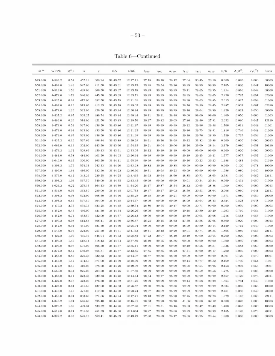
– 53 –

Table 6—Continued

ID a WFPC s(′′) x y RA DEC t160 i160 a160 t110 i110 a110 S/N A(2′′) r1(′′) tests

549.000 4-583.2 0.51 457.18 308.94 36:43.52 12:17.11 27.75 30.18 28.12 27.64 30.45 28.10 0.600 0.020 0.000 00003

550.000 4-492.0 1.46 527.00 411.50 36:43.61 12:29.73 29.25 29.54 29.26 99.99 99.99 99.99 2.105 0.080 0.047 10000

551.000 4-513.0 1.56 489.00 366.50 36:43.67 12:23.78 99.99 99.99 99.99 29.11 29.65 28.95 1.914 0.816 0.049 00000

552.000 4-479.0 1.73 546.00 445.50 36:43.69 12:33.71 99.99 99.99 99.99 28.95 29.69 28.65 2.226 0.787 0.051 02000

553.000 4-525.0 0.92 472.00 352.50 36:43.75 12:21.61 99.99 99.99 99.99 28.90 29.63 28.85 2.313 0.827 0.058 01000

554.000 4-492.0 0.10 513.66 412.33 36:43.78 12:29.02 99.99 99.99 99.99 28.76 29.19 28.45 2.487 0.832 0.087 02010

555.000 4-479.0 1.20 522.00 429.50 36:43.84 12:30.94 99.99 99.99 99.99 29.16 29.64 28.90 1.829 0.822 0.050 00000

556.000 4-437.2 0.97 565.27 489.74 36:43.84 12:38.44 28.11 29.11 28.48 99.00 99.00 99.00 1.400 0.050 0.000 01003

557.000 4-486.0 0.20 514.00 421.50 36:43.85 12:29.76 29.27 29.82 29.05 27.86 28.46 27.91 2.052 0.080 0.047 12110

558.000 4-479.0 0.53 527.00 438.50 36:43.86 12:31.97 99.99 99.99 99.99 29.22 29.96 29.38 1.706 0.611 0.048 01001

559.000 4-479.0 0.94 523.00 433.50 36:43.86 12:31.32 99.99 99.99 99.99 29.16 29.75 28.91 1.816 0.746 0.048 01000

560.000 4-479.0 0.67 525.00 436.50 36:43.86 12:31.69 99.99 99.99 99.99 29.20 29.76 28.90 1.759 0.737 0.054 01000

561.000 4-437.2 0.10 567.66 498.44 36:43.89 12:39.29 28.31 30.20 28.68 29.42 31.82 29.88 0.600 0.020 0.000 00013

562.000 4-663.0 0.19 302.00 143.50 36:43.90 11:54.15 29.21 30.04 29.06 28.26 29.00 28.14 2.179 0.080 0.051 20110

563.000 4-479.2 1.32 529.66 450.43 36:43.91 12:33.05 28.12 30.19 28.49 99.00 99.00 99.00 0.600 0.020 0.000 00003

564.000 4-481.0 0.58 484.00 401.50 36:44.03 12:26.34 99.99 99.99 99.99 29.19 29.45 29.41 1.777 0.977 0.057 01000

565.000 4-640.0 0.15 300.00 163.50 36:44.11 11:55.69 99.99 99.99 99.99 29.46 30.22 29.22 1.388 0.483 0.054 01010

566.000 4-393.2 1.76 574.33 542.33 36:44.20 12:43.28 29.82 30.20 29.85 99.99 99.99 99.99 0.960 0.120 0.071 10000

567.000 4-499.0 1.61 416.00 332.50 36:44.22 12:16.50 29.31 29.68 29.23 99.99 99.99 99.99 1.986 0.080 0.049 10000

568.000 4-577.0 0.12 343.25 239.25 36:44.25 12:4.465 28.93 29.64 28.60 28.85 29.73 28.65 2.381 0.110 0.082 22111

569.000 4-393.2 1.06 567.50 549.00 36:44.35 12:43.45 99.99 99.99 99.99 30.01 30.34 29.34 0.969 0.431 0.050 01000

570.000 4-624.2 0.22 275.15 164.43 36:44.39 11:54.20 28.17 29.87 28.54 28.42 30.65 28.88 1.000 0.030 0.000 00013

571.000 4-534.0 0.06 363.50 289.00 36:44.45 12:9.753 29.47 30.17 29.02 28.70 29.53 28.64 2.006 0.060 0.041 22111

572.000 4-393.2 0.93 572.00 568.50 36:44.46 12:45.28 29.48 30.09 29.21 99.99 99.99 99.99 1.671 0.080 0.050 20000

573.000 4-393.2 0.66 567.50 564.00 36:44.48 12:44.67 99.99 99.99 99.99 28.99 29.64 28.43 2.424 0.823 0.048 01000

574.000 4-430.2 2.36 535.36 523.28 36:44.48 12:39.34 28.80 29.75 29.17 99.00 30.71 99.00 0.900 0.030 0.000 00003

575.000 4-452.0 0.46 456.00 421.50 36:44.54 12:26.26 99.99 99.99 99.99 29.18 29.80 29.29 1.793 0.710 0.054 01000

576.000 4-452.0 0.71 453.50 422.00 36:44.57 12:26.13 99.99 99.99 99.99 29.39 30.05 29.08 1.716 0.563 0.055 01000

577.000 4-400.2 0.08 512.66 506.41 36:44.60 12:36.57 28.25 30.15 28.62 27.50 29.88 27.96 0.600 0.020 0.000 00013

578.000 4-452.0 0.94 451.00 421.50 36:44.60 12:25.94 99.99 99.99 99.99 28.99 29.80 29.14 2.129 0.712 0.049 01000

579.000 4-546.0 0.06 322.00 251.50 36:44.61 12:4.163 29.41 30.42 29.20 29.01 29.74 28.85 1.805 0.080 0.056 22111

580.000 4-422.2 1.05 465.15 446.94 36:44.63 12:28.82 27.73 30.07 28.10 30.19 99.00 30.65 0.700 0.020 0.000 00003

581.000 4-400.2 1.40 518.14 518.43 36:44.64 12:37.89 28.49 29.55 28.86 99.00 99.00 99.00 1.300 0.040 0.000 00003

582.000 4-409.0 0.98 501.00 496.50 36:44.67 12:35.11 99.99 99.99 99.99 29.10 29.56 28.81 1.936 0.883 0.060 00000

583.000 4-377.2 0.52 550.08 565.31 36:44.67 12:43.65 27.85 29.35 28.22 27.71 29.90 28.17 1.700 0.040 0.000 00003

584.000 4-483.0 0.87 376.33 332.33 36:44.68 12:14.07 28.87 29.88 28.70 99.99 99.99 99.99 2.391 0.120 0.070 10001

585.000 4-455.0 1.42 404.50 371.00 36:44.69 12:18.99 99.99 99.99 99.99 29.14 29.77 28.82 2.169 0.730 0.054 01001

586.000 4-472.2 0.56 410.00 378.50 36:44.70 12:19.92 99.99 99.99 99.99 28.98 29.54 28.96 2.153 0.902 0.055 02001

587.000 4-566.0 0.31 275.00 204.50 36:44.76 11:57.50 99.99 99.99 99.99 28.79 29.59 28.56 1.775 0.430 0.088 02000

588.000 4-483.0 0.11 373.33 339.33 36:44.78 12:14.44 28.84 29.77 28.79 99.99 99.99 99.99 2.467 0.120 0.078 20011

589.000 4-422.0 2.48 473.00 476.50 36:44.82 12:31.76 99.99 99.99 99.99 29.14 29.68 29.29 1.864 0.794 0.049 01000

590.000 4-423.0 0.64 441.50 437.00 36:44.83 12:26.57 29.30 29.86 29.38 99.99 99.99 99.99 2.334 0.060 0.063 10000

591.000 4-446.0 1.45 421.00 417.50 36:44.90 12:23.74 29.07 30.02 28.79 99.99 99.99 99.99 2.481 0.080 0.049 20000

592.000 4-458.0 0.04 383.66 371.66 36:44.94 12:17.71 29.13 29.92 28.90 27.75 28.09 27.78 1.979 0.110 0.080 22111

593.000 4-340.2 1.94 546.66 595.40 36:44.98 12:45.91 28.33 29.93 28.70 31.66 99.00 32.12 0.600 0.020 0.000 10003

594.000 4-378.2 1.86 499.87 533.32 36:44.98 12:37.98 27.81 29.31 28.18 28.03 29.47 28.49 1.700 0.040 0.000 10003

595.000 4-519.0 0.14 281.33 251.33 36:45.08 12:1.664 28.97 29.73 28.88 99.99 99.99 99.99 2.185 0.120 0.073 20011

596.000 4-329.2 0.85 528.13 583.41 36:45.09 12:43.79 27.80 28.83 28.17 28.08 30.25 28.54 1.900 0.060 0.000 00003

– 54 –

Table 6—Continued

ID a WFPC s(′′) x y RA DEC t160 i160 a160 t110 i110 a110 S/N A(2′′) r1(′′) tests

597.000 4-596.0 0.69 206.00 154.50 36:45.12 11:49.16 29.64 30.21 29.77 99.99 99.99 99.99 1.451 0.080 0.050 20000

598.000 4-573.0 0.51 207.50 162.00 36:45.17 11:49.90 99.99 99.99 99.99 29.66 30.37 29.04 1.348 0.421 0.049 01000

599.000 4-593.2 0.40 178.97 132.62 36:45.23 11:45.73 28.12 29.81 28.49 27.92 31.87 28.38 0.700 0.030 0.000 10003

600.000 4-368.0 0.94 459.66 522.33 36:45.37 12:34.63 29.11 29.66 29.23 99.99 99.99 99.99 2.215 0.090 0.060 20000

601.000 4-487.0 0.96 264.00 261.50 36:45.38 12:1.472 99.99 99.99 99.99 29.70 30.24 29.64 1.107 0.473 0.051 01000

602.000 4-368.0 0.65 449.00 511.50 36:45.40 12:33.15 99.99 99.99 99.99 29.48 29.80 29.33 1.355 0.713 0.052 00000

603.000 4-342.0 0.75 482.00 556.50 36:45.41 12:38.83 99.99 99.99 99.99 28.92 29.48 29.16 2.286 0.951 0.055 00000

604.000 4-559.2 0.21 179.98 154.42 36:45.41 11:47.56 27.85 29.37 28.22 27.82 29.38 28.28 1.600 0.050 0.000 01013

605.000 4-454.0 0.01 332.74 358.70 36:45.41 12:13.54 22.07 22.10 22.35 21.43 21.45 21.68 119.0 5.920 0.206 22111

606.000 4-593.2 1.28 163.66 136.45 36:45.45 11:45.10 28.36 30.40 28.73 29.23 32.69 29.69 0.500 0.020 0.000 00003

607.000 4-384.2 0.54 414.66 472.43 36:45.45 12:27.81 28.57 30.41 28.94 30.15 99.00 30.61 0.800 0.020 0.000 10003

608.000 4-397.0 0.13 388.50 442.00 36:45.49 12:23.74 29.51 30.24 29.14 99.99 99.99 99.99 1.935 0.060 0.047 10011

609.000 4-582.0 0.17 150.00 126.50 36:45.52 11:43.46 30.12 30.39 30.21 99.99 99.99 99.99 0.938 0.080 0.048 10010

610.000 4-330.0 1.27 483.66 576.33 36:45.56 12:40.54 99.99 99.99 99.99 28.83 29.00 28.49 2.319 0.987 0.072 01000

611.000 4-312.0 0.82 499.50 599.00 36:45.57 12:43.31 29.63 30.14 29.05 99.99 99.99 99.99 1.709 0.060 0.050 10000

612.000 4-312.0 0.70 497.66 596.33 36:45.57 12:43.04 99.99 99.99 99.99 28.77 29.05 28.53 2.442 0.942 0.071 01000

613.000 4-307.0 1.02 485.50 581.00 36:45.57 12:40.99 29.34 30.04 28.90 99.99 99.99 99.99 2.245 0.060 0.049 10000

614.000 4-330.2 1.04 478.16 572.94 36:45.58 12:39.88 27.81 28.94 28.18 30.44 30.50 30.90 2.000 0.060 0.000 10003

615.000 4-389.2 0.72 384.66 450.45 36:45.60 12:24.18 28.39 30.65 28.76 99.00 33.11 99.00 1.300 0.020 0.000 00003

616.000 4-330.0 1.60 476.00 577.50 36:45.65 12:40.13 29.16 30.10 28.82 99.99 99.99 99.99 2.278 0.080 0.045 10001

617.000 4-371.0 0.04 396.00 474.50 36:45.69 12:26.85 29.35 30.22 29.18 99.99 99.99 99.99 1.912 0.080 0.054 20011

618.000 4-563.2 0.75 140.18 135.94 36:45.71 11:43.61 27.87 30.36 28.24 99.00 99.00 99.00 0.500 0.020 0.000 00003

619.000 4-307.0 0.88 478.50 589.00 36:45.73 12:41.21 29.40 29.80 29.01 99.99 99.99 99.99 2.085 0.060 0.049 10000

620.000 4-563.2 1.19 141.66 140.19 36:45.73 11:44.05 27.98 29.63 28.35 27.75 29.77 28.21 1.100 0.040 0.000 00003

621.000 4-520.2 1.45 187.16 202.94 36:45.75 11:51.95 28.71 30.57 29.08 99.00 34.48 99.00 0.500 0.020 0.000 00003

622.000 4-563.2 1.13 136.16 138.44 36:45.78 11:43.57 27.67 29.24 28.04 28.70 30.35 29.16 1.800 0.050 0.000 01003

623.000 4-510.0 0.76 172.50 186.00 36:45.78 11:49.68 29.90 30.50 29.53 99.99 99.99 99.99 1.344 0.060 0.051 10000

624.000 4-484.0 0.14 217.66 250.66 36:45.82 11:57.70 29.35 30.09 29.16 99.99 99.99 99.99 1.575 0.110 0.065 20011

625.000 4-389.0 1.54 374.50 461.00 36:45.83 12:24.47 99.99 99.99 99.99 29.42 29.70 28.97 1.682 0.781 0.062 01000

626.000 4-441.0 0.07 259.00 315.50 36:45.90 12:5.509 29.12 30.13 28.79 99.99 99.99 99.99 2.364 0.080 0.066 20011

627.000 4-448.2 1.65 219.18 276.94 36:46.02 11:59.93 28.13 30.45 28.50 28.14 32.26 28.60 0.500 0.020 0.000 00003

628.000 4-522.0 0.53 129.50 162.00 36:46.07 11:45.10 29.27 30.15 28.72 99.99 99.99 99.99 2.382 0.060 0.052 00000

629.000 4-293.0 0.02 431.50 568.00 36:46.09 12:36.64 29.34 29.92 29.01 28.94 29.36 28.60 2.259 0.060 0.057 22111

630.000 4-528.0 0.44 123.50 155.00 36:46.09 11:44.19 99.99 99.99 99.99 29.76 30.04 29.13 1.217 0.570 0.053 01000

631.000 4-300.0 1.10 408.33 540.33 36:46.12 12:32.96 28.91 29.47 28.85 99.99 99.99 99.99 2.315 0.120 0.090 10000

632.000 4-288.0 0.94 441.50 585.00 36:46.13 12:38.67 99.99 99.99 99.99 29.28 29.28 29.29 1.912 1.142 0.048 01000

633.000 4-396.2 0.12 283.68 379.63 36:46.16 12:12.23 28.32 30.17 28.69 28.87 32.16 29.33 0.900 0.020 0.000 00013

634.000 4-362.0 0.08 329.66 442.83 36:46.19 12:20.20 28.60 28.90 28.40 28.86 29.46 28.67 2.309 0.200 0.091 22111

635.000 4-470.2 2.10 156.18 213.44 36:46.20 11:50.91 27.92 29.93 28.29 28.57 30.97 29.03 1.300 0.010 0.000 00003

636.000 4-396.0 0.50 283.50 384.00 36:46.22 12:12.63 99.99 99.99 99.99 29.28 29.95 28.87 1.916 0.619 0.049 01000

637.000 4-294.0 0.08 416.00 562.50 36:46.22 12:35.24 29.38 30.19 29.22 99.99 99.99 99.99 1.860 0.080 0.050 10010

638.000 4-418.0 1.61 238.50 326.00 36:46.23 12:5.125 29.49 30.30 29.41 99.99 99.99 99.99 1.972 0.060 0.049 10000

639.000 4-418.0 0.83 230.50 323.00 36:46.30 12:4.383 29.51 30.36 28.89 99.99 99.99 99.99 1.903 0.060 0.052 10000

640.000 4-372.0 0.50 298.00 415.50 36:46.32 12:16.04 29.42 30.26 29.10 99.99 99.99 99.99 1.784 0.080 0.057 00000

641.000 4-390.0 0.26 271.50 384.00 36:46.37 12:11.89 99.99 99.99 99.99 29.60 30.14 29.51 1.418 0.520 0.042 01000

642.000 4-390.2 0.00 268.66 383.45 36:46.37 12:11.63 28.44 30.55 28.81 28.07 30.47 28.53 0.500 0.020 0.000 00013

643.000 4-470.0 0.62 141.50 212.50 36:46.38 11:49.95 29.11 29.91 29.01 99.99 99.99 99.99 1.894 0.120 0.081 10000

644.000 4-470.0 0.36 137.50 212.00 36:46.42 11:49.66 29.86 30.73 29.62 99.99 99.99 99.99 1.389 0.060 0.050 10000

– 55 –

Table 6—Continued

ID a WFPC s(′′) x y RA DEC t160 i160 a160 t110 i110 a110 S/N A(2′′) r1(′′) tests

645.000 4-461.0 1.38 155.00 236.50 36:46.43 11:52.72 29.76 30.60 29.94 99.99 99.99 99.99 1.301 0.080 0.046 00000

646.000 4-262.2 0.08 415.66 590.43 36:46.47 12:37.47 28.37 30.05 28.74 28.24 30.64 28.70 0.700 0.020 0.000 00013

647.000 4-504.0 0.93 93.500 159.00 36:46.47 11:42.64 29.27 29.80 28.92 99.99 99.99 99.99 2.366 0.060 0.057 10000

648.000 4-443.0 0.16 172.50 265.00 36:46.47 11:56.11 29.57 30.39 29.01 28.20 29.09 28.19 1.833 0.060 0.047 21111

649.000 4-470.0 0.51 131.33 215.16 36:46.53 11:49.57 99.99 99.99 99.99 28.84 29.23 28.72 1.544 0.401 0.118 01000

650.000 4-262.0 0.93 407.50 588.00 36:46.55 12:36.83 99.99 99.99 99.99 29.19 29.64 28.85 2.078 0.819 0.054 01000

651.000 4-434.0 0.44 175.50 281.00 36:46.58 11:57.59 29.73 30.39 29.17 99.99 99.99 99.99 1.562 0.060 0.047 00000

652.000 4-442.0 0.85 143.50 250.00 36:46.68 11:53.12 30.06 30.58 30.33 99.99 99.99 99.99 1.158 0.060 0.051 20000

653.000 4-388.0 0.06 225.33 359.33 36:46.68 12:7.034 28.91 29.67 28.65 99.99 99.99 99.99 2.303 0.120 0.080 10011

654.000 4-241.0 1.36 388.00 588.50 36:46.78 12:35.69 99.99 99.99 99.99 29.12 29.72 28.82 1.880 0.766 0.041 00000

655.000 4-415.0 1.20 153.00 280.00 36:46.83 11:56.15 29.33 29.50 29.87 99.99 99.99 99.99 1.637 0.110 0.063 10000

656.000 4-241.2 1.31 384.00 592.50 36:46.87 12:35.76 99.99 99.99 99.99 29.58 29.95 31.04 1.209 0.618 0.054 00000

657.000 4-280.0 1.76 357.00 556.50 36:46.87 12:31.17 99.99 99.99 99.99 29.53 29.94 29.44 1.294 0.621 0.049 01000

658.000 4-336.0 1.44 265.00 440.50 36:46.93 12:16.11 99.99 99.99 99.99 29.22 30.06 29.06 1.722 0.556 0.045 01000

659.000 4-415.0 0.93 143.50 279.00 36:46.94 11:55.52 99.99 99.99 99.99 29.29 30.20 29.20 1.881 0.493 0.049 01000

660.000 4-470.0 3.52 105.00 230.50 36:46.96 11:49.18 29.23 30.06 29.16 99.99 99.99 99.99 2.129 0.080 0.048 00000

661.000 4-382.0 1.03 193.50 350.00 36:46.97 12:4.314 29.78 30.41 29.29 99.99 99.99 99.99 1.488 0.060 0.051 00000

662.000 4-298.0 2.26 264.00 451.50 36:47.04 12:16.94 99.99 99.99 99.99 29.26 30.08 29.00 1.673 0.550 0.054 01000

663.000 4-381.0 0.68 161.00 326.50 36:47.14 12:0.428 29.30 30.37 29.05 99.99 99.99 99.99 2.011 0.080 0.047 10001

664.000 4-216.2 0.04 351.16 585.43 36:47.17 12:33.12 28.03 29.17 28.40 27.92 29.38 28.38 1.200 0.040 0.000 10013

665.000 4-315.2 1.68 220.00 409.50 36:47.18 12:10.78 29.51 30.09 29.61 28.46 29.14 28.37 1.653 0.080 0.044 11101

666.000 4-386.0 3.29 101.50 255.00 36:47.21 11:50.95 29.58 29.68 29.63 99.99 99.99 99.99 1.804 0.060 0.042 20000

667.000 4-216.2 0.74 344.01 582.62 36:47.23 12:32.46 27.79 30.03 28.16 32.90 99.00 33.36 1.300 0.030 0.000 00003

668.000 4-281.2 1.27 272.66 491.44 36:47.27 12:20.67 28.35 30.54 28.72 99.00 99.00 99.00 0.700 0.020 0.000 00003

669.000 4-386.0 3.28 95.000 254.50 36:47.28 11:50.51 29.69 30.02 29.93 99.99 99.99 99.99 1.403 0.080 0.050 10001

670.000 4-298.2 0.06 239.00 452.50 36:47.34 12:15.50 99.99 99.99 99.99 29.22 30.00 28.79 1.716 0.589 0.036 01010

671.000 4-386.2 2.22 95.660 265.43 36:47.36 11:51.44 27.97 30.56 28.34 28.12 31.86 28.58 1.100 0.020 0.000 10003

672.000 4-250.2 1.14 281.89 515.12 36:47.37 12:23.17 28.19 29.47 28.56 99.00 31.74 99.00 1.500 0.050 0.000 10003

673.000 4-298.0 1.12 245.00 465.50 36:47.38 12:16.92 99.99 99.99 99.99 28.97 29.84 28.68 2.179 0.681 0.055 01000

674.000 4-232.11 1.40 333.50 584.00 36:47.38 12:31.98 99.99 99.99 99.99 29.35 29.58 29.23 1.785 0.869 0.050 00000

675.000 4-188.0 0.33 320.50 592.00 36:47.60 12:31.83 99.99 99.99 99.99 29.06 29.80 28.58 2.332 0.713 0.055 01000

676.000 4-346.2 1.64 141.15 369.94 36:47.74 12:2.735 28.16 30.70 28.53 30.20 32.51 30.66 0.800 0.020 0.000 00003

677.000 4-188.0 1.24 311.33 599.33 36:47.77 12:31.86 99.99 99.99 99.99 28.83 29.04 28.66 1.970 0.950 0.082 00000

678.000 4-174.2 2.34 283.13 564.44 36:47.78 12:27.26 27.93 29.49 28.30 27.60 29.66 28.06 1.100 0.040 0.000 10003

679.000 4-212.0 0.50 258.66 539.33 36:47.86 12:23.73 29.03 29.38 28.96 99.99 99.99 99.99 2.389 0.090 0.075 10000

680.000 4-198.0 1.22 251.00 531.50 36:47.89 12:22.66 99.99 99.99 99.99 28.96 29.72 28.96 2.192 0.766 0.056 01000

681.000 4-236.0 0.45 226.66 499.66 36:47.89 12:18.54 29.15 29.88 28.86 28.40 29.11 28.32 1.931 0.110 0.081 21100

682.000 4-304.0 0.75 144.33 396.33 36:47.95 12:5.083 28.97 29.83 28.81 99.99 99.99 99.99 2.160 0.120 0.085 20000

683.000 4-212.0 1.24 259.50 551.00 36:47.96 12:24.76 99.99 99.99 99.99 29.38 29.72 29.10 1.744 0.765 0.050 01000

684.000 4-170.0 0.89 229.00 541.50 36:48.23 12:22.07 29.31 30.08 29.27 99.99 99.99 99.99 1.973 0.080 0.042 10000

685.000 4-158.0 0.35 235.50 562.00 36:48.33 12:24.15 29.64 29.95 29.04 99.99 99.99 99.99 1.716 0.060 0.059 10000

686.000 4-158.0 0.11 232.66 561.66 36:48.36 12:23.95 28.89 29.62 28.62 99.99 99.99 99.99 2.462 0.110 0.066 10010

687.000 4-260.2 1.67 163.32 470.60 36:48.36 12:12.28 27.98 30.07 28.35 29.74 99.00 30.20 0.800 0.030 0.000 00003

688.000 4-122.0 0.79 249.00 597.50 36:48.49 12:27.90 99.99 99.99 99.99 29.62 29.57 29.99 1.200 0.880 0.052 00000

689.000 4-122.0 0.33 241.00 599.50 36:48.60 12:27.59 99.99 99.99 99.99 29.23 29.71 29.32 1.699 0.768 0.044 01000

690.000 4-203.2 0.24 115.00 455.00 36:48.81 12:8.105 99.99 99.99 99.99 28.98 29.54 28.82 1.814 0.601 0.108 01010

691.000 4-203.2 0.20 116.66 459.66 36:48.82 12:8.544 29.13 29.85 29.04 99.99 99.99 99.99 1.967 0.110 0.079 20010

692.000 4-105.2 1.07 205.17 581.44 36:48.84 12:23.87 27.80 29.46 28.17 28.52 30.19 28.98 1.400 0.040 0.000 10003

– 56 –

Table 6—Continued

ID a WFPC s(′′) x y RA DEC t160 i160 a160 t110 i110 a110 S/N A(2′′) r1(′′) tests

693.000 4-128.0 0.48 185.75 556.00 36:48.85 12:20.62 29.24 29.54 29.02 29.72 29.91 29.77 1.611 0.130 0.063 22101

694.000 4-148.2 0.32 161.16 526.94 36:48.88 12:16.74 27.91 30.40 28.28 27.47 30.43 27.93 0.500 0.020 0.000 00003

695.000 4-120.0 0.74 173.50 559.00 36:49.02 12:20.12 29.61 30.30 29.32 99.99 99.99 99.99 1.741 0.060 0.042 10000

696.000 4-131.0 1.95 127.50 511.00 36:49.14 12:13.39 29.57 30.13 29.25 99.99 99.99 99.99 1.826 0.060 0.046 10000

697.000 4-124.0 0.07 140.50 534.00 36:49.19 12:16.05 29.39 30.02 28.91 99.99 99.99 99.99 2.155 0.060 0.055 20011

698.000 4-99.0 1.53 169.50 579.00 36:49.25 12:21.49 29.81 30.26 29.13 99.99 99.99 99.99 1.420 0.060 0.057 00000

699.000 4-95.0 2.30 133.50 555.00 36:49.47 12:17.37 99.99 99.99 99.99 29.14 29.79 29.04 2.173 0.716 0.050 01000

700.000 4-74.0 1.57 148.00 596.50 36:49.66 12:21.64 99.99 99.99 99.99 29.05 29.47 29.17 2.029 0.958 0.058 01000

701.000 4-50.0 1.35 101.00 556.50 36:49.86 12:15.52 99.99 99.99 99.99 28.96 29.64 28.68 2.200 0.820 0.048 01000

702.000 4-50.2 1.75 94.330 552.61 36:49.88 12:14.73 28.00 29.68 28.37 99.00 99.00 99.00 1.000 0.030 0.000 00003

703.000 4-50.2 1.04 105.07 571.55 36:49.93 12:16.93 27.78 29.29 28.15 30.77 99.00 31.23 1.600 0.050 0.000 00003

704.000 4-50.0 0.78 93.500 562.00 36:49.99 12:15.45 29.30 29.51 28.96 99.99 99.99 99.99 2.346 0.060 0.047 10000

705.000 4-33.0 2.13 107.00 596.50 36:50.12 12:19.07 29.29 29.93 28.85 99.99 99.99 99.99 1.986 0.080 0.064 10000

aSources with signal to noise levels less than 2.5 have id numbers of 500 or greater