Embed Size (px)
Citation preview
arX
iv:a
stro
-ph/
9801
057v
1 7
Jan
199
8
The Hubble Deep Field and the Disappearing Dwarf Galaxies
HENRY C. FERGUSON
Space Telescope Science Institute, 3700 San Martin Drive
Baltimore, MD 21218
email: [email protected]
ARIF BABUL
Department of Physics & Astronomy
University of Victoria
3800 Finnerty Road, Victoria, BC V8W 3P6
email: [email protected]
ABSTRACT
Several independent lines of reasoning, both theoretical and observational,
suggest that the very faint (B >∼ 24) galaxies seen in deep images of the sky
are small low-mass galaxies that experienced a short epoch of star formation
at redshifts 0.5 <∼ z <
∼ 1 and have since faded into low luminosity, low surface
brightness objects. Such a scenario, which arises naturally if star formation
in dwarf galaxies is delayed by photoionisation due to the metagalactic UV
radiation field, provides an attractive way to reconcile the Einstein-de Sitter
(Ω = 1; Λ = 0) cosmological model to the steeply rising galaxy counts observed
at blue wavelengths. Babul and Ferguson (1996) constructed a specific
realisation of this model, deriving the dwarf galaxy mass function from the
CDM power spectrum, and arguing that the gas in these halos will recombine
at z ∼ 1. The Hubble Deep Field (HDF) images provide a stringent test of this
model. We compare the model to the data by constructing simulated images
that reproduce the spatial resolution and noise properties of the real data and
carrying out source detection and photometry for the simulations in the same
way they were carried out for the real data. The selection biases and systematic
errors that are inevitable in dealing with faint galaxies are thus incorporated
directly into the model. We compare the model predictions for the counts, sizes,
and colours of galaxies observed in the HDF, and to the predictions from a low
q0 pure-luminosity-evolution (PLE) model. Both models fail to reproduce the
observations. The low q0 model predicts far more Lyman-break “dropouts” than
are seen in the data. The fading dwarf model predicts too many remnants: faded
dwarf galaxies in the redshift range 0.2 < z < 0.5 that should be detectable
– 2 –
in the HDF as low-surface brightness red objects but are not seen. If fading
dwarf galaxies are to reconcile the Einstein-de Sitter geometry to the counts,
then the dwarf population must (a) form earlier than z ∼ 1, with a higher initial
luminosity; (b) have an initial-mass function more heavily weighted toward
massive stars than the Salpeter IMF; or (c) expand much more than assumed
during the supernova wind phase.
Subject headings: galaxies: formation — galaxies:luminosity function, mass
function — galaxies:photometry
1. Introduction
Any self-consistent theory of galaxy evolution and cosmology must now pass the
test of matching the distribution of galaxy properties in the Hubble Deep Field. The
theory must simultaneously match the counts, redshift and colour distributions, clustering
properties, and size distribution of faint galaxies. Even at ground-based depths (e.g. Lilly
et al. 1995; Ellis et al. 1996; Cowie et al. 1996), matching the observed distributions
within an Einstein-de Sitter (Ω = 1, Λ = 0) cosmology has required either introducing
heuristic modifications to the local luminosity function and the evolution of low-mass
galaxies (Phillipps & Driver 1995), or introducing additional physical processes into
theories of galaxy evolution beyond simple passive evolution of the stellar populations. In
hierarchical prescriptions (e.g. Kauffmann, Guiderdoni, & White 1994; Cole et al. 1994)
the additional physics has been a detailed treatment of the merging histories of galaxies,
coupled with prescriptions for how star formation proceeds during the merger events. The
primary physical process driving the counts in these models is triggered star formation.
An alternative view (Babul & Rees 1992; Babul & Ferguson 1996) is that the important
physics driving the counts at very faint magnitudes is the delayed formation of dwarf
galaxies, where the cooling and collapse timescales of the interstellar gas is governed by
photoionisation by the UV background.
The purpose of this paper is to test this latter model against the Hubble Deep Field
(HDF) observations. The comparison involves constructing simulated HDF images from
Monte-Carlo realisations of the underlying model and then analyzing them in exactly the
same manner as the actual images. In this way all of the details of galaxy selection and
photometry are properly taken into account.
It is illustrative to consider the q0 = 0.5 dwarf-dominated model not in isolation,
but in comparison to a low−Ω giant-dominated model. Gronwall & Koo (1995) and
– 3 –
Pozzetti, Bruzual, & Zamorani (1996) have demonstrated that for low values of q0
straightforward “pure-luminosity evolution” models, without large populations of dwarf
galaxies or substantial number-evolution, can be reasonably successful at matching the
observed counts and redshift distributions (to 1995 ground-based limits). Thus, as a foil to
the dwarf-dominated q0 = 0.5 model, we construct a giant-dominated q0 = 0.01 model and
carry out the same comparisons to the observations.
We emphasize that our goal in this paper is not to tune the models to try to match the
observations, but to test the models in their simplest form to illustrate their differences (and
their deficiencies) at the depths probed by the Hubble Deep Field. The models incorporate
the simplest, most conservative, assumptions for the luminosity function of local giant
galaxies, their stellar initial mass functions and evolution, their star-formation histories,
and their surface-brightness distributions. The predictions of both models turn out to be
very sensitive to the redshift of formation, which has not been tuned post-facto to try to
meet the constraints imposed by the observations. The dwarf galaxies are incorporated
into the q0 = 0.5 model with only three free parameters (described in section 1). These
parameters were fixed from physical arguments and ground-based observations (Babul &
Ferguson 1996) and have not been tuned to match the HDF observations.
In §2, we briefly review the q0 = 0.5 dwarf-dominated model and the q0 = 0.01 model,
and discuss the construction of simulated HDF images from the corresponding Monte-Carlo
realisations. In §3, we compare the results for the two models to the observations. In §4 we
outline the implications of these comparisons, specifically identifying changes that might be
made to each model to bring it more into agreement.
2. The Models
2.1. The q0 = 0.5, bursting-dwarf model
In a q0 = 0.5 cosmology, matching the galaxy number counts and redshift distributions
observed to ground-based limits requires a large population of low-luminosity galaxies at
moderate redshifts. Babul & Ferguson (1996) outlined a dwarf-dominated model that
appeared capable of reproducing existing ground based observations. The model consists of
“giant” galaxies (types E through Sdm) that form at zf = 5 and a large population of dwarf
galaxies that begin forming stars at z ≈ 1. (Babul & Ferguson refer to these objects as
“boojums,” for blue objects observed just undergoing a moderate starburst). The comoving
number density of each galaxy type is conserved, but the dwarfs are entirely gaseous until
z < 1.
– 4 –
In hierarchical clustering scenarios with realistic initial conditions on galactic and
sub-galactic scales (i.e. spectral index −2 <∼ n <
∼ −1), the distribution of M ∼ 108–109 M⊙
halos is a steep function of mass (d lnN/d lnM ≈ −2) and the bulk of the halos are expected
to form at z >∼ 3. Under “ordinary” conditions, the gas in these halos would rapidly cool,
collect in the cores and undergo star-formation. Studies of Lyα clouds, however, suggest
that the universe at high redshifts is permeated by an intense metagalactic UV flux. This
UV background will photoionise the gas and hence prevent it from cooling and collecting in
the cores of low mass halos until z <∼ 2 when the photoionising background begins to decline
rapidly (Babul & Rees 1992; Quinn, Katz, & Efstathiou 1996). In our model, the power
spectrum of density fluctuations that grow into halos of circular velocity less than 35 km s−1
is described by the standard cold dark matter (SCDM) power spectrum normalized such
that the rms density fluctuations on the scale of 8h−1Mpc are σ8 = 0.67. The comoving
number density of minihalos existing at z ≈ 1, estimated using the analytic Press-Schecter
(1974) formalism, is
dN
d ln(M)≈ 2.3
(
M
109 M⊙
)−0.9
Mpc−3. (1)
The mass function of dwarf galaxies is thus fixed with no free parameters. Once the gas
in dwarf galaxy halo can recombine and cool, star-formation occurs rapidly, ceasing at
107 years (the typical lifetime of massive stars) when supernova explosions heat and expel
the gas. The probability of such a burst occuring in a dwarf galaxy is assumed to decline
exponentially with redshift from z = 1, with the timescale (t∗ = 2 × 10⁹ yr) fixed by
the requirement that the model must match the observed B-band redshift distribution of
Glazebrook et al. (1995).
Apart from the dwarf-galaxy mass function, which is fixed, the three most important
parameters of the model are (1) star-formation efficiency 1 , assumed to be 10%, (2) t∗, the
burst probability timescale, and (3) the redshift, zf , at which the dwarfs start to form stars
— which could plausibly be as high as z = 1.5 and as low as z = 0 and could vary as a
function of mass. The choice of these parameters is discussed by Babul & Ferguson (1996);
they have not been adjusted to fit the HDF data.
1Babul & Ferguson (1996) incorrectly computed the total stellar mass for their dwarf galaxies; their
assumed star-formation efficiency of 30% resulted in luminosities a factor of 2.8 too high, for the adopted
IMF. To make the results directly comparable, we have kept the same total luminosities for the dwarf
galaxies, but lowered the corresponding star-formation efficiency to 10% (for a Salpeter IMF from 0.1 to
100 M⊙). Nevertheless, as most of the light is produced by massive stars and most of the stellar mass is
in low-mass stars, the conversion from dwarf-galaxy mass to dwarf-galaxy luminosity carries with it large
uncertainties.
– 5 –
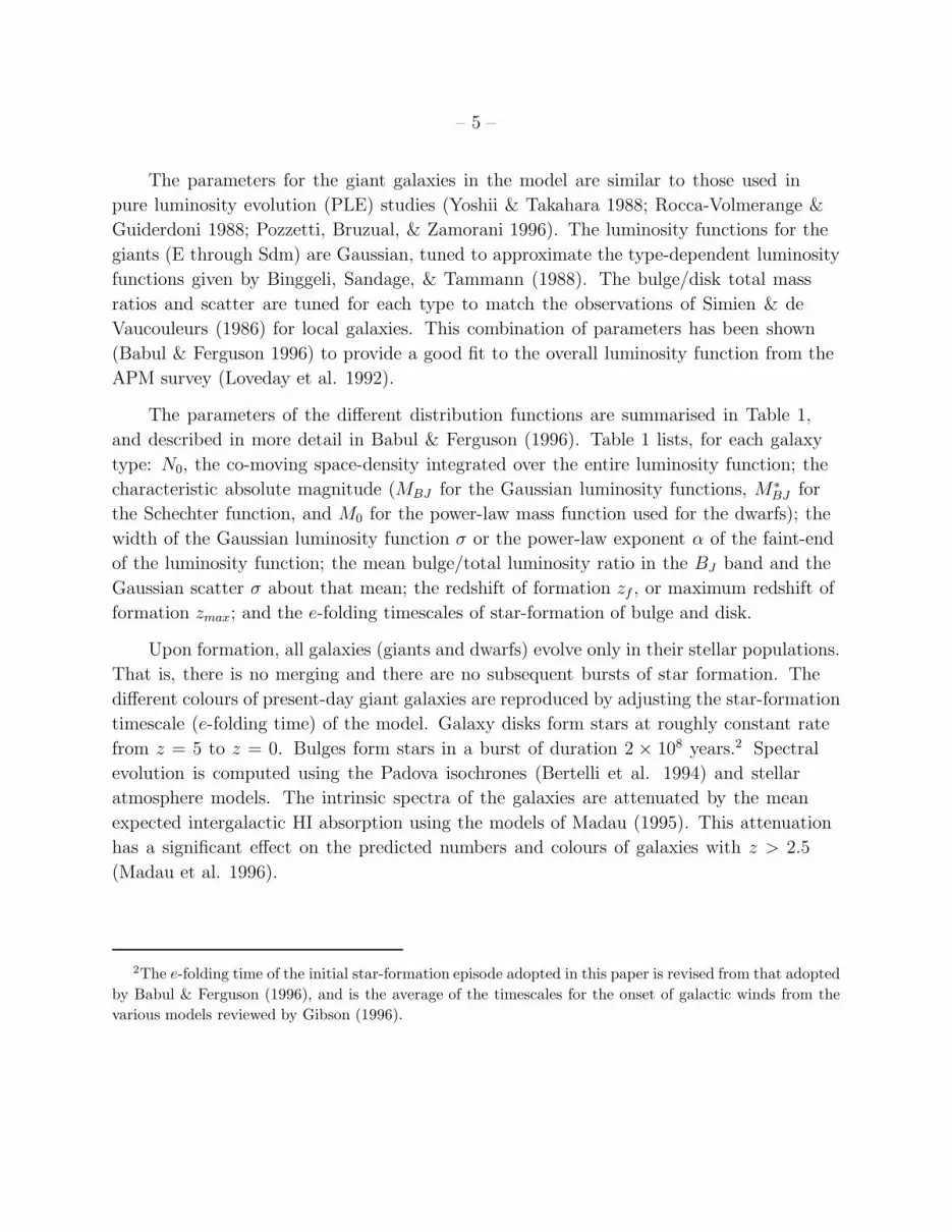
The parameters for the giant galaxies in the model are similar to those used in
pure luminosity evolution (PLE) studies (Yoshii & Takahara 1988; Rocca-Volmerange &
Guiderdoni 1988; Pozzetti, Bruzual, & Zamorani 1996). The luminosity functions for the
giants (E through Sdm) are Gaussian, tuned to approximate the type-dependent luminosity
functions given by Binggeli, Sandage, & Tammann (1988). The bulge/disk total mass
ratios and scatter are tuned for each type to match the observations of Simien & de
Vaucouleurs (1986) for local galaxies. This combination of parameters has been shown
(Babul & Ferguson 1996) to provide a good fit to the overall luminosity function from the
APM survey (Loveday et al. 1992).
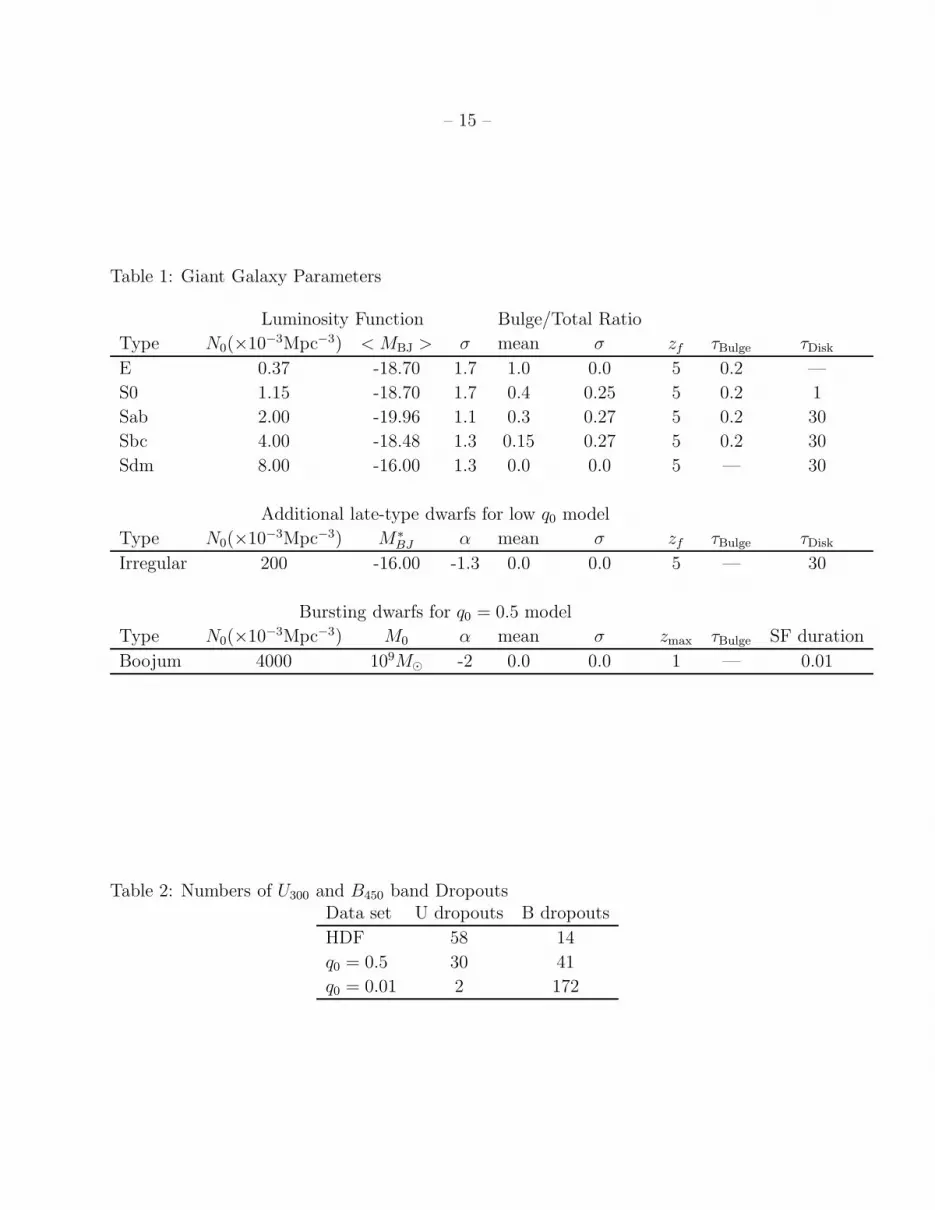
The parameters of the different distribution functions are summarised in Table 1,
and described in more detail in Babul & Ferguson (1996). Table 1 lists, for each galaxy
type: N0, the co-moving space-density integrated over the entire luminosity function; the
characteristic absolute magnitude (MBJ for the Gaussian luminosity functions, M∗
BJ for
the Schechter function, and M0 for the power-law mass function used for the dwarfs); the
width of the Gaussian luminosity function σ or the power-law exponent α of the faint-end
of the luminosity function; the mean bulge/total luminosity ratio in the BJ band and the
Gaussian scatter σ about that mean; the redshift of formation zf , or maximum redshift of
formation zmax; and the e-folding timescales of star-formation of bulge and disk.
Upon formation, all galaxies (giants and dwarfs) evolve only in their stellar populations.
That is, there is no merging and there are no subsequent bursts of star formation. The
different colours of present-day giant galaxies are reproduced by adjusting the star-formation
timescale (e-folding time) of the model. Galaxy disks form stars at roughly constant rate
from z = 5 to z = 0. Bulges form stars in a burst of duration 2 × 10⁸ years.2 Spectral
evolution is computed using the Padova isochrones (Bertelli et al. 1994) and stellar
atmosphere models. The intrinsic spectra of the galaxies are attenuated by the mean
expected intergalactic HI absorption using the models of Madau (1995). This attenuation
has a significant effect on the predicted numbers and colours of galaxies with z > 2.5
(Madau et al. 1996).
2The e-folding time of the initial star-formation episode adopted in this paper is revised from that adopted
by Babul & Ferguson (1996), and is the average of the timescales for the onset of galactic winds from the
various models reviewed by Gibson (1996).
– 6 –
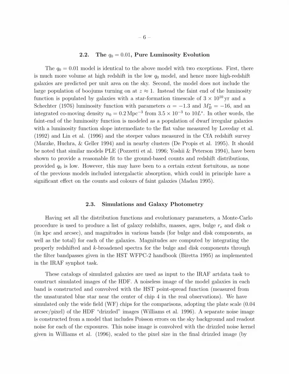
2.2. The q0 = 0.01, Pure Luminosity Evolution
The q0 = 0.01 model is identical to the above model with two exceptions. First, there
is much more volume at high redshift in the low q0 model, and hence more high-redshift
galaxies are predicted per unit area on the sky. Second, the model does not include the
large population of boojums turning on at z ≈ 1. Instead the faint end of the luminosity
function is populated by galaxies with a star-formation timescale of 3 × 10¹⁰ yr and a
Schechter (1976) luminosity function with parameters α = −1.3 and M∗
B = −16, and an
integrated co-moving density n0 = 0.2 Mpc−3 from 3.5 × 10⁻³ to 10L∗. In other words, the
faint-end of the luminosity function is modeled as a population of dwarf irregular galaxies
with a luminosity function slope intermediate to the flat value measured by Loveday et al.
(1992) and Lin et al. (1996) and the steeper values measured in the CfA redshift survey
(Marzke, Huchra, & Geller 1994) and in nearby clusters (De Propis et al. 1995). It should
be noted that similar models PLE (Pozzetti et al. 1996; Yoshii & Peterson 1994), have been
shown to provide a reasonable fit to the ground-based counts and redshift distributions,
provided q0 is low. However, this may have been to a certain extent fortuitous, as none
of the previous models included intergalactic absorption, which could in principle have a
significant effect on the counts and colours of faint galaxies (Madau 1995).
2.3. Simulations and Galaxy Photometry
Having set all the distribution functions and evolutionary parameters, a Monte-Carlo
procedure is used to produce a list of galaxy redshifts, masses, ages, bulge re and disk α
(in kpc and arcsec), and magnitudes in various bands (for bulge and disk components, as
well as the total) for each of the galaxies. Magnitudes are computed by integrating the
properly redshifted and k-broadened spectra for the bulge and disk components through
the filter bandpasses given in the HST WFPC-2 handbook (Biretta 1995) as implemented
in the IRAF synphot task.
These catalogs of simulated galaxies are used as input to the IRAF artdata task to
construct simulated images of the HDF. A noiseless image of the model galaxies in each
band is constructed and convolved with the HST point-spread function (measured from
the unsaturated blue star near the center of chip 4 in the real observations). We have
simulated only the wide field (WF) chips for the comparisons, adopting the plate scale (0.04
arcsec/pixel) of the HDF “drizzled” images (Williams et al. 1996). A separate noise image
is constructed from a model that includes Poisson errors on the sky background and readout
noise for each of the exposures. This noise image is convolved with the drizzled noise kernel
given in Williams et al. (1996), scaled to the pixel size in the final drizzled image (by

– 7 –
multiplying by 0.4), and multiplied by a factor of 1.1 to account for the stochastic loss of
exposure time in each pixel due to cosmic-ray rejection. The contribution from Poisson
errors on counts from the objects is not included, but is negligible for objects near the sky
level. The scaled noise image is then added to the noiseless object image to produce the
final simulated image. This prescription reproduces the noise properties of the real HDF
images remarkably well, as can be seen by examination of the simulated images in Figures
1-3, and by detailed comparison of image statistics on different scales.
For quantitative comparisons, analysis of the images is carried out using the FOCAS
galaxy detection and photometry software (Jarvis & Tyson 1981; Valdes 1982; revised by
Adelberger & Steidel 1996). The detection algorithm, as applied to the HDF images, is
discussed by Williams et al. (1996). Briefly, objects with S/N greater than 4σ within a
contiguous area of 25 pixels (each 0.04 square arcseconds in area) are considered detections.
Isophotal magnitudes are estimated by summing the sky-subtracted counts within the
detection isophote. For a point source on the WF, this minimum area encompasses roughly
60% of the total object flux. FOCAS total magnitudes are computed from the total counts
within an area that is a factor of two larger. The photometry of the simulated images and
the HDF images is identical, except for one minor difference. For the HDF images, the
individual pixels are weighted by the inverse variance, to account for the small differences
in exposure time between adjacent pixels in the sub-sampled image. For the simulations,
the exposure time is assumed to be constant for all pixels. This difference is likely to be
unimportant, as the variations in exposure time between pixels in the real HDF images are
typically less than 20%.
In the case where there are multiple peaks within the initial detection isophote, FOCAS
computes photometric parameters for both the “parent” and “daughter” objects. Because
we only want to count objects once, we have to decide, for each object, whether to keep
the parent or the daughters. For both the true HDF images and the simulations, we have
adopted the separation and colour criteria of Williams et al. (1996), keeping the parent if
the daughters have ∆(V606 − I814) < C, and separation Sij < F × (ri + rj), with C = 0.3
mag and F = 5, and ri and rj are galaxy radii determined from the FOCAS isophotal areas
as ri =√
A/π. In the real HDF images, galaxy counts are only mildly affected by the
choice of whether to count parents or daughters, growing by 20% if all the subcomponents
(daughters) rather than the parents are counted as individual objects (Williams et al.
1996). The two main issues that may affect the comparison of our models to the real images
are (1) clustering on small scales, and (2) substructure within galaxies. Galaxy positions in
our simulations are stastically independent. Intrinsic clustering in the real universe is likely
to lead to a reduction in counts, as overlapping objects will in some cases be counted as one
object. The Villumsen, Freudling, & da Costa (1997) analysis of the angular correlation
– 8 –
function in the HDF suggests that clustering will lead to an excess probability of about
10% for galaxies to have a separation of 1 arcsec. Hence, we expect that clustering will lead
to only a very slight undercounting of galaxies. (Note that the higher probability found by
Colley et al. (1997) applies only to galaxies with photometric redshifts z > 2.4, and their
analysis used a different algorithm for counting galaxies and merging subcomponents.)
Substructure within galaxies will work in the opposite direction. Galaxies in our models
have smooth profiles, while real galaxies, especially those being observed at rest-frame UV
wavelengths, tend to have substructures. Even with the merging algorithm described above,
it is likely that some individual galaxies in the real HDF have been counted as multiple
objects.
These effects, while ultimately of great interest, have only a mild effect on the counts.
The change in luminosities of the individual components compensates for the change in the
number of components. Thus both the slope and normalization of the faint counts stays
approximately the same. The effect on galaxy colors and size distributions is likely to be
larger, but we have not attempted to model it in this paper. The gross differences between
the models and the data, described below, are likely to be relatively insensitive to the
details of the merging and splitting algorithms, although further investigation is certainly
warranted.
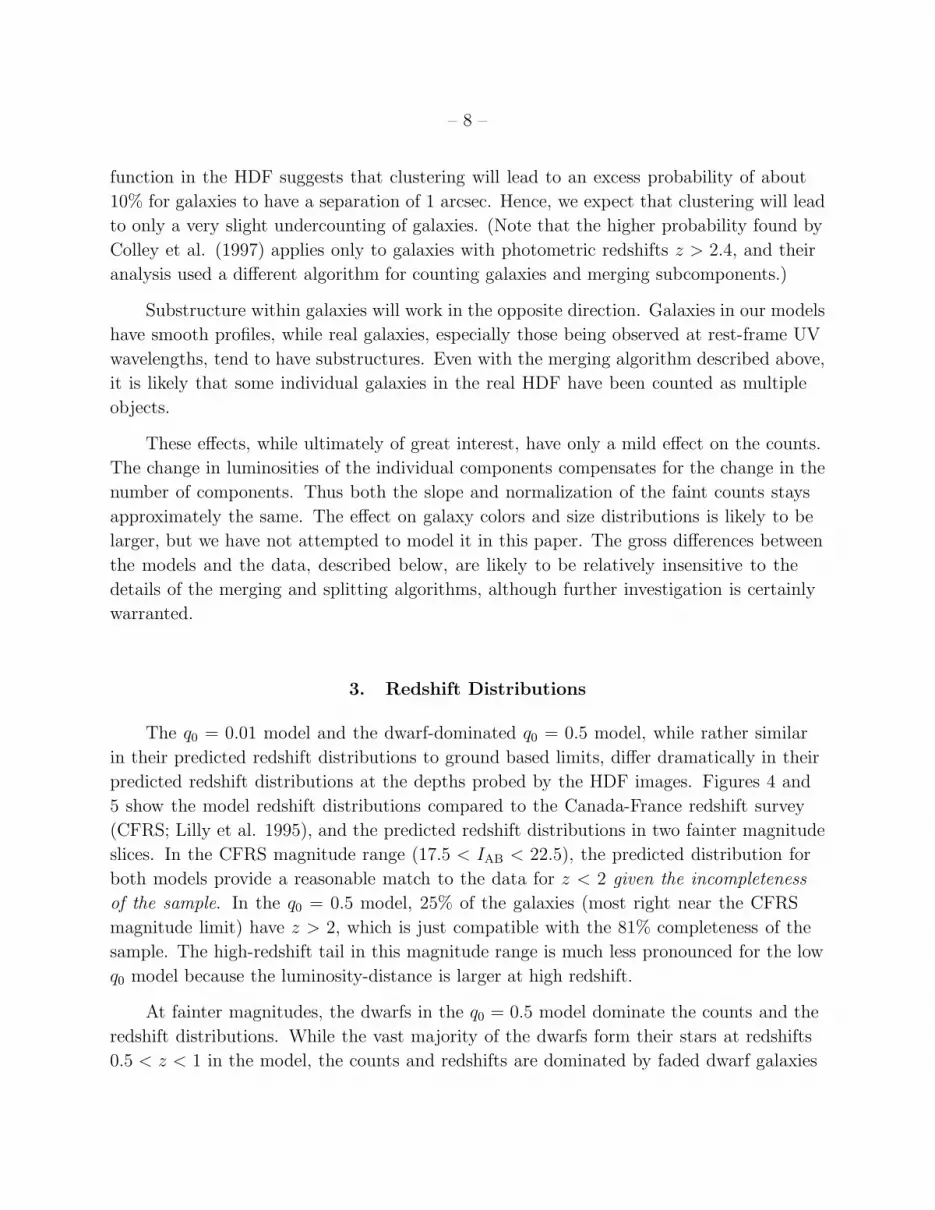
3. Redshift Distributions
The q0 = 0.01 model and the dwarf-dominated q0 = 0.5 model, while rather similar
in their predicted redshift distributions to ground based limits, differ dramatically in their
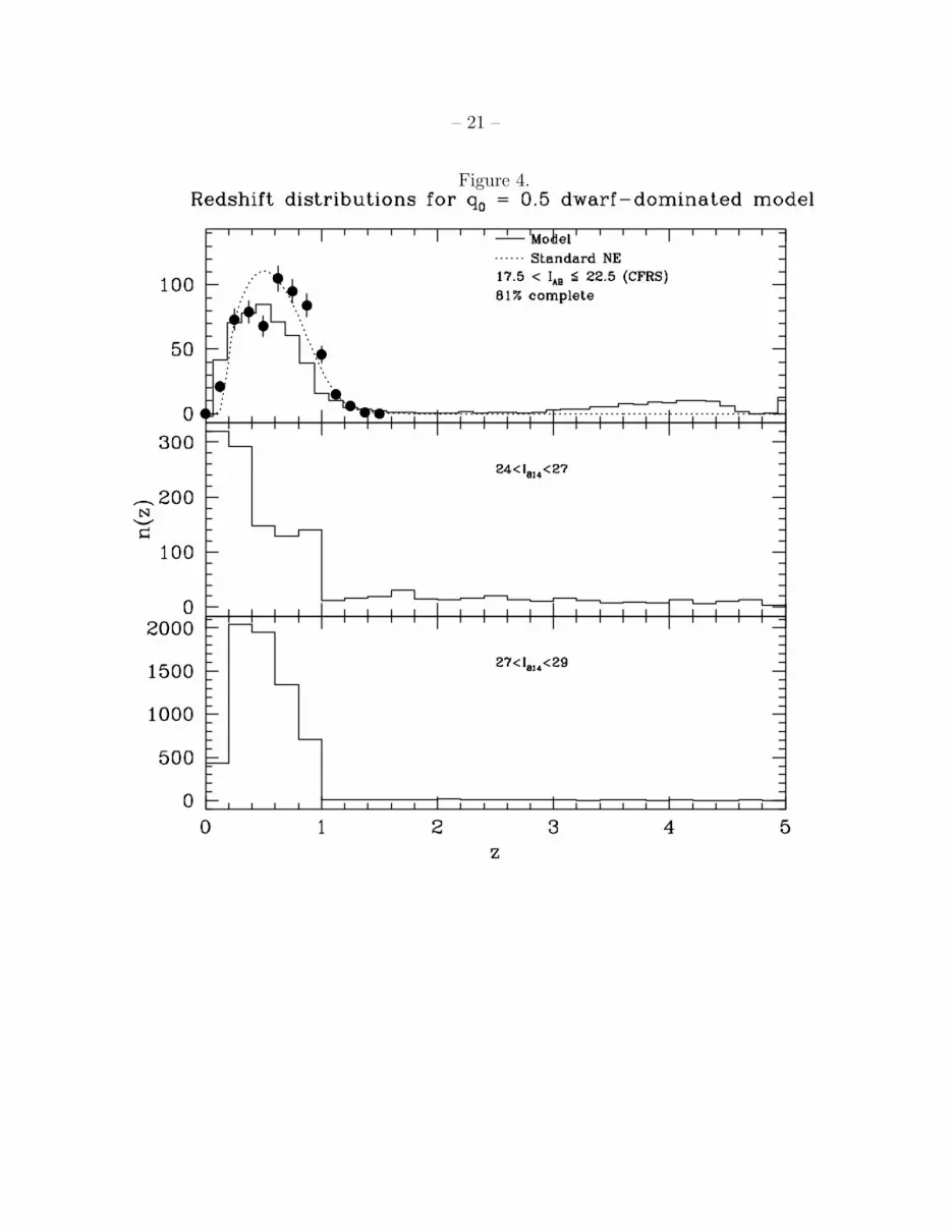
predicted redshift distributions at the depths probed by the HDF images. Figures 4 and
5 show the model redshift distributions compared to the Canada-France redshift survey
(CFRS; Lilly et al. 1995), and the predicted redshift distributions in two fainter magnitude
slices. In the CFRS magnitude range (17.5 < IAB < 22.5), the predicted distribution for
both models provide a reasonable match to the data for z < 2 given the incompleteness
of the sample. In the q0 = 0.5 model, 25% of the galaxies (most right near the CFRS
magnitude limit) have z > 2, which is just compatible with the 81% completeness of the
sample. The high-redshift tail in this magnitude range is much less pronounced for the low
q0 model because the luminosity-distance is larger at high redshift.
At fainter magnitudes, the dwarfs in the q0 = 0.5 model dominate the counts and the
redshift distributions. While the vast majority of the dwarfs form their stars at redshifts
0.5 < z < 1 in the model, the counts and redshifts are dominated by faded dwarf galaxies
– 9 –
at lower redshifts. This is root of the problems with matching the distributions of colour
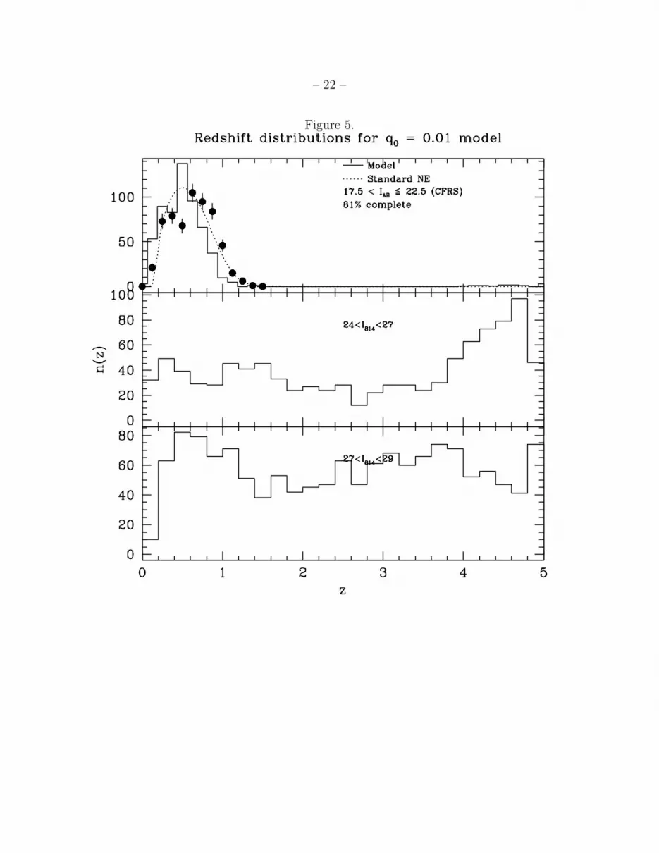
and radius described in the next section. In the low q0 model, the redshift distribution at
HDF magnitudes 24 < I814 < 27 is dominated by high-redshift bulges and ellipticals. The
redshift distribution is much more uniform at fainter magnitudes 27 < I814 < 29. The
peak is missing at high redshift because most of the ellipticals and bulges are brighter than
I814 = 26 during the epoch of rapid star formation. The ellipticals and bulges that appear
in the faint magnitude cut come from the faint tail of the adopted Gaussian luminosity
function. For redshifts z < 2, faint sample is dominated by late-type low-luminosity
galaxies, which in this model are forming stars at roughly constant rates.
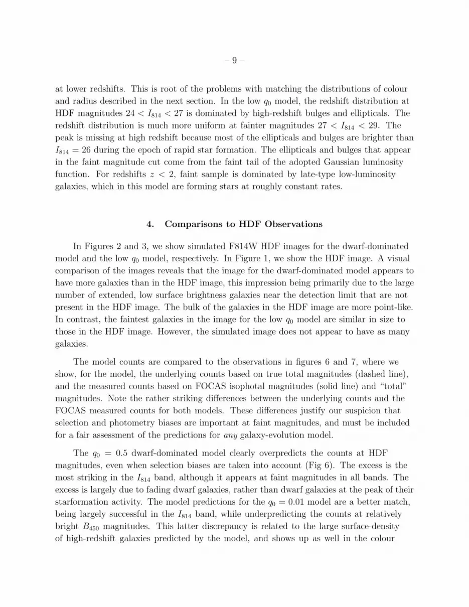
4. Comparisons to HDF Observations
In Figures 2 and 3, we show simulated F814W HDF images for the dwarf-dominated
model and the low q0 model, respectively. In Figure 1, we show the HDF image. A visual
comparison of the images reveals that the image for the dwarf-dominated model appears to
have more galaxies than in the HDF image, this impression being primarily due to the large
number of extended, low surface brightness galaxies near the detection limit that are not
present in the HDF image. The bulk of the galaxies in the HDF image are more point-like.
In contrast, the faintest galaxies in the image for the low q0 model are similar in size to
those in the HDF image. However, the simulated image does not appear to have as many
galaxies.
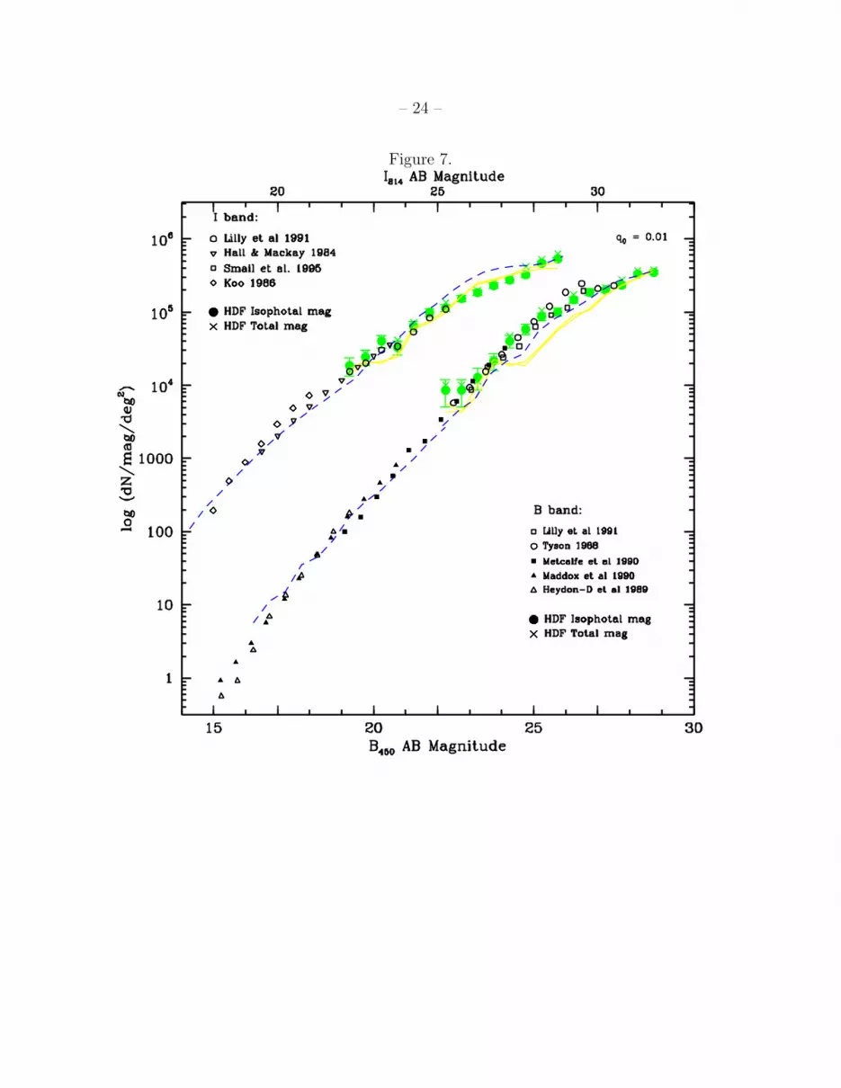
The model counts are compared to the observations in figures 6 and 7, where we
show, for the model, the underlying counts based on true total magnitudes (dashed line),
and the measured counts based on FOCAS isophotal magnitudes (solid line) and “total”
magnitudes. Note the rather striking differences between the underlying counts and the
FOCAS measured counts for both models. These differences justify our suspicion that
selection and photometry biases are important at faint magnitudes, and must be included
for a fair assessment of the predictions for any galaxy-evolution model.
The q0 = 0.5 dwarf-dominated model clearly overpredicts the counts at HDF
magnitudes, even when selection biases are taken into account (Fig 6). The excess is the
most striking in the I814 band, although it appears at faint magnitudes in all bands. The
excess is largely due to fading dwarf galaxies, rather than dwarf galaxies at the peak of their
starformation activity. The model predictions for the q0 = 0.01 model are a better match,
being largely successful in the I814 band, while underpredicting the counts at relatively
bright B450 magnitudes. This latter discrepancy is related to the large surface-density
of high-redshift galaxies predicted by the model, and shows up as well in the colour

– 10 –
distributions discussed below. Note that this discrepancy would not have been seen in
earlier PLE models, which did not include the attenuation of the intergalactic medium
(Yoshii & Takahara 1988; Gronwall & Koo 1995; Pozzetti et al. 1996).
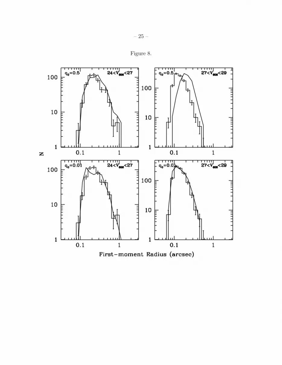
The distribution of radii are compared in Figure 8. The radii plotted are first-moment
radii measured by FOCAS within the detection isophotes.3
The observed distribution peaks at 0.2 arcsec in the magnitude range 24 < V606 < 27,
and at about 0.15 arcsec in the range 27 < V606 < 29. These distributions of radii are almost
perfectly matched by both models at the brighter magnitudes, and by the low q0 model in
the fainter magnitude bin. However, in spite of being dwarf-dominated, the q0 = 0.5 model
predicts galaxies that are systematically larger than observed at the faintest magnitudes.
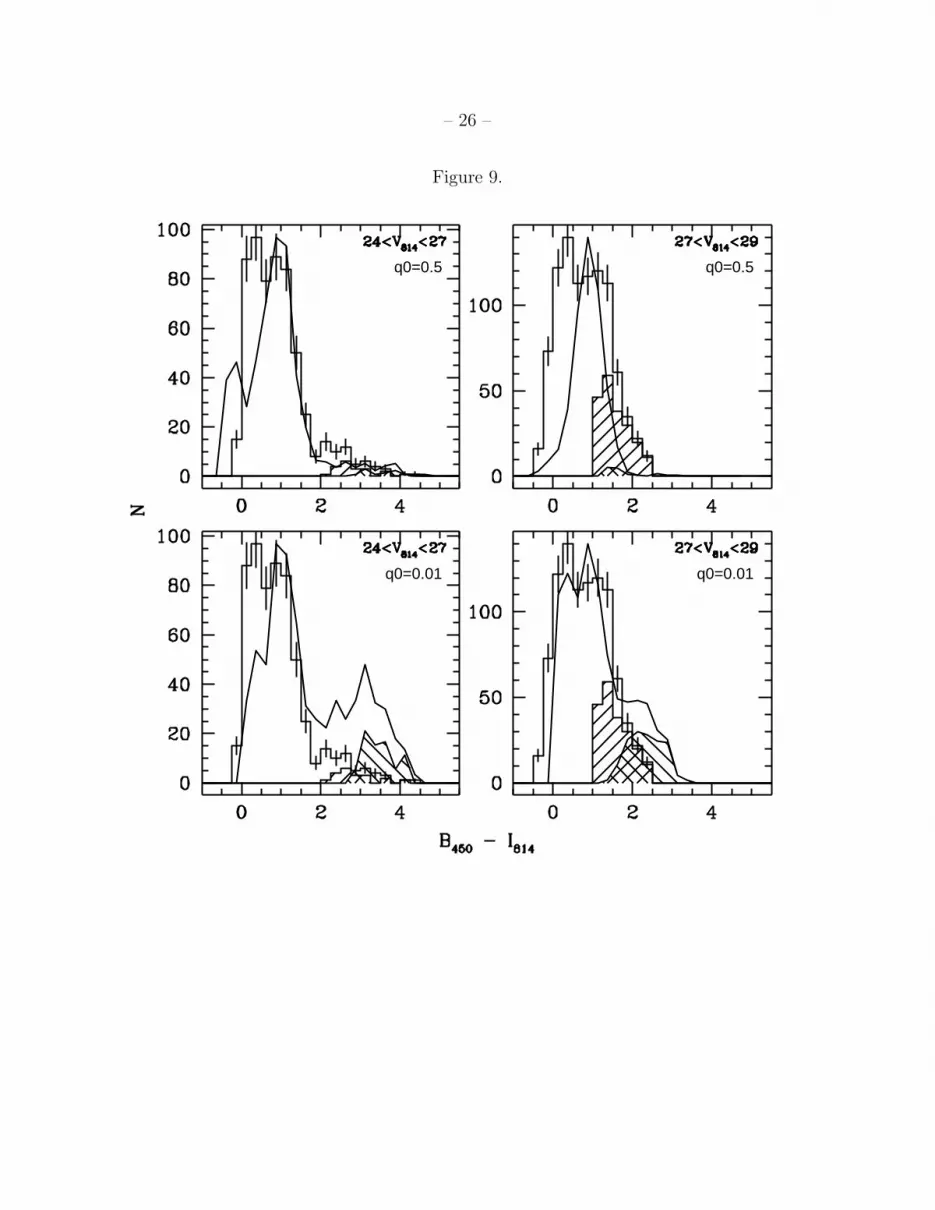
Figure 9 compares the B450 − I814 colours for the models and data. While the peaks in
the model colour distributions roughly agree with the observations, neither model provides
a very good match to the overall distributions. The q0 = 0.5 model has a blue peak in the
brighter magnitude bin that is not observed, while it predicts a red tail similar to that seen
in the real HDF images. At fainter magnitudes (27 < I814 < 29) there is no blue peak,
and hence the model predicts a narrower distribution than observed. The q0 = 0.01 model
does not have enough blue galaxies at the brighter magnitudes, and greatly overpredicts
the number of very red galaxies (B450 − I814 > 2). At fainter magnitudes the distribution is
a better match, but there is still an excess of very red galaxies relative to the observations.
The differences reflect both the different redshift distributions of the models, and the
different proportions of galaxies undergoing star-formation at moderate redshifts. During
the starburst phase, the dwarfs in the q0 = 0.5 model show up as nearly flat spectrum
objects, giving rise to the blue peak in the magnitude range 24 < I814 < 27. There are few
galaxies in the HDF with colours this blue. At fainter magnitudes, the colour distribution is
dominated by faded, lower-redshift remnants of the starburst epoch. The blue tail is missing
because there are no dwarf galaxies in the model with star-formation rates less than 1.8
M⊙ per year. This is due the cutoff of the dwarf-galaxy mass function at 15 kms−1. Lower
mass potentials are not deep enough to retain 104 K gas during the formation epoch. While
the lower mass cutoff has a physical justification, the adopted star-formation efficiency
of 10%, and star-formation timescale of 107 years are not highly constrained. Thus it is
3 The FOCAS first-moment radius is defined as
r1 =∑
rI(x, y)/∑
I(x, y), (2)
where I(x, y) is the intensity in each pixel within the detection isophote.
– 11 –
may be possible to achieve a better match to the colour distribution without revising the
fundamental assumption that dwarf galaxies are dominating the counts.
For the low q0 model, the most serious discrepancy is the prediction that there should
be a large population of very red galaxies, primarily in the brighter magnitude bin, but
extending also to the faintest magnitudes seen in the HDF. This red tail is due to bulges and
ellipticals forming stars at z > 3.5. It is an extremely robust prediction of the models that
such galaxies should have red B450 − I814 colours, since the colours are determined largely
by the intrinsic Lyman limits in galaxies, and by absorption due to intervening Lyman α
clouds (Madau 1995). In the bright magnitude bin, the low q0 model, even ignoring the very
red tail, is skewed to the red of the observed distribution. It is apparently underabundant in
star-forming galaxies at moderate redshifts. At fainter magnitudes, the colour distribution
is a more reasonable match to the observations, with a higher proportion of blue objects.
This is in part explained by the virtual disappearance of passively evolving ellipticals from
the sample at moderate redshifts, because the observations have gone beyond the peak of
the assumed Gaussian luminosity functions. The counts are thus dominated by star-forming
galaxies.
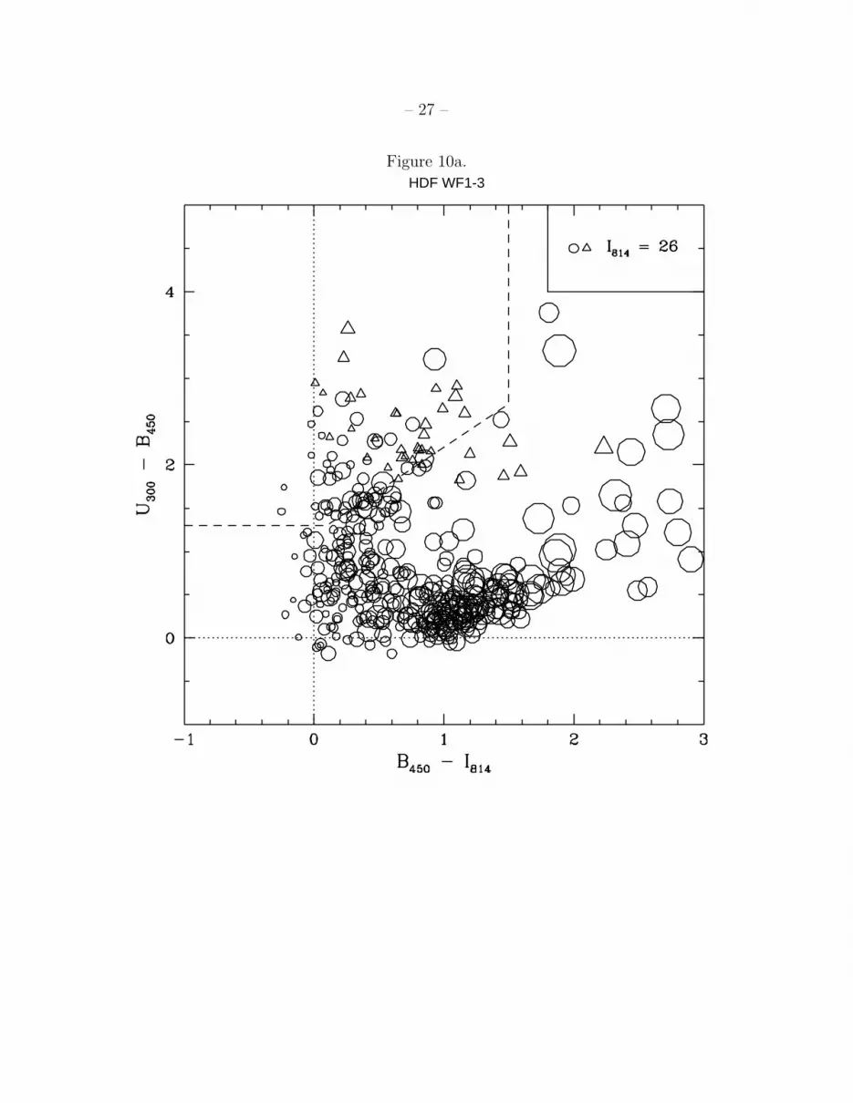
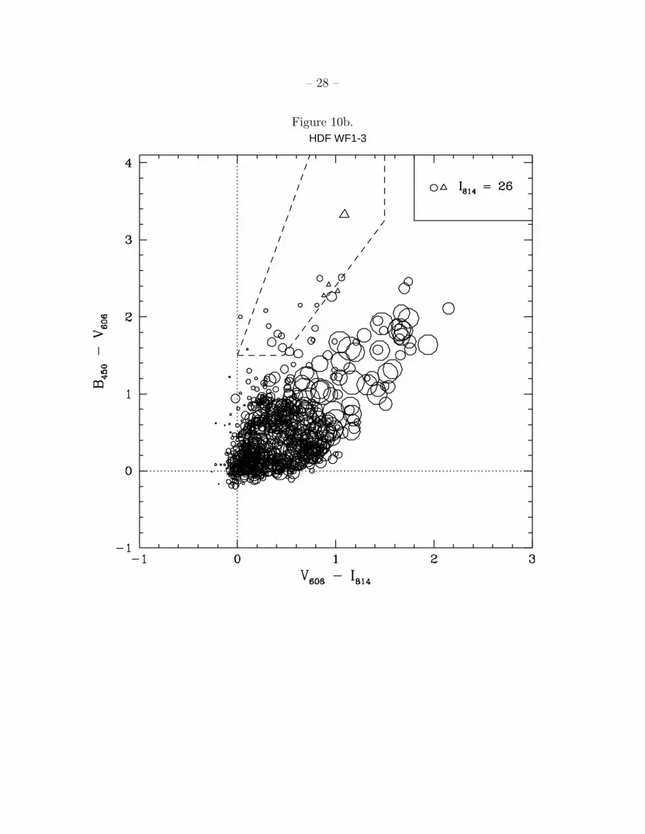
Figure 10, reproduced from Madau et al. (1996), shows colour-colour diagrams for
galaxies on the three WF chips in the HDF. The dashed lines show regions designed to
select galaxies in the redshift range 2.3 < z < 3.5 (in the U300 − B450 vs. B450 − I814
plane shown in Fig. 10a) and 3.5 < z < 4.5 (in the B450 − V606 vs. V606 − I814 plane in
Fig. 10b). Galaxies within these regions are very likely to be star-forming (relatively blue)
galaxies at high redshifts that have “dropped out” of the bluer band due to Lyman limit
and intergalactic Lyα absorption. The number of dropouts seen and predicted by the
models are listed in Table 2. It is interesting and important to note that this prediction is
extremely sensitive to biases in the selection and photometry of galaxies within FOCAS.
Because the counts of high-redshift galaxies in both models are steep at faint magnitudes,
the ∼ 0.5 mag difference between FOCAS isophotal magnitudes and the model galaxy total
magnitudes can introduce large differences in the predicted number of dropout galaxies.
These differences are largely taken into account by using FOCAS on the simulated images,
but our conclusions below must certainly be tempered by the lack of knowledge of the true
surface-brightness profiles of high-redshift galaxies.
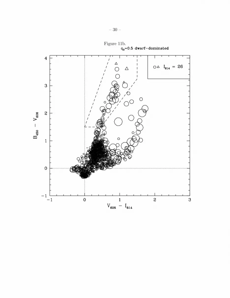
The predictions of the dwarf-dominated q0 = 0.5 model are shown in Fig. 11. The
model underpredicts the number of U-band dropouts and overpredicts the number of
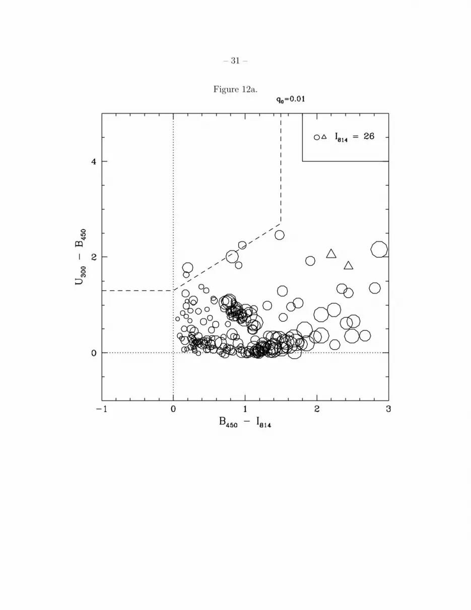
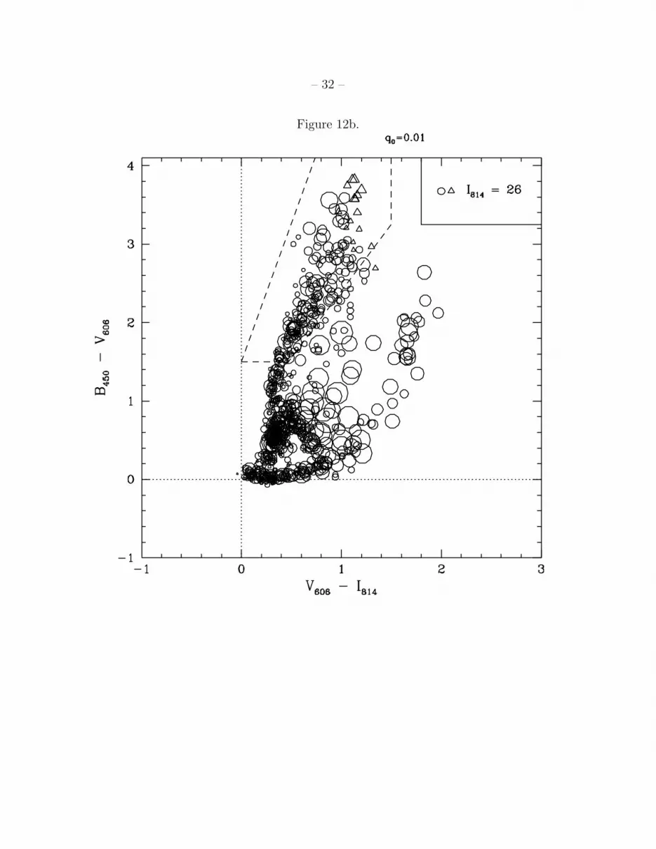
B-band dropouts. The discrepancy is significantly worse for the low q0 model (Fig. 12),
which greatly underpredicts the number of U dropouts, and greatly overpredicts the
number of B dropouts. Furthermore, for both models, B dropouts are seen at magnitudes

– 12 –
considerably brighter than those observed.
The differences between the two models can be understood as follows. The volume at
high redshifts is considerably higher in the low q0 model, leading to a higher surface density
of objects projected on the sky. Thus, for the same local density and redshift of formation,
a low q0 model predicts more sources near z = 5 than a q0 = 0.5 model. However, there
is also more time between redshifts of 3 and 5 in the low q0 model (1.6 Gyr) than in the
q0 = 0.5 model (0.7 Gyr). Therefore galaxies that form at z = 5 have more time to fade
in the open model, and, if the star-formation timescale is sufficiently short, can fade and
redden sufficiently that they do not meet the U-dropout selection criteria. The specific
predictions are very sensitive to the assumed redshift of formation and duration of the
star-forming epoch, points to which we will return in the next section.
There are significant discrepancies between the models and the observations in other
parts of these diagrams as well. In particular, during the burst phase, the dwarfs in the
q0 = 0.5 model populate a region slightly blueward of flat spectrum (in the lower left corner
of Fig. 11a). There are virtually no galaxies in this region in the HDF data.
The heavy concentration of galaxies at (0 < U300 − B450 < 0.5; B450 − I814 ≈ 0.5) is
not present in either model. Galaxies in this portion of the diagram are likely to lie in the
redshift range 1 < z < 2.
5. Discussion
As outlined in the introduction, our purpose in this paper is to examine the constraints
imposed on the bursting-dwarf model by the Hubble Deep Field observations. By way of
comparison, we perform the same analysis on a standard low q0 PLE model, to highlight
the differences between the predictions of the models, and the discriminatory power of these
deep images. Both types of models have been shown previously to provide a reasonable fit
to ground-based counts and redshift distributions. The preceding sections have presented a
detailed comparison of these models to the HDF data. The comparisons have highlighted
(a) the importance of including selection biases into the comparisons of models to the HDF
data, (b) the large differences in the predicted counts and colour distributions for these two
rather different models, and (c) the failure of either model to reproduce the observations.
The most important discrepancy for the low q0 PLE model is the prediction of a
substantial number of z > 3.5 galaxies at relatively bright magnitudes. Previous PLE
models (Gronwall & Koo 1995; Pozzetti, Bruzual, & Zamorani 1996) have shown reasonable
agreement with ground-based data in the magnitude range 24 < B < 26, where we see the
– 13 –
discrepancy, but this may have been fortuitous, as these models did not include the effects
of intergalactic absorption, which is clearly important at faint magnitudes in the U and B
bands. The number and brightness distribution of high-redshift galaxies is sensitive to the
redshift of formation zf , the star-formation timescale, the stellar initial mass function, and
the amount and distribution of dust in young galaxies. Thus it is not possible to rule out
PLE models simply on the basis of the overprediction of z > 3.5 galaxies. However, simply
hiding these galaxies is not sufficient to reconcile the model to the observations because
then the PLE model will substantially underpredict the counts. The most straightforward
solution, of course, is to posit different redshifts of formation for different types of galaxies,
or to incorporate merging into the model. Such possibilities are certainly viable, but are no
longer in the spirit of PLE models.
The disagreement between the q0 = 0.5 dwarf-dominated model and the HDF
observations can be largely attributed to the overproduction of faded remnants. The model
counts near the HDF limits are dominated by low-redshift non-starforming dwarfs. These
remnants are both redder and larger than the typical galaxies seen in the HDF. There
are two plausible modifications to the model which might reconcile it to the observations
without contradicting the underlying assumptions of q0 = 0.5, a CDM mass-spectrum for
the dwarfs, and a redshift of formation governed by the ionisation history of the universe.
The first is that the formation epoch of the dwarfs could extend to higher redshifts than
we have assumed (possibly up to z = 1.5), and could depend on galaxy mass. This would
allow the boojums to be brighter and leave them more time to fade. The second is that the
initial mass function in the boojums could be skewed toward high mass stars, or truncated
at some fairly high lower mass limit. The skewed IMF would cause the dwarfs to fade
faster, possibly curing the problem of remnants at low redshifts.
In a broader sense, the HDF observations clearly provide new and important constraints
on galaxy-evolution models. At the faint magnitudes probed by these observations, the
problems with the simple models discussed in this paper are particularly acute. It is
difficult to tell at present whether the problems lie in the details (e.g. the IMF, dust
content, metallicity distributions) or in the fundamental assumptions (e.g. that merging
is unimportant, or that giant galaxies all began forming at roughly the same time, with
different star-forming rates). It is clear that further modeling of the growing database of
galaxy properties in this small patch of sky, with careful attention to selection effects, has
the potential to discriminate between widely different world models that heretofore seemed
equally plausible.
This paper is based on observations made with the Hubble Space Telescope; support
for this work was provided in part by NASA through Hubble Archival Research grant
– 14 –
#AR-06337.20-94A awarded by Space Telescope Science Institute, which is operated by
the Association of Universities for Research in Astronomy, Inc., under NASA contract
NAS5-26555. A.B. is grateful for support through the Bergen Career Award from the
Dudley Observatory. We would like to acknowledge Bob Williams and the STScI HDF
team for their efforts in planning and carrying out the HDF observations. We acknowledge
in particular Mark Dickinson, Andy Fruchter, Mauro Giavalisco, and Piero Madau for many
fruitful discussions and collaborations on the HDF and galaxy evolution.
– 15 –
Table 1: Giant Galaxy Parameters
Luminosity Function Bulge/Total Ratio
Type N0(×10−3Mpc−3) < MBJ > σ mean σ zf τBulge τDisk
E 0.37 -18.70 1.7 1.0 0.0 5 0.2 —
S0 1.15 -18.70 1.7 0.4 0.25 5 0.2 1
Sab 2.00 -19.96 1.1 0.3 0.27 5 0.2 30
Sbc 4.00 -18.48 1.3 0.15 0.27 5 0.2 30
Sdm 8.00 -16.00 1.3 0.0 0.0 5 — 30
Additional late-type dwarfs for low q0 model
Type N0(×10−3Mpc−3) M∗
BJ α mean σ zf τBulge τDisk
Irregular 200 -16.00 -1.3 0.0 0.0 5 — 30
Bursting dwarfs for q0 = 0.5 model
Type N0(×10−3Mpc−3) M0 α mean σ zmax τBulge SF duration
Boojum 4000 109M⊙ -2 0.0 0.0 1 — 0.01
Table 2: Numbers of U300 and B450 band DropoutsData set U dropouts B dropouts
HDF 58 14
q0 = 0.5 30 41
q0 = 0.01 2 172
– 16 –
References
Adelberger K., Steidel C. C., 1996, private communication
Babul A., Ferguson H. C., 1996, ApJ, 458, 100
Babul A., Rees M., 1992, MNRAS, 255, 346
Bertelli G., Bressan A., Chiosi C., Fagotto F., Nasi E., 1994, A&AS, 106, 275
Binggeli B., Sandage A., Tammann G. A., 1988, ARA&A, 26, 509
Biretta J., 1995, WFPC-2 Instrument Handbook. STScI, Baltimore
Cole S., Aragon-Salamanca A., Frenk C. S., Navarro J. F., Zepf S. E., 1994, MNRAS, 271,
781
Colley W., Gnedin O., Ostriker J. P., Rhoads J. E., 1997, ApJ, 488, 579
Cowie L. L., Songaila A., Hu E. M., Cohen J. G., 1996, AJ, 112, 839
De Propis R., Pritchett C. J., Harris W. E., McClure R. D., 1995, ApJ, 450, 534
Ellis R. S., Colless M., Broadhurst T., Heyl J., Glazebrook K., 1996, MNRAS, 280, 235
Gibson B., 1996, ApJ, 468, 167
Glazebrook K., Ellis R., Colless M., Broadhurst T., Allington-Smith J., Tanvir N., 1995,
MNRAS, 273, 157
Gronwall C., Koo D. C., 1995, ApJ, 440, L1
Jarvis J. F., Tyson J. A., 1981, AJ, 86, 476
Kauffmann G., Guiderdoni B., White S. D. M., 1994, MNRAS, 267, 981
Lilly S. J., Le Fevre O., Crampton D., Hammer F., Tresse L., 1995, ApJ, 455, 50
Lin H., Kirshner R. P., Schectman S. A., Landy S. D., Oemler A., Tucker D. L., Schechter
P. L., 1996, ApJ, 464, 60
Loveday J., Peterson B. A., Efstathiou G., Maddox S., 1992, ApJ, 390, 338
Madau P., 1995, ApJ, 441, 18
Madau P., Ferguson H. C., Dickinson M., Giavalisco M., Steidel C. C., Fruchter A. S., 1996,
MNRAS, 283, 1388
Marzke R. O., Huchra J. P., Geller M. J., 1994, ApJ, 428, 43
Phillipps S., Driver S., 1995, MNRAS, 274, 832
Pozzetti L., Bruzual G., Zamorani G., 1996, MNRAS, 281, 953
Press W. H., Schechter P. L., 1974, ApJ, 187, 425
– 17 –
Quinn T., Katz N., Efstathiou G., 1996, MNRAS, 278, L41
Rocca-Volmerange B., Guiderdoni B., 1988, A&AS, 75, 93
Schechter P., 1976, ApJ, 203, 297
Simien F., de Vaucouleurs G., 1986, ApJ, 302, 564
Valdes F., 1982, Faint Object Classification and Analysis System. KPNO Internal
Publication
Villumsen J., Freudling W., da Costa L. N., 1997, ApJ, 481, 578
Williams R. E. et al., 1996, AJ, 112, 1335
Yoshii Y., Peterson B., 1994, ApJ, 436, 551
Yoshii Y., Takahara F., 1988, ApJ, 326, 1
This preprint was prepared with the AAS LATEX macros v4.0.
– 18 –
Fig. 1.— Hubble Deep Field. The image shows an 80” × 80” portion of the field, in the
F814W band, from the version 2 drizzled data (Williams et al. 1996).
Fig. 2.— Simulated Hubble Deep Field for the q0 = 0.5 dwarf-dominated model. The image
shows an 80” × 80” portion of the field in the F814W band.
Fig. 3.— Simulated Hubble Deep Field in the low-q0 model. The image shows an 80”× 80”
portion of the field in the F814W band.
Fig. 4.— Redshift distribution for the q0 = 0.5 dwarf-dominated model. The top panel
shows the measured redshift distribution from the CFRS survey (Lilly et al. 1995) as solid
dots, the predicted distribution from the dwarf-dominated model as a histogram, and the
prediction of a standard no-evolution model as a dotted curve. For the dwarf-dominated
model the predicted distribution includes observational selection as described by Babul &
Ferguson (1996). The model distributions are normalized to have the same total number of
galaxies as the survey. The middle panel shows the predicted redshift distribution from the
dwarf-dominated model in the magnitude range 24 < I814 < 27. The bottom panel shows
the same for 27 < I814 < 29.
Fig. 5.— Same as Figure 4, for the low-q0 PLE model.
Fig. 6.— Galaxy counts for the q0 = 0.5 model as a function of AB magnitude in the
F450W and F814W bands, together with a compilation of existing ground-based data.
FOCAS isophotal and total magnitudes are shown as solid dots and X’s, respectively. Model
predictions based on total magnitudes (i.e. without accounting for observational selection
or photometric biases) are shown as dashed lines. Model predictions from the FOCAS-
generated catalogs of simulated galaxies are shown as solid lines. No colour corrections have
been applied to the ground-based data. For the typical colours of galaxies in the HDF, the
colour corrections are less than 0.1 mag.
Fig. 7.— Same as Fig. 6, for the low q0 model.
– 19 –
Fig. 8.— Distribution of radii for both models, compared to the data. The radii for
both the models and the data are the first-moment radii measured by FOCAS. The HDF
measurements are shown as histograms with Poisson error bars. The model predictions are
the light solid curves.
Fig. 9.— Distribution of B450 − I814 colours for both models, compared to the data. The
colours for both the models and the data are from FOCAS measurements of the images. The
HDF measurements are shown as histograms with Poisson error bars. The model predictions
are the light solid curves. For both the models and the data there are galaxies that are
detected in the F814W image but not in the F450W image. For these galaxies, the colour is
assigned from the 1σ lower limit to the B450 magnitude. The hashed regions indicate portion
of the diagrams populated by these lower limits. Hashes slant in opposite directions for the
models and the data.
Fig. 10.— (a) U300 − B450 vs. B450 − I814 colour-colour plot of galaxies in the HDF
with B450 < 26.8. Objects undetected in F300W (with signal-to-noise < 1) are plotted
as triangles at the 1σ lower limits to their U300 − B450 colours. Symbol size scales with the
I814 magnitude of each object. The dashed lines outline the selection region within which we
identify candidate 2 < z < 3.5 objects. Details of the selection criteria are given by Madau
et al. (1996). (b) B450 − V606 vs. V606 − I814 colour-colour plot of galaxies in the HDF with
V606 < 28.0. Meanings of the symbols are the same as in the previous plot. The dashed lines
bound the region that isolates galaxies with 3.5 < z < 4.5.
Fig. 11.— Same as Figure 10, for the q0 = 0.5 dwarf-dominated model. Galaxy magnitudes
are from FOCAS measurements, as for the data.
Fig. 12.— Same as Figure 11, for the q0 = 0.01 PLE model. Galaxy magnitudes are from
FOCAS measurements, as for the data.
– 20 –
Figs 1-3 are in separate files.
– 21 –
Figure 4.
– 22 –
Figure 5.

– 23 –
Figure 6.
– 24 –
Figure 7.
– 25 –
Figure 8.
– 26 –
Figure 9.
q0=0.01 q0=0.01
q0=0.5 q0=0.5
– 27 –
Figure 10a.
HDF WF1-3
– 28 –
Figure 10b.
HDF WF1-3

– 29 –
Figure 11a.
– 30 –
Figure 11b.
– 31 –
Figure 12a.
– 32 –
Figure 12b.

This figure "fig1color.jpg" is available in "jpg" format from:
http://arXiv.org/ps/astro-ph/9801057v1

This figure "fig2color.jpg" is available in "jpg" format from:
http://arXiv.org/ps/astro-ph/9801057v1
This figure "fig3color.jpg" is available in "jpg" format from:
http://arXiv.org/ps/astro-ph/9801057v1


