New Parametric Equations for Estimating Stress Concentration Factors In

Tubular KK-Joints Under Axial Loading

A. Aghaei*, A. M. Gharabaghi, M. R. Chenaghlou

Department of Civil Engineering, Sahand University of Technology, Tabriz, Iran

Abstract

The most popular offshore structures, jacket platforms, are made of tubular members that

welded to gather. Due to dynamic and harsh environment, fatigue analysis and assessment of

these structures is an essential problem. The S-N curve method is an accepted procedure for

estimating fatigue life of jackets. In this method the maximum range of stress occurred during

loading is needed. In consequence of geometry, stress distribution in tubular joints under

various loadings is complicated and they have some points of concentrated stress; thus these

regions are the most critical places of jackets in any loading. The general method to calculate

the maximum stress of tubular joints is employing equations that give factors multiplied in

brace’s stresses and lead to considered values. At the present there are no such equations for

tubular KK-joints. In present research a wide data bank of stress concentration factors (SCFs)

is produced by parametric study on these joints under balanced axial loading. To obtain the

SCFs we applied Finite Element method. Before working on main FE analysis a vast study on

convergence and best element for the study is conducted and methods are verified with some

reliable experimental data sets. Finally, by applying the data bank and nonlinear regression

analysis, a series of new equations for estimating the SCF values in KK-joints under balanced

axial loading have been derived. These equations conform to conditions of UK Department of

Energy and have good correlation with the data bank.

Keywords: offshore platform; Jacket platform; Tubular joint; Fatigue; SCF (Stress

Concentration Factor); Parametric equation

1. Introduction

Hot spot stress method is one of the most applied methods for fatigue design of offshore

jacket platforms. Based on this method the nominal stress is multiplied by a proper stress

concentration factor (SCF) and the geometric stress or the hot spot stress will be obtained [1].

k

nomkk SCFS (1)

In this equation S' is the geometric stress or Hot Spot Stress that would be obtained for

different loads. By estimation of geometric stresses under different loadings and using them

in formulas proposed by design codes a stress range is calculated; this stress range used in a

proper S-N curve will give the failing number of load cycle. The reason for this procedure

lies in the geometrical complexity of tubular joints which cause stress concentration in

specific spots in the vicinity of the weld. The stress magnitude in these spots is several times

higher than the remote parts and therefore the fatigue cracks would appear in these spots.

Conventional method for calculation of the SCFs is using parametric equations which are

proposed by researchers for various types of tubular joints. Up to now there has been no such

equations proposed for KK-joints which are extensively employed in jacket platforms.

Although Romeijn in a 1994 study has presented the SCF values for different types of planar

joints such as K, X, Y, T and multi-planar joints as XX, TT and KK but has not proposed any

equation for KK-joints [1]. Presently in practical design of multi-planar KK joints the

equations for planar K joints are employed which is not accurate because the brace members

in other planes have significant interaction with each other.

In present research by an extensive parametric study, the effects of various dimensionless

geometrical parameters of KK joints on SCFs are surveyed and a data bank of 110 different

joints is generated. By employing the mentioned data bank in nonlinear regression analysis a

series of equations for calculation of SCF values are proposed. The validity of the results of

these equations has been evaluated by standard criteria.

2. KK joints, boundary conditions and loading

2. 1. Geometry of KK joints

KK joints have two pairs of braces each pair are placed in one plane and the two planes of

braces make a particular angle. The number of geometrical dimensionless parameters of this

type is far more than the planar types of joints. In fig. 1 these parameters are explained. These

parameters are defined by Lee and Wilmshurst [3].

If the out of plane eccentricity is 0 then it would be provable by geometrical formulation that

the is dependent on other parameters [12] and therefore would be removed from the study.

2L

D

d

t

T

tg

te

2L

Dg

Tg

Tt

TD

Dd

DL

tt

ll

2

2

Fig. 1. Geometrical parameters of KK joint

2180

lg

2. 2. Boundary conditions of joints in simulation

Researchers in their study of tubular joints selected different boundary conditions. Lee and

Wilmshurst [3] in their study of multi-planar tubular joints have investigated various types of

end conditions; the result of their study show that the variations of results in different

conditions are small and about 6 percent.

Morgan and Lee [4] who presented new sets of equations by employing Finite Element

simulation fixed the chord ends in all degrees of freedom. Fig. 2 shows an experiment on a T

joint by Zerbst et al. [5] and it is obvious that the chord ends in this experiment are also fixed.

Regarding these previous experiments, in this study the end conditions of models has been

fixed.

2. 3. Loading

The balanced axial loading is the most important type of loading in joints with more than

one brace members. In this condition the axial loads applied on the members of the joint must

be balanced (Fig. 3).

Fig. 2. T joint in experiment by Zerbst et al. [5]

Fig. 3. Balanced axial loading

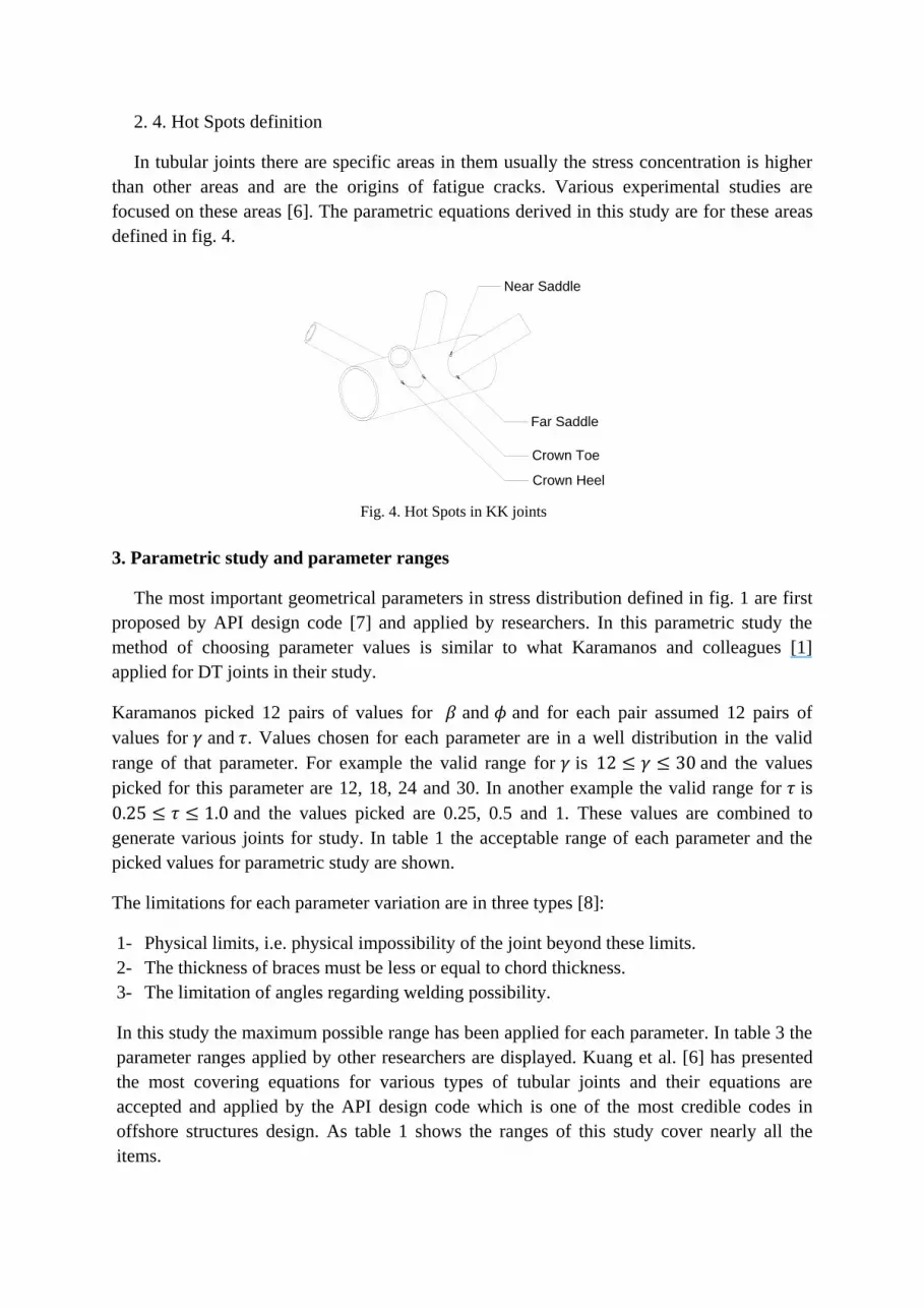
2. 4. Hot Spots definition

In tubular joints there are specific areas in them usually the stress concentration is higher

than other areas and are the origins of fatigue cracks. Various experimental studies are

focused on these areas [6]. The parametric equations derived in this study are for these areas

defined in fig. 4.

3. Parametric study and parameter ranges

The most important geometrical parameters in stress distribution defined in fig. 1 are first

proposed by API design code [7] and applied by researchers. In this parametric study the

method of choosing parameter values is similar to what Karamanos and colleagues [1]

applied for DT joints in their study.

Karamanos picked 12 pairs of values for and and for each pair assumed 12 pairs of

values for and . Values chosen for each parameter are in a well distribution in the valid

range of that parameter. For example the valid range for is and the values

picked for this parameter are 12, 18, 24 and 30. In another example the valid range for is

and the values picked are 0.25, 0.5 and 1. These values are combined to

generate various joints for study. In table 1 the acceptable range of each parameter and the

picked values for parametric study are shown.

The limitations for each parameter variation are in three types [8]:

1- Physical limits, i.e. physical impossibility of the joint beyond these limits.

2- The thickness of braces must be less or equal to chord thickness.

3- The limitation of angles regarding welding possibility.

In this study the maximum possible range has been applied for each parameter. In table 3 the

parameter ranges applied by other researchers are displayed. Kuang et al. [6] has presented

the most covering equations for various types of tubular joints and their equations are

accepted and applied by the API design code which is one of the most credible codes in

offshore structures design. As table 1 shows the ranges of this study cover nearly all the

items.

Far Saddle

Near Saddle

Crown Toe

Crown Heel

Fig. 4. Hot Spots in KK joints

4. Finite Element analysis

4. 1. Element selection in simulation

There are various elements and methods which different researchers applied them for

modeling and analyzing of tubular joints. In order to find the best and most accurate method

of simulation a literature review in this respect has been conducted which is briefed here. In a

research presented in OTC conference, Fessler and Edwards [9] presented the study of stress

distribution results comparison between three methods of finite element, photoelastic

technique and strain gauge technique; they concluded that shell elements have the technical

problem of showing higher stress results as they have an intrinsic defect which is connecting

to each other by their middle plane.

Hoffman and Sharifi [10] have examined different methods of tubular joint modeling and

they concluded that the 3D elements are far more reliable. Hellier et al. [11] also pointed out

the mentioned problem of shell elements.

Puthli et al. [12] has presented an instruction report for determination of SCFs. In that report

5 types of models have been examined and their results have been compared with the results

of 20 node 3D element model which are by their definition the most accurate models for this

purpose. By modeling with different meshing density they concluded that the models which

their elements of welding area are 1/16 of perimeter of the joint have sufficient accuracy.

Regarding mentioned researches, in this study the element used for modeling is 20 node 3D

elements. For FE simulation the ANSYS software [13] has been used for its well

performance with complex geometries. The other advantage of ANSYS over other softwares

Table 1. Valid ranges of geometrical parameters and the chosen values

Table 2. Parameter ranges applied by researchers

min max min max min max min max min max

Beale , Toprac [20] 7.7 15.4 0.17 1 12.3 31.5 0.4 1 - -

Kuang et al. [21] 7 40 0.3 0.8 8.3 33.3 0.2 0.8 30 90

Gibstein [15] 7 16 0.3 0.9 10 30 0.47 1 - -

Wordsworth, Smedley [22] 8 40 0.13 1 12 32 0.25 1 30 90

Hellier et al. [22] 0.21 13.1 0.2 0.8 7.6 32 0.2 1 35 90

Chang, Dover [8] 6 40 0.2 0.8 7.6 32 0.2 1 35 90

Morgan, Lee [23] 12 12 0.3 0.8 10 40 0.4 1 45 45

Karamanos et al. [1] - - 0.3 0.6 8 32 0.25 1 - -

Chiew et al. [24] - - 0.3 0.6 15 30 0.4 1 - -

LimitationReference

Limitation Limitation Limitation Limitation

such as ABAQUS and PATRAN is that for analysis it use lower amount of memory than the

others.

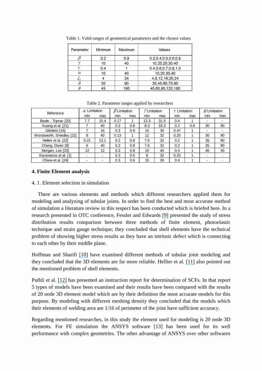
Fig. 5 shows the geometrical complexity of a tubular KK joint with its welding.

The SOLID186 element in ANSYS has the appropriate specifications for the purpose of this

study. This high order element has quadratic displacement behavior and is defined by 20

nodes; in each of them it has 3 degrees of freedom [13].

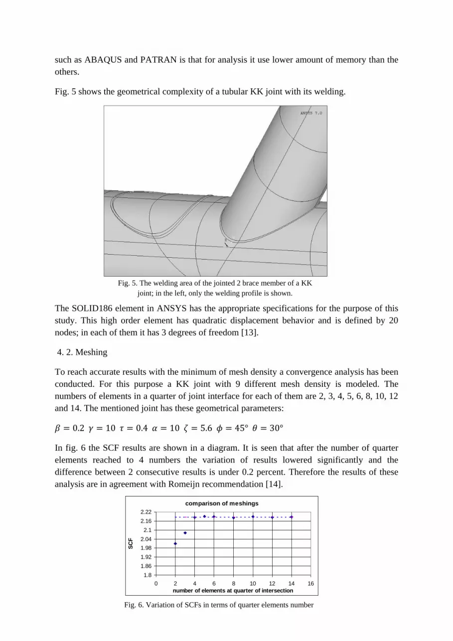
4. 2. Meshing

To reach accurate results with the minimum of mesh density a convergence analysis has been

conducted. For this purpose a KK joint with 9 different mesh density is modeled. The

numbers of elements in a quarter of joint interface for each of them are 2, 3, 4, 5, 6, 8, 10, 12

and 14. The mentioned joint has these geometrical parameters:

In fig. 6 the SCF results are shown in a diagram. It is seen that after the number of quarter

elements reached to 4 numbers the variation of results lowered significantly and the

difference between 2 consecutive results is under 0.2 percent. Therefore the results of these

analysis are in agreement with Romeijn recommendation [14].

Fig. 5. The welding area of the jointed 2 brace member of a KK

joint; in the left, only the welding profile is shown.

comparison of meshings

1.8

1.86

1.92

1.98

2.04

2.1

2.16

2.22

0 2 4 6 8 10 12 14 16

number of elements at quarter of intersection

SC

F

Fig. 6. Variation of SCFs in terms of quarter elements number

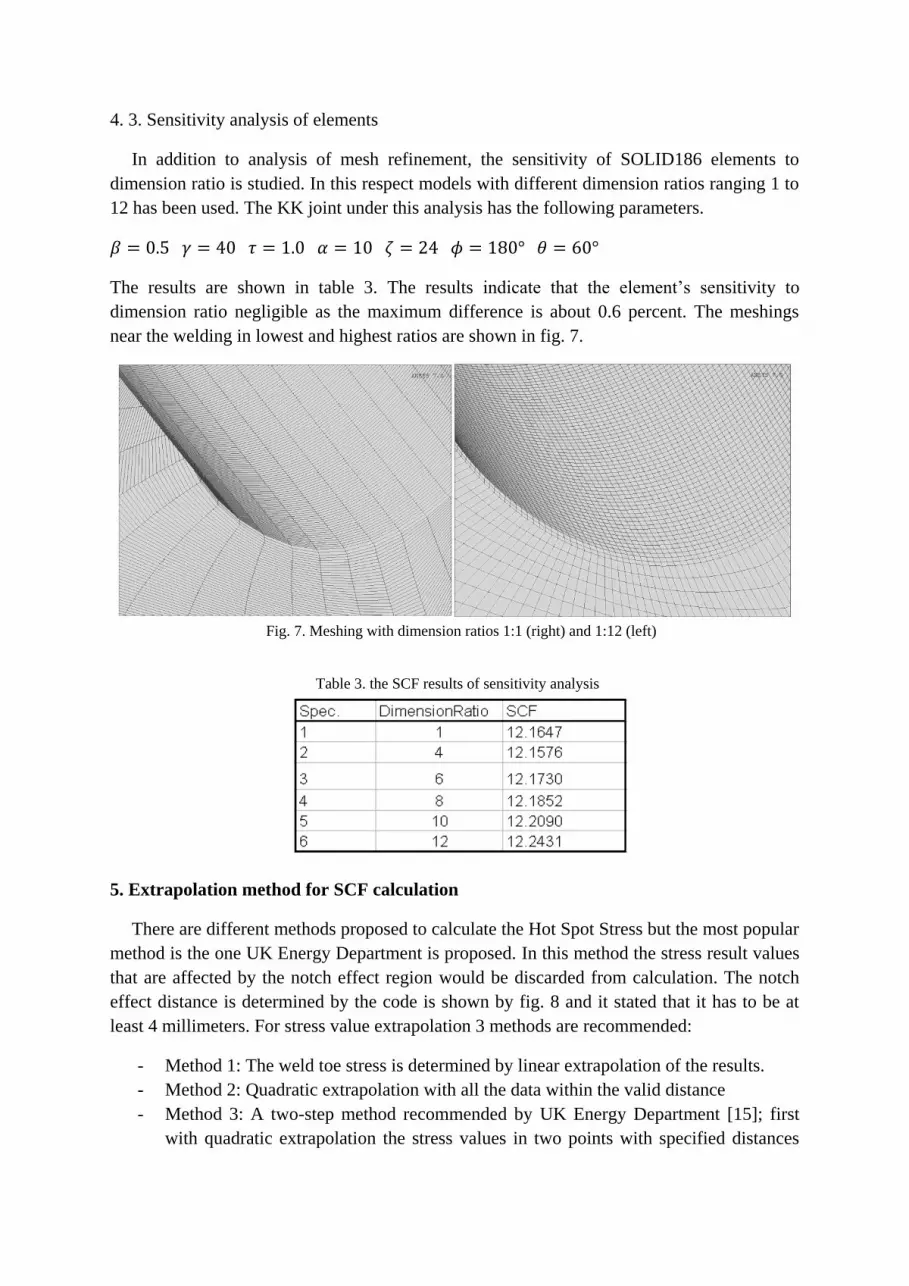
4. 3. Sensitivity analysis of elements

In addition to analysis of mesh refinement, the sensitivity of SOLID186 elements to

dimension ratio is studied. In this respect models with different dimension ratios ranging 1 to

12 has been used. The KK joint under this analysis has the following parameters.

The results are shown in table 3. The results indicate that the element’s sensitivity to

dimension ratio negligible as the maximum difference is about 0.6 percent. The meshings

near the welding in lowest and highest ratios are shown in fig. 7.

5. Extrapolation method for SCF calculation

There are different methods proposed to calculate the Hot Spot Stress but the most popular

method is the one UK Energy Department is proposed. In this method the stress result values

that are affected by the notch effect region would be discarded from calculation. The notch

effect distance is determined by the code is shown by fig. 8 and it stated that it has to be at

least 4 millimeters. For stress value extrapolation 3 methods are recommended:

- Method 1: The weld toe stress is determined by linear extrapolation of the results.

- Method 2: Quadratic extrapolation with all the data within the valid distance

- Method 3: A two-step method recommended by UK Energy Department [15]; first

with quadratic extrapolation the stress values in two points with specified distances

Fig. 7. Meshing with dimension ratios 1:1 (right) and 1:12 (left)

Table 3. the SCF results of sensitivity analysis

from the weld toe have to be calculated and in second step by linear extrapolation

with the two points the weld toe projected stress will be determined.

In this study the third method is applied for SCF calculation.

6. Parametric study of SCFs in KK joints under balanced axial loading

In some equations proposed for different types of tubular joints the Parameter is

neglected. The effect of this parameter on Hot Spot Stress of KK joints under axial loading is

studied. In this respect 7 KK joints with different parameter are analyzed. The analyses

indicate that the SCFs variation is ceased with surpassing over 12 (Fig. 9). The maximum

variation in SCF values for chord is 2.2 percent and for brace is 5 percent. Hence it should be

concluded that this parameter is not important for SCF calculation in axial loading.

The effects of other parameters are also shown in fig. 10 to 14. As it is seen, the parameter

has opposite effect with other parameters and it has almost a reducer effect. In all results it is

noticeable that the SCFs in saddle locations are usually more than crown locations and in far

saddle the maximum SCFs would be found.

The effect is unique. With increasing to all SCFs increase in 4 areas and after that

angle to they take declining trend and after that the variations is ceased; the later

outcome is a result of departing the two brace planes and lowering the interaction between

them.

With the graphs it can be concluded that the most important parameters in SCF distribution

are , and .

a

a

a

a

R

T

rt

rta 2.0

Fig. 8. Definition of minimum acceptable distance for extrapolation

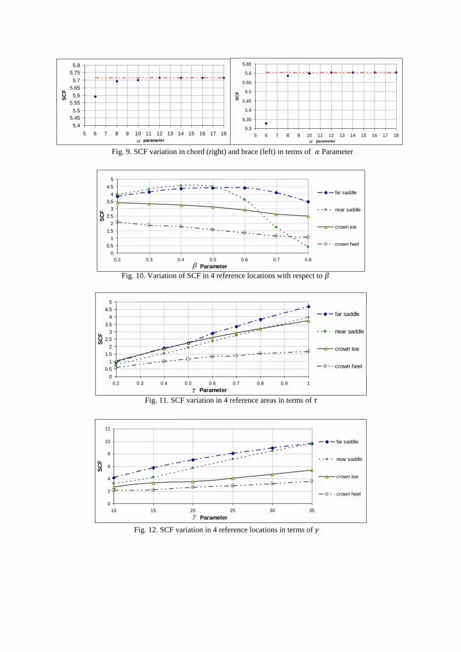
Fig. 9. SCF variation in chord (right) and brace (left) in terms of Parameter

5.4

5.45

5.5

5.55

5.6

5.65

5.7

5.75

5.8

5 6 7 8 9 10 11 12 13 14 15 16 17 18

parameter

SC

F

5.3

5.35

5.4

5.45

5.5

5.55

5.6

5.65

5 6 7 8 9 10 11 12 13 14 15 16 17 18

parameter

SC

F

0

0.5

1

1.5

2

2.5

3

3.5

4

4.5

5

0.2 0.3 0.4 0.5 0.6 0.7 0.8

Parameter

SC

F

far saddle

near saddle

crown toe

crown heel

Fig. 10. Variation of SCF in 4 reference locations with respect to

Fig. 11. SCF variation in 4 reference areas in terms of

0

0.5

1

1.5

2

2.5

3

3.5

4

4.5

5

0.2 0.3 0.4 0.5 0.6 0.7 0.8 0.9 1

Parameter

SC

F

far saddle

near saddle

crown toe

crown heel

Fig. 12. SCF variation in 4 reference locations in terms of

0

2

4

6

8

10

12

10 15 20 25 30 35

Parameter

SC

F

far saddle

near saddle

crown toe

crown heel

7. Nonlinear regression analysis

In addition to the models for single parametric studies 76 other KK joint models with

various parameters in the explained ranges in section 3 are generated and analyzed. In order

to achieve accurate and reliable equations the nonlinear regression analysis is applied. The

algorithm used for nonlinear regression is the iteration method of Levenberg-Marquardt

which is applied by the regression analysis software DataFit [25].

8. SCF parametric equations

By analysis on 106 KK joints a considerable data bank has been produced and with

nonlinear regression analysis a series of equations has been generated.

8. 1. Validity criteria of proposed equations

The UK Energy Department has recommended the validity criteria for SCF equations.

These criteria have been used by many researchers [1, 4, 11, 17 and 18] .

These criteria are based on the ratio of calculated SCFs by the equations and the SCFs

derived from analysis. they are as follows:

1- For a data bank the number of calculated SCF which their values are lower than the

analysis values has to be less than 25 percent:

[ ⁄ ] (2)

Fig. 13. SCF variation in 4 reference locations with respect to

0

2

4

6

8

10

12

14

30 35 40 45 50 55 60 65 70 75

Parameter

SC

F

far saddle

near saddle

crown toe

crown heel

Fig. 14. SCF Variation in 4 reference locations with respect to

1

1.5

2

2.5

3

3.5

4

4.5

45 60 75 90 105 120 135 150 165 180

Parameter

SC

F

far saddle

near saddle

crown toe

crown heel

In this relation P is the calculated SCF value by an equation and R is the counterpart

SCF derived by FE analysis.

2- The percentage of SCFs that are significantly lower than the actual value has to be

less than 5 percent:

[ ⁄ ] (3)

3- If the number of calculated SCFs which are significantly higher than the actual FE

value is more than 50 percent of the data bank, the equation would be accepted as a

conservative equation:

[ ⁄ ] (4)

4- If the following relations are happened then the equation would be accepted

conditional to engineering judgment:

[ ⁄ ] (5)

[ ⁄ ] (6)

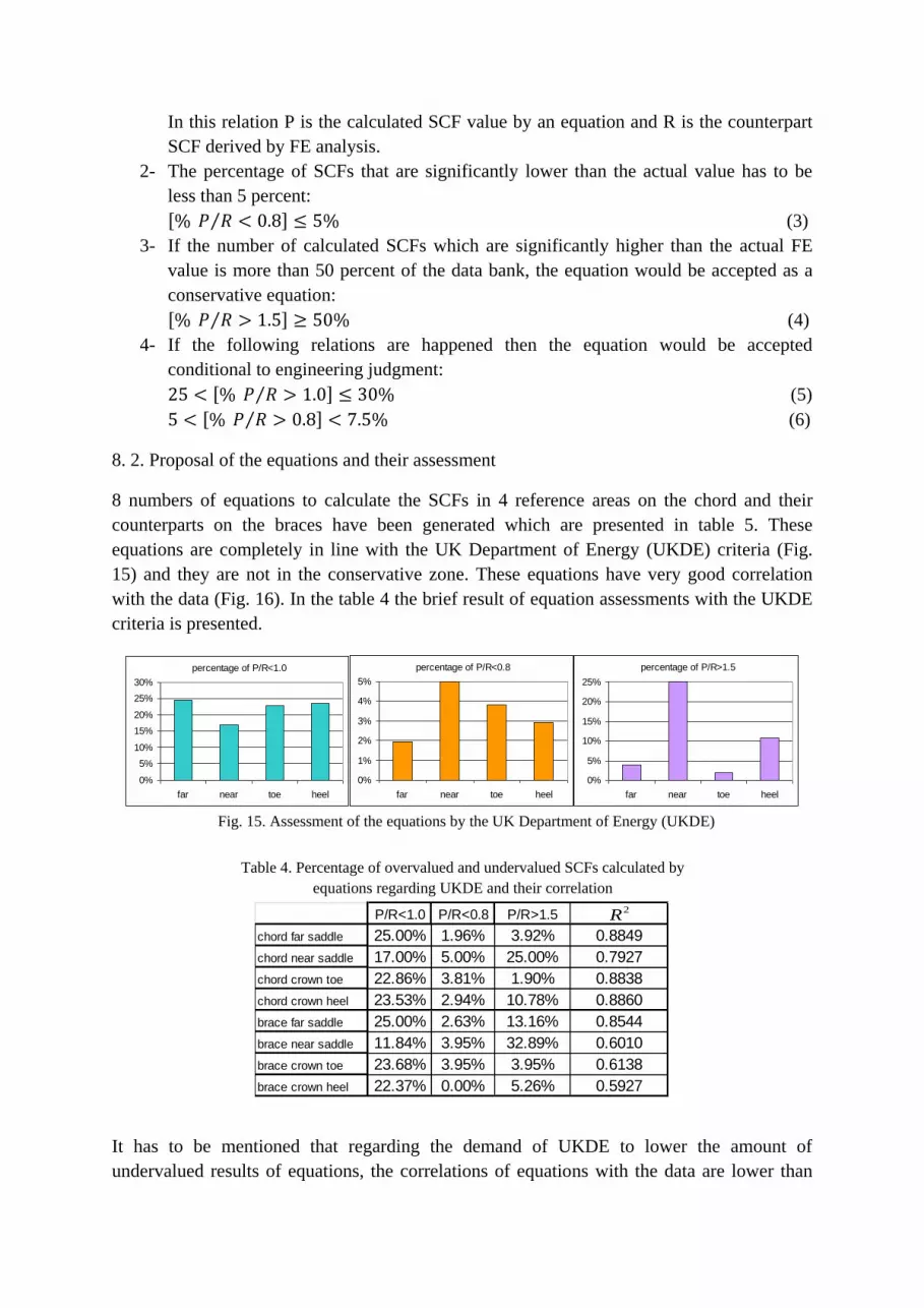
8. 2. Proposal of the equations and their assessment

8 numbers of equations to calculate the SCFs in 4 reference areas on the chord and their

counterparts on the braces have been generated which are presented in table 5. These

equations are completely in line with the UK Department of Energy (UKDE) criteria (Fig.

15) and they are not in the conservative zone. These equations have very good correlation

with the data (Fig. 16). In the table 4 the brief result of equation assessments with the UKDE

criteria is presented.

It has to be mentioned that regarding the demand of UKDE to lower the amount of

undervalued results of equations, the correlations of equations with the data are lower than

percentage of P/R<1.0

0%

5%

10%

15%

20%

25%

30%

far near toe heel

percentage of P/R<0.8

0%

1%

2%

3%

4%

5%

far near toe heel

percentage of P/R>1.5

0%

5%

10%

15%

20%

25%

far near toe heel

Fig. 15. Assessment of the equations by the UK Department of Energy (UKDE)

P/R<1.0 P/R<0.8 P/R>1.5

chord far saddle 25.00% 1.96% 3.92% 0.8849

chord near saddle 17.00% 5.00% 25.00% 0.7927

chord crown toe 22.86% 3.81% 1.90% 0.8838

chord crown heel 23.53% 2.94% 10.78% 0.8860

brace far saddle 25.00% 2.63% 13.16% 0.8544

brace near saddle 11.84% 3.95% 32.89% 0.6010

brace crown toe 23.68% 3.95% 3.95% 0.6138

brace crown heel 22.37% 0.00% 5.26% 0.5927

2R

Table 4. Percentage of overvalued and undervalued SCFs calculated by

equations regarding UKDE and their correlation

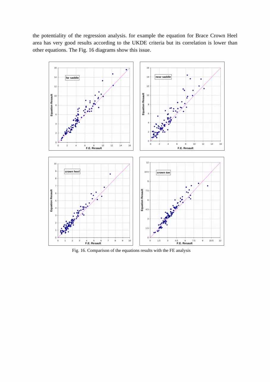
the potentiality of the regression analysis. for example the equation for Brace Crown Heel

area has very good results according to the UKDE criteria but its correlation is lower than

other equations. The Fig. 16 diagrams show this issue.

far saddle

0

2

4

6

8

10

12

14

16

0 2 4 6 8 10 12 14 16

F.E. Resault

Eq

ua

tio

n R

es

au

lt

near saddle

0

2

4

6

8

10

12

14

16

0 2 4 6 8 10 12 14 16

F.E. Resault

Eq

ua

tio

n R

esau

lt

crown toe

0

1.5

3

4.5

6

7.5

9

10.5

12

0 1.5 3 4.5 6 7.5 9 10.5 12

F.E. Resault

Eq

ua

tio

n R

es

au

lt

crown heel

0

1

2

3

4

5

6

7

8

9

10

0 1 2 3 4 5 6 7 8 9 10

F.E. Resault

Eq

ua

tio

n R

es

au

lt

Fig. 16. Comparison of the equations results with the FE analysis

*

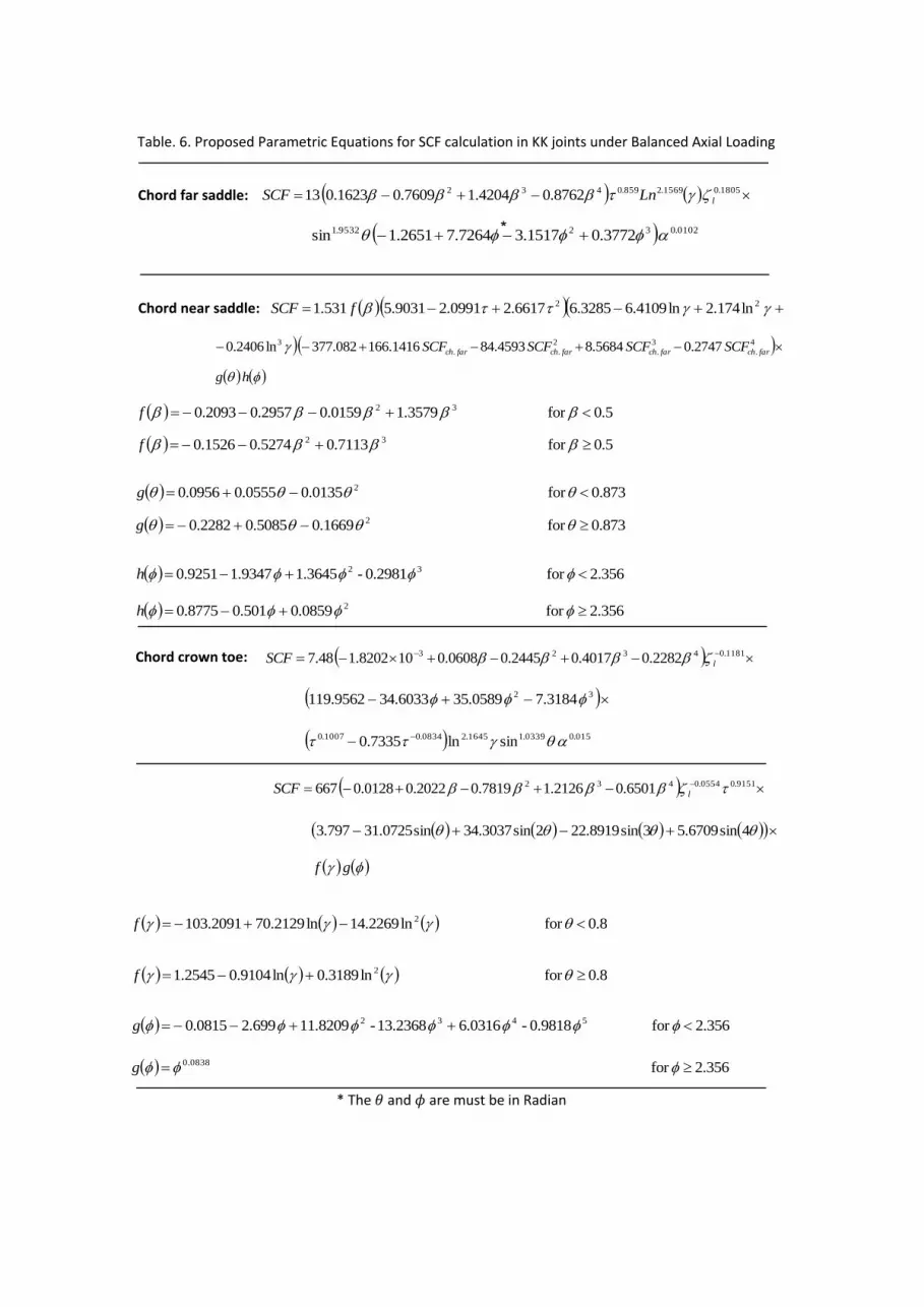
Chord far saddle: 1805.01569.2859.0432 8762.04204.17609.01623.013 lLnSCF

0102.0329532.1 3772.01517.37264.72651.1sin

Chord near saddle: 22 ln174.2ln4109.63285.66617.20991.29031.5531.1 fSCF

4

.

3

.

2

..

3 2747.05684.84593.841416.166082.377ln2406.0 farchfarchfarchfarch SCFSCFSCFSCF

hg

0.5for 3579.10159.02957.02093.0 32 f

0.5for 7113.05274.01526.0 32 f

873.0for 0135.00555.00956.0 2 g

873.0for 1669.05085.02282.0 2 g

356.2for 0.2981-3645.19347.19251.0 32 h

356.2for 0859.0501.08775.0 2 h

Chord crown toe: 1181.04323 2282.04017.02445.00608.0108202.148.7 lSCF

015.00339.11645.20834.01007.0 sinln7335.0

32 3184.70589.356033.349562.119

9151.00554.0432 6501.02126.17819.02022.00128.0667 lSCF

4sin6709.53sin8919.222sin3037.34sin0725.31797.3

gf

8.0for ln2269.14ln2129.702091.103 2 f

8.0for ln3189.0ln9104.02545.1 2 f

356.2for 0.9818-6.031613.2368-8209.11699.20815.0 5432 g

356.2for 0.0838 g

* The and are must be in Radian

Table. 6. Proposed Parametric Equations for SCF calculation in KK joints under Balanced Axial Loading

Brace far saddle: 22 8144.00960.0445.15257.10059.015.1 chch SCFSCFSCF

2233 0099.04827.19636.10035.00416.1 chchchch SCFSCFSCFSCF

Brace near saddle: 432

0749.03686.11331.80566.3902056.18021.0 chchchch SCFSCFSCFSCFSCF

gf

.0942for 160.5666-9368.1177689.272271.329793.5 432 f

.0942for 0712.0 f

5.0for 0.0409221.03087.02583.0 32 g

0.5for 0.06033128.03698.01259.0 32 g

Brace crown toe: 432

3617.03479.61728.289278.693127.17175.0 chchchch SCFSCFSCFSCFSCF

22888.02 ln1132.3ln3797.98984.91629.02157.01747.0

f4sin0011.03sin3765.02sin4945.0sin2802.19123.0ln3446.0 3

5.0for 0.83618176.44033.82315.8 32 f

0.5for 0.28737015.13825.3968.0 32 f

Brace crown heel: 432

6085.06768.85558.352182.551762.1490054.0 chchchch SCFSCFSCFSCFSCF

23695.02 ln7213.2ln6441.34363.70051.00369.00757.0

f4sin1219.03sin2892.02sin3049.0sin7058.07472.0ln4914.0 3

5.0for 0.45378332.26008.59861.13 32 f

0.5for .41781011.100166.223441.25 32 f

Table. 6. continued

References

[1] Karamanos S. A., Romeijn A., Wardenier J., SCF equations in multi planar welded tubular DT-joints

including bending effects, Marine Structures Journal, 15(2002), pp. 157- 173

[2] Wolpi D. J., Understanding how components fail., American Society of Metals, 1991, ISBN: 0-87170-

189-8

[3] Lee M. M. K., Wilmshurst S. R., Strength of multi planar tubular KK-joints under antisymmetrical axial

loading, J. Structural Engineering, June 1997, pp. 755-764

[4] Morgan M. R., Lee M. M. K., Parametric equations for distribution of stress concentration factors in tubular

K-joints under out of plane moment loading, International Journal of Fatigue, Vol. 20, No. 6, pp. 449-461

[5] Zerbst U., Heerens J., Schwable K. H., The fracture behavior of a welded tubular joint- an ESIS TC1.3 round

robin on failure assessment methods Part1: experimental data base and brief summary of the results, J.

engineering Fracture Mechanics, 69(2002), pp. 1093-1110

[6] Underwater Engineering Group (UEG), Design of tubular joints for offshore structures, UEG publication UR-

33, Vol. 2, 1985

[7] API-RP2A-1993, Recommended practice for planning, design and constructing fixed offshore platforms, 20th

edition

[8] ESDEP, European Steel Design Education Programme Publications, Lectures WG 15A, Structural Systems:

Offshore [9] Fessler H., Edwards C. D., Comparison of Stress Distribution in a Simple Tubular Joint Using Finite Element,

Photoelastic and Strain Gauge Techniques., Offshore Technology Conference, Paper OTC 4646

[10] Hoffman R. E., Sharifi A., the Accuracy of Difference Finite Element Types for the Analysis of Complex

Welded Tubular Joints, Offshore Technology Conference, Paper OTC 3691.

[11] Hellier A. K., Connolly M. P., Dover W. D., Stress concentration factors for tubular Y and T joints,

International Journal of Fatigue, 1990, No. 1, pp. 13-23 [12] Dover W. D., Madhava Rao A. G., Fatigue in Offshore Structures, 1996, ISBN: 90-5410-713-8

[13] ANSYS. Users’ manual, Swanson Analysis Systems Inc., 1999

[14] Romeijn A., Putli R. S., Wardenier J., Guidelines on the numerical determination of stress concentration

factors in tubular joints, Proceedings of the 5th International Simposium on Tubular Structures,

Nottingham(UK), 1993, pp. 625-639

[15] UK Department of Energy, Background to new fatigue design guidance for steel welded joints in offshore

structures, ISBN: 0-11-411456-0

[16] DataFit V.8.1.69, User Manual, Oakdale Engineering, 2005-08-01

[17] Karamanos S. A., Romeijn A., Wardenier J., Stress concentrations in multiplanar welded CHS XX-

connections, Journal of Constructional Steel Research, 50(1999), pp. 259-282

[18] Chang E., Dover W. D., Stress concentration factor parametric equations for tubular X and DT joints, Int. J.

Fatigue, vol. 18, No. 6, pp. 363-387, 1996

[19] Lee M. M. K., Strength stress and fracture analysis of offshore tubular joints using finite element, J.

Constructional Steel Research, 51(1999), pp. 265-286

[20] Beale L. A., Toprac A. A., Analysis of in plane T,Y and K welded tubular connections, Welding Research

Council Bulletin 125, Oct. 1967

[21] Mc Cleland B., Reifel M. D., Planning and design of fixed offshore platforms, 1986, ISBN: 0-442-25223-4

[22] Etube L. S., Fatigue and fracture mechanics of offshore structures, Professional Engineering Publishing

Limited, 2001, ISBN: 1-86058-312-1

[23] ISO, 1999, Petroleum and natural gas industries -offshore structures- part 2: fixed steel structures, BSEN ISO

13819-2

[24] Lee M. M. K., Dexter E. M., Finite element modeling of multi-planar offshore tubular joints, ASME, Journal

of Offshore Mechanics and Arctic Engineering, Vol. 126, Feb. 2004, pp. 120-128

[25] DataFit V.8.1.69, User Manual, Oakdale Engineering, 2005-08-01