New Alternatives in the Design and Planning of Multiproduct Batch Plants in a Multiperiod Scenario

New Alternatives in the Design and Planning of Multiproduct Batch Plants in aMultiperiod Scenario

Marta S. Moreno† and Jorge M. Montagna*,†,‡

INGAR-Instituto de Desarrollo y Disenõ-CONICET, AVellaneda 3657, S3002 GJC Santa Fe, Argentina, andUniVersidad Tecnolo´gica Nacional-Facultad Regional Santa Fe, Argentina

New alternatives for the simultaneous design and planning of multiproduct batch plants in a multiperiodscenario are presented in this article. This formulation allows the flexible configuration of the plant in everytime period for each product considering the assignment of parallel units of different sizes operating eitherin-phase or out-of-phase. Capacity expansion during the time horizon is also allowed in order to satisfy newvariable requirements. For each batch stage, following the usual procurement policy, units are selected froma set of standard and discrete sizes that are available to perform each operation. The model is formulatedthrough a mixed-integer linear programming (MILP) formulation that maximizes the net present value ofprofit. From the planning point of view, product sales, raw materials purchases, inventories, waste disposal,and late deliveries are taken into account. Thus, this model simultaneously solves both design and productionplanning for given forecasts of product demands and pricing in each time period.

1. Introduction

Continuous growth in complexity, competitiveness, anduncertainty of the market of high-added-value chemicals andfood products with a short life cycle have renewed the interestin batch operations and the development of optimization models.The main advantage of batch plants in this context is theirinherent flexibility to use the various available resources formanufacturing relatively small amounts of several differentproducts within the same facilities. Since the demands for suchproducts typically vary from period to period because of marketor seasonal changes, in the last few years an increased amountof research effort has been made to develop multiperiodoptimization models.

This is an area with many works that reflect the intense rateof research production. Then, it is very difficult to summarizethe most outstanding articles. However, most published studiesdeal with restricted formulations of multiperiod problems. Forexample, some authors have only considered either the planningor the design problem in their formulations. Birewar andGrossmann1 proposed a nonlinear programming (NLP) modelfor simultaneous planning and scheduling in multiproduct batchplants that considers benefits and product inventory costs.Sahinidis and Grossmann2 proposed a mixed-integer linearprogramming (MILP) formulation for selecting capacity expan-sion policies for both continuous and batch operation modes.Norton and Grossmann3 described a simplified, high-level,multiperiod MILP planning investment model that maximizesthe net present value of network’s operations and expansiondecisions with dedicated and flexible plants. Iyer and Gross-mann4 reported multiperiod operation planning for utilitysystems. Ryu5 highlighted the different time scales betweendemands and capacity expansion in multiperiod planningconsidering capacity augmentation.

Some studies consider design and planning problems simul-taneously. Varvarezos et al.6 proposed a decomposition method

for solving MINLP multiperiod design problems. Voudouris andGrossmann7 integrated synthesis, design, operation planning,and scheduling issues in an MILP model considering repeatedcycles in the design horizon, which avoids the time perioddependence of the problem. Several articles studied the optimaldesign of multiproduct plants under uncertainty in the productdemands assuming probability distributions.8,9 For utility sys-tems, Iyer and Grossmann10 presented a model for synthesisand multiperiod operational planning. An extension of this workwas proposed by Oliveira Francisco and Matos11 to includeglobal emissions of atmospheric pollutant issues. Van denHeever and Grossmann12 treated the design of multiproductplants by means of a disjunctive multiperiod nonlinear optimiza-tion model that simultaneously incorporates design and operationas well as expansion planning.

Different tools and approaches have been used to pose andsolve these problems. Most of them have preferred a determin-istic approach, but several works also pose models where data,for example demands, are uncertain.13-16 Different methods havebeen used to formulate the corresponding models. Most of theworks pose a mathematical model, generally MILP17 orMINLP18 formulations. However, there exist works that resortto simulation19 or heuristic20 approaches.

A multiperiod MILP model that simultaneously optimizesdesign and production planning decisions applied to multiprod-uct batch plants was presented in a previous study.21 Theseauthors developed an optimization model that maximizes thenet profit of the plant accounting for parameters variation dueto seasonal or market fluctuations.

In a multiproduct batch plant, one product is manufacturedat a time, in a sequence of one or more processing steps. Eachstep is carried out in a single equipment unit or in several parallelunits. Processing of other products is carried out using the sameequipment in successive campaigns. The unit with the minimumcapacity limits the batch size, while the limiting cycle time isfixed by the stage with the longest processing time.

In order to reduce the investment cost of multiproduct plants,several unit arrangements are available; the usual one is aparallel unit working either in- or out-of-phase.22,23 If parallelunits operate out-of-phase, this reduces the cycle time of thestage, i.e., the time elapsed between successive batches leaving

* To whom all correspondence should be addressed. Tel.:+54 3424534451. Fax:+54 342 4553439. E-mail: [email protected].

† INGAR.‡ Universidad Tecnolo´gica Nacional.

5645Ind. Eng. Chem. Res.2007,46, 5645-5658

10.1021/ie070022v CCC: $37.00 © 2007 American Chemical SocietyPublished on Web 07/26/2007

the stage. This also decreases the idle time of the other stageswhen the duplicated stage represents the bottleneck for theproduction train, thus reducing the size of these stages. If parallelunits operating in-phase are adopted, they operate simultaneouslyas if they were the same unit. The batch fed to the stage is splitamong the available units, while the batches leaving these unitsare merged after their processing. This arrangement is particu-larly useful when the batch size exceeds the upper-boundcapacity of the equipment.

In this paper, a new mixed-integer linear programming(MILP) model is addressed, which can simultaneously handledesign and planning decisions in a multiperiod approach. Thisarticle expands the previous study by Moreno et al.21 in orderto present a more flexible formulation. From the design pointof view, the capacity expansion is allowed in the new model,and then new units can be added in different time periods,accounting for the tradeoff between the scale-economy savingsof large initial capacities and the cost of installing the capacitybefore it is required. Unlike previous approaches, the unitsoperating in parallel at each stage can have different sizes. Also,this model takes into account flexible plant configurations, whereavailable units at every stage can be arranged in differentstructures for each product in every time period. Thus, perfor-mance can be improved since units can be configurated indifferent ways for every product, increasing either its productionrate (units working out-of-phase) or its capacity (units workingin-phase). Finally, discrete sizes of equipment items are assumedand a set of sizes is available for each unit operation. Thisassumption is justified, since most of the available equipmentin fine chemistry has standard sizes. Thus, by making choicesamong available discrete sizes, the model determines the optimaldesign that corresponds to the real procurement of equipments.

From the planning point of view, variations in prices, costs,product demands, and raw material supplies due to market andseasonal fluctuations are included. Moreover, this approachconsiders different period lengths and inventories of both finalproducts and raw materials.

In addition, this approach can be also applied to the retrofitproblem when redesigning the facilities is necessary to expandthe existing capacity in order to accommodate the increaseddemand or to manufacture new products.

The remainder of this paper is organized as follows. First,the main characteristics of this problem are presented in detailin Section 2. Then, Section 3 describes the multiperiodformulation including all the elements of the design and planningproblems. The versatility of the proposed approach is demon-strated via its application to representative examples in Section4. Finally, some remarkable conclusions are presented in Section5.

2. Problem Definition

The problem addressed in this paper can be stated as follows.In a multiperiod scenario, a multiproduct batch plant processesi ) 1, 2, ..., I products. Every product follows the sameproduction sequence throughout thej ) 1, 2, ..., J batchprocessing stages of the plant. Each stagej may consist of oneor more unitsk ) 1, 2, ...,Kj, whereKj is the maximum numberof units that can be added at stagej. These duplicated units canhave different sizes, operating either in-phase to increasecapacity or out-of-phase to decrease the cycle time.

Since this is a multiperiod problem, the time horizonH isdiscretized intot ) 1, 2, ...,T specified time periodsHt, notnecessarily of the same length. Production producti at stagejin every periodt requires a given processing timetijt and a

material balance factorSijt called the size factor, which specifiesthe volume required at stagej to produce a unit mass of finalproduct i. For each producti, lower and upper bounds on itsdemands in every periodt, DEit

L/DEitU, are known. Costs and

availability of raw materials vary from period to period and arealso assumed to be known.

Regarding design decisions, this model involves the selectionof the size for each batch unitk at stagej, Vjk, which arerestricted to take values from a set SVj ) {Vj1, Vj2, ..., Vjnj} ofavailable discrete sizes, wherenj is the number of available sizesat stagej.

Yoo et al.24 developed a generic retrofit model that presenteda generalized superstructure with the interesting concept ofgroup. Group is defined as a set of units, which are operatedin-phase, but those in different groups are operated out-of-phase.The division of units of each stage into groups differs fromproduct to product; i.e., for each producti, units can be groupedin different ways. New and old units can be used in-phase andout-of-phase, forming groups. Lee et al.25 developed a modelfor the capacity-expansion problem of multisite batch plants,where this concept was used again. A generalized superstructurewas generated to assign units to groups in each considered plant.Montagna26 extended the model proposed by Yoo et al.24

through the allocation of intermediate storage tanks. Then, amore realistic formulation is obtained, although with anincreased level of resolution complexity.

Following the concept of group introduced in the abovestudies, in this article the configuration of groups using theavailable batch units must be determined at each stagej forevery producti in each time periodt.

One key feature of this approach is that units can be addedin different time periodst, for example, in order to satisfy theprojected expansion of the plant or to fulfill higher demandsthrough the time horizon.

It will be assumed that the plant operates in single-productcampaign (SPC) mode in every period. Also, batches aretransferred from stage to stage without delay, i.e., a zero-wait(ZW) transfer policy is used. Taking into account the adoptedmultiperiod approach and depending on the periods length, thisassumption does not constitute such a serious constraint as inprevious formulations.

In the plant design, the model incorporates the batch unitsVjk, selecting among available discrete sizesVjs. At each timeperiodt, the model determines the number of groupsGijt at stagej and which of the existing units in that period are assigned toeach one for every producti.

In this model, two scenarios are considered. In the first one,the elaboration of producti depends on a unique raw materialthat is identified with the same subscripti of the product. Inthe second general scenario, production of producti requires aset of raw materials CT.

On the other hand, production planning decisions allowdetermining at each periodt and for each producti the amountof product to be producedqit, the number of batchesnit, andthe total timeTit required to produce producti. Moreover, atthe end of every periodt, the levels of both final product IPitand raw material inventories IMit are obtained. Also, the totalsales QSit, the amount of purchased raw materialCit, and theamount of raw material to be used for the production RMit ofproducti in each periodt are determined with this formulation.

Then the model simultaneously considers the design and theproduction planning of the plant. The performance criterion isto maximize the net present value along the global time horizon,taking into account incomes from product sales, expenditures

5646 Ind. Eng. Chem. Res., Vol. 46, No. 17, 2007

from raw materials purchases, inventories, penalties, and invest-ment costs. If time periods are equal, waste disposal costs arealso added to the objective function.

3. Problem Formulation

This section describes the basic constraints and majorcharacteristics of the mathematical formulation.

3.1. Unit and Group Assignment Constraints. Severalvariables are introduced to determine the plant structure. Sincethe units can be added at any time period, a binary variablewjkt

is used. The value of this variable is 1 if unitk is included inthe plant structure at stagej in periodt; otherwise, the value iszero. Each unitk at stagej can be added only in one period:

The units are included in a sequential manner in order to avoidalternative optimal solutions with the same value for theobjective function:

These constraints ensure that a unit is incorporated only if allthe previous ones are also included.

The concept of group introduced by Yoo et al.24 and extendedby Montagna26 is used to handle the simultaneous considerationof parallel batch units working in- and out-of-phase. In orderto illustrate the unit arrangements to conform groups, Figure 1shows an example of four units (Kj ) 4) at stagej. These unitsmust not be necessarily identical. In this way, up to four groupsof one unit each could exist at stagej. Units can be arranged indifferent ways to determine groups. Figure 1 is one option wherethe units have been arranged into two groups. Both groups 1and 2 operate out-of-phase. Units closed by the dotted line forma group, e.g., units 1 and 4 form group 1 and operate in-phase.

The variables related to both existence of groups and unitsallocations to groups are defined in the same way as in previousarticles, adapted to the multiperiod approach adopted in thisstudy.

Since the units can be grouped in different ways at each stagedepending on the product and the time period, the binaryvariableyijkgt is introduced. This variable is equal to 1 if unitkof stage j is assigned to groupg for product i in period t;otherwise; the variable is equal to zero. Each unitk at stagejcan be assigned at most to one groupg for producti in periodt:

ParameterGjT is the maximum number of groups allowed at

stage j. A pseudobinary variableyijgt is also introduced toindicate whether groupg exists or not at stagej in periodt forproducti. Groupg is generated at stagej in periodt only if atleast one unitk is assigned to it in that period:

If unit k is assigned to groupg at stagej in periodt, the groupmust exist:

By introducing constraint 6 into the formulation, the continuousvariableyijgt behaves like a binary variable since it is boundedby binary variables through eqs 4 and 5.

If unit k is assigned to groupg at stagej for producti in periodt, the unit must exist in that period:

If unit k exists at stagej in periodt, then it must be included ina groupg. This is written as

In order to avoid redundant assignment of units to groups, whichresults in the same value for the objective function, the followingconstraints are added:24

This constraint orders the different groups through a weight 2Kj-k

assigned to each unitk. The order of the group is obtained byadding the weights of all units in the group.

3.2. Design Constraints.As mentioned in the problemdefinition, the unit sizesVjk are available in discrete sizesVjs,which correspond to the real commercial procurement ofequipment. To rigorously tackle this situation, the binary variablezjks is introduced, whose value is 1 if unitk at stagej has sizes; otherwise, it is zero. The variableVjk is restricted to takevalues from the set SVj ) {Vj1, Vj2, ..., Vjnj}, wherenj is thenumber of discrete sizes available for each stage. Using theprevious definition,Vjk can be expressed in terms of discretevariables as

If unit k at stagej is added in some periodt, it must take a sizes for the volume from the available sizes at that stage:

Figure 1. Groups at stagej.

∑t

T

wjkt e 1 ∀ j, k (1)

∑τ)1

t

wjkτ g ∑τ)1

t

wj,k+1,τ ∀ j, k ) 1, 2, ...,Kj - 1, t (2)

∑g)1

GjT

yijkgt e 1 ∀ i, j, k, t (3)

yijgt e ∑k)1

Kj

yijkgt ∀ i, j, g, t (4)

yijkgt e yijgt ∀ i, j, k, g, t (5)

yijgt e 1 ∀ i, j, g, t (6)

yijkgt e ∑τ)1

t

wjkτ ∀ i, j, k, g, t (7)

∑τ)1

t

wjkτ ) ∑g)1

GjT

yijkgt ∀ i, j, k, t (8)

∑k)1

Kj

2Kj-k yijkgt g ∑k)1

Kj

2Kj-k yijk,g+1,t

∀ i, j, g ) 1, 2, ...,GjT - 1, t (9)

Vjk ) ∑s

nj

Vjs zjks ∀ j, k (10)

∑s

nj

zjks ) ∑t)1

T

wjkt ∀ j, k (11)

Ind. Eng. Chem. Res., Vol. 46, No. 17, 20075647

Only one of the available sizes at stagej must be selected ifunit k at stagej exists:

The amount of producti produced in time periodt, qit, dependson the number of batchesnit and the batch sizeBit of finalproducti processed in that period as follows:

The sizing equation described in general literature that relatesthe unit size with the batch size of a producti at each stagejand regarding the multiperiod approach is

whereSijt is the size factor at stagej for producti, which canvary in each periodt taking into account seasonal effects. Thisis the minimum capacity required at this stage for producingone unit mass of producti.

By combining eq 13 and eq 14, the constraints take thefollowing form:

The aforementioned constraints must be modified to considernot only the volume of each unitk at every stagej, Vjk, but alsothe volume of the units in a group, that is to say, units operatingin-phase. The volume of a group is equal to the total volume ofall units that are operated in-phase. Thus, the unit sizes includedin group g at stagej must be added. Then, the allocation ofunits to groups must be taken into account: volumesVjk mustbe related to the binary variableyijkgt, as shown by the followingexpression:

Equation 16 is a Big-M constraint that guarantees that batchescan be processed in the batch stagej if groupg exists for producti in time periodt; otherwise, the constraint is redundant becauseof the large value of BMijt. The value of BMijt can be calculatedby

By substituting eq 10 into eq 16, new constraints can beformulated that restrict the volumes to discrete sizes:

Constraint 18 is nonlinear because of the product between binaryand continuous variables. In order to reformulate these con-straints as linear ones, the cross-productzjksyijkgtnit can beeliminated by introducing the continuous variablehijkgst that isequal tonit if zjks andyijkgt are 1; otherwise, the variable is equalto zero. The following constraints must be posed,

wherenitU is the upper bound fornit and the value of BM2it is

the upper boundnitU.

3.3. Timing Constraints. The timetij during which a batchof a producti is processed in a unit at stagej and then transferredto the next one is defined as the processing time of producti atstagej. The maximum time between two successive batches ofproducti in the process determines the limiting cycle time ofproduct i, TLi. Considering the multiperiod approach of thisformulation, the limiting cycle time of producti in period t isgiven by

As pointed out in the Introduction, the addition of unitsoperating out-of-phase at time-limiting stages reduces idle timesand increases the units utilization. In this way, if stagej hasgroups of parallel units, TLit can be calculated by the divisionbetween processing timetijt and the number of out-of-phasegroups for producti in every periodt:

The total time for producing producti in time periodt is definedas

By multiplying eq 25 by the number of batchesnit, theexpression takes this form:

Equation 27, however, is nonlinear. In order to obtain a linearexpression, the number of groups at each stagej in every periodt can be expressed by the following constraint,

∑s

nj

zjks e 1 ∀ j, k (12)

qit ) Bit nit ∀ i, t (13)

Vj g Sijt Bit ∀ i, j, t (14)

qit e Vj

nit

Sijt∀ i, j, t (15)

qit e ∑k)1

Kj

(Vjk yijkgt)nit

Sijt

+ BMijt (1 - yijgt) ∀ i, j, g, t

(16)

BM ijt ) Kj maxs

(Vjs) maxt

(nitU/Sijt) ∀ i, j, t (17)

qit e ∑k)1

Kj

∑s

nj (Vjs

Sijt

zjks yijkgt nit) + BM ijt (1 - yijgt)

∀ i, j, g, t (18)

qit e ∑k)1

Kj

∑s

nj (Vjs

Sijt) hijkgst + BM ijt (1 - yijgt) ∀ i, j, g, t

(19)

∑s

nj

hijkgst e nitU yijkgt ∀ i, j, k, g, t (20)

hijkgst e nitU zjks ∀ i, j, k, g, s, t (21)

∑s

nj

hijkgst e nit + BM2it (1 - yijkgt) ∀ i, j, k, g, t (22)

∑s

nj

hijkgst g nit - BM2it (1 - yijkgt) ∀ i, j, k, g, t (23)

TL it g tijt ∀ i, j, t (24)

TL it gtijt

∑g)1

GjT

yijgt

∀ i, j, t (25)

Tit ) TL it nit ∀ i, t (26)

Tit gtijt nit

∑g)1

GjT

yijgt

∀ i, j, t (27)

∑g)1

GjT

yijgt ) ∑g)1

GjT

g uijgt ∀ i, j, t (28)


where the variable binaryuijgt is 1 if there areg groups operatingout-of-phase in time periodt for product i at stagej. Bysubstitutingyijgt for uijgt in eq 27, the following expression canbe posed as follows:

This constraint is also nonlinear. To eliminate bilinear termsnituijgt, a new non-negative continuous variableeijgt is definedto represent this cross-product.8,27 Then, the following linearconstraints are obtained:

By considering the case of SPC-ZW policy in periodt, thetotal time required to produce all batches scheduled within aperiod cannot exceed the length of periodHt:

By taking into account eq 26, the following expression isobtained:

The length of each time periodHt is adopted by the designer.It is possible to aggregate many periods or divide them asnecessary depending on the specific scenarios to be assessed.For this reason, the constraint of SPC is not too restrictive froma practical point of view. With this approach, it is possible toobtain more flexible production programs and a more realisticformulation for the design problem.

3.4. Planning and Inventory Constraints. The followingplanning constraints manage raw materials and products inven-tories and force total production to meet product demands, overall time periodst. As was previously mentioned, this modelassumes two scenarios.

3.4.1. Scenario 1: One Raw Material.In this case, eachproduct requires only one ingredient that is processed to obtainthe final product, and it is not shared by other products. Here,the unique ingredient being used is identified with subscriptiof the product. This case is applied when only one raw materialis purified, isolated, or extracted to obtain the final product. Arepresentative example is a vegetable-extraction process.

In constraint 36, the amount of final producti stored at theend of periodt, IPit, depends on the stock at the previous timeperiod, IPi,t-1; the net amount produced during this period,qit;the amount sold, QSit; and the amount wasted due to the expiredproduct shelf life, PWit, as follows:

The stock of raw materiali at the end of a time periodt,IM it, depends on the amount stored in the previous period,IM i,t-1; the purchases during periodt, Cit; the consumption forproduction, RMit; and the wastes due to the limited productlifetime, RWit:

Furthermore, stocks of both raw material and final product storedduring periodt cannot exceed the respective maximum availablestorage capacities, IPit

U and IMitU:

At the beginning of the time horizon, the initial inventories ofboth raw material and product, IMi0 and IPi0, are assumed tobe given. The uses of IMi0 and IPi0 have a strong impact whenthis model is only used for production planning withoutconsidering design, for example, in an existing plant.

The raw material necessary for the production of producti isobtained from a mass balance,

whereFit is a parameter that accounts for the process conversionand may suffer variations in every periodt, for example, becauseof changes in composition of raw materials.

3.4.2. Scenario 2: Two or More Raw Materials.In a moregeneral case, the previous approach can be easily extended forplants that involve several raw materials for producing eachproduct. In this case, the process handlesc ) 1, 2, ..., CTcommon ingredients to manufacture the products. LetFcit be aparameter that accounts for the process conversion of rawmaterialc to produce producti during periodt. The amount ofraw materialc consumed in periodt to elaborate producti, RMcit,is obtained from a mass balance. Then,

The total consumption of raw materialc for production inperiod t, RMct, is obtained from the following expression:

Then, eqs 37, 39, and 44 must be rewritten using new variablesthat consider each ingredientc in every period, i.e.,Cct, IMct,RWct, and RMct.

3.4.3. Lifetime Considerations.When the problem takes intoaccount time periods of equal length, lifetime considerationsof both raw materials and products can be added into theformulation.31 Let úi andøi be the time periods during whichthey have to be used. Thus, to guarantee that the stock of bothraw materials and products in each period cannot be used afterthe next úi or øi time periods, respectively, the followingconstraints are imposed:

∑g)1

GjT

uijgt ) 1 ∀ i, j, t (29)

Tit g ∑g)1

GjT (tijt nit

g ) uijgt ∀ i, j, t (30)

Tit g ∑g)1

GjT (tijtg) eijgt ∀ i, j, t (31)

eijgt e nitU uijgt ∀ i, j, g, t (32)

∑g)1

GjT

eijgt ) nit ∀ i, j, t (33)

∑i)1

I

nit TL it e Ht ∀ t (34)

∑i)1

I

Tit e Ht ∀ t (35)

IPit ) IPi,t-1 + qit - QSit - PWit ∀ i, t (36)

IM it ) IM i,t-1 + Cit - RMit - RWit ∀ i, t (37)

0 e IPit e IPitU ∀ i, t (38)

0 e IM it e IM itU ∀ i, t (39)

RMit ) Fit qit ∀ i, t (40)

RMcit ) Fcit qit ∀ c, i, t (41)

RMct ) ∑i)1

I

RMcit ∀ c, t (42)

IPit e ∑τ)t+1

t+øi

QSiτ ∀ i, t (43)


Equation 43 ensures the lifetime of producti by enforcingthat it is sold in less thanøi time periods from its storage, whileeq 44 ensures that raw materiali is processed in less thanúi

time periods. It should be mentioned that the above constraintshave sense only when the time periods are equal in length, aswell as the last term in the objective function and the last termsin eqs 36 and 37.

3.4.4. Penalty Constraint. By using appropriate penaltyconstraints, failures to fulfill commitments can be quantified.If a given batch of producti meets a minimum product demandDEit

L with delay, then a late deliveryϑit takes place in thatperiod.31,32 Late deliveries are undesirable; therefore, they canbe quantified through the variablesϑit by an appropriate penaltyfunction that is minimized in the objective function.

3.5. Objective Function. The objective function for thismodel,ψ, is the maximization of the net present value of thebenefit over the horizon time. It takes into account the value ofthe products, the cost of the purchased raw materials, theinventory cost for final products and raw materials, and theinvestment costs for the units. Furthermore, operation, wastedisposal, and late delivery costs are included in the objective.Each of these terms are considered separately below for scenario1, i.e., only one ingredient for producing each product.

3.5.1. Value of Products and Cost of Raw Materials.

The summations in the above expressions are taken over allproducts and periods considered. The first equation correspondsto the incomes for saleable products, where npit is the price offinal producti in periodt. The following expression representsthe cost of purchases of raw materials whereκit is the unit priceof the ingredient used to manufacture producti in every periodt.

3.5.2. Inventory Costs.To determine the cost of holdinginventory, the variation of each material kept in storage duringthe time horizon must be considered. Birewar and Grossmann1

proposed an average in periodt, which is used here. Thus, theinventory costs for raw materials and final products, respectively,can be expressed as

whereεit andσit are inventory cost coefficients for every productand raw material in each period, respectively.

3.5.3. Operation, Waste Disposal, and Late Delivery.Ashas been already mentioned, considerations of costs due to wastedisposal, late delivery, and operation are included in theobjective function. Mathematically, these terms take the fol-lowing form

By taking into account that wpit and writ are the waste disposalcoefficients costs per product and per raw material, respectively,the first equation corresponds to the total waste disposal costs.The following expression represents the costs incurred due tolate deliveries through the cost coefficient cpit. The final termcorresponds to the cost of operation where coit is the costcoefficient for each product in every period.

3.5.4. Investment Costs.The investment cost of the batchunits is obtained using a power law expression on the capacitywhereRjt andâj are specific cost coefficients for each stagejin every periodt.

CoefficientsRjt take into account the allocation periods.γjkt

corresponds to the fixed cost associated with each unitk at stagej added in periodt.

As can be seen, the above function involves nonlinear terms.Replacing the unit sizesVjk with the appropriate discrete sizesusing constraint 13, the following expression can be obtained:

The nonlinear terms involved in the above expression can besubstituted by equivalent linear ones after some straightforwardtransformations. New continuous variablesrjkst are introducedto eliminate the product of binary variableszjkswjkt through theconstraints

Note that variablerjkst is equal to 1 when both variableszjks andwjkt are equal to 1. The following bounds are added to force thevariablesrjkst to take these values:

By using variablesrjkst and termscjkst ) γjkt + Rjt Vjsâj, which

represent the costs of standard batch vessels, eq 53 can bereplaced by the following linear expression:

Thus, by considering the above expressions, the completefunction objective is outlined below:

All the parameters in the above equations are based on givenpresent values. Both income and outcome terms of the sum-

IM it e ∑τ)t+1

t+úi

RMiτ ∀ i, t (44)

ϑit g ϑi,t-1 + DEitL - QSit ∀ i, t (45)

ψP ) ∑t

T

∑i

I

npit QSit (46)

ψRM ) ∑t

T

∑i

I

κit Cit (47)

ψI ) ∑t

T

∑i

I [εit (IM i,t-1 + IM it

2 ) Ht + σit (IPi,t-1 + IPit

2 ) Ht](48)

ψW ) ∑t

T

∑i

I

(wpit PWit + writ RWit) (49)

ψD ) ∑t

T

∑i

I

cpit ϑit (50)

ψO ) ∑t

T

∑i

I

coit qit (51)

ψEQ ) ∑t

T

∑j

J

∑k

Kj

(γjkt + Rjt Vjkâj) wjkt (52)

ψEQ ) ∑t

T

∑j

J

∑k

Kj

∑s

nj

(γjkt + Rjt Vjsâj) zjks wjkt (53)

rjkst g zjks + wjkt - 1 ∀ j, k, s, t (54)

0 e rjkst e 1 (55)

ψEQ ) ∑t

T

∑j

J

∑k

Kj

∑s

nj

cjkst rjkst (56)

maxψ ) ψP - ψRM - ψEQ - ψI - ψW - ψD - ψO (57)


mation that defines the objective function are discounted at thespecified interest rate.

3.6. Summary of Formulation. The final formulation forthe multiperiod model of a multiproduct batch plant presentedin this paper involves the maximization of the objective functionrepresented by eq 57 and subject to the constraints in eqs 1-9,11, 12, 19-23, 28, 29, 31-33, 35-40, 43-45, 54, and 55, plusthe bounds constraints that may apply. Bilinear terms have beeneliminated through an efficient method in order to generate aMILP model that can be solved to global optimality.

4. Examples

In this section, two examples that illustrate the use of theproposed model will be discussed. The first case is an oleoresinsplant, where only one main raw material is used for theproduction of each final product. A second example is consid-ered where production of each product depends on two rawmaterials. Besides the usual design problem, two retrofit casesinvolving an existing multiproduct batch plant will be consideredin order to demonstrate the potential of the proposed approach.Finally, the advantages of the multiperiod formulation over asingle-period one considering simultaneously design and plan-ning decisions are demonstrated.

4.1. Example 1.This case involves the design and planningof a batch plant producing three oleoresins, specifically, sweetbay (A), pepper (B), and rosemary (C) oleoresins. Each productrecipe requires the following stages: (1) extraction in a four-stage countercurrent arrangement, (2) expression, (3) evapora-tion, and (4) blending. All of these stages can be duplicated upto two either identical or not identical units; therefore, themaximum number of groups that can exist at a stage is alsotwo. A global horizon time of 3 years has been considered,which is divided into six equal time periods of 6 months each(3000 h).

In order to obtain the parameterFit necessary for eq 40, themass balances for batch extraction have to be made.21 The datafor parameterFit, processing times, and size factors are givenin Table 1. For simplicity purposes, these values for all timeperiods are assumed to be equal. Table 2 shows the availablediscrete sizes for each stage and cost coefficients associated.CoefficientsRjt are calculated by using the values ofRj (thatcorrespond to one period) and taking into account the periodsinvolved. Fixed costsγjkt are considered identical in all periods,for all units and stages. Prices of raw materials and final

products, and maximum bounds on demand forecasts over theseperiods, are given in Table 3. Minimum product demands ineach period are assumed as 50% of maximum product demands.The discount rate is 10% annually. Products and raw materialslifetimes in time periods are 3 and 2, respectively. The inventorycoefficient costs per ton of both final products and raw materialsare $1.5/(ton h) and $0.2/(ton h), respectively.

The mathematical formulation involves 2687 variables, 516of which are binary variables; also, it involves 4439 linearconstraints. The problem was solved with the modeling systemGAMS via CPLEX 9.0 solver with a 0% margin of optimality.The optimal solution was obtained after a CPU time of 143.0 son a Pentium (R) IV processor (3.00 GHz).

An optimal objective function value of $1,533,821.3 wasobtained. The produced final amounts produced and sales,besides inventories of both raw materials and products for eachproduct in every period, are summarized in Table 4. Table 5shows the equipment sizes at each stage. Between brackets, theperiod is indicated when the unit is allocated.

The following conclusions can be obtained from Table 4. Noinventory of final product A exists because it is produced in alltime periods and the amount produced in each period meetsthe maximum demands. On the other hand, for product B intime periods 2 and 4, an extra amount is produced that is keptas inventory to satisfy maximum demands in the subsequentperiods where production is smaller. Production of product Cin time periods 1 and 5 is higher than maximum demands. Thisexcess of production is stored to meet demands in the followingintervals. Moreover, no raw material inventory exists for allproducts.

Figure 2 corresponds to the optimal structure of the plant ineach period for every product. In this figure, units closed by adotted line are included in the same group.

As can be seen, only one unit is added at all stages in timeperiod 1. In period 3, a second unit is incorporated at stage 1,and those with unit 1 are operated out-of-phase, conformingtwo groups for all products in order to reduce their processingtimes (see Table 1). In period 4, a new unit is added at stage 3.For both products B and C, the units at stages 1 and 3 aredivided into two groups, i.e., they are operated out-of-phaseand the same unit structure is maintained until period 6. On theother hand, for product A in period 4, units at stage 1 areoperated out-of-phase, while at stage 3, the units are grouped,i.e., they are operated in-phase. In the last two time periods,duplicated units conform two groups working out-of-phase.

4.2. Example 2.A batch plant manufactures products A, B,and C through six different stages using two raw materials R1and R2. A planning horizon of 2 years with four 6-month periods(3000 h) is considered. It is assumed that a maximum of twogroups may exist at each stage, and thus, up to two units canbe added.

The process data for the design problem are given in Table6. Available discrete sizes to perform every stage involved inthe plant are shown in Table 7. Data related to maximum

Table 1. Process Data of Example 1

size factorsSijt (L/kg)

processing timetijt (h)

conversionfactor

initialinventory

i 1 2 3 4 1 2 3 4 Fit IM0

A 20 15 12 1.5 3.8 1.4 2.3 0.5 13.382 2500B 20 15 12 1.5 3.2 2 2.5 2 13.811 2500C 40 25 24 1.5 2.9 1 2.2 1 22.409 2500

Table 2. Available Standard Sizes of Example 1

batch stagesdiscrete volumes,νjs (L)

option 1 2 3 4

1 50 200 200 252 100 400 400 503 250 600 600 1004 500 800 1000 2505 1000 1000 1500 500Rj 350 548 430 350fixed installation cost γj 5,050cost exponent âj 0.6

Table 3. Prices and Demand Bounds of Example 1

costs of raw materialsκit ($/kg)

products pricesnpit ($/kg)

maximum demandsDEit

U (× 102 kg)

t A B C A B C A B C

1 1.2 1.2 1.4 20 38 35 20 30 252 1.2 1.2 1.4 20 38 36 25 35 303 1.3 1.5 1.4 20 42 37 45 50 404 1.5 1.5 1.5 25 42 38 50 50 455 1.5 1.8 1.5 25 45 39 55 60 506 1.6 1.8 1.6 25 45 40 60 60 60


demand patterns, raw material costs, and final product salesprices for all products are given in Table 8. Minimum productdemands in each period are assumed as 50% of maximumproduct demands. ParametersFcit and data of raw materials aregiven in Table 9.

The inventory cost coefficient for all final products is 0.4$/(ton h), and the product lifetime is 4 periods. Cost coefficientsfor late delivery are assumed as 50% of product prices. Anannual discount rate of 10% is employed here.

The above example was modeled using GAMS modelingsystem coupled with CPLEX 9.0 for the MILP optimization. A0% margin of optimality was used during the branch-and-boundsolution procedure.

Table 4. Optimal Plan for Example 1

A (× 102kg) B (× 102kg) C (× 102kg)

t qit QSit IPit Cit IM it qit QSit IPit Cit IM it qit QSit IPit Cit IM it

1 20.0 20.0 0.0 242.6 0.0 30.0 30.0 0.0 389.3 0.0 32.55 25.0 7.55 704.2 0.02 25.0 25.0 0.0 334.5 0.0 46.8 35.0 11.8 646.3 0.0 22.45 30.0 0.0 503.2 0.03 45.0 45.0 0.0 602.2 0.0 38.2 50.0 0.0 527.5 0.0 40.0 40.0 0.0 896.3 0.04 50.0 50.0 0.0 669.1 0.0 63.75 50.0 13.75 880.4 0.0 45.0 45.0 0.0 1008 0.05 55.0 55.0 0.0 736.0 0.0 46.25 60.0 0.0 638.7 0.0 61.38 50.0 11.38 1375 0.06 60.0 60.0 0.0 802.9 0.0 60.0 60.0 0.0 828.6 0.0 48.62 60.0 0.0 1089 0.0

Table 5. Optimal Unit Sizes of Example 1

stages (L)

unit 1 2 3 4

k1 250 (t1) 200 (t1) 200 (t1) 25 (t1)k2 250 (t3) 200 (t4)

Table 6. Process Data of Example 2

size factorsSijt (L/kg)

processing timetijt (h)

i 1 2 3 4 5 6 1 2 3 4 5 6

A 5.0 2.6 1.6 3.6 2.2 2.9 9.3 5.4 4.2 2.0 1.5 1.3B 4.7 2.3 1.6 2.7 1.2 2.5 8.5 5.8 4.1 2.5 1.4 1.5C 4.2 3.6 2.4 4.5 1.6 2.1 9.7 5.5 4.3 2.1 1.2 1.3

Figure 2. Optimal structure of the plant for example 1.

Table 7. Available Standard Sizes of Example 2

batch stagesdiscrete volumes,νjs (L)

option 1 2 3 4 5 6

1 1500 500 400 700 500 5002 2000 750 700 1000 750 7503 2500 1000 1250 1500 1000 10004 3000 1500 1500 2500 1250 12505 3500 2000 2000 3000 1500 1500Rj 135 148 140 150 150 145fixed installation cost γj 2,500cost exponent âj 0.6

Table 8. Costs, Prices, and Demand Bounds of Example 2

costs of rawmaterials ($/kg)

κit

products prices($/kg)npit

bounds on demandsDEit

U (× 103 kg)

t R1 R2 A B C A B C

1 1.0 0.5 2.20 2.80 2.10 50.0 45.0 40.02 1.5 0.8 2.25 2.70 2.30 55.0 51.0 45.03 1.6 0.6 2.20 2.80 2.10 63.0 53.0 52.04 1.1 0.9 2.25 2.70 2.30 72.0 59.0 55.0

Table 9. Conversion Factors, Initial Inventories, and Costs of RawMaterials of Example 2

conversionfactorFci

initialinventory (kg)

storage cost($/(ton h))

lifetime(time periods)

A B C IM0 εc úi

R1 0.5 1.0 0.7 20 000 0.05 2R2 1.5 1.2 1.0 40 000 0.05 2

Table 10. Economic Evaluation Results of Example 2

description optimal value

sales incomes 1,317,286.9raw material costs 777,309.4investment cost for batch units 256,517.7raw material inventory costs 98,435.7product inventory costs 2,805.4operating costs 55,120.2waste disposal costs 0.0late delivery penalties 0.0

total 127,098.4

Table 11. Optimal Unit Sizes of Example 2

stages (L)

unit 1 2 3 4 5 6

k1 1500 (t1) 750 (t1) 700 (t1) 1000 (t1) 750 (t1) 1000 (t1)k2 1500 (t1) 750 (t3)


The resulting mathematical model, which comprises 4403equations, 534 binary variables, and 2091 continuous variables,was solved in a CPU time of 215.89 s. The optimal solutionhas a value of $127,098.4. The detailed analysis of the economicresults for this case is shown in Table 10, and the optimal unitassignment is summarized in Table 11, including the periodwhen the unit is allocated.

Table 12 shows the different unit configurations for everyproduct in each time period. In this table, the units betweenbrackets are included in the same group, i.e., they are units inparallel operating in-phase. In the first time period, there is oneunit in all stages except at stage 1, where a second unit is added.Also, a second unit at stage 2 is aggregated in the third timeperiod. At these stages, the units form two groups operatingout-of-phase to decrease the limiting cycle time for all products.

Finally, the optimal flows of all products and raw materialsare illustrated in Figures 3-7. Figures 3 and 4 show the pricesand quantities used, purchased, and held as inventory for bothraw materials R1 and R2 through every period. Both rawmaterials are purchased in periods where costs are the lowestones. For raw material R1, the extra material purchased in period1 is kept as inventory in periods 1 and 2 for production infollowing periods.

As shown in Figure 5, almost all maximum demands ofproduct A are satisfied mainly with the production made in every

time period except for the last one. In time period 3, a smallextra amount is produced and is held as inventory that is usedin the following period. For product B, Figure 6 shows thatproduction in period 1 is higher than maximum demand for thatperiod because of the lowest values of raw materials. Thus, theamount in excess is stored in inventory to satisfy maximumdemand in the second period. Figure 7 shows that productionof C occurs in all periods. Only in time period 2, the productionis slightly lower than the corresponding maximum demand forthat interval.

Table 12. Optimal Plant Configuration of Example 2 for Each Period and Product

time periods

t1 t2 t3 t4

stage A B C A B C A B C A B C

1 (k1)-(k2) (k1)-(k2) (k1)-(k2) (k1)-(k2) (k1)-(k2) (k1)-(k2) (k1)-(k2) (k1)-(k2) (k1)-(k2) (k1)-(k2) (k1)-(k2) (k1)-(k2)2 (k1) (k1) (k1) (k1) (k1) (k1) (k1)-(k2) (k1)-(k2) (k1)-(k2) (k1)-(k2) (k1)-(k2) (k1)-(k2)3 (k1) (k1) (k1) (k1) (k1) (k1) (k1) (k1) (k1) (k1) (k1) (k1)4 (k1) (k1) (k1) (k1) (k1) (k1) (k1) (k1) (k1) (k1) (k1) (k1)5 (k1) (k1) (k1) (k1) (k1) (k1) (k1) (k1) (k1) (k1) (k1) (k1)6 (k1) (k1) (k1) (k1) (k1) (k1) (k1) (k1) (k1) (k1) (k1) (k1)

Figure 3. Profiles for raw material R1.

Figure 4. Profiles for raw material R2.

Figure 5. Profile for product A.

Figure 6. Profile for product B.

Figure 7. Profile for product C.


4.2.1. Retrofit Problems.The posed model is also valid fora retrofit approach.24,26,28-30 In this problem, starting from anexisting plant, a new structure has to be determined because ofmodifications in the original condition. In this example, twocases are considered: (i) new demand patterns for all productsand (ii) the manufacture of a new product. Only added unitsare considered in the objective function. Unlike previous citedworks in retrofit, this formulation also includes planningdecisions (inventories, raw material purchases, etc.)

4.2.1.1. Case i.Using the above example, new productiontargets and selling prices have to be considered for subsequentperiods. A retrofit problem is formulated to fulfill them. Newunits can be added and the net benefit is maximized by takinginto account design, operation, and planning decisions.

Assuming an existing plant like the optimal solution obtainedin Table 11, the following 2 years are assumed as a globalhorizon that is divided into four equal time periods. Size factors,processing times, and available discrete sizes are the same asthose in the previous problem (Tables 6 and 9). New data onmaximum demands, raw materials, and product prices are givenin Table 13.

The solution of this problem involving 4117 continuous and1058 binary variables in 8525 constraints results in the additionof a new unit at stages 1 and 3 in the second period with aprofit of $391,708.2. The optimal sizes of these units are 1500L at stage 1 and 750 L at stage 3. The solution was obtained ina CPU time of 280.51 s.

The economic results of the optimal solution for this problemare summarized in Table 14. The detailed production planningdecisions obtained for the solution are shown in Table 15. Ascan be seen, the extra amounts of both raw materials purchasedin time periods with the lowest costs are maintained as inventory.All products are produced in all time periods in order to satisfyspecified maximum demands for most periods, except forproduct C in the first time period.

As is shown in Table 16, different arrangements of the unitsare proposed for each product. In this table, units betweenbrackets form a group. In the first period, the structure of theplant does not change and duplicated units at stages 1 and 2operate out-of-phase to reduce the limiting cycle time for allproducts. As mentioned above, the optimal structure is obtainedby adding in the second period one unit at both stages 1 and 3.For product B, two groups exists at stage 1 where units 1 and2 are grouped, while for both products A and C, three groupswith one unit each are generated that operate out-of-phase. Atstage 3, parallel units operate out-of-phase for products A andC, while for product B, they conform a group, i.e., they areoperated in-phase. For all the subsequent time periods, at bothstages 2 and 3 there are two groups with one unit each and thethree units at stage 1 conform three groups, to reduce the limitingcycle time for all products.

4.2.1.2. Case ii.An existing plant corresponding to theoptimal solution of example 2 is assumed that currentlymanufactures the before-mentioned products A, B, and C. Inthis case, a new product D is introduced to be produced in thisplant in a horizon time of 2 years divided into four time periods.Maximum demands for products A, B, and C in all periods areequal to the amounts corresponding to those in the last timeperiod in example 2 (Table 8), while for product D, they showa growing trend along the intervals, i.e., 42 000, 47 000, 55 000,and 60 000 kg, respectively. Costs of raw materials and pricesof final products A, B, and C are the same as those in case i(see Table 13). Data for new product D are given in Table 17,and the selling price of product D is $2.6 in all time periods.

The optimal plant requires the allocation of a new unit of1500 L at stage 1 and a unit of 750 L at stage 3 in the secondtime period, with an expected profit of $390,861.2. Table 18shows the optimal production planning decisions, and Table 19summarizes the economics results for this case. The detailedconformation of units for the new product D is shown in Figure8. The other products present the same structure as that in Table17 except for product B in time period 2, for which all parallelunits at stages 1 and 3 operate out-of-phase.

As shown in Figure 8, duplicated units in stages 1 and 2 inthe first period conform one group, i.e., they are operated in-phase to produce a larger amount of D. In period 2, a third unitis incorporated at stage 1 that, with units 1 and 2, conforms agroup. At stage 3, the new added unit operates out-of-phasewith unit 1 conforming two groups. For the last two periods,all parallel units in stages 1, 2, and 3 are divided into groups ofone unit each, which operate out-of-phase to reduce the limitingcycle time.

4.2.2. Comparing Approaches.The advantages of a mul-tiperiod formulation versus a single-period approach are il-lustrated here as well as the simultaneous consideration of designand planning decisions through two examples, the differencesbetween the presented formulation and previous approaches.

First, a single-period problem (1) consisting of the productdemands of the first time period of example 2 (the lowestdemands) is solved. Then, a second problem (2) with similarcharacteristics is formulated, where the demands coincide withthe highest values of the last period. For both problems, demands

Table 13. Costs, Prices, and Demand Bounds for the RetrofitProblem

costs of rawmaterials ($/kg)

κit

prices ofproducts ($/kg)

npit

bounds on demandsDEit

U (× 103 kg)

t R1 R2 A B C A B C

1 1.6 0.6 2.25 2.90 2.20 75.0 65.0 60.02 1.1 0.9 2.30 2.80 2.40 78.5 67.0 62.53 1.7 0.7 2.25 2.90 2.20 90.0 80.0 75.04 1.2 1.0 2.30 2.80 2.40 92.0 83.0 80.0

Table 14. Economic Evaluation Results for Case i of the RetrofitProblem


sales incomes 1,929,385.7raw material costs 1,308,314.3investment cost for batch units 51,207.9raw material inventory costs 99,743.8product inventory costs 510.3operating costs 77,901.0waste disposal costs 0.0late delivery penalties 0.0

total 391,708.2

Table 15. Optimal Production Planning for Case i of the Retrofit Problem

A (× 103 kg) B (× 103 kg) C (× 103 kg) R1 (× 103 kg) R2 (× 103 kg)

t qit QSit IPit qit QSit IPit qit QSit IPit Cct IM ct Cct IM ct

1 75.00 75.00 0.0 65.00 65.00 0.0 37.75 37.75 0.0 108.9 0.0 448.1 259.92 78.00 78.00 0.0 67.00 67.00 0.0 62.50 62.50 0.0 328.2 178.5 0.0 0.03 92.02 90.00 2.02 80.00 80.00 0.0 75.00 75.00 0.0 0.0 0.0 623.6 314.64 89.98 92.00 0.0 83.00 83.00 0.0 80.00 80.00 0.0 183.9 0.0 0.0 0.0


have to be satisfied as usual in design problems. The resultingoptimal plant structures for these problems are summarized inTable 20. In this way, both solutions show the results with atraditional approach in the limiting periods.

Taking into account the results of Table 20, both plantstructures are adopted in order to satisfy the demands posed inthe problem with four periods. First, the problems are solvedwithout considering planning decisions, for example, inventoriesof raw materials and products are not allowed. The optimal

solutions are $39,953.3 and $17,768.4 (Table 21). Thesesolutions are significantly lower than the optimal profit of$127,098.4 previously obtained.

Second, the original data of example 2 are used by takinginto account the plant structures of Table 20, but now planningalternatives are considered. The optimal economical assessmentof both solutions is presented in Table 21. For problem 1, theoptimal solution is $117,706.2, which is lower than the bestprofit of $127,098.4 attained in the original example 2. Thisreduction is due to the fact that a small plant has been obtainedand it cannot satisfy the growing demands of the followingperiods. In this case, the plant has been designed withoutforecasts of next periods, and only the data of period 1 has beentaken into account. Comparing Tables 10 and 21, the incomesfor sales have been decreased. In the case of problem 2, the

Table 16. Optimal Unit Conformation for the Case (i) of the Retrofit Problem

time periods

t1 t2

stage A B C A B C

1 (k1)-(k2) (k1)-(k2) (k1)-(k2) (k1)-(k2)-(k3) (k1,k2)-(k3) (k1)-(k2)-(k3)2 (k1)-(k2) (k1)-(k2) (k1)-(k2) (k1)-(k2) (k1)-(k2) (k1)-(k2)3 (k1) (k1) (k1) (k1)-(k2) (k1, k2) (k1)-(k2)4 (k1) (k1) (k1) (k1) (k1) (k1)5 (k1) (k1) (k1) (k1) (k1) (k1)6 (k1) (k1) (k1) (k1) (k1) (k1)

time periods

t3 t4

stage A B C A B C

1 (k1)-(k2)-(k3) (k1)-(k2)-(k3) (k1)-(k2)-(k3) (k1)-(k2)-(k3) (k1)-(k2)-(k3) (k1)-(k2)-(k3)2 (k1)-(k2) (k1)-(k2) (k1)-(k2) (k1)-(k2) (k1)-(k2) (k1)-(k2)3 (k1)-(k2) (k1)-(k2) (k1)-(k2) (k1)-(k2) (k1)-(k2) (k1)-(k2)4 (k1) (k1) (k1) (k1) (k1) (k1)5 (k1) (k1) (k1) (k1) (k1) (k1)6 (k1) (k1) (k1) (k1) (k1) (k1)

Table 17. Size Factors and Processing Times for Product D

stages

product D 1 2 3 4 5 6

Sijt (L/kg) 5.5 4.2 1.5 2.9 1.4 2.3tijt (h) 5.5 5.2 3.9 2.7 1.5 1.9

Figure 8. Optimal structure of units for product D in every period.

Table 18. Optimal Production Planning for Case ii of the Retrofit Problem

A (× 103 kg) B (× 103 kg) C (× 103 kg) D (× 103 kg)

t qit QSit IPit qit QSit IPit qit QSit IPit qit QSit IPit

1 72.00 7200 0.0 59.00 59.00 0.0 28.95 28.95 0.0 21.00 21.00 0.02 72.00 72.00 0.0 59.00 59.00 0.0 55.00 55.00 0.0 48.65 47.00 1.643 72.00 72.00 0.0 59.00 59.00 0.0 55.00 55.00 0.0 53.35 55.00 0.04 63.00 63.00 0.0 59.00 59.00 0.0 55.00 55.00 0.0 60.00 60.00 0.0


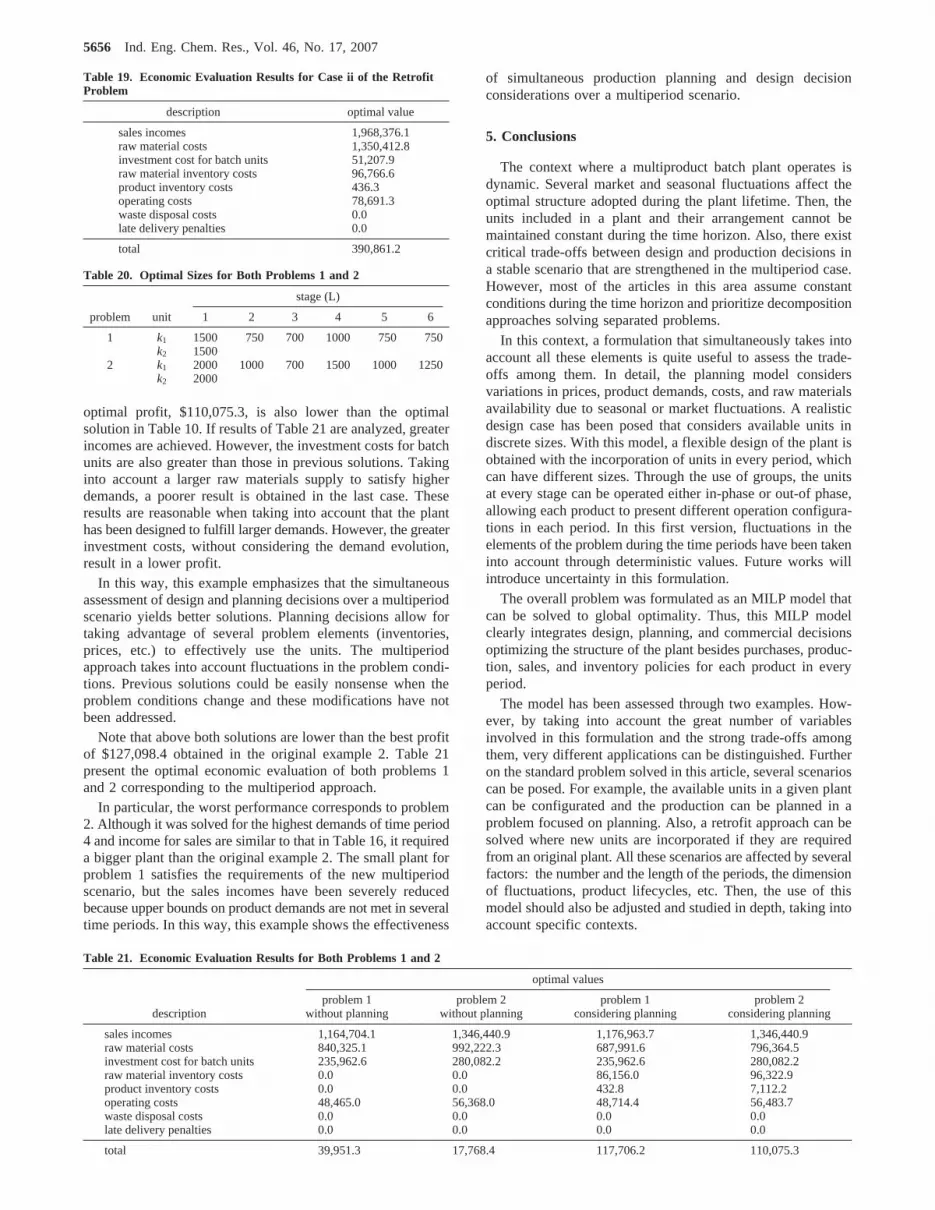
optimal profit, $110,075.3, is also lower than the optimalsolution in Table 10. If results of Table 21 are analyzed, greaterincomes are achieved. However, the investment costs for batchunits are also greater than those in previous solutions. Takinginto account a larger raw materials supply to satisfy higherdemands, a poorer result is obtained in the last case. Theseresults are reasonable when taking into account that the planthas been designed to fulfill larger demands. However, the greaterinvestment costs, without considering the demand evolution,result in a lower profit.

In this way, this example emphasizes that the simultaneousassessment of design and planning decisions over a multiperiodscenario yields better solutions. Planning decisions allow fortaking advantage of several problem elements (inventories,prices, etc.) to effectively use the units. The multiperiodapproach takes into account fluctuations in the problem condi-tions. Previous solutions could be easily nonsense when theproblem conditions change and these modifications have notbeen addressed.

Note that above both solutions are lower than the best profitof $127,098.4 obtained in the original example 2. Table 21present the optimal economic evaluation of both problems 1and 2 corresponding to the multiperiod approach.

In particular, the worst performance corresponds to problem2. Although it was solved for the highest demands of time period4 and income for sales are similar to that in Table 16, it requireda bigger plant than the original example 2. The small plant forproblem 1 satisfies the requirements of the new multiperiodscenario, but the sales incomes have been severely reducedbecause upper bounds on product demands are not met in severaltime periods. In this way, this example shows the effectiveness

of simultaneous production planning and design decisionconsiderations over a multiperiod scenario.

5. Conclusions

The context where a multiproduct batch plant operates isdynamic. Several market and seasonal fluctuations affect theoptimal structure adopted during the plant lifetime. Then, theunits included in a plant and their arrangement cannot bemaintained constant during the time horizon. Also, there existcritical trade-offs between design and production decisions ina stable scenario that are strengthened in the multiperiod case.However, most of the articles in this area assume constantconditions during the time horizon and prioritize decompositionapproaches solving separated problems.

In this context, a formulation that simultaneously takes intoaccount all these elements is quite useful to assess the trade-offs among them. In detail, the planning model considersvariations in prices, product demands, costs, and raw materialsavailability due to seasonal or market fluctuations. A realisticdesign case has been posed that considers available units indiscrete sizes. With this model, a flexible design of the plant isobtained with the incorporation of units in every period, whichcan have different sizes. Through the use of groups, the unitsat every stage can be operated either in-phase or out-of phase,allowing each product to present different operation configura-tions in each period. In this first version, fluctuations in theelements of the problem during the time periods have been takeninto account through deterministic values. Future works willintroduce uncertainty in this formulation.

The overall problem was formulated as an MILP model thatcan be solved to global optimality. Thus, this MILP modelclearly integrates design, planning, and commercial decisionsoptimizing the structure of the plant besides purchases, produc-tion, sales, and inventory policies for each product in everyperiod.

The model has been assessed through two examples. How-ever, by taking into account the great number of variablesinvolved in this formulation and the strong trade-offs amongthem, very different applications can be distinguished. Furtheron the standard problem solved in this article, several scenarioscan be posed. For example, the available units in a given plantcan be configurated and the production can be planned in aproblem focused on planning. Also, a retrofit approach can besolved where new units are incorporated if they are requiredfrom an original plant. All these scenarios are affected by severalfactors: the number and the length of the periods, the dimensionof fluctuations, product lifecycles, etc. Then, the use of thismodel should also be adjusted and studied in depth, taking intoaccount specific contexts.

Table 19. Economic Evaluation Results for Case ii of the RetrofitProblem


sales incomes 1,968,376.1raw material costs 1,350,412.8investment cost for batch units 51,207.9raw material inventory costs 96,766.6product inventory costs 436.3operating costs 78,691.3waste disposal costs 0.0late delivery penalties 0.0

total 390,861.2

Table 20. Optimal Sizes for Both Problems 1 and 2

stage (L)

problem unit 1 2 3 4 5 6

1 k1 1500 750 700 1000 750 750k2 1500

2 k1 2000 1000 700 1500 1000 1250k2 2000

Table 21. Economic Evaluation Results for Both Problems 1 and 2

optimal values

descriptionproblem 1

without planningproblem 2

without planningproblem 1

considering planningproblem 2

considering planning

sales incomes 1,164,704.1 1,346,440.9 1,176,963.7 1,346,440.9raw material costs 840,325.1 992,222.3 687,991.6 796,364.5investment cost for batch units 235,962.6 280,082.2 235,962.6 280,082.2raw material inventory costs 0.0 0.0 86,156.0 96,322.9product inventory costs 0.0 0.0 432.8 7,112.2operating costs 48,465.0 56,368.0 48,714.4 56,483.7waste disposal costs 0.0 0.0 0.0 0.0late delivery penalties 0.0 0.0 0.0 0.0

total 39,951.3 17,768.4 117,706.2 110,075.3


Acknowledgment

The authors are grateful for financial support from CONICET(Consejo Nacional de Investigaciones Cientı´ficas y Tecnicas)and Agencia Nacional de Promocioń Cientıfica y Tecnologicaof Argentina.

Nomenclature

Subscripts

g ) groupi ) productj ) batch stagek ) equipments ) discrete sizes for the unitst ) time periodτ ) time period

Superscripts

T ) totalL ) lower boundU ) upper bound

Parameters

coit ) operating cost coefficient of producti at periodtDEit ) demand for producti in period tFci ) conversion of raw materialc to producei at periodtGj

T ) total number of groups at stagejH ) time horizonHt ) net available production time for all products in periodtKj ) maximum number of units that can be added at stagejnj ) number of discrete sizes available for stagejnpit ) price of producti in period tSijt ) size factor of producti at stagej for each periodttijt ) processing time of producti in batch stagej in period twpi ) waste disposal cost coefficient per productiwri ) waste disposal cost coefficient per raw materialiRj ) cost coefficient for a batch unit in stagejâj ) cost exponent for a batch unit at stagejεi ) inventory cost coefficient for raw materialiκit ) price for the raw material of producti in period tVjs ) standard volume of sizes for batch unit at stagejσi ) inventory cost coefficient for productiúi ) time periods during which raw materials have to be usedøi ) time periods during which products have to be used

Binary Variables

uijgt ) it is 1 if at stagej for product i there areg groups inperiod t

wjkt ) it is 1 if unit k at stagej is added in periodtyijgt ) it is 1 if groupg at stagej exists in periodt for product

iyijkgt ) it is 1 if unit k at batch stagej is assigned to groupg for

producti in period tzjks ) it is 1 if equipmentk at batch stagej has sizes

Integer Variables

Gijt ) number of groups at stagej for every producti in a periodt

Continuous Variables

Bit ) batch size of producti in period tCit ) amount of raw material for producingi purchased in period

t

eijgt ) continuous variable that represents the product of thevariablesnituijgt

hijkgst ) continuous variable that represents the product of thevariableszjksyijkgtnit

IM it ) inventory of raw materiali at the end of a periodtIPit ) inventory of final producti at the end of a periodtnit ) number of batches of producti in period tPWit ) producti wasted at periodt due to the limited product

lifetimeqit ) amount of producti to be produced in periodtQSit ) amount of producti sold at the end of periodtRMit ) raw material inventory for producti in period tRWit ) raw materiali wasted at periodt due to the limited

product lifetimerjkst ) continuous variable that represents the product of the

binary variableszjswjkt

Tit ) total time for producing producti in period tTL it ) limiting cycle time of producti in period tVjk ) size of a batch unitk at stagejϑit ) late delivery for producti in period t

Literature Cited

(1) Birewar, D. B.; Grossmann, I. E. Simultaneous production planningand scheduling in multiproduct batch plants.Ind. Eng. Chem. Res.1990,29, 570-580.

(2) Sahinidis, N. V.; Grossmann, I. E. Multiperiod investment modelfor processing networks with dedicated and flexible plants.Ind. Eng. Chem.Res.1991, 30, 1165-1171.

(3) Norton, L. C.; Grossmann, I. E. Strategic planning model forcomplete process flexibility.Ind. Eng. Chem. Res.1994, 33, 69-76.

(4) Iyer, R. R.; Grossmann, I. E. Optimal multiperiod operationalplanning for utility systems.Comput. Chem. Eng.1997, 21, 787-800.

(5) Ryu, J. Multiperiod planning strategies with simultaneous consid-eration of demand fluctuations and capacity expansion.Ind. Eng. Chem.Res.2006, 45, 6622-6625.

(6) Varvarezos, D. K.; Grossmann, I. E.; Biegler, L. T. An outer-approximation method for multiperiod design optimization.Ind. Eng. Chem.Res.1992, 31, 1466-1477.

(7) Voudouris, V. T.; Grossmann, I. E. Optimal synthesis of multiproductbatch plants with cyclic scheduling and inventory considerations.Ind. Eng.Chem. Res.1993, 32, 1962-1980.

(8) Ierapetritou, M. G.; Pistikopoulos, E. N. Batch plant design andoperations under uncertainty.Ind. Eng. Chem. Res.1996, 35, 772-787.

(9) Petkov, S. B.; Maranas, C. D. Design of multiproduct batch plantsunder demand uncertainty with staged capacity expansions.Comput. Chem.Eng.1998, 22, S789-S792.

(10) Iyer, R. R.; Grossmann, I. E. Synthesis and operational planningof utility systems for multiperiod operation.Comput. Chem. Eng.1998,22, 979-993.

(11) Oliveira Francisco, A. P.; Matos, H. A. Strategic planning modelfor complete process flexibility.Comput. Chem. Eng.2004, 28, 745-753.

(12) Van den Heever, S. A.; Grossmann, I. E. Disjunctive multiperiodoptimization methods for design and planning of chemical process systems.Comput. Chem. Eng.1999, 23, 1075-1095.

(13) Cao, D.; Yuan, X. Optimal design of batch plants with uncertaindemands considering sitch over of operating modes of parallel units.Ind.Eng. Chem. Res.2002, 41, 4616-4625.

(14) Lee, Y. G.; Malone, M. F. A general treatment of uncertainties inbatch process planning.Ind. Eng. Chem. Res.2001, 40 (6), 1507-1515.

(15) Cheng, L.; Subrahmanian, E.; Westerberg A. W. Design andplanning under uncertainty: Issues on problem formulation and solution.Comput. Chem. Eng.2003, 27, 781-801.

(16) Alonso-Ayuso, A.; Escudero, L. F.; Garıń, A.; Ortuno, M. T.; Perez,G. On the product selection and plant dimensioning problem underuncertainty.Omega2005, 33, 307-318.

(17) Ortız-Gomez, A.; Rico-Ramirez, V.; Hernandez-Castro, S. Mixed-integer multiperiod model for the planning of oilfield production.Comput.Chem. Eng.2002, 26, 703-714.

(18) Ostermark, R.; Skrifvars, H.; Westerlund, T. A nonlinear mixedinteger multiperiod firm model.Int. J. Prod. Econ.2000, 67, 183-199.

(19) Dietz, A.; Azzaro-Pantel, C.; Pibouleau, L.; Domenech, S. Aframework for multiproduct batch plant design with environmental con-


sideration: application to protein production.Ind. Eng. Chem. Res.2005,44, 2191-2206.

(20) Cavin, L.; Fischer, U.; MosˇatÄ, A.; Hungerbu¨hler, K. Batch processoptimization in a multipurpose plant using Tabu Search with a design-space diversification.Comput. Chem. Eng.2005, 29, 1770-1786.

(21) Moreno, M. S.; Montagna, J. M.; Iribarren, O. A. Multiperiodoptimization for the design and planning of multiproduct batch plants.Comput. Chem. Eng.2007, 31, 1159-1173.

(22) Ravermark, D. E; Rippin D. W. T. Optimal design of a multi-product batch plant.Comput. Chem. Eng.1998, 22, 177-183.

(23) Montagna, J. M.; Vecchietti, A. R.; Iribarren, O. A.; Pinto, J. M.;Asenjo, J. A. Optimal design of protein production plants with time andsize factors process models.Biotechnol. Prog.2000, 16, 228-237.

(24) Yoo, D. J.; Lee, H.; Ryu, J.; Lee, I. Generalized retrofit design ofmultiproduct batch plants.Comput. Chem. Eng.1999, 23, 683-695.

(25) Lee, H. K.; Lee, I. B.; Reklaitis, G. V. Capacity expansion problemof multisite batch plants with production and distribution.Comput. Chem.Eng.2000, 24, 1597-1602.

(26) Montagna, J. M. The optimal retrofit of multiproduct batch plants.Comput. Chem. Eng.2003, 27, 1277-1290.

(27) Voudouris, V. T.; Grossmann, I. E. Mixed-Integer linear program-ming reformulations for batch process design with discrete equipment sizes.Ind. Eng. Chem. Res.1992, 31, 1315-1325.

(28) Vaselenak, J. A.; Grossmann, I. E.; Westerberg, A. W. Optimalretrofit design of multipurpose batch plants.Ind. Eng. Chem. Res.1987,26, 718-726.

(29) Fletcher, R.; Hall, J. A.; Johns, W. R. Flexible retrofit design ofmultiproduct batch plants.Comput. Chem. Eng.1991, 12, 843-852.

(30) Goel, H.; Weijnen, M.; Grievink, J. Optimal reliable retrofit designof multiproduct batch plants.Ind. Eng. Chem. Res.2004, 43, 3799-3811.

(31) Lakhdar, K.; Savery, J.; Titchener-Hooker, N. J.; Papageorgiou,L. G. Medium term planning of biopharmaceutical manufacture usingmathematical programming.Biotechnol. Prog.2005, 21, 1478-1489.

(32) El Hafsi, M.; Bai, S. X. Multiperiod production planning withdemand and cost fluctuation.Math. Comput. Modell.1998, 28, 103-109.

ReceiVed for reView January 5, 2007ReVised manuscript receiVed June 6, 2007

AcceptedJune 11, 2007

IE070022V


Documents

New Alternatives in the Design and Planning of Multiproduct Batch Plants in a Multiperiod Scenario