Submitted to: IEEE Transactions on Circuits and Systems for Video Technology

October 1997

Motion Compensation of Wavelet Coefficients

with Wavelet Packet Based Motion Residual Coding

Francois G. Meyer 1, Amir Z. Averbuch 3, Ronald R. Coifman 21Department of Diagnostic Radiology and Computer Science,2Department of MathematicsYale University, New Haven, CT 06520, USA3School of Mathematical Sciences, Tel Aviv University, Tel Aviv 69978, Israele-mail: francois.meyer@yale.edu

1 Introduction

The recent emergence of multimedia applications in the last few years has motivated a con-

siderable interest in the development of video compression algorithms aimed at the trans-

mission (or storage) of video sequences at a variety of bandwidths. The ability to code,

decode and display a video at different resolutions is of fundamental importance for a large

class of applications such as: multipoint video distribution over the internet, video confer-

encing on ATM networks,etc.

Existing video compression standards [2] have been tailored to a small set of specific bit

rates. However, it becomes more and more important to be able to encode video streams at

a variety of spatial and temporal resolutions (spatial and temporal scalability) with a single

compression method. It would also be desirable to be able to apply some post-processing

and enhancement algorithms after the video signal has been decoded. This is especially im-

portant when the channel capacity is significantly reduced. Most video compression stan-

1

dards [2] use 2D Discrete Cosine Transform (DCT) to perform the intra frame coding of the

reference image, and inter frame coding of the prediction error. Unfortunately the fixed size

DCT is not well adapted to achieve spatial scalability. As opposed to a multiscale repre-

sentation (e.g the wavelet transform), the DCT cannot be decomposed into different layers

which correspond to different resolutions. Furthermore, for a given resolution, the image

quality degrades with disgraceful blocking artifacts when the channel capacity decreases.

The fixed block size DCT is thus not well adapted for SNR scalability. Finally, the blocking

artifacts at very low bit rate make it very difficult to apply post processing algorithms on the

decoded signal.

As opposed to the fixed size DCT the discrete wavelet transform (DWT) offers an alter-

native well adapted for spatial and SNR scalability. For this reasons several authors have

very recently started to investigate the potential use of the wavelet representation for video

coding. Wavelet (and subband) based video coding algorithms can be classified into two

broad classes of methods. The first class encompasses algorithms that compress the three

dimensional (3-D) (two spatial dimensions and time) video signal as a whole. In [18] the

authors present a multirate coding algorithm. First they realign the video frames to increase

the temporal redundancy. They assume that the motion of the camera is only panning. A

separable 3D subband decomposition is then applied, and the coefficients of subband are

progressively quantized and coded. A similar approach was proposed in [19] where more

complex motion models were used to compensate for global as well as local motions inside

a group of frames. Again, a 3D wavelet transform is applied on each group of realigned im-

ages. A zero tree data structure is then introduced that extends the EZW [17] data structure

and results in a progressive video coding.

Hybrid DPCM-wavelet transform coding scheme constitute the second class of methods.

Even though the video signal can be considered as a three-dimensional signal, the complex-

ity of the overall signal may be reduced by decoralating the signal along the temporal di-

mension. This is usually achieved by estimating the motion of the camera, or the motion

of the objects in the scene between two successive frames. Each successive frame can be

predicted with respect to the previous frame using the motion vectors. As a result the video

signal is decomposed into the combination of one (or multiple) reference image(s) (intra

2

frame coding) and the sequence of differences between the reference image, and the succes-

sive realigned frames (inter frame coding). Some authors have used the DWT to encode the

motion compensated residuals. This approach can only perform well if the residual error

is smooth, and does not contain block discontinuities, which is rarely the case. In [10] the

authors proposed a hybrid DPCM-DWT coding scheme similar to MPEG and H263 [2], but

they replaced the DCT by the DWT. An overlapped motion compensation scheme provides

a smooth residual error.

In fact, the DWT can provide a very compact representation of a smooth, or a piecewise

smooth, signal [1]. Consequently, most wavelet based video coding algorithms applied the

DWT on the original video signal before motion compensation [23, 22, 21, 15, 3]. It would

be then desirable to perform the motion estimation and the motion compensation directly

on the wavelet coefficients. The motion of each subband can be estimated from the motion

of the lowpass bands at each resolution level [20]. The lowpass band of each frame can

then be predicted from the lowpass band of the previous frame. A problem occurs with the

high subband images: it is not possible to accurately predict the highpass coefficients of the

current frame, from the highpass coefficients of the previous image. In the case where the

motion is only a translation, the problem can be explained from the fact that the translation

operator does not commute with the decimation operator. In [15] the authors also raised the

same problem. They proposed to estimate the motion from lowpass filtered non decimated

coefficients. The motion is then applied on the non decimated, filtered subband images of

the previous frame to predict the decimated subband coefficients of the current frame. At

the finest scale their scheme essentially requires the motion estimation and the prediction

of the lowpass filtered original image. Their approach accurately predicts the subband, but

requires the construction of a highly redundant representation of the image. Similarly in [3]

the authors proposed another approach: - instead of predicting directly the highpass coef-

ficients at a given resolution, they perform the motion compensation on the lowpass image

at the next finer resolution, and they calculate the decimated highpass coefficients of this

predicted lowpass image. At the finest resolution, their scheme also requires the motion

compensation of the entire image. In this paper we will propose a different approach, where

we preserve the advantage of the wavelet representation: sparse encoding of both the high-

3

pass coefficients, and the smooth regions.

We propose in this paper a video compression algorithm that can operate at a variety of

bit rates (from 10kbits/s to 10 Mbits/s). This highly scalable video codec exploits three key

ingredients:

1. a multiscale representation of the reference frames using wavelets,

2. multiresolution motion estimation, and motion prediction of the wavelet coefficients,

3. coding of the error frames, with a wavelet packet based texture compression algorithm

[12].

Our approach exploits a successive approximation technique that permits to rate the co-

efficients according to their importance and to transmit them accordingly. As a result we can

achieve SNR scalability. The spatial scalability is achieved through the use of the wavelet

and wavelet packet transforms which make it possible to encode the video at different res-

olution layers. The coarse layer contains a small set of large coefficients that describe the

smooth regions of the image. Whereas the enhancement layers provide finer and finer de-

tails about edges and textures present in the image. Finally, post processing that exploit the

wavelet representation can be applied to enhance the decoded image.

This paper is organized as follows. In the next section we provide a general description

of the algorithm. This is followed in section 3 by a description of the multiresolution mo-

tion estimation and prediction of the wavelet coefficients. In section 4 we describe the new

wavelet packet based texture coding scheme to encode the residual images after motion pre-

diction. The successive approximation quantization scheme, that quantize the wavelet and

wavelet packet coefficients is presented in Section 5. Results of experiments are presented

in Section 6.

4

2 General overview of the algorithm

We give in this section a general description of the coder and the decoder. Each building

block: reference frame coding, motion estimation, motion prediction, residual error coding

are detailed in the following.

2.1 Coder

A block-diagram schematically describes the coder in Fig. 1. The original video sequence

is divided into group of frames (GOF) of fixed size = 2M + 1 (in the experiments we havetested several values for M , ranging from 3 to 9). The coder encodes each group of framesseparately.

We consider in the following a group of 2M+1 frames, that we denote f0; : : : ; fM ; : : : ; f2M .The central frame fM is the reference frame and is intra coded (see (1) and (2) in Fig. 1). Theother frames in the GOF aremotion predicted. In reference to theMPEG terminology we call

the reference frames I-frames, and the motion predicted frames P-frames. For each frame fiwe calculate the discrete wavelet transform: Wfi. After the DWT the wavelet coefficients ofthe reference frame are quantized, entropy coded, and sent to the decoder. The coefficients

of the central frame are quantized using a successive approximation scheme.

In order to diminish the temporal redundancy between the frames inside a GOF we es-

timate the motion between the reference frame fM , and the other frames fi; i 6= M insidethe GOF. To achieve this we estimate the motion displacement that gives the best prediction

of frame fi from frame fM . In practice we assume that the displacement is piecewise con-stant over square blocks of fixed size. The displacement is estimated with a multiresolution

approach using the pyramid of the wavelet coefficients (see (4) in Fig. 1).

Once the displacement between frame fi and frame fM is estimated, we can predict thevalues of the pixels inside each block of frame fi. Rather than working at the pixel level, wecan directly predict the wavelet coefficientsWfi.Amultiresolution motion prediction algorithm yields a smooth (free from block artifacts)

prediction dWf i of the wavelets coefficients of frame i from frameM (see (5) in Fig. 1).We calculate the motion prediction error �Wfi = dWf i �Wfi for each frame in the GOF.

5

Video

Wavelet

Transform

Motion

Wavelet Packets

PredictionMotionEstimation

ExpansionP-frame

I-frame

Input 6

4

5

3

-1QIntra frame

Frame bufferMotion vectors

Motion vectors

1

Q

2Q

Figure 1: Block diagram of the encoder. Q = quantization, DWT = discrete wavelet trans-

form, Q �1 = inverse quantizationThe nature of the residual images is very different from the nature of the original images:

– the residual images are textured, and contain many edges. In order to encode efficiently

these residual images, we use a library of patterns that provides a very sparse representa-

tion of textures, as well as edges. This library is called the wavelet packet library [6]. An

advantage of this library is that we can directly calculate the wavelet packet coefficients from

the wavelet coefficients of the residual. This is a very important advantage, since we need

not apply an inverse wavelet transform in order to reconstruct the residual image before

calculating the wavelet packet coefficients.

Finally, the wavelet packet coefficients are quantized, entropy coded and sent to the de-

coder (see (5) and (6) in Fig. 1). Themotion vectors, are spatially decoralated, entropy coded,

and sent to the decoder.

2.2 Decoder

A block diagram of the decoder is described in Fig. 2. The decoder reconstructs each group

of frames independently. We consider in the following a group of 2M+1 frames: f0; : : : ; f2M .Firstly, the reference frame fM is decoded: – the coefficients are inverse quantized (see (1) in

6

Wavelet PacketsExpansion

Q-1

Intra frameFrame buffer

-1P-frame

residual Q

Motion Video

I-frame

1

2

5

3

4Output

Prediction

motion

vectors

WaveletTransform

P-frame

I-frame

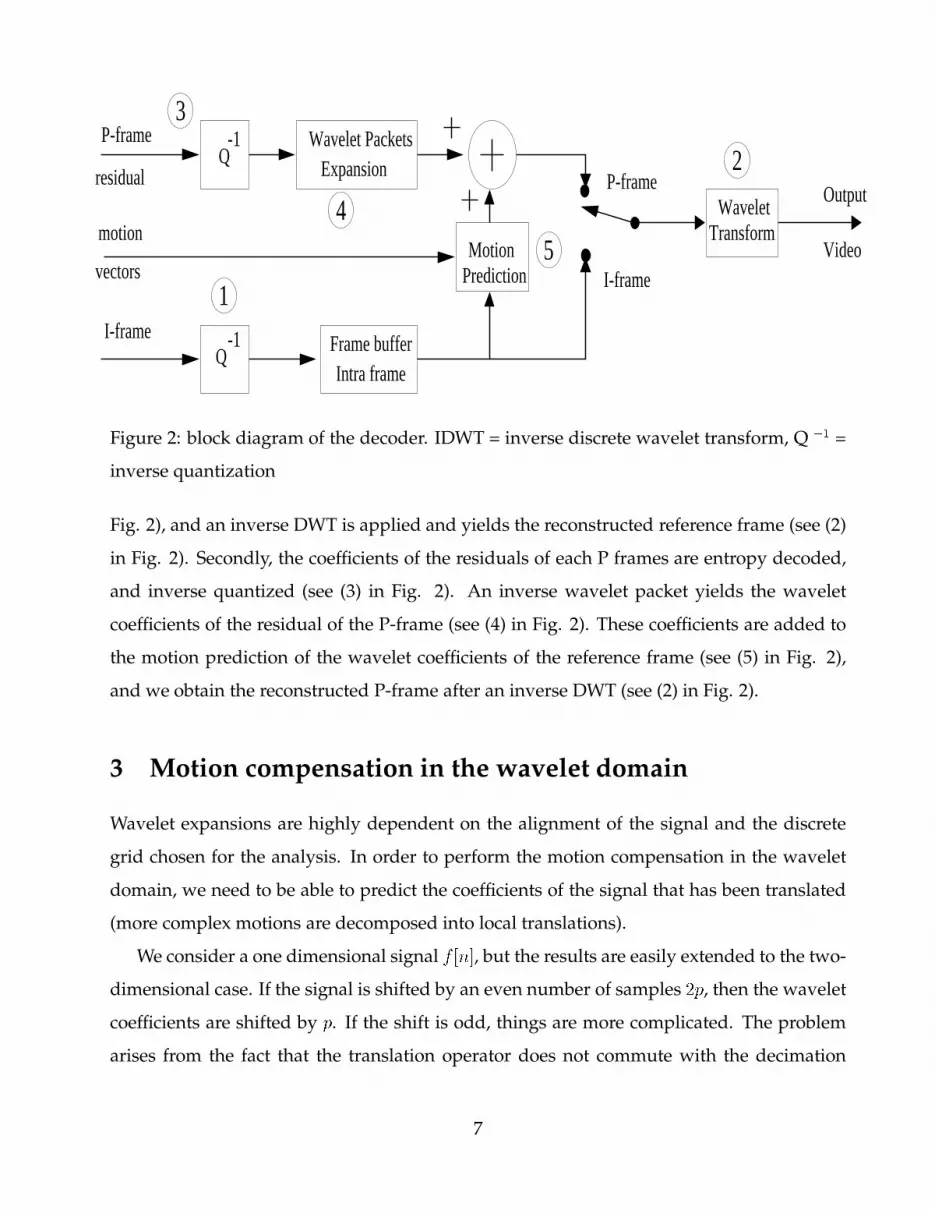
Figure 2: block diagram of the decoder. IDWT = inverse discrete wavelet transform, Q �1 =inverse quantization

Fig. 2), and an inverse DWT is applied and yields the reconstructed reference frame (see (2)

in Fig. 2). Secondly, the coefficients of the residuals of each P frames are entropy decoded,

and inverse quantized (see (3) in Fig. 2). An inverse wavelet packet yields the wavelet

coefficients of the residual of the P-frame (see (4) in Fig. 2). These coefficients are added to

the motion prediction of the wavelet coefficients of the reference frame (see (5) in Fig. 2),

and we obtain the reconstructed P-frame after an inverse DWT (see (2) in Fig. 2).

3 Motion compensation in the wavelet domain

Wavelet expansions are highly dependent on the alignment of the signal and the discrete

grid chosen for the analysis. In order to perform the motion compensation in the wavelet

domain, we need to be able to predict the coefficients of the signal that has been translated

(more complex motions are decomposed into local translations).

We consider a one dimensional signal f [n], but the results are easily extended to the two-dimensional case. If the signal is shifted by an even number of samples 2p, then the waveletcoefficients are shifted by p. If the shift is odd, things are more complicated. The problemarises from the fact that the translation operator does not commute with the decimation

7

operator. Therefore the coefficient of the translated image is not equal to the translated

coefficient of the original image. In the case of the lowpass coefficients, we will show that

the translated coefficient is a good approximation of the coefficient of the translated image.

Let us assume now that the signal has been shifted by an odd number, 2p+1, of samples,and let us examine how the wavelet coefficients evolve. Since a shift by 2p can be obtainedby a shift of p on the wavelet coefficients, we need only to understand the case where theshift is 1.

We first analyze the lowpass coefficients of the translated signal. Let s1 be the lowpasswavelet coefficients of the original signal: s1[n] is the value of the undecimated lowpasscoefficients of the unshifted signal at the grid point 2n (see Fig. 9). Let s1t be the lowpasswavelet coefficients of the translated signal. Since s1t [n] is the value of the undecimatedlowpass filtered unshifted signal at 2n� 1, we can interpolate s1t [n] from s1[n� 1], s1[n] ands1[n+1]. The lowpass filtered signal is smooth, and the interpolation error will be small. Weconclude that it is possible to accurately interpolate the lowpass coefficients of the shifted

signal from the lowpass coefficients of the unshifted signal.

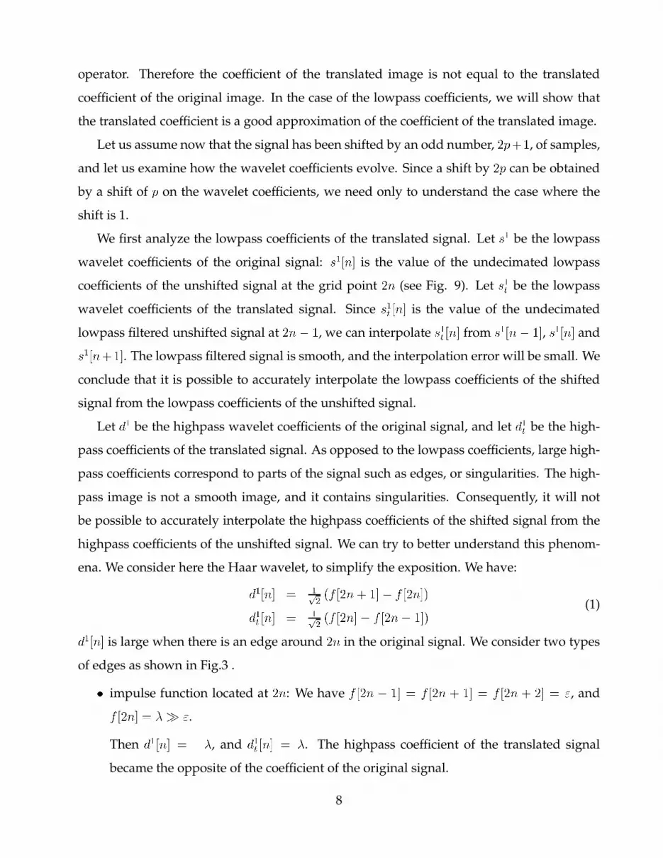
Let d1 be the highpass wavelet coefficients of the original signal, and let d1t be the high-pass coefficients of the translated signal. As opposed to the lowpass coefficients, large high-

pass coefficients correspond to parts of the signal such as edges, or singularities. The high-

pass image is not a smooth image, and it contains singularities. Consequently, it will not

be possible to accurately interpolate the highpass coefficients of the shifted signal from the

highpass coefficients of the unshifted signal. We can try to better understand this phenom-

ena. We consider here the Haar wavelet, to simplify the exposition. We have:d1[n] = 1p2 (f [2n+ 1]� f [2n])d1t [n] = 1p2 (f [2n]� f [2n� 1]) (1)d1[n] is large when there is an edge around 2n in the original signal. We consider two typesof edges as shown in Fig.3 .� impulse function located at 2n: We have f [2n � 1] = f [2n + 1] = f [2n + 2] = ", andf [2n] = �� ".

Then d1[n] = ��, and d1t [n] = �. The highpass coefficient of the translated signalbecame the opposite of the coefficient of the original signal.

8

2n 2n+12n-1 2n+12n2n-1

Figure 3: Two type of edges, left: “impulse” edge, right “ramp” edge.� ramp function: we have f [2n � 1] = ", f [2n] = f [2n + 1] = f [2n + 2] = � � ". In thiscase d1[n] = 0, but d1t [n] = �.

Such phenomena will happen frequently around the edges of the image. This shows that it

is not possible to predict the large highpass wavelet coefficients.

Several authors [3, 15, 21, 23] proposed to directly predict the lowpass and highpass

wavelet coefficients using motion compensation. In [3] the authors also raised the problem

that we documented here. Instead of predicting directly the highpass coefficients at a given

resolution, they perform the motion compensation on the lowpass image at the next finer

resolution, and they calculate the decimated highpass coefficients of this predicted lowpass

image. At the finest resolution, their scheme effectively requires the motion compensation

of the entire image. We propose a different approach, where we preserve the advantage of

the wavelet representation: sparse highpass coefficients, and sparse lowpass representation.

We first define a new pyramid structure that will permit us to predict the highpass wavelet

coefficients of the shifted image.

3.1 A new pyramid structure for motion compensation of wavelet coeffi-

cients

As opposed to the traditional wavelet expansion, we do not decimate the highpass coef-

ficients at each resolution. In practice this is not a major overhead since many of these

coefficients are set to zero after quantization when compressing at the required bit rate. The

lowpass coefficients in our pyramidal representation also differ from the traditional wavelet

9

lowpass coefficients: the signal is lowpass filtered twice, instead of only once. Let H be thehighpass filter, L be the lowpass filter, and let 2# be the decimation operator (subsamplingby 2). Let f be a 2-D image. The algorithm that calculates the coefficients of the pyramid isdefined as follows (see Fig.4):

HLd

2

and decimation

filtering

1

2

1

11

sLL

(twice)

highpass

filtering

sLL

0

highpass

lowpass

lowpassfiltering(twice)

and decimation

filtering

2

sLL

2

LH

HL

ddLH HH

HH

d

dd

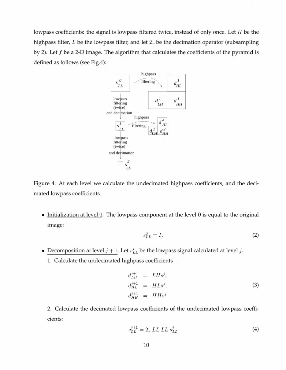
Figure 4: At each level we calculate the undecimated highpass coefficients, and the deci-

mated lowpass coefficients� Initialization at level 0. The lowpass component at the level 0 is equal to the originalimage: s0LL = I: (2)� Decomposition at level j + 1. Let sjLL be the lowpass signal calculated at level j.1. Calculate the undecimated highpass coefficientsdj+1LH = LHsj;dj+1HL = HLsj;dj+1HH = HHsj (3)

2. Calculate the decimated lowpass coefficients of the undecimated lowpass coeffi-

cients: sj+1LL = 2# LL LL sjLL (4)

10

sj+1LL , is not kept in the pyramid, but it will be the input of the decomposition at thenext coarser scale.� Final level J :1. Calculate the undecimated highpass coefficients: dJLH; dJHL; dJHH .2. Calculate the decimated lowpass filtered coefficients: sJLL, and save it into the pyra-mid.

3.2 Reconstruction of an image from the pyramid

Lemma 1 We can reconstruct a 2-D image f from(i) the decimated, twice lowpass filtered images1LL = 2#LLLLf(ii) and the three undecimated highpass filtered imagesd1LH = LH fdjHL = HLfdjHH = HH fThe proof exploit two ingredients. Firstly, we reconstruct the undecimated lowpass fil-

tered image, LLf , from the decimated twice lowpass filtered image, and from the undec-imated highpass images, as shown in (1) in Fig. 5. We apply the lowpass filter LL on theundecimated highpass images: d1HL; : : : andwe decimate (see (1) in Fig. 5). We notice that wecan commute the highpass filtersHL; : : : and the lowpasss filter LL before the subsampling.Finally, we obtain 2#LLd1HL = 2# HL (LLf)2#LLd1LH = 2# LH (LLf)2#LLd1HH = 2# HH (LLf) (5)

Since we also have the decimated lowpass filtered signal, 2# LL (LLf) (see (2) in Fig. 5),we have all the coefficients of the traditional wavelet transform of LLf . As a result we can

11

d

HH

1

HHd

HL

LH

2

d21

4

2

3s2

sLL

1

LL

HL

1

s 2

LL

1

1

d

d

d

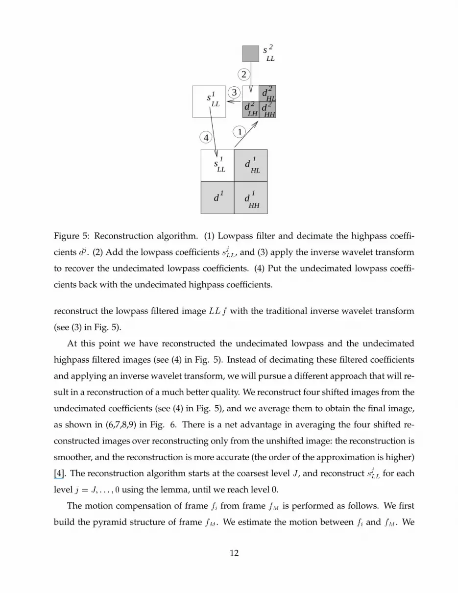
Figure 5: Reconstruction algorithm. (1) Lowpass filter and decimate the highpass coeffi-

cients dj. (2) Add the lowpass coefficients sjLL, and (3) apply the inverse wavelet transformto recover the undecimated lowpass coefficients. (4) Put the undecimated lowpass coeffi-

cients back with the undecimated highpass coefficients.

reconstruct the lowpass filtered image LLf with the traditional inverse wavelet transform(see (3) in Fig. 5).

At this point we have reconstructed the undecimated lowpass and the undecimated

highpass filtered images (see (4) in Fig. 5). Instead of decimating these filtered coefficients

and applying an inverse wavelet transform, we will pursue a different approach that will re-

sult in a reconstruction of a much better quality. We reconstruct four shifted images from the

undecimated coefficients (see (4) in Fig. 5), and we average them to obtain the final image,

as shown in (6,7,8,9) in Fig. 6. There is a net advantage in averaging the four shifted re-

constructed images over reconstructing only from the unshifted image: the reconstruction is

smoother, and the reconstruction is more accurate (the order of the approximation is higher)

[4]. The reconstruction algorithm starts at the coarsest level J , and reconstruct sjLL for eachlevel j = J; : : : ; 0 using the lemma, until we reach level 0.The motion compensation of frame fi from frame fM is performed as follows. We first

build the pyramid structure of frame fM . We estimate the motion between fi and fM . We12

10

9

8

76

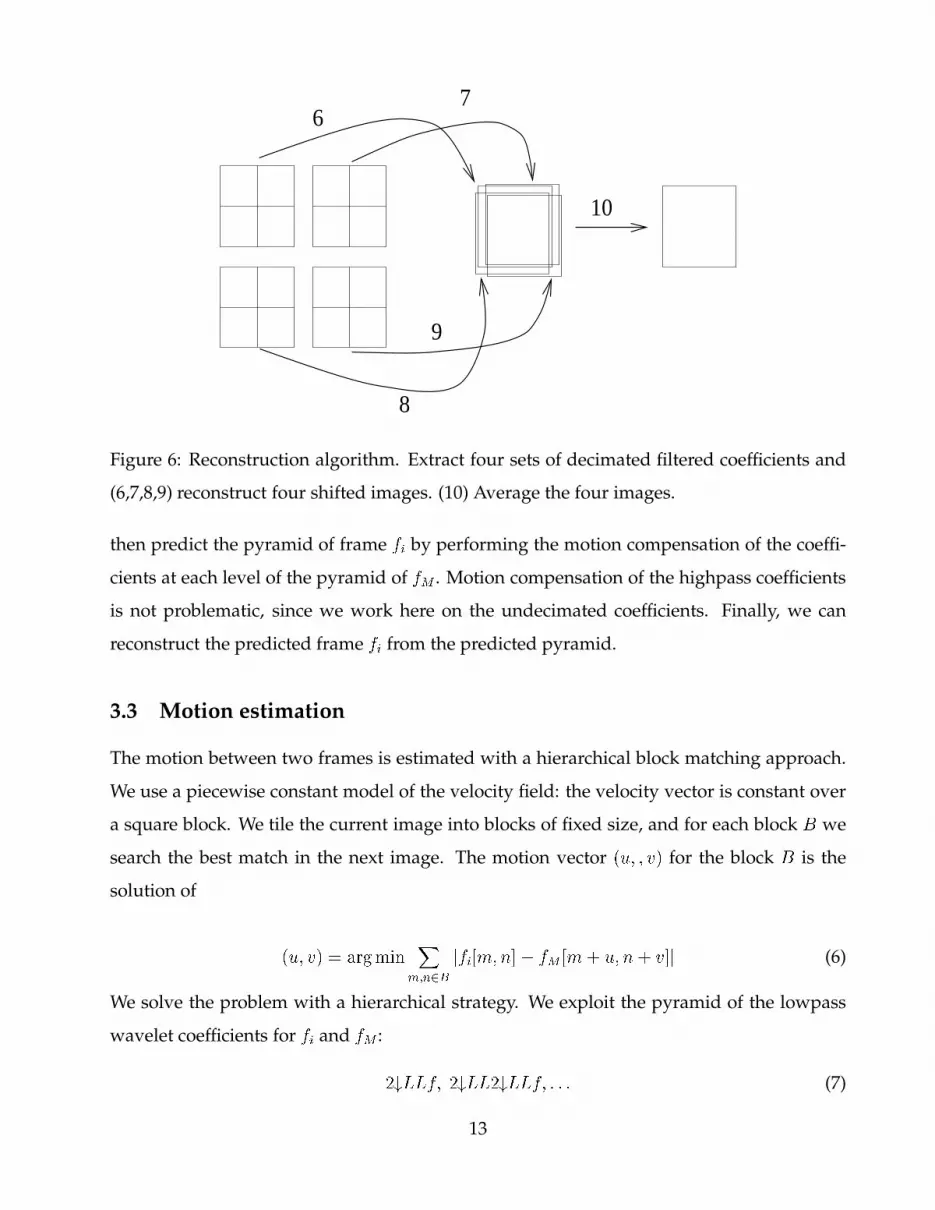
Figure 6: Reconstruction algorithm. Extract four sets of decimated filtered coefficients and

(6,7,8,9) reconstruct four shifted images. (10) Average the four images.

then predict the pyramid of frame fi by performing the motion compensation of the coeffi-cients at each level of the pyramid of fM . Motion compensation of the highpass coefficientsis not problematic, since we work here on the undecimated coefficients. Finally, we can

reconstruct the predicted frame fi from the predicted pyramid.3.3 Motion estimation

The motion between two frames is estimated with a hierarchical block matching approach.

We use a piecewise constant model of the velocity field: the velocity vector is constant over

a square block. We tile the current image into blocks of fixed size, and for each block B wesearch the best match in the next image. The motion vector (u; ; v) for the block B is thesolution of (u; v) = argmin Xm;n2B jfi[m;n]� fM [m + u; n+ v]j (6)

We solve the problem with a hierarchical strategy. We exploit the pyramid of the lowpass

wavelet coefficients for fi and fM : 2#LLf; 2#LL2#LLf; : : : (7)

13

The number of blocks is kept constant at each resolution, and the block size is doubled along

each direction at each finer resolution. An initial motion estimate is obtained for each block

with the coarsest resolution images. At each higher resolution we calculate an incremental

value of the blocks displacements. We note that the search of the incremental value is per-

formed within a small window, and is thus quite fast. The hierarchical approach regularizes

the motion field, and is much faster than the brute force search at the finest resolution level.

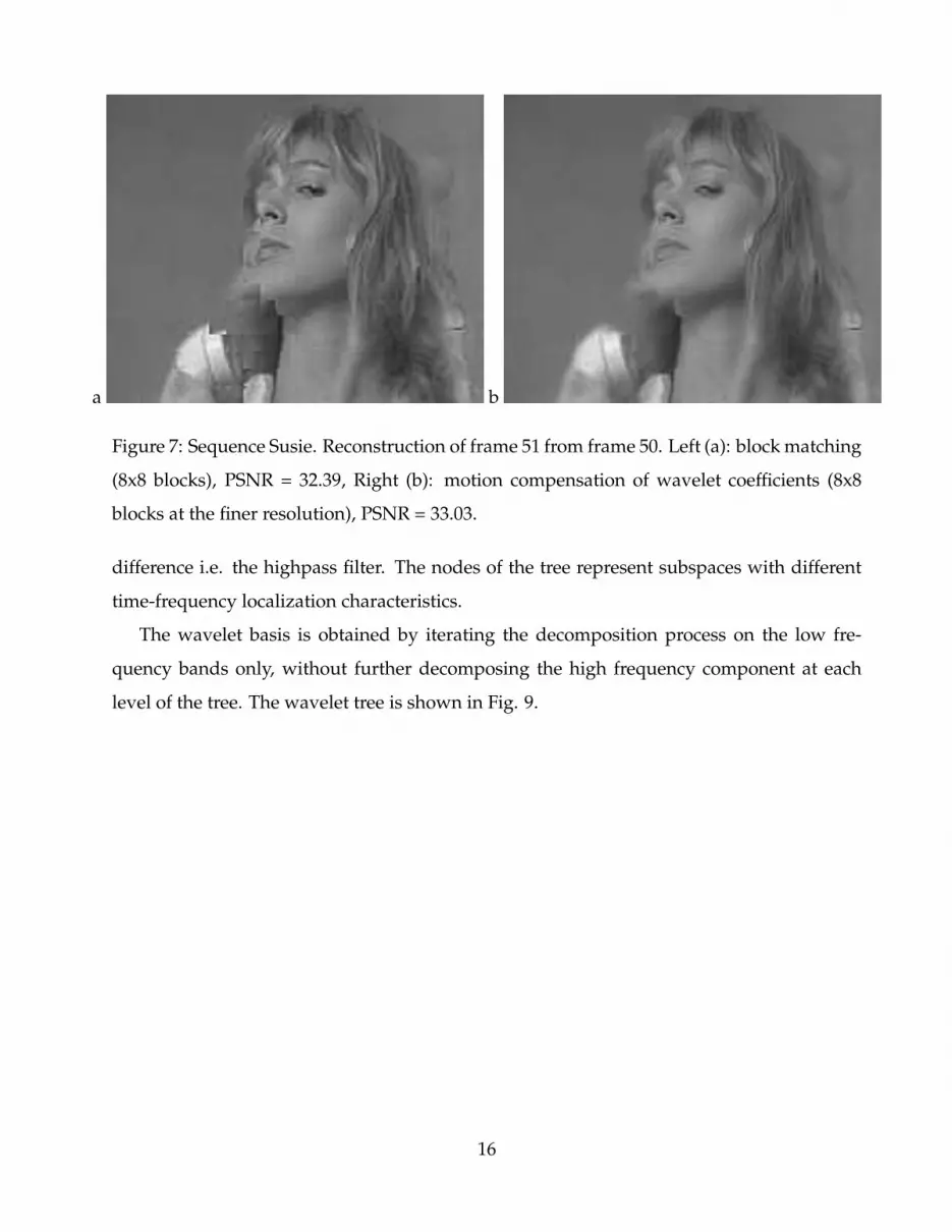
Figure 7.a shows the result of the prediction of frame 51 from frame 50 of the QCIF test

sequence Susie using integer resolution (8�8) block matching. We note the visually unpleas-ant blocking artifacts. Figure 7.b shows the result of the wavelet basedmotion compensation

(8� 8 blocks at the finer resolution). Even though there is a significant motion between thetwo frames, the new prediction has a better PSNR, and has a better perceptual quality. Also

note that the edges (the highpass coefficients) have been accurately predicted.

4 Wavelet packet coding of the motion residuals

Themotion prediction algorithm yields a prediction dWf i of the wavelet coefficients of framei, Wfi. Usually the prediction does not coincide with the original wavelet coefficients, andthe residual�Wfi = dWf i�Wfi has to be coded. In the image domain the motion predictionerror contains many edges, and textured regions.

As a result, the residual image should not be coded with wavelets ; but it should be

coded with that basis, which can provide a very sparse representation of textures and edges.

Neff and Zakhor [14] proposed to use a Gabor dictionary to encode the motion residuals.

Unfortunately, the Gabor dictionary is not composed of orthogonal “atoms”, and thus the

final signal representation is not constructed with orthonormal waveforms. With regards to

our goal: compression, the algorithmmay therefore yield a representation that is redundant.

Another problem stems from the fact that the decomposition, and the reconstruction cannot

be performed using a very fast algorithm; furthermore there is no fast algorithm, that can be

applied in real time, to select the optimal decomposition over the dictionary.

We propose instead to use very large libraries of waveforms, called wavelet packets [6].

In the two dimensional case the wavelet packets are patterns that can vary in scale, oscilla-

14

tion, and location. In order to select an orthonormal basis among all the wavelet packets,

these patterns are matched to the image, and a selection of best matches which are suffi-

cient for an efficient reconstruction is made. The selected collection of patterns is called

the “best basis” [7]. Wavelet packets have been successfully used to code textured images

[9, 16, 13, 12]. An important feature of the wavelet packet library is that the wavelet packet

coefficients can be calculated directly from the wavelet coefficients without reconstructing

the residual image.

4.1 Wavelet packets library

We consider two conjugate quadrature filters, the lowpass filter fhng , and the highpass filterfgng. Let ' be the scaling function, and let be the wavelet associated with this multireso-lution analysis. We define a new sequence of functions:2n(x) = p2Xk hkn(2x� k) (8)2n+1(x) = p2Xk gkn(2x� k) (9)

where 0 is the scaling function '. The collection fng constitutes the “basic wavelet pack-ets”. In fact we consider a larger library: the “multiscale wavelet packets”. This library is

defined to be the set of functionsn; j; l = 2j=2n(2jx� l); j 2 Z ; l 2 Z ; n 2 N : (10)

The indexes are interpreted as follows:� j is the scaling index: the size of the support is approximatively 2�j ,� l is the localization parameter: the function is roughly located at l 2�j� and n is the frequency index: the function has approximatively n oscillations.Clearly the library provides an over-complete description of L2(R). We need to know

how to assemble the elements of the library to obtain an orthogonal basis. We note that

the library organizes itself into a binary tree. Fig. 8 shows the wavelet packet tree for an 8

sample signal. The prefix “s” stands for the sum i.e. the lowpass filter, and “d” stands for

15

a b

Figure 7: Sequence Susie. Reconstruction of frame 51 from frame 50. Left (a): blockmatching

(8x8 blocks), PSNR = 32.39, Right (b): motion compensation of wavelet coefficients (8x8

blocks at the finer resolution), PSNR = 33.03.

difference i.e. the highpass filter. The nodes of the tree represent subspaces with different

time-frequency localization characteristics.

The wavelet basis is obtained by iterating the decomposition process on the low fre-

quency bands only, without further decomposing the high frequency component at each

level of the tree. The wavelet tree is shown in Fig. 9.

16

sd1 dd1

d1

sd2

ddssdsdsssss

ds2

d2s4s3s2 d3

ds1ss2ss1

d4

ssd

G G

GH

H H H HG

dd2

dddsdddsd

H

G

GH

G

s1

x1 x2 x3 x4 x8x7x6x5

Figure 8: Wavelet packet tree. At each node of the tree, we apply a convolution and a

decimation with the lowpass filter H , and the highpass filter, G. The prefix “s” stands forthe sum, or lowpass filter, and “d” stands for difference or highpass filter.

sss dss

s2

ds2

s3 s4

ss1 ss2 ds1

H

d2 d3 d4

G

d1

H G

GH

x8x5 x6 x7

s1

x4x1 x2 x3

Figure 9: Wavelet tree in gray. Only the result of the lowpass filtering is further decomposed

with the lowpass filter H , and the highpass filter, G. The prefix “s” stands for the sum, orlowpass filter, and “d” stands for difference or highpass filter.

17

If we associate the dyadic frequency interval [2jn; 2j(n+1) ) to the wavelet packetn; j; l,then we can build orthonormal bases from the binary tree, using very a fast algorithm. We

have the following result [5]:

Theorem 1 [5] If a subset E � N � Z has the property that the union of intervals[2jn; 2j(n+ 1) ); j 2 N ; 0 � n < 2 j ; (n; j ) 2 Eis a disjoint cover of [0;1), then the corresponding wavelet packetsn; j; l = 2j=2n(2jx� l); (n; j) 2 Eform an orthonormal basis.

We explain now how to calculate the wavelet packet coefficients in the discrete case.

4.2 Discrete case: calculation of the wavelet packets coefficients

We consider a discrete signal f = ffng n = 0; : : : ; N�1. We assume in fact that these samplesconstitute an approximation of the signal at the finer scale:f(x) = Xk2Z fk'(x� k) where fk =< f; '(x� k) > (11)

The wavelet packet coefficients are defined as the projection of the function f on the basisfunctions: dn; j; l = 2j=2 < f;n; j; l > (12)

The algorithm to calculate the set of coefficients f< f;n; j; l >g of the wavelet packets ex-pansion is given by the following recursion:< f;2n;j;l > = Xk hk�2l < f;n;j+1;k > (13)< f;2n+1;j;l > = Xk gk�2l < f;n;j+1;k > (14)

(15)

with < f;0;0;k >= fk (16)

18

Note that we effectively jump to a coarser resolution, from j + 1 to j, when we increasethe “frequency index” n of the wavelet packet.From (13) and (14) we obtain the lowpass, and highpass filtered and decimated versions

of the original sampled signal < f;n;j+1;k >. In order to calculate the wavelet packet co-efficients, we apply the two filter-and-decimation operators at each node of the tree. The

collection of wavelet packet coefficients of the signal f has a binary tree structure where thenodes of the tree are the coordinates of the signal viewed from the corresponding wavelet

packet.

The fundamental question now is how to select an orthogonal basis among all possible

choices given by theorem 1. If we consider only dyadic subdivision, then we can use a fast

(O(N logN)) split and merge algorithm to select the best basis [7].4.3 Calculation of the wavelet packet coefficients from the wavelet coef-

ficients

After the motion prediction of the wavelet coefficients of frame i we calculate the waveletresidual�Wfi = dWf i�Wfi. Instead of reconstructing the residual image from the waveletcoefficients of the residual, we can directly calculate the wavelet packet coefficients of the

residual. In order to evaluate the wavelet packet coefficients we need to explore the rest of

the tree, starting from the wavelet nodes. The algorithm is shown in the one dimensional

case in Fig. 10, and in the two dimensional case in Fig. 11. Each node in the wavelet packet

node can be reached using the lowpass filter (13), and highpass filter (14).

4.4 Best basis algorithm

The ”best basis” paradigm [7] permits a rapid (order N log(N), where N is the number ofpixels in the image) search among the large collection of orthogonal bases to find that ba-

sis which permits the best approximation according to a given cost function (e.g. coding

efficiency). A complete basis called best-basis which minimizes this criterion is searched in

this binary tree using the divide and conquer algorithm. At each node, the cost is compared

with the cost of the union of its two children’s nodes and if the node’s cost is smaller than

19

ds2ds1ss2ss1

d4

dss

sd1

d1

sd2

sss

dd1

sds dds ssd

H G G G

G

H H H

H

G

dsd sdd ddd

dd2

GH

GH

s3

x7 x8

s1 s2 s4 d2 d3

x6x1 x2 x3 x4 x5

Figure 10: Wavelet packet expansion of the wavelet tree: the nodes of the wavelet packet

tree (in light gray) below the wavelet nodes (in dark gray) are explored.

the children’s costs, the node is retained; otherwise, the children nodes are retained instead

of the node itself. This process is recursively applied from the bottom to the top of the

tree. Before selecting the best basis, we perform a denoising of the image [8]: we apply a

hard thresholding on the coefficients in the wavelet packet tree to remove those coefficients

whose magnitude are below a given threshold. The threshold is defined as the amplitude of

the smallest non zero coefficients that can be reconstructed after inverse quantization. Sec-

ondly, we measure the compactness of the bases with the l1 norm. Our cost function is thusdefined as follows

cost(x; �) = Xi;jxij>� jxij (17)

We have tried several approaches, including calculating the first order entropy for each node

(from the histogram at that node). After denoising, the l1 norm provides a very good mea-sure of the overall budget required to encode the coefficients.

20

Figure 11: Wavelet packet expansion of the wavelet tree, in two dimensions.

4.5 Frequency ordering of the coefficients

Once the best basis has been chosen, the residual is represented by a set of wavelet packet

coefficients. As opposed to a wavelet tree, there is no natural multiscale hierarchy in a best

basis tree. Therefore, algorithms that exploit zero-tree cannot be easily extended to a best

basis wavelet packet tree. Nevertheless we have tried to extend this idea, and we have

proposed two different scanning methods of the wavelet packet coefficients that both result

in sequence of coefficients with very rapid decay. Both scanning methods are based on the

ordering of the wavelet packet coefficients in the Fourier plane [12]. If the image f is smooth,the amplitude of the coefficients decreases as the frequency of the wavelet packet increases.

Organizing the wavelet packets consists in traveling in the spatial-frequency domain. There

are essentially two ways to travel in this domain:

1. we scan the positions, and for each position we gather all those wavelet packet by

increasing frequencies that have their support located at this position,

2. or, we scan the frequencies, and for each frequency band we gather all those wavelet

packets that have their Fourier transform in this band.

21

Both scanning algorithms yield long runs of contiguous zeros. Because we are using a suc-

cessive approximation quantization scheme, we need to be able to stop the quantization

loop in the middle of the coefficient list. When we stop in the middle of the list, we obtain

some artifacts. If use the scanning path (1), then the artifacts are localized in the part of the

image that could not be visited because of the budget constraint. If we use the scanning path

(2), then the artifacts are localized in the higher frequencies of the Fourier transform of the

image. As a result, artifacts created by the scanning path (2) are spread all over the image,

and are visually less unpleasant.

4.6 The Quantization Loop

Once the wavelet packet coefficients are properly ordered, we quantize the coefficients. The

coefficients are quantized during a number of iterations of what is called the “Quantization

loop”. This loop generates the quantization code. Whenever the stopping condition is met

the loop is terminated (possibly in a middle of a phase) and with it the whole process.

In each phase of the quantization loop the following is determined:

The threshold - for each phase a new smaller threshold is defined. This threshold deter-

mines which of the wavelet coefficients should be classified as important. Since the

threshold decreases, essentially the group of important coefficients widens from one

phase to the next. The exact determination of the threshold is explained later .

The precision - in which each of the important coefficients is quantized, is doubled from

one phase to the next.

The threshold is a parameter for the quantization loop that influences the generation of

the quantized code. During quantization the coefficients with absolute value greater than

the threshold, are considered to be important. During the quantization stage, the size of the

quantization bin is threshold=2. In our implementation the initial threshold is set to be halfof the maximal absolute value of all wavelet coefficients. At each phase of the quantization

loop the threshold is decreased by a factor of 2.

During the quantization loop a classification of each coefficient is calculated according to

the current threshold. For a more detailed description of the method please refer to [12].

22

4.6.1 Entropy coding of the symbols

The 0 and 1 symbols are entropy coded using a run length coding technique.

5 Experiments

We have implemented the wavelet based video algorithm. We have compared the perfor-

mance of the new algorithm against MPEG-1 [11]. We present the results of the algorithm

using three test sequences: flower, tennis, and mobile.

Figure 12 shows the frame by frame distortion for the luminance component of the recon-

structed flower sequence, for three different bit rates: 789kbits/s, 1 Mbits/s, and 1.5 Mbits/s.

Figure 16 shows the frame by frame distortion for the luminance component of the recon-

structedmobile sequence, for three different bit rates: 850kbits/s, 1 Mbits/s, and 1.5 Mbits/s.

Figure 13 shows the frame by frame distortion for the luminance component of the recon-

structed tennis sequence, for three different bit rates: 500kbits/s, 1 Mbits/s, and 1.5 Mbits/s.

Figure 14 shows frame 53 decoded at 1.5 Mbits/s with the MPEG coder. We note that the

texture on the wall, and the edges on the wall poster are smeared. The motion prediction of

the ball is blurred.

Figure 15 shows frame 53 decoded at 1.5 Mbits/s with the wavelet coder. We note that

the texture on the wall, and the edges on the wall poster are of very good quality. Themotion

prediction of the ball is quite sharp, and not blurred.

These results indicate that our coder reconstructs a video signal that is of good visual

quality. Our current implementation is currently outperformed by MPEg in terms of PSNR,

but in term of visual quality. When examining the detailed budget it appears that our algo-

rithm encodes less efficiently the motion vectors thanMPEG does. However we are working

on a new version of the coder with a more advanced coding of the motion vectors.

23

19

20

21

22

23

24

25

26

27

28

0 20 40 60 80 100 120

Y-PS

NR

Frame

Flower: 789 kbits/s

Wavelet coderMPEG-1

20

22

24

26

28

30

32

34

36

0 20 40 60 80 100 120

Y-PS

NR

Frame

Flower: 1 Mbits/s

Wavelet coderMPEG-1

22

24

26

28

30

32

34

36

38

40

0 20 40 60 80 100 120

Y-PS

NR

Frame

Flower: 1,5 Mbits/s

Wavelet coderMPEG-1

Figure 12: Frame by frame distortion for the luminance component of the “flower” se-

quence, at different bit rates.24

20

22

24

26

28

30

32

0 20 40 60 80 100 120

Y-PS

NR

Frame

Tennis: 500 kbits/s

Wavelet coderMPEG-1

22

24

26

28

30

32

34

36

0 20 40 60 80 100 120

Y-PS

NR

Frame

Tennis: 1 Mbits/s

Wavelet coderMPEG-1

24

26

28

30

32

34

36

38

0 20 40 60 80 100 120

Y-PS

NR

Frame

Tennis: 1,5 Mbits/s

Wavelet coderMPEG-1

Figure 13: Frame by frame distortion for the luminance component of the “tennis” sequence,

at different bit rates.25

Figure 14: Frame 53 from “tennis” decoded at 1.5 Mbits/s with the MPEG coder.

Figure 15: Frame 53 decoded at 1.5 Mbits/s with the wavelet coder.

26

20

21

22

23

24

25

26

0 20 40 60 80 100 120 140

Y-PS

NR

Frame

Mobile: 850 kbits/s

Wavelet coderMPEG-1

20

22

24

26

28

30

32

34

0 20 40 60 80 100 120 140

Y-PS

NR

Frame

Mobile: 1 Mbits/s

Wavelet coderMPEG-1

20

22

24

26

28

30

32

34

36

38

0 20 40 60 80 100 120 140

Y-PS

NR

Frame

Mobile: 1,5 Mbits/s

Wavelet coderMPEG-1

Figure 16: Frame by frame distortion for the luminance component of the “mobile” se-

quence, at different bit rates.27

6 Conclusion

We have proposed a new wavelet based video coder, with motion compensation of the

wavelet coefficients, and coding of the motion residual with wavelet packets. Reference

frames are decomposed with a wavelet transform, and the quantized coefficients are effi-

ciently encoded. Motion residual frames are decomposed on wavelet packet bases. These

bases provide very sparse representations of textures, as well as edges, and are therefore

very well adapted to motion residual frames. These two multiscale representation permits

to obtain a video codec that can achieve spatial, temporal and SNR scalability.

We have implemented the algorithm and we have studied its capabilities. We are cur-

rently working on an improved version of the algorithm that should improve the rate for a

given distortion.

28

References

[1] A. Averbuch, D. Lazar, andM. Israeli. Image compression using wavelet transform and

multiresolution decomposition. IEEE Trans. on Image Processing, Vol.5, No.1:pp 14–15,

1996.

[2] V. Bhaskaran. Image and video compression standards : algorithms and architectures. Kluwer

Academic Publishers, 1995.

[3] P. Cheng, J. Li, and C.-C J. Kuo. Multiscale video compression using wavelet transform

and motion compensation. In Intern. Conf. on Image Process., pages 606–609, 1995.

[4] R.R. Coifman and D.L. Donoho. Translation-invariant denoising. In A. Antoniadis and

G. Oppenheim, editors,Wavelets and Statistics, pages pp. 125–150. Springer, 1995.

[5] R.R. Coifman and Y. Meyer. Size properties of wavelet packets. In Ruskai et al, editor,

Wavelets and their Applications, pages pp. 125–150. Jones and Bartlett, 1992.

[6] R.R. Coifman, Y. Meyer, and V.Wickehauser. Wavelet analysis and signal processing. In

Ruskai et al, editor,Wavelets and their Applications, pages pp. 153–178. Jones and Bartlett,

1992.

[7] R.R. Coifman and M.V. Wickerhauser. Entropy-based algorithms for best basis selec-

tion. IEEE Trans. on Information Theory, Vol 38,No 2:713–718, March 1992.

[8] D.L. Donoho. De-noising by soft-thresholding. IEEE Trans. on Information Theory, Vol

38,No 2:613–627, May 1995.

[9] J. Li, P.Y. Cheng, and C.C.J. Kuo. An embedded wavelet packet transform technique

for texture compression. In Proceedings of Mathematical Imaging: Wavelet Applications in

Signal and Image Processing’95, pages 602–613. SPIE Vol 2569, 1995.

[10] S.A. Martucci, I. Sodagar, T. Chiang, and Y.Q. Zhang. A zerotree wavelet video coder.

IEEE Trans. on Image Processing, pages 109–118, Feb. 1997.

[11] Portable Research Video Group (PRVG) Stanford University. PRVG-MPEG Codec 1.1.

ftp: havefun.stanford.edu:pub/mpeg/MPEGv1.2tar.Z, 1993.

29

[12] F.G. Meyer, A.Z. Averbuch, J-O. Stromberg, and R.R. Coifman. Hybrid multi-layered

image compression. Submitted, 1997.

[13] F.G.Meyer and R.R. Coifman. Brushlets: a tool for directional image analysis and image

compression. Applied and Computational Harmonic Analysis, pages 147–187, 1997.

[14] R. Neff and A. Zakhor. Very low bit-rate video coding based on matching pursuits.

IEEE Trans. Circuits Syst. Video Technol., Vol 7, No 1, Feb. 1997.

[15] A. Nosratinia and M.T. Orchard. Multi-resolution backward video coding. In Intern.

Conf. on Image Process., pages 563–566, 1995.

[16] K. Ramchandran and M. Vetterli. Best wavelet packet bases in a rate-distortion sense.

IEEE Trans. on Image Processing, pages pp 160–175, April 1993.

[17] J.M. Shapiro. Embedded image coding using zerotrees of wavelet coefficients. IEEE

Trans. on Signal Processing, pages 3445–3462, Dec. 1993.

[18] D. Taubman and A. Zakhor. Multirate 3-D subband coding of video. IEEE Trans. on

Image Processing, Vol.3, No.5:pp 572–588, 1994.

[19] J.Y. Tham, S. Ranganath, and A.A. Kassim. Multirate 3-D subband coding of video.

Submitted to IEEE Trans. on Circuits and Systems for Video Technology, 1996.

[20] K. Uz, M. Vetterli, and D. LeGall. Interpolative multi-resolution coding of advanced

television and compatible subchannels. IEEE Trans. Circuits Syst. Video Technol., Vol 1,

No 1, Mar. 1991.

[21] K.H. Yang, S.J. Lee, and C.W. Lee. Motion-compensated wavelet transform coder for

very low bit-rate visual telephony. Signal Processing, pages 581–592, 1995.

[22] S. Zafar, Y-Q. Zhang, and B. Jabbari. Multiscale video representation using multireso-

lution motion compensation and wavelet decomposition. IEEE Trans. Selected Areas in

Comm., 11(1):24–35, 1993.

[23] Y-Q. Zhang and S. Zafar. Motion compensated wavelet transform coding for color

video compression. IEEE Trans. Circuits Syst. Video Technol., 2(3):285–296, 1992.

30