Monopoly with Resale∗ - CiteSeerX

Monopoly with Resale∗

Giacomo Calzolari† Alessandro Pavan‡

This Version: December 2002

Abstract

This paper examines a stylized game of incomplete information in which a buyer and aseller trade a durable good which is subsequently sold to a third party in a resale market. Therevenue maximizing mechanism in the primary market is obtained by investigating the optimalinformational linkage with the secondary market: We show that to sustain higher resale pricesthe monopolist may find it optimal a) to induce stochastic allocations in the primary market,and b) to design a disclosure policy that optimally controls for the information revealed to theparticipants in the secondary market.

In the case of auctions followed by inter-bidders resale, we show that the optimal auction inthe primary market can be designed by selecting an allocation rule and a disclosure policy thatmaximize the sum of the bidders’ resale-augmented virtual valuations, taking into account theeffect of information disclosure on the price formation process in the secondary market.

Keywords: monopoly, information linkage between primary and secondary markets, optimalauction with resale, resale-augmented virtual valuations, competition and efficiency in secondarymarkets.

Journal of Economic Literature Classification Numbers: D44, D82.

∗We are grateful for their helpful comments to Leonardo Felli, Ignatius Horstmann, Benny Moldovanu, MikePeters, William Rogerson, Jean Tirole, Charles Zheng and seminar participants at University of Milan-Bicocca,Bocconi University, Asset Meeting - Crete 2001-, Fondazione Eni-Enrico Mattei, Northwestern University, Universityof Toronto, University of Venice, UCLA (2002 North American Econometric Society Summer Meeting).

†Department of Economics, University of Bologna, Italy. E-mail: [email protected]‡Corresponding author. Department of Economics, Northwestern University, 2003 Sheridan Road, Andersen

Hall Room 3239, Evanston, IL 60208-2600, USA. Phone: (847) 491-8266. Fax: (847) 491-7001. Email: [email protected]

1

2 G. Calzolari and A. Pavan

1 Introduction

Durable goods are typically traded in primary and secondary markets. Indeed, auctions for realestates, artwork and antiques are often followed by resale. The same is true for licenses, patents,pollution and spectrum rights. Similarly, IPOs and privatizations generate ownership structureswhich evolve over time as a consequence of active trading in secondary markets.

Resale may have different explanations. First, an auction may be followed by resale becausea buyer may not participate to the primary market. For example, a buyer may attach value to agood only if it first goes through the hands of another agent. This is the case with intermediarieswho buy in primary markets and resell in secondary markets. One can think of the intermediary’stemporary ownership of the good as value-enhancing for the final buyer. Similarly, participationonly to secondary markets may be due to a change in valuations (see, also, Haile (2001) and Schwarzand Sonin (2001)): At the time the government decides to sell spectrum rights, a company maynot bid in the auction simply because at that point it does not attach a high value to the rights,possibly because of its current position in the market, or because of the business strategy of itsmanagement. After a merger, or following a successful takeover, the same firm may face a newunanticipated interest in possessing the rights and decide to buy them from the winner of theprimary market.

Resale may also be a direct consequence of misallocations in the primary market. As first shownin Myerson (1981), optimal auctions are typically inefficient if bidders’ valuations are asymmetric.By misplacing the good into the hands of a buyer who does not value it the most, a seller caninduce more aggressive bidding and raise higher expected revenues. However, when resale cannotbe prohibited, bidders will typically try to correct misallocations in primary markets by furthertrading in a secondary market.

In this paper we analyze the relationship between primary and secondary markets and studythe properties of optimal mechanisms for a monopolist who expects her buyers to resell. Followingthe literature on optimal auctions (see, among others, Harris and Raviv (1981), Bulow and Roberts(1989), Maskin and Riley (1984), Myerson (1981), Riley and Samuelson (1981)), we assume the sellerdoes not know the buyers’ valuations so that she has to provide incentives for truthful revelation.Contrary to standard auction design, the allocation in the primary market is not final, as biddershave the option to trade in a secondary market. As a consequence, the bidders’ valuations reflectthe expectations of the resale price. Even if bidders’ utilities from the direct possession of thegood are independent, resale introduces a common value component in the willingness to pay (seealso Haile, 1999, 2001). Nevertheless, although bidders’ valuations depend also on the informationavailable to other bidders, the design of the optimal selling mechanism when buyers are expectedto resell differs from standard optimal auctions for common value environments. The reason is thatthe informational linkage between the two markets is endogenous and so are bidders’ valuations forthe good on sale. Indeed, the price in the resale game reflects the information bidders have learned

Monopoly with Resale 3

from the outcome of the primary market. This information can be fashioned by the monopolistthrough her choice of a disclosure policy.

To characterize the optimal informational linkage between primary and secondary markets ina tractable way, we analyze a stylized game of incomplete information with only three players. Theprimary market is synthesized by the contractual relationship between the initial seller (hereafterS) and a representative informed buyer (B). If he receives the good, B can either keep it forhimself, or resell it to a third party (T ) in a secondary market. The resale game is such that Band T exchange take-it-or-leave-it offers with a probability that reflects their relative bargainingpower, as well as the level of competition in the secondary market. When T has access to someinformation regarding the first-stage contractual relationship between S and B, she may be able toupdate her beliefs on the value B attaches to the good and use it to make a better offer.

In the first part of the paper, we assume the monopolist cannot sell directly to the third party.In this case, the monopolist always gains from the existence of a secondary market. Indeed, resaleenables S to use B as an intermediary, or a middleman, to extract surplus also from T . We showthat to sustain higher resale prices, the monopolist may favor stochastic allocations in the primarymarket, for example, selling lottery tickets, using stochastic reserve prices, or inducing B to followa mixed strategy. Randomizations are motivated by the fact that the allocation of the good inthe primary market is itself a signal of B’s valuation. Contrary to deterministic procedures, astochastic allocation gives the monopolist a better control over the beliefs of T in the secondarymarket and hence over the resale price. This, in turn, enables the monopolist to achieve higherexpected revenues.

The optimal control for the informational linkage with the secondary market also requires thedesign of an optimal disclosure policy which specifies what information disclosed in the primarymarket will be revealed to the participants in the secondary market. In the context of the simpleenvironment described above, the optimal disclosure policy may consist either in announcing theprice B pays in the primary market, or in keeping all information secret, depending on the distri-butions of the private valuations, as well as the relative bargaining power of B and T in the resalegame.

The revenue in the primary market also depends on the monopolist’s ability to commit toa selling mechanism and to a disclosure policy. The main results in the paper are obtained byassuming the monopolist has full commitment. When this assumption is relaxed, the only cred-ible information transmitted to the secondary market is the allocation of the good. In this case,stochastic allocations emerge as mixed strategy equilibria where S randomizes over the decision tosell to B anticipating T will also randomize over the price she will offer in the secondary market.

Trading under asymmetric information results in misallocations in either market. In this re-spect, this paper differs from Ausubel and Cramton (1999) who consider the case of perfect resalemarkets. They show that if all gains from trade are exhausted through resale, then it is strictly


optimal for the monopolist to induce an efficient allocation directly in the primary market. Thecase of perfect resale markets, although an important benchmark, abstracts from a few importantelements of resale. First, when bidders trade under asymmetric information, misallocations arenot necessarily corrected in secondary markets (Myerson and Satterthwaite (1983)). Second, andmore important, efficiency in the secondary market is endogenous as it depends on the informationrevealed in the primary market, which is optimally fashioned by the monopolist through her choiceof the disclosure policy. We show that efficiency is typically not monotone in the distribution ofbargaining power between B and T , which may reflect the level of competition in the secondarymarket.

The extremely stylized model sketched above is extended in two directions. First, we introducemultiple bidders in the primary market, maintaining the assumption that the monopolist cannottrade with a potential buyer who participates only to the secondary market. As in the single-bidder case, when S can prohibit the winner to resell to the losers, the presence of a secondarymarket is always revenue-enhancing for the monopolist. Lastly, we show how to design optimalauctions when the initial seller can contract with all potential buyers but cannot prevent inter-bidders resale. To our knowledge, this problem has been examined only by Zheng (2002). Ouranalysis differs from his in two respects. First, we assume the allocation of bargaining power in theresale market is identity-dependent, whereas in Zheng it is always the winner who fixes the price inthe secondary market. Second, we explicitly model the design of an optimal disclosure policy usinga direct revelation mechanism approach. Zheng shows that in two-bidder cases, under standardassumptions on valuations supplemented by two additional conditions, the seller’s impossibility toprevent resale does not result in a loss of expected revenue. Instead of selling to the bidder with thehighest virtual valuation, the monopolist should sell to the bidder who is more likely to implementin the secondary market the same allocation as in the static optimal auction when resale canbe prohibited (i.e. the one suggested in Myerson, 1981). Although a remarkable result, Zheng’smechanism relies on the possibility to transfer monopolistic power from one player (the initialseller) to another (the winner in the primary market). On the contrary, in environments wherethe distribution of bargaining power in the resale game is identity-dependent, we show that it isin general impossible to replicate Myerson’s expected revenue. Hence, the impossibility to prohibitinter-bidder resale typically results in a loss of expected revenue for the initial monopolist. As inthe single bidder case, the revenue maximizing mechanism may then require the use of stochasticallocation rule and the design of an optimal disclosure policy. We show that the seller’s optimalauction can be obtained by maximizing the sum of the bidders’ resale-augmented virtual valuations,taking into account the effect of information disclosure on prices in the secondary market.

Auctions with resale have also been examined by Haile (1999, 2001). Haile (1999) studies theproperties of equilibria of standard auction formats (First Price, Second Price and English) whenthe winner in the primary market can resell in a secondary market (possibly via another auction).


Our analysis differs from his in that we assume the monopolist is not constrained to use standardauction formats in the primary market. Also, the choice of the disclosure policy is endogenousand is obtained through a mechanism design approach. Haile (2001) considers the performanceof standard auction formats in the presence of resale when new information about the value thebidders attach to the good is exogenously revealed at the end of the auction. On the contrary,we assume here the bidders learn their valuations prior to participating in the auction and noadditional information is revealed.

The rest of the paper is organized as follows. Section 2 introduces the basic model. Section 3investigates how the resale price is influenced by the information disclosed in the primary market.Section 4 derives the optimal mechanism for the monopolist. Section 5 examines how ex-anteefficiency varies with the distribution of bargaining power and/or the level of competition in thesecondary market. Section 6 relaxes the assumption of full commitment and derives the collusion-proof mechanism. Section 7 extends the analysis to the case of multiple bidders in the primarymarket. Section 8 analyzes the optimal auction in the presence of inter-bidders resale. Section 9concludes. All proofs are confined to the Appendix.

2 A Stylized Model of Primary and Secondary Markets

There are three players and two markets. In the primary market, a monopolistic seller (S hereafter)trades a durable good with a (representative) buyer, B. If B receives the good from S, he can eitherkeep it for his own use, or resell it to a (representative) third party, T , in a secondary market.1 Inthe first part of the paper, we assume S cannot trade directly with T . This assumption may havedifferent justifications. It may reflect the monopolist’s inability to contract with a potential buyerwho decides not to participate to the primary market (see also McMillan (1994) and Jehiel andMoldovanu (1996)). Alternatively, T may have value for the good only if it first goes through thehands of B (value-enhancing intermediation).2 Finally, T may not be available at the time S needsto sell3. The case where S can contract with either B and T will be addressed in Section 8.

Let xiB ∈ {0, 1} represent the decision to trade between B and player i, with i = S, T. WhenxiB = 1, the good “changes hands”. For example, for i = S, xSB = 1 means that B obtains thegood from S. Similarly, for i = T , xTB = 1 means that T obtains the good from B. On the contrary,if xiB = 0, there is no trade between B and player i. An allocation yi =

©tiB, x

iB

ª, consists of a

1We adopt the convention of using masculine pronouns for B and feminine pronouns for S and T.2When this is the case, we also assume T ’s value is unknown to all players at the time S trades with B in the

primary market. It follows that S cannot gain from making the outcome in the primary market contingent on T ’sreport about her type.

3For example, T may represent a new company that is expected to appear in the market in the next future as theresult of a merger.


monetary transfer tiB ∈ R between B and player i and the decision to trade xiB. Let θi be thevalue of the good to player i, with i = B,T and θ := (θB, θT ) ∈ Θ := ΘB ×ΘT .

The payoffs for the three players are respectively

US(yS, yT ,θ) = tSBUB(yS , yT ,θ) = θBx

SB(1− xTB)− tSB + tTB

UT (yS , yT ,θ) = θTxSBx

TB − tTB.

We make the following assumptions on valuations.A1: For i ∈ {B,T} , Θi =

©θi, θi

ªwith ∆θi := θi−θi ≥ 0, θi > 0, and Pr(θi) = pi = 1−Pr(θi).

A2: For any θ ∈ Θ, Pr(θ) = Pr(θB) · Pr(θT ).A3: B is the only player who knows θB and T is the only player who knows θT .A4: θB ≤ θT and θB < θT .

Assumptions A1-A4 identify two markets in which (i) agents have discrete independent privatevalues, (ii) trade occurs under asymmetric information, and (iii) there are gains from trade in eithermarket. Assumption A4 leads to two possible cases:

A4.1) θB ≤ θT ≤ θB ≤ θT ,

A4.2) θB ≤ θB ≤ θT ≤ θT .

These are the two configurations of the supports of the private values where information disclo-sure is of interest for either this simple model and its extension to inter-bidders resale analyzed inSection 8. In all other cases, the price T offers or B asks in the secondary market does not dependon the information revealed in the primary market.

Primary MarketIn the primary market S offers B a contract which consists in a trading mechanism with

a disclosure policy. As proved in Pavan and Calzolari (2002), there is no loss of generality inrestricting attention to direct revelation mechanisms φS ∈ ΦS, such that

φS : ΘB → 4({0, 1} × Z ×R).

With the standard abuse of notation in mechanism design, we refer to φS(1, z|θB) as the probabilityB receives the good from S in the primary market and information z is disclosed to T in thesecondary market, conditional on B reporting θB ∈ ΘB to S. Furthermore, since players havequasi-linear payoffs, without loss of generality we will also treat transfers as residuals and simplylet tSB(θB) ∈ R stand for the (expected) transfer from B to S, when the former reports θB.

4

Note that the signal z ∈ Z may represent any information T receives from S.We do not assign anyprecise meaning to the set Z at this stage, but we assume it is finite. This abstract representation of

4Hence, without loss of optimality, we restrict attention to mechanisms φS : ΘB → 4({0, 1} × Z) × R in whichfor any message θB ∈ ΘB , B pays an expected transfer tSB(θB) ∈ R and with probability φS(1, z|θB) he receives thegood and information z ∈ Z is disclosed to T in the secondary market.


the information transmission technology between the two markets embeds fairly general disclosurepolicies. The implementation of the optimal mechanism in Proposition 2 will suggest possibleinterpretations of Z. Also note that the disclosure policy is stochastic for two reasons. First, tradebetween B and S may be subject to uncertainty which may well be reflected into the signal z.Second, it may be in the interest of S to commit not to fully disclose to T the information that hasbeen revealed in the primary market.

We also assume S is not exogenously constrained to release any information, so that disclosureis voluntary. In the case she decides to release information, S cannot charge T for the observationof z. Finally, S cannot make the allocation in the primary market contingent on the outcome inthe secondary market.

Secondary MarketThe price in the resale market is determined by the following simple trading procedure. With

probability λ, B makes a take-it-or-leave-it offer to T. With probability 1− λ, T makes a take-it-or-leave-it offer to B.5 One can interpret λ as the relative bargaining power of the two players andalso assume it is (negatively) correlated with the level of competition in the secondary market.

Timing

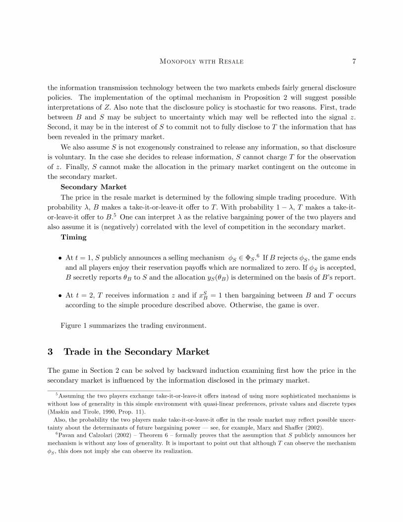
• At t = 1, S publicly announces a selling mechanism φS ∈ ΦS.6 If B rejects φS , the game endsand all players enjoy their reservation payoffs which are normalized to zero. If φS is accepted,B secretly reports θB to S and the allocation yS(θB) is determined on the basis of B’s report.

• At t = 2, T receives information z and if xSB = 1 then bargaining between B and T occursaccording to the simple procedure described above. Otherwise, the game is over.

Figure 1 summarizes the trading environment.

3 Trade in the Secondary Market

The game in Section 2 can be solved by backward induction examining first how the price in thesecondary market is influenced by the information disclosed in the primary market.

5Assuming the two players exchange take-it-or-leave-it offers instead of using more sophisticated mechanisms iswithout loss of generality in this simple environment with quasi-linear preferences, private values and discrete types(Maskin and Tirole, 1990, Prop. 11).Also, the probability the two players make take-it-or-leave-it offer in the resale market may reflect possible uncer-

tainty about the determinants of future bargaining power – see, for example, Marx and Shaffer (2002).6Pavan and Calzolari (2002) — Theorem 6 — formally proves that the assumption that S publicly announces her

mechanism is without any loss of generality. It is important to point out that although T can observe the mechanismφS , this does not imply she can observe its realization.


Reject

S offers B a mechanism

Sφ B

All players enjoy their reservation utilities

Accept

T makes a take-it-or-leave-it offer to B

B makes a take-it-or-leave-it offer to T

t=1 t=2 PRIMARY MARKET SECONDARY MARKET

T receives information z

Probability λ−1

Probability λ

Sφ is executed

0=SBx

1=SBx

Game over

Figure 1: The trading game

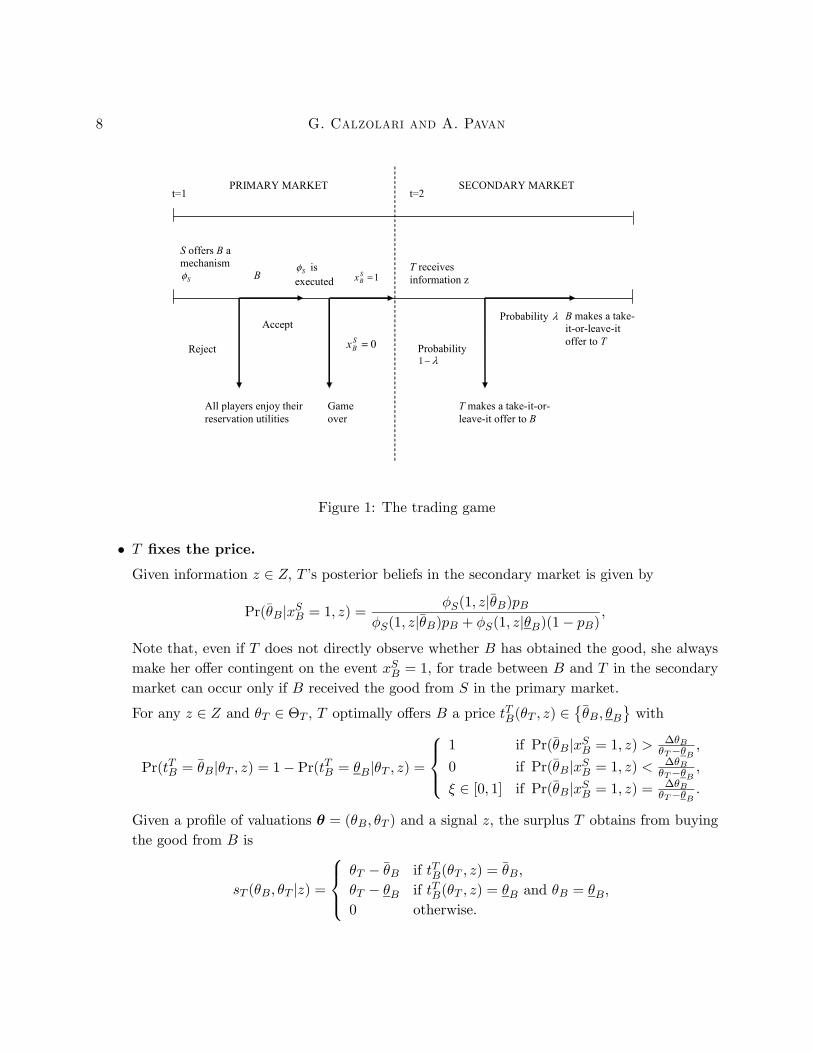
• T fixes the price.

Given information z ∈ Z, T ’s posterior beliefs in the secondary market is given by

Pr(θB|xSB = 1, z) =φS(1, z|θB)pB

φS(1, z|θB)pB + φS(1, z|θB)(1− pB),

Note that, even if T does not directly observe whether B has obtained the good, she alwaysmake her offer contingent on the event xSB = 1, for trade between B and T in the secondarymarket can occur only if B received the good from S in the primary market.

For any z ∈ Z and θT ∈ ΘT , T optimally offers B a price tTB(θT , z) ∈©θB, θB

ªwith

Pr(tTB = θB|θT , z) = 1− Pr(tTB = θB|θT , z) =

1 if Pr(θB|xSB = 1, z) > ∆θB

θT−θB ,0 if Pr(θB|xSB = 1, z) < ∆θB

θT−θB ,ξ ∈ [0, 1] if Pr(θB|xSB = 1, z) = ∆θB

θT−θB .

Given a profile of valuations θ = (θB, θT ) and a signal z, the surplus T obtains from buyingthe good from B is

sT (θB, θT |z) =

θT − θB if tTB(θT , z) = θB,

θT − θB if tTB(θT , z) = θB and θB = θB,

0 otherwise.


The surplus B obtains from selling to T is

rB(θB, θT |z) = 0 for any θT ∈ ΘT and z ∈ Z.

rB(θB, θT |z) =(∆θB if tTB(θT , z) = θB,

0 otherwise.

Note that B obtains extra-surplus from resale only if he has a low valuation and T offershim a high price. The probability of this event depends on the information T receives fromthe primary market. Indeed, if T offers B a price tTB(θT , z) = θB, she receives the good withcertainty with a surplus equal to θT − θB. On the other hand, when T offers θB, she saveson the price, but trade occurs only if θB = θB. Hence, a high price is preferable for T if andonly if Pr(θB|xSB = 1, z)(θT − θB) ≤ θT − θB, or equivalently Pr(θB|xSB = 1, z) > ∆θB

θT−θB . Theprice T offers B is thus increasing in θT and in Pr(θB|xSB = 1, z).

• B fixes the price.

Let tTB(θB) ∈©θT , θT

ªbe the price B asks T when he has value θB for the good he purchased

in the primary market. We have

Pr(tTB = θT |θB) = 1− Pr(tTB = θT |θB) =

1 if pT >

θT−θBθT−θB ,

0 if pT <θT−θBθT−θB ,

η ∈ [0, 1] if pT =θT−θBθT−θB .

Given a profile of valuations θ = (θB, θT ), the additional surplus B obtains from selling thegood to T at a price tTB(θB) is

sB(θB, θT ) =

θT − θB if tTB(θB) = θT , and θT = θT ,

θT − θB if tTB(θB) = θT ,

0 otherwise.

The surplus T obtains from purchasing the good from B is

rT (θB, θT ) =

(∆θT if tTB(θB) = θT ,

0 otherwise.

rT (θB, θT ) = 0 for any θB ∈ ΘB.

Since T does not participate to the primary market, there is no information S can disclose toB about T ’s value for the good. When B fixes the price in the resale market, he never asksless than θT . At that price B obtains θT − θB with certainty. On the contrary, by asking aprice θT , trade occurs only if T has a high valuation. Asking a high price is then optimal ifand only if pT (θT − θB) ≥ θT − θB; the price tTB(θB) is thus increasing in θB and in pT .


4 The Optimal Mechanism in the Primary Market

In this section we show how the revenue-maximizing mechanism can be obtained by optimallycontrolling for the informational linkage between primary and secondary markets. We assume Scan fully commit to the disclosure policy associated with φS . This assumption will be relaxed inSection 6 where we derive the optimal collusion-proof contract for the case where S can colludewith B to the expenses of T.

Let XSB(θB) :=

Pz∈Z

φS(1, z|θB) be the probability B receives the good in the primary market

when he reports θB. Furthermore, let r(θB) and s(θB) be the buyer’s expected surplus from resalewhen he receives the good in the primary market by truthfully reporting his type, respectively inthe case T and B fix the price in the secondary market. Formally,

sB(θB) :=XθT

Pr(θT )sB(θB, θT ) and rB(θB) :=XθT

Xz

Pr(θT ) Pr(z|xSB = 1, θB)rB(θB, θT |z),

where Pr(z|xSB = 1, θB) =φS(1,z|θB)XSB(θB)

. To simplify notation, let X := XSB(θB), X := XS

B(θB) and

∆X := X −X. The same notation applies to the other variables that refer to the two types forplayer B.

At t = 1, S anticipates the price formation process in the secondary market and designs amechanism φS ∈ ΦS which solves the following program.

PS :

maxφS∈ΦS

pBt+ (1− pB)t

subject toX£θB + λsB + (1− λ)rB

¤− t ≥ 0, (IR)

X [θB + λsB + (1− λ) rB]− t ≥ 0, (IR)

X£θB + λsB + (1− λ)rB

¤− t ≥ X£θB + λsB(θB, θB) + (1− λ)rB(θB, θB)

¤− t, (IC)

X [θB + λsB + (1− λ) rB]− t ≥ X£θB + λsB(θB, θB) + (1− λ) rB(θB, θB)

¤− t, (IC)

λsB(θB,bθB)+(1−λ)rB(θB,bθB) represents the surplus B expects from the secondary market whenhe misreports his type in the primary market. In the case it is B who fixes the price in the resalegame, tTB(θB) does not depend on the behavior B follows in the primary market and thereforesB(θB,bθB) = sB(θB) for any θB and bθB, with

∆sB =

−pT∆θB if pT ≥ θT−θB

θT−θB ,

−∆θB if pT <θT−θBθT−θB ,

pT θT − θT + (1− pT )θB − pT∆θB if θT−θBθT−θB ≤ pT <

θT−θBθT−θB .

Conditional on having the possibility to fix the price, the low type always expects a higher surplusfrom resale than a high type, with ∆sB ∈ [−∆θB, 0].


On the contrary, the price T offers B in the secondary market depends on the information shereceives from the primary market. As a consequence, when B misreports his type in the primarymarket not only does he affect the probability to receive the good and the price he pays to S, butalso the surplus from trading with T in the secondary market. Given the price formation processexamined in Section 3, one can partition Z into three sets, Z1, Z2 and Z3 such that

Z1 :=©z : tTB(θT , z) = θB for any θT

ª,

Z2 :=©z : tTB(θT , z) = θB for any θT

ª,

Z3 :=©z : tTB(θT , z) = θB if and only if θT = θT

ª.

The probability measure of these three sets, conditional on B receiving the good in the primarymarket by reporting θB is

α1(θB) :=P

z∈Z Pr(z|xSB = 1, θB)IhPr(θB|xSB = 1, z) ≥ ∆θB

θT−θB

i,

α2(θB) :=P

z∈Z Pr(z|xSB = 1, θB)IhPr(θB|xSB = 1, z) ≤ ∆θB

θT−θB

i,

α3(θB) :=P

z∈Z Pr(z|xSB = 1, θB)IhPr(θB|xSB = 1, z) ∈

h∆θB

θT−θB ,∆θB

θT−θB

ii,

where I(a ≥ b) is the indicator function which takes value 1 if a ≥ b and 0 otherwise.7 It followsthat the probability B receives an offer from T at a high price, conditional on B obtaining the goodin the primary market by announcing θB is simply α(θB) = α1(θB)+ pTα3(θB). Hence, in the caseit is T who fixes the price in the secondary market, the expected resale surplus for θB conditionalon receiving the good in the primary market by truthfully announcing his type is rB = α∆θB. Onthe contrary, by pretending he has a high valuation, θB obtains rB(θB, θB) = α∆θB. Clearly, forthe high type, rB(θB, θB) = rB = 0, as B never expects to receive any offer from T at a pricehigher than θB. We then have that

∆rB = −α∆θB = −(α1 + pTα3)∆θB

From the analysis above it should also be clear that there is no loss of generality in assuming S

discloses only three signals, say z1, z2 and z3, with Pr(zj |1, θB) = αj(θB) for j = 1, ..., 3. Indeed,take any two signals that induce T to make the same offer in the resale market. It is always possibleto replace them with a single signal that has probability equal to the sum of the probabilities ofthe two signals and which induces the same price in the secondary market. The formal argumentis in Lemma 1. Let #φSZ be the cardinality of the subset of Z which is in the support of the rangeof φS ,

#φSZ := # {z ∈ Z : φS(1, z|θB) > 0 for some θB ∈ ΘB} .7We are deliberately ignoring the possibility T randomizes over tTB in the case she is just indifferent between

offering a high or a low price (this happens when Pr(θB|1, z) = ∆θBθT−θB ). In fact, S can always induce the most

favorable offer simply breaking the indifference by a cent.


Lemma 1 For any mechanism φS such that #φSZ > 3, there exists another mechanism φ0S suchthat #φ0SZ = 3 which is payoff-equivalent for all players.

Using Lemma 1, one can simplify PS. The reduced program is in Lemma 2. We show that theoptimal mechanism for S can be analyzed in terms of resale-augmented virtual valuations, whichare defined as the sum of the standard virtual valuations, as in Myerson (1981), along with the(endogenous) payoff that each type expects from resale, conditional on the information disclosedin the primary market.

Definition 1 Let V (θB|zj) be the resale-augmented virtual valuation for a buyer with private valueθB, conditional on S disclosing information zj to T in the secondary market. We have

V (θB|zj) := θB + λsB for any j = 1, ..., 3,

V (θB|z1) := θB −pB

1− pB∆θB + λ

·sB −

pB1− pB

∆sB

¸+ (1− λ)

·∆θB +

pB1− pB

∆θB

¸,


1− pB∆θB + λ

·sB −

pB1− pB

∆sB

¸,


1− pB∆θB + λ

·sB −

pB1− pB

∆sB

¸+ (1− λ) pT

·∆θB +

pB1− pB

∆θB

¸.

The high type does not expect any surplus from resale if it is T who makes the offer in thesecondary market. As a consequence, V (θB|zj) does not depend on zj . Furthermore, as we prove inLemma 2, the high type can always guarantee himself at least the same payoff as the low type byannouncing θB. Hence, θB must be given a price discount (informational rent) to truthfully reporthis type in the primary market. This discount depends on the probability of receiving the good byannouncing θB, as well as on the payoff differential between the high and the low types, which is afunction of the information disclosed to T in the secondary market. Formally, the rent for the hightype is

UB = X£θB + λsB

¤− t = X [∆θB + λ∆sB + (1− λ)∆rB]

=3X

j=1

φS (1, zj |θB) [∆θB + λ∆sB]− (1− λ) [φS (1, z1|θB) + pTφS (1, z3|θB)]∆θB.

For each signal zj , the resale-augmented virtual valuation of type θB is then simply the differencebetween the (endogenous) surplus θB expects from reselling to T in the secondary market, and thediscount S must offer the high type to induce him to reveal his type in the primary market; that is

V (θB|zj) : = θB + λsB + (1− λ)XθT

[rB(θB, θT |zj)] Pr(θT ) +

− pB1− pB

∆θB + λ∆sB − (1− λ)XθT

[rB(θB, θT |zj)] Pr(θT ) .


As XθT

[rB(θB, θT |z1)] Pr(θT ) >XθT

[rB(θB, θT |z3)] Pr(θT ) >XθT

[rB(θB, θT |z2)] Pr(θT ),

we have that V (θB|z1) > V (θB|z3) > V (θB|z2).Also note that the resale-augmented virtual valuations are higher than the standard virtual

surpluses absent the possibility to resell in a secondary market. This confirms the intuition thatwhenever a monopolist cannot contract with a potential buyer, she may gain from favoring resale:by using B as a middleman in the secondary market, S can indirectly extract surplus also fromT. As we will see in Section 8, this is not necessarily true when resale takes place among the verysame bidders who compete in the primary market.

The optimal selling mechanism for S is obtained by choosing a disclosure policy that maximizesthe probability of those signals associated with the highest resale-augmented virtual valuations,taking into account the effect of disclosure on prices in the secondary market.

Lemma 2 The optimal selling mechanism in the primary market φ∗S maximizesPθB∈ΘB

nP3j=1 φS (1, zj |θB)V (θB|zj)

oPr(θB)

subject to

[∆θB + λ∆sB]£X −X

¤ ≥ (1− λ)∆θB£φS¡1, z1|θB

¢− φS (1, z1|θB)¤+

+(1− λ)∆θBpT£φS¡1, z3|θB

¢− φS (1, z3|θB)¤ (IC)

andPr(θB|xSB = 1, z1) ≥ ∆θB

θT−θB , (1)

Pr(θB|xSB = 1, z2) ≤ ∆θBθT−θB

, (2)

Pr(θB|xSB = 1, z3) ∈h

∆θBθT−θB

, ∆θBθT−θB

i. (3)

Constraints (1)− (3) guarantee that, given the mechanism φ∗S and information z, it is sequen-tially optimal for T to follow the equilibrium strategy in the secondary market.

Constraint (IC) guarantees that the low type does not gain from mimicking the high type.Note that, contrary to standard monopolistic screening mechanisms, (IC) is equivalent to themonotonicity condition X ≤ X only when λ = 1, in which case the outcome in the primary markethas no effect on the resale price. The remaining constraints, (IC), (IR) and (IR) are embeddedinto the reduced program via the resale-augmented virtual valuations.

In the following Proposition, we use Lemma 2 to characterize the optimal mechanism for thecase of overlapping supports. Similar results can be derived under A4.2.

Proposition 1 Let J(θT ) :=pB(θT−θB)(1−pB)∆θB

and K := [∆θB+λ∆sB ]J(θT )

[∆θB+λ∆sB ]J(θT )+[1−J(θT )](1−λ)pT∆θB. Under as-

sumptions A1-A4.1, the revenue-maximizing mechanism in the primary market φ∗S is the following.


• If J(θT ) ≥ 1, φ∗S¡1, z3|θB

¢= 1, φ∗S (1, z2|θB) = 0 and

φ∗S (1, z3|θB) =(1 if V (θB|z3) ≥ 0,0 otherwise.

• If J(θT ) < 1,

φ∗S¡1, z3|θB

¢= 1− φ∗S

¡1, z2|θB

¢=

(1 if V (θB|z2) ≤ K V (θB|z3),0 otherwise,

φ∗S (1, z2|θB) =

0 if V (θB|z2) < 0,[∆θB+λ∆sB−(1−λ)pT∆θB ][1−J(θT )]

∆θB+λ∆sBif V (θB|z2) ∈ (0,K V (θB|z3)],

1 if V (θB|z2) > K V (θB|z3),φ∗S (1, z3|θB) =

(J(θT ) if V (θB|z3) > 0 and V (θB|z2) ≤ K V (θB|z3),0 otherwise.

The optimal mechanism is such that S sells with certainty to B when the latter has a highvaluation (X = 1). As far as the low type is concerned, the probability to trade depends on theasymmetry of information in the primary market, as well as the expected resale surplus in thesecondary market. This, in turn, depends on the price T is ready to offer and hence reflects theinformation disclosed in the primary market. Note that, under assumption A4.1, there are nosignals that can induce T to offer B a high price when she has a low valuation. It follows thatφS (1, z1|θB) = 0 for any θB ∈ ΘB. When J(θT ) ≥ 1, θT offers B a high price in the case she learnsnothing from the primary market. This is clearly the most favorable case for S who then sells toeither type provided that V (θB|z3) ≥ 0.

Things are more difficult for the monopolist when J(θT ) < 1. In this case, T offers B a lowprice when the information she receives from the primary market does not result in a significantchange of her prior beliefs. S can then try to sustain a higher expected resale price by disclosingsome information to T . However, this comes at a cost. Because of incentives reasons, when S

discloses information, she has to sacrifice the possibility to trade with the low type with certainty.To see this, suppose trade occurs with probability one with either type. In this case, the pricediscount for the high valuation buyer would be UB = ∆θB + λ∆sB − pTφ

∗S (1, z3|θB) (1− λ)∆θB.

But then if the low type pretends he has a high valuation, he gets

UB −£∆θB + λ∆sB − (1− λ)φ∗S

¡1, z3|θB

¢pT∆θB

¤=

= (1− λ) pT£φ∗S¡1, z3|θB

¢− φ∗S (1, z3|θB)¤∆θB > 0

as information z3 leads to a high price in the secondary market if and only if φ∗S (1, z3|θB) ≤φ∗S (1, z3|θB) . Faced with the trade-off between selling with higher probability or sustaining higher


resale prices, S finds it optimal to favor the probability to trade when V (θB|z2) > K V (θB|z3),that is when the low type has a high virtual valuation even when T offers him a low price. Onthe contrary, when V (θB|z2) is positive but less than K V (θB|z3), the optimal mechanism consistsin selling with probability X = φ∗S (1, z2|θB) + φ∗S (1, z3|θB) < 1 to the low type and disclosinginformation z3 with probability φ∗S (1, z3|θB) = J(θT )φ

∗S

¡1, z3|θB

¢. Since the right hand side is

increasing in φ∗S¡1, z3|θB

¢, S sends information z3 with certainty when B has a high valuation.

Furthermore, as φ∗S (1, z3|θB) is bounded above by J(θT ) < 1, it is optimal for S to trade withB also with the other (less favorable) signal z2: that is, φ∗S (1, z2|θB) > 0. However, as indicatedabove, to sort the two types in the primary market, φ∗S (1, z2|θB)+φ∗S

¡1, z3|θB

¢< 1, and the upper

bound on φ∗S (1, z2|θB) is determined by (IC).Finally, when V (θB|z2) < 0, but V (θB|z3) > 0, S finds it optimal to trade with θB only when

the expected resale surplus is high, which occurs if and only if information z3 is disclosed to T . Inthis case, φ∗S (1, z3|θB) = J(θT ), and φ∗S (1, z2|θB) = 0.

The next proposition suggests a possible implementation for the optimal mechanism.

Proposition 2 The optimal mechanism of Proposition 1 has the following implementation.

1. If J(θT ) ≥ 1, S makes a take-it-or-leave-it offer to B at a price

t =

(θB + λsB if V (θB|z3) < 0,θB + λsB + pT (1− λ)∆θB, otherwise.

2. If J(θT ) < 1 and V (θB|z2) < 0, S offers B two prices,

t =

(θB + λsB if V (θB|z3) < 0,θB + λsB − J(θT ) (∆θB + λ∆sB) + J(θT )pT (1− λ)∆θB, otherwise.

t =

(0 if V (θB|z3) < 0,J(θT ) [θB + λsB + pT (1− λ)∆θB] , otherwise.

B receives the good with certainty if he pays t, and with probability J(θT )I[V (θB|z3) ≥ 0] ifhe pays t.

3. If J(θT ) < 1, and V (θB|z2) ∈ [0,K V (θB|z3)], B receives the good with certainty if he pays

τH = θB + λsB − [φ∗S (1, z3|θB) + φ∗S (1, z2|θB)] (∆θB + λ∆sB)+

+ φ∗S (1, z3|θB) pT (1− λ)∆θB.

and with probability δ =φ∗S(1,z2|θB)1−φ∗S(1,z3|θB) if he pays τL = δ [θB +∆θB + λsB] . The high type

always pays τH . The low type pays τH with probability φ∗S (1, z3|θB) and τL with probability1− φ∗S (1, z3|θB) .


4. If J(θT ) < 1, and V (θB|z2) > K V (θB|z3), S makes a take-it-or-leave-it offer to B at a pricet = θB + λsB

In all cases but 2), without loss of optimality, S discloses the price B pays in the primarymarket.

To create the optimal informational linkage with the secondary market, the monopolist hastwo natural instruments: First, she can sell to the two types with different probabilities so that thedecision to trade becomes itself a signal of the buyer’s valuation. Second, she can disclose the priceB pays in the primary market.

When J(θT ) ≥ 1, S sells to either type at a price t = θB+λsB+pT (1− λ)∆θB if V (θB|z3) ≥ 0,and only to the high type at a price t = θB +λsB otherwise. In either case, disclosing the price hasno effect on the seller’s expected revenue.

Suppose now J(θT ) < 1. When V (θB|z3) < 0, S sells only to the high type at a price t =θB + λsB and hence disclosing the price is again revenue-neutral. When instead V (θB|z3) ≥0, the optimal disclosure policy depends on the sign of V (θB|z2). If V (θB|z2) < 0, the optimalinformational linkage is obtained by giving B the possibility to pay a high price t and receive thegood with certainty, or a low price t and receive the good with probability J(θT ) < 1. In thecontinuation game, the high type is indifferent and in equilibrium pays t, whereas the low typestrictly prefers t. In this case, the price B pays conveys too much information about B’s type andhence must be kept secret.

When V (θB|z2) ≥ 0, but V (θB|z2) < K V (θB|z3), S offers B two prices, τH and τL. If B paysτH , he receives the good with certainty, whereas if he pays τL with probability δ. Contrary to theprevious case, since in equilibrium θB receives the good with probability J(θT ) + [1 − J(θT )]δ >

J(θT ), the decision to trade is no longer sufficient to induce θT to offer θB in the resale game.In this case, it becomes necessary for S to disclose also the price and use it as a signal of B’svaluation. In the continuation game, θB pays τH whereas θB randomizes paying τH with probabilityφ∗S (1, z3|θB) = J(θT ). Given B’s strategy, it is sequentially optimal for θT to offer a high price whenshe observes τH and a low price otherwise, making θB just indifferent between the two prices.

Finally, in case 4) S offers B a single price that either type accepts to pay and which, withoutany effect on the revenue, is made public.

Note that to create the optimal informational linkage S may need to combine lotteries withmixed strategies. This happens precisely in case 3). Suppose, for example, that S tries to makeB randomize over two prices τL and τH with τL < τH without using lotteries, i.e. by selling withcertainty with either price. In this case, the high type, who does not care about the informationdisclosed to T, will always pay the low price τL. But then, anticipating that T will never offer a highprice if she observes τH , the low type will also pay τL. To avoid this outcome, S must associate τLwith a lottery. Similarly, suppose S tries to implement the optimal informational linkage without


making B play a mixed strategy. If S separates the two types and discloses the prices, she perfectlyinforms T about B’s valuation, which is clearly not optimal. If, on the other hand, she keeps theprice secret, then the only thing S can do to sustain a high resale price is to use the decision totrade as a signal of B’s valuation selling to the low type with probability at most equal toJ(θT ).On the contrary, by disclosing the price and making B randomize over τH and τL, S can inducea high resale price with the same probability and at the same time sell to θB with probabilityJ(θT ) + [1− J(θT )]δ, which in case 3) leads to a higher expected revenue.

5 Efficiency

Trade in either market may result in inefficient allocations which are due to asymmetric information.The inefficiency in the primary market comes from the fact that S may find it optimal to retainthe good with positive probability. The inefficiency in the secondary market arises when T offerstoo little, and/or B asks too high a price. Whereas this latter possibility is not influenced by theoutcome in the primary market, the price T offers depends on the disclosure policy selected by themonopolist.

In this section, we investigate how ex ante efficiency is influenced by λ, i.e. by the probabilitythe resale price is fixed by B. Although in this stylized model λ is exogenous, we assume it reflectsthe distribution of bargaining power between B and T and is negatively correlated with the levelof competition in the secondary market.

Let π(θ) be the probability the good is allocated to the player who values it the most whenthe state is θ. If θ = (θB,θT ), we have that

π(θ) = λ3X

j=1

φ∗S¡1, zj |θB

¢+ (1− λ)

£φ∗S¡1, z1|θB

¢+ φ∗S

¡1, z3|θB

¢¤.

In the secondary market B never asks more than θT and hence efficient trade always occurs if it isB who fixes the price. On the contrary, if it is T who makes the offer, trade occurs if and only ifT receives information that induces her to offer a high price, i.e. signals z1 and z3.

When θ = (θB,θT ), the secondary market may be inefficient when either player makes theprice: B may ask too much, whereas T may offer too little to induce B to sell. Inefficiency neveroccurs under A4.1, but it may occur under A4.2. Hence, if A4.1 holds π(θ) =

P3j=1 φ

∗S

¡1, zj |θB

¢,

whereas if A4.2 holds

π(θ) = λ3X

j=1

φ∗S¡1, zj |θB

¢ ·I µpT ≤ θT − θB

θT − θB

¶¸+ (1− λ)φ∗S

¡1, z1|θB

¢.

When θ = (θB,θT ), the secondary market is always efficient. In this case, π(θ) =P3

j=1 φ∗S (1, zj |θB) .

On the contrary, when B and T have low valuations, the secondary market may be inefficient only


when it is B who makes the price (inefficiency occurs if and only if pT >θT−θBθT−θB ). It follows that

for θ = (θB,θT ),

π(θ) = λ3X

j=1

φ∗S (1, zj |θB)·IµpT ≤ θT − θB

θT − θB

¶¸+ (1− λ)

3Xj=1

φ∗S (1, zj |θB) .

Assume now A4.1 holds. From Proposition 1, trade in the primary market always occurs if Bhas a high type (X

∗= 1). On the contrary, X∗ depends on the value of the resale-augmented

virtual valuations, V (θB|z2) and V (θB|z3), which can be either increasing, or decreasing in λ. Itfollows that efficiency in the primary market may either increase or decrease with λ. As indicatedabove, inefficiency in the secondary market may occur when φ∗S

¡1, z3|θB

¢< 1 (i.e. when J(θT ) < 1

and V (θB|z2) > K V (θB|z3)), and/or pT >θT−θBθT−θB ; furthermore, when it occurs, it may either

increase or decrease with λ. We can conclude that ex-ante efficiency, Eθπ(θ) =P

θ∈Θ π(θ) Pr(θ),is typically non monotone in the distribution of bargaining power, and/or the level of competitionin the secondary market. The same non-monotonicity results hold true under assumption A4.2.We summarize the above considerations in the following.

Proposition 3 Misallocations in either the primary or the secondary market may increase ordecrease with λ. As a consequence, ex-ante efficiency of the two markets Eθπ(θ) is typically nonmonotone in λ.

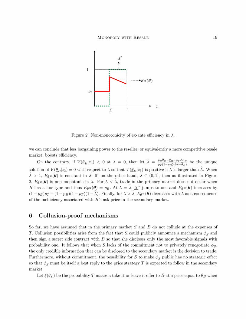
To illustrate the non-monotonicity of Eθπ(θ) with respect to λ, suppose A4.1 holds so thatthe optimal mechanism in the primary market is as in Proposition 1 (with implementation asin Proposition 2). If J(θT ) ≥ 1, S makes a take-it-or-leave-it offer to B at a price θB + λsB ifV (θB|1, z3) < 0, and at a price θB + λsB + pT (1− λ)∆θB, otherwise. In the first case, X

∗= 1

and X∗ = 0. In the second, X∗= 1 and X∗ = 1. In either case, S discloses the price B pays in the

primary market. In the resale game, T offers a high price if and only if she has a high valuation,whereas B asks a high price if he has a high valuation, or if he has a low valuation and pT >

θT−θBθT−θB .

Assume this inequality holds. In this case, sB = pT (θT − θB), ∆sB = −pT∆θB and hence


1− pB∆θB + λ

·sB −

pB1− pB

∆sB

¸+ (1− λ) pT

·∆θB +

pB1− pB

∆θB

¸.

is increasing in λ. If V (θB|z3) ≥ 0 at λ = 0, then ex-ante efficiency

Eθπ(θ) = pBpT + pB(1− pT ) + (1− pB)pT + (1− pB)(1− pT )(1− λ)

is decreasing in λ: in this case, the primary market is always efficient, whereas the inefficiency in thesecondary market occurs only when it is B who fixes the price. If λ is positively correlated with B’sbargaining power and negatively correlated with the level of competition in the secondary market,


1 λ

λ

X*

( )Eπ θ

1

pB

Figure 2: Non-monotonicity of ex-ante efficiency in λ.

we can conclude that less bargaining power to the reseller, or equivalently a more competitive resalemarket, boosts efficiency.

On the contrary, if V (θB|z3) < 0 at λ = 0, then let bλ =pBθB−θB−pT∆θBpT (1−pB)(θT−θB) be the unique

solution of V (θB|z3) = 0 with respect to λ so that V (θB|z3) is positive if λ is larger than bλ. Whenbλ > 1, Eθπ(θ) is constant in λ. If, on the other hand, bλ ∈ (0, 1], then as illustrated in Figure2, Eθπ(θ) is non monotonic in λ. For λ < bλ, trade in the primary market does not occur whenB has a low type and thus Eθπ(θ) = pB. At λ = bλ, X∗ jumps to one and Eθπ(θ) increases by(1− pB)pT +(1− pB)(1− pT )(1− bλ). Finally, for λ > bλ, Eθπ(θ) decreases with λ as a consequenceof the inefficiency associated with B’s ask price in the secondary market.

6 Collusion-proof mechanisms

So far, we have assumed that in the primary market S and B do not collude at the expenses ofT. Collusion possibilities arise from the fact that S could publicly announce a mechanism φS andthen sign a secret side contract with B so that she discloses only the most favorable signals withprobability one. It follows that when S lacks of the commitment not to privately renegotiate φS,the only credible information that can be disclosed to the secondary market is the decision to trade.Furthermore, without commitment, the possibility for S to make φS public has no strategic effectso that φS must be itself a best reply to the price strategy T is expected to follow in the secondarymarket.

Let ξ(θT ) be the probability T makes a take-it-or-leave-it offer to B at a price equal to θB when


she has a valuation θT . To compact notation, let ξ = ξ(θT ), ξ = ξ(θT ), and ξ = pT ξ + (1 − pT )ξ.

Without commitment, no signals are disclosed to T and the (collusion proof) resale-augmentedvirtual valuations reduce to

V (θB) := θB + λsB,

V (θB|ξ) := θB −pB

1− pB∆θB + λ

·sB −

pB1− pB

∆sB

¸+ (1− λ) ξ

·∆θB +

pB1− pB

∆θB

¸.

Contrary to the commitment case, the standard monotonicity condition (X ≥ X) is sufficientto guarantee that also (IC) is satisfied. Hence, with standard substitutions, the seller’s optimal(collusion-proof) mechanism simply maximizes US = pBXV (θB) + (1 − pB)XV (θB|ξ) under themonotonicity condition X ≥ X. The equilibrium of the game without commitment (X∗,X∗, ξ∗, ξ∗)is summarized in the following proposition. For simplicity, we report only the results for the caseA4.1. Assumption A4.2 induces a similar characterization and it is omitted for brevity.

Proposition 4 Under assumptions A1-A4.1, the optimal collusion-proof mechanism in the pri-mary market is such that B always receives the good if he has a high valuation, i.e. X∗ = 1. As faras X∗ is concerned, the following cases are possible.

• For J(θT ) ≥ 1, X∗ = 1 if V (θB|ξ = pT ) ≥ 0 and X∗ = 0 otherwise.

• For J(θT ) < 1, X∗ = 1 if V (θB|ξ = 0) ≥ 0, X∗ = 0 if V (θB|ξ = pT ) ≤ 0, and X∗ = J(θT ) ifV (θB|ξ = 0) < 0 and V (θB|ξ = pT ) > 0.

As in the case with full commitment, the optimal mechanism in the primary market can bedesigned by looking at the value of the resale-augmented virtual valuations, which is increasing inξ, i.e. in the probability T offers a high price in the secondary market. Under assumption A4.1,T always offers a low price when she has a low valuation (ξ∗ = 0). It follows that ξ ∈ [0, pT ]. IfV (θB|ξ = pT ) < 0, it is optimal for S to exclude the low type from trade even if θT is expected tooffer a high price. If, on the other hand, V (θB|ξ = pT ) ≥ 0, the optimal mechanism in the primarymarket depends on the initial prior of player T. When θT offers a high price even if she learnsnothing from the allocation of the good in the primary market (this occurs when J(θT ) ≥ 1), thenS sells to either type with probability one. On the contrary, if θT offers a low price if she learnsnothing, then S has to trade-off the possibility to induce a high resale price with the possibilityto sell the good with certainty in the primary market. If V (θB|ξ = 0) ≥ 0, the trade-off is alwayssolved in favor of efficiency. If, on the other hand, V (θB|ξ = pT ) < 0, then S is better off by sellingonly to the high type, i.e. X∗ = 0. Finally, in the intermediate case where V (θB|ξ = 0) < 0,

but V (θB|ξ = pT ) > 0, the equilibrium is in mixed strategy with θT offering a high price withprobability ξ∗ ∈ (0, 1) and S selling to θB with probability J(θT ).


Note that even when S cannot commit to a credible disclosure policy, the endogenous informa-tional linkage between the two markets does not vanish. Indeed, the decision to trade in the primarymarket represents valuable information for T and is reflected in the equilibrium resale price.

Although the comparison between commitment versus no commitment is, in general, am-biguous, it turns out that the inability for S to commit not to renegotiate with B may actu-ally favor efficiency in the primary market. As indicated in Proposition 1, when J(θT ) < 1 andV (θB|1, z2) ∈ [0,K V (θB|1, z3)], the low type does not receive the good with certainty, i.e. X∗ < 1.On the contrary, from Proposition 4, when V (θB|ξ = 0) = V (θB|1, z2) ≥ 0, the good is alwaysallocated efficiently in the primary market.

A final remark concerns the implementation of the optimal collusion-proof mechanism. In allcases, S simply fixes a single price which, without loss of optimality, she also makes public. In themixed strategy equilibrium, this price is τ = θB +λs+ ξ∗ (1− λ)∆θB. Anticipating T will proposea high price with probability ξ∗, B purchases with probability one if he has a high type and withprobability X∗ = J(θT ), otherwise.

7 Multiple Bidders in the Primary Market

In this section we show how the analysis for the single buyer case can be extended to primarymarkets where the monopolist designs an auction to sell toN bidders. Without any loss of generalitylet N = 2 and denote the two bidders by Bi, with i = 1, 2. At the end of the auction, the winnermay keep the good for himself or resell it to T in the secondary market, in which case the resalegame is exactly as in Section 2 with λi denoting the relative bargaining power of Bi with respectto T. Note that in this section resale does not take place among the bidders who participate in theprimary market, but between the winner and a representative third party in the secondary market.This may correspond, for example, to an environment where S can prevent inter-bidders resale,but is not able to contract with all potential buyers at the time she needs to sell. The analysis ofoptimal auctions with inter-bidders resale is postponed to the next section.

An allocation in the primary market is now defined by yS := (xS , tS), where

xS := (xS1 , x

S2 ) ∈ XS :=

n(xS1 , x

S2 ) ∈ {0, 1}2 such that xS1 + xS2 ≤ 1

odenotes the allocation of the good, and tS = (tS1 , t

S2 ) ∈ R2 the expected transfers from B1 and B2

to S.Assumptions A1 and A2 are replaced byA1’: For i ∈ {1, 2} , Θi =

©θi, θi

ªwith ∆θi := θi − θi ≥ 0, Pr(θi) = pi = 1−Pr(θi). For i = T,

ΘT =©θT , θT

ªwith ∆θT := θT − θT ≥ 0, and Pr(θT ) = pT = 1− Pr(θT ).

A2’: (independent private values) For any θ : = (θ1, θ2, θT ) ∈ Θ := Θ1 × Θ2 × ΘT , Pr(θ) =

Pr(θ1) · Pr(θ2) · Pr(θT ).


A selling mechanism for S is represented by an auction with an endogenous disclosure policy.Formally,

φS : ΘB → ∆(XS × Z)×R2.When the two bidders announce valuations θB := (θ1, θ2) ∈ ΘB := Θ1 × Θ2, with probabilityφS(xS , z|θB) the allocation is xS ∈ XS and information z ∈ Z is transmitted to T . As in Section4, we assume S can fully commit to φS . Let Xi(θB) :=

Pz∈Z

φS(xi = 1, z|θB) be the probability Bi

wins the auction when the two bidders announce θB = (θ1, θ2). Similarly,

Xi(θi) := p3−iXi(θi, θ3−i) + (1− p3−i)Xi(θi, θ3−i),

andtSi (θi) := p3−itSi (θi, θ3−i) + (1− p3−i) tSi (θi, θ3−i).

denote, respectively, the probability to win and the expected payment to S when Bi announces θi.To compact notation let Xi = Xi(θi), Xi = Xi(θi) and similarly for all other variables that refer tothe two types of Bi. From Lemma 1, we know that S does not need to use more than three signals.Using the same notation as in Section 4, let z1 be a signal such that tTi (θT , z1) = θi for any θT ,

where tTi is the price T offers Bi when she has valuation θT and receives information z. Similarly,z2 is a signal such that tTi (θT , z2) = θi for any θT , and z3 a signal for which tTi (θT , z

i3) = θi if and

only if θT = θT .

Proposition 5 Let N = 2. The optimal auction in the primary market maximizes the sum of thetwo bidders’ resale-augmented virtual valuations, taking into account the effect of disclosure on theprice formation process in the secondary market. Formally, φ∗S solves

MaxφS∈ΦS

XθB∈ΘB

Pr(θB)

Xi=1,2

3Xj=1

[V (θi|zj)]φS (xi = 1, zj |θB)

subject toPr(θi|xi = 1, z1) ≥ ∆θi

θT−θi , (i.1)

Pr(θi|xi = 1, z2) ≤ ∆θiθT−θi

, (i.2)

Pr(θi|xi = 1, z3) ∈h

∆θiθT−θi

, ∆θiθT−θi

i(i.3)

and Pθ3−i

nP3j=1 [∆θi + λi∆si]φS (xi = 1, zj |(θi, θ3−i))+

− (1− λi) [φS (xi = 1, z1|(θi, θ3−i)) + pTφS (xi = 1, z3|(θi, θ3−i))]∆θi}Pr(θ3−i) ≤Pθ3−i

nP3j=1 [∆θi + λi∆si]φS

¡xi = 1, zj |(θi, θ3−i)

¢+

− (1− λi)£φS¡xi = 1, z1|(θi, θ3−i)

¢+ pTφS

¡xi = 1, z3|(θi, θ3−i)

¢¤∆θi

ªPr(θ3−i).

(ICi)

for i = 1, 2.


The only difference with respect to the single bidder case is that S now compares the twobidders’ resale-augmented virtual valuations for each state θB. However, note that contrary tostandard auction design, in the presence of resale, S does not necessarily assign the good to thebidder with the highest virtual valuation. Indeed, this would be the case if the resale price wereexogenous. When, instead, the price in the secondary market depends on the information disclosedin the primary market, S may find it optimal to assign the good to a bidder with a lower resale-augmented virtual valuation in state θB if this allows to relax constraints (i1)− (i3) and increasethe probability of selling the good to the bidder with the highest virtual valuation in another stateθ0B. Assume, for example, that in state θB = (θ1, θ2), V (θ1|zj) > V (θ2|zl) for any j and l. Ifconstraint (2.1) is binding, assigning the good to B2 in state θB = (θ1, θ2) may be more effectivein relaxing constraint (2.1) than assigning the good to B1. By giving the good to B2 in state θB,S can increase the probability she sells to B2 with signal z1 in state θ0B = (θ1, θ2), which in turnmay result in a higher expected revenue if the probability of state θB is relatively low comparedto that of state θ0B and if V (θ2|z1) is high. We will see in Section 8 that similar incentives formisallocations arise in the case of auctions with inter-bidders resale.

Apart from the inter-bidders comparisons of the resale-augmented virtual valuations, the pro-gram in Proposition 5 is very similar to that for the single bidder case as in Proposition 1. Hence,instead of further characterizing the properties of the optimal auction for this environment, wemove directly to the study of optimal auctions for the case where resale takes place among thebidders who participate in the primary market.

8 Optimal Auctions with Inter-Bidders Resale

In this section we assume S can contract with all buyers, but she cannot prohibit bidders to resell,nor can she make her mechanism contingent on the outcome in the secondary market. As in Section4, assume the two bidders are B and T. Before deriving the optimal selling procedure, we illustratethe effect of resale on two other optimal mechanisms suggested in the literature.

Myerson’s AuctionAssume S designs an optimal auction à la Myerson, i.e. an auction which gives the good to

the bidder with the highest virtual valuation Mi(θi), where Mi(θi) = θi and Mi(θi) = θi − pi∆θi1−pi

with i = B,T.

When MT (θT ) ≥ MB(θB),8 the allocation rule is efficient and consists in selling the goodto T at a price equal to θT . In this case, the impossibility to prevent resale does not have anybite since there are no gains from trade in the secondary market. Suppose on the contrary thatMT (θT ) < MB(θB). If S uses a Myerson’s auction and bidders can resale, then the final allocation inthe secondary market may differ from the one which maximizes the monopolist’s expected revenue.

8This possibility arises only if A4.2 holds.


Assume, for example, thatMT (θT ) ≤MB(θB). Myerson’s auction prescribes that θT should alwayswin and pay θT , whereas θT should never receive the good. As far as B is concerned, θB shouldreceive the good if and only if T has a low valuation. Furthermore, if MB(θB) ≥ 0, then θB shouldalso receive the good if and only if θT = θT . A simple way to implement this allocation rule is tofix two personalized reserve prices respectively equal to θT for T and θB for B and use any auctionformat which assigns the good to the player who submits the highest bid.

When bidders have the possibility to resell, this auction is no longer a truthful mechanism as Tcan simply decide not to buy (equivalently announce any bid below θT ) and purchase in the resalemarket at a price lower than θT . Indeed, the equilibrium in this game is for player B to pay θB andreceive the good with certainty and for T to bid less than θT and lose the auction with probabilityone. In the secondary market, B and T trade according to the game described in Section 2. In thiscase, the revenue in the auction falls from pT θT +(1− pT )θB to θB and thus the possibility for thebidders to resell results in a loss of expected revenue for the initial seller.

Zheng’s AuctionZheng (2002) recently proposed an alternative optimal mechanism which is designed to replicate

Myerson’s expected revenue in an environment where resale cannot be prohibited. We sketch herethe main idea. Assume it is always the winner in the primary market who fixes the price in thesecondary market and letMT (θT ) ≤MB(θB). Zheng’s optimal mechanism prescribes that S shouldsimply sell to B at a price equal to pT θT +(1−pT )θB and use B as a middleman to extract surplusfrom T in the resale market. Since in this case B asks a price θT independently of his valuation(indeed,MT (θT ) ≤MB(θB) implies pT >

θT−θBθT−θB for any θB ∈ ΘB), through resale S can implement

the same final allocation as in Myerson optimal auction where resale is not allowed. Furthermore,since either bidder receives zero surplus when he, or she, has a low valuation, from the RevenueEquivalence Theorem, this mechanism generates the same expected revenue as the static optimalauction without resale.

Although a remarkable result, Zheng’s optimal mechanism crucially relies upon the assumptionthat the winner is always the player who fixes the price in the secondary market (equivalently, whodesigns the resale mechanism). Suppose, on the contrary, that the distribution of the bargainingpower in the resale game is a function of the identity of the two bidders. In this case, it is impossibleto implement an allocation rule that assigns the good to player B with certainty when θ = (θB, θT ).Whenever T has some bargaining power in the secondary market (in our model λ < 1), she willalways offer B at least θB and therefore trade will ultimately transfer the good to T with positiveprobability. In this case, the impossibility to prohibit resale may well result in a loss of expectedrevenue for the initial seller, as we show in this section. Furthermore, the optimal auction in theprimary market may require the use of a stochastic allocation rule and the design of an optimaldisclosure policy to create the desired informational linkage between the primary and the secondarymarket.


8.1 How Resale Prices are Influenced by the Bidding Strategy in the PrimaryMarket

Let zi ∈ Zi be the information disclosed to bidder i = B,T in the primary market. If T winsthe auction, she either keeps the good for herself (this occurs when A4.2 holds or when A4.1 holdsand T has a high valuation), or she makes an offer to B at a price θB (under A4.1, if θT = θT ).Similarly, when T wins the auction, B offers T a price equal to θT if he has a high valuation andA4.1 holds, and equal to zero, otherwise. It follows that the resale price and the surplus in thesecondary market is not influenced by the information disclosed in the auction when T is the winnerin the primary market. Hence, without loss of generality, S does not disclose any signal to eitherbidder when the allocation of the good is xS := (xSB, x

ST ) = (0, 1). In what follows, we assume

xS = (1, 0).9

• Let us consider first the outcome in the secondary market when B makes the price. FollowingSection 2, B asks tTB(θB,bθB,zB) ∈ ©θT , θTª , with

Pr(tTB = θT |θB,bθB, zB) =1 if Pr(θT |xSB = 1, zB,bθB) > θT−θB

θT−θB ,0 if Pr(θT |xSB = 1, zB,bθB) < θT−θB

θT−θB ,η ∈ [0, 1] if Pr(θT |xSB = 1, zB,bθB) = θT−θB

θT−θB .

Note that when θB announces bθB he affects not only the probability to win and the price hepays to S (as in standard auctions), but also the information he receives from the primarymarket. For any θ := (θB, θT ), the surplus B obtains from selling the good to T at a pricetTB(θB,

bθB,zB) issB(θB, θT |bθB,zB) = ( (θT − θB)I(θT = θT ) if tTB(θB,bθB,zB) = θT ,

θT − θB otherwise

and the surplus T obtains from purchasing the good from B is

rT (θB, θT |bθB,zB) =

(∆θT if tTB(θB,bθB,zB) = θT ,

0 otherwise.

rT (θB, θT |bθB,zB) = 0 for any (θB,bθB) ∈ Θ2B and zB ∈ ZB.

Now consider the case where it is T who deviates from the equilibrium bidding strategy in theprimary market. If it is B who makes the price in the resale game, a deviation from T in the

9As in Section 7, the allocation of the good in the primary market is denoted by a vector xS := (xSB , xST ) ∈ XS :=©

(xSB , xST ) ∈ {0, 1}2 such that xSB + xST ≤ 1

ª. To save notation, we will also write xSB = 1 for xS = (1, 0), and x

ST = 1

for xS = (0, 1). Also note that the payoff of bidder i is now Ui = θixSi (1− xTB) + θix

Sj x

TB − tSi + tTB , where x

TB = 1 if

the good changes hands in the secondary market, and xTB = 0 otherwise.


primary market may affect the probabilityB wins the auction and receives information zB, butnot the price B asks contingent on xSB = 1 and z

B. Hence, sB(θB, θT |bθT,zB) = sB(θB, θT |zB),where sB(θB, θT |zB) is the surplus in the case both players follow the equilibrium biddingstrategies in the primary market. Similarly, rT (θB, θT |bθT,zB) = rT (θB, θT |zB).

• Next, consider the case where T makes the price. T offers tTB(θT ,bθT , zT ) ∈ ©θB, θBª , withPr(tTB = θB|θT ,bθT , zT ) =

1 if Pr(θB|xSB = 1, zT ,bθT ) > ∆θB

θT−θB ,0 if Pr(θB|xSB = 1, zT ,bθT ) < ∆θB

θT−θB ,ξ ∈ [0, 1] if Pr(θB|xSB = 1, zT ,bθT ) = ∆θB

θT−θB .

The surplus T obtains from buying the good from B is

sT (θB, θT |bθT , zT ) = ( θT − θB if tTB(θT ,bθT , zT ) = θB,

(θT − θB)I(θB = θB) otherwise.

The surplus B obtains from reselling to T is

rB(θB, θT |bθT , zT ) = 0 for any (θT ,bθT ) ∈ Θ2T and zT ∈ ZT .

rB(θB, θT |bθT , zT ) =(∆θB if tTB(θT ,bθT , zT ) = θB,

0 otherwise.

Note that when it is B who deviates from the equilibrium bidding strategy in the pri-mary market, the surplus for the two bidders in the secondary market in case T makesthe price does not depend on bθB. Hence for any zT , sT (θB, θT |bθB,zT ) = sT (θB, θT |zT ), andrB(θB, θT |bθB,zT ) = rB(θB, θT |zT ).

8.2 Optimal Auction Design

In this section we show how to design a revenue-maximizing auction when the seller cannot preventinter-bidders resale. Formally, an auction is mapping

φS : Θ→ 4(XS × Z)×R2,

where z := (zB, zT ) ∈ Z := ZB × ZT is the vector of the two private signals10 B and T receivefrom S when B wins the auction and the two reports are θ = (θB, θT ) ∈ Θ. Let

ti(bθi) := pjti(bθi, θj) + (1− pj)ti(bθi, θj)10 Implicitly, we are assuming there are no exogenous constraints that oblige S to disclose any information apart

from xS . Hence, by examining the case where S sends private (possibly correlated) signals to B and T, we are defacto considering the most favorable scenario for the monopolist.


be player i’s expected payment to S, for i, j ∈ {B,S} and j 6= i.

The probability bidder i wins by announcing bθi isXi(bθi) := pjXi(bθi, θj) + (1− pj)Xi(bθi, θj)

where Xi(bθi, θj) := Pz∈Z

φS(xSi = 1, z|bθi, θj).

Similarly, the probability the rival wins when bidder i announces bθi is Xj(bθi) with j 6= i. Sincethe initial owner is not constrained to sell the good, Xi(bθi) +Xj(bθi) ≤ 1.

Letsi(θi,bθi) := pjsi(θi, θj |bθi) + (1− pj)si(θi, θj |bθi)

be the expected surplus θi obtains by announcing bθi, conditional on B winning the auction andbidder i making the price in the resale game. Formally,

si(θi, θj |bθi) :=Xz∈Z

φS(xSB = 1, z|bθi, θj)XB(bθi) si(θi, θj |bθi, zi),

Similarly, letri(θi,bθi) := pjri(θi, θj |bθi) + (1− pj) ri(θi, θj |bθi)

be the expected surplus for θi, conditional on B winning the auction and player j making the pricein the secondary market. For simplicity, we refer to ri(θi) and si(θi) as ri(θi,bθi) and si(θi,bθi) forbθi = θi. Similarly, ri(θi, θj) and si(θi, θj) stand for ri(θi, θj |bθi) and si(θi, θj |bθi) for bθi = θi The sameconvention applies to all other variables.

When T wins the auction, S does not disclose any information to B and T as the strategy thetwo bidders follow in the resale game does not depend on the beliefs about the rival’s valuation.Hence, let

Qi(θi,bθi) := pjφS(x

ST = 1|bθi, θj)XT (bθi) Qi(θi, θj) + (1− pj)

φS(xST = 1|bθi, θj)XT (bθi) Qi(θi, θj)

be the expected resale surplus of bidder i when he, or she, announces bθi, normalized by the proba-bility T wins the auction. As above, Qi(θi) := Qi(θi,bθi). Also note that Qi(θi, θj) does not dependon the report bθi. If A4.2 holds, T retains the good and Qi(θ) = 0 for any θ ∈ Θ and for i = B,T.

Conversely, if A4.1 holds, then

QB(θ) =

(λ(θB − θT ) if θ = (θB, θT ),0 otherwise,

QT (θ) =

((1− λ)(θB − θT ) if θ = (θB, θT ),0, otherwise.


The optimal auction must satisfy the following constraints. For any θB ∈ ΘB and θT ∈ ΘT ,

UB(θB) := XB(θB) {θB + λsB(θB) + (1− λ)rB(θB)}+XT (θB) {QB(θB)}− tB(θB) ≥ 0, (IRB)

UT (θT ) := XB(θT ) {λrT (θT ) + (1− λ) sT (θT )}+XT (θT ) {θT +QT (θT )}− tT (θT ) ≥ 0. (IRT )

Furthermore, for any (θB,bθB) ∈ Θ2B and any (θT ,bθT ) ∈ Θ2T ,UB(θB) ≥ XB(bθB)nθB + λsB(θB,bθB) + (1− λ)rB(θB,bθB)o+XT (bθB)nQB(θB,bθB)o− tB(bθB), (ICB)

UT (θT ) ≥ XB(bθT )nλrT (θT ,bθT ) + (1− λ) sT (θT ,bθT )o+XT (bθT )nθT +QT (θT ,bθT )o− tT (bθT ). (ICT )

As in Section 4, constraints (IR)i and (IC)i must be binding in the optimal auction. This alsoimplies that (IR)i are verified. Contrary to standard auctions without resale, the monotonicitycondition Xi ≤ Xi is not sufficient to guarantee that (IC)i constraints are satisfied and hence theymust be included in the reduced program for the optimal mechanism.

Let

VB(θB, θT |xST = 1) := QB(θB, θT ),

VB(θB, θT |xST = 1) := QB(θB, θT )−pB

1− pB

£QB(θB, θT )−QB(θB, θT )

¤,

VT (θB, θT |xST = 1) := θT +QT (θB, θT ),

VT (θB, θT |xST = 1) := θT −pT

1− pT∆θT +QT (θB, θT )−

pT1− pT

£QT (θB, θT )−QT (θB, θT )

¤,

be the resale-augmented virtual valuations, respectively for B and T, in the case T wins the auctionand

VB(θB, θT |xSB = 1, z) := θB + λsB(θB, θT |zB) + (1− λ) rB(θB, θT |zT ),

VB(θB, θT |xSB = 1, z) := θB − pB1−pB∆θB + λ

·sB(θB, θT |zB)−

pB[sB(θB ,θT |θB ,zB)−sB(θB ,θT |zB)]1−pB

¸+

+(1− λ)

·rB(θB, θT |zT )− pB[rB(θB ,θT |zT )−rB(θB ,θT |zT )]

1−pB

¸,

and

VT (θB, θT |xSB = 1, z) := λrT (θB, θT |zB) + (1− λ) sT (θB, θT |zT ),

VT (θB, θT |xSB = 1, z) := λ

·rT (θB, θT |zB)−

pT [rT (θB ,θT |zB)−rT (θB ,θT |zB)]1−pT

¸+

+(1− λ)

·sT (θB, θT |zT )−

pT [sT (θB ,θT |θT ,zT )−sT (θB ,θT |zT )]1−pT

¸,

when B is the winner.


Note that, contrary to static optimal auctions, the virtual valuations depend on the profile ofall bidders’ types, as well as the information disclosed in the primary market. As indicated in Haile(1999, 2001), resale introduces a common value component in the bidders’ valuations. Furthermore,this value is endogenous as it can be fashioned by the monopolist through the choice of a disclosurepolicy.

The next proposition shows that the revenue-maximizing auction when bidders have the optionto resell can be obtained by choosing an allocation rule and a disclosure policy that maximize theexpected sum of the bidders’ resale-augmented virtual valuations, taking into account the effect ofdisclosure on the resale price.

Proposition 6 An optimal auction when bidders can resale maximizesPθ∈Θ

½Pz∈Z

£VB(θ|xSB = 1, z) + VT (θ|xB = 1, z)

¤φS(x

SB = 1, z|θ)+

+£VB(θ|xST = 1) + VT (θ|xST = 1)

¤φS(x

ST = 1|θ)

ªPr(θ)

subject to ICB, ICT , and

Pr(θT |xSB = 1, zB1 ,bθB) ≥ θT−θBθT−θB , (B.1)

Pr(θT |xSB = 1, zB2 ,bθB) ≤ θT−θBθT−θB , (B.2)

Pr(θT |xSB = 1, zB3 ,bθB) ∈ hθT−θBθT−θB ,θT−θBθT−θB

i, (B.3)

Pr(θB|xSB = 1, zT1 ,bθT ) ≥ ∆θBθT−θB , (T.1)

Pr(θB|xSB = 1, zT2 ,bθT ) ≤ ∆θBθT−θB

, (T.2)

Pr(θB|xSB = 1, zT3 ,bθT ) ∈ h ∆θBθT−θB

, ∆θBθT−θB

i. (T.3)

for bθB = θB, θB, and bθT = θT , θT .

From Lemma 1, there is no loss of generality in restricting attention to disclosure policies thatmap any profile of announcements θ into three possible signals for each bidder. Conditional on B

winning the auction, signal zi1 stands for information that induces either type of player i to ask(offer) a high price. Signal zi2 induces either type to ask (offer) a low price. Finally, signal zi3represents information that induces a high type to ask (offer) a high price and a low type to ask(offer) a low price, respectively for i = B,T .

Note that constraints (i.1) − (i.3) control also for the out-of-equilibrium prices that followpossible deviations in the primary market. For example, given the announcement bθB = θB, signalzB3 stands for information that off equilibrium induces B to offer a high price and on equilibriuma low price. Similarly for the other signals.

The following is a direct implication of Proposition 6.


Remark 1 (Revenue equivalence theorem for auctions with resale).Any two truthful revelation mechanisms φ1S and φ

2S in which the (IR) and (IC) constraints are

binding, respectively for the low and the high types of each bidder, are revenue equivalent if theyare characterized by the same allocation rule and the same disclosure policy, i.e. if φ1S(xS, z|θ) =φ2S(xS , z|θ) for any xS, z and θ.

When bidders have the option to resell, two mechanisms that generate the same allocation inthe primary market are not necessarily revenue equivalent if they induce a different disclosure ofinformation. The reader can refer to Haile (1999) for a comparison of the performance of standardauction formats (English, First price sealed bid, Second price sealed bid) in the presence of resale.

Note that the version of the revenue equivalence theorem in Remark 1 is in terms of theallocation in the primary market; an alternative version can be stated in terms of the final allocationin the secondary market.

In what follows, we study the properties of the optimal auction in the two polar cases where,respectively, B and T fix the price in the secondary market, i.e. λ ∈ {0, 1}. The purpose forrestricting the analysis to these polar cases is twofold. First, they are particularly tractable (notethat even in this very stylized model with just two bidders and two types, deriving the optimalauctions for all possible parameters’ configurations is not an easy task : the program in Proposition6, although linear, has forty control variables and sixty two constraints.) Second, it suffices to lookat these two polar cases to see that 1) the impossibility to prevent resale may result in a loss ofexpected revenue for the initial seller; 2) the optimal mechanism in the primary market may requirethe use of a stochastic allocation rule to create the desired informational linkage with the secondarymarket.

Proposition 7 Suppose λ = 1. Under A1-A4.1, the following is an optimal auction when bid-ders can resell. Let vT :=

Pi=B,T

Vi(θB, θT |xST = 1) = MT (θT ) − pB1−pB (θB − θT ), and vB :=P

i=B,TVi(θB, θT |xSB = 1, zB1 ) =MB(θB).

1. Assume max {vT , vB} ≥ 0.(i) If vT ≤ vB, S sells the good to B with probability one.

(ii) If vT > vB, S sells to B if θ = (θB, θT ) and to T otherwise.

2. If max {vT , vB} < 0, B wins the auction if one of the two bidders has a high valuation.Otherwise, S retains the good.

Without loss of optimality, S discloses only the identity of the winner.In all cases, the impossibility to prevent resale may result in a loss of expected revenue for the

initial seller.


Consider first case 1. When vT ≤ vB, pT >θT−θBθT−θB , meaning that B always asks T a high

price if he learns nothing from the outcome in the primary market. If MT (θT ) ≤ MB(θB), theimpossibility to prevent resale does not hurt the monopolist. Indeed, S can simply sell to B at aprice pT θT + (1− pT )θB which is the same expected revenue as in the static optimal auction whenS can prohibit resale. Suppose, on the contrary, that MT (θT ) > MB(θB). In the static optimalauction, S assigns the good to B if θ = (θB, θT ) and to T otherwise; this allocation can be achieved,for example, through a second price auction with reserve prices11, respectively for B and T, equalto θB and θT (the expected revenue of the static optimal auction is thus pBθB +(1− pB)θT ). Nowassume S runs Myerson auction when bidders can resell. In this case, θB is strictly better off bylosing the auction (bidding strictly less than θB) and then purchasing from T (in the event the latterhas a low valuation) at a price θT . It follows that the expected revenue falls from pBθB+(1−pB)θTto θT . As we prove in Proposition 7, the best S can do in this case is selling to B at a price equalto pT θT + (1 − pT )θB when 0 ≤ MT (θT ) −MB(θB) ≤ pB

1−pB (θB − θT ), and to run a second priceauction with reserve price θT , when the second inequality is reversed. In the first case, B alwaysasks T a high price in the secondary market and hence when θ = (θB, θT ) the good remains in thehands of B, contrary to what prescribed in the static optimal auction. The impossibility to preventresale results in a loss of expected revenue equal to pBθB +(1−pB)θT − [pT θT +(1−pT )θB] > 0.12In the second case, the final allocation is exactly as in Myerson, but the expected revenue is justpBpT θB + (1− pBpT )θT instead of pBθB + (1− pB)θT .

13

Also note that, in the presence of resale, the optimal allocation in the primary market is notunique. For example, when 0 ≤ MT (θT ) −MB(θB) ≤ pB

1−pB (θB − θT ), selling to B with certainty

for all θ 6= (θB, θT ), and assigning the good to B with probabilityh

pT∆θT(1−pT )(θT−θB)

i−1and to T with

the complementary probability when θ = (θB, θT ) is also optimal. In this case, when B wins theauction, his posterior beliefs that T has a high valuation are sufficiently high to induce him toalways ask a high price so that the final allocation and the expected revenue are exactly the sameas when S sells to B with probability one.

Next consider case 2, where maxnMT (θT )− pB

1−pB (θB − θT ),MB(θB)o

< 0. In this case, S

sells to B if θ 6= (θB, θT ) and retains the good otherwise. When MT (θT ) ≤ 0, the impossibility to11A second price auction with personalized reserve prices is a mechanism which allocates the good to the bidder

who submits the highest acceptable bid at a price equal to the maximum between the second highest acceptable bidand the winner’s reserve price.12Note that the possibility to resell would not bite if the (re)seller had always full bargaining power in the secondary

market. In this case, S could simply sell to T at a price pBθB + (1− pB)θT (see Zheng (2002)).13That the allocation is the same as in Myerson and yet the expected revenue is lower is not in constrast with the

Revenue Equivalence Theorem. Indeed, if one looks at the convex hull of the type space ΘB, in Myerson B receivesthe good only if θB = θB, whereas in the optimal auction with resale of Proposition 7 for any θB ≥ θT . Althoughthe two mechanisms are characterized by the same final allocation in the secondary market, they do not give B andT the same rents, and thus are not revenue equivalent for S.


prohibit resale does not result in a loss of expected revenue. On the other hand, when MT (θT ) ≥0 ≥MB(θB), S must withhold the good when θ = (θB, θT ), whereas this would not be necessary ifbidders could not resell. The problem with resale is that if S sells to T when θ = (θB, θT ), then shehas to increase the rent for θB by θB−θT , which is suboptimal whenMT (θT )− pB

1−pB (θB−θT ) < 0.On the other hand, without resale, selling to T when θ = (θB, θT ) has an impact on the rent forθT , but not on that for θB and thus if MT (θT ) ≥ 0, trade always occurs in the primary market.

Let us consider now the other polar case where T has the bargaining power in the resale market(i.e. λ = 0). As usual, we show the properties of the optimal mechanism for A4.1.

Proposition 8 Assume λ = 0. Under A1-A4.1, the following is an optimal auction when bidderscan resell. Let vT (θ) :=

Pi=B,T

Vi(θ|xST = 1), and vB (θ) :=P

i=B,TVi(θ|xSB = 1, zT3 ).

1. Suppose first J(θT ) ≥ 1. For θ = (θB, θT ) and θ = (θB, θT ), T wins the good. For θ = (θB, θT ),B wins if vB (θ) ≥ 0, or if EθB {vB (θB, θT )} ≥ 0. Otherwise, S retains the good. Forθ = (θB, θT ), T wins if vT (θ) ≥ 0 and pT < pB. B wins if vB (θ) ≥ 0, pT ≥ pB andEθB {vB (θB, θT )} ≥ 0. In all other cases, S retains the good.

2. Assume now J(θT ) < 1. Again for θ = (θB, θT ) and θ = (θB, θT ), T is the winner. Forθ = (θB, θT ), B wins if vB (θ) ≥ 0, or if

vB (θB, θT )J(θT ) +

µpB

1− pB

¶vB¡θB, θT

¢ ≥ 0.Otherwise, S retains the good. For θ = (θB, θT ), T wins if vT (θ) ≥ 0 and pT < pB, shereceives the good with probability 1 − J(θT ) if vT (θ) ≥ 0 and pT ≥ pB, and never winsotherwise. B receives the good with probability J(θT ) if

vB (θ) ≥ max½0; vT (θ) ;−

µpB

1− pB

¶J(θT )

−1vB¡θB, θT

¢¾and looses in all other cases.

Without loss of optimality, S discloses only the identity of the winner.The impossibility to prevent resale may result in a loss of expected revenue for the initial seller.

Assume MT (θT ) ≤ MB(θB), and MB(θB) ≥ 0. The static optimal auction then prescribes Sshould assign the good to T when the latter has a high valuation and to B otherwise. In theabsence of resale, this allocation can be achieved, for example, through a first price auction withpersonalized reserve prices equal to θT for T and θB for B. On the contrary, when resale cannot beprohibited and T has some bargaining power, it is no longer possible to implement an allocationrule that assigns the good to B with probability one when both bidders have a low valuation.


Starting from this observation, Proposition 8 exhibits an optimal auction for λ = 0. A fewproperties of the optimal mechanism are worth being highlighted. First, as in the case λ = 1, theimpossibility to prevent resale may result in a loss of expected revenue for the initial seller. Forexample, contrary to the static optimal auction, it is impossible for S to extract the full surplus fromT when she has a high valuation, unless S commits not to sell to B, which is typically suboptimal.Second, contrary to the case where it is B who has full bargaining power, the optimal auction mayrequire the use of a stochastic allocation rule. As in Section 4, this happens exactly when J(θT ) < 1,i.e. when T offers B a low price in the event she learns nothing from the outcome of the primarymarket. To sketch the intuition for the optimality of a stochastic allocation rule, suppose S designsa mechanism that assigns the good to T when the latter reports a high valuation and to B otherwise.In this case, if θT announces θT in the auction, she offers B a low price in the resale game and thusto induce her to truthfully reveal her type, S must give her a rent at least equal to (1−pB)∆θT . Onthe contrary, by selling to B with probability J(θT ) and to T with the complementary probabilitywhen θ = (θB, θT ), S induces θT to offer a high price after announcing θT in the auction. In thiscase, the rent S has to give to θT is just pB(θT −θB)+(1−pB)[∆θT −J(θT )∆θB], which is smallerthan (1− pB)∆θT for J(θT ) < 1.

A final remark concerns the optimal disclosure policy. In either Proposition 7 and Proposition8, the optimal informational linkage between the two markets can be implemented by disclosingonly the identity of the winner. This result is, however, specific to the two polar cases. When bothbidders have some bargaining power in the secondary market, creating the desired informationallinkage only through the design of an optimal stochastic allocation rule is, in general, not feasible.In fact, even if a certain allocation rule induces the right posterior for one bidder, it is unlikely thatthe same rule also induces the desired beliefs for the others. When this is the case, S may gain bydisclosing to the bidders more information than the simple identity of the winner. In particular, theoptimal disclosure policy may require the announcement of the winning price or, more generally,of statistics of the bids submitted in the auction14.

9 Concluding Remarks

In primary markets where buyers have the option to resell, bidders’ valuations reflect the expec-tations of future gains from trade in secondary markets. The resale price is also endogenous as itdepends on the information disclosed in the primary market. Starting from this observation, wehave used a simple model to examine the revenue-maximizing mechanism for a monopolist who ex-pects her buyers to resell. Although extremely stylized, the analysis has indicated a few importantelements of resale.

14Simulations for the general program of Proposition 6 when λ ∈ (0, 1) confirm this intuition.


First, a monopolist may benefit from the existence of secondary markets if (a) she cannotcontract with a potential buyer and (b) can prohibit the winner in the primary market to resell tothe losers.

Second, in order to sustain higher resale prices, the monopolist must create an optimal infor-mational linkage with the secondary market. This may require the use of a stochastic allocationrule as well as the design of an optimal disclosure policy.

All the results in the paper have been derived using a simple two-bidder two-type model.Although this is clearly not without loss of generality, we believe the properties of the results,as well as the methodology used to characterize the optimal mechanisms, extend to richer envi-ronments. For example, the idea that the optimal allocation rule and disclosure policy can bedesigned supplementing standard direct revelation mechanisms with abstract signals to control forthe informational linkage with the secondary market extends to cases with N bidders andM types.Similarly, the fact that the optimal mechanism maximizes the sum of the bidders’ resale-augmentedvirtual valuations, taking into account the effect of disclosure on resale prices, is not specific to thetwo-bidder two-type model. On the other hand, extending the analysis to environments where thebidders’ valuations have a continuous distribution seems more difficult as the cardinality of thesignal space is not always well defined.

A last remark concerns the foundations for the existence of secondary markets. In this paperwe have assumed resale occurs as a result of the impossibility for the monopolist either to contractwith a potential buyer, or to prevent bidders from correcting misallocations in the primary market.Enriching the model to capture other foundations for resale, such as change in valuations, representsan interesting line for future research.

References

[1] Ausubel, L., and P. Cramton, (1999): “The Optimality of Being Efficient,” mimeo Universityof Maryland.

[2] Bulow, J., and J. Roberts (1989): The Simple Economics of Optimal Auctions,” Journal ofPolitical Economy, Vo. 97, 1060-1090.

[3] Calzolari, G., and A. Pavan, (2002): “Optimal Design of Privacy Policies,” mimeo Northwest-ern University.

[4] Haile P., (2001): “Auctions with Private Uncertainty and Resale Opportunities,” mimeo Uni-versity of Wisconsin at Madison, forthcoming in Journal of Economic Theory.

[5] Haile P., (1999): “Auctions with Resale,” mimeo University of Wisconsin-Madison.


[6] Harris, M., and A. Raviv, (1981): “Allocation Mechanisms and the Design of Auctions,”Econometrica Vo. 49, 1477-1499.

[7] Jehiel P., and B. Moldovanu, (1999): “Resale Markets and the Assignment of Property Rights,”Review of Economic Studies, Vo., 971-991.

[8] Jehiel P., and B. Moldovanu, (1996): “Strategic Non-Participation, ” RAND Journal of Eco-nomics, Vo. 27, 84-98.

[9] McMillan, J., (1994): “Selling Spectrum Rights,” Journal of Economic Perspectives, Vo. 8,145-162.

[10] Marx, L., and G. Shaffer, (2001): “Bargaining Power in Sequential Contracting,” mimeoUniversity of Rochester.

[11] Maskin, E., and J. Riley, (1984): “Monopoly with Incomplete Information,” RAND Journalof Economics, Vo. 15, 171-196.

[12] Maskin, E., and J. Tirole, (1990): “The Principal-Agent Relationship with an Informed Prin-cipal: The Case of Private Values,” Econometrica, Vo. 58, 379—409.

[13] Myerson, R. (1981): “Optimal Auction Design,” Mathematics Operations Research, Vo. 6,58-73.

[14] Myerson, R., and M. Satterthwaite (1983): “Efficient Mechanisms for Bilateral Trading,”Journal of Economic Theory, Vo. 29, 265-281.

[15] Pavan, A. and G. Calzolari, (2002): “A Markovian Revelation Principle for Common AgencyGames,” mimeo Northwestern University.

[16] Riley, J., and W. Samuelson, (1981): “Optimal Auctions,” American Economic Review, Vo.71, 381-392.

[17] Schwarz, M. and K. Sonin, (2001): “The Variable Value Environment: Auctions and Actions,”mimeo Harvard University.

[18] Zheng, C., (2002): “Optimal Auctions with Resale,” Econometrica, Vo. 70, 2197-2224.

10 Appendix

Proof of Lemma 1


Suppose S replaces φS with a mechanisms φ0S that maps ΘB into lotteries that assign positive

measure to at most three signals, i.e. #φ0SZ = 3. Without loss of generality, let these three signals

be zj with j = 1, ..., 3. Construct φ0S so that for any θB ∈ ΘB,

φ0S(1, zj |θB) =

Xz∈Zj

φS(1, z|θB),

where Zj is as in Section 4. The mechanism φ0S is payoff-equivalent to φS for all players if in theresale game that follows φ0S

tTB(θT , z1) = θB for any θT ,tTB(θT , z2) = θB for any θT ,tTB(θT , z3) = θB if and only if θT = θT .

From Section 3, this is true if given φ0S

Pr(θB|xSB = 1, z1) ≥ ∆θBθT−θB ,

Pr(θB|xSB = 1, z2) ≤ ∆θBθT−θB

,

Pr(θB|xSB = 1, z3) ∈h

∆θBθT−θB ,

∆θBθT−θB

i,

where

Pr(θB|xSB = 1, zj) =φ0S(1, zj |θB)pB

φ0S(1, zj |θB)pB + φ

0S(1, zj |θB)(1− pB)

=

Pz∈Zj φS(1, z|θB)pBP

z∈Zj£φS(1, z|θB)pB + φS(1, z/θB)(1− pB)

¤Since for any z ∈ Z1

φS(1, z|θB)pBφS(1, z|θB)pB + φS(1, z/θB)(1− pB)

≥ ∆θBθT − θB

it follows that Pr(θB|xSB = 1, z1) > ∆θBθT−θB . Repeating the same argument for z2 and z3 gives the

result.

Proof of Lemma 2The proof is in two steps. First, we reduce PS by showing that in the optimal mechanism

the (IR) and (IC) constraints are saturated, which also implies that (IR) is satisfied. However,contrary to standard screening mechanisms, (IC) cannot be reduced to a monotonicity conditionX ≤ X and may bind. Second, we express the reduced program for φS in terms of resale-augmentedvirtual valuations.


Let UB := X£θB + λsB + (1− λ)rB

¤ − t and UB := X [θB + λsB + (1− λ) rB] − t be theexpected payoff, respectively for θB and θB. Using sB(θB,bθB) = sB(θB) for any θB ∈ ΘB, andrB(θB, θB) = rB = 0, one can rewrite the two incentive compatibility constraints as

UB +X [∆θB + λ∆sB − (1− λ) rB] ≤ UB ≤ UB + X£∆θB + λ∆sB − (1− λ) rB(θB, θB)

¤.

It follows that it is optimal for S to set UB = 0 and UB = X [∆θB + λ∆sB − (1− λ) rB], i.e. (IC)and (IR) are saturated. Furthermore, as ∆θB + λ∆sB − (1− λ) rB ≥ 0, (IC) and (IR) implythat (IR) is satisfied. If λ = 1, the standard monotonicity condition X ≤ X then guarantees thatconstraint (IC) is also satisfied. However, this is not necessarily true if λ < 1, as rB−rB(θB, θB) =(α− α)∆θB may well be negative. Substituting

t = X£θB + λsB

¤−X [∆θB + λ∆sB − (1− λ) (α1 + pTα3)∆θB]

t = X [θB + λsB + (1− λ) (α1 + pTα3)∆θB]

into PS and (IC) and using X(θB) =P3

j=1 φS (1, zj |θB) and αj(θB) =φS(1,zj |θB)

X(θB)for j = 1, .., 3,

gives the following reduced program

P 0S :

MaxφS∈ΦS

pB

nP3j=1 φS

¡1, zj |θB

¢ £θB + λsB

¤o+

−pBnP3

j=1 φS (1, zj |θB) [∆θB + λ∆sB]− (1− λ) [φS (1, z1|θB) + pTφS (1, z3|θB)]∆θBo+

+(1− pB)nP3

j=1 φS (1, zj |θB) [θB + λsB] + (1− λ) [φS (1, z1|θB) + pTφS (1, z3|θB)]∆θBo

subject toP3j=1 [∆θB + λ∆sB]φS (1, zj |θB)− (1− λ) [φS (1, z1|θB) + pTφS (1, z3|θB)]∆θB ≤

≤P3j=1 φS

¡1, zj |θB

¢[∆θB + λ∆sB]− (1− λ)

£φS¡1, z1|θB

¢+ pTφS

¡1, z3|θB

¢¤∆θB

(IC)

Pr(θB|xSB = 1, z1) = φS(1,z1|θB)pBφS(1,z1|θB)pB+φS(1,z1|θB)(1−pB) ≥

∆θBθT−θB , (1)

Pr(θB|xSB = 1, z2) = φS(1,z2|θB)pBφS(1,z2|θB)pB+φS(1,z2|θB)(1−pB) ≤

∆θBθT−θB

, (2)

Pr(θB|xSB = 1, z3) = φS(1,z3|θB)pBφS(1,z3|θB)pB+φS(1,z3|θB)(1−pB) ∈

h∆θB

θT−θB, ∆θBθT−θB

i. (3)

Constraints (1) to (3) take into account the sequential optimality of T ’s offer in the secondarymarket: They guarantee that given the mechanism φS and the posterior beliefs associated witheach of the three signals, it is indeed optimal for T to offer

tTB(θT , z1) = θB for any θT ,tTB(θT , z2) = θB for any θT ,tTB(θT , z3) = θB if and only if θT = θT .

Using the expressions for resale-augmented virtual valuations as in Definition 1, P 0S reduces to theprogram in Lemma 2.


Proof of Proposition 1Take the program for the optimal mechanism as in Lemma 2. Under assumptions A1-A4.1, T

always offers B a low price when she has a low valuation. In this case, there are no signals z1 thatcan result in tTB(θT , z1) = θB for any θT , and hence φ∗S(1, z1|θB) = φ∗S(1, z1|θB) = 0. Constraint (1)can then be neglected, whereas constraints (2)− (3) can be written as

φS(1, z2|θB) ≥ J(θT )φS(1, z2|θB), (2)

φS(1, z3|θB) ≤ J(θT )φS(1, z3|θB). (3)

• Consider first the case in which J(θT ) ≥ 1, meaning that θT offers B a high price whenshe receives no information from the primary market. Since V (θB|z3) > V (θB|z2), andV (θB|z3) = V (θB|z2), the optimal mechanism is φ∗S

¡1, z3|θB

¢= 1, φ∗S (1, z2|θB) = 0, and

φ∗S (1, z3|θB) =(1 if V (θB|z3) ≥ 0,0 otherwise.

Constraint (IC) is clearly satisfied in this case.

• Next consider the case where J(θT ) < 1. The solution depends on the value of V (θB|z2). IfV (θB|z2) < 0, the optimal mechanism is φ∗S

¡1, z3|θB

¢= 1, φ∗S (1, z2|θB) = 0, and

φ∗S (1, z3|θB) =(

J(θT ) if V (θB|z3) ≥ 0,0 otherwise.

Again, constraint (IC) is satisfied.

If, instead, V (θB|z2) ≥ 0, then, ignoring (IC), the solution would be φ∗S¡1, z3|θB

¢= 1,

φ∗S (1, z3|θB) = J(θT ), and φ∗S (1, z2|θB) = 1− φ∗S (1, z3|θB) . However, in this case, given theprice discount for the high type, UB = ∆θB+λ∆sB−pTφ∗S (1, z3|θB) (1− λ)∆θB, it becomesattractive for the low type to pretend he has a high valuation and get

UB − [∆θB + λ∆sB − (1− λ) pT∆θB] = (1− λ) pT [1− φ∗S (1, z3|θB)]∆θB > 0 = UB.

Hence, (IC) must be binding, i.e.

[∆θB + λ∆sB]P3

j=2 φS (1, zj |θB)− [(1− λ) pT∆θB]φS (1, z3|θB) == [∆θB + λ∆sB]

P3j=2 φS

¡1, zj |θB

¢− [(1− λ) pT∆θB]φS¡1, z3|θB

¢.

(IC)

We proceed ignoring (2), and then show it is satisfied at the optimum. Given any φS(1, z3|θB) ∈[0, 1] , it is optimal to set φS(1, z2|θB) = 1−φS(1, z3|θB). Indeed, Us is increasing in φS(1, z2|θB)and maximizing φS(1, z2|θB) relaxes (IC) and hence allows S to increase φS (1, z2|θB) . At


the optimum, constraint (3) must also bind. If not, S could increase φS(1, z3|θB) and de-crease φS (1, z2|θB) enhancing US and relaxing (IC). Using (3) and (IC), we have that US isincreasing in φS(1, z3|θB) if and only if

J(θT )V (θB|z3)−·[∆θB + λ∆sB − (1− λ)pT∆θB]J(θT ) + (1− λ)pT∆θB

∆θB + λ∆sB

¸V (θB|z2) ≥ 0,

or, equivalently V (θB|z2) ≤ K V (θB|z3), where

K :=[∆θB + λ∆sB]J(θT )

[∆θB + λ∆sB]J(θT ) + [1− J(θT )] (1− λ) pT∆θB.

The optimal mechanism is then φ∗S¡1, z3|θB

¢= 1, φ∗S (1, z3|θB) = J(θT ), and φ∗S (1, z2|θB) =

[∆θB+λ∆sB−(1−λ)pT∆θB ][1−J(θT )]∆θB+λ∆sB

if V (θB|z2) ∈ [0,K V (θB|z3)], and φ∗S¡1, z2|θB

¢= φ∗S (1, z2|θB) =

1 if V (θB|z2) > K V (θB|z3). Since constraint (2) is satisfied in either case, this proves theresult.

Proof of Proposition 2In what follows we give the proof for the case J(θT ) < 1, and V (θB|z2) ∈ [0,K V (θB|z3)]. In

all other cases the proof is immediate and hence is omitted.Let z3 = τH = t and z2 = τL and assume S discloses the price. Given the equilibrium mixed

strategy of player B, it is optimal for T to offer θB when she observes τH and θB when she observesτL. Now assume T follows the equilibrium strategy in the resale market. For the low type to beindifferent between τH and τL, it must be that

θB + (1− λ)pT∆θB + λsB − τH = δ [θB + λsB]− τL.

Since τH = t, the left hand side is also equal to the payoff θB obtains from announcing θB in thedirect mechanism of Proposition 1, which is equal to zero because IC and IR are binding in theoptimal contract. As a consequence, τL = δ [θB + λsB] .

The value of δ is then obtained by imposing δ[1−φ∗S (1, z3|θB)] = φ∗S (1, z2|θB) which guaranteesthat the indirect mechanism of Proposition 2 induces the same distribution over xSB and Z as thedirect mechanism of Proposition 1.

Next, we prove that the high type is also indifferent between τH and τL, that is U = δ£θB + λsB

¤−τL. Using the values of δ and τL, this equality is equivalent to U = [∆θB + λ∆sB − (1− λ)pT∆θB],which holds true since IC and IR are binding in the optimal contract.

From the fact that the mechanism in Proposition 2 induces the same distribution over xSB andZ as the direct mechanism of Proposition 1 and gives B the same expected payoff, it follows thatit also induces the same expected transfers from B to S.


Proof of Proposition 4

Three preliminary remarks simplify the analysis. First, since US is strictly increasing in X forany ξ, in all equilibria S sells with certainty to the high type, i.e. X∗ = 1. This also implies thatmonotonicity, and hence (IC), is always verified. Second, under A4.1, T always offers a low priceif she has a low valuation, i.e. ξ∗ = 0 and ξ∗ ∈ [0, pT ]. Third, given ξ, if V (θB|ξ) < 0, it is optimalfor S to set X = 0. But then any equilibrium in which V (θB|ξ∗) < 0 must have ξ∗ = pT .

The rest of the proof considers equilibria in which V (θB|ξ = pT ) ≥ 0.We distinguish two casesdepending on the initial prior pB, and hence the value of J(θT ).

If J(θT ) ≥ 1, θT always offers a high price in the secondary market. In this case, X∗ = 1

if V (θB|ξ = pT ) ≥ 0, and X∗ = 0 otherwise (For V (θB|ξ = pT ) = 0, any X∗ ∈ [0, 1] is also anequilibrium).

If J(θT ) < 1, the price θT offers depends on the probability S sells to the low type. There arethree possibilities. When V (θB|ξ = 0) ≥ 0, it is dominant for S to set X∗ = 1 and hence ξ∗ = 0 (ForV (θB|ξ = 0) = 0, any X∗ ≥ J(θT ) is also an equilibrium). If, on the contrary, V (θB|ξ = pT ) ≤ 0,the only equilibrium is X∗ = 0 and ξ

∗= 1 (For V (θB|ξ = pT ) = 0, any X∗ ≤ J(θT ) is also an

equilibrium). Finally, if V (θB|ξ = 0) < 0 and V (θB|ξ = pT ) > 0, the equilibrium is in mixed

strategy with X∗ = J(θT ) and ξ∗=

pBV (θB)−θB−λsBpT∆θB(1−λ) , where ξ∗ solves V (θB|ξ∗) = 0.


Using the same notation as in Section 4, the optimal auction solves

Ps :

maxφS∈ΦS

Pi=1,2

piti + (1− pi)ti

subject toXi

£θi + λisi

¤− ti ≥ 0, (IR)iXi

£θi + λisi + (1− λi)α

i∆θi¤− ti ≥ 0, (IR)i

Xi

£θi + λisi

¤− ti ≥ Xi

£θi + λisi

¤− ti, (IC)iXi


i∆θi¤− ti ≥ Xi

£θi + λisi + (1− λi) α

i∆θi¤− ti, (IC)i

where αi(θi) is the probability T makes an offer to Bi at a price θi, conditional on Bi winning theauction by announcing θi. From Lemma 1, αi(θi) = αi1(θi) + pTα

i3(θi).

One can show that it is always optimal to have (IR)i and (IC)i binding for i = 1, 2. In thiscase, constraints (IR)i are also satisfied. However, contrary to standard optimal auction design,(IC)i cannot be neglected and at the optimum may bind. From (IR)i and (IC)i we obtain

ti = Xi

£θi + λisi

¤−Xi

£∆θi + λi∆si − (1− λi)α

i∆θi¤,

ti = Xi


i∆θi¤.


Substituting ti and ti into Ps gives the reduced program

P 0s

MaxφS

Pi piXi

£θi + λisi

¤+

+P

i(1− pi)Xi

½θi + λisi + (1− λi)

(αi1+pTαi3)1−pi ∆θi − pi

(1−pi) [∆θi + λi∆si]

¾subject toXi

£∆θi + λi∆si − (1− λi)

¡αi1 + pTα

i3

¢∆θi

¤≤ Xi

£∆θi + λi∆si − (1− λi)

¡αi1 + pTα

i3

¢∆θi

¤. (IC)i

Linearizing P 0s by using Xi(θi) := p3−iXi(θi, θ3−i) + (1− p3−i)Xi(θi, θ3−i), Xi(θB) :=3P

j=1φS(xi =

1, zj |θB), αij(θB) := φS(xi=1,zj |θB)Xi(θB)

and the expression for the resale-augmented virtual valuationsof Definition 1, gives the result.


To write the objective function US in terms of resale-augmented virtual valuations it suffices torecover the expected transfers from the four binding constrains (ICB), (ICT ), (IRB), (IRT ) and

substitute them into US =Pθ∈Θ

" Pi=B,T

ti(θ)

#Pr(θ) =

Pi=B,T

piti + (1− pi)ti.

Using Lemma 1, one can then show that for each profile of announcements θ ∈ Θ, there is noloss of generality in assuming S sends to each bidder i just three signals.


When λ = 1, S does not need to disclose any information to T as it is always B who makes theprice in the secondary market. Hence, for simplicity we drop the presence of zTj in the mappingφS , and let φS(x

SB = 1, z

Bj |θ) =

P3l=1 φS(x

SB = 1, z

Bj , z

Tl |θ), for any j = 1, ..., 3.

As indicated in Proposition 6, the optimal auction φ∗S maximizes the expected sum of the twobidders’ resale-augmented virtual valuations subject to (ICB), (ICT ), and the constraints on the

sequential optimality of B’s strategy in the resale game, B.1 and B.3. Under A4.1, θT−θBθT−θB < 0

and thus there are no signals zB2 that can induce either type of B to offer a low price; that isφS(x

SB = 1, zB2 |θ) = 0 for any θ ∈ Θ. Substituting for the expressions for the resale-augmented


virtual valuations as in Section 8, the optimal mechanism φ∗S maximizes

US = pBpT©θT£φS(x

ST = 1|θB, θT ) + φS(x

SB = 1, z

B1 |θB, θT ) + φS(x

SB = 1, z

B3 |θB, θT )

¤ª+

+(1− pB) pT©θT£φS(x


SB = 1, z

B1 |θB, θT )

¤+

+hθT − pB

1−pB∆θTiφS(x

SB = 1, z

B3 |θB, θT )

o+

+pB (1− pT )nh

θB − pT1−pT∆θT

iφS(x

ST = 1|θB, θT )+

+θB£φS(x

SB = 1, z

B1 |θB, θT ) + φS(x

SB = 1, z

B3 |θB, θT )

¤ª+

+(1− pB) (1− pT )nh

θB − pB1−pB∆θB

iφS(x

SB = 1, z

B1 |θB, θT )+

+hθT − pT

1−pT∆θT −pB1−pB (θB − θT )

i £φS(x


SB = 1, z

B3 |θB, θT )

¤o,

subject to

φS(xSB = 1, z

B1 |θB, θT ) ≤

hpT∆θT

(1−pT )(θT−θB)iφS(x

SB = 1, z

B1 |θB, θT ), (B.1)

φS(xSB = 1, z

B3 |θB, θT ) ≥

hpT∆θT

(1−pT )(θT−θB)iφS(x

SB = 1, z

B3 |θB, θT ), (B.3)

respectively for θB = θB, and θB = θB,

pT∆θT£φS¡xSB = 1, z

B3 |θB, θT

¢− φS¡xSB = 1, z

B3 |θB, θT

¢¤+

+(1− pT )∆θB£φS¡xSB = 1, z

B1 |θB, θT

¢− φS¡xSB = 1, z

B1 |θB, θT

¢¤+

+(1− pT )¡θB − θT

¢ £φS¡xST = 1|θB, θT

¢− φS¡xST = 1|θB, θT

¢¤+

+(1− pT )¡θB − θT

¢ £φS¡xSB = 1, z

B3 |θB, θT

¢− φS¡xSB = 1, z

B3 |θB, θT

¢¤ ≥ 0,(ICB)

andpB£φS(x

ST = 1|θB, θT )− φS(x

ST = 1|θB, θT )

¤+

+(1− pB)£φS(x


ST = 1|θB, θT )

¤+

+(1− pB)£φS(x

SB = 1, z

B3 |θB, θT )− φS(x

SB = 1, z

B3 |θB, θT )

¤ ≥ 0. (ICT )

1. Assume first maxnMT (θT )− pB

1−pB (θB − θT ),MB(θB)o≥ 0.

(i) If MT (θT ) −MB(θB) ≤ pB1−pB (θB − θT ), then φ∗S(xSB = 1, zB1 |θ) = 1 for any θ ∈ Θ is

optimal (note that MT (θT )−MB(θB) ≤ pB1−pB (θB − θT ) implies

pT∆θT(1−pT )(θT−θB) ≥ 1 so that all

constraints are trivially satisfied). Alternatively, the following is also a solution:

φ∗S(xSB = 1, zT1 |θB, θT ) = φ∗S(x

SB = 1, z

T1 |θB, θT ) = φ∗S(x

SB = 1, z

T1 |θB, θT ) = 1,

φ∗S(xSB = 1, zT1 |θB, θT ) ≥

·pT∆θT

(1− pT ) (θT − θB)

¸−1,

φ∗S(xST = 1|θB, θT ) = 1− φ∗S(x

SB = 1, z

T1 |θB, θT ).

(ii) If MT (θT )−MB(θB) >pB1−pB (θB − θT ), the following is an optimal auction:

φ∗S(xST = 1|θB, θT ) = φ∗S(x

ST = 1|θB, θT ) = φ∗S(x

ST = 1|θB, θT ) = φ∗S(x

SB = 1, z

B3 |θB, θT ) = 1.


2. Assume now maxnMT (θT )− pB

1−pB (θB − θT ),MB(θB)o< 0. In this case, S retains the good

when θ = (θB, θT ). IfpT∆θT

(1−pT )(θT−θB) ≥ 1, then φ∗S(xSB = 1, zB1 |θ) = 1 for any θ 6= (θB, θT ) is

optimal. If, on the contrary, pT∆θT(1−pT )(θT−θB) < 1, then

φ∗S(xSB = 1, z

B3 |θB, θT ) = φ∗S(x

SB = 1, z

B3 |θB, θT ) = φ∗S(x

SB = 1, z

B1 |θB, θT ) = 1.

Proof of Proposition 8When λ = 0, S does not need to disclose any information to B as it is always T who makes the

price in the secondary market. Hence, for simplicity we drop the presence of zBj in the mappingφS , and let φS(x

SB = 1, z

Tj |θ) =

P3l=1 φS(x

SB = 1, z

Bl , z

Tj |θ), for any j = 1, ..., 3.

The optimal auction φ∗S then maximizes the expected sum of the two bidders’ resale-augmentedvirtual valuations subject to (ICB), (ICT ), and the constraints on the resale price T offers B in

the secondary market, T.2 and T.3. Under A4.1, J(θT ) :=pB(θT−θB)(1−pB)∆θB

< 0 and hence there are no

signals zT1 that can induce either type of T to offer a high price to B in the secondary market; thatis φS(x

SB = 1, z

T1 |θ) = 0 for any θ ∈ Θ. Furthermore, as λ = 0, constraints B.1-B.3 do not have any

bite on the solution of the program in Proposition 6, and thus can be eliminated. Substituting forthe expressions for the resale-augmented virtual valuations as in Section 8, the optimal mechanismφ∗S maximizes

US = pBpT©θT£φS(x


SB = 1, z

T3 |θB, θT )

¤+ θBφS(x

SB = 1, z

T2 |θB, θT )

ª+

+(1− pB) pT©θT£φS(x


SB = 1, z

T3 |θB, θT )

¤+

+hθT − pB

1−pB∆θBiφS(x

SB = 1, z

T2 |θB, θT )

o+

+pB (1− pT )nh

θB − pT1−pT

¡θT − θB

¢i £φS(x


SB = 1, z

T3 |θB, θT )

¤+

+θBφS(xSB = 1, z

T2 |θB, θT )

ª+ (1− pB) (1− pT )

nhθT − pT

1−pT∆θTiφS(x

ST = 1|θB, θT )+

+hθT − pT

1−pT∆θT −pB1−pB∆θB

iφS(x

SB = 1, z

T2 |θB, θT )+

+hθT − pT

1−pT∆θT +³

pT1−pT −

pB1−pB

´∆θB

iφS(x

SB = 1, z

T3 |θB, θT )

osubject to the following constraints:

a) Constraints on the resale price T offers B in the secondary market, respectively for bθT = θT ,

and bθT = θT ,

φS¡xSB = 1, z

T2 |θB, θT

¢ ≥ J(θT )φS¡xSB = 1, z

T2 |θB, θT

¢, (T.2)

φS¡xSB = 1, z

T3 |θB, θT

¢J(θT ) ≥ φS

¡xSB = 1, z

T3 |θB, θT

¢, (T.3)


b) The incentive compatibility constraints for the low types of B and T,

pT£φS¡xSB = 1, z

T2 |θB, θT

¢− φS¡xSB = 1, z

T2 |θB, θT

¢¤+

+(1− pT )

" Pj=2,3

φS

³xSB = 1, z

jT |θB, θT

´− P

j=2,3φS

³xSB = 1, z

jT |θB, θT

´#≥ 0, (ICB)

pB¡θT − θB

¢ £φS(x


ST = 1|θB, θT )

¤+

+pB¡θT − θB

¢ £φS(x

SB = 1, z

T3 |θB, θT )− φS(x

SB = 1, z

T3 |θB, θT )

¤+

+(1− pB)∆θT [φS(xST = 1|θB, θT )− φS(x

ST = 1|θB, θT )]+

+(1− pB)∆θT£φS(x

SB = 1, z

T2 |θB, θT )− φS(x

SB = 1, z

T2 |θB, θT )

¤+(1− pB) (∆θT −∆θB) [φS(xSB = 1, zT3 |θB, θT )− φS(x

SB = 1, z

T3 |θB, θT )]} ≥ 0.

(ICT )

Note that the controls φS(·|θ) associated with the states θ =¡θB, θT

¢, θ =(θB, θT ) are linked

to the controls associated with the other two states θ =¡θB, θT

¢and θ =

¡θB, θT

¢only through

the two incentive compatibility constraints, (ICB) and (ICT ).

• Suppose first J(θT ) ≥ 1.

1. For θ = (θB, θT ) and θ = (θB, θT ), φ∗S

¡xST = 1|θ

¢= 1. Indeed, this is payoff maximizing

and since φS¡xSB = 1, z

T2 |θB, θT

¢< φS

¡xSB = 1, z

T2 |θB, θT

¢– from T.2 – it also relaxes

(ICB). Furthermore, it implies (ICT ) is always satisfied and thus can be neglected.15

2. For θ = (θB, θT ), and θ = (θB, θT ), constraint T.2 is necessarily binding. If not, one canalways reduce φS(x

SB = 1, z

T2 |θB, θT ) and increase φS(xST = 1|θB, θT ) increasing US and

relaxing (ICB).

3. Without loss of optimality, φ∗S(xSB = 1, zT2 |θ) = 0 for θ = (θB, θT ) and θ = (θB, θT ). To

see this, take first the case where θB − pT1−pT

¡θT − θB

¢ ≥ 0 so that S always sells thegood when B has a high valuation. Since

pB (1− pT )

½θB −

·θB − pT

1− pT

¡θT − θB

¢¸¾J(θT )

−1+

+ (1− pB) (1− pT )

½θT −

pT1− pT

∆θT − pB1− pB

∆θB

¾=

= (1− pB) (1− pT )

½θT −

pT1− pT

∆θT +

µpT

1− pT− pB1− pB

¶∆θB

¾we have that ∆US

∆φS(xSB=1,z

T2 |θB ,θT )

≤ 0. Hence, any mechanism where φS(xSB = 1, zT2 |θ) > 0for θ = (θB, θT ) and θ = (θB, θT ) cannot be strictly better than an optimal mechanismwhere φS(x

SB = 1, z

T2 |θ) = 0.

15Note that φS (xT = 1|θ) = 1 is payoff equivalent to φS(xB = 1, zT3 |θ) = 1 for θ =(θB , θT ), and θ =(θB, θT ).

Nevertheless, selling to T in these two states is more effective in relaxing (ICT ) than selling to B. This also impliesthat when (ICT ) does not bind at the optimum, the optimal mechanism may not be unique.


Next assume θB − pT1−pT

¡θT − θB

¢< 0. In this case, (ICB) must also bind as otherwise

one could reduce φ∗S¡xSB = 1, z

T3 |θB, θT

¢and increase US without violating T.3 which is

always implied by (ICB) and hence can be neglected.

Then

pB (1− pT )

½θB + [J(θT )− 1]

·θB − pT

1− pT

¡θT − θB

¢¸¾J(θT )

−1+

+ (1− pB) (1− pT )

½θT −

pT1− pT


∆θB

¾=

= (1− pB) (1− pT )

½θT −

pT1− pT

∆θT +

µpT


¶∆θB

¾+

+ pB (1− pT )

·θB − pT

1− pT

¡θT − θB

¢¸

and hence ∆US∆φS(x

SB=1,z

T2 |θB ,θT )

is again negative. Again, any mechanism where φS(xSB =

1, zT2 |θ) > 0 for θ = (θB, θT ) and θ = (θB, θT ) cannot be strictly better than an optimalmechanism where φS(x

SB = 1, z

T2 |θ) = 0.

4. For θ = (θB, θT ), φ∗S

¡xSB = 1, z

T3 |θ

¢= 1 is clearly optimal when θB− pT

1−pT¡θT − θB

¢ ≥ 0.In this case (ICB) is always satisfied. If, on the other hand, θB − pT

1−pT¡θT − θB

¢< 0,

then (ICB) is binding and φ∗S¡xSB = 1, z

T3 |θB, θT

¢= 1 if and only if

pB

·θB − pT

1− pT

¡θT − θB

¢¸+(1− pB)

·θT −

pT1− pT

∆θT +

µpT


¶∆θB

¸≥ 0.

In either case, without loss of optimality, φ∗S(xST = 1|θB, θT ) = 0. The solution forθ = (θB, θT ) then follows from the previous steps.

• Suppose now J(θT ) < 1. In this case (ICB) can be neglected as, as we show below, it is neverbinding at the optimum.

1. For θ = (θB, θT ) and θ = (θB, θT ), φ∗S

¡xST = 1|θ

¢= 1 is again payoff maximizing. This

also implies (ICT ) is always satisfied.

2. For θ = (θB, θT ), and θ = (θB, θT ), constraint T.2 is necessarily binding. The argumentis the same as for J(θT ) ≥ 1.

3. Without loss of optimality, φ∗S(xSB = 1, zT2 |θ) = 0 for θ = (θB, θT ) and θ = (θB, θT ). To


prove this, consider first the case where θB − pT1−pT

¡θT − θB

¢ ≥ 0. SincepB (1− pT )

½θB −

·θB − pT

1− pT

¡θT − θB

¢¸¾+

+ (1− pB) (1− pT )J(θT )

½θT −

pT1− pT


∆θB

¾= pB (1− pT )

"¡θT − θB

¢∆θB

#½θT −

pT1− pT

∆θT +

µpT


¶∆θB

¾,

we have that ∆US∆φS(x

SB=1,z

T2 |θB ,θT )

≤ 0 so that it is (weakly) optimal to set φ∗S(xB =

1, zT2 |θ) = 0. Next assume θB − pT1−pT

¡θT − θB

¢< 0. In this case, T.3 is always binding.

If

pB (1− pT ) θB + (1− pB) (1− pT )J(θT )

½θT −

pT1− pT


∆θB

¾< 0, (1)

then clearly ∆US∆φS(x

SB=1,z

T2 |θB ,θT )

< 0. If, on the contrary, the left hand side in (1) is

positive, then θT − pT1−pT∆θT +

³pT1−pT −

pB1−pB

´∆θB > 0, and in this case one can reduce

φS(xSB = 1, z

T2 |θB, θT ) and increase φS(xSB = 1, zT3 |θB, θT ) maintaining US constant.

4. If θB − pT1−pT

¡θT − θB

¢ ≥ 0, then φ∗S(xSB = 1, zT3 |θB, θT ) = 1. If, on the other hand,

θB − pT1−pT

¡θT − θB

¢< 0, then φ∗S

¡xSB = 1, z

T3 |θB, θT

¢= 1 if and only ifh

θT − pT1−pT∆θT +

³pT1−pT −

pB1−pB

´∆θB

iJ(θT )+³

pB1−pB

´ hθB − pT

1−pT¡θT − θB

¢i ≥ 0.In either case, there is no loss of optimality in setting φ∗S(xST = 1|θB, θT ) = 0. Thesolution for θ = (θB, θT ) then follows from that for θ = (θB, θT ).

Documents

Monopoly with Resale∗ - CiteSeerX