Monopoly Rights, Dynamics and Barriers to Riches∗

Igor D. Livshits†

University of Western Ontario, CIAR

James C. MacGeeUniversity of Western Ontario

December 29, 2005

Abstract

Are monopoly rights (a la Parente and Prescott (1999, 2000)) essential for barriersto technology adoption? Surprisingly, we find the answer is “sometimes”! Using apolitical economy model, we find that when governments are not too “bad”, monopolyrights are necessary for barriers. For “bad” governments, eliminating monopoly rightsleads to more extreme barriers to technology adoption and larger deviations in TFPfrom the frontier. This counter-intuitive result is driven by two forces. First, allowingthe entry of unskilled workers into protected industries limits the distortion in relativeprices. More importantly, the entry of young workers into protected industries perpet-uates the industry lobby and leads to multiple periods of protection. In contrast, withmonopoly rights, young workers do not work in protected industries.

JEL Codes: O4, D42, D73.Keywords: Monopoly rights, technology adoption, lobbying, entry.

∗We thank Martin Gervais and seminar participants at the CIAR 2004 meetings in Toronto for usefulcomments. We are especially grateful to Ben Bridgman for his insights in related joint work.

†Corresponding author. Department of Economics, University of Western Ontario, London, Ontario,N6A 5C2, Canada. Tel.: + 1-519-661-2111, ext 85539; fax: + 1-519-661-3666. E-mail: livshits@uwo.ca

1

1 Introduction

There are large differences in total factor productivity (TFP) across countries (see Prescott

(1998)). Recent work by Parente and Prescott (1999, 2000) has argued that monopoly

rights acquired by vested interests are a significant contributor to these large cross-country

differences in productivity. Their work has motivated a growing literature on the relationship

between monopoly rights and cross-country productivity differences (e.g., Herrendorf and

Teixeira (2005b)).

An important element of the Parente and Prescott story is the monopoly rights of labor

supply of industry insiders. In this paper, we ask whether these monopoly rights are essential

for barriers to technology adoption to arise in equilibrium. Surprisingly, we find that the

answer is “sometimes”! Our results suggest that when governments are not too “bad”,

restrictions on monopoly rights can lead to the elimination of barriers to technology adoption.

However, for “bad” governments, restrictions on monopoly rights can lead to more extreme

barriers to the adoption of superior technologies and much larger deviations in TFP from

the technology frontier.

To answer our question, we analyze a political economy model where industry insider

groups lobby a government for barriers to technology adoption. We compare a version of the

world where industry lobby groups have a monopoly power on labor supply with one where

industry outsiders are free to work in any industry, including industries which have barriers

to technology adoption.

The model environment builds upon Bridgman et al. (2005). The production environ-

ment has three key elements. First, to capture the idea that industry insiders (vested inter-

ests) are affected asymmetrically by the adoption of new technology, we assume that workers

productivity (skill level) increases via learning by doing. As a result, older workers are more

productive in the technology used in the previous period then younger workers. Formally,

our environment builds upon the vintage human capital model of Chari and Hopenhayn

(1991). Workers are two-period lived and are skilled when old in the technology they used

when young. These skills cannot be transferred across industries or vintages. Hence, skilled

2

workers have a vested interest in incumbent technologies, since the adoption of new tech-

nology renders their skills obsolete. As a result, the benefits from the non-adoption of new

technology in an industry are highly concentrated, while the costs are broadly spread among

all other workers. Second, as we see protection arising in both small and large industries,

we assume that there are (infinitely) many industries to abstract from economies of scale.

This assumption plays a key role in generating the concentrated benefits and diffused costs

of policies favoring specific industries. Finally, we abstract from innovation, and assume that

new, more productive vintages become available for adoption in each industry each period.

This focus on technology adoption rather than innovation seems natural, as the large differ-

ences in productivity across countries appear to be largely due to the non-adoption of best

practice technologies (Jovanovic (1997)).1

The political economy side of the model features (vested) interest groups that lobby the

government for desired policy. For simplicity, we assume that the only policy dimension in

which the government is active is the decision of whether or not to regulate technology adop-

tion at the industry level. We say that an industry is protected if the government imposes a

barrier to technology adoption in that industry. The lobbying game builds upon Grossman

and Helpman (1994). The government’s payoff is a weighted sum of real GDP (a measure of

social welfare) and contributions (bribes) from lobby groups. Workers (households) choose

whether or not to form coalitions to lobby (bribe) the government to block (or not) the

adoption of new technologies.

We consider (and ultimately compare) two alternative assumptions about the ability of

coalitions of insiders in individual industries to exclude others from working in that industry.

In the first arrangement, which we term the monopoly rights environment, coalitions of skilled

workers in an industry can exclude anyone who fails to make contributions towards the bribe

from working in that industry. In the second environment, we relax this assumption and

1Differences in adoption exist between developed countries with similar relative factor prices. Bailey and

Gersbach (1995) examine manufacturing industries in the U.S., Germany and Japan and argue that much

of the variation in relative productivities is due to the non-adoption of best practice technologies.

3

assume that these coalitions can only exclude industry insiders – workers who are skilled in

that technology. This means that unskilled workers can work in a protected industry without

contributing to the bribe offer. In both environments, we assume that “broad based” lobby

groups which oppose protection are unable to exclude non-contributing members from the

benefits of lower protection. This captures the fact that while it is typically difficult to

exclude people from purchasing goods, exclusion from certain workplaces (i.e. closed union

shops) is common in many countries.

Since the complexity of our model makes it impossible to make general statements, we

illustrate our claims about the (un)importance of monopoly rights for barriers to technol-

ogy adoption using a numerical example. What we find is that the natural intuition that

eliminating monopoly rights should lead to lower levels of protection in equilibrium holds for

governments which do not place too high a weight on “bribes” paid by lobby groups rela-

tive to GDP. This suggests that monopoly rights may be essential for barriers to technology

adoption when governments are relatively benign.

We find that this result is dramatically reversed for “bad” governments (ones which place

a large weight on bribes relative to GDP). In the monopoly rights environment, “bad” gov-

ernments lead to modest levels of short-lived protection. In contrast, for the same parameter

values, we find that the environment without monopoly rights can generate several periods

of non-adoption of new technologies in all industries. This leads to large gaps between the

level of TFP and the world technology frontier. These large TFP gaps cannot be generated

in a world with monopoly rights. Hence, relaxing monopoly rights can sometimes lead to

extremely perverse outcomes.

This counter-intuitive result is driven by two underlying forces. First, allowing the entry

of unskilled workers into protected industries limits the distortion in relative prices caused

by protection. This dramatically reduces the cost to the government of protecting a large

fraction of industries. The second underlying force is a dynamic one. Prolonged protection

requires the perpetuation of industry lobby groups across generations. In the monopoly

rights environment, young workers do not work in protected industries, and hence protection

4

is never demanded by industries more than 1 vintage behind the technology frontier. In

contrast, in the environment without monopoly rights, we find equilibria where young work

in protected industries. This leads to a perpetuation of the industry lobby into the following

period.

Our paper is related to two literatures. The first branch builds upon Parente and Prescott

(1999, 2000) and Prescott (1998), and takes as given a technology for acquiring barriers to

technology adoption. Herrendorf and Teixeira (2005b) build upon Parente and Prescott

(1999, 2000) by incorporating capital accumulation. They argue that these monopoly rights

are quantitatively important in accounting for cross-country productivity differences. Holmes

and Schmitz (1995) and Herrendorf and Teixeira (2005a) examine the linkages between

monopoly rights, trade policy, and productivity. The second branch of the literature in-

corporates political economy elements into the barriers literature. Although much of the

intuition about the interaction between political process and vested interests are discussed

in Olson (1982), there have been few attempts to formalize the these stories. Bridgman

et al. (2005) show, for reasonable parameter values, that barriers to technology adoption

arise in equilibrium in a political economy model of lobbying. In an important contribution,

Krusell and Rios-Rull (1996) construct an overlapping generations model in which agents

vote on whether to allow innovation to take place. In these papers, the (political) conflict

is primarily between generations, as older skilled workers resist the adoption (innovation) of

new technologies that would lower their productivity while increasing the productivity of the

young. They show that this generational conflict can lead to cycles in adoption (innovation).

The paper is organized as follows. The next section outlines the model. The third section

specifies our equilibrium concept. In the fourth section, we examine a one period version of

the model to develop intuition and characterize equilibria. The fifth section discusses the

key insights and implications of our model. The sixth section concludes.

5

2 Model

The model draws heavily upon Bridgman et al. (2005). The economy is populated by two-

period lived overlapping generations households and a government. There is a continuum of

measure one of consumption goods. All variables are in per capita terms.

2.1 Technology

There are a continuum of industries of measure one. Each industry produces a distinct

consumption good and takes as inputs unskilled labor l and skilled labor s. Productivity is

determined by the vintage of the technology vt employed at date t. A new vintage, γ > 1

times more productive than the previous, arrives exogenously at the beginning of each period

for each industry. Output of industry i is:

yt(i) = γvt(i) (λst (i) + lt (i)) . (1)

Skilled labor is industry and vintage specific, and is λ > 1 times as productive as unskilled

labor. Skill in a particular industry and vintage can only be acquired by working as an

unskilled worker in that industry using that vintage.

2.2 Households

At the beginning of each period t, a continuum of measure (1+n)t of generation t households

is born. Each household lives for two periods and is endowed with one unit of time in each

period. The household inelastically supplies labor to firms and consumes consumption goods

ct(i). Households have identical preferences represented by:

ut(ct) =

∫ 1

0

ln ctt(i)di + β

∫ 1

0

ln ctt+1(i)di (2)

We assume Cobb-Douglas utility for analytical tractability. Households choose which indus-

try to work in and the quantity of each good to consume.

6

2.3 Lobby Groups

Each period, all workers (both skilled and unskilled) can form coalitions to lobby the govern-

ment. Lobbying is an offer of a bribe payment to the government in exchange for enacting

a desired policy. Lobby groups behave non-cooperatively with respect to each other.

A key issue is the ability of coalitions to force individual members to make contribu-

tions towards the bribe payment. We consider two alternative environments. In the first

environment, industry specific coalitions can exclude anyone who fails to pay the bribe from

working in the industry. In the second environment, industry specific coalitions can only

exclude skilled workers who fail to pay the bribe from working in the industry. As a result,

unskilled workers are free to choose to work in that industry using whatever technology is

permitted.

It is worth emphasizing that all workers are free to form coalition(s) to lobby against

industry protection. Such lobbies, however, are unable to exclude members from working in

any industry or punish them in any other fashion for failure to contribute towards the bribe.

2.4 Government

The government consists of a positive measure of agents who cannot provide labor to firms.

The government may provide protection to industries. Protection for an industry consists

of a ban on the adoption of a new vintage. A government policy is given by an integrable

function π : [0, 1] → {0, 1} where π(i) takes the value 1 if industry i is protected and 0, if it

is not protected.

The government acts myopically. It has preferences over social welfare and the bribes it

receives. The income received by the government as bribes (B) is used to purchase consump-

tion goods. The government’s preferences over consumption goods are identical to those of

households. Its objective is:

UG =Y + φB

P(3)

where Y is nominal GDP, B is total bribes and P is the price index. The price index P is

7

given by ln P =∫ 1

0ln p(i)di. The parameter φ denotes the venality of the government. Note

that since bribes are included in GDP the parameter φ is the extra weight that government

places on its own consumption. Taking government preferences to be the weighted sum of

real GDP and real bribes (also used by Grossman and Helpman (1994)) provides us with

a tractable way of varying the relative weight the government puts on private gains versus

social welfare.

2.5 Timing

At the beginning of each period, new agents are born and new vintages become available.

The number (density) of skilled workers in industry i, st(i), is the number (density) of old

workers who worked in that industry at t− 1.

The game in each period proceeds as follows. First, each lobby group simultaneously

presents a bribe offer to the government. The government either accepts or declines each

bribe offer. After the policy is announced, adoption occurs, and people decide where to work.

Finally, the government collects bribes from lobby groups whose industries were protected.

3 Equilibrium

This section defines political economy equilibrium. We begin by defining a competitive

equilibrium for any given outcome of the lobbying game. This determines the payoffs to

agents for any outcome of the lobbying game. We then define our equilibrium concept for

the lobbying game.

3.1 Competitive Equilibrium

The state of the economy at the beginning of the period is the distribution of vintages v and

the density of skilled workers s. vt(i) denotes the vintage of industry i while st(i) denotes

the (per capita) density of skilled workers in industry i that are skilled in vt(i).

8

Firms act competitively, and choose inputs and vintages so as to maximize profits, taking

prices and policies as given. If adoption is not prohibited (πt(i) = 0), industry i solves:

maxy,s,l,v′

[pt(i)y − wl,t(i)l − ws,t(i)s] (4)

s.t. y = γv′(λs + l) 0 ≤ v′ ≤ t

where wl,t(i) and ws,t(i) are the wages paid to an unskilled and skilled worker in industry

i, respectively. If the industry is protected (πt(i) = 1), then the firm can no longer choose

whether to adopt. In this case, the last constraint becomes v′ = vt(i).

Households take the sequence of policies {πt}∞t=0, bribe offers {bt}∞t=0, prices {pt}∞t=0, wages

{(ws,t, wl,t)}∞t=0, and firm’s adoption decisions {v′t}∞t=0 as given. Each period, households

decide in which industry to work. In addition to the aggregate state variables, an old agent’s

state is determined by the industry (i) she is skilled in. The old agent’s value function is

V Ot (πt, bt, wt, pt, i) = max

c

∫ 1

0

ln ct(j) dj (5)

s.t.

∫ 1

0

ct(j)pt(j) dj ≤ max {πt(i) (ws,t(i)− bt(i)) ; wl,t} ,

where wl,t = maxi

[wl,t(i)− πt(i)but (i)] is the highest (after bribe) unskilled wage. In the

environment where unskilled can be excluded from the industry, the bribe paid by each

unskilled worker in industry i is equal to that paid by skilled workers (but (i) = bt(i)). In the

alternative environment, unskilled workers do not contribute to the bribe, so but (i) = 0.

The problem of a young agent is to choose the industry i and {ct(j)}1j=0 to solve:

maxi,c

∫ 1

0

ln ct(j) dj + βEtVOt+1 (πt+1, bt+1, wt+1, pt+1, i) (6)

s.t.

∫ 1

0

ct(j)pt(j)dj ≤ wl,t(i)− πt(i)bt(i).

The density (number) of old people skilled in industry i who choose to work in i in period

t is denoted σt (i) (σt (i) ≤ st(i)). Similarly, the density (number) of people who choose to

work as unskilled in industry i is ϑt (i). In equilibrium, labor markets clear: ϑt (i) = lt(i)

and σt (i) = st(i). Since the population each period is normalized to one:∫ 1

0

lt (i) di +

∫ 1

0

πt (i) st (i) di = 1 . (7)

9

Goods markets clear:∫

ct(i, ω)dω = yt(i) for all i ∈ [0, 1], where ω’s are consumers’ names.

Definition 1 Given sequences of government policy functions {πt}, bribes {bt} and initial

state (s0, v0), a Competitive Equilibrium is sequences of states {st(i), vt(i)}, prices {pt(i)},

wages {ws,t(i), wl,t(i)}, and household allocations {(cτ (ω), iτ (ω))τ=t,t+1} and firm allocations

{lt(i), st(i), yt(i), v′t(i)} such that

1. Given the state, policy, bribes, prices and wages, each household’s allocation solves the

household’s problem.

2. Given policy, state, prices, and wages, each firm’s allocation solves the firm’s problem.

3. Markets clear.

4. The state variables st+1(i) evolve according to the density of young people working in

industry i at time t, and vt+1(i) = v′t(i).

3.2 Game between the Government and Industry Insiders

Free rider problems prevent many possible coalitions from making a credible bribe offer.

This follows from their inability to “punish” members who do not contribute towards the

bribe. For this reason, in the game specified below, we do not explicitly model coalitions

other then those of skilled (old) workers in a given industry. These coalitions of industry

insiders are able to exclude non-paying members from working in the industry, which allows

them to overcome the free rider problem.

Policy and contributions are determined by a game between the government and the

coalitions of industry insiders. Coalitions of industry insiders simultaneously select bribe

offers to maximize the expected value of the skill premium, net of bribes, for their members.

The value of protection to a member of lobby group i is the difference between the wage

that workers could earn if adoption of the new vintage in their industry was prohibited and

the wage they could otherwise earn as an unskilled worker:

V pt (i) = ws,t(i)− wl,t (8)

10

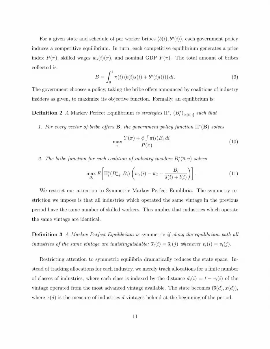
For a given state and schedule of per worker bribes (b(i), bu(i)), each government policy

induces a competitive equilibrium. In turn, each competitive equilibrium generates a price

index P (π), skilled wages ws(i)(π), and nominal GDP Y (π). The total amount of bribes

collected is

B =

∫ 1

0

π(i) (b(i)s(i) + bu(i)l(i)) di. (9)

The government chooses a policy, taking the bribe offers announced by coalitions of industry

insiders as given, to maximize its objective function. Formally, an equilibrium is:

Definition 2 A Markov Perfect Equilibrium is strategies Π∗, (B∗i )i∈[0,1] such that

1. For every vector of bribe offers B, the government policy function Π∗(B) solves

maxπ

Y (π) + φ∫

π(i)Bi di

P (π)(10)

2. The bribe function for each coalition of industry insiders B∗i (s, v) solves

maxBi

E

[Π∗

i (B∗−i, Bi)

(ws(i)− wl −

Bi

s(i) + l(i)

)]. (11)

We restrict our attention to Symmetric Markov Perfect Equilibria. The symmetry re-

striction we impose is that all industries which operated the same vintage in the previous

period have the same number of skilled workers. This implies that industries which operate

the same vintage are identical.

Definition 3 A Markov Perfect Equilibrium is symmetric if along the equilibrium path all

industries of the same vintage are indistinguishable: st(i) = st(j) whenever vt(i) = vt(j).

Restricting attention to symmetric equilibria dramatically reduces the state space. In-

stead of tracking allocations for each industry, we merely track allocations for a finite number

of classes of industries, where each class is indexed by the distance dt(i) = t − vt(i) of the

vintage operated from the most advanced vintage available. The state becomes (s(d), x(d)),

where x(d) is the measure of industries d vintages behind at the beginning of the period.

11

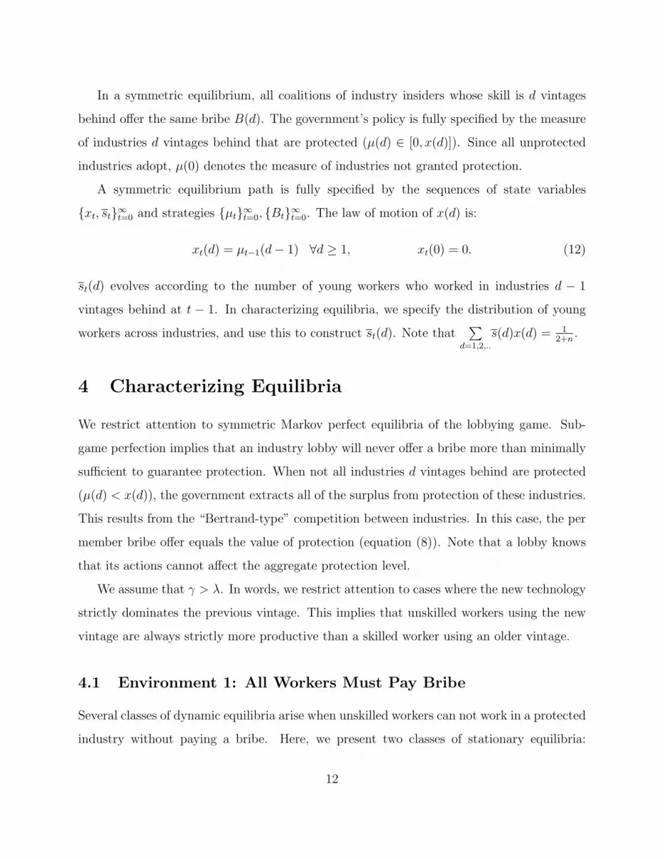
In a symmetric equilibrium, all coalitions of industry insiders whose skill is d vintages

behind offer the same bribe B(d). The government’s policy is fully specified by the measure

of industries d vintages behind that are protected (µ(d) ∈ [0, x(d)]). Since all unprotected

industries adopt, µ(0) denotes the measure of industries not granted protection.

A symmetric equilibrium path is fully specified by the sequences of state variables

{xt, st}∞t=0 and strategies {µt}∞t=0, {Bt}∞t=0. The law of motion of x(d) is:

xt(d) = µt−1(d− 1) ∀d ≥ 1, xt(0) = 0. (12)

st(d) evolves according to the number of young workers who worked in industries d − 1

vintages behind at t − 1. In characterizing equilibria, we specify the distribution of young

workers across industries, and use this to construct st(d). Note that∑

d=1,2,..

s(d)x(d) = 12+n

.

4 Characterizing Equilibria

We restrict attention to symmetric Markov perfect equilibria of the lobbying game. Sub-

game perfection implies that an industry lobby will never offer a bribe more than minimally

sufficient to guarantee protection. When not all industries d vintages behind are protected

(µ(d) < x(d)), the government extracts all of the surplus from protection of these industries.

This results from the “Bertrand-type” competition between industries. In this case, the per

member bribe offer equals the value of protection (equation (8)). Note that a lobby knows

that its actions cannot affect the aggregate protection level.

We assume that γ > λ. In words, we restrict attention to cases where the new technology

strictly dominates the previous vintage. This implies that unskilled workers using the new

vintage are always strictly more productive than a skilled worker using an older vintage.

4.1 Environment 1: All Workers Must Pay Bribe

Several classes of dynamic equilibria arise when unskilled workers can not work in a protected

industry without paying a bribe. Here, we present two classes of stationary equilibria:

12

Constant Protection Levels (CPL) and Two-Period Cycles (TPC).2 CPL occurs when the

government venality (φ) is low, with zero protection as a special case. As the government’s

venality increases, cycles arise. Our description of these equilibria is deliberately terse, as a

more detailed analysis can be found in Bridgman et al. (2005).

4.1.1 Static Lobbying Game

To illustrate the workings of the dynamic equilibria, we begin by characterizing the equilib-

rium of the (static) lobbying game in period t, taking the aggregate state (xt(d), st(d)) as

given. We assume that all old workers are skilled in vintage t− 1 (this is always the case in

this environment).

For a given government policy µ (the fraction of industries protected) and lobby contri-

bution b(1) (bribe per worker), it is straightforward to solve for the competitive equilibrium.

We normalize the price of unprotected goods to 1. Since workers are paid their marginal

products, the unskilled wage in unprotected industries is wl,t(d = 0) = γt, and the skilled

wage in protected industries is ws,t(1) = γt−1λpt(1). Workers are employed either as skilled

workers in a protected industry or as unskilled workers in an unprotected industry. The

unskilled wage in a protected industry would be wl,t(1) = γt−1pt(1). We verify that unskilled

workers do not want to work in protected industries: wl,t(1)− b(1) ≤ wl,t(0).3

The number of unskilled workers in each unprotected industry is

lt(0) =1− µt(1)st(1)

1− µt(1)(13)

and the price of protected goods is

pt(1) =γ

λst(1)lt(0). (14)

We now turn to the payoffs of the lobbying game players. The value of protection to an

2See Bridgman et al. (2005) for a more complete characterization of the set of dynamic equilibria.3In most equilibria, the entire surplus from protection is extracted, so ws,t(1) − b(1) = wl,t(0). Since

ws,t(1) = λwl,t(1), unskilled workers strictly prefer working in unprotected industries.

13

old worker is

V pt (1) = ws,t(1)− wl,t(0) = γt 1− st(1)

st(1)(1− µt(1))(15)

Clearly, skilled workers demand protection only if st(1) < 1. Otherwise, no protection is

the unique equilibrium outcome. When st(1) < 1, protection increases the relative price

of protected goods. Protection also lowers the level of output in protected sectors, while

increasing the output in unprotected industries. This is primarily driven by the young

workers being spread across fewer (unprotected) industries.

Taking into account the effects of its policy choice on the competitive equilibrium, the

government chooses µt(1) to maximize:

UG(µt(1)) =γt

(1−µt(1)st(1)

1−µt(1)

)+ φBt(1)µt(1)[

γλst(1)

(1−µt(1)st(1)

1−µt(1)

)]µt(1). (16)

Protection increases nominal GDP and nominal bribes, but also increases the price index. In

fact, a sufficient condition for real GDP to be decreasing in the level of protection is γ > λ.

Hence, the unique equilibrium for φ = 0 is no protection.

If some industries one vintage behind are not protected in equilibrium, then the govern-

ment extracts all of the surplus from protection. In other words, the contribution of each

industry insider to the bribe equals the value of protection. The bribe offer from each lobby

is the product of the value of protection to each worker and the number of workers:

Bt(1) = V pt (1)st(1) =

γt

(1− µt(1))(1− st(1)) . (17)

If st(1) ≤ ln(

γλst(1)

), then the equilibrium of this static game is unique. Furthermore,

there is an open set of parameter values for which not all industries one vintage behind are

protected.

4.1.2 Dynamic Equilibria

The dynamic aspect is the endogeneity of the state variables – the number of old workers

in each industry {st(d)} and the measure of industries d vintages behind {xt(d)}. Since all

14

workers in a protected industry have to pay the same bribe, it is never in the best interest

of unskilled workers to join a protected industry. Hence, in equilibrium, all young work in

unprotected industries, and there are no workers skilled in vintages more than one generation

behind the frontier (st(d) = 0 ∀ d > 1). Thus there is no one with a vested interest in any

technology more than 1 vintage behind the frontier. This implies xt(d) = 0 ∀ d > 2 and

µt(1) + µt(0) = 1. Using the law of motion (12), xt(1) = 1− µt−1(1) and xt(2) = µt−1(1).

Below we characterize stationary symmetric Markov perfect equilibria. Since young work-

ers spread evenly across unprotected industries,

st(1) =1

(2 + n)µt−1(0)=

1

(2 + n)(1− µt−1(1)). (18)

In equilibrium, old workers who were not granted protection also spread evenly across the

unprotected industries.

4.1.3 Constant Protection Levels

The easiest equilibria to characterize are Constant Protection Levels (CPL). While a con-

stant fraction of industries (less than half) are protected each period, the specific industries

protected vary from period to period. Since µt(1) < 0.5 < xt(1), the equilibrium bribe offers

are equal to the value of protection. While stationary equilibrium may not be unique, the

equilibrium path is pinned down by the initial condition. A special case is zero protection

equilibrium, which occurs when φ ≤ 2+n1+n

ln(

(2+n)γλ

)− 1.

4.1.4 Cycles

Cycles are driven by the endogeneity of the state variables. The “size” of vested interest

groups (st(1)) is pinned down by the allocation of young workers in the previous period,

which in turn is determined by the extent of protection in that period (µt−1(1)).

The easiest cycles to characterize are Two-Period Cycles (TPC). They feature periods of

zero protection alternating with periods of extensive, but not complete, protection. Suppose

that all industries adopted in the previous period (xt(1) = 1, st(1) = 12+n

). A sufficiently

15

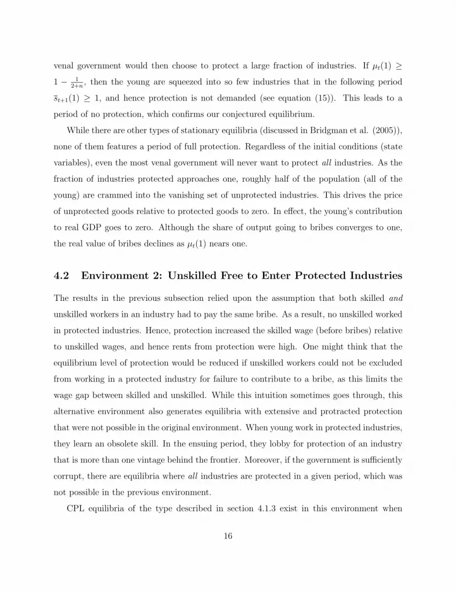
venal government would then choose to protect a large fraction of industries. If µt(1) ≥

1 − 12+n

, then the young are squeezed into so few industries that in the following period

st+1(1) ≥ 1, and hence protection is not demanded (see equation (15)). This leads to a

period of no protection, which confirms our conjectured equilibrium.

While there are other types of stationary equilibria (discussed in Bridgman et al. (2005)),

none of them features a period of full protection. Regardless of the initial conditions (state

variables), even the most venal government will never want to protect all industries. As the

fraction of industries protected approaches one, roughly half of the population (all of the

young) are crammed into the vanishing set of unprotected industries. This drives the price

of unprotected goods relative to protected goods to zero. In effect, the young’s contribution

to real GDP goes to zero. Although the share of output going to bribes converges to one,

the real value of bribes declines as µt(1) nears one.

4.2 Environment 2: Unskilled Free to Enter Protected Industries

The results in the previous subsection relied upon the assumption that both skilled and

unskilled workers in an industry had to pay the same bribe. As a result, no unskilled worked

in protected industries. Hence, protection increased the skilled wage (before bribes) relative

to unskilled wages, and hence rents from protection were high. One might think that the

equilibrium level of protection would be reduced if unskilled workers could not be excluded

from working in a protected industry for failure to contribute to a bribe, as this limits the

wage gap between skilled and unskilled. While this intuition sometimes goes through, this

alternative environment also generates equilibria with extensive and protracted protection

that were not possible in the original environment. When young work in protected industries,

they learn an obsolete skill. In the ensuing period, they lobby for protection of an industry

that is more than one vintage behind the frontier. Moreover, if the government is sufficiently

corrupt, there are equilibria where all industries are protected in a given period, which was

not possible in the previous environment.

CPL equilibria of the type described in section 4.1.3 exist in this environment when

16

skilled workers are much more productive then unskilled (i.e. λ is large) and venality of

government (φ) is low. In this case, unskilled workers do not find it in their interest to

join protected industries and the analysis of section 4.1.3 applies directly. For parameters

that generate CPL equilibria with higher µt(1) in the original environment, the counterparts

of these equilibria in the altered environment may feature lower levels of protection. The

possibility of unskilled workers joining a protected industry introduces an upper bound on

the skill premium, and thus lowers the value of protection.

The employment of unskilled in protected industries limits the distortions created by

protection. Ironically, this allows for equilibria where the economy is sometimes completely

closed (µt(0) = 0). In fact, for some parameter values, multi-period cycles featuring several

consecutive periods of non-adoption exist.

We begin our description of these cycles in the period t following zero protection. Then the

state in period t is as in section 4.1.1 – all skilled workers are in industries one vintage behind.

As in section 4.1.1, the price of unprotected goods is 1, the unskilled wage in unprotected

industries is wl,t(0) = γt, and the skilled wage in protected industries is ws,t(1) = γt−1λpt(1).

When unskilled workers work in protected industries, they receive the same wage in protected

and unprotected industries: wl,t(0) = wl,t(1) = ws,t(1)/λ. It follows that pt(1) = γ. Equation

(7) reduces to µt(1) (st(1) + lt(1)) + µt(0)lt(0) = 1. Since the value of output is the same for

all industries, yt/γt = lt(0) = λst(1) + lt(1). It follows that

lt(0) = 1 + µt(1) (λ− 1) st(1) (19)

and the government maximizes

UG(µt(1)) =γt (1 + µt(1) (λ− 1) st(1)) + φBt(1)µt(1)

γµt(1). (20)

The value of protection is

V pt (1) = ws,t(1)− wl,t = γt (λ− 1) . (21)

Since UG is concave with respect to µt(1), an equilibrium features complete protection

in period t if and only if ∂UG

∂µt(1)|µt(1)=1, B=st(1)V

pt (1) ≥ 0. This is equivalent to (1 + φ)(λ −

17

1)st(1)(1 − ln γ) ≥ ln γ. So long as ln γ < 1, a sufficiently venal government (high φ) will

protect all industries.

In the period following full protection (t+1), all old are distributed evenly across protected

industries, which are now two vintages behind the frontier: xt+1(2) = 1, st+1(2) = 12+n

.

This situation is the same as described above, with the frontier technology being γ2 more

productive than the incumbent (simply replace γ with γ2). Hence, if 2 ln γ < 1, a sufficiently

venal government would protect all industries for the second period in the row. This could

continue for up to N − 1 periods, where N ln γ ≥ 1 > (N − 1) ln γ. However, in the example

we construct in the next section, this continues for N − 2 periods (where N = 4). In period

t + N − 1, roughly half the industries are protected. In this period, all of the young work in

the unprotected industries, and the demand for unskilled workers in protected industries is

satisfied by old workers whose industries are not protected. Since the young are concentrated

in roughly half the industries, they do not demand protection in the following period as

st+N(1) ≥ 1 (see section 4.1.1). Industries N vintages behind no longer have any skilled

workers. Hence, the economy is completely open in period t + N , the young spread evenly

across the industries, and the cycle is ready to repeat itself.

5 Discussion and Illustrative Example

Are Parente and Prescott (1999, 2000) style monopoly rights on labor supply necessary for

barriers to technology adoption to arise in equilibrium? The political economy features of

our model preclude us from making general statements. Hence, we illustrate the effects of

limiting monopoly rights to labor supply using a numerical example.

Natural intuition suggests that eliminating monopoly rights should lower the value of

protection and lead to lower levels of protection in equilibrium. Starting from the benchmark

parameter values of Bridgman et al. (2005), we find that this intuition is correct. In fact, for

these parameter values, eliminating monopoly rights leads to zero protection in equilibrium.

Thus, for these parameter values, monopoly rights turn out to be essential for barriers to

18

technology adoption.

This result is not robust to variations in parameter values. We show that for very bad

governments (ones with large values of φ), this result is dramatically reversed. Whereas in

the monopoly rights environment, these governments lead to modest levels of short lived

protection, with the relaxation of monopoly rights to labor supply they can generate several

periods of non-adoption of new technologies in all industries. This leads to large gaps

between the level of TFP and the world technology frontier. These large TFP gaps cannot be

generated in a world with monopoly rights. Hence, relaxing monopoly rights can sometimes

lead to extremely perverse outcomes.

This reversal is driven by two underlying forces. First, since protected industries employ

(young) unskilled workers, the distortion in relative prices caused by protection is reduced.

This is due both to an expansion in output of protected industries and a reduction in the

output of unprotected industries. Recall that in the environment with monopoly rights, full

protection could never be an equilibrium outcome. As the fraction of industries protected

approaches one, all of the young workers are “crammed” into increasingly few industries.

This “cramming” effect does not occur in the absence of monopoly rights.

The second underlying force is a dynamic one. Prolonged protection requires the perpetu-

ation of industry lobby groups across generations. Since in the monopoly rights environment,

young workers do not work in protected industries, protection is never demanded by indus-

tries more than 1 vintage behind the technology frontier. In contrast, in the environment

without monopoly rights, we find equilibria where young work in protected industries. This

leads to a perpetuation of the industry lobby into the following period.

5.1 Illustrative Example

Given our demographic structure, we assume that each period corresponds to 20 years. We

abstract from population growth (n = 0). The technology growth factor is set to γ = 1.42,

which corresponds to a 1.8% annual growth rate. λ = 1.25, which implies that skilled workers

are 25% more productive then unskilled workers. The venality of government (φ) is 0.75,

19

which implies that the government values its own consumption 1.75 times as much as the

consumption of others. In all equilibria we analyze, the discount factor is irrelevant since

all members of the same generation have the same net income and intergenerational trade

is impossible. For simplicity, we set β = 1.

With these parameter values, the stationary equilibrium of the monopoly rights economy

is a constant protection equilibrium. Each period, 27.5% of industries are protected. The

resulting reduction in real GDP due to this protection is roughly 5.5%. For the same parame-

ter values, the environment without monopoly rights generates no protection in equilibrium.

This confirms the basic intuition that limiting the value of protection should lead to lower

levels of protection.

This result, however, is reversed for high values of government venality. Increasing φ to

18 generates a two period cycle in the monopoly rights environment. This cycle features

alternating periods of complete openness and partial adoption, when 50.2% of industries are

protected. The reduction in real GDP in periods of partial protection is 18.8%. Both the

extent and longevity of protection are much higher when insiders do not have monopoly

rights on labor supply. The equilibrium in this environment is a four period cycle which

features 2 periods of complete protection, which leads to a drop in real GDP relative to the

frontier of a factor of 2.4 In the third period of the cycle, 53% of industries are protected,

while the remaining industries adopt frontier technologies. In the last period of the cycle,

protection is not demanded so all industries adopt best practice technologies.

6 Conclusion

In this paper, we asked whether industry insiders’ monopoly rights to supply labor are essen-

tial for barriers to technology adoption to arise in equilibrium. Surprisingly, we found that

the answer is “sometimes”! We show that when governments are not too “bad”, restrictions

4This goes a long way in accounting for measured differences between rich and poor countries, which vary

by roughly a factor of three (see Parente and Prescott (2000), page 80).

20

on monopoly rights can lead to the elimination of barriers to technology adoption. However,

for “bad” governments, restrictions on monopoly rights can lead to more extreme barriers to

the adoption of superior technologies and much larger deviations in TFP from the technology

frontier.

The key driving force behind these surprising results is the dynamics of the endogenous

vested interest formation. Having young workers acquire skills in obsolete technologies per-

petuates insider groups who have a vested interest in industries whose productivity is falling

further and further behind the frontier. This, combined with lower relative price distortions,

can (surprisingly) generate much larger and long-lived barriers to technology adoption than

are possible in an environment with monopoly rights. While the model is very stylized, we

think that this dynamic effect should be incorporated in future work on barriers to riches.

21

References

Bailey, M. N., Gersbach, H., 1995. Manufacturing efficiency and the need for global com-

petition. Brookings Papers on Economic Activity: Microeconomics, 307-347.

Bridgman, B., Livshits, I., MacGee, J., 2005. Vested Interests and Technology Adoption.

mimeo

Chari, V.V., Hopenhayn, H., 1991. Vintage human capital, growth, and the diffusion of new

technology. Journal of Political Economy 99, 1142-1165.

Grossman, G., Helpman, E., 1994. Protection for sale. American Economic Review 84,

833-850.

Herrendorf, B., Teixeira, A., 2005a . How barriers to international trade affect TFP. Review

of Economic Dynamics, Forthcoming.

Herrendorf, B., Teixeira, A., 2005b . Barriers to entry and development. mimeo.

Holmes, T., Schmitz, J., 1995. Resistance to new technology and trade between areas.

Federal Reserve Bank of Minneapolis Quarterly Review 19, 2-17.

Jovanovic, B., 1997. Learning and growth. In: Kreps, D., Wallis, K., (Eds.), Advances in

Economics and Econometrics: Theory and Applications Seventh World Congress, Vol.

II. Cambridge University Press, New York, pp. 318-339.

Krusell, P., Rios-Rull, J.-V., 1996. Vested interests in a positive theory of stagnation and

growth, Review of Economic Studies 63, 301-329.

Mokyr, J., 1990. The lever of riches: Technological creativity and economic progress. Oxford

University Press, New York.

Olson, M., 1982. The rise and decline of nations. Yale University Press, New Haven.

Parente, S., Prescott, E., 1994. Barriers to Technology Adoption and Development, Journal

of Political Economy 102(2), 298-321.

22

Parente, S., Prescott, E., 1999. Monopoly rights: A barrier to riches. American Economic

Review 89, 1216-1233.

Parente, S., Prescott, E., 2000. Barriers to riches. MIT Press, Cambridge.

Prescott, E., 1998. Needed: A Theory of Total Factor Productivity, International Economic

Review, 39(3), 525-551.

23