Monitoring of the primary drying  

of a lyophilization process in vials 

 

 

Antonello A. Barresi1 , Roberto Pisano1, Davide Fissore1,*, Valeria Rasetto1,  

Salvatore A. Velardi1,  Alberto Vallan2, Marco Parvis2 , Miquel Galan3 

 

 

 

 

1. Dipartimento di Scienza dei Materiali ed Ingegneria Chimica, Politecnico di Torino,   

corso Duca degli Abruzzi 24, 10129 Torino (Italy) 

2. Dipartimento di Elettronica, Politecnico di Torino,  

corso Duca degli Abruzzi 24, 10129 Torino (Italy) 

3. Telstar Lyo,  

Josep Tapiolas 120, 08226 Terrassa (Spain) 

 

* Corresponding author: 

Dr. Davide Fissore 

e‐mail: davide.fissore@polito.it 

Tel.: +39‐011‐0904693 

Fax.: +39‐011‐0904699

This is an electronic version (author's version) of the paper:

Barresi A. A., Pisano R., Fissore D., Rasetto V., Velardi S. A., Vallan A., Parvis M., Galan M. (2009). Monitoring of the primary drying of a lyophilization process in vials. Chemical Engineering & Processing: Process Intensification (Elsevier), 48(1), 408-423. DOI: 10.1016/j.cep.2008.05.004.

1

Abstract 

 

An innovative and modular system (LyoMonitor) for monitoring the primary drying 

of  a  lyophilization  process  in  vials  is  illustrated:  it  integrates  some  commercial 

devices  (pressure  gauges,  moisture  sensor,  mass  spectrometer),  an  innovative 

balance and a Manometric Temperature Measurement system based on an improved 

algorithm (DPE) to estimate sublimating interface temperature and position, product 

temperature profile, heat and mass transfer coefficients and parameters required for 

control purposes and recipe optimisation. A soft‐sensor using a multipoint wireless 

thermometer can also estimate  the previous parameters  in a  large number of vials. 

The performances  of  the previous devices  for  the determination  of  the  end  of  the 

primary  drying  are  compared.  Finally,  all  these  sensors  can  be  used  for  control 

purposes and for the optimisation of the process recipe; the use of DPE in a control 

loop will be shown as an example. 

 

 

Topical heading 

 

Process systems engineering  

 

 

Keywords 

 

Freeze‐drying; monitoring; primary drying; pressure rise test; observer. 

 

2

Introduction 

 

Freeze‐drying (FD) is the process where water (or another solvent) is removed from a 

frozen solution by sublimation, thus obtaining a porous and friable structure that can 

be  easily  re‐hydrated.  This  process  is  used  as  an  alternative  to  traditional  drying 

processes  because  of  the  lower  operating  temperatures  that  make  it  particularly 

suitable  for  those  heat‐sensitive  materials  (e.g.  pharmaceuticals)  that  could  be 

damaged  by  the  higher  temperature  required  by  traditional  drying  treatments. 

Anyway, due  to  the  slow drying  rate,  to  the  very  low  temperature,  to  the  use  of 

vacuum and, generally, to the high investment and operating costs, FD is employed 

only for valuable goods: FD is in fact ubiquitous in the pharmaceutical field, where 

working at low temperature and in sterile conditions is mandatory (Snowman, 1991; 

Liapis, 1987). 

After  freezing  the  product  most  of  the  solvent  is  removed  by  sublimation 

during the primary drying stage (PD) by exposing the frozen solution to a very low 

solvent  partial  pressure.  PD  has  to  be  carried  out  at  an  optimal  temperature  that 

minimises the duration of the process, beside maintaining the maximum temperature 

below the upper limit corresponding to the value that causes the collapse of the solid 

product;  this  requires  to monitor  the product  temperature  and  the position  of  the 

moving front.  

A limitation of the present technology is the impossibility of obtaining a direct 

measure of the parameters of interest without interfering with the process dynamics 

or  impairing  the sterile conditions needed by some products. A  thin  thermocouple 

(or a thermoresistence) inserted in a vial is a widespread, but invasive, system used 

to  monitor  the  process.  This  method  may  alter  the  elementary  phenomena  of 

nucleation  and  ice  crystal  growth;  it  has  been  evidenced  that  the  freezing  bias  is 

small  in  the  semi‐clean  laboratory  environment,  but may  be much more  relevant, 

posing  scale‐up  problems,  in  the  clean  environment  of  the  sterile  production 

operation  (Roy and Pikal, 1989). Measurable  freezing bias may not occur  for every 

3

product, but, in any case, the insertion of thin thermocouples affects the heat transfer 

to  the product: as a consequence,  the drying kinetics  is  faster  in  the monitored vial 

and the results are not representative of the whole system. Nevertheless, this method 

has been proposed  to monitor  the PD and  to detect  the end‐point of  the PD stage. 

Finally, the probe insertion itself compromises the sterility of the product.  

Moisture  sensors,  as  well  as  mass  spectrometry  and  thermal  conductivity 

gauges,  have  been  proposed  in  the  past  to monitor  the  PD  (Oetjen  and Haseley, 

2004):  they can be very useful  to detect  the end of  the PD, but  they do not provide 

any  information  about  the  status of  the product during  the operation. A  technical 

comparison of these and other recently proposed devices is given in Mayeresse et al. 

(2007). 

Non‐invasive monitoring  techniques have been  recently proposed as valuable 

alternatives to the use of thermocouples, as they can monitor the state of the whole 

system. These techniques are based on the Pressure Rise Test (PRT): they use the in‐

line measure of the pressure rise due to the shut‐off of the valve placed between the 

drying  chamber  and  the  condenser  for  a  short  time  interval  (e.g.  30  seconds):  the 

plateau  value  of  the  chamber  pressure  is  related  to  the  temperature  of  the 

sublimating  interface by means of a mathematical model. Various algorithms were 

proposed  in  the  past  to  this  purpose,  namely  the  Manometric  Temperature 

Measurement (MTM) of Milton et al. (1997), the Dynamic Pressure Rise of Liapis and 

Sadikoglu  (1997),  the Pressure Rise Analysis  (PRA) of Chouvenc et al.  (2004, 2005). 

Moreover, performing some Pressure Rise Tests  (PRTs)  throughout all  the PD,  it  is 

possible to monitor the evolution of the product temperature and, since the slope of 

the curve at the beginning of the test gives the sublimation flux of the solvent, it can 

be used to detect the end‐point of the PD.  

In  this  paper  an  innovative  and modular monitoring  system  is  illustrated:  it 

uses several commercial and proprietary sensors to monitor both single vials and the 

whole  batch  and  a  special  balance  to weigh  groups  of  vials.  In‐line measures  of 

temperature and of pressure are also used with a mathematical model of the process 

4

to estimate those variables of interest that cannot be directly measured (e.g. interface 

temperature  and  position,  full  temperature  profile  in  the  product,  heat  and mass 

transfer  coefficients).  To  this  purpose,  a  soft‐sensor  (observer),  that  uses  the 

measurement of  the  temperature  in  a vial,  and  an  innovative  algorithm  (Dynamic 

Parameters Estimation, DPE) that uses the measure of the pressure during the PRT, 

are discussed:  the  former provides  information about  the monitored vial, while  the 

latter gives estimations about the whole batch.  

All  these devices have been  tested  in a prototype  freeze‐dryer  (Lyobeta 25 by 

Telstar)  with  a  chamber  volume  of  0.2  m3  and  equipped  with  thermocouples, 

capacitance  and  thermal  conductivity  gauges, moisture  analyser  and Quadrupole 

Mass Spectrometer (QMS); the pressure in the chamber has been generally regulated 

by controlled leakage, but runs using only the valve on the vacuum pump have been 

also  carried  out.  The  performances  of  these  sensors  and  their  reliability  in 

determining  the  end  of  the PD will be  compared  and discussed. Finally  it will be 

shown how  the  information about  the  state of  the  system can be used  in a control 

loop designed to minimise the drying time, beside ensuring product quality, and an 

example using the DPE algorithm will be presented. 

 

 

Monitoring of the primary drying stage 

 

As it has been stated in the Introduction, monitoring of PD stage is needed to carry 

out  the  process  at  a  controlled  temperature,  thus  avoiding  irreversible  product 

damages and minimising  the  time  required by  this step. Moreover,  the monitoring 

system has  to be  able  to detect  the  end‐point of  the PD, beyond which  secondary 

drying  has  to  be  started.  In  recent  years,  some  devices  have  been  realised  and 

patented  by  our  research  group  in  order  to  monitor  the  PD  of  a  lyophilization 

process  in  vials.  Figure  1  gives  a  sketch  of  the  monitoring  system  that  will  be 

discussed  in  the  following;  a  special  software,  called  LyoMonitor  (see  the  user 

5

interface in Figure 2), has been realised in order to manage the various sensors and to 

collect  their  measurements;  currently,  the  following  systems  are  included  in  the 

prototype: 

i. a  multi‐point  wired  thermometer  (see  (1)  in  Figure  1):  this  instrument  is 

composed  of  a  set  of  nine  copper‐constantan  thermocouples,  a  conditioning 

circuit  and  a  commercial  multimeter  equipped  with  a  multiplexer.  The 

multimeter is connected to the PC #1 by means of the IEEE‐488 interface and it 

is  able  to  perform  an  auto‐diagnosis  test  in  order  to  detect  the  damaged 

thermocouples (see the ʺTestʺ button in Figure 2).  

ii. a new wireless  thermometer  (Vallan et al., 2005a):  this  instrument  (see  (8b)  in 

Figure 1) is a modular thermometer that has been specifically designed in order 

to  provide  a  large  number  of  sensors.  This  can  be  useful,  for  example,  for 

temperature mapping. No wires  are  required  to  connect  the  sensors  placed 

inside  the  vacuum  chamber  to  the  external  acquisition  system.  The 

thermometer can manage one or more measurement modules, equipped with 

14 thermocouples each, and it sends the results to a ʺreaderʺ placed outside the 

vacuum  chamber  and  connected  by means  of  a  serial  interface  to  a  PC  that 

schedules,  acquires  and  collects  the  measurements.  The  reader  powers  the 

thermometer  and  the modules  through  the  same  radio‐frequency  link  that  is 

employed  for  the data communication, so  that  the modules can work without 

batteries. Up to 20 modules can be connected at the same time thus extending 

the measurement capability up  to 280  temperature  sensors. The modules also 

embed an auto‐diagnosis system in order to detect damaged thermocouples. 

iii. a weighing device, proprietary and patented (Vallan et al., 2005b; Vallan, 2007) 

working  inside  the vacuum chamber and able  to measure contemporaneously 

weigh  and  temperature  of  a  group  of  vials  during  the  drying  process.  This 

device is composed of a motorised balance (see (2) in Figure 1), which is able to 

rise and weigh up to 15 vials, and a miniaturized radio‐controlled thermometer 

(7) that is located near the group of vials and transmits their temperatures to the 

6

balance.  In  this  way  both  mass  and  temperature  of  the  same  vials  can  be 

measured contemporaneously. The balance is connected to PC #1 by means of a 

serial  interface  and  can be  controlled  and  calibrated  through  the LyoMonitor 

control panel. The balance,  that has been characterized by comparison with a 

commercial analytical balance both  in vacuum and  in air, has  a  resolution of 

about 10 mg and a total uncertainty of about 100 mg from –40°C to +40°C. 

iv. a valve  control  (6b) and an acquisition  system  (6a)  for  the PRT. The PC #1  is 

equipped  with  a  Digital  Acquisition  Board  that  collects  the  pressure 

measurements during the PRT: the sampling frequency used is 10 Hz, but other 

values, ranging from few Hz to some kHz, can be set. 

v. pressure  (5) and moisture  (4) sensors:  the system  is able  to acquire  the output 

signal of a thermal conductivity gauge (Pirani PSG‐101‐S: full scale pressure = 2 

bar), of a capacitance manometer (MKS Type 626A Baratron: full scale pressure 

= 100 Pa, accuracy = 0.001% of full scale, resolution = 0.25% of reading) and of a 

moisture  analyser  (Panametrics MMS35‐131‐1‐100:  accuracy  of  the M  series 

probe in the measure of the dew/frost point temperature = ±2 °C from 60°C to   ‐

65 °C and ±3 °C from ‐66°C to ‐110 °C; repeatability = ±0.5 °C from 60°C to ‐65 

°C and ±1.0 °C from  ‐66°C to  ‐110 °C) thanks to an external multimeter that  is 

interfaced  to  the  PC  through  the  IEEE‐488  interface;  the  ratio  between  the 

signals of the Pirani and Baratron sensors can be calculated as  it can be useful 

for monitoring purposes. 

LyoMonitor  continuously acquires and  stores  the measures obtained by  the devices 

listed above: moreover some other process variables that are measured in the freeze‐

dryer using embedded devices (i.e. shelf and fluid temperatures, controlled‐leakage 

valve  opening  and  inert  mass  flow  rate  for  pressure  control)  are  acquired  by 

LyoMonitor  through  a  dedicated  RS485  interface,  thus  providing  a  complete 

evaluation of  the  status of  the  system. LyoMonitor can be controlled by means of a 

remote PC  through an  Internet  connection. The measuring cycle  is  set by  the user, 

but  also  spot measurements  are  allowed.  As  it  has  been  designed  as  a modular 

7

system, other measuring devices can obviously be added to LyoMonitor; in particular 

the  implementation of a new device  for monitoring mixed solvent  lyophilization  is 

ongoing. 

A  Quadrupole  Mass  Spectrometer  GeneSys  300  by  European  Spectrometry 

Systems  (upper mass detection  limit  =  300  amu, detector  =  Faraday  cup)  has  also 

been used  to monitor  the FD  (see  (9)  in Figure 1);  the  instrument  is managed by a 

dedicated computer (PC #2 in Figure 1).  

 

Monitoring of single vials 

Through a simple temperature measurement it is possible to monitor the dynamics of 

a single vial by means of a soft‐sensor (or observer, that we called smart vial, see (8a) 

in Figure 1): it is a device that combines the a priori knowledge of the physical system 

(i.e. a mathematical model of  the process) with some experimental data  (i.e.  in‐line 

measurements, like temperature of the product or of the vial) to provide a real‐time 

estimation of some parameters or state variables (Barresi et al., 2008). The smart vial 

consists  of  a  special  vial  equipped  with  a  thermocouple:  the  whole  product 

temperature profile and the mass/heat transfer coefficients are estimated by the soft‐

sensor using the temperature measurement and a simplified mathematical model of 

the  process.  The main  drawback  of  this  approach  is  that  the  state  estimation  is 

limited to a single vial, but, on the other hand, the temperature estimation concerns 

the entire temperature profile of the product in the vial and not only the temperature 

in  a  particular  point,  as  obtained  using  a  thermocouple.  Moreover,  the  results 

obtained  for  a  particular  vial  can  be  compared  to  those  obtained  for  other  vials 

placed  in different positions  into the drying chamber, thus allowing to evaluate the 

heterogeneity  of  the  batch.  With  this  respect,  the  use  of  the  multiple  wireless 

thermometer allows easily and economically the monitoring even of a large number 

of vials. 

The synthesis of an observer is a complex task and a lot of different approaches 

have been proposed in the Literature. The Extended Kalman Filter (KF) is one of the 

8

most  common  techniques  (Becerra  et  al.,  2001)  and  it  has  been  applied  to  the  FD 

process using a simplified model:  the heat  transfer  in  the dried and  frozen  layer  is 

accounted for, but heat transfer by radiation is not considered and pseudo‐stationary 

conditions  are  assumed  (Velardi  and  Barresi,  2008).  The  observer  uses  the 

measurement of  the product  temperature at  the bottom of  the vial  to  estimate  the 

temperature and position of the moving front (and thus it can be used to detect the 

end‐point of  the PD) as well as  the heat and mass  transfer coefficients; Appendix 1 

gives  the equations of  this observer. As an alternative, a High Gain  (HG) observer 

has  been designed  and  tested  as  this  approach  allows  for  a  simpler mathematical 

formulation of the problem and the computational time required for the estimation is 

lower;  moreover,  the  HG  observer  exhibits  less  sensitivity  towards  noisy 

measurements.  

Both soft‐sensors have been validated by numerical simulations using firstly a 

detailed mono‐dimensional model  as  a  source  of  experimental data  (Barresi  et  al., 

2008;  Velardi  et  al.,  2008a);  preliminary  experimental  results  confirm  that  in‐line 

estimations are very good, as it is shown in Figure 3, which shows the prediction of 

the interface temperature and the calculated position of the frozen interface obtained 

using  the  KF.  The  quality  of  the  estimations  given  by  both  observers  has  been 

verified to be roughly the same, but the computational effort requested by the KF is 

higher and  its  tuning  is quite  tricky, while  the estimations of  the HG observer are 

provided faster and the tuning is simpler. 

These observers can be used to monitor the behaviour of several vials located in 

different positions on the shelf. Figures 3b and 3c show an example of the estimations 

of the time evolution of the interface temperature and of the temperature profile at a 

certain  instant  in  four different vials.  In Figure 3b  the  front  temperature of  several 

vials  estimated  by  the  KF  is  compared with  the  interface  temperature  calculated 

using the DPE algorithm (that will be described in the following): it can be remarked 

that  DPE  gives  an  average  product  temperature  of  the  whole  batch  while  the 

observer  estimates  the  temperature  in  the  single  vial monitored.  In  Figure  3d  the 

9

moving  front  position  estimated  by  the  KF  for  the  vial  #2  is  compared  to  that 

estimated by DPE: the agreement between the two profiles is good, as it can be seen 

also for the interface temperatures given in Figure 3b. This is due to the fact that DPE 

estimates a mean value of the interface temperature and position for the whole batch 

and most of the vials have a behaviour similar to that of vial #3, as this vial is placed 

in the central part of the tray. 

Since  the  insertion  of  a  probe,  although  extremely  tiny,  in  contact with  the 

product  should  be  avoided  because  of  the  various  troubles  mentioned  in  the 

Introduction, another observer has been designed, exploiting the measurement of the 

external temperature at the bottom of the vial (Barresi et al., 2007; Barresi et al., 2008; 

Galan  et  al.,  2007)  and using  a different  simplified mathematical model  that  takes 

into account also the heat transfer along the glass vial (Velardi and Barresi, 2008). 

Other  indirect methods  that have been proposed  in  the past  to monitor single 

vials are briefly reviewed in the following: these are alternatives to the collection of 

samples  inside  the  freeze‐drier  chamber  and  direct weighing,  a  technique  that  is 

generally  applicable  only  in  small  laboratory  apparatuses,  and  that  has  several 

drawbacks. 

NMR technique was proposed by Monteiro Marques et al. (1991) to detect the 

end‐point of PD by observing an abrupt increase in the longitudinal and transverse 

relaxation times.  

XRD  photography  was  proposed  by  Schelenz  et  al.  (1994)  to  check  the 

estimations of the temperature profile inside a vial.  

Jennings  and  Duan  (1995)  proposed  a  different  technique  to  calculate  the 

duration of the PD: it is required to know the total energy necessary to carry out the 

PD process  and  to make  a  calorimetric measurement  to  calculate  the heat  transfer 

coefficient  in  the  vial,  and  thus  the  rate  of  heat  transport.  To  this  purpose  a 

differential  method,  called  Drying  Process  Monitoring  (DPM),  is  used:  two 

thermocouples are fixed to the bottom of an empty vial and of a vial filled with the 

product,  thus  allowing  to  calculate  the heat  transfer  to  the  filled vial used  for  the 

10

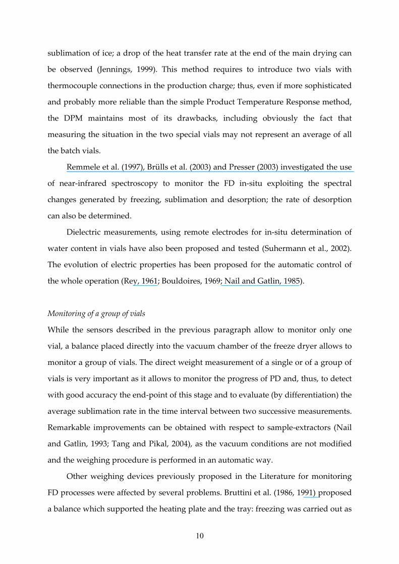
sublimation of ice; a drop of the heat transfer rate at the end of the main drying can 

be  observed  (Jennings,  1999).  This  method  requires  to  introduce  two  vials  with 

thermocouple connections in the production charge; thus, even if more sophisticated 

and probably more reliable than the simple Product Temperature Response method, 

the  DPM  maintains  most  of  its  drawbacks,  including  obviously  the  fact  that 

measuring the situation in the two special vials may not represent an average of all 

the batch vials.  

Remmele et al. (1997), Brülls et al. (2003) and Presser (2003) investigated the use 

of  near‐infrared  spectroscopy  to  monitor  the  FD  in‐situ  exploiting  the  spectral 

changes generated by  freezing,  sublimation  and desorption;  the  rate of desorption 

can also be determined.  

Dielectric measurements, using  remote  electrodes  for  in‐situ determination of 

water content in vials have also been proposed and tested (Suhermann et al., 2002). 

The evolution of electric properties has been proposed  for  the automatic control of 

the whole operation (Rey, 1961; Bouldoires, 1969; Nail and Gatlin, 1985). 

 

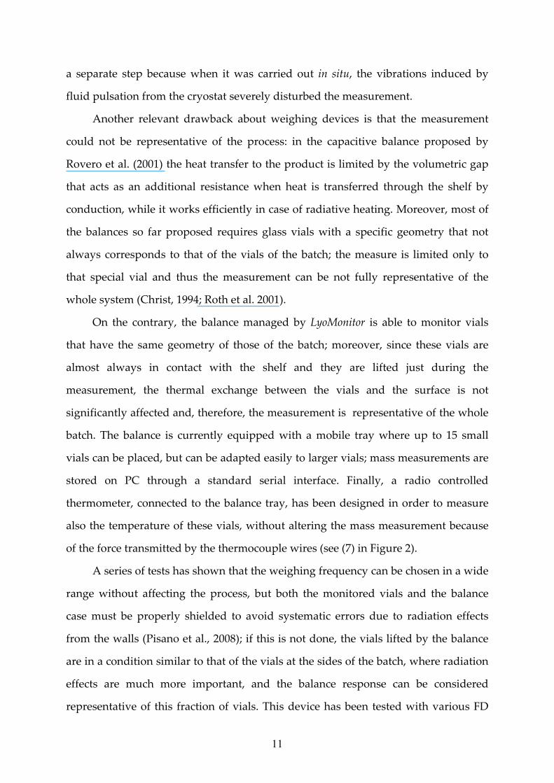
Monitoring of a group of vials 

While  the  sensors described  in  the previous paragraph  allow  to monitor  only one 

vial, a balance placed directly into the vacuum chamber of the freeze dryer allows to 

monitor a group of vials. The direct weight measurement of a single or of a group of 

vials is very important as it allows to monitor the progress of PD and, thus, to detect 

with good accuracy the end‐point of this stage and to evaluate (by differentiation) the 

average sublimation rate in the time interval between two successive measurements. 

Remarkable  improvements can be obtained with  respect  to  sample‐extractors  (Nail 

and Gatlin, 1993; Tang and Pikal, 2004), as the vacuum conditions are not modified 

and the weighing procedure is performed in an automatic way.  

Other weighing devices previously proposed  in  the Literature  for monitoring 

FD processes were affected by several problems. Bruttini et al. (1986, 1991) proposed 

a balance which supported the heating plate and the tray: freezing was carried out as 

11

a  separate  step because when  it was  carried out  in  situ,  the vibrations  induced by 

fluid pulsation from the cryostat severely disturbed the measurement.  

Another  relevant drawback  about weighing devices  is  that  the measurement 

could  not  be  representative  of  the  process:  in  the  capacitive  balance  proposed  by 

Rovero et al. (2001) the heat transfer to the product is limited by the volumetric gap 

that  acts  as  an  additional  resistance when heat  is  transferred  through  the  shelf by 

conduction, while it works efficiently in case of radiative heating. Moreover, most of 

the balances  so  far proposed  requires glass vials with a  specific geometry  that not 

always corresponds  to  that of  the vials of  the batch;  the measure  is  limited only  to 

that  special  vial  and  thus  the measurement  can  be  not  fully  representative  of  the 

whole system (Christ, 1994; Roth et al. 2001). 

On  the  contrary,  the balance managed by LyoMonitor  is able  to monitor vials 

that have  the  same geometry of  those of  the batch; moreover,  since  these vials are 

almost  always  in  contact  with  the  shelf  and  they  are  lifted  just  during  the 

measurement,  the  thermal  exchange  between  the  vials  and  the  surface  is  not 

significantly affected and, therefore, the measurement is  representative of the whole 

batch. The balance  is  currently  equipped with a mobile  tray where up  to 15  small 

vials can be placed, but can be adapted easily to larger vials; mass measurements are 

stored  on  PC  through  a  standard  serial  interface.  Finally,  a  radio  controlled 

thermometer, connected to the balance tray, has been designed  in order to measure 

also the temperature of these vials, without altering the mass measurement because 

of the force transmitted by the thermocouple wires (see (7) in Figure 2). 

A series of tests has shown that the weighing frequency can be chosen in a wide 

range without  affecting  the process, but both  the monitored vials  and  the balance 

case must be properly  shielded  to  avoid  systematic  errors due  to  radiation  effects 

from the walls (Pisano et al., 2008); if this is not done, the vials lifted by the balance 

are in a condition similar to that of the vials at the sides of the batch, where radiation 

effects  are  much  more  important,  and  the  balance  response  can  be  considered 

representative of  this  fraction of vials. This device has been  tested with various FD 

12

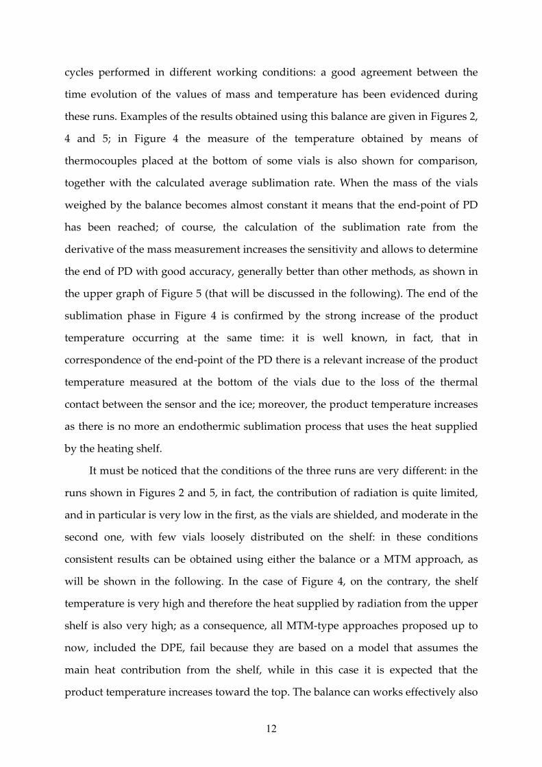
cycles  performed  in  different working  conditions:  a  good  agreement  between  the 

time  evolution  of  the values  of mass  and  temperature has been  evidenced during 

these runs. Examples of the results obtained using this balance are given in Figures 2, 

4  and  5;  in  Figure  4  the  measure  of  the  temperature  obtained  by  means  of 

thermocouples  placed  at  the  bottom  of  some  vials  is  also  shown  for  comparison, 

together with  the  calculated  average  sublimation  rate. When  the mass of  the vials 

weighed by the balance becomes almost constant  it means that the end‐point of PD 

has  been  reached;  of  course,  the  calculation  of  the  sublimation  rate  from  the 

derivative of the mass measurement increases the sensitivity and allows to determine 

the end of PD with good accuracy, generally better than other methods, as shown in 

the upper graph of Figure 5 (that will be discussed in the following). The end of the 

sublimation  phase  in  Figure  4  is  confirmed  by  the  strong  increase  of  the  product 

temperature  occurring  at  the  same  time:  it  is  well  known,  in  fact,  that  in 

correspondence of the end‐point of the PD there is a relevant increase of the product 

temperature measured  at  the  bottom  of  the  vials  due  to  the  loss  of  the  thermal 

contact between the sensor and the ice; moreover, the product temperature increases 

as there is no more an endothermic sublimation process that uses the heat supplied 

by the heating shelf.  

It must be noticed that the conditions of the three runs are very different: in the 

runs shown in Figures 2 and 5, in fact, the contribution of radiation is quite limited, 

and in particular is very low in the first, as the vials are shielded, and moderate in the 

second  one,  with  few  vials  loosely  distributed  on  the  shelf:  in  these  conditions 

consistent  results can be obtained using either  the balance or a MTM approach, as 

will be  shown  in  the  following.  In  the  case  of Figure  4,  on  the  contrary,  the  shelf 

temperature is very high and therefore the heat supplied by radiation from the upper 

shelf  is also very high; as a consequence, all MTM‐type approaches proposed up to 

now,  included  the DPE,  fail  because  they  are  based  on  a model  that  assumes  the 

main  heat  contribution  from  the  shelf, while  in  this  case  it  is  expected  that  the 

product temperature increases toward the top. The balance can works effectively also 

13

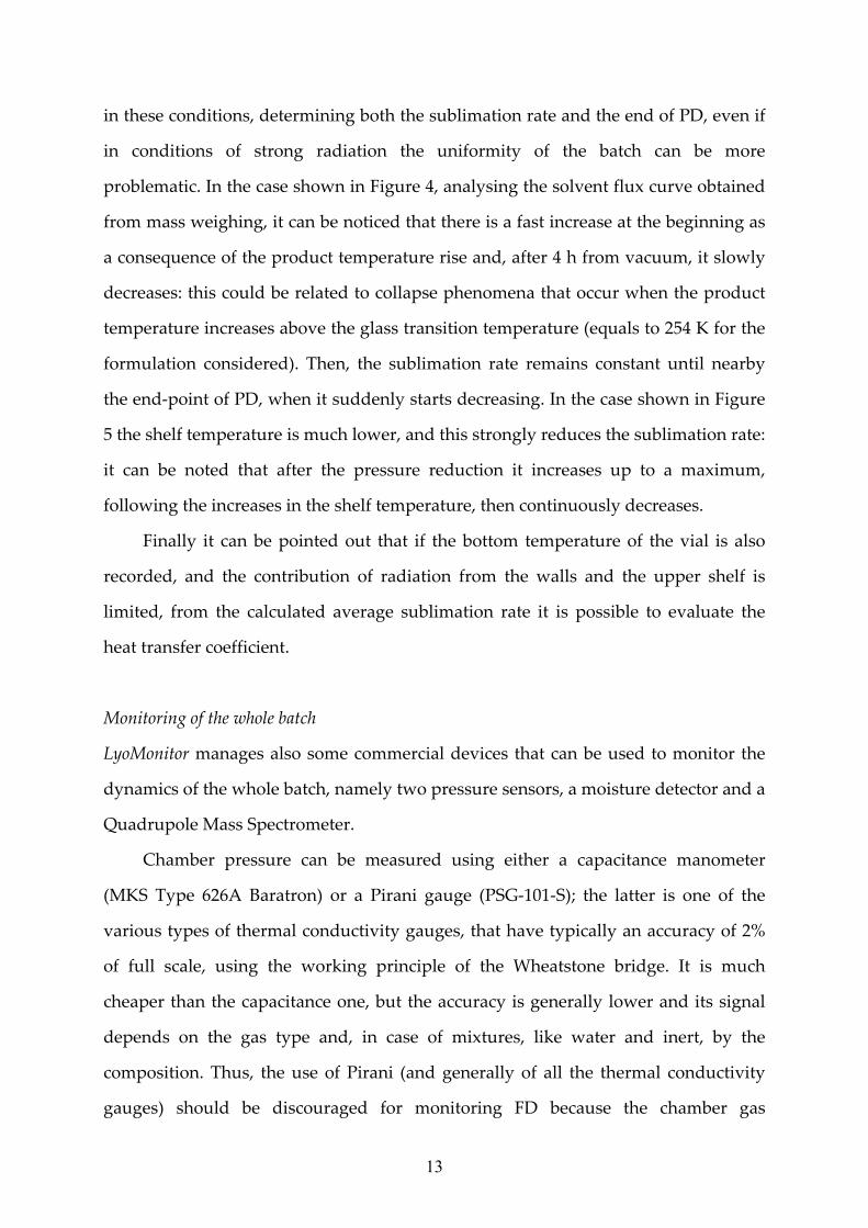
in these conditions, determining both the sublimation rate and the end of PD, even if 

in  conditions  of  strong  radiation  the  uniformity  of  the  batch  can  be  more 

problematic. In the case shown in Figure 4, analysing the solvent flux curve obtained 

from mass weighing, it can be noticed that there is a fast increase at the beginning as 

a consequence of the product temperature rise and, after 4 h from vacuum, it slowly 

decreases: this could be related to collapse phenomena that occur when the product 

temperature increases above the glass transition temperature (equals to 254 K for the 

formulation  considered). Then,  the  sublimation  rate  remains  constant until nearby 

the end‐point of PD, when it suddenly starts decreasing. In the case shown in Figure 

5 the shelf temperature is much lower, and this strongly reduces the sublimation rate: 

it  can  be  noted  that  after  the  pressure  reduction  it  increases  up  to  a maximum, 

following the increases in the shelf temperature, then continuously decreases.  

Finally  it can be pointed out  that  if  the bottom  temperature of  the vial  is also 

recorded,  and  the  contribution  of  radiation  from  the walls  and  the  upper  shelf  is 

limited,  from  the  calculated  average  sublimation  rate  it  is possible  to  evaluate  the 

heat transfer coefficient. 

 

Monitoring of the whole batch 

LyoMonitor manages also some commercial devices  that can be used  to monitor  the 

dynamics of the whole batch, namely two pressure sensors, a moisture detector and a 

Quadrupole Mass Spectrometer. 

Chamber  pressure  can  be  measured  using  either  a  capacitance  manometer 

(MKS Type  626A Baratron)  or  a Pirani  gauge  (PSG‐101‐S);  the  latter  is  one  of  the 

various types of thermal conductivity gauges, that have typically an accuracy of 2% 

of  full  scale,  using  the  working  principle  of  the Wheatstone  bridge.  It  is  much 

cheaper than the capacitance one, but the accuracy  is generally  lower and  its signal 

depends  on  the  gas  type  and,  in  case  of mixtures,  like  water  and  inert,  by  the 

composition. Thus,  the use of Pirani  (and generally of all  the  thermal  conductivity 

gauges)  should  be  discouraged  for  monitoring  FD  because  the  chamber  gas 

14

composition  continuously  changes  during  each  run  and  is  generally  different  in 

different cycles as  it depends on  set up,  loading and product  features  (Armstrong, 

1980). On  the other hand,  taking  into account  the known dependence of  the Pirani 

response on the water vapour fraction, it is possible to evaluate the partial pressure 

of water  into  the  drying  chamber  elaborating  the  different  signals  obtained  from 

Baratron and Pirani sensors. Moreover, as suggested by Nail (Armstrong, 1980), it is 

possible to detect the end of the PD as at that point the concentration of water  into 

the drying chamber becomes very low and the pressure measured by Pirani (that is 

generally calibrated  for air) approaches  that of  the capacitive gauge. The use of  the 

ratio of the pressure signal given by the two gauges, that approaches unity at the end 

of  the  PD,  instead  of  the  simple measure  by  the  Pirani,  is more  reliable  to  this 

purpose, because  eliminates  the possible  effect of a variation of  the  total pressure. 

One possible  limitation to the application of this simple method  is the restriction  in 

the use of the thermal conductivity sensors in equipment where steam sterilisation is 

required, even if producers claim that new models using different filament materials 

(nickel,  platinum)  rather  than  the  standard  tungsten  can  cope  with  sterilisation. 

Recently, new  sensors based on  the  same principle of  the Pirani gauge have been 

proposed: a  stainless  steel  shield  is used  to protect against  condense and a pulsed 

mode  of  operation  allows  for  a  higher  signal  resolution,  an  extended  range  of 

measure and a higher long‐term stability (Salzberg, 2007). 

Other  methods  are  available  to  monitor  the  time  evolution  of  the  water 

concentration in the chamber, e.g. the use of moisture sensors or mass spectrometers. 

Dew point sensors can detect the gas composition or the relative humidity owing to a 

change  in  the dielectric  constant of a gold  sputtered  foil material:  they  indicates a 

sharp  decrease  in  the  dew  point when  the water  vapour  decreases  to  almost  0% 

(Bardat  et  al.,  1993)  and  they  can  have  a  greater  sensitivity with  respect  to  other 

known methods  such  as  thermal  conductivity gauge. Roy  and Pikal  (1989) used  a 

moisture  sensor  (Ondyne,  by Endress+Hauser HydroGuard  2250, Greenwood,  IN) 

that exploits  the variation of  the  capacity of a  thin  film of aluminum oxide due  to 

15

moisture:  according  to  the  authors,  the  sensor has  the  sensitivity  to determine  the 

presence of ice in less than 1% of the vials. This device, that had been firstly proposed 

by Bouldoires (1969), was successively used by Genin et al. (1996) and Rambhatla et 

al. (2004) to monitor the process and to detect the sublimation end‐point. Genin et al. 

(1996) developed also a procedure based on  the standard  law of mass  transfer  that 

lead to a patented method (René et al., 1995) to estimate the residual water content of 

the  product  at  any  time  during  the  process;  this method was  initially  applied  to 

apparatus with  internal  condenser  and  then  proposed  also  for  freeze‐driers with 

external  condenser.  Trelea  et  al.  (2007)  and Chouvenc  et  al.  (2004)  used  a  similar 

moisture  sensor, developed by Panametrics; as  said before, our  freeze‐drier  is also 

equipped  with  a  Panametrics Moisture  Analyser  (Panametrics MMS35‐131‐1‐100) 

and  its performance will be  compared with  those  of  the  other  systems previously 

described. 

The use of a QMS to monitor the PD has been proposed  in the past (Jennings, 

1980, 1999; Connelly and Welch, 1993). The working principle of a QMS is simple: the 

gas  is sampled to the  instrument, where the molecules are fragmented,  ionised and 

accelerated by an electric field and the ions are driven to the detector which gives a 

signal proportional  to  the concentration and  to  the  type of  the  impacting  fragment. 

The  resulting  mass  spectrum,  constituted  by  the  intensity  of  the  current 

corresponding to each ion as a function of time, has thus to be manipulated to get the 

gas composition, but this operation can be quite tricky, mainly due to the difficulties 

in the calibration. The signal measured by the QMS is in fact the sum of: 

i. a base signal, varying with time over a long time interval, which is the response 

of the instrument when the species is not present in the feeding; 

ii. a  false  signal  (named  “interaction”)  generated  by  the  fact  that  each molecular 

species entering  in  the QMS  chamber originates a wide variety of  ions and, as 

there  is no chromatographic separation of  the different species, an  ion with  the 

same  mass/charge  ratio  may  belong  to  different  compounds.  It  is  therefore 

necessary to select, for each species, the ion that should be monitored in order to 

16

avoid, or  at  least  to minimise,  these  interferences.  In our  application,  the  only 

specie that we desire to monitor is water, whose spectrum is constituted mainly 

by the fragment of mass 18; nitrogen (or air) is present, but none of the fragments 

originated by O2 and N2 can give interference with the fragment of mass 18;  

iii. the  true  signal  generated  by  the  molecule  identified  by  the  selected  mass 

fragment. 

Even if the base signal can be easily computed and the interactions can be minimised, 

the calculation of the response factor of the instrument is difficult as it is not obvious 

at all how  to “create” a calibration mixture with water; moreover,  it  is necessary  to 

repeat this calibration before each run as the response factor of the instrument can be 

variable.  Jennings  (1980)  suggested  to use a  capacitance manometer  in  conjunction 

with  the  QMS  to  make  the  calibration;  anyway,  significant  information  can  be 

obtained  from  the QMS  even  if  only  the  ionic  currents  are  investigated:  the  time 

evolution of the ionic current corresponding to mass 18 divided by the total pressure 

reading made by the QMS was proposed by Jennings (1980) to detect the end of the 

PD  as  this  signal  was  almost  constant  during  all  the  PD  and  decreased  in 

correspondence  of  the  ending  point.  Our  freeze‐drier  is  equipped  with  a  QMS 

GeneSys 300 by European Spectrometry Systems: the results that we obtained will be 

compared in the following with those of the other systems previously described. 

Recent  developments  and  proposals  in  the  monitoring  of  the  whole  batch 

comprise  the use  of  a mass  flow  controller  to measure  the  gas  flow necessary  for 

pressure  control  (Chase,  1998),  a  Tuneable  Diode  Laser  Absorption  Spectroscopy 

sensor,  that  was  shown  to  be  effective  for  real‐time  determination  of  vapour 

concentration and mass flux (Kessler et al., 2004) and a cold plasma ionisation device 

for the monitoring of the moisture content in the freeze‐drying chamber (Mayeresse 

et al., 2007). The measure of the inert mass flow for pressure control and the measure 

of the water vapour concentration in the chamber, using one of the previous devices, 

are  closely  related methods  as  they  all  are  sensible  to  a  strong  variation  of  the 

sublimation rate and, thus, they can be used to detect the end of PD. Nevertheless, it 

17

must be taken into account that these devices give only an indirect evaluation of this 

quantity as  the partial pressure  that  is established  in  the chamber  (at constant  total 

pressure), and the controlled  leakage required to maintain a constant pressure, also 

depend on  the performance of condenser and of  the vacuum pump, which  in  turn 

can  be  affected  by  the  nature  of  the  inert.  The  cold‐plasma  sensor  seems  anyway 

particularly  promising:  it  is  steam  sterilisable,  simple  to  integrate  even  in  an 

industrial‐scale  freeze‐drier,  reproducible  and  sensitive;  the  limitations  include 

suitable positioning in the lyophilization chamber, calibration and signal integration. 

Finally  it  can  be  remembered  that  heat  balance  at  the  condenser  has  also  been 

proposed for sublimation monitoring. 

A  first  example  of  the  results  obtained  in  our  system  is  shown  in  Figure  5, 

where  the  output  from  the  balance  and  the  ratio  of  the  pressure  sensors  are 

compared; the estimations given by DPE are also shown. In this cycle 28 vials were 

placed over the heating shelf in group of 7 vials (a central vial rounded by six vials) 

and 15 vials were placed on the balance: the radiating contribution is thus similar for 

the vials on the shelf and for those on the balance. From these data it can be observed 

that the end of the PD (estimated at about 11 hours from the beginning of the drying 

and evidenced with the vertical line) is more clearly defined if detected through the 

mass  measurement  than  using  other  sensors,  like  for  the  example  the  pressure 

gauges, even  if a very  small and uniform batch  is  considered.  In  large batches  the 

end of PD may be much more widespread, as will be shown later, as a consequence 

of the fact that some of the vials can experience conditions different from the average, 

and thus have a different drying rate, while the  lot of vials weighed by the balance 

takes into account the normal variability between vials, but, if properly shielded, it is 

representative  of  the  core  of  the  batch.  It  must  be  remarked  that  the  mass 

measurement is affected by an uncertainties of 0.1 g, hence the end‐point estimation 

can vary in a range of 0.2 h as it is shown in Figure 5 by the grey bar.  

All  the  devices  discussed  in  this  section  (with  the  exception  of  the  balance), 

even  if useful, do not provide any  information about the state of the whole system, 

18

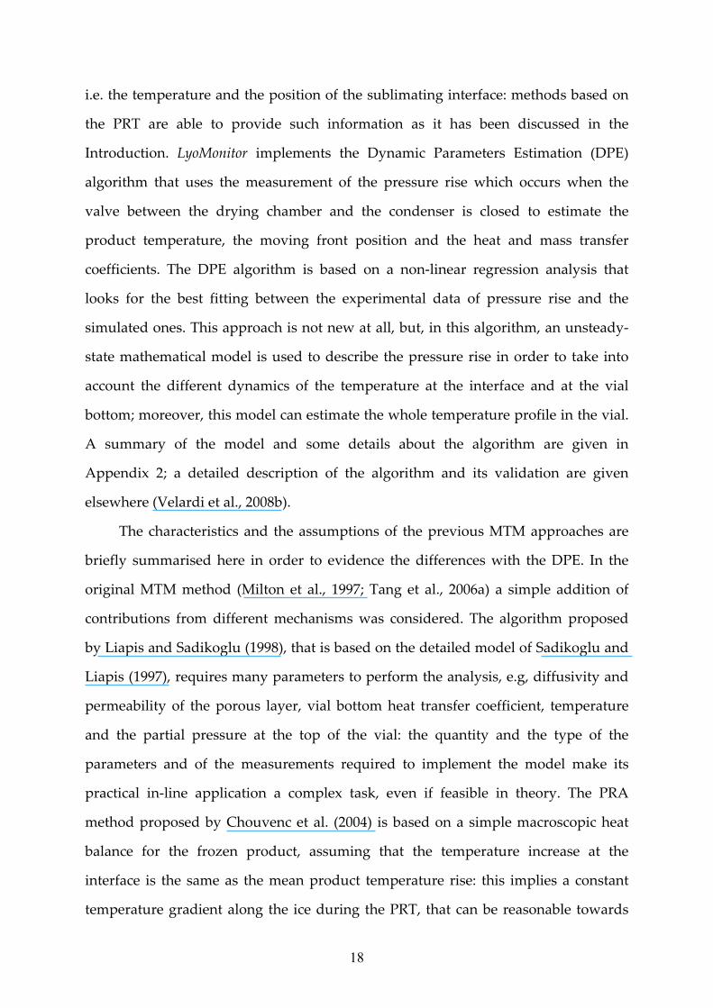
i.e. the temperature and the position of the sublimating interface: methods based on 

the  PRT  are  able  to  provide  such  information  as  it  has  been  discussed  in  the 

Introduction.  LyoMonitor  implements  the  Dynamic  Parameters  Estimation  (DPE) 

algorithm  that  uses  the measurement  of  the  pressure  rise which  occurs when  the 

valve  between  the  drying  chamber  and  the  condenser  is  closed  to  estimate  the 

product  temperature,  the moving  front  position  and  the  heat  and mass  transfer 

coefficients.  The DPE  algorithm  is  based  on  a  non‐linear  regression  analysis  that 

looks  for  the  best  fitting  between  the  experimental  data  of  pressure  rise  and  the 

simulated ones. This approach is not new at all, but, in this algorithm, an unsteady‐

state mathematical model  is used  to describe  the pressure rise  in order  to  take  into 

account  the different dynamics  of  the  temperature  at  the  interface  and  at  the  vial 

bottom; moreover, this model can estimate the whole temperature profile in the vial. 

A  summary  of  the  model  and  some  details  about  the  algorithm  are  given  in 

Appendix  2;  a  detailed  description  of  the  algorithm  and  its  validation  are  given 

elsewhere (Velardi et al., 2008b). 

The characteristics and  the assumptions of  the previous MTM approaches are 

briefly  summarised here  in order  to  evidence  the differences with  the DPE.  In  the 

original MTM method  (Milton  et al., 1997; Tang et al., 2006a) a  simple addition of 

contributions  from different mechanisms was  considered. The  algorithm proposed 

by Liapis and Sadikoglu (1998), that is based on the detailed model of Sadikoglu and 

Liapis (1997), requires many parameters to perform the analysis, e.g, diffusivity and 

permeability of  the porous  layer, vial bottom heat  transfer  coefficient,  temperature 

and  the  partial  pressure  at  the  top  of  the  vial:  the  quantity  and  the  type  of  the 

parameters  and  of  the measurements  required  to  implement  the model make  its 

practical  in‐line  application  a  complex  task,  even  if  feasible  in  theory.  The  PRA 

method proposed by Chouvenc et al.  (2004)  is based on a simple macroscopic heat 

balance  for  the  frozen  product,  assuming  that  the  temperature  increase  at  the 

interface  is  the same as  the mean product  temperature  rise:  this  implies a constant 

temperature gradient along  the  ice during  the PRT,  that can be reasonable  towards 

19

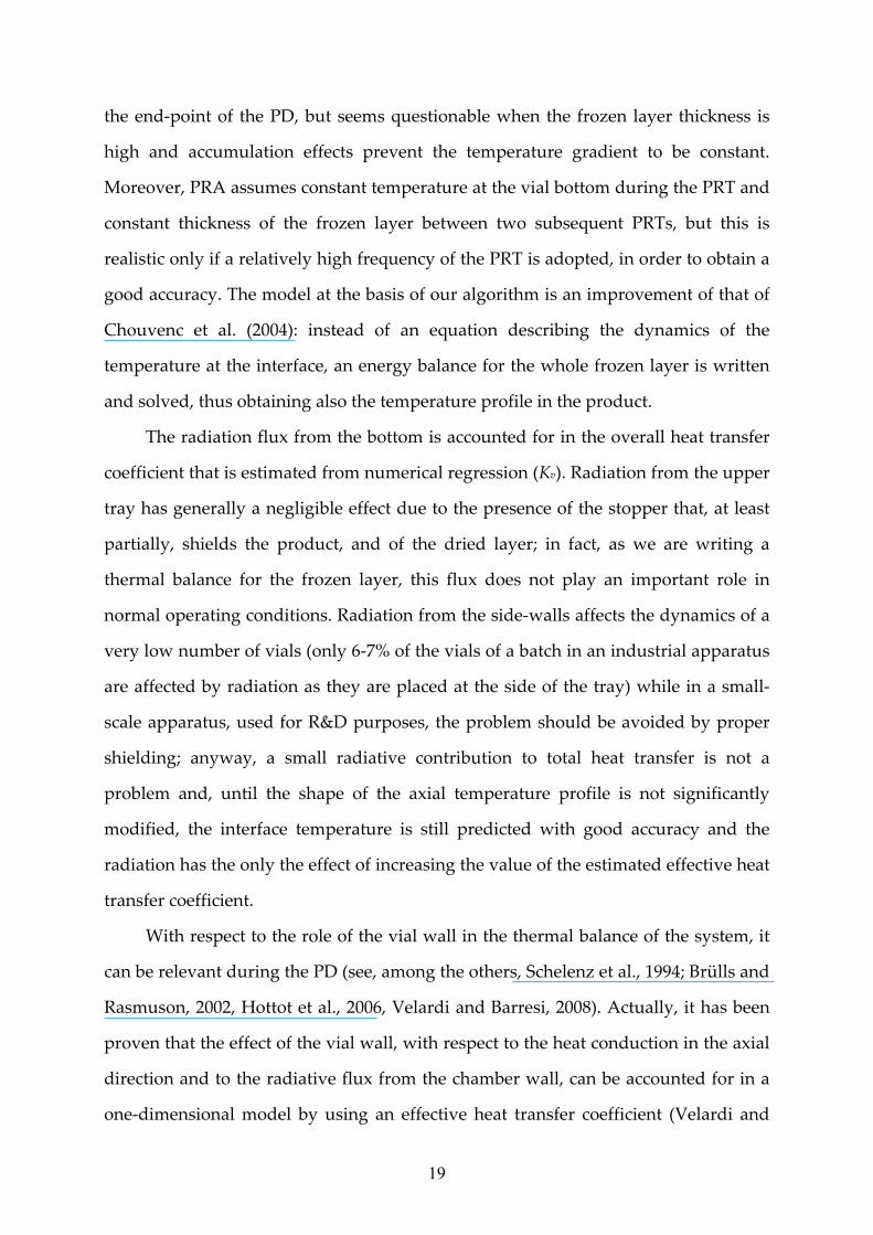
the end‐point of  the PD, but seems questionable when  the  frozen  layer  thickness  is 

high  and  accumulation  effects  prevent  the  temperature  gradient  to  be  constant. 

Moreover, PRA assumes constant temperature at the vial bottom during the PRT and 

constant  thickness  of  the  frozen  layer  between  two  subsequent  PRTs,  but  this  is 

realistic only if a relatively high frequency of the PRT is adopted, in order to obtain a 

good accuracy. The model at the basis of our algorithm is an improvement of that of 

Chouvenc  et  al.  (2004):  instead  of  an  equation  describing  the  dynamics  of  the 

temperature at the interface, an energy balance for the whole frozen layer is written 

and solved, thus obtaining also the temperature profile in the product.  

The radiation flux from the bottom is accounted for in the overall heat transfer 

coefficient that is estimated from numerical regression (Kv). Radiation from the upper 

tray has generally a negligible effect due to the presence of the stopper that, at least 

partially,  shields  the  product,  and  of  the  dried  layer;  in  fact,  as we  are writing  a 

thermal  balance  for  the  frozen  layer,  this  flux  does  not  play  an  important  role  in 

normal operating conditions. Radiation from the side‐walls affects the dynamics of a 

very low number of vials (only 6‐7% of the vials of a batch in an industrial apparatus 

are affected by radiation as they are placed at the side of the tray) while in a small‐

scale apparatus, used for R&D purposes, the problem should be avoided by proper 

shielding;  anyway,  a  small  radiative  contribution  to  total  heat  transfer  is  not  a 

problem  and,  until  the  shape  of  the  axial  temperature  profile  is  not  significantly 

modified,  the  interface  temperature  is  still  predicted with  good  accuracy  and  the 

radiation has the only the effect of increasing the value of the estimated effective heat 

transfer coefficient.  

With respect to the role of the vial wall in the thermal balance of the system, it 

can be relevant during the PD (see, among the others, Schelenz et al., 1994; Brülls and 

Rasmuson, 2002, Hottot et al., 2006, Velardi and Barresi, 2008). Actually, it has been 

proven that the effect of the vial wall, with respect to the heat conduction in the axial 

direction and to the radiative flux from the chamber wall, can be accounted for in a 

one‐dimensional model by using an  effective heat  transfer  coefficient  (Velardi and 

20

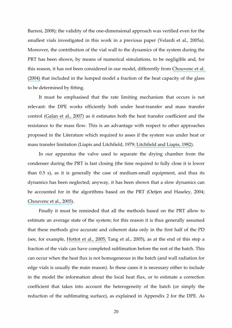
Barresi, 2008); the validity of the one‐dimensional approach was verified even for the 

smallest vials  investigated  in  this work  in a previous paper  (Velardi  et al., 2005a). 

Moreover, the contribution of the vial wall to the dynamics of the system during the 

PRT has been shown, by means of numerical simulations,  to be negligible and,  for 

this reason, it has not been considered in our model, differently from Chouvenc et al. 

(2004) that included in the lumped model a fraction of the heat capacity of the glass 

to be determined by fitting. 

It must  be  emphasised  that  the  rate  limiting mechanism  that  occurs  is  not 

relevant:  the  DPE  works  efficiently  both  under  heat‐transfer  and  mass  transfer 

control  (Galan et al., 2007) as  it estimates both  the heat  transfer coefficient and  the 

resistance  to  the mass  flow. This  is an advantage with  respect  to other approaches 

proposed  in  the Literature which required  to asses  if the system was under heat or 

mass transfer limitation (Liapis and Litchfield, 1979; Litchfield and Liapis, 1982). 

In  our  apparatus  the  valve  used  to  separate  the  drying  chamber  from  the 

condenser during the PRT is fast closing (the time required to fully close it is lower 

than  0.5  s),  as  it  is  generally  the  case  of medium‐small  equipment,  and  thus  its 

dynamics has been neglected; anyway, it has been shown that a slow dynamics can 

be  accounted  for  in  the  algorithms  based  on  the  PRT  (Oetjen  and Haseley,  2004; 

Chouvenc et al., 2005).  

Finally  it must be  reminded  that  all  the methods based  on  the PRT  allow  to 

estimate an average state of the system; for this reason it is thus generally assumed 

that  these methods give accurate and coherent data only  in  the  first half of  the PD 

(see,  for example, Hottot et al., 2005; Tang et al., 2005), as at  the end of  this step a 

fraction of the vials can have completed sublimation before the rest of the batch. This 

can occur when the heat flux is not homogeneous in the batch (and wall radiation for 

edge vials is usually the main reason). In these cases it is necessary either to include 

in  the model  the  information  about  the  local heat  flux, or  to  estimate  a  correction 

coefficient  that  takes  into  account  the  heterogeneity  of  the  batch  (or  simply  the 

reduction of  the  sublimating  surface), as explained  in Appendix 2  for  the DPE. As 

21

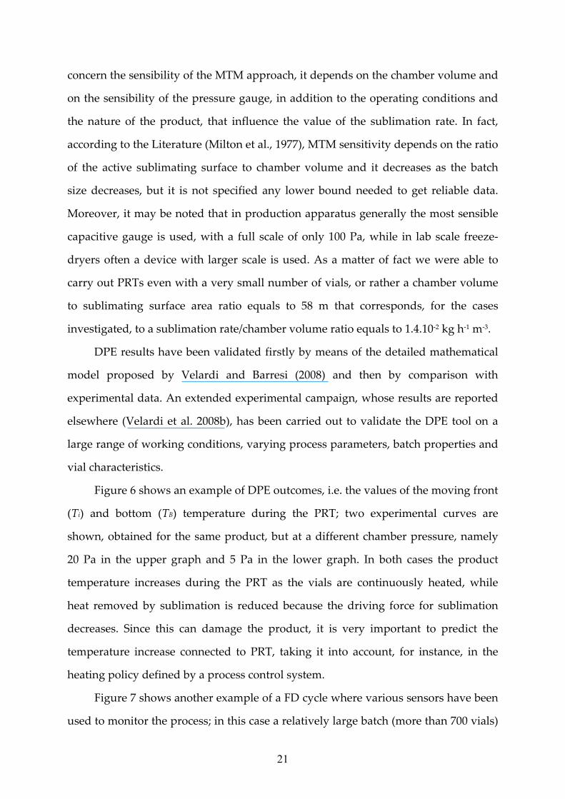
concern the sensibility of the MTM approach, it depends on the chamber volume and 

on the sensibility of the pressure gauge, in addition to the operating conditions and 

the nature of  the product,  that  influence  the value of  the  sublimation  rate.  In  fact, 

according to the Literature (Milton et al., 1977), MTM sensitivity depends on the ratio 

of  the active  sublimating  surface  to  chamber volume and  it decreases as  the batch 

size decreases, but  it  is not  specified any  lower bound needed  to get  reliable data. 

Moreover, it may be noted that in production apparatus generally the most sensible 

capacitive gauge  is used, with a  full scale of only 100 Pa, while  in  lab scale  freeze‐

dryers often a device with  larger scale  is used. As a matter of  fact we were able  to 

carry out PRTs even with a very small number of vials, or rather a chamber volume 

to  sublimating  surface  area  ratio  equals  to  58 m  that  corresponds,  for  the  cases 

investigated, to a sublimation rate/chamber volume ratio equals to 1.4.10‐2 kg h‐1 m‐3. 

DPE results have been validated firstly by means of the detailed mathematical 

model  proposed  by  Velardi  and  Barresi  (2008)  and  then  by  comparison  with 

experimental data. An extended experimental campaign, whose results are reported 

elsewhere  (Velardi et al. 2008b), has been carried out  to validate  the DPE  tool on a 

large range of working conditions, varying process parameters, batch properties and 

vial characteristics.  

Figure 6 shows an example of DPE outcomes, i.e. the values of the moving front 

(Ti)  and  bottom  (TB)  temperature  during  the  PRT;  two  experimental  curves  are 

shown, obtained for the same product, but at a different chamber pressure, namely 

20 Pa  in  the upper graph  and  5 Pa  in  the  lower graph.  In both  cases  the product 

temperature  increases during  the PRT  as  the  vials  are  continuously  heated, while 

heat  removed by  sublimation  is  reduced because  the driving  force  for  sublimation 

decreases.  Since  this  can  damage  the  product,  it  is  very  important  to  predict  the 

temperature  increase  connected  to PRT,  taking  it  into  account,  for  instance,  in  the 

heating policy defined by a process control system. 

Figure 7 shows another example of a FD cycle where various sensors have been 

used to monitor the process; in this case a relatively large batch (more than 700 vials) 

22

of lactose solution, with no empty vial as radiation shield, is considered. In the upper 

graph  the  temperature at  the bottom of  the product estimated by DPE  is compared 

with  the  value measured  by  the  thermocouple  inserted  into  a  vial  (close  to  the 

bottom): measured and estimated values are  in good agreement until the PD  in the 

monitored  vial  is  completed  (but  in  the monitored  vial  ice  sublimation  seems  to 

terminate much earlier than in the rest of the batch).  

The  water  vapour  concentration  in  the  chamber,  measured  using  the 

Panametrics moisture  sensor,  as well  as  the pressure  ratio between  the Pirani  and 

Baratron  sensors  are  shown  in  the  middle  and  lower  graph  respectively;  in  the 

middle graph  the results obtained  for  the same experiment using  the QMS are also 

given: here the time evolution of the ionic current corresponding to mass 18 divided 

by the total pressure reading made by the QMS is shown. The response of the three 

devices is consistent, and taking as estimation of the end of PD the point where the 

signal reaches a minimum and constant value, a time of about 28‐29 hours results in 

all cases. Actually all  the devices measure  the concentration, or partial pressure, of 

water,  even  if  adopting  a  different  principle;  as  the  chamber  gas  composition  is 

dependent on the sublimation rate, and this is generally strongly reduced at the end 

of PD, a large variation of its value can be easily captured and used as indication of 

end of sublimation step, but, as already discussed, it must be taken into account that 

this is an indirect measurement, affected by several variables, and problems can arise 

changing  the  scale of  the  apparatus,  the  size of  the batch,  the method of pressure 

control  in  the  chamber,  or  even  the  nature  of  the  product.  The  variation  of  the 

sublimation rate, estimated by the initial slope of the pressure rise curve, is shown in 

the upper graph; it can be noted that the sublimation rate reduces almost to zero in 

correspondence  of  the  point  where  also  the  signal  of  the  other  devices  reach  a 

minimum,  but  the  same  signal  starts  to  drop  only when  the  sublimation  rate  is 

already very low. 

The  shape  of  the  curves  obtained with  the different devices  is  anyway  quite 

different.  The  moisture  sensor  shows  quite  a  typical  behaviour:  after  the  total 

23

pressure has been reduced  to  the operating value  the signal sharply  increases  first, 

and  after  reaching  a maximum  slowly  decreases  for  almost  all  the  PD,  to  drop 

toward  the  end. This behaviour had been already described by Genin  et al.  (1999) 

who explained the slow decrease with the slight reduction in the drying rate due to 

increased thickness of the dry layer and, thus, of the mass transfer resistance, in the 

phase of almost linear variation of residual ice with time; the fast drop was explained 

with  a  large  reduction  in  the  sublimation  rate.  Comparison  with  the  actual 

sublimation  rate,  shown  in  the  upper  graph,  evidences  that  the  explanation  is 

probably more  complicated. The moisture  sensor was  considered very  sensible by 

the first authors that studied it, being able to sense as few as 0.3% of the vials with ice 

remaining  (Roy and Pikal, 1989);  in  fact, variation  in  the signal are  large enough  to 

detect  the  end  of  PD,  but  is  suffers  for  low  accuracy,  that  strongly  limits  the 

possibility  of  accurately  estimating  the  amount  of  sublimated  water  from  the 

integration  of  the moisture  sensor  signal,  and  low  response  time, mainly  due  to 

water desorption from alumina, as noted by Genin et al. (1999) who reported that in 

the third phase the water desorption rate from the porous alumina could be an order 

of  magnitude  greater  than  desorption  from  the  product  at  the  beginning  of 

secondary drying.  

The QMS requires a relatively  long  initial  time  interval  for  the stabilisation of 

the pressure  inside  it; after  that,  the  signal  remains almost constant, until  it drops, 

similarly to the moisture sensor. It can be concluded that, in case of water solvent, the 

performances may  be  comparable  to  that  of  the moisture  sensor,  but  it must  be 

reminded that calibration is extremely difficult for QMS, the drift of the baseline may 

be large, the cost is much higher and operation require caution. 

The use of the two pressure gauges, in our opinion, offers the best ratio between 

cost and performance:  the signal remain practically constant, until  it starts  to drop, 

and  the use of  the ratio of  the  two pressure signals,  instead of a simple differential 

measure, allows a good sensitivity. The presence of a leakage valve for the chamber 

pressure control did not give  significant  trouble  in our  case, differently  from what 

24

reported by Mayeresse et al.  (2007), even  if  it  can  cause negative  spikes after each 

PRT,  and  the  system  can  be  applied  also  in  case  the  total  pressure  is  controlled 

manipulating  the valve on  the vacuum pump, as shown  in Figure 5, even  if  in  this 

case  the  typical saw‐tooth behaviour appears. The only  inconvenient  that has been 

observed is the fact that sometimes the ratio of the two pressure gauges, at the end of 

PD, can show a baseline signal shift, mainly due to the relatively low accuracy of the 

Pirani  instrument  that  can  make  uncertain  the  determination  of  the  end  of 

sublimation, but the decrease is initially very sharp and in very good agreement with 

the signal of the other devices. 

The  previous  considerations may  change  if  a  third  component  is  present  in 

addition to inert and water (as in the case of use of mixed solvents). In that case the 

response  of  the  Pirani will  be  affected  by  the  presence  of  the  new  species,  being 

unable  to  discriminate,  even  if  the  signal will  get  close  to  that  of  the  capacitive 

gauges when the composition of the chamber becomes constituted only by inert. The 

moisture  sensor  response  in  principle  is  independent  of  the  presence  of 

hydrocarbons,  freon  and  carbon  dioxide,  but  can  be  affected  by  low  molecular 

weight alcohols, even if Roy and Pikal (1989) report to have used it for lyophilization 

of  solutions  containing  up  to  10%  ethanol  without  problems.  The  residual  gas 

analyzer in this case can obviously work efficiently and monitor the different species 

simultaneously. In any case it must be taken into consideration that the response of 

all these devices can be biased by the fact that the atmosphere that they measure  is 

not exactly  the average one  in  the chamber and  this depends on  the positioning of 

the  sensor,  on  the  use  of  controlled  leakage  and  on  the  hydrodynamics  of  the 

chamber:  the moisture  sensor  can  be positioned  properly  in  the  chamber,  but  the 

movements  of  the  shelf  for  stoppering  limit  generally  its  use  to  a  peripherical 

position, while the Pirani is connected to the chamber by a short duct and the QMS 

has to sample the gas from the chamber. This aspect will surely deserve an accurate 

investigation in the next future. 

It can be remembered that the cold plasma ionization device also measures the 

25

water  concentration  in  the  chamber  and  gives  a  response  curve  similar  to  the 

previous ones: the sensitivity seems to be very high in that case, but the uncertainty 

on  the  final point determination,  the problem of calibration and  the dependence of 

the response on the probe location must be considered also in that case (Mayeresse et 

al., 2007). 

As  concerns  the detection of  the end of  sublimation, as discussed above,  it  is  

generally assumed in previous works that it corresponds to the decrease of the signal 

to a low constant value, but it has been already pointed out that it may be difficult to 

define  a  numerical  criterion  and  an  uncertainty  of  a  few  hours  can  derive:  a 

significant difference in the value of the first derivative (end of plateau value), a zero 

value for the first derivative (end of the sharp signal decrease) or a zero value for the 

second derivative  (inflection point  in  the middle of  the sharp signal decrease) have 

been proposed, but without a  link  to a  theoretical background, while  in  the case of 

the moisture sensor, on the base of an inspectional analysis, a special function called 

SEP(t)  has  been  proposed which makes  use  of  the  values  of  the  total  and  partial 

pressure  in  the chamber and of  the partial pressure  in  the condenser  (Genin et al., 

1996). It must be also considered that the exact determination of the end point with 

the previous  type of sensors may be made  intrinsically difficult by  the  fact  that  the 

desorption rate from the fraction of dried material and from the chamber walls may 

be comparable with the sublimation rate at the end of the PD. 

A last comment concerns the duration of the period in which the signal drops; 

this is surely related to the heterogeneity of the batch (compare for example the case 

shown  in  Figure  5,  where  also  a  different  method  for  total  pressure  control  is 

adopted), and can be quite  long, e.g. about 4‐5 hours  in the case shown  in Figure 7 

which  refers  to  a  relatively  large  batch  where  the  side  vials  can  be  affected  by 

radiation;  in  any  case,  as  shown,  this  corresponds  only  the  very  last  period  of 

sublimation  rate decaying  (see  the upper graph).  It must be stressed  that  the point 

where the signal start decreasing with a large slope does not correspond to the point 

where some vials have completed drying:  in fact, Roy and Pikal (1989) and Tang et 

26

al. (2005) have evidenced that the signal of the moisture sensor does not change slope 

even when a significant  fraction of  the vials have completed PD;  these results have 

been confirmed using the different sensors by our experiments carried out on a batch 

in which the heat flow was different on purpose for a fraction of the vials, stopping 

the cycle and measuring the residual water in the different vials. 

DPE temperature estimations are consistent almost up to the main drying end‐

point, as detected by Pirani‐Baratron pressure ratio, QMS and Panametrics moisture 

sensor.  One  point  to  be  evidenced  is  that  generally  the  estimated  product 

temperature decreases nearby  the end‐point, but  this drop may be only an artefact 

because  a  fraction  of  vials,  the  edge‐vials,  has  already  finished  sublimating while 

DPE continues interpreting pressure rise curves assuming batch uniformity, or rather 

a  constant  number  of  sublimating  vials.  Thus,  a  decrease  in  pressure  rise, 

corresponding to a lower sublimation rate, may be interpreted by the DPE algorithm 

as a reduction of the front temperature, even if must be pointed out that generally the 

DPE predict quite accurately the interface temperature, while in these conditions it is 

the  prediction  of  the mass  transfer  resistance  that  becomes  less  reliable,  as  it  is 

modified for compensation. As a matter of fact it can be noticed in the upper graph 

that  the estimated  temperature actually  start decreasing when  the  sublimation  rate 

becomes significantly lower, and this can approximately correspond, as discussed in 

the previous paragraph, to the time where some vial have completed ice sublimation. 

This decrease  in  the  interface  temperature  estimated by  a MTM method was 

already reported (Tang et al., 2005), and actually Oetjen and Haseley (2004) proposed 

to use it as an indication of end of sublimation; according to the results shown this is 

not correct, or at  least should be  interpreted as an  indication of end of  the  fist vial, 

but in our opinion this criterion is not very robust. Anyway the end of PD could be 

reasonably  estimated  by  extrapolating  the  predictions  of  the  interface  position 

obtained  in  the  initial part of  the run. A better way  to detect  the main drying end‐

point  could  be  by  assessing  the  solvent  flux  evolution  estimated,  for  instance, 

through PRT or using a balance; anyway this information must be used with caution 

27

and should be better coupled with information coming from other devices. 

Beside  the  product  state,  DPE  estimates  the  overall  heat  transfer  coefficient 

(between the heating fluid and the frozen product) as well as the product resistance 

to mass  transfer. To  this purpose  it must be  remembered, as discussed before,  that 

the  mathematical  model  used  in  the  DPE  algorithm  (see  Appendix  2)  does  not 

account explicitly  for  the role played by  the vial wall. Actually,  the energy coming 

from the shelf is provided to the product mainly at the bottom of the sample, but to 

same extent is transferred to the product from the vial side too as a consequence of 

conduction  through  the glass  (Velardi and Barresi, 2008). Thus,  the coefficient Kv  is 

an effective heat  transfer  coefficient  that also account  for  the additional heat  input 

due  to  heat  transfer  from  the  vial  sides.  This must  be  taken  into  account when 

comparing  the obtained values with  those  that can be estimated using correlations 

from  the Literature  (e.g. Pikal et al., 1984) or measured with direct methods. As an 

example for 4 mL tubing vials (dv = 14.2∙10‐3 m) over a tray the maximum estimated 

heat  transfer  coefficient  ranged  from  11.5  to  14.1 W m‐2 K‐1  varying  the  chamber 

pressure from 5 to 15 Pa; in the case of 12 mL vials (dv = 20.8∙10‐3 m) Kv varied from 5.4 

(Pc = 5 Pa)  to 9.7 W m‐2 K‐1  (Pc = 20 Pa)  (Velardi et al., 2008b). Figure 9,  that will be 

discussed in the following paragraph about the design of a control system, gives an 

example of the in‐line estimations of Kv, considering also a change of the set‐point of 

the chamber pressure during the cycle. The previous values are consistent with those 

calculated using the correlations of Pikal et al. (1984) and in good agreement with the 

values reported by Hottot et al. (2005), taking into account the additional resistance 

due to the steel tray that approximately halved the value of the overall heat transfer 

coefficient, according to Oetjen and Haseley (2004). 

As  said  before, when  side‐wall  radiation  gives  a  non‐negligible  (but  limited) 

contribution to the energy balance, as  in the case shown  in Figure 5, DPE  is able to 

take  it  into  account:  here Kv  =  40.0 W m‐2 K‐1  is  estimated  by DPE,  a  significantly 

higher  effective  heat  transfer  coefficient  than  in  the  runs  carried  out  at  the  same 

pressure (Pc = 15 Pa), but where the vials has been shielded with a row of empty vials 

28

and were placed over a tray. 

 

 

Control of the primary drying stage 

 

Poor process control is a limitation of the current technology due to the difficulty of 

measuring  the parameters of  interest  (product  temperature and  interface position). 

Currently, even the most advanced industrial freeze‐dryers have control systems that 

are  no more  than  data  acquisition  systems  for  certain  key  variables  (Liapis  et  al., 

1996).  Control  actions  are  often  based  on  the  monitored  data  and  on  empirical 

information obtained in previous experimental runs carried out with the product of 

interest. 

A  major  limitation  concerning  the  control  of  FD  of  pharmaceuticals  at  the 

manufacturing  scale was  the  fact  that  regulatory guidance  imposed  to operate  the 

process  in  open  loop,  so  that  only  an  activity  of monitoring was  allowed  during 

production. Nevertheless, during  the phase of  cycle development, which  is  carried 

out at laboratory or pilot scale, it would be very useful to have an in‐line control that 

minimises the drying time, taking into account the final quality of the product. Cycle 

development, in fact, can be expensive and highly time consuming, but no regulatory 

restrictions apply during this phase, where the use of an efficient control system can 

give significant advantages.  

Guidance  for  Industry PAT  (Process Analytical Technology)  issued by  the US 

Food  and  Drug  Administration  in  September  2004  introduces  some  novelty, 

encouraging  the design,  the analysis and  the  control of  the manufacturing process 

through  timely  measurements  (i.e.  during  processing)  of  critical  quality  and 

performance attributes of raw and in‐process materials and processes, with the goal 

of ensuring final product quality. The goal of PAT is to enhance understanding and 

control of  the manufacturing process as quality should not be  tested  into products, 

but it has to be built‐in or it should be by design. It has been recently shown that an 

29

in‐line  adaptive  control  procedure  aiming  to minimise  the  drying  time  is  feasible 

using some of the monitoring devices described in the previous section (Tang et al., 

2005; Velardi et al. 2005b; Fissore et al., 2008). 

In this section the application of DPE for the optimisation and control of the PD 

is presented:  the goal  is  to show  that  it can be used  to realise a control  tool able  to 

reduce the drying time using an optimal control strategy for the heating shelf, which 

continuously  adjusts  the heating  fluid  temperature  throughout  all  the PD. By  this 

way,  it  is  possible  to maintain  the  product  temperature  just  below  a  limit  value, 

selected  by  the  user,  thus  avoiding  to  overcome  the  collapse  temperature  of  the 

product.  This  tool  allows  also  to  determine with  few  tests  the  optimal  FD  cycle 

recipe. This novel control software, named LyoDriver, uses the estimates of the time 

varying  temperature of  the product, of  the effective global heat  transfer and of  the 

diffusivity coefficient obtained by means of DPE, as well as some process variables 

(i.e. the temperature of the fluid, the pressure in the chamber and the cooling rate of 

the  freeze  dryier)  and  a  simplified mathematical model  for  the  PD  validated  by 

Velardi and Barresi  (2008). The controlled variable  is  the maximum  temperature of 

the product, while the manipulated variable is the temperature of the heating fluid. 

The goal  is  to maintain  the  temperature of  the product  as  close  as possible  to  the 

maximum allowable value. 

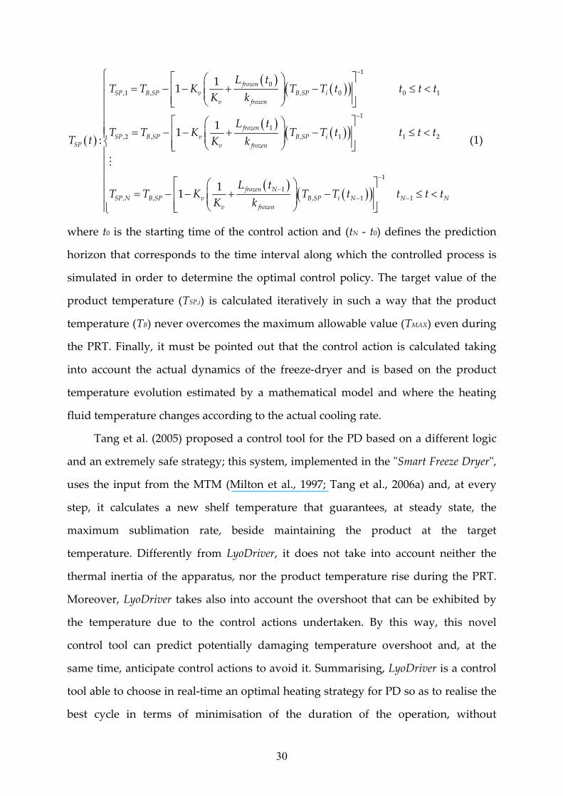
If  a model‐based  predictive  approach  is  used,  the  optimal  sequence  of  shelf 

temperature  set‐points,  TSP,i,  is  calculated  as  a  piecewise‐linear  function  imposing 

that the value of the product temperature at the bottom, TB, is equal to its target value 

TB,SP: 

30

1

0

,1 , , 0 0 1

1

1

,2 , , 1 1 2

1

, , ,

11

11

:

11

frozen

SP B SP v B SP i

v frozen

frozen

SP B SP v B SP iSP v frozen

frozen N

SP N B SP v B SP

v frozen

L tT T K T T t t t t

K k

L tT T K T T t t t t

T t K k

L tT T K T

K k

1

1 1i N N NT t t t t

  (1) 

where  t0  is  the starting  time of  the control action and  (tN  ‐  t0) defines  the prediction 

horizon  that corresponds  to  the  time  interval along which  the controlled process  is 

simulated  in order  to determine  the optimal control policy. The  target value of  the 

product  temperature  (TSP,i)  is  calculated  iteratively  in  such  a way  that  the product 

temperature (TB) never overcomes the maximum allowable value (TMAX) even during 

the PRT. Finally,  it must be pointed out  that  the control action  is calculated  taking 

into  account  the  actual dynamics  of  the  freeze‐dryer  and  is  based  on  the product 

temperature  evolution  estimated  by  a mathematical model  and where  the heating 

fluid temperature changes according to the actual cooling rate.  

Tang et al. (2005) proposed a control tool for the PD based on a different logic 

and an extremely safe strategy; this system, implemented in the ʺSmart Freeze Dryerʺ, 

uses  the  input  from  the MTM  (Milton et al., 1997; Tang et al., 2006a) and, at every 

step,  it  calculates  a  new  shelf  temperature  that  guarantees,  at  steady  state,  the 

maximum  sublimation  rate,  beside  maintaining  the  product  at  the  target 

temperature. Differently  from  LyoDriver,  it  does  not  take  into  account  neither  the 

thermal  inertia of  the apparatus, nor  the product  temperature  rise during  the PRT. 

Moreover, LyoDriver  takes also  into account  the overshoot  that can be exhibited by 

the  temperature  due  to  the  control  actions  undertaken.  By  this  way,  this  novel 

control  tool  can  predict  potentially  damaging  temperature  overshoot  and,  at  the 

same time, anticipate control actions to avoid it. Summarising, LyoDriver is a control 

tool able to choose in real‐time an optimal heating strategy for PD so as to realise the 

best  cycle  in  terms  of  minimisation  of  the  duration  of  the  operation,  without 

31

impairing product quality. 

In order  to  test LyoDriver  some FD  cycles were  carried out, varying both  the 

number of the vials and the total pressure in the chamber. A typical result is shown 

in Figure 8: the mean values of several temperatures (detected by thermocouples) are 

shown, together with the ice temperature at the bottom of the vial estimated by DPE. 

As it has been previously pointed out, this curve shows a good agreement with the 

experimental data until the thermocouples are in contact with the ice. Finally, it can 

be  observed  that,  thanks  to  the  policy  of  the  controller,  the  maximum  product 

temperature,  both  estimated  and  measured  experimentally,  never  overcomes  the 

limit value  fixed by  the user  (equals  to 241 K  in  this run) and,  thus,  the maximum 

allowable heating rate is exploited throughout all PD, thus minimising the duration 

of this step.  

Figure 9 shows some  results obtained using LyoDriver  to monitor and control 

the PD  in  case of  larger vials. After 5 h  from vacuum,  chamber pressure has been 

reduced  (see upper graph)  in order  to  investigate how LyoDriver  controller acts  in 

case  of  imposed  transients:  according  to  Literature  and  as  shown  in  Figure  10 

(middle  graph),  both  product  temperature  and  heat  transfer  coefficient,  estimated 

through DPE, decrease when  the pressure  is  reduced; as a  consequence, LyoDriver 

rises fluid temperature in order to maximise the sublimation rate, beside maintaining 

the product temperature close to its limit as shown in the lower graph of Figure 9. 

The  progressive  reduction  of  the  estimated  Kv  is  not  surprising,  and  is  a 

consequence of the fact that the estimation of Kv is strongly related to that of the mass 

transfer  resistance, which  is  affected  by  a  larger uncertainty  at  very  low  chamber 

pressure, as already evidenced also by Tang et al. (2006b); in any case the estimations 

of  the  two parameters compensate each other and  the controller  is able  to estimate 

the evolution of the product temperature with good accuracy. 

 

 

Conclusions  

32

 

Monitoring  of PD  is  a  subject  of  remarkable  importance  and  several  studies  have 

been focused on this topic in the past, most of them based on either invasive methods 

or even non‐intrusive techniques that can be surely improved.  

The use  of  thermocouples, pressure  gauges, mass  spectrometer  and moisture 

sensor  for  in‐line  monitoring  of  the  PD  has  been  addressed,  pointing  out  and 

comparing  the  results  that can be obtained. The couple of capacitance and  thermal 

conductivity  gauges  can  be  very  useful  to  detect  the  end‐point  of  the  PD  and  its 

measurement  seems  even  more  sensitive    than  that  of  the  moisture  sensor 

investigated in this work (especially if the ratio of their output is considered). In any 

case all  the previous systems suffer a strong  limitation  for application  in  industrial 

plants as  they are not  steam  sterilisable. An alternative method  for monitoring  the 

PD, based on mass measurements, has been proposed and validated to determine in‐

line the progress state of the process. Other sensors have been recently proposed, and 

have been reviewed, but they are still in the developing stage, are applicable only in 

lab‐scale  equipment,  or  are  quite  expensive.  The most  important  point  is  that  all 

these  systems do not give  any  information  about  the  state of  the product  and  are 

useful  only  for  the  detection  of  the  end  of  PD;  thus,  some  new  instruments  that 

combine the measure of the temperature in the product (observer) or the measure of 

the pressure during the PRT (DPE) with a mathematical model have been presented 

and experimentally  compared with  the  ʺtraditionalʺ  sensors. The proposed devices 

were tested in a wide range of conditions, with a number of vials ranging from about 

40  to 700, different vial sizes and products, chamber pressure varying  from 5  to 20 

Pa.  They  demonstrated  to  give  a  quick  and  reliable  estimations  not  only  of  the 

temperature of  the product, but also of  the position of  the moving  front and of  the 

transfer coefficients, which must be known a priori in most approaches presented in 

the Literature. Reliable estimations of heat and mass transfer coefficients as well as of 

sublimation flow rate can be obtained by this way. On the other hand, the DPE does 

not  give  a  clear  estimation  of  the  end‐point,  at  list  at  the  current  state  of 

33

development, even  if the  information obtained evaluating the sublimation rates can 

be used to this purpose, as shown also by Tang et al. (2005). Moreover, its use, like all 

the MTM‐type approaches,  towards  the end of  the PD can be problematic, and can 

cause  an  excessive  increase  in  the  product  temperature.  Nevertheless,  using  the 

information coming from DPE and Baratron‐Pirani pressure ratio (or from a moisture 

sensor) we get a tool able to both monitor some product‐quality affecting parameters 

as well as the evolution of the process itself.  

Moreover, these devices may be used for controlling and optimising the PD. An 

example of  the application of DPE  in a very  simple control  system has been given 

and it has been shown how it can actually optimise the heating policy for the PD and, 

consequently, minimise the process costs. Moreover, this tool allows to determine the 

optimal  processing  conditions  for  the  PD  by  carrying  out  a  small  number  of 

experimental tests, thus avoiding a  large number of time consuming and expensive 

runs required to determine the optimal recipe in a FD cycle by trial and error. 

 

 

Acknowledgements 

 

Part of  this work was  supported by E.U.  in  the  framework of  the  research project 

LYO‐PRO ‐ Optimization and control of the freeze‐drying of pharmaceutical proteins 

(GROWTH  Project  GRD1‐2001‐40259‐RTD)  and  constitutes  the  dissemination  of 

Deliverable #17  ‐ Suggestions for modification of equipment and control system for 

enhanced freeze‐drying. LyoDriver has been developed with the financial support of 

Telstar (Terrassa, Spain). 

34

Notation 

 

A      cross surface of a sample, m2 

cp      specific heat at constant pressure, J kg‐1 K‐1 

dv      vial diameter, m 

f       vectorial function giving the derivatives of the state 

Fleak      leakage rate, Pa s‐1 

h       vector of equations giving the state space equations of the measures 

Hs      heat of sublimation, J kg‐1 

k      thermal conductivity, J m‐1 s‐1 K‐1 

k1      effective diffusivity coefficient, m2 s‐1 

tK       observer gain 

Kv      overall heat transfer coefficient, J m‐2 s‐1 K‐1 

i      ionic current measured by the QMS, A 

L      total product thickness, m 

Lfrozen      frozen layer thickness, m 

M      molecular weight, kg kmol‐1 

Nv      number of vials in the batch 

P      total pressure (or pressure measured by gauges) 

p      partial pressure, Pa 

R      ideal gas constant, J kmol‐1 K‐1 

Rp      mass transfer resistance in the dried layer, m s‐1 

Rs      mass transfer resistance in stopper, m s‐1 

rsub      sublimation rate, kg m‐2 s‐1 

tS       matrix giving the solution of the dynamic Riccati equation 

t      time, s 

T      temperature, K 

Tgʹ  glass transition temperature for the product in equilibrium with ice 

35

u       vector of the control variables 

V      volume, m3 

x       state space vector 

y       vector of the measured outputs of the system 

z      axial coordinate in the frozen layer, m 

 

Greek letters 

, , ,     variables defined by eq. (A.8) 

      matrix of tuning parameters for the Kalman filter 

  correction coefficient to take into account the heterogeneity of the 

batch 

      mass density, kg m‐3 

 

Subscripts and superscripts 

^       observer estimate 

0      value at t = 0 

(‐1)      PRT before the actual one 

B      sample bottom, corresponding to z = Lfrozen   

c      chamber  

dried     dried product 

f      end of a PRT 

fluid      heating fluid   

frozen    frozen product 

i      sublimating interface, corresponding to z = 0 

in      inert gas 

MAX    maximum value 

meas      measured 

N      pressure rise test number 

shelf      heating shelf 

36

SP      set point 

w      water vapour 

 

Abbreviations 

DPE      Dynamic Parameters Estimation 

DPM     Drying Process Monitoring 

FD      Freeze‐drying 

HG      High Gain 

KF      Kalman Filter 

MTM    Manometric Temperature Measurement 

PC      Personal Computer 

PD      Primary drying 

PRA     Pressure Rise Analysis 

PRT      Pressure Rise Test 

QMS     Quadrupole Mass Spectrometer 

 

37

References 

 

Armstrong, J. G. (1980). Use of the capacitance manometer gauge in vacuum freeze‐

drying. Journal of the Parenteral Drug Association, 34, 473‐483. 

Bardat, A.,  Biguet,  J., Chatenet,  E., Courteille,  F.  (1993). Moisture measurement:  a 

new method  for monitoring  freeze‐drying  cycles.  PDA  Journal  of  Parenteral 

Science and Technology, 47, 293‐299. 

Barresi, A. A.,  Baldi, G.,  Parvis, M., Vallan, A., Velardi,  S., Hammouri, H.  (2007). 

Optimization  and  control  of  the  freeze‐drying  process  of  pharmaceutical 

products. International patent application No PCT/IB2007/051276. International 

Publication  No.  WO2007/116371  A2  (18  October  2007),  World  Intellectual 

Property Organization [Priority data TO2006A000270, 11/04/2006]. 

Barresi, A. A., Velardi, S., Fissore, D., Pisano, R.  (2008). Monitoring and controlling 

processes with complex dynamics using soft sensors. In: Control and optimisation 

of continuous processes, Chapter 7. Ottawa: ISA/O3NEDIA. In press. 

Becerra, V. M., Roberts, P. D., Griffiths, G. W. (2001). Applying the extended Kalman 

filter  to  systems  described  by  non‐linear  differential‐algebraic  equations. 

Control Engineering Practice, 9, 267‐281. 

Bouldoires, J. P. (1969). Etude expérimentale des transferts de chaleur et de masse en 

cours de lyophilisation par mesures diélectriques et par mesure de pression de 

vapeur.  Symposium  on  Thermodynamic  Aspects  of  Freeze‐drying, 

International Institute of Refrigeration, Cleveland, USA. 

Brülls, M., Rasmuson, A.  (2002). Heat  transfer  in  vial  lyophilization.  International 

Journal of Pharmaceutics, 246, 1‐16. 

Brülls,  M.,  Folestad,  S.,  Sparén,  A.,  Rasmuson,  A.  (2003).  In‐situ  near‐infrared 

spectroscopy  monitoring  of  the  lyophilization  process.  Pharmaceutical 

Research, 20, 494‐499. 

Bruttini, R., Rovero, G., Baldi, G. (1986). Impiego di un impianto pilota per lo studio 

cinetico di un processo di  liofilizzazione.  Il  farmaco. Edizione Pratica, 11, 346‐

38

357. 

Bruttini,  R.,  Rovero,  G.,  Baldi,  G.  (1991).  Experimentation  and  modelling  of 

pharmaceutical  lyophilisation  using  a  pilot  plant.  Chemical  Engineering 

Journal, 45, 67–77. 

Chase, D. R. (1998). Monitoring and control of a lyophilization process using a mass 

flow controller. Pharmaceutical Engineering, 18, 11‐17. 

Chouvenc, P., Vessot,  S., Andrieu,  J., Vacus, P.  (2004). Optimization  of  the  freeze‐

drying  cycle:  a new model  for pressure  rise  analysis. Drying Technology,  22, 

1577‐1601. 

Chouvenc, P., Vessot,  S., Andrieu,  J., Vacus, P.  (2005). Optimization  of  the  freeze‐

drying  cycle:  adaptation  of  the  Pressure  Rise Analysis  to  non‐instantaneous 

isolation  valves.  PDA  Journal  of  Pharmaceutical  Science  and  Technology,  5, 

298‐309. 

Christ,  M.  (1994).  Freeze‐drying  plant.  International  Patent  Classification  n. 

WO1994EP02426 19940722. 

Connelly,  J. P., Welch,  J. V.  (1993). Monitor  lyophilization with mass  spectrometer 

gas analysis. Journal of Parenteral Science and Technology, 47, 70‐75. 

Fissore, D., Velardi,  S. A.,  Barresi, A. A.  (2008).  In‐line  control  of  a  freeze‐drying 

process in vial. Drying Technology, 26, 685‐694. 

Galan, M., Velardi, S. A., Pisano, R., Rasetto, V., Barresi, A. A. (2007). A gentle PAT 

approach  to  in‐line  control  of  the  lyophilization  process.  In: New  ventures  in 

freeze‐drying, Refrigeration Science and Technology Proceedings No 2007‐3 (IIR 

& Aerial),  Strasbourg,  France,  7‐9 November  2007. CD‐ROM  Edition,  Institut 

International du Froid, Paris, 17 pp. 

Genin,  N.,  Rene,  F.,  Corrieu,  G.  (1996).  A  method  for  on‐line  determination  of 

residual  water  content  and  sublimation  end‐point  during  freeze‐drying. 

Chemical Engineering and Processing, 35, 255‐263. 

Hottot, A., Vessot,  S., Andrieu,  J.  (2005). Determination  of mass  and heat  transfer 

parameters  during  freeze‐drying  cycles  of  pharmaceutical  products.  PDA 

39

Journal of Pharmaceutical Science and Technology, 59, 138‐1‐53. 

Hottot,  A.,  Peczalski,  R.,  Vessot,  S.,  Andrieu,  J.  (2006).  Freeze‐drying  of 

pharmaceutical proteins  in vials: modeling of  freezing  and  sublimation  steps. 

Drying Technology, 24, 561‐570.  

Jennings, T. A.  (1980). Residual gas analysis and vacuum  freeze drying.  Journal of 

Parenteral Drug Association, 34, 62‐69. 

Jennings,  T.  A.  (1999).  Lyophilization:  introduction  and  basic  principles.  Boca  Raton: 

Interpharm/CRC Press. 

Jennings,  T.  A., Duan, N.  (1995).  Calorimetric monitoring  of  lyophilization.  PDA 

Journal of Pharmaceutical Science and Technology, 49, 272‐282. 

Kessler, W.  J., Davis,  S.  J., Mulhall, P. A.,  Silva, M., Pikal, M.  J., Luthra,  S.  (2004). 

Lyophilizer  monitoring  using  Tunable  Laser  Absorption  Spectroscopy. 

Proceedings of 18th International Forum Process Analytical Chemistry (IFPAC), 

Arlington, VA, USA. 

Liapis, A.  I.  (1987). Freeze drying.  In: Handbook  of  industrial drying  (edited by A. S. 

Mujumdar). Chapter 9, 295‐326. New York: Marcel Dekker, Inc. 

Liapis, A. I., Litchfield, R. J. (1979). Optimal control of a freeze dryer ‐ I. Theoretical 

development and quasi steady‐state analysis. Chemical Engineering Science, 34, 

975‐981. 

Liapis, A.  I., Pikal, M.  J., Bruttini, R.  (1996). Research and development needs and 

opportunities in freeze‐drying. Drying Technology, 14, 1265‐1300. 

Liapis, A. I., Sadikoglu, H. (1998). Dynamic pressure rise in the drying chamber as a 

remote sensing method  for monitoring  the  temperature of  the product during 

the primary drying stage of freeze‐drying. Drying Technology, 16, 1153‐1171. 

Litchfield, R.  J., Liapis, A.  I.  (1982). Optimal control of a  freeze dryer  ‐  II. Dynamic 

analysis. Chemical Engineering Science, 37, 45‐55. 

Mayeresse, Y., Veillon, R.,  Sibille, P. H., Nomine, C.  (2007).  Freeze‐drying process 

monitoring  using  a  cold  plasma  ionization  device.  PDA  Journal  of 

Pharmaceutical Science and Technology, 61, 160‐174. 

40

Milton, N.,  Pikal, M.  J.,  Roy, M.  L., Nail,  S.  L.  (1997).  Evaluation  of manometric 

temperature  measurement  as  a  method  of  monitoring  product  temperature 

during lyophilisation. PDA Journal Pharmaceutical Sciences, 5, 7‐16. 

Monteiro Marques,  J. P., Le Loch, C., Wolff, E., Rutledge, D. N.  (1991). Monitoring 

freeze‐drying by low resolution NMR: Determination of sublimation endpoint. 

Journal of Food Science, 56, 1707‐1728. 

Nail,  S.  L., Gatlin,  L. A.  (1985). Advances  in  control  of  production  freeze‐dryers. 

Journal of Parenteral Science and  Technology, 39, 16‐27. 

Nail, S., Gatlin, L.  (1993). Freeze drying: principles  and practice.  In: Pharmaceutical 

dosage  forms (edited by A. Avis, A. Liebermann, L. Lachmann), Vol. 2, 163‐333. 

Marcel Dekker, New York. 

Oetjen, G. W., Haseley, P. (2004). Freeze‐Drying. Weinheim: Wiely‐VHC. 

Pikal, M. J., Roy, M. L., Shah, S. (1984). Mass and heat transfer in vial freeze‐drying of 

pharmaceuticals: role of  the vial.  Journal of Pharmaceutical Sciences, 73, 1224‐

1237. 

Pisano, R., Rasetto, V., Barresi, A. A., Vallan, A. (2008). Modelling and experimental 

investigation of radiation effects in a freeze‐drying process. Proceedings of 5th 

Chemical  Engineering  Conference  for  Collaborative  Research  in  Eastern 

Mediterranean Countries (EMCC5), May 24‐29, Cetraro, Italy, 4 pp. In press. 

Presser,  I.  (2003).  Innovative  Online  Messverfahren  zur  Optimierung  von 

Gefriertrocknungsprozessen. Ph.D. Thesis. University  of Munich, Department 

of Pharmaceutical Technology, Germany. 

Rambhatla, S., Ramot, R., Bhugra, C., Pikal, M. J. (2004). Heat and mass transfer scale‐

up issues during freeze drying: II. Control and characterization of the degree of 

supercooling. AAPS Pharmaceutical Science and Technology, 5(4), article 58, 9 

pp. (http://www.aapspharmscitech.org). 

Rasetto,  V.,  Marchisio,  D.  L.,  Fissore,  D.,  Barresi,  A.  A.  (2008).  Model‐based 

monitoring  of  a  non‐uniform  batch  in  a  freeze‐drying  process,  in:  ʺ18th 

European  Symposium  on  Computer  Aided  Process  Engineering  (B. 

41

Braunschweig & X. Joulia, Eds.); Computer‐Aided Chemical Engineering Series, 

Vol. 25, paper FP_00210, 6 pp. Elsevier, Amsterdam, CD Edition. 

Remmele, R. L., Stushnoff, C., Carpenter, J. F. (1997). Real‐rime in situ monitoring of 

lysozyme during lyophilization using infrared spectroscopy: Dehydration stress 

in the presence of sucrose. Pharmaceutical Research, 14, 1548‐1555. 

René,  F.,  Genin,  N.,  Corrieu,  G.  (1995).  Procédé  et  dispositif  de  contrôle  de  la 

lyophilisation  sous  vide.  International  application  No  PCT/FR95/00563. 

International  Publication  No.  WO95/30118  (9  November  1995),  World 

Intellectual Property Organization [Priority data 94/05398, 3/05/1994 FR]. 

Rey,  L.  R.  (1961). Automatic  regulation  of  the  freeze‐drying  of  complex  systems. 

Biodynamica, 8, 241‐260. 

Roth,  C., Winter,  G.,  Lee,  G.  (2001).  Continuous measurement  of  drying  rate  of 

crystalline  and  amorphous  systems  during  freeze‐drying  using  an  in  situ 

microbalance technique. Journal of Pharmaceutical Science, 90, 1345‐1355. 

Rovero, G., Ghio,  S., Barresi, A. A.  (2001). Development  of  a prototype  capacitive 

balance for freeze‐drying studies. Chemical Engineering Science, 56, 3575‐3584. 

Roy, M. L, Pikal, M. J. (1989). Process control  in freeze drying: determination of the 

end point  of  sublimation drying  by  an  electronic moisture  sensor.  Journal  of 

Parenteral Science and Technology, 43, 60‐66. 

Sadikoglu,  H.,  Liapis,  A.  I.  (1997).  Mathematical  modelling  of  the  primary  and 

secondary stages of bulk solution  freeze‐drying  in  trays: parameter estimation 

and  model  discrimination  by  comparison  of  theoretical  results  with 

experimental data. Drying Technology, 13, 43‐72. 

Salzberg,  F.  (2007).  Pulsed  Pirani  Vacuum  Gauge.  Abstracts  of  4th  International 

Conference on Lyophilization and Freeze‐Drying. Dublin, 17‐19 October. 

Schelenz,  G.,  Engel,  J.,  Rupprecht,  H.  (1994).  Sublimation  drying  lyophilization 

detected by  temperature profile and X‐ray  technique.  International  Journal of 

Pharmaceutics, 113, 133‐140. 

Snowman,  J. W.  (1991).  Freeze drying  of  sterile  products.  In:  Sterile  pharmaceutical 

42

manufacturing  (edited by M.  J. Groves, W. Olson, M. Anisfeld). Chapter 5, 79‐

108. Buffalo Grove: Interpharm Press. 

Suherman, P. M., Taylor, P. M., Smith, G. (2002). Development of a remote electrode 

system  for  monitoring  the  water  content  of  materials  inside  a  glass  vial. 

Pharmaceuticals Research, 19, 337‐344. 

Tang, X., Pikal, M.  J.  (2004). Design of  freeze‐drying processes  for pharmaceuticals: 

practical advice. Pharmaceuticals Research, 21, 191‐200. 

Tang,  X.  C.,  Nail,  S.  L.,  Pikal,  M.  J.  (2005).  Freeze‐drying  process  design  by 

manometric  temperature  measurement:  design  of  a  smart  freeze‐dryer. 

Pharmaceutical Research, 22, 685‐700. 

Tang, X. C., Nail,  S.L., Pikal, M.  J.  (2006a). Evaluation of manometric  temperature 

measurement,  a  Process Analytical  Technology  tool  for  freeze‐drying:  part  I, 

product  temperature  measurement.  AAPS  Pharmaceutical  Science  and 

Technology, 7(1), article 14, 9 pp. (http://www.aapspharmscitech.org). 

Tang, X. C., Nail, S. L., Pikal, M.  J.  (2006b). Evaluation of manometric  temperature 

measurement  (MTM),  a  Process Analytical  Technology  tool  in  freeze  drying, 

part  III:  heat  and mass  transfer measurement. AAPS  Pharmaceutical  Science 

and Technology, 7(4), article 97, 7 pp. (http://www.aapspharmscitech.org). 

Trelea,  I. C.,  Passot,  S.,    Fonseca,  F., Marin, M.  (2007). An  interactive  tool  for  the 

optimization  of  freeze‐drying  cycles  based  on  quality  criteria.  Drying 

Technology, 25, 741‐751. 

Vallan, A., Corbellini, S., Parvis, M. (2005a). A Plug&Play architecture for low‐power  

measurement  systems.  Proceedings  of  Instrumentation  and  Measurement 

Technology Conference ‐ IMTC 2005, 16‐19 May 2005, Ottawa, Canada, Volume 

1, 565–569. [DOI: 10.1109/IMTC.2005.1604180] 

Vallan, A., Parvis, M., Barresi, A. A.  (2005b). Sistema per  la misurazione  in  tempo 

reale  di massa  e  temperatura  di  sostanze  sottoposte  a  liofilizzazione.  Italian 

Patent Application n. B02005A000320. 

Vallan,  A.  (2007).  A  measurement  system  for  lyophilization  process  monitoring. 

43

Proceedings  of  Instrumentation  and Measurement  Technology  Conference  ‐ 

IMTC  2007,  1‐3  May  2007,  Warsaw,  Poland,  5  pp.  [DOI: 

10.1109/IMTC.2007.379000]. 

Velardi, S. A., Barresi, A. A. (2008). Development of simplified models for the freeze‐

drying process and investigation of the optimal operating conditions. Chemical 

Engineering Research & Design, 86, 9‐22. 

Velardi S., Barresi A. A., Hottot A., Andrieu J. (2005a). Pharmaceuticals freeze‐drying 

in  vials:  a  new  heat  transfer model  including  the  effect  of  the  vial  sidewall. 

Proceedings  of  the  Joint  conference  of AFSIA  and Drying Working  group  of 

EFCE. Paris, France, 12‐13 May, 20‐21. 

Velardi, S. A., Hammouri, H., Barresi, A. A. (2005b). A non‐linear observer for real‐

time monitoring and control of the freeze‐drying process of pharmaceuticals in 

vial. Proceedings of AFSIA 2005 conference, 12‐13 May 2005, Paris, France. 

Velardi,  S.  A.,  Hammouri,  H.,  Barresi,  A.  A.  (2008a).  On  line monitoring  of  the 

primary drying of a freeze‐drying process in vial: High Gain and Kalman filter 

based observers. Chemical Engineering Research & Design. Submitted. 

Velardi, S. A., Rasetto, V., Barresi, A. A. (2008b). The Dynamic Parameters Estimation 

method (DPE): an advanced Manometric Temperature Measurement approach 

for  freeze‐drying  monitoring  of  pharmaceutical  solutions.  Industrial  & 

Engineering Chemistry Research. Submitted. 

 

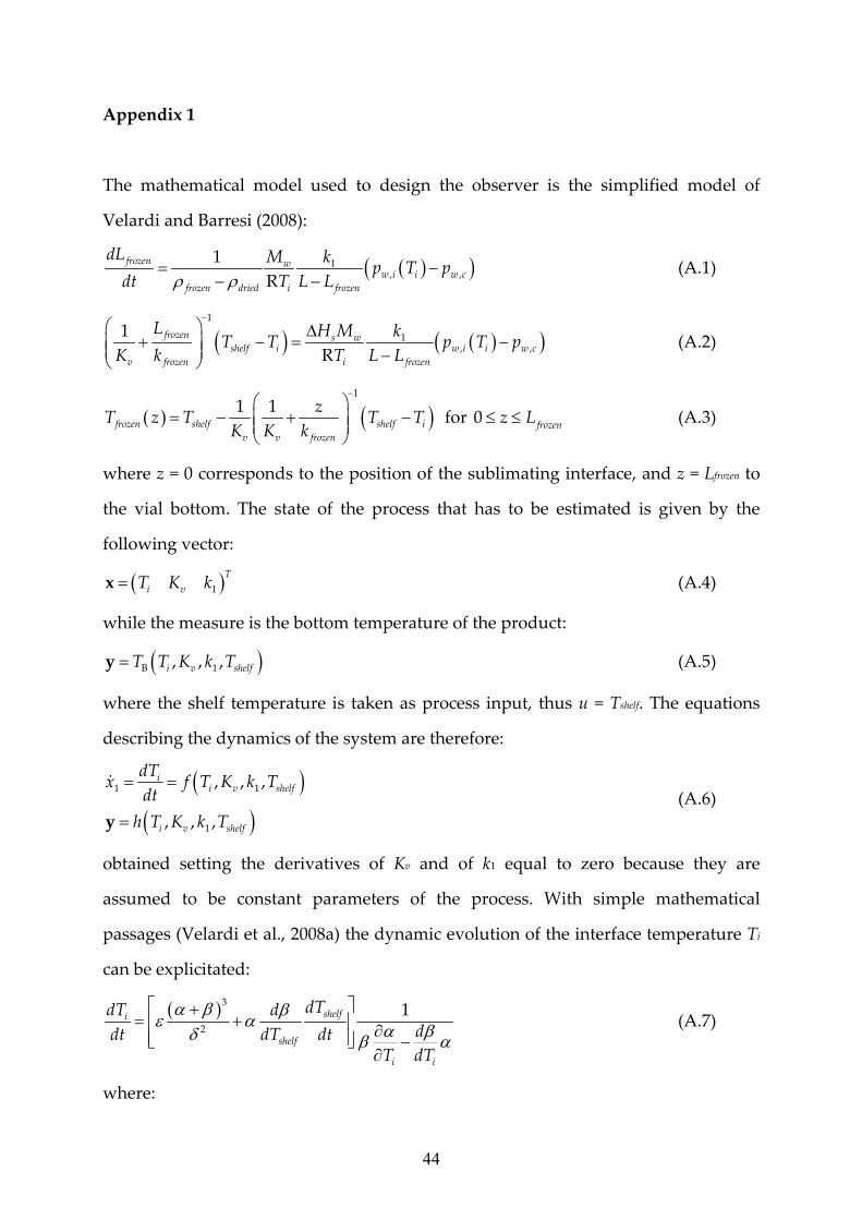
44

Appendix 1 

 

The mathematical model  used  to  design  the  observer  is  the  simplified model  of 

Velardi and Barresi (2008):  

1, ,

1

R

frozen ww i i w c

frozen dried i frozen

dL M kp T p

dt T L L

          (A.1) 

1

1, ,

1

R

frozen s wshelf i w i i w c

v frozen i frozen

L H M kT T p T p

K k T L L

        (A.2) 

1

1 1frozen shelf shelf i

v v frozen

zT z T T T

K K k  for  0

frozenz L   (A.3) 

where z = 0 corresponds to the position of the sublimating interface, and z = Lfrozen to 

the  vial  bottom. The  state  of  the process  that  has  to  be  estimated  is  given  by  the 

following vector: 

1

T

i vT K kx                 (A.4) 

while the measure is the bottom temperature of the product: 

B 1, , ,i v shelfT T K k Ty                      (A.5) 

where  the shelf  temperature  is  taken as process  input,  thus u = Tshelf. The equations 

describing the dynamics of the system are therefore: 

1 1

1

, , ,

, , ,

ii v shelf

i v shelf

dTx f T K k T

dt

h T K k Ty

(A.6) 

obtained  setting  the  derivatives  of  Kv  and  of  k1  equal  to  zero  because  they  are 

assumed  to  be  constant  parameters  of  the  process.  With  simple  mathematical 

passages (Velardi et al., 2008a) the dynamic evolution of the interface temperature Ti 

can be explicitated: 

3

2

1shelfi

shelf

i i

dTdT dddt dT dt

T dT

            (A.7) 

where: 

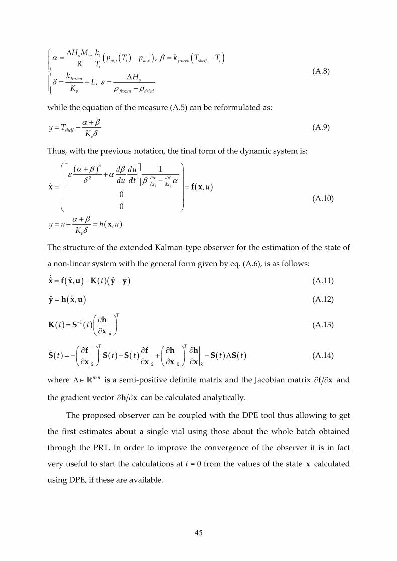
45

1  R

 

s ww ,i i w ,c frozen shelf i

i

frozen s

v frozen dried

H M kp T p , k T T

T

k HL,

K

          (A.8) 

while the equation of the measure (A.5) can be reformulated as: 

shelf

v

y TK

                (A.9) 

Thus, with the previous notation, the final form of the dynamic system is: 

1 1

3

2

1

0

0

d

x dx

v

d du

du dt,u

y u h ,uK

x f x

x

            (A.10) 

The structure of the extended Kalman‐type observer for the estimation of the state of 

a non‐linear system with the general form given by eq. (A.6), is as follows: 

ˆ ˆ ˆ, t x f x u K y y                     (A.11) 

ˆˆ ,y h x u                         (A.12) 

1

T

ˆ

t t x

hK S

x                     (A.13) 

T T

ˆ ˆ ˆ ˆ

t t t t t x x x x

f f h hS S S S S

x x x x         (A.14) 

where  n n  is a semi‐positive definite matrix and the Jacobian matrix  f x  and 

the gradient vector  h x  can be calculated analytically.  

The proposed observer can be coupled with the DPE tool thus allowing to get 

the  first  estimates  about  a  single  vial using  those  about  the whole  batch  obtained 

through  the PRT.  In order  to  improve  the  convergence of  the observer  it  is  in  fact 

very useful to start the calculations at t = 0 from the values of the state  x  calculated 

using DPE, if these are available. 

 

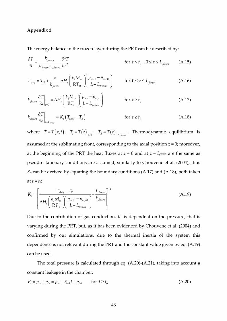
46

Appendix 2 

 

The energy balance in the frozen layer during the PRT can be described by: 

2

2,

frozen

frozen p frozen

kT T

t c z                 for 

0t t ,   0

frozenz L   (A.15) 

, 0 , 0100

0Rw i w cw

i stfrozen i frozen

p pk MzT T H

k T L L

      for  0frozen

z L      (A.16) 

, ,1

0 Rw i w cw

frozen sz i frozen

p pk MTk H

z T L L

         for  0

t t         (A.17) 

frozen

frozen v shelf Bz L

Tk K T T

z

         for 

0t t         (A.18) 

where  ,T T z t , 

0i z

T T t ,  frozen

B z LT T t

.  Thermodynamic  equilibrium  is 

assumed at the sublimating front, corresponding to the axial position z = 0; moreover, 

at  the beginning of  the PRT  the heat fluxes at z = 0 and at z = Lfrozen are  the same as 

pseudo‐stationary conditions are assumed, similarly  to Chouvenc et al.  (2004),  thus 

Kv can be derived by equating the boundary conditions (A.17) and (A.18), both taken 

at t = t0: 

1

0

, 0 , 01

0R

shelf i frozen

v

frozenw i w cws

i frozen

T T LK

kp pk MH

T L L

              (A.19) 

Due  to  the contribution of gas conduction, Kv  is dependent on  the pressure,  that  is 

varying during the PRT, but, as it has been evidenced by Chouvenc et al. (2004) and 

confirmed  by  our  simulations,  due  to  the  thermal  inertia  of  the  system  this 

dependence is not relevant during the PRT and the constant value given by eq. (A.19) 

can be used. 

The total pressure is calculated through eq. (A.20)‐(A.21), taking into account a 

constant leakage in the chamber:  

0c w in w leak inP p p p F t p        for  0

t t               (A.20) 

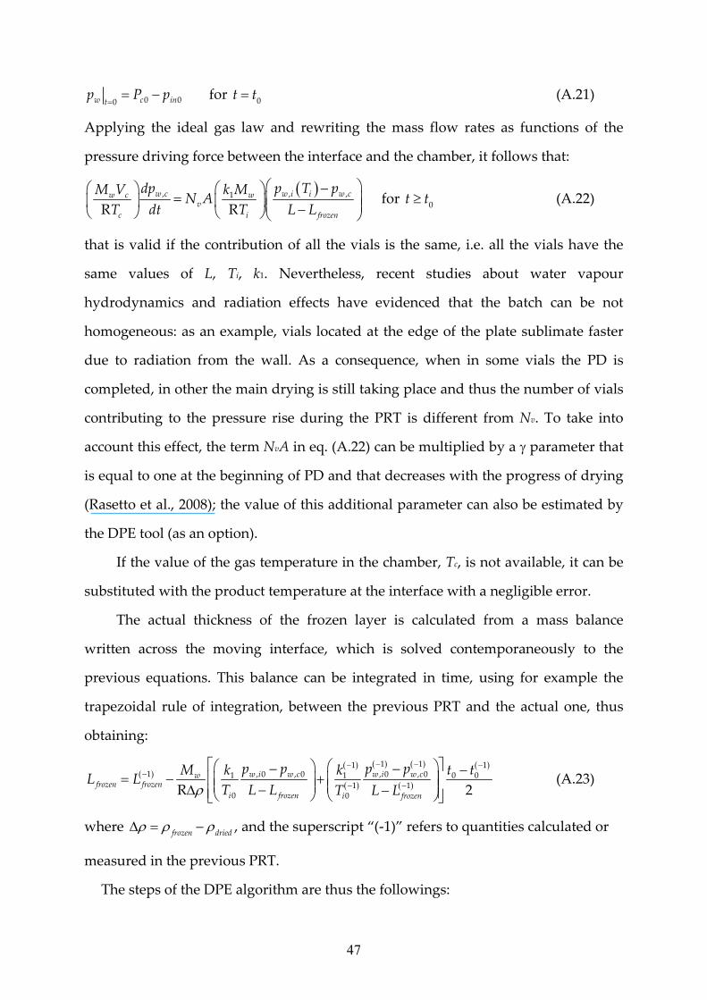
47

0 00w c int

p P p        for  0

t t                     (A.21) 

Applying  the  ideal  gas  law  and  rewriting  the mass  flow  rates  as  functions  of  the 

pressure driving force between the interface and the chamber, it follows that: 

, , ,1

R Rw c w i i w cw c w

v

c i frozen

dp p T pM V k MN A

T dt T L L

     for  0

t t         (A.22) 

that  is valid  if the contribution of all the vials  is the same,  i.e. all the vials have the 

same  values  of  L,  Ti,  k1.  Nevertheless,  recent  studies  about  water  vapour 

hydrodynamics  and  radiation  effects  have  evidenced  that  the  batch  can  be  not 

homogeneous: as an example, vials  located at the edge of the plate sublimate faster 

due  to  radiation  from  the wall. As  a  consequence, when  in  some  vials  the  PD  is 

completed, in other the main drying is still taking place and thus the number of vials 

contributing  to  the pressure  rise during  the PRT  is different  from Nv. To  take  into 

account this effect, the term NvA in eq. (A.22) can be multiplied by a  parameter that 

is equal to one at the beginning of PD and that decreases with the progress of drying 

(Rasetto et al., 2008); the value of this additional parameter can also be estimated by 

the DPE tool (as an option).  

If the value of the gas temperature in the chamber, Tc, is not available, it can be 

substituted with the product temperature at the interface with a negligible error.  

The  actual  thickness  of  the  frozen  layer  is  calculated  from  a  mass  balance 

written  across  the  moving  interface,  which  is  solved  contemporaneously  to  the 

previous  equations. This balance  can be  integrated  in  time, using  for  example  the 

trapezoidal  rule of  integration, between  the previous PRT and  the actual one,  thus 

obtaining: 

1 1 111 , 0 , 0 , 0 , 0 0 01 1

1 10 0R 2

w i w c w i w cwfrozen frozen

i frozen i frozen

p p p pM t tk kL L

T L L T L L    (A.23) 

where  frozen dried

, and the superscript “(‐1)” refers to quantities calculated or 

measured in the previous PRT. 

The steps of the DPE algorithm are thus the followings: 

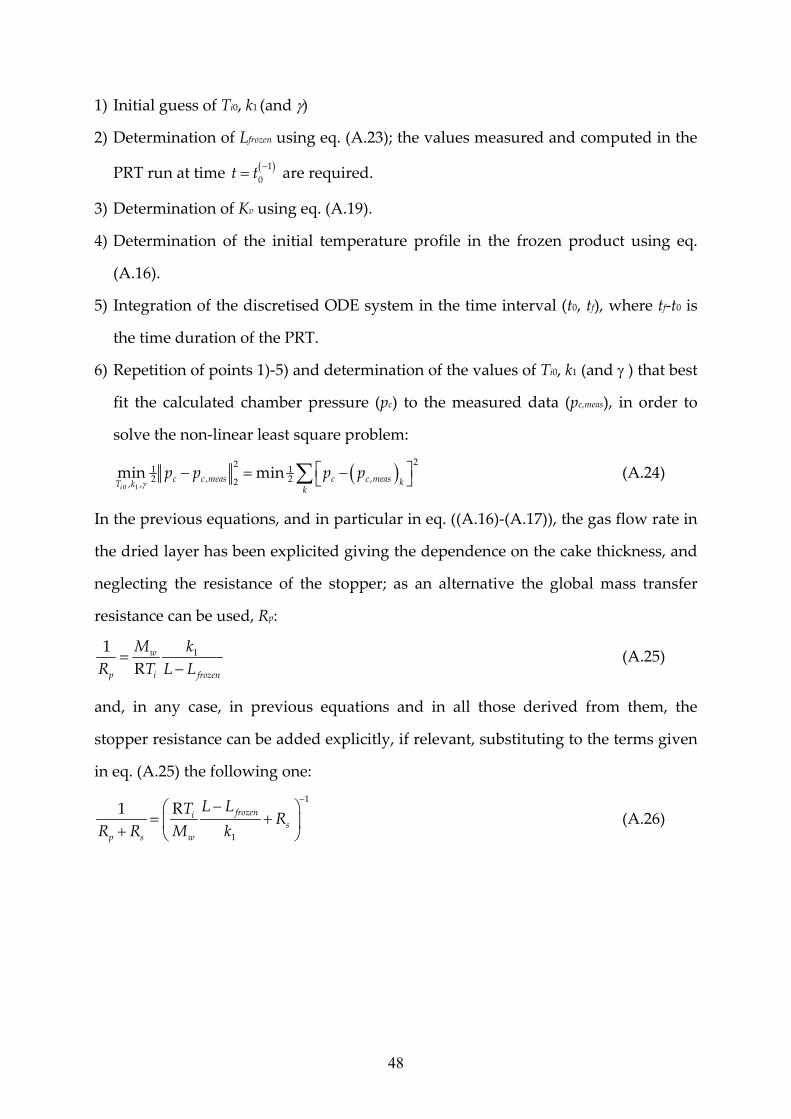
48

1) Initial guess of Ti0, k1 (and ) 

2) Determination of Lfrozen using eq. (A.23); the values measured and computed in the 

PRT run at time  1

0t t  are required. 

3) Determination of Kv using eq. (A.19). 

4) Determination of  the  initial  temperature profile  in  the  frozen product using  eq. 

(A.16). 

5) Integration of the discretised ODE system in the time interval (t0, tf), where tf‐t0 is 

the time duration of the PRT. 

6) Repetition of points 1)‐5) and determination of the values of Ti0, k1 (and  ) that best 

fit  the  calculated  chamber pressure  (pc)  to  the measured data  (pc,meas),  in order  to 

solve the non‐linear least square problem:  

 

0 1

221 12 , 2 ,2, ,

min mini

c c meas c c meas kT kk

p p p p             (A.24) 

In the previous equations, and in particular in eq. ((A.16)‐(A.17)), the gas flow rate in 

the dried layer has been explicited giving the dependence on the cake thickness, and 

neglecting  the  resistance  of  the  stopper;  as  an  alternative  the  global mass  transfer 

resistance can be used, Rp: 

11

Rw

p i frozen

M k

R T L L

                      (A.25) 

and,  in  any  case,  in  previous  equations  and  in  all  those  derived  from  them,  the 

stopper resistance can be added explicitly, if relevant, substituting to the terms given 

in eq. (A.25) the following one: 

1

1

R1 frozenis

p s w

L LTR

R R M k

                  (A.26) 

 

49

List of Figures 

 

Figure 1  Scheme  of  the  LyoMonitor  system:  (1)  multi‐point  thermometer 

equipped with fault diagnosis for product and chamber monitoring; (2) 

proprietary  in‐line  balance;  (3)  signal  acquisition  from  embedded 

devices; (4) capacitive moisture sensor; (5) pressure sensors: capacitance 

manometer  (a)  and  thermal  conductivity  gauge  (b);  (6)  ʺDynamic 

Parameters Estimationʺ (DPE) with fast pressure data acquisition through 

an acquisition board (6a) and valve control for pressure rise test (6b); (7) 

miniaturized radio‐controlled thermometer for the vials weighed by the 

balance;  (8)  ʺsmart  vialʺ  observer  (a)  and  wireless  additional 

thermometer (b); (9) quadrupole mass‐spectrometer.  

 

Figure 2  LyoMonitor interface, showing the in‐line measurements and the control 

panel.  The  reference  numbers  correspond  to  the  devices  shown  in 

Figure  1:  product  temperature  measured  by  some  thermocouples 

inserted in different vials (1) and mass variation measured over 15 vials 

by the special balance (2); the spikes in product temperature are caused 

by the PRT (6). The fluid temperature is also given (3). Some signals are 

not plotted in this case for clarity, but LyoMonitor can show their values: 

moisture  sensor  (4),  pressure  and  Pirani/Baratron  pressure  ratio  (5), 

temperature  of  the  vials  weighed  by  the  balance  (7)  (and  some 

additional  balance  temperatures used  for mass  correction  as Tcold  and 

Tag,cold). The data  refer  to  FD  of  a  10% w/w  sucrose  solution  (Nv  =  98, 

shielded, dv = 14.2∙10‐3 m, L = 7.2∙10‐3 m, Pc = 10 Pa) 

   

Figure 3  Measurements and estimations of  the product  temperature and of  the 

moving front position during the FD of a 10% w/w sucrose solution (Nv 

= 636 on tray, dv = 14.2∙10‐3 m, L = 7.2∙10‐3 m, Pc = 10 Pa).  

50

(a):  Product  temperature  at  the moving  front  (solid  line)  and  at  the 

bottom (dashed line) estimated using the Kalman filter; (o) temperature 

at the bottom of the product measured by a thermocouple.  

(b): Estimated  front  temperature  in vials placed  in different positions 

on the shelf (solid  lines); the average value estimated using DPE ()  is 

shown for comparison. 

(c):  Estimated  product  temperature  profiles  of  some monitored  vials 

(the same shown in graph b) at t = 5000 s after the beginning of the PD.  

(d):  Interface position estimated by  the Kalman  filter  (solid  line)  from 

the temperature measurement (given in graph a) and through DPE ().  

 

Figure 4  Example  of  results  obtained  during  a  FD  cycle  run using  the  special 

balance  with  the  embedded  wireless  temperature  measurement  in 

order to monitor the PD stage of a mannitol‐dextran solution (6‐14% by 

weight, Tg’ = 254 K) in a pilot‐scale freeze‐drier. The freezing phase has 

been run at 223 K for about 5 h, while the main drying has been carried 

out setting the fluid temperature at 293 K and the chamber pressure at 

10 Pa (Nv = 98 on tray, dv = 14.210‐3 m, L = 7.210‐3 m). 

  Upper graph: time evolution of the product mass (line: the gross mass 

of 15 vials containing 1 cm3 of solution each,  including glass vials and 

rising tray, is shown) and average sublimation rate calculated from this 

measure (symbols).  

  Lower  graph:  time  evolution  of  the  heating  fluid  temperature  (solid 

line)  and  of  the  product  temperature  measured  by  thermocouples 

inserted  close  to  the  bottom  into  three  of  the  vials  weighed  by  the 

balance. 

   

Figure 5  Example of the results obtained during a FD cycle run using LyoMonitor 

to follow the primary drying stage of a 10% by weight sucrose solution 

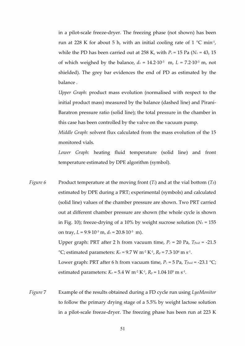
51

in a pilot‐scale  freeze‐dryer. The  freezing phase  (not shown) has been 

run  at  228 K  for  about  5 h, with  an  initial  cooling  rate of  1  °C min‐1, 

while the PD has been carried out at 258 K, with Pc = 15 Pa (Nv = 43, 15 

of which weighed by  the balance, dv = 14.2∙10‐3   m, L = 7.2∙10‐3 m, not 

shielded). The  grey  bar  evidences  the  end  of PD  as  estimated by  the 

balance . 

  Upper Graph: product mass  evolution  (normalised with  respect  to  the 

initial product mass) measured by the balance (dashed line) and Pirani‐

Baratron pressure ratio (solid line); the total pressure in the chamber in 

this case has been controlled by the valve on the vacuum pump. 

  Middle Graph: solvent flux calculated from the mass evolution of the 15 

monitored vials. 

  Lower  Graph:  heating  fluid  temperature  (solid  line)  and  front 

temperature estimated by DPE algorithm (symbol). 

 

Figure 6  Product temperature at the moving front (Ti) and at the vial bottom (TB) 

estimated by DPE during a PRT; experimental (symbols) and calculated 

(solid line) values of the chamber pressure are shown. Two PRT carried 

out at different chamber pressure are shown (the whole cycle is shown 

in Fig. 10); freeze‐drying of a 10% by weight sucrose solution (Nv = 155 

on tray, L = 9.910‐3 m, dv = 20.810‐3  m). 

Upper graph: PRT after 2 h from vacuum time, Pc = 20 Pa, Tfluid =  ‐21.5 

°C; estimated parameters: Kv = 9.7 W m‐2 K‐1, Rp = 7.3104 m s‐1.  

Lower graph: PRT after 6 h from vacuum time, Pc = 5 Pa, Tfluid = ‐23.1 °C; 

estimated parameters: Kv = 5.4 W m‐2 K‐1, Rp = 1.04105 m s‐1.  

 

Figure 7  Example of the results obtained during a FD cycle run using LyoMonitor 

to follow the primary drying stage of a 5.5% by weight lactose solution 

in a pilot‐scale freeze‐dryer. The freezing phase has been run at 223 K 

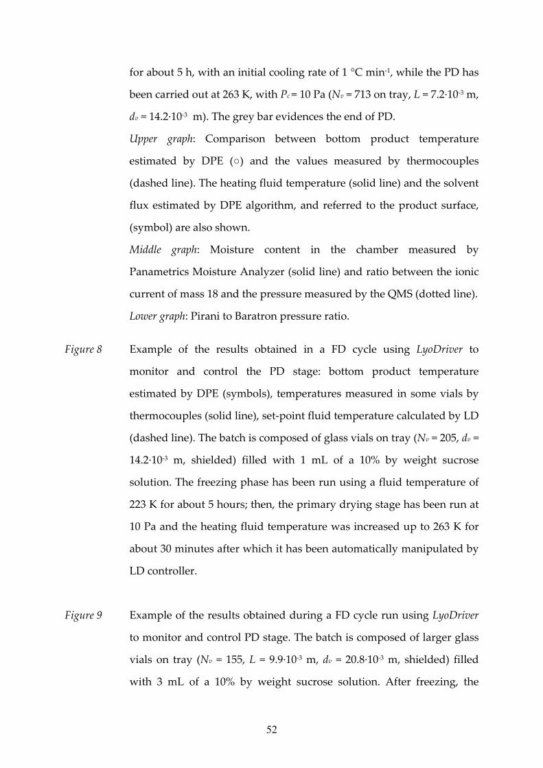
52

for about 5 h, with an initial cooling rate of 1 °C min‐1, while the PD has 

been carried out at 263 K, with Pc = 10 Pa (Nv = 713 on tray, L = 7.2∙10‐3 m, 

dv = 14.2∙10‐3  m). The grey bar evidences the end of PD. 

Upper  graph:  Comparison  between  bottom  product  temperature 

estimated  by  DPE  (○)  and  the  values  measured  by  thermocouples 

(dashed line). The heating fluid temperature (solid line) and the solvent 

flux estimated by DPE algorithm, and referred  to  the product surface, 

(symbol) are also shown. 

Middle  graph:  Moisture  content  in  the  chamber  measured  by 

Panametrics Moisture Analyzer (solid line) and ratio between the ionic 

current of mass 18 and the pressure measured by the QMS (dotted line). 

Lower graph: Pirani to Baratron pressure ratio.  

Figure 8  Example  of  the  results  obtained  in  a  FD  cycle  using  LyoDriver  to 

monitor  and  control  the  PD  stage:  bottom  product  temperature 

estimated by DPE  (symbols),  temperatures measured  in some vials by 

thermocouples (solid line), set‐point fluid temperature calculated by LD 

(dashed line). The batch is composed of glass vials on tray (Nv = 205, dv = 

14.2∙10‐3 m,  shielded)  filled  with  1 mL  of  a  10%  by  weight  sucrose 

solution. The freezing phase has been run using a fluid temperature of 

223 K for about 5 hours; then, the primary drying stage has been run at 

10 Pa and the heating fluid temperature was increased up to 263 K for 

about 30 minutes after which it has been automatically manipulated by 

LD controller. 

 

Figure 9  Example of the results obtained during a FD cycle run using LyoDriver 

to monitor and control PD stage. The batch is composed of larger glass 

vials on  tray  (Nv = 155, L = 9.9∙10‐3 m, dv = 20.8∙10‐3 m,  shielded)  filled 

with  3 mL  of  a  10%  by weight  sucrose  solution. After  freezing,  the 

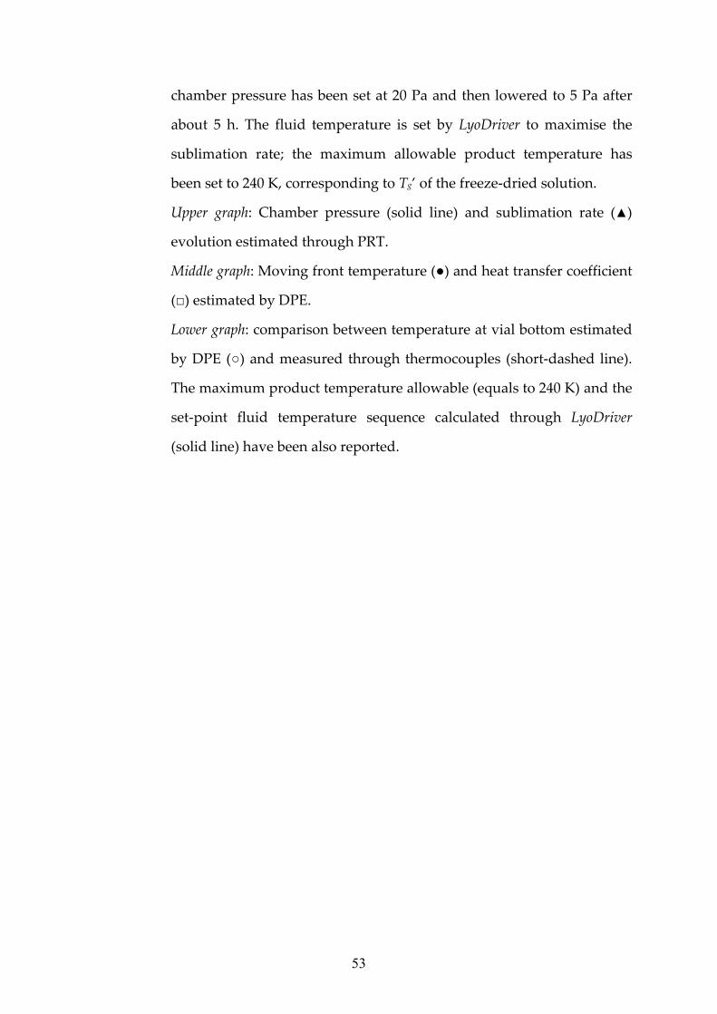
53

chamber pressure has been set at 20 Pa and then lowered to 5 Pa after 

about  5 h. The  fluid  temperature  is  set by LyoDriver  to maximise  the 

sublimation  rate;  the  maximum  allowable  product  temperature  has 

been set to 240 K, corresponding to Tg’ of the freeze‐dried solution.  

Upper  graph:  Chamber  pressure  (solid  line)  and  sublimation  rate  (▲) 

evolution estimated through PRT. 

Middle graph: Moving front temperature (●) and heat transfer coefficient 

(□) estimated by DPE. 

Lower graph: comparison between temperature at vial bottom estimated 

by DPE  (○) and measured  through  thermocouples  (short‐dashed  line). 

The maximum product temperature allowable (equals to 240 K) and the 

set‐point  fluid  temperature  sequence  calculated  through  LyoDriver 

(solid line) have been also reported.  

 

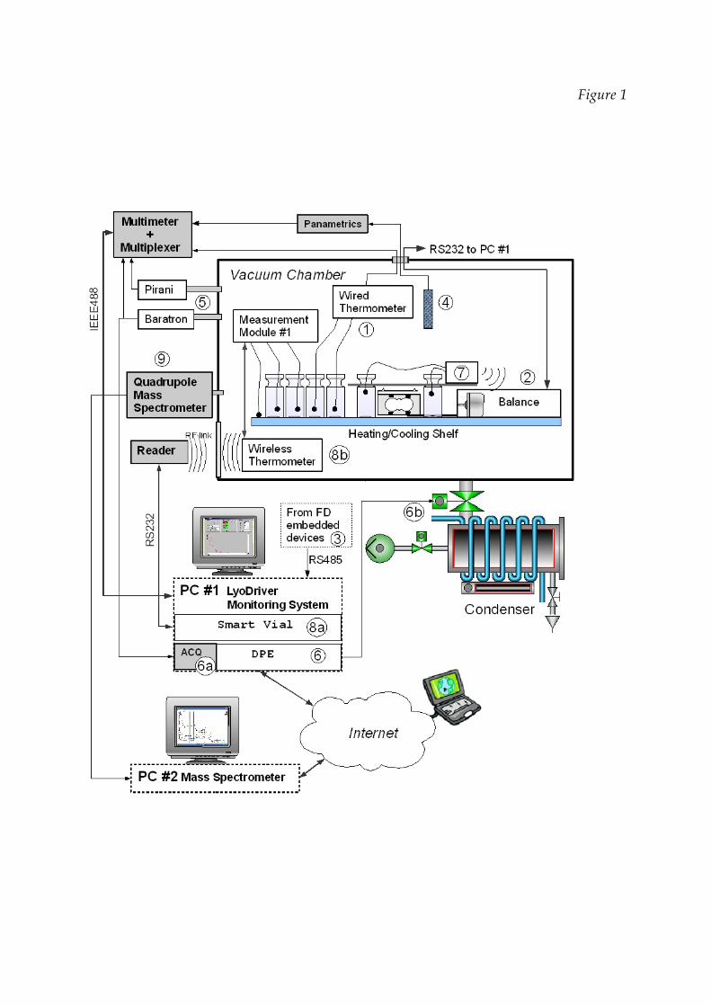
Figure 1 

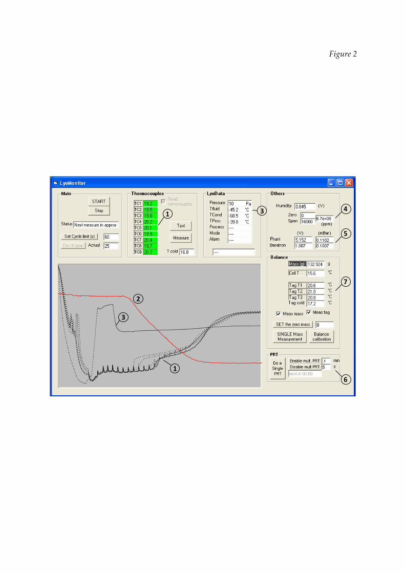
Figure 2 

1 

2 

3 

4 

5 

7 

6 

1

1

2 

3

3

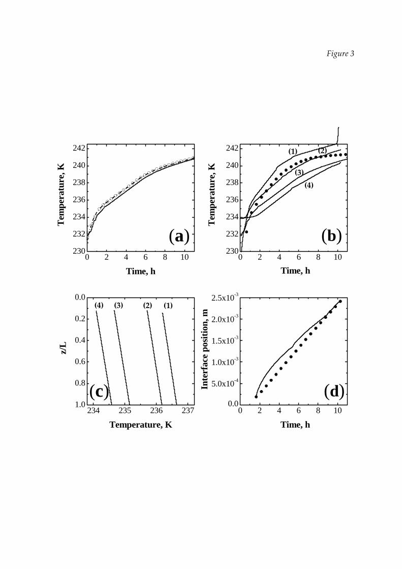
Figure 3 

0 2 4 6 8 10230

232

234

236

238

240

242

Time, h

Tem

pera

ture

, K

0 2 4 6 8 10230

232

234

236

238

240

242

(4)

(3)

(2)(1)

Time, h

Tem

pera

ture

, K

234 235 236 2371.0

0.8

0.6

0.4

0.2

0.0(4) (3) (1)(2)

Temperature, K

z/L

0 2 4 6 8 100.0

5.0x10-4

1.0x10-3

1.5x10-3

2.0x10-3

2.5x10-3

(d)(c)

(b)

Time, h

Inte

rfac

e po

siti

on, m

(a)

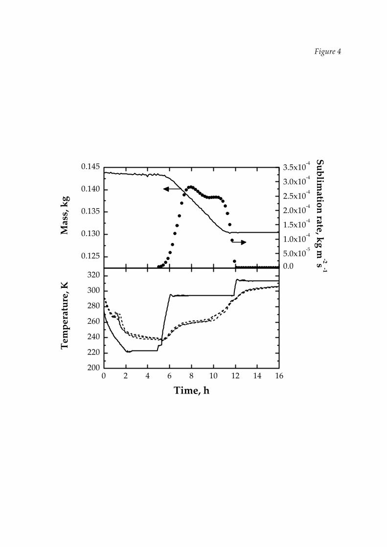
Figure 4 

 

 

 

 

0.0

5.0x10‐5

1.0x10‐4

1.5x10‐4

2.0x10‐4

2.5x10‐4

3.0x10‐4

3.5x10‐4

0.125

0.130

0.135

0.140

0.145

Mass, kg

0 2 4 6 8 10 12 14 16200

220

240

260

280

300

320

Temperature, K

Time, h

 Sublim

ation rate, k

g m

‐2s‐1

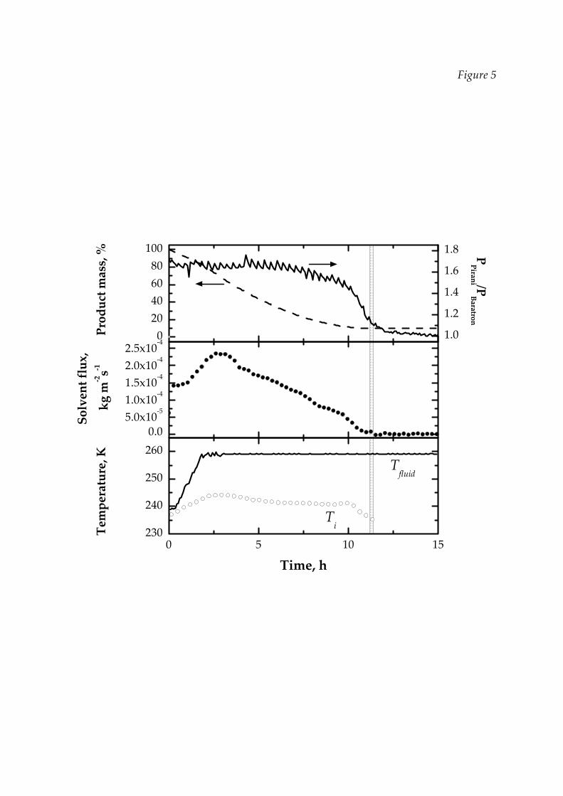
Figure 5 

 

 

 

 

 

 

 

 

 

1.0

1.2

1.4

1.6

1.8

0

20

40

60

80

100

Product mass, %

0.05.0x10

‐5

1.0x10‐4

1.5x10‐4

2.0x10‐4

2.5x10‐4

Solvent flux,

 kg m

‐2s‐1

 PPiran

i /PBaratro

n

0 5 10 15230

240

250

260

Tfluid

Temperature, K

Time, h

Ti

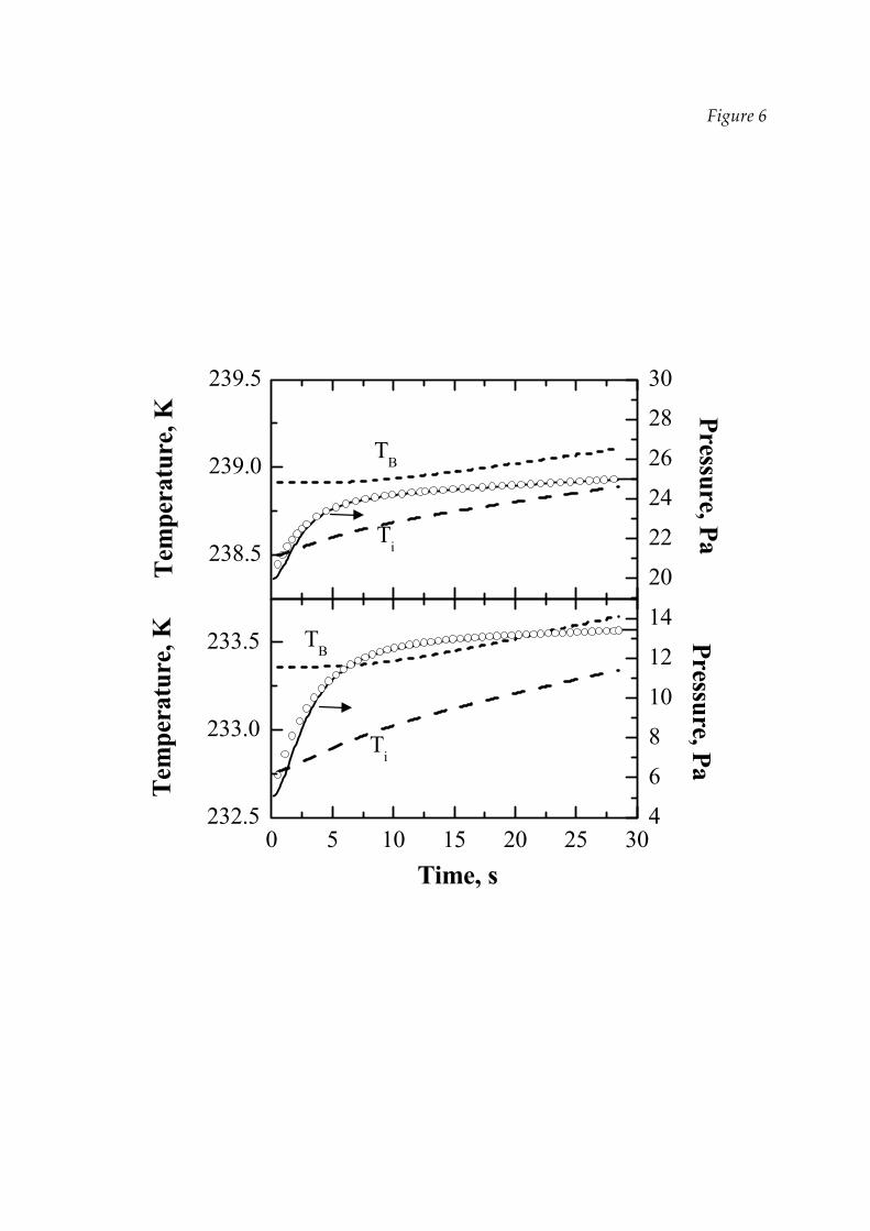
Figure 6 

 

20

22

24

26

28

30

4

6

8

10

12

14

Pressure, Pa

238.5

239.0

239.5

Ti

Tem

pera

ture

, K

TB

0 5 10 15 20 25 30232.5

233.0

233.5

Time, s

Ti

Tem

pera

ture

, K TB

Pressure, Pa

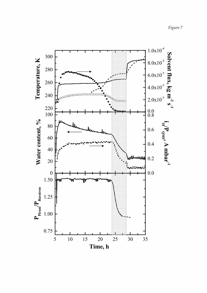
0.0

2.0x10-5

4.0x10-5

6.0x10-5

8.0x10-5

1.0x10-4

220

240

260

280

300

Te

mpe

ratu

re, K

0

20

40

60

80

100

Wat

er c

onte

nt, %

5 10 15 20 25 30 35

0.75

1.00

1.25

1.50

Time, h

P Pira

ni/P

Bara

tron

0.0

0.2

0.4

0.6

0.8 i18 /PQ

MS , A

mbar

-1Solvent flux, kg m

-2 s -1

Figure 7 

   

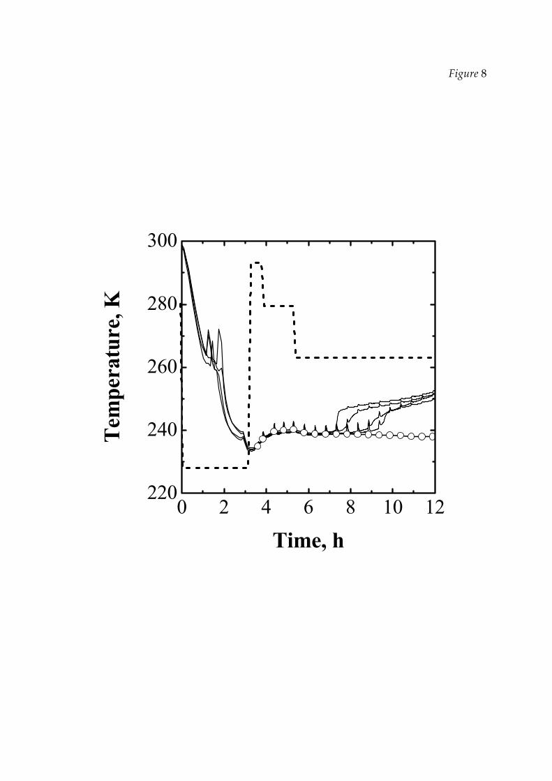
Figure 8 

0 2 4 6 8 10 12220

240

260

280

300

Time, h

Tem

pera

ture

, K

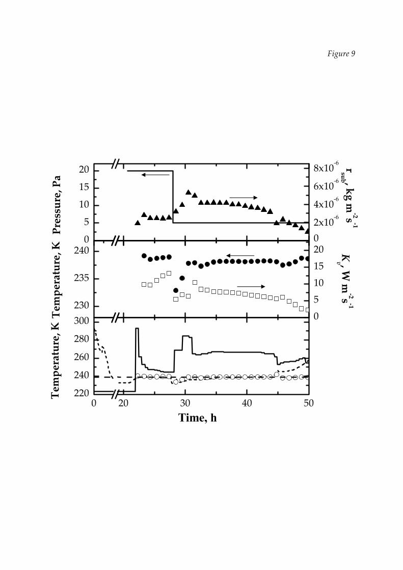
0

2x10‐6

4x10‐6

6x10‐6

8x10‐6

0

5

10

15

200

5

10

15

20

Pressure, Pa

230

235

240

Temperature, K

 rsub , kg m

‐2s‐1

0 20 30 40 50220

240

260

280

300

Temperature, K

Time, h

Kv , W

 m‐2s‐1

Figure 9