Monitoring Desertification Using Remote Sensing Techniques

Monitoring Desertification

Using Remote Sensing

Techniques

I. Chapter 7

Luis Morales, Fernando Santibáñez, Andrés

de la Fuente and Juan Manuel Uribe

Chapter 7: Monitoring Desertification Using Remote Sensing Techniques

IBM/ERP Program - Universidad de Chile

I - 101

Introduction.

To evaluate desertification using Remote Sensing satellite instruments, it is necessary to

find physical phenomena occurring on the Earth’s surface that can be identified by changes in

spectral properties of reflected or emitted radiation. These parameters from the visual, thermal or

microwave ranges can be jointly used or combined through the generation of complex indices.

The quantification of biomass from satellite imagery in a given ecosystem is possible by

using the concept of reflectance which relates incident electromagnetic energy with reflected

energy. Every body on the Earth’s surface has reflectance, the degree of which depends on the

characteristics of the surface (color, roughness, mineral content, etc.). Two different bodies are

highly unlikely to reflect electromagnetic energy in the same proportion in all bands of the

spectrum. Therefore, reflectance is a characteristic of the status of the surface. The different states

it can have over time can be monitored through this physical magnitude. In general, reflectance of

rocks, soil, vegetation, water, snow or man-made surfaces, such as in urban areas, have different

spectral responses. A sustained increment in the reflectance of a surface over time can confirm the

presence of a desertification process.

When solar radiation strikes the Earth it is modified in direction as well as in composition

in a very complex way, depending on its interaction with distinct surfaces. This interaction

includes processes of reflection, absorption and transmission. These three processes are closely

related, but only reflection determines the amount of energy that can be captured and measured by

satellite sensors. From this perspective, the success of applying remote sensing to monitor

desertification depends on the capability to correlate reflectivity measurements with surface

measurements. This can only be achieved by understanding the nature of the modification of solar

radiation by surface characteristics and environmental factors. To monitor desertification, we have

used several spectral indices as described in the following paragraphs.

Vegetation index

Vegetation indices are used to better distinguish bare soil from vegetation. The physical

principle behind these indices comes from the spectral behavior of vegetation in response to

electromagnetic radiation (Chuvieco, 1990). Measurements performed on healthy vegetation show

a marked contrast between the visible red (0.6 - 0.7 µm) and infrared (0.7 - 1.1 µm). This is caused

by the strong absorption by leave pigments in the visible band, while the infrared is essentially

reflected by the same pigments. This explains the low reflectance of vegetation in the red band and

the high reflectance in the near infrared band. This is very important since the combined contrast

between soil and vegetation can be easily detected. Soil in general shows a lower spectral variation

for different bands. In summary, higher contrast between red and infrared reflectance implies

higher vegetation vigor.

Part One : EIMS - Desertification - Section II, Monitoring

Desertification

EIMS - Environmental Information and Modeling Systems

I - 102

NOAA-AVHRR Sensor Calibration

To provide a quantitative measurement of the energy received from objects on the Earth’s surface, it

is necessary to know the mean radiance in a given spectral bandwidth. Raw satellite images provide a brightness that is proportional to the absolute value of reflected surface energy. However, to study the state of vegetation it is more appropriate to use reflectance because this relative parameter does not depend on actual received energy. The digital count N captured by the radiometer in a given bandwidth can be converted to spectral radiance through a linear conversion algorithm which relates the computed spectral radiance to the central wavelength of the band under analysis.

Li = αi Ni + βi ( W / m2

sr µm ) (2.1)

where, Ni is the digital count value on the image, αi (W/m2 sr µm/count) and βi (W / m

2

sr µm) are radiometer calibration coefficients, established prior to satellite launch. The equivalent reflectance in the

spectral band [λ1 , λ2 ]. ρi is defined by:

ρi = ( π d2

s Li / Si µs ) x 100 (2.2)

where Si is the solar equivalent constant (W m

-2 Sr

-1 µm

-1) for the spectral band, i.e., the mean annual

solar radiation reaching the Earth’s surface vertically in 1 m2 for the range [λ1 , λ2] before entering the

atmosphere. This value is commonly found in the satellite image header files. The actual value reaching the ground is different due to dependence on atmospheric transparency. W i is the spectral bandwidth, defined by:

Wi = ∫ Φ ( λ ) d λ

where, Φ (λ) is the normalized sensor spectral response function, ds is the Sun-Earth distance in astronomical units, given by:

ds = 1.000110 + 0.034221 cos Γ + 0.001280 sin Γ + 0.000719 cos 2Γ + 0.000077 sin 2Γ

where, Γ = 2 Π ( n - 1 ) / 365 with n being the Julian day of the year. A simplified expression is

ds = 1 + 0.033 COS [ ( 2 Π n / 365 ) ]

Finally, µs is the cosine of the zenith solar angle as a function of the date and the time of the day. The algorithm to compute the reflectance values for each count in the digital image can be derived from 2.1 and 2.2,

ρ i = d2

s ( γ Ni + δ ) / µs (2.3)

where γ = 100 π αi / Si(% count-1

) and δ = 100 π βi / Si (%). This parameter allows for easy monitoring of the ground surface response as it changes due to variations in vegetation cover. Ground covered by vegetation has less reflectance than bare soil. This is the basis for multi-temporal comparisons. Negative differences between two images show those zones that have lost vegetation cover (Rovinone et al., 1981). (See http ://www2.ncdc.noaa.gov)



I - 103

Based on the described principle (Pearson and Miller, 1972) proposed the RVI (Ratio

Vegetation Index), given by

RVI = ρ nir / ρ red

which represents a relative value between the reflectance observed on each band.

The RVI has been used in vegetation cartography and control (Tucker, 1979). In the case of

LANDSAT-TM images the RVI is computed using the reflectance calculated from bands 4 and 3,

for SPOR-HRV, bands 3 and 2 are used and, for NOAA-AVHRR, bands 2 and 1.

Several other studies have used the Normalized Difference Vegetation Index (NDVI)

(Rouse et al., 1976) defined as the normalized difference between the near infrared and red

reflectance (ρnir and ρred, respectively) (Morales and Parra, 1996), i.e.,

NDVIi = ( ρ nir - ρred ) / ( ρ nir + ρ red ) (2.4)

The main advantage of this index, compared to the RVI, is its explicitness, since it can vary

between -1 and +1 with a discerning threshold of about 0.2 for vegetation. It can also be used

systematically to study vegetation in large areas, allowing the detection, analysis and monitoring of

large scale phenomena, such as desertification. The NDVI has been used to conduct global studies

using NOAA-AVHRR images (Goward, 1989). Due to the characteristics of this satellite series,

monitoring can be done almost in real time. There have been some studies on desertification

(Towsend and Justicel, 1986) and on deforestation (Malingreau and Tucker, 1987) that have used

this index.

In studies at more detailed scale, using LANDSAT and SPOT images, the NDVI is highly

influenced by the soil type below the vegetation (Huete, 1987). To reduce this influence, the SAVI

(Soil Adjusted Vegetation Index) (Huete, 1988) was proposed:

SAVIi = ( 1 + L ) ( ρ nir - ρ red ) / ( ρ nir + ρ red + L )

where L is a parameter to minimize the soil influence, its value, as determined by Huete, is 0.5.

Another index, the ARVI (Atmospherically Resistant Vegetation Index) (Kaufman and

Tanré, 1992) minimizes the effect introduced by the atmosphere using the difference between the

blue and red bands. This index provides more stable measurements in time and space as it reduces

the influence of atmospheric aerosols.

ARVI = ( ρ *nir - ρ * rb ) / ( ρ * nir + ρ *rb )

where, ρ * rb = ρ * red - γ ( ρ * blue - ρ * red )

where ρ * corresponds to reflectance corrected by molecular scattering and ozone absorption.

https://www.researchgate.net/publication/23612974_The_contribution_of_AVHRR_data_for_measuring_and_understanding_global_processes_-_Large-scale_deforestation_in_the_Amazon_basin?el=1_x_8&enrichId=rgreq-f452ff54-4e21-4f35-9e88-40e027a19eb3&enrichSource=Y292ZXJQYWdlOzI4MTEwMjcwMjtBUzoyNjQzNDEwMTg2NDAzODdAMTQ0MDAzNTIxODkzMA==


Desertification


I - 104

The SAVI and ARVI indexes are combined to form the SARVI (Soil and Atmospheric

Resistant Vegetation Index) (Lui and Huete, 1995) which includes the blue band corrections to

compensate for atmospheric aerosols and ozone.

SARVI = f ( ρ nir - ρ red ) / ( C1 + ρ nir + C2 * ρ red - C3 * ρ blue )

where, f is a scale factor, defined as 2, C1 = 0.6, this is a factor to minimize the influence of the

soil, C2 = 3 and C3 = 4.4 are correction coefficients for the red band using the blue band. It is

important to mention that each band must be atmospherically corrected before computing these

indexes, for that purpose there are several computer programs, such as LOWTRAN (Kneizys, F. et

al, 1988) and 6S (Vermote, 1995).

Leaf area index and biomass estimation

The vegetation indexes show a high correlation with some vegetation parameters, such as

total biomass and Leaf Area Index (LAI) (Curran, 1980, Jensen, 1983). LAI is defined as the total

leaf area per unit of surface, and is closely related to biomass production, depending on the type of

vegetation. Recently, Gong and Miller (1995) found several relationships between the LAI and the

vegetation indexes for coniferous forests. Two of them correspond to relationships derived from

the NDVI:

LAI = 1/(1.2383/(NDVI + 0.3348) -0.9061) (2.5)

LAI = (1/0.416) Ln(NDVI - 0.9/0.01925-0.9) (2.6)

Additionally, Goel and Quin (1994) studied the influence of the architecture of the vegetal

formations and the relationship to several vegetation indexes, the LAI and FPAR (Fraction of

Photosynthetically Active Absorbed Radiation). Other authors estimated photosynthesis and

primary production for polystratified areas (Tucker and Sellers, 1986), (Sellers, 1986) (Diallo et al.,

1990) and (Price, 1992). In this work, the LAI was estimated using a regression between the LAI

as calculated by the model SIMPROC and the NDVI. The resulting equation is:

LAI = -0.096809 + 4.919291 NDVI (2.7)

the correlation index was 0.8.

Vegetation cover is estimated in a similar way, establishing the following relationship:

COB = 0.084389 + 0.701925 NDVI (2.8)



I - 105

for this formula the correlation factor was 0.91.

Figure 7.1.- LANDSAT-TM from August 31, 1986, false color composition, of the Fourth Region

of Chile.


Desertification


I - 106

Mean biomass is estimated using:

Pmass = -43.774883 + 1614.19861 NDVI kg/Ha (2.9)

with a correlation coefficient of 0.8.

Rainfall erosion estimation

To calculate soil loss, the Universal Soil Loss Equation (USLE) factors were adapted for

conditions in the area of study. The adaptation was done using field data and satellite images.

Rain Erosivity Factor (R).

The R factor used for manual computation originates by averaging R values determined by

Perret et al (1995), for 1994 and 1995. The authors determined these factors analyzing rainfall data

collected at 30 minute intervals. The R factor was estimated using the Fournier Modified Index

(Arnoldus, 1978, cited by Mansilla, L. and Granero, C., 1994). This index corresponds to the

theoretical computation of the factor. Its expression is:

Fm = Σi = 1,12 Pi2 / Pann

RArnoldus,i = a + b Fm

where, Fm is the Fournier Modified Index, Pi is the average rainfall in month i (in mm), Pann is

annual rainfall, RArnoldus,i is the estimated R factor for month i as proposed by Arnoldus, a and b are

empirical constants specific for each site. The information to perform the Fournier Index

computations in the IV Region was obtained from an isohyete chart (MOP,1987). This chart is of

annual rainfall records. The a and b values have not been established for Chile. In order to adjust

the USLE, a was assigned the value zero and b was assigned the value one, i.e., the Fournier

Modified Index was used alone.



I - 107

1900 PRESENT 2040

Figure 7.2. Rain Erosivity R factor for the Universal Soil Loss Equation (USLE).

Soil Erodability Factor (K)

For the manual computation of the USLE, this factor was calculated using the formula

proposed by Wischmeir and Smith (1978):

K = [ 2.1 * M1.14

* (10-4

) * (12-a) + 3.25 * (b-2) + 2.5 * (c-3) ] /100

where, M is a parameter related to the size of small particles (a percentage of lime and very fine

sand)*(100% clay), a is organic matter in percentages, b is the soil structure code (1 = very fine, 2

= fine, 3 = medium to coarse, 4 = massive or blocky), c is the permeability class (1 fast, 2 moderate

to fast, 3 moderate, 4 slow to moderate, 5 slow, 6 very slow). The information to perform the

manual computations was obtained from soil analysis conducted in the experimental area of the

project (Tunga Norte).

The information required to compute this factor for the study area was obtained from a soil

classification map (Rovira, 1984). In this map there are 4 soil types for the IV Region according to

the Soil Large Groups Classification (7th approximation) including order and suborder levels. The

names for these classes are:

Order Sub-order

Aridisol Argid Alfisol Xeralf Entisol Fluvent Mountain Area

Part One : EIMS - Desertification - Section II, Remote sensing

techniques


I - 108

0.0000000

0.0164667

0.0329333

0.0494000

0.0658667

0.0823333

0.0988000

0.1526700

0.1317330

0.1482000

0.1646670

0.1811330

0.1976000

0.2140670

0.2140670

0.2305330

0.2470000

N

Degree

Figure 7.3. Soil Erodability K factor for the Universal Soil Loss Equation (USLE).

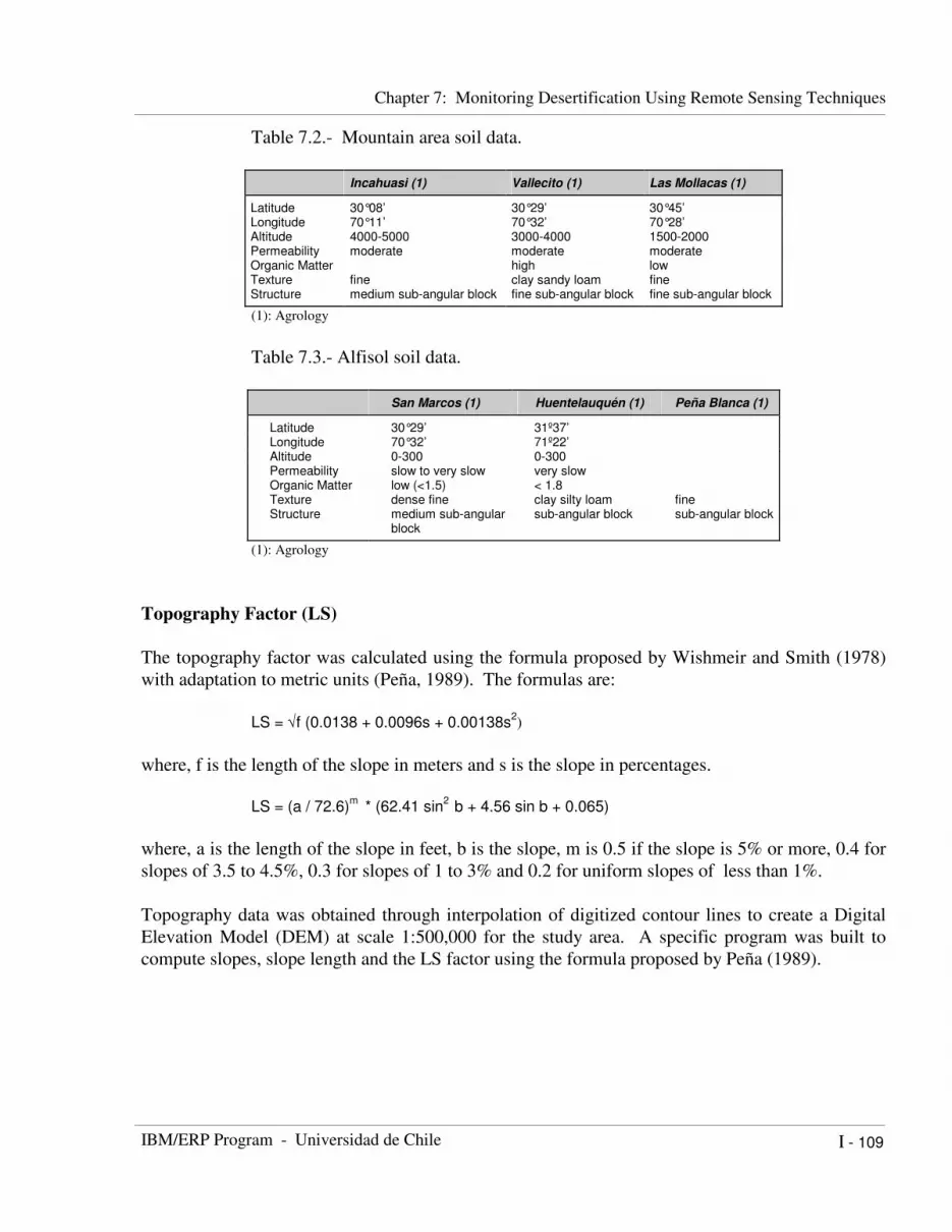
The geographic location of several representative places for each sub-order was defined to

determine the physical characteristics of each soil group. The physical soil structure was estimated

by averaging the observations. The averages were used to select the codes and values for a, b, c,

and M in the K factor formula for each of the 4 classes. The aridisol soil is described by Luzio,

(1979), as permitting no percolation of water and having low organic content. For the sand, lime

and clay percentages for each soil suborder, the values assigned by the USDA (Strahler, 1987)

were used. The soil data used is shown in tables 7.1 through 7.3.

Table 7.1.- Entisol soils data

Limarí (1) Mincha (1) Vicuña (2)

Latitude 30°38’ 31°35’ 30°04’ Longitude 71°21’ 71°26’ 70°43’ Altitude 0-300 0-300 Permeability slow to very slow slow to very slow Organic Matter scarce (< 2%) < 1.7 % Texture fine fine clay loam Structure fine sub-angular block coarse sub-angular block

(1): Alcayaga y Narbona, 1977

(2): Osorio, 1978

.



I - 109

Table 7.2.- Mountain area soil data.

Incahuasi (1) Vallecito (1) Las Mollacas (1)

Latitude 30°08’ 30°29’ 30°45’ Longitude 70°11’ 70°32’ 70°28’ Altitude 4000-5000 3000-4000 1500-2000 Permeability moderate moderate moderate Organic Matter high low Texture fine clay sandy loam fine Structure medium sub-angular block fine sub-angular block fine sub-angular block

(1): Agrology

Table 7.3.- Alfisol soil data.

San Marcos (1) Huentelauquén (1) Peña Blanca (1)

Latitude 30°29’ 31º37’

Longitude 70°32’ 71º22’ Altitude 0-300 0-300 Permeability slow to very slow very slow Organic Matter low (<1.5) < 1.8 Texture dense fine clay silty loam fine Structure medium sub-angular

block sub-angular block sub-angular block

(1): Agrology

Topography Factor (LS)

The topography factor was calculated using the formula proposed by Wishmeir and Smith (1978)

with adaptation to metric units (Peña, 1989). The formulas are:

LS = √f (0.0138 + 0.0096s + 0.00138s2)

where, f is the length of the slope in meters and s is the slope in percentages.

LS = (a / 72.6)m

* (62.41 sin2

b + 4.56 sin b + 0.065)

where, a is the length of the slope in feet, b is the slope, m is 0.5 if the slope is 5% or more, 0.4 for

slopes of 3.5 to 4.5%, 0.3 for slopes of 1 to 3% and 0.2 for uniform slopes of less than 1%.

Topography data was obtained through interpolation of digitized contour lines to create a Digital

Elevation Model (DEM) at scale 1:500,000 for the study area. A specific program was built to

compute slopes, slope length and the LS factor using the formula proposed by Peña (1989).


techniques


I - 110

N

degrees

0.00000

18.7698

37.5396

56.3094

75.0792

93.8490

112.6190

131.3890

150.1580

168.9280

187.6980

206.4680

225.2380

244.0080

262.7777

281.5470

Figure 7.4. Topography LS Factor for the Universal Soil Loss Equation (USLE).

Vegetation Cover Factor (C)

The vegetation cover factor was obtained from the NDVI as the estimator. Vegetation cover is

derived from the LAI using the equation:

COB = 1 - e -0.5 * LAI

This percentage was classified by ranges assigning values for the C factor using the tables proposed

by Wischmeir and Smith (1978). The tables used were for permanent grassland and inactive land.

The values used are in table 7.4. For percentage values of COB not shown in the tables, C was

interpolated from existing values.



I - 111

Table 7.4. C Factor Values for various vegetation coverage.

Percentage C Factor

0 0.4500 10 0.3250 20 0.2000 30 0.1500 40 0.1000 50 0.0710 60 0.0420 70 0.0275 80 0.0130

> 95 0.0030

Finally, a C factor map was developed using a specially devised computational program. Three

images of the C factor were calculated : the year 1900, the present, and projected for the year 2040,

considering desertification trends in the region.

1900 CURRENT 2040

N

0.00

0.03

0.06

0.09

0.12

0.15

0.18

0.21

0.24

0.27

0.30

0.33

0.36

0.39

0.42

0.45

Figure 7.5. Vegetation cover C Factor for the Universal Soil Loss Equation (USLE).


techniques


I - 112

Factor of Conservation Practices (P)

This value was estimated using the slopes as computed from the DEM used to compute the

LS factor. P values were considered for contour crop farming systems, according to table 7.5.

Table 7.5. P values for contour crop farming

Slope (%) P Value

1 - 2 0.60 3 - 5 0.50 6 - 8 0.50 9 - 12 0.60

13 - 16 0.70 17 - 20 0.80 21 - 25 0.90

> 25 1.00

0.000000

0.066667

0.133333

0.200000

0.333333

0.400000

0.466667

0.533333

0.600000

0.666667

0.733333

0.800000

0.866667

0.933333

1.000000

N

degree

Figure 7.6. Conservation practices P factor for the Universal Soil Loss Equation (USLE).



I - 113

Computing regional soil loss by erosion

Erosion shows a similar situation due to its relationship with the loss of vegetation cover in

the study area. Table 7.6. shows a summary of the erosion caused by rain in terms of the affected

area for each range of erosion in km2. This table uses the erosion ranges established by FAO. The

table denotes the increasing trend of Very High, High, Moderate and Low ranks along with the

diminishing trend of Very Low erosion areas. Figure 7.7 shows the same data in graphic form.

Table 7.6. Potential Rain Erosion areas in the IV Region.

Rank 1990 Current 2040

Very Low 30170 29176 28334 Low 3785 4278 4296

Moderate 1847 1918 1969 High 1190 1187 1327

Very High 3572 4005 4638

-2.000

-1.500

-1.000

-500

0

Ch

an

ge

s i

n e

ros

ion

cla

se

s (

km

2)

1900 Current 2040

Very Low

0

500

1.000

1.500

2.000

Very High

Figure 7.7. Temporal evolution of areas affected by erosion in

the IV Region, according to the FAO

classification.

Part One : EIMS - Desertification - Section II, Remote sensing techniques


I - 114

Monitoring desertification dynamics

Land degradation affects both total and seasonal ecosystemic biomass. Biomass reduction is

a consequence of overgrazing, clearing for agricultural purposes, extraction of wood for fuel, and

the decline in soil productivity due to degradation. Seasonal changes are a response to changes in

the specific structure of the vegetation. Valuable species from the woody stratum are replaced by

other rustic species. Reduced cover by woody plants increases the relative contribution of annual

plants, leading to greater changes in seasonal biomass production.

Using a time series of satellite images (NOAA) it is possible to detect both changes in total

biomass and seasonal changes. To conduct space-time monitoring of desertification dynamics in

the IV Region of Chile, a 10-year series of NOAA-AVHRR images (1986-1995) was used,

acquired from the Center for Space Studies of the University of Chile.

This series was georeferenced using pixel resampling. The NDVI was computed using

equation 2.4. To perform a statistical analysis of this time series, a Mean Weekly Image (MWI) was

created to compensate for cloudiness in the area. The MWI was obtained by selecting the

maximum value for each pixel found in all images corresponding to the period. Additionally, MMI

(Mean Monthly Images) were created using the same method. Images in figure 7.8 were extracted

from the MMI series. The maximum NDVI and a variation coefficient for annual maximum

images were used to create a Biological Homogeneity Index (BHI) image, shown in figure 7.10.

This index combines three levels of biomass (high, medium and low) with three levels of

variability in biomass production (high, medium and low). High biomass combined with low

variability corresponds to a healthy ecosystem containing a high contribution of perennial woody

plants. In contrast, low biomass combined with low variability suggests a total lack of biological

signals, indicating extreme desert conditions. As a general rule, increasing variability in ecosystems

with high maximum biomass indicates increasing biological “instability”, associated with initial

states of degradation. On the other hand, increasing biomass variability in ecosystems showing low

total biomass indicates a better capacity to respond to climatic stimuli, and consequently less

degradation. Based on these basic principles, with field observations to verify this theory, we have

proposed nine categories to identify the state and the structure of vegetation (Figure 7.9).

Chapter 7 : Monitoring desertification using remote sensing techniques


I - 115

(a) (b) (c)

0.00000000

0.00651163

0.01302330

0.01953490

0.02604650

0.03255810

0.03906980

0.04558140

0.05209300

0.05860460

0.06511630

0.07162690

0.07813950

0.08465110

0.09116280

0.09767440

(d)

Figure 7.8. Normalized Difference Vegetation Index (NDVI). (a) minimum, (b) maximum, (c)

mean and (d) variation coefficient from a NOAA-AVHRR image time series, years

1986 through 1995.



I - 116

200.00 300.00 400.00 500.00 600.00 700.00 800.00

100.00

200.00

1.00

2.00

3.00

4.00

5.00

6.00

7.00

8.00

9.00

0.02 0.03 0.04 0.05 0.06 0.07

-0.1

0.7

VARIATION COEFFICIENT

MA

XIM

UM

N

DV

I

2.0

3.0

4.0

5.0

7.0

6.0

8.0

1 2 3

6 5 4

9 8 7

Figure 7. 9 . Table of the NDVI maximum and the variation coefficient for the NOAA/AVHRR

time series images.

This table represents the state of desertification or the state of the biological system. Y-axe

represents an indirect measure of ecosystem biomass. X-axe represents seasonal variability of the

ecosystem biomass. In the lower part of this area, low biomass is the general characteristic

representing degraded vegetation shown in red (class 1, 2 and 3). By contrast, in the upper part,

class 7, 8 and 9, high biomass, represent the best ecosystem conditions (in green colors)..



I - 117

The combinations from this matrix can be represented as follows :

9

High biomass-low variability

8

High biomass - medium variability

7

High biomass - high variability

6

Medium biomass - medium variability

5

Medium biomass - medium varibility

4

Medium biomass - high variability

1

Low biomass - low variability

2

Low biomass - low variability

3

Low biomass - high variability

N

(1)

(2)

(3)

(4)

(5)

(6)

(7)

(8)

(9)

Figure 7.10. Biological Homogeneity Index image determined by reclassification of maximum

NDVI and NDVI variation coefficient.

This figure shows the spatial variation of vegetation activity, stratified in biological

patterns. Class 7 (yellow) corresponds to areas with high biomass and low variability, which, in

biological terms, represent perennial vegetation and irrigated agricultural lands Class 9, high NDVI



I - 118

and high variability, (dark green) represents mainly annual grasslands in good condition near the

coast. Class 1 (red), on the contrary, represents low biomass and low variability, meaning inland

zones with high losses of vegetation due to desertification.

Vegetation zoning by biomass analogy

Comparing biomass variation over time, pixel by pixel, it is possible to regroup those pixels

having the same intensity and seasonality in their biological signals. By means of a field survey,

representative vegetation units are defined. These units are geo-referenced using a GPS to select a

representative point within each unit. Processing the time series of NOAA images (1986 - 1995)

this program compares all pixels of the image with the selected reference point. The similarity

estimator used was the Pearson correlation coefficient. The result is a selection of pixels

conforming to a homogeneous area referred to as the reference location. This procedure is based on

similarities in quantity and seasonality of biomass curves so that the resulting areas are probably

similar in specific composition and structure. The MMI images were organized as a matrix of 120

columns (total number of months) by 127,359 rows (number of pixels per image). The correlation

analysis is performed on a class by class basis, a class representative row (time series for the

reference pixel) is used to compute the regression against all other matrix elements. After finishing

regressions with the first representative point (pixel) the program repeats the procedure with the

other representative points. At the end, each pixel of the image is associated to the reference point

with which it has the highest correlation coefficient.

Figure 7.10 shows the resulting homogeneous zones for each of the 9 selected field

reference. Classes 3 and 6 (low and medium NDVI with high variability) do not appear in figure

7.10 due to their low statistical occurrence. The result of this analysis for the 7 classes is shown in

figure 7.11. The images show the similarity between the reference point and all other points in the

area of study. It can be observed that vegetation zones are stratified from the coast to the interior,

with a maximum in the coastal area. This coincides with in situ observations and is the result of

the influence of marine moisture. This analysis is very interesting, since it confirms the

polystratification of vegetation cover and provides an accurate spatial representation of what was

previously only perceived as the condition of vegetation in the IV Region.

Estimating vegetation cover and biomass from satellite images and their

possible changes in response to desertification

Using satellite information, it is possible to estimate diverse environmental parameters on

the Earth’s surface. Among these are vegetation cover, leaf area index, and biomass. LAI,

vegetation cover and biomass were calculated for the study area. (figures 7.8 and 7.9) Figure 7.12

shows the maximum LAI estimated from the annual mean NDVI. Additionally, the LAI for the

years 1900 and 2040 were estimated using historical and projected rainfall data, with a scenario of

atmospheric CO2 doubling by 2040. The mean annual biomass that the ecosystem is capable of

producing was estimated using the same technique and scenario.



I - 119

(1) (2) (4)

(5) (7) (8)

(9) (Max)

0.00000

0.06666

0.10000

0.20000

0.26666

0.33333

0.40000

0.53333

0.60000

0.66666

0.73333

0.80000

0.86666

0.93333

1.00000

Figure 7.11. Vegetation dynamic patterns associated with Biological Homogeneity Index (BHI)

well the major features of the terrain using well-shaped triangles.



I - 120

1900 CURRENT 2040

0.000000

0.105247

0.210483

0.315740

0.420987

0.526233

0.631480

0.736727

0.841973

0.947220

1.052470

1.157710

1.262960

1.368210

1.473450

1.578700

N

Figure 7.12. Maximum LAI estimated from the mean annual NDVI.

1900 CURRENT 2040

Figure 7.13. Estimated potential biomass from the NDVI average value.

N



I - 121

Figure 7.13 shows estimated potential biomass production in the study area. The increasing

deterioration of primary productivity since 1900 to present can be seen. By the year 2040 the

ecosystem will have lost about 30% of primary productivity. This is a vital issue since animal

raising activities in the region are based mainly on goats, which only feed on natural prairie. This,

in turn, relates to the carrying capacity of the ecosystem which depends on the botanical

composition of vegetation and its quality as forage. The basic idea of sustainable planning is

determining the sustainable carrying capacity of a given grassland so as to preserve its status and

condition. From the perspective of plant cover in the region, figure 7.14 shows the same decreasing

trend. Loss of vegetation cover since 1900, as shown in figure 7.14, can be traced to two main

causes: global climatic change and anthropic activities, i.e., the land tenure system and agricultural

practices.

About 50% of the territory in this region is unsuitable for agriculture since it is located in

the Andean mountain range. However its value resides in its role of capturing and retaining rain

and snow. The rest of the land in the region is used for animal raising and small-scale, rainfed and

irrigated agriculture. Land tenure is based on large single-owner farms and communally-owned

farms. The communal system, which accounts for about 25 % of the total area, is unusual in that a

farm is owned by several individuals (10 to 20) who are not necessarily related nor coordinated by

an organization. The system dates to colonial times when the Spanish paid troops in land rights.

The same system was used in all of Latin America but it disappeared elsewhere, having survived in

the IV Region because of both tradition and poverty.

The problem is that each co-owner has free access to use any part of the entire land with no

restrictions or concern for future use. Therefore, every co-owner tries to maximize resources

extraction in the short term for his own good under the premise that the others co-owners will do

the same. This kind of practice is extremely aggressive to the environment and is the cause of

serious degradation. By contrast, single-owner farms show much less degradation of natural

resources since long term interests are taken into account.



I - 122

1900 CURRENT 2040

N

Figure 7.14. Mean Annual Vegetation Cover estimated from the Mean Annual NDVI.

To estimate the trends in degradation of vegetation cover, six pilot areas were used in the

region. The temporal variations of the NDVI were extracted for each pilot area.

The six pilot areas are Haciendas, Combarbalá, Canela, Elqui, Limarí and Choapa. Figure

7.15 shows the variations of the NDVI in the Haciendas (single owner) and Canela (communal)

sites. The Haciendas area always shows a higher value, which coincides with field data. The

Canela site shows more degradation. Figure 7.16 shows the comparison between Haciendas and

Combarbalá (communal) sites where the trend is the same.



I - 123

190

200

210

220

230

240

250

(ND

VI+

2)

x 1

00

0 364 728 1092 1456 1820 2184

Canela Hacienda

Comparación de la Variación Interanual

entre Areas Pilotos

1987 1988 1989 1990 1991 1992

Canela Valley Hacienda Valley

Figure 7.15. Interannual variation of the NDVI in Haciendas area (single owner) and Canela area

(community).

190

200

210

220

230

240

250

(ND

VI+

2)

x 1

00

Combarbala Hacienda

Comparación de la Variación Interanual

entre Areas Pilotos

1987 1988 1989 1990 1991 1992

Combarbalá V. Hacienda V.

Figure 7.16. Interannual variation of the NDVI in Haciendas area (single owner) and Combarbalá

area (Communal).



I - 124

Spatial modeling with satellite data of surface phenomena

Very frequently the intensity of phenomena occurring on the Earth’s surface has a spatial

configuration that can be modeled as a function of specific driving factors. Among the phenomena

that we can observe from satellites are : vegetation cover, surface temperature, flooded areas, plant

seasonality and changes in optical properties of the plant-soil system.

To study these phenomena we created a software that can analyze images pixel by pixel

(statistical option), generating a complete diagnosis of the behavior of each pixel in different

situations (images) corresponding to different moments and the relationships of this behavior with

other environmental variables considered “drivers”. Among the drivers we can select are altitude,

NDVI, soil, climate, geomorphology, topography and many others which the user considers

important. In some cases the value of the variable to be modeled in a reference pixel can be

considered a “driver”. Each row in the input matrix is treated as a time series. The software allows for

statistical analysis of the differences between one pixel and a reference pixel throughout several

images. In some cases, the reference value can be the mean value of the entire image. The software

carries out lineal regressions between any pixel and a reference pixel, generating a file containing the

A and B coefficients, and an IDRISI image of the Pearson coefficient.

Application of spatial modeling techniques to surface temperature

Surface temperature is one of the most dynamic phenomenon of the Earth’s surface. Extreme

temperatures have crucial impacts on agriculture, while minimum temperature is directly related to

frost risk. It is also part of the so-called thermal amplitude, which is related to vegetation and soil

moisture content. Thermal amplitude can be used as an indicator of plant water stress. Through

ongoing monitoring it can be a feasible indicator of biophysical desertification.

Owing to mountainous topography, spatial variation of the intensity of frost is notable. Surface

configurations mold the circulation of night air in such a way that within a few dozen meters distance

notable thermal differences are produced. In this regard, measurements done in France have shown

differences of up to 5 degrees between the temperature of higher slopes and the base of a valley, over

a distance of 250 meters. This leads us to suppose that in rough topographies microadvection creates

attenuated and intensified frost conditions. Thermal inversion within the boundary, microadvection,

the slope of the terrain and its nature, produce spatial patterns of thermal distribution, or areas where

temperature behaves as an organic system. This allows the development of models based on

algorithms which relate the entire area covered by a thermal pattern and a reference point that

coincides with a meteorological station. This is based on the fact that thermal patterns exist and have

an organic conduct that can be described by algorithms. The goal is to develop a simple topoclimatic

model able to integrate the effect of topography on minimal surface temperature. This is possible by

means of a geo-referenced grid that allows for resampling thermal satellite images. In the grid,

temperature, elevation and other attributes can be integrated pixel by pixel. Starting from the digital

elevation model (DEM) we produced maps of exposure and position in relation to the influence of the

ocean. It is possible to overlay every other kind of cartographic information, with the goal of

modeling the influence on surface temperature of multiple environment variables at once.



I - 125

As an example we modeled minimum surface temperature using five meteorological stations

as a reference. One meteorological station represents an area where the Pearson coefficient between

the pixels of the image and the reference meteorological station is greater than a given value.

Normally the neighboring pixels to the reference pixel (the meteorological station) exhibit the highest

coefficient of correlation. The further the pixels are from the reference pixel the more the Pearson

cofficient decreases. This is shown in Figure 7.17. We can observe the spatial distribution of the

Pearson coefficient for each of the five meteorological stations. These images are interpreted as the

area of representativeness of each station, which is to say, the area of validity of the lineal model

relating any pixel with each station. This indicates that starting with a known temperature in a

meteorological station, it is possible to determine, with acceptable accuracy, the temperature in all the

other points within the representative area, corresponding to this meteorological station.

The model the program provides is

t(i) = a(i) + b(i) * tr + e

where t(i) is the temperature of the i-pixel, a(i) y b(i) are the parameters of lineal equation relating the

i-pixel to the reference station and e is the error associated with the model.

In order to be able to verify the validity of this model four computer programs were created,

designed to generate estimated thermal images. The first is SIM, which reproduces entire satellite

images using as input only the average regional temperature. This regional temperature value is

calculated by means of a conventional forecasting method. The second model, SIP, reproduces entire

satellite images using specific meteorological stations as reference points. The temperature at each

station is obtained by conventional forecasting methods. The third model, MULTIR, produces a

multiple regression between images in IDRISI format, such as temperature, exposure, geographic

position, elevation, vegetation index (NDVI) and many others. One of these variables must be chosen

as an independent variable (or parameter) This model generates a file containing the multiple

regression coefficients. By means of this set of computer programs we can generate topoclimatic

models to study the spatial distribution of minimum temperature in the central zone of Chile.



I - 126

fig. 3.11.- Area de representatividad de cada estación meteorológica, expresada en términos del coeficiente de

correlación de Pearson.

JARDIN BOTANICO CASABLANCA CERRO CALAN

ANTUMAPU MELIPILLA 0.000000

0.066666

0.133333

0.200000

0.266666

0.333333

0.400000

0.466666

0.533333

0.600000

0.666666

0.733333

0.800000

0.866666

0.933333

1.000000

Fig. 7.17. Representative areas of meteorological stations. Homogeneous climatic areas were

obtained by spatial correlation in a series of NOAA thermal images.

The regression model can be expressed as follows:

N

T( i) = ao + [ Σ bo(k) * Xk(i) ] + co * t(i) + e k=1

where ao, bo(k) and co are coefficients emanating from the lineal regression between various

images/parameters and e represents the error associated with the fitting process. X1(i) represents

elevation (MNT), X2 represents aspect, X3 represents the distance to the coast, t(i) is the temperature

image generated by the SIP model and i represents a selected pixel from the images. The temperature

of the i-pixel is given as:

T(i) = ao + bo(1) * MNT(i) + bo(2) * Aspect(i) + bo(3) * Distance_to_Sea(i) + co * Temperature_Simulated_Image(i)

with ao = 0.3870929 , bo(1) = 4.81261 E-03, bo(2) = 1.376564 E-03, bo(3) = -2.24386, co = 0.9602945 ( R² = 0.93).



I - 127

(b)

(a)

Fig. 3.18.- Campo de temperaturas observado por el satélite meteorológico NOAA (a) y

simulado (b) por modelo MULTIR (°C).

Norte

Grados

N

Degree

Fig. 7.18. Real (a) and simulated (b) image by means of topoclimatic thermal images.

Figure (7.18-a) shows the image obtained from channel 4 of the NOAA satellite for July 23rd,

1988, in which one can note the different thermal patterns represented by color ranges, associated

with ranges of temperature values. Figure (7.18-b) shows an image produced by the SIF model for

the same day. The input values for the SIF model are: the representative area of each meteorological

station, the elevation map, the exposure map, the distance from the coast, and an image generated by

the SIP program for the same conditions. In order to generate the SIP image temperature values are

required from the five meteorological stations. The correlation coefficient between the original

satellite image (figure 7.18-a) and that generated by the SIP model is 0.57. The correlation coefficient

between the original image and the generated one is 0.93. It is important to note that this simple

model is capable of quantitatively describing the spatial behavior of surface temperature related to

point references.

Starting from this model, images are simulated corresponding to historic extremes of minimal

temperature in the stations that are used. This procedure generated a series of images that were

analyzed pixel by pixel in order to find the probability of frost occurrence. The results are shown in

figure (7.19), where the probability of a negative temperature occurrence in an i-pixel can be seen

when a negative temperature occurs in the related meteorological station. This can be interpreted as a

frost-risk map showing areas at greater risk to frost due to topographic position.



I - 128

Fig. 3.26.- Distribución probabilìstica de las heladas (%).Grados

Norte

-70.5°-72°

-34°

-33°

N

Degree

Fig. 7.19. Areas having different probabilities of frost. Image obtained by NOAA/AVHRR time

series image processing.

The linkage of temperature forecasting methods and topoclimatic models allows for

regionalizing a frost risk forecasting system. By means of topoclimatic models we can demonstrate

the high correlation between surface temperature patterns and topography. The temperature

forecasting method has predicted temperatures with an error of less one degree Celsius. NOAA

thermal images have shown themselves to be a useful tool for studying the meso-climotology of air

temperature, as related to low atmospheric dynamics. Starting from this analysis we show that

thermal spatial units behave as one. This could be a tool for studying representative areas of

individual meteorological stations.



I - 129

REFERENCES

BRUTSAERT, W. 1982. Evaporation into the atmosphere: Theory, history and applications.

Dordrecht: Reidel.

CASELLES, V. and SOBRINO, J. 1989. Determination of frost in orange groves from NOAA-9

AVHRR data. Remote Sensing of Environment 29 : 135 - 146.

COLWELL, J. 1974. Vegetation canopy reflectance. Remote Sensing of Environment. 3 : 175 -

183.

COLL, C., CASELLES, V., and SCHUMUGGE, T. 1988. Estimation of land surface emissivity

differences in the split-window channels of AVHRR. Remote Sensing of Environment, 48:127-

134.

COLL, C., V. CASELLES y J. SOBRINO. 1991. El contínuo de absorción del vapor de agua en la

ventana atmosférica de los 8-14 µm. Revista Española de Física 5 , 4: 25-30.

COLL, C., V. CASELLES y J. SOBRINO. 1992. Desarrollo de un modelo de corrección

atmosférica en el térmico. II. Aplicación a los canales 4 y 5 del NOAA. Anales de Física 88: 120-

132.

CHANDRASSEKHAR, S.. 1960. Radiative transfer. New York, Dover Publications.

CHUVIECO, E. 1990. Fundamentos de teledetección espacial. Ediciones Rialp, S.A., Madrid,

España.

CURRAN, P. , 1980, Remote sensing systems for monitoring crops and vegetation, Progress in

Physical Geography, 4: 315 - 341.

DIALLO, O., DIOUF, A., HANAN, N., NDIAYE, A . y Y. PREVOST. 1990. AVHRR monitoring

of savanna primary production in Senegal, West Africa: 1987-1988. International Journal of

Remote Sensing, 117: 1259 - 1279.

ELWYNN TAYLOR S. 1979. Measured emissivity of soils in the southeast United States. Remote

Sensing of Environment 8 : 359 - 364.

GONG, N. S., y J. R. Miller, 1995, Coniferous forest leaf area index estimation along the Oregon

transepts using compact airborne spectrographic image data, Photogrametric Engineering &

Remote Sensing, 61, n° 9, 1107-1117.

GOWARD, S., 1989, Satellite bioclimatology, Journal of Climate 2: 710 - 720.



I - 130

HUETE , A. R., 1987, Spectral signatures and Vegetation indices, II Reunión Nac. del grupo de

trabajo en teledetección, Valencia, España , pp. 13 - 26.

HUETE, A. R. 1988. A soil-adjusted vegetation index (SAVI). Remote Sensing of Environment

25 : 295 - 309.

HUETE, A. R., 1985, Extension of soil spectra to the satellite: atmosphere, geometric, and sensors

considerations, SPECTEL: Propiedades Espectrales y Teledetección de los Suelos y Rocas del

Visible al infrarrojo Medio, La Serena, Chile, pp. 163 - 194.

ITIER, B. y CH. Riou. 1990. Une nouvelle mèthode de dètermination de l’evapotranspiration

rèelle par thermographie infrarouge. Journal de Recherches Atmospheriques. Vol. 16:, 2: 113-125.

JANSEN, J. R., 1983, Biophysical remote sensing, Annals of the Association of American

Geographers, 73: 111 - 132.

JUSTICE, C. O. , J. R. G. TOWNSHEND, B. N. HOLBEN y C. J. TUCKER, 1985, Analysis of

the phonology of global vegetation using meteorological satellite data, International Journal of

Remote Sensing, 6: 1271 - 1318.

KAUFMAN, Y. y D. TANRÊ. 1992. Atmospherically resistant vegetation index(ARVI) for EOS-

MODIS, IEEE Trans. Geosci. Remote Sensing 30 : 261 - 270.

KNEIZYS, F. X., SHETTLE, E. P., ABREU, L. W., ANDERSON, G. P., CHETWYND, J. H.,

GALLERY, W. O., SELBY, J. E. A., and CLOUGH, S. A. , 1988. Users guide to LOWTRAN 7.

Technical Report AFGL-TR-88-0177, Optical/Infrared Technology Division, U.S. Air Force

Geophysics Laboratory, Hanscom Air Force Base, Massachusetts.

LIU, H. Q. and HUETE, A.R. 1995. A feedback based modification of the NDVI to minimize

canopy background and atmospheric noise. IEEE Trans. Geosci. Remote Sensing 33 : 457 - 465.

MALINGREAU, J. P. y C. J. TUCKER, 1987, The contribution of AVHRR data for measuring and

understanding global processes: Large-scale deforestation in the Amazon basin, Proc. IGARS`87,

Ann Arbor, pp. 443 - 448.

MILLER G., M. FUCHS, M. HALL, G. ASRAR, E. KANEMASU y D. JOHNSON. 1984.

Analysis of seasonal multispectral reflectance of small grains. Remote Sensing of Environment 14

: 153 - 157.

MORALES, L. y PARRA, J., 1996, Determinación del índice de vegetación a partir de parámetros

físicos usando datos NOAA/AVHRR, Actas VI Simposio Nac. de Física Experimental y Aplicada,

Temuco, Chile, pp. 51 - 55.

MORALES , L. y SANTIBAÑEZ, F., 1996, Estimación de la emisividad de superficie usando

datos de satélite, Actas VI Simposio Nac. de Física Experimental y Aplicada, Temuco, Chile, pp.



I - 131

84 - 88.

PEARSON R. y L. MILLER. 1972. Remote mapping of standing crop biomass for estimation of

the productivity of the short-grass prairie. Pawnee National Grassland, Colorado, In Proc. 8th Intl.

Symp. on Remote Sensing of Environment, Ann Arbor, 1357-1381.

PRICE, J. 1977. Thermal inertia mapping: A new view of the Earth. Journal of Geophysical

Research, 82:2582-2590.

PRICE, J. 1990. Using spatial context in satellite data to infer regional scale evapotranspiration.

IEEE Transactions on Geoscience and remote sensing 28 : 940 - 948.

PRICE, J. 1992. Estimation vegetation amount from visible and near infrared reflectance. Remote

Sensing of Environment 41 : 29 - 34.

REGINATO, R., R. JACKSON y P. PINTER. 1985. Evapotranspiration calculated from remote

multiespectral and ground station meteorological data. Remote Sensing of Environment 18 : 75 -

89.

ROUSE J., R. HASS, J. SCHELL, D. DEERING y J. HARLAN. 1976. Monitoring the vernal

advancement of retrogradation of natural vegetation. NASA/GSFC, Type III Final Report, Geenbelt

MD, 371 pp.

ROVINOVE, J. C., P. S. CHAVEZ, D. GEHRING and R. HOLGREN, 1981, Arid land monitoring

using LANDSAT albedo difference images. Remote Sensing of Environment, 11:133 - 156.

SELLERS P. 1986. Canopy reflectance, photosynthesis and transpiration. Int. J. of Remote Sensing

23 : 287 - 321.

TOWNSHED, J. and JUSTICE, C. 1986. Analysis of the dynamics of African vegetation using the

normalized difference vegetation index. Int. J. of Remote Sensing 7 : 1435 - 1445.

TUCKER, C. J. 1979. Red and photographic infrared linear combinations for monitoring

vegetation, Remote Sensing of Environment, 18: 127 - 150.

TUCKER, C. y P. SELLERS. 1986. Satellite remote sensing of primary production. Int. J. Remote

Sensing, 7:1395-1416.

VALOR E., V. CASELLES. 1995. The use of thermal infrared remote sensing in desertification

studies. First results of the EFEDA, HAPEX-Sahel and DEMON projects. Desertification in a

European context: Physical and socio-economic aspects. European Commission on Environment

and the Quality of Life, Final Report. p 627-635.

VERMOTE, E., D. TANRÊ, J. DEUZÊ, M. HERMAN y J. MORCRETTE. 1995. Second

Simulation of the satellite signal in the solar spectrum(6S), 6S User Guide Version 1.



I - 132



I - 133

An enviromental Information and

Modeling System (EIMS) for Sustainable

Development

Computer tools for sustainable management of arid and

Antarctic ecosystems

Edited by

Fernando Santibáñez Q. and Victor Marín B.

Santiago, 1998. Chile.

Universidad de Chile

IBM International Foundation

Enviromental Research Program

Documents

Monitoring Desertification Using Remote Sensing Techniques