Citation: Njemcevic, P.; Kaljic, E.;

Maric, A. Moment-Based Parameter

Estimation for the Γ-Parameterized

TWDP Model. Sensors 2022, 22, 774.

https://doi.org/10.3390/s22030774

Academic Editors: Peppino Fazio,

Carlos Tavares Calafate, Miroslav

Voznak and Miralem Mehic

Received: 24 December 2021

Accepted: 14 January 2022

Published: 20 January 2022

Publisher’s Note: MDPI stays neutral

with regard to jurisdictional claims in

published maps and institutional affil-

iations.

Copyright: © 2022 by the authors.

Licensee MDPI, Basel, Switzerland.

This article is an open access article

distributed under the terms and

conditions of the Creative Commons

Attribution (CC BY) license (https://

creativecommons.org/licenses/by/

4.0/).

sensors

Article

Moment-Based Parameter Estimation for the Γ-ParameterizedTWDP Model

Pamela Njemcevic * , Enio Kaljic and Almir Maric

Department of Telecommunications, Faculty of Electrical Engineering, University of Sarajevo, Zmaja od Bosneb.b., Kampus Univerziteta, 71000 Sarajevo, Bosnia and Herzegovina; enio.kaljic@etf.unsa.ba (E.K.);almir.maric@etf.unsa.ba (A.M.)* Correspondence: pamela.njemcevic@etf.unsa.ba

Abstract: Two-wave with diffuse power (TWDP) is one of the most promising models for descriptionof a small-scale fading effects in the emerging wireless networks. However, its conventional parame-terization based on parameters K and ∆ is not in line with model’s underlying physical mechanisms.Accordingly, in this paper, we first identified anomalies related to usage of conventional TWDPparameterization in moment-based estimation, showing that the existing ∆-based estimators areunable to provide meaningful estimates in some channel conditions. Then, we derived moment-basedestimators of recently introduced physically justified TWDP parameters K and Γ and analyzed theirperformance through asymptotic variance (AsV) and Cramer–Rao bound (CRB) metrics. Performedanalysis has shown that Γ-based estimators managed to overcome all anomalies observed for ∆-basedestimators, simultaneously improving the overall moment-based estimation accuracy.

Keywords: TWDP fading channel; moment-based estimation; Cramer–Rao bound; asymptotic variance

1. Introduction

Small-scale fading severely degrades performance of wireless communication sys-tems [1]. Thus, in order to design highly reliable and efficient transceivers for communi-cation in deep fading conditions, it is of profound significance to have an accurate andtractable fading model [2,3]. Traditionally, the signal affected by small-scale fading innonline-of-sight (NLOS) environments has been modeled as a sum of many diffuse com-ponents and described by Rayleigh distribution. Withal, the Rician fading model hasbeen used for the description of received signal variations in better-than-Rayleigh chan-nel conditions, since, except for many diffuse components, it also assumes the presenceof one dominant specular component [4]. However, in some multipath sparse channels,traditional fading models fall short of accurately describing small-scale variations of thereceived complex envelope [4], which makes them nonviable for accurate modeling of allpropagation conditions [5].

The aforementioned is especially pronounced in mmWave 5G communication net-works equipped with directional antennas or arrays [6] as well as in wireless sensornetworks deployed in cavity environments [3], where measurements have shown that thesignal in multipath sparse propagation conditions may, in some cases, experience fadingwith characteristics worse than those in Rayleigh channels [4].

In such scenarios, the TWDP fading model—which assumes the presence of twospecular components instead of just one considered by Rician model—appears to beappropriate for modeling small-scale fading effects [7]. In this regard, it is shown that TWDPdistribution describes small-scale fading more accurately than conventional distributions instatic sensor networks with their nodes placed within cavity environments, such as aircraftsand buses [3] and abroad a large transport helicopter [8]. It is also shown that its PDF shapesignificantly coincides with empirical results obtained for train-to-infrastructure wirelesscommunication [9], vehicle-to-vehicle 60 GHz urban communication [10], and mmWavecommunication in indoor environments [11,12].

Sensors 2022, 22, 774. https://doi.org/10.3390/s22030774 https://www.mdpi.com/journal/sensors

Sensors 2022, 22, 774 2 of 12

Thereat, the TWDP model itself represents generalization of Rayleigh and Ricianfading models and can be used for modeling both better-than-Rayleigh and worse-than-Rayleigh fading conditions. It is based on the assumption that the waves arriving at thereceiver can be observed as a sum of two specular components with constant magnitudesV1 and V2 and uniformly distributed phases, plus many diffuse components treated as acomplex zero-mean Gaussian random process with average power 2σ2. As such, the modelis conventionally parameterized by K and ∆, defined as [13]:

K =V2

1 + V22

2σ2(1)

∆ =2V1V2

V21 + V2

2(2)

where parameter K (K ≥ 0) characterizes the ratio of the average power of specular compo-nents to the average power of remaining diffuse components (like the Rician parameterKRice = V2

1 /(2σ2)) and parameter ∆ (0 ≤ ∆ ≤ 1) characterizes the relation between magni-

tudes of specular components. Consequently, the average received signal power Ω is equalto V2

1 + V22 + 2σ2.

However, as it is elaborated in [14], the definition of parameter ∆ is not in accordancewith the model’s underlying physical mechanisms. Namely, according to the model’sdefinition, specular components have constant magnitudes and are propagating in a linearmedium. Consequently, V2 can be nothing but the linear combination of V1, wherefore thefunction which characterizes the ratio between V1 and V2 has to be linear [14]. However,∆-based parameterization introduces a nonlinear relation between magnitudes of specularcomponents, since V2 = V1(1−

√(1− ∆2))/∆. This hinders accurate observation of the

impact of the ratio between V1 and V2 on a system’s performance metrics and causesanomalies within the expressions obtained by integration or derivation with respect toparameter ∆ [14].

Considering that previously mentioned, Γ-based parameterization was recently pro-posed in [14], by introducing parameters K and Γ:

K =V2

1 + V22

2σ2(3)

Γ =V2

V1(4)

where Γ (0 ≤ Γ ≤ 1, for 0 ≤ V2 ≤ V1) obviously ensures linear dependence betweenV1 and V2. On the other side, the definition of parameter K remains unchanged, but thedefinition expression of normalized K/KRice with respect to the ratio between V1 and V2, e.g.,K/KRice = 1 + (V2/V1)

2 (where KRice is the Rician parameter), is affected by the choice ofsecond parameter (∆ vs. Γ). Obviously, parameter ∆ completely changes its character sinceK/KRice = 2(1− 1

√1− ∆2)/∆2, while Γ does not, since K/KRice = 1 + Γ2 [14].

Despite that aforementioned, Γ-based parameterization has up to now been consideredonly in [14], by elaborating its benefits on ASEP observation accuracy. However, no otherbenefits of Γ-based parameterization or the anomalies caused by the nonphysical definitionof a ∆ parameter within the expressions which involve integration or derivation withrespect to ∆ have been presented yet. Accordingly, in this paper, one such anomaly isidentified within ∆-parameterized TWDP moment-based estimators and overcome byintroducing the appropriate estimators for Γ-parameterized TWDP fading model. In thatsense, this paper focuses on performance analysis of moment-based parameter estimators,for both ∆- and Γ-based TWDP parameterizations.

Considering that aforementioned, in Section 2, an overview of the results related toestimation of TWDP parameters is foremost presented, elaborating in detail anomaliescaused by conventional ∆-based parameterization and indicating the absence of thoserelated to a Γ-parameterized TWDP model. In Section 3, a closed-form moment-based

Sensors 2022, 22, 774 3 of 12

estimator is derived for Γ-based parameterization, and their behavior is examined forvarious values of proposed parameters. In Section 4, performance analysis of proposedestimators is performed. First, corresponding asymptotic variances are derived and graphi-cally presented and then the limits of estimation problem are explored and determined interms of Cramer–Rao bound. Finally, ∆- and Γ-based estimators are compared in Section 5,in order to gain insight into the differences in their behavior and their estimation accuracy.Conclusions are outlined in Section 6.

2. Related Works

The estimation of parameters that characterize fading channel is of practical impor-tance in a variety of wireless scenarios. It includes not only delay insensitive channelcharacterization and link budget calculations, but also online adaptive coding/modulationfor which the estimation of parameters must be both accurate and prompt [15]. In thatsense, inaccurate estimation of channel parameters leads to a non-optimal channel capacityutilization, which might significantly affect highly mobile communication systems such asvehicular-to-vehicular and vehicular-to-infrastructure. Accordingly, different approaches inestimation of TWDP parameters are proposed to make a deal between their computationalcomplexity and estimation accuracy. These approaches usually assume that the value ofparameter Ω can be directly estimated from the data set as a second moment [10], so theestimation problem has become focused on determination of values of K and ∆.

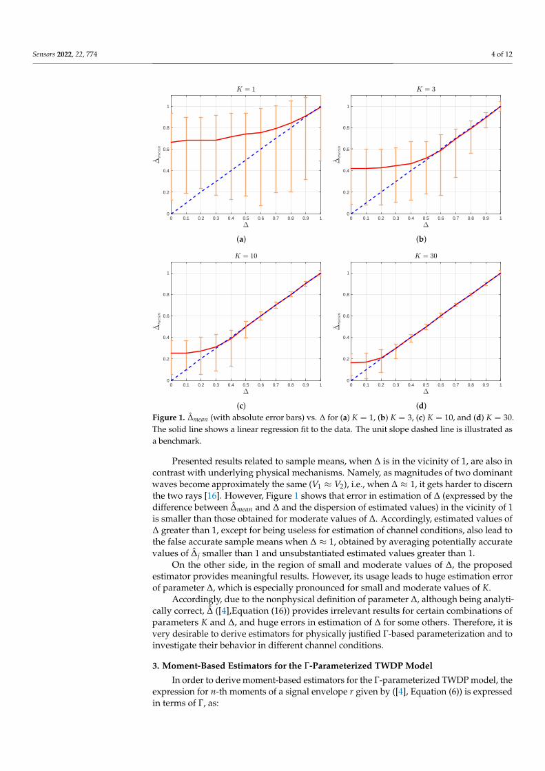
Among the investigated approaches used to estimate parameters of ∆-based parame-terization, the distribution fitting approach is used for measurements performed in air-craftand buses at 2.4 GHz [3], while the maximum likelihood procedure (ML) is used formeasurements performed at 60 GHz in the indoor environment [11] and in vehicular-to-vehicular propagation scenarios [10]. However, it is shown that both approaches arecomputationally very complex and inappropriate for online applications. Accordingly, themoment-based approach is considered in [4,7,12], as a compromise between estimator’scomplexity and its accuracy. Thereat, in [7], estimators are derived only as conditionalexpressions which can not be used for practical estimations in which both parametersare unknown. To overcome the issue, the exact joint estimators of TWDP parameters arederived in [4] as computationally simple expressions. However, for certain combinationsof parameters K and ∆, the estimator of parameter ∆, ∆, derived in [4], provides physicallyunsubstantiated results, which can be demonstrated by applying ([4], Equation (16)) onMonte Carlo simulated samples.

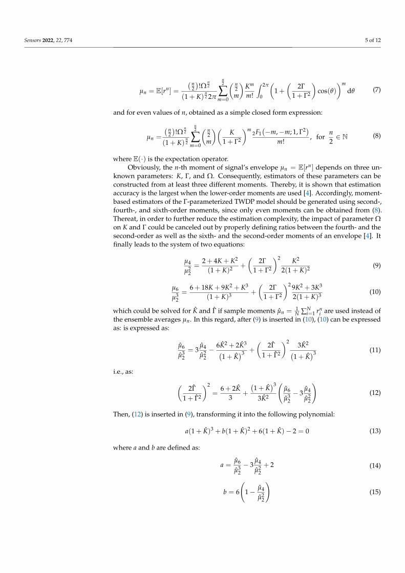
Accordingly, for each combination of K and ∆, where K = 1, 3, 10, 30 and∆ = 0, 0.1, 0.2, . . . , 1, 500 realizations of the TWDP process with N = 104 i.i.d. sam-ples are generated. The estimate of parameter ∆ from j-th realization, ∆j, is obtainedby ([4], Equation (16)) and, for each combination of K and ∆, sample mean value ∆mean iscalculated as (1/500)∑500

j=1 ∆j. The results are presented in Figure 1.From Figure 1, it can be observed that, for large values of ∆ (i.e., for ∆ ≈ 1), ∆ estimates

may exceed 1 regardless of the value of parameter K. However, according to definitionof ∆:

(1− ∆) =(V1 −V2)

2

V21 + V2

2(5)

(1− ∆) ≥ 0, for (V1, V2) ∈ R2 (6)

the parameter has to be lower or equal to one (∆ ≤ 1) for any (V1, V2) ∈ R2. Accordingly,estimates of ∆ greater than 1 are physically unsubstantiated and can not be used to gainany insight into the relation between V1 and V2.

Sensors 2022, 22, 774 4 of 12

"0 0.1 0.2 0.3 0.4 0.5 0.6 0.7 0.8 0.9 1

"m

ean

0

0.2

0.4

0.6

0.8

1

K = 1

(a)

"0 0.1 0.2 0.3 0.4 0.5 0.6 0.7 0.8 0.9 1

"m

ean

0

0.2

0.4

0.6

0.8

1

K = 3

(b)

"0 0.1 0.2 0.3 0.4 0.5 0.6 0.7 0.8 0.9 1

"m

ean

0

0.2

0.4

0.6

0.8

1

K = 10

(c)

"0 0.1 0.2 0.3 0.4 0.5 0.6 0.7 0.8 0.9 1

"m

ean

0

0.2

0.4

0.6

0.8

1

K = 30

(d)Figure 1. ∆mean (with absolute error bars) vs. ∆ for (a) K = 1, (b) K = 3, (c) K = 10, and (d) K = 30.The solid line shows a linear regression fit to the data. The unit slope dashed line is illustrated asa benchmark.

Presented results related to sample means, when ∆ is in the vicinity of 1, are also incontrast with underlying physical mechanisms. Namely, as magnitudes of two dominantwaves become approximately the same (V1 ≈ V2), i.e., when ∆ ≈ 1, it gets harder to discernthe two rays [16]. However, Figure 1 shows that error in estimation of ∆ (expressed by thedifference between ∆mean and ∆ and the dispersion of estimated values) in the vicinity of 1is smaller than those obtained for moderate values of ∆. Accordingly, estimated values of∆ greater than 1, except for being useless for estimation of channel conditions, also lead tothe false accurate sample means when ∆ ≈ 1, obtained by averaging potentially accuratevalues of ∆j smaller than 1 and unsubstantiated estimated values greater than 1.

On the other side, in the region of small and moderate values of ∆, the proposedestimator provides meaningful results. However, its usage leads to huge estimation errorof parameter ∆, which is especially pronounced for small and moderate values of K.

Accordingly, due to the nonphysical definition of parameter ∆, although being analyti-cally correct, ∆ ([4],Equation (16)) provides irrelevant results for certain combinations ofparameters K and ∆, and huge errors in estimation of ∆ for some others. Therefore, it isvery desirable to derive estimators for physically justified Γ-based parameterization and toinvestigate their behavior in different channel conditions.

3. Moment-Based Estimators for the Γ-Parameterized TWDP Model

In order to derive moment-based estimators for the Γ-parameterized TWDP model, theexpression for n-th moments of a signal envelope r given by ([4], Equation (6)) is expressedin terms of Γ, as:

Sensors 2022, 22, 774 5 of 12

µn = E[rn] =

( n2)!Ω

n2

(1 + K)n2 2π

n2

∑m=0

( n2m

)Km

m!

∫ 2π

0

(1 +

(2Γ

1 + Γ2

)cos(θ)

)mdθ (7)

and for even values of n, obtained as a simple closed form expression:

µn =

( n2)!Ω

n2

(1 + K)n2

n2

∑m=0

( n2m

)(K

1 + Γ2

)m2F1(−m,−m; 1, Γ2)

m!, for

n2∈ N (8)

where E(·) is the expectation operator.Obviously, the n-th moment of signal’s envelope µn = E[rn] depends on three un-

known parameters: K, Γ, and Ω. Consequently, estimators of these parameters can beconstructed from at least three different moments. Thereby, it is shown that estimationaccuracy is the largest when the lower-order moments are used [4]. Accordingly, moment-based estimators of the Γ-parameterized TWDP model should be generated using second-,fourth-, and sixth-order moments, since only even moments can be obtained from (8).Thereat, in order to further reduce the estimation complexity, the impact of parameter Ωon K and Γ could be canceled out by properly defining ratios between the fourth- and thesecond-order as well as the sixth- and the second-order moments of an envelope [4]. Itfinally leads to the system of two equations:

µ4

µ22=

2 + 4K + K2

(1 + K)2 +

(2Γ

1 + Γ2

)2 K2

2(1 + K)2 (9)

µ6

µ32=

6 + 18K + 9K2 + K3

(1 + K)3 +

(2Γ

1 + Γ2

)2 9K2 + 3K3

2(1 + K)3 (10)

which could be solved for K and Γ if sample moments µn = 1N ∑N

i=1 rni are used instead of

the ensemble averages µn. In this regard, after (9) is inserted in (10), (10) can be expressedas: is expressed as:

µ6

µ32= 3

µ4

µ22− 6K2 + 2K3(

1 + K)3 +

(2Γ

1 + Γ2

)2 3K2(1 + K

)3 (11)

i.e., as: (2Γ

1 + Γ2

)2

=6 + 2K

3+

(1 + K

)3

3K2

(µ6

µ32− 3

µ4

µ22

)(12)

Then, (12) is inserted in (9), transforming it into the following polynomial:

a(1 + K)3 + b(1 + K)2 + 6(1 + K)− 2 = 0 (13)

where a and b are defined as:

a =µ6

µ32− 3

µ4

µ22+ 2 (14)

b = 6

(1− µ4

µ22

)(15)

Sensors 2022, 22, 774 6 of 12

By analyzing the discriminant of the polynomial (13), it can be shown that, for any valuesof K and Γ, the considered polynomial has one real root and one pair of complex conjugateones. Thus, following the [17], one can find the real root of polynomial (13) as:

1 + K =−b + 2 Re(Z)

3a(16)

where Re(·) gives the real part of the complex number, and Z is defined as:

Z =

(p +

√q3 + p2

)1/3(17)

where

p = 27a2 + 27ab− b3 (18)

q = 18a− b2 (19)

Considering the aforementioned, moment-based estimators of parameters K and Γcan be obtained as simple, closed form expressions:

K =−b + 2 Re(Z)

3a− 1 (20)

Γ =

1−

√1−

(6+2K

3 +(1+K)

3

3K2 (a− 2))

√6+2K

3 +(1+K)

3

3K2 (a− 2)

(21)

where parameters a, b, Z, p, and q can be easily calculated by inserting the second-, thefourth-, and the sixth-order sample moment of an envelope into the Equations (14), (15),(17), (18) and (19).

Simulation-Based Performance Analysis of the Γ Estimator

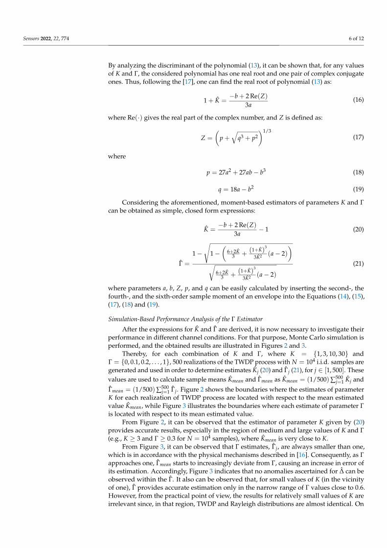
After the expressions for K and Γ are derived, it is now necessary to investigate theirperformance in different channel conditions. For that purpose, Monte Carlo simulation isperformed, and the obtained results are illustrated in Figures 2 and 3.

Thereby, for each combination of K and Γ, where K = 1, 3, 10, 30 andΓ = 0, 0.1, 0.2, . . . , 1, 500 realizations of the TWDP process with N = 104 i.i.d. samples aregenerated and used in order to determine estimates Kj (20) and Γj (21), for j ∈ [1, 500]. Thesevalues are used to calculate sample means Kmean and Γmean as Kmean = (1/500)∑500

j=1 Kj and

Γmean = (1/500)∑500j=1 Γj. Figure 2 shows the boundaries where the estimates of parameter

K for each realization of TWDP process are located with respect to the mean estimatedvalue Kmean, while Figure 3 illustrates the boundaries where each estimate of parameter Γis located with respect to its mean estimated value.

From Figure 2, it can be observed that the estimator of parameter K given by (20)provides accurate results, especially in the region of medium and large values of K and Γ(e.g., K ≥ 3 and Γ ≥ 0.3 for N = 104 samples), where Kmean is very close to K.

From Figure 3, it can be observed that Γ estimates, Γj, are always smaller than one,which is in accordance with the physical mechanisms described in [16]. Consequently, as Γapproaches one, Γmean starts to increasingly deviate from Γ, causing an increase in error ofits estimation. Accordingly, Figure 3 indicates that no anomalies ascertained for ∆ can beobserved within the Γ. It also can be observed that, for small values of K (in the vicinityof one), Γ provides accurate estimation only in the narrow range of Γ values close to 0.6.However, from the practical point of view, the results for relatively small values of K areirrelevant since, in that region, TWDP and Rayleigh distributions are almost identical. On

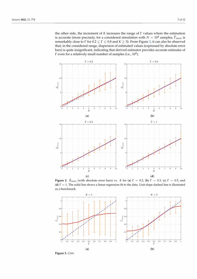
Sensors 2022, 22, 774 7 of 12

the other side, the increment of K increases the range of Γ values where the estimationis accurate (more precisely, for a considered simulation with N = 104 samples, Γmean isremarkably close to Γ for 0.2 ≤ Γ ≤ 0.8 and K ≥ 3). From Figure 3, it can also be observedthat, in the considered range, dispersion of estimated values (expressed by absolute errorbars) is quite insignificant, indicating that derived estimator provides accurate estimates ofΓ even for a relatively small number of samples (i.e., 104).

K0 1 2 3 4 5 6 7 8 9 10

Km

ean

0

5

10

15! = 0:2

(a)

K0 1 2 3 4 5 6 7 8 9 10

Km

ean

0

5

10

15! = 0:3

(b)

K0 1 2 3 4 5 6 7 8 9 10

Km

ean

0

5

10

15! = 0:5

(c)

K0 1 2 3 4 5 6 7 8 9 10

Km

ean

0

5

10

15! = 1

(d)Figure 2. Kmean (with absolute error bars) vs. K for (a) Γ = 0.2, (b) Γ = 0.3, (c) Γ = 0.5, and(d) Γ = 1. The solid line shows a linear regression fit to the data. Unit slope dashed line is illustratedas a benchmark.

!0 0.1 0.2 0.3 0.4 0.5 0.6 0.7 0.8 0.9 1

!m

ean

0

0.2

0.4

0.6

0.8

1

K = 1

(a)

!0 0.1 0.2 0.3 0.4 0.5 0.6 0.7 0.8 0.9 1

!m

ean

0

0.2

0.4

0.6

0.8

1

K = 3

(b)Figure 3. Cont.

Sensors 2022, 22, 774 8 of 12

!0 0.1 0.2 0.3 0.4 0.5 0.6 0.7 0.8 0.9 1

!m

ean

0

0.2

0.4

0.6

0.8

1

K = 10

(c)

!0 0.1 0.2 0.3 0.4 0.5 0.6 0.7 0.8 0.9 1

!m

ean

0

0.2

0.4

0.6

0.8

1

K = 30

(d)Figure 3. Γmean (with absolute error bars) vs. Γ for (a) K = 1, (b) K = 3, (c) K = 10, and (d) K = 30.The solid line shows a linear regression fit to the data. The unit slope dashed line is illustrated asa benchmark.

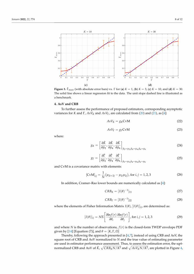
4. AsV and CRB

To further assess the performance of proposed estimators, corresponding asymptoticvariances for K and Γ, AsVK and AsVΓ, are calculated from (20) and (21), as [4]:

AsVK = gKCvM (22)

AsVΓ = gΓCvM (23)

where:

gK =

[∂K∂µ2

,∂K∂µ4

,∂K∂µ6

]µ2=µ2,µ4=µ4,µ6=µ6

(24)

gΓ =

[∂Γ∂µ2

,∂Γ∂µ4

,∂Γ∂µ6

]µ2=µ2,µ4=µ4,µ6=µ6

(25)

and CvM is a covariance matrix with elements:

[CvM]ij =1N(µ2i+2j − µ2iµ2j

), for i, j = 1, 2, 3 (26)

In addition, Cramer–Rao lower bounds are numerically calculated as [4]:

CRBK = [I(θ)−1]11 (27)

CRBΓ = [I(θ)−1]22 (28)

where the elements of Fisher Information Matrix I(θ), [I(θ)]ij, are determined as:

[I(θ)]ij = NE[

∂ln f (r)∂θi

∂ln f (r)∂θj

], for i, j = 1, 2, 3 (29)

and where N is the number of observations, f (r) is the closed-form TWDP envelope PDFgiven by [14] [Equation (7)], and θ = [K, Γ, Ω]

Thereby, following the approach presented in [4,7], instead of using CRB and AsV, thesquare root of CRB and AsV normalized to N and the true value of estimating parameterare used in estimator performance assessment. Thus, to assess the estimation error, the sqrt-normalized CRB and AsV of K,

√CRBK N/K2 and

√AsVK N/K2, are plotted in Figure 4,

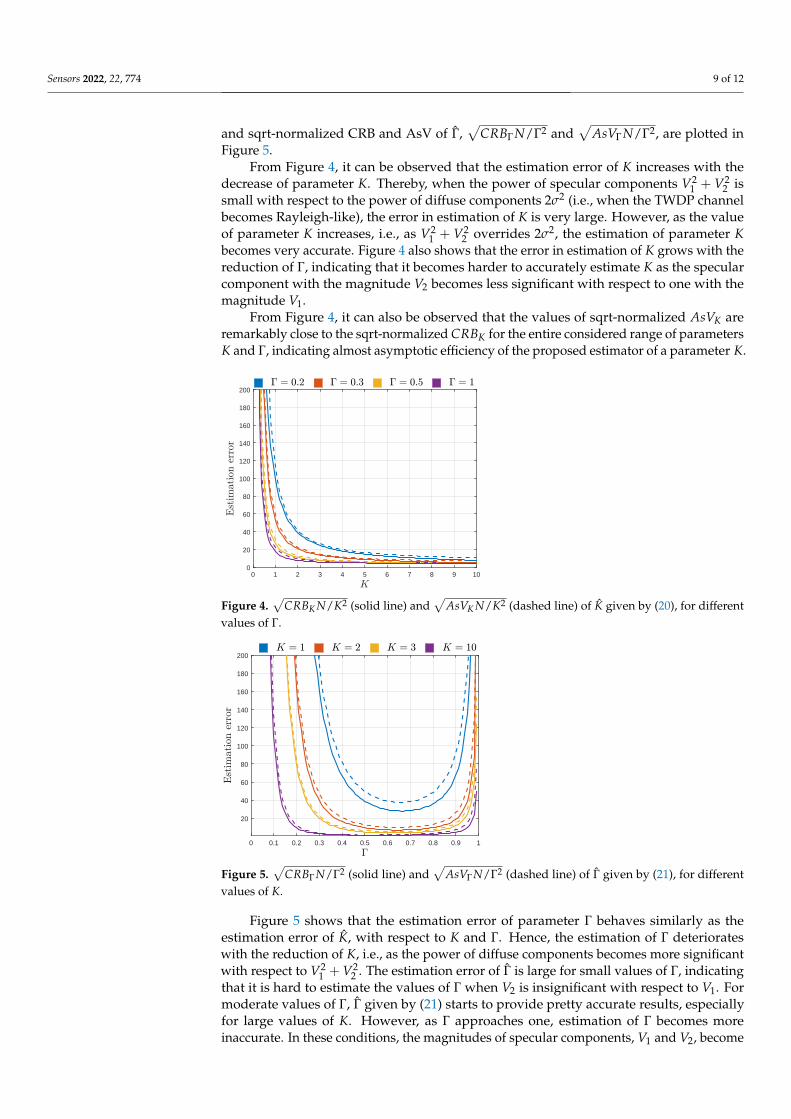
Sensors 2022, 22, 774 9 of 12

and sqrt-normalized CRB and AsV of Γ,√

CRBΓN/Γ2 and√

AsVΓN/Γ2, are plotted inFigure 5.

From Figure 4, it can be observed that the estimation error of K increases with thedecrease of parameter K. Thereby, when the power of specular components V2

1 + V22 is

small with respect to the power of diffuse components 2σ2 (i.e., when the TWDP channelbecomes Rayleigh-like), the error in estimation of K is very large. However, as the valueof parameter K increases, i.e., as V2

1 + V22 overrides 2σ2, the estimation of parameter K

becomes very accurate. Figure 4 also shows that the error in estimation of K grows with thereduction of Γ, indicating that it becomes harder to accurately estimate K as the specularcomponent with the magnitude V2 becomes less significant with respect to one with themagnitude V1.

From Figure 4, it can also be observed that the values of sqrt-normalized AsVK areremarkably close to the sqrt-normalized CRBK for the entire considered range of parametersK and Γ, indicating almost asymptotic efficiency of the proposed estimator of a parameter K.

K0 1 2 3 4 5 6 7 8 9 10

Est

imat

ion

erro

r

0

20

40

60

80

100

120

140

160

180

200! = 0:2 ! = 0:3 ! = 0:5 ! = 1

Figure 4.√

CRBK N/K2 (solid line) and√

AsVK N/K2 (dashed line) of K given by (20), for differentvalues of Γ.

!0 0.1 0.2 0.3 0.4 0.5 0.6 0.7 0.8 0.9 1

Est

imat

ion

erro

r

20

40

60

80

100

120

140

160

180

200K = 1 K = 2 K = 3 K = 10

Figure 5.√

CRBΓ N/Γ2 (solid line) and√

AsVΓ N/Γ2 (dashed line) of Γ given by (21), for differentvalues of K.

Figure 5 shows that the estimation error of parameter Γ behaves similarly as theestimation error of K, with respect to K and Γ. Hence, the estimation of Γ deteriorateswith the reduction of K, i.e., as the power of diffuse components becomes more significantwith respect to V2

1 + V22 . The estimation error of Γ is large for small values of Γ, indicating

that it is hard to estimate the values of Γ when V2 is insignificant with respect to V1. Formoderate values of Γ, Γ given by (21) starts to provide pretty accurate results, especiallyfor large values of K. However, as Γ approaches one, estimation of Γ becomes moreinaccurate. In these conditions, the magnitudes of specular components, V1 and V2, become

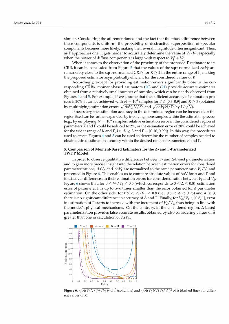
Sensors 2022, 22, 774 10 of 12

similar. Considering the aforementioned and the fact that the phase difference betweenthese components is uniform, the probability of destructive superposition of specularcomponents becomes more likely, making their overall magnitude often insignificant. Thus,as Γ approaches one, it gets harder to accurately determine the value of V2/V1, especiallywhen the power of diffuse components is large with respect to V2

1 + V22 .

When it comes to the observation of the proximity of the proposed Γ estimator to itsCRB, it can be concluded from Figure 5 that the values of the sqrt-normalized AsVΓ areremarkably close to the sqrt-normalized CRBΓ for K ≥ 2 in the entire range of Γ, makingthe proposed estimator asymptotically efficient for the considered values of K.

Accordingly, except for providing estimation errors significantly close to the cor-responding CRBs, moment-based estimators (20) and (21) provide accurate estimatesobtained from a relatively small number of samples, which can be clearly observed fromFigures 4 and 5. For example, if we assume that the sufficient accuracy of estimation pro-cess is 20%, it can be achieved with N = 104 samples for Γ ∈ [0.3, 0.9] and K ≥ 3 (obtainedby multiplying estimation errors

√AsVK N/K2 and

√AsVΓN/Γ2 by 1/

√N).

If necessary, the estimation accuracy in the determined region can be increased, or theregion itself can be further expanded, by involving more samples within the estimation process(e.g., by employing N = 106 samples, relative estimation error in the considered region ofparameters K and Γ could be reduced to 2%, or the estimation error of 20% could be achievedfor the wider range of K and Γ, i.e., K ≥ 3 and Γ ∈ [0.16, 0.99]). In this way, the proceduresused to create Figures 4 and 5 can be used to determine the number of samples needed toobtain desired estimation accuracy within the desired range of parameters K and Γ.

5. Comparison of Moment-Based Estimators for the ∆- and Γ-ParameterizedTWDP Model

In order to observe qualitative differences between Γ- and ∆-based parameterizationand to gain more precise insight into the relation between estimation errors for consideredparameterizations, AsV∆ and AsVΓ are normalized to the same parameter ratio V2/V1 andpresented in Figure 6. This enables us to compare absolute values of AsV for ∆ and Γ andto discover differences in their estimation errors for considered ratios between V1 and V2.Figure 6 shows that, for 0 ≤ V2/V1 ≤ 0.5 (which corresponds to 0 ≤ ∆ ≤ 0.8), estimationerror of parameter Γ is up to two times smaller than the error obtained for ∆ parameterestimation. On the other side, for 0.5 < V2/V1 < 0.8 (i.e., 0.8 < ∆ < 0.96) and K ≥ 3,there is no significant difference in accuracy of ∆ and Γ. Finally, for V2/V1 ∈ [0.8, 1], errorin estimation of Γ starts to increase with the increment of V2/V1, thus being in line withthe model’s physical mechanisms. On the contrary, in the considered region, ∆-basedparameterization provides false accurate results, obtained by also considering values of ∆greater than one in calculation of AsV∆.

V2=V1

0 0.1 0.2 0.3 0.4 0.5 0.6 0.7 0.8 0.9 1

Est

imat

ion

erro

r

20

40

60

80

100

120

140

160

180

200K = 1 K = 2 K = 3 K = 10

Figure 6.√

AsVΓ N/(V2/V1)2 of Γ (solid line) and√

AsV∆ N/(V2/V1)2 of ∆ (dashed line), for differ-ent values of K.

Sensors 2022, 22, 774 11 of 12

Accordingly, in the region of ∆ ≤ 0.8, i.e., Γ ≤ 0.5, estimation accuracy is significantlyimproved by using Γ-based parameterization instead of ∆-based, while in the region of∆ ≈ 1, i.e., Γ ≈ 1, Γ-based parameterization prevents the occurrence of nonphysicalsolutions obtained by estimating parameter ∆.

Except for benefits of Γ-based parameterization observed with respect to Γ, it alsoenables reduction of the estimation error of a parameter K, for a much wider set of valuesof a parameter, which reflects the relation between V1 and V2. Namely, based on theexpression of parameter K given in terms of ∆ and the results presented in [14] [Figure 2], itcan be concluded that K/KRice is almost constant for the entire range of small and mediumvalues of ∆, implying that values of V2 ∈ [0, V1/2] make almost no impact on the valueof parameter K. This causes quite pronounced errors in estimation of K for the entirerange of small and medium values of ∆ (i.e., 0 ≤ ∆ < 0.5), which can be clearly observedfrom [4] [Figure 1]. On the contrary, Figure 4 shows that, when K is expressed in terms ofΓ, no such anomaly can be observed. In these circumstances, errors in estimation of K arehuge only for small values of Γ (i.e., Γ < 0.2).

6. Conclusions

In this paper, the problem of TWDP parameters’ estimation has been investigatedin depth. The investigation revealed that the existing moment-based estimators of con-ventional TWDP parameters are not able to provide accurate estimations for variouscombinations of their values, due to a nonphysical definition of parameter ∆. Accordingly,in this paper, moment-based estimators for physically justified parameters K and Γ arederived. It is shown that derived estimators provide estimates from 104 samples with theestimation error smaller than 20%, when parameters K and Γ are in the range K ≥ 3 and0.3 ≤ Γ ≤ 0.9. This indicates that the parameters K and Γ can be efficiently estimated usingderived expressions within the range of these parameters expected to be obtained in themmWave band, even from a relatively small number of samples. Since Γ-based estimatorsenable us to gain precise insight into the ratios between two specular and specular to dif-fuse components in the wide varieties of propagation conditions, simultaneously reducingestimation errors with respect to ∆-based parameterization, it is recommended to adoptparameters K and Γ as the only relevant parameters for a description of TWDP fadingand to revise the existing measurement-based results related to the estimation of TWDPparameters in specific propagation conditions.

Author Contributions: Conceptualization, A.M., P.N. and E.K.; methodology, P.N.; software, A.M.and P.N.; validation, A.M. and P.N.; formal analysis, A.M.; investigation, P.N.; resources, P.N., E.K.and A.M.; data curation, A.M.; writing—original draft preparation, P.N.; writing—review and editing,P.N.; visualization, A.M.; supervision, A.M.; project administration, A.M.; funding acquisition, A.M.,P.N. and E.K. All authors have read and agreed to the published version of the manuscript.

Funding: This research received no external funding.

Institutional Review Board Statement: Not applicable.

Informed Consent Statement: Not applicable.

Data Availability Statement: Not applicable.

Acknowledgments: The authors would like to thank Ivo M. Kostic for many valuable discussionsand advice.

Conflicts of Interest: The authors declare no conflict of interest.

References1. Dixit, D.; Sahu, P.R. Performance of QAM signaling over TWDP fading channels. IEEE Trans. Wirel. Commun. 2013, 12, 1794–1799.

[CrossRef]2. Lu, Y.; Yang, N. Symbol error probability of QAM with MRC diversity in two-wave with diffuse power fading channels. IEEE

Commun. Lett. 2011, 15, 10–12. [CrossRef]3. Frolik, J. A case for considering hyper-Rayleigh fading channels. IEEE Trans. Wirel. Commun. 2007, 6, 1235–1239. [CrossRef]

Sensors 2022, 22, 774 12 of 12

4. Lopez-Fernandez, J.; Moreno-Pozas, L.; Lopez-Martinez, F.J.; Martos-Naya, E. Joint Parameter Estimation for the Two-Wave withDiffuse Power Fading Model. Sensors 2016, 16, 1014. [CrossRef] [PubMed]

5. Singh, S.; Kansal, V. Performance of M-ary PSK over TWDP fading channels. Int. J. Electron. Lett. 2016, 4, 433–437. [CrossRef]6. Rappaport, T.; Heath, R.; Daniels, R.; Murdock, J. Millimeter Wave Wireless Communications; Prentice Hall: Upper Saddle River, NJ,

USA, 2015.7. Lopez-Fernandez, J.; Moreno-Pozas, L.; Martos-Naya, E.; Lopez-Martinez, F.J. Moment-Based Parameter Estimation for the

Two-Wave with Diffuse Power Fading Model. In Proceedings of the 2016 IEEE 84th Vehicular Technology Conference (VTC-Fall),Montreal, QC, Canada, 18–21 September 2016; pp. 1–5. [CrossRef]

8. Frolik, J. On appropriate models for characterizing hyper-Rayleigh fading. IEEE Trans. Wirel. Commun. 2008, 7, 5202–5207.[CrossRef]

9. Zöchmann, E.; Blumenstein, J.; Marsalek, R.; Rupp, M.; Guan, K. Parsimonious channel models for millimeter wave railwaycommunications. In Proceedings of the 2019 IEEE Wireless Communications and Networking Conference (WCNC), Marrakesh,Morocco, 15–18 April 2019; pp. 1–6. [CrossRef]

10. Zöchmann, E.; Hofer, M.; Lerch, M.; Pratschner, S.; Bernadó, L.; Blumenstein, J.; Caban, S.; Sangodoyin, S.; Groll, H.;Zemen, T.; et al. Position-Specific Statistics of 60 GHz Vehicular Channels During Overtaking. IEEE Access 2019, 7, 14216–14232. [CrossRef]

11. Zöchmann, E.; Caban, S.; Mecklenbräuker, C.F.; Pratschner, S.; Lerch, M.; Schwarz, S.; Rupp, M. Better than Rician: Modellingmillimetre wave channels as two-wave with diffuse power. EURASIP J. Wirel. Commun. Netw. 2019, 2019, 21. [CrossRef]

12. Mavridis, T.; Petrillo, L.; Sarrazin, J.; Benlarbi-Delaï, A.; De Doncker, P. Near-body shadowing analysis at 60 GHz. IEEE Trans.Antennas Propag. 2015, 63, 4505–4511. [CrossRef]

13. Durgin, G.D.; Rappaport, T.S.; de Wolf, D.A. New analytical models and probability density functions for fading in wirelesscommunications. IEEE Trans. Commun. 2002, 50, 1005–1015. [CrossRef]

14. Maric, A.; Kaljic, E.; Njemcevic, P. An Alternative Statistical Characterization of TWDP Fading Model. Sensors 2021, 21, 7513.[CrossRef] [PubMed]

15. Tepedelenlioglu, C.; Abdi, A.; Giannakis, G. The Ricean K factor: Estimation and performance analysis. IEEE Tran. Wirel.Commun. 2003, 2, 799–810. [CrossRef]

16. Shi, B.; Pallotta, L.; Giunta, G.; Hao, C.; Orlando, D. Parameter Estimation of Fluctuating Two-Ray Model for Next, GenerationMobile Communications. IEEE Trans. Veh. Technol. 2020, 69, 8684–8697. [CrossRef]

17. Weisstein, E.W. Cubic Formula. https://mathworld.wolfram.com/CubicFormula.html (accessed on 1 October 2021).