1794 VOLUME 61J O U R N A L O F T H E A T M O S P H E R I C S C I E N C E S

q 2004 American Meteorological Society

Mesoscale Predictability of Moist Baroclinic Waves: Experiments withParameterized Convection

ZHE-MIN TAN

Department of Atmospheric Sciences, Nanjing University, Nanjing, China

FUQING ZHANG

Department of Atmospheric Sciences, Texas A&M University, College Station, Texas

RICHARD ROTUNNO AND CHRIS SNYDER

National Center for Atmospheric Research,* Boulder, Colorado

(Manuscript received 7 May 2003, in final form 22 January 2004)

ABSTRACT

Recent papers by the authors demonstrated the possible influence of initial errors of small amplitude and scaleon the numerical prediction of the ‘‘surprise’’ snowstorm of 24–25 January 2000. They found that initial errorsgrew rapidly at scales below 200 km, and that the rapid error growth was dependent on moist processes. In anattempt to generalize these results from a single case study, the present paper studies the error growth in anidealized baroclinic wave amplifying in a conditionally unstable atmosphere. The present results show thatwithout the effects of moisture, there is little error growth in the short-term (0–36 h) forecast error (startingfrom random noise), even though the basic jet used here produces a rapidly growing synoptic-scale disturbance.With the effect of moisture included, the error is characterized by upscale growth, basically as found by theauthors in their study of the numerical prediction of the surprise snowstorm.

1. Introduction

Lorenz (1969) hypothesized that even if forecast er-rors were to be reduced through improvements in eitherthe forecast models or their initial conditions, errors dueto small-scale motions may grow in amplitude and scaleso rapidly that they place an effective limit on the pre-dictive skill of a model. Recent papers by Zhang et al.(2002, hereafter ZSR02) and Zhang et al (2003, here-after ZSR03) focusing on the ‘‘surprise’’ snowstorm of24–25 January 2000 demonstrate the influence of initialerrors of small amplitude and scale on the numericalprediction of that storm. They found that initial errorsgrew rapidly at scales below 200 km, and that the rapiderror growth was dependent on moist processes. Here,we report on our attempt to isolate within an idealizedcontext this error-growth behavior.

The snowstorm of 24–25 January 2000 on the south-

* The National Center for Atmospheric Research is sponsored bythe National Science Foundation.

Corresponding author address: Dr. Fuqing Zhang, Department ofAtmospheric Sciences, Texas A&M University, College Station, TX77845-3150.E-mail: fzhang@tamu.edu

eastern coast of the United States was the result of anamplifying, eastward-moving, synoptic-scale wave (seeFig. 8 of Langland et al. 2002). Using the U.S. Navyglobal forecast model and (dry) adjoint system, Lang-land et al. (2002, see their Table 1) showed that the 3–4-day forecast for the East Coast for 1200 UTC 25January 2000 was in considerable error, and very sen-sitive to the model initial condition; in comparison withthe 3–4-day forecasts, the 1–2-day forecasts were con-sidered to be moderately good from the synoptic-scaleperspective, and far less sensitive to initial-conditionerror. Using the fifth-generation Pennsylvania State Uni-versity (PSU)–National Center for Atmospheric Re-search (NCAR) Mesoscale Model (MM5; Dudhia 1993),ZSR02 investigated the 0–36-h forecast for the samecase; MM5 forecasts initialized from several differentoperational initial analyses showed, consistent withLangland et al. (2002), similarly good skill from a large-scale perspective, but rather large differences among theforecasts in their mesoscale precipitation patterns.

By comparing simulations of the same case in whichthe initial conditions differed by a small-amplitude per-turbation concentrated at the smallest resolvable scale,ZSR03 showed how the error in the 36-h forecast pre-cipitation pattern originates in small scales and then

15 JULY 2004 1795T A N E T A L .

amplifies as it spreads upscale and that the error growthis associated with conditional instability and (parame-terized) moist convection. This is in general agreementwith the results of Ehrendorfer et al. (1999), using amesoscale model and its adjoint including moist pro-cesses; they also showed that, in the presence of param-eterized moist convection, errors may grow more rapidlyand at smaller scales than in a dry version of the model.In their highest-resolution experiments (inner grid of3.3-km horizontal resolution without a parameterizationof moist convection), ZSR03 found that the small-scaledifferences appeared first as differences in the timingand placement of convective cells and then spread up-scale to alter the shape and location of the surface cy-clone in the 36-h forecast.

Our focus in this paper is on the potential for initialerrors of small scale and small amplitude to impose anintrinsic limit on the predictability of mesoscale flows,even in the absence of other sources of error. In practice,of course, the skill of today’s weather forecast may beinfluenced by numerous factors, such as analysis errorsof significant amplitude and synoptic scale, errors in thelateral boundary conditions and errors in the forecastmodel itself. For the snowstorm of 24–25 January 2000,ZSR02 showed that each of those additional factors maywell have contributed to the poor operational forecast.Although the scope of the present paper will be limitedto the growth of small-scale and small-amplitude initialerrors, we emphasize that, as in the snowstorm of 24–25 January 2000, other sources of forecast error arepossible. A discussion of these other sources and a morecomplete review of the literature on mesoscale predict-ability can be found in ZSR02 and ZSR03.

Motivated by the observation that the snowstorm of24–25 January 2000 was associated with the down-stream amplification of a synoptic-scale wave and wish-ing to generalize the results of ZSR02 and ZSR03 froma single case, we have carried out MM5 simulations ofan idealized baroclinic jet in a channel with a prescribedinitial synoptic-scale perturbation restricted to the west-ern (upstream) end of the channel. The latter problemhas been extensively studied (see Hakim 2000 for arecent review) as a model for the observed amplificationof synoptic-scale waves. To the idealized baroclinic jet,we have added a moisture distribution so that the ide-alized atmosphere is conditionally (as well as baroclin-ically) unstable. This experimental setup allows us toinvestigate in a simpler, but still realistic, context thesuggestion of ZSR03 that the rapid error growth seenin their simulations required conditional instability andeither moist convection (in the highest-resolution runs)or its parameterization.

The paper is structured as follows. A brief introduc-tion to the numerical model, initial condition and ex-perimental design for the work are presented in section2, followed in section 3 by a description of the simu-lation of the idealized moist baroclinic wave. Section 4analyzes the error growth within that baroclinic wave.

Dependence of the error growth on the waves’ initialmoisture distributions is explored in section 5. Section6 contains a summary.

2. Model description, initial condition, andexperimental design

a. Model description

To study the mesoscale structure within an evolvingsynoptic-scale wave, we employ here MM5 (version 2)on two model domains (D1, D2) with 90- and 30-kmhorizontal grid resolution, respectively, and 60 verticallayers. For simplicity, the model employs Cartesian co-ordinates and a constant Coriolis parameter. Domain D1is configured in the shape of a channel 18 000 km long(east–west or x direction) and 8010 km wide (north–south or y direction), while D2 is a rectangular sub-domain 8400 km long and 4800 km wide centered at(9720 km, 3960 km) within D1. The Grell (1993) cu-mulus parameterization, the MRF planetary boundarylayer scheme (Hong and Pan 1996), the Reisner micro-physics scheme with graupel (Reisner et al. 1998), anda simple radiation parameterization are used in bothdomains. At the lower boundary, a drag law (with uni-form surface roughness length 5 1024 m) and no heat/moisture flux are applied throughout the domain. In ad-dition to its use of an idealized initial flow, the presentsimulation thus also neglects physiographic effects as-sociated with orography and heat and moisture fluxesfrom the ocean. Although the latter certainly plays somerole in coastal storms of the type that produced thesnowstorm of 24–25 January 2000, their conscious ne-glect here eliminates a potential sensitivity and simpli-fies the interpretation of the results.

b. Initial condition

The initial condition of an idealized two-dimensionalbaroclinic jet with a balanced three-dimensional per-turbation is generated through the following steps.

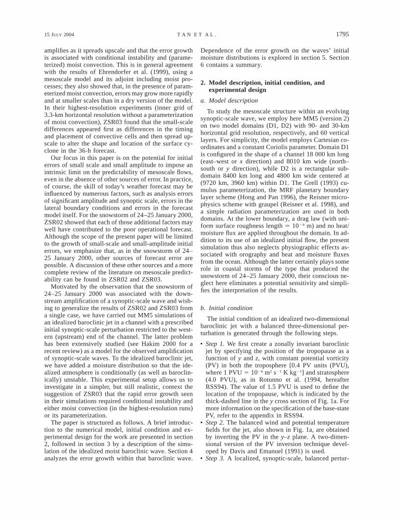
• Step 1. We first create a zonally invariant baroclinicjet by specifying the position of the tropopause as afunction of y and z, with constant potential vorticity(PV) in both the troposphere [0.4 PV units (PVU),where 1 PVU 5 1026 m2 s21 K kg21] and stratosphere(4.0 PVU), as in Rotunno et al. (1994, hereafterRSS94). The value of 1.5 PVU is used to define thelocation of the tropopause, which is indicated by thethick-dashed line in the y cross section of Fig. 1a. Formore information on the specification of the base-statePV, refer to the appendix in RSS94.

• Step 2. The balanced wind and potential temperaturefields for the jet, also shown in Fig. 1a, are obtainedby inverting the PV in the y–z plane. A two-dimen-sional version of the PV inversion technique devel-oped by Davis and Emanuel (1991) is used.

• Step 3. A localized, synoptic-scale, balanced pertur-

1796 VOLUME 61J O U R N A L O F T H E A T M O S P H E R I C S C I E N C E S

FIG. 1. (a) Vertical cross section of initial potential temperature(thin line, D 5 6 K) and zonal velocity (thick line, D 5 10 m s21)for the initial basic-state jet. The gray thick line denotes the locationof the tropopause where potential vorticity equals 1.5 PVU. (b) Ver-tical distribution of the initial relative humidity for the control ex-periment (D 5 10%). (c) Meridional variation of surface CAPE (solid)and CIN (dashed) for both the CNTL experiment and EXP70.

bation of moderate amplitude is then added to the basestate from step 2 to represent the early phase of atypical midlatitude cyclogenesis. Similar to Rotunnoand Bao (1996), the perturbation is obtained by spec-ifying a horizontal displacement field, calculating aPV perturbation by multiplying that displacement bythe meridional gradient of PV. For more informationon the specification of the PV perturbation, refer toRotunno and Bao (1996, p. 1057).

• Step 4. We then invert the 3D perturbed PV fieldsfrom step 3 to obtain the streamfunction and geopo-tential (and thus wind and temperature) fields againusing the PV inversion technique of Davis and Eman-uel (1991).

• Step 5. The initial relative humidity (RH) is given by(A1) in the appendix. The control experiment uses(RH)0 5 100% in (A1), which yields strong condi-tional instability in the southern portion of the domainin the control experiment. The resulting initial distri-bution of RH in the control experiment varies from100% at the lowest level to 10% above a height of 8km and is shown in Fig. 1b. The surface convectiveavailable potential energy (CAPE) and surface con-vective inhibition (CIN) along the meridional crosssection are shown in Fig. 1c.

The combination of the baroclinic jet and a balancedmoderate-amplitude PV disturbance ensures the strongdevelopment of a baroclinic wave as discussed in Hakim(2000). The same balanced initialization method but fora dry baroclinic wave was used in Zhang (2004).

c. Experimental design

For the control experiment (CNTL), the model is in-tegrated on the coarse domain (D1) for 72 h using thebalanced initial conditions constructed as detailed aboveand fixed lateral boundary conditions. We envision thisintegration to be analogous to a global model forecastingan amplifying, eastward-propagating synoptic-scale dis-turbance. The inner domain (D2) of the model is ini-tialized at 36 h by interpolating from the solution onD1. The integration on D1 then proceeds for 36 h withlateral boundary conditions provided by D1 throughone-way nesting. Hence, the simulation on D2 (CNTL-D2) may be viewed as a limited-area mesoscale forecastdriven by a hemispheric forecast (from D1).

To investigate how small changes to the initial con-ditions evolve during this forecast, another simulationof the nested domain is performed that is identical toCNTL-D2 but with perturbed initial conditions(CNTL-D2P). The perturbation to the initial conditionsconsists of random, Gaussian noise added to the tem-perature field on D2; the noise has a zero mean, stan-dard deviation 0.2 K, and is independent at each gridpoint and each grid level. Unlike the perturbations usedin ZSR03, which were monochromatic with a wave-

15 JULY 2004 1797T A N E T A L .

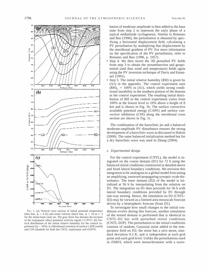
FIG. 2. CNTL-D1 simulated surface potential temperature (thinline, D 5 6 K) and sea level pressure (thick line, D 5 8 hPa) validat (a) 36 and (b) 72 h of the coarse-grid forecast. The gray box denotesthe location of the nested domain (D2). The distance between tickmarks is 900 km.

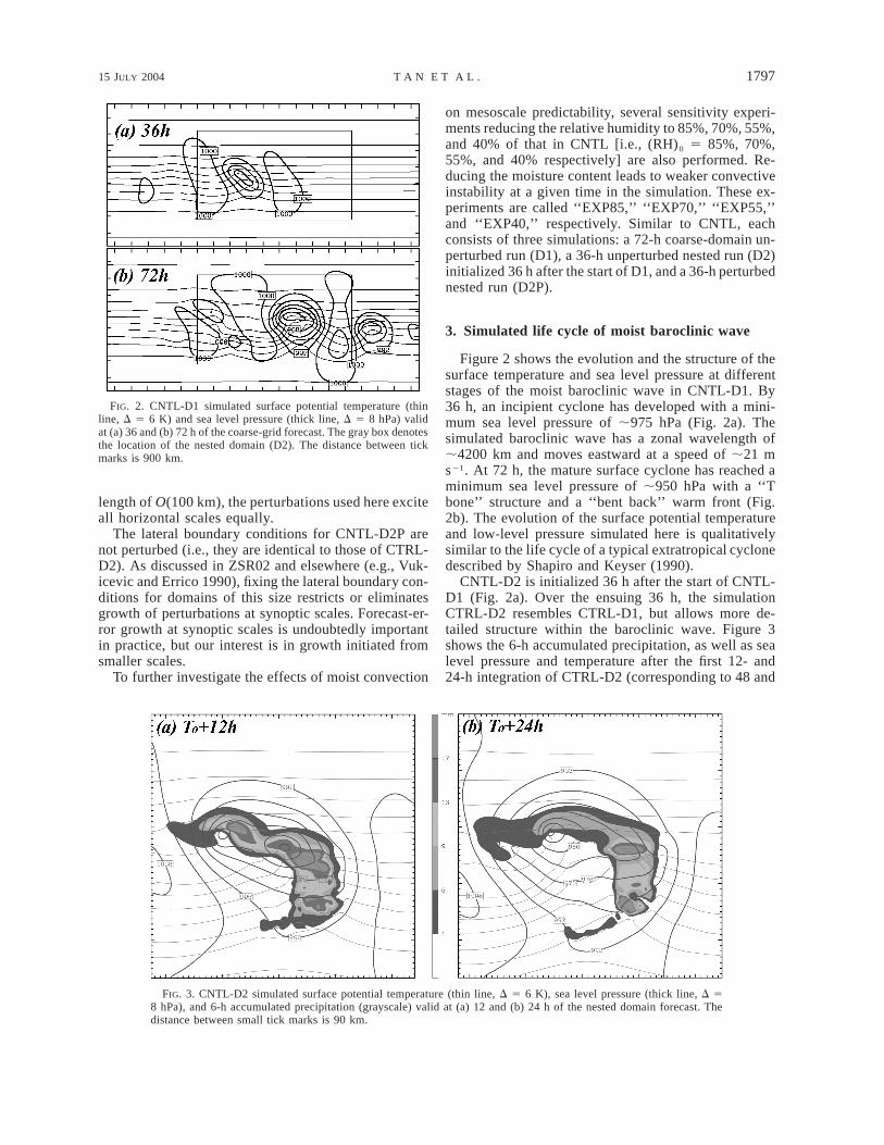
FIG. 3. CNTL-D2 simulated surface potential temperature (thin line, D 5 6 K), sea level pressure (thick line, D 58 hPa), and 6-h accumulated precipitation (grayscale) valid at (a) 12 and (b) 24 h of the nested domain forecast. Thedistance between small tick marks is 90 km.

length of O(100 km), the perturbations used here exciteall horizontal scales equally.

The lateral boundary conditions for CNTL-D2P arenot perturbed (i.e., they are identical to those of CTRL-D2). As discussed in ZSR02 and elsewhere (e.g., Vuk-icevic and Errico 1990), fixing the lateral boundary con-ditions for domains of this size restricts or eliminatesgrowth of perturbations at synoptic scales. Forecast-er-ror growth at synoptic scales is undoubtedly importantin practice, but our interest is in growth initiated fromsmaller scales.

To further investigate the effects of moist convection

on mesoscale predictability, several sensitivity experi-ments reducing the relative humidity to 85%, 70%, 55%,and 40% of that in CNTL [i.e., (RH)0 5 85%, 70%,55%, and 40% respectively] are also performed. Re-ducing the moisture content leads to weaker convectiveinstability at a given time in the simulation. These ex-periments are called ‘‘EXP85,’’ ‘‘EXP70,’’ ‘‘EXP55,’’and ‘‘EXP40,’’ respectively. Similar to CNTL, eachconsists of three simulations: a 72-h coarse-domain un-perturbed run (D1), a 36-h unperturbed nested run (D2)initialized 36 h after the start of D1, and a 36-h perturbednested run (D2P).

3. Simulated life cycle of moist baroclinic wave

Figure 2 shows the evolution and the structure of thesurface temperature and sea level pressure at differentstages of the moist baroclinic wave in CNTL-D1. By36 h, an incipient cyclone has developed with a mini-mum sea level pressure of ;975 hPa (Fig. 2a). Thesimulated baroclinic wave has a zonal wavelength of;4200 km and moves eastward at a speed of ;21 ms21. At 72 h, the mature surface cyclone has reached aminimum sea level pressure of ;950 hPa with a ‘‘Tbone’’ structure and a ‘‘bent back’’ warm front (Fig.2b). The evolution of the surface potential temperatureand low-level pressure simulated here is qualitativelysimilar to the life cycle of a typical extratropical cyclonedescribed by Shapiro and Keyser (1990).

CNTL-D2 is initialized 36 h after the start of CNTL-D1 (Fig. 2a). Over the ensuing 36 h, the simulationCTRL-D2 resembles CTRL-D1, but allows more de-tailed structure within the baroclinic wave. Figure 3shows the 6-h accumulated precipitation, as well as sealevel pressure and temperature after the first 12- and24-h integration of CTRL-D2 (corresponding to 48 and

1798 VOLUME 61J O U R N A L O F T H E A T M O S P H E R I C S C I E N C E S

60 h of CTRL-D1, respectively) on a 4200 km 3 4200km window. An elongated warm front is stronger thanthe cold front, similar to the moist baroclinic wavessimulated by Whitaker and Davis (1994) and Fantini(1999). Over the 36-h of nested-grid simulation, thesurface cyclone continues to deepen and the total pre-cipitation (6-h accumulations) continues to increase.

In a broad outline, the control simulations reproducethe features found in past primitive equation simulationsof dry and moist baroclinic waves (e.g., RSS94; Whi-taker and Davis 1994; Shapiro et al. 1999), which fea-tures are, in turn, fairly realistic. Hence, we use thesesimulations as a testbed in which to examine the influ-ence of moist convection on mesoscale predictability.

4. Error growth in simulated moist baroclinicwaves

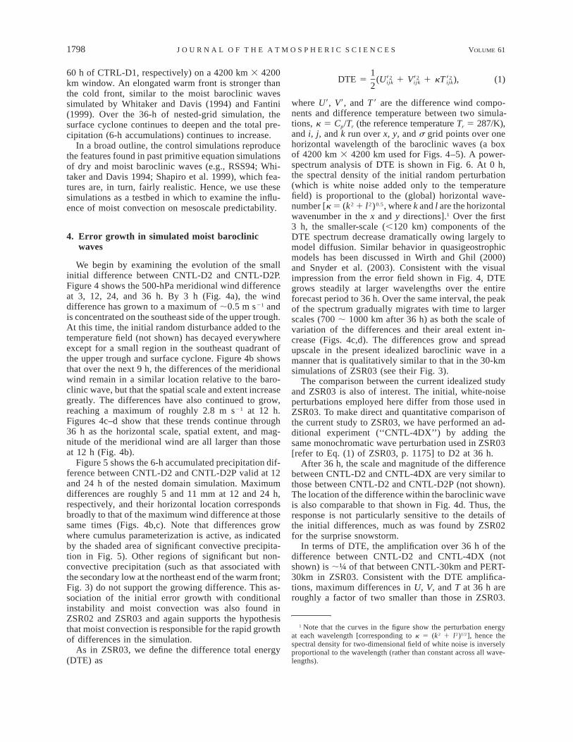
We begin by examining the evolution of the smallinitial difference between CNTL-D2 and CNTL-D2P.Figure 4 shows the 500-hPa meridional wind differenceat 3, 12, 24, and 36 h. By 3 h (Fig. 4a), the winddifference has grown to a maximum of ;0.5 m s21 andis concentrated on the southeast side of the upper trough.At this time, the initial random disturbance added to thetemperature field (not shown) has decayed everywhereexcept for a small region in the southeast quadrant ofthe upper trough and surface cyclone. Figure 4b showsthat over the next 9 h, the differences of the meridionalwind remain in a similar location relative to the baro-clinic wave, but that the spatial scale and extent increasegreatly. The differences have also continued to grow,reaching a maximum of roughly 2.8 m s21 at 12 h.Figures 4c–d show that these trends continue through36 h as the horizontal scale, spatial extent, and mag-nitude of the meridional wind are all larger than thoseat 12 h (Fig. 4b).

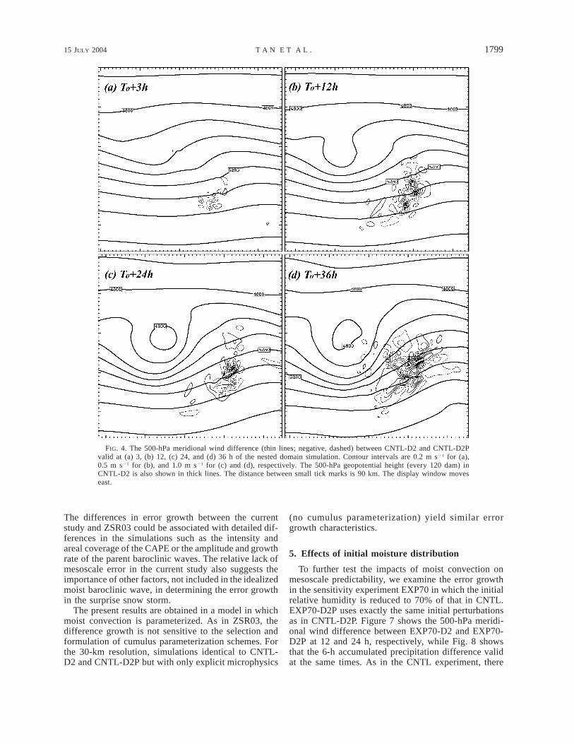
Figure 5 shows the 6-h accumulated precipitation dif-ference between CNTL-D2 and CNTL-D2P valid at 12and 24 h of the nested domain simulation. Maximumdifferences are roughly 5 and 11 mm at 12 and 24 h,respectively, and their horizontal location correspondsbroadly to that of the maximum wind difference at thosesame times (Figs. 4b,c). Note that differences growwhere cumulus parameterization is active, as indicatedby the shaded area of significant convective precipita-tion in Fig. 5). Other regions of significant but non-convective precipitation (such as that associated withthe secondary low at the northeast end of the warm front;Fig. 3) do not support the growing difference. This as-sociation of the initial error growth with conditionalinstability and moist convection was also found inZSR02 and ZSR03 and again supports the hypothesisthat moist convection is responsible for the rapid growthof differences in the simulation.

As in ZSR03, we define the difference total energy(DTE) as

12 2 2DTE 5 (U9 1 V9 1 kT9 ), (1)i jk ijk ijk2

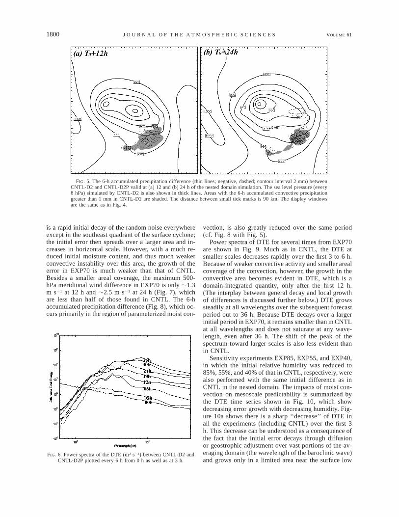
where U9, V9, and T9 are the difference wind compo-nents and difference temperature between two simula-tions, k 5 Cp/Tr (the reference temperature Tr 5 287/K),and i, j, and k run over x, y, and s grid points over onehorizontal wavelength of the baroclinic waves (a boxof 4200 km 3 4200 km used for Figs. 4–5). A power-spectrum analysis of DTE is shown in Fig. 6. At 0 h,the spectral density of the initial random perturbation(which is white noise added only to the temperaturefield) is proportional to the (global) horizontal wave-number [k 5 (k2 1 l2)0.5, where k and l are the horizontalwavenumber in the x and y directions].1 Over the first3 h, the smaller-scale (,120 km) components of theDTE spectrum decrease dramatically owing largely tomodel diffusion. Similar behavior in quasigeostrophicmodels has been discussed in Wirth and Ghil (2000)and Snyder et al. (2003). Consistent with the visualimpression from the error field shown in Fig. 4, DTEgrows steadily at larger wavelengths over the entireforecast period to 36 h. Over the same interval, the peakof the spectrum gradually migrates with time to largerscales (700 ; 1000 km after 36 h) as both the scale ofvariation of the differences and their areal extent in-crease (Figs. 4c,d). The differences grow and spreadupscale in the present idealized baroclinic wave in amanner that is qualitatively similar to that in the 30-kmsimulations of ZSR03 (see their Fig. 3).

The comparison between the current idealized studyand ZSR03 is also of interest. The initial, white-noiseperturbations employed here differ from those used inZSR03. To make direct and quantitative comparison ofthe current study to ZSR03, we have performed an ad-ditional experiment (‘‘CNTL-4DX’’) by adding thesame monochromatic wave perturbation used in ZSR03[refer to Eq. (1) of ZSR03, p. 1175] to D2 at 36 h.

After 36 h, the scale and magnitude of the differencebetween CNTL-D2 and CNTL-4DX are very similar tothose between CNTL-D2 and CNTL-D2P (not shown).The location of the difference within the baroclinic waveis also comparable to that shown in Fig. 4d. Thus, theresponse is not particularly sensitive to the details ofthe initial differences, much as was found by ZSR02for the surprise snowstorm.

In terms of DTE, the amplification over 36 h of thedifference between CNTL-D2 and CNTL-4DX (notshown) is ;¼ of that between CNTL-30km and PERT-30km in ZSR03. Consistent with the DTE amplifica-tions, maximum differences in U, V, and T at 36 h areroughly a factor of two smaller than those in ZSR03.

1 Note that the curves in the figure show the perturbation energyat each wavelength [corresponding to k 5 (k2 1 l2)1/2], hence thespectral density for two-dimensional field of white noise is inverselyproportional to the wavelength (rather than constant across all wave-lengths).

15 JULY 2004 1799T A N E T A L .

FIG. 4. The 500-hPa meridional wind difference (thin lines; negative, dashed) between CNTL-D2 and CNTL-D2Pvalid at (a) 3, (b) 12, (c) 24, and (d) 36 h of the nested domain simulation. Contour intervals are 0.2 m s 21 for (a),0.5 m s21 for (b), and 1.0 m s21 for (c) and (d), respectively. The 500-hPa geopotential height (every 120 dam) inCNTL-D2 is also shown in thick lines. The distance between small tick marks is 90 km. The display window moveseast.

The differences in error growth between the currentstudy and ZSR03 could be associated with detailed dif-ferences in the simulations such as the intensity andareal coverage of the CAPE or the amplitude and growthrate of the parent baroclinic waves. The relative lack ofmesoscale error in the current study also suggests theimportance of other factors, not included in the idealizedmoist baroclinic wave, in determining the error growthin the surprise snow storm.

The present results are obtained in a model in whichmoist convection is parameterized. As in ZSR03, thedifference growth is not sensitive to the selection andformulation of cumulus parameterization schemes. Forthe 30-km resolution, simulations identical to CNTL-D2 and CNTL-D2P but with only explicit microphysics

(no cumulus parameterization) yield similar errorgrowth characteristics.

5. Effects of initial moisture distribution

To further test the impacts of moist convection onmesoscale predictability, we examine the error growthin the sensitivity experiment EXP70 in which the initialrelative humidity is reduced to 70% of that in CNTL.EXP70-D2P uses exactly the same initial perturbationsas in CNTL-D2P. Figure 7 shows the 500-hPa meridi-onal wind difference between EXP70-D2 and EXP70-D2P at 12 and 24 h, respectively, while Fig. 8 showsthat the 6-h accumulated precipitation difference validat the same times. As in the CNTL experiment, there

1800 VOLUME 61J O U R N A L O F T H E A T M O S P H E R I C S C I E N C E S

FIG. 5. The 6-h accumulated precipitation difference (thin lines; negative, dashed; contour interval 2 mm) betweenCNTL-D2 and CNTL-D2P valid at (a) 12 and (b) 24 h of the nested domain simulation. The sea level pressure (every8 hPa) simulated by CNTL-D2 is also shown in thick lines. Areas with the 6-h accumulated convective precipitationgreater than 1 mm in CNTL-D2 are shaded. The distance between small tick marks is 90 km. The display windowsare the same as in Fig. 4.

FIG. 6. Power spectra of the DTE (m2 s22) between CNTL-D2 andCNTL-D2P plotted every 6 h from 0 h as well as at 3 h.

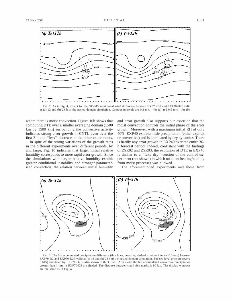
is a rapid initial decay of the random noise everywhereexcept in the southeast quadrant of the surface cyclone;the initial error then spreads over a larger area and in-creases in horizontal scale. However, with a much re-duced initial moisture content, and thus much weakerconvective instability over this area, the growth of theerror in EXP70 is much weaker than that of CNTL.Besides a smaller areal coverage, the maximum 500-hPa meridional wind difference in EXP70 is only ;1.3m s21 at 12 h and ;2.5 m s21 at 24 h (Fig. 7), whichare less than half of those found in CNTL. The 6-haccumulated precipitation difference (Fig. 8), which oc-curs primarily in the region of parameterized moist con-

vection, is also greatly reduced over the same period(cf. Fig. 8 with Fig. 5).

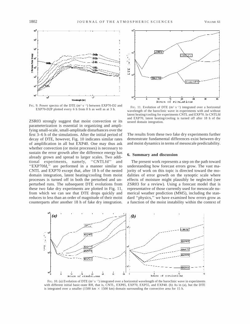
Power spectra of DTE for several times from EXP70are shown in Fig. 9. Much as in CNTL, the DTE atsmaller scales decreases rapidly over the first 3 to 6 h.Because of weaker convective activity and smaller arealcoverage of the convection, however, the growth in theconvective area becomes evident in DTE, which is adomain-integrated quantity, only after the first 12 h.(The interplay between general decay and local growthof differences is discussed further below.) DTE growssteadily at all wavelengths over the subsequent forecastperiod out to 36 h. Because DTE decays over a largerinitial period in EXP70, it remains smaller than in CNTLat all wavelengths and does not saturate at any wave-length, even after 36 h. The shift of the peak of thespectrum toward larger scales is also less evident thanin CNTL.

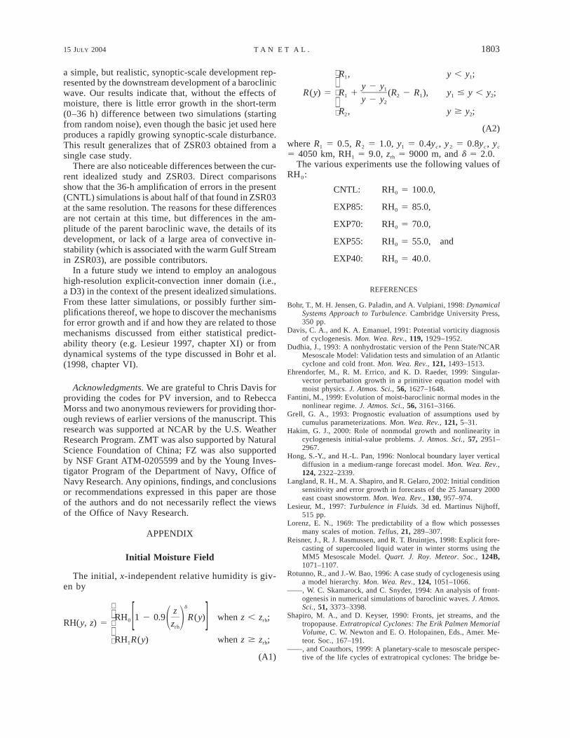
Sensitivity experiments EXP85, EXP55, and EXP40,in which the initial relative humidity was reduced to85%, 55%, and 40% of that in CNTL, respectively, werealso performed with the same initial difference as inCNTL in the nested domain. The impacts of moist con-vection on mesoscale predictability is summarized bythe DTE time series shown in Fig. 10, which showdecreasing error growth with decreasing humidity. Fig-ure 10a shows there is a sharp ‘‘decrease’’ of DTE inall the experiments (including CNTL) over the first 3h. This decrease can be understood as a consequence ofthe fact that the initial error decays through diffusionor geostrophic adjustment over vast portions of the av-eraging domain (the wavelength of the baroclinic wave)and grows only in a limited area near the surface low

15 JULY 2004 1801T A N E T A L .

FIG. 7. As in Fig. 4, except for the 500-hPa meridional wind difference between EXP70-D2 and EXP70-D2P validat (a) 12 and (b) 24 h of the nested domain simulation. Contour intervals are 0.2 m s21 for (a) and 0.5 m s21 for (b).

FIG. 8. The 6-h accumulated precipitation difference (thin lines; negative, dashed; contour interval 0.5 mm) betweenEXP70-D2 and EXP70-D2P valid at (a) 12 and (b) 24 h of the nested domain simulation. The sea level pressure (every8 hPa) simulated by EXP70-D2 is also shown in thick lines. Areas with the 6-h accumulated convective precipitationgreater than 1 mm in EXP70-D2 are shaded. The distance between small tick marks is 90 km. The display windowsare the same as in Fig. 4.

where there is moist convection. Figure 10b shows thatcomputing DTE over a smaller averaging domain (1500km by 1500 km) surrounding the convective activityindicates strong error growth in CNTL even over thefirst 3 h and ‘‘less’’ decrease in the other experiments.

In spite of the strong variations of the growth ratesin the different experiments over different periods, byand large, Fig. 10 indicates that larger initial relativehumidity corresponds to more rapid error growth. Sincethe simulations with larger relative humidity exhibitgreater conditional instability and stronger parameter-ized convection, the relation between initial humidity

and error growth also supports our assertion that themoist convection controls the initial phase of the errorgrowth. Moreover, with a maximum initial RH of only40%, EXP40 exhibits little precipitation (either explicitor convective) and is dominated by dry dynamics. Thereis hardly any error growth in EXP40 over the entire 36-h forecast period. Indeed, consistent with the findingsof ZSR02 and ZSR03, the evolution of DTE in EXP40is similar to a ‘‘fake dry’’ version of the control ex-periment (not shown) in which no latent heating/coolingfrom moist processes was allowed.

The aforementioned experiments and those from

1802 VOLUME 61J O U R N A L O F T H E A T M O S P H E R I C S C I E N C E S

FIG. 9. Power spectra of the DTE (m2 s22) between EXP70-D2 andEXP70-D2P plotted every 6 h from 0 h as well as at 3 h.

FIG. 11. Evolution of DTE (m2 s22) integrated over a horizontalwavelength of the baroclinic wave in experiments with and withoutlatent heating/cooling for experiments CNTL and EXP70. In CNTLfdand EXP70, latent heating/cooling is turned off after 18 h of thenested domain integration.

FIG. 10. (a) Evolution of DTE (m2 s22) integrated over a horizontal wavelength of the baroclinic wave in experimentswith different initial basic-state RH, that is, CNTL, EXP85, EXP70, EXP55, and EXP40. (b) As in (a), but the DTEis integrated over a smaller (1500 km 3 1500 km) domain surrounding the convective area for 15 h.

ZSR03 strongly suggest that moist convection or itsparameterization is essential in organizing and ampli-fying small-scale, small-amplitude disturbances over thefirst 3–6 h of the simulations. After the initial period ofdecay of DTE, however, Fig. 10 indicates similar ratesof amplification in all but EXP40. One may thus askwhether convection (or moist processes) is necessary tosustain the error growth after the difference energy hasalready grown and spread to larger scales. Two addi-tional experiments, namely, ‘‘CNTLfd’’ and‘‘EXP70fd,’’ are performed in a manner similar toCNTL and EXP70 except that, after 18 h of the nesteddomain integration, latent heating/cooling from moistprocesses is turned off in both the perturbed and un-perturbed runs. The subsequent DTE evolutions fromthese two fake dry experiments are plotted in Fig. 11,from which we can see that DTE drops quickly andreduces to less than an order of magnitude of their moistcounterparts after another 18 h of fake dry integration.

The results from these two fake dry experiments furtherdemonstrate fundamental differences exist between dryand moist dynamics in terms of mesoscale predictability.

6. Summary and discussion

The present work represents a step on the path towardunderstanding how forecast errors grow. The vast ma-jority of work on this topic is directed toward the mo-dalities of error growth on the synoptic scale whereeffects of moisture might plausibly be neglected (seeZSR03 for a review). Using a forecast model that isrepresentative of those currently used for mesoscale nu-merical weather prediction (MM5), including the stan-dard ‘‘physics,’’ we have examined how errors grow asa function of the moist instability within the context of

15 JULY 2004 1803T A N E T A L .

a simple, but realistic, synoptic-scale development rep-resented by the downstream development of a baroclinicwave. Our results indicate that, without the effects ofmoisture, there is little error growth in the short-term(0–36 h) difference between two simulations (startingfrom random noise), even though the basic jet used hereproduces a rapidly growing synoptic-scale disturbance.This result generalizes that of ZSR03 obtained from asingle case study.

There are also noticeable differences between the cur-rent idealized study and ZSR03. Direct comparisonsshow that the 36-h amplification of errors in the present(CNTL) simulations is about half of that found in ZSR03at the same resolution. The reasons for these differencesare not certain at this time, but differences in the am-plitude of the parent baroclinic wave, the details of itsdevelopment, or lack of a large area of convective in-stability (which is associated with the warm Gulf Streamin ZSR03), are possible contributors.

In a future study we intend to employ an analogoushigh-resolution explicit-convection inner domain (i.e.,a D3) in the context of the present idealized simulations.From these latter simulations, or possibly further sim-plifications thereof, we hope to discover the mechanismsfor error growth and if and how they are related to thosemechanisms discussed from either statistical predict-ability theory (e.g. Lesieur 1997, chapter XI) or fromdynamical systems of the type discussed in Bohr et al.(1998, chapter VI).

Acknowledgments. We are grateful to Chris Davis forproviding the codes for PV inversion, and to RebeccaMorss and two anonymous reviewers for providing thor-ough reviews of earlier versions of the manuscript. Thisresearch was supported at NCAR by the U.S. WeatherResearch Program. ZMT was also supported by NaturalScience Foundation of China; FZ was also supportedby NSF Grant ATM-0205599 and by the Young Inves-tigator Program of the Department of Navy, Office ofNavy Research. Any opinions, findings, and conclusionsor recommendations expressed in this paper are thoseof the authors and do not necessarily reflect the viewsof the Office of Navy Research.

APPENDIX

Initial Moisture Field

The initial, x-independent relative humidity is giv-en by

dzRH 1 2 0.9 R(y) when z , z ;0 rh1 2RH(y, z) 5 [ ] zrhRH R(y) when z $ z ; 1 rh

(A1)

R , y , y ;1 1 y 2 y1R(y) 5 R 1 (R 2 R ), y # y , y ;1 2 1 1 2y 2 y2R , y $ y ; 2 2

(A2)

where R1 5 0.5, R2 5 1.0, y1 5 0.4yc, y2 5 0.8yc, yc

5 4050 km, RH1 5 9.0, zrh 5 9000 m, and d 5 2.0.The various experiments use the following values of

RH0:

CNTL: RH 5 100.0,0

EXP85: RH 5 85.0,0

EXP70: RH 5 70.0,0

EXP55: RH 5 55.0, and0

EXP40: RH 5 40.0.0

REFERENCES

Bohr, T., M. H. Jensen, G. Paladin, and A. Vulpiani, 1998: DynamicalSystems Approach to Turbulence. Cambridge University Press,350 pp.

Davis, C. A., and K. A. Emanuel, 1991: Potential vorticity diagnosisof cyclogenesis. Mon. Wea. Rev., 119, 1929–1952.

Dudhia, J., 1993: A nonhydrostatic version of the Penn State/NCARMesoscale Model: Validation tests and simulation of an Atlanticcyclone and cold front. Mon. Wea. Rev., 121, 1493–1513.

Ehrendorfer, M., R. M. Errico, and K. D. Raeder, 1999: Singular-vector perturbation growth in a primitive equation model withmoist physics. J. Atmos. Sci., 56, 1627–1648.

Fantini, M., 1999: Evolution of moist-baroclinic normal modes in thenonlinear regime. J. Atmos. Sci., 56, 3161–3166.

Grell, G. A., 1993: Prognostic evaluation of assumptions used bycumulus parameterizations. Mon. Wea. Rev., 121, 5–31.

Hakim, G. J., 2000: Role of nonmodal growth and nonlinearity incyclogenesis initial-value problems. J. Atmos. Sci., 57, 2951–2967.

Hong, S.-Y., and H.-L. Pan, 1996: Nonlocal boundary layer verticaldiffusion in a medium-range forecast model. Mon. Wea. Rev.,124, 2322–2339.

Langland, R. H., M. A. Shapiro, and R. Gelaro, 2002: Initial conditionsensitivity and error growth in forecasts of the 25 January 2000east coast snowstorm. Mon. Wea. Rev., 130, 957–974.

Lesieur, M., 1997: Turbulence in Fluids. 3d ed. Martinus Nijhoff,515 pp.

Lorenz, E. N., 1969: The predictability of a flow which possessesmany scales of motion. Tellus, 21, 289–307.

Reisner, J., R. J. Rasmussen, and R. T. Bruintjes, 1998: Explicit fore-casting of supercooled liquid water in winter storms using theMM5 Mesoscale Model. Quart. J. Roy. Meteor. Soc., 124B,1071–1107.

Rotunno, R., and J.-W. Bao, 1996: A case study of cyclogenesis usinga model hierarchy. Mon. Wea. Rev., 124, 1051–1066.

——, W. C. Skamarock, and C. Snyder, 1994: An analysis of front-ogenesis in numerical simulations of baroclinic waves. J. Atmos.Sci., 51, 3373–3398.

Shapiro, M. A., and D. Keyser, 1990: Fronts, jet streams, and thetropopause. Extratropical Cyclones: The Erik Palmen MemorialVolume, C. W. Newton and E. O. Holopainen, Eds., Amer. Me-teor. Soc., 167–191.

——, and Coauthors, 1999: A planetary-scale to mesoscale perspec-tive of the life cycles of extratropical cyclones: The bridge be-

1804 VOLUME 61J O U R N A L O F T H E A T M O S P H E R I C S C I E N C E S

tween theory and observations. The Life Cycles of ExtratropicalCyclones, M. A. Shapiro and S. Gronas, Eds., Amer. Meteor.Soc., 1228–1251.

Snyder, C., T. M. Hamill, and S. Trier, 2003: Linear evolution offorecast error covariances in a quasigeostrophic model. Mon.Wea. Rev., 131, 189–205.

Vukicevic, T., and R. M. Errico, 1990: The influence of artificial andphysical factors upon predictability estimates using a complexlimited-area model. Mon. Wea. Rev., 118, 1460–1482.

Whitaker, J. S., and C. A. Davis, 1994: Cyclogenesis in a saturatedenvironment. J. Atmos. Sci., 51, 889–907.

Wirth, A., and M. Ghil, 2000: Error evolution in the dynamics of anocean general circulation model. Dyn. Atmos. Oceans, 32, 419–431.

Zhang, F., 2004: Generation of mesoscale gravity waves in upper-tropospheric jet–front systems. J. Atmos. Sci., 61, 440–457.

——, C. Snyder, and R. Rotunno, 2002: Mesoscale predictability ofthe ‘‘surprise’’ snowstorm of 24–25 January 2000. Mon. Wea.Rev., 130, 1617–1632.

——, ——, and ——, 2003: Effects of moist convection on mesoscalepredictability. J. Atmos. Sci., 60, 1173–1185.