Embed Size (px)
Citation preview
Published in Journal of Fluid Mechanics, Vol. 755 pp. 142-175, September 2014
© Cambridge University Press 2014
http://dx.doi.org/10.1017/jfm.2014.394
† Email address for correspondence: [email protected]
Modeling of Material Pitting from Cavitation Bubble Collapse
Chao-Tsung Hsiao†, A. Jayaprakash, A. Kapahi, J.-K Choi, and
Georges L. Chahine
DYNAFLOW, INC., 10621-J Iron Bridge Road, Jessup, MD, USA
Material pitting from cavitation bubble collapse is investigated numerically including
two-way fluid structure interaction. A hybrid numerical approach which links an
incompressible boundary element method (BEM) solver and a compressible finite
difference flow solver is applied to capture nonspherical bubble dynamics efficiently
and accurately. The flow codes solve the fluid dynamics while intimately coupling the
solution with a finite element structure code to enable simulation of the full fluid
structure interaction. During bubble collapse high impulsive pressures result from the
impact of the bubble reentrant jet on the material surface and from the collapse of the
remaining bubble ring. A pit forms on the material surface when the impulsive pressure
is large enough to result in high equivalent stresses exceeding the material yield stress.
The results depend on bubble dynamics parameters such as the size of the bubble at its
maximum volume, the bubble standoff distance from the material wall, and the pressure
driving the bubble collapse. The effects of these parameters on the reentrant jet, the
following bubble ring collapse pressure, and the generated material pit characteristics
are investigated.
Key words: Authors should not enter keywords on the manuscript, as these must be
chosen by the author during the online submission process and will then be added
during the typesetting process (see http://journals.cambridge.org/data/relatedlink/jfm-
keywords.pdf for the full list)
1 INTRODUCTION
Cavitation erosion in rotating machinery such as pumps, impellers, propellers, etc. is
a main concern for the marine, pump, and other industries. Cavitation is due to the high
relative motion between the liquid and the subject lifting surface. As a result of the high
velocities, the local pressure in the liquid drops below a critical pressure (e.g. the liquid
vapor pressure) and this drives nuclei (microbubbles always present in liquids) to grow
explosively. When the pressure returns to a high value along the path of these bubbles,
volume implosions occur and this can generate high pressure pulses and shock waves
Published in Journal of Fluid Mechanics, Vol. 755 pp. 142-175, September 2014
© Cambridge University Press 2014
http://dx.doi.org/10.1017/jfm.2014.394
(Rayleigh 1917). Many pioneering studies (Naude & Ellis 1961; Plesset & Chapman
1971; Crum 1979; Chahine 1982) have shown, experimentally as well as analytically,
that the collapse of these cavitation bubbles near a rigid boundary also results in high-
speed reentrant liquid jets, which penetrate the highly deformed bubbles and strike the
nearby boundary generating water hammer like impact pressures. Both shock waves and
high-speed reentrant liquid jets produce high local stresses on the adjacent material
surface and are responsible for material micro-deformations and damage.
While a “weak” material may fail rapidly under the repeated shock waves and liquid
jet impacts, a resistant material actually experiences the symptoms of fatigue. Initially
the material surface gets deformed and is modified microscopically without any loss of
material. This is accompanied with work hardening of the surface. During this initial
phase called incubation period, permanent deformation occurs accompanied with plastic
and local displacement of material micro particles as well as with development of
micro-cracks in brittle materials. The pits formed on the material surface during the
incubation period are good indicators of the material strength, although advanced
damage to the material, resulting in weight loss and fracture, occurs at a later stage of
the cavitation erosion process (Kim et al 2004).
Since the formation of a pit on the material surface is reasonably associated with a
single cavitation event caused by bubble collapse, the amount of permanent deformation
should depend on the stresses the collapsing bubble creates on the material. It is thus
expected that the formation of material pitting can be simulated using a fluid-structure
interaction model of the dynamics of the bubbles (single bubble or clouds of bubble)
and the concerned material. Simulation of the collapse of a bubble near a rigid wall has
been an active research area since the pioneering work of Plesset & Chapman (1971).
The resulting reentrant jet has been found to play an important role in hydrodynamics
and ultrasonic cavitation, as well as in large-scale underwater explosion problems
(Chahine et al. 1989; Kalumuck et al. 2003; Jayaprakash et al. 2012) and in small-scale
medical applications (Hsiao & Chahine 2013b).
It is known that the formation of the reentrant jet and the resultant pressures are
highly dependent on the standoff distance, i.e. the distance between the initial bubble
center and the wall (Chahine 1982; Blake & Gibson 1987; Zhang et al. 1993; Wardlaw
& Luton 2000). Classically the numerical simulations start from the bubble being
spherical and at its maximum radius. The bubble is then allowed to collapse in response
to the high ambient pressure. Such an approach is not suitable for studying cavitation
bubbles growing very close to the boundary. For these small standoff distances
scenarios (standoff less than one bubble radius) the impact pressures due to the reentrant
jet have been computed numerically (Chahine 1996; Chahine et al. 2006, Jayaprakash et
al. 2012) and measured experimentally (Vogel et al. 1988, Philipp et al. 1998, Harris,
2009) to attain a maximum at distances of the order of three quarters of the maximum
bubble radius. Therefore, simulations of the bubble dynamics starting from a small
nucleus are necessary to cover a more complete range of standoff distances to
understand such effects on the material pitting.

Published in Journal of Fluid Mechanics, Vol. 755 pp. 142-175, September 2014
© Cambridge University Press 2014
http://dx.doi.org/10.1017/jfm.2014.394
3
Since both the impact of high-speed liquid jet on the wall and bubble collapse will
generate local high pressure waves, a compressible flow solver is desired to capture
accurately pressure waves and any shock wave emission and propagation. However,
such flow solvers usually use a finite difference method which requires very fine spatial
resolution and small time step sizes especially for resolving the formation of the
reentrant jet accurately (Wardlaw & Luton 2000). This makes them not very efficient
for simulating the relatively long duration bubble period. To overcome this, a hybrid
numerical procedure combining an incompressible solver and a compressible code is
applied here to capture both the full period of the bubble dynamics as well as the shock
phases occurring at initiation for an explosion bubble and during bubble collapse and
rebound for both cavitation and underwater explosion bubbles. This numerical
procedure takes advantage of an accurate shock capturing method and of a boundary
element method both shown to be very efficient in modeling underwater explosion and
cavitation bubble dynamics problems and very accurate in capturing the reentrant jet.
As already shown by previous studies (Duncan & Zhang 1991; Duncan et al. 1996;
Wardlaw & Luton 2000, Madadi-Kandjani & Xiong 2014), the deformable wall can
alter bubble dynamics during collapse. Therefore, simulation of both fluid and material
responses and their interaction is required to model accurately material pitting due to
bubble collapse. Both the impact of the high-speed reentrant liquid jet on the wall and
the emission and propagation of shock waves from the bubble collapse require a
compressible flow solver. In this study, a finite element structure code is coupled with
such a compressible flow solver to investigate the material response to the pressure field
generated by the bubble dynamics. In the case of highly deformable materials the
motion of the material interface also affects the bubble dynamics. This paper aims at
isolating the influence of the various physical parameters such as the pressure driving
the bubble collapse, the bubble size, the bubble distance from the wall, and the
properties of the damaged material.
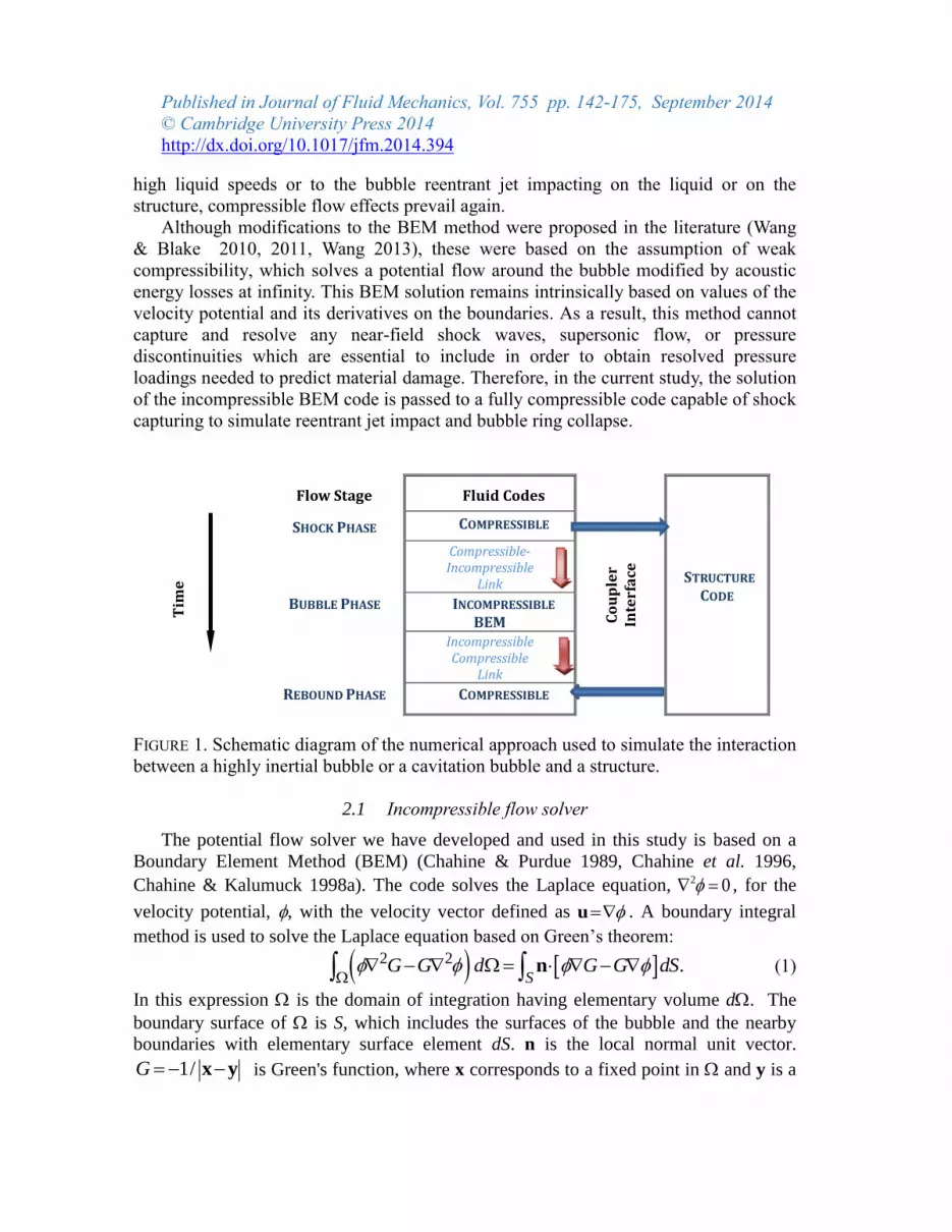
2 Numerical approach
The numerical approach applied to model material pitting in this paper is part of a
general hybrid approach which was developed by the authors to simulate fluid structure
interaction (FSI) problems involving shock and bubble pressure pulses (Hsiao &
Chahine 2010, 2013a). As illustrated in FIGURE 1, for a highly inertial bubble such as
underwater explosion bubble (UNDEX) or a laser generated bubble (Vogel et al. 1988,
Philipp et al. 1998), a compressible-incompressible link is required at the beginning to
handle the emitted shock wave and the flow field generated by the exploding bubble.
Cavitation bubbles on the other hand, generate a small pressure peak and no shock wave
during the growth phase. As a result, no initial shock phase compressible solution is
required. An incompressible Boundary Element Method (BEM) code can then be used
to simulate most of the bubble period until the end of the bubble collapse where, due to
Published in Journal of Fluid Mechanics, Vol. 755 pp. 142-175, September 2014
© Cambridge University Press 2014
http://dx.doi.org/10.1017/jfm.2014.394
high liquid speeds or to the bubble reentrant jet impacting on the liquid or on the
structure, compressible flow effects prevail again.
Although modifications to the BEM method were proposed in the literature (Wang
& Blake 2010, 2011, Wang 2013), these were based on the assumption of weak
compressibility, which solves a potential flow around the bubble modified by acoustic
energy losses at infinity. This BEM solution remains intrinsically based on values of the
velocity potential and its derivatives on the boundaries. As a result, this method cannot
capture and resolve any near-field shock waves, supersonic flow, or pressure
discontinuities which are essential to include in order to obtain resolved pressure
loadings needed to predict material damage. Therefore, in the current study, the solution
of the incompressible BEM code is passed to a fully compressible code capable of shock
capturing to simulate reentrant jet impact and bubble ring collapse.
Flow Stage Fluid Codes
C
ou
ple
r In
terf
ace
STRUCTURE
CODE T
ime
SHOCK PHASE COMPRESSIBLE
Compressible-Incompressible
Link
BUBBLE PHASE INCOMPRESSIBLE
BEM Incompressible
Compressible Link
REBOUND PHASE COMPRESSIBLE
FIGURE 1. Schematic diagram of the numerical approach used to simulate the interaction
between a highly inertial bubble or a cavitation bubble and a structure.
2.1 Incompressible flow solver
The potential flow solver we have developed and used in this study is based on a
Boundary Element Method (BEM) (Chahine & Purdue 1989, Chahine et al. 1996,
Chahine & Kalumuck 1998a). The code solves the Laplace equation, 2 0 , for the
velocity potential, , with the velocity vector defined as u . A boundary integral
method is used to solve the Laplace equation based on Green’s theorem:
2 2 .S
G G d G G dS
n (1)
In this expression is the domain of integration having elementary volume d. The
boundary surface of is S, which includes the surfaces of the bubble and the nearby
boundaries with elementary surface element dS. n is the local normal unit vector.
1/G x y is Green's function, where x corresponds to a fixed point in and y is a
Published in Journal of Fluid Mechanics, Vol. 755 pp. 142-175, September 2014
© Cambridge University Press 2014
http://dx.doi.org/10.1017/jfm.2014.394
5
point on the boundary surface S. Equation (1) reduces to Green’s formula with a
being the solid angle under which x sees the domain, :
( ) ( ) ( , ) ( , ) ( ) ,S
Ga G dS
n n
x y x y x y y (2)
where a is the solid angle. To solve (2) numerically, the boundary element method,
which discretizes the surface of all objects in the computational domain into panel
elements, is applied.
Equation (2) provides a relationship between and /n at the boundary surface S.
Thus, if either of these two variables (e.g. ) is known everywhere on the surface, the
other variable (e.g. /n) can be obtained.
To advance the solution in time, the coordinates of the bubble and any free surface
nodes, x, are advanced according to /d dt x . on the bubble and free surface nodes
is obtained through the time integration of the material derivative of , i.e. d/dt, which
can be written as
.d
dt t
, (3)
where /t can be determined from the Bernoulli equation:
1.
2lgz p p
t
. (4)
p is the hydrostatic pressure at infinity at z=0 where z is the vertical coordinate. lp is
the liquid pressure at the bubble surface, which balances the internal pressure and
surface tension,
l v gp p p C . (5)
vp is the vapor pressure, is the surface tension, and C is the local bubble wall
curvature. gp is the gas pressure inside bubble and is assumed to follow a polytropic law
with a compression constant, k, which relates the gas pressure to the gas volume, V , and
reference value, 0gp , and 0V .
0
k
g gp p
0
V
V. (6)
2.2 Compressible flow solver
The multi-material compressible Euler equation solver used here is based on a finite
difference method (Wardlaw et al. 2003). The code solves continuity and momentum
equations for a compressible inviscid liquid in Cartesian coordinates. These can be
written in the following format:

Published in Journal of Fluid Mechanics, Vol. 755 pp. 142-175, September 2014
© Cambridge University Press 2014
http://dx.doi.org/10.1017/jfm.2014.394
Q E F G
St x y z
, (7)
2
2
2
0
0
, , , , 0 ,
t t t t
u v wvuu u p wu
Q v E uv F v p G wv S
w uw vw gw pe gwe p u e p v e p w
(8)
where is the fluid density, p is the pressure, u, v, and w are the velocity components in
the x, y, z directions respectively (z is vertical), g is the acceleration of gravity, and
et=e+0.5(u2+v
2+w
2) is the total energy with e being the internal energy. The system is
closed by using an equation of state for each material, which provides the pressure as a
function of the material specific internal energy and the density. Here, a
-law (with =1.4) is used for the gas-vapor mixture (Anderson 1990)
=( -1)p e, (9)
and the Tillotson equation is used for water (Zel'Dovich & Raizer 2002):
2 3
0 0
0
( ) , 1p p e e A B C
. (10)
, A, B, C are constants and 0p , 0e and 0 are the reference pressure, specific internal
energy, and density respectively: 0 . 2 8 , 92 . 2 0 1 0 P a ,A 99 . 5 4 1 0 P a ,B 101.48 10 Pa, C 5 2 2
0 3 . 5 4 1 0 m / s ,e 5
0 1 . 0 1 0 P a ,p 3
0 1 0 0 0 k g / m
The compressible flow solver uses a high order Godunov scheme. It employs the
Riemann problem to construct a local flow solution between adjacent cells. The
numerical method is based on a higher order MUSCL scheme and tracks each material.
To improve efficiency, an approximate Riemann problem solution replaces the full
problem. The MUSCL scheme is augmented with a mixed cell approach (Colella 1990)
to handle shock wave interactions with fluid or material interfaces. This approach uses a
Lagrangian treatment for the cells including an interface and an Eulerian treatment for
cells away from interfaces. A re-map procedure is employed to map the Lagrangian
solution back to the Eulerian grid. The code has been extensively validated against
experiments (Wardlaw et al. 2003, Kapahi et al. 2014).
2.3 Compressible-incompressible link procedure
Both incompressible and compressible flow solvers are able to model the full bubble
dynamics on their own. However, each method has its shortcomings when it comes to
specific parts of the bubble history. The BEM based incompressible flow solver is
efficient, reduces the dimension of the problem by one (line integrals for an

Published in Journal of Fluid Mechanics, Vol. 755 pp. 142-175, September 2014
© Cambridge University Press 2014
http://dx.doi.org/10.1017/jfm.2014.394
7
axisymmetric problem, and surface integrals for a 3D problem) and thus allows very
fine gridding and increased accuracy with reasonable computations times. It has been
shown to provide reentrant jet parameters and speed accurately (Chahine & Perdue
1989, Zhang et al. 1993, Chahine et al. 2006, Jayaprakash et al. 2012). However, it has
difficulty pursuing the computations beyond surface impacts (liquid-liquid and liquid
solid).
On the other hand, the compressible flow solver is most adequate to model shock
wave emission and propagation, liquid-liquid, and liquid solid impacts. The method
requires, however, very fine grids and very small time steps to resolve shock wave
fronts. This makes it appropriate to model time portions of the bubble dynamics.
Concerning bubble-liquid interface and the reentrant jet dynamics, the procedure is
diffusive since the interface is not directly modeled, and reentrant jet characteristics are
usually less accurate than obtained with the BEM approach.
Hence a general novel approach would combine the advantages of both methods and
would consist in executing the following steps:
1. Setup the initial flow field using the Eulerian compressible flow solver and run
the simulation until the initial shock fronts go by and the remnant flow field can be
assumed to be incompressible with bubble dynamics independent of initial
treatments.
2. Transfer at that instant to the Lagrangian BEM potential flow solver 3DYNAFS
all the flow field variables needed by the solver: geometry, bubble pressure,
boundary velocities to specify the moving boundary’s normal velocities, / n .
3. Solve for bubble growth and collapse using fine BEM grids to obtain a good
description of the reentrant jet until the point where the jet is very close to the
opposite side of the bubble.
4. Transfer the solution back to the compressible flow solver with the required
flow variables. To do so, compute using the Green equation all flow field quantities
on the Eulerian grid.
5. Continue solution progress with the compressible code to obtain pressures due
to jet impact and remnant bubble ring collapse.
2.4 Structure dynamics solver
To model the dynamics of the material, the finite element model DYNA3D is used.
DYNA3D is a non-linear explicit structure dynamics code developed by the Laurence
Livermore National Laboratory. Here it computes the material deformation when the
loading is provided by the fluid solution. DYNA3D uses a lumped mass formulation for
efficiency. This produces a diagonal mass matrix M, to express the momentum equation
as: 2
ext int2,
d
dt
xM F F (11)
Published in Journal of Fluid Mechanics, Vol. 755 pp. 142-175, September 2014
© Cambridge University Press 2014
http://dx.doi.org/10.1017/jfm.2014.394
where Fext represents the applied external forces, and Fint the internal forces. The
acceleration,2 2/d d ta x for each element, is obtained through an explicit temporal
central difference method. Additional details on the general formulation can be found in
(Whirley & Engelmann 1993).
2.5 Material models
In the present study, two metal alloys (Aluminum 7075 and Stainless Steel A2205),
two rubbers (a Neoprene synthetic rubber and a Polyurethane), and a Versalink based
polyurea are considered. The metals are modeled using elastic-plastic models with linear
slopes (moduli), one for the initial elastic regime and the second, a tangent modulus, for
the plastic regime. The material parameters of the metal alloys used in this study are
shown in TABLE 1.
Concerning the rubbers, a Blatz-Ko’s hyper-elastic model is used. This model is
appropriate for materials undergoing moderately large strains and is based on the
implementation in (Key 1974). The material motion satisfies the formal equation 2
2s
d
dt
xσ , (12)
where s is the material density, x is the position vector of the material and σ is the
Cauchy stress tensor. If we denote F the deformation gradient tensor, then the Cauchy
stress tensor is computed by
T1
Jσ FSF , (13)
where J is the determinant of F and S is the second Piola-Kirchoff stress tensor and is
computed by
1/(1 2 )/ .ij ij ijS G C V V (14)
G is the shear modules, V is the relative volume to original which is related to excess
compression and density, Cij is the right Cauchy-Green strain tensor, and is Poisson’s
ratio and is set to 0.463. TABLE 2 shows the material parameters of the two rubbers of
different strengths. Rubber #1 is about three times stiffer than the rubber #2.
The Versalink based polyurea was modeled as a viscoelastic material with the
following time dependent values for the shear modulus, G:
t
oG t G G G e , (15)
with 141.3 , 79.1 , 4.948 , 15,600 oG MPa G MPa K GPa s
. (16)
While the time dependence of G is considered in this model, the bulk modulus, K,
was assumed to be constant. The material parameters in (16) are derived from
simplification of 4th
order Prony series in Amirkhizi (2006) taking the 2nd
term as the
major contributor.

Published in Journal of Fluid Mechanics, Vol. 755 pp. 142-175, September 2014
© Cambridge University Press 2014
http://dx.doi.org/10.1017/jfm.2014.394
9
Published in Journal of Fluid Mechanics, Vol. 755 pp. 142-175, September 2014
© Cambridge University Press 2014
http://dx.doi.org/10.1017/jfm.2014.394
Metallic
Material
Yield Stress
(MPa)
Young’s
Modulus
(GPa)
Tangent
Modulus
(MPa)
Elongation
at Break
Density
(g/cm3)
Al 7075 503 71.7 670 0.11 2.81
A2205 515 190 705 0.35 7.88
TABLE 1. Material properties of the metal alloys investigated in this study.
Compliant
Material
Shear Modulus
(MPa)
Density
(g/cm3)
Rubber # 1
(Neoprene) 99.7 1.18
Rubber # 2
Polyurethane 34.17 1.20
TABLE 2. Material properties of the two rubbers investigated in this study.
2.6 Fluid structure interaction coupling
Fluid/structure interaction effects are captured in the simulations by coupling the
fluid codes and DYNA3D through a coupler interface. The coupling is achieved through
the following steps:
The fluid code solves the flow field and deduces the pressures at the structure
surface using the positions and normal velocities of the wetted body nodes.
In response, the structure code computes material deformations and velocities in
response to this loading.
The new coordinates and velocities of the structure surface nodes become the
new boundary conditions for the fluid code at the next time step.
Additional details on the procedure can be found in Chahine & Kalumuck (1998)
and Wardlaw & Luton (2000). This FSI coupling procedure has only a first-order time
accuracy. A predictor-corrector approach is also implemented in the coupling to iterate
and improve the solution but was not used here. This is because the numerical error due
the time lag is negligible thanks to the very small time steps used. These are controlled
by the steep pressure waves, which have a time scale that is two orders of magnitude
shorter than the time response of the material. This method has been shown in UNDEX
studies to correlate very well with experiments (Harris et al. 2009)

Published in Journal of Fluid Mechanics, Vol. 755 pp. 142-175, September 2014
© Cambridge University Press 2014
http://dx.doi.org/10.1017/jfm.2014.394
11
3 Problem definition
3.1 Pressure field driving bubble collapse
It is known that microbubbles or nuclei are always present in liquids and are
entrained in the flow (Brennen 1995). Also nano-cavities at the solid surfaces and solid
particles in the fluid serve as nucleation sites for the formation of microbubbles under
cavitating conditions. Once excited by local pressures decreasing below a critical value
(Chahine and Shen 1986), bubbles grow explosively until their internal pressure drops
below the surrounding local pressure. The bubbles can then collapse violently,
producing intense pressures, emitting sound, and eroding any solid surfaces in their
proximity.
To mimic such a cavitation scenario in this contribution, we consider a nucleus
initially at equilibrium with the surrounding liquid and subject it to a time dependent
pressure field, which would correspond to what it would see while moving in the flow
close to the material surface. As illustrated in FIGURE 2 the pressure first drops to a
value below the bubble critical pressure and then remains at this pressure for a
prescribed time, t. The pressure then rises to a high value and remains there until the
end of the computation.
FIGURE 2 illustrates this for the case of a bubble of initial radius R0=50 m at
equilibrium in the liquid at 1 atm (105 Pa). The pressure then suddenly decreases to a
pressure of 103 Pa, stays there for 2.415t ms , and then rises sharply to Pd = 10 MPa,
which is commonly encountered in cavitation erosion measurement (Chahine et al.
2014). FIGURE 2 also shows the response of a hypothetical spherical bubble to this
pressure function obtained by integrating the Rayleigh-Plesset equation. It is seen that as
soon as the ambient pressure drops to the low 103 Pa value, the bubble responds and
starts growing. Since the ambient pressure drops below the bubble critical pressure
(Chahine 1993; Chahine et al. 2014) the bubble cannot reach an equilibrium size and
continues to grow during t until the sudden pressure rise to 10 MPa occurs. A
maximum bubble size, Rmax , is reached a little time after the overpressure is imposed
due to liquid inertia. This is followed by a strong collapse of the bubble.

Published in Journal of Fluid Mechanics, Vol. 755 pp. 142-175, September 2014
© Cambridge University Press 2014
http://dx.doi.org/10.1017/jfm.2014.394
FIGURE 2. Imposed time dependent pressure field (red curve) around an initially
spherical bubble of 50 μm radius, and resulting bubble radius versus time (blue curve)
as predicted by the solution of the Rayleigh-Plesset equation.
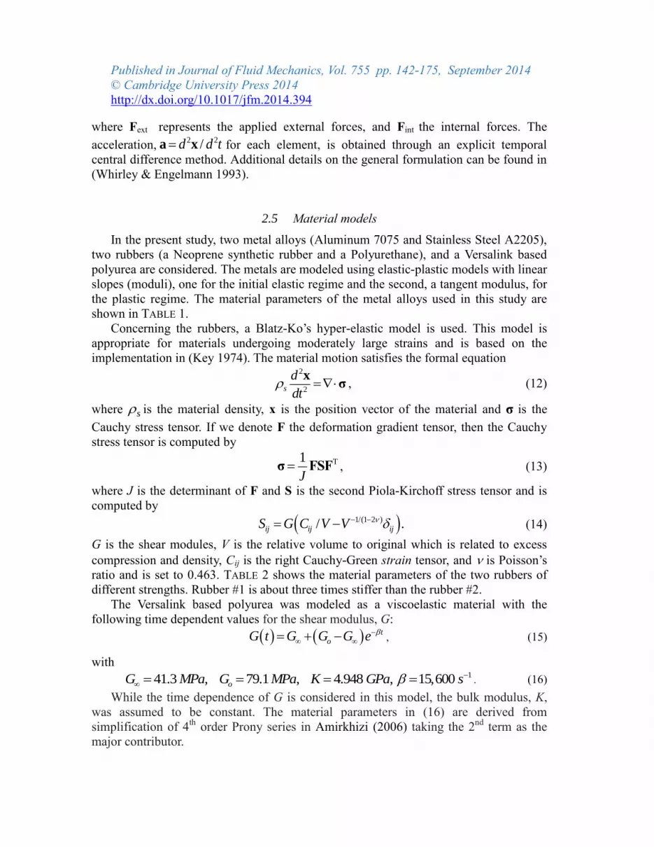
3.2 Numerical discretization
To simulate the bubble dynamics with the incompressible BEM solver, a total of 400
nodes and 800 panels were used to discretize the bubble surface. This corresponds to a
grid density, which provides grid independent solution (Chahine et al. 1996). The Fluid
Structure Interaction (FSI) simulations were conducted during the bubble collapse phase
when the stresses were of consequence to the material response or deformation. An
axisymmetric domain with a total of 220 × 1,470 grid points was used with a stretched
grid in a 1 m × 1 m domain concentrating the grids in the immediate region surrounding
the bubble. The grid was distributed such that there was a uniform fine mesh with a size
of 10 µm covering the area of interest where the interaction between bubble and plate is
important as shown in FIGURE 3. The axisymmetric computational domain was bounded
at selected distances in the far field (radial direction and away from the wall) and at the
plate material wall for FSI simulations.
A reflection boundary condition was imposed on the axis of symmetry, i.e. all
physical variables such as density, pressure, velocities and energy are reflected from the
axis, while transmission non-reflective boundary conditions, i.e. the flow variables are
extrapolated along the characteristic wave direction, were imposed at the far field
boundaries.
R
Pd
t
Published in Journal of Fluid Mechanics, Vol. 755 pp. 142-175, September 2014
© Cambridge University Press 2014
http://dx.doi.org/10.1017/jfm.2014.394
13
FIGURE 3. Axisymmetric computational domain used for the computation of the bubble
dynamics by the compressible flow solver: (a) full domain, (b) zoomed area at the
bubble location. The blue region is the inside of the bubble after it formed a reentrant jet
on the axis of symmetry.
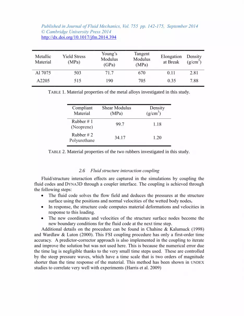
For the structure computations, axisymmetry was used and a circular plate with a
radius of 1 m and a thickness of 0.01 m was discretized using rectangular brick
elements. As shown in FIGURE 4a stretched grid with 220 elements in the radial
direction, r, and 446 elements in the axial direction, z, were used to discretize the plate.
The elements were distributed such that a uniform fine mesh size of 10 µm existed near
the center of the plate where the high pressure loading occurs. Other mesh sizes were
also tested to establish convergence and grid independence of the solution. The motion
of the nodes at the plate bottom was restricted in all directions. The nodes along the
vertical axis were only allowed to move in the vertical direction.
FIGURE 4. Finite element axisymmetric grid used in DYNA3D to study the material
response to loads due to collapsing cavitation bubbles.
r z
o
(b) (a)
Reentrant
Jet
Bubble

Published in Journal of Fluid Mechanics, Vol. 755 pp. 142-175, September 2014
© Cambridge University Press 2014
http://dx.doi.org/10.1017/jfm.2014.394
4 Material pitting simulations
4.1 Generation of loads
Let us consider, as a base case, an initially spherical bubble of radius 50 μm, located
at a distance of 1.5X mm from a flat material surface and subjected to an imposed
pressure field as represented in FIGURE 2. The time dependence of this pressure can be
written as follows:
5
3
6
10 ; 0,
( ) 10 ; 0 2.415 ,
10 ; 2.415 .
Pa t
p t Pa t ms
Pa t ms
(17)
The bubble dynamics near the wall up to the point of reentrant jet impact can be
simulated using the 3D BEM solver. FIGURE 5 compares the bubble radius versus time
between the Rayleigh-Plesset solution and the 3D solution. The three dimensional
dynamics results in a reduction of the bubble maximum volume relative to the free field
Rayleigh-Plesset solution due to material wall confinement effects.
Figure 5. Comparison of the equivalent radius versus time of the deforming bubble with
the Rayleigh-Plesset solution. Initially spherical bubble of 50 μm radius located at a
distance of X = 1.5 mm above a flat material surface and subjected to the pressure field
as described by (17).
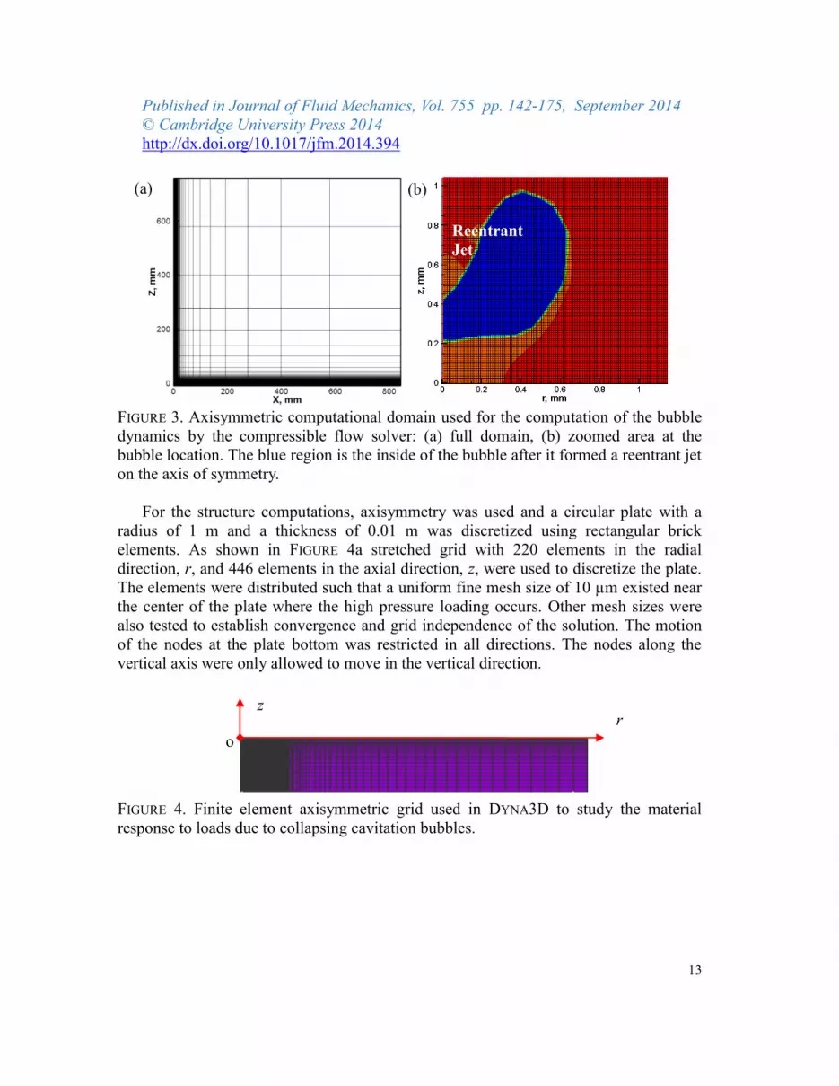
FIGURE 6 shows the variations of the bubble outer contour versus time. As the
bubble grows between t = 0 and t ~2.4ms, it behaves almost spherically on its portion
away from the wall, while the side close to the material flattens and expands in the
direction parallel to the wall actually never touching the wall as a layer of liquid remains
between the bubble and the wall. Such a behavior has been confirmed experimentally by
Published in Journal of Fluid Mechanics, Vol. 755 pp. 142-175, September 2014
© Cambridge University Press 2014
http://dx.doi.org/10.1017/jfm.2014.394
15
Chahine et al. (1996). Note that at maximum bubble volume, the non-dimensional
standoff, max/ ,X X R is 0.75 (less than one) where maxR is the maximum equivalent
bubble radius deduced from its volume.
FIGURE 6. Bubble shape outlines at different times showing (a) bubble growth (0 < t <
2.415 ms) and (b) collapse (2.415 ms < t < 2.435ms). Results obtained from the three-
dimensional BEM simulations for R0 = 50 μm, Pd = 10 MPa, 𝑋 ̅ = 0.75, and p(t)
described by (17).
The bubble will continue expanding at the starting of reverse pressure due to the
inertia of the outward flow of the liquid. Due to the asymmetry of the flow, the pressures
at the bubble interface on the side away from the wall are much higher than those near
the material; thus the collapse proceeds with the far side moving towards the material
wall. The resulting acceleration of the liquid flow perpendicular to the bubble free
surface develops a Taylor instability at the axis of symmetry, which results into a
reentrant jet that penetrates the bubble and moves much faster than the rest of the bubble
surface to impact the opposite side of the bubble and the material boundary. In the
present approach, the simulation of the bubble dynamics is switched from the BEM to
the compressible solver right before the jet touches the opposite side of the bubble.
Ideally, the link time should be at the time the bubble becomes multi-connected.
However, to avoid increased errors/ fluctuations in the BEM solution when the distance
between a jet panel and the opposite bubble side panels continues to decrease as the jet
advances, the “link” time was selected to be when the distance between the jet front and
the opposite bubble surface becomes less than or equal to 1.5 times the local panel size.
This results in an underestimate of tlink by less than 1 %. FIGURE 7a shows the pressure
contours and velocity vectors at the selected time, tlink, when the compressible flow
solver and the FSI start their computations. FIGURE 7b shows the corresponding
1.5
mm
Time Time
(a) (b)

Published in Journal of Fluid Mechanics, Vol. 755 pp. 142-175, September 2014
© Cambridge University Press 2014
http://dx.doi.org/10.1017/jfm.2014.394
velocity vectors and velocity magnitude contour levels. Note that, for this bubble
collapse condition, prior to jet impact on the opposite side of the bubble, the liquid
velocities near the tip of the jet exceeds 1400 m/s. The maximum liquid velocity of the
jet exceeds the sound speed after the “link” time when the computation was continued
with the compressible code. The peak value reaches about 1600 m/s at the time when
the jet touches down the opposite side of the bubble. The variations of the jet speed with
the imposed collapse pressure are discussed further below in the parametric study
section.
FIGURE 7. a) Pressure contour levels with velocity vectors and b) velocity vectors and
magnitude contour levels at t = 2.435 ms, time at which the incompressible-
compressible link procedure is applied. These serve as initial conditions for the
compressible flow and FSI solvers for R0 = 50 μm, Pd = 10 MPa, �̅�= 0.75 and p(t)
described by Equation (17).
(a) t-tlink=0.05 s (b) t-tlink=0.2 s (c) t-tlink=0.4 s
(a) (b)
Published in Journal of Fluid Mechanics, Vol. 755 pp. 142-175, September 2014
© Cambridge University Press 2014
http://dx.doi.org/10.1017/jfm.2014.394
17
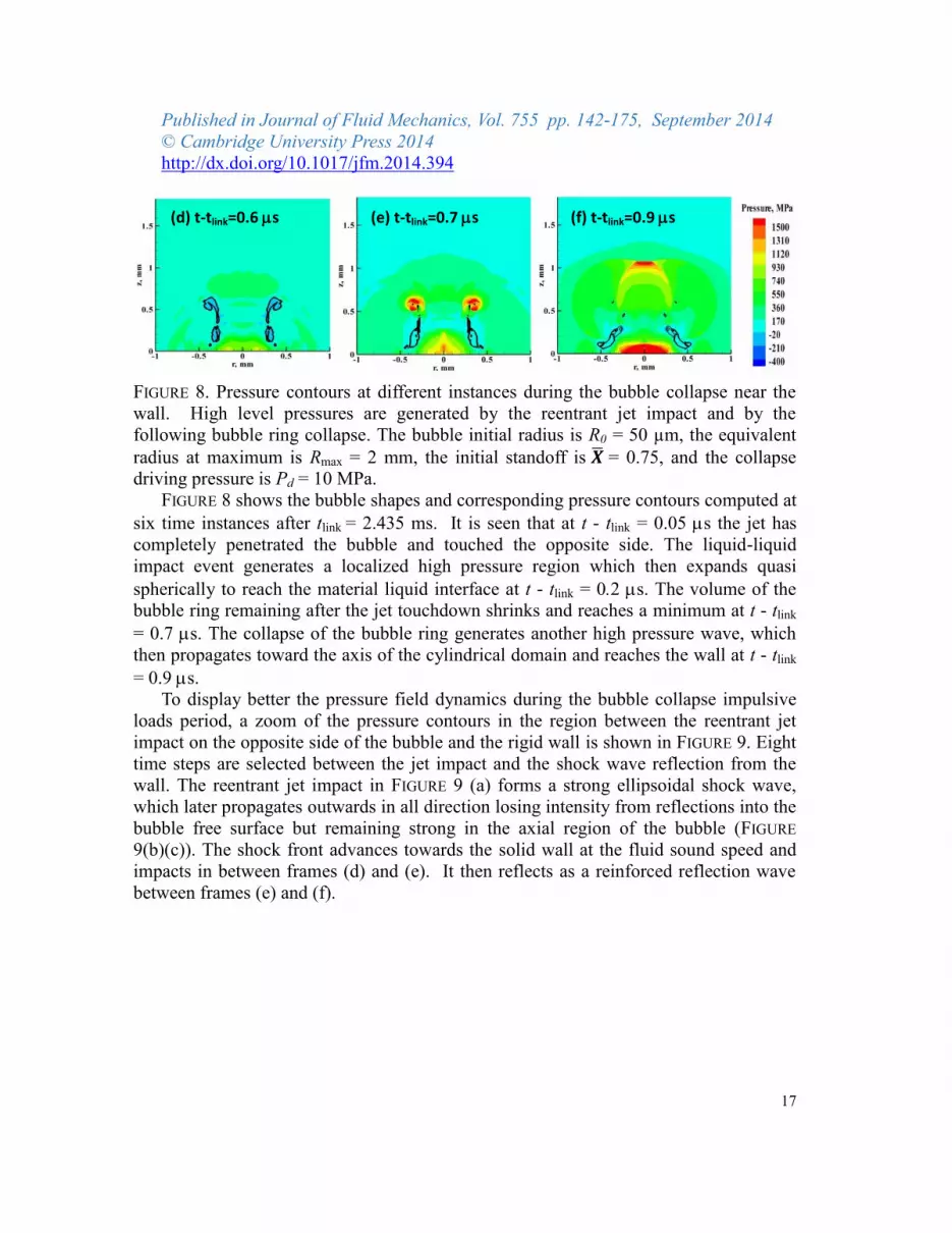
FIGURE 8. Pressure contours at different instances during the bubble collapse near the
wall. High level pressures are generated by the reentrant jet impact and by the
following bubble ring collapse. The bubble initial radius is R0 = 50 µm, the equivalent
radius at maximum is Rmax = 2 mm, the initial standoff is �̅� = 0.75, and the collapse
driving pressure is Pd = 10 MPa.
FIGURE 8 shows the bubble shapes and corresponding pressure contours computed at
six time instances after tlink = 2.435 ms. It is seen that at t - tlink = 0.05 s the jet has
completely penetrated the bubble and touched the opposite side. The liquid-liquid
impact event generates a localized high pressure region which then expands quasi
spherically to reach the material liquid interface at t - tlink = 0.2 s. The volume of the
bubble ring remaining after the jet touchdown shrinks and reaches a minimum at t - tlink
= 0.7 s. The collapse of the bubble ring generates another high pressure wave, which
then propagates toward the axis of the cylindrical domain and reaches the wall at t - tlink
= 0.9 s.
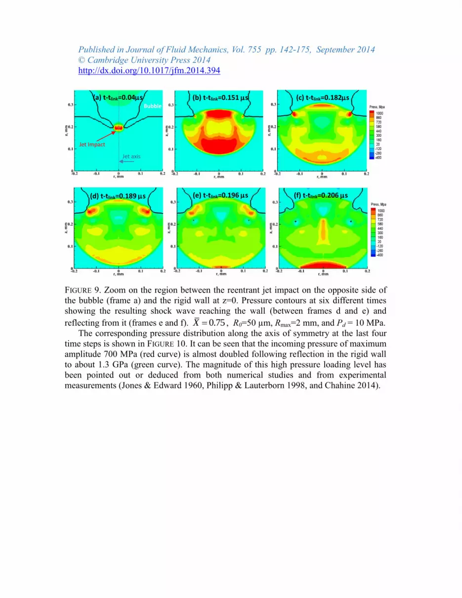
To display better the pressure field dynamics during the bubble collapse impulsive
loads period, a zoom of the pressure contours in the region between the reentrant jet
impact on the opposite side of the bubble and the rigid wall is shown in FIGURE 9. Eight
time steps are selected between the jet impact and the shock wave reflection from the
wall. The reentrant jet impact in FIGURE 9 (a) forms a strong ellipsoidal shock wave,
which later propagates outwards in all direction losing intensity from reflections into the
bubble free surface but remaining strong in the axial region of the bubble (FIGURE
9(b)(c)). The shock front advances towards the solid wall at the fluid sound speed and
impacts in between frames (d) and (e). It then reflects as a reinforced reflection wave
between frames (e) and (f).
(d) t-tlink=0.6 s (e) t-tlink=0.7 s (f) t-tlink=0.9 s
Published in Journal of Fluid Mechanics, Vol. 755 pp. 142-175, September 2014
© Cambridge University Press 2014
http://dx.doi.org/10.1017/jfm.2014.394
FIGURE 9. Zoom on the region between the reentrant jet impact on the opposite side of
the bubble (frame a) and the rigid wall at z=0. Pressure contours at six different times
showing the resulting shock wave reaching the wall (between frames d and e) and
reflecting from it (frames e and f). 0.75X , R0=50 µm, Rmax=2 mm, and Pd = 10 MPa.
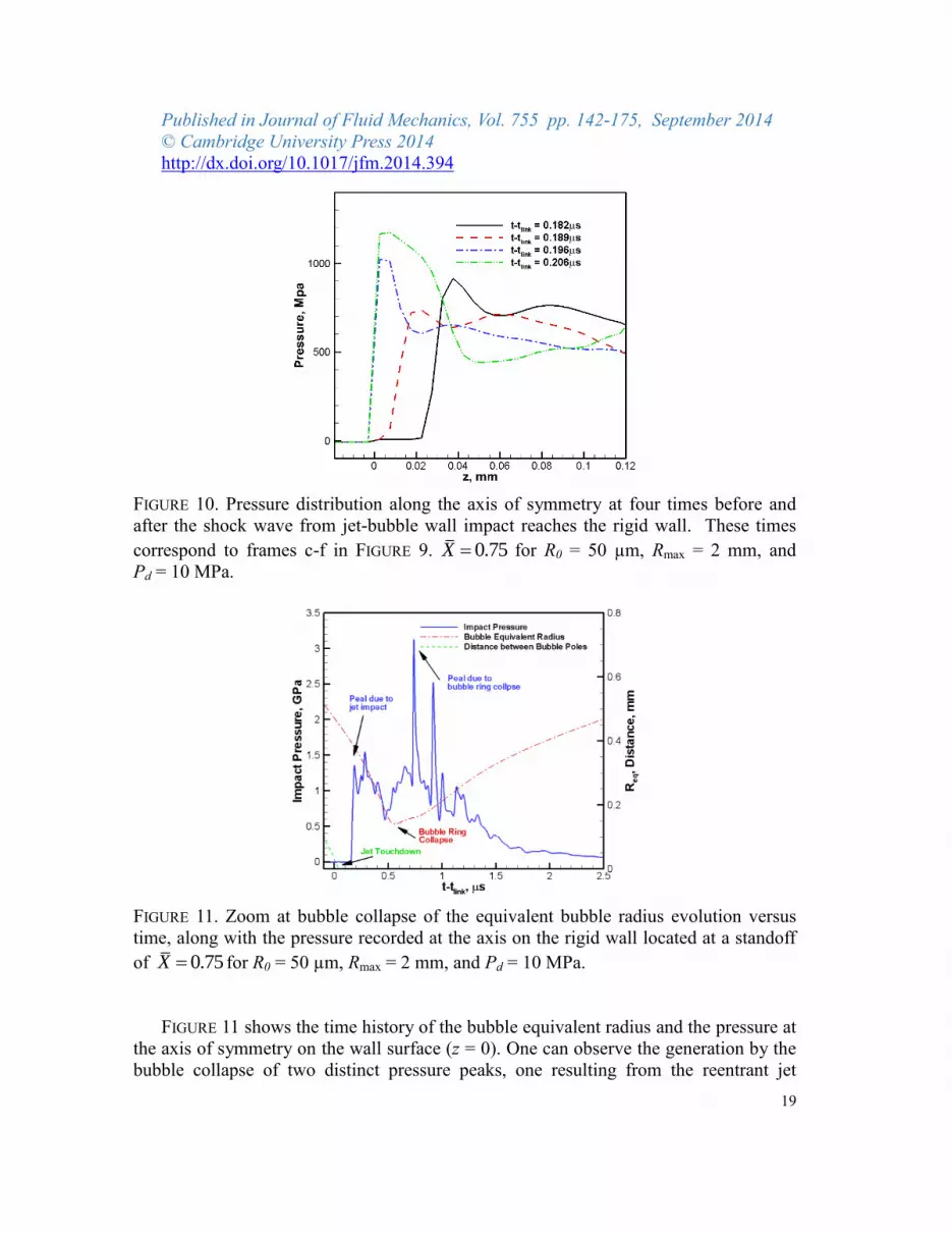
The corresponding pressure distribution along the axis of symmetry at the last four
time steps is shown in FIGURE 10. It can be seen that the incoming pressure of maximum
amplitude 700 MPa (red curve) is almost doubled following reflection in the rigid wall
to about 1.3 GPa (green curve). The magnitude of this high pressure loading level has
been pointed out or deduced from both numerical studies and from experimental
measurements (Jones & Edward 1960, Philipp & Lauterborn 1998, and Chahine 2014).
(b) t-tlink=0.151 s (a) t-tlink=0.04s (c) t-tlink=0.182s
Jet Impact
Jet Impact
Jet axis
Bubble
(f) t-tlink=0.206 s (e) t-tlink=0.196 s (d) t-tlink=0.189 s
Published in Journal of Fluid Mechanics, Vol. 755 pp. 142-175, September 2014
© Cambridge University Press 2014
http://dx.doi.org/10.1017/jfm.2014.394
19
FIGURE 10. Pressure distribution along the axis of symmetry at four times before and
after the shock wave from jet-bubble wall impact reaches the rigid wall. These times
correspond to frames c-f in FIGURE 9. 0.75X for R0 = 50 µm, Rmax = 2 mm, and
Pd = 10 MPa.
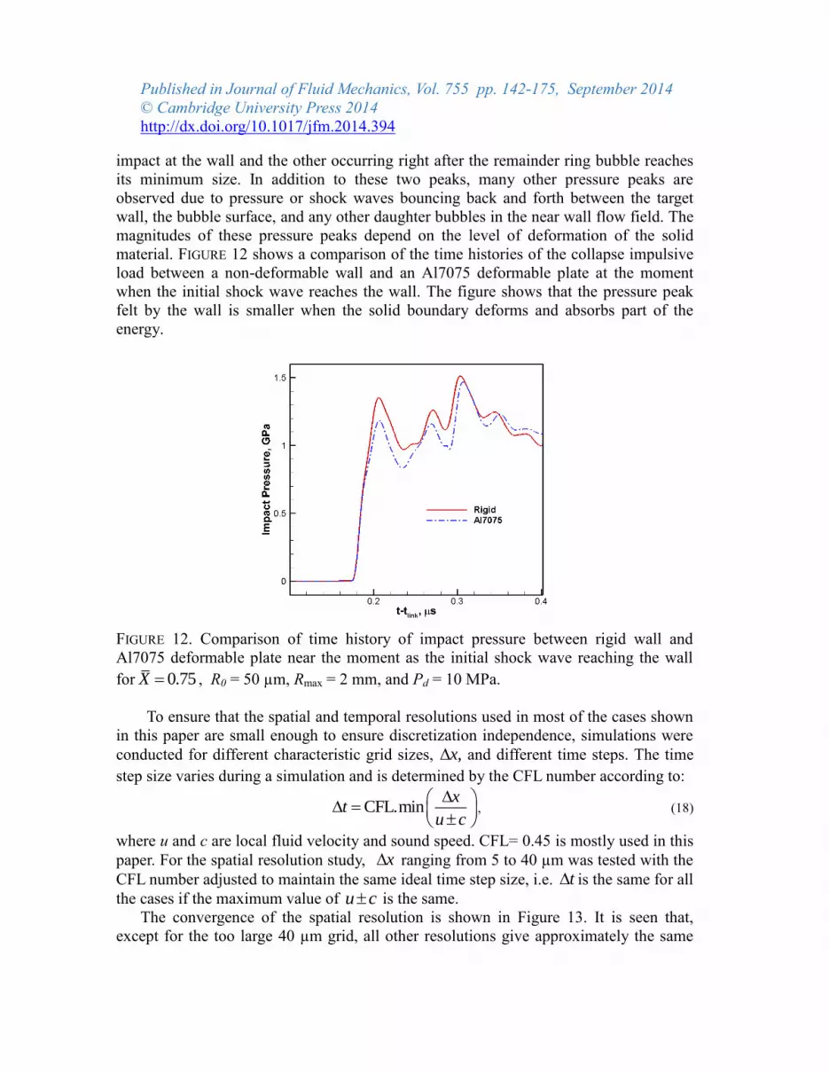
FIGURE 11. Zoom at bubble collapse of the equivalent bubble radius evolution versus
time, along with the pressure recorded at the axis on the rigid wall located at a standoff
of 0.75X for R0 = 50 µm, Rmax = 2 mm, and Pd = 10 MPa.
FIGURE 11 shows the time history of the bubble equivalent radius and the pressure at
the axis of symmetry on the wall surface (z = 0). One can observe the generation by the
bubble collapse of two distinct pressure peaks, one resulting from the reentrant jet
Published in Journal of Fluid Mechanics, Vol. 755 pp. 142-175, September 2014
© Cambridge University Press 2014
http://dx.doi.org/10.1017/jfm.2014.394
impact at the wall and the other occurring right after the remainder ring bubble reaches
its minimum size. In addition to these two peaks, many other pressure peaks are
observed due to pressure or shock waves bouncing back and forth between the target
wall, the bubble surface, and any other daughter bubbles in the near wall flow field. The
magnitudes of these pressure peaks depend on the level of deformation of the solid
material. FIGURE 12 shows a comparison of the time histories of the collapse impulsive
load between a non-deformable wall and an Al7075 deformable plate at the moment
when the initial shock wave reaches the wall. The figure shows that the pressure peak
felt by the wall is smaller when the solid boundary deforms and absorbs part of the
energy.
FIGURE 12. Comparison of time history of impact pressure between rigid wall and
Al7075 deformable plate near the moment as the initial shock wave reaching the wall
for 0.75X , R0 = 50 µm, Rmax = 2 mm, and Pd = 10 MPa.
To ensure that the spatial and temporal resolutions used in most of the cases shown
in this paper are small enough to ensure discretization independence, simulations were
conducted for different characteristic grid sizes, ,x and different time steps. The time
step size varies during a simulation and is determined by the CFL number according to:
CFL.min
xt
u c, (18)
where u and c are local fluid velocity and sound speed. CFL= 0.45 is mostly used in this
paper. For the spatial resolution study, x ranging from 5 to 40 µm was tested with the
CFL number adjusted to maintain the same ideal time step size, i.e. t is the same for all
the cases if the maximum value of u c is the same.
The convergence of the spatial resolution is shown in Figure 13. It is seen that,
except for the too large 40 µm grid, all other resolutions give approximately the same
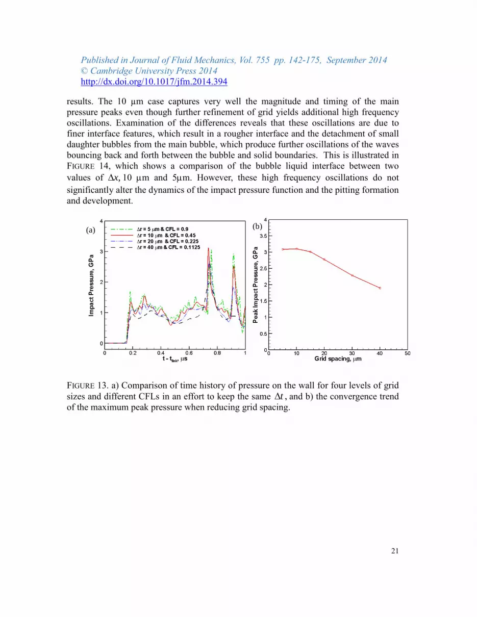
Published in Journal of Fluid Mechanics, Vol. 755 pp. 142-175, September 2014
© Cambridge University Press 2014
http://dx.doi.org/10.1017/jfm.2014.394
21
results. The 10 µm case captures very well the magnitude and timing of the main
pressure peaks even though further refinement of grid yields additional high frequency
oscillations. Examination of the differences reveals that these oscillations are due to
finer interface features, which result in a rougher interface and the detachment of small
daughter bubbles from the main bubble, which produce further oscillations of the waves
bouncing back and forth between the bubble and solid boundaries. This is illustrated in
FIGURE 14, which shows a comparison of the bubble liquid interface between two
values of ,x 10 m and 5m. However, these high frequency oscillations do not
significantly alter the dynamics of the impact pressure function and the pitting formation
and development.
FIGURE 13. a) Comparison of time history of pressure on the wall for four levels of grid
sizes and different CFLs in an effort to keep the same t , and b) the convergence trend
of the maximum peak pressure when reducing grid spacing.
(a) (b)

Published in Journal of Fluid Mechanics, Vol. 755 pp. 142-175, September 2014
© Cambridge University Press 2014
http://dx.doi.org/10.1017/jfm.2014.394
x = 10 µm x = 5 µm
FIGURE 14. Comparison of the bubble liquid interface (bubble ring cross-section with
r=0 being the axis of symmetry) at a selected time between a grid size determined by
x =10 m and x =5m (right). Notice smaller features appearing with the finer grids.
FIGURE 15. a) Comparison of the time history of the pressure on the wall for three CFL
numbers for x =10 m, and b) convergence trend of the maximum peak pressure when
changing CFL number.
For the temporal resolution study, three different CFL numbers were tested for the
same grid size, x =10 µm. FIGURE 15 shows the convergence of the peak pressure as
obtained for each CFL computations. The figure illustrates that the solution is well
resolved and converged with the selected temporal resolution.
(a) (b)

Published in Journal of Fluid Mechanics, Vol. 755 pp. 142-175, September 2014
© Cambridge University Press 2014
http://dx.doi.org/10.1017/jfm.2014.394
23
4.2 Material deformation
As observed experimentally and recovered in the present simulations, the pressures
generated by the bubble collapse and rebound are at least two orders of magnitude
higher than the pressures generated during the rest of the bubble period. In order to
evaluate whether, under the present conditions, ignoring fluid structure interactions
before bubble collapse and reentrant jet impact have any significant influence on the
computations of cavitation pit formation, we analyze a full period fluid structure
interaction computation for the base case bubble dynamics conditions near the softest
material (Rubber#1) in TABLE 2. We concentrate first on the material maximum
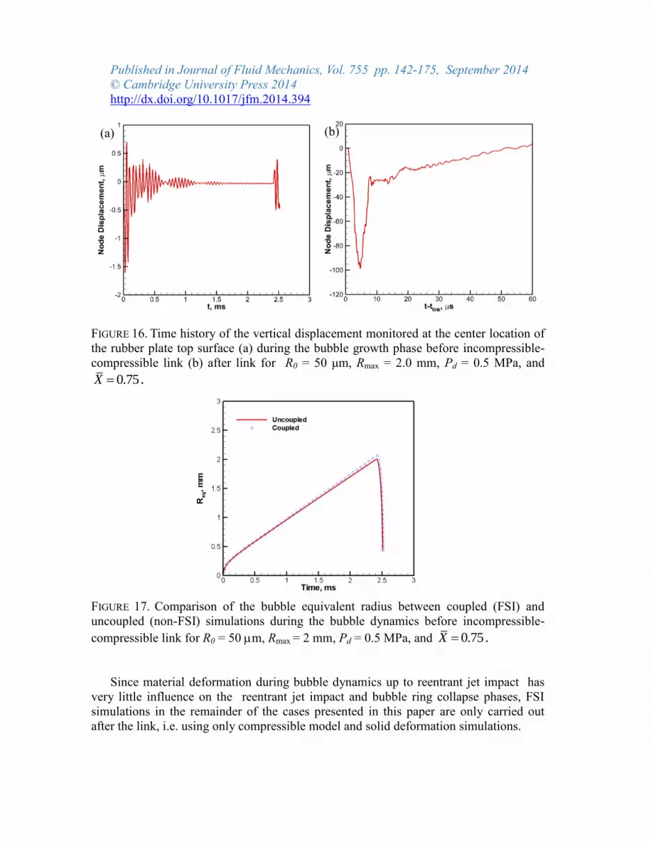
deformation location. FIGURE 16 shows the time history of the vertical displacement of
the material surface at the center of the rubber plate. FIGURE 16(a) shows the
deformation during the bubble growth and initial collapse phase captured by the coupled
BEM/ DYNA3D code (the corresponding bubble radius versus time is shown in FIGURE
17). The soft rubber is seen to react to the initial sharp pressure drop (see FIGURE 2) by
bulging out and then oscillating up and down at its own resonance frequency, which is
much higher than the present bubble excitation frequency. The bubble growth does not
add any significant enhancement to the initial pressure perturbation and the rubber
material returns practically to its initial stage until the bubble contents start to
recompress and the pressures in the liquid start to rise rapidly. This again excites the
material into small oscillations. We should note, however, that during this whole period
the deformations remain of the order of 1m. The computations are pursued beyond
2.51linkt s using the coupled compressible and solid codes and the resulting material
deformation at the plate center are shown in FIGURE 16(b). During this phase the
pressures increase significantly (as shown in FIGURE 11) and the material deformation is
two orders of magnitude higher than during the bubble growth due to bubble reentrant
jet impact and remaining bubble ring collapse. The maximum deformation generated by
the bubble collapse is 100m and is shown using different vertical and horizontal scales
than in FIGURE 16(a). For this “worst-case” condition amongst the cases considered
here, the initial material deformation is only of the order of 1% of the deformations due
to bubble collapse.
FIGURE 17 illustrates the importance of the inclusion of fluid structure interaction
during the bubble growth phase on the bubble dynamics. The time history of the bubble
radius is compared between coupled (FSI) and uncoupled simulations. Here again, the
influence of the initial rubber motion on the bubble dynamics is less than 1 %.
Published in Journal of Fluid Mechanics, Vol. 755 pp. 142-175, September 2014
© Cambridge University Press 2014
http://dx.doi.org/10.1017/jfm.2014.394
FIGURE 16. Time history of the vertical displacement monitored at the center location of
the rubber plate top surface (a) during the bubble growth phase before incompressible-
compressible link (b) after link for R0 = 50 μm, Rmax = 2.0 mm, Pd = 0.5 MPa, and
0.75X .
FIGURE 17. Comparison of the bubble equivalent radius between coupled (FSI) and
uncoupled (non-FSI) simulations during the bubble dynamics before incompressible-
compressible link for R0 = 50 m, Rmax = 2 mm, Pd = 0.5 MPa, and 0.75X .
Since material deformation during bubble dynamics up to reentrant jet impact has
very little influence on the reentrant jet impact and bubble ring collapse phases, FSI
simulations in the remainder of the cases presented in this paper are only carried out
after the link, i.e. using only compressible model and solid deformation simulations.
(a) (b)

Published in Journal of Fluid Mechanics, Vol. 755 pp. 142-175, September 2014
© Cambridge University Press 2014
http://dx.doi.org/10.1017/jfm.2014.394
25
FIGURE 18 shows a time sequence of the contours of the von Mises equivalent
stresses in the material for one of the two metallic alloys considered here, AL7075. It is
seen that high stresses appear at the plate center near the surface when the reentrant jet
impact pressure reaches the wall at t - tlink = 0.2 s. The high stress wave is observed to
propagate and move radially away from the impact location. As the first high stress
wave starts to attenuate, another high stress is observed initiating from the top center of
the plate at t - tlink = 0.9 s, time at which the high pressure wave generated by the
collapse of the remaining bubble ring reaches the wall (see FIGURE 8f). It is interesting
to note that the speed of stress wave propagation in the longitudinal direction (along the
axis of symmetry) is about 3,700 m/s, i.e. significantly smaller than the
expected 6,400 m/s longitudinal wave speed in AL7075. This is due to the plastic
deformation of the material, which modifies the material properties and wave behavior.
All high stresses due to the bubble dynamics eventually attenuate. However, residual
stresses remain below the plate surface due to the plastic deformations of the material.
In the conditions of FIGURE 18, these have their highest value occurring at a depth of 0.2
mm below the surface as shown in Figure 18f. Since the material is modeled as elastic-
plastic, permanent deformation should occur wherever the local equivalent stresses
exceed the material yield point. With the yield stress of AL7075 being 503 MPa, all
regions that have seen the top red stress contour level shown in FIGURE 18 experience
permanent deformation due to either reentrant jet impact or bubble ring collapse.
(a) t-tlink=0.2 s (b) t-tlink=0.4 s (c) t-tlink=0.6 s
(d) t-tlink=0.7 s (e) t-tlink=0.9 s (f) t-tlink=4.0 s

Published in Journal of Fluid Mechanics, Vol. 755 pp. 142-175, September 2014
© Cambridge University Press 2014
http://dx.doi.org/10.1017/jfm.2014.394
FIGURE 18. Time sequence of the equivalent stress contours in the Al 7075 plate for
R0 = 50 μm, Rmax = 2.0 mm, Pd = 10 MPa, and 0.75X .
To quantitatively examine the material response to the pressure loading, the time
histories of the liquid pressure and the vertical displacement of the material surface at
the center of the Al 7075 plate / liquid interface are shown together in FIGURE 19. The
material starts to get compressed as the high pressure loading due to the reentrant jet
impact reaches it, and the plate surface center point starts to move in at
t - tlink = 0.45 s. The maximum deformation occurs when the highest pressure loading
peak due to the bubble ring collapse reaches the center of the plate at time
t - tlink = 1.15 s. Once the pressure loading due to the full bubble dynamics has virtually
vanished at t - tlink = 4 s, the surface elevation continues to oscillate due to stress waves
propagating back and forth through the metal alloy thickness and lack of damping in the
model. Finally, a permanent deformation (pit) remains as a result of the high pressure
loading causing local stresses that exceed the Al 7075 elastic limit. As shown in the
FIGURE 19, the vertical displacement of the monitored location eventually converges to
a non-zero value (~9m).
FIGURE 19. Time history of pressure and vertical displacement monitored at the center
location of the Al 7075 plate top surface following the collapse of a cavitation bubble
near the plate for R0 = 50 μm, Rmax = 2.0 mm, Pd = 10 MPa, and 0.75X .
Published in Journal of Fluid Mechanics, Vol. 755 pp. 142-175, September 2014
© Cambridge University Press 2014
http://dx.doi.org/10.1017/jfm.2014.394
27
FIGURE 20. Profile of the permanent deformation an Al 7075 plate surface following the
collapse of a cavitation bubble for R0 = 50 μm, Rmax = 2.0 mm, Pd = 10 MPa, and
0.75X .
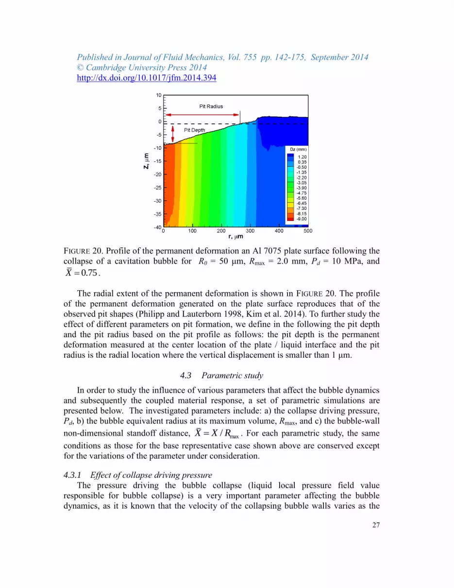
The radial extent of the permanent deformation is shown in FIGURE 20. The profile
of the permanent deformation generated on the plate surface reproduces that of the
observed pit shapes (Philipp and Lauterborn 1998, Kim et al. 2014). To further study the
effect of different parameters on pit formation, we define in the following the pit depth
and the pit radius based on the pit profile as follows: the pit depth is the permanent
deformation measured at the center location of the plate / liquid interface and the pit
radius is the radial location where the vertical displacement is smaller than 1 μm.
4.3 Parametric study
In order to study the influence of various parameters that affect the bubble dynamics
and subsequently the coupled material response, a set of parametric simulations are
presented below. The investigated parameters include: a) the collapse driving pressure,
Pd, b) the bubble equivalent radius at its maximum volume, Rmax, and c) the bubble-wall
non-dimensional standoff distance, max/X X R . For each parametric study, the same
conditions as those for the base representative case shown above are conserved except
for the variations of the parameter under consideration.
4.3.1 Effect of collapse driving pressure
The pressure driving the bubble collapse (liquid local pressure field value
responsible for bubble collapse) is a very important parameter affecting the bubble
dynamics, as it is known that the velocity of the collapsing bubble walls varies as the

Published in Journal of Fluid Mechanics, Vol. 755 pp. 142-175, September 2014
© Cambridge University Press 2014
http://dx.doi.org/10.1017/jfm.2014.394
square root of that pressure (Jayaprakash et al. 2013; Chahine et al. 2006, 2014). In this
section we vary the magnitude of the collapse driving pressure, Pd, to study its effect on
the resulting material pitting. FIGURE 21 shows the time history of the equivalent radius
of the bubble for a set of values of pressures Pd between 0.1 to 20 MPa. In all cases
shown, the bubble starts with a R0 = 50 m nucleus, then grows to a maximum
equivalent radius of Rmax = 2 mm, at which time the pressure is raised to Pd. The
considered bubble is located at an initial standoff X = 1.5 mm (i.e. 0.75X ) from the
material surface. It can be clearly seen in FIGURE 21 that, with increasing amplitudes of
the driving pressure, the bubble collapses with increasing speed.
FIGURE 21. Comparison of the bubble equivalent radius for different collapse driving
pressures, Pd : a) full history, b) zoom on the collapse period for R0 = 50 m,
Rmax = 2 mm, and 0.75X .
(b) (a)
Published in Journal of Fluid Mechanics, Vol. 755 pp. 142-175, September 2014
© Cambridge University Press 2014
http://dx.doi.org/10.1017/jfm.2014.394
29
FIGURE 22. Bubble contours at the time of incompressible/compressible link for
different collapse driving pressures. R0 = 50 m, Rmax = 2 mm, and 0.75X .
FIGURE 23. Variation of the reentrant jet momentum averaged velocity with the collapse
driving pressure for R0 = 50 m, Rmax = 2 mm, and 0.75X .
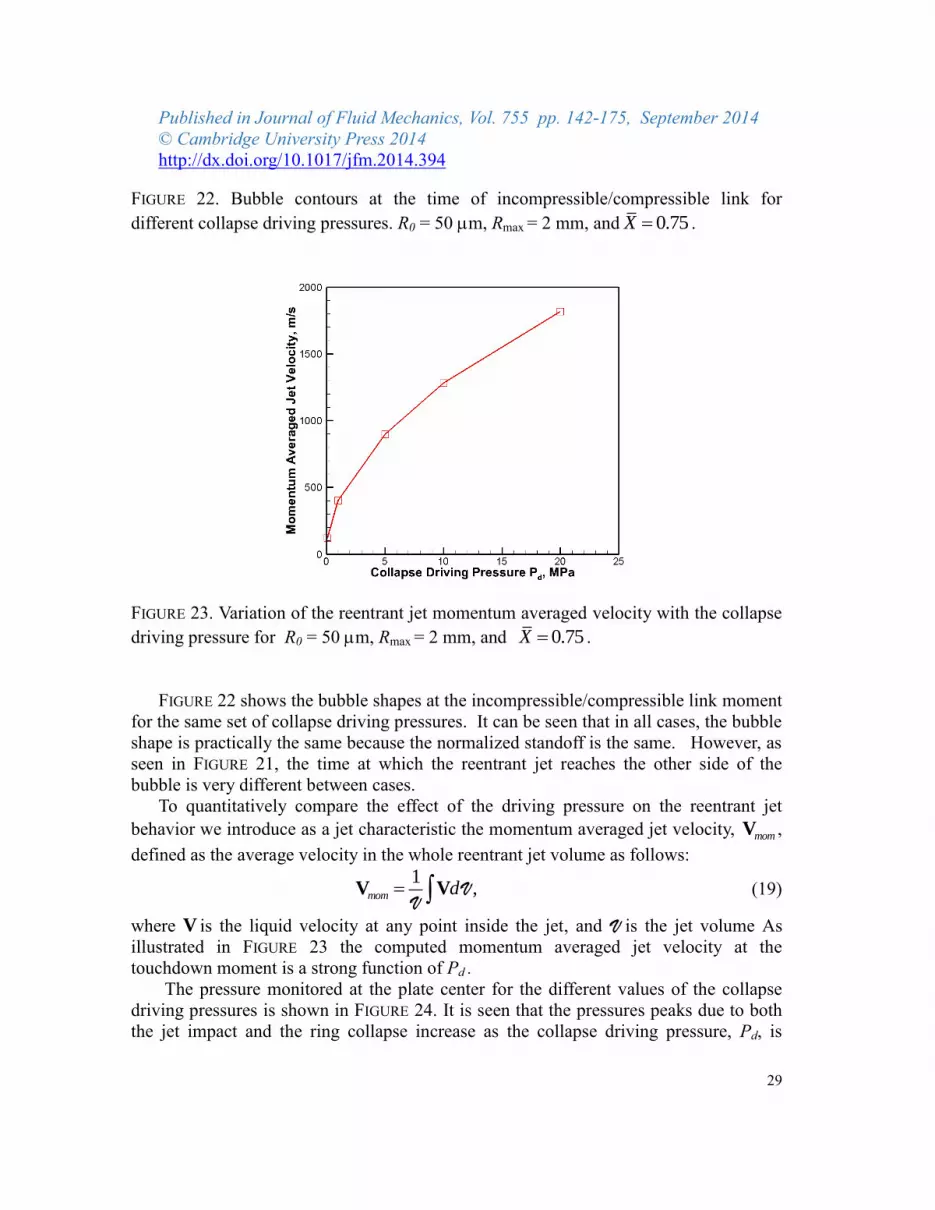
FIGURE 22 shows the bubble shapes at the incompressible/compressible link moment
for the same set of collapse driving pressures. It can be seen that in all cases, the bubble
shape is practically the same because the normalized standoff is the same. However, as
seen in FIGURE 21, the time at which the reentrant jet reaches the other side of the
bubble is very different between cases.
To quantitatively compare the effect of the driving pressure on the reentrant jet
behavior we introduce as a jet characteristic the momentum averaged jet velocity, momV ,
defined as the average velocity in the whole reentrant jet volume as follows:
1
,mom d V V VV
(19)
where V is the liquid velocity at any point inside the jet, and V is the jet volume As
illustrated in FIGURE 23 the computed momentum averaged jet velocity at the
touchdown moment is a strong function of Pd .
The pressure monitored at the plate center for the different values of the collapse
driving pressures is shown in FIGURE 24. It is seen that the pressures peaks due to both
the jet impact and the ring collapse increase as the collapse driving pressure, Pd, is
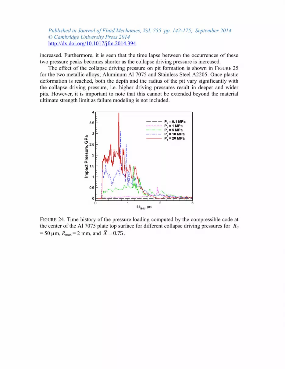
Published in Journal of Fluid Mechanics, Vol. 755 pp. 142-175, September 2014
© Cambridge University Press 2014
http://dx.doi.org/10.1017/jfm.2014.394
increased. Furthermore, it is seen that the time lapse between the occurrences of these
two pressure peaks becomes shorter as the collapse driving pressure is increased.
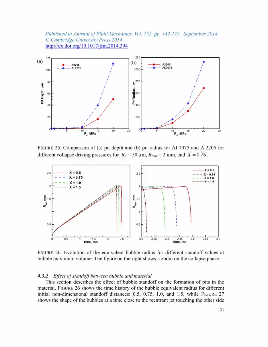
The effect of the collapse driving pressure on pit formation is shown in FIGURE 25
for the two metallic alloys; Aluminum Al 7075 and Stainless Steel A2205. Once plastic
deformation is reached, both the depth and the radius of the pit vary significantly with
the collapse driving pressure, i.e. higher driving pressures result in deeper and wider
pits. However, it is important to note that this cannot be extended beyond the material
ultimate strength limit as failure modeling is not included.
FIGURE 24. Time history of the pressure loading computed by the compressible code at
the center of the Al 7075 plate top surface for different collapse driving pressures for R0
= 50 m, Rmax = 2 mm, and 0.75X .
Published in Journal of Fluid Mechanics, Vol. 755 pp. 142-175, September 2014
© Cambridge University Press 2014
http://dx.doi.org/10.1017/jfm.2014.394
31
FIGURE 25. Comparison of (a) pit depth and (b) pit radius for Al 7075 and A 2205 for
different collapse driving pressures for R0 = 50 m, Rmax = 2 mm, and 0.75X .
FIGURE 26. Evolution of the equivalent bubble radius for different standoff values at
bubble maximum volume. The figure on the right shows a zoom on the collapse phase.
4.3.2 Effect of standoff between bubble and material
This section describes the effect of bubble standoff on the formation of pits in the
material. FIGURE 26 shows the time history of the bubble equivalent radius for different
initial non-dimensional standoff distances: 0.5, 0.75, 1.0, and 1.5, while FIGURE 27
shows the shape of the bubbles at a time close to the reentrant jet touching the other side
(b) (a)

Published in Journal of Fluid Mechanics, Vol. 755 pp. 142-175, September 2014
© Cambridge University Press 2014
http://dx.doi.org/10.1017/jfm.2014.394
of the bubble. Compressible flow computations were conducted after these points in
time. In all cases shown, the bubble starts at R0 = 50 m, grows to a bubble maximum
Rmax = 2 mm, and is then subjected to a pressure driving the collapse Pd =10 Mpa. The
duration of the pressure drop, t, was adjusted such that the sudden pressure rise, Pd,
was imposed at the time when the bubble radius reached 2 mm.
The bubble shapes show that the jet becomes more pronounced when the bubble is
closer to the wall. At the larger standoffs, the bubble volume shrinks significantly
before the jet develops, while closer to the wall the reentrant jet develops much earlier
and the bubble still has a larger volume when the jet reaches the opposite side of the
bubbles. From these contours one can expect very different pressure loadings on the
material surface for different values of X.
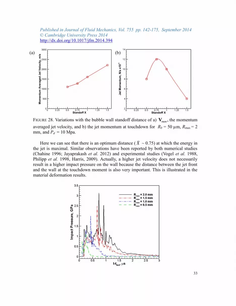
FIGURE 28a compares the momentum average jet velocity, momV , at the touchdown
moment (time the jet reaches the other side of the bubble) for different standoff
distances. It is seen that the jet velocity increases as the standoff distance is increased.
This is not surprising since actually the largest bubble wall speed will be achieved when
the bubble is spherical (Chahine et al. 2006, Jayaprakash et al. 2013). A better
illustration of the energy in the jet could be the total momentum of the jet, momV V , at the
moment it touches the opposite side of the bubble, which is shown in FIGURE 28b.
FIGURE 27. Bubble contours at the time of compressible-incompressible link for
different standoff distances between the bubble and the wall for R0 = 50 m,
Rmax = 2 mm, and Pd = 10 Mpa.
Published in Journal of Fluid Mechanics, Vol. 755 pp. 142-175, September 2014
© Cambridge University Press 2014
http://dx.doi.org/10.1017/jfm.2014.394
33
FIGURE 28. Variations with the bubble wall standoff distance of a) momV , the momentum
averaged jet velocity, and b) the jet momentum at touchdown for R0 = 50 m, Rmax = 2
mm, and Pd = 10 Mpa.
Here we can see that there is an optimum distance ( X ~ 0.75) at which the energy in
the jet is maximal. Similar observations have been reported by both numerical studies
(Chahine 1996; Jayaprakash et al. 2012) and experimental studies (Vogel et al. 1988,
Philipp et al. 1998, Harris, 2009). Actually, a higher jet velocity does not necessarily
result in a higher impact pressure on the wall because the distance between the jet front
and the wall at the touchdown moment is also very important. This is illustrated in the
material deformation results.
(a) (b)

Published in Journal of Fluid Mechanics, Vol. 755 pp. 142-175, September 2014
© Cambridge University Press 2014
http://dx.doi.org/10.1017/jfm.2014.394
FIGURE 29. Pressure versus time at the center of the Al 7075 plate for different bubble
plate standoff distances for R0 = 50 m, Rmax = 2 mm, and Pd = 10 Mpa.
FIGURE 29 shows the pressure versus time monitored at the plate center for different
standoff distances. It is seen that the pressure loading due to the jet impact is much
higher for smaller standoff, especially for 0.5X , since in this case the reentrant jet
directly impacts on the material surface when it penetrates the other side of the bubble.
As the standoff increases, the magnitude of the pressure due to the jet impact is reduced
because the high speed liquid has to travel a longer distance while submerged before
reaching the material surface. For 1.5X , only one significant pressure peak with a
typical exponential decay is observed because the jet touchdown occurs almost at the
same time as when the bubble reaches the minimum size and no jet reaches the wall.
Instead, a shock wave type pressure profile is observed.
Standoff X
Pit
Vo
lum
e,
m3
0.4 0.6 0.8 1 1.2 1.4 1.60
1000
2000
3000
4000
5000
6000
A2205
AL7075
(b) (a)
(c)

Published in Journal of Fluid Mechanics, Vol. 755 pp. 142-175, September 2014
© Cambridge University Press 2014
http://dx.doi.org/10.1017/jfm.2014.394
35
FIGURE 30. Variation of (a) pit depth (b) pit radius and (c) pit volume with the
normalized standoff distance for Al 7075 and A 2205 for R0 = 50 m, Rmax = 2 mm and
Pd = 10 Mpa.
The effect of the bubble material standoff distance on the pit characteristics is
actually the most important and relevant information for damage assessment. FIGURE 30
shows the pit characteristics for the two metallic alloys studied: depth, radius, and
volume respectively as a function of the normalized standoff distance. FIGURE 30 shows
that pit depth and volume continually decrease when the standoff distance increases.
However, as for the jet momentum, pit radius goes through a maximum when the
standoff distance is close to 0.75X . The volume, not provided directly by the
software, was approximated by the volume of a cone with the same base diameter and
height. Actually, the shape of the pit varies with standoff as shown in FIGURE 31. At the
smallest standoffs, the pit radius is smaller with 0.5X than with 0.75X , while the
pit depth is larger with 0.5X than with 0.75X .
FIGURE 31. Comparison of pit shape between 0.5X and 0.75X for AL7075 for
R0 = 50 m, Rmax = 2 mm, and Pd = 10 MPa.

Published in Journal of Fluid Mechanics, Vol. 755 pp. 142-175, September 2014
© Cambridge University Press 2014
http://dx.doi.org/10.1017/jfm.2014.394
FIGURE 32. Bubble contours at compressible-incompressible link for different standoff
distances between the bubble and the wall for R0 = 50 m, Pd = 10 MPa and 0.75.X
4.3.3 Effect of maximum bubble size
This section describes the effect of the maximum bubble size, Rmax, on the
characteristics of the material pits formed in response to cavitation bubble collapse. For
this study the duration of the pressure drop, t, in (17) was adjusted to obtain the desired
Rmax. The shapes of the bubbles close to reentrant jet touching the other side of the
bubble for the different Rmax (0.5, 1.0, 1.5 and 2.0 mm) are shown in FIGURE 32. These
shapes indicate that the moment of jet touchdown on the opposite side of the bubble
occurs closer to the moment when the jet impacts the wall as Rmax decreases. However,
the volume and thus the momentum in the jet varies in the opposite direction, i.e. the
bubble volume and the momentum at collapse are smaller for smaller Rmax.
The momentum average jet velocity, momV , and the jet momentum, momV V , at the
touchdown moment for different Rmax are shown in FIGURE 33. It is seen that the jet
velocity is almost independent of the value of Rmax even though the time of jet impact
decreases as Rmax is decreased. The momentum is therefore more dependent on the jet
volume and increases with Rmax and it is expected that damage will simply increase also
with Rmax.
FIGURE 34 shows the pressure monitored at the plate center for different standoff
distances. For all cases, the initial pressure peak due the jet impact and the second peak
due to bubble ring collapse are observed and they both increase as Rmax is increased. It is
also seen that the time lapse between the occurrences of these two pressure peaks
becomes longer and results in a higher impulse as Rmax is increased. This implies the jet
momentum at touchdown has a better correlation with the pressure loading on the
material surface.

Published in Journal of Fluid Mechanics, Vol. 755 pp. 142-175, September 2014
© Cambridge University Press 2014
http://dx.doi.org/10.1017/jfm.2014.394
37
FIGURE 33. Variation with Rmax of (a) momentum averaged jet velocity, momV , and (b)
jet momentum at touchdown, momV V , for R0 = 50 m, Pd = 10 MPa, and 0.75.X
FIGURE 34. Pressure versus time at the center of the Al 7075 plate for different values of
the maximum bubble radius for R0 = 50 m, Pd = 10 MPa, and 0.75.X
The effect of the Rmax on pit formation is shown in FIGURE 35 by comparing the pit
characteristics: depth and radius respectively for the two metallic alloys studied. Both
pit depth and pit radius are seen to increase as Rmax is increased as expected from the
(b) (a)

Published in Journal of Fluid Mechanics, Vol. 755 pp. 142-175, September 2014
© Cambridge University Press 2014
http://dx.doi.org/10.1017/jfm.2014.394
observations in the previous figures. The relationship between the pit dimensions and
the bubble radius is practically linear.
FIGURE 35. Comparison of (a) pit depth and (b) pit radius between Al 7075 and A 2205
for cases with different values of maxR for R0 = 50 m, Pd = 10 MPa, and 0.75.X
FIGURE 36. Time history of the pressure at the plate center for two metallic alloys, a
rigid wall, and two compliant materials for R0 = 50 m, Rmax = 2 mm, Pd = 0.1 MPa and
0.75.X
(a) (b)
Published in Journal of Fluid Mechanics, Vol. 755 pp. 142-175, September 2014
© Cambridge University Press 2014
http://dx.doi.org/10.1017/jfm.2014.394
39
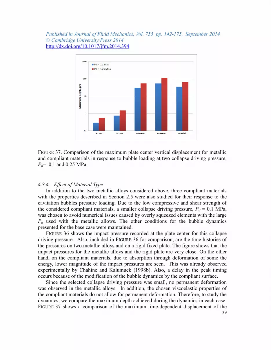
FIGURE 37. Comparison of the maximum plate center vertical displacement for metallic
and compliant materials in response to bubble loading at two collapse driving pressure,
Pd= 0.1 and 0.25 MPa.
4.3.4 Effect of Material Type
In addition to the two metallic alloys considered above, three compliant materials
with the properties described in Section 2.5 were also studied for their response to the
cavitation bubbles pressure loading. Due to the low compressive and shear strength of
the considered compliant materials, a smaller collapse driving pressure, Pd = 0.1 MPa,
was chosen to avoid numerical issues caused by overly squeezed elements with the large
Pd used with the metallic allows. The other conditions for the bubble dynamics
presented for the base case were maintained.
FIGURE 36 shows the impact pressure recorded at the plate center for this collapse
driving pressure. Also, included in FIGURE 36 for comparison, are the time histories of
the pressures on two metallic alloys and on a rigid fixed plate. The figure shows that the
impact pressures for the metallic alloys and the rigid plate are very close. On the other
hand, on the compliant materials, due to absorption through deformation of some the
energy, lower magnitude of the impact pressures are seen. This was already observed
experimentally by Chahine and Kalumuck (1998b). Also, a delay in the peak timing
occurs because of the modification of the bubble dynamics by the compliant surface.
Since the selected collapse driving pressure was small, no permanent deformation
was observed in the metallic alloys. In addition, the chosen viscoelastic properties of
the compliant materials do not allow for permanent deformation. Therefore, to study the
dynamics, we compare the maximum depth achieved during the dynamics in each case.
FIGURE 37 shows a comparison of the maximum time-dependent displacement of the

Published in Journal of Fluid Mechanics, Vol. 755 pp. 142-175, September 2014
© Cambridge University Press 2014
http://dx.doi.org/10.1017/jfm.2014.394
plate surface center recorded for the two metallic alloys and for the three compliant
materials. Loadings for two bubble collapse driving pressures are considered. As
expected, the stainless steel, A 2205, shows the smallest depth value, while amongst the
compliant materials Rubber # 2 (polyurethane) shows the maximum deformation.
5 Conclusions
Material pitting due to cavitation bubble collapse is studied by modeling the
dynamics of growing and collapsing cavitation bubble near a deforming material with
an initial flat surface. The bubble nucleus, initially at equilibrium with the surrounding
liquid near wall, is subjected to a time dependent pressure field. The pressure first drops
to a value below the bubble critical pressure, stays at this pressure for a prescribed time,
and then rises to a high pressure value. The nucleus then grows explosively and
collapses violently near the wall forming a fast reentrant jet, which hits the wall and
deforms it permanently when the collapse intensity is high enough to results in stresses
exceeding the material elastic limit.
The pressure loading on the material surface during the bubble collapse is found to
be due to the reentrant jet impact and to the collapse of the remaining bubble ring. The
magnitude of the pressure peaks felt by the material depends on the response and
amount of deformation of the solid. The fluid structure interaction simulations show that
the load on the material is reduced and this reduction increases when the solid boundary
deformation increases and more energy is absorbed. For the conditions studied in this
paper, during bubble growth and dynamics till the reentrant jet impact, material
deformations remain negligible as compared to the later material deformations resulting
from bubble reentrant jet impact and bubble ring collapse.
The high pressure loading results in high stress waves, which propagate radially
from the loading location into the material and cause the deformation. A pit (permanent
deformation) is formed when the local equivalent stresses exceed the material yield
stress.
The loading is highly dependent on the amplitude of the pressure which drives the
bubble collapse, the standoff distance, and the duration of the depressurization. The
parametric investigation conducted in this study shows that the pressure peaks due to
both the jet impact and the ring collapse increase as the collapse driving pressure is
increased, and the time lapse between the occurrences of these two pressure peaks
becomes shorter as the collapse driving pressure is increased. Also, higher collapse
driving pressures cause the bubble to collapse faster and result in higher pressure
loadings on the materials and deeper and wider pits. The initial standoff distance
between the bubble and the material affects the jet characteristics in a non-monotonic
fashion. Higher jet velocities occur at the larger standoff distances. However, the energy
in the jet is maximum at a normalized standoff distance close to X = 0.75. A higher jet
velocity does not necessarily result in a higher impact pressure, since the impact
pressure also depends on the distance between the wall and the jet front at the
touchdown moment. A more concentrated pressure loading on the material surface is

Published in Journal of Fluid Mechanics, Vol. 755 pp. 142-175, September 2014
© Cambridge University Press 2014
http://dx.doi.org/10.1017/jfm.2014.394
41
obtained for smaller standoffs where the jet touches downs and the bubble ring collapses
very close to the wall. Such concentrated pressure loadings result in deeper but narrower
pits. As a result, the shape of the pit, i.e. the ratio of pit radius and depth does not vary
monotonically with standoff.
The maximum bubble size does not have a significant effect on the jet velocity.
However, it significantly affects the momentum in the jet as it influences a larger
material surface area. This results in deeper and wider pits for larger bubble sizes.
From the study of different material types, it was found that material response has a
strong effect on the impact pressures due to strong fluid structure interaction. Impact
pressures for metallic alloys are very close to those on a rigid plate while compliant
materials deform and absorb energy. This results in lower magnitude of the impact
pressures and delays in peak occurrence due to lengthening of the bubble period.
Acknowledgements
This work was conducted under partial support from DYNAFLOW, INC. internal
IR&D and from the Office of Naval Research under Contract N00014-12-M-0238,
monitored by Dr. Ki-Han Kim. We would also like to thank ONR and Gregory Harris
from the Naval Surface Warfare Center, Indian Head, for allowing us access to the
GEMINI code and contribution to its coupling to the DYNA3D Structure code. Their
support is greatly appreciated.
REFERENCES
Amirkhizi, A.V., Isaacs, J., McGee, J. & Nemat-Nasser, S. 2006 An experimentally-
based viscoelastic constitutive model for polyurea, including pressure and
temperature effects. Philosophical Magazine, 86 (36), 5847-5866.
Anderson, J.D. 1990 Modern compressible flow: with historical perspective. Vol. 12.
McGraw-Hill New York.
Blake, J.R. & Gibson, D.C. 1987 Cavitation bubbles near boundaries. Ann. Rev. Fluid
Mech., 19, 99-124.
Brennen, C.E. 1995 Cavitation and Bubble Dynamics. New York, Oxford University
Press,
Chahine G.L. 1982 Experimental and asymptotic study of nonspherical bubble collapse.
Applied Scientific Research, 38, 187-197.
Chahine, G.L. & Shen, Y.T. 1986 Bubble dynamics and cavitation inception in
cavitation susceptibility meter. ASME Journal of Fluid Engineering, 108, 444-
452.
Chahine, G.L. & Perdue, T.O. 1989 Simulation of the three-dimensional behavior of an
unsteady large bubble near a structure. 3rd International Colloquium on Drops
and Bubbles, Monterey, CA, Sept.
Published in Journal of Fluid Mechanics, Vol. 755 pp. 142-175, September 2014
© Cambridge University Press 2014
http://dx.doi.org/10.1017/jfm.2014.394
Chahine, G.L. 1993 Cavitation dynamics at microscale level. Journal of Heart Valve
Disease, 3, 102-116.
Chahine G. L., Duraiswami, R. and Kalumuck, K.M. 1996 Boundary element method
for calculating 2-D and 3-D underwater explosion bubble loading on nearby
structures. Naval Surface Warfare Center, Weapons Research and Technology
Department, Report NSWCDD/TR-93/46, September (limited distribution).
Chahine, G.L. & Kalumuck, K.M. 1998a BEM software for free surface flow simulation
including fluid structure interaction effects. Int. Journal of Computer Application
in Technology, Vol. 3/4/5.
Chahine, G.L., and Kalumuck, K.M. 1998b The Influence of Structural deformation on
Water Jet Impact Loading, Journal of Fluids and Structures, Vol. 12, (1), pp.
103-121, Jan.
Chahine G.L., Annasami R., Hsiao C.-T. & Harris G. 2006 Scaling rules for the
prediction on UNDEX bubble re-entering jet parameters. SAVIAC Critical
Technologies in Shock and Vibration, 4 (1), 1-12.
Chahine, G.L. 2014 Modeling of Cavitation Dynamics and Interaction with Material,
Chap. 6 in Advanced Experimental and Numerical Techniques for Cavitation
Erosion Prediction Editors Kim, K.H., Chahine, G.L., Franc, J.P., & Karimi, A.,
Springer.
Colella, P. 1985 A direct Eulerian MUSCL scheme for gas dynamics. SIAM Journal on
Scientific and Statistical Computing, 6(1): 104-117.
Crum L.A., 1979. Surface Oscillations and jet development in pulsating bubbles.
Journal de Physique, colloque c8, supplément au N. 11, tome 40, c8-285.
Duncan, J.H., Milligan, C.D. & Zhange, S. 1991 On the interaction of a collapsing
cavity and a compilant wall. J. Fluid Mech. 226, 401-423.
Duncan, J.H., Milligan, C.D. & Zhang, S. 1996 On the interaction between a bubble and
submerged compliant structure. J. Sound & Vibration, 197, 17-44.
Harris, G.S., Illamni, R., Lewis, W., Rye, K., and Chahine, G.L. 2009 Underwater
Explosion Bubble Phenomena Tests Near a Simulated Dam Structure", Naval
Surface Warfare Center - Indian Head Division, IHTR 10-3055, Nov. 1.
Hsiao, C.-T. & Chahine, G.L., 2010 Incompressible-compressible link to accurately
predict wall Pressure. 81th
Shock and Vibration Symposium, Orlando, FL,
October 24-28.
Hsiao, C.-T. & Chahine, G.L. 2013a Development of compressible-incompressible link
to efficiently model bubble dynamics near floating body. Advances in Boundary
Element & Meshless Techniques XIV, pp. 141-152.
Hsiao, C.-T. & Chahine, G.L. 2013b Breakup of finite thickness viscous shell
microbubbles by ultrasound: a simplified zero thickness shell model. J. Acoust.
Soc. Am., 133 (4), 1897-1910.
Published in Journal of Fluid Mechanics, Vol. 755 pp. 142-175, September 2014
© Cambridge University Press 2014
http://dx.doi.org/10.1017/jfm.2014.394
43
Jayaprakash, A., Hsiao, C.-T. & Chahine, G.L. 2012 Numerical and experimental study
of the interaction of a spark-generated bubble and a vertical wall. ASME Journal
of Fluids Engineering, 134, 031301,
Jones , I.R. and Edwards, D.H., 1960 An experimental study of the forces generated by
the collapse of transient cavities in water, J. Fluid Mech., 7, 596-609.
Kalumuck, K.M., Duraiswami, R. & Chahine, G.L. 1995 Bubble dynamics fluid-
structure interaction simulation on coupling fluid BEM and structural FEM
codes, Journal of Fluids and Structures, 9, 861-883. Kalumuck, K.M., Chahine, G.L. & Hsiao, C.-T. 2003 Simulation of surface piercing
body coupled response to underwater bubble dynamics utilizing 3DYNAFS
, a
three-dimensional BEM code. Computational Mechanics, 32, 319-326
Kapahi, A., C.-T. Hsiao, and G.L. Chahine., A multi-material flow solver for high speed
compressible flow applications, to appear in Computers & Fluids, 2014.
Kim, K.H., Chahine, G.L., Franc, J.P., & Karimi, A. 2014 “Advanced Experimental and
Numerical Techniques for Cavitation Erosion Prediction”, ISBN: 978-94-017-
8538-9 (Print) 978-94-017-8539-6 (Online), Springer.
Key, S.W. 1974 HONDO- A finite element computer program for the large deformation
dynamics response of axisymmetric solids. Sandia National Laboratories,
Albuquerque, N.M, Report. 74-0039.
Madadi-Kandjani, E., Xiong, Q., 2014 Validity of the spring-backed membrane model
for bubble-wall interactions with compliant walls. Computers & Fluids, doi:
http://dx.doi.org/10.1016/j.compfluid.2014.03.010
Naude, C.F. & Ellis, A.T. 1961 On the mechanism of cavitation damage by non-
hemispherical cavities collapsing in contact with a solid boundary. ASME J.
Basic Engineering, 83, 648-656.
Philipp, A. & Lauterborn W., 1998 Cavitation erosion by single laser-produced bubbles.
J. Fluid Mech., 361, 75-116.
Plesset, M.S. & Chapman, R.B. 1971 Collapse of an initially spherical vapour cavity in
the neighborhood of a solid boundary. J . Fluid Mech. 47, part 2, 283-290.
Rayleigh, Lord, 1917 On the pressure developed in a liquid during the collapse of a
spherical cavity. Phil. Mag. 34, 94-98.
Vogel, A. & Lauterborn W., 1988 Acoustic transient generation by laser-produced
cavitation bubbles near solid boundaries. J. Acoust. Soc. Am., 84, 719-731.
Wang, Q. X. and Blake, J. R. 2010 Non-spherical bubble dynamics in a compressible
liquid. Part 1. Travelling acoustic wave. J. Fluid Mech. 659, 191-224.
Wang, Q. X. and Blake J. R. 2011 Non-spherical bubble dynamics in a compressible
liquid. Part 2. J. Fluid Mech. 679, 559–581.
Wang, Q. X. 2013 Underwater explosion bubble dynamics in a compressible liquid.
Phys. Fluids 25, 072104.
Wardlaw, A.B. Jr. & Luton, A.J, 2000 Fluid structure interaction for close-in explosion.
Shock and Vibration, 7, 265-275.

Published in Journal of Fluid Mechanics, Vol. 755 pp. 142-175, September 2014
© Cambridge University Press 2014
http://dx.doi.org/10.1017/jfm.2014.394
Wardlaw, A.B., Luton, J.A., Renzi, J.R., Kiddy, K.C. & McKeown, R.M. 2003 The
Gemini Euler solver for the coupled simulation of underwater explosions. Indian
Head Technical Report 2500, November.
Whirley, R.G. & Engelmann, B.E., 1993 DYNA3D: A nonlinear, explicit, three-
dimensional finite element code for solid and structural mechanics – user
manual. Lawrence Livermore National Laboratory, Report UCRL-MA-107254
Rev. 1, November.
Zel'Dovich, Y.B. & Y.P. Raizer, 2002 Physics of shock waves and high-temperature
hydrodynamic phenomena. Dover Pubns.
Zhang S., Duncan J. H. & Chahine G. L. 1993 The final stage of the collapse of a
cavitation bubble near a rigid wall. J. Fluid Mech., 257, 147-181.