Modeling category-level purchase timing with brand-level marketing variables

Modeling Category-level Purchase Timing with

Brand-level Marketing Variables

Dennis Fok∗ Richard Paap

Econometric Institute & ERIM Econometric Institute

Erasmus University Rotterdam Erasmus University Rotterdam

Econometric Institute Report EI 2003-15

Abstract

Purchase timing of households is usually modeled at the category level. Mar-

keting efforts are however only available at the brand level. Hence, to describe

category-level interpurchase times using marketing efforts one has to construct a

category-level measure of marketing efforts from the marketing mix of individual

brands. In this paper we discuss two standard approaches suggested in the literature

to solve this problem, that is, using individual choice shares as weights to average

the marketing mix, and the inclusive value approach. Additionally, we propose three

alternative novel solutions, which have less limitations than the two standard ap-

proaches. The new approaches use brand preferences following from a brand choice

model to capture the relevance of the marketing mix of individual brands. One

of these approaches integrates the purchase timing model with a brand preference

model.

To empirically compare the two standard and the three new approaches, we con-

sider household scanner data in three product categories. One of the main conclu-

sions is that the inclusive value approach performs worse than the other approaches.

This holds in-sample as well as out-of-sample. The performance of the individual

choice share approach is best unless one allows for unobserved heterogeneity in the

brand choice models, in which case the three new approaches based on modeled

brand preferences are superior.

∗We thank Philip Hans Franses and participants of the Marketing Science conference 2002 in Alberta

for helpful comments. All calculations are done using Ox 3.20 (Doornik, 1999). Address for correspon-

dence: D. Fok, Econometric Institute H11-2, Erasmus University Rotterdam, P.O.Box 1738, NL-3000 DR

Rotterdam, The Netherlands, e-mail: [email protected]

1

1 Introduction

To describe purchase timing several models are proposed in the literature, see Seethara-

man and Chintagunta (2003) for a recent overview. One usually aims at describing the

relation between interpurchase times and various explanatory variables. These explana-

tory variables can be divided into two groups. The first group corresponds to household-

specific variables, like household size and family income, but also variables as the current

stock of the product and the time since last purchase within the product category. These

variables can be directly linked to the interpurchase times. The second group contains

marketing-mix variables, like price and the presence of promotional activities. These vari-

ables cannot be directly linked to the interpurchase times, as marketing-mix variables are

observed at the brand level and purchase timing is modeled at the category level.

In the ideal case, we would have knowledge of the preferred brand of each household

at every moment in time. To explain purchase timing we could then use the marketing

mix of the brand that is bought or would be bought at any moment in time. In practice

this is of course infeasible. First of all the data collection would be practically impossible.

Second, the household may not have a unique preferred brand at every point in time. It is

therefore up to the researcher to somehow summarize the marketing efforts of all brands

into category-level indices. This task is exactly the research question we address in this

paper. The key question can be summarized as

— What to do with the marketing mix when modeling purchase timing? —

or in other words: how to construct a category-level measure of marketing efforts from the

marketing mix of individual brands that can be included in a category-level interpurchase

time model?

One may think that the answer to this question is to use the marketing mix of the

purchased brand. There are however two major problems with this approach. First of all,

in the decision process of a household, the purchase timing decision precedes the brand

choice decision. To the researcher, knowledge of the purchased brand therefore includes

the information that a purchase is made in the category. Technically speaking, one there-

fore cannot use information on the purchased brand to construct explanatory variables for

a purchase timing model. A second problem is that brand choice is not available at non-

purchase moments. One may opt to use the marketing mix of the previously purchased

brand, but this is likely to be sub-optimal as households may switch brands. In fact, a

household may change preferences several times in between two purchases, especially if

2

the marketing mix changes in this period.

We are of course not the first to notice these problems in modeling interpurchase

time. In every purchase timing study the researcher will have to decide upon how to con-

struct category-level marketing-mix variables. An often-used solution is to use a weighted

average of brand specific marketing-mix variables. The weights are usually household spe-

cific and obtained from choice shares of the particular household, see for example Gupta

(1988, 1991). A disadvantage of weighting the marketing mix using choice shares is that

household-specific information is required to obtain the weights. This approach is there-

fore less suitable for out-of-sample forecasting. Finally, as choice shares are by definition

constant over (periods) of time the model does not take into account that preferences may

change over time.

Another popular approach amounts to using the so-called inclusive value from a brand

choice model as a summary statistic for the marketing efforts in a category, see among

others Bucklin and Gupta (1992), Chintagunta and Prasad (1998) and Bell et al. (1999).

The inclusive value has the interpretation of the expected maximum utility over all brands

in the category. The inclusive value naturally depends on the marketing mix of all brands.

A large expected utility is expected to be positively correlated with the probability of a

purchase in the category. Although theoretically appealing, this specification is rather

restrictive. In the corresponding purchase timing model there is only one parameter that

relates all marketing efforts of all brands to the purchase timing, that is, the coefficient

corresponding to the inclusive value. Moreover the effects of marketing variables are

restricted to be more or less the same on choice as on purchase timing. Another problem

may be that the relation between the inclusive value and purchase incidence may only hold

within households. Between households there may be substantial differences in inclusive

value that are not related to differences in purchase timing. A household with a strong

brand preference may have a larger inclusive value than a household with less pronounced

preferences. Of course, one cannot conclude from this that the first household will on

average have shorter interpurchase times. The between-household differences will be even

more pronounced when the brand choice model allows for unobserved heterogeneity in

brand preferences.

To meet the limitations of the above-mentioned solutions, we introduce in this paper

some alternative specifications. The idea behind these specifications is to use brand choice

probabilities as indicators of brand preferences. One method to summarize the marketing

efforts of all brands to the category level is again to use a weighted average of the marketing

3

mix of each brand, but now using the current preferences of the household as weights.

This approach is very similar to using choice shares as weights as in Gupta (1988, 1991).

However, in our case the preference weights may change over time as they are captured

by a brand choice model. Another method is to specify brand-specific purchase incidence

probabilities, or, in a continuous model, brand-specific hazard functions. The category

purchase probability is then obtained as the weighted average of these probabilities using

preference probabilities.

Although these solutions meet the limitations of the standard approaches in the liter-

ature, they still consider brand choice and purchase timing as separate issues. However,

the fact that a household does not make a purchase in a particular week, reveals informa-

tion about the preferences of this household. For example, consider the situation where

a household frequently purchases a certain brand that is also frequently promoted. As-

sume that this household never purchases other brands when they are promoted. If one

only considers purchase occasions one may overestimate the effect of promotions on brand

choice as the non-purchase promotional activities are completely ignored. The fact that

the household does not purchase the other brands while they are promoted implies that

it has a strong base preference for the frequently purchased brand. It would therefore be

better to integrate the interpurchase time model with a brand choice model. In this model

the brand choice of households are revealed at purchase occasions, while at non-purchase

occasions the preferred brand is treated as a latent (unobserved) variable. In this way, we

also use information revealed by households at non-purchase occasions to model brand

choices and interpurchase timing. We will call this specification the latent preferences

purchase timing model.

To answer the question concerning the inclusion of the marketing mix, we consider the

two standard approaches (based on choice shares and based on the inclusive value) and

compare them with our two alternative approaches (based on brand choice probabilities)

and the latent preference model. In Section 2 we discuss the statistical differences of the

various model specifications and we discuss parameter estimation. The analysis is done

using a continuous time hazard specification but can easily be adjusted to the discrete

case, where one models purchase incidence using binary logit models. In Section 3 we

compare different specifications using data on purchases in three product categories. The

comparison is based on in-sample fit and out-of-sample forecasting performance. Finally,

in Section 4 we conclude. In this section we also discuss the practical implications for

modeling purchase timing.

4

2 Modeling interpurchase timing

One of the most popular models to describe duration data is the hazard model. This model

is also frequently used to describe purchase timing at the category level, see for example

Jain and Vilcassim (1991), Vilcassim and Jain (1991), Helsen and Schmittlein (1993) and

Chintagunta and Haldar (1998) among many others. The marketing-mix variables which

are used to explain purchase timing are measured at the brand level. In this section we

propose several solutions to incorporate explanatory variables that are measured at the

brand level in a category-level hazard model. To highlight the differences between the

solutions we first have to introduce some notation. Although the notation may sometimes

be complex, it is not necessary to fully understand the mathematics to follow the ideas

in this paper.

Denote by din the purchase timing of the n-th purchase of household i in calendar

time, n = 0, . . . , Ni. The Ni observed interpurchase times are therefore defined as tin =

din − di,n−1, with n = 1, . . . , Ni. Note that t refers to the time in a particular duration.

The value of t is set to 0 at the beginning of each duration. We assume that the marketing-

mix variables are constant within one week, which leads to the natural assumption that

the brand choice preferences of households are constant within a week. Denote by τl,

l = 1, . . . , L, the time indices of a change in the covariates. Using this notation, week 1

corresponds to the interval [τ0, τ1]. Furthermore, denote by Kin(t) the week number

corresponding to t time periods after the start of the n-th interpurchase spell. Note that

after a purchase a new “week” will start. In Figure 1 we give a graphical representation

of the purchase process. In this example we have purchases in weeks 2 and 4, and in this

case we would have Kin(0) = 2 and Kin(tin) = 4.

/.-,()*+1 /.-,()*+2 /.-,()*+3 /.-,()*+4 /.-,()*+5

| | × | | × | |

τ0 τ1 τ2 τ3 τ4 τ5

di,n−1 di,n

ti,n

1

Figure 1: Graphical representation of purchase occasion di,n, interpurchase time ti,n and

time indexes of changes in covariates τl

The hazard function for the n-th interpurchase time for household i is denoted by

λin(t), where t = 0 corresponds with the start of the interpurchase spell. As the basic

building block of the model we use a general hazard function g(t; win(t)), where win(t)

5

denotes the explanatory variables at duration t associated with the n-th interpurchase

time. The specification of g(·) depends on the type of hazard model chosen, for example

the proportional hazard may look like

g(t; win(t)) = exp(win(t)′γ)λ0(t), (1)

where λ0(t) is a baseline hazard function, see Gupta (1991) for a similar approach. In

this specification the sign of γ gives the direction of the effect of an increase in win(t) on

the hazard. That is, if γ > 0 an increase in win(t) results in a decrease of the expected

interpurchase time.

The brand preferences of household i at duration t associated with the n-th purchase

time is denoted by yin(t) = yi,Kin(t). Note that we impose that the brand preferences

are constant during weeks. Although one could consider smaller time intervals to allow

for more frequent changes in preference, the (discrete) preference process, by definition,

cannot develop in continuous time.

It is obvious how household-specific variables can be included in the hazard specifi-

cation (1). However, if one wants to include marketing instruments in the model, it is

unclear which brand’s marketing-mix variables or which combination of brand-specific

variables should be included in win(t) as brand choice is only revealed at purchase occa-

sions and not in between. Below we present several possibilities to solve this problem. For

simplicity of notation we will assume that the model only includes marketing instruments.

Other types of explanatory variables can be included in the usual way.

Choice share weighted average of marketing mix

One may weigh the marketing mix over the J brands using observed market shares as in

Gupta (1991). Hence, we have

λin(t) = g(t;J∑

j=1

cijxinj(t)), (2)

where cij denotes observed choice share of brand j for household i and xinj(t) denotes

the marketing mix of brand j experienced by household i at time t of the n-th purchase

occasion. The values of the xinj(t) variables typically change on a weekly basis.

The household-specific choice shares are usually estimated using the in-sample pur-

chases. Out-of-sample forecasts would have to be based on the in-sample choice shares.

This approach is therefore not useful in case one wants to predict purchase timing of

6

households for which no purchase history is available. If this type of forecasting is one of

the aims of the analysis, one has to rely on one of the other solutions discussed below.

The model parameters can be estimated by Maximum Likelihood. The likelihood

function reads

L =I∏

i=1

Ni∏n=1

Lin, (3)

where Lin denotes the likelihood contribution of the n-th purchase of household i. The

likelihood contribution of the n-th interpurchase time follows from standard duration

theory, see for example Kiefer (1988), and is given by

Lin = λin(tin)Sin(tin) = g(tin;J∑

j=1

cijxinj(tin)) exp(−∫ tin

0

g(s;J∑

j=1

cijxinj(s))ds), (4)

where Sin(t) = exp(− ∫ t

0λin(s)ds) denotes the survivor function.

Inclusive value

Another frequently used approach is to include the inclusive value from a brand choice

model as an explanatory variable in the hazard function as in Chintagunta and Prasad

(1998). To describe brand choice we consider a multinomial logit model

Pr[Yin(t) = j] =exp(αj + xijn(t)′β)∑Js=1 exp(αs + xisn(t)′β)

, (5)

where Yin(t) denotes the brand choice of household i for the n-th purchase occasion,

αJ = 0 for identification, and where β measures the effect of the marketing mix on brand

choice. For simplicity we again assume that there are no other explanatory variables

besides the marketing mix. Note that the household only makes a purchase in some of

the periods. Therefore, Yin(t) is only observed at purchase occasions. Although one only

observes Yin(t) at purchase occasions, we assume that the choice probabilities do represent

the household’s preference for the brands at every point in time.

The inclusive or category value is defined by

Iin(t) = log( J∑

j=1

exp(αj + xinj(t)′β)

). (6)

This expression has the interpretation of the expected maximum utility over all brands in

the category. The inclusive value is added to the hazard function as explanatory variable.

7

Note that the hazard function will be constant over periods of time. The hazard function

is in this case given by λin(t) = g(t; Iin(t)).

Again, this model can be estimated by Maximum Likelihood. The likelihood contribu-

tion of the n-th interpurchase spell of length tin resulting in a purchase of brand yin(tin)

for this specification reads

Lin = Pr[Yin(tin) = yin(tin)]× λin(tin)Sin(tin)

= Pr[Yin(tin) = yin(tin)]× g(tin; Iin(tin)) exp(−∫ tin

0

g(s; Iin(s))ds).(7)

The brand choice probability enters the likelihood contribution as the inclusive value is

obtained from a brand choice model.

If one decides to model purchase incidence using a binary logit specification, the in-

clusion of an inclusive value can also be justified as a nested logit model specification, see

for example Ben-Akiva and Lerman (1985), Franses and Paap (2001) and Train (2003).

In this specification, the inclusive value captures the correlation between the purchase

timing and brand choice decision. This approach is followed by for example Ailawadi and

Neslin (1998) and Bell et al. (1999).

Preference weighted average of the marketing mix

An alternative to the choice share approach is to use a weighted average of the marketing

mix, where the weighting scheme follows from choice/preference probabilities Pr[Yin(t) =

j] at time t. For this weighting scheme, the hazard specification is given by

λin(t) = g(t;

J∑j=1

Pr[Yi,n(t) = j]xinj(t)), (8)

The advantage of this approach over using choice shares as weights, is that this method

allows the weights to evolve over time. Changes in preferences, for example due to promo-

tions, are therefore accounted for in this weighting scheme. Additionally, this approach

can be used to construct out-of-sample weights for households with unknown purchase

history.

8

Preference weighted average of hazards

Instead of taking a weighted average of the marketing mix, one may also consider a

weighted average of brand-specific hazard functions

λin(t) =J∑

j=1

Pr[Yin(t) = j]g(t; xinj(t)). (9)

This specification is very similar to the previous one where the weighting occurs inside

the hazard function g(·). However due to the nonlinearity of the hazard function it will

give different results.

The likelihood function for the weighted hazards and weighted marketing mix have

the same form, that is,

Li,n = Pr[Yin(tin) = yin(tin)]× λin(tin) exp(−∫ tin

0

λin(s)ds), (10)

where either (8) or (9) is used for λin(t).

Latent preference purchase timing model

Instead of using brand choice probabilities as convenient weights, it seems more sensible

to integrate the duration model and the brand choice model. We assume that the brand

choice of a household in a certain week is observable if a household makes a purchase in

the product category. During non-purchase weeks, we do not observe brand choice but we

assume that households do have a preferred brand. The preferred brand choice is treated

as a latent variable and takes the role of the brand choice.

To explain the model, consider the hypothetical situation where we know the preferred

brands of household in all weeks, including those where no purchase is made. Assume

that the preferred brand in week k is given by yik and that the hazard function in this

week is given by λ(t|Yik = yik). The brand choice probabilities are given by the logit

probabilities Pr[Yik = yik]. The joint density function of a duration from di,n−1 to din and

preferred brands yik for weeks k = Kin(0), . . . , Kin(t) is given by

f(t, {yik}Kin(t)k=Kin(0)) = λ(t|Yi,Kin(t) = yi,Kin(t))S(t|{yik}Kin(t)

k=Kin(0))

Kin(t)∏

k=Kin(0)

Pr[Yik = yik]. (11)

In practice, the marketing-mix variables are constant during a week. We assume that the

brand preferences given the marketing mix are also constant during a week. Given these

9

assumptions, we can expand the survivor function to obtain

f(t, {yik}Kin(t)k=Kin(0)) =

λ(t|Yi,Kin(t) = yi,Kin(t)) Pr[Yi,Kin(t) = yi,Kin(t)] exp

(−

∫ t

τKin(t)−1−di,n−1

λ(v|yi,Kin(t))dv

)×

Pr[Yi,Kin(0) = yi,Kin(0)] exp(−

∫ τKin(0)−di,n−1

0

λ(v|yi,Kin(0))dv)×

Kin(t)−1∏

k=Kin(0)+1

Pr[Yik = yik] exp

(−

∫ τk−di,n−1

τk−1−di,n−1

λ(v|yik)dv

).

(12)

The first part of (12) refers to the week in which the purchase is made, the middle part

concerns the period of the start of the duration to the first change in the marketing mix.

The third part of (12) deals with all other periods of constant preferences and marketing

mix.

So far we have assumed that we know the preferred brands, even at weeks where

there is no purchase at all. Of course, we do not observe brand preferences at weeks

without purchases. Hence, we have to sum over all possible realizations of the latent

brand preferences in these weeks to obtain the joint density of the interpurchase time and

the brand choice at the purchase occasion. Hence, we sum (12) over all possible values of

yik in weeks k = Kin(0), . . . , Kin(t)− 1, that is,

f(t,yi,Kin(t)) =J∑

yi,Kin(0)=1

· · ·J∑

yi,Kin(t)−1=1

f(t, {yik}Kin(t)k=Kin(0))

= λ(t|Yi,Kin(t) = yi,Kin(t)) Pr[Yi,Kin(t) = yi,Kin(t)] exp(−

∫ t

τKin(t)−1−di,n−1

λ(v|yi,Kin(t))dv)×

J∑yi,Kin(0)=1

Pr[Yi,Kin(0) = yi,Kin(0)] exp(−

∫ τKin(0)−di,n−1

0

λ(v|yi,Kin(0))dv)×

Kin(t)−1∏

k=Kin(0)+1

(J∑

j=1

Pr[Yik = j] exp(−

∫ τk−di,n−1

τk−1−di,n−1

λ(v|yik)dv))

.

(13)

The likelihood contribution Lin of the n-th interpurchase time of household i resulting in

a purchase of brand yi,Kin(tin) now equals f(tin, yi,Kin(tin)).

10

3 Empirical comparison

In this section we compare the various model specifications for the interpurchase timing

model using household panel scanner data. For three different categories of fast-moving

consumer goods we will estimate the five different specifications discussed in Section 2.

The performance of the different specifications is measured using in-sample and out-of-

sample criteria.

The data we use is part of the so-called ERIM database, which is collected by A.C.

Nielsen. The data span the years 1986 to 1988, and the particular subset we use concerns

purchases of catsup, laundry detergent and yogurt by households in Sioux Falls (South

Dakota, USA). We split the data sets in two parts such that the number of households is

roughly the same in both samples. The first part is used to estimate the parameters of

the various models, while the second part is used for out-of-sample evaluation. Table 1

provides an overview of the number of brands, households and number of purchases in

the samples. The catsup category contains the brands Del Monte, Heinz and Hunts, the

yogurt category contains Dannon, Nordica, W-B-B, Yoplait and a rest brand, while for

the detergent category we have Cheer, Oxydol, Surf, Tide, Wisk and a rest brand.

– Insert Table 1 about here–

We use a standard multinomial logit model to describe brand choice and to describe

interpurchase timing we use a proportional hazard model with a log-logistic baseline

hazard, to be more precise the baseline hazard reads

λ0(t) =αγtα−1

1 + γtα, (14)

where α > 0 and γ > 0. This specification allows the baseline hazard to be monoton-

ically decreasing or inverted U-shaped. Chintagunta and Haldar (1998) show that for

modeling purchase timing this baseline hazard outperforms commonly used alternatives

as the Weibull or Erlang-2 specification. The multinomial logit model we use to model

brand choice contains brand-specific intercepts, the marketing mix of all brands in the

market (price, display and feature) and a lagged brand choice dummy capturing state-

dependence. As explanatory variables in the hazard model we use household size and

household income as these variables are known to influence interpurchase timing. To

control for inventory effects, such as stockpiling, we use the volume previously bought

in the category as an additional variable, see also Chintagunta and Prasad (1998) for a

11

similar approach. These variables are household specific and therefore are not subject to

the difficulties presented in this paper for brand-specific variables. Finally, we use the

available marketing instruments, that is, price, display and feature. The five different

ways to include the marketing mix in the hazard specification discussed in Section 2 lead

to five alternative models.

In this paper we are not so much interested in specific values of estimated parameters,

the focus lies on the comparison of the various model specifications. To this end the

analysis is split up in two parts. First, we analyze the differences in descriptive power,

where we do not allow for unobserved heterogeneity in the brand choice model. In this

case the model specification using individual choice shares to obtain a category average

of the marketing efforts of the different brands in a category (2) clearly has an advantage

over the other specifications. It allows for an easy representation of between-household

heterogeneity in brand preferences. Differences in brand preferences will have a large

influence on the relative importance of the marketing mix of individual brands on the

purchase incidence decision. We expect this specification to be superior in in-sample fit.

For out-of-sample prediction, individual choice shares may not be available if we consider

households outside the estimation sample. One may use the in-sample average choice

share across households as a predictor for the out-of-sample individual choice shares.

In this case the forecasting performance of the individual choice share specification will

probably be lower.

Concerning in-sample performance we expect that explicit modeling of (unobserved)

heterogeneity in brand preferences will lead to the same or even better fit of the alternative

models compared to the specification based on choice shares. This assertion is analyzed

in the second part of this section.

No unobserved heterogeneity

First of all we compare the performance of the different specifications without controlling

for unobserved heterogeneity. Table 2 shows some performance statistics of six models for

the three categories under investigation. As in-sample measures we consider the maximum

log likelihood value, the AIC and the BIC. The value of the log likelihood function for the

out-of-sample observations evaluated at the estimate based on the in-sample observations

is used to evaluate the forecasting performance of the various model specifications. For

the choice share specification we consider two values of the out-of-sample log likelihood.

The first is based on household-specific choice shares estimated using out-of-sample ob-

12

servations, while for the second the choice shares are set to the in-sample average choice

shares. This measure represents the case in which choice share information is not available

when forecasting interpurchase times.

– Insert Table 2 about here –

Table 2 displays an overview of the results. Several conclusions can be drawn from this

table. First, if we consider in-sample measures, the specification that uses the household-

specific choice shares as weights performs best for all criteria. Note that we did not count

the choice shares as parameters in computing the information criteria, although strictly

speaking these estimated shares are to be seen as parameters. If we would count the

weights as parameters, the choice-share specification would be the lowest in rank on the

AIC and BIC measures. Secondly, the inclusive value specification turns out to perform

worst on all measures. Finally, if we ignore the choice share specification, the latent

preference model performs best for all performance measures.

If we consider out-of-sample measures we notice the same pattern. The only difference

is that for the catsup category both the weighted hazard and the weighted marketing-mix

specifications outperform the latent preference model. Furthermore, if we compute the

out-of-sample log likelihood value using an average of in-sample household-specific choice

shares, the forecasting performance of the “choice share model” is almost always worse

than of the other specifications, with the exception of the inclusive value specification for

the catsup category.

Unobserved heterogeneity

We have seen that the model based on household-specific choice shares performs best on

in-sample and out-of-sample measures. As already discussed before, we expect this superi-

ority to vanish if we explicitly model heterogeneity in brand preference among households.

To validate this claim, we estimate the models while allowing for unobserved heterogeneity

in brand preferences and the average purchase rate. That is, we allow the brand intercepts

and the intercept of the hazard function to differ across households through the use of

latent segments, see Wedel and Kamakura (1999).

To reduce the probability of ending up in a local maximum of the likelihood, we

estimate the heterogeneous models with ten different starting values. The results below

are based on the best of these ten starting values.

13

To summarize the results we only compare the performance of the individual choice

share model with the latent preference model in detail. Note that the latent preference

model turned out to be second best in the homogeneous case. Table 3 provides an overview

of the results for the three product categories. If we correct for unobserved heterogeneity

the relative performance of the latent preference model versus the model based on choice

shares indeed improves. As we only want to illustrate that the latent preference model

with unobserved heterogeneity can outperform the choice share model, we stop adding

segments when this goal is reached in-sample as well as out-of-sample. We see that with 6

segments the latent preference model outperforms the choice share model both in-sample

as out-of-sample for all three categories. Unreported results show that similar results

are found for all other suggested specifications, except for the inclusive value model for

catsup. For this category the inclusive value model has the worst in-sample performance

for all segments. For one to five segments the out-of-sample performance is also worst of

all, when six segments are considered the inclusive value model performs better than the

choice share specification.


To analyze the relative performance of all specifications in case of unobserved hetero-

geneity, we consider the detergent category in more detail. As can be seen from Table 3,

for this category it holds that up to two segments the specification based on choice shares

outperforms the latent preference model on the basis of in-sample log likelihood value.

In case three or more segments are used the advantage of the household-specific choice

shares is compensated by the heterogeneity captured by the part of the model that cap-

tures brand choice. In Table 4 we present the in-sample and out-of-sample log likelihood

value for the detergent category for all non-choice share models. We conclude that the

latent preference model performs relatively best for most number of segments. Only when

four segments are used it is beaten by the specification based on a weighted marketing

mix. This last specification however performs worst for three segments. The out-of-sample

performance measures show a similar pattern.


To check whether these results also hold for the other two categories, we provide in

Table 5 an overview of the performance of the non-choice share based models. To prevent

that our results are influenced by the number of segments imposed, we report in the final

14

column of the table the average rank of the model across the three product categories for

the different segment sizes. If we consider the in-sample measures, the latent preference

model specification performs best for all segment sizes. For out-of-sample measures the

latent preference model is best or second best. The final column of the table shows the

overall rank. We see that the overall rank of the latent preference model is best and that

the inclusive value specification has the largest average rank value. This result holds for

in-sample as well as out-of-sample performance.


4 Conclusions

In this paper we have considered the practical question of what to do with brand-specific

marketing efforts when modeling interpurchase timing. As purchase timing is measured

on the category level, one has to somehow aggregate the brand level information. In the

literature there are two popular techniques. Category marketing efforts are often formed

by calculating a weighted average of the marketing mix of individual brands. As weights

household-specific choice shares are often used. Another approach is to summarize all

marketing-mix variables of all brands into the so-called inclusive value.

We have proposed three alternative specifications. For the first alternative we create

category level marketing instruments using household-specific weights that are obtained

from a brand choice model. The second alternative uses the same weights to aggregate over

brand-specific incidence probabilities (or hazards). Finally we suggested a specification

that integrates a brand choice model with the purchase timing.

In an empirical comparison of the resulting five specifications for three categories of

fast-moving consumer goods, we find that when unobserved heterogeneity is not accounted

for the specification using choice shares performs best. However, this specification is less

useful for out-of-sample forecasting as in this case household’s choice shares are in general

unknown. For out-of-sample forecasting the latent preference model tends to perform best.

If unobserved heterogeneity is accounted for the latent preference model also performs best

in sample.

We conclude with a practical summary of the results. If one is only interested in

describing purchase timing and not in brand choice, one obtains the best performance

by weighting the marketing mix in the interpurchase time model using individual choice

15

shares. However, if one wants to use the model for out-of-sample forecasting and out-of-

sample individual choice shares are unknown, one has to use one of the other models. In

that case, information from a brand choice model can be used to weight brand-specific

marketing efforts for the interpurchase model. These models outperform the choice share

based model if one explicitly models the unobserved heterogeneity in the brand choices.

The overall performance of the latent preference model where one integrates brand choice

and interpurchase timing is best, although the differences with the weighted marketing

mix and weighted hazard specification are sometimes not substantial. However, the latent

preference model outperforms the inclusive value specification.

16

Table 1: Data characteristics of three categories of fast-moving consumer goods

Category No. brands No. households No. purchases

In-sample Out-of-sample In-sample Out-of-sample

Catsup 3 363 356 3742 3610

Detergent 6 303 295 2318 2080

Yogurt 5 210 209 4337 3605

17

Table 2: Performance measures of different interpurchase models without correcting for

unobserved heterogeneity1

Duration/Choice models

choice model choice inclusive weighted weighted latent

shares2 value hazard mark. mix preferences

Catsup category

log L −1909.36 -13872.4 -13892.5 -13883.6 -13881.9 -13878.2

AIC 3830.72 27775.9 27810.9 27799.2 27795.8 27788.3

BIC 3854.08 27838.3 27861.6 27861.5 27858.1 27850.6

out-of-sample log L −1541.13 -13072.1 -13110.4 -13092.3 -13093.1 -13095.0

with in-sample shares -13094.1

Detergent category

log L −2335.37 -8996.27 -9012.75 -9004.35 -9004.11 -8998.17

AIC 4688.73 18030.5 18057.5 18046.7 18046.2 18034.3



Yogurt category

log L −3869.15 -13277.2 -13414.7 -13399.0 -13402.0 -13387.3

AIC 7754.30 26590.4 26859.5 26834.0 26840.0 26810.6

BIC 7784.01 26657.2 26915.2 26900.8 26906.8 26877.5



1 Underlined entries indicate the best performing model, per performance measure. For the out-of-

sample likelihood the best performing model based on in-sample shares is also underlined.2 The interpurchase timing model using choice shares can be estimated independently from the brand

choice model. To allow for easy comparison, the performance statistics however show the results of

the combination of the duration model and the brand choice model.

18

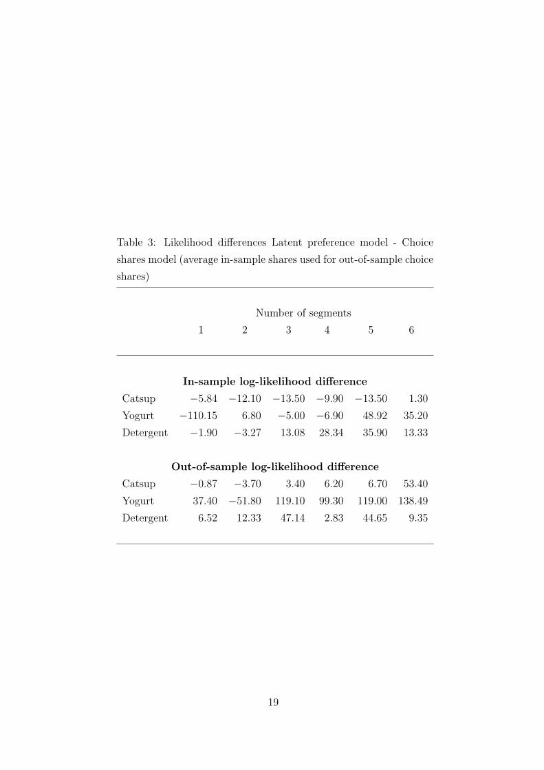
Table 3: Likelihood differences Latent preference model - Choice

shares model (average in-sample shares used for out-of-sample choice

shares)

Number of segments

1 2 3 4 5 6

In-sample log-likelihood difference

Catsup −5.84 −12.10 −13.50 −9.90 −13.50 1.30

Yogurt −110.15 6.80 −5.00 −6.90 48.92 35.20

Detergent −1.90 −3.27 13.08 28.34 35.90 13.33

Out-of-sample log-likelihood difference

Catsup −0.87 −3.70 3.40 6.20 6.70 53.40

Yogurt 37.40 −51.80 119.10 99.30 119.00 138.49

Detergent 6.52 12.33 47.14 2.83 44.65 9.35

19

Table 4: Performance measures for interpurchase time models with unobserved hetero-

geneity for the detergent category (largest likelihood value per number of segments in

boldface)

Number of segments

1 2 3 4 5 6

In-sample log L

Choice model -2335.37 -2213.76 -2133.46 -2085.64 -2046.62 -2016.14

Inclusive value -9012.75 -8680.78 -8582.07 -8522.32 -8452.02 -8423.58

Weighting hazard -9004.35 -8677.84 -8583.75 -8519.96 -8459.35 -8418.73

Weighting mark. mix -9004.11 -8677.62 -8596.64 -8513.10 -8449.39 -8421.50

Latent preferences -8998.17 -8673.07 -8578.36 -8516.65 -8443.07 -8410.93

Out-of-sample log L

choice model -2254.69 -2195.01 -2132.77 -2115.76 -2077.77 -2071.70

Inclusive value -8317.58 -8164.67 -8120.61 -8113.00 -8084.83 -8058.41

Weighting hazard -8312.68 -8154.85 -8124.28 -8097.82 -8073.05 -8063.59

Weighting mark. mix -8312.20 -8154.02 -8149.01 -8086.90 -8042.93 -8042.36

Latent preferences -8311.87 -8145.12 -8101.84 -8088.08 -8039.82 -8062.23

20

Table 5: Average ranks of model performance over three categories

(excluding choice shares specification)

1 2 3 4 5 6 overall

In-sample average rank

Inclusive value 4.00 3.33 2.33 3.00 2.67 4.00 3.22

Weighted hazard 2.67 3.33 3.33 3.33 3.33 2.67 3.11

Weighted mark. mix 2.33 2.33 3.00 2.00 2.67 2.33 2.44

Latent preferences 1.00 1.00 1.33 1.67 1.33 1.00 1.22

Out-of-sample average rank

Inclusive value 4.00 3.67 3.33 4.00 4.00 3.33 3.72

Weighted hazard 2.33 2.33 2.67 2.67 2.33 2.67 2.50

Weighted mark. mix 2.00 2.00 3.00 1.33 2.33 1.67 2.06

Latent preferences 1.67 2.00 1.00 2.00 1.00 2.33 1.67

21

References

Ailawadi, K. L. and S. A. Neslin (1998), The Effect of Promotion on Consumption: Buying

More and Consuming it Faster, Journal of Marketing Research, 35, 390–398.

Bell, D. R., J. Chiang, and V. Padmanabhan (1999), The Decomposition of Promotional

Response: An Empirical Generalization, Marketing Science, 18, 504–526.

Ben-Akiva, M. and S. R. Lerman (1985), Discrete Choice Analysis: Theory and Appli-

cation to Travel Demand , vol. 9 of MIT Press Series in Transportation Studies , MIT

Press, Cambridge (MA).

Bucklin, R. E. and S. Gupta (1992), Brand Choice, Purchase Incidence, and Segmentation:

An Integrated Approach, Journal of Marketing Research, 29, 201–215.

Chintagunta, P. K. and S. Haldar (1998), Investigating Purchase Timing Behavior in Two

Related Product Categories, Journal of Marketing Research, 35, 43–53.

Chintagunta, P. K. and A. R. Prasad (1998), An Empirical Investigation of the ”Dynamic

McFadden” Model of Purchase Timing and Brand Choice: Implications for Market

Structure, Journal of Business & Economic Statistics , 16, 2–12.

Doornik, J. A. (1999), Object-Oriented Matrix Programming Using Ox , 3rd edn., London:

Timberlake Consultants Press and Oxford: www.nuff.ox.ac.uk/Users/Doornik.

Franses, P. H. and R. Paap (2001), Quantitative Models in Marketing Research, Cam-

bridge University Press, Cambridge.

Gupta, S. (1988), Impact of Sales Promotions on When, What, and How Much to Buy,

Journal of Marketing Research, 25, 342–355.

Gupta, S. (1991), Stochastic Models of Interpurchase Time With Time-Dependent Co-

variates, Journal of Marketing Research, 28, 1–15.

Helsen, K. and D. C. Schmittlein (1993), Analyzing Duration Times in Marketing: Evi-

dence for the Effectiveness of Hazard Rate Models, Marketing Science, 11, 395–414.

Jain, D. C. and N. J. Vilcassim (1991), Investigating Household Purchase Timing Deci-

sions: A Conditional Hazard Function Approach, Marketing Science, 10, 1–23.

22

Kiefer, N. M. (1988), Economic Duration Data and Hazard Functions, Journal of Eco-

nomic Literature, 26, 646–679.

Seetharaman, P. B. and P. K. Chintagunta (2003), The Proportional Hazard Model for

Purchase Timing: A Comparison of Alternative Specifications, Journal of Business &

Economic Statistics , forthcoming.

Train, K. E. (2003), Discrete Choice Models with Simulation, Cambridge University Press,

Cambridge.

Vilcassim, N. J. and D. C. Jain (1991), Modeling Purchase-Timing and Brand-Switching

Behavior Incorporating Explanatory Variables and Unobserved Heterogeneity, Journal

of Marketing Research, 28, 29–41.

Wedel, M. and W. A. Kamakura (1999), Market Segmentation: Conceptual and Method-

ological Foundations , Kluwer Academic Publishers, Dordrecht.

23

Documents

Modeling category-level purchase timing with brand-level marketing variables