Embed Size (px)
Citation preview
Rare Category Analysis
Jingrui He
May 2010CMU-ML-10-XXX
Machine Learning DepartmentSchool of Computer ScienceCarnegie Mellon University
Pittsburgh, PA
Thesis Committee:Jaime Carbonell, CMU, Chair
John Lafferty, CMULarry Wasserman, CMU
Foster Provost, NYU
Submitted in partial fulfillment of the requirementsfor the degree of Doctor of Philosophy.
Copyright c© 2010 Jingrui He

Keywords: majority class, minority class, rare category, supervised, unsupervised, detection, character-ization, feature selection

To my parents, Fan He and Rongzhen Zhai.
AbstractIn many real world problems, rare categories (minority classes) play an essential role despite
of their extreme scarcity. For example, in financial fraud detection, the vast majority of thefinancial transactions are legitimate, and only a small number may be fraudulent; in Medicarefraud detection, the percentage of bogus claims is small, but the total loss is significant; innetwork intrusion detection, malicious network activities are hidden among huge volumes ofroutine network traffic; in astronomy, only 0.001% of the objects in sky survey images are trulybeyond the scope of current science and may lead to new discoveries; in spam image detection,the near-duplicate spam images are difficult to discover from the large number of non-spamimage; in rare disease diagnosis, the rare diseases affect less than 1 out of 2000 people, but theconsequences can be very severe. Therefore, the discovery, characterization and prediction ofrare categories or rare examples may protect us from fraudulent or malicious behaviors, providethe aid for scientific discoveries, and even save lives.
This thesis focuses on rare category analysis, where the majority classes have a smoothdistribution, and the minority classes exhibit a compactness property. Furthermore, we focuson the challenging cases where the support regions of the majority and minority classes overlapeach other. To the best of our knowledge, this thesis is the first systematic investigation of rarecategories.
Depending on the availability of the label information, we can perform either supervised orunsupervised rare category analysis. In the supervised settings, our first task is rare categorydetection, which is to discover at least one example from each minority class with the help ofa labeling oracle. Then given labeled examples from all the classes, our second task is rarecategory characterization. The goal here is to find a compact representation for the minorityclasses in order to identify all the rare examples. On the other hand, in the unsupervised settings,we do not have access to a labeling oracle. Here we propose to co-select candidate examplesfrom the minority classes and the relevant features, which benefits both tasks (rare categoryselection and feature selection). For each of the above tasks, we have developed effectivealgorithms with theoretical guarantees as well as good empirical results.
In the future, we plan to apply rare category analysis on rich data, such as medical images,texts / blogs, Electronic Health Records (EHR), web link graphs, stream data, etc; we planto build statistical models for the rare categories in order to understand how they emerge andevolve over time; we plan to study complex fraud based on rare category analysis; we plan tomake use of transfer learning to help with our analysis; we also plan to build a complete systemfor rare category analysis.

AcknowledgmentsLooking back upon the many years I spent in school, I feel greatly indebted to the numerous
people who have made me the person I am today.I would like to thank Jaime Carbonell for being my advisor. I could not have hoped for a
better advisor to guide me through my PhD studies. He is smart, professional, fun and knowseverything. Every time I came to him with a new idea, he was always able to sharpen mythoughts and point out possible directions which turned out to be very fruitful. I would like tothank Christos Faloutsos for being both a wise mentor and a great friend. He shared with me alot of his advices and experiences so that I would not take detours in my career. I would like tothank John Lafferty, Larry Wasserman, and Foster Provost for serving on my thesis committee.Their comments and suggestions really helped me improve my thesis work. And I would liketo thank Avrim Blum for invaluable and insightful discussions.
I would also like to thank all my collaborators during my internship. These include: Hong-Jiang Zhang, Mingjing Li, and Lei Li from Microsoft Research Asia, who set up a very highstandard for me at the beginning of my research life; Bo Thiesson from Microsoft Research,who constantly encouraged me to pursue one step further; Rick Lawrence and Yan Liu fromIBM Research, the discussions with whom really expanded my horizon.
During my undergraduate studies in Tsinghua University, I was greatly inspired by the fac-ulty in Automation Department, including Nanyuan Zhao, Changshui Zhang, Zongxia Liang,Yuanlie Lin, Yanda Li, Shi Yan, Mei Lu, to name a few. Their enthusiasm towards scienceand rigorous attitude towards research have a long impact on my own career. They deserve mydeepest appreciation.
I am also grateful to Yanxi Liu. She interviewed me 5 years ago and her nice commentsgot me into CMU, the best place for studying computer science. Diane Stidle, who is alwaysthere for the students. Whenever I have a problem, her name is the first one I can think of toask for help. Michelle Pagnani, who is always able to squeeze my meeting into Jaime’s busyschedule. And all my friends, including Zhenzhen Kou, Fan Guo, Lei Li, Rong Yan, XiaojingFu, Jin Peng, Xiaomeng Chang, and many more.
Special gratitude goes to my grandparents, whose warm smiles always blessed me; myparents, who have the strongest belief in me all the time; Hanghang Tong, who has been nothingbut a great husband; and my daughter Emma, who is the most naughty girl ever. Actually thisthesis is a gift to her for her upcoming one year’s birthday, though she could not understand asingle word at this time.
Contents
1 Introduction 11.1 Motivation . . . . . . . . . . . . . . . . . . . . . . . . . . . . . . . . . . . . . . . . . . . . 11.2 Problem Definition . . . . . . . . . . . . . . . . . . . . . . . . . . . . . . . . . . . . . . . 21.3 General Assumptions . . . . . . . . . . . . . . . . . . . . . . . . . . . . . . . . . . . . . . 21.4 Thesis Outline . . . . . . . . . . . . . . . . . . . . . . . . . . . . . . . . . . . . . . . . . . 3
1.4.1 Rare Category Detection . . . . . . . . . . . . . . . . . . . . . . . . . . . . . . . . 31.4.2 Rare Category Characterization . . . . . . . . . . . . . . . . . . . . . . . . . . . . 41.4.3 Unsupervised Rare Category Analysis . . . . . . . . . . . . . . . . . . . . . . . . . 5
1.5 Main Contributions . . . . . . . . . . . . . . . . . . . . . . . . . . . . . . . . . . . . . . . 51.6 General Notation . . . . . . . . . . . . . . . . . . . . . . . . . . . . . . . . . . . . . . . . 6
2 Survey and Overview 72.1 Active Learning . . . . . . . . . . . . . . . . . . . . . . . . . . . . . . . . . . . . . . . . . 72.2 Imbalanced Classification . . . . . . . . . . . . . . . . . . . . . . . . . . . . . . . . . . . . 82.3 Anomaly Detection (Outlier Detection) . . . . . . . . . . . . . . . . . . . . . . . . . . . . 82.4 Rare Category Detection . . . . . . . . . . . . . . . . . . . . . . . . . . . . . . . . . . . . 92.5 Unsupervised Feature Selection . . . . . . . . . . . . . . . . . . . . . . . . . . . . . . . . 92.6 Clustering . . . . . . . . . . . . . . . . . . . . . . . . . . . . . . . . . . . . . . . . . . . . 102.7 Co-clustering . . . . . . . . . . . . . . . . . . . . . . . . . . . . . . . . . . . . . . . . . . 10
3 Rare Category Detection 123.1 Rare Category Detection with Priors for Data with Features . . . . . . . . . . . . . . . . . . 12
3.1.1 Rare Category Detection for the Binary Cases . . . . . . . . . . . . . . . . . . . . . 133.1.2 Rare Category Detection for Multiple Classes . . . . . . . . . . . . . . . . . . . . . 163.1.3 Experimental Results . . . . . . . . . . . . . . . . . . . . . . . . . . . . . . . . . . 20
3.2 Prior-free Rare Category Detection for Data with Features . . . . . . . . . . . . . . . . . . 263.2.1 Semiparametric Density Estimation for Rare Category Detection . . . . . . . . . . . 263.2.2 Algorithm . . . . . . . . . . . . . . . . . . . . . . . . . . . . . . . . . . . . . . . . 323.2.3 Experimental Results . . . . . . . . . . . . . . . . . . . . . . . . . . . . . . . . . . 32
3.3 Rare Category Detection for Graph Data . . . . . . . . . . . . . . . . . . . . . . . . . . . . 383.3.1 GRADE Algorithm . . . . . . . . . . . . . . . . . . . . . . . . . . . . . . . . . . . 383.3.2 GRADE-LI Algorithm . . . . . . . . . . . . . . . . . . . . . . . . . . . . . . . . . 433.3.3 Experimental Results . . . . . . . . . . . . . . . . . . . . . . . . . . . . . . . . . . 443.3.4 Discussion . . . . . . . . . . . . . . . . . . . . . . . . . . . . . . . . . . . . . . . 50
3.4 Summary of Rare Category Detection . . . . . . . . . . . . . . . . . . . . . . . . . . . . . 51
vi
CONTENTS vii
4 Rare Category Characterization 534.1 Optimization Framework . . . . . . . . . . . . . . . . . . . . . . . . . . . . . . . . . . . . 54
4.1.1 Additional Notation . . . . . . . . . . . . . . . . . . . . . . . . . . . . . . . . . . 544.1.2 Assumptions . . . . . . . . . . . . . . . . . . . . . . . . . . . . . . . . . . . . . . 544.1.3 Pre-processing: Filtering . . . . . . . . . . . . . . . . . . . . . . . . . . . . . . . . 554.1.4 Problem Formulations . . . . . . . . . . . . . . . . . . . . . . . . . . . . . . . . . 55
4.2 Optimization Algorithm: RACH . . . . . . . . . . . . . . . . . . . . . . . . . . . . . . . . 574.2.1 Initialization Step . . . . . . . . . . . . . . . . . . . . . . . . . . . . . . . . . . . . 574.2.2 Projected Subgradient Method for Problem 4.3 . . . . . . . . . . . . . . . . . . . . 584.2.3 RACH for Problem 4.1 . . . . . . . . . . . . . . . . . . . . . . . . . . . . . . . . . 61
4.3 Kernelized RACH Algorithm . . . . . . . . . . . . . . . . . . . . . . . . . . . . . . . . . . 624.4 Experimental Results . . . . . . . . . . . . . . . . . . . . . . . . . . . . . . . . . . . . . . 62
4.4.1 Synthetic Data Set . . . . . . . . . . . . . . . . . . . . . . . . . . . . . . . . . . . 624.4.2 Real Data Sets . . . . . . . . . . . . . . . . . . . . . . . . . . . . . . . . . . . . . 64
4.5 Summary of Rare Category Characterization . . . . . . . . . . . . . . . . . . . . . . . . . . 72
5 Unsupervised Rare Category Analysis 735.1 Optimization Framework . . . . . . . . . . . . . . . . . . . . . . . . . . . . . . . . . . . . 73
5.1.1 Additional Notation . . . . . . . . . . . . . . . . . . . . . . . . . . . . . . . . . . 745.1.2 Objective Function . . . . . . . . . . . . . . . . . . . . . . . . . . . . . . . . . . . 745.1.3 Justification . . . . . . . . . . . . . . . . . . . . . . . . . . . . . . . . . . . . . . . 75
5.2 Partial Augmented Lagrangian Method . . . . . . . . . . . . . . . . . . . . . . . . . . . . . 765.3 Experimental Results . . . . . . . . . . . . . . . . . . . . . . . . . . . . . . . . . . . . . . 78
5.3.1 Synthetic Data Sets . . . . . . . . . . . . . . . . . . . . . . . . . . . . . . . . . . . 795.3.2 Real Data Sets . . . . . . . . . . . . . . . . . . . . . . . . . . . . . . . . . . . . . 83
5.4 Summary of Unsupervised Rare Category Analysis . . . . . . . . . . . . . . . . . . . . . . 92
6 Conclusion and Future Directions 94

Chapter 1
Introduction
Imbalanced data sets are prevalent in real applications, i.e., some classes occupy the majority of the data set,a.k.a., the majority classes; whereas the remaining classes only have a few examples, a.k.a., the minorityclasses or the rare categories. For example, in financial fraud detection, the vast majority of the finan-cial transactions are legitimate, and only a small number may be fraudulent [Bay et al., 2006]; in Medicarefraud detection, the percentage of bogus claims is small, but the total loss is significant; in network in-trusion detection, new malicious network activities are hidden among huge volumes of routine networktraffic [Wu et al., 2007][Vatturi & Wong, 2009]; in astronomy, only 0.001% of the objects in sky survey im-ages are truly beyond the scope of current science and may lead to new discoveries [Pelleg & Moore, 2004];in spam image detection, near-duplicate spam images are difficult to discover from the large number of non-spam images [Wang et al., 2007]; in health care, the rare diseases affect less than 1 out of 2000 people, butthe consequences are severe. Compared with the majority classes, the minority classes are often of muchgreater interest to the users. The main focus of my research is rare category analysis, which refers to theproblem of analyzing the minority classes in an imbalanced data set. In this thesis, we plan to address thisproblem from different perspectives.
1.1 Motivation
When dealing with highly imbalanced data sets, there are a number of challenges. For example, in financialfraud detection, we may want to discover new types of fraud transactions from a large number of unexaminedfinancial transactions with the help of a domain expert. In a more abstract way, given an imbalanced data set,our goal is to discover a few examples from the minority classes when we have access to a labeling oracle.Due to the extreme scarcity of the new types of fraud transactions compared with the normal transactions,simple methods such as random sampling would result in a huge number of label requests from the domainexpert, which can be very expensive. Therefore, to reduce the labeling cost, we need more effective methodsfor discovering the new types of fraud transactions. Take rare disease diagnosis as another example. Givena small number of patients with a specific rare disease, how can we characterize this rare disease basedon a subset of the medical measurements? With this characterization, we hope to better understand themechanism of this disease, distinguish it from other diseases for the best treatment, and identify potentialpatients with the same disease. The major challenge here is the insufficiency of label information, whichmight be alleviated by leveraging the information of health people as well as patients with similar diseases.Yet another example is in Medicare fraud detection. Due to the large number of medical claims submittedto the computer system for Medicare services, it is impossible for a domain expert to examine each of themand report suspicious ones. Therefore, an automated program that is able to detect complex fraud patternswith a high accuracy will greatly reduce the demand for human labor. The major challenge here is the lack
1
2 CHAPTER 1. INTRODUCTION
of label information, which might be compensated by studying the properties of know fraud patterns. All theabove challenges are associated with rare category analysis, where the main theme is to provide powerfultools for analyzing the rare categories in real applications.
1.2 Problem Definition
In rare category analysis, we are given an imbalanced data set, which is unlabeled initially. Dependingon the availability of the label information, rare category analysis can be performed in the supervised orunsupervised fashion.
In supervised rare category analysis, we have access to a labeling oracle, which is able to provide us withthe label information of any example with a fixed cost. In this case, rare category analysis can be dividedinto the following two tasks.
1. Rare category detection: in this task, we start from de-novo, and propose initial candidates of eachminority class to the labeling oracle (one candidate in each round) in an active learning fashion,hoping to find at least one example from each minority class with the least total label requests. Thistask serves as the initial exploration step of the data set, and generates a set of labeled examples fromeach class, which can be used in the second task.
2. Rare category characterization: in this task, we have labeled examples from each class (both major-ity and minority classes), which are obtained from the first task, as well as a set of unlabeled examplesas input. The goal is to find a compact representation for the minority classes in order to identify allthe rare examples. This task serves as the exploitation step of the data set, and constructs a reliableclassifier, which can be used to identify future unseen examples from the minority classes.
In unsupervised rare category analysis, we do not have such a labeling oracle, and the goal here is toaddress the following two problems.
1. Rare category selection: selecting a set of examples which are likely to come from the same minorityclasses;
2. Feature selection: selecting the features that are relevant to the minority classes.
1.3 General Assumptions
When dealing with examples with feature representations, we make the following general assumptionsthroughout this thesis.
1. Smoothness assumption: the underlying distribution of each majority class is sufficiently smooth.
2. Compactness (clustering) assumption: the examples from the same minority class form a compactcluster in the feature space or feature subspace;
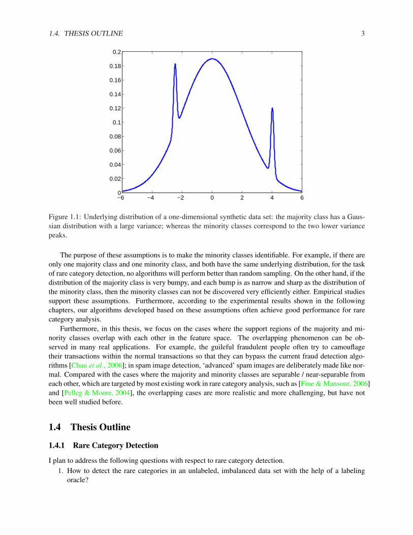
An example of the underlying distribution where these assumptions are satisfied is shown in Fig. 1.1. Itshows the underlying distribution of a one-dimensional synthetic data set. The majority class has a Gaussiandistribution with a large variance; whereas the minority classes correspond to the two lower variance peaks.
1.4. THESIS OUTLINE 3
−6 −4 −2 0 2 4 60
0.02
0.04
0.06
0.08
0.1
0.12
0.14
0.16
0.18
0.2
Figure 1.1: Underlying distribution of a one-dimensional synthetic data set: the majority class has a Gaus-sian distribution with a large variance; whereas the minority classes correspond to the two lower variancepeaks.
The purpose of these assumptions is to make the minority classes identifiable. For example, if there areonly one majority class and one minority class, and both have the same underlying distribution, for the taskof rare category detection, no algorithms will perform better than random sampling. On the other hand, if thedistribution of the majority class is very bumpy, and each bump is as narrow and sharp as the distribution ofthe minority class, then the minority classes can not be discovered very efficiently either. Empirical studiessupport these assumptions. Furthermore, according to the experimental results shown in the followingchapters, our algorithms developed based on these assumptions often achieve good performance for rarecategory analysis.
Furthermore, in this thesis, we focus on the cases where the support regions of the majority and mi-nority classes overlap with each other in the feature space. The overlapping phenomenon can be ob-served in many real applications. For example, the guileful fraudulent people often try to camouflagetheir transactions within the normal transactions so that they can bypass the current fraud detection algo-rithms [Chau et al., 2006]; in spam image detection, ‘advanced’ spam images are deliberately made like nor-mal. Compared with the cases where the majority and minority classes are separable / near-separable fromeach other, which are targeted by most existing work in rare category analysis, such as [Fine & Mansour, 2006]and [Pelleg & Moore, 2004], the overlapping cases are more realistic and more challenging, but have notbeen well studied before.
1.4 Thesis Outline
1.4.1 Rare Category Detection
I plan to address the following questions with respect to rare category detection.1. How to detect the rare categories in an unlabeled, imbalanced data set with the help of a labeling
oracle?
4 CHAPTER 1. INTRODUCTION
2. How to detect the rare categories for graph data, or relational data?
3. How to do rare category detection with the least prior information about the data set?The first question is fundamental in rare category detection. Given an unlabeled, imbalanced data set,
a naive way for finding examples from the minority classes is to randomly select examples from the dataset to be labeled by the oracle until we have identified at least one example from each minority class. Amajor drawback of this random sampling strategy is the following. If a minority class is extremely rare, sayits proportion in the data set is only 0.001%, in order to discover this minority class, the number of labelrequests by random sampling would be very large. Therefore, we need more effective methods to addressthe rare category detection challenge.
The second question is similar to the first one except that here we are interested in graph data (relationaldata) instead of data points with feature representations. Since graph data is very common in real applica-tions, how to adapt the rare category detection algorithms for data points with feature representations to thisdata type is of key importance.
The third question aims at doing rare category detection with less prior information about the data set,and the ultimate goal is prior-free rare category detection, i.e., the algorithm is given no prior informationabout the data set, such as the number of classes, the proportions of different classes, etc. This questionis more difficult than the first two, and yet quite important, since in real applications, given an unlabeleddata set, it is sometimes difficult to estimate the number of classes in the data set a prior, not to mention theproportions of different classes.
Although both Rare category detection and traditional active learning proceed by actively selecting ex-amples to be labeled by an oracle, they are different in the following two aspects. First, in rare categorydetection, initially we do not have any labeled examples; whereas in traditional active learning, initially wehave labeled examples from all the classes as input. Second, in rare category detection, our goal is to dis-cover at least one example from each minority class with the least label requests from the oracle; whereas intraditional active learning, the goal is to improve the performance of the current classifier with the least labelrequests from the oracle. Furthermore, rare category detection is a bottleneck in reducing the overall sam-pling complexity of active learning [Balcan et al., 2006, Dasgupta, 2005]. That is, the sampling complexityof many active learning algorithms are dominated by the initial stage of finding at least one example fromeach class, especially the minority classes. Therefore, effective rare category detection algorithms couldhelp reduce the sampling complexity of active learning by a large margin.
The major difference between rare category detection and outlier detection is the following. In rarecategory detection, the examples from the same minority class are often self-similar, potentially formingcompact clusters in the feature space; and we assume that the support regions of the majority and minorityclasses are NOT separable from each other, which is more challenging than the separable cases. On the otherhand, in anomaly detection (outlier detection), each anomaly (outlier) is a single data point; the anomalies(outliers) are typically scattered in the feature space; and the anomalies (outliers) are often separable fromthe normal points.
1.4.2 Rare Category Characterization
Rare category characterization follows rare category detection. Given labeled examples from all the classesas input, the goal is to identify all the rare examples from the know minority classes. Here, our question is:how to characterize the minority classes with a compact representation?
Rare category characterization is of key importance in many applications, such as text retrieval wherethe number of documents relevant to a particular query is very small, and the goal is to retrieve all of themon the top of the ranked list returned to the user.

1.5. MAIN CONTRIBUTIONS 5
Rare category characterization bears similarity but also fundamental differences with imbalanced clas-sification. In both tasks, the data set is imbalanced, and we have labeled training examples from eachclass. However, in imbalanced classification, the goal is to construct a classifier that optimizes a dis-criminative criterion for both the majority and the minority classes, such as balanced accuracy, G-mean,etc [Chawla, 2009]; whereas in rare category characterization, we only focus on the minority classes, andaim to identify all (or nearly all) the rare examples from the unlabeled data set. On the other hand, in rarecategory characterization, our algorithm is based on the clustering property of the minority classes; whereasin imbalanced classification, such property is not exploited.
1.4.3 Unsupervised Rare Category Analysis
In unsupervised rare category analysis, we do not have access to any labeling oracle. Under certain as-sumptions, we can perform both rare category selection, which is to select a set of examples that are likelyto come from the minority classes, and feature selection, which is to select a set of feature relevant to theminority classes.
Rare category selection is similar to rare category detection in that both start de-novo, i.e., no labelinformation is available at the beginning. However, in rare category detection, the labeling oracle gives thelabel information of the candidate example selected in each round, and the learning algorithm can adjust itsmodel based on this information and propose new candidates, hoping to find at least one example from eachminority class with only a few label requests; whereas in rare category selection, no label information isavailable during the training stage, and the goal is to select a set of examples which are likely to come fromthe minority classes.
In many imbalanced data sets, the examples from the same minority class are close to each other in somedimensions, and far apart in others. For example, in financial fraud detection, small-amount-probing typeof fraud transactions are similar to each other in terms of the small amount being stolen in each transaction;however, different transactions may occur in different locations, at different time, etc. Therefore, to betterdescribe the minority classes, we need to identify the relevant features.
Notice that existing co-clustering algorithms would fail in our settings due to the following two reasons.First, we are dealing with the cases where the majority and minority classes overlap in the feature space;whereas existing co-clustering algorithms mainly work in the separable / near-separable cases. Second, inour applications, we hope to find the features relevant to the minority classes; whereas existing co-clusteringalgorithms would simply ignore the rare examples due to their scarcity, and the selected features would berelevant to the majority classes only.
1.5 Main Contributions
To the best of our knowledge, this thesis is the first systematic investigation of rare categories in imbalanceddata sets. To be specific, our main contributions can be summarized below.
1. We distill different tasks in rare category analysis, namely rare category detection and rare categorycharacterization in the supervised settings; rare category selection and feature selection in the unsu-pervised settings.
2. For rare category detection, we develop different algorithms for data with feature representations andgraph data, given full prior information, partial prior information, or even no prior information. Foreach of the proposed algorithms, we provide theoretical justification as well as empirical evaluations,showing the superiority of these algorithms over existing ones.
3. For rare category characterization, we propose an optimization problem which captures the idea of the

6 CHAPTER 1. INTRODUCTION
minimum-radius hyper-ball for the minority classes. Then we develop an effective algorithm to findits solution based on projected subgradient method. Experimental results show that its performance isbetter than state-of-the-art techniques.
4. For unsupervised rare category analysis, we propose to co-select the rare examples and the relevantfeatures of the minority classes, which benefits both tasks. To this end, we design an optimizationframework, which is well justified theoretically, and an optimization algorithm based on augmentedLagrangian method. The performance of this algorithm is evaluated by extensive experiments.
1.6 General Notation
Given a set of n unlabeled examples S = {x1, . . . , xn}, xi ∈ Rd, which come from m distinct classes,i.e., yi ∈ {1, . . . , m}. Without loss of generality, assume that
∑ni=1 xi = ~0 and 1
n
∑ni=1(x
ji )
2 = 1, wherexj
i is the jth feature of xi. For the sake of simplicity, assume that there is one majority class with prior p1,which corresponds to yi = 1, and all the other classes are minority classes with priors p2, . . . , pm, p1 À pc,c 6= 1. Notice that in real applications, we may have multiple majority classes. If all of them satisfy thesmoothness assumption introduced in Section 1.3, they can be seen as a single class for the purpose of rarecategory analysis. This is because if a certain example is from one of the majority classes, we do not carewhich majority class it comes from.
Let fc denote the probability density function (pdf) of class c, where c = 1, . . . , m. Based on ourdiscussion in Section 1.3, f1 for the majority class should satisfy the smoothness assumption; whereas fc,c = 2, . . . ,m for the minority classes should satisfy the compactness assumption.
Table 1.1 summarizes the general notation used in this thesis.
Table 1.1: NotationSymbol Definition
S The set of unlabeled examplesn The number of examples in S
m The number of classes in S
xi The ith unlabeled examplexj
i The jth feature of xi
d The dimensionality of the feature spaceyi The class label of xi
fc The probability density function of class c, c = 1, . . . , m
Other more specific notation will be introduced where needed.

Chapter 2
Survey and Overview
In this chapter, we review related work in the following directions, including active learning, imbalancedclassification, anomaly detection (outlier detection), rare category detection, unsupervised feature selection,clustering, and co-clustering.
2.1 Active Learning
The key idea behind active learning is that a machine learning algorithm can achieve greater accuracy withfewer training labels if it is allowed to choose the data from which it learns [Settles, 2010]. In active learning,we assume that the class labels are obtained from a labeling oracle with some cost, and under a fixed budget,we hope to maximally improve the performance of the learning algorithm. According to [Settles, 2010],there are three main settings in active learning: membership query synthesis, stream-based selective sam-pling, and pool-based sampling.
Many early active learning algorithms belong to membership query synthesis, such as [Angluin, 1987][Angluin, 2001] [Cohn et al., 1996]. One major problem with membership query synthesis is that the syn-thesized queries often have no practical meanings, and thus no appropriate labels. On the other hand, withstream-based active learning and pool-based sampling, the queries always correspond to real examples.Therefore, their label information can be readily provided by the oracle.
In stream-based selective sampling, given an unlabeled example, the learner must decide whether toquery its class label or to discard it. For example, in [Cohn et al., 1992], Cohn et al compute region of uncer-tainty, and query examples within in; in [Dagan & Engelson, 1995], Dagan et al proposed committee-basedsampling, which evaluates the informativeness of an example by measuring the degree of disagreementbetween several model variants and only queries the more informative ones.
On the other hand, in pool-based sampling, queries are selected from a pool of unlabeled examples. Itsmajor difference from stream-based selective sampling is the large amount of unlabeled data available atquery time, which reveals additional information about the underlying distribution. For example, Tong etal [Tong et al., 2001] proposed an active learning algorithm that minimizes the size of the version space; Mc-callum [Mccallum, 1998] modified the Query-by-Committee method of active learning to use the unlabeleddata for density estimation, and combined with EM to find the class labels of the unlabeled examples.
It should be mentioned that in traditional active learning, initially we have labeled examples from allthe classes in order to build the very first classifier, which can be improved by actively selecting the trainingdata. On the other hand, in rare category detection, initially we do not have any labeled examples, andthe goal is to discover at least one example from each minority class with the least label requests. Com-bining rare category detection and traditional active learning, it has been noticed in [Balcan et al., 2006]
7
8 CHAPTER 2. SURVEY AND OVERVIEW
and [Dasgupta, 2005] that if the learning algorithm starts de-novo, finding the initial labeled examples fromeach class (i.e., rare category detection) becomes the bottleneck for reducing the sampling complexity. Fur-thermore, in supervised rare category analysis, following rare category detection, the second task is rarecategory characterization, which works in a semi-supervised fashion. In this task, in order to get a moreaccurate representation of the minority classes, we can make use of active learning to select the most infor-mative examples to be added to the labeled set.
2.2 Imbalanced Classification
In imbalanced classification, the goal is to construct an accurate classifier that optimizes a discriminativecriterion, such as balanced accuracy, G-mean, etc [Chawla, 2009]. Existing methods can be roughly catego-rized into 3 groups [Chawla, 2009], i.e., sampling-based methods [Kubat & Matwin, 1997][Chawla et al., 2002],adapting learning algorithms by modifying objective functions or changing decision thresholds [Wu & Chang, 2003][Huang et al., 2004], and ensemble based methods [Sun et al., 2006][Chawla et al., 2003]. To be specific,in sampling-based methods, some methods under-sample the majority classes. For example, the one-sidedsampling strategy proposed in [Kubat & Matwin, 1997] employs Tomek links [Tomek, 1976] followed byclosest nearest neighbor [HART, 1968] to discard the majority class examples that lie in the borderline re-gion, are noisy or redundant. In contrast, some sampling-based methods over-sample the hard examples.For example, the DataBoost-IM method proposed in [Guo & Viktor, 2004] generates synthetic examplesaccording to the hard examples identified during the boosting algorithm; the SMOTEBoost algorithm pro-posed in [Chawla et al., 2003] applies the SMOTE algorithm [Chawla et al., 2002] to create new examplesfrom the minority class in each boosting round. Furthermore, some methods combine over-sampling theminority class and under-sampling the majority class. For example, the SMOTE algorithm combined withunder-sampling [Chawla et al., 2002] was proven to outperform only under-sampling the majority class andvarying the loss ratios; in [Tang et al., 2009], different rebalance heuristics were incorporated into SVMmodeling to tackle the problem of class imbalance, including over-sampling, under-sampling, etc.
Imbalanced classification and rare category characterization bear similarity but also fundamental dif-ference. On one hand, both tasks need labeled examples from all the classes as input. On the other hand,imbalanced classification and rare category characterization have different goals as well as different method-ology. To be specific, in rare category characterization, the goal is to find a compact representation for theminority classes in order to identify all the rare examples, and our algorithm for rare category characteri-zation is based on the clustering property of the minority classes; whereas in imbalanced classification, thegoal is to construct a classifier that optimizes a discriminative criterion, and the clustering property of theminority classes is not exploited.
2.3 Anomaly Detection (Outlier Detection)
Anomaly detection refers to the problem of finding patterns in data that do not conform to expected behav-ior [Chandola et al., 2009]. Anomalies are often referred to as outliers. According to [Chandola et al., 2009],the majority of anomaly detection techniques can be categorized into classification based, nearest neighborbased, clustering based, information theoretic, spectral, and statistical techniques. For example, in [Barbara et al., 2001],the authors propose a method based on a technique called pseudo-Bayes estimators to enhance an anomalydetection systems’s ability to detect new attacks while reducing the false alarm rate as much as possi-ble. In [Ramaswamy et al., 2000], the authors propose a novel formulation for distance-based outliers thatis based on the distance of a point from its kth nearest neighbor. Then they rank each point on the ba-sis of its distance to its kth nearest neighbor and declare the top n points in this ranking to be outliers.
2.4. RARE CATEGORY DETECTION 9
In [Yu et al., 2002], the authors propose the FindOut algorithm, which is an extension of the WaveClusteralgorithm [Sheikholeslami et al., 1998] in which the detected clusters are removed from the data and theresidual instances are declared as nomalies. [He et al., 2005b], the authors formally define the problem ofoutlier detection in categorical data as an optimization problem from a global viewpoint, and present a local-search heuristic based algorithm for efficiently finding feasible solutions. In [Dutta et al., 2007], the authorsdescribe distributed algorithms for doing Principal Component Analysis (PCA) using random projectionand sampling based techniques. Using the approximate principal components, they develop a distributedoutlier detection algorithm based on the fact that the last principal component enables identification of datapoints which deviate sharply from the ‘correlation structure’ of the data. And in [Aggarwal & Yu, 2001],the authors discuss a new technique for outlier detection which is especially suited to very high dimensionaldata sets. The method works by finding lower dimensional projections which are locally sparse, and cannotbe discovered easily by brute force techniques because of the number of combinations of possibilities.
In general, anomaly detection finds individual and isolated examples that differ from a given class inan unsupervised fashion. Typically, there is no way to characterize the anomalies since they are oftendifferent from each other. There exist a few works dealing with the case where the anomalies are clus-tered [Papadimitriou et al., 2003]. However, they still assume that the anomalies are separable from thenormal data points. On the other hand, in rare category detection, each rare category consists of a group ofpoints, which form a compact cluster in the feature space and are self-similar. Furthermore, we are dealingwith the challenging cases where the support regions of the majority and minority classes overlap with eachother.
2.4 Rare Category Detection
Here, the goal is to find at least one example from each minority class with the help of a labeling oracle,minimizing the number of label requests. Up till now, researchers have developed several methods forrare category detection. For example, in [Pelleg & Moore, 2004], the authors assumed a mixture modelto fit the data, and experimented with different hint selection methods, of which Interleaving performs thebest; in [Fine & Mansour, 2006], the authors studied functions with multiple output values, and used activesampling to identify an example for each of the possible output values; in [Dasgupta & Hsu, 2008], theauthors presented an active learning scheme that exploits cluster structure in the data, which was proven tobe effective in rare category detection; and in [Vatturi & Wong, 2009], the authors proposed a new approachto rare category detection based on hierarchical mean shift, where a hierarchy is created by repeatedlyapplying mean shift with an increasing bandwidth on the data. Different from most existing work on rarecategory detection, which assume that the majority and minority classes are separable / near-separable fromeach other in the feature space, in Chapter 3 of this thesis, we target the more challenging cases where thesupport regions of different classes are not separable. Furthermore, besides empirical evaluations of theproposed algorithms, we also proved their effectiveness theoretically; whereas most existing algorithms donot have such guarantees.
2.5 Unsupervised Feature Selection
Generally speaking, existing feature selection methods in the unsupervised settings can be categorized aswrapper models and filter models. The wrapper models evaluate feature subsets based on the clusteringresults, such as the FSSEM algorithm [Dy & Brodley, 2000], the mixture-based approach which extendsto the unsupervised context the mutual-information based criterion [Law et al., 2002], and the ELSA algo-rithm [Kim et al., 2000]. The filter models are independent of the clustering algorithm, such as the feature

10 CHAPTER 2. SURVEY AND OVERVIEW
selection algorithm based on maximum information compression index [Mitra et al., 2002], the feature se-lection method using distance-based entropy [Dash et al., 2002], and the feature selection method based onLaplacian score [He et al., 2005a].
In unsupervised rare category analysis, one of the problems we want to address is feature selection,i.e., selecting a set of features relevant to the minority classes. In our settings, since the class proportionsare extremely skewed, the general-purpose wrapper and filter methods would fail by selecting the featuresprimarily relevant to the majority classes. Therefore, we need new feature selection methods that are tailoredfor rare category analysis.
2.6 Clustering
According to [Glenn & Fung, 2001], clustering refers to the grouping together of similar data items intoclusters. Existing clustering algorithms can be categorized into the following 2 main classes [Glenn & Fung, 2001]:parametric clustering and non-parametric clustering. In general, parametric methods attempt to minimize acost function or an optimality criterion which associates a cost to each example-cluster assignment. It canbe further classified into 2 groups: generative models and reconstructive models. In generative models, thebasic idea is that the input examples are observations from a set of unknown distributions. For example, inGaussian mixture models [Reynolds & Rose, 1995], the data are viewed as coming from a mixture of proba-bility Gaussian distribution, each representing a different cluster; in C-means fuzzy clustering [Dunn, 1973],the membership of a point is shared among various clusters. On the other hand, reconstructive methods gen-erally attempt to minimize a cost function. For example, K-means clustering forms clusters in numericdomains, partitioning examples into disjoint clusters [Duda et al., 2000]; in Deterministic Annealing EMAlgorithm (DAEM) [Hofmann & Buhmann, 1997], the maximization of the likelihood function is embed-ded in the minimization of the thermodynamic free energy, depending on the temperature which controlsthe annealing process. For nonparametric methods, two good representative examples are the agglomerativeand divisive algorithms, also called hierarchical algorithms [Johnson, 1967], that produce dendrogram.
In unsupervised rare category analysis, another important problem we want to address is rare categoryselection, i.e., selecting a set of examples which are likely to come from the minority classes. General-purpose clustering algorithms do not fit here because the proportions of different classes are extremelyskewed and the support regions of the majority and minority classes overlap with each other. In this case,general-purpose clustering algorithms tend to overlook the minority classes and generate clusters within themajority classes. Therefore, we need to develop new methods for rare category selection which leverage theproperty of the minority classes.
2.7 Co-clustering
The idea of using compression for clustering can be traced back to the information-theoretic co-clusteringalgorithm [Dhillon et al., 2003], where the normalized non-negative contingency table is treated as a jointprobability distribution between two discrete random variables that take values over the rows and columns.Then co-clustering is defined as a pair of mappings from rows to row clusters and from columns to columnclusters. According to information theory, the optimal co-clustering is the one that minimizes the differencein mutual information between the original random variables and the mutual information between the clus-tered random variables. The algorithm for minimizing the above criterion intertwines both row and columnclustering at all stages. Row clustering is done by assessing closeness of each row distribution, in relativeentropy, to certain ‘row cluster prototypes’. Column clustering is done similarly, and this process is iterateduntil it converges to a local minimum. It can be theoretically proved that the proposed algorithm never

2.7. CO-CLUSTERING 11
increases the criterion, and gradually improves the quality of co-clustering.Although the information-theoretic co-clustering algorithm can only be applied to bipartite graphs, the
idea behind this algorithm can be generalized to more than two types of heterogeneous objects. For example,in [Gao et al., 2007], the authors proposed the CBGC algorithm. It aims to do collective clustering for star-shaped inter-relationships among different types of objects. First, it transforms the star-shaped structureinto a set of bipartite graphs; then it formulates a constrained optimization problem, where the objectivefunction is a weighted sum of the Rayleigh quotients on different bipartite graphs, and the constraints arethat clustering results for the same type of objects should be the same. Follow-up work includes the highorder co-clustering [Greco et al., 2007]. Another example is the spectral relational clustering algorithmproposed in [Long et al., 2006]. Unlike the previous algorithm, this algorithm is not restricted to star-shapedstructures. It is based on a general model, the collective factorization on related matrices. This modelclusters multi-type interrelated objects simultaneously based on both the relation and the feature information.It exploits the interactions between the hidden structures of different types of objects through the relatedfactorizations which share matrix factors, i.e., cluster indicator matrices. The resulting spectral relationalclustering algorithm iteratively updates the cluster indicator matrices using the leading eigenvectors of aspecially designed matrix until convergence. More recently, the collective matrix factorization proposedby Singh et al. [Singh & Gordon, 2008a] [Singh & Gordon, 2008b] can also be used for clustering k-partitegraphs.
Other related work includes (1) GraphScope [Sun et al., 2007], which uses a similar information-theoreticcriterion as cross association for time-evolving graphs to segment time into homogeneous intervals; and (2)multi-way distributional clustering (MDC) [Bekkerman et al., 2005] which is demonstrated to outperformthe previous information-theoretic clustering algorithms by the time the algorithm was proposed.
At the first glance, one may apply co-clustering algorithms to simultaneously address the problem of rarecategory selection and feature selection. The problem here is similar to the one mentioned in Section 2.6.That is, due to the extreme skewness of the class proportions and the overlapping support regions, general-purpose co-clustering algorithms may not be able to correctly identify the few rare examples or the featuresrelevant to the rare categories; whereas our proposed algorithm for co-selecting the rare examples and therelevant features addresses this problem by making use of the clustering property of the minority classes.
Chapter 3
Rare Category Detection
In this chapter, we focus on rare category detection, the first task in the supervised settings. In this task,we are given an unlabeled, imbalanced data set, which is often non-separable, and have access to a labelingoracle, which is able to give us the class label of any example with a fixed cost. The goal here is to discoveran least one example from each minority class with the least label requests.
The main contributions of this chapter can be summarized as follows.
Algorithms with Theoretical Guarantees. To the best of our knowledge, we propose the first rarecategory detection algorithms with theoretical guarantees;
Algorithms for Different Data Types. For data with feature representations and graph data (rela-tional data), we propose different algorithms that exploit their specific properties. These algorithmswork with different amount of prior information.
The rest of this chapter is organized as follows. In Section 3.1, we introduce the detection algorithmswith prior information for data with feature representation. The prior-free algorithm is introduced in Sec-tion 3.2. Then in Section 3.3, we present our detection algorithms for graph data, or relational data, givenfull prior information or partial prior information. Finally, in Section 3.4, we give a brief summary of rarecategory detection.
3.1 Rare Category Detection with Priors for Data with Features
In this section, we propose prior-dependent algorithms for rare category detection in the context of activelearning, which are designed for data with feature representations. We typically start de-novo, no categorylabels, though our algorithms make no such assumption. Different from existing methods, we aim to solvethe difficult cases, i.e., we do not assume separability or near-separability of the classes. Intuitively, ouralgorithms make use of nearest neighbors to measure local density around each example. In each iteration,the algorithms select an example with the maximum change in local density on a certain scale, and asksthe oracle for its label. The algorithms stop once they have found at least one example from each class(given the knowledge of the number of classes). When the two assumptions in Section 1.3 are satisfied, theproposed algorithms will select examples both on the boundary and in the interior of the minority classes,and are proven to be effective theoretically. Experimental results on both synthetic and real data sets showthe superiority of our algorithms over existing methods.
The rest of the section is organized as follows. In Subsection 3.1.1, we introduce our algorithm for thebinary cases and provide theoretical justification. In Subsection 3.1.2, we discuss about the more generalcases where there are more than one minority classes in the data set. Finally, Subsection 3.1.3 provides someexperimental results demonstrating the effectiveness of the proposed algorithms.
12

3.1. RARE CATEGORY DETECTION WITH PRIORS FOR DATA WITH FEATURES 13
3.1.1 Rare Category Detection for the Binary Cases
Algorithm
First let us focus on the simplest case where m = 2. Therefore, p1 = 1− p2, and p2 ¿ 1. Here, we assumethat we have an estimate of the value of p2 a priori. Next, we introduce our algorithm for rare categorydetection based on nearest neighbors, which is presented in Alg. 1. The basic idea is to find maximumchanges in local density, which might indicate the location of a rare category.
The algorithm works as follows. Given the unlabeled set S and the prior of the minority class p2, wefirst estimate the number K of minority class examples in S. Then, for each example, we record its distancefrom the K th nearest neighbor, which could be realized by kd-trees [Moore, 1991]. The minimum distanceover all the examples is assigned to r′. Next, we draw a hyper-ball centered at each example with radiusr′, and count the number of examples enclosed by this hyper-ball, which is denoted as ni. ni is roughly inproportion to the local density. To measure the change of local density around a certain point xi, in eachiteration of Step 3, we subtract nk of neighboring points from ni, and let the maximum value be the scoreof xi. The example with the maximum score is selected for labeling by the oracle. If the example is fromthe minority class, stop the iteration; otherwise, enlarge the neighborhood where the scores of the examplesare re-calculated and continue.
Before giving the theoretical justification, here, we give an intuitive explanation of why the algorithmworks. Assume that the minority class is concentrated in a small region and the probability density function(pdf) of the majority class is locally smooth. Firstly, since the support region of the minority class is verysmall, it is important to find its scale. The r′ value obtained in Step 1 will be used to calculate the localdensity ni. Since r′ is based on the minimum K th nearest neighbor distance, it is never too large to smoothout changes of local density, and thus it is a good measure of the scale. Secondly, the score of a certain point,corresponding to the change in local density, is the maximum of the difference in local density between thispoint and all of its neighboring points. In this way, we are not only able to select points on the boundary of theminority class, but also points in the interior, given that the region is small. Finally, by gradually enlargingthe neighborhood where the scores are calculated, we can further explore the interior of the support region,and increase our chance of finding a minority class example.
Algorithm 1 Nearest-Neighbor-Based Rare Category Detection for the Binary Case (NNDB)Input: S, p2
1: Let K = np2. For each example, calculate the distance to its K th nearest neighbor. Set r′ to be theminimum value among all the examples.
2: ∀xi ∈ S, let NN(xi, r′) = {x|x ∈ S, ‖x− xi‖ ≤ r′}, and ni = |NN(xi, r
′)|.3: for t = 1 : n do4: ∀xi ∈ S, if xi has not been selected, then si = max
xk∈NN(xi,tr′)(ni − nk); otherwise, si = −∞.
5: Query x = arg maxxi∈S si.6: If the label of x is 2, break.7: end for
Justification
Next we prove that if the minority class is concentrated in a small region and the pdf of the majority class islocally smooth, the proposed algorithm will repeatedly sample in the region where the rare examples occurwith a high probability.
First of all, we make the following specific assumptions.Assumptions

14 CHAPTER 3. RARE CATEGORY DETECTION
1. f2(x) is uniform within a hyper-ball B of radius r centered at b, i.e., f2(x) = 1V (r) , if x ∈ B; and 0
otherwise, where V (r) ∝ rd is the volume of B.
2. f1(x) is bounded and positive in B1, i.e., f1(x) ≥ κ1p2
(1−p2)V (r) , ∀x ∈ B and f1(x) ≤ κ2p2
(1−p2)V (r) ,∀x ∈ Rd, where κ1, κ2 > 0 are two constants.
With the above assumptions, we have the following lemma and theorem. Note that variants of thefollowing proof apply if we assume a different minority class distribution, such as a tight Gaussian.Lemma 1. ∀ε, δ > 0, if n ≥ max{ 1
2κ21p2
2log 3
δ , 12(1−2−d)2p2
2log 3
δ , 1ε4V (
r22
)4log 3
δ}, where r2 = r
(1+κ2)1d
, and
V ( r22 ) is the volume of a hyper-ball with radius r2
2 , then with probability at least 1 − δ, r22 ≤ r′ ≤ r and
|nin − E(ni
n )| ≤ εV (r′), 1 ≤ i ≤ n, where V (r′) is the volume of a hyper-ball with radius r′.
Proof. First, notice that the expected proportion of points falling inside B, E( |NN(b,r)|n ) ≥ (κ1 + 1)p2, and
that the maximum expected proportion of points falling inside any hyper-ball of radius r22 , max
x∈Rd[E( |NN(x,
r22
)|n )] ≤
2−dp2. Then
Pr[r′ > r or r′ <r2
2or ∃xi ∈ S s.t., |ni
n− E(
ni
n)| > εV (r′)]
≤ Pr[r′ > r] + Pr[r′ <r2
2] + Pr[r′ ≥ r2
2and ∃xi ∈ S s.t., |ni
n−E(
ni
n)| > εV (r′)]
≤ Pr[|NN(b, r)| < K] + Pr[maxx∈Rd
|NN(x,r2
2)| > K] + nPr[|ni
n− E(
ni
n)| > εV (r′)|r′ ≥ r2
2]
= Pr[|NN(b, r)n
| < p2] + Pr[maxx∈Rd
|NN(x, r22 )
n| > p2] + nPr[|ni
n− E(
ni
n)| > εV (r′)|r′ ≥ r2
2]
≤ e−2nκ21p2
2 + e−2n(1−2−d)2p22 + 2ne−2nε2V (r′)2
where the last inequality is based on Hoeffding bound.Let e−2nκ2
1p22 ≤ δ
3 , e−2n(1−2−d)2p22 ≤ δ
3 and 2ne−2nε2V (r′) ≤ 2ne−2nε2V (r22
)2 ≤ δ3 , we obtain n ≥
12κ2
1p22log 3
δ , n ≥ 12(1−2−d)2p2
2log 3
δ , and n ≥ 1ε4V (
r22
)4log 3
δ .
Based on Lemma 1, we get the following theorem, which shows the effectiveness of the proposedalgorithm.Theorem 1. If
1. Let B2 be the hyper-ball centered at b with radius 2r. The minimum distance between the points insideB and the ones outside B2 is not too large, i.e., min{‖xi−xk‖|xi, xk ∈ S, ‖xi− b‖ ≤ r, ‖xk− b‖ >2r} ≤ α, where α is a positive parameter.
2. f1(x) is locally smooth, i.e., ∀x, y ∈ Rd, |f1(x) − f1(y)| ≤ β‖x−y‖α , where β ≤ p2
2OV (r22
,r)
2d+1V (r)2and
OV ( r22 , r) is the volume of the overlapping region of two hyper-balls: one is of radius r, the other
one is of radius r22 , and its center is on the sphere of the bigger one.
3. The number of examples is sufficiently large,i.e., n ≥ max{ 1
2κ21p2
2log 3
δ , 12(1−2−d)2p2
2log 3
δ , 1(1−p2)4β4V (
r22
)4log 3
δ}.
then with probability at least 1 − δ, after d2αr2e iterations, NNDB will query at least one example whose
probability of coming from the minority class is at least 13 , and it will continue querying such examples until
the b( 2d
p2(1−p2) − 2) · αr cth iteration.
1Notice that here we are only dealing with the hard case where f1(x) is positive within B. In the separable case where thesupport regions of the two classes do not overlap, we can use other methods to detect the minority class, such as the one proposedin [Pelleg & Moore, 2004].

3.1. RARE CATEGORY DETECTION WITH PRIORS FOR DATA WITH FEATURES 15
Proof. Based on Lemma 1, using condition 3, if the number of examples is sufficiently large, then withprobability at least 1 − δ, r2
2 ≤ r′ ≤ r and |nin − E(ni
n )| ≤ (1 − p2)βV (r′), 1 ≤ i ≤ n. According tocondition 2, ∀xi, xk ∈ S s.t., ‖xi − b‖ > 2r, ‖xk − b‖ > 2r and ‖xi − xk‖ ≤ α, E(ni
n ) and E(nkn ) will not
be affected by the minority class, and |E(nin ) − E(nk
n )| ≤ (1 − p2)βV (r′) ≤ (1 − p2)βV (r). Note that αis always bigger than r. Based on the above inequalities, we have
|ni
n− nk
n| ≤ |ni
n−E(
ni
n)|+ |nk
n−E(
nk
n)|+ |E(
ni
n)− E(
nk
n)| ≤ 3(1− p2)βV (r) (3.1)
From Inequality 3.1, it is not hard to see that ∀xi, xk ∈ S, s.t., ‖xi − b‖ > 2r and ‖xi − xk‖ ≤ α,nin − nk
n ≤ 3(1− p2)βV (r), i.e., when tr′ = α,
si
n≤ 3(1− p2)βV (r) (3.2)
This is because if ‖xk − b‖ ≤ 2r, the minority class may also contribute to nkn , and thus the score may be
even smaller.On the other hand, based on condition 1, there exist two points xk, xl ∈ S, s.t., ‖xk−b‖ ≤ r, ‖xl−b‖ >
2r, and ‖xk − xl‖ ≤ α. Since the contribution of the minority class to E(nkn ) is at least p2·OV (
r22
,r)
V (r) , so
E(nkn )− E(nl
n ) ≥ p2·OV (r22
,r)
V (r) − (1− p2)βV (r′) ≥ p2·OV (r22
,r)
V (r) − (1− p2)βV (r). Since for any examplexi ∈ S, we have |ni
n − E(nin )| ≤ (1− p2)βV (r′) ≤ (1− p2)βV (r), therefore
nk
n− nl
n≥ p2 ·OV ( r2
2 , r)V (r)
− 3(1− p2)βV (r) ≥ p2 ·OV ( r22 , r)
V (r)− 3(1− p2)p2
2 ·OV ( r22 , r)
2d+1V (r)
Since p2 is very small, p2 À 3(1−p2)p22
2d+1 ; therefore, nkn − nl
n > 3(1− p2)βV (r), i.e., when tr′ = α,
sk
n> 3(1− p2)βV (r) (3.3)
In Step 4 of the proposed algorithm, we gradually enlarge the neighborhood to calculate the change of localdensity. When tr′ = α, based on inequalities (2) and (3), ∀xi ∈ S, ‖xi − b‖ > 2r, we have sk > si.Therefore, in this round of iteration, we will pick an example from B2. In order for tr′ to be equal to α, thevalue of t would be d α
r′ e ≤ d2αr2e.
If we further increase t so that tr′ = wα, where w > 1, we have the following conclusion: ∀xi, xk ∈ S,s.t., ‖xi−b‖ > 2r and ‖xi−xk‖ ≤ wα, ni
n − nkn ≤ (w+2)(1−p2)βV (r), i.e., si
n ≤ (w+2)(1−p2)βV (r).
As long as p2 ≥ (w+2)(1−p2)p22
2d , i.e., w ≤ 2d
p2(1−p2) − 2, then ∀xi ∈ S, ‖xi − b‖ > 2r, sk > si, and wewill pick examples from B2. Since r′ ≤ r, the algorithm will continue querying examples in B2 until theb( 2d
p2(1−p2) − 2) · αr cth iteration.
Finally, we show that the probability of picking a minority class example from B2 is at least 13 . To this
end, we need to calculate the maximum probability mass of the majority class within B2. Consider the casewhere the maximum value of f1(x) occurs at b, and this pdf decreases by β every time x moves away fromb in the direction of the radius by α, i.e., the shape of f1(x) is a cone in (d + 1) dimensional space. Sincef1(x) must integrate to 1, i.e., V (αf1(b)
β ) · f1(b)d+1 = 1, where V (αf1(b)
β ) is the volume of a hyper-ball with
radius αf1(b)β , we have f1(b) = ( d+1
V (α))1
d+1 βd
d+1 . Therefore, the probability mass of the majority class within

16 CHAPTER 3. RARE CATEGORY DETECTION
B2 is:
V (2r)(f1(b)− 2r
αβ) +
2r
α
β
d + 1V (2r) < V (2r)f1(b)
= V (2r)(d + 1V (α)
)1
d+1 βd
d+1 = 2d V (r)
V (α)1
d+1
(d + 1)1
d+1 βd
d+1
< (d + 1)1
d+1 (2d+1V (r)β)d
d+1 ≤ (d + 1)1
d+1 (p22 ·OV ( r2
2 , r)V (r)
)d
d+1 < 2p2
where V (2r) is the volume of a hyper-ball with radius 2r. Therefore, if we select a point at random fromB2, the probability that this point is from the minority class is at least p2
p2+(1−p2)·2p2≥ p2
p2+2p2= 1
3 .
3.1.2 Rare Category Detection for Multiple Classes
In many real applications, there are often more than one minority classes2. Therefore, we need to developan algorithm that is able to discover examples from all the minority classes.
Algorithm
In Subsection 3.1.1, we have discussed about rare category detection for the binary case. In this subsection,we focus on the case where m > 2. To be specific, let p1, . . . , pm be the priors of the m classes, andp1 À pc, c 6= 1. Our goal is to use as few label requests as possible to find at least one example from eachclass.
The NNDB algorithm proposed in Subsection 3.1.1 can be easily generalized to multiple classes, whichis presented in Alg. 2. It works as follows. Given the priors for the minority classes, we first estimate thenumber Kc of examples from class c in the set S. Then, for class c, at each example, we record its distancefrom the K th
c nearest neighbor. The minimum distance over all the examples is the class specific radius,and is assigned to r′c. Next, we draw a hyper-ball centered at example xi with radius r′c, and count thenumber of examples enclosed by this hyper-ball, which is denoted as nc
i . nci is roughly in proportion to the
local density. To find examples from class c, in each iteration of Step 10, we subtract the local density ofneighboring points from nc
i , and let the maximum value be the score of xi. The example with the maximumscore is selected for labeling by the oracle. If the example is from class c, stop the iteration; otherwise,enlarge the neighborhood where the scores of the examples are re-calculated and continue.
Justification
Similarly as before, next we prove that if the minority classes are concentrated in small regions and the pdfof the majority class is locally smooth, the proposed algorithm will repeatedly sample in the regions wherethe rare examples occur with a high probability.
First of all, we make the following specific assumptions.Assumptions
1. The pdf fc(x) of minority class c is uniform within a hyper-ball Bc of radius rc3 centered at bc,
c = 2, . . . , m, i.e., fc(x) = 1V (rc)
, if x ∈ Bc; and 0 otherwise, where V (rc) ∝ rdc is the volume of Bc.
2As discussed in Section 1.6, more than one majority classes can be seen as a single majority class if they all satisfy thesmoothness assumption introduced in Section 1.3
3This is the actual radius, as opposed to the class specific radius r′c.

3.1. RARE CATEGORY DETECTION WITH PRIORS FOR DATA WITH FEATURES 17
Algorithm 2 Active Learning for Initial Class Exploration (ALICE)Input: S, p2, . . . , pm
1: Initialize all the minority classes as undiscovered.2: for c = 2 : m do3: Let Kc = npc, where n is the number of examples.4: For each example, calculate the distance between this example and its K th
c nearest neighbor. Set r′cto be the minimum value among all the examples.
5: end for6: for c = 2 : m do7: ∀xi ∈ S, let NN(xi, r
′c) = {x|x ∈ S, ‖x− xi‖ ≤ r′c}, and nc
i = |NN(xi, r′c)|.
8: end for9: for c = 2 : m do
10: If class c has been discovered, continue.11: for t = 2 : n do12: For each xi that has been selected, sc
i = −∞; for all the other examples, sci = max
xk∈NN(xi,tr′c)(nc
i −nc
k).13: Select and query the label of x = arg maxxi∈S sc
i .14: If the label of x is equal to c, break; otherwise, mark the class that x belongs to as discovered.15: end for16: end for
2. f1(x) is bounded and positive in Bc, c = 2, . . . ,m, i.e., f1(x) ≥ κc1pc
p1V (rc), ∀x ∈ Bc and f1(x) ≤
κc2pc
p1V (rc), ∀x ∈ Rd, where κc1, κc2 > 0 are two constants.4
Furthermore, for each minority class c, c = 2, . . . , m, let rc2 = rc
(1+κc2)1d
; and let OV ( rc22 , rc) be the
volume of the overlapping region of two hyper-balls: one is of radius rc; the other one is of radius rc22 , and
its center is on the sphere of the previous one.
To prove the performance of the proposed ALICE algorithm, we first have the following lemma.
Lemma 2. For each minority class c, c = 2, . . . , m, ∀εc, δc > 0, if n ≥ max{maxmc=2
12κ2
c1p2clog 3m−3
δ ,
maxmc=2
12(1−2−d)2p2
clog 3m−3
δ , maxmc=2
1ε4V (
rc22
)4log 3m−3
δ }, then with probability at least 1−δ, rc22 ≤ r′c ≤
rc and |nci
n −E(nci
n )| ≤ εV (r′c), 1 ≤ j ≤ n.
Proof. First, notice that for each minority class c, the expected proportion of points falling inside Bc,E( |NN(bc,rc)|
n ) ≥ (κc1 + 1)pc, and that the maximum expected proportion of points falling inside any
4Notice that here we are only dealing with the hard case where f1(x) is positive within Bc. In the separable case where thesupport regions of the majority and the minority classes do not overlap, we can use other methods to detect the minority classes,such as the one proposed in [Pelleg & Moore, 2004].
18 CHAPTER 3. RARE CATEGORY DETECTION
hyper-ball of radius rc22 , max
x∈Rd[E( |NN(x,
rc22
)|n )] ≤ 2−dpc. Then
Pr[∃c, s.t., r′c > rc OR ∃c, s.t., r′c <rc2
2OR ∃c,∃xi ∈ S s.t., |n
ci
n− E(
nci
n)| > εV (r′c)]
≤m∑
c=2
Pr[r′c > rc] +m∑
c=2
Pr[r′c <rc2
2] +
m∑
c=2
Pr[r′c ≥rc2
2AND ∃xi s.t., |n
ci
n− E(
nci
n)| > εV (r′c)]
≤m∑
c=2
Pr[|NN(bc, rc)| < Kc] +m∑
c=2
Pr[maxx∈Rd
|NN(x,rc2
2)| > Kc] +
m∑
c=2
n Pr[|nci
n− E(
nci
n)| > εV (r′c)|r′c ≥
rc2
2]
=m∑
c=2
Pr[|NN(bc, rc)n
| < pc] +m∑
c=2
Pr[maxx∈Rd
|NN(x, rc22 )
n| > pc] + n
m∑
c=2
Pr[|nci
n−E(
nci
n)| > εV (r′c)|r′c ≥
rc2
2]
≤m∑
c=2
e−2nκ2c1p2
c +m∑
c=2
e−2n(1−2−d)2p2c + 2n
m∑
c=2
e−2nε2V (r′c)2
where the last inequality is based on Hoeffding bound.Let e−2nκ2
c1p2c ≤ δ
3m−3 , e−2n(1−2−d)2p2c ≤ δ
3m−3 and 2ne−2nε2V (r′c) ≤ 2ne−2nε2V (rc22
)2 ≤ δ3m−3 , we
obtain n ≥ 12κ2
c1p2clog 3m−3
δ , n ≥ 12(1−2−d)2p2
clog 3m−3
δ , and n ≥ 1ε4V (
rc22
)4log 3m−3
δ .
Based on Lemma 2, we get the following theorem, which shows the effectiveness of the proposedalgorithm.Theorem 2. If
1. For minority class c, c = 2, . . . , m, let B2c be the hyper-ball centered at bc with radius 2rc. The mini-
mum distance between the points inside Bc and the ones outside B2c is not too large, i.e., maxm
c=2 min{‖xi−xk‖|xi, xk ∈ S, ‖xi − bc‖ ≤ rc, ‖xi − bc‖ > 2rc} ≤ α.
2. The minority classes are far apart, i.e., if xi, xk ∈ S, ‖xi − bc‖ ≤ rc, ‖xk − bc′‖ ≤ rc′ , c, c′ =2, . . . , m, and c 6= c′, then ‖xi − xk‖ > α.
3. f1(x) is locally smooth, i.e., ∀x, y ∈ Rd, |f1(x)− f1(y)| ≤ β‖x−y‖α , where β ≤ minm
c=2p2
cOV (rc22
,rc)
2d+1V (rc)2.
4. The number of examples is sufficiently large, i.e., n ≥ max{maxmc=2
12κ2
c1p2clog 3m−3
δ ,
maxmc=2
12(1−2−d)2p2
clog 3m−3
δ ,maxmc=2
1p41β4V (
rc22
)4log 3m−3
δ }.
then with probability at least 1 − δ, in every iteration of Step 8, after d 2αrc2e rounds of Step 10, ALICEwill
query at least one example whose probability of coming from a minority class is at least 13 .
Proof. Based on this Lemma 2, using condition 4, let ε = p1β, if the number of examples is sufficientlylarge, then with probability at least 1 − δ, for each minority class c, c = 2, . . . , m, rc2
2 ≤ r′c ≤ r and|nc
in − E(nc
in )| ≤ p1βV (r′c), 1 ≤ i ≤ n.
To better prove the theorem, given a point xi ∈ S, we say that xi is ‘far from all the minority classes’ ifffor every minority class c, ‖xi − bc‖ > 2rc, i.e., xi is not within B2
c . According to condition 3, ∀xi, xk ∈ S
s.t., xi and xk are far from all the minority classes and ‖xi−xk‖ ≤ α, E(nci
n ) and E(nck
n ) will not be affectedby the minority classes. Therefore, in iteration i of Step 8 where we aim to find examples from minorityclass c, |E(nc
in )−E(nc
kn )| ≤ p1βV (r′c) ≤ p1βV (rc). Furthermore, since α is always bigger than rc, we have
|nci
n− nc
k
n| ≤ |n
ci
n− E(
nci
n)|+ |n
ck
n− E(
nck
n)|+ |E(
nci
n)−E(
nci
n)| ≤ 3p1βV (rc) (3.4)
3.1. RARE CATEGORY DETECTION WITH PRIORS FOR DATA WITH FEATURES 19
From Inequality 3.4, it is not hard to see that ∀xi, xk ∈ S, s.t., xi is far from all the minority classes and‖xi − xk‖ ≤ α, nc
in − nc
kn ≤ 3p1βV (rc), i.e., when tr′c = α,
sci
n≤ 3p1βV (rc) (3.5)
This is because if xk is not far from any of the minority classes, the minority classes may also contribute tonc
kn , and thus the score of xi may be even smaller.
On the other hand, based on conditions 1 and 2, there exist two points xu, xv ∈ S, s.t., ‖xu − bc‖ ≤ rc,xv is far from all the minority classes, and ‖xu − xv‖ ≤ α. Since the contribution of minority class c to
E(ncu
n ) is at least pc·OV (rc22
,rc)
V (rc), so E(xc
un )−E(xc
vn ) ≥ pc·OV (
rc22
,rc)
V (rc)−p1βV (r′c) ≥ pc·OV (
rc22
,rc)
V (rc)−p1βV (rc).
Since for any example xi ∈ S, we have |nci
n −E(nci
n )| ≤ p1βV (r′c) ≤ p1βV (rc), therefore
nu
n− nv
n≥ pc ·OV ( rc2
2 , rc)V (rc)
− 3p1βV (rc)
≥ pc ·OV ( rc22 , rc)
V (rc)− 3p1p
2c ·OV ( rc2
2 , rc)2d+1V (rc)
Since pc is very small, pc À 6p1p2c
2d+1 ; therefore, ncu
n − ncv
n >3p1p2
c ·OV (rc22
,rc)
2d+1V (rc)≥ 3p1βV (rc), i.e., when tr′c = α,
scu
n> 3p1βV (rc) (3.6)
In Step 10 of the proposed method, we gradually enlarge the neighborhood to calculate the change of localdensity to continue seeking an example of the minority class. When tr′c = α, based on Inequalities 3.5and 3.6, ∀xi ∈ S s.t., xi is far from all the minority classes, we have sc
u > sci . Therefore, in this round
of iteration, we will pick an example that is NOT far from one of the minority classes, i.e., there exists aminority class ct s.t., the selected example is within B2
ct. Note that ct is not necessarily equal to c, which is
the minority class that we would like to discover in Step 8 of the method.Finally, we show that the probability of picking an example that belongs to minority class ct from B2
ct
is at least 13 . To this end, we need to calculate the maximum probability mass of the majority class within
B2ct
. Consider the case where the maximum value of f1(x) occurs at bct , and this pdf decreases by β everytime x moves away from bct in the direction of the radius by α, i.e., the shape of f1(x) is a cone in (d + 1)dimensional space. Since f1(x) must integrate to 1, i.e., V (αf1(bct )
β ) · f1(bct )d+1 , where V (αf1(bct )
β ) is the
volume of a hyper-ball with radius αf1(bct )β , we have f1(bct) = ( d+1
V (α))1
d+1 βd
d+1 . Therefore, the probabilitymass of the majority class within B2
ctis:
V (2rct)(f1(bct)−2rct
αβ) +
2rct
α
β
d + 1V (2rct)
< V (2rct)f1(bct) = V (2rct)(d + 1V (α)
)1
d+1 βd
d+1
= 2d V (rct)
(V (α))1
d+1
(d + 1)1
d+1 βd
d+1
< (d + 1)1
d+1 (2d+1V (rct)β)d
d+1
≤ (d + 1)1
d+1 (p2
ct·OV ( rct2
2 , rct)V (rct)
)d
d+1 < 2pct
where V (2rct) is the volume of a hyper-ball with radius 2rct . Therefore, if we select a point at random fromB2
ct, the probability that this point is from minority class ct is at least pct
pct+p1·2pct≥ pct
pct+2pct= 1
3 .

20 CHAPTER 3. RARE CATEGORY DETECTION
Implementation Issues
According to our theorem, in each iteration of Step 8, with high probability, we may pick examples belong-ing to the rare classes after selecting a small number of examples. However, the discovered rare class ct maynot be the same as the rare class c that we hope to discover in this iteration of Step 8. Furthermore, we mayrepeatedly select examples from class ct before finding one example from class c. To address these issues,we have modified the original ALICE algorithm to produce MALICE, which is shown in Alg. 3.
Algorithm 3 Modified Active Learning for Initial Class Exploration (MALICE)Input: S, p2, . . . , pm
1: Initialize all the rare classes as undiscovered.2: for c = 2 : m do3: Let Kc = npc.4: For each example, calculate the distance between this example and its K th
c nearest neighbor. Set r′cto be the minimum value among all the examples.
5: end for6: Let r′1 = maxm
c=2 r′c.7: for c = 2 : m do8: ∀xi ∈ S, let NN(xi, r
′c) = {x|x ∈ S, ‖x− xi‖ ≤ r′c}, and nc
i = |NN(xi, r′c)|.
9: end for10: for c = 2 : m do11: If class c has been discovered, continue.12: for t = 2 : n do13: For each xi that has been selected, ∀xk ∈ S, s.t., ‖xi − xk‖ ≤ r′yi
, sck = −∞; for all the other
examples, sci = max
xk∈NN(xi,tr′c)(nc
i − nck).
14: Select and query the label of x = arg maxxi∈S sci .
15: If the label of x is equal to c, break; otherwise, t = t − 1, mark the class that x belongs to asdiscovered.
16: end for17: end for
There are two major differences between MALICE and ALICE. (1) In Step 12 of MALICE, once we havelabeled an example, any unlabeled example within the class specific radius of this example will be precludedfrom selection. Since we have proved that with high probability, the class specific radius is less than theactual radius, this modification will help prevent examples of the same class from being selected repeatedly.(2) In Step 14 of MALICE, if the labeled example belongs to a rare class other than class c, we will notenlarge the neighborhood based on which the scores of the examples are re-calculated. This is to increasethe chance that if tr′c is close to α, we will select examples from B2
c .
3.1.3 Experimental Results
In this subsection, we compare our algorithms (NNDB and MALICE) with the best method proposed in[Pelleg & Moore, 2004] (Interleave) and random sampling (RS) on both synthetic and real data sets. InInterleave, we use the number of classes as the number of components in the mixture model. For bothInterleave and RS, we run the experiment multiple times and report the average results.

3.1. RARE CATEGORY DETECTION WITH PRIORS FOR DATA WITH FEATURES 21
Synthetic Data Sets
Fig. 3.1(a) shows a synthetic data set where the pdf of the majority class is Gaussian and the pdf of theminority class is uniform within a small hyper-ball. There are 1000 examples from the majority class andonly 10 examples from the minority class. Using Interleave, we need to label 35 examples, using RS, weneed to label 101 examples, and using NNDB, we only need to label 3 examples in order to sample onefrom the minority class, which are denoted as ‘x’s in Fig. 3.1(b). Notice that the first 2 examples that NNDBselects are not from the correct region. This is because the number of examples from the minority class isvery small, and the local density may be affected by the randomness in the data.
In Fig. 3.2(a), the X-shaped data consisting of 3000 examples correspond to the majority class, and thefour characters ‘NIPS’ correspond to four minority classes, which consist of 138, 79, 118, and 206 examplesrespectively. Using Interleave, we need to label 1190 examples, using RS, we need to label 83 examples,and using MALICE, we only need to label 5 examples in order to get one from each of the minority classes,which are denoted as ‘x’s in Fig. 3.2(b). Notice that in this example, Interleave is even worse than RS. Thismight be because some minority classes are located in the region where the density of the majority class isnot negligible, and thus may be ‘explained’ by the majority-class mixture-model component.
Real Data Sets
In this subsection, we compare different methods on two real data sets: Abalone [Asuncion & Newman, 2007]and Shuttle [Asuncion & Newman, 2007]. The first data set consists of 4177 examples, described by 7 di-mensional features. The examples come from 20 classes: the proportion of the largest class is 16.50%, andthe proportion of the smallest class is 0.34%. For the second data set, we sub-sample the original trainingset to produce a smaller data set with 4515 examples, described by 9 dimensional features. The examplescome from 7 classes: the proportion of the largest class is 75.53%, and the proportion of the smallest classis 0.13%.
The comparison results are shown in Fig. 3.3 and Fig. 3.4 respectively. From these figures, we can seethat MALICE is significantly better than Interleave and RS: with Abalone data set, to find all the classes,Interleave needs 280 label requests, RS needs 483 label requests, and MALICE only needs 125 label requests;with Shuttle data set, to find all the classes, Interleave needs 140 label requests, RS needs 512 label requests,and MALICE only needs 87 label requests. This is because as the number of components becomes larger,the mixture model generated by Interleave is less reliable due to the lack of labeled examples, thus we needto select more examples. Furthermore, the majority and minority classes may not be near-separable, whichis a disaster for Interleave. On the other hand, MALICE does not assume a generative model for the data,and only focuses on the change in local density, which is more effective on the two data sets.
Imprecise Priors
The proposed algorithms need the priors of the minority classes as input. In this subsection, we test therobustness of MALICE against modest mis-estimations of the class priors. The performance of NNDBis similar to MALICE so we omit the results here. In the experiments, we use the same data sets as inSubsubsection 3.1.3, and add/subtract 5%, 10%, and 20% from the true priors of the minority classes. Theresults are shown in Fig. 3.5 and Fig. 3.6. From these figures, we can see that MALICE is very robust tosmall perturbations in the priors. For example, with Abalone data set, if we subtract 10% from the truepriors, only one more label request is needed in order to find all the classes.
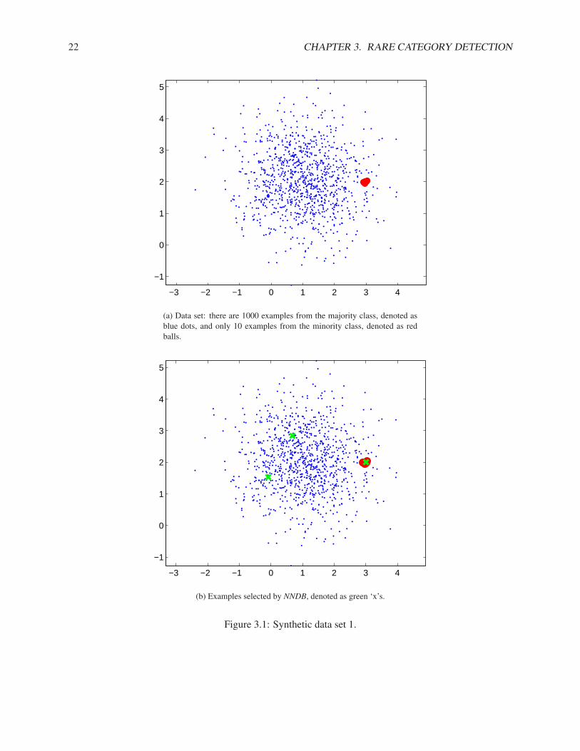
22 CHAPTER 3. RARE CATEGORY DETECTION
−3 −2 −1 0 1 2 3 4
−1
0
1
2
3
4
5
(a) Data set: there are 1000 examples from the majority class, denoted asblue dots, and only 10 examples from the minority class, denoted as redballs.
−3 −2 −1 0 1 2 3 4
−1
0
1
2
3
4
5
(b) Examples selected by NNDB, denoted as green ‘x’s.
Figure 3.1: Synthetic data set 1.
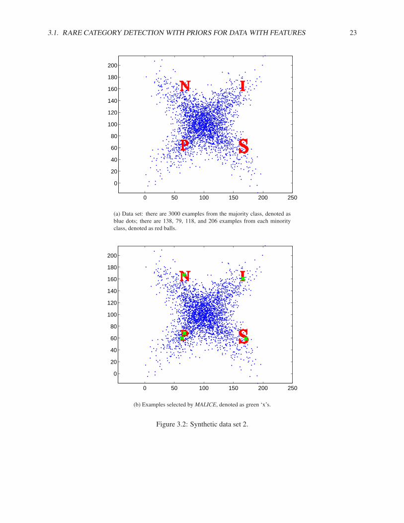
3.1. RARE CATEGORY DETECTION WITH PRIORS FOR DATA WITH FEATURES 23
0 50 100 150 200 250
0
20
40
60
80
100
120
140
160
180
200
(a) Data set: there are 3000 examples from the majority class, denoted asblue dots; there are 138, 79, 118, and 206 examples from each minorityclass, denoted as red balls.
0 50 100 150 200 250
0
20
40
60
80
100
120
140
160
180
200
(b) Examples selected by MALICE, denoted as green ‘x’s.
Figure 3.2: Synthetic data set 2.
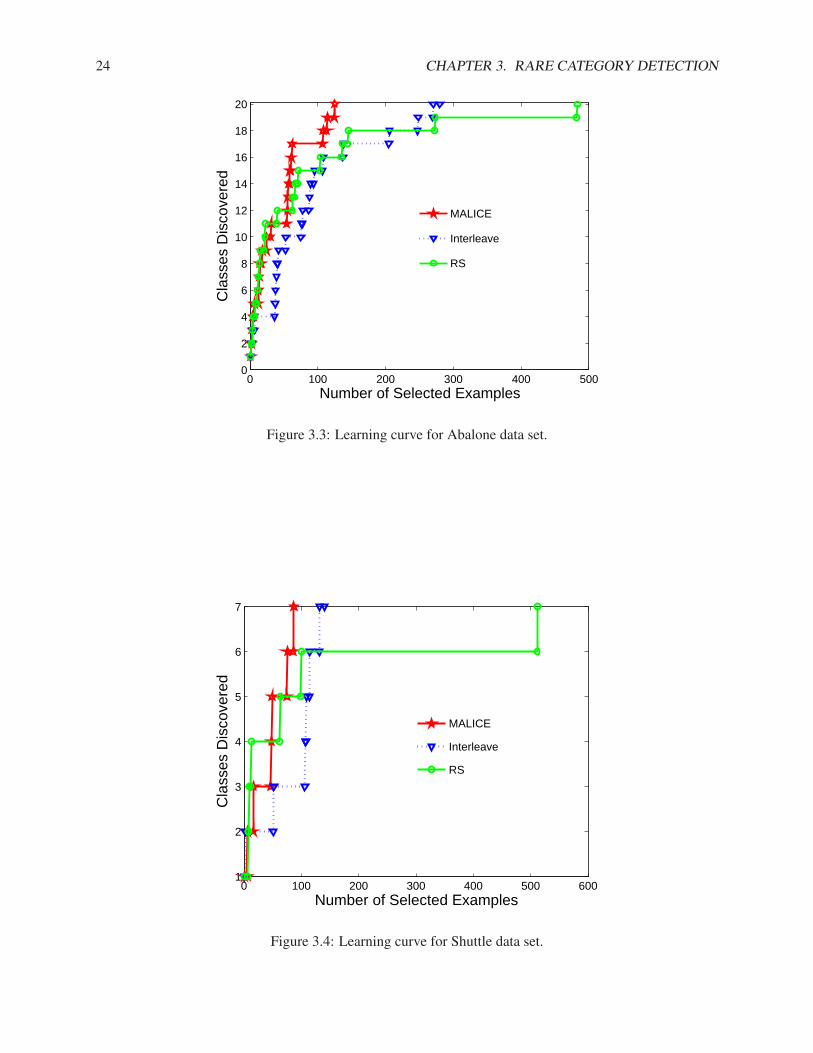
24 CHAPTER 3. RARE CATEGORY DETECTION
0 100 200 300 400 5000
2
4
6
8
10
12
14
16
18
20
Number of Selected Examples
Cla
sses
Dis
cove
red
MALICE
Interleave
RS
Figure 3.3: Learning curve for Abalone data set.
0 100 200 300 400 500 6001
2
3
4
5
6
7
Number of Selected Examples
Cla
sses
Dis
cove
red
MALICE
Interleave
RS
Figure 3.4: Learning curve for Shuttle data set.
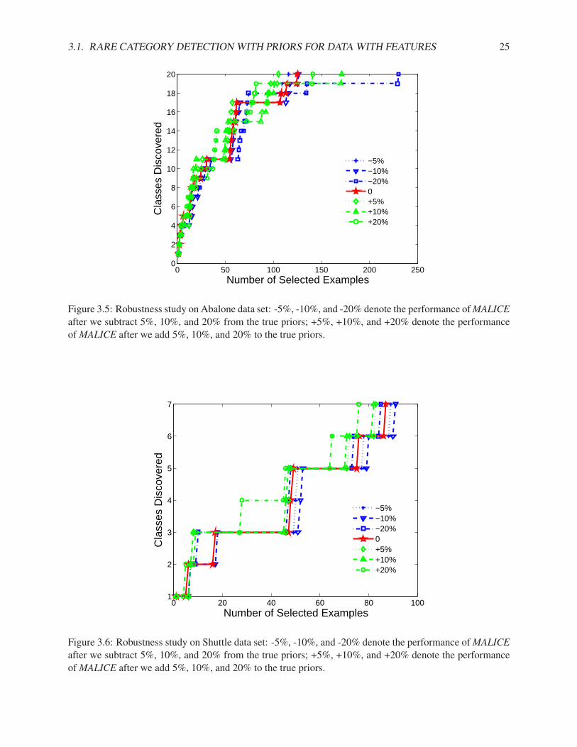
3.1. RARE CATEGORY DETECTION WITH PRIORS FOR DATA WITH FEATURES 25
0 50 100 150 200 2500
2
4
6
8
10
12
14
16
18
20
Number of Selected Examples
Cla
sses
Dis
cove
red
−5%−10%−20%0+5%+10%+20%
Figure 3.5: Robustness study on Abalone data set: -5%, -10%, and -20% denote the performance of MALICEafter we subtract 5%, 10%, and 20% from the true priors; +5%, +10%, and +20% denote the performanceof MALICE after we add 5%, 10%, and 20% to the true priors.
0 20 40 60 80 1001
2
3
4
5
6
7
Number of Selected Examples
Cla
sses
Dis
cove
red
−5%−10%−20%0+5%+10%+20%
Figure 3.6: Robustness study on Shuttle data set: -5%, -10%, and -20% denote the performance of MALICEafter we subtract 5%, 10%, and 20% from the true priors; +5%, +10%, and +20% denote the performanceof MALICE after we add 5%, 10%, and 20% to the true priors.
26 CHAPTER 3. RARE CATEGORY DETECTION
3.2 Prior-free Rare Category Detection for Data with Features
In the last section, we have discussed about rare category detection algorithms that need prior informationabout the data set as input, including the number of classes and the proportions of different classes. However,in some real applications, it is often the case that we do not know the number of classes in the data set, not tomention the proportions of different classes. For example, in outbreaks of epidemics, the number of classes(indicating the number of different diseases) and the class proportions could vary drastically over time as newdiseases occur, strain or die out. To address this problem, in this section, we focus on the more challengingcase where we do not have any prior information about the data set. The proposed method, SEmiparametricDensity Estimation based Rare category detection (SEDER), implicitly performs semiparametric densityestimation using specially designed exponentially families, and selects the examples with the largest normof the gradients for labeling by the oracle. In this way, it focuses on the areas with the maximum change inthe local density. Different from existing methods, SEDER does not require any prior information about thedata set. Therefore, it is more suitable for real applications.
The rest of the section is organized as follows. In Subsection 3.2.1, we introduce the specially designedexponentially families used in SEDER and derive the scoring function. The complete algorithm of SEDERis presented in Subsection 3.2.2. Finally, in Subsection 3.2.3, we compare SEDER with state-of-the-arttechniques on both synthetic and real data sets.
3.2.1 Semiparametric Density Estimation for Rare Category Detection
In rare category detection, based on our assumptions introduced in Section 1.3, abrupt changes in localdensity indicate the presence of rare classes. By sampling in these areas, we have a high probability offinding examples from the rare classes. Following this line of reasoning, our proposed method SEDERimplicitly estimates the density using specially designed exponential families, which essentially define asemiparametric model. At each data point, we set the score to be the norm of the gradient of the estimateddensity, which measures the maximum change rate of the local density, and pick the examples with thelargest scores to be labeled by the oracle. Although the intuition of SEDER and ALICE (MALICE) is quitesimilar: to pick the examples with the maximum change in the local density, ALICE (MALICE) is a nearest-neighbor-based method, it depends on the proportions of different classes to set the size of the neighborhood,and the scores of the examples roughly indicate the change in the local density; whereas SEDER is based onsemiparametric density estimation, it is prior-free, i.e., it does not require any prior information about thedata set, and the scores measure exactly the maximum change rate in the local density.
Additional Notation
Besides the general notation introduced in Section 1.6, we further define the following additional notationin Table 3.1.
Specially Designed Exponential Families
Traditional density estimation methods belong to two categories [Efron & Tibshirani, 1996]: by fitting aparametric model via maximum likelihood, or by nonparametric methods such as kernel density estimation.For the purpose of rare category detection, parametric models are not appropriate since we can not assumea specific form of the underlying distribution for a given data set. On the other hand, the estimated densitybased on nonparametric methods tends to be under-smoothed, and the examples from rare classes will beburied among numerous spikes in the estimated density.

3.2. PRIOR-FREE RARE CATEGORY DETECTION FOR DATA WITH FEATURES 27
Table 3.1: NotationSymbol Definitiongβ(x) The density defined by specially designed
exponential familiesg0(x) The carrier densityβ0 The normalizing parameter in gβ(x)
t(x) The p× 1 vector of sufficient statisticstj(x) The jth component of t(x)β1 The p× 1 parameter vectorβj
1 The jth component of β1
σj The bandwidth for the jth featureβ (β1, β0)β The maximum likelihood estimate of β
l(β) The log-likelihood of the datagjβ(xj) The marginal distribution of the jth feature
based on gβ(x)gj(xj) The true marginal distribution of the jth
featurebj Positive parameter which is a function of βj
1
bj The maximum likelihood estimate of bj
A 1n
∑nk=1
∑ni=1 exp(− (x
jk−x
ji)2
2(σj)2)(xj
i )2
∑ni=1 exp(− (x
jk−x
ji)2
2(σj)2)
B (σj)2
C 1n
∑nk=1(x
jk)
2
Di(x) 1n
∏dj=1
1√2πbjσj
exp(− (xj−bjxji )
2
2(σj)2bj )si The score of xi
As proposed in [Efron & Tibshirani, 1996], these two kinds of methods can be combined by putting anexponential family through a kernel density estimator, the so-called specially designed exponential families.It is a favorably compromise between parametric and nonparametric density estimation: the nonparametricsmoother allows local adaptation to the data, while the exponential term matches some of the data’s globalproperties, and makes the density much smoother [Efron & Tibshirani, 1996]. To be specific, the estimateddensity gβ(x) = g0(x) exp(β0 + βT
1 t(x)) [Efron & Tibshirani, 1996]. Here, x ∈ Rd, g0(x) is a carrierdensity, t(x) is a p× 1 vector of sufficient statistics, β1 is a p× 1 parameter vector, and β0 is a normalizingparameter that makes gβ(x) integrate to 1. In our application, we use the kernel density estimator with
the Gaussian kernel as the carrier density, i.e., g0(x) = 1n
∑ni=1
∏dj=1
1√2πσj exp(− (xj−xj
i )2
2(σj)2), where xj is
the jth feature of x, xji is the jth feature of the ith data point, and σj is the bandwidth for the jth feature.
In SEDER, σj is determined by cross validation [Scott, 1992] on the jth feature. Here, the parametersβ = (β1, β0) can be estimated according to the following theorem.Theorem 3. The maximum likelihood estimate β of β satisfies the following conditions [Efron & Tibshirani, 1996]:∀j ∈ {1, . . . , p} ∫
x1
· · ·∫
xd
tj(x)gβ(x)dxd · · · dx1 =1n
n∑
i=1
tj(xi)
28 CHAPTER 3. RARE CATEGORY DETECTION
where tj(x) is the jth component of the vector t(x).
Proof. Firstly, notice that β0 is a normalizing parameter that makes gβ(x) integrate to 1, i.e.,
β0 = − log∫
x1
· · ·∫
xd
g0(x) exp(βT1 t(x))dxd · · · dx1
Therefore, ∀j ∈ {1, . . . , p}∂β0
∂βj1
= −∫x1 · · ·
∫xd tj(x)g0(x) exp(βT
1 t(x))dxd · · · dx1
∫x1 · · ·
∫xd g0(x) exp(βT
1 t(x))dxd · · · dx1
= −∫
x1
· · ·∫
xd
tj(x)g0(x) exp(β0 + βT1 t(x))dxd · · · dx1
= −∫
x1
· · ·∫
xd
tj(x)gβ(x)dxd · · · dx1
where βj1 is the jth component of the vector β1.
Secondly, the log-likelihood of the data is l(β) =∑n
i=1 log(gβ(xi)) =∑n
i=1 log(g0(xi)) + nβ0 +∑ni=1 βT
1 t(xi). Taking the partial derivative of l(β) with respect to βj1, we have:
∂l(β)
∂βj1
= n∂β0
∂βj1
+n∑
i=1
tj(xi) = −n
∫
x1
· · ·∫
xd
tj(x)gβ(x)dxd · · · dx1 +n∑
i=1
tj(xi)
Setting the partial derivative to 0, we have that the maximum likelihood estimate β of β satisfies∫x1 · · ·
∫xd tj(x)gβ(x)dxd · · · dx1 = 1
n
∑ni=1 tj(xi), ∀j ∈ {1, . . . , p}.
In SEDER, we set the vector of sufficient statistics to be t(x) = [(x1)2, . . . , (xd)2]T 5. If we estimate theparameters according to Theorem 3, different parameters will be coupled due to the normalizing parameterβ0. Let βj
1 be the jth component of the vector β1. In order to de-couple the estimation of different βj1s, we
make the following changes. Firstly, we decompose β0 into βj0s such that
∑dj=1 βj
0 = β0, then gβ(x) can be
seen as a kernel density estimator with a ‘special’ kernel, i.e., gβ(x) = 1n
∑ni=1
∏dj=1[
1√2πσj exp(− (xj−xj
i )2
2(σj)2) exp(βj
0+
βj1(x
j)2)]. Next, we relax the constraint on βj0s, and let them depend on xj
i in such a way that∫
xj
1√2πσj
exp(−(xj − xji )
2
2(σj)2) exp(βj
0i + βj1(x
j)2)dxj = 1 (3.7)
where βj0i implies the dependence of βj
0 on xji . In this way, the marginal distribution of the jth feature is
gjβ(xj) =
∫
x1
· · ·∫
xj−1
∫
xj+1
· · ·∫
xd
gβ(x)dxd · · · dxj+1dxj−1 · · · dx1
=1n
n∑
i=1
{ 1√2πσj
exp(−(xj − xji )
2
2(σj)2) exp(βj
0i + βj1(x
j)2)·
∏
k 6=j
∫
xk
1√2πσk
exp(−(xk − xki )
2
2(σk)2) exp(βk
0i + βk1 (xk)2)dxk}
=1n
n∑
i=1
1√2πσj
exp(−(xj − xji )
2
2(σj)2) exp(βj
0i + βj1(x
j)2)
5Note that the following analysis also applies to other forms of the sufficient statistics, such as t(x) = [x1, . . . , xd]T . In all ourexperiments, the second order sufficient statistics perform the best. So we use this form in SEDER.
3.2. PRIOR-FREE RARE CATEGORY DETECTION FOR DATA WITH FEATURES 29
To estimate the parameters in our current model, we have the following theorem.Theorem 4. The maximum likelihood estimates βj
1 and βj0i of βj
1 and βj0i satisfy the following conditions:
∀j ∈ {1, . . . , d}
n∑
k=1
(xjk)
2 =n∑
k=1
∑ni=1 exp(βj
0i −(xj
k−xji )
2
2(σj)2)Ej
i ((xj)2)
∑ni=1 exp(βj
0i −(xj
k−xji )
2
2(σj)2)
(3.8)
where Eji ((x
j)2) =∫xj (xj)2 1√
2πσj exp(− (xj−xji )
2
2(σj)2) exp(βj
0i + βj1(x
j)2)dxj .
Proof. First of all, according to Equation 3.7, we have βj0i = − log
∫xj
1√2πσj exp(− (xj−xj
i )2
2(σ)2) exp(βj
1(xj)2)dxj .
Therefore,
∂βj0i
βj1
= −∫xj
1√2πσj exp(− (xj−xj
i )2
2(σ)2) exp(βj
1(xj)2)(xj)2dxj
∫xj
1√2πσj exp(− (xj−xj
i )2
2(σ)2) exp(βj
1(xj)2)dxj
= −∫
xj
1√2πσj
exp(−(xj − xji )
2
2(σj)2) exp(βj
0i + βj1(x
j)2)(xj)2dxj = −Eji ((x
j)2)
Then the log-likelihood of the data on the jth component is
l(βj1) =
n∑
k=1
log(gjβ(xj
k)) =n∑
k=1
log(1n
n∑
i=1
1√2πσj
exp(−(xjk − xj
i )2
2(σj)2) · exp(βj
0i + βj1(x
jk)
2))
=n∑
k=1
log(1
n√
2πσjexp(βj
1(xjk)
2) ·n∑
i=1
exp(−(xjk − xj
i )2
2(σj)2) exp(βj
0i))
Taking the partial derivative of l(βj1) with respect to βj
1, we have:
∂l(βj1)
∂βj1
=n∑
k=1
(xjk)
2 +n∑
k=1
∑ni=1 exp(βj
0i −(xj
k−xji )
2
2(σj)2)∂βj
0i
∂βj1∑n
i=1 exp(βj0i −
(xjk−xj
i )2
2(σj)2)
=n∑
k=1
(xjk)
2 −n∑
k=1
∑ni=1 exp(βj
0i −(xj
k−xji )
2
2(σj)2)Ej
i ((xj)2)
∑ni=1 exp(βj
0i −(xj
k−xji )
2
2(σj)2)
Setting the partial derivative to 0, we have that the maximum likelihood estimate βj1 and βj
0i of βj1 and
βj0i satisfy
∑nk=1(x
jk)
2 =∑n
k=1
∑ni=1 exp(βj
0i−(x
jk−x
ji)2
2(σj)2)Ej
i ((xj)2)
∑ni=1 exp(βj
0i−(x
jk−x
ji)2
2(σj)2)
.
Notice that according to Theorem 4, βj1s can be estimated separately, which greatly simplifies our prob-
lem. At the first glance, Equation 3.8 is hard to solve. Next, we let βj1 = (1 − 1
bj ) 12(σj)2
, where bj 6= 1 is
30 CHAPTER 3. RARE CATEGORY DETECTION
a positive parameter, the introduction of which will simplify this equation. According to Equation 3.7, βj0i
can be expressed in terms of bj , i.e.,
βj0i = − log
∫
xj
1√2πσj
exp(−(xj − xji )
2
2(σj)2+ βj
1(xj)2)dxj
= − log∫
xj
1√2πσj
exp(−(xj)2 + bj(xji )
2 − 2bjxjxji
2(σj)2bj)dxj =
(1− bj)(xji )
2
2(σj)2− 1
2log bj
Therefore, the estimated density becomes
gb(x) =1n
n∑
i=1
d∏
j=1
1√2πbjσj
exp(−(xj − bjxji )
2
2(σj)2bj) (3.9)
Replacing βj1 and βj
0i with functions of bj (the maximum likelihood estimate of bj) in the definition ofEj
i ((xj)2), we have Ej
i ((xj)2) = bj(σj)2 + (bj)2(xj
i )2, and Equation 3.8 becomes
n∑
k=1
(xjk)
2 = nbj(σj)2 + (bj)2n∑
k=1
∑ni=1 exp( (1−bj)(xj
i )2
2(σj)2− (xj
k−xji )
2
2(σj)2)(xj
i )2
∑ni=1 exp( (1−bj)(xj
i )2
2(σj)2− (xj
k−xji )
2
2(σj)2)
In general, the value of βj1 is very close to 0, and gβ(x) is a smoothed version of g0(x). Therefore, bj
should be close to 1, and we can re-write the above equation as follows.
1n
n∑
k=1
(xjk)
2 ≈ bj(σj)2 + (bj)21n
n∑
k=1
∑i exp(− (xj
k−xji )
2
2(σj)2)(xj
i )2
∑i exp(− (xj
k−xji )
2
2(σj)2)
This is a second-degree polynomial equation of bj , and the roots can be easily obtained by Vieta’stheorem6, i.e., ∀j ∈ {1, . . . , d}
bj =−B +
√B2 + 4AC
2A(3.10)
where A = 1n
∑nk=1
∑ni=1 exp(− (x
jk−x
ji)2
2(σj)2)(xj
i )2
∑ni=1 exp(− (x
jk−x
ji)2
2(σj)2)
, B = (σj)2, and C = 1n
∑nk=1(x
jk)
2.
Theorem 5. Let gj(xj) be the true density for the jth feature. If 1n
∑ni=1
xji
gj(xji )· dgj(xj
i )
dxji
≥ −1 + O(1), then
bj ≤ 1 and βj1 ≤ 0.
Proof. For the sake of simplicity, let z = xj , h = σj , and f(z) = gj(xj). Then A = 1n
∑nk=1
∑ni=1 exp(− (zk−zi)
2
2h2 )(zi)2
∑ni=1 exp(− (zk−zi)
2
2h2 ),
B = h2, and C = 1n
∑nk=1(zk)2. Consider the following regression problem where the true regres-
sion function r(z) = z2, the noise has mean 0, and we use kernel regression to estimate this function.Then A − C is the bias of kernel regression on the training data, i.e., A − C = 1
n
∑ni=1 h2(1
2r′′(zi) +r′(zi)f
′(zi)f(zi)
)∫
z2k(z)dz + O(h2) [Wasserman, 2005], where k(z) is the Gaussian kernel used in kernel
regression, i.e., k(z) = 1√2π
exp(− z2
2 ). Therefore, A − C = h2 + h2
n
∑ni=1
2zif′(zi)
f(zi)+ O(h2), and
6Note that the other root −B−√
B2+4AC
2Ais disregarded since it is negative.

3.2. PRIOR-FREE RARE CATEGORY DETECTION FOR DATA WITH FEATURES 31
A + B − C ≥ 0 if and only if 1n
∑ni=1
zif′(zi)
f(zi)≥ −1 + O(1). Given that A + B − C ≥ 0, we can
show that bj = −B+√
B2+4AC2A ≤ −B+
√B2+4A(A+B)
2A = 1, and βj1 = (1− 1
bj) 12(σj)2
≤ 0.
In Section 1.3, we have made the following assumptions: 1) the distribution of the majority classes issufficiently smooth; and 2) the minority classes form compact clusters in the feature space. In this case, thefirst order derivative of the density would be close to 0 for most examples, and have large absolute valuesfor a few examples near the rare classes. Therefore, the condition in Theorem 5 is always satisfied, and theexponential term appended to the carrier density decreases away from the origin.
Scoring Function
Once we have estimated all the parameters using Equation 3.10, we can measure the change in the localdensity at each data point based on the estimated density in Equation 3.9. Note that at each data point, if wepick a different direction, the change in local density would be different. In SEDER, we measure the changealong the gradient, which gives the maximum change at each data point.Theorem 6. Using the estimated density in Equation 3.9, ∀x ∈ Rd, the maximum change rate of the density
at x is
√∑dl=1
(∑n
i=1 Di(x)(xl−blxli))
2
((σl)2bl)2, where Di(x) = 1
n
∏dj=1
1√2πbjσj
exp(− (xj−bjxji )
2
2(σj)2bj ) is the contribution
of xi to the estimated density at x.
Proof. ∀x ∈ Rd, let the gradient vector be w ∈ Rd. We have ∀l ∈ {1, . . . , d}
wl =∂gb(x)
∂xl=
1n
n∑
i=1
(−xl − blxli
(σl)2bl)
d∏
j=1
exp(− (xj−bjxji )
2
2(σj)2bj )√
2πbjσj= −
n∑
i=1
Di(x)(xl − blxli)
(σl)2bl
where wl is the lth component of w.Therefore, the maximum change rate of the density at x is
‖w‖2 =
√√√√d∑
l=1
(−n∑
i=1
Di(x)(xl − blxli)
(σl)2bl)2 =
√√√√d∑
l=1
(∑n
i=1 Di(x)(xl − blxli))2
((σl)2bl)2
If the distribution of the majority classes is sufficiently smooth, and the minority classes form compactclusters in the feature space, the minority classes are always located in the regions where the density changesthe most. Therefore, in SEDER, to discover the rare classes, we set the score of each example to be themaximum change rate of the density at this example, i.e., ∀k ∈ {1, . . . , n}
sk =
√√√√d∑
l=1
(∑n
i=1 Di(xk)(xlk − blxl
i))2
((σl)2bl)2(3.11)
where sk is the score of xk. We pick the examples with the largest scores for labeling until we find at leastone example from each class.

32 CHAPTER 3. RARE CATEGORY DETECTION
3.2.2 Algorithm
The intuition of SEDER is to select the examples with the maximum change in the local density for labelingby the oracle. As introduced in Subsubsection 3.2.1, the scores of the examples measure the maximumchange rate in the local density, and they do not take into account the fact that nearby examples tend to havethe same class label. Therefore, if we ask the oracle to label all the examples with large scores, we mayrepeatedly select examples from the most distinctive rare class, rather than discovering all the rare classes.To address this problem in SEDER, we make use of the following heuristic: if xi ∈ S has been labeled,∀xk ∈ S, xk 6= xi, if ∀j ∈ {1, . . . , d}, |xj
i −xjk| ≤ 3σj , we would preclude xk from being selected. In other
words, if an unlabeled example is very close to a previously labeled one, it is quite likely that the labels ofthe two examples are the same, and labeling that example will not have a high probability of detecting anew rare class. The size of the neighborhood is set to 3σj such that the estimated density for the examplesoutside this neighborhood using Gaussian kernel is hardly affected by the labeled example. It should bepointed out that the feedback strategy is orthogonal to the remaining parts of the proposed algorithm. In ourexperiments, we find that despite its simplicity, the current strategy leads to satisfactory performance.
Algorithm 4 SEmiparametric Density Estimation based Rare category detection (SEDER)Input: Unlabeled data set SOutput: The set I of selected examples and the set L of their labels
1: Initialize I = φ and L = φ.2: for j = 1 : d do3: Calculate the bandwidth σj using cross validation [Scott, 1992].4: Calculate the maximum likelihood estimate bj of the parameter bj according to Equation 3.10.5: end for6: for i = 1 : n do7: Calculate the score si of the ith example according to Equation 3.11 using the estimated parameters.8: end for9: while the labeling budget is not exhausted do
10: Set S′ = {x|x ∈ S,∀i ∈ I, ∃j ∈ {1, . . . , d}, s.t., |xj − xji | > 3σj}
11: Query x = argmaxxi∈S′si for its label yx
12: I = I ∪ {x}, L = L ∪ {yx};13: end while
The proposed method, SEDER, is summarized in Alg. 4. It works as follows. Firstly, we initialize theset I of selected examples and the set L of their labels to empty sets. Then step 2 to step 5 calculate theparameters in our model. Step 6 to step 8 calculate the score for each example in S. Finally, step 9 to step13 gradually include the example with the maximum score into I and its label into L until we run out of thelabeling budget. In each round, the selected example should be far away from all the labeled examples.
Note that: 1) unlike the methods proposed in Section 3.1, SEDER does not need to be given the numberof classes in S or any other information, hence it is more suitable for real applications; 2) in SEDER, we donot need to explicitly calculate the density at each example; 3) SEDER does not depend on the assumptionthat the majority and minority classes be separable or near-separable.
3.2.3 Experimental Results
In this subsection, we compare SEDER with MALICE proposed in Section 3.1, Interleave (the best methodproposed in [Pelleg & Moore, 2004]), random sampling (RS) and SEDER with bj = 1 for j = 1, . . . , d(abbreviated as Kernel, which is equivalent to using kernel density estimator to estimate the density and

3.2. PRIOR-FREE RARE CATEGORY DETECTION FOR DATA WITH FEATURES 33
to get the scores) on both synthetic and real data sets. For this purpose, we run these methods until allthe classes have discovered, and compare the number of label requests by each method in order to find acertain number of classes. Note that SEDER MALICE and Kernel are deterministic, whereas the results forInterleave and random sampling are averaged over 100 runs.
Here we would like to emphasize that only SEDER RS and Kernel do not need any prior informationabout the data set, whereas MALICE and Interleave need extra information about the data set as inputs,such as the number of classes and the proportions of different classes. When such prior information is notavailable, which is quite common in real applications, MALICE and Interleave are not applicable.
Synthetic Data Sets
Fig. 3.7(a) shows the underlying distribution of a 1-dimensional synthetic data set. The majority class with2000 examples has a Gaussian distribution with a large variance; whereas the minority classes with 50examples each correspond to the two lower-variance peaks. As can be seen from this figure, the first twoexamples selected by SEDER (red stars) are both from the regions where the density changes the most.
Fig. 3.7(b) shows a 2-dimensional synthetic data set. The majority class has 2000 examples (blue dots)with a Gaussian distribution. The four minority classes (red balls) all have different shapes, and each has 267,280, 84 and 150 examples respectively. This data set is similar to the one used in [He & Carbonell, 2008].To discover all the classes, SEDER only needs to label 6 examples, which are represented by green ‘x’s inthe figure; whereas random sampling needs to label more than 50 examples on average.
Real Data Sets
In this subsubsection, we present the experimental results on some real data sets. The properties of the datasets are summarized in Table 3.2. Notice that all these data sets are skewed: the proportion of the smallestclass is less than 5%. For the last three data sets (Page Blocks, Abalone and Shuttle), it is even less than1%. We refer to these three data sets as ‘extremely’ skewed; whereas the remaining two data sets (Ecoli andGlass) are referred to as ‘moderately’ skewed.
First, let us focus on the ‘moderately’ skewed data sets, which are shown in Fig. 3.8 and Fig. 3.9. WithEcoli data set, to discover all the classes, MALICE needs 36 label requests, Interleave needs 41 label requestson average, RS needs 43 label requests on average, Kernel needs 78 label requests, and SEDER only needs20 label requests; with Glass data set, to discover all the classes, MALICE needs 18 label requests, Interleaveneeds 24 label requests on average, RS needs 31 label requests on average, Kernel needs 102 label requests,and SEDER needs 22 label requests. Therefore, if the data set is ‘moderately’ skewed, the performanceof SEDER is better than or comparable with MALICE, which requires more prior information than SEDERincluding the number of classes in the data set and the proportions of different classes.
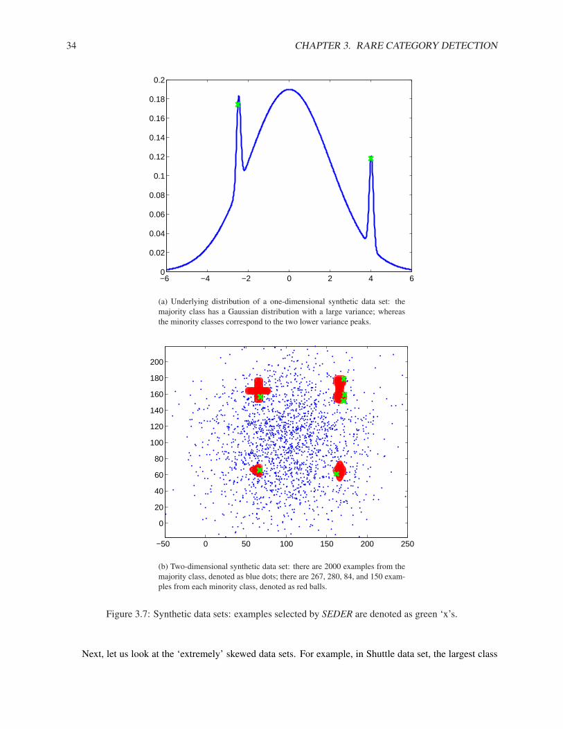
34 CHAPTER 3. RARE CATEGORY DETECTION
−6 −4 −2 0 2 4 60
0.02
0.04
0.06
0.08
0.1
0.12
0.14
0.16
0.18
0.2
(a) Underlying distribution of a one-dimensional synthetic data set: themajority class has a Gaussian distribution with a large variance; whereasthe minority classes correspond to the two lower variance peaks.
−50 0 50 100 150 200 250
0
20
40
60
80
100
120
140
160
180
200
(b) Two-dimensional synthetic data set: there are 2000 examples from themajority class, denoted as blue dots; there are 267, 280, 84, and 150 exam-ples from each minority class, denoted as red balls.
Figure 3.7: Synthetic data sets: examples selected by SEDER are denoted as green ‘x’s.
Next, let us look at the ‘extremely’ skewed data sets. For example, in Shuttle data set, the largest class
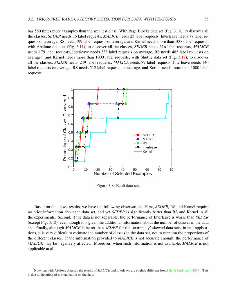
3.2. PRIOR-FREE RARE CATEGORY DETECTION FOR DATA WITH FEATURES 35
has 580 times more examples than the smallest class. With Page Blocks data set (Fig. 3.10), to discover allthe classes, SEDER needs 36 label requests, MALICE needs 23 label requests, Interleave needs 77 label re-quests on average, RS needs 199 label requests on average, and Kernel needs more than 1000 label requests;with Abalone data set (Fig. 3.11), to discover all the classes, SEDER needs 316 label requests, MALICEneeds 179 label requests, Interleave needs 333 label requests on average, RS needs 483 label requests onaverage7, and Kernel needs more than 1000 label requests; with Shuttle data set (Fig. 3.12), to discoverall the classes, SEDER needs 249 label requests, MALICE needs 87 label requests, Interleave needs 140label requests on average, RS needs 512 label requests on average, and Kernel needs more than 1000 labelrequests.
0 10 20 30 40 50 60 70 800.1
0.2
0.3
0.4
0.5
0.6
0.7
0.8
0.9
1
Number of Selected Examples
Per
cent
age
of C
lass
es D
isco
vere
d
SEDERMALICERSInterleaveKernel
Figure 3.8: Ecoli data set.
Based on the above results, we have the following observations. First, SEDER, RS and Kernel requireno prior information about the data set, and yet SEDER is significantly better than RS and Kernel in allthe experiments. Second, if the data is not separable, the performance of Interleave is worse than SEDER(except Fig. 3.12), even though it is given the additional information about the number of classes in the dataset. Finally, although MALICE is better than SEDER for the ‘extremely’ skewed data sets, in real applica-tions, it is very difficult to estimate the number of classes in the data set, not to mention the proportions ofthe different classes. If the information provided to MALICE is not accurate enough, the performance ofMALICE may be negatively affected. Moreover, when such information is not available, MALICE is notapplicable at all.
7Note that with Abalone data set, the results of MALICE and Interleave are slightly different from [He & Carbonell, 2007]. Thisis due to the effect of normalization on the data.
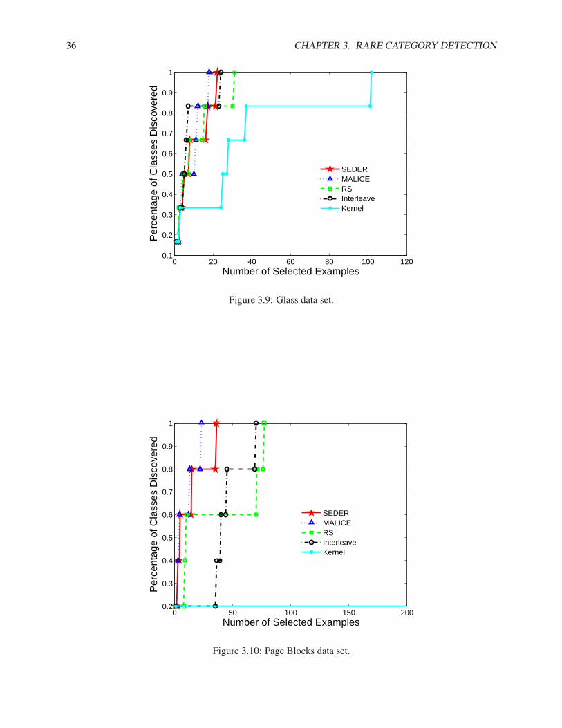
36 CHAPTER 3. RARE CATEGORY DETECTION
0 20 40 60 80 100 1200.1
0.2
0.3
0.4
0.5
0.6
0.7
0.8
0.9
1
Number of Selected Examples
Per
cent
age
of C
lass
es D
isco
vere
d
SEDERMALICERSInterleaveKernel
Figure 3.9: Glass data set.
0 50 100 150 2000.2
0.3
0.4
0.5
0.6
0.7
0.8
0.9
1
Number of Selected Examples
Per
cent
age
of C
lass
es D
isco
vere
d
SEDERMALICERSInterleaveKernel
Figure 3.10: Page Blocks data set.
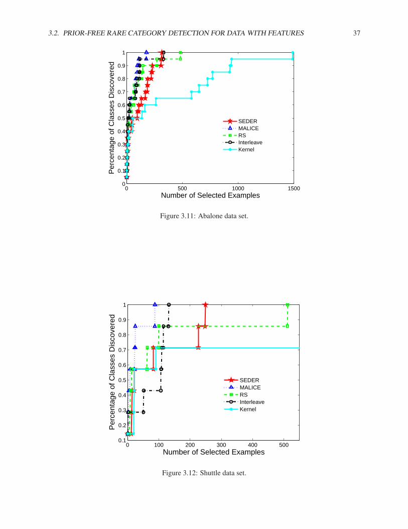
3.2. PRIOR-FREE RARE CATEGORY DETECTION FOR DATA WITH FEATURES 37
0 500 1000 15000
0.1
0.2
0.3
0.4
0.5
0.6
0.7
0.8
0.9
1
Number of Selected Examples
Per
cent
age
of C
lass
es D
isco
vere
dSEDERMALICERSInterleaveKernel
Figure 3.11: Abalone data set.
0 100 200 300 400 5000.1
0.2
0.3
0.4
0.5
0.6
0.7
0.8
0.9
1
Number of Selected Examples
Per
cent
age
of C
lass
es D
isco
vere
d
SEDERMALICERSInterleaveKernel
Figure 3.12: Shuttle data set.
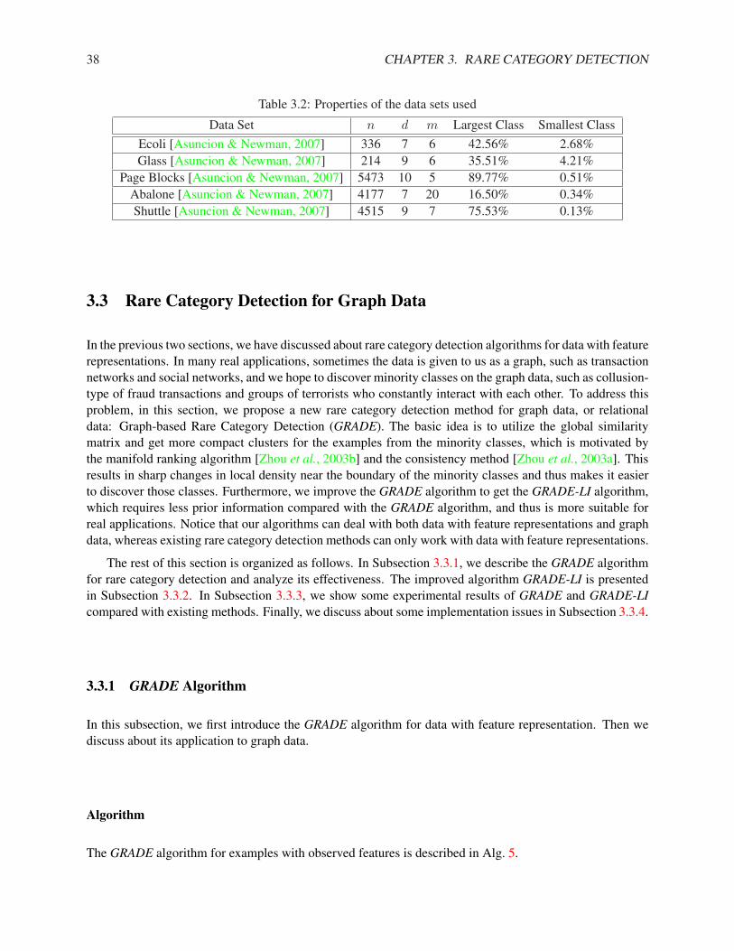
38 CHAPTER 3. RARE CATEGORY DETECTION
Table 3.2: Properties of the data sets used
Data Set n d m Largest Class Smallest ClassEcoli [Asuncion & Newman, 2007] 336 7 6 42.56% 2.68%Glass [Asuncion & Newman, 2007] 214 9 6 35.51% 4.21%
Page Blocks [Asuncion & Newman, 2007] 5473 10 5 89.77% 0.51%Abalone [Asuncion & Newman, 2007] 4177 7 20 16.50% 0.34%Shuttle [Asuncion & Newman, 2007] 4515 9 7 75.53% 0.13%
3.3 Rare Category Detection for Graph Data
In the previous two sections, we have discussed about rare category detection algorithms for data with featurerepresentations. In many real applications, sometimes the data is given to us as a graph, such as transactionnetworks and social networks, and we hope to discover minority classes on the graph data, such as collusion-type of fraud transactions and groups of terrorists who constantly interact with each other. To address thisproblem, in this section, we propose a new rare category detection method for graph data, or relationaldata: Graph-based Rare Category Detection (GRADE). The basic idea is to utilize the global similaritymatrix and get more compact clusters for the examples from the minority classes, which is motivated bythe manifold ranking algorithm [Zhou et al., 2003b] and the consistency method [Zhou et al., 2003a]. Thisresults in sharp changes in local density near the boundary of the minority classes and thus makes it easierto discover those classes. Furthermore, we improve the GRADE algorithm to get the GRADE-LI algorithm,which requires less prior information compared with the GRADE algorithm, and thus is more suitable forreal applications. Notice that our algorithms can deal with both data with feature representations and graphdata, whereas existing rare category detection methods can only work with data with feature representations.
The rest of this section is organized as follows. In Subsection 3.3.1, we describe the GRADE algorithmfor rare category detection and analyze its effectiveness. The improved algorithm GRADE-LI is presentedin Subsection 3.3.2. In Subsection 3.3.3, we show some experimental results of GRADE and GRADE-LIcompared with existing methods. Finally, we discuss about some implementation issues in Subsection 3.3.4.
3.3.1 GRADE Algorithm
In this subsection, we first introduce the GRADE algorithm for data with feature representation. Then wediscuss about its application to graph data.
Algorithm
The GRADE algorithm for examples with observed features is described in Alg. 5.

3.3. RARE CATEGORY DETECTION FOR GRAPH DATA 39
Algorithm 5 Graph-based Rare Category Detection (GRADE)Input: Unlabeled data set S, p1, . . . , pm, αOutput: The set I of selected examples and the set L of their labels
1: Let K = maxmc=2 n× pc.
2: For each example, calculate the distance between this example and its K th nearest neighbor. Set σ to bethe minimum value of all such distances.
3: Construct the pair-wise similarity matrix W ′, n × n, where n is the number of examples, and ∀i, k =1, . . . , n,
W ′ik = exp(−‖xi − xk‖2
2σ2)I(i 6= k) (3.12)
where I(·) is the indicator function.4: Construct the diagonal matrix D, n× n, where Dii =
∑nk=1 W ′
ik, i = 1, . . . , n.5: Calculate the normalized matrix W = D−1/2W ′D−1/2.6: Calculate the global similarity matrix A = (In×n − αW )−1, where In×n is an n× n identity matrix.7: for c = 2 : m do8: Let Kc = npc.9: For each row of A, find the (Kc)th largest element. Set ac to be the largest value of all such elements.
10: ∀xi ∈ S, let NN(xi, ac) = {x|x ∈ S,A(x, xi) ≥ ac}, and nci = |NN(xi, ac)|, where A(x, xi) is
the corresponding element in A.11: end for12: for c = 2 : m do13: If class c has been discovered, continue.14: for t = 2 : n do15: For each xi that has been labeled yi, ∀xk ∈ S, if A(xi, xk) ≥ ayi , sk = −∞; for all the other
examples, si = maxxk∈NN(xi,
act
)(nc
i − nck).
16: Select and query the label of x = arg maxxi∈S si.17: If the label of x is equal to c, break; otherwise, mark the class that x belongs to as discovered.18: end for19: end for
Here α is a positive parameter which is very close to 1. It works as follows. First of all, we calculate themaximum number of examples K in each minority class. Then using this number, we pick the parameterσ, which is the smallest distance to the K th nearest neighbor. Next, we construct the pair-wise similaritymatrix W ′, whose elements are calculated using the Gaussian kernel. In Step 4, we construct the diagonalmatrix D, whose elements are the row sums of W ′. Next, we calculate the normalized matrix W and theglobal similarity matrix A. The specific form of the global similarity matrix has been used in the manifoldranking algorithm [Zhou et al., 2003b] for ranking data with respect to a query point and the consistencymethod [Zhou et al., 2003a] for semi-supervised learning. The following steps are based on the similaritymeasure in A. For each class c, we calculate the number of examples Kc from this class, and find the largestglobal similarity to the (Kc)th nearest neighbor, which is the class specific similarity ac. Then, for eachexample xi, we find all of its neighbors with global similarity bigger than or equal to ac, which is denotedNN(xi, ac), and let nc
i be the number of examples in this set. In Step 12 to Step 19, we calculate the scorefor each example and ask the oracle to label the example with the largest score. To be specific, for each classc, if we have not found any example from this class, we set the score of xi to be the maximum differenceof nc
i and that of the neighboring points with similarity bigger than or equal to act , where t is the iteration
index. By querying the label of the example with the largest score, we are focusing on the regions where
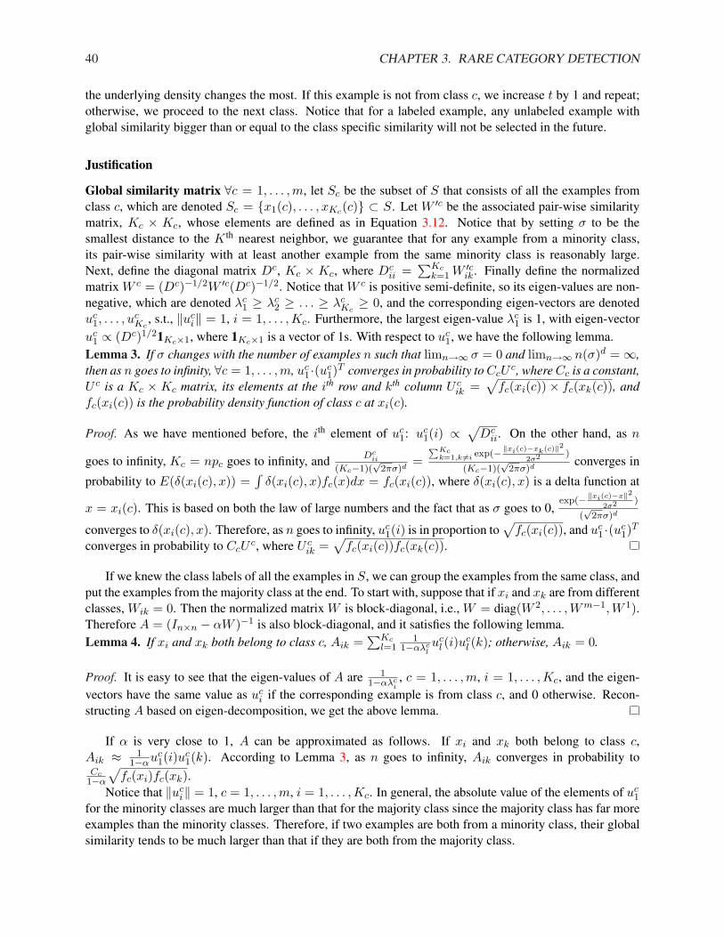
40 CHAPTER 3. RARE CATEGORY DETECTION
the underlying density changes the most. If this example is not from class c, we increase t by 1 and repeat;otherwise, we proceed to the next class. Notice that for a labeled example, any unlabeled example withglobal similarity bigger than or equal to the class specific similarity will not be selected in the future.
Justification
Global similarity matrix ∀c = 1, . . . , m, let Sc be the subset of S that consists of all the examples fromclass c, which are denoted Sc = {x1(c), . . . , xKc(c)} ⊂ S. Let W ′c be the associated pair-wise similaritymatrix, Kc × Kc, whose elements are defined as in Equation 3.12. Notice that by setting σ to be thesmallest distance to the K th nearest neighbor, we guarantee that for any example from a minority class,its pair-wise similarity with at least another example from the same minority class is reasonably large.Next, define the diagonal matrix Dc, Kc × Kc, where Dc
ii =∑Kc
k=1 W ′cik. Finally define the normalized
matrix W c = (Dc)−1/2W ′c(Dc)−1/2. Notice that W c is positive semi-definite, so its eigen-values are non-negative, which are denoted λc
1 ≥ λc2 ≥ . . . ≥ λc
Kc≥ 0, and the corresponding eigen-vectors are denoted
uc1, . . . , u
cKc
, s.t., ‖uci‖ = 1, i = 1, . . . , Kc. Furthermore, the largest eigen-value λc
1 is 1, with eigen-vectoruc
1 ∝ (Dc)1/21Kc×1, where 1Kc×1 is a vector of 1s. With respect to uc1, we have the following lemma.
Lemma 3. If σ changes with the number of examples n such that limn→∞ σ = 0 and limn→∞ n(σ)d = ∞,then as n goes to infinity, ∀c = 1, . . . , m, uc
1·(uc1)
T converges in probability to CcUc, where Cc is a constant,
U c is a Kc × Kc matrix, its elements at the ith row and kth column U cik =
√fc(xi(c))× fc(xk(c)), and
fc(xi(c)) is the probability density function of class c at xi(c).
Proof. As we have mentioned before, the ith element of uc1: uc
1(i) ∝√
Dcii. On the other hand, as n
goes to infinity, Kc = npc goes to infinity, and Dcii
(Kc−1)(√
2πσ)d =∑Kc
k=1,k 6=i exp(− ‖xi(c)−xk(c)‖22σ2 )
(Kc−1)(√
2πσ)d converges in
probability to E(δ(xi(c), x)) =∫
δ(xi(c), x)fc(x)dx = fc(xi(c)), where δ(xi(c), x) is a delta function at
x = xi(c). This is based on both the law of large numbers and the fact that as σ goes to 0,exp(− ‖xi(c)−x‖2
2σ2 )
(√
2πσ)d
converges to δ(xi(c), x). Therefore, as n goes to infinity, uc1(i) is in proportion to
√fc(xi(c)), and uc
1 ·(uc1)
T
converges in probability to CcUc, where U c
ik =√
fc(xi(c))fc(xk(c)).
If we knew the class labels of all the examples in S, we can group the examples from the same class, andput the examples from the majority class at the end. To start with, suppose that if xi and xk are from differentclasses, Wik = 0. Then the normalized matrix W is block-diagonal, i.e., W = diag(W 2, . . . ,Wm−1,W 1).Therefore A = (In×n − αW )−1 is also block-diagonal, and it satisfies the following lemma.Lemma 4. If xi and xk both belong to class c, Aik =
∑Kcl=1
11−αλc
luc
l (i)ucl (k); otherwise, Aik = 0.
Proof. It is easy to see that the eigen-values of A are 11−αλc
i, c = 1, . . . , m, i = 1, . . . , Kc, and the eigen-
vectors have the same value as uci if the corresponding example is from class c, and 0 otherwise. Recon-
structing A based on eigen-decomposition, we get the above lemma.
If α is very close to 1, A can be approximated as follows. If xi and xk both belong to class c,Aik ≈ 1
1−αuc1(i)u
c1(k). According to Lemma 3, as n goes to infinity, Aik converges in probability to
Cc1−α
√fc(xi)fc(xk).
Notice that ‖uci‖ = 1, c = 1, . . . , m, i = 1, . . . , Kc. In general, the absolute value of the elements of uc
1
for the minority classes are much larger than that for the majority class since the majority class has far moreexamples than the minority classes. Therefore, if two examples are both from a minority class, their globalsimilarity tends to be much larger than that if they are both from the majority class.

3.3. RARE CATEGORY DETECTION FOR GRAPH DATA 41
Compared with the pair-wise similarity matrix W ′, the global similarity matrix A is better suited forrare category detection. This is because if the minority class has a manifold structure, two examples onthis manifold may be far away from each other in terms of Euclidean distance, so their pair-wise similarityis very small; whereas their global similarity is large since it is roughly in proportion to the density ofthe minority class at both points. Fig.3.13a shows an example where the majority class (blue dots) has auniform distribution, and the minority class (red balls) forms a 1-dimensional manifold. The black trianglesat both ends of the manifold have a small pair-wise similarity. However, in terms of the global similarity,they are quite similar, which matches our intuition. Furthermore, if we take the global similarity matrixas the pair-wise similarity matrix, and map all the points to the original feature space while preserving thepair-wise similarity, the examples from the minority classes tend to form more compact clusters comparedwith the original feature representation (Fig.3.13b), whereas the probability density function of the majorityclass is still quite smooth, which makes the following querying process more effective. This is particularlybeneficial if the manifold structures of the minority classes are elongated, as shown in Fig.3.13a.
Querying process Step 7 to Step 19 select examples to be labeled by the oracle. According to ourdiscussion in the last subsubsection, if we reconstruct the features according to the global similarity matrix,the minority classes will form compact clusters and the probability density function of the majority class willbe locally smooth. Generally speaking, the querying process selects the examples from the regions wherethe local density changes the most, which have a high probability of coming from the minority classes. Tobe specific, as discussed before, if two examples are both from a minority class, their global similarity tendsto be much larger than that if they are both from the majority class. So the class specific similarity ac islikely to be determined by the examples from the minority classes. Furthermore, as n goes to infinity, Aik isroughly in proportion to the density of class c at xi and xk if they both belong to minority class c. Therefore,if fc(xi) is large, the global similarity between xi and the other examples from class c tends to be large,and nc
i is large accordingly. In other words, if we take the global similarity as the pair-wise similarity basedon the new feature representation, nc
i is the number of neighbors within a fixed distance. Therefore, nci is
roughly in proportion to the local density at xi.
For each class c, we calculate the score of each example xi, which is the maximum difference in the localdensity between xi and the other examples with global similarity bigger than or equal to ac
t . By queryingthe data point with the largest score, we focus on the regions where the local density changes the most, sowe have a high probability of finding examples from the minority classes. Furthermore, by increasing thevalue of t, we gradually enlarge the size of the neighborhood. In this way, we are not only able to selectpoints on the boundary of the minority classes, but also points in the interior, thus increase our chance offinding the minority class examples. Finally, we make use of a simple feedback strategy: if an unlabeledexample is quite similar to a labeled one, we preclude it from being selected in the future. In this way, weavoid wasting the labeling effort on the minority classes that have been discovered already. Notice that thefeedback strategy is orthogonal to the other components of our algorithm. Currently, we are exploring moreeffective feedback strategies.
It should be mentioned that we do not make any assumption about the separability between the majorityclass and the minority classes, which is different from [Fine & Mansour, 2006] and [Pelleg & Moore, 2004].In fact, our algorithm works well when the support regions of the majority class and the minority classesoverlap.
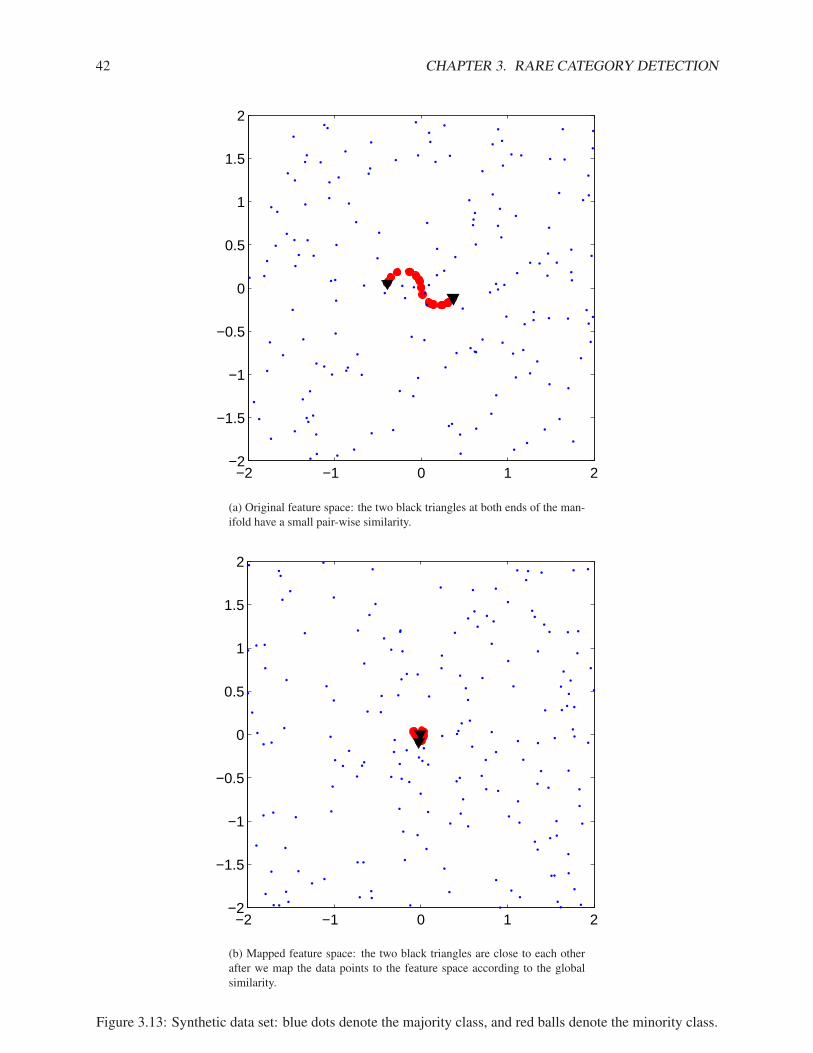
42 CHAPTER 3. RARE CATEGORY DETECTION
−2 −1 0 1 2−2
−1.5
−1
−0.5
0
0.5
1
1.5
2
(a) Original feature space: the two black triangles at both ends of the man-ifold have a small pair-wise similarity.
−2 −1 0 1 2−2
−1.5
−1
−0.5
0
0.5
1
1.5
2
(b) Mapped feature space: the two black triangles are close to each otherafter we map the data points to the feature space according to the globalsimilarity.
Figure 3.13: Synthetic data set: blue dots denote the majority class, and red balls denote the minority class.
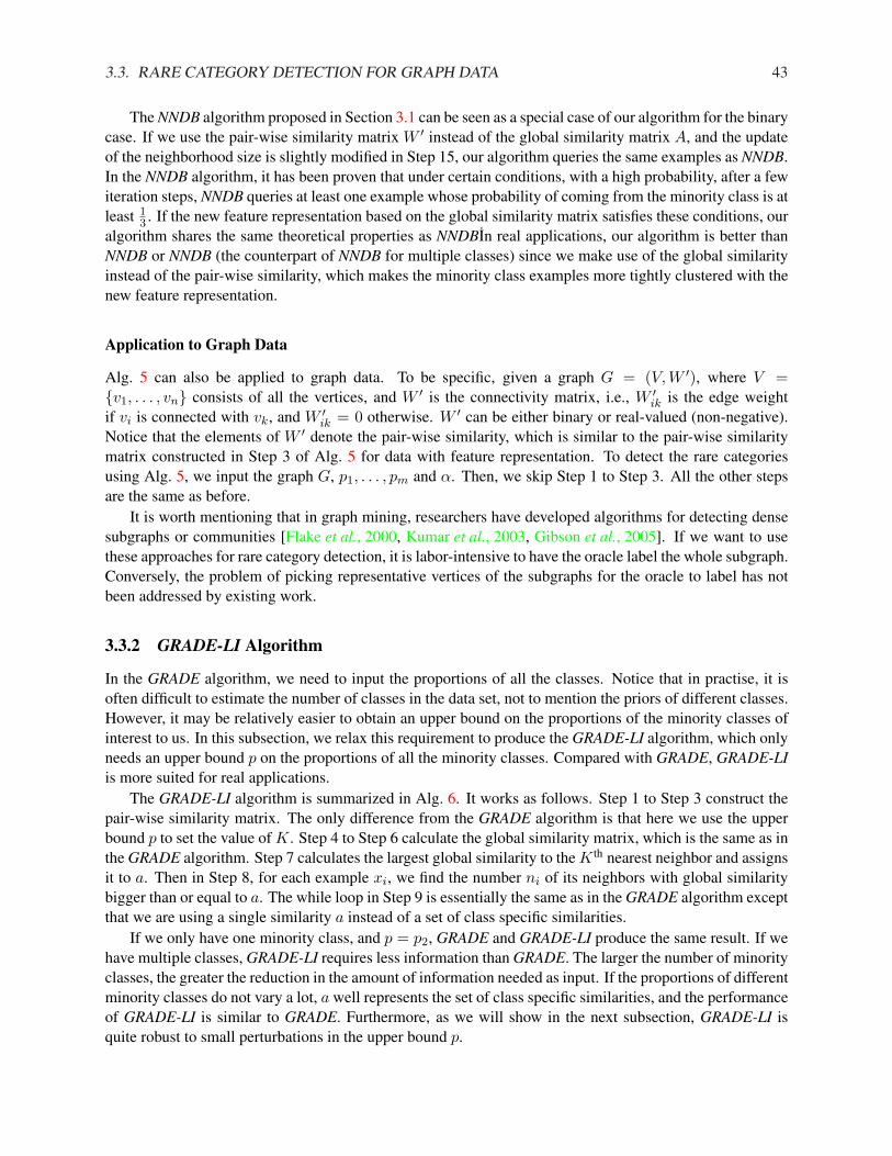
3.3. RARE CATEGORY DETECTION FOR GRAPH DATA 43
The NNDB algorithm proposed in Section 3.1 can be seen as a special case of our algorithm for the binarycase. If we use the pair-wise similarity matrix W ′ instead of the global similarity matrix A, and the updateof the neighborhood size is slightly modified in Step 15, our algorithm queries the same examples as NNDB.In the NNDB algorithm, it has been proven that under certain conditions, with a high probability, after a fewiteration steps, NNDB queries at least one example whose probability of coming from the minority class is atleast 1
3 . If the new feature representation based on the global similarity matrix satisfies these conditions, ouralgorithm shares the same theoretical properties as NNDBIn real applications, our algorithm is better thanNNDB or NNDB (the counterpart of NNDB for multiple classes) since we make use of the global similarityinstead of the pair-wise similarity, which makes the minority class examples more tightly clustered with thenew feature representation.
Application to Graph Data
Alg. 5 can also be applied to graph data. To be specific, given a graph G = (V,W ′), where V ={v1, . . . , vn} consists of all the vertices, and W ′ is the connectivity matrix, i.e., W ′
ik is the edge weightif vi is connected with vk, and W ′
ik = 0 otherwise. W ′ can be either binary or real-valued (non-negative).Notice that the elements of W ′ denote the pair-wise similarity, which is similar to the pair-wise similaritymatrix constructed in Step 3 of Alg. 5 for data with feature representation. To detect the rare categoriesusing Alg. 5, we input the graph G, p1, . . . , pm and α. Then, we skip Step 1 to Step 3. All the other stepsare the same as before.
It is worth mentioning that in graph mining, researchers have developed algorithms for detecting densesubgraphs or communities [Flake et al., 2000, Kumar et al., 2003, Gibson et al., 2005]. If we want to usethese approaches for rare category detection, it is labor-intensive to have the oracle label the whole subgraph.Conversely, the problem of picking representative vertices of the subgraphs for the oracle to label has notbeen addressed by existing work.
3.3.2 GRADE-LI Algorithm
In the GRADE algorithm, we need to input the proportions of all the classes. Notice that in practise, it isoften difficult to estimate the number of classes in the data set, not to mention the priors of different classes.However, it may be relatively easier to obtain an upper bound on the proportions of the minority classes ofinterest to us. In this subsection, we relax this requirement to produce the GRADE-LI algorithm, which onlyneeds an upper bound p on the proportions of all the minority classes. Compared with GRADE, GRADE-LIis more suited for real applications.
The GRADE-LI algorithm is summarized in Alg. 6. It works as follows. Step 1 to Step 3 construct thepair-wise similarity matrix. The only difference from the GRADE algorithm is that here we use the upperbound p to set the value of K. Step 4 to Step 6 calculate the global similarity matrix, which is the same as inthe GRADE algorithm. Step 7 calculates the largest global similarity to the K th nearest neighbor and assignsit to a. Then in Step 8, for each example xi, we find the number ni of its neighbors with global similaritybigger than or equal to a. The while loop in Step 9 is essentially the same as in the GRADE algorithm exceptthat we are using a single similarity a instead of a set of class specific similarities.
If we only have one minority class, and p = p2, GRADE and GRADE-LI produce the same result. If wehave multiple classes, GRADE-LI requires less information than GRADE. The larger the number of minorityclasses, the greater the reduction in the amount of information needed as input. If the proportions of differentminority classes do not vary a lot, a well represents the set of class specific similarities, and the performanceof GRADE-LI is similar to GRADE. Furthermore, as we will show in the next subsection, GRADE-LI isquite robust to small perturbations in the upper bound p.

44 CHAPTER 3. RARE CATEGORY DETECTION
Algorithm 6 Graph-based Rare Category Detection with Less Information (GRADE-LI)Input: Unlabeled data set S, p, αOutput: The set I of selected examples and the set L of their labels
1: Let K = n× p.2: For each example, calculate the distance between this example and its K th nearest neighbor. Set σ to be
the minimum value of all such distances.3: Construct the pair-wise similarity matrix W ′, n × n, where n is the number of examples, and ∀i, k =
1, . . . , n,
W ′ik = exp(−‖xi − xk‖2
2σ2)I(i 6= k)
4: Construct the diagonal matrix D, n× n, where Dii =∑n
k=1 W ′ik, i = 1, . . . , n.
5: Calculate the normalized matrix W = D−1/2W ′D−1/2.6: Calculate the global similarity matrix A = (In×n − αW )−1.7: For each row of A, find the K th largest element. Set a to be the largest value of all such elements.8: ∀xi ∈ S, let NN(xi, a) = {x|x ∈ S, A(x, xi) ≥ a}, and ni = |NN(xi, a)|.9: while not all the classes have been discovered do
10: for t = 2 : n do11: For each xi that has been labeled yi, ∀xk ∈ S, if A(xi, xk) ≥ a, sk = −∞; for all the other
examples, si = maxxk∈NN(xi,
at)(ni − nk).
12: Select and query the label of x = arg maxxi∈S si.13: Mark the class that x belongs to as discovered.14: end for15: end while
3.3.3 Experimental Results
In this subsection, we present the experimental results on both synthetic and real data sets to show theeffectiveness of GRADE and GRADE-LI.
Synthetic Data Sets
Fig. 3.14 shows the result of applying GRADE on the synthetic data set in Fig. 3.13a. There are 1000 ex-amples from the majority class, and only 20 examples from the minority class. Using random sampling, weneed to label 51 examples to discover the minority class on average, whereas using the GRADE algorithm,we only need to label 1 example, denoted as the green ‘x’. Note that in this data set, we only have oneminority class. If we run GRADE-LI with the prior of the minority class as input, we get exactly the sameresult as GRADE.
Fig. 3.15 shows another synthetic data set. It has one majority class (blue dots) and 4 minority classes(red balls), which form the 4 characters. The majority class has 1000 examples, whereas each minorityclass has 100 examples. In order to find all the minority classes, using random sampling, we need to label29 examples on average, whereas using the GRADE algorithm, we only need to label 4 examples, one fromeach minority class, which are denoted as green ‘x’s. Similar as GRADE, if we apply GRADE-LI on this dataset with the exact upper bound, i.e., p = maxm
c=2 pc, we also need 4 label requests to find all the minorityclasses.
Based on the synthetic data set in Fig. 3.15, we gradually reduce the number of examples that form thecharacter ‘I’, and compare the total number of label requests needed by GRADE and GRADE-LI in Fig. 3.16.As the number of examples from ‘I’ decreases, the proportions of different minority classes become more
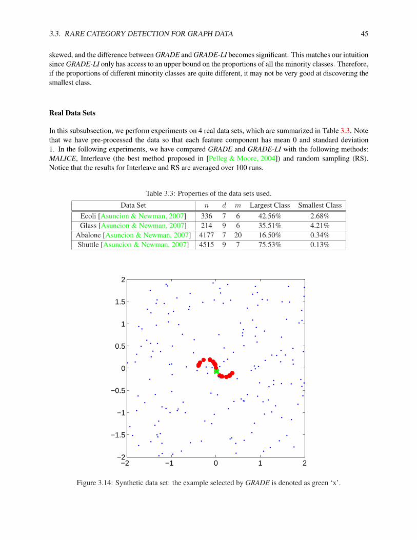
3.3. RARE CATEGORY DETECTION FOR GRAPH DATA 45
skewed, and the difference between GRADE and GRADE-LI becomes significant. This matches our intuitionsince GRADE-LI only has access to an upper bound on the proportions of all the minority classes. Therefore,if the proportions of different minority classes are quite different, it may not be very good at discovering thesmallest class.
Real Data Sets
In this subsubsection, we perform experiments on 4 real data sets, which are summarized in Table 3.3. Notethat we have pre-processed the data so that each feature component has mean 0 and standard deviation1. In the following experiments, we have compared GRADE and GRADE-LI with the following methods:MALICE, Interleave (the best method proposed in [Pelleg & Moore, 2004]) and random sampling (RS).Notice that the results for Interleave and RS are averaged over 100 runs.
Table 3.3: Properties of the data sets used.
Data Set n d m Largest Class Smallest ClassEcoli [Asuncion & Newman, 2007] 336 7 6 42.56% 2.68%Glass [Asuncion & Newman, 2007] 214 9 6 35.51% 4.21%
Abalone [Asuncion & Newman, 2007] 4177 7 20 16.50% 0.34%Shuttle [Asuncion & Newman, 2007] 4515 9 7 75.53% 0.13%
−2 −1 0 1 2−2
−1.5
−1
−0.5
0
0.5
1
1.5
2
Figure 3.14: Synthetic data set: the example selected by GRADE is denoted as green ‘x’.
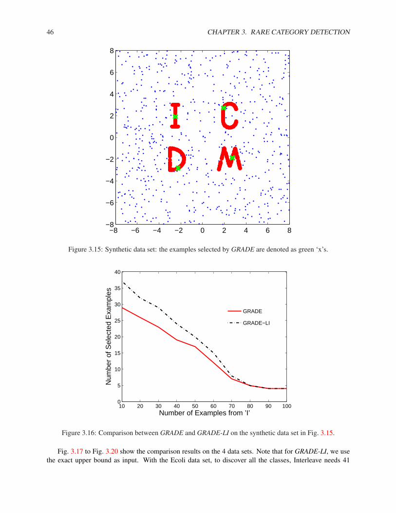
46 CHAPTER 3. RARE CATEGORY DETECTION
−8 −6 −4 −2 0 2 4 6 8−8
−6
−4
−2
0
2
4
6
8
Figure 3.15: Synthetic data set: the examples selected by GRADE are denoted as green ‘x’s.
10 20 30 40 50 60 70 80 90 1000
5
10
15
20
25
30
35
40
Number of Examples from ’I’
Num
ber
of S
elec
ted
Exa
mpl
es
GRADE
GRADE−LI
Figure 3.16: Comparison between GRADE and GRADE-LI on the synthetic data set in Fig. 3.15.
Fig. 3.17 to Fig. 3.20 show the comparison results on the 4 data sets. Note that for GRADE-LI, we usethe exact upper bound as input. With the Ecoli data set, to discover all the classes, Interleave needs 41
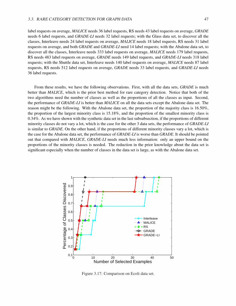
3.3. RARE CATEGORY DETECTION FOR GRAPH DATA 47
label requests on average, MALICE needs 36 label requests, RS needs 43 label requests on average, GRADEneeds 6 label requests, and GRADE-LI needs 32 label requests; with the Glass data set, to discover all theclasses, Interleave needs 24 label requests on average, MALICE needs 18 label requests, RS needs 31 labelrequests on average, and both GRADE and GRADE-LI need 14 label requests; with the Abalone data set, todiscover all the classes, Interleave needs 333 label requests on average, MALICE needs 179 label requests,RS needs 483 label requests on average, GRADE needs 149 label requests, and GRADE-LI needs 318 labelrequests; with the Shuttle data set, Interleave needs 140 label requests on average, MALICE needs 87 labelrequests, RS needs 512 label requests on average, GRADE needs 33 label requests, and GRADE-LI needs36 label requests.
From these results, we have the following observations. First, with all the data sets, GRADE is muchbetter than MALICE, which is the prior best method for rare category detection. Notice that both of thetwo algorithms need the number of classes as well as the proportions of all the classes as input. Second,the performance of GRADE-LI is better than MALICE on all the data sets except the Abalone data set. Thereason might be the following. With the Abalone data set, the proportion of the majority class is 16.50%,the proportion of the largest minority class is 15.18%, and the proportion of the smallest minority class is0.34%. As we have shown with the synthetic data set in the last subsubsection, if the proportions of differentminority classes do not vary a lot, which is the case for the other 3 data sets, the performance of GRADE-LIis similar to GRADE. On the other hand, if the proportions of different minority classes vary a lot, which isthe case for the Abalone data set, the performance of GRADE-LI is worse than GRADE. It should be pointedout that compared with MALICE, GRADE-LI needs much less information: only an upper bound on theproportions of the minority classes is needed. The reduction in the prior knowledge about the data set issignificant especially when the number of classes in the data set is large, as with the Abalone data set.
0 10 20 30 40 500.1
0.2
0.3
0.4
0.5
0.6
0.7
0.8
0.9
1
Number of Selected Examples
Per
cent
age
of C
lass
es D
isco
vere
d
InterleaveMALICERSGRADEGRADE−LI
Figure 3.17: Comparison on Ecoli data set.
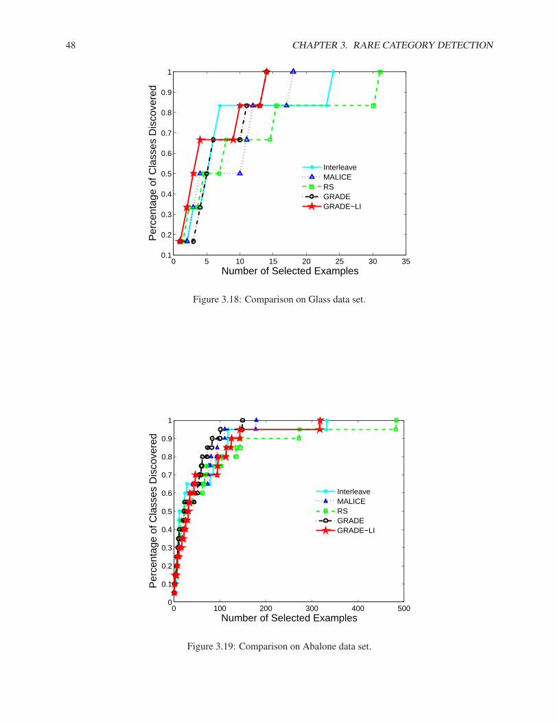
48 CHAPTER 3. RARE CATEGORY DETECTION
0 5 10 15 20 25 30 350.1
0.2
0.3
0.4
0.5
0.6
0.7
0.8
0.9
1
Number of Selected Examples
Per
cent
age
of C
lass
es D
isco
vere
dInterleaveMALICERSGRADEGRADE−LI
Figure 3.18: Comparison on Glass data set.
0 100 200 300 400 5000
0.1
0.2
0.3
0.4
0.5
0.6
0.7
0.8
0.9
1
Number of Selected Examples
Per
cent
age
of C
lass
es D
isco
vere
d
InterleaveMALICERSGRADEGRADE−LI
Figure 3.19: Comparison on Abalone data set.
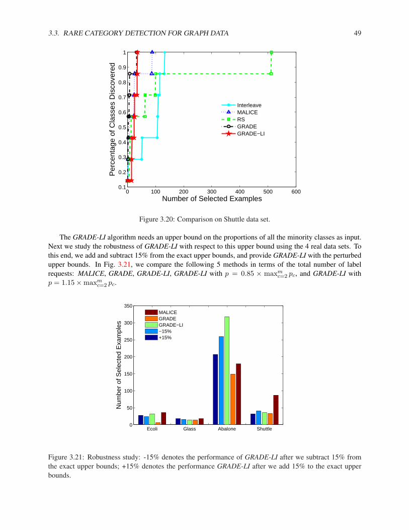
3.3. RARE CATEGORY DETECTION FOR GRAPH DATA 49
0 100 200 300 400 500 6000.1
0.2
0.3
0.4
0.5
0.6
0.7
0.8
0.9
1
Number of Selected Examples
Per
cent
age
of C
lass
es D
isco
vere
dInterleaveMALICERSGRADEGRADE−LI
Figure 3.20: Comparison on Shuttle data set.
The GRADE-LI algorithm needs an upper bound on the proportions of all the minority classes as input.Next we study the robustness of GRADE-LI with respect to this upper bound using the 4 real data sets. Tothis end, we add and subtract 15% from the exact upper bounds, and provide GRADE-LI with the perturbedupper bounds. In Fig. 3.21, we compare the following 5 methods in terms of the total number of labelrequests: MALICE, GRADE, GRADE-LI, GRADE-LI with p = 0.85 × maxm
c=2 pc, and GRADE-LI withp = 1.15×maxm
c=2 pc.
Ecoli Glass Abalone Shuttle0
50
100
150
200
250
300
350
Num
ber
of S
elec
ted
Exa
mpl
es
MALICEGRADEGRADE−LI−15%+15%
Figure 3.21: Robustness study: -15% denotes the performance of GRADE-LI after we subtract 15% fromthe exact upper bounds; +15% denotes the performance GRADE-LI after we add 15% to the exact upperbounds.

50 CHAPTER 3. RARE CATEGORY DETECTION
From Fig. 3.21, we can see that GRADE-LI is quite robust against small perturbations in the upperbounds. For example, with the Glass data set, to find all the classes, using GRADE-LI, if p = maxm
c=2 pc,we need 14 label requests; if p = 0.85 ×maxm
c=2 pc, we need 16 label requests; if p = 1.15 ×maxmc=2 pc,
we need 18 label requests.
3.3.4 Discussion
In this subsection, we discuss about some implementation issues of GRADE and GRADE-LI.
Pair-wise similarity
Note that in Step 3 of Alg. 5 and Alg. 6, the Gaussian kernel is used to get the pair-wise similarity(Equation 3.12). In general, we can use the function ϕ(·, ·) to define W ′, which satisfies the follow-ing conditions: ϕ(xi, xk) = φ(xi−xk
σ ), ∀x ∈ Rd, φ(x) ≥ 0,∫
φ(x)dx = 1, supx φ(x) < ∞, andlim‖x‖→∞ φ(x)
∏dj=1 xj = 0, where xj is the jth feature component of x. In this case, it can be proven
that Lemma 3 still holds. In practise, besides the above similarity functions, we can use the one that is bestsuited for our application, such as the cosine similarity for text data.
Calculating the global similarity matrix
The time complexity of both GRADE and GRADE-LI is dominated by the matrix inversion in calculatingthe global similarity matrix in Step 6 of Alg. 5 and Alg. 6, which is O(n3) with naive implementation, andO(n2.376) with Coppersmith and Winograd’s implementation [Coppersmith & Winograd, 1987]. To speedup this process, we can make use of one of the following two strategies.
• The global similarity matrix A is defined as (In×n − αW )−1. Based on Taylor’s expansion, wehave A = In×n +
∑∞i=1 αiW i. Therefore, we can use the following iterative process to get A, i.e.,
A0 = In×n, Al = αW × Al−1 + In×n. It is easy to see that A = A∞, and we can approximateA with AL, i.e., A ≈ In×n +
∑Li=1 αiW i. This strategy is best suited for the cases where W is
a sparse matrix with z non-zero elements. In this case, with naive implementation, the complexityof calculating A is O(Lnz), which can be further improved with more sophisticated methods suchas [Yuster & Zwick, 2005].
• Another way to accelerate the calculation of the global similarity matrix is by means of eigen-decomposition of W . Let W =
∑ni=1 λiuiu
Ti , where λi is the ith largest eigen-value, and ui is the
corresponding eigen-vector s.t., ‖ui‖ = 1. Therefore, A =∑n
i=11
1−αλiuiu
Ti . We can approximate
W using the r largest eigen-values, i.e., W ≈ ∑ri=1 λiuiu
Ti . In this way, A ≈ ∑r
i=11
1−αλiuiu
Ti .
Since we are only interested in the r largest eigen-values of W , by making use of efficient algorithmssuch as [Lehoucq & Sorensen, 1996], the processing time will be greatly reduced.
Stopping criterion
In GRADE-LI the querying process is stopped once we have at least one labeled example from each class.Note that the rest of GRADE-LI does not need the information of the number of classes to work. When thisinformation is not available, we need to design a stopping criterion for the querying process. One possiblecriterion is to set a threshold on the number of consecutive uninformative label requests, which is the numberof consecutive labeled examples whose classes have already been discovered, and stop the querying processonce the threshold is reached. A very small threshold may result in the overlook of certain minority classes;whereas a very large threshold may result in unaffordable labeling efforts. Therefore, we need to set a proper

3.4. SUMMARY OF RARE CATEGORY DETECTION 51
threshold according to specific applications. It should be pointed out that when the stopping criterion is notbased on the number of classes in the data set, GRADE-LI may need to label more examples, but the numberof label requests to discover all the class is the same as reported in Subsection 3.3.3.
Picking the value of α
As we have discussed in Subsection 3.3.1, if the pair-wise similarity between examples from different classesis 0, and the value of α is close to 1, the global similarity matrix A can be approximated using the eigen-vectors that correspond to eigen-value 1. In real applications, the pair-wise similarity between examplesfrom different classes is rarely 0. In this case, if the value of α is close to 1, the resulting matrix A would beunreliable since the eigen-vectors that correspond to eigen-value 1 are not directly related to the probabilitydensity function of each class. Therefore, for the synthetic data sets, we set α = 0.8; whereas for the realdata sets, we set α = 0.6.
3.4 Summary of Rare Category Detection
In this chapter, we have discussed about our work on rare category detection. Different from existing work,we target the challenging cases where the support regions of the majority and minority classes overlap witheach other in the feature space. The overlapping phenomenon is observed in many real applications, such asfinancial fraud detection and spam image detection. Yet it has not been well studied before.
For data with feature representations, we propose NNDB, ALICE, and MALICE algorithms, which needfull prior information of the data set as input, including the number of classes and the proportions of differentclasses. We also propose SEDER algorithm, which is prior-free. The basic idea of these algorithms is toselect the examples from the regions where the density changes the most, since these examples have ahigh probability of coming from the minority classes. For graph data (relational data), we propose GRADEalgorithm, which needs full prior information of the data set as input, and GRADE-LI algorithm, whichonly needs an upper bound on the proportions of the minority classes. The basic idea of these algorithmsis to perform implicit feature transformation based on the global similarity, which results in more compactclusters of the minority classes. Furthermore, we provide theoretical guarantees for these algorithms underthe smoothness assumption of the majority classes and the compactness assumption of the minority classes.Based on the experimental results on both synthetic data sets and real data sets, we have the followingconclusions.
1. Given full prior information about the data set, including the number of classes and the proportionsof different classes, the proposed GRADE algorithm performs the best, since it enjoys the benefits ofboth the global similarity and the MALICE algorithm.
2. If we only know an upper bound on the proportions of the minority classes, but do not know thenumber of classes or the exact proportions of different classes, we can apply the GRADE-LI algorithmto detect the rare categories.
3. The GRADE-LI algorithm is robust to small perturbations in the upper bound.
4. The GRADE and GRADE-LI algorithms apply to both data with feature representations and graphdata. For data with feature representations, we first need to construct a pair-wise similarity matrixbased on the features.
5. Generally speaking, the performance of GRADE is better than MALICE, and both of them are muchbetter than existing methods, such as random sampling and Interleave (the best method proposedin [Pelleg & Moore, 2004]). However, the processing time of GRADE is more than MALICE since itneeds to compute the global similarity for each pair of data points.

52 CHAPTER 3. RARE CATEGORY DETECTION
6. The MALICE algorithm is robust to small perturbations in the class priors.
7. If we do not have any prior information about the data set, we can apply the SEDER algorithm todetect the rare categories. If a data set is ‘moderately’ skewed, its performance is comparable toMALICE; if a data set is ‘extremely’ skewed, its performance is not as good as MALICE. However,for rare category detection, the performance of SEDER is always better than random sampling.
Chapter 4
Rare Category Characterization
In Chapter 3, we have introduced various algorithms for rare category detection, which result in a set oflabeled examples. Based on this labeled set, a natural follow-up step is rare category characterization, i.e.,to characterize the minority classes in order to identify all the rare examples in the data set. For example, inMedicare fraud detection, once we have discovered a bogus claim for durable equipments (e.g., wheelchairs,breathing machines), we may want to find the fraud patterns related to such equipments in order to preventsimilar fraudulent claims in the future. To this end, in this chapter, we focus on rare category characteriza-tion, the second task in the supervised settings.
Based on our discussion in Section 1.3, it is a very important challenge to accurately classify the minorityclasses given that they are (1) highly skewed and (2) non-separable from the majority classes. In addition, ifthe minority classes can be characterized by a concise representation, we may better understand the nature ofthe minority classes, and thus better identify examples from those classes. Rare category characterization isto characterize the minority classes for the purpose of understanding and correctly classifying those classes.
Here, our key observation is as follows: although the minority classes are non-separable from the ma-jority classes, they often exhibit compactness. That is, each minority class often forms a compact cluster.For example, the fraudulent people often make multiple similar transactions to maximize their profits [?].For rare diseases, the patients with the same type of rare disease often share similar genes or chromosomalabnormalities [EURODIS, 2005].
In this chapter, we propose RACH by exploring such compactness for rare category characterization. Thecore of RACH is to represent the minority classes with a hyper-ball. We present the optimization frameworkas well as an effective algorithm to solve it. Furthermore, we show how RACH can be naturally kernelized.We also analyze the complexity of RACH. Finally, we justify the effectiveness of the proposed RACH byboth theoretical analysis and empirical evaluations.
The main contributions of this chapter can be summarized as follows.
Problem Formulation. We formulate the problem of rare category characterization as an optimiza-tion problem, which takes into account both labeled an unlabeled examples, and imposes differentconstraints for different types of data;
Algorithm Design. We design an effective algorithm to find the solution of the optimization problem.It repeatedly converts the original problem into a convex optimization problem, and solves it in itsdual form by a projected subgradient method, which is well justified theoretically.
The rest of this chapter is organized as follows. In Section 4.1, we propose the optimization frameworkto provide a compact representation for the minority class with justification, followed by the conversion ofthis framework to the convex optimization problem as well as its dual form. Then we introduce the RACHalgorithm to solve the dual problem with performance guarantees in Section 4.2, and the kernelized RACH
53

54 CHAPTER 4. RARE CATEGORY CHARACTERIZATION
algorithm in Section 4.3. Finally, following the experimental results presented in Section 4.4, we give a briefsummary of rare category characterization in Section 4.5.
4.1 Optimization Framework
In this section, we present our optimization framework, after we introduce the additional notation and thepre-processing step.
4.1.1 Additional Notation
For the sake of simplicity, we assume that there is only one majority class and one minority class in thedata set, i.e., m = 2. (Multiple majority and minority classes can be converted into several binary prob-lems.) Throughout this chapter, we will use calligraphic capital letters to denote sets. Let x1, . . . , xn1 ∈Rd denote the labeled examples from the majority class, which correspond to yi = 1, i = 1, . . . , n1;let xn1+1, . . . , xn1+n2 ∈ Rd denote the labeled examples from the minority class, which correspond toyj = 2, j = n1 + 1, . . . , n1 + n2; let x′n1+n2+1, . . . , x
′n′ ∈ Rd denote all the unlabeled examples. Here, n1,
n2, and n′ denote the number of labeled examples from the majority class, the number of labeled examplesfrom the minority class, and the total number of examples, both labeled and unlabeled. d is the dimension-ality of the input space. Our goal is to identify a list of unlabeled examples which are believed to come fromthe minority class with high precision and recall.
4.1.2 Assumptions
In many imbalanced problems, it is often the case that the rare examples from the same minority class arevery close to each other, whereas the examples from the same majority class may be scattered in the featurespace. This assumption is also used in [He & Carbonell, 2007][Wu et al., 2007][Pelleg & Moore, 2004],etc, when dealing with imbalanced data sets, either explicitly or implicitly. Furthermore, we also assumethat the rare examples can be enclosed by a minimum-radius hyper-ball in the input space without includingtoo many majority class examples. This seemingly rigorous assumption will become more flexible when weuse the high-dimensional feature space instead of the input space via the kernel trick in Section 4.3. Withthis assumption, we allow the support regions of the majority and minority classes to overlap with eachother.
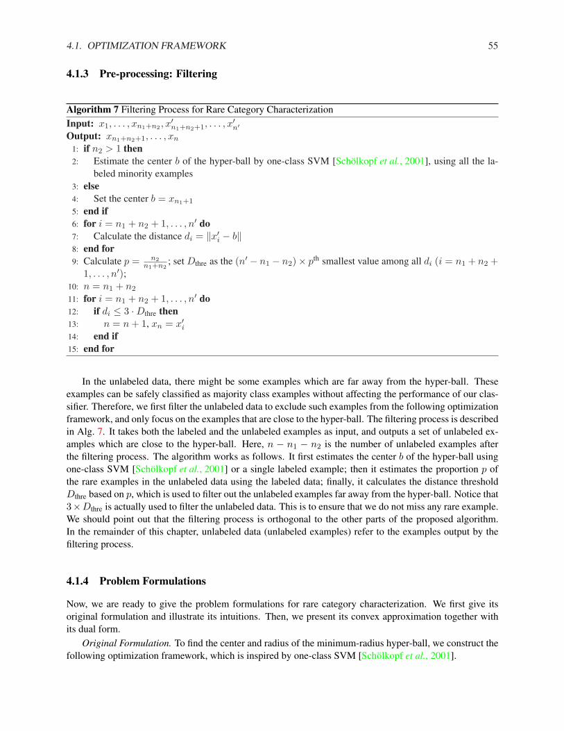
4.1. OPTIMIZATION FRAMEWORK 55
4.1.3 Pre-processing: Filtering
Algorithm 7 Filtering Process for Rare Category CharacterizationInput: x1, . . . , xn1+n2 , x
′n1+n2+1, . . . , x
′n′
Output: xn1+n2+1, . . . , xn
1: if n2 > 1 then2: Estimate the center b of the hyper-ball by one-class SVM [Scholkopf et al., 2001], using all the la-
beled minority examples3: else4: Set the center b = xn1+1
5: end if6: for i = n1 + n2 + 1, . . . , n′ do7: Calculate the distance di = ‖x′i − b‖8: end for9: Calculate p = n2
n1+n2; set Dthre as the (n′ − n1 − n2)× pth smallest value among all di (i = n1 + n2 +
1, . . . , n′);10: n = n1 + n2
11: for i = n1 + n2 + 1, . . . , n′ do12: if di ≤ 3 ·Dthre then13: n = n + 1, xn = x′i14: end if15: end for
In the unlabeled data, there might be some examples which are far away from the hyper-ball. Theseexamples can be safely classified as majority class examples without affecting the performance of our clas-sifier. Therefore, we first filter the unlabeled data to exclude such examples from the following optimizationframework, and only focus on the examples that are close to the hyper-ball. The filtering process is describedin Alg. 7. It takes both the labeled and the unlabeled examples as input, and outputs a set of unlabeled ex-amples which are close to the hyper-ball. Here, n − n1 − n2 is the number of unlabeled examples afterthe filtering process. The algorithm works as follows. It first estimates the center b of the hyper-ball usingone-class SVM [Scholkopf et al., 2001] or a single labeled example; then it estimates the proportion p ofthe rare examples in the unlabeled data using the labeled data; finally, it calculates the distance thresholdDthre based on p, which is used to filter out the unlabeled examples far away from the hyper-ball. Notice that3×Dthre is actually used to filter the unlabeled data. This is to ensure that we do not miss any rare example.We should point out that the filtering process is orthogonal to the other parts of the proposed algorithm.In the remainder of this chapter, unlabeled data (unlabeled examples) refer to the examples output by thefiltering process.
4.1.4 Problem Formulations
Now, we are ready to give the problem formulations for rare category characterization. We first give itsoriginal formulation and illustrate its intuitions. Then, we present its convex approximation together withits dual form.
Original Formulation. To find the center and radius of the minimum-radius hyper-ball, we construct thefollowing optimization framework, which is inspired by one-class SVM [Scholkopf et al., 2001].
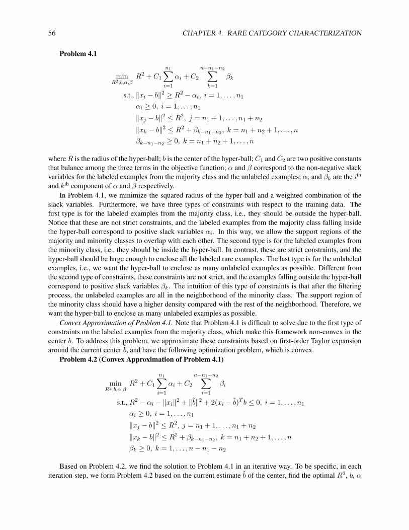
56 CHAPTER 4. RARE CATEGORY CHARACTERIZATION
Problem 4.1
minR2,b,α,β
R2 + C1
n1∑
i=1
αi + C2
n−n1−n2∑
k=1
βk
s.t., ‖xi − b‖2 ≥ R2 − αi, i = 1, . . . , n1
αi ≥ 0, i = 1, . . . , n1
‖xj − b‖2 ≤ R2, j = n1 + 1, . . . , n1 + n2
‖xk − b‖2 ≤ R2 + βk−n1−n2 , k = n1 + n2 + 1, . . . , n
βk−n1−n2 ≥ 0, k = n1 + n2 + 1, . . . , n
where R is the radius of the hyper-ball; b is the center of the hyper-ball; C1 and C2 are two positive constantsthat balance among the three terms in the objective function; α and β correspond to the non-negative slackvariables for the labeled examples from the majority class and the unlabeled examples; αi and βk are the ith
and kth component of α and β respectively.In Problem 4.1, we minimize the squared radius of the hyper-ball and a weighted combination of the
slack variables. Furthermore, we have three types of constraints with respect to the training data. Thefirst type is for the labeled examples from the majority class, i.e., they should be outside the hyper-ball.Notice that these are not strict constraints, and the labeled examples from the majority class falling insidethe hyper-ball correspond to positive slack variables αi. In this way, we allow the support regions of themajority and minority classes to overlap with each other. The second type is for the labeled examples fromthe minority class, i.e., they should be inside the hyper-ball. In contrast, these are strict constraints, and thehyper-ball should be large enough to enclose all the labeled rare examples. The last type is for the unlabeledexamples, i.e., we want the hyper-ball to enclose as many unlabeled examples as possible. Different fromthe second type of constraints, these constraints are not strict, and the examples falling outside the hyper-ballcorrespond to positive slack variables βk. The intuition of this type of constraints is that after the filteringprocess, the unlabeled examples are all in the neighborhood of the minority class. The support region ofthe minority class should have a higher density compared with the rest of the neighborhood. Therefore, wewant the hyper-ball to enclose as many unlabeled examples as possible.
Convex Approximation of Problem 4.1. Note that Problem 4.1 is difficult to solve due to the first type ofconstraints on the labeled examples from the majority class, which make this framework non-convex in thecenter b. To address this problem, we approximate these constraints based on first-order Taylor expansionaround the current center b, and have the following optimization problem, which is convex.
Problem 4.2 (Convex Approximation of Problem 4.1)
minR2,b,α,β
R2 + C1
n1∑
i=1
αi + C2
n−n1−n2∑
i=1
βi
s.t., R2 − αi − ‖xi‖2 + ‖b‖2 + 2(xi − b)T b ≤ 0, i = 1, . . . , n1
αi ≥ 0, i = 1, . . . , n1
‖xj − b‖2 ≤ R2, j = n1 + 1, . . . , n1 + n2
‖xk − b‖2 ≤ R2 + βk−n1−n2 , k = n1 + n2 + 1, . . . , n
βk ≥ 0, k = 1, . . . , n− n1 − n2
Based on Problem 4.2, we find the solution to Problem 4.1 in an iterative way. To be specific, in eachiteration step, we form Problem 4.2 based on the current estimate b of the center, find the optimal R2, b, α
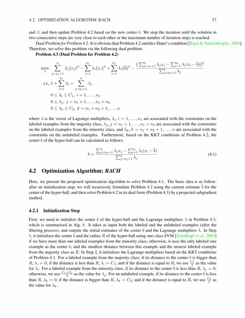
4.2. OPTIMIZATION ALGORITHM: RACH 57
and β, and then update Problem 4.2 based on the new center b. We stop the iteration until the solution intwo consecutive steps are very close to each other or the maximum number of iteration steps is reached.
Dual Problem for Problem 4.2. It is obvious that Problem 4.2 satisfies Slater’s condition [Boyd & Vandenberghe, 2004].Therefore, we solve this problem via the following dual problem.
Problem 4.3 (Dual Problem for Problem 4.2)
maxλ
n∑
j=n1+1
λj‖xj‖2 −n1∑
i=1
λi‖xi‖2 +n1∑
i=1
λi‖b‖2 − ‖∑nj=n1+1 λjxj −
∑n1i=1 λi(xi − b)‖2
∑nj=n1+1 λj
s.t., 1 +n1∑
i=1
λi =n∑
j=n1+1
λj
0 ≤ λi ≤ C1, i = 1, . . . , n1
0 ≤ λj , j = n1 + 1, . . . , n1 + n2
0 ≤ λk ≤ C2, k = n1 + n2 + 1, . . . , n
where λ is the vector of Lagrange multipliers, λi, i = 1, . . . , n1 are associated with the constraints on thelabeled examples from the majority class, λj , j = n1 + 1, . . . , n1 + n2 are associated with the constraintson the labeled examples from the minority class, and λk, k = n1 + n2 + 1, . . . , n are associated with theconstraints on the unlabeled examples. Furthermore, based on the KKT conditions of Problem 4.2, thecenter b of the hyper-ball can be calculated as follows.
b =
∑nj=n1+1 λjxj −
∑n1i=1 λi(xi − b)∑n
j=n1+1 λj(4.1)
4.2 Optimization Algorithm: RACH
Here, we present the proposed optimization algorithm to solve Problem 4.1. The basic idea is as follow:after an initialization step; we will recursively formulate Problem 4.2 using the current estimate b for thecenter of the hyper-ball; and then solve Problem 4.2 in its dual form (Problem 4.3) by a projected subgradientmethod.
4.2.1 Initialization Step
First, we need to initialize the center b of the hyper-ball and the Lagrange multipliers λ in Problem 4.3,which is summarized in Alg. 8. It takes as input both the labeled and the unlabeled examples (after thefiltering process), and outputs the initial estimates of the center b and the Lagrange multipliers λ. In Step1, it initializes the center b and the radius R of the hyper-ball using one-class SVM [Scholkopf et al., 2001]if we have more than one labeled examples from the minority class; otherwise, it uses the only labeled rareexample as the center b, and the smallest distance between this example and the nearest labeled examplefrom the majority class as R. In Step 2, it initializes the Lagrange multipliers based on the KKT conditionsof Problem 4.1. For a labeled example from the majority class, if its distance to the center b is bigger thanR, λi = 0; if the distance is less than R, λi = C1; and if the distance is equal to R, we use C1
2 as the valuefor λi. For a labeled example from the minority class, if its distance to the center b is less than R, λj = 0;otherwise, we use C1+C2
2 as the value for λj . For an unlabeled example, if its distance to the center b is lessthan R, λk = 0; if the distance is bigger than R, λk = C2; and if the distance is equal to R, we use C2
2 asthe value for λk.
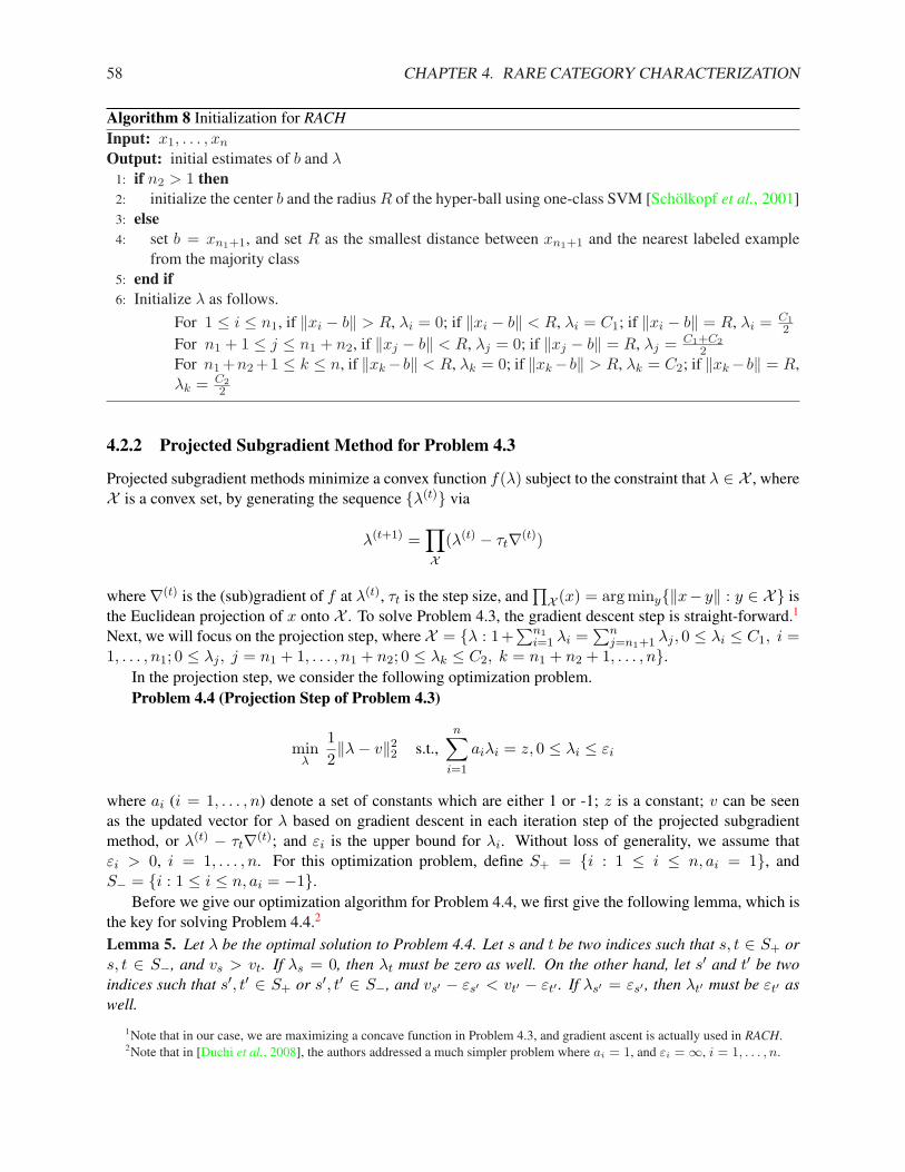
58 CHAPTER 4. RARE CATEGORY CHARACTERIZATION
Algorithm 8 Initialization for RACHInput: x1, . . . , xn
Output: initial estimates of b and λ1: if n2 > 1 then2: initialize the center b and the radius R of the hyper-ball using one-class SVM [Scholkopf et al., 2001]3: else4: set b = xn1+1, and set R as the smallest distance between xn1+1 and the nearest labeled example
from the majority class5: end if6: Initialize λ as follows.
For 1 ≤ i ≤ n1, if ‖xi − b‖ > R, λi = 0; if ‖xi − b‖ < R, λi = C1; if ‖xi − b‖ = R, λi = C12
For n1 + 1 ≤ j ≤ n1 + n2, if ‖xj − b‖ < R, λj = 0; if ‖xj − b‖ = R, λj = C1+C22
For n1 +n2 +1 ≤ k ≤ n, if ‖xk−b‖ < R, λk = 0; if ‖xk−b‖ > R, λk = C2; if ‖xk−b‖ = R,λk = C2
2
4.2.2 Projected Subgradient Method for Problem 4.3
Projected subgradient methods minimize a convex function f(λ) subject to the constraint that λ ∈ X , whereX is a convex set, by generating the sequence {λ(t)} via
λ(t+1) =∏
X(λ(t) − τt∇(t))
where∇(t) is the (sub)gradient of f at λ(t), τt is the step size, and∏X (x) = arg miny{‖x− y‖ : y ∈ X} is
the Euclidean projection of x onto X . To solve Problem 4.3, the gradient descent step is straight-forward.1
Next, we will focus on the projection step, where X = {λ : 1+∑n1
i=1 λi =∑n
j=n1+1 λj , 0 ≤ λi ≤ C1, i =1, . . . , n1; 0 ≤ λj , j = n1 + 1, . . . , n1 + n2; 0 ≤ λk ≤ C2, k = n1 + n2 + 1, . . . , n}.
In the projection step, we consider the following optimization problem.Problem 4.4 (Projection Step of Problem 4.3)
minλ
12‖λ− v‖2
2 s.t.,n∑
i=1
aiλi = z, 0 ≤ λi ≤ εi
where ai (i = 1, . . . , n) denote a set of constants which are either 1 or -1; z is a constant; v can be seenas the updated vector for λ based on gradient descent in each iteration step of the projected subgradientmethod, or λ(t) − τt∇(t); and εi is the upper bound for λi. Without loss of generality, we assume thatεi > 0, i = 1, . . . , n. For this optimization problem, define S+ = {i : 1 ≤ i ≤ n, ai = 1}, andS− = {i : 1 ≤ i ≤ n, ai = −1}.
Before we give our optimization algorithm for Problem 4.4, we first give the following lemma, which isthe key for solving Problem 4.4.2
Lemma 5. Let λ be the optimal solution to Problem 4.4. Let s and t be two indices such that s, t ∈ S+ ors, t ∈ S−, and vs > vt. If λs = 0, then λt must be zero as well. On the other hand, let s′ and t′ be twoindices such that s′, t′ ∈ S+ or s′, t′ ∈ S−, and vs′ − εs′ < vt′ − εt′ . If λs′ = εs′ , then λt′ must be εt′ aswell.
1Note that in our case, we are maximizing a concave function in Problem 4.3, and gradient ascent is actually used in RACH.2Note that in [Duchi et al., 2008], the authors addressed a much simpler problem where ai = 1, and εi = ∞, i = 1, . . . , n.
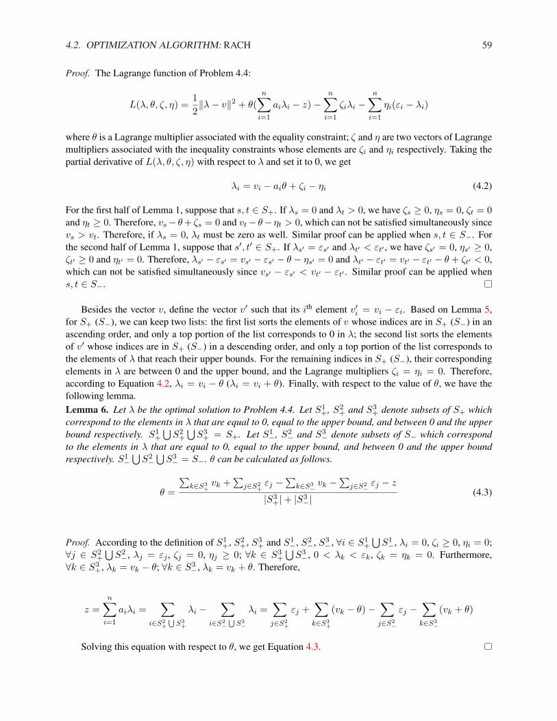
4.2. OPTIMIZATION ALGORITHM: RACH 59
Proof. The Lagrange function of Problem 4.4:
L(λ, θ, ζ, η) =12‖λ− v‖2 + θ(
n∑
i=1
aiλi − z)−n∑
i=1
ζiλi −n∑
i=1
ηi(εi − λi)
where θ is a Lagrange multiplier associated with the equality constraint; ζ and η are two vectors of Lagrangemultipliers associated with the inequality constraints whose elements are ζi and ηi respectively. Taking thepartial derivative of L(λ, θ, ζ, η) with respect to λ and set it to 0, we get
λi = vi − aiθ + ζi − ηi (4.2)
For the first half of Lemma 1, suppose that s, t ∈ S+. If λs = 0 and λt > 0, we have ζs ≥ 0, ηs = 0, ζt = 0and ηt ≥ 0. Therefore, vs− θ + ζs = 0 and vt− θ− ηt > 0, which can not be satisfied simultaneously sincevs > vt. Therefore, if λs = 0, λt must be zero as well. Similar proof can be applied when s, t ∈ S−. Forthe second half of Lemma 1, suppose that s′, t′ ∈ S+. If λs′ = εs′ and λt′ < εt′ , we have ζs′ = 0, ηs′ ≥ 0,ζt′ ≥ 0 and ηt′ = 0. Therefore, λs′ − εs′ = vs′ − εs′ − θ − ηs′ = 0 and λt′ − εt′ = vt′ − εt′ − θ + ζt′ < 0,which can not be satisfied simultaneously since vs′ − εs′ < vt′ − εt′ . Similar proof can be applied whens, t ∈ S−.
Besides the vector v, define the vector v′ such that its ith element v′i = vi − εi. Based on Lemma 5,for S+ (S−), we can keep two lists: the first list sorts the elements of v whose indices are in S+ (S−) in anascending order, and only a top portion of the list corresponds to 0 in λ; the second list sorts the elementsof v′ whose indices are in S+ (S−) in a descending order, and only a top portion of the list corresponds tothe elements of λ that reach their upper bounds. For the remaining indices in S+ (S−), their correspondingelements in λ are between 0 and the upper bound, and the Lagrange multipliers ζi = ηi = 0. Therefore,according to Equation 4.2, λi = vi − θ (λi = vi + θ). Finally, with respect to the value of θ, we have thefollowing lemma.Lemma 6. Let λ be the optimal solution to Problem 4.4. Let S1
+, S2+ and S3
+ denote subsets of S+ whichcorrespond to the elements in λ that are equal to 0, equal to the upper bound, and between 0 and the upperbound respectively. S1
+
⋃S2
+
⋃S3
+ = S+. Let S1−, S2− and S3− denote subsets of S− which correspondto the elements in λ that are equal to 0, equal to the upper bound, and between 0 and the upper boundrespectively. S1−
⋃S2−
⋃S3− = S−. θ can be calculated as follows.
θ =
∑k∈S3
+vk +
∑j∈S2
+εj −
∑k∈S3
−vk −
∑j∈S2
−εj − z
|S3+|+ |S3−|
(4.3)
Proof. According to the definition of S1+, S2
+, S3+ and S1−, S2−, S3−, ∀i ∈ S1
+
⋃S1−, λi = 0, ζi ≥ 0, ηi = 0;
∀j ∈ S2+
⋃S2−, λj = εj , ζj = 0, ηj ≥ 0; ∀k ∈ S3
+
⋃S3−, 0 < λk < εk, ζk = ηk = 0. Furthermore,
∀k ∈ S3+, λk = vk − θ; ∀k ∈ S3−, λk = vk + θ. Therefore,
z =n∑
i=1
aiλi =∑
i∈S2+
⋃S3
+
λi −∑
i∈S2−
⋃S3−
λi =∑
j∈S2+
εj +∑
k∈S3+
(vk − θ)−∑
j∈S2−
εj −∑
k∈S3−
(vk + θ)
Solving this equation with respect to θ, we get Equation 4.3.

60 CHAPTER 4. RARE CATEGORY CHARACTERIZATION
Based on Lemma 5 and Lemma 6, to solve Problem 4.4, we gradually increase the number of elementsin S1
+, S2+, S1− and S2−, calculate θ accordingly, and determine the value of λ which has the smallest value
of 12‖λ− v‖2
2. Alg. 9 gives the details for solving Problem 4.3 in RACH.
Algorithm 9 Projected Subgradient Method for Problem 4.3
Input: x1, . . . , xn; step size τ ; C1, C2; N2; b; initial estimate of λOutput: λ
1: Define S+ = {n1 + 1, . . . , n} and S− = {1, . . . , n1}2: for step = 1 to N2 do3: Calculate ∇ as follows:
l = 1, . . . , n1 :
∇l = −‖xl‖2 + ‖b‖2 +2(
∑nj=n1+1 λj(xj)T −∑n1
i=1 λi(xi − b)T )(xl − b)∑nj=n1+1 λj
l = n1 + 1, . . . , n :
∇l = ‖xl‖2 − (∑n
j=n1+1 λj(xj)T −∑n1i=1 λi(xi − b)T )
(∑n
j=n1+1 λj)2· (
n∑
j=n1+1
λj(2xl − xj) +n1∑
i=1
λi(xi − b))
4: Update λ via gradient ascent to obtain: v = λ + τ∇5: Calculate v′ as follows:
v′i = vi − C1, i = 1, . . . , n1
v′j = −∞, j = n1 + 1, . . . , n1 + n2
v′k = vk − C2, k = n1 + n2 + 1, . . . , n
6: Set D = ∞7: for I1 = 1, I2 = 1, I3 = 1, I4 = 1 to I1 = |S+|+1, I2 = |S−|+1, I3 = |S+|+1, I4 = |S−|+1 do8: Let S1
+ ⊂ S+ denote the subset of indices in S+ such that the corresponding elements in v are nolarger than the I th
1 largest element; let S2+ ⊂ S+ denote the subset of indices in S+ such that the
corresponding elements in v′ are no smaller than the I th3 smallest element
9: If S1+
⋂S2
+ 6= ∅ or S2+
⋂{n1 + 1, . . . , n1 + n2} 6= ∅, continue; otherwise, S3+ = S+\(S1
+
⋂S2
+)10: Let S1− ⊂ S− denote the subset of indices in S− such that the corresponding elements in v are no
larger than the I th2 largest element; let S2− ⊂ S− denote the subset of indices in S− such that the
corresponding elements in v′ are no smaller than the I th4 smallest element
11: If S1−⋂
S2− 6= ∅, continue; otherwise, S3− = S−\(S1−⋂
S2−)
12: Calculate θ =∑
k∈S3+
vk−∑
k∈S3−vk+|S2
+|C2−|S2−|C1−1
|S3+|+|S3
−|13: Calculate w as follows: wi = 0, i ∈ S1
+
⋃S1−; wi = C2, i ∈ S2
+; wi = C1, i ∈ S2−; wi =vi − θ, i ∈ S3
+; wi = vi + θ, i ∈ S3−14: If ‖v − w‖ < D, set λ = w and D = ‖v − w‖.15: end for16: end for
In Step 3 of Alg. 9, we calculate the gradient of the objective function in Problem 4.3 at the current value
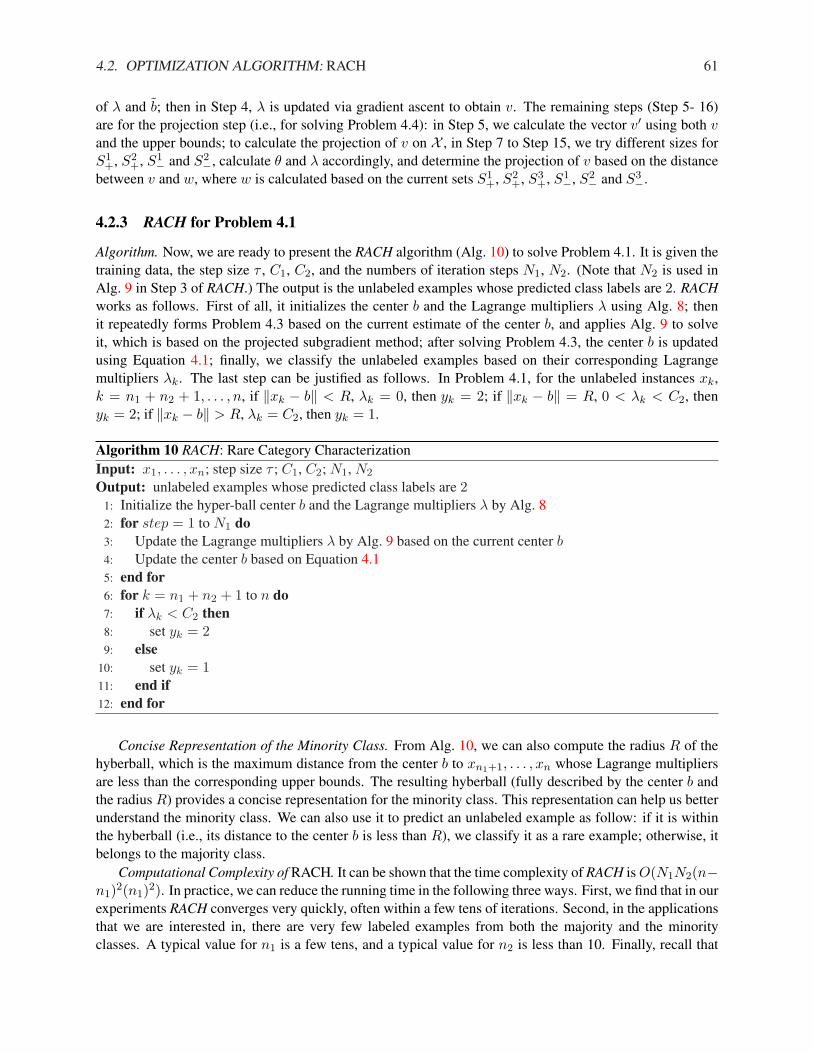
4.2. OPTIMIZATION ALGORITHM: RACH 61
of λ and b; then in Step 4, λ is updated via gradient ascent to obtain v. The remaining steps (Step 5- 16)are for the projection step (i.e., for solving Problem 4.4): in Step 5, we calculate the vector v′ using both vand the upper bounds; to calculate the projection of v on X , in Step 7 to Step 15, we try different sizes forS1
+, S2+, S1− and S2−, calculate θ and λ accordingly, and determine the projection of v based on the distance
between v and w, where w is calculated based on the current sets S1+, S2
+, S3+, S1−, S2− and S3−.
4.2.3 RACH for Problem 4.1
Algorithm. Now, we are ready to present the RACH algorithm (Alg. 10) to solve Problem 4.1. It is given thetraining data, the step size τ , C1, C2, and the numbers of iteration steps N1, N2. (Note that N2 is used inAlg. 9 in Step 3 of RACH.) The output is the unlabeled examples whose predicted class labels are 2. RACHworks as follows. First of all, it initializes the center b and the Lagrange multipliers λ using Alg. 8; thenit repeatedly forms Problem 4.3 based on the current estimate of the center b, and applies Alg. 9 to solveit, which is based on the projected subgradient method; after solving Problem 4.3, the center b is updatedusing Equation 4.1; finally, we classify the unlabeled examples based on their corresponding Lagrangemultipliers λk. The last step can be justified as follows. In Problem 4.1, for the unlabeled instances xk,k = n1 + n2 + 1, . . . , n, if ‖xk − b‖ < R, λk = 0, then yk = 2; if ‖xk − b‖ = R, 0 < λk < C2, thenyk = 2; if ‖xk − b‖ > R, λk = C2, then yk = 1.
Algorithm 10 RACH: Rare Category CharacterizationInput: x1, . . . , xn; step size τ ; C1, C2; N1, N2
Output: unlabeled examples whose predicted class labels are 21: Initialize the hyper-ball center b and the Lagrange multipliers λ by Alg. 82: for step = 1 to N1 do3: Update the Lagrange multipliers λ by Alg. 9 based on the current center b4: Update the center b based on Equation 4.15: end for6: for k = n1 + n2 + 1 to n do7: if λk < C2 then8: set yk = 29: else
10: set yk = 111: end if12: end for
Concise Representation of the Minority Class. From Alg. 10, we can also compute the radius R of thehyberball, which is the maximum distance from the center b to xn1+1, . . . , xn whose Lagrange multipliersare less than the corresponding upper bounds. The resulting hyberball (fully described by the center b andthe radius R) provides a concise representation for the minority class. This representation can help us betterunderstand the minority class. We can also use it to predict an unlabeled example as follow: if it is withinthe hyberball (i.e., its distance to the center b is less than R), we classify it as a rare example; otherwise, itbelongs to the majority class.
Computational Complexity of RACH. It can be shown that the time complexity of RACH is O(N1N2(n−n1)2(n1)2). In practice, we can reduce the running time in the following three ways. First, we find that in ourexperiments RACH converges very quickly, often within a few tens of iterations. Second, in the applicationsthat we are interested in, there are very few labeled examples from both the majority and the minorityclasses. A typical value for n1 is a few tens, and a typical value for n2 is less than 10. Finally, recall that
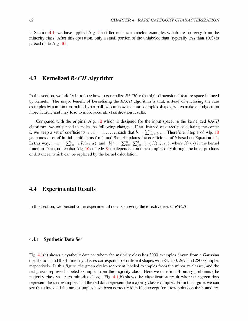
62 CHAPTER 4. RARE CATEGORY CHARACTERIZATION
in Section 4.1, we have applied Alg. 7 to filter out the unlabeled examples which are far away from theminority class. After this operation, only a small portion of the unlabeled data (typically less than 10%) ispassed on to Alg. 10.
4.3 Kernelized RACH Algorithm
In this section, we briefly introduce how to generalize RACH to the high-dimensional feature space inducedby kernels. The major benefit of kernelizing the RACH algorithm is that, instead of enclosing the rareexamples by a minimum-radius hyper-ball, we can now use more complex shapes, which make our algorithmmore flexible and may lead to more accurate classification results.
Compared with the original Alg. 10 which is designed for the input space, in the kernelized RACHalgorithm, we only need to make the following changes. First, instead of directly calculating the centerb, we keep a set of coefficients γi, i = 1, . . . , n such that b =
∑ni=1 γixi. Therefore, Step 1 of Alg. 10
generates a set of initial coefficients for b, and Step 4 updates the coefficients of b based on Equation 4.1.In this way, b · x =
∑ni=1 γiK(xi, x), and ‖b‖2 =
∑ni=1
∑nj=1 γiγjK(xi, xj), where K(·, ·) is the kernel
function. Next, notice that Alg. 10 and Alg. 9 are dependent on the examples only through the inner productsor distances, which can be replaced by the kernel calculation.
4.4 Experimental Results
In this section, we present some experimental results showing the effectiveness of RACH.
4.4.1 Synthetic Data Set
Fig. 4.1(a) shows a synthetic data set where the majority class has 3000 examples drawn from a Gaussiandistribution, and the 4 minority classes correspond to 4 different shapes with 84, 150, 267, and 280 examplesrespectively. In this figure, the green circles represent labeled examples from the minority classes, and thered pluses represent labeled examples from the majority class. Here we construct 4 binary problems (themajority class vs. each minority class). Fig. 4.1(b) shows the classification result where the green dotsrepresent the rare examples, and the red dots represent the majority class examples. From this figure, we cansee that almost all the rare examples have been correctly identified except for a few points on the boundary.
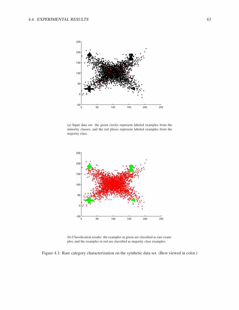
4.4. EXPERIMENTAL RESULTS 63
(a) Input data set: the green circles represent labeled examples from theminority classes, and the red pluses represent labeled examples from themajority class.
(b) Classification results: the examples in green are classified as rare exam-ples, and the examples in red are classified as majority class examples.
Figure 4.1: Rare category characterization on the synthetic data set. (Best viewed in color.)
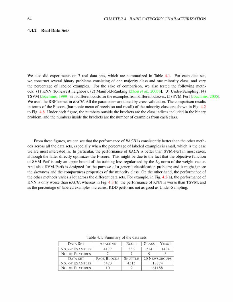
64 CHAPTER 4. RARE CATEGORY CHARACTERIZATION
4.4.2 Real Data Sets
We also did experiments on 7 real data sets, which are summarized in Table 4.1. For each data set,we construct several binary problems consisting of one majority class and one minority class, and varythe percentage of labeled examples. For the sake of comparison, we also tested the following meth-ods: (1) KNN (K-nearest neighbor); (2) Manifold-Ranking [Zhou et al., 2003b]; (3) Under-Sampling; (4)TSVM [Joachims, 1999] with different costs for the examples from different classes; (5) SVM-Perf [Joachims, 2005].We used the RBF kernel in RACH. All the parameters are tuned by cross validation. The comparison resultsin terms of the F-score (harmonic mean of precision and recall) of the minority class are shown in Fig. 4.2to Fig. 4.8. Under each figure, the numbers outside the brackets are the class indices included in the binaryproblem, and the numbers inside the brackets are the number of examples from each class.
From these figures, we can see that the performance of RACH is consistently better than the other meth-ods across all the data sets, especially when the percentage of labeled examples is small, which is the casewe are most interested in. In particular, the performance of RACH is better than SVM-Perf in most cases,although the latter directly optimizes the F-score. This might be due to the fact that the objective functionof SVM-Perf is only an upper bound of the training loss regularized by the L2 norm of the weight vector.And also, SVM-Perfs is designed for the purpose of a general classification problem; and it might ignorethe skewness and the compactness properties of the minority class. On the other hand, the performance ofthe other methods varies a lot across the different data sets. For example, in Fig. 4.2(a), the performance ofKNN is only worse than RACH; whereas in Fig. 4.3(b), the performance of KNN is worse than TSVM, andas the percentage of labeled examples increases, KDD performs not as good as Under-Sampling.
Table 4.1: Summary of the data setsDATA SET ABALONE ECOLI GLASS YEAST
NO. OF EXAMPLES 4177 336 214 1484NO. OF FEATURES 7 7 9 8
DATA SET PAGE BLOCKS SHUTTLE 20 NEWSGROUPS
NO. OF EXAMPLES 5473 4515 18774NO. OF FEATURES 10 9 61188
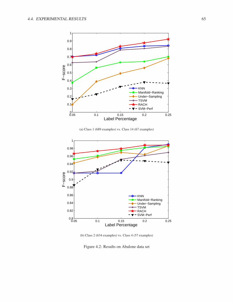
4.4. EXPERIMENTAL RESULTS 65
0.05 0.1 0.15 0.2 0.250
0.1
0.2
0.3
0.4
0.5
0.6
0.7
0.8
0.9
1
Label Percentage
F−
scor
e
KNNManifold−RankingUnder−SamplingTSVMRACHSVM−Perf
(a) Class 1 (689 examples) vs. Class 14 (67 examples)
0.05 0.1 0.15 0.2 0.250.8
0.82
0.84
0.86
0.88
0.9
0.92
0.94
0.96
0.98
1
Label Percentage
F−
scor
e
KNNManifold−RankingUnder−SamplingTSVMRACHSVM−Perf
(b) Class 2 (634 examples) vs. Class 4 (57 examples)
Figure 4.2: Results on Abalone data set
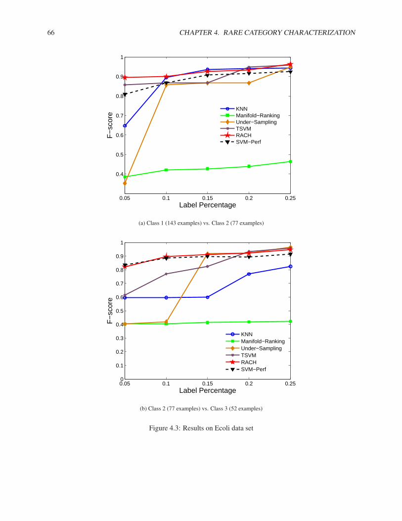
66 CHAPTER 4. RARE CATEGORY CHARACTERIZATION
0.05 0.1 0.15 0.2 0.25
0.4
0.5
0.6
0.7
0.8
0.9
1
Label Percentage
F−
scor
e
KNNManifold−RankingUnder−SamplingTSVMRACHSVM−Perf
(a) Class 1 (143 examples) vs. Class 2 (77 examples)
0.05 0.1 0.15 0.2 0.250
0.1
0.2
0.3
0.4
0.5
0.6
0.7
0.8
0.9
1
Label Percentage
F−
scor
e
KNNManifold−RankingUnder−SamplingTSVMRACHSVM−Perf
(b) Class 2 (77 examples) vs. Class 3 (52 examples)
Figure 4.3: Results on Ecoli data set
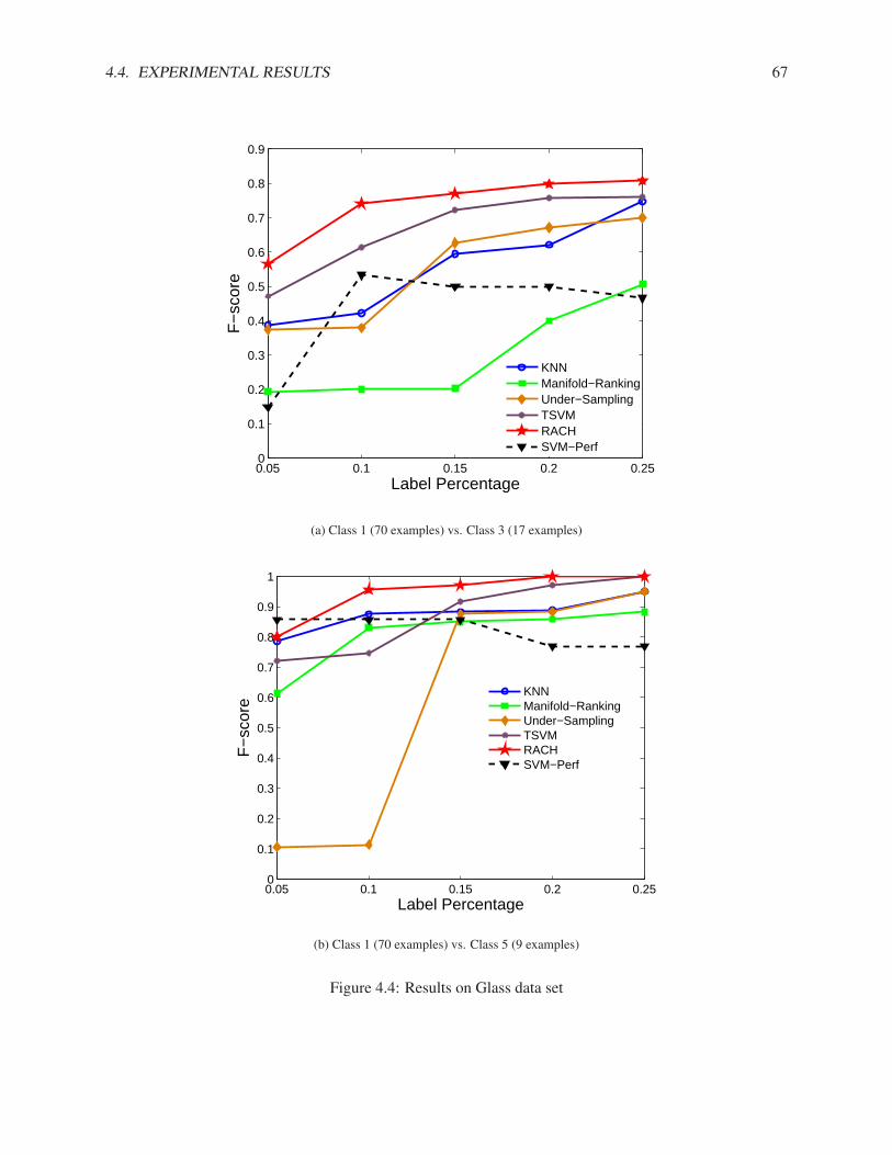
4.4. EXPERIMENTAL RESULTS 67
0.05 0.1 0.15 0.2 0.250
0.1
0.2
0.3
0.4
0.5
0.6
0.7
0.8
0.9
Label Percentage
F−
scor
e
KNNManifold−RankingUnder−SamplingTSVMRACHSVM−Perf
(a) Class 1 (70 examples) vs. Class 3 (17 examples)
0.05 0.1 0.15 0.2 0.250
0.1
0.2
0.3
0.4
0.5
0.6
0.7
0.8
0.9
1
Label Percentage
F−
scor
e
KNNManifold−RankingUnder−SamplingTSVMRACHSVM−Perf
(b) Class 1 (70 examples) vs. Class 5 (9 examples)
Figure 4.4: Results on Glass data set
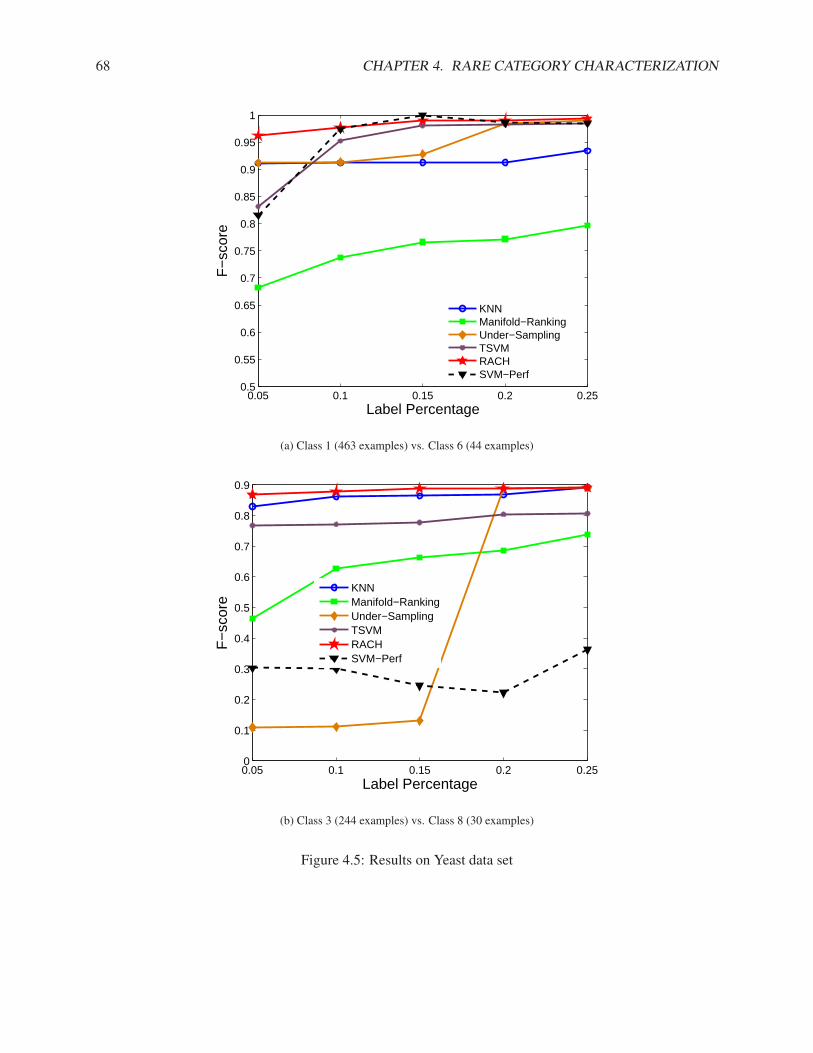
68 CHAPTER 4. RARE CATEGORY CHARACTERIZATION
0.05 0.1 0.15 0.2 0.250.5
0.55
0.6
0.65
0.7
0.75
0.8
0.85
0.9
0.95
1
Label Percentage
F−
scor
e
KNNManifold−RankingUnder−SamplingTSVMRACHSVM−Perf
(a) Class 1 (463 examples) vs. Class 6 (44 examples)
0.05 0.1 0.15 0.2 0.250
0.1
0.2
0.3
0.4
0.5
0.6
0.7
0.8
0.9
Label Percentage
F−
scor
e
KNNManifold−RankingUnder−SamplingTSVMRACHSVM−Perf
(b) Class 3 (244 examples) vs. Class 8 (30 examples)
Figure 4.5: Results on Yeast data set
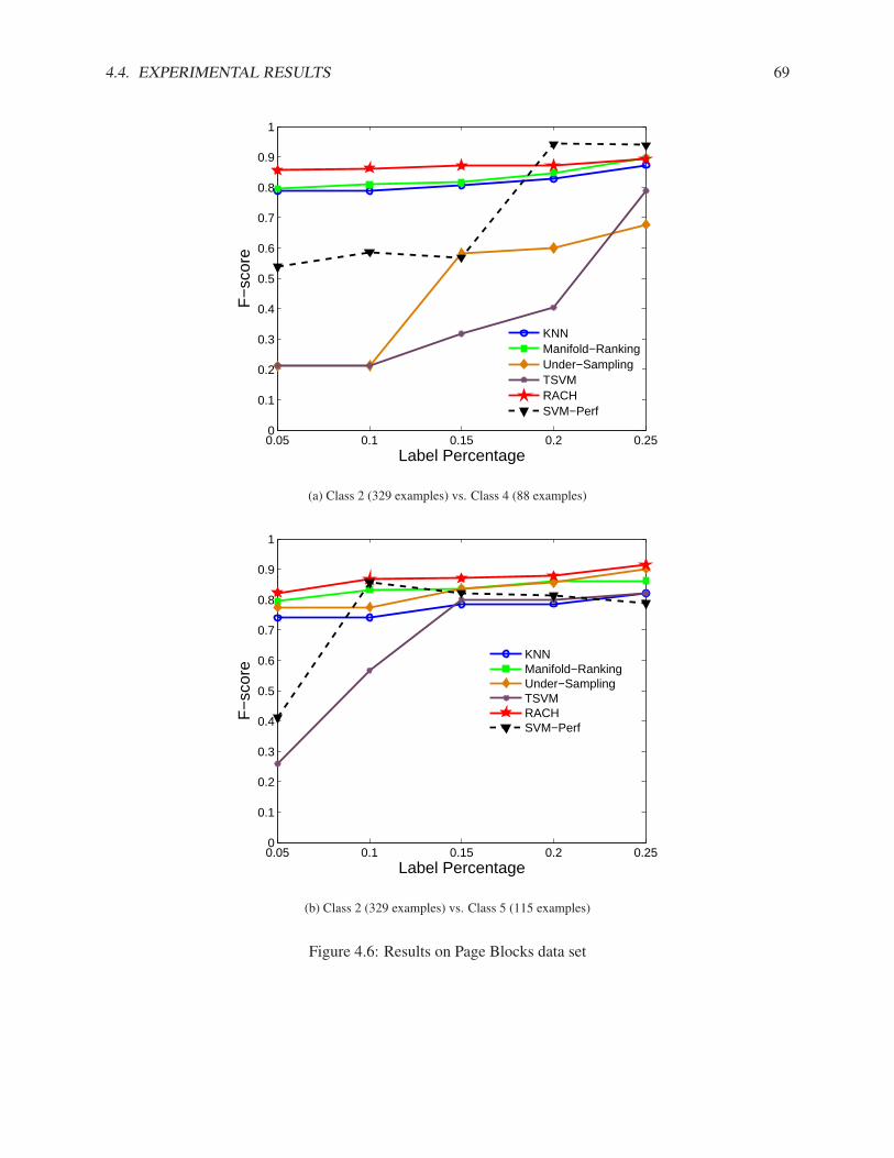
4.4. EXPERIMENTAL RESULTS 69
0.05 0.1 0.15 0.2 0.250
0.1
0.2
0.3
0.4
0.5
0.6
0.7
0.8
0.9
1
Label Percentage
F−
scor
e
KNNManifold−RankingUnder−SamplingTSVMRACHSVM−Perf
(a) Class 2 (329 examples) vs. Class 4 (88 examples)
0.05 0.1 0.15 0.2 0.250
0.1
0.2
0.3
0.4
0.5
0.6
0.7
0.8
0.9
1
Label Percentage
F−
scor
e
KNNManifold−RankingUnder−SamplingTSVMRACHSVM−Perf
(b) Class 2 (329 examples) vs. Class 5 (115 examples)
Figure 4.6: Results on Page Blocks data set
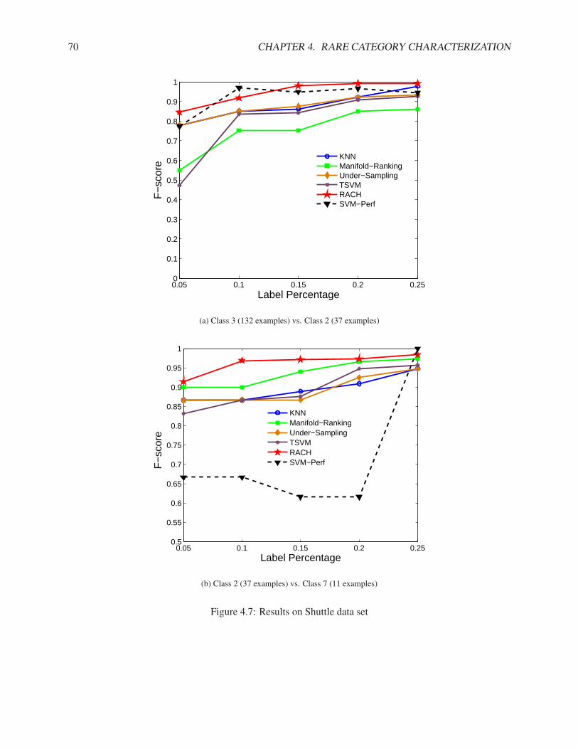
70 CHAPTER 4. RARE CATEGORY CHARACTERIZATION
0.05 0.1 0.15 0.2 0.250
0.1
0.2
0.3
0.4
0.5
0.6
0.7
0.8
0.9
1
Label Percentage
F−
scor
e
KNNManifold−RankingUnder−SamplingTSVMRACHSVM−Perf
(a) Class 3 (132 examples) vs. Class 2 (37 examples)
0.05 0.1 0.15 0.2 0.250.5
0.55
0.6
0.65
0.7
0.75
0.8
0.85
0.9
0.95
1
Label Percentage
F−
scor
e
KNNManifold−RankingUnder−SamplingTSVMRACHSVM−Perf
(b) Class 2 (37 examples) vs. Class 7 (11 examples)
Figure 4.7: Results on Shuttle data set
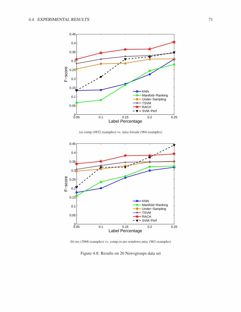
4.4. EXPERIMENTAL RESULTS 71
0.05 0.1 0.15 0.2 0.250
0.05
0.1
0.15
0.2
0.25
0.3
0.35
0.4
0.45
Label Percentage
F−
scor
e
KNNManifold−RankingUnder−SamplingTSVMRACHSVM−Perf
(a) comp (4852 examples) vs. misc.forsale (964 examples)
0.05 0.1 0.15 0.2 0.250
0.05
0.1
0.15
0.2
0.25
0.3
0.35
0.4
0.45
Label Percentage
F−
scor
e
KNNManifold−RankingUnder−SamplingTSVMRACHSVM−Perf
(b) rec (3968 examples) vs. comp.os.ms-windows.misc (963 examples)
Figure 4.8: Results on 20 Newsgroups data set

72 CHAPTER 4. RARE CATEGORY CHARACTERIZATION
4.5 Summary of Rare Category Characterization
In this chapter, we have discussed about our work on rare category characterization. It follows the task ofrare category detection, and makes use of labeled data from all the classes to find a compact representationfor the minority classes. The goal is to identify all the rare examples in the data set. Different from the largeamount of work on imbalanced classification, we target the challenging cases where the support regionsof the majority and minority classes overlap with each other in the feature space, take advantage of theclustering property of the minority classes, and find a compact representation for these classes.
In our algorithm, the basic idea is to enclose the rare examples with a minimum-radius hyper-ball basedon the clustering property of the minority classes. We formulate this idea as an optimization problem andpresent the effective optimization algorithm RACH to find its solution. In RACH, we repeatedly (1) convertthe original problem into a convex optimization problem, and (2) solve it in its dual form by a projectedsubgradient method. Furthermore, we generalize RACH to the high-dimensional feature space induced bykernels. Experimental results demonstrate the effectiveness of the proposed RACH.
Chapter 5
Unsupervised Rare Category Analysis
In this chapter, we focus on unsupervised rare category analysis, i.e., no label information is available in thelearning process, and address the following two problems: (1) rare category selection, i.e., selecting a set ofexamples which are likely to come from the minority class; (2) feature selection, i.e., selecting the featuresthat are relevant to identify the minority class.
The key observation is that the above two tasks are correlated with each other. On one hand, the analysisof the minority class examples helps us identify the relevant features; on the other hand, the identificationof the relevant features is crucial to the selection of the minority class examples. Therefore, we propose tojointly deal with the two tasks so that they can benefit from each other. To this end, we formulate the problemas a well justified optimization framework, which co-selects the relevant features and the examples from theminority class. Furthermore, we design an effective search procedure based on augmented Lagrangianmethod. The basic idea is to alternatively find the relevant features and the minority class examples. Finally,we demonstrate the performance of the proposed method by extensive experimental results.
The main contributions of this chapter can be summarized as follows.
Problem Definition. To the best of our knowledge, we are the first to address the two important tasksin unsupervised rare category analysis; and we propose to jointly deal with them;
Problem Formulation. We design an optimization framework for the co-selection of features andexamples, which is well justified theoretically;
Search Procedure. We develop an effective algorithm to solve the optimization problem which isbased on augmented Lagrangian.
The rest of this chapter is organized as follows. In Section 5.1, we present the optimization frameworkwith theoretical justification. Section 5.2 introduces the algorithm for solving the optimization problem.Experimental results are given in Section 5.3. Finally, we conclude this chapter with a brief summary inSection 5.4.
5.1 Optimization Framework
In this chapter, we focus on the binary case, i.e., one majority class and one minority class, and our goal isto (1) select a set of examples which are likely to come from the minority class, and (2) identify the featuresrelevant to this minority class. In this section, we formulate this problem as an optimization framework, andprovide some theoretical justification.
73
74 CHAPTER 5. UNSUPERVISED RARE CATEGORY ANALYSIS
5.1.1 Additional Notation
In this chapter, we are dealing with the binary cases, i.e., m = 2. Therefore, p1 = 1 − p2. Furthermore,of the d features, only dr features are relevant to the minority class. In other words, the examples from theminority class have very similar values on those features, and their values on the other features may be quitediverse. For the sake of simplicity, assume that the dr features are independent to each other. Therefore,the examples from the minority class are tightly clustered in the dr-dimensional subspace spanned by therelevant features, which we call the relevant subspace.
Let Sdr denote the set of all dr-dimensional subspaces of Rd, and let Smin denote the relevant sub-space, Smin ∈ Sdr . Let f(x) denote the probability density function (pdf) of the data in Rd, i.e., f(x) =(1 − p2)f1(x) + p2f2(x), where f1(x) and f2(x) are the pdf of the majority and minority classes in Rd
respectively. Given feature subspace S ∈ Sdr and x ∈ Rd, let x(S) denote the projection of x on S, andf (S)(x(S)), f
(S)1 (x(S)) and f
(S)2 (x(S)) denote the projection of f(x), f1(x) and f2(x) on S respectively.
To co-select the minority class examples and the relevant features, we define two vectors: a ∈ Rn andb ∈ Rd. Let ai and bj denote the ith and jth elements of a and b respectively. ai = 1 if xi is from theminority class, and 0 otherwise; bj = 1 if the jth feature is relevant to the minority class, and 0 otherwise.
5.1.2 Objective Function
Given the prior p2 of the minority class and the number of relevant features dr, we hope to find np2 datapoints whose corresponding ai = 1, and dr features whose corresponding bj = 1. Intuitively, the np2 pointsshould form a compact cluster in the relevant subspace, and due to the characteristic of the minority class,this cluster should be more compact than any other np2 data points in any dr-dimensional subspace. To bemore strict, we have the following optimization problem.
Problem 5.1
min f(a, b) =1
np2
n∑
i=1
n∑
k=1
aiak(d∑
j=1
bj(xji − xj
k)2)
s.t.,n∑
i=1
ai = np2, ai = 0, 1
d∑
j=1
bj = dr, bj = 0, 1
In the objective function f(a, b),∑d
j=1 bj(xji − xj
k)2 is the squared distance between xi and xk in the
subspace Sb spanned by the features with non-zero bj . This squared distance contributes to f(a, b) if andonly if both ai and ak are equal to 1. Given a set of np2 points, define the set distance of every data pointto be the sum of the squared distances between this point and all the points within this set. Therefore, bysolving this optimization problem, we aim to find a set of np2 points and dr features such that the averageset distance of these points to this set in the corresponding subspace Sb is the minimum.
Problem 5.1 can be easily applied to the case where either a or b is known, and we want to solve forthe other vector. To be specific, if a is known, i.e., we know the examples that belong to the minority class,and we want to find the dr-dimensional subspace where the minority class can be best characterized, we canuse the same objective function f(a, b), and solve for b using the minority class examples. Similarly, if b isknown, i.e., we know which features are relevant to the minority class, and we want to find the examplesfrom the minority class, we can also use f(a, b), and solve for a in the subspace Sb spanned by the relevantfeatures.
5.1. OPTIMIZATION FRAMEWORK 75
5.1.3 Justification
The optimization problem we introduced in the last subsection is reasonable intuitively. Next, we look at itfrom a theoretical perspective.
∀S ∈ Sdr , define function ψS as follows. ∀S ∈ Sdr , x ∈ Rd, let ψS(x(S)) = minDnp2⊂D,|Dnp2 |=np2
1np2∑
y∈Dnp2‖x(S) − y(S)‖2 = 1
np2
∑np2i=1 ‖x(S) − z
(i)
x(S)‖2, where z(i)
x(S) denotes the ith nearest neighbor of
x(S) within x(S)1 , . . . , x
(S)n , i.e., ψS(x(S)) is the average squared distance between x(S) and its np2 nearest
neighbors. Furthermore, define function φS as follows. φS(x(S)) = E(ψS(x(S))). Here, the expectation iswith respect to z
(i)
x(S) , i = 1, . . . , np2.Based on the above definitions, we have the following theorem.
Theorem 7. If1. In Smin, the support region of the minority class is within hyper-ball B of radius r;2. The support region of f in any dr-dimensional subspace is bounded, i.e.,
maxS∈Sdrmaxx,y∈Rd,f (S)(x(S))>0,f (S)(y(S))>0 ‖x(S) − y(S)‖ = α < +∞;
3. The density of the majority class in hyper-ball B is non-zero, i.e.,miny∈Rd,y(Smin)∈B(1− p2)f
(Smin)1 (y(Smin)) = f0 > 0;
4. The function value of φS is big enough if the projection of the data point in the dr-dimensionalsubspace S is not within B, i.e., minS∈Sdr ,x∈Rd,x(S) /∈B φS(x(S))− 4r2 > β > 0;
5. The number of examples is sufficiently large, i.e., n ≥ max{ 12(VBf0)2
log 2δ , α8
4p22β4 log 2Cdr
dδ }, where
VB is the volume of hyper-ball B, and Cdrd is the number of d choose dr;
then with probability at least 1− δ, in the solution to Problem 5.1, the subspace Sb spanned by the featureswith bj = 1 is the relevant subspace Smin, and the data points with ai = 1 are within B.
Proof. The basic idea of the proof is to show that if the selected feature subspace Sb is NOT Smin, or atleast one point in the set of np2 points is outside B in Smin, we can always use Smin, and find another setof np2 points such that all the points are within B, and its objective function is smaller than the original set.To do this, first, notice that according to condition (3), the expected proportion of data points falling insideB, E(nB
n ) ≥ p2 + VBf0, where nB denotes the number of points within B. Second, according to condition
(2), ∀x ∈ D, Pr[0 ≤ ‖x(S) − z(i)
x(s)‖2 ≤ α2] = 1, i = 1, . . . , np2. Therefore,
Pr[nB
n< p2 or ∃x ∈ D, ∃S ∈ Sdr , s.t., ψS(x(S)) < φS(x(S))− β]
≤ Pr[nB
n< p2] + Pr[∃x ∈ D,∃S ∈ Sdr , s.t., ψS(x(S)) < φS(x(S))− β]
≤ Pr[nB
n− E(
nB
n) < −VBf0] + nCdr
d Pr[ψS(x(S)) < φS(x(S))− β]
≤ Pr[nB
n− E(
nB
n) < −VBf0] + nCdr
d
∫
z(np2+1)
x(S)
Pr[ψS(x(S)) < φS(x(S))− β|z(np2+1)
x(S) ]dPr[z(np2+1)
x(S) ]
≤ exp(−2n(VBf0)2) + nCdrd exp(−2np2β
2
α4)
where Cdrd is an upper bound on the number of subspaces in Sdr , and the last inequality is based on Hoeffd-
ing’s inequality1.
1Note that given z(np2+1)
x(S) , ψS(x(S)) can be seen as the average of np2 independent items.
76 CHAPTER 5. UNSUPERVISED RARE CATEGORY ANALYSIS
Let exp(−2n(VBf0)2) ≤ δ2 , and nCdr
d exp(−2np2β2
α4 ) ≤ δ2 , we get n ≥ 1
2(VBf0)2log 2
δ , and n ≥α8
4p22β4 log 2Cdr
dδ . In other words, if the number of examples n is sufficiently large, i.e.,
n ≥ max{ 12(VBf0)2
log2δ,
α8
4p22β
4log
2Cdrd
δ}
then with probability at least 1−δ, there are at least np2 points within hyper-ball B, and ∀x ∈ D, ∀S ∈ Sdr ,ψS(x(S)) ≥ φS(x(S)) − β. Furthermore, according to condition (4), ∀x ∈ D, ∀S ∈ Sdr , if x(S) /∈ B,ψS(x(S)) > 4r2.
Notice that ∀a, ∀b, f(a, b) ≥ ∑i:ai=1 ψSb(x(Sb)
i ). On the other hand, if Sb = Smin, and the points withai = 1 are within B in Smin, then f(a, b) < 4np2r
2. This is because the squared distance between any twopoints within B in Smin is no bigger than 4r2.
Given a and b, if Sb is not Smin, we can design a′ and b′ in such a way that Sb′ is Smin, and thepoints that correspond to a′i = 1 are within B in Smin. We can always find such a vector a′ since wehave shown that there are at least np2 points within B. Therefore, f(a, b) ≥ ∑
i:ai=1 ψSb(x(Sb)i ) >
4np2r2 > f(a′, b′). On the other hand, if Sb is Smin, but at least one point with ai = 1 is outside
B, we can design a′ and b′ in such a way that b′ = b, and a′ replaces the points with ai = 1 that areoutside B with some points within B that are different from existing points in a. For the sake of simplic-ity, assume that only xt is outside B. Therefore, f(a, b) = 1
np2
∑i6=t
∑k 6=t aiak‖x(Smin)
i − x(Smin)k ‖2 +
2np2
∑ni=1 ai‖x(Smin)
i − x(Smin)t ‖2 ≥ 1
np2
∑i 6=t
∑k 6=t aiak‖x(Smin)
i − x(Smin)k ‖2 + 2ψSmin(x(Smin)
t ) >
1np2
∑i6=t
∑k 6=t aiak‖x(Smin)
i − x(Smin)k ‖2 + 8r2 ≥ f(a′, b′). The above derivation can be easily gener-
alized to the case where more than one point with ai = 1 are outside B. Therefore, in the solution toProblem 5.1, Sb is the relevant subspace Smin, and the data points with ai = 1 are within B.
The conditions of Theorem 7 are straight-forward except condition (4). According to this condition,∀S ∈ Sdr , if x(S) /∈ B and y(Smin) ∈ B, φS(x(S)) is bigger than φSmin(y(Smin)) by at least β when thereare at least np2 points within B in Smin. Therefore, this condition can be roughly interpreted as follows.The density around x(S) is smaller than the density around y(Smin) such that the expected average squareddistance between x(S) and its np2 nearest neighbors is much larger than that between y(Smin) and its np2
neighbors. In this way, assuming the other conditions in Theorem 7 are also satisfied, with high probability,we can identify the relevant subspace and pick the examples within B according to a.
It should be pointed out that if we want to select np2 points from the minority class, picking them fromhyper-ball B is the best we can hope for. In this way, each selected example has a certain probability ofcoming from the minority class. On the other hand, if some selected points are outside B, their probabilityof coming from the minority class is 0.
5.2 Partial Augmented Lagrangian Method
In this section, we introduce the Partial Augmented Lagrangian Method (PALM) to effectively solve Problem4.1. In our method, we alternate the optimization of a and b, i.e., given the current estimate of a, we solvefor b that leads to the minimum value of f(a, b); given the current estimate of b, we solve for a that decreasesthe value of f(a, b) as much as possible.
To be specific, f(a, b) can be rewritten as f(a, b) =∑d
j=1 bj∑n
i=1
∑nk=1
1np2
aiak(xji−xj
k)2. Therefore,
given a, we can solve for b as follows. For each feature j, calculate its score saj = 1
np2
∑ni=1
∑nk=1 aiak(x
ji−
xjk)
2. Then find the dr features with the smallest scores, and set their corresponding bj = 1. It is easy to
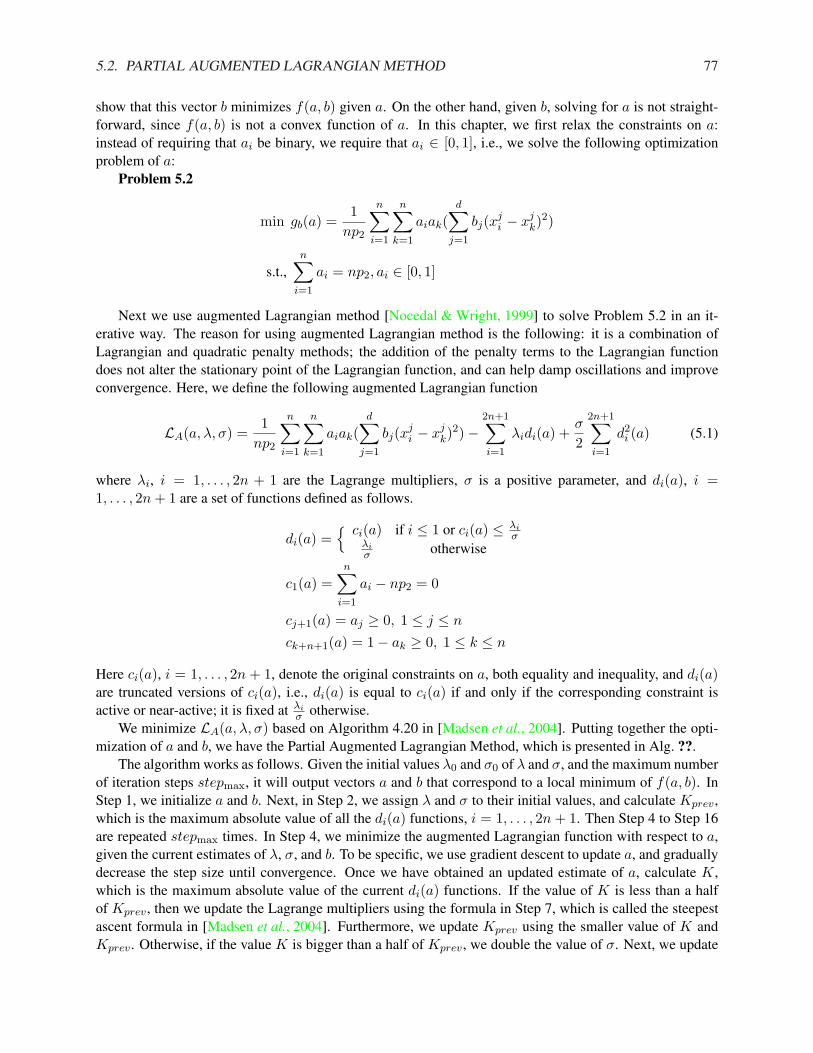
5.2. PARTIAL AUGMENTED LAGRANGIAN METHOD 77
show that this vector b minimizes f(a, b) given a. On the other hand, given b, solving for a is not straight-forward, since f(a, b) is not a convex function of a. In this chapter, we first relax the constraints on a:instead of requiring that ai be binary, we require that ai ∈ [0, 1], i.e., we solve the following optimizationproblem of a:
Problem 5.2
min gb(a) =1
np2
n∑
i=1
n∑
k=1
aiak(d∑
j=1
bj(xji − xj
k)2)
s.t.,n∑
i=1
ai = np2, ai ∈ [0, 1]
Next we use augmented Lagrangian method [Nocedal & Wright, 1999] to solve Problem 5.2 in an it-erative way. The reason for using augmented Lagrangian method is the following: it is a combination ofLagrangian and quadratic penalty methods; the addition of the penalty terms to the Lagrangian functiondoes not alter the stationary point of the Lagrangian function, and can help damp oscillations and improveconvergence. Here, we define the following augmented Lagrangian function
LA(a, λ, σ) =1
np2
n∑
i=1
n∑
k=1
aiak(d∑
j=1
bj(xji − xj
k)2)−
2n+1∑
i=1
λidi(a) +σ
2
2n+1∑
i=1
d2i (a) (5.1)
where λi, i = 1, . . . , 2n + 1 are the Lagrange multipliers, σ is a positive parameter, and di(a), i =1, . . . , 2n + 1 are a set of functions defined as follows.
di(a) ={ ci(a) if i ≤ 1 or ci(a) ≤ λi
σλiσ otherwise
c1(a) =n∑
i=1
ai − np2 = 0
cj+1(a) = aj ≥ 0, 1 ≤ j ≤ n
ck+n+1(a) = 1− ak ≥ 0, 1 ≤ k ≤ n
Here ci(a), i = 1, . . . , 2n + 1, denote the original constraints on a, both equality and inequality, and di(a)are truncated versions of ci(a), i.e., di(a) is equal to ci(a) if and only if the corresponding constraint isactive or near-active; it is fixed at λi
σ otherwise.We minimize LA(a, λ, σ) based on Algorithm 4.20 in [Madsen et al., 2004]. Putting together the opti-
mization of a and b, we have the Partial Augmented Lagrangian Method, which is presented in Alg. ??.The algorithm works as follows. Given the initial values λ0 and σ0 of λ and σ, and the maximum number
of iteration steps stepmax, it will output vectors a and b that correspond to a local minimum of f(a, b). InStep 1, we initialize a and b. Next, in Step 2, we assign λ and σ to their initial values, and calculate Kprev,which is the maximum absolute value of all the di(a) functions, i = 1, . . . , 2n + 1. Then Step 4 to Step 16are repeated stepmax times. In Step 4, we minimize the augmented Lagrangian function with respect to a,given the current estimates of λ, σ, and b. To be specific, we use gradient descent to update a, and graduallydecrease the step size until convergence. Once we have obtained an updated estimate of a, calculate K,which is the maximum absolute value of the current di(a) functions. If the value of K is less than a halfof Kprev, then we update the Lagrange multipliers using the formula in Step 7, which is called the steepestascent formula in [Madsen et al., 2004]. Furthermore, we update Kprev using the smaller value of K andKprev. Otherwise, if the value K is bigger than a half of Kprev, we double the value of σ. Next, we update
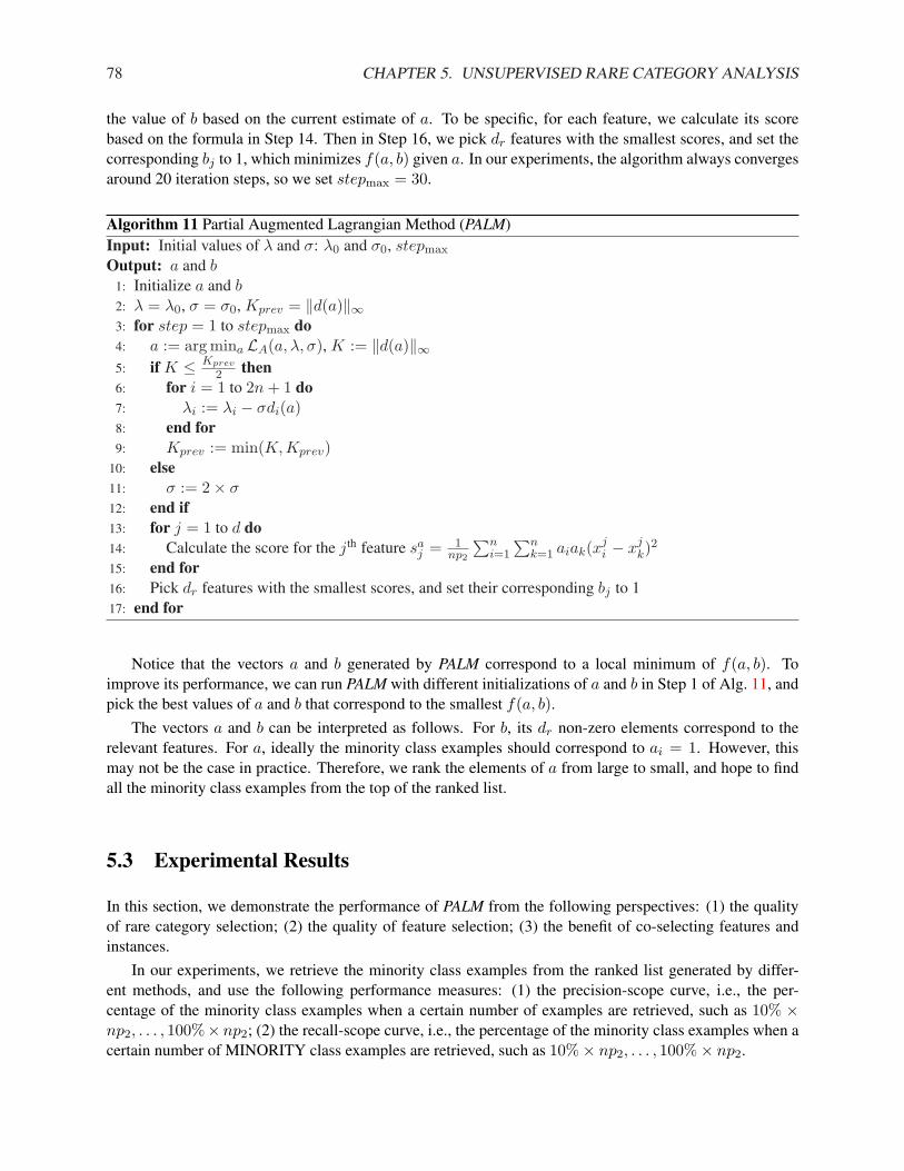
78 CHAPTER 5. UNSUPERVISED RARE CATEGORY ANALYSIS
the value of b based on the current estimate of a. To be specific, for each feature, we calculate its scorebased on the formula in Step 14. Then in Step 16, we pick dr features with the smallest scores, and set thecorresponding bj to 1, which minimizes f(a, b) given a. In our experiments, the algorithm always convergesaround 20 iteration steps, so we set stepmax = 30.
Algorithm 11 Partial Augmented Lagrangian Method (PALM)Input: Initial values of λ and σ: λ0 and σ0, stepmax
Output: a and b1: Initialize a and b2: λ = λ0, σ = σ0, Kprev = ‖d(a)‖∞3: for step = 1 to stepmax do4: a := arg mina LA(a, λ, σ), K := ‖d(a)‖∞5: if K ≤ Kprev
2 then6: for i = 1 to 2n + 1 do7: λi := λi − σdi(a)8: end for9: Kprev := min(K, Kprev)
10: else11: σ := 2× σ12: end if13: for j = 1 to d do14: Calculate the score for the jth feature sa
j = 1np2
∑ni=1
∑nk=1 aiak(x
ji − xj
k)2
15: end for16: Pick dr features with the smallest scores, and set their corresponding bj to 117: end for
Notice that the vectors a and b generated by PALM correspond to a local minimum of f(a, b). Toimprove its performance, we can run PALM with different initializations of a and b in Step 1 of Alg. 11, andpick the best values of a and b that correspond to the smallest f(a, b).
The vectors a and b can be interpreted as follows. For b, its dr non-zero elements correspond to therelevant features. For a, ideally the minority class examples should correspond to ai = 1. However, thismay not be the case in practice. Therefore, we rank the elements of a from large to small, and hope to findall the minority class examples from the top of the ranked list.
5.3 Experimental Results
In this section, we demonstrate the performance of PALM from the following perspectives: (1) the qualityof rare category selection; (2) the quality of feature selection; (3) the benefit of co-selecting features andinstances.
In our experiments, we retrieve the minority class examples from the ranked list generated by differ-ent methods, and use the following performance measures: (1) the precision-scope curve, i.e., the per-centage of the minority class examples when a certain number of examples are retrieved, such as 10% ×np2, . . . , 100%×np2; (2) the recall-scope curve, i.e., the percentage of the minority class examples when acertain number of MINORITY class examples are retrieved, such as 10%× np2, . . . , 100%× np2.
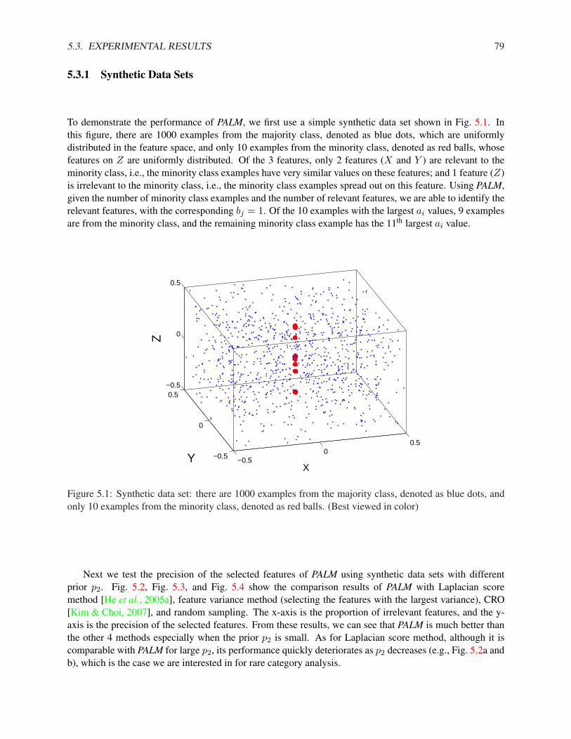
5.3. EXPERIMENTAL RESULTS 79
5.3.1 Synthetic Data Sets
To demonstrate the performance of PALM, we first use a simple synthetic data set shown in Fig. 5.1. Inthis figure, there are 1000 examples from the majority class, denoted as blue dots, which are uniformlydistributed in the feature space, and only 10 examples from the minority class, denoted as red balls, whosefeatures on Z are uniformly distributed. Of the 3 features, only 2 features (X and Y ) are relevant to theminority class, i.e., the minority class examples have very similar values on these features; and 1 feature (Z)is irrelevant to the minority class, i.e., the minority class examples spread out on this feature. Using PALM,given the number of minority class examples and the number of relevant features, we are able to identify therelevant features, with the corresponding bj = 1. Of the 10 examples with the largest ai values, 9 examplesare from the minority class, and the remaining minority class example has the 11th largest ai value.
−0.50
0.5
−0.5
0
0.5−0.5
0
0.5
XY
Z
Figure 5.1: Synthetic data set: there are 1000 examples from the majority class, denoted as blue dots, andonly 10 examples from the minority class, denoted as red balls. (Best viewed in color)
Next we test the precision of the selected features of PALM using synthetic data sets with differentprior p2. Fig. 5.2, Fig. 5.3, and Fig. 5.4 show the comparison results of PALM with Laplacian scoremethod [He et al., 2005a], feature variance method (selecting the features with the largest variance), CRO[Kim & Choi, 2007], and random sampling. The x-axis is the proportion of irrelevant features, and the y-axis is the precision of the selected features. From these results, we can see that PALM is much better thanthe other 4 methods especially when the prior p2 is small. As for Laplacian score method, although it iscomparable with PALM for large p2, its performance quickly deteriorates as p2 decreases (e.g., Fig. 5.2a andb), which is the case we are interested in for rare category analysis.
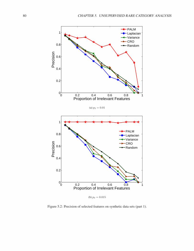
80 CHAPTER 5. UNSUPERVISED RARE CATEGORY ANALYSIS
0 0.2 0.4 0.6 0.8 10
0.2
0.4
0.6
0.8
1
Proportion of Irrelevant Features
Pre
cisi
on
PALMLaplacianVarianceCRORandom
(a) p2 = 0.01
0 0.2 0.4 0.6 0.8 10
0.2
0.4
0.6
0.8
1
Proportion of Irrelevant Features
Pre
cisi
on
PALMLaplacianVarianceCRORandom
(b) p2 = 0.015
Figure 5.2: Precision of selected features on synthetic data sets (part 1).
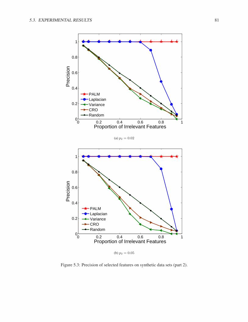
5.3. EXPERIMENTAL RESULTS 81
0 0.2 0.4 0.6 0.8 10
0.2
0.4
0.6
0.8
1
Proportion of Irrelevant Features
Pre
cisi
on
PALMLaplacianVarianceCRORandom
(a) p2 = 0.02
0 0.2 0.4 0.6 0.8 10
0.2
0.4
0.6
0.8
1
Proportion of Irrelevant Features
Pre
cisi
on
PALMLaplacianVarianceCRORandom
(b) p2 = 0.05
Figure 5.3: Precision of selected features on synthetic data sets (part 2).
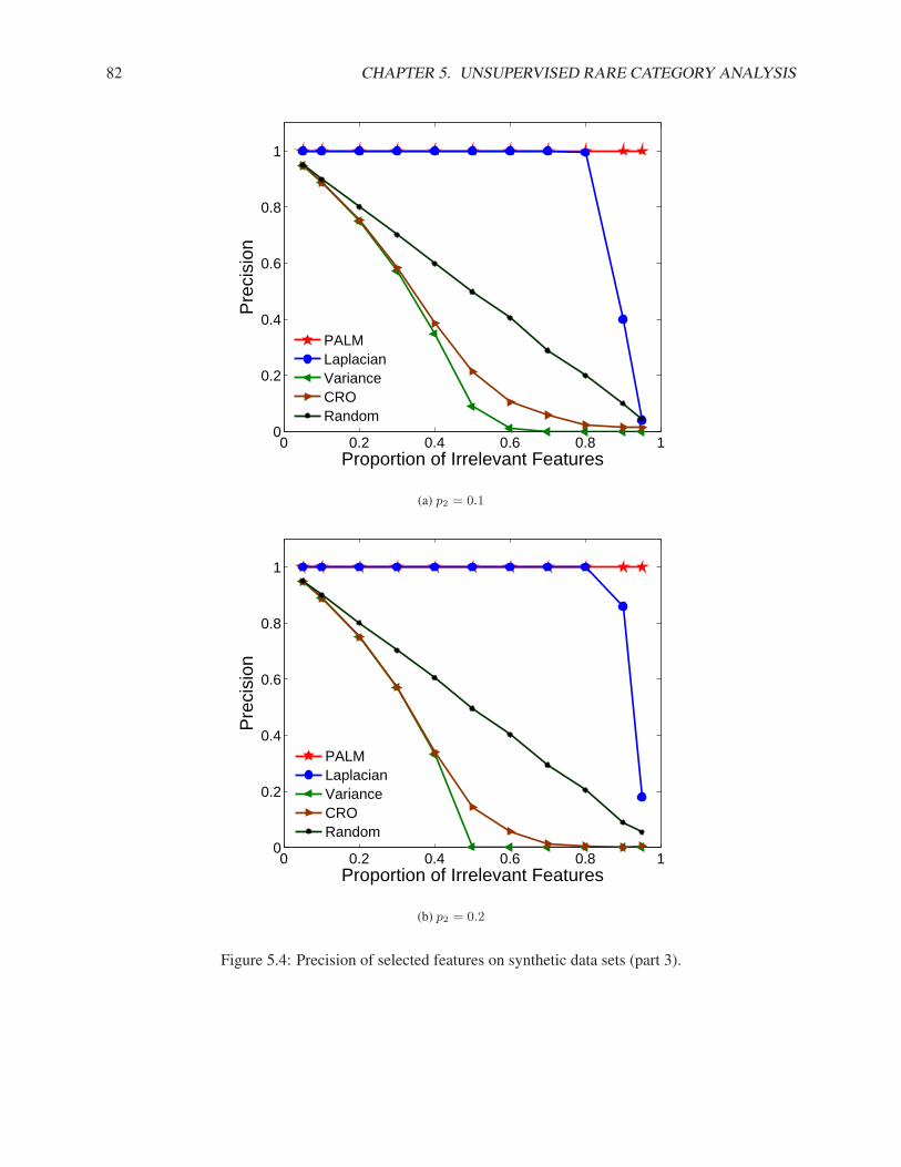
82 CHAPTER 5. UNSUPERVISED RARE CATEGORY ANALYSIS
0 0.2 0.4 0.6 0.8 10
0.2
0.4
0.6
0.8
1
Proportion of Irrelevant Features
Pre
cisi
on
PALMLaplacianVarianceCRORandom
(a) p2 = 0.1
0 0.2 0.4 0.6 0.8 10
0.2
0.4
0.6
0.8
1
Proportion of Irrelevant Features
Pre
cisi
on
PALMLaplacianVarianceCRORandom
(b) p2 = 0.2
Figure 5.4: Precision of selected features on synthetic data sets (part 3).

5.3. EXPERIMENTAL RESULTS 83
5.3.2 Real Data Sets
In this subsection, we test the performance of PALM on rare category selection. To the best of our knowledge,there are no existing methods for this task. Therefore, we have designed the following methods for the sakeof comparison.
1. Random: randomly rank all the examples, and select the first np2 points from the ranked list as theminority class examples.
2. NNDB-based: calculate the score of each example using NNDB [He & Carbonell, 2007]. Note thatno feedback from the labeling oracle is available, so the scores are not updated.
3. Interleave-based: calculate the score of each example using the Interleave principle [Pelleg & Moore, 2004].Similar as the NNDB-based method, the scores of the examples are not updated in this method.
4. PALM-full: assume that all the features are relevant to the minority class, i.e., bj = 1, j = 1, . . . , d,and run PALM with dr = d.
Note that NNDB-based method and Interleave-based method are both derived from rare category detectionmethods.
Here we use 4 real data sets, which are summarized in Table 5.1. In this chapter, we focus on binaryproblems, i.e., there is only one majority class and one minority class in the data set. Therefore, for eachdata set, we construct several subproblems as follows. We combine the examples from two different classesinto a smaller binary data set, using the larger class as the majority class, the smaller class as the minorityclass, and test the different methods on these binary data sets. For PALM, we tune the number of relevantfeatures dr without any label information. For each data set, we present the results on 2 binary subproblems,which are shown in Fig. 5.5 to Fig. 5.12. On the other binary subproblems, similar results are observed andtherefore omitted for space. In these figures, the left figure shows precision vs. scope, and the right figureshows recall vs. scope.
On all the data sets, PALM performs the best: the precision and recall sometimes reach 100%, suchas Fig. 5.10 and Fig. 5.11. As for the other methods (Interleave-based, NNDB-based, and PALM-full),their performance depends on different data sets, and none of them is consistently better than Random.Comparing with Random, Interleave-based, and NNDB-based, we can see that PALM does a better job atselecting the minority class examples; comparing with PALM-full, we can see that the features selected byPALM indeed help improve the performance of rare category selection.
Notice that in some figures (Fig. 5.5b, Fig. 5.6b, Fig. 5.7b, Fig. 5.9b, and Fig. 5.10b), at the end of therecall curves, the different methods seem to overlap with each other. This is because with no supervision,it is sometimes difficult to retrieve all the examples from the minority class, and the last example from theminority class tends to appear towards the end of the ranked list. Therefore, the recall value at 100%np2 isoften close to the prior of the minority class in the data set.
Table 5.1: Properties of the data sets [Asuncion & Newman, 2007] used.DATA SET n d LARGEST CLASS SMALLEST CLASS
ECOLI 336 7 42.56% 2.68%GLASS 214 9 35.51% 4.21%
ABALONE 4177 7 16.50% 0.34%YEAST 1484 8 31.20% 1.68%
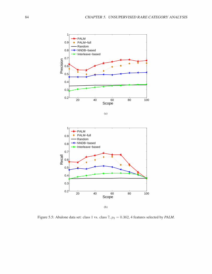
84 CHAPTER 5. UNSUPERVISED RARE CATEGORY ANALYSIS
20 40 60 80 1000.2
0.3
0.4
0.5
0.6
0.7
0.8
0.9
1
Scope
Pre
cisi
on
PALMPALM−fullRandomNNDB−basedInterleave−based
(a)
20 40 60 80 1000.2
0.3
0.4
0.5
0.6
0.7
0.8
0.9
1
Scope
Rec
all
PALMPALM−fullRandomNNDB−basedInterleave−based
(b)
Figure 5.5: Abalone data set: class 1 vs. class 7, p2 = 0.362, 4 features selected by PALM.
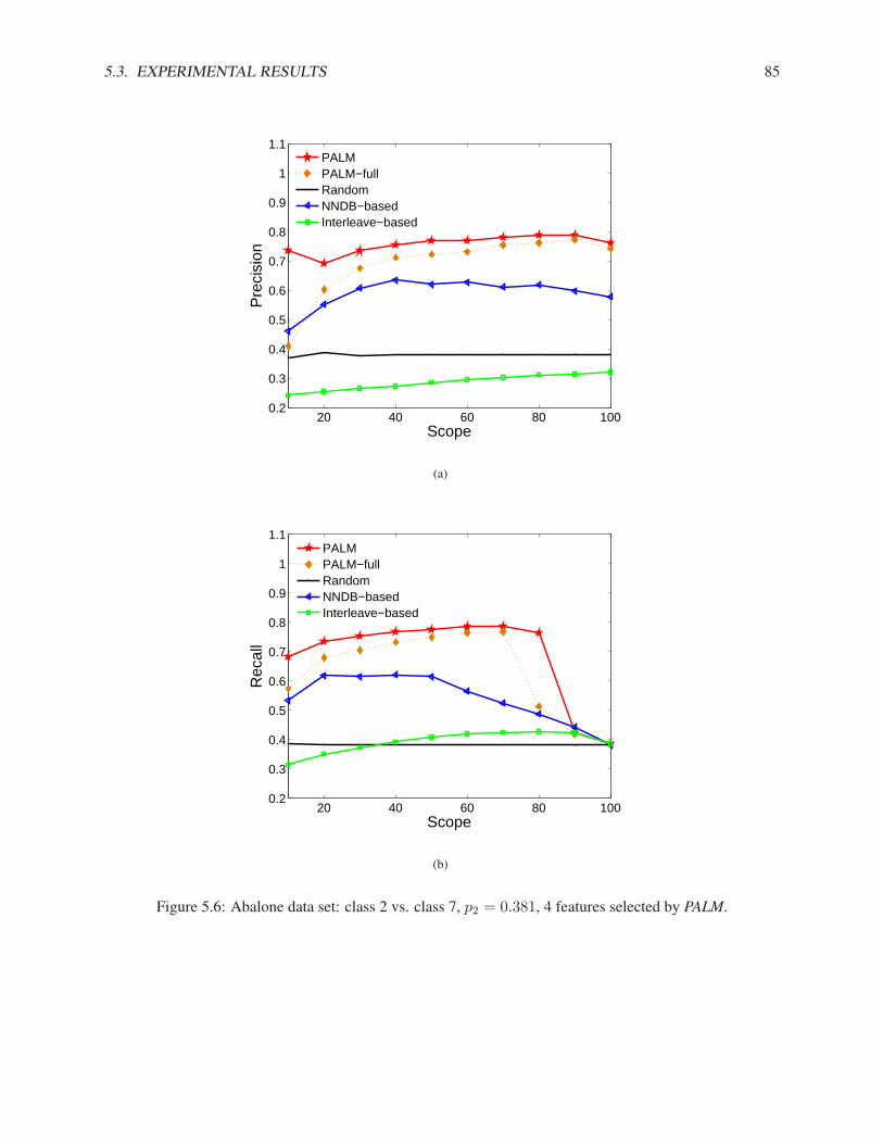
5.3. EXPERIMENTAL RESULTS 85
20 40 60 80 1000.2
0.3
0.4
0.5
0.6
0.7
0.8
0.9
1
1.1
Scope
Pre
cisi
on
PALMPALM−fullRandomNNDB−basedInterleave−based
(a)
20 40 60 80 1000.2
0.3
0.4
0.5
0.6
0.7
0.8
0.9
1
1.1
Scope
Rec
all
PALMPALM−fullRandomNNDB−basedInterleave−based
(b)
Figure 5.6: Abalone data set: class 2 vs. class 7, p2 = 0.381, 4 features selected by PALM.
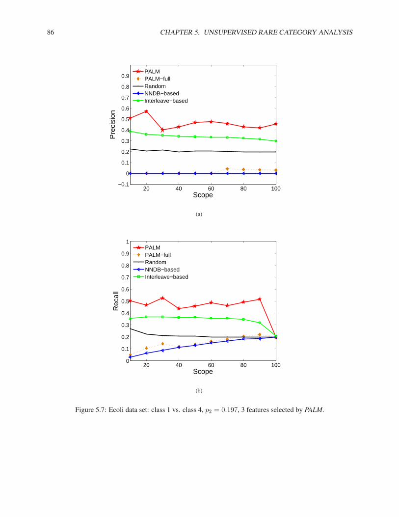
86 CHAPTER 5. UNSUPERVISED RARE CATEGORY ANALYSIS
20 40 60 80 100−0.1
0
0.1
0.2
0.3
0.4
0.5
0.6
0.7
0.8
0.9
Scope
Pre
cisi
on
PALMPALM−fullRandomNNDB−basedInterleave−based
(a)
20 40 60 80 1000
0.1
0.2
0.3
0.4
0.5
0.6
0.7
0.8
0.9
1
Scope
Rec
all
PALMPALM−fullRandomNNDB−basedInterleave−based
(b)
Figure 5.7: Ecoli data set: class 1 vs. class 4, p2 = 0.197, 3 features selected by PALM.
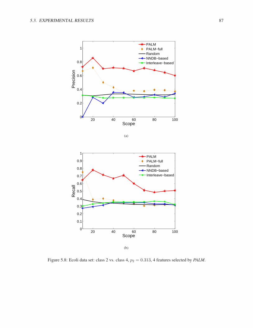
5.3. EXPERIMENTAL RESULTS 87
20 40 60 80 1000
0.2
0.4
0.6
0.8
1
Scope
Pre
cisi
on
PALMPALM−fullRandomNNDB−basedInterleave−based
(a)
20 40 60 80 1000
0.1
0.2
0.3
0.4
0.5
0.6
0.7
0.8
0.9
1
Scope
Rec
all
PALMPALM−fullRandomNNDB−basedInterleave−based
(b)
Figure 5.8: Ecoli data set: class 2 vs. class 4, p2 = 0.313, 4 features selected by PALM.
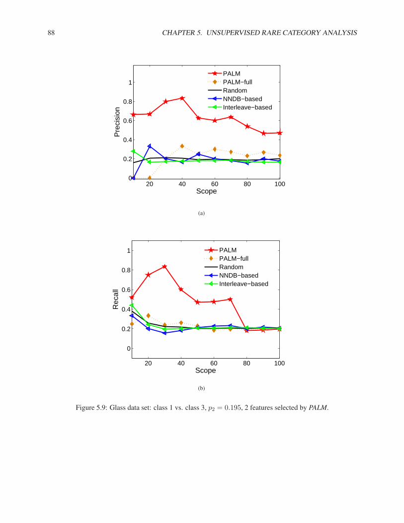
88 CHAPTER 5. UNSUPERVISED RARE CATEGORY ANALYSIS
20 40 60 80 1000
0.2
0.4
0.6
0.8
1
Scope
Pre
cisi
on
PALMPALM−fullRandomNNDB−basedInterleave−based
(a)
20 40 60 80 100
0
0.2
0.4
0.6
0.8
1
Scope
Rec
all
PALMPALM−fullRandomNNDB−basedInterleave−based
(b)
Figure 5.9: Glass data set: class 1 vs. class 3, p2 = 0.195, 2 features selected by PALM.
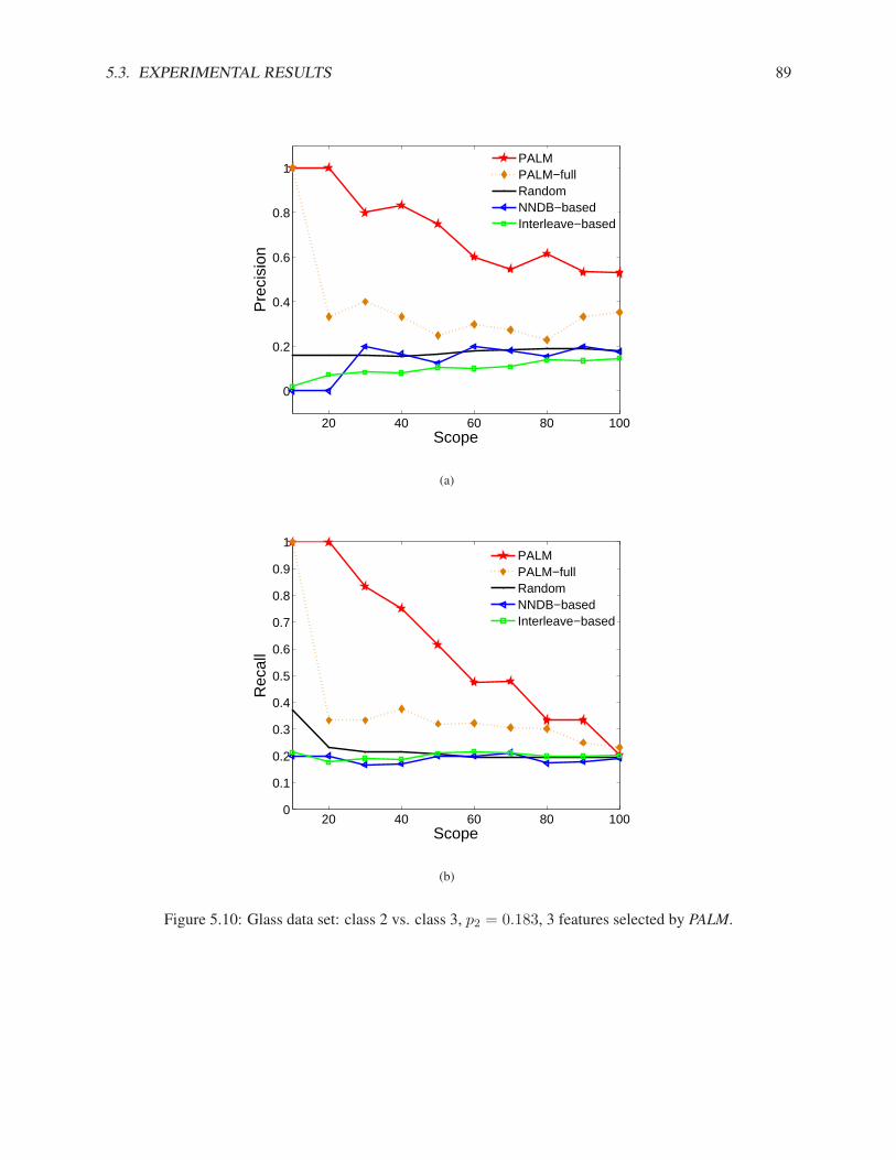
5.3. EXPERIMENTAL RESULTS 89
20 40 60 80 100
0
0.2
0.4
0.6
0.8
1
Scope
Pre
cisi
on
PALMPALM−fullRandomNNDB−basedInterleave−based
(a)
20 40 60 80 1000
0.1
0.2
0.3
0.4
0.5
0.6
0.7
0.8
0.9
1
Scope
Rec
all
PALMPALM−fullRandomNNDB−basedInterleave−based
(b)
Figure 5.10: Glass data set: class 2 vs. class 3, p2 = 0.183, 3 features selected by PALM.
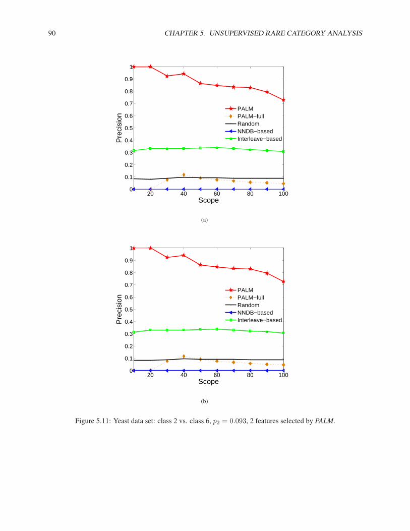
90 CHAPTER 5. UNSUPERVISED RARE CATEGORY ANALYSIS
20 40 60 80 1000
0.1
0.2
0.3
0.4
0.5
0.6
0.7
0.8
0.9
1
Scope
Pre
cisi
on
PALMPALM−fullRandomNNDB−basedInterleave−based
(a)
20 40 60 80 1000
0.1
0.2
0.3
0.4
0.5
0.6
0.7
0.8
0.9
1
Scope
Pre
cisi
on
PALMPALM−fullRandomNNDB−basedInterleave−based
(b)
Figure 5.11: Yeast data set: class 2 vs. class 6, p2 = 0.093, 2 features selected by PALM.
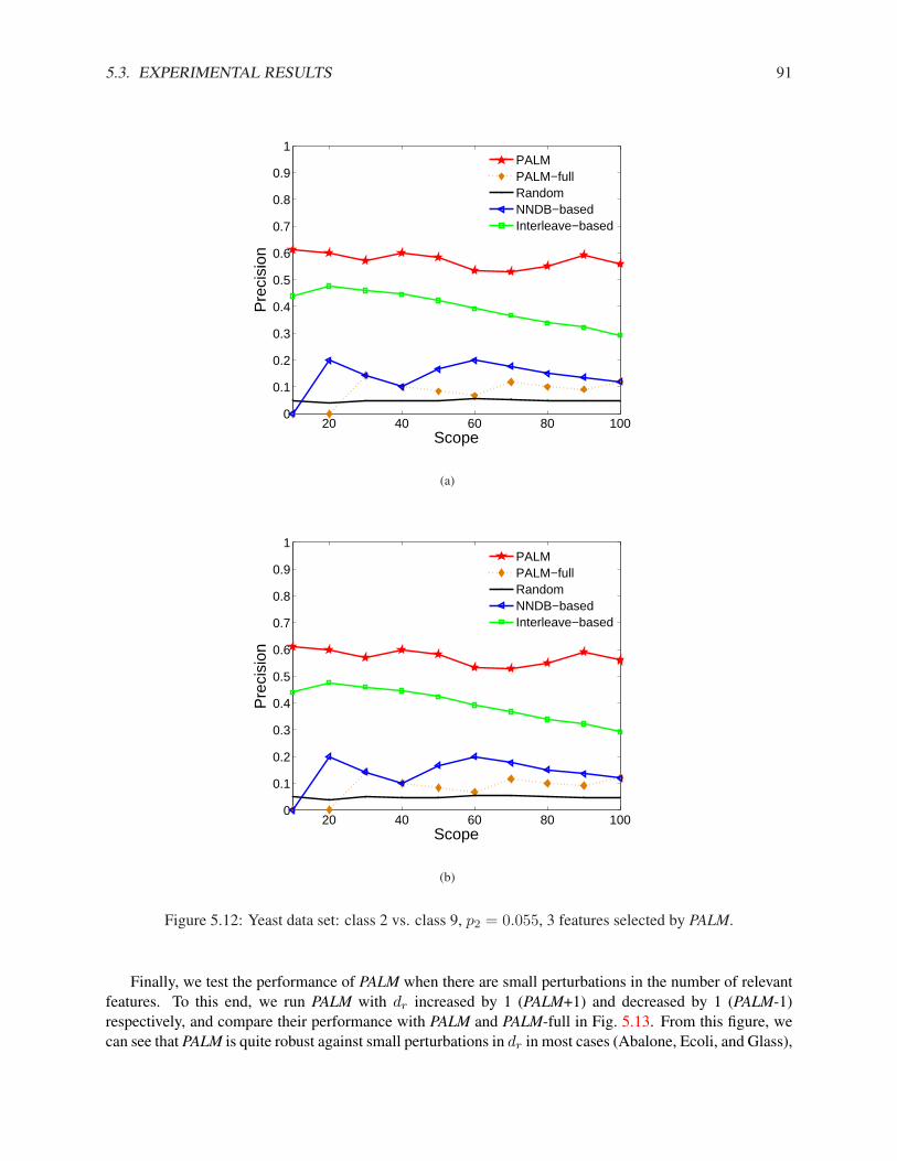
5.3. EXPERIMENTAL RESULTS 91
20 40 60 80 1000
0.1
0.2
0.3
0.4
0.5
0.6
0.7
0.8
0.9
1
Scope
Pre
cisi
on
PALMPALM−fullRandomNNDB−basedInterleave−based
(a)
20 40 60 80 1000
0.1
0.2
0.3
0.4
0.5
0.6
0.7
0.8
0.9
1
Scope
Pre
cisi
on
PALMPALM−fullRandomNNDB−basedInterleave−based
(b)
Figure 5.12: Yeast data set: class 2 vs. class 9, p2 = 0.055, 3 features selected by PALM.
Finally, we test the performance of PALM when there are small perturbations in the number of relevantfeatures. To this end, we run PALM with dr increased by 1 (PALM+1) and decreased by 1 (PALM-1)respectively, and compare their performance with PALM and PALM-full in Fig. 5.13. From this figure, wecan see that PALM is quite robust against small perturbations in dr in most cases (Abalone, Ecoli, and Glass),
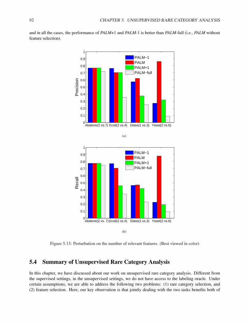
92 CHAPTER 5. UNSUPERVISED RARE CATEGORY ANALYSIS
and in all the cases, the performance of PALM+1 and PALM-1 is better than PALM-full (i.e., PALM withoutfeature selection).
Abalone(2 vs.7) Ecoli(2 vs.4) Glass(1 vs.3) Yeast(2 vs.6)0
0.1
0.2
0.3
0.4
0.5
0.6
0.7
0.8
0.9
1
Pre
cisi
on
PALM−1PALMPALM+1PALM−full
(a)
Abalone(2 vs. 7) Ecoli(2 vs.4) Glass(1 vs.3) Yeast(2 vs.6)0
0.1
0.2
0.3
0.4
0.5
0.6
0.7
0.8
0.9
1
Rec
all
PALM−1PALMPALM+1PALM−full
(b)
Figure 5.13: Perturbation on the number of relevant features. (Best viewed in color)
5.4 Summary of Unsupervised Rare Category Analysis
In this chapter, we have discussed about our work on unsupervised rare category analysis. Different fromthe supervised settings, in the unsupervised settings, we do not have access to the labeling oracle. Undercertain assumptions, we are able to address the following two problems: (1) rare category selection, and(2) feature selection. Here, our key observation is that jointly dealing with the two tasks benefits both of

5.4. SUMMARY OF UNSUPERVISED RARE CATEGORY ANALYSIS 93
them. To this end, we propose an optimization framework, which is well justified theoretically. To solve thisoptimization problem, we design the Partial Augmented Lagrangian Method (PALM), which alternativelyfinds the relevant features and the minority class examples. The effectiveness of PALM is demonstrated byextensive experimental results.

Chapter 6
Conclusion and Future Directions
Rare categories are of key importance in many real applications: although the occurrence of such examplesis rare, their impact is significant. Applications of rare category analysis include: financial fraud detection,Medicare fraud detection, network intrusion detection, astronomy, spam image detection and health care.Based on our empirical studies, we make the following two assumptions: (1) smoothness assumption for themajority classes, and (2) compactness assumption for the minority classes. Notice that we do not assumethe majority and minority classes are separable / near-separable from each other in the feature space, whichis assumed by most existing work on rare category analysis. In other words, we target the more challengingcases where the support regions of the majority and minority classes overlap with each other in the featurespace, since many real applications exhibit the overlapping phenomenon.
In this thesis, we have focused on rare category analysis in both the supervised and unsupervised settings.In particular, the following three tasks are addressed.
1. Rare category detection: discovering at least one example from each minority class with the leastlabel requests from the labeling oracle. For data with feature representations, we propose the NNDB,ALICE, and MALICE algorithms that need full prior information of the data set as input, includingthe number of classes and the proportions of different classes; we also propose the SEDER algorithm,which is prior-free. For graph data (relational data), we propose the GRADE algorithm that needs fullprior information as input; we also generalize this algorithm to produce the GRADE-LI algorithm thatonly needs an upper bound on the proportions of all the minority classes. For each of these algorithms,we provide theoretical justifications as well as empirical evaluations, showing that their performanceis better than state-of-the-art techniques.
2. Rare category characterization: given labeled examples from all the classes, finding a compact rep-resentation for the minority classes in order to identify all the rare examples. To this end, we proposeto enclose the rare examples with a minimum-radius hyper-ball based on the clustering property ofthe minority classes. This idea is further formulated as an optimization problem, and we design theRACH algorithm to find its solution. There are two key components in RACH: (1) converting theoriginal problem into a convex optimization problem, and (2) solving it in its dual form by a projectedsubgradient method. RACH can be easily kernelized. Experimental results demonstrate the effective-ness of RACH. Furthermore, with the compact representation, we are able to better understand thenature of the minority classes.
3. Unsupervised rare category analysis: selecting the examples that are likely to come from the minor-ity classes and selecting the features relevant to the minority classes in an unsupervised fashion. Wepropose to co-select the rare examples and the relevant features, which benefits both tasks. To this end,we design an optimization framework, which is well justified theoretically. To solve this optimization
94

95
problem, we propose the Partial Augmented Lagrangian Method (PALM), which alternatively findsthe relevant features and the minority class examples. The effectiveness of PALM is demonstrated byextensive experimental results.
Rare category analysis can be extended in multiple dimensions. For example,
1. Understanding the dynamics of rare categories. To be specific, how does a rare category emergeand evolve over time? Take emerging research topics as an example. A new research topic may startfrom a single paper exploring a new research direction, which can be followed by more researchersworking in the same area, forming a minority class. Finally, it may become a major research topic.Understanding the dynamics of rare categories can help us gain deeper insights of these categoriesand provide tools for predicting the occurrence of these categories. To address this problem, as a firststep, we may want to monitor the number of papers on a new research topic over time to see if there isany change in the distribution once the research topic has become a minority class. Then we may usethe above observation to predict if a new research topic will eventually become a major research topicor gradually disappear. These techniques can also be used in disease evolution to monitor possiblevariations of a certain disease over time.
2. Understanding complex fraud. In many real world problems, the fraud patterns may be more com-plex than a single fraudulent transaction or a bogus claim. For example, in eBay, the fraudsters andaccomplices form a bipartite core. The fraud identities are eventually used to carry out the actualnon-delivery fraud, while the accomplices exist only to help the fraudsters by boosting their feedbackrating [Chau et al., 2006]. Such bipartite cores are a tell-tale sign of a popular fraud scheme, whichhas resulted in the total loss in the order of millions. To discover these fraud patterns, we need to focuson the subgraph level. As a first step, we may apply the GRADE or GRADE-LI algorithms proposedin Section 3.3 on the whole transaction graph to discover the complex fraud. Then we can incorporatethe bipartite nature of the subgraphs into the algorithms. For example, we may try to modify theglobal similarity so that vertices in the same bipartite graph tend to have larger global similarity.
3. Transfer learning for rare category analysis. In this aspect, we focus on both inter-domain andintra-domain transfer learning. In the first case, the goal is to leverage the information of rare cate-gories in a source domain to help us understand the rare categories in the target domain. Here, themajor challenge is the lack of label information related to the rare categories in the target domain.For example, compared with financial fraud, Medicare fraud is less studied, but the different areasmay share common fraud patterns. To address this problem, first of all, in order to leverage the labelinformation from the source domain, we need to build some connection between the rare categoriesin the source domain and the target domain. Do they have similar distributions in the feature space?Are certain parameters shared by these rare categories across different domains? Do they evolve overtime in a similar way? Then based on the shared properties of these rare categories, we can effectivelytransfer the label information from the source domain to the target domain.
In the second case, we work in a single domain, and the goal is to make use of known rare categoriesto help us detect new rare categories. Here, the major challenge is the lack of label information relatedto the new rare categories. For example, in disease diagnosis, studying patients with known flu typesmay help us detect new flu variants. Similar as before, to address this problem, we first need to findthe shared properties of the rare categories, both known and unknown. Then we may have a betterclue of the support regions for the new rare categories. By sampling in these regions, we may be ableto reduce the number of label requests from the labeling oracle.
4. Rare category exploration system. We would like to build a complete system for rare categoryexploration. The goal here is to provide the domain experts, who have little or no engineering knowl-

96 CHAPTER 6. CONCLUSION AND FUTURE DIRECTIONS
edge, with an intuitive user interface. In this way, it may be easier for the domain experts to interactwith the data, convert domain knowledge into certain parameters, understand the learning results, andprovide feedback. On the input side, the system should be able to deal with different types of data,make use of different amount of prior information, and if some label information is available, it shouldalso be able to use this information to improve the performance. Some major modules of the systeminclude detection, characterization, prediction, feature selection, transfer learning, modeling, etc. Onthe output side, we hope to discover new minority class as well as new examples from known minorityclasses; identify key features to the minority classes as well as find their compact representations; builtstatistical models for the rare categories, etc. Furthermore, we plan to incorporate relevant feedbackinto the system to better serve the users’ need.

Bibliography
[Aggarwal & Yu, 2001] Aggarwal, C. C. & Yu, P. S. (2001). Outlier detection for high dimensional data.in SIGMOD Conference pp. 37–46.
[Angluin, 1987] Angluin, D. (1987). Queries and concept learning. Machine Learning 2(4), 319–342.
[Angluin, 2001] Angluin, D. (2001). Queries revisited. in ALT pp. 12–31.
[Asuncion & Newman, 2007] Asuncion, A. & Newman, D. (2007). UCI machine learning repository.
[Balcan et al., 2006] Balcan, M.-F., Beygelzimer, A., & Langford, J. (2006). Agnostic active learning. inICML pp. 65–72.
[Barbara et al., 2001] Barbara, D., Wu, N., & Jajodia, S. (2001). Detecting novel network intrusions usingbayes estimators. in Proceedings of the First SIAM Conference on Data Mining.
[Bay et al., 2006] Bay, S., Kumaraswamy, K., Anderle, M. G., Kumar, R., & Steier, D. M. (2006). Largescale detection of irregularities in accounting data. in ICDM pp. 75–86.
[Bekkerman et al., 2005] Bekkerman, R., El-Yaniv, R., & McCallum, A. (2005). Multi-way distributionalclustering via pairwise interactions. in ICML pp. 41–48 New York, NY, USA. ACM.
[Boyd & Vandenberghe, 2004] Boyd, S. & Vandenberghe, L. (2004). (Cambridge University Press ).
[Chandola et al., 2009] Chandola, V., Banerjee, A., & Kumar, V. (2009). Anomaly detection: A survey.ACM Comput. Surv. 41(3).
[Chau et al., 2006] Chau, D. H., Pandit, S., & Faloutsos, C. (2006). Detecting fraudulent personalities innetworks of online auctioneers. in PKDD pp. 103–114.
[Chawla, 2009] Chawla, N. (2009). Mining when classes are imbalanced, rare events matter more, anderrors have costs attached. in SDM.
[Chawla et al., 2002] Chawla, N. V., Bowyer, K. W., Hall, L. O., & Kegelmeyer, W. P. (2002). Smote:Synthetic minority over-sampling technique. J. Artif. Intell. Res. (JAIR) 16, 321–357.
[Chawla et al., 2003] Chawla, N. V., Lazarevic, A., Hall, L. O., & Bowyer, K. W. (2003). Smoteboost:Improving prediction of the minority class in boosting. in PKDD pp. 107–119.
[Cohn et al., 1992] Cohn, D., Atlas, L., & Ladner, R. (1992). Improving generalization with active learning.
[Cohn et al., 1996] Cohn, D. A., Ghahramani, Z., & Jordan, M. I. (1996). Active learning with statisticalmodels. JOURNAL OF ARTIFICIAL INTELLIGENCE RESEARCH 4, 129–145.
[Coppersmith & Winograd, 1987] Coppersmith, D. & Winograd, S. (1987). Matrix multiplication via arith-metic progressions. in STOC pp. 1–6 New York, NY, USA. ACM.
[Dagan & Engelson, 1995] Dagan, I. & Engelson, S. P. (1995). Committee-based sampling for trainingprobabilistic classifiers. in In Proceedings of the Twelfth International Conference on Machine Learningpp. 150–157. Morgan Kaufmann.
97
98 BIBLIOGRAPHY
[Dasgupta, 2005] Dasgupta, S. (2005). Coarse sample complexity bounds for active learning. in NIPS.
[Dasgupta & Hsu, 2008] Dasgupta, S. & Hsu, D. (2008). Hierarchical sampling for active learning. inICML pp. 208–215.
[Dash et al., 2002] Dash, M., Choi, K., Scheuermann, P., & Liu, H. (2002). Feature selection for clustering- a filter solution. in ICDM pp. 115–122.
[Dhillon et al., 2003] Dhillon, I., Mallela, S., & Modha, D. (2003). Information-theoretic co-clustering. inKDD pp. 89–98.
[Duchi et al., 2008] Duchi, J., Shalev-Shwartz, S., Singer, Y., & Chandra, T. (2008). Efficient projectionsonto the l1-ball for learning in high dimensions. in ICML pp. 272–279.
[Duda et al., 2000] Duda, R. O., Hart, P. E., & Stork, D. G. (2000). (Wiley-Interscience Publication ).
[Dunn, 1973] Dunn, J. (1973). A fuzzy relative of the isodata process and its use in detecting compactwell-separated clusters. Cyber. and Sys. 3, 32–57.
[Dutta et al., 2007] Dutta, H., Giannella, C., Borne, K. D., & Kargupta, H. (2007). Distributed top-k outlierdetection from astronomy catalogs using the demac system. in SDM.
[Dy & Brodley, 2000] Dy, J. G. & Brodley, C. E. (2000). Feature subset selection and order identificationfor unsupervised learning. in ICML pp. 247–254.
[Efron & Tibshirani, 1996] Efron, B. & Tibshirani, R. (1996). Using specially designed exponential fami-lies for density estimation. in Proc. of the Annals of Statistics pp. 2431–2461.
[EURODIS, 2005] EURODIS (2005). Rare diseases: Understanding this public health priority.
[Fine & Mansour, 2006] Fine, S. & Mansour, Y. (2006). Active sampling for multiple output identification.in COLT pp. 620–634.
[Flake et al., 2000] Flake, G., Lawrence, S., & Giles, C. (2000). Efficient identification of web communi-ties. in KDD pp. 150–160.
[Gao et al., 2007] Gao, B., Liu, T., Zheng, X., Cheng, Q., & Ma, W. (2007). Consistent bipartite graphco-partitioning for star-structured high-order heterogeneous data co-clustering. in KDD pp. 41–50.
[Gibson et al., 2005] Gibson, D., Kumar, R., & Tomkins, A. (2005). Discovering large dense subgraphs inmassive graphs. in VLDB pp. 721–732.
[Glenn & Fung, 2001] Glenn, C. A. & Fung, G. (2001). A comprehensive overview of basic.
[Greco et al., 2007] Greco, G., Guzzo, A., & Pontieri, L. (2007). An information-theoretic framework forhigh-order co-clustering of heterogeneous objects. in SEBD pp. 397–404.
[Guo & Viktor, 2004] Guo, H. & Viktor, H. L. (2004). Learning from imbalanced data sets with boostingand data generation: the databoost-im approach. SIGKDD Explorations 6(1), 30–39.
[HART, 1968] HART, P. (1968). The condensed nearest neighbor rule. IEEE Trans. Inform. Th. 14, 515–516.
[He & Carbonell, 2008] He, J. & Carbonell, J. (2008). Rare class discovery based on active learning. inISAIM.
[He & Carbonell, 2007] He, J. & Carbonell, J. G. (2007). Nearest-neighbor-based active learning for rarecategory detection. in NIPS.
[He et al., 2005a] He, X., Cai, D., & Niyogi, P. (2005a). Laplacian score for feature selection. in NIPS.
[He et al., 2005b] He, Z., Xu, X., & Deng, S. (2005b). An optimization model for outlier detection incategorical data. CoRR abs/cs/0503081.
BIBLIOGRAPHY 99
[Hofmann & Buhmann, 1997] Hofmann, T. & Buhmann, J. M. (1997). Pairwise data clustering by deter-ministic annealing. IEEE Trans. Pattern Anal. Mach. Intell. 19, 1–14.
[Huang et al., 2004] Huang, K., Yang, H., King, I., & Lyu, M. R. (2004). Learning classifiers from imbal-anced data based on biased minimax probability machine. in CVPR (2) pp. 558–563.
[Joachims, 1999] Joachims, T. (1999). Transductive inference for text classification using support vectormachines. in ICML pp. 200–209.
[Joachims, 2005] Joachims, T. (2005). A support vector method for multivariate performance measures. inICML pp. 377–384.
[Johnson, 1967] Johnson, S. (1967). Hierarchical clustering schemes. Psychometrika 32(3), 241–254.
[Kim et al., 2000] Kim, Y., Street, W. N., & Menczer, F. (2000). Feature selection in unsupervised learningvia evolutionary search. in KDD pp. 365–369.
[Kim & Choi, 2007] Kim, Y.-D. & Choi, S. (2007). A method of initialization for nonnegative matrixfactorization. in ICASSP pp. II–537–II–540.
[Kubat & Matwin, 1997] Kubat, M. & Matwin, S. (1997). Addressing the curse of imbalanced trainingsets: One-sided selection. in ICML pp. 179–186.
[Kumar et al., 2003] Kumar, R., Novak, J., Raghavan, P., & Tomkins, A. (2003). On the bursty evolutionof blogspace. in WWW pp. 568–576.
[Law et al., 2002] Law, M. H. C., Jain, A. K., & Figueiredo, M. A. T. (2002). Feature selection in mixture-based clustering. in NIPS pp. 625–632.
[Lehoucq & Sorensen, 1996] Lehoucq, R. & Sorensen, D. (1996). Deflation techniques for an implicitlyrestarted arnoldi iteration. SIAM J. Matrix Anal. Appl. 17(4), 789–821.
[Long et al., 2006] Long, B., Zhang, Z., Wu, X., & Yu, P. (2006). Spectral clustering for multi-type rela-tional data. in ICML pp. 585–592.
[Madsen et al., 2004] Madsen, K., Nielsen, H. B., & Tingleff, O. (2004). Optimization with constraints,2nd ed.
[Mccallum, 1998] Mccallum, A. K. (1998). Employing em in pool-based active learning for text classifica-tion. in In Proceedings of the 15th International Conference on Machine Learning pp. 350–358. MorganKaufmann.
[Mitra et al., 2002] Mitra, P., Murthy, C. A., & Pal, S. K. (2002). Unsupervised feature selection usingfeature similarity. IEEE Trans. Pattern Anal. Mach. Intell. 24(3), 301–312.
[Moore, 1991] Moore, A. (1991). A tutorial on kd-trees Technical report University of Cambridge Com-puter Laboratory.
[Nocedal & Wright, 1999] Nocedal, J. & Wright, S. J. (1999). (Springer ).
[Papadimitriou et al., 2003] Papadimitriou, S., Kitagawa, H., Gibbons, P. B., & Faloutsos, C. (2003). Loci:Fast outlier detection using the local correlation integral. in ICDE pp. 315–327.
[Pelleg & Moore, 2004] Pelleg, D. & Moore, A. W. (2004). Active learning for anomaly and rare-categorydetection. in NIPS.
[Ramaswamy et al., 2000] Ramaswamy, S., Rastogi, R., & Shim, K. (2000). Efficient algorithms for miningoutliers from large data sets. in SIGMOD (Chen, W., Naughton, J. F., & Bernstein, P. A., eds.) pp. 427–438. ACM.
[Reynolds & Rose, 1995] Reynolds, D. & Rose, R. (1995). Robust text-independent speaker identification

100 BIBLIOGRAPHY
using gaussian mixture speaker models. IEEE Trans. Speech and Audio Processing 3, 72–83.
[Scholkopf et al., 2001] Scholkopf, B., Platt, J. C., Shawe-Taylor, J., Smola, A. J., & Williamson, R. C.(2001). Estimating the support of a high-dimensional distribution. Neural Computation 13(7), 1443–1471.
[Scott, 1992] Scott, D. (1992). (Wiley-Interscience ).
[Settles, 2010] Settles, B. (2010). Active learning literature survey Computer Sciences Technical Report1648 University of Wisconsin–Madison.
[Sheikholeslami et al., 1998] Sheikholeslami, G., Chatterjee, S., & Zhang, A. (1998). Wavecluster: Amulti-resolution clustering approach for very large spatial databases. in VLDB pp. 428–439.
[Singh & Gordon, 2008a] Singh, A. P. & Gordon, G. J. (2008a). Relational learning via collective matrixfactorization. in KDD pp. 650–658.
[Singh & Gordon, 2008b] Singh, A. P. & Gordon, G. J. (2008b). A unified view of matrix factorizationmodels. in ECML/PKDD (2) pp. 358–373.
[Sun et al., 2007] Sun, J., Faloutsos, C., Papadimitriou, S., & Yu, P. (2007). Graphscope: parameter-freemining of large time-evolving graphs. in KDD pp. 687–696.
[Sun et al., 2006] Sun, Y., Kamel, M. S., & Wang, Y. (2006). Boosting for learning multiple classes withimbalanced class distribution. in ICDM pp. 592–602.
[Tang et al., 2009] Tang, Y., Zhang, Y.-Q., Chawla, N. V., & Krasser, S. (2009). Svms modeling for highlyimbalanced classification. Trans. Sys. Man Cyber. Part B 39(1), 281–288.
[Tomek, 1976] Tomek, I. (1976). Two modifications of cnn. IEEE Trans. Systems, Man and Cybernetics 6,769–772.
[Tong et al., 2001] Tong, S., Koller, D., & Kaelbling, P. (2001). Support vector machine active learningwith applications to text classification. in Journal of Machine Learning Research pp. 999–1006.
[Vatturi & Wong, 2009] Vatturi, P. & Wong, W.-K. (2009). Category detection using hierarchical meanshift. in KDD pp. 847–856.
[Wang et al., 2007] Wang, Z., Josephson, W. K., Lv, Q., Charikar, M., & Li, K. (2007). Filtering imagespam with near-duplicate detection. in CEAS.
[Wasserman, 2005] Wasserman, L. (2005). (Springer ).
[Wu & Chang, 2003] Wu, G. & Chang, E. Y. (2003). Adaptive feature-space conformal transformation forimbalanced-data learning. in ICML pp. 816–823.
[Wu et al., 2007] Wu, J., Xiong, H., Wu, P., & Chen, J. (2007). Local decomposition for rare class analysis.in KDD pp. 814–823.
[Yu et al., 2002] Yu, D., Sheikholeslami, G., & Zhang, A. (2002). Findout: Finding outliers in very largedatasets. Knowl. Inf. Syst. 4(4), 387–412.
[Yuster & Zwick, 2005] Yuster, R. & Zwick, U. (2005). Fast sparse matrix multiplication. ACM Trans.Algorithms 1(1), 2–13.
[Zhou et al., 2003a] Zhou, D., Bousquet, O., Lal, T., Weston, J., & Scholkopf, B. (2003a). Learning withlocal and global consistency. in NIPS.
[Zhou et al., 2003b] Zhou, D., Weston, J., Gretton, A., Bousquet, O., & Scholkopf, B. (2003b). Rankingon data manifolds. in NIPS.


