Embed Size (px)
Citation preview

Seediscussions,stats,andauthorprofilesforthispublicationat:https://www.researchgate.net/publication/301280347
MedicalimagesmodalityclassificationusingdiscreteBayesianNetworks
ArticleinComputerVisionandImageUnderstanding·April2016
ImpactFactor:1.54·DOI:10.1016/j.cviu.2016.04.002
READS
27
5authors,including:
JesusMartínez-Gómez
UniversityofCastilla-LaMancha
44PUBLICATIONS59CITATIONS
SEEPROFILE
JoséA.Gámez
UniversityofCastilla-LaMancha
153PUBLICATIONS904CITATIONS
SEEPROFILE
AlbaGarcíaSecodeHerrera
NationalLibraryofMedicine
38PUBLICATIONS213CITATIONS
SEEPROFILE
HenningMüller
HES-SOValais-Wallis
525PUBLICATIONS6,052CITATIONS
SEEPROFILE
Allin-textreferencesunderlinedinbluearelinkedtopublicationsonResearchGate,
lettingyouaccessandreadthemimmediately.
Availablefrom:HenningMüller
Retrievedon:19April2016
Medical images modality classification using discreteBayesian Networks
Jacinto Ariasa, Jesus Martınez-Gomeza,b, Jose A. Gameza, Alba G. Seco deHerrerac, Henning Mullerc
aUniversity of Castilla-La Mancha, SpainbUniversity of Alicante, Spain
cUniversity of Applied Sciences Western Switzerland, Switzerland
Abstract
In this paper we propose a complete pipeline for medical image modality clas-sification focused on the application of discrete Bayesian network classifiers.Modality refers to the categorization of biomedical images from the literatureaccording to a previously defined set of image types, such as X-ray, graph orgene sequence. We describe an extensive pipeline starting with feature extrac-tion from images, data combination, pre-processing and a range of differentclassification techniques and models. We study the expressive power of sev-eral image descriptors along with supervised discretization and feature selectionto show the performance of discrete Bayesian networks compared to the usualdeterministic classifier used in image classification. We perform an exhaustiveexperimentation by using the ImageCLEFmed 2013 collection. This problempresents a high number of classes so we propose several hierarchical approaches.In a first set of experiments we evaluate a wide range of parameters for ourpipeline along with several classification models. Finally, we perform a compar-ison by setting up the competition environment between our selected approachesand the best ones of the original competition. Results show that the BayesianNetwork classifiers obtain very competitive results. Furthermore, the proposedapproach is stable and it can be applied to other problems that present inherenthierarchical structures of classes.
Keywords: Medical Image Analysis, Visual Features Extraction, BayesianNetworks, Hierarchical Classification
1. Introduction
Medical images are essential for diagnosis and treatment planning. Thesetypes of images are produced in ever-increasing quantities and varieties [1]. A
Email addresses: [email protected] (Jacinto Arias), [email protected](Jesus Martınez-Gomez), [email protected] (Jose A. Gamez), [email protected](Alba G. Seco de Herrera), [email protected] (Henning Muller)
Preprint submitted to Computer Vision and Image Understanding March 18, 2016
recent European report estimates medical images of all kind occupied 30% ofthe global digital storage in 2010 [2].
Clinicians use images of past cases in comparison with current images todetermine the diagnosis and potential treatment options of new patients. Imagesare also used in teaching and research [3, 4]. Thus, the goal of a clinician is oftento solve a new problem by making use of previous similar cases/images togetherwith contextual information, by reusing information and knowledge [5].
Systematic and quantitative evaluation activities using shared tasks on sharedresources have been instrumental in contributing to the success of informationretrieval as a research field and as an application area in the past few decades.Evaluation campaigns have enabled the reproducible and comparative evalu-ation of new approaches, algorithms, theories and models through the use ofstandardized resources and common evaluation methodologies within regularand systematic evaluation cycles. The tasks organized over the years by Image-CLEF1 [6] have provided an evaluation forum and framework for evaluating thestate of the art in biomedical image retrieval.
In this article, we evaluate a probabilistic approach for medical image clas-sification by using the ImageCLEF 2013 medical image modality classificationtask [7] as a benchmarking environment. We propose a reproducible methodol-ogy based on the use of discrete Bayesian Network Classifiers (BNCs) [8]. Ourapproach first explores details of the modality classification and medical imageprocessing. This is done by defining a basic pipeline in which the applicationof BNCs is straightforward. The defined pipeline includes a problem transfor-mation from its usual continuous domain to a discrete one that is more naturalfor probabilistic approaches. In the classification stage we dive into the prob-lem of modality classification to evaluate several proposals in order to deal withthe relatively large number of classes (31) that the task presents; for this wefocus on hierarchical classification and multi-class approaches. Fig. 1 shows ascheme with all the stages taking part in the described pipeline for the classifiergeneration process.
Our proposal is based on an extensive experimental evaluation of the pro-posed pipeline using a collection of probabilistic instead of deterministic classi-fiers that are the common approaches to tackle this kind of problem [9, 10]. TheBN models selected for the experimental analysis show an advantage in theirtrade-off between efficiency and quality. They also demonstrate a promisingperformance in a wide range of domains such as document classification [11],object detection [12] or semantic localization [13].
Moreover, probabilistic graphical models are suitable for the integrationof contextual categorical variables in conjunction with descriptors extractedfrom computer vision techniques. Contextual information, such as human an-notations or semantic attributes, are becoming more frequent and they canbe obtained automatically by means of external tools like Amazon mechanicalturk [14]. This kind of information cannot be directly incorporated in other
1http://imageclef.org/
2
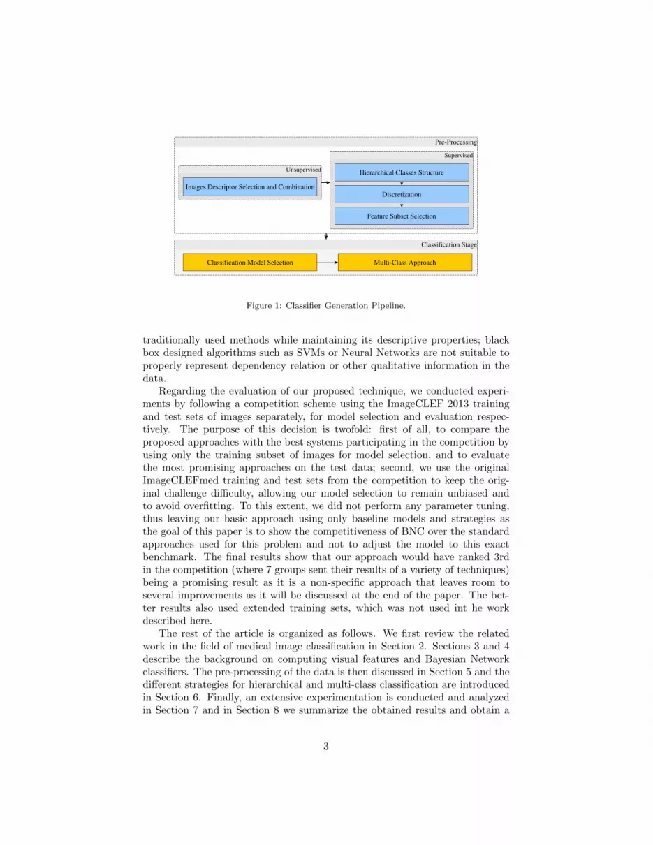
Figure 1: Classifier Generation Pipeline.
traditionally used methods while maintaining its descriptive properties; blackbox designed algorithms such as SVMs or Neural Networks are not suitable toproperly represent dependency relation or other qualitative information in thedata.
Regarding the evaluation of our proposed technique, we conducted experi-ments by following a competition scheme using the ImageCLEF 2013 trainingand test sets of images separately, for model selection and evaluation respec-tively. The purpose of this decision is twofold: first of all, to compare theproposed approaches with the best systems participating in the competition byusing only the training subset of images for model selection, and to evaluatethe most promising approaches on the test data; second, we use the originalImageCLEFmed training and test sets from the competition to keep the orig-inal challenge difficulty, allowing our model selection to remain unbiased andto avoid overfitting. To this extent, we did not perform any parameter tuning,thus leaving our basic approach using only baseline models and strategies asthe goal of this paper is to show the competitiveness of BNC over the standardapproaches used for this problem and not to adjust the model to this exactbenchmark. The final results show that our approach would have ranked 3rdin the competition (where 7 groups sent their results of a variety of techniques)being a promising result as it is a non-specific approach that leaves room toseveral improvements as it will be discussed at the end of the paper. The bet-ter results also used extended training sets, which was not used int he workdescribed here.
The rest of the article is organized as follows. We first review the relatedwork in the field of medical image classification in Section 2. Sections 3 and 4describe the background on computing visual features and Bayesian Networkclassifiers. The pre-processing of the data is then discussed in Section 5 and thedifferent strategies for hierarchical and multi-class classification are introducedin Section 6. Finally, an extensive experimentation is conducted and analyzedin Section 7 and in Section 8 we summarize the obtained results and obtain a
3

brief perspective of future work and extensions.
2. Background and Related work
The interest of the visual retrieval community in the automatic analysis ofmedical information was motivated in part thanks to the medical ImageCLEFchallenge. The medical task has run at ImageCLEF since 2004, with manychanges between different editions [6]. The underlying objective of this challengeis the retrieval of similar images to fulfill a precise information need and imageclassification. The 2009 edition of the task [15] focused on the retrieval ofarticles from the biomedical literature that might best suit a provided medicalcase description (including images). In 2010 [16], the organizers introduced themodality classification task.
The goal of modality classification is to classify the images of the literatureinto medical modalities and other image types, such as Computer Tomography(CT), X–ray or general graphs. Medical image classification by modality canimprove the retrieval step by filtering or re–ranking the results lists [17]. More-over, it can reduce the search space to a set of relevant categories improvingthe speed and precision of the retrieval [18]. Some example images used in themodality classification task are shown in Fig. 2.
(a) Ultrasound (b) Light microscopy (c) Endoscopy (d) CT
Figure 2: Examples of medical images from various moralities.
The modality classification task was maintained until 2013 [6]. The imagecollection provided in 2013 was used for the evaluation in this article. Thiscollection includes 2896 annotated training images and 2582 test images to beclassified. Each image belong to one of the 31 classes that present an intrinsichierarchy shown in Fig. 3.
The techniques presented, rely mainly on two key stages: a.- extraction ofvisual features from the images, and b.- generation of classification models. Re-garding the feature extraction, several studies have shown that the modalitycan be extracted from the visual content using only visual features [19, 20].The extracted visual features must then be transformed to obtain meaningfuldescriptors. For instance, Kitanovski et al. [9] use a spatial pyramid in combi-nation with dense sampling using an opponentSIFT descriptor for each imagepatch.
Support Vector Machines (SVMs), in combination with the χ2 kernel, arethe most common classification model used in the competition [21, 9, 10]. How-ever, other deterministic classifiers such as k–Nearest Neighbor [22] were also
4

Figure 3: The image class hierarchy provided by ImageCLEFmed for document images oc-curring in the biomedical open access literature.
used. Despite their lack of descriptive capabilities, these classification modelspresent properties that have encouraged their use in image classification prob-lems. They can work with numeric input data, which is the most commonoutput from feature extraction techniques. They can properly cope with thehigh dimensionality of the image descriptors.
The hierarchical relationship between the categories in the medical task canalso be found in other problems, such as object categorization [23]. In thisproblem, we can find solutions where SVM classifiers are applied over the com-bination of different 3D descriptors [24], as well as hierarchical decompositionof the descriptors [25] but the explicit management of the object hierarchy isvery seldom adopted.
Though different Bayesian and non-Bayesian probabilistic methods havebeen applied for medical image analysis (see e.g. [26]), the use of BNCs hasbeen scarce to the best of our knowledge. None of the participants of the Im-ageCLEFmed modality classification task presented approaches based on BNCs.One of the main reasons could be the continuous domain of the features usedin medical image classification, while the developments for BNCs have beenmainly devoted to the discrete case. In fact, some BN models are availableto deal with numerical variables, but they have two major shortcomings: theGaussian assumption and structural constraints, e.g. a discrete variable cannotbe conditioned on a numerical one. Nevertheless, some approaches to medicalimage analysis problems have been carried out by using discrete BN [27], al-
5
though they reduce to the use of Naive Bayes and Tree Augmented Naive Bayes(TAN) algorithms.
3. Feature extraction and descriptor generation
The transformation of an input image into a set of features tht describe it isa key stage for a subsequent classification task. This process is known as featureextraction and can be accomplished in different ways, as it is discussed in [28].In this paper, we follow the scheme proposed in [29], where a combination ofmultiple low–level visual features is explored. In this paper, the same combi-nation of visual descriptors is applied. Therefore, the descriptors used are thefollowing:
• Bag of Visual Words (BoVW) using Scale Invariant Feature Transform(SIFT) (BoVW–SIFT) [30] – Each image is represented by an histogramsymbolizing a set of local descriptors represented in visual words from avocabulary previously learned with 238 visual words. This leads to a 238bin histogram;
• Bag of Colors (BoC) [31] – Each image is represented by a 100 bin his-togram symbolizing the colors from a vocabulary previously learned;
• Color and Edge Directivity Descriptor (CEDD) [32] – Color and textureinformation is produced by a 144 bin histogram. Only little computationalpower is required for its extraction;
• Fuzzy Color and Texture Histogram (FCTH) [33] – This descriptor con-tains results from the combination of 3 fuzzy systems including color andtexture information in 192 bin histogram;
• Fuzzy Color Histogram (FCH) [34] – The color similarity of each pixel’scolor associated with a 192 histogram bin through a fuzzy–set membershipfunction is used;
These descriptors are extracted using the ParaDISE (Parallel DistributedImage Search Engine) [35]. The combination of all these features generatesdescriptors with a dimensionality of 866.
4. Bayesian Network classifiers
Bayesian Networks (BNs) [36] are one of the most frequently used knowledgerepresentation techniques when dealing with uncertainty, mostly owing to theirpredictive/descriptive capabilities. They are based on sound mathematical prin-ciples and, as a probabilistic graphical model, they output a graphical structurethat provides an interpretative representation of the relationships between thevariables of the problem.
6

Learning general BNs is known to be a complex problem [37] involving thetask of structural learning as well as parameter estimation [38]. As learninggeneral BNs is usually problematic, this has lead to the definition and wideusage of specific models that are explicitly designed to tackle the standard clas-sification problem, these are commonly known as Bayesian Network Classifiers(BNCs) [39, 8].
The simplest BNC model is the Naive Bayes classifier (NB) that avoidsstructural learning by assuming that all attributes are conditionally independentgiven the value of the class. Although this independence assumption can be con-sidered too strong for some domains, the NB classifier has shown very good re-sults in many real applications such as computing, marketing and medicine [40].Its results can be improved by slightly alleviating its independence assumptionand using a more complex graphical structure. The techniques using this prin-ciple are known as semi-naive Bayesian network classifiers, some of them areamong the most competitive classification techniques.
We evaluated the performance of different semi-naive BNC models to solvethe proposed classification problem, specifically: NB, TAN, K-Dependence Bayesianclassifiers (KDB) and Average One Dependence Estimators (AODE).
4.1. Naive Bayes
NB classifier [41] is the simplest BNC, due to its independence assump-tion which avoids any needs for structural learning. This classifier uses a fixedgraphical structure in which all predictive attributes are considered independentgiven the class, as it is depicted in Fig. 4a. This implies the following factoriza-tion: ∀c ∈ ΩC p(~e|c) =
∏ni=1 p(ai|c). Here, the maximum a posteriori (MAP)
hypothesis is used to classify:
cMAP = argmaxc∈ΩCp(c|~e) = argmaxc∈ΩC
(p(c)
n∏i=1
p(ai|c)
). (1)
4.2. Tree-Augmented Naive Bayes
The TAN classifier [39] can be considered a structural augmentation ofthe NB classifier in which the conditional independence assumption is relaxedby allowing a restricted number of relationships between the predictive at-tributes. This strategy implies that a structural learning process must be per-formed. However, TAN can still obtain competitive learning times with moder-ate datasets establishing a good trade-off between model complexity and modelaccuracy. In particular, every predictive attribute is allowed to have an extraparent in the model in addition to the class. In order to learn these depen-dencies a Maximum Weighted Spanning tree (MWST) is learned by using theChow-Liu algorithm [42] with the conditional mutual information between eachpair of attributes and the class as metric to measure each arc weight:
MI(Ai, Al | C) =∑r=1
p(cr)∑i=1
∑j=1
p(ai, aj | cr)logp(ai, aj | cr)
p(ai | cr)p(aj | cr)(2)
7

(a) NB structure (b) TAN(KDB k = 1) structure
(c) KDB k = 2 structure (d) SPODE structure
Figure 4: Graphical structure of semi-naive Bayesian Network Classifiers.
This process guarantees that the tree learned from the training data is op-timal, i.e. it is the best possible probabilistic representation from the availabledata as a tree as it maximizes the log likelihood. Once the tree is obtained,an arbitrary node is selected as the root of the tree and the edges are orientedto create a directed acyclic graph in which all attributes are conditioned to theclass, creating the final BNC structure of a TAN classifier. An example is shownin Fig. 4b.
4.3. K-Dependence Bayesian classifiers
The basic KDB classifier is based on the notion of a k-dependence estimatorintroduced by Sahami [43] in which the structure of a basic NB classifier canbe augmented by allowing an attribute to be conditioned to a maximum of kparent attributes in addition to the class, thus covering the full spectrum fromthe NB classifier to a general full BN structure by varying the parameter k. Anexample for a given value of k is shown in Fig. 4c.
The KDB classifier itself performs a three-stage learning process:
1. A ranking is established between the predictive attributes by means oftheir mutual information with the class variable.
2. For each attribute Ai, i being its position on the previous ranking, the kattributes taken from A1, . . . , Ai−1 with the highest conditional mutualinformation MI(·, Ai | C) are set as the parents of Ai.
8

3. The class variable C is added as a parent for all the predictive attributes.
This classifier presents a more flexible approach to the TAN classifier (in fact,the TAN classifier is a particular case of KBD with K = 1), as it is capable ofadjusting the mentioned trade-off between model complexity and model quality.
4.4. Averaged One Dependence Estimators
AODE [44] are an alternative to other semi-naive BNC approaches. Theypresent a fixed structure model that avoids structural learning, improving itsefficiency when compared to other BNCs that require the step. Moreover, AODEmaintains very competitive model quality.
Therefore, AODE is restricted exclusively to 1-dependence estimators. Thisclassifier can be seen as an ensemble of models, concretely, it considers eachmodel belonging to a specific family of classifiers (known as SPODEs (Super-parent One-Dependence Estimators)) in which every attribute is dependent onthe class and on another shared attribute, designated as superparent. Thestructure of a specific SPODE is depicted in Fig. 4d.
For classification, AODE computes the average of the n possible SPODEclassifiers:
CMAP = arg maxc∈ΩC
n∑j=1,N(aj>q)
p(c) · p(aj | c)n∏
i=1,i6=j
p(ai | c, aj)
(3)
5. Data pre-processing
Input data can be pre-processed to meet the requirements of the classifica-tion models, to reduce their complexity but also to increase their performance.Here, we enumerate three data pre-processing techniques. First, we propose acombination of the different descriptors extracted from the image. Then, wediscretize the input data to obtain nominal variables suitable for their use inthe classification models. Finally, we select a subset of variables from the wholeset.
5.1. Descriptor combination
In this article, we opted to use five descriptors generated from visual featuresextracted from the input images: BoVW-SIFT, CEDD, FCTH, FCH, BoC (seeSection 3). Every descriptor consists of numeric variables with dimensionalitybetween 100 and 238, which represents visual feature frequencies (see Sec. 3 formore details on the visual features). They can be concatenated to create a singledescriptor, as it is commonly done when working with SVMs. However, we canalso follow an aggregation approach to merge descriptors in a recursive way,where we can include pruning strategies. From an initial set of n descriptors,we can generate the following number of combinations,
n∑i=1
n!
i!(n− i)!
9

which would result in 31 different combinations from an initial set of 5 descrip-tors (5+10+10+5+1).
5.2. Discretization
Some of the internal variables of the image descriptors contain discriminantinformation but others can be useless for the problem we are facing. WhileBayesian classifiers exist tackling numeric variables [45] (e.g. Gaussian NaiveBayes), we opted for the exclusive use of discrete classification models. The mainreason for this decision is that some numeric versions of the classifiers assumethat input data can be modeled with uni-modal distributions [46], which isnot always true. Here, we propose the use of the Fayyad Irani discretizationmethod [47], which can be considered a standard approach. This discretizationmethod takes into account the class information when selecting the number ofbins and breaking points by using mutual information. Moreover, it selectsthe optimal number of bins separately for each input variable. As seen in theexperimentation (see Section 7), this discretization step produces a number ofbinary partitions. It also discretizes input variables into a single bin, whichmeans that the variable has no discriminant power with respect to the class,thus resulting in useless variables that are removed in subsequent steps.
5.3. Feature Subset Selection
The number of input variables, which comes from the descriptors combi-nation, can be successfully reduced by following an appropriate procedure. Inaddition to data reduction, this step can also increase the accuracy of the clas-sification model by finding redundant or irrelevant input variables. Moreover,using fewer variables also provides non-overfitted and more interpretable clas-sification models, which requires shorter training times. In order to avoid thebias introduced by the classification method while using wrapper approaches,we selected a filter strategy. We opted for the Correlation Feature Selection(CFS [48]), which has shown its value in several scenarios.
6. Strategies
In addition to the classical data pre-processing (discretization and featuresubset selection, which only affects the predictive attributes), we can also takeadvantage from strategies that cope with multi-class problems. The first alter-native consists of partitioning the original problem into recursive sub-problemsusing a hierarchy of classes. The second strategy splits the multi-class probleminto n binary problems with decisions being merged to select the final decision.This second strategy was discarded in a first round of preliminary experimentswhere no significant improvements were obtained when using several multi-classapproaches, such as One-versus-All (OvA) [49]. The improvements of OvA werelimited to the absence of hierarchical approaches due to the large number ofclasses (31).
10
6.1. Hierarchical classification
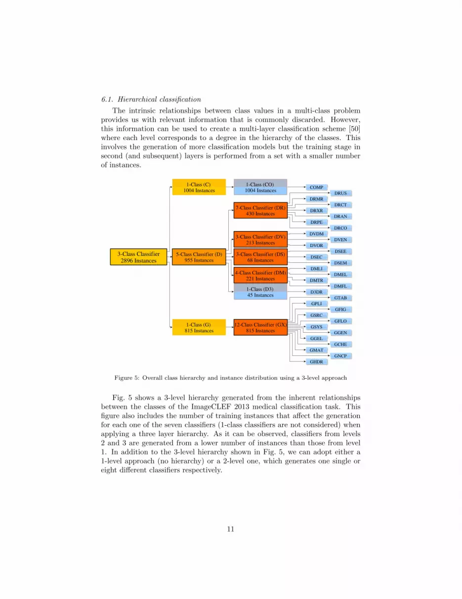
The intrinsic relationships between class values in a multi-class problemprovides us with relevant information that is commonly discarded. However,this information can be used to create a multi-layer classification scheme [50]where each level corresponds to a degree in the hierarchy of the classes. Thisinvolves the generation of more classification models but the training stage insecond (and subsequent) layers is performed from a set with a smaller numberof instances.
Figure 5: Overall class hierarchy and instance distribution using a 3-level approach
Fig. 5 shows a 3-level hierarchy generated from the inherent relationshipsbetween the classes of the ImageCLEF 2013 medical classification task. Thisfigure also includes the number of training instances that affect the generationfor each one of the seven classifiers (1-class classifiers are not considered) whenapplying a three layer hierarchy. As it can be observed, classifiers from levels2 and 3 are generated from a lower number of instances than those from level1. In addition to the 3-level hierarchy shown in Fig. 5, we can adopt either a1-level approach (no hierarchy) or a 2-level one, which generates one single oreight different classifiers respectively.
11
7. Results
7.1. Parameter Selection
The first round of experiments was conducted with two main objectives: val-idating the proposed methodology, and performing an initial selection from theset of internal parameters. The experiments were carried out using the trainingset from the ImageCLEF 2013 medical classification task, which includes 2896images and 31 nominal classes by performing a 5 fold cross-validation.
7.1.1. Descriptor Combination
There are 31 descriptor combinations as result of merging the 5 initial setsof descriptors: SIFT(D1), BoC(D2), CEDD (D3), FCTH(D4), and FCH (D5).Each combination was evaluated using the following options:
• Hierarchical Classification (see Fig. 5)
– 1-level hierarchy (no hierarchy)
– 2-level hierarchy
– 3-level hierarchy
• Discretization
– Fayyad-Irani
• Feature Subset Selection
– Correlation Feature Selection (CFS)
• Classification Model / Algorithm
– Naive Bayes (NB)
– Tree Augmented Naive Bayes (TAN)
– Average One Dependence Estimators (AODE)
– K-Dependence Bayesian Classifier (KDB)
By combining all these options for the described parameters, we generated andtested a total of 465 classifiers. Results are graphically presented in Fig. 6and detailed in Table A.4. Results show a clear difference in performancebetween the combinations of descriptors where higher accuracy is obtainedfrom larger descriptor combination. This result implies that integrating de-scriptors increases the expressive power of the classifier and that the proposedpre-processing pipeline is effective in practice, as the feature subset selection(FSS) process copes properly with an increasing number of input attributes,retaining useful information for each one of the combined descriptors. Fig. 7shows the evolution of the number of attributes in the final combination whenwe increase the size of the combined descriptors by adding new ones; the figure
12

L0
L1+L0
L2+L1+L0
0.0
0.2
0.4
0.6
0.0
0.2
0.4
0.6
0.0
0.2
0.4
0.6
1 2 3 4 5
Number of descriptors
Me
an
ac
cu
racy
Classifier AODE KDB TAN NB
Figure 6: Preliminary results for each hierarchical approach, classifier and descriptor combi-nation using a 5-fold cross validation over the full training set. The results are summarised asthe mean accuracy for all the different combination of the same number of descriptors. Theerror bars correspond to the maximum and minimum values for such an experiment.
exposes how a combination of a larger number of descriptors does not necessar-ily involves higher dimensionality once FSS in applied, in fact we can observean asymptotic behavior when the number of descriptors in the combination isincreased. Given these results, we decided to continue the experimentation byselecting the entire combination of descriptors D1,2,3,4,5 as the candidate.
Regarding the classification models and the proposed hierarchies, resultsfrom the Table A.4 show that the usage of a hierarchy improves upon the resultswhen compared to dealing with the 31 original classes using a single classifier.If we compare the models we can observe a better performance of AODE whenperforming hierarchical classification, however KDB is superior when dealingwith the flat class structure (31 classes). To analyze these results we performeda statistical evaluation on the performance of each model for each one of the hi-erarchy approaches. The Friedman test [51] with a 0.05 confidence level rejectsthe three hypotheses of all classifier being equivalent when using any of the hier-archy levels. A further post-hoc statistical analysis using the Holm procedure isincluded in Table 1, in which we compare the performance of all classifiers withthe best one for each one of the hierarchies. This confirms how KDB clearlyoutperforms the other classification models within a 1-level hierarchy. However,AODE stood out when taking advantage of the 2 or 3 levels of the hierarchy.This exposes KDB as the optimal classifier when coping with a large number of
13

classes, while AODE performs notoriously better in the remaining scenarios.
3 4
5
2
1
3,4
3,5
3,2
3,1
4,5
4,2
4,1
5,2
5,12,1
3,4,5
3,4,2
3,4,1
3,5,2
3,5,1
3,2,1
4,5,2
4,5,1
4,2,15,2,1
3,4,5,2
3,4,5,1
3,4,2,1
3,5,2,1 4,5,2,1 3,4,5,2,1
34
5
2
1
3,4
3,5
3,2
3,1
4,54,2
4,1
5,2
5,1
2,1
3,4,5
3,4,2
3,4,1
3,5,2
3,5,1
3,2,1
4,5,2
4,5,14,2,15,2,1
3,4,5,2
3,4,5,1
3,4,2,13,5,2,1
4,5,2,1 3,4,5,2,1
0
40
80
120
0
40
80
120
L0
L2
+L
1+
L0
250 500 750
Total amount of attributes
Se
lec
ted
att
rib
ute
s
Figure 7: Effect on the FSS procedure for two different hierarchical approaches when usingdifferent combinations of descriptors.
Table 1: Classification model ranking. w/t/l denote the number of scenarios the first rankingmethod wins(w) ties(t) and looses(l) the evaluated method
method rank pvalue w/t/lKDB 1.03TAN 2.26 <0.01 31/0/0AODE 2.71 <0.01 30/0/1NB 4.00 <0.01 31/0/0
method rank pvalue w/t/lAODE 1.00TAN 2.03 <0.01 31/0/0KDB 2.97 <0.01 31/0/0NB 4.00 <0.01 31/0/0
method rank pvalue w/t/lAODE 1.00TAN 2.13 <0.01 31/0/0KDB 3.16 <0.01 31/0/0NB 3.71 <0.01 31/0/0
1-level hierarchy 2-level hierarchy 3-level hierarchy
7.2. Final Results
The last experimental stage was carried out following the procedure pro-posed in the ImageCLEF 2013 medical classification task. Namely, we learnedclassification systems using the 2896 training images and evaluated such sys-tems against the 2582 test images. In order to perform a fair evaluation wefollowed the original rules of the competition. We selected the best 10 classifi-cation systems that achieved highest results in previous experiments using onlythe training data, i.e., we evaluated the selected models over the provided thetest set and computing the accuracy of our systems. We used the ten best re-sults because this was the limit in the number of task submissions. The internal
14

parameters for the systems, as well as the accuracy obtained both against thetraining set that was used to rank the models (with 5-folds cross-validation) andtest sequences are shown in Table 2.
Table 2: Final results obtained against the test set with the 10 configurations that rankedfirst in previous experiments.
Ranking Parameters Accuracy(training) Classifier Hierarchy Descriptor Training (5-cv) Test1st AODE L1+L0 D1,2,4,5 0.6622 0.68402nd AODE L1+L0 D1,2,3,4,5 0.6600 0.67743rd AODE L1+L0 D1,2,3,5 0.6569 0.67394th AODE L1+L0 D1,2,5 0.6547 0.67005th AODE L2+L1+L0 D1,2,4,5 0.6474 0.69216th AODE L2+L1+L0 D1,2,3,4,5 0.6455 0.69057th AODE L1+L0 D1,3,4,5 0.6433 0.66428th AODE L2+L1+L0 D1,2,3,5 0.6419 0.68639th AODE L1+L0 D1,2,3,4 0.6401 0.660710th AODE L2+L1+L0 D1,2,5 0.6400 0.6789
If we compare the training and test columns in Table 2, we can observe thatwe are obtaining higher results over the test set. This trend supports the stabil-ity of our methodology, allowing the generation of non-overfitted classificationsystems. All the evaluated systems share the following internal parameters:AODE as classification model, 2 or 3 levels of hierarchy and large combinationsof initial descriptors. As previously pointed out, the multi-class approach didnot obtain significant improvements on the accuracy once the hierarchy is ap-plied. An important detail is that the best result for the training set is obtainedby using the 2 level hierarchy whereas the best results for the test set corre-sponds to those approaches using the 3 level hierarchy. This is probably dueto the small size of the training set compared to the size of the test set, whichsupports the generalization capabilities of the proposed framework.
7.3. ImageCLEF 2013 medical task results
Our maximum accuracy obtained over the test set was 69.21%. This resultranked 3rd in the modality classification task of ImageCLEF 2013, as shown inTable 3. We can observe how most of the teams used Support Vector Machines(SVMs) as classifier, while none of them used a probabilistic model. Apartfrom SVMs, only the K-Nearest Neighbor (K-NN) and the Stochastic gradientdescent (SGD) were used. With respect to the image descriptors used by theparticipants, most were based on histogram representations or bag of words ap-proaches managing continuous information, but other more complex techniques(such as the spatial pyramid [52]) were also used. The best results both useda training set expansion, which can explain part of the gains. On the contrary,our proposal relies on just the training provided by the task organizers, which
15

is not biased nor optimized to artificially increase the accuracy at the expenseof lack of generalization.
Table 3: Highest accuracies (by group) in the ImageCLEF 2013 modality classification taskincluding our best result.
Ranking Group Name Classifier Accuracy1st IBM [53] SVMs 80.792nd FCSE [9] SVMs 77.143rd Our proposal BNs(AODE) 69.214th MiiLab [10] SVMs,K-NN 66.465th medGIFT [29] K-NN 63.786th ITI [54] SVMs 61.507th CITI [55] SGD 56.628th IPL [56] SVMs 52.05
7.4. Analysis of the results
We carried a posterior analysis of the results to identify the points suitablefor improvements of our methodology. The first study examined the accuracy ofthe internal classifiers involved in the hierarchical classification. We evaluatedthe system that ranked 5th in Table 2 which is best in the test set. It uses a3-level hierarchy with 7 internal classifiers (see Fig. 5). For each of these sevenclassifiers, we computed two accuracy measures: Acc(a).- the overall accuracy,and Acc(b).- the accuracy obtained only with instances that were correctlyclassified in upper levels. Acc(b) reflects the isolated behavior of each classifier,while Acc(a) is affected by the rest of the system.
Figure 8: Acc(a) and Acc(b) computed for a classification system including D1,2,3,4,5 descrip-tors, 3-hierarchy levels and AODE as classification model without multi-class approach.
16
The accuracy from the first level classifier (80.33% Fig. 8) shows how nearly20% of the test instances were wrongly classified at this level. The classifier iscrucial because it processes the full test sequence and its errors are thereforepropagated through the hierarchy structure. Concretely, 62.46% of the classi-fication error came from the first classifier, while the remaining 37.54% camefrom the other 6 classifiers.
8. Conclusions
We propose a pipeline for modality classification of medical images by usingprobabilistic classifiers, namely BNCs. We have identified an extensive descrip-tor set, a combination of descriptors, a detailed pre-processing scheme and sev-eral approaches for hierarchical and multi-class classification. We evaluated alarge number of parameter combinations by using a selected range of the mostpopular BNCs.
Evaluation was carried out on the ImageCLEFmed 2013 collection. TheAODE classifier shows superior results when combined with hierarchical classi-fication and a large number of combined descriptors over the training set. Formodel selection we replicated the competition conditions by using the test setof images to compare our proposal with the best results in the competition. Weobtain results that rank 3rd. From this analysis we can draw useful conclusions:
• Descriptor combinations have proven to be an expressive tool showingalso the robustness of discrete supervised preprocessing techniques suchas MDL discretization and feature selection. The hierarchical approachproved to be an excellent pairing with these methods, as they can bereplicated easily for the hierarchy levels.
• Among all the BNCs evaluated, ensemble methods such as AODE proveto obtain highest discrimination power and thus overall best classificationresults. The best results are obtained when a deeper hierarchy and a largernumber are combined.
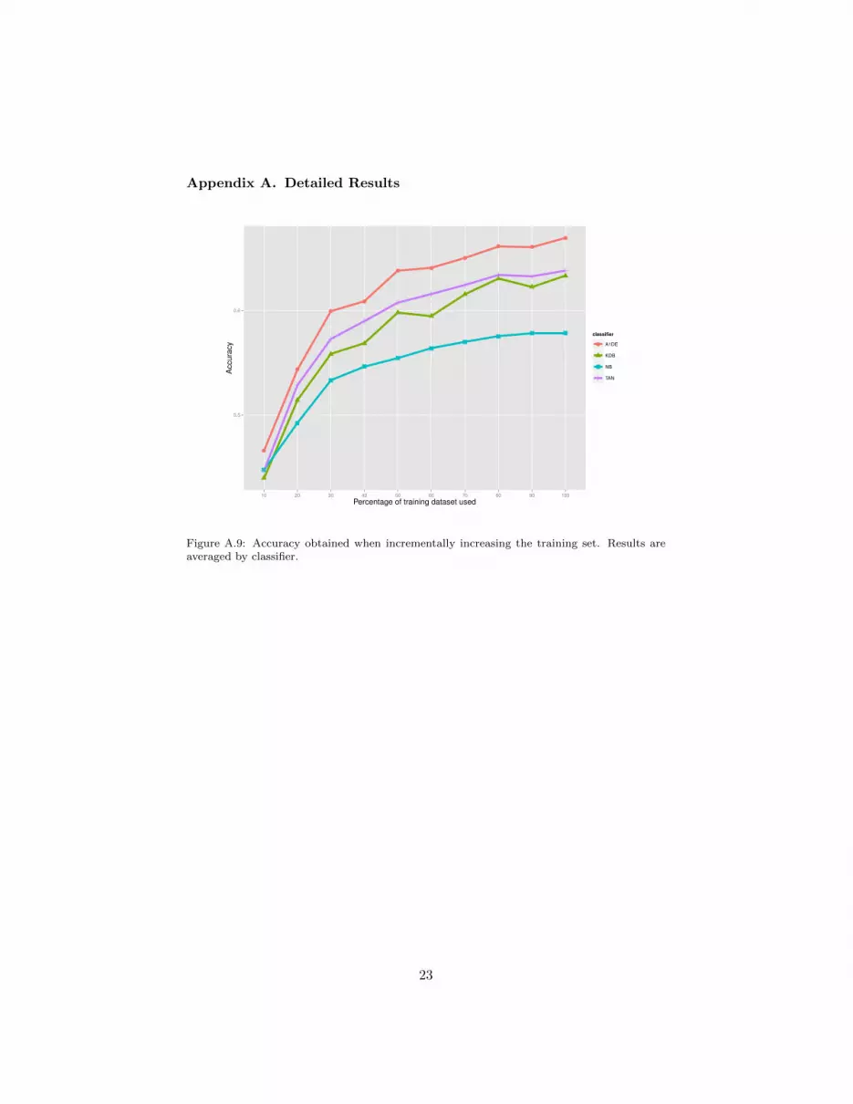
• The above points suggests that, AODE, being a low-bias learner can bea suitable candidate to tackle these problems. To contrast this we per-formed an additional experiment in which we evaluate the models whenthe training set is increased incrementally. We used the best parametercombination mentioned above and the training/test split modifying thesize of the training set by means of 10% random sample partitions. Theresults are shown in Fig. A.9 where one can clearly observe the superiorbehaviour of AODE as well as a tendency to improve its results at thepresence of additional data.
We believe that this is a positive result for probabilistic classifiers, as thismethodology is not the most popular to be applied for solving these kind of prob-lems. Furthermore, our selected models were not tuned or adjusted to optimizethe results for the competition dataset. This means that usual techniques for
17

learning can still be applied to improve upon the results for the ImageCLEFmed2013 collection such as model averaging, ensemble learning or training data ex-pansion.
Finally, we have conducted a brief analysis of the behavior of our approachby using a probabilistic view, trying to detect the main weak points in thediscrimination capabilities of the different levels of the hierarchy. The resultshows that the classification error is high for many instances, either correctly orwrongly classified. In future work, we will explore the possibilities of the pro-posed pipeline in other classification problems where classes present an intrinsichierarchy. We plan to apply our system to indoor scene classification problemsas well.
Acknowledgments
This work is partially funded by the FEDER funds and the Spanish Gov-ernment (MICINN) through projects TIN2013-46638-C3-3-P, PPII-2014-015-P, and TIN2015-65686-C5-3-R. Jacinto Arias is funded by the MECD grantFPU13/00202. Jesus Martınez-Gomez is funded by the JCCM grant POST2014/8171.
References
[1] C. Akgul, D. Rubin, S. Napel, C. Beaulieu, H. Greenspan, B. Acar,Content–based image retrieval in radiology: Current status and future di-rections, Journal of Digital Imaging 24 (2) (2011) 208–222.
[2] Unknown, Riding the wave: How europe can gain from the rising tide ofscientific data, Submission to the European Commission, available online athttp://cordis.europa.eu/fp7/ict/e-infrastructure/docs/hlg-sdi-report.pdf
(October 2010).
[3] S. Montani, R. Bellazzi, Supporting decisions in medical applications: theknowledge management perspective, International Journal of Medical In-formatics 68 (2002) 79–90.
[4] P. Welter, T. Deserno, B. Fischer, R. Gunther, C. Spreckelsen, Towardscase–based medical learning in radiological decision making using content–based image retrieval, BMC Medical Informatics and decision Making11 (68).
[5] A. Aamodt, E. Plaza, Case-based reasoning: Foundational issues, method-ological variations, and system approaches, AI communications 7 (1) (1994)39–59.
[6] J. Kalpathy-Cramer, A. Garcıa Seco de Herrera, D. Demner-Fushman,S. Antani, S. Bedrick, H. Muller, Evaluating performance of biomedicalimage retrieval systems– an overview of the medical image retrieval task atImageCLEF 2004–2014, Computerized Medical Imaging and Graphics.
18

[7] A. Garcıa Seco de Herrera, J. Kalpathy-Cramer, D. Demner Fushman,S. Antani, H. Muller, Overview of the ImageCLEF 2013 medical tasks, in:Working Notes of CLEF 2013, 2013.
[8] C. Bielza, P. Larranaga, Discrete bayesian network classifiers: a survey,ACM Computing Surveys (CSUR) 47 (1) (2014) 5.
[9] I. Kitanovski, I. Dimitrovski, S. Loskovska, FCSE at medical tasks of Im-ageCLEF 2013, in: Working Notes of CLEF 2013, 2013.
[10] X. Zhou, M. Han, Y. Song, Q. Li, Fast filtering techniques in medical imageclassification and retrieval, in: Working Notes of CLEF 2013, 2013.
[11] L. Denoyer, P. Gallinari, Bayesian network model for semi-structured doc-ument classification, Information processing & management 40 (5) (2004)807–827.
[12] H. Schneiderman, Learning a restricted bayesian network for object de-tection, in: Proceedings of the 2004 IEEE Computer Society Conferenceon Computer Vision and Pattern Recognition., Vol. 2, IEEE, 2004, pp.631–639.
[13] F. Rubio, M. J. Flores, J. Martınez-Gomez, A. Nicholson, Dynamic se-mantic network for semantic localization, in: 15th Workshop of PhysicalAgents., 2014, pp. 144–155.
[14] P. G. Ipeirotis, Analyzing the amazon mechanical turk marketplace, XRDS:Crossroads, The ACM Magazine for Students 17 (2) (2010) 16–21.
[15] H. Muller, J. Kalpathy–Cramer, I. Eggel, S. Bedrick, S. Radhouani,B. Bakke, J. Kahn, C. E., W. Hersh, Overview of the clef 2009 medicalimage retrieval track, in: Multilingual Information Access Evaluation II.Multimedia Experiments, Vol. 6242 of Lecture Notes in Computer Science,Springer Berlin Heidelberg, 2010, pp. 72–84.
[16] H. Muller, J. Kalpathy-Cramer, I. Eggel, S. Bedrick, J. Reisetter, C. E.Kahn Jr., W. Hersh, Overview of the CLEF 2010 medical image retrievaltrack, in: Working Notes of CLEF 2010, 2010.
[17] P. Tirilly, K. Lu, X. Mu, T. Zhao, Y. Cao, On modality classification and itsuse in text-based image retrieval in medical databases, in: 9th InternationalWorkshop on Content–Based Multimedia Indexing, 2011.
[18] M. Rahman, D. You, M. S. Simpson, S. K. Antani, D. Demner-Fushman,G. R. Thoma, Multimodal biomedical image retrieval using hierarchicalclassification and modality fusion, International Journal of Multimedia In-formation Retrieval 2 (3) (2013) 159–173.
[19] A. P. Pentland, R. W. Picard, S. Scarloff, Photobook: Tools for content–based manipulation of image databases, International Journal of ComputerVision 18 (3) (1996) 233–254.
19

[20] A. K. Jain, A. Vailaya, Image retrieval using color and shape, PatternRecognition 29 (8) (1996) 1233–1244.
[21] M. Simpson, M. Rahman, S. Phadnis, E. Apostolova, D. Demmer-Fushman,S. Antani, G. Thoma, Text– and content–based approaches to image modal-ity classification and retrieval for the ImageCLEF 2011 medical retrievaltrack, in: Working Notes of CLEF 2011, 2011.
[22] D. Markonis, I. Eggel, A. Garcıa Seco de Herrera, H. Muller, The medGIFTgroup in ImageCLEFmed 2011, in: Working Notes of CLEF 2011, 2011.
[23] K. Lai, L. Bo, X. Ren, D. Fox, A large-scale hierarchical multi-view rgb-dobject dataset, in: IEEE International Conference on Robotics and Au-tomation., IEEE, 2011, pp. 1817–1824.
[24] H. Ali, Z.-C. Marton, Evaluation of feature selection and model trainingstrategies for object category recognition, in: IEEE/RSJ International Con-ference on Intelligent Robots and Systems., IEEE, 2014, pp. 5036–5042.
[25] V. Kramarev, S. Zurek, J. L. Wyatt, A. Leonardis, Object categorizationfrom range images using a hierarchical compositional representation, in:22nd International Conference on Pattern Recognition., IEEE, 2014, pp.586–591.
[26] P. A. Bromiley, N. A. Thacker, M. L. Scott, M. Pokric, A. Lacey, T. F.Cootes, Bayesian and non-bayesian probabilistic models for medical imageanalysis, Image and Vision Computing 21 (10) (2003) 851–864.
[27] M. Velikova, P. J. Lucas, M. Samulski, N. Karssemeijer, On the interplayof machine learning and background knowledge in image interpretation bybayesian networks, Artificial Intelligence in Medicine 57 (1) (2013) 73–86.
[28] J. Martınez-Gomez, A. Fernandez-Caballero, I. Garcıa-Varea,L. Rodrıguez, C. Romero-Gonzalez, A taxonomy of vision systemsfor ground mobile robots, International Journal of Advanced RoboticSystems 11 (2014) 1–26.
[29] A. Garcıa Seco de Herrera, D. Markonis, R. Schaer, I. Eggel, H. Muller,The medGIFT group in ImageCLEFmed 2013, in: Working Notes of CLEF2013, 2013.
[30] D. G. Lowe, Distinctive image features from scale-invariant keypoints, In-ternational Journal of Computer Vision 60 (2) (2004) 91–110.
[31] A. Garcıa Seco de Herrera, D. Markonis, H. Muller, Bag of colors forbiomedical document image classification, in: H. Greenspan, H. Muller(Eds.), Medical Content–based Retrieval for Clinical Decision Support,MCBR–CDS 2012, Lecture Notes in Computer Sciences (LNCS), 2013,pp. 110–121.
20
[32] S. A. Chatzichristofis, Y. S. Boutalis, CEDD: Color and edge directivitydescriptor: A compact descriptor for image indexing and retrieval, in: Lec-ture notes in Computer Sciences, Vol. 5008, 2008, pp. 312–322.
[33] S. A. Chatzichristofis, Y. S. Boutalis, FCTH: Fuzzy color and texture his-togram: A low level feature for accurate image retrieval, in: Proceedingsof the 9th International Workshop on Image Analysis for Multimedia In-teractive Service, 2008, pp. 191–196.
[34] J. Han, K. Ma, Fuzzy color histogram and its use in color image retrieval,IEEE Transactions on Image Processing 11 (8) (2002) 944–952.
[35] R. Schaer, D. Markonis, H. Muller, Architecture and applications of theparallel distributed image search engine (ParaDISE), in: FoRESEE 2014,1st International Workshop on Future Search Engines, 2014.
[36] J. Pearl, Probabilistic reasoning in intelligent systems: networks of plausi-ble inference, Morgan Kaufmann, 2014.
[37] D. M. Chickering, Learning bayesian networks is np-complete, in: Learningfrom Data: Artificial Intelligence and Statistics V, Springer-Verlag, 1996,pp. 121–130.
[38] F. V. Jensen, T. D. Nielsen, Bayesian Networks and Decision Graphs, 2ndEdition, Springer Verlag, New York, 2007.
[39] N. Friedman, D. Geiger, M. Goldszmidt, Bayesian network classifiers, Ma-chine Learning 29 (2-3) (1997) 131–163.
[40] M. J. Flores, J. A. Gamez, A. M. Martınez, Supervised classification withbayesian networks, in: R. M. et al. (Ed.), Intelligent Data Analysis for Real-Life Applications: Theory and Practice, IGI Global, 2012, pp. 72–102.
[41] M. Minsky, Steps toward artificial intelligence, Proceedings of the IRE49 (1) (1961) 8–30.
[42] C. I. Chow, C. N. Liu, Approximating discrete probability distributionswith dependence trees, IEEE Transactions on Information Theory 14 (1968)462–467.
[43] M. Sahami, Learning limited dependence bayesian classifiers, in: KDD,Vol. 96, 1996, pp. 335–338.
[44] G. Webb, J. Boughton, Z. Wang, Not so naive bayes: Aggregating one-dependence estimators, Machine Learning 58 (1) (2005) 5–24.
[45] M. J. Flores, J. A. Gamez, A. M. Martınez, J. M. Puerta, Gaode andhaode: two proposals based on aode to deal with continuous variables,in: Proceedings of the 26th Annual International Conference on MachineLearning, ACM, 2009, pp. 313–320.
21
[46] G. H. John, P. Langley, Estimating continuous distributions in bayesianclassifiers, in: Proceedings of the Eleventh Conference on Uncertainty inArtificial Intelligence, Morgan Kaufmann Publishers Inc., 1995, pp. 338–345.
[47] U. Fayyad, K. Irani, Multi-interval discretization of continuous-valued at-tributes for classification learning.
[48] M. A. Hall, Correlation-based feature selection for discrete and numericclass machine learning, in: Proceedings of the Seventeenth InternationalConference on Machine Learning, Morgan Kaufmann, 2000, pp. 359–366.
[49] M. Galar, A. Fernandez, E. Barrenechea, H. Bustince, F. Herrera, Anoverview of ensemble methods for binary classifiers in multi-class prob-lems: Experimental study on one-vs-one and one-vs-all schemes, PatternRecognition 44 (8) (2011) 1761–1776.
[50] A. D. Gordon, A review of hierarchical classification, Journal of the RoyalStatistical Society. (1987) 119–137.
[51] M. Friedman, A comparison of alternative tests of significance for the prob-lem of m rankings, The Annals of Mathematical Statistics (1940) 86–92.
[52] S. Lazebnik, C. Schmid, J. Ponce, Beyond bags of features: Spatial pyra-mid matching for recognizing natural scene categories, in: IEEE ComputerSociety Conference on Computer Vision and Pattern Recognition., Vol. 2,IEEE, 2006, pp. 2169–2178.
[53] M. Abedini, L. Cao, N. Codella, J. H. Connell, R. Garnavi, A. Geva,M. Merler, Q.-B. Nguyen, S. U. Pankanti, J. R. Smith, et al., IBM re-search at ImageCLEF 2013 medical tasks.
[54] M. S. Simpson, D. You, M. Rahman, D. Demner-Fushman, S. Antani,G. Thoma, ITI’s participation in the 2013 medical track of ImageCLEF,in: Working Notes of CLEF 2013, 2013.
[55] A. Mourao, F. Martins, J. Magalhaes, Novasearch on medical imageclef2013, in: Working Notes of CLEF 2013, Vol. 2013, 2013, pp. 1–10.
[56] S. Stathopoulos, I. Lourentzou, A. Kyriakopoulou, T. Kalamboukis, IPL atCLEF 2013 medical retrieval task, in: Working Notes of CLEF 2013, 2013.
22
Appendix A. Detailed Results
0.5
0.6
10 20 30 40 50 60 70 80 90 100
Percentage of training dataset used
Accura
cy
classifier
A1DE
KDB
NB
TAN
Figure A.9: Accuracy obtained when incrementally increasing the training set. Results areaveraged by classifier.
23
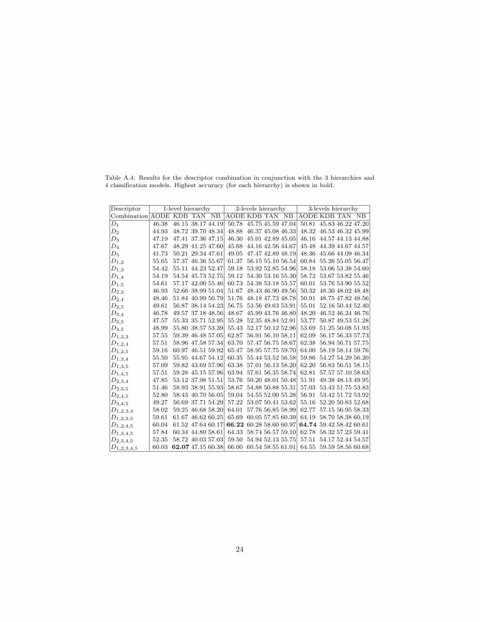
Table A.4: Results for the descriptor combination in conjunction with the 3 hierarchies and4 classification models. Highest accuracy (for each hierarchy) is shown in bold.
Descriptor 1-level hierarchy 2-levels hierarchy 3-levels hierarchyCombination AODE KDB TAN NB AODE KDB TAN NB AODE KDB TAN NBD1 46.38 46.15 38.17 44.19 50.78 45.75 45.59 47.04 50.81 45.83 46.22 47.20D2 44.93 48.72 39.70 48.34 48.88 46.37 45.08 46.33 48.32 46.53 46.32 45.99D3 47.19 47.41 37.36 47.15 46.30 45.01 42.89 45.05 46.16 44.57 44.13 44.88D4 47.67 48.29 41.25 47.60 45.68 44.16 42.56 44.67 45.48 44.39 44.67 44.57D5 41.73 50.21 29.34 47.61 49.05 47.47 42.89 48.19 48.36 45.66 44.09 46.34D1,2 55.65 57.37 46.36 55.67 61.37 56.15 55.10 56.54 60.84 55.26 55.05 56.47D1,3 54.42 55.11 44.23 52.47 59.18 53.92 52.85 54.96 58.18 53.06 53.38 54.60D1,4 54.19 54.54 45.73 52.75 59.12 54.30 53.16 55.30 58.72 53.67 53.82 55.46D1,5 54.61 57.17 42.00 55.46 60.73 54.38 53.18 55.57 60.01 53.76 53.90 55.52D2,3 46.93 52.66 38.99 51.04 51.67 48.43 46.90 49.56 50.32 48.30 48.02 48.48D2,4 48.46 51.84 40.99 50.79 51.76 48.18 47.73 48.78 50.91 48.75 47.82 48.56D2,5 49.61 56.87 38.14 54.23 56.75 53.56 49.63 53.91 55.01 52.16 50.44 52.40D3,4 46.78 49.57 37.18 48.56 48.67 45.99 43.76 46.80 48.20 46.52 46.24 46.76D3,5 47.57 55.33 35.71 52.95 55.28 52.35 48.84 52.91 53.77 50.87 49.53 51.28D4,5 48.99 55.80 38.57 53.39 55.43 52.17 50.12 52.96 53.69 51.25 50.08 51.93D1,2,3 57.55 59.39 46.48 57.05 62.87 56.91 56.10 58.11 62.09 56.17 56.33 57.73D1,2,4 57.51 58.96 47.58 57.34 63.70 57.47 56.75 58.67 62.38 56.94 56.71 57.75D1,2,5 59.16 60.97 46.51 59.92 65.47 58.95 57.75 59.70 64.00 58.19 58.14 59.76D1,3,4 55.50 55.95 44.67 54.12 60.35 55.44 53.52 56.58 59.86 54.27 54.29 56.20D1,3,5 57.09 59.82 43.69 57.96 63.38 57.01 56.13 58.20 62.20 56.83 56.51 58.15D1,4,5 57.51 59.28 45.15 57.96 63.94 57.61 56.35 58.74 62.81 57.57 57.10 58.63D2,3,4 47.85 53.12 37.98 51.51 53.76 50.20 48.01 50.48 51.91 49.38 48.13 49.95D2,3,5 51.46 58.93 38.91 55.93 58.67 54.88 50.88 55.31 57.03 53.43 51.75 53.83D2,4,5 52.80 58.43 40.70 56.05 59.04 54.55 52.00 55.28 56.91 53.42 51.72 53.92D3,4,5 49.27 56.69 37.71 54.29 57.22 53.07 50.41 53.62 55.16 52.20 50.83 52.68D1,2,3,4 58.02 59.25 46.68 58.20 64.01 57.76 56.85 58.99 62.77 57.15 56.95 58.33D1,2,3,5 59.61 61.67 46.62 60.25 65.69 60.05 57.85 60.39 64.19 58.70 58.38 60.19D1,2,4,5 60.04 61.52 47.64 60.17 66.22 60.28 58.60 60.97 64.74 59.42 58.42 60.61D1,3,4,5 57.84 60.34 44.80 58.61 64.33 58.74 56.57 59.10 62.78 58.32 57.23 59.41D2,3,4,5 52.35 58.72 40.03 57.03 59.50 54.94 52.13 55.75 57.51 54.17 52.44 54.57D1,2,3,4,5 60.03 62.07 47.15 60.38 66.00 60.54 58.55 61.01 64.55 59.59 58.56 60.68
24


