Embed Size (px)
Citation preview

International Journal on Artificial Intelligence Tools © World Scientific Publishing Company
A BAYESIAN METANETWORK
VAGAN TERZIYAN
Department of Mathematical Information Technology, University of Jyvaskyla, P.O. Box 35 (Agora), FIN-40014 Jyvaskyla, Finland
Received (9 July 2003) Accepted (15 March 2004)
Bayesian network (BN) is known to be one of the most solid probabilistic modeling tools. The theory of BN provides already several useful modifications of a classical network. Among those there are context-enabled networks such as multilevel networks or recursive multinets, which can provide separate BN modelling for different combinations of contextual features’ values. The main challenge of this paper is the multilevel probabilistic meta-model (Bayesian Metanetwork), which is an extension of traditional BN and modification of recursive multinets. It assumes that interoperability between component networks can be modeled by another BN. Bayesian Metanetwork is a set of BN, which are put on each other in such a way that conditional or unconditional probability distributions associated with nodes of every previous probabilistic network depend on probability distributions associated with nodes of the next network. We assume parameters (probability distributions) of a BN as random variables and allow conditional dependencies between these probabilities. Several cases of two-level Bayesian Metanetworks were presented, which consist on interrelated predictive and contextual BN models. Keywords: Bayesian networks, context, multinets
1 Introduction A Bayesian network (BN) has proven to be a valuable tool for encoding, learning and reasoning about probabilistic (causal) relationships [1]. A BN for a set of variables X ={X1, …, Xn} is a directed acyclic graph with a network structure S that encodes a set of conditional independence assertions about variables in X, and a set P of local probability distributions associated with each variable [2]. Simple BN example is shown in Fig. 1.
Inference in BN generally targets the calculation of some probability of interest. Inference algorithms exploit the conditional (in)dependence between variables (1), see e.g. joint probability (2) for Fig. 1; marginalization rule (3); and Bayesian rule (4).
∏=
=n
iiin XParentsXPXXXP
121 ))(|(),...,,( (1)

)|()(),( ijiij xXyYPxXPxXyYP ==⋅==== (2)
X
Y
P(X)
P(Y)-?
P(Y|X)
Fig. 1. Example of a simple Bayesian network
∑ ==⋅===i
ijij xXyYPxXPyYP )|()()( (3)
)()|()(
)|(j
ijiji yYP
xXyYPxXPyYxXP
===⋅=
=== (4)
Learning BN generally means the refinement of the structure and local probability distributions of a BN given data. The simplest version of this problem is using data to update the probabilities of a given BN network structure. An important task in learning BN from data is model selection [3]. Each attribute in ordinary BN has the same status, so they are just combined into possible models-candidates to encode conditional dependencies. Some modifications of BN however require distinguishing between attributes, e.g. as follows: • Target attribute, which probability is being estimated based on set of evidence. • Predictive attribute, which values being observed effect probability distribution of a
target attribute(s) via some structure of other predictive attributes according to causal dependencies among them.
• Contextual attribute, which has no direct visible effect to target attributes but influences some of probability distributions within the predictive model. A contextual attribute can be conditionally dependent on some other contextual attribute. Causal independence in a BN refers to the situation where multiple causes provided
by predictive attributes contribute independently to a common effect on a target attribute. With causal independence, the probability function can be described using a binary operator that can be applied to values from each of the parent predictive attributes (see (1)). Context specific independence refers to the fact that some random variables are probabilistically independent of each other in a certain context.
In [4], Butz exploited contextual independencies based on assumption that while a conditional independence must hold over all contexts, a contextual independence need only hold for one particular context. He shows how contextual independencies can be modeled using multiple BN. Boutilier et al [5] presents two algorithms to exploit context specific independence in a BN. The first is network transformation and clustering. With this method, the context specific independencies are qualitatively encoded within the
2

network structure of the transformed network and appropriate conditional probability tables are represented as decision trees. The other algorithm works by selecting a set of variables that, once instantiated, makes the network singly connected. With context specific independence this essentially reduces total inference time for queries. Zhang [6] used generalized rules for contextual variable elimination algorithm, which capture context specific independence in variables. Geiger and Heckerman [7] used similarity networks to make context specific independencies explicit in BN. In a similarity network, the edges between the variables can be thought of as a network whose edges can appear or disappear depending on the values of certain variables in the network. This allows for different BNs to perform inference for different contexts.
Domain ontologies seem to be an excellent source of contextual data, which can be used for modelling context-sensitive BNs. Additional knowledge about (semantic) relations between BN nodes other than causal ones can be considered as a sample of a very useful context, which can affect the interpretation of the original structure of the BN. Helsper and Gaag [8] describe an interesting combination of medical ontologies as explicit documentation of the cancer domain knowledge and the BN, which encodes cause-symptom relationships in this domain. For example, the knowledge that pertains to haematogenous metastases may be considered from different points of view and resulting in the two alternative depictions (see Fig. 2).
primary tumour depth outside site
primary tumourdepth at site
metastasis via blood vessels presence
metastasis liver presence
metastasis lungspresence
haematogenous metastasis presence
is-a
resulting resulting
is-a
initiating initiating
(a)
primary tumourdepth outside site
primary tumour depth at site
metastasis via blood vessels presence
metastasis liver presence
metastasis lungs presence
haematogenous metastasis presence
is-a
resulting
is-a
initiating initiating
(b)
Fig 2. Combining BN with ontology [9]
Alternative (a) in Fig. 2 describes that the process of metastasis via blood vessels
may result in metastases in the lungs and metastases in the liver, which are known from the ontological context to be subclasses of the class haematogenous metastasis. Alternative (b) captures a relation at a higher level: the process of metastasis via blood vessels may result in haematogenous metastases, which according to the context may be in the lungs or in the liver. Imagine a scenario when some BN learning algorithm has produced structure (a). Imagine also that our context as part of OWL ontology is knowledge about: class haematogenous metastasis is a disjoint_union_of class metastases in the lungs and class metastases in the liver. According to this context it is possible to automatically transfer BN structure from alternative (a) to more compact alternative (b) and then make appropriate recalculation of the BN parameters.
3

If a Bayesian network is to be modified to better represent probability of a target attribute, one can either change its graphical structure, or its parameters or both [9]. There are two ways for changing the structure of a Bayesian network: one can change the nodes in the graph (add, delete or combine nodes) or change the arrows in the graph (add, delete or re-orient arrows) or both. In Bang et al. [9] a combination of these two strategies for network modification is considered. To generate a causal network that satisfies the causal Markov condition the flexibility is needed to add either a new arrow or a new common cause (a hidden node). The complexity of generated network can be measured in terms of the number of parameters required in the network. Results show that in most situations adding an arrow will increase complexity least, but in cases where two or more nodes share a large number of parents, adding a hidden node can even decrease complexity.
In [10] a multi-level BN was presented that accurately models the system and allows for sensor integration in an evidential framework. It was shown that a multi-level BN performs better than a simple single-level BN. Multilayer networks are usually sensitive to conditional probabilities, which should be defined with greater accuracy because small differences in their values may result in radically different target concept estimation. Choosing between a simple BN and a multilevel network one needs to carefully evaluate an expected benefit against the increased costs of the knowledge management [11].
Bayesian multinets were first introduced in [12] and then studied in [13] as a type of classifiers. A Bayesian multinet is composed of the prior probability distribution of the class node and a set of local networks, each corresponding to a value that the class node can take. Bayesian multinets can be viewed as a generalization of BNs. A BN forces the relations among the features to be the same for all the values that the class node takes; by contrast a Bayesian multinet allows the relations among the features to be different, i.e. for different values the class node takes, the features can form different local networks with different structures. While multinet is more general than BN, it is often less complex since some of the local networks can be simpler than others, while BN needs to have a complex structure in order to express all the relationships among the features [13]. In [14] dynamic Bayesian multinets are introduced where a Markov chain state at time determines conditional independence patterns between random variables lying within a local time window surrounding it. It is demonstrated that multinets can in many cases outperform other dynamic models with a similar number of parameters. A recursive Bayesian multinet was introduced by Pena et al [15] as a decision tree with component Bayesian networks at the leaves. The key idea was to decompose the learning Bayesian network problem into learning component networks from incomplete data.
As our main goal in this paper, we are presenting another view to the Bayesian “multinets” towards making them to be really “metanetworks”, i.e. by assuming that interoperability between component Bayesian networks can be also modeled by another Bayesian network.
The rest of paper organized as follows. In Section 2 we present two models of a contextual effect to probability distributions in BN. In Section 3 we introduce a Bayesian Metanetwork, basic inference in it and few cases of interaction between its predictive and contextual levels. We conclude in Section 4.
4

2 Modelling Contextual Effect on Bayesian Network Parameters In this chapter, we first consider the model of direct effect of a contextual parameter on conditional (2.1) and unconditional (2.2) probabilities in a BN (or actually indirect effect to a target attribute’s probability), which is one of the basic components of the Bayesian Metanetwork concept. 2.1. Contextual Effect on Conditional Probability Simplest possible case is shown in Fig. 3 where one contextual attribute affects the conditional probability between one predictive and one target attribute.
X
Y
P(X)
P(Y)-?P(P(Y|X)|Z)
Z
P(Z) P(Y|X)
pk(Y|X)
P(P(Y|X))
Fig. 3. Simple model of contextual effect on conditional probability
The case shown in Fig. 3 can be described as follows: • X ={x1, x2, …, xn} – predictive attribute with n values; • Z ={z1, z2, …, zq} – contextual attribute with q values; • P(Y|X) = {p1(Y|X), p2(Y|X), …, p r(Y|X)} – conditional dependence attribute
(random variable) between X and Y with r possible values; • P(P(Y|X)|Z) – conditional dependence between attribute Z and attribute P(Y|X);
Assume that our goal is to compute P(Y). For that first we calculate the probability for the “conditional dependence” attribute:
∑=
==⋅===q
mmkmk zZXYpXYPPzZPXYpXYPP
1
]}|)|()|([)({))|()|(( (5)
Then we estimate the following joint probability:
)()]|()|([)]|()|(,|[
))|()|(,,(
ikkij
kij
xXPXYpXYPPXYpXYPxXyYP
XYpXYPxXyYP
=⋅=⋅====
==== (6)
Taking into account that:
)|()]|()|(,|[ ijkkij xXyYpXYpXYPxXyYP ====== we can rewrite (6) as follows:
5

)()]|()|([)|(
))|()|(,,(
ikijk
kij
xXPXYpXYPPxXyYp
XYpXYPxXyYP
=⋅=⋅===
==== (7)
Substituting (5) to (7) we get:
∑=
==⋅=⋅=⋅===
====q
mmkmiijk
kij
zZXYpXYPPzZPxXPxXyYp
XYpXYPxXyYP
1]}|)|()|([)({)()|(
))|()|(,,((8)
Applying marginalization in (8) we obtain:
})]|)|()|(()([
)()|({)(
1
1 1
∑
∑∑
=
= =
==⋅=×
×=⋅====
q
mmkm
r
k
n
iiijkj
zZXYpXYPPzZP
xXPxXyYpyYP (9)
or in more compact form (with attributes only and without values) the general calculation scheme will be as follows:
})]|)|(()([)|()({)()|( 4444 34444 21
metalevel
ZXYP XZXYPPZPXYPXPYP ∑∑ ∑
∀∀ ∀
⋅⋅⋅= . (10)
Consider artificial example scenario for Fig. 3: • Target attribute (someone’s wellness): Y = {Rich, Poor}; • Predictive attribute (someone’s intension to work): X = {Hardworking, Lazy}; • Known probability distribution: P(Hardworking) = 0.3; P(Lazy) = 0.7. • Contextual attribute (someone’s country of residence): Z = {USA, Ukraine,
TheRestWorld}; • Probability distribution: P(USA) =0.2; P(Ukraine) = 0.1; P(TheRestWorld) = 0.7. • Assume that we know two possible conditional probability distributions for P(Y|X)
as it is shown in Table 1.
Table 1. Probability distribution for P(X|Y) in the example ________________________________________________
p1(Y|X) Hardworking Lazy ________________________________________________
Rich 0.8 0.1 Poor 0.2 0.9
________________________________________________
p2(Y|X) Hardworking Lazy ________________________________________________
Rich 0.6 0.5 Poor 0.4 0.5
________________________________________________
• Assume conditional dependence between contextual attribute Z and P(Y|X) to be as shown in Table 2.
6
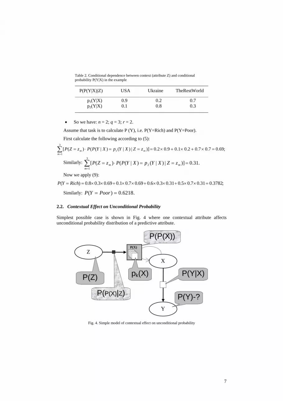
Table 2. Conditional dependence between context (attribute Z) and conditional probability P(Y|X) in the example
______________________________________________________________________
P(P(Y|X)|Z) USA Ukraine TheRestWorld ______________________________________________________________________
p1(Y|X) 0.9 0.2 0.7 p2(Y|X) 0.1 0.8 0.3
______________________________________________________________________
• So we have: n = 2; q = 3; r = 2.
Assume that task is to calculate P (Y), i.e. P(Y=Rich) and P(Y=Poor).
First calculate the following according to (5):
;69.07.07.02.01.09.02.0)]|)|()|(()([3
11 =×+×+×===⋅=∑
=mmm zZXYpXYPPzZP
Similarly: . 31.0)]|)|()|(()([3
12 ===⋅=∑
=mmm zZXYpXYPPzZP
Now we apply (9):
;3782.031.07.05.031.03.06.069.07.01.069.03.08.0)( =××+××+××+××== RichYP
Similarly: .6218.0)( == PoorYP 2.2. Contextual Effect on Unconditional Probability Simplest possible case is shown in Fig. 4 where one contextual attribute affects unconditional probability distribution of a predictive attribute.
X
Y
P(Y)-?P(P(X)|Z)
Z
P(Z)
P(X)
pk(X)
P(P(X))
P(Y|X)
Fig. 4. Simple model of contextual effect on unconditional probability
7

In the case shown in the Fig. 4 we have the following input data: • X ={x1, x2, …, xn} – predictive attribute with n values; • Z ={z1, z2, …, zq} – contextual attribute with q values and P(Z) – probability
distribution for values of Z; • P(X) = {p1(X), p2(X), …, pr(X)} – probability distribution attribute for X (random
variable) with r possible values (different possible probability distributions for X) and P(P(X)) is probability distribution for values of attribute P(X);
• P(Y|X) is a conditional probability distribution of Y given X; • P(P(X)|Z) is a conditional probability distribution for attribute P(X) given Z;
Assuming that goal is to compute P(Y), first we calculate the following probability:
∑=
==⋅===q
mmkmk zZXpXPPzZPXpXPP
1]}|)()([)({))()(( . (11)
Then we estimate the following joint probability:
))()(())()(|())()(,|(
))()(,())()(,|(
))()(,,(
XpXPPXpXPxXPXpXPxXyYP
XpXPxXPXpXPxXyYP
XpXPxXyYP
kkikij
kikij
kij
=⋅==⋅====
===⋅====
====(12)
Taking into account the independence of parameters Y and P(X) given X and also that:
)())()(,( ikki xXpXpXPxXP ====
we can rewrite (12) as follows:
)())()(()|(
))()(,,(
ikkij
kij
xXpXpXPPxXyYP
XpXPxXyYP
=⋅=⋅===
==== (13)
Substituting (11) to (13) we get:
∑=
==⋅=⋅=⋅===
====q
mmkmikij
kij
zZXpXPPzZPxXpxXyYP
XpXPxXyYP
1
))|)()(()(()()|(
))()(,,((14)
Applying summarization in (14) we obtain:
})]|)()(()([
)()|({)(
1
1 1
∑
∑∑
=
= =
==⋅=×
×=⋅====
q
mmkm
r
k
n
iikijj
zZXpXPPzZP
xXpxXyYPyYP (15)
or in more compact form the general calculation scheme will be as follows:
})]|)(()([)|()({)()( 4444 34444 21
metalevel
ZXP XZXPPZPXYPXPYP ∑∑ ∑
∀∀ ∀
⋅⋅⋅= . (16)
8

Consider artificial example scenario for Fig. 4: • Target attribute (someone’s wellness): Y = {Rich, Poor}; • Predictive attribute (someone’s intension to work): X = {Hardworking, Lazy}; • Assume that we have two possible probability distributions for X as it is shown in
Table 3.
Table 3. Two probability distributions for X in the example ________________________________________________
P(X) Hardworking Lazy ________________________________________________
p1(X) 0.2 0.8 p2(X) 0.5 0.5
________________________________________________ • Contextual attribute (someone’s country of residence): Z = {USA, Ukraine,
TheRestWorld}; • Probability distribution: P(USA) =0.2; P(Ukraine) = 0.1; P(TheRestWorld) = 0.7. • Assume that we know conditional probability distribution matrix for P(Y|X) as it is
presented in Table 4.
Table 4. Conditional probability P(Y|X) in the example ________________________________________________
P(Y|X) Hardworking Lazy ________________________________________________
Rich 0.7 0.4 Poor 0.3 0.6
________________________________________________ • Let conditional dependence between contextual attribute Z and attribute P(X) to be as
it is shown in Table 5.
Table 5. Conditional dependence between context (attribute Z) and probability distribution P(X) in the example
______________________________________________________________________
P(P(X)|Z) USA Ukraine TheRestWorld ______________________________________________________________________
p1(X) 0.4 0.2 0.3 p2(X) 0.6 0.8 0.7
______________________________________________________________________
• So we have: n = 2; q = 3; r = 2. Assume that task is to calculate P (Y), i.e. P(Y=Rich) and P(Y=Poor).
First we calculate the following according to (11):
;31.03.07.02.01.04.02.0)]|)()(()([3
11 =×+×+×===⋅=∑
=mmm zZXpXPPzZP
;69.07.07.08.01.06.02.0)]|)()(()([3
12 =×+×+×===⋅=∑
=mmm zZXpXPPzZP
9

Now we apply (15): ;5221.069.05.04.069.05.07.031.08.04.031.02.07.0)( =××+××+××+××== RichYP
.4779.0)( == PoorYP 3 Bayesian Metanetwork for Managing Probability Distributions We define a Bayesian Metanetwork in a way implementing the basic intuition we had defining a Semantic Metanetwork few years ago. Semantic Metanetwork [16] was defined as a set of semantic networks, which are put on each other in such a way that links of every previous semantic network are in the same time nodes of the next network. In a Semantic Metanetwork every higher level controls semantic structure of the lower level. Simple controlling rules might be, for example, in what contexts certain link of a semantic structure can exist and in what context it should be deleted from the semantic structure.
Definition. Bayesian Metanetwork is a set of Bayesian networks, which are put on each other in such a way that conditional or unconditional probability distributions associated with nodes of every previous probabilistic network depend on probability distributions associated with nodes of the next network.
First consider 2-level Bayesian Metanetwork (the idea is shown in Fig. 5). Context variables in it are considered to be on a second (contextual) level to control the conditional probabilities associated with predictive level of the network. Standard Bayesian inference is applied in Bayesian network of each level.
Contextual level
Predictive levelA
B
X
Y
P(B|A)P(Y|X)
Fig. 5. Two-level Bayesian Metanetwork for managing conditional probabilities
A sample of a Bayesian Metanetwork (for simplicity projected to 2-D space), which is part of the metanetwork in Fig. 5, is presented in Fig. 6. Bayesian (meta)network in Fig. 6 has the following parameters:
Attributes of the predictive level: A with values {a1,a2,…,ana}; B with values {b1,b2,…,bnb} and probability P(A); X with values {x1,x2,…,xnx}; Y with values {y1,y2,…,yny} and probability P(X);
Conditional probabilities of the predictive level: P(B|A) which is random variable with set of values {p1(B|A), p2(B|A),…, pmp(B|A)}. Important to notice that this parameter serves as an ordinary conditional probability in the predictive level of Bayesian metanetwork and it also serves as an attribute node on the contextual level.
10

P(Y|X) which is random variable with possible values {p1(Y|X), p2(Y|X),…, pnp(Y|X)} and also considered as an attribute node on a contextual level of Bayesian Metanetwork.
Conditional probability from the contextual level: P(P(Y|X),P(B|A)), which defines conditional probability between two contextual attributes P(B|A) and P(Y|X).
X
Y
P(X)
P(Y)-?P(P(Y|X)|P(B|A))
A
B
P(A)
pr(B|A)
P(P(B|A)) P(B|A) P(Y|X)
pk(Y|X)
P(P(Y|X))
Fig. 6. An example of Bayesian Metanetwork. The nodes of the 2nd-level network correspond to the conditional probabilities of the 1st-level network P(B|A) and P(Y|X). The arc in the 2nd-level network corresponds to the conditional probability P(P(Y|X)|P(B|A))
The probability of the target attribute P(Y) can be computed by applying basic Bayesian inference on both levels of the metanetwork. First we are exploring the basic level of the BMN. Finding joint probability:
));|()|(()()|(
))|()|(,())|()|(,|())|()|(,,(
)|(
XYpXYPPxXPxXyYp
XYpXYPxXPXYpXYPxXyYPXYpXYPxXyYP
kiijk
tindependen
ki
xXyYp
kij
kij
ijk
=⋅=⋅===
===⋅====
====
==44444 344444 214444444 34444444 21
Then making marginalization:
;))]|()|(()()|([)( ∑∑ =⋅=⋅====k i
kiijkj XYpXYPPxXPxXyYpyYP (17)
Now exploring the metalevel (joint probability first):
));|()|(())|()|(|)|()|(())|()|(),|()|((
ABpABPPABpABPXYpXYPPABpABPXYpXYPP
rrk
rk
=⋅======
Then marginalization on the metalevel:
];))|()|(())|()|(|)|()|(([))|()|((
∑ =⋅===
==
rrrk
k
ABpABPPABpABPXYpXYPPXYpXYPP
(18)
11

Finally from (17) and (18) we are getting the target probability:
))]}.|()|(())|()|((|)|()|(([
)()|({)(
ABpABPPABpABPPXYpXYPP
xXPxXyYpyYP
rr
rk
i kiijkj
=×==×
×=⋅====
∑
∑∑
Similar inference as for above case can be also applied to other cases of a Metanetwork where unconditional, conditional or both probability distributions associated with nodes of predictive level of the metanetwork depend on probability distributions associated with nodes of the contextual level of the metanetwork (Fig. 7).
P(A)P(X)
X
A
Contextual level
Predictive level
a)
P(P(X)|P(A))
A
pr(A)
P(P(A))
P(A) X
pk(X)
P(P(X))
P(X)
b)
P(A)P(Y|X)
X A
Contextual level
Predictive level
Y
c)
X
Y
P(X)
P(Y)-? P(P(Y|X)|P(A))
A
pr(A)
P(P(A))
P(A) P(Y|X)
pk(Y|X)
P(P(Y|X))
d)
P(A)
P(Y|X)
X A
Contextual level
Predictive level
Y
P(B)
B
e)
X
Y
P(X)
P(Y)-?
P(P(Y|X)|P(A))
A
pr(A)
P(P(A))
P(A)
P(Y|X)
pk(Y|X)
P(P(Y|X))
B
ps(B) P(P(B))
P(B)
P(P(A)|P(B))
f)
Fig. 7. Some other (than in Fig. 5) cases of Bayesian Metanetwork: In metanetwork (a) unconditional probability distributions associated with nodes of the predictive level network depend on probability distributions associated with nodes of the contextual level network, 2-D fragment is shown in (b); in (c) the contextual level metanetwork models conditional dependence particularly between unconditional and conditional probabilities of the predictive level (see also (d)); in (e) and (f) the combination of two previous cases is shown.
12

4 Conclusions The main challenge of this paper is the multilevel probabilistic meta-model (Bayesian Metanetwork), which is an extension of traditional BN and modification of recursive multinets. The model assumes that interoperability between component networks can be also modeled by another BN. Bayesian Metanetwork is a set of BN, which are put on each other in such a way that conditional or unconditional probability distributions associated with nodes of every previous probabilistic network depend on probability distributions associated with nodes of the next network. We assume parameters (probability distributions) of a BN as random variables and allow conditional dependencies between these probabilities. Several cases of two-level Bayesian Metanetworks were presented, which consist on interrelated predictive and contextual BN models. By recursive application of the same “meta”-principle we can assume that a Bayesian metanetwork might have as many levels as necessary depending on the dynamics and complexity of the context. In this paper we have considered only some basic concepts, definitions and inference in a Bayesian Metanetwork. Some preliminary usage cases were discussed in [17], where context-sensitive mobile user preferences were modeled by Bayesian metanetworks. The basic algorithm for learning Bayesian metanetworks from data can be found in [18]. However further research is needed for providing advanced learning algorithms for such networks as well as for proving its efficiency on real-world examples. Acknowledgements I am grateful for Dr. Oleksandra Vitko for fruitful discussions and valuable comments within the scope of this paper. Also I appreciate anonymous reviewers for their useful feedback and concrete suggestions to improve the paper. The partial support for this research, provided by TEKES (SmartResource project) and cooperating companies: TeliaSonera, Metso Automation, TietoEnator, Science Park, Agora Center and University of Jyvaskyla, was also highly appreciated. References
1. J. Pearl, Probabilistic Reasoning in Intelligent Systems: Networks of Plausible Inference, (Morgan Kaufmann, 1988).
2. M. Henrion, Some Practical Issues in Constructing Belief Networks, In: Proceedings of the 3-rd Annual Conference on Uncertainty in Artificial Intelligence, (Elsevier, 1989), pp. 161-174.
3. D. Heckerman, A Tutorial on Learning with Bayesian Networks, Technical Report MSR-TR-95-06, (Microsoft Research, March 1995).
4. C. J. Butz, Exploiting Contextual Independencies in Web Search and User Profiling, In: Proceedings of the World Congress on Computational Intelligence, (Hawaii, USA, 2002), pp. 1051-1056.
13

5. C. Boutiler, N. Friedman, M. Goldszmidt and D. Koller, Context-Specific Independence in Bayesian Networks, In: Proceedings of the 12-th Conference on Uncertainty in Artificial Intelligence, (Portland, USA, 1996), pp. 115-123.
6. N.L. Zhang, Inference in Bayesian networks: The Role of Context-Specific Independence, International Journal of Information Technology and Decision Making, 1(1) 2002, 91-119.
7. D. Geiger and D. Heckerman, Knowledge Representation and Inference in Similarity Networks and Bayesian Multinets, Artificial Intelligence, Vol. 82, (Elsevier, 1996), pp. 45-74.
8. E. M. Helsper and L. C. van der Gaag, Building Bayesian Networks through Ontologies, In: Proceedings of the 15th European Conference on Artificial Intelligence, ed. F. van Harmelen, (IOS Press, Amsterdam, 2002), pp. 680-684.
9. J.-W. Bang, R. Chaleil and J. Williamson, Two-Stage Bayesian Networks for Metabolic Network Prediction, In: Proceedings of the Workshop on Qualitative and Model-Based Reasoning in Biomedicine, ed. P. Lucas (Protaras, Cyprus, 2003), pp. 19-23.
10. A. Singhal, J. Luo and C. Brown, A Multi-Level Bayesian Network Approach to Image Sensor Fusion, In: Proceedings of FUSION 2000: 3rd International Conference on Information Fusion, Vol. 2, (IEEE, 2000), pp. 9-16.
11. K. W. Przytula and D. Thompson, Construction of Bayesian Networks for Diagnostics, In: Proceedings of the 2000 IEEE Aerospace Conference, (IEEE Aerospace and Electronics Systems Society, 2000).
12. N. Friedman, D. Geiger, and M. Goldszmidt, Bayesian Network Classifiers, Machine Learning, 29(2-3), (Kluwer, 1997), pp. 131-161.
13. J. Cheng and R. Greiner, Learning Bayesian Belief Network Classifiers: Algorithms and System, In: Proceedings of the 14-th Canadian Conference on Artificial Intelligence, Lecture Notes in Computer Science, Vol. 2056, (Springer-Verlag Heidelberg, 2001), pp. 141-151.
14. J. A. Bilmes, Dynamic Bayesian Multinets, In: Proceedings of the 16-th Conference on Uncertainty in Artificial Intelligence, (Morgan Kaufmann, San Francisco, 2000), pp. 38-45.
15. J. Pena, J. A. Lozano, and P. Larranaga, Learning Bayesian Networks for Clustering by Means of Constructive Induction, Machine Learning, 47(1), (Kluwer, 2002), pp. 63-90.
16. V. Terziyan and S. Puuronen, Reasoning with Multilevel Contexts in Semantic Metanetworks, In: Formal Aspects in Context, eds. P. Bonzon, M. Cavalcanti, R. Nossun (Kluwer, 2000), pp. 107-126.
17. V. Terziyan and O. Vitko, Bayesian Metanetwork for Modelling User Preferences in Mobile Environment, In: Proceedings of KI 2003: Advances in Artificial Intelligence, Lecture Notes in Artificial Intelligence, Vol. 2821, ed. A. Gunter, R. Kruse and B. Neumann, (Springer-Verlag, 2003), pp.370-384.
18. V. Terziyan and O. Vitko, Learning Bayesian Metanetworks from Data with Multilevel Uncertainty, In: Proceedings of the First IFIP International Conference on Artificial Intelligence and Innovations (AIAI-2004), Toulouse, France, (Kluwer, 2004), to appear.
14


