Embed Size (px)
Citation preview

Digital Signal Processing 22 (2012) 54–65
Contents lists available at SciVerse ScienceDirect
Digital Signal Processing
www.elsevier.com/locate/dsp
A grid-based Bayesian approach to robust visual tracking ✩
Xinmin Liu, Zongli Lin, Scott T. Acton ∗
Charles L. Brown Department of Electrical & Computer Engineering, University of Virginia, P.O. Box 400473, Charlottesville, VA 22904-4743, United States
a r t i c l e i n f o a b s t r a c t
Article history:Available online 7 September 2011
Keywords:Visual trackingBayes’ lawKalman filterReal-timeOcclusionMultiple object tracking
Visual tracking encompasses a wide range of applications in surveillance, medicine and the militaryarena. There are however roadblocks that hinder exploiting the full capacity of the tracking technology.Depending on specific applications, these roadblocks may include computational complexity, accuracyand robustness of the tracking algorithms. In the paper, we present a grid-based algorithm for trackingthat drastically outperforms the existing algorithms in terms of computational efficiency, accuracy androbustness. Furthermore, by judiciously incorporating feature representation, sample generation andsample weighting, the grid-based approach accommodates contrast change, jitter, target deformationand occlusion. Tracking performance of the proposed grid-based algorithm is compared with tworecent algorithms, the gradient vector flow snake tracker and the Monte Carlo tracker, in the contextof leukocyte (white blood cell) tracking and UAV-based tracking. This comparison indicates that theproposed tracking algorithm is approximately 100 times faster, and at the same time, is significantlymore accurate and more robust, thus enabling real-time robust tracking.
© 2011 Elsevier Inc. All rights reserved.
1. Introduction
Automatically tracking targets over a sequence images withoutlatency is critical to applications such as video surveillance [1],human–computer interaction [2], and visual servo control [3]. Vi-sual tracking involves two tasks, target prediction and localization.Target prediction involves computing the location of the target inthe next frame, based on the previously estimated location infor-mation of the target and a motion model of the target. On theother hand, the task of localization is the designation of a searchregion and the estimation of the location of the target in the nextframe within this region on the basis of the predicted location ofthe target. Target localization is a more challenging task as it in-volves the representation and identification of the target.
Overall, target tracking can be formulated as an optimizationproblem. Based on the features of the target, a certain objectivefunction can be defined. By searching for a locally optimal valueof the objective function around the predicted location, the tar-get may be localized. For example, a snake (or active contour) isan energy-minimizing spline guided by external constraint forcesand influenced by image forces that pull it toward features suchas lines and edges [4]. Snakes are widely used in edge detection,shape modeling and segmentation. In [5], an active contour that
✩ Work supported in part by Army Research Office under Contract NumbersW911NF0710503 and W911NF1010367.
* Corresponding author.E-mail addresses: [email protected] (X. Liu), [email protected] (Z. Lin),
[email protected] (S.T. Acton).
1051-2004/$ – see front matter © 2011 Elsevier Inc. All rights reserved.doi:10.1016/j.dsp.2011.08.003
uses gradient vector flow as its external force is presented. Theminimization of a certain energy function is achieved by solving apair of decoupled linear partial differential equations that diffusesthe gradient vectors of a gray-level or binary edge map computedfrom the image. The active contour of [5] can be effectively usedin target tracking due to the extended capture range provided bygradient vector flow.
In the kernel-based tracking [6], the feature histogram-basedtarget representations are regularized by spatial masking with anisotropic kernel, and the mean shift procedure is used to performthe optimization. The use of geodesic active contours [7] allows theconnection between classical snakes based on energy minimizationand geometric active contours based on the theory of curve evo-lution to be established. The localization problem is solved in avariational framework. In [8], an active contour model based onMumford–Shah segmentation techniques was proposed in which alevel set method was used to detect objects with boundaries thatare not necessarily well defined by strong gradient magnitude.
Target tracking can also be formulated as an estimation prob-lem, which may be solved by way of Bayes’ law. This Bayesian ap-proach involves the construction of a probability density function(pdf) on a set of samples on the basis of all the available informa-tion. The chosen assumptions imposed on the system model andthe selected methods for sample generation lead to different track-ing solutions. Excellent reviews of Bayesian tracking methods canbe found in Refs. [9–11].
Kalman filtering assumes that the system model is linear andthe distribution is Gaussian. It results in an optimal solution thatis parameterized in the mean and covariance of the Gaussian
X. Liu et al. / Digital Signal Processing 22 (2012) 54–65 55
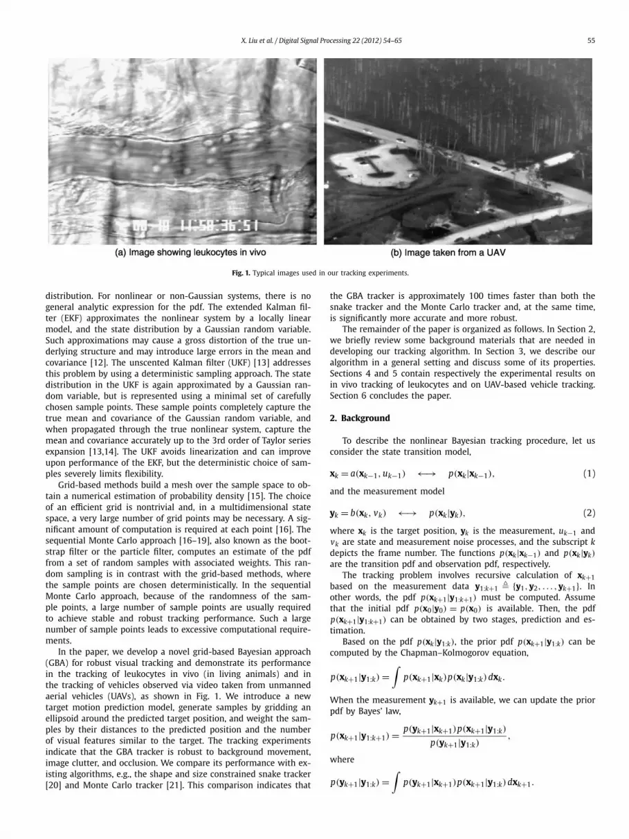
Fig. 1. Typical images used in our tracking experiments.
distribution. For nonlinear or non-Gaussian systems, there is nogeneral analytic expression for the pdf. The extended Kalman fil-ter (EKF) approximates the nonlinear system by a locally linearmodel, and the state distribution by a Gaussian random variable.Such approximations may cause a gross distortion of the true un-derlying structure and may introduce large errors in the mean andcovariance [12]. The unscented Kalman filter (UKF) [13] addressesthis problem by using a deterministic sampling approach. The statedistribution in the UKF is again approximated by a Gaussian ran-dom variable, but is represented using a minimal set of carefullychosen sample points. These sample points completely capture thetrue mean and covariance of the Gaussian random variable, andwhen propagated through the true nonlinear system, capture themean and covariance accurately up to the 3rd order of Taylor seriesexpansion [13,14]. The UKF avoids linearization and can improveupon performance of the EKF, but the deterministic choice of sam-ples severely limits flexibility.
Grid-based methods build a mesh over the sample space to ob-tain a numerical estimation of probability density [15]. The choiceof an efficient grid is nontrivial and, in a multidimensional statespace, a very large number of grid points may be necessary. A sig-nificant amount of computation is required at each point [16]. Thesequential Monte Carlo approach [16–19], also known as the boot-strap filter or the particle filter, computes an estimate of the pdffrom a set of random samples with associated weights. This ran-dom sampling is in contrast with the grid-based methods, wherethe sample points are chosen deterministically. In the sequentialMonte Carlo approach, because of the randomness of the sam-ple points, a large number of sample points are usually requiredto achieve stable and robust tracking performance. Such a largenumber of sample points leads to excessive computational require-ments.
In the paper, we develop a novel grid-based Bayesian approach(GBA) for robust visual tracking and demonstrate its performancein the tracking of leukocytes in vivo (in living animals) and inthe tracking of vehicles observed via video taken from unmannedaerial vehicles (UAVs), as shown in Fig. 1. We introduce a newtarget motion prediction model, generate samples by gridding anellipsoid around the predicted target position, and weight the sam-ples by their distances to the predicted position and the numberof visual features similar to the target. The tracking experimentsindicate that the GBA tracker is robust to background movement,image clutter, and occlusion. We compare its performance with ex-isting algorithms, e.g., the shape and size constrained snake tracker[20] and Monte Carlo tracker [21]. This comparison indicates that
the GBA tracker is approximately 100 times faster than both thesnake tracker and the Monte Carlo tracker and, at the same time,is significantly more accurate and more robust.
The remainder of the paper is organized as follows. In Section 2,we briefly review some background materials that are needed indeveloping our tracking algorithm. In Section 3, we describe ouralgorithm in a general setting and discuss some of its properties.Sections 4 and 5 contain respectively the experimental results onin vivo tracking of leukocytes and on UAV-based vehicle tracking.Section 6 concludes the paper.
2. Background
To describe the nonlinear Bayesian tracking procedure, let usconsider the state transition model,
xk = a(xk−1, uk−1) ←→ p(xk|xk−1), (1)
and the measurement model
yk = b(xk, vk) ←→ p(xk|yk), (2)
where xk is the target position, yk is the measurement, uk−1 andvk are state and measurement noise processes, and the subscript kdepicts the frame number. The functions p(xk|xk−1) and p(xk|yk)
are the transition pdf and observation pdf, respectively.The tracking problem involves recursive calculation of xk+1
based on the measurement data y1:k+1 � {y1,y2, . . . ,yk+1}. Inother words, the pdf p(xk+1|y1:k+1) must be computed. Assumethat the initial pdf p(x0|y0) = p(x0) is available. Then, the pdfp(xk+1|y1:k+1) can be obtained by two stages, prediction and es-timation.
Based on the pdf p(xk|y1:k), the prior pdf p(xk+1|y1:k) can becomputed by the Chapman–Kolmogorov equation,
p(xk+1|y1:k) =∫
p(xk+1|xk)p(xk|y1:k)dxk.
When the measurement yk+1 is available, we can update the priorpdf by Bayes’ law,
p(xk+1|y1:k+1) = p(yk+1|xk+1)p(xk+1|y1:k)p(yk+1|y1:k)
,
where
p(yk+1|y1:k) =∫
p(yk+1|xk+1)p(xk+1|y1:k)dxk+1.

56 X. Liu et al. / Digital Signal Processing 22 (2012) 54–65
Based on the factored sampling [22], the function p(xk+1|y1:k+1)
can be approximated by the sample set {s(m)
k+1,ω(m)
k+1}, where s(m)
k+1 is
the sample m with ω(m)
k+1 as its weight, and M is the sample size.
The weight ω(m)
k+1 is computed by
ω(m)
k+1 = p(yk+1|xk+1 = s(m)
k+1)∑Mj=1 p(yk+1|xk+1 = s( j)
k+1), i = 1,2, . . . , M.
The target position is then estimated as
xk+1 = E p(xk+1|y1:k+1)(x) ≈M∑
j=1
ω( j)k+1s( j)
k+1.
In target tracking, the state transition model can be obtained bylearning directly from training data [23], or by an assumed modelsuch as the constant-velocity model,
xk = xk−1 + uk−1,
where uk−1 = RoUo . Here, Ro is a constant, and Uo is a stan-dardized random variable. An adaptive-velocity model [24] is alsopossible, using
xk = xk−1 + νk + uk−1,
where νk is the predicted shift in the motion. These models can-not, however, handle complete occlusion. In this paper, we willintroduce a new state transition model that can accommodate oc-clusion.
Image registration has proven to be an important pre-processingstep in the overall tracking process. Registration is the process ofoverlaying two or more images of the same scene taken at dif-ferent times and by different image conditions. It geometricallyaligns two images, the reference and sensed images [25]. A ma-jor impediment to automated leukocyte tracking, for example, isthe background movement caused by abrupt movement of thesubject due to the action of the circulatory and respiratory sys-tems [26]. Image registration helps to stabilize such jitter, but itis time consuming and/or requires separate hardware implementa-tion. Similarly, in aerial video, due to the motion of the platform,the background changes frequently, and frame-to-frame alignmentis required for the motion compensation. In our approach, we at-tempt to design a technique that avoids the expensive registrationpre-processing step.
3. The GBA visual tracking algorithm
The development of the algorithm was motivated by the ideabehind the particle filter and the concept of feedback in controltheory. In our algorithm, we first construct a target motion model,and based on this model, predict the target position using themovement information of the previous steps. The samples are thengenerated around the predicted position. Unlike in the Monte Carlotracker [21] where samples are generated randomly, here samplesare generated by gridding a region around the predicted position.The number and the density of the samples are adjusted based onthe target feature. At each of these samples, radial edge detectionis applied to determine if the point is within the target boundary.A weighted average among the positions of those sample pointsdeemed to be within the target boundary is taken as the estimatedposition of the center of the target at the current image frame. Theweighting for a sample is assigned according to a normal distribu-tion with respect to its distance from the predicted position andthe number of features detected around the sample. In the follow-ing sections, we will describe the various components of the GBAalgorithm in more detail.
3.1. Position prediction
Samples are generated around a predicted position of the tar-get. We predict the target position using the movement informa-tion of previous steps. Unlike the motion model of [21,23,24], weuse the following model to predict target position,{
xc,k+1 = xc,k + (xc,k − xc,k−n)/n,
yc,k+1 = yc,k + ( yc,k − yc,k−n)/n, n = min(α,k) − 1,(3)
where (xc,k+1, yc,k+1) is the predicted target position in framek + 1, (xc,k, yc,k) and (xc,k−n, yc,k−n) are the estimated positionsin frame k and k − n, respectively, and α is an integer which dic-tates how far back a frame in which the estimated target positionis used to predict the target position in the next frame. In particu-lar, if k � α, the estimated positions of frames k and k −n are usedto predict the position in frame k + 1. If k < α, we use only theinformation of the first and k-th frames to predict the position inframe k + 1. This prediction model (3) is valid under the assump-tion that the target velocity does not vary abruptly in n consecutiveframes. As will be seen later, stepping back several frames will helpto avoid a target from being lost when occlusion occurs.
The prediction model (3) is useful, when the target temporarily“disappears” in the frames due to complete occlusion and imageclutter. Traditional state transition models usually use only theprevious two or three estimated positions to predict the next po-sition. Because the obstructions may have similar features as thetarget, the estimated position tends to lock onto the obstruction.For a similar reason, the adaptive velocity model may not workwell either. On the other hand, for α = 2 or 3, the model (3)works similarly to the traditional state transition models. But ifwe choose 5 � α � 15, the predicted positions will pass throughthe obstructions, and represent a more robust prediction of thetarget positions. Because of the averaging effect in the prediction,the prediction model (3) is also robust to image jitter, leading to areduction in the effect of image jitter.
We note that the model with too large an α may lose sensi-tivity to the abrupt change of target velocity, and thus, in someframes, the prediction may not be adequate. But as long as thesearch region covers the target, the target will not be lost. Indeed,based on (3), we can also apply an adaptive motion model. If oc-clusion is detected, we set 5 � α � 15; otherwise, we set α = 2,or 3, as in the traditional state transition models.
3.2. Sample generation
In GBA, we generate the samples by gridding within an ellipsoidthat is centered at the predicted position,
(x − xc,k+1)2
a2+ (y − yc,k+1)
2
b2� 1, (4)
where 5 � a,b � 15, which are chosen based on the size of thetarget and magnitude of the background movement. The numberand density of samples are adjusted by for different tracking tar-gets. Shown in Fig. 2 is an illustration of a set of samples. Wedenote the samples in the (k + 1)-th frame as s(m)
k+1 = (x(m)
k+1, y(m)
k+1),m = 1,2, . . . , M .
3.3. Image feature detection
Features are prominent aspects of an object in an image, andmay include edges, shapes, sizes, colors and textures. To local-ize the target, we detect the target features around the samples.Edges have been commonly used as features in image processing,and edge detection, based on differentiation, has been intensivelystudied [27]. Radial edge detection around the samples s(m) are
k+1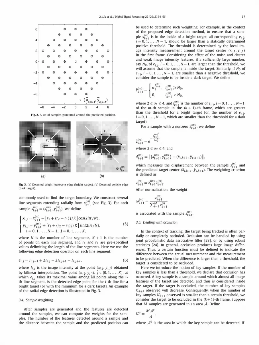
X. Liu et al. / Digital Signal Processing 22 (2012) 54–65 57
Fig. 2. A set of samples generated around the predicted position.
Fig. 3. (a) Detected bright leukocyte edge (bright target). (b) Detected vehicle edge(dark target).
commonly used to find the target boundary. We construct severalline segments extending radially from s(m)
k+1 (see Fig. 3). For each
sample s(m)
k+1 = (x(m)
k+1, y(m)
k+1), we define⎧⎪⎨⎪⎩
xi, j = x(m)
k+1 + [r1 + (r2 − r1) j/K
]cos(2iπ/N),
yi, j = y(m)
k+1 + [r1 + (r2 − r1) j/K
]sin(2iπ/N),
i = 0,1, . . . , N − 1, j = 0,1, . . . , K ,
(5)
where N is the number of line segments, K + 1 is the numberof points on each line segment, and r1 and r2 are pre-specifiedvalues delimiting the length of the line segments. Here we use thefollowing edge detection operator on each line segment:
ei, j = Ii, j−1 + 2Ii, j − 2Ii, j+1 − Ii, j+2, (6)
where Ii, j is the image intensity at the point (xi, j, yi, j) obtainedby bilinear interpolation. The point (xi, j, yi, j), j ∈ {0,1, . . . , K }, atwhich ei, j takes its maximal value among all points along the i-th line segment, is the detected edge point for the i-th line for abright target (or with the minimum for a dark target). An exampleof the radial edge detection is illustrated in Fig. 3.
3.4. Sample weighting
After samples are generated and the features are detectedaround the samples, we can compute the weights for the sam-ples. The number of the features detected around a sample andthe distance between the sample and the predicted position can
be used to determine such weighting. For example, in the contextof the proposed edge detection method, to ensure that a sam-ple s(m)
k+1 is in the inside of a bright target, all corresponding ei, j ,i = 0,1, . . . , N − 1, should be larger than a statically determinedpositive threshold. The threshold is determined by the local im-age intensity measurement around the target center (xc,1, yc,1)
in the first frame. Considering the effect of the noise and clutterand weak image intensity features, if a sufficiently large number,say N0, of ei, j , i = 0,1, . . . , N −1, are larger than the threshold, wewill assume that the sample is inside the target. Similarly, if N0 ofei, j , i = 0,1, . . . , N − 1, are smaller than a negative threshold, weconsider the sample to be inside a dark target. We define
z(m)
k+1 =⎧⎨⎩σ
l(m)
k+11 , l(m)
k+1 � N0,
0, l(m)
k+1 < N0,
where 2 � σ1 � 4, and l(m)
k+1 is the number of ei, j , i = 0,1, . . . , N −1,of the m-th sample in the (k + 1)-th frame, which are greaterthan the threshold for a bright target (or, the number of ei, j ,i = 0,1, . . . , N − 1, which are smaller than the threshold for a darktarget).
For a sample with a nonzero z(m)
k+1, we define
z(m)
k+1 = e− d(m)2
k+12σ2
2 ,
where 2 � σ2 � 4, and
d(m)
k+1 = ∥∥(x(m)
k+1, y(m)
k+1
) − (xc,k+1, yc,k+1)∥∥,
which measures the displacement between the sample s(m)
k+1 andthe predicted target center (xc,k+1, yc,k+1). The weighting criterionis defined as
z(m)
k+1 = z(m)
k+1 z(m)
k+1.
After normalization, the weight
ω(m)
k+1 = z(m)
k+1∑Mi=1 z(i)
k+1
is associated with the sample s(m)
k+1.
3.5. Dealing with occlusion
In the context of tracking, the target being tracked is often par-tially or completely occluded. Occlusion can be handled by usingjoint probabilistic data associative filter [28], or by using robuststatistics [24]. In general, occlusion produces large image differ-ences. Thus, a certain function must be defined to indicate thedifference between the actual measurement and the measurementto be predicted. When the difference is larger than a threshold, thetarget is considered to be occluded.
Here we introduce the notion of key samples. If the number ofkey samples is less than a threshold, we declare that occlusion hasoccurred. A key sample is a sample around which almost all imagefeatures of the target are detected, and thus is considered insidethe target. If the target is occluded, the number of key samplesKk+1 observed will decrease. Consequently, when the number ofkey samples Kk+1 observed is smaller than a certain threshold, weconsider the target to be occluded in the (k +1)-th frame. Supposethat M samples are generated in an area A. Define
Ko = M Ao
A,
where A0 is the area in which the key sample can be detected. If

58 X. Liu et al. / Digital Signal Processing 22 (2012) 54–65
Fig. 4. Cumulative probability distributions of leukocyte movement and jitter displacement, both in pixels, from one frame to the next.
Kk+1 < Ko,
we consider the target to be occluded. As there is a delay of severalframes before the occlusion is detected, the target motion model(3) has been developed to keep track of the occluded target.
3.6. Estimation of target positions
Based on the sample set {s(m)
k+1,ω(m)
k+1} and the number of keysamples, we can estimate the center position of the target in the(k + 1)-th frame as follows,
(xc,k+1, yc,k+1)
={∑M
l=1 s(l)k+1ω
(l)k+1, if the target is not occluded,
(xc,k+1, yc,k+1), if the target is occluded.
3.7. Robustness in parameters selection
A robust algorithm should be insensitive to the choice of thevalues of the parameters involved. In other words, as long as thevalues of the parameters are in some reasonable ranges, the per-formance remain more or less unchanged. We will show in thetracking implementations in the next two sections that our GBAtracking algorithm is robust to parameter selection.
4. Experimental results: in vivo tracking of leukocytes
Tracking leukocytes in vivo contributes to the understanding ofthe inflammatory process and thus has attracted significant atten-tion from medical research community. Conventionally, leukocytetracking is performed manually after each intravital experiment.Real-time automated tracking could replace this time-consumingand tedious work, to obtain the results more quickly and moreconsistently. Difficulties associated with leukocyte tracking includethe severe image noise and clutter, the cell deformation and con-trast change, the occlusion of the target leukocyte by other leuko-cytes and structures and the jitter caused by the breathing move-ment of the living specimen.
There are several approaches to leukocyte tracking. The shapeand size constrained snake tracker was described in [20]. It cap-tures the leukocyte to be tracked through minimizing an energyfunction, defined on the basis of internal energy, external energy,shape, size, position, and sampling of the contour. Under most cir-cumstances, the snake tracker is able to successfully track a rollingleukocyte. A Monte Carlo solution was reported in [21]. Based on
the leukocyte movement information and the image intensity fea-tures, a specialized sample-weighting criterion is tailored to rollingleukocytes observed in vivo. As demonstrated in [21], as the noiseintensity level increases, the performance of a snake-based trackerdegrades more rapidly than that of the Monte Carlo tracker. Boththe snake tracker and the Monte Carlo tracker provide improvedperformance over the centroid tracker [29] and the correlationtracker [30].
4.1. Leukocytes tracking by the GBA
In our leukocyte experiment, the video is recorded at a spatialresolution of 320 × 240 pixels, where the pixel-to-micron ratio is2.47 pixels/μm horizontally and 2.34 pixels/μm vertically, and thetemporal resolution is 30 frames per second. The ground truth po-sitions of all targets have been manually determined previously.We test the GBA tracker using 98 sequences, each of which con-sists of 91 frames. In these tests, we use the ground truth positionin the first frame as the initial detection.
For these 98 sequences, the distributions of the tracked targetmotion and jitter displacement are shown in Fig. 4. Without regis-tration, the mean of the target movement is 1.27 pixels per frame,the standard deviation is 1.01 pixels per frame. There are 5.4% ofsequences where the target moving velocity is higher than 3 pix-els per frame, and 2.4% of them higher than 4 pixels per frame.With registration, the mean is 1.14 pixels per frame, the standarddeviation is 0.75 pixels per frame. There are 2.2% of them wherethe target moving velocity is larger than 3 pixels per frame, and0.7% of them larger than 4 pixels per frame. Here, the registrationis achieved through template matching to align each frame withthe first frame.
There are 10.6% of frames that have a jitter displacement largerthan 4 pixels, and 4.6% of the frames have a jitter displacementlarger than 6 pixels.
According to the statistical data of the sizes of leukocytes, asin [21], we set r1 = 2 pixels and r2 = 8 pixels in (5). As shown inFig. 3, there are 8 radial edge detection segments around a sample,that is, N = 8. Set α = 15 in (3). We choose the distance betweenthe closest samples to be 2 pixels. Considering (4) with a = b = 7,we obtain a set of sample as shown in Fig. 2, with a sample sizeof M = 69.
In the first frame, for (xc,1, yc,1), compute ei, j , i = 0,1, . . . ,7,j = 1,2, . . . , K . For a bright leukocyte, we define a threshold
T = e1/σ3,

X. Liu et al. / Digital Signal Processing 22 (2012) 54–65 59
Fig. 5. The tracking of a leukocyte in a 91 frame video sequence (3 s) with the GBA tracker.
where e1 is the second smallest of ei, j, i = 0,1, . . . ,7, and 1 <
σ3 � 5 is a constant number tuned on the basis of the overallquality of the video. The parameter σ3 is set higher if the videohas severe image noise and clutter, and lower otherwise. In the(k + 1)-th frame, for the sample s(m)
k+1, if its ei, j > T , we considerthe edge on the i-th line detected. Similarly, for a dark leukocyte,ei, j is the second largest of ei, j , i = 0,1, . . . ,7, and consider theedge on its i-th line is detected if ei, j < T . If edge is detected on
no less than seven lines from the sample s(m)
k+1, we consider thissample a key sample. If, on the other hand,
Kk+1 <M
πσ 24 = Mσ 2
4 ,
πab abTable 1Parameter values in the GBA tracker for leukocytes tracking.
σ1 σ2 σ3 σ4
2 3 4√
2
where πσ 24 is the area the key samples can be detected with 1 �
σ 24 � 4, we consider the target is occluded in the (k + 1)-th frame.
We choose the values of parameters σi , i = 1,2,3,4, as shownin Table 1.
Shown in Fig. 5 is the tracking of a leukocyte in a typical threesecond segment in a video sequence without registration. In this

60 X. Liu et al. / Digital Signal Processing 22 (2012) 54–65
sequence, there exist severe image noise and clutter, leukocyte de-formation, contrast change, and strong jitter caused by the breath-ing movement of the living animal (7 pixels in horizontal directionand 6 pixels in vertical direction). The leukocyte being tracked isalso occluded by muscle striation. The GBA tracker is however ableto track the leukocyte in all 91 frames, while the snake tracker[20] and the Monte Carlo tracker [21] lost the target in 83 and 13frames, respectively.
4.2. Comparison with Monte Carlo tracker and GVF snake tracker
We compare the performance of the GBA tracker with those ofthe Monte Carlo (MC) tracker and the snake tracker using 98 videosequences. Each sequence consists of 91 frames. The parametersfor GBA tracker are set as in Table 1 and are fixed for all 98 se-quences.
All simulations were carried out in MATLAB 7.1.0.246 (R14) ona PC with an Intel Core 2 CPU (2 GHz and 1 GB RAM). Each trackeris evaluated in the following four aspects.
(1) Percentage of the frames tracked:The target in each frame is considered as tracked if the dis-tance between the estimated position and the ground truthposition (manually recorded by a technician) is less than athreshold (8 pixels).
(2) Time taken to process each sequence:We evaluate only the “computing” time of the algorithms. Wedo not include the time associated with waiting for the data tobe read from the hard disk or camera to memory, which canvary significantly for different hardware.
(3) Number of sequences (out of 98 sequences) with all frames tracked:Number of sequences on which the tracked is tracked in allthe 91 frames.
(4) RMSE (root mean square error):
RMSE =√∑N
i=1[(xc,i − xc,i)2 + ( yc,i − yc,i)
2]N
,
where (xc,i, yc,i) and (xc,i, yc,i) are the estimated position andthe ground truth position in frame i, and N is the numberof the frames tracked in a video sequence. We compare theaverage of RMSE among all 98 sequences.
Shown in Fig. 6 is the comparison of percentage of framestracked. As seen in the figure, with registration, the GBA trackertracks 14% more frames than the MC tracker, and 25% more framesthan the snake tracker. Without registration, the performance ofthe GBA tracker decreases by 3%, while the performance of thesnake tracker degrades 2%, and the performance of the MC trackerdegrades drastically. This indicates that the GBA tracker is not onlymuch more accurate than the other two trackers, but is also robustto jitter.
Shown in Fig. 7 is the number of sequences (out of 98 se-quences) with all 91 frames tracked, both with and without reg-istration. With registration, the GBA tracker is able to track all 91frames in 82 out of 98 sequences, the MC tracker is able to trackall 91 frames in 57 sequences and the snake tracker is able to trackall 91 frames only in 44 out of 98 sequences. Without registration,the number of sequences with all 91 frames tracked is 75 for theGBA tracker, while this number for the snake tracker decreases to41 and the number for the MC tracker decreases to 32. These dataonce again indicate that the GBA tracker significantly outperformsthe other two trackers both in accuracy and robustness.
The average of RMSE of all sequences is shown in Fig. 8. Thisfigure reveals that the GBA tracker significantly outperforms theother two trackers both in accuracy and robustness.
Fig. 6. Percentage of the frames tracked.
Fig. 7. Number of sequences (out of 98 sequences) with all 90 frames tracked.
Fig. 8. Average of RMSE (pixels).
Shown in Fig. 9 is the differences in numbers of frames trackedby the three different trackers for each of the 98 sequences, withand without registration. The top graphs in these two figures showthat the MC tracker and the snake tracker outperform each otherin about the same number of sequences and by about the samemargin. The middle plots show that the GBA tracker drasticallyoutperforms the snake tracker. In particular, with registration, inonly four of the 98 sequences does the snake tracker track a fewmore frames than the GBA tracker. On the other hand, there are 30sequences in which the GBA tracker tracks over 40 more framesthan the snake tracker. Without registration, the GBA tracker out-performs the snake tracker by about the same margin. The bottomgraphs show that the GBA tracker also outperforms the MC tracker.With registration, in only seven of the 98 sequences does the MCtracker track more frames than the GBA tracker. On the other hand,there are 17 sequences in which the GBA tracker tracks over 40more frames than the MC tracker. Without registration, the GBAtracker outperforms the MC tracker more drastically. In only twoof the 98 sequences does the MC tracker track a few more frames

X. Liu et al. / Digital Signal Processing 22 (2012) 54–65 61
Fig. 9. The differences in numbers of frames tracked by three different trackers for each of the 98 sequences. In all plots, each point in the x-axis represents one of the 98sequences and the y-axis is the difference in numbers of frames tracked by two different trackers.
Fig. 10. Average time (s) required for tracking in each sequence.
than the GBA tracker. On the other hand, there are 43 sequencesin which the GBA tracker tracks over 40 more frames than the MCtracker.
The average time required for computation in each sequenceis shown in Fig. 10. The GBA tracker is approximately 100 timesfaster than the snake tracker and over 160 times faster than theMC tracker.
The success of MC tracker is highly dependent on the accuracyof the predicted position of the target. If the target is a few pixelsaway from predicted position, the tracker will lose the target. TheMC tracker also needs the target positions in the first two framesto initialize the process to make sure the predicted position is ac-curate. The GBA tracker can track a target even when it is manypixels away from the predicted position due to the gridding pro-cedure. Also, we need only the target position in the first frame
Fig. 11. Distribution of velocity errors by the GBA tracker without registration.
to begin the tracking, and require no initial motion model. On theother hand, the snake tracker is sensitive to noise and is severelyaffected by the image clutter caused by the vessel wall.
For all 98 sequences, the average of ground truth leukocyte ve-locity is 21.40 pixel/second, while the average of measurements bythe GBA tracker (without registration) is 22.12 pixel/second. Theerror is +3.2%. The probability distribution of velocity errors isshown in Fig. 11.

62 X. Liu et al. / Digital Signal Processing 22 (2012) 54–65
Fig. 12. Multi-leukocyte tracking in a video sequence with 181 frames (6 seconds).
Table 2Tracking rates with different parameters.
Tracking rate (%) σ2
2 3 4
σ1 1 91.3 91.8 92.72 93.9 93.6 92.94 94.0 92.7 92.7
Tracking rate (%) σ4
1√
2 2
σ3 3 94.1 92.7 92.04 93.0 93.6 93.05 92.9 92.9 93.0
4.3. Robustness to parameter selection
We changed the values of two of the parameters in Table 1, asshown in Table 2, and executed the algorithm without registrationto investigate robustness to parameter selection.
Note that all parameters, σ1, σ2, σ3 and σ 24 , in Tables 1 and
2 are chosen to be integers. When the parameters are varied overa large range, the performance remains almost unchanged. This isdesired in real-time applications.
For the MC tracker [21], σ2 is set as 1.5 if leukocyte radii areless than 6 pixels; otherwise, σ2 is set as 2. If we multiply σ2
by 1.5 in the MC tracker, the tracked rate decreases from 55.5%to 51.3% without registration, and from 82.7% to 79.2% with reg-
istration. On the other hand, if we multiply σ2 by 1.5 in the GBAtracker, the tracked rate decreases only from 93.6% to 93.1% with-out registration, and from 96.4% to 95.8% with registration.
4.4. Multi-leukocyte tracking
The GBA algorithm can be easily adapted for tracking multi-ple leukocytes. As shown in Fig. 12, without registration, the GBAtracker is able to track 11 of the 12 leukocytes that appear inFrame 1, in which Targets 5, 7, 8 and 11 disappear in Frames 103,140, 115 and 105, respectively due to image clutter. The trackerloses Target 12 in Frame 165. The video sequence encompasses 6 swith 181 frames. In the tracking, the parameter values in Table 1were used. The computation time for tracking is 0.533 s.
X. Liu et al. / Digital Signal Processing 22 (2012) 54–65 63
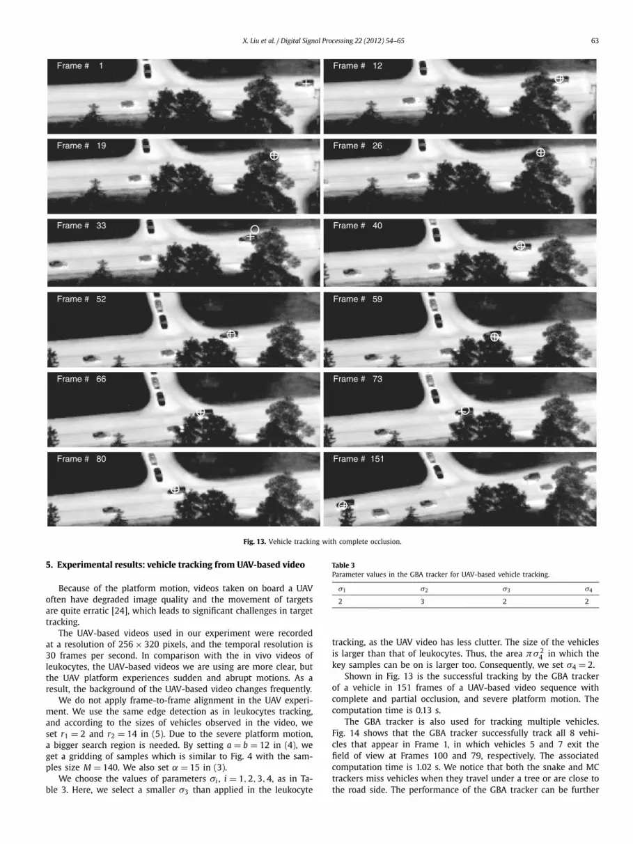
Fig. 13. Vehicle tracking with complete occlusion.
5. Experimental results: vehicle tracking from UAV-based video
Because of the platform motion, videos taken on board a UAVoften have degraded image quality and the movement of targetsare quite erratic [24], which leads to significant challenges in targettracking.
The UAV-based videos used in our experiment were recordedat a resolution of 256 × 320 pixels, and the temporal resolution is30 frames per second. In comparison with the in vivo videos ofleukocytes, the UAV-based videos we are using are more clear, butthe UAV platform experiences sudden and abrupt motions. As aresult, the background of the UAV-based video changes frequently.
We do not apply frame-to-frame alignment in the UAV experi-ment. We use the same edge detection as in leukocytes tracking,and according to the sizes of vehicles observed in the video, weset r1 = 2 and r2 = 14 in (5). Due to the severe platform motion,a bigger search region is needed. By setting a = b = 12 in (4), weget a gridding of samples which is similar to Fig. 4 with the sam-ples size M = 140. We also set α = 15 in (3).
We choose the values of parameters σi , i = 1,2,3,4, as in Ta-ble 3. Here, we select a smaller σ3 than applied in the leukocyte
Table 3Parameter values in the GBA tracker for UAV-based vehicle tracking.
σ1 σ2 σ3 σ4
2 3 2 2
tracking, as the UAV video has less clutter. The size of the vehiclesis larger than that of leukocytes. Thus, the area πσ 2
4 in which thekey samples can be on is larger too. Consequently, we set σ4 = 2.
Shown in Fig. 13 is the successful tracking by the GBA trackerof a vehicle in 151 frames of a UAV-based video sequence withcomplete and partial occlusion, and severe platform motion. Thecomputation time is 0.13 s.
The GBA tracker is also used for tracking multiple vehicles.Fig. 14 shows that the GBA tracker successfully track all 8 vehi-cles that appear in Frame 1, in which vehicles 5 and 7 exit thefield of view at Frames 100 and 79, respectively. The associatedcomputation time is 1.02 s. We notice that both the snake and MCtrackers miss vehicles when they travel under a tree or are close tothe road side. The performance of the GBA tracker can be further

64 X. Liu et al. / Digital Signal Processing 22 (2012) 54–65
Fig. 14. Tracking 8 targets by the GBA tracker in a 5 seconds segment of typical UAV-based video.
improved by considering the constraint in the sizes and shapes ofthe vehicles.
We also note that, with the parameters varied over a largerange, the GBA tracker can still successfully track all vehicles thatappear in Frame 1 of Fig. 14.
Finally, we observe that, although the videos in the leukocytetracking and in the vehicle tracking are quite different, the GBAtracker was able to perform in a superior manner in both caseswith similar choices of parameter values. This is another indicationof the robustness of the GBA tracker.
6. Conclusions
The grid-based approach (GBA) to visual tracking combines theversatility of Bayesian estimation with the robustness of feedbackcontrol. In experiments with significant jitter, we show that theGBA tracker is able to robustly track the target with and with-out spatial registration. In 98 cell microscopy experiments, the GBAtracker excels over the snake tracker and the Monte Carlo trackerin all four quantitative measures of tracking success. Moreover, theGBA solution reduces the computational complexity (as compared
to the snake and Monte Carlo trackers) by over two orders of mag-nitude, and is unsensitive to selection of parameters within thealgorithm. Finally, to demonstrate that our tracking approach isnot limited to biological applications, we apply the GBA trackersuccessfully to unregistered UAV-acquired videos of vehicles.
References
[1] R. Wildes, R. Kumar, H. Sawhney, S. Samasekera, S. Hsu, H. Tao, Y. Guo,K. Hanna, A. Pope, D. Hirvonen, M. Hansen, P. Burt, Aerial video surveillanceand exploitation, Proc. IEEE 89 (10) (2001) 1518–1539.
[2] A. Dix, J. Finlay, G. Abowd, Human–Computer Interaction, Prentice Hall, 2004.[3] S. Hutchinson, G. Hager, P. Corke, A tutorial on visual servo control, IEEE Trans.
Robot. Automat. 12 (5) (1996) 651–670.[4] M. Kass, A. Witkin, D. Terzopoulos, Snakes: Active contour models, Int. J. Com-
put. Vis. 1 (4) (1988) 321–331.[5] C. Xu, J. Prince, Snakes, shapes, and gradient vector flow, IEEE Trans. Image
Process. 7 (3) (1998) 359–369.[6] D. Comaniciu, V. Ramesh, P. Meer, Kernel-based object tracking, IEEE Trans.
Pattern Anal. Mach. Intell. (2003) 564–577.[7] V. Caselles, R. Kimmel, G. Sapiro, Geodesic active contours, Int. J. Comput.
Vis. 22 (1) (1997) 61–79.

X. Liu et al. / Digital Signal Processing 22 (2012) 54–65 65
[8] T. Chan, L. Vese, Active contours without edges, IEEE Trans. Image Pro-cess. 10 (2) (2001) 266–277.
[9] A. Doucet, S. Godsill, C. Andrieu, On sequential Monte Carlo sampling methodsfor Bayesian filtering, Statist. Comput. 10 (3) (2000) 197–208.
[10] M. Arulampalam, S. Maskell, N. Gordon, T. Clapp, D. Sci, T. Organ, S. Adelaide,A tutorial on particle filters for online nonlinear/non-Gaussian Bayesian track-ing, IEEE Trans. Signal Process. 50 (2) (2002) 174–188.
[11] O. Cappe, S. Godsill, E. Moulines, An overview of existing methods and recentadvances in sequential Monte Carlo, Proc. IEEE 95 (5) (2007) 899.
[12] G. Welch, G. Bishop, An introduction to the Kalman filter, University of NorthCarolina, 1995.
[13] S. Julier, J. Uhlmann, A new extension of the Kalman filter to nonlinear systems,in: Int. Symp. Aerospace/Defense Sensing, Simul. and Controls, vol. 3, 1997.
[14] E. Wan, R. Van Der Merwe, The unscented Kalman filter for nonlinear esti-mation, in: IEEE Adaptive Systems for Signal Processing, Communications, andControl Symposium, AS-SPCC, 2000, pp. 153–158.
[15] H. Sorenson, Recursive estimation for nonlinear dynamic systems, in: J.C. Spall(Ed.), Bayesian Analysis of Time Series and Dynamic Models, Marcel Dekker,New York, 1988.
[16] N. Gordon, D. Salmond, A. Smith, Novel approach to nonlinear/non-GaussianBayesian state estimation, in: Radar and Signal Processing, IEE Proceedings F,vol. 140 (2), 1993, pp. 107–113.
[17] M. Isard, A. Blake, CONDENSATION – Conditional density propagation for visualtracking, Int. J. Comput. Vis. 29 (1) (1998) 5–28.
[18] J. Liu, R. Chen, Sequential Monte Carlo methods for dynamic systems, J. Amer.Statist. Assoc. 93 (1998) 1032–1044.
[19] A. Doucet, On sequential simulation-based methods for Bayesian filtering,1998.
[20] N. Ray, S.T. Acton, K. Ley, Tracking leukocytes in vivo with shape and size con-strained active contours, IEEE Trans. Med. Imag. 21 (10) (2002) 1222–1235.
[21] J. Cui, S.T. Acton, Z. Lin, A Monte Carlo approach to rolling leukocyte trackingin vivo, Med. Image Anal. 10 (4) (2006) 598–610.
[22] U. Grenander, Y. Chow, D. Keenan, Hands: A Pattern Theoretic Study of Biolog-ical Shapes, Springer-Verlag, New York, 1991.
[23] B. North, A. Blake, M. Isard, J. Rittscher, Learning and classification of complexdynamics, IEEE Trans. Pattern Anal. Mach. Intell. (2000) 1016–1034.
[24] S.K. Zhou, R. Chellappa, B. Moghaddam, Visual tracking and recognition us-ing appearance-adaptive models in particle filters, IEEE Trans. Image Pro-cess. 13 (11) (2004) 1491–1506.
[25] B. Zitová, J. Flusser, Image registration methods: a survey, Image Vision Com-put. 21 (11) (2003) 977–1000.
[26] S.T. Acton, K. Wethmar, K. Ley, Automatic tracking of rolling leukocytes in vivo,Microvascul. Res. 63 (1) (2002) 139–148.
[27] B. Jähne, Practical Handbook on Image Processing for Scientific and TechnicalApplications, CRC Press, 2004.
[28] C. Rasmussen, G. Hager, Probabilistic data association methods for trackingcomplex visual objects, IEEE Trans. Pattern Anal. Mach. Intell. (2001) 560–576.
[29] R. Ghosh, W. Webb, Automated detection and tracking of individual and clus-tered cell surface low density lipoprotein receptor molecules, Biophys. J. 66 (5)(1994) 1301–1318.
[30] A. Kusumi, Y. Sako, M. Yamamoto, Confined lateral diffusion of membrane re-ceptors as studied by single particle tracking (nanovid microscopy). Effects ofcalcium-induced differentiation in cultured epithelial cells, Biophys. J. 65 (5)(1993) 2021–2040.
Xinmin Liu received the M.S. from Xiamen Uni-versity, Xiamen, China, in 1998, the M.E. degree fromthe National University of Singapore in 2000, and thePh.D. degree from the University of Virginia, Char-lottesville, in 2010. His current research interests in-clude nonlinear control, biological control, numericalanalysis, and image processing.
Zongli Lin is a professor of Electrical and Com-puter Engineering at University of Virginia. He re-ceived his B.S. degree in mathematics and computerscience from Xiamen University, Xiamen, China, in1983, his Master of Engineering degree in automaticcontrol from Chinese Academy of Space Technology,Beijing, China, in 1989, and his Ph.D. degree in electri-cal and computer engineering from Washington StateUniversity, Pullman, Washington, USA, in 1994. His
current research interests include nonlinear control, robust control, andimage processing. He was an Associate Editor of the IEEE Transactionson Automatic Control and IEEE/ASME Transactions on Mechatronics. He hasserved on the operating committees and program committees of severalconferences and was an elected member of the Board of Governors of theIEEE Control Systems Society. He currently serves on the editorial boardsof several journals and book series, including Automatica, Systems & ControlLetters, Science China: Information Science, and IEEE Control Systems Magazine.He is a Fellow of the IEEE and a Fellow of IFAC, the International Federa-tion of Automatic Control.
Scott T. Acton was born in Los Angeles, California.He graduated from Oakton High School, Vienna, Vir-ginia, in 1984.
Dr. Acton has worked in industry for AT&T, Oak-ton, VA, the MITRE Corporation, McLean, VA and Mo-torola, Inc., Phoenix, AZ and in academia for Okla-homa State University, Stillwater. Currently, he is Pro-fessor of Electrical and Computer Engineering andBiomedical Engineering at the University of Virginia
(U.Va.). At U.Va., he was named the Outstanding New Teacher in 2002,Faculty Fellow in 2003, and Walter N. Munster Chair for Intelligence En-hancement in 2003.
Dr. Acton is an active participant in the IEEE, serving as Associate Ed-itor for the IEEE Transactions on Image Processing and for the IEEE SignalProcessing Letters. He was the 2004 Technical Program Chair and the 2006General Chair for the Asilomar Conference on Signals, Systems and Computers.His research interests include sinkholes, anisotropic diffusion, basketball,active models, biomedical segmentation problems and biomedical track-ing problems. During 2007–2008, Dr. Acton was on sabbatical in Santa Fe,New Mexico, USA.


