Embed Size (px)
Citation preview
A discrete Adomian decomposition method
for discrete nonlinear Schrodinger equations
Athanassios Bratsos a , Matthias Ehrhardt b,∗ andIoannis Th. Famelis a
aDepartment of Mathematics, Technological Educational Institution (T.E.I.) ofAthens, GR–122 10 Egaleo, Athens, Greece
bInstitut fur Mathematik, Technische Universitat Berlin, Strasse des 17. Juni 136,D–10623 Berlin, Germany
Abstract
We present a new discrete Adomian decomposition method to approximate thetheoretical solution of discrete nonlinear Schrodinger equations. The method isexamined for plane waves and for single soliton waves in case of continuous, semi–discrete and fully discrete Schrodinger equations. Several illustrative examples andMathematica program codes are presented.
Key words: Adomian decomposition method, discrete nonlinear Schrodingerequations, finite difference schemes, solitons, plane waves, MathematicaPACS: 02.70.Bf, 31.15.Fx
1 Introduction
In this work we want to describe a discrete version of the well–known Adomiandecomposition method (ADM) applied to nonlinear Schrodinger equations. TheADM was introduced by Adomian [5], [6] in the early 1980s to solve nonlin-ear ordinary and partial differential equation. This method avoids artificial
∗ Corresponding author.Email addresses: [email protected] (Athanassios Bratsos),
[email protected] (Matthias Ehrhardt), [email protected](Ioannis Th. Famelis).
URLs: http://math.teiath.gr/bratsos/ (Athanassios Bratsos),http://www.math.tu-berlin.de/~ehrhardt/ (Matthias Ehrhardt),http://math.teiath.gr/ifamelis/ (Ioannis Th. Famelis).
Preprint submitted to Applied Mathematics and Computation 11 April 2007
boundary conditions, linearization and yields an efficient numerical solutionwith high accuracy.
The nonlinear cubic Schrodinger equation (NLS) [12,34] is a typical dispersivenonlinear partial differential equation that plays a key role in a variety ofareas in mathematical physics. It describes the spatio–temporal evolution ofthe complex field u = u(x, t) ∈ C and has the general form
i∂tu + ∂2xu + q|u|2u = 0, x ∈ R, t > 0, (1a)
u(x, 0) = f(x), (1b)
where the parameter q ∈ R corresponds to a focusing (q > 0) or defocusing(q < 0) effect of the nonlinearity.
The NLS equation (1a) describes many problems in physics. The fields ofapplication varies from optics [27], propagation of the electric field in opticalfibers [23], self–focusing and collapse of Langmuir waves in plasma physics [42]to modelling deep water waves and freak waves (so–called rogue waves) in theocean [30].
The theoretical solution for the NLS equation (1a) has been given amongothers [38–40]. Moreover, the NLS equation (1a) is completely S–integrable(in the sense of Calogero [11]) with the inverse scattering method (ISM) [3,7,41]and a single soliton solution is given by
u(x, t) =(
2a
q
)1/2
exp[
i( c
2x − θt
)]
sech[
a1/2(x − ct)]
, (2)
with θ = c2/4 − a. For fixed t the function u in (2) decays exponentially as|x| → ∞. It travels with the envelope speed c and its amplitude is governedby the parameter a ∈ R.
An N–soliton solution for q 6= 0 is given by the function [31]
u(x, t) =(
2a
q
)1/2 N∑
p=1
exp[
i(cp
2xp − θpt
)]
sech[
a1/2(xp − cpt)]
, (3)
with θp = c2p/4 − a, the position xp of the p–soliton and cp its velocity.
Finally a particular simple form of solutions to the Schrodinger equation (1a)are the plane wave solutions
u(x, t) = exp[
i(
κx − ωt)]
, x ∈ R, t > 0, (4)
where κ is the wave number and ω denotes the frequency. Substituting the
2

ansatz (4) into the NLS (1a) yields the dispersion relation
κ2 − ω = q. (5)
Since (1a) is S–integrable it is a Hamiltonian system with an infinite numberof conserved quantities, cf. [36,37]. Here we will only present the two mostimportant quantities. First the L2-norm (mass, number of particles) is con-served:
N =2
q
∫∞
−∞
|u(x, t)|2 dx = const . (6)
Note that this conservation property (6) has an important meaning in physicalapplications. It can be interpreted as the conservation of the power of thebeam in nonlinear optics and in Bose–Einstein condensation it denotes theconservation of the number of atoms in the condensate.
Another conserved quantity is the Hamiltonian
H =∫
∞
−∞
[
|∂xu(x, t)|2 +q
2|u(x, t)|4
]
dx = const . (7)
with i∂tu = ∂u∗H = {H,u}, where the standard Poisson brackets have beenused and ∗ denotes complex conjugation. For more details on nonlinear Schro-dinger equations and their conserved quantities we refer the reader to [12,34].
To the authors’ knowledge, the Adomian decomposition method was regardedonly for the continuous equation, cf. the articles [18,20,26] for the applicationof the ADM to the NLS (1). In this paper we will first review the basic ideasof the ADM for the NLS and show afterwards how a symbolic package likeMathematica can help using the ADM. Secondly, we will turn to the solutionof spatially discrete Schrodinger–type equations by a discrete ADM. Finally,we end with the consideration of the fully discrete case.
2 The Adomian Decomposition Method
In this Section we shall sketch the ADM for partial differential equationsapplied to the cubic NLS (1). To this end, we consider (1a) written in operatorform as
Ltu = i∂2xu + iqF (u), x ∈ R, t > 0, (8)
with the notation Lt = ∂t and the cubic nonlinear term F (u) = |u|2u. Thenthe inverse operator of Lt is defined by the indefinite integral
[L−1t v](t) =
∫ t
0v(τ) dτ, t > 0. (9)
3

Now applying formally the inverse operator L−1t to (8) yields with the initial
condition (1b) the formal solution to (1)
u(x, t) = f(x) + iL−1t ∂2
xu + iqL−1t F (u), x ∈ R, t > 0. (10)
The Adomian decomposition method [6] assumes a solution of the series formu(x, t) =
∑∞
l=0 ul(x, t), where the components ul(x, t) are going to be deter-mined recurrently. The nonlinear term F (u) in (10) is decomposed into aninfinite series of polynomials of the form F (u) =
∑∞
l=0 Al(u), where the Al arethe so–called Adomian polynomials. Substituting these decomposition seriesinto (10) gives
∞∑
l=0
ul(x, t) = f(x) + i∞∑
l=0
L−1t ∂2
xul(x, t) + iq∞∑
l=0
L−1t Al. (11)
According to Adomian, u0(x, t) is identified with the initial data f(x) and thefollowing recurrence is proposed:
u0(x, t) = f(x), (12a)
ul+1(x, t) = iL−1t ∂2
xul(x, t) + iqL−1t Al, l = 0, 1, 2, . . . . (12b)
It remains to determine the Adomian polynomials Al. They are defined by
Al =1
l!
dl
dλl
[
F( ∞∑
p=0
λpup
)]
λ=0, for l = 0, 1, 2, . . . (13)
and constructed for all classes of nonlinearity according to algorithms giveneither by Adomian [6] or alternatively by Wazwaz [37]. To do so, we set F (u) =u2u and obtain in a straight forward calculation
A0 = u20u0, (14a)
A1 = 2u0u1u0 + u20u1, (14b)
A2 = 2u0u2u0 + u21u0 + 2u0u1u1 + u2
0u2, (14c)
A3 = 2(u0u3u0 + u1u2u0 + u0u2u1 + u0u1u2) + u21u1 + u2
0u3, (14d)
. . . .
The polynomials Al, l ≥ 4 can be computed in a similar manner.
Let us finally note that the convergence of this method was established in[13], [14] using a fixed point theorem. Since in practice not all terms (12)of the series u(x, t) =
∑∞
l=0 ul(x, t) can be calculated we use a finite sumUL(x, t) =
∑Ll=0 ul(x, t) to approximate the solution.
Remark 1 There also exists the modified decomposition technique by Wazwaz[36] that accelerates the rapid convergence of the series solution without any
4
need to use Adomian polynomials. The recursive relation reads
u0(x, t) = f(x), (15a)
ul+1(x, t) = f(x) + iL−1t ∂2
xul(x, t) + iqL−1t F (ul(x, t)), l = 0, 1, 2, . . . , (15b)
where the function f(x) is properly decomposed (mainly on trial basis) as
f(x) = f(x) + f(x).
3 The computation for the cubic Schrodinger equation
In this section we want to clarify the ADM approach using the Adomianpolynomials (14) by two examples.
Example 2 First we consider the simple example of a plane wave solution(4). We obtain by the Adomian decomposition technique (12):
u0(x, t) = f(x) = eiκx, (16a)
u1(x, t) = iL−1t ∂2
xu0(x, t) + iqL−1t A0
= iL−1t ∂2
xeiκx + iqL−1
t [u20u0]
= −iκ2teiκx + iqteiκx = −i(κ2 − q)teiκx, (16b)
u2(x, t) = iL−1t ∂2
xu1(x, t) + iqL−1t A1
= iL−1t ∂2
x[−i(κ2 − q)teiκx] + iqL−1t [2u0u1u0 + u2
0u1]
= −1
2κ2(κ2 − q)t2eiκx +
1
2q(κ2 − q)t2eiκx
= −1
2(κ2 − q)2t2eiκx, (16c)
u3(x, t) = iL−1t ∂2
xu2(x, t) + iqL−1t A2
= iL−1t ∂2
x[−1
2(κ2 − q)2t2eiκx]
+ iqL−1t [2u0u2u0 + u2
1u0 + 2u0u1u1 + u20u2]
=i
6(κ2 − q)3t3eiκx. (16d)
Now summing up these components yields
u(x, t) =∞∑
l=0
ul(x, t)
= eiκx{
1 − i(κ2 − q)t − 1
2(κ2 − q)2t2 +
i
6(κ2 − q)3t3 + . . .
}
= eiκxe−iωt = ei(κx−ωt),
5
with ω = κ2 − q already given in (5), i.e. the method converges to the exactsolution.
Example 3 Secondly, we consider the special case of a x–independent solu-tion u(t) = f exp(iq|f |2t), where f denotes the constant initial value. We getby the ADM (12):
u0(t) = f, (17a)
u1(t) = iqL−1t A0 = iqL−1
t [u20u0] = iq|f |2ft, (17b)
u2(t) = iqL−1t A1 = iqL−1
t [2u0u1u0 + u20u1] = −q2|f |4f t2
2, (17c)
u3(t) = iqL−1t A2 = iqL−1
t [2u0u2u0 + u21u0 + 2u0u1u1 + u2
0u2]
= −iq3|f |6f t3
6. (17d)
Again, summing up these components yields obviously the exact solution.
Example 4 In the third example we turn to the soliton solution (2). Followingthe above we get for the terms ul(x, t); l = 1, 2, 3
u0(x, t) = f(x) =
√
2a
qe
i
2c x sech
(√a x
)
, (18a)
u1(x, t) =1
4
√
2a
qe
i
2c x t c1 sech2
(√a x
)
, (18b)
wherec1 = i
(
4 a − c2)
cosh(√
a x) + 4√
a c sinh(√
a x),
u2(x, t) = − 1
26
√
2a
qe
i
2c x t2 c2 sech3(
√a x), (18c)
where
c2 = 16 a2 + 40 a c2 + c4 +(
16 a2 − 24 a c2 + c4)
cosh(2√
a x)
− (8 i)√
a c(
4 a − c2)
sinh(2√
a x),
u3(x, t) =1
3 · 29
√
2a
qe
i
2c x t3 c3 sech4(
√a x), (18d)
where
c3 = −3 i cosh(√
a x)(
64 a3 + 272a2c2 − 68 a c4 − c6)
− i cosh(3√
a x)(
64 a3 − 240 a2 c2 + 60 a c4 − c6)
− 8√
a c d3 sinh(√
a x),
with
d3 = 48 a2 + 152 a c2 + 3 c4 +(
48 a2 − 40 a c2 + 3 c4)
cosh(2√
a x).
6
This tedious calculation above was performed using the symbolic computingpackage Mathematica. The code can be downloaded from the authors’ home-pages. Using the code the complicated u4(x, t) can be evaluated.
Mathematica–Program 1 The Mathematica code
Clear["@"]
u[x , t ]:=(2a/q)∧(1/2) Exp[I(1/2cx − (c∧2/4 − a)t)] ∗ Sech[a∧(1/2)(x − ct)]
u[x, t]/.Complex[0, n ]-> − Complex[0,n]
f [x ] = u[x,0];
g[x ] = Simplify[D[u[x, t], t]/.t → 0];
u0[x , t ] = f [x]
A0[x ] = Simplify[u0[x, t]∧2 ∗ (u0[x, t]/.Complex[0, n ]-> − Complex[0,n])];
u1[x , t ] =Simplify[Expand[I ∗ (q ∗ Integrate[A0[x], {t,0, t}] + Integrate[D[u0[x, t], {x,2}], {t,0, t}])]]
A1[x ] = Simplify[2u0[x, t] ∗ u1[x, t] ∗ (u0[x, t]/.Complex[0, n ]-> − Complex[0,n])+u0[x, t]∧2 ∗ (u1[x, t]/.Complex[0, n ]-> − Complex[0,n])]
u2[x , t ] =Simplify[I ∗ (q ∗ Integrate[A1[x], {t,0, t}] + Integrate[D[u1[x, t], {x,2}], {t,0, t}])]
A2[x ] = Simplify[2u0[x, t] ∗ u2[x, t] ∗ (u0[x, t]/.Complex[0, n ]-> − Complex[0,n])+u1[x, t]∧2 ∗ (u0[x, t]/.Complex[0, n ]-> − Complex[0,n])+2 ∗ u0[x, t] ∗ u1[x, t] ∗ (u1[x, t]/.Complex[0, n ]-> − Complex[0,n])+u0[x, t]∧2 ∗ (u2[x, t]/.Complex[0, n ]-> − Complex[0,n])]
u3[x , t ] =Simplify[I ∗ (q ∗ Integrate[A2[x], {t,0, t}] + Integrate[D[u2[x, t], {x,2}], {t,0, t}])]
A3[x ] = Simplify[2u0[x, t] ∗ u3[x, t] ∗ (u0[x, t]/.Complex[0, n ]-> − Complex[0,n])+2u1[x, t] ∗ u2[x, t] ∗ (u0[x, t]/.Complex[0, n ]-> − Complex[0,n])+2u0[x, t] ∗ u2[x, t] ∗ (u1[x, t]/.Complex[0, n ]-> − Complex[0,n])+u1[x, t]∧2 ∗ (u1[x, t]/.Complex[0, n ]-> − Complex[0,n])+2 ∗ u0[x, t] ∗ u1[x, t] ∗ (u2[x, t]/.Complex[0, n ]-> − Complex[0,n])+u0[x, t]∧2 ∗ (u3[x, t]/.Complex[0, n ]-> − Complex[0,n])]
u4[x , t ] =Simplify[I ∗ (q ∗ Integrate[A3[x], {t,0, t}] + Integrate[D[u3[x, t], {x,2}], {t,0, t}])]
7
solu[x , t ] = u0[x, t] + u1[x, t] + u2[x, t] + u3[x, t] + u4[x, t];
Now using the Adomian decomposition method a solution to the NLS (1) isapproximated by the following expansion
u(x, t) ≈ U3(x, t) = u0(x, t) + u1(x, t) + u2(x, t) + u3(x, t) + u4(x, t). (19)
The approximating Adomian decomposition method was tested to the NLSequation (1) for the single soliton wave to the problems proposed by Bratsos[9], [10] with the homogeneous boundaries at L0 = −80 and L1 = 100, and thetheoretical solution given by (2).
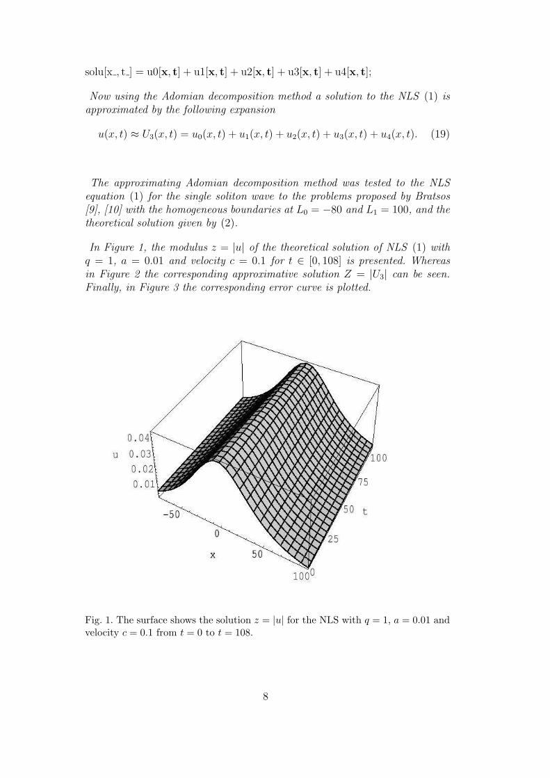
In Figure 1, the modulus z = |u| of the theoretical solution of NLS (1) withq = 1, a = 0.01 and velocity c = 0.1 for t ∈ [0, 108] is presented. Whereasin Figure 2 the corresponding approximative solution Z = |U3| can be seen.Finally, in Figure 3 the corresponding error curve is plotted.
Fig. 1. The surface shows the solution z = |u| for the NLS with q = 1, a = 0.01 andvelocity c = 0.1 from t = 0 to t = 108.
8
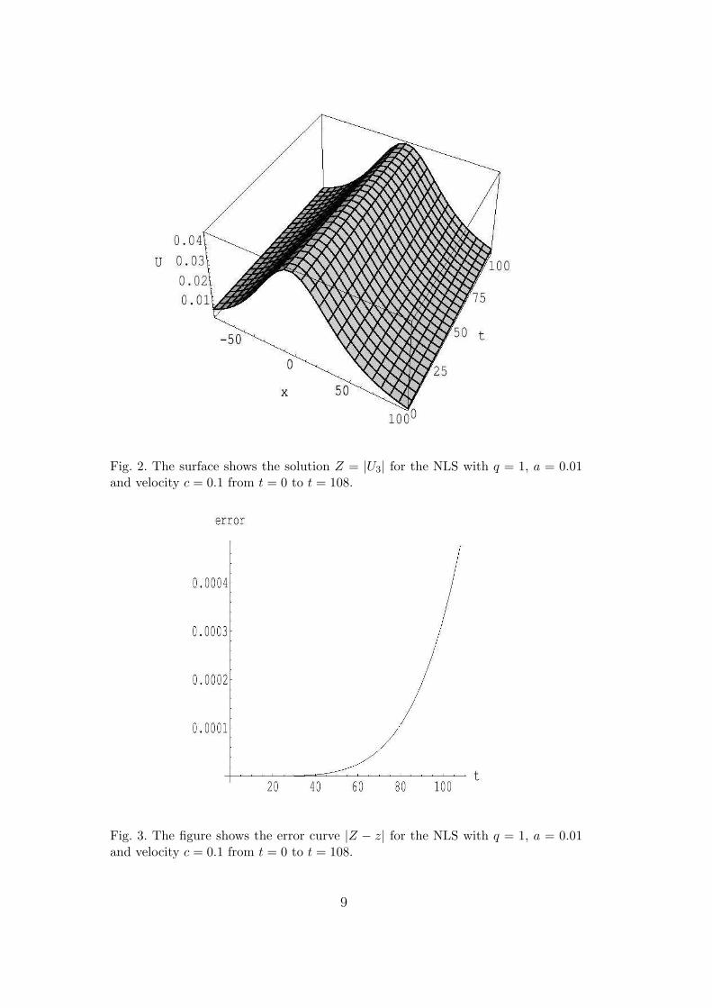
Fig. 2. The surface shows the solution Z = |U3| for the NLS with q = 1, a = 0.01and velocity c = 0.1 from t = 0 to t = 108.
Fig. 3. The figure shows the error curve |Z − z| for the NLS with q = 1, a = 0.01and velocity c = 0.1 from t = 0 to t = 108.
9
4 Discrete nonlinear Schrodinger equations
Discrete nonlinear Schrodinger equations are omnipresent [25] in applied sci-ences, e.g. describing the propagation of electromagnetic waves in glass fibers,one–dimensional arrays of coupled optical waveguides [17] and light–inducedphotonic crystal lattices [16]. Moreover, they are used to describe Bose–Einsteincondensates in optical lattices [35] and they are an established model for op-tical pulse propagation in various doped fibers [21], [22].
In this section we will consider the two most common discrete versions of thecubic NLS equation (1a) that arise from different spatial discretizations. Thesediscrete nonlinear Schrodinger equations (DNLS) are also called lattice NLSequations and we refer the reader to [33, Chapter 5.2.2] for a concise discussionon this topic.
4.1 The standard discrete NLS
If one applies the standard spatial discretization to (1a) and replaces F (u) =|u|2u with a diagonal discretization FD(uj) = |uj|2uj , we obtain the usualDNLS equation:
i∂tuj + D2huj + q|uj|2uj = 0, j ∈ Z, t > 0, (20a)
uj(0) = fj , j ∈ Z, (20b)
with uj = uj(t), h = ∆x and D2huj = (uj+1 − 2uj + uj−1)/h
2 denotes thestandard second order difference quotient. The parameter ε := h−2 is called(discrete) dispersion and the parameter q is called anharmonicity, since equa-tion (20a) with ε = 0 describes a set of uncoupled anharmonic oscillators.
The DNLS equation (20a) has a discrete conserved number (mass, total exci-tation norm, power in nonlinear optics)
ND =2
q
∑
j∈Z
|uj|2 (21)
and the discrete Hamiltonian
HD = −∑
j∈Z
[
u∗
j(uj+1 + uj−1) − 2|uj|2 +q
2|uj |4
]
, (22)
where ∗ denotes the complex conjugate.
However, the standard DNLS equation (20a) is not an exactly integrable DNLS(if the spatial grid consists of more than 2 points) and thus less amenable
10
to mathematical analysis. We can only give particular discrete plane wavesolutions to the DNLS equation (20a) of the form
uj(t) = exp[
i(
jκh − ωt)]
, j ∈ Z, t > 0. (23)
Inserting (23) into the DNLS (20a) yields the discrete dispersion relation
4
h2sin2
(κh
2
)
− ω = q, (24)
which is obviously consistent with the continuous relation (5). Hence we willturn in the sequel to an integrable discrete NLS equation.
4.2 The Ablowitz–Ladik equation
After a discretization in space by replacing the cubic nonlinearity F (u) = |u|2uin (1a) with an off–diagonal discretization FAL(uj) = |uj|2(uj+1 + uj−1)/2and keeping the time variable continuous we obtain the Ablowitz–Ladik (AL)equation [1], [2]:
i∂tuj + D2huj + q|uj|2
uj+1 + uj−1
2= 0, j ∈ Z, t > 0, (25a)
uj(0) = fj, j ∈ Z. (25b)
Note that one term in (25a) can be removed through the transformation
uj(t) = vj(t) exp(−i2t), t > 0,
and equation (25a) reduces to the normalized form
i∂tvj +vj+1 + vj−1
h2+ q|vj|2
vj+1 + vj−1
2= 0, j ∈ Z, t > 0. (26)
The AL equation has a conserved number
NAL =2
q
∑
j∈Z
log(
1 +q
2|uj |2
)
(27)
and the Hamiltonian
HAL = −∑
j∈Z
[
u∗
j(uj+1 + uj−1) −4
qlog
(
1 +q
2|uj|2
)]
. (28)
The nonlinear differential–difference equation (25a) is the most famous inte-grable DNLS equation. As the AL equation (25a) is integrable it is possible
11
to give exact travelling–wave solutions on the real line j ∈ Z, including (cf.[4], [32], [33])
vj(t) = A exp[
i(ωt + αj + v0)]
cn[
β(j − vt); k]
, t > 0, (29)
where cn[·; k] is a Jacobi elliptic function of modulus k. For the case h = 1,q = 2 the parameters in (29) can be written as
A =k sn[β; k]
dn[β; k], ω =
2 cn[β; k] cos α
dn2[β; k], v =
2 sn[β; k] sin α
β dn[β; k],
where −π ≤ α ≤ π, β > 0, 0 < k < 1 are free parameters. In the limiting casek → 1 (hyperbolic limit) we get for the Jacobi elliptic (sn, cn, dn) functions[28]:
limk→1
sn[β; k] = tanh β, limk→1
cn[β; k] = limk→1
dn[β; k] = sechβ,
and obtain the discrete soliton solution of (26)
vj(t) = sinh β exp[
−i(ωt + αj + v0)]
sech[
β(j − vt)]
, t > 0, (30)
with
ω = −2 coshβ cosα, v = − 2
βsinh β sinα,
that can travel at any velocity. It can be easily seen that the discrete soliton(30) is a fairly obvious discrete version of the continuous soliton solution (2).
There exist discrete plane wave solutions to the Ablowitz–Ladik equation(25a) of the form (23). Inserting (23) into the AL equation (25a) gives thediscrete dispersion relation
4
h2sin2
(κh
2
)
− ω = q cos(κh). (31)
Remark 5 Let us remark that there also exists an explicit solution to the ALequation (25a) on a periodic interval [8].
The main interest in the AL equation arises from mathematics (in contrast tothe standard DNLS equation); only a few physical models [29] can be describedby an AL–type equation.
Remark 6 We note that there also exists another integrable DNLS equation,namely the Izergin–Korepin (IK) equation [24] that shares an important prop-erty with the continuous NLS: it has the same r–matrix [19]. However, theIK equation is a quite complicated system and no applications are known yet.Thus we will skip it here.
12
5 The semi–discrete Adomian Decomposition Method
The analogue discrete steps to the continuous ADM of §2 are simply the formalsolution to the DNLS equation (20) or the AL equation (25):
uj(t) = fj + iL−1t D2
huj + iqL−1t FD,AL(uj), j ∈ Z, t > 0, (32)
and the assumption that there exists a solution of the series form uj(t) =∑
∞
l=0 uj,l(t). The nonlinear term FD,AL(uj) in (32) is decomposed into an infi-nite series of discrete Adomian polynomials FD,AL(uj) =
∑∞
l=0 Al(uj). Substi-tuting these decompositions into (32) gives
∞∑
l=0
uj,l(t) = fj + i∞∑
l=0
L−1t D2
huj(t) + iq∞∑
l=0
L−1t Al. (33)
Again, uj,0(t) is identified with the initial data fj and the following recurrenceis proposed to determine the solution components uj,l(t):
uj,0(t) = fj, (34a)
uj,l+1(t) = iL−1t D2
huj,l(t) + iqL−1t Al, l = 0, 1, 2, . . . (34b)
For the standard DNLS equation the Adomian polynomials are the same as(14), but for the AL equation we write FAL(uj) = |uj |2(uj+1 + uj−1)/2 andobtain analogously to (14)
A0 = uj,0uj+1,0 + uj−1,0
2uj,0, (35a)
A1 =[
uj,0uj+1,1 + uj−1,1
2+
uj+1,0 + uj−1,0
2uj,1
]
uj,0 + uj,0uj+1,0 + uj−1,0
2uj,1,
(35b)
A2 =[
uj,0uj+1,2 + uj−1,2
2+
uj+1,0 + uj−1,0
2uj,2
]
uj,0 + uj,1uj+1,1 + uj−1,1
2uj,0
+[
uj,0uj+1,1 + uj−1,1
2+
uj+1,0 + uj−1,0
2uj,1
]
uj,1 + uj,0uj+1,0 + uj−1,0
2uj,2,
(35c)
A3 =[
uj,0uj+1,3 + uj−1,3
2+
uj+1,0 + uj−1,0
2uj,3
]
uj,0
+[
uj,1uj+1,2 + uj−1,2
2+
uj+1,1 + uj−1,1
2uj,2
]
uj,0
+[
uj,0uj+1,2 + uj−1,2
2+
uj+1,0 + uj−1,0
2uj,2
]
uj,1
+[
uj,0uj+1,1 + uj−1,1
2+
uj+1,0 + uj−1,0
2uj,1
]
uj,2
+ uj,1uj+1,1 + uj−1,1
2uj,1 + uj,0
uj+1,0 + uj−1,0
2uj,3, (35d)
. . . .
13
The polynomials Al, l ≥ 4 can be computed analogously in a tedious calcula-tion. The calculation to obtain the Adomian polynomials for the AL equation(35) was performed using the following Mathematica code.
Mathematica–Program 2 We define the functions:
F[l ]:=1
2Expand[
∑l
k=0u[k, t, j]
∑l
k=0u[k, t, j]
(∑
l
k=0u[k, t, j + 1] +
∑l
k=0u[k, t, j − 1]
)]
u[k , t , l ]:=u[k, t, j]/.Complex[0, n ]-> − Complex[0,n]
A[0]:=F[0]
A[l ]:=Expand[
F[l] − ∑l−1
k=0A[k]
]
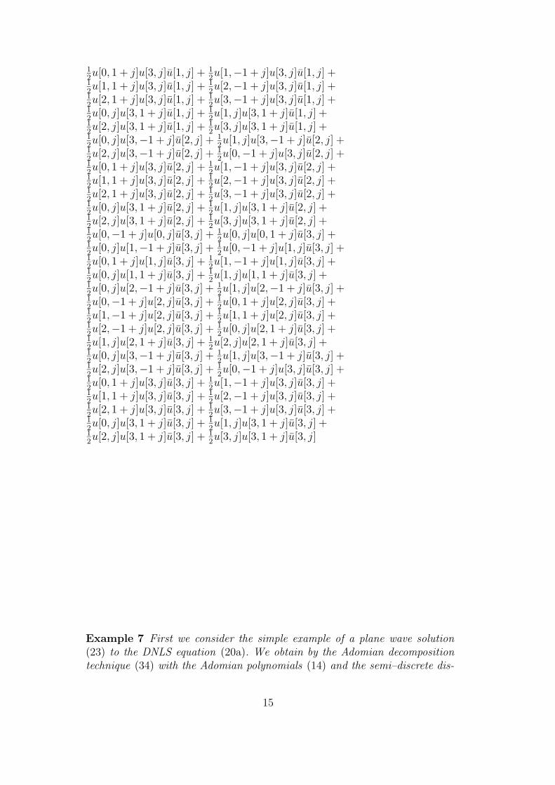
Using the functions defined we can easily furnish the desired Adomian poly-nomials, e.g.
A[2] =
12u[0, t, j]2u[2, t,−1 + j] + u[0, t, j]u[1, t, j]u[2, t,−1 + j] +
12u[1, t, j]2u[2, t,−1 + j] + u[0, t,−1 + j]u[0, t, j]u[2, t, j] +
u[0, t, j]u[0, t, 1 + j]u[2, t, j] + u[0, t, j]u[1, t,−1 + j]u[2, t, j] +u[0, t,−1 + j]u[1, t, j]u[2, t, j] + u[0, t, 1 + j]u[1, t, j]u[2, t, j] +u[1, t,−1 + j]u[1, t, j]u[2, t, j] + u[0, t, j]u[1, t, 1 + j]u[2, t, j] +u[1, t, j]u[1, t, 1 + j]u[2, t, j] + u[0, t, j]u[2, t,−1 + j]u[2, t, j] +u[1, t, j]u[2, t,−1 + j]u[2, t, j] + 1
2u[0, t,−1 + j]u[2, t, j]2 +
12u[0, t, 1 + j]u[2, t, j]2 + 1
2u[1, t,−1 + j]u[2, t, j]2 +
12u[1, t, 1 + j]u[2, t, j]2 + 1
2u[2, t,−1 + j]u[2, t, j]2 +
12u[0, t, j]2u[2, t, 1 + j] + u[0, t, j]u[1, t, j]u[2, t, 1 + j] +
12u[1, t, j]2u[2, t, 1 + j] + u[0, t, j]u[2, t, j]u[2, t, 1 + j] +
u[1, t, j]u[2, t, j]u[2, t, 1 + j] + 12u[2, t, j]2u[2, t, 1 + j]
A[3] =
12u[0, j]u[3,−1 + j]u[0, j] + 1
2u[1, j]u[3,−1 + j]u[0, j] +
12u[2, j]u[3,−1 + j]u[0, j] + 1
2u[0,−1 + j]u[3, j]u[0, j] +
12u[0, 1 + j]u[3, j]u[0, j] + 1
2u[1,−1 + j]u[3, j]u[0, j] +
12u[1, 1 + j]u[3, j]u[0, j] + 1
2u[2,−1 + j]u[3, j]u[0, j] +
12u[2, 1 + j]u[3, j]u[0, j] + 1
2u[3,−1 + j]u[3, j]u[0, j] +
12u[0, j]u[3, 1 + j]u[0, j] + 1
2u[1, j]u[3, 1 + j]u[0, j] +
12u[2, j]u[3, 1 + j]u[0, j] + 1
2u[3, j]u[3, 1 + j]u[0, j] +
12u[0, j]u[3,−1 + j]u[1, j] + 1
2u[1, j]u[3,−1 + j]u[1, j] +
12u[2, j]u[3,−1 + j]u[1, j] + 1
2u[0,−1 + j]u[3, j]u[1, j] +
14
12u[0, 1 + j]u[3, j]u[1, j] + 1
2u[1,−1 + j]u[3, j]u[1, j] +
12u[1, 1 + j]u[3, j]u[1, j] + 1
2u[2,−1 + j]u[3, j]u[1, j] +
12u[2, 1 + j]u[3, j]u[1, j] + 1
2u[3,−1 + j]u[3, j]u[1, j] +
12u[0, j]u[3, 1 + j]u[1, j] + 1
2u[1, j]u[3, 1 + j]u[1, j] +
12u[2, j]u[3, 1 + j]u[1, j] + 1
2u[3, j]u[3, 1 + j]u[1, j] +
12u[0, j]u[3,−1 + j]u[2, j] + 1
2u[1, j]u[3,−1 + j]u[2, j] +
12u[2, j]u[3,−1 + j]u[2, j] + 1
2u[0,−1 + j]u[3, j]u[2, j] +
12u[0, 1 + j]u[3, j]u[2, j] + 1
2u[1,−1 + j]u[3, j]u[2, j] +
12u[1, 1 + j]u[3, j]u[2, j] + 1
2u[2,−1 + j]u[3, j]u[2, j] +
12u[2, 1 + j]u[3, j]u[2, j] + 1
2u[3,−1 + j]u[3, j]u[2, j] +
12u[0, j]u[3, 1 + j]u[2, j] + 1
2u[1, j]u[3, 1 + j]u[2, j] +
12u[2, j]u[3, 1 + j]u[2, j] + 1
2u[3, j]u[3, 1 + j]u[2, j] +
12u[0,−1 + j]u[0, j]u[3, j] + 1
2u[0, j]u[0, 1 + j]u[3, j] +
12u[0, j]u[1,−1 + j]u[3, j] + 1
2u[0,−1 + j]u[1, j]u[3, j] +
12u[0, 1 + j]u[1, j]u[3, j] + 1
2u[1,−1 + j]u[1, j]u[3, j] +
12u[0, j]u[1, 1 + j]u[3, j] + 1
2u[1, j]u[1, 1 + j]u[3, j] +
12u[0, j]u[2,−1 + j]u[3, j] + 1
2u[1, j]u[2,−1 + j]u[3, j] +
12u[0,−1 + j]u[2, j]u[3, j] + 1
2u[0, 1 + j]u[2, j]u[3, j] +
12u[1,−1 + j]u[2, j]u[3, j] + 1
2u[1, 1 + j]u[2, j]u[3, j] +
12u[2,−1 + j]u[2, j]u[3, j] + 1
2u[0, j]u[2, 1 + j]u[3, j] +
12u[1, j]u[2, 1 + j]u[3, j] + 1
2u[2, j]u[2, 1 + j]u[3, j] +
12u[0, j]u[3,−1 + j]u[3, j] + 1
2u[1, j]u[3,−1 + j]u[3, j] +
12u[2, j]u[3,−1 + j]u[3, j] + 1
2u[0,−1 + j]u[3, j]u[3, j] +
12u[0, 1 + j]u[3, j]u[3, j] + 1
2u[1,−1 + j]u[3, j]u[3, j] +
12u[1, 1 + j]u[3, j]u[3, j] + 1
2u[2,−1 + j]u[3, j]u[3, j] +
12u[2, 1 + j]u[3, j]u[3, j] + 1
2u[3,−1 + j]u[3, j]u[3, j] +
12u[0, j]u[3, 1 + j]u[3, j] + 1
2u[1, j]u[3, 1 + j]u[3, j] +
12u[2, j]u[3, 1 + j]u[3, j] + 1
2u[3, j]u[3, 1 + j]u[3, j]
Example 7 First we consider the simple example of a plane wave solution(23) to the DNLS equation (20a). We obtain by the Adomian decompositiontechnique (34) with the Adomian polynomials (14) and the semi–discrete dis-
15

persion relation ω = (4/h2) sin2(
κh/2)
− q given in (24):
uj,0(t) = fj = eijκh, (36a)
uj,1(t) = iL−1t D2
huj,0(t) + iqL−1t A0 = iL−1
t D2he
ijκh + iqL−1t [u2
j,0uj,0]
= −i4
h2sin2
(κh
2
)
teijκh + iqteijκh = −iωteijκh, (36b)
uj,2(t) = iL−1t D2
huj,1(t) + iqL−1t A1
= iL−1t D2
h[−iωteijκh] + iqL−1t [2uj,0uj,1uj,0 + u2
j,0uj,1]
= −1
2ω
4
h2sin2
(κh
2
)
t2eijκh +1
2qωt2eiκx = −1
2ω2t2eiκx, (36c)
uj,3(t) = iL−1t D2
huj,2(t) + iqL−1t A2
= iL−1t D2
h[−1
2ω2t2eijκh]
+ iqL−1t [2uj,0uj,2uj,0 + u2
j,1uj,0 + 2uj,0uj,1uj,1 + u2j,0uj,2]
=i
6ω3t3eijκh. (36d)
Finally summing up the iterates yields
uj(t) =∞∑
l=0
uj,l(t) = eijκh{
1 − iωt − 1
2ω2t2 +
i
6ω3t3 + . . .
}
= eijκhe−iωt = ei(jκh−ωt).
Example 8 Secondly, we want to compute the x–independent solution uj(t) =f exp(iq|f |2t) (cf. Example 3). In this special case the DNLS equation (20) andthe AL equation (25) coincide and it is fairly easy to see that the ADM yieldsexactly the desired solution.
Example 9 Now we consider the AL equation (25a) and a plane wave solu-tion (23). We get using the Adomian decomposition technique (34) and the
16
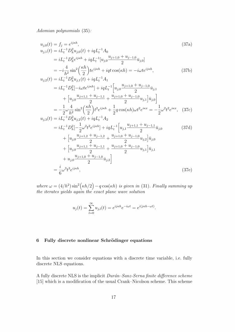
Adomian polynomials (35):
uj,0(t) = fj = eijκh, (37a)
uj,1(t) = iL−1t D2
huj,0(t) + iqL−1t A0
= iL−1t D2
heijκh + iqL−1
t [uj,0uj+1,0 + uj−1,0
2uj,0]
= −i4
h2sin2
(κh
2
)
teijκh + iqt cos(κh) = −iωteijκh, (37b)
uj,2(t) = iL−1t D2
huj,1(t) + iqL−1t A1
= iL−1t D2
h[−iωteijκh] + iqL−1t
[
uj,0uj+1,0 + uj−1,0
2uj,1
+[
uj,0uj+1,1 + uj−1,1
2+
uj+1,0 + uj−1,0
2uj,1
]
uj,0
]
= −1
2ω
4
h2sin2
(κh
2
)
t2eijκh +1
2q cos(κh)ωt2eiκx = −1
2ω2t2eiκx, (37c)
uj,3(t) = iL−1t D2
huj,2(t) + iqL−1t A2
= iL−1t D2
h[−1
2ω2t2eijκh] + iqL−1
t
[
uj,1uj+1,1 + uj−1,1
2uj,0 (37d)
+[
uj,0uj+1,2 + uj−1,2
2+
uj+1,0 + uj−1,0
2uj,2
]
uj,0
+[
uj,0uj+1,1 + uj−1,1
2+
uj+1,0 + uj−1,0
2uj,1
]
uj,1
+ uj,0uj+1,0 + uj−1,0
2uj,2
]
=i
6ω3t3eijκh, (37e)
where ω = (4/h2) sin2(
κh/2)
−q cos(κh) is given in (31). Finally summing upthe iterates yields again the exact plane wave solution
uj(t) =∞∑
l=0
uj,l(t) = eijκhe−iωt = ei(jκh−ωt).
6 Fully discrete nonlinear Schrodinger equations
In this section we consider equations with a discrete time variable, i.e. fullydiscrete NLS equations.
A fully discrete NLS is the implicit Duran–Sanz-Serna finite difference scheme[15] which is a modification of the usual Crank–Nicolson scheme. This scheme
17

is very well designed for computing soliton solutions [15]. It is given by
iD+τ un
j + D2hu
n+ 1
2
j + q∣∣∣u
n+ 1
2
j
∣∣∣
2u
n+ 1
2
j = 0, j ∈ Z, n ∈ N0, (38a)
u0j = fj, j ∈ Z, (38b)
with unj ∼ u(jh, nτ), τ = ∆t, where D+
τ unj = (un+1
j − unj )/τ denotes the
standard forward–in–time difference quotient and we used in (38a) the time
average in un+ 1
2
j = (un+1j + un
j )/2. The cubic nonlinearity is discretized by
FDSS(un+ 1
2
j ) =∣∣∣u
n+ 1
2
j
∣∣∣
2u
n+ 1
2
j .
Since (38a) is not integrable we can only give particular discrete plane wavesolutions to the DSS–scheme (38) of the form
unj = exp
[
i(
jκh − nωτ)]
, j ∈ Z, n ∈ N. (39)
Inserting the solution ansatz (39) into (38a) yields
ie−iωτ − 1
τ− 2
h2(e−iωτ + 1) sin2
(κh
2
)
+ q|e−iωτ + 1|2
4
e−iωτ + 1
2= 0,
i.e. we obtain the discrete dispersion relation
4
h2sin2
(κh
2
)
− 2
τtan
(ωτ
2
)
= q|e−iωτ + 1|2
4. (40)
Finally, using the series representation of the tan function in (40) we get
4
h2sin2
(κh
2
)
− 2
τ
(ωτ
2+
(ωτ)3
24+ . . .
)
= q(
1 − (ωτ)2
4+
(ωτ)4
48+ . . .
)
, (41)
which is consistent with the semi–discrete relation (24) of the DNLS equation.
7 The fully discrete Adomian Decomposition Method
Finally we adopt the steps of the semi–discrete ADM of §5 to solve fullydiscrete equations. To do so, we assume a formal solution to the Duran–Sanz-Serna scheme (38):
unj = fj + i(D+
τ )−1D2hu
n+ 1
2
j + iq(D+τ )−1FDSS(u
n+ 1
2
j ), j ∈ Z, n ∈ N0, (42)
where the inverse discrete operator is given by
(D+τ )−1vn = τ
n−1∑
m=0
vm, n ∈ N0. (43)
18
Note that using this definition (43) we get
(D+τ )−1D+
τ unj = un
j − u0j .
We assume that there exists a solution of the series form unj =
∑∞
l=0 unj,l,
where the components unj,l are going to be determined recurrently. Again,
the nonlinear term FDSS(un+ 1
2
j ) in (42) is decomposed into an infinite seriesof discrete Adomian polynomials FDSS(uj) =
∑∞
l=0 Al(uj). Substituting thesedecompositions into (42) gives
∞∑
l=0
unj,l = fj + i
∞∑
l=0
(D+τ )−1D2
hun+ 1
2
j + iq∞∑
l=0
(D+τ )−1Al. (44)
Again, unj,0 is identified with the initial data fj and the following recurrence is
proposed to determine the solution components un+ 1
2
j,l :
unj,0 = fj, (45a)
unj,l+1 = i(D+
τ )−1D2hu
n+ 1
2
j,l + iq(D+τ )−1Al, l = 0, 1, 2, . . . (45b)
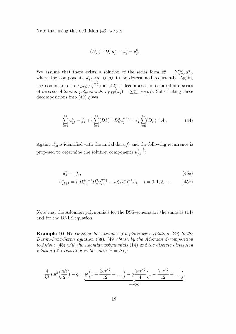
Note that the Adomian polynomials for the DSS–scheme are the same as (14)and for the DNLS equation.
Example 10 We consider the example of a plane wave solution (39) to theDuran–Sanz-Serna equation (38). We obtain by the Adomian decompositiontechnique (45) with the Adomian polynomials (14) and the discrete dispersionrelation (41) rewritten in the form (τ = ∆t):
4
h2sin2
(κh
2
)
− q = w(
1 +(ωτ)2
12+ . . .
)
− q(ωτ)2
4
(
1 − (ωτ)2
12+ . . .
)
︸ ︷︷ ︸
=:ω(κ)
,
19
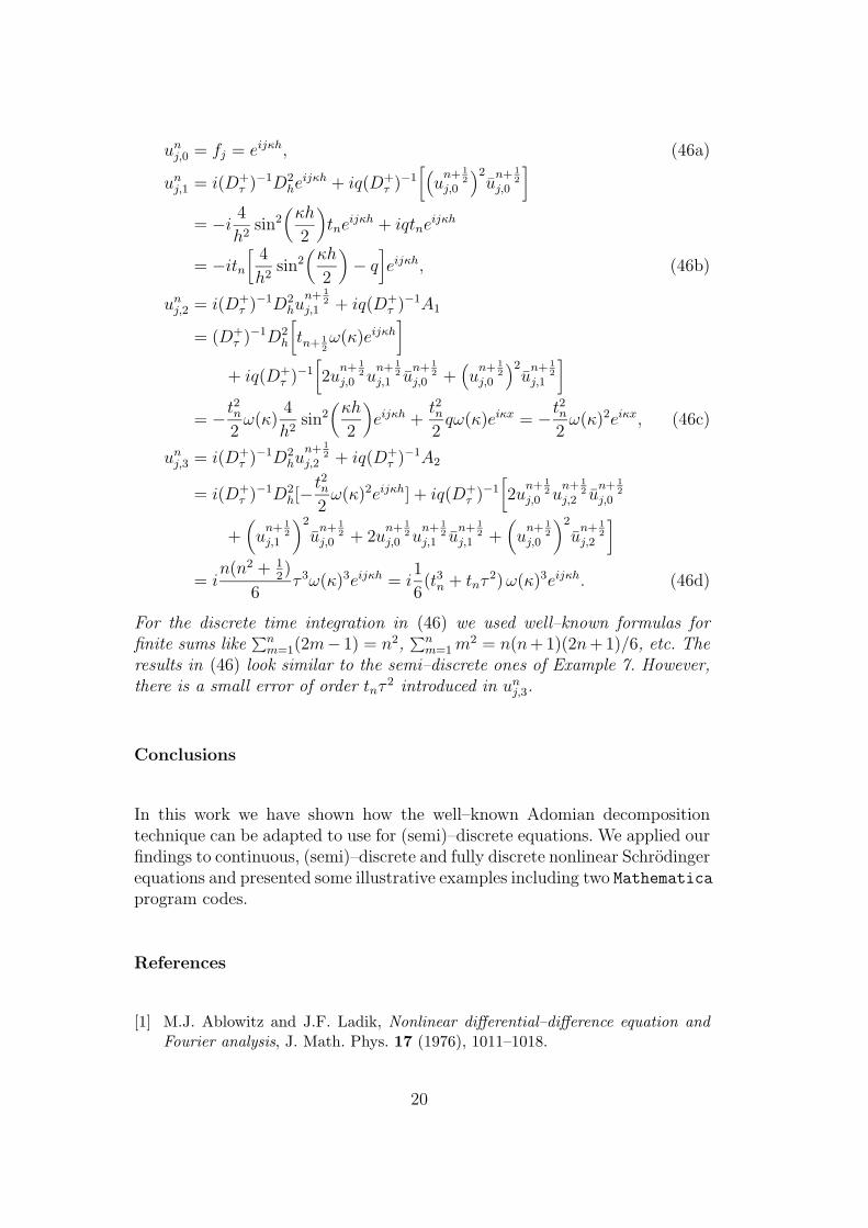
unj,0 = fj = eijκh, (46a)
unj,1 = i(D+
τ )−1D2he
ijκh + iq(D+τ )−1
[(
un+ 1
2
j,0
)2u
n+ 1
2
j,0
]
= −i4
h2sin2
(κh
2
)
tneijκh + iqtneijκh
= −itn
[4
h2sin2
(κh
2
)
− q]
eijκh, (46b)
unj,2 = i(D+
τ )−1D2hu
n+ 1
2
j,1 + iq(D+τ )−1A1
= (D+τ )−1D2
h
[
tn+ 1
2
ω(κ)eijκh]
+ iq(D+τ )−1
[
2un+ 1
2
j,0 un+ 1
2
j,1 un+ 1
2
j,0 +(
un+ 1
2
j,0
)2u
n+ 1
2
j,1
]
= −t2n2
ω(κ)4
h2sin2
(κh
2
)
eijκh +t2n2
qω(κ)eiκx = −t2n2
ω(κ)2eiκx, (46c)
unj,3 = i(D+
τ )−1D2hu
n+ 1
2
j,2 + iq(D+τ )−1A2
= i(D+τ )−1D2
h[−t2n2
ω(κ)2eijκh] + iq(D+τ )−1
[
2un+ 1
2
j,0 un+ 1
2
j,2 un+ 1
2
j,0
+(
un+ 1
2
j,1
)2
un+ 1
2
j,0 + 2un+ 1
2
j,0 un+ 1
2
j,1 un+ 1
2
j,1 +(
un+ 1
2
j,0
)2
un+ 1
2
j,2
]
= in(n2 + 1
2)
6τ 3ω(κ)3eijκh = i
1
6(t3n + tnτ
2) ω(κ)3eijκh. (46d)
For the discrete time integration in (46) we used well–known formulas forfinite sums like
∑nm=1(2m− 1) = n2,
∑nm=1 m2 = n(n+1)(2n+1)/6, etc. The
results in (46) look similar to the semi–discrete ones of Example 7. However,there is a small error of order tnτ 2 introduced in un
j,3.
Conclusions
In this work we have shown how the well–known Adomian decompositiontechnique can be adapted to use for (semi)–discrete equations. We applied ourfindings to continuous, (semi)–discrete and fully discrete nonlinear Schrodingerequations and presented some illustrative examples including two Mathematicaprogram codes.
References
[1] M.J. Ablowitz and J.F. Ladik, Nonlinear differential–difference equation andFourier analysis, J. Math. Phys. 17 (1976), 1011–1018.
20
[2] M.J. Ablowitz and J.F. Ladik, A nonlinear difference scheme and inversescattering, Stud. Appl. Math. 55 (1976), 213–229.
[3] M.J. Ablowitz and P. Clarkson, Solitons, Nonlinear Evolution Equations andInverse Scattering, Cambridge University Press, 1992.
[4] M.J. Ablowitz, B. Prinari and A.D. Trubatch, Discrete and continuousnonlinear Schrodinger systems, Cambridge University Press, 2004.
[5] G. Adomian, A Review of the Decomposition Method in Applied Mathematics,J. Math. Anal. Appl. 135 (1988), 501–544.
[6] G. Adomian, Solving frontier problems of physics: the decomposition method,Boston: Kluwer Academic Publishers, 1994.
[7] J. Argyris and M. Haase, An Engineer’s Guide to Soliton Phenomena:Application of the Finite Element Method, Comput. Methods Appl. Mech.Engrg. 61 (1987) 71–122.
[8] N.N. Bogolyubov and A.K Prikarpatskii, The inverse periodic problem for adiscrete approximation of a nonlinear Schrodinger equation, Sov. Phys. Dokl.27 (1982), 113–116.
[9] A.G. Bratsos, A Linearized Finite-difference Method for the solution of the non-linear Cubic Schrodinger Equation, Commun. Appl. Anal. 4 (2000), 133–139.
[10] A.G. Bratsos, A Linearized finite-difference scheme for the numerical solution ofthe nonlinear Cubic Schrodinger Equation, Korean J. Comput. & Appl. Math.8 (2001), 459–467.
[11] F. Calogero, Why are certain nonlinear PDEs both widely applicable andintegrable? in: What is Integrability?, 1–62, edited by V.E. Zakharov, SpringerSeries in Nonlinear Dynamics, Springer–Verlag, Berlin, 1991.
[12] T. Cazenave, An Introduction to Nonlinear Schrodinger Equations, Textos deMetodos Matematicos de Universidade Federal de Rio de Janeiro, 26, 1996.
[13] Y. Cherruault, Convergence of Adomian’s method, Kybernetes 18 (1989), 31–38.
[14] Y. Cherruault and G. Adomian, Decomposition methods: a new proof ofconvergence, Math. Comp. Model. 18 (1993), 103–106.
[15] A. Duran and M. Sanz–Serna, The numerical integration of relative equilibriumsolutions. The nonlinear Schrodinger equation., IMA J. Numer. Anal. 20 (2000),235–261.
[16] N.K. Efremidis, S. Sears, D.N. Christodoulides, J.W. Fleischer and M. Segev,Discrete solitons in photorefractive optically induced photonic lattices, Phys.Rev. E 66 (2002), 046602.
[17] H.S. Eisenberg, Y. Silberberg, R. Morandotti, A.R. Boyd, and J.S. Aitchison,Discrete Spatial Optical Solitons in Waveguide Arrays, Phys. Rev. Lett. 81
(1998), 3383–3386.
21
[18] S.M. El-Sayed and D. Kaya, A numerical solution and an exact explicit solutionof the NLS equation, Appl. Math. Comput. 172 (2006) 1315–1322.
[19] L.D. Faddeev and L.A. Takhtajan, Hamiltonian Methods in the Theory ofSolitons, Springer–Verlag, Berlin, 1987.
[20] I.Th. Famelis and A.G. Bratsos, A solution of the cubic Schrodingerequation using the Adomian decomposition method, Proceedings of the 7thHellenic-European Conference on Computer Mathematics and its Applications(HERCMA 2005), 22–24 September 2005, Athens, Greece.
[21] S. Gatz and J. Herrmann, Soliton propagation in materials with saturablenonlinearity, J. Opt. Soc. Am. B, 8 (1991), 2296–2302.
[22] S. Gatz and J. Herrmann, Soliton propagation and soliton collision in double-doped fibers with a non-Kerr-like nonlinear refractive-index change, Optics Lett.17 (1992), 484–486.
[23] A. Hasegawa, Solitons in Optical Communications, Clarendon Press, Oxford,NY, 1995.
[24] A.G. Izergin and V.E. Korepin, A lattice model related to the nonlinearSchrodinger equation, Sov. Phys. Dokl. 26 (1981) 653–654.
[25] P.G. Kevrekidis, K.Ø. Rasmussen and A.R. Bishop, The Discrete NonlinearSchrodinger equation: a survey of recent results, Int. J. Modern Physics B 15
(2001), 2833–2900.
[26] S.A. Khuri, A new approach to the cubic Schrodinger equation: An applicationof the decomposition technique, Appl. Math. Comput. 97 (1998), 251–254.
[27] Yu.S. Kivshar and G.P. Agrawal, Optical Solitons: From Fibers to PhotonicCrystals, Academic Press, San Diego, 2003.
[28] D.F. Lawden, Elliptic Functions and Applications, Springer–Verlag, New York,1989.
[29] P. Marquie, J.-M. Bilbault and M. Remoissenet, Observation of nonlinearlocalized modes in an electrical lattice, Phys. Rev. E, 51 (1995), 6127–6133.
[30] M. Onorato, A.R. Osborne, M. Serio and S. Bertone, Freak waves in randomoceanic sea states, Phys. Rev. Lett. 86 (2001) 5831–5834.
[31] J. Satsuma and N. Yajima, Initial Value Problems of One–dimensional Self–Modulation of Nonlinear Waves in Dispersive Media, Prog. Theor. Phys. Suppl.55 (1974), 284–295.
[32] R. Scharf and A.R. Bishop, Properties of the nonlinear Schrodinger equationon a lattice, Phys. Rev. A 43 (1991), 6535–6543.
[33] A. Scott, Nonlinear Science: Emergence & Dynamics of Coherent Structures,Oxford University Press, 1999.
22
[34] C. Sulem and P.-L. Sulem, The nonlinear Schrodinger equation, Appliedmathematical sciences 139, Springer, 1999.
[35] A. Trombettoni and A. Smerzi, Discrete Solitons and Breathers with DiluteBose-Einstein Condensates, Phys. Rev. Lett. 86 (2001), 2353–2356.
[36] A.M. Wazwaz, A reliable modification of Adomian’s decomposition method,Appl. Math. Comput. 102 (1999), 77–86.
[37] A.M. Wazwaz, A reliable technique for solving linear and nonlinear Schrodingerequations by Adomian decomposition method, Bull. Inst. Math. 29 (2001), 125–134.
[38] A.M. Wazwaz, Reliable analysis for nonlinear Schrodinger equations with acubic nonlinearity and a power law nonlinearity, Math. Comp. Model. 43
(2006), 178–184.
[39] A.M. Wazwaz, Exact solutions for the fourth order nonlinear Schrodingerequations with cubic and power law nonlinearities, Math. Comp. Model. 43
(2006), 802–808.
[40] A.M. Wazwaz. A study on linear and nonlinear Schrodinger equations by thevariational iteration method, in press: Chaos, Solitons & Fractals, 2007.
[41] V.E. Zakharov and A.B. Shabat, Exact theory of two–dimensional self–modulation of waves in nonlinear media, Sov. Phys. JETP 34 (1972), 62–69.
[42] V.E. Zakharov, Collapse of Langmuir waves, Sov. Phys. JETP 35 (1972), 908–914.
23


