Measurement Bias in Price Indexes for Capital Goods

MEASUREMENT BIAS IN PRICE INDEXES FOR CAPITAL GOODS*

University of Chicago and the National Bureau of Economic ResenrcR

The official U.S. price deflators for investment goods continue to be based on defective methodology, despite frequent criticism in recent years. This paper contributes new price information, which is combined with the empirical results from other studies to yield a revised investment deflator for the 1954-1963 period which (a) rises much more slowly than the official index and (b) declines relative to a revised price index for consumption expenditures.

The official price indexes published by government statistical agencies have been subjected to a steady barrage of criticism during the ten years which have passed since the publication of the "Stigler report", The Price Statistics of the Federal Government (Stigler, 1961). Despite this fact, official U.S. price deflators for capital goods are based on essentially the same methodology as ten years ago. This paper reviews the growing body of literature on measurement bias in price indexes for capital goods, contributes new information of several different types, and concludes that over the 1954-1963 period for which the most information is available the official U.S. capital goods price indexes contain a serious upward bias. The adjustments suggested in this paper result in a revised capital goods deflator which declines relative to the price of consumption during this period, in contrast to the usual conclusion that the price of capital goods has been rising relative to the price of consumption. Although this paper is entirely concerned with the U.S. indexes, the same set of issues doubtless applies to the price indexes of other nations, where in fact problems may be greater due to a smaller absolute investment of resources in statistics-gathering.

Critics generally agree that among the various defects from which the capital goods price indexes suffer, the most important are the use of sellers' list prices instead of buyers' prices and the failure to take full account of quality change. Section I1 below reviews the evidence on the relation of transaction to list prices and presents new results based on unit value data from the Census of Manufacturers. Both sets of evidence suggest that the ratio of "true" buyers' prices to sellers' list prices moves procyclically, implying that a "true" measure of real output fluctuates less over the business cycle than the official real output measures which are computed from deflators based on list prices. More

*I am grateful for research support to the National Bureau of Economic Research. A preliminary version of this paper was presented to the Business and Economic Statistics Section of the American Statistical Association, Detroit, December 29,1970. Comments on that version by E. Denison, T. Rymes, J. Triplett, T. W. Schultz, R. E. Lipsey, and Z. Griliches were valuable in developing this revision. I am also grateful to G. Jaszi for providing me with the opportunity to learn about the various new deflators for single-family houses which have been recently developed inside the Federal government.

surprisingly, both sets also suggest that there is a secular upward trend of list prices relative to transaction prices.

The literature on quality change has concentrated on price indexes of consumer goods, where most economists approve a goal of attempting to measure the cost of maintaining a constant level of satisfaction or utility. There is less agreement on the desirability of adjusting capital goods price indexes for quality change. Jorgenson and Griliches (1967) claim that previous measures of the growth of total factor productivity in the U.S. are biased upward in part because of insufficient adjustments in official price indexes for improvements in the quality of capital inputs. But the position of most national income accountants, best expressed by Denison (1957), is that investment and capital indexes should not be adjusted for all changes in quality, but only for those quality improvements requiring an increase in the cost of production. Despite the support of the Stigler committee for quality adjustments in consumption goods price indexes, the report was "not prepared to take a stand" on the appropriate criteria for quality adjustments in investment goods price indexes. (Stigler, 1961, p. 37).

Our discussion of quality change begins in part I11 below with a formal statement of the proposition that a quality change index should adjust for any increase in the ability of a capital good to contribute to production. Then two empirical techniques of quality adjustment, the "conventional" methodology used in existing official U.S. price indexes and the "hedonic" regression technique, are described and compared. Both methods are similar in principle, both can measure some but not all quality change, and both are more useful when used together rather than separately because their defects are complementary.

Part IV is devoted to a review and evaluation of the empirical evidence on the importance of quality change in producers' durable equipment; most of the results imply that there is a substantial upward bias in existing price indexes. Existing evidence on automobiles and refrigerators is supplemented by new results based on the method of "direct comparison of closely similar models," which suggests that previous studies may have understated the bias in existing official indexes. The empirical evidence from parts I1 and IV is combined at the end of part IV to compute a revised deflator for total producers' durable equipment which rises about 2 percent per annum more slowly over the 1954-1963 period than the official index, a bias which may be larger than in earlier or later periods.

The deflation of investment in structures is inherently less tractable than equipment because of the heterogeneity of buildings. A number of new structures indexes are reviewed in part V, the best of which (the FHAIOBE deflator for single-family houses) is available for the post-1953 period but has not been cited or discussed previously. Other techniques evaluated include a hedonic regression index for single-family houses, which has been initiated recently by the Bureau of the Census, surveys of labor requirements for different kinds of structures, and surveys of housing market values as reported by individual homeowners.

Part V concludes with a calculation of the 1954-1963 price trends of consumption and investment prices using the adjustments from part IV and reasonable assumptions regarding the biases in the structures and consumption deflators. The result, which is intuitively plausible, is that, in place of the previously accepted "standard conclusion" that investment goods prices have risen faster

122

than the price of consumption, in fact investment goods prices appear to have risen substantially more slowly over the 1954-1963 period.

11. THE VALIDITY OF PRICE QUOTATIONS FOR CAPITAL GOODS

A. Introduction Soon after the inception of the Wholesale Price Index, observers took

notice of the incredible rigidity of the price indexes for individual industrial cornmoditie~.~ Those who accepted the validity of the WPI price quotations cited their rigidity as support for the proposition that industrial prices are "administered" by firms rather than determined by the interaction of market supply and demand. Another explanation, however, was that the price quotations are sellers' list prices which do not reflect actual market conditions.

Flueck (1961, p. 422) gives various reasons why actual market prices might differ from list prices, of which the most important is discounting:

Apparently the most popular and widely used method is to offer discounts of varying degrees (depending on the market supply and demand situation) from the list price which is quoted in trade journals, newspapers, by trade associations, and unfortunately for many commodities, the WPI. For discounting appears to be very common in normal markets, rampant in weak (buyers') markets, and zero or negative in strong (sellers') markets.

Although most discussion of discrepancies between list prices and actual transaction prices has been motivated by the interest of price theorists in administered pricing, important macroeconomic issues are at stake as well. If transaction prices are more responsive than list prices to cyclical fluctuations, policymakers with their eyes on the official (list) price indexes may needlessly aggravate the instability of the economy, pushing up unemployment at the end of a boom longer than necessary to achieve stability in actual transaction prices, and allowing the economy to expand at the end of a recession too long after inflation has begun in transaction prices. Further, econometric equations that explain the behavior of real expenditure variables might be changed in character if true prices fluctuate more over the business cycle than official price indexes, since this would imply that the dependent variable in these equations, actual real deflated expenditures, in fact varies less over the cycle than present official estimates.

B. Direct Evidence on Transactions Prices. Several studies have collected data on prices paid by buyers, but few of these

series refer to capital goods. While a seller can provide price information on a given model of a complicated piece of machinery over a period of time, most buyers purchase capital goods only occasionally and thus cannot provide a continuous price series. Evidence on buyers' prices is limited mainly to crude and semi-finished materials which are purchased regularly, with a few exceptions noted below.

lFor references to the literature see Stigler and Kindahl (1970, pp. 11-20).

123

1. The Bureau of Labor Statistics Steel Study. Evidence for the 1939-1942 period for 629 steel buyers confirms the hypothesis of a procyclical pattern in the ratio of transaction to list prices. "The average ratio of invoice to quoted price for hot rolled sheets was 92 percent in the second quarter of 1939 and 85 percent in the third quarter, 94 percent in the second quarter of 1940, and essentially 100 percent thereafter" (quoted by Stigler, and Kindahl, 1970, p. 18).

2. Rees on Mail Order Prices. Rees (1961) compares BLS list price indexes for eleven commodities with an index constructed from the average Sears and Montgomery Ward catalogue prices over the 1947-1959 period. Most of the commodities were items of clothing, and are not relevant to this study of capital goods prices, but one commodity was auto tires, a component of an important capital good. Rees' findings are summarized in Table 1, line 1 where we compute the average rate of growth of the ratio of Rees' index to the comparable BLS index over individual business cycles. (Our cycle reference dates are identical for all commodities in Table 1, subject to limitations of the data and do not correspond to standard NBER reference cycle dates, since the timing of price fluctuations differs from that of the production fluctuations on which the NBER data are based). The tire ratio shows no average trend during expansions but declines markedly during contractions and thus declines on average over the entire p e r i ~ d . ~

3. Transaction Prices of Electrical Equipment. Lines 2-12 illustrate movements in the transaction/list price ratio for various pieces of electrical equipment. Unfortunately, none of the cyclical comparisons in columns 4 and 5 refer to more than one cycle except those in lines 3 and 9-12. In all cases except lines 6 (which suffers from a data period which does not include a complete contraction) and 9, the average algebraic change in the ratio is smaller in contractions than in expansions. The unweighted average of column 4, lines 1-12, is -7.2 percent, compared to + 1.6 percent for column 5. Further, in every case but line 3 there is a significant secular downward trend in the ratios over contractions and expansions taken together. This is a surprising result, since hypotheses about the behavior of the transaction/list ratio predict procyclical fluctuations but not a secular downward trend. Thus the data in Table 1, even though for a limited number of products and a small number of years, raise the possibility of a significant upward bias in the WPI indexes for the commodities in question, for reasons which are not self-evident but may be related to a growing permanent use of discounts off list prices, or to an inertia in list price quotations which creates an upward bias in the WPI for commodities like electrical goods where the underlying price trend was downward during the late 1950's and early 1960's.

4. All Industrial Commodities. The recent Stigler-Kindahl study represents the most extensive effort to compile buyers' price data, but it is mainly concerned with basic industrial materials. The weighted average transactions/list ratio for all industrial commodities in the study (line 13) shows movements of much smaller amplitude than for the individual commodities of lines 1-12, suggesting perhaps that sellers' price indexes are more reliable for intermediate than for

?3ecular averages are taken between comparable cyclical phases; thus the figure in the last column of line 1 extends from the 1948 peak to the 1957 peak and excludes the 1958 trough.

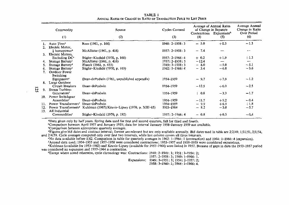
TABLE 1 ANNUAL RATES OF CHANGE IN RATIO OF TRANSACTION PRICE TO LIST PRICE

Average of Annual Rates Average Annual Commodity Source Cycles Covered of Change in Separate Change in Ratio

Contractions Expansionsh Over Period (1) (2) (3) (4) (5) (6)

Auto Tiresa Electric Motor,

-& horsepowerb Electric Motors,

Excluding DCC Storage Batteryc Storage Batteryd Storage Batterye Outdoor Power

Switching EquipmentC

Large Outdoor Circuit Breakers

Steam Turbine- Generatorsf

Power Switchgear Assembliesf

Power Transformersf Power Transformersg All Industrial

Commoditiesc

Rees (1961, p. 166)

McAllister (1961, p. 416)

Stigler-Kindahl (1970, p. 168) McAllister (1961, p. 416) Flueck (1961, p. 455) Stigler-Kindahl (1970, p. 169)

Dean-dePodwin (1961, unpublished appendix)

Dean-dePodwin Dean-dePodwin Kuhlman (1967)lKravis-Lipsey (1970, p. XIII-85)

Stigler-Kindahl (1970, p. 192)

"Data given only by half years. Spring data used for first and second quarters, fall for third and fourth. *Comparison between April 1957 and January 1959; data for interval January 1958-January 1959 not available. "Comparison between appropriate quarterly averages. dFigures give bid dates and contract interval; former are relevant but are only available annually. Bid dates used in table are 2/2/49,1/31/51,2/1/54,

and 2/4/59. Cycle averages computed only over first two intervals, while last column covers all three intervals. eNo data available before 1/62. Comparison in table for quarterly averages in 1962: 1-1964: 1 (contraction) and 1964: 1-1966: 4 (expansion). 'Annual data used; 1954-1955 and 1957-1958 were considered contractions; 1955-1957 and 1958-1959 were considered expansions. 'Kuhlman (available for 1953-1962) and Kravis-Lipsey (available for 1957-1964) were linked in 1957. Because of gaps in data the 1953-1957 period

was considered an expansion and 1957-1964 a contraction. h E ~ ~ e p t where noted otherwise, cycle chronology was: Contractions : 1948 : 2-1949: 3 ; 1951 : 3-1954: 2;

1957: 2-1958: 3; 1960: 1-1964: 1. Expansions: 1949: 3-1951 : 3; 1954: 2-1957: 2;

1958: 3-1960: 1; 1964: 1-1966: 4.

final goods. Nevertheless, the procyclical pattern is confirmed for the aggregate Stigler-Kindahl transaction/list price ratio.

5. The CPI compared to the WPI. The Consumer Price Index measures transaction prices on most items, since retail discounts are usually announced explicitly on price tags. In a comparison of CPI and WPI indexes for 10 identical consumer durables, Jorgenson and Griliches (1970, p. 31) report an average annual decline of 1.9 percent in the CPI/WPI ratio for 1947-1949 to 1958. While this tends to confirm the evidence of Table 11-1 regarding a secular upward bias in the transaction/list ratio, another possible cause is a secular decline in retail margins due to the spreading of discount stores. Without further research the CPI/WPI secular "drift" is not conclusive evidence on the validity of WPI quotations.

C. Indirect Evidence Using Unit Value Indexes The U.S. Census Bureau collects data on the value of shipments (V) and

the number of units shipped (X) for numerous manufacturing commodities. Since V is recorded from actual invoices, the unit values (V/X) measure transaction rather than list prices. A comparison of the V/X indexes for individual commodities with list price indexes for the same commodities may reveal cyclical fluctuations in the transaction/list ratio. In any study of the validity of WPI quotations, a comparison of the WPI with actual transactions prices is preferable to a comparison with the unit value indexes employed here, because of the likelihood that changes in the mix of quality characteristics within a given Census product classification may make the unit value indexes inaccurate indicators of true price movements. Unfortunately, because previous studies of buyers' prices have virtually eliminated producers' durables from consideration (except for the commodities of Table l), census unit value data are virtually the only available information on transactions prices for machinery, and to my knowledge they have not previously been exploited for this p u r p o ~ e . ~

In considering unit value data for narrowly defined individual commodities as potential replacements for WPI quotations, we receive the explicit approval of the 1961 Stigler report:

Where buyers' prices are not available, we recommend extensive use of unit values, at least as benchmarks to which the monthly prices are adjusted. Unit values are inferior to specification transaction prices, but when unit values are calculated for fairly homogeneous commodities, they are more realistic than quoted prices in a large number of industrial markets (1961, p. 71).

In this study I have minimized the quality-mix problem by selecting a limited number of product categories, most of which are narrowly defined in terms of an important quality dimension. Examples of these product categories are gasoline-powered tractors with 35-39 horsepower motors, diesel engines of

3McAllister (1961) calculated two unit value indexes for machinery: standard typewriters (1948-59) and a 4 horsepower "Jet Type Deep Well Water System" (1952-56). I am grateful to Zvi Griliches for introducing me to the Census data and Current Industrial Reports. He has commented on the secular trend in many unit value/list price ratios (Jorgenson-Griliches, 1970, pp. 29-34) but has not discussed their cyclical behavior.

81-90 horsepower, construction power cranes with shovels of 314 cubic yards of capacity, and square feet of cast iron radiators and convectors. Other product classifications are selected on the basis of a subjective feeling that quality change per unit has been relatively minor, e.g., manual typewriters, escalators, and furnace^.^

The cyclical hypothesis, if valid, would lead us to expect that the ratios of unit value to list prices would rise more in expansions than in contractions. Calculations were made for two different choices regarding the timing of U.S. postwar cycles. The first is the conventional NBER definition, with postwar expansions in 1949-1953, 1954-1957, 1958-1960, and after 1961, and with contractions in 1948-1949, 1953-1954, 1957-1958, and 1960-1961 (the 1945- 1948 expansion is excluded due to the absence of unit value data for 1945 and 1946). The second "alternative definition" of reference cycles attempts to date cyclical peaks as years of excess demand in the machinery industry: 1951, 1956, and 1966 (these years correspond to peaks in the ratio of new orders to shipments for durable goods). The first two troughs are the conventional ones- 1949 and 1954--but the "alternative" treats the entire 1956-1966 period as one cycle with a single trough in 1963 (the ratio of current-dollar equipment investment to GNP was 0.063 in 1956, remained at 0.060 or below from 1958 to 1963, and rose above 0.063 in 1964-1966). In short, the alternative pattern defines three expansions (1949-1951, 1954-1957, and 1963-1967) and three contractions (1948-1949, 1951-1954, and 1956-1963).

The results for both definitions are shown in Table 2. The unweighted averages for all industry sectors in line 9 indicate (comparing columns 4 and 5) that the annual rate of growth of the unit valuellist price ratio in expansions exceeds that in contractions by 2.98 percent for the NBER definition and (comparing columns 7 and 8) by 3.17 percent for the "alternative definition." These average differences rise to 3.22 and 3.55 percent if the 1948-1949 contraction is excluded, for a number of ratios rose during that contraction but fell during others. The electric industrial and miscellaneous electrical categories (lines 7 and 8) are substantial contributors to these cyclical differentials, and the averages are recomputed in line 10 with these two industry sectors excluded. The excess of the rate of growth in expansions then drops to 1.05 percent and 1.85 percent for the two respective definitions with 1948-1949 included, and to 1.39 and 2.35 with 1948-1949 excluded. By any definition, then, the averages for all sectors appear to support the cyclical hypothesis that unit value indexes rise relative to WPI quotations during expansions and fall relatively during contractions. Our findings are strongly confirmed for each of the eight industry sectors shown in Table 2. For the NBER definition the cyclical hypothesis is confirmed for five out of eight industries if 1948-1949 is included, and for seven

4A detailed list of the 38 categories chosen is available on request. Data were collected on the value of shipments and numbers of machines shipped for various 7-digit product classes as published by the U.S. Bureau of the Census. The 38 used in Table 2 are copied from Current Industrial Reports and its predecessor (before 1960) Facts for Industry. Data used in Table 3 below were collected for 19 additional product classes for census years (1947, 54, 58, and 63) from Volume 2 of the Census of Manufactures. The present discussion is preliminary and is presented for illustrative purposes only. The author is currently conducting a detailed study of unit value data for the Federal Reserve Board Price Statistics Committee.

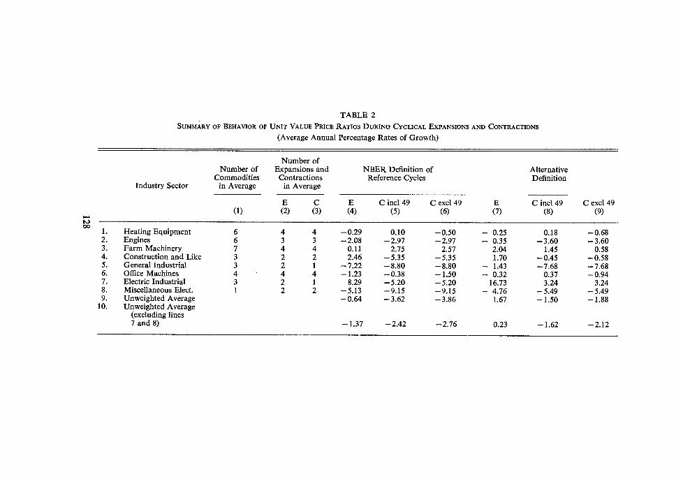
TABLE 2 SUMMARY OF BEHAVIOR OF UNIT VALUE PRICE RATIOS DURING CYCLICAL EXPANSIONS AND CONTRACTIONS

(Average Annual Percentage Rates of Growth)

Number of Number of Expansions and NBER Definition of Alternative

Commodities Contractions Reference Cycles Definition Industry Sector in Average in Average

E C E C incl49 C exc149 E C incl49 C excl49 (1) (2) (3) (4) (5) (6) (7) (8) (9)

Heating Equipment Engines Farm Machinery Construction and Like General Industrial Office Machines Electric Industrial Miscellaneous Elect. Unweighted Average Unweighted Average

(excluding lines 7 and 8)

out of eight if that contraction is excluded. For the alternative definition the score is six out of eight with 1948-1949 included and eight out of eight with 1948-1949 excluded.

The distinct upward secular bias in the WPI appears as an unexpected result of our summary in Table 1 above of evidence on buyers' price data. Table 2 also suggests that there may be a secular downdrift of unit value indexes relative to WPI quotations, which would be even more unexpected since (as we shall see below in part 111) the WPI indexes are partially adjusted for quality change whereas the unit value indexes are not.

Table 3 summarizes two kinds of evidence on secular drift. Where annual data are available for most of the 1947-1967 period, the secular trend of the unit value/list price ratio is determined by the coefficient on two time-trend terms (pre- and post-1958) in a time-series regre~sion.~ In cases where data were available only for Census years (1947, 1954, 1958, and 1963) Table 3 shows percentage rates of growth of the ratio between Census year^.^

Line 14 presents in the first two columns the unweighted average of the sectoral averages of the two time-trend regression coefficients; these overall averages are in the vicinity of minus one percent per annum for both time periods. The nonregression time trends decline considerably faster, at a rate of about minus two percent for the earlier period and at about minus 29 percent in the later period. The regression results are closer to the nonregression trends if the farm and electric industrial sectors are excluded, however, as shown in line 15.7

The sizeable secular downtrend in the unit value/WPI ratio exhibited in Table 3 confirms the conclusion of Table 1, which is based on superior data but a much narrower group of commodities. The agreement between the two tables is reassuring, but further research is necessary before we can have much confidence in the unit value results. Recently an internal U.S. government study (Searle, 1970) was conducted to "aid in choosing between price data (largely from the BLS industrial price program) and the unit-value data derived from Census product and value data. . ." (p. 1). The report concludes by recom- mending "that more extensive use be made of specification price data than heretofore, largely because unit value measures tend to be affected by changes in product mix" (p. 1). An appendix of the report examines detailed WPI and unit value data for 25 7-digit items, often at the company level, and concludes that there is "a persistent tendency of unit values between 1958 and 1963 to reflect

5The regressions, which were run for 38 commodity classes of producers' durable equipment, also include an excess demand variable, either the ratio of new orders to shipments or the unemployment rate. Few of the coefficients on the excess demand variables are significantly different from zero, which in light of the cyclical differences of Table 2 suggests that the wrong cyclical variable may have been chosen. Further experiments are being conducted in an extension of this research.

6The nonregression evidence is based on 19 commodity classes. 7The relatively slow rise in WPI farm equipment prices as indicated above may be due to

quality adjustments. The atypical behavior of the electric industrial sector is due to the rapid decline in the WPI indexes for two sizes of integral horsepower electric motors (those indexes, unlike the unit value data for the same products, drop by half between 1957-1959 and 1967). It is more likely that the WPI rather than the unit value indexes are wrong, since Stigler-Kindahl find that their data on actual buyers' prices for electric motors (like the unit value data) do not show the rapid price declines indicated by the WPI indexes; see Table 1, line 3 above.

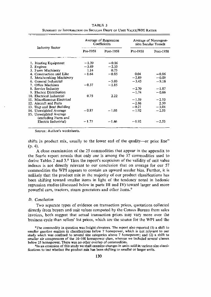
TABLE 3 SUMMARY OF INFORMATION ON SECULAR DRIFT OF UNIT VALUE/WPI RATIOS

Average of Regression Average of Nonregres- Coefficients sion Secular Trends

Industry Sector Pre-1958 Post-1958 Pre-1958 Post-1958

1. Heating Equipment - 1.39 -0.16 2. Engines -3.69 -2.33 3. Farm Machinery 1.14 0.75 4. Construction and Like - 1.64 -0.85 0.04 - 0.86 5. Metalworking Machinery -2.89 - 0.09 6. General Industrial - 5.03 - 3.43 -9.16 7. Office Machines -0.37 - 1.85 8. Service Industry - 2.70 -1.87 9. Electric Distribution - 1.74 - 0.66

10. Electrical Industrial 0.75 2.22 11. Miscellaneous Electrical - 1.59 -2.10 12. Aircraft and Parts -2.86 2.50 13. Ship and Boat Building - 0.21 - 3.04 14. Unweighted Average -0.87 - 1.03 -1.92 -2.53 15. Unweighted Average

(excluding Farm and Electric Industrial) - 1.77 - 1.46 - 1.92 -2.53

Source: Author's worksheets.

shifts in product mix, usually to the lower end of the quality-or price line" (P. 4).

A close examination of the 25 commodities that appear in the appendix to the Searle report reveals that only one is among the 57 commodities used to derive Tables 2 and 3.* Thus the report's scepticism of the validity of unit value indexes is not directly relevant to our conclusion that on average for our 57 commodities the WPI appears to contain an upward secular bias. Further, it is unlikely that the product mix in the majority of our product classifications has been shifting toward smaller items in light of the tendency noted in hedonic regression studies (discussed below in parts I11 and IV) toward larger and more powerful cars, tractors, steam generators and other items.g

D. Conclusion Two separate types of evidence on transaction prices, quotations collected

directly from buyers and unit values computed by the Census Bureau from sales invoices, both suggest that actual transaction prices may vary more over the business cycle than sellers' list prices, which are the source for the WPI and the

8The commodity in question was freight elevators. The report also reported (1) a shift to smalIer gasoline engines in classifications below 7 horsepower, which is not relevant to our study which was confined to several size categories above 7 horsepower; and (2) a shift to smaller air compressors of the 16-100 horsepower class, whereas we included several classes below 25 horsepower. There was no other overlap of commodities.

OIn an extension of this study we shall examine changes in units sold in various size classifications to test whether the product mix has been shifting to smaller or larger units.

official price deflators for producers' equipment. As a result official data exag- gerate the inflexibility of equipment prices in recessions and overstate cyclical variations in real equipment investment.

A more novel result suggested by both types of evidence is a secular upward bias in the WPI price indexes for equipment. If true, the secular growth rates of real output and investment have been understated and the secular growth in total factor productivity has been exaggerated.1° For additional evidence on secular bias, we turn next to the most commonly cited source of an upward bias in WPI indexes for equipment-inadequate adjustment for quality improvements.

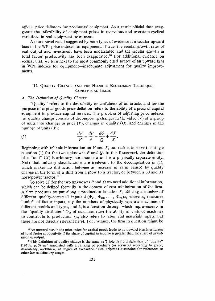
A. The Dejinition of Quality Change "Quality" refers to the desirability or usefulness of an article, and for the

purpose of capital goods price deflation refers to the ability of a piece of capital equipment to produce capital services. The problem of adjusting price indexes for quality change consists of decomposing changes in the value (V) of a group of units into changes in price (P), changes in quality (Q), and changes in the number of units (X):

dV dP dQ d X (1) -- -- +-+-.

V P X

Beginning with reliable information on V and X, our task is to solve this single equation (1) for the two unknowns P and Q. In this framework the definition of a "unit" ( X ) is arbitrary; we assume a unit is a physically separate entity. Note that industry classifications are irrelevant to the decomposition in (I), which makes no distinction between an increase in value caused by quality change in the form of a shift from a plow to a tractor, or between a 30 and 31 horsepower tractor.ll

To solve (1) for the two unknowns P and Q we need additional information, which can be defined formally in the context of cost minimization of the firm. A firm produces output along a production function F, utilizing a number of different quality-corrected inpnts hi(azl, Qi2, . . . , aim)xi where xi measures "units" of factor inputs, say the numbers of physically separate machines of different models and types, and h, is a function through which improvements in the "quality attributes" Qif of machines raise the ability of units of machines to contribute to production. (xi also refers to labor and materials inputs, but these are not directly relevant here). For instance, the firm in question might be

1°An upward bias in the price index for capital goods leads to an upward bias in estimates of total factor productivity if the share of capital in income is greater than the share of investment in output.

llThis definition of quality change is the same as Triplett's third definition of "quality" (197 lb, p. 5) as "associated with a ranking of products (or services) according to grade, desirability, usefulness, or degree of excellence." See Triplett's discussion for references to other less satisfactory usages.

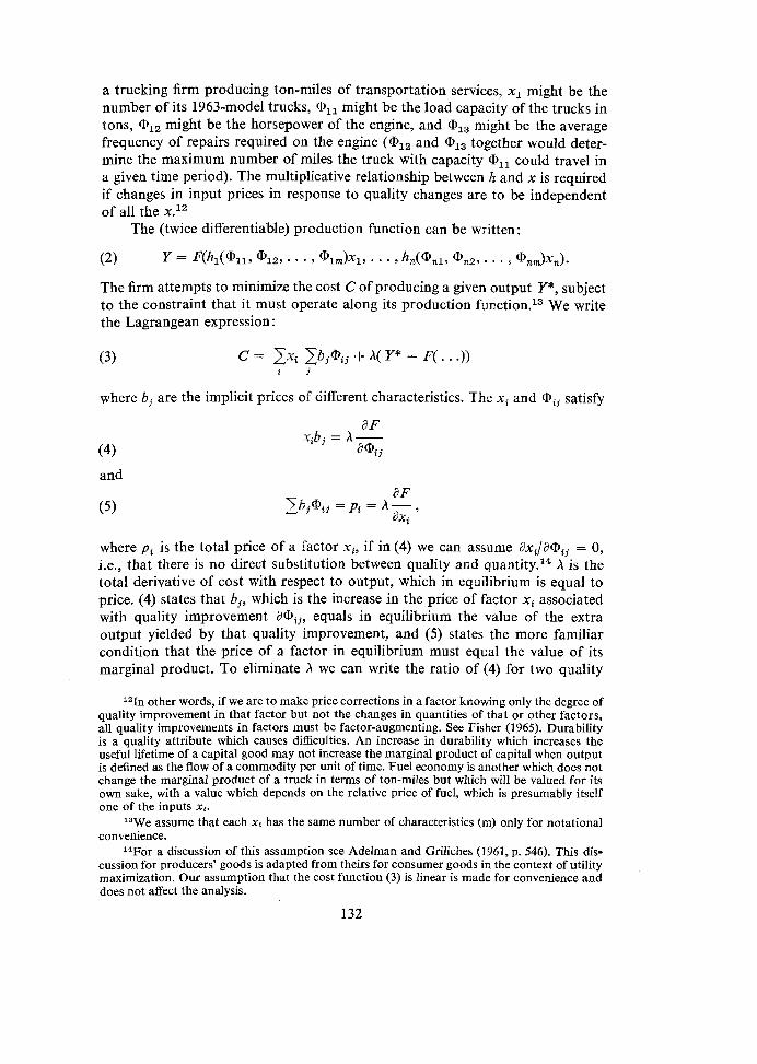
a trucking firm producing ton-miles of transportation services, x, might be the number of its 1963-model trucks, all might be the load capacity of the trucks in tons, @,, might be the horsepower of the engine, and Q13 might be the average frequency of repairs required on the engine (a,, and @,, together would determine the maximum number of miles the truck with capacity @,, could travel in a given time period). The multiplicative relationship between I? and x is required if changes in input prices in response to quality changes are to be independent of all the x.12

The (twice differentiable) production function can be written :

The firm attempts to minimize the cost C of producing a given output Y*, subject to the constraint that it must operate along its production fu'unction.13 We write the Lagrangean expression :

where bi are the implicit prices of different characteristics. The xi and Dij satisfy

and

where pi is the total price of a factor xi, if in (4) we can assume a ~ , / a @ , ~ = 0, i.e., that there is no direct substitution between quality and quantity.14 X is the total derivative of cost with respect to output, which in equilibrium is equal to price. (4) states that bi, which is the increase in the price of factor xi associated with quality improvement a@ii, equals in equilibrium the value of the extra output yielded by that quality improvement, and (5) states the more familiar condition that the price of a factor in equilibrium must equal the value of its marginal product. To eliminate h we can write the ratio of (4) for two quality

l2In other words, if we are to make price corrections in a factor knowing only the degree of quality improvement in that factor but not the changes in quantities of that or other factors, all quality improvements in factors must be factor-augmenting. See Fisher (1965). Durability is a quality attribute which causes difficulties. An increase in durability which increases the useful lifetime of a capital good may not increase the marginal product of capital when output is defined as the flow of a commodity per unit of time. Fuel economy is another which does not change the marginal product of a truck in terms of ton-miles but which will be valued for its own sake, with a value which depends on the relative price of fuel, which is presumably itself one of the inputs xt.

13We assume that each x, has the same number of characteristics (m) only for notational convenience.

14For a discussion of this assumption see Adelman and Griliches (1961, p. 546). This discussion for producers' goods is adapted from theirs for consumer goods in the context of utility maximization. Our assumption that the cost function (3) is linear is made for convenience and does not affect the analysis.

attributes of different factors x, and xs:

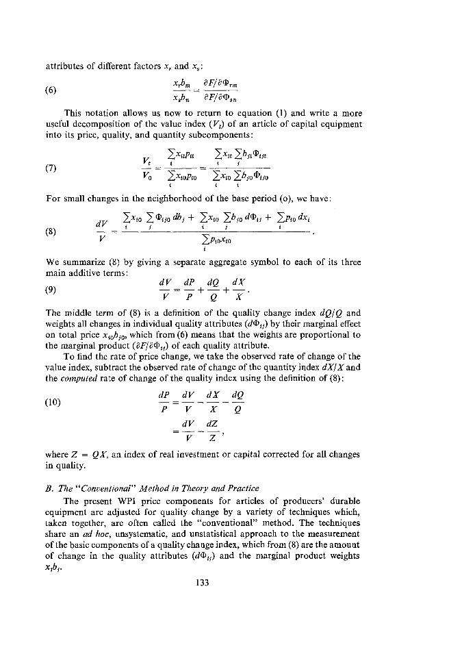
This notation allows us now to return to equation (I) and write a more useful decomposition of the value index (Vt) of an article of capital equipment into its price, quality, and quantity subcomponents:

For small changes in the neighborhood of the base period (o), we have:

We summarize (8) by giving a separate aggregate symbol to each of its three main additive terms:

The middle term of (8) is a definition of the quality change index dQ/Q and weights all changes in individual quality attributes (dBij) by their marginal effect on total price xiobjo, which from (6) means that the weights are proportional to the marginal product (aFJaQij) of each quality attribute.

To find the rate of price change, we take the observed rate of change of the value index, subtract the observed rate of change of the quantity index dX/X and the computed rate of change of the quality index using the definition of (8):

dP dV d X dQ -

P V X Q

where Z = QX, an index of real investment or capital corrected for all changes in quality.

B. The "Conventional" Method in Theory and Practice The present WPI price components for articles of producers' durable

equipment are adjusted for quality change by a variety of techniques which, taken together, are often called the "conventional" method. The techniques share an ad hoc, unsystematic, and unstatistical approach to the measurement of the basic components of a quality change index, which from (8) are the amount of change in the quality attributes (dQij) and the marginal product weights xtbi.

133

The essence of the conventional method is the technique of specification pricing. If a product is specified by all relevant quality characteristics, none of the increase in unit value ( V / X ) due to increases in the quantity of the quality characteristics will be considered as pure price change. A weighted average of the price indexes of each commodity classification will increase only when there is "pure" inflation. A quality index computed as a residual, d(V/X)/(V/X) minus dP/P, would correspond precisely to the conceptual definition of equation (8). Unfortunately, this ideal cannot be attained in practice. A price increase on a new model containing a small additional amount of a given quality characteristic will be counted as price change rather than quality change if the new model remains in the same commodity classification as the old, and the price increase will be ignored only if the quality improvement shifts the model into a different commodity classification. If the price of the new model is the same as that of other occupants of the new classification, no price increase will be registered in that class. Since the required comparison cannot be made if the classification was previously empty, the specification method cannot effectively distinguish between price and quality change when a new model replaces an old model unless there are an infinite number of occupied classifications defined along every dimension in which quality change takes place.

Since it is impossible to create a classification scheme with the infinite number of classes necessary to shift every new model into a new class, in practice class boundaries are broadened and some quality characteristics are omitted, so that many instances of quality change fail to shift a product into a new classification. Unless the price of the new model which remains in its old classification is explicitly adjusted for quality change, the price index for the relevant classification will erroneously register an increase. In the current WPI, for instance, prices are collected for two-horsepower-size classes of gas tractors, four of integral horsepower electric motors, three of diesel engines, etc. The introduction of a new model tractor with a higher price due solely to higher horsepower will not raise the WPI if the new model falls in a higher horsepower classification, but the WPI will rise when the new model stays in the same class in the absence of an explicit adjustment. Further, improvements in quality characteristics other than horsepower will raise the WPI unless adjustments are made. To the extent that there are these quality improvements for which no adjustments are made, the WPI rises faster than the true change in "pure" price, but because some increases in horsepower cause a shift in commodity classification, thus causing the price increase associated with the quality change to be ignored, the WPI even without explicit adjustments does not rise as fast as a unit value index for all tractors. There are several different methods of adjustment used when there is a quality change in a product which remains in the same commodity classification:

1. For some products prices are compared directly from period to period, a method which assumes no quality change between periods. In practice, the method is used when "explicit valuations of the quality difference cannot be made," which implies that relevant dimensions for subcategories cannot be determined.15 The resulting index is the equivalent of a unit value index (within a

15More detailed descriptions of methods 1, 2, 3, and 4 are given by Hoover (1961) and Triplett (1971a).

given product class) which makes no adjustment for the relative mix of low- quality and high-quality items.

2. When a model with a new quality characteristic is introduced, and price data are available for models with both quality characteristics at a given date, the new price is "linked" to the old one with the difference between the prices of new and old models on the transition date used to estimate the change in quality. This method is equivalent to the hedonic regression method discussed below but is much less useful because in practice new models often replace old ones completely, preventing the necessary simultaneous comparison of the prices of the two models.

3. When simultaneous price quotations on new and old models are not available, direct estimates are made of the value of quality changes, using manufacturers' cost data. These adjustments tend to be incomplete; most adjustments refer to items whose costs are relatively easy to estimate and apply to equipment price indexes beginning only in the early 1960s. Even now, adjustments are not generally made for changes which may have been important, such as changes in size, weight, power, speed of operation, durability, or fuel economy.16

4. When no information to "link" two models can be obtained from manufacturers or by the technique of simultaneous price comparisons, there are two possibilities. First, in cases where the price of the new model at time t i - 1 exceeds that of the old model at time t by a relatively small amount (defined arbitrarily), the two prices are compared directly, thus ignoring quality change entirely and leading to an upward bias in the resulting price index if the quality of the new model exceeds that of the old. On the other hand, when the price difference exceeds a "relatively small amount," the observation at time t+ 1 is simply dropped from the index. Since the change in the index number for the commodity will then be determined by the other observations in the commodity class, the assumption is thus being made that the unobserved "true price change" betweent and t+ 1 is identical to the price change of the remaining included observations.

16"In such a comparison we would make no allowances for such things as greater length or more wrap in the windshield, because we have no objective standard by which to determine the relationship between quality and price for such features" Jaffe (1959, p. 195). Apparently the adjustments for automobiles were made much more comprehensive "in 1959 and were made possible by quality and cost data supplied by manufacturers" Stotz (1966, p. 178). Stotz' list of quality adjustments is very comprehensive (p. 181), but no details are given of the exact method of adjustment for an increase in horsepower or length. The new post-1959 procedure seems to rely heavily on manufacturers' evaluations, and the indexes are subject to a downward bias due to a possible eagerness by firms (especially in the guidepost era) to disguise the extent of true price increase:

If possible, an attempt is made to get the manufacturer of a changed product to estimate the proportion of the total price difference between the two varieties attributable to quality change. It is not always clear, however, whether the manufacturer's estimate is based on the added costs of changed features or his evaluation of the added value to the user. Gavett (1967, p. 20). Regarding machinery other than autos, Professor Triplett states in a letter to the author

dated March 17, 1969: "There is a great amount of manufacturer's production cost data used for quality adjustment in the machinery and vehicles components of the WPI, but I cannot say what proportion of the components are so adjusted nor how often. Use of this is growing in the WPI, but it still, I gather, is a special adjustment, rather than a routine adjustment, matter: if a special problem comes up in a particular machinery or vehicle item, and/or if the manufacturer provides data on the cost of the quality change, there will be an adjustment."

It is clear that methods 1,2, 3, and 4 are too unreliable to correct the specification technique for its insufficient numbers of characteristics and size classifications. But the errors in the different methods can bias the estimates of "pure7' price change both upwards and downwards; without further evidence no a priori case can be made supporting the frequent charge that the WPI producers' equipment indexes overstate the rate of "pure" inflation. While methods 1 and 4 may in general bias the WPI upwards, on the other hand there is a high pro- bability that firms overstate the proportion of a price change due to quality change when submitting cost estimates under method 3, which creates the distinct possibility of a downward bias in the WPI.

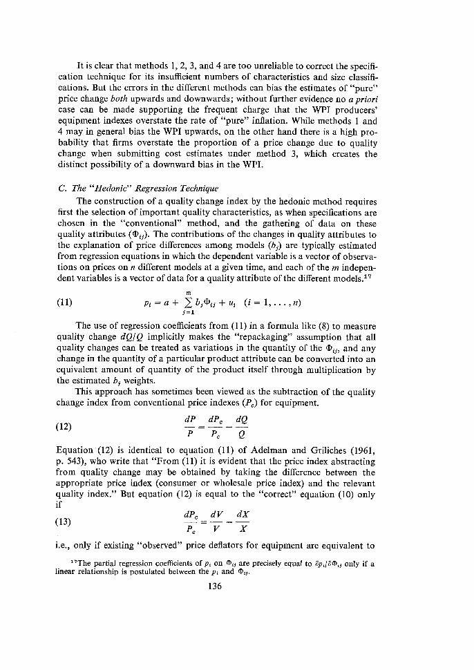
C. The "Hedonic" Regression Technique The construction of a quality change index by the hedonic method requires

first the selection of important quality characteristics, as when specifications are chosen in the "conventional" method, and the gathering of data on these quality attributes (dD,,). The contributions of the changes in quality attributes to the explanation of price differences among models (bJ are typically estimated from regression equations in which the dependent variable is a vector of observations on prices on n different models at a given time, and each of the m independent variables is a vector of data for a quality attribute of the different models.17

The use of regression coefficients from (1 1) in a formula like (8) to measure quality change dQ/Q implicitly makes the "repackaging" assumption that all quality changes can be treated as variations in the quantity of the Qij, and any change in the quantity of a particular product attribute can be converted into an equivalent amount of quantity of the product itself through multiplication by the estimated bi weights.

This approach has sometimes been viewed as the subtraction of the quality change index from conventional price indexes (PC) for equipment.

Equation (12) is identical to equation (11) of Adelman and Griliches (1961, p. 543), who write that "From (11) it is evident that the price index abstracting from quality change may be obtained by taking the difference between the appropriate price index (consumer or wholesale price index) and the relevant quality index." But equation (12) is equal to the "correct" equation (10) only if

dPc dV dX (13) -=- - -

PC v X

i.e., only if existing "observed" price deflators for equipment are equivalent to

''The partial regression coefficients of pi on Dij are precisely equal to apijaDij only if a linear relationship is postulated between the p i and Qij.

quality-uncorrected unit value indexes, which is not true because of quality corrections introduced in the WPI through multiple classifications and adjustment methods 2-4 above.

It is difficult to determine whether this problem affects Griliches' work (1961) (1964) on automobiles. Griliches presents several "quality-adjusted" price indexes for the period 1937-1961 derived by the deflation of the CPI auto index by a Q index which is calculated from regressions with horsepower, weight, and length as the three quality characteristics. According to Larsgaard and Mack (1961, p. 522) no adjustments were made to the CPI during Grjliches' sample period (at least through the model year 1960) for changes in horsepower, weight, or length other than an adjustment for a shift in the 1956 model year from six-cylinder to V-8 engines, a linking which Griliches takes into account by computing separate quality indexes for sixes and V-8's. However, by 1960 in the computation of the CPI auto index approximately $620 had been deducted from the list price of autos for equipment which was standard in 1960 but was not standard in 1939.18

Without the $620 deduction the CPI auto index would have risen by about 224 percent instead of 152 percent over the period.lQ While these adjustments do not directly involve the quality characteristics used in Griliches' regressions, there may be an indirect effect. Griliches' regressions explain the high price of relatively large cars by assigning coefficients to horsepower, length, and weight, but some of the price differential in any given year is actually caused by the inclusion as standard equipment in certain large cars of accessories which are later introduced as standard equipment on small cars and linked out in the CPI. To the extent that (a) these pieces of standard equipment on large cars make these cars weigh more or (b) differences among models in the inclusion of these accessories are correIated with inter-model differentials of horsepower, weight, or length, Griliches' coefficients stand partly as a proxy for the prices of these pieces of equipment and their subsequent inclusion on low-priced cars raises his quality index. Division of this quality index into the CPI then amounts to "double counting" of some types of quality change. There is no way of measuring this bias short of a detailed study of the equipment included as standard on some expensive models in the regressions and later included on lower-priced models (i.e., quality change which "trickles down"). To the extent that a given accessory is included as standard on all models at the same time, there is no bias.20

18This figure is in September 1960 prices and is derived from the $831.52 figure shown in Larsgaard and Mack by the subtraction of an estimated $150 for the shift from sixes to V-8's and $63.11 for a change in the sample of dealerships. These adjustments, of which Griliches was not aware when he wrote his 1961 article, account for his failure to duplicate the CPI from his information of list prices (see his discussion [1961, pp. 187-8 and pp. 193-61).

lgThe CPI auto index rose from 57.1 in 1939 to 144.3 in 1960, according to Griliches (1964, p. 397). The average price of a low-priced car, which according to Larsgaard and Mack was $850 in 1939, was therefore measured by the CPI as equal to $2,140 in 1960. Without the $620 in deductions, the price would have been $2,760, and the index (1939 = 100) would have been 2760/850 = 324 instead of 252.

20For further evidence on this problem see footnote 24. If the relative value of standard equipment included in large cars compared to small cars were to have decreased between the beginning and end of Griliches' sample period, this would partially explain the decline in the size of his regression coefficients on horsepower and length in cross sections for later years and the increase in the size of the constant.

An alternative approach to the estimation of pure price change by the subtraction of a d Q / Q index from the change in unit value is to estimate pure price change directly as the coefficient on one or more time dummy variables (D, ) in cross-section regressions for two or more years:

An aggregate index of price change then is obtained either from the series of at coefficients obtained in one regression like (14) run on data for a number of years, or from a string of a, coefficients obtained from a series of regressions on data for successive pairs of years. To the extent that the prices of quality characteristics are changing through time, the latter two-year technique allows the regression coefficients on the Qij , to change frequently and is preferable.

Griliches (1967, p. 326) has pointed out that changing samples of models in a regression like (14) for two adjacent years will cause some of the sample variation to be picked up in the time dummy coefficients, unless the sum (Xui) of the "model effects" (the effect of left-out qualities) for both groups of models is identical. For instance, if we run a regression for two years, 1959 and 1960, and include only in the latter period models of compact cars which are more expensive per unit of size than full-sized cars, the regression will yield a positive coefficient on the 1960 time dummy even in the absence of "pure" inflation because the coefficients on the Qij , variables are constrained to be equal in the two years. This does not strike me as a major obstacle to the use of (l4), however, because it is easy with only a small reduction in sample size (in most cases) to restrict the sample in years t and t + 1 to be identical, and then include the new models in a regression on years t + 1 and t + 2.

D. Relative Advantages of the Hedonic and Conventional Methods 1. What Both Can Do. The conventional specification method is similar

in principle to the hedonic method. A hedonic study which has sufficient data to perform regressions of price on three characteristics, say length, horsepower, and weight, also provides sufficient data to compute a conventional price index for each of several length-horsepower-weight classes. In a period during which no pure price change occurs and any excluded quality characteristics are un- altered, an increase in unit value due to a shift in quality to a higher length- horsepower-weight class is treated as quality change rather than price change in the conventional method because there is no price change for any individual commodity class, and in the hedonic method by the subtraction from the increase in unit value of a quality change index calculated from regression coefficients.

This point was originally made by Jaszi (1964), supported by Denison (1964), as a criticism of the implied claim of novelty put forth by the developers of the hedonic method. Griliches objected that the Jaszi-Denison point "calls that which is rarely applied 'the conventional method' " (1964, p. 414). While the conventional method would be able to come close to the results of the hedonic

method if more observations were collected, and if the same quality characteristics were used, in practice there could never be enough continually occupied classifications to avert the need for special adjustments when a new higher quality model is introduced but remains within the same length-horsepower-weight class as the old model. Even in this case the methods would be identical if a simultaneous overlapping price observation on the new and old model were available, since the same market price information used to estimate quality change in the hedonic regressions could be used for a special adjustment in the conventional method. But when no overlap period is available, the conventional method has no systematic method of adjustment, whereas the hedonic method "creates" an overlap observation by estimating a regression line relating price to quality and calculating the implicit price of a model containing any given amount of the quality characteristics used in the regressions.

2. What Neither Can Do. The most serious disadvantage of both methods is that neither can measure changes in the relationship between excluded and included quality dimension^.^^ Assume that the price of different models in two adjacent years can be completely described as follows (with no error):

c D i , m + l , is one additional quality characteristic which in the first period is a simple multiple of one of the first m characteristics:

(15) cannot be estimated as it stands because of multicollinearity and is estimated instead with the additional characteristic excluded. This causes no problems if (16) is valid for both time periods, for the estimated value of b, will include the effect of the omitted variable and the estimate of pure price change will be correct:

A A (17) b, = bl + a; al = a,.

Trouble arises, however, if in period 2 the additional quality characteristic yields a marginal product per unit of the first quality characteristic which increases by E over its value in period 1 :

Now the coefficient of b, estimated in a regression which excludes variable m + 1 understates the combined influence of characteristics 1 and m+ 1 in period 2, and the extra "quality" of characteristic 2 is soaked up by the time dummy and is thus interpreted as pure price change:

How serious is this problem? No bias will result if all excluded quality characteristics maintain a fixed relationship with included characteristics. For instance, when we estimate the difference between the price of a 1950 Cadillac

='This point has been recognized by Denison (1964), Griliches (1967), and Triplett (1971b).

and 1950 Chevrolet as depending on differences in length, weight, and horsepower, our coefficients are also picking up the influence of the Cadillac's wall- to-wall carpeting, fancy doorknobs, and leather upholstery. If we discover that a 1960 Chevrolet has the same length, weight and horsepower as a 1950 Cadillac, a quality index computed from the 1950 coefficients will imply that both cars are identical in every other respect. In fact, the 1960 Chevrolet could be either higher or lower quality in "other" respects than the 1950 Cadillac. Below in our review of empirical evidence on cars and houses, we suggest that the "quality" of excluded characteristics per unit of included characteristics has exhibited a net increase over the post-war period, implying that "pure" price indexes yielded by either the hedonic or conventional methods are biased upward.

There is no escape from the excluded variable problem with either the hedonic or conventional methods. When pure price change is estimated by the hedonic method using equation (10) rather than a time dummy, i.e., when the change in a quality index is subtracted from the change in unit value, (19) above shows that the estimated bj coefficients will misstate the contribution of excluded variables. Similarly, in the conventional method an increase in the amount of "excluded quality" per unit of "included quality" will show up as an increase in the price index within any commodity class defined by the included specifications.

3. Advantages of the Conventional Method. The above comparison of the hedonic and conventional methods implicitly assumes that both use the same number of "included" quality characteristics. But the hedonic method is limited by multicollinearity in the number of variables which can be included, whereas the conventional method can adjust for numerous small improvements through the use of manufacturers' cost data and option prices. For instance, in some hedonic regression studies of single-family house prices the coefficient on the "central air conditioning" variable is extremely unstable because houses with this characteristic tend to be high in the ranking of other included quality characteristics. A quality change index based on a manufacturer's cost estimate for an "average" central air conditioning unit would be preferable to the use of the hedonic coefficients in this case.22

Thus the "excluded variable" problem outlined above may be inherently less intractible for the conventional method. Care must be used, however, in the application of manufacturers' cost or option price data. If air conditioning is made standard on an automobile model, the option price for air conditioning in the previous year is the prime candidate for an estimate of the increase in quality of this year's "standard" model. But if only 20 percent of last year's purchasers bought the option, last year's price will overestimate the increase in quality as evaluated by all of this year's buyers.

Many of the early hedonic studies weighted all models equally in regressions, but an estimate of price per unit of quality for a model is only relevant to the extent that it captures a portion of the market, since a small market share indicates that quality has been ~verpr iced .~~ This problem is handled in two

22Cost estimates, of course, may not correspond to user evaluations of relative marginal products. This is particularly true of "legal" accessories like seat belts and anti-pollution devices.

23Griliches (1967, p. 325) comments on this weakness in his earlier work.

ways by the conventional method. First, a badly selling model is often not included in the sample. More important, within any commodity classification different models are sometimes weighted by market shares. But this is no solution, since the conventional indexes use Laspeyres weights which miss falling market shares caused by a deterioration of quality per dollar.

4. Advantages of the Hedonic Method. While hedonic proponents would probably admit that the multicollinearity problem prevents accurate regression estimates of quality improvements in the form of small added items (e.g., directional signals and heaters in automobiles), they would claim that "conventional" price estimates for these items based on option prices or manufacturers' cost data can be incorporated easily into the hedonic method by subtracting the prices for these items from the total price to be explained in the regression. The regression can then estimate price changes due to changes in major quality characteristics, which in the absence of overlapping observations the conventional method either ignores or adjusts in an unsystematic manner.

For instance, the conventional method cannot handle an increase in quality which causes an increasing number of data observations to lie above the existing WPI classification boundaries. In the hedonic method the prices of a new larger model can be compared with an implicit price lying on a linear extrapolation of the fitted regression line from a previous sample to determine the extent of "pure price change," but the conventional method must determine some arbitrary method of linking. The most common approach is to add a new observation for the larger objects, thus assuming that price change in the first period for the new observation is the same as for the average of other observations in the classification. This procedure will tend to bias the conventional method upwards if economies of scale or technical improvements permit a reduction in price- per-unit-of-quality to accompany a shift to larger models. And if outside information is used to "link in" the larger units, it is based in the conventional method on single points rather than the whole set of observations, as in the hedonic method.

A final advantage of the hedonic method is more basic; only by statistical experimentation can the relevant quality characteristics be discovered. Without some evidence that the characteristics used to specify WPI classes are "relevant" to consumer or producer evaluations of product quality, how are we to know what to make of the specifications used in the WPI indexes? This argument alone is enough to convince me that hedonic studies should be carried out on items in the indexes where relevant quality dimensions are not obvious. While this will require an expensive data-gathering effort, more data will be required to perform the conventional specification technique properly. Conventional techniques will have to be used to adjust the prices which are "explained" in the hedonic method for changes in small options, thus minimizing the excluded variable problem. The combined use of the hedonic method together with the conventional method may, however, lead to double counting as in the Griliches example discussed above. The importance of double counting can be assessed if the validity of the price index created from the combined method is cross checked by the method of "direct comparison of closely similar models," the usefulness of which is demonstrated in section IV-C below.

141

IV. EMPIRICAL EVIDENCE ON QUALITY CHANGE IN PRODUCERS' DURABLE EQUIPMENT

A. Results of Hedonic Regression Studies The discussion of WPI methodology in part I11 pointed out that the "con-

ventional" technique could either over- or underadjust for quality change. Here we survey some of the recent empirical studies of quality change, most of which rely on the hedonic method to compute quality-corrected price indexes, which we shall compare with official government indexes for the same product. Our aim is the compilation of a new quality-corrected price index for U.S. producers' durable equipment which incorporates, to the maximum degree possible, the results of recent studies of individual product quality. Since space limitations prevent extensive comments on each study, the remarks below briefly summarize results and point to possible sources of discrepancies when conclusions differ for the same commodity.

1. All Automobiles. Automobiles, which have been treated by most investiga- tors solely as consumer goods, are also one of the most important types of producers' durables, accounting for 8.7 percent of U.S. equipment investment in 1968. Since consumers dominate the market for most automobile models, the implicit prices for quality characteristics determined in hedonic regressions reflect the utility of these characteristics to consumers rather than producers. To utilize the results of hedonic studies to adjust unit values of cars purchased for business purposes we must assume that producers' evaluations of quality characteristics are similar to those of consumers.

Hedonic studies can compute quality-adjusted price indexes by three different techniques, (1) the computation of an index number from time dummy variables in regressions for successive pairs of adjacent years; (2) the computation of a quality index from the implicit prices of characteristics in successive single- year regressions which is then subtracted from an index of unit values; and (3) the same quality index as in (2) subtracted from an official price index for the same sample of models. (3) has the advantage that the official adjustments may "catch" quality changes (or changes in the prevalence of discounting) which are unmeasurable by the hedonic technique, but this may be outweighed by the disadvantage that the hedonic and official techniques applied simultaneously may "double-adjust" for some quality improvements. The conservative approach taken here is to rule out estimates made with method (3) and to use methods (1) and (2) instead, which thus may understate the importance of quality change if improvements have been made which raise quality without increasing the weight, power, and length characteristics which are usually included in these regres- s i o n ~ , ~ * but at least our approach avoids the double-counting problem.

In section 1 of Table 4 all "adjusted" price indexes have been computed by method (1) above. From these, a set of Official "unadjusted" indexes are

24The CPI adjustments to Chevrolets and Buicks in the 1953-1964 period are listed by Kravis and Lipsey (1970, pp. XV-28 and XV-29). Almost all of the items added to the "standard" Chevrolet during these years appear to be small accessories which were included as standard on high-priced cars during most or all of the sample period. These quality improvements are captured in the hedonic method as increases in weight multiplied by the implicit "price of weight." This suggests that method (3) may lead to serious double-counting of quality change.

subtracted to yield the "bias" in the last column.25 A positive number means that the adjusted price index rises faster than the unadjusted, suggesting quality deterioration not measured in the official indexes, whereas a negative number implies unmeasured quality i rnpro~ement .~~ Taken together, the results tell a story of quality deterioration during the Korean war period, quality improvement during the mid-1950's era of the "horsepower race," and further quality deterioration in the 1 9 6 0 ' ~ . ~ ~ An alternative interpretation of the 1960's is not that quality deteriorated, but that improvements in official measurement methods in the 196OYs, particularly the increasing use of manufacturers' cost data, allowed more quality change to be captured than is possible with the hedonic method. Quality change in automobiles in the 1960's is discussed further in section IV-C below. It is impossible to determine from published tables why Kravis-Lipsey estimate a higher rate of true price increase in the 1953-1961 period than Griliches. The difference occurs in equal proportions in the 1953-1957 and 1957-1961 subperiods.28

2. The "Low-Priced Three." Because until its 1962 revision the CPI included only Chevrolet, Ford, and Plymouth models, Griliches and Triplett constructed separate quality indexes for these makes. The figures in section 2 of Table 4 subtract these quality indexes from list prices, not from the CPI index. The general postwar pattern of price bias in section 2 is similar to that in section 1, with apparent quality deterioration in 1947-1953, quality improvement in 1953-1960, and either quality deterioration or improvement in the CPI in 1960- 1966. Section 2 also includes estimates for 1939-1947, when there was quite a large upward bias in the CPI, either because of substantial quality improvements or possibly because quality adjustments were made less carefully or not at all before 1947. This conclusion is extremely important, because it suggests that some of the apparent increase in the rate of growth of aggregate U.S. real output in the postwar as compared to the prewar period may have been due to improvements in the compilation of the price indexes, rather than an acceleration of technical change.

In summary, the adjusted automobile indexes are not radically different from the official series and indicate that there has been little if any net upward

25The OBE indexes are based on the WPI, which used a broader sample than the CPI during the 1950's.

26Line l b differs from a similar index computed by Triplett (1970, Table 1, p. 7), who did not notice that Griliches' dependent variable is stated in logs to the base 10, requiring that the coefficients of the time dummies be multiplied by 2.3 before an index number can be computed. Readers who attempt to reproduce figures in Table 4 are advised that all annual rates of change are arithmetic rather than geometric averages, except in the case of computers and refrigerators where geometric averages have been used.

27Regression coefficients for a more recent year, 1968, are available in Dewees (1970), but his study does not publish sufficient data on quality characteristics to allow computation of an updated price index for the 1960's. An attempt to compute an index by the method of "direct comparison" is presented below in section IV-C.

28During the 1953-1955 period the CPI was adjusted downward to take account of the apparent widening of discounts (Triplett, 1970). Since the regressions in Table 4 are all based on manufacturers' list prices, the true rate of price increase may be less for the 1953-1961 period than either the Griliches or Kravis-Lipsey estimates. However, Kravis-Lipsey are sceptical of the CPI adjustment and cite evidence that dealer profit margins were not reduced during 1953-1 955 (1 970, p. XV-9).

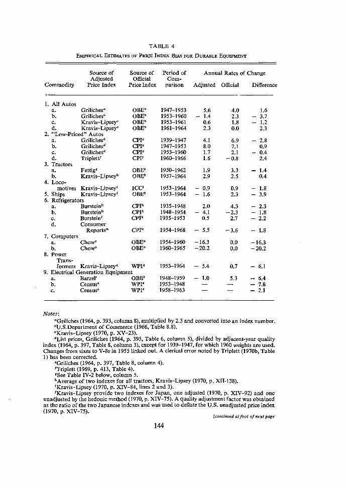
TABLE 4

EMPIRICAL ESTIMATES OF PRICE INDEX BIAS FOR DURABLE EQUKPMENT

Source of Source of Period of Annual Rates of Change Adjusted Official Com-

Commodity Price Index Price Index parison Adjusted Official Difference

1. All Autos a. Grilichesa b. Grilichesa c. Kravis-Lipseyc d. Kravis-LipseyC

2. "Low-Priced" Autos a. Grilichesd b. Grilichesd c. Grilichesd d. Triplettr

3. Tractors a. Fettigr b. Kravis-Lipseyh

4. Loco- motives Kravis-Lipsey'

5. Ships Kravis-Lipseyf 6. Refrigerators

a. Bursteink b. Bursteink c. Burstein' d. Consumer

Reportsm 7. Computers

a. Chow" b. Chow"

8. Power Trans- formers Kravis-Lipsey"

OBEb OBEb OBEb OBEb

CPIe CPIe CPI" CPIf

OBEb OBEb

ICCC OBEb

CPIk CPIk CPF

CPIk

OBEp OBEP

W P I ~ 9. Electrical Generation Equipment

a. Barzelr OBEb b. Censuss WPIs c. Censuss WPIS

Notes : "Griliches (1964, p. 393, column 8), multiplied by 2.3 and converted into an index number. bU.S.Department of Commerce (1966, Table 8.8). CKravis-Lipsey (1970, p. XV-23). *List prices, Griliches (1964, p. 395, Table 6, column 5), divided by adjacent-year quality

index (1964, p. 397, Table 8, column 3), except for 1939-1947, for which 1960 weights are used. Changes from sixes to V-8s in 1955 linked out. A clerical error noted by Triplett (1970b, Table 1) has been corrected.

eGriliches (1964, p. 397, Table 8, column 4). 'Triplett (1969, p. 413, Table 4). 'See Table IV-2 below, column 5. hAverage of two indexes for all tractors, Kravis-Lipsey (1970, p. XII-138). 'Kravis-Lipsey (1970, p. XIV-84, lines 2 and 3). 'Kravis-Lipsey provide two indexes for Japan, one adjusted (1970, p. MV-92) and one

unadjusted by the hedonic method (1970, p. XIV-75). A quality adjustment factor was obtained as the ratio of the two Japanese indexes and was used to deflate the U.S. unadjusted price index (1970, p. XIV-75).

[continued a t foot o fnex tpage

144

bias in the latter during the postwar period taken as a whole, thus tending to refute the conclusions of Griliches' studies (1961) (1964) and supporting Triplett (1969). This leaves open, however, the possibility of quality change which has not been measured by either the conventional or hedonic methods, a subject considered in section IV-C below.2g

3. Tractors. The hedonic and official price indexes for tractors are in relatively close agreement. The absence of any dramatic bias in the official tractor index is not surprising, since changes in tractor characteristics appear to have been treated more carefully by the BLS than any other commodity besides automobile^.^^ The Fettig results are probably more reliable than those of Kravis- Lipsey, because the latter study, which includes both construction-type and wheel tractors, estimates a relatively high rate of price increase due to the dominance in the regressions of the faster rising prices of construction tractors.31 Also, Fettig's results are preferable because he allows the coefficients on the quality characteristics to differ in each year, while Kravis-Lipsey constrain the coefficients to be identical over the entire 1953-1964 period.32

4. Locomotives. Very little research has been done on locomotive prices, probably because they are not sold as widely as cars or tractors, and data are harder to gather. The Kravis-Lipsey results in Table 4 should be viewed as tentative, since the samples are small and the coefficients (on horsepower) are quite erratic. Fortunately, the coefficients in 1953 and 1963 are very similar

29We do not consider the evidence of Dhrymes (1967) on refrigerators and automobiles, because his coefficients are erratic and his results are hard to decipher. For an attempted interpretation, see Triplett (1970).

301n the WPI there were 27 specification changes in the 1947-65 period for one size class of tractors and 37 for the other, far more changes than for any other item of producers' durable equipment in the WPI.

31See Kravis-Lipsey (1970, p. XII-139). 3aAnother advantage of Fettig's study is the use of domestic list prices, compared to Kravis-

Lipsey's export list prices. [conrinuedfrom previous page

kBurstein (1960, p. 134, Table A6), index I used because the 1941-1948 transition seems more reasonable, based on the size-price table which suggests that an 8 cu. ft. model cost $166 in 1941 and $252 in 1948 (the mean of the less-than-8 and 9-10 feet classes).

'Price per cubic foot of a 5 cubic foot model in 1935 and of a 9-10 cubic foot model (assumed capacity = 9.5) in 1953, from Burstein (1961, Table A3, p. 132).

"1954 prices and cubic foot estimates for dual-zone refrigerators are obtained from Consumer Reports, September 1954, p. 402; 1968 data for similar models from September 1968, pp. 479-80. In both cases only the top-rated models are included in the averages (seven models in each year). 1954 prices are manufacturer' list prices, whereas by 1968 list prices had been discontinued, and average transaction prices are used for estimates. The resulting calculation of price change overstates the rate of price decline to the extent that discounting was common in 1954 (there is no mention of discounting in the 1954 report). On the other hand, all 1968 models had no-frost freezers, whereas the 1954 models had automatic defrosting only in the refrigerator compartments and not in the freezer, so that an adjustment for this unmeasured quality change would increase the rate of price decline.

"Triplett (1971a, Table 5). "Chow (1967, p. 1124, Table 2, column 4). PInterview with Robert C. Wasson, Office of Business Economics, July 2, 1969. 91957-1964: Kravis-Lipsey (1970, p. XIII-85), linked for 1953-1957 to Kuhlman (1967). 'Barzel(1964, p. 148, column 1). "Census of Manufacturing index of value of shipmentslcapacity for steam turbine genera-

tors compared with index for WPI commodity class 117391.

145

and almost all of the price decline occurs between those two years. Very little is known about the official index for this product.

5. Ships and Boats. The "adjusted" index for ships and boats in Table IV-1 requires a leap of faith. Kravis-Lipsey construct a "conventional" price index for ships produced in the U.S. which shows no change between 1953 and 1964. They do not run any hedonic regressions for the U.S. but they do for Japan. I have taken the hedonic quality adjustment of the Japanese conventional price index and applied it to the U.S. conventional index. If quality change in the U.S. has actually been slower than in Japan, which is not unlikely, the "true" U.S. figure lies between 0.0 and the figure of - 1.6 shown in Table 4.

6. Refrigerators. Burstein's adjustment of the CPI index takes account both of quality change and of the possibility that mail-order-catalogue price quotations better reflect actual transactions prices than the CPI list prices. No hedonic regressions are calculated, but instead Burstein computes an index of year-to- year price changes on identical models, with chain-weights to reflect the growing importance of large models. I have made another use of Burstein's data by calculating the average price per cubic foot of the "median" (5 cubic foot) 1935 and (9.5 cubic foot) 1953 refrigerators. My implied CPI bias (line 6.c) is very similar to Burstein's. A similar calculation for the 1954-1968 period can be made from price and capacity data in Consumer Reports (possible sources of error are discussed in Table 4, note m), and the result indicates a continued bias at almost the same rate as in the earlier period. Compounded annually, the bias over the entire 1935-1968 period amounts to 94.5 percent!

7. Computers. What is amazing about section 7 of Table 4 is not the rapid decline in a quality-corrected price index for computers (based on multiplication speed, memory size, and other quality characteristics), but the fact that the OBE has been assuming no change in computer prices throughout the postwar period! Just as the OBE has based its aircraft deflators partly on the price index of "fabricated metal products," ignoring changes in the way the fabricated metal parts are fitted together, so it apparently regards 1970 and 1955 computers as big roughly identical metal boxes.

8. Power Transformers. A very rapid decline in power transformer prices began in the mid-1950's and continued almost to the end of Kravis-Lipsey's study in 1964. Part of the bias illustrated in Table 4 is due to quality improvements unmeasured by the WPI, but captured by Kravis-Lipsey's regressions, and the remainder is due to Kravis-Lipsey's use of buyers' rather than sellers' prices. The 1953-1964 experience probably cannot be extrapolated either back- wards or forwards, because a part of the price decline for electrical equipment during that period was due to the end of the infamous pricing conspiracy. In this light it is interesting that Kuhlman (1967) was able to derive quality adjustments similar to those of Kravis-Lipsey out of a book of list prices without running any regressions.

9. Electrical Generation Equipment. Barzel's estimates from a production function study (line 9.a) are compared with a simple computation from the Census of Manufacturers of the value of shipments divided by capacity (lines 9.b and 9.c). Both quality-corrected price indexes rise at a much slower rate than official indexes. The similarity of the results for power transformers and electrical

146

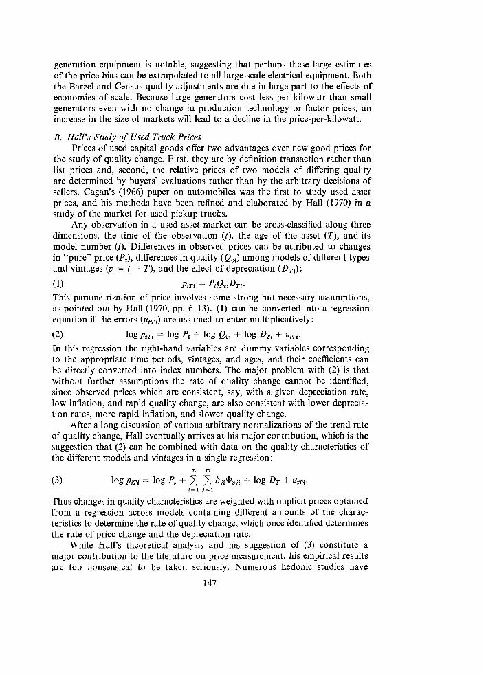
generation equipment is notable, suggesting that perhaps these large estimates of the price bias can be extrapolated to all large-scale electrical equipment. Both the Barzel and Census quality adjustments are due in large part to the effects of economies of scale. Because large generators cost less per kilowatt than small generators even with no change in production technology or factor prices, an increase in the size of markets will lead to a decline in the price-per-kilowatt.

B. Hall's Study of Used Truck Prices Prices of used capital goods offer two advantages over new good prices for

the study of quality change. First, they are by definition transaction rather than list prices and, second, the relative prices of two models of differing quality are determined by buyers' evaluations rather than by the arbitrary decisions of sellers. Cagan's (1966) paper on automobiles was the first to study used asset prices, and his methods have been refined and elaborated by Hall (1970) in a study of the market for used pickup trucks.

Any observation in a used asset market can be cross-classified along three dimensions, the tine of the observation (t), the age of the asset (T), and its model number ( i ) . Differences in observed prices can be attributed to changes in "pure" price (P,), differences in quality (QVJ among models of different types and vintages (v = t - T), and the effect of depreciation (DTi):

This parametrization of price involves some strong but necessary assumptions, as pointed out by Hall (1970, pp. 6-13). (1) can be converted into a regression equation if the errors (utTi) are assumed to enter multiplicatively:

In this regression the right-hand variables are dummy variables corresponding to the appropriate time periods, vintages, and ages, and their coefficients can be directly converted into index numbers. The major problem with (2) is that without further assumptions the rate of quality change cannot be identified, since observed prices which are consistent, say, with a given depreciation rate, low inflation, and rapid quality change, are also consistent with lower depreciation rates, more rapid inflation, and slower quality change.

After a long discussion of various arbitrary normalizations of the trend rate of quality change, Hall eventually arrives at his major contribution, which is the suggestion that (2) can be combined with data on the quality characteristics of the different models and vintages in a single regression:

Thus changes in quality characteristics are weighted with implicit priws obtained from a regression across models containing different amounts of the characteristics to determine the rate of quality change, which once identified determines the rate of price change and the depreciation rate.

While Hall's theoretical analysis and his suggestion of (3) constitute a major contribution to the literature on price measurement, his empirical results are too nonsensical to be taken seriously. Numerous hedonic studies have

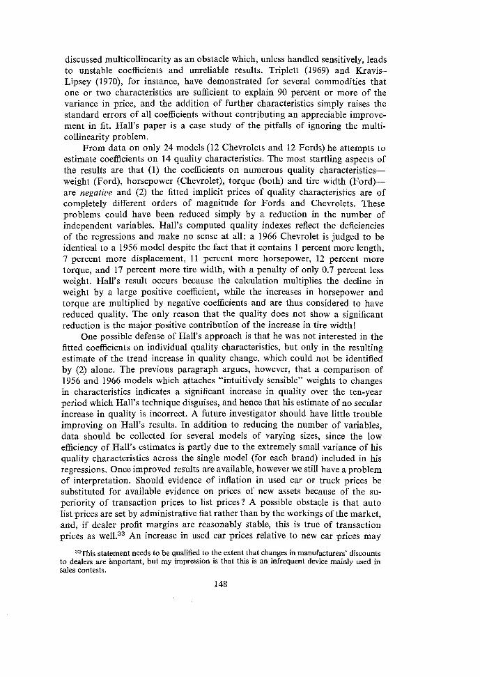
discussed multicollinearity as an obstacle which, unless handled sensitively, leads to unstable coefficients and unreliable results. Triplett (1969) and Kravis- Lipsey (1970), for instance, have demonstrated for several commodities that one or two characteristics are sufficient to explain 90 percent or more of the variance in price, and the addition of further characteristics simply raises the standard errors of all coefficients without contributing an appreciable improvement in fit. Hall's paper is a case study of the pitfalls of ignoring the multicollinearity problem.

From data on only 24 models (12 Chevrolets and 12 Fords) he attempts to estimate coefficients on 14 quality characteristics. The most startling aspects of the results are that (1) the coefficients on numerous quality characteristics- weight (Ford), horsepower (Chevrolet), torque (both) and tire width (Ford)- are negative and (2) the fitted implicit prices of quality characteristics are of completely different orders of magnitude for Fords and Chevrolets. These problems could have been reduced simply by a reduction in the number of independent variables. Hall's computed quality indexes reflect the deficiencies of the regressions and make no sense at all: a 1966 Chevrolet is judged to be identical to a 1956 model despite the fact that it contains 1 percent more length, 7 percent more displacement, 11 percent more horsepower, 12 percent more torque, and 17 percent more tire width, with a penalty of only 0.7 percent less weight. Hall's result occurs because the calculation multiplies the decline in weight by a large positive coefficient, while the increases in horsepower and torque are multiplied by negative coefficients and are thus considered to have reduced quality. The only reason that the quality does not show a significant reduction is the major positive contribution of the increase in tire width!

One possible defense of Hall's approach is that he was not interested in the fitted coefficients on individual quality characteristics, but only in the resulting estimate of the trend increase in quality change, which could not be identified by (2) alone. The previous paragraph argues, however, that a comparison of 1956 and 1966 models which attaches "intuitively sensible" weights to changes in characteristics indicates a significant increase in quality over the ten-year period which Hall's technique disguises, and hence that his estimate of no secular increase in quality is incorrect. A future investigator should have little trouble improving on Hall's results. In addition to reducing the number of variables, data should be collected for several models of varying sizes, since the low efficiency of Hall's estimates is partly due to the extremely small variance of his quality characteristics across the single model (for each brand) included in his regressions. Once improved results are available, however we still have a problem of interpretation. Should evidence of inflation in used car or truck prices be substituted for available evidence on prices of new assets because of the superiority of transaction prices to list prices? A possible obstacle is that auto list prices are set by administrative fiat rather than by the workings of the market, and, if dealer profit margins are reasonably stable, this is true of transaction prices as An increase in used car prices relative to new car prices may

33This statement needs to be qualified to the extent that changes in manufacturers' discounts to dealers are important, but my impression is that this is an infrequent device mainly used in sales contests.

148

not mean that '"rue" new car prices are increasing, but rather that demand is increasing and is met in the new market by an increase in production rather than an increase in price. (Aspects of the relation of used and new prices are discussed again below in relation to the housing market in Section V-E below.)

C. Another method: "Direct Comparison of Closely Similar Models" A topic of great importance is experimental research on previously un-

measured quality change. One approach is to take detailed specification sheets on models of, say, automobiles or tractors ten years apart and try to estimate the total value of previously unmeasured cost-increasing options. These adjustments should not be made in addition to hedonic-type adjustments for changes in major characteristics because of the danger of double-counting. Two models for, say, 1959 and 1970 can be chosen which are roughly equal in horsepower and length, thus eliminating the need for a hedonic regression to estimate the "value" of horsepower and length. The value of additional standard features in the 1970 model can then be estimated using option prices from earlier years and/or manufacturers' cost data.

The estimated value of options included in the 1970 model can be separated into two categories, options which the manufacturer includes as standard equipment of his own "free will", and options like seat belts which are included because of Federal regulations. (The latter can be treated as either quality or price change, depending on a value judgment regarding the benefits which consumers feel they receive from the improvements). If each option is costed individually, weight does not have to be treated as a separate quality variable, since the significance of weight in previous hedonic regressions over and above length and other size characteristics is probably due more to omitted weight-increasing characteristics, e.g., more insulation, than to any qualities inherent in weight itself. (Although weight does make a contribution to an automobile's riding characteristics, it worsens acceleration, performance, and gas mileage for an engine of given size).

Careful quality comparisons for models several years apart may yield improved estimates of the bias in official price indexes. An unsettled issue at present is the direction of bias in the official price indexes for automobiles in the 1960's. The two existing hedonic studies of automobiles for the early 1960's yield evidence of quality deterioration which is not reflected in the official indexes and conclude therefore that the apparent upward bias of the CPI in the 1950's was reversed and became a downward bias in the 1960's (Table 4, lines 1.d and 2.d). Both hedonic studies explain a major portion of automobile price variance by differences in weight, so that weight reductions in 1961-1962 cause a drop in computed quality. But if weight is not desired for itself and instead stands as a proxy for excluded variables, and if the quantity of excluded variables per unit of weight increased during this period, "true" quality may not have declined and the CPI may have been more accurate than the hedonic indexes.34

34Trip1ett (1969) mentions the invention of the "thin wall" casting process as one weight- saving technical improvement during this period, which might negate his conclusion of quality deterioration. Kravis-Lipsey (1970, pp. XV-9/12 present a list of options added to automobiles over their sample period which increased quality enough to explain the divergence between the official and hedonic indexes, although some of these were weight-increasing, so that their influence was already picked up at least partially by the hedonic method.

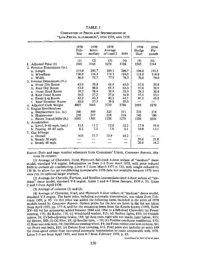
TABLE 5

COMPARISON OF PRICES AND SPECIFICATIONS OF

"LQw-PRICED AUTOMOBILES", 1954 1959, AND 1970

1. Adjusted Price ($) 2. Exterior Dimensions (in.)

a. Length b. Wheelbase c. Width

3. Interior Dimensions (in.) a. Front Hip Room b. Rear Hip Room c. Front Head Room d. Rear Head Room e. Front Leg Room f. Rear Shoulder Room

4. Adjusted Curb Weight 5. Engine Speciiications

a. Displacement (cu. in.) b. Horsepower c. Piston TravelIMile (ft.)

6. Acceleration a. Level, 0-60 mph. (sec.) b. Passing, 45-65 mph.

7. Gas Mileage a. Overall b. Steady 30 mph c. Steady 60 mph

I970 1970 1970 Full- Inter- Average Size mediate of 1 and 2 1959

1970 1954 Dodge Ply- Dart mouth

Source: Date and page number references from Consumers' Union, Consumer Reports, cita- tions by column : (1) Average of Chevrolet, Ford, Plymouth full-sized 4-d00r sedans of "medium" decor

model, standard V-8 engine. Information on lines 1-3 from April 1970, with price reduced $400 to exclude air conditioning. Lines 4-7 from March 1971 p. 155, with weight reduced by 150 lb. to allow for air conditioning (comparable 1970 data not available because 1970 tests were run on optional larger engines).

(2) Average for Chevelle, Fairlane, and Satellite intermediate-sized 4-door sedans of "medium" decor model, standard V-8 engine. Lines 1 and 4-7 from January, 1970 p. 53. Lines 2 and 3 from April 1970.

(3) Average of columns (1) and (2). (4) Average of Chevrolet, Ford, and Plymouth %door sedans of "medium" decor model,

standard V-8 engine. The basic price, including automatic transmission, was taken from Feb- ruary 1959, p. 85. To this price was added the following items included in the price of 1970 models tested by Consumer Reports. Option prices for the first six items in the list are taken from April 1959, pp. 177-8, and for the remaining items from the Kravis-Lipsey (1970, Table XV-10) list for accessories added between 1960 and 1964 to a full-sized Chevrolet: (a) Power steering, $75; (b) Radio, $75, (c) Windshield washer, $15; (d) Backup lights, $10; (e) Outside mirror, $6; (f) Self-adjusting brakes, $10; (g) Arm rests, right side sun shade, cigar lighter, $15; (h) Heater, $69; (i) Oil filter, $9; (j) Smaller tires, - $9; (k) Positive crankcase ventilation, $10; (1) Rear seat arm rests, $9; (m) Deluxe steering wheel, $4; (n) Foam rubber rear seat cushion, $4; (0) Front seat belts, $10; (p) Deluxe floor covering, $11. Ford price also includes an extra $40 for three-speed rather than two-speed automatic transmission to make comparable with 1970. Lines 2-3 are from April 1959, and lines 4-7 from February 1959, p. 85.

[continued at foot of next page

150

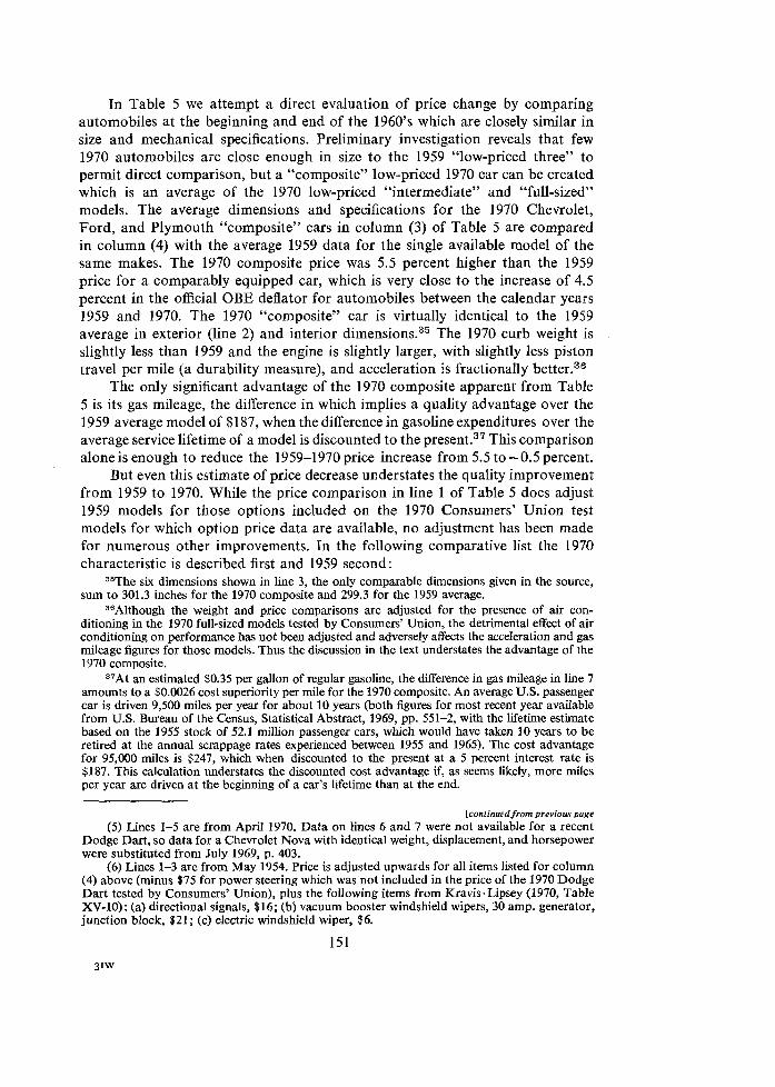
In Table 5 we attempt a direct evaluation of price change by comparing automobiles at the beginning and end of the 1960's which are closely similar in size and mechanical specifications. Preliminary investigation reveals that few 1970 automobiles are close enough in size to the 1959 "low-priced three" to permit direct comparison, but a "composite" low-priced 1970 car can be created which is an average of the 1970 low-priced "intermediate" and "full-sized" models. The average dimensions and specifications for the 1970 Chevrolet, Ford, and Plymouth "composite" cars in column (3) of Table 5 are compared in column (4) with the average 1959 data for the single available model of the same makes. The 1970 composite price was 5.5 percent higher than the 1959 price for a comparably equipped car, which is very close to the increase of 4.5 percent in the official OBE deflator for automobiles between the calendar years 1959 and 1970. The 1970 "composite" car is virtually identical to the 1959 average in exterior (line 2) and interior dimension^.^^ The 1970 curb weight is slightly less than 1959 and the engine is slightly larger, with slightly less piston travel per mile (a durability measure), and acceleration is fractionally better.36

The only significant advantage of the 1970 composite apparent from Table 5 is its gas mileage, the difference in which implies a quality advantage over the 1959 average model of $187, when the difference in gasoline expenditures over the average service lifetime of a model is discounted to the present.37 This comparison alone is enough to reduce the 1959-1970 price increase from 5.5 to - 0.5 percent.

But even this estimate of price decrease understates the quality improvement from 1959 to 1970. While the price comparison in line 1 of Table 5 does adjust 1959 models for those options included on the 1970 Consumers' Union test models for which option price data are available, no adjustment has been made for numerous other improvements. In the following comparative list the 1970 characteristic is described first and 1959 second:

35The six dimensions shown in line 3, the only comparable dimensions given in the source, sum to 301.3 inches for the 1970 composite and 299.3 for the 1959 average.

36Altho~gh the weight and price comparisons are adjusted for the presence of air conditioning in the 1970 full-sized models tested by Consumers' Union, the detrimental effect of air conditioning on performance has not been adjusted and adversely affects the acceleration and gas mileage figures for those models. Thus the discussion in the text understates the advantage of the 1970 composite.

37At an estimated $0.35 per gallon of regular gasoline, the difference in gas mileage in line 7 amounts to a $0.0026 cost superiority per mile for the 1970 composite. An average U.S. passenger car is driven 9,500 miles per year for about 10 years (both figures for most recent year available from U.S. Bureau of the Census, Statistical Abstract, 1969, pp. 551-2, with the lifetime estimate based on the 1955 stock of 52.1 million passenger cars, which would have taken 10 years to be retired at the annual scrappage rates experienced between 1955 and 1965). The cost advantage for 95,000 miles is $247, which when discounted to the present at a 5 percent interest rate is $187. This calculation understates the discounted cost advantage if, as seems likely, more miles per year are driven at the beginning of a car's hfetime than at the end.

[continued from previous page

(5) Lines 1-5 are from April 1970. Data on lines 6 and 7 were not available for a recent Dodge Dart, so data for a Chevrolet Nova with identical weight, displacement, and horsepower were substituted from July 1969, p. 403.

(6) Lines 1-3 are from May 1954. Price is adjusted upwards for all items listed for column (4) above (minus $75 for power steering which was not included in the price of the 1970 Dodge Dart tested by Consumers' Union), plus the following items from Kravis-Lipsey (1970, Table XV-10): (a) directional signals, $16; (b) vacuum booster windshield wipers, 30 amp. generator, junction block, $21 ; (c) electric windshield wiper, $6.

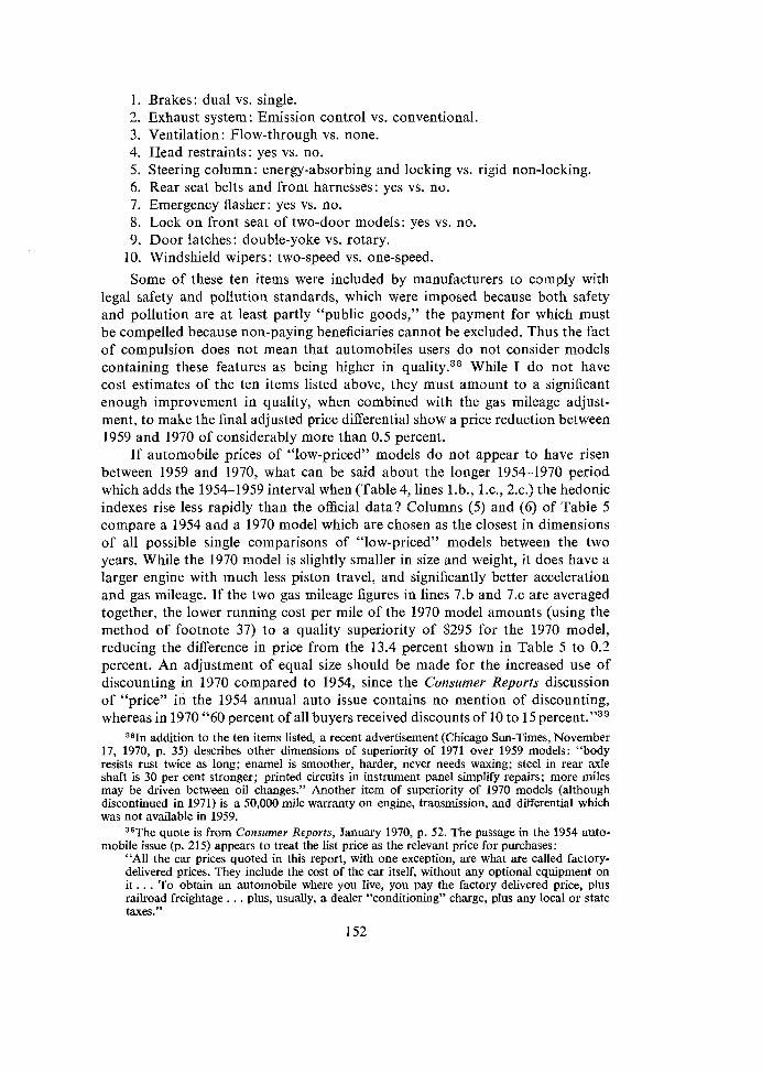
1. Brakes: dual vs. single. 2. Exhaust system: Emission control vs. conventional. 3. Ventilation: Flow-through vs. none. 4. Head restraints: yes vs. no. 5. Steering column: energy-absorbing and locking vs. rigid non-locking. 6. Rear seat belts and front harnesses: yes vs. no. 7. Emergency flasher: yes vs. no. 8. Lock on front seat of two-door models: yes vs. no. 9. Door latches: double-yoke vs. rotary.

10. Windshield wipers : two-speed vs. one-speed.

Some of these ten items were included by manufacturers to comply with legal safety and pollution standards, which were imposed because both safety and pollution are at least partly "public goods," the payment for which must be compelled because non-paying beneficiaries cannot be excluded. Thus the fact of compulsion does not mean that automobiles users do not consider models containing these features as being higher in quality.38 While I do not have cost estimates of the ten items listed above, they must amount to a significant enough improvement in quality, when combined with the gas mileage adjustment, to make the final adjusted price differential show a price reduction between 1959 and 1970 of considerably more than 0.5 percent.

If automobile prices of "low-priced" models do not appear to have risen between 1959 and 1970, what can be said about the longer 1954-1970 period which adds the 1954-1959 interval when (Table 4, lines l.b., I.c., 2.c.) the hedonic indexes rise less rapidly than the official data? Columns (5) and (6) of Table 5 compare a 1954 and a 1970 model which are chosen as the closest in dimensions of all possible single comparisons of "low-priced" models between the two years. While the 1970 model is slightly smaller in size and weight, it does have a larger engine with much less piston travel, and significantly better acceleration and gas mileage. If the two gas mileage figures in lines 7.b and 7.c are averaged together, the lower running cost per mile of the 1970 model amounts (using the method of footnote 37) to a quality superiority of $295 for the 1970 model, reducing the difference in price from the 13.4 percent shown in Table 5 to 0.2 percent. An adjustment of equal size should be made for the increased use of discounting in 1970 compared to 1954, since the Consumer Reports discussion of "price" in the 1954 annual auto issue contains no mention of discounting, whereas in 1970 "60 percent of all buyers received discounts of 10 to 15 per~ent."~'

381n addition to the ten items listed, a recent advertisement (Chicago Sun-Times, November 17, 1970, p. 35) describes other dimensions of superiority of 1971 over 1959 models: "body resists rust twice as long; enamel is smoother, harder, never needs waxing; steel in rear axle shaft is 30 per cent stronger; printed circuits in instrument panel simplify repairs; more miles may be driven between oil changes." Another item of superiority of 1970 models (although discontinued in 1971) is a 50,000 mile warranty on engine, transmission, and differential which was not available in 1959.

39The quote is from Consumer Reports, January 1970, p. 52. The passage in the 1954 automobile issue (p. 215) appears to treat the list price as the relevant price for purchases:

"All the car prices quoted in this report, with one exception, are what are called factory- delivered prices. They include the cost of the car itself, without any optional equipment on i t . . . To obtain an automobile where you live, you pay the factory delivered price, plus railroad freightage. . . plus, usually, a dealer "conditioning" charge, plus any local or state taxes."

A discount at the bottom of this range would reduce the 1970 price in column (5) to $2291, which is 9.8 percent less than the 1954 price after adjustment for the difference in gas mileage. To this difference a further reduction in the 1970 relative price should be made for the ten items listed above which differ between 1959 and 1970 cars, plus a further adjustment to allow for the inferior two-speed automatic transmission available on the 1954 Plymouth which had, according to Consumer Reports, "poor" downhill braking. It is conceivable that the 1970 price after full adjustment may have been 15 percent or more below the 1954 price, as compared to an increase of 27 percent in the OBE index, and the only unlisted characteristic of the 1954 model which may have been superior (in addition to the size and weight dimensions of Table 5) is a greater freedom from assembly defects.40

In short, the method of "direct comparison of closely similar models" reveals a serious upward bias in the official price indexes in the 1950's and in the hedonic price indexes in the 1960's. The results are sufficiently interesting to indicate that similar comparisons for other types of durable goods might provide a useful test of the accuracy of the official and/or hedonic price indexes. To facilitate such comparisons, a substantial improvement in the measurement of quality change in producers' durable equipment could be achieved by the estab- lishment of a "Producers' Union" which, along the lines of the existing Con- sumers' Union, could test and evaluate the comparative performance of new and old models of producers' durable equipment.

A pioneering engineering comparison of new and old models, which has not to my knowledge been performed since, was published by Davidson, McCuen and Blasingame (1932). They made meticulous comparisons of 1910-1914 and 1932 models of 25 types of agricultural machinery and found rates of quality improvement ranging from 30 to 115 percent, with an average of 70 percent. The criterion of comparison was relative marginal products, precisely the standard of comparison needed for measuring the capital services provided by a given machine; "the object of the inquiry has been to appraise or evaluate the changes in design, material, or construction in farm machines made during the period 1910-1914 to 1932, which in any way affect the value of the machines to the user in accomplishing the purpose or work for which they were designed" (1932, p. 5). Considerable emphasis was given to design improvements which reduced the tendency of machines to break down and which thus improved the capital services obtainable in a given span of time. Many other changes involved a combination of cost-reducing design improvements and the "costly" use of heavier, larger, or more expensive materials and parts.

D. Summary: Revised Deflators for Producers' DurabEes

This paper has compiled two varieties of adjustments to the official equipment deflators, the unit value indexes of part I1 and the quality-adjusted indexes summarized in Table 4. Unfortunately our adjustments are incomplete, since for most types of producers' durable equipment (PDE) we have either a unit

40The problem of assembly defects, featured prominently in Conszrmer Reports in the late 19603, was not mentioned in either the 1954 or 1959 volumes.

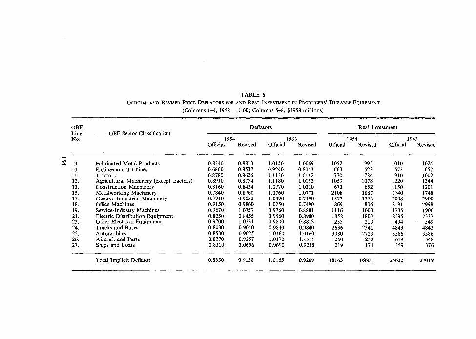
TABLE 6 OFFICIAL AND REVISED PRICE DEFLATORS FOR AND REAL INVESTMENT IN PRODUCERS' DURABLE EQUIPMENT

(Columns 1-4, 1958 = 1.00; Columns 5-8, 961958 millions)

OBE Deflators Real Investment Line OBE Sector Classification - No. 1954 1963 1954 1963

Official Revised Official Revised Official Revised Official Revised

Fabricated Metal Products Engines and Turbines Tractors Agricultural Machinery (except tractors) Construction Machinery Metalworking Machinery General Industrial Machinery Office Machines Service-Industry Machines Electric Distribution Equipment Other Electrical Equipment Trucks and Buses Automobiles Aircraft and Parts Ships and Boats

Total Implicit Deflator 0.8350 0.9138 1.0165 0.9269 18163 16601 24632

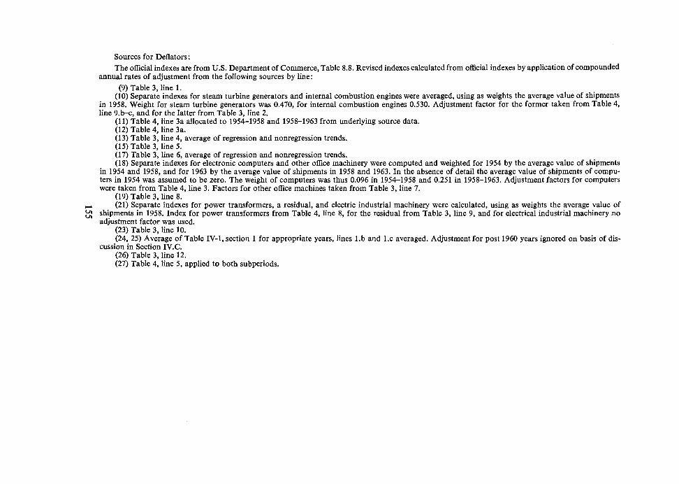
Sources for Deflators : The official indexes are from U.S. Department of Commerce, Table 8.8. Revised indexes calculated from official indexes by application of compounded

annual rates of adjustment from the foIIowing sources by line: (9) Table 3, line 1.

(10) Separate indexes for steam turbine generators and internal combustion engines were averaged, using as weights the average value of shipments in 1958. Weight for steam turbine generators was 0.470, for internal combustion engines 0.530. Adjustment factor for the former taken from Table 4, Iine 9.b-c, and for the latter from Table 3, line 2.

(11) Table 4, line 3a allocated to 1954-1958 and 1958-1963 from underlying source data. (12) Table 4, line 3a. (13) Table 3, line 4, average of regression and nonregression trends. (15) Table 3, line 5. (17) Table 3, line 6, average of regression and nonregression trends. (18) Separate indexes for electronic computers and other office machinery were computed and weighted for 1954 by the average value of shipments

in 1954 and 1958, and for 1963 by the average value of shipments in 1958 and 1963. In the absence of detail the average value of shipments of computers in 1954 was assumed to be zero. The weight of computers was thus 0.096 in 1954-1958 and 0.251 in 1958-1963. Adjustment factors for computers were taken from Table 4, line 3. Factors for other office machines taken from Table 3, Iine 7.

(19) Table 3, line 8. (21) Separate indexes for power transformers, a residual, and electric industrial machinery were calculated, using as weights the average value of

2 shipments in 1958. Index for power transformers from Table 4, line 8, for the residual from Table 3, line 9, and for electrical industrial machinery no adjustment factor was used.

(23) Table 3, line 10. (24, 25) Average of Table IV-1, section 1 for appropriate years, lines 1.b and 1.c averaged. Adjustment for post 1960 years ignored on basis of dis-

cussion in Section 1V.C. (26) Table 3, line 12. (27) Table 4, line 5, applied to both subperiods.

value adjustment, to reflect deviations of transaction and list prices, or a quality- corrected index, but not both (except for one or two cases like power transformers). Thus the adjustments summarized in this section are probably conservative, and further research may yield higher estimates of bias in the official indexes.

One example of "further research", our experimental calculation for automobiles in section IV-C, does yield a higher estimate of bias than the hedonic studies in Table 4. This is particularly true for the period of the 1960's, when the hedonic index rises relative to the official price index (Table 4, lines 1.d and 2.d) while our experimental calculation indicates a decline in price relative to the official index. We use the experiment of section IV-C to justify selecting the official index as closer to the true price in the 1960's than the hedonic index, which is therefore disregarded for the 1960's in the calculation of our final revised index in Table 6 below. We do not make the full adjustment suggested by the experiment, in order to maintain a conservative approach. If the experiment is correct, our final index overestimates the rate of inflation of auto prices and, therefore, of all prices of PDE in the 1960's. Similar experiments to quantify previously unmeasured quality change in other producers' durables are needed before an estimate of the "complete" bias can be made.

Our suggested revision of the official PDE deflator corrects for part of the apparent secular bias in the WPI-based official index but not explicitly for its apparent cyclical bias. The information used in our cyclical analysis is based on a small sample of products, and for some of these products covers a shorter time period than our information on the secular bias.*l Although our unit value data do not allow us to calculate cyclically adjusted deflators for most product classes, they do suggest that the 1954-1963 period was chacterized by a cyclical decline in transaction prices relative to list prices. Thus the portion of our revision of the official OBE PDE index to eliminate "secular bias" which is based on Part I1 above really amounts to a combined secular-cyclical revision, since the downward trend exhibited by the unit values relative to the WPI data between 1954 and 1963 occurred during a cyclical contraction (by our "alternative definition"). One would expect revisions for the 1963-1967 period, which will be attempted when data become available, to reveal a smaller upward bias in the OBE series or even a downward bias.

The revised magnitudes for the deflators and real investment by sector are shown in Table 6. New indexes have been substituted for 15 of the 23 OBE equipment categories, covering 73.7 percent of the value of equipment spending in 1954 and 72.0 percent in 1963. The major omitted categories are special industry machines, furniture, communications equipment, and instruments. The adjustments are a mixture of unit value trends from Table 3 and quality-corrected indexes from Table 4.42

41The reader will recall that a number of the "nonregression" series used in Table 3 are based only on census years. Several other series are available annually only for recent years, say since 1957 or 1958, and are available earlier only for 1947 and 1954.

42When in Table 3 both regression and nonregression trends are shown, a simple average of the two is used in the calculation of the substitute indexes. In several cases where the OBE category encompasses several of our commodity classes, we use a weighted average of the relevant prices, as spelled out in the source notes to Table 3.

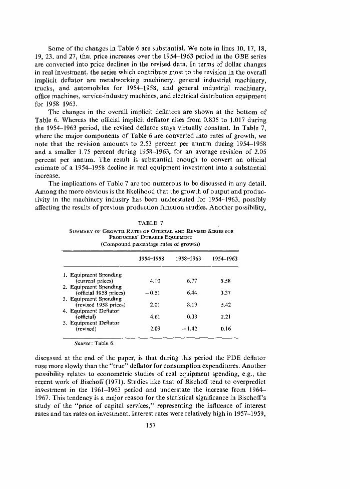
Some of the changes in Table 6 are substantial. We note in lines 10, 17, 18, 19, 23, and 27, that price increases over the 1954-1963 period in the OBE series are converted into price declines in the revised data. In terms of dollar changes in real investment, the series which contribute most to the revision in the overall implicit deflator are metalworking machinery, general industrial machinery, trucks, and automobiles for 1954-1958, and general industrial machinery, office machines, service-industry machines, and electrical distribution equipment for 1958-1963.

The changes in the overall implicit deflators are shown at the bottom of Table 6. Whereas the official implicit deflator rises from 0.835 to 1.017 during the 1954-1963 period, the revised deflator stays virtually constant. In Table 7, where the major components of Table 6 are converted into rates of growth, we note that the revision amounts to 2.53 percent per annum during 1954-1958 and a smaller 1.75 percent during 1958-1963, for an average revision of 2.05 percent per annum. The result is substantial enough to convert an official estimate of a 1954-1958 decline in real equipment investment into a substantial increase.

The implications of Table 7 are too numerous to be discussed in any detail. Among the more obvious is the likelihood that the growth of output and productivity in the machinery industry has been understated for 1954-1963, possibly affecting the results of previous production function studies. Another possibility,

TABLE 7 SUMMARY OF GROWTH RATES OF OFFICIAL AND REVISED SERIES FOR

PRODUCERS' DURABLE EQUIPMENT (Compound percentage rates of growth)

1. Equipment Spending (current prices) 4.10 6.77 5.58

2. Equipment Spending (official 1958 prices) -0.51 6.44 3.37

3. Equipment Spending (revised 1958 prices) 2.01 8.19 5.42

4. Equipment Deflator (official) 4.61 0.33 2.21

5. Equipment Deflator (revised) 2.09 - 1.42 0.16

Source: Table 6.

discussed at the end of the paper, is that during this period the PDE deflator rose more slowly than the "true" deflator for consumption expenditures. Another possibility relates to econometric studies of real equipment spending, e.g., the recent work of Bischoff (1971). Studies like that of Bischoff tend to overpredict investment in the 1961-1963 period and understate the increase from 1964- 1967. This tendency is a major reason for the statistical significance in Bischoff's study of the "price of capital services," representing the influence of interest rates and tax rates on investment. Interest rates were relatively high in 1957-1959,

157

helping to explain (with long lags) the sluggish investment performance of 1961- 1963, and the introduction of the investment tax credit helps explain the 1964- 1967 investment boom. But our analysis suggests that real equipment investment in 1958-1963 may have been underestimated, and, if our crude confirmation of the "cyclical hypothesis" is valid, the increase in real investment in the 1964-1967 period may have been overestimated in the national accounts. Thus Bischoff's estimates of the elasticity of real investment to changes in the price of capital services may be too high.

A. Special Features of Structures Dejlation The differences between various construction price deflators are clarified

with the aid of a conceptual framework, suggested by Kaplan, which distinguishes between construction projects, components, and inputs.43 The terms "projects" and "inputs" are given their conventional meanings-the final products of construction and the factors of production used to produce them. "Components" are completed intermediate products which are assembled into projects-e.g., six square feet of floor in place or 17.5 bricks laid. Components can be given either broad definitions (a whole wall in place) or narrow ones (one pane of glass inserted into a window in a wall) depending on the task at hand. A component can be completely analyzed in terms of its inputs, and productivity improvement continually changes the input requirements for the production of given components. Similarly, projects can be analyzed in terms of their components, and the quantities of components prescribed for a project are its specifications.

In the following notation, o denotes the base year and t the current period. As many as three dates are enclosed in parentheses-the first stands for the date of the specifications, the second for the year to which input requirements refer, and the final one for the date of measurement of factor prices. The subscripts refer to individual components, inputs, or projects. Thus pk(o, o, t) is the price using input prices in the current year of project k which has base-year specifications and input requirements. The following summarizes the notation:

xij(t) is the requirement of input i in component j at time t. ajk(t) is the amount of component j in project k at time t. qi(t) is the price of input i at time t. b,(t, t) is the price of component j produced at time t with the input require-

ments of period t. p,(t, t, t) is the price of project k at time t with the input requirements and

specifications of period t. Pk(t) with appropriate superscripts is an index number showing the relation

of current and base-year project prices.

431n what follows the conceptual distinction between projects, components, and inputs is Kaplan's (1959). His inpenetrable notation, however, has been completely changed, and the application to actual U.S. indexes is new.

The basic assumption that projects can be analyzed in terms of their components, and components in terms of inputs, can be expressed as follows, using base-period prices, input requirements, and specifications:

An ideal construction price index would compare the price charged by a current- year contractor with the price which would have been charged for a project with the same specifications by a base-year contractor using base-year technology. The price relatives Pc(t) in this ideal world would be similar to the indexes for individual types of equipment in the WPI:

where the projects compared are required to have the same specifications cDjk(o) during each time period. Input requirements, however, can change between the two periods. Even though wage rates and materials prices are much higher in 1971 than in a base year like 1929, a 1971 contractor might still manage to bid less on a given project if his input requirements xij(t) had declined sufficiently.

In the past the ideal price relative (3) has been impossible to calculate because the output of construction is so heterogeneous. Almost every structure is different, and 1971 contractors do not construct 1929-style buildings. The Federal government could have performed a great service if it had regularly submitted detailed plans to contractors so that the annual succession of their bids on a given project could be made into an index. New types of structures would have to be introduced frequently to keep pace with changing specifications, and the price indexes linked to those computed for older types of buildings.

While no comprehensive program of bid submission has been carried out over a long historical period, two less comprehensive indexes are available which in principle approximate the ideal deflator (3). First, since 1953 the Federal Housing Administration (FHA) has compiled bids for U.S. single-family FHA- insured houses. Second, for the years since 1963 the Bureau of the Census, Construction Statistics Division (CSD) has attempted to approximate the ideal index with the hedonic regression technique. Most of the discussion of structures deflation in this paper concentrates on single-family houses because the data are better, despite our basic interest in the topic of deflators for nonresidential

structures and equipment. Possible alternatives for the deflation of nonresidential structures are reviewed briefly at the end of part V.44

B. The FHAIOBE Index for Single-Family Houses The FHA/OBE index approaches the "ideal index" (3) because bids are

collected over a period of time for houses with exactly the same specifications Bik(o). Because the index has not been described in any publication, and its existence is known only to a few government officials, it is described here in considerable detail. It was constructed by the U.S. Office of Business Economics (OBE) as an experiment to compare it with other measures of the price of resi- dences. OBE feels that the index may have serious shortcomings and is continuing work on it without having come to a conclusion whether or in what form to use it in its

1. What the FHA Collects. The FHA data originate in the need for the FHA to know what a given house should cost, so that a contractor cannot obtain an FHA loan based on an inflated price. Data are collected in each of about 70 regions, some of which are large metropolitan areas and some of which are individual medium-sized towns. For each area a "book" is made up every four to eight years which describes in detail the specifications of various types of houses which are typical to the region. When a new book is introduced in, say, May 1966, price bids are obtained from contractors on every separate component of the house, e.g., the price pk(o, o, o) is collected for a "basic house" of 1100 square feet, 1 bathroom, and no fireplace, and bids are also collected for the prices b,(o, o) of various "add-on" components, like an extra bathroom, a fireplace, more square feet, high quality materials, etc.

What should a house cost at some date after the base period, say in May1968 ? Every six months contractors are again asked for bids, but only for a very "typical" house and not for all the separate add-on components. The ratio of the May 1968 bid to the "book" May 1966 bid of this particular typical house becomes a "Locality Adjustment Percentage" (LAP), or in more familiar language "Price index, May 1966 = 100" which is multiplied by the appraisers' book-based estimates whenever specifications are presented to the FHA. Thus the prices of all "add-ons", including extra square feet, are assumed to increase at the same rate as the LAP.

Inspection of bid sheets for one city revealed that in this particular case three to four contractors were contacted to submit bids for each of about twenty components of the typical house, and this process was repeated every six months. Only about ten contractors were contacted in all, since most contractors submitted bids on several different components. When the bid prices differed among

44Another interesting index is the rent portion of the Consumer Price Index (CPI). This cannot be used as a proxy for prices of new buildings, since rent is paid not only for the occupancy of a structure but also for taxes, maintenance, interest cost, and profit. Further, the CPI rent index is biased downward because it is a Laspeyres hed-weight index of continually aging buildings which gradually diminish in quality. For an initial attempt to estimate regressions to explain rent differences, see Gillingham and Lund (1970).

450BE's present view regarding the index was communicated to me on September 28, 1970 by George Jaszi, OBE director, to whom I am extremely grateful for allowing me to describe and cite the index.

contractors the lowest bid was not generally chosen; casual inspection indicated that the bid used was closer to a median bid.46

2. How the OBE Compiles the FHA "LAPs". LAPs were available between books for each of the 70 cities and successive LAPs were linked together whenever a new book was introduced. Information is not available to determine whether two prices were available on the date of the new book for use in linking, or whether the change in prices which occurs in the six months before the introduction of the new book is "lost". This is not a serious problem because new books are introduced at intervals of six to eight years. The individual area indexes are aggregated using population and housing units as weights. Since in principle the area indexes should be weighted by the value of construction, the method of aggregation across states gives too much weight to areas with relatively low-priced construction, which would cause a downward bias in the FHA-OBE index if construction prices in low-price regions rise more slowly than in the rest of the country.

The end result of the FHA/OBE computations is extremely interesting. The annual rate of increase in the FHAIOBE index is only 1.6 percent per year between 1947 and 1968, compared to a 3.2 percent rate of increase for the Boeckh index which is presently used in the U.S. national accounts to deflate residential structures. The discrepancy occurs consistently during the early, middle, and recent portions of the postwar period. The respective annual rates of growth in the 1947-53, 1953-63, and 1963-68 periods are 2.6, 0.3, and 2.7 for FHAjOBE and 4.0, 2.1, and 4.8 for Boeckh (Table 8 below). The discrepancy is not particularly surprising, since the Boeckh index is calculated by a naive technique which combines wage rates and materials prices with no adjustments for secular changes in productivity. The difference between FHAIOBE and Boeckh is of roughly the same size as the difference between the rates of growth of the official "Commerce Composite" index and a new index which I recently proposed (Gordon, 1968). Further, the stability of the FHA/OBE index between 1953 and 1963 is not surprising, as both the Bureau of Public Roads and Bureau of Reclamation indexes (discussed below) exhibit the same stability over the period.47 In this connection it is interesting to refer to the demonstration in Table 7 above that the implicit price deflator for producers' durable equipment, instead of rising at an annual rate of 2.3 percent between 1954 and 1963 as shown in the official data, in fact does not appear to have risen at all.

3. Criticisms of the FHAIOBE Approach. A defect which may be serious is the limitation to houses insured by the FHA. The FHA cannot insure houses with a value over a given ceiling (currently $30,000), and therefore the average value of FHA houses tends to be considerably below the national average ($18,700 in 1967 compared with the national average of $24,600 [U.S.F.H.A.,

46All information on FHA procedures was obtained July 2, 1969, in an interview with Eldon R. Matthews, head of the construction cost division of the FHA. Except for records of bids of individual contractors, all FHA information is in the public domain. What has previously been administratively restricted is the index compiled by OBE from the FHA files.

47The "Component-Price Hybrid" from Gordon (1968), which is an average of various subcomponents of the Bureau of Public Roads and Bureau of Reclamation indexes, has the following values in the early 1950's and 1960's: 0.918 (1951), 0.938 (1952), 0.924 (1953); 0.920 (1962), 0.962 (1963), 0.958 (1964), 1.000 (1965).

19671). To the extent that smaller houses are built by large contractors who are quicker to adopt labor-saving innovations, the prices of small houses may increase more slowly than larger houses and the trend rate of increase of the FHA/OBE index may be biased downward. Convincing evidence against this conjecture is a worksheet from the CSD hedonic regression study of house prices (discussed below), which shows that between 1963 and 1968 houses in all size categories increased in price by approximately the same amount except for two size categories which increased by more than average, one small (below 1,000 square feet) and one large (2,200-2,399 square feet). There is no firm evidence, then, that the limitation to FHA-insured houses imparts any particular bias to the FHA/OBE index.

The use of bid prices rather than actual transaction prices might lead to problems, but fortunately there is an automatic safety valve in the FHA procedure. If the FHA indexes began to drift downwards compared to actual prices, this would reduce the amount the FHA would be willing to lend on houses relative to their actual cost, and contractors would begin to complain to FHA field offices. The opposite bias could not continue for long because FHA field offices check final transaction prices to make sure that the FHA-insured loan is not an excessive fraction of the actual sales price.48

While the bid-price approach is not likely to lead to a serious secular bias in the FHAIOBE index, short-run cyclical errors may occur. If competitive conditions improve in a given area between the time of a contractor's bid and the time of an actual sale, the sale price may be higher than the bid price. And this upward movement in prices may not necessarily be reflected in an upward revision in bids during the next bid-collection period, if contractors believe the improvement in business conditions to be temporary. Thus a risk-averting bias in the behavior of contractors may lead them to understate cyclical fluctuations in true market prices. So the constancy of the FHA/OBE index between 1953 and 1963, and the steady rate of increase before 1953 and after 1963, may not reflect price inflexibility but rather that some cyclical fluctuations in actual sales prices are disguised. This analysis, however, does not suggest any obvious reason to believe that the secular trend of the FHAIOBE index is inaccurate.

C. The Census Regression-based Index For the years since 1963 the Census has computed an index based on the

hedonic regression technique. In terms of the ideal index of equation (3), the Census method is first to run cross-section regressions each year on a large sample of houses to determine the prices b,(t, t) of major components and then to calculate P,*(t) by applying the estimated bj(t, t ) to base-year (currently 1964-1965) specifications @,,(o). An alternative technique would be to divide the unit value of all houses by a quality index calculated by multiplying current-year specifications @,,(t) by prices estimated in a single regression in a base year bi(o, 0).

The calculations are described by Musgrave (1968) and explain house prices by eight quality characteristics: floor area, number of stories, number of bathrooms, presence or absence of central air conditioning, garage, and basement, and

48This argument was suggested by E. Matthews in the interview cited above.

162

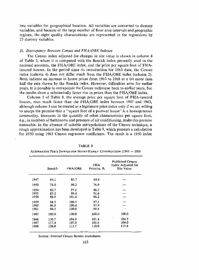
two variables for geographical location. All variables are converted to dummy variables, and because of the large number of floor area intervals and geographic regions, the eight quality characteristics are represented in the regressions by 27 dummy variables.

D. Discrepancy Between Census and FHAIOBE Indexes The Census index adjusted for changes in site value is shown in column 4

of Table 3, where it is compared with the Boeckh index presently used in the national accounts, the FHA/OBE index, and the price per square foot of FHA- insured houses. In the period since its introduction for 1963 data, the Census index (column 4) does not differ much from the FHA/OBE index (column 2). Both indicate an increase in house prices from 1963 to 1968 at a bit more than half the rate shown by the Boeckh index. However, difficulties arise for earlier years. It is possible to extrapolate the Census technique back to earlier years, but the results show a substantially faster rise in prices than the FHAIOBE index.

Column 3 of Table 8, the average price per square foot of FHA-insured houses, rises much faster than the FHA/OBE index between 1947 and 1963, although column 3 can be treated as a legitimate price index only if we are willing to accept the premise that a "square foot of a postwar house" is a homogeneous commodity. Increases in the quantity of other characteristics per square foot, e.g., in numbers of bathrooms and presence of air conditioning, make this premise untenable. In the absence of suitable extrapolations of the Census technique, a rough approximation has been developed in Table 9, which presents a calculation for 1950 using 1963 Census regression coefficients. The result is a 1950 index

TABLE 8

ALTERNATIVE PRICE INDEXES FOR SINGLE-FAMILY CONSTRUCTION (1963 = 100)

Published Census FHA Index Adjusted for

Boeckh FHA/OBE Pricelsq. ft. Site Value

Source: Internal Census Bureau worksheets.

163

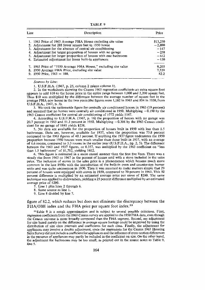
TABLE 9

Line Description Price

1. 1963 Price of 1963 Average FHA House excluding site value 2. Adjustment for 288 fewer square feet in 1950 house 3. Adjustment for the absence of central air conditioning 4. Adjustment for larger proportion of houses with no garage 5. Adjustment for larger proportion of houses with one bathroom 6. Estimated adjustment for fewer built-in appliances

7. 1963 Price of "1950 Average FHA House," excluding site value 8. 1950 Average FHA Price, excluding site value 9. 1950 Price, 1963 = 100.

Sources by Line: 1. U.S.F.H.A. (1967, p. 25, column 2 minus column 1). 2. In the worksheets showing the Census 1963 regression coefficients an extra square foot

appears to add $10 to the house price in the entire range between 1,000 and 2,200 square feet. Thus $10 was multiplied by the difference between the average number of square feet in the average FHA new house in the two years (the figures were 1,182 in 1963 and 894 in 1950, from u.s.F.H.A., 1967, p. 3).

3. We rook the nationwide figure for centrally air conditioned homes in 1963 (19 vercent) and assumed that no homes were centrally air conditioned in 1950. Multiplying -0.1% by thk 1963 Census coefficient for central air conditioning of $772 yields $147.

4. According to U.S.F.H.A. (1967, p. 16) the proportion of houses with no garage was 20.7 percent in 1963 and 51.3 percent in 1950. Multiplying -0.306 by the 1963 Census coefficient for no garage of $841 yields $258.

5. No data are available for the proportion of houses built in 1950 with less than 1.5 bathrooms. Data are, however, available for 1937, when the proportion was 75.8 percent compared to the 1963 figures of 40.1 percent. If anything the 1937 figure understates the 1950 proportion because 1950 houses were much smaller than those built in 1937, with an average of 4.6 rooms, compared to 5.5 rooms in the earlier year (U.S.F.H.A., pp. 2, 5). The difference between the 1963 and 1937 figures, or 0.357, was multiplied by the 1963 coefficient on "less than 1.5 bathrooms" of $1,712, yielding $612.

6. This figure is estimated in a more casual manner than the first five lines. There was a steady rise from 1963 to 1967 in the percent of homes sold with a stove included in the sales price. The inclusion of stoves in the sales price is a phenomenon which became much more common in the late 1950s with the introduction of the built-in oven and counter-top burner units and was quite uncommon in 1950. Thus it was assumed to make matters simple that 29 percent of houses were equipped with stoves in 1950, compared to 70 percent in 1963. This 50 percent difference is multiplied by an estimated average price per stove of $200. The same technique was applied to dishwashers, yielding a 25 percent difference multiplied by an estimated average price of $200.

7. Line 1 plus lines 2 through 6. 8. Same source as line 1. 9. Line 8 divided by line 7.

figure of 82.2, which reduces but does not eliminate the discrepancy between the FHAIOBE index and the FHA price per square foot index.49

49Table 9 is a rough approximation and is subject to several possible criticisms. First, regression coefficients from the 1963 Census survey are applied to the 1950 FHA data, even though the Census universe is more broadly composed than the FHA segment. Second, my adjustment for size based merely on the difference in average square footage could be improved by using the distribution of size class intervals and coefficients for each class. Finally, the adjustment for appliances may involve a double adjustment, since the regressions for the Census 1963 Housing Sales Survey did not include a coefficient for appliances and the influence of cross-section differences in the presence of appliances may partly be included in the coefficient on size. On the other hand, the adjustment for bathrooms may be too small, as pointed out in the source notes to Table 9, line 5.

Are there any obvious biases in either method which might further reduce the discrepancy? The possibility of a downward bias (probably slight) in the rate of growth of the FHA/OBE index was discussed above in Section V.B.3. Much more important is the likelihood of an upward bias in the Census hedonic index due to the "excluded variable" problem described above in section III.D.2. The regression makes an estimate of what a hypothetical house containing "typical" 1950 specifications of, say, 900 square feet, one bathroom, no garage, and no central air conditioning would cost ifbuilt in 1963. In comparing this calculated price with the actual price of a typical 1950 house we make the implicit assumption that the hypothetical 1963 house is identical to the 1950 house in all other respects. Any characteristic of the hypothetical 1963 house which is "better" than that of a similarly sized 1950 house and is not included in the regression will bias upward the hypothetical 1963 price.

Published data present only a limited amount of information on quality change along dimensions not included in the regressions. In new FHA houses, for instance, the ratio of one-car to two-car-and-larger garages fell from 84/16 in 1950 to 58/50 in 1963 and had fallen to 39/61 by 1966. Similarly, the proportion of houses with inexpensive wood siding declined between 1947 and 1963 from 42.2 to 10.6 percent and the proportion with relatively expensive brick or combination siding increased from 15.2 to 46.0 percent (all figures from U.S.F.H.A., 1967, p. 17). Casual observation suggests that new houses are superior to early postwar houses of a similar size in the inclusion of numerous "extras" such as larger and more built-in appliances, larger furnaces and hot water heaters, more electric plugs and light fixtures, fireplaces, bathroom vanities, more and sturdier built-in kitchen cabinets, and pre-installed wall-to-wall carpeting.50

In conclusion, the Census regression technique is inherently unable to correct for all quality improvements, nor is the "conventional" method of Part I11 available to correct for added features with option price or manufacturers' cost data because there are no nation-wide data on the percentage of new houses equipped with each item. The FHA/OBE index is the only method free of this bias because the underlying FHA data are explicit prices for houses with specifications which actually remain unchanged over a series of years.

E. Surveys of the Value of the Housing Stock In a recent unpublished paper Bhatia (1969) has proposed a new index for

one-family new and used houses which increases at a 4.2 percent average annual rate between 1950 and 1964, a much faster pace than the 2.2 percent rate of the Boeckh input-cost index or the 0.8 percent rate of the FHA/OBE index. The

50Some of these differences were pointed out by a close relative of the author in a comparison of new three-bedroom houses in Houston with houses of the same size built in 1950-52. Further evidence can be collected from the Sunday real estate section of local newspapers. Recent Chicago newspapers, for instance, carried advertisements for three bedroom homes which in one case included in the price "Zcar attached garage, finished family room, built-in oven-range, dishwasher, disposal, sculptured kitchen cabinets, color co-ordinated kitchen, full vanities, luxurious wall-to-wall carpeting." Another builder advertised the following features as included in the price: "central air-conditioning, deluxe patio, built-in gas bar-b-q, automatic garage door opener, all- weather storm windows and screens, wall-to-wall carpeting, dishwasher, garbage disposer, and built-in ovenlrange."

Bhatia index begins with survey data from the Census of Housing and Survey of Consumer Finances on the value of the housing stock in successive years and subtracts from each stock estimate the market value of new one-family residential construction since the most recent survey (a "reverse perpetual inventory"). The rate of change of the resulting '6adjusted stock" is assumed entirely to represent price change on the assumption that the real quantity of the housing stock can be altered only through new construction. While Bhatia's technique is a fair approximation for his main purpose, which is an attempt to measure personal capital gains on one-family houses, his index cannot be viewed as even a rough approximation to a price deflator for new structures for several reasons:

1. Respondents' estimates of the values of their houses include the price of both the structure and the land under it. Duringthe 1950-1963 period the estimated site value of new FHA-insured houses more than tripled, so that the increase in the landlstructure value ratio for old houses must have been even greater since they benefited from an increasingly central location relative to new houses.51 Thus, the extremely rapid increase in land prices accounts for a substantial part of the discrepancy between the Bhatia and other indexes.

2. The assumption that the quality of the existing stock never changes ignores both alterations and depreciation, which Bhatia explicitly assumes to cancel out. Additions and alterations to houses must have been substantial during the postwar period and are not accurately recorded at present, since many are carried out by homeowners in their spare time and have a market value far above the purchases of materials involved. Since Bhatia's survey figures include land and structures, all landscape and garden improvements are included as pure price change in his index in addition to improvements in structures. Furthermore, estimates of the average service lives of houses, say 80 years, may give the mis- leading impression that homeowners (in the absence of additions and alterations and "pure" inflation) annually deduct 1/80 of original cost in making value estimates. But persistent overoptimism among homeowners would lead to estimated annual rates of depreciation considerably below 100/80 percent, even if true service lives were 80 years, since an owner may disregard the possibility that his 70-year-old house is due to fall apart in ten years. Casual observation suggests that a 40-year-old house costs much more than 50 percent as much as a new house similar to it in all respects but age. Survey estimates may thus contain considerably greater upvaluations for additions and alterations than deductions for depreciation, and if so homeowners do not view the average quality of the "adjusted" housing stock to be constant, as Bhatia assumes.

3. Even if the preceding factors were not relevant, the true market value of used houses may be estimated inaccurately by survey respondents. This is particularly likely to have occurred in the first part of the postwar era, when survey respondents on average had purchased their houses at depressed prewar prices and probably tended to underestimate the inflated postwar market value. As postwar inflation continued, the value estimates of survey respondents gradually caught up to reality and thus raised the rate of growth of Bhatia's index above the increase in the true market value of houses. Respondents are

Y3ite values on new FHA houses from U.S.F.H.A. (1967, p. 25, column 1). Bhatia (1969, Figure 3) seriously understates the increase in FHA site values.

particularly likely to have regarded the "permanent" value of their houses as considerably below actual market values during the 1947-50 period, when there were widespread expectations of deflation.52

F. Alternatives for the Deflation of Norzresidential Structures The FHAIOBE and Census indexes for single-family houses are superior

to any other method but unfortunately are not available for other types of construction. The principal alternative in the past has been the deflation of different types of projects not by price indexes at all but by naive indexes of input costs, which are simple averages of wage rates and the prices of a few standard materials. An input-cost relative PkC(t) for a project assumes that there has been no change in input requirements and hence no change in productivity, as shown in the following expression in which all elements except input costs are expressed in the values of the base period:

Originally developed before World War I to take advantage of the scanty data then available, the input-cost approach has maintained its importance in the U.S. National Accounts largely because of inertia and an unwillingness to sacri- fice comparability with earlier periods.

In addition to the input-cost indexes used for the bulk of construction deflation, two other somewhat more satisfactory approaches have been used. The component-price method assumes that the heterogeneity of construction projects over time and space results from the different combinations of components which are used, but that the basic components themselves are homogeneous. "600 bricks in place", then, means exactly the same thing in 1971 as it did in 1929, regardless of any intervening changes in the use of brick relative to other components. In the component-price approach the relative price index PiCP(t) for a component would be:

The input requirements in the two periods are now allowed to vary, so that the component-cost index allows for changes in productivity. Note that an implicit deflator for the entire economy could be developed from the PjCP(t) by deflating each component separately and summing over all components, thus eliminating the need for project data. This approach has not been followed in practice because of the absence of sufficient data on the prices and particularly the quantities of components.

52Data on the expectationsof price change over subsequent six- and 12-month periods have been collected since 1947 from a panel of business economists by J. A. Livingstone and are analyzed by Turnovsky (1969).

An equivalent index could in theory be obtained by the adjustment of each factor's input-cost index by an index of its productivity improvement, yielding an input-productivity price relative PjP(t) for each component:

Even though (6) and (7) appear to be identical, in practice quite different data have been used to compute (7), with standard input-cost supplemented with figures on the changing productivity of inputs. Most actual U.S.input-productivity indexes adjust input requirements for only some types of workers but not others, and ignore changes in the efficiency of use of materials and capital (all automati- cally taken account of in the component-price approach).

1. Alternative component-price indexes. The best candidate is the Bureau of Public Roads (BPR) price index for highway construction. Actual bid prices are collected rather than input costs; changes in materials discounts, productivity of all inputs, and profit margins are taken into account. The index differs from most other construction index in the extremely pronounced cyclical fluctuations which have occurred during the postwar period, with pronounced peaks in 1947-1948, 1951-1953, 19561957 and after 1965, and slumps in between. These peaks coincide with peaks in general business conditions and in fixed nonresidential investment, so that the BPR cyclical pattern is not necessarily unrepre- sentative of nonresidential construction as a whole.

The main defect of the BPR does not pertain to the deflation of highway construction but to the suitability of the BPR as a proxy deflator for other structures. Productivity improvement has apparently been faster in excavation and paving than in highway structures, making the BPR composite index a bad choice as a deflator for nonresidential buildings. But the BPR sub-index for highway structures (bridges, tunnels, etc.) might not be a bad choice, particularly if the index is corrected for differences in price trends between the materials used in highway structures and nonresidential buildings (this is the approach followed by Gordon (1968)).53

The Bureau of Reclamation also compiles a component-price index for various projects, including sub-indexes for "pumping stations" and "power stations", which are tempting choices to use as deflators for nonresidential buildings, particularly industrial structures. But closer inspection reveals that the BR index is not a component-price index but rather a strange hybrid of the input-cost and component-price approaches. Bid prices are only used for labor cost, and these actual unit labor costs are weighted together with list (WPI) prices for construction equipment and materials. Since WPI construction equipment indexes are probably biased upward due to inadequate adjustments for changes in quality and in the transaction/list price ratio, the BR index is biased upward also.54

53For further details on the BPR index see Stem (1961). 54Another component-price index is compiled by the ICC and was used in my earlier study

(1968). Unfortunately it is impossible to obtain details on the methods of compilation of the index, leaving open the possibility that the ICC index contains a flaw like that in the BR procedure.

2. The "Income-Dacy" Index. The intractability of price estimation in the building industry is caused by the heterogeneity of construction, which prevents the use of any physical measure of real output. Dacy (1964) (1965) suggested that this obstacle could be surmounted by use of the simple assumption that real output is proportional to real materials input. While permitting substitution between capital and labor and different kinds of materials, his assumption disallows any substitution between materials and other factors. In his studies Dacy also assumed constant profit margins, but fluctuations in profit margins have probably been an important source of variation in construction prices. In our adaptation of his approach, therefore, Dacy's method has been altered to allow profit margins to vary.

First we write an identity between the value V, of construction output X,, value added N,, the materials price m,, and real materials input M,:

Making Dacy's key assumption that M, = ax t , converting to an index number, (denoted by a prime), we can solve (8) forp' and obtain an expression in which the output index does not appear:

(9) tells us that the price index of construction p' increases at the same rate as the price index of materials unless there is a change in the ratio of the index of value added to the index of the value of output (N'JV').

While it drops the restriction of fixed profit margins, the Income-Dacy index is subject to error if the real share of materials has increased, a likely occurrence in light of the continual substitution in the construction industry away from on-site labor toward prefabricated components built in factories (evidence on this is presented in the next section). If the share of real materials in real output has been growing, the Income-Dacy approach will understate the true rate of price increase for given values of m', N', and V'.55 This flaw in the Income-Dacy approach leads me to prefer the technique of using the Bureau of Public Roads structures index adjusted for differences in the mix of materials between highway and general construction-in my earlier paper this was called the "Component- Price Hybrid" (CPH) technique. Until better data on nonresidential construction becomes available, CPH is virtually the only alternative.

3. Labor Requirements Surveys. Existing official structures deflators are for the most part built up from a number of individual input-cost indexes. Since these underlying ingredients of the aggregate deflators assume no productivity change, it is not surprising to find that measures of output per man-hour yielded by the aggregate deflators show very little increase during the postwar period. A dramatic example is the 1959-1965 period, when the official series shows a decrease in productivity in the construction industry at a rate of 0.4 percent per year.56 If "true" productivity measures could be obtained for comparison with

66This is demonstrated in Gordon (1968). 6eU.S. Office of the President (1968, Table 8, p. 123).

I69

this "derived" aggregate total productivity index, we might obtain an indication of the bias in the official price indexes.

Fortunately in the late 1950s the Labor Department began to collect detailed information on labor requirements for different classes of construction. At the present time most of these studies have been conducted only once for a given type of construction and so cannot be used for time-series comparisons, but two studies have been conducted for schools and three for highway cons t r~c t ion .~~

Once on-site labor requirements data have been collected, the measurement of productivity change in highway construction is easy because good estimates of real output are available due to the relative accuracy of the BPR highway price index. Real output per man-hour of on-site labor has increased very rapidly during the entire postwar period at a rate faster than the average rate of the economy as a whole, 4.3 percent for highway construction compared to 2.6 percent for the nonfarm private economy. Productivity improvement was most rapid during the mid-1950s and was less rapid before and after. Rates for 1947- 1953, 1953-1958, and 1958-1964 were, respectively, 4.1, 6.0, and 3.2 percent per a n n ~ m . ~ ~

Data on labor requirements in school construction are available only for 1959 and 1964-1965. Productivity calculations are less easy than for highways because there is no good price index for school construction. However, the labor requirements studies did collect data on the square footage of each school in the sample, and from these we can compute "square feet per man-hour on-site" as a productivity measure, which yields an annual rate of advance of 3.1 percent over the interval.59 The use of square feet as a proxy for output understates productivity change since the average quality of a square foot appears to have been rising over the period.60

VI. SUMMARY AND CONCLUSION

Available evidence on structures prices is too fragmentary to allow a defin- itive estimate of the bias in the existing official deflators. The hints which are collected in section V, however, all seem to point in roughly the same direction. If the FHA/OBE index is taken to represent prices of single-family houses, the official Boeckh index appears to have an upward bias of about 1.6 percent per annum during the postwar period. The author's aggregate structures deflator, which is based on a combination of the Component-Price-Hybrid and Income- Dacy approaches, suggests a bias of 1.7 percent per annum in the postwar period for the official aggregate construction deflator. An index of the price per square foot of school construction from the BLS labor requirements study rises 2.2 percent less rapidly over the 1959-1965 period than either the Boeckh index or the aggregate official deflator. Given these orders of magnitude, it would not be

57All these studies are included in the reference list under "U.S. Department of Labor." 58U.S. Department of Labor (1966, p. 8). 59U.S. Department of Labor (1968, p. 4). 6oThe major change was an increase in the proportion of schools with central air conditioning

from zero to about 27 per cent.

170

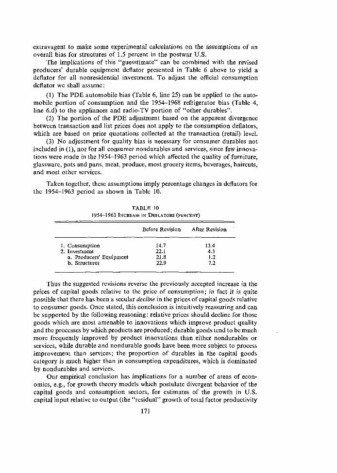
extravagent to make some experimental calculations on the assumptions of an overall bias for structures of 1.5 percent in the postwar U.S.

The implications of this "guesstimate" can be combined with the revised producers' durable equipment deflator presented in Table 6 above to yield a deflator for all nonresidential investment. To adjust the official consumption deflator we shall assume:

(1) The PDE automobile bias (Table 6, line 25) can be applied to the automobile portion of consumption and the 1954-1968 refrigerator bias (Table 4, line 6.d) to the appliances and radio-TV portion of "other durables".

(2) The portion of the PDE adjustment based on the apparent divergence between transaction and list prices does not apply to the consumption deflators, which are based on price quotations collected at the transaction (retail) level.

(3) No adjustment for quality bias is necessary for consumer durables not included in (I), nor for all consumer nondurables and services, since few innovations were made in the 1954-1963 period which affected the quality of furniture, glassware, pots and pans, meat, produce, most grocery items, beverages, haircuts, and most other services.

Taken together, these assumptions imply percentage changes in deflators for the 1954-1963 period as shown in Table 10.

TABLE 10 1954-1963 INCREASE IN DEFLATORS (PERCENT)

Before Revision After Revision

1. Consumption 14.7 13.4 2. Investment 22.1 4.3

a. Producers' Equipment 21.8 1.2 b. Structures 22.9 7.2

Thus the suggested revisions reverse the previously accepted increase in the prices of capital goods relative to the price of consumption; in fact it is quite possible that there has been a secular decline in the prices of capital goods relative to consumer goods. Once stated, this conclusion is intuitively reassuring and can be supported by the following reasoning: relative prices should decline for those goods which are most amenable to innovations which improve product quality and the processes by which products are produced; durable goods tend to be much more frequently improved by product innovations than either nondurables or services, while durable and nondurable goods have been more subject to process improvement than services; the proportion of durables in the capital goods category is much higher than in consumption expenditures, which is dominated by nondurables and services.

Our empirical conclusion has implications for a number of areas of economics, e.g., for growth theory models which postulate divergent behavior of the capital goods and consumption sectors, for estimates of the growth in U.S. capital input relative to output (the "residual" growth of total factor productivity

is reduced by these revisions), for the estimation of aggregate and two-sector production functions, and for the construction of econometric models explaining investment behavior as a function of output.61 Substantial further research is called for, both in exploring these and other implications of the results, and in improving the reliability of these estimates of measurement bias in capital goods. Among the first items on the research agenda should be:

1. Updating the study of the unit value/list price ratio from the 1963 Census of Manufacturing to 1967, in order to determine what portion of the combined cyclical and secular decline in the ratio between 1954 and 1963 was reversed during the cyclical upswing of 1963-1967.

2. A study of changes in the relative sales of machines in different commodity classifications to assess the claim of the Searle report (1970) that the decline in the unit valuellist price ratio is primarily due to shift in product mix toward smaller machines.

3. Additional hedonic studies of quality change in new and used equipment, where adequate data and sufficiently large cross sections are available.

4. Further use of the suggested method "direct comparison of closely similar models", both to check on the plausibility of previous hedonic studies, as in sections 1V.B and 1V.C above, and to adjust official price indexes in cases where data are lacking to create adequately sized cross-section samples for the hedonic technique.

5. Further work, particularly inside the Federal government, to create FHAIOBE-type bid-price structures price indexes for multi-family residential dwellings and important types of nonresidential buildings.

6. Continuation of the BLS program of labor requirements studies, with questionnaires supplemented by additional questions on quality characteristics of buildings, so that the resulting "man-hours per square foot" indexes can be corrected for changes in the average quality of a square foot.

Editor's Note: Comments by Joel Popkin and Robert Gillingham (both from the Bureau of Labor Statistics) will appear in the next issue of the Review of Income and Wealth (series 17, number 3).

1. I. Adelman and Z. Griliches, "On an Index of Quality Change", Journal of the American Statistical Association (September 1961), 56: 535-48.

2. Y. Barzel, "The Production Function and Technical Change in the Steam-Power Industry", Journal of Political Economy (April 1964),72: 133-50.

3. C. W. Bischoff, "Lags in Fiscal and Monetary Impacts on Investment in Producers' Durable Equipment", in G. Fromm, ed., Tax Incentives and Investment Behavior (Washing- ton: Brookings, 1971).

4. K. Bhatia, "A Price Index for Nonfarm One-Family Houses, 1947-1964", mimeo, 1969. 5. S. L. Brown, "Price Variations in New Houses, 1959-1961", U.S. Department of Commerce,

Bureau of the Census, Working Paper No. 6, May 1964.

?3everal implications can be explored simply by reversing the analysis in R. A. Gordon (1961), which assumes that capital goods prices rise more rapidly than the price of consumption expenditures.

6. M. L. Burstein, "The Demand for Household Refrigeration in the United States", in A. C. Harberger, ed., The Demand for Durable Goods (Chicago: The University of Chicago Press, 1960), pp. 99-145.

7. P. Cagan, "Measuring Quality Changes and the Purchasing Power of Money: An Explor- atory Study of Automobiles", NationalBanking Review (March 1966), 3 : 217-36. Reprinted in Griliches (1971).

8. Consumers' Union, Consumer Reports, various issues. 9. D. C. Dacy, "A Price and Productivity Index for a Nonhomogeneous Product", Journal

of the American Statistical Association (June 1964), 59: 469-80. 10. - , "Productivity and Price Trends in Construction Since 1947", Review of Economics

and Statistics (November 1965), 47: 40f5-11. 11. J. B. Davidson, G. W. McCuen, and R. U. Blasingame, Report of an Inquiry into Changes

in Quality Values of Farm Machines between 1910-1914 and 1932 (St. Joseph, Michigan: American Society of Agricultural Engineers, June 1933).

12. E. F. Denison, "Comment on Griliches", in Conference on Research in Income and Wealth, Models of Income and Determination, Studies in Income and Wealth, Vol. 28 (Princeton: Princeton University Press, 1964), pp. 410-13.

13. D. N. Dewees, "Econometric Valuation of Automotive Attributes", Harvard University Environmental Systems Program, discussion paper number 70-4, December 1970.

14. P. Dhrymes, "On the Measurement of Price and Quality Changes in some Consumer Capital Goods", American Economic Review (May 1967), 57: 501-18.

15. L. P. Fettig, "Adjusting Farm Tractor Prices for Quality Changes, 1950-1962", Journal of Farm Economics (August 1963), 45: 599-61 1.

16. F. M. Fisher, "Embodied Technical Change and the Existence of an Aggregate Capital Stock", Review of Economic Studies (1965), 32: 263-88.

17. J. Fleuck, "A Study in Validity: BLS Wholesale Price Quotations", in Stigler (1961), pp. 419-58.

18. M. Gilbert, "The Problem of Quality Changes and Index Numbers", Monthly Labor Review (September 1961), pp. 992-7.

19. R. Gillingharn and D. C. Lund, "A Hedonic Approach to Rent Determination", Proceed- ings of the American Statistical Association, 1970 Business and Economics Section.

20. R. A. Gordon, "Differential Changes in the Prices of Consun~ers' and Capital Goods", American Economic Review (December 1961), 51 : 937-47.

21. R. J. Gordon, "A New View of Real Investment in Structures", Review of Economics and Statistics (November 1968), 50: 417-28.

22. 2. Griliches, "Hedonic Price Indexes for Automobiles: An Econometric Analysis of Quality Change", in Stigler (1961), pp. 173-96.

23. - , "Notes on the Measurement of Price and Quality Changes", in Conference on Research in Income and Wealth, Models of Income Determination, Studies in Income and Wealth, Vol. 28 (Princeton: Princeton University Press, 1964), pp. 381-404.

24. - , "Hedonic Price Indexes Revisited: Some Notes on the State of the Art", Pro- ceedings of the American Statistical Association, 1967 Business and Economic Statistics Section, pp. 324-32.

25. - , editor, Price Indexes and Quality Change: Studies in New Methods of Measurement (Cambridge: Harvard University Press, 1971).

26. R. E. Hall, "The Measurement of Quality Change from Vintage Price Data", in Griliches (1971).

27. E. D. Hoover, "The CPI and Problems of Quality Change", Monthly Labor Review (November 1961), pp. 1175-85.

28. G. Jaszi, "Comment on Griliches", in Conference on Research in Income and Wealth Models of Income Determination, Studies in Income and Wealth, Vol. 28 (Princeton: Princeton University Press, l964), pp. 404-9.

29. S. A. Jaffe, "The Consumer Price Index-Technical Questions and Practical Answers", Proceedings of the American Statistical Association, 1959 Business and Economic Statistics Section, pp. 191-7.

30. D. W. Jorgenson and Z. Griliches, "The Explanation of Productivity Change", The Review of Economic Studies (July 1967), 34: 249-84, reprinted in The Survey of Current Business (May 1969, Part TI), 49: 29-64.

31. - , "The Sources of Economic Growth: A Reply to Edward F. Denison", Harvard Institute of Economic Research, discussion paper 131, August 1970.

32. N. F. Kaplan, "Some Methodological Notes in the Deflation of Construction", Journal of the American Statistical Association (September 1959), 54: 535-55.

173

33. I. B. Kravis and R. E. Lipsey, Price Competitiveness in World Trade (preliminary manuscript, National Bureau of Economic Research, 1970).

34. J. M. Kuhlman, "Theoretical Issues in the Estimation of Damages in a Private Antitrust Action", Southern Economic Journal (April 1967), 33: 548-58.

35. 0. A. Larsgaard and L. J. Mack, "Compact Cars in the Consumer Price Index", Monthly Labor Review (May 1961), 84: 519-23.

36. J. C. Musgrave, "New Bureau of the Census Construction Price Indexes", U.S. Bureau of the Census manuscript, presented at the Annual Meeting of the American Statistical Association, August 20-23, 1968, Pittsburgh, Pa.

37. A. D. Searle (Chairman), "Considerations on the Choice of Prices or Unit Values as Deflators for the Census Benchmark Production Indexes", report submitted to the U.S. Interagency Committee on Real Output, June 15, 1970.

38. E. L. Stern, "A New Base for the Highway Construction Bid Price Index Compiled by the Bureau of Public Roads", Public Roads (October 1961), pp. 195-9.

39. G. J. Stigler, chairman, The Price Statistics of the Federal Government (New York: National Bureau of Economic Research, 1961).

40. - and J. Kindahl, The Behavior of Industrial Prices (New York: National Bureau of Economic Research, 1970).

41. M. S. Stotz, "Introductory Prices of 1966 Automobile Models", Monthly Labor Review (February 1966), pp. 178-81.

42. J. E. Triplett, "Automobiles and Hedonic Quality Measurement", Journal of Political Economy (MayIJune 1969), 77: 408-17.

43. - , "The 'Quality Problem': A Survey of Empirical Studies Relating to Quality Bias in Price Indexes", discussion paper, Department of Economics, Washington University, St. Louis, September, 1970.

44. - "Quality Bias in Price Indexes and New Methods of Measurement", in Griliches (1971).'(a).

45. - , "The Theory of Hedonic Quality Measurement and its Use in Price Indexes", U.S. Bureau of Labor Statistics, staff paper no. 5, U.S. Government Printing Office, 1971 (b).

46. S. J. Turnovsky, "Some Empirical Evidence on the Formation of Price Expectations", University of Pennsylvania Discussion Paper No. 143, December 1969.

47. U.S. Bureau of the Census, Industry Division, Current Zndustrial Reports (Washington, various years). Prior to 1960 titled Facts for Industry.

48. - , Census of Manufactures, Volume 2, Industry Statistics (Washington: U.S. Govern- ment Printing Office, 1966 and earlier years).

49. - , Statistical Abstract of the United States, 89th edition, 1969. 50. U.S. Department of Commerce, Office of Business Economics, The National Income and

Product Accounts of the United States, 1929-65 (Washington: Government Printing Office, 1966), updated in various July issues of the Survey of Current Business.

51. U.S. Department of Labor, Labor Requirements Studies: Bulletin 1299: School Construction (1961). Bulletin 1331 : Federal Office Buildings (1962). Bulletin 1390: Civil Works Construction (1964). Bulletin 1404: Private One-Family House Construction (1964). Bulletin 1490: Sewer Works Construction (1965). Bulletin 1586: School Construction (1968). Report 299: Federally Aided Highways (1966).

52. U.S. Federal Housing Administration, Series Data Handbook (Washington: FHA Stat- istics Section, April 1967).

53. U.S. Office of the President, Economic Report of the President, 1968 (Washington: Govern- ment Printing Office, February 1968).

Documents

Measurement Bias in Price Indexes for Capital Goods