McSAS: A package for extracting quantitative form-free distributions

arX

iv:1

412.

1900

v1 [

phys

ics.

data

-an]

5 D

ec 2

014

1

McSAS: A package for extracting quantitative form-free

distributions

[email protected] [email protected]

I. Breßler,a B. R. Pauwb and A. Thunemanna

aBAM Federal Institute for Materials Research and Testing, 12205 Berlin,

Germany, and bNational Institute of Materials Science, 305-0047 Tsukuba, Japan

(Received 0 XXXXXXX 0000; accepted 0 XXXXXXX 0000)

Abstract

A reliable and user-friendly characterisation of nano-objects in a target material

is presented here in the form of a software data analysis package for interpreting

small-angle X-ray scattering (SAXS) patterns. When provided with data on absolute

scale with reasonable uncertainty estimates, the software outputs (size) distributions in

absolute volume fractions complete with uncertainty estimates and minimum evidence

limits, and outputs all distribution modes of a user definable range of one or more

model parameters. A multitude of models are included, including prolate and oblate

nanoparticles, core-shell objects, polymer models (Gaussian chain and Kholodenko

worm) and a model for densely packed spheres (using the LMA-PY approximations).

The McSAS software can furthermore be integrated as part of an automated reduction

and analysis procedure in laboratory instruments or at synchrotron beamlines.

PREPRINT: Journal of Applied Crystallography A Journal of the International Union of Crystallography

http://de.arxiv.org/abs/1412.1900v1

2

1. Introduction

Quantification of nanoscale structures is set to become a requirement in industrial

preparation of materials (EU, 2011). An accurate and reliable toolset is therefore

sought to obtain quantitative size distributions of disperse nanoparticle mixtures,

spanning a wide size-range with minimal effort and high flexibility.

The most commonly used technique for nanostructural quantification is transmis-

sion electron microscopy (TEM). TEM is essential in determining the overall mor-

phology of the nanostructural features, and can often be used to coarsely quan-

tify their parameters. Obtaining a statistically representative quantification of the

nanostructure, however, is reliant on the probing of large numbers of objects. To

improve its representation of the bulk of the sample, it should preferably be per-

formed through sampling from multiple locations throughout a bulk-scale sample

(Klein et al., 2011; Meli et al., 2012). As TEM has remained largely resilient to

automation efforts, this commonly remains a tedious and labour-intensive task. It

is therefore beneficial to combine the localised resolving power of microscopy with

another technique more suited for bulk-scale nanostructural quantification such as

Small-angle Scattering (SAS) (ISO, 2014; Pauw, 2013).

SAS offers one reliable route to bulk quantification of materials: it can characterise

the nanostructure of large amounts of material with a minimum of tedium, easily

extracting size distributions and volume fractions. Practically, however, one of the

biggest stumbling blocks in its application has been the data correction and analysis,

in particular for the disperse systems discussed herein. While the discussion of data

corrections is beyond the scope of this work (c.f. (Jacques et al., 2012; Pauw, 2013;

Kieffer & Karkoulis, 2013)), it has to be stressed that reliable analysis of data is reliant

on the quality thereof. There can be no good results without proper data which cannot

be considered complete without reasonable uncertainty estimates.

IUCr macros version 2.1β1: 2007/05/15

3

Analysis can be performed through a “classical” approach: by least-squares optimi-

sation of model function parameters describing a scattering pattern (Pedersen, 1997).

However, the assumptions made in such model functions (on the scatterer shape and

its size distribution) are often insufficiently flexible to describe the morphology of

many samples. Good agreement between the model function and the measured data

will then not be achieved, in particular for samples where the actual size dispersity

does not adhere to the inherently assumed model size distribution shape.

Modern analysis methods are available for this class of samples (size-disperse) which

allow for the retrieval of size distributions without assumptions on its form. While the

general shape of the scatterer still has to be defined in order to arrive at a unique

solution (see, for example (Rosalie & Pauw, 2014)), these modern methods are no

longer restricted to a limited set of idealized size distributions.

There are a variety of approaches for these modern methods, including indirect

fourier transform methods based on smoothness criteria (Glatter, 1977; Svergun,

1991), maximum entropy optimisation (Hansen & Pedersen, 1991) or Bayesian hyper-

parameter estimation (Hansen, 2000). Alternative methods include using Titchmarsh

transforms for extraction of size distributions (Fedorova & Schmidt, 1978; Botet &

Cabane, 2012). While these carry a certain mathematical elegance, they can be chal-

lenging to implement, understand and apply. This mathematical obscurity furthermore

hinders thorough understanding of the failure modes, which can lead to crucial errors

in their application.

Recently, a (conceptually) straightforward method was presented for determining

size distributions from small-angle scattering patterns (Pauw et al., 2013b), which

has since been applied to a variety of sample types including metal alloys (Rosalie

& Pauw, 2014), novel oxygen reduction reaction catalysts (Schnepp et al., 2013) and

polymer fibres (Pauw et al., 2013a). While these results have been encouraging, the


4

lack of user-friendliness of the method has hindered its adoption by a broader audience.

Through a multinational, collaborative effort spanning several years, a drastic improve-

ment on the software usability was effected. This was mostly accomplished through

a comprehensive rewrite of the implementation following modern coding standards

and conventions, and the addition of a graphical user interface (c.f. Figure 2). After a

brief recapitulation of the method concept, the software capabilities and interface are

detailed, and an application example is given.

2. McSAS fitting procedure

2.1. Concept overview

Start End

Calculate χ2r

Pick Pj∀[1,n]

Compute I(Pj∀[1,n]

)

Calculate χ2r,new

Itest

=I-I(Pj)+I(P

new)

Pick Pnew

χ2r ≤ 1

True

False

χ2r,new

≤ χ2r

True

False

Pj = P

new

I = I

test

χ2r = χ2

r,new

j = j + 1

Fig. 1. The main process of the McSAS software for parameter optimisation.


5

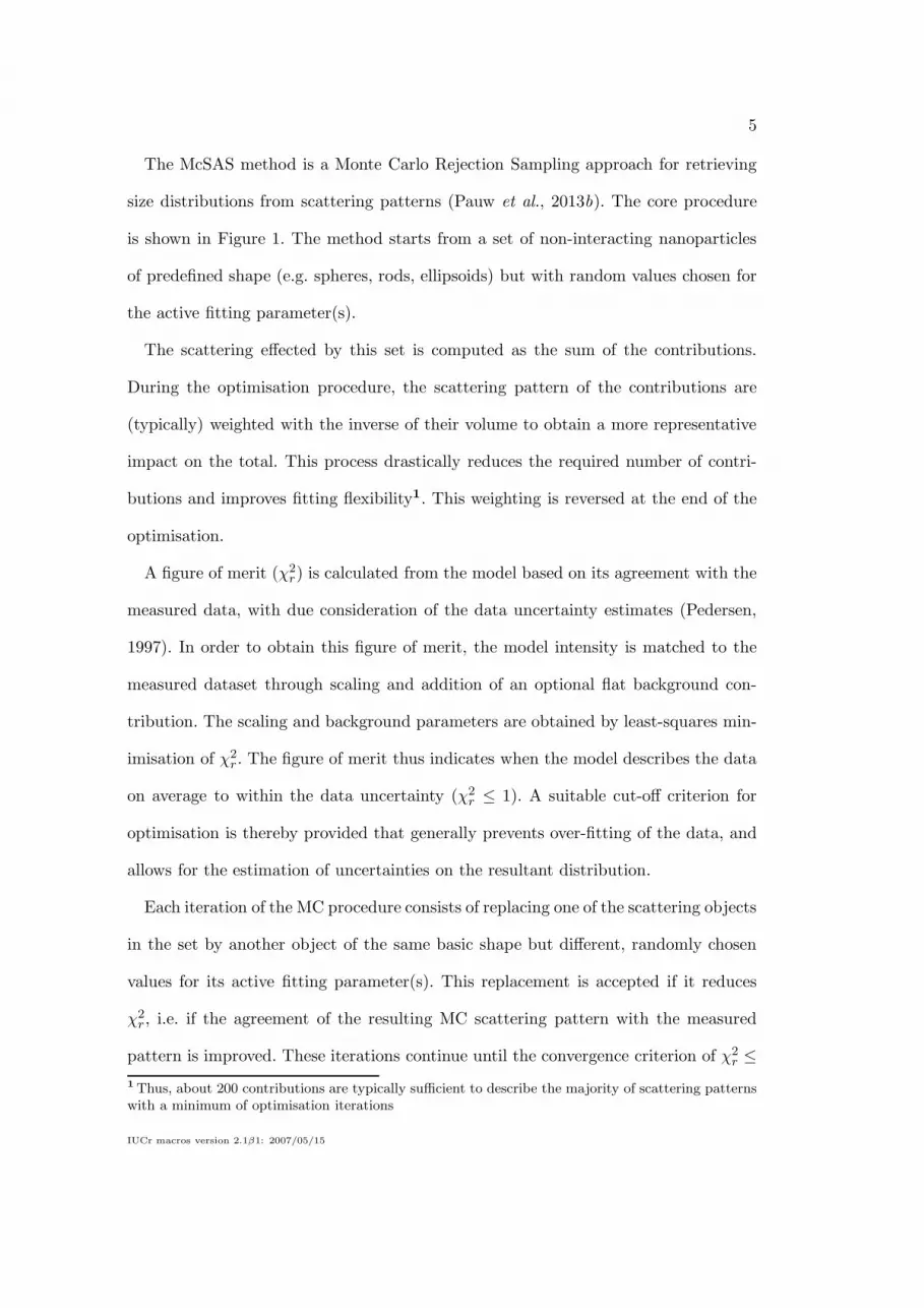
The McSAS method is a Monte Carlo Rejection Sampling approach for retrieving

size distributions from scattering patterns (Pauw et al., 2013b). The core procedure

is shown in Figure 1. The method starts from a set of non-interacting nanoparticles

of predefined shape (e.g. spheres, rods, ellipsoids) but with random values chosen for

the active fitting parameter(s).

The scattering effected by this set is computed as the sum of the contributions.

During the optimisation procedure, the scattering pattern of the contributions are

(typically) weighted with the inverse of their volume to obtain a more representative

impact on the total. This process drastically reduces the required number of contri-

butions and improves fitting flexibility1. This weighting is reversed at the end of the

optimisation.

A figure of merit (χ2r) is calculated from the model based on its agreement with the

measured data, with due consideration of the data uncertainty estimates (Pedersen,

1997). In order to obtain this figure of merit, the model intensity is matched to the

measured dataset through scaling and addition of an optional flat background con-

tribution. The scaling and background parameters are obtained by least-squares min-

imisation of χ2r. The figure of merit thus indicates when the model describes the data

on average to within the data uncertainty (χ2r ≤ 1). A suitable cut-off criterion for

optimisation is thereby provided that generally prevents over-fitting of the data, and

allows for the estimation of uncertainties on the resultant distribution.

Each iteration of the MC procedure consists of replacing one of the scattering objects

in the set by another object of the same basic shape but different, randomly chosen

values for its active fitting parameter(s). This replacement is accepted if it reduces

χ2r, i.e. if the agreement of the resulting MC scattering pattern with the measured

pattern is improved. These iterations continue until the convergence criterion of χ2r ≤

1Thus, about 200 contributions are typically sufficient to describe the majority of scattering patterns

with a minimum of optimisation iterations


6

1 is reached (different convergence criteria can be set by the user for data whose

uncertainties are over- or underestimated).

The size distribution is determined through analysis of the active fitting parameter

values throughout the set. At this stage, the scattering contrast is taken into account to

establish the absolute volume fractions. Finally, the uncertainty on the size distribution

is determined through analysis of the sample standard deviation of a multitude of

independent MC solutions.

In addition to this, a “minimum observability limit” is defined for each size, which

specifies the minimum required volume fraction of scatterers required to make a dis-

tinguishable contribution to the scattering pattern (i.e. a contribution exceeding the

measurement uncertainty). More specifically, a minimum observability limit ϕmin,k

(in units of volume fraction) can be defined for any method where the total model

intensity is comprised of a set of quantised components, whose partial contributions

are Ik(q) for a given component volume fraction ϕk, and where the measurement data

uncertainty σ(q) is available:

ϕmin,k = minq∈[qmin,qmax]

[

σ(q)ϕk

Ik(q)

]

(1)

Its derivation and use is further explored elsewhere (Pauw et al., 2013b).

The uncertainty estimates and the observability limits are key values in the applica-

tion of the method. They provide information to distinguish between numerical noise

and size distribution components which are evidenced by the data, and furthermore

allow for the assessment of the statistical significance of differences in resultant size

distributions. The accuracy of the uncertainty estimates and observability limits are,

however, directly reliant on the provision of reasonable uncertainty estimates on the

measured data.

Using the aforementioned method, McSAS is able to retrieve any freeform size


7

distribution provided a basic scatterer shape is given. A test of the retrievability of a

wide range of unimodal and multimodal size distributions has been demonstrated for a

large variety of simulated size distributions in the supplementary information of Pauw

et al. (Pauw et al., 2013b). A comparison between size distributions of precipitates

in alloys is also available, obtained from electron microscopy and McSAS analysis of

SAXS data (Rosalie & Pauw, 2014).

2.2. MC method benefits and drawbacks

The MC method has already demonstrated its versatility in a variety of practical

applications, including monitoring of precipitation processes in alloys and bulk val-

idation of nanoparticle sizes in catalysts. It can work in absolute units to retrieve

absolute volume fractions. Several scatterer shapes have been implemented, and a

model for densely packed spheres has also been included based on the Local Monodis-

perse Approximation (LMA)2 coupled with the Percus-Yevick (PY) approximation

(example given vide infra) (Kinning & Thomas, 1984).

On the downside, due to its “brute force”, iterative nature, the method is not as

fast as some of the alternatives. Optimisation of a reasonably accurate dataset can

take a minute or more on a modern desktop computer. This is expected to improve

in the near future through implementation of multithreading.

Furthermore, there is a risk of under-specifying the fitting model when more com-

plex models are chosen. For example, if a cylindrical scatterer model is chosen, and

its length and radius allowed to span the same size range, the solution is no longer

unique and a multitude of valid solutions will be found. This is indicated by exces-

sive uncertainties resulting from large discrepancies between the independent McSAS

repetitions, and such ambiguity can be easily arrived at when using models such as

2This is one of the few structure factors that can be directly implemented given the internal design

of the MC method.


8

core-shell objects and anisotropic objects. For such shapes, the allowed size ranges

for the shape parameters may require the application of strict limits before a unique

solution is obtained.

Lastly, experimentally obtained SAS data represents a volume-weighted size distri-

bution for broad size distributions rather than a number-weighted size distribution due

to the physical weighting of contributions in SAS experiments. In other words, there

is not a lot of evidence in SAS data to allow the extraction of broad number-weighted

size distributions (explored, amongst others, in section 3 of (Pauw et al., 2013b)). For

this reason, when trying to extract number-weighted size distributions using McSAS,

excessively large contributions, uncertainties and observability limits are often seen at

small sizes. It is therefore recommended to extract volume-weighted size distributions

with McSAS instead. While this is not strictly a drawback of the McSAS method (but

rather a limitation of SAS measurements on disperse systems), it stands in strong

contrast with classical methods. In classical methods, the strict assumptions placed

on the size distribution shape belie the lack of evidence for the absence or presence of

scatterers at the small end of the distribution (and the number-weighted distributions

are mostly determined by the evidence for the larger sizes alone).

3. Current implementation

3.1. Feature overview

Besides the sphere model, a variety of alternative models are also provided. Spe-

cial attention should be given to prevent fitting ambiguity for these more complex

shapes. These include core-shell ellipsoids and core-shell spheres, a Kholodenko worm

and Gaussian chain model, isotropic cylinders and a sphere model suitable for dense

packings of size-disperse spheres.

The code is unit-aware, and can translate between the units used in the user inter-


9

face (often chosen based on tradition, such as A−2 for the scattering length density

difference and ◦ for angle), and the SI units used for the internal calculations (m−2

and radian, respectively). In our experience, the strict internal adherence to SI units

drastically reduces the risk of programming errors.

Once set up, the MC code can run with or without user interface, to allow integration

into existing data processing procedures. When run using the interface, the data file(s)

can be loaded from the command line, if necessary using regular expressions. The

fitting procedure can then be automatically initiated, inheriting the settings of the

previous GUI instance.

To aid the user with the provision requirement of reasonable uncertainty estimates,

any provided uncertainties will be limited to be no less than 1% of the magnitude of

the scattering signal. This has been previously found to be a practical limit from data

correction considerations (Pauw et al., 2013b), and is a value supported by experimen-

tal results (Hura et al., 2000). Naturally, this lower limit can be adapted or bypassed

if better estimates can be guaranteed.

Graphical output and population statistics can be calculated for a user-specified

number of parameter ranges, with the size axes in logarithmic or linear scales. The

distributions can be shown as number-weighted or volume-weighted size distributions,

though for broad distributions volume-weighting is strongly recommended (see the

note in section 2.2). The size distributions shown include the observability limit, i.e.

the minimum required amount for each contribution to be statistically significantly

contributing.

Lastly, population statistics of the solution are determined independently of the

histogramming procedure. For each selected parameter and range, the total value and

the four distribution modes are provided: the mean, variance, skew and kurtosis. These

are number- or volume-weighted depending on the user’s choice. Such parameters


10

simplify the analysis of population trends in in-situ experiments or other inter-related

datasets.

3.2. User interface features

Fig. 2. The main interface of the McSAS software upon start-up, showing four con-figuration panels. The ”Data Files” panel allows selection and input of the dataof interest, the ”Algorithm” panel contains settings to adjust the optimisationmethod behaviour, ”Model” contains all parameters and settings relevant to thechosen morphology, and ”Post-fit Analysis” holds the settings for histogrammingand visualisation of the result.

The user interface is divided into several panels, each limited to a different aspect of

the process (See Figure 2). These consist of a “Data files”-panel, an “Algorithm”-panel,

a “Model”-panel and a “Post-fit Analysis”-panel, and will be discussed forthwith.

The “Data files”-panel shows datafiles loaded upon startup (as command-line argu-

ments) or files added through the right-click menu. All files will be treated identically


11

when the fit is run, though their order of processing can be changed as desired. Avail-

able data is guessed from the input file, which is expected to consist of three semi-

colon separated columns of q (nm), I ((m sr)−1) and the uncertainty estimate σ(I) ((m

sr)−1). An optional fourth column can be used to indicate the azimuthal angle φ to

aid fitting of anisotropic scattering patterns.

To aid the user with determining reasonable limits of size parameters, basic analysis

is performed when loading each data file. The minimum and maximum values of the

provided q-vector are used to estimate the maximum and minimum possible scatterer

size under the assumption of solid spherical scatterers. Those estimates are displayed

next to each data file and, by double-click, can be applied as optimisation limits for

radius-type model parameters.

The “Algorithm”-panel contains a subset of MC algorithm settings addressable

by the user. The most important of these is the chi-squared criterion. While this is

per default set to 1, it may prevent reaching a state of convergence (χ2r ≤ 1) with

insufficiently large or poorly estimated uncertainty values. Increasing this value will

allow the convergence condition to be reached, after which the fit may be evaluated.

This increase directly affects the uncertainties on the resultant distribution.

Additionally, the number of shape contributions can be increased. While the default

setting of 200 is sufficiently large to reach the convergence criterion for most scatter-

ing patterns, and small enough to reach it rapidly, there may be cases for which an

increased number is desired. Using the timing information shown in the graphical

output, the number of shape contributions can be optimised to reach convergence as

fast as possible (a method discussed in (Pauw et al., 2013b)). Likewise, the number

of repetitions can be changed. These independent repetitions are used to estimate the

uncertainties on the resultant size distribution, but a reduced number will suffice for

initial testing. Here too, a selection can be made on whether a flat background con-


12

tribution is to be taken into account when matching the MC intensity to the detected

signal.

The “Model”-panel contains all information on the model used to describe the

scatterer morphology. The pulldown menu offers a selection of models that can be

used as basic scatterer. The associated parameters and options for the model chosen

will then be shown on the right-hand side. The models allow setting of a scattering

length density difference as well, which (when used in combination with absolute units

in the input intensity) will result in absolute volume fractions in the final distribution.

Some parameters can be set “Active”, which implies they are active fitting parameters

for the MC model. When set, lower and upper limits have to be provided for the

parameter to vary between.

The “Post-fit Analysis”-panel offers basic analysis capabilities for interpretation of

the MC result. When a range entry is added, the user can select which parameter to

histogram, what parameter range to consider, and how many bins to histogram in.

Increasing the number of histogram bins will lead to increased detail in the resulting

histogram at the cost of larger uncertainties and evidence requirements via observabil-

ity limits. Furthermore, a choice can be made whether to use a linear or logarithmic

parameter-scale (useful for distributions spanning several decades) and whether to

plot volume- or number-weighted size distributions. When using absolute units, only

the volume-weighted distribution will contain absolute values, the number-weighted

distribution is normalised for lack of information. Again it should be stressed that the

evidence in SAS experiments supports volume-weighted rather than number-weighted

distributions (vide supra).

Finally, the “Start”-button starts the process, and the ”log” shows the output of

the program as it runs (and is automatically stored in a file).


13

3.3. Support, availability and licensing

A reasonable degree of support is provided by the authors subject to the availability

of time. Instructional videos are available to help the user get started.

The software is written in the Python 2.7 programming language, and available as

a Git DVCSS repository. Binary packages of stable versions are available for selected

operating systems. The software is released under an open-source GPLv3 license,

allowing for academic and commercial adoption given proper attribution. Users for

whom the software has been useful may refer to this work.

4. Application example to densely packed nanoparticles

Dense systems add a degree of complexity to small-angle scattering, and are therefore

interesting as a test case for MC methods.

A suitable dataset of densely packed, dry SiO2 spheres (with a stated radius of

75 nm) has been provided by Peter Høghøj of Xenocs, as part of a demonstration

dataset measured on their Xeuss SAXS instrument. The SiO2 spheres are packed in

a randomly jammed fashion, implying that the volume fraction vf is approximately

0.63 (Song et al., 2008).


14

I (Q)

Q 1/nm

0.1

0.1 1

1

10

100

1000

Fig. 3. Best fit using a classical model (implemented in SASFit) to a scattering patternobtained from packed SiO2 spheres. Model uses a sphere form factor with a LMA-PY structure factor and a Gaussian size distribution.

A reasonable fit can be obtained using classical fitting methods implemented in

SASfit, with a model of Gaussian distributed spheres and a structure factor consisting

of a PY hard-sphere interaction model assuming the local monodisperse approximation

(LMA). This resulting fit is shown in Figure 3. Most of the intensity can be described

well, apart from the region at low q, which is remarkable given that the structure

factors are not strictly valid for application to very dense systems.


15

q (nm-1)

Intensity ((m sr)-1)

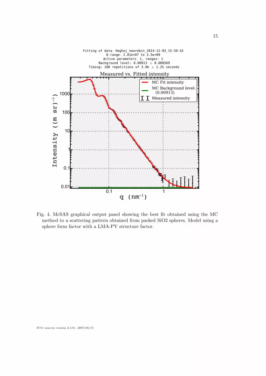
Fig. 4. McSAS graphical output panel showing the best fit obtained using the MCmethod to a scattering pattern obtained from packed SiO2 spheres. Model using asphere form factor with a LMA-PY structure factor.


16

radius (nm)

[Rel.] Volume Fraction

Fig. 5. McSAS graphical output panel showing volume-weighted size distribution asso-ciated with the MC fit of Figure 4.

A fit to within data uncertainty can be obtained using the McSAS model (c.f. Figure

4), where the volume fraction vf is set to 0.63. Note that the instrumental resolution

has not been considered in either the classical or the MC approach. The main feature

in the resultant size distribution (shown in Figure 5) is indeed at the size indicated

for the sample (number-weighted mean radius of 76.1(2) nm), but a minor component

is visible at about half the radius of the main component.


17

Whether these minor features are due to a breakdown of approximations in the

LMA-PY structure factor, issues with sample purity or due to unaccounted-for compo-

nents in the data cannot be determined without further investigation. What is found,

however, is that a similar good fit can be obtained for other volume fractions (possi-

ble between ≈ 0.5 ≤ vf ≤ 0.7). Changing the volume fraction drastically affects the

size distribution and demonstrates that there are a multitude of solutions accessible

through adjustment of the volume fraction. This highlights once more that information

must be supplied on the sample to allow SAS analyses to arrive at a unique solution.

However, the overall result is quite satisfactory and a clear improvement compared to

the classical approach.

5. Conclusion

A complete data analysis package is presented capable of extracting form-free size

distributions from small-angle scattering patterns. A variety of shape functions have

been included such as (core-shell) spheres, rods and ellipsoids, but also polymer mod-

els and a model for packed spheres. Care must be taken (in particular with more

complex models) that sufficient external information is supplied to ensure a unique

solution. When provided with data in absolute units, the resulting volume-weighted

size distribution units will reflect absolute volume fractions.

The authors would like to acknowledge Peter Høghøj and Xenocs for their provision

of the dense spheres dataset. I.B. acknowledges financial support by the MIS program

of BAM.

References

Botet, R. & Cabane, B. (2012). J. Appl. Cryst. 45, 406–416.

EU (2011). Commission Recommendation of 18 October 2011 on the definition of nanomaterialText with EEA relevance. Tech. Rep. OJ L 275, 20.10.2011. European Commission.URL: http://eur-lex.europa.eu/legal-content/EN/TXT/?uri=CELEX:32011H0696

Fedorova, I. & Schmidt, P. (1978). J. Appl. Cryst. 11(OCT), 405–411.


18

Glatter, O. (1977). J. Appl. Cryst. 10, 415–421.

Hansen, S. (2000). J. Appl. Cryst. 33, 1415–1421.

Hansen, S. & Pedersen, J. S. (1991). J. Appl. Cryst. 24, 541–548.

Hura, G., Sorenson, J. M., Glaeser, R. M. & Head-Gordon, T. (2000). J. Chem. Phys. 113,9140–9148.

ISO (2014). Particle size analysis — Small-angle X-ray scattering. Tech. Rep. ISO/FDIS17867:2014(E). .

Jacques, D. A., Guss, J. M., Svergun, D. I. & Trewhella, J. (2012). Acta Crystallog. D68,620–626.

Kieffer, J. & Karkoulis, D. (2013). J. Phys.:Conf. Ser. 425, 202012–1–202012–5.

Kinning, D. J. & Thomas, E. L. (1984). Macromolecules, 17, 1712–1718.

Klein, T., Buhr, E., Johnsen, K.-P. & Frase, C. G. (2011). Meas. Sci. Technol. 22, 094002.

Meli, F., Klein, T., Buhr, E., Frase, C. G., Gleber, G., Krumrey, M., Duta, A., Duta, S.,Korpelainen, V., Belliotti, R., Picotto, G. B., Boyd, R. D. & Cuenat, A. (2012). Meas.Sci. Technol. 23, 125005–1–125005–15.

Pauw, B. R. (2013). J. Phys.: Condens. Matter, 25, 383201.

Pauw, B. R., Ohnuma, M., Sakurai, K. & Klop, E. A. (2013a). 2D anisotropic scatteringpattern fitting using a novel Monte Carlo method: Initial results. ArXiv:1303.2903.

Pauw, B. R., Pedersen, J. S., Tardif, S., Takata, M. & Iversen, B. B. (2013b). J. Appl. Cryst.46, 365–371.

Pedersen, J. S. (1997). Adv. Coll. Interf. Sci. 70, 171–210.

Rosalie, J. M. & Pauw, B. R. (2014). Acta Materialia, 66, 150–162. ArXiv:1210.5366.

Schnepp, Z., Zhang, Y., Hollamby, M. J., Pauw, B. R., Tanaka, M., Matsushita, Y. & Sakka,Y. (2013). J. Mater. Chem. A, 1, 13576.

Song, C., Wang, P. & Makse, H. A. (2008). Nature, 453, 629–632.

Svergun, D. I. (1991). J. Appl. Cryst. 24, 485–492.


Documents

McSAS: A package for extracting quantitative form-free distributions