Embed Size (px)
Citation preview
[DEPARTMENT OF DEFENCE
DEFENCE SCIENCE & TECHNOLOGY ORGANISATION DSTO
Mathematical Modelling of Helicopter Slung-Load Systems
R. A. Stuckey
DSTO-TR-1257
DISTRIBUTION STATEMENT A Approved for Public Release
distribution Unlimited
20020514 142
Mathematical Modelling of Helicopter Slung-Load Systems
R.A. Stuckey
Air Operations Division Aeronautical and Maritime Research Laboratory
DSTO-TR-1257
ABSTRACT
The primary goal of this work is to use mathematical modelling to assist in defin- ing the operational limits of the Australian Army CH-47D Chinook when carrying mixed density slung loads. This report presents the first phase in the program: the development of a simple helicopter slung-load model for simulation and analysis of the system dynamics.
General system equations of motion are obtained from the Newton-Euler equations in terms of generalized coordinates and velocities. The system is partitioned into coordinates such that the motion due to cable stretching is separated from that due to rigid-body, coupled dynamics. In the formulation used, the constraint forces appear explicitly and a solution to the resultant generalized accelerations can be determined by modelling the cable as a simple spring. An inelastic solution is also possible by nulling the stretching coordinates to obtain a relation for the suspension forces. The system equations are also extended for the multiple load case.
The model is verified by imposing certain constraints in order to approximate a simple pendulum system and then comparing its behaviour with analytical results. Various configurations of the complete helicopter slung-load system, based on the CH-47B Chinook carrying standard military containers, are then examined in an in- vestigation of the open-loop characteristics. In the investigation, several parameters such as the helicopter-load mass ratio, suspension configuration, and number of loads are varied and the resulting system modes examined. A number of simulations are also presented which demonstrate the characteristic behaviour of such systems.
APPROVED FOR PUBLIC RELEASE
DEPARTMENT OF DEFENCE
DEFENCE SCIENCE & TECHNOLOGY ORGANISATION DSTO
fö2-0?- &$£

DSTO-TR-1257
Published by
DSTO Aeronautical and Maritime Research Laboratory 506 Lorimer St, Fishermans Bend, Victoria, Australia 3207
Telephone: (OS) 9626 7000 Facsimile: (03) 9626 7999
© Commonwealth of Australia 2002 AR No. AR-01B-U4 December, 2001
APPROVED FOR PUBLIC RELEASE
DSTO-TR-1257
Mathematical Modelling of Helicopter Slung-Load Systems
EXECUTIVE SUMMARY
In the past, the operations of helicopters carrying externally slung loads has often been limited and, in some cases, seriously hindered by stability and control problems. Several incidences have been reported by the Australian Army alone, in which possible aerodynamic excitation or dynamic instability, resulting in uncontrollable oscillations, has forced premature release of the load. Hence, the main goal of the study is to develop a comprehensive helicopter slung-load model which will provide a better understanding of the system dynamics and various effects involved. Furthermore, there is a requirement for the carriage of multiple loads of varying type, which has not previously been investigated in this manner. This report presents the first phase in the program: the development of a simple helicopter slung-load model for simulation and analysis of the system dynamics. Following this, a full nonlinear flight dynamic model is to be developed, incorporating additional detail, such as the automatic flight control system, rotor wake effects, load aerodynamics, and sling elasticity.
The simulation model used for this first phase of work is based on the helicopter slung load system first introduced at NASA Ames Research Center. In this formulation, the gen- eral system equations of motion are obtained from the Newton-Euler equations in terms of generalized coordinates and velocities. Using the explicit constraint method, the system is then partitioned into coordinates such that the motion due to cable stretching is separated from that due to rigid-body, coupled dynamics. As a consequence, the constraint forces appear explicitly and a solution to the resultant generalized accelerations is determined by assuming a simple spring model for the cable. It is also possible to obtain a solution to the inelastic approximation by nulling the stretching coordinates, yielding an explicit relation for the suspension forces. The result is computationally more efficient than the conven- tional formulation and is readily integrated with the elastic suspension model. Another benefit of the formulation is that it is easily applied to complex multiple body systems, and in the current work, the system equations are extended for the case of multiple loads. All code development has been done in the MATLAB numerical computing environment, which provides a high-performance language amenable to modelling and simulation type work. The main functions used in the simulation and analysis have been included in the report.
The model is verified by imposing certain constraints in order to approximate a simple pendulum system and then comparing its behaviour against both analytical solutions and previously documented numerical results. A complete helicopter slung-load system, based on a CH-47B Chinook carrying a standard military container, is then examined in an investigation of the open loop characteristics. In this simple model, neither the load aerodynamics nor the effect of rotor downwash on the load is taken into account. Several parameters such as the helicopter-load mass ratio, suspension configuration, and number of loads are varied and the resulting system modes examined. In order to extract these modes, a linearised form of the model is first obtained by numerical approximation of the partial derivatives. For the configurations examined, an increase in the load mass was generally found to have a mild destabilising effect, particularly in the lateral axes. A number of
in
DSTO-TR-1257
simulations were also run in order to demonstrate the dynamic characteristics of several different configurations. Prom the response data, the oscillatory modes in longitudinal and lateral axes were identified, including the unstable phugoid and pendulum modes. In all of the simulations examined, the cable tension was found to reach a maximum of approximately 1.5 times the static load.
IV
DSTO-TR-1257
Author
Roger A Stuckey Air Operations Division
Roger Stuckey received the degree of Bachelor of Engineer- ing in Aeronautical Engineering from the University of Syd- ney in 1990. He then stayed on with the Department to begin postgraduate studies and in 1995 received the degree of Doc- tor of Philosophy in Aeronautical Engineering. His research thesis involved the development of an approach for the iden- tification of parameters that characterise nonlinear behaviour in high-order dynamic systems. The software was successfully used in estimating the unsteady aerodynamics associated with wing-spoilers on the F-111C aircraft. Roger currently holds the position of Research Scientist in the Air Operations Divi- sion of AMRL and is working on helicopter modelling tasks. His research interests include aircraft flight dynamics and con- trol, nonlinear system analysis, and parameter identification and simulation in aeronautical systems.

DSTO-TR-1257
DSTO-TR-1257
Contents
Acronyms xi
Nomenclature xiii
1 Introduction 1
2 Background 2
2.1 Analytical Studies 2
2.2 Experimental Testing 3
2.3 Flight Simulation and Control 3
2.4 Surveys and Overviews 5
3 System Representation 6
3.1 Description of System 6
3.2 Generalized Equations of Motion 6
3.3 Simulation of Helicopter Slung Load System 11
4 Simple Pendulum System Dynamics 15
4.1 System Properties 15
4.2 Analysis of System Modes 15
4.3 Longitudinal and Lateral Simulations 17
5 Helicopter Slung-Load Dynamics 22
5.1 Unloaded Helicopter Dynamic Modes 22
5.2 Analysis of Helicopter Slung-Load System Modes 25
5.3 Flight Simulation 31
6 Concluding Remarks 38
References 39
Appendices
A Governing System Equations 42
B Analytical Results for Pendulum-Type Systems 48
DSTO-TR-1257
C CH-47D Chinook Helicopter Aerodynamic Model 53
D Matlab Source Code 57
Figures
1 Single Point Slung-Load Configurations 7
2 Suspension Forces on a Rigid Body 10
3 Simulation Flow Diagram 12
4 Two-body Pendulum Simulation System 16
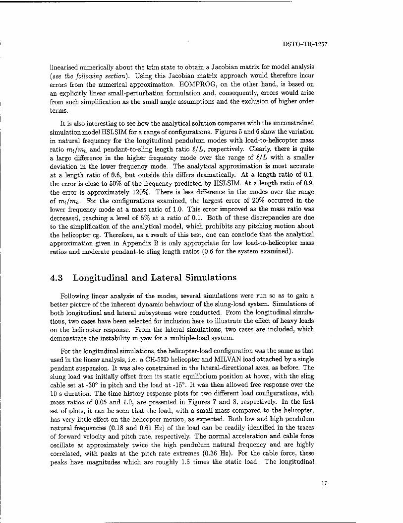
5 CH-53D-MILVAN System Longitudinal Pendulum Modes - Variation in Fre- quency with Load-to-Helicopter Mass Ratio 18
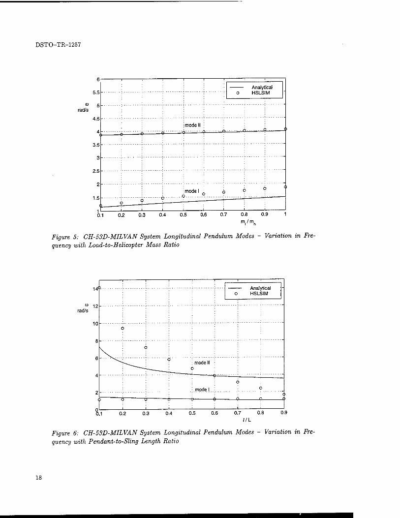
6 CH-53D-MILVAN System Longitudinal Pendulum Modes - Variation in Fre- quency with Pendant-to-Sling Length Ratio 18
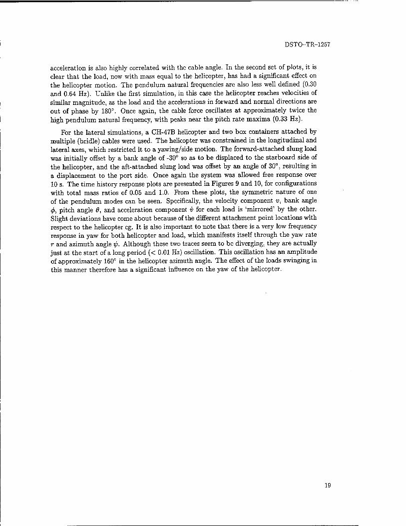
7 CH-53D-MILVAN System Time History Response — Mass Ratio 0.05 .... 20
8 CH-53D-MILVAN System Time History Response — Mass Ratio 1.00 .... 20
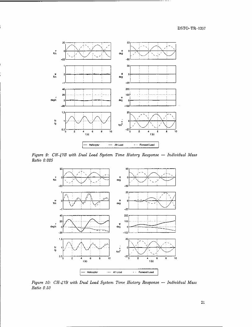
9 CH-47B with Dual Load System Time History Response — Individual Mass Ratio 0.025 21
10 CH-47B with Dual Load System Time History Response — Individual Mass Ratio 0.50 ■ • 21
11 CH-53D System Eigenvalues — Variation with Trim Airspeed (in KTAS) . . 23
12 CH-47B System Eigenvalues — Variation with Trim Airspeed (in KTAS) . . 24
13 CH-53D with Single Slung Load Longitudinal Eigenvalues at Hover — Vari- ation with Load-to-Helicopter Mass Ratio 26
14 CH-53D with Single Slung Load Lateral Eigenvalues at Hover — Variation with Load-to-Helicopter Mass Ratio 26
15 Multiple Cable Sling Configuration 27
16 CH-47B with Single Slung Load Longitudinal Eigenvalues at 0.1 KTAS — Variation with Load-to-Helicopter Mass Ratio 28
17 CH-47B with Single Slung Load Lateral Eigenvalues at 0.1 KTAS — Variation with Load-to-Helicopter Mass Ratio 28
18 Single Cable Sling Configuration 29
19 CH-47B with Single Slung Load Longitudinal Eigenvalues at 0.1 KTAS — Variation with Pendant-to-Sling Length Ratio 30
20 CH-47B with Single Slung Load Lateral Eigenvalues at 0.1 KTAS — Variation with Pendant-to-Sling Length Ratio 30
21 CH-47B with Multiple Slung Loads Eigenvalues at 0.1 KTAS — Variation with Number of Loads 31
vni
DSTO-TR-1257
22 Longitudinal Dynamic Response Simulation of CH-47B with Single Slung Load — Time Histories (mi/rrih = 0.05) 33
23 Longitudinal Dynamic Response Simulation of CH-47B with Single Slung Load — Simulation Frames (mi/rrih = 0.05) 33
24 Coupled Dynamic Response Simulation of CH-47B with Single Slung Load — Time Histories {mi/rrih = 1.0) 34
25 Coupled Dynamic Response Simulation of CH-47B with Single Slung Load — Simulation Frames (mi/rrih = 1.0) 35
26 Coupled Dynamic Response Simulation of CH-47B with Three Slung Loads — Simulation Frames (mi/rrih = 0.33) 35
27 Coupled Dynamic Response Simulation of CH-47B with Three Slung Loads — Time Histories (m//m/i = 0.33) 37
Al General Helicopter Slung-load System 42
Bl Generalized Two-body Pendulum-type System 48
B2 Single-cable Pendulum System 51
B3 Multi-cable Pendulum System 52
Tables
1 Pendulum Mode Frequencies (rad/s) for CH-47B-MILVAN System in Hover . 16
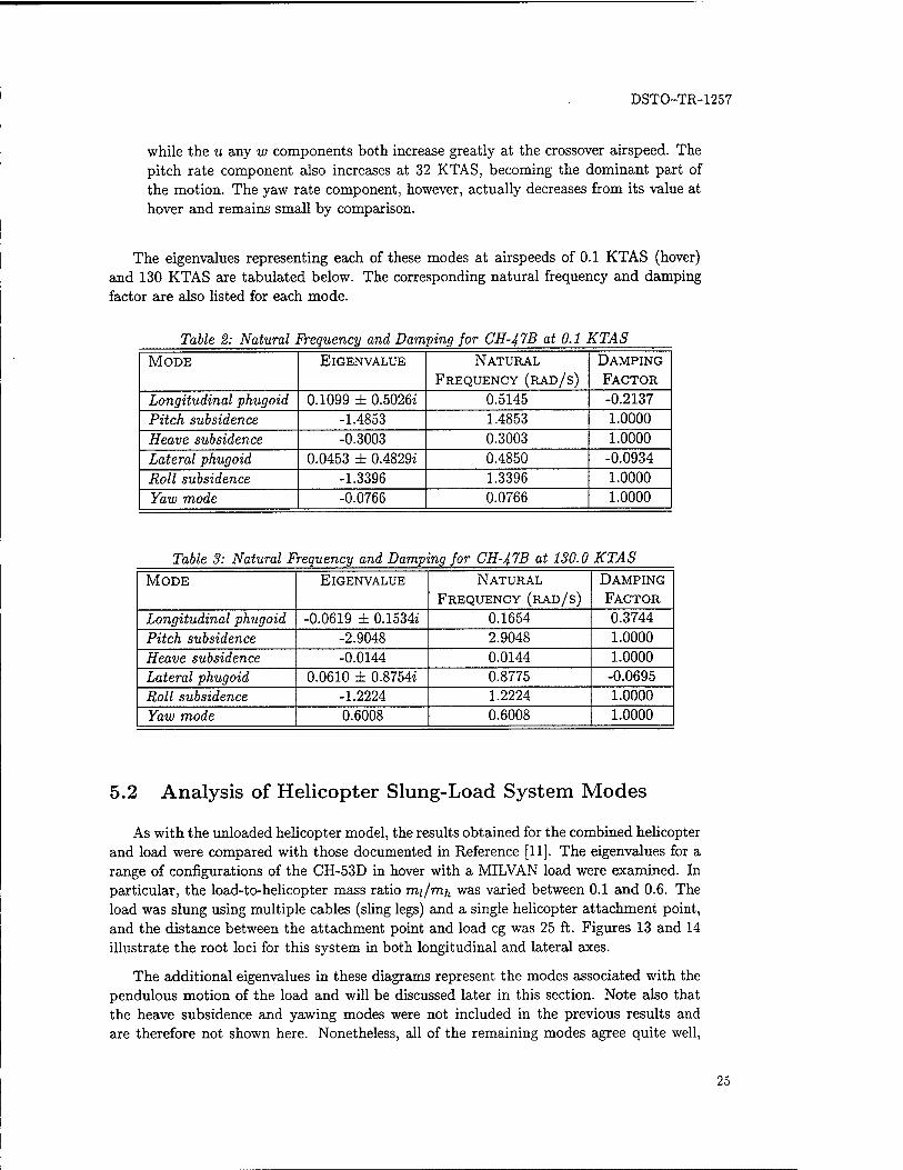
2 Natural Frequency and Damping for CH-47B at 0.1 KTAS 25
3 Natural Frequency and Damping for CH-47B at 130.0 KTAS 25
IX
DSTO-TR-1257
DSTO-TR-1257
Acronyms AFCS Automatic Flight Control System
AOSC Air Operations Simulation Centre
AOD Air Operations Division
AMRL Aeronautical and Maritime Research Laboratory
eg Centre of Gravity
DOF Degrees of Freedom
DSTO Defence Science and Technology Organisation
HSLSIM Helicopter Slung-Load Simulation
KTAS Knots True Airspeed
SAS Stability Augmentation System

DSTO-TR-1257
xn
DSTO-TR-1257
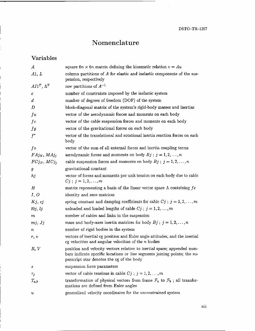
Variables
Nomenclature
A square 6n x 6n matrix defining the kinematic relation v = Au
Al, L column partitions of A for elastic and inelastic components of the sus- pension, respectively
AIlT, AT row partitions of A-1
c number of constraints imposed by the inelastic system
d number of degrees of freedom (DOF) of the system
D block-diagonal matrix of the system's rigid-body masses and inertias
fa vector of the aerodynamic forces and moments on each body
fc vector of the cable suspension forces and moments on each body
fg vector of the gravitational forces on each body
/* vector of the translational and rotational inertia reaction forces on each body
fo vector of the sum of all external forces and inertia coupling terms
FAJN, MAjj aerodynamic forces and moments on body Bj ; j = l,2,...,n
FCJN, MCjj cable suspension forces and moments on body Bj ; j = 1,2,..., n
g gravitational constant
hj vector of forces and moments per unit tension on each body due to cable Cj ; j = l,2,...,m
H matrix representing a basis of the linear vector space A containing fc
I, O identity and zero matrices
Kj, cj spring constant and damping coefficients for cable Cj ; j = 1,2,... ,m
10j, Ij unloaded and loaded lengths of cable Cj ; j = 1,2,..., m
m number of cables and links in the suspension
mj, Jj mass and body-axes inertia matrices for body Bj ; j = 1,2,... ,n
n number of rigid bodies in the system
r, v vectors of inertial eg position and Euler angle attitudes, and the inertial eg velocities and angular velocities of the n bodies
R, V position and velocity vectors relative to inertial space; appended num- bers indicate specific locations or line segments joining points; the su- perscript star denotes the eg of the body
s suspension force parameters
Tj vector of cable tensions in cable Cj ; j — 1,2,..., m
Ta£ transformation of physical vectors from frame Ta to Tb ; all transfor- mations are defined from Euler angles
u generalised velocity coordinates for the unconstrained system
Xlll
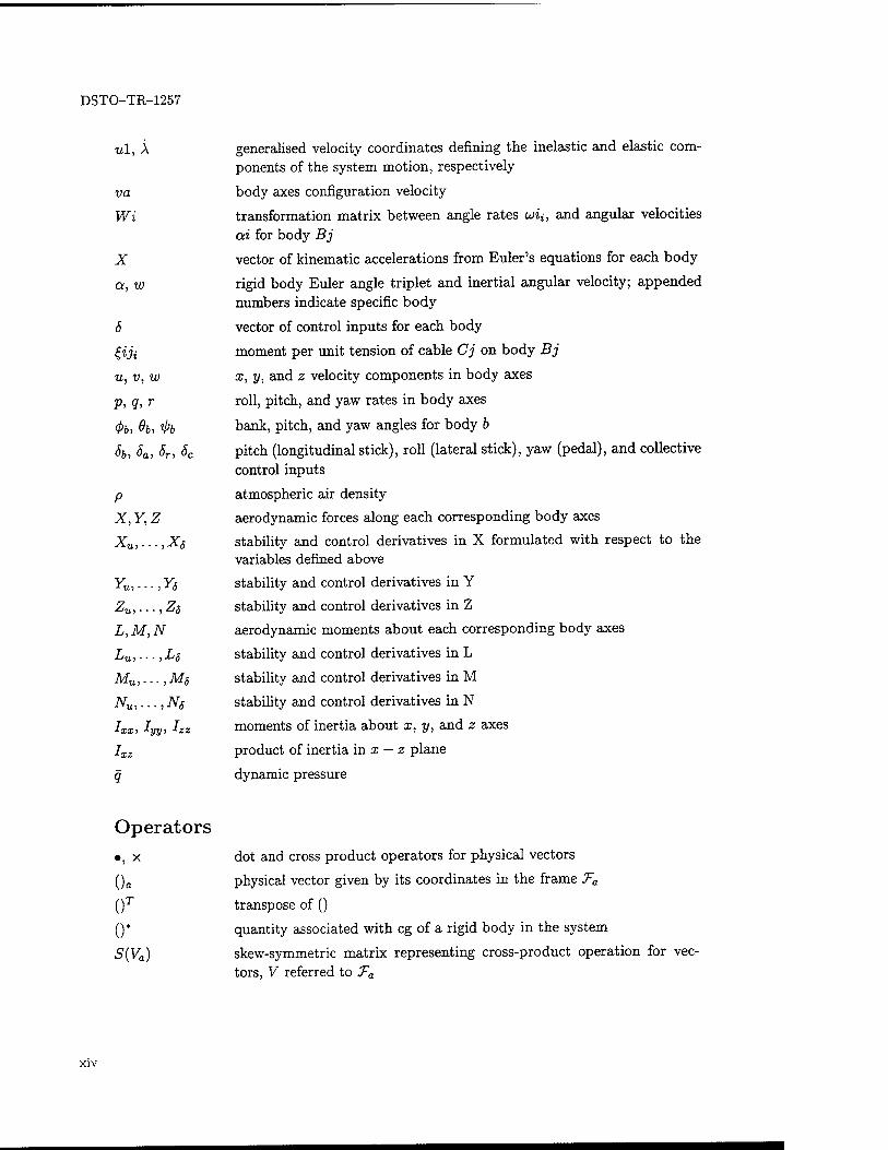
DSTO-TR-1257
K1, Ä generalised velocity coordinates defining the inelastic and elastic com- ponents of the system motion, respectively
va body axes configuration velocity
Wi transformation matrix between angle rates uii, and angular velocities ai for body Bj
X vector of kinematic accelerations from Euler's equations for each body
a, w rigid body Euler angle triplet and inertial angular velocity; appended numbers indicate specific body
ö vector of control inputs for each body
£iji moment per unit tension of cable Cj on body Bj
u, v, w x, y, and z velocity components in body axes
p, <jr, r roll, pitch, and yaw rates in body axes
(f>b, 9b, i>b bank, pitch, and yaw angles for body b
5b,6a,5r, Sc pitch (longitudinal stick), roll (lateral stick), yaw (pedal), and collective
control inputs
p atmospheric air density
X, y, Z aerodynamic forces along each corresponding body axes
Xu,...,Xs stability and control derivatives in X formulated with respect to the variables defined above
Yu,..., Yg stability and control derivatives in Y
Zu,..., Zs stability and control derivatives in Z
L, M, N aerodynamic moments about each corresponding body axes
Lu,...,Ls stability and control derivatives in L
Mu,...,Ms stability and control derivatives in M
Nu,...,Ns stability and control derivatives in N
Ixx, Iyy, Izz moments of inertia about x, y, and z axes
Ixz product of inertia in x — z plane
q dynamic pressure
Operators •, x dot and cross product operators for physical vectors
0O physical vector given by its coordinates in the frame Ta
()T transpose of ()
()* quantity associated with eg of a rigid body in the system
S{Va) skew-symmetric matrix representing cross-product operation for vec- tors, V referred to Ta
DSTO-TR-1257
1 Introduction
The operations of helicopters carrying externally slung loads has often been limited and, in some cases, seriously hindered by stability and control problems. Several incidences have been reported by the Australian Army alone in which aerodynamic excitation or dynamic instability, resulting in uncontrollable oscillations, has forced premature release of the load.
A program was consequently initiated within the Defence Science and Technology Organisation (DSTO) to use computer modelling and simulation to assist in defining the operational limits of the Australian Army CH-47D Chinook when carrying slung loads. The first phase in this program has entailed the development of a simple helicopter slung- load model for simulation and analysis in order to provide a better understanding of the system dynamics and various effects involved. The results from this work are presented here. In the second phase, a more comprehensive helicopter model is to be integrated into the multi-body system. The simulation model will incorporate additional detail, such as the automatic flight control system, load aerodynamics, rotor wake effects, and sling elasticity. Furthermore, there is a requirement to model the dynamics of the helicopter with multiple slung loads of varying mass and aerodynamic properties, which has not previously been investigated in this manner.
In this report, Section 2 presents a broad overview of prior research into helicopter slung-load systems. The three areas of analytical studies, experimental testing and, flight simulation are covered.
Section 3 introduces the equations of motion for a generalised helicopter slung-load model. Both inelastic and elastic formulations are included. The overall simulation pro- cedure is then explained in general terms. The full set of equations which constitute the simulation model are listed in Appendix A.
In Section 4, the results obtained from the analysis of a simple pendulum-type model are presented. These include a comparison of the characteristic system modes and longi- tudinal and lateral simulations of two different configurations.
In Section 5, the dynamics of the helicopter slung-load model are discussed. The modes of the linearised system are displayed over a range of mass and sling configurations and the characteristic behaviour of a Super Stallion CH-53D cargo helicopter with MILVAN container load are compared against previous results.
Finally, some concluding remarks are drawn and proposals for further research made.
DSTO-TR-1257
2 Background
There has been a small but significant amount of work done in investigating the be- haviour and control of helicopter slung-load systems. This work can be roughly divided into three veins: analytical studies, experimental testing, and flight simulation and au- tomatic control. In the early years, most of this effort was concentrated in analytical studies, including various control designs. Experimental testing in flight and wind tunnel was mainly limited to the establishment of operational limits based on gross aerodynamic instabilities. With the advancement of digital computing, however, came the ability to perform dynamic, piloted simulations in real time and develop more complex models. This increase in the complexity of the system led to a requirement for better aerodynamic models — for both helicopter and load — and the emphasis in experimental work shifted accordingly. These days, there is still some analytical work being conducted, particularly in the design of automatic control systems, but much of the research is now undertaken
using simulation.
2.1 Analytical Studies
Some of the earliest studies in helicopter slung-load behaviour was carried out by Lucassen and Sterk [1] in 1965 to provide a better understanding of the dynamics and indicate means to avoid undesirable effects, since they were known to cause a reduction in the helicopter's operational capabilities. In this work, the equations of motion were restricted to the vertical plane with three degrees of freedom (DOF), and load aerody- namics was not included. Later, Dukes [2] used a similar approximation to examine the modes of the system in the frequency domain and explore various feedback and open-loop control systems for damping the pendulous helicopter-load motion. Cliff and Bailey [3] also used a simplified model of a helicopter with a singly tethered load, which neglected all aerodynamics other than drag. In their formulation, the nonlinear equations of motion were linearised about a steady level flight condition, and then the resulting perturba- tion equations were separated into longitudinal and lateral-directional sets. Although the authors were able to make some inferences regarding the stability effects of various param- eters, such as mass ratio and tether length, they suggested that more complete dynamical models needed investigation. An attempt to increase the fidelity of the aerodynamic load model was made by Feaster [4] and Feaster et al [5] using an experimentally determined yaw-damping coefficient in a linearised small perturbation stability analysis, which con- sidered both single-cable and two-cable tandem suspension systems. The results agreed well with the previous model and full-scale tests and also demonstrated that the two-cable tandem suspension system offered a satisfactory means of transporting the standard cargo container examined. Around the same time, Prabhakar and Sheldon [6] and Prabhakar [7] undertook a theoretical study of a Westland Sea King helicopter carrying a standard cargo container on a two point longitudinal suspension. Again, the aerodynamic stability derivatives used in the model were determined through experiment and it was found that the pitch and yaw rate derivatives were strongly destabilising.
Over the following several years, Nagabhushan [8, 9] and Nagabhushan and Cliff [10] produced several reports on the dynamics, stability, and control of helicopters carrying
DSTO-TR-1257
externally suspended loads. Several mathematical models of varying order were developed to describe the dynamics of such systems. However, unlike much of the previous analytical work, which was based on the Newton-Euler equations, the nonlinear formulation was derived from Lagrange's equations for general dynamical systems. In these reports, the low-speed stability characteristics of a conventional helicopter with an external sling load on a single-point suspension were investigated. Typically, towing cable length, towed body-to-vehicle mass ratio, and load factor in a turn were found to affect the stability of the aircraft and its sling load.
In 1986, Ronen [11] and Ronen et cd [12] developed a new model for a helicopter carrying a sling load on a single point suspension in order to improve on the existing dynamic models and investigate the open loop characteristics of the system. For the first time, the model took into account the effects of rotor downwash on the load and the unsteady aerodynamics of bluff-body type loads. The nonlinear equations of motion were derived and then separated into two sets: the nonlinear trim equations and the linearised equations for small perturbation about the equilibrium. More recently, Curtiss [13] derived a full set of equations for the twin lift system, linearised about a hover trim condition.
2.2 Experimental Testing
Although there has been a substantial amount of experimental work in determining the aerodynamic behaviour of various slung loads using wind-tunnels, little has been done through full scale flight-testing. In 1968, Gabel and Wilson [14] presented the results of an extensive program of simulation, wind-tunnel, and flight tests, which were conducted to assist in solving the problems of sling load vertical bounce, sling-leg web flapping, and aerodynamic yaw instability. Some years later, Hone [15] utilised the data from actual flight tests on a Sikorsky CH-54 heavy-lift helicopter to investigate the validity of a model developed by Briczinski and Karas [16]. The aim of this work was to explore phenomena associated with the carriage of externally suspended loads on helicopters, and to establish more reliable strength requirement data for the load slings and their interfaces.
Other work in experimental testing includes those presented by Kesler et al [17], Feaster [4], Feaster et al [5], and Matheson [18].
2.3 Flight Simulation and Control
One of the first investigations into automatic control for helicopters with slung loads was conducted by Wolkovitch and Johnston [19] in 1965. The single-cable dynamic model was developed in a straightforward application of the Lagrange equations. Abzug [20] later expanded on this model to consider the case of two tandem cables. However, his formulation was based on the Newton-Euler equations of motion for small perturbations, separated into longitudinal and lateral sets. Aerodynamic forces on the cables and the load were neglected, as were the rotor dynamic modes.
In recognition of suspension-related problems encountered with the carriage of external cargo by helicopters, the US Army in 1970 initiated a program aimed at the establishment of design criteria for sling members and hard-points. This program, as well as many
DSTO-TR-1257
subsequent investigations, were undertaken by the Eustace Directorate, US Army Air Mobility Research and Development Laboratory (USAAMRDL). Part of the first phase in the contract, reported by Briczinski and Karas [16], involved the computerised simulation of a helicopter and external load in real time with a pilot in the loop. Load aerodynamics were incorporated into the model, as well as rotor-downwash effects in hover. Soon after this program, Liu [21] conducted an extensive study to select the best technical approaches for stabilising a wide spectrum of externally slung helicopter loads at forward speeds. The simulation model used extended that of Abzug [20] to include load aerodynamics. Several stabilisation systems were evaluated using a moving-base simulator and of those, an electronic system providing rate and acceleration inputs to the helicopter's stability augmentation system (SAS) was favoured. The design and assessment of automatic control systems continued with Asseo and Whitbeck [22] in their paper on the control requirements for sling-load stabilisation. Linearised equations of motion of the helicopter, winch, cable, and load complex were developed for a variable suspension geometry and were then used in conjunction with modern control theory to design several control systems for each type of suspension. The next year, Gera and Farmer [23] examined the feasibility of stabilising external loads by means of controllable fins attached to the cargo. In their simple linear model representing the yawing and the pendulous oscillations of the slung-load system, it was assumed that the helicopter motion was unaffected by the load.
Following the first program of work sponsored by the Eustace Directorate, a further study to define important flight control system design and handling qualities criteria for moving loads slung beneath tandem-rotor helicopters was conducted by Kesler et al [17]. It included theoretical analyses, acquisition, and evaluation of both wind tunnel and flight test data, analysis of various problems, and the actual flight simulation of a Model-347 advanced tandem-rotor helicopter with an external load. Another program under the same sponsorship, investigated by Alansky et al [24], looked into the quantitative limitations of the CH-47 helicopter performing terrain flying with external loads. The simulation used in this investigation comprised a fully coupled total force and moment model and an alternative method of load-control named the Active Arm External Load Stabilisation System (AAELSS).
Some time later, a generalised real time, piloted, visual simulation of a single rotor helicopter, suspension system, and external load was developed by Shaughnessy et al [25], and subsequently validated for the full flight envelope of a CH-54 helicopter and cargo container. The mathematical model described used modified nonlinear classical rotor theory for both the main rotor and tail rotor, nonlinear fuselage aerodynamics, an elastic suspension system, nonlinear load aerodynamics, and a load-ground contact model.
In 1980, Sampath [26] completed his PhD dissertation on the dynamics of a tandem- rotor helicopter slung-load system, which involved modelling and simulation as well as experimental wind-tunnel tasks. In his formulation, Lagrange's equations were used to write the equations of motion and were divided into two sets: one for the towing vehicle and the other for the slung load. The cables of the sling were modelled as massless linear springs with viscous damping and no aerodynamic properties. The aerodynamic models for the helicopter and load were both implemented using tabulated static data. Some years later, a full nonlinear simulation model of the CH-47B helicopter, developed by the Boeing Vertol Company, was adapted for use in the NASA Ames Research Center (ARC) simulation facility by Weber et al [27]. The mathematical model developed was based
DSTO-TR-1257
on a total force approach in six rigid-body DOF along with the option for an externally- suspended load in three DOF. The aerodynamic models were also quite comprehensive, including steady-state rotor flapping and load aerodynamic effects.
More recently, research into the automatic control of load dynamics has continued with Raz et al [28] in an investigation of an active aerodynamic Load Stabilisation System (LSS) for a helicopter sling-load system. The general theoretical model used was based on previous work [11] for configurations with a single suspension point.
Some of the most recent work in the simulation of helicopter slung-load systems has been conducted by Cicolani and Kanning [29, 30] and Cicolani et al [31] at the NASA ARC. In this work, the general simulation equations were derived for the motion of slung- load systems consisting of several rigid bodies connected by straight-line cables or links, assumed to be either elastic or inelastic. A formulation for the general system was obtained from the Newton-Euler rigid-body equations with the introduction of generalised velocity coordinates. The same approach for simulating helicopter slung-load dynamics has been adopted in the current work at AMRL. In addition, the equations of motion have been extended to the case of multiple loads with disparate mass and aerodynamic characteristics and sling configurations.
2.4 Surveys and Overviews
In his book on the dynamics of helicopter flight, Saunders [32] devoted one section to piloting problems associated with the carriage of external loads. The normal trim state and origins of load oscillation were first examined using a simple helicopter-load mass model. Various problems, including uncontrollable load oscillations, aerodynamic excitation, active control, and poor visibility were then discussed in a broad context.
In 1976, Matheson [18] compiled a review of the developments and data concerning the operation of helicopters with slung loads. The report focused on the problems of aerodynamic instability, vertical bounce, and sling-leg flapping. Methods for reducing these instabilities and procedures for extending the operating limits of a helicopter with different types of slung loads were also discussed.
Around the same time, Shaughnessy and Pardue [33] conducted a survey of the heli- copter sling load accident/incident records provided by various US organisations for the period from 1968 to 1974. From the data, the highest percentage of accidents occurred during hover, and it was therefore concluded that hovering was the most critical sling load flight operation. Furthermore, the accidents and incidents caused by swinging loads during cruise were generally much less severe than the hover mishaps.
DSTO-TR-1257
3 System Representation
3.1 Description of System
Helicopter slung-load systems fall into a class of multibody dynamic systems consisting of two or more rigid bodies connected by massless links. The links can be considered either elastic or inelastic, although the rigid-body assumption excludes any helicopter or load elastic modes. Typically, the system is characterised by the configuration geometry, mass, inertia, and aerodynamic behaviour of both helicopter and load, as well as the elastic properties of the links.
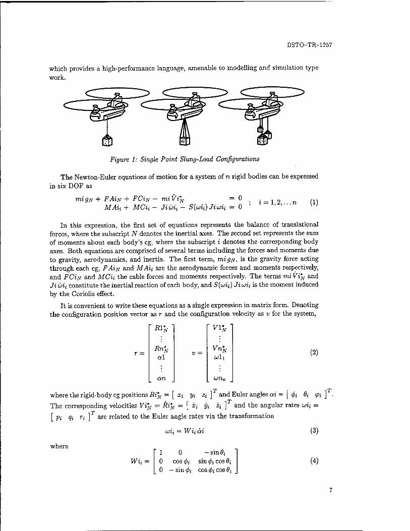
In general terms, the system of interest consists of a single helicopter supporting one or more loads by means of some suspension. Several examples of the various configurations under consideration are illustrated in Figure 1. The model is comprised of n rigid bodies, Bl,B2,...,Bn, with m straight-line links supporting a single force in the direction of the link. For cables, this is strictly a tensile force — cable collapse is not considered. If the links are modelled as inelastic, c(<m) holonomic constraints1 are imposed on the motion of the bodies and the system has d = 6n - c DOF. If the links are modelled as elastic, there are 6n DOF.
In the model used, a number of simplifying assumptions were made. These included the exclusion of cable aerodynamics and rotor-downwash effects. Furthermore, load aero- dynamics have been neglected for this initial stage of the work. Despite these limitations, the system defined above has proven adequate for simulation studies [31] in which the low-frequency behaviour is of primary interest.
3.2 Generalized Equations of Motion
The simulation model used for this first stage of work was based on the helicopter slung-load system introduced by Cicolani and Kanning [29]. In this formulation, the general system equations of motion are obtained from the Newton-Euler equations in terms of generalised coordinates and velocities. Following the explicit constraint method, which utilises d'Alembert's principle, the system is partitioned into coordinates such that the motion due to cable stretching is separated from that due to rigid-body, coupled dynamics. As a consequence, the constraint forces appear explicitly and a solution to the resultant generalised accelerations is determined by assuming a simple spring model for the cable.
It is also possible to obtain a solution to the inelastic approximation by nulling the stretching coordinates to obtain an explicit relation for the suspension forces. The result is computationally more efficient than conventional procedures and is readily integrated with the formulation for elastic suspension. Another benefit of the formulation is that it is easily applied to complex, multiple body systems, as in the current work. To date, all code development has been done in the MATLAB numerical computing environment,
'Holonomic constraints represent excess coordinates which are independent and can be eliminated through equations of constraint.
DSTO-TR-1257
which provides a high-performance language, amenable to modelling and simulation type work.
Figure 1: Single Point Slung-Load Configurations
The Newton-Euler equations of motion for a system of n rigid bodies can be expressed
in six DOF as
mi 5JV + FAitf + FCix — mi Vi*N = 0 . _ MAii+ MCU - Jidiii— S(wii)Jicüii = 0 ' > >••• (1)
In this expression, the first set of equations represents the balance of translational forces, where the subscript N denotes the inertial axes. The second set represents the sum of moments about each body's eg, where the subscript i denotes the corresponding body axes. Both equations are comprised of several terms including the forces and moments due to gravity, aerodynamics, and inertia. The first term, migx, is the gravity force acting through each eg, FAi^ and MA%i are the aerodynamic forces and moments respectively, and FCiN and MCii the cable forces and moments respectively. The terms mi Vi*N and Ji Coii constitute the inertial reaction of each body, and S(wii) Ji uiii is the moment induced by the Coriolis effect.
It is convenient to write these equations as a single expression in matrix form. Denoting the configuration position vector as r and the configuration velocity as v for the system,
r =
R1*N 'vvN
Rn*N
al v =
Vn*N
wli
an wnn
(2)
where the rigid-body eg positions Ri*N = [ xi
The corresponding velocities Vi*N = Ri*N =
rp r
yi Z{ ] and Euler angles ai = [ <j>i 6i <pi\ rp
[ ii yi Zi ] and the angular rates uii =
Pi Qi n
where
are related to the Euler angle rates via the transformation
cüii = Wii äi
Wii = 1 0 -sinöj 0 cos fa sin <pi cos 6i 0 — sin fa cos 4>i cos Qi
(3)
(4)
DSTO-TR-1257
Using fg, fa, fc, and /*, for the combined force-moment vectors due to gravity, aerodynamics, cable suspension, and inertia plus Coriolis effects, the equations of motion can be written
fg + fa + fc + f* = 0 (5)
where
fg =
mlgN
mngN
0 fa =
FA1 N
FAUN
MAh
MAnn
fc =
FC1 N
FCnN
MCh
MCnn
(6)
and
where
f* = -Dv - X (7)
D
ml
mn Jl
Jn
X = 0
S{uh)Jluh
S(umn) Jn umn
(8)
Here, D is a block-diagonal matrix comprising masses and inertias along the main diagonal, v is the configuration acceleration and the matrix X contains the Coriolis terms due to the use of rotational coordinates in body-axes
In order to derive a set of simulation equations for the system, a solution to the equa- tions of motion described above must be found; that is, an expression for the configuration acceleration in terms of the system states and applied forces. For the helicopter slung-load system under consideration, it is useful to first formulate a set of generalized coordinates and velocities which describe the motion of the inelastic system and the effect of cable stretching as two distinct subsets. An inelastic system with n bodies and c constraints will have d = 6n - c DOF. The cable constraints on the helicopter slung-load system can be considered holonomic. In addition, for the following system, the constraints will be posed as time invariant. The special cases of cable winching and attachment-point movement are not considered.
The system can be partitioned according to the 6n generalized position coordinates as follows:
<? = A (9)
where ql is the list of d position coordinates for a system with inejastic suspension and A are the c coordinates which describe the variation in cable length due to stretching. The configuration velocity can be expressed as a linear function of the generalized velocity coordinates
v = Au (10)
DSTO-TR-1257
where «I X
Al L
Differentiating Equation (10) and substituting v into Equation (7) yields
/* = -DÄu - DAü - X
(11)
(12)
Now, replacing /* in Equation (5), the following simplified version of the equations of motion can be written:
fo + fc- DAü = 0 (13)
where the vector fo is the sum of all external forces and inertial coupling terms, i.e.
fo = fg + fa- DAu - X (14)
Since the system has been specified in terms of its generalized coordinates, A is a square 6n x 6n nonsingular matrix and a solution for the generalized acceleration coordinates exists. Prom Equation (13), the acceleration equation is
u = A-1D-1[fo + fc] (15)
It should be noted here that the inverse matrix A-1 simply represents the relation u(v) that can be derived analytically from the kinematics. Therefore, it is unnecessary to perform a costly numerical inversion to obtain ü. In partitioned form, the acceleration equation is
«1 Ä
All1
AT D-l[fo + fc) (16)
where AIlT and AT are the 6n — c and c rows of A'1 which define the relations til and Ä respectively. From the first set of equations representing the inelastic component, the solution for til is
til = AIlTD-1 [fo + fc] (17)
The second set of equations represents the elastic component
X = ATD-1[fo + fc] (18)
An alternate formulation for the accelerations til can be obtained by first differentiating the expanded form of the configuration velocity from Equation (10) as follows:
v = Alul + L\
and then substituting into Equation (7) to give
/* = -DÄlul - DAlül - D(LX + LX)-X
If fo is redefined: fo = fg + fa- DAlul - X
(19)
(20)
(21)
DSTO-TR-1257
then replacing /* in Equation (5) and solving for ül produces
Ü1 = [A^DAlj^A^ifo - D{L\ + LX) + fc] (22)
The last step required in determining a solution for the generalized accelerations is to calculate the constraint force fc. For a system with c constraints, the constraint force can be expressed as
fc = Hs (23)
where the columns of the matrix H are configuration vectors and rank H = c. The elements of the vector s are arbitrary scalars to be determined. The exact form of this equation and its solution depend on whether the cables are considered elastic or not.
Elastic System
For a general elastic system with M cable-body attachments, the suspension forces on each body can be given as the sum of forces and moments applied at each attachment point on that body, i.e.
M
/c = £>>,• (24)
o=i
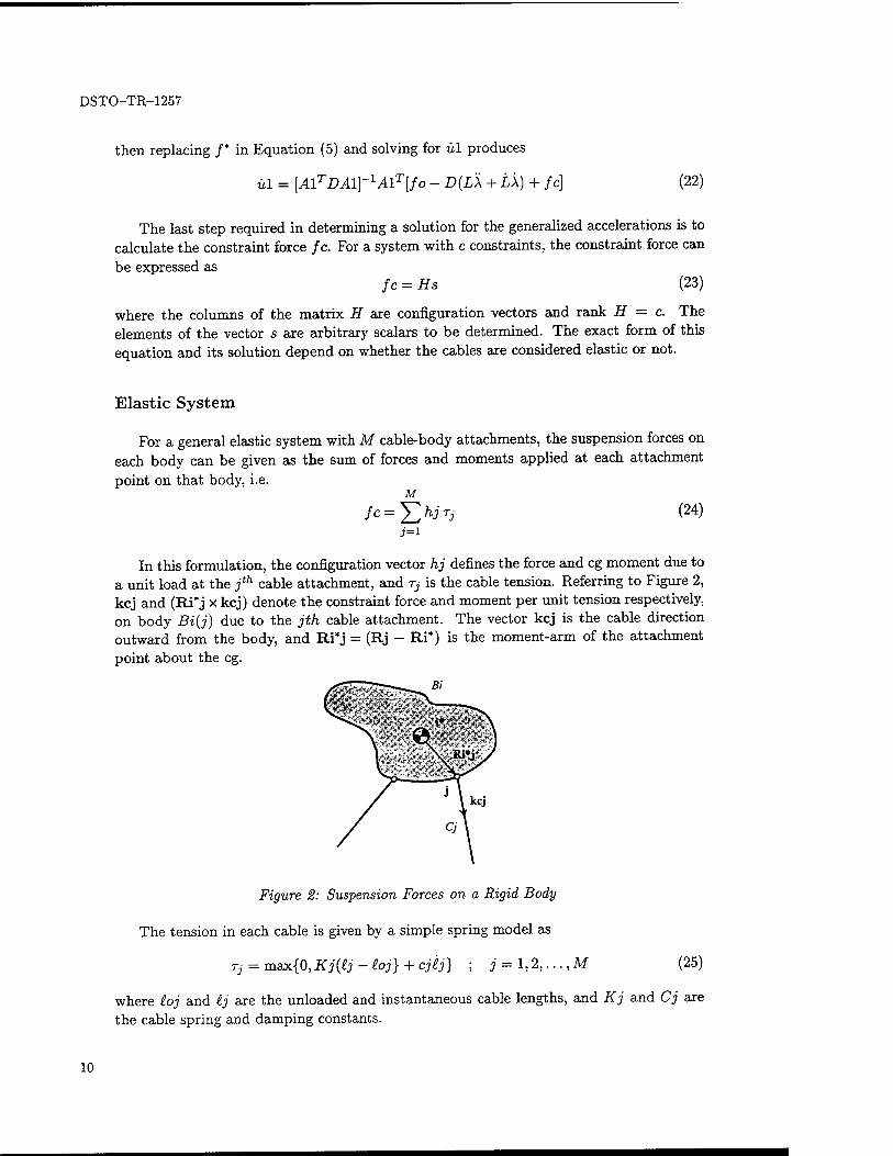
In this formulation, the configuration vector hj defines the force and eg moment due to a unit load at the jth cable attachment, and TJ is the cable tension. Referring to Figure 2, kcj and (Ri*j x kcj) denote the constraint force and moment per unit tension respectively, on body Bi{j) due to the jth cable attachment. The vector kcj is the cable direction outward from the body, and Ri*j = (Rj - Ri*) is the moment-arm of the attachment point about the eg.
Figure 2: Suspension Forces on a Rigid Body
The tension in each cable is given by a simple spring model as
Tj = max{0, Kj(tj-loj} + cjij} ; ; = 1,2,...,M (25)
where £oj and tj are the unloaded and instantaneous cable lengths, and Kj and Cj are the cable spring and damping constants.
10
DSTO-TR-1257
Inelastic System
It can be shown that the columns of H and A both form bases of the same linear vector space and therefore A can be used to define the constraint force, i.e.
fc = As (26)
where the vector s will have units of force if the coordinates A are lengths. To find a solution for the inelastic system, the constraint acceleration is set to zero, i.e. A = 0. Substituting into Equation (18) gives
0 = ATD-1[fo + As] (27)
the solution to which is s = -[ATD-1A]-1ATD-lfo (28)
3.3 Simulation of Helicopter Slung Load System
Prior to executing the simulation, several components must be customised to the helicopter slung-load configuration of interest.
The first step in setting up the simulation equations involves determining the con- straints of the inelastic system and then defining the generalised velocity coordinates (ul, Ä). Using these coordinates in kinematic relations for the system, it is then possible to obtain expressions for the system matrices A, A'1, and A. The selection of appropriate coordinates is case specific; however, it is possible to choose them so that they consist largely of natural vectors. In most applications, including that discussed in this report, u is comprised of the eg velocity of a reference body (typically the helicopter), the cable velocities, and the angular velocities of all bodies including both helicopter and loads.
Next, an appropriate representation for the suspension cables must be chosen. For inelastic cables, fc is calculated from any basis of the constraint force space A and the corresponding constraint force parameters s as in Equation (28).
For the last step, the aerodynamic and inertial properties of both the helicopter and loads need to be implemented in the model. For most rigid bodies, the aerodynamic forces and moments are a function of the configuration velocities and displacements v and r, and the control inputs 6. Typically, the helicopter aerodynamic model neglects position-dependent and acceleration-dependent effects such as interbody-ground interfer- ence and unsteady aerodynamics. However, these are often secondary in nature and the resulting model is adequate for simulation under most conditions. Aerodynamic models for loads, which are generally unsteady and of much higher order, axe less well understood or replicated.
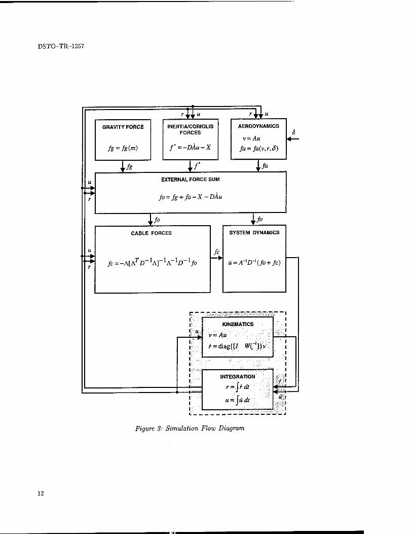
Once the system has been configured, the dynamic simulation can proceed. First, the initial state (u,r) and the trim state (uo,r0) must be set. Then the integration loop is started and the following steps are executed in sequence, according to the flow-diagram of Figure 3:
11
DSTO-TR-1257
GRAVITY FORCE
fg=fg(m)
-\nr
INERTIA/CORIOLIS FORCES
f'=-DÄu-X
fg
ynr
AERODYNAMICS
v = Au fa = fa(v,r,8)
f fa
EXTERNAL FORCE SUM
fo = fg + fa-X-DAu
fa
CABLE FORCES
fc = -A[ATD~ :A]~! A" lD~ lfo
fa
fa
SYSTEM DYNAMICS
ü = A-iD-\fo + fc)
KINEMATICS
v = Aü
INTEGRATION
r = jrdt
umlädt
Figure 3: Simulation Flow Diagram
12
DSTO-TR-1257
1. Determine the aerodynamic force fa, inertia, and Coriolis forces /*, and gravity force fg, all in inertial axes. Assuming the aerodynamic model is written in body axes, an angular transformation will be required for fa. The configuration velocity v can be calculated from the generalised velocity u using the kinematic matrix A.
2. Sum the external forces fa, /*, and fg to yield the configuration force fo.
3. Using the configuration force along with matrices derived from the current state (u, r) and the configuration geometry, solve the cable force fc for either elastic or inelastic suspension models.
4. Compute the generalised accelerations ü from the inverse kinematic matrix A-1, and the inverse mass matrix D~l.
5. Compute the velocity r from the configuration velocity and inverse transformation matrix W~l.
6. Apply an integration step to predict the new state (u, r) and repeat the sequence.
At this early stage, all code development has been done in the MATLAB [34] numerical computing environment, which provides a high-performance language amenable to mod- elling and simulation work. It is important to stress that this pilot simulation was not intended to run in real time, but rather produce the appropriate output for subsequent re- play and analysis. At a later stage, the code will be ported to a platform-specific compiled language suitable for piloted, real time simulation.
The Helicopter Slung-Load Simulation (HSLSIM) program, consists of several modules. These including the main script, integration function, differential equation solution, aero- dynamic model, and various output and replay functions. The simulation is run through the main script, which generates the control inputs, configures the helicopter-load system properties (geometric and inertial), sets the initial system state, and then executes the integration function. The integration function ODE45 is problem independent and based on an algorithm which combines 4th and 5th order Runge-Kutta formulas for ordinary dif- ferential equations. It requires a function tailored to the problem at hand, which provides a point solution to the differential equation. For the helicopter slung-load simulation, this function represents the core of the code and implements much of the above flow diagram. The aerodynamic models for both helicopter and loads are called from within this func- tion. They can be as simple or as complex as desired, but must output total force and moment variables. Hence, if small-perturbation aerodynamic models are to be used, they must be augmented with the corresponding trim forces and moments. The cable elastic model can also be implemented as a separate function, although this was not done, since the spring-damper model is fairly standard and easily included in the solution function. Following summation of the external forces and solution of the internal (cable) forces, the solution function computes the generalised accelerations and velocities (ii, r) at the current state. This point solution is passed to the integration function and the simulation loop continues.
It is also possible to calculate a linear model by numerical approximation of the Jaco- bians yau and \/sü from the nonlinear system.
13
DSTO-TR-1257
This model will have the form
« = [Vutt]« + [V<5^]£ (29)
and can be used for an alternative linear simulation about the trim state. Another use is in various linear system analyses, such as the determination of the natural modes, which will be discussed in the following section.
14
DSTO-TR-1257
4 Simple Pendulum System Dynamics
The first phase of the analysis involved an investigation of the dynamics of pendulum- type systems. For this purpose, the full helicopter slung-load simulation model developed in Section 3 was constrained so as to approximate a two-body pendulum system. Fur- thermore, the aerodynamic effects of both helicopter and load were excluded from the model.
4.1 System Properties
The simulation was validated for both free and constrained models using the system given in Reference [11] for a CH-53D helicopter with a single slung load. The CH-53D is a twin-turbine, main and tail rotor transport helicopter with mass and inertia properties as outlined below.
MASS (lb) MOMENTS OF INERTIA (slug.ft2) mh 1-xx *yy Izz *xz
35000 36100 191500 179200 14800
The slung load chosen was a standard military container, known as a MILVAN, which is a common helicopter cargo used in many commercial and military operations. The dimensions of a MILVAN container are 20 x 20 x 8 ft and the mass typically varies from 4000 lb (empty) to 20000 lb (full). In the Reference cited above, examples with masses outside this range were also checked to demonstrate very low density and very heavy loads. The moments of inertia for the container load were approximated with linear functions of its mass by
Ixx = 0.33 * mi Iyy = Izz = 1.20 * mi (30)
where the moments of inertia are in slug.ft2 and the mass is in lb.
4.2 Analysis of System Modes
In order to validate the simulation developed, comparisons were made against those previously reported in a numerical example given in Reference [11]. In addition, analyt- ical results were calculated for the modes of similar pendulum systems. The governing equations for these systems are detailed in Appendix B, along with several simplifying approximations and solutions to each in terms of their natural frequencies.
For the example cited, the mass ratio is mi/mh = 0.05. Using Equation (30), this yields the following load properties,
MASS (lb) MOMENTS OF INERTIA (slug.ft2) TTli lXx -lyy *zz -*xz
1750 577.5 2100 2100 0
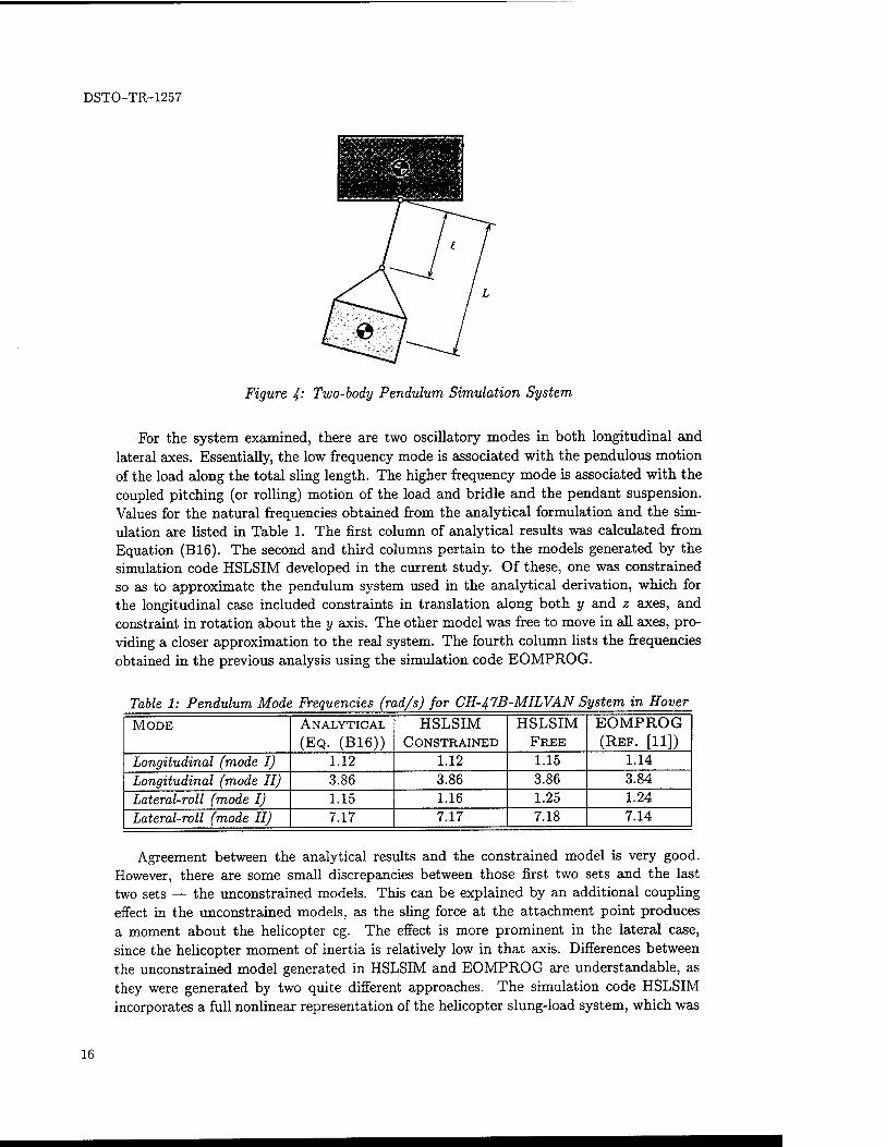
The sling configuration used consisted of a single pendant suspension and bridle, as illustrated in Figure 4. The total sling length L between helicopter attachment point and the load eg is 25 ft, and the pendant-to-sling length ratio tjL is 0.6.
15
DSTO-TR-1257
Figure 4: Two-body Pendulum Simulation System
For the system examined, there are two oscillatory modes in both longitudinal and lateral axes. Essentially, the low frequency mode is associated with the pendulous motion of the load along the total sling length. The higher frequency mode is associated with the coupled pitching (or rolling) motion of the load and bridle and the pendant suspension. Values for the natural frequencies obtained from the analytical formulation and the sim- ulation are listed in Table 1. The first column of analytical results was calculated from Equation (B16). The second and third columns pertain to the models generated by the simulation code HSLSIM developed in the current study. Of these, one was constrained so as to approximate the pendulum system used in the analytical derivation, which for the longitudinal case included constraints in translation along both y and z axes, and constraint in rotation about the y axis. The other model was free to move in all axes, pro- viding a closer approximation to the real system. The fourth column lists the frequencies obtained in the previous analysis using the simulation code EOMPROG.
Table 1: Pendulum Mode Frequencies (rad/s) for CH-47B-MILVAN System in Hover
MODE ANALYTICAL
(EQ. (B16)) HSLSIM
CONSTRAINED
HSLSIM FREE
EOMPROG (REF. [11])
Longitudinal (mode I) 1.12 1.12 1.15 1.14
Longitudinal (mode II) 3.86 3.86 3.86 3.84
Lateral-roll (mode I) 1.15 1.16 1.25 1.24
Lateral-roll (mode II) 7.17 7.17 7.18 7.14
Agreement between the analytical results and the constrained model is very good. However, there are some small discrepancies between those first two sets and the last two sets — the unconstrained models. This can be explained by an additional coupling effect in the unconstrained models, as the sling force at the attachment point produces a moment about the helicopter eg. The effect is more prominent in the lateral case, since the helicopter moment of inertia is relatively low in that axis. Differences between the unconstrained model generated in HSLSIM and EOMPROG are understandable, as they were generated by two quite different approaches. The simulation code HSLSIM incorporates a full nonlinear representation of the helicopter slung-load system, which was
16
DSTO-TR-1257
linearised numerically about the trim state to obtain a Jacobian matrix for model analysis (see the following section). Using this Jacobian matrix approach would therefore incur errors from the numerical approximation. EOMPROG, on the other hand, is based on an explicitly linear small-perturbation formulation and, consequently, errors would arise from such simplification as the small angle assumptions and the exclusion of higher order terms.
It is also interesting to see how the analytical solution compares with the unconstrained simulation model HSLSIM for a range of configurations. Figures 5 and 6 show the variation in natural frequency for the longitudinal pendulum modes with load-to-helicopter mass ratio mijrnh and pendant-to-sling length ratio £/L, respectively. Clearly, there is quite a large difference in the higher frequency mode over the range of £/L with a smaller deviation in the lower frequency mode. The analytical approximation is most accurate at a length ratio of 0.6, but outside this differs dramatically. At a length ratio of 0.1, the error is close to 50% of the frequency predicted by HSLSIM. At a length ratio of 0.9, the error is approximately 120%. There is less difference in the modes over the range of mi/rnh- For the configurations examined, the largest error of 20% occurred in the lower frequency mode at a mass ratio of 1.0. This error improved as the mass ratio was decreased, reaching a level of 5% at a ratio of 0.1. Both of these discrepancies are due to the simplification of the analytical model, which prohibits any pitching motion about the helicopter eg. Therefore, as a result of this test, one can conclude that the analytical approximation given in Appendix B is only appropriate for low load-to-helicopter mass ratios and moderate pendant-to-sling length ratios (0.6 for the system examined).
4.3 Longitudinal and Lateral Simulations
Following linear analysis of the modes, several simulations were run so as to gain a better picture of the inherent dynamic behaviour of the slung-load system. Simulations of both longitudinal and lateral subsystems were conducted. From the longitudinal simula- tions, two cases have been selected for inclusion here to illustrate the effect of heavy loads on the helicopter response. From the lateral simulations, two cases are included, which demonstrate the instability in yaw for a multiple-load system.
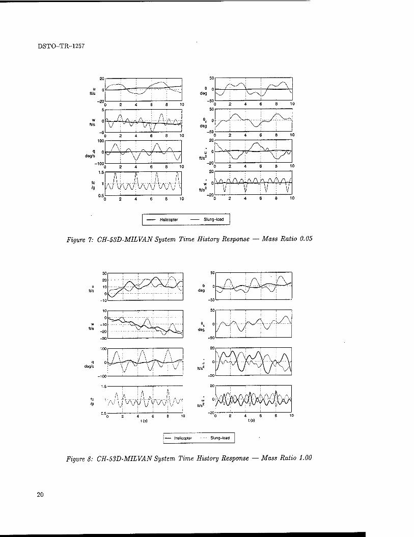
For the longitudinal simulations, the helicopter-load configuration was the same as that used in the linear analysis, i.e. a CH-53D helicopter and MILVAN load attached by a single pendant suspension. It was also constrained in the lateral-directional axes, as before. The slung load was initially offset from its static equilibrium position at hover, with the sling cable set at -30° in pitch and the load at -15°. It was then allowed free response over the 10 s duration. The time history response plots for two different load configurations, with mass ratios of 0.05 and 1.0, are presented in Figures 7 and 8, respectively. In the first set of plots, it can be seen that the load, with a small mass compared to the helicopter, has very little effect on the helicopter motion, as expected. Both low and high pendulum natural frequencies (0.18 and 0.61 Hz) of the load can be readily identified in the traces of forward velocity and pitch rate, respectively. The normal acceleration and cable force oscillate at approximately twice the high pendulum natural frequency and are highly correlated, with peaks at the pitch rate extremes (0.36 Hz). For the cable force, these peaks have magnitudes which are roughly 1.5 times the static load. The longitudinal
17
DSTO-TR-1257
6 , , , 1 , i i
Analytical 5.5 O MöLbIM
<° 5 rad/s
4.5
4 (
:mode II ;
>__ ©- —y -9 —T—
3.5
3
2.5
2
1.5
: : : : : Q o ; mode 1 ■ ö ?
>___-2—-2—-T ! ! : ; : i i i J 1 1 1 1
0.1 0.2 0.3 0.4 0.5 0.6 0.7 0.8 0.9 1 m,/m.
I h
Figure 5: CH-53D-MILVAN System Longitudinal Pendulum Modes - Variation in Fre- quency with Load-to-Helicopter Mass Ratio
, 1 1 i i
14(
O HSLSIM
w 12 rad/s
10
8
p
\ c 3
6
4
2
: mode II
——-—_■ °
; I.mode.l... 6
c 3 (
n i i i J i i i 0.1 0.2 0.3 0.4 0.5 0.6 0.7 0.8 0.9
l/L
Figure 6: CH-53D-MILVAN System Longitudinal Pendulum Modes - Variation in Fre- quency with Pendant-to-Sling Length Ratio
18
DSTO-TR-1257
acceleration is also highly correlated with the cable angle. In the second set of plots, it is clear that the load, now with mass equal to the helicopter, has had a significant effect on the helicopter motion. The pendulum natural frequencies are also less well defined (0.30 and 0.64 Hz). Unlike the first simulation, in this case the helicopter reaches velocities of similar magnitude, as the load and the accelerations in forward and normal directions are out of phase by 180°. Once again, the cable force oscillates at approximately twice the high pendulum natural frequency, with peaks near the pitch rate maxima (0.33 Hz).
For the lateral simulations, a CH-47B helicopter and two box containers attached by multiple (bridle) cables were used. The helicopter was constrained in the longitudinal and lateral axes, which restricted it to a yawing/side motion. The forward-attached slung load was initially offset by a bank angle of -30° so as to be displaced to the starboard side of the helicopter, and the aft-attached slung load was offset by an angle of 30°, resulting in a displacement to the port side. Once again the system was allowed free response over 10 s. The time history response plots are presented in Figures 9 and 10, for configurations with total mass ratios of 0.05 and 1.0. From these plots, the symmetric nature of one of the pendulum modes can be seen. Specifically, the velocity component v, bank angle <p, pitch angle 0, and acceleration component v for each load is 'mirrored' by the other. Slight deviations have come about because of the different attachment point locations with respect to the helicopter eg. It is also important to note that there is a very low frequency response in yaw for both helicopter and load, which manifests itself through the yaw rate r and azimuth angle ip. Although these two traces seem to be diverging, they are actually just at the start of a long period (< 0.01 Hz) oscillation. This oscillation has an amplitude of approximately 160° in the helicopter azimuth angle. The effect of the loads swinging in this manner therefore has a significant influence on the yaw of the helicopter.
19
DSTO-TR-1257
20
u o ft/s
-20 (
5
w o ft/s
100
<? o deg/s
-100 I
1.5
V. *x?
8 10
>..,.A^/!\ V :' \/\
8 10
A ̂\ v
/ V ZA ̂r /\
6 8 10
;\ •■/
/g '[/VVW 0.5
i y... ...A ,.,.
v V V " v v '
8 10
20
ft/s' -20
I 20
\
8 10
-20 tt/s2 V; v i v ; V
6 8 10
Helicopter Slung-load
Figure 7: CH-53D-MILVANSystem Time History Response — Mass Ratio 0.05
8 10
Helicopter Slung-load
Figure 8: CH-53D-MILVAN System Time History Response — Mass Ratio 1.00
20
DSTO-TR-1257
ft/s
ft/s
deg/s
fc /g
-1
40
20
0
-20
1.5
4 6 Us)
:\/
/
8 10
♦ 0 deg
-50
20
8 0 deg
-20
200
100
deg o
-100
20
ft/s'
-20
X/'~N- /"" \.-~\ -''V>f\.- ̂ w
,'-NJ /^ v \ \
A V 4 6
t(s) 8 10
— Helicopter Aft Load Forward Load
Figure 9: CH-47B with Dual Load System Time History Response Ratio 0.025
Individual Mass
20
ft/s
A^~^\. '
Vj'V y s - ' y / '-V
f~\
vA/ ^x ^-^
4 6 t(s)
8 10
deg
50
6 oh deg
ft/s"
-20
: : / '. „ : / \ /
" T-'IV. A
\ / A \/' X
\ A \ A _A 4 6 8 10
t(s)
— Helicopter Aft Load Forward Load
Figure 10: CH-47B with Dual Load System Time History Response — Individual Mass Ratio 0.50
21
DSTO-TR-1257
5 Helicopter Slung-Load Dynamics
The second phase of the analysis examined the dynamics of the full helicopter slung- load simulation model. Both the CH-53D and the CH-47B helicopters with various slung- load configurations were considered. These models were free in all axes and incorporated basic helicopter aerodynamics.
The CH-53D helicopter model was essentially the same as used in the previous section, but with the inclusion of aerodynamic effects. Furthermore, the same MILVAN slung load was used in all of the single-load configurations examined. The main focus of the analysis, however, was various configurations of the CH-47B helicopter with slung loads. The CH-47B is a twin-turbine, tandem rotor transport helicopter with multiple sling attachment points. It has the following mass and inertia properties:
MASS (lb) MOMENTS OF INERTIA (slug.ft2) TTlh *xx lyy ■'■zz *xz
33000 34000 202500 191000 14900
5.1 Unloaded Helicopter Dynamic Modes
The aerodynamic model used for both helicopters was based on simple linear state- space formulation with six degrees of freedom and four control inputs. For the CH-53D, the stability and control derivatives, as well as the corresponding trim conditions, were obtained from Reference [35]. Several small modifications were also made as applied in Reference [11] in order to perform a valid comparison. For the CH-47B, the derivatives and trim conditions were obtained from Reference [27]. Since the aim of this analysis was simply to determine the modes of oscillation for the helicopter slung-load system, the Automatic Flight Control System (AFCS) was not implemented.
In the above references, the stability and control derivatives for both helicopter models were tabulated for a range in trim airspeed. For the CH-53D, the derivatives were given for speeds of 0, 10, 20, 40, 60, 80, 100, 120, and 140 KTAS. Furthermore, to illustrate the change in behaviour of the unloaded helicopter, the eigenvalues were calculated at each of these airspeeds and drawn on the complex plane in the form of a root locus plot.
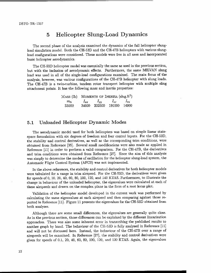
Validation of the helicopter model developed in the current work was performed by calculating the same eigenvalues at each airspeed and then comparing against those re- ported in Reference [11]. Figure 11 presents the eigenvalues for the CH-53D obtained from both analyses.
Although there are some small differences, the eigenvalues are generally quite close. As in the previous section, those differences can be explained by the different linearisation approaches. There was also some inherent error in transcribing the published results to another graph by hand. The behaviour of the CH-53D is fully analysed in Reference [11] and will not be discussed here. Instead, the behaviour of the CH-47B over a range of airspeeds will be examined. In Reference [27], the stability and control derivatives were given for speeds of 0.1, 20, 40, 60, 80, 100, 120, and 130 KTAS. Again, the eigenvalues
22
DSTO-TR-1257
2.5
lm(s)
1.5
-o—• HSLSIM Model + EOMPROG(Ref. [12])
.140.0
'••..dutch roll ;20.t>..:.
.short period
-d H 60^ i Ao^to^a^*'
lateral ." ■ phugpid
■0-0- /phugoid ..
iiMö ..
-1 -0.5 0 pitch heave yaw
0.5
Re(s)
Figure 11: CH-53D System Eigenvalues — Variation with Trim Airspeed (in KTAS)
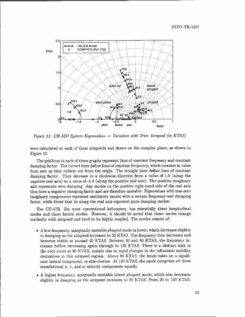
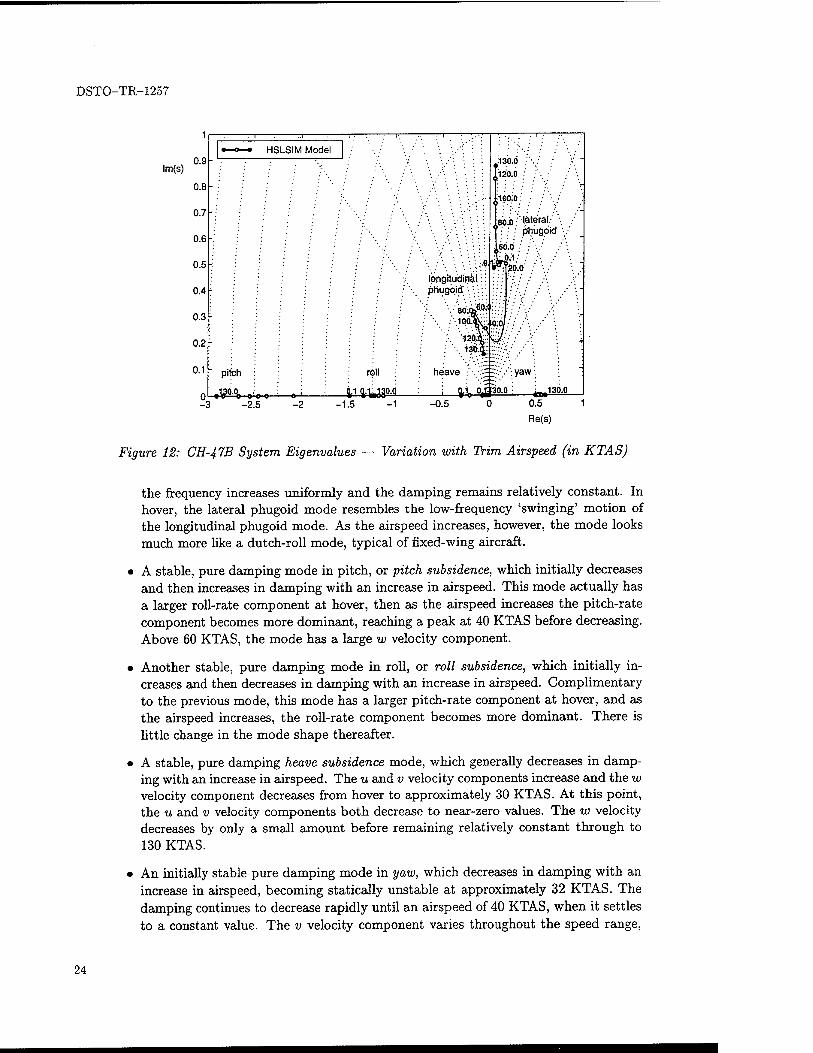
were calculated at each of these airspeeds and drawn on the complex plane, as shown in Figure 12.
The gridlines in each of these graphs represent lines of constant frequency and constant damping factor. The curved lines define lines of constant frequency, which increase in value from zero as they radiate out from the origin. The straight lines define lines of constant damping factor. They decrease in a clockwise direction from a value of 1.0 (along the negative real axis) to a value of-1.0 (along the posisive real axis). The positive imaginary axis represents zero damping. Any modes on the positive right-hand side of the real axis thus have a negative damping factor and are therefore unstable. Eigenvalues with non-zero imaginary components represent oscillatory modes with a certain frequency and damping factor, while those that lie along the real axis represent pure damping modes.
The CH-47B, like most conventional helicopters, has essentially three longitudinal modes and three lateral modes. However, it should be noted that these modes change markedly with airspeed and tend to be highly coupled. The modes consist of:
• A low-frequency, marginally unstable phugoid mode in hover, which decreases slightly in damping as the airspeed increases to 20 KTAS. The frequency then decreases and becomes stable at around 40 KTAS. Between 40 and 60 KTAS, the frequency in- creases before decreasing again through to 130 KTAS. There is a distinct kink in the root locus at 60 KTAS, mainly due to rapid changes in the influential stability derivatives in this airspeed regime. Above 80 KTAS, the mode takes on a signifi- cant lateral component, or side-motion. At 130 KTAS, the mode comprises all three translational u, v, and w velocity components equally.
• A higher frequency, marginally unstable lateral phugoid mode, which also decreases slightly in damping as the airspeed increases to 20 KTAS. From 20 to 130 KTAS,
23
DSTO-TR-1257
lm(s)
1
0.9
0.8
0.7
0.6
0.5
0.4^
0.3
0.2
0.1 f-
0
HSLSIM Model
pitch
Ä^ roll
414W3M
longitudinal: phugoid
80.Oif0;(
12Q.4
heave ^
L_?A-3
^130.0
,120.0
100.0
soj)/''lateral/ \ phugoid
60.0
m 0,1- .
"fccLo'
I : yaw.
jpo.o ; .130.0
-2.5 -1.5 -1 -0.5 0.5
Re(s)
Figure 12: CH-47B System Eigenvalues — Variation with Trim Airspeed (in KTAS)
the frequency increases uniformly and the damping remains relatively constant. In hover, the lateral phugoid mode resembles the low-frequency 'swinging' motion of the longitudinal phugoid mode. As the airspeed increases, however, the mode looks much more like a dutch-roll mode, typical of fixed-wing aircraft.
• A stable, pure damping mode in pitch, or pitch subsidence, which initially decreases and then increases in damping with an increase in airspeed. This mode actually has a larger roll-rate component at hover, then as the airspeed increases the pitch-rate component becomes more dominant, reaching a peak at 40 KTAS before decreasing. Above 60 KTAS, the mode has a large w velocity component.
• Another stable, pure damping mode in roll, or roll subsidence, which initially in- creases and then decreases in damping with an increase in airspeed. Complimentary to the previous mode, this mode has a larger pitch-rate component at hover, and as the airspeed increases, the roll-rate component becomes more dominant. There is little change in the mode shape thereafter.
• A stable, pure damping heave subsidence mode, which generally decreases in damp- ing with an increase in airspeed. The u and v velocity components increase and the w velocity component decreases from hover to approximately 30 KTAS. At this point, the u and v velocity components both decrease to near-zero values. The w velocity decreases by only a small amount before remaining relatively constant through to 130 KTAS.
• An initially stable pure damping mode in yaw, which decreases in damping with an increase in airspeed, becoming statically unstable at approximately 32 KTAS. The damping continues to decrease rapidly until an airspeed of 40 KTAS, when it settles to a constant value. The v velocity component varies throughout the speed range,
24
DSTO-TR-1257
while the u any w components both increase greatly at the crossover airspeed. The pitch rate component also increases at 32 KTAS, becoming the dominant part of the motion. The yaw rate component, however, actually decreases from its value at hover and remains small by comparison.
The eigenvalues representing each of these modes at airspeeds of 0.1 KTAS (hover) and 130 KTAS are tabulated below. The corresponding natural frequency and damping factor are also listed for each mode.
Table 2: Natural Frequency and Damping for CH-47B at 0.1 KTAS MODE EIGENVALUE NATURAL
FREQUENCY (RAD/S)
DAMPING
FACTOR
Longitudinal phugoid 0.1099 ± 0.5026i 0.5145 -0.2137 Pitch subsidence -1.4853 1.4853 1.0000 Heave subsidence -0.3003 0.3003 1.0000 Lateral phugoid 0.0453 ± 0.4829i 0.4850 -0.0934 Roll subsidence -1.3396 1.3396 1.0000 Yaw mode -0.0766 0.0766 1.0000
Table 3: Natural Frequency and Damping for CH-47B at 130.0 KTAS MODE EIGENVALUE NATURAL
FREQUENCY (RAD/S)
DAMPING
FACTOR
Longitudinal phugoid -0.0619 ± 0.1534z 0.1654 0.3744 Pitch subsidence -2.9048 2.9048 1.0000 Heave subsidence -0.0144 0.0144 1.0000 Lateral phugoid 0.0610 ± 0.8754J 0.8775 -0.0695 Roll subsidence -1.2224 1.2224 1.0000 Yaw mode 0.6008 0.6008 1.0000
5.2 Analysis of Helicopter Slung-Load System Modes
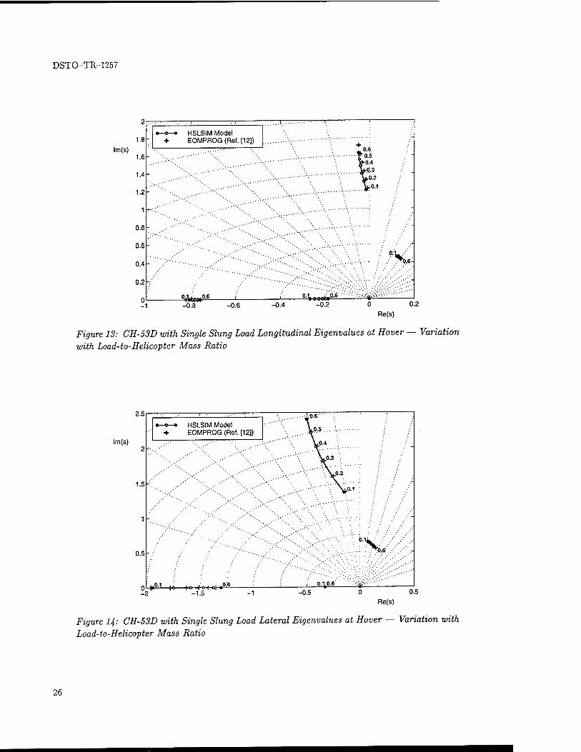
As with the unloaded helicopter model, the results obtained for the combined helicopter and load were compared with those documented in Reference [11]. The eigenvalues for a range of configurations of the CH-53D in hover with a MILVAN load were examined. In particular, the load-to-helicopter mass ratio mi/irih was varied between 0.1 and 0.6. The load was slung using multiple cables (sling legs) and a single helicopter attachment point, and the distance between the attachment point and load eg was 25 ft. Figures 13 and 14 illustrate the root loci for this system in both longitudinal and lateral axes.
The additional eigenvalues in these diagrams represent the modes associated with the pendulous motion of the load and will be discussed later in this section. Note also that the heave subsidence and yawing modes were not included in the previous results and are therefore not shown here. Nonetheless, all of the remaining modes agree quite well,
25
DSTO-TR-1257
lm(s)
2
1.8
1.6
1.4
1.2
1
0.8
0.6
0.4
0.2
0
-o—• HSLSiM Model + EOMPROG (Ref. [12])
r0.6-
aAt r,ya-6
-1 2*W -0.8 -0.6 -0.4 -0.2 0 0.2
Re(s)
Figure 13: CH-53D with Single Slung Load Longitudinal Eigenvalues at Hover — Variation with Load-to-Helicopter Mass Ratio
2.5
lm(s)
1.5
1 -
0.5
-o—• HSLSIM Model + EOMPROG (Ref. [12])
0.6
0>-»°-1 it 1-o-fo-f-oH»9^ L- 0.^0.6
-1.5 -0.5 0 0.5
Re(s)
Figure U: CH-53D with Single Slung Load Lateral Eigenvalues at Hover — Variation with Load-to-Helicopter Mass Ratio
26
DSTO-TR-1257
particularly in the lateral axes. Small discrepancies have come about due to the same reasons discussed above.
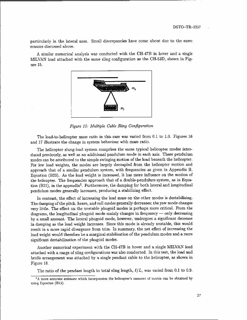
A similar numerical analysis was conducted with the CH-47B in hover and a single MILVAN load attached with the same sling configuration as the CH-53D, shown in Fig- ure 15.
^ mh
A HPÜI m<
Figure 15: Multiple Cable Sling Configuration
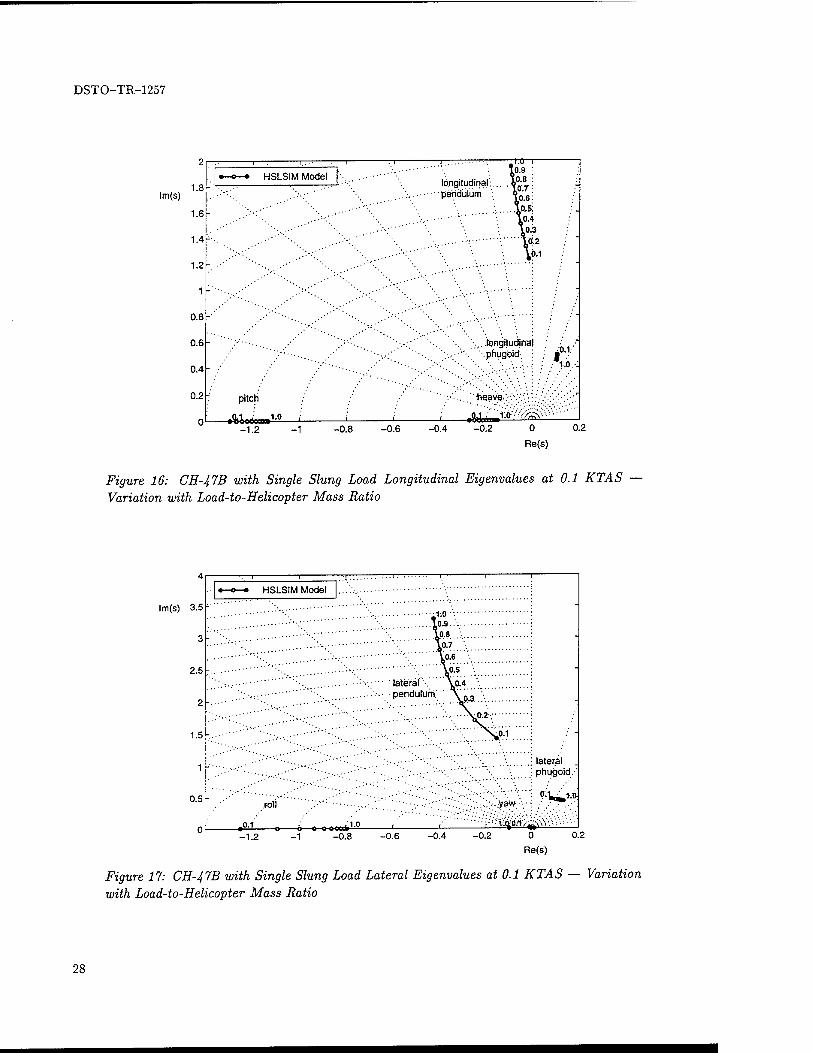
The load-to-helicopter mass ratio in this case was varied from 0.1 to 1.0. Figures 16 and 17 illustrate the change in system behaviour with mass ratio.
The helicopter slung-load system comprises the same typical helicopter modes intro- duced previously, as well as an additional pendulum mode in each axis. These pendulum modes can be attributed to the simple swinging motion of the load beneath the helicopter. For low load weights, the modes are largely decoupled from the helicopter motion and approach that of a similar pendulum system, with frequencies as given in Appendix B, Equation (B23). As the load weight is increased, it has more influence on the motion of the helicopter. The frequencies approach that of a double-pendulum system, as in Equa- tion (B21), in the appendix2. Furthermore, the damping for both lateral and longitudinal pendulum modes generally increases, producing a stabilising effect.
In contrast, the effect of increasing the load mass on the other modes is destabilising. The damping of the pitch, heave, and roll modes generally decreases; the yaw mode changes very little. The effect on the unstable phugoid modes is perhaps more critical. From the diagrams, the longitudinal phugoid mode mainly changes in frequency — only decreasing by a small amount. The lateral phugoid mode, however, undergoes a significant decrease in damping as the load weight increases. Since this mode is already unstable, this would result in a more rapid divergence from trim. In summary, the net effect of increasing the load weight would therefore be a marginal stabilisation of the pendulum modes and a more significant destabilisation of the phugoid modes.
Another numerical experiment with the CH-47B in hover and a single MILVAN load attached with a range of sling configurations was also conducted. In this test, the load and bridle arrangement was attached by a single pendant cable to the helicopter, as shown in Figure 18.
The ratio of the pendant length to total sling length, £/L, was varied from 0.1 to 0.9. 2A more accurate estimate which incorporates the helicopter's moment of inertia can be obtained by-
using Equation (B15).
27
DSTO-TR-1257
lm(s)
2
1.8
1.6
1.4
1.2
1
0.8
0.6
0.4
0.2
0
:I.O I
HSLSIM Model longitudinal';
• pendulum •
. longitudinal phugoid
1:0.
pitch
-VtKxxJcca»-
fieave-:
1.0 JO* .i:o^/y^\v -1.2 -1 -0.8 -0.6 -0.4 -0.2 0.2
Re(s)
Figure 16: CH-47B with Single Slung Load Longitudinal Eigenvalues at 0.1 KTAS Variation with Load-to-Helicopter Mass Ratio
4 .—, , *-o—• HSLSIM Model
#r.o •. : lm(s) 3.5 ... - •-. 10.9..- :
3 ■"''::;.'.y''" •'■■-•:
...LP..8..':. : \0.7
\0.6
2.5 AÖ.5 '■. :
lateral \o.4 \
2 • : pendulurn.'""\n3 '■
■'••.• ■■•\^0.2:-;
1.5 //■".' >iM...
1 :,. lateral .
phugoid
0.5 .roll .... yaw- .^™.
n J±l 0 6—o-o-occd»!^ r ":'^dtrf^\Y: ■'■■'■
-1.2 -0.8 -0.6 -0.4 -0.2 0 0.2
Re(s)
Figure 17: CH-47B with Single Slung Load Lateral Eigenvalues at 0.1 KTAS — Variation with Load-to-Helicopter Mass Ratio
28
DSTO-TR-1257
I' "V r~i N«M«äi^
1
\
\ 1 t
1
\
L
i rf£*i
Figure 18: Single Cable Sling Configuration
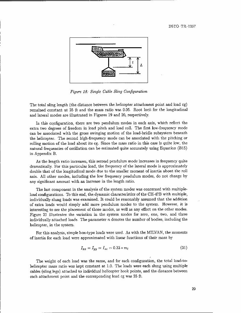
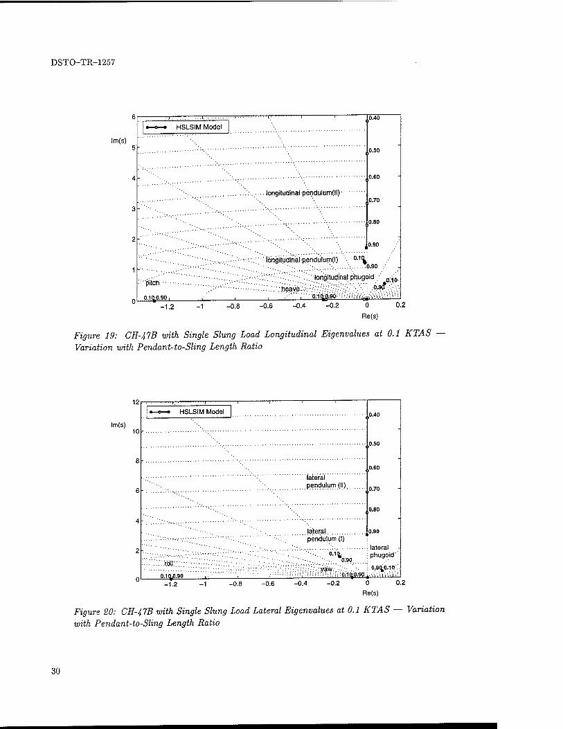
The total sling length (the distance between the helicopter attachment point and load eg) remained constant at 25 ft and the mass ratio was 0.05. Root loeii for the longitudinal and lateral modes are illustrated in Figures 19 and 20, respectively.
In this configuration, there are two pendulum modes in each axis, which reflect the extra two degrees of freedom in load pitch and load roll. The first low-frequency mode can be associated with the gross swinging motion of the load-bridle subsystem beneath the helicopter. The second high-frequency mode can be associated with the pitching or rolling motion of the load about its eg. Since the mass ratio in this case is quite low, the natural frequencies of oscillation can be estimated quite accurately using Equation (B15) in Appendix B.
As the length ratio increases, this second pendulum mode increases in frequency quite dramatically. For this particular load, the frequency of the lateral mode is approximately double that of the longitudinal mode due to the smaller moment of inertia about the roll axis. All other modes, including the low frequency pendulum modes, do not change by any significant amount with an increase in the length ratio.
The last component in the analysis of the system modes was concerned with multiple- load configurations. To this end, the dynamic characteristics of the CH-47B with multiple, individually slung loads was examined. It could be reasonably assumed that the addition of extra loads would simply add more pendulum modes to the system. However, it is interesting to see the placement of those modes, as well as any effect on the other modes. Figure 21 illustrates the variation in the system modes for zero, one, two, and three individually attached loads. The parameter n denotes the number of bodies, including the helicopter, in the system.
For this analysis, simple box-type loads were used. As with the MILVAN, the moments of inertia for each load were approximated with linear functions of their mass by
Iyv = hz = 0.33 * mi (31)
The weight of each load was the same, and for each configuration, the total load-to- helicopter mass ratio was kept constant at 1.0. The loads were each slung using multiple cables (sling legs) attached to individual helicopter hook points, and the distance between each attachment point and the corresponding load eg was 25 ft.
29
DSTO-TR-1257
lm(s)
HSLSIM Model
.'.-.,.. • ■ Jongitud'malpendulurrr(ll) •
; o.4o
0.50
.0.60
.0.70
0.80
0.90
longitudinal pendulum(l) °-1<^
pitch
0,1(^0.90 i
0.90
. longitudinal phugoid 0 :,0
:heaiye-V-:r;:-'-'-''.::V-:-':'-'-'.-'-'.'- 0.95
-1.2 -1 -0.8 -0.6 -0.4 O.HypQ i/i(/c|i.-,V
-0.2 0 0.2
Re(s)
Figure 19: CH-47B with Single Slung Load Longitudinal Eigenvalues at 0.1 KTAS Variation with Pendant-to-Sling Length Ratio
lm(s)
12
10
8-
HSLSIM Model
lateral pendulum (II)
late/a! pendulum (I)
.0.50
0.60
0.70
.0.80
0.90
'.'.ron;;
0.10J0.5
..':.. : lateral - 0-1lL. : phugoid'
o:ao 0.90,0.10'. yaw. u.snyj.iy
,' : ■•■.'■':ii[:0i1Pj0;9D^..,,iiiiiriii
-1.2 -0.8 -0.6 -0.4 -0.2 0 0.2
Re(s)
Figure 20: CH-47B with Single Slung Load Lateral Eigenvalues at 0.1 KTAS — Variation with Pendant-to-Sling Length Ratio
30
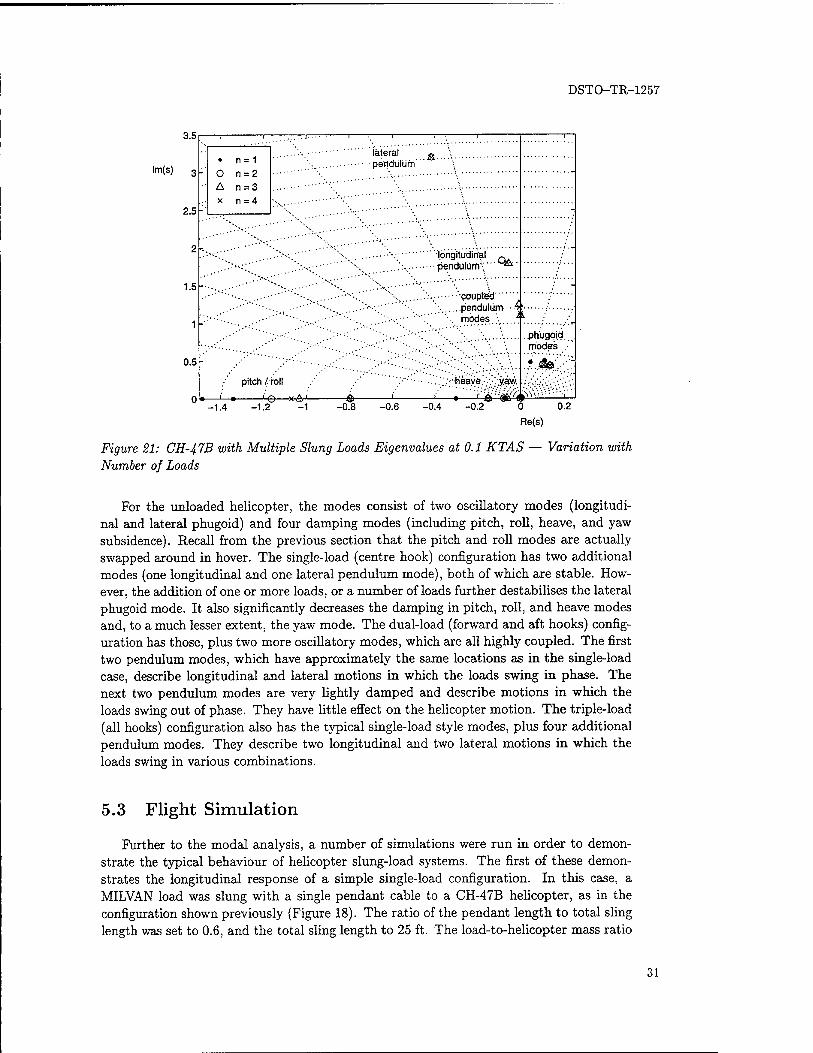
DSTO-TR-1257
3.5
lm(s)
2.5
1.5
0.5
• n = 1 0 n = 2 A n = 3 X n = 4
lateral •pendulum'
'longitudinal £...C&. ■ pendulum'
'couplea ' pendulum •• •4; '•■. modes.\..........;.
pitch /'roll
->-e—)«A
; •Heaye;;./.yaw. -i • 'i &:'ä&/Ü'
-1.4 -1.2 -1 -0.8 -0.6 -0.4 -0.2
. phjjgojd modes .■
0.2
Re(s)
Figure 21: CH-47B with Multiple Slung Loads Eigenvalues at 0.1 KTAS — Variation with Number of Loads
For the unloaded helicopter, the modes consist of two oscillatory modes (longitudi- nal and lateral phugoid) and four damping modes (including pitch, roll, heave, and yaw subsidence). Recall from the previous section that the pitch and roll modes are actually swapped around in hover. The single-load (centre hook) configuration has two additional modes (one longitudinal and one lateral pendulum mode), both of which are stable. How- ever, the addition of one or more loads, or a number of loads further destabilises the lateral phugoid mode. It also significantly decreases the damping in pitch, roll, and heave modes and, to a much lesser extent, the yaw mode. The dual-load (forward and aft hooks) config- uration has those, plus two more oscillatory modes, which are all highly coupled. The first two pendulum modes, which have approximately the same locations as in the single-load case, describe longitudinal and lateral motions in which the loads swing in phase. The next two pendulum modes are very lightly damped and describe motions in which the loads swing out of phase. They have little effect on the helicopter motion. The triple-load (all hooks) configuration also has the typical single-load style modes, plus four additional pendulum modes. They describe two longitudinal and two lateral motions in which the loads swing in various combinations.
5.3 Flight Simulation
Further to the modal analysis, a number of simulations were run in order to demon- strate the typical behaviour of helicopter slung-load systems. The first of these demon- strates the longitudinal response of a simple single-load configuration. In this case, a MILVAN load was slung with a single pendant cable to a CH-47B helicopter, as in the configuration shown previously (Figure 18). The ratio of the pendant length to total sling length was set to 0.6, and the total sling length to 25 ft. The load-to-helicopter mass ratio
31
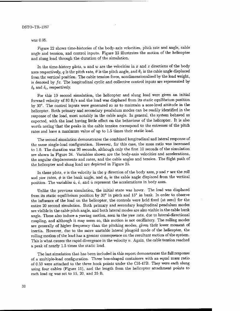
DSTO-TR-1257
was 0.05.
Figure 22 shows time-histories of the body-axis velocities, pitch rate and angle, cable angle and tension, and control inputs. Figure 23 illustrates the motion of the helicopter and slung load through the duration of the simulation.
In the time-history plots, u and w are the velocities in x and z directions of the body axes respectively, q is the pitch rate, 6 is the pitch angle, and 6C is the cable angle displaced from the vertical position. The cable tension force, nondimensionalised by the load weight, is denoted by fc. The longitudinal cyclic and collective control inputs are represented by Ob and 8C, respectively.
For this 10 second simulation, the helicopter and slung load were given an initial forward velocity of 80 ft/s and the load was displaced from its static equilibrium position by 30°. The control inputs were generated so as to maintain a nose-level attitude in the helicopter. Both primary and secondary pendulum modes can be readily identified in the response of the load, most notably in the cable angle. In general, the system behaved as expected, with the load having little effect on the behaviour of the helicopter. It is also worth noting that the peaks in the cable tension correspond to the extremes of the pitch rates and have a maximum value of up to 1.5 times their static load.
The second simulation demonstrates the combined longitudinal and lateral response of the same single-load configuration. However, for this case, the mass ratio was increased to 1.0. The duration was 20 seconds, although only the first 10 seconds of the simulation are shown in Figure 24. Variables shown are the body-axis velocities and accelerations, the angular displacements and rates, and the cable angles and tension. The flight path of the helicopter and slung load are depicted in Figure 25.
In these plots, v is the velocity in the y direction of the body axes, p and r are the roll and yaw rates, <p is the bank angle, and <f>c is the cable angle displaced from the vertical position. The variables ü, v, and ü represent the accelerations in body axes.
Unlike the previous simulation, the initial state was hover. The load was displaced from its static equilibrium position by 30° in pitch and 15° in bank. In order to observe the influence of the load on the helicopter, the controls were held fixed (at zero) for the entire 20 second simulation. Both primary and secondary longitudinal pendulum modes are visible in the cable pitch angle, and both lateral modes are also visible in the cable bank angle. These also induce a yawing motion, seen in the yaw rate, due to lateral-directional coupling, and although it may seem so, this motion is not oscillatory. The rolling modes are generally of higher frequency than the pitching modes, given their lower moment of inertia. However, due to the more unstable lateral phugoid mode of the helicopter, the rolling motion of the load has a greater consequence on the resultant motion of the system. This is what causes the rapid divergence in the velocity v. Again, the cable tension reached a peak of nearly 1.5 times the static load.
The last simulation that has been included in this report demonstrates the full response of a multiple-load configuration. Three box-shaped containers with an equal mass ratio of 0.33 were attached to the three hook points under the CH-47B. They were each slung using four cables (Figure 15), and the length from the helicopter attachment points to each load eg was set to 15, 20, and 25 ft.
32
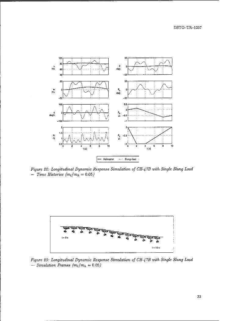
DSTO-TR-1257
50
ft/s
\ /"v y\ j V
ft/s
q aegis
— Helicopter — Slung-load
Figure 22: Longitudinal Dynamic Response Simulation of CH-47B with Single Slung Load — Time Histories (mi/mh = 0.05,)
Figure 23: Longitudinal Dynamic Response Simulation of CH-47B with Single Slung Load — Simulation Frames (mi/mh — 0.05,)
33
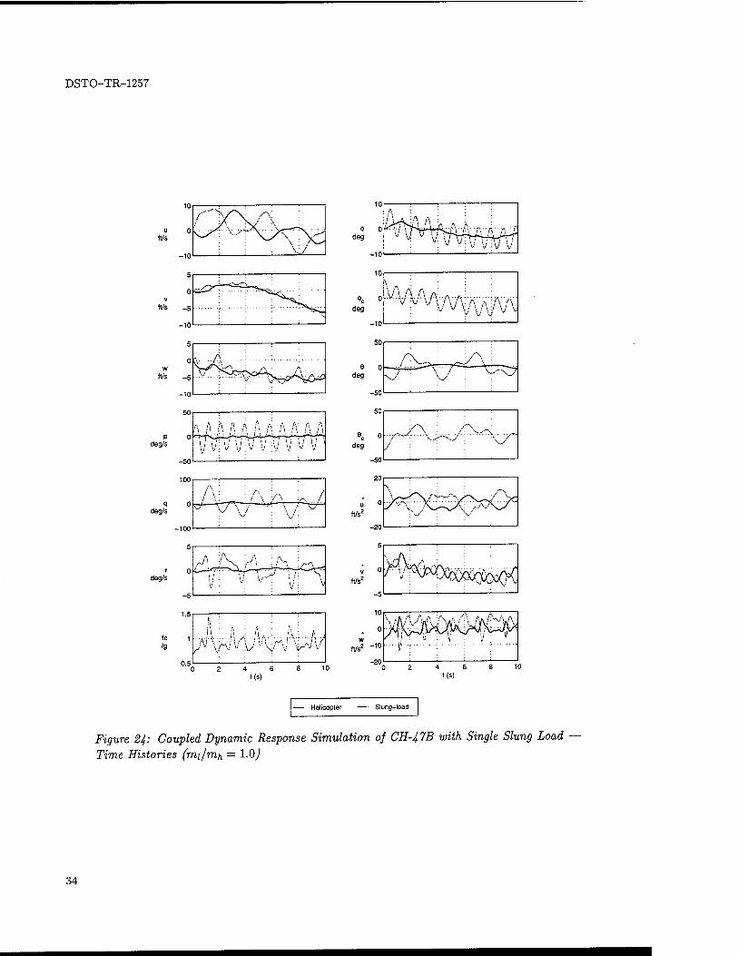
DSTO-TR-1257
ft/s
-10
5
0 v
ft/s -5
-10
S
0 w
ft/s _s^
-10
50
^•>^~<^ciw. :
v
P 0 deg/s
-50
100
q 0 deg/s
-100
5
A A A A A A A \i v \J \l -j V V y y v
A
tTTT^ ■y\
deg/s
fo 1 /g
/\ N S" ^ i /
V : '" : " v V
0.5 2 4 6
t(s) 8 10
— Helicopter Slung-load
Figure 24: Coupled Dynamic Response Simulation of CH-47B with Single Slung Load
Time Histories (mi/mh = 1.0,)
34
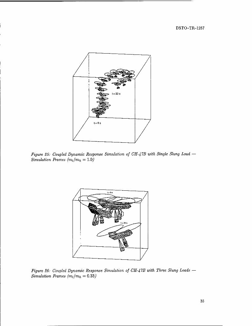
DSTO-TR-1257
Figure 25: Coupled Dynamic Response Simulation of CH-47B with Single Slung Load Simulation Frames (mi/mh = l.Oj
Figure 26: Coupled Dynamic Response Simulation of CH-47B with Three Slung Loads Simulation Frames (mi/nth = 0.33,)
35
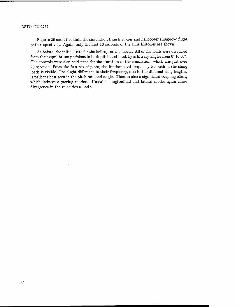
DSTO-TR-1257
Figures 26 and 27 contain the simulation time histories and helicopter slung-load flight path respectively. Again, only the first 10 seconds of the time histories are shown.
As before, the initial state for the helicopter was hover. All of the loads were displaced from their equilibrium positions in both pitch and bank by arbitrary angles from 0° to 30°. The controls were also held fixed for the duration of the simulation, which was just over 20 seconds. From the first set of plots, the fundamental frequency for each of the slung loads is visible. The slight difference in their frequency, due to the different sling lengths, is perhaps best seen in the pitch rate and angle. There is also a significant coupling effect, which induces a yawing motion. Unstable longitudinal and lateral modes again cause divergence in the velocities u and v.
36
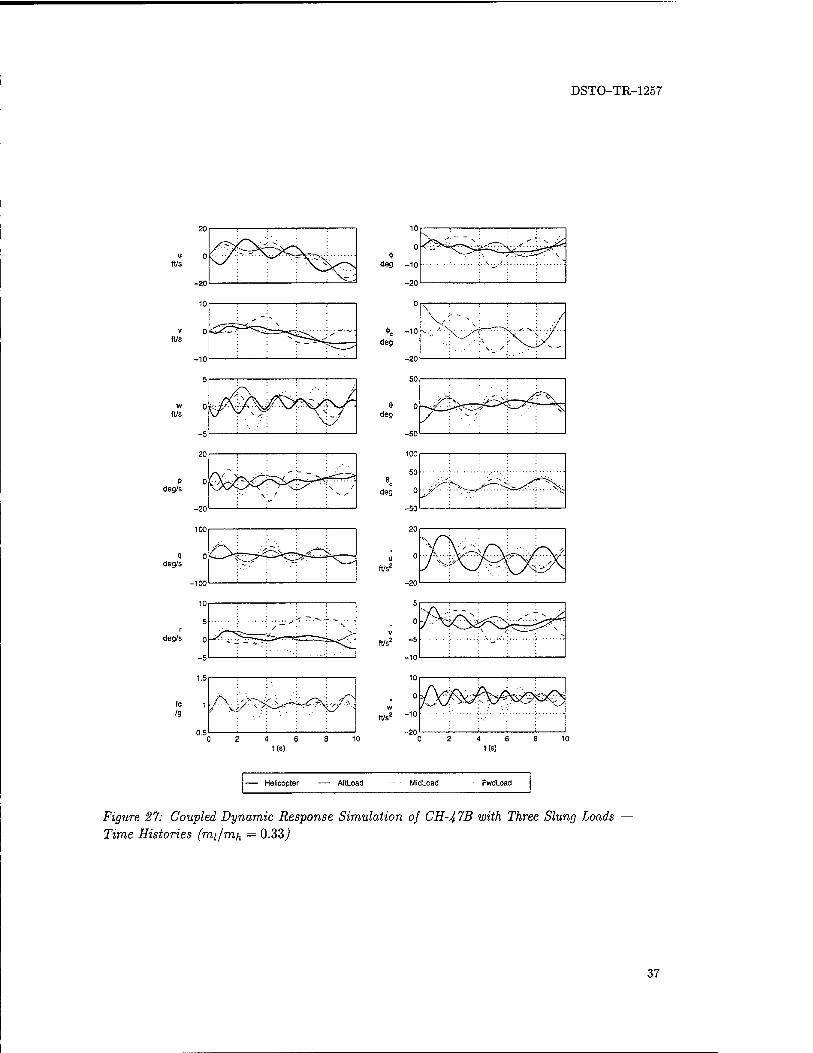
DSTO-TR-1257
ft/s
ft/s
ft/s
20r
/^J?
p/\
:'■' \ / N. ,•
deg/s
-100
10
5
0
-5
1.5
^_^ ■ J : -^
/\.^Si^ ̂ r?\ y^
deg
e deg
9c deg
ft/s'
ft/s'
ft/s'
4 6 t(s)
-50
100
50
0
-50
20
-20
5
0
-5
-10
10
0
-10
-20
\ \ ■■■ - ■s ./ ^:
"■-'■;;' K J>^' Nc ^ ...
V / •^ *- -*
5^"^t'^:r' \
1 V„ \ '--V
y\r /~\. ^ >-"—~x •<■' -'-^ \ S ^.r^-ii*-
3ÖÖ %Ä^^S> €^N
4 6 8 10 t(s)
Helicopter AftLoad MidLoad FwdLoad
Figure 27: Coupled Dynamic Response Simulation of CH-47B with Three Slung Loads Time Histories (mi/mh — 0.33J
37
DSTO-TR-1257
6 Concluding Remarks
A simulation model was produced using the equations of motion for general slung-load systems developed by Cicolani and Kanning [29]. The formulation used is based on the Newton-Euler equations written in terms of generalised coordinates and can be readily adapted to systems with either elastic or inelastic suspension. All code development, including the simulation routine, linear analysis, and graphical replay tools, was done in MATLAB. Further to the model described, the simulation has also been extended to incorporate multiple-load systems.
Following comparison of the behaviour of a simple pendulum-type system against both analytical solutions and previously published results, the open-loop characteristics of a full helicopter slung-load system was examined. The results presented include the modal analysis of a single-load system and the simulation of a multiple-load system. It was found that the frequency of the longitudinal and lateral pendulum modes generally increases with the load-to-helicopter mass ratio. More importantly, the lateral phugoid mode becomes significantly unstable as the mass ratio is increased. For the simulation demonstrated, the dominant natural frequencies were identified.
38
DSTO-TR-1257
References
1. Lucassen, L. & Sterk, F. (1965) Dynamic stability analysis of a hovering helicopter with a sling load, Journal of the American Helicopter Society 10, 6-12.
2. Dukes, T. (1972) The Princeton Pennsylvania Army Avionics Research Program. El- ements of Helicopter Hovering and Near Hover Operations with a Sling Load Final Report, 1 Sep. 1966 - 30 Dec. 1971, Technical Note AD-750618, Princeton Univ., NJ.
3. Cliff, E. & Bailey, D. (1975) Dynamic stability of a translating vehicle with a simple sling load, AIAA Journal of Aircraft 12, 773-777.
4. Feaster, L. (1975) Dynamics of a Slung Load, PhD thesis, Massachusetts Univ., MA.
5. Feaster, L., Poli, C. & Kirchhoff, R. (1977) Dynamics of a slung load, AIAA Journal of Aircraft 14, 115-121.
6. Prabhakar, A. & Sheldon, D. (1976) Dynamic Stability of a Helicopter Carrying an Underslung Load, Technical Note RCMS TN-AM-78, Dept. of Mechanical Engineering, Royal Military College of Science.
7. Prabhakar, A. (1978) Stability of a helicopter carrying an underslung load, Vertica 2(2), 121-143.
8. Nagabhushan, B. (1977) Systematic Investigation of Models of Helicopter with a Slung Load, PhD thesis, Virginia Polytechnic Inst. and State Univ., VA.
9. Nagabhushan, B. (1985) Low-speed stability characteristics of a helicopter with a sling load, Vertica 9(4), 345-361.
10. Nagabhushan, B. & Cliff, E. (1982) Maneuver stability of a vehicle with a towed body, in AIAA Atmospheric Flight Mechanics Conference, number AIAA-82-1347, American Institute of Aeronautics and Astronautics.
11. Ronen, T. (1986) Dynamics of a Helicopter with a Sling Load, PhD thesis, Stanford Univ., CA.
12. Ronen, T., Bryson, A. J. &: Hindson, W. (1986) Dynamics of a helicopter with a sling load, in AIAA Atmospheric Flight Mechanics Conference, number AIAA-86- 2288, American Institute of Aeronautics and Astronautics.
13. Curtiss, H.C., J. (1988) Studies of the Dynamics of the Twin-Lift System. Interim Re- port, Jul. 1983 - Sep. 1987, Contractor Report NASA-CR-183273, Dept. of Mechanical and Aerospace Engineering, Princeton Univ., NJ.
14. Gabel, R. &: Wilson, G. (1968) Test approaches to external sling load instabilities, in 24th Annual National Forum, number AHS-230, American Helicopter Society.
15. Hone, H. (1975) Flight Load Investigation of Helicopter External Loads, Technical Report USAAMRDL-TR-74-104, U.S. Army Air Mobility Research and Development Laboratory.
39
DSTO-TR-1257
16. Briczinski, S. & Karas, G. (1971) Criteria for Externally Suspended Helicopter Loads, Technical Report USAAMRDL-TR-71-61, U.S. Army Air Mobility Research and De- velopment Laboratory.
17. Kesler, D., Murakoshi, A. & Sinacori, J. (1974) Flight Simulation of the Model 347 Advanced Tandem-Rotor Helicopter. Final Report, Jul. 1972 - Oct. 1973, Technical Report NOR-73-190, Aircraft Div., Northrop Corp., CA.
18. Matheson, N. (1976) Stability of Helicopter Slung Loads, Aerodynamics Note ARL/AERO-NOTE-364, Aeronautical & Maritime Research Labs., VIC, Australia.
19. Wolkovitch, J. & Johnston, D. (1965) Automatic Control Considerations for Helicopter and VTOL Aircraft With and Without Sling Loads, Technical Report 138-1, Sytems Technology Inc.
20. Abzug, M. (1970) Dynamics and control of helicopters with two cable sling loads, in AIAA 2nd Aircraft Design and Operations Meeting, number AIAA-70-929, American Institute of Aeronautics and Astronautics.
21. Liu, D. (1973) In-Flight Stabilization of Externally Slung Helicopter Loads Final Re- port, 25 Jun. 1970 - 17 Jan. 1972, Technical Report NORT-72-39, Electronics Div., Northrop Corp., CA.
22. Asseo, S. & Whitbeck, R. (1973) Control requirements for sling-load stabilization in heavy lift helicopters, Journal of the American Helicopter Society 18, 23-31.
23. Gera, J. k Farmer, S.W., J. (1974) A Method of Automatically Stabilizing Helicopter Sling Loads, Technical Note NASA-TN-D-7593, NASA Langley Research Center.
24. Alansky, I., Davis, J. & Garnett, T.S., J. (1977) Limitations of the CH-47 Helicopter in Performing Terrain Flying with External Loads, Technical Report USAAMRDL- TR-77-21, Boeing Vertol Co., PA.
25. Shaughnessy, J., Deaux, T. & Yenni, K. (1979) Development and Validation of a Piloted Simulation of a Helicopter and External Sling Load, Technical Paper NASA- TP-1285, NASA Langley Research Center.
26. Sampath, P. (1980) Dynamics of a Helicopter-Slung Load System, PhD thesis, Mary- land Univ., MA.
27. Weber, J., Liu, T. & Chung, W. (1984) A Mathematical Simulation Model of the CH- 47B Helicopter, Volumes 1 & 2, Technical Memorandum NASA-TM-84351-VOL-1/2, NASA Ames Research Center.
28. Raz, R., Rosen, A. & Ronen, T. (1989) Active aerodynamic stabilization of a helicopter/sling-load system, AIAA Journal of Aircraft 26, 822-828.
29. Cicolani, L. & Kanning, G. (1986) General Equilibrium Characteristics of a Dual-Lift Helicopter System, Technical Paper NASA-TP-2615, NASA Ames Research Center.
30. Cicolani, L. & Kanning, G. (1992) Equations of Motion of Slung-load Systems, In- cluding Multilift Systems, Technical Paper NASA-TP-3280, NASA Ames Research Center.
40
DSTO-TR-1257
31. Cicolani, L., Kanning, G. & Synnestvedt, R. (1995) Simulation of the dynamics of helicopter slung load systems, Journal of the American Helicopter Society 40(4), 44- 61.
32. Saunders, G. (1975) Dynamics of Helicopter Flight, Wiley-Interscience, New York.
33. Shaughnessy, J. & Pardue, M. (1977) Helicopter Sling Load Accident/Incident Survey: 1968 - 1974, Technical Memorandum NASA-TM-X-74007, NASA Langley Research Center.
34. The MathWorks, Inc. (1997) MATLAB, The Language of Technical Computing: Using Matlab Version 5, The Mathworks, 24 Prime Park Way, Natick, MA.
35. Heffley, R., Jewell, W., Lehman, J. & Van Winkle, R. (1979) A Compilation and Analy- sis of Helicopter Handling Qualities Data. Volume One: Data Compilation, Contractor Report NASA-CR-3144, Systems Technology Inc., Mountain View, CA.
36. Blevins, R. (1979) Formulas for Natural Frequency and Mode Shape, Krieger Publish- ing Co., Florida.
41
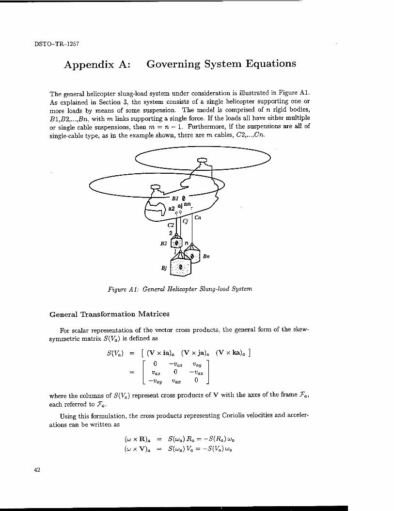
DSTO-TR-1257
Appendix A: Governing System Equations
The general helicopter slung-load system under consideration is illustrated in Figure Al. As explained in Section 3, the system consists of a single helicopter supporting one or more loads by means of some suspension. The model is comprised of n rigid bodies, Bl,B2,...,Bn, with m links supporting a single force. If the loads all have either multiple or single cable suspensions, then m = n - 1. Furthermore, if the suspensions are all of single-cable type, as in the example shown, there are m cables, C2,...,Cn.
Figure Al: General Helicopter Slung-load System
General Transformation Matrices
For scalar representation of the vector cross products, the general form of the skew- symmetric matrix S(Va) is defined as
S(Va) = [ (V x ia)fl (V x ja)0 (V x ka)a ]
0 —vaz vay
Vaz 0 — Vax
uay uax
where the columns of S{Va) represent cross products of V with the axes of the frame Ta, each referred to Ta-
Using this formulation, the cross products representing Coriolis velocities and acceler- ations can be written as
(w X R)a = S(cJa) Ra = -S(Ra) "a
(uxV)a = S(uja)Va = -S(Va)oja
42
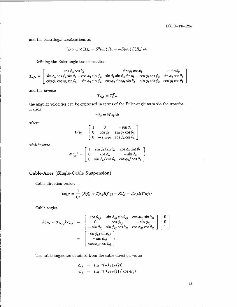
DSTO-TR-1257
and the centrifugal accelerations as
(wxwxR)a = S2{ua) Ra = -S(Wa) S(Ra) ua
Defining the Euler-angle transformation
cos ipf, cos 6b sin tpb cos 6b - sin 9b
sin 4>b cos tpb sin 6b — cos fa sin V>& sin fa sin ?/>;, sin #;> + cos fa cos ^ sin fa cos 6>(, cos fa cos ^»6 sin fy, + sin fa sin V'fc cos fa sin ?/>;, sin 6b — sin <£j cos ipb cos <&, cos #&
Tb,N =
and the inverse TN,b = T6>JV
the angular velocities can be expressed in terms of the Euler-angle rates via the transfor- mation mation
where
Wbb =
with inverse
wbb = Wbbäb
1 0 -sin06
0 cos fa sin fa cos 6b 0 — sin <f>b cos 4>b cos 6b
Wb7l = 1 sin (f>b tan 6b cos ^ tan 6b
0 cos $& — sin fa 0 sm<pb/ cosdb cos fa/ cos 9b
Cable-Axes (Single-Cable Suspension)
Cable-direction vector:
kcjN = j- {Rj*N + TN!JRj*jj - R1*N - Tff,iRl*aji)
Cable angles:
kcJN = TN,cjkcjcj cos 6Cj
0 — sin 9Cj
.,- sin Ö,
sin <^>cj sin öcj cos faj sin 0cj cos ^>Cj — sin faj
cos <^>Cj sin 6Cj — sin ^>Cj
COS (pcj COS #cj
sin ^>cj cos 9cj cos $cj cos #Cj
The cable angles are obtained from the cable direction vector
4>d = sin~1(-kcjN(2))
6cj = sin-1 ( kcjN{l) / cos <f>cj)
43
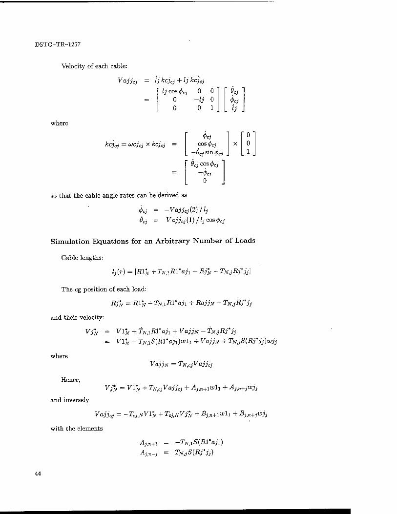
DSTO-TR-1257
Velocity of each cable:
Vajjcj lj kcjCj + lj kcjcj
lj cos 4>cj 0 0 0 -lj 0 0 0 1
4>Cj
ij
where
KCJcj — LJCJcj * kcjcj —
0 0 1
<j>cj COS <f>cj
—6 cj sin 4>cj
6cj cos <f)cj
-<t>cj 0
so that the cable angle rates can be derived as
j>cj = -VajjCj(2)/lj
Qcj = Vajjcj (1) / lj cos <f)cj
Simulation Equations for an Arbitrary Number of Loads
Cable lengths:
lj(r) = \RVN + rjv,iÄl*aji - Rj*N - TNdRj*jj\
The eg position of each load:
Rj*N = R1*N + TNtlRl*aji + RajjN - TN,jRj*jj
and their velocity:
VJN = Vl% + fN,xRVah + VajjN - TNJRj*jj
= V1*N - T^SiRVaJdwU + VajjN + TNtjS{Rj*jj)wjj
where VajjN = TNtCjVajjcj
Hence, VJN = V1*N + TNtCjVajjCj + Ajtn+1wh + Aj,n+jwjj
and inversely
Vajjcj = -Tcj,NVl*N + Tcj,NVj*N + Bjin+1wh + Bjtn+jwjj
with the elements
Ajtn+i = -TN,iS(Rl*aji)
Aj,n+j = TN>jS(Rj*jj)
44
DSTO-TR-1257
Bj,n+i —
£>j,n+j =
Configuration kinematics:
v — Au
\vi*N- V2*N
Vn*N
— =
lull
w22
wnn
I 0 I ?V,c2
I 0
0 | 0 0 0 I A2,n+1 -<4.2,n+2
TN,C in,n+l An. In
vrN Va22c2
Vannc
toll
wnn
u = A 1v
Va22c2
Vanncn
wli w22
wnn
I 0 ••• 0 | 0 0 •■• 0
-TC2,N TC2,N ■■■ 0 | B2,n+1 B%,n+2 ••• 0
0 TcntN | Bntn+1 0 Bn, -T, cn.N 2n
VI
V2
Vn*N
toll
w22
wnn
Acceleration vector:
v — Au + Aü
Applied forces and inertia coupling:
fo = fg + fa- X - DÄu
45
DSTO-TR-1257
r FOIN i " migN ' r FAIN - F02N 17129 N FA2N
FOnN mngN FATIN
— = — + - —
MOli 0 MAli
M022 0 MA22
_ MOnn _ 0 _ MAnn _
where
A =
0 0 0 i2,2
0 0
0 0
0
5(wli)Jlwli S(u)22)J2u22
S(umn)Jnu:nn
0 | 0 0 0 | -A2,n+1 -^-2,71+2
I . ; :
Anjn I -^n,n+l U - +
0
where the elements
Ajtn+j
Suspension forces:
TN,CJS(WCJCJ)
-T^xSiwlJSiRl'aJ!)
TNjSiwjjWRfjj)
fc = Hr
0 1712A2U
mnAnu
0 0
An, 2n
where
yielding
kc2w —JCC2N
0
-£222
£lji = (RVaj x fccj')i
r FCIN 1 FC2N
FCnN
MCli MC22
_ MCnn _
T2
rn
kcriN 0
—kcriN
£1*1 0
—£,nnn
SiRVaj^Ti^kcJN S(Rj*j)jTj>N kcjN
(max{0, Xj(Zj - /o;')}, j = 2,...,n)T (elastic cables) -[HTD-lH)-lHTD~lfo (inelastic cables)
46
DSTO-TR-1257
Total specific force: sf = D-1(fo + fc)
SF1N
SF2N
SFnN
SMU SM22
SMnn
Configuration acceleration:
Configuration position vector:
(FOl/v + FClN)/ml {F02N + FC2N)/m2
(F0nN + FCnN)/mn
Jl-^MOli+MCli) J2-1(M022+MC22)
. Jn-l{M0nn + MCnn)
Ü = A~lsf
= / r{r,v) dt
r =
R1*N
R2*N
Rn N
a2
an
I
VV V2
Vri N
W2zlw22
Wn^wrin
dt
47
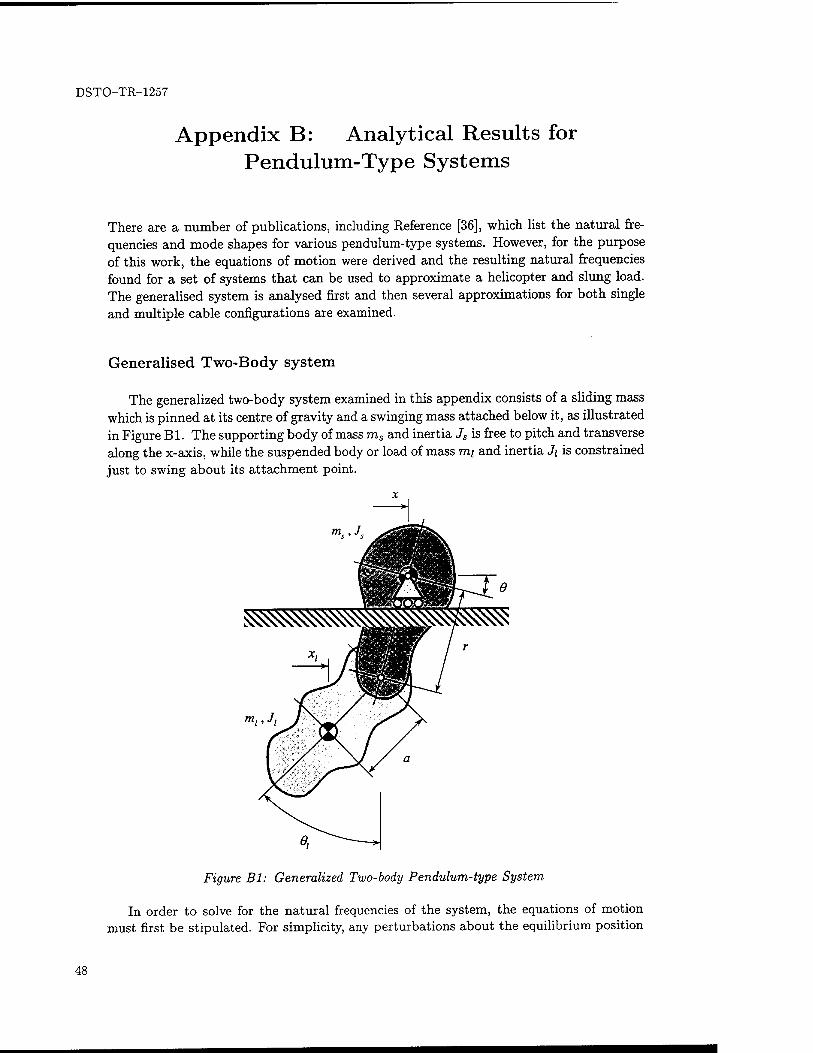
DSTO-TR-1257
Appendix B: Analytical Results for Pendulum-Type Systems
There are a number of publications, including Reference [36], which list the natural fre- quencies and mode shapes for various pendulum-type systems. However, for the purpose of this work, the equations of motion were derived and the resulting natural frequencies found for a set of systems that can be used to approximate a helicopter and slung load. The generalised system is analysed first and then several approximations for both single and multiple cable configurations are examined.
Generalised Two-Body system
The generalized two-body system examined in this appendix consists of a sliding mass which is pinned at its centre of gravity and a swinging mass attached below it, as illustrated in Figure Bl. The supporting body of mass ms and inertia Js is free to pitch and transverse along the x-axis, while the suspended body or load of mass mi and inertia Ji is constrained just to swing about its attachment point.
Figure Bl: Generalized Two-body Pendulum-type System
In order to solve for the natural frequencies of the system, the equations of motion must first be stipulated. For simplicity, any perturbations about the equilibrium position
48
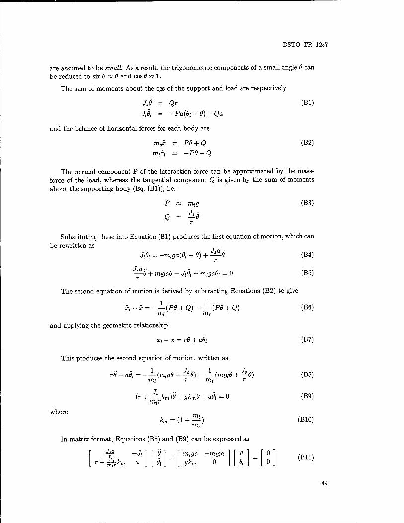
DSTO-TR-1257
are assumed to be small. As a result, the trigonometric components of a small angle 6 can be reduced to sin# « 6 and cos# « 1.
The sum of moments about the cgs of the support and load are respectively
Js9 = Qr (Bl)
Jt9i = -Pa{6l-9) + Qa
and the balance of horizontal forces for each body are
msx = P9 + Q (B2)
mm = -P6-Q
The normal component P of the interaction force can be approximated by the mass- force of the load, whereas the tangential component Q is given by the sum of moments about the supporting body (Eq. (Bl)), i.e.
P ~ mig
Q = ^e
(B3)
Substituting these into Equation (Bl) produces the first equation of motion, which can be rewritten as
JiOi = -miga{6i -9) + —0 r
Jsa 9 + miga9 — J$\ — m\ga9i = 0
The second equation of motion is derived by subtracting Equations (B2) to give
xi - x = -—{P9 + Q)- —(P9 + Q) mi ms
and applying the geometric relationship
xi — x = T9 + a9i
(B4)
(B5)
(B6)
(B7)
This produces the second equation of motion, written as
r'8 + a9i = -—{mig9 + —Ö) mi r
Js
±{rnig9+J-±e)
m., r
(r + -*-km)6 + gkm9 + a9t = 0 mir
where
(1 + mi
m.
In matrix format, Equations (B5) and (B9) can be expressed as
-Ji Jsa
T J.,
mir' r + ^zkm a 9
0i
miga —rrnga gkm 0
9
01
(B8)
(B9)
(BIO)
(Bll)
49
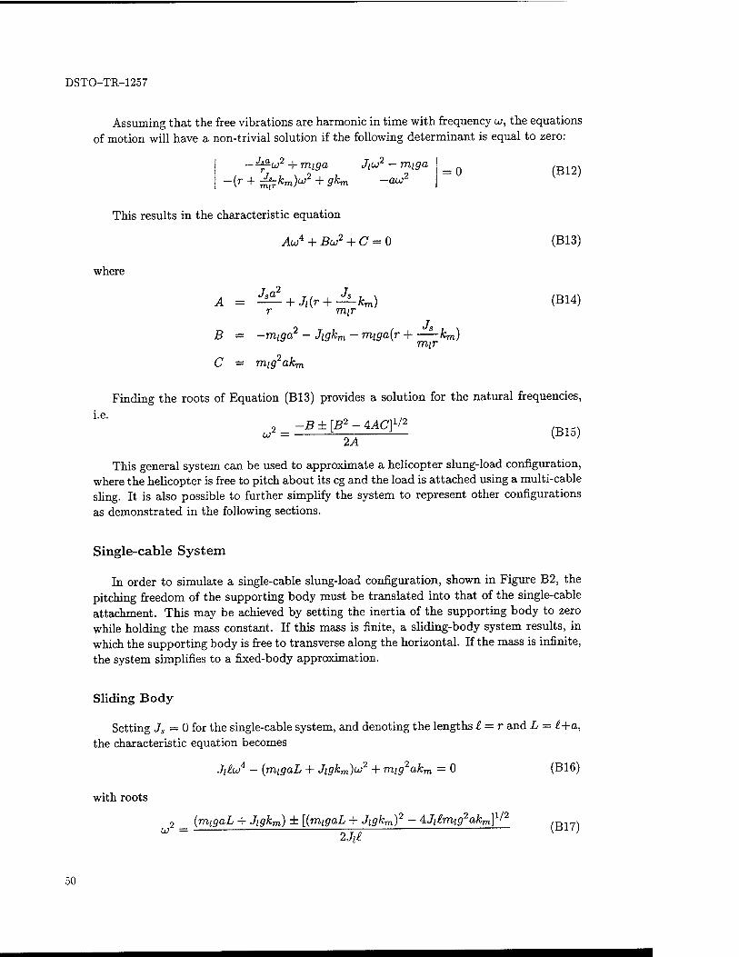
DSTO-TR-1257
Assuming that the free vibrations are harmonic in time with frequency u, the equations of motion will have a non-trivial solution if the following determinant is equal to zero:
^u)2 + miga Jiu2 — nuga
~(r + ^7km)u} + 9km -aw 2 = 0 (B12)
This results in the characteristic equation
AOJ4 + Bu2 + C = 0 (B13)
where
A = i^ + Jl(r + -^km) (B14) r mir
B = -miga2 - Jigkm - miga{r H —A;m) mir
C = mig2akm
Finding the roots of Equation (B13) provides a solution for the natural frequencies, i.e.
u? = -B ± [B2 - AAC]1'2
2A (B15)
This general system can be used to approximate a helicopter slung-load configuration, where the helicopter is free to pitch about its eg and the load is attached using a multi-cable sling. It is also possible to further simplify the system to represent other configurations as demonstrated in the following sections.
Single-cable System
In order to simulate a single-cable slung-load configuration, shown in Figure B2, the pitching freedom of the supporting body must be translated into that of the single-cable attachment. This may be achieved by setting the inertia of the supporting body to zero while holding the mass constant. If this mass is finite, a sliding-body system results, in which the supporting body is free to transverse along the horizontal. If the mass is infinite, the system simplifies to a fixed-body approximation.
Sliding Body
Setting Js = 0 for the single-cable system, and denoting the lengths I = r and L = £+a, the characteristic equation becomes
JilujA - {migaL + Jigkm)u>2 + mlg2akm = 0 (B16)
with roots
2 _ (mi9aL + Jigkm) ± [{rnigaL + Jigkm)2 - 4J[£mig2akm]1/2 . . u ~ 2jte
[
50
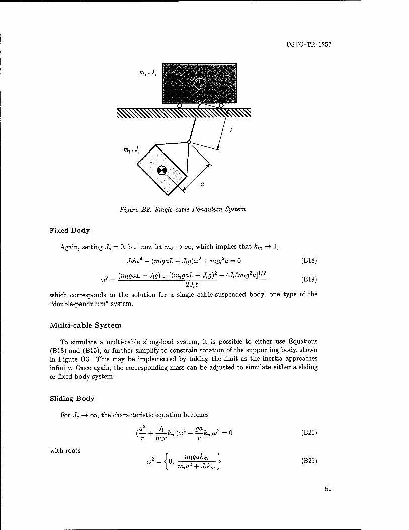
DSTO-TR-1257
ms>Jt
Figure B2: Single-cable Pendulum System
Fixed Body
Again, setting Js = 0, but now let ms -» oo, which implies that km -» 1,
Jiloo4 - {migaL + Jtg)u2 + rrng2a = 0 (B18)
(rrngaL + Jig) ± [{nugaL + Jig)2 - AJ^m^a]1/2
o,2 = 2Ji£
(B19)
which corresponds to the solution for a single cable-suspended body, one type of the "double-pendulum" system.
Multi-cable System
To simulate a multi-cable slung-load system, it is possible to either use Equations (B13) and (B15), or further simplify to constrain rotation of the supporting body, shown in Figure B3. This may be implemented by taking the limit as the inertia approaches infinity. Once again, the corresponding mass can be adjusted to simulate either a sliding or fixed-body system.
Sliding Body
For Js —> oo, the characteristic equation becomes
with roots
r mir
uj2 = i0 -{< migakm
mia2 + Jikn
(B20)
(B21)
51
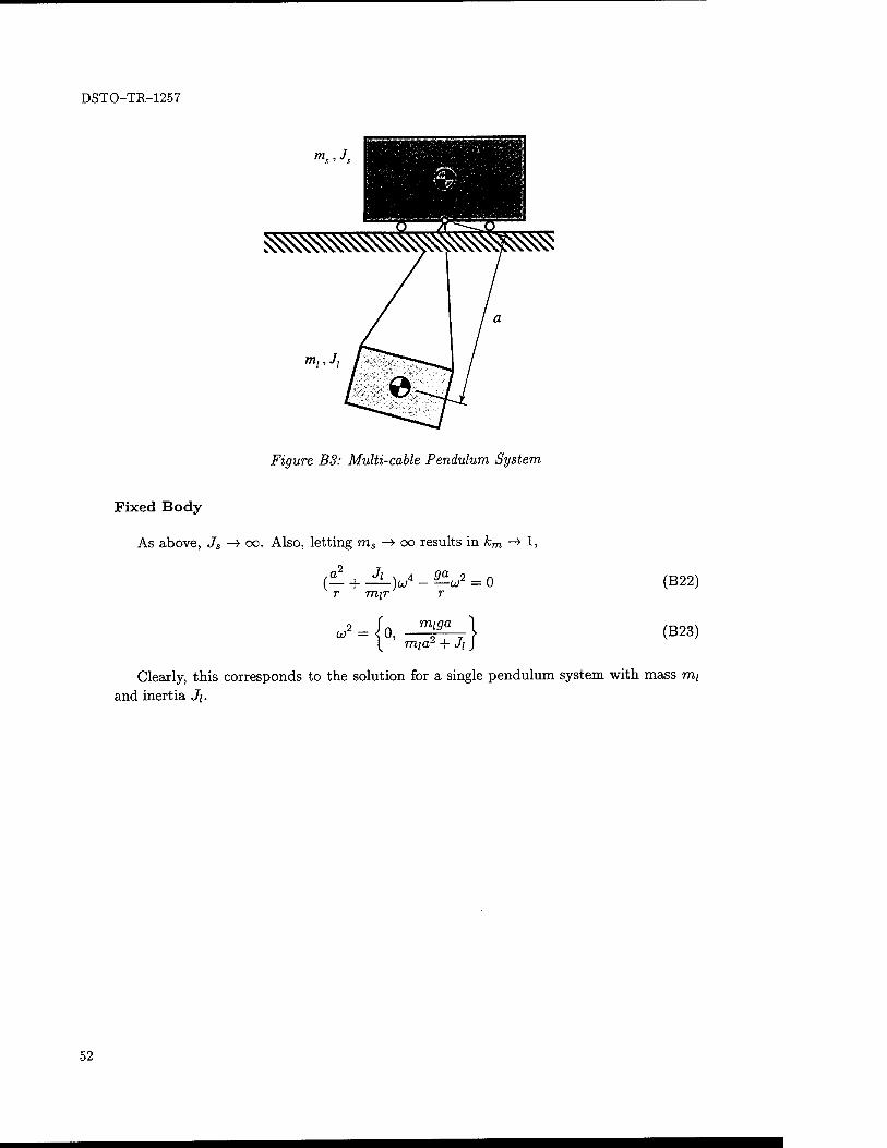
DSTO-TR-1257
m,>J,
Figure B3: Multi-cable Pendulum System
Fixed Body-
As above, Js —> oo. Also, letting ms —> oo results in km -> 1,
{al + JL)UJ* _ «V = 0 r mir r
(V "{* miga
mia2 + Ji
(B22)
(B23)
Clearly, this corresponds to the solution for a single pendulum system with mass mi
and inertia Jj.
52
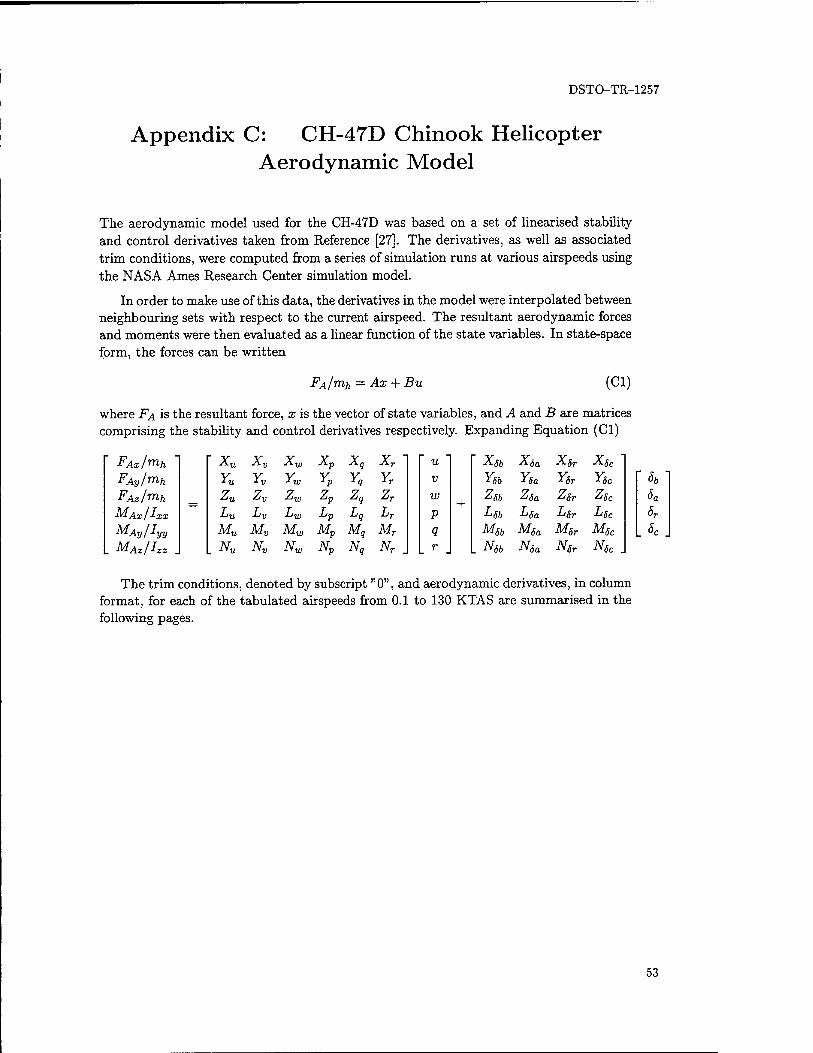
DSTO-TR-1257
Appendix C: CH-47D Chinook Helicopter Aerodynamic Model
The aerodynamic model used for the CH-47D was based on a set of linearised stability and control derivatives taken from Reference [27]. The derivatives, as well as associated trim conditions, were computed from a series of simulation runs at various airspeeds using the NASA Ames Research Center simulation model.
In order to make use of this data, the derivatives in the model were interpolated between neighbouring sets with respect to the current airspeed. The resultant aerodynamic forces and moments were then evaluated as a linear function of the state variables. In state-space form, the forces can be written
FAI^H — Ax + Bu (Cl)
where FA is the resultant force, x is the vector of state variables, and A and B are matrices comprising the stability and control derivatives respectively. Expanding Equation (Cl)
Xgb Xga Xgr X$C
Yöb Yia Yör Ygc
Zsb Zoo. %5r %6c Lsb Lga L$r Lsc
M5b MSa MSr MSc
NSb N5a NSr NSc
FAx/mh Xu Xv Xw Xp xq FAy/rrih Yu Yv %w YP Yq
FAz/rrih Zy. Zv %w Zp zq MAX/IXX Lu Lv ■L>w Lp Lq
MAy/Iyy Mu Mv Mw Mp Mq
MAZ/IZZ . [ Nu Nv Nw Np Nq
Xr 1 U
YT V
w
V +
MT q Nr _ r
sb 8a 8r
The trim conditions, denoted by subscript "0", and aerodynamic derivatives, in column format, for each of the tabulated airspeeds from 0.1 to 130 KTAS are summarised in the following pages.
53
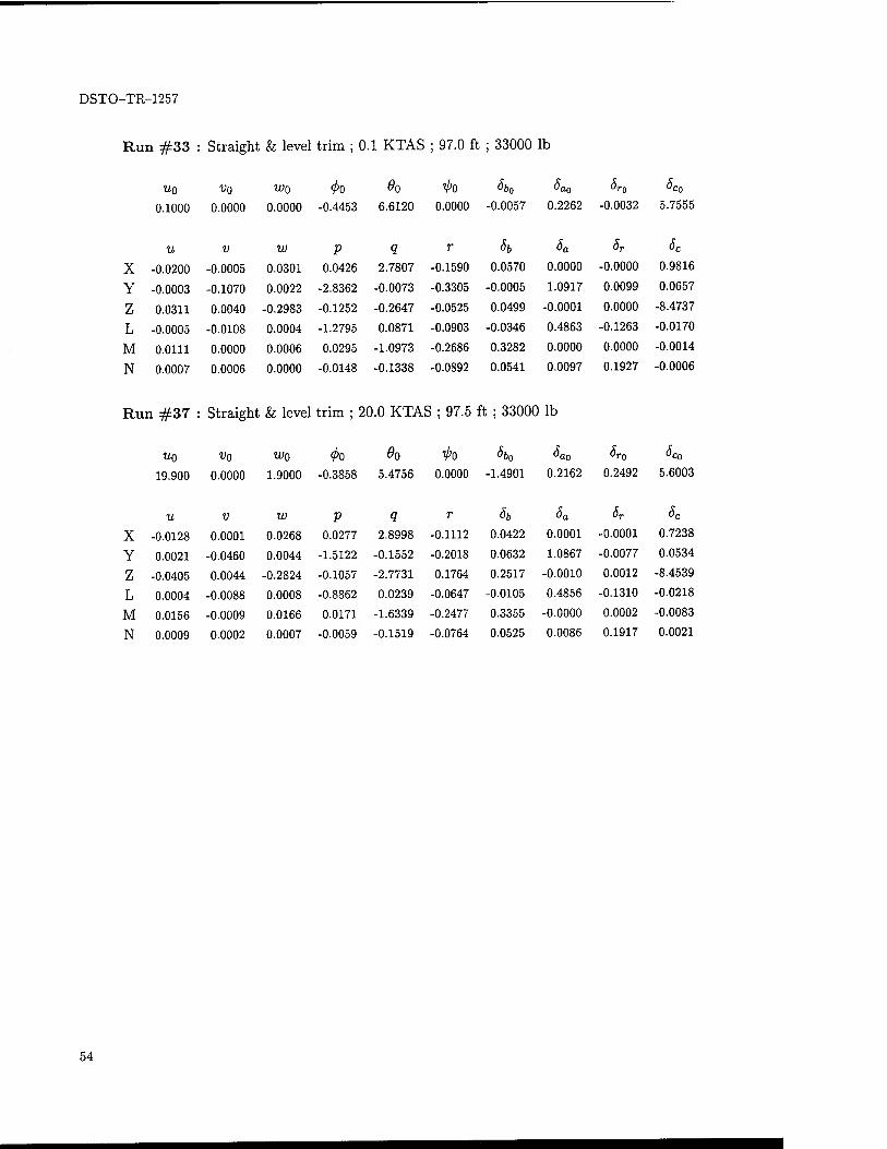
DSTO-TR-1257
Run #33 : Straight & level trim ; 0.1 KTAS ; 97.0 ft ; 33000 lb
U0 Vo too 4>0 #0 V'O h0 ^ao <^0 ^c0
0.1000 0.0000 0.0000 -0.4453 6.6120 0.0000 -0.0057 0.2262 -0.0032 5.7555
u v w p q r Sb 6a ST Sc
X -0.0200 -0.0005 0.0301 0.0426 2.7807 -0.1590 0.0570 0.0000 -0.0000 0.9816
Y -0.0003 -0.1070 0.0022 -2.8362 -0.0073 -0.3305 -0.0005 1.0917 0.0099 0.0657
Z 0.0311 0.0040 -0.2983 -0.1252 -0.2647 -0.0525 0.0499 -0.0001 0.0000 -8.4737
L -0.0005 -0.0108 0.0004 -1.2795 0.0871 -0.0903 -0.0346 0.4863 -0.1263 -0.0170
M 0.0111 0.0000 0.0006 0.0295 -1.0973 -0.2686 0.3282 0.0000 0.0000 -0.0014
N 0.0007 0.0006 0.0000 -0.0148 -0.1338 -0.0892 0.0541 0.0097 0.1927 -0.0006
Run #37 : Straight & level trim ; 20.0 KTAS ; 97.5 ft ; 33000 lb
Uo vo wo 4>Q 00 ipo K £ao ^r0 öco
19.900 0.0000 1.9000 -0.3858 5.4756 0.0000 -1.4901 0.2162 0.2492 5.6003
u V w P 1 r Sb 5a Sr <5c
X -0.0128 0.0001 0.0268 0.0277 2.8998 -0.1112 0.0422 0.0001 -0.0001 0.7238
Y 0.0021 -0.0460 0.0044 -1.5122 -0.1552 -0.2018 0.0632 1.0867 -0.0077 0.0534
Z -0.0405 0.0044 -0.2824 -0.1057 -2.7731 0.1764 0.2517 -0.0010 0.0012 -8.4539
L 0.0004 -0.0088 0.0008 -0.8862 0.0239 -0.0647 -0.0105 0.4856 -0.1310 -0.0218
M 0.0156 -0.0009 0.0166 0.0171 -1.6339 -0.2477 0.3355 -0.0000 0.0002 -0.0083
N 0.0009 0.0002 0.0007 -0.0059 -0.1519 -0.0764 0.0525 0.0086 0.1917 0.0021
54
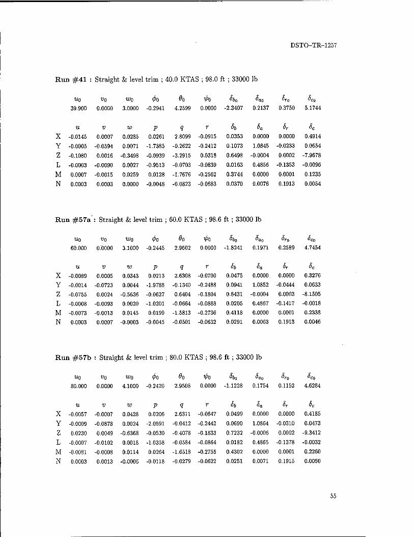
DSTO-TR-1257
Run #41 : Straight & level trim ; 40.0 KTAS ; 98.0 ft ; 33000 lb
Uo vo W0 00 00 ■00 6b0 6ao 6r0 6Co 39.900 0.0000 3.0000 -0.2941 4.2599 0.0000 -2.3407 0.2137 0.3750 5.1744
u V W P Q r 5b Sa Sr 6c X -0.0145 0.0007 0.0285 0.0261 2.8099 -0.0915 0.0353 0.0000 0.0000 0.4914
Y -0.0005 -0.0594 0.0071 -1.7385 -0.2622 -0.2412 0.1073 1.0845 -0.0233 0.0654
Z -0.1080 0.0016 -0.3498 -0.0939 -3.2915 0.0318 0.6498 -0.0004 0.0002 -7.9678
L -0.0003 -0.0090 0.0027 -0.9513 -0.0703 -0.0839 0.0163 0.4856 -0.1353 -0.0096
M 0.0007 -0.0015 0.0259 0.0128 -1.7676 -0.2562 0.3744 0.0000 0.0001 0.1235
N 0.0003 0.0003 0.0000 -0.0048 -0.0823 -0.0683 0.0370 0.0076 0.1913 0.0054
Run #57a': Straight & level trim ; 60.0 KTAS ; 98.6 ft ; 33000 lb
uo Vo wo <£o 00 V'O 6b0 Sao 6r0 6co 60.000 0.0000 3.1000 -0.2445 2.9602 0.0000 -1.8241 0.1971 0.2589 4.7454
u V w P Q r sb 6a 5r 6c X -0.0089 0.0005 0.0343 0.0213 2.6308 -0.0700 0.0475 0.0000. 0.0000 0.3276
Y -0.0014 -0.0723 0.0044 -1.9788 -0.1340 -0.2488 0.0941 1.0852 -0.0444 0.0633
Z -0.0755 0.0024 -0.5636 -0.0627 0.6404 -0.1804 0.8431 -0.0004 0.0003 -8.1505
L -0.0008 -0.0093 0.0020 -1.0201 -0.0664 -0.0888 0.0205 0.4867 -0.1417 -0.0018
M -0.0073 -0.0013 0.0145 0.0199 -1.5813 -0.2736 0.4118 0.0000 0.0001 0.2338
N 0.0003 0.0007 -0.0003 -0.0045 -0.0501 -0.0632 0.0291 0.0063 0.1913 0.0046
Run #57b : Straight & level trim ; 80.0 KTAS ; 98.6 ft ; 33000 lb
uo ^0 WQ 00 00 ^0 <5&o 6ao 6r0 6CQ
80.000 0.0000 4.1000 -0.2420 2.9508 0.0000 -1.1228 0.1754 0.1152 4.6284
u V W P 9 r *6 Sa 6r 6C
X -0.0057 -0.0007 0.0428 0.0206 2.6311 -0.0647 0.0499 0.0000 0.0000 0.4185
Y -0.0009 -0.0878 0.0024 -2.0591 -0.0412 -0.2442 0.0690 1.0864 -0.0310 0.0473
Z 0.0230 0.0049 -0.6368 -0.0530 -0.4078 -0.1833 0.7232 -0.0006 0.0002 -9.3412
L -0.0007 -0.0102 0.0018 -1.0358 -0.0584 -0.0864 0.0182 0.4865 -0.1378 -0.0032
M -0.0081 -0.0008 0.0114 0.0264 -1.6518 -0.2755 0.4302 0.0000 0.0001 0.2260
N 0.0003 0.0013 -0.0006 -0.0118 -0.0279 -0.0622 0.0251 0.0071 0.1915 0.0050
55
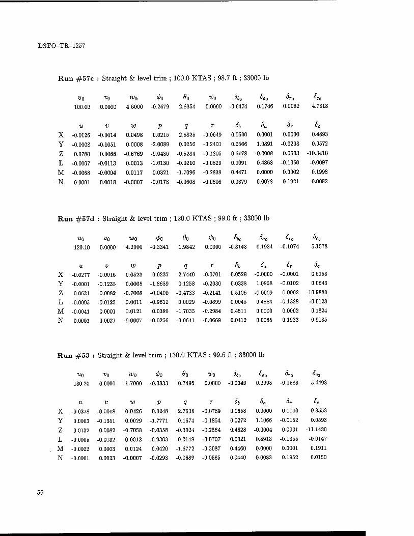
DSTO-TR-1257
Run #57c : Straight & level trim ; 100.0 KTAS ; 98.7 ft ; 33000 lb
Uo Vo Wo 00 #0 V'O ^60 6ao 6ro 5Co
100.00 0.0000 4.6000 -0.2679 2.6354 0.0000 -0.6474 0.1746 0.0082 4.7818
u v w p q r Si, Sa 5r Sc
X -0.0126 -0.0014 0.0498 0.0215 2.6825 -0.0649 0.0500 0.0001 0.0000 0.4893
Y -0.0008 -0.1051 0.0008 -2.0089 0.0256 -0.2401 0.0566 1.0891 -0.0203 0.0572
Z 0.0780 0.0066 -0.6769 -0.0486 -0.5284 -0.1805 0.6178 -0.0008 0.0003 -10.3410
L -0.0007 -0.0113 0.0013 -1.0130 -0.0210 -0.0829 0.0091 0.4868 -0.1350 -0.0097
M -0.0068 -0.0004 0.0117 0.0321 -1.7096 -0.2839 0.4471 0.0000 0.0002 0.1998
N 0.0001 0.0018 -0.0007 -0.0178 -0.0608 -0.0606 0.0379 0.0078 0.1921 0.0082
Run #57d : Straight & level trim ; 120.0 KTAS ; 99.0 ft ; 33000 lb
uo vo Wo 00 00 V>0 K <^o 6r0 <*c0
120.10 0.0000 4.2000 -0.3341 1.9842 0.0000 -0.3143 0.1934 -0.1074 5.1578
U V W P Q r sb Sa 6r 6c X -0.0277 -0.0016 0.0523 0.0237 2.7440 -0.0701 0.0528 -0.0000 -0.0001 0.5153
Y -0.0001 -0.1235 0.0005 -1.8659 0.1258 -0.2030 0.0338 1.0958 -0.0102 0.0643
Z 0.0631 0.0082 -0.7008 -0.0400 -0.4733 -0.2141 0.5106 -0.0009 0.0002 -10.9880
L -0.0005 -0.0125 0.0011 -0.9612 0.0029 -0.0699 0.0045 0.4884 -0.1328 -0.0128
M -0.0041 0.0001 0.0121 0.0389 -1.7035 -0.2984 0.4511 0.0000 0.0002 0.1824
N 0.0001 0.0021 -0.0007 -0.0256 -0.0641 -0.0669 0.0412 0.0085 0.1933 0.0135
Run #53 : Straight & level trim ; 130.0 KTAS ; 99.6 ft ; 33000 lb
UQ vo wo 00 00 ^0 £&o 6a0 6r0 6c0
130.20 0.0000 1.7000 -0.3833 0.7495 0.0000 -0.2349 0.2098 -0.1583 5.4493
u V VJ P Q r sb 6a Sr 6C
X -0.0378 -0.0018 0.0426 0.0248 2.7638 -0.0789 0.0658 0.0000 0.0000 0.3553
Y 0.0003 -0.1351 0.0029 -1.7771 0.1674 -0.1854 0.0272 1.1066 -0.0152 0.0593
Z 0.0132 0.0082 -0.7058 -0.0358 -0.3024 -0.2564 0.4628 -0.0004 0.0001 -11.1430
L -0.0005 -0.0132 0.0013 -0.9303 0.0149 -0.0707 0.0021 0.4918 -0.1355 -0.0147
M -0.0022 0.0003 0.0124 0.0420 -1.6772 -0.3087 0.4460 0.0000 0.0001 0.1911
N -0.0001 0.0023 -0.0007 -0.0293 -0.0689 -0.0565 0.0440 0.0083 0.1952 0.0150
56
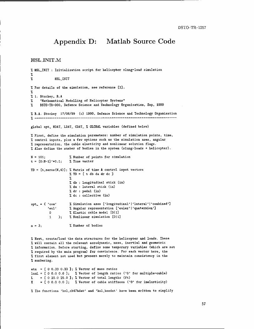
DSTO-TR-1257
Appendix D: Matlab Source Code
HSLJNIT.M
7, HSL_INIT : Initialisation script for helicopter slung-load simulation
7. 7. HSL.INIT
'/, For details of the simulation, see reference [1] .
7. 7. 1. Stuckey, R.A 7. "Mathematical Modelling of Helicopter Systems" 7. DSTO-TR-000, Defence Science and Technology Organisation, Sep. 1999
'/. R.A. Stuckey 17/08/99 (c) 1999, Defence Science and Technology Organisation %
global opt_ HDAT_ LDAT_ CDAT_ 7. GLOBAL variables (defined below)
7. First, define the simulation parameters: number of simulation points, time, 7. control inputs, plus a few options such as the simulation axes, angular
7. representation, the cable elasticity and nonlinear solution flags. '/. Also define the number of bodies in the system (slung-loads + helicopter) .
N = 101; '/, Number of points for simulation t = [0:N-1]'*0.1; 7. Time vector
TD = [t,zeros(N,4)] ; 7, Matrix of time & control input vectors 7. TD = [ t db da dr dc ]
7. 7. db : longitudinal stick (in) 7. da : lateral stick (in) 7. dr : pedal (in) 7. dc : collective (in)
opt_ = { 'com' '/. Simulation axes ['longitudinal'I'lateral'I'combined'] 'eul' 7. Angular representation ['euler'I'quaternion'] 0 7. Elastic cable model [Oil] 1 }; 7. Nonlinear simulation [Oil]
n = 3; 7. Number of bodies
7. Next, create/load the data structures for the helicopter and loads. These 7. will contain all the relevent aerodynamic, mass, inertial and geometric
7, information. Before starting, define some temporary variables (which are not 7, required by the main program) for convinience. For each vector here, the 7. first element not used but present merely to maintain consistency in the
7, numbering.
eta = [ 0 0.33 0.33 ]; 7. Vector of mass ratios lonL = [00.00.6]; 7. Vector of length ratios CO' for multiple-cable)
L = [ 0 20.0 25.0 ]; 7. Vector of total lengths (ft) K =[00.00.0]; 7. Vector of cable stiffness CO' for inelasticity)
7, The functions 'hsl_ch47bdat' and 'hsl.boxdat' have been written to simplify
57
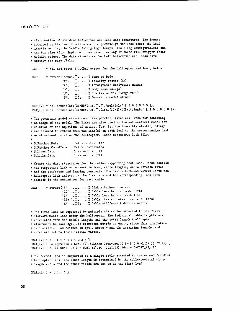
DSTO-TR-1257
'/. the creation of standard helicopter and load data structures. The inputs 7, required by the load function are, respectively: the load mass; the load '/. inertia matrix; the bridle (sling-leg) length; the sling configuration; and 7. the box size (ft) . Empty matrices given for any of these will trigger their 7. default values. The data structures for both helicopter and loads have
7. exactly the same fields.
HDAT. hsl_ch47bdat; 7. GLOBAL struct for the helicopter and load, below
LDAT_ = struct (' Name', [] ,
'V, D, 'A', [], 'm\ [],
'J\ [], 'S', []);
7, Name of body 7. Velocity vector (kn) "/, Aerodynamic derivative matrix
7. Body mass (slugs) 7. Inertia matrix (slugs.ft"2)
7. Geometric model struct
LDAT_(2) = hsl_boxdat(eta(2)*HDAT_.m, [],[],'multiple', [ 3.0 3.0 3.0 ]); LDAT_(3) = hsl_boxdat(eta(3)*HDAT_.m,[],(lonL(3)-l)*L(3), 'single', [ 3.0 3.0 3.0 ]);
7, The geometric model struct comprises patches, lines and links for rendering
7. an image of the model. The links are also used in the mathematical model for
7, solution of the equations of motion. That is, the (possibly elastic) slings
7. are assumed to extend from the link(s) on each load to the correspondign link
7, or attachment point on the helicopter. These structures look like:
7. 7. S.Patches.Data 7. S.Patches.Coordlndex
S.Lines.Data 7. S.Links.Data
Patch matrix (ft) Patch coordinates Line matrix (ft) Link matrix (ft)
7, Create the data structures for the cables supporting each load. These contain 7, the respective link attachment indices, cable lengths, cable stretch rates 7, and the stiffness and damping constants. The link attachment matrix lists the 7, helicopter link indices in the first row and the corresponding load link
7. indices in the second row for each cable.
CDAT_ = struct (' i' , [] , '10' ,D, 'l' ,D, ■ •ldot'.D, 'K' ,[]);
7, Link attachment matrix 7. Cable lengths - unloaded (ft) 7. Cable lengths - current (ft) 7, Cable stretch rates - current (ft/s) 7. Cable stiffness & damping matrix
7, The first load is supported by multiple (4) cables attached to the first 7. (forward-most) link under the helicopter. The individual cable lengths are
7. calculated from the bridle lengths and the total length (helicopter 7. attachment to load eg). The stiffness matrix is empty, since this simulation 7, is inelastic - as defined in opt_, above - and the remaining lengths and
7. rates are set to their initial values.
CDAT_(2).i =[1111:1234]; CDAT_(2).10 = sqrt(sum((-LDAT_(2).S.Links.Data+ones(4,l)*[ 0 0 -L(2) ])."2,2))'; CDAT_(2).K = []; CDAT_(2).l = CDAT_(2).10; CDAT_(2) .ldot = 0*CDAT_(2) .10;
7. The second load is supported by a single cable attached to the second (middle) 7, helicopter link. The cable length is determined by the cable-to-total sling
7. length ratio and the other fields are set as in the first load.
CDAT_(3).i = [ 3 ; 1 ];
58
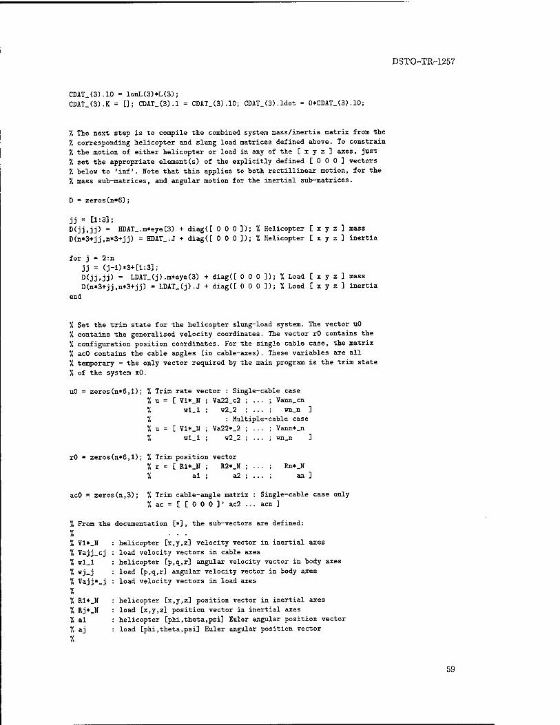
DSTO-TR-1257
CDAT_(3).10 = lonL(3)*L(3); CDAT_(3).K = []; CDAT_(3).l = CDAT_(3).10; CDAT_(3).ldot = 0*CDAT_(3).10;
'/, The next step is to compile the combined system mass/inertia matrix from the
'/, corresponding helicopter and slung load matrices defined above. To constrain 7. the motion of either helicopter or load in any of the [ x y z ] axes, just
'/. set the appropriate element (s) of the explicitly defined [000] vectors '/. below to 'inf. Note that this applies to both rectillinear motion, for the
'/, mass sub-matrices, and angular motion for the inertial sub-matrices.
D = zeros(n*6);
jj = [1:3]; D(jj»jj) = HDAT_.m*eye(3) + diag([ 0 0 0]); 7. Helicopter [ x y z ] mass D(n*3+jj,n*3+jj) = HDAT..J + diag([ 0 0 0]); 7. Helicopter [ x y z ] inertia
for j = 2:n jj = (j-l)*3+[l:3]; D<jj»jj> = LDAT_(j).m*eye(3) + diag([ 0 0 0]); 7. Load [ x y z ] mass D(n*3+jj,n*3+jj) = LDAT_(j).J + diag([ 0 0 0]); 7. Load [ x y z ] inertia
end
7. Set the trim state for the helicopter slung-load system. The vector uO 7. contains the generalised velocity coordinates. The vector rO contains the
7. configuration position coordinates. For the single cable case, the matrix 7, acO contains the cable angles (in cable-axes). These variables are all 7. temporary - the only vector required by the main program is the trim state
7. of the system xO.
uO = zeros(n*6,1); 7. Trim rate vector : Single-cable case 7. u = [ V1*_N ; Va22_c2 ; . .. ; Vann.cn 7. wl_l ; u2_2 ; ... ; wn_n ] 7, : Multiple-cable case
7. u = [ V1*_N ; Va22*_2 ; . . . ; Vann*_n 7. wl_l ; w2_2 ; ... ; un_n ]
rO = zeros(n*6,l); 7. Trim position vector 7. r = [ R1*_N ; R2*_N ; ... ; Rn*_N 7, al ; a2 ; .. . ; an ]
acO = zeros (n,3); 7, Trim cable-angle matrix : Single-cable case only 7. ac = [ [000]' ac2 ... acn ]
7. From the documentation [*] , the sub-vectors are defined:
7. ... 7, V1*_N : helicopter [x,y,z] velocity vector in inertial axes 7, Vajj_cj : load velocity vectors in cable axes 7. wl_l : helicopter [p,q,r] angular velocity vector in body axes 7. wj_j : load [p,q,r] angular velocity vector in body axes 7. Vajj*_j : load velocity vectors in load axes 7. 7. R1*_N : helicopter [x,y,z] position vector in inertial axes 7. Rj*_N : load [x.y.z] position vector in inertial axes 7. al : helicopter [phi.theta.psi] Euler angular position vector 7, aj : load [phi.theta.psi] Euler angular position vector
7.
59
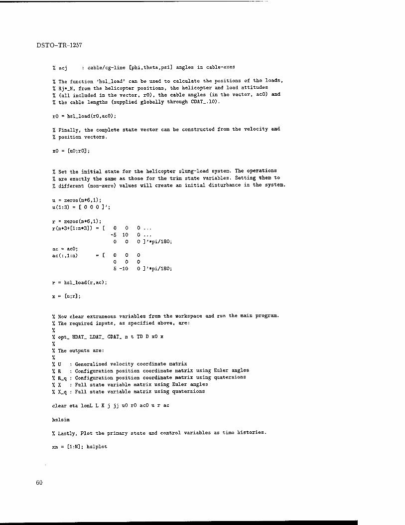
DSTO-TR-1257
7. acj : cable/cg-line [phi.theta.psi] angles in cable-axes
'/. The function 'hsl_load' can be used to calculate the positions of the loads, 7. Rj*_N, from the helicopter positions, the helicopter and load attitudes 7. (all included in the vector, rO), the cable angles (in the vector, acO) and
7. the cable lengths (supplied globally through CDAT_.10).
rO = hsl_load(rO,acO);
7. Finally, the complete state vector can be constructed from the velocity and
7. position vectors.
xO = [uO;rO];
7, Set the initial state for the helicopter slung-load system. The operations
7. are exactly the same as those for the trim state variables. Setting them to
7. different (non-zero) values will create an initial disturbance in the system.
u = zeros(n*6,l);
u(l:3) = [000]';
r = zeros(n*6,l); r(n*3+[l:n*3]) = [ 0 0 0 ...
-5 10 0 ... 0 0 0 ]'*pi/180;
ac = acO; ac(:,l:n) =[000
0 0 0 5 -10 0 ]'*pi/180;
r = hsl_load(r,ac);
x = [u;r] ;
7. Now clear extraneous variables from the workspace and run the main program.
7. The required inputs, as specified above, are:
7. 7. opt_ HDAT_ LDAT_ CDAT_ n t TD D xO x
7. 7. The outputs are:
7. 7, U : Generalised velocity coordinate matrix 7, R : Configuration position coordinate matrix using Euler angles 7. R_q : Configuration position coordinate matrix using quaternions 7, X : Full state variable matrix using Euler angles
7. X_q : Full state variable matrix using quaternions
clear eta lonL L K j jj uO rO acO u r ac
hslsim
7, Lastly, Plot the primary state and control variables as time histories.
xn = [1:N]; hslplot
60
DSTO-TR-1257
HSL_CH47BDAT.M
function D = hsl_ch47bdat(mass,inertia,links)
'/, HSL.CH47BDAT : Aircraft aerodynamic, mass, inertial and geometric data
V. */. DAT = HSL_CH47BDAT((mass) (.inertia) (.links))
*/. 7, mass : Helicopter mass (slugs)
'/, inertia : Inertia matrix (slug.ft"2)
'/, links : Links data matrix (see HSL_INIT)
'/. '/. DAT : Data structure (see HSL_INIT)
*/, Mass, inertial and aerodynamic data obtained from reference [1].
7. '/. 1. Weber, J.M. and Liu, T.Y. and Chung, W. '/. "A Mathematical Simulation Model of the CH-47B Helicopter, Volumes 1 & 2" '/, NASA-TM-84351-V0L-1/2, NASA Ames Research Center, Aug. 1984
7, R.A. Stuckey 01/06/99 (c) 1999, Defence Science and Technology Organisation %
if nargin<3, links = [] ; end if nargin<2, inertia = []; end
if nargin<l, mass = []; end
'/. Set some defaults
if isempty(mass), mass = 33000/32.174; end if isempty(inertia)
inertia = [ 34000 0 14900 0 202500 0 14900 0 191000 ];
end
D = structCName'.n.'V'.n.'A'.a.'m'.n.'J'.D.'S'.E]);
D.Name = 'CH-47B';
D.V = [ 0.1 20 40 60 80 100 120 130 ]'; '/. Trim airspeed (KTAS)
'/, Construct the aerodynamic coefficient matrix
D.A = zeros(8,10*6,2);
7. SAS Off
7. 7. v = 0.1 KTAS
7. A = [ -1.99980e-002 -2.78070e-004 3.11490e-002 -5.32570e-004 1.10900e-002 7.34520e-004
-4.59450e-004 -1.07040e-001 4.00190e-003 -1.07710e-002 9.49780e-006 5.81320e-004 3.00850e-002 2.23380e-003 -2.98310e-001 3.99760e-004 6.38150e-004 4.24930e-005
4.26000e-002 -2.83620e+000 -1.25200e-001 -1.27950e+000 2.95300e-002 -1.48080e-002 2.78070e+000 -7.31250e-003 -2.64720e-001 8.71280e-002 -1.09730e+000 -1.33780e-001
-1.59040e-001 -3.30450e-001 -5.25060e-002 -9.02880e-002 -2.68610e-001 -8.91680e-002
5.70000e-002 -4.84860e-004 4.98650e-002 -3.46400e-002 3.28160e-001 5.40720e-002
61
DSTO-TR-1257
1.00060e-005 1.09170e+000 -7.62340e-005 -4.76460e-007 9.86840e-003 O.OOOOOe+000 9.81570e-001 6.56800e-002 -8.47370e+000
]'; D.A(1,:,1) = A(:)';
4.86300e-001 7.42500e-006 9.74910e-003 -1.26340e-001 O.OOOOOe+000 1.92690e-001 -1.70400e-002 -1.43180e-003 -5.52630e-004
•/. v = 20.0 KTAS
'/. A = [ -1.28440e-002
1.43630e-004 2.67660e-002 2.76530e-002
2.89980e+000
-1.11160e-001 4.21820e-002
9.33870e-005
-7.28990e-005
7.23840e-001
]'; D.A(2,:,1)
2.05350e-003 ■4.60310e-002 4.35330e-003
■1.51220e+000 55240e-001 01820e-001 31740e-002
08670e+000
71500e-003
33870e-002
-4.05230e-002
4.43150e-003 -2.82440e-001
-1.05700e-001 -2.77310e+000
1.76410e-001 2.51680e-001
-1.04440e-003
1.22740e-003 -8.45390e+000
3.66750e-004 -8.76990e-003 8.33700e-004
-8.86220e-001 2.38660e-002
-6.46980e-002 -1.04610e-002 4.85580e-001
-1.30970e-001 -2.18100e-002
1.55770e-002 -8.73300e-004 1.66480e-002 1.71360e-002
-1.63390e+000 -2.47710e-001 3.35480e-001
-2.16560e-005 2.10380e-004
-8.30050e-003
9.33590e-004 2.30440e-004 7.13630e-004
-5.86890e-003 -1.51860e-001 -7.64320e-002 5.25400e-002
8.61240e-003
1.91730C-001
2.06350e-003
= A(:)'
'/. v = 40.0 KTAS
'/. A = [ -1.45080e-002 - 7.12390e-004 - 2.85410e-002 2.60640e-002 - 2.80990e+000 -
-9.15160e-002 - 3.53470e-002 3.09700e-005 9.52930e-006 - 4.91350e-001
]'; D.A(3,:,1) =
4.56290e-004 5.94030e-002 7.10780e-003 1.73850e+000 2.62180e-001 2.41250e-001 1.07320e-001 1.08450e+000 2.32600e-002 6.53500e-002
' A(:)';
-1.07970e-001 1.55100e-003 -3.49780e-001 -9.39210e-002 -3.29150e+000 3.18470e-002 6.49750e-001 -4.11670e-004 1.90590e-004 -7.96780e+000
-2.78280e-004 -8.99530e-003 2.74400e-003 -9.51320e-001 -7.03350e-002 -8.39020e-002 1.62620e-002 4.85580e-001 -1.35310e-001 -9.56590e-003
7.31330e-004
-1.53180e-003 2.58770e-002 1.28110e-002
-1.76760e+000 -2.56190e-001 3.74440e-001 7.42500e-006 1.06420e-004 1.23530e-001
2.52740e-004 3.20370e-004 2.49070e-005
-4.82000e-003 -8.23200e-002 -6.83260e-002 3.69750e-002 7.62330e-003 1.91260e-001 5.36610e-003
'/. v = 60.0 KTAS
7. A = [ -8.90430e-003 • 4.56690e-004 ■ 3.42780e-002 2.12800e-002 ■ 2.63080e+000 -
-6.99840e-002 - 4.75450e-002 2.38230e-005 9.52930e-006 ■ 3.27550e-001
]'; D.A(4,:,1) =
■1.36390e-003 ■7.23000e-002 4.36120e-003
■1.97880e+000 ■1.34030e-001 2.48750e-001 9.41300e-002 1.08520e+000 4.43990e-002 6.33380e-002
■■ A(:>';
-7.54850e-002 2.38840e-003 -5.63570e-001 -6.27030e-002 6.40370e-001 -1.80370e-001
8.43060e-001 -3.58300e-004 2.59200e-004 -8.15050e+000
-7.78620e-004 -9.29200e-003 2.04470e-003 -1.02010e+000 -6.64380e-002 -8.87950e-002 2.05270e-002 4.86690e-001 -1.41650e-001 -1.81260e-003
-7.26000e-003 -1.28440e-003 1.45080e-002 1.99240e-002 -1.58130e+000 -2.73610e-001
4.11840e-001 1.48500e-005 1.04570e-004 2.33770e-001
2.75770e-004 7.42330e-004 -3.09370e-004
-4.54600e-003 -5.01390e-002 -6.32470e-002 2.91390e-002 6.29670e-003 1.91280e-001 4.56090e-003
7. v = 80.0 KTAS
7. A = [ -5.70700e-003 -8.59470e-004 2.30150e-002 -7 -7.31440e-004 -8.77940e-002 4.89230e-003 -1
4.27800e-002 2.40690e-003 -6.36790e-001 1 2.05520e-002 -2.05910e+000 -5.30210e-002 -1 2.63110e+000 -4.12240e-002 -4.07800e-001 -5
,20310e-004 -8.07210e-003
01780e-002 -7.76930e-004 81170e-003 1.14460e-002 03580e+000 2.64380e-002 84190e-002 -1.65180e+000
2.93460e-004 1.34520e-003 -5.56030e-004 -1.17890e-002 -2.79330e-002
62
DSTO-TR-1257
-6.46630e-002 -2.44250e-001 4.99400e-002 6.90110e-002 4.24050e-005 1.08640e+000 1.14350e-005 -3.10170e-002 4.18550e-001 4.72800e-002
]'; D.A(5,:,1) = A(:)';
-1.83310e-001 -8.63580e-002 -2.75520e-001 -6.21810e-002 7.23190e-001 1.81860e-002 4.30170e-001 2.50860e-002 -5.71760e-004 4.86460e-001 1.98000e-005 7.14560e-003 2.28700e-004 -1.37820e-001 1.31180e-004 1.91540e-001
-9.34120e+000 -3.23580e-003 2.26040e-001 5.02230e-003
7. v = 100.0 KTAS
A
-1 -1 4
2 2
-6
5
6 1 4
[ ,26360e-002
.35680e-003
.98200e-002
.15280e-002
,68250e+000 .49300e-002
,00190e-002
,24170e-005
.04820e-005
.89300e-001
D.A(6,:,1)
-7.51370e-004 -1.05140e-001 8.41670e-004
-2.00890e+000 2.56190e-002
-2.40140e-001
5.66120e-002
1.08910e+000
-2.02930e-002 5.72410e-002
= A(:)';
7.79880e-002
6.60610e-003 -6.76910e-001 -4.85800e-002
-5.28360e-001
-1.80540e-001
6.17770e-001
-7.85210e-004
3.12560e-004
-1.03410e+001
-6.59260e-004 -1.12800e-002
1.32360e-003
-1.01300e+000 -2.10030e-002 -8.29250e-002
9.06130e-003
4.86820e-001
-1.34970e-001
-9.66370e-003
-6.81070e-003 -3.57580e-004 1.16510e-002 3.20850e-002
-1.70960e+000
-2.83950e-001
4.47050e-001
1.36120e-005 1.52830e-004
1.99790e-001
8.58610e-005 1.77010e-003
-7.02930e-004
-1.78010e-002 -6.07910e-002
-6.06080e-002
3.78660e-002
7.83530e-003 1.92080e-001
8.24070e-003
'/. v = 120.0 KTAS
7. A = [ -2.77000e-002
-1.64920e-003 5.22720e-002 2.36600e-002 2.74400e+000 -7.00630e-002 5.27850e-002
-2.66820e-005 -7.33760e-005 5.15320e-001
]>; D.A(7,:,1)
-1.34170e-004
-1.23550e-001 5.28050e-004 -1.86590e+000
1.25820e-001 -2.03000e-001 3.37610e-002 1.09580e+000 -1.02440e-002 6.42760e-002
= A(:)';
6.30760e-002
8.15140e-003 -7.00810e-001 -3.99660e-002 -4.73260e-001 -2.14120e-001 5.10630e-001 -8.69070e-004 1.67720e-004 -1.09880e+001
-4.79240e-004 -1.24840e-002 1.12150e-003
-9.61180e-001 2.85120e-003 -6.99070e-002 4.49670e-003 4.88370e-001 -1.32770e-001 -1.27980e-002
-4.14310e-003
9.20080e-005 1.20600e-002 3.89050e-002 -1.70350e+000 -2.98380e-001 4.51130e-001
8.04370e-006 1.72630e-004 1.82350e-001
8.77130e-005 2.10200e-003 -7.09630e-004 -2.55800e-002 -6.41210e-002 -6.68580e-002 4.12170e-002
8.50380e-003 1.93300e-001 1.35210e-002
7. v = 130.0 KTAS
7. A = [ -3.78490e-002
-1.78130e-003 4.26380e-002 2.47760e-002
2.76380e+000 -7.88740e-002 6.57840e-002 2.38230e-005 1.76290e-005 3.55270e-001
]'; D.A(8,:,1)
2.51630e-004 -1.35140e-001 2.86170e-003 -1.77710e+000 1.67400e-001
-1.85370e-001 2.71970e-002
1.10660e+000 -1.51530e-002 5.92710e-002
= A(:)';
1.32080e-002 8.17960e-003 -7.05780e-001 -3.57920e-002
-3.02350e-001 -2.56380e-001 4.62770e-001 -3.58300e-004
5.33640e-005 -1.11430e+001
-4.70110e-004 -1.31600e-002 1.31020e-003
-9.30250e-001 1.48530e-002 -7.06540e-002 2.11230e-003
4.91790e-001 -1.35500e-001 -1.47050e-002
-2.21120e-003 2.78040e-004 1.24230e-002 4.19650e-002 -1.67720e+000 -3.08690e-001 4.46010e-001
6.80620e-006 7.92000e-005 1.91100e-001
-1.31000e-004 2.27430e-003
-6.89930e-004 -2.93120e-002 -6.89040e-002 -5.64850e-002 4.39730e-002
8.25240e-003 1.95170e-001 1.50040e-002
7. SAS On
7. 7. v = 0.1 KTAS
7. A = [
63
DSTO-TR-1257
-2.00190e-002 -4.58720e-004 2.95890e-002 4.26580e-002
2.76530e+000 -1.59080e-001 5.69980e-002
-4.76460e-007
0.OOOOOe+000 9.82140e-001
]'; D.A(1,:,2)
-2.79300e-004
-1.07040e-001 2.20110e-003
-4.80530e+000
-8.48820e-003 -3.54870e-001 -4.73250e-004
1.09170e+000 9.87340e-003 6.57510e-002
= A(:)';
3.13430e-002
3.99430e-003 -2.93800e-001 -1.25310e-001
-1.16850e-001 -5.24300e-002 4.98950e-002
0.OOOOOe+000
-7.62340e-006 -8.47890e+000
-5.33410e-004 -1.07860e-002 3.92040e-004 -2.16340e+000
8.65030e-002 5.98430e-002
-3.46380e-002
4.86300e-001 -i.26340e-001 -1.70130e-002
1.10900e-002
8.69340e-006 6.48540e-004 2.95170e-002
-1.09920e+000 -2.68650e-001
3.28170e-001 6.18750e-007
6.18750e-007 -1.43490e-003
7.34570e-004
6.02580e-004 4.01240e-005 -2.27710e-002
-1.33820e-001 -3.23810e-001 5.40740e-002
9.74810e-003 1.92690e-001
-5.47820e-004
•/. v = 20.0 KTAS
X A = [ -1.28450e-002
1.43680e-004 -
2.67660e-002
2.73040e-002 -
2.90000e+000 •
-1.11040e-001 ■ 4.22050e-002
-1.95350e-005 -8.67170e-005 ■ 7.23850e-001
]'; D.A(2,:,2) =
2.05360e-003
4.69260e-002
4.35350e-003
3.47460e+000
1.55300e-001
1.93430e-001 6.31900e-002 1.08670e+000 7.72250e-003 5.34030e-002
' AC:)';
-4.05190e-002
4.44410e-003
-2.82440e-001
-1.00800e-001
-2.77560e+000
1.74270e-001 2.51470e-001 2.82070e-004 1.15880e-003
-8.45410e+000
3.68320e-004 -1.19320e-002 8.35320e-004
-1.76990e+000 2.38450e-002 9.46100e-002
-1.04580e-002 4.85580e-001
-1.30970e-001 -2.18080e-002
1.55760e-002 -8.70520e-004 1.66470e-002 1.76080e-002
-1.63400e+000 -2.47990e-001 3.35490e-001
5.07370e-005 1.16320e-004 -8.30980e-003
9.31240e-004
4.54010e-003
7.11290e-004
-1.10830e-002
-1.51840e-001
-3.10110e-001 5.25420e-002
8.61630e-003 1.91730e-001 2.06790e-003
7. v = 40.0 KTAS
7. A = [ -1.42800e-002 7.12670e-004 - 2.85590e-002 2.59480e-002 - 2.80990e+000 -
-9.15410e-002 - 3.53760e-002 3.38290e-005 7.62340e-006 - 4.91340e-001
]'; D.A(3,:,2) =
2.09760e-004 6.16240e-002 7.19340e-003 3.69780e+000 2.62190e-001 2.41250e-001 1.07330e-001 1.08450e+000 2.32630e-002 6.53570e-002
AC:)';
-1.04060e-001 1.55750e-003 -3.49160e-001 -9.25870e-002 -3.29140e+000 3.20760e-002 6.49480e-001 -4.11670e-004 1.90590e-004 -7.96770e+000
-1.66880e-004 -1.53840e-002
2.75790e-003 -1.83520e+000 -7.03380e-002 -8.39040e-002 1.62660e-002 4.85580e-001 -1.35310e-001 -9.56410e-003
3.02760e-003 -1.52910e-003 2.61800e-002 1.27460e-002 -1.76760e+000 -2.56190e-001 3.74470e-001 1.67060e-005 1.01470e-004 1.23540e-001
4.71550e-004 8.83450e-003 5.38230e-005
-8.27830e-003 -8.23200e-002 -6.83270e-002 3.69740e-002 7.62280e-003 1.91260e-001 5.36710e-003
7. v 7. A = -8. 4. 3. 2.
2.
-6.
4.
1.
1.
3.
60.0 KTAS
c 27460e-003 55900e-004 43190e-002 11980e-002
63080e+000
99690e-002
75450e-002
90590e-005
28650e-005
27530e-001
D.AC4,:,2)
-4.85040e-005 -7.65220e-002 4.43620e-003 -3.94060e+000 -1.33990e-001
-2.48740e-001
9.41200e-002
1.08520e+000
-4.44340e-002
6.33311e-002
= AC:)';
-6.34290e-002 2.40440e-003 -5.62920e-001 -6.09110e-002 -6.40410e-001
-1.80520e-001 8.43140e-001
-3.88800e-004
1.82960e-004
-8.15030e+000
-4.90270e-004 -1.89950e-002 2.06160e-003 -1.90630e+000 -6.64230e-002
-8.87900e-002
2.05240e-002
4.86690e-001
-1.41660e-001
-1.81280e-003
-1.49840e-003 -1.27800e-003 1.48370e-002 2.00350e-002 -1.58130e+000
-2.73610e-001
4.11830e-001
4.33130e-006
1.03330e-004
2.33750e-001
6.84190e-004 1.33160e-002 -2.86400e-004 -5.59910e-003 -5.01410e-002
-6.32470e-002
2.91370e-002
6.29400e-003
1.91280e-001
4.55900e-003
7. v = 80.0 KTAS
64
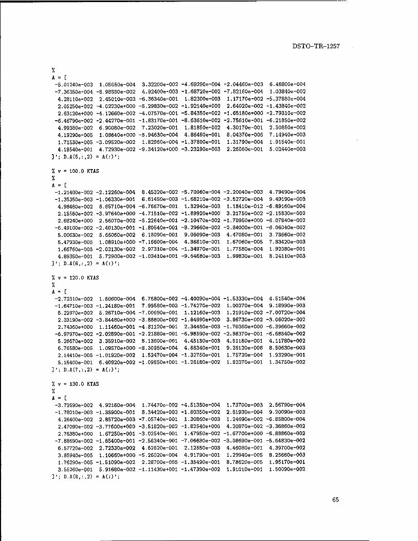
DSTO-TR-1257
7. A = [
-5.01240e-003 -7.36350e-004
4.28110e-002
2.0S250e-002 2.63120e+000
-6.46790e-002 4.99380e-002
4.19290e-005
1.71530e-005
4.18540e-001 ]'; D.A(5,:,2)
1.05650e-004
-8.98880e-002
2.45010e-003
-4.02230e+000 -4.12660e-002
-2.44270e-001 6.90080e-002
1.08640e+000 -3.09520e-002
4.72930e-002
= A(:)';
3.32200e-002
4.92400e-003
-6.36340e-001
-5.29830e-002 -4.07570e-001
-1.83170e-001
7.23020e-001 -5.94630e-004
1.82960e-004
-9.34120e+000
-4.69290e-004
-1.68720e-002
1.82300e-003
-1.92140e+000 -5.84350e-002
-8.63610e-002
1.81850e-002 4.86460e-001
-1.37800e-001
-3.23290e-003
-2.04460e-003 -7.82160e-004
1.17170e-002
2.64020e-002
-1.65180e+000
-2.75610e-001 4.30170e-001 8.04370e-006
1.31790e-004 2.26060e-001
6.48800e-004
1.03840e-002
-5.37880e-004
-1.43840e-002 -2.79310e-002
-6.21850e-002 2.50850e-002
7.14940e-003
1.91540e-001
5.02440e-003
'/. v
•/. A = -1. -1. 4. 2. 2.
-6.
5. 5. 1. 4.
]';
= 100.0 KTAS
[ 21400e-002 35350e-003 98460e-002 15560e-002 68240e+000
49100e-002 00630e-002
47930e-005 66760e-005 89350e-001 D.A(6,:,2)
-2.12260e-004 -1.06330e-001
8.65710e-004 -3.97640e+000 2.56070e-002
-2.40130e-001 5.66060e-002 1.08910e+000
-2.03130e-002 5.72900e-002
= A(:)';
8.45320e-002 6.61450e-003
-6.76670e-001 -4.71510e-002 -5.22640e-001
-1.80540e-001 6.18090e-001 -7.16600e-004 2.97310e-004 -1.03410e+001
-5.70060e-004 -1.68210e-002
1.32940e-003 -1.89920e+000 -2.10470e-002 -8.29660e-002
9.06090e-003
4.86810e-001 -1.34970e-001
-9.64680e-003
-2.20040e-003 -3.52720e-004 1.18410e-012 3.21750e-002 -1.70950e+000 -2.84000e-001
4.47080e-001 1.67060e-005 1.77580e-004
1.99830e-001
4.79490e-004 9.49190e-003 -6.89160e-004 -2.15830e-002 -6.07840e-002
-6.06040e-002 3.78660e-002
7.83420e-003 1.92080e-001 8.24110e-003
7. v = 120.0 KTAS
7. A = [ -2.72310e-002 -1.64710e-003 5.22970e-002 2.33190e-002 2.74360e+000
1.60600e-004 6.76800e-002 -4.40090e-004 -1.53330e-004 4.51540e-004 -1.24180e-001 7.99580e-003 -1.74270e-002 1.00270e-004 9.18990e-003 5.26710e-004 -7.00690e-001 1.12160e-003 1.21910e-002 -7.00720e-004 -3.84480e+000 -3.88800e-002 -1.84990e+000 3.86730e-002 -3.06020e-002 1.11460e-001 -4.81120e-001 2.34480e-003 -1.70360e+000 -6.39660e-002
-6.97970e-002 -2.02890e-001 -2.21880e-001 -6.98590e-002 -2.98370e-001 -6.68540e-002 5.26670e-002 3.35910e-002 5.13600e-001 4.45150e-003 4.51180e-001 4.11780e-002 6.76580e-005 1.09570e+000 -8.30950e-004 4.88340e-001 9.28120e-006 8.50630e-003 2.14410e-005 -1.01920e-002 1.52470e-004 -1.32750e-001 1.75720e-004 1.93290e-001 5.15400e-001 6.40920e-002 -1.09850e+001 -1.28180e-002 1.82370e-001 1.34750e-002
]'; D.A(7,:,2) = A(:)';
'I, v = 130.0 KTAS
7. A = [ -3.72690e-002 4.92160e-004 -1.78010e-003 -1.35900e-001 4.26400e-002 2.85720e-003 2.47090e-002 -3.77600e+000 2.76380e+000 1.67250e-001
-7.88690e-002 -1.85400e-001 6.57720e-002 2.72330e-002 3.85940e-005
1.76290e-005 3.55260e-001
]'; D.A(8,:,2)
1.10660e+000 -1.51090e-002
5.91680e-002 = A(:)';
1.74470e-002 8.34420e-003 -7.05740e-001 -3.51820e-002
-3.02540e-001
-2.56340e-001 4.62820e-001 -5.26020e-004
2.28700e-005 -1.11430e+001
-4.51350e-004 -1.80350e-002 1.30860e-003
-1.82540e+000 1.47950e-002 -7.06680e-002
2.12550e-003 4.91790e-001
-1.35490e-001 -1.47390e-002
1.73700e-003 2.81930e-004 1.24690e-002 4.20970e-002 -1.67700e+000
-3.08690e-001
4.46080e-001 1.29940e-005 8.78620e-005
1.91010e-001
2.56790e-004 9.20090e-003 -6.85800e-004 -3.36860e-002
-6.88860e-002 -5.64830e-002
4.39700e-002 8.25660e-003
1.95170e-001 1.50090e-002
65
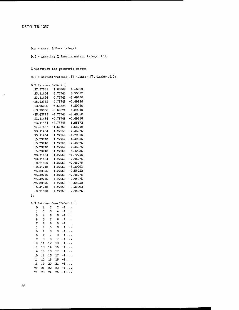
DSTO-TR-1257
D.m = mass; '/. Mass (slugs)
D.J = inertia; '/. Inertia matrix (slugs.ft"2)
'/, Construct the geometric struct
D.S = struct('Patches',[],'Lines',[],'Links', []);
D.S.Patches
27.57681 23.11464
23.11464
-25.42775
-13.96066
-13.96066
-25.42775
23.11464
23.11464
27.57681 23.11464 23.11464 15.73240 15.73240 15.73240 15.73240 23.11464 23.11464 -8.21890
-10.41718 -25.08325 -25.42775 -25.42775 -25.08325 -10.41718 -8.21890
];
.Data = [
1.60769
4.75745
4.75745
4.75745
6.69324
-6.69324
-4.75745
-4.75745
-4.75745
-1.60769 1.27959 1.27959 1.27959 1.27959
-1.27959 -1.27959 -1.27959 -1.27959
27959 27959 27959 27959 27959
1.27959 1.27959 1.27959
4.56059
6.95572
49356
49356
89010
89010
.49356
.49356
95572
56059
,46075 -4.79026 -4.42935 -2.46075 -2.46075 -4.42935 -4.79026 -2.46075 -2.46075 -8.30093 -9.58052 -2.46075 -2.46075 -9.58052 -8.30093 -2.46075
D.S.Patches.Coordlndex = [
10 11 12 13 - 12 13 14 15 -
14 15 16 17 -
10 11 16 17 - 11 12 15 16 -
18 19 20 21 -
20 21 22 23 -
22 23 24 25 -
66
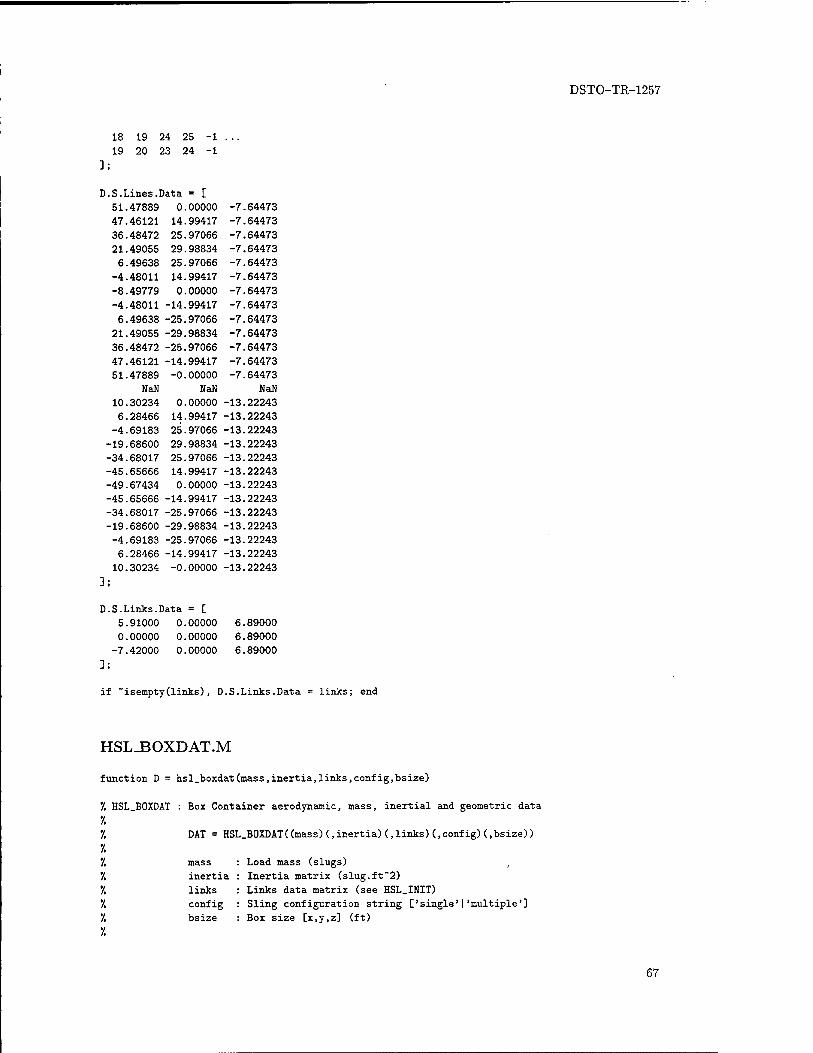
DSTO-TR-1257
18 19 24 25 19 20 23 24
];
D.S.Lines.Data 51.47889 47.46121 36.48472 21.49055 6.49638
-4.48011 -8.49779 -4.48011 -14 6.49638 -25
21.49055 -29 36.48472 -25 47.46121 -14 51.47889 -0
NaN 10.30234 6.28466
-4.69183 -19.68600 -34.68017 -45.65666 -49.67434 -45.65666 -34.68017 -19.68600 -4.69183 6.28466 -14 10.30234 -0
3;
0 14 25 29 25 14 0
-14 -25 -29 -25
= [ .00000 ,99417 ,97066 .98834 ,97066 ,99417 ,00000 ,99417 ,97066 ,98834 ,97066 ,99417 ,00000
NaN ,00000 .99417 ,97066 ,98834 ,97066 ,99417 ,00000 ,99417 97066 98834 97066 99417 ,00000
D.S.Links.Data = [ 5.91000 0.00000
-7.42000
0.00000 0.00000 0.00000
-7.64473 -7.64473 -7.64473 -7.64473 -7.64473 -7.64473 -7.64473 -7.64473 -7.64473 -7.64473 -7.64473 -7.64473 -7.64473
NaN -13.22243 -13.22243 -13.22243 -13.22243 -13.22243 -13.22243 -13.22243 -13.22243 -13.22243 -13.22243 -13.22243 -13.22243 -13.22243
6.89000 6.89000 6.89000
];
if "isempty(links), D.S.Links.Data = links; end
HSL_BOXDAT.M
function D = hsl_boxdat(mass,inertia,links,config,bsize)
'/. HSL_B0XDAT : Box Container aerodynamic, mass, inertial and geometric data •/. '/, DAT = HSL_B0XDAT((mas s)(,inertia)(.links)(,config)(,bsize)) •/. '/, mass : Load mass (slugs) 7. inertia : Inertia matrix (slug.ft"2) 7, links : Links data matrix (see HSL_INIT) 7. config : Sling configuration string ['single'I'multiple'] 7, bsize : Box size [x,y,z] (ft) 7.
67
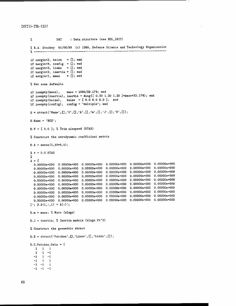
DSTO-TR-1257
•/ DAT : Data structure (see HSL.INIT)
7. R.A. Stuckey 01/06/99 (c) 1999, Defence Science and Technology Organisation •/§
if nargin<5, bsize = G; end if nargin<4, config = []; end if nargin<3, links = D ; end if nargin<2, inertia = D; end if nargin<l, mass = D; end
'/, Set some defaults
if isempty(mass), mass = 1000/32.174; end if isempty(inertia), inertia = diag([ 0.33 1.20 1.20 ]*mass*32.174); end
if isempty(bsize), bsize = [ 6.0 6.0 6.0 ]; end
if isempty(config), config = 'multiple'; end
D = structCName'.ü.'V'.D.'A'.D.'m'.G.'J'.n.'S'.ü);
D.Name = 'BOX';
D.V = [ 0.0 ]; 7. Trim airspeed (KTAS)
7, Construct the aerodynamic coefficient matrix
D.A = zeros(1,10*6,1);
7. v = 0.0 KTAS
7. A = [
0.00000e+000 0.00000e+000 0.00000e+000 0.00000e+000 0.00000e+000 0.00000e+000 0.00000e+000 0.00000e+000 0.00000e+000 0.00000e+000 0.00000e+000 0.00000e+000 0.00000e+000 0.00000e+000 0.00000e+000 0.00000e+000 0.00000e+000 0.00000e+000 0.00000e+000 0.00000e+000 0.00000e+000 0.00000e+000 0.00000e+000 0.00000e+000 0.00000e+000 0.00000e+000 0.00000e+000 0.00000e+000 0.00000e+000 0.00000e+000 0.00000e+000 0.00000e+000 0.00000e+000 0.00000e+000 0.00000e+000 0.00000e+000 0.00000e+000 0.00000e+000 0.00000e+000 0.00000e+000 0.00000e+000 0.00000e+000 0.00000e+000 0.00000e+000 0.00000e+000 0.00000e+000 0.00000e+000 0.00000e+000 0.00000e+000 0.00000e+000 0.00000e+000 0.00000e+000 0.00000e+000 0.00000e+000 0.00000e+000 0.00000e+000 0.00000e+000 0.00000e+000 0.00000e+000 0.00000e+000
]'; D.A(1,:,1) = A(:)';
D.m = mass; 7. Mass (slugs)
D.J = inertia; 7. Inertia matrix (slugs.ft"2)
7, Construct the geometric struct
D.S = struct ('Patches', D,'Lines',[],'Links',[]);
D.S.Patches.Data = [
111 11-1
-1 1 -1 -1 1 1 -1 -1 1 -1 -1 -1
68
DSTO-TR-1257
1 -1 -1 1 -1 1
]*diag (bsize/2);
D.S.Patche s.Cc ordlndex = 0 1 2 3 -1 ... 2 3 4 5 -1 ... 4 5 6 7 -1 ... 1 2 5 6 -1 ... 0 1 6 7 -1 ... 0 3 4 7 -1
];
if strcmpi(config,'single')
D.S.Lines.Data = [ 11-1 0 0-1
NaN NaN NaN 1 -1 -1 0 0-1
NaN NaN NaN -1 1 -1
0 0-1 NaN NaN NaN -1 -1 -1
0 0-1 NaN NaN NaN
]*diag(bsize/2);
D.S.Links.Data = [ 0 0-1
]*diag(bsize.*[ 0.0 0.0 1.0 ]);
if "isempty(links) if (length(links) == 1)
D.S.Links.Data(3) = links; else
D.S.Links.Data = links; end
end
D.S.Lines.Data([2,5,8,ll],:) = ones(4,l)*D.S.Links.Data;
elseif strcmpi(config, 'multiple')
D.S.Lines.Data = [] ; D.S.Links.Data = [
11-1
-1 1 -1 -1 -1 -1
1 -1 -1 ]*diag(bsize.*[ 0.5 0.5 0.5 ]);
if "isempty(links), D.S.Links.Data = links; end
end
69
DSTO-TR-1257
HSLJLOAD.M
function r = hsl_load(r,acj)
7. HSL.LOAD : Calculate load positions from the helicopter positions, the 7, helicopter and load attitudes and the cable lengths ft orientation
7. 7. r = HSL_LOAD(r(,acj))
7. 7. r : Configuration position vector
7. = [ R1*_N ; R2*_N ; ... ; Rn*_N 7. al ; a2 ;...;■ an ] 7, acj : Cable-angle matrix : Single-cable case only
7. = [ [ 0 0 0 ] ' ac2 ... acn ]
7. 7. The sub-vectors are defined:
7. • • ■ 7, R1*_N : helicopter [x,y,z] position vector in inertial axes 7. Rj*_N : load [x,y,z] position vector in inertial axes 7, al : helicopter [phi.theta.psi] Euler angular position vector 7, .aj : load [phi.theta.psi] Euler angular position vector
7. 7, acj : cable/cg-line [phi.theta.psi] angles in cable-axes 7. 7. See HSL.INIT for more information
7. R.A. Stuckey 01/10/97 (c) 1997, Defence Science and Technology Organisation >L
global HDAT_ LDAT_ CDAT_
n = length(LDAT_); n = n+("n);
if nargin<2, acj = zeros(n,3); end
'/, Create some transformation matrices
T_jN = zeros(3,3,n); T.cjN = NaN*ones(3,3,n);
T_jN(:,:,l) = euler(r(n*3+[1:3]));
7. Determine sling configuration
mj = zeros(l,n); MultipleCables = NaN; SingleCable = NaN;
for j = 2:n mj(j) = length(CDAT_(j).10);
MultipleCables(j) = (mj(j)>2) ft (~any(diff(sort(CDAT_(j).i(l,:)))));
SingleCable(j) = (mj(j)==l);
end
7. Calculate the load positions
for j = 2:n
jj = (j-l)*3+[l:3];
70
DSTO-TR-1257
T_jN(:,:,j) = euler(r(n*3+jj)); 7. Load-axes transformation
toplinks = HDAT_.S.Links.Data(CDAT_(j).i(l,:),:); botlinks = LDAT_(j) .S.Links.Data(CDAT_(j) .i(2,:),:);
if MultipleCables(j)
if any(diff(CDAT_(j).D) error(' Cable lengths must be equal !')
end
*/. Calculate load length (x) and width (y)
Rili4_j = diff(botlinks([4,l],:))'; b = sqrt(sum(Rili4_j.*2)) ;
Rili2_j = diff(botlinks([2,1],:))'; c = sqrt(sum(Rili2_j.'2)) ;
7. Calculate distance from load eg to helicopter attachment point
zl = sqrt(CDAT_(j).l(l)-2-(b/2)-2-(c/2)-2)-botlinks(l,3);
7. Update the (load) position vector
r(jj) = r(l:3) ... +T_jN(:,:,l),*toplinks(l,:)' ...
+T_jN(:,:,j)'*C 0 0 zl ]';
elseif SingleCable(j)
T_cjN(:,:,j) = euler(acj (:, j)) ; 7. Cable-axes transformation
7, Update the (load) position vector
r(jj) = r(l:3) ... +T_jN(:,:,l)'»toplinks' ... +T_cjN(:,:,j)'*[ 0 0 CDAT_(j).l ]' ... -T_jN(:,:,j)'»botlinks';
end end
HSLSIM.M
'/, HSLSIM : Helicopter Slung-Load dynamic Simulation
7. 7. 7. 7. 7.
HSLSI
Input
7. 7.
opt_
HDAT.
7. LDAT_
7. CDAT_
7. n 7. t
7. 7.
TD D
7. xO
GLOBAL options cell array [4x1]
GLOBAL helicopter struct GLOBAL loads struct array [lxn] GLOBAL loads struct array [lxn]
Number of bodies
Time vector [Nil] Time & control input matrix [Nx5] System mass/inertia matrix [n*6xn*6] Trim state vector [n*6xl]
71
DSTO-TR-1257
'/. x : Initial state vector [n*6xl] '/. '/, Outputs: 7. '/, U : Generalised velocity coordinate matrix [Nxn*6] J5 R : Configuration position coordinate matrix using Euler angles [Nxn*6] 55 R_q : Configuration position coordinate matrix using quaternions [Nxn*7]
55 X : Full state variable matrix using Euler angles [Nxn*12] 55 X_q : Full state variable matrix using quaternions [Nxn*13]
"/. 55 See HSL_INIT for more information
'/. R.A. Stuckey 01/10/97 (c) 1997, Defence Science and Technology Organisation %
global HDAT. LDAT_ CDAT_ opt_
55 Check input variables and set defaults
if length(opt_)<4
{'combined','euler',0,1}; for i = length(opt_)+1:4
opt_{i} = ans{i}; warning([' Using opt_{',int2str(i) ,'} = ',opt_{i}])
end end
if C"stmcmpi(opt_-[l},'longitudinal'.length(opt_{l}))) ... & (~strncmpi(opt_{l}, 'lateral', length (opt_-Cl>))) ... & (~strncmpi(opt_-{l}, 'combined' ,length(opt_{l}))) errorC Option, opt_{l> = ',opt_{l},' not recognised !')
end
opt_2 = strncmpi(opt_{2},'quaternion',length(opt_{2})); o2 = opt_2+3; if (~opt_2)&C"strncmpi(opt_{2},'euler' ,length(opt_{2»))
errorC Option, opt_{2> = ',opt_{2},' not recognised !')
end
if ~any(opt_{3}==[0,l]) errorC Option, opt_{3} = ' ,int2str(opt_{3» ,' not recognised !')
end
if opt_{3} for j = 2:n
if isempty(CDAT_(j).K) errorC Empty stiff ness/damping matrix, CDAT.C ,int2str(j) ,') .K !')
end end
end
if -any(opt_{4>==[0,l]) errorC Option, opt-(4} = ' ,int2str(opt_{4}),' not recognised !')
end if ("opt_-C4})&("existCcontrol','dir'))
errorC Linear simulation requires CONTROL SYSTEM TOOLBOX !')
end
55 Determine sling configuration
72
DSTO-TR-1257
mj = zeros(l,n); MultipleCables = NaN; SingleCable = NaN; for j = 2:n
mj(j) = length (CDAT_(j). 10);
MultipleCables(j) = (mj(j)>2) & (_any(diff(sort(CDAT_(j).i(l,:)))));
SingleCable (j) = (mj(j)==l);
end
'/, Construct inverse mass/inertia matrix
finD = isfinite(diag(D)); finDn = find(finD);
diag(inf*ones(l,n*6)); ans(finDn,finDn) = D(finDn,finDn); D = ans;
zeros(n*6); ans(finDn,finDn) = inv(D(finDn,finDn)); Di = ans;
'/, Determine trim configuration velocities
[xdotO.vaO] = hsl_fun(0,zeros(n*12,l),[],D,Di,xO,zeros(n*6,l),zeros(l,5)) ;
'I, Set initial, perturbed state from trim
if "opt_2 dx = x-xO;
else xO_q = [x0(l:n*9) ;zeros(n*4,D] ; x_q = [x(l:n*9) ;zeros(n*4,D] ;
for j = l:n x0_q(n*9+(j-l)*4+[l:4]) = e2ql(x0(n*9+(j-l)*3+[l:3])); x_q(n*9+(j-l)*4+[l:4]) = e2ql(x(n*9+(j-l)*3+[l:3]));
end dx_q = x_q-x0_q;
end
'/, Run the simulation
if opt_{4}==l '/. Nonlinear simulation: '/, Uses 4/5th order R-K integration routine oith fixed step-size
options = odeset;
if "opt_2 '/, Euler representation [t,dX] = ode45f('hsl_fun',t,dx,options, D,Di,xO,vaO,TD);
else '/, Quaternion representation [t,dX_q] = ode45f('hsl_fun',t,dx_q,options, D,Di,xO_q,vaO,TD);
end else 7. Linear simulation:
'/, Uses linear time-invariant time response kernel
if "opt_2 7, Euler representation del = le-3*ones(n*12,l); VII DELTA FOR JACOBIAN COMPUTATION
dxO = zeros(n*12,l);
'/, Compute the state and control jacobian matrices
fac = []; vec = [] ; del = le-3*ones(n*12,l); DFDY = numjac('hsl_fun' ,0,dx0,fty,del,fac,vec, [],[],[] , D,Di,x0,va0,zeros(l,5));
73
DSTO-TR-1257
del = le-3*ones(4,l); '/.'/.'/. DELTA ydel = diag(del); fdel = zeros(n*12,4);
for j = 1:4 fdel(:,j) = hsl_fun(0,dxO,[], D,Di,xO,vaO, [0,ydel(:,j)']);
end DFDD = (fdel-fty(:,ones(l,4)))*diag(l ./del);
'/. Convert linear system from continuous to discrete
sys = ss(DFDY,DFDD,eye(n*12),zeros(n*12,4));
sysd = c2d(sys,t(2)-t(l),'foh');
7. Implement any initial velocities and perform the simulation
rOdot = [vO(l :n*3);zeros(n*3,1)];
for j = l:n Wij_j = eratesi(x0(n*9+(j-l)*3+[l:3]));
r0dot(n*3+(j-l)*3+[l:3]) = Wij_j*v0(n*3+(j-l)*3+[l:3]);
end
dX = lsim(sysd,TD(:,2:5),t,dx)+t*[zeros(l,n*6),r0dot'];
else '/• Quaternion representation del = le-3*ones(n*13,l); %'l,% DELTA FOR JACOBIAN COMPUTATION
dxO_q = zeros(n*13,1);
'/. Compute the state and control jacobian matrices
fac = [] ; vec = [] ; del = le-3*ones(n*12,l); DFDY = numjac('hsl_fun',0,dxO_q,fty,del,fac,vec, [],[],[] , D,Di,xO_q,vaO,zeros(l,5));
del = le-3*ones(4,l); •/.'/.'/. DELTA ydel = diag(del); fdel = zeros(n*13,4);
for j = 1:4 fdel(:,j) = hsl_fun(0,dxO,[], D,Di,xO,vaO, [O.ydeK:, j)']) ;
end DFDD = (fdel-fty(:,ones(l,4)))*diag(l ./del);
'/. Convert linear system from continuous to discrete
sys = ss(DFDY,DFDD,eye(n*13),zeros(n*13,4));
sysd = c2d(sys,t(2)-t(l),'foh');
'/, Implement any initial velocities and perform the simulation
rOdot_q = [v0(l:n*3);zeros(n*4,l)];
for j = l:n Wij-j = qratesi(x0_q(n*9+(j-l)*4+[l:4])); r0dot_q(n*3+(j-l)*4+[l:4]) = Wij_j*v0(n*3+(j-l)*3+[l :3]);
end
dX_q = lsim(sysd,TD(:,2:5),t,dx_q)+t*[zeros(l,n*6).rOdot.q'] ;
end end
7, Create the full state variable matrices
74
DSTO-TR-1257
if ~opt_2 '/, Euler representation
'/, Detect and remove erroneous (divergent) observations from the simulation
isdiv = (sign(abs(imag(dX)))lisinf(dX)lisnan(dX)) ;
if any(any(isdiv)) warning('Divergent solution !') N = min(find(sum(isdiv,2)))-l; dX = dX(l:N,:);
else N = size(dX.l);
end t = t(l:N); TD = TD(1:N,:);
'/. Add initial state to perturbed state and calculate quaternions
X = dX+ones(N,l)*xO'; R = X(:,n*6+[l:n*6]);
U = X(:,l:n*6); R_q = [R(:,l:n*3),zeros(N,n*3)];
for j = l:n R_q(:,n*3+(j-l)*4+[l:4]) = e2q(R(: ,n*3+(j-l)*3+[l:3]));
end
X_q = [U,R_q] ; else '/, Quaternion representation
7, Detect and remove erroneous (divergent) observations from the simulation
isdiv = (sign(abs(imag(dX_q)))lisinf(dX_q)Iisnan(dX_q)) ;
if any(any(isdiv)) warning('Divergent solution !') N = min(find(sum(isdiv,2)))-l; dX_q = dX_q(l:N,:);
else N = size(dX_q,l);
end t = t(l:N); TD = TD(1:N,:);
'/. Add initial state to perturbed state and calculate Euler angles
X_q = dX_q+ones(N,l)*xO_q'; R_q = X_q(:,n*6+[l:n*7]) ;
U = X_q(:,l:n*6); R = [R_q(:,l:n*3),zeros(N,n*4)];
for j = l:n R(:,n*3+(j-l)*3+[l:3]) = q2e(R_q(: ,n*3+(j-l)*4+[l:4]));
end
X = [U,R] ; end
'/. Compute body-axes velocities, cable angles and internal cable forces
Va = zeros(N,n*6); Vadot = zeros(N,n*6); TDD = zeros(N,5);
if n>l Acj = zeros(N,(n-l)*3); FC = zeros(N.n-l);
end
for i = 1:N '/, Evaluation loop (no integration)
'/. Call the function with all output arguments
75
DSTO-TR-1257
if ~opt_2 7, Euler representation [xdot,va,vadot,acj,fc,d] = hsl_fun(t(i) ,dX(i,:)',[] ,D,Di,xO,vaO,TD);
else 'I, Quaternion representation [xdot_q,va,vadot,acj,fc,d] = hsl_fun(t(i) ,dX_q(i,:)',[] ,D,Di,xO_q,vaO,TD) ;
end
7, Insert the variables into their respective observation matrices
Va(i,:) = va'; Vadot(i,:) = vadot'; if n>l
squeeze(acj(:,l,2:n)); Acj(i,:) =ans(:)'; FC(i,:) = (fc./diag(D([2:n]*3,[2:n]*3))/32.174)';
end TDD(i,:) = [t(i),d'];
end
ODE45F.M
function [T,Y,Yd] = ode45f(odefile.T.yO,options,varargin)
7. DDE45F : Solve differential equations - higher order method
7. 7. [T,Y,Yd] = 0DE45F('F',T,y0,options(,varargin))
7. •/, F : String containing the name of the ODE function
7. 7, where yd = F(t,y)
7. 7, T : Time vector [Nxl] 7, yO : Initial conditions [nxl]
7. 7. Y : Solution matrix [Nxn] 7, Yd : Differential matrix [Nxn]
7. 7. See 0DE45, ODE
7. Modified from 0DE45.M:
7. 7. C.B. Moler, 3-25-87, 8-26-91, 9-08-92. 7. Copyright (c) 1984-94 by The MathWorks, Inc.
7, R.A. Stuckey 10/12/97 (c) 1997, Defence Science and Technology Organisation %
7. Initialise the integration parameters and matrices
alf=[ 1/4 3/8 12/13 1 1/2 ]'; bet=[ [1 0 0 0 0 0 ]/4
[3 9 0 0 0 0 ]/32 [ 1932 -7200 7296 0 0 0 ]/2197 [ 8341 -32832 29440 -845 0 0 ]/4104 [-6080 41040-28352 9295 -5643 0 ]/20520 ];
gam=[ [ 902880 0 3953664 3855735 -1371249 277020 ]/7618050 [-2090 0 22528 21970 -15048 -27360 ]/752400 ];
76
DSTO-TR-1257
T = T(:);
N = sized,1); ny = size(yO,l); Nb = size(bet);
H = diff(T); f = zeros(ny,Nb(2)); Y = zeros(N.ny); Yd = Y;
Y(l,:) = yO';
'/. Set the output function
if isempty(options)
outfun = " ;
else outfun = odeget(options,'OutputFcn');
end
if "isempty(outfun)
feval(outfun,T([l,N]),yO,'init'); end
for n = 1:N-1 7, The main loop ...
'/, Compute the slopes
f(:,l) = feval(odefile,T(n),Y(n,:)',[],varargin{:});
Yd(n,:) = f(:,l)';
for j = l:Nb(l) f (:,j+l) = feval(odefile,T(n)+H(n)*alf (j),Y(n,:)'+H(n)*f*bet(j,:)',[] ,varargin{:});
end
'/. Estimate the error
7. 7. delta = norm(H(n)*f*gam(2,:)\'infJ);
7, Update the solution
Y(n+1,:) = Y(n,:)+H(n)*gam(l,:)*f';
7, Check the status of the output function
if "isempty(outfun) status = feval(outfun,T(n+l),Y(n+l,:));
if status, break, end
end
end
7. Evaluate the last time point and truncate output matrices if necessary
Yd(n+1,:) = fevaKodef ile,T(n+l) ,Y(n+l,:)',[] ,varargin{:}) ';
N = n+1; T = T(1:N); Y = Y(1:N,:); Yd = Yd(l:N,:);
7. Set the output status
if "isempty(outfun)
77
DSTO-TR-1257
f eval (outf un,[],[],' done'); end
HSL.FUN.M
function [xdot,va,vadot,acj,Fc,d] = hsl_fun(t,dx,FLAG,D,Di,xO,vaO,TD)
ODE function for helicopter slung-load system
[xdot,va,vadot, ac j,Fc,d] = HSL.FUN(t,dx,FLAG,D,Di,xO,vaO,TD)
Current time variable Current perturbed state vector [n*6xl] String with the type of information to return *N0T USED*
System mass/inertia matrix [n*6xn*6]
Inverse system mass/inertia matrix [n*6xn*6]
Trim state vector [n*6xl] Trim body-axes velocity vector [n*6xl]
Time & control input matrix [Nx5]
Current state rate vector [n*6xl] Current body-axes velocity vector [n*6xl] Current body-axes acceleration vector [n*6xl] Cable angle matrix [3x4xn] Internal cable force vector [n-lxl] Current control input vector [4x1]
See HSLSIM for details
'/. R.A. Stuckey 01/10/97 (c) 1997, Defence Science and Technology Organisation
X
global HDAT_ LDAT_ CDAT_ opt_ tdd_ vadot_ rdot_
n = length(LDAT_); n = n+("n); nx = length(xO);
opt_2 = (nx==n*13); o2 = opt_2+3;
'/. Early exit if dx is in err
if ("isreal(dx)|any(isinf(dx)lisnan(dx))) xdot = dx; return
end
7. Define some strings for FEVAL function evaluation, below
if opt_2 anglestr = 'quaternion'; ratesstr = 'qratesi';
else anglestr = 'euler'; ratesstr = 'eratesi';
end
7. HSL.FUN : ODE f
•/. */. [xdot
7. y. t
7. dx
7. FLAG
7. D
7. Di
7. xO
7. vaO
7. TD
7. 7. xdot
7. va 7. vadot 7. acj 7. Fc 7. d . 7. 7. See H
7. Determine axes to be used in solution (the sub-space)
if strncmpi(opt_{l>,'longitudinal',length(opt_{1})) 7. For n=2, ans = [1,3,8,4,6,11]; nsys = [ans,ans+12];
78
DSTO-TR-1257
[l,3,n*3+2,n*6+[l,3]]'*ones(l,n)+ones(5,l)*[0:n-l]*3; nsys = ans(:)';
if opt_2 [n*9+ [1,3]]' »ones (1 ,n) +ones (2,1) * [0: n-1] *4;
else [n*9+[2]]'*ones(l,n)+ones(l,l)*[0:n-l]*3;
end
nsys = [nsys,ans(:)'] ;
elseif stmcmpi(opt_{l},'lateral' ,length(opt_{l})) '/. For n=2, ans = [2,7,9,5,6,10,12]; nsys = [ans,ans+12] ;
[2,n*3+[l,3],n*6+[2,3]]'*ones(l,n)+ones(5,l)*[0:n-l]*3; nsys = ans(:)';
if opt_2 [n*9+ [1:4]]' »ones (1 ,n) +ones (4,1) * [0:n-1] »4;
else [n*9+[l,3]]'*ones(l,n)+ones(2,l)*[0:n-l]*3;
end nsys = [nsys,ans(:)'] ;
else 7. For n=2, ans = [1:3,7:9,4:6,10:12]; nsys = [ans,ans+12] ;
[l:3,n*3+[l:3] ,n*6+[l:3]]'*ones(l,n)+ones(9,l)*[0:n-l]*3; nsys = ans(:)';
if opt_2 [n*9+[l:4]]'*ones(l,n)+ones(4,l)*[0:n-l]*4;
else [n*9+[l:3]]'*ones(l,n)+ones(3,l)*[0:n-l]*3;
end nsys = [nsys,ans(:)'] ;
end
i = xO+dx; '/. Current state = trim + perturbation
7. Set all other variables, outside the solution space, to zero
zeros(nx,l); ans(nsys) = x(nsys); x = ans; uO = x0(l:n*6); rO = x0(n*6+[l:n*(o2+3)]); u = x(l:n*6); r = x(n*6+[l:n*(o2+3)]);
'/, Create some transformation matrices
T_jN = zeros(3,3,n); T.cjN = NaN*ones(3,3,4,n);
T_jN(:,:,l) = feval(anglestr,r(n*3+[l:o2]));
'/, Determine sling configuration
mj = zeros(l,n); MultipleCables = NaN; SingleCable = NaN;
for j = 2:n mj(j) = length(CDAT_(j).10);
MultipleCables (j) = (mj(j)>2) & (~any(diff(sort(CDAT_(j).i(l,:)))));
SingleCable(j) = (mj(j)==l);
end
kcj_N = NaN*ones(3,4,n); acj = NaN*ones(3,4,n); wcj_cj = NaN*ones(3,4,n);
79
DSTO-TR-1257
Rlsjs_N = NaN*ones(3,n);
7. Calculate the cable properties for each load
for j = 2:n
T_jN(:,:,j) = f evaKanglestr ,r (n*3+(j-l)*o2+ [1: o2])); '/. Load-axes
Rlsjs_N(:,j) = -r(l:3)+r((j-l)*3+[l:3]);
toplinks = HDAT_.S.Links.Data(CDAT_(j) .i(l,:), :) ; botlinks = LDAT_(j).S.Links.Data(CDAT_(j).i(2,:), :);
if MultipleCables(j) Rajjs.N = Rlsjs_N(:,j)*ones(l,mj(j))-T_jN(:,:,l)' »toplinks'; CDAT_(j) .Raji_N = Rajjs_N+T_jN(:,:,j) '»botlinks'; */. Attachment-attachment
CDAT_(j).l = sqrt(sum((CDAT_(j).Raji_N).-2,l)); '/. Cable length CDAT_(j).ldot = u((j-2)*3+3+[l:3])'*(T_jN(:,:,j)*CDAT_(j).Raji_N)./(CDAT_(j).l);
elseif SingleCable(j) Rajjs.N = Rlsjs_N(:,j)-T_jN(:,:,l)'*toplinks';
CDAT_(j) .RajiJI = Rajjs_N+T_jN(:,:, j) '»botlinks'; 7. Attachment-attachment
CDAT_(j).l = sqrt(sum((CDAT_(j).Raji_N)."2,D); 7. Cable length
CDAT_(j).ldot = u((j-2)*3+3+[3]);
end
for i = l:mj(j) kcj_N(:,i,j) = CDAT_(j).Raji_N(:,i)/CDAT_(j).l(i); 7. Cable unit-vectors
acj(:,i,j) = k2a(kcj_N(:,i,j)); 7. Cable angles T_cjN(:,:,i,j) = euler(acj (: ,i, j)) ; 7. Transformations
end end
7. Construct the configuration matrices
[A,Ai,Adot,H] = hsl_config(u,T_jN,T_cjN,Rlsjs_N,acj);
X Correct the system mass/inertia matrix for implementation into the equations
finD = isfinite(diag(D)); finDn = find(finD); D2 = zeros(n*6,n*6); D2(finDn,finDn) = D(finDn,finDn);
for j = l:n jj = (j-l)*3+[l:3]; D2(jj,jj) = [ 1 -1 -1 ; -1 1 -1 ; -1 -1 1 ].*D2(jj,jj);
end
X Compute the gravitational force
g = 32.174; g_N = [ 0 0 g ]'*[ones(l,n),zeros(l,n)];
fg = zeros(n*6,l);
for j = l:n
jj = (j-l)*3+[l:3]; fg(jj) = D2(jj(3),jj(3))*[ 0 0 g ]';
end
'/, Calculate the body-axes velocities and current control inputs
v = A*u; va = v;
for j = l:n
80
DSTO-TR-1257
jj = (j-l)*3+[l:3]; va(jj) = T_jN(:,:, j)*v(jj);
end
if all(size(TD)==[1,5])
d = TD(2:5)';
else tdi = (TD(:,l)==t); if any(tdi)
d = TD(find(tdi),2:5)'; else
d = interplq(TD(:,l),TD(:,2:5),t)';
end
end
7. Compute the aerodynamic force and convert back to inertial axes
[AA.BA] = hsl.faero(va); fa = AA*(va-vaO) + BA*d; fa = diag(D2).*fa;
for j = l:n jj = (j-l)*3+[l:3]; fa(jj) = T_jN(:,:, j) >*fa(jj) ;
end
'/, Calculate the total static weight and moments on the helicopter
dl = D2(l,l); ml = 0;
for j = 2:n jj = (j-l)*3+[l:3]; dl = dl+D2(jj(l),jJÜ)); ml = ml+D2(jj(l),jj(l))*(rO(l)-rO(jj(l)));
end
'/. Compute the thrust force (approximation) and convert back to inertial axes
ft = zeros(n*6,l);
if 0 7. thrust (resultant) is vertical
ft(3) = -dl*32.174; ft(n*3+2) = -ml*32.174;
else 7, thrust is normal to body
ft(3) = -dl*32.174; ft(n*3+2) = -ml*32.174;
for j = l:n jj = (j-l)*3+[l:3]; ft(jj) = T_jN(:,:, j) '*ft(jj);
end
end
7. Compute the Coriolis forces and then the combined forces
X = zeros(n*6,l); for j = l:n
jj = (n+j-l)*3+[l:3]; X(jj) = skew3(u(jj))*D2(jj,jj)*u(jj);
end
81
DSTO-TR-1257
fx = -X-D2*Adot*u; fo = fa+fg+ft+fx;
'/, Determine a solution for the cable forces
fc = zeros(n*6,l); sf = fc;
H = HCfinDn,:); Di = Di(finDn.f inDn) ; 7. The sub-space defined above
if opt_{3} 7. Elastic solution
FC = zeros(n*12,1); hi = zeros(1,n*12);
for j = 2:n
jj = (j-l)*3+[l:3];
if HultipleCables(j) fC = (CDAT_(j).K(l,:)).*(l-(CDAT_(j).10)./(CDAT_(j).D) ...
+(CDAT_(j).K(2,:)).*(CDAT_(j).ldot)./(CDAT_(j).l);
FC(jj) = sum(ones(3,l)*max(0,f«.*(CDAT_(j).Raji_N),2); hi(jj) = 1;
elseif SingleCable(j) fC = (CDAT_(j).K(l)).*(l-(CDAT_(j).10)./(CDAT_(j).D) ...
+(CDAT_(j).K(2)).*(CDAT_(j).ldot)./(CDAT_(j).1);
FC(jjU)) = max(0,f«.*(CDAT_(j).l); hi(jj(D) = 1;
end end
FC = FC(find(hi)); else */, Inelastic solution
FC = -(H'*Di*H)\(H'*Di*fo(finDn));
end
fc(finDn) = H*FC; 7. The cable forces
Fc = zeros(n-1,1);
for j = 2:n jj = (j-D*3+[l:3]; Fc(j-l) = sqrt(fc(jj)'*fc(jj)); 7. The total cable force for each load
end
7. Compute the specific force
sf(finDn) = Di*(fo(finDn)+fc(finDn));
7, Calculate the accelerations and rates required by the integration
udot = Ai*sf; rdot = zeros(n*(o2+3),1); rdot(l:n*3) = v(l:n*3);
for j = l:n Wij.j = feval(ratesstr,r(n*3+(j-l)*o2+[l:o2]));
rdot(n*3+(j-l)*o2+[l:o2]) = Wij_j*v(n*3+(j-l)*3+[l:3]) ;
end
7. Update the body-axes accelerations for the next iteration
vdot = Adot*u+A*udot; vadot = vdot;
82
DSTO-TR-1257
for j = l:n jj = (j-i)*3+[l:3]; vadot(jj) = T_jN(:,: , j)*vdot(j j);
end
7, Combine the velocities and positions into the state rate vector
xdot = [udot;rdot];
7. Augment the state rate with the null axes (non-solution space)
zeros(nx,l); ans(nsys) = xdot(nsys); xdot = ans;
HSL_FAERO.M
function [A,B] = hsl_faero(va)
7, HSL_FAER0 : Function to compute aerodynamic state-space matrices
7. 7. [A,B] = HSL.FAERO(va)
7. 7. va : Body-axes velocity vector [n*6xl]
7. 7. A : State matrix [n*6xn*6] 7. B : Control matrix [n*6x4]
7. 7, See HSL_FUN for more information
7. R.A. Stuckey 01/10/97 (c) 1997, Defence Science and Technology Organisation
global BDAT_ LDAT_ opt.
n = length(va)/6;
% Determine aerodynamic derivatives to be used in solution
if strncmpi(opt_{l},'longitudinal',length(opt_{l})) [101010]'*[1010101001];I=ans(:)';
elseif strncmpi(opt_-[l}, 'lateral' ,length(opt_{l})) [010101]'*[0101010111];I=ans(:)';
else I = ones(1,60);
end
7, Aerodynamic coefficient matrices for the helicopter
Vj = sqrt(va(l:3)'*va(l:3))*0.5925; nv = length(HDAT_.V); 7. Velocity (knots)
if Vj<HDAT_.V(l) Vj = HDAT_.V(1);
elseif Vj>HDAT_.V(nv)
Vj = HDAT_.V(nv);
end if nv>l
'/, Interpolate between state/control matrices based on velocity
83
DSTO-TR-1257
if i '/:/:/. SAS off Aj = interplq(HDAT_.V,HDAT_.A(:,:,l),Vj).*I;
else ■/.'/.'/. SAS on Aj = interplq(HDAT_.V,HDAT_.A(:,:,2),Vj).*I;
end else
Aj = HDAT_.A.*I;
end
7. Integrate derivatives into the system state-space matrices
a = zeros(6,6); A = zeros(n*6,n*6); b = zeros(6,4); B = zeros(n*6,4);
jj = [l:3,n*3+[l:3]];
a(:) = Aj(l:36); A(jj,jj) = a; b(:) = Aj(37:60); B(jj,:) = b;
7, Aerodynamic coefficient matrices for each load
for j = 2:n jj = (j-l)*3+[l:3];
Vj = sqrt(va(jj)'*va(jj))*0.5925; nv = length(LDAT_(j).V);
if Vj<LDAT_(j).V(l) Vj = LDAT_(j).V(l);
elseif Vj>LDAT_(j).V(nv) Vj = LDAT_(j).V(nv);
end
7, Interpolate between state/control matrices based on velocity
if nv>l Aj = interplq(LDAT_(j).V,LDAT_(j).A,Vj).*I;
else Aj = LDAT_(j).A.*I;
end
7. Integrate derivatives into the system state-space matrices
jj = [(j-l)*3+[l:3],n*3+(j-l)*3+[l:3]];
a(:) = Aj(l:36); A(jj,jj) = a; b(:) = Aj(37:60); B(jj,:) = b;
end
if 0 7.7.7. CONTROL INPUTS ARE IN 0.1IN UNITS B = B+0.1;
end
HSL_CONFIG.M
function [A,Ai,Adot,H] = hsl.config(u,T_jN,T_cjN,Rlsjs_N,acj)
7. HSL_CONFIG : Calculate the configuration matrix and its inverse
84
DSTO-TR-1257
•/. [A,Ai,Adot,H] = HSL_CONFIG(u,T_jN,T_cjN,Rlsjs_N,acj)
7. 7, u : Generalised velocity vector [n*6xl] 7, T_jN : Load-axes transformation matrix [3x3xn]
7, T_cjN : Cable-axes transformation matrix [3x3xn] 7, Rlsjs.N : Position vector from helicopter to load eg [3xn]
7, acj : Cable angle matrix [3x4xn]
7. 7. A : Configuration matrix [n*6xn*6] 7. Ai : Inverse configuration matrix [n*6xn*6] 7. Adot : Configuration rate matrix [n*6xn*6] 7. H : Basis matrix [n*6xnh]
7. 7. See HSL_FUN for more information
7. Also see reference [1] for details of the configuration matrices.
7. 7. 1. Stuckey, R.A 7, "Mathematical Modelling of Helicopter Systems" 7. DSTO-TR-000, Defence Science and Technology Organisation, Sep, 1999
7, R.A. Stuckey 28/07/98 (c) 1998, Defence Science and Technology Organisation X
global HDAT_ LDAT_ CDAT_ opt.
n = length(LDAT_); n = n+("n);
'/, Determine sling configuration
mj = zeros(l,n); MultipleCables = NaN; SingleCable = NaN;
for j = 2:n mj(j) = length(CDAT_(j).10);
MultipleCables(j) = (mj(j)>2) & (~any(diff(sort(CDAT_(j).i(l,:)))));
SingleCable (j) = (mj(j)==l);
end
7. Construct the configuration matrices
A = eye(n*6,n*6); Ai = A; Adot = zeros(n*6,n*6) ; H = zeros(n*6,n*12);
for j = 2:n jj = (j-l)*3+[l:3];
toplinks = HDAT_.S.Links.Data(CDAT_(j).i(l,:),:); botlinks = LDAT_(j).S.Links.Data(CDAT_(j).i(2,:),:);
if MultipleCables(j) RJsaJ-J = T_jN(:,:,j)*(-Rlsjs_N(:,j)+T_jN(:,:,1)'*toplinks(l,:)');
A(jj,l:3) = eye(3);
A(jj,jj) = T_jN(:,:,j)'; A(jj,n*3+[1:3]) = -T_jN(: ,: ,1)'*skew3(toplinks(l,: )) ; 7. A_j,n+1
A(jj,n*3+jj) = T_jN(:,:,j)'*skeo3(Rjsaj_j); 7. A_j ,n+j
85
DSTO-TR-1257
if nargout>l Ai(jj,l:3) = -T_jN(:,:,j);
Ai(jj.jj) = T_jN(:,:,j); Ai(jj,n*3+[1:3]) = -T_jN(:,: , j)*A(jj ,n*3+[l:3]); '/. B_j,n+1 Ai(jj,n*3+jj) = -T_jN(:,:,j)*A(jj,n*3+jj); 7. B_j,n+j
end if nargout>2
Adot(jj.jj) = T_jN(:,:,j)'*skew3(u(n*3+jj)); Adot(jj,n*3+[l:3]) = ... -T_jN(:,:,l)'*skev3(u(n*3+[l:3]))*skew3(toplinks(l,:)); 7. Adot_j,n+l
Adot(jj,n*3+jj) = ... T_jN(: ,:,j)'*( skew3(u(n*3+jj))*skew3(Rjsaj_j)-skew3(u(jj)) ); 7. Adot_j,n+j
end if nargout>3
H(l:3,jj) = eye(3); H(jj.jj) = -eye (3); H(n*3+[l:3],jj) = skew3(toplinks(l, :))*T_jN(:,: ,1) ; '/. Zlj_l
H(n*3+jj,jj) = -skew3(Rjsaj_j)*T_jN(:,:,j); 7. Zjj-J end
elseif SingleCable(j)
A(jj,l:3) = eye(3);
A(jj.jj) = T_cjN(:,:,l,j)'; A(jj,n*3+[1:3]) = -T_jN(:,:,1)'*skew3(toplinks); 7. A_j,n+1
A(jj,n*3+jj) = T_jN(:,:,j)'*skew3(botlinks); 7. A_j ,n+j
if nargout>l Ai(jj,l:3) = -T_cjN(:,:,l,j);
Ai(jj.jj) = T_cjN(:,:,l,j); Ai(jj,n*3+[1:3]) = -T_cjN(: , : ,1, j)*A(j j ,n*3+[l:3]) ; '/. B_j,n+1 Ai(jj,n*3+jj) = -T_cjN(:,:,l,j)*A(jj,n*3+jj); 7. B_j,n+j
end if nargout>2
acjdot = hsl_config_ac(acj(l,l,j)»CDAT_(j).l,ia(jj));
Wcj_cj = erates(acj(:,l,j))! wcj_cj = Wcj_cj*acjdot;
Adot(jj,jj) = T_cjN(:,:,l,j)'*skew3(wcj_cj);
Adot(jj,n*3+[l:3]) = ... -T_jN(:,:, 1) ' *skew3 (u(n*3+ [1:3] )) *skew3 (toplinks) ; 7. Adot_j ,n+l
Adot(jj,n*3+jj) = ... T_jN(:,:,j)'*( skew3(u(n*3+j j))*skew3(botlinks) ); 7. Adot_j ,n+j
end if nargout>3
H(l:3,jj) = eye(3); H(jj.jj) = -eye(3); H(n*3+[l:3],jj) = skew3 (toplinks) *T_jN(: ,: ,1) ; 7. Zlj_l H(n*3+jj,jj) = -skew3(botlinks)*T_jN(:,:,j); 7. Zjj_j
end
end
if 0 I'/.'/. CHECK EXPLICIT INVERSE fprintf('\n CHECKING INVERSE ...') inverr = max(mai(abs(inv(A)-Ai))) ;
if (inverr>le-6) error(sprintfC Inverse not accurate: ERR = 7.g',inverr))
end
end end
86
DSTO-TR-1257
7. Construct the basis matrix
hi = zeros(l,n*12);
kcj_N = zeros(3,n); kcl_N = kcj_N; kc2_N = kcj.N;
for j = 2:n jj = (j-l)*3+[l:3];
if MultipleCables(j) '/, Use entire force-space
hi(jj) = 1; elseif SingleCable(j) '/. Use only cable z-axis
kcj_N(:,j) = T_cjN(3,:,l,j)'; H(:,jj(l» -H(:.jj>*kcj_H(:,j); hi(jj(l)) = 1;
end
end
H = H(:,find(hi));
./
function acdot = hsl_config_ac(ac,l,vc)
'/, hsl_conf ig_ac : Calculate cable angular rates
X acdot = HSL_CONFIG_AC(ac,l,vc)
'/. X ac : Cable angle vector [lxn] X 1 : Cable length vector [lxn] X vc : Cable velocity vector [lxn] '/. X acdot : Cable angle-rate matrix [3xn] X X See HSL.CONFIG
m = length(1);
acdot = [ vc(l)./l./cos(ac(l,:)) ; -vc(2)./l ; zeros(l,m) ];
EULER.M
function T = euler(e)
X EULER : Euler-angle transformation matrix
X X T = EULER(e)
X X e : vector of Euler angles [1x3]
X = [ phi theta psi ]
7. X T : transformation matrix [3x3]
X X where the transformation from inertial (N) to body (b) axes follows:
87
DSTO-TR-1257
F_b = T_bN * F_N ; T_bN = euler(e)
See HSL_FUN
'/. R.A. Stuckey 01/10/97 (c) 1997, Defence Science and Technology Organisation %
ce = cos(e); se = sin(e);
T = [ ce(2)*ce(3) ce(2)*se(3) -se(2) se(l)*se(2)*ceC3)-se(3)*ce(l) se(3)*se(2)*se(l)+ce(3)*ce(l) seCl)*ce(2) ce(3)*ce(l)*se(2)+se(3)*se(l) se(3)*ce(l)*se(2)-ce(3)*se(l) ce(l)*ce(2) ];
E2Q.M
function Q = e2q(E)
'/. E2Q : Convert angular positions from Euler to quaternion representation
'/. 7. Q = E2Q(E)
E : Euler matrix [mx3]I[3xn] = [ Phi Theta Psi ]
Q : quaternion matrix [mx4]I[4xn] = [ E0 El E2 E3 ]
See also Q2E
7. R.A. Stuckey 07/05/98 (c) 1998, Defence Science and Technology Organisation
%
Ne = size(E); trans = (Ne(2)"=3);
if trans, E = E'; Ne = Ne([2,l]); end
SE = sin(E/2); CE = cos(E/2); Q = zeros(Ne(l),4);
Q(:,D Q(:,2) Q(:,3) Q(:,4)
SEC -CEC SEC
CEC
,1).*SE(:,2).*SE(:,3) + CEC ,1).*SEC:,2).*SEC:,3) + SE( ,1).*CEC:,2).*SEC:,3) + CEC ,1).*CEC:,2).*SEC:,3) - SEC
,1).*CEC:,2).*CE(:,3) ,1).*CE(:,2).*CE(:,3) ,1).*SEC:,2).*CEC:,3)
,1).*SE(:,2).*CE(:,3)
if trans, Q = Q'; end
ERATES.M
function U = erates(e)
7. ERATES : Euler transform matrix for angular velocities
7. 7. W = ERATES Ce)
DSTO-TR-1257
7. '/, e : vector of Euler angles [1x3] '/, = [ phi theta psi ] '/. '/, W : transformation matrix [3x3] '/. '/, where '/. ... 7. [ p q r ] ' = W * [ phi theta psi ] ' 7. 7. See also ERATESI
'I. R.A. Stuckey 07/05/98 (c) 1998, Defence Science and Technology Organisation
ce = cos(e); se = sin(e);
W = [ 1 0 -se(2) 0 ce(l) se(l)*ce(2) 0 -se(l) ce(l)*ce(2) ];
ERATESI.M
function Wi = eratesi(e)
7. ERATESI : Inverse Euler transform matrix for angular velocities 7. 7. Wi = ERATESI (e) 7. 7, e : vector of Euler angles [1x3] 7, = [ phi theta psi ] 7. 7, Wi : inverse transformation matrix [3x3] 7. '/. where 7. ... 7. [ phi theta psi ]' =Wi* [ p q r ] ' 7. 7. See also ERATES
7. R.A. Stuckey 07/05/98 (c) 1998, Defence Science and Technology Organisation Z
ce = cos(e); se = sin(e); te = tan(e);
Wi = [ 1 se(l)*te(2) ce(l)*te(2) 0 ce(l) -se(l) 0 se(l)/ce(2) ce(l)/ce(2) ];
K2A.M
function acj = k2a(kcj)
89
DSTO-TR-1257
7. K2A : Convert k-unit vectors to cable-oriented Euler angles '/. '/. a = K2A(k) '/. 7. k : unit vectors [nx3] 7. 7. a : Euler angle vector [nx3] 7. 7. See HSL_FUN
7. R.A. Stuckey 20/04/99 (c) 1999, Defence Science and Technology Organisation •/t
nk = size(kcj);
if "any(nk==3), error(' size(kcj,2)"=3!'), end
if nk(2)"=3, kcj = kcj'; end
ac j = 0*kcj;
acj(:,l) = asin(-kcj(: ,2)); acj(:,2) = asin( kcj(:,1)./cos(acj(:,1)) ); acj(: ,3) = 0;
if nk(2)"=3, acj = acj'; end
SKEW3.M
function S = skew3(v)
7, SKEW3 : The general skew-symmetric matrix, S(x,y,z) 7. 7. S = skew3(v) 7. 7, v : Generic [x,y,z] vector 7. '/, S : Skew matrix [3x3] 7. 7. See HSL.CONFIG, HSL_FUN
7. R.A. Stuckey 20/04/99 (c) 1999, Defence Science and Technology Organisation -/t
S = [ 0 -v(3) v(2) v(3) 0 -v(l)
-v(2) v(l) 0 3;
HSLPLOT.M
7. HSLPL0T : Plot output from HSLSIM 7. 7, HSLPLOT
90
DSTO-TR-1257
'/.
•1 Input
7. opt_
•/. 7. Va 7. Vadot
'/. FC 7. R 7. Acj 7. TDD 7. 7. See H
GLOBAL options cell array [4x1]
Body-axes velocity matrix [Nxn*6] Body-axes acceleration matrix [Nxn*6]
Cable force matrix [Nx(n-l)] Configuration position coordinate matrix [Nxn*6]
Cable angle matrix [Nx(n-1)*3] Updated time ft control input matrix [Nx5]
See HSL_INIT, HSLSIM
7. R.A. Stuckey 01/10/97 (c) 1997, Defence Science and Technology Organisation y>
yv = {'Rotation',0,'HorizontalAlignment','right'};
7. Determine axes to be plot
if strncmpi(opt_{l}, 'longitudinal' .length(opt_-[l}))
Plots = { 'u' 't' ; 'w' 'tc' ; 'q' Mb' ; 'fc' 'dc' };
if "any(any(TDD(xn, [2,5]))) Plots = { 'u' 't' ; 'w' 'tc' ; 'q' 'ud' ; 'fc' 'wd' };
end
elseif strncmpi(opt_{l},'lateral',length(opt_{l}))
'r' 's' ; 'fc' 'da' ; " 'dr' ; " 'dc' };
'r' 's' ; 'fc' 'vd' ; " 'wd' };
'r' 's' ; 'fc' 'vd' };
elseif strncmpi(opt_{l},'combined',length(opt_{l}))
Plots = { 'v' 'h' ; 'w' 't' if "any(any(TDD(xn,[3:5])))
Plots = -C 'v' 'h' ; 'u' 't' end Plots = { 'v' 'h' ; 'w' 't'
Plots = { 'u' 'p' ; 'v' 'q' ; 's' 'r' ; 'h' 'da' ; 'he' 'db' ; 't' 'dr' ; 'tc' 'dc' };
if -any(any(TDD(xn,[2:5]))) Plots = { 'u' 'h' ; 'v' 'he' ; 'w' 't' ; 'p' 'tc' ; 'q' 'ud' ; 'r' 'vd' ; 'fc' 'wd' };
end end
sp = {size (Plots, 1), size (Plots, 2))-;
Plots(sp{l}+l,:) = { " " >; sp{l} = sp{l>+l;
if (sp{l}>8), warningC Too many subplots ! Figure size will be reduced.'), end
ha = zeros(sp{:}); hL = zeros(n,sp{l}*sp{2});
pos = get(0,'DefaultFigurePosition'); pos(2) = pos(2)-pos(4)*(sp{l}-4)/4; pos(4) = pos(4)*sp{l}/4; pos(3) = pos(3);
h = f igureCPosition',pos);
set(h.'DefaultAxesPosition', [0.26 0.19 0.70 0.73])
91
DSTO-TR-1257
for i = l:sp{l> for j = l:sp{2}
if ~isempty(Plots{i,j}) k = (i-l)*sp{2}+j;
ha(i,j) = subplot(sp{:},k);
if (i<sp-Cl})&("isempty(Plots{i+l,j») set(ha(i,j),'XTickLabel',Ü);
else xlabelCt, sec')
end
end
'/. Plot each set of variables
nn = [0:n-l] ; switch Plots{i,j}
case 'u' hL(:,k) = plot(t(xn),Va(xn,nn*3+l),'-k'); ylabel({'u','ft/s'hyv-C:})
case 'v' hL(:,k) = plot(t(xn),Va(xn,nn*3+2),'-k'); ylabeltt'v','ft/s'},yv{:})
case 'w' hL(:,k) = plot(t(xn),Va(xn,nn*3+3),'-k'); ylabel({'V ,'ft/s'},yv{:})
case 'p' hL(:,k) = plot(t(xn),Va(xn,n*3+nn*3+l)*180/pi,'-k'); ylabeK-C'p','deg/s'},yv{:})
case 'q' hL(:,k) = plot(t(xn),Va(xn,n*3+nn*3+2)*180/pi,'-k'); ylabel({'q', 'deg/s'} ,yv{:})
case 'r' hL(:,k) = plot(t(xn),Va(xn,n*3+nn*3+3)*180/pi,'-k'); ylabel({'r','deg/s'},yv[:})
case 'fc' hL(2:n,k) = plot(t(xn) ,FC(xn,:),'-k') ; ylabel(-(>f c>,'/g'},yv-[:})
case 'h' hL(:,k) = plot(t(xn),R(xn,n*3+nn*3+l)*180/pi,'-k'); ylabel({'\phi', 'deg>},yv-[:})
case 't' hL(:,k) = plot(t(xn),R(xn,n*3+nn*3+2)*180/pi,'-k'); ylabel({'\theta',>deg'},yv{:})
case 's' hL(:,k) = plot(t(xn),R(xn,n*3+nn*3+3)*180/pi,*-k'); ylabel({'\psi','deg'>,yv{:})
case 'he' hL(2:n,k) = plot(t(xn),Acj(xn,[0:n-2]*3+l)*180/pi,'-k'); ylabel ({'\phi_c','deg'},yv[:»
case 'tc' hL(2:n,k) = plot(t(xn),Acj(xn, [0:n-2]*3+2)*180/pi,'-k'); ylabel({'\theta_c','deg'},yv{:})
case 'sc' hL(2:n,k) = plot(t(xn) ,Acj (xn, [0:n-2]*3+3)*180/pi,'-k') ; ylabel({'\psi_c','deg'},yv-[:})
case 'db' hL(l,k) = plot(t(xn),TDD(xn,2)); ylabel({'\delta_b','in'},yv[:})
case 'da' hL(l,k) = plot(t(xn),TDD(xn,3)); ylabel({'\delta_a','in'},yv{:})
case 'dr' hL(l,k) = plot(t(xn),TDD(xn,4)); ylabel({'\delta_r','in'},yv{:})
case 'dc' hL(l,k) = plot(t(xn),TDD(xn,5)); ylabel({'\delta_c','in'},yv{:})
case 'ud' hL(:,k) = plot(t(xn),Vadot(xn,nn*3+l),'-k'); ylabel({*\fontsize-C6}\bullet','\fontsize{10}u','ft/s-2,},yv{:»
case 'vd'
92
DSTO-TR-1257
hL(:,k) = plot(t(xn),Vadot(xn,nn*3+2),'-k'); ylabel({'\fontsize{6}\bullet','\fontsize{10}v','ft/s-2'},yv{:})
case 'wd' hL(:,k) = plot(t(xn),Vadot(xn,nn*3+3),'-k'); ylabel({'\fontsize{6}\bullet','\fontsize{10}w','ft/s-2'},yv-[:})
case 'pd' hL(:,k) = plot(t(xn),Vadot(xn,n*3+nn*3+l)*180/pi,'-k'); ylabel({'\fontsize{6}\bullet','\fontsize{10}pVdeg/s-2'},yv{:})
case 'qd' hL(:,k) = plot(t(xn),Vadot(xn,n*3+nn*3+2)*180/pi,'-k'); ylabel({'\fontsize{6}\bullet','\fontsize{10}q','deg/s"2'},yv{:»
case 'rd' hL(:,k) = plot(t(xn),Vadot(xn,n*3+nn*3+3)*180/pi,'-k'); ylabel({'\fontsize{6}\bulletV\fontsize{10}r','deg/s-2'},yv-[:})
end end
end
SP = diag([l:sp{l}])*(ha>0); [ans,ans] =max(SP); [spi.spj] =max(ans);
set(ha(find(ha)),'XLim',[0 round(t(xn(end)))]) set(ha(find(ha)),'XGrid','on','YGrid','on')
'/. Change line properties for clarity
set(hL(l,find(hL(l,:))),'LineStyle','-VLinewidth',1.0,'Color',[ 0 0 0])
if n>l, set(hL(2,find(hL(2,:))),'LineStyle','-','LineWidth',0.5,'Color',0.5*[ 111]), end if n>2, set(nL(3,find(hL(3,:))),'LineStyle','--','LineWidth',0.5,'Color',0.5*[ 111]), end if n>3, set(hL(4,find(hL(4,:))),'LineStyle',':','LineWidth',0.5,'Color',0.5*[ 111]), end
7. Add a legend
if n==l return
elseif n==2 [hi,ho] = legend(hL(1:2,1),'Helicopter','Slung-load',2);
elseif n==3 [hi,ho] = legend(hL(1:3,1),'Helicopter','Aft Load','Forward Load',3);
elseif n==4 [hi,ho] = legend(hL(l:4,l),'Helicopter','AftLoad','MidLoad','FwdLoad',4);
end
'/. Remove those pesky callbacks (created by LEGEND)
set(hi,'ButtonDownFcn', " , ... 'DeleteFcn',", ... >UserData',[])
set (ho, 'ButtonDownFcn', ")
'/, Fix up the legend text
at = findobj(ho,'Type','text');
set(ht,'FontUnits','points');
tpl = get(ht(l),'Position'); set(ht(1),'Units','pixels')
93
DSTO-TR-1257
a5e = get(ht(l),'Extent'); set(ht(l), 'Units','data','Position',tpl)
set(hi,'Units','pixels')
lp = get(hi,'Position');
lp(4) = 1.5*a5e(4); set(hl,'Position',lp) set (hi,'Units','normalized')
lp = get(hi,'Position');
alp = get(ha(l,1),'position'); a2p = get(ha(l,2),'position'); a3p = get(ha(spi-l,spj),'position'); a4p = get(ha(spi,spj),'position');
lp(l) = (alp(l)+alp(3)+a2p(l))/2-lp(3)/2; lp(2) = a4p(2)-2*(a3p(2)-(a4p(2)+a4p(4)))-lp(4);
set(hi,'Position',lp)
94
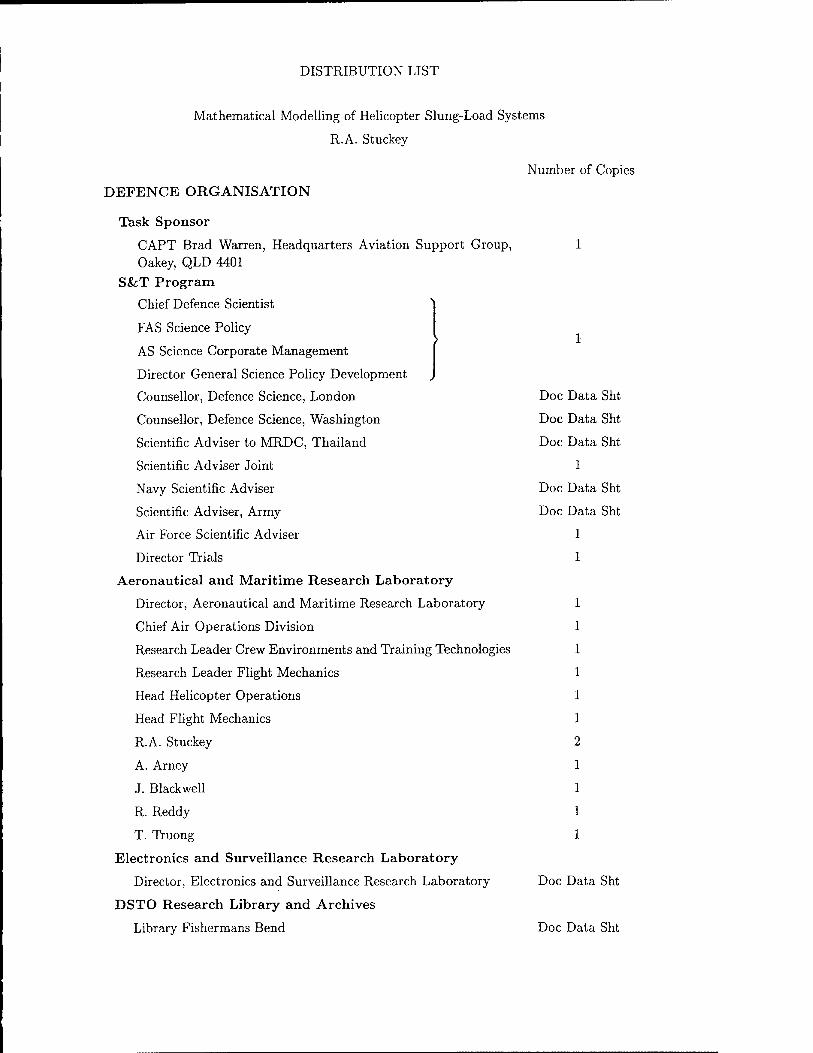
DISTRIBUTION LIST
Mathematical Modelling of Helicopter Slung-Load Systems
R.A. Stuckey
Number of Copies
DEFENCE ORGANISATION
Task Sponsor
CAPT Brad Warren, Headquarters Aviation Support Group, 1 Oakey, QLD 4401
S&T Program
Chief Defence Scientist
FAS Science Policy
AS Science Corporate Management
Director General Science Policy Development
Counsellor, Defence Science, London Doc Data Sht
Counsellor, Defence Science, Washington Doc Data Sht
Scientific Adviser to MRDC, Thailand Doc Data Sht
Scientific Adviser Joint 1
Navy Scientific Adviser Doc Data Sht
Scientific Adviser, Army Doc Data Sht
Air Force Scientific Adviser
Director Trials
Aeronautical and Maritime Research Laboratory
Director, Aeronautical and Maritime Research Laboratory
Chief Air Operations Division
Research Leader Crew Environments and Training Technologies
Research Leader Flight Mechanics
Head Helicopter Operations
Head Flight Mechanics
R.A. Stuckey
A. Arney
J. Blackwell
R. Reddy
T. Truong
Electronics and Surveillance Research Laboratory
Director, Electronics and Surveillance Research Laboratory Doc Data Sht
DSTO Research Library and Archives
Library Fishermans Bend Doc Data Sht

Library Maribyrnong
Library Salisbury
Australian Archives
Library, MOD, Pyrmont
US Defense Technical Information Center
UK Defence Research Information Centre
Canada Defence Scientific Information Service
NZ Defence Information Centre
National Library of Australia
Capability Systems Staff
Director General Maritime Development
Director General Land Development
Director General C3I Development
Director General Aerospace Development
Navy
SO (Science), Director of Naval Warfare, Maritime Headquarters Annex, Garden Island
Army
FLTLT Gerry Van Leeuwen, CENGR, AMTDU, RAAF Base Richmond, NSW 2755
LTCOL Philip Smith, SOI Aviation Development Branch, Vic- toria Barracks, Paddington, NSW 2021
ABCA Standardisation Officer, Puckapunyal
SO(Science), DJFHQ(L), MILPO, Enoggera, QLD 4057
Intelligence Program
DGSTA, Defence Intelligence Organisation
Manager, Information Centre, Defence Intelligence Organisa- tion
Corporate Support Program
Officer in Charge, TRS, Defence Regional Library, Canberra
INTERNATIONAL COLLABORATIVE PARTNERS
Defence Research & Development Canada, Ottawa, CA
LCOL M Haines
National Research Council of Canada, Ottawa, CA
S Zan
S Cariguan
Doc Data Sht
1
1
Doc Data Sht
2
2
1
1
1
Doc Data Sht
1
Doc Data Sht
Doc Data Sht
Doc Data Sht
1
1
4
Doc Data Sht
1
1

Defence Science and Technology Laboratory, Farnborough, UK
T Cansdale 1
Defence Science and Technology Laboratory, Bedford, UK
B Lumsden 1
Ames Research Center, California, USA
M Whalley 1
J Schroeder 1
L Cicolani 1
Naval Air Systems Command, Patuxent River, USA
J Clark Jr 1
UNIVERSITIES AND COLLEGES
Australian Defence Force Academy Library 1
Head of Aerospace and Mechanical Engineering, ADFA 1
Deakin University Library, Serials Section (M List) 1
Hargrave Library, Monash University Doc Data Sht
Librarian, Flinders University 1
OTHER ORGANISATIONS
NASA (Canberra) 1
Info Australia 1
SPARES
DSTO Melbourne Research Library 6
Total number of copies: 57
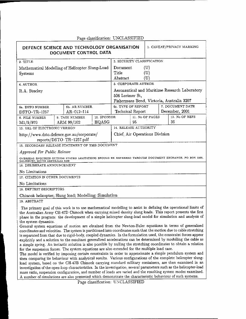
Page classification: UNCLASSIFIED
DEFENCE SCIENCE AND TECHNOLOGY ORGANISATION DOCUMENT CONTROL DATA
2. TITLE
Mathematical Modelling of Helicopter Slung-Load Systems
4. AUTHOR
R.A. Stuckey
6a. DSTO NUMBER
DSTO-TR-1257 8. FILE NUMBER
Ml/9/970
6b. AR NUMBER
AR-012-114 9. TASK NUMBER
ARM 99/102
1. CAVEAT/PRIVACY MARKING
3. SECURITY CLASSIFICATION
Document (U) Title (U) Abstract (U) 5. CORPORATE AUTHOR
Aeronautical and Maritime Research Laboratory 506 Lorimer St, Fishermans Bend, Victoria, Australia 3207 6c. TYPE OF REPORT
Technical Report 10. SPONSOR
HQASG
13. URL OF ELECTRONIC VERSION
http://www.dsto.defence.gov.au/corporate/ reports/DSTO-TR-1257.pdf
7. DOCUMENT DATE
December, 2001 11. No OF PAGES
95 12. No OF REFS
36
14. RELEASE AUTHORITY
Chief, Air Operations Division
15. SECONDARY RELEASE STATEMENT OF THIS DOCUMENT
Approved For Public Release
OVERSEAS ENQUIRIES OUTSIDE STATED LIMITATIONS SHOULD BE REFERRED THROUGH DOCUMENT EXCHANGE, PO BOX 1500, SALISBURY, SOUTH AUSTRALIA 5108 ___^
16. DELIBERATE ANNOUNCEMENT
No Limitations 17. CITATION IN OTHER DOCUMENTS
No Limitations 18. DEFTEST DESCRIPTORS
Chinook helicopter; Slung load; Modelling; Simulation 19. ABSTRACT
The primary goal of this work is to use mathematical modelling to assist in defining the operational limits of the Australian Army CH-47D Chinook when carrying mixed density slung loads. This report presents the first phase in the program: the development of a simple helicopter slung-load model for simulation and analysis of the system dynamics. General system equations of motion are obtained from the Newton-Euler equations in terms of generalized coordinates and velocities. The system is partitioned into coordinates such that the motion due to cable stretching is separated from that due to rigid-body, coupled dynamics. In the formulation used, the constraint forces appear explicitly and a solution to the resultant generalized accelerations can be determined by modelling the cable as a simple spring. An inelastic solution is also possible by nulling the stretching coordinates to obtain a relation for the suspension forces. The system equations are also extended for the multiple load case. The model is verified by imposing certain constraints in order to approximate a simple pendulum system and then comparing its behaviour with analytical results. Various configurations of the complete helicopter slung- load system, based on the CH-47B Chinook carrying standard military containers, are then examined in an investigation of the open-loop characteristics. In the investigation, several parameters such as the helicopter-load mass ratio, suspension configuration, and number of loads are varied and the resulting system modes examined. A number of simulations are also presented which demonstrate the characteristic behaviour of such systems.
Page classification: UNCLASSIFIED


