Embed Size (px)
Citation preview
Analytical load-deflection behavior of slender load-bearing reinforced concrete walls
by
Lujain Alkotami
B.S., Kansas State University, 2018
A THESIS
submitted in partial fulfillment of the requirements for the degree
MASTER OF SCIENCE
Department of Architectural Engineering and Construction Science
College of Engineering
KANSAS STATE UNIVERSITY
Manhattan, Kansas
2019
Approved by:
Major Professor
Professor Kimberly Kramer

Copyright
© Lujain Alkotami 2019
Abstract
Nearly 790 million square feet or approximately 11,000 to 12,000 buildings are constructed using
tilt-up concrete panels per year since 2007 according to the Tilt-Up Concrete Association. In Tilt-
Up panel design P-delta effects control slender concrete wall panel design. Therefore,
understanding the nonlinear deflection behavior of these walls is the first step in refining their
design, which may make them more sustainable by using less material. The American Concrete
Institute (ACI) 318 Building Code Requirements for Structural Concrete provisions for slender
vertical wall panels take into consideration the self-weight of the panel along with uniformly
distributed lateral wind pressure in estimating the mid-height deflection. In doing so, the Branson
deflection equation is used to compute central lateral displacement while adjusting for the effect of
axial force. In this study, a more rigorous formulation is proposed taking into account the axial
force effect on the moment curvature calculation and integration to yield more accurate load-
deflection values. In this formulation, the stiffness variation along the slender wall panel allowing
for un-cracked, post cracked and post yielded regions was taken into consideration. Accordingly,
the full analytical load-deflection response is made available for the designers based on accurate
simplifying assumptions. The developed equation is used to compare the present analytical results
to some available experimental results along with the predictions of other deflection equations
proposed in the literature such as the latest ACI 318, Branson and the Bischoff effective moment of
inertia equations. The experimental results are full-scale panel testing data conducted by a joint
venture of the Southern California Chapter of ACI and SEAOC. These results reflect representative
stiffness variation of the panels beyond cracking. More specifically, the latest ACI 318 linear
moment-deflection expression will be examined against the present equation that considers less

simplifying assumptions. A parametric study is extended for the purpose of further proposing a
simplified equation based on the rigorous approach.
v
Table of Contents
List of Figures .............................................................................................................................. viii
List of Tables ................................................................................................................................. xi
Acknowledgements ....................................................................................................................... xii
Dedication .................................................................................................................................... xiii
Chapter 1 - Introduction .................................................................................................................. 1
1.1 Background ........................................................................................................................... 2
1.1.1 Usage of Tilt Up ............................................................................................................. 2
1.2 Scope ..................................................................................................................................... 5
Chapter 2 - Literature Review ......................................................................................................... 7
2.0 Literature Review ................................................................................................................. 7
2.1 Experimental Data ................................................................................................................ 7
2.3 Analysis Methods ............................................................................................................... 11
2.3.1 ACI 318 Alternative Method for Out-of-Plane Slender Wall Analysis ....................... 11
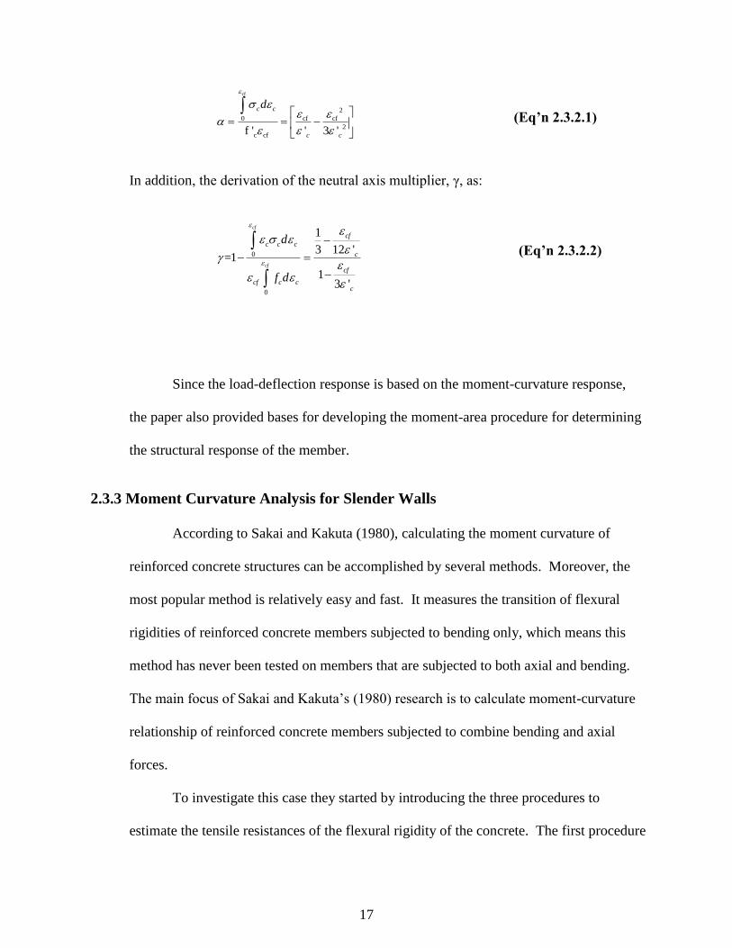
2.3.2 Tri-linear moment-curvature analysis .......................................................................... 16
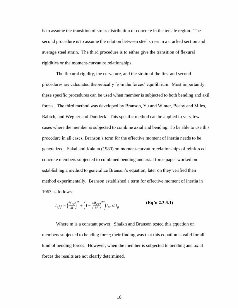
2.3.3 Moment Curvature Analysis for Slender Walls ........................................................... 17
2.3.4 Cracked Sectional Analysis ......................................................................................... 20
2.2.5 Bi-linear Behavior ........................................................................................................ 22
2.2.6 Effective Moment of inertia ......................................................................................... 23
Chapter 3 - Sectional Analysis: Load Deflection Behavior .......................................................... 25
Chapter 4 - Structural Response: Load-Deflection Behavior ....................................................... 51
4.0 Uniform Loads and Axial Load .......................................................................................... 51
4.1 Wall Behavior ..................................................................................................................... 51
4.2 Analysis Methods for Deflection on Slender Walls ........................................................... 54
4.2.1 Moment Area Theorem ................................................................................................ 55
4.2.2 Differential Equations .................................................................................................. 57
4.2.3 Moment Magnifier Method .......................................................................................... 60
4.2.4 ACI Slender Wall Provisions: Latest ACI 318 Approach ........................................... 65
4.2.4.1 Ultimate Deflectin ................................................................................................. 65
4.2.4.2 Service Deflection ................................................................................................. 67
vi
4.2.5 The Effective Moment of Inertia Approach ................................................................. 68
4.2.5.1 Branson’s Effective Moment of Inertia ................................................................ 69
4.2.5.2 Bischoff’s Effective Moment of Inertia ................................................................ 70
4.3 Slender Walls Test Results ................................................................................................. 70
4.3.1 Panels behavior ............................................................................................................ 71
4.3.2 Deflection Curves ........................................................................................................ 72
4.3.3 Cracking ....................................................................................................................... 73
4.3.4 P-Delta Effects ............................................................................................................. 74
Chapter 5 - Structural Application ................................................................................................ 75
5.0 Comparisons with Experimental Results ............................................................................ 75
5.1 Latest ACI 318 Section 11.8 vs. Test Results..................................................................... 76
5.1.1 Panels 4.75” in Thickness with a Slenderness Ratio of 60 .......................................... 77
5.1.2 Panels 5.75” in Thickness with a Slenderness Ratio of 50 .......................................... 78
5.1.3 Panels 7.25” in Thickness with a Slenderness Ratio of 40 .......................................... 80
5.1.4 Panels 9.5” in Thickness with a Slenderness Ratio of 30 ............................................ 81
5.2. Branson's Effective Moment of Inertia vs. 1980s Test Results ......................................... 83
5.2.1 Panels 4.75” in Thickness with a Slenderness Ratio of 60 .......................................... 84
5.2.2 Panels 5.75” in Thickness with a Slenderness Ratio of 50 .......................................... 85
5.2.3 Panels 7.25” in Thickness with a Slenderness Ratio of 40 .......................................... 86
5.2.4 Panels 9.5” in Thickness with a Slenderness Ratio of 30 ............................................ 88
5.3 Bischoff's Effective Moment of Inertia vs. 1980s Test Results .......................................... 89
5.3.1 Panels 4.75” in Thickness with a Slenderness Ratio of 60 .......................................... 89
5.3.2 Panels 5.75” in Thickness with a Slenderness Ratio of 50 .......................................... 90
5.3.3 Panels 7.25” in Thickness with a Slenderness Ratio of 40 .......................................... 92
5.3.4 Panels 9.5” in Thickness with a Slenderness Ratio of 30 ............................................ 93
5.4 Proposed Effective Moment of Inertia Derived by Kramer and Alkotami ......................... 94
5.4.1 Equation One: Proposed Effective Moment of Inertia by Kramer & Alkotami .......... 96
5.4.1.1 Panels 4.75” in Thickness with a Slenderness Ratio of 60 ................................... 96
5.4.1.2 Panels 5.75” in Thickness with a Slenderness Ratio of 50 ................................... 97
5.4.1.3 Panels 7.5” in Thickness with a Slenderness Ratio of 40 ..................................... 99
5.4.1.4 Panels 9.5” in Thickness with a Slenderness Ratio of 30 ................................... 100
vii
5.4.2 Equation Two: Proposed Effective Moment of Inertia by Kramer &Alkotami ........ 101
5.4.2.1 Panels 4.75” in Thickness with a Slenderness Ratio of 60 ................................. 101
5.4.2.2 Panels 5.75” in Thickness with a Slenderness Ratio of 50 ................................. 102
5.4.2.3 Panels 7.25” in Thickness with a Slenderness Ratio of 40 ................................. 103
5.4.2.4 Panels 9.5” in Thickness with a Slenderness Ratio of 30 ................................... 105
Chapter 6 - Conclusion and Recommendations .......................................................................... 106
6.1 Conclusion ........................................................................................................................ 106
6.2 Recommendations ............................................................................................................. 111
References ................................................................................................................................... 116
Appendix A - Notations .............................................................................................................. 120
Appendix B - Cracked Moment of Inertia Derivation ................................................................ 139
viii
List of Figures
Figure 1.1:Tilt-Up Market Growth across the Globe (Tilt-Up Concrete Association). ................. 4
Figure 2.1:Side Elevation of Test Setup – Loading Frame Showing Drums of Water for Vertical
Load and Air Bag for Lateral Load. ..................................................................................... 10
Figure 2.2: Cracked section Analysis. .......................................................................................... 22
Figure 2.3: Normalized Moment-Curvature Curve. ..................................................................... 23
Figure 3.1: Hognestad’s Parabolic Curve. .................................................................................. 26
Figure 3.2: The Linear and Non-Linear Behavior of Concrete Members. ................................... 26
Figure 3.3: ASTM A615-grade 60 Reinforcing Steel Stress-Strain Curve. .................................. 27
Figure 3.4: Tension Stiffening Relationship at Cracked Section (a) ............................................ 28
Figure 3.5: Tension Stiffening Relationship at Cracked Section. ................................................. 29
Figure 3.6: Tension Stiffening Relationship at Cracked Section – Load vs. Deflection .............. 29
Figure 3.7: Mathematical Representation of Load-Deflection Relations. ................................... 31
Figure 3.8: Strain and Stress Distribution for the Tilt Up Panel Cross Section. ......................... 32
Figure 3.9: Whitney’s Equivalent Stress Block. ........................................................................... 36
Figure 3.10: Nomenclature for Stress-Strain Curve of Reinforcing Bars. ................................... 38
Figure 3.11: The Behavior of Steel (Hogenstad, 1952). ............................................................... 38
Figure 3.12: Loading Case Acting on the Tilt-Up Panel.............................................................. 41
Figure 3.13: Deflected Shape of the Tilt Up Panel. ..................................................................... 42
Figure 4.1: Maximum Moment Due to Vertical and Lateral Loading. ........................................ 53
Figure 4.2: Deflected Shape of Out of Plane Load Bearing Walls. ............................................. 54
Figure 4.3: Moment Area Theorem. ............................................................................................. 55
Figure 4.4: General Loading of Beam-Column. ........................................................................... 58
Figure 4.5: Primary and Secondary Bending Moment. ................................................................ 62
Figure 4.6: Idealized Composite Stress/Strain Relation for Reinforced Concrete Panel. ........... 72
Figure 4.7: Deflection of Tilt Up Panels at Mid-Height in Inches. .............................................. 73
Figure 5.1: Deflection Comparison for Actual Test results and Latest ACI 318 Approach (4.75”)
Panel. .................................................................................................................................... 77
Figure 5.2: Deflection Comparison for Actual Test results and Latest ACI 318 Approach (5.75”)
Panel. .................................................................................................................................... 79
ix
Figure 5.3: Deflection Comparison for Actual Test results and Latest ACI 318 Approach (7.25”)
Panel. .................................................................................................................................... 80
Figure 5.4: Deflection Comparison for Actual Test results and Latest ACI 318 Approach (9.5”)
Panel. .................................................................................................................................... 82
Figure 5.5: Deflection Comparison for Actual Test results and Branson’s Approach (4.75”)
Panel. .................................................................................................................................... 84
Figure 5.6: Deflection Comparison for Actual Test results and Branson’s Approach (5.75”)
Panel. .................................................................................................................................... 85
Figure 5.7: Deflection Comparison for Actual Test results and Branson’s (7.25”) Panel. ......... 87
Figure 5.8: Deflection Comparison for Actual Test results and Branson’s Approach (9.5”)
Panel. .................................................................................................................................... 88
Figure 5.9: Deflection Comparison for Actual Test results and Bischoff’s Approach (4.75”)
Panel. .................................................................................................................................... 90
Figure 5.10: Deflection Comparison for Actual Test results and Bischoff’s Approach (5.75”)
Panel. .................................................................................................................................... 91
Figure 5.11: Deflection Comparison for Actual Test results and Bischoff’s Approach (7.25”)
Panel. .................................................................................................................................... 92
Figure 5.12: Deflection Comparison for Actual Test results and Bischoff’s Approach (9.5”)
Panel. .................................................................................................................................... 93
Figure 5.13: Deflection Comparison for Actual Test results and Kramer & Alkotami’s Approach
1 (4.75”) Panel. .................................................................................................................... 96
Figure 5.14: Deflection Comparison for Actual Test results and Kramer & Alkotami’s Approach
1 (5.75”) Panel. .................................................................................................................... 98
Figure 5.15: Deflection Comparison for Actual Test results and Kramer & Alkotami’s Approach
1 (7.25”) Panel. .................................................................................................................... 99
Figure 5.16: Deflection Comparison for Actual Test results and Kramer and Alkotami’s
Approach 1 (9.5”) Panel. .................................................................................................... 100
Figure 5.17: Deflection Comparison for Actual Test results and Kramer & Alkotami’s Approach
2 (4.75”) Panel. .................................................................................................................. 101
Figure 5.18: Deflection Comparison for Actual Test results and Kramer & Alkotami’s Approach
2 (5.75”) Panel. .................................................................................................................. 102
x
Figure 5.19: Deflection Comparison for Actual Test results and Kramer & Alkotami’s Approach
2 (7.25”) Panel. .................................................................................................................. 104
Figure 5.20: Deflection Comparison for Actual Test results and Kramer & Alkotami’s Approach
2 (9.5”) Panel. .................................................................................................................... 105
Figure 6.1: 4.75” Panels’ Deflection Behavior .......................................................................... 107
Figure 6.2: 5.75” Panels’ Deflection Behavior. ......................................................................... 108
Figure 6.3: 7.25” Panels’ Deflection Behavior. ......................................................................... 109
Figure 6.4: 9.5” Panels’ Deflection Behavior............................................................................ 110
Figure 6.5: 5.75” Panel Deflection Comparison of Actual ACI 318, Proposed ACI 318, and
Actual Test Results. ............................................................................................................. 113
Figure 6.6: 4.75” Panel Deflection Comparison of Actual ACI 318, Proposed ACI 318, and
Actual Test Results. ............................................................................................................. 113
Figure 6.7: 9.5” Panel Deflection Comparison of Actual ACI 318, Proposed ACI 318, and
Actual Test Results. ............................................................................................................. 114
Figure 6.8: 7.25” Panel Deflection Comparison of Actual ACI 318, Proposed ACI 318, and
Actual Test Results. ............................................................................................................. 114
xi
List of Tables
Table 2-1: The Development of Slender Wall Provisions in the UBC 1997 and the ACI 318-99
through ACI 318-05. ............................................................................................................. 14
Table 2-2: The Development of Slender Wall Provisions in the ACI 318-08 through ACI 318-19.
............................................................................................................................................... 15
Table 6-1: 4.75” Panels’, slenderness ratio of 60, Deflection Error Percentages. ................... 107
Table 6-2: 5.75” Panels’, slenderness ratio of 50, Deflection Error Percentages. ................... 108
Table 6-3: 7.25” Panels’, slenderness ratio of 40, Deflection Error Percentages. ................... 109
Table 6-4: 9.5” Panels’, slenderness ratio of 30, Deflection Error Percentages. ..................... 110

xii
Acknowledgements
I would like to thank my family for supporting me through my journey here at K-State.
Special thanks to my mom, Nadyah Abdullah, for being with me whenever I needed you; your
support was endless. Having you here by my side meant a lot to me and I want you to know that
I am proud of you as much as you proud of me. Special thanks to my father, Mohammed
Alkotami, thank you for supporting me to continue my higher education. Your words and
guidance made me stronger. Special thanks to my siblings; I am glad I got the chance to go to
college with you. Special thanks to my major advisor, professor Kimberly Kramer; I appreciate
your help, time, and support. You believed in me and supported me through my grad and
undergrad study here at K-State. You made me passionate about this field and believed in me
that I can make a change when I go back home to Saudi Arabia. Special thanks to my committee
members, thank you for supporting me and providing me the needed help. Special thanks to my
friends, to all my friends across the words although distance separated us but you always were
here for me when I needed you. I am blessed to be surrounded with amazing people.

xiii
Dedication
I would like to dedicate my work to my parents; I love both of you.
1
Chapter 1 - Introduction
Nearly 790 million square feet or approximately 11,000 to 12,000 buildings are
constructed using tilt-up concrete panels per year since 2007 according to the Tilt-Up Concrete
Association (TCA, 2011). Tilt-up wall panels are constructed where the concrete panels are
casted horizontally on site on a slab. After the required concrete strength for lifting is reached,
usually 7 days, they are lifted by a crane and placed in their final vertical position. Tilt-up can be
referred to as “slender walls” per the American Concrete Institute (ACI) 318-19 Building Code
Requirements for Structural Concrete. Slender walls are concrete walls designed to resist
eccentric axial loads and any possible lateral load such as wind, seismic, and soil. Slender walls
can be bearing, non-bearing, or exterior basement or foundation walls. The ACI 318 code
specifies a minimum requirement for the thickness of the slender walls in table 11.3.1.1
depending on their usage in the structure. The main concern regarding this type of construction
is P-delta effect that occurs due to the extra bending in the member.
When tilt-up construction first started, it was referred to site-cast precast since the wall
panels were not cast in a fabrication shop similar to other precast concrete elements. Tilt-up and
precast wall panels may seem similar, but they are very different in properties and code
requirements. Precast panels are made in factories and then transported to the job site via trucks,
limiting the size of the panels. Precast panels are constructed in specific sizes and cannot be
modified or changed easily on site, which mean less flexibility. In addition, precast panels are
most often nonloadbearing.
Tilt-Up and Precast have different design provisions in the ACI 318-19. For tilt-up walls,
per the current ACI 318-19, P-delta effects control slender, concrete wall panel design.
Therefore, understanding the nonlinear deflection behavior of these walls is the first step in
2
refining their design. Tilt-up panels are designed to fully resist all applied loads, which is why
the effective moment of inertia is used when designing the panels. On the other hand, for
precast, ACI 553R-11 states in Table 3.5.2 Deflection Limits for Precast Wall Panels, limit
deflection to span/240 or ¾” for dead loads, and span/360 or ¾” for live loads. According to
ACI 553R, the precast panels are usually designed not to crack; therefore, the gross moment of
inertia is used for deflection calculations and no p-delta effects are incorporated because the
panels are not slender.
1.1 Background
1.1.1 Usage of Tilt Up
The development of the concrete industry occurred in the period from 1895 to 1918.
American Concrete Institute (ACI), the Portland Cement Association (PCA), and the
American Society of Civil Engineers (ASCE) worked on developing the specifications for
concrete, as the demand on the market was mostly concrete building.
Robert Aiken led the tilt up construction growth in 1903. The first building to use tilt up
was the Camp Logan Illinois Rifle Range. It was constructed using 5” retaining walls. By
1916 there was less than 20 buildings constructed using tilt up (Johnson, 2002).
After the World War I, the tilt up society stopped developing as precast was introduced.
In 1930’s tilt up construction remained dormant as public funded construction lead the
industry and the country was not looking for the labor cost savings.
The next development in the tilt up history started in the late 1940s’ after world War II
when contractors found tilt up to be cost effective. The tilt up techniques started to develop
3
in 1950’s and 1960’s as contractors used custom lifting devices, temporary braces, chemical
bond breakers, and other specialized products in the construction process.
In 1970’s several events affected the tilt up industry after the capabilities were recognized
and the panels were allowed to be used as load bearing walls. Those events included a full-
scale test was performed, K. M. Kripanarayanan introduced P∆ effects, and tilt up was
introduced in Florida.
In 1986 the Tilt-Up Concrete Association (TCA) was formed. In 1990’s panels varied in
complexity, shifting from a simple rectangle to complicated lifts with strong backs, to four-
story panels with two-crane lift.
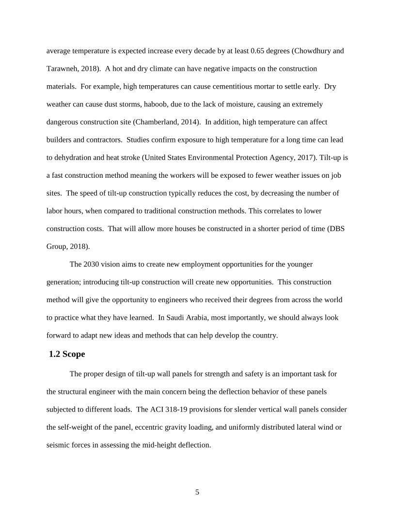
Currently, tilt-up is extensively used across the United States. It is also emergent in other
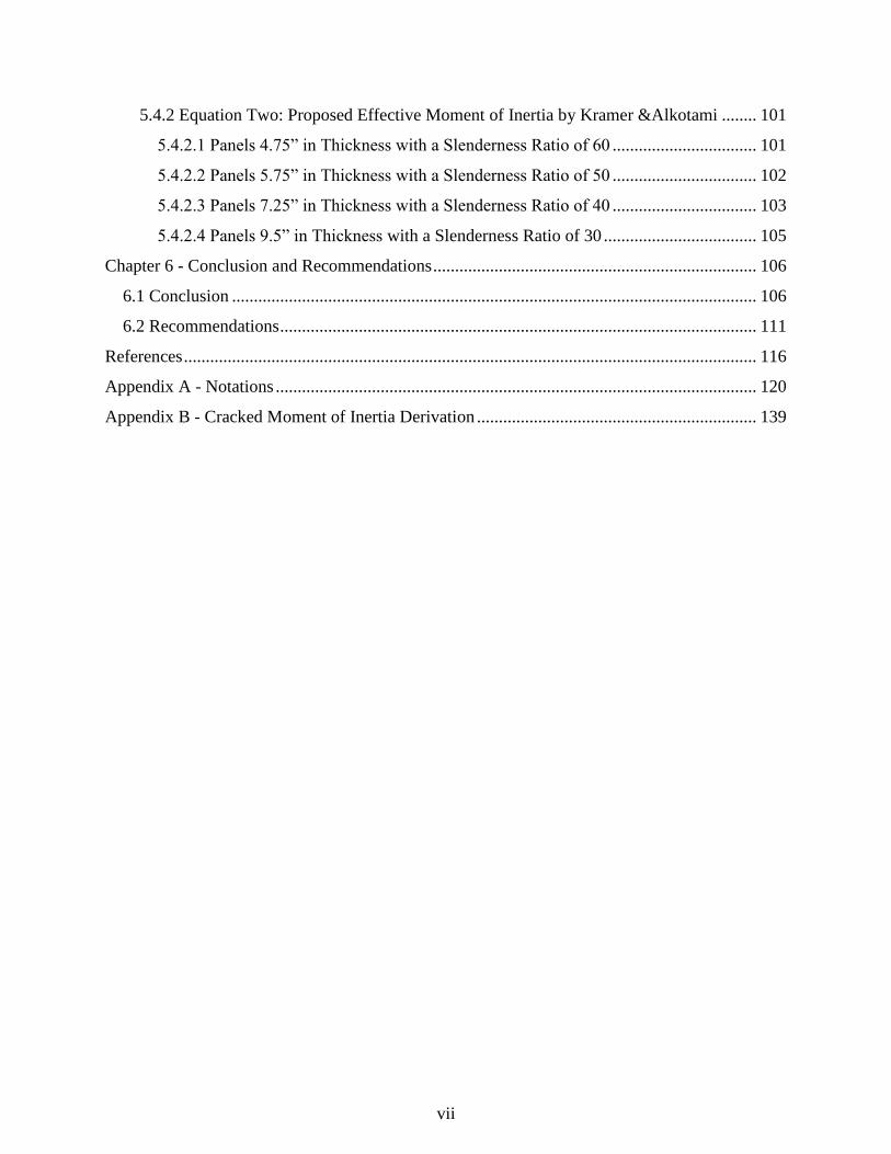
countries. Figure 1.1 Tilt-Up Market Growth across the Globe shows a global image
displaying the locations of tilt up construction in red. Design engineers in these various
countries use an assortment of code mandated design methodologies. Some countries use
various versions of the ACI 318 code; those countries are South America, Central America,
Mexico, Indonesia, Russia, Brazil, China, and South Africa. Additionally, some countries
have their own code and provisions regarding this type of construction, such as, Saudi
Arabia.

4
Figure 1.1.1.1 Tilt-Up Market Growth across the Globe (Tilt-Up Concrete Association).
As shown on the map, tilt-up construction is recently occurring in eastern Saudi Arabia.
A possible reason is an ACI chapter exists in that province. As a future engineer and a Saudi
citizen, I wish that Saudi Arabia expands the usage of this type of construction for several
reasons.
Introducing Tilt-up will have positive impacts on both the population and the economy of
the country. The crown prince, Mohammed bin Salman, generated the 2030 vision that aims to
develop all aspects of Saudi Arabia. The 2030 vision promised to deliver stability and create a
brighter future for Saudi Arabia and the citizens (Vision 2030, 2016). Spreading the usage of
Tilt-up will help achieve some of the 2030 vision goals by enhancing the construction economy
and creating more job opportunities for young engineers.
Beyond the 2030 vision goals, tilt up construction has several advantages. One important
factor is the climate in Saudi Arabia. As of 2017, Saudi Arabia reached its highest temperature
of 53 Celsius degrees which is equivalent to 127.4 Fahrenheit (Khalaf, 2017). Moreover, the
Figure 1.1:Tilt-Up Market Growth across the Globe (Tilt-Up Concrete Association).
5
average temperature is expected increase every decade by at least 0.65 degrees (Chowdhury and
Tarawneh, 2018). A hot and dry climate can have negative impacts on the construction
materials. For example, high temperatures can cause cementitious mortar to settle early. Dry
weather can cause dust storms, haboob, due to the lack of moisture, causing an extremely
dangerous construction site (Chamberland, 2014). In addition, high temperature can affect
builders and contractors. Studies confirm exposure to high temperature for a long time can lead
to dehydration and heat stroke (United States Environmental Protection Agency, 2017). Tilt-up is
a fast construction method meaning the workers will be exposed to fewer weather issues on job
sites. The speed of tilt-up construction typically reduces the cost, by decreasing the number of
labor hours, when compared to traditional construction methods. This correlates to lower
construction costs. That will allow more houses be constructed in a shorter period of time (DBS
Group, 2018).
The 2030 vision aims to create new employment opportunities for the younger
generation; introducing tilt-up construction will create new opportunities. This construction
method will give the opportunity to engineers who received their degrees from across the world
to practice what they have learned. In Saudi Arabia, most importantly, we should always look
forward to adapt new ideas and methods that can help develop the country.
1.2 Scope
The proper design of tilt-up wall panels for strength and safety is an important task for
the structural engineer with the main concern being the deflection behavior of these panels
subjected to different loads. The ACI 318-19 provisions for slender vertical wall panels consider
the self-weight of the panel, eccentric gravity loading, and uniformly distributed lateral wind or
seismic forces in assessing the mid-height deflection.
6
The scope of this research is to examine the current design practices for calculating the
mid-height deflection and propose a more rigorous formulation, of effective moment of inertia,
including the axial force effect on the moment curvature calculation and integration to yield
more accurate load-deflection values. The stiffness variation along the slender wall panel is
taken into account to allow for uncracked, post cracked and post yielded regions. Accordingly,
the full analytical load-deflection response is made available for the designers based on accurate
simplifying assumptions.
The developed equation is used to compare the present analytical results to the available
experimental test results along with the predictions of other deflection equations proposed in the
literature, such as, the ACI 318, Branson, and the Bischoff effective moment of inertia equations.
More specifically, the latest ACI 318 linear moment-deflection expressions examined against the
present equation that considers fewer simplifying assumptions.
7
Chapter 2 - Literature Review
2.0 Literature Review
This chapter summarizes some studies reviewed for the area of interest. The books and
articles reviewed contained experimental data and analytical methods pertaining to slender
reinforced concrete wall design controlled by tension flexure, which includes moment-curvature
analysis and load-deflection computation. In particular, references cited by the current American
Concrete Institute Building Code Requirements for Structural Concrete, ACI 318-19 Code, are
highlighted.
2.1 Experimental Data
Very little testing on tilt-up slender walls has been performed. The American Concrete
Institute-Structural Engineers Association of Southern California (ACI_SEASC) joint task
committee in the early 1980s Test Report on Slender Walls is one of the few (ACI_SEASC,
1982). The ACI-SEASC Task Committee on slender walls was created in 1980 to determine
their behavior when subjected to eccentric axial and lateral forces that simulated gravity loads,
along with wind or seismic pressures. Prior to these tests, the design of slender walls was
limited by specific height/thickness ratio limit of 25 for load bearing walls and 30 for non-load
bearing walls (Lawson and Lai, 2010). At the time, an increase usage of slender walls was
occurring with a trend toward more slender wall for increased cost savings. The ACI-SEASC
Task committee realized the need to design more slender walls in order to save money by using
less materials. Deflection tests were performed to obtain the stability behavior of the wall under
lateral and vertical load. Twelve tilt-up concrete panels were tested in the upright position as the
self-weight of the panels act as a vertical load. The panels were tested in a special frame
8
allowing eccentric roof loads and lateral forces to be both applied at the same time. Horizontal
deflection of the panels was measured under different increments of load to regulate the ultimate
capacity of each panel.
The 12 tilt-up panels were constructed using a concrete mix supplied by a local firm in
California. The water to cement ration is 0.67. The design mix consisted of Portland Cement,
Washed Concrete Sand, 1-in gravel, and water. To measure the concrete strength of the panels,
16 cylinders and six concrete beams specimens were sent to the Twinning laborites. The lab
measured the specimens’ strengths for 7 -Day test results, 28-Day test, and 167-Days (job cured).
Tilt Up panels were casted on October 3, 1980 and then lifted by the inserts in the long edges on
October 15, 1980 to ensure the safety against any damage that can occur in the lifting process.
The panels were stored on edge for 160 days prior to lifting into their final position to perform
the test. This allowed for drying shrinkage to occur when the panels were stored on edge.
Upon the completion of the deflection test program, cores were drilled and prisms were sawn
from tilt-up panels in order to measure the properties of the actual test specimens. A difference
in strength values were noticed. The ACI-SEASC Task committee attribute the difference in
strength results between the actual wall panels and the lab specimens to the fact that the actual
wall panels strengths were measured a year after the panels were casted and that two different
labs performed the tests. The differences were not significant since the values were not used in
the original design calculations.
All panels were 4’-0” wide and 24’-8” high. The panels were horizontally supported at the
base and at 24 feet with the lateral loaded portion of the wall equaling 24 feet. This height was
selected to represent the current construction trend for slender walls at that time. Twelve tilt-up
9
panels were tested, three each with thicknesses of 4- ¾”, 5- ¾”, 7- ¼”, and 9- ½” resulting in
nominal height/thickness (h/t) ratios of 60, 50, 40, and 30, respectively.
Panels were reinforced vertically with four #4 grade 60 reinforcing steel. All vertical bars
were in full-length pieces without splices. The strain of reinforcement ranges from 0.0025 to
0.0032. Panels were also reinforced in the horizontal direction with #3 bars grade 40 spaced at 2
feet on center for the 4- ¾” and 5- ¾” panels; and reinforced with #4 bars grade 40 spaced at 2
feet on center for the 7- ¼” and 9- ¼” panels. All reinforcing steel met the requirement of
ASTM A615-78 standard specifications for deformed and Plain Billet-Steel Bars for Concrete
Reinforcement.
The vertical reinforcements were designed to be located on the middle of the panel. The
actual location of the bars was measured after the test. Post the deflection test, tilt-up panels
were broken apart specifically in the middle third and the location of the bars were measured in
relation to the loading face. For the 9 ¼” thick panels, the location of reinforcement was on
average off by 2% of the specified d location, where d is the distance from the extreme fiber in
compression to the center of the tension reinforcing steel. For the 7 ¼”, 5 ¾”, and 4 ¾” panels,
the reinforcement location was on average off by 14%, 19.3% and 9%, respectively, of the
specified d. It is important to measure the exact location of d because it could increase or
decrease the panel capacity to resist the specified forces.
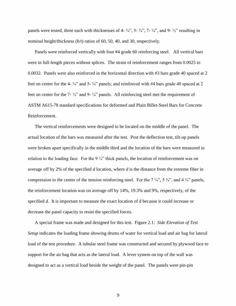
A special frame was made and designed for this test. Figure 2.1: Side Elevation of Test
Setup indicates the loading frame showing drums of water for vertical load and air bag for lateral
load of the test procedure. A tubular steel frame was constructed and secured by plywood face to
support for the air bag that acts as the lateral load. A lever system on top of the wall was
designed to act as a vertical load beside the weight of the panel. The panels were pin-pin
10
connected. The bottom edge of the wall was attached to a rocker base to eliminate any moment
that can occur. Also, a rectangular steel frame was attached to the bottom of the wall to prevent
the base from any lateral load that can occur from the airbag.
Figure 2.1:Side Elevation of Test Setup – Loading Frame Showing Drums of Water for Vertical Load and
Air Bag for Lateral Load.
11
The lever arm at the top of the wall was loaded with water. The amount of water was
adjusted depending on the desired vertical load (roof load). The distributed lateral load (wind or
seismic) was supplied by airbag that added pressure to the wall. The airbag was inflated by ½
Horsepower compressor. The pressure inside the bag was then measured by double water tube
manometer correlating one-inch of water to 5.2 pounds per square foot air pressure in the bag.
To acquire the shape of the elastic curve, the deflection of the panels was measured at the
supports of the wall and at the intermediate tenth points. Three methods were used to measure
the deflection of the wall: attaching yardsticks to the wall, using dial gages, and using steel wire
tension line from the wall. The electric transducers values were the main measurement used for
this test. There was an attempt to make the deflection control in loading the walls, however load
control was used in most cases. As the maximum load was approached, the loading increments
became smaller. The results of this test are used in further chapters of this thesis.
2.3 Analysis Methods
Several published works were reviewed that proposed moment-curvature analysis and load-
deflection analysis procedures for load-bearing slender walls. In particular, works referenced by
ACI 318-19 Code methods are reviewed. In addition, works pertaining to tri-linear moment-
curvature analysis of reinforced concrete analysis is reviewed.
2.3.1 ACI 318 Alternative Method for Out-of-Plane Slender Wall Analysis
ACI 318 Alternative Method for Out-of-Plane Slender Wall Analysis provisions are
based on the full-scale testing of slender concrete wall panels that occurred in the early 1980’s by
a joint venture of the ACI_SEASC. The testing program and results are published in a
document referred to as the Green Book that included all testing details and recommended design
12
equations. These equations and methodology was adopted by the Uniform Building Code (UBC)
in 1988. When the International Building Code (IBC) created a single national model code, the
slender wall provision from the UBC were adopted into the ACI 318-99 Building Code
Requirements for Structural Concrete that was referenced by the 2000 IBC.
The ACI 318 code started to incorporate requirements for slender walls, tilt-up, in the
early 1980’s. One of the first items incorporated was in Chapter 10, which indicated walls with
height-to-thickness ratio of 36 and larger is need to consider second order effects.. Prior to this,
the tilt-up design requirements were included in the Yellow Book that was issued in 1979 by the
Structural Engineers Association of Southern California (SEAOSC). In the Yellow Book, the
design of tilt-up panels was restricted by height-to-thickness ratio of 36 and P-delta effects must
be considered, which resulted in designing thinner walls than the UBC 1984 provisions of
height-to-thickness ratio h/t of 25. The design provisions for slender walls were quickly
modified by SEAOSC; they issued a Green Book in 1982 that included a full-scale test of 12
panels. The test of these panels proved that thinner walls could still resist the applied load before
they reach failure. The Green Book eliminated the specified thickness-to-height ratio limit of
t/150 for slender walls. However, the deflection behavior including P-delta affects was still a
concern since some of the panels tested deflected 18 inches without failure, which is why the
SEAOSC committee proposed a 1/100 height of the panel as a deflection limit. At that time, the
UBC did include provisions for slender walls and they limited the deflection of walls to h/150.
In the late 1990s with the push to develop a uniform national building code, the
IBC, all slender wall provisions were incorporated from the UBC to the ACI 318 code.
In fact, the first ACI 318 code to have a slender wall chapter was the ACI 318-99. The
13
design moment procedure in the ACI 318 and UBC were the same, but the approach to
calculate the service deflection equations is completely different in the two codes.
The ACI uses Branson’s effective moment of inertia and the magnified moment to
calculate combined moment due to lateral and vertical load, P-delta effect, for the service
deflections. On the other hand, the UBC used a bilinear load deflection equation for the
service load, which is a linear interpolation between Δcr and Δn. Also, the cracked
moment in the UBC-97 code is 2/3 the cracked moment based on the ACI 318-99. The
difference in the cracking moment is due to the different values used for the modulus of
rupture. Section 1914.8 in the UBC-97 code uses𝑓𝑟 = 5 √𝑓′𝑐 while Section 14.8 in the
ACI 318-99 uses 𝑓𝑟 = 7.5√𝑓𝑐′. The 2/3 accounts for this difference.
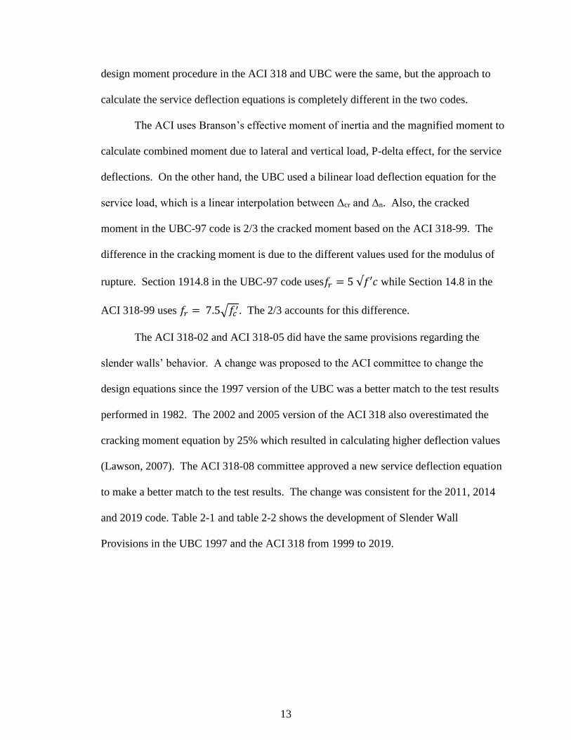
The ACI 318-02 and ACI 318-05 did have the same provisions regarding the
slender walls’ behavior. A change was proposed to the ACI committee to change the
design equations since the 1997 version of the UBC was a better match to the test results
performed in 1982. The 2002 and 2005 version of the ACI 318 also overestimated the
cracking moment equation by 25% which resulted in calculating higher deflection values
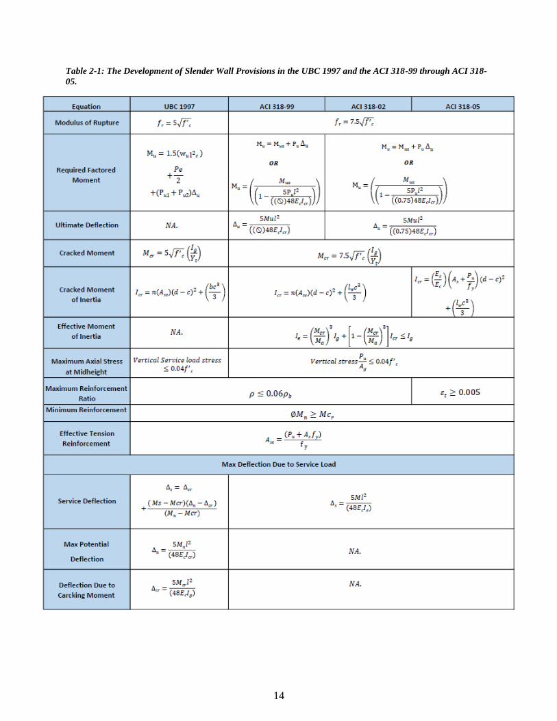
(Lawson, 2007). The ACI 318-08 committee approved a new service deflection equation
to make a better match to the test results. The change was consistent for the 2011, 2014
and 2019 code. Table 2-1 and table 2-2 shows the development of Slender Wall
Provisions in the UBC 1997 and the ACI 318 from 1999 to 2019.
14
Table 2-1: The Development of Slender Wall Provisions in the UBC 1997 and the ACI 318-99 through ACI 318-
05.
15
Table 2-2: The Development of Slender Wall Provisions in the ACI 318-08 through ACI 318-19.
16
2.3.2 Tri-linear moment-curvature analysis
Alwis (1990) presented a moment-curvature analysis for reinforced concrete
beams using a tri-linear representation dependent on the cracking and yielding points for
rectangular cross-sections. The moment-curvature response after the yielding point was
assumed to be perfectly plastic. Therefore, the tri-linear moment-curvature response was
defined by three points, the cracking point, the yielding point, and the ultimate point.
However, Alwis concluded that the method was not suitable for curvatures significantly
larger than the curvature at yielding point, as the member was assumed to be perfectly
plastic after yielding. Alwis did find good correlation between load-deflection curves
derived from the moment-curvature method and load-deflection curves using Branson’s
formula within the service load range. In addition, Alwis concluded that the methods
would produce only minor differences in their predictions in the service load range due to
their use of cracked and uncracked sectional properties in their derivations. Alwis
presented several numerical and experimental comparisons to further support his
conclusions.
Charkas, Rasheed, and Melhem (2003) presented a tri-linear moment-curvature
analysis method for reinforced concrete beams. However, the method included the
effects of fiber-reinforce polymer, FRP, for strengthening the member. While the use of
FRP strengthened members is outside the scope of the present method, the paper presents
relevant concrete analysis and moment-area integration procedures. In addition, the
derivation of the equivalent stress block factor, α, is useful:
17
cf
2
0 cf cf
2
c cff ' ' 3 '
c c
c c
d
(Eq’n 2.3.2.1)
In addition, the derivation of the neutral axis multiplier, γ, as:
0
0
1
3 12 '=1
13 '
cf
cf
cf
c c c
c
cf
cf c cc
d
f d
(Eq’n 2.3.2.2)
Since the load-deflection response is based on the moment-curvature response,
the paper also provided bases for developing the moment-area procedure for determining
the structural response of the member.
2.3.3 Moment Curvature Analysis for Slender Walls
According to Sakai and Kakuta (1980), calculating the moment curvature of
reinforced concrete structures can be accomplished by several methods. Moreover, the
most popular method is relatively easy and fast. It measures the transition of flexural
rigidities of reinforced concrete members subjected to bending only, which means this
method has never been tested on members that are subjected to both axial and bending.
The main focus of Sakai and Kakuta’s (1980) research is to calculate moment-curvature
relationship of reinforced concrete members subjected to combine bending and axial
forces.
To investigate this case they started by introducing the three procedures to
estimate the tensile resistances of the flexural rigidity of the concrete. The first procedure
18
is to assume the transition of stress distribution of concrete in the tensile region. The
second procedure is to assume the relation between steel stress in a cracked section and
average steel strain. The third procedure is to either give the transition of flexural
rigidities or the moment-curvature relationships.
The flexural rigidity, the curvature, and the strain of the first and second
procedures are calculated theoretically from the forces’ equilibrium. Most importantly
these specific procedures can be used when member is subjected to both bending and axil
forces. The third method was developed by Branson, Yu and Winter, Beeby and Miles,
Rabich, and Wegner and Duddeck. This specific method can be applied to very few
cases where the member is subjected to combine axial and bending. To be able to use this
procedure in all cases, Branson’s term for the effective moment of inertia needs to be
generalized. Sakai and Kakuta (1980) on moment-curvature relationships of reinforced
concrete members subjected to combined bending and axial force paper worked on
establishing a method to generalize Branson’s equation, later on they verified their
method experimentally. Branson established a term for effective moment of inertia in
1963 as follows
(Eq’n 2.3.3.1)
Where m is a constant power. Shaikh and Branson tested this equation on
members subjected to bending force; their finding was that this equation is valid for all
kind of bending forces. However, when the member is subjected to bending and axial
forces the results are not clearly determined.
𝐼𝑒𝑓𝑓 = (𝑀𝑐𝑟𝑀
)𝑚
+ (1 − (𝑀𝑐𝑟𝑀
)𝑚
) 𝐼𝑐𝑟 ≤ 𝐼𝑔
19
The procedure to generalize the effective moment of inertia equation is described
as follows. The bending moment and the moment of inertia on the center of gravity of
the section is used first. When a member is subjected to both bending and axial forces,
the neutral axis is separated from the center of the gravity. The following equation can
be used to calculate the average curvature after the member cracks.
The effective moment of inertia should be calculated at the center of the gravity
for both cracked and uncracked sections. When the member is subjected to both bending
and axial loading, the location of the neutral axis is separated from the center of the
gravity. In order to the keep the relationship in the previous equation between the
moment and the curvature we need to use the center of gravity. It is important to find the
moment of inertia at the center of gravity for gross moment then the cracked moment in
order to calculate the effective the moment of inertia.
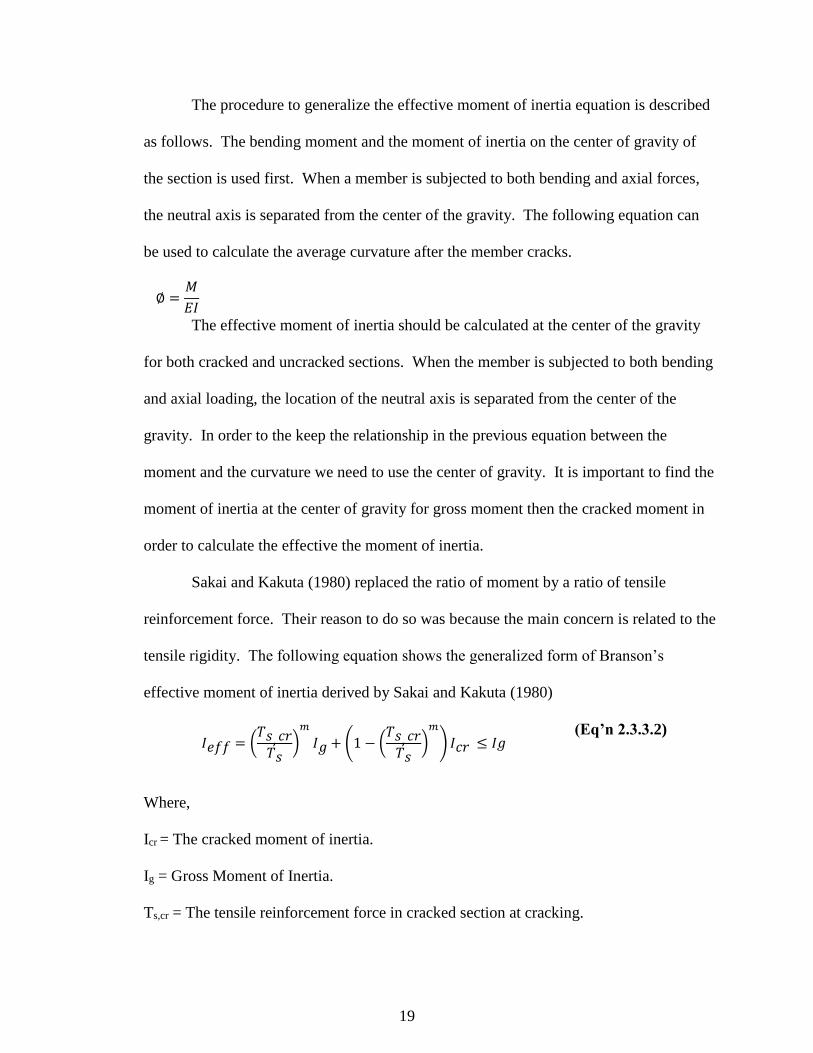
Sakai and Kakuta (1980) replaced the ratio of moment by a ratio of tensile
reinforcement force. Their reason to do so was because the main concern is related to the
tensile rigidity. The following equation shows the generalized form of Branson’s
effective moment of inertia derived by Sakai and Kakuta (1980)
(Eq’n 2.3.3.2)
Where,
Icr = The cracked moment of inertia.
Ig = Gross Moment of Inertia.
Ts,cr = The tensile reinforcement force in cracked section at cracking.
∅ =𝑀
𝐸𝐼
𝐼𝑒𝑓𝑓 = (𝑇𝑠, 𝑐𝑟𝑇𝑠
)𝑚
𝐼𝑔 + (1 − (𝑇𝑠, 𝑐𝑟𝑇𝑠
)𝑚
) 𝐼𝑐𝑟 ≤ 𝐼𝑔
20
Ts = The tensile reinforcement force in cracked section at arbitrary load levels.
To prove the validity of the provided equation, two tests were completed. The
first test was when the member is subjected to bending. The second test was when the
member sis subjected to both forces axial and bending. The results of this test indicate
that calculating the average curvature is possible for members subjected to bending and
axial loading if we consider both the moment of inertia and the effective center of gravity
of the effective section. In addition, the authors indicated that it is reasonable to replace
the moment ratio with the tensile ratio in the effective moment of inertia equation
because the main concern with concrete members is related to the rigidity of the tensile
zone. They concluded their research by indicating that the validity of the presented
method presented is valid and can be confirmed experimentally.
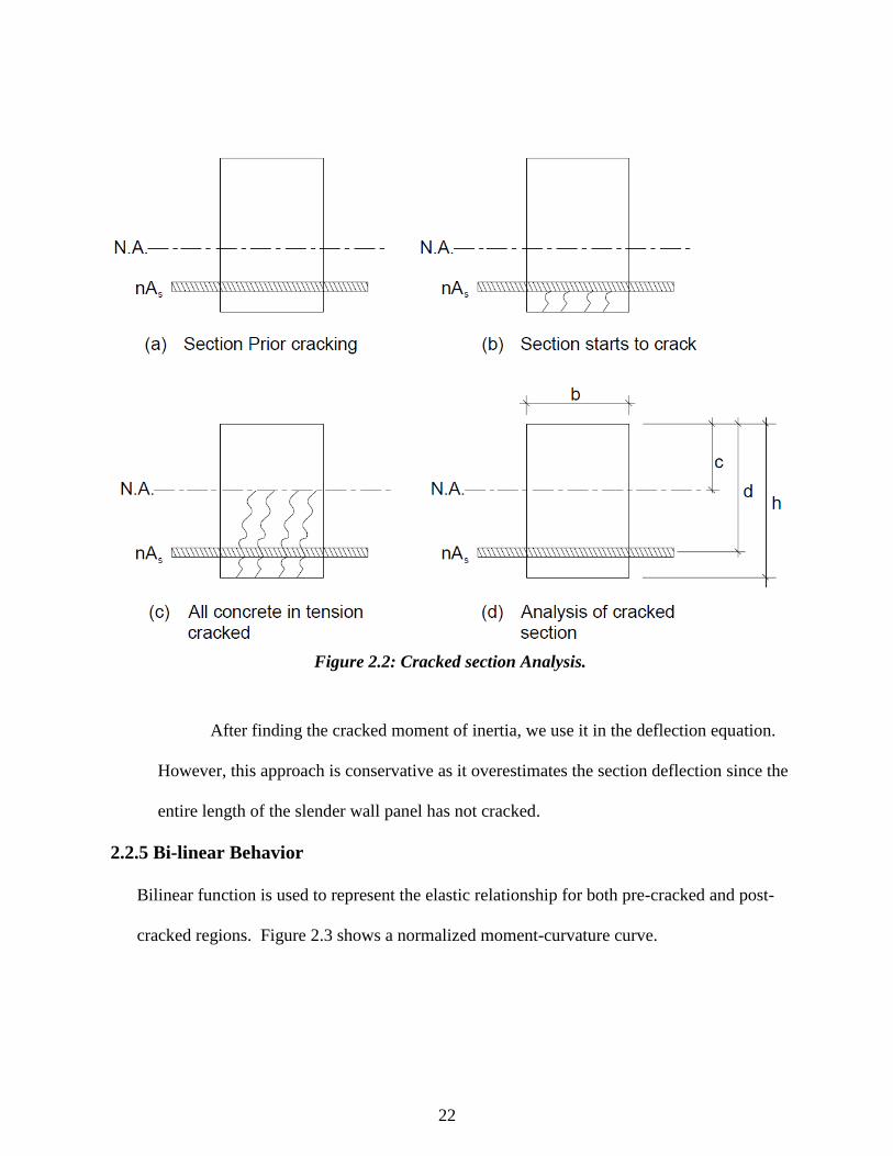
2.3.4 Cracked Sectional Analysis
This section discusses the analysis of cracked concrete members. It is important
to understand the behavior of the section after it starts to crack in order to find the
deflection. The section cracks as the load increases. When the applied moment exceeds
the cracking moment, the section cracks. Cracking starts at the tension area; when the
tension region starts to crack it can’t hold any tension stresses. The following steps show
the analysis of cracked section as presented in the ACI 318:
1- Neutral axis: As shown in Figure 2.2, the concrete below the current neutral axis
is cracked. Thus, we need to find new location of the neutral axis. To calculate
the new location of the neutral axis, follow to provided steps:
a- The centroid of the cracked section needs to be calculated. Assume a trial
section of the value c.
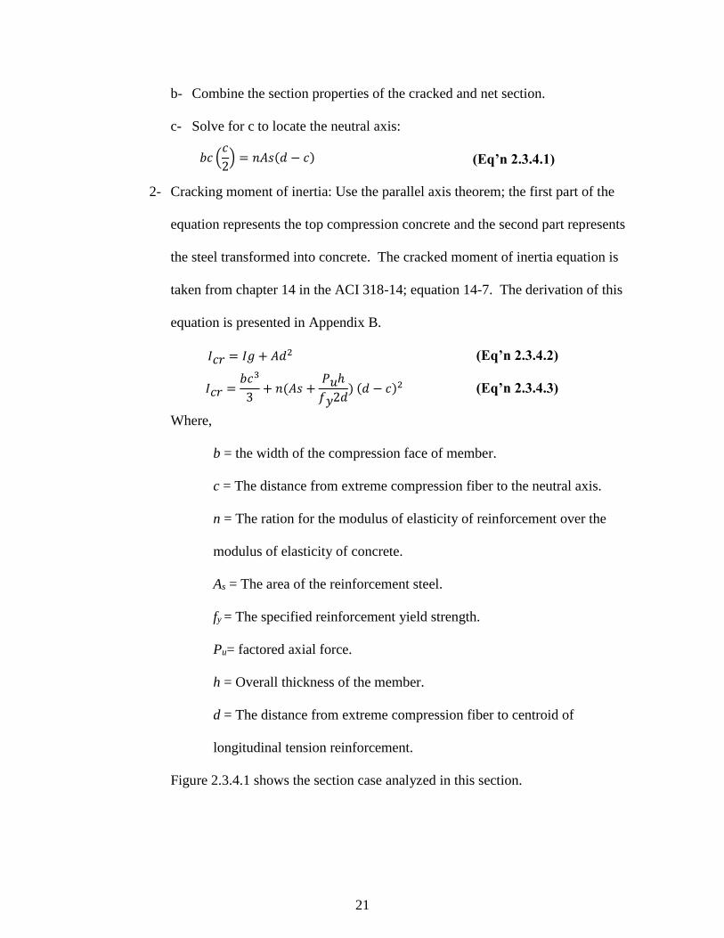
21
b- Combine the section properties of the cracked and net section.
c- Solve for c to locate the neutral axis:
(Eq’n 2.3.4.1)
2- Cracking moment of inertia: Use the parallel axis theorem; the first part of the
equation represents the top compression concrete and the second part represents
the steel transformed into concrete. The cracked moment of inertia equation is
taken from chapter 14 in the ACI 318-14; equation 14-7. The derivation of this
equation is presented in Appendix B.
(Eq’n 2.3.4.2)
(Eq’n 2.3.4.3)
Where,
b = the width of the compression face of member.
c = The distance from extreme compression fiber to the neutral axis.
n = The ration for the modulus of elasticity of reinforcement over the
modulus of elasticity of concrete.
As = The area of the reinforcement steel.
fy = The specified reinforcement yield strength.
Pu= factored axial force.
h = Overall thickness of the member.
d = The distance from extreme compression fiber to centroid of
longitudinal tension reinforcement.
Figure 2.3.4.1 shows the section case analyzed in this section.
𝑏𝑐 (𝑐
2) = 𝑛𝐴𝑠(𝑑 − 𝑐)
𝐼𝑐𝑟 = 𝐼𝑔 + 𝐴𝑑2
𝐼𝑐𝑟 =𝑏𝑐3
3+ 𝑛(𝐴𝑠 +
𝑃𝑢ℎ
𝑓𝑦2𝑑) (𝑑 − 𝑐)2
22
After finding the cracked moment of inertia, we use it in the deflection equation.
However, this approach is conservative as it overestimates the section deflection since the
entire length of the slender wall panel has not cracked.
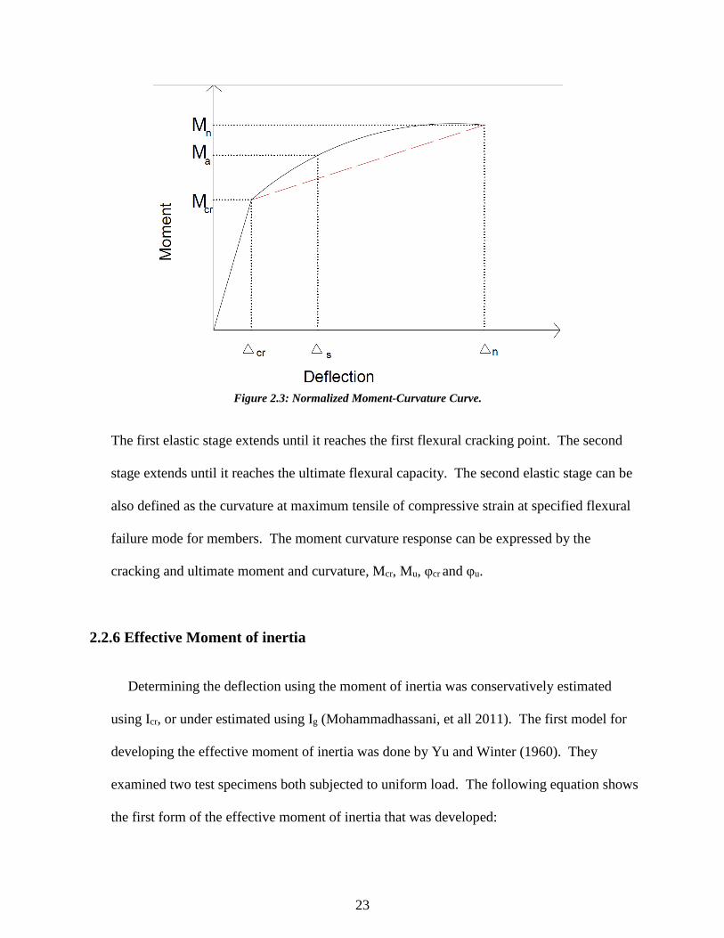
2.2.5 Bi-linear Behavior
Bilinear function is used to represent the elastic relationship for both pre-cracked and post-
cracked regions. Figure 2.3 shows a normalized moment-curvature curve.
Figure 2.2: Cracked section Analysis.
23
The first elastic stage extends until it reaches the first flexural cracking point. The second
stage extends until it reaches the ultimate flexural capacity. The second elastic stage can be
also defined as the curvature at maximum tensile of compressive strain at specified flexural
failure mode for members. The moment curvature response can be expressed by the
cracking and ultimate moment and curvature, Mcr, Mu, φcr and φu.
2.2.6 Effective Moment of inertia
Determining the deflection using the moment of inertia was conservatively estimated
using Icr, or under estimated using Ig (Mohammadhassani, et all 2011). The first model for
developing the effective moment of inertia was done by Yu and Winter (1960). They
examined two test specimens both subjected to uniform load. The following equation shows
the first form of the effective moment of inertia that was developed:
Figure 2.3: Normalized Moment-Curvature Curve.
24
(Eq’n 2.2.6.1)
where M1 is computed as follows:
(Eq’n 2.2.6.2)
Later on, in 1963 Branson developed the second form of Ieff. His goal was to accounts for the
cracked part of the concrete not having any tension in it. The following equation represents
Branson’s work for Ieff:
(Eq’n 2.2.6.3)
The ACI 318 approved his equation and added it to the design guide for calculating the
deflection in 1971. In 2005, Bischoff reevaluated Ieff, his work was based on the moment
curvature relation established by the Euro code. The following equation shows Bischoff’s
approach:
(Eq’n 2.2.6.4)
𝐼𝑒 =𝐼𝑐𝑟
1 − ( 𝑀𝑐𝑟𝑀𝑎
)2
[ 1 −𝐼𝑐𝑟𝐼𝑔
]
𝐼𝑒 = ( 𝑀𝑐𝑟𝑀𝑎
)3
𝐼𝑔 + [ 1 − ( 𝑀𝑐𝑟𝑀𝑎
)3
] 𝐼𝑐𝑟
𝐼𝑒𝑓𝑓 =𝐼𝑐𝑟
(1 − 𝑏 (𝑀1𝑀𝑎
))
𝑀1 = 0.1(𝑓′𝑐)
23 ℎ(ℎ − 𝑘𝑑)
25
Chapter 3 - Sectional Analysis: Load Deflection Behavior
3.0 Moment-Curvature Response
This section presents assumptions used for rectangular cross sections, uniformly loading
in bending with axial load, and all two-moment curvature points: cracking point and yield point.
The given assumptions aim to simplify the deflection calculations, describe the behavior of the
materials, and note the members’ behaviors. The assumptions are:
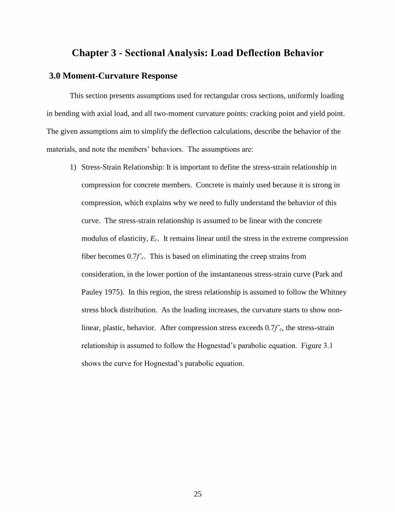
1) Stress-Strain Relationship: It is important to define the stress-strain relationship in
compression for concrete members. Concrete is mainly used because it is strong in
compression, which explains why we need to fully understand the behavior of this
curve. The stress-strain relationship is assumed to be linear with the concrete
modulus of elasticity, Ec. It remains linear until the stress in the extreme compression
fiber becomes 0.7f’c. This is based on eliminating the creep strains from
consideration, in the lower portion of the instantaneous stress-strain curve (Park and
Pauley 1975). In this region, the stress relationship is assumed to follow the Whitney
stress block distribution. As the loading increases, the curvature starts to show non-
linear, plastic, behavior. After compression stress exceeds 0.7f’c, the stress-strain
relationship is assumed to follow the Hognestad’s parabolic equation. Figure 3.1
shows the curve for Hognestad’s parabolic equation.
26
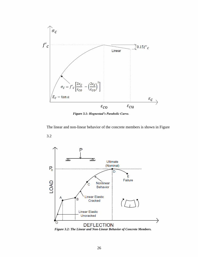
The linear and non-linear behavior of the concrete members is shown in Figure
3.2
Figure 3.1: Hognestad’s Parabolic Curve.
Figure 3.2: The Linear and Non-Linear Behavior of Concrete Members.
27
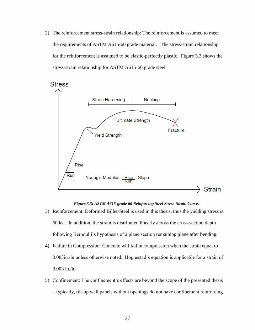
2) The reinforcement stress-strain relationship: The reinforcement is assumed to meet
the requirements of ASTM A615-60 grade material. The stress-strain relationship
for the reinforcement is assumed to be elastic-perfectly plastic. Figure 3.3 shows the
stress-strain relationship for ASTM A615-60 grade steel.
3) Reinforcement: Deformed Billet-Steel is used in this thesis, thus the yielding stress is
60 ksi. In addition, the strain is distributed linearly across the cross-section depth
following Bernoulli’s hypothesis of a plane section remaining plane after bending.
4) Failure in Compression: Concrete will fail in compression when the strain equal to
0.003in./in unless otherwise noted. Hognestad’s equation is applicable for a strain of
0.003 in./in.
5) Confinement: The confinement’s effects are beyond the scope of the presented thesis
– typically, tilt-up wall panels without openings do not have confinement reinforcing.
Figure 3.3: ASTM A615-grade 60 Reinforcing Steel Stress-Strain Curve.
28
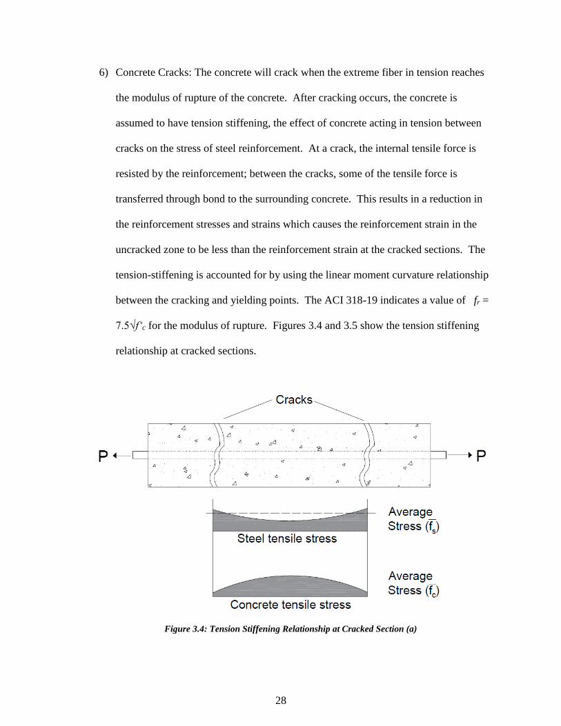
6) Concrete Cracks: The concrete will crack when the extreme fiber in tension reaches
the modulus of rupture of the concrete. After cracking occurs, the concrete is
assumed to have tension stiffening, the effect of concrete acting in tension between
cracks on the stress of steel reinforcement. At a crack, the internal tensile force is
resisted by the reinforcement; between the cracks, some of the tensile force is
transferred through bond to the surrounding concrete. This results in a reduction in
the reinforcement stresses and strains which causes the reinforcement strain in the
uncracked zone to be less than the reinforcement strain at the cracked sections. The
tension-stiffening is accounted for by using the linear moment curvature relationship
between the cracking and yielding points. The ACI 318-19 indicates a value of fr =
7.5√f‘c for the modulus of rupture. Figures 3.4 and 3.5 show the tension stiffening
relationship at cracked sections.
Figure 3.4: Tension Stiffening Relationship at Cracked Section (a)
29
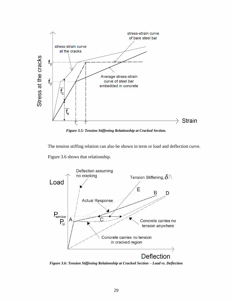
The tension stiffing relation can also be shown in term or load and deflection curve.
Figure 3.6 shows that relationship.
Figure 3.5: Tension Stiffening Relationship at Cracked Section.
Figure 3.6: Tension Stiffening Relationship at Cracked Section – Load vs. Deflection
30
7) Strain are assumed to be distrubted lineraly over the depth of the wall panel.
8) Tension and compression forces acting on the cross section must be in equilibrium for
the wall panel with flexure and axial load.
9) The ultimate moment corresponds to the occurrence of a strain in the concrete, which
causes crushing (0.003 in./in.).
10) The failure analyzed is in combined flexure and axial load, and it is assumed that
adequate shear strength exists to prevent shear failure. Bond and anchorage of the
steel is assumed to be adequate to prevent development length failure or bond slip
allowing full flexural strength at the section being analyzed.
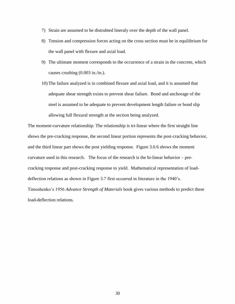
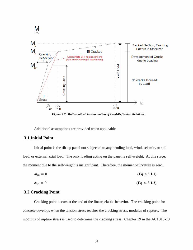
The moment-curvature relationship: The relationship is tri-linear where the first straight line
shows the pre-cracking response, the second linear portion represents the post-cracking behavior,
and the third linear part shows the post yielding response. Figure 3.0.6 shows the moment
curvature used in this research. The focus of the research is the bi-linear behavior – pre-
cracking response and post-cracking response to yield. Mathematical representation of load-
deflection relations as shown in Figure 3.7 first occurred in literature in the 1940’s.
Timoshenko’s 1956 Advance Strength of Materials book gives various methods to predict these
load-deflection relations.
31
Additional assumptions are provided when applicable
3.1 Initial Point
Initial point is the tilt-up panel not subjected to any bending load, wind, seismic, or soil
load, or external axial load. The only loading acting on the panel is self-weight. At this stage,
the moment due to the self-weight is insignificant. Therefore, the moment-curvature is zero..
𝑀𝑖𝑛 = 0 (Eq’n 3.1.1)
𝜙𝑖𝑛 = 0 (Eq’n. 3.1.2)
3.2 Cracking Point
Cracking point occurs at the end of the linear, elastic behavior. The cracking point for
concrete develops when the tension stress reaches the cracking stress, modulus of rupture. The
modulus of rupture stress is used to determine the cracking stress. Chapter 19 in the ACI 318-19
Figure 3.7: Mathematical Representation of Load-Deflection Relations.
32
code specifies Equation 19.2.3.1 to calculate the modulus of rupture. For normal weight
concrete, the ‘lambda’ term, which modifies the modulus of rupture based on the density of the
concrete, equals one. Therefore, the modulus of rupture for this study is calculated using
Equation 3.2.1.
(Eq’n 3.2.1)
In this specific analysis, the self-weight of the panel is considered as an external axial
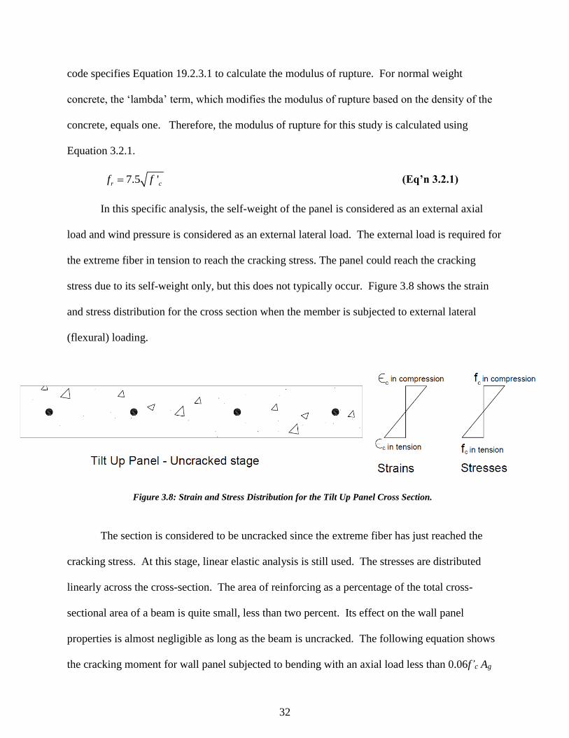
load and wind pressure is considered as an external lateral load. The external load is required for
the extreme fiber in tension to reach the cracking stress. The panel could reach the cracking
stress due to its self-weight only, but this does not typically occur. Figure 3.8 shows the strain
and stress distribution for the cross section when the member is subjected to external lateral
(flexural) loading.
The section is considered to be uncracked since the extreme fiber has just reached the
cracking stress. At this stage, linear elastic analysis is still used. The stresses are distributed
linearly across the cross-section. The area of reinforcing as a percentage of the total cross-
sectional area of a beam is quite small, less than two percent. Its effect on the wall panel
properties is almost negligible as long as the beam is uncracked. The following equation shows
the cracking moment for wall panel subjected to bending with an axial load less than 0.06f’c Ag
7.5 'r cf f
Figure 3.8: Strain and Stress Distribution for the Tilt Up Panel Cross Section.
33
(similar to a tilt-up concrete panel), P-delta affect is not considered since the section has not
cracked:
𝑴𝒄𝒓 =𝒇𝒓𝑰𝒈
𝒚𝒕 (Eq’n 3.2.2)
Where:
Ig = gross moment of inertia of the reinforced concrete section. The tilt-up concrete wall
panels in this study have one layer of reinforcement, which is very close to gross
transformed section’s neutral axis. Therefore, the gross moment of inertia and the gross
transformed moment of inertia are almost equal; the effects of reinforcement is neglected.
yt = distance from the centroid to extreme tension fiber. For a tilt-up panel reinforced
with a single layer of reinforcing steel that is located in the center of the panel, the
centroid of the wall section occurs approximately at the same location as the reinforcing
steel depending on size of chairs used and accuracy of construction.
Since the section is still uncracked and is assumed to act elastically, the strains, ɛ, are linearly
distributed over the depth of the member and can be determined by dividing the stresses, f, by the
modulus of elasticity of the concrete, Ec :
휀 =𝑓
𝐸𝑐 (Eg’n 3.2.3)
Where:
𝑬𝒄 = 𝟓𝟕𝟎𝟎𝟎√𝒇𝒄′ (ACI 318-19 Eq’n 19.2.2.1.a)
The deflection of a wall panel is calculated by integrating the curvatures along the length
of the wall panel. For an elastic wall panel, the curvature is equal to the moment divided
by the flexural stiffness, EI, of the member. Thus, the cracking curvature is shown as
follows:
34
𝜙𝑐𝑟 =𝑀𝑐𝑟
𝐸𝑐𝐼𝑔 (Eq’n 3.2.4)
3.3 Yielding Point
The yielding point in concrete members occurs when the steel reaches the specified
yielding stress. The yielding stress permitted by the ACI 318 ranges from 40,000 psi to 80,000
psi (Paulson et al. 2016). The most common reinforcing steel used in tilt-up wall panels is
ASTM C615-60 grade. Therefore, for the purpose of this research, the reinforcing steel yield
stress is 60,000 psi. Since the reinforcing steel strain is greater than the concrete cracking strain,
the section is defined as cracked at the reinforcing yielding. It is not possible to determine the
yielding moment and curvature using the internal stress analysis since the section is cracked.
When the section is cracked, the stresses are not distributed linearly across the cross-section,
which is why we need to use the strain-compatibility analysis instead.
Strain-compatibility analysis is used to establish computable internal stresses and forces
relationships; it is assumed that within the cross-section the strain is distributed. The analysis
uses the following assumptions for cracked sections:
1) Plane section remains plane.
2) Steel and concrete strains are the same at all locations.
3) Strains within the cross-section are distributed linearly is applicable.
Reinforced steel is a bilinear material, which means we can apply Hooke’s Law until it reaches
the yield stress. Since strain-compatibility is being used, the strain equation that causes the
reinforcement to yield is:
(Eq’n 3.3.1) 휀𝑦 =𝑓𝑦
𝐸𝑠=
0.002
𝑐𝑑
35
To determine the tension force of the reinforcement, the area of the steel is multiplied by the
steel stress using the following equation:
T = Asfy (Eq’n 3.3.2)
By using strain-compatibility, the extreme compression fiber strain is determined from:
𝑐𝑓
𝑐𝑦=
𝑦𝑐𝑦
(𝑑−𝑐𝑦)⟹ 𝜎𝑐𝑓 =
𝑦𝑐𝑦
(𝑑−𝑐𝑦)𝐸𝑐 (Eq’n 3.3.3)
The location of the neutral axis from the extreme compression fiber, cy, is unknown and will be
determine from the internal force equilibrium of the cross section. After determining the steel-
concrete strain relationship, the stress-block model shown in Figure3.3.1 is used to replace the
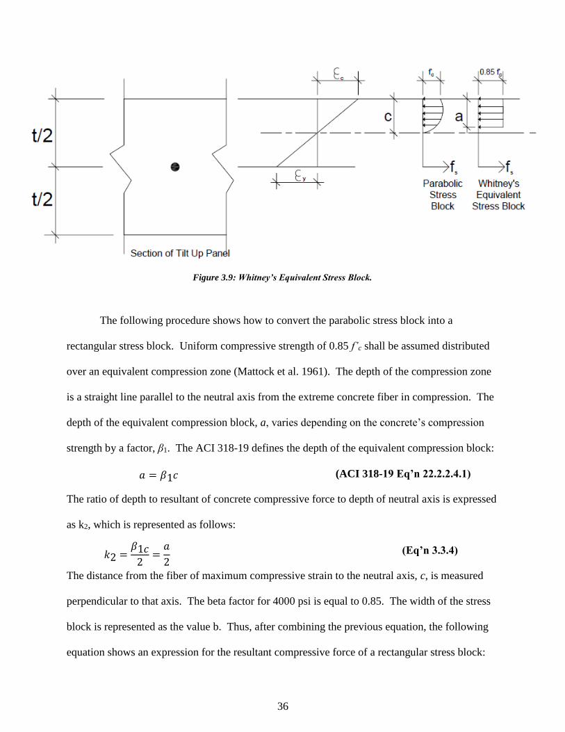
actual parabolic concrete stress distribution. The coefficient β1 is multiplied by the depth to the
neutral axis, c, to get the depth of the stress block, a. The concrete is assumed to carry no tension
- no concrete stress distribution below the neutral axis. The assumed stress block is the Whitney
stress block to specify concrete stresses in compression. The ACI 318-19 Section 22.2.2.4
allows for an approximation for the force in the stress block. The approximation is based on the
work done by Whitney in 1930’s. Whitney (1937) proposed to replace the parabolic stress block
to a rectangular stress block. Figure 3.9 shows the parabolic stress block and Whitney’s
rectangular stress block distribution:
36
The following procedure shows how to convert the parabolic stress block into a
rectangular stress block. Uniform compressive strength of 0.85 f’c shall be assumed distributed
over an equivalent compression zone (Mattock et al. 1961). The depth of the compression zone
is a straight line parallel to the neutral axis from the extreme concrete fiber in compression. The
depth of the equivalent compression block, a, varies depending on the concrete’s compression
strength by a factor, β1. The ACI 318-19 defines the depth of the equivalent compression block:
(ACI 318-19 Eq’n 22.2.2.4.1)
The ratio of depth to resultant of concrete compressive force to depth of neutral axis is expressed
as k2, which is represented as follows:
(Eq’n 3.3.4)
The distance from the fiber of maximum compressive strain to the neutral axis, c, is measured
perpendicular to that axis. The beta factor for 4000 psi is equal to 0.85. The width of the stress
block is represented as the value b. Thus, after combining the previous equation, the following
equation shows an expression for the resultant compressive force of a rectangular stress block:
𝑘2 =𝛽1𝑐2
=𝑎
2
𝑎 = 𝛽1𝑐
Figure 3.9: Whitney’s Equivalent Stress Block.
37
(Eq’n 3.3.5)
Then, the compression and tension forces are set equal to each other to find the depth of the
neutral axis:
T = C (Eq’n 3.3.6)
(Eq’n 3.3.7)
Once cy is determined the curvature and the corresponding moment are found from the equation:
𝜙𝑦 =𝑐𝑓
𝑐𝑦=
𝑦
(𝑑−𝑐𝑦) (Eq’n 3.3.8)
The corresponding moment for yielding point is found by summing the moments about the
centroid of the compressive force. The bending moment equation is:
(Eq’n 3.3.9)
3.4 Ultimate Point
This section discusses the derivation of equations for determining the slender wall
members’ ultimate moment and corresponding curvatures. Since confinement reinforcement is
not typically provided, a rectangular cross-section without compression steel is discussed. The
two possible failure modes for reinforced concrete panels are steel rupture and concrete crushing
(Stowik, 2019).
3.4.1 Steel Rupture
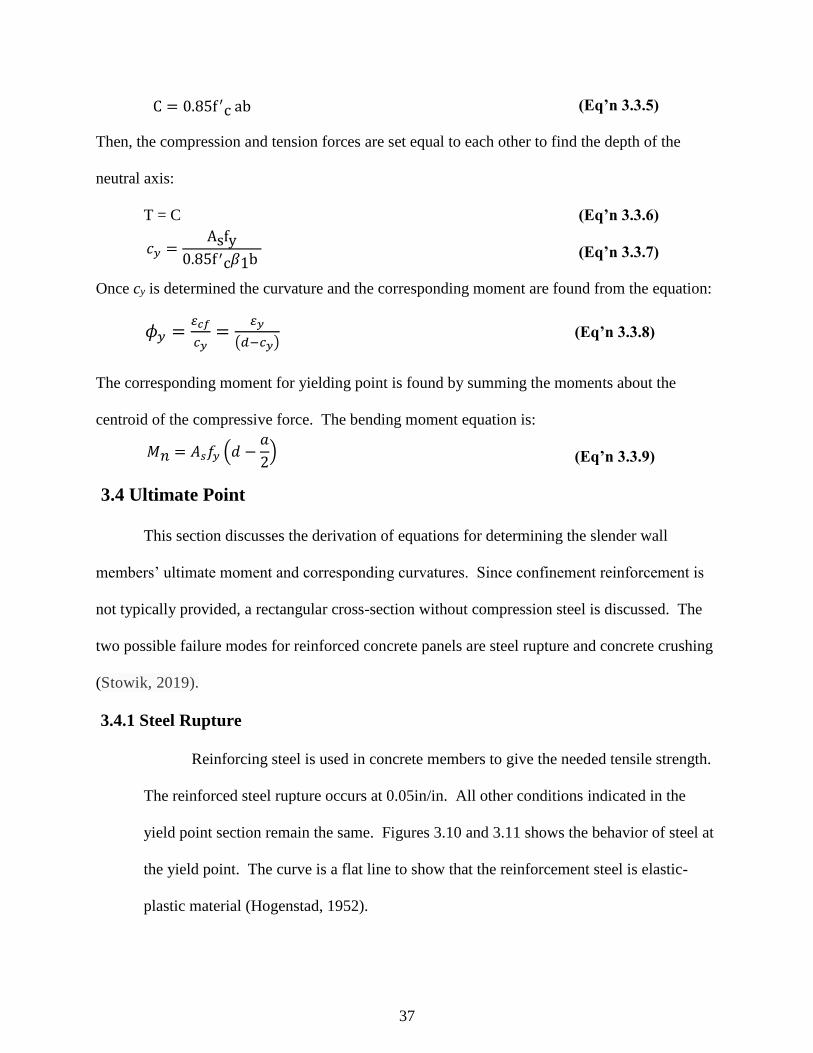
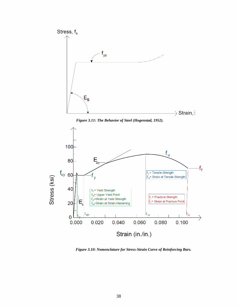
Reinforcing steel is used in concrete members to give the needed tensile strength.
The reinforced steel rupture occurs at 0.05in/in. All other conditions indicated in the
yield point section remain the same. Figures 3.10 and 3.11 shows the behavior of steel at
the yield point. The curve is a flat line to show that the reinforcement steel is elastic-
plastic material (Hogenstad, 1952).
C = 0.85f ′c ab
𝑐𝑦 =Asfy
0.85f ′c𝛽1b
𝑀𝑛 = 𝐴𝑠𝑓𝑦 (𝑑 −𝑎
2)
38
Figure 3.11: The Behavior of Steel (Hogenstad, 1952).
Figure 3.10: Nomenclature for Stress-Strain Curve of Reinforcing Bars.
39
In most cases, concrete fail before steel reaches the yielding point (Hogenstad,
1952). The derivation of the equations has been shown in the previous section. For a
rectangular section, the neutral axis for a linear stress distribution is as follows:
(0.5)휀𝑢𝑐𝑛2𝐸𝑐𝑏 = 𝐴𝑠𝑓𝑦(𝑑 − 𝑐𝑛) ⇒ ((0.5)휀𝑢𝐸𝑐𝑏)𝑐𝑛
2 + (𝐴𝑠𝑓𝑦)𝑐𝑛 − 𝐴𝑠𝑓𝑦𝑑 = 0 (Eq’n 3.4.1.1)
After summing the forces in about the compression force, the moment for steel rupture
failure mode is as follows:
(Eq’n 3.4.1.2)
3.4.2 Concrete Crushing Failure
The concrete crushing failure mode occurs when the strain at the concrete extreme
compressive fiber equals to 0.003in/in. Since concrete crushing is the failure mode, it is
assumed that the compressive stress distribution is parabolic. A stress above 0.7f’c in the
compression zone is required to achieve a strain of 0.003 in./in. in the extreme concrete
compression fiber. To determine the ultimate moment and corresponding curvature,
strain-compatibility analysis must be used. Keeping in mind that both the tension and
compression forces vary depending on the location of the neutral axis. The only
difference is both the tension and the compression force are dependent on the neutral axis
location.
For a rectangular section, the neutral axis for a linear stress distribution is as follows:
𝑐𝑢
𝑐𝑛=
0.003
𝑐𝑛= 𝑠
(𝑑−𝑐𝑛)⇒ 휀𝑠 =
(𝑑−𝑐𝑛)
𝑐𝑛0.003 (Eq’n 3.4.2.1)
The stress distribution is converted into an equivalent rectangular stress block by the
following procedure:
𝑀𝑛 = 𝐴𝑠𝑓𝑦 (𝑑 −𝛽1𝑐𝑛
2)
40
(Eq’n 3.4.2.2)
where α captures the height of the equivalent rectangular block, which is a function of the
extreme compressive fiber strain, εcf, and the strain at maximum compressive stress, ε’c.
This stress block is used to determine the compressive force attributed to the concrete.
However, while this stress block gives the equivalent magnitude of the compression
force; the location of the compression force is not located at the center of the block.
Since the centroid of the actual compressive stress is based off of the parabolic shape.
The location of the compression force is placed at a distance of γcy from the extreme
compressive fiber. The neutral axis multiplier, γ, is based of the following equation used
by Charkas, Rasheed and Melhem (2003):
(Eq’n 3.4.2.3)
The neutral axis multiplier, γ, is also dependent on the strain at maximum compressive,
ε’c and extreme compressive fiber strain, εcf. The strain is converted to a stress by
multiplying by the modulus of elasticity of concrete, Ec. The parabolic distribution is
valid at an extreme fiber stress greater than 0.7f‘c. If the stress is greater than 0.7f‘c, the
stress is distributed in accordance with Hognestad’s parabolic equation. With the steel
and concrete stress-strain relationships are known it is possible to find cn by force
equilibrium.
2 2 32 3
2 2
0 0 0
2' ' ' '
' ' ' 3 ' ' 3 '
cfcf cf
cf cfc c c cc cf c c c c c c
c c c c c c
f d f d f f
2
2' '
' 3 '
cf cf
cf c c
c c
f f
1
3 12 '
13 '
cf
c
cf
c
41
((3휀𝑠휀𝑐′)𝑓𝑐
′𝑏)𝑐𝑛3 + (𝐴𝑠𝑓𝑦3휀𝑐
′2 − 3휀𝑠𝑓𝑐′𝑏휀𝑐
′𝑑)𝑐𝑛2 − (𝐴𝑠𝑓𝑦6휀𝑐
′2𝑑)𝑐𝑛
+𝐴𝑠𝑓𝑦3휀𝑐′2𝑑2 = 0 (Eq’n 3.4.2.4)
After summing the forces in the compression, the moment for a parabolic stress
distribution in the concrete crushing failure mode is as follows:
𝑀𝑛 = 𝑇(𝑑 − 𝛾𝑐𝑛) = 𝐴𝑠𝑓𝑦(𝑑 − 𝛾𝑐𝑛) (Eq’n 3.4.2.5)
𝝓𝒏 =𝜺𝒄𝒖
𝒄𝒏=
𝜺𝒔
(𝒅−𝒄𝒏) (Eq’n 3.4.2.5)
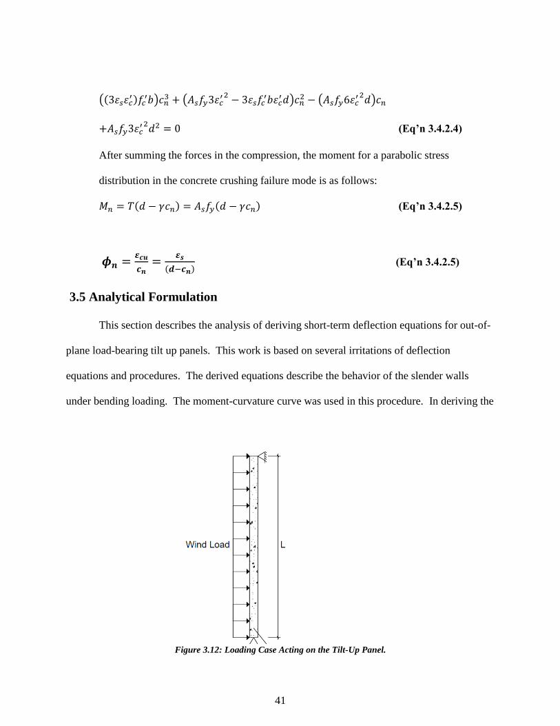
3.5 Analytical Formulation
This section describes the analysis of deriving short-term deflection equations for out-of-
plane load-bearing tilt up panels. This work is based on several irritations of deflection
equations and procedures. The derived equations describe the behavior of the slender walls
under bending loading. The moment-curvature curve was used in this procedure. In deriving the
Figure 3.12: Loading Case Acting on the Tilt-Up Panel.
42
equations, closed forms of analytical expressions are obtained for the pre-cracking, post-
cracking, and post-yielding regions. Figure 3.12 Shows the load case analyzed in this research.
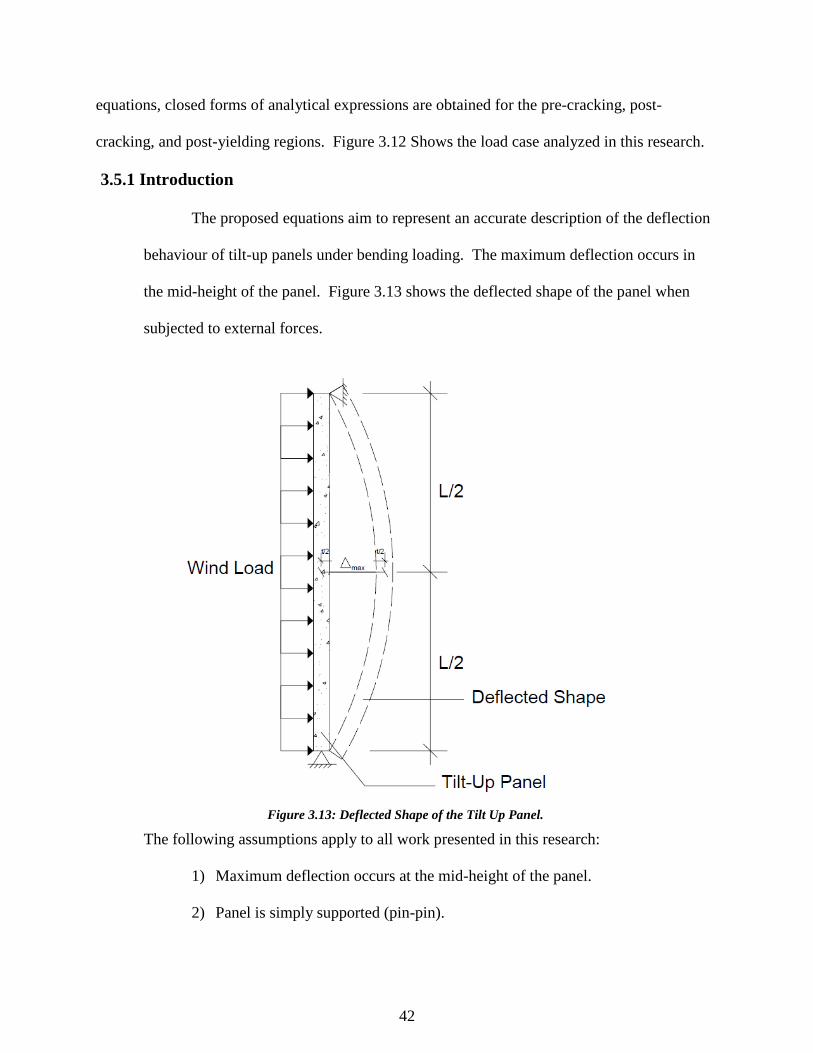
3.5.1 Introduction
The proposed equations aim to represent an accurate description of the deflection
behaviour of tilt-up panels under bending loading. The maximum deflection occurs in
the mid-height of the panel. Figure 3.13 shows the deflected shape of the panel when
subjected to external forces.
The following assumptions apply to all work presented in this research:
1) Maximum deflection occurs at the mid-height of the panel.
2) Panel is simply supported (pin-pin).
Figure 3.13: Deflected Shape of the Tilt Up Panel.
43
3) Panels are lightly reinforced load bearing walls.
4) Self-weight of the panel is considered as axial load.
5) Concrete in compression region is assumed to behave linearly up to an
extreme fiber stress of 0.7fc’ then Hogenstad’s parabolic stress distribution is
used.
6) Steel has elastic-perfectly plastic response.
7) Prior cracking gross moment of inertia (Ig) is used in the deflection equation
neglecting reinforcing steel since the steel is located near the neutral axis.
8) Post-cracking proposed effective moment of inertia (Iey) equation is used.
9) Moment-Curvature assumed to have Tri-linear behavior.
3.5.2 Pre-Cracking Stage
The member is considered to be in the pre-cracking stage if it is not subjected to
any loading or lightly loaded. In this region the cracking moment is greater than the
applied moment due to bending and axial loading. The first step if the derivation is to use
the moment- curvature relationship equation:
(Eq’n 3.5.2.1)
The moment of inertia used at this stage is the gross moment of inertia of the section:
(Eq’n 3.5.2.2)
M(x) term represents the moment of the forces acting on the panel:
(Eq’n 3.5.2.3)
The deflection of the panel in the pre-cracked region is equal to the integral of the
moment-curvature equation:
(Eq’n 3.5.2.4)
∅(𝑥) =𝑀(𝑥)
𝐸𝐼
Δc=𝛿𝑢𝑛
∅𝑢𝑛(𝑥) =𝑀(𝑥)
𝐸𝑐𝐼𝑔𝑡
𝑀(𝑥) =𝑤𝐿
2x −
wx2
2
44
(Eq’n 3.5.2.5)
We plug equations 3.5.2.2 and 3.5.2.2 into equation 3.5.2.5. The integral limit is from 0
to L/2:
(Eq’n 3.5.2.6)
The following equations show the progress of the integration with respect to x:
(Eq’n 3.5.2.7)
(Eq’n 3.5.2.8)
We replace the x term by the limit 0 to L/2:
(Eq’n 3.5.2.9)
(Eq’n 3.5.2.10)
Then we use algebra to find a common denominator and simplify the equation:
(Eq’n 3.5.2.11)
The final form of the deflection equation for out of plane load-bearing walls in the pre-
cracking region is as follows:
(Eq’n 3.5.2.12)
𝛥𝑐 = ∫ Ø𝑢𝑛(𝑥) (𝑥) 𝑑𝑥
𝐿2
0
𝛥𝑐 =1
𝐸𝑐 𝐼𝑔𝑡
∫ (𝑤𝐿
2𝑥 −
𝑤𝑥2
2)𝑥 𝑑𝑥
𝐿2
0
𝛥𝑐 =1
𝐸𝑐 𝐼𝑔𝑡
∫ (𝑤𝐿
2𝑥2 −
𝑤𝑥3
2) 𝑑𝑥
𝐿2
0
𝛥𝑐 =1
𝐸𝑐 𝐼𝑔𝑡
[𝑤𝐿
2.𝑥3
3−
𝑤𝑥4
(2)(4)]| 1
𝐿/2
0
𝛥𝑐 =1
𝐸𝑐 𝐼𝑔𝑡
[ 𝑤𝐿
6(𝐿
2)3
−𝑤
8(𝐿
2)4
]
𝛥𝑐 =1
𝐸𝑐𝐼𝑔𝑡 [
8𝑤𝐿4
384−
3𝑤𝐿4
384 ]
𝛥𝑐 =5𝑤𝐿4
384𝐸𝑐𝐼𝑔𝑡
𝛥𝑐 =1
𝐸𝑐𝐼𝑔𝑡 [
𝑤𝐿
6𝑥3 −
𝑤
8𝑥4 ]| 1
𝐿/2
0
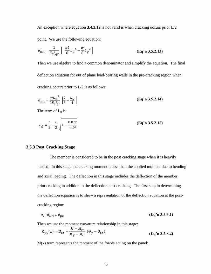
45
𝐿𝑔 =𝐿
2−
𝐿
2 √1 −
8𝑀𝑐𝑟
𝑤𝐿2
An exception where equation 3.4.2.12 is not valid is when cracking occurs prior L/2
point. We use the following equation:
(Eq’n 3.5.2.13)
Then we use algebra to find a common denominator and simplify the equation. The final
deflection equation for out of plane load-bearing walls in the pre-cracking region when
cracking occurs prior to L/2 is as follows:
(Eq’n 3.5.2.14)
The term of Lg is:
(Eq’n 3.5.2.15)
3.5.3 Post Cracking Stage
The member is considered to be in the post cracking stage when it is heavily
loaded. In this stage the cracking moment is less than the applied moment due to bending
and axial loading. The deflection in this stage includes the deflection of the member
prior cracking in addition to the deflection post cracking. The first step in determining
the deflection equation is to show a representation of the deflection equation at the post-
cracking region:
(Eq’n 3.5.3.1)
Then we use the moment curvature relationship in this stage:
(Eq’n 3.5.3.2)
M(x) term represents the moment of the forces acting on the panel:
𝛿𝑢𝑛 =1
𝐸𝑐𝐼𝑔𝑡 [
𝑤𝐿
6𝐿𝑔
3 −𝑤
8𝐿𝑔
4 ]
𝛿𝑢𝑛 =𝑤𝐿𝑔
3
2𝐸𝑐𝐼𝑔𝑡 [
𝐿
3−
𝐿𝑔4
]
Δc=𝛿𝑢𝑛 + 𝛿𝑝𝑐
∅𝑝𝑐(𝑥) = Ø𝑐𝑟 +𝑀 − 𝑀𝑐𝑟
𝑀𝑦 − 𝑀𝑐𝑟 (Ø𝑦 − Ø𝑐𝑟)
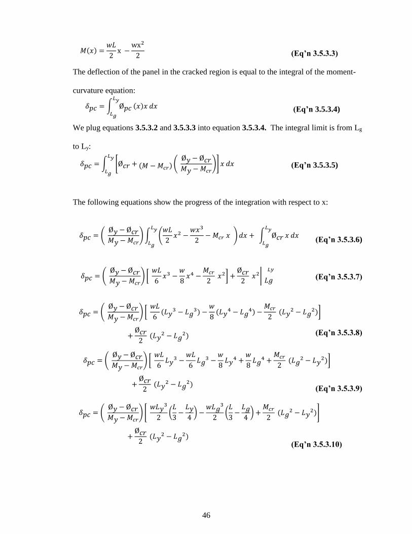
46
(Eq’n 3.5.3.3)
The deflection of the panel in the cracked region is equal to the integral of the moment-
curvature equation:
(Eq’n 3.5.3.4)
We plug equations 3.5.3.2 and 3.5.3.3 into equation 3.5.3.4. The integral limit is from Lg
to Ly:
(Eq’n 3.5.3.5)
The following equations show the progress of the integration with respect to x:
(Eq’n 3.5.3.6)
(Eq’n 3.5.3.7)
(Eq’n 3.5.3.8)
(Eq’n 3.5.3.9)
(Eq’n 3.5.3.10)
𝛿𝑝𝑐 = ∫ Ø𝑝𝑐 (𝑥)𝑥 𝑑𝑥𝐿𝑦
𝐿𝑔
𝑀(𝑥) =𝑤𝐿
2x −
wx2
2
𝛿𝑝𝑐 = ∫ [Ø𝑐𝑟 + (𝑀 − 𝑀𝑐𝑟) ( Ø𝑦 − Ø𝑐𝑟𝑀𝑦 − 𝑀𝑐𝑟
)]𝑥 𝑑𝑥𝐿𝑦
𝐿𝑔
𝛿𝑝𝑐 = ( Ø𝑦 − Ø𝑐𝑟𝑀𝑦 − 𝑀𝑐𝑟
)∫ (𝑤𝐿
2𝑥2 −
𝑤𝑥3
2− 𝑀𝑐𝑟
𝑥 ) 𝑑𝑥 +
𝐿𝑦
𝐿𝑔
∫ Ø𝑐𝑟 𝑥 𝑑𝑥 𝐿𝑦
𝐿𝑔
𝛿𝑝𝑐 = ( Ø𝑦 − Ø𝑐𝑟𝑀𝑦 − 𝑀𝑐𝑟
) [ 𝑤𝐿
6(𝐿𝑦
3 − 𝐿𝑔3) −
𝑤
8(𝐿𝑦
4 − 𝐿𝑔4) −
𝑀𝑐𝑟
2 (𝐿𝑦
2 − 𝐿𝑔2)]
+Ø𝑐𝑟2
(𝐿𝑦2 − 𝐿𝑔
2)
𝛿𝑝𝑐 = ( Ø𝑦 − Ø𝑐𝑟𝑀𝑦 − 𝑀𝑐𝑟
) [ 𝑤𝐿
6𝐿𝑦
3 −𝑤𝐿
6𝐿𝑔
3 −𝑤
8𝐿𝑦
4 +𝑤
8𝐿𝑔
4 +𝑀𝑐𝑟
2 (𝐿𝑔
2 − 𝐿𝑦2)]
+Ø𝑐𝑟2
(𝐿𝑦2 − 𝐿𝑔
2)
𝛿𝑝𝑐 = ( Ø𝑦 − Ø𝑐𝑟𝑀𝑦 − 𝑀𝑐𝑟
) [ 𝑤𝐿𝑦
3
2(𝐿
3−
𝐿𝑦4
) −𝑤𝐿𝑔
3
2(𝐿
3−
𝐿𝑔4
) +𝑀𝑐𝑟
2 (𝐿𝑔
2 − 𝐿𝑦2)]
+Ø𝑐𝑟2
(𝐿𝑦2 − 𝐿𝑔
2)
𝛿𝑝𝑐 = ( Ø𝑦 − Ø𝑐𝑟𝑀𝑦 − 𝑀𝑐𝑟
) [ 𝑤𝐿
6𝑥3 −
𝑤
8𝑥4 −
𝑀𝑐𝑟
2 𝑥2] +
Ø𝑐𝑟2
𝑥2|1𝐿𝑦
𝐿𝑔
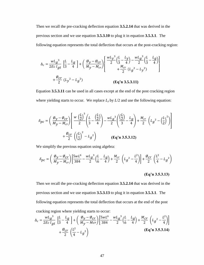
47
Then we recall the pre-cracking deflection equation 3.5.2.14 that was derived in the
previous section and we use equation 3.5.3.10 to plug it in equation 3.5.3.1. The
following equation represents the total deflection that occurs at the post-cracking region:
(Eq’n 3.5.3.11)
Equation 3.5.3.11 can be used in all cases except at the end of the post cracking region
where yielding starts to occur. We replace Ly by L/2 and use the following equation:
(Eq’n 3.5.3.12)
We simplify the previous equation using algebra:
(Eq’n 3.5.3.13)
Then we recall the pre-cracking deflection equation 3.5.2.14 that was derived in the
previous section and we use equation 3.5.3.13 to plug it in equation 3.5.3.1. The
following equation represents the total deflection that occurs at the end of the post
cracking region where yielding starts to occur:
(Eq’n 3.5.3.14)
𝛿𝑝𝑐 = ( Ø𝑦 − Ø𝑐𝑟𝑀𝑦 − 𝑀𝑐𝑟
) [ 𝑤 (
𝐿2)3
2(𝐿
3−
(𝐿2)
4) −
𝑤𝐿𝑔3
2((𝐿2)
3−
𝐿𝑔4
) +𝑀𝑐𝑟
2 (𝐿𝑔
2 − (𝐿
2)2
)]
+Ø𝑐𝑟2
((𝐿
2)2
− 𝐿𝑔2)
𝛿𝑝𝑐 = ( Ø𝑦 − Ø𝑐𝑟𝑀𝑦 − 𝑀𝑐𝑟
) [5𝑤𝐿4
384−
𝑤𝐿𝑔3
2(𝐿
6−
𝐿𝑔4
) +𝑀𝑐𝑟
2 (𝐿𝑔
2 −𝐿2
4)] +
Ø𝑐𝑟2
(𝐿2
4− 𝐿𝑔
2)
Δ𝑐 =𝑤𝐿𝑔
3
2𝐸𝑐 𝐼𝑔𝑡 [
𝐿
3−
𝐿𝑔4
] + ( Ø𝑦 − Ø𝑐𝑟𝑀𝑦 − 𝑀𝑐𝑟
)
[
𝑤𝐿𝑦3
2(𝐿
3−
𝐿𝑦4
) −𝑤𝐿𝑔
3
2(𝐿
3−
𝐿𝑔4
)
+𝑀𝑐𝑟
2 (𝐿𝑔
2 − 𝐿𝑦2) ]
+Ø𝑐𝑟2
(𝐿𝑦2 − 𝐿𝑔
2)
Δ𝑐 =𝑤𝐿𝑔
3
2𝐸𝑐 𝐼𝑔𝑡 [
𝐿
3−
𝐿𝑔4
] + ( Ø𝑦 − Ø𝑐𝑟𝑀𝑦 − 𝑀𝑐𝑟
) [5𝑤𝐿4
384−
𝑤𝐿𝑔3
2(𝐿
6−
𝐿𝑔4
) +𝑀𝑐𝑟2
(𝐿𝑔2 −
𝐿2
4)]
+Ø𝑐𝑟2
(𝐿2
4− 𝐿𝑔
2)
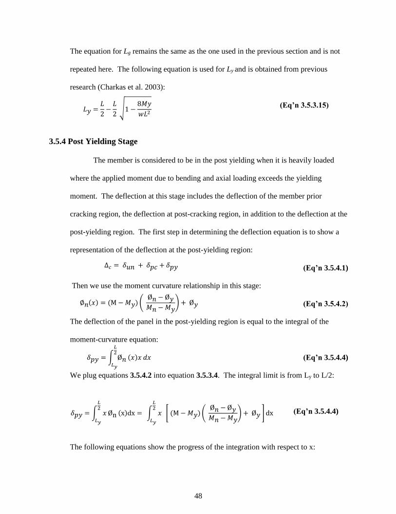
48
The equation for Lg remains the same as the one used in the previous section and is not
repeated here. The following equation is used for Ly and is obtained from previous
research (Charkas et al. 2003):
(Eq’n 3.5.3.15)
3.5.4 Post Yielding Stage
The member is considered to be in the post yielding when it is heavily loaded
where the applied moment due to bending and axial loading exceeds the yielding
moment. The deflection at this stage includes the deflection of the member prior
cracking region, the deflection at post-cracking region, in addition to the deflection at the
post-yielding region. The first step in determining the deflection equation is to show a
representation of the deflection at the post-yielding region:
(Eq’n 3.5.4.1)
Then we use the moment curvature relationship in this stage:
(Eq’n 3.5.4.2)
The deflection of the panel in the post-yielding region is equal to the integral of the
moment-curvature equation:
(Eq’n 3.5.4.4)
We plug equations 3.5.4.2 into equation 3.5.3.4. The integral limit is from Ly to L/2:
(Eq’n 3.5.4.4)
The following equations show the progress of the integration with respect to x:
𝐿𝑦 =𝐿
2−
𝐿
2 √1 −
8𝑀𝑦
𝑤𝐿2
Δ𝑐 = 𝛿𝑢𝑛 + 𝛿𝑝𝑐 + 𝛿𝑝𝑦
𝛿𝑝𝑦 = ∫ 𝑥
𝐿2
𝐿𝑦
Øn (x)dx = ∫ 𝑥
𝐿2
𝐿𝑦
[ (M − 𝑀𝑦)( Ø𝑛 − Ø𝑦𝑀𝑛 − 𝑀𝑦
) + Ø𝑦 ] dx
∅𝑛(𝑥) = (M − 𝑀𝑦) ( Ø𝑛 − Ø𝑦𝑀𝑛 − 𝑀𝑦
) + Ø𝑦
𝛿𝑝𝑦 = ∫ Ø𝑛 (𝑥)𝑥 𝑑𝑥
𝐿2
𝐿𝑦
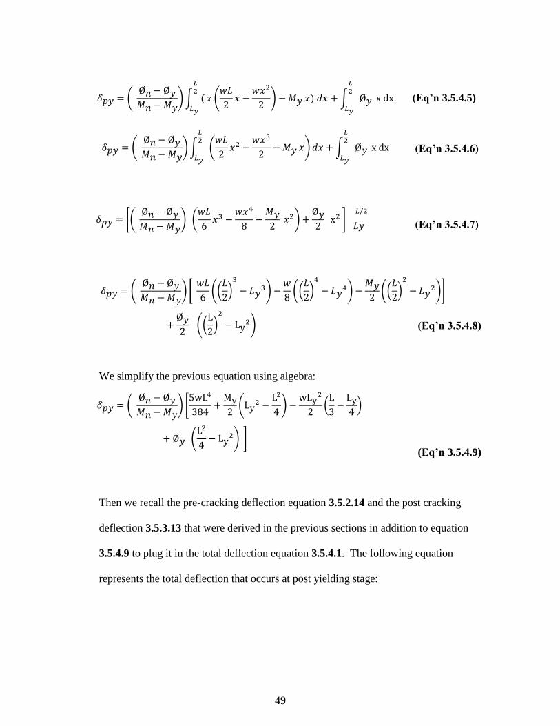
49
(Eq’n 3.5.4.5)
(Eq’n 3.5.4.6)
(Eq’n 3.5.4.7)
(Eq’n 3.5.4.8)
We simplify the previous equation using algebra:
(Eq’n 3.5.4.9)
Then we recall the pre-cracking deflection equation 3.5.2.14 and the post cracking
deflection 3.5.3.13 that were derived in the previous sections in addition to equation
3.5.4.9 to plug it in the total deflection equation 3.5.4.1. The following equation
represents the total deflection that occurs at post yielding stage:
𝛿𝑝𝑦 = ( Ø𝑛 − Ø𝑦𝑀𝑛 − 𝑀𝑦
)∫ (
𝐿2
𝐿𝑦
𝑥 (𝑤𝐿
2𝑥 −
𝑤𝑥2
2) − 𝑀𝑦 𝑥) 𝑑𝑥 + ∫
𝐿2
𝐿𝑦
Ø𝑦 x dx
𝛿𝑝𝑦 = ( Ø𝑛 − Ø𝑦𝑀𝑛 − 𝑀𝑦
)∫
𝐿2
𝐿𝑦
(𝑤𝐿
2𝑥2 −
𝑤𝑥3
2− 𝑀𝑦 𝑥)𝑑𝑥 + ∫
𝐿2
𝐿𝑦
Ø𝑦 x dx
𝛿𝑝𝑦 = ( Ø𝑛 − Ø𝑦𝑀𝑛 − 𝑀𝑦
) [ 𝑤𝐿
6((
𝐿
2)3
− 𝐿𝑦3) −
𝑤
8((
𝐿
2)4
− 𝐿𝑦4) −
𝑀𝑦2
((𝐿
2)2
− 𝐿𝑦2)]
+Ø𝑦2 ((
L
2)2
− Ly2)
𝛿𝑝𝑦 = ( Ø𝑛 − Ø𝑦𝑀𝑛 − 𝑀𝑦
) [5wL4
384+
My2
(Ly2 −
L2
4) −
wLy2
2(L
3−
Ly4
)
+ Ø𝑦 (L2
4− Ly
2) ]
𝛿𝑝𝑦 = [( Ø𝑛 − Ø𝑦𝑀𝑛 − 𝑀𝑦
) (𝑤𝐿
6𝑥3 −
𝑤𝑥4
8−
𝑀𝑦2
𝑥2) +Ø𝑦2 x
2 ] 1𝐿/2
𝐿𝑦
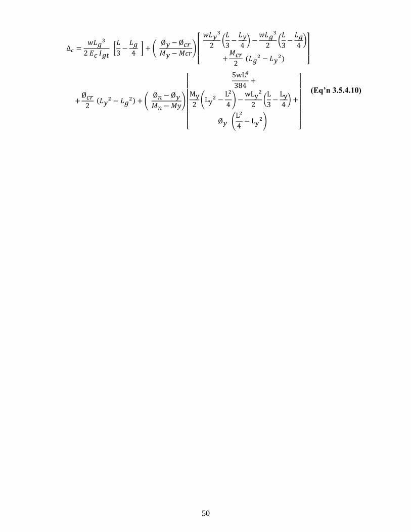
50
(Eq’n 3.5.4.10)
Δ𝑐 =𝑤𝐿𝑔
3
2 𝐸𝑐 𝐼𝑔𝑡 [
𝐿
3−
𝐿𝑔4
] + ( Ø𝑦 − Ø𝑐𝑟𝑀𝑦 − 𝑀𝑐𝑟
)
[
𝑤𝐿𝑦3
2(𝐿
3−
𝐿𝑦4
) −𝑤𝐿𝑔
3
2(𝐿
3−
𝐿𝑔4
)
+𝑀𝑐𝑟2
(𝐿𝑔2 − 𝐿𝑦
2) ]
+Ø𝑐𝑟2
(𝐿𝑦2 − 𝐿𝑔
2) + ( Ø𝑛 − Ø𝑦𝑀𝑛 − 𝑀𝑦
)
[
5wL4
384+
My2
(Ly2 −
L2
4) −
wLy2
2(L
3−
Ly4
) +
Ø𝑦 (L2
4− Ly
2) ]
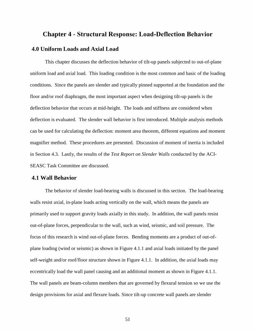
51
Chapter 4 - Structural Response: Load-Deflection Behavior
4.0 Uniform Loads and Axial Load
This chapter discusses the deflection behavior of tilt-up panels subjected to out-of-plane
uniform load and axial load. This loading condition is the most common and basic of the loading
conditions. Since the panels are slender and typically pinned supported at the foundation and the
floor and/or roof diaphragm, the most important aspect when designing tilt-up panels is the
deflection behavior that occurs at mid-height. The loads and stiffness are considered when
deflection is evaluated. The slender wall behavior is first introduced. Multiple analysis methods
can be used for calculating the deflection: moment area theorem, different equations and moment
magnifier method. These procedures are presented. Discussion of moment of inertia is included
in Section 4.3. Lastly, the results of the Test Report on Slender Walls conducted by the ACI-
SEASC Task Committee are discussed.
4.1 Wall Behavior
The behavior of slender load-bearing walls is discussed in this section. The load-bearing
walls resist axial, in-plane loads acting vertically on the wall, which means the panels are
primarily used to support gravity loads axially in this study. In addition, the wall panels resist
out-of-plane forces, perpendicular to the wall, such as wind, seismic, and soil pressure. The
focus of this research is wind out-of-plane forces. Bending moments are a product of out-of-
plane loading (wind or seismic) as shown in Figure 4.1.1 and axial loads initiated by the panel
self-weight and/or roof/floor structure shown in Figure 4.1.1. In addition, the axial loads may
eccentrically load the wall panel causing and an additional moment as shown in Figure 4.1.1.
The wall panels are beam-column members that are governed by flexural tension so we use the
design provisions for axial and flexure loads. Since tilt-up concrete wall panels are slender
52
elements, the second-order bending effects, P-delta effects, caused by axial load acting on the
deflected panel shape increase the primary moments. The maximum bending moment can be
categorized into two components: primary moment due to applied loads, and secondary moments
due to P-delta effects. Initial lateral deflections caused by panel out-of-straightness are not
considered as part of this study. In addition, the moments caused by small horizontal
displacements of the top of the panel in relation to the bottom of the panel are small and
negligible.
The ACI 318-19 has three design procedures for walls. The first procedure is to idealize
the wall as a column considering the slenderness affects, which can be found in Sections 22.2
and 22.4. The second design procedure is the simplified wall design expressed in Section
11.5.3. The third procedure is the alternative method for out-of-plane slender wall analysis in
Section 11.8 – the focus of this research.
Vertical loading may act with eccentricity, which induces a moment. Figure 4.1 shows
the maximum bending moment due vertical and lateral loads in a simply supported wall panel.
The maximum moment is due to the eccentric, vertical load occurring at the roofline where the
joist is supported, and the out-of-plane lateral load. Since the panel is idealized as pinned-pinned
support conditions, the maximum moment occurs at mid-height.
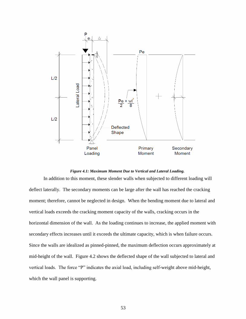
53
In addition to this moment, these slender walls when subjected to different loading will
deflect laterally. The secondary moments can be large after the wall has reached the cracking
moment; therefore, cannot be neglected in design. When the bending moment due to lateral and
vertical loads exceeds the cracking moment capacity of the walls, cracking occurs in the
horizontal dimension of the wall. As the loading continues to increase, the applied moment with
secondary effects increases until it exceeds the ultimate capacity, which is when failure occurs.
Since the walls are idealized as pinned-pinned, the maximum deflection occurs approximately at
mid-height of the wall. Figure 4.2 shows the deflected shape of the wall subjected to lateral and
vertical loads. The force “P” indicates the axial load, including self-weight above mid-height,
which the wall panel is supporting.
Figure 4.1: Maximum Moment Due to Vertical and Lateral Loading.
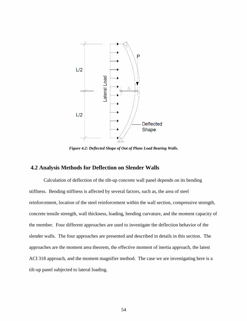
54
4.2 Analysis Methods for Deflection on Slender Walls
Calculation of deflection of the tilt-up concrete wall panel depends on its bending
stiffness. Bending stiffness is affected by several factors, such as, the area of steel
reinforcement, location of the steel reinforcement within the wall section, compressive strength,
concrete tensile strength, wall thickness, loading, bending curvature, and the moment capacity of
the member. Four different approaches are used to investigate the deflection behavior of the
slender walls. The four approaches are presented and described in details in this section. The
approaches are the moment area theorem, the effective moment of inertia approach, the latest
ACI 318 approach, and the moment magnifier method. The case we are investigating here is a
tilt-up panel subjected to lateral loading.
Figure 4.2: Deflected Shape of Out of Plane Load Bearing Walls.
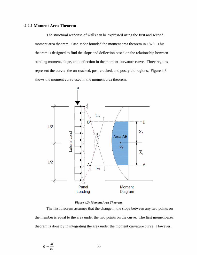
55
4.2.1 Moment Area Theorem
The structural response of walls can be expressed using the first and second
moment area theorem. Otto Mohr founded the moment area theorem in 1873. This
theorem is designed to find the slope and deflection based on the relationship between
bending moment, slope, and deflection in the moment-curvature curve. Three regions
represent the curve: the un-cracked, post-cracked, and post yield regions. Figure 4.3
shows the moment curve used in the moment area theorem.
The first theorem assumes that the change in the slope between any two points on
the member is equal to the area under the two points on the curve. The first moment-area
theorem is done by in integrating the area under the moment curvature curve. However,
∅ =𝑀
𝐸𝐼
Figure 4.3: Moment Area Theorem.
56
in a simply supported member with uniform loading the curvature is equal to M/EI at any
point due to symmetry. The curvature equation is as follows:
(Eq’n 4.2.1.1)
The second moment area theorem is used to compute the deflection through
obtaining the vertical distance between two tangent points on the member. The
difference between the two points equals to the moment of the area under the curve. The
deflection equation can be calculated by finding the integral of the curvature equation
4.2.1.1 founded in theorem one; then multiply it by the distance, x, from the vertical axis
of the point to the centroid of the moment area. The integral can be expressed as follows,
where y and z are the integral limits:
(Eq’n 4.2.1.2)
For the un-cracked region, we use equation 4.2.1.2 and the integration limit is from 0 to
L/2, the location of maximum deflection. The equation can be expressed as follows:
(Eq’n 4.2.1.3)
For the post-cracked region, the deflection equals to the un-cracked section deflection in
addition to the post-cracked section deflection. For the post-cracked section, we use
equation 4.2.1.2 and the integration limit is from Ly to Lg. The equation can be expressed
as follows:
(Eq’n 4.2.1.4)
Lg and Ly equation are provided in the previous section and not repeated here.
For the post-yield region, the deflection equals to the un-cracked section deflection and
post-cracked deflection in addition to the post-yield section deflection. For the post-yield
𝛿𝑝𝑐 = 𝛿𝑢𝑛 +∫ Ø𝑐𝑟 (𝑥) 𝑑𝑥
𝐿𝑦
𝐿𝑔
𝛿 = ∫ Ø (𝑥) 𝑑𝑥𝑧
𝑦
𝛿𝑢𝑛 = ∫ Ø (𝑥) 𝑑𝑥
𝐿2
0
𝛿𝑝𝑦 =𝛿𝑢𝑛 + 𝛿𝑝𝑐 + ∫ Ø𝑛 (𝑥) 𝑑𝑥
𝐿
2𝐿𝑦
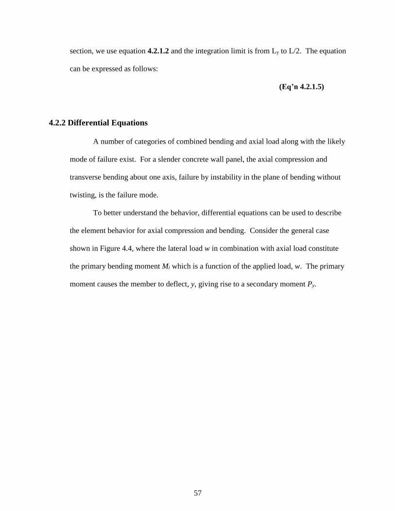
57
section, we use equation 4.2.1.2 and the integration limit is from Ly to L/2. The equation
can be expressed as follows:
(Eq’n 4.2.1.5)
4.2.2 Differential Equations
A number of categories of combined bending and axial load along with the likely
mode of failure exist. For a slender concrete wall panel, the axial compression and
transverse bending about one axis, failure by instability in the plane of bending without
twisting, is the failure mode.
To better understand the behavior, differential equations can be used to describe
the element behavior for axial compression and bending. Consider the general case
shown in Figure 4.4, where the lateral load w in combination with axial load constitute
the primary bending moment Mi which is a function of the applied load, w. The primary
moment causes the member to deflect, y, giving rise to a secondary moment Py.
58
Stating the moment Mz at the location z in Figure 4.2.2.1, gives:
𝑀𝑧 = 𝑀𝑖 + 𝑃𝑦 = −𝐸𝐼𝑑2𝑦
𝑑𝑧2 (Eq’n 4.2.2.1)
For sections with constant EI and dividing by EI gives the deflection differential
equation:
𝑑2𝑦
𝑑𝑧2 +𝑃
𝐸𝐼𝑦 = −
𝑀𝑖
𝐸𝐼 (Eq’n 4.2.2.2)
For design purposes, the general expression for moment Mz is of greater importance than
the deflection y. Differentiating Equation 4.2.2.2 twice gives:
𝑑4𝑦
𝑑𝑧4 +𝑃
𝐸𝐼
𝑑2𝑦
𝑑𝑧2 = −1
𝐸𝐼
𝑑2𝑀𝑖
𝑑𝑧2 (Eq’n 4.2.2.3)
Figure 4.4: General Loading of Beam-Column.
59
From Equation (4.2.2.1),
𝑑2𝑦
𝑑𝑧2 = −𝑀𝑧
𝐸𝐼 𝑎𝑛𝑑
𝑑4𝑦
𝑑𝑧4 = −1
𝐸𝐼
𝑑2𝑀𝑧
𝑑𝑧2 (Eq’n 4.2.2.4)
Substitution in Equation 4.2.2.3, gives:
−1
𝐸𝐼
𝑑2𝑀𝑧
𝑑𝑧2 +𝑃
𝐸𝐼(−
𝑀𝑧
𝐸𝐼) = −
1
𝐸𝐼
𝑑2𝑀𝑖
𝑑𝑧2 (Eq’n 4.2.2.5)
Or, simplifying and letting k2=P/EI,
𝑑2𝑀𝑧
𝑑𝑧2 + 𝑘2𝑀𝑧 =𝑑2𝑀𝑖
𝑑𝑧2 (Eq’n 4.2.2.6)
Which is of the same form as the deflection differential equation. The homogenous
solution form equation 4.2.2.6 is:
𝑀𝑧 = 𝐴 sin 𝑘𝑧 + 𝐵 cos 𝑘𝑧 (Eq’n 4.2.2.7)
Applying the boundary conditions, (a) y=0 at z=0; and (b) y=0 at z=L, one obtains for
condition (a), B=0; and for condition (b),
0 = 𝐴 sin 𝑘𝐿 (Eq’n 4.2.2.8)
To this must be added the particular solution that will satisfy the right-hand side of the
differential equation. Since Mi = f(z), where f(z) is usually a polynomial in z, the
particular solution will be of the same form; thus the complete solution may be written
as:
Alternate to differential equation approach, a simple approximate procedure is
satisfactory for many common situations.
𝑀𝑧 = 𝐴 sin 𝑘𝑧 + 𝐵 cos 𝑘𝑧 + 𝑓1(𝑧) (Eq’n 4.2.2.9)
Where f1(z) = value of Mz satisfying Equation 4.2.2.5. When Mz is a continuous function,
the maximum value of Mz may be found by differentiation:
60
𝑑𝑀𝑧
𝑑𝑧= 0 = 𝐴𝑘 cos 𝑘𝑧 − 𝐵𝑘 sin 𝑘𝑧 +
𝑑𝑓1(𝑧)
𝑑𝑧 (Eq’n 4.2.2.10)
For most cases, such as concentrated loads, uniform loads, and end moments, or
combination thereof, it may be shown that
𝑑𝑓1(𝑧)
𝑑𝑧= 0 (Eq’n 4.2.2.11)
In which case a general expression for maximum Mz can be established; from Equation
4.2.2.10:
𝐴𝑘 cos 𝑘𝑧 = 𝐵𝑘 sin 𝑘𝑧 (Eq’n 4.2.2.12)
tan𝑘𝑧 =𝐴
𝐵 (Eq’n 4.2.2.13)
At maximum Mz,
𝑀𝑧𝑚𝑎𝑥= √𝐴2 + 𝐵2 + 𝑓1(𝑧) (Eq’n 4.2.2.14)
4.2.3 Moment Magnifier Method
The moment magnifier method was adopted by the ACI 318 to account for the P-delta
effect in axially loaded members. It can provide the same results as the iterative method
if the section stiffness, EI, is assumed the same. To calculate the deflection, we use the
following steps. After finding the section properties, gross moment of inertia, and
cracked moment of inertia, we obtain the bending stiffness, kb, for a slender wall as
follows:
(Eq’n 4.2.3.1)
This slightly overestimates the deflection and maximum bending moment of a slender
wall subjected to the combined effects of lateral and axial load for all axial loads that
produce P-delta moments larger than the moment produced by lateral loads.
k𝑏 =48𝐸𝑐𝐼𝑐𝑟
5𝑙𝑐2
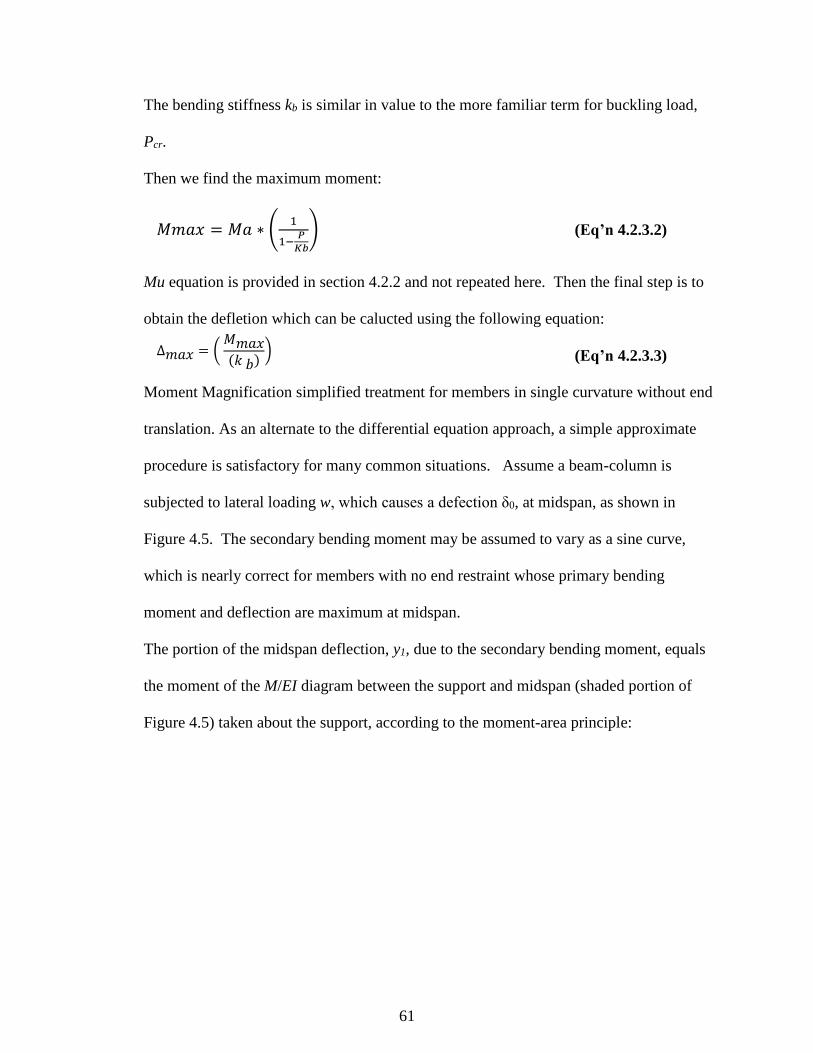
61
The bending stiffness kb is similar in value to the more familiar term for buckling load,
Pcr.
Then we find the maximum moment:
𝑀𝑚𝑎𝑥 = 𝑀𝑎 ∗ (1
1−𝑃
𝐾𝑏
) (Eq’n 4.2.3.2)
Mu equation is provided in section 4.2.2 and not repeated here. Then the final step is to
obtain the defletion which can be calucted using the following equation:
(Eq’n 4.2.3.3)
Moment Magnification simplified treatment for members in single curvature without end
translation. As an alternate to the differential equation approach, a simple approximate
procedure is satisfactory for many common situations. Assume a beam-column is
subjected to lateral loading w, which causes a defection δ0, at midspan, as shown in
Figure 4.5. The secondary bending moment may be assumed to vary as a sine curve,
which is nearly correct for members with no end restraint whose primary bending
moment and deflection are maximum at midspan.
The portion of the midspan deflection, y1, due to the secondary bending moment, equals
the moment of the M/EI diagram between the support and midspan (shaded portion of
Figure 4.5) taken about the support, according to the moment-area principle:
Δ𝑚𝑎𝑥 = ( 𝑀𝑚𝑎𝑥(𝑘 𝑏)
)
𝑀𝑚𝑎𝑥𝐾 𝑏2
62
𝑦1 =𝑃
𝐸𝐼(𝑦1 + 𝛿0) (
𝐿
2)
2
𝜋(
𝐿
𝜋) = (𝑦1 + 𝛿0)
𝑃𝐿2
𝜋2𝐸𝐼 (Eq’n 4.2.3.1)
Or
𝑦1 = (𝑦1 + 𝛿0)𝑃
𝑃𝑒 (Eq’n 4.2.3.2)
Where
𝑃𝑒 =𝜋2𝐸𝐼
𝐿2 (Eq’n 4.2.3.3)
Solving for y1,
Figure 4.5: Primary and Secondary Bending Moment.
63
𝑦1 = 𝛿0 [𝑃
𝑃𝑒⁄
1−𝑃𝑃𝑒
⁄] = 𝛿0 (
𝛼
1−𝛼) (Eq’n 4.2.3.4)
Where
𝛼 = 𝑃𝑃𝑒
⁄ (Eq’n 4.2.3.5)
Since ymax is the sum of δ0 and y1
𝑦𝑚𝑎𝑥 = 𝛿0 + 𝑦1 = 𝛿0 + 𝛿0 (𝛼
1−𝛼) =
𝛿0
1−𝛼 (Eq’n 4.2.3.6)
The maximum bending moment including the axial effect becomes
𝑀𝑧𝑚𝑎𝑥= 𝑀0 + 𝑃𝑦𝑚𝑎𝑥 (Eq’n 4.2.3.7)
Substituting the expression for ymax into Equation 4.2.3.5 and setting
𝑃 = 𝛼𝑃𝑒 =𝛼𝜋2𝐸𝐼
𝐿2 (Eq’n 4.2.3.8)
Equation 4.2.3.7 may be written as the primary moment M0 multiplied by a magnification
factor B1.
𝑀𝑧𝑚𝑎𝑥= 𝑀0𝐵1 (Eq’n 4.2.3.9)
Where
𝐵1 =𝐶𝑚
1−𝛼 (Eq’n 4.2.3.10)
And
𝐶𝑚 = 1 + (𝜋2𝐸𝐼𝛿0
𝑀0𝐿2− 1)𝛼 (Eq’n 4.2.3.11)
For the case of uniform lateral load and a concentric axial load, Cm=1, the magnified
moment becomes:
64
𝑀𝑧𝑚𝑎𝑥= 𝑀0 (
1
1−𝑃𝜋2𝐸𝐼
𝐿2⁄
) (Eq’n 4.2.3.12)
For the particular case of transverse uniform loading and axial compression the primary
moment may be expressed as:
(Eq’n 4.2.3.13)
Since:
(Eq’n 4.2.3.14)
F1(z) doesn’t equal to zero, thus the particular solution for the differential eqaution is
required. Let f1(z)= C1+Cz z. Subtitute the particular solution into equation 4.2.4.13
(Eq’n 4.2.3.15)
(Eq’n 4.2.3.16)
Thus,
(Eq’n 4.2.3.17)
(Eq’n 4.3.3.18)
Then the moment equation becomes:
(Eq’n 4.2.3.19)
Applying boundary consditions, first boundary condition at z =0:
(Eq’n 4.2.3.20)
(Eq’n 4.2.3.21)
Thus,
(Eq’n 4.2.3.22)
𝑀𝑖 =𝑤
2 𝑧(𝐿 − 𝑧)
𝑑2𝑀𝑖𝑑𝑧2
= − 𝑤
𝑑2[𝑓1(𝑧)]
𝑑𝑧2= 0
0 + 𝑘2(𝐶1 + 𝐶2𝑧) = −𝑤
𝐶1 = −𝑤/𝑘2
𝐶2 = 0
𝑀𝑧 = 𝐴 𝑠𝑖𝑛(𝑘𝑧) + 𝐵 𝑐𝑜𝑠(𝑘𝑧) − 𝑤/𝑘2
𝑀𝑧 = 0
0 = 𝐵 − 𝑤/𝑘2
𝐵 = 𝑤/𝑘2
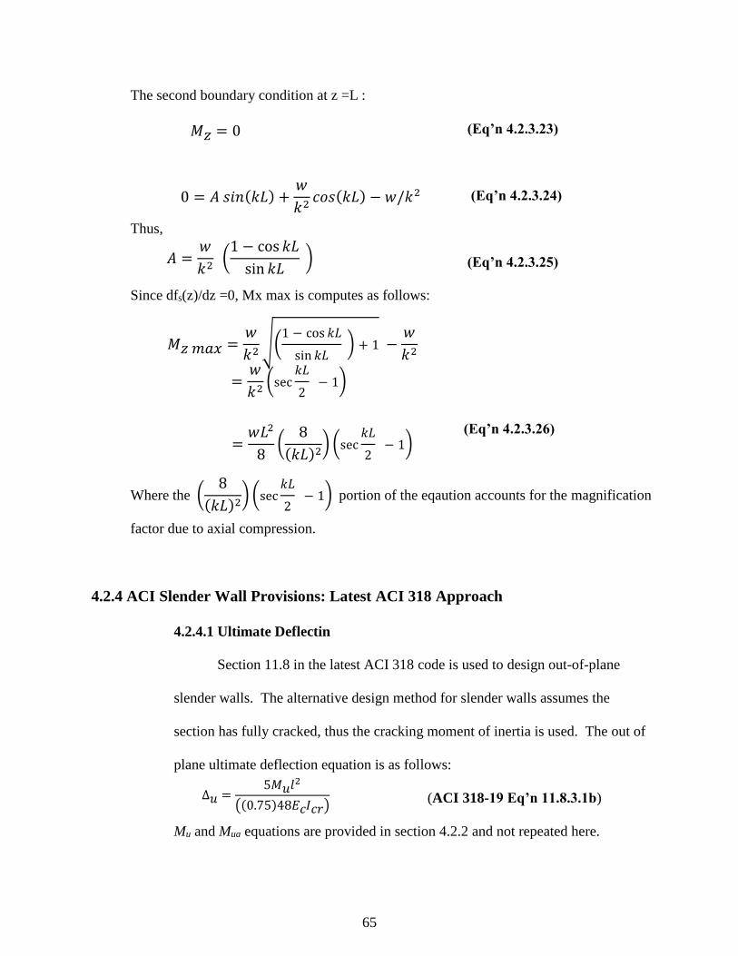
65
The second boundary condition at z =L :
(Eq’n 4.2.3.23)
(Eq’n 4.2.3.24)
Thus,
(Eq’n 4.2.3.25)
Since dfs(z)/dz =0, Mx max is computes as follows:
(Eq’n 4.2.3.26)
Where the portion of the eqaution accounts for the magnification
factor due to axial compression.
4.2.4 ACI Slender Wall Provisions: Latest ACI 318 Approach
4.2.4.1 Ultimate Deflectin
Section 11.8 in the latest ACI 318 code is used to design out-of-plane
slender walls. The alternative design method for slender walls assumes the
section has fully cracked, thus the cracking moment of inertia is used. The out of
plane ultimate deflection equation is as follows:
(ACI 318-19 Eq’n 11.8.3.1b)
Mu and Mua equations are provided in section 4.2.2 and not repeated here.
Δ𝑢 =5𝑀𝑢𝑙2
((0.75)48𝐸𝑐𝐼𝑐𝑟)
𝑀𝑧 = 0
0 = 𝐴 𝑠𝑖𝑛(𝑘𝐿) +𝑤
𝑘2𝑐𝑜𝑠(𝑘𝐿) − 𝑤/𝑘2
𝐴 =𝑤
𝑘2 (
1 − cos 𝑘𝐿
sin 𝑘𝐿 )
𝑀𝑧 𝑚𝑎𝑥 =𝑤
𝑘2√(
1 − cos 𝑘𝐿
sin 𝑘𝐿 ) + 1 −
𝑤
𝑘2
=𝑤
𝑘2(sec
𝑘𝐿
2 − 1)
=𝑤𝐿2
8(
8
(𝑘𝐿)2) (sec
𝑘𝐿
2 − 1)
(8
(𝑘𝐿)2) (sec
𝑘𝐿
2 − 1)
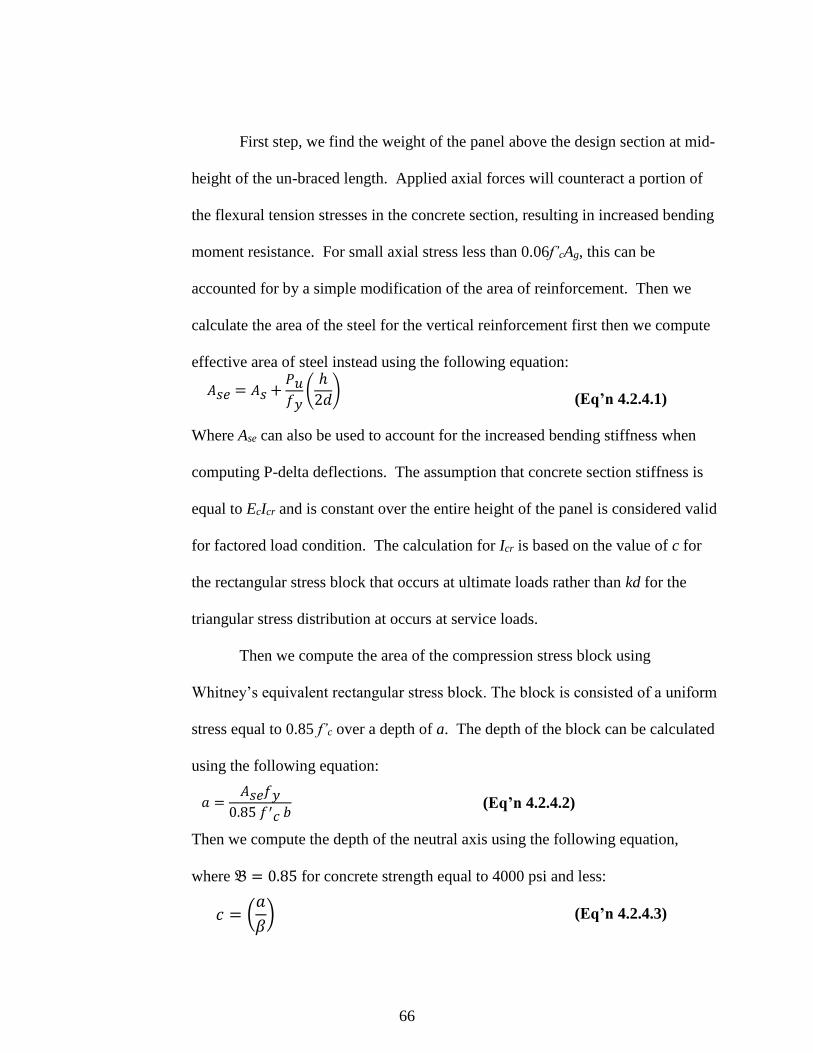
66
First step, we find the weight of the panel above the design section at mid-
height of the un-braced length. Applied axial forces will counteract a portion of
the flexural tension stresses in the concrete section, resulting in increased bending
moment resistance. For small axial stress less than 0.06f’cAg, this can be
accounted for by a simple modification of the area of reinforcement. Then we
calculate the area of the steel for the vertical reinforcement first then we compute
effective area of steel instead using the following equation:
(Eq’n 4.2.4.1)
Where Ase can also be used to account for the increased bending stiffness when
computing P-delta deflections. The assumption that concrete section stiffness is
equal to EcIcr and is constant over the entire height of the panel is considered valid
for factored load condition. The calculation for Icr is based on the value of c for
the rectangular stress block that occurs at ultimate loads rather than kd for the
triangular stress distribution at occurs at service loads.
Then we compute the area of the compression stress block using
Whitney’s equivalent rectangular stress block. The block is consisted of a uniform
stress equal to 0.85 f’c over a depth of a. The depth of the block can be calculated
using the following equation:
(Eq’n 4.2.4.2)
Then we compute the depth of the neutral axis using the following equation,
where 𝔅 = 0.85 for concrete strength equal to 4000 psi and less:
(Eq’n 4.2.4.3)
𝐴𝑠𝑒 = 𝐴𝑠 +𝑃𝑢𝑓𝑦
(ℎ
2𝑑)
𝑎 =𝐴𝑠𝑒𝑓𝑦
0.85 𝑓′𝑐 𝑏
𝑐 = (𝑎
𝛽)
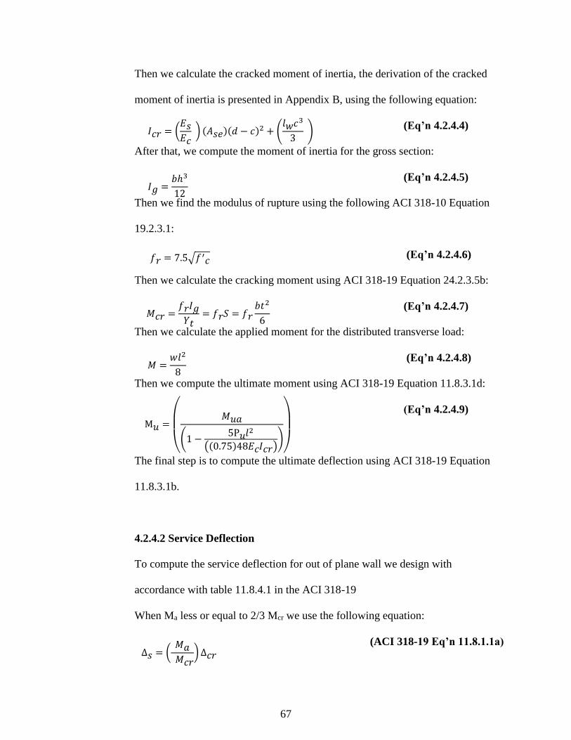
67
Then we calculate the cracked moment of inertia, the derivation of the cracked
moment of inertia is presented in Appendix B, using the following equation:
(Eq’n 4.2.4.4)
After that, we compute the moment of inertia for the gross section:
(Eq’n 4.2.4.5)
Then we find the modulus of rupture using the following ACI 318-10 Equation
19.2.3.1:
(Eq’n 4.2.4.6)
Then we calculate the cracking moment using ACI 318-19 Equation 24.2.3.5b:
(Eq’n 4.2.4.7)
Then we calculate the applied moment for the distributed transverse load:
(Eq’n 4.2.4.8)
Then we compute the ultimate moment using ACI 318-19 Equation 11.8.3.1d:
(Eq’n 4.2.4.9)
The final step is to compute the ultimate deflection using ACI 318-19 Equation
11.8.3.1b.
4.2.4.2 Service Deflection
To compute the service deflection for out of plane wall we design with
accordance with table 11.8.4.1 in the ACI 318-19
When Ma less or equal to 2/3 Mcr we use the following equation:
(ACI 318-19 Eq’n 11.8.1.1a)
𝐼𝑔 =𝑏ℎ3
12
𝑓𝑟 = 7.5√𝑓′𝑐
𝑀 =𝑤𝑙2
8
𝑀𝑐𝑟 =𝑓𝑟𝐼𝑔𝑌𝑡
= 𝑓𝑟𝑆 = 𝑓𝑟𝑏𝑡2
6
𝐼𝑐𝑟 = (𝐸𝑠𝐸𝑐
) (𝐴𝑠𝑒)(𝑑 − 𝑐)2 + (𝑙𝑤𝑐3
3 )
M𝑢 =
(
𝑀𝑢𝑎
(1 −5P𝑢𝑙2
((0.75)48𝐸𝑐𝐼𝑐𝑟)))
∆𝑠 = (𝑀𝑎
(𝑀𝑐𝑟)∆𝑐𝑟
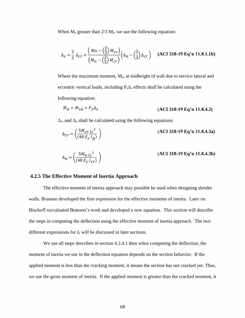
68
When Ma greater than 2/3 Mcr we use the following equation:
(ACI 318-19 Eq’n 11.8.1.1b)
Where the maximum moment, Ma, at midheight of wall due to service lateral and
eccentric vertical loads, including PsΔs effects shall be calculated suing the
following equation:
(ACI 318-19 Eq’n 11.8.4.2)
Δcr and Δn shall be calculated using the following equations:
(ACI 318-19 Eq’n 11.8.4.3a)
(ACI 318-19 Eq’n 11.8.4.3b)
4.2.5 The Effective Moment of Inertia Approach
The effective moment of inertia approach may possible be used when designing slender
walls. Branson developed the first expression for the effective moments of inertia. Later on
Bischoff reevaluated Branson’s work and developed a new equation. This section will describe
the steps in computing the deflection using the effective moment of inertia approach. The two
different expressions for Ie will be discussed in later sections.
We use all steps describes in section 4.2.4.1 then when computing the deflection, the
moment of inertia we use in the deflection equation depends on the section behavior. If the
applied moment is less than the cracking moment, it means the section has not cracked yet. Thus,
we use the gross moment of inertia. If the applied moment is greater than the cracked moment, it
∆𝑠 =2
3 ∆𝑐𝑟 +
( 𝑀𝑎 − (23)𝑀𝑐𝑟)
(𝑀𝑛 − (23)𝑀𝑐𝑟)
(∆𝑛 − (2
3) ∆𝑐𝑟 )
𝑀𝑎 = 𝑀𝑠𝑎 + 𝑃𝑠∆𝑠
∆𝑐𝑟 = (5𝑀𝑐𝑟 𝑙𝑐
2
(48 𝐸𝑐 𝐼𝑔) )
∆𝑛 = (5𝑀𝑛 𝑙𝑐
2
(48 𝐸𝑐 𝐼𝑐𝑟) )
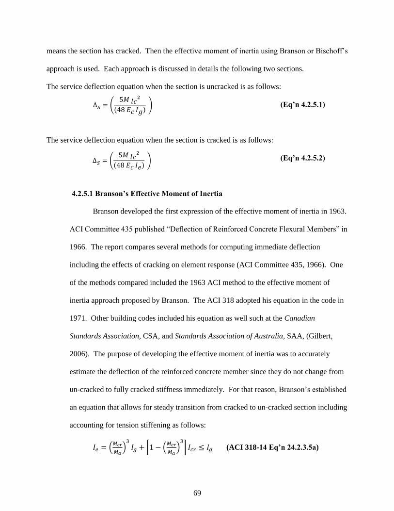
69
means the section has cracked. Then the effective moment of inertia using Branson or Bischoff’s
approach is used. Each approach is discussed in details the following two sections.
The service deflection equation when the section is uncracked is as follows:
(Eq’n 4.2.5.1)
The service deflection equation when the section is cracked is as follows:
(Eq’n 4.2.5.2)
4.2.5.1 Branson’s Effective Moment of Inertia
Branson developed the first expression of the effective moment of inertia in 1963.
ACI Committee 435 published “Deflection of Reinforced Concrete Flexural Members” in
1966. The report compares several methods for computing immediate deflection
including the effects of cracking on element response (ACI Committee 435, 1966). One
of the methods compared included the 1963 ACI method to the effective moment of
inertia approach proposed by Branson. The ACI 318 adopted his equation in the code in
1971. Other building codes included his equation as well such at the Canadian
Standards Association, CSA, and Standards Association of Australia, SAA, (Gilbert,
2006). The purpose of developing the effective moment of inertia was to accurately
estimate the deflection of the reinforced concrete member since they do not change from
un-cracked to fully cracked stiffness immediately. For that reason, Branson’s established
an equation that allows for steady transition from cracked to un-cracked section including
accounting for tension stiffening as follows:
𝐼𝑒 = (𝑀𝑐𝑟
𝑀𝑎)3
𝐼𝑔 + [1 − (𝑀𝑐𝑟
𝑀𝑎)3
] 𝐼𝑐𝑟 ≤ 𝐼𝑔 (ACI 318-14 Eq’n 24.2.3.5a)
∆𝑠 = (5𝑀
𝑙𝑐2
(48 𝐸𝑐 𝐼𝑔) )
∆𝑠 = (5𝑀
𝑙𝑐2
(48 𝐸𝑐 𝐼𝑒) )
70
This equation adequately predicted the deflection of beams with reinforcement
ratios above 1%. The Australian Standard AS3600 limited the effective moment of
inertia to a value of 0.6Ig for flexure members with a reinforcing ratio less than 0.5%
(Gilbert, 2001).
4.2.5.2 Bischoff’s Effective Moment of Inertia
Bischoff reevaluated the effective moment of inertia proposed by Branson in his
research for the applicability of Branson’s equation to members reinforced with fiber
reinforced polymer (FRP) bars. He found that a correction factor is necessary to correct
for over prediction of member stiffness when FRP bars are used. He used the integration
of curvature to find a new expression for the effective moment of inertia. Bischoff’s
work was based on the Eurocode since their code affirms that the moment curvature
relation can predict an accurate form of the deflection. (AlSunna et al. 2012) Bischoff’s
equation accounts for the change in stiffness along the length of a member as well as
accounting for tension and reinforcement stiffening. The first form of Bischoff equation
was published in 2005. Bischoff revised his work in 2007 and later on in 2011. The final
form of Bischoff’s equation for the effective moment of inertia is as follows:
(Eq’n 4.2.5.2.1)
4.3 Slender Walls Test Results
As stated previously in Chapter 1, the ACI-SEASC Task Committee on Slender Walls,
performed test of 12 Tilt-Up panels back in early 1980’s. The tested panels have four different
𝐼𝑒 =𝐼𝑐𝑟
(1 − ( 𝑀𝑐𝑟𝑀𝑎
)2
[ 1 −𝐼𝑐𝑟𝐼𝑔
])
71
thicknesses 4.75”, 5.75”, 7.25”, and 9.5”. Three specimens of each thickness were tested. The
height of all panels was 24 feet. The panels were lightly reinforced with 4#4 grade 60 bars in the
vertical direction with reinforcement ratio varying from 0.7% to 0.3%). Welded trussed frame
was used to load the panels. The panels were placed against airbag to apply pressure from the
side and a vertical lever system was used for the external axial load. The maximum deflection
was measured at the mid-height of each panel.
The applied maximum lateral load was different for each panel thickness. The maximum
loads are as follows 40 psf for the 4.75” panel, 55 psf for the 5.75” panel, 70 psf for the 7.25”
panel, and 90 psf for the 9.50” panel. The maximum load readings do not include correction due
loss of contact with the airbag when the deflection exceeded 7 to 8 inches.
4.3.1 Panels behavior
The behavior of tilt-up panel deflection curves was a linear straight line until the panel
exceeds the cracking moment, which is when a sharp break occurs. The deflection keeps
increasing and the slope starts to flatten out as it started to reach the yield moment. The
deflection behavior was very similar to an idealized stress/strain curve for a reinforced panel.
Figure 4.6 shows the Idealized composite stress/strain relation for reinforced concrete panel.
72
The test results confirmed that the behavior of the walls is very similar to the behavior of
columns when subjected to lateral load. That explains why shear failure and reduction in panel
resistance did not occur. Walls were very flexible after cracking and the deflection curve
flattened out after yielding.
4.3.2 Deflection Curves
The test results confirmed good performance of the panels, as they were loaded. The
panels continued to resist the load until the steel reached the yielding point. However, the test
did not note any elastic or inelastic lateral instability. The relationship of the lateral load and
mid-height deflection was confirmed to be a bilinear behavior.
Load-Deflection were plotted to show the performance of each panel. The results
indicated that panels with height to thickness ratio ranging between 30 and 60 resist 50%-90% of
their weight in the lateral direction. In addition, it was noted that even when deflection was very
Figure 4.6: Idealized Composite Stress/Strain Relation for Reinforced Concrete Panel.
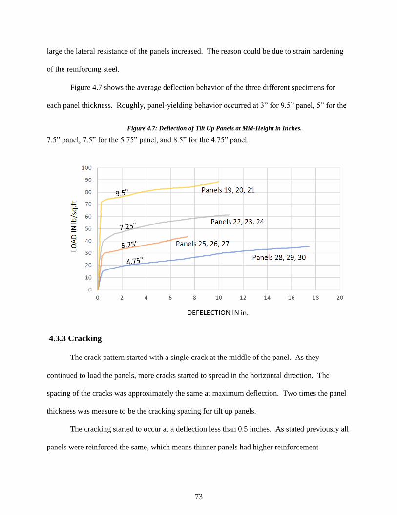
73
large the lateral resistance of the panels increased. The reason could be due to strain hardening
of the reinforcing steel.
Figure 4.7 shows the average deflection behavior of the three different specimens for
each panel thickness. Roughly, panel-yielding behavior occurred at 3” for 9.5” panel, 5” for the
7.5” panel, 7.5” for the 5.75” panel, and 8.5” for the 4.75” panel.
4.3.3 Cracking
The crack pattern started with a single crack at the middle of the panel. As they
continued to load the panels, more cracks started to spread in the horizontal direction. The
spacing of the cracks was approximately the same at maximum deflection. Two times the panel
thickness was measure to be the cracking spacing for tilt up panels.
The cracking started to occur at a deflection less than 0.5 inches. As stated previously all
panels were reinforced the same, which means thinner panels had higher reinforcement
Figure 4.7: Deflection of Tilt Up Panels at Mid-Height in Inches.
74
percentage. As a result, thinner panels had higher percent of load capacity from cracking to
yielding compared to thicker panels. Thus, it was determined that the performance of the panels
is controlled by the reinforcing percentage.
4.3.4 P-Delta Effects
The test results indicated P-delta effect through comparing the P-delta moment to the
actual moment caused by the lateral and axial load. The following equation was used to find the
percentage of P-delta moment at mid-height:
(4.3.4.1)
The test results also confirmed that P-delta moment is minor compared to the total moment since
the percentage was found to be less than 15% when the deflection to height ratio is less than
0.01. At higher deflection to height ratio’s, the secondary moments induce by the P-delta effect
will not be minor.
% 𝑃∆ 𝑀𝑜𝑚𝑒𝑛𝑡 =𝑃∆ 𝑀𝑜𝑚𝑒𝑛𝑡 ∗ 100
𝑤𝑙2
8 +𝑃 ∗ 𝑒
2
75
Chapter 5 - Structural Application
5.0 Comparisons with Experimental Results
This chapter discusses and compares the deflection results for the tilt-up panels from
research conducted by ACI-SEASC joint committee and reported in the Test Report on Slender
Walls using some of the methods presented in Chapter 4 and then compare each method to the
actual test results. The comparison is to determine which equations reflect the actual behavior
of the wall panels tested and if additional stiffness can be accounted for by using an effective
moment of inertia instead of cracked moment of inertia to determine the deflection. Four
approaches are compared: ACI 318-19 Section 11.8, Branson’s effective moment of inertia,
Bischoff’s effective moment of inertia, and a proposed effective moment of inertia done by
Kramer and Alkotami.
The tilt-up panels properties are taken from the actual test results to ensure the use of
accurate properties and have a valid comparison. The properties were measured after the panels
were cured, 167 days after the panels were poured. The following characteristics were reported
in the Test Report on Slender Walls and apply to all panels:
1) The compressive strength of concrete is 4,009 psi.
2) The modulus of elasticity for concrete is 3,540,000 psi.
3) The modulus of elasticity for the reinforcement is 28,600,000 psi.
4) The reinforcement average yield strength is 70,000 psi.
5) The reinforcement located in the middle of the panel.
6) The concrete weight is 149 pcf.
7) Vertical reinforcement: Four #4 reinforcing bars.
8) Unbraced eight of panel is 24 feet.
76
9) Width of panel is 4 feet.
10) Three specimens of each thickness were tested.
11) Thicknesses are as follows: 4.75”, 5.75”, 7.25”, and 9.5”.
12) Yielding point was 8.5” for the 4.75” panel, 7.5” for the 5.75” panel, 5” for the 7.25”
panel, and 3” for the 9.5” panel.
13) The average deflection of the different specimens for each thickness is used.
14) The eccentricity for the axial loading is 3 inches.
Additional properties are indicated when applicable.
5.1 Latest ACI 318 Section 11.8 vs. Test Results
This section discusses the assumed service deflection for different thicknesses of tilt-up
panels following Section 11.8 in the ACI 318-19; the Alternative Design Method for Out-of-
Plane Slender Walls. The steps to compute the deflection was presented in Section 4.2.4.2 in
Shapter 4 and not repeated here. The modulus of rupture equation used is as follows:
(ACI 318-19 Eq’n 19.2.3.1)
The service deflection equations are as follows:
a) When Ma ≤ (2/3) Mcr
(ACI 318-19 Eq’n 11.8.1.1a)
b) When Ma > (2/3) Mcr
(ACI 318-19 Eq’n 11.8.1.1b)
∆𝑠 = (𝑀𝑎
(𝑀𝑐𝑟)∆𝑐𝑟
∆𝑠 =2
3 ∆𝑐𝑟 +
( 𝑀𝑎 − (23)𝑀𝑐𝑟)
(𝑀𝑛 − (23)𝑀𝑐𝑟)
(∆𝑛 − (2
3) ∆𝑐𝑟 )
𝑓𝑟 = 7.5√𝑓′𝑐
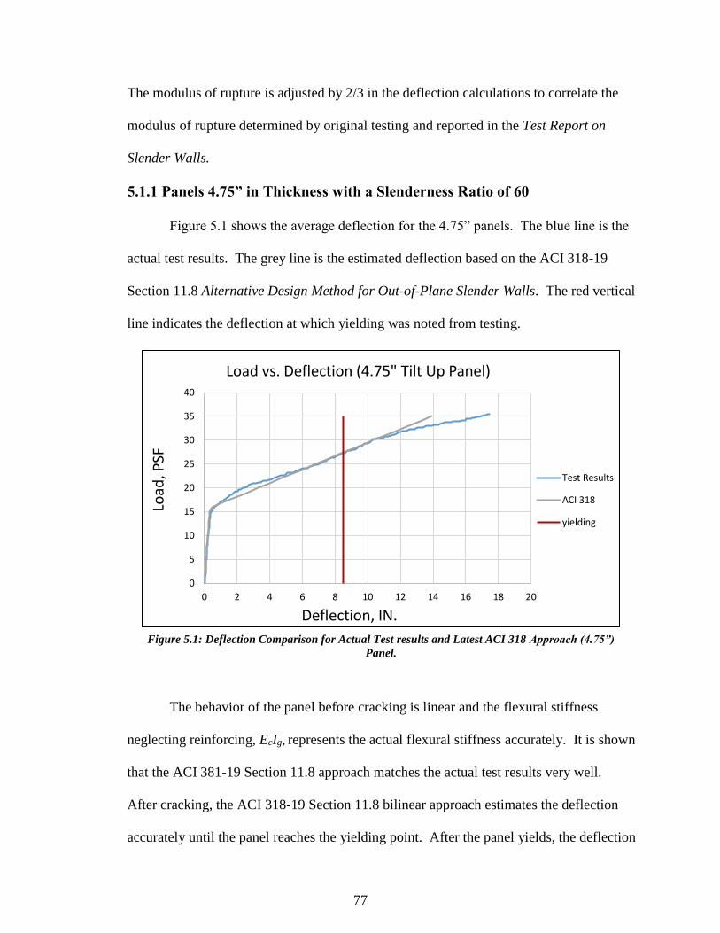
77
The modulus of rupture is adjusted by 2/3 in the deflection calculations to correlate the
modulus of rupture determined by original testing and reported in the Test Report on
Slender Walls.
5.1.1 Panels 4.75” in Thickness with a Slenderness Ratio of 60
Figure 5.1 shows the average deflection for the 4.75” panels. The blue line is the
actual test results. The grey line is the estimated deflection based on the ACI 318-19
Section 11.8 Alternative Design Method for Out-of-Plane Slender Walls. The red vertical
line indicates the deflection at which yielding was noted from testing.
The behavior of the panel before cracking is linear and the flexural stiffness
neglecting reinforcing, EcIg, represents the actual flexural stiffness accurately. It is shown
that the ACI 381-19 Section 11.8 approach matches the actual test results very well.
After cracking, the ACI 318-19 Section 11.8 bilinear approach estimates the deflection
accurately until the panel reaches the yielding point. After the panel yields, the deflection
0
5
10
15
20
25
30
35
40
0 2 4 6 8 10 12 14 16 18 20
Load
, PSF
Deflection, IN.
Load vs. Deflection (4.75" Tilt Up Panel)
Test Results
ACI 318
yielding
Figure 5.1: Deflection Comparison for Actual Test results and Latest ACI 318 Approach (4.75”)
Panel.
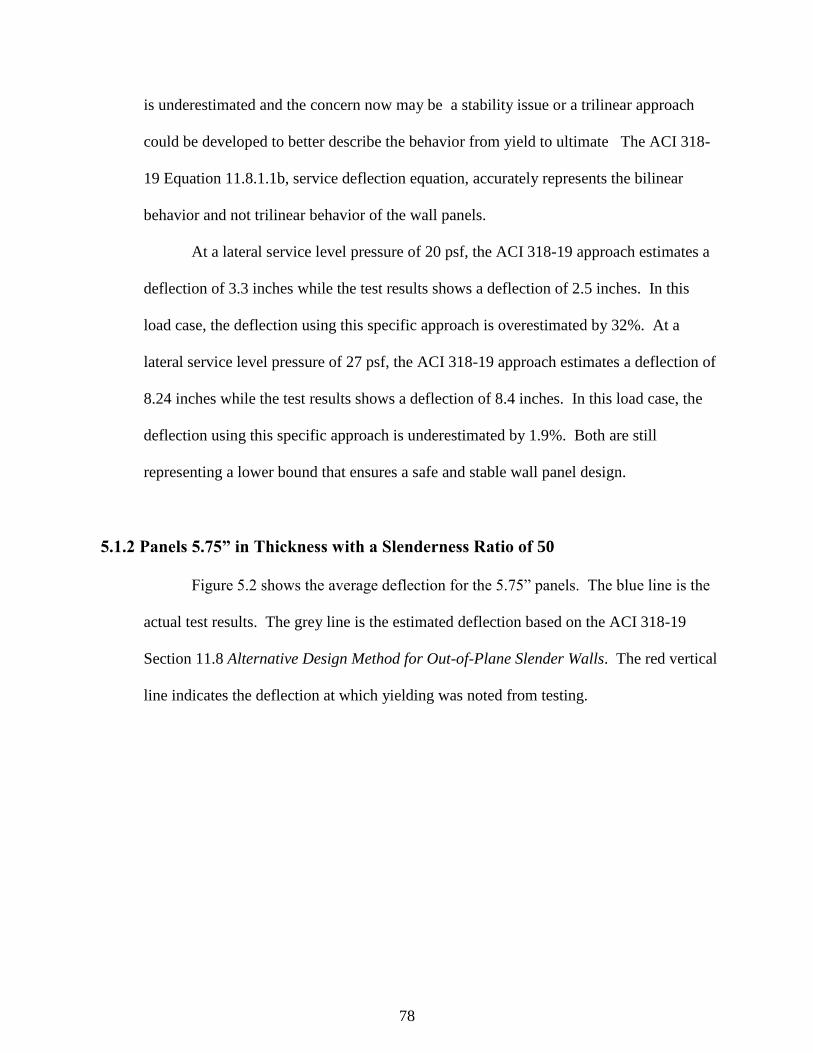
78
is underestimated and the concern now may be a stability issue or a trilinear approach
could be developed to better describe the behavior from yield to ultimate The ACI 318-
19 Equation 11.8.1.1b, service deflection equation, accurately represents the bilinear
behavior and not trilinear behavior of the wall panels.
At a lateral service level pressure of 20 psf, the ACI 318-19 approach estimates a
deflection of 3.3 inches while the test results shows a deflection of 2.5 inches. In this
load case, the deflection using this specific approach is overestimated by 32%. At a
lateral service level pressure of 27 psf, the ACI 318-19 approach estimates a deflection of
8.24 inches while the test results shows a deflection of 8.4 inches. In this load case, the
deflection using this specific approach is underestimated by 1.9%. Both are still
representing a lower bound that ensures a safe and stable wall panel design.
5.1.2 Panels 5.75” in Thickness with a Slenderness Ratio of 50
Figure 5.2 shows the average deflection for the 5.75” panels. The blue line is the
actual test results. The grey line is the estimated deflection based on the ACI 318-19
Section 11.8 Alternative Design Method for Out-of-Plane Slender Walls. The red vertical
line indicates the deflection at which yielding was noted from testing.
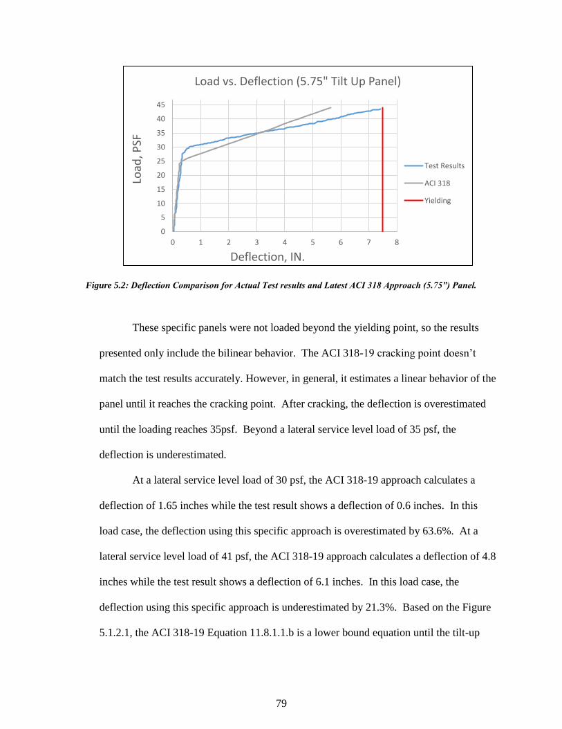
79
Figure 5.2: Deflection Comparison for Actual Test results and Latest ACI 318 Approach (5.75”) Panel.
These specific panels were not loaded beyond the yielding point, so the results
presented only include the bilinear behavior. The ACI 318-19 cracking point doesn’t
match the test results accurately. However, in general, it estimates a linear behavior of the
panel until it reaches the cracking point. After cracking, the deflection is overestimated
until the loading reaches 35psf. Beyond a lateral service level load of 35 psf, the
deflection is underestimated.
At a lateral service level load of 30 psf, the ACI 318-19 approach calculates a
deflection of 1.65 inches while the test result shows a deflection of 0.6 inches. In this
load case, the deflection using this specific approach is overestimated by 63.6%. At a
lateral service level load of 41 psf, the ACI 318-19 approach calculates a deflection of 4.8
inches while the test result shows a deflection of 6.1 inches. In this load case, the
deflection using this specific approach is underestimated by 21.3%. Based on the Figure
5.1.2.1, the ACI 318-19 Equation 11.8.1.1.b is a lower bound equation until the tilt-up
0
5
10
15
20
25
30
35
40
45
0 1 2 3 4 5 6 7 8
Load
, PSF
Deflection, IN.
Load vs. Deflection (5.75" Tilt Up Panel)
Test Results
ACI 318
Yielding
80
wall panel deflections 3-inches. After a deflection of 3-inches, the ACI 318-19 Equation
11.8.1.1.b is no longer accurate for determining service level deflections.
5.1.3 Panels 7.25” in Thickness with a Slenderness Ratio of 40
Figure 5.3 shows the average deflection for the 7.25” panels. The blue line is the
actual test results. The grey line is the calculated deflection based on the ACI 318-19
Section 11.8 Alternative Design Method for Out-of-Plane Slender Walls. The red vertical
line indicates the deflection at which yielding was noted from testing..
The behavior of the panel before cracking is linear and the flexural stiffness
neglecting reinforcing, EcIg, represents the actual flexural stiffness accurately. The ACI
318-19 Equation 11.8.1.1a calculates the uncracked section deflection well. Beyond
0
10
20
30
40
50
60
0 2 4 6 8 10 12 14 16
Load
, PSF
.
Deflection, IN.
Load vs. Deflection (7.25" Tilt Up Panel)
Test Results
ACI 318
Yielding
Figure 5.3: Deflection Comparison for Actual Test results and Latest ACI 318 Approach (7.25”)
Panel.
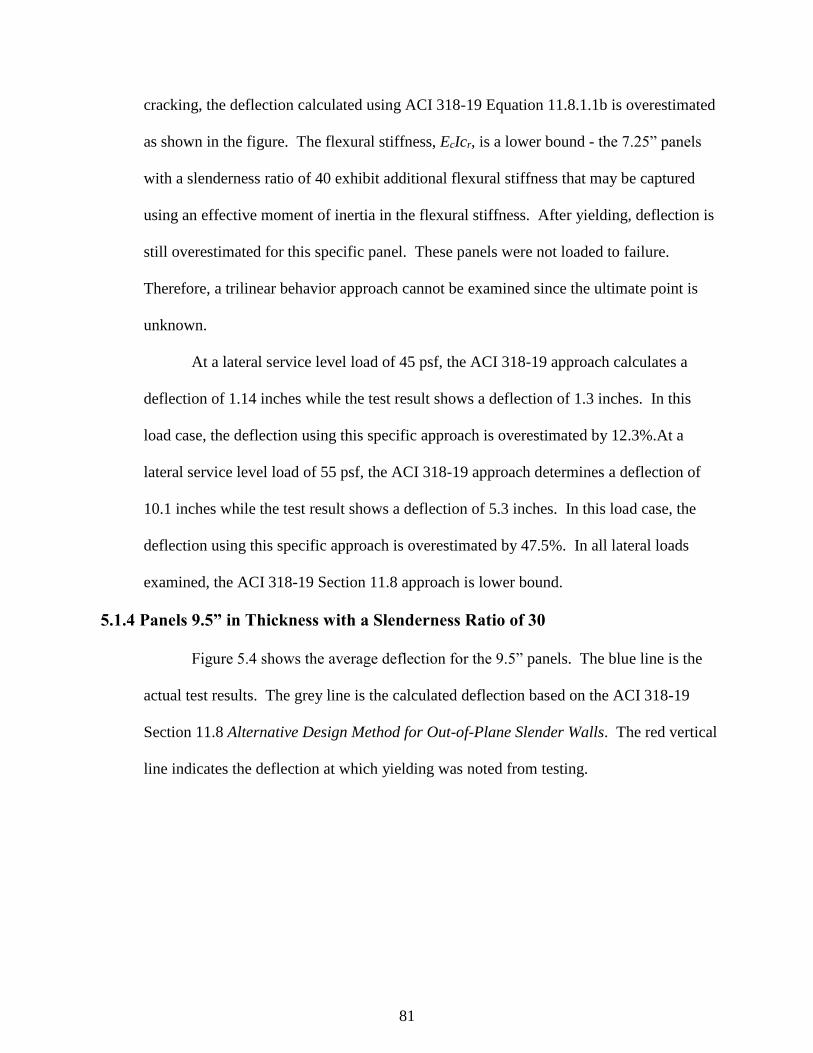
81
cracking, the deflection calculated using ACI 318-19 Equation 11.8.1.1b is overestimated
as shown in the figure. The flexural stiffness, EcIcr, is a lower bound - the 7.25” panels
with a slenderness ratio of 40 exhibit additional flexural stiffness that may be captured
using an effective moment of inertia in the flexural stiffness. After yielding, deflection is
still overestimated for this specific panel. These panels were not loaded to failure.
Therefore, a trilinear behavior approach cannot be examined since the ultimate point is
unknown.
At a lateral service level load of 45 psf, the ACI 318-19 approach calculates a
deflection of 1.14 inches while the test result shows a deflection of 1.3 inches. In this
load case, the deflection using this specific approach is overestimated by 12.3%.At a
lateral service level load of 55 psf, the ACI 318-19 approach determines a deflection of
10.1 inches while the test result shows a deflection of 5.3 inches. In this load case, the
deflection using this specific approach is overestimated by 47.5%. In all lateral loads
examined, the ACI 318-19 Section 11.8 approach is lower bound.
5.1.4 Panels 9.5” in Thickness with a Slenderness Ratio of 30
Figure 5.4 shows the average deflection for the 9.5” panels. The blue line is the
actual test results. The grey line is the calculated deflection based on the ACI 318-19
Section 11.8 Alternative Design Method for Out-of-Plane Slender Walls. The red vertical
line indicates the deflection at which yielding was noted from testing.
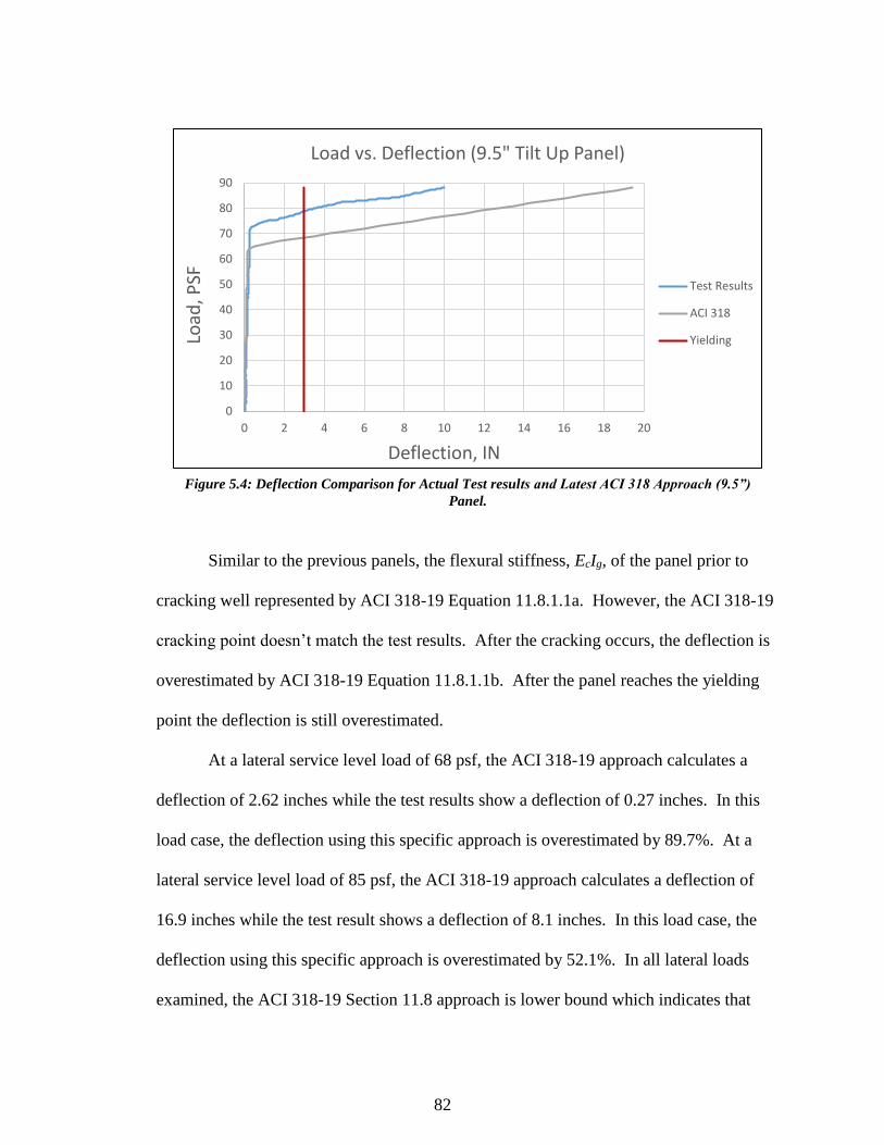
82
Similar to the previous panels, the flexural stiffness, EcIg, of the panel prior to
cracking well represented by ACI 318-19 Equation 11.8.1.1a. However, the ACI 318-19
cracking point doesn’t match the test results. After the cracking occurs, the deflection is
overestimated by ACI 318-19 Equation 11.8.1.1b. After the panel reaches the yielding
point the deflection is still overestimated.
At a lateral service level load of 68 psf, the ACI 318-19 approach calculates a
deflection of 2.62 inches while the test results show a deflection of 0.27 inches. In this
load case, the deflection using this specific approach is overestimated by 89.7%. At a
lateral service level load of 85 psf, the ACI 318-19 approach calculates a deflection of
16.9 inches while the test result shows a deflection of 8.1 inches. In this load case, the
deflection using this specific approach is overestimated by 52.1%. In all lateral loads
examined, the ACI 318-19 Section 11.8 approach is lower bound which indicates that
0
10
20
30
40
50
60
70
80
90
0 2 4 6 8 10 12 14 16 18 20
Load
, PSF
Deflection, IN
Load vs. Deflection (9.5" Tilt Up Panel)
Test Results
ACI 318
Yielding
Figure 5.4: Deflection Comparison for Actual Test results and Latest ACI 318 Approach (9.5”)
Panel.
83
using an effective moment of inertia approach for the flexural stiffness, EcIe, could
capture the actual stiffness.
5.2. Branson's Effective Moment of Inertia vs. 1980s Test Results
This section comparse the calculated service deflection for different thicknesses of tilt-up
panels following Branson’s effective moment of inertia approach. The steps to compute the
deflection using Branson’s effective moment of inertia was presented in Sections 4.2.5 and
4.2.5.1 in Chapter 4 and not repeated. The equation for Branson’s effective moment of inertia is:
𝐼𝑒 = ( 𝑀𝑐𝑟𝑀𝑎
)3𝐼𝑔 + [ 1 − (
𝑀𝑐𝑟𝑀𝑎
)3] 𝐼𝑐𝑟
(ACI 318-14 Eq’n 24.2.3.5a)
Due to the nature of the panels during testing, it was determine that the panels had a
modulus of rupture shown in the following equation::
(Eq’n 5.2.1)
Since the coefficient for the modulus of rupture is computed as 5 (instead of 7.5 as used in the
ACI 318-19 code, the service deflection equation doesn’t have the 2/3 ratio multiplied by the
cracking moment.
The service deflection equations are as follows:
c) When Ma < Mcr
(Eq’n 4.2.5.1)
𝑓𝑟 = 5 √𝑓′𝑐
∆𝑠 = (5𝑀
𝑙𝑐2
(48 𝐸𝑐 𝐼𝑔) )
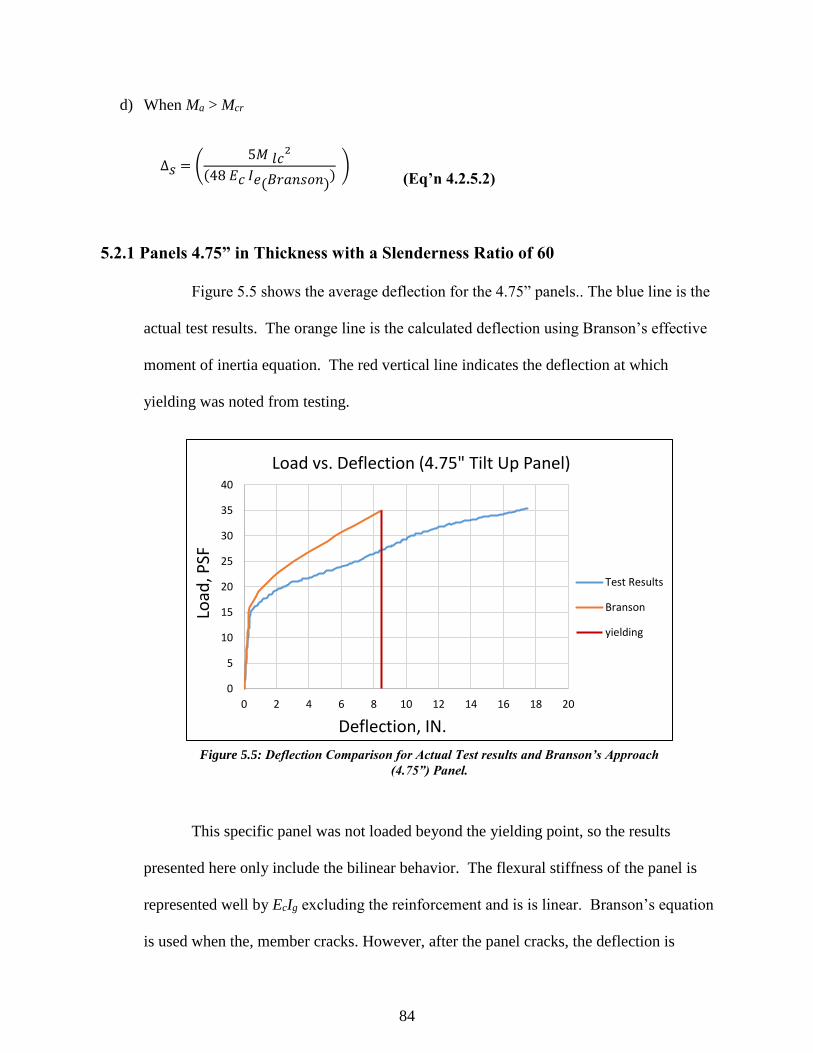
84
d) When Ma > Mcr
(Eq’n 4.2.5.2)
5.2.1 Panels 4.75” in Thickness with a Slenderness Ratio of 60
Figure 5.5 shows the average deflection for the 4.75” panels.. The blue line is the
actual test results. The orange line is the calculated deflection using Branson’s effective
moment of inertia equation. The red vertical line indicates the deflection at which
yielding was noted from testing.
This specific panel was not loaded beyond the yielding point, so the results
presented here only include the bilinear behavior. The flexural stiffness of the panel is
represented well by EcIg excluding the reinforcement and is is linear. Branson’s equation
is used when the, member cracks. However, after the panel cracks, the deflection is
∆𝑠 = (5𝑀
𝑙𝑐2
(48 𝐸𝑐 𝐼𝑒(𝐵𝑟𝑎𝑛𝑠𝑜𝑛))
)
0
5
10
15
20
25
30
35
40
0 2 4 6 8 10 12 14 16 18 20
Load
, PSF
Deflection, IN.
Load vs. Deflection (4.75" Tilt Up Panel)
Test Results
Branson
yielding
Figure 5.5: Deflection Comparison for Actual Test results and Branson’s Approach
(4.75”) Panel.
85
underestimated for this specific panel. Branson’s approach does not take an account of
the panel beyond the yielding point, the Trilinear behavior.
At a lateral service level load of 20 psf, Branson’s effective moment of inertia
approach calculates a deflection of 1.2 inches while the test result shows a deflection of
2.5 inches. In this load case, the deflection using this specific approach is underestimated
by 52%.At a lateral service level load of 27 psf, Branson’s approach calculates a
deflection of 4.1 inches while the test result shows a deflection of 8.4 inches. In this load
case, the deflection using this specific approach is underestimated by 51.2%.
5.2.2 Panels 5.75” in Thickness with a Slenderness Ratio of 50
Figure 5.6 shows the average deflection for the 5.75” panel. The blue line is the
actual test results. The orange line is the calculated deflection using Branson’s effective
moment of inertia equation. The red vertical line indicates the deflection at which
yielding was noted from testing.
0
5
10
15
20
25
30
35
40
45
0 1 2 3 4 5 6 7 8
Load
, PSF
Deflection, IN.
Load vs. Deflection (5.75" Tilt Up Panel)
Test Results
Branson
Yielding
Figure 5.6: Deflection Comparison for Actual Test results and Branson’s
Approach (5.75”) Panel.
86
Same at the previous panel, the behavior of the panel before cracking is linear and
assumed accurately. However, after the panel cracks, the deflection is underestimated for
this specific panel. Branson’s approach does not take an account of the panel beyond the
yielding point, the Trilinear behavior. At a lateral service level load of 30 psf, Branson’s
effective moment of inertia determines a deflection of 0.61 inch while the test result
indicate a deflection of 0.6 inch. In this load case the deflection using this specific
approach is overestimated by 1.7%. At a lateral service level load of 41 psf, Branson’s
effective moment of inertia equation calculates a deflection of 2.1 inches while the test
result indicarte a deflection of 6.1 inches. In this load case, the deflection using this
specific approach is underestimated by 65.6%.
5.2.3 Panels 7.25” in Thickness with a Slenderness Ratio of 40
Figure 5.7 shows the average deflection for the 7.25” panels. The blue line is the actual
test results. The orange line is the calculated deflection using Branson’s effective
moment of inertia equation. The red vertical line indicates the deflection at which
yielding was noted from testing.
87
Similar to the panels with slenderness ratios of 60 and 50, the behavior of the
panel before cracking is linear and assumed accurately. However, after the panel cracks
the deflection is underestimated for this specific panel. At a lateral service level load of
45 psf, Branson’s effective moment of inertia equation results in a deflection of 0.6 inch
while the test results shows a deflection of 1.3 inches. In this load case, the deflection
using this specific approach is underestimated by 53.8%.At a lateral service level load of
55 psf Branson’s effective moment of inertia equation results in a deflection of 1.7 inches
while the test results indicates a deflection of 5.3 inches. In this load case, the deflection
using this specific approach is underestimated by 67.9%.
0
10
20
30
40
50
60
0 2 4 6 8 10 12
Load
, PSF
.
Deflection, IN.
Load vs. Deflection (7.25" Tilt Up Panel)
Test Results
Branson
Yielding
Figure 5.7: Deflection Comparison for Actual Test results and Branson’s (7.25”) Panel.
88
5.2.4 Panels 9.5” in Thickness with a Slenderness Ratio of 30
Figure 5.8 shows the average deflection for the 9.25” panel. The blue line is the
actual test results. The orange line is the calculated deflection using Branson’s effective
moment of inertia equation. The red vertical line indicates the deflection at which
yielding was noted from testing.
Same as all other thicknesses, slenderness ratios, discussed previously, the
behavior of the panel before cracking is linear and assumed accurately. After the panel
cracks, the deflection is underestimated for this specific panel.
At a service level lateral load of 68 psf, a deflection of 0.24 inches is calculated
when using Branson’s effective moment of inertia equation while the test result shows a
deflection of 0.27 inch which underestimates the deflection by 11.1%.At a service level
0
10
20
30
40
50
60
70
80
90
0 2 4 6 8 10 12
Load
, PSF
Deflection, IN
Load vs. Deflection (9.5" Tilt Up Panel)
Test Results
Branson
Yielding
Figure 5.8: Deflection Comparison for Actual Test results and Branson’s Approach (9.5”) Panel.
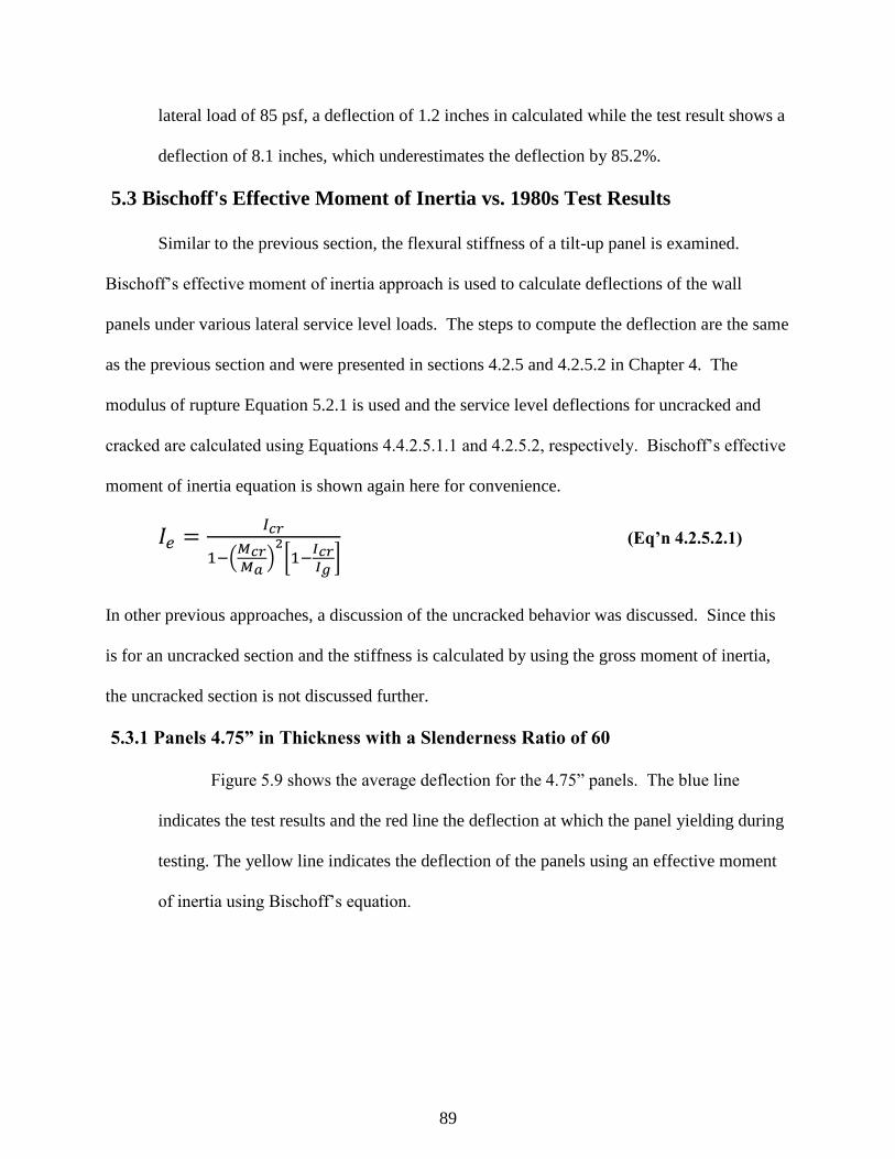
89
lateral load of 85 psf, a deflection of 1.2 inches in calculated while the test result shows a
deflection of 8.1 inches, which underestimates the deflection by 85.2%.
5.3 Bischoff's Effective Moment of Inertia vs. 1980s Test Results
Similar to the previous section, the flexural stiffness of a tilt-up panel is examined.
Bischoff’s effective moment of inertia approach is used to calculate deflections of the wall
panels under various lateral service level loads. The steps to compute the deflection are the same
as the previous section and were presented in sections 4.2.5 and 4.2.5.2 in Chapter 4. The
modulus of rupture Equation 5.2.1 is used and the service level deflections for uncracked and
cracked are calculated using Equations 4.4.2.5.1.1 and 4.2.5.2, respectively. Bischoff’s effective
moment of inertia equation is shown again here for convenience.
𝐼𝑒 =𝐼𝑐𝑟
1−(𝑀𝑐𝑟𝑀𝑎
)2[1−
𝐼𝑐𝑟𝐼𝑔
] (Eq’n 4.2.5.2.1)
In other previous approaches, a discussion of the uncracked behavior was discussed. Since this
is for an uncracked section and the stiffness is calculated by using the gross moment of inertia,
the uncracked section is not discussed further.
5.3.1 Panels 4.75” in Thickness with a Slenderness Ratio of 60
Figure 5.9 shows the average deflection for the 4.75” panels. The blue line
indicates the test results and the red line the deflection at which the panel yielding during
testing. The yellow line indicates the deflection of the panels using an effective moment
of inertia using Bischoff’s equation.
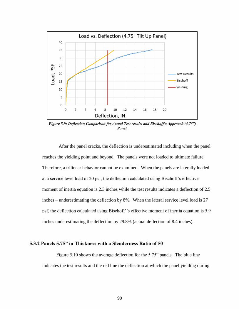
90
After the panel cracks, the deflection is underestimated including when the panel
reaches the yielding point and beyond. The panels were not loaded to ultimate failure.
Therefore, a trilinear behavior cannot be examined. When the panels are laterally loaded
at a service level load of 20 psf, the deflection calculated using Bischoff’s effective
moment of inertia equation is 2.3 inches while the test results indicates a deflection of 2.5
inches – underestimating the deflection by 8%. When the lateral service level load is 27
psf, the deflection calculated using Bischoff’’s effective moment of inertia equation is 5.9
inches underestimating the deflection by 29.8% (actual deflection of 8.4 inches).
5.3.2 Panels 5.75” in Thickness with a Slenderness Ratio of 50
Figure 5.10 shows the average deflection for the 5.75” panels. The blue line
indicates the test results and the red line the deflection at which the panel yielding during
0
5
10
15
20
25
30
35
40
0 2 4 6 8 10 12 14 16 18 20
Load
, PSF
Deflection, IN.
Load vs. Deflection (4.75" Tilt Up Panel)
Test Results
Bischoff
yielding
Figure 5.9: Deflection Comparison for Actual Test results and Bischoff’s Approach (4.75”)
Panel.
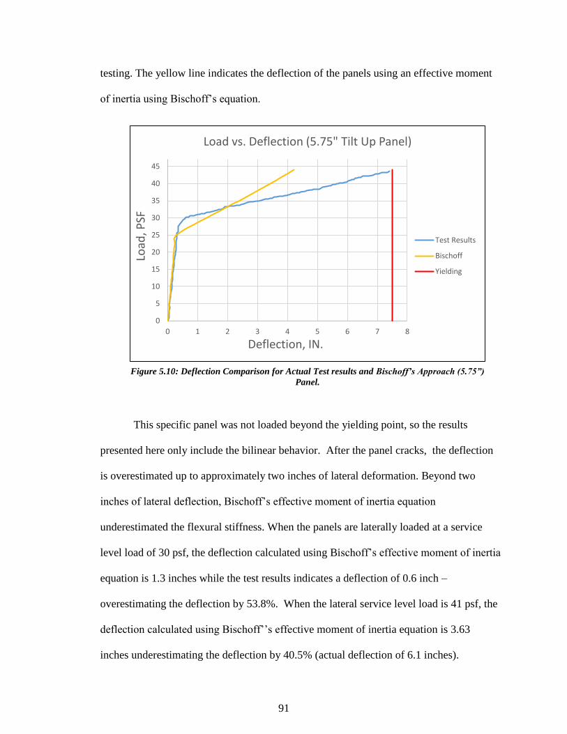
91
testing. The yellow line indicates the deflection of the panels using an effective moment
of inertia using Bischoff’s equation.
This specific panel was not loaded beyond the yielding point, so the results
presented here only include the bilinear behavior. After the panel cracks, the deflection
is overestimated up to approximately two inches of lateral deformation. Beyond two
inches of lateral deflection, Bischoff’s effective moment of inertia equation
underestimated the flexural stiffness. When the panels are laterally loaded at a service
level load of 30 psf, the deflection calculated using Bischoff’s effective moment of inertia
equation is 1.3 inches while the test results indicates a deflection of 0.6 inch –
overestimating the deflection by 53.8%. When the lateral service level load is 41 psf, the
deflection calculated using Bischoff’’s effective moment of inertia equation is 3.63
inches underestimating the deflection by 40.5% (actual deflection of 6.1 inches).
0
5
10
15
20
25
30
35
40
45
0 1 2 3 4 5 6 7 8
Load
, PSF
Deflection, IN.
Load vs. Deflection (5.75" Tilt Up Panel)
Test Results
Bischoff
Yielding
Figure 5.10: Deflection Comparison for Actual Test results and Bischoff’s Approach (5.75”)
Panel.
92
5.3.3 Panels 7.25” in Thickness with a Slenderness Ratio of 40
Figure 5.11 shows the average deflection for the 7.25” panel. The blue line
indicates the test results and the red line the deflection at which the panel yielding during
testing. The yellow line indicates the deflection of the panels using an effective moment
of inertia using Bischoff’s equation.
The behavior of the panel before cracking is linear and assumed accurately. After
cracking, Bischoff’s effective moment of inertia approach matches the actual deflection
behavior until the panel is loaded more than 47 psf. When the lateral load exceeds 47
psf, the deflection is underestimated for the bilinear and trilinear behavior. At 45 psf,
Bischoff’s approach estimates a deflection of 1.53 inch while the test result shows a
deflection of 1.3 inch, overestimated by 15%. At 55 psf, Bischoff’s approach estimates
a deflection of 3.8 inches with test results of 5.3 inches, an underestimation by 28.3%.
0
10
20
30
40
50
60
0 2 4 6 8 10 12
Load
, PSF
.
Deflection, IN.
Load vs. Deflection (7.25" Tilt Up Panel)
Test Results
Bischoff
Yielding
Figure 5.11: Deflection Comparison for Actual Test results and Bischoff’s Approach (7.25”)
Panel.
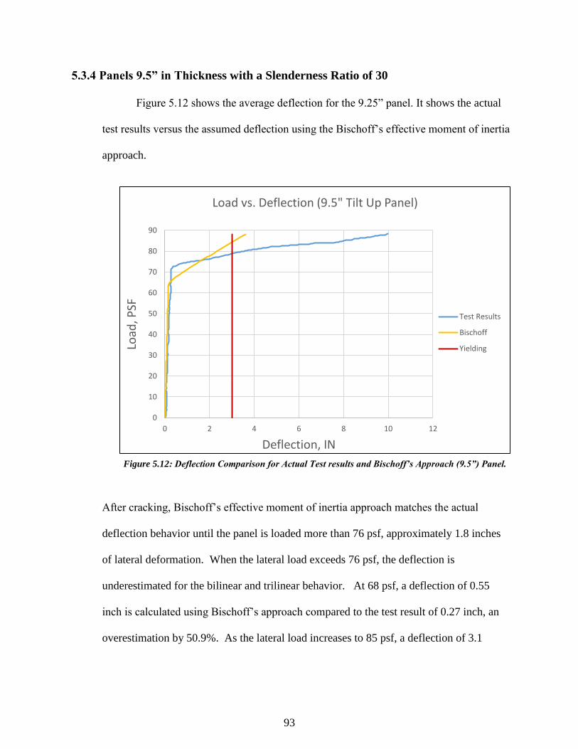
93
5.3.4 Panels 9.5” in Thickness with a Slenderness Ratio of 30
Figure 5.12 shows the average deflection for the 9.25” panel. It shows the actual
test results versus the assumed deflection using the Bischoff’s effective moment of inertia
approach.
After cracking, Bischoff’s effective moment of inertia approach matches the actual
deflection behavior until the panel is loaded more than 76 psf, approximately 1.8 inches
of lateral deformation. When the lateral load exceeds 76 psf, the deflection is
underestimated for the bilinear and trilinear behavior. At 68 psf, a deflection of 0.55
inch is calculated using Bischoff’s approach compared to the test result of 0.27 inch, an
overestimation by 50.9%. As the lateral load increases to 85 psf, a deflection of 3.1
0
10
20
30
40
50
60
70
80
90
0 2 4 6 8 10 12
Load
, PSF
Deflection, IN
Load vs. Deflection (9.5" Tilt Up Panel)
Test Results
Bischoff
Yielding
Figure 5.12: Deflection Comparison for Actual Test results and Bischoff’s Approach (9.5”) Panel.
94
inches is calculated using Bischoff’s approach compared to the actual deflection of 8.1
inches - underestimated by 61.7%.
5.4 Proposed Effective Moment of Inertia Derived by Kramer and Alkotami
This section discuss the deflection results for the derived deflection equation presented in
the analytical formulation in Section 3.5 in Chapter 4 and compared to the actual test results.
The deflection equations for Kramer and Kimberly are as follows:
a) For Pre-Cracking region:
- When Cracking occurs After L/2:
(Eq’n 3.5.2.13)
- When Cracking occurs prior L/2:
(Eq’n 3.5.2.14)
b) For Post-Cracking Region:
- In all cases, except at the end of the cracking region where yielding start to occur:
(Eq’n 3.5.3.11)
- At the end of the cracking region where yielding start to occur:
(Eq’n 3.5.3.14)
𝛿𝑢𝑛 =1
𝐸𝑐𝐼𝑔𝑡 [
𝑤𝐿
6𝐿𝑔
3 −𝑤
8𝐿𝑔
4 ]
𝛿𝑢𝑛 =𝑤𝐿𝑔
3
2𝐸𝑐𝐼𝑔𝑡 [
𝐿
3−
𝐿𝑔4
]
𝛿𝑝𝑐 =𝑤𝐿𝑔
3
2𝐸𝑐 𝐼𝑔𝑡 [
𝐿
3−
𝐿𝑔4
] + ( Ø𝑦 − Ø𝑐𝑟𝑀𝑦 − 𝑀𝑐𝑟
)
[
𝑤𝐿𝑦3
2(𝐿
3−
𝐿𝑦4
) −𝑤𝐿𝑔
3
2(𝐿
3−
𝐿𝑔4
)
+𝑀𝑐𝑟2
(𝐿𝑔2 − 𝐿𝑦
2) ]
+Ø𝑐𝑟2
(𝐿𝑦2 − 𝐿𝑔
2)
𝛿𝑝𝑐 =𝑤𝐿𝑔
3
2𝐸𝑐 𝐼𝑔𝑡 [
𝐿
3−
𝐿𝑔4
] ( Ø𝑦 − Ø𝑐𝑟𝑀𝑦 − 𝑀𝑐𝑟
) [5𝑤𝐿4
384−
𝑤𝐿𝑔3
2(𝐿
2−
𝐿𝑔4
)
+𝑀𝑐𝑟2
(𝐿𝑔2 −
𝐿2
2)] +
Ø𝑐𝑟2
(𝐿2
4− 𝐿𝑔
2)
95
c) For Post-Yielding region:
(Eq’n 3.5.4.10)
These equations were used to calculate deflections of the tilt-up panels and these
deflections were used to compare the actual deflections from the test results. Once a comparison
was completed, different ways of normalizing the flexural stiffness was examined. Rasheed et.
al. 2004 found a good correlation and proposed a modified cracked moment of inertia to use in
Branson’s effective moment of inertia equation for reinforced concrete beams strengthened with
fiber-reinforced polymers. Therefore, the first item used to normalizing the cracking moment of
inertia was the gross moment of inertia. Unfortunately, no accurate correlation was made.
Several other factors was considered including reinforcement ratio and slenderness ratio. The
following paragraphs indicated the finding of this research.
Two different equations are proposed for effective moment of inertia used in the service
deflection equations for slender tilt-up wall panels. The following sections present the difference
between the two equations in detail. A comparison with the actual test results is presented as
well.
𝛿𝑝𝑦 =𝑤𝐿𝑔
3
2 𝐸𝑐 𝐼𝑔𝑡 [
𝐿
3−
𝐿𝑔4
] + ( Ø𝑦 − Ø𝑐𝑟𝑀𝑦 − 𝑀𝑐𝑟
)
[
𝑤𝐿𝑦3
2(𝐿
3−
𝐿𝑦4
) −𝑤𝐿𝑔
3
2(𝐿
3−
𝐿𝑔4
)
+𝑀𝑐𝑟2
(𝐿𝑔2 − 𝐿𝑦
2) ]
+Ø𝑐𝑟2
(𝐿𝑦2 − 𝐿𝑔
2) + ( Ø𝑛 − Ø𝑦𝑀𝑛 − 𝑀𝑦
)
[
5wL4
384+
My2
(Ly2 −
L2
4) −
wLy2
2(L
3−
Ly4
) +
Ø𝑦 (L2
4− Ly
2) ]
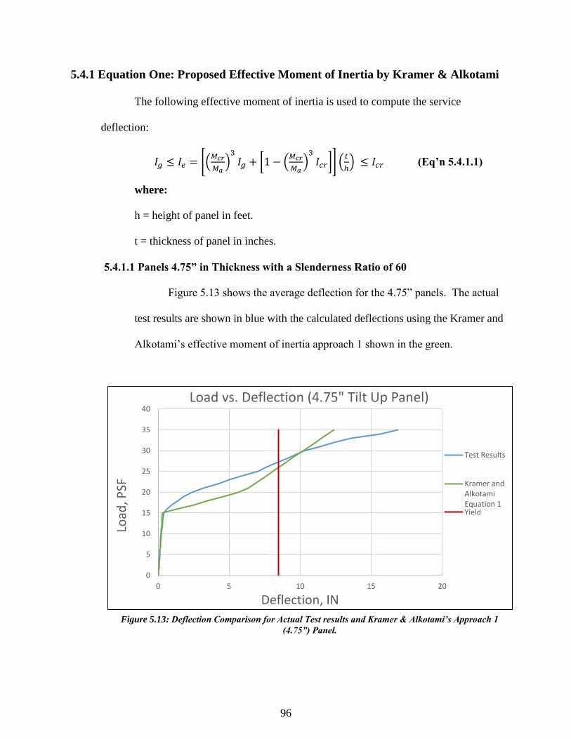
96
5.4.1 Equation One: Proposed Effective Moment of Inertia by Kramer & Alkotami
The following effective moment of inertia is used to compute the service
deflection:
𝐼𝑔 ≤ 𝐼𝑒 = [(𝑀𝑐𝑟
𝑀𝑎)3
𝐼𝑔 + [1 − (𝑀𝑐𝑟
𝑀𝑎)3
𝐼𝑐𝑟]] (𝑡
ℎ) ≤ 𝐼𝑐𝑟 (Eq’n 5.4.1.1)
where:
h = height of panel in feet.
t = thickness of panel in inches.
5.4.1.1 Panels 4.75” in Thickness with a Slenderness Ratio of 60
Figure 5.13 shows the average deflection for the 4.75” panels. The actual
test results are shown in blue with the calculated deflections using the Kramer and
Alkotami’s effective moment of inertia approach 1 shown in the green.
0
5
10
15
20
25
30
35
40
0 5 10 15 20
Load
, PSF
Deflection, IN
Load vs. Deflection (4.75" Tilt Up Panel)
Test Results
Kramer andAlkotamiEquation 1Yield
Figure 5.13: Deflection Comparison for Actual Test results and Kramer & Alkotami’s Approach 1
(4.75”) Panel.
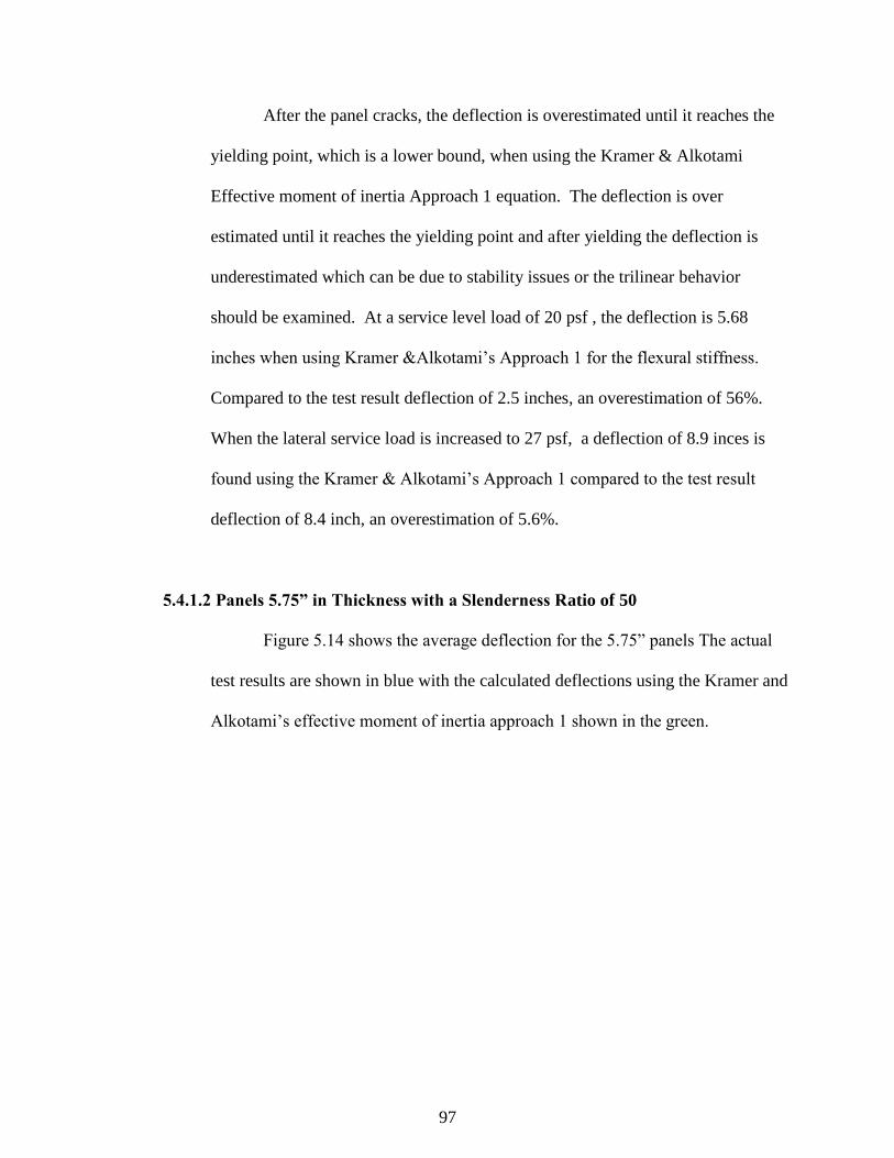
97
After the panel cracks, the deflection is overestimated until it reaches the
yielding point, which is a lower bound, when using the Kramer & Alkotami
Effective moment of inertia Approach 1 equation. The deflection is over
estimated until it reaches the yielding point and after yielding the deflection is
underestimated which can be due to stability issues or the trilinear behavior
should be examined. At a service level load of 20 psf , the deflection is 5.68
inches when using Kramer &Alkotami’s Approach 1 for the flexural stiffness.
Compared to the test result deflection of 2.5 inches, an overestimation of 56%.
When the lateral service load is increased to 27 psf, a deflection of 8.9 inces is
found using the Kramer & Alkotami’s Approach 1 compared to the test result
deflection of 8.4 inch, an overestimation of 5.6%.
5.4.1.2 Panels 5.75” in Thickness with a Slenderness Ratio of 50
Figure 5.14 shows the average deflection for the 5.75” panels The actual
test results are shown in blue with the calculated deflections using the Kramer and
Alkotami’s effective moment of inertia approach 1 shown in the green.
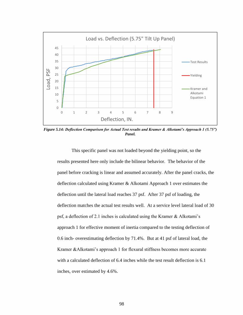
98
This specific panel was not loaded beyond the yielding point, so the
results presented here only include the bilinear behavior. The behavior of the
panel before cracking is linear and assumed accurately. After the panel cracks, the
deflection calculated using Kramer & Alkotami Approach 1 over estimates the
deflection until the lateral load reaches 37 psf. After 37 psf of loading, the
deflection matches the actual test results well. At a service level lateral load of 30
psf, a deflection of 2.1 inches is calculated using the Kramer & Alkotami’s
approach 1 for effective moment of inertia compared to the testing deflection of
0.6 inch- overestimating deflection by 71.4%. But at 41 psf of lateral load, the
Kramer &Alkotami’s approach 1 for flexural stiffness becomes more accurate
with a calculated deflection of 6.4 inches while the test result deflection is 6.1
inches, over estimated by 4.6%.
0
5
10
15
20
25
30
35
40
45
0 1 2 3 4 5 6 7 8 9
Load
, PSF
Deflection, IN.
Load vs. Deflection (5.75" Tilt Up Panel)
Test Results
Yielding
Kramer andAlkotamiEquation 1
Figure 5.14: Deflection Comparison for Actual Test results and Kramer & Alkotami’s Approach 1 (5.75”)
Panel.
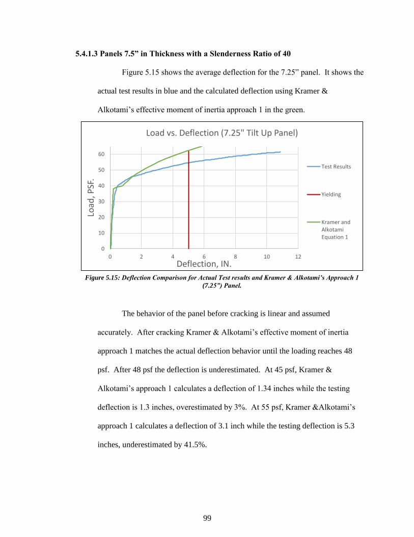
99
5.4.1.3 Panels 7.5” in Thickness with a Slenderness Ratio of 40
Figure 5.15 shows the average deflection for the 7.25” panel. It shows the
actual test results in blue and the calculated deflection using Kramer &
Alkotami’s effective moment of inertia approach 1 in the green.
The behavior of the panel before cracking is linear and assumed
accurately. After cracking Kramer & Alkotami’s effective moment of inertia
approach 1 matches the actual deflection behavior until the loading reaches 48
psf. After 48 psf the deflection is underestimated. At 45 psf, Kramer &
Alkotami’s approach 1 calculates a deflection of 1.34 inches while the testing
deflection is 1.3 inches, overestimated by 3%. At 55 psf, Kramer &Alkotami’s
approach 1 calculates a deflection of 3.1 inch while the testing deflection is 5.3
inches, underestimated by 41.5%.
0
10
20
30
40
50
60
0 2 4 6 8 10 12
Load
, PSF
.
Deflection, IN.
Load vs. Deflection (7.25" Tilt Up Panel)
Test Results
Yielding
Kramer andAlkotamiEquation 1
Figure 5.15: Deflection Comparison for Actual Test results and Kramer & Alkotami’s Approach 1
(7.25”) Panel.
100
5.4.1.4 Panels 9.5” in Thickness with a Slenderness Ratio of 30
Figure 5.16 shows the average deflection for the 9.25” panel. It shows the
actual test results versus the calculated deflection using the Kramer &Alkotami’s
effective moment of inertia approach 1.
Kramer & Alkotami’s effective moment of inertia approach 1 matches the
actual deflection behavior until the loading exceeds 75 psf. After 75 psf, the
deflection is underestimated. At 68 psf, Kramer and Alkotami’s approach 1 finds
a deflection of 0.53 inch while the test result deflection is 0.27 inch,
overestimated by 49.1%. At 85 psf, Kramer & Alkotami’s approach 1 calculates
a deflection of 1.52 inches while the test result deflection is 8.1 inches,
underestimated by 80.5%.
0
10
20
30
40
50
60
70
80
90
0 2 4 6 8 10
Load
, PSF
Deflection, IN
Load vs. Deflection (9.5" Tilt Up Panel)
Test Results
Yielding
Kramer andAlkotamiEquation 1
Figure 5.16: Deflection Comparison for Actual Test results and Kramer and Alkotami’s Approach 1
(9.5”) Panel.
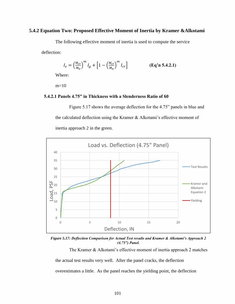
101
5.4.2 Equation Two: Proposed Effective Moment of Inertia by Kramer &Alkotami
The following effective moment of inertia is used to compute the service
deflection:
𝐼𝑒 = (𝑀𝑐𝑟
𝑀𝑎)𝑚
𝐼𝑔 + [1 − (𝑀𝑐𝑟
𝑀𝑎)𝑚
𝐼𝑐𝑟] (Eq’n 5.4.2.1)
Where:
m=10
5.4.2.1 Panels 4.75” in Thickness with a Slenderness Ratio of 60
Figure 5.17 shows the average deflection for the 4.75” panels in blue and
the calculated deflection using the Kramer & Alkotami’s effective moment of
inertia approach 2 in the green.
The Kramer & Alkotami’s effective moment of inertia approach 2 matches
the actual test results very well. After the panel cracks, the deflection
overestimates a little. As the panel reaches the yielding point, the deflection
0
5
10
15
20
25
30
35
40
0 5 10 15 20
Load
, PSF
Deflection, IN
Load vs. Deflection (4.75" Panel)
Test Results
Kramer andAlkotamiEquation 2
Yielding
Figure 5.17: Deflection Comparison for Actual Test results and Kramer & Alkotami’s Approach 2
(4.75”) Panel.
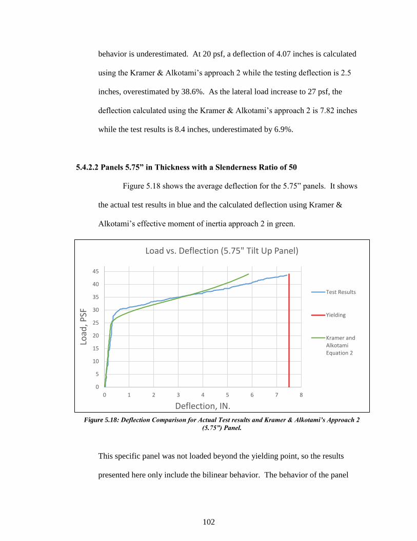
102
behavior is underestimated. At 20 psf, a deflection of 4.07 inches is calculated
using the Kramer & Alkotami’s approach 2 while the testing deflection is 2.5
inches, overestimated by 38.6%. As the lateral load increase to 27 psf, the
deflection calculated using the Kramer & Alkotami’s approach 2 is 7.82 inches
while the test results is 8.4 inches, underestimated by 6.9%.
5.4.2.2 Panels 5.75” in Thickness with a Slenderness Ratio of 50
Figure 5.18 shows the average deflection for the 5.75” panels. It shows
the actual test results in blue and the calculated deflection using Kramer &
Alkotami’s effective moment of inertia approach 2 in green.
This specific panel was not loaded beyond the yielding point, so the results
presented here only include the bilinear behavior. The behavior of the panel
0
5
10
15
20
25
30
35
40
45
0 1 2 3 4 5 6 7 8
Load
, PSF
Deflection, IN.
Load vs. Deflection (5.75" Tilt Up Panel)
Test Results
Yielding
Kramer andAlkotamiEquation 2
Figure 5.18: Deflection Comparison for Actual Test results and Kramer & Alkotami’s Approach 2
(5.75”) Panel.
103
before cracking is linear and assumed accurately. After cracking, the deflection is
slightly overestimated until the loading reaches 37 psf. When the pressure is
more than 37 psf, the deflection is underestimated. For example at 30 psf, a
deflection of 1.24 inches is calculated using the Kramer & Alkotami’s approach 2
while the test deflection is 0.6 inch, overestimated by 51.6%. However, as the
load is increase to 41 psf, the Kramer & Alkotami’s approach 2 for effective
moment of inertia estimates the stiffness well with a calculated deflection of 5.1
inches compared to the actual deflection of 6.1 inches, underestimated by 16.4%.
5.4.2.3 Panels 7.25” in Thickness with a Slenderness Ratio of 40
Figure 5.19 shows the average deflection for the 7.25” panels. It shows
the actual test results in blue versus the calculated deflection using Kramer &
Alkotami’s effective moment of inertia approach 2 in the green.
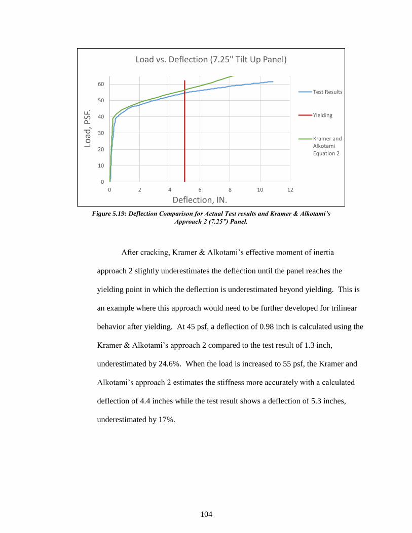
104
After cracking, Kramer & Alkotami’s effective moment of inertia
approach 2 slightly underestimates the deflection until the panel reaches the
yielding point in which the deflection is underestimated beyond yielding. This is
an example where this approach would need to be further developed for trilinear
behavior after yielding. At 45 psf, a deflection of 0.98 inch is calculated using the
Kramer & Alkotami’s approach 2 compared to the test result of 1.3 inch,
underestimated by 24.6%. When the load is increased to 55 psf, the Kramer and
Alkotami’s approach 2 estimates the stiffness more accurately with a calculated
deflection of 4.4 inches while the test result shows a deflection of 5.3 inches,
underestimated by 17%.
0
10
20
30
40
50
60
0 2 4 6 8 10 12
Load
, PSF
.
Deflection, IN.
Load vs. Deflection (7.25" Tilt Up Panel)
Test Results
Yielding
Kramer andAlkotamiEquation 2
Figure 5.19: Deflection Comparison for Actual Test results and Kramer & Alkotami’s
Approach 2 (7.25”) Panel.
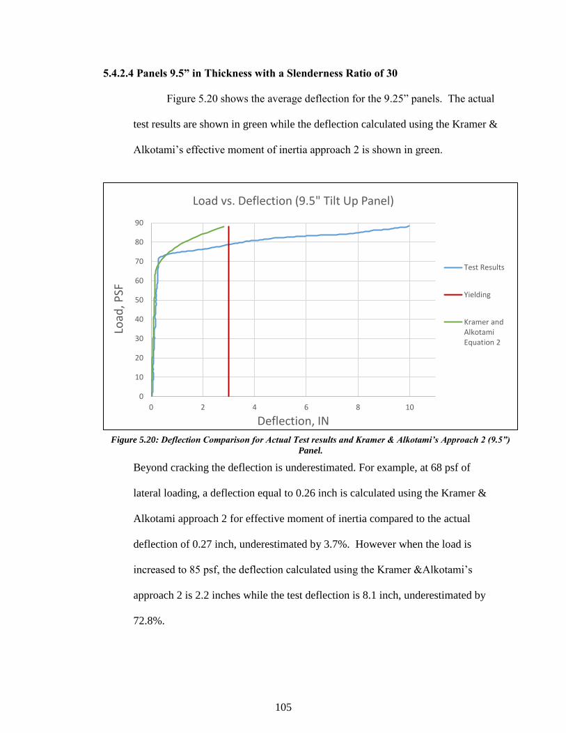
105
5.4.2.4 Panels 9.5” in Thickness with a Slenderness Ratio of 30
Figure 5.20 shows the average deflection for the 9.25” panels. The actual
test results are shown in green while the deflection calculated using the Kramer &
Alkotami’s effective moment of inertia approach 2 is shown in green.
Beyond cracking the deflection is underestimated. For example, at 68 psf of
lateral loading, a deflection equal to 0.26 inch is calculated using the Kramer &
Alkotami approach 2 for effective moment of inertia compared to the actual
deflection of 0.27 inch, underestimated by 3.7%. However when the load is
increased to 85 psf, the deflection calculated using the Kramer &Alkotami’s
approach 2 is 2.2 inches while the test deflection is 8.1 inch, underestimated by
72.8%.
0
10
20
30
40
50
60
70
80
90
0 2 4 6 8 10
Load
, PSF
Deflection, IN
Load vs. Deflection (9.5" Tilt Up Panel)
Test Results
Yielding
Kramer andAlkotamiEquation 2
Figure 5.20: Deflection Comparison for Actual Test results and Kramer & Alkotami’s Approach 2 (9.5”)
Panel.
106
Chapter 6 - Conclusion and Recommendations
This Chapter 6 presents the conclusion of this research and highlights some
recommendations for future researches.
6.1 Conclusion
The following tables summarize the deflection behavior for each panel thickness and
slenderness ratio using all presented approaches in Chapter 5 and a comparison to the actual test
results is also presented. Two different lateral loads are presented to investigate the percent
difference between each approach and the actual deflection value. The red error percentage
indicates that the deflection was underestimated, which can be an unsafe design. The green error
percentage indicates that the deflection is overestimated, which would be a conservative
following design. The figures show a visual representation of the deflection behavior of the tilt-
up panels following all presented approaches compared to the actual test results.
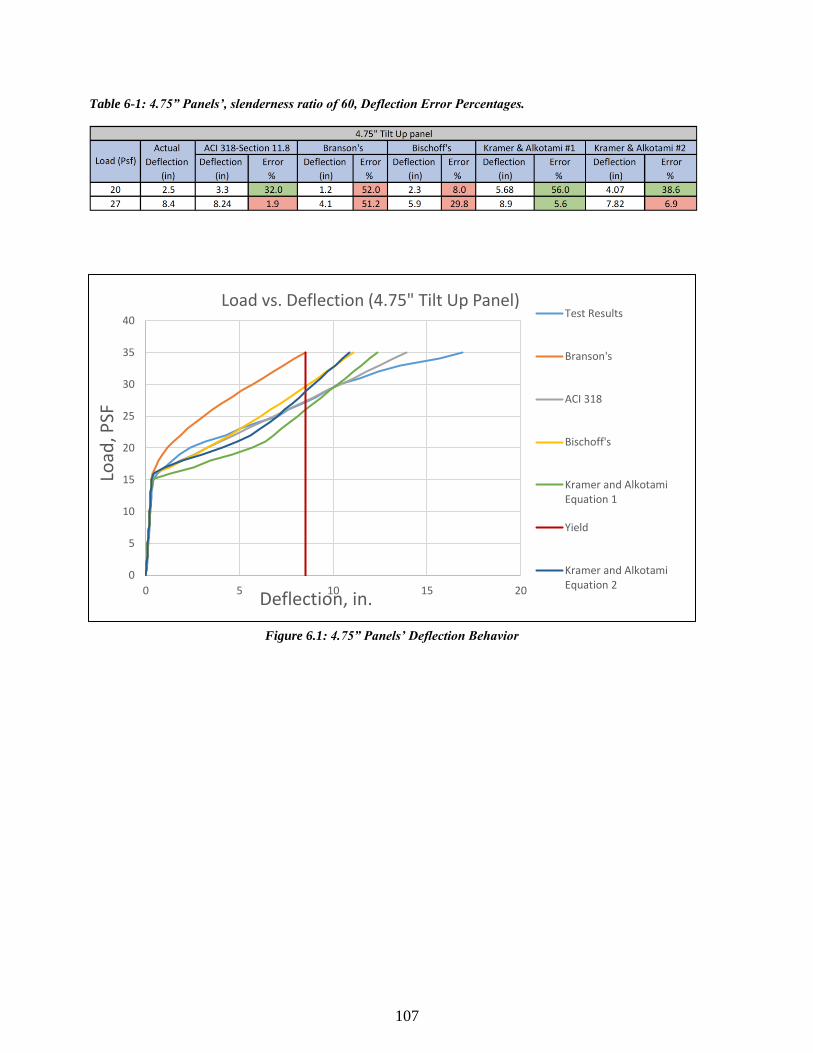
107
0
5
10
15
20
25
30
35
40
0 5 10 15 20
Load
, PSF
Deflection, in.
Load vs. Deflection (4.75" Tilt Up Panel)Test Results
Branson's
ACI 318
Bischoff's
Kramer and AlkotamiEquation 1
Yield
Kramer and AlkotamiEquation 2
Table 6-1: 4.75” Panels’, slenderness ratio of 60, Deflection Error Percentages.
Figure 6.1: 4.75” Panels’ Deflection Behavior
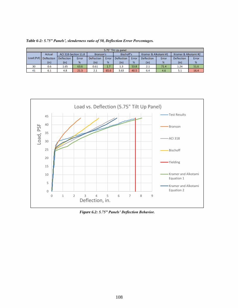
108
0
5
10
15
20
25
30
35
40
45
0 1 2 3 4 5 6 7 8 9
Load
, PSF
Deflection, in.
Load vs. Deflection (5.75" Tilt Up Panel)
Test Results
Branson
ACI 318
Bischoff
Yielding
Kramer and AlkotamiEquation 1
Kramer and AlkotamiEquation 2
Table 6-2: 5.75” Panels’, slenderness ratio of 50, Deflection Error Percentages.
Figure 6.2: 5.75” Panels’ Deflection Behavior.
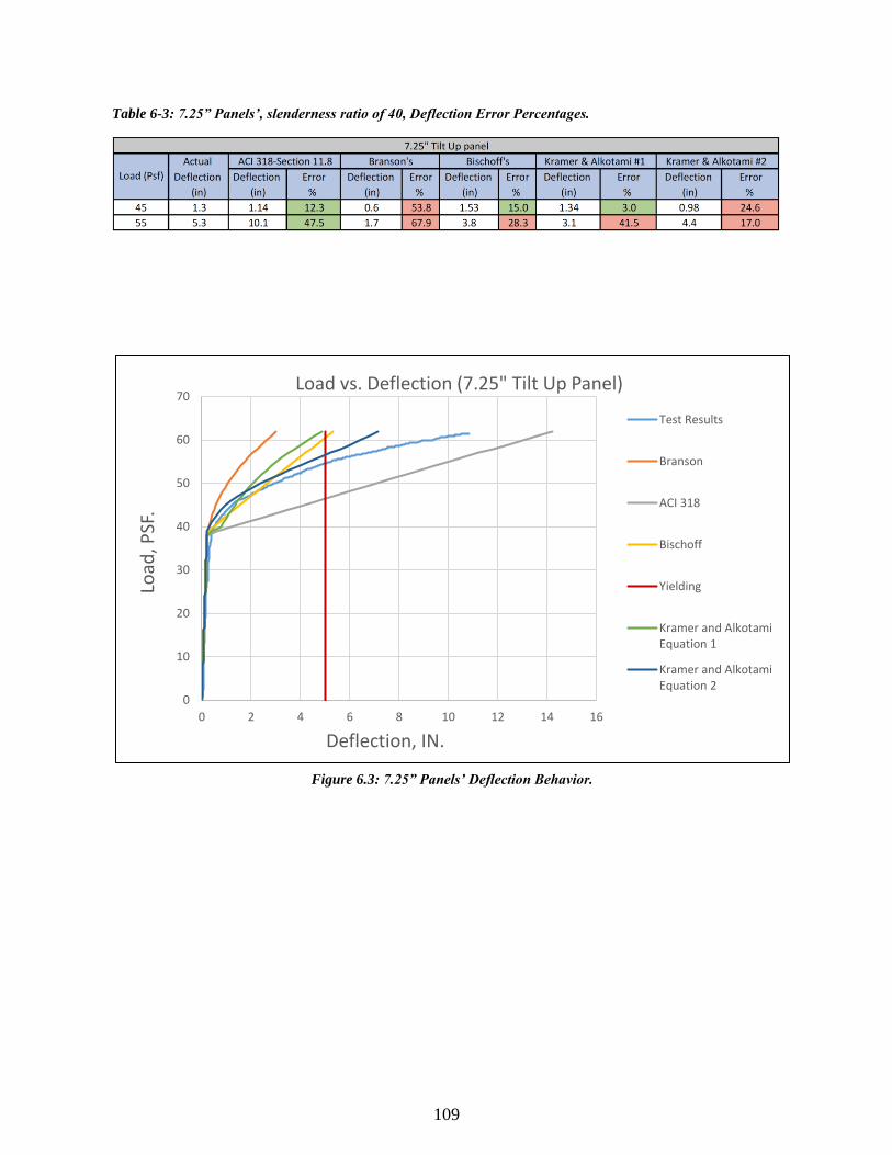
109
0
10
20
30
40
50
60
70
0 2 4 6 8 10 12 14 16
Load
, PSF
.
Deflection, IN.
Load vs. Deflection (7.25" Tilt Up Panel)
Test Results
Branson
ACI 318
Bischoff
Yielding
Kramer and AlkotamiEquation 1
Kramer and AlkotamiEquation 2
Table 6-3: 7.25” Panels’, slenderness ratio of 40, Deflection Error Percentages.
Figure 6.3: 7.25” Panels’ Deflection Behavior.
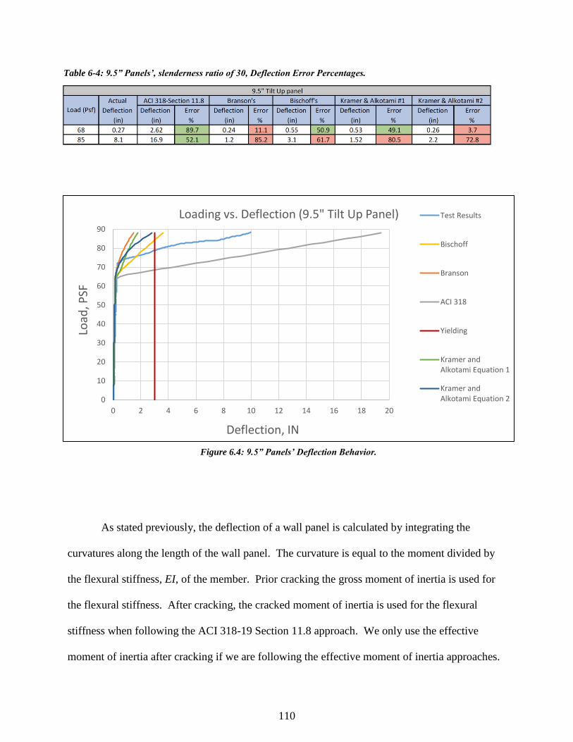
110
As stated previously, the deflection of a wall panel is calculated by integrating the
curvatures along the length of the wall panel. The curvature is equal to the moment divided by
the flexural stiffness, EI, of the member. Prior cracking the gross moment of inertia is used for
the flexural stiffness. After cracking, the cracked moment of inertia is used for the flexural
stiffness when following the ACI 318-19 Section 11.8 approach. We only use the effective
moment of inertia after cracking if we are following the effective moment of inertia approaches.
0
10
20
30
40
50
60
70
80
90
0 2 4 6 8 10 12 14 16 18 20
Load
, PSF
Deflection, IN
Loading vs. Deflection (9.5" Tilt Up Panel) Test Results
Bischoff
Branson
ACI 318
Yielding
Kramer andAlkotami Equation 1
Kramer andAlkotami Equation 2
Table 6-4: 9.5” Panels’, slenderness ratio of 30, Deflection Error Percentages.
Figure 6.4: 9.5” Panels’ Deflection Behavior.
111
The deflection behavior of the panel is linear until it reaches the end of the elastic region.
At the end of the elastic region, the stiffness changes drastically that can be seen in the load
deflection figures. After cracking, the deflection is considered to be the elastic-plastic region;
this region is referred to as the bilinear region for the ACI 318-19 Section 11.8 method until it
reaches the yield moment. The load-deflection slope typically changes from the yield moment to
the ultimate moment. After yield point the curve starts to flatten out; therefore, it can be
idealized as a trilinear behavior. Unfortunately, the original panels were not tested or loaded to
the ultimate point. Therefore, the trilinear behavior of slender wall panels was not examined in
this research.
As the load increases to near yielding of the panels, the four effective moment of inertia
approaches examined become irregular ,which may be caused by the P-delta effects, stability
issues. For a slender concrete wall panel, the axial compression and transverse bending about
one axis, failure by instability in the plane of bending without twisting, is the failure mode.
However, the actual test results did not note any elastic or inelastic lateral instability.
6.2 Recommendations
This section will provide multiple recommendations for future work to improve the slender walls
provisions in the code.
1) Design Approach:
After comparing ACI 318-19 Section 11.8 approach, Branson’s effective moment of
inertia, Bischoff’s effective moment of inertia, and two proposed effective moment of
inertia by Kramer & Alkotami, using the ACI 318-19 Section 11.8 Alternate Design
Method for Slender Walls should be used. The bilinear approach is a lower bound,
112
conservative, approach that represents walls with slenderness ratio ranging from 30 to
60.
2) Modification for ACI 318 service Equation:
The service deflection equation for the un-cracked region is as follows:
(ACI 318-19 Eq’n 11.8.1.1a)
Using the previous equation, the deflection is slightly off and underestimated.
Adding a (2/3) coefficient to the cracking moment has been examined and should be
used to match the test results. The propose equation for the service deflection in the
un-cracked region is as follows:
(Proposed Equation)
To prove the validity of the proposed equation, comparison of the original service
deflection equation to the proposed equation was performed. The following figures
show the actual and modified ACI 318 service deflection equations compared to the
actual test results for all panels thicknesses. If this equation is modified, the service
deflection equation for after cracking should remove the 2/3 from the cracked
deflection
∆𝑠 = (𝑀𝑎
(𝑀𝑐𝑟)∆𝑐𝑟
∆𝑠 = (𝑀𝑎
((𝟐𝟑)𝑀𝑐𝑟
)∆𝑐𝑟
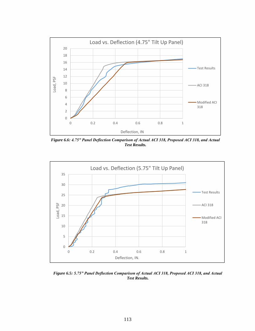
113
0
2
4
6
8
10
12
14
16
18
20
0 0.2 0.4 0.6 0.8 1
Load
, PSF
Deflection, IN
Load vs. Deflection (4.75" Tilt Up Panel)
Test Results
ACI 318
Modified ACI318
0
5
10
15
20
25
30
35
0 0.2 0.4 0.6 0.8 1
Load
, PSF
Deflection, IN.
Load vs. Deflection (5.75" Tilt Up Panel)
Test Results
ACI 318
Modified ACI318
Figure 6.6: 4.75” Panel Deflection Comparison of Actual ACI 318, Proposed ACI 318, and Actual
Test Results.
Figure 6.5: 5.75” Panel Deflection Comparison of Actual ACI 318, Proposed ACI 318, and Actual
Test Results.
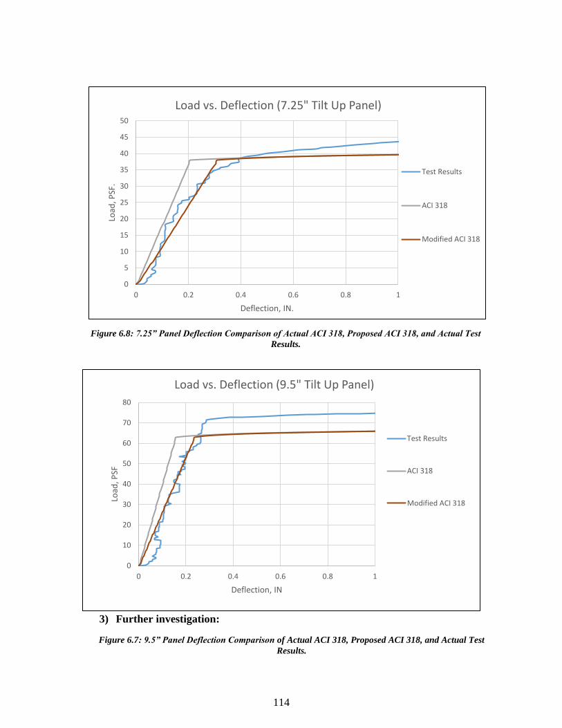
114
3) Further investigation:
0
5
10
15
20
25
30
35
40
45
50
0 0.2 0.4 0.6 0.8 1
Load
, PSF
.
Deflection, IN.
Load vs. Deflection (7.25" Tilt Up Panel)
Test Results
ACI 318
Modified ACI 318
0
10
20
30
40
50
60
70
80
0 0.2 0.4 0.6 0.8 1
Load
, PSF
Deflection, IN
Load vs. Deflection (9.5" Tilt Up Panel)
Test Results
ACI 318
Modified ACI 318
Figure 6.8: 7.25” Panel Deflection Comparison of Actual ACI 318, Proposed ACI 318, and Actual Test
Results.
Figure 6.7: 9.5” Panel Deflection Comparison of Actual ACI 318, Proposed ACI 318, and Actual Test
Results.
115
Further investigation to ensure validity of the ACI 318-19 Section 11.8 method
beyond yielding is recommended. Stability issues could occur beyond yielding.
4) Testing of Panels:
a) More full-scale testing of tilt-up panels with higher slenderness ratios.
b) More than one layer of reinforcement.
It is also recommend loading the panels to ultimate to ensure the validity of
equation for the trilinear behavior.
5) Modulus of Rupture:
Since concrete materials, mix designs, have changed considerable in the last forty
years, it is recommended that additional research on the modulus of rupture of slender
load-bearing wall panels occur. This research would confirm the use of 5√f’c for the
modulus of rupture.
116
References
ACI Committee 318. (1999). Building code requirements for structural concrete (ACI 318-99)
and commentary (ACI 318R-99). Farmington Hills, MI: American Concrete Institute.
ACI Committee 318. (2002). Building code requirements for structural concrete (ACI 318-02)
and commentary (ACI 318R-02). Farmington Hills, MI: American Concrete Institute.
ACI Committee 318. (2005). Building code requirements for structural concrete (ACI 318-05)
and commentary (ACI 318R-05). Farmington Hills, MI: American Concrete Institute.
ACI Committee 318. (2008). Building code requirements for structural concrete (ACI 318-08)
and commentary (ACI 318R-08). Farmington Hills, MI: American Concrete Institute.
ACI Committee 318. (2011). Building Code Requirements for Structural Concrete (ACI 318-11)
and Commentary (ACI 318R-11). Farmington Hills, MI: American Concrete Institute.
ACI Committee 318. (2014). Building code requirements for structural concrete (ACI 318-14)
and commentary (ACI 318R-14). Farmington Hills, MI: American Concrete Institute.
ACI Committee 318. (2019). Building code requirements for structural concrete (ACI 318-19)
and commentary (ACI 318R-19). Farmington Hills, MI: American Concrete Institute.
ACI Committee 551. (2015). Design guide for tilt-up concrete panels. Farmington Hills, MI:
American Concrete Institute.
Al-Sunna, R., Pilakoutas, K., Hajirasouliha, I., & Guadagnini, M. (2012). Deflection behaviour
of FRP reinforced concrete beams and slabs: An experimental investigation. Composites
Part B: Engineering, 43(5), 2125–2134.
117
Alwis, W. A. M. (1990). Trilinear moment-curvature relationship for reinforced concrete beams.
Structural Journal, 87(3), 276–283.
Bischoff, P. H. (2005). Reevaluation of Deflection Prediction for Concrete Beams Reinforced
with Steel and Fiber Reinforced Polymer Bars. Journal of Structural Engineering, 131(5),
752–767.
Bischoff, P. H., & Gross, S. P. (2011). Equivalent Moment of Inertia Based on Integration of
Curvature. Journal of Composites for Construction, 15(3), 263–273.
Bischoff, P. H., & Scanlon, A. (2007). Effective Moment of Inertia for Calculating Deflections
of Concrete Members Containing Steel Reinforcement and Fiber-Reinforced Polymer
Reinforcement. ACI Structural Journal, 104(1), 68–75.
Burns, N. H. (1964). Moment Curvature Relationships for Partially Prestressed Concrete Beams.
PCI Journal, 9(1), 2815–2823
Chamberland, S. (2014). 3 Weather conditions that severely affect construction equipment.
Retrieved from http://www.equipmentfa.com/error.aspx?aspxerrorpath=/blogs/2708/3-
weather-conditions-that-severely-affect-construction-equipement.
Charkas, H., Rasheed, H. A., & Melhem, H. (2003). Rigorous procedure for calculating
deflections of fiber-reinforced polymer-strengthened reinforced concrete beams. Structural
Journal, 100(4), 529–539.
Council of Economic and Development Affairs. (2017). Vision 2030: Quality of Life Program
2020. Government of Saudi Arabia.
DBS Group. (2018). This vs that: precast vs. site-cast concrete. Retrieved from
https://www.dbsg.com/blog/this-vs-that-precast-vs-site-cast-concrete
118
Gilbert, I. R. (2006). Discussion of “Reevaluation of Deflection Prediction for Concrete Beams
Reinforced with Steel and Fiber Reinforced Polymer Bars” by Peter H. Bischoff. Journal of
Structural Engineering, 132(8), 1328–1330.
Hognestad, E. (1952). Inelastic Behavior in Tests of Eccentrically Loaded Short Reinforced
Concrete Columns. Retrieved from https://books.google.com/books?id=jF-gGwAACAAJ
Johnson, M. (2002, August). Tilt-Up pioneer Robert Aiken developed tilt up construction nearly
100 years ago. Concrete Construction. C02H037. Retrieved
from https://www.concreteconstruction.net/how-to/construction/tilt-up-pioneer_o
Khalaf, R. (2017). Saudi Arabia just reached its highest-ever temperature. Retrieved from
https://stepfeed.com/saudi-arabia-just-recorded-its-highest-ever-temperature-3409
McCormac, J. C. (2006). Structural Analysis: Using Classical and Matrix Methods. Retrieved
from https://books.google.com/books?id=bPFoDwAAQBAJ
Paulson, C., Rautenberg, J. M., Graham, S. K., & Darwin, D. (2016). Defining Yield Strength for
Nonprestressed Reinforcing Steel. ACI Structural Journal, 113(1), 169–178.
Sakai, K. K., & Yakuta, Y. (1980). Moment-Curvature Relationships of Reinforced Concrete
Members Subjected to Combined Bending and Axial Force. ACI Journal Proceedings,
77(3), 189–194.
Słowik, M. (2019). The analysis of failure in concrete and reinforced concrete beams with
different reinforcement ratio. Archive of Applied Mechanics, 89(5), 885–895.
Tarawneh, Q., & Chowdhury, S. (2018). Trends of climate change in Saudi Arabia: implications
on water resources. Climate, 6(1), 8.
Tilt-Up Concrete Association. (2011). The Construction of Tilt-up. Mt Vernon, IA: Author.

119
United States Environmental Protection Agency. (n.d.). Climate Impacts on Human Health.
Retrieved from https://19january2017snapshot.epa.gov/climate-impacts/climate-impacts-
human-health_.html
Whitney, C. S. (1937). Design of reinforced concrete members under flexure or combined
flexure and direct compression. Journal Proceedings, 33(3), 483–498.
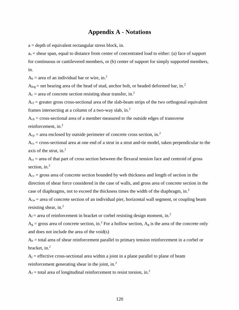
120
Appendix A - Notations
a = depth of equivalent rectangular stress block, in.
av = shear span, equal to distance from center of concentrated load to either: (a) face of support
for continuous or cantilevered members, or (b) center of support for simply supported members,
in.
Ab = area of an individual bar or wire, in.2
Abrg = net bearing area of the head of stud, anchor bolt, or headed deformed bar, in.2
Ac = area of concrete section resisting shear transfer, in.2
Acf = greater gross cross-sectional area of the slab-beam strips of the two orthogonal equivalent
frames intersecting at a column of a two-way slab, in.2
Ach = cross-sectional area of a member measured to the outside edges of transverse
reinforcement, in.2
Acp = area enclosed by outside perimeter of concrete cross section, in.2
Acs = cross-sectional area at one end of a strut in a strut and-tie model, taken perpendicular to the
axis of the strut, in.2
Act = area of that part of cross section between the flexural tension face and centroid of gross
section, in.2
Acv = gross area of concrete section bounded by web thickness and length of section in the
direction of shear force considered in the case of walls, and gross area of concrete section in the
case of diaphragms, not to exceed the thickness times the width of the diaphragm, in.2
Acw = area of concrete section of an individual pier, horizontal wall segment, or coupling beam
resisting shear, in.2
Af = area of reinforcement in bracket or corbel resisting design moment, in.2
Ag = gross area of concrete section, in.2 For a hollow section, Ag is the area of the concrete only
and does not include the area of the void(s)
Ah = total area of shear reinforcement parallel to primary tension reinforcement in a corbel or
bracket, in.2
Aj = effective cross-sectional area within a joint in a plane parallel to plane of beam
reinforcement generating shear in the joint, in.2
Aℓ = total area of longitudinal reinforcement to resist torsion, in.2
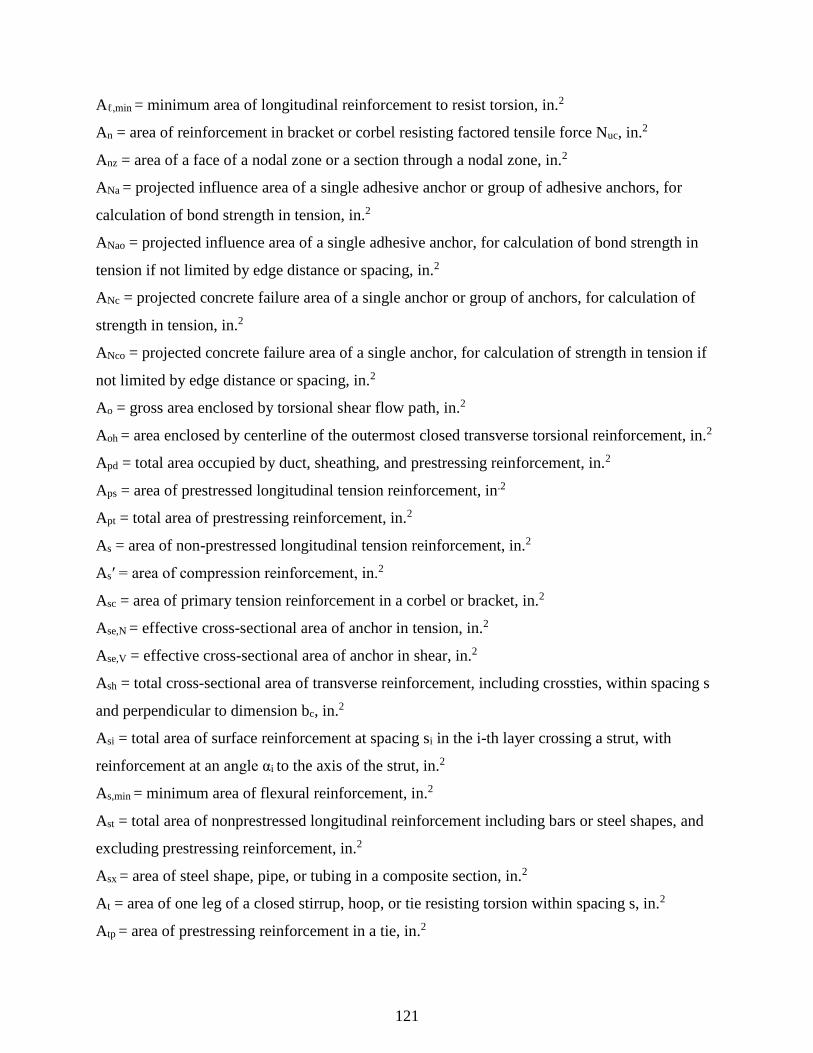
121
Aℓ,min = minimum area of longitudinal reinforcement to resist torsion, in.2
An = area of reinforcement in bracket or corbel resisting factored tensile force Nuc, in.2
Anz = area of a face of a nodal zone or a section through a nodal zone, in.2
ANa = projected influence area of a single adhesive anchor or group of adhesive anchors, for
calculation of bond strength in tension, in.2
ANao = projected influence area of a single adhesive anchor, for calculation of bond strength in
tension if not limited by edge distance or spacing, in.2
ANc = projected concrete failure area of a single anchor or group of anchors, for calculation of
strength in tension, in.2
ANco = projected concrete failure area of a single anchor, for calculation of strength in tension if
not limited by edge distance or spacing, in.2
Ao = gross area enclosed by torsional shear flow path, in.2
Aoh = area enclosed by centerline of the outermost closed transverse torsional reinforcement, in.2
Apd = total area occupied by duct, sheathing, and prestressing reinforcement, in.2
Aps = area of prestressed longitudinal tension reinforcement, in.2
Apt = total area of prestressing reinforcement, in.2
As = area of non-prestressed longitudinal tension reinforcement, in.2
As′ = area of compression reinforcement, in.2
Asc = area of primary tension reinforcement in a corbel or bracket, in.2
Ase,N = effective cross-sectional area of anchor in tension, in.2
Ase,V = effective cross-sectional area of anchor in shear, in.2
Ash = total cross-sectional area of transverse reinforcement, including crossties, within spacing s
and perpendicular to dimension bc, in.2
Asi = total area of surface reinforcement at spacing si in the i-th layer crossing a strut, with
reinforcement at an angle αi to the axis of the strut, in.2
As,min = minimum area of flexural reinforcement, in.2
Ast = total area of nonprestressed longitudinal reinforcement including bars or steel shapes, and
excluding prestressing reinforcement, in.2
Asx = area of steel shape, pipe, or tubing in a composite section, in.2
At = area of one leg of a closed stirrup, hoop, or tie resisting torsion within spacing s, in.2
Atp = area of prestressing reinforcement in a tie, in.2
122
Atr = total cross-sectional area of all transverse reinforcement within spacing s that crosses the
potential plane of splitting through the reinforcement being developed, in.2
Ats = area of nonprestressed reinforcement in a tie, in.2
Av = area of shear reinforcement within spacing s, in.2
Avd = total area of reinforcement in each group of diagonal bars in a diagonally reinforced
coupling beam, in.2
Avf = area of shear-friction reinforcement, in.2
Avh = area of shear reinforcement parallel to flexural tension reinforcement within spacing s2, in.2
Av,min = minimum area of shear reinforcement within spacing s, in.2
AVc = projected concrete failure area of a single anchor or group of anchors, for calculation of
strength in shear, in.2
AVco = projected concrete failure area of a single anchor, for calculation of strength in shear, if
not limited by corner influences, spacing, or member thickness, in.2
A1 = loaded area for consideration of bearing strength, in.2
A2 = area of the lower base of the largest frustum of a pyramid, cone, or tapered wedge contained
wholly within the support and having its upper base equal to the loaded area. The sides of the
pyramid, cone, or tapered wedge shall be sloped one vertical to two horizontal, in.2
b = width of compression face of member, in.
bc = cross-sectional dimension of member core measured to the outside edges of the transverse
reinforcement composing area Ash, in.
bf = effective flange width of T section, in.
bo = perimeter of critical section for two-way shear in slabs and footings, in.
bs = width of strut, in.
bslab = effective slab width resisting γfMsc, in.
bt = width of that part of cross section containing the closed stirrups resisting torsion, in.
bv = width of cross section at contact surface being investigated for horizontal shear, in.
bw = web width or diameter of circular section, in.
b1 = dimension of the critical section bo measured in the direction of the span for which moments
are determined, in.
b2 = dimension of the critical section bo measured in the direction perpendicular to b1, in.
Bn = nominal bearing strength, lb
123
Bu = factored bearing load, lb
c = distance from extreme compression fiber to neutral axis, in.
cac = critical edge distance required to develop the basic strength as controlled by concrete
breakout or bond of a post-installed anchor in tension in uncracked concrete without
supplementary reinforcement to control splitting, in.
ca,max = maximum distance from center of an anchor shaft to the edge of concrete, in.
ca,min = minimum distance from center of an anchor shaft to the edge of concrete, in.
ca1 = distance from the center of an anchor shaft to the edge of concrete in one direction, in. If
shear is applied to anchor, ca1 is taken in the direction of the applied shear. If tension is applied to
the anchor, ca1 is the minimum edge distance. Where anchors subject to shear are located in
narrow sections of limited thickness, see 17.5.2.4 in ACI 318-14
c′a1 = limiting value of ca1 where anchors are located less than 1.5ca1 from three or more edges,
in.; see Fig. R17.5.2.4 in ACI 318-14
ca2 = distance from center of an anchor shaft to the edge of concrete in the direction
perpendicular to ca1, in.
cb = lesser of: (a) the distance from center of a bar or wire to nearest concrete surface, and (b)
one-half the center-to-center spacing of bars or wires being developed, in.
cc = clear cover of reinforcement, in.
cNa = projected distance from center of an anchor shaft on one side of the anchor required to
develop the full bond strength of a single adhesive anchor, in.
ct = distance from the interior face of the column to the slab edge measured parallel to c1, but not
exceeding c1, in.
c1 = dimension of rectangular or equivalent rectangular column, capital, or bracket measured in
the direction of the span for which moments are being determined, in.
c2 = dimension of rectangular or equivalent rectangular column, capital, or bracket measured in
the direction perpendicular to c1, in.
C = cross-sectional constant to define torsional properties of slab and beam
C = compressive force acting on a nodal zone, lb
Cm = factor relating actual moment diagram to an equivalent uniform moment diagram
d = distance from extreme compression fiber to centroid of longitudinal tension reinforcement,
in.
124
d′ = distance from extreme compression fiber to centroid of longitudinal compression
reinforcement, in.
da = outside diameter of anchor or shaft diameter of headed stud, headed bolt, or hooked bolt, in.
da′ = value substituted for da if an oversized anchor is used, in.
dagg = nominal maximum size of coarse aggregate, in.
db = nominal diameter of bar, wire, or prestressing strand, in.
dburst = distance from the anchorage device to the centroid of the bursting force, Tburst, in.
dp = distance from extreme compression fiber to centroid of prestressing reinforcement, in.
dpile = diameter of pile at footing base, in.
D = effect of service dead load
eanc = eccentricity of the anchorage device or group of devices with respect to the centroid of the
cross section, in.
eh = distance from the inner surface of the shaft of a J- or L-bolt to the outer tip of the J- or L-
bolt, in.
e′N = distance between resultant tension load on a group of anchors loaded in tension and the
centroid of the group of anchors loaded in tension, in.; eN′ is always positive
e′V = distance between resultant shear load on a group of anchors loaded in shear in the same
direction, and the centroid of the group of anchors loaded in shear in the same direction, in.; eV′
is always positive
E = effect of horizontal and vertical earthquake-induced forces
Ec = modulus of elasticity of concrete, psi
Ecb = modulus of elasticity of beam concrete, psi
Ecs = modulus of elasticity of slab concrete, psi
EI = flexural stiffness of member, in.2-lb
(EI)eff = effective flexural stiffness of member, in.2-lb
Ep = modulus of elasticity of prestressing reinforcement, psi
Es = modulus of elasticity of reinforcement and structural steel, excluding prestressing
reinforcement, psi
fc′ = specified compressive strength of concrete, psi
′f c = square root of specified compressive strength of concrete, psi
fci′ = specified compressive strength of concrete at time of initial prestress, psi
125
′f ci = square root of specified compressive strength of concrete at time of initial prestress, psi
fce = effective compressive strength of the concrete in a strut or a nodal zone, psi
fcm = measured average compressive strength of concrete, psi
fct = measured average splitting tensile strength of lightweight concrete, psi
fd = stress due to unfactored dead load, at extreme fiber of section where tensile stress is caused
by externally applied loads, psi
fdc = decompression stress; stress in the prestressing reinforcement if stress is zero in the concrete
at the same level as the centroid of the prestressing reinforcement, psi
fpc = compressive stress in concrete, after allowance for all prestress losses, at centroid of cross
section resisting externally applied loads or at junction of web and flange where the centroid lies
within the flange, psi. In a composite member, fpc is the resultant compressive stress at centroid
of composite section, or at junction of web and flange where the centroid lies within the flange,
due to both prestress and moments resisted by precast member acting alone
fpe = compressive stress in concrete due only to effective prestress forces, after allowance for all
prestress losses, at extreme fiber of section if tensile stress is caused by externally applied loads,
psi
fps = stress in prestressing reinforcement at nominal flexural strength, psi
fpu = specified tensile strength of prestressing reinforcement, psi
fpy = specified yield strength of prestressing reinforcement, psi
fr = modulus of rupture of concrete, psi
fs = tensile stress in reinforcement at service loads, excluding prestressing reinforcement, psi
fs′ = compressive stress in reinforcement under factored loads, excluding prestressing
reinforcement, psi
fse = effective stress in prestressing reinforcement, after allowance for all prestress losses, psi
fsi = stress in the i-th layer of surface reinforcement, psi
ft = extreme fiber stress in the precompressed tension zone calculated at service loads using gross
section properties after allowance of all prestress losses, psi
futa = specified tensile strength of anchor steel, psi
fy = specified yield strength for nonprestressed reinforcement, psi
fya = specified yield strength of anchor steel, psi
fyt = specified yield strength of transverse reinforcement, psi
126
F = effect of service lateral load due to fluids with well-defined pressures and maximum heights
Fnn = nominal strength at face of a nodal zone, lb
Fns = nominal strength of a strut, lb
Fnt = nominal strength of a tie, lb
Fun = factored force on the face of a node, lb
Fus = factored compressive force in a strut, lb
Fut = factored tensile force in a tie, lb
h = overall thickness, height, or depth of member, in.
ha = thickness of member in which an anchor is located, measured parallel to anchor axis, in.
hanc = dimension of anchorage device or single group of closely spaced devices in the direction
of bursting being considered, in.
hef = effective embedment depth of anchor, in.
h′ef = limiting value of hef where anchors are located less than 1.5hef from three or more edges,
in.
hsx = story height for story x, in.
hu = laterally unsupported height at extreme compression fiber of wall or wall pier, in.,
equivalent to ℓu for compression members
hv = depth of shear head cross section, in.
hw = height of entire wall from base to top, or clear height of wall segment or wall pier
considered, in.
hx = maximum center-to-center spacing of longitudinal bars laterally supported by corners of
crossties or hoop legs around the perimeter of the column, in.
H = effect of service load due to lateral earth pressure, ground water pressure, or pressure of bulk
materials, lb
I = moment of inertia of section about centroidal axis, in.4
Ib = moment of inertia of gross section of beam about centroidal axis, in.4
Icr = moment of inertia of cracked section transformed to concrete, in.4
Ie = effective moment of inertia for calculation of deflection, in.4
Ig = moment of inertia of gross concrete section about centroidal axis, neglecting reinforcement,
in.4
Is = moment of inertia of gross section of slab about centroidal axis, in.4
127
Ise = moment of inertia of reinforcement about centroidal axis of member cross section, in.4
Isx = moment of inertia of structural steel shape, pipe, or tubing about centroidal axis of
composite member cross section, in.4
k = effective length factor for compression members
kc = coefficient for basic concrete breakout strength in tension
kcp = coefficient for pryout strength
kf = concrete strength factor
kn = confinement effectiveness factor
Kt = torsional stiffness of member; moment per unit rotation
Ktr = transverse reinforcement index, in.
K05 = coefficient associated with the 5 percent fractile
ℓ = span length of beam or one-way slab; clear projection of cantilever, in.
ℓa = additional embedment length beyond centerline of support or point of inflection, in.
ℓanc = length along which anchorage of a tie must occur, in.
ℓb = width of bearing, in.
ℓc = length of compression member, measured center to-center of the joints, in.
ℓd = development length in tension of deformed bar, deformed wire, plain and deformed welded
wire reinforcement, or pretensioned strand, in.
ℓdc = development length in compression of deformed bars and deformed wire, in.
ℓdb = debonded length of prestressed reinforcement at end of member, in.
ℓdh = development length in tension of deformed bar or deformed wire with a standard hook,
measured from outside end of hook, point of tangency, toward critical section, in.
ℓdt = development length in tension of headed deformed bar, measured from the bearing face of
the head toward the critical section, in.
ℓe = load bearing length of anchor for shear, in.
ℓext = straight extension at the end of a standard hook, in.
ℓn = length of clear span measured face-to-face of supports, in.
ℓo = length, measured from joint face along axis of member, over which special transverse
reinforcement must be provided, in.
ℓsc = compression lap splice length, in.
ℓst = tension lap splice length, in.
128
ℓt = span of member under load test, taken as the shorter span for two-way slab systems, in. Span
is the lesser of: (a) distance between centers of supports, and (b) clear distance between supports
plus thickness h of member. Span for a cantilever shall be taken as twice the distance from face
of support to cantilever end
ℓtr = transfer length of prestressed reinforcement, in.
ℓu = unsupported length of column or wall, in.
ℓv = length of shearhead arm from centroid of concentrated load or reaction, in.
ℓw = length of entire wall, or length of wall segment or wall pier considered in direction of shear
force, in.
ℓ1 = length of span in direction that moments are being determined, measured center-to-center of
supports, in.
ℓ2 = length of span in direction perpendicular to ℓ1, measured center-to-center of supports, in.
L = effect of service live load
Lr = effect of service roof live load
M = moment acting on anchor or anchor group, in.-lb
Ma = maximum moment in member due to service loads at stage deflection is calculated, in.-lb
Mc = factored moment amplified for the effects of member curvature used for design of
compression member, in.-lb
Mcr = cracking moment, in.-lb
Mcre = moment causing flexural cracking at section due to externally applied loads, in.-lb
Mmax = maximum factored moment at section due to externally applied loads, in.-lb
Mn = nominal flexural strength at section, in.-lb
Mnb = nominal flexural strength of beam including slab where in tension, framing into joint, in.-
lb
Mnc = nominal flexural strength of column framing into joint, calculated for factored axial force,
consistent with the direction of lateral forces considered, resulting in lowest flexural strength, in.-
lb
Mo = total factored static moment, in.-lb
Mp = required plastic moment strength of shearhead cross section, in.-lb

129
Mpr = probable flexural strength of members, with or without axial load, determined using the
properties of the member at joint faces assuming a tensile stress in the longitudinal bars of at
least 1.25fy and a strength reduction factor ϕ of 1.0, in.-lb
Msa = maximum moment in wall due to service loads, excluding P∆ effects, in.-lb
Msc = factored slab moment that is resisted by the column at a joint, in.-lb
Mu = factored moment at section, in.-lb
Mua = moment at mid height of wall due to factored lateral and eccentric vertical loads, not
including P∆ effects, in.-lb
Mv = moment resistance contributed by shearhead reinforcement, in.-lb
M1 = lesser factored end moment on a compression member, in.-lb
M1ns = factored end moment on a compression member at the end at which M1 acts, due to loads
that cause no appreciable sidesway, calculated using a first-order elastic frame analysis, in.-lb
M1s = factored end moment on compression member at the end at which M1 acts, due to loads
that cause appreciable sidesway, calculated using a first-order elastic frame analysis, in.-lb
M2 = greater factored end moment on a compression member. If transverse loading occurs
between supports, M2 is taken as the largest moment occurring in member. Value of M2 is
always positive, in.-lb
M2,min = minimum value of M2, in.-lb
M2ns = factored end moment on compression member at the end at which M2 acts, due to loads
that cause no appreciable sidesway, calculated using a first-order elastic frame analysis, in.-lb
M2s = factored end moment on compression member at the end at which M2 acts, due to loads
that cause appreciable sidesway, calculated using a first-order elastic frame analysis, in.-lb
n = number of items, such as, bars, wires, monostrand anchorage devices, anchors, or shearhead
arms
nℓ = number of longitudinal bars around the perimeter of a column core with rectilinear hoops
that are laterally supported by the corner of hoops or by seismic hooks. A bundle of bars is
counted as a single bar
nt = number of threads per inch
N = tension force acting on anchor or anchor group, lb
Na = nominal bond strength in tension of a single adhesive anchor, lb
Nag = nominal bond strength in tension of a group of adhesive anchors, lb
130
Nb = basic concrete breakout strength in tension of a single anchor in cracked concrete, lb
Nba = basic bond strength in tension of a single adhesive anchor, lb
Nc = resultant tensile force acting on the portion of the concrete cross section that is subjected to
tensile stresses due to the combined effects of service loads and effective prestress, lb
Ncb = nominal concrete breakout strength in tension of a single anchor, lb
Ncbg = nominal concrete breakout strength in tension of a group of anchors, lb
Ncp = basic concrete pryout strength of a single anchor, lb
Ncpg = basic concrete pryout strength of a group of anchors, lb
Nn = nominal strength in tension, lb
Np = pullout strength in tension of a single anchor in cracked concrete, lb
Npn = nominal pullout strength in tension of a single anchor, lb
Nsa = nominal strength of a single anchor or individual anchor in a group of anchors in tension as
governed by the steel strength, lb
Nsb = side-face blowout strength of a single anchor, lb
Nsbg = side-face blowout strength of a group of anchors, lb
Nu = factored axial force normal to cross section occurring simultaneously with Vu or Tu; to be
taken as positive for compression and negative for tension, lb
Nua = factored tensile force applied to anchor or individual anchor in a group of anchors, lb
Nua,g = total factored tensile force applied to anchor group, lb
Nua,i = factored tensile force applied to most highly stressed anchor in a group of anchors, lb
Nua,s = factored sustained tension load, lb
Nuc = factored horizontal tensile force applied at top of bracket or corbel acting simultaneously
with Vu, to be taken as positive for tension, lb
pcp = outside perimeter of concrete cross section, in.
ph = perimeter of centerline of outermost closed transverse torsional reinforcement, in.
Pδ = secondary moment due to individual member slenderness, in.-lb
Pc = critical buckling load, lb
Pn = nominal axial compressive strength of member, lb
Pn,max = maximum nominal axial compressive strength of a member, lb
Pnt = nominal axial tensile strength of member, lb
131
Pnt,max = maximum nominal axial tensile strength of member, lb
Po = nominal axial strength at zero eccentricity, lb
Ppu = factored prestressing force at anchorage device, lb
Ps = unfactored axial load at the design, midheight section including effects of self-weight, lb
Pu = factored axial force; to be taken as positive for compression and negative for tension, lb
PΔ = secondary moment due to lateral deflection, in.-lb
qDu = factored dead load per unit area, lb/ft2
qLu = factored live load per unit area, lb/ft2
qu = factored load per unit area, lb/ft2
Q = stability index for a story
r = radius of gyration of cross section, in.
R = cumulative load effect of service rain load
R = reaction, lb
s = center-to-center spacing of items, such as longitudinal reinforcement, transverse
reinforcement, tendons, or anchors, in.
si = center-to-center spacing of reinforcement in the i-th direction adjacent to the surface of the
member, in. so = center-to-center spacing of transverse reinforcement within the length ℓo, in.
ss = sample standard deviation, psi
sw = clear distance between adjacent webs, in.
s2 = center-to-center spacing of longitudinal shear or torsional reinforcement, in.
S = effect of service snow load
Se = moment, shear, or axial force at connection corresponding to development of probable
strength at intended yield locations, based on the governing mechanism of inelastic lateral
deformation, considering both gravity and earthquake effects
Sm = elastic section modulus, in.3
Sn = nominal moment, shear, axial, torsional, or bearing strength
Sy = yield strength of connection, based on fy of the connected part, for moment, shear, or axial
force, psi
t = wall thickness of hollow section, in.
tf = thickness of flange, in.
132
T = cumulative effects of service temperature, creep, shrinkage, differential settlement, and
shrinkage-compensating concrete
T = tension force acting on a nodal zone in a strut-and tie model, lb (T is also used to define the
cumulative effects of service temperature, creep, shrinkage, differential settlement, and
shrinkage-compensating concrete in the load combinations)
Tburst = tensile force in general zone acting ahead of the anchorage device caused by spreading of
the anchorage force, in.
Tcr = cracking torsional moment, in.-lb
Tt = total test load, lb
Tth = threshold torsional moment, in.-lb
Tn = nominal torsional moment strength, in.-lb
Tu = factored torsional moment at section, in.-lb
U = strength of a member or cross section required to resist factored loads or related internal
moments and forces in such combinations as stipulated in this Code
vc = stress corresponding to nominal two-way shear strength provided by concrete, psi
vn = equivalent concrete stress corresponding to nominal two-way shear strength of slab or
footing, psi
vs = equivalent concrete stress corresponding to nominal two-way shear strength provided by
reinforcement, psi
vu = maximum factored two-way shear stress calculated around the perimeter of a given critical
section, psi
vug = factored shear stress on the slab critical section for two-way action due to gravity loads
without moment transfer, psi
V = shear force acting on anchor or anchor group, lb
Vb = basic concrete breakout strength in shear of a single anchor in cracked concrete, lb
Vc = nominal shear strength provided by concrete, lb
Vcb = nominal concrete breakout strength in shear of a single anchor, lb
Vcbg = nominal concrete breakout strength in shear of a group of anchors, lb
Vci = nominal shear strength provided by concrete where diagonal cracking results from
combined shear and moment, lb
Vcp = nominal concrete pryout strength of a single anchor, lb
133
Vcpg = nominal concrete pryout strength of a group of anchors, lb
Vcw = nominal shear strength provided by concrete where diagonal cracking results from high
principal tensile stress in web, lb
Vd = shear force at section due to unfactored dead load, lb
Ve = design shear force for load combinations including earthquake effects, lb
Vi = factored shear force at section due to externally applied loads occurring simultaneously with
Mmax, lb
Vn = nominal shear strength, lb
Vnh = nominal horizontal shear strength, lb
Vp = vertical component of effective prestress force at section, lb
Vs = nominal shear strength provided by shear reinforcement, lb
Vsa = nominal shear strength of a single anchor or individual anchor in a group of anchors as
governed by the steel strength, lb,
Vu = factored shear force at section, lb
Vua = factored shear force applied to a single anchor or group of anchors, lb
Vua,g = total factored shear force applied to anchor group, lb
Vua,i = factored shear force applied to most highly stressed anchor in a group of anchors, lb
Vuh = factored shear force along contact surface in composite concrete flexural member, lb
Vus = factored horizontal shear in a story, lb
V|| = maximum shear force that can be applied parallel to the edge, lb
V┴ = maximum shear force that can be applied perpendicular to the edge, lb
wc = density, unit weight, of normal-weight concrete or equilibrium density of lightweight
concrete, lb/ft3
ws = width of a strut perpendicular to the axis of the strut, in.
wt = effective height of concrete concentric with a tie, used to dimension nodal zone, in.
wt,max = maximum effective height of concrete concentric with a tie, in.
wu = factored load per unit length of beam or one-way slab, lb/in.
w/cm = water-cementitious material ratio
W = effect of wind load
Wa = service-level wind load, lb
x = shorter overall dimension of rectangular part of cross section, in
134
y = longer overall dimension of rectangular part of cross section, in
yt = distance from centroidal axis of gross section, neglecting reinforcement, to tension face, in.
α = angle defining the orientation of reinforcement
αc = coefficient defining the relative contribution of concrete strength to nominal wall shear
strength
αf = ratio of flexural stiffness of beam section to flexural stiffness of a width of slab bounded
laterally by centerlines of adjacent panels, if any, on each side of the beam
αfm = average value of αf for all beams on edges of a panel
αf1 = αf in direction of ℓ1
αf2 = αf in direction of ℓ2
αi = angle between the axis of a strut and the bars in the i-th layer of reinforcement crossing that
strut
αs = constant used to calculate Vc in slabs and footings
αv = ratio of flexural stiffness of shear-head arm to that of the surrounding composite slab section
α1 = orientation of distributed reinforcement in a strut
α2 = orientation of reinforcement orthogonal to α1 in a strut
β = ratio of long to short dimensions: clear spans for two-way slabs, sides of column,
concentrated load or reaction area; or sides of a footing
βb = ratio of area of reinforcement cut off to total area of tension reinforcement at section
βdns = ratio used to account for reduction of stiffness of columns due to sustained axial loads
βds = the ratio of maximum factored sustained shear within a story to the maximum factored
shear in that story associated with the same load combination
βn = factor used to account for the effect of the anchorage of ties on the effective compressive
strength of a nodal zone
βs = factor used to account for the effect of cracking and confining reinforcement on the effective
compressive strength of the concrete in a strut
βt = ratio of torsional stiffness of edge beam section to flexural stiffness of a width of slab equal
to span length of beam, center-to-center of supports
β1 = factor relating depth of equivalent rectangular compressive stress block to depth of neutral
axis
135
γf = factor used to determine the fraction of Msc transferred by slab flexure at slab-column
connections
γp = factor used for type of prestressing reinforcement
γs = factor used to determine the portion of reinforcement located in center band of footing
γv = factor used to determine the fraction of Msc transferred by eccentricity of shear at slab-
column connections
δ = moment magnification factor used to reflect effects of member curvature between ends of a
compression member
δs = moment magnification factor used for frames not braced against side-sway, to reflect lateral
drift resulting from lateral and gravity loads
δu = design displacement, in.
Δcr = calculated out-of-plane deflection at mid-height of wall corresponding to cracking moment
Mcr, in.
Δn = calculated out-of-plane deflection at mid-height of wall corresponding to nominal flexural
strength Mn, in.
Δo = relative lateral deflection between the top and bottom of a story due to Vus, in.
Δfp = increase in stress in prestressing reinforcement due to factored loads, psi
Δfps = stress in prestressing reinforcement at service loads less decompression stress, psi
Δfpt = difference between the stress that can be developed in the strand at the section under
consideration and the stress required to resist factored bending moment at section, Mu/ϕ, psi
Δr = residual deflection measured 24 hours after removal of the test load. For the first load test,
residual deflection is measured relative to the position of the structure at the beginning of the
first load test. For the second load test, residual deflection is measured relative to the position of
the structure at the beginning of the second load test, in.
Δs = out-of-plane deflection due to service loads, in.
Δu = calculated out-of-plane deflection at mid-height of wall due to factored loads, in.
Δx = design story drift of story x, in.
Δ1 = maximum deflection, during first load test, measured 24 hours after application of the full
test load, in.
136
Δ2 = maximum deflection, during second load test, measured 24 hours after application of the
full test load. Deflection is measured relative to the position of the structure at the beginning of
the second load test, in.
εcu = maximum usable strain at extreme concrete compression fiber
εt = net tensile strain in extreme layer of longitudinal tension reinforcement at nominal strength,
excluding strains due to effective prestress, creep, shrinkage, and temperature
εty = value of net tensile strain in the extreme layer of longitudinal tension reinforcement used to
define a compression-controlled section
θ = angle between axis of strut, compression diagonal, or compression field and the tension
chord of the members
λ = modification factor to reflect the reduced mechanical properties of lightweight concrete
relative to normal-weight concrete of the same compressive strength
λa = modification factor to reflect the reduced mechanical properties of lightweight concrete in
certain concrete anchorage applications
λΔ = multiplier used for additional deflection due to long-term effects
μ = coefficient of friction
ξ = time-dependent factor for sustained load
ρ = ratio of As to bd
ρ′ = ratio of As′ to bd
ρℓ = ratio of area of distributed longitudinal reinforcement to gross concrete area perpendicular to
that reinforcement
ρp = ratio of Aps to bdp
ρs = ratio of volume of spiral reinforcement to total volume of core confined by the spiral,
measured out-to-out of spirals
ρt = ratio of area of distributed transverse reinforcement to gross concrete area perpendicular to
that reinforcement
ρv = ratio of tie reinforcement area to area of contact surface
ρw = ratio of As to bwd
ς = exponent symbol in tensile/shear force interaction equation
ϕ = strength reduction factor
ϕK = stiffness reduction factor

137
σ = wall boundary extreme fiber concrete nominal compressive stress, psi
τcr = characteristic bond stress of adhesive anchor in cracked concrete, psi
τuncr = characteristic bond stress of adhesive anchor in uncracked concrete, psi
ψc = factor used to modify development length based on cover
ψc,N = factor used to modify tensile strength of anchors based on presence or absence of cracks in
concrete
ψc,P = factor used to modify pullout strength of anchors based on presence or absence of cracks
in concrete
ψc,V = factor used to modify shear strength of anchors based on presence or absence of cracks in
concrete and presence or absence of supplementary reinforcement
ψcp,N = factor used to modify tensile strength of post-installed anchors intended for use in
uncracked concrete without supplementary reinforcement to account for the splitting tensile
stresses due to installation
ψcp,Na = factor used to modify tensile strength of adhesive anchors intended for use in uncracked
concrete without supplementary reinforcement to account for the splitting tensile stresses due to
installation
ψe = factor used to modify development length based on reinforcement coating
ψec,N = factor used to modify tensile strength of anchors based on eccentricity of applied loads
ψec,Na = factor used to modify tensile strength of adhesive anchors based on eccentricity of
applied loads
ψec,V = factor used to modify shear strength of anchors based on eccentricity of applied loads
ψed,N = factor used to modify tensile strength of anchors based on proximity to edges of concrete
member
ψed,Na = factor used to modify tensile strength of adhesive anchors based on proximity to edges of
concrete member
ψed,V = factor used to modify shear strength of anchors based on proximity to edges of concrete
member
ψh,V = factor used to modify shear strength of anchors located in concrete members with ha <
1.5ca1
ψr = factor used to modify development length based on confining reinforcement
ψs = factor used to modify development length based on reinforcement size
138
ψt = factor used to modify development length for casting location in tension
ψw = factor used to modify development length for welded deformed wire reinforcement in
tension
Ωo = amplification factor to account for overstrength of the seismic-force-resisting system
determined in accordance with the general building code
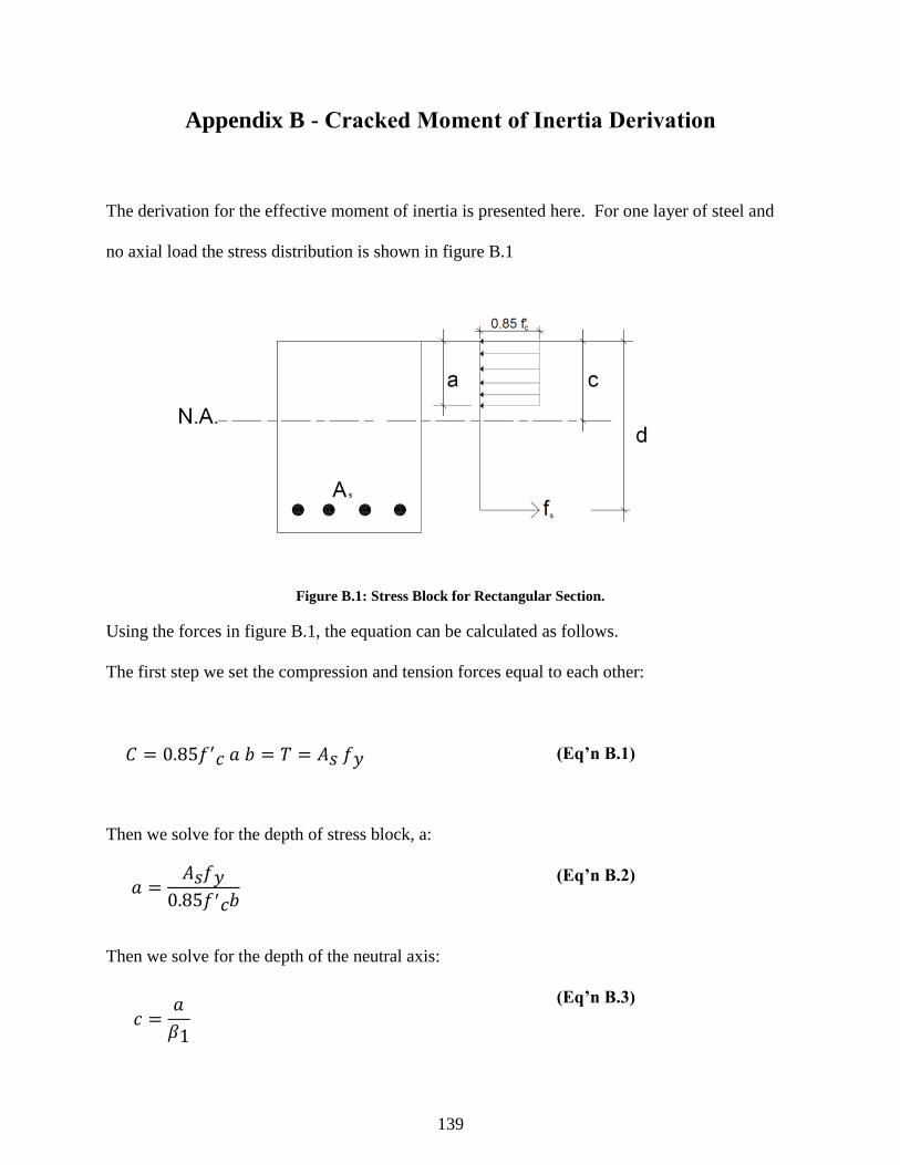
139
Appendix B - Cracked Moment of Inertia Derivation
The derivation for the effective moment of inertia is presented here. For one layer of steel and
no axial load the stress distribution is shown in figure B.1
Figure B.1: Stress Block for Rectangular Section.
Using the forces in figure B.1, the equation can be calculated as follows.
The first step we set the compression and tension forces equal to each other:
(Eq’n B.1)
Then we solve for the depth of stress block, a:
(Eq’n B.2)
Then we solve for the depth of the neutral axis:
(Eq’n B.3)
𝐶 = 0.85𝑓′𝑐 𝑎 𝑏 = 𝑇 = 𝐴𝑠 𝑓𝑦
𝑎 =𝐴𝑠𝑓𝑦
0.85𝑓′𝑐𝑏
𝑐 =𝑎
𝛽1
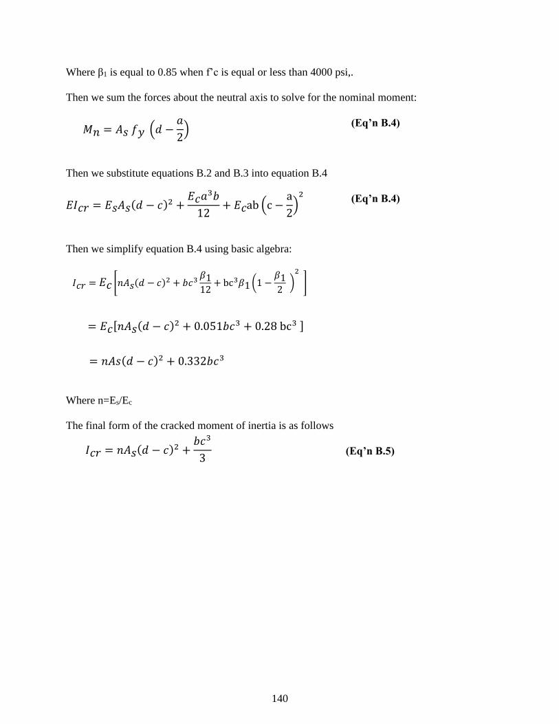
140
Where β1 is equal to 0.85 when f’c is equal or less than 4000 psi,.
Then we sum the forces about the neutral axis to solve for the nominal moment:
(Eq’n B.4)
Then we substitute equations B.2 and B.3 into equation B.4
(Eq’n B.4)
Then we simplify equation B.4 using basic algebra:
Where n=Es/Ec
The final form of the cracked moment of inertia is as follows
(Eq’n B.5)
𝑀𝑛 = 𝐴𝑠 𝑓𝑦 (𝑑 −𝑎
2)
𝐸𝐼𝑐𝑟 = 𝐸𝑠𝐴𝑠(𝑑 − 𝑐)2 +𝐸𝑐𝑎
3𝑏
12+ 𝐸𝑐ab (c −
a
2)
2
𝐼𝑐𝑟 = 𝑛𝐴𝑠(𝑑 − 𝑐)2 +𝑏𝑐3
3
𝐼𝑐𝑟 = 𝐸𝑐 [𝑛𝐴𝑠(𝑑 − 𝑐)2 + 𝑏𝑐3𝛽112
+ bc3𝛽1(1 −𝛽12
)2
]
= 𝐸𝑐[𝑛𝐴𝑠(𝑑 − 𝑐)2 + 0.051𝑏𝑐3 + 0.28 bc3 ]
= 𝑛𝐴𝑠(𝑑 − 𝑐)2 + 0.332𝑏𝑐3


