Seediscussions,stats,andauthorprofilesforthispublicationat:https://www.researchgate.net/publication/1858035

MagnetocaloricStudiesofthePeakEffectinNb

ArticleinPhysicalreview.B,Condensedmatter·November2006

DOI:10.1103/PhysRevB.75.174519·Source:arXiv

CITATIONS

8

READS

22

5authors,including:

NikosDaniilidis

UniversityofCalifornia,Berkeley

27PUBLICATIONS157CITATIONS

SEEPROFILE

I.K.Dimitrov

BrookhavenNationalLaboratory

32PUBLICATIONS176CITATIONS

SEEPROFILE

X.S.Ling

BrownUniversity

98PUBLICATIONS2,965CITATIONS

SEEPROFILE

Allin-textreferencesunderlinedinbluearelinkedtopublicationsonResearchGate,

lettingyouaccessandreadthemimmediately.

Availablefrom:NikosDaniilidis

Retrievedon:11September2016

arX

iv:c

ond-

mat

/061

1066

v1 [

cond

-mat

.sup

r-co

n] 2

Nov

200

6

Magnetocaloric Studies of the Peak Effect in Nb

N. D. Daniilidis,∗ I. K. Dimitrov, V. F. Mitrovic, C. Elbaum, and X. S. Ling†

Department of Physics, Brown University, Providence, Rhode Island 02912

(Dated: February 6, 2008)

Abstract

We report a magnetocaloric study of the peak effect and Bragg glass transition in a Nb single

crystal. The thermomagnetic effects due to vortex flow into and out of the sample are measured.

The magnetocaloric signature of the peak effect anomaly is identified. It is found that the peak

effect disappears in magnetocaloric measurements at fields significantly higher than those reported

in previous ac-susceptometry measurements. Investigation of the superconducting to normal tran-

sition reveals that the disappearance of the bulk peak effect is related to inhomogeneity broadening

of the superconducting transition. The emerging picture also explains the concurrent disappear-

ance of the peak effect and surface superconductivity, which was reported previously in the sample

under investigation. Based on our findings we discuss the possibilities of multicriticality associated

with the disappearance of the peak effect.

PACS numbers: 74.25.Op, 74.25.Qt, 61.12.Ex

∗Corresponding author: nikos@brown.edu†Corresponding author: xsling@brown.edu

1

I. INTRODUCTION

One very fascinating result in condensed matter physics in recent decades is the under-

standing that, in spite of early predictions,[1] the long-range topological order associated

with broken continuous symmetries can survive in systems with random pinning.[2, 3] In

bulk type-II superconductors with weak point-like disorder the existence of a novel Bragg

glass phase has been predicted.[3] This reaffirmed experimental facts known since the 1970s,

that vortex lattices in weak-pinning, bulk, type-II superconductors can produce pronounced

Bragg peaks in neutron diffraction.[4] Recent experiments[5, 6] have shown that a genuine

order-disorder transition occurs in vortex matter. This transition appears to be the un-

derlying mechanism of the well-known anomaly of the peak effect[7] in the critical current

near Hc2. However there are still many outstanding issues concerning the Bragg glass phase

boundary and the nature of the disordered vortex state above the peak effect.

Previous studies in a Niobium single crystal have revealed an intriguing picture of the

peak effect in weakly-pinned conventional superconductors. Neutron scattering has shown

that a vortex lattice order-disorder transition occurs in the peak effect region. This transition

shows hysteresis and is believed to be first order, separating a low temperature ordered phase

from a high temperature disordered one.[5] The hysteresis was not observed across the lower

field part of the superconducting-to-normal phase boundary. Magnetic ac-susceptometry

showed that at lower fields the peak effect disappears as well, indicating further connection

between the peak effect and the order-disorder transition.[8] In addition, the line of sur-

face superconductivity, Hc3, terminates in the vicinity of the region where the peak effect

disappears. This picture is summarized in Fig. 1.

It was thus proposed that the peak effect is the manifestation of a first-order transition

which terminates at a multicritical point (MCP) where the peak effect line meets a contin-

uous, Abrikosov transition, Hc2. The MCP would be bicritical if a third line of continuous

transitions ends there. The transition lines considered as a possible third candidate were a

continuous vortex glass transition, Tc2, and the line of surface superconductivity. Alterna-

tively, the MCP would be tricritical if the disordered phase is a pinned liquid with no high

field transition into the normal state.[8] Subsequently, the disappearance of the peak effect

at low fields has also been reported in other systems.[9, 10]

Thermodynamic considerations[8] suggest that the MCP is likely a bicritical point. Since

2

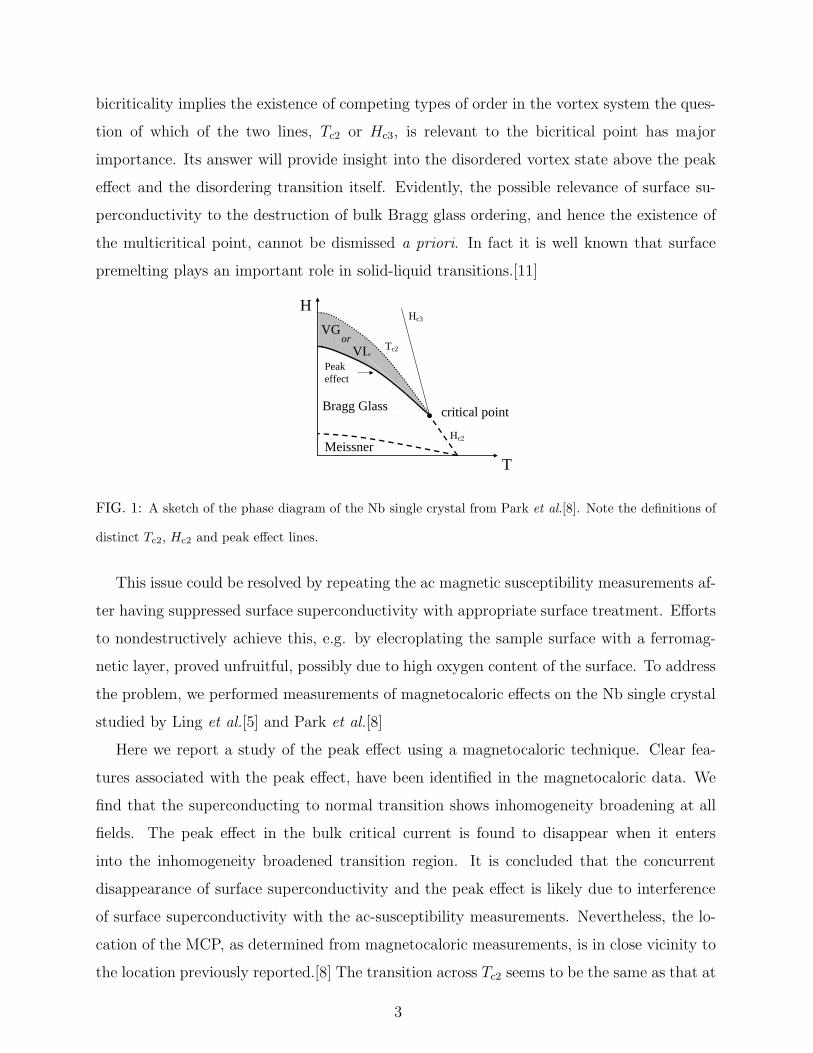
bicriticality implies the existence of competing types of order in the vortex system the ques-

tion of which of the two lines, Tc2 or Hc3, is relevant to the bicritical point has major

importance. Its answer will provide insight into the disordered vortex state above the peak

effect and the disordering transition itself. Evidently, the possible relevance of surface su-

perconductivity to the destruction of bulk Bragg glass ordering, and hence the existence of

the multicritical point, cannot be dismissed a priori. In fact it is well known that surface

premelting plays an important role in solid-liquid transitions.[11]

T

H

Bragg Glass

Meissner

VL Tc2

Hc2

critical point

Peak effect

or VG

Hc3

FIG. 1: A sketch of the phase diagram of the Nb single crystal from Park et al.[8]. Note the definitions of

distinct Tc2, Hc2 and peak effect lines.

This issue could be resolved by repeating the ac magnetic susceptibility measurements af-

ter having suppressed surface superconductivity with appropriate surface treatment. Efforts

to nondestructively achieve this, e.g. by elecroplating the sample surface with a ferromag-

netic layer, proved unfruitful, possibly due to high oxygen content of the surface. To address

the problem, we performed measurements of magnetocaloric effects on the Nb single crystal

studied by Ling et al.[5] and Park et al.[8]

Here we report a study of the peak effect using a magnetocaloric technique. Clear fea-

tures associated with the peak effect, have been identified in the magnetocaloric data. We

find that the superconducting to normal transition shows inhomogeneity broadening at all

fields. The peak effect in the bulk critical current is found to disappear when it enters

into the inhomogeneity broadened transition region. It is concluded that the concurrent

disappearance of surface superconductivity and the peak effect is likely due to interference

of surface superconductivity with the ac-susceptibility measurements. Nevertheless, the lo-

cation of the MCP, as determined from magnetocaloric measurements, is in close vicinity to

the location previously reported.[8] The transition across Tc2 seems to be the same as that at

3

Hc2, and surface superconductivity plays only a coincidental role in the critical point. This

result suggests that the disordered vortex state, which is represented by the shaded part in

Fig. 1, is a distinct thermodynamic phase. Bicriticality implies that this phase has an order

parameter competing with that of the Bragg glass phase. We also discuss an alternative

scenario, in which no critical point exists at any finite field or temperature.

The paper is organized as follows: In Sec. II we review the basic principle of magne-

tocaloric measurements, and give the experimental details of the sample and the technique

used. In Sec. III we present our main results, discuss the consequences of irreversible and

nonequilibrium effects on magnetocaloric measurements, and proceed to interpretation of the

data and estimates of sample properties. Finally we summarize our findings and conclusions,

and propose experimental work necessary to address the issues raised.

II. EXPERIMENTAL

A. Basic principle of magnetocaloric measurements

1. Heat flow in magnetocaloric measurements

In studies of vortex phases in bulk superconductors, various experimental techniques

provide complementary pieces of information. Combining these in a consistent picture is a

non-trivial task. Magnetic ac-susceptibility measurements are sensitive to screening currents,

and thus to the location of peak effect features, but are not suitable for the identification and

study of the mean field Hc2 transition itself.[8] Commercial magnetometers are not suited for

study of large samples. Calorimetric[12, 13] and ultrasonic attenuation[14, 15] measurements

determine the upper critical field where bulk condensation of Cooper pairs occurs, but

it remains unclear under what circumstances they also provide a peak effect signature.

Moreover the combination of information obtained with different techniques has to rely

on thermometer calibration issues. Furthermore, the dynamical measurements suffer from

thermal gradients in the studied samples. Magnetocaloric measurements overcome these

difficulties because they are sensitive to both the presence of bulk superconductivity and

to dynamical, flux-flow related effects. Moreover they can be performed in quasi-adiabatic

conditions, where virtually no thermal gradients are present in the sample. Finally, they

can be easily performed using a common calorimeter.

4

The magnetocaloric effect is a special case of thermomagnetic effects in the mixed-state

of superconductors which have long been known and investigated.[16] These arise from the

coexistence of the superconducting condensate which is not involved in entropy-exchange

processes for the superconductor, and the quasiparticles, localized in the vortex cores, which

are entropy carriers. Due to the presence of localized quasiparticles in the vortex cores,

vortex motion results in entropy transport, which causes measurable thermal effects. Specfi-

cally, during field increase, new vortices are created at the edge of the sample, quasiparticles

inside the vortices absorb entropy from the atomic lattice and cause quasi-adiabatic cooling

of the sample. Conversely, during field decrease, the exiting vortices release their entropy to

the atomic lattice, causing quasi-adiabatic heating.

Typically, in an experiment, the amount of entropy carried by the vortices entering or

leaving the sample is not the exact thermodynamic equilibrium vortex entropy. The rea-

son is that the vortex assembly is not equilibrated due to pinning as well as metastability

associated with the underlying first-order phase transition at the peak effect. In practice,

the magnetocaloric cooling and heating due to vortex entry and exit can be understood

formally in terms of the actual entropy exchange between the vortex and atomic lattices. A

superconductor subject to a changing magnetic field and allowed to exchange heat with the

environment, undergoes a temperature change.[17] This process is described by the relation:

dQabs/dt = n Ts (∂s/∂H)T dH/dt + n Cs dTs/dt (1)

where dQabs/dt is the net rate of heat absorption, positive for absorption of heat by the

sample, n is the molar number of the superconductor, Ts its temperature, Ts (∂s/∂H)T

the molar magnetocaloric coefficient, and Cs the specific heat of the superconductor. The

magnetocaloric term in the equation induces temperature changes. These are smeared out by

the last term, describing the effect of specific heat. Nevertheless, in practice this last term is

constrained to be negligible when magnetocaloric effects are measured. In our measurements,

we use very low field ramp rates (dH/dt), which result in very low temperature change rates

(dTs/dt) causing the last term to be negligible.

A schematic of our setup is represented in Fig. 2a. In this setup, absorption or release

of heat from the sample results in minute, but measurable, variation of its temperature.

In a typical measurement, the sample temperature is first fixed at a selected value, Ts0.

Subsequently, the field is ramped at a steady rate, resulting in quasi-adiabatic absorption

5

or release of heat from the sample. The resulting sample temperature change is recorded.

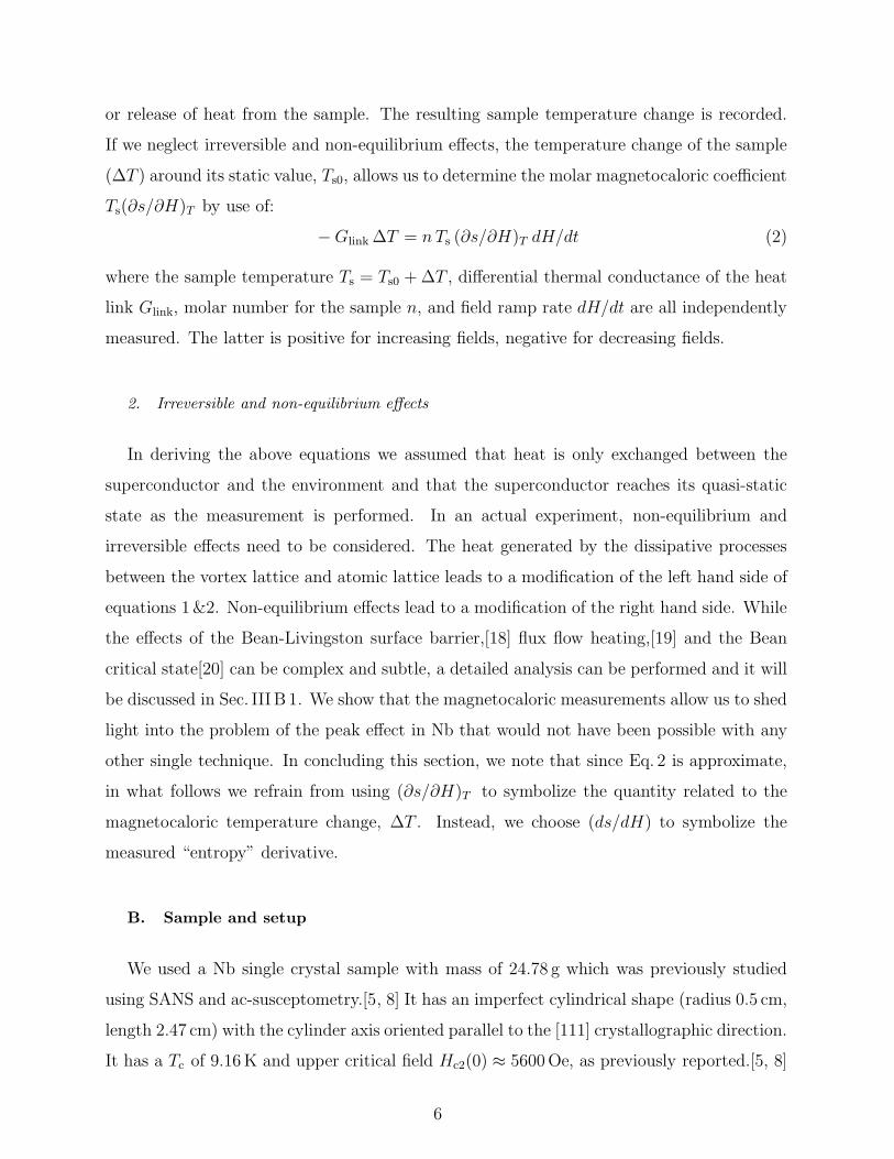
If we neglect irreversible and non-equilibrium effects, the temperature change of the sample

(∆T ) around its static value, Ts0, allows us to determine the molar magnetocaloric coefficient

Ts(∂s/∂H)T by use of:

− Glink ∆T = n Ts (∂s/∂H)T dH/dt (2)

where the sample temperature Ts = Ts0 + ∆T , differential thermal conductance of the heat

link Glink, molar number for the sample n, and field ramp rate dH/dt are all independently

measured. The latter is positive for increasing fields, negative for decreasing fields.

2. Irreversible and non-equilibrium effects

In deriving the above equations we assumed that heat is only exchanged between the

superconductor and the environment and that the superconductor reaches its quasi-static

state as the measurement is performed. In an actual experiment, non-equilibrium and

irreversible effects need to be considered. The heat generated by the dissipative processes

between the vortex lattice and atomic lattice leads to a modification of the left hand side of

equations 1&2. Non-equilibrium effects lead to a modification of the right hand side. While

the effects of the Bean-Livingston surface barrier,[18] flux flow heating,[19] and the Bean

critical state[20] can be complex and subtle, a detailed analysis can be performed and it will

be discussed in Sec. III B 1. We show that the magnetocaloric measurements allow us to shed

light into the problem of the peak effect in Nb that would not have been possible with any

other single technique. In concluding this section, we note that since Eq. 2 is approximate,

in what follows we refrain from using (∂s/∂H)T to symbolize the quantity related to the

magnetocaloric temperature change, ∆T . Instead, we choose (ds/dH) to symbolize the

measured “entropy” derivative.

B. Sample and setup

We used a Nb single crystal sample with mass of 24.78 g which was previously studied

using SANS and ac-susceptometry.[5, 8] It has an imperfect cylindrical shape (radius 0.5 cm,

length 2.47 cm) with the cylinder axis oriented parallel to the [111] crystallographic direction.

It has a Tc of 9.16 K and upper critical field Hc2(0) ≈ 5600 Oe, as previously reported.[5, 8]

6

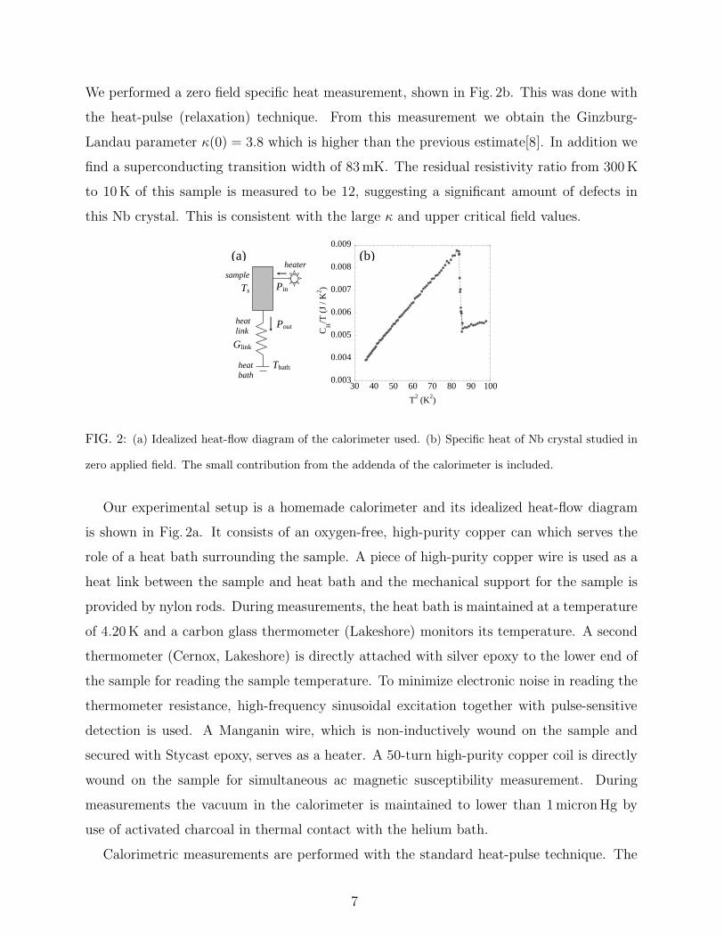
We performed a zero field specific heat measurement, shown in Fig. 2b. This was done with

the heat-pulse (relaxation) technique. From this measurement we obtain the Ginzburg-

Landau parameter κ(0) = 3.8 which is higher than the previous estimate[8]. In addition we

find a superconducting transition width of 83 mK. The residual resistivity ratio from 300 K

to 10 K of this sample is measured to be 12, suggesting a significant amount of defects in

this Nb crystal. This is consistent with the large κ and upper critical field values.

0.003

0.004

0.005

0.006

0.007

0.008

0.009

30 40 50 60 70 80 90 100

CH/T

(J

/ K2 )

T2 (K2)

(b)

Pout

Pin

Tbath

Ts

Glink

(a) heater

sample

heat bath

heat link

FIG. 2: (a) Idealized heat-flow diagram of the calorimeter used. (b) Specific heat of Nb crystal studied in

zero applied field. The small contribution from the addenda of the calorimeter is included.

Our experimental setup is a homemade calorimeter and its idealized heat-flow diagram

is shown in Fig. 2a. It consists of an oxygen-free, high-purity copper can which serves the

role of a heat bath surrounding the sample. A piece of high-purity copper wire is used as a

heat link between the sample and heat bath and the mechanical support for the sample is

provided by nylon rods. During measurements, the heat bath is maintained at a temperature

of 4.20 K and a carbon glass thermometer (Lakeshore) monitors its temperature. A second

thermometer (Cernox, Lakeshore) is directly attached with silver epoxy to the lower end of

the sample for reading the sample temperature. To minimize electronic noise in reading the

thermometer resistance, high-frequency sinusoidal excitation together with pulse-sensitive

detection is used. A Manganin wire, which is non-inductively wound on the sample and

secured with Stycast epoxy, serves as a heater. A 50-turn high-purity copper coil is directly

wound on the sample for simultaneous ac magnetic susceptibility measurement. During

measurements the vacuum in the calorimeter is maintained to lower than 1 micron Hg by

use of activated charcoal in thermal contact with the helium bath.

Calorimetric measurements are performed with the standard heat-pulse technique. The

7

heat input to the sample is increased incrementally, with step duration of 60-100 sec. Every

incremental increase of the heat input results in exponential temporal relaxation of the

sample temperature to its new equilibrium value. The sample heat capacity is determined

through the decay time of the exponential. This technique offers moderate resolution and

is not suited for studying the thermodynamics of the peak effect. Nevertheless, it allows us

to characterize our sample. In Fig. 2b, we show the data acquired in zero applied field, from

which we measured the sample properties quoted above.

During magnetocaloric measurements, a constant heat input, Pin, is supplied to the

sample through the manganin heater, fixing the temperature at a selected static value, Ts0.

After the sample temperature has stabilized to Ts0, the magnetic field is ramped up, then

down, at a constant rate. During a field ramp, the sample temperature as a function of field,

Ts(H), is recorded. The magnetocaloric signal, ∆T (H), has to be measured with respect to

a field dependent, static sample temperature reading : Ts0 = Ts0(H). This is the thermometer

reading obtained at a given field, H , in the absence of field ramping. In other words one

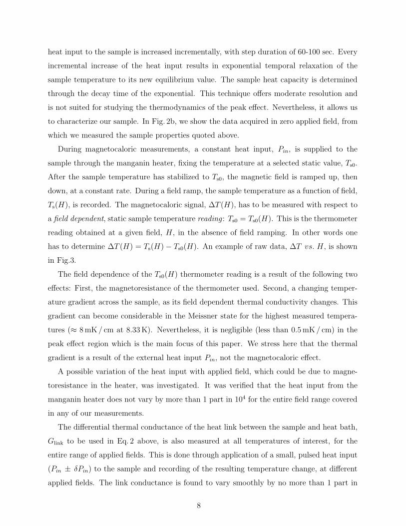
has to determine ∆T (H) = Ts(H) − Ts0(H). An example of raw data, ∆T vs. H , is shown

in Fig.3.

The field dependence of the Ts0(H) thermometer reading is a result of the following two

effects: First, the magnetoresistance of the thermometer used. Second, a changing temper-

ature gradient across the sample, as its field dependent thermal conductivity changes. This

gradient can become considerable in the Meissner state for the highest measured tempera-

tures (≈ 8 mK / cm at 8.33 K). Nevertheless, it is negligible (less than 0.5 mK / cm) in the

peak effect region which is the main focus of this paper. We stress here that the thermal

gradient is a result of the external heat input Pin, not the magnetocaloric effect.

A possible variation of the heat input with applied field, which could be due to magne-

toresistance in the heater, was investigated. It was verified that the heat input from the

manganin heater does not vary by more than 1 part in 104 for the entire field range covered

in any of our measurements.

The differential thermal conductance of the heat link between the sample and heat bath,

Glink to be used in Eq. 2 above, is also measured at all temperatures of interest, for the

entire range of applied fields. This is done through application of a small, pulsed heat input

(Pin ± δPin) to the sample and recording of the resulting temperature change, at different

applied fields. The link conductance is found to vary smoothly by no more than 1 part in

8

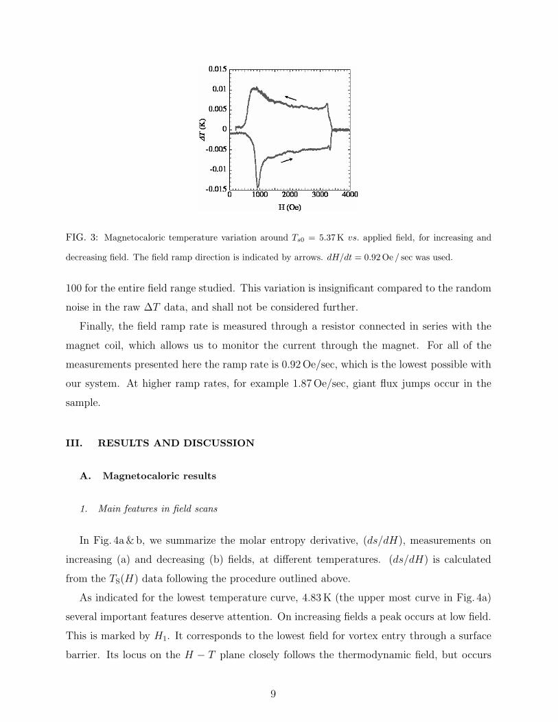
FIG. 3: Magnetocaloric temperature variation around Ts0 = 5.37K vs. applied field, for increasing and

decreasing field. The field ramp direction is indicated by arrows. dH/dt = 0.92 Oe / sec was used.

100 for the entire field range studied. This variation is insignificant compared to the random

noise in the raw ∆T data, and shall not be considered further.

Finally, the field ramp rate is measured through a resistor connected in series with the

magnet coil, which allows us to monitor the current through the magnet. For all of the

measurements presented here the ramp rate is 0.92 Oe/sec, which is the lowest possible with

our system. At higher ramp rates, for example 1.87 Oe/sec, giant flux jumps occur in the

sample.

III. RESULTS AND DISCUSSION

A. Magnetocaloric results

1. Main features in field scans

In Fig. 4a&b, we summarize the molar entropy derivative, (ds/dH), measurements on

increasing (a) and decreasing (b) fields, at different temperatures. (ds/dH) is calculated

from the TS(H) data following the procedure outlined above.

As indicated for the lowest temperature curve, 4.83 K (the upper most curve in Fig. 4a)

several important features deserve attention. On increasing fields a peak occurs at low field.

This is marked by H1. It corresponds to the lowest field for vortex entry through a surface

barrier. Its locus on the H − T plane closely follows the thermodynamic field, but occurs

9

slightly lower. This behavior is expected for a sample with finite demagnetizing factor and

mesoscopic surface irregularities.[21] No corresponding peak is present on decreasing fields.

Rather, a smoother increase of (ds/dH) occurs as the field is lowered, before entry of part

of the sample into the Meissner state where the magnetocaloric signal vanishes, as seen in

figures 3&4b.

In intermediate fields, we identify a novel feature which was not observed in previous

magnetic susceptibility studies.[8] This appears as a knee in (ds/dH), which shows larger

negative slope as a function of field for fields lower than Hknee, as illustrated in Fig. 4c.

The feature is the same for both field-ramp directions. With our setup we can identify the

Hknee feature up to 7.41 K. As the temperature is increased, the region between H1 and Hc2

narrows and it becomes increasingly difficult to discern Hknee. Thus it is unclear how this

new feature terminates, i.e. whether it ends on the Hc2 line at around H = 1000 Oe, or if it

continues to lower fields.

At high field, across Hc2, the equilibrium mean-field theory of Abrikosov predicts a step

function for (∂m/∂T )H .[26] Thus, in the simplest picture one would expect a simple step

function for the molar entropy derivative (∂s/∂H)T at Hc2. Instead, we observe that across

the peak-effect regime, complex features of valley and peak appear in (ds/dH) below the

field marked Hupc2 . The valley in (ds/dH) corresponds to the peak effect, as seen in Fig. 4.

Similar features appear in decreasing field. At fields above the peak effect, the disappearance

of the magnetocaloric effect marks the upper critical field, Hc2. As we will soon discuss,

our magnetocaloric measurements indicate that the upper critical field shows inhomogeneity

broadening, in agreement with the zero field calorimetric data mentioned in section IIC. In

Fig. 4 we mark with Hupc2 the upper end of the upper critical field. This is the value of field

at which the magnetocaloric signal in the mixed state exceeds noise levels. Our technique

is not sensitive to Hc3 effects and the data are featureless above Hupc2 .

2. Identification of the peak effect

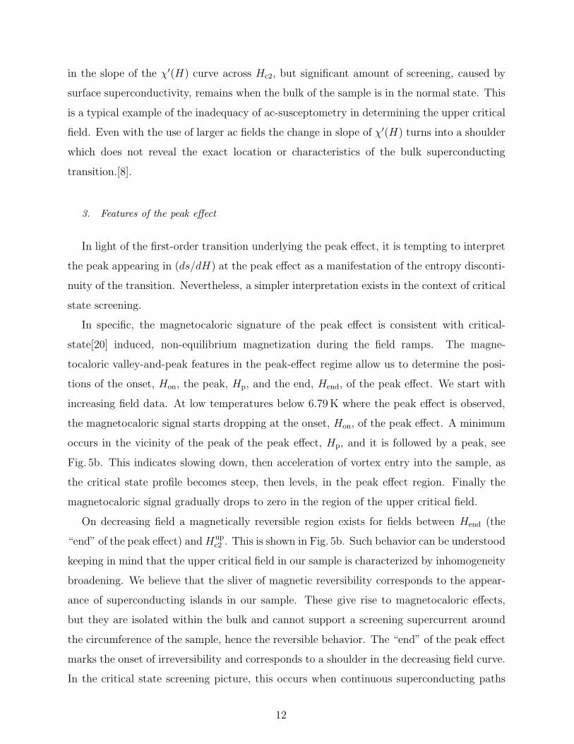
To verify the identification of the peak effect in our measurements, we performed simul-

taneous magnetocaloric and ac-susceptibility measurements, as shown in Fig. 5a. In the

quasi-adiabatic magnetocaloric setup, the ac-amplitude used in this procedure has to be

small. For large amplitudes inductive heating occurs in the mixed state on increasing dc

10

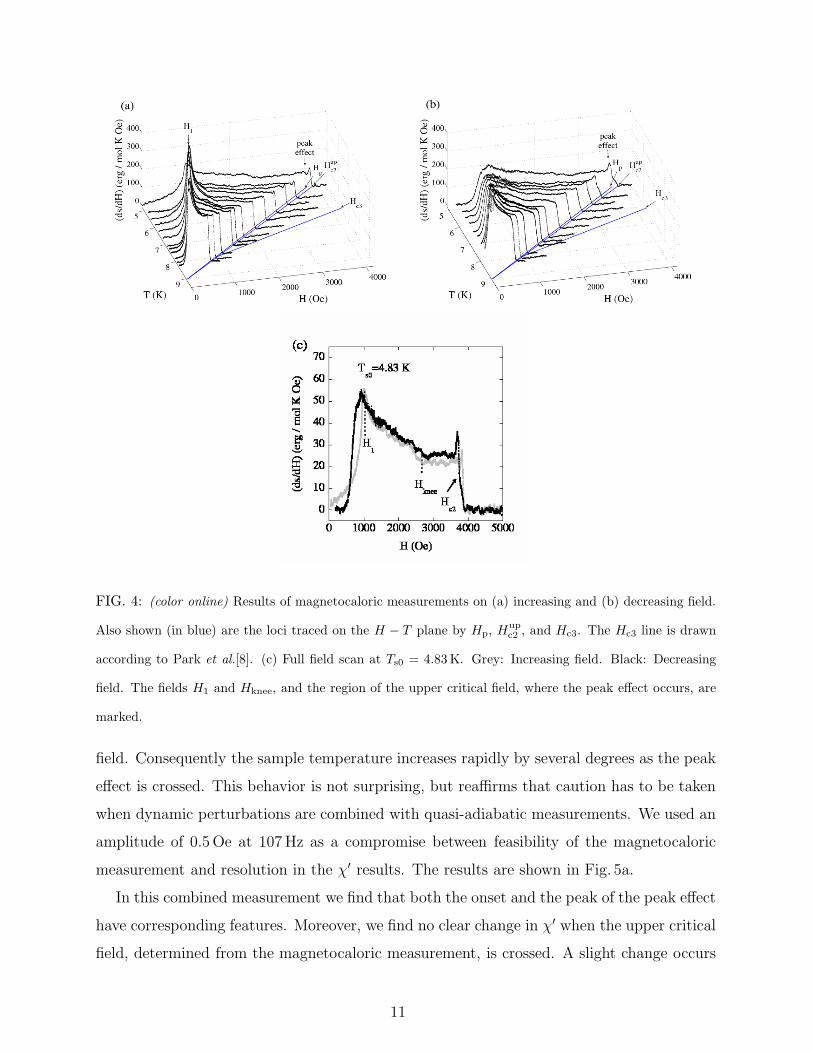
FIG. 4: (color online) Results of magnetocaloric measurements on (a) increasing and (b) decreasing field.

Also shown (in blue) are the loci traced on the H − T plane by Hp, Hupc2 , and Hc3. The Hc3 line is drawn

according to Park et al.[8]. (c) Full field scan at Ts0 = 4.83 K. Grey: Increasing field. Black: Decreasing

field. The fields H1 and Hknee, and the region of the upper critical field, where the peak effect occurs, are

marked.

field. Consequently the sample temperature increases rapidly by several degrees as the peak

effect is crossed. This behavior is not surprising, but reaffirms that caution has to be taken

when dynamic perturbations are combined with quasi-adiabatic measurements. We used an

amplitude of 0.5 Oe at 107 Hz as a compromise between feasibility of the magnetocaloric

measurement and resolution in the χ′ results. The results are shown in Fig. 5a.

In this combined measurement we find that both the onset and the peak of the peak effect

have corresponding features. Moreover, we find no clear change in χ′ when the upper critical

field, determined from the magnetocaloric measurement, is crossed. A slight change occurs

11

in the slope of the χ′(H) curve across Hc2, but significant amount of screening, caused by

surface superconductivity, remains when the bulk of the sample is in the normal state. This

is a typical example of the inadequacy of ac-susceptometry in determining the upper critical

field. Even with the use of larger ac fields the change in slope of χ′(H) turns into a shoulder

which does not reveal the exact location or characteristics of the bulk superconducting

transition.[8].

3. Features of the peak effect

In light of the first-order transition underlying the peak effect, it is tempting to interpret

the peak appearing in (ds/dH) at the peak effect as a manifestation of the entropy disconti-

nuity of the transition. Nevertheless, a simpler interpretation exists in the context of critical

state screening.

In specific, the magnetocaloric signature of the peak effect is consistent with critical-

state[20] induced, non-equilibrium magnetization during the field ramps. The magne-

tocaloric valley-and-peak features in the peak-effect regime allow us to determine the posi-

tions of the onset, Hon, the peak, Hp, and the end, Hend, of the peak effect. We start with

increasing field data. At low temperatures below 6.79 K where the peak effect is observed,

the magnetocaloric signal starts dropping at the onset, Hon, of the peak effect. A minimum

occurs in the vicinity of the peak of the peak effect, Hp, and it is followed by a peak, see

Fig. 5b. This indicates slowing down, then acceleration of vortex entry into the sample, as

the critical state profile becomes steep, then levels, in the peak effect region. Finally the

magnetocaloric signal gradually drops to zero in the region of the upper critical field.

On decreasing field a magnetically reversible region exists for fields between Hend (the

“end” of the peak effect) and Hupc2 . This is shown in Fig. 5b. Such behavior can be understood

keeping in mind that the upper critical field in our sample is characterized by inhomogeneity

broadening. We believe that the sliver of magnetic reversibility corresponds to the appear-

ance of superconducting islands in our sample. These give rise to magnetocaloric effects,

but they are isolated within the bulk and cannot support a screening supercurrent around

the circumference of the sample, hence the reversible behavior. The “end” of the peak effect

marks the onset of irreversibility and corresponds to a shoulder in the decreasing field curve.

In the critical state screening picture, this occurs when continuous superconducting paths

12

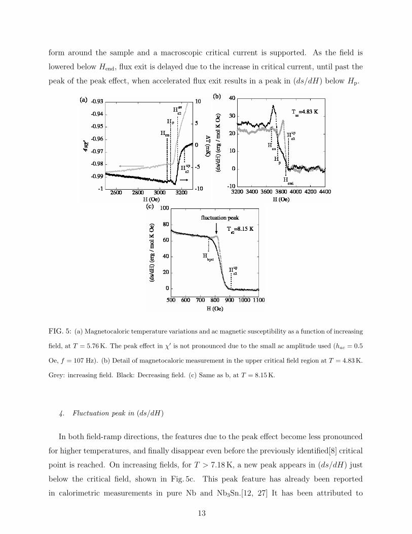
form around the sample and a macroscopic critical current is supported. As the field is

lowered below Hend, flux exit is delayed due to the increase in critical current, until past the

peak of the peak effect, when accelerated flux exit results in a peak in (ds/dH) below Hp.

FIG. 5: (a) Magnetocaloric temperature variations and ac magnetic susceptibility as a function of increasing

field, at T = 5.76 K. The peak effect in χ′ is not pronounced due to the small ac amplitude used (hac = 0.5

Oe, f = 107 Hz). (b) Detail of magnetocaloric measurement in the upper critical field region at T = 4.83 K.

Grey: increasing field. Black: Decreasing field. (c) Same as b, at T = 8.15 K.

4. Fluctuation peak in (ds/dH)

In both field-ramp directions, the features due to the peak effect become less pronounced

for higher temperatures, and finally disappear even before the previously identified[8] critical

point is reached. On increasing fields, for T > 7.18 K, a new peak appears in (ds/dH) just

below the critical field, shown in Fig. 5c. This peak feature has already been reported

in calorimetric measurements in pure Nb and Nb3Sn.[12, 27] It has been attributed to

13

critical fluctuations in the superconducting order parameter which set in as the critical

field is approached.[28] In our measurements we see the effect of critical-fluctuation entropy

enhancement in (∂s/∂H)T . We expect the same peak to exist in the curves displaying

the peak effect feature, but its presence will be obscured by the dramatic results of non-

equilibrium magnetization discussed above. Interestingly a similar peak is not observed

on the decreasing field data, Fig. 5c. Moreover, it is evident in Fig. 5c, that apart from

hysteretic behavior over an approximately 100 Oe wide region between Hhyst and Hupc2 the

behavior of the sample is reversible to within noise levels. This behavior occurs consistently

at all temperatures where the peak effect is not observed.

5. The superconducting to normal transition region

A very striking feature of our data is the invariance of the shape of the transition into (or

out of) the bulk normal state with changing temperature, or critical field. For increasing

fields, the transition into the normal state occurs between the fields H0 and Hupc2 , where

(ds/dH) drops to zero monotonically, as shown in Fig. 6a. To illustrate this, in Fig.6 we

show the normalized entropy derivatives as a function of field for temperatures ranging from

4.83 K to 8.33 K, with an expanded view of the upper critical field region. The normalization

has been performed such that the average of (ds/dH)norm over a 50 Oe wide region below

the onset of the peak effect equals unity. The curves have also been horizontally offset, on

a ∆H = H−Hupc2 axis. The horizontal alignment can alternatively be performed by aligning

the ordinate of either H0, or the part of the curve where the signal equals a given value, for

example 0.1 in the normalized Y axis. All different criteria result in alignments differing by

only a few Oe. The case is similar for decreasing fields.

In Fig. 6a we present increasing field data that display the peak effect on the normal-

ized/offset axes. For comparison, one curve which does not display the peak effect has been

included. This corresponds to T=7.41K. In Fig. 6b we present the corresponding decreas-

ing field data. In Fig. 6c we show only curves without a peak effect, for both increasing

and decreasing field. These figures illustrate the uniform characteristics of the transition

between the mixed state and the normal state. This is most evident in Fig. 6c: All different

curves collapse onto one uniform curve for each field ramp direction. In figures 6a&b, the

occurrence of the peak effect results in variations of the magnetocaloric signal around this

14

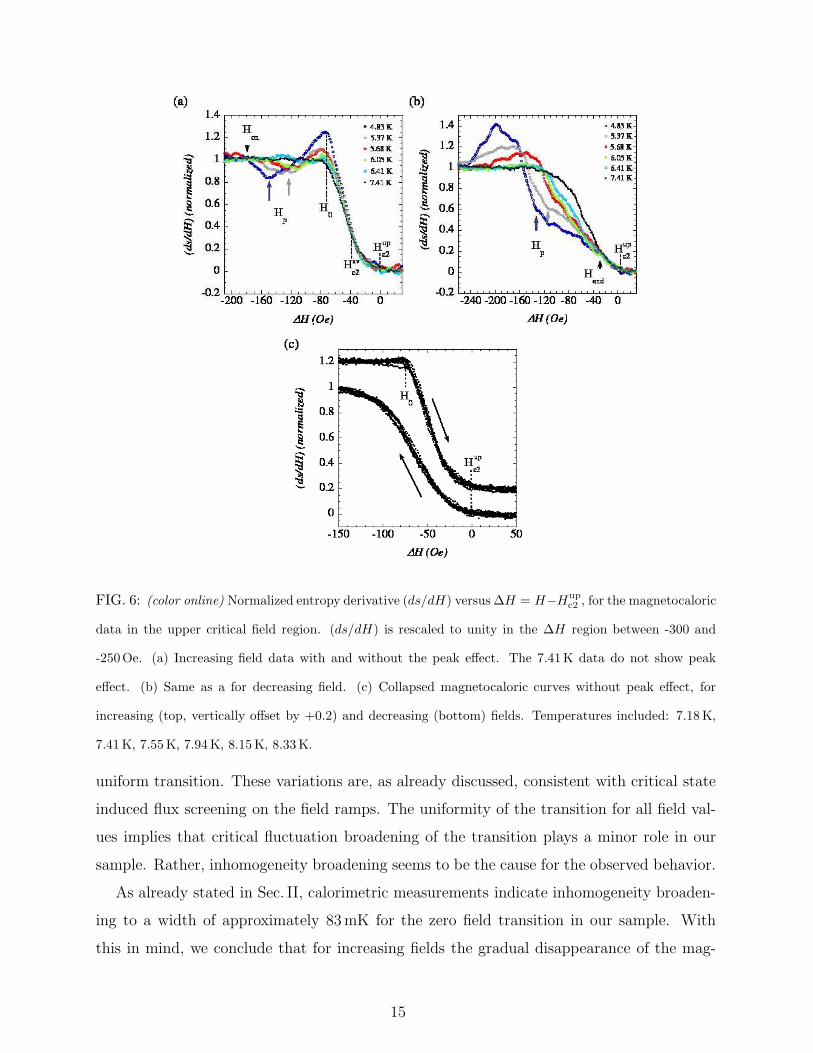
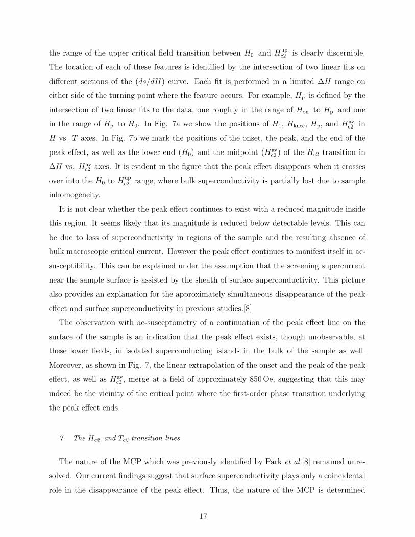
FIG. 6: (color online) Normalized entropy derivative (ds/dH) versus ∆H = H−Hupc2 , for the magnetocaloric

data in the upper critical field region. (ds/dH) is rescaled to unity in the ∆H region between -300 and

-250Oe. (a) Increasing field data with and without the peak effect. The 7.41K data do not show peak

effect. (b) Same as a for decreasing field. (c) Collapsed magnetocaloric curves without peak effect, for

increasing (top, vertically offset by +0.2) and decreasing (bottom) fields. Temperatures included: 7.18 K,

7.41 K, 7.55 K, 7.94 K, 8.15 K, 8.33 K.

uniform transition. These variations are, as already discussed, consistent with critical state

induced flux screening on the field ramps. The uniformity of the transition for all field val-

ues implies that critical fluctuation broadening of the transition plays a minor role in our

sample. Rather, inhomogeneity broadening seems to be the cause for the observed behavior.

As already stated in Sec. II, calorimetric measurements indicate inhomogeneity broaden-

ing to a width of approximately 83mK for the zero field transition in our sample. With

this in mind, we conclude that for increasing fields the gradual disappearance of the mag-

15

0

1000

2000

3000

4000

5000

4 5 6 7 8 9

H (

Oe)

T (K)

Hknee

H1

Hc2

av

Hp

(a)

-200

-150

-100

-50

0

0 1000 2000 3000 4000

H-H

c2 (

Oe)

Hc2

(Oe)av

up

Hc2

avH

end

H0

Hp

Hon

(b)

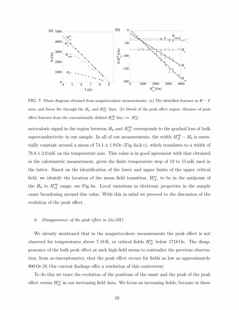
FIG. 7: Phase diagram obtained from magnetocaloric measurements. (a) The identified features in H − T

axes, and linear fits through the Hp and Havc2 lines. (b) Detail of the peak effect region: distance of peak

effect features from the conventionally defined Hupc2 line, vs. Hav

c2 .

netocaloric signal in the region between H0 and Hupc2 corresponds to the gradual loss of bulk

superconductivity in our sample. In all of our measurements, the width Hupc2 − H0 is essen-

tially constant around a mean of 74.1 ± 1.9 Oe (Fig. 6a& c), which translates to a width of

78.8± 2.0 mK on the temperature axis. This value is in good agreement with that obtained

in the calorimetric measurement, given the finite temperature step of 10 to 15mK used in

the latter. Based on the identification of the lower and upper limits of the upper critical

field, we identify the location of the mean field transition, Havc2 , to be in the midpoint of

the H0 to Hupc2 range, see Fig. 6a. Local variations in electronic properties in the sample

cause broadening around this value. With this in mind we proceed to the discussion of the

evolution of the peak effect.

6. Disappearance of the peak effect in (ds/dH)

We already mentioned that in the magnetocaloric measurements the peak effect is not

observed for temperatures above 7.18 K, or critical fields Havc2 below 1718 Oe. The disap-

pearance of the bulk peak effect at such high field seems to contradict the previous observa-

tion, from ac-susceptometry, that the peak effect occurs for fields as low as approximately

900 Oe.[8] Our current findings offer a resolution of this controversy.

To do this we trace the evolution of the positions of the onset and the peak of the peak

effect versus Havc2 in our increasing field data. We focus on increasing fields, because in these

16

the range of the upper critical field transition between H0 and Hupc2 is clearly discernible.

The location of each of these features is identified by the intersection of two linear fits on

different sections of the (ds/dH) curve. Each fit is performed in a limited ∆H range on

either side of the turning point where the feature occurs. For example, Hp is defined by the

intersection of two linear fits to the data, one roughly in the range of Hon to Hp and one

in the range of Hp to H0. In Fig. 7a we show the positions of H1, Hknee, Hp, and Havc2 in

H vs. T axes. In Fig. 7b we mark the positions of the onset, the peak, and the end of the

peak effect, as well as the lower end (H0) and the midpoint (Havc2 ) of the Hc2 transition in

∆H vs. Havc2 axes. It is evident in the figure that the peak effect disappears when it crosses

over into the H0 to Hupc2 range, where bulk superconductivity is partially lost due to sample

inhomogeneity.

It is not clear whether the peak effect continues to exist with a reduced magnitude inside

this region. It seems likely that its magnitude is reduced below detectable levels. This can

be due to loss of superconductivity in regions of the sample and the resulting absence of

bulk macroscopic critical current. However the peak effect continues to manifest itself in ac-

susceptibility. This can be explained under the assumption that the screening supercurrent

near the sample surface is assisted by the sheath of surface superconductivity. This picture

also provides an explanation for the approximately simultaneous disappearance of the peak

effect and surface superconductivity in previous studies.[8]

The observation with ac-susceptometry of a continuation of the peak effect line on the

surface of the sample is an indication that the peak effect exists, though unobservable, at

these lower fields, in isolated superconducting islands in the bulk of the sample as well.

Moreover, as shown in Fig. 7, the linear extrapolation of the onset and the peak of the peak

effect, as well as Havc2 , merge at a field of approximately 850 Oe, suggesting that this may

indeed be the vicinity of the critical point where the first-order phase transition underlying

the peak effect ends.

7. The Hc2 and Tc2 transition lines

The nature of the MCP which was previously identified by Park et al.[8] remained unre-

solved. Our current findings suggest that surface superconductivity plays only a coincidental

role in the disappearance of the peak effect. Thus, the nature of the MCP is determined

17

from the nature of the Hc2 and Tc2 lines discussed in section I.

We have a means of comparing the Hc2 and Tc2 transitions. The approximate location of

the MCP in ac-susceptometry is at T =8.1K, H =900Oe. The disappearance of the peak

effect below 1718 Oe in the magnetocaloric measurements but only below approximately

900 Oe in ac-susceptometry, allows us to compare the transitions into the bulk normal state

on the two sides of the MCP. As shown in Fig. 6c, all the curves with Havc2 < 1718 Oe (or

equivalently T > 7.18 K) for both increasing and decreasing fields collapse strikingly on two

different curves. These data include transitions on both sides of the MCP. This suggests that

the phase transitions out of the Bragg Glass (Hc2) and disordered (Tc2) phases are of the

same nature. In other words, well defined vortices exist in the disordered vortex state above

the peak effect. Here “well defined” is taken to mean that their magnetocaloric signature is

indistinguishable from the one obtained in the transition between the normal and the Bragg

Glass phases. However, it has to be borne in mind that changes in critical behavior can be

subtle and hard to identify in our sample which shows significant inhomogeneity broadening.

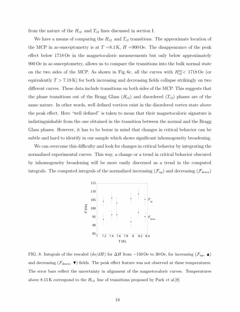
We can overcome this difficulty and look for changes in critical behavior by integrating the

normalized experimental curves. This way, a change or a trend in critical behavior obscured

by inhomogeneity broadening will be more easily discerned as a trend in the computed

integrals. The computed integrals of the normalized increasing (Fup) and decreasing (Fdown)

85

90

95

100

105

110

115

7 7.2 7.4 7.6 7.8 8 8.2 8.4

� (

Oe)

T (K)

�up

�down

FIG. 8: Integrals of the rescaled (ds/dH) for ∆H from −150Oe to 30Oe, for increasing (Fup, N)

and decreasing (Fdown, H) fields. The peak effect feature was not observed at these temperatures.

The error bars reflect the uncertainty in alignment of the magnetocaloric curves. Temperatures

above 8.15 K correspond to the Hc2 line of transitions proposed by Park et al.[8]

18

field curves around the region of the upper critical field are shown in Fig. 8. The integration

has been performed between ∆H = −150 Oe and 30 Oe in the aligned axis. More explicitly:

F =

∫ ∆H=30

∆H=−150

(ds/dH)normalized d(∆H) .

The error bars arise from the alignment uncertainty. All temperatures refer to the Tc2

transition, except for the two marked with an asterisk which correspond to Hc2. We see no

systematic trend in the result in any of the available temperatures. In conclusion, as far as

the inhomogeneity of our sample allows us to discern, there is no detectable change between

the low-field Hc2 transition and the high-field Tc2 transition to the normal state.

8. End of the peak effect

Finally, we discuss the “end” of the peak effect. Its position in the phase diagram is shown

in Fig. 7b. In our data Hend occurs in a range between 32 and 39Oe below Hupc2 and slightly

above the position of the average superconducting transition, Havc2 . Hend has been identified

as the field at which a superconducting network which can support a macroscopic screening

supercurrent forms inside the sample. The “end” feature occurs slightly above the midpoint

of the H0 to Hupc2 range, as shown in Fig. 7b. This indicates that the critical current appears

when roughly half of the sample is in the mixed state while the rest is still in the normal

state. This observation is very interesting but requires further investigation. The role of

surface superconductivity in establishing macroscopic supercurrents in the superconducting

network can be examined experimentally.

B. Discussion

1. Surface barrier, flux-flow heating, critical state screening

We can extend the conclusions from our measurements by evaluating the results of non-

equilibrium and irreversible processes in the magnetocaloric effect.

We start with the surface barrier. Its presence results in delay of flux entry into the

sample on increasing fields, up to a field approximately equal to the thermodynamic critical

field, HC .[21] In addition, the surface barrier has the more subtle consequence of introducing

an asymmetry between the measured ∆T on increasing and decreasing fields. On increasing

19

fields, vortices have to enter the sample through an energy barrier in a vortex free region.[22,

23] In this process, energy is dissipated approximately at a rate

Φ0 ·(

(HC2 + H2)1/2 − H

)

· (V/4π) · dH/dt ,

where V is the sample volume and HC the thermodynamic critical field.

In our measurements, for example at H ≈ 3000 Oe, this amounts to approximately 2 µW,

and will reduce the (negative) ∆T observed on increasing fields by roughly 1 mK. On

decreasing fields, the surface barrier has essentially no effect, and no irreversible heating is

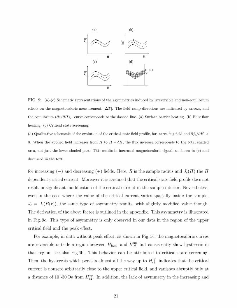
expected.[22] An asymmetry of this kind is shown schematically in Fig. 9a, and it is present

in our data, for example in Fig. 5b. Moreover, this type of asymmetry disappears for lower

values of the critical field, where surface superconductivity has disappeared,[8] for example

in Fig. 5c.

Flux flow heating of the sample also leads to a similar asymmetry between the ascending

and descending field branches. On increasing fields the negative ∆T is reduced and on

decreasing fields the positive ∆T increased. An order of magnitude estimate of flux-flow

heating can be obtained on the basis of the Bardeen-Stephen model.[24] For a cylindrical

sample of radius R, length L, and for smooth field ramping at a rate dH/dt, one obtains

Pff ≈ 107(dH/dt)2πR4L/(8ρff ). This turns out to be negligible for the field ramp rates,

approximately 1Oe/sec, used in our measurements. We show the effect of this mechanism,

grossly exaggerated, in Fig. 9b. Between the above two sources of irreversible heating, it is

clear that low field ramp rates will render the latter (∝ (dH/dt)2) negligible, but will not

reduce the effect of the former which scales as dH/dt, as does the magnetocaloric ∆T .

Next we examine the case of a non-equilibrium critical state profile outside the peak

effect region. A critical current that monotonically decreases with field, i.e. away from the

peak effect region, will result in the opposite asymmetry than the one just mentioned. This

is so, because on increasing fields the critical state profile becomes less steep, resulting in

faster loss of flux than the field ramp rate, and thus increased ∆T . The opposite occurs on

decreasing fields, resulting in a lower ∆T than indicated by the equilibrium Ts(∂s/∂H)T .

This mechanism is shown schematically in Fig. 9d. A simplified calculation for cylindrical

sample geometry, like the ones found in the literature, [20, 25] yields an asymmetry factor

in ∆T equal to:

1 ± (4πR/3c)(∂Jc/∂H)T (3)

20

(a)

H

|∆T

|

(b)

H

|∆T

|

(c)

H |∆

T|

(d)

FIG. 9: (a)-(c) Schematic representations of the asymmetries induced by irreversible and non-equilibrium

effects on the magnetocaloric measurement, |∆T |. The field ramp directions are indicated by arrows, and

the equilibrium (∂s/∂H)T curve corresponds to the dashed line. (a) Surface barrier heating. (b) Flux flow

heating. (c) Critical state screening.

(d) Qualitative schematic of the evolution of the critical state field profile, for increasing field and ∂jc/∂H <

0. When the applied field increases from H to H + δH , the flux increase corresponds to the total shaded

area, not just the lower shaded part. This results in increased magnetocaloric signal, as shown in (c) and

discussed in the text.

for increasing (−) and decreasing (+) fields. Here, R is the sample radius and Jc(H) the H

dependent critical current. Moreover it is assumed that the critical state field profile does not

result in significant modification of the critical current in the sample interior. Nevertheless,

even in the case where the value of the critical current varies spatially inside the sample,

Jc = Jc(B(r)), the same type of asymmetry results, with slightly modified value though.

The derivation of the above factor is outlined in the appendix. This asymmetry is illustrated

in Fig. 9c. This type of asymmetry is only observed in our data in the region of the upper

critical field and the peak effect.

For example, in data without peak effect, as shown in Fig. 5c, the magnetocaloric curves

are reversible outside a region between Hhyst and Hupc2 but consistently show hysteresis in

that region, see also Fig 6b. This behavior can be attributed to critical state screening.

Then, the hysteresis which persists almost all the way up to Hupc2 indicates that the critical

current is nonzero arbitrarily close to the upper critical field, and vanishes abruptly only at

a distance of 10 -30 Oe from Hupc2 . In addition, the lack of asymmetry in the increasing and

21

decreasing field curves below the hysteretic region, implies that the critical current density

varies very weakly with applied field. More specifically, the asymmetry in any of the data

without peak effect is less than 5% of the magnitude of (ds/dH). By Eq. 3 we obtain

(∂Jc/∂H)T < (1/2) · 0.05 · (3c/4πR) ≈ 0.36 A / cm2 Oe ,

where the numerical result is expressed in conventional units for convenience.

2. Critical current estimates

From the measurements we can estimate the value of the critical current before it vanishes

in the upper critical field region, in the context of critical state screening. We assume that

the entropy per vortex is essentially constant in the neighborhood of the upper critical

field and the peak effect.[29] Therefore changes in magnetic flux (∆Φ) are proportional to

changes in entropy, ∆Φ ∝ ∆S. Then an integral of ds/dH , such as Fup and Fdown, can be

approximately taken to represent a change in magnetic flux in the sample. In the critical

state model, we can relate changes in flux to the critical current.

At the temperatures where no peak effect is observed, we estimate the critical current in

the neighborhood of Hhyst. For simplicity we consider a linear field profile in the sample,

with slope

dH/dr = (4π/c) Jc ,

where r is the radial distance from the axis of the (cylindrical) sample. In the vicinity

of Hhyst simple integration gives a macroscopic magnetic flux difference (∆Φ) between the

increasing and decreasing field branch approximately equal to:

∆Φ =

(

1 +1

ζ

)

(16π2/3c) Jc(Hhyst) R3 .

see Eq.A.2 in the appendix. Due to the normalization performed for the integrals in Fig. 8

the flux difference is also approximately given by:

∆Φ = (Fup − Fdown) πR2 .

These two relations, allow us to obtain estimates for the critical current in the sample

before this collapses to zero in the upper critical field region. We show these in Fig. 10,

for temperatures above 7K, corresponding to the symbol for Jc. One should note that

22

0

100

200

300

400

500

600

700

800

4.5 5 5.5 6 6.5 7 7.5 8 8.5

J (A

/cm

2 )T (K)

c

FIG. 10: Estimated values of critical current in the neighborhood of the upper critical field in our sample.

For T > 7 K we show Jc (marked by H), the critical current at the limit of hysteresis, Hhyst, in temperatures

where no peak effect was observed. At temperatures below 7.18K where peak effect was observed we show

Jpc (N), the estimated critical current at the peak of the peak effect. The line is a guide to the eye.

critical currents with the values given for Jc in the figure, will lead to radial variation

of the induction inside the sample by roughly 10Oe. Due to the constraint imposed on

(∂Jc/∂H)T , (see discussion above), the critical current density will vary inside the sample

due to screened induction by less than 3.6A/cm2. This represents only 10% of its value,

and thus the assumption that the slope of the critical state profile (i.e. Jc(r)) is essentially

constant is self consistent.

A similar procedure can be followed for the curves showing the peak effect, in order to

estimate the critical current at the peak of the peak effect. This is most easily done for the

decreasing field, curves, under the additional assumption that the critical current increases

linearly from zero at Hend to Jpc at Hp. The integration relating the screened flux (∆Φ) to

these three quantities leads to the rather complicated equation:

{

∆H −∆Φ

πR2(1 + 1ζ)

}

x2 − 2∆Hx + 2∆H = 2∆He−x , (4)

where ∆H = Hend−Hp, x = (4π R Jpc )/(c ∆H). The screened flux for a curve with peak

effect is obtained via integration between Hp and Hupc2 with respect to the universal curve

of Fig. 6b (bottom). The resulting equations are solved numerically, and the results for Jpc

are shown in Fig. 10. The value at 6.79 K is not included, because the peak effect is barely

observable at that temperature, which makes the procedure we outlined inapplicable.

23

3. Low field hysteresis: alternative interpretaion

We return to the low-field hysteresis near Hc2, illustrated in Fig. 5b. The combination

of hysteretic and reversible behavior in the vicinity of Hc2 is striking. Furthermore this

behavior persists in all of the measurements which do not show the peak effect, down to an

upper critical field of 676 Oe. In addition, we suggested earlier that the disappearance of

the peak effect in our bulk measurements is due to loss of superconductivity in parts of the

sample, while in ac-susceptometry it is due to the disappearance of surface superconductivity.

Thus the possibility arises that the peak effect continues to exist at low fields, but it is not

observable with the techniques used so far. In other words, our data raise the question

whether the hysteretic order-disorder transition reported previously[5] continues down to

low fields, where no peak effect is observed, but hysteresis occurs over a range too narrow to

be detectable in neutron scattering. In this scenario, the hysteresis seen in Fig. 5c is related

to a first order phase transition. If this is the case the hysteresis presented here will be

observable in high resolution calorimetric measurements.

4. The “knee” feature

Finally we return to the newly identified “knee” feature, shown in Fig. 4c. From the occur-

rence of the knee in both ramp directions we conclude that it corresponds to an equilibrium

feature of the thermodynamic behavior inside the Bragg Glass phase. To appreciate this

argument, note that all three sources of irreversible and non-equilibrium effects discussed at

the beginning of this subsection, will induce asymmetry on the (ds/dH) curves for opposite

field-ramp directions. For example, the two curves of Fig. 4c show asymmetry, as already

mentioned. This is due to surface barrier-related heating on increasing field. On the other

hand, symmetric trends in the measured (ds/dH) curves have to be related to equilibrium

behavior, and we thus conclude that Hknee corresponds to an equilibrium feature. Neutron

scattering did not reveal any structural changes in the vortex lattice[5, 8] around Hknee,

which suggests that the nature of this feature is rather subtle. It would be interesting to

investigate the corresponding part of the phase diagram for changes in dynamical response,

as well as for a possible relation of this novel feature to the thermomagnetic instability in

Nb.

24

C. Summary

From the reported magnetocaloric-effect results, we gain a significant amount of novel

information about the Nb sample previously studied using SANS and ac-susceptometry.

The upper critical field shows significant inhomogeneity broadening. The broad Hc2

transition is related to the disappearance of the peak effect in bulk measurements. The

peak effect disappears in the phase diagram when it enters the range where regions of the

sample are normal. Yet, magnetic irreversibility, indicating nonzero critical currents, occurs

when regions of the sample are normal. The peak effect is observable with ac-susceptometry

at fields much lower than with magnetocaloric measurements. In the former case screening

occurs locally, near the surface,[8] presumably assisted by a superconducting surface layer.

This could indicate that the peak effect still occurs in the bulk of the sample in regions that

are superconducting.

The low field transition from the Bragg Glass phase into the normal state seems to be the

same as the high field transition between the structurally disordered[5] vortex state and the

normal state. Moreover, hysteresis occurs in magnetocaloric curves that do not display the

peak effect, but in the neighborhood of this hysteresis the non-equilibrium and irreversible

effect signatures that we discussed are absent. Finally a new feature corresponding to a

knee in the magnetocaloric coefficient has been identified and its position mapped out in

the phase diagram, Fig. 7 a. These new findings allow us to refine the previously proposed

peak effect phase diagram (Fig. 1), but also point to an alternative picture.

In the multicritical point picture, the magnetocaloric-effect results reported here have

strong implications for understanding the nature of the multicritical point where the peak

effect disappears.[8, 9, 10] A tricritical point can be ruled out since the change in slope

between the Hp and low field Hc2 lines would lead to violation of the 180◦ rule[8, 30] imposed

by thermodynamics. The fact that the magnetocaloric transition appears to be continuous

and of the same character across both Tc2 and Hc2, suggests that the critical point is bicritical.

Bicriticality implies the competition of two bulk vortex phases, an ordered Bragg glass[2, 3]

and a disordered vortex glass. The vortex glass phase is not necessarily superconducting

in the sense of the original proposal,[31] but it has to be a genuine phase possessing an

order parameter absent in the normal state,[33] and in competition with that of the Bragg

glass. In addition, it possesses superconducting phase rigidity even under partial loss of bulk

25

(mixed state) superconductivity.

Finally, we wish to discuss an alternative picture in which the order-disorder transition

does not end at the previously identified critical point. The experimental disappearance of

the peak effect in magnetocaloric measurements may be due to sample inhomogeneity. In

addition, the peak effect disappears in ac-susceptometry due to the disappearance of surface

superconductivity.[8] Nevertheless, the vortex lattice disordering transition can continue to

lower fields, where the peak effect is not detectable. Hysteresis related to a first order phase

transition occurs over a narrow range in this part of the phase diagram, and the width of the

hysteresis region grows appreciably only at higher fields where the peak effect is sufficiently

far from the Hc2 region. In this picture, no critical point associated with the disordering

transition exists at any finite field or temperature.[33]

IV. CONCLUSIONS

We have identified the magnetocaloric signatures of the peak effect in a Nb single crystal.

In addition we classified and outlined the various sources of irreversible and non-equilibrium

effects occurring in such measurements and offered ways for their evaluation. With these in

mind, magnetocaloric measurements prove very useful in studies of the mixed state. They

are suitable for studying the upper critical field region. They allow the identification and

study of dynamical effects, such as the onset, the peak and the end of the peak effect, and

provide estimates of the critical currents involved. Moreover they are useful in identification

of changes in thermodynamic behavior deeper inside the mixed state, e.g. the “knee” feature

identified here.

With the wealth of novel information obtained in our measurements we were able to

shed light into the diasppearance of the peak effect in Nb. We refined the multicritical

point scenario drawn previously.[8] In addition, based on experimental facts, we proposed

an alternative scenario which can be experimentally tested.

We thank J. J. Rush and J. W. Lynn from NIST for providing the Nb crystal and

acknowledge numerous helpful discussions with D. A. Huse, J. M. Kosterlitz and M. C.

Marchetti. This work was supported by NSF under grant No. nsf-dmr 0406626.

26

APPENDIX: MAGNETIC FLUX CHANGES DUE TO THE CRITICAL STATE

1. Asymmetry factor of (ds/dH)

First we derive the critical state asymmetry factor of (ds/dH) discussed in Section IIIB.

We limit our discussion to cylindrical sample geometry, with the field applied along the

cylindrical axis. The critical current is taken to depend on B, or equivalently on H . We

focus on the region close to Hc2, where these are linearly related by : B = (1+1/ζ)H−Hc2/ζ ,

with ζ = βA (2κ2 − 1).[26] Due to critical current screening, the local induction (or field)

inside the sample is modified with respect to the applied field and depends on radial distance

from the axis (r) of the sample: H = H(r). From the Ampere law the field variation resulting

from the critical current is:dH

dr= ±

4π

cJc

(

H(r))

,

for increasing (+) and decreasing (−) field. The critical current depends on B, but we make

the simplifying assumption that for a given value of applied field Ha, the local induction

inside the sample leads to a negligible critical current variation: Jc(r) = Jc = const. In

addition we neglect demagnetizing effects. We then obtain:

H(r) = Ha ± (4π/c) Jc · (r − R) ,

where R is the sample radius and again the solutions correspond to increasing (+) and

decreasing (−) field. The corresponding magnetic induction is simply:

B(r) =

{

Ha ±4π

cJc · (r − R)

}

· (1 + 1/ζ)− Hc2/ζ .

This is easily integrated over the cross sectional area of the sample, in order to obtain the

magnetic flux through the sample:

Φ =

∫ R

0

B(r) 2πr · dr , (A.1)

to yield:

Φ =

{

Ha

(

1 +1

ζ

)

− Hc2/ζ ∓

(

1 +1

ζ

)

4πR Jc

3c

}

· πR2 . (A.2)

27

Note that here the significance of the signs is reversed for increasing (−) and decreasing (+)

field. The rate of change in magnetic flux through the sample for changes in applied field is:

dΦ

dHa

=

{

1 ∓4πR

3c

(

∂Jc

∂H

)

T

}

·

(

1 +1

ζ

)

· πR2 .

This is proportional to the magnetocaloric signal, and includes the asymmetry factor given

in Eq. 3, with negative (−) sign for increasing field, positive (+) for decreasing.

2. Flux screening in the peak effect region

The critical current between Hp and Hend is taken to be:

Jc =

0 , if H > Hend

Jpc

(

Hend−HHend−Hp

)

, if Hp < H < Hend

Then the Ampere law for the field (Hp < H < Hend) inside the sample is:

dH

dr= −

4π Jpc

c·

(

Hend − H

Hend − Hp

)

This is solved for applied field Ha = Hp, with the boundary condition H(r = R) = Hp

(again by neglecting demagnetizing effects), and yields:

H(r) = Hend − (Hend − Hp) e(r−R)/l ,

with l−1 = (4π Jpc )/(c (Hend − Hp)). From this, the local induction is obtained, and via

integration over the sample cross-section, see Eq.A.1 the magnetic flux through the sample

is:

Φ =

(

1 +1

ζ

)

×{

Hend πR2 − 2∆Hπ(Rl − l2) − 2∆Hπl2e−R/l}

−Hc2 πR2/ζ ,

where we used the notation ∆H = Hend −Hp. The flux in the absence of screening (Jc = 0)

is:

Φ′ =

(

1 +1

ζ

)

Hp πR2 − Hc2 πR2/ζ .

28

Therefore the amount of screened flux ∆Φ = Φ − Φ′, turns out to be:

∆Φ = πR2

(

1 +1

ζ

)

×

{

∆H − 2 ∆H

(

l

R−

l2

R2

)

− 2 ∆Hl2

R2e−R/l

}

.

The additional definition x = R/l, straightforwardly leads to Eq.4:

∆H −∆Φ

πR2(

1 + 1ζ

)

x2 − 2∆Hx + 2∆H = 2∆He−x .

[1] A. I. Larkin, Sov. Phys. JETP 31, 784 (1970); Y. Imry and S. Ma, Phys. Rev. Lett. 35 1399

(1975).

[2] T. Nattermann, Phys. Rev. Lett., 64, 2454 (1990).

[3] T. Giamarchi and P. Le Doussal, Phys. Rev. Lett., 72, 1530, (1994).

[4] D. Christen, F. Tasset, S. Spooner, and H. A. Mook, Phys. Rev. B 15, 4506 (1977).

[5] X. S. Ling, S. R. Park, B. A. McClain, S. M. Choi,, D. C. Dender and J. W. Lynn , Phys.

Rev. Lett. 86, 712 (2001).

[6] A. M. Troyanovski, M. van Hecke, N. Saha, J. Aarts, and P. H. Kes, Phys. Rev. Lett. 89,

147006 (2002).

[7] W. DeSorbo, Rev. Mod. Phys. 36, 90 (1964).

[8] S. R. Park, S. M. Choi, D. C. Dender, J. W. Lynn, and X. S. Ling, , Phys. Rev. Lett. 91,

167003 (2003)

[9] M. G. Adesso, D. Uglietti, R. Flukiger, M. Polichetti, and S. Pace, Phys. Rev. B 73, 092513

(2006).

[10] D. Jaiswal-Nagar, D. Pal, M. R. Eskildsen, P. C. Canfield, H. Takeya, S. Ramakrishnan, and

A. K. Grover, PRAMANA-J. of Phys. 66, 113 (2006).

29

[11] R. L. Cormia, J. D. Mackenzie, J. D. Turnbull, J. Phys. Chem., 65, 2239 (1963); J. Dages,

H. Gleiter, J. H. Perepezko, Mat. Res. Soc., Symposium Proceedings, 57 (1986); R. W. Cahn,

Nature, 323, 667 (1986).

[12] R. Lortz, F. Lin, N. Musolino, Y. Wang, A. Junod, B. Rosenstein, and N. Toyota, Phys. Rev.

B, 74 104502 (2006).

[13] N. Daniilidis et al. (unpublished).

[14] Y. Shapira and L.J. Neuringer, Phys. Rev. 154, 375 (1967).

[15] I. K. Dimitrov, Ph.D. Thesis, Brown University (2007).

[16] A. T. Fiory and B. Serin, Phys. Rev. Letters 16, 308 (1966); F. A. Otter Jr., and P. R.

Solomon, Phys. Rev. Letters 16, 681 (1966).

[17] In perfectly adiabatic conditions, the heat is “exchanged” within the superconductor itself

resulting in a change of its temperature.

[18] C. P. Bean and J. D. Livingston, Phys. Rev. Lett. 12, 14 (1964).

[19] J. Bardeen and M. J. Stephen, Phys. Rev. 140, A1197 (1965).

[20] C. P. Bean, Phys. Rev. Lett. 8, 250 (1962).

[21] P. G. deGennes, Solid State Commun. 3, 127 (1965).

[22] J. R. Clem, Low Temperature Physics-LT13, edited by K. D. Timmerhaus, W. J. O’Sullivan,

and E. F. Hammel (Plenum, New York, 1974), Vol. 3, p.102.

[23] L. Burlachkov, Phys Rev. B 47, 8056 (1993).

[24] J. Bardeen and M. J. Stephen, Phys. Rev. 140, A1197 (1965).

[25] Ming Xu, Phys. Rev. B, 44, 2713 (1991).

[26] P. G. deGennes, Superconductivity of metals and alloys, W. A. Benjamin Inc., New York,

Amsterdam, 1966.

[27] S. P. Farrant and C. E. Gough, Phys. Rev. Lett. 34, 943 (1975).

[28] D. J. Thouless, Phys. Rev. Lett. 34, 947 (1975)

[29] A possible change of vortex entropy at the peak effect is expected to be very small, if present,

and is certainly not detectable with our technique.

[30] J. C. Wheeler, Phys. Rev. A 12, 267 (1975).

[31] D. S. Fisher, M. P. A. Fisher, and D. A. Huse, Phys. Rev. B 43, 130 (1991).

[32] T. Nattermann and S. Scheidl, Adv. Phys 49, 607 (2000).

[33] G. Menon Phys. Rev. B 65, 104527 (2002).

30