IFPRI Discussion Paper 01531

May 2016

Long-Term Drivers of Food and Nutrition Security

David Laborde

Fahd Majeed

Simla Tokgoz

Maximo Torero

Markets, Trade and Institutions Division

INTERNATIONAL FOOD POLICY RESEARCH INSTITUTE

The International Food Policy Research Institute (IFPRI), established in 1975, provides evidence-based policy solutions to sustainably end hunger and malnutrition and reduce poverty. The Institute conducts research, communicates results, optimizes partnerships, and builds capacity to ensure sustainable food production, promote healthy food systems, improve markets and trade, transform agriculture, build resilience, and strengthen institutions and governance. Gender is considered in all of the Institute’s work. IFPRI collaborates with partners around the world, including development implementers, public institutions, the private sector, and farmers’ organizations, to ensure that local, national, regional, and global food policies are based on evidence. IFPRI is a member of the CGIAR Consortium.

AUTHORS David Laborde (d.laborde@cgiar.org) is a senior research fellow in the Markets, Trade and Institutions Division of the International Food Policy Research Institute (IFPRI), Washington, DC. Fahd Majeed is a senior research assistant in the Markets, Trade and Institutions Division of IFPRI, Washington, DC. Simla Tokgoz is a research fellow in the Markets, Trade and Institutions Division of IFPRI, Washington, DC. Maximo Torero is division director of the Markets, Trade and Institutions Division of IFPRI, Washington, DC.

Notices 1. IFPRI Discussion Papers contain preliminary material and research results and are circulated in order to stimulate discussion and critical comment. They have not been subject to a formal external review via IFPRI’s Publications Review Committee. Any opinions stated herein are those of the author(s) and are not necessarily representative of or endorsed by the International Food Policy Research Institute. 2. The boundaries and names shown and the designations used on the map(s) herein do not imply official endorsement or acceptance by the International Food Policy Research Institute (IFPRI) or its partners and contributors.

Copyright 2016 International Food Policy Research Institute. All rights reserved. Sections of this material may be reproduced for personal and not-for-profit use without the express written permission of but with acknowledgment to IFPRI. To reproduce the material contained herein for profit or commercial use requires express written permission. To obtain permission, contact ifpri-copyright@cgiar.org.

iii

Contents

Abstract v

Acknowledgments vi

1. Introduction 1

2. Individual and Household-level Drivers 4

3. Market Equilibrium Drivers 13

4. Conclusions 24

Appendix: Supplementary Tables and Figures 25

References 34

iv

Tables

2.1 Variables determining long-term food and nutrition security at the individual and household levels 6 3.1 Average annual per capita consumption growth rates (2000–2015) 16 A.1 Definitions 25 A.2 Gini index 28 A.3 Population growth rates (decades) 28 A.4 Gross domestic product per capita (2000 US dollars) 29 A.5 Crop yields (annual average growth rates) 33

Figures

2.1 Relation between percentage change in real GNI per capita and percentage change in prevalence of undernourishment (2000–2010) 5

2.2 GNI per capita and prevalence of undernourishment for 2010 5 2.3 Percentage change in agriculture value added per worker (constant 2005 US dollars) and

percentage change in prevalence of undernourishment (1995–2010) 6 2.4 GNI per capita against under-five stunting (percentages) 7 2.5 GNI per capita against under-five wasting (percentages) 7 2.6 GNI per capita of poorest 10 percent against undernourishment (percentages) 8 2.7 GNI per capita of poorest 10 percent against under-five stunting (percentages) 8 2.8 Relations between GHI and GNI per capita (selected countries from 1996 to 2012) 9 2.9 Gender inequality index against undernourishment (percentages) 10 2.10 Rural population (percentage of population) and improved sanitation facilities, 2010 11 3.1 Agricultural commodity prices (US dollars per metric ton) (real terms) 14 3.2 Energy and fertilizer prices (real terms) 19 3.3 Corn world real price against world ending stocks (1960–2014) 21 3.4 Rice world real price against world ending stocks (1960–2014) 21 3.5 Wheat world real price against world ending stocks (1960–2014) 22 3.6 Corn world real price against stock-to-use ratio (1960–2014) 22 3.7 Rice world real price against stock-to-use ratio (1960–2014) 23 3.8 Wheat world real price against stock-to-use ratio (1960–2014) 23 A.1 Real GNI per capita and prevalence of undernourishment (2000) 26 A.2 Real GNI per capita and prevalence of undernourishment (2005) 26 A.3 Gender inequality index against under-five stunting (percentages) 27 A.4 Gender inequality index against under-five wasting (percentages) 27 A.5 Population estimates by regions (in millions) 29 A.6 GDP per capita (2000 US dollars) 30 A.7 Sugarcane in ethanol production in Brazil 30 A.8 Grain use in ethanol production 31 A.9 Corn in ethanol production in the United States 31 A.10 Vegetable oil use in biodiesel production in the European Union 32 A.11 Vegetable oil use in biodiesel production 32

v

ABSTRACT

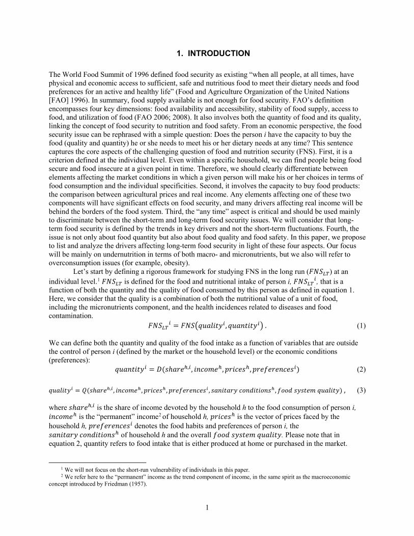
The 2015 Global Hunger Index suggests that despite progress in reducing hunger worldwide, hunger levels in 52 of 117 countries in the 2015 Global Hunger Index remain “serious” or “alarming.” Since achieving and maintaining food and nutrition security (FNS) remains a goal for all countries, it is important to understand the individual, national, and global factors that affect FNS. This paper proposes an analytical framework to identify and analyze the respective roles of key long-term drivers of FNS. We start by identifying what the key variables affecting FNS are at the household and country level, and then we continue by defining what the main exogenous or endogenous drivers affecting these variables are. We discuss the key drivers of both aggregated food supply and demand and therefore their impact on prices. Specifically, for aggregated food demand, we discuss demographic factors, income growth, changes in dietary preferences, aggregated domestic distortions, and overall quality of the food system. With respect to the drivers of aggregated food supply, we discuss land available for food products and the drivers behind land availability, the share of waste/losses generated by the food system, and the normalized average yield. We define yield as the amount of nutrients produced by unit of land. It depends both on the physical yield of the crop or the livestock and on the quality of the food produced. It also can be affected by the changes in production patterns linked to the different dietary patterns of the consumers and by climate change. We emphasize the fact that in many cases, key drivers may have ambiguous effects on the FNS situation of different agents. For instance, more liberal trade policies will affect real income, terms of trade, demand and supply, returns of factors, foreign direct investments, and food prices and thus may lead to the improvement of the global-level FNS, that is, the FNS of the majority of the population. At the same time, more liberal trade policies may bring food insecurity to some households. Therefore, careful quantitative assessment is needed for each policy option. Finally, we propose a typology of variables that will help modelers adapt their models to study the different drivers through both direct and indirect effects.

Keywords: agricultural production, climate change, food security, food prices, income distribution, income growth, long-term economic changes, nutrition security

vi

ACKNOWLEDGMENTS

This paper was undertaken as a part of, and partially funded by the CGIAR Research Program on Policies, Institutions and Markets, led by IFPRI. The authors also gratefully acknowledge financial support from the FOODSECURE “Exploring the Future of Global Food and Nutrition Security” Research Project (FP7 Grant Agreement No. 290693), funded by the European Commission. This paper has not gone through IFPRI’s standard peer-review process. The opinions expressed here belong to the author, and do not necessarily reflect those of PIM, IFPRI, CGIAR, or FOODSECURE.

1

1. INTRODUCTION

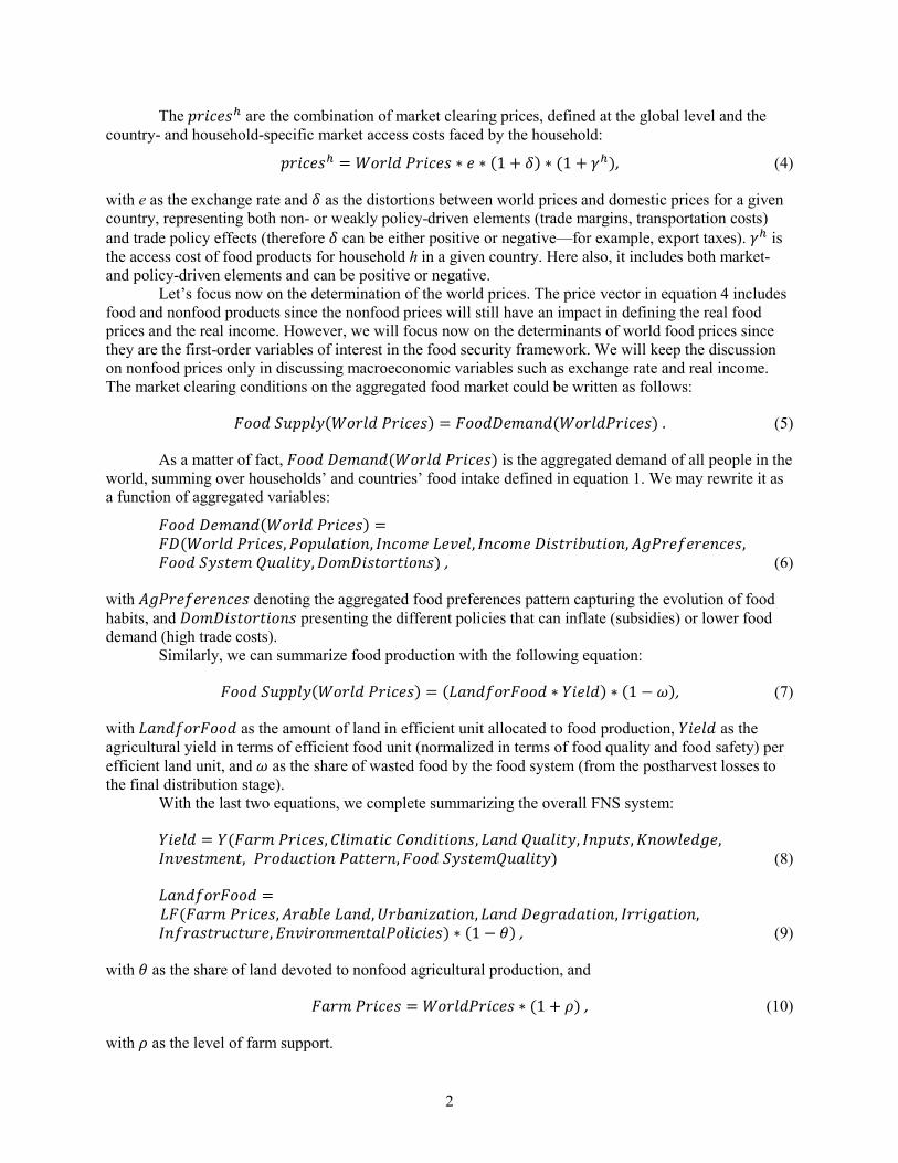
The World Food Summit of 1996 defined food security as existing “when all people, at all times, have physical and economic access to sufficient, safe and nutritious food to meet their dietary needs and food preferences for an active and healthy life” (Food and Agriculture Organization of the United Nations [FAO] 1996). In summary, food supply available is not enough for food security. FAO’s definition encompasses four key dimensions: food availability and accessibility, stability of food supply, access to food, and utilization of food (FAO 2006; 2008). It also involves both the quantity of food and its quality, linking the concept of food security to nutrition and food safety. From an economic perspective, the food security issue can be rephrased with a simple question: Does the person i have the capacity to buy the food (quality and quantity) he or she needs to meet his or her dietary needs at any time? This sentence captures the core aspects of the challenging question of food and nutrition security (FNS). First, it is a criterion defined at the individual level. Even within a specific household, we can find people being food secure and food insecure at a given point in time. Therefore, we should clearly differentiate between elements affecting the market conditions in which a given person will make his or her choices in terms of food consumption and the individual specificities. Second, it involves the capacity to buy food products: the comparison between agricultural prices and real income. Any elements affecting one of these two components will have significant effects on food security, and many drivers affecting real income will be behind the borders of the food system. Third, the “any time” aspect is critical and should be used mainly to discriminate between the short-term and long-term food security issues. We will consider that long-term food security is defined by the trends in key drivers and not the short-term fluctuations. Fourth, the issue is not only about food quantity but also about food quality and food safety. In this paper, we propose to list and analyze the drivers affecting long-term food security in light of these four aspects. Our focus will be mainly on undernutrition in terms of both macro- and micronutrients, but we also will refer to overconsumption issues (for example, obesity).

Let’s start by defining a rigorous framework for studying FNS in the long run (𝐹𝐹𝐹𝐹𝑆𝑆𝐿𝐿𝐿𝐿) at an individual level.1 𝐹𝐹𝐹𝐹𝑆𝑆𝐿𝐿𝐿𝐿 is defined for the food and nutritional intake of person i, 𝐹𝐹𝐹𝐹𝑆𝑆𝐿𝐿𝐿𝐿𝑖𝑖, that is a function of both the quantity and the quality of food consumed by this person as defined in equation 1. Here, we consider that the quality is a combination of both the nutritional value of a unit of food, including the micronutrients component, and the health incidences related to diseases and food contamination. 𝐹𝐹𝐹𝐹𝑆𝑆𝐿𝐿𝐿𝐿𝑖𝑖 = 𝐹𝐹𝐹𝐹𝑆𝑆�𝑞𝑞𝑞𝑞𝑞𝑞𝑞𝑞𝑞𝑞𝑞𝑞𝑞𝑞𝑖𝑖,𝑞𝑞𝑞𝑞𝑞𝑞𝑞𝑞𝑞𝑞𝑞𝑞𝑞𝑞𝑞𝑞𝑖𝑖� . (1)

We can define both the quantity and quality of the food intake as a function of variables that are outside the control of person i (defined by the market or the household level) or the economic conditions (preferences): 𝑞𝑞𝑞𝑞𝑞𝑞𝑞𝑞𝑞𝑞𝑞𝑞𝑞𝑞𝑞𝑞𝑖𝑖 = 𝐷𝐷(𝑠𝑠ℎ𝑞𝑞𝑎𝑎𝑎𝑎ℎ,𝑖𝑖, 𝑞𝑞𝑞𝑞𝑖𝑖𝑖𝑖𝑖𝑖𝑎𝑎ℎ,𝑝𝑝𝑎𝑎𝑞𝑞𝑖𝑖𝑎𝑎𝑠𝑠ℎ,𝑝𝑝𝑎𝑎𝑎𝑎𝑝𝑝𝑎𝑎𝑎𝑎𝑎𝑎𝑞𝑞𝑖𝑖𝑎𝑎𝑠𝑠𝑖𝑖) (2)

𝑞𝑞𝑞𝑞𝑞𝑞𝑞𝑞𝑞𝑞𝑞𝑞𝑞𝑞𝑖𝑖 = 𝑄𝑄(𝑠𝑠ℎ𝑞𝑞𝑎𝑎𝑎𝑎ℎ,𝑖𝑖 , 𝑞𝑞𝑞𝑞𝑖𝑖𝑖𝑖𝑖𝑖𝑎𝑎ℎ , 𝑝𝑝𝑎𝑎𝑞𝑞𝑖𝑖𝑎𝑎𝑠𝑠ℎ , 𝑝𝑝𝑎𝑎𝑎𝑎𝑝𝑝𝑎𝑎𝑎𝑎𝑎𝑎𝑞𝑞𝑖𝑖𝑎𝑎𝑠𝑠𝑖𝑖 , 𝑠𝑠𝑞𝑞𝑞𝑞𝑞𝑞𝑞𝑞𝑞𝑞𝑎𝑎𝑞𝑞 𝑖𝑖𝑖𝑖𝑞𝑞𝑐𝑐𝑞𝑞𝑞𝑞𝑞𝑞𝑖𝑖𝑞𝑞𝑠𝑠ℎ , 𝑝𝑝𝑖𝑖𝑖𝑖𝑐𝑐 𝑠𝑠𝑞𝑞𝑠𝑠𝑞𝑞𝑎𝑎𝑖𝑖 𝑞𝑞𝑞𝑞𝑞𝑞𝑞𝑞𝑞𝑞𝑞𝑞𝑞𝑞) , (3)

where 𝑠𝑠ℎ𝑞𝑞𝑎𝑎𝑎𝑎ℎ,𝑖𝑖 is the share of income devoted by the household h to the food consumption of person i, 𝑞𝑞𝑞𝑞𝑖𝑖𝑖𝑖𝑖𝑖𝑎𝑎ℎ is the “permanent” income2 of household h, 𝑝𝑝𝑎𝑎𝑞𝑞𝑖𝑖𝑎𝑎𝑠𝑠ℎ is the vector of prices faced by the household h, 𝑝𝑝𝑎𝑎𝑎𝑎𝑝𝑝𝑎𝑎𝑎𝑎𝑎𝑎𝑞𝑞𝑖𝑖𝑎𝑎𝑠𝑠𝑖𝑖 denotes the food habits and preferences of person i, the 𝑠𝑠𝑞𝑞𝑞𝑞𝑞𝑞𝑞𝑞𝑞𝑞𝑎𝑎𝑞𝑞 𝑖𝑖𝑖𝑖𝑞𝑞𝑐𝑐𝑞𝑞𝑞𝑞𝑞𝑞𝑖𝑖𝑞𝑞𝑠𝑠ℎ of household h and the overall 𝑝𝑝𝑖𝑖𝑖𝑖𝑐𝑐 𝑠𝑠𝑞𝑞𝑠𝑠𝑞𝑞𝑎𝑎𝑖𝑖 𝑞𝑞𝑞𝑞𝑞𝑞𝑞𝑞𝑞𝑞𝑞𝑞𝑞𝑞. Please note that in equation 2, quantity refers to food intake that is either produced at home or purchased in the market.

1 We will not focus on the short-run vulnerability of individuals in this paper. 2 We refer here to the “permanent” income as the trend component of income, in the same spirit as the macroeconomic

concept introduced by Friedman (1957).

2

The 𝑝𝑝𝑎𝑎𝑞𝑞𝑖𝑖𝑎𝑎𝑠𝑠ℎ are the combination of market clearing prices, defined at the global level and the country- and household-specific market access costs faced by the household:

𝑝𝑝𝑎𝑎𝑞𝑞𝑖𝑖𝑎𝑎𝑠𝑠ℎ = 𝑊𝑊𝑖𝑖𝑎𝑎𝑞𝑞𝑐𝑐 𝑃𝑃𝑎𝑎𝑞𝑞𝑖𝑖𝑎𝑎𝑠𝑠 ∗ 𝑎𝑎 ∗ (1 + 𝛿𝛿) ∗ (1 + 𝛾𝛾ℎ), (4)

with e as the exchange rate and 𝛿𝛿 as the distortions between world prices and domestic prices for a given country, representing both non- or weakly policy-driven elements (trade margins, transportation costs) and trade policy effects (therefore 𝛿𝛿 can be either positive or negative—for example, export taxes). 𝛾𝛾ℎ is the access cost of food products for household h in a given country. Here also, it includes both market- and policy-driven elements and can be positive or negative.

Let’s focus now on the determination of the world prices. The price vector in equation 4 includes food and nonfood products since the nonfood prices will still have an impact in defining the real food prices and the real income. However, we will focus now on the determinants of world food prices since they are the first-order variables of interest in the food security framework. We will keep the discussion on nonfood prices only in discussing macroeconomic variables such as exchange rate and real income. The market clearing conditions on the aggregated food market could be written as follows:

𝐹𝐹𝑖𝑖𝑖𝑖𝑐𝑐 𝑆𝑆𝑞𝑞𝑝𝑝𝑝𝑝𝑞𝑞𝑞𝑞(𝑊𝑊𝑖𝑖𝑎𝑎𝑞𝑞𝑐𝑐 𝑃𝑃𝑎𝑎𝑞𝑞𝑖𝑖𝑎𝑎𝑠𝑠) = 𝐹𝐹𝑖𝑖𝑖𝑖𝑐𝑐𝐷𝐷𝑎𝑎𝑖𝑖𝑞𝑞𝑞𝑞𝑐𝑐(𝑊𝑊𝑖𝑖𝑎𝑎𝑞𝑞𝑐𝑐𝑃𝑃𝑎𝑎𝑞𝑞𝑖𝑖𝑎𝑎𝑠𝑠) . (5)

As a matter of fact, 𝐹𝐹𝑖𝑖𝑖𝑖𝑐𝑐 𝐷𝐷𝑎𝑎𝑖𝑖𝑞𝑞𝑞𝑞𝑐𝑐(𝑊𝑊𝑖𝑖𝑎𝑎𝑞𝑞𝑐𝑐 𝑃𝑃𝑎𝑎𝑞𝑞𝑖𝑖𝑎𝑎𝑠𝑠) is the aggregated demand of all people in the world, summing over households’ and countries’ food intake defined in equation 1. We may rewrite it as a function of aggregated variables:

𝐹𝐹𝑖𝑖𝑖𝑖𝑐𝑐 𝐷𝐷𝑎𝑎𝑖𝑖𝑞𝑞𝑞𝑞𝑐𝑐(𝑊𝑊𝑖𝑖𝑎𝑎𝑞𝑞𝑐𝑐 𝑃𝑃𝑎𝑎𝑞𝑞𝑖𝑖𝑎𝑎𝑠𝑠) = 𝐹𝐹𝐷𝐷(𝑊𝑊𝑖𝑖𝑎𝑎𝑞𝑞𝑐𝑐 𝑃𝑃𝑎𝑎𝑞𝑞𝑖𝑖𝑎𝑎𝑠𝑠,𝑃𝑃𝑖𝑖𝑝𝑝𝑞𝑞𝑞𝑞𝑞𝑞𝑞𝑞𝑞𝑞𝑖𝑖𝑞𝑞, 𝐼𝐼𝑞𝑞𝑖𝑖𝑖𝑖𝑖𝑖𝑎𝑎 𝐿𝐿𝑎𝑎𝐿𝐿𝑎𝑎𝑞𝑞, 𝐼𝐼𝑞𝑞𝑖𝑖𝑖𝑖𝑖𝑖𝑎𝑎 𝐷𝐷𝑞𝑞𝑠𝑠𝑞𝑞𝑎𝑎𝑞𝑞𝑖𝑖𝑞𝑞𝑞𝑞𝑞𝑞𝑖𝑖𝑞𝑞,𝐴𝐴𝐴𝐴𝑃𝑃𝑎𝑎𝑎𝑎𝑝𝑝𝑎𝑎𝑎𝑎𝑎𝑎𝑞𝑞𝑖𝑖𝑎𝑎𝑠𝑠,𝐹𝐹𝑖𝑖𝑖𝑖𝑐𝑐 𝑆𝑆𝑞𝑞𝑠𝑠𝑞𝑞𝑎𝑎𝑖𝑖 𝑄𝑄𝑞𝑞𝑞𝑞𝑞𝑞𝑞𝑞𝑞𝑞𝑞𝑞,𝐷𝐷𝑖𝑖𝑖𝑖𝐷𝐷𝑞𝑞𝑠𝑠𝑞𝑞𝑖𝑖𝑎𝑎𝑞𝑞𝑞𝑞𝑖𝑖𝑞𝑞𝑠𝑠) , (6)

with 𝐴𝐴𝐴𝐴𝑃𝑃𝑎𝑎𝑎𝑎𝑝𝑝𝑎𝑎𝑎𝑎𝑎𝑎𝑞𝑞𝑖𝑖𝑎𝑎𝑠𝑠 denoting the aggregated food preferences pattern capturing the evolution of food habits, and 𝐷𝐷𝑖𝑖𝑖𝑖𝐷𝐷𝑞𝑞𝑠𝑠𝑞𝑞𝑖𝑖𝑎𝑎𝑞𝑞𝑞𝑞𝑖𝑖𝑞𝑞𝑠𝑠 presenting the different policies that can inflate (subsidies) or lower food demand (high trade costs).

Similarly, we can summarize food production with the following equation:

𝐹𝐹𝑖𝑖𝑖𝑖𝑐𝑐 𝑆𝑆𝑞𝑞𝑝𝑝𝑝𝑝𝑞𝑞𝑞𝑞(𝑊𝑊𝑖𝑖𝑎𝑎𝑞𝑞𝑐𝑐 𝑃𝑃𝑎𝑎𝑞𝑞𝑖𝑖𝑎𝑎𝑠𝑠) = (𝐿𝐿𝑞𝑞𝑞𝑞𝑐𝑐𝑝𝑝𝑖𝑖𝑎𝑎𝐹𝐹𝑖𝑖𝑖𝑖𝑐𝑐 ∗ 𝑌𝑌𝑞𝑞𝑎𝑎𝑞𝑞𝑐𝑐) ∗ (1 −𝜔𝜔), (7)

with 𝐿𝐿𝑞𝑞𝑞𝑞𝑐𝑐𝑝𝑝𝑖𝑖𝑎𝑎𝐹𝐹𝑖𝑖𝑖𝑖𝑐𝑐 as the amount of land in efficient unit allocated to food production, 𝑌𝑌𝑞𝑞𝑎𝑎𝑞𝑞𝑐𝑐 as the agricultural yield in terms of efficient food unit (normalized in terms of food quality and food safety) per efficient land unit, and 𝜔𝜔 as the share of wasted food by the food system (from the postharvest losses to the final distribution stage).

With the last two equations, we complete summarizing the overall FNS system:

𝑌𝑌𝑞𝑞𝑎𝑎𝑞𝑞𝑐𝑐 = 𝑌𝑌(𝐹𝐹𝑞𝑞𝑎𝑎𝑖𝑖 𝑃𝑃𝑎𝑎𝑞𝑞𝑖𝑖𝑎𝑎𝑠𝑠,𝐶𝐶𝑞𝑞𝑞𝑞𝑖𝑖𝑞𝑞𝑞𝑞𝑞𝑞𝑖𝑖 𝐶𝐶𝑖𝑖𝑞𝑞𝑐𝑐𝑞𝑞𝑞𝑞𝑞𝑞𝑖𝑖𝑞𝑞𝑠𝑠, 𝐿𝐿𝑞𝑞𝑞𝑞𝑐𝑐 𝑄𝑄𝑞𝑞𝑞𝑞𝑞𝑞𝑞𝑞𝑞𝑞𝑞𝑞, 𝐼𝐼𝑞𝑞𝑝𝑝𝑞𝑞𝑞𝑞𝑠𝑠,𝐾𝐾𝑞𝑞𝑖𝑖𝐾𝐾𝑞𝑞𝑎𝑎𝑐𝑐𝐴𝐴𝑎𝑎, 𝐼𝐼𝑞𝑞𝐿𝐿𝑎𝑎𝑠𝑠𝑞𝑞𝑖𝑖𝑎𝑎𝑞𝑞𝑞𝑞, 𝑃𝑃𝑎𝑎𝑖𝑖𝑐𝑐𝑞𝑞𝑖𝑖𝑞𝑞𝑞𝑞𝑖𝑖𝑞𝑞 𝑃𝑃𝑞𝑞𝑞𝑞𝑞𝑞𝑎𝑎𝑎𝑎𝑞𝑞,𝐹𝐹𝑖𝑖𝑖𝑖𝑐𝑐 𝑆𝑆𝑞𝑞𝑠𝑠𝑞𝑞𝑎𝑎𝑖𝑖𝑄𝑄𝑞𝑞𝑞𝑞𝑞𝑞𝑞𝑞𝑞𝑞𝑞𝑞) (8)

𝐿𝐿𝑞𝑞𝑞𝑞𝑐𝑐𝑝𝑝𝑖𝑖𝑎𝑎𝐹𝐹𝑖𝑖𝑖𝑖𝑐𝑐 = 𝐿𝐿𝐹𝐹(𝐹𝐹𝑞𝑞𝑎𝑎𝑖𝑖 𝑃𝑃𝑎𝑎𝑞𝑞𝑖𝑖𝑎𝑎𝑠𝑠,𝐴𝐴𝑎𝑎𝑞𝑞𝑖𝑖𝑞𝑞𝑎𝑎 𝐿𝐿𝑞𝑞𝑞𝑞𝑐𝑐,𝑈𝑈𝑎𝑎𝑖𝑖𝑞𝑞𝑞𝑞𝑞𝑞𝑈𝑈𝑞𝑞𝑞𝑞𝑞𝑞𝑖𝑖𝑞𝑞, 𝐿𝐿𝑞𝑞𝑞𝑞𝑐𝑐 𝐷𝐷𝑎𝑎𝐴𝐴𝑎𝑎𝑞𝑞𝑐𝑐𝑞𝑞𝑞𝑞𝑞𝑞𝑖𝑖𝑞𝑞, 𝐼𝐼𝑎𝑎𝑎𝑎𝑞𝑞𝐴𝐴𝑞𝑞𝑞𝑞𝑞𝑞𝑖𝑖𝑞𝑞, 𝐼𝐼𝑞𝑞𝑝𝑝𝑎𝑎𝑞𝑞𝑠𝑠𝑞𝑞𝑎𝑎𝑞𝑞𝑖𝑖𝑞𝑞𝑞𝑞𝑎𝑎𝑎𝑎,𝐸𝐸𝑞𝑞𝐿𝐿𝑞𝑞𝑎𝑎𝑖𝑖𝑞𝑞𝑖𝑖𝑎𝑎𝑞𝑞𝑞𝑞𝑞𝑞𝑞𝑞𝑃𝑃𝑖𝑖𝑞𝑞𝑞𝑞𝑖𝑖𝑞𝑞𝑎𝑎𝑠𝑠) ∗ (1 − 𝜃𝜃) , (9)

with 𝜃𝜃 as the share of land devoted to nonfood agricultural production, and

𝐹𝐹𝑞𝑞𝑎𝑎𝑖𝑖 𝑃𝑃𝑎𝑎𝑞𝑞𝑖𝑖𝑎𝑎𝑠𝑠 = 𝑊𝑊𝑖𝑖𝑎𝑎𝑞𝑞𝑐𝑐𝑃𝑃𝑎𝑎𝑞𝑞𝑖𝑖𝑎𝑎𝑠𝑠 ∗ (1 + 𝜌𝜌) , (10)

with 𝜌𝜌 as the level of farm support.

3

The system described by equations 1 to 10 defines our FNS analytical framework. Using permanent income in equations 2 and 3 but also the structural drivers of market equilibrium in equations 6 and 7, we differentiate the long-term drivers of food security from the short-term drivers.

The next sections will discuss the different drivers affecting each of the variables identified in our system of equations. Section 2 starts with the individual and household-specific variables. Then, in Section 3 we focus on the variables affecting the market equilibrium conditions. Section 4 discusses the transversality of some factors from the individual variables to the economywide ones and also proposes a policy matrix of intervention. Finally, we conclude.

4

2. INDIVIDUAL AND HOUSEHOLD-LEVEL DRIVERS

Before discussing the drivers of FNS at the individual and household levels, it is important to place undernourishment and malnourishment in a wider context. While the prevalence of undernourishment in the world has fallen from 23 percent in 1991 to 13 percent in 2013 (World Bank 2015b), 870 million people are still chronically undernourished, and almost 2 billion people suffer from negative health consequences of micronutrient deficiencies (FAO 2012). More than 100 million children younger than age five are underweight (FAO 2012), which has lifelong effects on their development and achievement. Overall, the prevalence of severe wasting of children younger than five was more than 7.7 percent (World Bank 2015b). Malnutrition prevalence as measured by height for age was greater than 15 percent, and weight for age was greater than 24.5 percent in 2013 (World Bank 2015b). Most of the world’s undernourished live in low-income and middle-income countries—with low-income countries having a prevalence of undernourishment at more than 24 percent (World Bank 2015b)—and suffer from micronutrient malnutrition, which is caused by lack of micronutrients in the diet. Fruits, vegetables, and animal products are rich in micronutrients, but these foods are often not available to the poor. The diets of the poor in developing countries usually consist of high amounts of staple foods (such as maize, wheat, and rice) but few micronutrient-rich foods (such as fruits, vegetables, and animal and fish products) (Harvest Plus 2012). This dietary pattern leads to negative consequences in terms of malnutrition and health. Income growth in these countries and access to these micronutrient-rich goods are both necessary to achieve nutrition security.

Another indicator that needs to be referred to while discussing FNS and malnutrition is obesity. According to recent World Health Organization (2016) estimates, in 2014, more than 1.9 billion adults were overweight (and of these more than 600 million were obese). In 2014, about 13 percent of the world’s adult population was obese, and 39 percent of adults were overweight. The worldwide prevalence of obesity more than doubled between 1980 and 2014. Most critically, once considered a high-income-country problem, overweight and obesity are now on the rise in low- and middle-income countries. In developing countries with emerging economies, the rate of increase of childhood overweight and obesity has been more than 30 percent higher than that of developed countries.

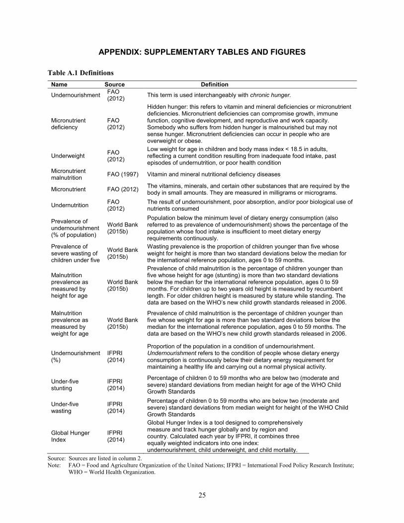
In the context of the above discussion, drivers of FNS at the household level deserve special attention in our analysis. Please note that Table A.1 in the appendix presents detailed definitions of FNS indicators, including the data used in this paper.

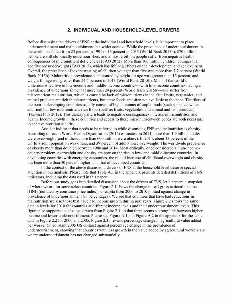
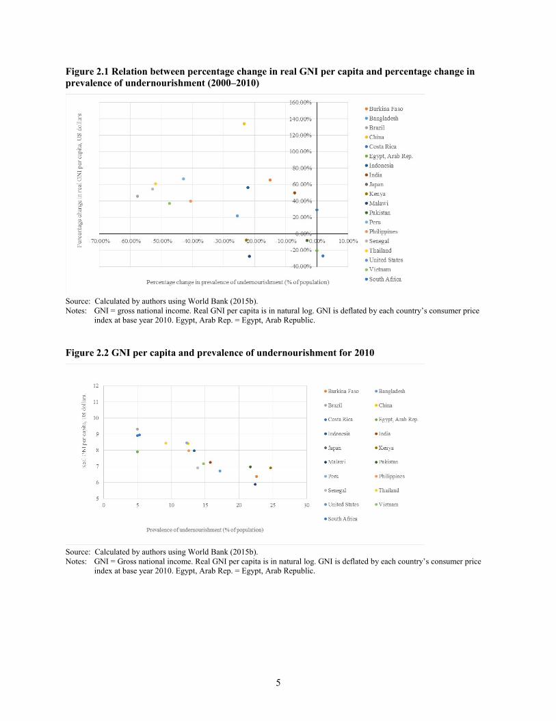
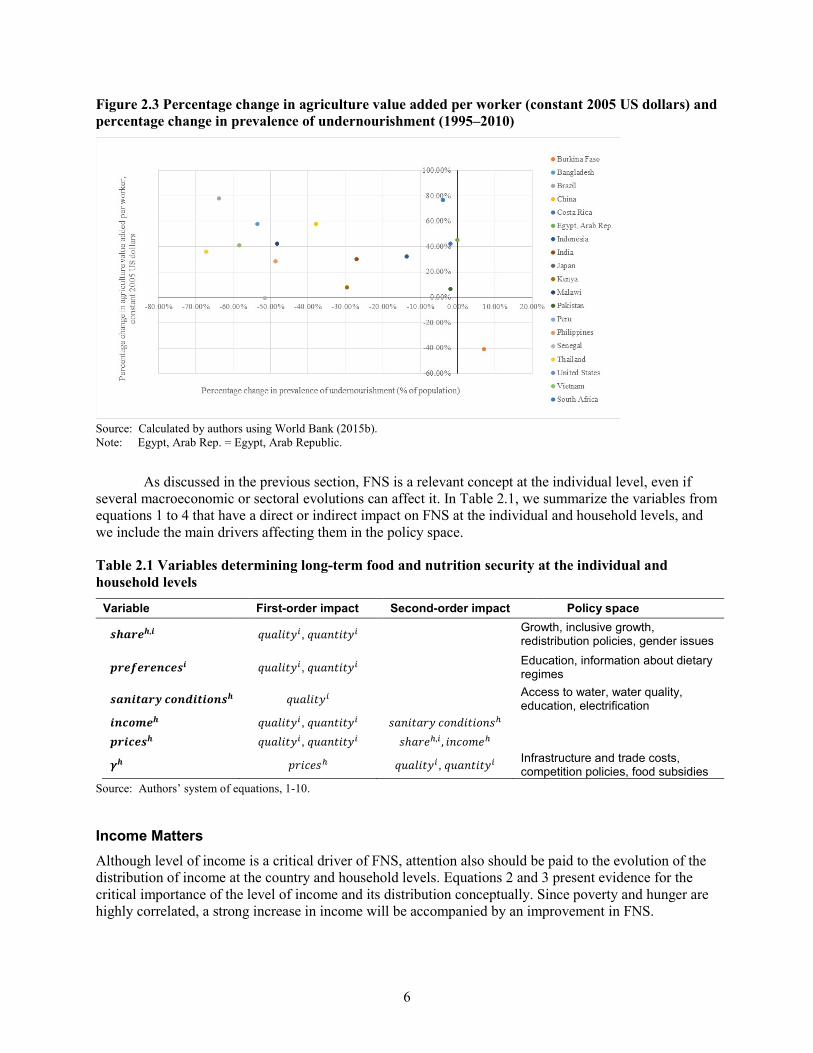
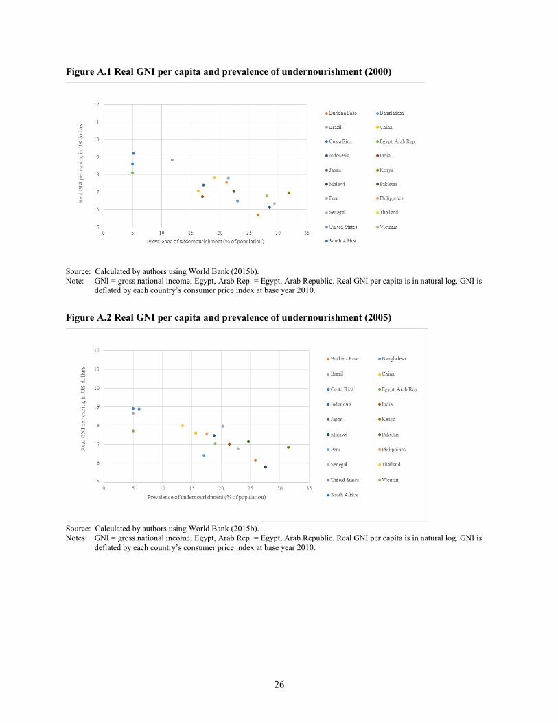
Before our study goes into detailed discussion about the drivers of FNS, let’s present a snapshot of where we are for some select countries. Figure 2.1 shows the change in real gross national income (GNI) (deflated by consumer price index) per capita from 2000 to 2010 plotted against change in prevalence of undernourishment (in percentages). We see that countries that have had reductions in malnutrition are also those that have had income growth during past years. Figure 2.2 shows the same data in levels for 2010 for countries at different income levels and their undernourishment levels. This figure also supports conclusions drawn from Figure 2.1, in that there seems a strong link between higher income and lower undernourishment. Please see Figure A.1 and Figure A.2 in the appendix for the same data in Figure 2.2 for 2000 and 2005. Figure 2.3 presents percentage change in agricultural value added per worker (in constant 2005 US dollars) against percentage change in the prevalence of undernourishment, showing that countries with less growth in the value added by agricultural workers are where undernourishment has not changed substantially.

5

Figure 2.1 Relation between percentage change in real GNI per capita and percentage change in prevalence of undernourishment (2000–2010)

Source: Calculated by authors using World Bank (2015b). Notes: GNI = gross national income. Real GNI per capita is in natural log. GNI is deflated by each country’s consumer price

index at base year 2010. Egypt, Arab Rep. = Egypt, Arab Republic.

Figure 2.2 GNI per capita and prevalence of undernourishment for 2010

Source: Calculated by authors using World Bank (2015b). Notes: GNI = Gross national income. Real GNI per capita is in natural log. GNI is deflated by each country’s consumer price

index at base year 2010. Egypt, Arab Rep. = Egypt, Arab Republic.

6

Figure 2.3 Percentage change in agriculture value added per worker (constant 2005 US dollars) and percentage change in prevalence of undernourishment (1995–2010)

Source: Calculated by authors using World Bank (2015b). Note: Egypt, Arab Rep. = Egypt, Arab Republic.

As discussed in the previous section, FNS is a relevant concept at the individual level, even if several macroeconomic or sectoral evolutions can affect it. In Table 2.1, we summarize the variables from equations 1 to 4 that have a direct or indirect impact on FNS at the individual and household levels, and we include the main drivers affecting them in the policy space.

Table 2.1 Variables determining long-term food and nutrition security at the individual and household levels

Variable First-order impact Second-order impact Policy space

𝒔𝒔𝒔𝒔𝒔𝒔𝒔𝒔𝒔𝒔𝒔𝒔,𝒊𝒊 𝑞𝑞𝑞𝑞𝑞𝑞𝑞𝑞𝑞𝑞𝑞𝑞𝑞𝑞𝑖𝑖, 𝑞𝑞𝑞𝑞𝑞𝑞𝑞𝑞𝑞𝑞𝑞𝑞𝑞𝑞𝑞𝑞𝑖𝑖 Growth, inclusive growth, redistribution policies, gender issues

𝒑𝒑𝒔𝒔𝒔𝒔𝒑𝒑𝒔𝒔𝒔𝒔𝒔𝒔𝒑𝒑𝒑𝒑𝒔𝒔𝒔𝒔𝒊𝒊 𝑞𝑞𝑞𝑞𝑞𝑞𝑞𝑞𝑞𝑞𝑞𝑞𝑞𝑞𝑖𝑖, 𝑞𝑞𝑞𝑞𝑞𝑞𝑞𝑞𝑞𝑞𝑞𝑞𝑞𝑞𝑞𝑞𝑖𝑖 Education, information about dietary regimes

𝒔𝒔𝒔𝒔𝒑𝒑𝒊𝒊𝒕𝒕𝒔𝒔𝒔𝒔𝒕𝒕 𝒑𝒑𝒄𝒄𝒑𝒑𝒄𝒄𝒊𝒊𝒕𝒕𝒊𝒊𝒄𝒄𝒑𝒑𝒔𝒔𝒔𝒔 𝑞𝑞𝑞𝑞𝑞𝑞𝑞𝑞𝑞𝑞𝑞𝑞𝑞𝑞𝑖𝑖 Access to water, water quality, education, electrification

𝒊𝒊𝒑𝒑𝒑𝒑𝒄𝒄𝒊𝒊𝒔𝒔𝒔𝒔 𝑞𝑞𝑞𝑞𝑞𝑞𝑞𝑞𝑞𝑞𝑞𝑞𝑞𝑞𝑖𝑖, 𝑞𝑞𝑞𝑞𝑞𝑞𝑞𝑞𝑞𝑞𝑞𝑞𝑞𝑞𝑞𝑞𝑖𝑖 𝑠𝑠𝑞𝑞𝑞𝑞𝑞𝑞𝑞𝑞𝑞𝑞𝑎𝑎𝑞𝑞 𝑖𝑖𝑖𝑖𝑞𝑞𝑐𝑐𝑞𝑞𝑞𝑞𝑞𝑞𝑖𝑖𝑞𝑞𝑠𝑠ℎ 𝒑𝒑𝒔𝒔𝒊𝒊𝒑𝒑𝒔𝒔𝒔𝒔𝒔𝒔 𝑞𝑞𝑞𝑞𝑞𝑞𝑞𝑞𝑞𝑞𝑞𝑞𝑞𝑞𝑖𝑖, 𝑞𝑞𝑞𝑞𝑞𝑞𝑞𝑞𝑞𝑞𝑞𝑞𝑞𝑞𝑞𝑞𝑖𝑖 𝑠𝑠ℎ𝑞𝑞𝑎𝑎𝑎𝑎ℎ,𝑖𝑖 , 𝑞𝑞𝑞𝑞𝑖𝑖𝑖𝑖𝑖𝑖𝑎𝑎ℎ

𝜸𝜸𝒔𝒔 𝑝𝑝𝑎𝑎𝑞𝑞𝑖𝑖𝑎𝑎𝑠𝑠ℎ 𝑞𝑞𝑞𝑞𝑞𝑞𝑞𝑞𝑞𝑞𝑞𝑞𝑞𝑞𝑖𝑖, 𝑞𝑞𝑞𝑞𝑞𝑞𝑞𝑞𝑞𝑞𝑞𝑞𝑞𝑞𝑞𝑞𝑖𝑖 Infrastructure and trade costs, competition policies, food subsidies

Source: Authors’ system of equations, 1-10.

Income Matters Although level of income is a critical driver of FNS, attention also should be paid to the evolution of the distribution of income at the country and household levels. Equations 2 and 3 present evidence for the critical importance of the level of income and its distribution conceptually. Since poverty and hunger are highly correlated, a strong increase in income will be accompanied by an improvement in FNS.

7

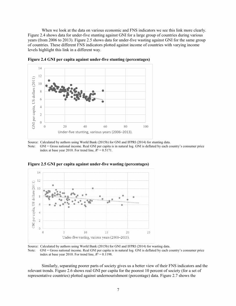
When we look at the data on various economic and FNS indicators we see this link more clearly. Figure 2.4 shows data for under-five stunting against GNI for a large group of countries during various years (from 2006 to 2013). Figure 2.5 shows data for under-five wasting against GNI for the same group of countries. These different FNS indicators plotted against income of countries with varying income levels highlight this link in a different way.

Figure 2.4 GNI per capita against under-five stunting (percentages)

Source: Calculated by authors using World Bank (2015b) for GNI and IFPRI (2014) for stunting data. Note: GNI = Gross national income. Real GNI per capita is in natural log. GNI is deflated by each country’s consumer price

index at base year 2010. For trend line, R² = 0.5171.

Figure 2.5 GNI per capita against under-five wasting (percentages)

Source: Calculated by authors using World Bank (2015b) for GNI and IFPRI (2014) for wasting data. Note: GNI = Gross national income. Real GNI per capita is in natural log. GNI is deflated by each country’s consumer price

index at base year 2010. For trend line, R² = 0.1198.

Similarly, separating poorer parts of society gives us a better view of their FNS indicators and the relevant trends. Figure 2.6 shows real GNI per capita for the poorest 10 percent of society (for a set of representative countries) plotted against undernourishment (percentage) data. Figure 2.7 shows the

0

2

4

6

8

10

12

14

0 20 40 60 80 100GN

I per

cap

ita, U

S do

llars

(201

1)

Under-five stunting, various years (2006–2013).

8

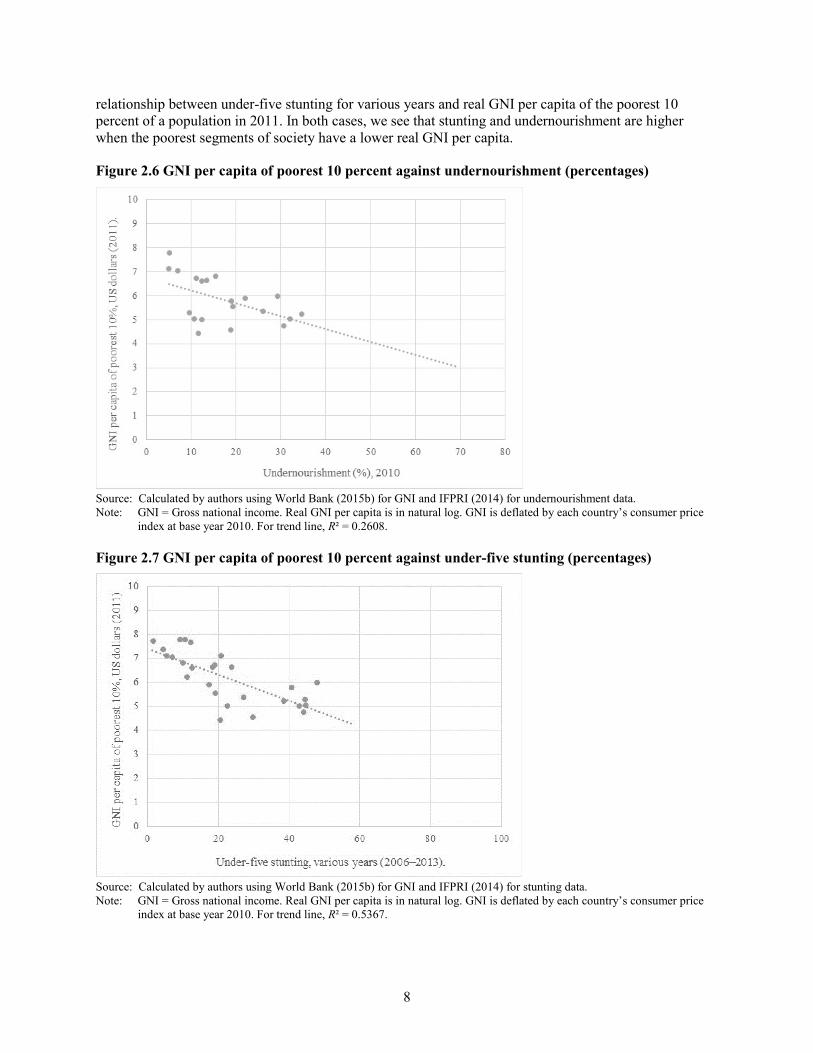
relationship between under-five stunting for various years and real GNI per capita of the poorest 10 percent of a population in 2011. In both cases, we see that stunting and undernourishment are higher when the poorest segments of society have a lower real GNI per capita.

Figure 2.6 GNI per capita of poorest 10 percent against undernourishment (percentages)

Source: Calculated by authors using World Bank (2015b) for GNI and IFPRI (2014) for undernourishment data. Note: GNI = Gross national income. Real GNI per capita is in natural log. GNI is deflated by each country’s consumer price

index at base year 2010. For trend line, R² = 0.2608.

Figure 2.7 GNI per capita of poorest 10 percent against under-five stunting (percentages)

Source: Calculated by authors using World Bank (2015b) for GNI and IFPRI (2014) for stunting data. Note: GNI = Gross national income. Real GNI per capita is in natural log. GNI is deflated by each country’s consumer price

index at base year 2010. For trend line, R² = 0.5367.

9

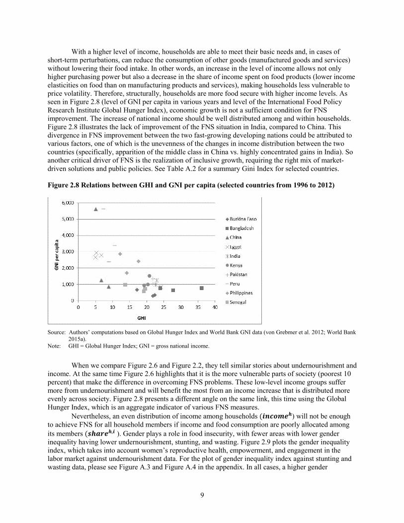
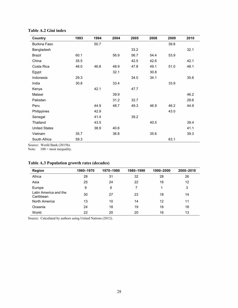
With a higher level of income, households are able to meet their basic needs and, in cases of short-term perturbations, can reduce the consumption of other goods (manufactured goods and services) without lowering their food intake. In other words, an increase in the level of income allows not only higher purchasing power but also a decrease in the share of income spent on food products (lower income elasticities on food than on manufacturing products and services), making households less vulnerable to price volatility. Therefore, structurally, households are more food secure with higher income levels. As seen in Figure 2.8 (level of GNI per capita in various years and level of the International Food Policy Research Institute Global Hunger Index), economic growth is not a sufficient condition for FNS improvement. The increase of national income should be well distributed among and within households. Figure 2.8 illustrates the lack of improvement of the FNS situation in India, compared to China. This divergence in FNS improvement between the two fast-growing developing nations could be attributed to various factors, one of which is the unevenness of the changes in income distribution between the two countries (specifically, apparition of the middle class in China vs. highly concentrated gains in India). So another critical driver of FNS is the realization of inclusive growth, requiring the right mix of market-driven solutions and public policies. See Table A.2 for a summary Gini Index for selected countries.

Figure 2.8 Relations between GHI and GNI per capita (selected countries from 1996 to 2012)

Source: Authors’ computations based on Global Hunger Index and World Bank GNI data (von Grebmer et al. 2012; World Bank

2015a). Note: GHI = Global Hunger Index; GNI = gross national income.

When we compare Figure 2.6 and Figure 2.2, they tell similar stories about undernourishment and income. At the same time Figure 2.6 highlights that it is the more vulnerable parts of society (poorest 10 percent) that make the difference in overcoming FNS problems. These low-level income groups suffer more from undernourishment and will benefit the most from an income increase that is distributed more evenly across society. Figure 2.8 presents a different angle on the same link, this time using the Global Hunger Index, which is an aggregate indicator of various FNS measures.

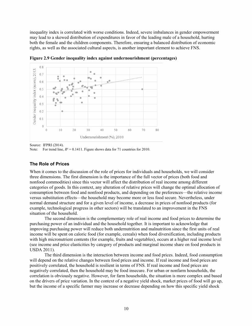
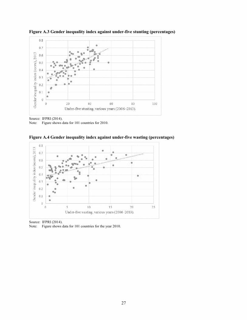
Nevertheless, an even distribution of income among households (𝒊𝒊𝒑𝒑𝒑𝒑𝒄𝒄𝒊𝒊𝒔𝒔𝒔𝒔) will not be enough to achieve FNS for all household members if income and food consumption are poorly allocated among its members (𝒔𝒔𝒔𝒔𝒔𝒔𝒔𝒔𝒔𝒔𝒔𝒔,𝒊𝒊 ). Gender plays a role in food insecurity, with fewer areas with lower gender inequality having lower undernourishment, stunting, and wasting. Figure 2.9 plots the gender inequality index, which takes into account women’s reproductive health, empowerment, and engagement in the labor market against undernourishment data. For the plot of gender inequality index against stunting and wasting data, please see Figure A.3 and Figure A.4 in the appendix. In all cases, a higher gender

10

inequality index is correlated with worse conditions. Indeed, severe imbalances in gender empowerment may lead to a skewed distribution of expenditures in favor of the leading male of a household, hurting both the female and the children components. Therefore, ensuring a balanced distribution of economic rights, as well as the associated cultural aspects, is another important element to achieve FNS.

Figure 2.9 Gender inequality index against undernourishment (percentages)

Source: IFPRI (2014). Note: For trend line, R² = 0.1411. Figure shows data for 71 countries for 2010.

The Role of Prices When it comes to the discussion of the role of prices for individuals and households, we will consider three dimensions. The first dimension is the importance of the full vector of prices (both food and nonfood commodities) since this vector will affect the distribution of real income among different categories of goods. In this context, any alteration of relative prices will change the optimal allocation of consumption between food and nonfood products, and depending on the preferences—the relative income versus substitution effects—the household may become more or less food secure. Nevertheless, under normal demand structure and for a given level of income, a decrease in prices of nonfood products (for example, technological progress in other sectors) will be translated to an improvement in the FNS situation of the household.

The second dimension is the complementary role of real income and food prices to determine the purchasing power of an individual and the household together. It is important to acknowledge that improving purchasing power will reduce both undernutrition and malnutrition since the first units of real income will be spent on caloric food (for example, cereals) when food diversification, including products with high micronutrient contents (for example, fruits and vegetables), occurs at a higher real income level (see income and price elasticities by category of products and marginal income share on food products in USDA 2011).

The third dimension is the interaction between income and food prices. Indeed, food consumption will depend on the relative changes between food prices and income. If real income and food prices are positively correlated, the household is resilient in terms of FNS. If real income and food prices are negatively correlated, then the household may be food insecure. For urban or nonfarm households, the correlation is obviously negative. However, for farm households, the situation is more complex and based on the drivers of price variation. In the context of a negative yield shock, market prices of food will go up, but the income of a specific farmer may increase or decrease depending on how this specific yield shock

11

has affected his own production and if the increase in prices is more or less, compensating the changes in production volume.

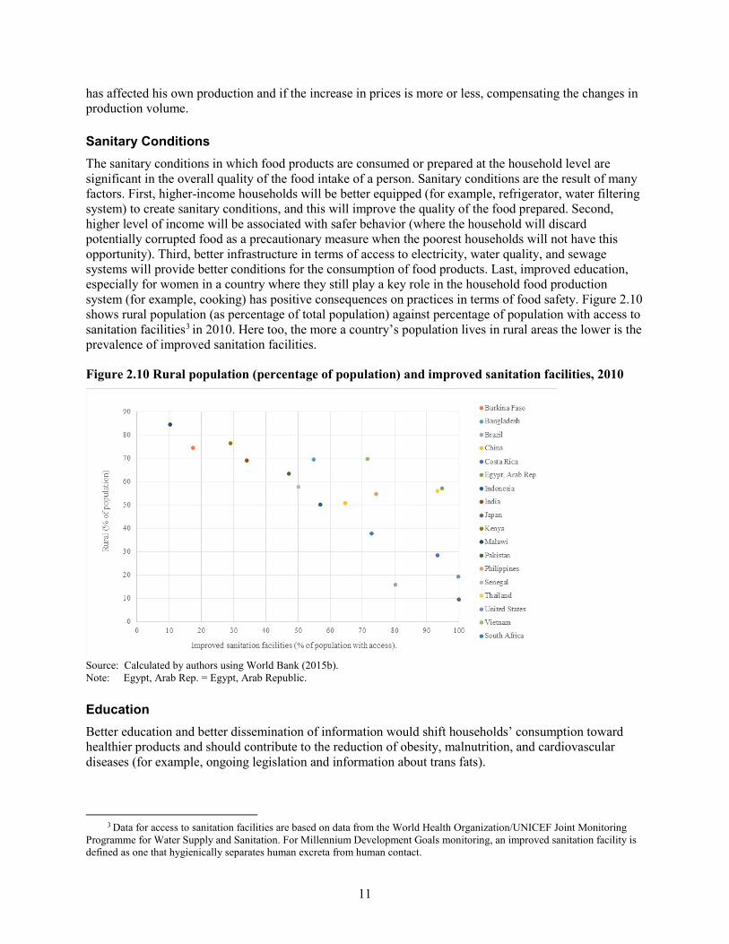
Sanitary Conditions The sanitary conditions in which food products are consumed or prepared at the household level are significant in the overall quality of the food intake of a person. Sanitary conditions are the result of many factors. First, higher-income households will be better equipped (for example, refrigerator, water filtering system) to create sanitary conditions, and this will improve the quality of the food prepared. Second, higher level of income will be associated with safer behavior (where the household will discard potentially corrupted food as a precautionary measure when the poorest households will not have this opportunity). Third, better infrastructure in terms of access to electricity, water quality, and sewage systems will provide better conditions for the consumption of food products. Last, improved education, especially for women in a country where they still play a key role in the household food production system (for example, cooking) has positive consequences on practices in terms of food safety. Figure 2.10 shows rural population (as percentage of total population) against percentage of population with access to sanitation facilities3 in 2010. Here too, the more a country’s population lives in rural areas the lower is the prevalence of improved sanitation facilities.

Figure 2.10 Rural population (percentage of population) and improved sanitation facilities, 2010

Source: Calculated by authors using World Bank (2015b). Note: Egypt, Arab Rep. = Egypt, Arab Republic.

Education Better education and better dissemination of information would shift households’ consumption toward healthier products and should contribute to the reduction of obesity, malnutrition, and cardiovascular diseases (for example, ongoing legislation and information about trans fats).

3 Data for access to sanitation facilities are based on data from the World Health Organization/UNICEF Joint Monitoring

Programme for Water Supply and Sanitation. For Millennium Development Goals monitoring, an improved sanitation facility is defined as one that hygienically separates human excreta from human contact.

12

Transaction and Market Access Costs As discussed in The Role of Prices section, prices play a significant role in FNS at the household and individual levels. However, a clear distinction needs to be made among global, country-level, and local prices since households may face different distortions in the prices they pay for food. For both food and nonfood products, the prices faced by a specific consumer is a combination of marketwide conditions, called here market prices, and specific market access costs paid by a household or a group of households. These costs (𝛾𝛾ℎ) can be the consequence of infrastructure, market structure, or domestic policies. For example, a household in a remote area will pay a higher transaction cost, that is, transportation cost, to access food (both in terms of monetary cost or time cost). In this case, improvements in infrastructure will help reduce the food costs for this category of households and improve its access to food. Similarly, if due to regulatory or nonregulatory measures, the food distribution system within a country or a region is inefficient (for example, concentration in the market structure), specific efforts could be targeted to reduce the markup behavior of some agents and improve the FNS situation of consumers. Please note that most of these measures will affect both food and nonfood prices and in turn will generate real income gains that will benefit FNS both directly and indirectly. Indeed, the right infrastructure and institutional policies can tackle both hunger and poverty pockets at a spatial level simultaneously. Finally, governments also can implement price distortions targeting certain households in the form of a food subsidy under eligibility criteria (𝛾𝛾ℎ < 0 , for example, food stamps or conditional cash transfers), especially to minimize potential long-term effects of malnutrition.

As we have seen, market prices play an important role in the individual FNS situation, through both the income channel and the consumption (price of food) effect. Since everyone is a price taker on the food market, the next section will focus on the drivers affecting the market conditions that define these prices.

13

3. MARKET EQUILIBRIUM DRIVERS

In this section, we discuss the key drivers of both aggregate food supply and aggregate food demand and the impact these drivers have on prices (equation 5). In cases where same drivers affect both the individual and the aggregate level of food demand and supply, we will discuss the impact of these drivers at the global market level. At the same time, these drivers may potentially have contrasted effects on FNS since the distributional effects within a country (among households) and among countries is crucial in this regard.

From a long-term perspective, we observe that real prices of food products have a downward trend since the beginning of recorded history thanks to the combination of extensive and intensive growth of the agricultural sector. As a matter of fact, the productivity gains (defined as output per worker, not output per hectare) have allowed us to sustain an accelerated growth of the world population by allocating a systematic declining share of the active population to the production of food. Even the quick development of the European population and the associated economic growth during the Industrial Revolution have not altered this tendency despite the fear of the Classical economists (Malthus 1798). In the 19th century, the fast-growing demand for food products in Europe has been matched by significant yield increases in Europe due to agronomic improvements and the activation of large agricultural areas in the new world (South and North America).

Furthermore, international trade has contributed significantly to the improvement of the overall FNS. David Ricardo has seen in international trade the only solution for long-term growth and the escape from the “steady state” due to the decrease of marginal productivity of land. It was a period in which it has been demonstrated that food security was achieved although food self-sufficiency was declining for most European countries.

With continued technological progress, the world has not reached its yield plateau (limits of yield per hectare) as a global average, with many developing countries expected to reach their yield potential with continuing technological progress and knowledge dissemination. During the 20th century, the continuation of the downward trend of agricultural prices has been cited as a reason for the lack of economic convergence between rich and poor countries. In this approach, the unfairness of international trade, and the transfer of producer surplus from developing to developed economies, was captured by the systematic deterioration of the terms of trade of countries producing and exporting primary products (Prebisch-Singer hypothesis). Since growth and trade theories have largely reduced the importance of this declining trend in terms of growth consequences, the conclusions for the 20th century were the same as for the previous period: food was more and more affordable in real terms. Of course, during periods of crisis (world wars, oil price shocks, major climatic events, and so forth), we have seen short periods of price increases, but the main trend was not affected.

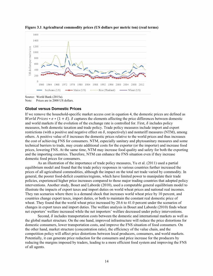
As shown in Figure 3.1, global food prices in real terms decreased for 10 years after the last food price spike in the 1970s and remained stable in the following decade (1996 to 2005). During the past decade, we have observed a slight upward trend, but it may be premature to conclude that the historical downward trend of food prices is reversed. This section will discuss the different long-term drivers behind these price evolutions, but first let’s reexamine equation 4 and discuss the gap between domestic and world prices.

14

Figure 3.1 Agricultural commodity prices (US dollars per metric ton) (real terms)

Source: World Bank (2015a). Note: Prices are in 2000 US dollars.

Global versus Domestic Prices If we remove the household-specific market access cost in equation 4, the domestic prices are defined as 𝑊𝑊𝑖𝑖𝑎𝑎𝑞𝑞𝑐𝑐 𝑃𝑃𝑎𝑎𝑞𝑞𝑖𝑖𝑎𝑎𝑠𝑠 ∗ 𝑎𝑎 ∗ (1 + 𝛿𝛿). 𝛿𝛿 captures the elements affecting the price differences between domestic and world markets if the evolution of the exchange rate is controlled for. First, 𝛿𝛿 includes policy measures, both domestic taxation and trade policy. Trade policy measures include import and export restrictions (with a positive and negative effect on 𝛿𝛿, respectively) and nontariff measures (NTM), among others. A positive value of 𝛿𝛿 increases the domestic prices relative to the world prices and thus increases the cost of achieving FNS for consumers. NTM, especially sanitary and phytosanitary measures and some technical barriers to trade, may create additional costs for the exporter (or the importer) and increase food prices, lowering FNS. At the same time, NTM may increase food quality and safety for both the exporting and the importing countries. Therefore, NTM can enhance the FNS situation even if they increase domestic food prices for consumers.

As an illustration of the importance of trade policy measures, Yu et al. (2011) used a partial equilibrium model and found that the trade policy responses in various countries further increased the prices of all agricultural commodities, although the impact on the total net trade varied by commodity. In general, the poorer food-deficit countries/regions, which have limited power to manipulate their trade policies, experienced higher price increases compared to those major trading countries that adopted policy interventions. Another study, Bouet and Laborde (2010), used a computable general equilibrium model to illustrate the impacts of export taxes and import duties on world wheat prices and national real incomes. They ran scenarios where there is a demand shock that increases world wheat price by 10 percent, and countries change export taxes, import duties, or both to maintain the constant real domestic price of wheat. They found that the world wheat price increased by 20.6 to 41.0 percent under the scenarios of changes in export taxes and import duties. The welfare analysis in Bouet and Laborde (2010) finds wheat net exporters’ welfare increased while the net importers’ welfare decreased under policy interventions.

Second, 𝛿𝛿 includes transportation costs between the domestic and international markets as well as the global market structure. On the one hand, improved infrastructure will reduce the price distortions for domestic consumers, lower transportation costs, and improve the FNS situation of food consumers. On the other hand, market structure (concentration ratio), the efficiency of the value chain, and the competition policy will affect price distortions between local producers, consumers, and world markets. Potentially, it can generate price reduction for the consumers and price increase for the producers by reducing the margins imposed by traders, leading to a more efficient food system and improving the FNS of all agents.

15

The other variable of interest is e, the exchange rate. Even if macroeconomic policies, especially monetary policy, can be used to manipulate the long-term exchange rate, most countries will not actively use these tools, and the effects on FNS of such policies will depend on the status of a country in terms of food trade balance. A net food-importing country keeping its currency undervalued is deteriorating its FNS by implementing a shadow tax on food consumers. More interesting is the market-driven evolution of the long-term real exchange rate, in particular for countries that are structurally net food importers and the interactions between food demand and the current account constraints. Two cases can occur. If the real prices of food products on world markets have a declining trend, a net food importer will face an improvement of its terms of trade. Even if the food imports will grow significantly in volume, the cost of these imports for the country will remain stable or even decline, leading to a strong improvement in FNS. On the other hand, if real prices of food are oriented upward compared to the prices of its exports, the importing country will suffer from deteriorating terms of trade. Its long-term FNS situation may deteriorate, especially if increasing domestic agricultural prices (driven by higher import prices) do not trigger a domestic supply response.

Next, an important aspect of long-term FNS stability is the relation between the food expenditure of a country (food imports) and its capacity to pay for it in foreign currency. A synthetic indicator is the degree of correlation between its revenue (value of exports) and its expenditures. Putting it differently, the evolution of the ratio between total exports and food imports, as well as the evolution of the country terms of trade, will show whether or not the country is more exposed to foreign—but also domestic—shocks. Therefore, two elements may contribute to a long-term shift in the FNS exposure of a country. If a country is a food exporter, it is naturally immune to global price variations since it does not need foreign currency to pay for its domestic consumption. If a country is a food importer, ensuring that the food import bill represents a limited share of the overall export revenue is crucial.

Finally, the long-term evolution of global governance of both international trade and capital markets will matter. For goods, it is important that both export restrictions on food products and import restrictions on other goods and services are bound. Otherwise, during a crisis period, a food-importing country can be a victim of foreign trade policies that will limit its supply of food and reduce its capacity to export other goods and services to pay for them. In addition, under these changes in terms of trade policies, the terms of trade will evolve in an adverse way for the importing country, hurting the FNS of its citizens. Similarly, ensuring stable and efficient international capital markets, especially for short- and medium-term transactions, is essential to countries facing short-term perturbation of their current accounts.

Drivers of Aggregate Food Demand This subsection is devoted to the four main drivers that will affect global demand and therefore global food prices. We are going to look at the exogenous drivers included in equation 7.

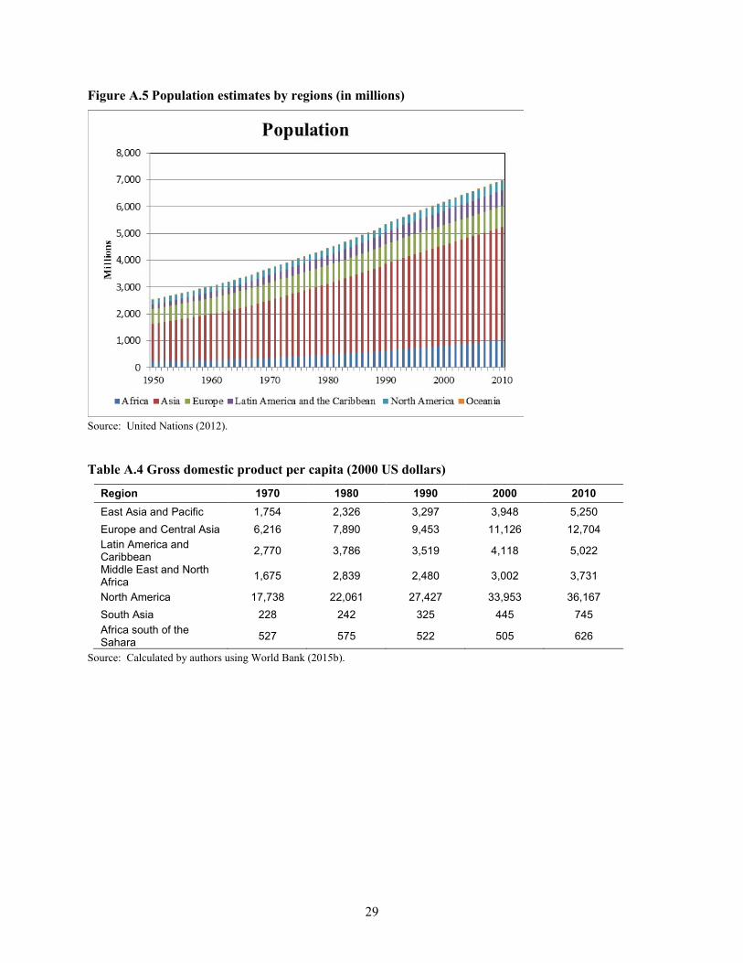
First, the accelerated increase of the world population has increased the number of mouths to feed, and demand for agricultural commodities is increasing worldwide, causing upward pressure on prices. The United Nations projects that the world population will increase from 6.9 billion in 2010 to 9.3 billion in 2050 (United Nations 2012) for the central scenario (see Table A.3 and Figure A.5). It is important to stress that based on more recent projections, including those by the demographic institutes for the largest countries, these estimates should be seen as an upper bound; the global population may stabilize at a lower level. A significant portion of this population growth would come from low-income countries that have limited potential to increase the domestic supply of food (for example, Bangladesh, Pakistan) and thus would turn to world markets to import their food supply. Demographic projections also should be seen as a starting point; it is more realistic to convert global populations to comparable terms such as “male adult equivalent” rather than looking at the total numbers. Indeed, countries with a larger

16

share of children or countries with populations that will age significantly during the period will have lower food consumption per capita.4

Second, another significant contributor to food demand growth is income growth. The expansion of income per capita will mechanically increase the demand for food per capita. At the same time, the net effects will strongly depend on the income distribution among countries (see Table A.4 and Figure A.6). Global income increase will have three main effects:

1. Additional food demand (even if income elasticities of food products decline with income level, they remain positive for most products for the range of income changes for most of the world population)

2. Changes in diet patterns, leading, for households moving to the middle of income distribution, to a shift toward meat and dairy products and in latter stages toward fruits and vegetables but also specific types of foods (for example, organic)

3. Reduction in the average food price elasticity of the global food system We illustrate in Table 3.1 the differentiated impacts of income growth for different types of

countries (item 2 above). Income growth in East and South Asia (China, India, and Vietnam, among other countries) allows consumers to shift their consumption toward livestock and dairy products and away from staple crops (cereals). For some low-income countries, higher income may mean higher demand for staples since their consumption patterns are not yet changing with income growth. China, India, and Vietnam have significantly higher growth rates of milk and meat consumption, in per capita terms, relative to higher-income countries (such as Canada, European Union countries, and the United States) that have already completed this transformation, or lower-income countries (such as the Philippines) that do not have the means to purchase these protein-rich goods. Furthermore, increased demand for meat and dairy translate into increased demand for livestock feed (maize, sorghum, or feed wheat). So world trade in feed grains or protein meals is expected to expand.

Table 3.1 Average annual per capita consumption growth rates (2000–2015) Country Total meata Total fluid milk % %

BRIC Brazil 1.87 1.94 China 2.00 10.41 India 5.16 2.62 Russia 3.77 –0.24

Higher-income countries Australia 1.14 –2.20 Canada –1.15 –0.64 European Union –0.33 0.51 United States –0.66 0.73

Lower-income countries Chile 1.84 –0.77 Egypt –4.37 –0.07 Philippines 1.87 1.27 Peru 3.50 2.24 Thailand 1.85 2.36 Vietnam 5.48 8.53

Source: Calculated by authors using USDA (2015b). Note: BRIC = Brazil, Russia, India, and China. a. Total meat consumption includes beef, veal, swine, broiler, and turkey, when

available.

4 Please note that daily recommended energy allowance varies by gender and age as described in U.S. Department of

Agriculture (2001), and this should be taken into account when discussing the role of population dynamics on food demand.

17

Therefore, from the demand point of view, the rise in world income will increase FNS for households with rising real income, as discussed in Section 2, and will lead to an increase in world food prices and will make these prices more volatile due to the trend toward a more inelastic food system. In this context, some households and countries that have no or limited income gains will suffer from the price evolution, and their FNS will deteriorate. Concerning the effect of the changes in diets, it is an improvement in FNS. At the same time, this demand shifter will have consequences on overall food prices. We will discuss in the next subsection the consequences for the supply side of these changes in dietary patterns.

Third, changes in preferences5 also will matter at the global level. Due to the global trend of increased urbanization, food habits are expected to change, even under constant income levels. This is related not only to changes in lifestyle but also to new access to different distribution services (for example, supermarkets). It will increase the share of processed foods consumed globally and the consumption of some product categories, such as dairy, that need specific distribution channels. For instance, a diversified supply of dairy products in supermarkets, based on an efficient cold chain, leads to more diversified consumption patterns by households. This global shift in aggregated preferences will increase the prices of specific products (for example, milk), leading to peculiar negative externalities for other consumers, and will force the overall supply system to adapt with consequences on the average cost by protein/calories as discussed in the next subsection.

Fourth, the effects of the aggregate domestic distortions will matter, from the trade policies implemented by each government to the lack of competition in the distribution sector of some countries. Indeed, they will lead to reduced demand in some countries by maintaining relatively high prices at the domestic level. The removing of these different distortions will shift domestic demand curves and boost global demand. Therefore, their elimination will lead to an increase in world food prices (see Keeney and Hertel 2005; Laborde, Martin, and van Der Mensbrugghe 2012 for the illustration of how global or partial trade reform will lead to an increase in world food prices). In terms of FNS, it is important to keep in mind that for domestic consumers, the effects of removal of global distortions will raise world prices, but since their own border distortions should go down, the net effect can still be a reduction in local food prices and a net improvement of their FNS under certain conditions. Concerning distortions and their demand effects, we focus on long-term drivers, and we will not discuss the short-term variations of trade policies aimed to stabilize food prices that can have positive effects of the FNS situation of the country implementing them and negative effects on its partners (see Bouet and Laborde 2010; 2012). Nevertheless, in this context it is important to underline again the importance of a secure trade system as promoted by the World Trade Organization with commitments on both import duties (bound rates) and export restrictions. Contrary to the discussion of the previous sections on the consequences of trade policy variations on a country exchange rate or current account constraints, we emphasize here the role of the cost for the consumers of the volatility of such policies (see, for instance, Manole, Martin, and Francois 2005).

Drivers of Aggregate Food Supply In the long run, the transformation of the supply side has structurally determined the evolution of world food prices. As we will discuss below, many factors will affect the capacity of the global food supply to meet the changing needs of demand in terms of both quality and quantity of food, leading to different outcomes in terms of food prices.

Equation 8 has defined three main drivers of food supply: the land available for food products, the normalized average yield, and the share of waste/losses generated by the food system. The last effect being the most simple to discuss, we start with it.

5 From the microeconomic point of view that we adopt here, a dietary change due to a change in income is not a

modification of preferences but the mechanical changes in a food demand system properly specified with constant preferences.

18

Roughly one-third of food produced for human consumption, about 1.3 billion tons per year, is not consumed by humans. Food waste is estimated to be higher in developed countries: per capita consumer waste is estimated to be 95 to 115 kilograms per year for Europe and North America but only 6 to 11 kilograms per year in Africa south of the Sahara and South Asia (Gustavsson et al. 2011). The underlying reasons for food waste differ between regions as well. In high-income countries food waste is due to consumer waste. The total avoidable food waste in the United States is 55.41 million metric tons per year for 2009, which amounts to 28.7 percent of total annual production by weight (Venkat 2011). For this country, consumer waste alone amounts to US$124.1 billion, or nearly 63 percent of the total retail value of wasted food (Venkat 2011). On the other hand, in developing countries, we observe high losses at the postharvest and processing stages due to spoilage. Factors leading to spoilage include lack of modern transport and storage infrastructure as well as financial, managerial, and technical limitations in difficult climatic conditions (Venkat 2011; Gustavsson et al. 2011). If increased household income can lead to increased food waste due to changes in food consumption habits, increased education and improved regulations can promote waste reduction and improved biomass use. On the producer side, improved value chain efficiency and investments in infrastructure (transportation and storage) will reduce losses and boost effective food supply with the same level of inputs, leading to a price decrease and a systematic improvement of FNS.

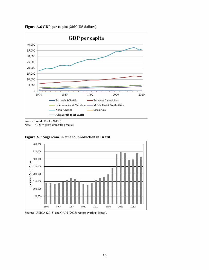
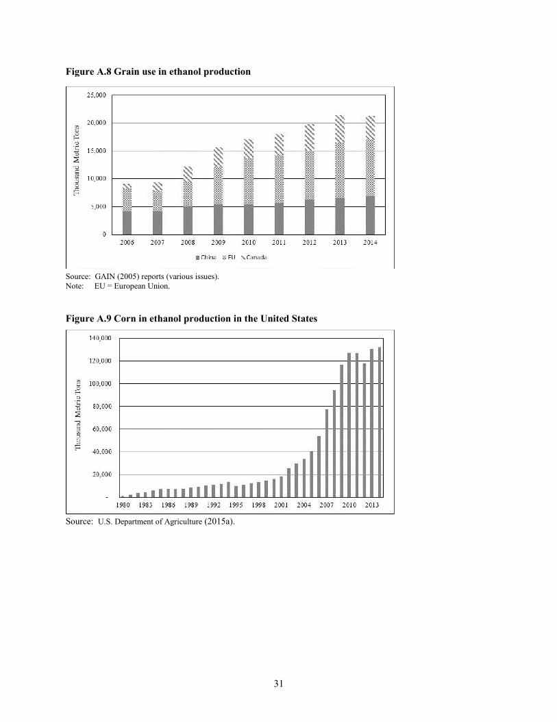
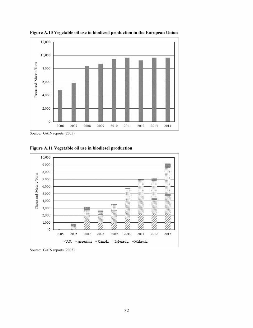
The other critical driver, that is, the extensive production factor, is the amount of land available for food production. This driver is affected by different factors as described by equation 10. First, 𝜃𝜃 defines the share of agricultural land used for nonfood production. It includes traditional crops such as cotton, natural rubber, tobacco, and forestry (paper, wood products). During the past decade, a new demand has emerged, the need for land for biomass-based energy and especially liquid biofuels to meet growing demand and to diversify sources of supply. Various biofuels initiatives, such as those in the European Union and the United States, have increased demand for agricultural feedstock. Maize, vegetable oils, and sugar cane, among other crops, are now being used to produce transportation fuels. Figures A.7 through A.11 show the growing demand for various feedstock. Brazil nearly doubled its use of sugarcane for ethanol in the past two decades. The United States increased its corn use for ethanol eightfold in the same period. The European Union’s vegetable oil use for biodiesel reached 9.7 million metric tons in 2014 from a nonexistent industry.

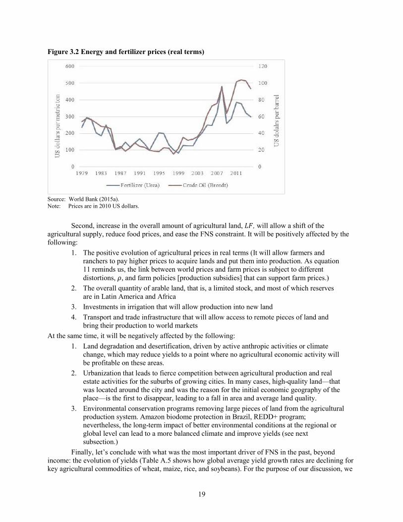
Higher crude oil prices in past years (Figure 3.2), which also affected gasoline and diesel prices, led refiners and consumers to increase their use of biofuels in transportation vehicles. Laborde (2011) shows that world production of biofuels will reach 110 million tons of oil equivalent by 2020, an increase of 176 percent compared to the 2008 level, absorbing in 2020 around 20–23 percent of world production of corn, sugar cane/beet, and rapeseed.6 This trend of increased demand for agricultural feedstock is expected to continue if second-generation biofuels are commercially viable enough to replace the first-generation biofuels. In addition, the effects of the latter on the arable land demand may still imply competition for food products. Overall, the growth of any nonfood demand for biomass will lead to competition with food products and will generate an increase in food prices that hurt FNS. Nevertheless, some households having stakes in the production of bioenergy of their feedstock can still benefit from net real income gains due to these policies.

6 These estimates refer to the gross use of crops and do not correct for the coproducts generated by the biofuel production

that will replace a part of the crops displaced.

19

Figure 3.2 Energy and fertilizer prices (real terms)

Source: World Bank (2015a). Note: Prices are in 2010 US dollars.

Second, increase in the overall amount of agricultural land, 𝐿𝐿𝐹𝐹, will allow a shift of the agricultural supply, reduce food prices, and ease the FNS constraint. It will be positively affected by the following:

1. The positive evolution of agricultural prices in real terms (It will allow farmers and ranchers to pay higher prices to acquire lands and put them into production. As equation 11 reminds us, the link between world prices and farm prices is subject to different distortions, 𝜌𝜌, and farm policies [production subsidies] that can support farm prices.)

2. The overall quantity of arable land, that is, a limited stock, and most of which reserves are in Latin America and Africa

3. Investments in irrigation that will allow production into new land 4. Transport and trade infrastructure that will allow access to remote pieces of land and

bring their production to world markets At the same time, it will be negatively affected by the following:

1. Land degradation and desertification, driven by active anthropic activities or climate change, which may reduce yields to a point where no agricultural economic activity will be profitable on these areas.

2. Urbanization that leads to fierce competition between agricultural production and real estate activities for the suburbs of growing cities. In many cases, high-quality land—that was located around the city and was the reason for the initial economic geography of the place—is the first to disappear, leading to a fall in area and average land quality.

3. Environmental conservation programs removing large pieces of land from the agricultural production system. Amazon biodome protection in Brazil, REDD+ program; nevertheless, the long-term impact of better environmental conditions at the regional or global level can lead to a more balanced climate and improve yields (see next subsection.)

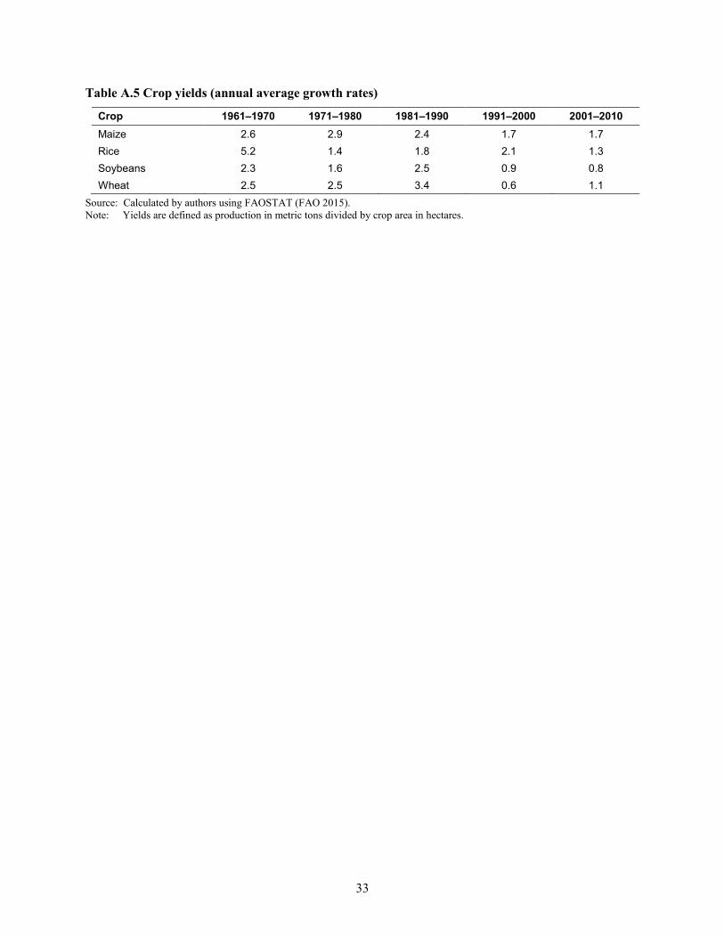
Finally, let’s conclude with what was the most important driver of FNS in the past, beyond income: the evolution of yields (Table A.5 shows how global average yield growth rates are declining for key agricultural commodities of wheat, maize, rice, and soybeans). For the purpose of our discussion, we

20

define yield as the amount of nutrients produced by unit of land. It depends both on the physical yield of the crop or the livestock and on the quality of the food. Yields are positively affected by the following:

1. Farm prices, which will trigger more intensification 2. Land quality (better land management to avoid land degradation) 3. Inputs including water (irrigation), improved seeds, and fertilizers (For the latter, we

should note that increasing prices may be an important factor in limiting potential yield increase [for example, limited global reserves of phosphates]. At the same time, different reforms in the market structure of fertilizer production can help to reduce the price of this input [Hernandez and Torero 2011], and the activation of new natural gas reserves [shale gas with fracking] can lead to an important decrease in nitrogen prices.)

4. Investments (mechanization, irrigation) 5. Knowledge created by research and development for improved yields, input savings

varieties, pest-resistant plants, and so forth (It also involves better human capital for farmers who can benefit from extension services.)

6. Improved agricultural practices and seeds with a multicropping, integrated agricultural system

At the same time, the average yield will be deteriorated by the changes in production patterns linked to the different dietary patterns of consumers. For each hectare of land, final animal production (based on grazing or intensive feeding solution) will generate less protein and calories than a pure crop-based system. Therefore, the average cost of producing protein and calories will increase the share of animal products in the overall food production pattern. Similarly, higher-quality food such as organic foods or those produced with better animal welfare rules, which can have positive effects on consumer health, will also lead to a less intensive production system with reduced yields.

The last important set of drivers of yields is climatic. Climate change adds further pressure to the dramatic transformation of global agricultural markets due to its effect on local temperature and precipitation conditions. Climate models (global circulation models) provide us with information about the effects of changes in water availability and temperature on yields given the probable evolution of rainfall and atmospheric conditions. Beyond the temperature and water channels, climate change may bring new pests and diseases to some regions and remove them from others. A first conclusion of the potential scenarios on climate change is that it will have uneven effects among crops and among countries, generating winners and losers. Using current technology (crops, practices, locations), climate change will reduce average yields during the transition period but may generate large opportunities of increased biomass production since higher temperatures, a wetter climate, and a higher concentration of carbon dioxide can support increased photosynthesis. Studies that combine global circulation models with economic models show that climate change has an impact on agricultural productivity, on commodity prices, and on factor prices. Through the factor price channels, factors will be reallocated in the economy, and thus sectoral specializations will change. In addition, incomes will be affected, and the demand behaviors will be modified. These changes, however, occur not in a closed economy but at the global level with heterogeneous effects across countries and across commodities. Comparative advantages evolve, trade patterns adapt, and countries are affected by the domestic effects of climate change and the modifications of relative prices on world markets (terms of trade effects). With time, considering income and current account constraints, production will be reallocated across sectors and across regions to adapt to the exogenous changes in yields. Depending on the situation, general equilibrium effects will mitigate or magnify the initial impacts. The effects of climate change include long-term shift in yields that will change the cropping strategy and the land allocation and conversion decisions made by farmers. These supply effects will lower exports or increase import demand, causing agricultural commodity prices to increase. Higher crop prices may induce farmers to increase input use (such as fertilizer) and increase yields to a certain extent. However, overall crop yields will suffer with climate change, causing available

21

food supply in world markets to shrink to a certain extent (Laborde et al. 2010) if no innovation in terms of crop varieties takes place.

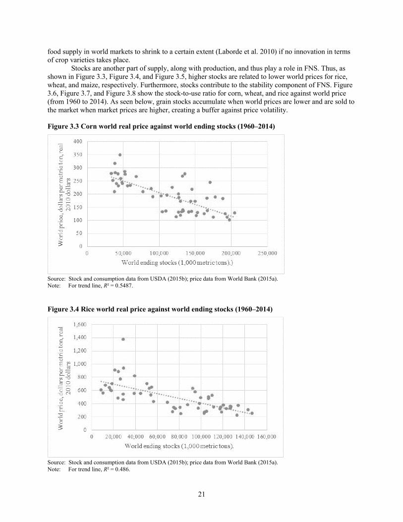
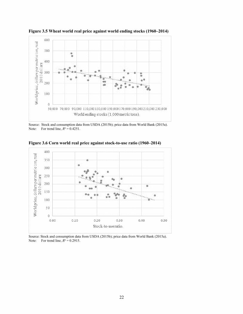
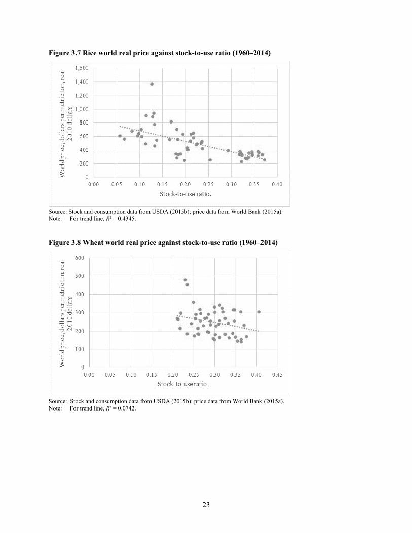
Stocks are another part of supply, along with production, and thus play a role in FNS. Thus, as shown in Figure 3.3, Figure 3.4, and Figure 3.5, higher stocks are related to lower world prices for rice, wheat, and maize, respectively. Furthermore, stocks contribute to the stability component of FNS. Figure 3.6, Figure 3.7, and Figure 3.8 show the stock-to-use ratio for corn, wheat, and rice against world price (from 1960 to 2014). As seen below, grain stocks accumulate when world prices are lower and are sold to the market when market prices are higher, creating a buffer against price volatility.

Figure 3.3 Corn world real price against world ending stocks (1960–2014)

Source: Stock and consumption data from USDA (2015b); price data from World Bank (2015a). Note: For trend line, R² = 0.5487.

Figure 3.4 Rice world real price against world ending stocks (1960–2014)

Source: Stock and consumption data from USDA (2015b); price data from World Bank (2015a). Note: For trend line, R² = 0.486.

22

Figure 3.5 Wheat world real price against world ending stocks (1960–2014)

Source: Stock and consumption data from USDA (2015b); price data from World Bank (2015a). Note: For trend line, R² = 0.4251.

Figure 3.6 Corn world real price against stock-to-use ratio (1960–2014)

Source: Stock and consumption data from USDA (2015b); price data from World Bank (2015a). Note: For trend line, R² = 0.2915.

23

Figure 3.7 Rice world real price against stock-to-use ratio (1960–2014)

Source: Stock and consumption data from USDA (2015b); price data from World Bank (2015a). Note: For trend line, R² = 0.4345.

Figure 3.8 Wheat world real price against stock-to-use ratio (1960–2014)

Source: Stock and consumption data from USDA (2015b); price data from World Bank (2015a). Note: For trend line, R² = 0.0742.

24

4. CONCLUSIONS

This paper provides a systematic analytical framework to study the long-term drivers of FNS. By describing the food system through a system of equations, from the household level to the global market level, we have identified the different drivers. For each main driver, we also underlined the different channels of intervention for policy makers, such as inclusive growth, education, competition policies, and food subsidies. We also have proposed a typology of variables that will help modelers adapt their models to study the different drivers, through both direct and indirect effects. As a matter of fact, many drivers can have contrasted effects on FNS among households, within countries, and among countries. For example, trade policies are known to have contrasted effects. At the same time, even more direct policies, such as yield improvement policies, can lead to some households’ being worse off if they are biased in favor of some regions or crops. Therefore, systematic quantitative assessments using the best available simulation models are required to analyze the issue since simple solutions and analyses are the wrong answers to such a complex issue of long-term drivers of FNS.

We also should acknowledge that at different points in time, some drivers may be more important than others. During the 19th century, the fear of decreasing marginal productivity of land and its consequences on yield were seen as the main obstacles attending FNS in the long run. Before the First World War, the lack of land fertility was blamed for food and nutrition problems. After the First World War, the focus in the literature was not on land fertility but on woman fertility and the increased demographic pressure. Nowadays, rise in income and its uneven distribution, demographic pressures, and yield uncertainties, driven by climate change, are among the main concerns.

The paper also provides a snapshot of the FNS situation for a range of countries using different FNS indicators such as undernourishment, under-five stunting, and the Global Hunger Index, among others. Data highlight that although significant progress has been made for achieving FNS, the situation is still dire in many countries and in different income strata of a given country. Data specifically accentuate the role of income growth and the inclusivity of income growth in achieving FNS. Supply-side drivers are manifold but have two common threads that run through: one is their impact on the level of supply, and the other is their impact on the stability of supply.

To sum up, achieving FNS for their entire populations is a common goal for all countries. To this end, first, countries should define what FNS entails for them. Second, they should choose specific FNS indicators that allow them to identify a benchmark against which they measure their success. Third, they should identify the drivers that they want to focus on (based on their comparative advantage) to achieve FNS in a consistent manner. Finally, they should select the most effective policy space that they want to utilize, where policy outcomes amplify each other and do not reduce each other’s effectiveness.

25

APPENDIX: SUPPLEMENTARY TABLES AND FIGURES

Table A.1 Definitions Name Source Definition

Undernourishment FAO (2012) This term is used interchangeably with chronic hunger.

Micronutrient deficiency

FAO (2012)

Hidden hunger: this refers to vitamin and mineral deficiencies or micronutrient deficiencies. Micronutrient deficiencies can compromise growth, immune function, cognitive development, and reproductive and work capacity. Somebody who suffers from hidden hunger is malnourished but may not sense hunger. Micronutrient deficiencies can occur in people who are overweight or obese.

Underweight FAO (2012)

Low weight for age in children and body mass index < 18.5 in adults, reflecting a current condition resulting from inadequate food intake, past episodes of undernutrition, or poor health condition

Micronutrient malnutrition FAO (1997) Vitamin and mineral nutritional deficiency diseases

Micronutrient FAO (2012) The vitamins, minerals, and certain other substances that are required by the body in small amounts. They are measured in milligrams or micrograms.

Undernutrition FAO (2012)

The result of undernourishment, poor absorption, and/or poor biological use of nutrients consumed

Prevalence of undernourishment (% of population)

World Bank (2015b)

Population below the minimum level of dietary energy consumption (also referred to as prevalence of undernourishment) shows the percentage of the population whose food intake is insufficient to meet dietary energy requirements continuously.

Prevalence of severe wasting of children under five

World Bank (2015b)

Wasting prevalence is the proportion of children younger than five whose weight for height is more than two standard deviations below the median for the international reference population, ages 0 to 59 months.

Malnutrition prevalence as measured by height for age

World Bank (2015b)

Prevalence of child malnutrition is the percentage of children younger than five whose height for age (stunting) is more than two standard deviations below the median for the international reference population, ages 0 to 59 months. For children up to two years old height is measured by recumbent length. For older children height is measured by stature while standing. The data are based on the WHO’s new child growth standards released in 2006.

Malnutrition prevalence as measured by weight for age

World Bank (2015b)

Prevalence of child malnutrition is the percentage of children younger than five whose weight for age is more than two standard deviations below the median for the international reference population, ages 0 to 59 months. The data are based on the WHO’s new child growth standards released in 2006.

Undernourishment (%)

IFPRI (2014)

Proportion of the population in a condition of undernourishment. Undernourishment refers to the condition of people whose dietary energy consumption is continuously below their dietary energy requirement for maintaining a healthy life and carrying out a normal physical activity.

Under-five stunting

IFPRI (2014)

Percentage of children 0 to 59 months who are below two (moderate and severe) standard deviations from median height for age of the WHO Child Growth Standards

Under-five wasting

IFPRI (2014)

Percentage of children 0 to 59 months who are below two (moderate and severe) standard deviations from median weight for height of the WHO Child Growth Standards

Global Hunger Index

IFPRI (2014)

Global Hunger Index is a tool designed to comprehensively measure and track hunger globally and by region and country. Calculated each year by IFPRI, it combines three equally weighted indicators into one index: undernourishment, child underweight, and child mortality.

Source: Sources are listed in column 2. Note: FAO = Food and Agriculture Organization of the United Nations; IFPRI = International Food Policy Research Institute;

WHO = World Health Organization.

26

Figure A.1 Real GNI per capita and prevalence of undernourishment (2000)

Source: Calculated by authors using World Bank (2015b). Note: GNI = gross national income; Egypt, Arab Rep. = Egypt, Arab Republic. Real GNI per capita is in natural log. GNI is

deflated by each country’s consumer price index at base year 2010.

Figure A.2 Real GNI per capita and prevalence of undernourishment (2005)

Source: Calculated by authors using World Bank (2015b). Notes: GNI = gross national income; Egypt, Arab Rep. = Egypt, Arab Republic. Real GNI per capita is in natural log. GNI is

deflated by each country’s consumer price index at base year 2010.

27

Figure A.3 Gender inequality index against under-five stunting (percentages)

Source: IFPRI (2014). Note: Figure shows data for 101 countries for 2010.

Figure A.4 Gender inequality index against under-five wasting (percentages)

Source: IFPRI (2014). Note: Figure shows data for 101 countries for the year 2010.

28

Table A.2 Gini index

Country 1993 1994 2004 2005 2008 2009 2010 Burkina Faso 50.7 39.8 Bangladesh 33.2 32.1 Brazil 60.1 56.9 56.7 54.4 53.9 China 35.5 42.5 42.6 42.1 Costa Rica 46.0 46.8 48.9 47.8 49.1 51.0 48.1 Egypt 32.1 30.8 Indonesia 29.3 34.0 34.1 35.6 India 30.8 33.4 33.9 Kenya 42.1 47.7 Malawi 39.9 46.2 Pakistan 31.2 32.7 29.6 Peru 44.9 48.7 49.3 46.9 46.2 44.9 Philippines 42.9 43.0 Senegal 41.4 39.2 Thailand 43.5 40.5 39.4 United States 38.9 40.6 41.1 Vietnam 35.7 36.8 35.6 39.3 South Africa 59.3 63.1

Source: World Bank (2015b). Note: 100 = most inequality.

Table A.3 Population growth rates (decades)

Region 1960–1970 1970–1980 1980–1990 1990–2000 2000–2010 Africa 28 31 32 28 26 Asia 25 24 22 16 12 Europe 9 6 7 1 3 Latin America and the Caribbean 30 27 23 18 14

North America 13 10 14 12 11 Oceania 24 18 19 16 18 World 22 20 20 16 13

Source: Calculated by authors using United Nations (2012).

29

Figure A.5 Population estimates by regions (in millions)

Source: United Nations (2012).

Table A.4 Gross domestic product per capita (2000 US dollars)

Region 1970 1980 1990 2000 2010 East Asia and Pacific 1,754 2,326 3,297 3,948 5,250 Europe and Central Asia 6,216 7,890 9,453 11,126 12,704 Latin America and Caribbean 2,770 3,786 3,519 4,118 5,022

Middle East and North Africa 1,675 2,839 2,480 3,002 3,731

North America 17,738 22,061 27,427 33,953 36,167 South Asia 228 242 325 445 745 Africa south of the Sahara 527 575 522 505 626

Source: Calculated by authors using World Bank (2015b).

30

Figure A.6 GDP per capita (2000 US dollars)

Source: World Bank (2015b). Note: GDP = gross domestic product.

Figure A.7 Sugarcane in ethanol production in Brazil

Source: UNICA (2015) and GAIN (2005) reports (various issues).

31

Figure A.8 Grain use in ethanol production

Source: GAIN (2005) reports (various issues). Note: EU = European Union.

Figure A.9 Corn in ethanol production in the United States

Source: U.S. Department of Agriculture (2015a).

32

Figure A.10 Vegetable oil use in biodiesel production in the European Union

Source: GAIN reports (2005).

Figure A.11 Vegetable oil use in biodiesel production

Source: GAIN reports (2005).

33

Table A.5 Crop yields (annual average growth rates)

Crop 1961–1970 1971–1980 1981–1990 1991–2000 2001–2010 Maize 2.6 2.9 2.4 1.7 1.7 Rice 5.2 1.4 1.8 2.1 1.3 Soybeans 2.3 1.6 2.5 0.9 0.8 Wheat 2.5 2.5 3.4 0.6 1.1

Source: Calculated by authors using FAOSTAT (FAO 2015). Note: Yields are defined as production in metric tons divided by crop area in hectares.

34

REFERENCES

Bouet, A., and D. Laborde. 2010. Economics of Export Taxation in a Context of Food Crisis. IFPRI Discussion Paper 0994. Washington, DC: International Food Policy Research Institute. www.ifpri.org/sites/default/files/publications/ifpridp00994.pdf.

———. 2012. “Food Crisis and Export Taxation: The Cost of Non-cooperative Trade Policies.” Review of World Economics 148 (1): 209–233.

FAO (Food and Agriculture Organization of the United Nations). 1996. Declaration on World Food Security. Rome. www.fao.org/docrep/003/w3613e/w3613e00.htm.

———. 2006. Food Security: Policy Brief. Issue 2. Rome. www.fao.org/es/esa/.

———. 2008. An Introduction to the Basic Concepts of Food Security. Food Security Information for Action Practical Guides. Rome. www.fao.org/docrep/013/al936e/al936e00.pdf.

———. 2012. The State of Food Insecurity in the World 2012: Economic Growth Is Necessary but Not Sufficient to Accelerate Reduction of Hunger and Malnutrition. Rome. www.fao.org/publications/sofi/en/.

———. 2015. FAOSTAT. Accessed January 23, 2013. http://faostat3.fao.org/home/E.

FAO and International Life Sciences Institute. 1997. Preventing Micronutrient Malnutrition: A Guide to Food-based Approaches. Washington, DC: ILSI Press.

Friedman, M. 1957. “Permanent Income Hypothesis.” Accessed January 23, 2013. www.nber.org/chapters/c4405.

GAIN (Global Agricultural Information Network). 2005. “GAIN Reports.” Accessed May 18, 2015. gain.fas.usda.gov/Pages/Default.aspx.

Gustavsson, J., C. Cederberg, U. Sonesson, R. van Otterdijk, and A. Meybeck. 2011. Global Food Losses and Food Waste. Rome: Food and Agriculture Organization of the United Nations.www.fao.org/fileadmin/user_ upload/ags/publications/ GFL_web.pdf.

Harvest Plus. 2012. “About Harvest Plus.” Accessed January 23, 2013. www.harvestplus.org/content/about-harvestplus.

Hernandez, M., and M. Torero. 2011. Fertilizer Market Situation: Market Structure, Consumption and Trade Patterns, and Pricing Behavior. IFPRI Discussion Paper 1058. Washington, DC: International Food Policy Research Institute. www.ifpri.org/sites/default/files/publications/ifpridp01058.pdf.

IFPRI (International Food Policy Research Institute). 2014. 2014 Global Nutrition Report Data. Washington, DC. doi.org/10.7910/DVN/27857.

Keeney, R., and T. Hertel. 2005. GTAP-AGR: A Framework for Assessing the Implications of Multilateral Changes in Agricultural Policies. GTAP Technical Paper 1869. West Lafayette, IN: Center for Global Trade Analysis, Department of Agricultural Economics, Purdue University.

Kennedy, Eileen. "Measurement and Assessment of Food Deprivation and Undernutrition." Paper prepared for the International Scientific Symposium “Measurement and Assessment of Food Deprivation and Undernutriton.” Rome: FAO.

Laborde, D. 2011. Assessing the Land Use Change Consequences of European Biofuel Policies. Accessed January 23, 2013. www.ifpri.org/sites/default/files/publications/biofuelsreportec2011.pdf.

Laborde, D., C. Lakatos, G. Nelson, R. Robertson, and M. Thomas. 2010. Climate Change and Agriculture in South Asia: Alternative Trade Policy Options. IFPRI Report for the World Bank. Washington, DC: World Bank.

Laborde, D., W. Martin, and D. van Der Mensbrugghe. 2012. Implications of the Doha Market Access Modalities for Developing Countries. World Trade Review 11 (1): 1–25. doi.org/10.1017/S1474745611000437.

Malthus, T., 1798. An Essay on the Principle of Population, as it Affects the Future Improvement of Society with Remarks on the Speculations of Mr. Godwin, M. Condorcet, and Other Writers. London: J. Johnson, in St. Paul's Church-Yard.

35

Manole, V., W. Martin, and J. Francois. 2005. Choosing Formulas for Market Access Negotiation: Efficiency and Market Access Considerations. Policy Research Working Paper Series 3474. Washington, DC: World Bank.

UNICA (União da Indústria de Cana-de-Açúcar). 2015. UNICADATA. Accessed May 18, 2015. www.unica.com.br/.

United Nations. 2012. Department of Economic and Social Affairs, Population Division, Population Estimates and Projections Section. World Population Prospects, the 2010 Revision, Updated June 2011. Accessed December 16, 2012. http://esa.un.org/wpp/Excel-Data/population.htm.

USDA (U.S. Department of Agriculture). 2001. National Survey of WIC Participants. Report No. WIC-01-NSWP. Accessed January 23, 2013. www.fns.usda.gov/ora/MENU/Published/WIC/FILES/WICSurvey.pdf.

———. 2015a. Feed Grains Database. Accessed January 23, 2013. www.ers.usda.gov/data-products/feed-grains-database.aspx.

———. 2015b. Production, Supply, and Distribution. Accessed May 18, 2015. www.fas.usda.gov/psdonline/psdHome.aspx.

Venkat, K. 2011. “The Climate Change and Economic Impacts of Food Waste in the United States.” International Journal of Food System Dynamics 2 (4): 431–446.

von Grebmer, K., C. Ringler, M. W. Rosegrant, T. Olofinbiyi, D. Wiesmann, H. Fritschel, O. Badiane, M. Torero, Y. Yohannes, J. Thompson, C. von Oppeln, and J. Rahall. 2012. 2012 Global Hunger Index: The Challenge of Hunger: Ensuring Sustainable Food Security under Land, Water, and Energy Stresses. Bonn, Germany: Welthungerhilfe; Washington, DC: International Food Policy Research Institute; Dublin, Ireland: Concern Worldwide. http://dx.doi.org/10.2499/9780896299429.

World Bank. 2015a. GEM Commodities. Accessed May 18, 2015. http://data.worldbank.org/data-catalog/commodity-price-data.

———. 2015b. World Development Indicators. Accessed May 7, 2015. http://data.worldbank.org/indicator.

World Health Organization. 2016. “Obesity and Overweight.” Fact Sheet No. 311. Accessed April 12, 2016. www.who.int/mediacentre/factsheets/fs311/en/.

Yu, T., S. Tokgoz, E. Wailes, and E. Chavez. 2011. “A Quantitative Analysis of Trade Policy Responses to Higher World Agricultural Commodity Prices.” Food Policy 36: 545–561.

RECENT IFPRI DISCUSSION PAPERS

For earlier discussion papers, please go to www.ifpri.org/pubs/pubs.htm#dp. All discussion papers can be downloaded free of charge.

1530. Understanding compliance in programs promoting conservation agriculture: Modeling a case study in Malawi. Patrick S. Ward, Andrew R. Bell, Klaus Droppelmann, and Tim Benton, 2016.

1529. A model of reporting and controlling outbreaks by public health agencies. Alexander E. Saak and David A. Hennessy, 2016.

1528. Boserupian pressure and agricultural mechanization in modern Ghana. Frances Cossar, 2016.

1527. Agricultural mechanization and agricultural transformation. Xinshen Diao, Jed Silver, and Hiroyuki Takeshima, 2016.

1526. Delegation of quality control in value chains. Alexander E. Saak, 2016.

1525. Structural transformation and intertemporal evolution of real wages, machine use, and farm size–productivity relationships in Vietnam. Yanyan Liu, William Violette, and Christopher B. Barrett, 2016.

1524. Can contract farming increase farmers’ income and enhance adoption of food safety practices?: Evidence from remote areas of Nepal. Anjani Kumar, Devesh Roy, Gaurav Tripathi, P. K. Joshi, and Rajendra P. Adhikari, 2016.

1523. Effectiveness of food subsidies in raising healthy food consumption: Public distribution of pulses in India. Suman Chakrabarti, Avinash Kishore, and Devesh Roy, 2016.

1522. Findings across agricultural public expenditure reviews in African countries. Stephen D. Mink, 2016.

1521. Risk and sustainable crop intensification: The case of smallholder rice and potato farmers in Uganda. Bjorn Van Campenhout, Emmanuel Bizimungu, and Dorothy Birungi, 2016.

1520. Varietal integrity, damage abatement, and productivity: Evidence from the cultivation of Bt cotton in Pakistan. Xingliang Ma, Melinda Smale, David J. Spielman, Patricia Zambrano, Hina Nazli, and Fatima Zaidi, 2016.

1519. Institutional arrangements to make public spending responsive to the poor—(where) have they worked?: Review of the evidence on four major intervention types. Tewodaj Mogues and Alvina Erman, 2016.

1518. A poverty-sensitive scorecard to prioritize lending and grant allocation: Evidence from Central America. Manuel A. Hernandez and Maximo Torero, 2016.

1517. Can information help reduce imbalanced application of fertilizers in India?: Experimental evidence from Bihar. Ram Fishman, Avinash Kishore, Yoav Rothler, Patrick S. Ward, Shankar Jha, and R. K. P. Singh, 2016.

1516. Pakistan’s fertilizer sector: Structure, policies, performance, and impacts. Mubarik Ali, Faryal Ahmed, Hira Channa, and Stephen Davies, 2016.

1515. Agriculture-nutrition linkages and child health in the presence of conflict in Nepal. Elizabeth Bageant, Yanyan Liu, and Xinshen Diao, 2016.

1514. “As a husband i will love, lead, and provide”: Gendered access to land in Ghana. Isabel Lambrecht, 2016.

1513. Formal versus informal: Efficiency, Inclusiveness, and financing of dairy value chains in India. Pratap S. Birthal, Ramesh Chand, P. K. Joshi, Raka Saxena, Pallavi Rajkhowa, Md. Tajuddin Khan, Mohd Arshad Khan, and Khyali R. Chaudhary, 2016.

1512. Measuring women’s disempowerment in agriculture in Pakistan. Nuzhat Ahmad and Huma Khan, 2016.

1511. The impact of conditional cash transfer programs on indigenous households in Latin America: Evidence from PROGRESA in Mexico. Esteban J. Quiñones and Shalini Roy, 2016.

1510. Why some are more equal than others: Country typologies of food security. Eugenio Díaz-Bonilla and Marcelle Thomas, 2016.

1509. Empowerment and agricultural production: Evidence from rural households in Niger. Fleur Wouterse, 2016.

1508. Is access to tractor service a binding constraint for Nepali Terai farmers? Hiroyuki Takeshima, Rajendra Prasad Adhikari, and Anjani Kumar, 2016.

1507. Determinants of chemical fertilizer use in Nepal: Insights based on price responsiveness and income effects. Hiroyuki Takeshima, Rajendra Prasad Adhikari, Basu Dev Kaphle, Sabnam Shivakoti, and Anjani Kumar, 2016.

INTERNATIONAL FOOD POLICY RESEARCH INSTITUTE

www.ifpri.org

IFPRI HEADQUARTERS 2033 K Street, NW Washington, DC 20006-1002 USA Tel.: +1-202-862-5600 Fax: +1-202-467-4439 Email: ifpri@cgiar.org