Embed Size (px)
Citation preview
1
Local Financial Development and SMEs Capital Structure. An Empirical Investigation
Mariarosaria Agostino* , Maurizio La Rocca** §, Tiziana La Rocca** and Francesco Trivieri*
*Department of Economics and Statistics, **Department of Business Sciences, University of Calabria, Italy
This version 15 April 2009
Abstract
The present study investigates the role of institutional differences at the local level as determinants of firms’ capital
structure. Specifically, the aim is to empirically assess whether and to what extent SMEs’ financial decisions are af-
fected by local financial development – evaluating this influence both ceteris paribus, and by allowing it to be condi-
tional on different levels of legal enforcement inefficiency. After controlling for debt inertia, firms’ heterogeneity and
endogeneity problems, the main finding of the analysis suggests that local financial development may be an important
determinant of SMEs’ capital structure. In fact, firms appear to have better access to financial debt in areas characterised
by a higher quality of the legal system – possibly as intermediaries may be more inclined to provide funds where the
enforcement systems allow a more effective credit protection. Despite the international process of integration in capital
markets, local financial institutions do not seem to become irrelevant for SMEs - which are in need of well developed
institutions at local level to gain easier access to external financial resources.
JEL code: G21; G30. Keywords: firms’ capital structure; bank debt; local financial development; local enforcement system, SMEs.
§ Corresponding author. Department of Business Sciences, cubo 3-C, University of Calabria, 87036 Rende, Cosenza, Italy. Tel.
+39 0984 492221. Email: [email protected].

2
1. Introduction
Corporate financing choices are likely to be determined by a host of factors that are related to the
characteristics of the firm, as well as to the institutional environment where the latter operates. Although
most contributes examine corporate financing choices focusing on firm characteristics, a recent strand
of the literature studies how institutional factors may affect firms’ capital structure choices (Demirguc-
Kunt and Maksimovic 2008, 2002, 1998, 1996a; Cheng and Shiu 2007; Lopez-Iturriaga and Rodriguez-
Sanz 2007; Utrero-González 2007; Bianco et al. 2005; Giannetti 2003; Titman et al. 2003; Booth et al.
2001; La Porta et al. 1997, 1998; Rajan and Zingales 1995).
Most of this research has examined large firms facing a wide range of institutional environments re-
lying on cross-country data, while recent works have highlighted differences in institutional setting at
local level (e.g. Guiso et al. 2004). The latter claim that, within a single country, local institutional dif-
ferences can exist and might play a crucial role in determining corporate financial decisions. One of
these local institutional characteristics which has received increasing interest from scholars is the degree
of financial development. Indeed, despite the process of financial markets integration and internationali-
zation, local financial markets may keep a great relevance in affecting firms’ capital structure, espe-
cially when firms cannot realize the benefits of moving to the international capital market or they con-
sider it too costly and not easily accessible.
Besides, several studies highlight the role of the judicial enforcement in shaping the functioning of a
financial system, and so affecting financing decisions (La Porta et al. 1997, 1998; Beck and Levine
2004). Indeed, the judicial enforcement is important as the regulations governing the financial system
work in the interest of investors, protecting creditors only to the extent that the rules are actually en-
forced. Due to the risk of default and the difficulty to get back the liquidation value of the collateral, en-
forcement affects the ex-ante availability of agents to provide finance. Likewise, as recent contributions
point out (e.g. Utrero-González 2007; Giannetti 2003), enforcement and investor protection foster fi-
nancial market development mitigating agency problems.
Inspired by the literature strands so far illustrated, the present paper aims to empirically investigate
whether and to what extent the financial decisions of small and medium sized firms (henceforth SMEs)

3
are influenced by the degree of financial development at the local level. We evaluate this relationship
both ceteris paribus, and by allowing the impact of the provincial financial development to be condi-
tional on different levels of legal enforcement inefficiency. Thus, our work distinguishes itself from the
extant literature as – in studying SMEs financial choices – it focuses on local instead of country factors,
and it allows for interaction between different institutional features.
The reason for which we consider SMEs is that, as shown by several contributions, the influence of
local institutional factors on capital structure decisions is particularly relevant for such firms, despite the
international phenomenon of market integration. For example, Demirguc-Kunt and Maksimovic (1998)
highlight that institutional factors have a different influence on the financial policies of SMEs, com-
pared to those of larger firms. Further, Beck et al. (2005) point out that market imperfections, such as
those caused by underdeveloped financial and legal systems, constrain funding decisions depending on
firms’ size.
To carry out our empirical analysis we employ Italian data, as Italy provides an ideal laboratory to
test the effect of local institutional factors on SMEs capital structure for at least two reasons. First, the
Italian economy is dominated by SMEs. In the second place, it is widely documented that the efficiency
degree of both financial and legal enforcement systems is quite dissimilar across the Italian local areas,
within a financial system and a legal/regulatory framework highly integrated and uniform.
Following Guiso et al. (2004), we consider as local markets the 103 existing Italian administrative
provinces (geographic entities very similar to a US counties). The Italian Antitrust Authority, as well,
considers the province as the 'relevant market’ in banking activities - and the single province was, until
1990, the unit of analysis considered by the Bank of Italy to decide whether to authorize the opening of
new branches.
The remainder of the paper is organized as follows. The next section presents a brief review of the
literature on the issue concerning the effects of local financial development on firms’ capital structure.
Section 3 provides a short overview on SMEs and the financial system in Italy. Section 4 illustrates the
econometric specification and the methodology adopted. Section 5 describes the data. Section 6 dis-
cuses the results obtained, and section 7 concludes.

4
2. Capital structure and local financial development: from the extant literature to our testing
hypotheses
Capital structure is a controversial topic in academia and in the business community (Rajan and Zin-
gales 1995). The facts about capital structure show that the optimal mix between debt and equity is in-
fluenced by many factors, that raise benefits and costs.1 It is growing the interest in empirically studying
the connection between institutions and firms’ capital structure to understand debt versus equity choices
(Demirguc-Kunt and Maksimovic 1998). The main literature is based on cross-country analysis empha-
sizing the effects of institutional differences on capital structure (Demirguc-Kunt and Maksimovic,
1999; Booth et al. 2001; Titman et al. 2003), and showing that financing decisions are shaped both by a
country’s legal and financial environment (La Porta et al. 1997, 1998; Demirguc-Kunt and Maksimovic
1998; Rajan and Zingales 1998). Specifically, the research on the relationship between law and finance
takes into account the role of institutional factors, such as the efficiency of financial and enforcement
systems (Lopez-Iturriaga and Rodriguez-Sanz 2007; Rajan and Zingales 2003; La Porta et al. 1998;
Demirguc-Kunt and Maksimovic 1996a). Institutions that work efficiently can reduce problems of op-
portunism and asymmetric information, with significant effect on the relative magnitude of costs and
benefits associated to the debt. The effect of financial development on financing decisions is become a
main research priority considering that, as suggested by Rajan and Zingales (1998), financial develop-
ment facilities the growth of the firms, affecting capital structure decisions through the reduction of the
costs of external finance. Although previous studies are based on cross-country analysis (Demirguc-
Kunt and Maksimovic 2008, 2002, 1999, 1998, 1996a, 1996b; Lopez-Iturriaga and Rodriguez-Sanz
2007; Utrero-González 2007; La Porta et al. 1997; Rajan and Zingales 1995),2 it may also be that,
1 Companies that use debt as a source of finance can benefit from tax advantages, due to interest deduction, a reduction in
asymmetric information, and managerial discipline. Nonetheless, there are also costs related to the use of debt that arise from
the presence of financial distress, agency problems, and loss of financial flexibility.
2 For example, Demirguc-Kunt and Maksimovic (1999) showed that differences in financing patterns are mostly due to the
differences in the financial development, as well as differences in the underlying legal infrastructure. Fan et al. (2003) also
confirmed earlier findings that institutional differences between countries are much more important in determining capital
structure choices of firms compared with other factors, such as industry affiliation.

5
within a country, differences in the companies’ financial structure are explained by differences in the
degree of financial development at the local level. There is upward evidence in the finance literature that
the local context is relevant. Recent financial papers (Degryse and Ongena 2005; Petersen and Rajan
2002) highlight the importance of distance in explaining the availability and pricing of bank loans. In
particular, Petersen and Rajan (2002) document the importance of distance in the provision of bank
credit to small firms, especially in a country where the problems of asymmetric information are substan-
tial. Studies on the local context are also close to contemporary debates in the economic geography lit-
erature, interested in understanding firm financing across different regional contexts (Martin 1999). Pol-
lard (2003) suggests the need of contextualizing firm finance, analysing how different geographical con-
figurations of financial institutions affect the access to credit for firms operating locally. In general, it is
suggested the idea that banks operating locally have more knowledge and control about local firms and
entrepreneurs (Alessandrini and Zazzaro 1999). Furthermore, with a distinctive approach, the regional
economic literature has considered similar arguments, typically based on aggregate analysis related to
the regional impact of monetary policy. It has suggested that, especially for SMEs, there are important
regional difference in the credit conditions (Dow and Montagnoli 2007).
In general, on the effect of local financial development on capital structure decisions there is a grow-
ing interest, from different perspective of analysis. Considering that firms face several menus of
choices, opportunities and constraints according to the geographic context where they are based, the
analysis of the role of the local financial development on debt choices can provide relevant insights. To
assess the role of financial institutions in an increasingly integrated capital market, we follow a distinc-
tive approach. We study the effect of local financial development within a single country, using a simi-
lar approach of Guiso et al. (2004) but applied at provincial level.
Specifically, as highlighted by Diamond (1993) and Flannery (1986), the existence of asymmetric in-
formation is likely to tilt capital structures toward a higher use of debt. According to Titman et al.
(2003), a principal source of the financial constraint, influencing capital-structure, may be the existence
of asymmetric information and the cost of contracting between companies and potential providers of ex-
ternal financing. Problems of financial constraint are potentially high in presence of a poorly developed

6
financial system.3 A well-developed financial system can facilitate the ability of a company to gain ac-
cess to external financing, providing cheaper finance to worthy companies (Guiso et al. 2004). With a
well-developed financial system the efficiency of the market helps to avoid opportunistic behaviours.4
Thus, among different provincial areas, an increase in the financial development is assumed - ceteris
paribus - to allow for a higher use of debt (hypothesis 1). Hence, finding that local financial develop-
ment is a determinant of firms’ financing decisions may suggest that, despite the international process of
capital markets integration, developed local financial intermediaries could still matter for the availability
of financing sources stimulating growth.
In addition to the function of the financial system, a burgeoning literature suggests to account for the
role of the judicial enforcement in shaping the operation of a financial systems, and so affecting financ-
ing decisions.5 In particular, the law and finance theory focuses on the role of legal institutions and en-
forcement in explaining international differences in financial development (La Porta et al. 1997, 1998;
Beck and Levine 2004). Specifically, the judicial enforcement is important, because the regulations
governing the financial system work in the interest of investors, protecting creditors only to the extent
that the rules are actually enforced. Due to the risk of default and the difficulty to get back the liquida-
tion value of the collateral, enforcement affects the ex-ante availability of agents to provide finance. As
suggested by La Porta et al. (1998), because a good legal environment protects the potential financiers
against expropriation by entrepreneurs, it raises their willingness to provide funds to firms. Thus, as re-
3 It seems that firms may raise finance more easily as the financial system develops, because physical collateral becomes less
important while intangible assets and future cash flows can be financed. As the financial system develops, it should be able to
appreciate the soundness of the firm’s projects and of its managerial behaviors (Rajan and Zingales 1998).
4 For example, the less developed the financial system, the more banks will want to use short-term credit as a way to control
borrowers (Diamond 1991).
5 A selective review of research on the role of legal institutions in shaping the operation of financial systems is provided by
Beck and Levine (2004). In particular, as highlighted by Beck and Levine (2004) and summarized by Hart (1995) studies on
financial decisions are related to the role of the control rights that financial securities bring to their owners and to the impact of
different legal rules on corporate control. Considering capital structure as a set of contracts, the enforcement of these latter de-
termine the rights of securities holders and the operation of financial systems.

7
cent contributions highlight (e.g. Utrero-González 2007; Giannetti 2003), enforcement and investor pro-
tection foster financial market development mitigating agency problems.
The role of legal institutions and enforcement in explaining international differences in financial de-
velopment across countries (Beck and Levine 2004) can also apply with regards of within-country
analyses: the efficiency of the courts at local level can be different although the same law applies. The
existence of differences in the quality of the enforcement at local level, providing diverse level of credi-
tors’ protection, affects the local financial development. As suggested by the law and finance view, the
local financial development would be higher where the judicial enforcement is more effective, while the
financial support to firms would be lower where the quality of the legal system is weaker. Therefore,
across different provincial areas, a more efficient enforcement system should strengthen the impact of
the local financial development on the use of SMEs’ debt. Stated differently, we expect that the higher
the local judicial costs the lower the local financial development impact on leverage (hypothesis 2). To
test this hypothesis, we will model the partial effect of local financial development conditional on the
efficiency of the local judicial enforcement.
To summarise, building on the predictions of the literature above discussed, it seems noteworthy to
verify whether differences in the corporate financing decisions can be explained by institutional factors
at local level. In particular, SMEs – which have limited access to alternative source of financing due to
their information opaqueness – seem potentially very sensitive to the degree of development and effi-
ciency of the financial system (Berger and Udell 1998). Cross-country research provided substantial
evidence that small firms face larger growth constraints and have less access to formal sources of exter-
nal finance, potentially explaining the lack of SMEs’ contribution to growth (Beck et al. 2008). Finan-
cial and institutional development helps alleviate SMEs’ growth constraints and increase their access to
external finance. The financing of SMEs is conducted in an institutional context that is very different
compared to that of corporation, operating in large and relatively more transparent capital market (Ber-
ger and Udell 1998). If firms are able to tap markets other than the local one, local market conditions
become irrelevant; however, due to the existence of frictions in the market and especially with regards
of SMEs, the local financial market can be still fundamental. Additionally, the local financial system

8
impact is likely to be dissimilar in areas where the judicial enforcement is more effective – areas which
may belong to the same country. In fact, though in a nation the same laws apply throughout, the en-
forcement system can differ at local level, thus providing different level of protection to creditor against
opportunistic behaviours. Since both the development of the financial system and the efficiency of the
courts are different across the Italian areas, our country represents a noteworthy case study to shed light
on the relationship between SMEs’ financing decisions and the institutional factors so far illustrated.
3. A short overview on SMEs and financial system in Italy
Research on the Italian economy must take into account the distinct features of the country’s indus-
trial and financial structures. As far as the former is concerned, a first important aspect is that the large
majority of firms (more than 95%) are SMEs. While the proliferation of small-scale enterprises has of-
ten been pointed to as one of the reasons for Italy’s economic success, the limited types of external
funds available to Italian companies make them prone to financing constraints. Cesarini (2003) high-
lights that, once internal funds are depleted, the banking channel is often the only way for Italian SMEs
- usually facing high costs in employing arm’s length finance (bond and the Stock Exchange markets
finance) - to gain access to external funds.
Another relevant feature of Italian firms is that, in the majority of the cases, the model of corporate
governance is quite far from that the one proposed by Berle and Means (1932); that is, there is not a
wide separation between ownership and control. Instead, it is widely documented that the ownership of
most Italian companies, even large ones, is strongly concentrated and based on a family business model
(Giacomelli and Trento 2005, Bianco and Casavola 1999). In a comprehensive study, La Porta et al.
(1999) found that ownership in publicly traded Italian companies is highly concentrated within single
families and controlling families participate in the top levels of management. Ownership is even more
concentrated among non-listed companies. This concentration, a by-product of the relative lack of pro-
tection of minority shareholders by Italian securities law, has been suggested to also restrict growth. The
tight concentration of ownership has its pluses and minuses. On the minus side, it acts as a factor influ-

9
encing financial decisions and may serve as a constraint on a firm’s expansion, since growth often re-
quires a significant amount of outside financing, which reduces family control.
Turning to consider the Italian financial system structure, one of its most important characteristic is
to be strongly bank-oriented. In fact, capital markets in Italy are relatively undeveloped compared not
only to those in the US but also, to some extent, to those of other large European countries. Like other
continental European countries, the Italian stock market is not an important source of finance in Italy.
Very few Italian companies trade publicly, not even companies that are quite large (e.g. Ferrero, Finin-
vest, Barilla).6
Although its central role in the national economy, the Italian banking system was until recently state
owned, heavily regulated and scarcely competitive. Up to the early 1990s, the main features of the bank-
ing industry in Italy were the results of the regulation introduced in 1936 in order to avoid banking in-
stability. Many restrictions were laid down on banks’ activity - among which the total control upon en-
try and exit in the industry, as well as on branching decisions.
A radical regulation reform, started at the beginning of the past decade, has modified this scenario
(see Costi 2007, for a vast discussion on this normative). Primed by the new legislative framework, the
selling-off of state-held banking shares, large consolidation waves and a rapid growth of branches num-
ber have transformed the physiognomy of the Italian banking sector. From 1990 to 2006, 444 mergers
and 205 acquisitions among Italian credit institutions (excluding operations that involved the same bank
more than once) were completed. In the same period, the number of banks operating in the country
dropped from 1064 to 793, whereas bank branches boosted from 17,721 to 32,337 (Bank of Italy An-
nual Reports 1991-2007) Focusing on geographical expansion of banks following the deregulation
process, Benfratello et al. (2008) show that branch density at provincial level: i) has increased largely,
on average; ii) has been characterised by a large interprovincial dispersion, and this latter has been in-
creasing with time; iii) displays much more variation between provinces than over time. Moreover,
bank geographical expansion and consolidation activities have led to a significant disparity of banking
6 In 2000, only 297 companies traded on the Milan stock exchange (266 in 1990 and 168 in 1980), and the total capitalized
value of companies was 818,384 million of euro, approximately 70% of the national GDP.

10
concentration across the Italian provinces, which characterises almost all the regions - as well as all the
macro-areas of the country (see also FinMonitor, 2006).
As a whole, these figures suggest that the transformations occurred in the Italian banking sector dur-
ing the last two decades have increased heterogeneity in the structure of credit markets, making the Ital-
ian experience a valuable scenario to conduct empirical studies on the implications that the degree of
local banking development might have, for instance, on the firms’ financial decisions.
4. Empirical question and econometric methodology
As mentioned above, the aim of this paper is to empirical assess whether and to what extent Italian
SMEs capital structure is affected by the local financial development – evaluating this relationship both
ceteris paribus (hypotheses 1), and by allowing the impact of the provincial financial development to be
conditional on different levels of legal enforcement inefficiency (hypothesis 2). To carry out this analy-
sis, we estimate the following equation:
ittt
tittiit TXJUDCOSTBRANCHJUDCOSTBRANCHLEVLEV εϕφββββα +++++++= ∑−'
4321,1 * (1)
where indices i and t refer to individuals and time periods, respectively. According to equation (1), capi-
tal structure decision (LEV) is a function of local financial development (BRANCH), local enforcement
(JUDCOST), the interaction between the latter two (BRANCH*JUDCOST), a set of control variables
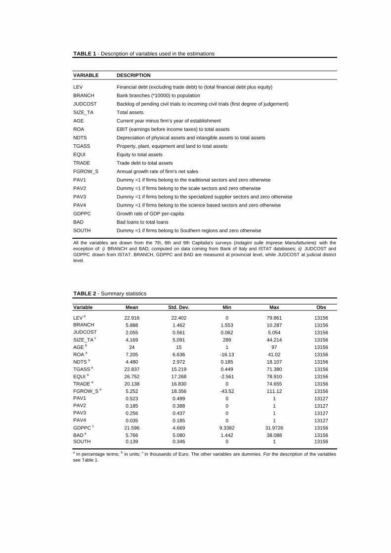
and the lagged dependent variable. A variables’ description is provided in Table 1, while Table 2 reports
some descriptive statistics.7
Insert Tables 1 and 2
The dependent variable (LEV) is calculated as the ratio of financial (or interest-bearing) debt (ex-
cluding trade debt) divided by the total financial debt plus equity (as in Titman et al. 2003, Giannetti
7 A correlation matrix is available from the authors upon request

11
2003, Rajan and Zingales 1995). On the right hand side, BRANCH and JUDCOST are our measures of
local financial development and inefficiency of legal system, respectively.
Following Benfratello et al. (2008), BRANCH is the provincial branch density (calculated as bank
branches on population). The authors indicate at least two motivations to choose this variable as a
measure of the level of local banking development. A first one is that it is widely used in the studies on
local banking development (e.g. Degryse and Ongena, 2005). A second one, and perhaps more impor-
tant, is that “it captures the dimension of banking development that is likely to be more heavily affected
by the deregulation process” (Benfratello et al. 2008, p.200) – a process that, as outlined in section 3,
has greatly contributed in transforming the physiognomy of the Italian banking system in the last two
decades.
Similarly to Fabbri and Padula (2004) and Bianco, Jappelli and Pagano (2005), JUDCOST is the ra-
tio of backlog of pending civil trials to incoming civil trials. 8 The hypothesis underlying the use of this
variable is that the quality of the legal enforcement system at local level depends inversely by the con-
gestion of the judicial district.
The vector X of control variables accounts for observable firms-specific characteristics. Theoretical
and empirical studies have shown that features such as size, age, profitability, non-debt tax-shields, tan-
gibility, trade debt, equity capitalization, and growth opportunities are likely to affect capital structure
(e.g. Hall et al. 2004; Van der Wijst et al. 1993). Large firms tend to have more collateralizable assets
8 The computation of JUDCOST relies on the trials at the first degree of judgment (lower court). However, as a robustness
check (see subsection 5.1), we have also considered the trials at the second degree of judgment (appeal court). It should be no-
ticed that lower court and appeal court represent the two degrees of judgment upon the merit on which civil trials can undergo.
It is also worth remarking that data on pending and incoming trials are available at judicial districts level only, these latter cor-
responding roughly to the Italian regions (for a matching of judicial districts with regions and provinces, see Fabbri and Padula
2004). Although it is possible to impute trials to each province, the standardization required to account for the province size
would result in inaccurate measures. Of course, using the same variable (for instance, the provincial population) for both im-
putation and standardization would lead back to the district level. As highlighted in sub-section 5.1, among other robustness
checks, we also employ a measure of judicial costs calculated at provincial level, using as imputation variable (for the backlog
of pending trials) the population and as standardizing variable the number of provincial crimes.
12
and more stable cash flows (Rajan and Zingales 1995; Harris and Raviv 1991). Thus, the variable SIZE,
measured by the log of total assets, is included in the model. To account for information opacity across
the different stages of the life cycle, the AGE variable is added. Most tax and asymmetric information
models of capital structure predict a relation between leverage and profitability (Rajan and Zingales
1995; Harris and Raviv 1991). Thus, our empirical model includes the return on asset (ROA), expressed
as the ratio of earnings before interest and taxes (EBIT) to total assets. De Angelo and Masulis (1980)
argue that firms that are able to reduce taxes using methods other than deducting interest, such as depre-
ciation, will employ less debt in their capital structure. The non-debt tax shields (NDTS) variable con-
sidered in this study is measured through the depreciation and amortization of tangible and intangible
assets, divided by total assets (MacKie-Mason 1990). Tangible assets (TGASS) may provide collateral
for loans, reducing agency costs and the cost for lenders, and thus are expected to be associated with
higher leverage (Titman and Wessels 1988, Rajan and Zingales 1995). Considering that trade debt may
be a substitute for bank debt (De Blasio, 2005), the TRD variable – expressed by the ratio of trade debt
to total assets – is also included. Similarly, to account for a potential substitution effect, the ratio of eq-
uity on total assets (EQUI) is considered. Firms with high growth opportunities may retain financial
flexibility through a low leverage to be able to exercise those opportunities in subsequent years (Myers
1977), while a firm with outstanding debt may forgo such opportunities (Jensen and Meckling 1976).
To capture this effect, we employ a measure of firm’s growth (FGROWTH), given by the growth rate
of annual net sales. Vector X also comprises industry dummies (PAV), to control for heterogeneity at
sectoral level,9 two variables at provincial level – the (log of) per capita real gross domestic product
(GDPPC) and the ratio of bad loans to total loans (BAD), this latter as a proxy for credit market riski-
ness – and a territorial dummy (SOUTH), to account for the dualism in the degree of socio-economic
development between Centre-North and South (this variable is coded 1 for firms located in the southern
regions, and zero otherwise). Besides, Tt is a set of time fixed effects; itiit u+=νε is a composite error,
where the individual effect (vi) summarizes unobserved firm characteristics (such as managerial risk
aversion, governance structure, and other relevant factors that are difficult to measure) that are time- 9 On the relevance of industry affiliation see, among others, Showalter (1999) and Harris and Raviv (1991).

13
invariant, and have been acknowledged as potential determinants of capital structure decisions (Lem-
mon et al. 2008; Flannery and Rangan 2006). The second term (uit) captures idiosyncratic shocks to lev-
erage.
Finally, it is worth highlighting the inclusion of lagged leverage as an explanatory variable. This lat-
ter term allows us to account for the dynamics suggested by the literature on capital structure adjustment
process (Flannery and Rangan 2006; Leary and Roberts 2005; Welch 2004; Fama and French 2002;
Bontempi and Golinelli 1996). These studies highlight that firms tend to achieve a desired leverage ratio
in the long run, and they cannot completely adjust toward their optimal leverage each period due to the
presence of adjustment costs. Hence, partial adjustment model are advocated to estimate the capital
structure adjustment process.
To test our first hypotheses, we estimate equation (1) without considering the interaction term be-
tween BRANCH and JUDCOST. Then, to verify our second hypothesis, we estimate model (1) –
which makes the effect of financial development conditional on different levels of enforcement ineffi-
ciency . In the latter case, we consider the partial effect of BRANCH conditional on the level of judicial
costs ( JUDCOST*ˆˆBRANCH/LEV 42 ββ +=∂∂ ), and the relative standard errors.10 Since both are de-
pendent on JUDCOST, the marginal effect of BRANCH may change sign and gain or lose significance
according to the value of the enforcement variable. To provide a concise report of these figures, we will
graph the marginal effect of BRANCH - along with its 95% confidence intervals - across the range of
the JUDCOST regressor.
From an econometric perspective, controlling for leverage inertia and unobserved heterogeneity (i.e.
adopting a dynamic panel model as the one specified in equation (1)) poses two major problems. The
first involves the potential correlation between fixed effects and regressors. The second concerns the
correlation between the lagged dependent variable and the past idiosyncratic error. This latter link
makes the strict exogeneity assumption fail, compromising the consistency of the most popular methods
employed in a static panel data setting (random effects, fixed effects and first differencing). Moreover,
10 Formally, the latter are: )ˆ,ˆcov(*JUDCOST2)ˆvar(*)JUDCOST()ˆvar(ˆ 424
22 ββββσ ++=
14
in model (1) the lag of the leverage measure is not the only endogenous variable. In fact, also other ex-
planatory variables are likely to be endogenous.11
A general approach for coping with both the just mentioned problems consists of two steps. First the
data are transformed in order to eliminate the unobserved individual effects, and then valid instrumental
variables are employed in order to cope with the endogeneity problem. Arellano and Bond (1991) pro-
pose a GMM procedure, exploiting the entire set of internal instruments that the model generates, under
the assumption of white noise errors. When the explanatory variables are persistent over time, however,
lagged level may results in poor instruments. Since our variables of interest (BRANCH and JUDCOST)
display a little variation across time, in what follows we adopt the so-called system GMM (SYS-GMM)
estimator of Arellano and Bover (1995) and Blundell and Bond (1998). This estimator employs extra
orthogonality conditions that “remain informative even for persistent series, and it has been shown to
perform well in simulations” (Bond et al., p. 4), increasing the efficiency of the estimation. 12
5. Data
The econometric analysis is based on data coming from several sources. Information on Italian
manufacturing firms is drawn from Capitalia’s 7th, 8th and 9th surveys (Indagini sulle Imprese Manifattu-
riere), conducted on all Italian manufacturing firms employing more than 500 workers and on a strati-
fied sample of firms with more than 10 workers. Each of these surveys, including mostly qualitative in-
formation, spans three years: the 7th survey, carried out in 1998, reports data for a panel of 4,493 firms
for the period 1995-1997; the 8th one was conducted in 2001 and has data for a panel of 4,680 firms for
the years 1998-2000, and the 9th, in 2004, on 4,289 firms for the period 2001-2003. Capitalia provides
also balance-sheet data on firms included in the surveys. By matching qualitative and accounting infor-
11 We treat as endogenous the variables that are likely to be determined simultaneously along with the leverage (BRANCH,
BRANCH* JUDCOST, SIZE, ROA, NDTS, TGASS, EQUI, TRADE, FGROWS, and BAD). The remaining regressors are
treated as exogenous.
12 More precisely, the system GMM estimator, along with the moment conditions of the difference GMM, uses the lagged dif-
ferences of the regressors as instruments for the equation in levels. The main assumption underlying the use of moment restric-
tions in levels is that the unobserved effects are not correlated with changes in the error term.

15
mation, we obtain an unbalanced panel of 5,998 firms in the period 1995-2003, for a total of 25,530 ob-
servations. As abovementioned, we focus on SMEs - which are bound to ask credit from banks with
branches in the same local market where they operate. Therefore, we drop firms with more than 250
workers and those listed on the Stock Exchange.
A second data source, which gives us figures on the territorial distribution of branches for each Ital-
ian bank over the period considered in the analysis, is provided by the Bank of Italy. From the same da-
tabase we draw information on banks non-performing loans and banks total loans (both at provincial
level), to compute the BAD variable. Finally, data on pending and incoming civil trials, on GDP and
population come from ISTAT.13
6. Empirical Results
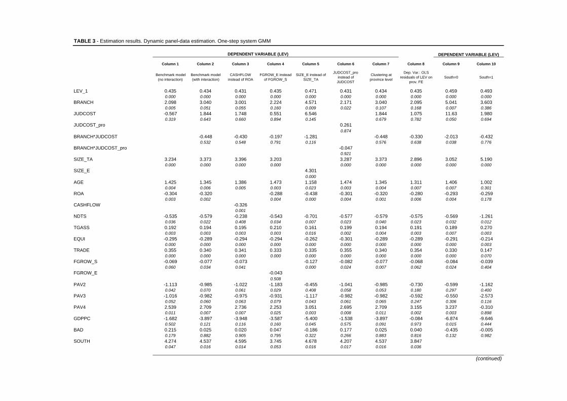
The SYS-GMM results are reported in Table 3. Column1 shows the results obtained when estimating
equation (1) without considering the interaction term between BRANCH and JUDCOST (hypothesis 1).
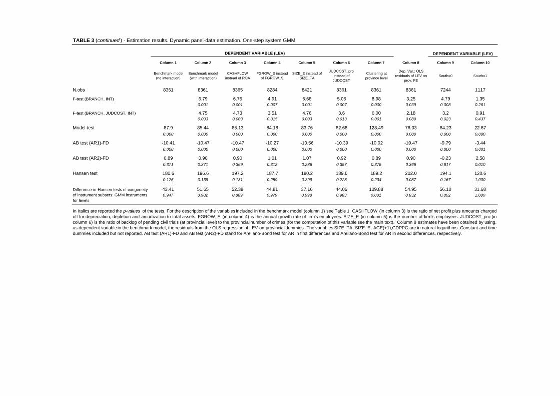
The key assumptions are verified. The autocorrelation tests signal a strong first order correlation in the
differenced residuals, but no higher order autocorrelation, therefore supporting the assumption of lack
of autocorrelation in the errors in levels, underlying the adopted estimator. 14 Further, the Hansen test
cannot reject the null hypothesis of validity of the over-identifying restrictions, and the difference in
Hansen test supports the validity of the additional instruments used by the SYS-GMM estimator.15
13 To moderate the influence of potential outliers, for each variable involved in the econometric analysis, the observations ly-
ing in the first and last half percentile of the distribution have been dropped.
14 Indeed, if the errors in level are characterized by lack of serial correlation, the error in differences are expected to display
first order autocorrelation and to be uncorrelated to all other lags.
15 The estimates are obtained by using a subset of the available instruments. This is because, as Altonji and Segal (1994) point
out, the use of all instruments implies small-sample downward bias of the coefficients and standard errors. It is worth mention-
ing, however, that doubling the number of instruments - or using all available ones - does not affect our main results.
16
Almost all control variables are statistically significant and their estimated coefficients are generally
consistent with those found in previous studies. 16 For instance, AGE and SIZE have a positive and sta-
tistically significant effect on leverage. Older and larger firms, which are likely to have more stable cash
flows and a track record of their business, seem to obtain more financial resources in terms of debt. The
variable ROA has a negative and statistically significant effect on leverage, suggesting that higher prof-
itability - possibly mitigating problems of asymmetric information in accessing capital markets - may
allow managers to be less dependent on creditors for financial resources. The NDTS parameter is nega-
tive and statistically significant as well; thus, managers seem to prefer reducing debt when it is possible
to use non-debt tax shields.17 As regards JUDCOST, its estimated coefficient is found negative - though
not statistically significant.
Finally, as far as our variable of interest is concerned, the BRANCH estimated coefficient displays
the expected sign and it is statistically significant. This finding seems to provide favourable evidence to
our first hypothesis.
Insert Table 3
16 The standard errors (not reported) are consistent in the presence of any pattern of heteroskedasticity and autocorrelation
within panels.
17 For the sake of completeness, we also mention that the positive effect of TGASS supports the hypothesis that fixed assets,
providing better collateral, can foster future capability to repay and guarantee the loan. The positive sign of the TRADE vari-
able indicates that trade debt may have a complementary effect to that of financial debt, while a substitute effect seems to
emerge when looking at the negative coefficient of the EQUI variable. Further, higher growth opportunities seem associated
with a lower employ of debt, possibly implying the use of other form of “patient” funds. The positive coefficient of the vari-
able GDPPC suggests that an increase in the gross domestic product may enable firms to self-generate financial resources,
avoiding the use of debt. Moreover, the industry dummies (PAV) coefficients, in all cases statistically significant, provide evi-
dence of the existence of different financial behaviors between industries. The dummy South variable is negatively and sig-
nificantly related to leverage, suggesting that the differences in the degree of social-economic development between the Italian
two biggest macro-areas may be relevant in determining the SMEs capital structure decisions. Finally, the coefficient of the
lagged dependent variable provides evidence that in the adjustment process to their optimal debt ratio firms face relatively im-
portant transaction costs.

17
Turning to column 2, it reports the estimates of our model (1). Specification tests and control vari-
ables estimated coefficients are similar to those discussed for column 1. Looking at the individual sign
and significance of our key variables, the BRANCH estimated parameter appears positive and signifi-
cantly related to leverage. Given the presence of the interaction term, though, such a positive effect cor-
responds to the marginal effect of BRANCH only when the JUDCOST variable is equal to zero, which
evidently does not represent a noteworthy case. The JUDCOST estimated coefficient is not statistically
significant. Again, given the inclusion of the interaction term, this means that our legal enforcement in-
dicator does not influence the dependent variable when the number of branches is zero, another mean-
ingless case. The interaction term (BRANCH* JUDCOST) is not statistically significant. An F-test,
however, supports the hypothesis of joint significance of BRANCH and its interaction term.18 The nega-
tive sign of the latter indicates that, as expected, the positive BRANCH effect tends to decrease as
JUDCOST raises. As mentioned in the previous section, however, these figures do not convey full in-
formation on the magnitude, sign and significance of the marginal effect of BRANCH (neither of JUD-
COST). Since we are interested in appraising whether the BRANCH’s effect on leverage is different in
magnitude and significance according to the level of JUDCOST, we have to consider the estimated
marginal impact of BRANCH and its confidence intervals for all JUDCOST values. Being the latter a
continuous variable, it is useful to consider the following figure, which condenses the information we
have need of.19
18 The divergence between individual and joint significance is usually interpreted as a symptom of multicollinearity (see
Wooldridge 2003 and Brambor et al. 2006) induced by the inclusion of an interaction term. As Brambor et al. (2006) high-
light, ‘‘even if there really is high multicollinearity and this leads to large standard errors on the model parameters, it is impor-
tant to remember that these standard errors are never in any sense too large… they are always the ‘correct’ standard errors.
High multicollinearity simply means that there is not enough information in the data to estimate the model parameters accu-
rately and the standard errors rightfully reflect this’’.
19 It is worth mentioning that we have also computed the marginal impact of JUDCOST on LEV for all values of
BRANCH. The resulting graph, which is available upon request, shows that this partial effect is always not statisti-
cally significant, being negative for the 89.65% of our sample observations.
18
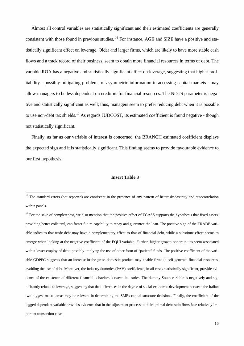
Figure 1 Marginal effect of BRANCH as JUDCOST changes
94.5% of the observations
According to this graph, the financial development influence on the amount of SMEs’ debt is indeed
dependent on the judicial system efficiency. At low levels of judicial costs, the BRANCH estimated
marginal effect is positive and statistically significant (the confidence band does not include the zero
line). When such costs increase, the impact of BRANCH decreases, turning to be statistically not sig-
nificant beyond a threshold value of about three. It is worth mentioning that more than 94% of our sam-
ple observations fall within the significance region.
Summarizing, our evidence suggests that the degree of local financial development is a statistically
significant determinant of SMEs capital structure decisions, but its relevance decreases at higher level of
local courts inefficiency.
6.1 Robustness Checks
To begin with, we check the sensitivity of our results to the specification adopted. Results do not
substantially change neither when controlling for non-linearity of firms’ age (i.e. the age squared is
added to equation (1)), nor when including the (log of) provincial population, nor when controlling for
the local credit market size by the (log of) deposits in the province. Besides, none of the added variables
is statistically significant. These results are not reported to avoid cluttering, and they are available from
the authors upon request.

19
Similarly, the outcome remains substantially unaltered when we replace some controls with other
ones. In column 3 of Table 3, we replace ROA with (operative) CASHFLOW; in column 4 the firm
growth is measured in terms of number of employees rather than net sales; in column 5, the log of the
total assets is replaced by the log of employees.
Furthermore, in order to check the sensitivity of our results to the particular measure of judicial costs
employed, we re-estimate our model: i) by replacing JUDCOST, computed at the judicial district level,
with an indicator worked out at the province level (JUDCOST_pro); 20 ii) by computing JUDCOST on
pending and incoming civil trials both at the first and the second degree of judgement. The results ob-
tained when implementing the former check are reported in Table 3 (column 6), while the other ones are
available upon request.
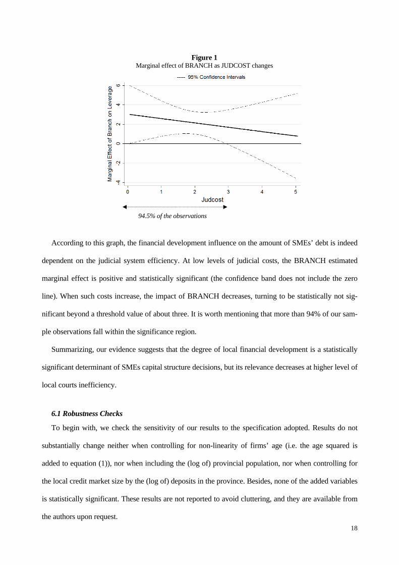
Moreover, as our dependent variable is likely to be sensitive to a variety of unobserved (or not
easily measurable) factors reflecting provincial characteristics, we perform two additional sensitivity
checks. First, to take into account that such features may imply some correlation among the error
terms over time for firms belonging to the same area, we re-estimate our benchmark model by cluster-
ing the observations at province level. Secondly, to eliminate the influence of provincial specific
characteristics on LEV, we regress the latter on provincial fixed-effects and then we employ the re-
siduals from this OLS regression as dependent variable in our benchmark model. The results relative
to these last two checks, which confirm our main finding, are reported in columns 7 and 8 of Table 3,
and summarized by the following figures. 21
20 As said before, our original data provide information at the judicial district level, that generally do not coincide with the prov-
ince geographical area. JUDCOST is measured as the number of district backlog of pending trials on the number of district in-
coming trials (first degree of judgement). JUDCOST_pro is computed by dividing the number of province backlog of pending
trials by the number of province crimes. The number of trials is imputed to each province using the respective population.
21 It has to be mentioned that, as Roodman (2009) points out, when clustering in GMM-SYS “most of the standard errors and
specification tests reported [… ] are consistent only as the number of clusters grows large”. In our case, the number of cluster
is 102 (missing firms from a Sicily’s province, which is Enna).
20
Figure 2
Marginal effect of BRANCH as JUDCOST changes
(Clustering at province level)
Figure 3
Marginal effect of BRANCH as JUDCOST changes
(Using as dependent variable the OLS residuals from re-gressing LEV on provincial fixed effect)
98.3% of the observations 81% of the obs.
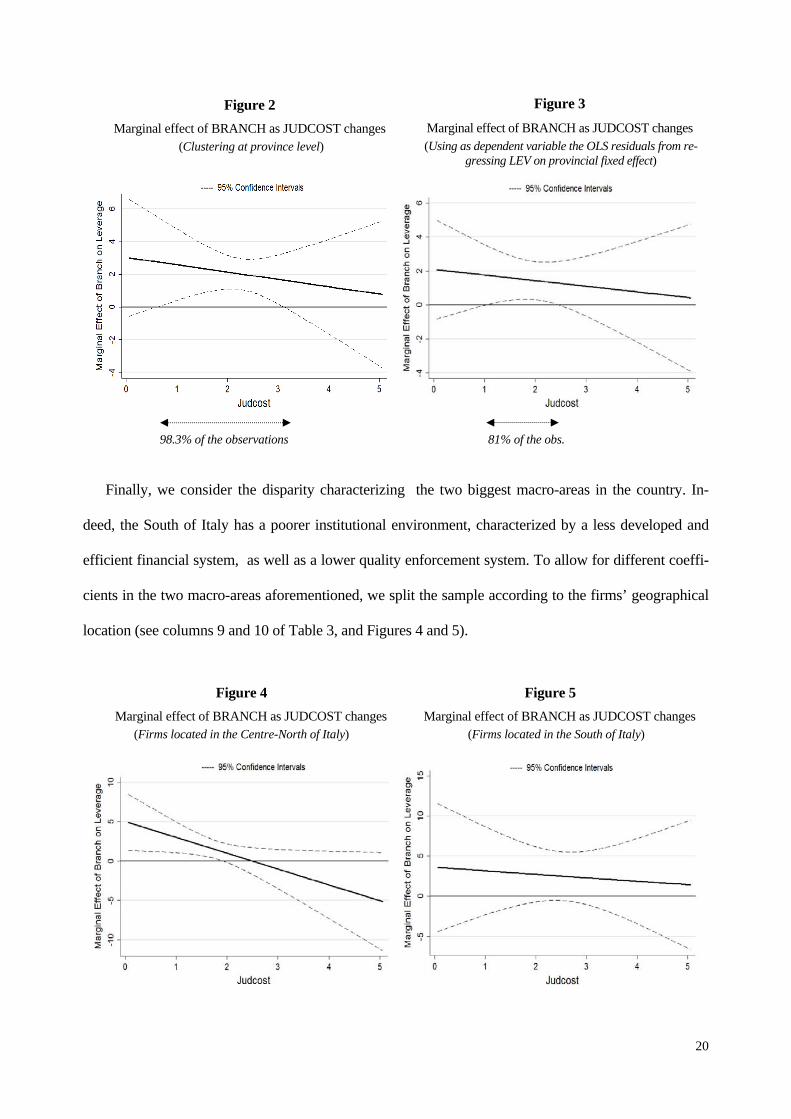
Finally, we consider the disparity characterizing the two biggest macro-areas in the country. In-
deed, the South of Italy has a poorer institutional environment, characterized by a less developed and
efficient financial system, as well as a lower quality enforcement system. To allow for different coeffi-
cients in the two macro-areas aforementioned, we split the sample according to the firms’ geographical
location (see columns 9 and 10 of Table 3, and Figures 4 and 5).
Figure 4
Marginal effect of BRANCH as JUDCOST changes
(Firms located in the Centre-North of Italy)
Figure 5
Marginal effect of BRANCH as JUDCOST changes
(Firms located in the South of Italy)

21
In the Centre-North of Italy, both the BRANCH coefficient and the negative influence of JUDCOST
on the BRANCH marginal effect seem higher than those obtained when using the whole sample. More-
over, while in the northern regions the marginal impact of BRANCH is statistically significant for most
observations, for the southern ones BRANCH is not significant for any level of legal system efficiency.
The latter result, though, has to be considered with caution, as – given the limited sub-sample size – the
Hansen and difference in Hansen tests are weakened by the presence of many instruments.
7. Conclusive remarks
The present study analyses the influence of institutional differences at the local level on capital struc-
ture choices of SMEs, taking into consideration the interaction between local financial development and
the effectiveness of the local enforcement system. Controlling for financial debt inertia, endogeneity
problems and firms heterogeneity, local financial development seems to exert a significant role in af-
fecting SMEs’ debt capacity, conditioned by the quality of the local enforcement system. In particular,
firms appear to have a better access to financial debt in areas characterised by a higher quality of the le-
gal system, possibly as intermediaries may be more inclined to provide funds where the enforcement
systems allow a more effective credit protection.
Overall, our findings suggest that local institutional environment may matter for financing decisions
of SMEs. Although the international process of integration in the capital market, local financial institu-
tions do not seem to become irrelevant for SMEs – which are in need of well developed institutions at
local level to get easier access to external financial resources. Moreover, an improvement in the local
enforcement system can play an important role in creating the conditions for better relationships be-
tween firms and banks, reducing asymmetric information and agency problems, thus increasing the
availability of credit for SMEs. In brief, corporate financial decisions seem not only the result of
firm/industry specific characteristics, but also a by product of the institutional environment in which a
firm operates.

22
As a final consideration, the results obtained in the present paper may inspire further investigation on
the role of local institutional characteristics, aiming at deepening the study of their interaction effects,
by extending the analysis to larger firms as well to other countries.
23
References
Alessandrini, P., Zazzaro, A., 1999. A “Possibilist” Approach to Local Financial Systems and Regional Development: the
Italian Experience”, in Martin R. (ed.), Money and the Space Economy, John Wiley & Sons.
Altonji, J., Segal, L. ,1994. Small sample bias in GMM estimation of covariance structures. NBER Working Paper,156.
Arellano, M. and Bond S.,1991 Some Tests of Specification for Panel Data: Monte Carlo Evidence and an Application to
Employment Equations, Review of Economic Studies, Vol. 58, 277–297.
Arellano, M., Bover, O., 1995. Another Look at the Instrumental Variable Estimation of Error Components Models, Journal
of Econometrics, 68, 29-51.
Beck T., Levine R., 2004, Legal Institutions and Financial Development, in Handbook of New Institutional Economics, C.
Menard and M. Shirley (eds)., Kluwer Dordrecht (The Netherlands).
Beck, T., Demirgüç-Kunt, A., Maksimovic, V., 2008, Financing patterns around the world: Are small firms different?, /
Journal of Banking & Finance, 30, 467-487.
Beck, T., Demirgüç-Kunt, A., Maksimovic, V., 2005, Financial and legal constraints to firm growth: Does size matter?,
Journal of Finance, 60(1), 137-177.
Benfratello, L., Schiantarelli, F., Sembenelli, A., 2008. Banks and innovation: Microeconometric evidence on Italian firms.
Journal of Financial Economics, 90, 197-217.
Berger, A., Udell, G., 1998. The Economics of Small Business Finance: the Roles of Private Equity and Debt Markets in the
Financial Growth Cycle. Journal of Banking and Finance 22, 613-673.
Berle, A. and Means, G. The Modern Corporation and Private Property, 1932, New York, Macmillan.
Bianco, M., Casavola, P., 1999. Italian Corporate Governance: Effects on Financial Structure and Firm Performance. Euro-
pean Economic Review , 43, 1057-1069
Bianco, M., Jappelli, T., Pagano, M., 2005. Courts and Banks: Effect of Judicial Enforcement on Credit Markets. Journal of
Money, Credit and Banking 37, 223-244.
Blundell, R., Bond, S., 1998. Initial Conditions and Moment Restrictions in Dynamic Panel Data Models, Journal of
Econometrics, 87, 115-143
Bond, S., Temple J., Hoeffler, A., 2001. GMM Estimation of Empirical Growth Models, Economics Papers, 21, Nuffield
College, University of Oxford
Bontempi, M.E., Golinelli, R., 1996. Le determinanti del leverage delle imprese: una applicazione empirica ai settori indu-
striali dell'economia italiana, Studi e note di economia, 2
Booth, L., Aivazian, V., Demirgüç-Kunt, A., 2001. Capital Structures in Developing Countries. Journal of Finance 56(1),
87-130
Brambor, T., William, C., Golder, M., 2006. Understanding Interaction Models: Improving Empirical Analyses. Political
Analysis 14, 63-82.
24
Cesarini, F. ,2003. Il rapporto banca-impresa. Paper presented at the workshop Impresa, risparmio e intermediazione finan-
ziaria: aspetti economici e profili giuridici, Trieste, 24-25 ottobre 2003.
Cheng, S., Shiu, C., 2007. Investor Protection and Capital Structure: International Evidence. Journal of Multinational Finan-
cial Management 17, 30–44
Costi, R., 2007. L’ordinamento bancario. Il Mulino, Bologna.
De Angelo, M., Masulis, R.W., 1980. Optimal Capital Structure Under Corporation and Personal Taxation. Journal of Fi-
nancial Economics 8, 3-29
De Blasio, G., 2005. Does Trade Credit Substitute Bank Credit? Evidence from Firm-level Data. Economic Notes, 34 (1),
85-112.
Degryse, H., Ongena, S., 2005, Distance, lending relationships and competition, Journal of Finance, 60(1), 231-266.
Demirgüç-Kunt, A., Maksimovic, V., 1996a. Stock Market Development and Financing Choices of Firms. World Bank
Economic Review 10(2), 341-370
Demirgüç-Kunt, A., Maksimovic, V., 1996b. Financial Constraints, Uses of Funds and Firm Growth: an International Com-
parison. Policy Research Working Paper - The World Bank.
Demirgüç-Kunt, A., Maksimovic, V., 1998. Law, Finance and Firm Growth. Journal of Finance 53, 2107-2137
Demirgüç-Kunt, A., Maksimovic, V., 1999. Institutions, Financial Markets, and Firms Debt Maturity. Journal of Financial
Economics 54, 295-336.
Demirgüç-Kunt, A., Maksimovic, V., 2002. Funding Growth in Bank-Based and Market-Based Financial System: Evidence
from Firm Level Data. Journal of Financial Economics 65, 337-363
Demirgüç-Kunt, A., Maksimovic, V., 2008. Financing Patterns Around the World: The Role of Institutions Policy Research
Working Paper - The World Bank, n. 2905
Diamond, D., 1991. Debt Maturity Structure and Liquidity Risk. Quarterly Journal of Economics 106(3), 709-737
Diamond, D., 1993. Seniority and Maturity of Debt Contracts. Journal of Financial Economics 33(3), 341-368
Dow, S., Montagnoli, A., 2007. The Regional Transmission of UK Monetary Policy. Regional Studies 41, 797-808.
Dow, S., Rodriguez-Fuentes, C., 1997. Regional Finance: A Survey. Regional Studies, 31, 903-920
Fabbri, D., Padula, M.,2004. Does poor legal enforcement make households credit-constrained? Journal of Banking and Fi-
nance 28, 2369-2397.
Fama, E., French, K., 2002. Testing Trade-Off and Pecking Order Prediction about Dividends and Debt. The Review of Fi-
nancial Studies 15, 1-33
FinMonitor, 2006. Rapporto semestrale su fusioni e aggregazioni tra gli intermediari finanziari in Europa, University of
Bergamo, Bergamo.
Flannery, M., 1986. Asymmetric Information and Risky Debt Maturity Choice. Journal of Finance 41, 19-37

25
Flannery, M.. Rangan, K., 2006. Partial adjustment toward target capital structures. Journal of Financial Economics 79,
469-506.
Giacomelli, S., Trento, S., 2005. Proprietà, Controllo e Trasferimenti nelle Imprese Italiane. Cosa è Cambiato nel Decennio
1993-2003? Bank of Italy, Temi di discussione n. 550.
Giannetti, M., 2003. Do Better Institutions Mitigate Agency Problems? Evidence from Corporate Finance Choices. Journal
of Financial and Quantitative Analysis 38, 185-212.
Guiso, L., Sapienza, P., Zingales, L., 2004. Does Local Financial Development Matter?. Quarterly Journal of Economics
119, 929-969
Hall, G., Hutchinson, P., Michaelas N., 2004, Determinants of the Capital Structure of European SMEs, Journal of Business
Finance and Accounting, 31, 711-728
Harris, M. and Raviv, A., 1991. The theory of capital structure, Journal of Finance, 46 1991, 297–355.
Jensen, M., Meckling, W., 1976. Theory of the Firm: Managerial Behavior, Agency Costs and Ownership Structure. Journal
of Financial Economics 3, 305-360.
La Porta, R., Lopez de Silanes, F., Shleifer, A., Vishny, R., 1998. Law and Finance. Journal of Political Economy 6, 1113-
1155.
La Porta, R., Lopez de Silanes, F., Shleifer, A., Vishny, R., 1999. Corporate Ownership Around the World. Journal of Fi-
nance 54, 471–518.
La Porta, R., Lopez-De-Silanes, F., Shleifer, A., Vishny, R., 1997. Legal Determinants of External Finance. Journal of Fi-
nance 52(3), 1131-1150
Leary, M., Roberts, M., 2005. Do Firms Rebalance their Capital Structure?. Journal of Finance, 60, 2575-2619.
Lemmon, M., Roberts, M., Zender, J., 2008. Back to the Beginning: Persistence and the Cross-Section of Corporate Capi-
tal Structure. Journal of Finance, 63(4), 1575-1608.
Lopez-Iturriaga, F., Rodriguez-Sanz, J., 2007. Capital Structure and Institutional Setting: a Decomposition and International
Analysis. Applied Economics 30, 1-14
MacKie-Mason, J., 1990. Do Taxes Affect Corporate Financing Decisions?. Journal of Finance 45, 1471-93
Martin, R., 1999. The New Economic Geography of Money, (Chapter 1) in Martin, R., Money and the Space Economy,
John Wiley & Sons.
Myers, S., Determinants of corporate borrowing, Journal of Financial Economics, Vol. 5, 1977, pp. 147–175.
Petersen, M., Rajan, R., 2002. Does Distance Still Matter: The Information Revolution in Small Business Lending. Journal
of Finance 57, 2533–2570.
Pollard, J., 2003. Small firm finance and economic geography, Journal of Economic Geography, 3(4): 429-452.

26
Rajan, R., Zingales, L., 1995. What do we Know about Capital Structure? Some Evidence from International Data. Journal
of Finance 50, 1421-1460.
Rajan, R., Zingales, L., 2003. Banks and Markets: the Changing Character of European Finance. CEPR Discussion Paper
3865.
Roodman, D. (2009). A reply to a Statalist user. Email. Mon, 26 Jan 2009.
Showalter, D., 1999. Strategic Debt: Evidence in Manufacturing. International Journal of Industrial Organization 17, 319–
333.
Titman, S., Fan, J., Twite, G., 2003. An International Comparison of Capital Structure and Debt Maturity Choices. working
paper Social Science Research Network.
Titman, S., Wessels, R., 1988. The Determinants of Capital Structure. Journal of Finance 43(2), 1–18
Utrero-González, N., 2007. Banking regulation, Institutional Framework and Capital Structure: International Evidence from
Industry Data. Quarterly Review of Economics and Finance 47, pp. 481-506
Van der Wijst, D., Thurik, A., 1993, Determinants of Small Firm Debt Ratios: an Analysis of Retail Panel Data, Small
Business Economics, 5, 55-65
Welch, I., 2004. Capital Structure and Stock Returns. Journal of Political Economy, 112, 106-131.
Wooldridge J., 2003. Introductory Econometrics, Thomson South-Western.
VARIABLE DESCRIPTION
LEV Financial debt (excluding trade debt) to (total financial debt plus equity)
BRANCH Bank branches (*10000) to population
JUDCOST Backlog of pending civil trials to incoming civil trials (first degree of judgement)
SIZE_TA Total assets
AGE Current year minus firm’s year of establishment
ROA EBIT (earnings before income taxes) to total assets
NDTS Depreciation of physical assets and intangible assets to total assets
TGASS Property, plant, equipment and land to total assets
EQUI Equity to total assets
TRADE Trade debt to total assets
FGROW_S Annual growth rate of firm's net sales
PAV1 Dummy =1 if firms belong to the traditional sectors and zero otherwise
PAV2 Dummy =1 if firms belong to the scale sectors and zero otherwise
PAV3 Dummy =1 if firms belong to the specialized supplier sectors and zero otherwise
PAV4 Dummy =1 if firms belong to the science based sectors and zero otherwise
GDPPC Growth rate of GDP per-capita
BAD Bad loans to total loans
SOUTH Dummy =1 if firms belong to Southern regions and zero otherwise
Variable Mean Std. Dev. Min Max Obs
LEV a 22.916 22.402 0 79.861 13156BRANCH 5.888 1.462 1.553 10.287 13156JUDCOST 2.055 0.561 0.062 5.054 13156SIZE_TA c 4,169 5,091 289 44,214 13156AGE b 24 15 1 97 13156ROA a 7.205 6.636 -16.13 41.02 13156NDTS a 4.480 2.972 0.185 18.107 13156TGASS a 22.837 15.219 0.449 71.380 13156EQUI a 26.752 17.268 -2.561 78.910 13156TRADE a 20.138 16.830 0 74.655 13156FGROW_S a 5.252 18.356 -43.52 111.12 13156PAV1 0.523 0.499 0 1 13127PAV2 0.185 0.388 0 1 13127PAV3 0.256 0.437 0 1 13127PAV4 0.035 0.185 0 1 13127GDPPC c 21.596 4.669 9.3382 31.9726 13156BAD a 5.766 5.080 1.442 38.088 13156SOUTH 0.139 0.346 0 1 13156
All the variables are drawn from the 7th, 8th and 9th Capitalia's surveys (Indagini sulle Imprese Manufatturiere) with theexception of: i) BRANCH and BAD, computed on data coming from Bank of Italy and ISTAT databases; ii) JUDCOST andGDPPC drawn from ISTAT. BRANCH, GDPPC and BAD are measured at provincial level, while JUDCOST at judicial districtlevel.
TABLE 1 - Description of variables used in the estimations
TABLE 2 - Summary statistics
a In percentage terms; b in units; c in thousands of Euro. The other variables are dummies. For the description of the variablessee Table 1.
Column 1 Column 2 Column 3 Column 4 Column 5 Column 6 Column 7 Column 8 Column 9 Column 10
Benchmark model (no interaction)
Benchmark model (with interaction)
CASHFLOW instead of ROA
FGROW_E instead of FGROW_S
SIZE_E instead of SIZE_TA
JUDCOST_pro instead of JUDCOST
Clustering at province level
Dep. Var.: OLS residuals of LEV on
prov. FESouth=0 South=1
LEV_1 0.435 0.434 0.431 0.435 0.471 0.431 0.434 0.435 0.459 0.4930.000 0.000 0.000 0.000 0.000 0.000 0.000 0.000 0.000 0.000
BRANCH 2.098 3.040 3.001 2.224 4.571 2.171 3.040 2.095 5.041 3.6030.005 0.051 0.055 0.160 0.009 0.022 0.107 0.168 0.007 0.386
JUDCOST -0.567 1.844 1.748 0.551 6.546 1.844 1.075 11.63 1.9800.319 0.643 0.660 0.894 0.145 0.679 0.782 0.050 0.694
JUDCOST_pro 0.2610.874
BRANCH*JUDCOST -0.448 -0.430 -0.197 -1.281 -0.448 -0.330 -2.013 -0.4320.532 0.548 0.791 0.116 0.576 0.638 0.038 0.776
BRANCH*JUDCOST_pro -0.0470.921
SIZE_TA 3.234 3.373 3.396 3.203 3.287 3.373 2.896 3.052 5.1900.000 0.000 0.000 0.000 0.000 0.000 0.000 0.000 0.000
SIZE_E 4.3010.000
AGE 1.425 1.345 1.386 1.473 1.158 1.474 1.345 1.311 1.406 1.0020.004 0.006 0.005 0.003 0.023 0.003 0.004 0.007 0.007 0.301
ROA -0.304 -0.320 -0.288 -0.438 -0.301 -0.320 -0.280 -0.293 -0.2590.003 0.002 0.004 0.000 0.004 0.001 0.006 0.004 0.178
CASHFLOW -0.3260.001
NDTS -0.535 -0.579 -0.238 -0.543 -0.701 -0.577 -0.579 -0.575 -0.569 -1.2610.036 0.022 0.408 0.034 0.007 0.023 0.040 0.023 0.032 0.012
TGASS 0.192 0.194 0.195 0.210 0.161 0.199 0.194 0.191 0.189 0.2700.003 0.003 0.003 0.003 0.016 0.002 0.004 0.003 0.007 0.003
EQUI -0.295 -0.289 -0.294 -0.294 -0.262 -0.301 -0.289 -0.289 -0.291 -0.2140.000 0.000 0.000 0.000 0.000 0.000 0.000 0.000 0.000 0.003
TRADE 0.355 0.340 0.341 0.333 0.335 0.355 0.340 0.354 0.330 0.1470.000 0.000 0.000 0.000 0.000 0.000 0.000 0.000 0.000 0.070
FGROW_S -0.069 -0.077 -0.073 -0.127 -0.082 -0.077 -0.068 -0.084 -0.0390.060 0.034 0.041 0.000 0.024 0.007 0.062 0.024 0.404
FGROW_E -0.0430.508
PAV2 -1.113 -0.985 -1.022 -1.183 -0.455 -1.041 -0.985 -0.730 -0.599 -1.1620.042 0.070 0.061 0.029 0.408 0.058 0.053 0.180 0.297 0.400
PAV3 -1.016 -0.982 -0.975 -0.931 -1.117 -0.982 -0.982 -0.592 -0.550 -2.5730.052 0.060 0.063 0.079 0.043 0.061 0.065 0.247 0.306 0.116
PAV4 2.539 2.709 2.736 2.253 3.051 2.695 2.709 3.155 3.237 -0.3100.011 0.007 0.007 0.025 0.003 0.008 0.011 0.002 0.003 0.898
GDPPC -1.682 -3.897 -3.948 -3.587 -5.400 -1.538 -3.897 -0.084 -6.874 -9.6460.502 0.121 0.116 0.160 0.045 0.575 0.091 0.973 0.015 0.444
BAD 0.215 0.025 0.020 0.047 -0.186 0.177 0.025 0.040 -0.435 -0.0050.179 0.882 0.905 0.795 0.322 0.266 0.883 0.816 0.132 0.982
SOUTH 4.274 4.537 4.595 3.745 4.678 4.207 4.537 3.8470.047 0.016 0.014 0.053 0.016 0.017 0.016 0.036
TABLE 3 - Estimation results. Dynamic panel-data estimation. One-step system GMM
DEPENDENT VARIABLE (LEV) DEPENDENT VARIABLE (LEV)
(continued)
Column 1 Column 2 Column 3 Column 4 Column 5 Column 6 Column 7 Column 8 Column 9 Column 10
Benchmark model (no interaction)
Benchmark model (with interaction)
CASHFLOW instead of ROA
FGROW_E instead of FGROW_S
SIZE_E instead of SIZE_TA
JUDCOST_pro instead of JUDCOST
Clustering at province level
Dep. Var.: OLS residuals of LEV on
prov. FESouth=0 South=1
N.obs 8361 8361 8365 8284 8421 8361 8361 8361 7244 1117
F-test (BRANCH, INT) 6.79 6.75 4.91 6.68 5.05 8.98 3.25 4.79 1.350.001 0.001 0.007 0.001 0.007 0.000 0.039 0.008 0.261
F-test (BRANCH, JUDCOST, INT) 4.75 4.73 3.51 4.76 3.6 6.00 2.18 3.2 0.910.003 0.003 0.015 0.003 0.013 0.001 0.089 0.023 0.437
Model-test 87.9 85.44 85.13 84.18 83.76 82.68 128.49 76.03 84.23 22.670.000 0.000 0.000 0.000 0.000 0.000 0.000 0.000 0.000 0.000
AB test (AR1)-FD -10.41 -10.47 -10.47 -10.27 -10.56 -10.39 -10.02 -10.47 -9.79 -3.440.000 0.000 0.000 0.000 0.000 0.000 0.000 0.000 0.000 0.001
AB test (AR2)-FD 0.89 0.90 0.90 1.01 1.07 0.92 0.89 0.90 -0.23 2.580.371 0.371 0.369 0.312 0.286 0.357 0.375 0.366 0.817 0.010
Hansen test 180.6 196.6 197.2 187.7 180.2 189.6 189.2 202.0 194.1 120.60.126 0.138 0.131 0.259 0.399 0.228 0.234 0.087 0.167 1.000
Difference-in-Hansen tests of exogeneity of instrument subsets: GMM instruments for levels
43.410.947
51.650.902
52.380.889
44.810.979
37.160.998
44.060.983
109.88 0.001
54.950.832
56.100.802
31.681.000
In Italics are reported the p-values of the tests. For the description of the variables included in the benchmark model (column 1) see Table 1. CASHFLOW (in column 3) is the ratio of net profit plus amounts chargedoff for depreciation, depletion and amortization to total assets. FGROW_E (in column 4) is the annual growth rate of firm's employees. SIZE_E (in column 5) is the number of firm's employees. JUDCOST_pro (incolumn 6) is the ratio of backlog of pending civil trials (at provincial level) to the provincial number of crimes (for the computation of this variable see the main text). Column 8 estimates have been obtained by using,as dependent variable in the benchmark model, the residuals from the OLS regression of LEV on provincial dummies. The variables SIZE_TA, SIZE_E, AGE(+1),GDPPC are in natural logarithms. Constant and timedummies included but not reported. AB test (AR1)-FD and AB test (AR2)-FD stand for Arellano-Bond test for AR in first differences and Arellano-Bond test for AR in second differences, respectively.
TABLE 3 (continued ) - Estimation results. Dynamic panel-data estimation. One-step system GMM
DEPENDENT VARIABLE (LEV) DEPENDENT VARIABLE (LEV)