Large torsion finite element model for thin-walled beams

This article was published in an Elsevier journal. The attached copyis furnished to the author for non-commercial research and

education use, including for instruction at the author’s institution,sharing with colleagues and providing to institution administration.

Other uses, including reproduction and distribution, or selling orlicensing copies, or posting to personal, institutional or third party

websites are prohibited.

In most cases authors are permitted to post their version of thearticle (e.g. in Word or Tex form) to their personal website orinstitutional repository. Authors requiring further information

regarding Elsevier’s archiving and manuscript policies areencouraged to visit:

http://www.elsevier.com/copyright

http://www.elsevier.com/copyright

Author's personal copy

Large torsion finite element model for thin-walled beams

Foudil Mohri a,c,*, Noureddine Damil b, Michel Potier Ferry c

a Nancy-Universite, Universite Henri Poincare, IUT Nancy-Brabois, Departement Genie Civil.

Le Montet. Rue du Doyen Urion CS 90137. 54601 Villers les Nancy, Franceb Laboratoire de Calcul Scientifique en Mecanique, Faculte des Sciences Ben M’Sik, Universite Hassan II – Mohammedia, BP 7955 Sidi Othman

Casablanca, Moroccoc LPMM, UMR CNRS 7554, ISGMP, Universite Paul Verlaine-Metz, Ile du Saulcy, 57045 Metz, France

Received 13 November 2006; accepted 20 July 2007Available online 17 September 2007

Abstract

Behaviour of thin-walled beams with open section in presence of large torsion is investigated in this work. The equilibrium equationsare derived in the case of elastic behaviour without any assumption on torsion angle amplitude. This model is extended to finite elementformulation in the same circumstances where 3D beams with two nodes and seven degrees of freedom per node are considered. Due tolarge torsion assumption and flexural–torsional coupling, new matrices are obtained in both geometric and initial stress parts of the tan-gent stiffness matrix. Incremental-iterative Newton–Raphson method is adopted in the solution of the nonlinear equations. Many appli-cations are presented concerning the nonlinear and post-buckling behaviour of beams under torsion and bending loads. The proposedbeam element is efficient and accurate in predicting bifurcations and nonlinear behaviour of beams with asymmetric sections. It is provedthat the bifurcation points are in accordance with nonlinear stability solutions. The convenience of the model is outlined and the limit ofmodels developed in linear stability is discussed.� 2007 Elsevier Ltd. All rights reserved.

Keywords: Beam; Finite element; Nonlinear; Open section; Post-buckling; Thin-walled

1. Introduction

Thin-walled elements with isotropic or anisotropic com-posite materials are extensively used as beams and columnsin engineering applications, ranging from buildings toaerospace and many other industry fields where require-ments of weight saving are of main importance. Due totheir particular shapes resulting from the fabrication pro-cess, these structures always have open sections that makethem highly sensitive to torsion, instabilities and to imper-fections. The instabilities are then the most important phe-

nomena that must be accounted for in the design.Nevertheless most of these flexible structures can undergolarge displacements and deformations without exceedingtheir yield limit. For these reasons the computation of thesestructures must be carried out according to nonlinearmodels.

Vlasov’s model [1] developed for small non-uniform tor-sion has been commonly adopted in most theoretical andfinite element works on thin-walled elements with open sec-tions [2–5]. Recently, based on this model, Kim [6] investi-gated a finite element formulation with consideration ofsemi-tangential moments and rotations. Kwak [7] formu-lated a finite element analysis to account for warping effecton the nonlinear behaviour of open section beams, by usingthe Total Lagrangian formulation. Pi [8] and Turkalj [9]have introduced a correction in the rotation matrix by con-sidering higher order terms. They obtained improved mod-els for linear and nonlinear stability analyses.

0045-7949/$ - see front matter � 2007 Elsevier Ltd. All rights reserved.

doi:10.1016/j.compstruc.2007.07.007

* Corresponding author. Address: Nancy-universite, Universite HenriPoincare, IUT Nancy-Brabois, Departement Genie Civil. Le Montet. Ruedu Doyen Urion CS 90137. 54601 Villers les Nancy, France. Tel.: +33 (0)383 68 25 77; fax: +33 (0)3 83 68 25 32.

E-mail address: [email protected] (F. Mohri).

www.elsevier.com/locate/compstruc

Available online at www.sciencedirect.com

Computers and Structures 86 (2008) 671–683


In the above studies, nonlinear terms such as flexural–torsional coupling or shortening effects are usually ignored.Many other studies have been devoted to nonlinear behav-iour of these structures in bending and torsion and provedthat in large torsion, the shortening effect is important andthat the agreement of Vlasov’s model is poor compared toexperimental results [10–13]. On the other hand, it has beenchecked that pre-buckling deformations have a predomi-nant influence on the stability of thin-walled beams espe-cially in lateral buckling behaviour. Some analyticalsolutions including pre-buckling deformations have beencarried out [14–16]. Many other finite element models havebeen formulated in finite and large torsion taking intoaccount shortening effect and pre-buckling deflections[17–21]. The effects of pre-buckling and shear deformationon lateral buckling of composite beams have been recentlystudied by Machado [22]. Extensive research is developedrecently in the filed of curved thin-walled beams with steeland concrete materials [23,24].

A nonlinear finite element analysis has been developedby Attard [17] for isotropic elements. Finite torsionassumption has been admitted and trigonometric functionshave been limited to cubic approximations, respectively tocosðhxÞ ¼ 1� h2

x2

and sinðhxÞ ¼ hx � h3x

6, where hx is the twist

angle. Recently, Ronagh [19] extended this model so thatit could be applied to variable cross-sections. The abovemodel has been successfully applied to the stability analysisof thin-walled elements either in buckling or lateral buck-ling behaviour. In the present work, a large torsion finiteelement model is investigated for elastic thin-walled beamswithout any assumption on the torsion angle amplitude.The calculation of the tangent stiffness matrix is possiblethanks to the introduction of new trigonometric variablesc = (coshx � 1) and s = sinhx. For the purpose, the equilib-rium equations and the material behaviour are established.Shortening effect, pre-buckling deflections and flexural–tor-sional coupling are naturally included. In the nonlinearfinite element analysis, we use a 3D beam element withtwo nodes and seven degrees of freedom per node includingwarping. In order to get the equilibrium paths, Newton–Raphson iterative method is utilized. The tangent stiffnessmatrix is carried out. Due to large torsion and flexural–tor-sional coupling, new matrices are obtained in both geomet-ric and initial stress parts of the tangent stiffness matrix.This element is incorporated in a homemade finite elementcode. In order to illustrate the accuracy and practical use-fulness of the proposed element, many examples are con-sidered in the numerical part. The convenience of themodel is outlined and the limit of models developed in lin-ear stability is discussed.

2. Kinematics

A straight thin-walled element with slenderness L andan open cross-section A is pictured in Fig. 1. A direct rect-angular co-ordinate system is chosen. Let us denote by x

the initial longitudinal axis and by y and z the first and sec-

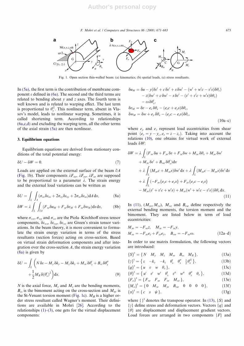
ond principal bending axes. The origin of these axes islocated at the centre G. The shear centre with co-ordinates(yc,zc) in Gyz is denoted C. Consider M, a point on the sec-tion contour with its co-ordinates ðy; z;xÞ;x being the sec-torial co-ordinate introduced in Vlasov’s model for non-uniform torsion [1]. Hereafter, it is admitted that there isno shear deformations in the mean surface of the sectionand the contour of the cross-section is rigid in its ownplane. The model will be applied to slender beams. Thismeans that local and distortional deformations are notincluded. Thin-walled open section beams possess largebending stiffness in comparison to torsion stiffness. In themodel, displacements and twist angle can be large butbending rotation are assumed to be small. Small deforma-tion are admitted and an elastic behaviour will be thenadopted in material behaviour. Under these conditions,displacements of a point M are derived from those of theshear centre as

uM ¼ u� yðv0 þ v0cþ w0sÞ � zðw0 þ w0c� v0sÞ � xh0x; ð1ÞvM ¼ v� ðz� zcÞsþ ðy � ycÞc; ð2ÞwM ¼ wþ ðy � ycÞsþ ðz� zcÞc; ð3Þ

Eqs. (1)–(3) are similar to the ones established in Attard[25], where ( Æ ) 0 denotes the x-derivative. u is the axial dis-placement of centroid and v and w are displacements ofshear point in y and z directions. We have introduced inEqs. (2) and (3) two additional variables c and s:

c ¼ cos hx � 1; s ¼ sin hx: ð4a; bÞ

Since the model is concerned with large torsion, the func-tions c and s are conserved without any approximation inboth theoretical and numerical analyses. In the case ofthin-walled beams, the components of Green’s strain tensorwhich incorporate the large displacements are reduced tothe following ones:

exx ¼ e� ykz � zky � xh00x þ1

2R2h02x ; ð5aÞ

exy ¼ �1

2z� zC þ

oxoy

� �h0x;

exz ¼1

2y � yC �

oxoz

� �h0x: ð5b; cÞ

In (5a), e denotes the membrane component, ky and kz arebeam curvatures about the main axes y and z and R definesthe distance between the point M and the shear centre C.They are given by

e ¼ u0 þ 1

2ðv02 þ w02Þ � wh0x;

R2 ¼ ðy � yCÞ2 þ ðz� zCÞ2; ð6a; bÞ

ky ¼ w00 þ w00c� v00s; kz ¼ v00 þ v00cþ w00s: ð6c; dÞ

The variable w associated with membrane component in(6a) is defined by

w ¼ yCðw0 þ w0c� v0sÞ � zCðv0 þ v0cþ w0sÞ: ð6eÞ

672 F. Mohri et al. / Computers and Structures 86 (2008) 671–683


In (5a), the first term is the contribution of membrane com-ponent e defined in (6a). The second and the third terms arerelated to bending about y and z axes. The fourth term iswell known and is related to warping effect. The last termis proportional to h02x . This nonlinear term, absent in Vla-sov’s model, leads to nonlinear warping. Sometimes, it iscalled shortening term. According to relationships(6a,c,d) and excluding the warping term, all the other termsof the axial strain (5a) are then nonlinear.

3. Equilibrium equations

Equilibrium equations are derived from stationary con-ditions of the total potential energy:

dU � dW ¼ 0: ð7Þ

Loads are applied on the external surface of the beam oA

(Fig. 1b). Their components kFxe, kFye, kFze are supposedto be proportional to a parameter k. The strain energyand the external load variations can be written as

dU ¼Z

L

ZAðrxxdexx þ 2rxydexy þ 2rxzdexzÞdA dx; ð8aÞ

dW ¼ kZ

L

ZoAðF xeduM þ F yedvM þ F zedwMÞdsdx; ð8bÞ

where rxx, rxy and rxz are the Piola–Kirchhoff stress tensorcomponents, dexx, dexy, dexz are Green’s strain tensor vari-ations. In the beam theory, it is more convenient to formu-late the strain energy variation in terms of the stressresultants (section forces) acting on cross-section. Basedon virtual strain deformation components and after inte-gration over the cross-section A, the strain energy variation(8a) is given by

dU ¼Z

L

�N de�My dky �Mz dkz þMsv dh0x þ Bx dh00x

þ 1

2MR dðh0xÞ

2

�dx: ð9Þ

N is the axial force, My and Mz are the bending moments,Bx is the bimoment acting on the cross-section and Msv isthe St-Venant torsion moment (Fig. 1c). MR is a higher or-der stress resultant called Wagner’s moment. Their defini-tions are available in Mohri [26]. According to therelationships (1)–(3), one gets for the virtual displacementcomponents:

duM ¼ du� yðdv0 þ cdv0 þ sdw0 � ðw0 þ w0c� v0sÞdhxÞ� zðdw0 þ cdw0 � sdv0 � ðv0 þ v0cþ w0sÞdhxÞ� xdh0x;

dvM ¼ dv� ez dhx � ðezcþ eysÞdhx;

dwM ¼ dwþ ey dhx � ðeyc� ezsÞdhx;

ð10a–cÞ

where ey and ez represent load eccentricities from shearpoint ðey ¼ y � yc; ez ¼ z� zcÞ. Taking into account therelations (10), one obtains for virtual work of externalloads dW:

dW ¼ kZ

LðF xe duþ F ye dvþ F zedwþMxe dhx þMye dw0

þMze dv0 þ Bxe dh0xÞdx

þ kZ

LðMyecþMzesÞdw0 dxþ k

ZLðMzec�MyesÞdv0 dx

þ kZ

Lð�F yefezcþ eysg þ F zefeyc� ezsg

�Myeðv0 þ v0cþ w0sÞ þMzeðw0 þ w0c� v0sÞÞdhx dx:

ð11Þ

In (11), (Mye,Mze), Mxe and Bxe define respectively theexternal bending moments, the torsion moment and thebimoment. They are listed below in term of loadeccentricities:

Mye ¼ �F xez; Mze ¼ �F zey;

Mxe ¼ �F yeez þ F zeey ; Bxe ¼ �F xex: ð12a–dÞ

In order to use matrix formulation, the following vectorsare introduced:

fSgt ¼ N My Mz Msv Bx MRf g; ð13aÞfcgt ¼ e �ky �kz h0x h00x

12h02x

� �; ð13bÞ

fqgt ¼ u v w hxf g; ð13cÞfhgt ¼ u0 v0 w0 h0x v00 w00 h00x hx

� �; ð13dÞ

fF egt ¼ F xe F ye F ze Mxef g; ð13eÞfMegt ¼ 0 Mze Mye Bxe 0 0 0 0f g; ð13fÞfagt ¼ c s wf g; ð13gÞ

where {}t denotes the transpose operator. In (13), {S} and{c} define stress and deformation vectors. Vectors {q} and{h} are displacement and displacement gradient vectors.Load forces are arranged in two components {F} and

z

x

y G

ω

C(yc zc)

M(x,y,z,ω)

θx

wv

uN

Msv

GC

Mz

MyBω

∂ Α(x,y,z,ω)

Fye

Fze

Fxe

,

/2

Fig. 1. Open section thin-walled beam: (a) kinematics; (b) spatial loads, (c) stress resultants.

F. Mohri et al. / Computers and Structures 86 (2008) 671–683 673


{M} which are the conjugate of {q} and {h}. The lastvector {a}, which includes trigonometric functions c, s

and the variable w will be called ‘‘rotation’’ vector. Itscomponents depend on trigonometric functions of the twistangle and the flexural–torsional coupling. Based on (13),one gets the following matrix formulation of the initialproblem (7):Z

LfdcgtfSgdx� k

ZLfdqgtfF egdxþ k

ZLfdhgtfMegdx

� �� k

ZLfdhgt½Mx1�fagdxþ k

ZLfdqgtð½Mx2�fhg

�þð½Mx3� þ ½Mx4ðhÞ�ÞfagÞdxÞ ¼ 0: ð14Þ

The first term is related to the strain energy variation. Theother terms are the contribution of the external loading.The first two terms of the virtual external load work repre-sent constant load contribution. They are familiar in beamtheory and lead to the right-hand side of the equilibriumequations. The other terms will contribute to the stiffnessmatrix if a nonlinear analysis is undertaken. They dependnonlinearly on displacement and load eccentricities. Thematrices [Mx1] to [Mx4], functions of load eccentricities,are listed below:

½Mx1� ¼

0 0 0

Mze �Mye 0

Mye Mze 0

0 0 0

0 0 0

0 0 0

0 0 0

0 0 0

266666666666664

377777777777775;

½Mx2� ¼

0 0 0

0 0 0

0 0 0

ð�F yeez ð�F yeey 0

þF zeeyÞ �F zezÞ

26666664

37777775

ð15a; bÞ

½Mx3� ¼

0 0 0 0 0 0 0 0

0 0 0 0 0 0 0 0

0 0 0 0 0 0 0 0

0 �Mye Mze 0 0 0 0 0

2666437775;

½Mx4ðhÞ� ¼

0 0 0

0 0 0

0 0 0ð�Myev0

þMzew0Þð�Myew0

�Mzev0Þ0

2666664

3777775:ð15c; dÞ

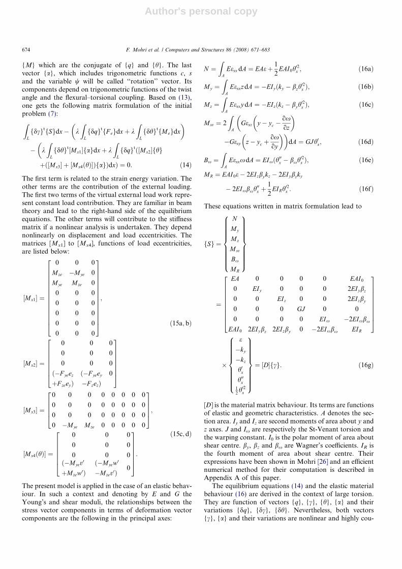
The present model is applied in the case of an elastic behav-iour. In such a context and denoting by E and G theYoung’s and shear moduli, the relationships between thestress vector components in terms of deformation vectorcomponents are the following in the principal axes:

N ¼Z

AEexx dA ¼ EAeþ 1

2EAI0h

02x ; ð16aÞ

My ¼Z

AEexxzdA ¼ �EIyðky � bzh

02x Þ; ð16bÞ

Mz ¼Z

AEexxy dA ¼ �EIzðkz � byh

02x Þ; ð16cÞ

Msv ¼ 2

ZA

Gexz y � yc �oxoz

� ��Gexy z� yc þ

oxoy

� ��dA ¼ GJh0x; ð16dÞ

Bx ¼Z

AEexxxdA ¼ EIxðh00x � bxh02x Þ; ð16eÞ

MR ¼ EAI0e� 2EIzbykz � 2EIybzky

� 2EIxbxh00x þ1

2EIRh

02x : ð16fÞ

These equations written in matrix formulation lead to

fSg ¼

N

My

Mz

Msv

Bx

MR

8>>>>>>>><>>>>>>>>:

9>>>>>>>>=>>>>>>>>;

¼

EA 0 0 0 0 EAI0

0 EIy 0 0 0 2EIybz

0 0 EIz 0 0 2EIzby

0 0 0 GJ 0 0

0 0 0 0 EIx �2EIxbx

EAI0 2EIybz 2EIzby 0 �2EIxbx EIR

2666666664

3777777775

�

e

�ky

�kz

h0xh00x

12h02x

8>>>>>>>><>>>>>>>>:

9>>>>>>>>=>>>>>>>>;¼ ½D�fcg: ð16gÞ

[D] is the material matrix behaviour. Its terms are functionsof elastic and geometric characteristics. A denotes the sec-tion area. Iy and Iz are second moments of area about y andz axes. J and Ix are respectively the St-Venant torsion andthe warping constant. I0 is the polar moment of area aboutshear centre. by, bz and bx are Wagner’s coefficients. IR isthe fourth moment of area about shear centre. Theirexpressions have been shown in Mohri [26] and an efficientnumerical method for their computation is described inAppendix A of this paper.

The equilibrium equations (14) and the elastic materialbehaviour (16) are derived in the context of large torsion.They are function of vectors {q}, {c}, {h}, {a} and theirvariations {dq}, {dc}, {dh}. Nevertheless, both vectors{c}, {a} and their variations are nonlinear and highly cou-



pled. According to (6a–c), the strain vector {c}, defined in(13b), is split into a linear part and two nonlinear parts as

fcg ¼

e

�ky

�kz

h0xh00x

12h02x

8>>>>>>>><>>>>>>>>:

9>>>>>>>>=>>>>>>>>;

¼

u0

�w00

�v00

h0xh00x0

8>>>>>>>><>>>>>>>>:

9>>>>>>>>=>>>>>>>>;þ 1

2

ðv02 þ w02Þ0

0

0

0

h02x

8>>>>>>>><>>>>>>>>:

9>>>>>>>>=>>>>>>>>;þ

�wh0x�w00cþ v00s

�v00c� w00s

0

0

0

8>>>>>>>><>>>>>>>>:

9>>>>>>>>=>>>>>>>>;¼ fclg þ fcnlðhÞg þ fcnlaðh; aÞg: ð17aÞ

{cl} is the classical linear part, {cnl(h)} and {cla(h,a)} arethe nonlinear parts related to quadratic and flexural–tor-sional coupling terms. These three parts can be easily for-mulated in term of the vector {h} by introducing threematrices [H], [A(h)] and [Aa(a)] as indicated below:

fclg¼

1 0 0 0 0 0 0

0 0 0 0 0 �1 0

0 0 0 0 �1 0 0

0 0 0 1 0 0 0

0 0 0 0 0 0 1

0 0 0 0 0 0 0

0

0

0

0

0

0

266666664

377777775

u0

v0

w0

h0xv00

w00

h00xhx

8>>>>>>>>>>>><>>>>>>>>>>>>:

9>>>>>>>>>>>>=>>>>>>>>>>>>;¼ ½H �fhg;

ð18aÞ

fcnlðhÞg¼1

2

0 v0 w0 0 0 0 0

0 0 0 0 0 0 0

0 0 0 0 0 0 0

0 0 0 0 0 0 0

0 0 0 0 0 0 0

0 0 0 h0x 0 0 0

0

0

0

0

0

0

266666664

377777775

u0

v0

w0

h0xv00

w00

h00xhx

8>>>>>>>>>>>><>>>>>>>>>>>>:

9>>>>>>>>>>>>=>>>>>>>>>>>>;¼ 1

2½AðhÞ�fhg;

ð18bÞ

fcnlaðh;aÞg¼

0 0 0 w 0 0 0

0 0 0 0 �s c 0

0 0 0 0 c s 0

0 0 0 0 0 0 0

0 0 0 0 0 0 0

0 0 0 0 0 0 0

0

0

0

0

0

0

266666664

377777775

u0

v0

w0

h0xv00

w00

h00xhx

8>>>>>>>>>>>><>>>>>>>>>>>>:

9>>>>>>>>>>>>=>>>>>>>>>>>>;¼ ½AaðaÞ�fhg:

ð18cÞ

Matrices [H] and [A(h)] are classical in nonlinear structuralmechanics. Matrix [Aa(a)] takes into account large torsionand flexural–torsional coupling. In this way, the deforma-tion {c} is obtained in term of {h} as

fcg ¼ ½H � þ 1

2½AðhÞ� � ½AaðaÞ�

� �fhg: ð19Þ

Applying variation to (19) and using the fact that thematrices [A(h)] and [Aa(a)] depend linearly on vectors {h}and {a}, {dc} is established as

fdcg ¼ ½H �fdhg þ ½AðhÞ�fdhg � ½AaðaÞ�fdhg � ½AaðdaÞ�fhg:ð20Þ

The last term in the right-hand side of (20) can be writtenas a product of a matrix ½bAðhÞ� depending on {h} and thevector {da}:

½AaðdaÞ�fhg ¼dwh0x

�v00 dsþw00dc

v00dcþw00ds

8><>:9>=>; ¼

0 0 h0xw00 �v00 0

v00 w00 0

0 0 0

0 0 0

0 0 0

2666666664

3777777775dc

ds

dw

8><>:9>=>;

¼ ½bAðhÞ�fdag: ð21Þ

According to definition (13g) for {a} and its componentsintroduced in (4a, 4b and 6e), one gets for the variationof the two first components:

dc ¼ �sdhx; ds ¼ ðcþ 1Þdhx: ð22a; bÞThe third component dW of {da} is derived from (6e) and(22a,b). After some arrangement, {da} is written in termsof {dh} and a new matrix [P(h,a)] as

fdag ¼0 0 0 0 0 0 0 �s

0 0 0 0 0 0 0 cþ 1

0 Qc RC 0 0 0 0 P c

264375

du0

dv0

dw0

dh0xdv00

dw00

dh00xdhx

8>>>>>>>>>>>>><>>>>>>>>>>>>>:

9>>>>>>>>>>>>>=>>>>>>>>>>>>>;¼ ½P ðh; aÞ�fdhg: ð22cÞ

The coefficients Pc, Qc and Rc utilized in the matrix P(h,a)are given by

P c ¼ �yCðw0sþ v0ðcþ 1ÞÞ þ zCðv0s� w0ðcþ 1ÞÞ; ð22dÞQc ¼ �yCs� zCðcþ 1Þ; ð22eÞRc ¼ yCðcþ 1Þ � zCs: ð22fÞ

Finally, injecting (22c) into (21), the last term in the right-hand side of (20) can be written in terms of {dh} and a newmatrix ½eAðh; aÞ� is introduced as

½AaðdaÞ�fhg ¼ ½bAðhÞ�½P ðh; aÞ�fdhg ¼ ½eAðh; aÞ�fdhg: ð23Þ



The above relationship permits us to write the vector {dc}in (20) in terms of {dh}. One arrives to

fdcg ¼ ð½H � þ ½AðhÞ� � ½AaðaÞ� � ½eAðh; aÞ�Þfdhg: ð24Þ

Based on formulas (19) for {c} and (24) for {dc}, one getsthe matrix formulation of the equilibrium equations (14)and the material behaviour (16g) into the following system:R

Lfdhgtð½H � þ ½AðhÞ� � ½AaðaÞ��½bAðh; aÞ�ÞtfSgdx� k

RLðfdqgtfF eg þ fdhgtfMegÞdx

� �;

�kR

Lðfdhgt½Mx1�fag þ fdqgt½Mx2�fhg�

þfdqgtð½Mx3� þ ½Mx4ðhÞ�ÞfagÞdx�¼ 0

fSg ¼ ½D� ½H � þ 12½AðhÞ� � ½AaðaÞ�

� �fhg:

8>>>>>>><>>>>>>>:ð25a; bÞ

In this way, the elastic equilibrium equations have been de-rived without any assumptions about the torsion angleamplitude. Trigonometric functions c = coshx�1 ands = sinhx have been included in the analysis and nonlinearand highly coupled kinematic relationships have beenencountered. Due to consideration of large torsion, newmatrices [Aa(a)] and ½eAðh; aÞ� depending on trigonometricfunctions c and s and flexural–torsional coupling have beenintroduced. Alternatively, in external work, effects of loadeccentricities have been considered. This leads to new sec-ond order bending moments and second order torsion mo-ments involving the trigonometric functions c and s.Consequently, other matrices [Mx1], [Mx2], [Mx3] and[Mx4(h)] have been introduced. In what follows, a beam fi-nite element will be formulated in the same circumstances.Nevertheless, in nonlinear analysis, only constant load con-tribution will be considered. The contribution of eccentricloads from centroid and shear point to second memberand tangent stiffness matrix is not included in the presentpaper (terms in second line of the equilibrium equation(25a)). Extensive work is done by the authors in order tomake this possible in future. This work is actually in pro-gress including the asymptotic numerical method for solu-tion of nonlinear problems [27].

4. Finite element discretisation

In literature about thin-walled beams with open section,warping deformation is of primary importance. For thisreason, the warping is considered as an independent dis-placement with regard to classical 3D beams. In mesh pro-cess, 3D beams elements with 14 degrees of freedom arecommonly utilized. Linear shape functions are assumedfor axial displacements and cubic functions for the otherdisplacements (i.e. v, w, hx) are used in natural co-ordinate[2,3,17]. Some other works have adopted hyperbolic shapefunctions for torsion angle [18,28,29].

In the present study, the beam of slenderness L isdivided into some finite elements of length l. Each element

is modelled with 3D beams elements with two nodes andseven degrees of freedom per node. The adopted shapefunctions are available in Lin [30] and Batoz [31].

The vectors {q} and {h} and their variations {dq} and{dh} are related to nodal variables {r} and {dr} by

fqg ¼ ½N �frge; fdqg ¼ ½N �fdrge;

fhg ¼ ½G�frge; fdhg ¼ ½G�fdrge;ð26a; dÞ

where [N] is the shape functions matrix and [G] is a matrixwhich links the nodal displacements to the gradient vector{h}. In the framework of finite element method, the equi-librium equations and the material behaviour are then writ-ten asP

e

l2

R 1

�1fdrgt

e½Bðh; aÞ�tfSgdn� k

Pe

l2

R 1

�1fdrgt

eff gedn ¼ 0

fSg ¼ ½D� ½Bl� þ 12½BnlðhÞ� � ½BnlaðaÞ�

� �frge

8<:8fdrg: ð27a; bÞPe denotes the assembling process over basic elements.

The matrices and vectors used in the formulation (27) arelisted below:

½Bðh; aÞ� ¼ ½Bl� þ ½BnlðhÞ� � ½BnlaðaÞ� � ½eBnlðh; aÞ�; ð28aÞ

½Bl� ¼ ½H �½G�; ð28bÞ

½BnlðhÞ� ¼ ½AðhÞ�½G�; ð28cÞ

½BnlaðaÞ� ¼ ½AaðaÞ�½G�; ð28dÞ

½eBnlðh; aÞ� ¼ ½eAðh; aÞ�½G�; ð28eÞ

ff ge ¼ ½N �tfF eg þ ½G�tfMeg: ð28fÞ

The vector {f}e is related to the nodal forces. Only constantload contribution in (25a) has been considered. The matri-ces [Bl] and [Bnl (h)] are familiar in nonlinear analysis. Inaddition one can remark the presence of new matrices[Bnla(a)] and ½eBnlðh; aÞ�. These matrices result from largetorsion assumptions and flexural–torsional coupling. Theyare function on the introduced trigonometric functions c

and s and flexural–torsional coupling.

5. Solution strategy in nonlinear context

To solve the nonlinear problem (27) we adopt a classicalincremental-iterative Newton–Raphson procedure. Withthis aim in view, we have to compute the tangent stiffnessmatrix. If the unknowns of the problem (28) fUgt ¼

�f frg fSg fag g; kÞ are sought in the form:

fUg ¼ fU 0g þ fDUg and k ¼ k0 þ Dk: ð29; 30Þ

Given an initial guess of the solution ({U0},k0), the incre-ments of the problem ({DU},Dk) satisfy the followingconditions:



Xe

l2

Z 1

�1

ð½Bðh0;a0Þ�tfDSgþ ½DBðh;aÞ�tfS0gÞdn�Dkff g¼f0g;

ð31aÞ

fDSg¼ ½D� ½Bl�þ1

2½Bnlðh0Þ�� ½Bnlaða0Þ�

� �fDrg

þ½D� 1

2½BnlðDhÞ�� ½BnlaðDaÞ�

� �fr0g: ð31bÞ

Due to highly nonlinear and coupling terms involved inmatrix [B(h,a)], the increment of [DB(h,a)] is not straight-forward and must be computed with more caution. Thefirst term in the left-hand side of (31a) leads directly tothe classical geometric stiffness part, while the second onegives the initial stiffness matrix. These parts are built sepa-rately in two main steps.

The first step is devoted to geometric stiffness matrix for-mulation. From (28), one can establish the identities:

½BnlðDhÞ�fr0g ¼ ½Bnlðh0Þ�fDrg; ð32aÞ½BnlaðDaÞ�fr0g ¼ ½eBnlðh0; a0Þ�fDrg: ð32bÞInserting (32) in (31b) and using (28a), we get

fDSg ¼ ½D�½Bðh0; a0Þ�fDrg: ð32cÞThe first term of (31a), leading to the geometric stiffnessmatrix, according to (32c) gives

½Bðh0; a0Þ�tfDSg ¼ ½Bðh0; a0Þ�t½D�½Bðh0; a0Þ�fDrg: ð32dÞThe second step concerns the formulation of the initialstress matrix. This matrix is obtained from the transforma-tion of the second term [DB(h,a)]t{S0} in (31a). From thedefinition of [B(h,a)] and its parts formulated in (28) andusing the fact that [Bnl(h)] and [Bnla(a)] are linear, permitto write

½DBðh;aÞ�tfS0g¼ ð½BnlðDhÞ�� ½BnlaðDaÞ�� ½DeBnlaðh;aÞ�ÞtfS0g:ð33aÞ

Additionally, considering the matrix [P(h0,a0)] in (22c) and

the following two matrices ½S0� and ½S0�:

½S0� ¼

0 0 0 0 0 0 0 0

0 N 0 0 0 0 0 0 0

0 0 N 0 0 0 0 0 0

0 0 0 MR00 0 0 0

0 0 0 0 0 0 0 0

0 0 0 0 0 0 0 0

0 0 0 0 0 0 0 0

0 0 0 0 0 0 0 0

26666666666664

37777777777775;

½S0� ¼

0 0 0

0 0 0

0 0 0

0 0 N 0

Mz0�My0

0

My0Mz0

0

0 0 0

0 0 0

26666666666664

37777777777775: ð33b; cÞ

we get the following identities after using Eq. (26d) relating{Dh} and {Dr}:

½BnlðDhÞ�tfS0g ¼ ½G�t½S0�½G�fDrg; ð33dÞ

½BnlaðDaÞ�tfS0g ¼ ½G�t½S0�½P ðh0; a0Þ�½G�fDrg: ð33eÞ

According to the definition of matrices ½eBnlðh; aÞ� and½bAðh; aÞ� introduced in (28e) and (23), we obtain

½DeBnlðh; aÞ� ¼ ½bAðDhÞ�½P ðh0; a0Þ�½G� þ ½bAðh0Þ�½DP ðh; aÞ�½G�:ð34aÞ

This relationship is taken into consideration in transforma-tion of vector ½DeBnlða; hÞ�tfS0g as

½DeBnlðh; aÞ�tfS0g ¼ ½G�tð½Pðh0; a0Þ�t½bAðDhÞ�t

þ ½DP ðh; aÞ�t½bAðh0Þ�tÞfS0g: ð34bÞ

On can check that the first term in the right-hand side of(34b) leads to

½P ðh0; a0Þ�t½bAðDhÞ�tfS0g ¼ ½P ðh0; a0Þ�t½S0�tfDhg: ð34cÞ

The second term in the right-hand side of (34b) yields to

½DP ðh; aÞ�t½bAðh0Þ�tfS0g ¼ ½S0�½P ðh0; a0Þ�fDhg; ð34dÞ

where the matrices ½S0� and ½P ðh0; a0Þ� are defined by

½S0� ¼

0 0 0

�zCN 0h0x0 �yCN 0h

0x0 0

yCN 0h0x0 �zCN 0h

0x0 0

0 0 0

0 0 0

0 0 0

0 0 0�My0v000þMz0w000

�My0w000�Mz0v000

N 0h0x0

26666666666666664

37777777777777775;

½P ðh0; a0Þ� ¼0 0 0 0 0 0 0 �s0

0 0 0 0 0 0 0 1þ c0

0 Q0 R0 0 0 0 0 P 0

264375 ð34e; fÞ

with P 0 ¼ ycðv00s0 � w00ð1þ c0ÞÞ þ zcðv00ð1þ c0Þ þ w00s0Þ,Q0 ¼ �ycðc0 þ 1Þ þ zcs0 and R0 ¼ �ycs0 � zcðc0 þ 1Þ.

Relationships (34c) and (34d) permit us to modify (34b)to

½DeBnlðh;aÞ�tfS0g¼ ½G�tð½P ðh0;a0Þ�t½S0�tþ½S0�½P ðh0;a0Þ�ÞfDhg:ð34gÞ

From the expression (26d) relating {Dh} and {Dr}, one ob-tains the finite element formulation of the above vector:

½DeBnlðh;aÞ�tfS0g¼ ½G�tð½Pðh0;a0Þ�t½S0�tþ½S0�½Pðh0;a0Þ�Þ½G�fDrg:ð34hÞ

Combining the relationships (33d), (33e) and (34h) allow usto write the initial stress part of the tangent stiffness matrixof (33a) as



½DBðh; aÞ�tfS0g ¼ ½G�tð½S0� � ½S0�½P ðh0; a0Þ� � ½Pðh0; a0Þ�t½S0�t

� ½S0�½P ðh0; a0Þ�Þ½G�fDrg¼ ½G�t½Sðh0; a0Þ�½G�fDrg: ð35aÞ

In order to facilitate the lecture, where we have introducedthe matrix [S(h0,a0)] given by

½Sðh0; a0Þ� ¼ ½S0� � ½S0�½Pðh0; a0Þ� � ½P ðh0; a0Þ�t½S0�t

� ½S0�½P ðh0; a0Þ�: ð35bÞ

These matrices depend on initial stresses and on flexural–

torsional coupling. Matrices ½S0�, ½S0� and ½S0� are functionon initial stresses. Matrices [P(h0,a0)] and ½P ðh0; a0Þ� in-clude flexural–torsional coupling.

Finally, the global matrix form of the incremental prob-lem (31) can be written as

½Kt�fDrg � Dkff g ¼ f0g; ð36Þ

where the tangent stiffness matrix [Kt] is given by

½Kt� ¼ ½Kg� þ ½Ks0� ð37aÞ

with

½Kg� ¼X

e

l2

Z 1

�1

½Bðh0; a0Þ�t½D�½Bðh0; a0Þ�dn;

½KS0� ¼X

e

l2

Z 1

�1

½G�t½Sðh0; a0Þ�½G�dn:

ð37b; cÞ

[Kg] is the geometric stiffness matrix and [KS0] is the initialstress stiffness matrix. By this way, a large torsion nonlin-ear finite element model for elastic thin-walled beams hasbeen investigated. The calculation of the tangent stiffnessmatrix was possible thanks to the introduction of new trig-onometric variables c = (coshx � 1) and s = sinhx.

6. Numerical investigations

A finite element model based on 3D beam elementincluding warping and large torsion has been presentedpreviously. Due to highly coupled and nonlinear equilib-rium equations, iterative methods are adopted in the solu-tion. The obtained tangent matrix accounts for largedisplacements, initial stresses, large torsion and flexural–torsional coupling. This element referenced B3Dw isimplanted in a general finite element package. Some exam-ples are presented hereafter. They concern the nonlinearbehaviour of beams in torsion. The validation is followedby investigation of post-buckling of struts and beams inbuckling and lateral buckling behaviour by reference tosome known examples. At the end, the performance ofthe proposed element is outlined by comparison of post-buckling behaviour of mono-symmetric sections with acommercial code. In what follows, the ability of the ele-ment to capture accurate bifurcations is demonstrated.When the equilibrium curves present singular points, New-

ton–Raphson iterative procedure based on arc lengthmethod is adopted.

6.1. Comparison examples

Example 1: Nonlinear behaviour of a cantilever beam

subjected to end torque

This example has been studied by Lin [30]. A doublysymmetric steel I section W21 · 93 was considered. Thegeometric dimensions of the section and the elastic con-stants are the following:b = 213.87, h = 549, tf = 23.6,tw = 14.73 mm , E = 200, G = 77 GPa (1.0 in. = 25.4 mm,1.0 lbf = 4.448 N). The warping effect on the nonlinearcantilever beam behaviour has been investigated.With thisaim in view, three boundary conditions have been consid-ered in [30]:

• free warping at both ends of the beam (a),• warping restrained at the fixed end and free warping at

the free end (b),• warping restrained at both ends of the beam (c).

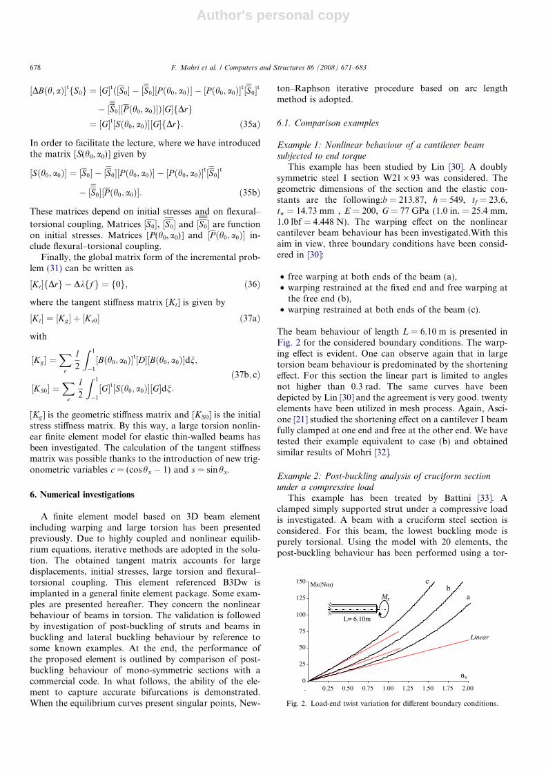
The beam behaviour of length L = 6.10 m is presented inFig. 2 for the considered boundary conditions. The warp-ing effect is evident. One can observe again that in largetorsion beam behaviour is predominated by the shorteningeffect. For this section the linear part is limited to anglesnot higher than 0.3 rad. The same curves have beendepicted by Lin [30] and the agreement is very good. twentyelements have been utilized in mesh process. Again, Asci-one [21] studied the shortening effect on a cantilever I beamfully clamped at one end and free at the other end. We havetested their example equivalent to case (b) and obtainedsimilar results of Mohri [32].

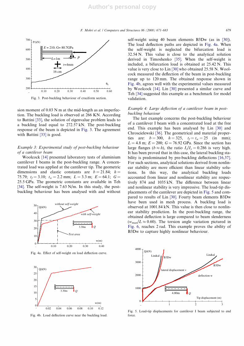
Example 2: Post-buckling analysis of cruciform sectionunder a compressive load

This example has been treated by Battini [33]. Aclamped simply supported strut under a compressive loadis investigated. A beam with a cruciform steel section isconsidered. For this beam, the lowest buckling mode ispurely torsional. Using the model with 20 elements, thepost-buckling behaviour has been performed using a tor-

0

25

50

75

100

125

150

0.25 0.50 0.75 1.00 1.25 1.50 1.75 2.00

θx

Mx(Nm)

a

cb

Linear

L= 6.10m

Mx

Fig. 2. Load-end twist variation for different boundary conditions.



sion moment of 0.03 N m at the mid-length as an imperfec-tion. The buckling load is observed at 266 KN. Accordingto Battini [33], the solution of eigenvalue problem leads toa buckling load equal to 272.57 kN. The post-bucklingresponse of the beam is depicted in Fig. 3. The agreementwith Battini [33] is good.

Example 3: Experimental study of post-buckling behaviour

of a cantilever beam

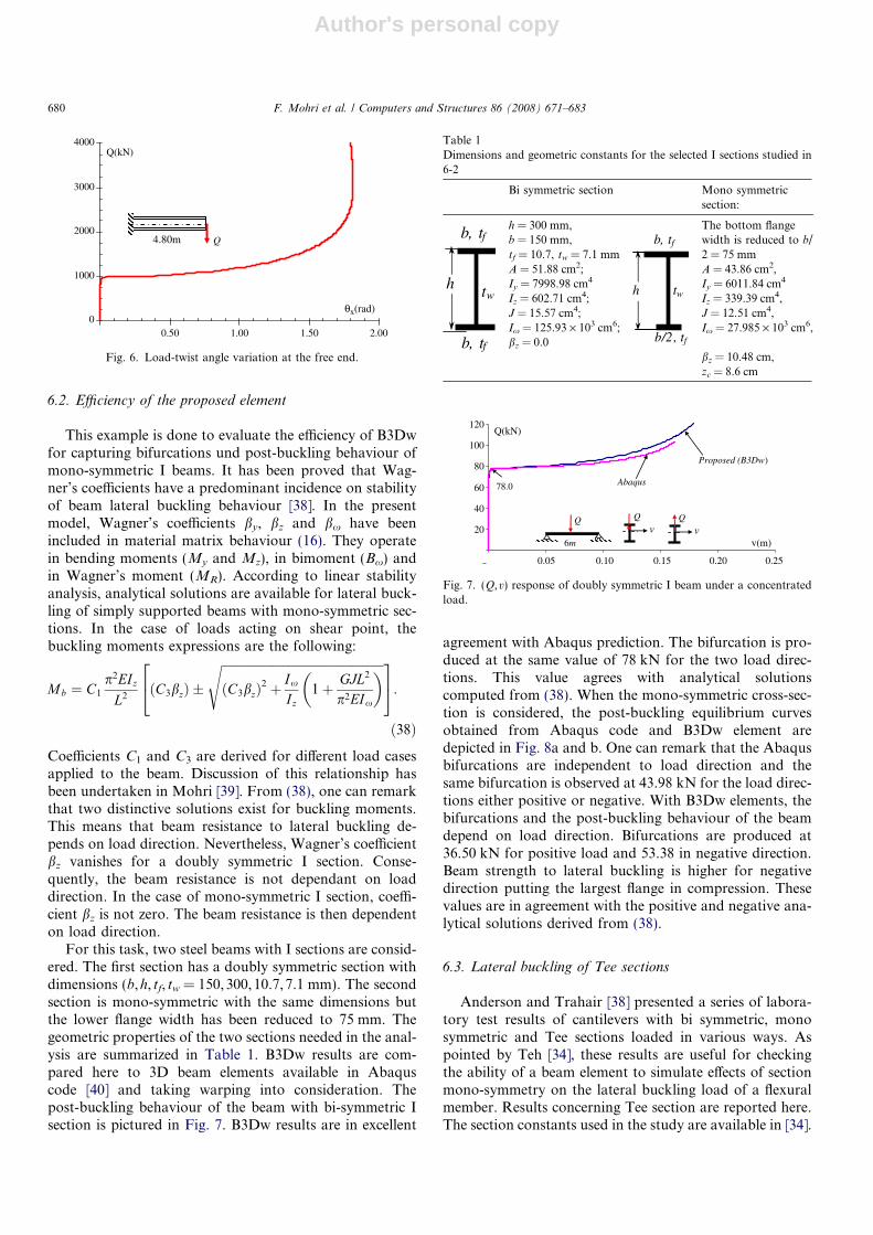
Woolcock [14] presented laboratory tests of aluminiumcantilever I beams in the post-buckling range. A concen-trated load was applied at the cantilever tip. The geometricdimensions and elastic constants are b = 21.84; h =75.79; tf = 3.10; tw = 2.2 mm; L = 3.3 m; E = 64.1; G =25.5 GPa. The geometric constants are available in Teh[34]. The self-weight is 7.63 N/m. In this study, the post-buckling behaviour has been analysed with and without

self-weight using 40 beam elements B3Dw (as in [30]).The load deflection paths are depicted in Fig. 4a. Whenthe self-weight is neglected the bifurcation load is32.54 N. This value is close to the analytical solutionderived in Timoshenko [35]. When the self-weight isincluded, a bifurcation load is obtained at 25.42 N. Thisvalue is very close to Lin [30] who obtained 25.58 N. Wool-cock measured the deflection of the beam in post-bucklingrange up to 120 mm. The obtained response shown inFig. 4b, agrees well with the experimental values measuredby Woolcock [14]. Lin [30] presented a similar curve andTeh [34] suggested this example as a benchmark for modelvalidation.

Example 4: Large deflection of a cantilever beam in post-

buckling behaviour

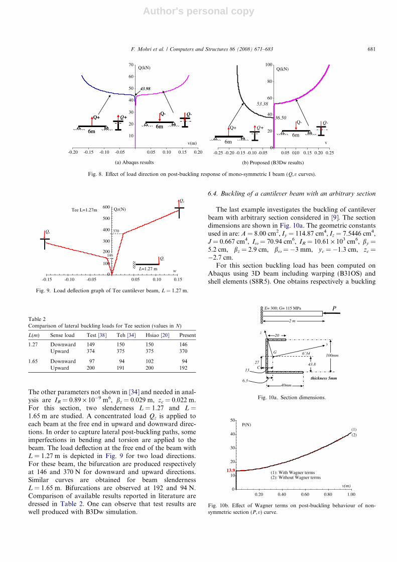
The last example concerns the post-buckling behaviourof a cantilever I beam with a concentrated load at the freeend. This example has been analysed by Lin [30] andChroscielewski [36]. The geometrical and material proper-ties are: b = 300, h = 325, tf = tw = 25 (in mm);L = 4.8 m; E = 200; G = 76.92 GPa. Since the section haslarge flanges (b � h), the ratio Iz/Iy = 0.286 is very high.It has been proved that in this case, the lateral buckling sta-bility is predominated by pre-buckling deflections [16,37].For such sections, analytical solutions derived from nonlin-ear stability are more efficient than linear stability solu-tions. In this way, the analytical buckling loadsaccounted from linear and nonlinear stability are respec-tively 874 and 1035 kN. The difference between linearand nonlinear stability is very impressive. The load-tip dis-placements of the cantilever are depicted in Fig. 5 and com-pared to results of Lin [30]. Fourty beam elements B3Dwhave been used in mesh process. A buckling load isobserved at 1001.84 kN. This value is then close to nonlin-ear stability prediction. In the post-buckling range, theobtained deflection is large compared to beam slenderness(wmax/L � 0.60). The torsion angle variation pictured inFig. 6, reaches 2 rad. This example proves the ability ofB3Dw to capture highly nonlinear behaviour.

200

300

400

500

600

700

0.10 0.20 0.30 0.40 0.50 0.60

θx

P(kN)

E = 210; G= 80.7GPa

16 cm

t=4mm

L=1m P

Fig. 3. Post-buckling behaviour of cruciform section.

with self-weight

without self-weight

Test area

0

10

20

30

40

50

0.10 0.20 0.30 0.40

w(m)

Q(kN)

3.30m Q

Fig. 4a. Effect of self-weight on load deflection curve.

0

5

10

15

20

25

30

0.02 0.04 0.06 0.08 0.10 0.12

w(m)

Q(kN)

3.30m Q

Fig. 4b. Load deflection curve near the buckling load.

0

1000

2000

3000

4000

1 2 3

Tip displacement (m)

Q(kN)

deflection w

lateral displacement v

B3Dw

Lin&alB3Dw

Lin&al

4.80m Q

Fig. 5. Load-tip displacements for cantilever I beam subjected to endforce.



6.2. Efficiency of the proposed element

This example is done to evaluate the efficiency of B3Dwfor capturing bifurcations und post-buckling behaviour ofmono-symmetric I beams. It has been proved that Wag-ner’s coefficients have a predominant incidence on stabilityof beam lateral buckling behaviour [38]. In the presentmodel, Wagner’s coefficients by, bz and bx have beenincluded in material matrix behaviour (16). They operatein bending moments (My and Mz), in bimoment (Bx) andin Wagner’s moment (MR). According to linear stabilityanalysis, analytical solutions are available for lateral buck-ling of simply supported beams with mono-symmetric sec-tions. In the case of loads acting on shear point, thebuckling moments expressions are the following:

Mb ¼ C1

p2EIz

L2ðC3bzÞ �

ffiffiffiffiffiffiffiffiffiffiffiffiffiffiffiffiffiffiffiffiffiffiffiffiffiffiffiffiffiffiffiffiffiffiffiffiffiffiffiffiffiffiffiffiffiffiffiffiffiffiffiffiffiðC3bzÞ

2 þ Ix

Iz1þ GJL2

p2EIx

� �s24 35:ð38Þ

Coefficients C1 and C3 are derived for different load casesapplied to the beam. Discussion of this relationship hasbeen undertaken in Mohri [39]. From (38), one can remarkthat two distinctive solutions exist for buckling moments.This means that beam resistance to lateral buckling de-pends on load direction. Nevertheless, Wagner’s coefficientbz vanishes for a doubly symmetric I section. Conse-quently, the beam resistance is not dependant on loaddirection. In the case of mono-symmetric I section, coeffi-cient bz is not zero. The beam resistance is then dependenton load direction.

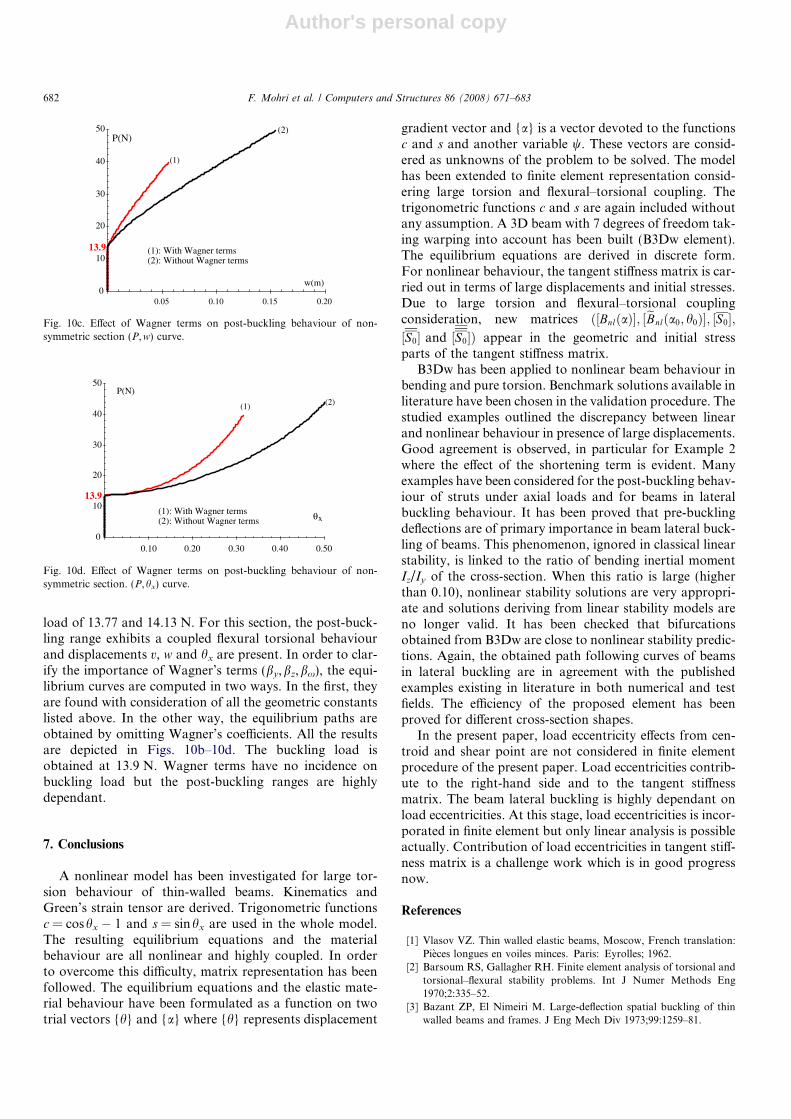
For this task, two steel beams with I sections are consid-ered. The first section has a doubly symmetric section withdimensions (b,h, tf, tw = 150,300,10.7,7.1 mm). The secondsection is mono-symmetric with the same dimensions butthe lower flange width has been reduced to 75 mm. Thegeometric properties of the two sections needed in the anal-ysis are summarized in Table 1. B3Dw results are com-pared here to 3D beam elements available in Abaquscode [40] and taking warping into consideration. Thepost-buckling behaviour of the beam with bi-symmetric Isection is pictured in Fig. 7. B3Dw results are in excellent

agreement with Abaqus prediction. The bifurcation is pro-duced at the same value of 78 kN for the two load direc-tions. This value agrees with analytical solutionscomputed from (38). When the mono-symmetric cross-sec-tion is considered, the post-buckling equilibrium curvesobtained from Abaqus code and B3Dw element aredepicted in Fig. 8a and b. One can remark that the Abaqusbifurcations are independent to load direction and thesame bifurcation is observed at 43.98 kN for the load direc-tions either positive or negative. With B3Dw elements, thebifurcations and the post-buckling behaviour of the beamdepend on load direction. Bifurcations are produced at36.50 kN for positive load and 53.38 in negative direction.Beam strength to lateral buckling is higher for negativedirection putting the largest flange in compression. Thesevalues are in agreement with the positive and negative ana-lytical solutions derived from (38).

6.3. Lateral buckling of Tee sections

Anderson and Trahair [38] presented a series of labora-tory test results of cantilevers with bi symmetric, monosymmetric and Tee sections loaded in various ways. Aspointed by Teh [34], these results are useful for checkingthe ability of a beam element to simulate effects of sectionmono-symmetry on the lateral buckling load of a flexuralmember. Results concerning Tee section are reported here.The section constants used in the study are available in [34].

0

1000

2000

3000

4000

0.50 1.00 1.50 2.00

θx(rad)

Q(kN)

4.80m Q

Fig. 6. Load-twist angle variation at the free end.

Table 1Dimensions and geometric constants for the selected I sections studied in6-2

Bi symmetric section Mono symmetricsection:

tw

b, tf

h

b, tfh = 300 mm,b = 150 mm,tf = 10.7, tw = 7.1 mm

tw

b/2, tf

h

b, tfThe bottom flangewidth is reduced to b/2 = 75 mm

A = 51.88 cm2;Iy = 7998.98 cm4

A = 43.86 cm2,Iy = 6011.84 cm4

Iz = 602.71 cm4;J = 15.57 cm4;

Iz = 339.39 cm4,J = 12.51 cm4,

Ix = 125.93 · 103 cm6;bz = 0.0

Ix = 27.985 · 103 cm6,

bz = 10.48 cm,zc = 8.6 cm

20

40

60

80

100

120

0.05 0.10 0.15 0.20 0.25

v(m)

Q(kN)

Proposed (B3Dw)

Abaqus

vQ Q

6m

Q

v

78.0

Fig. 7. (Q,v) response of doubly symmetric I beam under a concentratedload.



The other parameters not shown in [34] and needed in anal-ysis are IR = 0.89 · 10�9 m6, bz = 0.029 m, zc = 0.022 m.For this section, two slenderness L = 1.27 and L =1.65 m are studied. A concentrated load Qz is applied toeach beam at the free end in upward and downward direc-tions. In order to capture lateral post-buckling paths, someimperfections in bending and torsion are applied to thebeam. The load deflection at the free end of the beam withL = 1.27 m is depicted in Fig. 9 for two load directions.For these beam, the bifurcation are produced respectivelyat 146 and 370 N for downward and upward directions.Similar curves are obtained for beam slendernessL = 1.65 m. Bifurcations are observed at 192 and 94 N.Comparison of available results reported in literature aredressed in Table 2. One can observe that test results arewell produced with B3Dw simulation.

6.4. Buckling of a cantilever beam with an arbitrary section

The last example investigates the buckling of cantileverbeam with arbitrary section considered in [9]. The sectiondimensions are shown in Fig. 10a. The geometric constantsused in are: A = 8.00 cm2, Iy = 114.87 cm4, Iz = 7.5446 cm4,J = 0.667 cm4, Ix = 70.94 cm6, IR = 10.61 · 103 cm6, by =5.2 cm, bz = 2.9 cm, bx = �3 mm, yc = �1.3 cm, zc =�2.7 cm.

For this section buckling load has been computed onAbaqus using 3D beam including warping (B31OS) andshell elements (S8R5). One obtains respectively a buckling

10

20

30

40

50

60

70

-0.20 -0.15 -0.10 -0.05 0.05

(a) Abaqus results (b) Proposed (B3Dw results)

0.10 0.15 0.20

v(m)

Q(kN)

0

20

40

60

80

100

-0.25 -0.20 -0.15 -0.10 -0.05 0.05 0.10 0.15 0.20 0.25

v

Q(kN)

Q-

6m

Q-Q+

6m

Q+

43.98

Q-

6m

Q-Q+

6m

Q+

53.38

36.50Q-

6m

Q-Q+

6m

Q+

Fig. 8. Effect of load direction on post-buckling response of mono-symmetric I beam (Q,v curves).

Tee L=1.27m

0

100

200

300

400

500

600

-0.15 -0.10 -0.05 0.05 0.10 0.15

w

Qz(N)

370

146Qz

L=1.27 m

Qz

Qz

Fig. 9. Load deflection graph of Tee cantilever beam, L = 1.27 m.

Table 2Comparison of lateral buckling loads for Tee section (values in N)

L(m) Sense load Test [38] Teh [34] Hsiao [20] Present

1.27 Downward 149 150 150 146Upward 374 375 375 370

1.65 Downward 97 94 102 94Upward 200 191 200 192

E= 300; G= 115 MPa P

2 m

G

C

y

z

43.8

6.3

13

27

6˚34 100mm

40mm

20

thickness 5mm

Fig. 10a. Section dimensions.

0

10

20

30

40

50

0.20 0.40 0.60 0.80 1.00

v(m)

P(N)

13.9 (1): With Wagner terms (2): Without Wagner terms

(1)(2)

Fig. 10b. Effect of Wagner terms on post-buckling behaviour of non-symmetric section (P,v) curve.



load of 13.77 and 14.13 N. For this section, the post-buck-ling range exhibits a coupled flexural torsional behaviourand displacements v, w and hx are present. In order to clar-ify the importance of Wagner’s terms (by,bz,bx), the equi-librium curves are computed in two ways. In the first, theyare found with consideration of all the geometric constantslisted above. In the other way, the equilibrium paths areobtained by omitting Wagner’s coefficients. All the resultsare depicted in Figs. 10b–10d. The buckling load isobtained at 13.9 N. Wagner terms have no incidence onbuckling load but the post-buckling ranges are highlydependant.

7. Conclusions

A nonlinear model has been investigated for large tor-sion behaviour of thin-walled beams. Kinematics andGreen’s strain tensor are derived. Trigonometric functionsc = coshx � 1 and s = sinhx are used in the whole model.The resulting equilibrium equations and the materialbehaviour are all nonlinear and highly coupled. In orderto overcome this difficulty, matrix representation has beenfollowed. The equilibrium equations and the elastic mate-rial behaviour have been formulated as a function on twotrial vectors {h} and {a} where {h} represents displacement

gradient vector and {a} is a vector devoted to the functionsc and s and another variable w. These vectors are consid-ered as unknowns of the problem to be solved. The modelhas been extended to finite element representation consid-ering large torsion and flexural–torsional coupling. Thetrigonometric functions c and s are again included withoutany assumption. A 3D beam with 7 degrees of freedom tak-ing warping into account has been built (B3Dw element).The equilibrium equations are derived in discrete form.For nonlinear behaviour, the tangent stiffness matrix is car-ried out in terms of large displacements and initial stresses.Due to large torsion and flexural–torsional couplingconsideration, new matrices ð½BnlðaÞ�; ½eBnlða0; h0Þ�; ½S0�;½S0� and ½S0�Þ appear in the geometric and initial stressparts of the tangent stiffness matrix.

B3Dw has been applied to nonlinear beam behaviour inbending and pure torsion. Benchmark solutions available inliterature have been chosen in the validation procedure. Thestudied examples outlined the discrepancy between linearand nonlinear behaviour in presence of large displacements.Good agreement is observed, in particular for Example 2where the effect of the shortening term is evident. Manyexamples have been considered for the post-buckling behav-iour of struts under axial loads and for beams in lateralbuckling behaviour. It has been proved that pre-bucklingdeflections are of primary importance in beam lateral buck-ling of beams. This phenomenon, ignored in classical linearstability, is linked to the ratio of bending inertial momentIz/Iy of the cross-section. When this ratio is large (higherthan 0.10), nonlinear stability solutions are very appropri-ate and solutions deriving from linear stability models areno longer valid. It has been checked that bifurcationsobtained from B3Dw are close to nonlinear stability predic-tions. Again, the obtained path following curves of beamsin lateral buckling are in agreement with the publishedexamples existing in literature in both numerical and testfields. The efficiency of the proposed element has beenproved for different cross-section shapes.

In the present paper, load eccentricity effects from cen-troid and shear point are not considered in finite elementprocedure of the present paper. Load eccentricities contrib-ute to the right-hand side and to the tangent stiffnessmatrix. The beam lateral buckling is highly dependant onload eccentricities. At this stage, load eccentricities is incor-porated in finite element but only linear analysis is possibleactually. Contribution of load eccentricities in tangent stiff-ness matrix is a challenge work which is in good progressnow.

References

[1] Vlasov VZ. Thin walled elastic beams, Moscow, French translation:Pieces longues en voiles minces. Paris: Eyrolles; 1962.

[2] Barsoum RS, Gallagher RH. Finite element analysis of torsional andtorsional–flexural stability problems. Int J Numer Methods Eng1970;2:335–52.

[3] Bazant ZP, El Nimeiri M. Large-deflection spatial buckling of thinwalled beams and frames. J Eng Mech Div 1973;99:1259–81.

0

10

20

30

40

50

0.05 0.10 0.15 0.20

w(m)

P(N)

(1): With Wagner terms (2): Without Wagner terms

(1)

(2)

13.9

Fig. 10c. Effect of Wagner terms on post-buckling behaviour of non-symmetric section (P,w) curve.

0

10

20

30

40

50

0.10 0.20 0.30 0.40 0.50

θx

P(N)

13.9

(1): With Wagner terms (2): Without Wagner terms

(1) (2)

Fig. 10d. Effect of Wagner terms on post-buckling behaviour of non-symmetric section. (P,hx) curve.



[4] Yang YB, McGuire W. Stiffness matrix for geometric nonlinearanalysis. J Struct Eng 1986;112:853–77.

[5] Laudiero F, Zaccaria D. Finite element analysis of stability of thin-walled beams of open section. Int J Mech Sci 1988;30:543–57.

[6] Kim SB, Kim MY. Improved formulation for spatial stability andfree vibration of thin-walled tapered beams and space frames. EngStruct 2000;22:446–58.

[7] Kwak HY, Kim DY, Lee HW. Effect of warping in geometricnonlinear analysis of spatial beams. J Construct Steel Res2001;57:729–51.

[8] Pi YL, Bradford MA. Effects of approximations in analyses of beamsof open thin-walled cross-section. Part II: 3-D non-linear behaviour.Int J Numer Method Eng 2001;51:773–90.

[9] Turkalj G, Brnic J, Prpic-Orsic J. Large rotation analysis of elasticthin-walled beam-type structures using ESA approach. ComputStruct 2003;81:1851–64.

[10] Gregory M. Elastic torsion of members of thin open cross section.Aust J Appl Sci 1961;12:174–93.

[11] Gobarah AA, Tso WK. A non-linear thin-walled beam theory. Int JMech Sci 1971;13:1025–38.

[12] Black MM. Non-linear behaviour of thin-walled unsymmetric beamsections subject to bending and torsion. In: Thin-walled struc-tures. London: Chatto & Windus; 1967. p. 87–102.

[13] Moore DB. A non-linear theory for the behaviour of thin-walledsections subjected to combined bending and torsion. Thin-WalledStruct 1986;4:449–66.

[14] Woolcock ST, Trahair NS. Post-buckling behavior of determinatebeams. J Eng Mech Div ASCE 1974;100:151–71.

[15] Achour B, Roberts TM. Non-linear strains and stability of thin-walled bars. J Construct Steel Res 2000;56:237–52.

[16] Mohri F, Azrar L, Potier-Ferry M. Lateral post-buckling analysis ofthin-walled open section beams. Thin-Walled Struct 2002;40:1013–36.

[17] Attard MM. Lateral buckling analysis of beams by the FEM.Comput Struct 1986;23:217–31.

[18] De Ville de Goyet V. L’ analyse statique non lineaire des structuresspatiales formees de poutres a sections non symetrique par lamethode des elements finis. Doctorat dissertation, University ofLiege, Belgium, 1989.

[19] Ronagh HR, Bradford MA, Attard MM. Nonlinear analysis of thin-walled members of variable cross-section, Part I: theory. ComputStruct 2000;77:285–99.

[20] Hsiao KM, Lin WY. A co-rotational formulation for thin-walledbeams with monosymmetric open section. Comput Methods ApplMech Eng 2000;190:1163–85.

[21] Ascione L, Feo L. On the non-linear statical behaviour of thin-walledelements beams of open cross-sections: a numerical approach. Int JComput Eng Sci 2001;2:513–36.

[22] Machado SP, Cortinez VH. Lateral buckling of thin-walled opencomposite bisymmetric beams with pre-buckling and shear deforma-tion. Eng Struct 2005;27:1185–96.

[23] Pi Y-L, Bradford MA, Uy B. A rational elasto-plastic spatiallycurved thin-walled beam element. Int J Numer Methods Eng2007;70(3):253–90.

[24] Pi Y-L, Bradford MA, Tin-Loi F. Flexural–torsional buckling ofshallow arches with open thin-walled section under uniform radialloads. Thin Walled Struct 2007;45(3):352–62.

[25] Attard MM. Nonlinear theory of non-uniform torsion of thin-walledopen beams. Thin-Walled Struct 1986;4:101–34.

[26] Mohri F, Azrar L, Potier-Ferry M. Flexural–torsional post-bucklinganalysis of thin-walled elements with open sections. Thin-WalledStruct 2001;39:907–38.

[27] Cochelin B, Damil N, Potier-Ferry MM. ethode AsymptotiqueNumerique , Collection Methodes numeriques. Dirigee par PiotrBreitkopf. Edition Hermes Science Publications; 2007.

[28] Krajcinovic D. A consistent discrete elements technique for thin-walled assemblages. Int J Solids Struct 1969;5:639–62.

[29] Shakourzadeh H, Guo YQ, Batoz JL. A torsion bending element forthin-walled beams with open and closed cross sections. ComputStruct 1995;55:1045–54.

[30] Lin WY, Hsiao KM. Co-rotational formulation for geometricnonlinear analysis of doubly symmetric thin-walled beams. ComputMethods Appl Mech Eng 2001;190:6023–52.

[31] Batoz JL, Dhatt G. Modelisation des structures par elements finis,vol. 2. Paris: Hermes; 1990.

[32] Mohri F, Damil N, Potier-Ferry M. Un modele element fini pour lecalcul non lineaire des poutres a parois minces et a sections ouvertes.7�eme colloque national en calcul des structures, Giens 2005, vol.2. Lavoisier, Paris: Hermes; 2005. p. 571–6. ISBN 2-7462-1140-8.

[33] Battini JM, Pacoste C. Co-rotational beam elements with warpingeffects in instabilities problems. Comput Methods Appl Mech Eng2002;191:1755–89.

[34] Teh LH. Beam element verification for 3D elastic steel frame analysis.Comput Struct 2004;82:1167–79.

[35] Timoshenko SP, Gere JM. Theory of elastic stability. 2nded. NY: McGraw Hill; 1961.

[36] Chroscielewski J, Makowski J, Stumpf H. Finite element analysis ofsmith, folded and multi-shell structures. Comput Methods ApplMech Eng 1997;141:1–46.

[37] Trahair NS. Flexural–torsional buckling of structures. Lon-don: Chapman & Hall; 1993.

[38] Andeson JM, Trahair NS. Stability of monosymmetric beams andcantilevers. J Struct Div ASCE 1972;98:2647–62.

[39] Mohri F, Brouki A, Roth JC. Theoretical and numerical stabilityanalyses of unrestrained, mono-symmetric thin-walled beams. JConstruct Steel Res 2003;59:63–90.

[40] Hibbit, Karlsson and Sorensen Inc. Abaqus Standard User’s Manuel,Version 6.4. Abaqus, Pawtucket, RI, USA, 2003.


Documents

Large torsion finite element model for thin-walled beams