Large-scale pan-european forest monitoring network: A statistical perspective for designing and combining country estimates. Example for defoliation

Provided for non-commercial research and educational use only. Not for reproduction, distribution or commercial use.

This chapter was originally published in the book Developments in Environmental Science, Vol. 12, published by Elsevier, and the attached copy is provided by Elsevier for the author's benefit and for the benefit of the author's institution, for non-commercial research and educational use including without limitation use in instruction at your institution, sending it to specific colleagues who know you, and providing a copy to your institution’s administrator.

All other uses, reproduction and distribution, including without limitation commercial reprints, selling or licensing copies or access, or posting on open internet sites, your personal or institution’s website or repository, are prohibited. For exceptions, permission may be sought for such use through Elsevier's permissions site at:

http://www.elsevier.com/locate/permissionusematerial

From: Davide Travaglini, Gherardo Chirici, Francesca Bottalico, Marco Ferretti, Piermaria Corona, Anna Barbati and Lorenzo Fattorini, Large-Scale Pan-European Forest Monitoring

Network: A Statistical Perspective for Designing and Combining Country Estimates. Example for Defoliation. In Marco Ferretti and Richard Fischer, editors: Developments in

Environmental Science, Vol. 12, Oxford, UK, 2013, pp. 105-135. ISBN: 978-0-08-098222-9

© Copyright 2013 Elsevier Ltd. Elsevier

Author's personal copy

Chapter 7

Developments in Environmental Science, Vol. 12. http://dx.doi.org/10.1016/B978-0-

© 2013 Elsevier Ltd. All rights reserved.

Large-Scale Pan-EuropeanForest Monitoring Network:A Statistical Perspective forDesigning and CombiningCountry Estimates. Examplefor Defoliation

Davide Travaglini*,1, Gherardo Chirici{, Francesca Bottalico*, MarcoFerretti{, Piermaria Corona}, Anna Barbati} and Lorenzo Fattorini}*Dipartimento di Economia, Ingegneria, Scienze e Tecnologie Agrarie e Forestali, Universita

degli Studi di Firenze, Firenze, Italy{Dipartimento di Bioscienze e Territorio, Universita degli Studi del Molise, Contrada Fonte

Lappone s.n.c., Pesche, Isernia, Italy{TerraData Environmetrics, Monterotondo Marittimo (GR), Italy}Dipartimento per l’Innovazione dei sistemi Biologici, Agroalimentari e Forestali, Universita

degli Studi della Tuscia, Viterbo, Italy}Dipartimento di Economia Politica e Statistica, Universita degli Studi di Siena, Siena, Italy1Corresponding author: e-mail: [email protected]

Chapter Outline
7.1. Introduction 106
7.2. Sampling Designs in

Large-Scale Forest

Monitoring in Europe 107

7.3. Relationship Between

FCM and NFI Networks 110

7.4. Design-Based

European Monitoring

System of Forest

Condition 113

7.4.1. The Importance

of Clear Objectives 113

7.4.2. Defining Parameters

of Concern 115

7.4.3. Defining Accuracy

Measures for Status

Assessment 117

7.4.4. Defining Accuracy

Measures for

Change Assessment 118

08-098222-9.00007-8

105

http://dx.doi.org/10.1016/B978-0-08-098222-9.00007-8

SECTION II Designing Forest Monitoring106


7.5. Sampling Strategies at

the Country Level 119

7.5.1. Uniform Random

Sampling 119

7.5.2. URS Versus

Systematic and

Stratified Sampling 122

7.5.3. Sampling Effort: A

Preliminary Test 125

7.6. Aggregating Country

Estimates at the

European Level 125

7.6.1. Combining FCM

Estimates 127

7.6.2. Coupling FCM

and NFI Estimates

Across Europe 128

7.7. Conclusions 131

References 133

7.1 INTRODUCTION

National Forest Inventories (NFIs) and Forest Condition Monitoring (FCM)

networks are primary data sources for large area assessment of forest

resources. NFIs have been traditionally designed to provide country-based

estimates on the kind, amount, and condition of timber and nontimber forest

resources (Corona et al., 2011); with time, new variables have been included

to meet evolving demands of forest information related to international

conventions and policy process (Vidal et al., 2008). FCM was established

in 1980s in response to the concern of monitoring the alleged progressive

deterioration of forest condition due to atmospheric pollution (Innes, 1993).

In general terms, NFIs and FCM share the same approach: data from sample

surveys are used to estimate population parameters for the attribute(s) of con-

cern and to estimate changes over time.

The International Co-operative Programme on Assessment and Monitoring

of Air Pollution Effects on Forests (ICP Forests) large-scale (Level I, see

Chapters 2 and 6) monitoring network has a European-wide dimension and

the potential for providing forest information to fulfill reporting obligations

under several international agreements (e.g., Ministerial Conference on the

Protection of Forests in Europe-MCPFE, currently Forest Europe; Montreal

processes and for the purposes of forest certification; climate negotiations).

Yet, several authors argue about the quality of the data collected by the ICP

Forests surveys (e.g., Ferretti, 1997, 2004; Innes and Materna, 1992; Innes

et al., 1993; Neumann and Stowasser, 1986; Percy and Ferretti, 2004). Main

criticisms concerned the quality of defoliation assessments, while very few

authors addressed sampling-related issues (e.g., Ferretti, 1997; Ferretti and

Chiarucci, 2003; Innes, 1988; Kohl and Kaufmann, 1993; Percy and

Ferretti, 2004). This latter point, instead, deserves careful attention, as the

sampling approaches adopted by individual countries, which are responsible

for the implementation of Level I, have a significant impact on survey results.

Chapter 7 Large-Scale Pan-European Forest Monitoring Network 107


As a matter of fact, the ICP Forests Level I network is a composite of national

networks, based on different sampling schemes (Cozzi et al., 2002). Neverthe-

less, all national sampling schemes are required to follow a probabilistic

sampling design, ensuring, for each element of the population, a nonzero

probability of being selected. The density of sampling units within ICP For-

ests Level I network provides the basis for Europe-wide analysis rather than

for national assessments, which are partly based on denser national grids

(Ferretti et al., 2010a). Although several countries adopt a systematic sam-

pling to select sampling sites, the target population is not homogeneous within

the monitoring network, as different forest definitions are adopted by individ-

ual countries. Moreover, where applied, the so-called cross-cluster plot is sur-

veyed based on a fixed number of nearest trees (UNECE, 1998). As a

consequence, it may be very difficult to achieve statistically sound estimates

of forest condition parameters (e.g., mean defoliation, frequency of trees in

certain defoliation classes) and of their accuracy from the current structure

of ICP Forests surveys. Indeed, differences between countries in the definition

of the target population preclude the achievement of reliable estimates at the

European level. Likewise, the selection of a fixed number of nearest trees

around points precludes the estimation (at least from a design-based perspec-

tive) even at the country level, due to the difficulties in determining the inclu-

sion probabilities of trees, as pointed out by Kleinn and Vilcko (2006).

In this chapter, we will first introduce the main sampling designs that may

be applied in the context of large-scale forest monitoring; second, present the

relationships between FCM and NFI networks; and finally, explore and sug-

gest formal solutions to overcome the problems and drawbacks outlined

above. In this respect, we will move in the framework of design-based infer-

ence: accordingly, we will propose (i) a set of requirements for status and

change assessment and (ii) a harmonized sampling strategy able to provide

unbiased and consistent estimators of forest condition parameters and their

changes at both country and European levels.

7.2 SAMPLING DESIGNS IN LARGE-SCALE FORESTMONITORING IN EUROPE

Collecting data on forests over large areas can hardly cover all stands and

trees as complete enumeration (population census) is too time consuming

and costly. Thus, both forest inventories and forest monitoring systems are

based on data gathered from design-based surveys. Sampling consists of

making observations on parts of the investigated population (the forest and

its characteristics) to obtain estimates that are representative of the parameters

of the population (like volume per hectare or crown defoliation per cent) and

to assess the accuracy of the estimates.

Observations are carried out on sample units whose distribution on the

field is determined according to a sampling design. Multiphase sampling



strategies (e.g., Gregoire and Valentine, 2008; Mandallaz, 2008) are common

in many types of forest inventories (for a typology of forest inventories, see

Kohl et al., 2006). However, all design-based inventories over large areas

share a common methodological feature: sample units are objectively selected

by probabilistic rules as a means of guaranteeing the credibility of estimates

(Olsen and Schreuder, 1997). The histories of NFIs show a progressive evolu-

tion toward statistical sampling techniques, with the majority of countries now

using design-based sampling schemes (Lawrence et al., 2010). Similarly, sev-

eral countries participating in the ICP Forests Level I network declared to

adopt a design-based sampling (Cozzi et al., 2002) and the recently updated

monitoring manual also refers to this point (Ferretti et al., 2010a).

Traditionally, forest inventory data are analyzed in the framework of design-

based inference for which population values are regarded as fixed constants and

the randomization distribution resulting from the sampling design is the basis of

inference. In this framework, the bias and variance of an estimator of a popula-

tion parameter are determined from the set of all possible samples (the sample

space) and from the probability associated with each sample. Sarndal et al.

(1992), Gregoire (1998), and Fattorini (2001) provide extensive discussion of

design-based inference and contrast it with model-based inference. Usually, for-

est inventories adopt sampling schemes in which a set of points are randomly

selected from the study region in accordance with a spatial sampling design.

The main sampling designs that may be applied in the context of large-scale

forest monitoring are the Uniform Random Sampling (URS), the Pure System-

atic Sampling (PSS), and the Tessellation Stratified Sampling (TSS). Under the

URS, a set of points is randomly and independently selected in the study area.

URS is the fundamental selection method and all other sampling procedures

are modifications of URS. PSS, which is based on a regular grid of points with

a random start, represents the scheme most commonly adopted by NFIs, and it

has been used by ICP Forests to systematically select Level I plots

(Table 7.1). TSS is a random systematic scheme based on a regular tessellation

of the study area and the random placement of a point in each tessellation unit.

Once the sampling design has been chosen, plots of adequate size are then

established at the selected points, and forest attributes are recorded for the

trees within the plots (Corona, 2010).

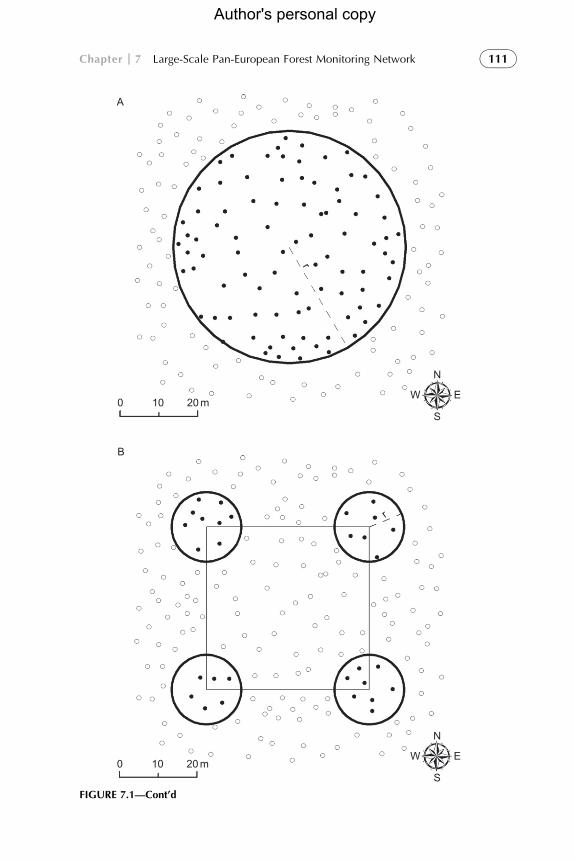
The shape of plots may be square, rectangular, or circular, although tran-

sect and angle count are used too (Figure 7.1). Circular plots are used by most

of European NFIs and many countries use cluster sampling in which multiple

plots (often four plots per cluster or more) are established in close spatial

proximity (Lawrence et al., 2010). Traditionally, on many Level I plots of

the ICP Forests network, a fixed number of nearest trees was customary

selected: for each point falling into a forest, the so-called cross-cluster plot

was performed, in which four further points are established along the direc-

tions N–S and E–W at a distance of 25 m from the central point and on each

point the six nearest trees are selected (UNECE, 1998). Recently, a shift to

fixed-area plot has been suggested (Ferretti et al., 2010a).

TABLE 7.1 Systematic Grid Spacing and Number of Plots Adopted by

European NFIs and ICP Forests Level I

Country

NFI ICP Forests Level I

Systematicgrid spacing(km�km)

Number ofplots


Numberof plots

Albania – – No survey in 2010

Andorra – – 16�16 3

Austria 3.889�3.889 22,236 16�16 135

Belarus – – 16�16 410

Belgium(WalloonRegion)

1�0.5 Approximately11,000

4�4/8�8 119

Bulgaria – – 4�4/8�8/16�16 159

Croatia – – 16�16 84

Cyprus – 1970 16�16 15

Czech Rep.a 2�2 Approximately39,000

8�8/16�16 132

Denmark 2�2 42,793 7�7/16�16 25

Estonia 5�5 4500 16�16 97

Finland 3�3 to10�10

69,388 16�16/24�32 932

Francea 1.41�1.41 275,000 16�16 532

Germany 2�2 to 4�4 54,009 4�4/16�16 415

Greece – 95,220 – 90

Hungary – – 16�16 77

Irelanda 2�2 17,423 16�16 36

Italya 1�1 301,000 16�16 253

Latvia 2�2 to 4�4 – 8�8 325

Liechtenstein – – No survey in 2010

Lithuania 4�4 7500 4�4/16�16 1065

Luxembourg 1�0.5 Approximately1800

No survey in 2010

Continued



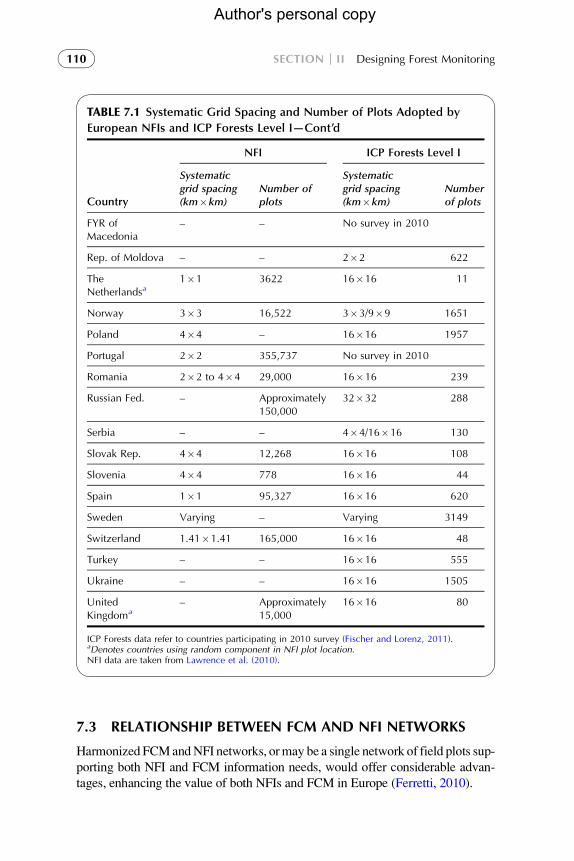
TABLE 7.1 Systematic Grid Spacing and Number of Plots Adopted by

European NFIs and ICP Forests Level I—Cont’d

Country

NFI ICP Forests Level I


Number ofplots


Numberof plots

FYR ofMacedonia

– – No survey in 2010

Rep. of Moldova – – 2�2 622

TheNetherlandsa

1�1 3622 16�16 11

Norway 3�3 16,522 3�3/9�9 1651

Poland 4�4 – 16�16 1957

Portugal 2�2 355,737 No survey in 2010

Romania 2�2 to 4�4 29,000 16�16 239

Russian Fed. – Approximately150,000

32�32 288

Serbia – – 4�4/16�16 130

Slovak Rep. 4�4 12,268 16�16 108

Slovenia 4�4 778 16�16 44

Spain 1�1 95,327 16�16 620

Sweden Varying – Varying 3149

Switzerland 1.41�1.41 165,000 16�16 48

Turkey – – 16�16 555

Ukraine – – 16�16 1505

UnitedKingdoma

– Approximately15,000

16�16 80

ICP Forests data refer to countries participating in 2010 survey (Fischer and Lorenz, 2011).aDenotes countries using random component in NFI plot location.NFI data are taken from Lawrence et al. (2010).



7.3 RELATIONSHIP BETWEEN FCM AND NFI NETWORKS

Harmonized FCMandNFI networks, ormay be a single network of field plots sup-

porting both NFI and FCM information needs, would offer considerable advan-

tages, enhancing the value of both NFIs and FCM in Europe (Ferretti, 2010).

10 20 m

r

S

E

N

W0

A

10 20 m

r

S

E

N

W

B

0

FIGURE 7.1—Cont’d



10 20 m

L

S

E

N

W

C

0

10 20 m

r1

r2

r3

S

E

N

W0

D





At present, the analysis of the relationship between the ICP Forests

Level I and NFIs shows that, in some countries, the ICP Forests and NFI net-

works are coincident while, in some others, the two grids are different for sev-

eral reasons. The most common are as follows:

l NFI and ICP Forests developed separately because they are under the

responsibility of different administrations (e.g., Spain);

l The ICP Forests plots were initially selected as a subsample of the NFI

grid, and then the NFI grid changed and the ICP Forests plots remained

unchanged (e.g., Italy).

Table 7.2 gives an overview of the status of integration between the ICP For-

ests Level I and NFI networks. The results are based on data provided by the

ICP Forests database integrated with an enquiry conducted in 2009–2010. In

most of the countries where integration is under study or where it has been

accomplished, the integration approach is based on the selection of the ICP

Forests plots as a subsample of the NFI network.

7.4 DESIGN-BASED EUROPEAN MONITORINGSYSTEM OF FOREST CONDITION

7.4.1 The Importance of Clear Objectives

Although the recent revision of the ICP Forest Manual (Ferretti et al., 2010b)

emphasizes the need for a formal and operational definition of objectives, this

has never been done for tree condition assessment (e.g., Eichhorn et al., 2010)

and the desired accuracy of the estimates was never addressed. This limits a

proper assessment of the effectiveness of the monitoring program in terms

of achievement of objectives and of cost-benefit. In addition, disregarding

the formal definitions of objectives has the undesired consequence of disre-

garding the field procedures necessary to achieve the objectives. Quantitative

assessment of forest condition parameters and of their changes rests on the

scheme adopted to select the observation sites and trees around selected sites.

In theory, a design-based European forest monitoring system should allow

FIGURE 7.1 Example of sample plot configuration for tree selection. Trees are depicted as

small white circles and sampled trees as small black circles. (A) Configuration of a circular plot

with radius r. (B) Configuration of a cluster with four circular plots of radius r. (C) ICP Forests

Level I plot configuration: the plot has four subplots assembled in a cross-cluster, oriented along

the main compass directions and at a distance L¼25 m from the plot center; on each subplot, the

six nearest trees to the subplot center are selected as sample trees, resulting in a total of 24 sample

trees per plot. (D) Configuration of concentric circular plots with radius r1, r2, and r3,

respectively.

TABLE 7.2 Status of Integration Between NFIs and ICP Forests Level I

Networks

Status of

integration Country Integration approach

None Andorra –

Belgium/Wallonia –

Bulgaria –

Croatia –

Czech Rep. –

France –

Germany (most regions) –

Lithuania –

Montenegro –

Russian Fed. –

Serbia –

Slovak Rep. –

Spain –

The Netherlands –

United Kingdom –

Under study Belgium/Flanders Plot design NFI in ICP Forests

Denmark ICP Forests subsample of NFI

Estonia ICP Forests subsample of NFI

Germany/Baden-Wurttemberg

A slightly modified version of the NFI wasassessed on ICP Forests for the first timein 2006

Ireland ICP Forests and NFI network run inparallel until a time series exists whichallows for the interpretation of trends

Italy Hypothesis of new ICP Forests grid assubsample of NFI. For 1 or 2 years oldICP grid still active to maintain time series

Latvia ICP Forests subsample of NFI

Norway –



TABLE 7.2 Status of Integration Between NFIs and ICP Forests Level I

Networks—Cont’d

Status of

integration Country Integration approach

Accomplished Austria ICP Forests subsample of NFI

Belarus –

Finland ICP Forests subsample of NFI

Germany/Bavaria ICP Forests subsample of NFI

Hungary ICP Forests subsample of GrowthMonitoring

Poland ICP Forests subsample of NFI

Romania New NFI plots on ICP Forests

Slovenia ICP Forests subsample of NFI

Sweden ICP Forests subsample of NFI

Switzerland –

Turkey –



(a) the quantitative estimates of the condition attribute of interest (e.g., pro-

portion of trees with defoliation >25%) for the target statistical population

(e.g., the whole population of forest trees) and for defined subgroups (e.g.,

the beech trees) at a specified level of accuracy for each country and at the

European level; (b) the quantitative estimates of change for the condition of

the attribute of interest at both country and European levels, with a subsequent

statistical assessment of the null hypothesis of no change. These generic

objectives are rather common in management-oriented environmental moni-

toring (e.g., Urquhart et al., 1998) and will be developed hereafter by defining

parameters and precision requirements for status and change detection.

7.4.2 Defining Parameters of Concern

Consider a population U of N trees over a delineated study area (e.g., the

whole forest trees or a defined subgroup of forest trees in a country) and

denote by yj( j2U) the value of defoliation level Y for the j-th tree in the pop-

ulation. Usually, the defoliation level is defined as needle/leaf loss in the

assessable crown as compared with a reference tree (Eichhorn et al., 2010;

see Chapter 8), ranging from 0 to 100% and assessed in 5% classes.



Accordingly, Y constitutes a discrete variable with range 0, 5, . . . , 95, 100.The average defoliation value

Y¼ 1

N

Xj2U

yj (7.1)

together with the fraction of trees with defoliation greater than 25%, say F25,

usually constitute the target parameters under estimation.

Denote by Nk the abundance of trees in the population whose defoliation

level equals k%, with k¼0(5)100 and by Pk the relative abundance, that is, the

proportion of trees for the same defoliation level. Denote by N¼ [N0, . . . , N100]T

the abundance vector of the 21 defoliation classes and by P¼ [P0, . . . , P100]T the

relative abundance vector. Accordingly, the average defoliation value can be

rewritten in terms of P as

Y¼X100k¼0

kPk (7.2)

while F25 can be rewritten as

F25 ¼X100k¼30

Pk (7.3)

Practically speaking, the main interest parameters Y and F25 are linear

combinations of the components of P of type

C¼ cTP¼X100k¼0

ckPk (7.4)

where c¼ [0, 5, . . . , 95, 100]T in the case of Yand c¼ [0, 0, 0, 0, 0, 1, . . . , 1]T

in the case of F25. Henceforth, Y and F25 will be viewed as particular cases of

parameters of type (1), which will be referred to as C-parameters. Obviously,

the estimation of C-parameters rests on the estimation of P, which, in turn,

rests on the estimation of N. Moreover, it is also worth noting that

C-parameters constitute percentages and as such they are not affected by stan-

dards, as opposite to other physical attributes of trees (e.g., bole volume, basal

area, living biomass, necromass).

As to change, denote byN1 andN2 the abundance vectors at periods 1 and 2,

in such a way that P1 and P2 are the corresponding relative abundance vectors

and C1 and C2 are the C-parameter values at periods 1 and 2. Change in

C-parameter is defined as

D¼C2�C1 ¼ cT P2�P1ð Þ (7.5)

Positive values of D denote (at least for nonnegative cks) increases in defolia-

tion and hence are considered undesirable. However, for the subsequent infer-

ence on changes, it is important to determine when a positive difference is

small enough to be considered biologically irrelevant (see, e.g., Elzinga



et al., 2001, p. 179). For the purposes of this proposal, it seems suitable to

consider positive changes lower than 5% as biologically irrelevant, so that 5

is taken as the minimum value for a biologically significant change (BSC).

The defoliation parameters considered for each country can be considered

at the European level, providing that the same definition of forest has been

established among European countries. In this case, suppose the presence

of L countries and denote by Nl the abundance vector of the 21 defoliation

classes for the l-th country (l¼1, . . ., L). Hence, NE¼N1þ� � �þNL denotes

the abundance vector for the whole Europe, while PE denotes the relative

abundance vector. Once the vector PE¼ [P0,E, . . . , P100,E]T is achieved, the

C-parameter at the European level is given by

CE ¼X100k¼0

ckPk,E (7.6)

It is worth noting that the estimation of C-parameters at the European level

ultimately rests on the estimation of the Nls in each country.

Finally, denote by Nl,1 and Nl,2 the abundance vectors at periods 1 and

2 for the l-th country, in such a way that NE,1¼N1,1þ� � �þNL,1 and

NE,2¼N1,2þ� � �þNL,2, respectively, denote the abundance vectors for the

whole Europe at periods 1 and 2 and PE,1 and PE,2 are the corresponding rel-

ative abundance vectors. Then, CE,1 and CE,2 are the values of C-parameter at

periods 1 and 2 at the European level and the change turns out to be

DE ¼CE,2�CE,1 ¼ cT PE,2�PE,1� �

(7.7)

As for any single country, a positive change of 5% points is considered as the

minimum BSC.

7.4.3 Defining Accuracy Measures for Status Assessment

A first need in planning amonitoring program is to fix the required accuracy level

for status and change estimates. Denote by S a sample of trees selected from the

population U according to a design-based sampling scheme. Once a sample S is

selected, the defoliation level is quantified for each tree in the sample, thus obtain-

ing the sample data, say, {yj; j2S}, from which an estimate of C, say, C, isachieved. Usually, statisticians tend to avoid biased estimators. Rather, they pre-

fer sampling strategies providing unbiased or, at least, nearly unbiased estimators.

Indeed, the accuracy of an unbiased estimator is straightforwardly determined by

its variance, say, VarðCÞ. Being a squared quantity, the sampling variance has a

more difficult interpretation than its positive square root, say SEðCÞ, usuallyreferred to as the standard error, or the ratio RSEðCÞ¼ SEðCÞ=C, referred to

as the relative standard error or PSEðCÞ¼ 100�RSEðCÞ% which gives the

percentage error. All these indexes can be used indifferently and are adopted by

statisticians to evaluate the accuracy of unbiased sampling strategies.

Unfortunately, the sampling variance of any estimator is actually unknown

and must be necessarily estimated from sample data. Once an estimate VC2 is



obtained for the sampling variance, the corresponding estimators of standard

error, relative standard error, and percentage standard error are VC, VC=C,and 100ðVC=CÞ%, respectively. Usually, statisticians tend to achieve unbiased

estimators of the sampling variances. However, when unbiasedness cannot be

ensured, conservative estimators are preferred, that is, estimators which, on

average, overestimate the sampling variance, thus avoiding false and optimis-

tic evaluations of accuracy. As far as the current status is concerned and for

the purposes of this proposal, an estimate of 5% seems to be a suitable target

for the accuracy of the estimators of C-parameters.

Finally, in the class of unbiased estimators, the normality of the sampling

distributions also constitutes a very attractive characteristic. Indeed, unbiased-

ness and normality allow for the construction of 0.95 confidence intervals,

which are simply obtained from C�2VC.

7.4.4 Defining Accuracy Measures for Change Assessment

The change detection objective is one of the most important outcomes for a

monitoring program. The reports on European forest condition always present

statistics about annual changes and graphs on long-term trends. In practice,

the objective is to determine whether there has been a change in C-parameters.

Suppose that two estimates of C, say, C1 and C2, are obtained from

the same sample S at periods 1 and 2, respectively, in such a way that the

estimate of change D is given by D¼ C2� C1. Thus, a test for statistical

significance must be conducted to determine if a true change has occurred

or if the difference is simply due to sampling errors. If the estimators C1

and C2 are (approximately) unbiased, their difference D is (approximately)

normal, and an unbiased (or conservative) estimator for the variance of D is

available, the p-value of the test is given by

p¼ 1�FD

VD

� �(7.8)

where F denote the standard normal distribution function and VD is an estimate

of the standard error of D. If p is smaller than a threshold value, say a, thehypothesis of no change is rejected at a significance level a. As to the purpose

of this proposal, a suitable value for a should be 0.05.

As Elzinga et al. (2001, p.179) point out, if the test yields a nonsignificant

result, it is important to evaluate the probability of refusing the hypothesis of

no change when a BSC of size D has actually occurred (power of test). For a

given value of a, under the same assumptions previously adopted to achieve

the p-value, the power of test turns out to be

1�b¼ 1�F z1�a� D

VD

� �(7.9)



where zq denotes the q-quantile of the standard normal distribution function.

If the resulting power is low, a change may have taken place notwithstanding

the hypothesis of no change has been accepted. Since 1�b is an increasing

function of D, power can be computed only for D equal to the minimum

BSC in order to obtain the lower bound for the power of detecting BSCs.

As to this study, for a¼0.05 and a minimum BSC equal to 5% points, the

lower bound turns out to be

1�b¼ 1�F 1:64� 5

VD

� �(7.10)

Alternatively, if a value of 1�b is fixed and Equation (7.9) is solved for D,
the so-called minimum detectable change (MDC)
MDC1�b ¼ z1�a� zb� �

VD (7.11)

is achieved, that is, the minimum change that can be detected with probability

1�b. As to this proposal, a suitable value for 1–b should be 0.9, in such a

way that MDC0.9¼2.92VD.

It is worth reminding that these definitions have never been suggested on a

formal basis for FCM at the European level.

7.5 SAMPLING STRATEGIES AT THE COUNTRY LEVEL

Plot sampling represents a unifying scheme to sample trees which, at the same

time, allows one to maintain the likely differences among the overall sampling

designs distinctively adopted by each European country. Indeed, plot sampling

simply involves the selection of a prefixed number of sites in accordance with a

spatial sampling scheme and the subsequent selection of all the trees lying within

the plots of prefixed size centered at the sites. Thus, each country may vary the

scheme to select site and its intensity (number of sites per 100 ha) as well as the

size and shape of plots. For the purposes of this proposal, the sampling schemes

introduced in Section 7.2 are considered to select sites: URS, PSS, and TSS.

7.5.1 Uniform Random Sampling

Consider an area G of size G covering the study area in such a way to elimi-

nate any edge effect (Gregoire and Valentine, 2008) Then, a point (site) is

randomly selected onto G and the sampled trees S are those lying within the

plot of prefixed shape and prefixed size b centered at the random site. By con-

struction, the probability of any trees to enter the sample (inclusion probabil-

ity) is invariably equal to b/G, from which the Horvitz–Thompson (HT)

estimator (Sarndal et al., 1992, Section 2.8) of Nk turns out to be

Nk ¼G

bnk, k¼ 0 5ð Þ100 (7.12)



where nk denotes the number of sampled trees whose defoliation level equal k.Accordingly, the HT estimate of the whole abundance vectorN can be written as

N¼G

bn (7.13)

where n¼ [n0, . . . , n100]T is the vector of the counts of sampled trees belonging to

the 21 defoliation classes. From the well-known result on plot sampling (e.g.,

Gregoire and Valentine, 2008), N is an unbiased estimator ofN with a variance–

covariance matrix, say VarURSðNÞ, where henceforth VURS will denote variances

and covariances arising from URS, that is, the complete random placement of

sites onto G. The variances of the Nks strictly depend on the spatial distribution

of trees within the study area: a distribution of trees evenly scattered throughout

the study area generally provides more accurate estimator than a clumped one.

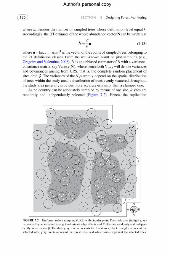
As no country can be adequately sampled by means of one site, R sites are

randomly and independently selected (Figure 7.2). Hence, the replication

S

E

N

W

FIGURE 7.2 Uniform random sampling (URS) with circular plots. The study area (in light gray)

is covered by an enlarged area G to eliminate edge effects and R plots are randomly and indepen-

dently located onto G. The dark gray zone represents the forest area, black triangles represent the

selected sites, gray points represent the forest trees, and white points represent the selected trees.



procedure gives rise to R independent samples, say S1, . . .,SR, which in turn giverise to R estimates, say N1, . . . ,NR, which constitute R independent realizations

of the HT estimator N. Accordingly, on the basis of the very standard results on

independently and identically distributed random vectors (e.g., Mardia et al.,

1979, Section 2.8 and Theorem 2.9.1), the arithmetic mean vector

N¼ 1

R

XRi¼1

Ni (7.14)

provides an estimator for N which is unbiased, consistent, and asymptotically

(R!1) normal with a variance–covariance matrix which is unbiasedly and

consistently estimated by VN¼S/R, where

S¼ 1

R�1

XRi¼1

Ni� N� �

Ni� N� �T

(7.15)

is the empirical variance–covariance matrix of the Nis.

In accordance with these results, an obvious estimator for P is given by

P¼ N=ð1TNÞ. After little algebra, it can be proven that the k-th component

of P can be simply rewritten as Pk ¼ Tk=T, where T denotes the total number

of trees sampled by the R sites and Tk denotes the number of these trees

belonging to the k-th defoliation class. From the most familiar version

of Delta method (see, e.g., Mardia et al., 1979, Theorem 2.9.2), it follows

that P constitutes a consistent and asymptotically normal estimator for Pwith a variance–covariance matrix which is consistently estimated by VP ¼ðI� P1TÞVNðI�1P TÞ where I denotes the identity matrix of appropriate

order. Finally, any C-parameter can be simply estimated by C¼ cTP. Thus,from the Delta method, C constitutes a consistent and asymptotically normal

estimator for C with variance which is consistently estimated by Vc2¼cTVPc.

Accordingly, the estimator of the percentage standard error for C is given by

100ðVC=CÞ%, while the confidence interval with an asymptotical coverage of

about 0.95 is given by C�2VC.

As to the inference on change, denote by Nt the HT estimators of Nt based

on a unique plot randomly selected onto G and then visited at period

t (t¼1,2). From the previous considerations on HT estimators, Nt is unbiased

with a variance–covariance matrix VarURSðNtÞ. Moreover, denote by

CovURSðN1;N2Þ the covariance matrix between the two estimators. As R sites

are randomly and independently thrown onto G, the replication procedure

gives rise to R pairs of estimates ðN1,1;N1,2Þ, . . . ,ðNR,1;NR,2Þ which constituteR independent realizations of the pair ðN1;N2Þ. From the above-mentioned

results on independently and identically distributed random vectors, the arith-

metic mean vector of theNi,ts, say Nt, is an unbiased, consistent, and asymptoti-

cally normal estimators of Nt with a variance–covariance matrix which is

unbiasedly and consistently estimated by VN,t¼St/R, where St is the empirical



variance–covariance matrix of the Ni, ts, while the covariance matrix is unbia-

sedly and consistently estimated by CN¼S1,2/R, where

S1,2 ¼ 1

R�1

XRi¼1

Ni,1� N1

� �Ni,2� N2

� �T

(7.16)

is the empirical covariance matrix of the Ni,1s and Ni,2s. From the Delta

method, Pt ¼ Nt=ð1TNtÞ is a consistent and asymptotically normal estimator

of Pt with a variance–covariance matrix which is consistently estimated by

VP, t ¼ðI� Pt1TÞVN, tðI�1P T

t Þ and covariance matrix which is consistently

estimated by CP ¼ðI� P11TÞCNðI�1P T

2 Þ. From these last results, the differ-

ence P2� P1 turns out to be a consistent and asymptotically normal estimator

of P2�P1, with a variance–covariance matrix which is consistently estimated

by VP,1þVP,2�CP�CPT. Hence, the difference estimator D¼ C2� C1 ¼

cTðP2� P1Þ is a consistent and asymptotically normal estimator of D with

variance which is consistently estimated by VD2 ¼cT(VP,1þVP,2� CP�CP

T)c.Owing to the asymptotic unbiasedness and normality of D as well as the con-

sistency of VD2 , the p-value, the power, and the MDC adopted for inference on

change can be computed via expressions (7.8), (7.9), and (7.11), respectively.

7.5.2 URS Versus Systematic and Stratified Sampling

Gregoire and Valentine (2008) provide an excellent introductory chapter on

the issue of sampling discrete objects (trees in the present case) scattered over

a region by means of plots, focusing on the problem of how to effectively

select these plots. Despite its theoretical simplicity, URS may lead to an

uneven coverage of the study area (Cordy and Thompson, 1995; Stevens,

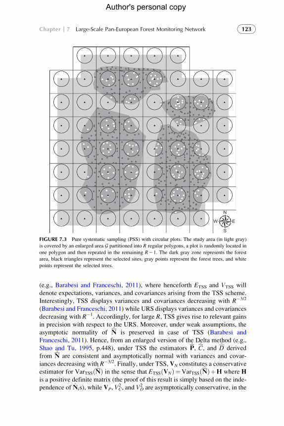
2006). To avoid this shortcoming, systematic schemes can be adopted. How-

ever, PSS based on a regular grid of plots with a random start (commonly

adopted in large-scale forest inventories; Figure 7.3) may be unsuitable in

the presence of some spatial regularity, leading to substantial losses of effi-

ciency with respect to URS. Accordingly, random systematic schemes based

on a regular tessellation of the study area and the random placement of a plot

in each tessellation unit have been theoretically preferred by statisticians. One

such scheme, usually referred by Cordy and Thompson (1995) and Stevens

(1997) to as TSS, involves enlarging the study area by a region G constituted

by R nonoverlapping polygons of equal size and such that each of them con-

tain at least a portion of the study area, and then selecting a plot in each

of these polygons (Figure 7.4). The scheme has a long-standing tradition in

statistical literature (see, e.g., Overton and Stehman, 1993).

If the R sites/plots are thrown onto the same reference region G, TSSinvariably outperforms URS, in the sense that under TSS, N is unbiased

with variance–covariance matrix such that VarURSðNÞ�VarTSSðNÞ

S

E

N

W

FIGURE 7.3 Pure systematic sampling (PSS) with circular plots. The study area (in light gray)

is covered by an enlarged area G partitioned into R regular polygons, a plot is randomly located in

one polygon and then repeated in the remaining R�1. The dark gray zone represents the forest

area, black triangles represent the selected sites, gray points represent the forest trees, and white

points represent the selected trees.



(e.g., Barabesi and Franceschi, 2011), where henceforth ETSS and VTSS will

denote expectations, variances, and covariances arising from the TSS scheme.

Interestingly, TSS displays variances and covariances decreasing with R�3/2

(Barabesi and Franceschi, 2011) while URS displays variances and covariances

decreasing with R�1. Accordingly, for large R, TSS gives rise to relevant gains

in precision with respect to the URS. Moreover, under weak assumptions, the

asymptotic normality of N is preserved in case of TSS (Barabesi and

Franceschi, 2011). Hence, from an enlarged version of the Delta method (e.g.,

Shao and Tu, 1995, p.448), under TSS the estimators P, C, and D derived

from N are consistent and asymptotically normal with variances and covar-

iances decreasing with R�3/2. Finally, under TSS, VN constitutes a conservative

estimator for VarTSSðNÞ in the sense that ETSSðVNÞ¼VarTSSðNÞþH where His a positive definite matrix (the proof of this result is simply based on the inde-

pendence of Nis), while VP, VC2 , and VD

2 are asymptotically conservative, in the

S

E

N

W

FIGURE 7.4 Tessellation stratified sampling (TSS) with circular plots. The study area (in light

gray) is covered by an enlarged area G partitioned into R regular polygons and a plot is randomly

located in each polygon. The dark gray zone represents the forest area, black triangles represent

the selected sites, gray points represent the forest trees, and white points represent the selected

trees.



sense that they are asymptotically equivalent to conservative estimators for

VarTSSðPÞ, VarTSSðCÞ, and VarTSSðDÞ.Even if these theoretical results cannot be proved under PSS (in the pres-

ence of some spatial regularity, PSS may be even worser than URS), however,

apart from anomalous situations which should not occur over large areas, the

performance of PSS are likely to be very similar (sometimes superior) to that

of TSS. Moreover, the use of systematic schemes is suitable in forest studies,

as it can be straightforwardly executed by a random shift of a grid superim-

posed onto a map of the study area (e.g., Gregoire and Valentine, 2008,

p. 119), taking the nodes as sample sites and locating the sites in the terrain

by a modern-day GPS system. Accordingly, under PSS the estimator N as

well as the subsequent estimators P, C, and D are henceforth supposed to

share the theoretical properties arising from TSS.



7.5.3 Sampling Effort: A Preliminary Test

As reported in Section 7.5.1, T denotes the total number of trees sampled by the Rsites selected at the country level and Tk denotes the number of these trees belong-

ing to the k-th defoliation class. These statistics are needed for the estimation of

the relative abundance vector P, which in turn allows for the computation of

any C-parameter estimate.

Descriptive statistics from the ICP Forests large-scale monitoring usually

report the number of sites assessed in each country, the total number of selected

trees, and the total number of selected trees belonging to the 21 defoliation clas-

ses. These statistics might be used as a reference to identify, for each country, the

number of sites needed to obtain an estimate of the parameter of concern, say the

proportion of defoliated trees greater than 25% (F25). Thus, a preliminary test

has been conducted to assess the theoretical number of sampling sites that should

be selected at the country level (Travaglini et al., 2012). To do this, the sampling

effort of the ICP Forests network in terms of number of plots (R) and number of

trees (T) has been compared with the theoretical sampling effort (R0.05, T0.05)required for estimating the proportion of defoliated trees greater than 25%

(F25) with a percentage standard error (e) of 5%. For each country, data related

to R, T, and F25 have been taken from the 2008 survey (Lorenz et al., 2009). The

theoretical sampling effort in term of trees has been computed by

T0:05 ¼ 1� F25

e2F25

(7.17)

and on the basis of the following assumptions: a common definition of forest

is applied across European countries; a simple random sampling with replace-

ment has been supposed to select trees from the population. R0.05 has been

derived dividing T0.05 by the average number of trees per plots (T/R) observedin 2008 surveys. The results are shown in Table 7.3. It is worth noting that, as

these sampling efforts are determined presuming a rough with-replacement

random selection of trees from the population, which should be less accurate

than the systematic grids of plots adopted in most European country, the

reported efforts are highly cautionary and likely provide standard errors smal-

ler than 5%. It is worth noting, however, that the number of plots reported in

Table 7.3 may be not appropriate for small countries and/or low frequency of

defoliated trees, and/or individual species (Kohl et al., 1994).

7.6 AGGREGATING COUNTRY ESTIMATES AT THEEUROPEAN LEVEL

Two statistical strategies are proposed when combining independent country

estimates for the assessment of forest condition at the European level: the first

one is solely based on information acquired from FCM networks (Travaglini

et al., 2012); the second one takes into consideration the potential outcome

from FCM and NFIs.

TABLE 7.3 Sampling Effort of ICP Forests Network in Term of Plots (R) and

Trees (T) Performed in 2008 Surveys Compared with Sampling Effort (R0.05,

T0.05) Required for Estimating the Proportion of Defoliated Trees Greater

than 25% (F25) with a Percentage Standard Error of 5%

Country T R T/R F25 (%) T0.05 R0.05

Andorraa 72 3 24.00 15.3 2215 92

Belarus 9460 400 23.65 8 4600 195

Belgium 2860 121 23.64 14.5 2359 100

Bulgaria 4531 136 33.32 31.9 854 24

Croatia 2039 85 23.99 23.9 1273 53

Cyprusa 360 15 24.00 46.9 452 19

Czech Rep. 5477 136 40.27 56.7 306 8

Denmarka 452 19 23.79 9.1 3996 168

Estoniaa 2196 92 23.87 9 4045 170

Finland 8819 475 18.57 10.2 3522 190

France 10,138 508 19.96 32.4 835 42

Germany 10,347 423 24.46 25.7 1157 43

Irelanda 679 31 21.90 10 3600 165

Italy 6579 236 27.88 32.8 820 30

Latvia 8090 342 23.65 15.3 2215 94

Lithuania 7539 1342 5.62 19.6 1641 292

Rep. Moldova 9841 528 18.64 33.6 791 43

Norway 9495 1720 5.52 22.7 1363 247

Poland 39,320 1916 20.52 18 1823 89

Serbiaa 2789 130 21.45 11.5 3079 144

Slovak Rep. 4083 108 37.81 29.3 966 26

Slovenia 1056 44 24.00 37 742 31

Spain 14,880 620 24.00 15.6 2165 90

Sweden 6890 3464 1.99 17.3 1913 961

Switzerlanda 1008 48 21.00 19 1706 82

Turkey 8978 398 22.56 24.6 1227 55

Ukraine 33,986 1465 23.20 8.2 4479 194

aDenotes countries that would need to increase plot numbers.Modified from Travaglini et al. (2012).





7.6.1 Combining FCM Estimates

Suppose a homogeneous definition of forest among the L countries participat-

ing in the forest monitoring network and denote by N1, . . . ,NL, the estimates

of their abundance vectors achieved by means of separate, independent

surveys performed in each country by means of plot sampling with sites

selected in accordance with PSS. Since each Nl constitutes an unbiased, con-

sistent, and asymptotically normal estimator of Nl with a variance–covariance

matrix which can be conservatively estimated by VN,l¼Sl/Rl, where Sl is theempirical variance–covariance matrix of the Rl estimates for the l-th country

and Rl is the number of sites adopted in the country, then the sum NE ¼ N1þ��þ NL is an unbiased and consistent (R1, . . .,RL!1) estimator of NE with a

variance–covariance matrix which (owing to the independence of the L esti-

mates) is conservatively estimated by

VN,E ¼VN,1

R1

þ�� þVN,L

RL(7.18)

Moreover, if the Rls are supposed to increase with constant ratios Rl/Rh, then

as R1, . . .,RL!1, NE is an asymptotically normal estimator of NE.

The properties of NE (unbiasedness, consistency, and asymptotic normal-

ity) once again allow for the application of the enlarged version of the

Delta method (Shao and Tu, 1995, p. 448). Thus, PE ¼ NE=ð1TNEÞ constitu-tes a consistent and asymptotically normal estimator for PE, while

VP,E ¼ðI� PE1TÞVN,EðI�1P T

E Þ constitutes an asymptotically conservative

estimator of the variance–covariance matrix. Finally, as to C-parameters at

the European level, CE ¼ cTPE constitutes a consistent and asymptotically

normal estimator for CE, while V2C,E¼cTVP,Ec constitutes an asymptotically

conservative estimator for the variance. The estimate of the percentage stan-

dard error for CE is given by 100ðVC,E=CEÞ%, while the confidence interval

with asymptotical coverage of 0.95 is given by CE�2VC,E.

As to the inference on change, denote by Nl, t the plot sampling estimators

of Nl,t (t¼1,2). Hence, Nl, t is unbiased, consistent, and asymptotically normal,

while VN,l,t¼Sl,t/Rl is a conservative estimator of the variance–covariance

matrix of Nl,t and Cl¼Sl,1,2/Rl is the estimator of the covariance matrix of

Nl,1 and Nl,2, where Sl,t is the empirical variance–covariance matrix at period

t and Sl,1,2 is the empirical covariance matrix between periods 1 and 2. Accord-

ingly, from the previous results of this section, NE, t ¼ N1, tþ�� þ NL, t is

an unbiased, consistent, and asymptotically normal estimator ofNE,t with a var-

iance–covariance matrix which can be conservatively estimated by

VN,E, t ¼VN,1, t

R1

þ�� þVN,L, t

RL(7.19)

Moreover, since correlation exists only among estimators achieved in the

same country at different times, the covariance matrix of NE,1 and NE,2 can

be estimated by



CN,E ¼CN,1

R1

þ�� þCN,L

RL(7.20)

From the enlarged version of the Delta method, the relative abundance vector

estimator PE, t ¼ NE, t=ð1TNE, tÞ is a consistent and asymptotically normal

estimators of PE,t. Moreover, VP,E, t ¼ðI� PE, t1TÞVN,E, tðI�1P T

E, tÞ is an

asymptotically conservative estimator of the variance–covariance matrix of

PE, t, while CP,E ¼ðI� PE,11TÞCN,EðI�1P T

E,2Þ is an estimator for the covari-

ance matrix of PE,1 and PE,2. From these last results, the difference

PE,2� PE,1 turns out to be a consistent and asymptotically normal estimator

of PE,2�PE,1, while VP,E,1þVP,E,2�CP,E�CTP,E is an asymptotically conser-

vative estimator of the variance–covariance matrix. Hence, the difference esti-

mator DE ¼ CE,2� CE,1 ¼ cTðPE,2� PE,1Þ is a consistent and asymptotically

normal estimator ofDEwith variance which can be conservatively estimated by

V2D,E ¼ cT VP,E,1þVP,E,2�CP,E�CT

P,E

� �c (7.21)

Once again, owing to the asymptotic unbiasedness and normality of DE, as

well as the conservative nature of VD,E2 , the p-value, the power, and the

MDC adopted for inference on change can be computed via expressions (7.8),

(7.9), and (7.11).

As to the number of sites to be selected within each country, it is worth not-

ing that the accuracy of estimates concerning small countries and regions, infre-

quent tree species, and their combination may be strongly impacted if a unique

density of sampling sites is adopted all over the Europe. This problem has been

investigated in Switzerland by Kohl and Kaufmann (1993) for the estimation of

mean defoliation (or transparency) and by Kohl et al. (1994) for the estimation

of proportions. Kohl et al. (1994, p. 217) conclude that “the results clearly indi-

cate the decreasing reliability of the results as the grid density is decreased from

4�4 to 16�16 km. However, from a practical point of view, the results

obtained from the 4�4 and 8�8-km grid for the whole Switzerland are similar.

However, further reductions result in a sharp increase in variability between

grids, suggesting that neither the 12�12-km nor the 16�16-km grids would

provide reliable data for Switzerland.” Thus, when designing a European net-

work, it is important to be aware that a sampling grid able to provide precise esti-

mates at the European level and for the most frequent tree species may be not

suited for individual countries and/or less frequent tree species.

7.6.2 Coupling FCM and NFI Estimates Across Europe

The aggregation at the European level of the outcome from FCM and NFIs can

provide an alternative estimation of C-parameters at the European level with

respect to the methodology proposed in the previous section which is instead

completely based on the information acquired from FCM. Indeed, the relative

abundance vector at the European level PE¼NE/(1TNE) can be rewritten as



PE ¼XLl¼1

wlPl (7.22)

where wl¼Nl/NE denotes the proportion of forest trees in the l-th country and

NE¼N1þ� � �þNL denotes the total number of forest trees in Europe. Accord-

ingly, while each Pl can be estimated by Pl ¼ Nl=ð1TNlÞ from FCM surveys,

the wl weights can be estimated by using the information arising from NFIs.

As NFIs are usually performed by intensive surveys, the resulting estimators

of the Nls are likely to be more accurate than those arising from FCM surveys.

Thus, if eN1, . . ., eNL denotes the NFI estimates of N1, . . .,NL in such a way that

the wls can be trivially estimated by ewl ¼ eNl= eNE where ~NE ¼ ~N1þ�� þ ~NL,

then PE can be estimated by

ePE ¼XLl¼1

ewlPl (7.23)

In order to derive the statistical properties of ePE, the statistical properties

of each eNl are needed. Usually, forest inventories are multiphase surveys

adopting unbiased (or approximately unbiased) estimators of the interest para-

meters as well as unbiased or conservative estimators of the sampling var-

iances. Accordingly, suppose El(eNl)�Nl with variance Varl(eNl) which can

be unbiasedly or conservatively estimated by eV2

l , where El and Varl denote

expectation and variance with respect to the sampling scheme adopted in

the NFI of the l-th country. Moreover, since the L estimates eN1, . . ., eNL are

obtained by means of separate surveys, they are independent to each other

as well as independent to P1, . . . , PL.

In accordance with these considerations, the weight vector estimatorew¼ ew1; . . . ; ewL½ �T is approximately unbiased with a variance–covariance

matrix which can be approximated up to the first term by VarðewÞ�ðI�w1TÞDðI�1wTÞ where w¼ [w1, . . . ,wL]

T is the vector of true weights

and D¼diag{Var1( ~N1), . . .,VarL( ~NL)} is the diagonal matrix having the var-

iances of the ~Nls as diagonal elements. Thus, an obvious estimator for

VarðewÞ is given by eVw ¼ðI� ew1TÞeDðI�1ewTÞ where ~D¼ diagð ~V2

1; . . . ;~V2

LÞ.Moreover, ePE is approximately unbiased, while generalizing the result of

Goodman (1960) on the variance of products of independent random variables

to the variance–covariance matrix and the covariance matrix of scalar pro-

ducts of random variables with independent random vectors, the variance–

covariance matrix of ePE can be approximated by

Var ePE

� ��XLl¼1

Var ~wlð ÞVarPSS Pl

� �þXLl¼1

Var ~wlð ÞPlPTl

þXLl¼1

w2lVarPSS Pl

� �þ

XLh>l¼1

Cov ~wl; ~whð Þ PlPTh þPhP

Tl

� � (7.24)



where VarPSS denotes variances and covariances with respect to PSS selection

of sites onto the l-th country. Thus, VarðePEÞ can be estimated by

~VP,E ¼XLl¼1

~V2

w, lVP; lþXLl¼1

~V2

w, lPlPT

l þXLl¼1

~w2w, lVP, lþ

XLh>l¼1

~Vw, l,h PlPT

h þ PhPT

l

� �(7.25)

where VP, l ¼ðI� Pl1TÞVN, lðI�1P

T

l Þ and eV2

w, l andeVw, l,h are the l,l and l,h ele-

ments of eVw. Finally, a C-parameter at the European level can be estimated byeCE ¼ cTePE, whereeC constitutes an approximately unbiased estimator for C

with variance which can be estimated by eV2

C,E ¼ cTeVP,Ec. The estimate of the

percentage standard error for eCE is given by 100ð eVC,E=eCEÞ%. Since nothing

ensures that the multiphase estimators arising from NFIs are normally

distributed, nothing ensures the normality ePE as well as the subsequent normal-

ity of eCE. If normality is (as customary) assumed, then the confidence interval

with approximate coverage of 0.95 is given by eCE�2 eVC,E.

As to the inference on change, by obvious notation we can write

PE, t ¼XLl¼1

wl, tPl, t in such a way that ePE, t ¼XLl¼1

ewl,1Pl, t constitutes the estima-

tor of PE,t (t¼1,2). Accordingly, the variance–covariance matrix of ePE, t is

estimated by

~VP,E, t ¼XLl¼1

~V2

w, l, tVP, l, tþXLl¼1

~V2

w, l, tPl, tPT

l, t

þXLl¼1

~w2l, tVP, l, tþ

XLh>l¼1

~Vw, l,h, t Pl, tPT

h, tþ Ph, tPT

l, t

� �(7.26)

where VP, l, t ¼ðI� Pl, t1TÞVN, l, tðI�1P

T

l, tÞ and eV2

w, l, t andeVw, l,h, t are the l,l

and l,h elements of eVw, t ¼ðI� ewt1TÞeDtðI�1ewT

t Þ. Moreover, generalizing

once again the results of Goodman (1960)

Cov ~PE,1;~PE,2

� �¼XLl¼1

Cov ~wl,1Pl,1, ~wl,2Pl,2

� �þ

XLh 6¼l¼1

Cov ~wl,1Pl,1, ~wh,2Ph,2

� �

�XLl¼1

Cov ~wl,1; ~wl,2� �

CovPSS Pl,1; Pl,2

� �þXLl¼1

Cov ~wl,1; ~wl,2� �

Pl,1PTl,2

þXLl¼1

wl,1wl,2CovPSS Pl,1; Pl,2

� �þ

XLh6¼l¼1

Cov ~wl,1; ~wh,2� �

Pl,1Ph,2

(7.27)

where CovPSS denotes covariances with respect to PSS performed in the l-th
country, Covðew1;ew2Þ¼ ðI�w11
TÞGðI�1wT2 Þ is the covariance matrix

between ew1 and ew2 and G¼diag{Cov1( ~N1,1, ~N1,2), . . .,CovL( ~NL,1, ~NL,2)} is

the diagonal matrix having the covariances of the estimators ~Nl,1 and ~Nl,2 as

diagonal elements. If estimates of these covariances, say eCl, are available



from each NFI, then Covðew1;ew2Þ can be estimated by eCw ¼ðI� ew11TÞeGðI�1ewT

2 Þ where eG¼ diagð eC1; . . . ; eCLÞ, in such a way that

~CP,E ¼XLl¼1

~Cw, lCP, lþXLl¼1

~Cw, lPl,1PT

l,2þXLl¼1

~wl,1 ~wl,2CP, l

þXLh6¼l¼1

~Cw, l,hPl,1Ph,2 (7.28)

constitutes an estimate of CovðePE,1;ePE,2Þ, where CP,l is the estimate of

CovPSSðPl,1; Pl,2Þ while eCw, l and eCw, l,h are the l,l and l,h elements of eCw.

From these last results, the difference ePE,2� ePE,1 turns out to be an

approximately unbiased estimator of PE,2�PE,1, with a variance–covariance

matrix which can be estimated by eVP,E,1þ eVP,E,2� eCP,E� eCTP,E. Hence, the

difference estimator eDE ¼ eCE,2� eCE,1 ¼ cTðePE,2� ePE,1Þ is an approximately

unbiased estimator of DE with variance which can be estimated byeV2

DE ¼ cTðeVP,E,1þ eVP,E,2� eCP,E� eCTP,EÞc. If the normality of eDE is presumed,

the p-value, the power, and the MDC adopted for inference on change can be

computed via expressions (7.8), (7.9), and (7.11).

7.7 CONCLUSIONS

The work presented here gives an overview on the current status of forest con-

dition assessments in Europe from a statistical point of view and takes into

account implications of different sampling designs. It presents an approach

to quantify and improve the accuracy of defoliation assessments and aggre-

gated evaluations. The proposal aims to (i) promote plot-based sampling as

a unifying sampling framework for forest condition assessments, (ii) introduce

concrete sampling objectives in terms of status and change detection, and (iii)

improve forest condition assessment at the European scale by using country

estimates. The approach relies on the assumption that a common definition

of forest is applied across all European countries. The proposal adopts a prob-

abilistic sampling scheme based on fixed-area plots selected over the target

region by means of systematic or stratified schemes. Statistical estimators at

the European level are based on two alternative strategies: the combination

of FCM estimates or the aggregation of FCM and NFI estimates

(Figure 7.5). Aggregation of FCM and NFI estimates may improve the results

by taking benefit from the larger numbers of NFI plots as a basis to upscale

the defoliation results from a smaller number of FCM plots with a much

higher temporal frequency of assessment.

Under this framework, some operative guidelines can be provided to adapt

the current structure of ICP Forests monitoring system to the proposed sam-

pling strategy:

l the shift from a fixed number of trees selected on a site to a fixed-area plot

centered at the site forms the basis for the approach presented;

Assumptions

Field survey

Estimation of the parameter of concern and its change at the country level

Field survey

Sampling scheme

Defining accuracy standards

Defining parameters of concern

Objectives

Common definition of forest among L countries

Country LCountry l

, with variance estimate

Combining FCM estimates Coupling FCM and NFI estimatesEstimation of the parameter of concern and its change at the European level


Country 1

Probabilistic sampling based on fixed-area plots with plots randomly located in accordance with PSS or TSS

For status assessment: for example percent error <5%For change assessment: for example, a positive change of 5% is the minimum BSC

For example, defoliation level, ranging from 0 to 100%

(1) Quantitative estimate of the parameter of concern for the target statistical population at specified level of accuracy foreach country and at European level;

(2) Quantitative estimate of change of the parameter of concern at both country and European levels, with statistical assessment of the hypothesis of no change

Change assessment:

Change assessment:

Status assessment:

Status assessment: Status assessment:

and percentage standard error =C VPc

VD2

CPTVP,1 VP,2 CP

=

= =–

=

=–

100(VC/C)–

C2–

C1–

D–

–

–

–cT

cT

cTP


and estimate of percentage standard error = 100(VC,E/ CE)

with variance estimate

CEVP,E cV2

C,E= =– –

cT cT

VP ,E,1 VP,E,2 CP,E CP,E CT

V2D,E = cT

PE

cT c–P2

–P1( (

= =– –CE,2–

CE,1–

DE–

cT –PE,2

–PE,1(

( )+ – –

(

Change assessment:

– , with variance estimate

and estimate of percentage standard error = 100(VC,E/ CE)

with variance estimate

CEVP,E cV2

C,E= =–~ –~ ~ ~

~cT cT

VP,E,1 VP,E,2 CP,E CP,E CT

V2DE = cT

PE

= =– –CE,2–

CE,1–

DE–

cT –PE,2

–PE,1(

( )+ – –

(

( + – – (

V2C

~

~ ~ ~ ~ ~

~~~~~

FIGURE 7.5 Statistical strategies for European-level forest condition assessment based on independent country estimates.




l it is not necessary that plots have the same area across Europe; rather, it is

essential that plots have the same area within individual countries;

l the number of plots should be decided at the country level taking into

account the desired level of accuracy of the estimators, in relation to the

desired level of detection (e.g., extent of proportion of defoliated trees)

and change detection;

l when a minimum number of plots is necessary, reference can be made to

the nominal density currently adopted on Level I plots, that is, one plot

every 256 km2; however, a density of one plot per 256 km2 may be not

appropriate for small countries and/or low frequency of defoliated trees,

and/or individual species, as shown in Table 7.3. In this regard, it is worth

noting that estimation at the country level on the basis of investigations

designed to provide results at the, for example, European level was never

an objective of the ICP Forests, which was by definition oriented towards

an international perspective. In this respect, the occurrence of countries

with theoretically "insufficient sampling" is not necessarily in contradic-

tion with the objective to obtain European-scale results.

Finally, it is worth noting that the proposal considers only the uncertainty

emanated by the sampling scheme; other sources of uncertainty, like those

induced from surveyor-related assessment errors and from nonresponse, when

a site is inaccessible, were not investigated; however, measurement errors

have been and are addressed by a series of Quality Assurance/Quality Control

(QA/QC) activities (e.g., Ferretti et al., 2010b): the data collected during

these QA/QC activities may allow models for measurement errors in order

to increase the variance estimates over the design-based level due to the

sampling procedures.

The application of such a proposal is of high relevance in current monitor-

ing as in the past years changes in sampling design have been made in many

countries, partly joining NFIs and FCM schemes on the national level and

partly maintaining self-standing systems with different sampling designs.

Differences in sampling schemes have been increasing between countries

and call for a separate treatment of national data. The new evaluation

approach presented would have in addition an important by-product: national

information with quantifiable accuracy could be provided in one evaluation

exercise in addition to and as basis for transnational evaluations.

REFERENCES

Barabesi, L., Franceschi, S., 2011. Sampling properties of spatial total estimators under tessella-

tion stratified designs. Environmetrics 22, 271–278.

Cordy, C.B., Thompson, C.M., 1995. An application of deterministic variogram to design-based

variance estimation. Math. Geol. 27, 173–205.

Corona, P., 2010. Integration of forest inventory and mapping to support forest management.

iForest 3, 59–64.



Corona, P., Chirici, G., McRoberts, R.E., et al., 2011. Contribution of large-scale forest inven-

tories to biodiversity assessment and monitoring. Forest Ecol. Manag. 262, 2061–2069.

Cozzi, A., Ferretti, M., Lorenz, M., 2002. Quality Assurance for Crown Condition Assessment in

Europe. UN/ECE, Geneva.

Eichhorn, J., Roskams, P., Ferretti, M., et al., 2010. Visual assessment of crown condition and

damaging agents. Manual part IV. In: Manual on Methods and Criteria for Harmonized Sam-

pling, Assessment, Monitoring and Analysis of the Effects of Air Pollution on Forests.

UNECE ICP Forests Programme Co-ordinating Centre, Hamburg, 49 pp.

Elzinga, C.L., Salzer, D.W., Willoughby, J.W., Gibbs, J.P., 2001. Monitoring Plant and Animal

Populations. Blackwell Science, Inc., Malden, MA.

Fattorini, L., 2001. Design-based and model-based inference in forest inventories. ISAFA, Comu-

nicazioni di Ricerca 2, 13–23.

Ferretti, M., 1997. Forest health assessment and monitoring. Issues for consideration. Environ.

Monit. Assess. 48, 45–72.

Ferretti, M., 2004. Forest health diagnosis, monitoring and evaluation. In: Burley, J., Evans, J.,

Youngquist, J. (Eds.), Encyclopedia of Forest Sciences. Elsevier Science, London,

pp. 285–299.

Ferretti, M., 2010. Harmonizing forest inventories and forest condition monitoring—the rise or the

fall of harmonized forest condition monitoring in Europe? iForest 3, 1–4.

Ferretti, M., Chiarucci, A., 2003. Design concepts adopted in long-term forest monitoring pro-

grams in Europe—problems for the future? Sci. Total Environ. 310 (1–3), 171–178.

Ferretti, M., Fischer, R., Mues, V., et al., 2010a. Basic design principles for the ICP Forests Mon-

itoring Networks. Manual part II. In: Manual on Methods and Criteria for Harmonized Sam-

pling, Assessment, Monitoring and Analysis of the Effects of Air Pollution on Forests.

UNECE ICP Forests Programme Co-ordinating Centre, Hamburg, 22 pp. http://www.icp-for-

ests.org/Manual.htm.

Ferretti, M., Konig, N., Granke, O., 2010b. Quality assurance within the ICP Forests monitoring

programme. Manual part III. In: Manual on Methods and Criteria for Harmonized Sampling,

Assessment,Monitoring andAnalysis of the Effects of Air Pollution on Forests. UNECE ICP For-

ests Programme Co-ordinating Centre, Hamburg, 11 pp. http://www.icpforests.org/Manual.htm.

Fischer, R., Lorenz, M. (Eds.), 2011. Forest condition in Europe, 2011 technical report of ICP

Forests and FutMon. Work report of the Institute for World Forestry 2011/1. ICP Forests,

Hamburg, 212 pp. http://icp-forests.net/page/icp-forests-technical-report.

Goodman, L.A., 1960. On the exact variance of products. J. Am. Stat. Assoc. 55, 708–713.

Gregoire, T.G., 1998. Design-based and model-based inference in survey sampling: appreciating

the difference. Can. J. Forest Res. 28, 1429–1447.

Gregoire, T.G., Valentine, H.T., 2008. Sampling Strategies for Natural Resources and the Envi-

ronment. Chapman & Hall, New York.

Innes, J.L., 1988. Forest health surveys: a critique. Environ. Pollut. 54, 1–15.

Innes, J.L., 1993. Forest Health: Its Assessment and Status. Commonwealth agricultural bureau,

Wallingford, CT.

Innes, J.L., Materna, J., 1992. Development of forest health since the beginning of systematic

surveys. In: Innes, J.L. (Ed.), Cause-Effect Relationships in Forest Decline. UNEP, Geneva,

pp. 24–29.

Innes, J.L., Landmann, G., Mettendorf, B., 1993. Consistency of observation of forest tree defoli-

ation in three European countries. Environ. Monit. Assess. 25, 29–40.

Kleinn, C., Vilcko, F., 2006. Design-unbiased estimation for point-to-tree distance sampling. Can.

J. Forest Res. 36, 1407–1414.

http://www.icp-forests.org/Manual.htm

http://www.icp-forests.org/Manual.htm

http://www.icpforests.org/Manual.htm

http://icp-forests.net/page/icp-forests-technical-report



Kohl, M., Kaufmann, E., 1993. Berechnung der Stichprobenfehler bei Waldschadeninventuren.

Schweiz. Z. Fortswes 144, 297–311.

Kohl, M., Innes, J.L., Kaufmann, E., 1994. Reliability of different densities of sample grids for the

monitoring of forest condition in Europe. Environ. Monit. Assess. 29, 201–221.

Kohl, M., Magnussen, S., Marchetti, M., 2006. Sampling Methods, Remote Sensing and GIS

Multiresource Forest Inventory. Springer Verlag, Berlin-Heidelberg, Germany Tropical

Forestry Series.

Lawrence, M., McRoberts, R.E., Tomppo, E., et al., 2010. Chapter 2. Comparison of national for-

est inventories. In: Tomppo, E., Gschwantner, T., Lawrence, M. et al., (Eds.), National Forest

Inventories. Springer ScienceþBusiness Media B.V.

Lorenz, M., Fischer, R., Becher, G., et al., 2009. Forest condition in Europe, 2009 technical report

of ICP Forests. Work report of the Institute for World Forestry 2009/1. ICP Forests, Ham-

burg, 2009, 169 pp. http://icp-forests.net/page/icp-forests-technical-report.

Mandallaz, D., 2008. Sampling Techniques for Forest Inventories. Chapman & Hall, New York.

Mardia, K.V., Kent, J.T., Bibby, J.M., 1979. Multivariate Analysis. Academic Press Inc., New

York.

Neumann, M., Stowasser, S., 1986. Waldzustandinventur: zur Objektivitat von Kronenklassifizier-

ung. Forstliche Bundesversuchsanstalt Wien. Jahresbericht 1986, 101–108.

Olsen, A.R., Schreuder, H.T., 1997. Perspectives on large-scale natural resource surveys when

cause-effect is a potential issue. Environ. Ecol. Stat. 4, 167–180.

Overton, W.S., Stehman, S.V., 1993. Properties of designs for sampling continuous spatial

resources from a triangular grid. Commun. Stat. Theory. Methods 22, 2641–2660.

Percy, K., Ferretti, M., 2004. Air pollution and forest health: towards new monitoring concepts.

Environ. Pollut. 130, 113–126.

Sarndal, C.E., Swensson, B., Wretman, J., 1992. Model Assisted Survey Sampling. Springer-

Verlag, New York.

Shao, J., Tu, D., 1995. The Jackknife and Bootstrap. Springer-Verlag, New York.

Stevens, D.L., 1997. Variable density grid-based sampling designs for continuous spatial popula-

tions. Environmetrics 8, 167–195.

Stevens, D.L., 2006. Spatial properties of design-based versus model-based approaches to envi-

ronmental samplin. In: Caetano, M., Paino, M. (Eds.), Proceedings of 7th International Sym-

posium on Spatial Accuracy Assessment of Natural Resources and Environmental Sciences

Lisbona119–125.

Travaglini, D., Fattorini, L., Barbati, A., et al., 2012. Towards a sampling strategy for the assess-

ment of forest condition at European level: combining country estimates. Environ. Monit.

Assess. Online FirstTM, August 3, 2012, with kind permission from Springer ScienceþBusi-

ness Media. http://dx.doi.org/10.1007/s10661-012-2788-5

UNECE, 1998. Manual on Methods and Criteria for Harmonizing Sampling, Assessment, Moni-

toring and Analysis of the Effects of Air Pollution on Forests. International Co-operative

Programme on Assessment and Monitoring of Air Pollution Effects on Forests, Hamburg,

Germany.

Urquhart, N.S., Paulsen, S.G., Larsen, P., 1998. Monitoring for policy relevant regional trends

over time. Ecol. Appl. 8, 246–257.

Vidal, C., Lanz, A., Tomppo, E., et al., 2008. Establishing forest inventory reference definitions

for forest and growing stock: a study towards common reporting. Silva Fennica 42, 247–266.

http://icp-forests.net/page/icp-forests-technical-report

http://dx.doi.org/10.1007/s10661-012-2788-5

Documents

Large-scale pan-european forest monitoring network: A statistical perspective for designing and combining country estimates. Example for defoliation