Large Farm Debt in Ukraine

David Sedik

ESA Working Paper No. 03-02

May 2003

www.fao.org/es/esa

Agriculture and Economic Development Analysis Division

The Food and Agriculture Organization of the United Nations

ESA Working paper No. 03-02 www.fao.org/es/esa

Large Farm Debt in Ukraine*

May 2003

David Sedik Regional Office for Europe

Food and Agriculture Organization Italy

e-mail: David.Sedik@fao.org

Abstract The present study analyzes the nature of Ukrainian farm debt by investigating whether the debt servicing problem of Ukrainian farms is more of a debt problem or a net income problem. Net income generation appears to be the more important underlying problem behind the debt problem. Second, the study recounts the main reasons for apparent farm losses in Ukraine. This analysis suggests that low profits are a result of public policies that reduce incentives for profit making, farm production of livestock products at a loss and lack of restructuring. The study concludes that the debt servicing problem of Ukrainian farms leaves them unable to utilize market instruments to secure seasonal financing and is the primary justification for the presence of the Ukrainian government in financing seasonal input supplies. Such financing creates a substantial burden on the state budget, and ultimately on taxpayers. It also leads to sizeable State claims on commodity markets that are similar to a continuation of the state order system for grain that was discontinued after 1997.

Key Words: Ukraine, Agriculture, Farms, Debt JEL: P31, Q14, O13

*From OECD, Agricultural Finance and Credit Infrastructure in Transition Economies: Focus on the South East Europe Region (Paris: OECD, 2001), pp. 105-122. The views expressed in this study are those of the author and do not represent official policies or views of FAO. I thank my co-authors on a previous paper on this topic (Sedik, et al., 2000), as well as Zvi Lerman (World Bank and Hebrew University of Jerusalem), Csaba Csaki (World Bank), Robert Jolly and Sergio Lence (Iowa State University) for their guidance and helpful comments.

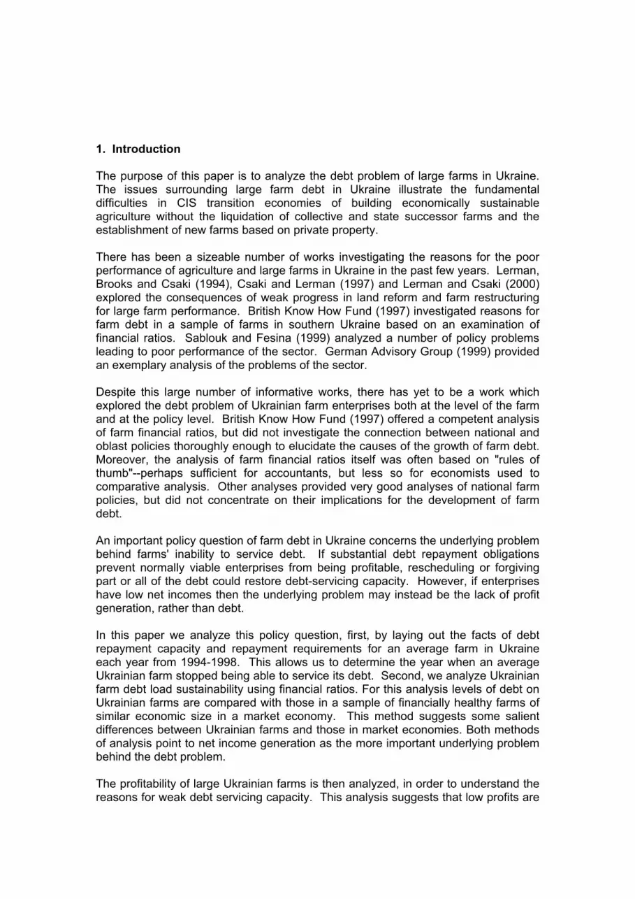
1. Introduction The purpose of this paper is to analyze the debt problem of large farms in Ukraine. The issues surrounding large farm debt in Ukraine illustrate the fundamental difficulties in CIS transition economies of building economically sustainable agriculture without the liquidation of collective and state successor farms and the establishment of new farms based on private property. There has been a sizeable number of works investigating the reasons for the poor performance of agriculture and large farms in Ukraine in the past few years. Lerman, Brooks and Csaki (1994), Csaki and Lerman (1997) and Lerman and Csaki (2000) explored the consequences of weak progress in land reform and farm restructuring for large farm performance. British Know How Fund (1997) investigated reasons for farm debt in a sample of farms in southern Ukraine based on an examination of financial ratios. Sablouk and Fesina (1999) analyzed a number of policy problems leading to poor performance of the sector. German Advisory Group (1999) provided an exemplary analysis of the problems of the sector. Despite this large number of informative works, there has yet to be a work which explored the debt problem of Ukrainian farm enterprises both at the level of the farm and at the policy level. British Know How Fund (1997) offered a competent analysis of farm financial ratios, but did not investigate the connection between national and oblast policies thoroughly enough to elucidate the causes of the growth of farm debt. Moreover, the analysis of farm financial ratios itself was often based on "rules of thumb"--perhaps sufficient for accountants, but less so for economists used to comparative analysis. Other analyses provided very good analyses of national farm policies, but did not concentrate on their implications for the development of farm debt. An important policy question of farm debt in Ukraine concerns the underlying problem behind farms' inability to service debt. If substantial debt repayment obligations prevent normally viable enterprises from being profitable, rescheduling or forgiving part or all of the debt could restore debt-servicing capacity. However, if enterprises have low net incomes then the underlying problem may instead be the lack of profit generation, rather than debt. In this paper we analyze this policy question, first, by laying out the facts of debt repayment capacity and repayment requirements for an average farm in Ukraine each year from 1994-1998. This allows us to determine the year when an average Ukrainian farm stopped being able to service its debt. Second, we analyze Ukrainian farm debt load sustainability using financial ratios. For this analysis levels of debt on Ukrainian farms are compared with those in a sample of financially healthy farms of similar economic size in a market economy. This method suggests some salient differences between Ukrainian farms and those in market economies. Both methods of analysis point to net income generation as the more important underlying problem behind the debt problem. The profitability of large Ukrainian farms is then analyzed, in order to understand the reasons for weak debt servicing capacity. This analysis suggests that low profits are

2

a result of public policies that reduce incentives for profit making, farm production of livestock products at a loss and lack of restructuring. The conclusion of this paper, then, is that the "farm debt problem" is largely a chimera. The more basic underlying problem is the continued unprofitability of large farms. Government schemes to "resolve" the farm debt problem by writing off debt have not significantly helped farms, because they have not been addressed at the underlying more basic problems of farm inviability. 2. Analysis of the Farm Debt Problem in Ukraine An analysis of the "farm debt problem" in Ukraine must begin with a definition of the nature of the problem. Debt financing is commonly used as part of a business strategy for improving financial performance, and the seasonality of farming is often cited as an important reason for use of debt financing as a normal tool of farm financial management. It is not debt per se, but the prevalence of bad debt that has made for a "debt problem" in Ukraine. Figure 1 illustrates that the portion of farm

Source: Ukrainian farm annual financial reports. debt to banks and government either overdue, deferred, restructured, or written off each year from 1990 to 1999 grew from nearly zero to over 80 percent.1 "State loans" are in fact restructured tax debts. In addition to banks and government,

1 Aggregate data used in this study are taken from annual Farm Accounting Statements. These statements include financial balances and income statements of Ukrainian large farms from 1985 to 1998 compiled from enterprise reports by the Ministry of Agriculture and the State Statistical Committee. Farm-level data used in this study are taken from two separate databases combined using enterprise codes from the Common Government Register of Enterprises and Organizations of Ukraine. The first database (12,296 observations) contains financial balances of agricultural enterprises in 1998 (form 1 of farm annual financial statements). The second contains selected indicators from Farm Accounting Forms 2, 6, 7, 9 and 13 for 1994 (11,980 observations), 1995 (12,227 observations), 1996 (12,345 observations) and 1998 (12,628 observations).

F ig u r e 1 . C u m u la t i v e P e r c e n t o f F a r m D e b t ( p lu s w r i t e o f f s ) t o B a n k s a n d G o v e r n m e n t t h a t is O v e r d u e , D e f e r r e d , R e s t r u c t u r e d o r W r i t t e n O f f , 1 9 9 0 - 1 9 9 9

0

1 0

2 0

3 0

4 0

5 0

6 0

7 0

8 0

9 0

1 9 9 0 1 9 9 1 1 9 9 2 1 9 9 3 1 9 9 4 1 9 9 5 1 9 9 6 1 9 9 7 1 9 9 8 1 9 9 9

Y e a r

Perc

ent

O v e r d u e t o B a n k s a n d G o v e r n m e n t

W r i t t e n o f f D e b t

S t a t e L o a n s D e f e r r e d , R e s t r u c t u r e dD e b t

3

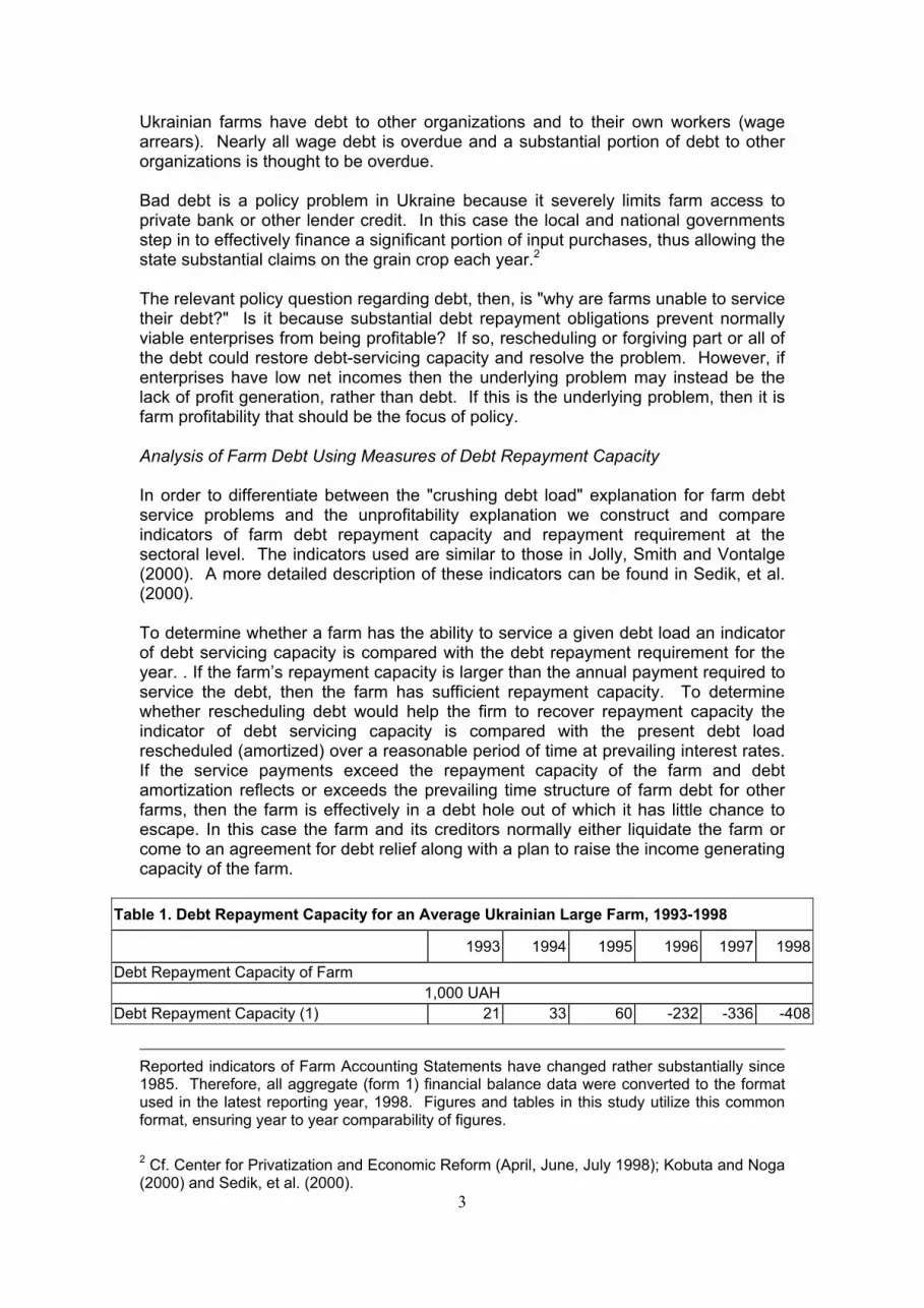
Ukrainian farms have debt to other organizations and to their own workers (wage arrears). Nearly all wage debt is overdue and a substantial portion of debt to other organizations is thought to be overdue. Bad debt is a policy problem in Ukraine because it severely limits farm access to private bank or other lender credit. In this case the local and national governments step in to effectively finance a significant portion of input purchases, thus allowing the state substantial claims on the grain crop each year.2 The relevant policy question regarding debt, then, is "why are farms unable to service their debt?" Is it because substantial debt repayment obligations prevent normally viable enterprises from being profitable? If so, rescheduling or forgiving part or all of the debt could restore debt-servicing capacity and resolve the problem. However, if enterprises have low net incomes then the underlying problem may instead be the lack of profit generation, rather than debt. If this is the underlying problem, then it is farm profitability that should be the focus of policy. Analysis of Farm Debt Using Measures of Debt Repayment Capacity In order to differentiate between the "crushing debt load" explanation for farm debt service problems and the unprofitability explanation we construct and compare indicators of farm debt repayment capacity and repayment requirement at the sectoral level. The indicators used are similar to those in Jolly, Smith and Vontalge (2000). A more detailed description of these indicators can be found in Sedik, et al. (2000). To determine whether a farm has the ability to service a given debt load an indicator of debt servicing capacity is compared with the debt repayment requirement for the year. . If the farm’s repayment capacity is larger than the annual payment required to service the debt, then the farm has sufficient repayment capacity. To determine whether rescheduling debt would help the firm to recover repayment capacity the indicator of debt servicing capacity is compared with the present debt load rescheduled (amortized) over a reasonable period of time at prevailing interest rates. If the service payments exceed the repayment capacity of the farm and debt amortization reflects or exceeds the prevailing time structure of farm debt for other farms, then the farm is effectively in a debt hole out of which it has little chance to escape. In this case the farm and its creditors normally either liquidate the farm or come to an agreement for debt relief along with a plan to raise the income generating capacity of the farm.

Table 1. Debt Repayment Capacity for an Average Ukrainian Large Farm, 1993-1998

1993 1994 1995 1996 1997 1998Debt Repayment Capacity of Farm

1,000 UAH Debt Repayment Capacity (1) 21 33 60 -232 -336 -408

Reported indicators of Farm Accounting Statements have changed rather substantially since 1985. Therefore, all aggregate (form 1) financial balance data were converted to the format used in the latest reporting year, 1998. Figures and tables in this study utilize this common format, ensuring year to year comparability of figures. 2 Cf. Center for Privatization and Economic Reform (April, June, July 1998); Kobuta and Noga (2000) and Sedik, et al. (2000).

4

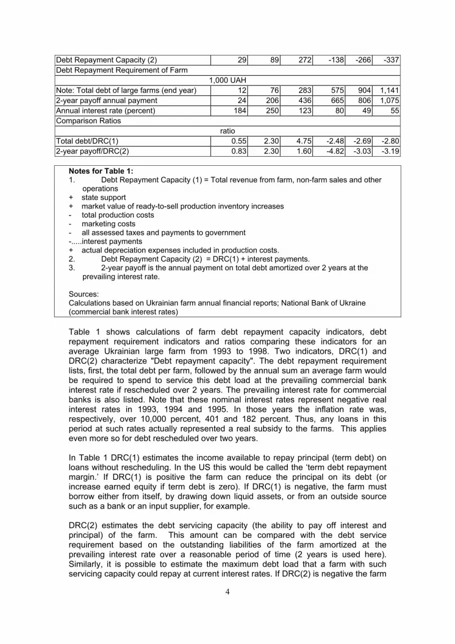
Debt Repayment Capacity (2) 29 89 272 -138 -266 -337Debt Repayment Requirement of Farm

1,000 UAH Note: Total debt of large farms (end year) 12 76 283 575 904 1,1412-year payoff annual payment 24 206 436 665 806 1,075Annual interest rate (percent) 184 250 123 80 49 55Comparison Ratios

ratio Total debt/DRC(1) 0.55 2.30 4.75 -2.48 -2.69 -2.802-year payoff/DRC(2) 0.83 2.30 1.60 -4.82 -3.03 -3.19

Notes for Table 1: 1. Debt Repayment Capacity (1) = Total revenue from farm, non-farm sales and other

operations + state support + market value of ready-to-sell production inventory increases - total production costs - marketing costs - all assessed taxes and payments to government -.....interest payments + actual depreciation expenses included in production costs. 2. Debt Repayment Capacity (2) = DRC(1) + interest payments. 3. 2-year payoff is the annual payment on total debt amortized over 2 years at the

prevailing interest rate. Sources: Calculations based on Ukrainian farm annual financial reports; National Bank of Ukraine (commercial bank interest rates) Table 1 shows calculations of farm debt repayment capacity indicators, debt repayment requirement indicators and ratios comparing these indicators for an average Ukrainian large farm from 1993 to 1998. Two indicators, DRC(1) and DRC(2) characterize "Debt repayment capacity". The debt repayment requirement lists, first, the total debt per farm, followed by the annual sum an average farm would be required to spend to service this debt load at the prevailing commercial bank interest rate if rescheduled over 2 years. The prevailing interest rate for commercial banks is also listed. Note that these nominal interest rates represent negative real interest rates in 1993, 1994 and 1995. In those years the inflation rate was, respectively, over 10,000 percent, 401 and 182 percent. Thus, any loans in this period at such rates actually represented a real subsidy to the farms. This applies even more so for debt rescheduled over two years. In Table 1 DRC(1) estimates the income available to repay principal (term debt) on loans without rescheduling. In the US this would be called the ‘term debt repayment margin.’ If DRC(1) is positive the farm can reduce the principal on its debt (or increase earned equity if term debt is zero). If DRC(1) is negative, the farm must borrow either from itself, by drawing down liquid assets, or from an outside source such as a bank or an input supplier, for example. DRC(2) estimates the debt servicing capacity (the ability to pay off interest and principal) of the farm. This amount can be compared with the debt service requirement based on the outstanding liabilities of the farm amortized at the prevailing interest rate over a reasonable period of time (2 years is used here). Similarly, it is possible to estimate the maximum debt load that a farm with such servicing capacity could repay at current interest rates. If DRC(2) is negative the farm

5

can not service any debt, no matter how small. In this case the problem with the farm is clearly not debt load, but repayment capacity of the farm. If DRC(2) is positive, the firm could pay off existing debt or even add new debt up to a level equal to DRC(2). In considering the comparison ratios of the table we should keep in mind that during the entire period under consideration the overwhelming majority of loans extended to agriuculture were short term, less than one year. Thus, rescheduling loans over 2 years is generous indeed. Consider the comparison ratios and their interpretation. The first ratio (total debt/DRC(1)) indicates the number of years (in terms of our indicator of debt repayment capacity) it would take an average farm to repay the loan principal it had accumulated at the end of the year without rescheduling. The second ratio “two year payoff/DRC(2)” poses the following question: If the accumulated debt of an average farm were rescheduled to be due in two years, financed at the prevailing interest rate, would an average farm be able to make its annual payments? If either of the ratios is less than zero, it makes little sense, since the enterprise can not service any debt. If the ratios range from 0 to 1, the enterprise is able to make its annual loan payments (either with or without rescheduling) within one year. In the case of DRC(1) repayment within a year would accord with the farm's obligations, since over 90 percent of loans in this period were short term, with a payment period of less than one year. In the case of DRC(2), repayment within a year would also accord with the farm's obligations, since the ratio compares the annual payment of the farm required if all obligations were rescheduled over two years. If the ratios are greater than unity, then the enterprise requires more than one year to pay off its annual loan obligations (either with or without rescheduling). In this case, it will find itself in default on those payments. For both scenarios (with and without rescheduling) 1994--the year of currency stabilization--appear to be a turning point. This is the first year when an average farm in Ukraine stopped being able to service its debts. Moreover, realistic debt rescheduling would made no difference. This implies that the underlying problem of Ukrainian farms since 1994 is more likely income generation, rather than debt. In a market economy the kind of comparison ratios between debt service requirements and debt repayment capacity indicators surveyed in the previous section are absent precisely because there are natural institutional limits to the accumulation of farm debt and deterioration of repayment capacity. When a farm in a market economy reaches a point at which it is unable to service its debt payments, it either arranges for debt rescheduling or settles up with its creditors and goes out of business. Because there is no such institutional mechanism for the settlement of debt and the passing of property from poor to better management in Ukraine, debt to repayment capacity ratios in Ukrainian large farms are far higher than what would be considered "normal" in a market economy. Despite the underlying problem of income generation, it is nevertheless true that the negative real interest rates through 1995 acted as an incentive to farms to run up debt. Note that in figure 1 the amount of "bad debt" was actually declining. But all that stoppted in 1996 when real interest rates turned positive. The percent of "bad debt" out of total debt rose sharply. Analysis of Farm Debt Using Financial Ratios

6

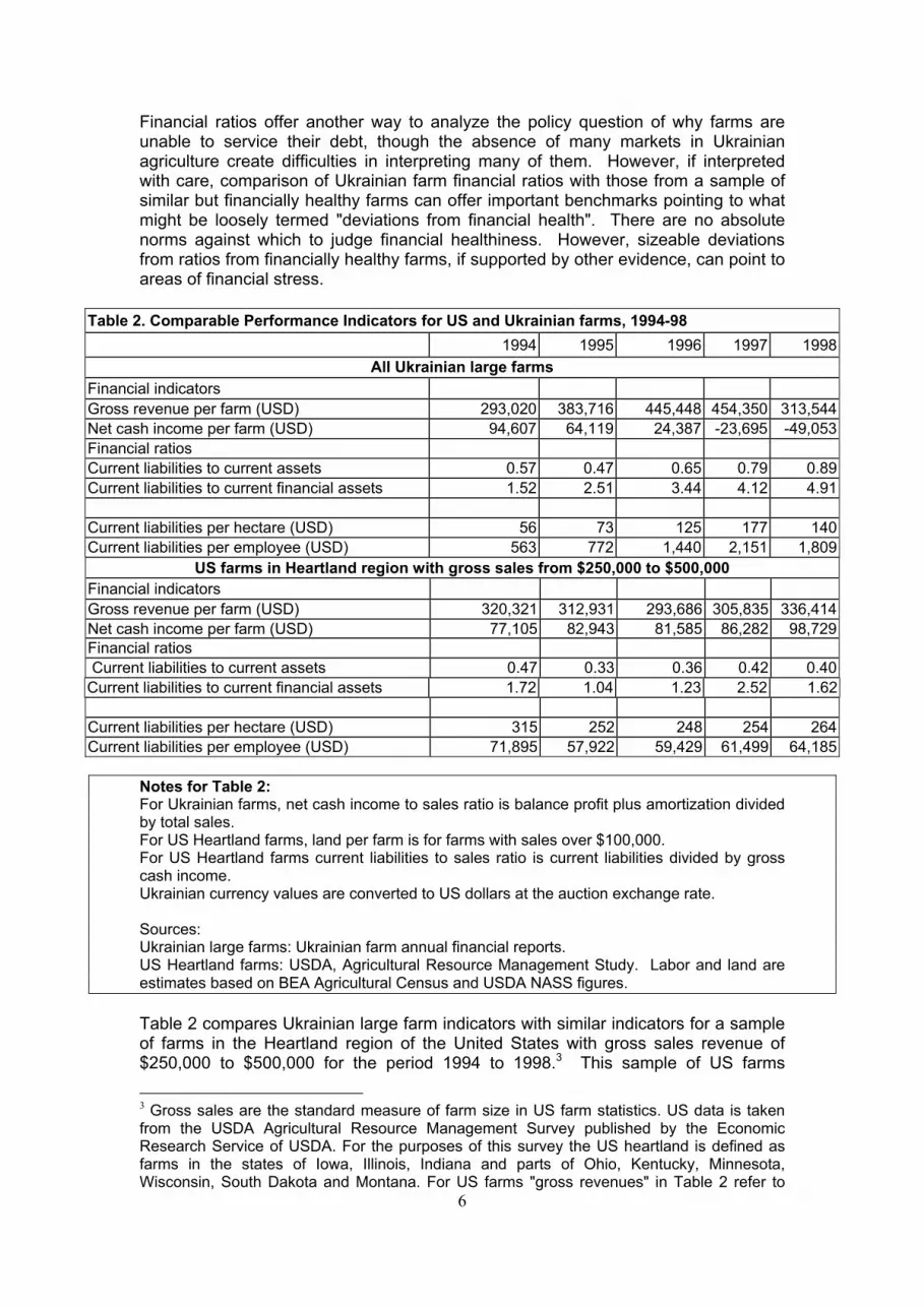
Financial ratios offer another way to analyze the policy question of why farms are unable to service their debt, though the absence of many markets in Ukrainian agriculture create difficulties in interpreting many of them. However, if interpreted with care, comparison of Ukrainian farm financial ratios with those from a sample of similar but financially healthy farms can offer important benchmarks pointing to what might be loosely termed "deviations from financial health". There are no absolute norms against which to judge financial healthiness. However, sizeable deviations from ratios from financially healthy farms, if supported by other evidence, can point to areas of financial stress.

Table 2. Comparable Performance Indicators for US and Ukrainian farms, 1994-98 1994 1995 1996 1997 1998

All Ukrainian large farms Financial indicators Gross revenue per farm (USD) 293,020 383,716 445,448 454,350 313,544Net cash income per farm (USD) 94,607 64,119 24,387 -23,695 -49,053Financial ratios Current liabilities to current assets 0.57 0.47 0.65 0.79 0.89Current liabilities to current financial assets 1.52 2.51 3.44 4.12 4.91 Current liabilities per hectare (USD) 56 73 125 177 140Current liabilities per employee (USD) 563 772 1,440 2,151 1,809

US farms in Heartland region with gross sales from $250,000 to $500,000 Financial indicators Gross revenue per farm (USD) 320,321 312,931 293,686 305,835 336,414Net cash income per farm (USD) 77,105 82,943 81,585 86,282 98,729Financial ratios Current liabilities to current assets 0.47 0.33 0.36 0.42 0.40Current liabilities to current financial assets 1.72 1.04 1.23 2.52 1.62 Current liabilities per hectare (USD) 315 252 248 254 264Current liabilities per employee (USD) 71,895 57,922 59,429 61,499 64,185

Notes for Table 2: For Ukrainian farms, net cash income to sales ratio is balance profit plus amortization divided by total sales. For US Heartland farms, land per farm is for farms with sales over $100,000. For US Heartland farms current liabilities to sales ratio is current liabilities divided by gross cash income. Ukrainian currency values are converted to US dollars at the auction exchange rate. Sources: Ukrainian large farms: Ukrainian farm annual financial reports. US Heartland farms: USDA, Agricultural Resource Management Study. Labor and land are estimates based on BEA Agricultural Census and USDA NASS figures. Table 2 compares Ukrainian large farm indicators with similar indicators for a sample of farms in the Heartland region of the United States with gross sales revenue of $250,000 to $500,000 for the period 1994 to 1998.3 This sample of US farms 3 Gross sales are the standard measure of farm size in US farm statistics. US data is taken from the USDA Agricultural Resource Management Survey published by the Economic Research Service of USDA. For the purposes of this survey the US heartland is defined as farms in the states of Iowa, Illinois, Indiana and parts of Ohio, Kentucky, Minnesota, Wisconsin, South Dakota and Montana. For US farms "gross revenues" in Table 2 refer to

7

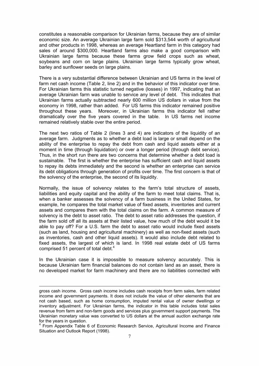
constitutes a reasonable comparison for Ukrainian farms, because they are of similar economic size. An average Ukrainian large farm sold $313,544 worth of agricultural and other products in 1998, whereas an average Heartland farm in this category had sales of around $300,000. Heartland farms also make a good comparison with Ukrainian large farms because these farms grow field crops such as wheat, soybeans and corn on large plains. Ukrainian large farms typically grow wheat, barley and sunflower seeds on large plains. There is a very substantial difference between Ukrainian and US farms in the level of farm net cash income (Table 2, line 2) and in the behavior of this indicator over time. For Ukrainian farms this statistic turned negative (losses) in 1997, indicating that an average Ukrainian farm was unable to service any level of debt. This indicates that Ukrainian farms actually subtracted nearly 600 million US dollars in value from the economy in 1998, rather than added. For US farms this indicator remained positive throughout these years. Moreover, in Ukrainian farms this indicator fell rather dramatically over the five years covered in the table. In US farms net income remained relatively stable over the entire period. The next two ratios of Table 2 (lines 3 and 4) are indicators of the liquidity of an average farm. Judgments as to whether a debt load is large or small depend on the ability of the enterprise to repay the debt from cash and liquid assets either at a moment in time (through liquidation) or over a longer period (through debt service). Thus, in the short run there are two concerns that determine whether a debt load is sustainable. The first is whether the enterprise has sufficient cash and liquid assets to repay its debts immediately and the second is whether an enterprise can service its debt obligations through generation of profits over time. The first concern is that of the solvency of the enterprise, the second of its liquidity. Normally, the issue of solvency relates to the farm’s total structure of assets, liabilities and equity capital and the ability of the farm to meet total claims. That is, when a banker assesses the solvency of a farm business in the United States, for example, he compares the total market value of fixed assets, inventories and current assets and compares them with the total claims on the farm. A common measure of solvency is the debt to asset ratio. The debt to asset ratio addresses the question, if the farm sold off all its assets at their listed value, how much of the debt would it be able to pay off? For a U.S. farm the debt to asset ratio would include fixed assets (such as land, housing and agricultural machinery) as well as non-fixed assets (such as inventories, cash and other liquid assets). It would also include debt related to fixed assets, the largest of which is land. In 1998 real estate debt of US farms comprised 51 percent of total debt.4 In the Ukrainian case it is impossible to measure solvency accurately. This is because Ukrainian farm financial balances do not contain land as an asset, there is no developed market for farm machinery and there are no liabilities connected with

gross cash income. Gross cash income includes cash receipts from farm sales, farm related income and government payments. It does not include the value of other elements that are not cash based, such as home consumption, imputed rental value of owner dwellings or inventory adjustment. For Ukrainian farms, the indicator in this table includes total sales revenue from farm and non-farm goods and services plus government support payments. The Ukrainian monetary value was converted to US dollars at the annual auction exchange rate for the years in question. 4 From Appendix Table 6 of Economic Research Service, Agricultural Income and Finance Situation and Outlook Report (1998).

8

land. The absence of working markets means that the valuations of fixed assets in farm balances are relatively meaningless for this issue. Absent an accurate measure of solvency, we must do with a measure of the liquidity of the farm. For this purpose there are two ratios which offer an indication of the liquidity of the farm. The first is the current debt to current asset ratio (line 3).5 This measures the ability of a farm to cover its short-term liabilities with its current (and presumably somewhat liquid) assets.6 However, the current debt to current asset ratio is only a rough indicator of farm liquidity with many limitations. It should be viewed as such an indicator only under very opportune circumstances for the farm. This is because the accuracy of the current liability to current asset ratio in reflecting the actual ability of farms to cover their current debt with current assets depends vitally on the liquidity of inventories. A typical Ukrainian large farm was unlikely to be able to sell its inventories at their listed price. This is partly because of the absence of developed markets for such assets and partly because book values of inventories reflect costs of production rather than market prices. Since nearly all large farms run losses, costs of production offer an exaggerated value of inventories. A better indication of the ability of Ukrainian farms to cover their debts with current assets is the current liability to current financial asset ratio. Current financial assets in the current liabilities to current financial asset ratio exclude potentially illiquid inventories of Ukrainian farms. Instead, only cash, accounts receivable and other liquid assets are counted. The current liabilities to current financial asset ratio in Table 2 (line 4) shows that the most visible change in the financial state of Ukrainian farms is a steep drop in financial liquidity after 1994. Ukrainian farms are extremely illiquid (i.e., short of "working capital") compared with similar financially healthy farms. Farms with such low levels of liquidity in a market economy would have probably been forced into bankruptcy long ago. The last two financial ratios give an indication of the burden of debt on the factors employed on similarly sized farms in the US and Ukraine. This comparison shows that, compared to US farms of similar economic size, debt levels on Ukrainian farms are quite small. In 1998 US farms carried 35 more times debt per employee and nearly twice as much debt per hectare. This is perhaps one of the most significant comparisons of Table 2. It indicates that debt levels on Ukrainian farms are really quite manageable, if only factors were used more efficiently. Evidence on labor and land per farm in the following section confirms this conclusion. To sell a similar value of products, Ukrainian farms use 8 times more land and 147 times more labor than US farms. With such low value of output per factor, it is not surprising that these farms run losses.

3. Farm Profitability in Ukraine

5 For a more complete examination of the correspondence between the Ukrainian farm balance sheet and the accounting concepts used here see Sedik, et al. (2000), particularly Appendix III. 6 For US Heartland farms current assets exclude real estate assets (such as land and buildings, operator dwelling), as well as farm equipment, breeding animals and investments in cooperatives. For liabilities, Heartland farm current liabilities exclude both real estate and non-real estate long-term liabilities. For Ukrainian farms neither current assets nor current liabilities cover land. In addition, short-term assets exclude buildings, breeding animals and farm machinery. The Ukrainian ratios are therefore quite comparable to the Heartland ratios.

9

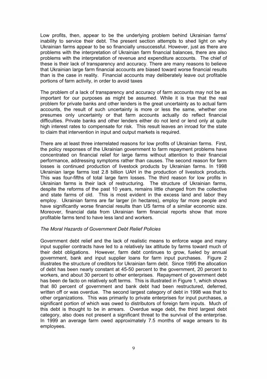
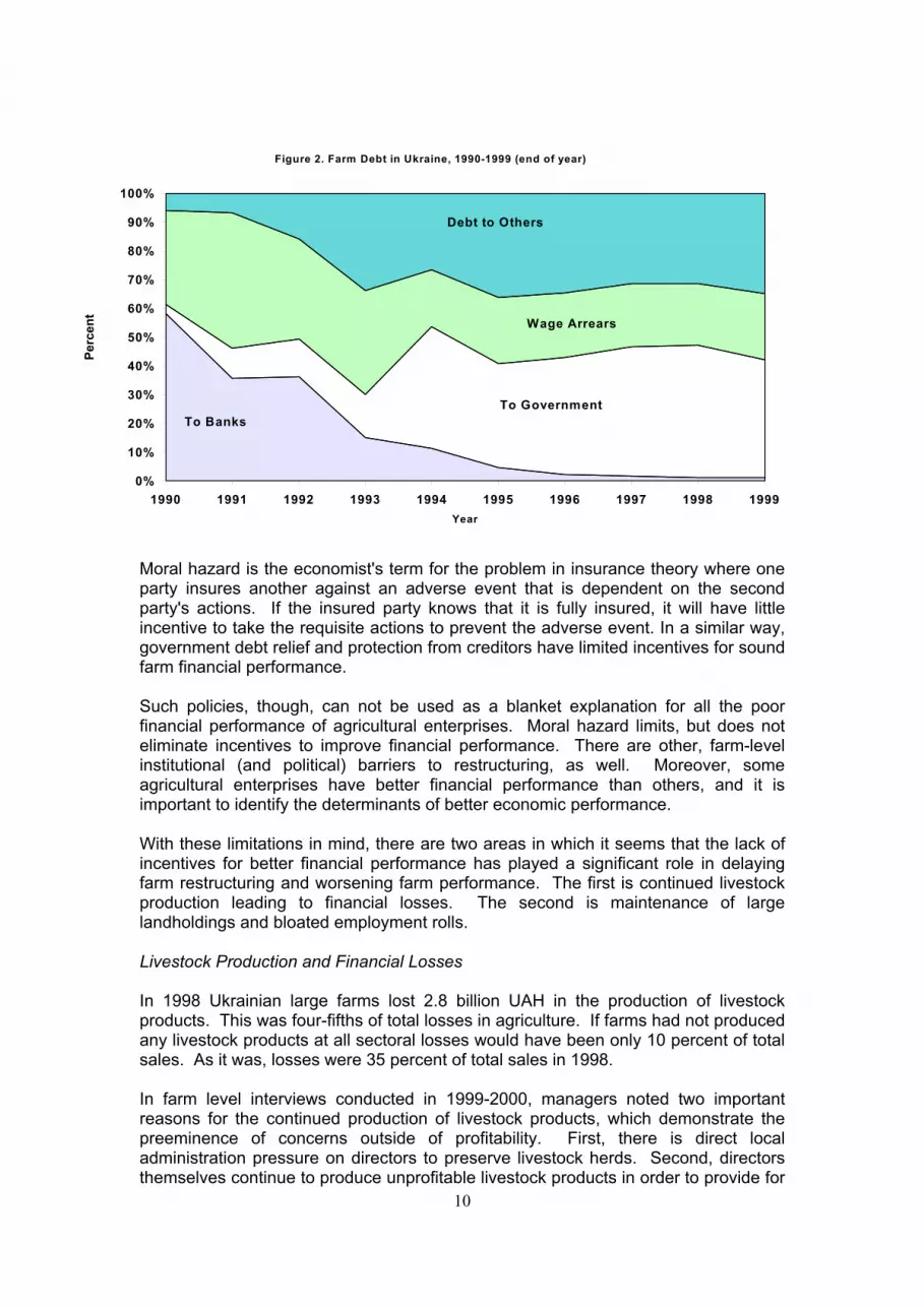
Low profits, then, appear to be the underlying problem behind Ukrainian farms' inability to service their debt. The present section attempts to shed light on why Ukrainian farms appear to be so financially unsuccessful. However, just as there are problems with the interpretation of Ukrainian farm financial balances, there are also problems with the interpretation of revenue and expenditure accounts. The chief of these is their lack of transparency and accuracy. There are many reasons to believe that Ukrainian large farm financial accounts are biased toward worse financial results than is the case in reality. Financial accounts may deliberately leave out profitable portions of farm activity, in order to avoid taxes The problem of a lack of transparency and accuracy of farm accounts may not be as important for our purposes as might be assumed. While it is true that the real problem for private banks and other lenders is the great uncertainty as to actual farm accounts, the result of such uncertainty is more or less the same, whether one presumes only uncertainty or that farm accounts actually do reflect financial difficulties. Private banks and other lenders either do not lend or lend only at quite high interest rates to compensate for risk. This result leaves an inroad for the state to claim that intervention in input and output markets is required. There are at least three interrelated reasons for low profits of Ukrainian farms. First, the policy responses of the Ukrainian government to farm repayment problems have concentrated on financial relief for large farms without attention to their financial performance, addressing symptoms rather than causes. The second reason for farm losses is continued production of livestock products by Ukrainian farms. In 1998 Ukrainian large farms lost 2.8 billion UAH in the production of livestock products. This was four-fifths of total large farm losses. The third reason for low profits in Ukrainian farms is their lack of restructuring. The structure of Ukrainian farms, despite the reforms of the past 10 years, remains little changed from the collective and state farms of old. This is most evident in the excess land and labor they employ. Ukrainian farms are far larger (in hectares), employ far more people and have significantly worse financial results than US farms of a similar economic size. Moreover, financial data from Ukrainian farm financial reports show that more profitable farms tend to have less land and workers. The Moral Hazards of Government Debt Relief Policies Government debt relief and the lack of realistic means to enforce wage and many input supplier contracts have led to a relatively lax attitude by farms toward much of their debt obligations. However, farm debt continues to grow, fueled by annual government, bank and input supplier loans for farm input purchases. Figure 2 illustrates the structure of creditors for Ukrainian farm debt. Since 1995 the allocation of debt has been nearly constant at 45-50 percent to the government, 20 percent to workers, and about 30 percent to other enterprises. Repayment of government debt has been de facto on relatively soft terms. This is illustrated in Figure 1, which shows that 80 percent of government and bank debt had been restructured, deferred, written off or was overdue. The second largest category of debt in 1998 was that to other organizations. This was primarily to private enterprises for input purchases, a significant portion of which was owed to distributors of foreign farm inputs. Much of this debt is thought to be in arrears. Overdue wage debt, the third largest debt category, also does not present a significant threat to the survival of the enterprise. In 1999 an average farm owed approximately 7.5 months of wage arrears to its employees.

10

Moral hazard is the economist's term for the problem in insurance theory where one party insures another against an adverse event that is dependent on the second party's actions. If the insured party knows that it is fully insured, it will have little incentive to take the requisite actions to prevent the adverse event. In a similar way, government debt relief and protection from creditors have limited incentives for sound farm financial performance. Such policies, though, can not be used as a blanket explanation for all the poor financial performance of agricultural enterprises. Moral hazard limits, but does not eliminate incentives to improve financial performance. There are other, farm-level institutional (and political) barriers to restructuring, as well. Moreover, some agricultural enterprises have better financial performance than others, and it is important to identify the determinants of better economic performance. With these limitations in mind, there are two areas in which it seems that the lack of incentives for better financial performance has played a significant role in delaying farm restructuring and worsening farm performance. The first is continued livestock production leading to financial losses. The second is maintenance of large landholdings and bloated employment rolls. Livestock Production and Financial Losses In 1998 Ukrainian large farms lost 2.8 billion UAH in the production of livestock products. This was four-fifths of total losses in agriculture. If farms had not produced any livestock products at all sectoral losses would have been only 10 percent of total sales. As it was, losses were 35 percent of total sales in 1998. In farm level interviews conducted in 1999-2000, managers noted two important reasons for the continued production of livestock products, which demonstrate the preeminence of concerns outside of profitability. First, there is direct local administration pressure on directors to preserve livestock herds. Second, directors themselves continue to produce unprofitable livestock products in order to provide for

Figure 2. Farm Debt in Ukraine, 1990-1999 (end of year)

0%

10%

20%

30%

40%

50%

60%

70%

80%

90%

100%

1990 1991 1992 1993 1994 1995 1996 1997 1998 1999Year

Perc

ent

Debt to Others

Wage Arrears

To GovernmentTo Banks

11

a constant income flow in order to pay in-kind wages or other monthly expenses. In addition, farms preserve livestock herds in order to preserve employment and provide organic fertilizer for crops. Despite official pressure and internal incentives to support livestock herds, farms have reduced their livestock herds rather dramatically in the past 10 years. The question is only one of the pace of reduction. The fact that most directors interviewed cited official pressure to maintain livestock herds as one reason for decreased profits indicates that they themselves might have reduced herds faster, had they sufficient freedom. The problem of a constant flow of income is solved in Western crop raising farms, first, by being profitable, second, by selling stocks throughout the year and, third, by earning income from non-farm sources. About half of farm income in the US is from non-farm sources. In Ukraine, however, the avenues for holding stocks and non-farm income are quite limited. Typically, the Ukrainian large farm must sell all its production in the fall, in order to pay off debt both from the current year and from previous years. Moreover, since Soviet times the business of Ukrainian farms has been farming. Though farms have made some efforts to develop non-farm income sources, there is little incentive for farm managers or farm workers to engage in risky, entrepreneurial activities. The Size and Employment of Farms and Financial Losses Lack of farm restructuring is most evident in the excess land and labor employed by Ukrainian farms. Ukrainian farms are far larger (in hectares), employ far more people and have significantly worse financial results than US farms of a similar economic size. The striking differences in size, employment and net farm income can be seen in Table 3. Table 3. Land, Employment and net cash income per Farm in US and Ukraine, 1994, 1998 Year 1994 1998

Land per Farm (ha) US Heartland 250-500K Farms 311 320 Ukrainian Large Farms 2,571 2,522

Labor per farm US Heartland 250-500K Farms 1.36 1.32 Ukrainian Large Farms 256 195

Net cash income per farm (USD) US Heartland 250-500K Farms 77,105 98,729 Ukrainian Large Farms 94,607 -49,053

Sources: Ukrainian large farms: Ukrainian farm annual financial reports. Heartland farms: USDA, Agricultural Resource Management Study. Labor and land are estimates based on BEA Agricultural Census and USDA NASS figures. The juxtaposition of figures in this table is interesting for two reasons. First, it illustrates that Ukrainian farms have been significantly larger (in terms of hectares and number of employees) than US farms of similar economic size over the entire period from 1994 to 1998. Second, it indicates that, though their size hardly changed between 1994 and 1998, the financial results of Ukrainian farms changed drastically. Large farms seemed to have large profits in 1994, but losses in 1998.

12

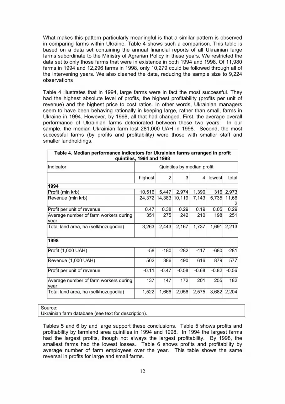
What makes this pattern particularly meaningful is that a similar pattern is observed in comparing farms within Ukraine. Table 4 shows such a comparison. This table is based on a data set containing the annual financial reports of all Ukrainian large farms subordinate to the Ministry of Agrarian Policy in these years. We restricted the data set to only those farms that were in existence in both 1994 and 1998. Of 11,980 farms in 1994 and 12,296 farms in 1998, only 10,279 could be followed through all of the intervening years. We also cleaned the data, reducing the sample size to 9,224 observations Table 4 illustrates that in 1994, large farms were in fact the most successful. They had the highest absolute level of profits, the highest profitability (profits per unit of revenue) and the highest price to cost ratios. In other words, Ukrainian managers seem to have been behaving rationally in keeping large, rather than small, farms in Ukraine in 1994. However, by 1998, all that had changed. First, the average overall performance of Ukrainian farms deteriorated between these two years. In our sample, the median Ukrainian farm lost 281,000 UAH in 1998. Second, the most successful farms (by profits and profitability) were those with smaller staff and smaller landholdings.

Table 4. Median performance indicators for Ukrainian farms arranged in profit quintiles, 1994 and 1998

Indicator Quintiles by median profit

highest 2 3 4 lowest total

1994 Profit (mln krb) 10,516 5,447 2,974 1,390 316 2,973Revenue (mln krb) 24,372 14,383 10,119 7,143 5,735 11,66

2Profit per unit of revenue 0.47 0.38 0.29 0.19 0.05 0.29Average number of farm workers during year

351 275 242 210 198 251

Total land area, ha (selkhozugodiia) 3,263 2,443 2,167 1,737 1,691 2,213

1998

Profit (1,000 UAH) -58 -180 -282 -417 -680 -281

Revenue (1,000 UAH) 502 386 490 616 879 577

Profit per unit of revenue -0.11 -0.47 -0.58 -0.68 -0.82 -0.56

Average number of farm workers during year

137 147 172 201 255 182

Total land area, ha (selkhozugodiia) 1,522 1,666 2,056 2,575 3,682 2,204

Source: Ukrainian farm database (see text for description). Tables 5 and 6 by and large support these conclusions. Table 5 shows profits and profitability by farmland area quintiles in 1994 and 1998. In 1994 the largest farms had the largest profits, though not always the largest profitability. By 1998, the smallest farms had the lowest losses. Table 6 shows profits and profitability by average number of farm employees over the year. This table shows the same reversal in profits for large and small farms.

13

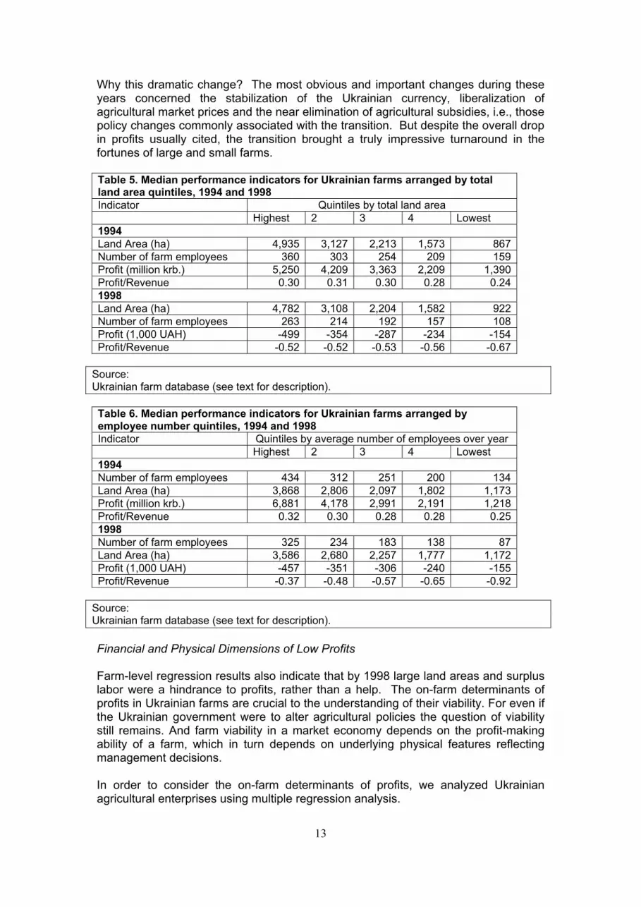
Why this dramatic change? The most obvious and important changes during these years concerned the stabilization of the Ukrainian currency, liberalization of agricultural market prices and the near elimination of agricultural subsidies, i.e., those policy changes commonly associated with the transition. But despite the overall drop in profits usually cited, the transition brought a truly impressive turnaround in the fortunes of large and small farms. Table 5. Median performance indicators for Ukrainian farms arranged by total land area quintiles, 1994 and 1998 Indicator Quintiles by total land area Highest 2 3 4 Lowest 1994 Land Area (ha) 4,935 3,127 2,213 1,573 867 Number of farm employees 360 303 254 209 159 Profit (million krb.) 5,250 4,209 3,363 2,209 1,390 Profit/Revenue 0.30 0.31 0.30 0.28 0.24 1998 Land Area (ha) 4,782 3,108 2,204 1,582 922 Number of farm employees 263 214 192 157 108 Profit (1,000 UAH) -499 -354 -287 -234 -154 Profit/Revenue -0.52 -0.52 -0.53 -0.56 -0.67

Source: Ukrainian farm database (see text for description). Table 6. Median performance indicators for Ukrainian farms arranged by employee number quintiles, 1994 and 1998 Indicator Quintiles by average number of employees over year Highest 2 3 4 Lowest 1994 Number of farm employees 434 312 251 200 134 Land Area (ha) 3,868 2,806 2,097 1,802 1,173 Profit (million krb.) 6,881 4,178 2,991 2,191 1,218 Profit/Revenue 0.32 0.30 0.28 0.28 0.25 1998 Number of farm employees 325 234 183 138 87 Land Area (ha) 3,586 2,680 2,257 1,777 1,172 Profit (1,000 UAH) -457 -351 -306 -240 -155 Profit/Revenue -0.37 -0.48 -0.57 -0.65 -0.92

Source: Ukrainian farm database (see text for description). Financial and Physical Dimensions of Low Profits Farm-level regression results also indicate that by 1998 large land areas and surplus labor were a hindrance to profits, rather than a help. The on-farm determinants of profits in Ukrainian farms are crucial to the understanding of their viability. For even if the Ukrainian government were to alter agricultural policies the question of viability still remains. And farm viability in a market economy depends on the profit-making ability of a farm, which in turn depends on underlying physical features reflecting management decisions. In order to consider the on-farm determinants of profits, we analyzed Ukrainian agricultural enterprises using multiple regression analysis.

14

By definition, profits are equal to: П = Total Revenue – Total Costs (1) = p*y – c(y;F) = r(A; x1,x2...xn;p) – c(Z,x1,x2,…xn;F;w) where p is a vector of output prices, y a vector of outputs, c(y) is a cost function, F is fixed costs, r is a revenue function x1,x2,…xn are factors of production, w is a vector of input prices, A is a variable denoting the technical efficiency of production, and Z is a variable, denoting the skill of the manager in controlling costs per unit of production. In constructing a model of profit, then, we must choose explanatory variables (Z, A, x1,x2,…xn) which are within the managerial choice set and which accurately predict the level of profits of the enterprise. The following variables corresponding to these criteria are in or can be constructed from our data set: Factors of production in quantitative terms: Labor Land Capital stock (animals) Indicators of managerial skill Cost control: deviance from the mean value for sample cost of production for crop and livestock products Technical efficiency of production: Production to asset ratio. The last two variables, cost control and technical efficiency, require explanation. The normal neo-classical profit maximization model presupposes that managers maximize profits (or minimize costs). This specification is probably appropriate for owner-managed private farms. However, our field studies showed that managers of Ukrainian agricultural enterprises are motivated by other factors as well, such as implementing government agricultural policies, which are often at odds with profit maximization. Thus, our specification does not assume that managers are primarily profit-seekers. Instead, we posit that both organizational skill and cost control are choice variables. The general nature of variables Z and A are difficult to capture quantitatively. Therefore, the variables chosen to reflect managerial choice should be viewed as imperfect proxy variables reflecting the underlying orientation of the manager. The cost control variable computes the deviation from average cost of production (captured in Ukrainian cost of production calculations). We constructed a scaled indicator of deviation from average cost by using Z variables defined in the following way: Cost of production deviation Z = (c – c)/ (std. deviation of c), (2) where c is the cost of production of the product,

15

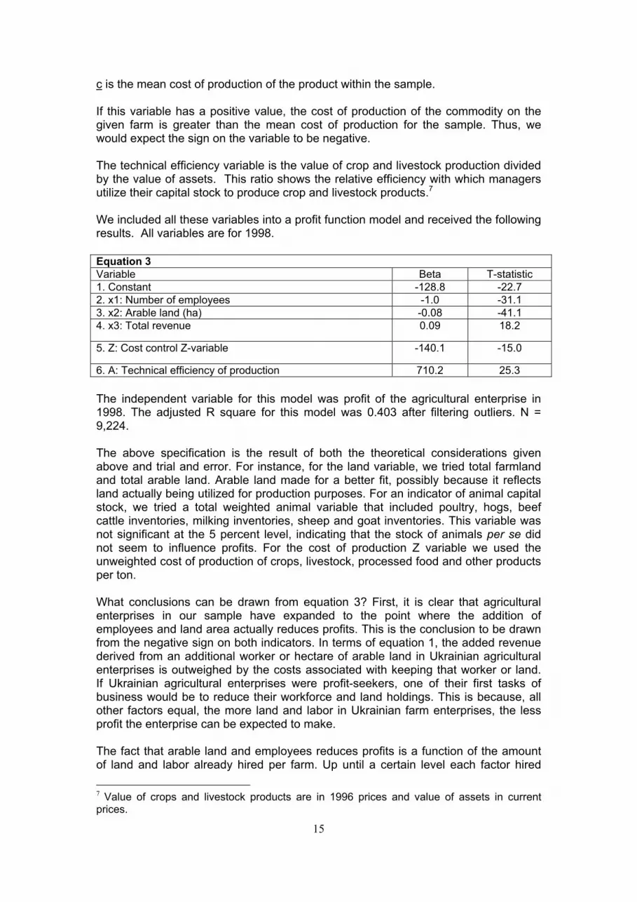
c is the mean cost of production of the product within the sample. If this variable has a positive value, the cost of production of the commodity on the given farm is greater than the mean cost of production for the sample. Thus, we would expect the sign on the variable to be negative. The technical efficiency variable is the value of crop and livestock production divided by the value of assets. This ratio shows the relative efficiency with which managers utilize their capital stock to produce crop and livestock products.7 We included all these variables into a profit function model and received the following results. All variables are for 1998. Equation 3 Variable Beta T-statistic 1. Constant -128.8 -22.7 2. x1: Number of employees -1.0 -31.1 3. x2: Arable land (ha) -0.08 -41.1 4. x3: Total revenue 0.09 18.2

5. Z: Cost control Z-variable -140.1 -15.0

6. A: Technical efficiency of production 710.2 25.3 The independent variable for this model was profit of the agricultural enterprise in 1998. The adjusted R square for this model was 0.403 after filtering outliers. N = 9,224. The above specification is the result of both the theoretical considerations given above and trial and error. For instance, for the land variable, we tried total farmland and total arable land. Arable land made for a better fit, possibly because it reflects land actually being utilized for production purposes. For an indicator of animal capital stock, we tried a total weighted animal variable that included poultry, hogs, beef cattle inventories, milking inventories, sheep and goat inventories. This variable was not significant at the 5 percent level, indicating that the stock of animals per se did not seem to influence profits. For the cost of production Z variable we used the unweighted cost of production of crops, livestock, processed food and other products per ton. What conclusions can be drawn from equation 3? First, it is clear that agricultural enterprises in our sample have expanded to the point where the addition of employees and land area actually reduces profits. This is the conclusion to be drawn from the negative sign on both indicators. In terms of equation 1, the added revenue derived from an additional worker or hectare of arable land in Ukrainian agricultural enterprises is outweighed by the costs associated with keeping that worker or land. If Ukrainian agricultural enterprises were profit-seekers, one of their first tasks of business would be to reduce their workforce and land holdings. This is because, all other factors equal, the more land and labor in Ukrainian farm enterprises, the less profit the enterprise can be expected to make. The fact that arable land and employees reduces profits is a function of the amount of land and labor already hired per farm. Up until a certain level each factor hired 7 Value of crops and livestock products are in 1996 prices and value of assets in current prices.

16

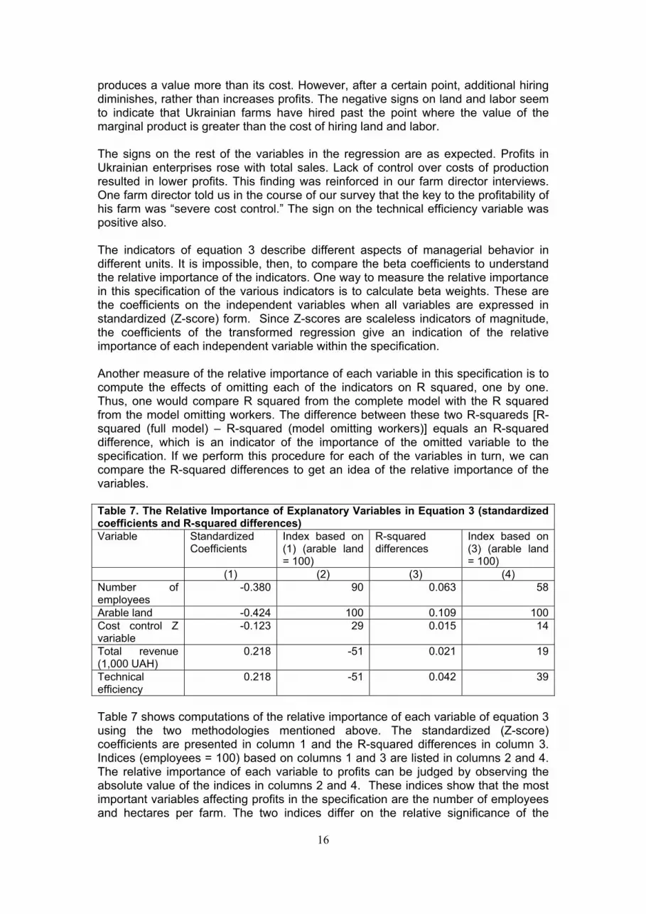
produces a value more than its cost. However, after a certain point, additional hiring diminishes, rather than increases profits. The negative signs on land and labor seem to indicate that Ukrainian farms have hired past the point where the value of the marginal product is greater than the cost of hiring land and labor. The signs on the rest of the variables in the regression are as expected. Profits in Ukrainian enterprises rose with total sales. Lack of control over costs of production resulted in lower profits. This finding was reinforced in our farm director interviews. One farm director told us in the course of our survey that the key to the profitability of his farm was “severe cost control.” The sign on the technical efficiency variable was positive also. The indicators of equation 3 describe different aspects of managerial behavior in different units. It is impossible, then, to compare the beta coefficients to understand the relative importance of the indicators. One way to measure the relative importance in this specification of the various indicators is to calculate beta weights. These are the coefficients on the independent variables when all variables are expressed in standardized (Z-score) form. Since Z-scores are scaleless indicators of magnitude, the coefficients of the transformed regression give an indication of the relative importance of each independent variable within the specification. Another measure of the relative importance of each variable in this specification is to compute the effects of omitting each of the indicators on R squared, one by one. Thus, one would compare R squared from the complete model with the R squared from the model omitting workers. The difference between these two R-squareds [R-squared (full model) – R-squared (model omitting workers)] equals an R-squared difference, which is an indicator of the importance of the omitted variable to the specification. If we perform this procedure for each of the variables in turn, we can compare the R-squared differences to get an idea of the relative importance of the variables. Table 7. The Relative Importance of Explanatory Variables in Equation 3 (standardized coefficients and R-squared differences) Variable Standardized

Coefficients Index based on (1) (arable land = 100)

R-squared differences

Index based on (3) (arable land = 100)

(1) (2) (3) (4) Number of employees

-0.380 90 0.063 58

Arable land -0.424 100 0.109 100Cost control Z variable

-0.123 29 0.015 14

Total revenue (1,000 UAH)

0.218 -51 0.021 19

Technical efficiency

0.218 -51 0.042 39

Table 7 shows computations of the relative importance of each variable of equation 3 using the two methodologies mentioned above. The standardized (Z-score) coefficients are presented in column 1 and the R-squared differences in column 3. Indices (employees = 100) based on columns 1 and 3 are listed in columns 2 and 4. The relative importance of each variable to profits can be judged by observing the absolute value of the indices in columns 2 and 4. These indices show that the most important variables affecting profits in the specification are the number of employees and hectares per farm. The two indices differ on the relative significance of the

17

physical size of the farm, farm revenues and technical efficiency. However, within this specification it is quite clear that the number of employees and physical size are the most important, while cost control, revenues and technical efficiency are less important. This table gives a clear idea of the comparative importance of reductions in employees and land area to the profitability of Ukrainian farming enterprises based on actual data from 1998. 4. Conclusions The main conclusion of this paper is that the "farm debt problem" is largely a chimera in the following sense: The underlying problem of Ukrainian farms appears to be not debt but lack of profits. Table 1 illustrates that by 1994 an average Ukrainian large farm was not capable of servicing its debts, even if they were rescheduled on generous terms (over two years). By 1996 an average Ukrainian large farm was not able to service any debt. The comparative analysis of financial ratios in Table 2 for large Ukrainian farms and similarly sized US farms indicates that Ukrainian debt loads (on average) would be quite manageable for normally profitable farms with an efficiency considerably less than in the US. The main reasons for low profits of Ukrainian large farms appear to be public policies that diminish incentives for good financial performance, continued production of livestock products by farms and considerably more labor and land employed in Ukrainian farms than in comparable market oriented farms. The apparent inability of Ukrainian farms to service debt and their resulting inability to utilize market instruments to secure seasonal financing is the primary justification for the presence of the Ukrainian government in financing seasonal input supplies. Such financing creates a substantial burden on the state budget, and ultimately on taxpayers. A suggestion of the cost of input financing for the Ukrainian government can be seen in calculations concluded for spring sowing 2000 (Kobuta, Noga, 2000). For spring sowing 2000, the value of inputs (mineral fertilizers and oil products) supplied to farms in accordance with government resolutions was 296 million UAH (53.6 million US dollars). However, the cost to the Ukrainian budget in order to interest banks, distributors, processors and others in working with agricultural enterprises was much larger, 922 million UAH (167 million US dollars). These economic incentives included central bank subsidies to the sectoral bank responsible for agriculture, interest rate subsidies, local budget funds, government losses from oil import tariff discounts, milk and meat subsidies for input purchases, VAT discounts to farms for input purchases and discounted sales of oil by government enterprises to distributors. The government role in agricultural input markets in Ukraine and accumulated farm debt related to government loans and taxes give the Ukrainian government a substantial claim on agricultural commodities (particularly grain, since it has become the primary numeraire) produced in Ukraine. For the past three years these claims have been far greater than farms have met.8 It is not the ex post amount of grain the state has collected, but the effects of the claims on grain markets that is most important. State claims on commodity markets are similar to a continuation of the state order system for grain that was discontinued after 1997. Oblast governments have utilized the traffic police, the secret police and other state instruments to ensure priority of payment before private companies. Such efforts effectively make sales to private purchasers illegal before the state satisfies its claims on the market.

8 See Center for Privatization and Economic Reform (May, June and July, 1998).

18

Bibliography Center for Privatization and Economic Reform (CPER). How Much Grain has the Ukrainian Government Promised? issue 1 (Kyiv, April 1998). Center for Privatization and Economic Reform (CPER). How Much Grain has the Ukrainian Government Claimed? issue 2 (Kyiv, June 1998). Center for Privatization and Economic Reform (CPER). How Much Grain has the Ukrainian Government Claimed? issue 3 (Kyiv, July 1998). Economic Research Service, United States Department of Agriculture. Agricultural Income and Finance Situation and Outlook Report, AIS-70 (Washington, 1998). Jolly, R., D. Smith and A. Vontalge. 2000. "Assessing the Financial Condition of Iowa's Commercial Farm Businesses, 1999-2001" FM-1868. Iowa State University Extension, Iowa State University, Ames, Iowa. Kobuta, I. and Noga, V. "Rol' gosudarstva v obespechenii sel'skogo khoziaistva material'no-tekhnicheskimi resursami" Iowa State University Ukraine Agricultural Policy Project Discussion Paper no. 8 (Kyiv, 2000). Sedik, D., N. Seperovich, N. Pugachev, I. Chapko, I. Kobuta, V. Noga and V. Zhygadlo. 2000. Farm Debt in the CIS: A Multi Country Study of Major Causes and Proposed Solutions: Ukraine Country Study, The World Bank, ECSSD Environmentally and Socially Sustainable Development Working Paper no. 28, September 26, 2000. United States Department of Agriculture. National Agricultural Statistics Service. Farms and Land in Farms (July 30, 1996; February 12, 1998; February 26, 1999). United States Department of Agriculture. National Agricultural Statistics Service. Farms and Land in Farms: Final Estimates 1993-97, Statistical Bulletin Number 955 (October 1999).

19

ESA Working Papers WORKING PAPERS The ESA Papers are produced by the Agriculture and Economic Development Analysis Division (ESA) of the Economic and Social Department of the United Nations Food and Agriculture Organization (FAO). The series presents ESA’s ongoing research. Working papers are circulated to stimulate discussion and comments. They are made available to the public through the Division’s website. The analysis and conclusions are those of the authors and do not indicate concurrence by FAO. ESA The Agriculture and Economic Development Analysis Division (ESA) is FAO’s focal point for economic research and policy analysis on issues relating to world food security and sustainable development. ESA contributes to the generation of knowledge and evolution of scientific thought on hunger and poverty alleviation through its economic studies publications which include this working paper series as well as periodic and occasional publications.

Agriculture and Economic Development Analysis Division (ESA) The Food and Agriculture Organization

Viale delle Terme di Caracalla 00100 Rome

Italy

Contact: Office of the Director

Telephone: +39 06 57054368 Facsimile: + 39 06 57055522 Website: www.fao.org/es/esa

e-mail: ESA@fao.org