International Debt Shifting: Do Multinationals Shift Internal or External Debt?

Jarle Møen Dirk Schindler

Guttorm Schjelderup Julia Tropina

CESIFO WORKING PAPER NO. 3519 CATEGORY 1: PUBLIC FINANCE

JULY 2011

An electronic version of the paper may be downloaded • from the SSRN website: www.SSRN.com • from the RePEc website: www.RePEc.org

• from the CESifo website: Twww.CESifo-group.org/wp T

CESifo Working Paper No. 3519

International Debt Shifting: Do Multinationals Shift Internal or External Debt?

Abstract Multinational companies can exploit the tax advantage of debt more aggressively than national companies by shifting debt from affiliates in low tax countries to affiliates in high tax countries. Previous papers have either omitted internal debt or external debt from the analysis. We are the first to model the companies’ choice between internal and external debt shifting and show that it is optimal for them to use both types of debt to save taxes. Using a large panel of German multinationals, we find strong empirical support for our model. The estimated coefficients suggest that internal and external debt shifting are of about equal relevance. Since the tax variables that determine the incentive to shift internal and external debt are correlated both with each other and with the host country tax rate, previous estimates of the tax sensitivity of debt suffer from omitted variable bias.

JEL-Code: H250, G320, F230.

Keywords: corporate taxation, multinationals, capital structure, international debt-shifting, tax avoidance.

Jarle Møen Department of Finance and Management

Science Norwegian School of Economics

Bergen / Norway jarle.moen@nhh.no

Dirk Schindler Department of Economics

University of Konstanz Konstanz / Germany

dirk.schindler@uni-konstanz

Guttorm Schjelderup Department of Finance and Management

Science Norwegian School of Economics

Helleveien 30 Norway – 5045 Bergen

guttorm.schjelderup@nhh.no

Julia Tropina Department of Economics

Norwegian School of Economics Bergen / Norway

julia.tropina@nhh.no

June 30, 2011 We are grateful to Carsten Bienz, Roger Gordon, Heinz Herrmann, Erling Røed Larsen, Tore Leite, Martin Ruf, Georg Wamser, and Alfons Weichenrieder for very helpful suggestions. Special thanks go to the people at Deutsche Bundesbank, in particular to Alexander Lipponer, for their invaluable support and for the hospitality of their research center.

1 Introduction

Globalization has made tax planning strategies of multinational companies a topic of great

importance for practitioners and policy makers alike.1 High corporate taxes make it prof-

itable to finance investments by debt since interest paid is deductible from corporate profits.

Both national and multinational companies benefit from this tax induced advantage of debt.

Multinational companies, however, can shift debt from affiliates in low-tax countries to af-

filiates in high-tax countries so that the tax savings arising from the deductions in high-tax

countries exceed the corresponding tax payments in low-tax countries.

Several recent papers find that such international debt shifting is an important aspect of

multinational firms’ capital structure. They disagree, however, on the mechanism. Huizinga

et al. (2008) model the optimal allocation of external debt and find that ignoring inter-

national debt shifting understates the impact of national taxes on debt policies by about

25 %. Egger et al. (2010) model debt shifting by the use of internal debt and find that

multinationals have a significantly higher debt-to-asset ratio than national firms, and that

this difference is larger in high-tax countries.2 Both Huizinga et al. (2008) and Egger et al.

(2010) use total debt, i.e., the sum of internal and external debt, in their empirical analyses.

Because of this, the papers do not provide unambiguous empirical evidence in favor of their

respective theory models.

To settle this ambiguity, we model the joint allocation of internal and external debt in

a multinational company, and show that the optimal debt shifting strategy is always to use

both types of debt. Our model also predicts that studies of the tax sensitivity of debt that

omit either internal or external debt shifting will suffer from omitted variable bias. Using a

large panel of German multinationals where total debt can be split between its internal and

external components, we find strong support for our model and prediction. The economic

importance of the estimated coefficients can be illustrated by looking at a hypothetical case

where a multinational group consists of two affiliates of equal size. If the affiliate located

in the country with the highest tax rate experiences a 10 percentage points tax increase,

the debt-to-asset ratio will fall by 1.4 percentage points in the low-tax country and increase

by 4.6 percentage points in the high-tax country. For a company with an average debt-to-

1See Mintz and Weichenrieder (2010) for a recent account.2Internal debt is also a topic in, e.g., Desai et al. (2004), Buttner et al. (2009), and Barion et al. (2010).

2

asset ratio at the outset, a 4.6 percentage points increase in the debt-to-asset ratio implies

a 7.4 % increase in debt. About 40 percent of the increase in debt is due to the tax induced

advantage of debt that both national and multinational firms benefit from, while about 60

percent is due to international debt shifting. In the case of international debt shifting we

find that the shifting of internal and external debt is of about equal importance.

The financial structure of multinational firms is not determined by tax motives alone, a

fact which is incorporated into our model. Important non-tax factors include the use of debt

as a disciplining device for overspending managers, and the need to balance indebtedness

against the probability of costly bankruptcy. In fact, early studies on firms’ capital structure

found no or very weak effects of tax incentives on the use of debt.3 One reason for this

may be the lack of variation in corporate tax rates in the time period these studies span.

In the early to mid 1980s, however, most OECD countries liberalized their foreign exchange

rules, thereby making capital fully mobile internationally. In the wake of this, most OECD

countries reformed their tax systems, and the most prominent change being a substantial

reduction in statutory corporate tax rates combined with a broadening of the tax base (see

Devereux et al., 2002).

The tax sensitivity of debt has recently been established in a string of papers. Desai et

al. (2004) analyze the capital structure of multinational corporations, using data from 3,900

U.S. multinationals and their foreign affiliates. The data set distinguishes borrowing from

external sources and borrowing from parent companies, but does not allow them to take into

account internal capital market transactions between affiliates. Desai et al. (2004) find that

a 10 % rise in local tax rates leads to a 2.8 % higher affiliate debt as a fraction of assets.

Furthermore, the estimated elasticity of external borrowing with respect to the tax rate is

0.19, whilst the tax elasticity of borrowing from parent companies is 0.35. Their study thus

shows that internal debt is more tax sensitive than external debt, and they also find that

affiliates in countries with weak creditor rights and shallow capital markets tend to borrow

more from their parent companies than from external sources. Since their data does not

include internal capital market transactions between affiliates, Desai et al. (2004) cannot

study internal lending from affiliates of multinationals that serve as financial coordination

3For surveys of this literature see, e.g., Auerbach (2002) and Graham (2003). A notable exception isMackie-Mason (1990) who avoids the lack of tax rate variation by focusing on whether a firm is near taxexhaustion.

3

centers performing banking services for the multinational firm. Such centers are widely used

among some of the world’s largest multinational firms and are located in countries with

special tax provisions for such activities (e.g., Belgium). It is likely that their results for this

reason underestimate the tax sensitivity of internal debt, all else equal. This would work

against a bias from omitting international shifting of external debt.

Mintz and Smart (2004) study corporate taxation when firms operate in multiple ju-

risdictions and shift income using tax planning strategies. Their model predicts that a

multinational firm should use internal debt so that its borrowing occurs in high-tax jurisdic-

tions and declare all interest income in the affiliate located in the jurisdiction with the lowest

effective tax rate. This way, the firm maximizes the value of the tax-deductible interest and

minimizes the tax paid on interest income within the group. Their model also yields the

results that income shifting affects real investments, government tax revenue, and tax base

elasticities. The model is tested on Canadian data. Using their preferred estimate, the elas-

ticity of taxable income with respect to tax rates for income shifting firms is 4.9, while for

other comparable firms it is 2.3. Buttner and Wamser (2009) study borrowing and lending

within German multinational companies. They find - just like Mintz and Smart (2004) -

that tax differences within the multinational group have a robust impact on internal debt.

They find, however, that the estimated effect is rather small.

Our study is most closely related to Huizinga et al. (2008) who study how differences

in national tax systems affect the use of external debt. They assume that the parent firm

provides explicit and implicit credit guarantees for the debts of all of its affiliates, and that

a higher total debt-to-asset ratio for the group increases the risk of bankruptcy. This leads

them to predict that multinational firms will balance external debt across affiliates by taking

into account the tax rate in all the countries where they are present. An increase in the tax

rate in one country will make it profitable to use more debt in the affiliate located in this

country. More debt will, however, increase the risk of bankruptcy for the group. This effect

is mitigated by lowering the use of debt in all other affiliates. By shifting external debt this

way, multinationals can exploit the debt tax shield more aggressively than national firms

while holding the overall risk of bankruptcy in check.

Huizinga et al. (2008) test their model on firm data from 32 European countries in the

Amadeus data base covering the years 1994 to 2003. Their empirical investigation shows

that tax changes do indeed lead to a rebalancing of debt. For a multinational firm with

4

affiliates of equal size in two countries, a 10 % overall tax increase in one country increases

the debt-to-asset ratio in that country by 2.4 %, whilst the debt-to-asset ratio in the other

country falls by 0.6 %. These results are, however, based on variation in total debt, as

external debt cannot be isolated in the Amadeus database. It is therefore possible that the

use of internal debt in multinational firms confounds the analysis.4 Our model takes the

study of Huizinga et al. one step further by allowing for internal debt. Moreover, we test

our model on data that contain information on both internal and external debt. That way

we can establish that the incentive to shift external debt does, in fact, affect external debt

but not internal debt, and vice versa.

The remainder of this paper is organised as follows: Section 2 outlines the model. Section

3 presents the data set. Section 4 discusses the variables used in the empirical analysis.

Section 5 provides descriptive statistics. Section 6 discusses potential endogeneity issues.

Section 7 contains our empirical results. Section 8 explores the robustness of our results

with respect to various sample and specification choices. Section 9 contains some concluding

remarks.

2 The Model

A multinational company (henceforth MNC) is domiciled in country p, but has fully owned

affiliates in i = 1, ..., n countries. Without loss of generality we assume that the parent is

a pure holding company and that all affiliates are directly owned by the MNC, i.e., there

are no ownership chains. Each affiliate has fixed assets Ki and for the purpose of exposition

we let this asset be capital used to produce a homogenous good by the production function

yi = f(Ki). Rental costs of capital are exogenous (small country assumption) and equal to r.

Capital Ki is financed either by equity Ei, external (third party) debt DEi , or internal debt

DIi from related affiliates. The balance sheet of affiliate i can be stated as Ki = Ei+DE

i +DIi ,

and the balance sheet of the MNC is∑

i 6=p Ei = Ep + DEp + DI

p. The MNC provides each

4It should be noted that Huizinga et al. (2008) discuss internal debt in an extension to the empiricalanalysis. In order to explore the robustness of their results, they utilize the tax rate differential between theparent firm and an affiliate. They do not find a significant effect of this variable and conclude that theirmain result is not affected by the incentive to use internal debt. As will become clear in the next section, itis the tax rate differential to the lowest taxed affiliate that is best suited as a variable to measure the use ofinternal debt.

5

affiliate i with the equity necessary to reach both a tax-efficient financing structure and the

optimal level of real capital.

The use of external and internal debt leads to different types of benefits and costs for

an affiliate.5 Although internal debt holds many of the same properties as equity, it is,

in contrast to equity, tax deductible.6 However, the use of internal debt is costly due to

various tax engineering expenses incurred in order to avoid or relax regulations such as thin

capitalization rules and/or controlled-foreign-company (CFC) rules.7 We adopt the common

assumption that the cost functions of external and internal debt are (additively) separable,

convex in the debt-to-asset ratios, and proportional in capital employed.8 Thus, we can

express the cost function of internal debt as

CI(bIi ) =

η

2· (bI

i )2 ·Ki, if bI

i > 0, and CI(bIi ) = 0, if bI

i ≤ 0, (1)

where bIi =

DIi

Kirepresents the internal debt-to-asset ratio in affiliate i, and η is a positive

constant.

External debt can be beneficial in reducing informational asymmetries between managers

and shareholders and in enforcing discipline on overspending managers (see Jensen and

Meckling, 1976; Jensen, 1986). However, too much external debt may induce managers to

behave too risk-averse by refraining from profitable investments (Myers, 1977). As pointed

out by Kraus and Litzenberger (1973), the preferences given to debt may also lead to excessive

borrowing and higher risk of bankruptcy.9 The costs and benefits of using external debt mean

that there is an optimal external debt-to-asset ratio in absence of taxation, which we define

as b∗ in each affiliate. The cost function for external debt is written as

CE(bEi ) =

µ

2· (bE

i − b∗)2 ·Ki − µ

2· (b∗)2 ·Ki, (2)

5See Hovakimian et al. (2004) and Aggarwal and Kyaw (2010) for recent overviews on factors affectingthe optimal capital structure.

6See Gertner et al. (1994) for a discussion on internal debt and how it relates to external debt and equity.Chowdhry and Coval (1998, pp. 87f) and Stonehill and Stitzel (1969) argue that internal debt should in factbe seen as tax-favored equity.

7For a more detailed discussion, see Mintz and Smart (2004) and Fuest and Hemmelgarn (2005).8See, e.g., Fuest and Hemmelgarn (2005) and Huizinga et al. (2008) for similar approaches.9The ‘trade-off’ theory of capital structures balances bankruptcy costs with returns from the tax shield.

See, for instance, Graham (2000), who estimates a tax shield value (before personal taxes) close to 10 % ofthe value of the firm.

6

where µ is a positive constant, bEi =

DEi

Kirepresents the external debt-to-asset ratio in affiliate

i, and the cost function is scaled to be zero when bEi is zero.

The use of external debt entails costs to the MNC related to the risk of bankruptcy.

The link between external debt shifting and such bankruptcy costs at the holding level was

first analyzed by Huizinga et al. (2008) who assume that MNCs are willing to bail out any

affiliate facing bankruptcy.10 We let Cf be the overall bankruptcy cost at the parent level

of the MNC. It depends on the firm wide external debt-to-asset ratio defined as bf =∑

i DEi∑

i Ki.

We also follow Huizinga et al. (2008, p. 94) and assume that overall bankruptcy costs are a

convex function of the firm-wide debt-to-asset ratio, and proportional to the MNC’s overall

assets. The overall bankruptcy cost is specified at the holding level as follows

Cf =γ

2· b2

f ·∑

i

Ki =γ

2·(∑

i DEi

)2

∑i Ki

, (3)

where γ is a positive constant.

True and taxable profit in affiliate i, πei and πt

i , is defined as

πei = f(Ki)− r ·Ki − CE(bE

i )− CI(bIi ), πt

i = f(Ki)− r · (DEi + DI

i ).

We assume that the rental costs of equity are not tax deductible as this is the case in most

real-world tax systems. Moreover, neither the cost of external nor the cost of internal debt

is deductible from the corporate tax base. This is a strong assumption which implies that

not all the costs related to the debt-to-asset ratio show up on the income sheet for corpo-

rate taxation.11 However, this assumption is necessary for deriving well-defined structural

equations for the empirical investigation and is used in, e.g., Huizinga et al. (2008).

We let V Li and V U

i be the values of an affiliate with and without debt-financing respec-

tively in country i, and define ti as the statutory corporate tax rate in country i. Affiliate

10Gopalan et al. (2007) find that business groups do in fact support financially weaker firms in the groupin order to avoid default. They also find that bankruptcy by a group firm gives negative spillovers to otheraffiliates in the form of a significant drop in external financing, investments and profits, and an increase inthe bankruptcy probability.

11Note, however, that this assumption does not imply that the costs of debt do not reduce potentialwithholding and repatriation taxes.

7

i’s profit after corporate taxation in country i is then

πi = πei − ti · πt

i︸ ︷︷ ︸=V L

i

= (1− ti) · f(Ki)− r ·Ki︸ ︷︷ ︸=V U

i

+ti · r · (DEi + DI

i )− CE(bEi )− CI(bI

i ), (4)

where it is seen from (4) that affiliate specific debt costs, CE(bEi ) + CI(bI

i ), reduce potential

dividend payouts.

In a static one-period model such as this, the value of an MNC(V L

)and the MNC’s after

tax profit (Πp) are identical and can be calculated by summing up profits across all affiliates.

Repatriated dividends πi can, in principle, be subject to a non-resident withholding tax,

a parent tax rate on repatriated dividends (possibly adjusted for various credit schemes),

and the corporate tax rate ti. However, in the empirical section, we focus on European

countries, where the exemption method is in place and where withholding taxes do not

matter. Accordingly, we will neglect these issues.

The value of the holding (MNC) can now be written as

Πp = V L =∑

i

V Li − Cf =

∑i

πi − Cf . (5)

Maximizing Πp, taking into account that the overall sum of lending and borrowing from

related companies must be equal to zero (∑

i r ·DIi = 0) and applying equations (1) to (4),

the maximization problem can be stated as12

maxDE

i ,DIi

Πp =∑

i

{(1− ti) · f(Ki)− r ·Ki + ti · r · (DE

i + DIi )

− µ

2·(

DEi

Ki− b∗

)2

·Ki − µ

2· (b∗)2 ·Ki − η

2·(

DIi

Ki

)2

·Ki

}− γ

2·(∑

i DEi

)2

∑i Ki

s.t.∑

i

r ·DIi = 0,

12It can be shown that from the viewpoint of a shareholder in an MNC, maximizing profits of the MNCafter global corporate taxation and maximizing the net pay-off on equity investment after opportunity costsand personal (income) taxes, yield identical results under mild assumptions.

8

The resulting first order conditions are

DEi : ti · r − µ ·

(DE

i

Ki

− b∗)− γ

∑i D

Ei∑

i Ki

= 0, (6)

DIi : ti · r − η · DI

i

Ki

−m · r = 0, (7)

where m is the Lagrangian multiplier. This gives the shadow price of shifted interest ex-

penses. In optimum, we have m = mini ti. It therefore follows that for the MNC to maximize

the internal debt tax shield it should let the affiliate with the lowest effective tax rate conduct

internal lending. For illustrative purposes we number the countries such that country 1 has

the lowest tax rate, i.e., mini ti = t1.

Examining the condition for internal debt in equation (7), we derive the optimal debt-

to-asset ratio in internal debt bIi as

bIi =

r

η· (ti −m) =

r

η· (ti − t1) > 0, ∀ i > 1. (8)

The internal debt-to-asset ratio in the financial coordination center(bI1

)is zero, since it is not

optimal for this affiliate to hold any internal debt. The amount of lending (L1) conducted

by the financial coordination center, is given by

L1 =∑i>1

DIi . (9)

We see from these two conditions that it is profit maximizing for an MNC to use internal

debt and that any analysis that omits internal debt does not model a tax-efficient financing

structure.

An important implication of equation (7) is that any affiliate can provide internal debt,

not only the parent firm. Furthermore, a tax efficient financing structure implies that it is

the affiliate located in the country with the lowest effective tax rate that will be the financial

coordination center (or the internal bank; we use these terms interchangeably).13 This point

13Indeed, this seems to explain why countries such as Belgium, Luxembourg and the Netherlands attractso many financial coordination centers of MNCs (see, e.g., Ruf and Weichenrieder, 2009, Table 4). All thesecountries have special tax rules for financial operations that lead to very low effective tax rates. The absenceof source taxes on dividends between EU member states then makes it easy to shift income streams tax free

9

was first brought forward in Mintz and Smart (2004) who refer to the location of the financial

coordination center as a tax haven and to the variable (ti − t1) as a net tax advantage. We

refer to this variable as the maximum tax difference in the empirical part of the paper.

Turning to the optimal external debt-to-asset ratio, bEi , we obtain by rearranging equa-

tion (6)

bEi = β0 + β1 · ti + β2 ·

∑

j 6=i

ρj(ti − tj), (10)

where details are given in Appendix A. We have defined β0 = µb∗µ+γ

, β1 = rµ+γ

and β2 = γr(µ+γ)µ

.

Moreover, ρj =Kj∑j Kj

denotes the share of real capital employed in affiliate j in total real

capital in the MNC.

The external debt-to-asset ratio (10) contains both the standard tax shield mechanism

and the external debt shifting mechanism. The former is represented by the second term on

the RHS and can be exploited by domestic firms as well. The higher the corporate tax rate in

country i, the larger is the external debt tax shield and, all else equal, the higher is bEi . The

external debt shifting mechanism is given by the third term, the weighted tax difference. For

a given level of overall bankruptcy costs Cf , it is optimal to allocate external debt in those

affiliates that produce the highest absolute tax savings, i.e., in those affiliates that have the

largest tax differentials. Then, a tax rate increase in one affiliate leads to an international

shifting of external debt, increasing the debt-to-asset ratio in the affiliate experiencing the

tax increase (all else equal), but decreasing the debt-to-asset ratio in all other affiliates in

order to keep overall bankruptcy costs in check. Note that a given tax change will change the

weighted tax difference variable for affiliate i more, the smaller the relative size of affiliate

i, since the weighted tax difference is a sum over all j 6= i. The intuition is simply that it

is the level of debt that matters for the overall bankruptcy cost. When a certain amount of

debt is shifted between a large and a small affiliate, the debt-to-asset ratio changes more in

the small affiliate than in the large affiliate.

Using the above definitions, the overall debt-to-asset ratio in the financial coordination

center is b1 = bE1 + bI

1, = bE1 , since bI

1, = 0, and its debt-to-asset ratio is given by

b1 = β0 + β1 · t1 + β2 ·∑

j 6=1

ρj(t1 − tj). (11)

across affiliates.

10

Defining β3 = rη

and collecting terms, the total debt-to-asset ratio bi = bEi + bI

i of affiliate

i > 1 can then be written as

bi = β0 + β1 · ti︸ ︷︷ ︸(i)

+ β2 ·∑

j 6=i

ρj(ti − tj)

︸ ︷︷ ︸(ii)

+ β3 · (ti − t1)︸ ︷︷ ︸(iii)

, ∀ i > 1, (12)

From equation (12) it follows that the debt-to-asset ratio increases in; (i) the domestic tax

rate ti due to the standard tax shield effect; (ii) the capital-weighted tax-differential to all

affiliates∑

j 6=i ρj(ti − tj) due to the overall bankruptcy costs; and (iii) the tax-differential

to the financial coordination center (ti − t1) due to the use of internal debt. Note that it is

crucial for the external debt shifting mechanism (ii) that the parent company guarantees for

debt at the affiliate level. If the MNC is not willing to bail out affiliates in need, it is not

optimal to shift external debt. The internal debt mechanism (iii) is in that case the only

driving force for international debt shifting.

3 Data

We use a micro-level dataset called the Midi data base, provided by the Deutsche Bundes-

bank, which holds information on German MNCs and private investors.14 The database

contains annual data on inward and outward foreign direct investments of German MNCs.

We have used data on German owned corporations since these data contain information

on the whole corporate structure of the MNCs, including the internal debt positions of all

affiliates. This contrasts, e.g., the Amadeus database used by Huizinga et al. (2008) and

others. The Amadeus database does not contain information on internal and external debt,

and it is also limited to affiliates located in Europe.

In our analysis, we include foreign affiliates that are at least 50 percent owned by the

MNC and have more than three million Euros in total assets.15 We use data from 1996 to

2006.

Our main sample consists of 33,857 firm-year observations of foreign affiliates of German

14A full documentation is given by Lipponer (2009).15From 2002 onwards only companies and investors with more than three million Euros in total assets are

required to report to the Deutsche Bundesbank.

11

MNCs in Europe that belong to corporate groups that only have affiliates in Europe (30

countries). We focus on Europe, partly to make our analysis more comparable to the analysis

of Huizinga et al. (2008), and partly because we believe other concerns than those we model

may play a larger role for investment decisions outside Europe, such as how developed the

financial markets are, the political stability of the country and the level of corruption.16

Nevertheless, we have also constructed two extended samples. One that includes all affiliates

of German MNCs in Europe irrespective of whether the MNC has affiliates outside Europe

as well, and one that includes affiliates in all countries where we have complete tax and

macro variables (68 countries). These samples are substantially larger, see section 8.2.

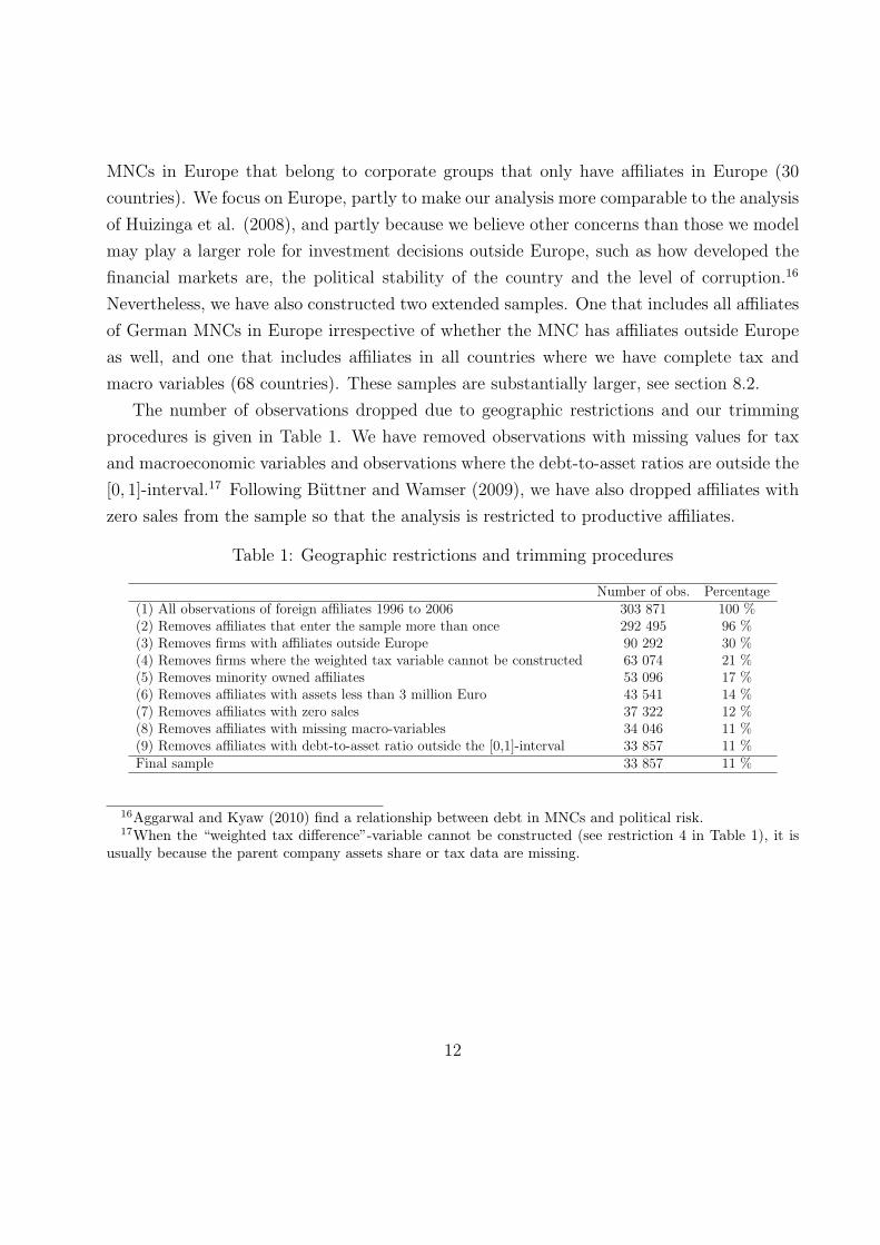
The number of observations dropped due to geographic restrictions and our trimming

procedures is given in Table 1. We have removed observations with missing values for tax

and macroeconomic variables and observations where the debt-to-asset ratios are outside the

[0, 1]-interval.17 Following Buttner and Wamser (2009), we have also dropped affiliates with

zero sales from the sample so that the analysis is restricted to productive affiliates.

Table 1: Geographic restrictions and trimming procedures

Number of obs. Percentage(1) All observations of foreign affiliates 1996 to 2006 303 871 100 %(2) Removes affiliates that enter the sample more than once 292 495 96 %(3) Removes firms with affiliates outside Europe 90 292 30 %(4) Removes firms where the weighted tax variable cannot be constructed 63 074 21 %(5) Removes minority owned affiliates 53 096 17 %(6) Removes affiliates with assets less than 3 million Euro 43 541 14 %(7) Removes affiliates with zero sales 37 322 12 %(8) Removes affiliates with missing macro-variables 34 046 11 %(9) Removes affiliates with debt-to-asset ratio outside the [0,1]-interval 33 857 11 %Final sample 33 857 11 %

16Aggarwal and Kyaw (2010) find a relationship between debt in MNCs and political risk.17When the “weighted tax difference”-variable cannot be constructed (see restriction 4 in Table 1), it is

usually because the parent company assets share or tax data are missing.

12

4 Variable definitions

4.1 Dependent variables

We use three different debt-to-asset ratio variables in our regression analysis. The total debt-

to-asset ratio (T-DAR) is constructed as the ratio between total non-equity liabilities and

total assets.18 The internal debt-to-asset ratio (I-DAR) is constructed as the ratio between

liabilities of German foreign affiliates to related parties and total assets, thus including the

liabilities to affiliated parties abroad as well as liabilities to German affiliates and the German

parent company.19 The external debt-to-asset ratio (E-DAR) is the difference between the

total debt-to-asset ratio and the internal debt-to-asset ratio.

4.2 Tax variables

In the main analysis, the host country tax rate, ti, is the host country statutory tax rate.

We use tax data collected by the University of Toronto’s International Tax program and

published in Mintz and Weichenrieder (2010).20 According to the model predictions, the tax

rate variable is relevant for the external debt-to-asset ratio of the affiliates and represents

the standard debt tax shield mechanism. The coefficient for this variable is expected to be

positive due to the fact that interest payments on debt are tax deductible.

The weighted tax difference,∑

j 6=i ρj(ti−tj), is a weighted sum of statutory tax differences

between the tax rate in the country where the affiliate is located (country i) and the tax rate

faced by each of its affiliated companies (including the parent which is always German in

our case).21 The weights are the asset share of each of the affiliates in the total assets of the

corporate group. Since data on the total assets of the parent company are not available in

MiDi before 2002, we use imputed values for the years 1996 to 2001. The imputed values are

18We have computed liabilities as “liabilities” plus “other liabilities.” It is not entirely clear what isincluded in the variable “other liabilities”, but accruals for pensions are one example. Whether or not “otherliabilities” are included have little effect on the empirical results.

19Buttner and Wamser (2009) do not count loans from the parent companies in the internal debt ratio asthey claim such loans cannot be given for tax reasons. Our model does not justify such a choice, but ourfindings are robust to excluding parent debt.

20We are grateful to Martin Ruf for providing the data to us electronically. For all countries, the ratesreflect the general corporate tax rates, including average or typical local taxes.

21This is the variable that corresponds to the variable called ‘tax incentive to shift debt ’ in Huizinga et al.(2008).

13

based on the first available value for each firm, usually the 2002 value. We have checked that

our main results are robust to other imputation procedures. The weighted tax difference

variable affects external debt through the external debt shifting mechanism of Huizinga et

al. (2008). We expect the coefficient to be positive, meaning that the higher the weighted

difference (either due to an increase in the tax rate in the country where the affiliate is

located, or due to a decrease in the tax rate in a country where one of the other affiliates is

located) the higher the use of external debt.

The maximum tax difference, (ti − t1), is the difference between the host country tax

rate and the group-specific lowest tax rate. This variable is the main determinant for tax-

motivated debt shifting by internal debt. The higher the maximum tax difference, the more

an affiliate is expected to borrow from the lowest taxed affiliate within the group.

The weighted tax difference and the maximum tax difference variables are defined before

we remove observations with missing or outlying values from the sample.

4.3 Control variables

Our theory model focuses on how tax incentives and bankruptcy costs affect the optimal

capital structure of MNCs. Obviously there may be other relevant factors that are not

included in our model. To account for this, we augment our regression analysis with a set

of control variables commonly used in the empirical literature. Our choice is in particular

inspired by Rajan and Zingales (1995), Huizinga et al. (2008) and Buttner and Wamser

(2009). We also include time and industry dummies, and parent (group) fixed effects. The

fixed effects account for unobserved heterogeneity with respect to debt policy between the

MNCs included in our sample.

We have been able to construct three firm level control variables:

The fixed asset ratio is measured as the ratio of fixed assets to total assets. The relation-

ship between the fixed asset ratio and external debt is ambiguous. Firms with a high ratio

of fixed assets to total assets may find it easier to borrow externally using these assets as

collateral, as pointed out, e.g., by Rajan and Zingales (1995). However, depreciable assets

carry tax deductible allowances that may be a substitute for the tax shield offered by debt,

as suggested by DeAngelo and Masulis (1980).

Firm size is measured by sales. More precisely, we control for firm size using dummy

14

variables for the sales quintile to which a firm belongs in a given year. The smallest firms are

in the left-out category. This means that a positive relationship between firm size and debt

will show up as positive signs for the rest of the sales quintile dummies. We expect a positive

relationship between size and the external debt-to-asset ratio, since large firms may be more

diversified and thus less risky borrowers (see, e.g., Frank and Goyal, 2009). Sales are also

correlated with cashflow and favorably lending conditions. It is hard to predict the effect of

size on firms’ internal-debt-to-asset ratio, but to the extent that internal and external debt

are substitutes, we might expect a negative relationship.

Loss carryforward is a dummy variable that equals one if the company has losses to be

carried forward that can reduce their future tax liabilities. The idea is that the demand for

debt tax shields may be lower if there are non-debt tax shields available (MacKie-Mason,

1990). Thus, we expect a negative relationship between the loss carryforward dummy and

both internal and external debt-to-asset ratios.

We have also been able to collect data on three country-level factors that are expected

to affect the debt-to-asset ratio of the affiliates of MNCs:

Inflation is the annual percentage change in the consumer price index, as reported in

the World Economic Outlook Database of the International Monetary Fund. The inflation

variable is expected to have a negative effect on the debt-to-asset ratio, since high inflation

reduces the real value of interest payments to be deducted and thereby the tax advantage

of debt (Mintz and Weichenrieder, 2010). In addition, countries with high inflation tend to

have a higher risk premium, something which discourages external borrowing (Huizinga et

al., 2008).

Corruption is the level of corruption in each of the host countries as measured by the

log of the Bribe Payers Index (BPI), provided by Transparency International. It is meant to

serve as a proxy for legal system efficiency and political risk in the host country. The index

measures the propensity to pay bribes, and is expressed as a number between 0 and 10, with

10 indicating lowest perceived propensity to pay bribes. Hence, the higher the index, the

less corrupt is the country. The corruption variable can be expected to have positive sign

(negative effect of corruption on the debt-to-asset ratio) as it can be more difficult to obtain

credit in corrupt countries. Also, firms may consider it less safe to borrow money in countries

where corruption is a problem. However, corruption may cause firms to substitute external

debt for internal debt, since the parent companies, when facing the risk of expropriation, will

15

prefer to risk the debt of external parties rather than their own debt (Aggarwal and Kyaw,

2008).

Growth opportunities are measured as the median annual sales growth in each industry

group in each country. We follow Huizinga et al. (2008) in this respect who find a posi-

tive association between growth opportunities measured this way and debt-to-asset ratios.

Building on Harris and Raviv (1991), their interpretation is that growth opportunities signal

future growth and possibly an ability to borrow. According to Myers (1977), however, highly

debt-financed companies are more likely to pass up profitable investment opportunities since

the return will mostly benefit existing debt-holders. Firms expecting high future growth

should therefore use less debt. This is confirmed by Rajan and Zingales (1995) and others,

see Myers (2001). One possible reason why the results differ may be that Rajan and Zingales

follow Myers (1977) and use the market-to-book-ratio as a proxy for growth opportunities.

5 Descriptive statistics

Descriptive statistics for the main variables in the European sample are presented in Table 2.

The 33,857 affiliate year observations represent 8,191 affiliates that belong to 3,660 parent

companies observed for 11 years. There are on average 3.95 observations per affiliate and

9.3 observations per corporate group (parent company). The distribution of the latter is,

however, rather skewed. The number of subsidiaries per group varies substantially with the

smallest number of observations per group being one, whereas the largest groups have several

hundred affiliates.

We separate out the group-specific lowest taxed affiliates in the main sample in order to

see whether these have the characteristics that our model predicts. The group-specific lowest

taxed affiliates are the affiliates that our model predicts to serve as financial coordination

centers in their group, lending money to the parent company and the other affiliates. We see

from Table 2 that the lowest taxed affiliates are on average smaller in size, both in terms of

assets and sales. More importantly, their net lending is indeed larger than that of the other

affiliates, but on average they still have net debt. Their average internal debt (in absolute

terms) is about half that of the others. Only 3.8 % of the affiliates have positive net lending.

Out of these, 61 % are the lowest taxed affiliates within their group. This suggests that

many internal loans are given directly from the parent company, despite the high tax level

16

in Germany. One explanation for this may be agency costs as pointed out by Dischinger and

Riedel (2009).

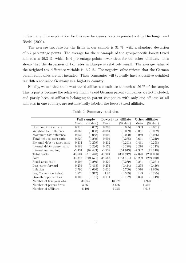
The average tax rate for the firms in our sample is 31 %, with a standard deviation

of 6.2 percentage points. The average for the subsample of the group-specific lowest taxed

affiliates is 29.3 %, which is 4 percentage points lower than for the other affiliates. This

shows that the dispersion of tax rates in Europe is relatively small. The average value of

the weighted tax difference variable is -6.2 %. The negative value reflects that the German

parent companies are not included. These companies will typically have a positive weighted

tax difference since Germany is a high-tax country.

Finally, we see that the lowest taxed affiliates constitute as much as 56 % of the sample.

This is partly because the relatively highly taxed German parent companies are not included,

and partly because affiliates belonging to parent companies with only one affiliate or all

affiliates in one country, are automatically labeled the lowest taxed affiliate.

Table 2: Summary statistics.

Full sample Lowest tax affiliate Other affiliatesMean (St.dev.) Mean (St.dev.) Mean (St.dev.)

Host country tax rate 0.310 0.062) 0.293 (0.065) 0.333 (0.051)Weighted tax difference -0.069 (0.068) -0.084 (0.069) -0.051 (0.062)Maximum tax difference 0.039 (0.058) 0.000 (0.000) 0.089 (0.056)Total debt-to-asset ratio 0.620 (0.259) 0.604 (0.265) 0.641 (0.249)External debt-to-asset ratio 0.431 (0.259) 0.432 (0.261) 0.431 (0.258)Internal debt-to-asset ratio 0.189 (0.236) 0.173 (0.228) 0.210 (0.243)Internal net lending -5 431 (62 483) -3 932 (54 643) -7 332 (71 148)Total assets 43 604 (316 448) 40 904 (360 242) 47 028 (250 093)Sales 43 343 (201 571) 35 563 (153 494) 53 209 (249 210)Fixed asset ratio 0.295 (0.280) 0.329 (0.289) 0.251 (0.261)Loss carry forward 0.253 (0.435) 0.251 (0.444) 0.255 (0.436)Inflation 2.790 (4.620) 3.030 (5.700) 2.510 (2.650)Log(Corruption index) 1.870 (0.317) 1.85 (0.339) 1.89 (0.285)Growth opportunities 0.105 (0.151) 0.111 (0.152) 0.098 (0.149)Number of firm-year obs. 33 857 18 929 14 928Number of parent firms 3 660 3 656 1 505Number of affiliates 8 191 5 345 4 613

17

6 Identification and endogeneity issues

There are three sources of variation in our tax variables that identify the effects on the firms’

capital structure. First, corporate tax rates vary across countries and within countries over

time. This variation is relevant for all three tax variables. Second, variation in the multi-

national groups’ location patterns will generate variation in the maximum and weighted tax

difference variables. Finally, variation in the allocation of capital across affiliates within

groups generates additional variation in the weighted tax difference variable. In our theo-

retical model we have implicitly assumed that all of this variation is exogenous with respect

to the firms’ internal and external debt-to-asset ratios. This assumption deserves further

consideration.

Although large MNCs are influential and likely to lobby for generous tax regimes, we have

no reason to believe that the result of this lobbying in a particular country is systematically

linked to the use of internal or external debt by the firms that are located there. It is

somewhat more plausible that countries on their own initiative respond to the firms’ debt

shifting strategies by changing their tax regimes. Huizinga et al. (2008) do not, however,

find support for such a hypothesis in their study when they instrument the effective tax rate

with the countries’ population size. Hence, it seems reasonable to assume that corporate

statutory tax rates are close to exogenous with respect to the firms’ capital structure.

The MNCs’ investment decisions represent a greater concern as investment decisions

are obviously made simultaneously with capital structure decisions and determine both the

location patterns of the firms and their allocation of capital across affiliates. We do not model

these decisions. One example of such an endogeneity problem is that firms, using internal

debt financing extensively for non-tax reasons, may also find it particularly profitable to

set up financial coordination centers in low-tax countries. Our response to this problem is

to follow the approach of Huizinga et al. (2008) and include both a set of affiliate specific

control variables and a parent specific fixed effect. As discussed by Buttner and Wamser

(2009), these variables should, at least to a large extent, control for variation in the internal

or external debt ratio that is not caused by tax planning, but that is possibly correlated

with our tax variables.

Buttner and Wamser (2009) discuss a related example where an MNC initially does not

have an affiliate in a country, but later establishes an affiliate there in response to the tax

18

rate being lowered below the current minimum tax rate within the group. This change in

the location pattern will increase the maximum tax difference variable for all the original

affiliates. Buttner and Wamser think of this as an endogenous change in the incentive to

engage in debt-shifting that may potentially bias their estimates even when parent specific

fixed effects are included in the specification. It is not obvious that this framing is correct.

Although the change in the location pattern is clearly an endogenous choice, the resulting

change in the tax difference variable reflects a response to an exogenous change in the tax

rates. Put differently, when the debt structure of an affiliate changes because a new sister

company is established and this changes the tax incentive variables, this is an effect we want

to capture. If the sensitivity of the location pattern with respect to taxes varies between

MNCs, this might be a concern, but such differences are likely to be permanent and should

be absorbed by the parent fixed effects. When controlling for parent fixed effects, we only

utilize variation in the tax variables within each multinational group.

7 Empirical results

In this section we test the empirical predictions of our model. We start out analyzing debt-

to-asset ratios and potential omitted variable biases before checking that separate regressions

for internal and external debt-to-asset ratios yield results that are consistent. In particular,

we check whether tax variables that according to our model are irrelevant in these equations

have significant explanatory power. In the next section, we discuss robustness with respect

to various sample and specification choices.

7.1 The total debt-to-asset ratio

The optimal total debt-to-asset ratio is the sum of the optimal internal and external debt-

to-asset ratios and is therefore determined by all three tax variables discussed above. In

our regression we build on equations (11) and (12). We add control variables and industry,

year and parent (group) fixed effects. We use a dummy variable to account for the difference

between the affiliate located in the country having the lowest effective tax rate (the predicted

financial coordination center) and the other affiliates in the group. The exact specification

is

19

bpit = β0 + β1tpit + β2

∑

j 6=i

ρpjt(tpit − tpjt) + β3(tpit − tp1t)NLSpit

+β4NLSpit + γXpit + δt + σI + αp + εpit (13)

The dependent variable bpit is the total debt-to-asset ratio of affiliate i belonging to parent

company p in year t. On the right hand side, tpit is the host country tax rate which affects

the optimal level of external debt.∑

i6=j ρpjt(tpit−tpjt) is the weighted tax difference variable,

which also affects the optimal level of external debt, and (tpit − tp1t) is the maximum tax

difference variable, which affects the optimal level of internal debt. Xpit is a vector of firm-

and country level control variables, δt is a vector of time dummies, σI is a vector of industry

dummies, αp is a parent specific fixed effect and εit is an error term. NLSpit is a dummy

variable that is 1 if affiliate pi is not the lowest taxed subsidiary in the group in year t, and

zero otherwise. Hence, it is a dummy for not being a predicted financial coordination center.

The interaction between this dummy and the maximum tax difference variable captures the

fact that the maximum tax difference variable affects internal debt for all firms except the

predicted financial coordination center which should lend out money. The coefficient on

the NLSpit- dummy itself should be close to zero. The main parameters of interest are the

coefficients β1, β2 and β3. We see from Table 3, columns (1) and (2) that all three are positive

and statistically significant at the one percent level. Comparing columns (1) and (2), we see

that none of the coefficients appears to be particularly sensitive to the inclusion of firm and

country level control variables.

Focusing on Table 3, column (2), we see that when the host country tax rate increases

by one percentage point, the direct effect is that the total debt-to-asset ratio of the affiliate

increases by 0.197 percentage points. This is very close to the estimate of 0.184 in Huizinga et

al. (2008). They call this a “domestic effect”, as it is relevant for domestic and multinational

firms alike. Next come the two international debt shifting effects that are only relevant for

multinational firms. When the weighted tax difference increases by one percentage point, the

total debt-to-asset ratio of the affiliate increases by 0.279 percentage points. This estimate is

about twice as large as what Huzinga et al. (2008) report based on data from the Amadeus

database. Finally, when the maximum tax difference variable increases by one percentage

point, the total debt-to-asset ratio of the affiliate increases by 0.120 percentage points.

20

Table 3: Effect of tax variables on the total debt-to-asset ratio.

Dependent variable: Total debt-to-asset ratio(1) (2) (3) (4) (5) (6) (7)

Tax rate 0.177*** 0.197*** 0.214*** 0.394*** 0.465*** - -(0.048) (0.048) (0.046) (0.035) (0.027) - -

Weighted tax difference 0.319*** 0.279*** 0.291*** - - 0.468*** -(0.048) (0.048) (0.045) - - (0.027) -

Maximum tax diff. x NLS 0.127*** 0.120*** - 0.171*** - - 0.404***(0.043) (0.042) - (0.041) - - (0.036)

NLS -0.014*** -0.013*** - -0.011*** - - -0.005(0.004) (0.004) - (0.004) - - (0.004)

Sales quintile 2 - 0.022*** 0.022*** 0.022*** 0.022*** 0.022*** 0.022***- (0.005) (0.005) (0.005) (0.005) (0.005) (0.005)

Sales quintile 3 - 0.050*** 0.049*** 0.050*** 0.050*** 0.049*** 0.050***- (0.005) (0.005) (0.005) (0.005) (0.005) (0.005)

Sales quintile 4 - 0.060*** 0.060*** 0.060*** 0.061*** 0.059*** 0.060***- (0.005) (0.005) (0.005) (0.005) (0.005) (0.005)

Sales quintile 5 - 0.078*** 0.079*** 0.080*** 0.080*** 0.078*** 0.080***- (0.006) (0.006) (0.006) (0.006) (0.006) (0.006)

Fixed asset ratio - 0.048*** 0.048*** 0.048*** 0.047*** 0.047*** 0.046***- (0.009) (0.009) (0.009) (0.009) (0.009) (0.009)

Loss carry forward - 0.087*** 0.087*** 0.087*** 0.087*** 0.087*** 0.088***- (0.003) (0.003) (0.003) (0.003) (0.003) (0.003)

Inflation - -0.000 -0.001 -0.001 -0.001 -0.000 -0.001- (0.000) (0.000) (0.000) (0.000) (0.000) (0.000)

Log of corruption - -0.017*** -0.018** -0.018*** -0.019*** -0.017** -0.014**- (0.006) (0.007) (0.006) (0.006) (0.006) (0.006)

Growth opportunities - 0.015 0.014 0.014 0.012 0.012 0.005- (0.015) (0.015) (0.015) (0.015) (0.015) (0.015)

Lowest tax affiliates excl. No No No No No No NoParent, industry and year fixed effects Yes Yes Yes Yes Yes Yes YesNumber of observations 33 857 33 857 33 857 33 857 33 857 33 857 33 857Number of parent companies 3 660 3 660 3 660 3 660 3 660 3 660 3 660R-square 0.5262 0.5464 0.5462 0.5459 0.5456 0.5459 0.5438

The regressions are estimated by ordinary least squares. The reported standard errors are heteroskedasticity robust and allowfor clustering of errors within corporate groups.* significant at the 10 % level, ** significant at the 5 % level, *** significant at the 1 % level

21

Note that a tax change in any country j where the group has an affiliate will affect

the total debt-to-asset ratio in affiliate pi through the weighted tax difference variable. An

increase in the host country tax rate increases the weighted tax difference and, thereby, the

total debt-to-asset ratio, while an increase in the tax rate in another country decreases the

weighted tax difference and thereby the total debt-to-asset ratio. For affiliate pi, a change

in the host country tax rate, tpit, by one percentage point will affect the debt-to-asset ratio

through all three variables given that pi itself is not the financial coordination center. The

total effect will be β1+β2(1−ρpit)+β3. The effect is decreasing in the relative size of affiliate

pi because shifting a certain amount of external debt from a small to a large affiliate will

change the debt-to-asset ratio in the small affiliate more than in the large affiliate.

The coefficients on the control variables are largely as expected. We will discuss these

coefficients when estimating their effects on internal and external debt separately in the next

two subsections.

Table 4: Correlation matrix.

Host country Weighted Maximumtax rate tax difference tax difference

Host country tax rate 1Weighted tax difference 0.4140 1Maximum tax difference 0.3782 0.2977 1

The three tax variables discussed above are correlated by construction, and the correlation

coefficients are around 0.3 to 0.4, as displayed in Table 4. We see from Table 3, column (2),

that the multicolinearity between them does not hinder statistically identifying the effects

of each of the three variables separately. However, the correlation will cause an omitted

variable bias if one or more variables is left out of the regression. From Table 3, columns

(5) to (7), we see that if only one of the tax variables is included, the omitted variable bias

is severe. In column (5), where the host country tax rate is the only included tax variable,

the bias is 136 %. See, e.g., Jog and Tang (2001) and Mintz and Weichenrieder (2010, ch.

5) for analyses using specifications that lack the tax difference variables.22 In columns (3)

22Note that the specification in Mintz and Weichenrieder (2010, ch. 5) includes affiliate specific fixedeffects while we control for fixed effects at the group level. Affiliate fixed effects will absorb a lot more of thevariation in the tax variables than group fixed effects, and the two specifications are therefore not directlycomparable. The specification used by Jog and Tang (2001) also include variables that may reduce the bias.

22

and (4) only one of the three tax variables is missing. Except Huizinga et al. (2008), all

previous papers using the total (or external) debt-to-asset ratio as the dependent variable,

omit the weighted tax difference variable. The omitted variable bias is then about 100 % for

the host country tax rate and about 40 % for the maximum tax difference variable. When

the maximum tax difference variable is omitted, as in Huizinga et al. (2008), the omitted

variable bias is more modest, about 9 % for the host country tax rate and about 4 % for

the weighted tax difference variable. It is hard to assess how general these results are with

respect to magnitude, but our results clearly suggest that the bias may be substantial.

Table 5: Relative importance of different mechanisms.

Coef. Change in tit ρit Percentage point Relativechange in total contribution

debt-to-asset ratioTax rate 0.197 0.10 1.97 43 %Weighted tax difference 0.279 0.10 0.5 1.40 31 %Maximum tax difference x NLS 0.120 0.10 1.20 26 %Total 4.57 100 %

To further illustrate the economic importance of the three mechanisms discussed above, it

may be useful to look at a hypothetical example inspired by Huizinga et al. (2008). Consider

a MNC consisting of two affiliates of equal size (implying that ρpit is 0.5). Assume that the

affiliate located in the country with the highest tax rate experiences a 10 percentage point

tax increase while all else remains equal. Table 5 reports the results based on our estimated

coefficients. We see that the total effect of the tax change is a 4.57 percentage point increase

in the debt-to-asset ratio. For a company with an average debt-to-asset ratio at the outset

(0.62), this will imply a 7.4 % increase in total debt. If we decompose this effect, we see that

the direct effect – where the mechanism is the firm’s preference for debt over equity – seems

to be the largest. Next comes the external debt shifting mechanism leading to external debt

shifting, and, finally, the internal debt shifting mechanism affecting the total debt-to-asset

ratio through internal debt. The latter two are of about equal importance. Note that the

1.40 percentage point increase in total debt that is due to external debt shifting, will reduce

the total debt-to-asset ratio by 1.40 percentage point for the other affiliate.

23

7.2 The external debt-to-asset ratio

According to our theory model, external debt is determined by the host country tax rate and

the weighted tax difference variable, while the maximum tax difference variable should not

be relevant. Based on equation (10), we run the following regression:

bEpit = β0 + β1tpit + β2

∑

i6=j

ρpjt(tpit − tpjt) + γXpit + δt + σI + αp + εpit, (14)

where bEpit is the external debt-to-asset ratio of affiliate i belonging to parent company p in

year t. The other variables are explained in the previous subsection.

We see from Table 6, columns (1) and (2), that both the host country tax rate and

the weighted tax difference variable have a positive and significant effect on external debt,

although the coefficients are smaller than the estimates we obtain from the total debt-to-

asset ratio regression. Comparing columns (1) and (2), we see that the coefficient on the

weighted tax difference variable is reduced by about 35 % when the set of control variables

is included in the regression. It is the controls for size and inflation that affect the weighted

tax difference variable the most. However, even after the inclusion of control variables, the

coefficient on the weighted tax difference is of economic significance. We see from column

(2) that when the weighted tax difference increases by one percentage point, the external

debt-to-asset ratio of the affiliate increases by 0.172 percentage points.

When the host country tax rate increases by one percentage point, the external debt-

to-asset ratio increases by 0.147 percentage points. The latter coefficient corresponds to a

semielasticity of external debt of 0.34 (evaluated at its mean), i.e., a one percentage point

increase in the host country tax rate increases the external debt-to-asset ratio by 0.34 %.

Using a specification similar to our column (4), Desai et al. (2004) find that the external

debt-to-asset ratio increases by 0.246 percentage points when the host country tax rate

increases by one percentage point. This is relatively close to our corresponding estimate in

column (4) of 0.296. The corresponding semielasticities are 0.55 and 0.69, respectively.23

According to our theory model, the maximum tax difference variable should not affect

the external debt-to-asset ratio, and we see from Table 6, column (3), that the coefficients

on the maximum tax difference variable and the NLS dummy are indeed very close to zero

23The semielasticity implied by the coefficient reported in Desai et al. (2004) is taken from Buttner andWamser (2009).

24

Table 6: Effect of tax variables on the external debt-to-asset ratio.

Dependent variable: External debt-to-asset ratio(1) (2) (3) (4) (5) (6)

Tax rate 0.132*** 0.147*** 0.158*** 0.296*** - -(0.048) (0.048) (0.049) (0.027) - -

Weighted tax difference 0.267*** 0.172*** 0.188*** - 0.294*** -(0.048) (0.047) (0.050) - (0.026) -

Max. tax difference x NLS - - 0.0084 - - 0.215***- - (0.043) - - (0.036)

NLS - - -0.006 - - -0.001- - (0.004) - - (0.004)

Sales quintile 2 - 0.040*** 0.040*** 0.041*** 0.040*** 0.040***- (0.005) (0.005) (0.005) (0.005) (0.005)

Sales quintile 3 - 0.079*** 0.079*** 0.080*** 0.079*** 0.079***- (0.005) (0.005) (0.005) (0.005) (0.005)

Sales quintile 4 - 0.106*** 0.106*** 0.106*** 0.105*** 0.106***- (0.005) (0.005) (0.005) (0.005) (0.005)

Sales quintile 5 - 0.143*** 0.143*** 0.144*** 0.142*** 0.144***- (0.006) (0.006) (0.006) (0.006) (0.006)

Fixed asset ratio - 0.012 0.012 0.012 0.012 0.010- (0.009) (0.009) (0.009) (0.009) (0.009)

Loss carry forward - 0.031*** 0.031*** 0.031*** 0.031*** 0.031***- (0.003) (0.003) (0.003) (0.003) (0.003)

Inflation - -0.0011*** -0.0012*** -0.0012*** -0.001*** -0.0012***- (0.000) (0.000) (0.000) (0.000) (0.000)

Log of corruption - 0.025*** 0.025*** 0.025*** 0.026*** 0.028***- (0.006) (0.006) (0.006) (0.006) (0.006)

Growth opportunities - 0.004 0.004 0.003 0.003 -0.003- (0.013) (0.013) (0.013) (0.013) (0.013)

Lowest tax affiliates excl. No No No No No NoParent, industry and year fixed effects Yes Yes Yes Yes Yes YesNumber of observations 33 857 33 857 33 857 33 857 33 857 33 857Number of parent companies 3 660 3 660 3 660 3 660 3 660 3 660R-square 0.5146 0.5331 0.5331 0.5329 0.5330 0.5318

The regressions are estimated by ordinary least squares. The reported standard errors are heteroskedasticity robust and allowfor clustering of errors within corporate groups.* significant at the 10 % level, ** significant at the 5 % level, *** significant at the 1 % level

25

In column (4), we show that omitting the weighted tax difference variable will lead to

an almost 100 % bias in the coefficient on the host country tax rate. This specification

corresponds to the one used by Altshuler and Grubert (2003), Desai et al. (2004), Ruf

(2008) and Buttner et al. (2009).

In columns (5) and (6), we demonstrate that both the weighted tax difference variable

and the maximum tax difference variable, when included alone, have a coefficient of similar

size and significance as that of the host country tax rate in column (4).

All firm-level control variables, except the fixed asset ratio, are highly significant. The

signs of the coefficients for the size dummy variables indicate that there is a positive relation-

ship between the size of the firms and their external debt-to-asset ratio. This is as expected

and indicates that bigger firms are more diversified and have easier access to external debt.

The coefficient on the fixed asset ratio is positive, but never statistically significant. The

loss carry forward dummy is both positive and significant. This is the opposite of what we

would expect, and indicates that tax shields from the presence of loss carryforwards do not

necessarily serve as a substitute for debt tax shields. One simple interpretation is that affili-

ates experiencing financial difficulties (affiliates with negative loss carryforwards) lose equity

and rely more on debt financing (Gopalan et al., 2007).24 Of the country-level variables,

inflation is significant through all the specifications. Its coefficient shows a negative sign.

This is as expected, and may be explained by the fact that firms are reluctant to borrow

external funds in inflationary, and thus more unstable, environments. Also in more corrupt

countries, borrowing from external sources seems to be less attractive, as indicated by the

positive coefficient for the log of corruption variable. Our finding here is in line with Aggar-

wal and Kyaw (2008). We find no significant effect of growth opportunities on the external

debt-to-asset ratio.

7.3 Internal debt-to-asset ratio

Our model predicts that internal debt is always part of a tax-efficient capital structure, and

that the only relevant tax variable is the maximum tax difference, i.e., the tax difference

24Inspired by Buttner et al. (2011), we have also tried to interact the loss carryforward dummy with thetax variables and to run separate regressions for firms with and without loss carryforwards. Buttner et al.find that loss carryforwards reduce the firms’ tax elasticity with respect to the debt-to-asset ratio. We donot find any clear-cut evidence for this effect in our sample.

26

between the host country tax rate and the tax rate faced by the lowest taxed affiliate within

the group (the predicted financial coordination center). Based on equation (8), we use the

following specification:

bIpit = β0 + β1(tpit − tp1t) + γXpit + δt + σI + αp + εpit,∀i > 1 (15)

The dependent variable bIpit is the internal debt-to-asset ratio, and the other variables are

explained above. We exclude the predicted financial coordination centers from the sample

used for this regression, as the internal debt of these centers is described by equation (9),

and discussed as part of the descriptive statistics.

The regression results are given in Table 7. We see from columns (1) and (2) that

the coefficients on the maximum tax difference variable are not particularly sensitive to

the inclusion of firm level control variables. Focusing on column (2), we see that when the

maximum tax difference variable increases by one percentage point, the internal debt-to-asset

ratio of the affiliate increases by 0.243 percentage points. This is considerably more than the

corresponding estimate in the total debt-to-asset ratio regression above. The semielasticity,

i.e., the percentage increase in the internal debt-to-asset ratio, evaluated at its mean, is

1.30. This can be compared to the semielasticities of internal debt of 1.02 in Desai et al.

(2004) and 0.69 reported in Buttner and Wamser (2009).25 Note that Buttner and Wamser

subtract internal loans from the German parent companies when they calculate the internal

debt ratio and this reduces their left hand side variable considerably.

According to our theory model, the host country tax rate and the weighted tax difference

variable should not affect the internal debt-to-asset ratio. In Table 7, column (3), we test

this prediction. We see that the coefficient on the host country tax rate fits the prediction

perfectly, while the coefficient on the weighted tax difference variable is slightly higher than

the coefficient on the maximum tax difference variable and significant at the ten percent level.

One reason for this may be that our structural model is too stylized, and does not capture

the fact that other concerns than taxes also influence where an MNC places its financial

coordination center. This will create measurement error in our maximum tax difference

variable. An example of such a concern may be the financial infrastructure offered at various

25The semielasticity implied by the coefficient reported in Desai et al. (2004) is taken from Buttner andWamser (2009).

27

Table 7: Effect of taxes on the internal debt-to-asset ratio.

Dependent variable: Internal debt-to-asset ratio(1) (2) (3) (4) (5)

Tax rate - - 0.003 - 0.285***- - (0.102) - (0.052)

Weighted tax difference - - 0.162* 0.282*** -- - (0.090) (0.048) -

Maximum tax difference 0.206*** 0.243*** 0.146*** - -(0.041) (0.040) (0.057) - -

Sales quintile 2 - -0.004 -0.004 -0.004 -0.003- (0.007) (0.007) (0.007) (0.007)

Sales quintile 3 - -0.027*** -0.026*** -0.027*** -0.026***- (0.008) (0.008) (0.008) (0.008)

Sales quintile 4 - -0.055*** -0.055*** -0.055*** -0.054***- (0.008) (0.008) (0.008) (0.008)

Sales quintile 5 - -0.070*** -0.070*** - 0.070*** -0.070***- (0.008) (0.008) (0.008) (0.008)

Fixed asset ratio - 0.048*** 0.050*** 0.049*** 0.049***- (0.013) (0.013) (0.013) (0.013)

Loss carry forward - 0.060*** 0.059*** 0.060*** 0.060***- (0.005) (0.005) (0.005) (0.005)

Lowest tax affiliate excl. Yes Yes Yes Yes YesParent, industry and year fixed effects Yes Yes Yes Yes YesNumber of observations 14 928 14 928 14 928 14 928 14 928Number of parent companies 1 505 1 505 1 505 1 505 1 505R-square 0.3834 0.4019 0.4022 0.4019 0.4017

The regressions are estimated by ordinary least squares. The reported standard errors are heteroskedasticity robust and allowfor clustering of errors within corporate groups.* significant at the 10 % level, ** significant at the 5 % level, *** significant at the 1 % level

28

locations. Moreover, so far we have based our analysis on statutory tax rates that are not

adjusted for special tax regimes designed to attract financial coordination centers. In cases

where the financial coordination center is not located in the lowest taxed affiliate according

to statutory tax rates, the weighted tax difference variable may be a better proxy for the

relevant tax difference.

Looking next at potential omitted variable biases, columns (4) and (5) show that when

the maximum tax difference variable is omitted, either two of the other tax variables will

pick up the effect with a coefficient of similar size and significance level.

All control variables are significant. Contrary to the effect of size on external debt, the

effect of size on internal debt is negative. If internal and external debt can be considered as

substitutes (Desai et al., 2004, Buttner et al., 2009), this may indicate that bigger firms have

easier access to external finance and thus less demand for internal debt. Looking back at

the effect of size on total debt estimated in Table 3, we see that the positive effect of size on

external debt dominates. The sign of the fixed asset ratio coefficient is positive, something

which contradicts the idea that depreciation allowances and debt are substitutable forms of

tax shields. Our finding here is in line with Rajan and Zingales (1995).26 The coefficient for

the loss carryforward variable is positive and significant. This is similar to the effect on the

external debt-to-asset ratio that we discussed above

8 Robustness tests

8.1 Adjustment for preferential tax regimes and CFC rules

The results in the previous section show that all three tax mechanisms in our model are

significant and well identified, but the economic importance – particularly of the internal

debt mechanism – is relatively modest. There may be several reasons for this. One possibility

is simply that debt shifting is not a very important vehicle for tax avoidance. Another

possibility is that statutory tax rates are not a good approximation for the effective tax

rates relevant for firms’ debt shifting decisions. This will create measurement error in our

tax variables that will bias the estimated coefficients towards zero. A particular concern

is that some countries provide widespread tax benefits for the internal banks or financial

26See also DeAngelo and Masulis (1980).

29

coordination centers that are at the heart of the internal debt mechanism. Examples of such

preferential tax regimes are the coordination center regime in Belgium, the coordination

center and special financial institution regimes in the Netherlands, the coordination center

and financial holding regimes in Luxembourg and the management companies regime in

Switzerland (see, e.g., Malherbe, 2002). Under the Belgian system, for example, the tax

base of financial coordination centers consists of business expenses minus wages and financial

costs, rather than profit. If a German MNC locates an internal bank in a country with a

preferential tax regime for financial coordination centers, we will not capture this when we

calculate the maximum tax difference variable. This is because the average statutory tax

rates used in the previous analyses are relatively high in all of these countries. A quick check

through available company registers in the Netherlands, Belgium and Luxembourg reveals

that many large German MNCs do have financial service affiliates or coordination centers in

either Belgium, the Netherlands or Luxembourg.

In order to explore whether the relatively small coefficient on the maximum tax difference

variable is due to measurement errors, we try to adjust our statutory tax rates for companies

involved in financial service and holding activities in Belgium, the Netherlands, Luxembourg

and Switzerland. For the selected companies, we adjust the tax rate down to 10 %. This

choice is based on available micro data for Norwegian companies that have financial coordi-

nation centers in these countries and pay an average corporate tax of about 10 % of their

profit.27

Regression results for the total debt-to-asset ratio with adjustment for Preferential Tax

Regimes as explained above are presented in the column labeled ‘PTR’ in Table 8. We see

that our results are robust to this adjustment. The coefficient for the tax rate variable has

gone up. However, the coefficients on the weighted tax difference and maximum tax differ-

ence variables have become somewhat smaller. This suggests that our adjustment may have

increased rather than decreased the extent of measurement error in the tax rates. One likely

reason for this is that an adjustment procedure based on country and industry classification

alone is too rough. It is, for example, possible that the use of financial coordination cen-

ters is limited to large MNCs. However, restricting the sample to affiliates of particularly

large parent companies does not change the results. Another reason may be the German

27The data source is the Annual Reports of International Activity to the Norwegian Directorate of Taxes(‘Utenlandsoppgaven’). No reliable source for the effective tax rate for German companies was found.

30

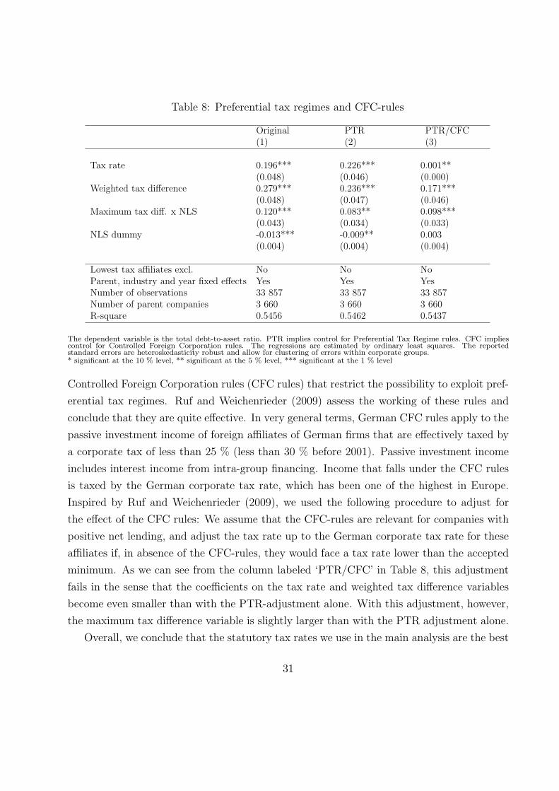
Table 8: Preferential tax regimes and CFC-rules

Original PTR PTR/CFC(1) (2) (3)

Tax rate 0.196*** 0.226*** 0.001**(0.048) (0.046) (0.000)

Weighted tax difference 0.279*** 0.236*** 0.171***(0.048) (0.047) (0.046)

Maximum tax diff. x NLS 0.120*** 0.083** 0.098***(0.043) (0.034) (0.033)

NLS dummy -0.013*** -0.009** 0.003(0.004) (0.004) (0.004)

Lowest tax affiliates excl. No No NoParent, industry and year fixed effects Yes Yes YesNumber of observations 33 857 33 857 33 857Number of parent companies 3 660 3 660 3 660R-square 0.5456 0.5462 0.5437

The dependent variable is the total debt-to-asset ratio. PTR implies control for Preferential Tax Regime rules. CFC impliescontrol for Controlled Foreign Corporation rules. The regressions are estimated by ordinary least squares. The reportedstandard errors are heteroskedasticity robust and allow for clustering of errors within corporate groups.* significant at the 10 % level, ** significant at the 5 % level, *** significant at the 1 % level

Controlled Foreign Corporation rules (CFC rules) that restrict the possibility to exploit pref-

erential tax regimes. Ruf and Weichenrieder (2009) assess the working of these rules and

conclude that they are quite effective. In very general terms, German CFC rules apply to the

passive investment income of foreign affiliates of German firms that are effectively taxed by

a corporate tax of less than 25 % (less than 30 % before 2001). Passive investment income

includes interest income from intra-group financing. Income that falls under the CFC rules

is taxed by the German corporate tax rate, which has been one of the highest in Europe.

Inspired by Ruf and Weichenrieder (2009), we used the following procedure to adjust for

the effect of the CFC rules: We assume that the CFC-rules are relevant for companies with

positive net lending, and adjust the tax rate up to the German corporate tax rate for these

affiliates if, in absence of the CFC-rules, they would face a tax rate lower than the accepted

minimum. As we can see from the column labeled ‘PTR/CFC’ in Table 8, this adjustment

fails in the sense that the coefficients on the tax rate and weighted tax difference variables

become even smaller than with the PTR-adjustment alone. With this adjustment, however,

the maximum tax difference variable is slightly larger than with the PTR adjustment alone.

Overall, we conclude that the statutory tax rates we use in the main analysis are the best

31

available approximation to the effective tax rates faced by MNCs. This is not to deny that

preferential tax regimes may be important. It is rather to admit that the data we have are

not rich enough to construct firm specific effective tax rates. Therefore, we should emphasize

again that our estimates in Tables 3, 7 and 6 are downward biased by measurement error to

the extent that the effective corporate tax rates deviate from the statutory tax rates.

8.2 Extended sample

In the main analysis, we have restricted the sample to German MNCs that have all their

affiliates within Europe. The reasons for this are discussed in section 3, but it implies that

large MNCs with activities worldwide are under-represented. It is therefore important to

check whether our results are sensitive to this sample choice.

In this section, we run the main regressions on two extended samples, a “World sample”

and an “extended European sample.” These samples are about three times larger than the

original sample. The World sample includes affiliates in all countries where we have complete

tax data and other necessary macro variables (68 countries).28 The extended European

sample is constructed by following Huizinga et al. (2008), i.e., we include all affiliates

of German MNCs in Europe (30 countries), irrespective of whether the MNCs also have

affiliates outside Europe. We calculate the tax variables as if the affiliates outside Europe

were not relevant. Huizinga et al. (2008) are forced to proceed this way since they do not

have information about affiliates outside Europe. The procedure implicitly assumes that

financial markets in non-European low-tax countries are not developed to the extent that

MNCs want to use them for financial coordination purposes.

28In the World sample, we only include affiliates that belong to corporate groups that have all affiliateslocated within the 68 countries covered. Without this restriction, the sample size increases by about 25,000observations. As compared to Table 9, columns (7) to (8) below, the coefficients on the weighted taxdifference variable then fall notably, and become insignificant. The other coefficient stays about the same.

32

Tab

le9:

Exte

nded

sam

ple

s

Ori

gina

lE

urop

ean

sam

ple

Ext

ende

dE

urop

ean

sam

ple

Wor

ldsa

mpl

e(1

)(2

)(3

)(4

)(5

)(6

)(7

)(8

)(9

)T

-DA

RE

-DA

RI-

DA

RT

-DA

RE

-DA

RI-

DA

RT

-DA

RE

-DA

RI-

DA

RTax

rate

0.19

7***

0.14

7***

0.20

9***

0.20

6***

0.21

7***

0.20

2***

(0.0

48)

(0.0

48)

(0.0

34)

(0.0

32)

(0.0

31)

(0.0

29)

Wei

ghte

dta

xdi

ffere

nce

0.27

9***

0.17

2***

0.21

1***

0.19

9***

0.13

9***

0.09

2***

(0.0

48)

(0.0

47)

(0.0

33)

(0.0

31)

(0.0

30)

(0.0

28)

Max

imum

tax

diffe

renc

ex

NLS

0.12

0***

0.24

3***

0.14

9***

0.12

7***

0.02

80.

077*

**(0

.042

)(0

.040

)(0

.024

)(0

.018

)(0

.017

)(0

.014

)N

LS

-0.0

13-0

.009

***

-0.0

09**

*(0

.004

)(0

.003

)(0

.002

)C

ontr

olva

riab

les

incl

uded

Yes

Yes

Yes

Yes

Yes

Yes

Yes

Yes

Yes

Low

est

tax

affilia

teex

clud

edN

oN

oY

esN

oN

oY

esN

oN

oY

esPar

ent,

indu

stry

and

year

fixed

effec

tsY

esY

esY

esY

esY

esY

esY

esY

esY

esN

umbe

rof

obse

rvat

ions

3385

733

857

1492

888

861

8886

159

148

105

772

105

772

7290

4N

umbe

rof

pare

ntco

mpa

nies

366

03

660

150

55

904

590

43

287

R-s

quar

e0.

546

0.53

30.

402

0.41

90.

435

0.28

90.

432

0.43

90.

301

The

regre

ssio

ns

are

esti

mate

dby

ord

inary

least

square

s.T

he

report

edst

andard

erro

rsare

het

erosk

edast

icity

robust

and

allow

for

clust

erin

gofer

rors

wit

hin

corp

ora

tegro

ups.

*si

gnifi

cant

at

the

10

%le

vel

,**

signifi

cant

at

the

5%

level

,***

signifi

cant

at

the

1%

level

33

The regression results are reported in Table 9. For comparison, columns (1) to (3)

summarize the main results from our previous analyses. Columns (4) to (6) give results from

the extended European sample while columns (7) to (9) give results from the World sample.

We see that the coefficients estimated from the extended European sample are relatively

close to the coefficients from the original sample, but they are more precisely estimated and

the model performs better in the sense that the coefficients from the external and internal

debt-to-asset ratio regressions are quite close to the corresponding coefficients from the total

debt-to-asset ratio regressions. The improved fit is most likely due to the larger sample size,

but it could also be that the small MNCs, which are over-represented in the original sample,

engage less in tax planning. We explore this question further in the next section.

When including affiliates outside Europe, the results are qualitatively the same as before,

but the model appears to perform less well. The cross-equation restrictions are further from

being fulfilled, and the coefficients on the weighted tax difference and the maximum tax

difference are much smaller. The maximum tax difference variable actually turns insignificant

in the total debt-to-asset ratio regression. These results are consistent both with the idea

that the data quality is better for European countries, and that concerns other than those

we model may play a role for investments outside Europe. Relevant concerns not modeled

may be how developed the financial markets are, the political stability of the country and

the level of corruption. Additionally, withholding taxes, which we disregard in our structural

model, also become relevant in a sample that includes non-European countries.

8.3 Splitting the sample into small and large MNCs

Large MNCs may both have more opportunities to engage in tax planning and lower costs

associated with tax planning. In this subsection, we explore this issue by splitting the original

European sample into large and small MNCs. In Table 10, columns (1) and (2), we split

according to the number of foreign affiliates; in columns (3) and (4), we split according to

the total assets of the group. Overall, we see that the results for small and large MNCs

are quite similar, particularly when splitting the sample into below and above median assets

(65 million Euro). When splitting according to the number of affiliates, we see that the

estimated coefficients are somewhat smaller for MNCs with only one or two foreign affiliates.

These MNCs constitute 43 % of the sample. Note that the parent company fixed effect in

34

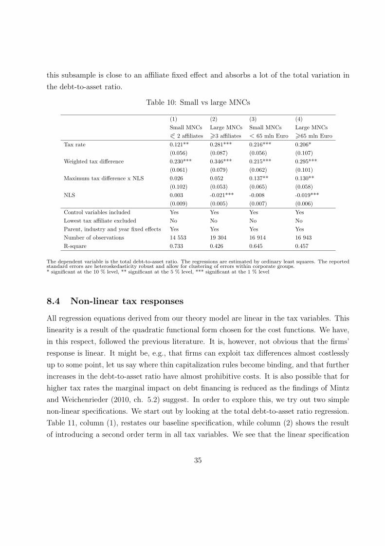
this subsample is close to an affiliate fixed effect and absorbs a lot of the total variation in

the debt-to-asset ratio.

Table 10: Small vs large MNCs

(1) (2) (3) (4)Small MNCs Large MNCs Small MNCs Large MNCs0 2 affiliates >3 affiliates < 65 mln Euro >65 mln Euro

Tax rate 0.121** 0.281*** 0.216*** 0.206*(0.056) (0.087) (0.056) (0.107)

Weighted tax difference 0.230*** 0.346*** 0.215*** 0.295***(0.061) (0.079) (0.062) (0.101)

Maximum tax difference x NLS 0.026 0.052 0.137** 0.130**(0.102) (0.053) (0.065) (0.058)

NLS 0.003 -0.021*** -0.008 -0.019***(0.009) (0.005) (0.007) (0.006)

Control variables included Yes Yes Yes YesLowest tax affiliate excluded No No No NoParent, industry and year fixed effects Yes Yes Yes YesNumber of observations 14 553 19 304 16 914 16 943R-square 0.733 0.426 0.645 0.457

The dependent variable is the total debt-to-asset ratio. The regressions are estimated by ordinary least squares. The reportedstandard errors are heteroskedasticity robust and allow for clustering of errors within corporate groups.* significant at the 10 % level, ** significant at the 5 % level, *** significant at the 1 % level

8.4 Non-linear tax responses

All regression equations derived from our theory model are linear in the tax variables. This

linearity is a result of the quadratic functional form chosen for the cost functions. We have,

in this respect, followed the previous literature. It is, however, not obvious that the firms’

response is linear. It might be, e.g., that firms can exploit tax differences almost costlessly

up to some point, let us say where thin capitalization rules become binding, and that further

increases in the debt-to-asset ratio have almost prohibitive costs. It is also possible that for

higher tax rates the marginal impact on debt financing is reduced as the findings of Mintz

and Weichenrieder (2010, ch. 5.2) suggest. In order to explore this, we try out two simple

non-linear specifications. We start out by looking at the total debt-to-asset ratio regression.

Table 11, column (1), restates our baseline specification, while column (2) shows the result

of introducing a second order term in all tax variables. We see that the linear specification

35

is well supported by the data. Only one of the three second order terms is significant, and

the significance level of this coefficient is only ten percent. In column (4) we look at the

internal debt-to-asset ratio regression. Also in this case, the second order specification is

insignificant, and it is very close to zero.

If choosing a cubic cost function, it is possible to derive a closed form solution for the

internal debt-to-asset ratio equation. As compared to a quadratic cost function, the cubic

cost function allows the costs to increase more slowly at first, and then more steeply after a

certain point. It is easy to show that this implies that the internal debt-to-asset ratio will

be a function of the square root of the maximum tax difference. This specification is used

in column (5). We see that it performs about as well as the linear specification, but when

introducing a linear term in addition to the square root term in column (6), we see that it is

the linear term that comes out as significant. Taken together, our analyses strongly suggest

that the linear specification used in our main analysis is a satisfactory approximation to

reality.

9 Concluding remarks

What shapes a tax-efficient financing structure for a multinational company is a central issue

in economic theory, and a practical question for multinationals with affiliates in different

countries. The literature in this field has established that multinational companies use both

internal and external debt, and that the debt-to-asset ratio of a multinational company

depends on tax factors and agency- and bankruptcy costs. Despite this fact, no single

paper in the literature studies both internal and external debt in combination with taxes

and bankruptcy costs. We have developed a model that incorporates all these mechanisms

and test the empirical implications of this model using the MiDi database provided by the

Deutsche Bundesbank.

Two of the tax mechanisms we investigate influence the debt-to asset ratio of the affil-

iates by affecting the external debt-to-asset ratio. These are the standard debt tax shield

mechanism relevant for national and multinational firms alike, and an external debt shifting

mechanism recently proposed by Huizinga et al. (2008). The former depends on the tax rate

alone, the latter on a weighted tax difference between the local tax rate and the tax rate

facing all other affiliates in the group. International shifting of internal debt is determined

36

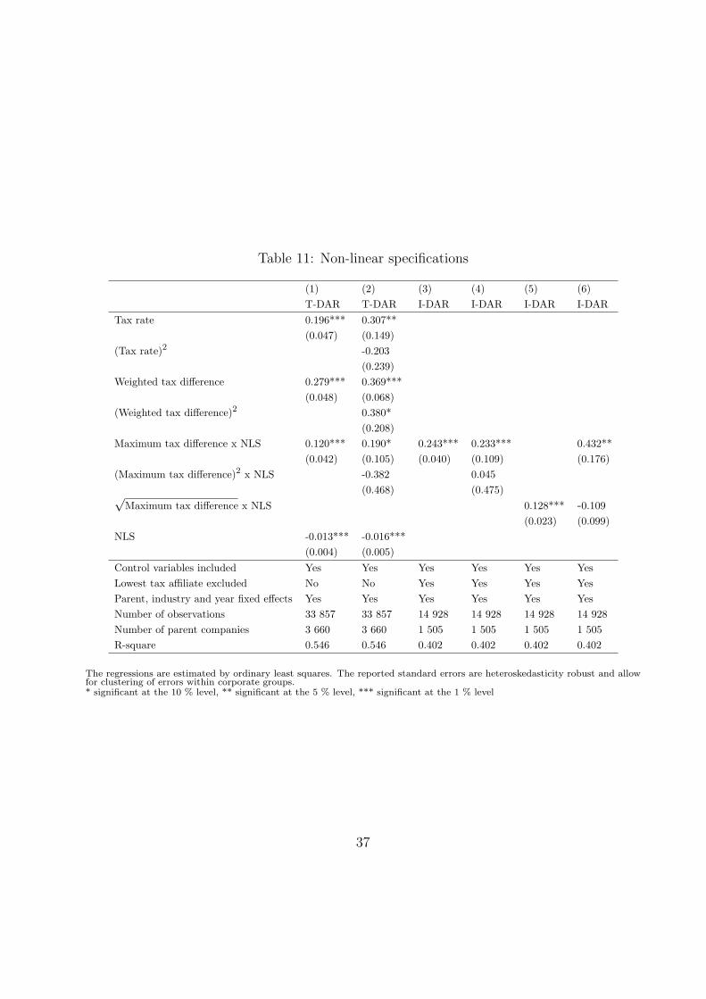
Table 11: Non-linear specifications

(1) (2) (3) (4) (5) (6)T-DAR T-DAR I-DAR I-DAR I-DAR I-DAR

Tax rate 0.196*** 0.307**(0.047) (0.149)

(Tax rate)2 -0.203(0.239)

Weighted tax difference 0.279*** 0.369***(0.048) (0.068)

(Weighted tax difference)2 0.380*(0.208)

Maximum tax difference x NLS 0.120*** 0.190* 0.243*** 0.233*** 0.432**(0.042) (0.105) (0.040) (0.109) (0.176)

(Maximum tax difference)2 x NLS -0.382 0.045(0.468) (0.475)√

Maximum tax difference x NLS 0.128*** -0.109(0.023) (0.099)

NLS -0.013*** -0.016***(0.004) (0.005)

Control variables included Yes Yes Yes Yes Yes YesLowest tax affiliate excluded No No Yes Yes Yes YesParent, industry and year fixed effects Yes Yes Yes Yes Yes YesNumber of observations 33 857 33 857 14 928 14 928 14 928 14 928Number of parent companies 3 660 3 660 1 505 1 505 1 505 1 505R-square 0.546 0.546 0.402 0.402 0.402 0.402

The regressions are estimated by ordinary least squares. The reported standard errors are heteroskedasticity robust and allowfor clustering of errors within corporate groups.* significant at the 10 % level, ** significant at the 5 % level, *** significant at the 1 % level

37

by the tax difference between the local tax rate and the tax rate of the lowest taxed affiliate

within the group.

Regressing the total debt-to-asset ratio on these tax mechanisms shows that all of them

are relevant, and that their effect can be identified separately despite the variables being

correlated by construction. However, the correlations cause a severe omitted variable bias if

one or more variables is left out.

We illustrate the economic importance of the estimated coefficients by analyzing a hy-

pothetical example inspired by Huizinga et al. (2008). Consider a multinational group

consisting of two affiliates of equal size (implying that ρpit is 0.5). If the affiliate located in

the country with the highest tax rate experiences a 10 percentage point tax increase while

all else remains equal, the total effect of the tax change is a 4.57 percentage point increase

in the total debt-to-asset ratio. For a company with an average debt-to-asset ratio at the

outset this implies a 7.4 % increase in total debt. The direct effect – where the mechanism

is the firm’s preference for debt over equity – is the largest. Next comes the external debt

shifting mechanism leading to external debt shifting, and, finally, the internal debt mecha-

nism affecting total debt-to-asset ratio through internal debt. The latter two are of about

equal importance.

We have tested the robustness of our results in a number of ways. Splitting the sample

into large and small MNCs, we find only minor differences in the tax response between the two

groups. Allowing for non-linearities in the tax response, we find that our linear specification

is well supported. Extending the sample, utilizing all affiliates of German MNCs in Europe,

irrespective of whether the MNC also has affiliates outside Europe, we obtain coefficients

that are close to those estimated on the original sample, but that are more precise. Moreover,

the model performs better in the sense that the coefficients from the external and internal

debt-to-asset ratio regressions are quite close to the corresponding coefficients from the total

debt-to-asset ratio regressions. Extending the sample further, including MNCs with affiliates

in all 68 countries for which we have complete tax and macro data, we obtain results that

are qualitatively the same as in the original sample, but with the external debt shifting

mechanism and internal debt mechanisms being less pronounced. We speculate that the

data quality is better for European countries, and that concerns other than those we model

may play a larger role for investment decisions outside Europe.

We also check robustness with respect to adjusting the tax variables to preferential tax

38

regimes for financial service affiliates in the BeNeLux countries and Switzerland. This leads

to a decrease in size for the weighted and maximum tax difference coefficients. When we

make a further adjustment to allow for German CFC rules, the coefficient for the internal

debt mechanism is lower than in the original regression, but higher than in the regression

where only preferential tax regimes were controlled for. The coefficients for the two other

tax variables become considerably smaller. These results may partly reflect that our adjust-

ment procedure, based on country and industry classification, is too rough, and partly that

the German CFC rules are effective in restricting the possibility to exploit preferential tax

regimes as concluded by Ruf and Weichenrieder (2009). Overall, it seems that the statutory

tax rates we use in the main analysis are the best available approximation to the effective

tax rates faced by MNCs. This is not to deny that preferential tax regimes and other special

rules such as CFC may be important. It is rather to admit that the data we have are not

rich enough to construct firm specific effective tax rates. Our main estimates are therefore

likely to be downward biased by measurement error.

39

Appendix A Optimal external debt-to-asset ratio

In order to derive the optimal debt-to-asset ratio of affiliate i in external debt, bEi , we start

by reordering the first order condition (6) to

µ · bEi = µ · b∗ + ti · r − γbE

i · ρi − γ ·∑

j 6=i

bEj · ρj, (16)

where ρi = Ki∑i Ki

represents the share of real capital employed in affiliate i in total real

capital employed by the MNC.

Subtracting equation (6) evaluated for affiliate j from equation (6) evaluated for affiliate

i delivers

bEj = bE

i −ti − tj

µ· r (17)

Applying (17) in (16), this leads to

µ · bEi = µ · b∗ + ti · r − γ · bE

i · ρi (18)

− γ · bEi ·

∑

j 6=i

ρj + γ ·∑

j 6=i

ti − tjµ

· r · ρj.

Note that these rearrangements necessarily require potential withholding taxes to be equal-

ized across all countries. This holds true both for our modeling and for the approach taken

in Huizinga et al. (2008).

Since ∑

j 6=i

ρj =∑

j 6=i

Kj∑i Ki

=

∑i Ki −Ki∑

i Ki

= 1− ρi, (19)

we can substitute equation (19) into (18). Then, by collecting all terms with a bEi on the left

hand side and rearranging, we end up with the optimal external debt-to-asset ratio (10) in

the text.

40

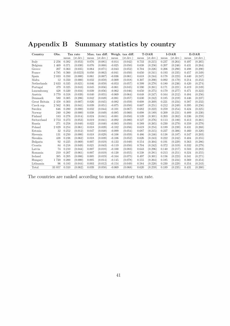
Appendix B Summary statistics by country

Country Obs. Tax rate Max. tax diff. Weigh. tax diff. T-DAR I-DAR E-DARmean (st.dev.) mean (st.dev.) mean (st.dev.) mean (st.dev.) mean (st.dev.) mean (st.dev.)

Italy 2 256 0.382 (0.053) 0.076 (0.081) -0.014 (0.042) 0.733 (0.215) 0.237 (0.264) 0.497 (0.265)Belgium 1 469 0.371 (0.030) 0.076 (0.068) -0.025 (0.050) 0.638 (0.256) 0.207 (0.246) 0.431 (0.264)Greece 207 0.363 (0.035) 0.064 (0.071) -0.043 (0.052) 0.704 (0.226) 0.206 (0.290) 0.498 (0.290)France 4 785 0.360 (0.0223) 0.050 (0.062) -0.041 (0.050) 0.650 (0.241) 0.193 (0.235) 0.457 (0.249)Spain 2 033 0.350 (0.000) 0.061 (0.067) -0.036 (0.061) 0.618 (0.244) 0.178 (0.223) 0.440 (0.247)Malta 12 0.350 (0.000) 0.032 (0.059) -0.009 (0.018) 0.307 (0.290) 0.092 (0.179) 0.214 (0.252)Netherlands 2 633 0.335 (0.021) 0.046 (0.059) -0.053 (0.057) 0.599 (0.278) 0.180 (0.236) 0.420 (0.274)Portugal 479 0.325 (0.043) 0.045 (0.056) -0.061 (0.045) 0.590 (0.261) 0.171 (0.221) 0.419 (0.249)Luxembourg 428 0.320 (0.034) 0.039 (0.056) -0.062 (0.046) 0.650 (0.275) 0.179 (0.277) 0.471 (0.322)Austria 3 770 0.318 (0.039) 0.040 (0.055) -0.069 (0.064) 0.648 (0.247) 0.164 (0.212) 0.484 (0.256)Denmark 580 0.305 (0.206) 0.042 (0.049) -0.081 (0.057) 0.630 (0.242) 0.185 (0.219) 0.446 (0.237)Great Britain 2 458 0.303 (0.007) 0.026 (0.045) -0.082 (0.059) 0.608 (0.269) 0.221 (0.234) 0.387 (0.232)Czech rep. 2 562 0.301 (0.041) 0.039 (0.051) -0.075 (0.050) 0.607 (0.251) 0.212 (0.249) 0.395 (0.256)Sweden 646 0.280 (0.000) 0.032 (0.044) -0.101 (0.067) 0.682 (0.222) 0.259 (0.254) 0.424 (0.225)Norway 240 0.280 (0.000) 0.038 (0.049) -0.085 (0.060) 0.698 (0.189) 0.209 (0.231) 0.489 (0.230)Finland 183 0.278 (0.014) 0.024 (0.041) -0.081 (0.050) 0.539 (0.301) 0.203 (0.262) 0.336 (0.259)Switzerland 2 753 0.273 (0.053) 0.019 (0.041) -0.092 (0.080) 0.527 (0.276) 0.113 (0.180) 0.413 (0.261)Russia 271 0.258 (0.040) 0.022 (0.040) -0.083 (0.050) 0.589 (0.265) 0.230 (0.279) 0.359 (0.279)Poland 2 829 0.254 (0.061) 0.018 (0.039) -0.102 (0.056) 0.619 (0.254) 0.189 (0.239) 0.431 (0.268)Estonia 32 0.252 (0.012) 0.047 (0.048) -0.099 (0.054) 0.687 (0.215) 0.227 (0.306) 0.460 (0.320)Slovenia 131 0.250 (0.000) 0.018 (0.029) -0.108 (0.059) 0.486 (0.246) 0.138 (0.187) 0.347 (0.203)Slovakia 438 0.238 (0.062) 0.018 (0.039) -0.106 (0.052) 0.626 (0.243) 0.222 (0.242) 0.404 (0.255)Bulgaria 92 0.225 (0.069) 0.007 (0.019) -0.133 (0.049) 0.554 (0.304) 0.191 (0.229) 0.363 (0.286)Croatia 84 0.218 (0.049) 0.021 (0.043) -0.119 (0.050) 0.704 (0.242) 0.372 (0.319) 0.332 (0.279)Latvia 74 0.210 (0.044) 0.007 (0.018) -0.100 (0.083) 0.643 (0.296) 0.140 (0.217) 0.503 (0.283)Romania 210 0.207 (0.061) 0.007 (0.019) -0.120 (0.055) 0.538 (0.281) 0.213 (0.251) 0.324 (0.255)Ireland 385 0.205 (0.086) 0.005 (0.019) -0.164 (0.075) 0.497 (0.301) 0.156 (0.223) 0.341 (0.271)Hungary 1 720 0.200 (0.000) 0.005 (0.014) -0.145 (0.078) 0.555 (0.264) 0.185 (0.234) 0.369 (0.254)Lithuania 96 0.183 (0.044) 0.003 (0.012) -0.154 (0.049) 0.584 (0.220) 0.230 (0.229) 0.354 (0.243)Total 33 857 0.310 (0.062) 0.039 (0.058) -0.069 (0.068) 0.620 (0.259) 0.189 (0.235) 0.431 (0.260)

The countries are ranked according to mean statutory tax rate.

41

References

Aggarwal, R., and N.A. Kyaw, 2008. Internal Capital Networks as a Source of MNC Com-

petitive Advantage: Evidence from Foreign Subsidiary Capital Structure Decisions.

Research in International Business and Finance 22, 409–439.

Aggarwal, R., and N.A. Kyaw, 2010. Capital Structure, Dividend Policy and Multination-

ality: Theory versus Empirical Evidence. International Review of Financial Analysis

19, 140–150.

Altshuler, R., and H. Grubert, 2003. Repatriation Taxes, Repatriation Strategies and

Multinational Financial Policy. Journal of Public Economics 87, 73–107.

Auerbach, A.J., 2002. Taxation and Corporate Financial Policy. In: Auerbach A.J., and

M. Feldstein (eds.), Handbook of Public Economics, Vol. 3, Amsterdam, 1251–1292.

Barion, F., R. Miniaci, P.M. Panteghini, and M.L. Parisi, 2010. Profit-Shifting via Debt

Financing in Europe. CESifo Working Paper No. 2985, Munich.

Buttner, T., and G. Wamser, 2009. Internal Debt and Multinationals’ Profit Shifting -

Empirical Evidence from Firm-level Panel Data. Oxford University Centre for Business

Taxation WP 09/18, Oxford.

Buttner, T., M. Overesch, U. Schreiber, and G. Wamser, 2009. Taxation and Capital

Structure Choice – Evidence from a Panel of German Multinationals. Economics

Letters 105, 309–311.

Buttner, T., M. Overesch, and G. Wamser, 2011. Tax Status and Tax Response Hetero-

geneity of Multinationals’ Debt Finance. Forthcoming in FinanzArchiv.

Chowdhry, B., and J.D. Coval, 1998. Internal Financing of Multinational Subsidiaries:

Debt vs. Equity. Journal of Corporate Finance 4, 87–106.

DeAngelo, H., and R. Masulis, 1980. Optimal Capital Structure under Corporate and

Personal Taxation. Journal of Financial Economics 8, 3–29.

Devereux, M.P., R. Griffith, and A. Klemm, 2002. Corporate Income Tax Reforms and

International Tax Competition. Economic Policy 35, 451–495.

42

Desai, M.A., C.F. Foley, and J.R. Hines, 2004. A Multinational Perspective on Capital

Structure Choice and Internal Capital Markets. Journal of Finance 59, 2451–2487.

Dischinger, M., and N. Riedel, 2009. There’s No Place like Home: The Profitability Gap

between Headquarters and Their Foreign Subsidiaries. CESifo Working Paper No.

2866, Munich.

Egger, P., W. Eggert, C. Keuschnigg, and H. Winner, 2010. Corporate Taxation, Debt

Financing and Foreign Plant Ownership. European Economic Review 54, 96–107.

Frank, M.Z., and V.K. Goyal, 2009. Capital Structure Decisions: Which Factors Are

Reliably Important? Financial Management 38, 1–37.

Fuest, C., and T. Hemmelgarn, 2005. Corporate Tax Policy, Foreign Firm Ownership, and

Thin Capitalization. Regional Science and Urban Economics 35, 508–526.

Gertner, R.H., D.S. Scharfstein, and J.C. Stein, 1994. Internal versus External Capital

Markets. Quarterly Journal of Economics 109, 1211–1230.

Gopalan, R., V. Nanda, and A. Seru, 2007. Affiliated Firms and Financial Support: Evi-

dence from Indian Business Groups. Journal of Financial Economics 86, 759–795.

Graham, J.R., 2000. How Big Are the Tax Benefits of Debt? Journal of Finance 55,

1901–1941.

Graham, J.R., 2003. Taxes and Corporate Finance: A Review. Review of Financial Studies

16, 1075–1129.

Harris, M., and A. Raviv, 1991. The Theory of Capital Structure. Journal of Finance 46,

297–355.

Hovakimian, A., G. Hovakimian, and H. Theranian, 2004. Determinants of Target Capital

Structure: The Case of Dual Debt and Equity Issues. Journal of Financial Economics

71, 517–540.

Huizinga, H., L. Laeven, and G. Nicodeme, 2008. Capital Structure and International

Debt-Shifting. Journal of Financial Economics 88, 80–118.

43

Jensen, M.C., 1986. Agency Costs of Free Cash Flow, Corporate Finance and Takeovers.

American Economic Review 76, 323–329.

Jensen, M.C., and W. Meckling, 1976. The Theory of the Firm: Managerial Behavior,

Agency Costs and Capital Structure. Journal of Financial Economics 3, 305–360.

Jog, V., and J. Tang, 2001. Tax Reforms, Debt Shifting and Tax Revenues: Multinational

Corporations in Canada. International Tax and Public Finance 8, 5–25.

Kraus, A., and R.H. Litzenberger, 1973. A State-Preference Model of Optimal Financial

Leverage. Journal of Finance 28, 911–922.

Lipponer, A., 2009. Microdatabase Direct Investment – MiDi. A Brief Guide. Economic

Research Centre, Deutsche Bundesbank, mimeo.

MacKie-Mason, J., 1990. Do Taxes Affect Corporate Financing Decisions? Journal of

Finance 45, 1471–1493.

Malherbe, J., 2002. Harmful Tax Competition and the Future of Financial Centres in the

European Union. Intertax 30, 219–224.

Mintz, J.M., and M. Smart, 2004. Income Shifting, Investment, and Tax Competition: The-

ory and Evidence from Provincial Taxation in Canada. Journal of Public Economics

88, 1149–1168.

Mintz, J.M., and A.J. Weichenrieder, 2010. The Indirect Side of Direct Investment –

Multinational Company Finance and Taxation. MIT Press, Cambridge.

Myers, S.C., 1977. The Determinants of Corporate Borrowing. Journal of Financial Eco-

nomics 5, 147–175.

Myers, S.C., 2001. Capital Structure. Journal of Economic Perspectives 15, 81–102.

Rajan, R.G., and L. Zingales, 1995. What Do We Know about Capital Structure? Some

Evidence from International Data. Journal of Finance 50, 1421–1460.

Ruf, M., 2008. How Can Firms Choose Their Leverage? Tax Planning for Implementing

Tax Induced Debt Finance. Mimeo.

44

Ruf, M., and A.J. Weichenrieder, 2009. The Taxation of Passive Foreign Investment.

Lessons from German Experience, CESifo Working Paper No. 2624, Munich.

Stonehill, A., and Stitzel, T., 1969. Financial Structure and Multinational Corporations.

California Management Review 12, 91–96.

45