Embed Size (px)
Citation preview
LABORATORIUM FOR REAKTORREGELUNG UNO ANLAGENSICHERUNG GARCHING
LEHRSTUHL FOR REAKTOROVNAMIK UNO REAKTORSICHERHEIT
LEITER: PROF. DR. A. BIRKHOFER
TECHNISCHE UNIVERSITAT MONCHEN
PROCEEDINGS OF THE JOINT NEACRP/CSNI SPECIAL ISTS' MEETING ON NEW DEVE-
LOPMENTS IN THREE-DIMENSIONAL NEUTRON KIf\lETICS AND REVIEW OF KINE-
TICS BENCHMARK CALCULATIONS
GARCHING,22nd - 24th JANUARY 1975
MRR 145 MARCH 1975
LABORATORIUM FUR REAKTORREGELUNGUND ANLAGENSICHERUNG GARCHINGLEHRSTUHL FOR REAKTOROYNAMIK UNO REAKTORSICHERHEIT
TECHNISCHE UNIVERSITAT MONCHEN
PROCEEDINGS OF THE JOINT NEACRP/CSNI SPECIALISTS' MEETING ONNEW DEVELOPMENTS IN THREE-DIMENSIONAL NEUTRON KINETICS ANDREVIEW OF KINETICS BENCHMARK CALCULATIONS
Garching, 22nd - 24th January 1975
The Specialists' Meeting was organized by the OECD NuclearEnergy Agency Committee on Reactor Physics (NEACRP), theCommittee on the Safety of Nuclear Installations (CSNI) andthe Laboratorium fUr Reaktorregelung und Anlagensicherungder Technischen Universitat MUnche~ (LRA)
MRR 145 MARCH 1975

The proceedings are available through:
LABORATORIUM FUR REAKTORREGELUNG UND ANLAGENSICHERUNGD-8046 GarchingFederal Republic of Germany
ABSTRACT
The papers presented at the meeting discuss problems relatedto three-dimensional kinetics calculations of nuclear reactorswith the inclusion of feedback effects.
Solutions of benchmark problems posed by NEACRP/CSNI andsubmitted by various contributors are compared and discussed.
INTRODUCTION
The main topics of the papers are the following:
1. Recent developments of computational methods for theanalysis of 3-d neutron kinetics:
- Numerical methods general.- Coarse mesh methods.- Analysis and evaluation of 3-d neutron kinetcs cal-
culations.
2. Comparison and discussion of benchmark problems posedby NEACRP/CSNI:
- Four 1-d benchmark problems for a gas-cooled thermalreactor (9 submitted solutions)
- 2-d benchmark problem for a LWR (5 submitted solutions)- 3-d benchmark problem for a LWR (2 submitted solutions)- Four2-d benchmark problems for a fast reactor (4 sub-
mitted solutions)
The meeting was attended by 41 officially accepted partici-pants from 15 countries and international organisations.14 papers have been presented from 8 different countriesand organisations.
W. Werner
CONTENTS
Session I
NUMERICAL METHODS GENERAL
Chairman: H. Klisters, Germany
A.F. Henry
APPROXIMATIONS THAT MAKE SPACE-DEPENDENT KINETICSCOMPUTATIONS MORE EFFICIENT
MIT, Cambridge, Massachusetts, USA
J. Devooght / E. Mund
A - STABLE ALGORITHMS FOR NEUTRON KINETICS
Universite Libre de Bruxelles / Charge derecherches FNRS, Belgium
A.A. Harms, W.J. Garland, W.A. Pearce,M.F. Harding, O.A. Trojan, J. Vlachopoulos
MULTIPLE TEMPORAL-MODE ANALYSIS FOR THREE-DIMEN-SIONAL REACTOR DYNAMICS
McMaster University, Hamilton, Ontario, Canada
3
21
73
Session II
COARSE MESH METHODS
Chairman: F.J. Fayers, United Kingdom
W. Werner 91
MATHEMATICAL PROBLEMS IN THREE-DIMENSIONALREACTOR CALCULATIONS
Laboratorium fUr Reaktorregelung und Anlagen-sicherung, Technische Universitat MUnchen,Germany
T.J. Burns / J.J. Dorning
THE PARTIAL CURRENT BALANCE METHOD: A NEWCOMPUTATIONAL METHOD FOR THE SOLUTION OFMULTIDIMENSIONAL NEUTRON DIFFUSION PROBLEMS
Oak Ridge National Laboratory, Oak Ridge,Tennessee / University of Jllinois, Urbana,Illinois, USA
H. Finnemann
A CONSISTENT NODAL METHOD FOR THE ANALYSISOF SPACE-TIME EFFECTS IN LARGE LWR
Kraftwerk Union AG, Erlangen, Germany
109
131
S. Langenbuch, W. Maurer, W. Werner
SIMULATION OF TRANSIENTS WITH SPACE-DEPENDENTFEEDBACK BY COARSE MESH FLUX EXPANSION METHOD
Laboratorium fUr Reaktorregelung und Anlagen-sicherung, Technische Universitat MUnchen,Germany
O. Norinder
THE BITNOD METHOD OF REACTOR COARSE MESHCALCULATIONS
AB Atomenergi, Studsvik, Sweden
173
191
Session III
EVALUATION OF MULTIDIMENSIONAL CALCULATIONS
Chairman: W. Werner, Germany
A.R. Dastur, D.B. Buss
SPACE-TIME KINETICS OF CANDU SYSTEMS
Atomic Energy of Canada Limited, Missisauga,Ontario, Canada
J.K. Fletcher, M.A. Perks
THE SPATIAL KINETICSPROGRN1SPARK AND ITSAPPLICATION TO FAST REACTOR TRANSIENTS
UKAEA, Risley, Warrington, UK
G. DuboisTHE IMPORTANCE OF FLUX SHAPE CHANGES IN SPACE-TIME KINETICS CALCULATIONS
Ecole Poly technique de Montreal, Quebec, Canada
209
257
287
Session IV/1
REVIEW OF KINETICS BENCffi1ARKCALCULATIONS
Chairman: A.F. Henry, USA
D.E. Billington, G. Buffoni, E.H. Childs,D.K. Cooper, A. Galati, S. Gnattas,F.M. McDonnell, R. Mosiello, A. Musco,F. Norelli, T. Otsuka, K. Porn, J. Sidell,S. Tsunoyana
SURVEY OF THE RESULTS OF A ONE-DIMENSIONALKINETIC BENCHMARK PROBLEM TYPICAL FOR ATHERMAL REACTOR
P.S. Christensen, F.J. Fayers, S. Langenbuch,F.N. ~cDonnell, A. Schmidt, E. Vincenti,H. Yoshikawa, W. Werner
SURVEY OF THE RESULTS OF A TWO- AND THREE-DIMENSIONAL KINETICS BENCHMARK PROBLEM TYPICALFOR A THERMAL REACTOR
323
413
Session IV/2
REVIEW OF KINETICS BENCHMARK CALCULATIONS
Chairman: D.A. Meneley, Canada
A. Buffoni, J.K. Fletcher, A. Galati,F.N. McDonnell, A. Musco, L. Vath
SURVEY OF THE RESULTS OF A TWO-DIMENSIONALKINETIC BENCHMARK PROBLEM TYPICAL FOR A FASTREACTOR
505
- 1 -
Session I
NUMERICAL METHODS GENERAL
Chairman: H. Klisters, Germany
A.F. Henry 3
APPROXIMATIONS THAT MAKE SPACE-DEPENDENTKINETICS COMPUTATIONS MORE EFFICIENT
MIT, Cambridge, Massachusetts, USA
J. Devooght / E. Mund
A - STABLE ALGORITHMS FOR NEUTRON KINETICS
Universite Libre de Bruxelles / Charge derecherches FNRS, Belgium
A.A. Harms, W.J. Garland, W.A. Pearce,M.F. Harding, O.A. Trojan, J. Vlachopoulos
MULTIPLE TEMPORAL-MODE ANALYSIS FOR THREE-DIMENSIONAL REACTOR DYNAMICS
McMaster University, Hamilton, Ontario, Canada
21
73

- 3 -
A.F. HenryAPPROXIMATIONS THAT MAKE SPACE-DEPENDENT KINETICS COMPUTA-TIONS MORE EFFICIENT
MIT, Cambridge, Massachusetts, USA

- 5 -
Approximations That I1ake Space Dependent KineticsComputations !10re Efficient
Introduction
A. F. Henry r1. I •T •
The predicted behavior of power reactors during transientoperaticn strongly influences certain design features of the syste~.The overall core size, the coolant-to-fuel volu~e ratio and thesafety detection system are examples. There is thus a significanteconomic incentive for developing accurate methods for predictinghow a reactor will 0ehave under transient conditions.
To predict transient behavior requires that both thermal-hydraulic and neutron behavior be nodelled and that the resultantequations be solved si~ultaneously. Fortunately, this non-linearproblem in both eie thern~l-hydraulic and neutron flux parameterscan be solved during each of n sequence of s~all time intervals bya thermal-hydraulic co~putation, for which the local po;vcr distri-bution is predicted from the local fluxes at the ~eginnin9 0-1= theinterval, follO\"eo by a neutron flux computation based on localtemperatures and densities obtained from the just-completed thermal-hydraulics calculation. If this tande~ procedure is used the nt~er-ical models for thermal-hydraulic behavior and neutron behaviorboth become linear. Driving terms and coefficients in the thermal-hydraulics model involve th1e-dependent neutron fluxes, and coeffi-cients (D's and L;'s) in the neutron equations are functions of thelocal thermal-hydraulic para~.eters.
In this paper we shall be concerned with approximate methodsfor solving equations belonging to the neutron part of this dualset. 1'10reover,we shall concentrate on scherr.esapplicable to situ-ations where there is no disassembly of the core. Thus we shall beconcerned with methods llsed to analyse transients associated \vithnormal maneuvering or with accidents that the core is desianed towithstand rather than 'vith catastrophies that lead to its destruction.
1) The Basic Neutron Model
Comparisons with experiments and with sophisticated analyticaltechniques provide strong support for the belief that enerav qroundiffusion theory is capable of predicting criticality and detailec1static power distributions for larae reactors. ror this Model tobe valid it is first necessary to find equivalent group-diffusiontheory parameters that account properly for the transport effectsassociated with control rods or lumps of burnable poison, and thatpermit a pin cell of fuel, clad and associated moderator to berepresented by homogenized group parameters that are averaoc~ overenergy ranges containing a number of resonances. nut \vhen this isdone and homoqenized fuel regions, control rods, flux suppressors,etc. are represented as geometrically distinct reoions, the evidenceis that diffusion theory, with 20 to 30 groups for a fast reactoror 2 to 4 groups for a thermal reactor, is an acceptably accuratemodel.
- 6 -
1110 ..1S::3um;Jtionthat the same qro'.lpdiffusion moclel~ ;oreap!'lica01e to time de!,endent cases has been made primarily on the
, . I . d" 1 oj! (z, t) fc:n,unQS tnat t 1e tlme er1vat1ve tcrros ,,- - -Q~ or qroup q9
are usually very small compared to other terns in the group eaua-tions. Thus in times longer than those refjuirecl f(jr neutrons totrJvel across a few pin cells or to slow dmID throClqh a few enerqyrrOUDS, static equivalent qroup diffusion theory parameters areexpected to be valid for transient situations. There is one quali-Fication that ITust be imposed on this statement. It appears necessaryto use effective delayed neutron fractions rather than physicalones in the time dependent equations [1]. ~'liththat qualification,we sllall Jssurne that time dependent aroup ~iffusion theory providesan accurate prediction of reactor behavior. Thus the basic set ofequations for which we shall discuss approximate solution methodsLlrc;
V.D (r,t)Vcp (r) - L: (r,t)cp (r,t.) +g- g- g- q-
GL:
q'=lL: ,(r,t)cp ,(r,t)
an - g- +
L:g'
IL:
i=lX. A.C. (r,t)1q 1 1
L: IS.jVL:Jf',(r,t)cp ,(r,t) - A.C. (r,t). 1 a - q - .1 1 -q' J' .
de. (r, t)1 -
= ------dt (1)
The notation in these group diffusion equations is fairlystandard. Subscripts q refer to aroup: su?erscri~ts j to differentfissionable isotopes; subscripts i to dif-ferent p.ecursor groups;L: ,(r,t) is the transfer cross section from g' to 0.gg - -
2) Syn~_hesi_~.2e!-_hods
The geometrical complexity of most larae povler reactors isso great that it is impractical to solve LqS. (1) by standard finitedifference procedures. For exa~ple, in thermal reactors, if controlrods or fingers, different zones of enrichment, lumps of burnablepoison, etc. are all represented as explicit regions,several millionmesh points may be needed just to describe the geometry. For sucha case, even with only two groups, the solution of Egs. (1) fornore than a few time steps would be unacceptably expensive.
In my opinion, if such geometrical complexity is to berepresented explicitly, the flux synthesis technique [2,3] remainsthe most efficient procedure for providing detailed flux informa-tion eluring a transient.
The basic idea of flux synthesis methods is to approximate thenrou:, fluxes cp (r,t) as
g K k k<p (r,t) = L: tjJ (x,y)Z (z) (2)q - k=l 9 g
- 7 -
",here the ~)qk(x,y) are predetermined expansion functions and theZgk(z) are mixing functions aenerally found by variational proce-dures. usually different sets of expansion functions are used atdifferent elevations [4].
For the analysis of transients involving possible tiltinG ofthe flux in the XY-plane (caused, for example, by the withdrawalof an asymmetrically positioned control rod) expansion functionscapable of representing that tilt must be included. Several alter-native methods that account for flux tilts without requiring thutextra two-dimensional calculations be run have been suggested.These may all be described by a slight generalization of Eq. (2) sothat it becomes
<P (r,t) =g -KkkE [F (x,y)Ij;(x,y)] Z (z)
k=l g g q( 3 )
where the Fg(x,y) are modulating functions having a single mathe-matical form that does not reflect any geometrical fine structure.In the multichannel synthesis method [5] the Fg(X,y) (=F(x,y» arethe same for all groups g, have a unit value over certain zones inthe XY-plane and are zero "elsewhere. For exam~le four F(x,y) 's maybe chosen, each equal to unity in one quadrant of the XY-pla~e andzero elsewhere. Four different expansion functions [F(x,y)1j;(x,y)]k,all with the same detailed Ij;g{x,y)but non-zero in differen~ quad-rants, result.The discontinu1ties in the radial ?lanes resultinCTfrom use of this ap?roximation are conceptually unsatisfying andapparently lead to numerical difficulties. I am unaware of anythree-dimensional computer programs implementing the idea. Selectinqthe F(x,y) to be overlanpinq tent-functions [6] avoids any radialdiscontinuities. This idea is being implemented for three-dimensionalstatic problems.
Another choice of modulating functions has been explored atrUT [7] .For this scheme the Ij;g{x,y)are not conputed for the fullXY-planes. Instead zero-current boundary conditions are used tocompute Ij;g(x,y)appropriate to various subregions of the XY plane(fuel subassemblies or clusters of fuel subassemblies). TheFgk(x,y)Zgk(~) are then ~odulating functions of the finite elementtype. The Fq (x,y) as well as the Zqk(z) contain unknown parameters(such as th~ magnitude of the flux ~t nodal corner points. Thenotation in Eg. (3) is rather clumsy for representing this particular"cell stitching" approximation. It may help to clarify matters topoint out that, in this method, if the Ij;qk(x,y)are taken to bespatially flat, the scheme provides a three-dimensional finite ele-ment approximation for the <Pg(~).
The cell stitching scheme has been tested successfully forone-dimensional static cases [7]. The testinCT for a two-dimensionalextE:msion is now in progress. .
Synthesis methods have not been widely accepted by t:.c reactoranalysis community for several reasons. The primary one is t~ntthere is no systematic error criterion through which their accuracycan be tested. (Halvinq the spatial mesh intervals of a finitedifference solution for Egs. (1) is guaranteed to improve accuracy;doublino the number of expansion functions in Ec[.(2) is not.) 7hus
- 8 -
it is necessary to validate synthesis methods em~irically. Acorollary of this situation is the fact that it is necessary tobuild experience before synthesis methods can be used in an op-timum fashion. The various modulating schemes now being tested forstatic cases are basically attempts to ease this problem. Finally,synthesis methods, although relatively fast running, are verydifficult to program.
Despite these limitations they remain the only ~ractical,tested method for obtaining detailed solutions for Equations (1)for geometrically complicated situations.3) Res.E?nse Matrix Techniques
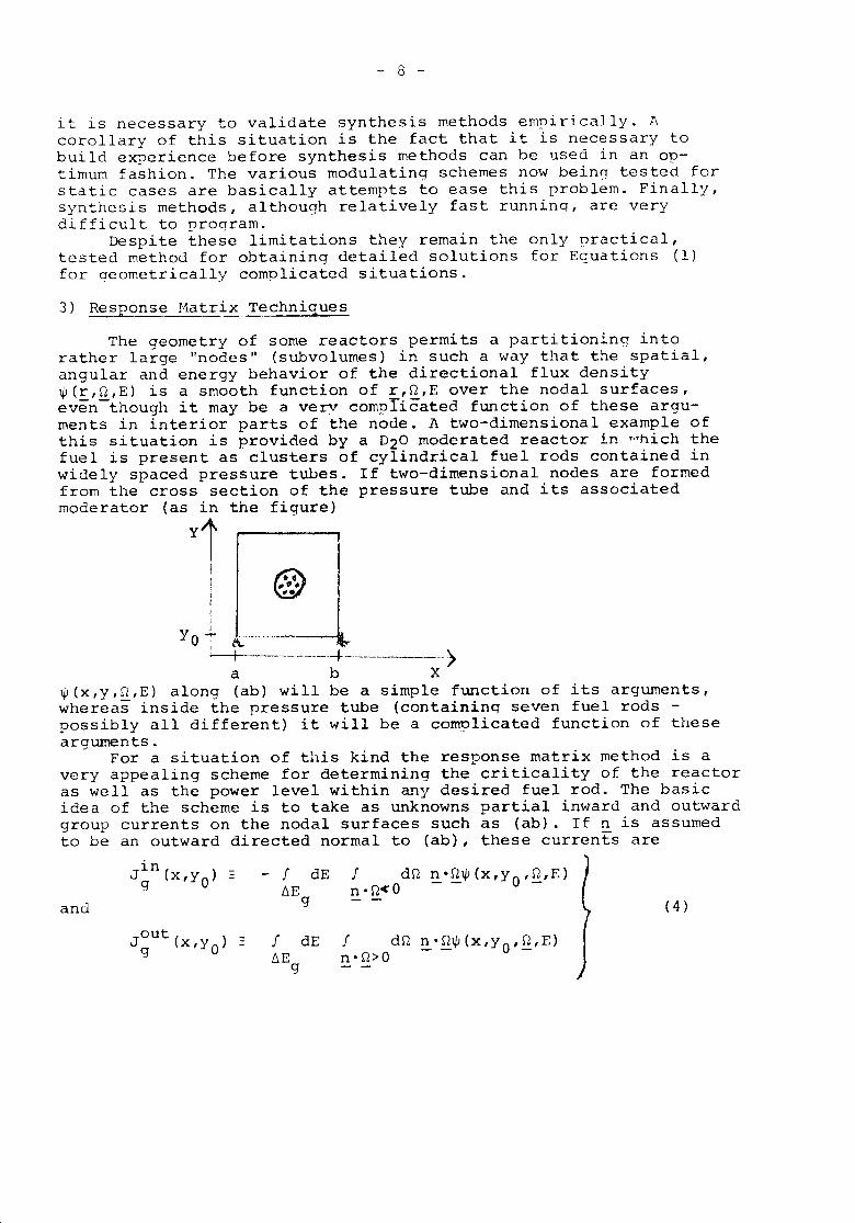
The geometry of some reactors permits a partitioning intorather large "nodes II (subvolumes) in such a way that the spatial,angular and energy behavior of the directional flux density~(r,~,E) is a smooth function of r,~,E over the nodal surfaces,even-though it may be a verv complicated function of these argu-ments in interior parts of the node. A two-dimensional example ofthis situation is provided by a D20 moderated reactor in ~hich thefuel is present as clusters of cylindrical fuel rods contained inwidely spaced pressure tubes. If two-dimensional nodes are formedfrom the cross section of the pressure tube and its associatedmoderator (as in the figure)Yl
i I) @.
YO';' I\:_.-=-1,I .....-.--- ...-+-.------- ..>a b X
~(x,y,~,E) along (ab) will be a simple function of its arguments,whereas inside the pressure tube (containing seven fuel rods -possibly all different) it will be a complicated function of thesearguments.
For a situation of this kind the response matrix method is avery appealing scheme for determining the criticality of the reactoras well as the power level within any desired fuel rod. The basicidea of the scheme is to take as unknowns partial inward and outwardgroup currents on the nodal surfaces such as (ab). If n is assumedto be an outward directed normal to (ab), these currents are
in f dE f d~ ~.~~ (x,yO,g,E)J (x,yO) -g tiE n .r2<Oand g (4 )
out f dE f d~ ~.g~(x'YO,g,E)Jg (x,yO) -tiE n.~>O
9
- 9 -
If, further, one assumes that the X-dependence of thesepartial currents has some simple mathematical form, the unknownsbecome the parameters that specify this form. Thus, if it isassumed that Jg1n(x,yO) and Jgout(x,yo) are linear functions of x,th~ unknowns of the problem become Jgln(x~,yO)' J out(x~,yO)'Jgln(xf),yO) and JaoU~(xb'YO) where superscripts (+ an8 -) mean,for example, that~J In(x+,yO) is the inward, group-g partial _current across (ab)gjustato the right of point (a,yO). (J~n(xa'YO)belongs to the node to the left of the one in the flqure andneed not necessarily equal Jqln(x~,yo).)
For each different kind-of node making up the overall reactorthe output currents from all faces and for all energy groups dueto a given, group, unit input current along (ab) can be determinedby solving auxiliary problems for the node isolated in a vacuum.Methods ranging in sophistication from Monte Carlo to few groupdiffusion theory may be used for these auxiliary computations asthe complexity of the problem demands. Assumptions about the angu-lar and energy shape of the incoming neutrons (as well as thespatial shape mentioned above) must be mane in performina thesecalculations, and the resultant output currents must be fit to theseassumed shapes. It is for this reason that ~(r,~,E) must be asmooth function of its arguments over the nodal-surfaces. (O~,if not simple, it must be known fairly accurately.) Otherwise onemust decompose the incoming and corres})onding outgoinG currentsinto more com~onent space, angular or enerqy shapes and do manvmore auxiliary problems in order to determine all output componentsfor each input component. ---
When the auxiliary computations are aone, it is possible toexpress a given outgoing partial current across a surfnce such as(ab) as a linear combination of all input partial currents tothe node for which (ab) is a surface. Since the output partialcurrent across (ab) is the input partial current for the adjacentnode, a matrix relationship inv?lving only input ~artial currentscan be constructed. Thus, if [Jln] is a column vector of allnodal-incoming partial currents for all energy qroups, we may con-struct an equation
(5 )
where [R] is the response matrix for the reactor, its elementsbeing computed by performing the auxiliary computations just des-cribed. The scalar quantity y is an eigenvalue that will be unityif the reactor is critical.
The same auxiliary calculations used to determine the ele~entsof [R] can be made to generate extra response matrices that,allowvarious reaction rates within a node to be computed once [Jln] isknown. Thus the method can yield both criticality and power distri-butions that are as detailed as desired.
For static problems sophisticated methods for deterr.ininoresponse matrices have been used for thermal heavy water reactors [8]and for fast reactors [9]. Results have been very encouraoino. AtMIT we have been looking at applications to light water ~oderatedthermal reactors [10] but with the response matrices (for hetero-geneous nodes containinG cross shaped control rods or water 1101e5)
- 10 -
(6 )in[R (t,T )] [J (T)]dT
t[Jln(t)]=!
COl'll1utCC:only by (~iffusion theory. Again results are veryer:couraging.
~he extension of the response matrix technique to transientsituations (11] is in principle strai0htfor~ard. One merely definesa tine dependent respoDse matrix (R(t,T)] giving the incomingcurrents at time t, [Jln(t)] in terms of the incominq currents attir.1c T :
In practice the determination of [R(t,T)] and the solution of~q. (6) is very complicated, particularly if delayed neutron andfeedback effects are considered. The strategy that is being exploredto overcome these difficulties at the Savannah River Laboratory [12]and at ~IT is to separate prompt and delayed neutron effects bytreating the population of delayed precursors within a node as anindependent variable. ~atrices specifying the creation rates ofdelayed precursors within a node due to unit incoming currentsacross the nodal surfaces and matrices specifying outgoing neutroncurrents due to decay of an average precursor are thus computed.These matrices are assumed to depend on the instantaneous pJ1"sicalcharacteristics of the node. Thus Eg. (6) will be approximated by
. t . t[Jl!1(t)] = J [f\ (t,T) ] [JIn (T) ]d T + J [E (t,T) ]2: A. [C. (T)]d T (7)
-- co P _ co illwhere [R (t,T)] is a reSDonse matrix analogous to [~(t,T)] but withall neut~ons emitted by the precursors that have been created byneutrons belongiT'g to [,}In(T)] omitted; [Ci (T)] is a column vectorof the total numJJer of group-i p-r:-ecursorspresent in the variousnodes of the reactor at time T, and [E(t,T)] is a matrix giving theincoming partial currents at time t throuqh the faces of all thenodes of the reactor due to emissions of delayed neutrons at time Tin the various :lodes. .I\q ain, if the dela'..'ec1neutrons emitted bythe [ei] themselves create delayed precursors, any neutrons emittedfrom these secondary precursors and s~)seauently crossina a nodalface are not accounted for by [E(t,T)]. Thus, for a fixed t, thedependency of the elements of both [Rp(t,T)] and [E(t,T)] on T isa very fast decaying function of (T-t). As a result it is a goodapproximation to use the values of these matrices appropriate totime t .'loreover, since the matrix elements of (Rp (t-T)] and[L(t,T)] are very small except for T close to t, it may be permis-sible for relatively slow t~ansients to approximate [Jln(T)] andthe (Ci(T)] in E'J.(7) by pln(t)] and the [Ci(t)). Then Eg. (7)!:Jecomes
[RST(t)] [Jin(t)] + [EST(t)]L:A. [C. (t)]P ill ( 8)
ST STHhcre [R (t)] and [r: (t)] are the static matrices apT'ropriateto the r2actor at time t and related to the corresoondinq timedenendent matrices by
(10 )
- 11 -
[RST(t»)t }- f [R (t,T))dT
P _00 P
[EST (t))t (9 )
- f [E(t,T»)dT-00
The response matrix technique shows promise of beina ableto deal practically with time dependent problems of considerableqeometrical complexity. Horeover, it is not restricted to a dif-fusion theory model. Its continued study therefore seems very"lOrthwhiIe.4) The Determination of Homogenized Group Diffusion Parameters
Synthesis and response matrix methods make it possible topredict the criticality and power distribution of geometricallycomplex reactors for which detailed finite difference solutionsof Eqs. (1) are impractical to obtain. There is another, much morecommon class of methods for dealing with such problems, the commonfeature of the class being that the behavior of heterogeneous nodes,containing possibly several zones of enrichment, lumps ~~ hurnablepoison, control rods or water holes, is represented by equivalenthomogenized group diffusion theory parameters, spatially constantover the entire node. A very common method for determining suchparameters is to compute detailed group flux shapes ~q(~) (~)throughout the node using zero current boundary conditions on thenodal surfaces and representing all material compositions in thenode explicitly. An equivalent parameter such as rfq, the homo-genized fission cross section for group-g is then defined as
(c)fnode ~fg(£)~g (~)dv
f <p (c) (r)dvnode g -where ~f (~) is the spatially dependent fission cross section forgroup-g gorresponding to the true enrichIT'entsand loading patternwithin the node.
(c)This is an appealing procedure since, if the difference between~Q (~) and the "true" detailed flux ~g(~) throughout the node(l.e, the one corresponding to a full core solution and thus to
non-zero-current boundary conditions) is disregarded, the ratio ofgroup reaction rates determined when the homogenized parametersare used (along wi~h ~he ~lux $q(~) res~lting from such use) ,willbe correct. Thus, 1f ~ag 1S the-homogen1zed, group-g absorpt10ncross section, we have
f fnode agf node ffg
$ (r)dvg --.-
$ (r)dvg -
= f node ~a~(~).!9.(c) (~)dvf d ~f (r)ep (c) (r)dvno e g - q -
(11)
- 12 -
Unfortunatelv there is no quarantee that an individual reac-tion ~ate such as~fnoneffg~g(£)dv will equal !nod~Lfg(£)~q(£)dv.!:quallty can be forced for one node by normall.zatl.onof~a(r). However the normalization of the flux will then be fixedfor-other grou!Js and other nodes, and the desired equality may belost.
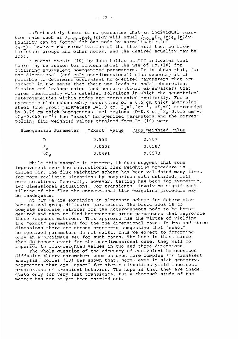
~ recent thesis [10] by John Kollas at MIT indicates thatthere may be reason for concern about the use of Eq. (10) forobtaining e0uivalent ho~ogenized parameters. It is shown that, forone-dimensional (and only one-dimensional) slab geometry it ispossible to determine equivalent homogenized parameters that are"exact" in the sense that their use leads to nonal absorption,fission and leakage rates (and hence critical eigenvalues) thatagree identically with detailed solutions in which the geometricalheterogeneities within nodes are represented explicitly. For asymmetric slab subassembly consisting of a 0.5 em thick absorbingsheet (one group parameters D=l.O em, La=l.Ocm-l, VLf=O) surroundedby 3.75 em thick homogeneous fuel regions (D=0.8 em, La=0.015 em-I,VLf=O.060 em-I) the "exact" homogenized paraJT\etersand the corres-ponding flux-weighted values obtainen from Eg. (10) were
Homogenized.Parame~ "Exact" Value Flux ~.veighte~ual u.::0.8070.05870.0573
0.5530.05020.0491
D
LavLf
While this example is extreme, it does suggest that Someimprovement over the conventional flux weighting nrocedure iscalled for. The flux Heiqhting scheme has been valida.ted many timesfor more realistic situations by cOJT\parisonwith detailed, fullcore solutions. Generally, however, testing has been for symmetric,two-dimensional situations. For transients involvinq significanttilting of the flux the conventional flux weightinq procedure maybe inadequate.
At MIT we are examining an alternate scheme for 0etermininahomogenized group diffusion paraMeters. The basic idea is tocom~ute response matrices for the heterogeneous node to be homo-genized and then to find homogeneous qroun parameters that reproducethese response matrices. This approach has the virtue of yieldingthe "exact" parameters for the one-dimensional case. In two and threedimensions there are strong arguments suggesting that "exact"homogenized parameters do not exist. Thus we expect to determineonly an approximate set for such cases. The hope is that, sincethey do become exact for the one-dimensional case, they will besuperior to flux-weighted values in two and three dimensions.
The whole question of the adequacy of equivalent homogenizeddiffusion theory parameters becomes even more complex ~0r transientanalysis. Kallas [10] has shown that, here, even in slab qeometry,)'arameters that are "exact" for static situations yield incorrectprecictions of transient behavior. The hope is that they are inade-~uate only for very fast transients. But a thorough studY of thematter has not as yet been carried out.
- 13 -
5) Methods For Predicting Flux Behavior in F~actor Composed ofLa:r;~~lo~ogeneoE __~__(or Homogenized) Nodes
If the methods just discussed for finding equivalent homo-genized parameters are successful, or if it turns out that fluxweighted parameters are adequate for cases of practical interest,the solution of Egs. (I) becomes much more simple since many fewermesh points are needed to describe geometrical details of the reac-tor. 'Under these circumstances! a spatial finite di fferencesolution of Eqs. (I), while quite possible, may be unnecessarilyexpensive. A number of alternative procedures are currently beinginvestigated. These fall roughly into two categories: higher orderdifference equation methods and nodal coupling schemes.
To the first category belong the finite element methods [13J,the scheme of Robinson and Eckard [14J and the method of Antono-poulos described in Reference [15J (although the latter two mightbe viewed as nodal coupling schemes). To date only the first ofthese methods has been extended to treat transient situations. Fora given degree of accuracy it appears to be faster than a standardfinite difference solution [16J. But, although there a~e ~~nyfewer unknowns in a given problem the equations determining themhave a higher de~ree of coupling. Thus the gain in running time isas yet not so great as had been hoped ori~inally,
One attractive feature of finite element schemes should benoted. They are not restricted to completely homogeneous rrodalcompositions [17]. Mild heterogeneities, such as different zonesof enrichment or non-uniform fuel loading due to depletion effectscan be accomodated.
The other two higher order difference equations mentionedhave fewer unknowns. ~10reover the difference equations which resulthave the same forn as the standard finite difference equationsexcept that the coefficients in the flux eauations depend on theflux values at ~revious time steps. Thus they should be much faster.However their tilT'.edeT)endent extensions have not yet been tested.Moreover, the Robinson and Eckard scheme is restricted to one-energy group, and, although an extension of the Antonopoulos schemeto two groups has been worked out theoretically, it has not vetbeen tested even for static cases.
The notion of nodal cou~ling schemes is essentially to dealwith nodal averaged or center roint qroup-fluxes as unknowns andto express the group currents across nocal interfaces in terms ofthese fluxes. They are discussed in a general way in R.eference [15],and References [18-22] deal with specific examples as applied tostatic situations. The recent extension of the method of Birkhofferand Werner to time-dependent situations [23] appears to be a parti-cularly attractive approach. Like the finite element method, itappears to be able to accomodate IT'ildheterogeneities iM the materialcompositions of the nodes. It is not restricted to one-grou~ nro-blems. However, it involves difference equations that have the saP1enon-linear form as those encountered by Robinson and Eckard. Thusit shows real promise of being both accurate and fast-running.
- 14 -
6) '!'I..1..e.. Use of ~~un<!ary Conditions to Eeplace Reflectors
Explicitly representing the reflector when solving theqroup diffusion equations for a reactor adds considerably to thecost of the calculation. This is particularly true if the reflectoris light water and there is no core baffle, for then, rather smallmesh spacings must be used in the reflector or else returninqneutron currents will not be correctly described with the resultthat criticality and the relative power level at the center of thereactor may be poorly estimated.
The one-group nodal code FLARE [18] and the code embodyingthe Robinson and Eckard scheme circumvent this difficulty by usingalbedo type boundary conditions relating flux to current over thesurface of the reactor. The required flux-to-current ratios arespecified as input and determined empirically by comparison withexperiment or with more detailed, few group calculations. Generallythe flux-to-current ratio is taken to be some constant averagevalue over the entire interface between the core and the reflector.
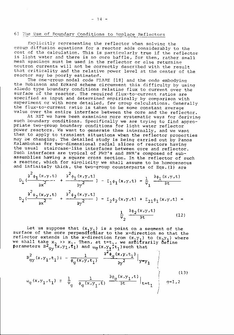
At HIT we have been examining more systematic ways for derivingsuch boundary conditions. Specifically we are trying to find appro-priate two-group boundary conditions for light water reflectorpower reactors. We want to generate them internally, and we wantthem to apply to transient situations when the reflector propertiesmay be changing. The detailed study is being carried out by PanosKalambokas for two-dimensional radial slices of reactors havingthe usual staircase-like interfaces between core and reflector.Such interfaces are typical of PWR's and BWR's composed of sub-assemblies having a square cross section. In the reflector of sucha reactor, which for sir'plicit~/ we shall assume to be homogeneousand infinitely thick, the two-gr.oup counterparts of Eqs. (1) are
2a <Pl(x,y,t)DI ( 2
ax2a cP2(x,y,t)
D2 ( 2ax
2a 1>1(x,y,t)+ 2)ay
2a <P2(x,y,t)+ 2)
dY
1 alfl2(x,y,t)V2 at (12 )
Let us suppose that (x Y ) is a point on a segment of thesurface of the core perpendtcnlar to the x-direction so that thereflector extends in the x-direction from (xJYI) to (x2Yt) wherewe shall take x2 » xl. Then, at t=tl, we ar~ierarily aefineparameters B2g ,x'YI,el) and Wg(x,y1,t1)such that
Y 2 )2 1 a <p (x,y,tl) IB (x, Y , t ):: - ( ) 9 Jgy 1 1 1>9 x, Y ,t1 cy 2 y=y 1 .
1vg
(13 )
q=1,2
- 15 -
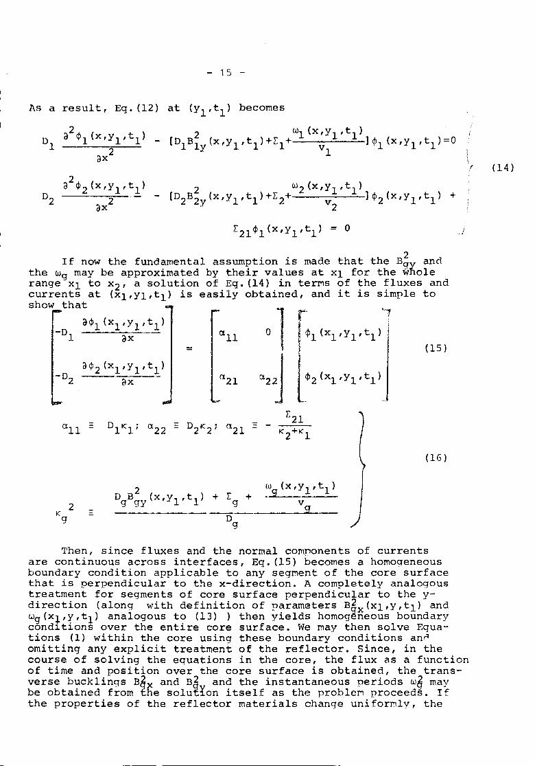
As a result, Eq. (12) at (yl,tl) becomes
2 wI (x, Y1 ' t 1 ) _- [DIBly(x'Yl,tl)+Ll+ vI ]$1 (x,yl,tl)-O i
~( (14)
(15)
.....,r14>1(xl'Yl ,tl)
it$2<X1'Y1.t11
L21K2+K1
-D3$1 (xl'Yl,tl)--------1 ax
=
-DacJl2(xl,yl,tl)
.-2 ax
If now the fundamental assumption is made that the B~ andthe wg may be approximated by their values at xl for the wholerange Xl to x2' a solution of Eq. (14) in terms of the fluxes andcurrents at (xl,Yl,tl) is easily obtained, and it is simple toshow that
(16)
2Kg
2D B (x,yl,tl) + L +g gy g
og
W9 (x ,Yl' t 1)v
9
'I'hen,since fluxes and the normal components of currentsare continuous across interfaces, Eq. (15) becomes a homogeneousboundary condition applicable to any segment of the core surfacethat is perpendicular to the x-direction. A completely analogoustreatment for segments of core surface perpendicular to the y-direction (along with definition of parameters B2x(Xl,y,tl) andWg(x~,y,tl) analogous to (13) ) then yields homog~neous boundarycond~tions over the entire core surface. We may then solve Equa-tions (1) within the core using these boundary conditions an0omitting any explicit treatment of the reflector. Since, in thecourse of solving the equations in the core, the flux as a functionof time and position over the core surface is obtained, the trans-verse buck lings B~x and n2 and the instantaneous periods w~ maybe obtained from the solu~ron itself as the problem proceeds. Ifthe properties of the reflector materials change uniformly, the
- 1G -
effect can be accounted for bv changing the Dq, Lq and ~2l inthe fornulas (16). If the changes are not unifor~; the reflectorcan be partitioned into reaions and Eq. (16) generalized so thatthe a's are found for a nultislab reflector. The generalization isstraiqhtforward although it does lead to complicated algebraicfor~ulas for the a's.
The accuracy of this procedure for replacing explicit con-sideration of a reflector by boundary conditions at the coresurface depends on the maqnitudes of the DqB~X' DqB~y and wg/vacompared to the Lg and, if they are not snaIl, on the validltyof replacing values of these parameters throughout the reflectorby values on the surface of the core. For light water reflectors(or steel-water mixtures) the wg/vq will be negligible for all butthe most extreme transients. Moreover, since the linear segmentsmaking up the perimeter of a radial slice of a liqht water powerreactor are about 20 cm in length, we expect the B2 and B2 tobe small except near corners ",here two segments jo<tfi(form~~g a90° angle facing either the reflector or the core material) .
Nu~erical testina of the method to date has been sufficientlyencouraging that we are incorporating the boundary conditions (15)(along with the capability for treating jaggen outer boundaries)into a three-di~ensional, transient code being developed for theelectric utility industry.
- 17 -
References. -
1. A. F. Henry, "Review of Computational Methods for Space-Dependent Kinetics", p. 9 of "Dynamics of Nuclear Systems",D. L. Hetrick, editor, Univ. of Ariz. Press, 1972.
2. "Space-Time Methods for Movable Fuel Problems", J. B. Yasinskyand L. R. Foulke, p. 467 of "Dynamics of Nuclear Systems",D. L. Hetrick, editor, Univ. of Ariz. Press, 1972.
3. D. Struwe, "A Two-Dimensional Model for Fast Reactor KineticsAnalysis with Space Dependent Feedback", p. 237, SoaceDependent Reactor Dynamics, EUR 4731f-e Ispra (1970).
4. J. B. Yasinsky and S. Kaplan, "Synthesis of Three DimensionalFlux Shapes Using Discontinuous Sets of Trial Functions",Nuc. Sci. Eng. 25, 426 (1967).
5. E. L. Wachspress, R. D. Burgess and S. Baron, "MultichannelFlux Synthesis", Nuc. Sci. Eng. ,;L2,381 (1962).
6. C. H. Adams and W. M. Stacey, Jr., "Flux Synthesis Calculationsfor Fast Reactors", Nuc. Sci. Eng. 54..,201 (1974).
7. P. G. Bailey and A. F. Henry, "A Consistent Coarse-MeshHomogenization Procedure", Trans. Amer. Nuc. Soc. 15, 283 (1972).
8. R. J. Pryor and ~'. E. Graves, "Response ~:atrix Method forTreating Reactor Ca' roll1ations",p. VII-179, "~tathematica1Models and Computational Techniques for Analysis of NuclearSystems ". CONF 730414-P2, Ann Arbor, Mich. 1973.
9. H. S. Bailey, "Response Matrix For Fast Reactors", P. VII-187"Mathematical !1ode1s cmd Computational Techniaues for Analysisof Nuclear Systems", CONF 730414-P2, Ann Arbor, Mich. 1973.
10. J. G. Kallas, "An Investigation of the Equivalent DiffusionTheory Constants ~ethod and the Response Matrix Method forCriticality Calculations", Phn Thesis, NIT (1974).
11. J. M. Sicilian and l\. Leonard, "A Pcsponse "1atrix r~ethod forSpace-Dependent Nuclear Reactor Kinetics Calculations", Trans.Amer. Nuc. Soc. 17, 252 (1973).
12. R. J. Pryor, Amer. Nuc. Soc. Topical Meeting, Atlanta (1~74)to be published.
13. C. H. Kanq and K. P. Hansen, "Finite Element Metho~c: forReactor Analysis", Nuc. Sci. Enq. 51, 456 (1973).
14. C. P. Robinson and J. D. Eckard, Jr., "A Higher Order DifferenceMethod for Diffusion Theory", Trans. Amer. Nuc. Soc. ~, 297(1972) .
- 18 -
15. 1\. F. Henry, "Pefinements In Accuracy of Coarse-Mesh Finite-Difference Solutions of the ~roup Diffusion Equations", p. 447"Numerical Reactor Calculations", IAEA, vienna (1972).
16. D. K. Ferguson and K. F. Hansen, "Solutions of the SpaceDependent Reactor Kinetics Equations in Three Dimensions",Nuc. Sci. Eng. 51, 189 (1973).
17. L. O. Deppe and K. F. Hansen, "Application of the FiniteElement Method to Two-Dimensional Diffusion Problems", Nuc.Sci. Eng. ~, 456 (1974).
18. D. L. Delp et al., "Flare, A Three Dimensional BoilingHater Reactor Simulation", GEAP-4598, General Electric Co.(1964).
19. L. Goldstein, F. Nakache and A. Varas, "Calculation of FuelCycle Burning and Power Distribution of Dresden-l Reactor withthe Trilux Fuel .~~anagementProqram", Trans. AJTler.Nuc. Soc.!Q, 300 (1967).
20. A. O. Krumbein, J. D. Luoma, S. J. Rafferty, "An IndependentNuclear Analysis of the La Grosse BWR", Trans. Amer. Nuc.Soc. !.~, 232 (1970).
21. P. T. Choong and H. Soodak, "Heterogeneous Treatment of FuelAssembly Boundaries in Nodal Diffusion Calculations", Trans.Amer. Nuc. Soc. 14, 650 (1971).
22. S. Borresen, "1\ Simplified Coarse-Mesh, Three-DimensionalDiffusion Scheme for Calculating the Gross Po~rer Distributionin a Boiling v7ater Reactor", Nuc. ScL Eng. !i, 37 (1971).
23. A. Birkhofer, S. Langenbuch and W. Werner, "Coarse MeshMethod for Space-Time Kinetics", Trans. Amer. Nuc. Sci. 18,153 (1974).
- 19 -
DISCUSSION
J.J. Dorning
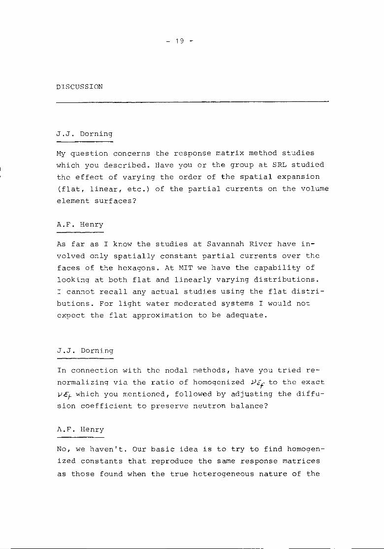
My question concerns the response matrix method studieswhich you described. Have you or the group at SRL studiedthe effect of varying the order of the spatial expansion(flat, linear, etc.) of the partial currents on the volumeelement surfaces?
A.F. Henry
As far as I know the studies at Savannah River have in-volved only spatially constant partial currents over thefaces of the hexagons. At MIT we have the capability oflooking at both flat and linearly varying distributions.I cannot recall any actual studies using the flat distri-butions. For light water moderated systems I would notexpect the flat approximation to be adequate.
J.J. Dorning
In connection with the nodal methods, have you tried re-normalizing via the ratio of homogenized VEf to the exactvCr which you mentioned, followed by adjusting the diffu-sion coefficient to preserve neutron balance?
A.F. Henry
No, we haven't. Our basic idea is to try to find homogen-ized constants that reproduce the same response matricesas those found when the true heterogeneous nature of the
- 20 -
region being homogenized is explicitly accounted for. Wehave so far stuck closely to the one criterion.
J.J. Dorning
How are you "matching" your coarse representation and finerepresentation response matrices?
A.F. Henry
We average absorption, fission and removal constants overthe detailed fluxes found when the heterogeneous problemsare run to obtain the "exact" response matrices. Then weadjust the (two group) homogenized diffusion constants un-til the matrices are produced when these homogenized para-meters are used to determine response matrices.
H. Klisters
From the various methods you have outlined as possibili-ties to achieve better efficiency in 3d calculations, whatwould be the favourable one in your opinion?
A.F. Henry
In my opinion, syntheses methods provide the most accurate,feasible procedures for determining detailed flux behaviourwhen geometrical structure is represented explicitly. Theyare fast-running and I believe, with further development,they can be made accurate. Their main drawback is of coursethe fact that they can provide no accurate measure of theirown error, but I believe that, with experience, we couldlive with that drawback.
- 21 -
J. Devooght / E. Mund
A - STABLE ALGORITHMS FOR NEUTRON KINETICS
Universite Libre de Bruxelles / Charge de recherches FNRS,Belgium

- 23 -
ABSTRACT
Benchmark problems are interesting not only as a common meetingground of different numerical algorithms but as a mean to check theirsoundness or conformity to the underlying theury, if any. Althoughsome numerical algorithms devised to integrate the ,:.;pacedependentkinetics are well founded, others are on a more shaky ground and there-fore not conlpletely trustworthy_ On the other hand, numerical schemeswith a theoretical small truncation error may not always fare <:lS \"011as they are supposed to. The first part of this paper deals witll som~general features of a space dependent kinetics code, stressing theproperties of A-stability and spectral matchillg. The second part sum-l1larizes the main characteristics of a new A-stable al~1;orithllltll.3.ti::;fl exi ble enough and encompa sse s many exi st ing s chet:;e~ _ Some ex tr3po.,lation procedures are discussed. A Newton series int8rJ)olation witha permanence property is introduced. The third part, finally, descri-be s two numeri cal appli ca tions of the W 11 (u I u l'u2) tirilC-inte gra t iOll
scheme and their related conclusions.
- 24 -
------_._------------------_ ...._-------1.1. Introduction
Pcin-L 1~i.n..,tics is a very simple problem, conrpu ta t ionally speaking,
co 1TIP i.\J. (;d t 0 spa cc de pen den t k i.net i.c oS, e s pee i a 11 y :2 Dan d 3 f). I tis
hard,) y nec~~3sary to improve method", as fur as point kinetics alone
is concerr,cdl considering the very small cornp1..,ting time. Ho,,,ever
some methods used ca.n be extcnded readily to space dependent kine-
tics (most of them not) and therefore it is useful to improve the
computing effj.c:;ency: lengthening of time steps, memory and c,yr.e
storage ete •.• I'lorcover some methods like the quasistatic method
rely on the frequent solution of a point l{inatics problem and the
infrequent solution - which means ",ith large time steps - of a
spilce dependent problem. It is SOITIC titlle argued th&t it is unncccs ...
l:;~~ry to extend the time step because in some reactor dynamics 1:ro ..
blems the time needed for the comput.ation of the thermohydraulic
feedback is the cOlllmanding :factor. F'irs t, it shculd be kept in I,,:i.nd
t.hat as long as neui.ronics is not a negligible part of the proble!:l,
the le}J~~th('ning of' the til!1C step is not unwarranted. Second, any
to chni qu e tha t a 110'''s a lengtheni ng of the time step can like ly be
applied ClJSO to the thcrtllol1yc1raulic vari,.1Jles.
1.:,~. Limits to time step lengthening
There are three main obstacles to the step lengthening in thodY.(t)
int(~gration of the initial. value problem ut = A(t) 'y'(t) (1.1)
a. tho glohi"ll accuracy limitation
b. the non-constancy of the operator A(t) which yields u:'iu;..\lly
a local t;'uncatioll error 0(h3)
c. the non--col1llJlutation of the Gperators when they are sJ,littcd,
1i1((; the ,\0:1 lJIethods i.'or 2D dnd 3D.
SOllie Illetbous h~\ve all l:i.I!J.iL;\tion~i. some on.ly the first two. As f[.r
as W(~ n:ra aW;\I~t' there i.~i yet no C(JlIIJ,Jet(\ illl;d.ysi.s for neutron killc-
tics of' the three pI'oblf\I:l:i. 11. h ..,:; been rcc(l~';ni zed ror a long tilllf'
Uli1tow i n g t 0 tll e .'3 t i :f f n iIt \l reo r tile e qUit t i 0 11S (i. t>. 1it r g e .s p r ('. :J
- 25 -
in the eigenvalues or i\), the time 1'ltcpshould be small i'or ~',l-JOjt
time s and pre SUllld bly long in Uw a symp to tic range, if any. TIle nr~ cdfor an adaptative meth.od that yields the optimal time step cOlllr:1tib!';with a given global accuracy is as great as ever ~inc8 u~Jy rule~of thumb are availuble. Error :llonitorir~g should tal(e into account 8,11three types of error. Up to now, authors have been satisfied byerrors of type 2 of order no less tban errors 01 typ~ 1, for whichthere is usually a qualitative knowledge, i.e. the ahsolute trunca-tion error is bounded by Chn• The order n is known but C is generallyunknown. The ambiguity resulting thereof will be shown in a laterparagraph.
1.3. One step method und rational approximations
We are int8rested in point kinetics problems to the extent thutmethods are transposable to space dependent problems. Aside fromthe problem 01 computin~ time, the most pressing problem is memorystorage ",hicll can be troublesome even for 2D-multigrollp problems.Therefore multistep methods arc almost automatically excluded, ex-cept maybe two-step methods. The restriction is severe lor integralformulation of tIle kinetics problems which need more than two puintsfor the quadrature. Since any interl)olatory quadrature method isbased on an assunlption for the integrand behaviour, u5ually the flux,the accuracy can be improved by a judicious choice of the assumedtime dependence, like for instance exponential behaviour. lIolI'cverthe accuracy is mostly dependent upon the number 01 points !:or agiven time step and the simplest scheme is given by
N(t) - N(o) f1(t) + NOd f2(t) (1.2)
with
f, (0) = 0i1 f, (h) -- J , ,)~ 1 1w
Introducing (1.2) into N(h)_N(O)=jh 1\(8) N(s) ds yields csselltiaUy
a scheme of the Crank-Nicolson 0 (or jJi\d(~11) ramily. Iligherorder schemes based on morc thCln two points quadrnture yield simi-l.:\rly higher or<1<:.:rPild(~npproxim;\tiol1s or ,Il;encril]ization~ 11If,.!'.~()f.
C(l n r 1u e n t poi Jl t 3 yi e 1d II(' r II Ii_ t e i n t e r J> (l L\ t i on. l-Ioreo vel' i L j.s h n u '" 11
thdt Illethods lil<..e CO]IOCiltioJ'l, Cii11erJcin iI/ld interj1olatory qUildrilLul":
- 26 -
arc idl cquivd.1(,nt C1J . .':iilJiililrly hT~IGIIT [2J has shown the .equivd-
1e tI C e 1J e (;'"e ('1\ C 0 .U 0 C i\ t J_ 0 n an duo; ub C 1ass 0 f i rnp1i c i t Hun .s .:.J. _ Ku L t u
method:.;. LiUTCilFH, I~IILE, CIIJ'pj\i:\N, AXELSSONhave shown that various
lH~ll l\ncnm q\lddrature scheme.", J.il<:e Giluss-Legendre, .l<u.dau, Lobatto,
led to PiICie: "pproxillliHlt;,; (d' orde~' (Il,ll), (n,n-1) and (n,n-:::) [3,/l:,5,G],
Hec i pro calI y GEAH h d S S110 l"11 t h d t it ny r L\ t :.!. ~) n a 1 a ppro xi mat ion ~ ~~ ~ wher e
the n poles "re distinct and the degree of P ~ degree of Q (.:; n) is
equi va len t to an impl i c i t Hunge -KlJ t t<.l scheme [7 J . Two point Hermi to
interpoliltions have also been used to generate rational approximutions.
It can therefore be asserted that in spite of appearances all me-
thods of integration thilt do not splii operators based either on ra-
tional apl1roxililations or on the trQatment of integral (or ini.:egro-dil'-
fer e n t i a 1 ) for 1IlS 0 f 1.h e kin e tic s e qu iJ t ion s, by colI 0 cat ion 0 l' GE\ ], (. i ;:i r.
l\'cightin,(2;, arc alJb<.lsicDlly al:i.];.c. It is then sufficient to iIIV;;:,!.j ...h/\
g<.lte rational approxj.IJlations tc e ",here l\ is suitably def'ined • .su";c
investigations have started directly from that point of viel". Gran,-
A which is out of question forP(A). 1 t J '1Uw gl ves a mos a .,,,ays comp.C:x
i.1 .schetlle uf DA NOnr{EGJ\ illld I--IEr\~r~yr:.\."
Fil c taring
extending
ting that any inte~,;ration scheme of the h:inetics equation is es:-;en-. P(A)
t i a 11y a l' a t ion il 1 fun c t l 0 n QTi\T ()f r\, we i 111111ed i ate lye n c 0 un t er thE'
difficulty of evaluating powers of
spuce ricI'endent problclllS.
Illlr,ll,(:~cs. Although TTJni\.-\GE
hCl~:.shuHn ho'.,' to deal with such probl(~JlI ill the case of a multipoint
reactor, Li.~J IIwthod Ci\nllot be extended to full space dependent pro-
LIen:::; becausc of' the need of' explicitly inverting matrices [8]Therefor0, we are left either with first degree rational approxima-
t1.0113 (like P 11) or approxilliations which have real coefficients illid
ITIi..lYbe factori7.ed like all those resulting from extr<.1polation.
1.4. Equiv<.1lcnt constant operators
In the Cilse of time dependent operators we are lert yet with the
problem of' de:fining il suitable average operator. Although this can be
done rigorousIy by IlICi:lns or
N(h) ds +h fa-~f d ,," d'C [ 1\ ( .~ ) ,
o 0
A(O-)J + ••• J N(o) (1.3)
in practice A(t) w.ill be knowIl onty ill discrete timos, and an approxi-
Illate qUi~dr;,ture should be UE3ed. As il nll(~ the r.ir~t operiltor ill
- 27 -
h [brackets is approximated by ~ A(o)and the second is neglected.
1.5. Spectral matching
Many methods make assumptions, one way or another, about the fluxbehaviour. The flux is expressed as a linear combination of functionsof tinle. A popular choice of the basis is either a polynomial, or anexponential times a polynomial. The first choice is dictated by thevast literature on spline fUllctions. We believe however that polyno-mials are unsuitable for the description of transients with large \
5 1'.' t )steps and that a more natural choice is a basis of exponentials Ie 1 Jwere the ~. are close to the eigenvalues. With such a choice we lcnow "
1
le<lst then -when the operator A is constant- that the solution isexact when the initial vector belongs to the ~ubspace spanned by t!10
eigenvectors associated ,,,,iththe eigenvalues A .• This property of1
spectral matching is a very essential requirement for any method de-vised to cope with large time steps. On the contrary, polynoinialsbasis and the ensuing Pade approximations are founded implicitly ontll,]fDlsc assumption that all eigenvalues are zero.
1.6. A-stability
The stability of the integrating scheme is a neces.snry rCcilJ:ir'::i1i'C'Lt
for any proposed method. Lax equivalence tlleorem provides the neccs.sary link between stability, convergence ilnd consi~tence ( ~ ,- U I 1.. )c1r17'P' ) .(" .J
Although some schemes have been proved to be stable, some arc notarat be stun cer ta in. For s tiff sY s terns 1i1{ e the n eu tr 0 n i cs e (p.W t i ()11,;
an even strong;er condition is necessary, namely the ;\-sLI1:.2.l2-~ 01
Dahlquist, which is defined as follows [10J
rinito portiol\in a
Definition 1 a one step method I.. 1=w(,\h) 'to applied to the cqll;\---d',..-------- 1+ 1
tion dt =Ar is A-stable i:f£'Iw(Ald)~ 1 i'or He>.~ O.It is obvious that if the condition is valid onlyor He <.. 0 errors would !;row exponentinlly [or the eigenv(".ctul':-ii.lS.C.O-
eiated f'or instance with large vi\lues of \ 1\ hi. Some approxi::wtiollS
like the Cri\1lh-Nicolson ~:~~:j~are such Ulilt liin IW(\ldl::-: 1. This 1';IA hl-;!.co
- 28 _.
iHI iillportallt d(.':feci: ror Gtiff' syst(~!IlS or (and) large time steps, Ac-
cordingly, He have
U(' f i ni. t ion 2
when \ A h 1-:>00 for He 1\ <. o.Inif
the words of GEAR [11.J adrUle equation dt'= ),r,llIethnd is strongly (or stif:fly)
the rapidly decaying components
A-sL ..blc
~ 1 !S 0 d e c it y
rapidly in the numericLll approximations, so that it would not be ne-
cessary to use small steps even when the components were still present.
Any metllod supposed to deal efficiently with step lengthening jn stiff
syste:ns is bou~d to be A-stable. The nature of the space or energy dis-
cretization is not essential for the discussion, as long as the dis-
cretization of A is dissipative.
1.7. Sumlllary
To summarize, a sui table method for space drq)cndent reactor dyna-
mics must fulfill the following conditions
1. The algorithm must be consistent and convcr~ent which by Lax
the 0i'e:11 en sure s s tf} bi1:i ty:
~. Th e s y s t C III £j s t u die d be in g II S t iff' ", t 11e a I go r i t hm s 11au 1d be 110 t
only stable, but A-stf\1Jle (or A«(>()-stabJe [llJ ), in order to handle
correctly large time constants with nlcdiUlll to large fime steps.
:;;. Th e a ppro x i mat c sol uti 0 n s110111 d J) 0 s s i.b J Y con t a ins 0 1TIe e sse n t :i d J
chi.l: ;.Ictcrist:i cs of the exact solution, which can be done b',:8t by
s pee !T' i\ 1. 112ate 11 in g .
Ii. Th e r.1 0 Iw.l Po r r 0 r s h 0 u 1. d bee 011t r ()J 1e din 0 I' de r too b t a in a t a
given til1lC a st;:;.ted dccuracy with the miniIllum number of time step~.
The local error shoulll be decreased preferably without discarding
previous rl~slllti;, il requirement ,~hich points towards iterdtive metIJodf-'
with ,1 £..~~:..~n(:~ prop.'rty (see S;~.!i)
5. In order to 11:;ll:illlize memory requirements, the algori thm I11U.s t bt'
on('-.':~s.:, c.itl)(~r of' rit~,~t dq,re,:. or f';t(:::..l~2Ei~£:.!?le in first degree ra-
tioJld:1 opl~r"tor-villuerl functj on,<,. l~xtri\})() liltion is a possible method
ror both Ii illld 5: it fw!; ,,1150 the ditd::i.lJcl. ndvnni.ilge to USl; factori~~"d
apl,roxirn,,1'l;joJl,':; dnd t1llCre[ore IH;(:rl only to invert linear systems one "t
a t.i.rne without squ;ll',lng rnntri.ccs. Tlli.s is Ull: C,lSC for instance [or:
- 29 -1
h/\ 1hA
p(l)(hA) Ii + 7i 'I 1+ 2
= hA)... - ::> hA (1.4)
11 3 1 1- 7! - T
although, as will be seen in ~2.3, this approximation is not A-stable.
We close this paragraph with two general remarks
1. We do not refer to any explicit form of neutron kinetics equa-tions which are only supposed to be linear or linearized. However thequasistatic method which gives probably the most general and versatilealgorithm yields two systems of equations: "point kinetics" and "spf'tcekinetics" with a translated spectrum. (29] (30J
2. A COlllplete theory of the spectrum of the matrix A is lacking.However so:ne resu.lts, on parti cular case s obta ined by HENRY i2lj,"],FOULKE and GYFTOPOULOS [25J ' and PORSCHING ~6] sugge st th1.1t the e iiS'~Ji'"
valueD occur in I+G clusters (I precursors, G grou~ associated witheigenvectors of similar shape. Insofar as the stifrness of the matrixis involved in the algorithm described below, only order of magnitudesof tho eigenvalues (except for tile dominant one) are needed (see ~3.3)and the cluster assumption will be made.
- 30 -
2. •.• F J HoST OlUJEH A-STABlE ALGUHITilt-1 \111'11 SI'ECTRAL !'L\1'CHING
~.1. Introduction
ive shall, in this introductory })ii: ..ilgr(~i)h.; recall Game theoretical
prelill!inaries which 10rrn the busis o.f the present work. For the sLlkr::
01 concision, only the statements of the theorems will be given. For- .,further detnils, the readers are referred to ~12: 13J •
\IT,,' '" 1'0 il) t.eres::ed, genera 11 y speuking, by the cons true tion of ra-
tion<.',1 C1.pf),"oxilll<1tion~ \-J(u) of the complex function eU having the in-
{'terpolil-Licn r.rop(~rty at arbitrarily given points u. > i:::1, ••• ,n1,.)
whose moduli lwl , for stability reasons, satisfy the inequality
and
l\oJl~N< 1 in the open left half plane. Some fifty years ago, an
analog problem was formulated and solved by NEVANLINNA and SCHUH.!'lore precisely, given a real positive constant H and two sets of n
eo:nplcx values {zi~' i\V~0)1, i=1, ••• ,n the first of which is entir;::.v
10cdtul in the uni t disc I Z I ~ 1 , the following question was rdi;:,ed:
would it be pOSsible to find an analytic function W(z) -unique, if
any- huving its modulus less or equal t6 M in the unit disc and ta-
leing [1.L {zi} the corresponding values {,v~o},? The complete answer to
thi\t question as well as Schur-Nevanlinna's (SN) algorithm whjch glvss
the so lu tiol1 of the problem Inny be sumillar izcd in a few theorems s ta. tc;c;.
be J. 0 W [1 3 'i!--'
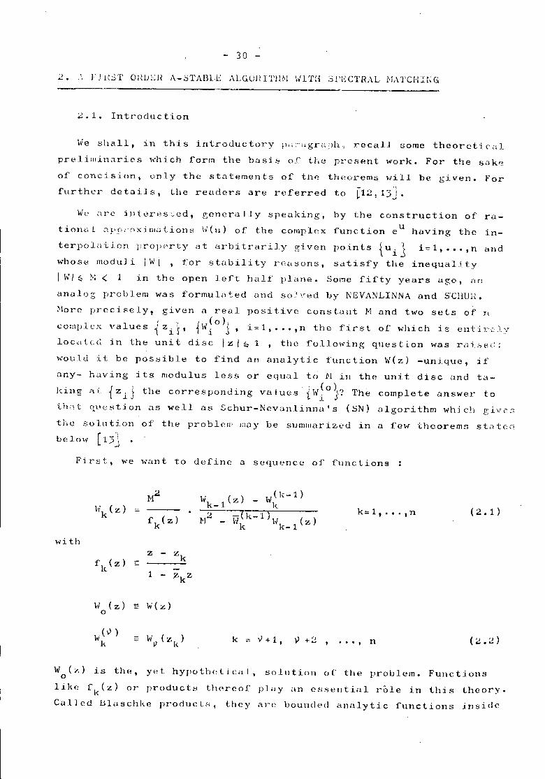
First, we wunt to define a sequence of functions
k = y + 1, V +2 , ••• , n
M2
"'k(z) =fk(z)
withZ - Z
fk(z) k-1 - .zkz
\V ( z ) e W(z)0
(v ),oJv(zl\.)W
k -
\oJ ( z) _ \oJ ( k ~1)k-l k
1"12 - W~ k'---1~)-,.,r-k-_-1-(Z-J-)k= 1, ••• , n (2.1)
W Cd is th(!, y(~t hypoth(d, leal, solution of the prol>1.em. Functionsolike lk(z) or productH tlwreol play an eSSclltial role in this theory.
Called IHuschke products, they are bounded analytic functions inside
- 31
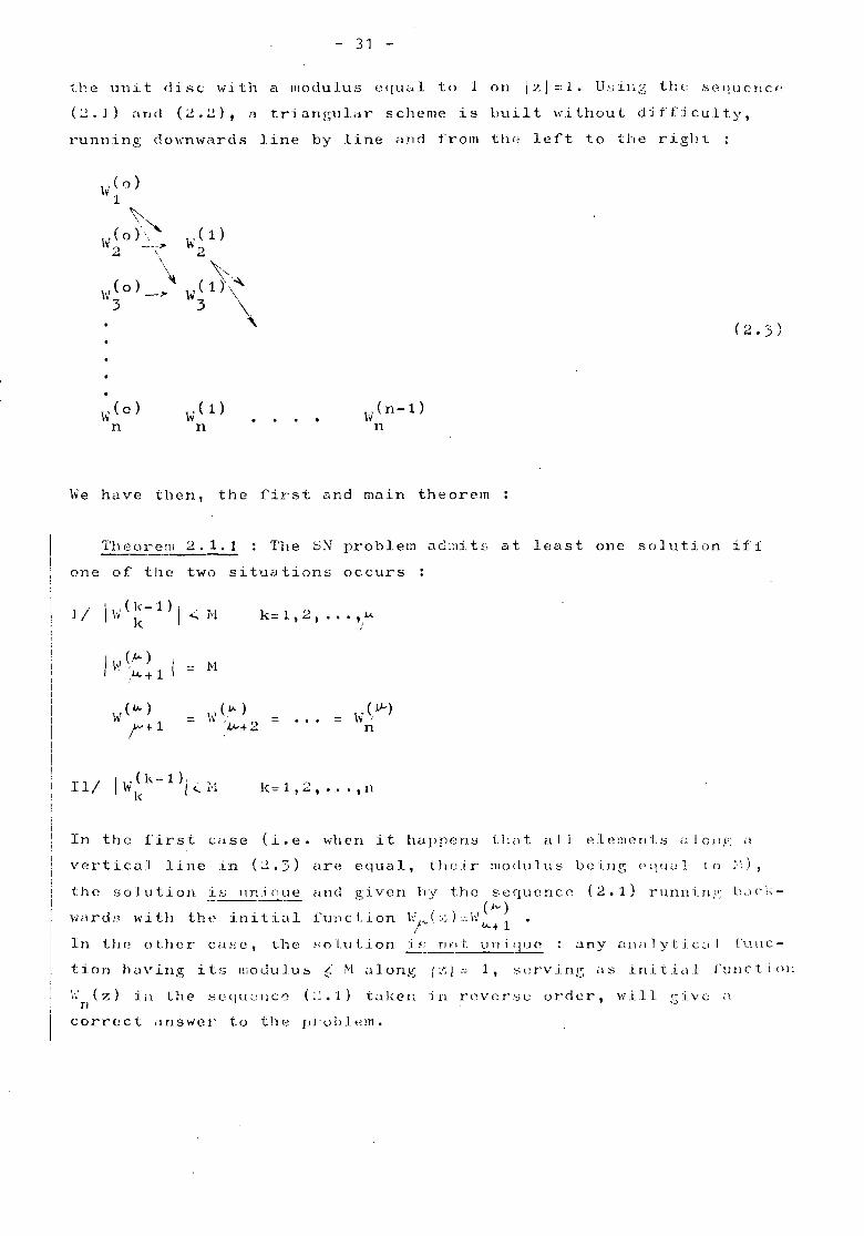
tbe llni_t disc with a Iliodulus equal to 1 on 1:61 ""'1. U~ill:;~ the S8qucnC('
(~.l) and (~.2), a triangular scheme is built without difficulty,running do),'nwards line by line and from tlj(" Ielt to the right
\\1(1)2
\>~\' ( 1) \~3 \
We have then, the first and mnin theorem
Th cor e tll 2. 1. 1. : The .::iNproblem ndl:lib" at least one solution i£"1
one of the two situations occurs
k= 1 , 2 I ••• , ,I./..I
I \,1 (,4 ) = 1'1,4+1
\'" (.I.\. ) = \\' CIA. ) = = \{ ())-)1"+1 ~+2 n
k = 1. , 2 , • _'• , n
In the i'irst case (i.e. when it happens i1:i1t all elements iJlcny: il
verticnl line in (2.3) are equal, their modulus being ('quill to ;.1),
the sohltion i~ llni Clue._-_.~-)"li\rd~~ with th\~ initial
and given hy the sequcnc(''. ( ~")
1'llJlction hj'_("':)'-'--\{~+1
runnin:.': 1)" C k-
In the 0 the rea !c; c, the >' 0 III t ion :i f; n ()tun i 1"1u C ~ny L\l\i1-'ytic~ll CUIlC-
tion huving its IlioJulus ~: H alon~ 1<::1:.:. 1, ~(~rvinl:j ilS initi,d rlJIlc-ti(ll~
\; (z) ];\ Lhe SCQ1U;llCC (:2.1) L~J;:en :i n revcr.':H.; order,ncorrect ilnSWCl' to th(~ fJl'obl\~m.
will ['-ivc: it"J .-
- 32 -OIl(? rn:\y l'dSj ly verilY tlPlt I r;-iven tile anillyticLlI structure or (:':.1) I
\\1(Z) wiJI. be il r:\tio11il1 J'unction iff the initial function introri1:<.'C(!
in :::N 's .:.l 1.p';(I r i t IJ m i s r i.\ t i on d l. \ve h a v e d J S 0
----_ ...._----minimUlll vnlue of
(' I . (0)1. . ')Gi v e11 t Z i\ and .' "':i. ..!.l. .:: 1 , ", .. • , n,t her e i s a
Ii to which corrc.':;!'-'~Jl1d~j a unique ~olution of SN's
problcll!. The c.l!~J'hr:\ic equLltion f'or the det2;'lllination of the srnClll(:,'CtI\'J is
I,.(n-l)i''In 1- i \1 (z)/n-l n = 1-1
Th e ,smit 11 est r e <::.1 pas i t i ve val u e 0 f N i s t ilh.en.
that there exists a function
t J tl I ,...('J)a,es on "'1e va ue.~ "k
: A sufficient
modulus ~. N alfmg Izl = 1 \';hich( 0 )
that h7k are the values tilJecn at zk by a bounded analytic
er(z) (h'ith i(.l"(Z)j ~ N along Izi :0.:1) and H-?<:J(n-l)n
1'JJ0.or(;II12.1.3--~-_._----\.' (z) o:f'oat Zl( 1.,S
:function
Let us now introduce the con:formnl mapping of the complex le:ft.
half plane Re u ~ a on the closed unit disc Izi ~ 1 I de:fined by
z \1-d
u+a il, real ~ 0 (2.it )
Our original problem may be stated in the equivalent form: filld ;\'(u)
an es~ential singularity at,jG .I :r(e' )1=1 alrnost every\dlcre.u:::co • i'lorcover
interpolates
ill1:,gc in the closed unit di5C is such that Ih'k,J'.l~ 1 alon:-;
') (z-; 1) f' .. - f'T ~Z ::: exp -[\ --1 a t a 1.nl1..C numb8r 0 nr-z-i=l, .•• ,n. Th.~ function ['--Cz) is Gl boun-
Lln d
the image point of
I z( :::1
who.-;(:)
bitrLlriJy given points
z= 1,
\(z , ~, J. J
de d a n a 1 y tic i'u n c L ion in I z I < 1, but has
It lIlay bo shown that this i.s not n restriction to the validity con-
ditions of theorl~l\l ~.1.3 which gUdrantees the exist(~llCe of at least
1 t' 'd d "J,_'.-I"'''n(n-l)/.one so U lon, provl C r,' J
\';0 further ir:troduce <.\ class or functions ~~(z) which are said to
satisfy pron0.r1.y-,'.] i:f for illl :::.'1
Iv 1
i\nLdyt'ic function .., in tlle closed unit disc satisfy J'-,'ol'>l:rty-h iff they
hD.ve i.\ consL~nt modu]us M on Iz! ::1. It iH e:.\:-Jily vcriried t.hat C-(z) I
- 33 -
althou.~h not analytic in the closed unit disc, has property-I'} (...:ithM~1) everywhere except at its essential singul~rity. It has beenshown [13J that when SN's algorithm is applied to elem(~nts of theclass (2.5), n additional interpolation properties may be statedoutside the unit circle. More precisely, we have
Theorem 2.1.1 •• : Let W(z) be a rational function Kith IW(eiQ)I~!-lwhich interpolates at n arbitrarily given points {zi} i=1, ••. ,ninside the unit circle a function r(z) satisfying property-No ThenW(z) - ~(z) has also n zeros {~k! k=1 •••• ,n outside the unit circleand there exists a positive constant L such that :
(~.6)
Returning once more to the exponential function and putting M=N=l,we find that each interpolation point Uk in the left half plane He u~. (j
has an associated interpolation point vk in He u ?- 0 with the remar-kable relationship
vk
k= 1••••• n
which will be used extensively in the next paragraph.
Up to now, no particular assumption was made f'or the "arbitrnry"starting function \\'n(z)of' 51'\'salgorithm, when j(/~n-l)I<~1, save itsrational nature. One might try, for instance. to take opportunity ofthe algorithm's flexibility to implement additional interpolationconditions. This possiblity, indeed, has been shown by DEVOOGIIT [l3].More precisely
Theoret" 2.1.5 : If the rational function W (z) satisfies the condi-otion of theorem 2.1.3. it can be made to interpolate ~(z) at the ad-ditional point 7, l' provided W (z 1) = ~n1) , with )W (z 1)/=",11:::'H.n+ n n+ n+ n n+ n+1ft he e 4.ua lit yap pI ies, \oJ (z) is con stan tun d \-1 (z) is the un i fJ 11 l?-n 0Iunction of' least maximum modulus in He u ~ 0 as established in C;1::;eI of' theorem 2.1.1.
It shouln be noted. however, that this additional mat.ching point ~..::.no counterp,lrt 011.t.si~dl! theunit.cir~l.e~, giving a total of 2n+l inter-polation points J'or the most general (n,n) rational Ell)proxirn':ltioIl.
- 34 -
T!l.i~; i" by no :1l(~,H1S c\ sl:rprisc, ::;iJ1CC such expressions contain llreci-
sc ly (:"~llt 1) illdejlClld(~!l 1.. cOL'fficien ts.
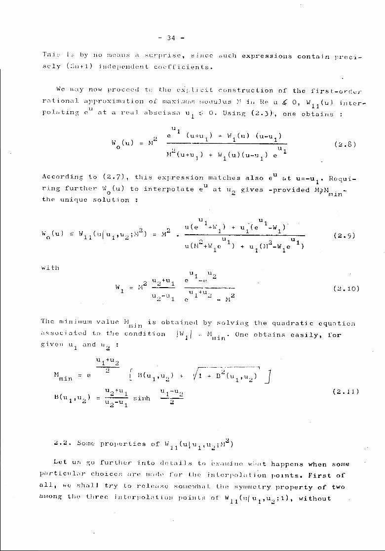
\~e lIi;\Y now proceed to the explicit construction of the first-ore!",}'
r"tionill appruximation o.l Illi.lxjmuill !l1odulus t.) ill It", u ~ 0, W11
(u) intcr-
poL,tin~~ eU
at a 1'e,,11 abscissa u1 (, D. Usin.~ (2.3)', one obtains
')
\~ (u) = }j"o u1
+ \-J 1 (u) (u-u 1) e
(2.8)
Accordin,~ to (2.7), this expression matches also
ring further \~o(u) to interpolate eU at u2
gives
the uni~ue solution
ue at u=-u1 R0qui--provided M~N . -
mlll
2 u1u (H +\\' 1e )
with
U1u (e + \i' 1)
. u1 .+ u1(e -W
1)
') u 1+ u1°r"'-\v1e )
= H2 u2+u1
u2-u1
(:.L 10)
associ utcd to the condition
obtained by solving the quadratic equ<ltioilThe minil1lum value l\'j min isI \~1 I M .
tIllnOne obtains easily, for
~1. = emln
8(u1,u2)
U1-U2 (2.11)
')
2.2. Some pro1J(~rties of I-JJ1
(ulu1
,U2
;N-)
Let us go furtl1l,r into d(~ti\i.1s to (~};'illl!i)](!Wj'ilt happens when some
}JiH'tic\lL,r choicc,'; ,Ire 1Il:1r11' i'or tllt' jTlt.(~rp());ttion points. First of
all, we shaLl try to relcilsc SOlllcwhal t1J(~ SY"!ll1ctry property of two
alilon.~ tlj(> three ill tcrpoL\ t ion po int. s of \V 11 (11/ U 1 ' u2; 1), ,vi thou t
35 -
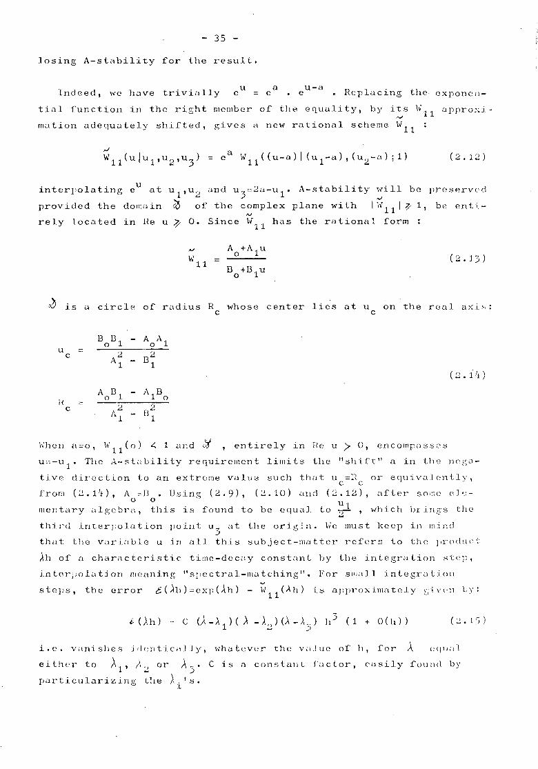
losing A-stability for the result.
Indeed, we have trivicdlyu a
e = e u-ae • H.cplacing the eXI)OnCll-
tial function in the right member of the equality, by its hill appro~:i-N
mation adequately shifted, gives a new rational scheme Wl1
(2.12)
interI10lating eU at u1,u2 and u3:.::2a-u1• A-stability :ill be preserved
provided the domoin <0 of the complex plane with I hr11 I ~ 1, be en ti-N
rely located in He u ~ O. Since W11 has the rational form:
.0 is a circl[~ of radius H. whose center lies at uc c on the real
u c =B Bo 1
2Al
- A Ao 1')
B""1
H :::C
- A B1 0
B21
1'1'0111 (2.111), A =n • Usinrr (2.9),o 0 "",
IIIentar y ,11geb l' C\, t his i s f 0 und to bee Clua1
\';hen <\:::0, \v11 (0) .::; 1 and ,;":1 entirely ln He u > 0, encomp,lSscS
u 'c - u l' The '\" stell) i 1i t Y l' eCluire I i1 C n t 1i mits t 11e"s h i f t 11 a in the IH' :s L1 -
tivc direction to an extreme value such that u:::R or equivalently,c c( ~ • 10) d n cl (2. 12 ), aft e l' s 0 1:18 C 1'-'-
Utto T 'which brings the
third interl;olation point u3 at the origin. \Ie must keep in I:L:nd
that the vdriable u in all this subject-matter refers to the product
All. of a characteristic tilllc-dec,IY constant by the integration ~tep,
interpolation 1ll8iuling "sjlcctral-l1latching". For sll"111 integr,lt:i.oll
steps, the error t(~IJ)=cxp(Ah) - W11(Ah) is approximately ~;ivvn Ly:
i ().h) '" C (). - >. 1) ( A - A., ) (), - ), ,;) h 3 (1 + () ( Id )~ - (:2.1))
i.e. vilnishes irlcnti,cil.lly, whatever the VilJUC of h, 1'01'.\ (:qllil]
either to Al, )") or A.}. Cis n COllstallL f"dctar, easily :found by~ .J
particularizin.\.': the >,. 's.- 1
- 36 -
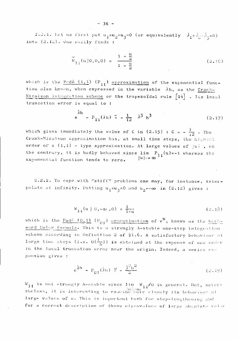
:2.2.1. J.l't 11::; Cil'sL put ul=u,,:-::u~=O (ar equivalently... :J
illto (:2.1:.;). Olle ci';O;Lly rinds
). 1::: )., ..., ) ..= 0 )<~ J
1,v
II" 1 J (u )0 , a , a )U
+- 2'1 _ u
2
(~.lG)
",II i cll is the F,lde (1, 1) (P 11) appraxim<J. tian af the eXllanen tial func-
tiall also l(nc."n, ,,,hen expressed in the variable Ah, as the Crnnl;:-
Nicolson ill L'.~2:r;d:i.()n scheme or the trapezoidal rule [14]truncc;tioll error is equal to
1- 12
which gives immedi<:ltely the villue af C in (2.15) C = 12 • The
CI'anl~-N:i.colson upproxirnation hi..ls, at small time steps', the 1,; .':',1'-::' ... :~
order of a (1,1) - type approximation. I\.t large values of I 'Jll i (' .-
" I
eXl'on Cllt ia 1 func tion tends to zero.
the con tr,u.'y, it i£; bodly behaved since lim Pll (u)=-lIu I--~00
whereas ths
2.2.2. To cope with "stiLL''' problems one may, for instunce, intel.-
polute at infjnity. Putting u1=u3=0 und u2=-00 in (2.12) gives
\\111(u I a,-w ,0) 1= 1-u
which i.s the Padro ( 0 , 1 ) (POJ
) ,I pf'rox illl;! t j on of ue , 1\.nown as tl1 c
----,--, ...._----- strongly A-stable one-step in tC!~l'.1 ti Oil
s cb eme <'1 C cor cI in g to/) c fin i t ion :2 0 f S 1 • 6. AsCI tis f u c tor y b e h Ll vi ()I JI' ;, t
large tillH, .,-"h~l)S (i.e. a(~» is ol>Llincd at the expense 01' O]W ('J'",'].
jn the J oC:.:l truncation error near the origin. Indeed, CI ~eri('s (":-.
IJLllJsiOll gives
( ~ • 1() )
Iv 11 i 8 n () t
t I) C .1 (! S ,';, j t
,';t I' U)j ,F; I y I\.-~, t (l 11I (~ ,''< j nee .1 i '~) \v 11/ U i 1I ~\ell cr ill. 1111t., II (: v" J'-.
, 111 , .. ,'U, ,j~'i ilILcre:stin,l!; to (!Xdl"l.IlC'IIIUl'e cll)~i't~ly .its IJl,llilV.i(II~I.' ;Il
larg~ v,,!ucs or lJ. 'J'hi:5 i.s illljlO]'lilllt both rOJ' SLCJl-:J('11,,,;Lhl~JLin6 ;<lIl!
lor i..I corr(~ct dc,'.;cri],LioJl of' those (~i,c':('/IV,I.1I)C,'; or l;\l'.l';(J il1J:;O.!ll(',' ,",,11:('
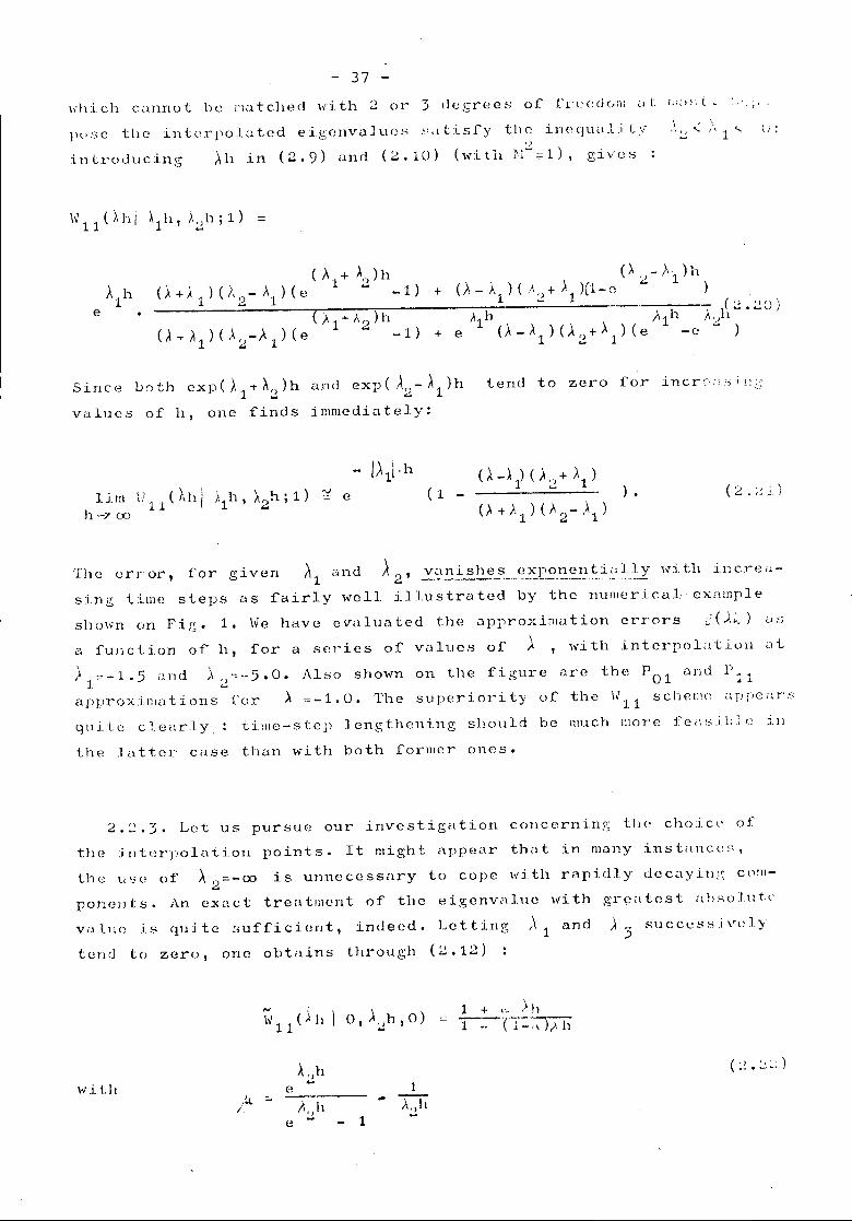
- 37 -
}H'~,C tile intcrl'oluted eip;cnvaJuc." .';itLLSfy the incquil.L:ity \ c"" £ ()' ""2 .....1\ 1 .....
introducing.,
All in (2.9) and (2.10) (with ~1";"=1), gives
( ,\ + A,,)h0+)1)0'2-,\)(e ... -1) +
, (A1+A2)1l(A+~1)U2-/.1)(e -1) + e
Since ooth cXP()'1+~2)h and exp( A2- ~1)h tend to zero for incrc.'-;'!!c;
values of h, one finds immediately:
lim \}11(}dlj A1h,/,r)h;1)"J e}1-700 ...
(l -O-~1)02+\)
0+/'1)°2-)1)
) . (2,~!.1.)
T]le error, for given ~1 and )2' :!..~\!2L~he_~_..(3EP..?.~~!:~i,~11~X ",itll increi~-
sing time steps as fairly well illustrated by the llumcr:i"al. exnlnple
shown on Fig. 1. He have evaluated the approximation errors
a function of h, for a series of values of\;\ , with interpolation ;)t
>1=-1.5 and ~2=-5.0. Also shown OIl the figure are the POl and P11
approxillwtions i'or ~ =-1.0. The superiority of the \>111 schel1!(~ C1r)r'eiH'~;
quite clcarly,: time-step lengt.hening should be much 1l10re fer\silllc i,l1
the latter case t.han with both former ones.
2.2.3. Let us pursuc our investigation conccrninp; the cho:ic~~ of
the j lltcrJ'olation points. It might appear that in many instilnccs,
tJle UC;C of ~ 2=-00 is unnecessary to cope with rapidly dccayil1:,~ cnrll-
poneni;s. An eXl\ct treatlllcnt of the l~igcnvi\lue with p;rciltcst ith"olutv
value is quite "ufficient, indeed. Letting
tend to zero, one obtains through (2.12)
) _ oS U C C L~S s i \'l~ .1. )'~
wi tll.'~t,.
I.
e:.. -----
"':.,:11e - 1
(:~.:.:.:)
- 38 -
i~ t.he "Il']'roxinlab on suggested by LINIGER and \HLLOUGHUY1'!li s" 1I 1 'j iL .. , LIt', whose local trunc~tion error is given by (2.15)
in
~h '" \ I '" 1 \ \ \2 3e - \"11 ( A h I0 I 1\2h , 0) ~ - 12 (1\ - 1\2 ),.. h
ForLl1'!~e time-steps L\v, unfortunetaly, has the same characteristic.':
cIS Pll which prevents it [rom being an interesting tool for ti"le-:~tq'
leJlgthening.
2.2.4. A more valuabl.e suggestion consists of the interpolation
at infinity and at two adequately chosen eigenvalues of the problem.
Provided ), ,. be > 0, this integr.ttion sC:lemc guurclntees .......-st.:lbility.J /
and even strong A- sta bil i ty. Le t A.) tend to -00 j one obtL! ins:...
This result, known as the G01 approximation, has been given jJreviou~.ly
by D1i; VOCGIiT, J J\UCOT and c'lACHGEELSfrom a qui te different po int of view
and hilS proved to be quite useful [l6J . Once again, strong ..\-stClbi-
lit::>, i.s obLlined at the price of one order in the truncation error
ne,d: tl18 ori.s;in :
(f) ,) r" \'-o • .:-'JI
2 •2 .:> \h~wCl nt cd to S how in t his ]I a r a ~rap 11, how the h' 11 [\1,~()r .i. t h r1I
uni rie~; most of the pxisting fi.rst-order integration SChCII1CS. There
is but orH~ imjJortil"nt of them which does not fit illto our fr,lIilc,,,orli::
the C1lebysr](?v-typc il]'l'roxilll;lLi.oll ~ou.C!;gestect by Vi\Hc;;\ [17,1/lJCh11()h),
wlljell drtIOni!;uJ.l ratiollil.l functions or t:ype (1,1) minimizes the lIIilx'i-
mum ,q'1Jroximution error, over the entire S]lectrUtll :
Ie ,.\h i) +il 1;' hICh 11 () h) tjill ( l"jdX
0 )\
it. ,11.~ lJ :... 0
1 -I b 1/, hJ. J.
( 2 .:.; (, )
- 39 -
The 1'esuI t, unfortuna tely, is not A-sta bi e bu t thi S n13Y be C0I11pCi. Sil-
ted by using a "shift" analogous to the one suggested at the begin-ning of this paragrLl)h [18J . The coefficients which define ChllUh)<:.ISwell as those corresponding to higher-order rational. ,:pproxi.matiol:.sare given in [19J
The main results of this paragraph <:.Iresynthesized in Table 1 theW
11algorithlll provides an integration scheme with spectral matching
at three eigenvalues at most. Its A-st<:.lbility is ensured provided oneinterpoJ.ation point be located in He (~h) ? O. If, moreover, ~2 isset equal to -00, the algori thm is strongly A-stable in tlJe senseof GEAH.
2.3. The extrapolation technique
Extrapolation is a well known and widely used technique allowin~the acceleration of convergence in the numerical process which lenJ~to the determination of an unknown quantity [2~J . \ve shall brieflyrccall its principle.
If the current numerical process T used to evaluate the quantitya has a power series expansion in terms of a paramcter h
o
OJ
T(h) - 0.0
= ,2.k=l
(') ,) -, '.£.0._(1
ll~ being positive und 3' 1"'; '(!."'::)3 ••. , one might try to combine insome way, evaluations of T at different values of h, to get a resul-ting process T whose power expansion (2.27) does not contnin anymoreBalTIC of the 1owe s t powers of h. The in tere s t of the me tllod lie s inthe fact that for [l given total number of clrithm(~ti.c operations, one'
mivht ohLtin i1 bet.ter p)ohaJ iICCUrnC).: __usir:,lj tll(~ extrnpnLtt:ion F1'()C~>::..:."!.
T instead of T with t.he correspondin;.-- refilled ll1e~3h.Tht-~re<.Irevarin1\.";
way!:;leLldiIl~ to that objective polynoillial extra]lolntio!l or I'a tintl,! 1.
extrapolation. The technique which is \u:lud horn belongs to the first
fi.llilily :i.t i~:l calJec:1 HOlllb(~J'g:'s iteriltivc lilJ(:ar extrnl'olilt,i.on.
(i:::O,l,.•. ) and Ti th(~ corresjHmding villu(:T(h.).o J
is buill column by column, still-ling; from tlJu
Let h,=-h/2i1-
A trinngular scheme
with the recurrence
The diagonal elements are the successive extr8polation schemes. An
exp.1icit determi1l2ltion of the first two terms gives
TO _. (4T1 - TO) / 31 ° ° (') "7' t' \..... ~) '.) i
T° ')
T1 TO)= ( 6'1 T"" - 20 + /11'].2 0 ° °These expre.ssions clr~ known, respectively, as Simpson's rule and
]JooJe's rule "-'hen applied to the trapczoJ:clal qu"drature [orlilulil.
HOI?lll(;rg's cxtrapO.L\tion algor.i.thm eliminates one term of' (~:,;~(.) :.:1:
each .':5 La,\!;e.. It haprens that ,,,hen "}llllied tot . f'. Ah tJ S . I 1 ( 11 1)111(\ .].0 n 0 e . 1e . 1.111P SOil S r u .. c .-= , _ -
J ;>of two or<!c)'s of rnagnitlJde, i.e.
the t r it pe z 0 'Id" Lit) .;. i '.I .\i -
.J 1)~U
which l.S COlil{Jitrdble lo the truncation (,,",-or of i.\ ~;(~coIJd-o.rdC'r d.i,l!':(~'-
nul l'ilo(; i.\jJjJroxilililtinn. Eilch stil,\';C oC L1J(; COII1]'uL\t.ion ilIVolv(',;:'; :l!'i-
thnwLic OJ!Cl''i'lt:i.uJ1S ill!.d.(;ad oJ' 1 tlJ(~ (':",tJ'itj'o1<lleJ fOrlll\d.il js ('.':)"'{'_'
. ') ( ), 1 )terl to g:ive bctt(~r ilccuri.lcy thiln 1'11 -;:;.... , '.IS 1,'iLI. be sholvn ill l:,l'- :;
next s(~cti()n. hor<:r;vcr it It.:.\.,; th(' COlllpIJti.\tj()llil.l ildvilnLI.\:,C or 1J('in,I'.
sibiljties occur
- 41 .-
it ':. \ , .l )N( ... }". (~.::..;. ) ...3
p 1( AI: )~~\h
) :: 1 1
e =-L! "N
,1 F!'-i lr)~ f :\}""! )
!\ I..),-;;--, -3 11 .~ J 1'.. -'
(~~.:;;c)
.:It time t. However these two schern::;s are Ylot e::pLi.vi.dC'Jd: on compuLi.d.i.,,'
nal ~rounds, the t-irst one neces:3itating twice the :-,.tora.!!,p of Lbo ;Jj)C-
ri1tor.
Since \vll
(~h) has exactly the same type of p.rror exp,c;.nsion than
Pi1 (},h) except for the coefficient (A-;\)(A +~l)('\- ~2) which may bf;
factorized, one has to expect similar results. This is illdccd the
case when the interpolation points are r.ot too widely spoced. For
" s t iff II s y s t 0 IJ1 S SU ch t h L1t \\~hi» 1 ! \V 11(Ah ) ;:;POl 0 h ) and j nth e
latter ca~e the Simpson's rule is no more valid. Pursuing Bomberp;'s
idea, a straightforward calculation gives
).h . \q (~)e - (2 P~l 2 - POl(Ah) 3h
The Simpson's rule applied to Wl1(~h) is not unconditionn~l]y
A.us ta ble a s shown oy :
5.- "3
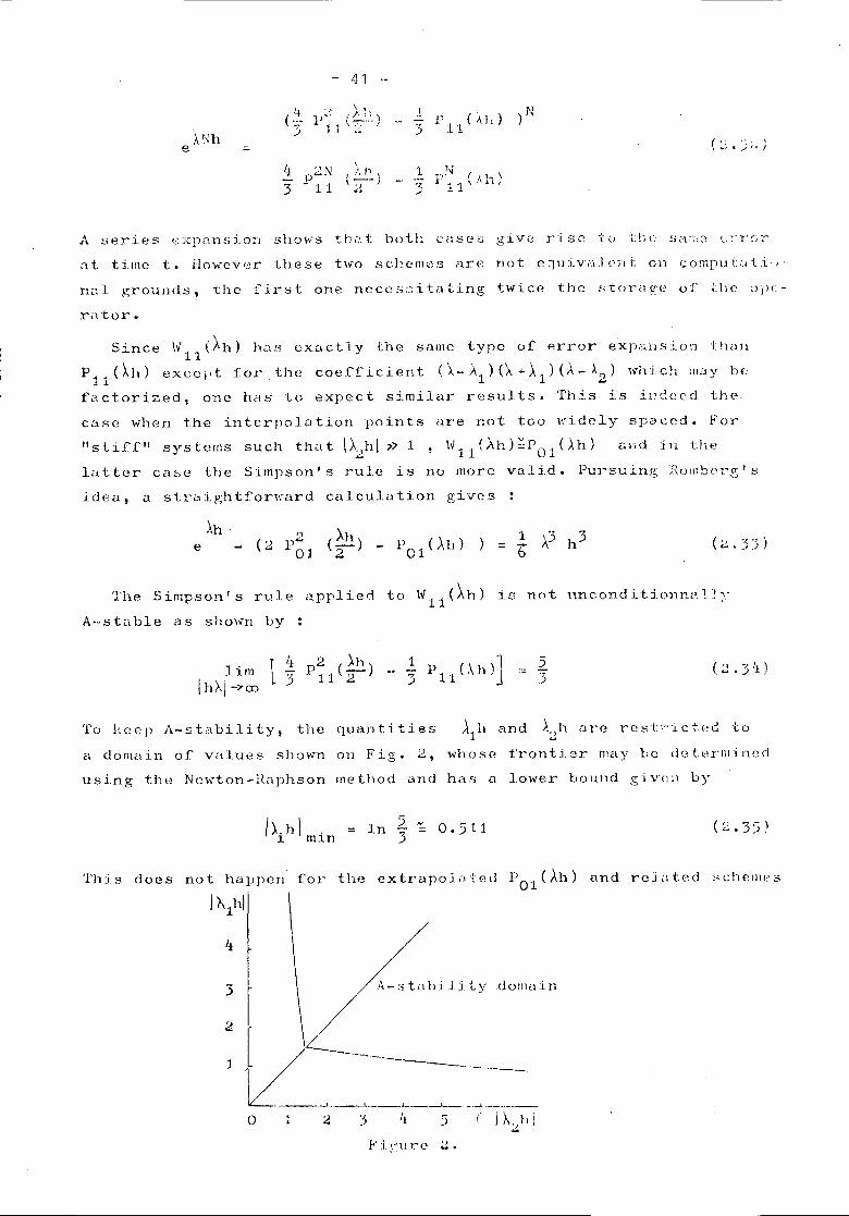
To keep i\-sti1bili ty, the quanti ties "111 and ,\.~h are restrict.ed to
a domain of values shown on Fig. 2, whose frontier may be detL!rminerl
using the Newton-Haphson method and has u lower bound given by
2o
This does not happen for the extrapo}"ted POl (~h) and reJ.iltcd schelllcs
l~lhl \4 /
3 ~t"hi lity do",,,in
2. /[/------~._~__'.___l '- _ __'_ , • _
(. i~,.1l l..r,;,;,
- 42 -
provided tile r('striction~ gi VCC'llill ;~.:~ arc 1ulfilled.
Series
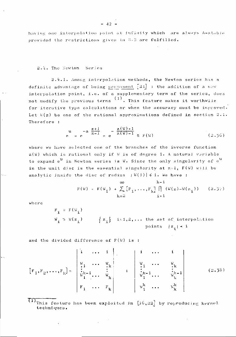
2.'*.1. ,\1l10L~:,intcrpo1<ttion methods, the Newt.on series hilS a
This feature makes it worthwi~e
the adGi tion of a Ii::'-,
not modify tlje previous terms
<.Joe .Sseries,i.e. of a supplementary term of the(1)
definite advi-ll1tage 01 bein.~ ~:!~:>Hlellt L2LJinterpolation point,
for itcl'o.tive type citlcu13tiol1s or when the accuracy must be improvecl.
Let iI'(z) be one of the rational approximations defined in section 2.1..
Therefore
eu
z+1-a z-J.
= e -- e
z (In + 1z(\-")-l
where we h<>vc s81 ected one of the bl'anches of the inverse 1unction
z(\1') which is rational only i:f IJ is 01 degree 1. A nntural v~\riable
to cxpund eU in Newton series is i-J. Since the only singularity of eU
in the unit disc is the essential ~dng111arity at z",l, F(II) ~~Lll be
analytic inside the disc of radius ilv(l)l~ 1. I-Je have
00
F ( Iv1) + _~ [F 1 '
k=;~
k-1(\J( z ) - Iv ( z . ) )
1
whereF - F ( \~ . )
1 1
W. - 1\' (z . )1 1
i:= 1, 2, •.• the set. of interpoLd:i.oll
point.s I z. I 4 11
and the divided difference of' F ( Iv ) is
1 1 I 1 1h' .
If 1 IvJ If 1 Iv J• < • <-
IF 1 ' F 2 ' • • • , F lJ :-: .Ic-l \.,1<-1 I~1< - 1(2.3B)
Iv 1 • • • Wk \ 1 k
F F Ivk \ .k... \'1 k 1 k
( 1) Th . 1ei.lturc has ueen exploited jn Ll(j ,,')1 uy rel,roliuci 1I~_r, kernplJ_ S ,_..-jtechniques.
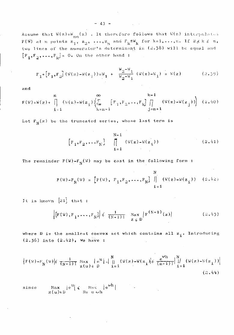
- 43 -
Assume tlwt IV(z)=lv (z)It therefore folloNs that \'1(7,) ir;tcJ']'()};lj-;'.'.nnF ( I~) a t H poi 11t oS Z <. z ')' "', Z nn (j F I =- Wk for 1<= 1 , ••• IE. If:.! _i. 1\: f: n,
! "" n <:two lines of the nUillcratO)-'sdeterminant in (;;;.38) will be equal and[ F 1'F2 '•••,FkJ = O. On the 0 the r hand :
and
F 1+ [F 1 ' F) .( Iv ( z ) - Iv( z 1. ) } =H1 +IV2 - \v 1--- (Iv ( Z ) - 'v 1) = \d Z )Iv2 - \.,r 1
( ,~• ;; 9 )
n 00 k-1
F (\n =W( Z ) + n (i-i( z ) - Iv ( Z i ){'.~ [F1 ' F 2 ' •• I FJ n (hI ( Z ) - W( Z j ») (~. if 0 )
i=l k=n+l j=n+1
Lct FN(z) be the truncated series, wllose last term is
N-l
ni=l
( \v ( z ) - \V ( z . ) )1
( 2 • Ill)
The remainder F(W)-FN(W) may be cast in the following form
N
F ( \V ) - FN (\"r) = [ F ( \'J), F 1 ' F2 ' • • • I FN] n
It is known [21] that:
( W ( z ) - Iv ( Z . ) )1
Max I F (N + 1) (z) Iz G D
where D is the smallest convex set which contains all z .• Introducing1
(2.36) into (2.42), We h~ve :
Wh N I
(e .l) , /1) (H(z)-h(z.»iIH • i = 1 1
(;~. 'l'i )
since Hax I cUl ~ Hi\X I eVJh I
z ( u ) to D He u ,,,,-11
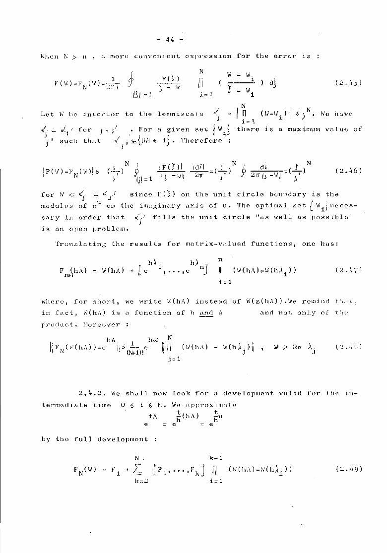
- 44 -
\"hen I\ > 11 , a more convenient CXjl3'l'ssion for the error is
J N W W., -F(In -F (\\')::.:~~~
rO) n 1. djN .'.1, J. ./ - Iv' !ISl :::1 J - W.i= 1 1.
a m~ximum value of
(\V-\Vi) I ~ )N. h'e havelemniscnle ,j --InJ i=l
~' '- 01., I for J -.. I ,For a given Be); f Wi~ tbere is
i' such Uw t if' ~tl\vl ~ 1j. Therefore :
Let \.; be intcJ,'Lor to the
IF ( \\l) - F N ( in i ~J j'
NJ( '-,))
{
9.UI = 1
for \V' (~,:.t ~ ,,) since F(:5) on the unit circle boundary is theJ Ju ( )
moduhl!5 of e on the imagin,ll-y axis of u. The optili1id, set t. \vij neces-
sary in order th.:\t .,:,,'/ fills the unit circle "as well as possible")
is an open problem.
Translating the results for matrix-vi\lued functions. one has:
F llt~hA) = Iv(hA)h~l h}
+ [e , ... ,e nJn
ni=l
where. :for short, we l.rite IIT(hA) insteud of \V(z(hA».\ve remind t"i1t,
in :facti W(hA) is a function of h and A und not only of' tlH,
product. 1'loreovcr
, hA" . 1 h1-0, Ni(FNC,'J(hA) )-0 l;~ -,,- e )1' n (IHhA)
j I (N+l)! 'j=l
\ I'- \oJ ( h A . ) II '
.l(:2.'i~~)
2.4.2. We shall now look for a development valid for the in-
o ~ t ~ h.tA
termcci:iate time
e
We approximatet th(J'IA) h'u
= e = e
by the full developllJp.nt
k-l
ni=l
N.F -+- },.-i-
,.. ]LF1 •••• ,FJ<.
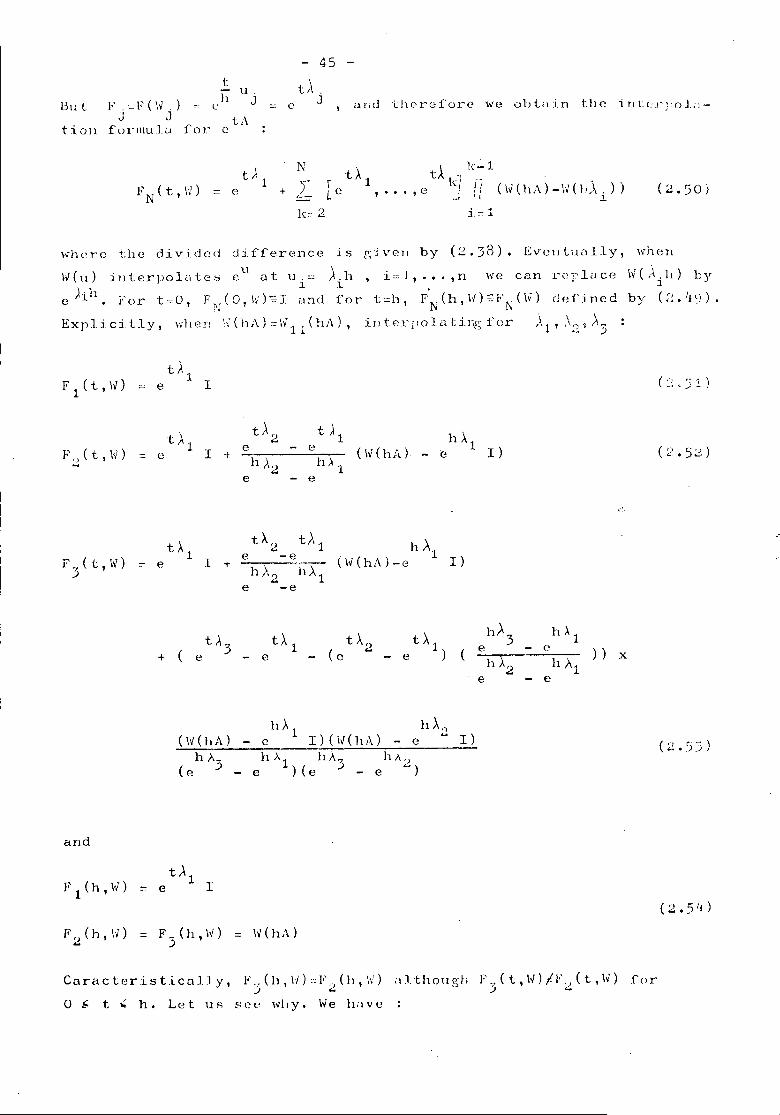
13u t
tion
tu
F .:..:.F (\~ .) = c h JJ J t \
furmula for c '
- 45 -
tt\ .c J, and tllC'refore we obtilin the ini.cJ"]:old-
N
1\:,,2 i.:: 1
w}wrc the divided dif.ference is gi_veJI by (2.38). Eventually, when
w(u) jnterpoldte~ eU at U.=-" ).h , i==l, ••• ,n we can r,,;:,lace) 1 1
e i h. For t := 0, FN( 0 I \d -= I i\ n cl for t :.::h, F'N(h , H) =: FN(hi) cl e :r j n e d
Explicitly, v,heD \{(I1,\)::=1111(h1\), interpoJatingi'or '\1"\~~'\3:
tAF 1 (t ,\1)
1I= e
tAL t ,\'J t ~1 . hAt...F:.:; ( t , \~) I e - e ( Iv (hA) r)= c +
h ;'2 11>'1 - c
e - e
\"J ( ,A. 11) by1
by' (2. li~) ) •
tA2 tAl fl
t~l h\F (t I~) I
e -e (\,/(hA)-o r)== e +1"1,\ 13 ' h '~'0...e -e
tA3 tAL tA2 t A 1h.A
3 h Ai( ( e
e - C' ) )+ e - e - e )h ):2 h A1
x
e - e
h)..1 h A.)( \IT (h A) - c I ) ( II(h A) - c ... I)
h},7. h>'l hA3 h;..,)(e J _ e )(e - e ...)
and
( ,', ,. ';' )4,...0 • .J .J I
F1(h,Vi)( 2 • 5 it )
F 'J ( h , Ii) = F .. (h , \</) == \oJ ( h A )... ;;
Caracteristical.ly, F.,(h,I';)=!". (h,I';) ,tlthou,<';h F.I(t,IV)/F.,(t,\I) forJ ~ J':"
o ~ t .; h. Let us SOl! why. \ole hilve
- 46 -
e
t }.1- ('
Il)'l- e
hA h\ 1 J) (c -e )
Developping tl1e fir~;t br,lc1\ct in POKI.;l"S of hand introduciYi2; (:-",L5)
into the second ono gj,ves :
F (t H) -2 '
tAe
Therefcre, the error ; "... ~, "'(J(Il.J) at tIle end-point only, onlyfor t < h. }Joreover as it tohould, the error is zero for vecto~~-s th;~t
belonl~ to the sub~>pnce sp<Jru~cd by 1.]113 eigenvcctors associated \y:ii.h
the eigenvaJuei~ ).1' A,2 £~~~--!.. Ii' He enlarge that subspace to '~::J
1»' () suiLlble shiFt, the r!~~;ult is on]y exact for the cnd-pc,in-i.. \:::
~<.:e thJC the la,~t term of F7(t,\n hrin,\~s the lIlissin,Q; term conL,'in,:;;:<).~t.J .
e;; giv'ing iHI cxnct result for the SUbSilPCC ,:ssociated ,.6th (Ai' )';2"\;;'
for al] t, ,,'ithouL modifyin,{!: F2(l~\-.') at the end-point, ,,'hich is c\h"Ci.ldy
exact.
J .• (' #
(t-'(;)Ac Q(v) d-c ( :' . ~;~ )
Can l)(~ I1Jilde HI'1'roximately by
t+N ( t) '" F N ( t , ~'J) f (() + j F N ( t - "C , h' ) Q (::) d 1:
o
- 47 -
or
I, (t''rN I
N
1\:=1ni=l
N
+ L_k", 1
k.•;
o
constallt~.
kr t:, 1 tA kJ \-Le , ••. ,e _. /
~
tAk j () h:,,.; j e := fk t where the o<..j al C
LetZk
1<-1.
fli=l
(2.CO)
k-1Vk(t)= n
i=l
The solution is built sequentially, using the following set ofequations
QN-l (t) +t).
--e 1f(0)
= (\V(hA)-\}(hAN_1)) ZN_l
tJ fN(t-c.) VN(l;') dro
VN(t)= (W(hA)-W(h~N_1)) VN_1(t)
V1(th U(t)
- 48 -
1. F,,(L,I-,1) j~, not in !2;<;llc'J:'dl ,\-;:;1;ilble, even if \v is A-stahJc •....lio,,'evcr the SL1JJd,\rd S"hur test CCllJ be i1pplied t~ the power ~'~'rje~_;
'"i t h A - " t:\ b i lit Y •
2. F1(t,\V) is connected with the Jilctastatic method of GALATI
provide,; t.hat. :'-'Jl Dddi lion",1 norl1l:1.1izatioll fuctor be introduced.
3. Each step ZN_l --}> Z~, or in general the eva.luution of \Y(hA)
needs the inversion 01' a matrix I-tA where !:> is a constant • IVlwnpv(c~r
the muLti'node model J.S u!;.,ed Dj\ NCJ:ll~i~GA-TuHNAGE-IlSNHY scheme [n,;2G]call be used, therefore cO:llhining the advantages of spectral Ii'dtchill~:
A-stability and fast inversion.
(' h,\e -
KhAe = \/ (hA )
/i.T'h(~ scheme l)rOposcci by DA NOBHEGA and BENny starts from the
identity
"here P, is the proj ector on the i th e igen subspn ce of A and K theJ.
toL.\l nUJllber of ei~;enva.lues (supposed di stinct) •. The surn is trunc:ltcd
and tlle projectol' evaluated lly di,:lgonalization which can be done expli-
citly fo!' s1I1all n,atrices. If we use inste:1d t11e equivalent operator
K A -~kP = n ( -_._,_.-
1. ~. - )1<k/i 1
P.1.
J(
= 11W(hA) •• \.,r ( 11), k )
we (Hid up with a LngrnJlgn for hA(.
Therefore our scheme is different in the following r(~~,.;:)Ccts
(;:d Iv(hA) i'O a general A-stable :l)lproxilllation intc~'l'olatjng at
arbitrary points, instead of a Pud(~ approximation ,,':Lth osculi.ILing
in t e r J1 () :~ i I t ion il t the 0 r i I!;:i.n
(h) it Newton s(~rjes is usc~d instead or 11 Li.\gr:\lli.~c ~H!rieS, ilddin,\!:
n perrJIanl~nce }lrOpcrty i
tllL~ annihilation of the error of the.th .:I e:t ~;cnl!lod(' i" done
- 49 -
S C Cl14en t i a .1. 1Y b Y S 0 1.v i n g d 1 i 11e ;1r s y s t em ins t e il d 0 f' C 0 Tn put in g (:xi' 1 i (::! t-
ly the eigcnvcctors. Both problems boil down to solving a static
"prompt neutron" problem.
2.5. The equivalent integral formulation
2.5.1. Let * = A(t) yet) + Set). Hultiplying both menlbers
to the left by the operator Vet) and integrating by parts over
t ~ [O,hJ gives
h
V(h)y(h)-V(O)y(o)=J (~f + V(t)A(t»y(t)dt
o
h
+ J V(t)S(t)dt
o
T(h,t) with V(o) -
h
+ J T(h,t)S(t)dt, +
o
I < \ve have then
hJ[~~ + T(h,t)A(t)j y(t)dt U~.G.'J.)o
This is an identity, so far as T(h,t) is defined. If' we choose
T(h,t):=F2(h-t,\V), and A some "averat~e" value of A(t), it is easily
shown by substitution of (2.52) into CL64) that:
h(
y(h)=W(h,A)y(o) + J F2(h-t,W)S(t)dt +o
{h).
(A-'\'~)(\V(h,Al.-e 1)
h>. 2 hA 1e - e
h
jo
(A- \ ) ( \v (h , A) -.
eb~ 2 hA1- c
h
h
jo
(h-t)A1e y(t) dt J
o
- 50 -
The third terlllincurr(!d by the use of the approximate semi-group3 3F2 is of order O(h ). The last term is also of order O(h" ) if
(h \we define, for ini;tCillce,A as A 2"). If we assulllenow, t"or aimplic.itf,A(t) constant over the interval [O,hJ and decompose A:::M+N,we havethe more general identity
y(h):::T(h)y(o)h;.J T(h-t)S(t)dt
o
h
+ Jf 0( dT(:~t) + T(h-t )t-1J y( t) dto
h
+ J I(1-'() d T~~- t) + T ( h - t) NJ Y ( t) d t
o
(2.66)
If we substitue in the right-hand side integrals, two-point inter-polation formulas for y(t) involving y(h) and y(o), we obtain a g(-:ne-rnl canvass for (probably) all kriown integration schemes of neutronkinetics, provided that
al the interpolation is not necessarily identical for each inte-gr.:ll
bl the calculation is cyclic, each step being in fact one-halfstep.
Table;}, contains a few ex<\mples of known algori thms, for both spli t.-
ted and unsplitteu operators. A glance at the table showB thdi..onlyIl fraction of the possible choices for T(h) , N, N, Yl(t) and Y2(t)h<.lsbeen used.
2.5.2. As a final remark, we 110te that the operutor-~plittingmay be handled in a much more natural WHY. For instance: [31]
h hB ~A h(A+D)2"1\ ')
O(h3)S(h,A,I3) ...::: e e e ::: e +
h ') 2 19
-;;-i\ =:'h8 -h1\ ]h13 1 hA h13o (h l! )'1'(h,1\,13) ~ e3
03or -. 'B' 0 e - n- e e + (2.GB)
Both expressions are optimul Cor their respective order of accurncyas fur as the number of operatiolls is concerned. If each exponentL\lch1\ and ehB is replaced by W(hA), correct to O(h3), we have

- 51 -
S(Jl,A,B)h(A+13)
- e
which is A-stable with respect to A+B, but does not reproduce cor-rectly, in general, the spectrum IF;].CSS A and 13 commute
order1-- "3S(h,A,B)
the maximum
(2.(,B) only ifinretainedisaccuracyto 0(h4) ,,,hichinvolves hi,sher-
Ii: ~2 (hthe extrapolation ~ S \~,A,B);) ...
is A •• stable if
are correctand
'1On the other h[md, 0 (h )
fomulas like W~2.• However,I ~
gives 0(h1) with B m~trix inversions, and
modulus of W(hA) and W(hB) is about 0.9.
- 52 -
3. NUi'lEHICAL TEST l'lW13LE!'lS.
Two mode 1 problolllSwi 11 be dnalysed to illustra te the can ten t ofthe preceding section.
3.1. A one-dimensional diffusion problem.
Let T(x,t) be the temperature distribution at time t, in a finiteone-dimensional medium devoid of any heat source (or heat sink)
~T(x,t)'Vt
')
= 'U"T ( x , t)2
't>Xa .( x ;( 1
with the boundary conditions
T(O,t) = T(1;t) = a V t " [0,00)
Given any initial temperat~re distribution T(x,O), (3.1)-(3.2) isknown to adl1lit a unique solu tion which is easily obtained usingFourier series. If, for instance, T(x,0)=sin2rx, one finds:
2 200 -(2k+1) 11 t8 ~ sin (2k+1)11" x
T(x,t)= - IT L (2k-1)(2h.+1)(2k+3) ek=o
We, first, discretise spatially the problem by introducing an equi-distant grid G on ~ 0,11 with N subintervals of length h=l/N :
)J- N 'If T(x. ,t)=T.(t) , and the usual finite difference representation
1 1is used for the spatial derivatives, the "continuous problem'l (3.1)-(3.2) with initial condition T(x,O) is transformed into:
dTdt = A T(t)
with
T(t) = ... , (3.6)
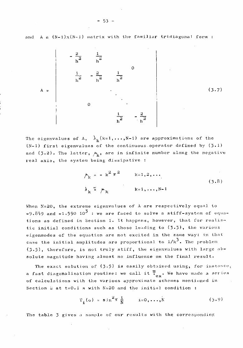
- 53 -
and A a (N-l)x(N-l) matrix with the familiar tridiagonaJ. form
2. 12. 2
h h
01 2 1
'J 2 h2.h'" h
A = (3.7)
0
1 2
h2 2h
The eigenvalues of A, ~k(k=1, ••• ,N-l) are approximations of the(N-1) first eigenvalues of the continuous operator defined by (3.1)aDd (3.2). The latter, /"'"k'are in infinite number along the negativereal axis, the system being dissipative
tk 2. rr2 k= 1 ,2., ..•:= - k
(3.8)
~kIV k:=1, .•• ,N-1:= fk
When N:=2.0, the extreme eigenvalues of A are respectively equal to-9.849 and -1.590 103 : we are faced to solve a stiff-systom of equ~-tions as defined in Section 1. It happens, however, that for realis-tic initial conditions such as those ledding to (3.3), the variouseigenmodes of the equation are not excited in the same way: in thatcase the initial amplitudes ore proportional to 1/k3• The problem(3.5), therefore, is not truly stiff, the eigenvalues with large ab-solute magnitude having almost no influence on the final result.
The exact solution of (3.5) is easily obLlined using, for inst;\l1ce:
a fast diaCTonalisation routine: we caLL it T • We have mildo a series"" ex
of culcula tions wi th the various approximate schemes mentionE~d inSection ~ at t=O.1 s with N~20 and the jnitiul condition
T. (0)1
2 ._ sin If ~ i",O, ••• ,N
The table 3 gives il Hample of our reslllts wi th the corresponding
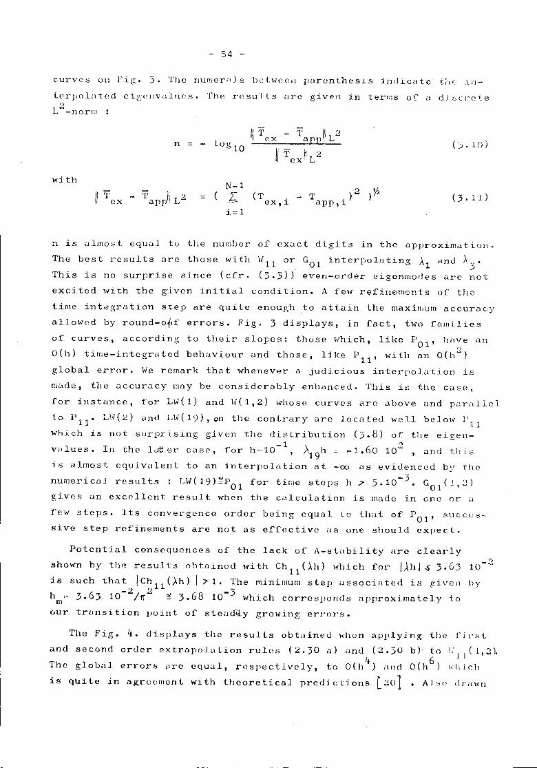
- 54 -
curves all Fig. 3. The nup;er;1Js bGl.\,CCH pi-Irenthesis indicate the :i.n-t c r lJ 0.1 <l t e d e i g (~ll \, i\ I u c s. '1'here s u 1 t S il reg i v en in t er rns of [J d j ,',ere t e
,)
L"'-norm :
n = - 10lr'''10
I( l' - T 1\ 2ex app L
II' T " 2exl!L
(j.Hl)
with"if T I: ')
ex - applL'"
N-l= ( r
i=l(1' . _ l' .)2)*eX,l app,l
n is almost equal to the number o~ exact digits in the approximatioll.Th e be st res u 1t s are tho sew ith \>1 11 ar GO 1 in ter pol a tin gAl and >':5'This is no surprise since (cfr. (3.3»' even-order eigenmodes arc notexcited with the given initial condition. A few re~inements of thetime integration step are quite enough to attain the maximum accuracyallowed by round-off errors. Fig. 3 displays, in fact, two familiesof curves, according to their slopes: those which, like POl' have anO(h) time-integrated behaviour and those, like P11, with an 0(h2)
global error. We remark that whenever a judicious interpolation ismade, the .:lCCUrClcymay be considerably enhanced. This is the case,for instance, for UJ(l) and \¥(1,2) whose curves <~re above and parallelto Pii' U.,r(2)and U¥( 1~), on the contrary ilre located well belol>'"1\ 1which is not surprising given the distribution (}.8) of the eigen-
-1 0values. In the lutter case, for h==10 , \9h == -1.60 10""", and tllis
is almost equivalent to an interpolation at -00 as evidenced by the-3numerical results : LhT(19H~POl for time steps h.;? 5.10 • G01(1,2)
gives an excellent result when the calculation is made in one or [I
few steps. Its convergence order being equal to that of POl' succe~-sive step refinements are not as effective as one should eXIlect.
Potential consequences of the lack of A-stability arc clearlyshown by the results obtained ,'lithCh110h) which for /).hl.$ 3.63
is such that ICh11 (,>.h)I'? 1. The minimum stell associated is given-2 2 -3h :::3.63 10 /rr ~ 3.68 10 which corresJlonds approximately tom
our transition point of steadi.ly growing errors.
C)
10-'.
by
The Fig. 4. displays the results obtained when applying the fil'stand second order extrapolation rules (2.30 a) and (2.30
ItThe global errors ore equal, respectively, to O(h ) andis qui te in agrccmen t wi th theoretical preclic Lions L ~o1
b)- to 1.:1J(1,2).
o ( h 6) Id I j c II
• AL,;(' dril\Vll
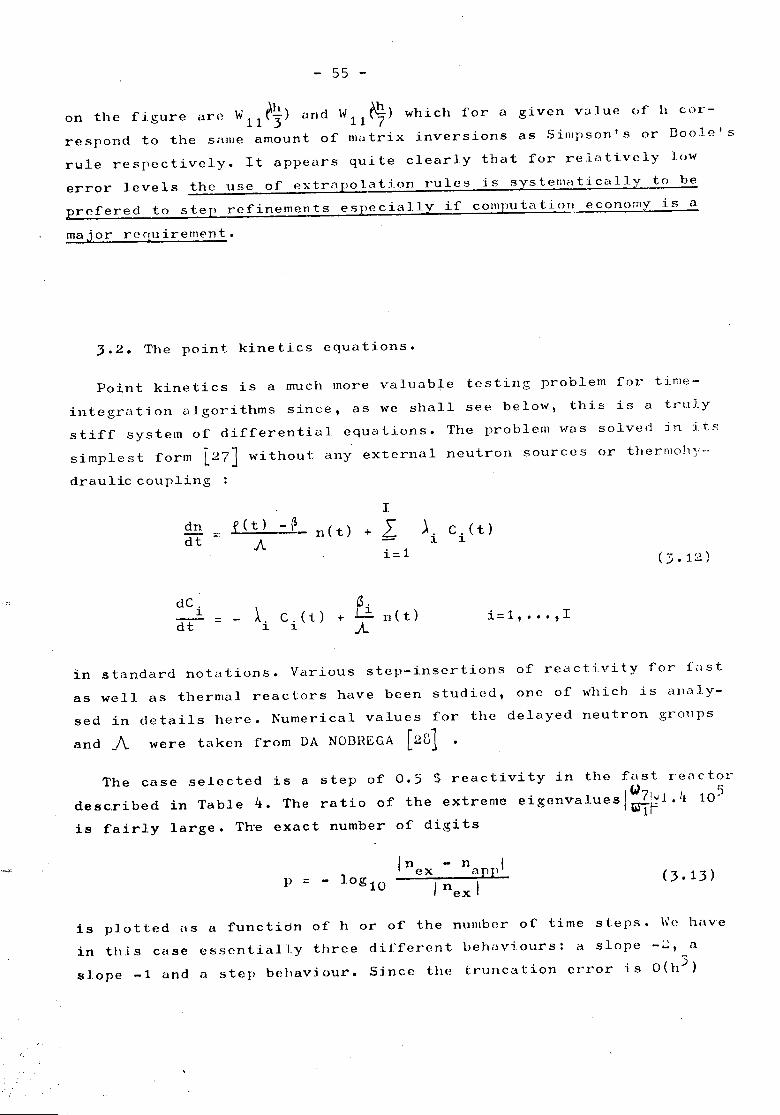
- 55 -
on the figure ar0 W 11 eX}) and W 11~) which for a given vo.lue ():f 11 cor-respond to the same amount of matrix inversions as Simpson's or Doole'srule respectively. It appears quite clearly that for relatively lowerror levels the use of extrapolation rules is systematically to beprcfered to step refinements especially if computation economy is amajor requirement.
3.2. The point kinetics equations.
Point kinetics is a much more valuable testillg problem for time-integration algorithms since, as we shall see below, this is a trulystiff system of differential equations. The problem was solved jn jts
simplest form [27J without any external neutroll sources or thermohy ..draulic coupling :
Idn f (t ) -~ net) I ). c. (t)dt - +
.A 1. 1.
i=l (:5.12)
dC. t ~.1. C. (t) 12:. net) i=1, ••• ,1= +dt 1. 1. A
in standard notations. Various step-insertions of reactivity for filstas well as thermal reactors have been studied, one of which is analy-sed in details here. Numerical values for the delayed neutron groupsand _A were taken from DA NOBREGA [281
The case selected is a step of 0.5 $ reactivity in the fast reactorW ')described in Table 4. The ratio of the extreme eigenvalues I ~~1 .11 10'is fairly large. Tae exact number of digits
p = - log10In - n Iex apE
I nex I(3.13)
is plotted as a functidn of h or of the number of time steps. \ve havein tIlls case essentially three different behaviours: a slope -~, aslope -1 and a step behaviour. Since the truncation error is O(h3)
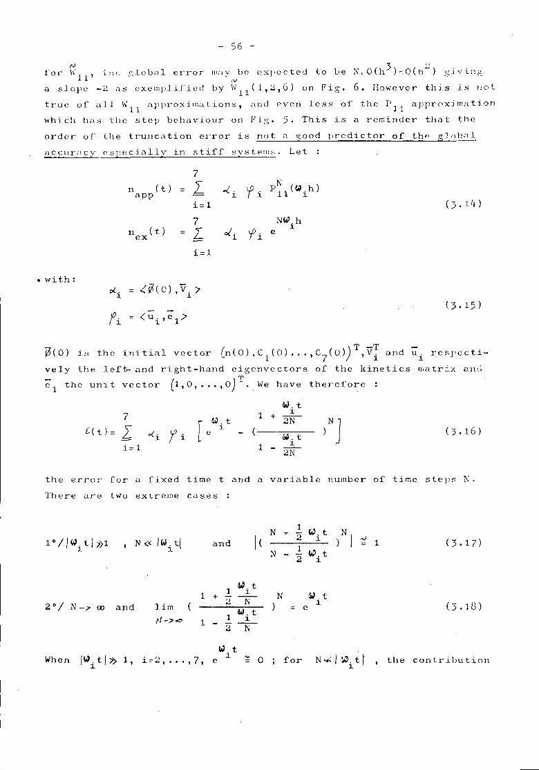
- 56 -
tv 3 <.for h
11, 'lllr: !~lobil1 error rI1:1Y be CX],cctcd to ue N.O(h ),cO(h""') !~iv-L;1,<
,"\I
u sIOIl(] -2 as eXellll)lified by \'il1(1,~,G) on Fig. 6. However this is not
true of all HI1 approximations, and even less of the Pl1 approxjmation
which has the step beha\'iour on Fig. 5. This is u reminder that the
order of the truncation error is not 2 .1I:0od predictor of the 51 nb.,1.
aCCllri\CY cspec:iallv in stiff systems. Let:
7( t ) L N
n = ~. fi PI1 ({.Jih)app 1
i=1
7 N",. h( t ) L o/i fi
1n = eex
i=1
• wi t.h:0/... = <'~(O) ,V. '1
1 1
= <'~. '-;1>.1.
rl ( ) T -T - .)')(0) i::; the initial vector "n(0),C1(0) ••• ,C7(0) ,Vi and ui respcctl-
vely the left,.. and right-hand eigenvectors of the h:inetics ll.atr:x un,;T
e1 the unit vector (1,0, ••• ,0) - •. We have therefore:
W. t1 1.+ 2N7
t(t)= I.i= 1
0(. <.p.1 / 1
1 -~. t
1
2N
(3.16)
the error for a fixed time t and a variable number of time ste]lS N.
There are two extreme cases :
N1
~. t) N I+ 2
10 II Y1. t I :?) 1 N « 1(.). tl and I ( l. N 1 <3.17),1 =
1 1.N 4lP. t- 2' 1.
1 ~.t1 1 N tW. t+
'j
2°1 N -~ and lim... N ) 1 (3.H\)CD w. t = e
,.J-;> 00 1 1 1.- ~2
W.tWllcn I~.tl)l> 1, i=2, ... ,7, 1 "" ° for N<i.:I~.tl the contributione ,
1 1.
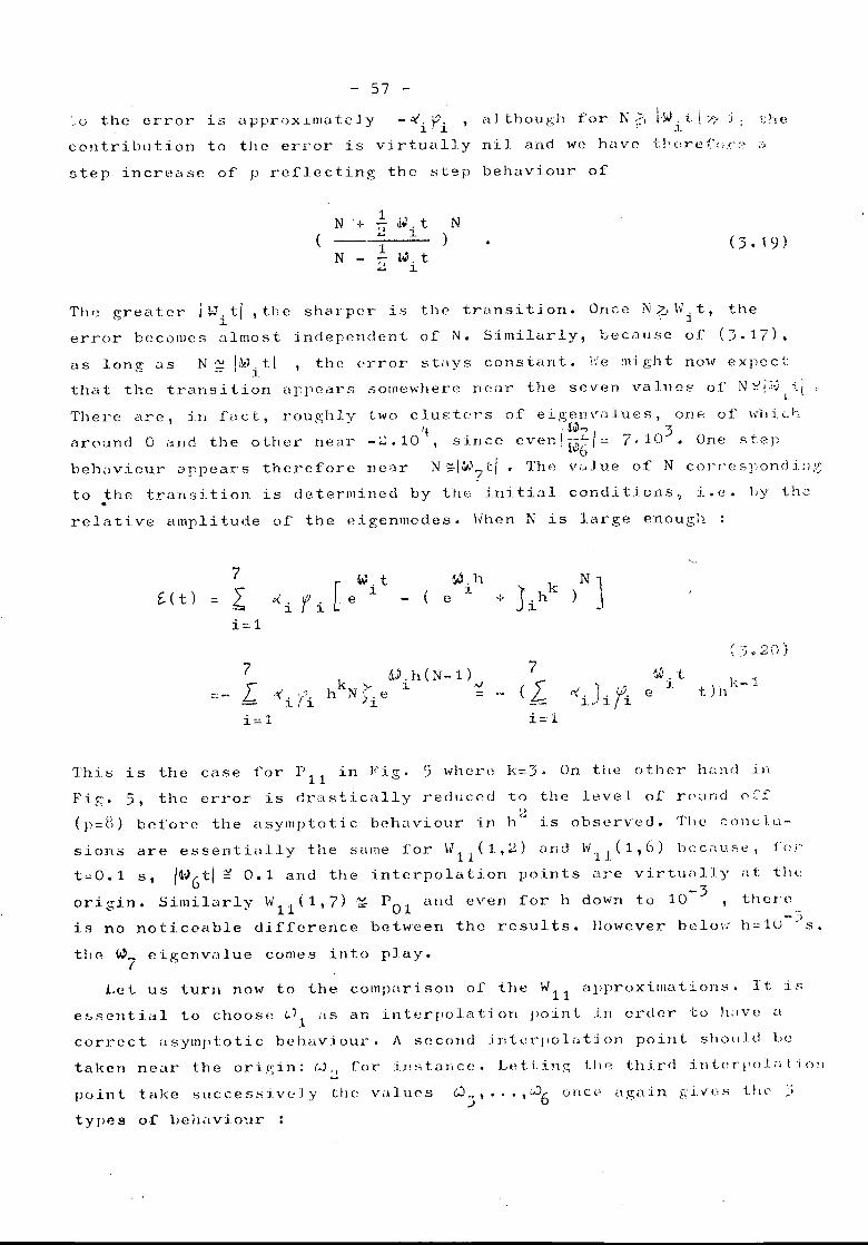
- 57 -
~,c; the error
contrilllltion
is approXlmately -c(, LJ. althouf';h for N ,>, 1.St) t i» j, the1 r 1 ' ,. J.' .
to the error is virtually nil and we hilve t,!~(~rer(ir:~ ;.,
step increase of p reflecting the ~t2P behaviour of
N1 JIi. t N+ 'I
( ... 1 )1
N - .:..:{.;.t
1
The greater J~itl ,the sharper is the transition. Once N7..,\vit, the
error bec()lIIcs ulmost independent of N. Similarly, lJec()use of (:::;.17).
around 0 and the other near
thereforebehaviour appears
a s 10n gas N ~ IIlJit lthat the transition
now expect\','e :ni gh tconstant.stays
somewhere near the seven valuefO of N:J;,i').~.i, .1. '
two clUEters of eig;cl1\'alues, OJlr, of Kbich~U~ 3
-~.10 - since evenl~~I~ 7.10 • One step
n e'1 r N~! Gt.' 7 t I . 1'h e v c;] u e 0 f N cor l' e s r 0 n d i :1,(:
the 81'1'01'
appears
roughlyin fact,There are,
to .t he t r a Jl 5 i t ion i s d e t e l' 111i n e d by the in i t 1.;11 c on d i t i G n s ~ i. e • by the
relative amplitude of the eigenmcdes. When N is large enough
7
= L 0<.l
e~,h
J,
i:.::l
7=c- L
i=l
7(I ~. t],
e
This is the case for P 11 in Fig. 5 whcrl~ k=3. On the other hi:nd in
Fig. 5 , the error is dr a s tic a 11y reduced to t bel eve 1 of r ():'ll1 d C' C' f'l
(p=B) bef'ore the asymptotic behetviour in h"" is observed. The ;:oncll.l-
sions are essentially the sume 101" W11(1,2) and W11(1,6) because, for
t=O.l s, 1~-)6tl ~ 0.1 and the interpolation I-lOints are virtually i.lt t]H~
" S' '1 1 1,/ (1 7) 'V P 1 "or 1'1 dow"'.\ to' 10-3 t'01'1 g1n. 11111.ar y "11 ' '~ 01 ant even ..L '11C),'C
is no noticeable difference between the results. 110wever below h=10-~s.
the ~7 eigenvalue comes into play.
Let us turn now to the comparison of the W11 approximations. It is
e~jselltial to choose "'\ ilS an interIJolation point in order to hilve a
correct ilSYIllI,totic behaviour. 1\ second inti.!r]>oL:.lti on point shoilld be
taken near the ori,U;in: (~J,) for instance. LetLi.ns~; t!Jc~ third illt.erl'oLd'ioll"-
point take successively Lhe values
types of bellilvio~lr
eJ .• , ••• ,c.J6 one!? np;i:\in S~ivc:s tile .:.>J
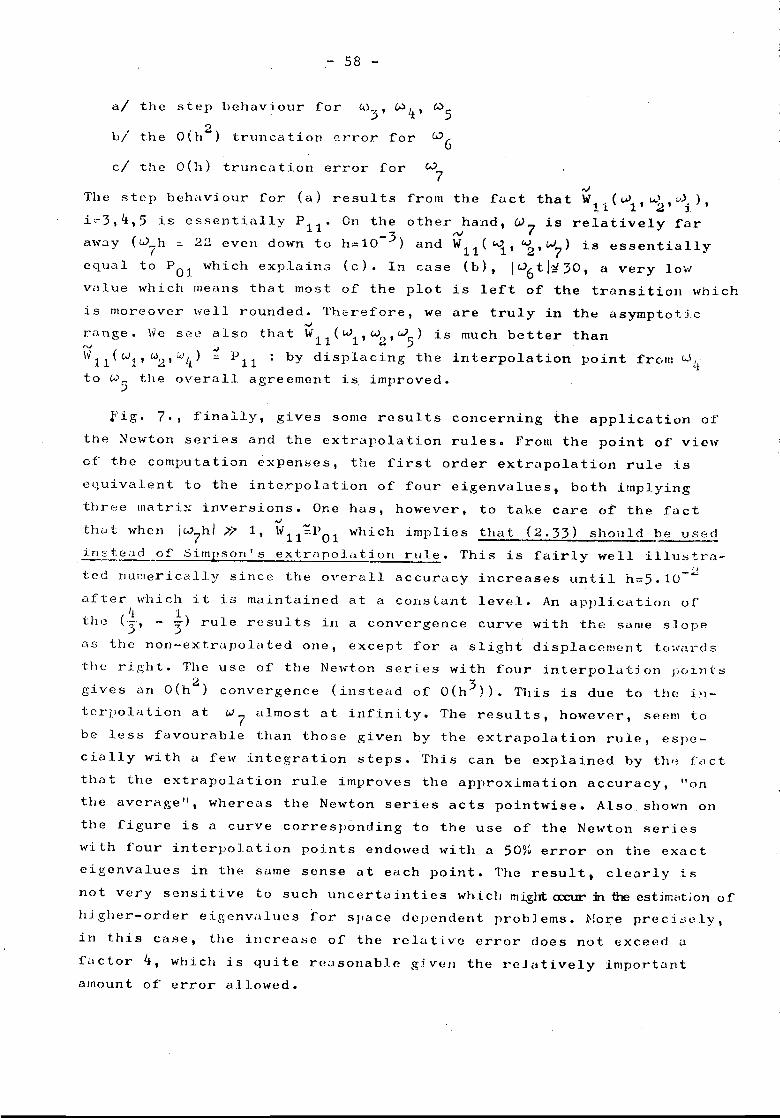
- 58 -
a/ the step behaviour for CI)". ,V) '* ' c.:>5)
ll/ the 0(h2) truncation error for (..)6
c/ the 0(11) truncation error for ""7,.JThe step behaviour for (a) results from the fact that W
1,(t..J1,l.I..),,(.').),_ 1 ... J.
i'"'3,4,5 is essentially P11• On the other rvhand, VJ7 is relatively faraway «(..)7h== 22 even do\vn to h=10-3) and W11(4., 2'(7) is essentiallyequi.llto POl which explain:., (c). In case (b), 1(.)6tl~30,a very lowvalue which means that most of the plot is left of the transition whichis moreover \'!"ellrounded. Therefore, we are truly in..,range. \ve set:'also that Wl1(Wl'W2'wS) is much better(...J ,.J
\V11(w1,W2'''}4) = Pl1 : by displacing the interpolationto we: the overall agreement is, improved.
:J
the asymptoticthan
point from kl,'t
fig. 7., finally, gives some results concerning ihe application ofthe Newton series and the extrapolation rules. From the point of viewof' the computation expenHes, the first order extrapolation rule isequivalent to the interpolation of four eigenvalues, both implyingth rf)e mo.trix inversions. One has, however, to take care of the fa ct
oJ Nthot when IW7hl~? 1, W11=POl which implies that (2.33) should be usedinst.eCld _of Simpson's extri'lpolation rlile. This is fairly well illuHtra-
,'j
ted numerically since the overall accuracy increases until h=5.10-~after ".hich it is maintained at a constant level. An application of'
It. 1the (5' - 3) rule results in a convergence curve with the sanle slopeas the non-extrapolated one, except for a slight displacement townr<lsthe right. The use of the Ne",ton series wi th four interpolation J)Oi11t$
2 3giv esan 0 (h ) con vel'gen ce (in stea d 0 f 0 (h ). Th is is due tot h e i!l_terpo12ltion at W7 almost at infinity. The results, however, seem tobe less favourable than those given by the extrapolation rule, espe-cially with a few integration steps. This can be explained by th~ f'~ctthat the extrapolation rule improves the approximation accuracy, "onthe averi:Q1e". whereas the Newton series acts pointwise. Also shown onthe figure is a curve corresponding to the use of the Newton series",ith four interpolation points endowed witll a 50% error on the exacteigenvalues in the same sense at each point. The result. clearly isnot very sensitive to such uncertainties which might ax:ur in the cst:imcttionof'ld ghar-order e igenva 1uo s for spa ce de pendent problems. 1'1or:-epre c i sc ly,
in this case, the increase of the relative error does not exceed ufactor 4, which is quite reasonable giVe!l the relatively importantamount of error al1o\ved.
- 59 -
co:~Cl ,l! S 1 ON S
\"0 have shown how to develop i1. .l!;ener~l A-stable nlgorithm for theintegr.::ltion of the neutron kinetics equa~ions. The algorithm can be
used itself as an element of a Newton series or of an extrapolationprocess. TIle implementation calls for the solution of static problemswith modified absorption and sources.
The sensi tiVlty of the resu1 t::: tv the choice of thc> interpolatin[.!;points, and ther(~fore t.o i'. :<::TIowlec1ge of t.he kineLic:" matl~ix eig0n\'i\.~.:.J(~'o
is not import;;lllt, and except ror the usyrnptotie ej.genva.luf~. ord •.3r" oi
lli21gni tucle are sLlr-Cicient. I,tos t knoHn algorithms cEter i;1tO t.he :Crc',r:~:>"
work of this integration sc11eme.
Sample problems indicate that improvements of accuracy rL'.JIg;i.J"~,t'; [.1"'lI'l
on(~ to "t,;'"o order or m;".g;nit.ude cnn be o,Jtain8d c::i'dler by one h' .. 1I11~tllc-G• .l 1
ai' by con:binilt:Loll of" spectral r.:atchillg ancl extrapolation. The 0I'Li.l'I'.tJ.
clloice of the i11t.8rpol~ti.r<:; points must probab.ly c!-t<:lI"J[je ClS th:) LrL;ll'~
,~:i en t de v c 1.0 P san d fu l' t h 8 r s t'.1 d yon t l;e sub j e c tis n'2 e d (~d. 1::.'/ j d f;:) J I ': l:'
ha3 b0cn given OV(;l' the influence of tIle stiffness of tl1e l\inct:i.c~3
r;;~1triA on the cf'f'cctive lccal truncation errol' which 1n.:1Y be qn:i. !:c:, d.i f.,
£'8r8n t from tlj(~ thC()1~e ti'cal one.
i\CKNO\yLSDGE~JENTS----_._------TIle authors ,,-:i.sh to' thl:lnl~Dr. J.J. Van Dinnebecl-:: and Dr. J.P. I'!cnlla)'t
£'0 r use £'u 1 c 0 111mc n t s a 11d s u g g.J s t ion f; •
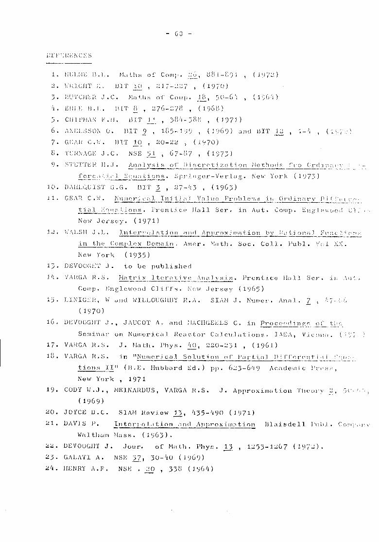
- GO -
1. IIUUiE U.L.
:2. \:JUGIIT ;:. BIT 10
). IH,rrCl"l:.:,.i.( ,.1. c. J\1a tlJ.s Or Cor:q;. }B I 5 u-G '1 ( 1 ')ell )
11'['[ n "'7("_"';<1. _ ~,"-',) ,~. {.J (196(1,)
:J. Clill'j'L\?, F .11. LlIT J1 ( j ') 71 )6. ,\XL::L:~sm~0. BIT 2 ,illS-,1)() (1)(j()) unc! JjIT 1:2
7. GU,/( C.h'. BIT 10 , :20-2~ , (J'-!70)
( "1 " "i' "
g. T~JH;\;,\GE J. C, NSE'jl
ir, (jrd:i.l~.lrv )lj ('(c.t. ('",._-----,---_._.~.~...._._ .... , ..- .Value Prnbl<:rl'.;3GEAH C. '.~'.
1.0. D,\lJLl~lJ 1ST C. G.
1. 1~
!-};:11 0"L'_IE~,~L~2.!2..::. l'l"ont:ic,~ Hall Ser. in Aut. COlllp. Ell,<!;l(>\";uod C!~' ;',
Nc \-{ J c :c s c y • (1 9 7 1 )
12. \.',\LSH J" L.
in th('~,.~ornI'}'~x Dc'main, ArneI'. l'Jath. Soc. ColJ.. Publ. \(<>1 XX.
New )'01']( (1935)
13. DEVOCGHT J. to be published
1/1. '/;.\I{GA n.s. l-ic:trix ]tcr ..\tiv(~ \lldJ'l'.sis .• Prentice Hi'll] Sor.
Compo Englew()ou Cli.cyf,;. 1",,1'l .Jersey (llj6S)
1":; . LJ1\"lG1:n, \,1 and \YILLOUiHBY H. J\. SLHJ J. 1'1'...:.l1Ier. An,,1.7 t. -,"l' '.'
(1<;)70)
16. l.n:V()UG1J'l' J., J AUC:OT A < and ,'lACIlGEELS C.
Sc :n in iI ~:' 0 n NU III e I' j C it 1 He i\ eta r C ,J 1 Cu.1 i\ t i 01) S. ].\ L:;\ I Vi (;:I I : ; I •.' ("-:. >' ( -
17. VAi~GA H.S.
1U. VAHGA n.s.J. t-lalh. Phys. 110, 220-~:::.l , (1961)
in "Nul1l c r i c a~l_S_'~.l_ll_t_i '<":.11o:f Pa r 1: LI 1 ~~.~'_(_''-_~_r.t:!2.t.-!~,-~__~<' (1\,:, ,.
t:i.OYlS II" (B.E. IIubbard Ld.) pp. 6::':3-611') Acadeii1:i.c ]';'('s':,
New York, 1971:> ( ~. '.' ", ,'1' 11(' U l' Y'J. Approxilllc.\ t:i.onNEINMWUS, VAHGA H. S.
SIIUI Heview 13, 1!35-lk90 (1'-)71)
IJltcrT,oLlt.ion i:..!2.c..!-Appro_xi~I2.:\t:i.~!2. lJlaisde.ll ]'\lId • COI'I]',II'"
\oJ n J. th L.l1fI ,,111 S oS. (1 <J G 3 ) •
of Hilt-h. Phys. 1')., 1~'j3-1~G7 (1~)';;':).
30 _/10 (1 <j G <) )
~:O 33(\ (lCJ()/!)
19. CODY \',J • J • ,
(1<)69)
:dO. JOYCE j) • C •
21. DAVIS P.
2~. DEVOUGJlT J • Jour.') 7. GALATI A. NSE )1. IwJ.2It, IlENHY A.Ii'. NSE .

- 61 -
.;i5. FOULKE L.H.\ GYFTOPOULOS E.P. N.::'.E. 30, 'i19 (1967)
26. POnSCIIL\G T.A. SlMl J. Apple Hath. Ji. ,301-317 (1968)27. HLTnICI~ D. "Dyn<1111ic.~;of Nuclcor Heactors" The University of
Chicago Press. (1971)
28. DA NODREGA N.S.E. 46, 366-375 (1971)29. aTT K., HENELEY D.i'.. , N.S.E. 36 , 402 (1969)}O. STACEY W.}1. Jr. "Space-.time nuclear reactor kinetics",
Academic Press (1969).31. S.Z. BURSTEIN, A. MIRIN, Jour. Compo Phys. ~ ' 547 (1970)
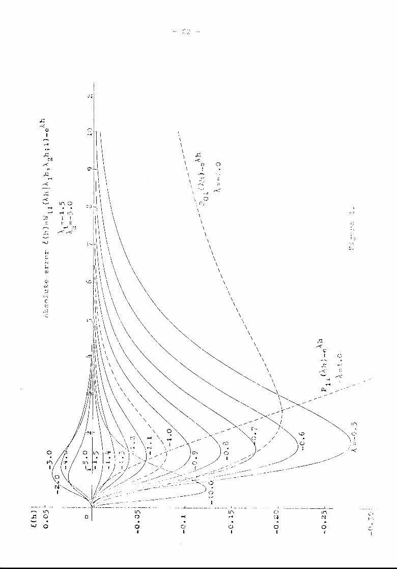
r '";- ~.'':'"
v
(,.I
.~-,
.oj
.-J _
If'•C\l
o
oI
. 1. _
o:~.QI
~ Ir'.,• !I: II~ .'.j
". ".....,::,,,-::,-<.......
-----~
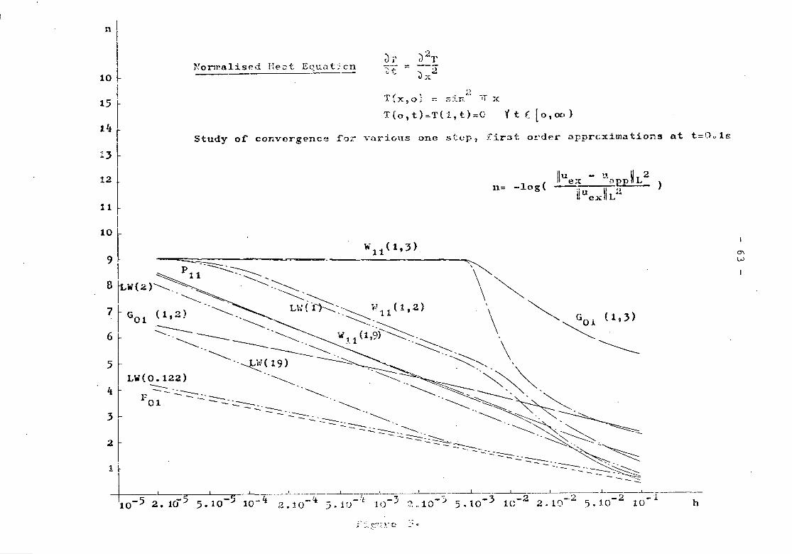
nl
0'1W
h
at t=Oole
~u - u U 2n= -log( e~ appnLU1U II 2 )ex.L
", .
;)21,(.
-~ --:)'\ ,.""-tJ .~
~i'"'St
....,T{x,o} ~ sin~' ~ xT ( 0 t t )=- T ( 1. , t )=0 t t r.. [0 f OC. )
various one stcp~ ?ir3t order apprcximations
He:l t EL}Ua t::.on
convergence for
~!or:T'alisp.d
Study 01
10 ~
I15 r14 r13 ~
12l
:, \; (1,3)I 11 ~
10 t ~~~ \ ~" G . (1,3)9 P "--- ',-- \ ""- 0,I ~11 ~ ..~~" "\,(1,2) \ ~8 ~W ( ,. ) -------.. '______- . L" ( n.~..~ :::-----.. . ______________. '------ ;>-----..'------. \? I '. • (1,9) -----'::::"71 G ( 1, - • ---------•._______.. ...11 ~~"
o 1 :----.. .'______ . .~ "-
~" ----------:-- ------- --------- ---:.:......~ '. ~ ,"-". ,
6 ~ .---------~(19) , ~~~~ ~,
-------. ----------. ~~ '"~5 LW( ':'.:!.22 ) .. '______,. _________.. ~~ • ~t -- -~'-"-.. '______.. ~ ..,~,,---~--- -"- . ~"1' . .. _ c. .'''="_ "_.:------.."'-
01 .. • '_="~'''''--_ .._ "'~3 _._ .. '='-'=':'~'c.--=:-::"':' _"'-,__~
.1-2- -1I I -2 10- 102 ,_ -2 2.10 5."-' "10-3 lC1__ _..-I :;., ~-T---' -3 0 10 >.1< ,_ ._,' 10 ,_k I -'i ,.. 1[)~ '-5 -" 2.>0 ,. , "
-5
10
10 __, 'C'.• ' e- 5 2. 10 5 • • '.10
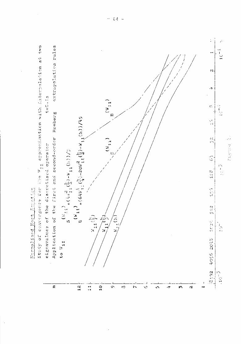
- 64 -
'"
0 III,~C! ,....,..
...' rl ... I;j t/i / /
u-;.1 ~.; ,....~
/' / / /~~~ c.. (vI;,/c 'd
'r< +'.; ~J
/ / / I(J r~/ I /,..~ ~
0 Po. / //1/1I', 'J .~~"
,f~
(j +..'.p lQ r;" ,< Q~ ......"I' .~
/,/1/(),/ '- ..
" II.,. /,'. ....
-ol ~ tory ~/ ,',i .•.. J!,~ ,,' 1.."'\ /" C>
.D -::l' /\,,~,. ........ .... ~.. E
/ / /~,() ...... ,/
'''; p;; --.+' r' ,/ /"""l(.'
'..~/ / /~ H / ."'f! ~) ..... \~ /
/1 /~~.",
~: l1 '0 ~ .,... ,':;
() 0 ~~ ,- ~ /;: .:..~ '.' t,", ,-, -' ID., (ll r "-. .c.:!C'J ll,l/I:" l: "0 ...... / .'. ,"cJ C) r: -< / \:.:s- 0 ,C-< N ,..l I
/ / /,-, 0 " '-' :; I !:\'~
oqr.; ;:J t-i 0 I~ "': ~l ,...( C\i / / / .
c:::.;:'j ~ ,
<.. .. '(', C!i ~f"'i I / ,-I
;', '''< ~~ ,r::;,;+</
/ I II...., rj ;-i l""" --,J','. ,.l..~f \ .. I() '-" .,....; I ,I I,ii i, ;... -{,) ..-1 ...:.,-Tt ":"'"-: i 1..;;.-.!.); " ':,,1 C"J ..~ :~ I / / /.
:.:.. 11) ~. >~ .::t' ;..(..... , 'f'" '", ..:;,.."" \:;j( ! C> "0 ~:.., '>..., ., l,I II Ii",
J- /' ~; ~; Ql Q) - q~:IC! .r:: .r:: ,.. ... ,.:
""...j +' +' 't'-! .; U-,;...; .~ :si..: ~ e;., (;-/ ..r.: ~l......,.C': I", r' /L;
" ' .::..~,c- ..' 0 0 v'1 w.' "'".1 .-:.:',,;1 ~.; :-,1 ,~:I ,
Cl tr! ~ 7 L. .:-:() Q) 0 ::: ~.~
c-, :.:J -.~(', ; t,.. ...~ .;J
't"\1 a ~'J rJ (\)
";1 "() .... _~4
lJl ::-., r.: .,...! ~ 0f:, '(:I Co' .-i :~ CII" ;'J t<l ,1,(i ~ 'r~ r.~ 0 '.{;~..... ' ([J C) -< ..., v'h'
C'4'
("J 1"\("",~, ( - )-(\) ,...
______ ._. ___ .&--._. __ ._._1_. _______I___ ..l--.-._....l-_._.l ___ . • 1 _ ..--.J.._ ... _.. _.L ____ ..L--..-----L.-_._. ____.1 _
t:: N ..i 0 0' m (.... \.~"' u"\ -"1' ~ .:;'I .-.I
~ d "
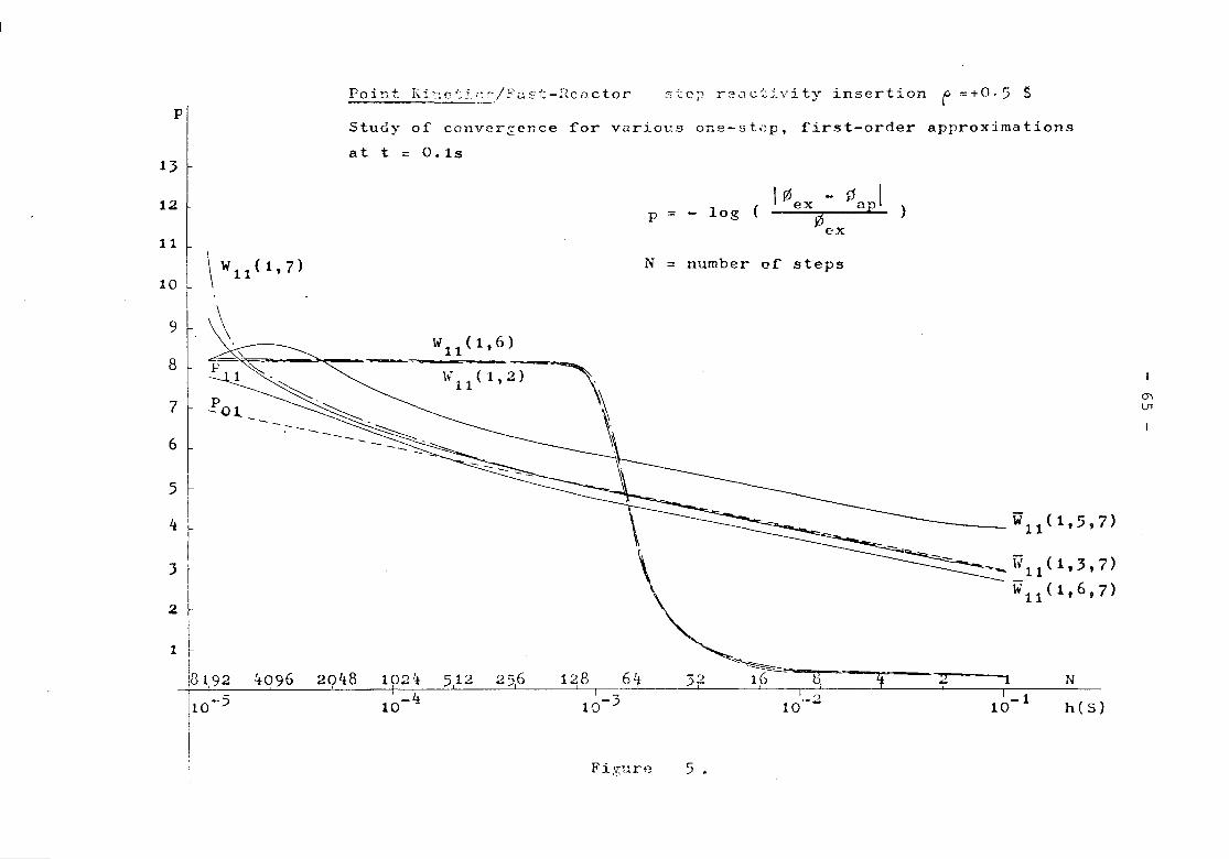
Study 01 convcrsence for variot:s one-5t~p, first-order approximations
0\U1
h(S)
N
W11(1,5,7)
...._ \7 11( 1, 3 , 7)
w11(1,6,7)
)10 - P Iex ap
~ex
:::-;';C;1 r2i:1cJ,::;'_vity insertion F =+0.5 $
p = - log (
N = number 01 steps
\\. ., I
.~-lj -:- 1-116 i 10312 I 1••
210
\Yl1(1,6)
\{ (1 '»11 ,..,
~
at t = 0.1s
Po int Ki:nc .'>!.:: _~I::' L\ st -Rc L\ ctor
,5 ~
4 ~I
3 'I.2 ~
1 ~I181,92 4q96 2948 192'* 5,12 25,6 1'18 6~110-5 1~-4 1~-3
l:r12l11
tOl \W11(1,7)
I9 r \\8 'l ---7 p-Ot6
1
-- - -
Fi,S,lre 5 •
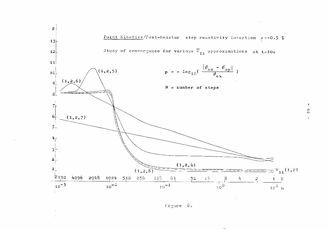
Point Kin0tics/~ast-Rcactor step reactivity insertion
N = number of steps
mm
1 l';+-
11,. h'0\. ... '
t=10s
fJ =+0.5 $I
2
Clt
8 L<.' -i,
:)00
• +- •apprOXlmn"lcns
i5
\0 - 0 Iex up)oex
i". 11
-:>;"~--'--
p = - log10(
ror vario:ls
lCJ-1
1. 2,(:. r: ,! r u.:..t:--.-----'
con'"Crge:1ceS tu(iy of
2r-i,1LiI
~192 4096 2048 1024 512 256~ I ! I j ! I
:10-3 10-2-I
3"-I
'rI6~
-':J~
iI
4~
9
8
Ie
I
PIi!;
13L
II
12LI
IllL
f'i ':;;'.lre 6 n
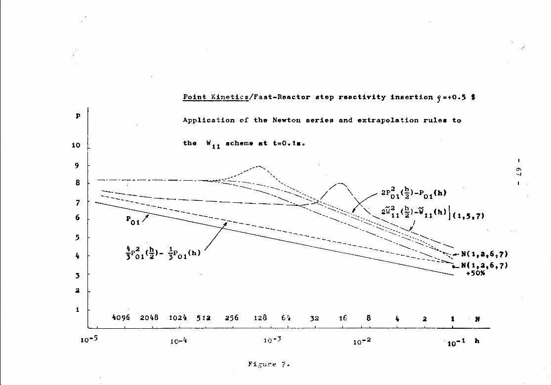
4 2 h 1jP01(2)- ,P01(h)
p
10 l9
8
7
6
5
It
,~
Point Kinetic!/Fast-Reactor step reactivity insertion 1=+0.5 I
Application of the Newton series and extrapolation rule. to
the Wit scheme at t=O.l.o
,,- ........." ",.... ....,
-~=-.-..:'-----. "'-- /-......, 2p2 (h)-P01(h)--------------~------.-----.----..::.::~-----/ 'y 01 2
. '- ---. - 1-----, ~---. "'2 h ,.., (h) )=::=-=-~-----------~, '--..:.:.::'.:.::----"2\0[11('2)-"11 (1,5,7------ --..-- ---.::---" I--- -- - -- ,
~-------- ---- ""'-::--- -'--...}iI -~----_ _''0-__>__..Po 1 __ _ _ ____.. <::::-_--
- ----- -~ ----- 6. 7)------------- '-~ - ...~...--N(l,a, ,----- ----.:~N( 1,~.6, 7)
+50"
./
'"-.J
t4096 20~8 102~ 51a 256 128 6'. 32 16 8 It 2 1 If
10-5 10-~
L -1____ _ -.1
10-3
Figu.re 7 ..
I L.
10-2 .10-1 h
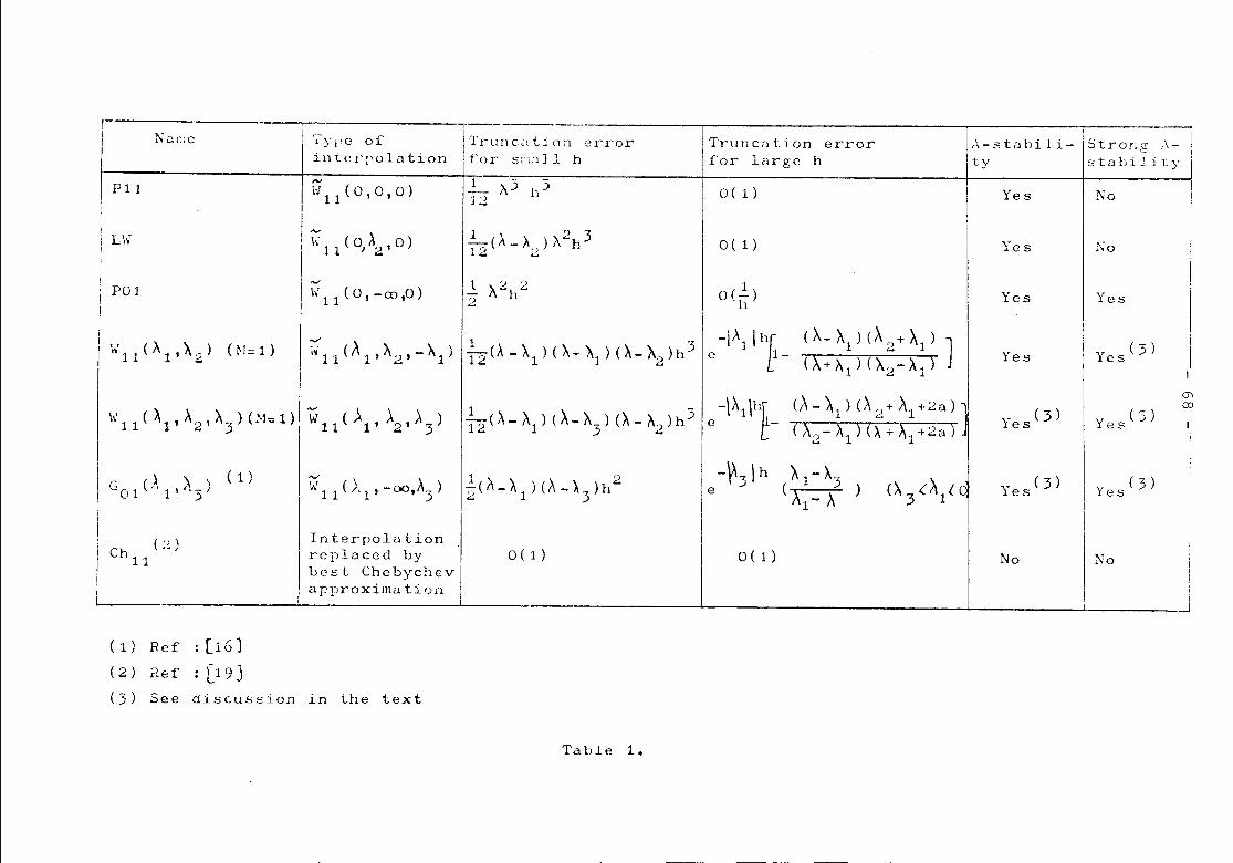
Yes
Yes(3)
;';0Yes
Yes
Yes
a ( 1)
or.!.)'11
1 ??- "-h-2
..!-(A_>' )A2h3; ') r)......... ...
W11("l'''2'-~1) 1~20\-Al)(~+\)(X_A.)h3Ie-i\lh~_ O'-A1)(A2+A1) J... L (A+A1)("2-Al)
11.1'11 (0,0,0)
I ~ (A ): \ 11 OJ 2' aI, ""
\\'1 1 ( a , - ill ,0 )
"T--------~- ,1\ <..\I';e i c1-YJ'C o~ ITrllnc~ltion '2rror Truncation error A-stabili- Stroy;.s ..\- I
intcrl'oliltion it'or slii::lJl h lor large h ty stabiJity'
1\ /\3 113 \;( 1) I Yes 1\0 :- I
i
Pll
pal
Lh'
W 11 ( A 1' ~2.) ( i-l= 1)
II
\v 11 ( \ ' ~2 ' X 3 ) 0'1= 1) ! W 11 ( ),l' ).2'). 3 )(~- \ ) (\ 2 + -\ +2a) )i(\~- Xl) (X + \1 +2-.;)
G ( ,\ \) (1)01 1,1'3 ~11 ()'1' -oo,A3)
~2 ( ).- \ ) (X - "3) (A - "2) h 3
1 22(I\-Al)(~-~3)h
e -\~1\hf--~3Ih
eAl -),3
( . (A 3 (\ ~
Yes(3)
Yes(3)
Yes(3)
Yes(3)
m(Xl
eh (;~)11
I In terpola tion
Ireplaced bybest Chebychev
, ar-proxima tiOfl I
a ( 1) 0(1) No No
ii
..J
(1) Ref : (16)(2) ?.ef : [19)(3) See discussion in the text
Table 1.
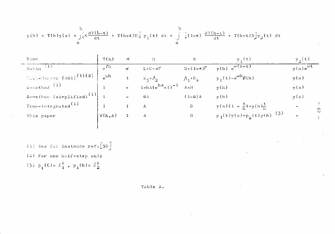
Y"(11) = T(h)y(o)
1-.l
+ IL.x:.dTCh-t)J d
o
+ T(h-t)Mj y.(t)~ di: +
h
IJ
o
! . dT(h-t) ./L ( 1- G( ) ,l + + T ( h - t )NJ Y 2 ( t) d t
y c~r:1P 1_ T (h) 0{ .~, f N y.(t) Y,) ( t ).1l. ...
r;'~=l!\ i I1'. 1 ) j fJ:l ~ L+U+..<f D+ (1-,,(}r y(h) t.J(h-t) y(o)e wt
e e
~~_.-'\.; ..-:f,-:;::, 2!: (;\01)(1)(2) (.)h1 E_ -+- 1\.-, A.+E, y ..Ct)=ewh0(ll) y(o)e
;; w 1. if ~(1) hA -1 y(h) y(o)~)--;,:et!1od 1 - 1-llA(e -1) A-H
G-r'le thOc.l r. -If" d)(l) 1 - Q~ (1-Q)A yell) y(o)~slrnp~l le~. "t t del) t ti lrr!e-J.~l egra e 1 1 A 0 y(o)(l - -)+y(h)-
h 11 m
(3 ) 'D
th:.s p3per I \.;(h, A) 1 A ° Pl(t)y(o)+p2(t)y(h)
( 1) See 1.. ()::-' ins tance;- l
ref.L30J(2) For one h~l£-step only(-' (c)- _i ()_ '"7i,;JJ Pi -~l' Pih -02
Ti:.ble 2.
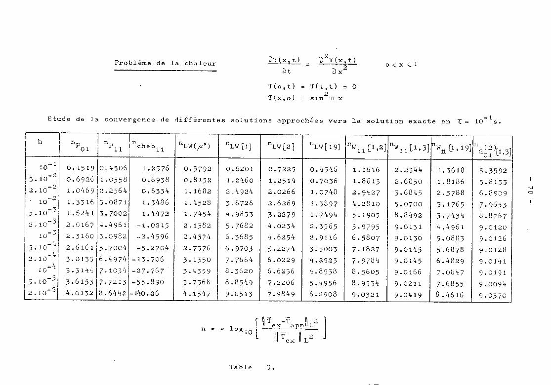
Probleme de la chaleur JT (x, t) =vt
2()T(x,t)20X
o<.x<..1
T(o,t)T(x,o)
= T(l,t) = 0r,. "'"Sln or x
Etude de l~ convergence de differentes solutions approchees vers la solution exacte en L = -110 s.
0.62011.2'160
204924I 3.8726. 4. 9853
I nu,r(j'-':) nLl, [19J Inw 11 [',2]ln" 11 [1, 3]~'''1l [1, 19]/nG~~ )[1.3JIr--~ Ij h I n I n 'nl---~ P11 I cheb11
I 10-:1 0.~519Io.45061 1.257615•10-2
1 0.692611.0558 0.69382.1.0-2! 1.0469120256411 0.6334
_.? I 6 8 8 ~. 10 -, 1.331 3.0 71 1.34 b
1:.10=~1 ~.624~ ~.70021 1.44~~,.LI0 I .... 016(1'1.49611 -1.02~)I 10-312.316015.09221 -2.'i596. 5.'0=~1 2.616115.7001'1 -5.2704 I
2.10_~1' 3.0135Ib.49741-13.706
I 10 - 3 . 3 1'f '~ 7. 103 If - 27 • 767
5.10-51 3.6153 7.72:3 -55.390I -,I .2 • 10-:> , 4. 0 132 l~ 4..2 -140. 26
0.57920.81521.16821.L1528
1.745L1:
2.13822.4374~L7376 I3.13503.4359 !
I3.73684.1347
nLW [1 ]
5.76826.36856.97037.76648.3620
8.85119
9.0513
nU{ [2]
0.72251.25142.02662.62693.22794.0234i1.62545.22746.02296.62367.22067.9849
0.451~6
0.70361.07481.38971.74911
2.35652.91163.50034.292311:.8938
5.49566.2908
1.16116
1. 86132.94274.28105.19055.97956.58077.18277.978'-:/;
8.56058.95349.0321
2.23442068503.68455007008.84929.01319.01309.01459.01459.01669.02119.0419
1. 36181.81862.57883.17653.74344:.4961
I 5.08835.68786.48297.081i7
7.68558.4616
5.35925.81536.89097.96538.87679.01209.01269.01289.01419.01919.00949.0370
-Jo
- T 1\ 2 1\~Tex- applL
n = - log 10 l --1\ TeA IIL2 J
Table .-.;; .
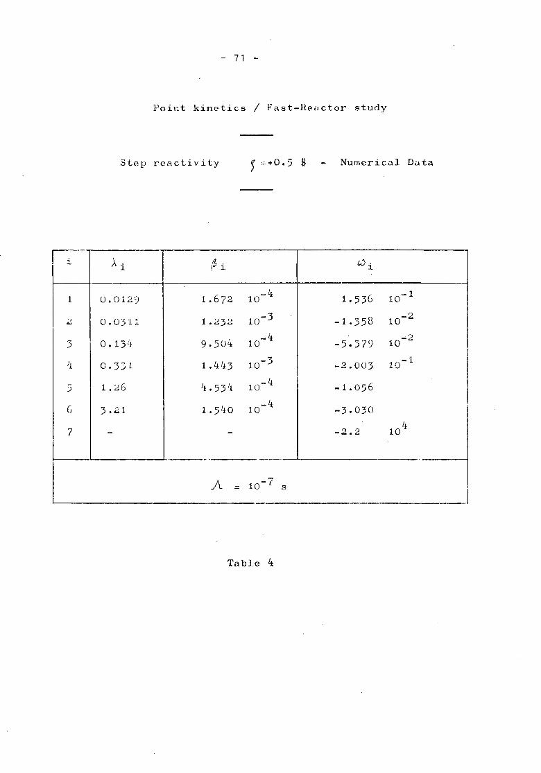
- 71 -
Point kinetics / Fast-Reactor study
Step reactivity ~ =+0.5 $ Numerical Data
~-~ ~i cJi
1 0.0129 1.672_ Li
1. 5}6 10-110
10-3 '}'} 0.0311 1.232 -1.358 10-'-"
10-4 . ')
3 o. 13 "1 9.504 -5.3"79 10-'"I
7- 10-1Li 0.3:}1 1.4 L13 10-":> -2.003
5 1.26 4.53L1_ L1
-1.05610
G 3.21 1.540 10-4 -3.0:;0
7 - - -2.2 10 Li
..."_. ---_ . ---
A = 10-7 s
J
Table 4
- 72 -
DISCUSSION
A.F. Henry
Could you comment on extension to space dependent problemsand also to situations in which the A matrix changes intime?
J. Devooght
A two-dimensional 1-group code, with triangular cell, cubicfinite elements is now in the process of debugging. Thecode incorporates the features mentioned in the paper. Ingeneral, one matrix inversion is needed per time step; thecase of splitted operators is dealt with on p. 50.
When the matrix is time dependent, it is necessary to dealwith proper averages, i.e. consistently keep the error tothe same order o(h3) as the one used in the W11 approxima-tion.
- 73 -
A.A. Harms, W.J. Garland, W.A. Pearce, M.P. Harding,O.A. Trojan, J. VlachopoulosMULTIPLE 'l'Er'lPORAL-MODE ANALYSIS :FOR THREE-DIMENSIONAL
REACTOR DYNAMICS
McMaster University, Hamilton, Ontario, Canada

- 75 -
MULTIPLE TEMPORAL-MODE ANALYSIS FORTHREE-DIMENSIONAL REACTOR DYNAMICS
A.A. Harms, W.J. Garland, W.A. Pearce,M.F. Harding, O.A. Trojan, and J. Vlachopoulos
Faculty of EngineeringMcMaster University
Hamil ton, Ontari 0, Canada
Abs tract
A multiple temporal-mode transformation combined with spatialdifferencing is developed and applied in a two-group, three-dimensionalreactor dynamics analysis using the diffusion approximation. It is foundthat this solution formalism leads to an apparently efficient and effectivemethod for the study of fast transients for time intervals before a globalflux trend has been established. Calculational results for a simplifiedcylindrical reactor under conditions of a fast transient and some generalproperties of the fOrllla'lislilare discussed.
- 76 -
IntroductionThe development of efficient and effective analytical and cal-
culational models which describe a wide range of dynamic characteristicsof a nuclear reactor in three dimensions has long represented a desirablegoal. Experience with low-dimensional calculations involving suitablychosen analytical descriptions and numerical strategies suggests thatthis goal may be attainable.
The three-dimensional, multi-group, time-dependent analysis of anuclear reactor generally provides a basis for considerable scope inexploring various strategies. Factors such as available computationalresources, detail of system description, temporal domain of interest,and others combine to provide various though restricted options.
Here we describe a three-dimensional, two-group, time-dependentneutron diffusion analysis based on the use of a multiple temporal-modetransformati on combi ned with fi nite differenci ng in space. As wi 11 becomeclear, the chosen analytical formalism seems particularly applicable forfast transients; in this context, this defines the dynamics of a nuclearreactor before a dominant global flux trend has been established. Inthe following we will describe the solution formalism and relate it to adynamic discretization. Finally, some preliminary calculational resultswill be presented and some general features of the solution formalismwill be identified.
Multiple-Mode Solution RepresentationThe three-dimensional, multi-group, time-dependent neutron diffusion
description of a nuclear reactor with or without delayed neutron can berepresented in symbolic form by
( 1 )
where ~ is a systems matrix and ~(!,t) is the vector containing the neutrongroup fluxes and the neutron precursor groups. We choose to base our analysison a functional prescription used effectively by Hansen and associates (1-3)and restrict our solution to the form
ljJ(ti+l) 'Iv lji'(ti)exp[0:6tiJ , (2)for a time step 6ti = ti+l - ti. Here, 0: is a suitable parameter validduring 6t.
To be specific, we consider the two-group, time-dependent equationin three-dimensions written in its common form
- 77 -
for g = 1,2 and where the symbols possess the usual meaning. Note thatherein we do not include delayed neutron precursors although the solutionformalism to be described here can be readily extended to include thiseffect as well as more than two groups. We interject to note that theexclusion of delayed neutron precursors will clearly effect the character-istic temporal evolution of the neutron flux in a calculational context.The above equations, Eq. (3), are coupled implying that a solution whichretains this coupling explicitly is desirable. Thus we choose to use anAnsatz given by
2~g(r,t) = ~g(r,t) \ S n(r)exp[an(r)tJ , (4)
-+ -+ Q,~lgx,-+ x,-+
for t e ti. Here ~g(r,t) may be called a transformed flux while SgQ,(r)and aQ,(r) may be termed moments and frequencies respectively. We emphasizetwo important properties of this Ansatz. First, the flux-coupling propertyspecifies here that the glth flux, ~g(!,t), is given in terms of themoments and frequencies associated with all other neutron group terms.Second, the proposed solution, Eq. (4), reduces to the standard point-kinetics solution if no spatial dependence is assumed to exist.
To place the multi-mode Ansatz, Eq. (4), in historical perspectivewe point out that it does possess some relation to the Ansatz previouslyused by Reed eta 1 (1) and Wig ht eta 1 (2 )
~g(!,t) = ~g(!,t)exp[ag(!)tJ ,and that used by Ferguson and Hansen (3)
(5)
(6)~g(r,t) = ~g(r,t)exp[a(r)tJ .-+ -+ -+
The distinction in these three solution models rests primarily in the extentto which the time variations of the various neutron groups are explicitlylisted as contributors in effecting a change in any given group flux.
Analytical DevelopmentIn the analysis to be pursued here, we restrict ourselves to an
arbitrary time step, ~ti = ti+l - ti' for which the system parameters,Dg(r) and Lqq' (r), are assumed to be given as a function of position only.Tnus, our describing equation for the glth neutron energy group is nowgiven by
2= ~.Dg(!)~~g(!,t) + 9II1Lggl(!)~gl (r,t) (7)
- 78 -
where again g = 1.2 and t e lit. Substituting Eq. (4) into Eq. (7) yields.after some algebraic rearrangement. the describing equations in terms of~gCr.t). Sg9,(r) and a9,C~:):
2 S 9,(r) a _ 2 Sg9,(r)a9,(!;')L exp[a9,(X)t]{ gv ~ 3f ~g(!.t)} - -nf_l
exp[a9,(!)t]{ vg ~g(!.t)}9,=1 9 N
2~.Dg(r)~g(r.t)~9,Ilexp[a9,(r)t]Sg9,(r)
2+ 9,I1Sg9,(r)exp[a9,(r)t]{~.Dg(r)~~g(r.t)} +
2 2+ L exp[an(r)t]{ L L: l(r)Sgln(r)~g,(r.t)}9.,=1 N ~ g'= 1 gg ~ N ~ ~
(8)
Writing the transformed describing equations in this form identifiesthe common multiplier containing the 9,'th order frequency. exp[a9,(r)t]. ineach but the third term of the right hand side of this equation; the "del"operator prevents a convenient extraction of this exponential term. Althoughan argument could be attempted that the contribution of this term might besmall and hence could be neglected. we propose to set this term equal tozero on the grounds that the resultant equation will be used only to evaluatethe moments. S 9,(X). and the frequencies. a9,(X). at ti = O. This latterimposition pos~esses the feature that it renders the terms upon which ~operates a constant and hence defines the entire 3'rd term equal to zero.We will comment on this point again in a subsequent section. Thus, viewingthe leading term, exp[a9,(r)t], as a common coefficient requires that the9,'th term in each summation be equated as follows:
2+ ~.Dg(r)~~g(r.t) + 9'~1l:gg'(r)Sg'9,(r)~g' (r.t) , (9 )
for 9 = 1.2 and t e liti. This equation will now be examined to permit theevaluation of ~g(r,t). Sg9,(r). and a9,(r) at all discrete values of r and for9, = 1.2.
Fin He An a 1ys isWe consider arbitrary time ste(:Gliti= ti+l - ti and. for convenience.
choose to use ti = 0 for all iterative time intervals. Either from thetime when the simulation is initiated or from the beginning of an arbitraryiteration in time. we set t = t; = 0 and use Eq. (4) to write
- 79 -
2~g(r.O) - ~g(r.O)l~lBgl(r) .
We choose to use a normalization on the moments Bg1(r) defined by2lI
1Bg1(r) = 1 ,
and thus have
(10)
(11 )
(12 )
(13 )
~g(r,O) = ~g(r,O) ,at the beginning of each time step.
To find the moments and frequencies, we use the value, ~g(!,O),associated with the beginning of each interval and assume that tne temporalevolution of the neutron flux during the interval ~ti is predominantlyexponential. That is, in Eq. (9) we impose the following condition on thetransformed flux ~g(r,t)
~t ~g(r,t)1 = 0,t e 6ti
and obtain an equation in terms of Bgl(r), al(r) and the initial conditions,~g(r,O) :
( 14 )
This equation can be written as an eigenvalue equation for the frequenciesal(r) and a2(r) corresponding to the values of Dg(r) and Bg1(r) at rand~g(r,O) about r:
-+ -+
or, symbolically,(16 )
- 80 -
Since all elements of ~ are assumed known at the coordinate of interest~ r~-rthe eigenvalues a£ can-be found by the solution to
( 17)
In this two-group representation~ al(r) and a2(r)~ are the two solutions ofa quadratic equation.
The componentsnon-zero column of thean arbitrary constant.fied by Sg£(r). Then~we find a constant hg~
of the eigenvector Sg,~ Eq. (17)~ are,giyen by anyadjoint of [C-a£JJ~ ADJ[~-a£JJ~ to wlthln
Supposing that these vector components are identi-according to the normalization condition~ Eq. (12)~g = 1 ~2 ~ such that
hg[Sgl (r) + S~2(r)J = 1 . (18)Hence~ the moments Sg~(r)~ g = 1 ~2~ £ = 1 ~2~ are determined. With thefunctions wg(r~O)~ a£~r) and S t(r) all known at ti = O~ we insert thesevalues into Eq. (8) and~ by fiRlte numerical methods solve for ~g(r~ti+1).With the use of Eq. (4) ~ this resultant expression yields the f1ux-+<pg(r~ti+1)at the end of the time step. -+
Numerical Modeling and Calculational ResultsFor the purpose of an initial exploratory three-dimensional examin-
ation of our forma1ism~ it is advantageous to adopt a simple and directnumerical model and to concentrate on relatively large scale effects, Oursimplified three-dimensional reactor is therefore chosen to be a homogeneous~bare cylinder penetrated by a control rod perpendicular to the axial direction.
We choose to restrict ourbelves to a coarse spatial mesh describingthe whole reactor with 1320 mesh points. Errors may arise from threesources: 1) numerical round-off~ 2) finite difference expressions~ and3) boundary condition approximations.
Round-off errors will not be a severe problem in our calculationboth because of the precision of the long (60 bit) capacity of the COC-6400computer used in our calculation and because our equations involve only tri-diagonal (three-stripe) matrices. Computer memory size limits the numberof values of the flux which can be conveniently stored; in particu1ar~ wecannot keep the value of the flux at many past times and thus are forced tocompute the flux at time t based on values of the flux and system parametersat time t-6t and accept the attendant truncation error in the time step, Ifthe boundaries of the reactor do not lie on our chosen grid points then wemust take an approximation to the actual boundary values; we can avoid thiserror~ however~ by describing our reactor in cylindrical co-ordinates (r~0~z).
- 31 -
We have chosen to describe the spatial domain by two diametricallyopposite 90° wedges of the core. Use of the physical bi-lateral symmetryof our reactor model allows us to construct all values not explicitly lyingwithin our grid thus reducing our computer storage requirements. The controlrod has been made to appear more regular by weighting the parameters accord-ingly within the control rod region. A grid with 12 points in the r-direction,10 points in the 8-direction and 11 points in the z-direction yielding 1320grid points has been chosen.
Starting with some initial array of values for the fluxcIJg(ri)= cIJ(ri,8i,zi), g = 1,2, we solve Eq. (17) - which here representsa quadrati@ equation - for the spatial frequencies at(ri) and for the spatialmoments S t(ri) according to Eq. (11) and Eq. (18). The diffusion termin Eq. (l~) is represented at the point ri = (ri ,8i,zi) in finite differentform. Equation (8) may subsequently be written as a tri-diagonal systemwhich is implicit in one of the three spatial directions and explicit inthe remaining two. In solving this system we have chosen to use the alter-nating two-direction implicit method (2).
The data used in the sample calculation here are listed in Table Iand correspond approximately to those appropriate for a heavy water reactor.Figure 1 shows the fast and thermal flux rise associated with two suddenwithdrawals of the control rod described by the following. At steady statewe consider the axial flux traverse adjacent to the cylindrical axis withthe control rod inserted 55% of the full cylindrical diameter. At t = 0the control rod is suddently withdrawn so that only 27.5% of the diametricaldistance of the core contains the control rod. After a time interval of320 ~s the control rod is withdrawn entirely. The flux rise is followedfor another 320 ~s up to t = 640 ~s, Fig. 1.
We note that during this very fast transient, the induced reactivitydisturbance effects both the fast and thermal flux only in the region closeto the control rod position. We also observe a contrast in the flux perturb-ation and response between the fast and thermal flux.
The computer time requirements for this three-dimension, two-group,1320 mesh-point calculation was found to be 0.84 slstep on the COC-6400computer used here. This is almost identical to the computer time require-ments reported by Reed (5) for an efficient two-dimensional calculationusing a faster computer (COC-6600).
Discussion of Solution FormalismThe describing equation, Eq. (1), used here can be easily extended
to G energy groups and include I delayed neutron precursor groups. Forthis case we write the vector ~Cr;.,t)and the matrix 8 in Eq. (1) as
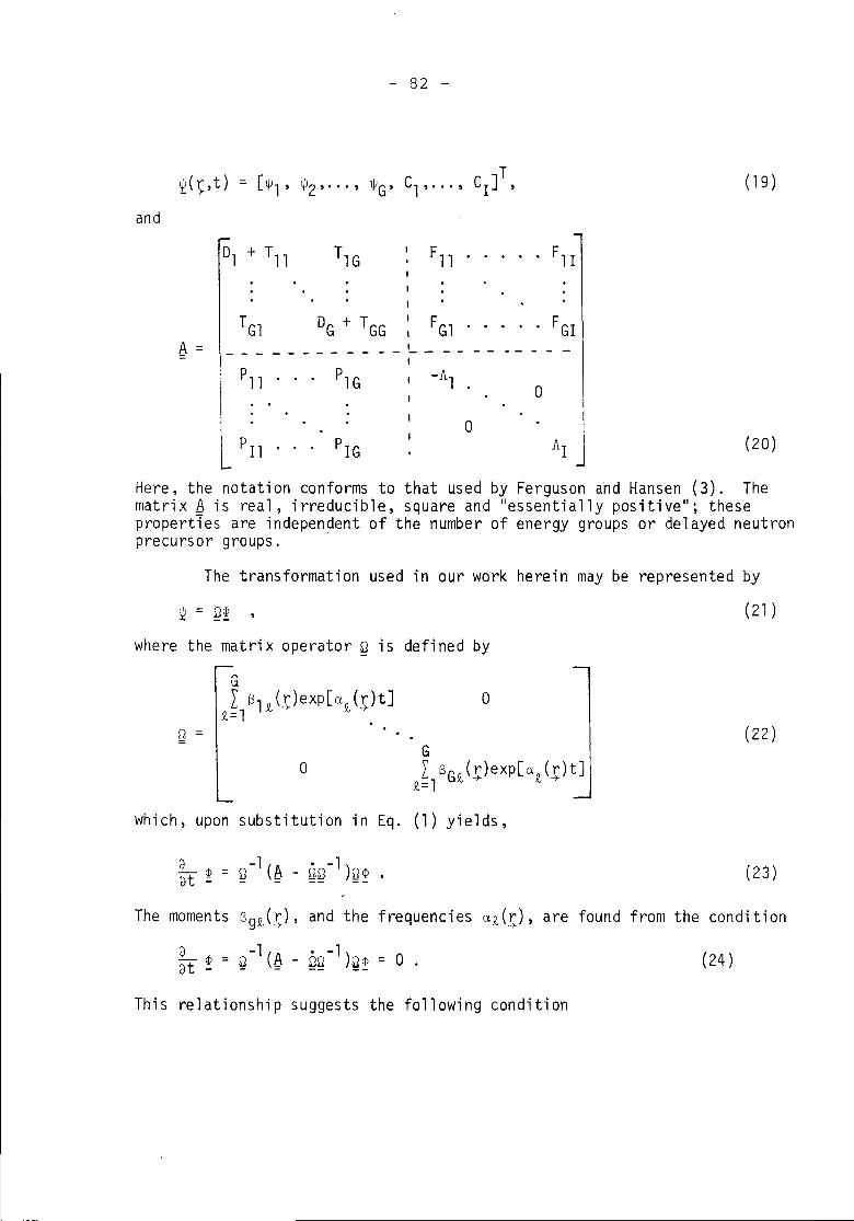
- 82 -
(19 )
and
T Gl DG + TGG IFGl F GI
8 = ---------- --,------ -----,
l~;~P1G -A,
0
0PIG AI (20)
Here, the notation conforms to that used by Ferguson and Hansen (3). Thematrix 8 is real, irreducible, square and "essentially positive"; thesepropertles are independent of the number of energy groups or delayed neutronprecursor groups.
The transformation used in our work herein may be represented by(21 )
where the matrix operator Q is defined by,..\;\
£~lSl£(r)exp[a£(r:t]
o
o(22)
which, upon substitution in Eq. (1) yields,
(23 )
The moments Sg£(r), and the frequencies a£(r), are found from the condition
~t ~ = g - 1 (~ - QQ - 1 )Q ~ = 0 . (24 )
This relationship suggests the following condition
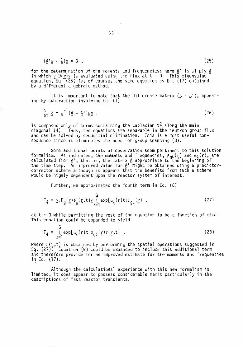
(~I~ - ~)~ = 0 ,
- 83 -
(25)
for the determination of the moments and frequencies; here 81 is simply 8in which v.D(r)v is evaluated using the flux at t = O. This eigenvalue -equation,-Eq.+(25) is, of course, the same equation as Eq. (17) obtainedby a different algebraic method.
It is important to note that the difference matrix (~ - ~I), appear-ing by subtraction involving Eq. (1)
(26)
is composed only of terms containing the Laplacian v2 along the maindiagonal (4). Thus, the equations are separable in the neutron group fluxand can be solved by sequential elimination. This is a most useful con-sequence since it eliminates the need for group scanning (3).
Some additional points of observation seem pertinent to this solutionformalism. As indicated, the moments and frequencies, Sg~(r) and a~(r), arecalculated from 81
, that is, the matrix 8 appropriate to the beginning ofthe time step. An improved value for 81-might be obtained using a predictor-corrector scheme although it appears tnat the benefits from such a schemewould be highly dependent upon the reactor system of interest.
Further, we approximated the fourth term in Eq. (8)
(27)
at t = 0 while permitting the rest of the equation to be a function of time.This equation could be expanded to yield
GT4 = ~~lexp[a~(!)tJSg~(!)r(~,t) , (28)
where r (r,t) is obtained by performing the spatial operations suggested inEq. (27); Equation (9) could be expanded to include this additional termand therefore provide for an improved estimate for the moments and frequenciesin Eq. (17).
I
Although the calculational experience with this new formalism islimited, it does appear to possess considerable merit particularly in thedescriptions of fast reactor transients.
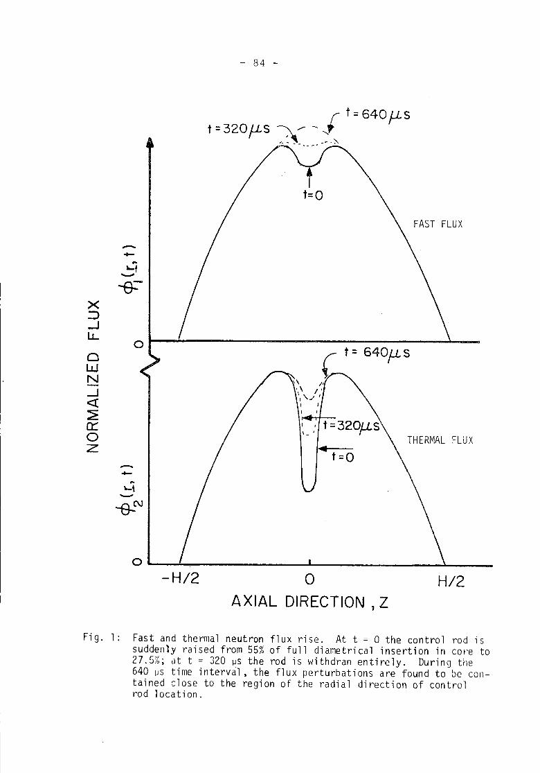
- 84 -
H/2
FAST FLUX
oAXIAL DIRECTION, Z
-H/2o
--..'-t
'-'
-e:-x:::>-Jl.L
0t = 640fLs0
wN '\ II
..J '\ I'",./ '« I I
~\I
0:: ~_,'t =320fLsa THERMALFLUXZ 411
t=o-.-..'-t
'-'
-e-N
Fig. 1: Fast and thermal neutron flux rise. At t = 0 the control rod issuddenly raised from 55% of full diametrical insertion in COI'e to27.5%; at t = 320 ~s the rod is withdran entirely. During the640 ~s time interval, the flux perturbations are found to be con-tained close to the region of the radial direction of controlrod 1ocati on.
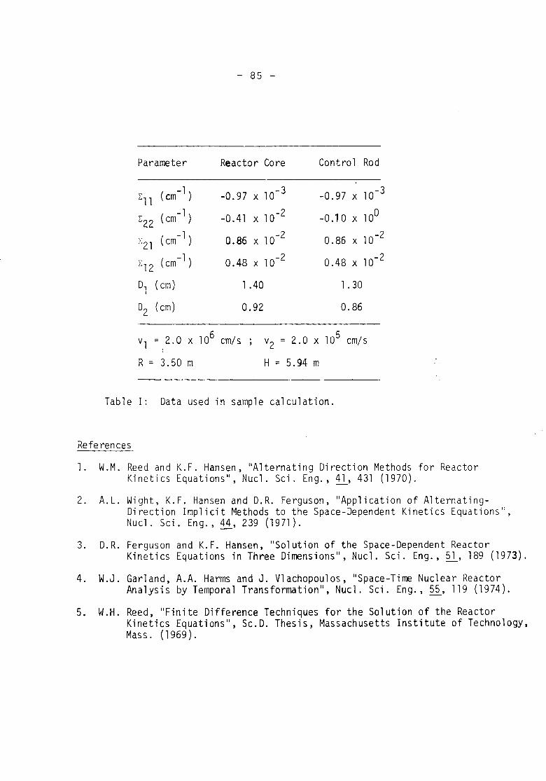
- 85 -
Parameter Reactor Core Control Rod
Lll(em -1 ) -0.97 x 10⁻³ -0.97 x 10⁻³
L22 (cm -1 ) -0.41 x 10⁻² -0.10 x 100
L21 (cm - 1 ) 0.86 x 10⁻² 0.86 x 10⁻²
L12(cm -1 ) 0.48 x 10⁻² 0.48 x 10⁻²
01 (cm) 1 .40 1. 30
O2 (cm) 0.92 0.86
vl =2.0 x 106 cm/s , v2 = 2.0 x 105 cm/s
R = 3.50 m H = 5.94 m
Table I: Data used in sample calculation.
References
1. W.M. Reed and K.F. Hansen, "Alternating Direction Methods for ReactorKinetics Equations", Nuc1. Sci. Eng., !l, 431 (1970).
2. A.L. Wight, K.F. Hansen and D.R. Ferguson, "Application of Alternating-Direction Implicit Methods to the Space-Dependent Kinetics Equations",Nucl. Sci. Eng., 44, 239 (1971).
3. D.R. Ferguson and K.F. Hansen, "Solution of the Space-Dependent ReactorKinetics Equations in Three Dimensions", Nuc1. Sci. Eng.,~, 189 (1973).
4. W.J. Garland, A.A. Harms and J. V1achopou1os, "Space-Time Nuclear ReactorAnalysis by Temporal Transformation", Nuc1. Sci. Eng., ~, 119 (1974).
5. W.H. Reed, "Finite Difference Techniques for the Solution of the ReactorKinetics Equations", SC.D. Thesis, Massachusetts Institute of Technology,Mass. (1969).
- 86 -
DISCUSSION
A. Siebertz
Your method could be called a quasi-static method with spe-cialized exponential form amplitude function.
Could you comment on the relative merits of both methods(accuracy, computing time ...)?
A.A. Harms
First, for very rapid changes with highly localized effects,this method seems more accurate and at least as fast. Se-cond, the one additional important merit point is associ-ated with the group-coupling solution representation whichdescribes an arbitrary group flux in terms of all othergroups; thus, increases in one group and concurrent de-creases in another group can be both described.
A.F. Henry
The improvement caused by these methods when applied to al-ternating directions schemes is much greater than when theyare applied to fully implicit schemes.
D.A. Meneley
1) The quasi-static method is best suited to fast reactorproblems.
2) Hansen's and Harm's methods have pointwise or/and group-wise exponential transformations with extrapolated coef-
- 87 -
ficients. The quasi-static method has a single amplitudefunction obtained by solution of the point kinetic equa-tion. Quasi-static methods are presently limited to lin-ear variation of shape functions with time; on the otherhand, the Hansen-Harm's methods are limited in maximumtime step length because of the extrapolation, constantproperties over the time step, and by alternating-direc-tion solution method. The question can only be answeredby running a series of benchmark problems with all me-thods.

- 89 -
Session II
COARSE MESH METHODS
Chairman: F.J. Fayers, United Kingdom
W. Werner 91
MATHEMATICAL PROBLEMS IN THREE-DIHENSIONALREACTOR CALCULATIONS
Laboratorium fur Reaktorregelung und Anlagen-sicherung, Technische Universitat Munchen,Germany
T.J. Burns / J.J. DorningTHE PARTIAL CURRENT BALANCE METHOD: A NEWCOMPUTATIONAL METHOD FOR THE SOLUTION OFMULTIDIMENSIONAL NEUTRON DIFFUSION PROBLEMS
Oak Ridge National Laboratory, Oak Ridge,Tennessee / University of Illinois, Urbana,Illinois, USA
H. FinnemannA CONSISTENT NODAL METHOD FOR THE ANALYSISOF SPACE-TIME EFFECTS IN LARGE LWR
Kraftwerk Union AG, Erlangen, Germany
109
131
- 90 -
S. Langenbuch, W. Maurer, W. Werner
SIMULATION OF TRANSIENTS WITH SPACE-DEPEN-DENT FEEDBACK BY COARSE MESH FLUX EXPANSIONMETHODLaboratorium flir Reaktorregelung und Anlagen-sicherung, Technische Universitat Mlinchen,Germany
O. Norinder
THE BITNOD METHOD OF REACTOR COARSE MESHCALCULATIONSAB Atomenergi, Studsvik, Sweden
173
1 91
- 91 -
W. Werner
MATHEMATICAL PROBLEMS IN THREE-DIMENSIONAL REACTOR CALCU-LATIONS
Laboratorium fUr Reaktorregelung und Anlagensicherung,Technische Universitat MUnchen, Germany

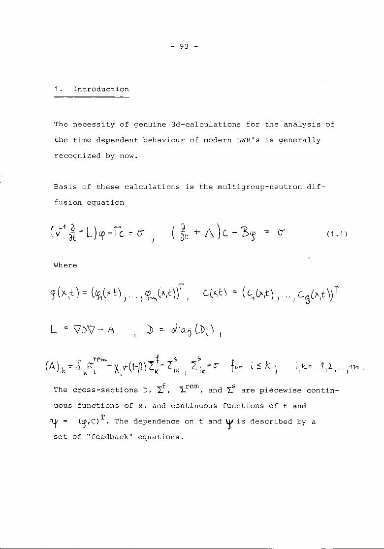
- 93 -
1. Introduction
The necessity of genuine 3d-calculations for the analysis of
the time dependent behaviour of modern LWR's is generally
recognized by now.
Basis of these calculations is the rnultigroup-neutron dif-
fusion equation
( 1 • 1 )
where
"Y'e"M. .. f. ~(A) ::: d, b- -Y .V'l1-~) 1: -l,,k II<. l f\ I I" K II<
The cross-sections D, Lf, Lrem, and LS are piecewise contin-
uous functions of x, and continuous functions of t and
~ = (~, C)T. The dependence on t and 0/ is described by aset of "feedback" equations.
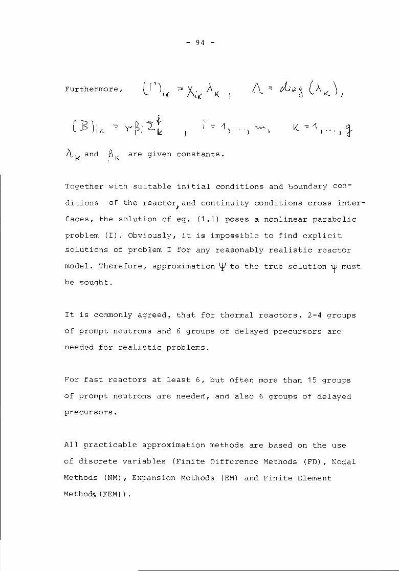
- 94 -
Furthermore,
.1A,AI
t\ 1< and P i< are given constants.
Together with suitable initial conditions and boundary con-
ditions of the reactor} and continuity conditions cross inter-
faces, the solution of eq. (1.1) poses a nonlinear parabolic
problem (I). Obviously, it is impossible to find explicitsolutions of problem I for any reasonably realistic reactor
model. Therefore, approximation \if to the true solution Y' must
be sought.
It is commonly agreed, that for thermal reactors, 2-4 groups
of prompt neutrons and 6 groups of delayed precursors are
needed for realistic problems.
For fast reactors at least 6, but often more than 15 groups
of prompt neutrons are needed, and also 6 groups of delayed
precursors.
All practicable approximation methods are based on the use
of discrete variables (Finite Difference Methods (FD), Nodal
Methods (NM) , Expansion Methods (EM) and Finite Element
Methods (FEM) ) .
- 95 -
2. Direct and Indirect Methods
Very coarsly, these approximation methods can be classified
into direct and indirect methods.
n+1 n 1In direct methods, the space R = R x R of independent
variables x1' ... , xn' t is subdivided into discrete regions
Gi, i = 1, ••• ,N, UGi = G,
Atj = tj - tj_1, j = 1, ... ,M. On Gi, resp. ~tj' suitable
"Basisfunctions" Pi(k), i = 1, ... ,N, resp. Qj(t) are defined.
Upon substitution of Pi and Qj into 1.1, and replacement of
differential operators by difference operators, eq. 1.1 is
converted into a matrix equation, which permits to compute
basis function Pl+1 (x), i = 1 ,... ,N, at time tj+1 from the
knowledge of basisfunctions P~(x) ,... ,p~-e(x), i = 1, ... ,N,1 1
at times t., ... ,t. D'J J-t,
The propagation of the approximate solutions is performedlocally, i.e., in each time-step, all basisfunctions p~+1 (x),
1
i = 1, ... ,N are new ly computed.
By using sufficiently many regions Gi and .1tj and by
employing basis functions of sufficiently high order, the
solution of (1.1) can in principle be approximated with any
desired accuracy. The relatively large amount of computational
- 96 -
work associated with the computation of all basisfunctions in
each time-step is only adequate, if the spatial flux distri-
bution changes significantly within the time-steps. The use
of direct methods is certainly uneconomical, if the spatial
flux distribution does not change between time-steps, since
in that case, a lot of computational work is spent to per-
petually calculate identical or almost identical basisfunc-
tions.
Besides the approximations introduced by discretisation,
which are of mathematical nature, indirect methods make use
of further approximations, which are justified by physical
properties.
In all useful indirect methods, the physical approximations
consist in a separation ,U (x,t) = .2..A.(t)lV. (x,t) withl;.(X,t)T • l T 1 T,L
being only "weakly" time dependent, relative to the time
dependence of Ai(t).
The complexity of space functions ~i (x,t) varies from being
constant in the whole reactor in the most simple case (point
kinetics), to being a function of all 3 space variables
(quasistatic method) .
The propagation of the approximate solution consists only in
the solution of a system of ordinary differential equations
- 97 -
for the determination of the amplitude functions A. (t).l
Changes of the space-functionsVi(x,t) due to changing
cross-sections are considered by exchanging the set of
space functions from time to time, but in intervals which
are long relatively to the integration steps for Ai (t}.
The most serious difficulty in the applications of in-direct methods is, that it is hard to find rigid criterions
which indicate the necessity to exchange the set of spacefunctions.
The main area of application of direct methods is the ana-lysis of events governed by localized changes of cross-
sections, while indirect methods are successfully used in
the analysis of events governed by global cross-sectionchanges.
A side condition imposed by the computer hardware is, that
the number of discrete variables to be stored in the fast
memory is limited by ca. 200 000. For thermal reactors, this
implies, that not more than 15000-20000 G. 's (boxes) can beJ
used, and this, in turn, implies that the average box size
for 3d-calculations of modern LWR's has to be about 20 x320 x 20 cm .
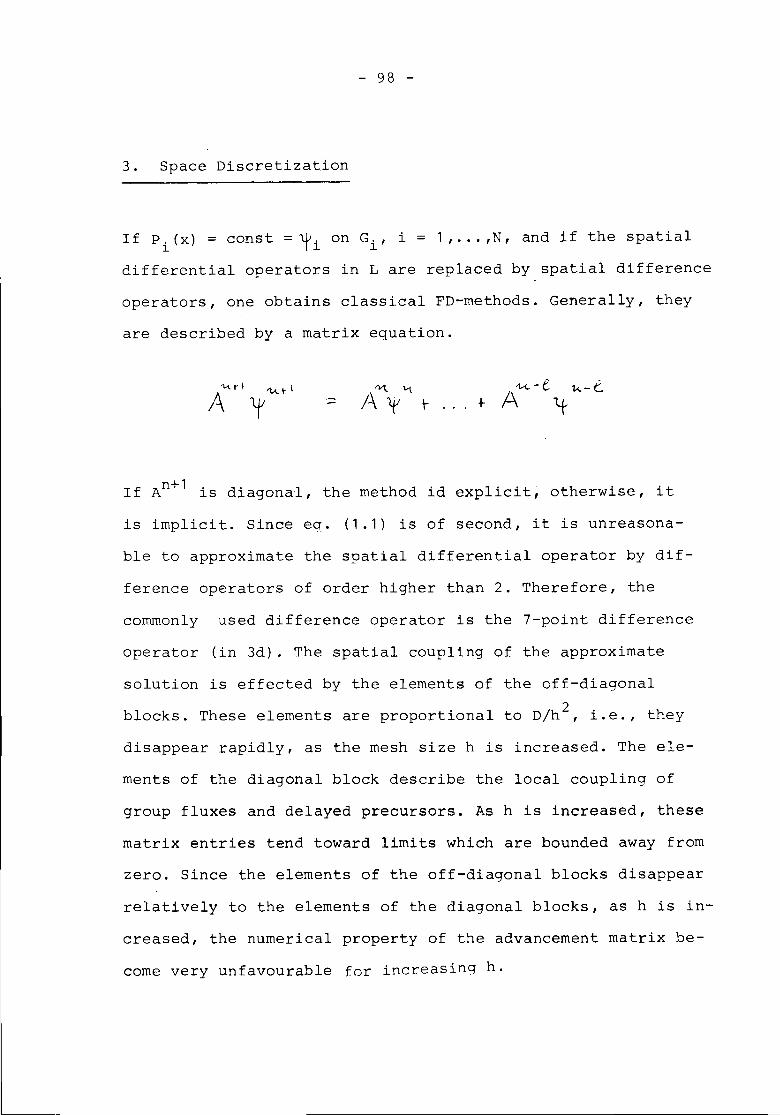
- 98 -
3. Space Discretization
If Pi(x) = const = Yi on Gi, i = 1, ... ,N, and if the spatial
differential operators in L are replaced by spatial difference
operators, one obtains classical FD-methods. Generally, they
are described by a matrix equation.
.....r1
/-\"Y\. -"t
!\y r ... +--u.-e
A
If An+1 is diagonal, the method id explicit~ otherwise, it
is implicit. Since eq. (1.1) is of second, it is unreasona-
ble to approximate the spatial differential operator by dif-
ference operators of order higher than 2. Therefore, the
commonly used difference operator is the 7-point difference
operator (in 3d). The spatial coupling of the approximate
solution is effected by the elements of the off-diagonal
blocks. These elements are proportional to D/h2, i.e., they
disappear rapidly, as the mesh size h is increased. The ele-
ments of the diagonal block describe the local coupling of
group fluxes and delayed precursors. As h is increased, these
matrix entries tend toward limits which are bounded away from
zero. Since the elements of the off-diagonal blocks disappear
relatively to the elements of the diagonal blocks, as h is in-
creased, the numerical property of the advancement matrix be-
come very unfavourable for increasing h.
- 99 -
Experience with FD-methods for LWR-calculations shows, that
acceptable accuracy, with relative errors of the spatial so-
lution less than a few percent, can only be reached with mesh
size smaller than 3-4 cm. Implementation of 3d-codes employing
such mesh size on present day computers is obviously impracti-
cal, since it would require the use of external storage to a
large extent.
4. Coarse Mesh Methods
The only way to decrease the amount of computational time sig-
nificantly is a dractic reduction of the number of unknowns
by the use of so called "Coarse Mesh Methods" (CM). The first
CM-methods /1-3/ used coupling coefficients which were pre-
determined, either empirically or theoretically, but adapted
to certain typical situations. Thus, the applicability of
such methods was very limited. The second generation of CM-
methods /4-8/ employs higher order (2-4) basis functions,
which permit an automatic computation of coupling coefficients.
The coefficients of the basis functions are either determined
through global Galerkin weighting (classical Finite Element
Methods (FE) /7,8/), or through integral relations and local
minimal principles (Expansion Method (EM)). In any case, local
operators describing the coupling of neighbouring nodes become
- 100 -
defined. In contrast to FD-methods, the coupling coefficients
of the local operators depend not only on the leakage terms
of one group flux, but on all group constants. Especially,
the elements of the off-diagonal blocks do not disappear,
relative to the elements of the diagonal blocks, as the mesh
size is increased.
Therefore, there are no principle difficulties to be encoun-
tered with the use of box sizes which are much larger than the
mean free path of neutrons. The only point of consideration in
the choice of mesh size is the question of adequacy of the se-
lected basis functions in relation to flux variation withinthe nodes.
Expansion method require a grid with uninterrupted grid lines
(like FD method). Also the advancement of expansion methods
is similar in structure to the advancement matrix of FD-methods.
Since the number of unknowns is relatively small in expansion
methods (several 1000 for realistic LWR's) a direct solution of
the advancement matrix equation is feasible; tho~gh it would
not be an efficient method. Potentially more efficient are re-
laxation methods with rebalancing /6,10/, and matrix decompo-
sition methods /5/. The latter have been applied successfully
in 2d-and 3d-FD-calculations /11,12/. However, since the con-
stancy or near constancy of the decomposed operators, which is
essential for the successful application of the method may be,
- 101 -
severly violated in expansion methods, modifications of the
basic method are required.
The implicit matrix decomposition method described in /12/
uses 2 corrector steps (in 3d-calculations) to balance the
instability caused by the components of the difference opera-
tors which are treated explicitly in the predictor step. A
theoretical proof of this balancing can only be given in the
constant operator case. For non constant operators, it is in-
tuitively clear, and also supported by numerous evidence, that
this balance becomes very tricky and great care is required in
maintaining it. This difficulty can be avoided by using stable
explicit approximations in the predictor step /e.g. 11, 15/.
Coarse mesh rebalancing methods have become very popular in the
past years; with n being the number of unknowns of the problem,
the computational work associated with coarse mesh rebalancing
methods depends on nln(n), which is much more favourable thanwith conventional relaxation methods.
Finite EleMent Methods do not reauire a regular grid; especiallYJ
grid lines may be interrupted. This is of great advantage in
classical applications of PE-methods, like structural analysis
or fluid dynamics; however, in LW~'s with their rather reqular
fuel-moderator structure, this offers no significant advantaae.
On the other hand, the advancement matrix of FD-methods is more
dense than for Expansion methods of comparable accuracy. Thus,
- 102 -
somewhat more computing time is to be expected, relative to
Expansion methods. 2d-calculations indicate about a relation
of 1:4 in favour of Expansion methods /13/, where direct so-
lution by Choleskis method is used in the FE-~ethod. In real-
istic 3d-calculations, efficiency competitive with expansion
methods can only be expected by application of modern relaxa-
tion methods with coarse mesh rebalancing /10, 14/. However,
only insufficient experience with 3d-FE-methods is yet availa-
ble /18/.
5. Conclusion
For the 3d-simulation of the time dependent behaviour of mo-
dern LWR's, CM-methods, especially Expansion method, are an
adequate tool. In principle, they permit an efficient compu-
tation of transient solutions. However, further work is re-
quired to determine optimal time-integration procedures, both
for FE-, and Expansion methods.
- 103 -
References
/1/ L. Goldstein, F. Nakache, A. Veras:
Calculations of Fuel-Cycle Burnup and Power Distribution
of Dresden-I Reactor with the TRILUX Fuel Management
Program.
ANS Transactions, 10, 300 (1967)
/2/ A. MUller, F. Bennewitz:Ein neues schnelles Verfahren zur Berechnung 3-dimen-
sionaler FluBverteilungen mit Hilfe von StoBwahrschein-
lichkeiten.
Reaktortagung 1971, Bonn
/3/ S. B~rresen:
A Simplified, Coarse Mesh, Three-Dimensional Diffusion
Scheme for Calculating the Gross Power Distribution in
a Boiling Water Reactor.
NSE 44, 37 - 43 (1971)
/4/ A. Birkhofer, W. Werner:
Efficiency of Various Methods for the Analysis of Space
Time Kinetics.
Proc. 1973 Conf. Math. Models and Computational Tech-
niques for Analysis of Nuclear Systems, IX 31 - 41
- 104 -
/5/ A. Birkhofer, S. Langenbuch, W. Werner:
Coarse-Mesh Methods for Space-Time Kinetics.
ANS Transactions, 18, 153 (1974)
/6/ M. Wagner:
Nodal Synthesis Method and Imbedded Flux Calculations.
ANS Transactions, 18, 152 (1974)
/7/ C.M. Kang, K.F. Hansen:
Finite Element Methods for Reactor Analysis.N'SE, 51, 456 (1973 )
/8/ H. Franke, F. Schmidt, H. Unger:
Zur Verwendung der Methode der Finiten Elemente inder Reaktorphysik.
Bericht Nr. 4-14D, IKE, Universitat Stuttgart (1973)
/9/ H. Finneman~ KWU Erlangen
private communication
/10/ S. Nakamura, NSE 39, 272 (1971)
/11/ A.L. Wight, K.F. Hansen, D.R. Ferguson:
NSE 44,239 (1971)
- 105 -
/12/ A. Birkhofer, W. Werner:
ANS Transactions 15, 789 (1972)
/13/ H. Franke, F. Schmidt:
FEM-3D Ein Prograrnrnzur Losung der zweidimensionalen
Diffusionsgleichung nach der Methode der Finiten Ele-
mente.
Bericht Nr. 4-25, IKE, Universitat Stuttgart (1974)
/14/ H. Fredericson,
private communication
/15/ J. Lambert:
Nonlinear Methods for Stiff Systems of Ordinary Differ-
ential Equations.
Conf. on the Numerical Solution of Differential Equations,
Dundee, 1973, Springer Verlag Lecture Notes, 363
- 106 -
DISCUSSION
A. Siebertz
In LMFBR's fast transient calculation, even the use of 13energy gruops (classical disjoint ones), leads to unaccep-table errors in the prediction of the sodium void reactivi-ty effect. According to some results obtained at Karlsruhe,the use of energy synthesis methods can give very good re-sults even with as few as 3 overlapped groups. But then,there is the difficult problem of the choice of the basicspectra. Could you please comment?
L. Vath, W. Werner
We found, in fact, at Karlsruhe, that 15 energy groups hadto be used with normal flux weighted collapsing for an ade-quate description of sodium voiding. On the other hand, wehad very encouraging results for bilinear weighting andenergy synthesis, but these results were arrived at usinga sirnple 1d kinetics code with simulated feedback. It isnot at all clear, for the moment, how well these methodswork for 2d or 3d problems with realistic feedback; in ad-dition, we encountered some problems with energy synthesis.
F.N. McDonnell
With the coarse-mesh method, is the spatial eigenvalue se-paration between the fundamental and first azimuthal modemaintained? For classical nodel models this is known tobe not so.
- 107 -
W. Werner
The eigenvalue separation is maintained.

- 109 -
T.J. Burns / J.J. DorningTHE PARTIAL CURRENT BALANCE METHOD: A NEW COMPUTATIONALMETHOD FOR THE SOLUTION OF MULTIDIMENSIONAL NEUTRONDIFFUSION PROBLEMS
Oak Ridge National Laboratory, Oak Ridge, Tennessee / Uni-versity of Illinois, Urbana, Illinois, USA

- 111 -
THE PARTIAL CURRENT BALANCE METHOD: A NEW COMPUTATIONAL METHOD FOR
THE SOLUTION OF MULTIDIMENSIONAL NEUTRON DIFFUSION PROBLEMS*
T. J. Burnst and J. J. Dorningtt
University of Illinois at Urbana-ChampaignUrbana, Illinois 61801
ABSTRACT
A new computational method for the solution of multidimensional neutron
diffusion problems which is based on local balances of partial currents is
described. After briefly motivating the ideas used in the metho~ the~formalism
is reviewed. The technique used for the solution of the final equations via local
expansions is then described, and the resulting matrix equations are developed.
The iteration schemes which were employed in the initial calculations are
described. Computational results for two simple one-dimensional PTGR models and
for a simple two-dimensional HTGR model are reported and compared with finite
element and finite difference calculations for accuracy and computing time. In
all cases studied, the partial current balance method compared very favorably with
both these widely used methods. Some advantages of the partial current balance
formulation are discussed.
*This work was supported by the U.S. Atomic Energy Commission under grantnumber AT(11-1)-246l.
tpresent address: Oak Ridge National Laboratory, OakRidge, Tenn. 37830ttM. . .eetlng partlclpant.
- 112 -
INTRODUCTIONThe partial current balance method is a coarse mesh technique based on a
local integral form of the multigroup neutron diffusion equations. The method
is formulated by converting the standard differential form of the neutron
diffusion equation for each energy group into a local integral equation. This
is done by formally using local group removal Green's functions for each of the
volume elements into which the nuclear assembly is partitioned. Each volume
element is coupled only to its nearest neighbors. This coupling is accomplished
by the partial current continuity conditions at the volume element interfaces
which naturally arise in the development of the formalism. The method has three
obvious advantages which may account for its speed and accuracy. These are:
it permits the use of large volume elements (a very coarse mesh) while still
retaining high accuracy; it has only nearest neighbor coupling among the volume
elements, which is not the case for most integral methods; the nucle~r coupling
parameters which are used in the iterative solution procedure are generated
independently for each group and can be calculated with relative ease.
As a motivation for the formalism it is convenient to consider the actual
equation which must be solved in practical neutron diffusion calculations such
as multigroup source iteration calculations. This equation has the general form
(1)
For example, an equation of this type must be solved in each inner iteration
of a multigroup source iteration criticality calculation, or at each time step
of an implicit space-time solution of the kinetics equations. Of course, it is
generally far too difficult to invert Eq. (1) exactly for a complicateJ rcalisti\."
reactor system. Hence, the operator in Eq. (1) is generally approxinmtcd (e.g.,
as in a finite difference scheme or a finite element scheme), and then the a]'proxi-
-113-
mate operator is inverted. The inversion of this approximate operator, which is
generally a large matrix operator for systems of practical interest, at each
inner iteration is a time-consuming process on a digital computer. Thus we are
motivated to exactly invert Eq. (1) instead of following the above procedure.
As stated above, however, an exact global inversion of such an equation is not
feasible. An alternative is to attempt an exact local inversion of Eq. (1) or of
a closely related equation, follow this inversion by some procedure which
establishes coupling of the locally inverted equations so that the overall
nuclear system is again fully described, and then generate an approximate solution
to the resulting system of equations. This general approach leads to the partial
current balance formalism 1 which is reviewed in the next section.
REVIEW OF FORMALIS~1
The partial current balance formalisml is developed by first partitioning
the nuclear assembly into K volume elements Vk. The equation for the group fluxin the volume element Vk is
(2)
where
(3)g'=lg'rg
It is convenient at this point to decompose the group removal cross section and
the group diffusion coefficient into some constant, or reference, part and a re-
mainder which is variable due to its explicit dependence upon position \vithin
the kth volume element or its implicit dependence .upon position through feedback
parameters and flux (for example, in a kinetics calculation).
(4 )
k .D (r,[<P(r)])g - -
- 114 -
(5)
For the purposes of the present development we now take the variable part of
the diffusion coefficient hk(r,[<P(r)]) to be zero. (That is, the group dif-g - -thfusion coefficient is taken to be constant within the k volume element.)
The effect of nonzero hk upon the final equations will be stated below afterg
the formalism is developed for the present case. The term which involves the
part of the group removal cross section which is variable within the kth VOlUTIle
element is transferred to the right hand side of Eq. (2) and incorporated in
the source term, giving
(6)
where
'Sk(r) =g-
and
tgl:=;l
Fk ~k() + sext,k(r)"'"t_rgg' b g - (7)
kF ,(r,[<P(r)])gg - -k( ~)k + ~s,k (l-~ )X v~f ' ~ , u ,g g g+g gg fk , (r, [<P ( r)]) 0 " (8 )g - _. gg
Equation (6) is a local equation for the group flux within the kth volume
element. This equation is solved formally using a locaZ Green's function
which satisfies the equation
subject to the boundary condition
(9)
An •k (10)
- 115 -
on the surface of the kth volume element. The formal solution for the local
group flux within the kth volume element is then given by
epk(r) Gg,k ""'k 2: Gg,k Jin,kS +g- VV g VS gSurf.
where
Gg,k. =1 d\ Gk(r Ir) .VV Vk0 g-o-
and
Gg,k. 21 d2r Gk(rSlr).vs o g-o-Sk
(11)
(12)
(13)
Equation (6) has now been locally inverted. This local inversion which is
given hy [q. (11) can be coupled to equations for adjacent volume elementsby balancing the partial currents across the volume element interfaces. The
outward partial currents from adjacent volume elements could then be eliminated
in favor of the adj aeent volume element fJ \J.xesby using Fick' sLaw. A system
of coupled locally inverted equat.ions which together describe the globo.l system
would then result. An opproximate solution technique could then be appljed to
this set of coupled cquation~. However, as an alternative to this procedure
an equation for the partial current out of the kth volume element across its
surface can be developed by applying Pick's Law to Eq. (11). The result is
where
Gg, k :Sk + ""SV g L....J
Surf.(14 )
and
• = '"n •k (15)
- 116 -
(16)
The balance of partial currents across volume element interfaces can then be
applied to these coupled equations for the group volume element flux and out-ward partial currents to give
(17)
and
J~ut,kQ.' (£s) = G~vk s~+ I: G~sQ.kJ~ut,.Q,k, k=l, .•. ,K;g=l, .•. ,G. (J.8)
.Q,
Here Q. and .Q,' indicate adjacent volume elements. These locally inverted
equations for the volume clement group fluxes and outward partial currents
form a coupled set which describe the global nuclear system. They represent
the local inversions of Eq. (6) for each group and volume element. We
now proceed to develop a straightforward approximation procedure for the
solution of these exact local inverse equations.
APPROXI~~TION PROCEDURE
The coupled set of local equations for the volume element group fluxes
and outward partial currents are scilved by a direct local application of tllCweighted residuals method. The fluxes and partial currents are treated as
independent variables and expanded in separate local expansionsNk
g
= L Z~,n P~,n(~)n=l
(19)
(20)
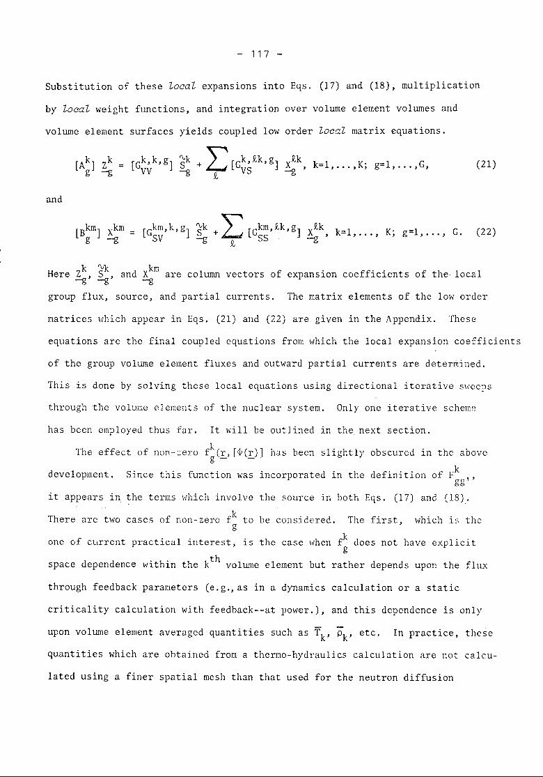
- 117 -
Substitution of these ZocaZ expansions into Eqs. (17) and (18), multiplication
by ZocaZ weight functions, and integration over volume element volumes and
volume element surfaces yields coupled low order ZocaZ matrix equations.
[ k,k,g] '\;k ~ [Gk,n,g] x9-k k-l K' -1 G= GVV ~ + 4-' VS -g' -, ... , , g- , ... , , (21)
and
[Gkm,9-k,g] XQ,k, k=l, ... , K; g=l, ... , G.SS. -g
(22)
Here Zk, ~k, and Xkm are column vectors of expansion coefficients of the. local-g -g -g
group flux, source, and partial currents. The matrix elements of the low order
matrices which appear in Eqs. (21) and (22) are given in the Appendix. These
equations are the final coupled equations from which the local expansion coefficients
of the group volume element fluxes and outward partial currents are deterJilined.
This is done by solving these local equations using directional iterative sweeps
through the volume elements of tIle nuclear system. Only one iterative scheme
has been employed thus far. It will be outlined in th~ next section.kThe effect of non-:::erof (1', [<r(r)] has been slightly obscured in the aboveg - -
development. Since this function was incorporated in the definition of Fkf'
gg
it appears in the terms which involve the source in both Eqs. (17) and (18).
There are two cases of non-zero fk to be considered. The first, which is theg
one of current practical interest, is the case when fk does not have explicitg
thspace dependence within the k volume element but rather depends upon the flux
through feedback parameters (e.g.,as in a dynamics calculation or a static
criticality calculation with feedback--at power.), and this dependence is only
upon volume element averaged quantities such as Tk, Pk' etc. In practice, these
quantities which are obtained from a thermo-hydraulics calculation are not calcu-
lated using a finer spatial mesh than that used for the neutron diffusion
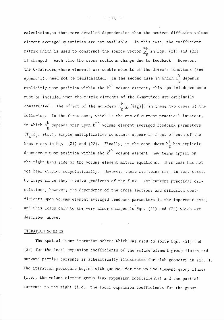
- 118 -
calculation,so that more detailed dependencies than the neutron diffusion volQme
element averaged quantities are not available. In this case, the coefficient'Vkmatrix which is used to construct the source vector S in Eqs. (21) and. (22)-g
is changed each time the cross sections change due to feedback. However,
the G-matrices,whose elements are double monlents of the Green's functions (seeAppendix), need not be recalculated. In the second case in which fk dependsg
explicitly upon position within the kth volume element, this spatial depenclence
must be included when the matrix elements of the G-matrices are originally
constructed. The effect of the non-zero hk(r, [~(r)]) in these two cases is theg - -
following. In the first case, which is the one of current practical interest,k thin which h depends only upon k volume element averaged feedback parametersg
(rk,Pk, etc.), simple multiplicative constants appear in front of each of the
G-matrices in Eqs. (21) and (22). Finally, in the case where hk has explicitg
d d ... h' h kth 1 1epen ence upon POSl.tlon Wl.t 1n t e' va ume e ement, new terms appear on
the right hand side of the volume element nlatrix equations. This case has not
yet been studi.ed computationally. However, these new terms may, in so~c cases,
be large since they involve gradients of the flux. For current practic~11 cal-
culations, however, the dependence of the cross sections and diffusion coef-
ficients upon volume element averaged feedback paru.meters is the important case,
and this leads only to the very minor' changes in Eqs. (21) and (22) which aredescribed above.
ITERATION SCHEMES
The spatial inner iteration scheme which was used to solve Eqs. (21) and
(22) for the local expansion coefficients of the volume element group fluxes and
outward partial currents is schematically illustrated for slab geometry in Fig. 1.
The iteration procedure begins with guesses for the volume element group fluxes
(i.e., the volume element group flux expansion coefficients) and the partial
currents to the right (i.e., the local expansion coefficients for the group
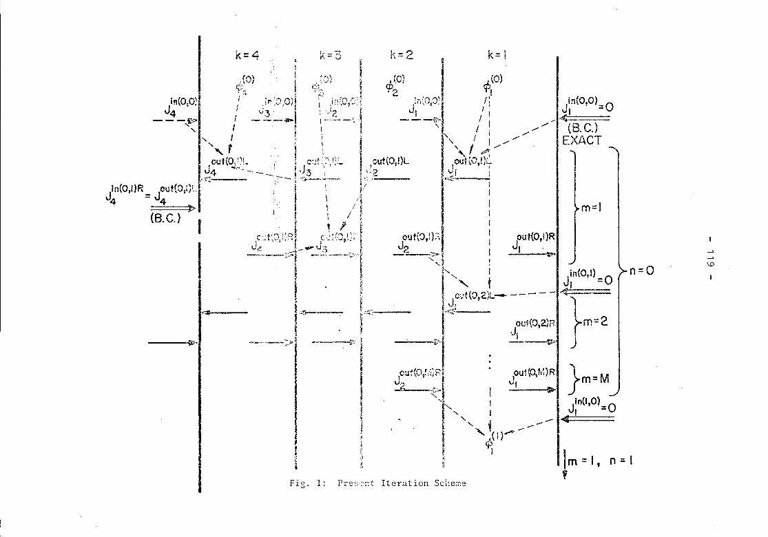
I.D
n=O
m=/
Im=l, n=\,
~J
out(O,I)RI .
Scheme
l'J1{Oi~.j.;Ri:. • oll1{0tM)R j'l-_.~.E J, m=M<1 ! ---.r I !~IOO
. '" I J! ' =0
. '" .- ..-"-- ~, "' ;(1).-4<'"'-
f, ~~t
IF:2 , .i K=!
,f..(O) I r,L.(0)~2 rl
ji'<OP..:li /; J:n(O,O)=O- - _.j;-.' I I ,. .1'+-__
\ l Ii..,. /..,. (8. C,)
i''\,11.,..,./,--' EXACT
"
"ft
I Out{O,!}LI I
t-~.._I I
IIII
- I
t'l"\ 1)'--1 IOU \VI' ~.;. IJ2_. ?>-~ I
' ...j !U" I . (0 I)IJ~;(O,2t-----_.:F ' =0
~d }-- OU1(O,2}R. m=2Ji-~.J?-
IterationPre ~-::::,r~tFig. l'
k=4
~----
i!'l(O~O>J4---~.,-,.
"
----- ....~ ..
~ ~"= 3!i. "
(n' 1 ~'\ ''''I ~ •
~~"r, i; (O) !I_~ E <;'.:..~ ~
"_!" ~f "r.-.;'l -0/\1 ('.. i, !, _0'";") .- - H
r...'". ~ I ",~",--~',_:';_ .:- I ~")2 -:
/-~. I'-'-~-! (" I ~ i < -~
"' , ~ I !IIX! Hc?;"L . I : I
J
1n(O,ilRout!" ", " ~~:.:. - - -' _ I,J~"".,:'. 'lL i, ou!(O,ilL4 - J '.,sl} ....-1 '. - ,-"'. I\,.."_ 4 " ! _7-~~.->- t .:/-
(B. C.) ~,.' f' i ,V'I
I I' •f ' .. ~f I / r.I ~
I:--:t;-" "......t 1 lJ ~. '. \" _..' ,r
.1 ~;'.'.',; c: .:(:'ll .,:--~.•.....,~_ r 1 ~"'''''I';' .-'_:..._. .._~_ ...,..'.)1 ~-'-I -;.-->1
t . ;J ;~
• I
~~ I! .....-----~ •I . ~~~
t iI '~~ ..---:.J.I~ ---:f i~
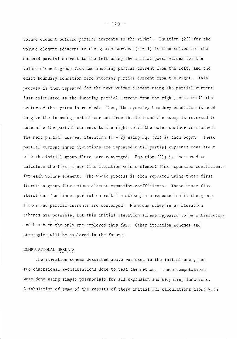
- 120 -
volume element outward partial currents to the right). Equation (22) for the
volume element adjacent to the system surface (k = 1) is then solved for the
outward partial current to the left using the initial guess values for the
volume element group flux and incoming partial current from the left, and the
exact boundary condition zero incoming partial current from the right. This
process is then repeated for the next volume element using the partial current
just calculated as the incoming partial current from the right, etc. until tIle
center of the system is reached. Then, the symmetry boundary condition is uscd
to give the incoming partial current from the left and the sweep is reversed to
determine the partial currents to the right until the outer surface is reached.
The next partial current iteration (m = 2) using Eq. (22) is then begun. These
partial current inner iterations are repeated until partial currents consistellt
with the initial group fluxes are converged. Equation (21) is then used to
calculate the first inner flux iteration volume element flux expansion coefficients
for each volume element. The whole process is then repeated using these first
iteration group flux volume element expansion coefficients. These inner flux
iterations (and inner partial current iterations) are repeated until the gro~l
fluxes aridpartial currents are converged. Numerous other inner iteration
schemes are possible, but this initial iteration scheme appeared to be satisf8ctoJ'Y
and has been the only one employed thus far. Other iteration schemes and
strategies will be explored in the future.
COMPUTATIONAL RESULTSThe iteration scheme described above was used in the initial one-, ~ld
two dimensional k-calculations done to test the method. These computations
were done using simple polynomials for all expansion and weighting functions.
A tabulation of some of the results of these initial PCB calculations along with
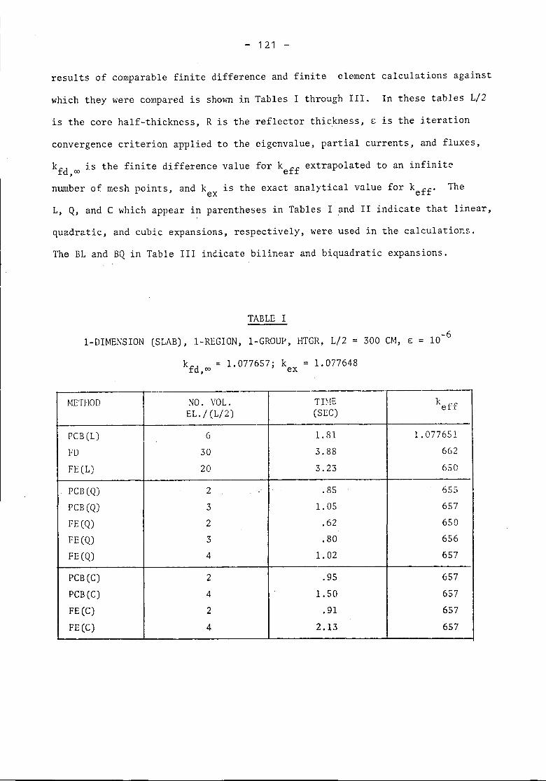
- 121 -
results of comparable finite difference and finite element calculations against
which they were compared is shown in Tables I through III. In these tables L/2
is the core half-thickness, R is the reflector thickness, £ is the iteration
convergence criterion applied to the eigenvalue, partial currents, and fluxes,
kfd,oo is the finite difference value for keff extrapolated to an infinitenumber of mesh points, and kex is the exact analytical value for keff. The
L, Q, and C which appear in parentheses in Tables I and II indicate that linear,quadratic, and cubic expansions, respectively, were used in the calculations.
The BL and BQ in Table III indicate bilinear and biquadratic expansions.
TABLE I
I-DIMENSION (SLAB), I-REGION, I-GROUP) HTGR, L/2 = 300 CM, £ = 10-6
kfd,oo = 1.077657; kex = 1.077648
--METHOD NO. VOL. TIME k
EL./(L/2) (SEe) eff
PCB (L) 6 1.81 1.077651FD 30 3.88 662FE (L) 20 3.23 650
PCB (Q) 2 .85 655
PCB(Q) 3 1.05 657FE (Q) 2 .62 650FE (Q) 3 .80 656FE (Q) 4 1.02 657
PCB (C) 2 .95 657PCB(C) 4 1.50 657FE(C) 2 .91 657FE (C) 4 2.13 657
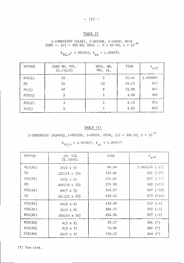
- 122 -
TABLE II
I-DU1ENSION (SLAB), 2-REGION, 2-GROUP, HTGR -6CORE -- L/2 = 300 CM, REFL -- R = 60 CM, E = 10
k = 1.059993; k = 1.059975fd,oo ex
HETHOD CORE NO. VOL. REFL. NO. TIME k f('EL. / (L/2) VOL. EL. e-r
PCB(L) 10 2 1.0.41 1. 059988FD SO 10 24.13 987FE (L) 40 8 21. 98 987PC13(Q) 2 1 3.00 988
PCB (C) 3 1. 4.12 99 =~FE (C) 5 1. 9.82 993 j
TABLE II I
2-DIMENSION (SQUARE), I-REGION, 1.-GROUP, HTGR, L/2 = 300 eM, E = 10-6
kf1 00 = 1.063557; k = 1.063577. c., ex
S)
2)
0)
")
))-.J
.---1-
-- ,-METHOD I~O. VOL TIME k
E1. /QUAD. eff
tPCr,(BL) 25(5 x 5) 86.04 1.063520 ( - -
FO 22S (15 x 15) 134.64 592 (4
PCB (BL) 36(6 x 6) 131. O~ 537 ' -l--
FO 400(20 x 20) 258.90 580 (+
PCB (BL) 49(7 x 7) 194.57 547 (-]
FD 625(25 x 25) 424.15 573 (+
PCB (EL) 64 (8 x 8) 239.49 552 (-.
PCB (BL) 3()(9 x 9) 304.47 555 (-
PCB (13L) 100(10 x 10) 432.96 557 (--
PC13(BQ) 4(2 x 2) 33.17 561 (*,
PCB(BQ) 9 (3 x 3) 76.80 565 (*'
PCB(BQ) 16 (t1 x 4) 136.13 566 (* .-
(*) See text.
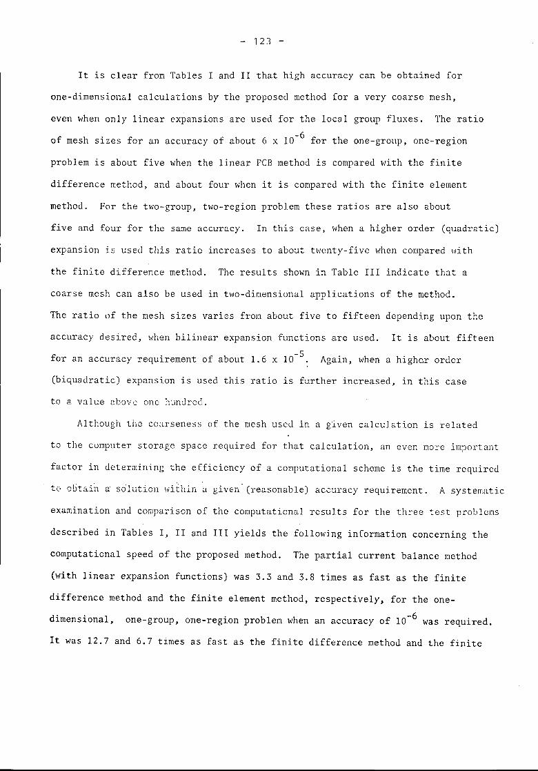
- 123 -
It is clear from Tables I and II that high accuracy can be obtained for
one-dimensional calculations by the proposed method for a very coarse mesh,
even when only linear expansions are used for the local group fluxes. The ratio
of mesh sizes for an accuracy of about 6 x 10⁻⁶ for the one-group, one-region
problem is about five when the linear PCB method is compared with the finite
difference method, and about four when it is compared with the finite element
method. For the two-group, two-region problem these ratios are also about
five and four for the same accuracy. In this case, when a higher order (quadratic)
expansion is used t)lis ratio increases to about twenty-five when compared with
the finite difference method. The results shown in Table III indicate that a
coarse mesh can also be used in two-dimensional applications of the method.
The ratio of the mesh sizes varies from about five to fifteen depending upon the
accuracy desired, when bilinear expansion functions are used. It is about fifteen
for an accuracy requirement of about 1.6 x 10⁻⁵. Again, \"hen a higher order(biquadratic) expansion is used this ratio is further increased, in this caseto a value above one hunared.
Although the coarseness of the mesh used in ~ given calculation is related
to the computer storage space required for that calculation, an even more important
factor in determining the efficiency of a computational scheme is the time required
LU obtai~ a scilution witllin a given- (reasonable) accuracy requirement. A systematic
examination and cOIilparisonof the computational results for the three test problems
described in Tables I, II and III yields the following information concerning the
computational speed of the proposed method. The partial current balance method
(with linear expansion functions) was 3.3 and 3.8 times as fast as the finitedifference method and the finite element method,
dimensional, one-group, one-region problem whenrespectively, for the one-
-6an accuracy of 10 was required.It was 12.7 and 6.7 times as fast as the finite difference method and the finite
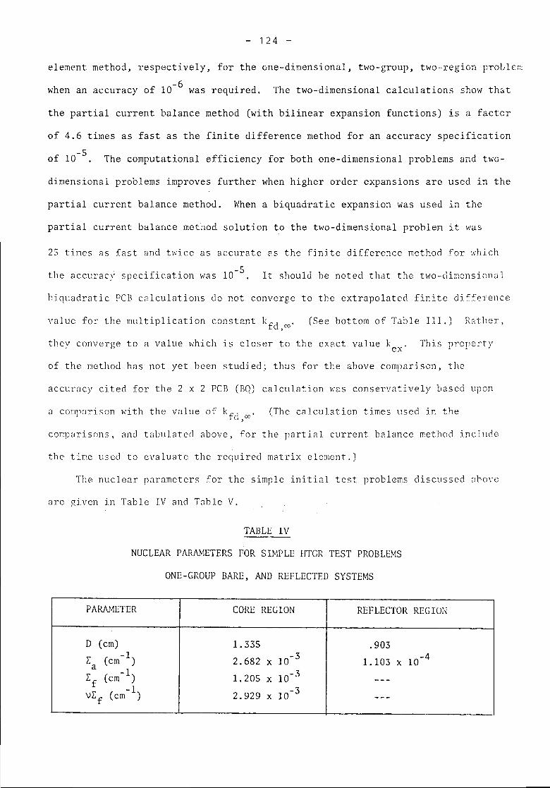
- 124 -
element method, respectively, for the one-dimensional, two-group, two-region problc~-6when an accuracy of 10 was required. The two-dimensional calculations show that
the partial current balance method (with bilinear expansion functions) is a factor
of 4.6 times as fast as the finite difference method for an accuracy specification
of 10-5. The computational efficiency for both one-dimensional problems and two-
dimensional problems improves further when higher order expansions are used in the
partial current balance method. When a biquadratic expansion was used in the
partial current balance metilOd solution to the two-dimensional problem it was
25 times as fast and twice as accurate as the finite difference method for which-5the accuracy specification was 10 . It should be noted that the two-dimensional
biquadratic PCB calculations do not converge to the extrapolated finite diffcJ'ellCe
value for the multiplication constant kfd OJ' (See bottom of Table II1.) Rather,,they converge to a value which is closer to the exact value kex
This proper.ty
of the method has not yet been studied; thus for the above comparison, the
accuracy cited for the 2 x 2 PCB (BQ) calculation was conservatively based upon
a cor~orison with the value of kfd OJ' (The calculation times used in the,cOr.lparisons,and tabulated above, for the parti~ll current b8lance method include
the time used to evaluate the required matrix element.)
The nuclear parameters for the simple initio.l test problems discussed ~lhovc
are given in Table IV and Table V.
TABLE IV
NUCLEAR PARAMETERS POR SIMPLE HTGR TEST PROBLEMS
ONE-GROUP BARE, AND REFLECTED SYSTEMS
PARAMETER CORE REGION REFLECTOR REGION
D (cm) 1.335 .903-1 10-3 x 10⁻⁴L (em ) 2.682 x 1.103a -1 10-3Lf (cm ) 1. 205 x-1 10-3VLf (em ) 2.929 x
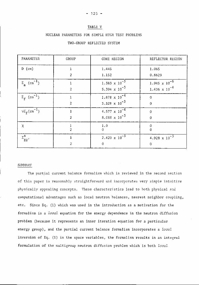
- 125 -
TABLE V
NUCLEAR PA~1ETERS FOR SIMPLE HTGR TEST PROBLEMS
TWO-GROUP REFLECTED SYSTEM
PARAMETER GROUP CORE REGION REFLECTOR REGION
D (em) 1 1.445 1.0652 1.152 0.8629
~ -1 10-3 10-6(cm ) 1 1.383 x 1.945 xa10-3 10-42 5.394 x 1.436 x
-1 10-4~f (cm ) 1 1.878 x 02 3.328 x 10⁻³ 0
-1 10-4\!~f(cm ) 1 4.577 x 02 8.088 x 10⁻³ 0
X 1 1.0 02 0 0
~s 1 2.420 x 10⁻³ 4.928 x 10⁻³gg'2 0 0
SUMMARY
The partial current balance formalism which is reviewed in the second section
of this paper is reasonably straightforward and incorporates very simple intuitive
physically appealing concepts. These characteristics lead to both physical andcomputational advantages such as local neutron balances, nearest neighbor coupling,etc. Since Eq. (1) which was used in the introduction as a motivation for the
formalism is a local equation for the energy dependence in the neutron diffusion
problem (because it represents an inner iteration equation for a particular
energy group), and the partial current balance formalism incorporates a local
inversion of Eq. (1) in the space variables, the formalism results in an integral
formulation of the multigroup neutron diffusion problem which is both local
- 126 -
in energy (within group), and local in space (within volume element). This
leads to several apparent advantages. The final equations represent an integral
formulation without long range coupling (nearest neighbor coupling, only). No
large matrices are directly involved. (See Appendix for the dimensions of the
various matrices which appear in the final matrix equations.) The matrb: elen18nts
are calculated separately for each group (local in enel'gy); hence, multigroup
equations need not be solved to construct the matrix elements. The number of
local expansion functions can be varied with volume element and with a group.
Either low order or high order approximations can be used. Low and high order
approximations can be combined. Little additional coding effort is required for
higher order calculations. The method naturally accommodates exact diffusion theory
bound8.ry conditions, interface conditions, and symmetry conditions. Finally, t.he
method is potentially useful on parallel array machines.
It is important, at this point, to note that in many cases it is not uctually
neces~.ary to eva J uote the Gl~cenIS functiono> to construct the required matr; x
elen~ents. l{athel',\'.'hen1'01YJlornidlexpansion and weightin:~ functions are u~ed,
as in all of the calculations clone ~o far, trJ8 matrix cclt'mellts ,,'hieh aTe thE'n
double moments of the Green's functions can be evaluated directly. This js impor-
tant in multidimensional calculations since the serjes representations of thf' Ji\.,trL\
e]emenj-s have f;]rbetter convergence projJ81'ticsth:m the series reprcsC'11t"tjU:1Sof the Green's functions.
It is also important to note that the elements of the matrices can also he
calculated directly (e.g., via transport theory, Monte Carlo, etc.) without
employing Green I s functions at all, simply by notinp: and using the physic1] me:lIllngs
of the matrix elements. For example, the various matrix clements correspollrlto:
the constant component of the outward partial current across a surface Jue to a
linear partial current input across a surface in the diffusion-removal problem

- 127 -
described by the left hand side of Eq. (6), the linear component of the outward
partial current due a quadratic-quadratic volume source, etc.An approximate method for directly generating the matrix elements which is
based upon their physical meanings and which utilizes a variational principle
h b d. 1.2as also een developed, and tested in one- imenSlonal calcu atlons.
The apparent advantages suggested above have been shown, by the test
problem results reported here, to lead to gains in actual computational
efficiency OVGr standard finite difference and finite element methods.
These gains have, of course, only been confirmed for the simple test problems
which have been studied. It is clear that extensive calculations in which
the method is applied to far more complicated reactor models must be done to
verify its potential advantages for practical reactor calculations. However,the results obtained thus far are encouraging. They indicate that it is verymuch worthwhile to apply the method to more elaborate benchmark probiems, aswell as to extend it to three-dimensional problems and reactor kinetics problemsand to test these extensions by three-dimensional neutron kinetics benchmark
studies and by calculatiolls for actual powe~ reactor models used in safety analyses.
REFERENCES1. For a more detailed presentatjon of the formalism (within the context of
reactor kinetics) see: T. J. Burns and J. J. Darning, "A Partial CurrentBalance Method for Space-, and Energy-Dependent Reactor Calculations,"Proc. Can£. on Ma!~~ Mod~s and Camp. Techniques for Analysis of NuclearSystems, CONF-7304l4, VII-162, USAEC (1973).
2. T. J. Burns and J. J. Dorning, "Approximate Generation of Coupling Parametersfor Multidimensional Neutron Diffusion Calculations," Trans. Am. Nucl. Soc . .!2.,174 (1974).
APPENDIXThe expressions for the matrix elements of the matrices which appear in
Eqs. (21) and (22), the low order local matrix equations for the solution vectors
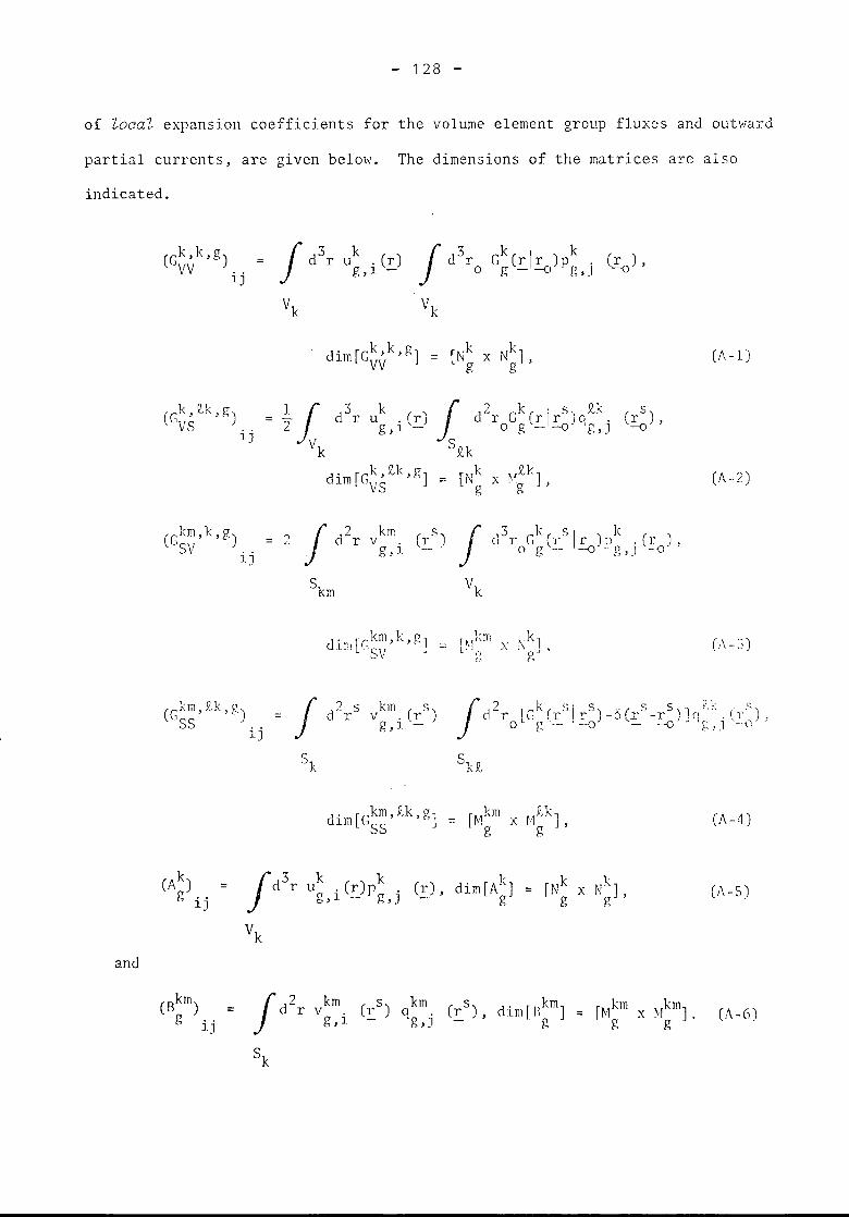
- 128 -
of local, expansion coefficients for the volume element group fluxes and out'lwrd
partial currents, are given below. The dimensions of the matrices are also
indicated.
(Gk,k,g)\TV , ,
1J f 3 kd l' U ,(1')g,1 - f 3 k I kd r G (1' r)p .o g - --0 g,J
Vk
(~) ,
d' [Gk,k,g]l.m '\T\T (A-l)
S(1' ),-Q
(A-2)
kmv ,g,1 f 3 k s I kc11'G(l' 1'))1 ,(1'),o g -- -Q . g, J -0
d' ! [Gkm,};,g]Hl 'S\!
(Gkm, n, y)ss , .
1J f ') S'd'- .
l' km ( s)v ,1'g,1 - f 2 k ,- 5 C" 5 V ~. c'
,.., ( ..J ( ,.J . '.~ • . ....ei :r [lJ '.1' 11' )-o,X -rJ]q .. IJJ,o g --- -.0 -- ~ i. ,J -~-
d' [C,km,n,g]1m JSS (1\-4 )
and
f 3 k kd l' U ,(1')p ,g,l -- g,J
Vk
k 1.[N x N"]g g' (A - S)
(Skm) f d2r
km ( s. km s dim[l\km] [Mkm Hkm] .v g,i E. ) a (~ ) , = x (A-C»g .. 'g, jIJ. g g g
Sk
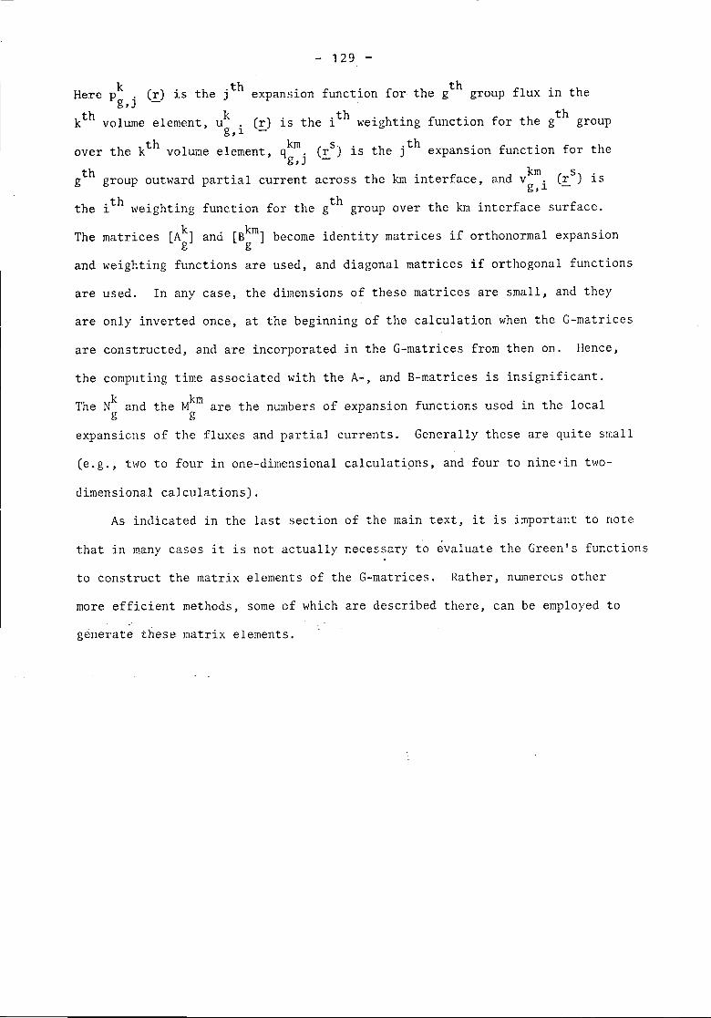
- 129 -
k ()' the J.th . f . f h th fl' hHere p . r 1S expans10n unct10n or t e g group ux 1n t eg,J -
kth 11k ()' h .th . h' f . f h thvo ume e ement, u . £ 1S tel we1g t1ng unct10n or t e g groupg,lh kth 1 km (s) . th .th . f . f hover t e vo ume element, qg,j £ 1S e J expans10n unct10n or t e
thg group outward
h .th . h .t e 1 welg t1ng
partial current across thefunC'.tionfor the gth group
km interface, and vkm. (rs) isg,l -over the km interface surface.
The matrices [Ak] and [Bkm] become identity matrices if orthonormal expansiong g
and weighting functions are used, and diagonal matrices if orthogonal functionsare used. In any case, the dimensions of these matrices are small, and theyare only inverted once, at the beginning of the calculation when the G-matrices
are constructed, and are incorporated in the G-matrices from then on. Hence,
the computing time associated with the A-, and B-matrices is insignificant.
The Nk and the Mkm are the numbers of expansion functions used in the localg g
expansions of the fluxes and partial currents. Generally these are quite small
(e.g., two to four in one-dimensional calculati9ns, and four to nine'in two-
dimensional calculations).As indicated in the last section of the main text, it is important to note
that in many cases it is not actually necessary to ~valuate the Green's functions
to construct the matrix elements of the G-matrices. Rather, numerous othermore efficient methods, some of which are described there, can be employed to
generate these matrix elements.

- 131 -
H. Finnemann
A CONSISTENT NODAL METHOD FOR THE ANALYSIS OF SPACE-TIMEEFFECTS IN LARGE LWR
Kraftwerk Union AG, Erlangen, Germany

- 133 -
A Consistent Nodal Method for the Analysis of Space-Time*Effects in Large LWR's
H. FinnemannKRAFTWERK UNION AKTIENGESELLSCHAFT, ERLANGEN, GERMANY
AbstractThe solution method of the computer code IQSBOX is discussed.IQSBOX solves the time dependent multidimensional neutrondiffusion equation by a combination of nodal methods withweighted residual techniques. This nodal technique relieson 1D diffusion calculations for determining the spatialcoupling coefficients. The 1D diffusion equations are solvedby polynomial expansion. For this reason, the method has beencalled Nodal-Expansion-Method (NEM). Several results forstatic and dynamic problems are discussed which demonstratethe accuracy and computational efficiency of the method.
Paper presented at the Joint NEACRP/CSNI Specialists' Meetingon New Developments in Three-Dimensional Neutron Kinetics andReview of Kinetics Benchmark Calculations.
Garching (Munich), 22 nd - 24 th January 1975
* Work supported in part by the Bundesminister fUr Forschungund Technologie, Grant RB 74 lis 26
- 134 -
I. Introduction
This paper discusses the solution method of the computerprogram IQSBOX and some numerical examples run with thiscode. The IQSBOX program solves the time dependent multi-dimensional neutron diffusion equation by a combinationof nodal methods with weighted residual techniques. Forthis reason, the method has been called NOdal-Expansion-Method (NEM).
Recently several improved coarse mesh methods were propos-ed (1, g, 2, 4, 2) in an attempt to overcome two basicdrawbacks of most nodal techniques presently used, namelyinsufficient accuracy in deriving the spatial couplingcoefficients and the lack of information about the fluxdistribution inside the nodes. The various approaches aresimilar in that they combine multidimensional coarse meshwith auxiliary calculations, the purpose of which is toobtain the coupling coefficients. In the method describedin (1, g) these calculations reduce to a direct eliminationof surface fluxes whereas in the so called nodal synthesismethod (2, ~) (NSM) one dimensional (1D) fine-mesh diffusioncalculations are performed through all channels for eachspace direction. In (2) a Green's function is used to elimi-nate the spatial differential operators in the equations foreach element of the nuclear system.
Since separability of the flux distribution in the nodes hasproven to be a reasonable assumption for deriving accuratecoupling coefficients (2, 4) it is also used in the nodalexpansion method. This nodal technique is similiar to NSMin that it relies on 1D diffusion calculations for deter-mining spatial coupling coefficients, but in contrast to NSMno complete 1D channel sweeps are performed to improve the
- 135 -
spatial coupling coefficients. Instead inhomogeneous1D diffusion equations are solved for each box and spacedirection such that the coupling coefficients can beupdated during the nodal iterational process. Further-more, the 1D diffusion equations are solved by polynomialexpansion, the expansion coefficients being determined bythe Galerkin method. In this way a strong coupling between1D and 3D calculations can be achieved which is the reasonfor the good convergence properties of the method. Anotherimportant property of the nodal expansion method is thatthe polynomial expansion coefficients need not be stored.Only the coarse mesh variables, average fluxes and partialcurrents or spatial coupling coefficients, must be kept instorage. One of the great advantages of this improved nodaltechnique is its convergence to the exact solution of thediffusion equation for finer mesh sizes.
In Sec. II, the method is formulated for the multigroupneutron diffusion equation. Sec. III discusses the appli-cation of the method to the two group diffusion equation.A set of equations is obtained which is formally identicalto the one used in the well known nodal collision proba-bility method (£, 1). Some numerical results using thenodal expansion method for both static and dynamic prob-lems are presented in Sec. IV.
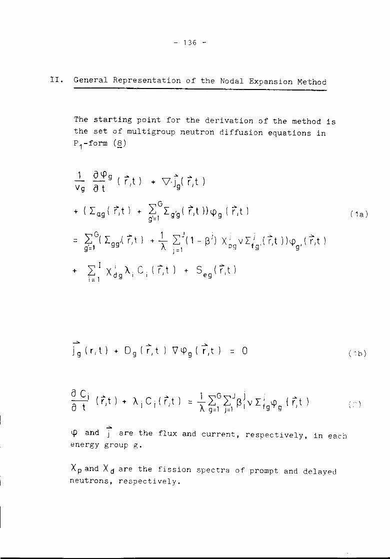
- 136 -
II. General Representation of the Nodal Expansion Method
The starting point for the derivation of the method isthe set of multigroup neutron diffusion equations inp1-form (Q)
"VG .,.) ~+ (L og ( rJ t) + ~ 1 L g'g ( r It) tp 9 ( r J t ) ( 1a)
- ~ G( L g g'( r) t) + ~ 2: J ( 1 - ~ j) X ~ V L/ I ( 1:t ) ) tp I ( rJ t )g=1 f\ J=I 9 9 9
+ 2:: I X ~ A i C i ( r,t) + S e 9 ( rJ t )i = 1 9
BaCti ( .....r)t) + 1," Cr" (r .....)t) _- 1 "VG"VJ(.l.J ~j (~t)
f\ ~~1tltJivLfg\.f'g r)
...::..
~ and J are the flux and current, respectively, in eachenergy group g.
Xp and X d are the fission spectra of prompt and delayedneutrons, respectively.
~" "" )
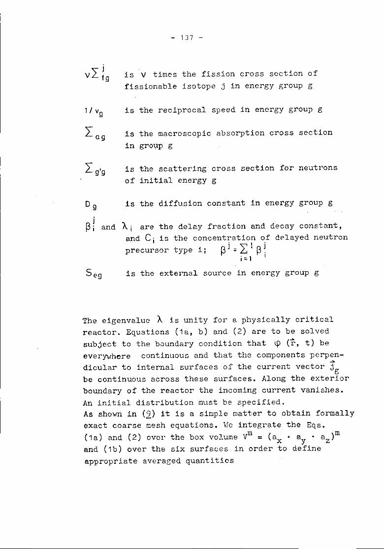
- 137 -
is V times the fission cross section offissionable isotope j in energy group g
is the reciprocal speed in energy group g
is the macroscopic absorption cross sectionin group g
L g'g is the scattering cross section for neutronsof initial energy g
1s the diffusion constant 1n energy group g
and Ai are the delay fraction and decay constant,and Cj is the concentration of delayed neutronpre cursor type i; ~ j = L I~ ~
i = 1 I
Seg is the external source in energy group g
The eigenvalue A is unity for a physically criticalreactor. Equations (1a, b) and (2) are to be solvedsubject to the boundary condition that ~ (r, t) beeverywhere continuous and that the components perpen-
-'>.dicular to internal surfaces of the current vector jgbe continuous across these surfaces. Along the exteriorboundary of the reactor the incoming current vanishes.An initial distribution must be specified.As shovm in (2) it is a simple matter to obtain formallyexact coarse mesh equations. We integrate the Eqs.(1a) and (2) over the box volume Vm = (ax • ay • az)mand (1b) over the six surfaces in order to defineappropriate averaged quantities
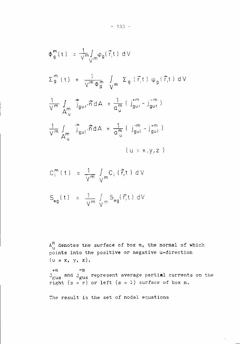
- 133 --
mLg (t)
1 J ~ ..::.. .+m - -mjgur,ndA - Jgur - Jgur
Vm - am
Am uu
~m J..::.. ..:. _1_ ( . -m . +mJ t,n d A = J gu I - J gu Iam
Amgu
uu
( u -- X1Y/Z )--
c ~ ( t ) 1 J ~- C i ( r, t ) d V- --Vm Vm
S (t) - 1 J S (rt)dV- --eg Vm eg J
Vm
Am denotes the surface of box m, the normal of whichu
points into the positive or negative u-direction(u = x, y, z).
+m -mjgus and jgus represent average parti~l currents on theright (s = r) or left (s = 1) surface of box m.
The result is the set of nodal equations
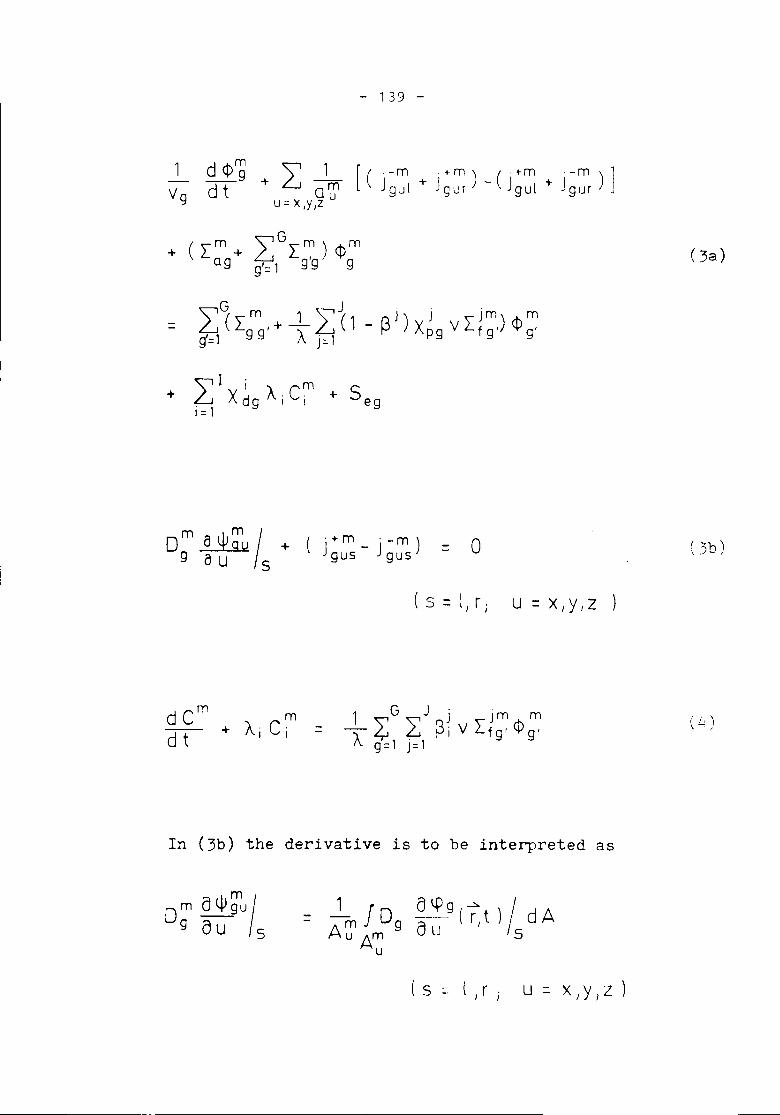
- 139 -
om~/+(o+m O_m)9 au s Jgus-Jgus o ( ~b)
\ )
1 G J j jm m~ ~ 2: ~i V Lfg' <Pg,f\ 9=1 J=1
( u)
In (3b) the derivative is to be interpreted as
om B 4J~ul9 Bus
1 J B\Pg ~ I- - 0 ---(rt) dAAm 9 BLJ I
U Am 5u
- 140 -
Conventional nodal methods define spatial couplingcoefficients by the relationship (2)
em/rlu) .+m/( mlt\m)gu = Jgur au 'Vg
em,llul_,-m / ( mlt\m)gu -Jgul au'Vg
If these coupling coefficients can be determined bysubsidiary calculations and/or by applying fittingprocedures Eq. (3b) is superfluous. Another way ofdealing with the problem is to determine the spatialdependence of 4J ~u(u, t) by concomitant~auxiliarycalculations (4). For this purpose, In (r, t) is- Ygapproximated in each time interval tn < t ~ tn+1 by
~ 9 (r, t) - <D ~ ( t ) IT f g~ (u )u= X/y,Z
(u)du -11aT
The shape functions r:u(u) are normalized to unity
a~J f;uo
Substituting Eq. (5) into Eqs. (1a) and (2) andintegrating over two space directions of box m weobtain
( _1 1Vg . ~g
- 141 -
+ Im+ ~G,\m)i1lmog ~ 1 L g'g Y gu
1A
~j(l nj) j ,jm)t1,mLJ - tJ Xpg VLfg' '¥g'uJ = 1
The third term on the left hand side of Eq. (6)describes the transverse leakage.
ill (~ U.....gu ' t) denotes the source of delayed neutrons
~ I X i A [C m (u t ) e- A i ( t - t 0)L.., dg I IU I 01=1
- 142 -
If we now introduce the diffusion theory expression
II, m = 2 ( J" + m . - m't'gus gus + Jgus
(s=llr)
(7)
the auxiliary one dimensional diffusion problem (6, 7)for the determination of ~:u (U, t) is completelydefined. The Eqs. (3, 4) and (6, 7) constitute a coupledsystem of ordinary and partial differential equationswhich can be solved simultaneously. The assumptionof separability (5) had to be introduced in order to beable to derive an expression for transverse leakage. Ofcourse, the assumption of separability is also of useif one wants to consider simple spatial dependence ofcross sections as given f. i. by partial insertion ofcontrol rods into boxes.
- 143 -
III. Reduction to Two Neutron Groups.Approximation Procedure
The underlying idea of the method as described inthe foregoing paragraph is that an approximate calcu-lation of spatial coupling coefficients suffices toobtain accurate spatial mean values of reaction rates.For this reason it is not necessary and even not desirableto calculate an exact solution of Eq. (6). Therefore, weapproximate the solution of (6) by an expansion in knownfunctions. Taking into account normalization and boundaryconditions we have
[ m m m]+ 3 2 <P 9 (t) - 4.!gur-4Jgul
Uamu
(1 - ~)o[]'
+
u-xly,Z)
o ~ U ~ o~
(8)
It is interesting to note that for n = 0 Eq. (8) reducesto a parabolic approximation of the flux, similarly tothat used in (£). As will be shown belo~ the parabolic
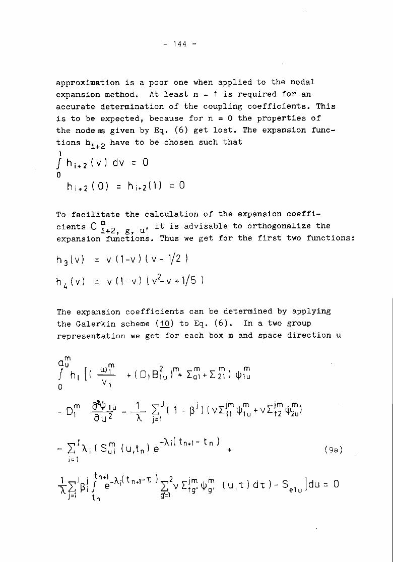
- 144 -
approximation is a poor one when applied to the nodalexpansion method. At least n = 1 is required for anaccurate determination of the coupling coefficients. Thisis to be expected, because for n = 0 the properties ofthe node as given by Eq. (6) get lost. The expansion func-tions hi+2 have to be chosen such that,J hi+2(V) dv = 0a
To facilitate the calculation of the expansion coeffi-cients C ~ 2 ' it is advisable to orthogonalize the~+ , g, uexpansion functions. Thus we get for the first two functions:
h 3 ( V ) - V (1 - V ) ( V - 1/2 )
h 4 ( V) - V (1 - V) ( v2_ V + 1/5 )
The expansion coefficients can be determined by applyingthe Galerkin scheme (lQ) to Eq. (6). In a two grouprepresentation we get for each box m and space direction u
mau mJhl[(~o V,
m- 0, atq> , uau21---A
'V J j jm m j m m ){-J ( 1 - ~ ) (v I f1 4J, u + v I f 2 4J2uJ='
(9a)
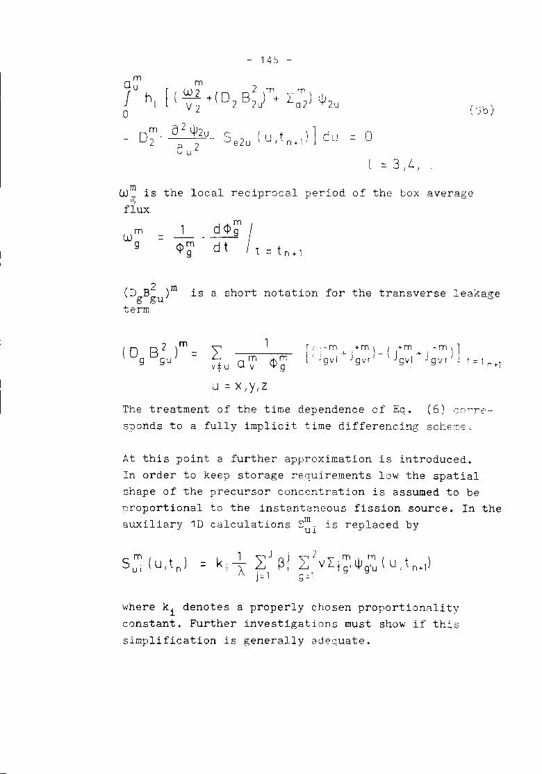
- 145 -
mW2 2 m m
( - + (0 B ) + I ) IIIV2 2 2u 02 'l'2u (t~b )
W~ is the local reciprocal period of the box average':Jflux
1 d ~~ I<P~ dt t=tn+1
(D B2 )m is a short notation for the transverse leakageg guterm
2:: a mvv t u
1<pm
9
r: .-m +m) r +m -m)ll' Jgvi .!- Jgvr - \ Jgvl + Jgvr J t = t r,+'
,J :
U=X,y,z
The treatment of the time dependence of Eq. (6) ca~re-sponds to a fully implicit time differencing sche'ne.
At this point a further approximation is introduced.In order to keep storage requirements low the spatialshape of the precursor concentration is assumed to beproportional to the instantaneous fission. source. In theauxiliary 1D calculations S~i is replaced by
where ki denotes a properly chosen proportionalityconstant. Further investigations must show if thissimplification is generally adequate.
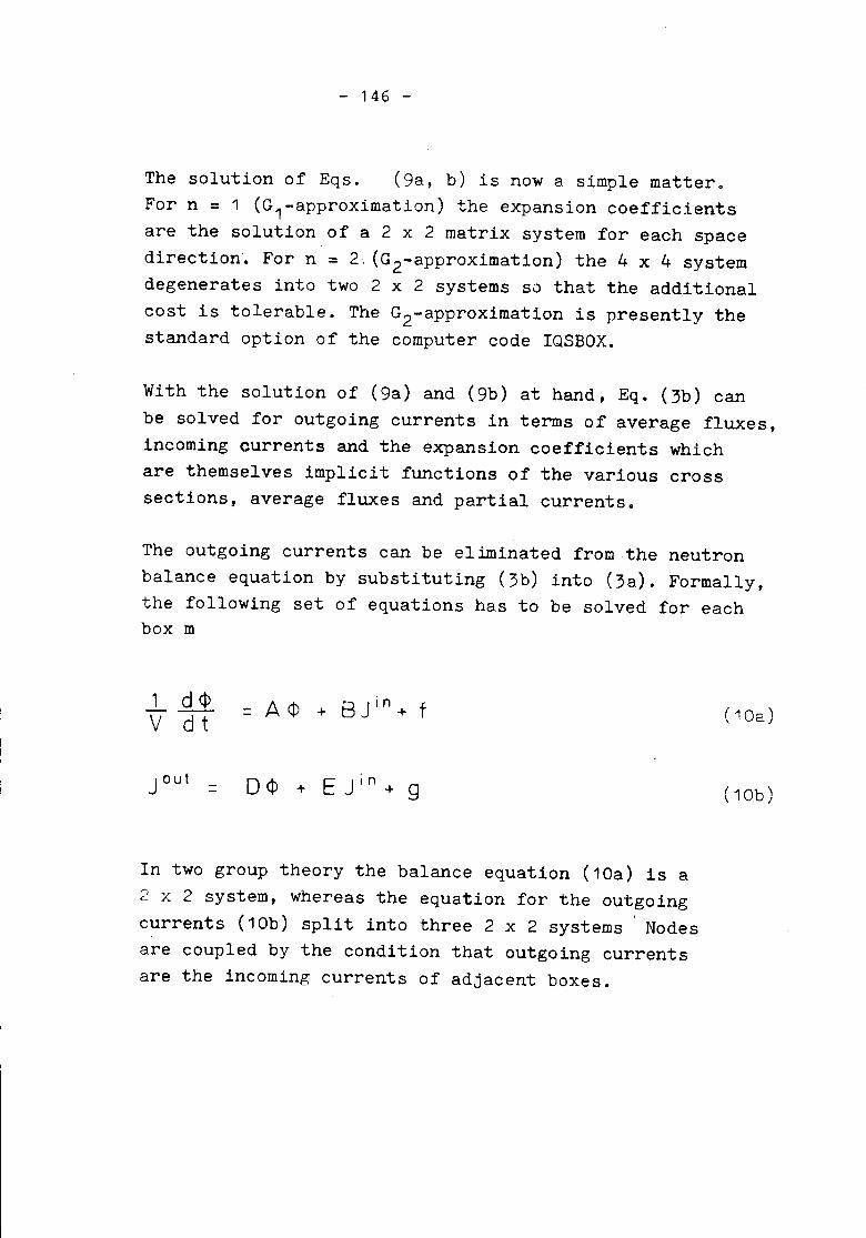
- 146 -
The solution of Eqs. (9a, b) is now a simple matter.For n = 1 (G1-approximation) the expansion coefficientsare the solution of a 2 x 2 matrix system for each spacedirection~ For n = 2: (G2-approximation) the 4 x 4 systemdegenerates into two 2 x 2 systems S0 that the additionalcost is tolerable. The G2-approximation is presently thestandard option of the computer code IQSBOX.
With the solution of (9a) and (9b) at hand, Eq. (3b) canbe solved for outgoing currents in terms of average fluxes,incoming currents and the expansion coefficients whichare themselves implicit functions of the various crosssections, average fluxes and partial currents.
The outgoing currents can be eliminated from the neutronbalance equation by substituting (3b) into (3a). Formally,the following set of equations has to be solved for eachbox m
1 d<t> = A<p + BJin+ fV dt
In two group theory the balance equation (10a) is a2 x 2 system, whereas the equation for the outgoingcurrents (10b) split into three 2 x 2 systems Nodesare coupled by the condition that outgoing currentsare the incoming currents of adjacent boxes.
( 1Oa)
(1 Ob)
- 147 -
In summary, the iterative solution procedure is asfollows
1. Determine expansion coefficients (Eq. 9a, b) byusing last known values of fluxes, currents andcross sections
2. Determine average fluxes by solving Eq. (10a)
3. Solve Eq. (10b) for outgoing currents.
Steps 1 to 3 have to be followed for each box m andmust be repeated until convergence. Several accelerationtechniques are used in combination: overrelaxation isused during a mesh sweep, coarse mesh rebalancing (11, 2£)after each mesh sweep, and asymptotic extrapolation (11)every time the iterative solution has adopted an asymptoticbehaviour.
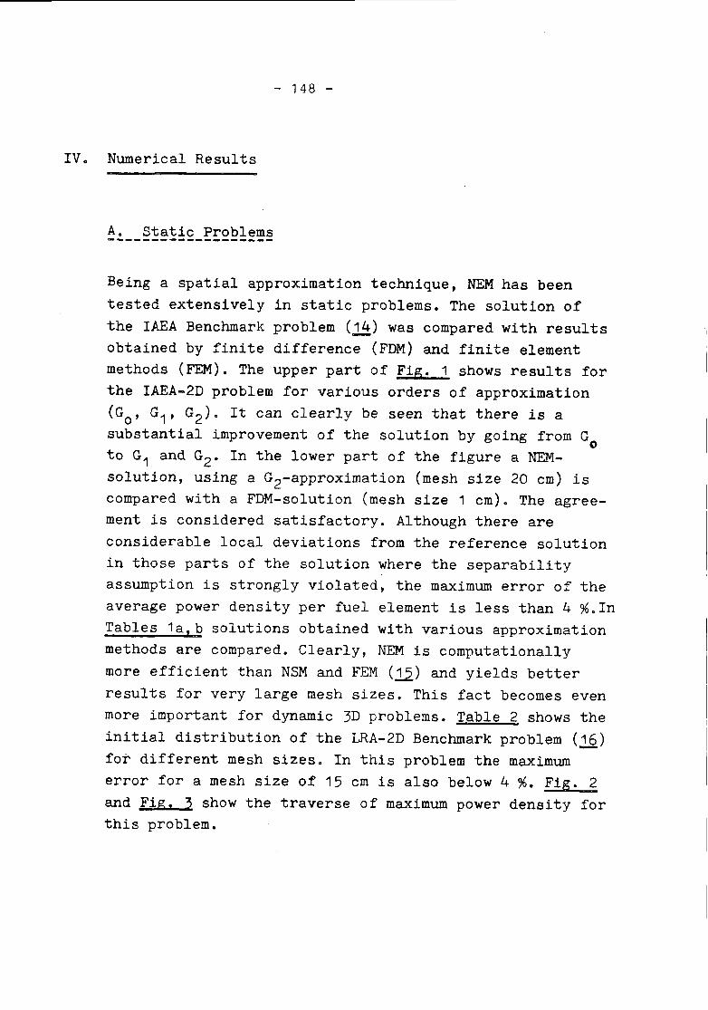
- 148 -
IV. Numerical Results
A. Static Problems
Being a spatial approximation technique, NEM has beentested extensively in static problems. The solution ofthe IAEA Benchmark problem (~) was compared with resultsobtained by finite difference (FDM) and finite elementmethods (FEM). The upper part of Fig. 1 shows results forthe IAEA-2D problem for various orders of approximation(Go' G1, G2). It can clearly be seen that there is asubstantial improvement of the solution by going from Goto G1 and G2• In the lower part of the figure a NEM-solution, using a G2-approximation (mesh size 20 cm) iscompared with a FDM-solution (mesh size 1 cm). The agree-ment is considered satisfactory. Although there areconsiderable local deviations from the reference solutionin those parts of the solution where the separabilityassumption is strongly violated, the maximum error of theaverage power density per fuel element is less than 4 %.InTables 1a, b solutions obtained with various approximationmethods are compared. Clearly, NEM is computationallymore efficient than NSM and FEM (12) and yields betterresults for very large mesh sizes. This fact becomes evenmore important for dynamic 3D problems. Table 2 shows theinitial distribution of the LRA-2D Benchmark problem (12)for different mesh sizes. In this problem the maximumerror for a mesh size of 15 cm is also below 4 %. Fig. 2and Fig. 3 show the traverse of maximum power density forthis problem.
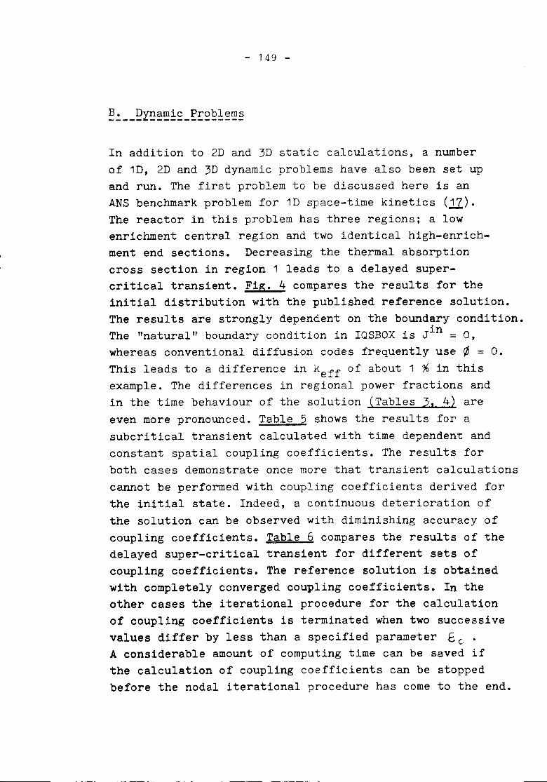
- 149 -
In addition to 2D and 3D static calculations, a numberof 1D, 2D and 3D dynamic problems have also been set upand run. The first problem to be discussed here is anANS benchmark problem for 1D space-time kinetics (11).The reactor in this problem has three regions; a lowenrichment central region and two identical high-enrich-ment end sections. Decreasing the thermal absorptioncross section in region 1 leads to a delayed super-critical transient. Fig. 4 compares the results for theinitial distribution with the published reference solution.The results are strongly dependent on the boundary condition.The "natural" boundary condition in IQSBOX is Jin = 0,whereas conventional diffusion codes frequently use ~ = 0.This leads to a difference in keff of about 1 % in thisexample. The differences in regional power fractions andin the time behaviour of the solution (Tables 3, 4) areeven more pronounced. Table 5 shows the results for asubcritical transient calculated with time dependent andconstant spatial coupling coefficients. The results forboth cases demonstrate once more that transient calculationscannot be performed with coupling coefficients derived forthe initial state. Indeed, a continuous deterioration ofthe solution can be observed with diminishing accuracy ofcoupling coefficients. Table 6 compares the results of thedelayed super-critical transient for different sets ofcoupling coefficients. The reference solution is obtainedwith completely converged coupling coefficients. In theother cases the iterational procedure for the calculationof coupling coefficients is terminated when two successivevalues differ by less than a specified parameter E. (. •A considerable amount of computing time can be saved ifthe calculation of coupling coefficients can be stoppedbefore the nodal iterational procedure has come to the end.
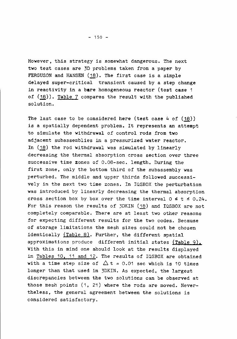
- 150 -
However, this strategy is somewhat dangerous. The nexttwo test cases are 3D problems taken from a paper byFERGUSON and HANSEN (18). The first case is a simpledelayed super-critical transient caused by a step changein reactivity in a bare homogeneous reactor (test case 1of (~)). Table 7 compares the result with the publishedsolution.
The last case to be considered here (test case 4 of (~))is a spatially dependent problem. It represents an attemptto simulate the withdrawal of control rods from twoadjacent subassemblies in a pressurized water reactor.In (~) the rod withdrawal was simulated by linearlydecreasing the thermal absorption cross section over threesuccessive time zones of 0.08-sec. length. During thefirst zone, only the bottom third of the subassembly wasperturbed. The middle and upper thirds followed successi-vely in the next two time zones. In IQSBOX the perturbationwas introduced by linearly decreasing the thermal absorptioncross section box by box over the time interval 0 ~ t ~ 0.24.For this reason the results of 3DKIN (~) and IQSBOX are notcompletely comparable. There are at least two other reasonsfor expecting different results for the two codes. Becauseof storage limitations the mesh sizes could not be chosenidentically (Table 8). Further, the different spatialapproximations produce different initial states (Table 9),With this in mind one should look at the results displayedin Tables 10, 11 and 12. The results of IQSBOX are obtainedwith a time step size of l::. t = 0.01 see which is 10 timeslonger than that used in 3DKIN. As expected, the largestdiscrepancies between the two solutions can be observed atthose mesh points (1, 21) where the rods are moved. Never-theless, the general agreement between the solutions isconsidered satisfactory.
- 151 -
v. Conclusions
This paper has almost exclusively dealt with the spatialapproximation method of the space-time kinetics codeIQSBOX. It has been shown that the nodal expansion methodis a useful variant of those nodal methods which generatespatial coupling coefficients during the solution process.The method is characterized by high accuracy and compu-tational efficiency.
The time integration of the nodal equations is presentlyperformed by the backwards-difference algorithm (~).In view of the flexibility of the method as to theiterational procedure other time integration schemes willprobably be more efficient. This is one of the problemswhich remain for further investigations.
- 152 -
References
A. Birkhofer,W. Werner:Efficiency of Various Methods for the Analysis ofSpace Time Kinetics.Proceedings of ANS Topical Meeting on MathematicalModels and Computational Techniques for Analysis ofNuclear Systems, CONF-730414-P2, IX 31 - 41 (1973)
A. Birkhofer, S. Langenbuch, W. Werner:"Coarse Mesh Method for Space-Time Kinetics"Trans. Am. Nucl. Soc. 18, 153 (1974)
M.R. Wagner:"Synthese von mehrdimensionalen Grob- und Feinmaschen-rechnungen"Reaktortagung des DAtF, Tagungsberichte Karlsruhe 1973
(~) M.R. Wagner:"Nodal Synthesis Method and Imbedded Flux Calculations"Trans. Am. Nucl. Soc. 18, 152 (1974)
T.J. Burns and J.J. Dorning:"A Partial Current Balance Method for Space-, and Energy-Dependent Reactor Calculations", Proc. Conf. Math. Modelsand Compo Tech. for Analysis of Nuclear Systems, CONF-730414, p. VII-162, USAEC (1973).
A. MUller, F. Bennewitz:"Ein neues schnelles Verfahren zur Berechnung 3-dimen-sionaler FluBverteilungen mit Hilfe von StoBwahrschein-lichkeiten". Reaktortagung des DAtF, TagungsberichteBonn 1971A. MUller and M.R. Wagner:"Use of Collision Probability Methods for Multidimen-sional Flux Calculations"Trans. Am. Nucl. Soc. 15, 280 (1972)
W.M. Stacey, Jr.:"Space-Time Nuclear Reactor Kinetics"Academic Press, New York (1969)
(.19)
(.1&.)
(.11)
- 153 -
A.F. Henry:"Refinements in Accuracy of Coarse Mesh FiniteDifference Solution of the Group Diffusion Equations"IAEA/SM-154/21, Seminar on Numerical Reactor Calculations,Vienna, January 17-21, 1972
L.W. Kantorowitsch, W.I. Krylow:"Naherungsmethoden der hoheren Analysis"VEB Deutscher Verlag der Wissenschaften Berlin 1956
E.L. Wachspress:Iterative Solution of Elliptic Systems, Prentice Hall,Ind., Englewood Cliffs, B.J., 1966
R. Frohlich:A Theoretical Foundation of Coarse Mesh VariationalTechniques, Report CNM-R-2, Vol. 1, p. 219,(CONF-670501), 1967
B. Noble:"Numerical Methods" The University Mathematical TextsOliver and Boyd, LTD., Edinburgh and London (1964)
B. Micheelsen:"The 3D IAEA Benchmark Problem"DAEC, Ris~ (1972). The 2D IAEA Problem represents thecore mid plane of the 3D-Problem with constant axialBuckling B~ = .8E-04 in both energy groups.
F.A.R. Schmidt et al.:"Experiences with the Finite Element Method for StandardReactor Calculations"Summary of a Paper to be presented to the Topical Meetingon Computational Methods in Nuclear Engineering.April 15-17, 1975, Charleston, S.C.
LRA-Benchmark as prepared for this Meeting, LaboratoriumfUr Reaktorregelung und ~11agensicherung, MUnchen
"Argonne Code Center: Benchmark Problem Book",ANL-7416, Sup. 1, 1972
D.R. Ferguson, K.F. Hansen:"Solution of the Space-Dependent Reactor KineticsEquations in Three Dimensions"Nucl. Sci. Eng., 51, 189 (1973).
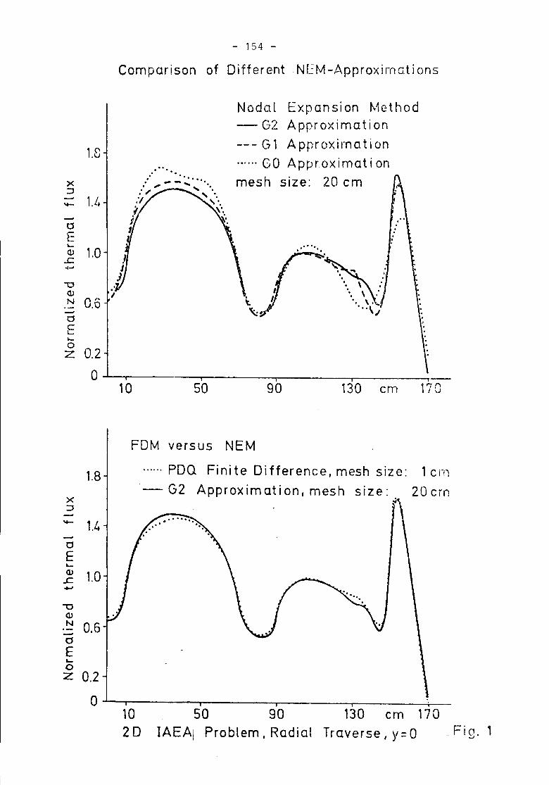
- 154 -
Comparison of Different NEM-Approximo.tions
Nodal Expansion Method- G2 Appro)<imation--- Gl Approximation...... GO Approximat ionmesh size: 20 em
1.8.... ' ... " .x , ,"'-,
;:)
'I- 1.L.
dE~(l) 1.0.c
.. ..J
"'0(l)N 0.60E....0
0.2z0
10i
50i90 i
130 em
.,,,
..r-
170
1.8
x;:)
..... 1.4aE~<1J 1.0.c....-0
<1JN 0.60E~0z 0.2
0
FDM versus NEM
...... PDQ Fi ni te 0 ifference, mesh siz e: 1c rTl
"- G2 Approximation, mesh sIze: 20 ern
10 50 90 130 em 17020 IAEAI Problem I Radial Traverse, y=O "Fig. 1
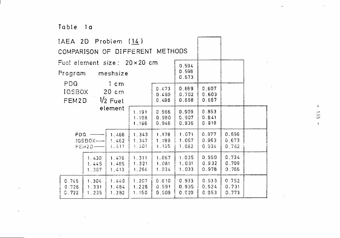
Table 1 a
->U1U1
~EA 20 Problenl (li)OMPARISON OF 01 FFt: RENT MFTHOOS
uet element size: 20 x 20 em 0.594
rogram meshsize 0.5980.673
PDQ 1 emIOSBOX ~O . 0.473 0.689 0.607~ em 0.460 0.702 0.603FEM2D 1/2 Fuel 0.496 0.698 0.687
element I 0.909 0.8531 . 191 0.966I 1.198 0.980 0.907 0.841I 1.166 0.946 0.936 0.918
!
PDQ 11.466 1.343 1 . 178 1 . 071 0.977 0.696IQS80X-1 ~. 462 1.347 i 1.198 11.057 0.963 0.673FE j\12 D - i "j.:~ 1 i I 1.~Ol 1.155 i.oa2 0.994 0.762 '
1. 430 1 .476 1 . 3 11 i .067 1. 035 0.950 0.7341.445 1.485 1.321 1 .031 1 . 031 0.932 0.7091.357 I 1.~13 ! 1.264 1 .034 1 . 033 0.978 a .766
I O. Z4 5,
1.207 10.6101.30/t I 1.449 0.933 I 0.933 a .752i O.! 26 1 . 331 1 .484 1 .228 0.591 0.935 10.924 0.731i 0.722 1 .235 1 .382 1 . 15 a 0.509 0.920 O. 9 53 0.773
P
.....P-o
I
C
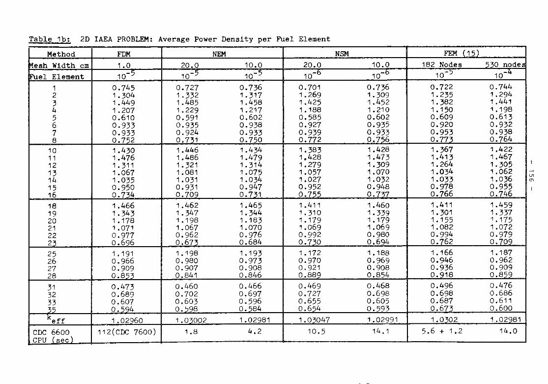
Table 1b: 2D lAEA PROBLEM: Average Power Density per Fuel ElementMethod FDM NEM NSM FEM (15)
Mesh Width em 1.0 20.0 10.0 20.0 10.0 182 Nodes 530 nodesFuel Element 10-5 10-5 10-~ 10-6 10-6 10-5 10-4
1 0.745 0.727 0.736 0.701 0.736 0.722 0.7442 1.304 1.332 1.317 1.269 1.309 1.235 1.2943 1.449 1.485 1.458 1.425 1 .452 1.382 1 .4414 1.207 1.229 1 .217 1.188 1.210 1.150 1 .1985 0.610 0.591 0.602 0.585 0.602 0.609 0.6136 0.933 0.935 0.938 0.927 0.935 0.920 0.9327 0.933 0.924 0.933 0.939 0.933 0.953 0.9388 0.752 0.731 0.750 0.772 0.756 0.773 0.764
10 1.430 1.446 1.434 1.383 1.428 1.367 1.42211 1.476 1.486 1.479 1.428 1.473 1.413 1.46712 1.311 1.321 1.314 1.279 1.309 1.264 1.30513 1.067 1.081 1.075 1.057 1.070 1.034 1.06214 1 .035 1.031 1.034 1.027 1.032 1.033 1.03615 0.950 0.931 0.947 0.952 0.948 0.978 0.95516 0.734 0.709 o. 7~1 0.7~~ 0.737 0.766 0.74618 1.466 1.462 1.465 1.411 1.460 1.411 1.45919 1 .343 1.347 1.344 1.310 1.339 1.301 1.33720 1.178 1.198 1.183 1.179 1.179 1.155 1.17521 1 .071 1.067 1.070 1.069 1.069 1.082 1 .07222 0.977 0.962 0.976 0.992 0.980 0.994 0.97923 0.696 0.673 0.684 0.7~0 0.694 0.762 0.70925 1.191 1 .198 1 .193 1.172 1.188 1.166 1.18726 0.966 0.980 0.973 0.970 0.969 0.946 0.96227 0.909 0.907 0.908 0.921 0.908 0.936 0.90928 0.853 0.841 0.846 0.889 0.854 0.918 0.85931 0.473 0.460 0.466 0.469 0.468 0.496 0.47632 0.689 0.702 0.697 0.727 0.698 0.698 0.68633 0.607 0.603 0.596 0.655 0.605 0.687 0.61135 0.5g4 0.598 0.~84 0.61)4 0.593 0.673 0.600keff 1.02g60 1 .03002 1.02981 1.0~047 1.02991 1.0302 1 .02981
CDC 6600 112(CDC 7600) 1.8 4.2 10.5 14.1 5.6 + 1.2 14.0CPU (see)
U1m
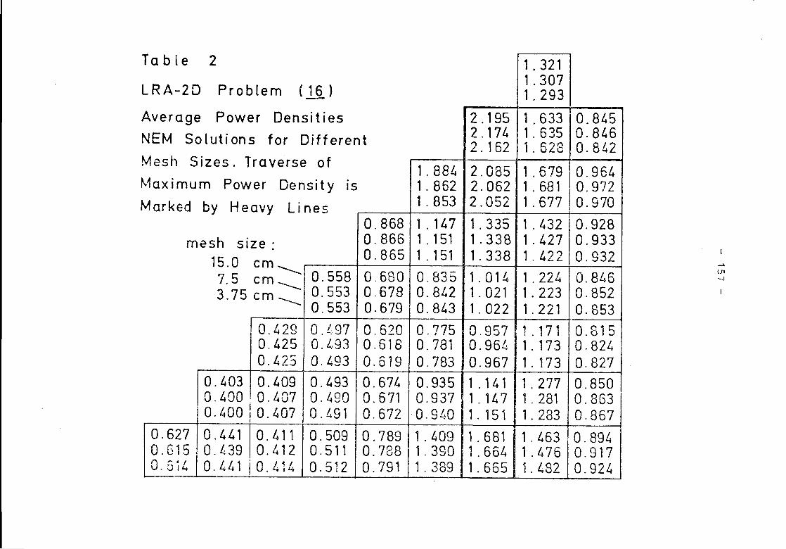
Table 2
LRA-2D Problem (12.)
-"Ul-J
0.8450.8460.842
0.9640.9720.9700.9280.9330.9320.8460.8520.8530.8150.8240.8270.8500.3630.867
0.8940.9170.924
1 . 3211 .3071 . 293
1 .6331 . 6351 . 528
1.6791 .6811 .677
1 .4321 .4271 . 4221 .2241 . 2231 .2211 . 1711 . 1731 . 1731 . 2771 . 2811 . 283
1 .4631.4761 . 482
2.1952.1742.162
1.884 2.0851.862 2.0621.8532.052
0.8681.1471.3350.8661.151 1.3380.8651.151 1.3380.680 0.835 1. 0140.678 0.842 1.0210.679 0.843 1.0220.620 0.775 0.9570.618 0.781 0.9640.619 0.783 0.967o . 674 0 . 935 1. 14 10.671 0.937,1.1470.6720.940 1.151
0.789 1.409 1.6810.788 11 . 390 1.6640.791 I 1 . 389 1. 665
0.5580.5530.5530.1:97O. L.\930.4930.4930.4900.491
0.5090.5110.512
0.4290.4250.425
-0 -.4-03-' O. 4090.400 10.4070.400 10.407
I
~0.411g. ~;~~ I 0.4120.441 10.414
mesh size:15.0 em _____7.5 em ___3.75 em ___
0.6270.615a.6il.
Average Power DensitiesNEM Solutions for DifferentMesh Sizes. Traverse ofMaximum Power Density IS
Marked by Heavy Lines
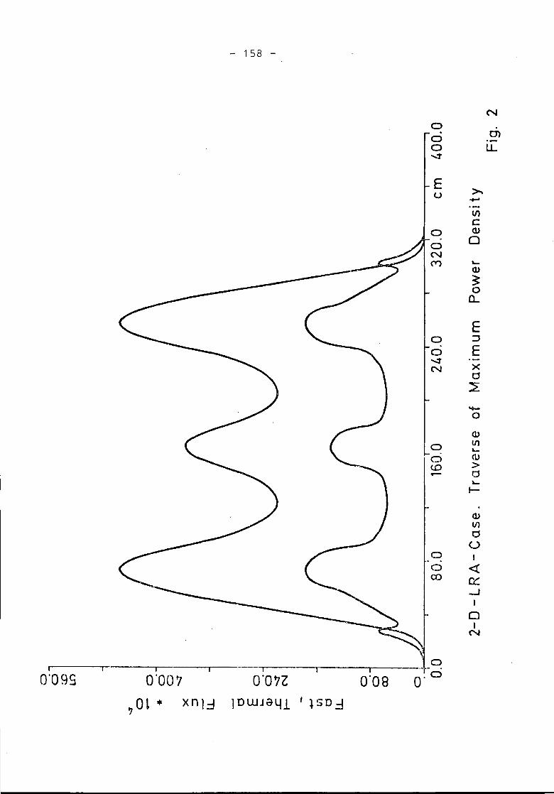
I
0'099
- 158 -
I ---I I
0'007 O'O'7l O'OB.,Ol If' xnl::l lOWJtH~l' l50=:J
N0. 0)0 '-0 lL.-...T
E ~u ....V)c
0 Q). 00N(Y') '-
<l>~0
n..
E0 :J
0 E-..:r xN
0~
'to-0
Cl>
0 lI)'-
0 (\)
<.0 >or- d
"-t-
Q)lI)
0u
0 I-0 «co fr::
.....JI
0IN
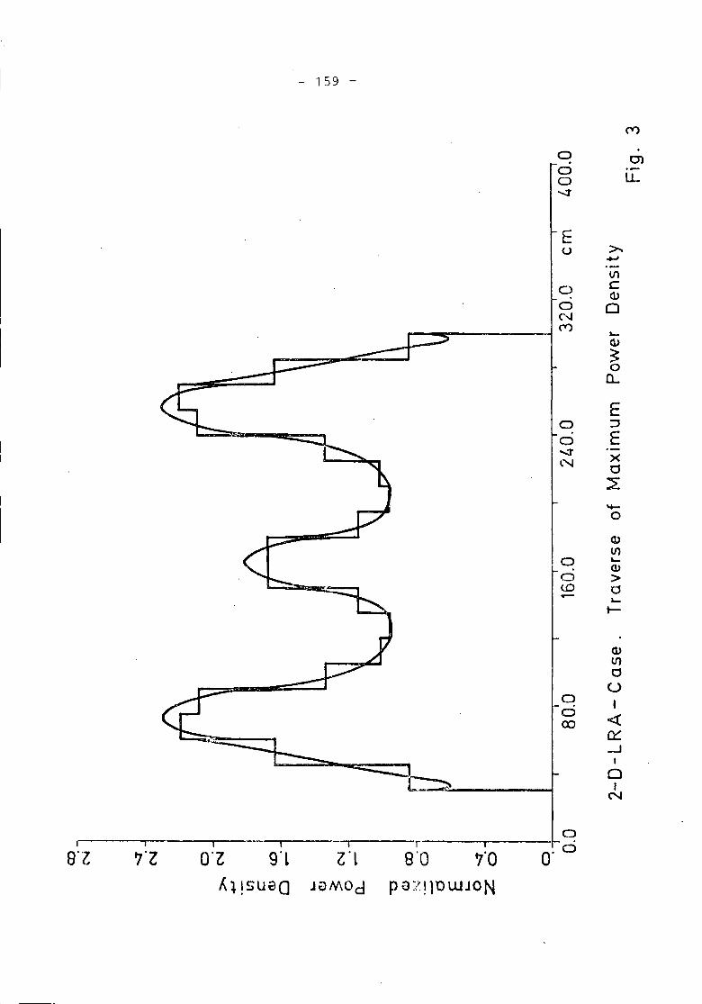
('Y')
0 Ol0 .-0 u..-..:r
Eu >.
+oJ
If)
0 cw0 0N(Y') ~w
30(L
E0 :J
0 E....:r x~""'J 0
~
'+-0
C1JIf)
0 ~(\)
0 >to d- ~
t-
,S'l
- 159 -
,tiO
ooCX)
o0.0
C1JIf)
oUI
«n::.....JI
oI
('oJ
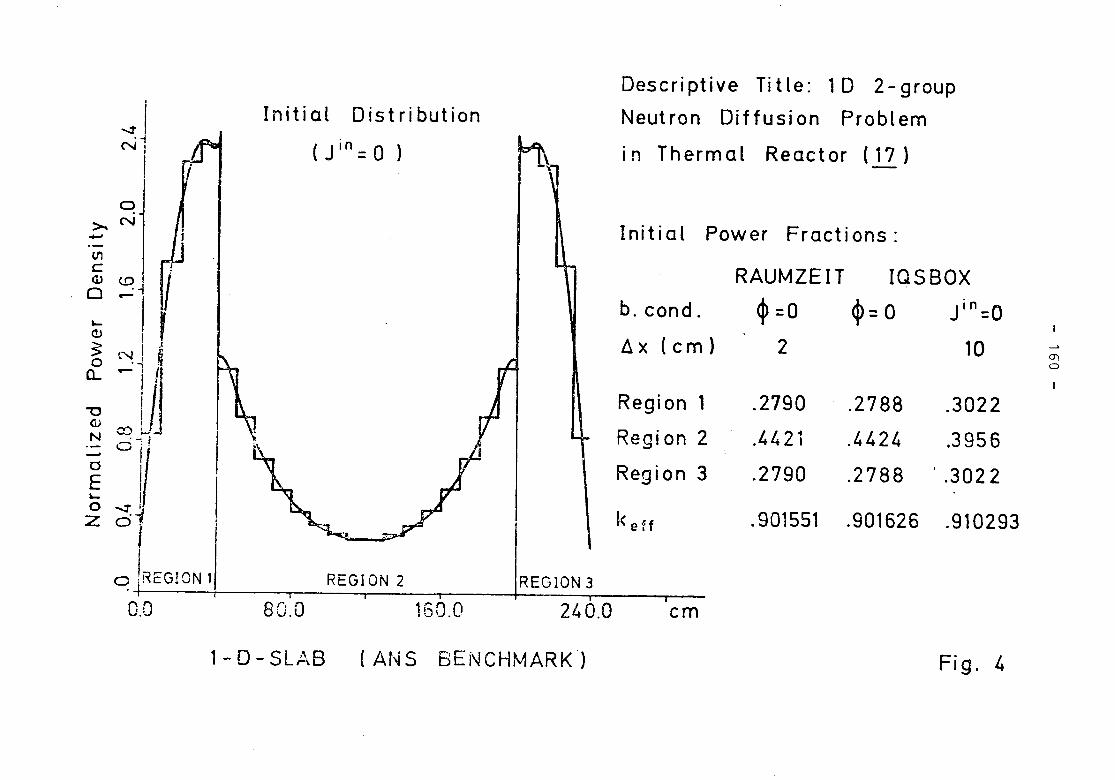
RAUMZEIT IQSBOX
~ =0 ~=o Jin:O
2 10 -"
~0
I
.2790 .. 2788 .3022
.4421 .4424 .3956
.2790 .2788 ' .3022
.901551 .901626 .910293
Descriptive Title: 1D 2-groupNeutron Diffusion Problem
in Thermal Reactor (17)
!:J.x (cm)
b. condo
Initial Power Fractions:
Initial Distribution
(Jin=O)~I.,NI
Ia
>.N-U'l
~ cp ~ II'o - I I
Q; I'~ N i ~o '. -i ft; :I~ I ~, A I II Region 1
; el/' I \ I:; :::;:~~'- Io ~li I I \ IZ o. ' ~,/ I '(eff
q jREGlON " ,REGI,ON 2 ,.REGION ~ ,
0.0 80.0 160.0 240.0 cm
l-D-SLAB (ANS BENCHMARK) Fig. 4
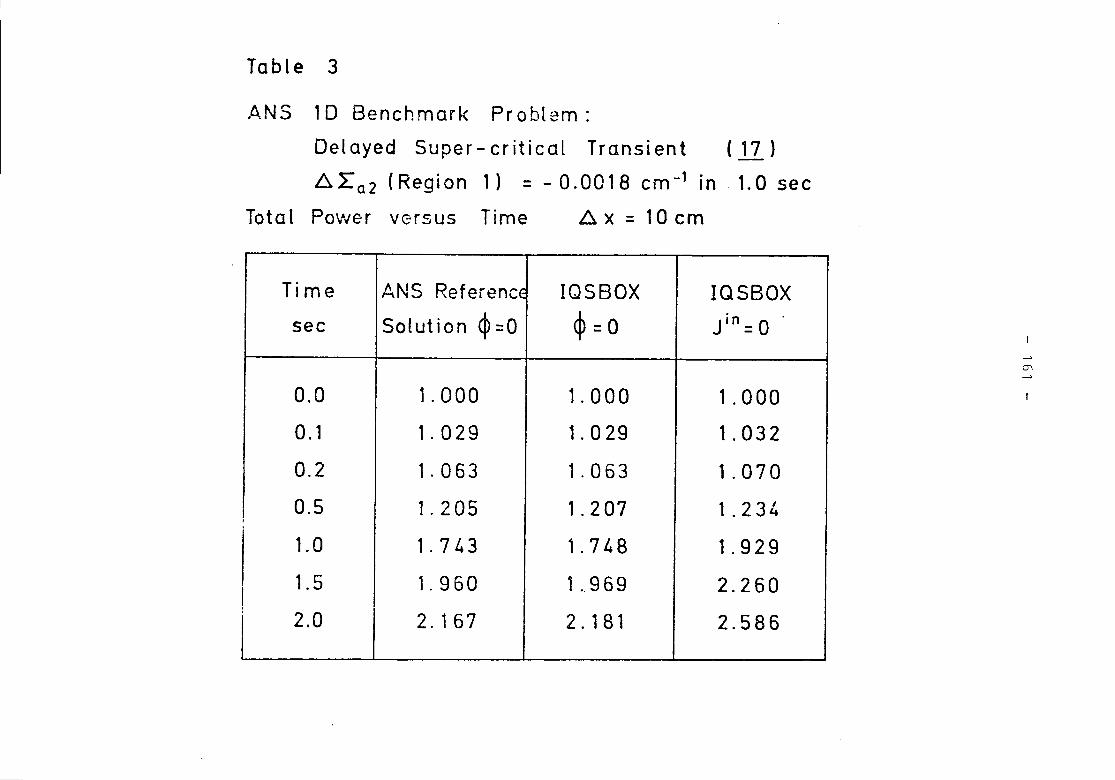
Table 3
ANS 1D Benchmark Problem:
Delayed Super-critical Transient (IT)
~2:a2 (Region 1) = - 0.0018 cm-1 in 1.0 see
Total Po\ver V0fSUS Time ~x = 10em
Time ANS RefeiencE IQSBOX IQSBOX
see Solution ~=O $=0 Jin = a
0.0 1. 000 1. 000 1 .000
0.1 1. 029 1. 029 1 . 032
0.2 1.063 1. 063 1 .070
0.5 1.205 1.207 1 .234,i
1.0 1.743 1.748 1.929
!1.5 1. 960 1.969 2.260
2.0 2.167 2. 181 2.586
-->m-->
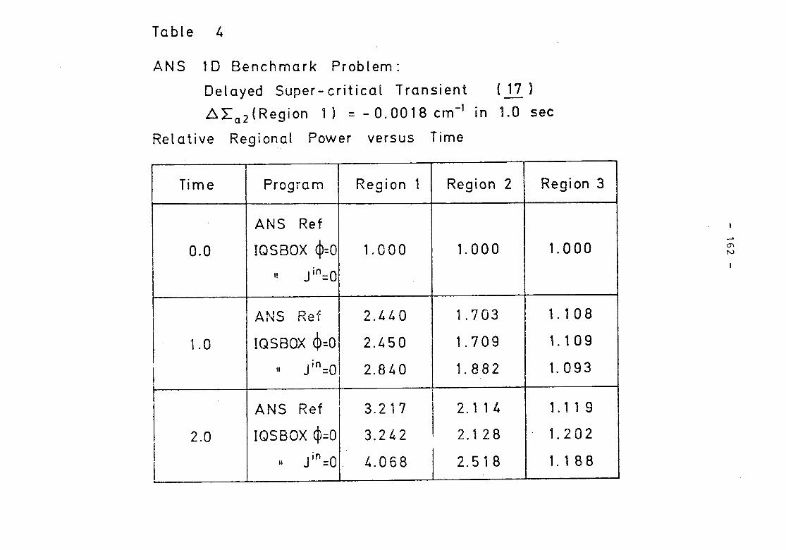
Table 4
ANS 10 Benchmark Problem:
Delayed Super-critical Transient (fl)
~La2 (Region 1) = - O. 00 18 cm-1 in 1.0 see
Relative Regional Power versus Time
Time Program Region 1 Region 2 Region 3
ANS Ref
0.0 IQSBOX ~=O 1.000 1.000 1.000
I! Jin=O
ANS Ref 2.440 1.703 1.108
1.0 IQSBOX ~=O 2.450 1.709 1.109
t II Jin=O 2.840 1. 882 1. 093
IANS Ref 3.2 17 I 2.1 1 4 1.119
2.0 IQSBOX ~=O 3.242 I 2.128 1.202
Jin:O.i
II 4.068 I . 2.51 8 1.188
~0"\tv
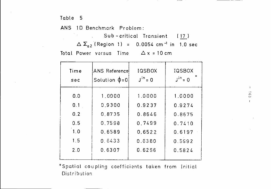
Table 5
ANS 1D Benchmark Problem:
Sub - critical Transient ( 17 )-b. 202 (Region 1) = 0.0054 cm -1 in 1.0 sec
I
Total Power V2rsus Time ~ x = 10 em
Time A NS Reference IQSBOX IQSBOX
Solution ~=O J in = a Jin: a +see
0.0 1 .0000 1.0000 1.0000O. , 0.9300 0.9237 0.9274
, 0.2 0.8735 0.8646 0.8675I
0.5 0.7598 0.7499 0.74101.0 0.6589 0.6522 0.6197
I 1.5 0.6433 0.6380 O. 5S 9 2II
2.0 I 0.6307 0.6256I
0.5824iI
+Spatial coupling coefficients taken from InitialDistribution
-'mw
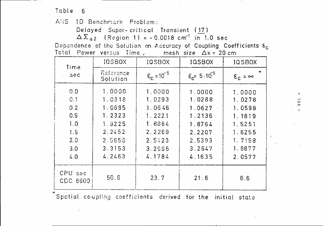
Table 6
A ~'1S 10 8 e n c hr. Q r k Pro b l 2ln :
Delayed Super- ciiti cal Transient (17).6. 2: Q 2 ( Reg ion 1) = - 0.00 j 8 C m-1 in 1. a 5 e c
Dependence of the Solution on t,ccuracy of Coupling Coefficients E.cTotal PovJer versus Time J mesh size .6.x = 20 cm
IIQSBOX IQSBOX IQSBOX IQSBOX
Time.." r"'"'\'~"'" - _ -s -s +I sec ~,cj c:.r:::nve t.c = 10 Ec= 5.10 £c = C>O! Solution
II 0.0 1.00 00 1.0000 1 . 0000 1.0000
0.1 1.03 18 I 1.0293 1 .0288 .1. 0278,I 0.2 1 . 0695 1. 0646 1.0627 1 . 0598I
i 0.5 1.2323 1. 222 1 1.2136 1. 1819i. LO 1 . 9225 1 . 8864 1 .8764 1. 525 1I
i
! 1.5 2. 2452 2.2269 2.2207 1 . 6255I!
I 2.0 2.5558 2 r.::l2? 2 5'"10"'" 1.7158,
I I • oJ --{ ..J • '::> ...J ,j I
I I I, 3.0 3.3153 3.2696 3.2647 1 . 88774.0 4.2463 I 4.1784 4.1635 2.0577
I CPU see j i
i CDC 6600 I 50.6 I 23.7 21.6I
8.6I I !
+Spatial coupl;ng coefficients derived for the initial state
--'0'1~
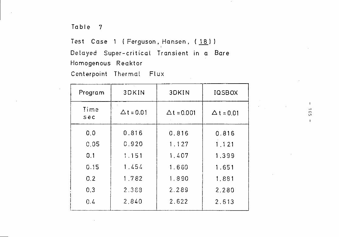
Table 7
Test Case 1 (Ferguson, Hansen, (JJi))Delayed Super-critical Transient in a Bare
Homogenous Reaktor
Centerpoint Thermal . Flux
Program 3DKIN 3DKI N IQSBOX
I
I Time .6.t=O.Ol b.t = 0.001 ,6 t = 0.01I
sec
I 0.0 0.816 0.816 0.81 6
C.OS 0.920 1 . 'I 27 1 .1 21
0.1 1 . 1 5 1 1.407 1 .399I I
1 0.15 I1 .454 1.660 I 1 .651
I
0.2 1 .782 1.890 I 1.881I
2.289 2.2800.3 I 2 1°8; I . ...,vI,I 0.4 2.840 2.622 2.513I!
---'mU1
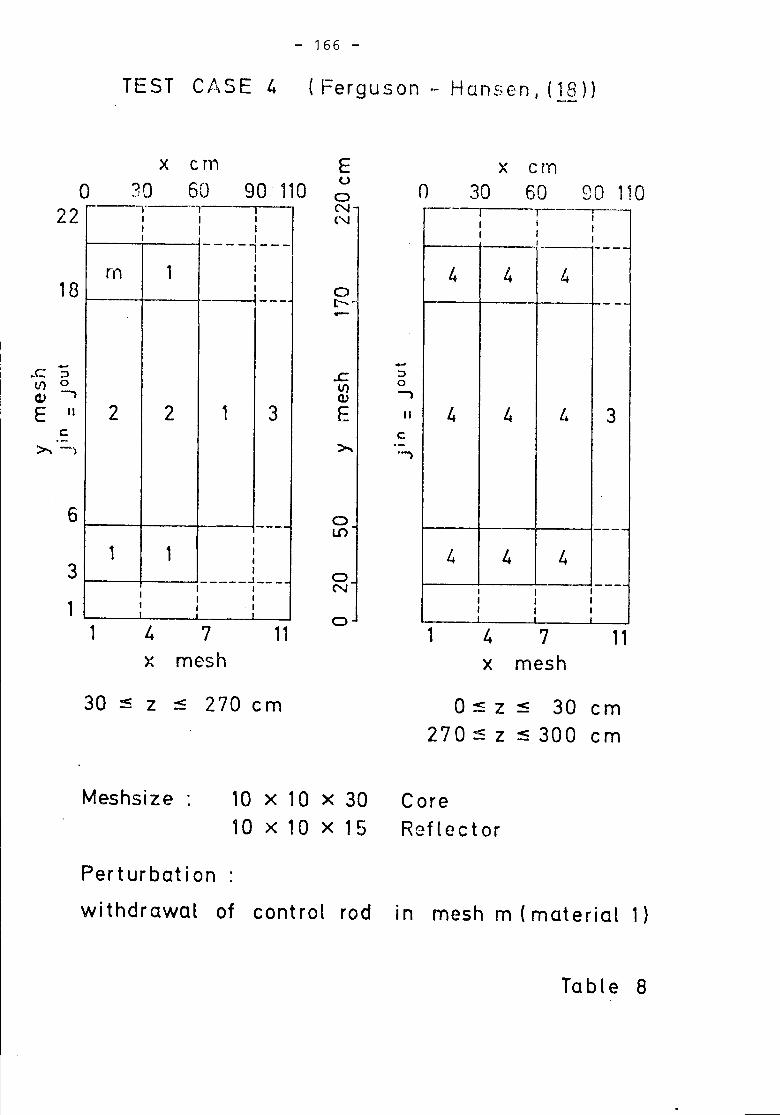
- 166 -
TEST CAS E 4 ( Fer 9 u son .~ H an s en, (l~))
114 7x mesh
x ern30 60 90 110
-' I r---- iI I
tI I
II---------4 4 4
--
4 4 l 3
--4 4 4
I I ,----I I II I II I
1
oEuoN('.I
.....r:. ::JIf) 0
Q) -,E II
c::>. .-.,
ot---
oN
o
oL.()
114 7x mesh
x ern30 60 90 110
1
,.....--.T 1 :I II I II I---l---
I
m 1 II,---
2 2 1 3
----I
1 1 III
I
____ .J ____
II I II ! II ,
6
3
1
c
18
o22
....~C: ::Jll) 0(1) -,E II
30 :5 Z ~ 270 em o ~ Z < 30 em270:5 Z :5 300 em
Meshsize 10 x 10 x 3010 x 10 x 15
CoreReflector
Perturbation:
withdrawal of control rod In mesh m (material 1)
Ta b l e 8
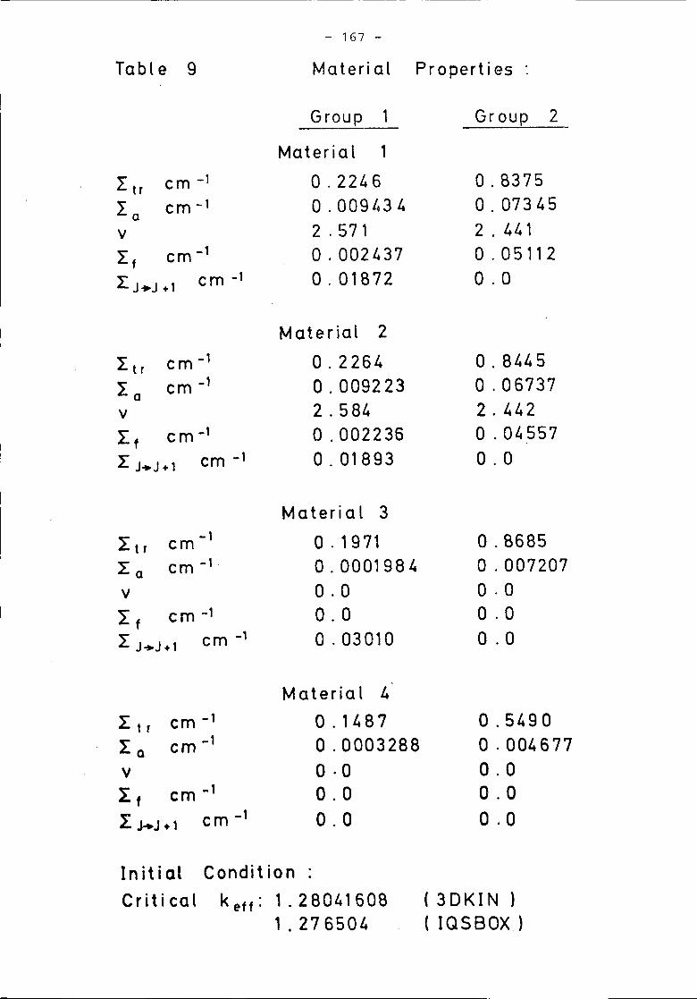
Tab Ie 9
- 167 -
Material Properties:
~ cm -1L t r't" cm-1LaV
Lf em-1
L c m -1J +-J + 1
Itr em-1
Io em-1
vL f c m-1
:r J.. J+1 em-1
l:tr em-1
:r a em -1 .
V
L f em -1
L J+J+1 em-1
~ em -1L. t rI Q em -1
v1:, em-1
~JJ 1 em-1L .. +
G rou p 1
Material 1
o .22460.0094342 .571a . 0024370.01872
Material 2
0.22640.0092232 .584a .0022360.01893
Material 3
0.19710.00019840.00.00.03010
Material 4
0.1487a . 00032880.00.00.0
Group 2
o . 83750.073452 . 4410.051120.0
a . 84450.067372 .442a .045570.0
o .8685o .0072070.00.00.0
0.5490a .0046770.00.00.0
Initial ConditionCritical keff: 1.28041608
, .276504(3DKIN )( IQSBOX )
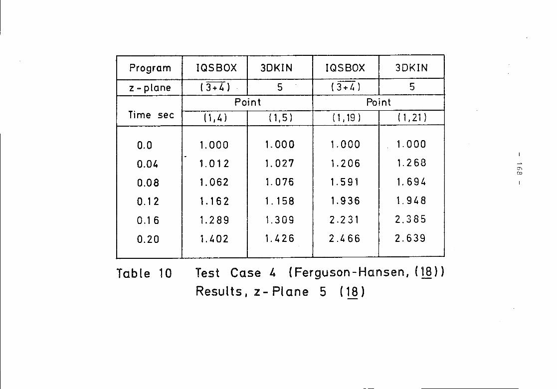
Program IQSBOX 3DKIN IQSBOX 3DKIN
z - plane (3+4) 5 (3+4) 5Point Point
Time see (1,4) ( 1,5 ) ( ',19 ) (1.21)
0.0 1.000 1. 00 a 1. 000 1. 000.
0.04 1.012 1. 027 1.2 06 '.268
o.oa 1.062 1. 076 1.591 1.694
0.12 1.162 1. 158 1.936 1.948
0.1 6 1.289 1.309 2.231 2.385
0.20 1.402 1.426 2.466 2.639
-->mco
Table 10 Test Case 4 (Ferguson-Hansen, (18))Results. z-Plane 5 (18)
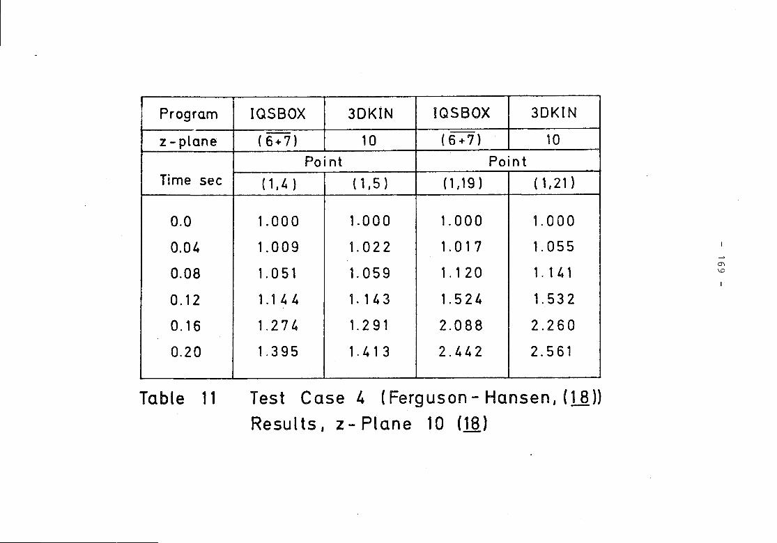
! Program IQSBOX 3DKIN IaSBOX 3DKIN
z - plane (6+7) 10 (6+7) 10
Point PointTime see (1,4) ( 1,5 ) (1,19) (1,21)
0.0 1. 00 a 1.000 1. 000 1.000
0.04 1.009 1.022 1.017 1.055
0.08 1.051 1. 059 1.120 1.141
0.12 1.144 1.143 1.524 1.532
0.16 1.274 1.291 2.088 2.260
0.20 1.395 1.413 2.442 2.561
->
mI..D
Table 11 Test Case 4 (Ferguson - Hansen, (La))
Resul ts, Z - Plane 10 C18J
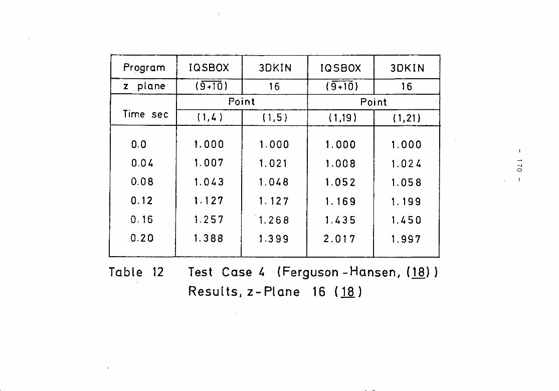
Program IQSBOX 3DKIN IQSBOX 3DKIN
z plane (9+10) 16 (9+10) 16Point Point
Time see (1,4) (1,5) (1,19) (1,21)
0.0 1. 000 1. 000 1. 000 1.000
0.04 1. 007 1.021 1.008 1.024
0.08 1.043 1.048 1.052 1.058
0.12 1. 127 1.127 1.169 1.199
0.16 1.257 1.268 1.435 1.450
0.20 1.388 1.399 2.017 1.997
-''-Jo
Table 12 Test Case 4 (Ferguson -Hansen, (~) )Results, z-Plane 16 (la)
- 171 -
DISCUSSION
F.N. McDonnell
What are the relative computing efficiencies between theconventional finite difference (3DKIN) method and yourcoarse-mesh method (IQSBOX)?
H. Finnemann
Using the same meshsize, the computing cost per time stepis of 'course lower in conventional finite difference me-thods. Taking into account accuracy and computing cost, theproposed nodal method is much more efficient. You gain afactor of at least 3 to 5 for each space direction. In fact,only by using coarse-mesh methods 3-D space-time calcula-tions become feasible.
G. Williams
How do you intend to develop your nodal programme in thefuture? What improvements do you have in mind?
H. Finnemann
Up to now, the efforts were concentrated on an accurate spa-tial approximation. The time integration is performed by thesimple backwards difference algorithm. Perhaps other integra-tion methods will be more efficient. Together with the pro-blem of an efficient time integration, the implementation ofthermal hydraulic feedback has high priority. At present, on-ly prompt feedback is consideren.

- 172 -
A.F. Henry
Since you are neglecting certain cross terms in the polyno-mial expression for the flux, would it not be somewhat moremeaningful to use a product of cubic functions with 10 cmmesh rather than quartic functions with 20 cm mesh?
H. Finnemann
Because of storage limitations, it is necessary to use boxesof approximately 20 x 20 x 20 (30) cm3 in 3-D calculations.For these large meshes, quartic functions yield generallyfar better results than cubic functions.
One advantage of the proposed nodal method is that these ex-pansion coefficients need not be stored. This means thatusing quartic functions instead of a cubic approximation re-sults in cost increase of about 10 %, whereas halving themeshsize increases cost and storage requirements by a factor8.
- 173 -
S. Langenbuch, W. Maurer, W. WernerSIMULATION OF TRANSIENTS WITH SPACE-DEPENDENT FEEDBACK BYCOARSE MESH FLUX EXPANSION METHODLaboratorium fUr Reaktorregelung und Anlagensicherung,Technische Universitat MUnchen, Germany

- 175 -
1. Introduction
For the simulation of the time-dependent behaviour oflarge LWR-cores, even the most efficient Finite-Differ-ence (FD) methods require a prohibitive amount of com-puting time in order to achieve results of acceptableaccuracy.
In /1/ a Coarse Mesh (CM) method was introduced, whichrequires significantly fewer unknowns without appreci-ably increasing the complexity of the calculations,thus achieving a drastic reduction of computing costs.In /2/ and /3/ it is substantiated that static CM-solu-tions computed with mesh-size corresponding to the fuelelement structure (about 20 cm) are at least as accurateas FD-solutions computed with about 5 cm mesh-size. For3d-calculations this results in a reduction of storagerequirements by a factor 60 and of computing costs by afactor 40, relative to FD-methods. These results havebeen obtained for pure neutronic calculations, where feed-back is not taken into account.
In this paper it will be demonstrated that the methodretains its accuracy also in kinetic calculations, evenat the presence of strong space dependent feedback.
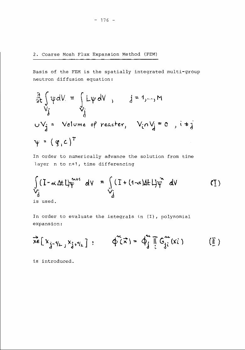
- 176 -
2. Coarse Mesh Flux Expansion Method (FEM)
Basis of the FEM is the spatially integrated multi-groupneutron diffusion equation:
In order to numerically advance the solution from timelayer n to n+1, time differencing
olv
is used.
In order to evaluate the integrals in (I), polynomialexpansion:
is introduced.
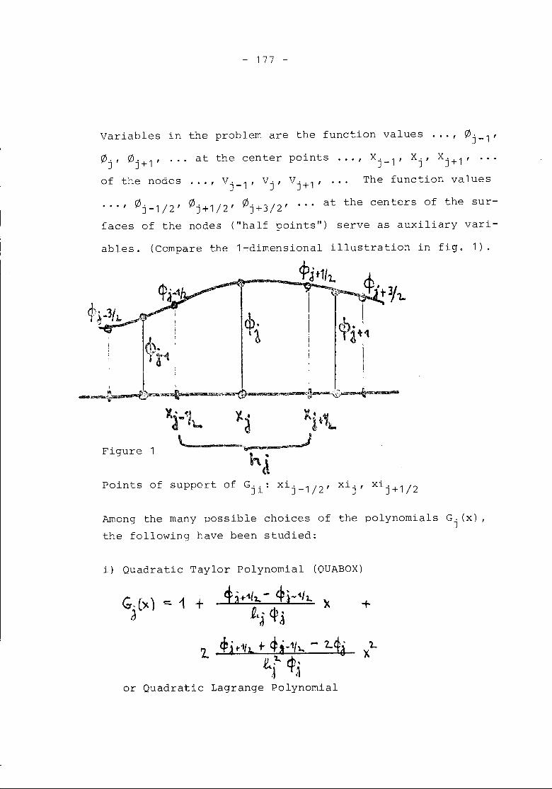
- 177 -
Variables in the problem are the function values ... , 0j-1,
0j, 0j+1, ... at the center points , Xj_1, Xj, Xj+1,
of the nodes ... , Vj_1, Vj, Vj+1, The function values
..., 0j-1/2, 0j+1/2, 0j+3/2, ... at the centers of the sur-faces of the nodes ("half points") serve as auxiliary vari-
abies. (Compare the 1-dimensional illustration in fig. 1).
Qii-3/A. .I,~
J,)"f1
~.~
, ,--~~;)~~.-.""" \.~
Figure
Points of support of Gji: xij_1/2, xi. ,J xij+1/2
+
'LX
Among the many possible choices of the polynomials G. (x),J
the following have been studied:
i) Quadratic Taylor Polynomial (QUABOX)
G ') 1 ~i ..1{1.. - ~i_1/1.. Xj (~-: + £~J 4'j
2. .cPjt1/1. ir ~3_1'l.. - 2..ti-~~ ct',1 .1
or Quadratic Lagrange Polynomial
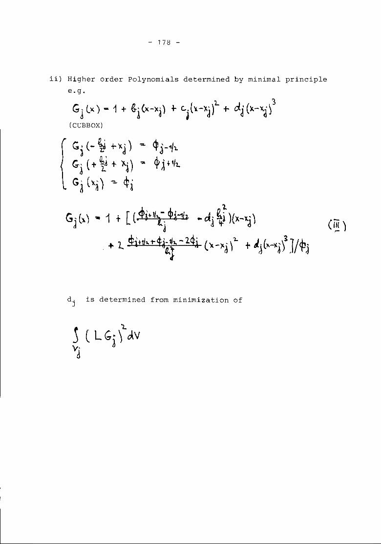
- 178 -
ii) Higher order Polynomials determined by minimal principlee.g.
Gj C") - 1 + ~i("-1<a) +- cl~-xl+ dJ (l<-'1)3
(CUBBOX)
(;i (- ~ +~J) ~ ~j-"/l.G-J ( + ~ + ~j) -:a ~ J ~1/l.
G' (~~) -:. ~.J a a
Gj(~)-1 + [(~ -dl~)(l<-"j)
+"t ~i+1J,.t-etd-~'&.-14~ ('x_)r.~\1.. + .J'(lI\-y.')~J/<P'-~l F a J A, J
d. is determined from minimization ofJ
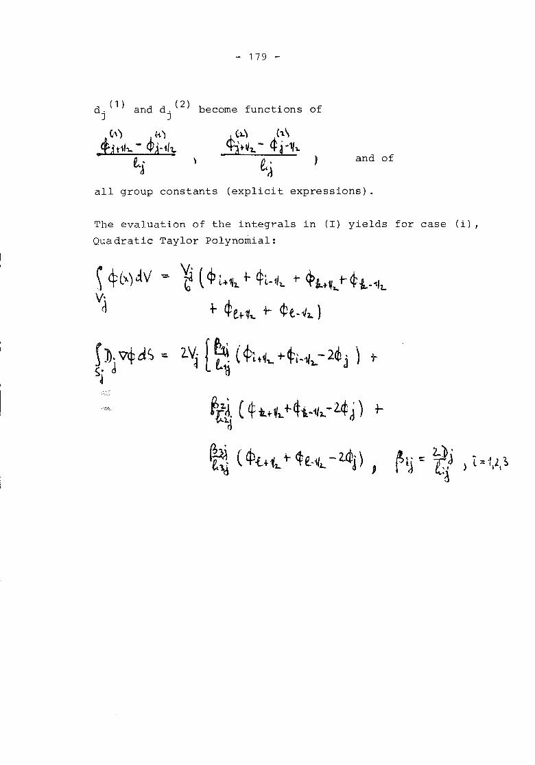
d .(1) and d. (2)J J
to') t1)
'pi t1h.. - ~ j..ilt.~.J
- 179 -
become functions of
and of
all group constants (explicit expressions) .
The evaluation of the integrals in (I) yields for case (i),Quadratic Taylor Polynomial:
- ~ ( ep t~1h.1- ~i.-11~+ <l>£..+~1..t- ~ -&.. .. 1/t.
+ ~e.+~1,. t- <Pe-1/2-)
~tJ.(~iz.+l~+4i-1f1..-2..~ J) ~~
If~(4Ji.-~1..+- ~e-~1..- ubj) ,
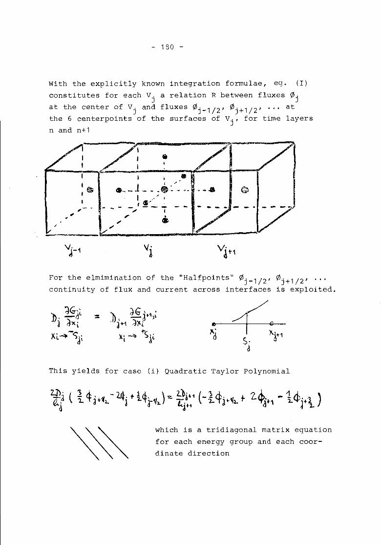
- 130 -
(I)
~.J
atlayers
With the explicitly known integration formulae, eq.constitutes for each V. a relation R between fluxes. Jat the center of Vj and fluxes ~j-1/2' ~j+1/2' ...the 6 centerpoints of the surfaces of Vj, for timenand n+1
------
- .. -- ...
, .•....-7f' e-~ :
""-:
Ii. , ,.,-• __1--- ~e: .~~.
I .,' I, S., ,- - - -1fI' - - i
i ~~' •
I,I
16)I
•,.
/
For the elmimination of the "Halfpoints" ~j-1/2' ~j+1/2' ...continuity of flux and current across interfaces is exploited.
». ~dlJ d~l
XL~-<)Jie~.(1
This yields for case (i) Quadratic Taylor Polynomial
which is a tridiagonal matrix equationfor each energy group and each coor-dinate direction
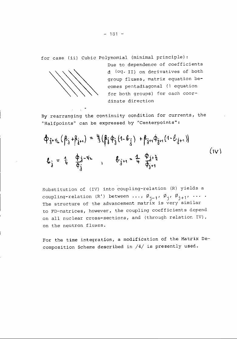
- 181 -
for case (ii) Cubic Polynomial (minimal principle) :Due to dependence of coefficientsd (eq. II) on derivatives of bothgroup fluxes, matrix equation be-comes pentadiagonal (1 equationfor both groups) for each coor-dinate direction
By rearranging the continuity condition for currents, the"Halfpoints" can be expressed by "Centerpoints":
Substitution of (IV) into coupling-relation (R) yields acoupling-relation (R') between ... , ~. l' ~., ~'+1' ....J- J JThe structure of the advancement matrix is very similarto FD-matrices, however, the coupling coefficients dependon all nuclear cross-sections, and (through relation IV),on the neutron fluxes.
For the time integration, a modification of the Matrix De-composition Scheme described in /4/ is presently used.
- 182 -
3. Numerical Examples
For a model LWR, a static solution without feedback, astatic solution with strong space dependent feedback, anda dynamic solution are computed. All calculations havebeen performed with 20 em mesh width, which corresponds tothe size of fuel elements, and with 10 em mesh size. Inaddition, the static calculations have also been performedwith 5 em mesh width. Feedback effects which act on groupconstants are considered by using the box-average of the feed-back quantities to compute the change of cross-sections withinthe box. Thus, an additional discretization effect is in-troduced into the numerical results.
Fig. 2 shows a horizontal cross-section of a quarter of themodel reactor. The numerals inside the heavily lined boxesrefer to the numbering of boxes in tables 1 and 2.
Static Calculations
Table 1 shows relative power densities in boxes 1, ... 6along A-C for a static solution without feedback. The solu-tions were obtained with mesh sizes of 5, 10 and 20 em meshsize, resp. In the lower part of table 1 the relative devia-tions of the 10 cm-, resp. 20 em-solution from the 5 em so-lutions are shown.
Table 2 shows relative power densities at the same locationsfor a solution with space dependent temperature- and xenon-feedback for the hot reactor (average power density: 300 W/ccmlAgain, the same three mesh sizes have been used. The devia-tions of the 10 cm-, resp. 20 em-solution from the 5 em-solu-tion are shown in the lower part of table 2.
- 183 -
The deviations between 5 cm- and 10 em-solution are lessthan 1 % everywhere, and also the 20 em-solution showsvery good agreement with the 5 em-solution.
Since there is no significant difference between the re-lative deviations in tables 1 and 2, resp., it can be con-cluded, that the global treatment of feedback within theindividual boxes does not appreciably affect the accuracyof the method, relative to calculations without feedback.
Dynamic Calculations
In the dynamic calculations only doppler-feedback is con-sidered. Because of the short duration of the transient,adiabatic heatup of fuel elements is assumed.
For reasons of economy, only 10 cm- and 20 em-solutionshave been calculated. This seems to be justified by theexcellent agreement between 5 cm- and 10 em-solutionsin the static case.As an example, a superprompt critical excursion is presen-ted, which is caused by a fast withdrawal of one of the 2absorber rods (fig. 2). Both the 10 cm- and 20 em-solutionhave been calculated with identical time step sizes.
For both mesh sizes, fig. 3 shows the time-history of aver-age power. The excursion starts out at a power level of250 W/ccm. Thus, feedback effects are significant alreadyat the beginning of the calculation.
Time to peak (of average power) agrees within .4 %, andthe power maxima differ by 1.4 %.
Table 3 shows the relative power densities in 20 em boxesof the core for 10 cm-, resp. 20 em-solutions. The 3rd
- 134 -
line in each box indicates the relative deviations be-tween 10 cm- and 20 em-solutions. Again, these deviationsare not appreciably different from the deviations foundfor static solutions without feedback.
Conclusion
The accuracy of the coarse mesh flux expansion methodQUABOX/CUBBOX reported for static calculations withoutfeedback is retained also for situations with strongspace dependent feedback, even when feedback effects areconsidered only by box-averages. At present, there seemsto be no need to go into a more elaborate treatment offeedback effects, e.g. by a subdivision of boxes intosubboxes to which are associated different cross-sections/5/.
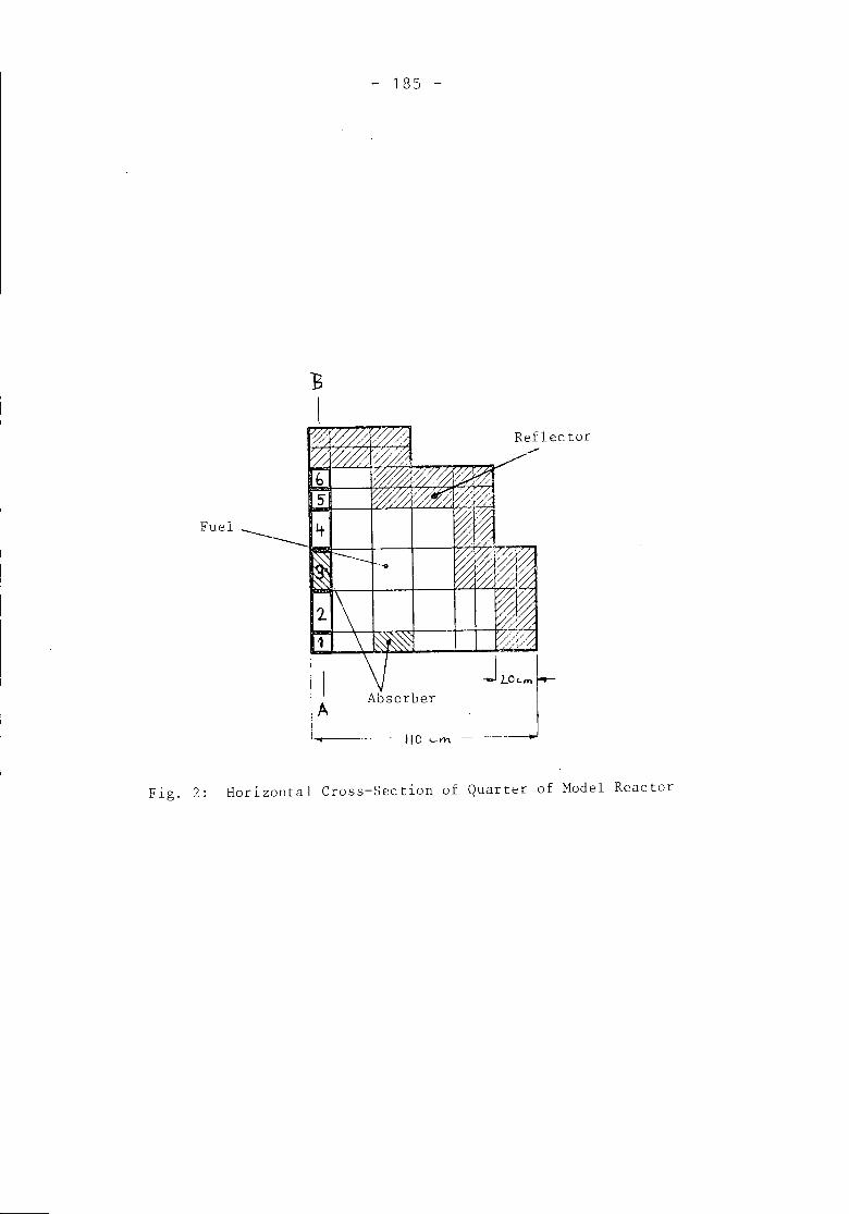
- 185 -
Fuel 4
'-'"
1I. II A A~sorber!I.. lie .....m.
Reflector../
Fig. 2: Horizontal Cross-Section of Quarter of Model Reactor
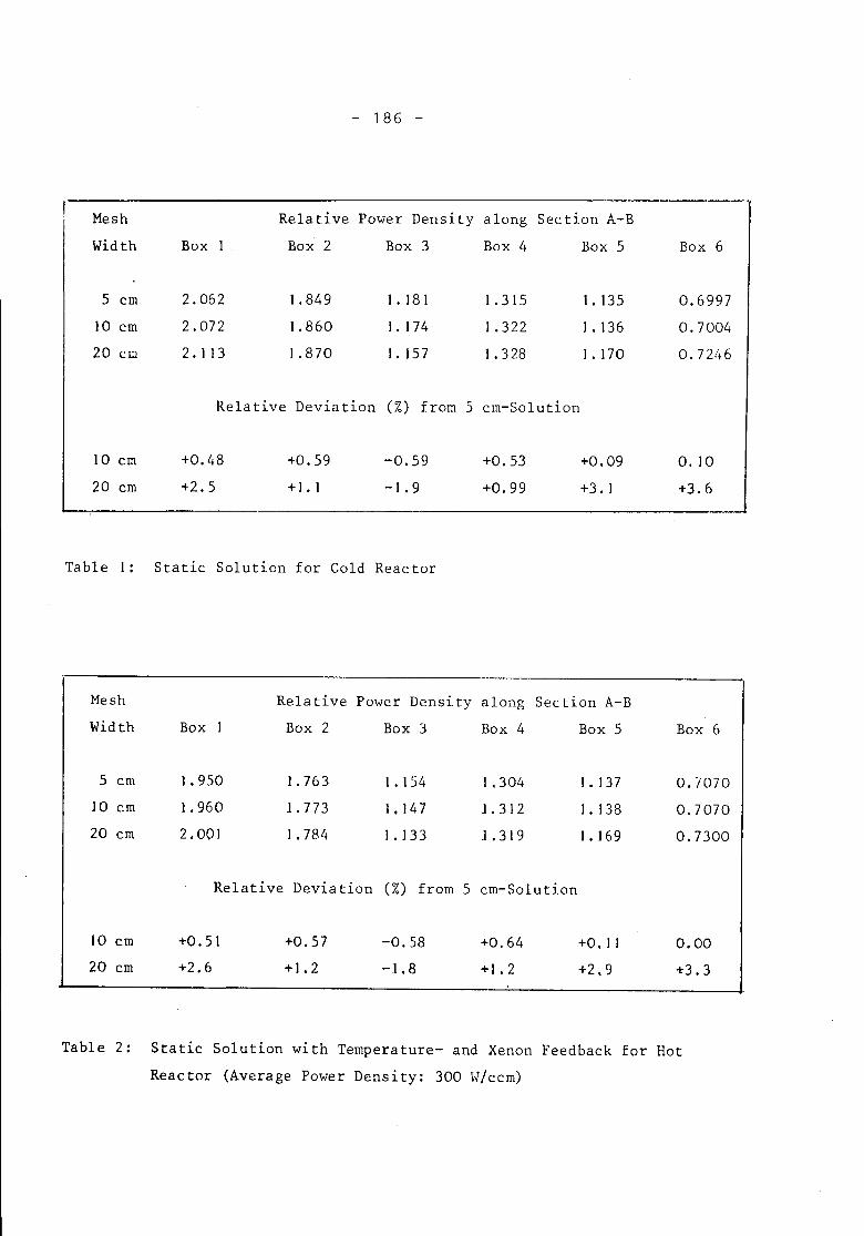
- 186 -
Mesh Relative Power Density along Section A-BWidth Box I Box 2 Box 3 Box 4 Box 5 Box 6
5 crn 2.062 1.849 1.181 1.315 1.135 0.6997
10 ern 2.072 1.860 I. 174 1.322 1.136 0.7004
20 ern 2.113 1.870 1.157 1.328 1.170 0.7246
Relative Deviation (%) from 5 ern-Solution
10 crn +0.48 +0.59 -0.59 +0.53 +0.09 0.10
20 ern +2.5 +1.1 -1.9 +0.99 +3. I +3.6
Table I: Static Solution for Cold Reactor
Mesh Relative Power Density along Section A-BWidth Box I Box 2 Box 3 Box 4 Box 5 Box 6
5 ern I.950 1.763 1.154 ) .304 I. )37 0.707010 ern 1.960 1.773 ). )47 1. 3) 2 1.138 0.707020 em 2.001 1.784 1.133 J .319 1.169 0.7300
Relative Deviation (%) from 5 crn-Solution
10 em +0.51 +0.57 -0.58 +0.64 +0.) ) 0.0020 crn +2.6 +1.2 -1.8 +1.2 +2.9 +3.3
Table 2: Static Solution with Temperature- and Xenon Feedback for HotReactor (Average Power Density: 300 W/ccm)
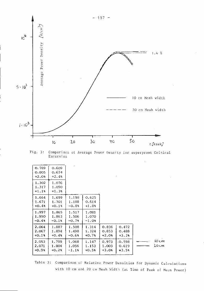
- 187 -
-~----- ] .4 %
10 cm Mesh width
20 cm Mesh width
10 10 30 lfO 5"0t[msek}
Fig. 3 : Comparison of Average Power Density for superpromt CriticalExcursion
0.789 0.6090.805 0.624+2.0% +2.4%1.302 1.0761.317 1.090+1.1% +1.3%1.664 1.699 1.198 0.6251.671 1.701 1.188 0.614+0.4% +0.1% -0.8% +1.8%1.997 1.865 1.517 1.0811.990 1.863 1.506 1.070-0.4% -0.1% -0.7% -1.0%2.064 1.887 1.508 1.314 0.836 0.4722.067 1.894 1.498 1.324 0.853 0.488+0.1% +0.4% -0.6% +0.7% +2.0% +3.3%2.053 1.799 1.068 1.147 0.973 .0.5982.071 1.804 1.056 1.153 1.003 0.619+0.9% +0.2% -1.1% +0.5% +3.0% +3.5%
10 <..M2..0<...m.
Table 3: Comparison of Relative Power Densities for Dynamic Calculationswith 10 cm and 20 cm Mesh Width (at Time of Peak of Mean Power)
- 188 -
References
/1/ A. Birkhofer, W. Werner:Efficiency of Various Methods for Analysis of SpaceTime Kinetics,Proc. 1973 Conf. Math. Models and Computational Tech-niques for Analysis of Nuclear Systems, IX 31-41.
/2/ A. Birkhofer, S. Langenbuch, W. Werner:Coarse-Mesh Method for Space-Time Kinetics,ANS Transactions, 18, 153 (1974)
/3/ S. Langenbuch, W. Werner:Losung der zeitabhangigen integralen Diffusionsglei-chung durch lokale Polynomapproximation,Reaktortagung des DatF (1974), S. 49-52
/4/ A. Birkhofer, W. Werner:Fully Implicit Matrix Decomposition Method for SpaceTime Kinetics,ANS Transactions, 15, 789 (1972)
/5/ L.O. Deppe, K.F. Hansen:NSE 54 (456) J 974
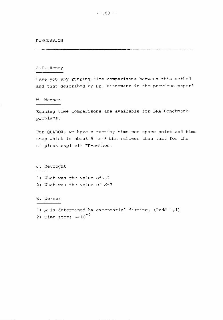
- 189 -
DISCUSSION
A.F. Henry
Have you any running time comparisons between this methodand that described by Dr. Finnemann in the previous paper?
W. Werner
Running time comparisons are available for LRA Benchmarkproblems.
For QUABOX, we have a running time per space point and timestep which is about 5 to 6 times slower than that for thesimplest explicit FD-method.
J. Devooght
1) What was the value of i~?
2) What was the value of ~?
W. Werner
1) ?t is determined by exponential fitting. (Pade 1,1)-42) Time step: ,..J 10

- 191 -
O. Norinder
THE BITNOD METHOD OF REACTOR COARSE MESH CALCULATIONS
AB Atomenergi, Studsvik, Sweden

Studsvik6AB ATOMENERGI SWEDEN - 193 -
8
The BITNOD Method of Reactor Coarse-Mesh CalculationsBy
Olav Norinder, AB Atomenergi, Studsvik, Sweden
Abstract
A new methodology is described for accurate deter-mination of flux distributions in coarse-mesh cal-culations. Principles, results of a first testphase and development status are noted.
Revised edition of a paper presented at NEACRP/CSNISpecialists' Meeting on New Developments on Three-Dimensional Kinetics, Garching, Munich, 1975-01-22--24
RF-75-70871975-02-06
AKTIEBOLAGET ATOMENERGI
1.
- 194 -
Introduction
This paper describes methods for accurate and with regardto computer effort economical calculations of reactor corepower distributions. The name BITNOD is selected as anacronym from "Buckling ITeration NODal".
The fundamental simplification in the method is that thenuclear cross sections are treated as constant in compara-tively large regions; in the following called nodes. Thissimplification is in general suitable in power reactor cal-culations, where each fuel assembly mostly is divided in asmall number of nodes.
In thermal reactor 3D calculations one often uses a fast anda thermal neutron flux group and this case is especiallytreated below.
Considerations and calculations make evident the importantfact that the neutron current between two nodes with onecommon surface fundamentally depends on the properties ofboth nodes.
Most of the ideas described have been stated in a technicalMemo [1] and particularly a later Memo [2]. In connectionwith the BITNOD development only restricted literaturesurveys have been made. At the presentation of the paperpublished ~ork [5] describing a similar approach to obtainnodal equations was pointed out [4].
2. BITNOD principles of solution
The neutron flux is described with a fast and a thermalgroup.
AKTIEBOLAGET ATOMENERGI- 195 -
In each node the general solution of the two-group equations~s used. Due to the approximation-of constant cross sections,it is possible to identify asymptotic and transient partsof the solution. The buckling of the asymptotic solution ~sclosely related to the material buckling of elementaryreactor theory.
The asymptotic buckling B2 ~s ~n the usual way split intothree parts corresponding to the Cartesian coordinates ofthe node. With self-explanatory notation one then has
In BITNOD the asymptotic buckling is treated as an an~so-tropic quantity. The necessity and convenience of thisapproach has also been recognized elsewhere [3]. The asymp-totic buckling may also have anisotropy [6].
Consider two nodes with a common boundary surface. TheaSYIllptotic and transient parts of the solutions in each nodemust combine to make fast and thermal neutron flux andcurrent continuous. The transient part must decrease nearlyexponentially away from the surface. If the components ofthe asymptotic bucklings normal to the boundary surface ar-eknovm, the flux may be represented with well-known soLlti,:T.Sfor the asymptotic parts, in the plane ~ase cos, si~" ccs~,sinh, and exponentials for the transient parts. SOlle r.odtsurfaces border reflectors. Arguments similar to the Ior-e--
going make it possible to write down the apprOpr1.lLe c:,p::c,.-sions also for this case.
T~e anisotropic distribution of the asymptotic buckling~s in general not known initialiy. Iteratl.ve met'1oa~ \,'£:;'1be used for the solution of the flux dist:;:-:...bution.Tr:eiterations will be starced with a trial distribution forboth the neutron source and the anisotropic buckling. ~n
AKTIEBOLAGET ATOMENERGI- 196 -
connection with investigations related to [5] it was found[4] that it was in many cases difficult to iterativelydetermine the buckling distributions in the nodes. Othercomments [6] also pointed to the possibility of difficultieswith the buckling iterations.
For subsets of the iterations only the average asymptoticfast flux of the nodes will be treated as variable. Betweenthese subsets the buckling distribution and the cross sectionswill be updated from current values of the leakages of thesolution, effective neutron multiplication or power - crosssection interaction.
As was realized at an early stage of the BITNOD deliberations,BITNOD will not give the true solution in the limit of smallnodes. In the ID case the true solution is obtained ~n thelimit of large nodes.
3. Detailed solution
For every internodal surface the selected general solutioncontains for each of the two nodes three coefficients, thatmultiply cos (cosh), s~n (sinh) and an exponential decreasingaway from the surface. The four boundary conditions and desiredvalues of fast asymptotic fluxes g~ve six equations thatdetermine the coefficients.
The choice of average asymptotic fast flux as retainedvari~ble is important as this quantity ~s easily identifiedfrom every surface bounding a node.
To simplify the formulation of the equations for the inter-action of all nodes two elementary solutions are found foreach internodal surface, the first with average asymptoticfluxes 1 and 0, the second with 0 and 1 about the surface.For a ~urface bordering a reflector only the solution withunit fast asymptotic flux is determined.
AKTIEBOLAGET ATOMENERGI- 197 -
The solutions are obtained through manipulation of a fewmatrices of the order two as is evident from Appendices 1and 2.
The set of elementary solutions for each internodal andnodal-reflector surface together with the two-group crosssections and diffusion coefficients make possible formulationof a neutron balance for each node with average asymptoticfast fiuxes of the node and its neighbors as unknowns.
The neutron balances contain large contributions from theasymptotic part of the solutions and smaller contributionsfrom the transient parts. Diffusion to other nodes and tothe reflector is represented by comparatively large termsin the sink sides of the balances. The source sides of thebalances include small contributions from the asymptoticfluxes of neighboring nodes. The latter contributions can becanceled by adjustment of terms in the sink sides.
4. Optional simplifications
Node-reflector interactions should be calculated with fullrepresentation of both flux groups.
For calculation of node-node interactions a formal reductionto one-group flux was attempted by collapsing the flux foreach node according to the asymptotic spectrum. This simpli-fication gave rise to large errors in the gross power distribu-tion in/systems with dimensions corresponding to half or fulllight water reactors.
In test calculations it was observed that the transients ~nthe f~st flux were small except near reflector boundaries.For that reason equations representing continuity of fastflux and fast neutron current were tested. In a representative
AKTIEBOLAGET ATOMENERGI - 198 -
\
set of 'different cases this approach approximated well thetrue two-group solutions. As one might expect, the approxima-tion deteriorated somewhat when there were control rods ~nthe system. This is probably not a serious disadvantage ofthe described simplificated method.
The advantage of the fast-flux approach is that the calcula-tion of the elements of the neutron balance matrices issimplified and that the nuclear properties of the nodes canbe described by a reduced number of parameters. The lattercircumstance is a significant advantage when interactionbetween power distribution and cross sections leads to muchupdating of cross sections. The equations of the fast-fluxapproximation are noted in Appendix 3.
5. Extension of BITNOD methods
The described principles can with some complications beextended to more than two neutron groups. Some deteriorationof the approximation will follow from the smaller modulusof the transient bucklings, which for each node will be oneless than the number of groups. The BITNOD methods can bemodified to RZ geometry and to hexagonal geometry.
6. Status of development
One-dimensional codes have been made and used for test pur-poses. Most of the essential features of BITNOD except theanisotropic buckling iteration have been tested. A code forXY geometry will be made and especially the buckling iterationinvestigated. If acceptable iterative schemes can be foundfor the buckling determination codes for RZ and probably alsoXYZ will be made.
AKTIEBOLAGET ATOMENERGI- 199 -
7. Summary of advantages with the BITNOD methods
The solution lies near the exact two-group solution.
Nodes and reflectors of arbitrary and varying sizecan be uEed.
Accurate treatment of reflectors. Calculations canbe extended to several reflector zones.
In the fast-flux simplification reduced number ofparameters for description of node nuclear properties.
Conveniently testable against experiments in bothsmaller and large systems.
Solution expandable so that details 1n nodes canbe rather well demonstrated.
References
1. Norinder, 0General theory and solution method for neutron fluxequations with arbitrary mesh sizesStudsvik Technical Memo RF-73-411, 1973-03-30(In Swedish)
2. Norinder, 0Project proposal re development of the computer codeBITNODStudsvik Technical Memo RF-74-2005, 1974-02-04/(In Swedish)
3. Weiss, ZPersonal communication at BITNODSymposium at Studsvik 1974-12-10
4. Forti, GComments at Garching Meeting, 1975-01-24
5. Rinaldini, CA nodal approach to solve few region neutron diffusionproblemsEnergia Nucleare, 17:7 p 429-435, July 1970
6. Henry, A FComments at Garching Meeting, 1975-01-24
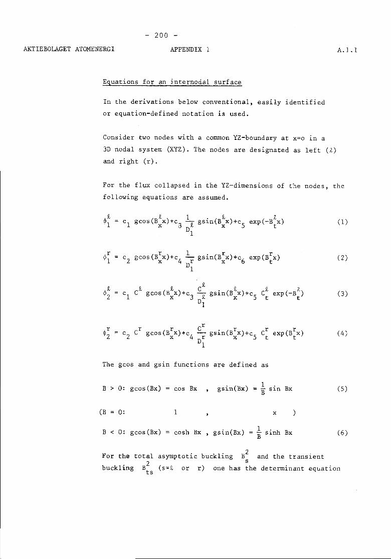
AKTIEBOLAGET ATOMENERGI- 200 -
APPENDIX 1 A.I.l
Equations for an internodal surface
In the derivations below conventional, easily identifiedor equation-defined notation is used.
Consider two nodes with a common YZ-boundary at x=o ~n a3D nodal system (XYZ). The nodes are designated as left (£)
and right (r).
For the flux collapsed in the YZ-dimensions of the nodes, thefollowing equations are assumed.
~r1
(1)
(2)
c£ ££:' gsin(B x)+cSD x1
(3)
~r r r Crgsin(B~X)+cS Cr r (4)c2 C gcos(Bxx)+c4 - exp(B x)2 Dr t t
1
The gcos and gsin functions are defined as
B > 0: gcos(Bx) cos Bx gsin(Bx) 1 Bx (5)B s~n
(B 0: 1 x )
B < 0: gcos(Bx) cosh Bx gsin(Bx) 1 sinh Bx (6), = -B
For the total asymptotic buckling B2 and the transients
buckling B2 (s=£ or r) one has the determinant equationts
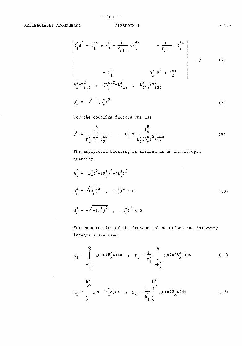
AKTIEBOLAGET ATOMENERGI- 201 -
APPENDIX 1 A. J . L
o (7)
_ ZR D~ B2+ Zas
s 22 2 (Bs)2=B2 2 2Bs=B(l) t (2) BO/B(2)
BS -1- (Bs)2t t
For the coupling factors one has
ZR ZRCS s Cs s
s BZ+Zas t D~(B~)2+z~SDZ s 2
( 8)
(9)
The asymptotic buckling ~s treated as an anisotropicquantity.
(10)
For construction of the fundamental solutions the followingintegrals are used
0 0
J£ 1 r gsin(B£x)dxgl gcos(B x)dx g3x £ J x
-h£Dl -h£x x
hr hrx x
J£
~r J gsin(Brx)dxg2 gcos(B x)dx g4x x0 1 0
( 11)
( 1~)
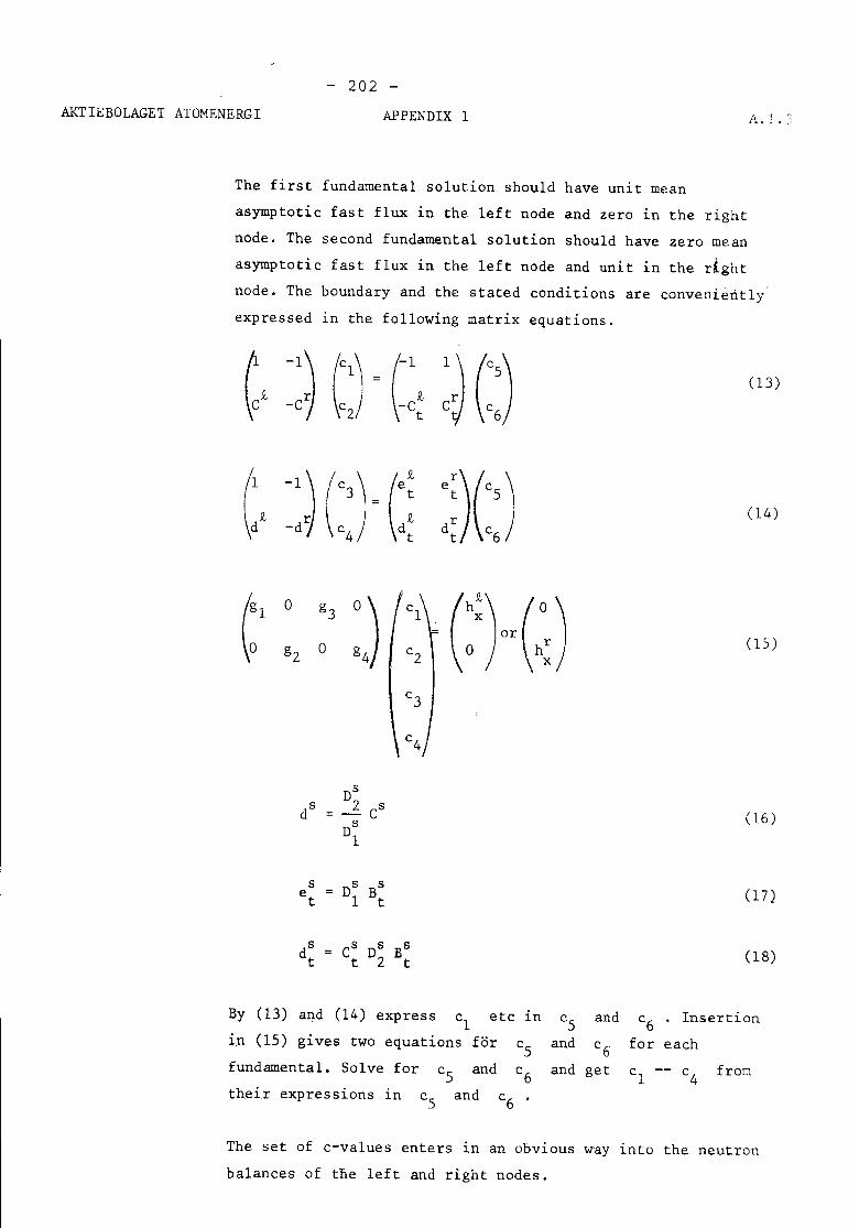
AKTIEBOLAGET ATOMENERGI- 202 -
APPENDIX 1 A.I. ~:
The first fundamental solution should have unit meanasymptotic fast flux in the left node and zero in the rightnode. The second fundamental solution should have zero meanasymptotic fast flux in the left node and unit in the rtghtnode. The boundary and the stated conditions are convenientlyexpressed in the following matrix equations.
(:' 0 g3
:4)cl - (::)or(::)
g2 0 c2
c3
c4
DS
dS 2 CSsDl
s DS BSet 1 t
dS = CS nS BSt t 2 t
(13)
(14)
(15 )
(16)
(17)
(18)
By (13) and (14) express cl etc in Cs and c6 . Insertionin (15) gives two equations for Cs and c6 for eachfundamental. Solve for Cs and c6 and get cl -- c4 fromtheir expressions in Cs and c6 .The set of c-values enters in an obvious way into the neutronbalances of the left and right nodes.
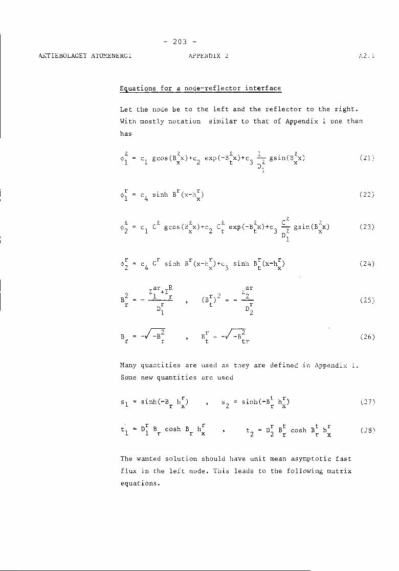
AKTIEBOLAGET ATOMENERGI- 203 -
APPENDIX L
Equations for a node-reflector interface
Let the node be to the left and the reflector to the right.With mostly notation similar to that of Appendix lone thenhas
. h Br(x_hr)c4 s~n x
B2L:ar+L:R
(Br)2L:ar
1 r 2r r t rDl D2
B -u Br -ur r t tr
(21 )
(22)
(23)
(24)
(25)
(26)
Many quantities are used as they are defined ~n Append~x 1.
Some new quantities are used
s 2 (271
Dr B cosh B hr1 r r x (28)
The wanted solution should have unit mean asymptotic fastflux in the left node. This leads to the following matrixequations.
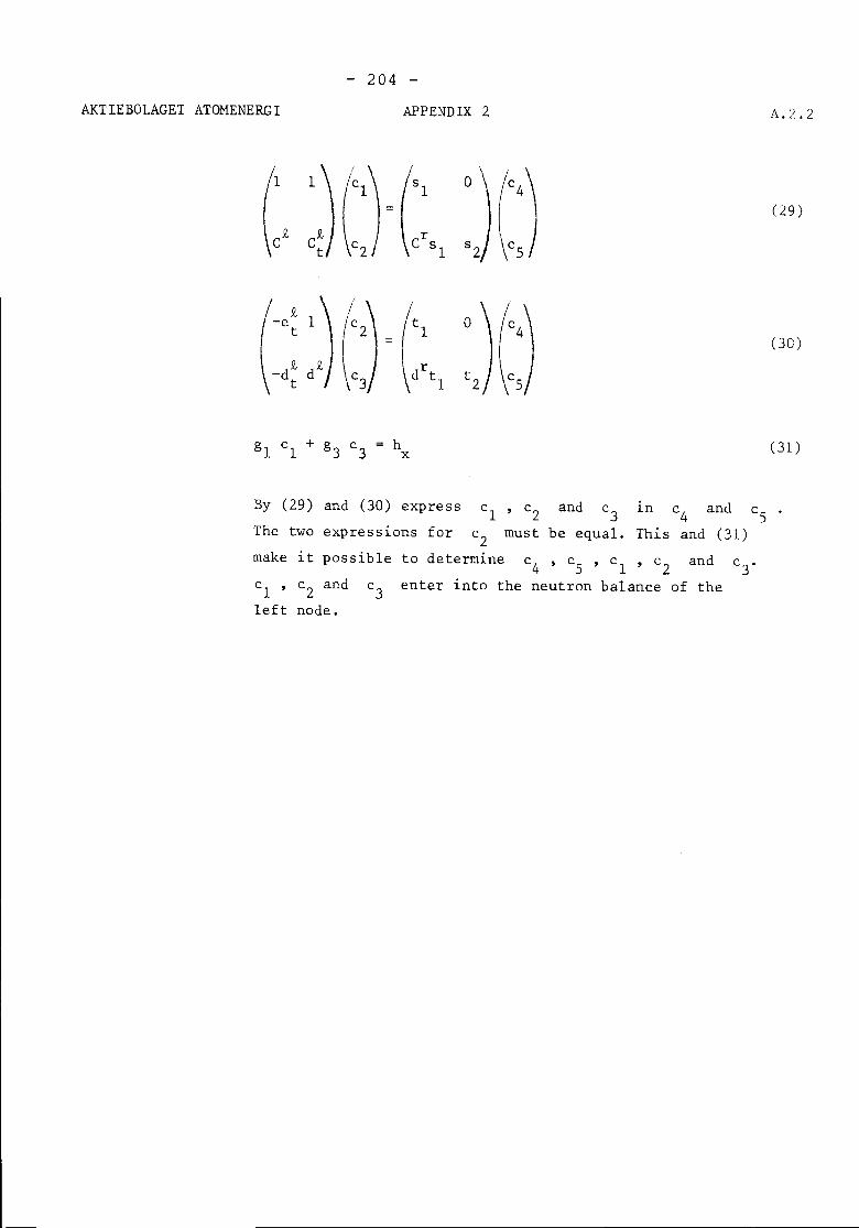
AKTIEBOLAGET ATOMENERGI- 204 -
APPENDIX 2 A.2.2
(29)
hx
(30)
(]1)
By (29) and (]O) express cl' c2 and c] ~n c4 and CsThe two expressions for c2 must be equal. This and (31)make it possible to determine c4' Cs ' cl ' c2 and c].cl ' c2 and c] enter into the neutron balance of theleft node.
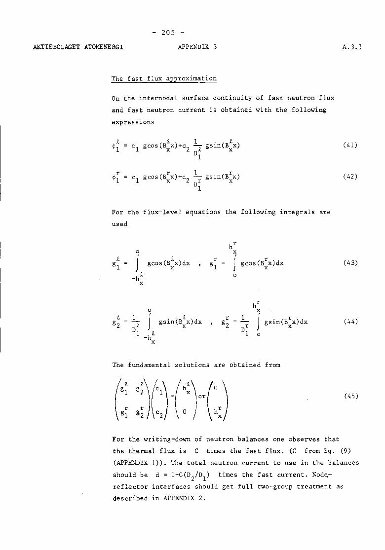
AKTIEBOLAGET ATOMENERGI- 205 -
APPENDIX 3 A.3.l
The fast flux approximation
On the internodal surface continuity of fast neutron fluxand fast neutron current is obtained with the followingexpress10ns
(41)
<pr1(42)
For the flux-level equations the following integrals areused
hr0 x
9-J
9- r f rgl gcos(B x)dx gl gcos(B x)dxx x
_h9- 0
x
hr0 x
9- 1J gsin(B9-x)dx r 1
J gsin(Brx)dxg2 - g2 -D9- x Dr x1 _h9- 1 0
x
The fundamental solutions are obtained from
(43)
(44 )
(45)
For the writing-down of neutron balances one observes thatthe thermal flux is C times the fast flux. (C from Eq. (9)(APPENDIX 1)). The total neutron current to use 1n the balancesshould be d = 1+C(D2/D1) times the fast current. Nod~-reflector interfaces should get full two-group treatment asdescribed in APPENDIX 2.

- 207 -
Session III
EVALUATION OF MULTIDIMENSIONAL CALCULATIONS
Chairman: W. Werner, Germany
A.R. Dastur, D.B. Buss
SPACE-TIME KINETICS OF CANDU SYSTEMS
Atomic Energy of Canada Limited,Missisauga, Ontario, Canada
J.K. Fletcher, M.A. Perks
THE SPATIAL KINETICS PROGRAM SPARK AND ITSAPPLICATION TO FAST REACTOR TRANSIENTS
UKAEA, Risley, Warrington, United Kingdom
G. DuboisTHE IMPORTANCE OF FLUX SHAPE CHANGES INSPACE-TIME KINETICS CALCULATIONS
Ecole Poly technique de Montreal, Quebec,Canada
209
257
287


- 209 -
A.R. Dastur, D.B. Buss
SPACE-TIME KINETICS OF CANDU SYSTEMS
Atomic Energy of Canada Limited, Missisauga, Ontario,Canada

- 211 -
ABSTRACT
Characteristics of CANDU systems which affect space dependentneutron transients have been studied. Major factors have been found tobe neutronic decoupl ing of reactor segments due to del iberate flatteningof the power distribution; retardation of the power shape transient dueto delayed neutron holdback; photoneutron production in heavy water;asymmetric insertion of reactivity devices. A full scale excursionanalysis in 3-dimensions is presented to show the degree and manner inwhich these characteristics contribute to produce the overal I spatially-dependent neutron transients when a detailed model of the system is usedin the simulation.
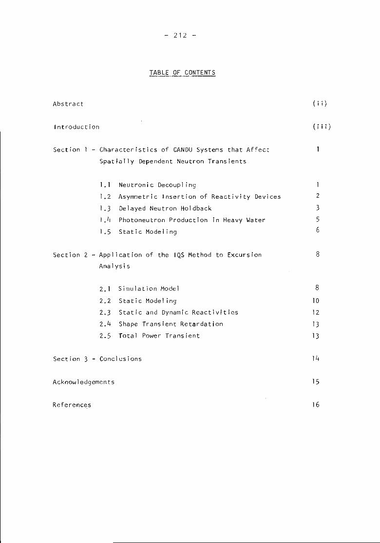
- 212 -
TABLE OF CONTENTS
Abstract
Introduct ion
Section I - Characteristics of CANDU Systems that AffectSpatially Dependent Neutron Transients
1.1 Neutronic Decoupl ing1.2 Asymmetric Insertion of Reactivity Devices1.3 Delayed Neutron Holdback1.4 Photoneutron Production in Heavy Water1.5 Static Model ing
Section 2 - Application of the IQS Method to ExcursionAnalysis
2. I Simulation Model2.2 Static Model ing2.3 Static and Dynamic Reactivities2.4 Shape Transient Retardation2.5 Total Power Transient
Section 3 - Conclusions
Acknowledgements
References
( i i )
( i i i)
1
2
356
8
8
10
12
1313
14
15
16
- 213 -
INTRODUCTION
Space dependent neutron transients in CANDU systems result froma combination of:
1. neutronic decoupl ing of reactor segments due to del iberateflattening of the power distribution,
2. significant retardation of the power shape transient dueto delayed neutron holdback, and
3. asymmetric insertion of reactivity devices.
In Section 1 of this study the above points are illustrated bytransients calculated using the Improved Quasistatic Method. The modelsused are relatively simple but are designed to exhibit the spatialcharacteristics of the CANDU system as regards neutronic decoupl ing, shutdownsystem configuration and prompt subcriticality. Wherever possible withoutlo~s of system characteristics, static flux shapes, i.e. solutions of thetime-independent equations, are used to illustrate certain points. Theuse of static flux shapes is justified when similar differences can beshown to exist between dynamic flux shapes, the latter being solutions ofthe time-dependent equations.
In Section 2, results of an excursion analysis carried out for a750 MWe system are presented. The power excursion is a result of LOC fromthe primary coolant circuit followed by tripping of the shutdown systems.These results are presented to show the degree and manner in which thecharacteristics described in Section 1 contribute to produce the overallspatially-dependent neutron transient when a detailed model of the systemis used in the simulation. A method of grouping reactivity devices withadjacent fuel channels into supercells is described. This allowssignificant reduction in problem size without loss of accuracy.
In Section 3 conclusions regarding the characteristics of CANDUsystems which affect space dependent neutron transients are summarized.
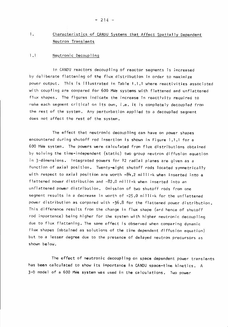
- 214 -
1. Characteristics of CANDU Systems that Affect Spatial Iv DependentNeutron Transients
1.1 Neutronic Decoupl ing
In CANDU reactors decoupling of reactor segments is increasedby deliberate flattening of the flux distribution in order to maximizepower output. This is illustrated in Table 1.1.1 where reactivities associatedwith coupling are compared for 600 MWe systems with flattened and unflattenedflux shapes. The figures indicate the increase in reactivity required tomake each segment critical on its own, i.e. it is completely decoupled fromthe rest of the system. Any perturbation applied to a decoupled segmentdoes not affect the rest of the system.
The effect that neutronic decoupling can have on power shapesencountered during shutoff rod insertion is shown in Figure 1.1.1 for a600 MWe system. The powers were calculated from flux distributions obtainedby solving the time-independent (static) two group neutron diffusion equationIn 3-dimensions. Integrated powers for 12 radial planes are given as afunction of axial position. Twenty-eight shutoff rods located symmetricallywith respect to axial position are worth -84.2 milli-k when inserted into aflattened power distribution and -82.0 milli-k when inserted into anunflattened power distribution. Omission of two shutoff rods from onesegment results in a decrease in worth of -25.0 milli-k for the unflattenedpower distribution as compared with -36.8 for the flattened power distribution.This difference results from the change in flux shape (and hence of shutoffrod importance) being higher for the system with higher neutronic decouplingdue to flux flattening. The same effect is observed when comparing dynamicflux shapes (obtained as solutions of the time dependent diffusion equation)but to a lesser degree due to the presence of delayed neutron precursors asshown below.
The effect of neutronic decoupling on space dependent power transientshas been calculated to show its importance in CANDU space-time kinetics. A3-D model of a 600 MWe system was used in the calculations. Two power
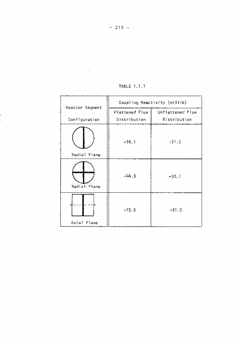
- 215 -
TABLE 1. 1. 1
Coupl ing Reactivity (m ill ik)Reactor Segment
Flattened Flux Unflattened FluxConfiguration Distribution Distribution
CD -16. 1 -21.2
Radial Plane
ED -44.3 -50.1
Radial Plane
ill -23.5 -31.5
Axial Plane
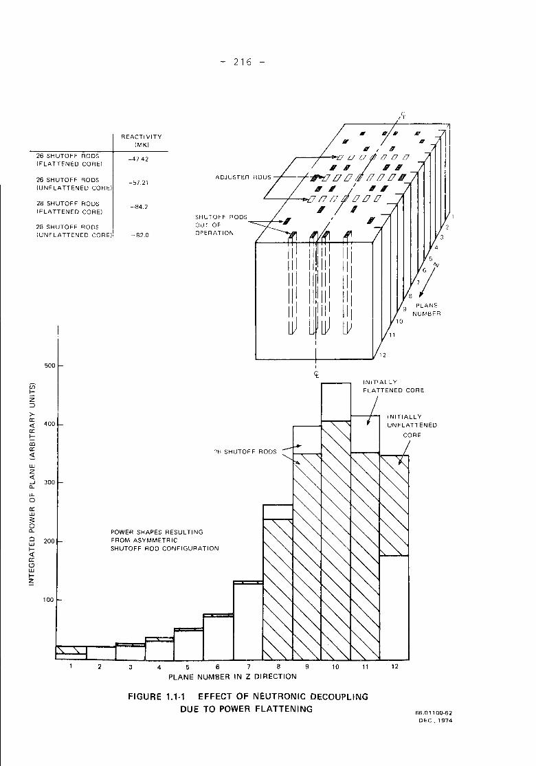
- 216 -
26 SHUTOFF RODS(FLATTENED CORE)
26 SHUTOF F RODS(UNF LATTENED COR E)
28 SHUTOFF RODS(FLATTENED CORE)
28 SHUTOF F RODSIUNFLATTENED COREl
REACTIVITY(MK)
-47.42
-57.21
-.84.2
-820
SHUTOFF RODSOUT OFOPERATION
IIIIIIIIIIIIII~
11,111III II
1111111
11'1111
1
1
~~
• , 11 D,
4
PLANENUMBER
3
2
12
500
POWER SHAPES RESULTINGFROM ASYMMETRICSHUTOFF ROD CONFIGURATION
INITIALL YFLATTENED CORE
12
INITIALLYUNFLATTENED
CORE
1110
?fi SHUTOF F RODS
4 5 6 7 8 9PLANE NUMBER IN Z DI RECTION
32
Vi"I-Z:J
>-~ 4000:I-CO0:<l:
100
UJZ<l:...J 300Cl..
LLo0:UJSoCl..
53 200I-<l:0:t:lUJI-Z
FIGURE ,.,-, EFFECT OF NEUTRONIC DECOUPLINGDUE TO POWER FLATTENING 66.01100.62
DEC., 1974
- 217 -
transients were obtained by solving the time-dependent neutron diffusionequations using the IQS method.
In model A (see Fig. 1.1.2) the flux shape was del iberatelyflattened along one direction as compared to Model B where the flux shapewas unflattened in all directions. When segmented into two halves acrossthe direction of flattened flux shape Model A exhibited a coupl ingreactivity of 7.6 mil li-k (obtained from the solution of the static diffusionequations) as compared with 14.5 mill i-k for Model B.
The reactivity transient due to loss-of-coolant and subsequentasymmetric insertion of reactivity devices was approximated by a 1inearincrease up to 0.5% in neutron yield per fission for 1 sec in both segmentsand subsequent 1 inear ramps amounting to 25% increase in absorptioncross-section over one segment for 2 secs. as illustrated in Figure 1.1.2.
Six delayed neutron groups and two energy groups were used.Delayed neutron data used is 1 isted in Fig. 1.1.2. The method used forcollapsing 33 delayed neutron precursors into six groups is discussedinSect ion 1. 3.
The total power and segment power transients are shown inFig. 1.1.2. Since negative reactivity insertion is restricted to onesegment the power transient in the unpoisoned segment is affected by theneutronic coupl ing of the segments. The energy produced in the unpoisonedsegment is ~ 50% higher in Model A which has less neutronic coupl ing thanin Model B. This difference is reflected in the total energy produced
which is ~ 20% higher in Model A than in Model B.
1.2 Asymmetric Insertion of Reactivity Devices
Shutoff rod failure is a consideration in shutdown system design.In CANDU systems. the 1 imiting case, i.e. one which dictates the final design,

2
APPLIED REACTIVITY TRANSIENT
c.oN.....
3.0
SEGMENT 1
A
SEGMENT 2
2.0 3.0
TIME (SEC)
IS
-x_ SEGMENT 1-A- SEGMENT 2----TOTAL
MODEL B
INITIALLYUNFLATTENED FLUX
~
2.0
nM' "'"
-.............~
1.0
x.... """' ......... ;x x .x 100.0
o
0.5
-20
-30
10.0
A
MODEL A
INITIALLYFLATTENED FLUX
o
.... -10
>-I-
>f=u<l:wa:-'<l:Uo-'
_x_ SEGMENT 1
-6- SEGMENT 2
- -TOTAL
•TIME (SEe)
.----x1.0
SEGMENT
!I
PHOTONEUTRONS INCLUDED
:A SEC.l fJ.0137856 .00072662.0305098 .000819557.1336881 .001041405.3155434 .002335201.225077 .0005790313.147497 .000225563
TOTAL fJ ~ .00572738
3000
0.1
x-ALi.
1000
a:w:;:oQ.
in!::z:J
>-a::«a:1-2000CDa:«
FIGURE 1.1-2 EFFECT OF NEUTRONIC DECOUPLING ON POWER PULSE66.01 100-69
DEC_.1974
- 219 -
involves failure of adjacent rods leaving an asymmetric configuration.Considering the 600 MWe system with a flattened power distribution, failureof 2 shutoff rods from a total of 28 as shown in Figure 1.2. I results in adecrease of -36.8 mil li-k in shutdown system worth. As shown in Section I. I,the effects of asymmetric reactivity perturbations are accentuated byneutronic decoup1 ing. The effects on power shape are shown in Figure 1.2.1.The power produced in the segment with unfai1ed rods is < 10% of the total,whereas symmetric insertion results in segments producing equal power. Thesame effects are observed when considering dynamic flux shapes but to alesser degree due to the presence of delayed neutron precursors (see Sections2.3 and 2.4).
1.3 Delayed Neutron Holdback
For a major part, the reactivity transients encountered in CANDUsystems are prompt sub-critical. This characteristic is the combined effectof the reactivity transient associated with loss-of-coo1ant and with shutdownsystem operation. Hence the shape of the delayed source distributionsignificantly affects the transient power shapes and reactivity.
The effect of delayed source shape is illustrated by selectedresults of a 3-D space-time kinetics calculation for a 750 MWe system usingthe IQS method. Six delayed groups and two energy groups were used. Resultsselected are at 60 sec following initiation of LaC, i.e. well after coolantvoiding and reactivity device insertion is complete. Subcritical multiplicationof the delayed source produces the power shape shown in Figure 1.3. I. Theshape of the delayed source is similar to the pre-event power shape. Itseffect on the present power shape is seen by reducing the delayed source termto an insignificant level and re-so1ving the flux shape equations. Theresulting power shape is shown in Figure 1.3.1. The resulting change inneutron importance of the reactivity devices increases the system reactivityfrom -91.8 mil li-k to -55.0 mill i-k.
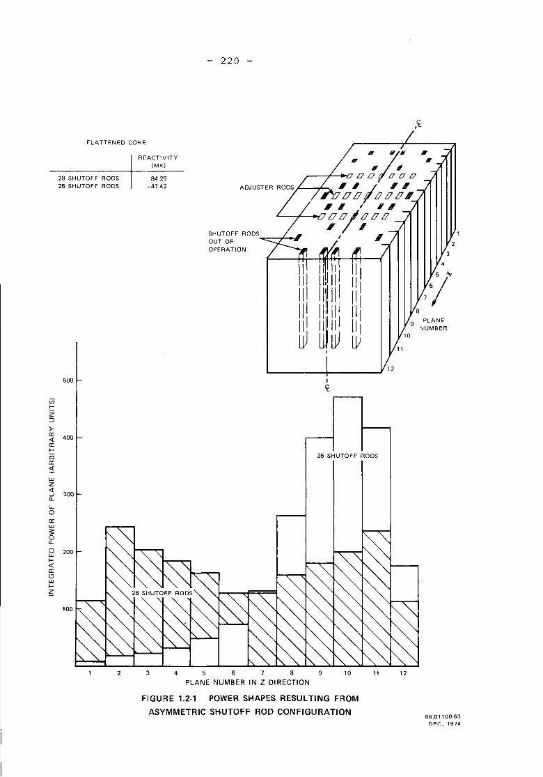
- 220 -
FLATTENED CORE
REACTIVITYIMKI
28 SHUTOFF RODS -842526 SHUTOFF RODS -47.42
SHUTOFF RODSOUT OFOPERATION
IT,
1
2
3
4:/PLANE
NUMBER
500 I
<tUlI-Z:J
>-a: 400<!a:I-en 26 SHUTOFF RODSa:~U.JZ<! 300-l0-
w..0a:U.J
~00-
0U.JI-<!OC~U.JI-~
100
2 3 4 5 6 7 8 9
PLANE NUMBER IN Z DIRECTION10 11 12
FIGURE 1.2-1 POWER SHAPES RESULTING FROM
ASYMMETRIC SHUTOFF ROD CONFIGURATION66.01100-63
DEC., 1974
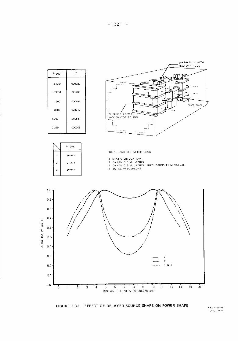
'A SEC.1 {3
.01261 .000329
.03051 .001003
.1200 .000856
.3209 .002319
1.262 .000587
3.239 .000206
221
---.-f - -~--~
r--J
r-- •.I,
.J
.,I: SUPERCELLS WITH: MODERATOR POISONl._"
[ .• Jr- - - -.. J
SUPERCELLS WITHSHUTOFF RODS
"" P Imk}
1 .55.013
2 .91.777
3 -55.017
TIME = 60.0 SEC AFTER LOCA
1 STATIC SIMULATION2 DYNAMIC SIMULATION3 DYNAMIC SIMULATION (PRECURSORS ELIMINATED)
4 TOTAL PRECUHSORS
1.0 .,,7" -::::-~"-.,,"I " k ~,
I '
0.9 / , \\ I' \'
1/ / " 4 '\,I , \\ I \ ,0.8 // /1 \\"1/ \\0.7 I I I I ' ,
(fJ ,II ' , /1 \\I- \\z I ,\ \
::J /jI I \\0.6 \ ,
/ I, "->- . \ , I \ 'a: / \ ,
,,/ I \« , '-, Ia: 0.5
, --- II-
, I\ Ico ,
a: , I, I« 0.4 , I, I
" -',.
,........ - _ ....,,'0.3 4
2
0.2 1 & 3
0.1
0.00 2 3 4 5 6 7 8 9 10 11 12 13 14 15
DISTANCE (UNITS OF 28575 ern)
FIGURE 1.3.1 EFFECT OF DELAYED SOURCE SHAPE ON POWER SHAPEG6.01100.56
DEC,1974
- 222 -
In the case of prompt super-critical transi:ents, delayed sourceshape is similar to the transient power shape due to the predominance ofprecursors formed during the transient at high power levels.
The significant effect of delayed source shape emphasizes adequaterepresentation of delayed neutron sources in the simulation model for CANDUsystems. Proper representation would involve 24 neutron precursors (six fromeach of the fissioning isotopes U235, Pu239, Pu241 and U238) and nine groupsof gamma precursors which produce photoneutrons in heavy water. These aregiven in reference (4). Various methods of collapsing the 33 groups areavailable. In order to demonstrate the effect these may have on the analysis,two methods have been used to produce data for a space-time simulation. Inmethod A, the 24 neutron precursors were collapsed into six groups. Theaverage delayed neutron fraction for each of the six groups was obtained byweighting with the fission rates for each of the four fissioning isotopesand dividing the weighted sum by the total fission rate. The average decayconstant was obtained by weighting with the delayed source produced by eachisotope and dividing the weighted sum by the total source. The nine gammaprecursors were collapsed into two groups and included by modifying groupsone and four. In method B the total decay transient of the 33 precursorswas approximated by the sum of six exponential decay terms. The coefficientsof the terms were obtained by a least square fit. The collapsed dataobtained by the two methods is 1isted in Figure 1.3.2.
The data produced by the two methods was used in the simulation ofa transient designed to accentuate spatial effects. The simulation model isdescribed in Section 1.4.
The effect on power shape following completion of the perturbationramp is shown in Figure 1.3.2. The simulation using data from method Bshows larger variations in flux shape following completion of the appliedperturbations. Method B favours the slower decaying precursors as comparedwith method A, which results in effectively larger delayed neutron holdup.After removal of the faster decaying precursors the flux shape is closer to
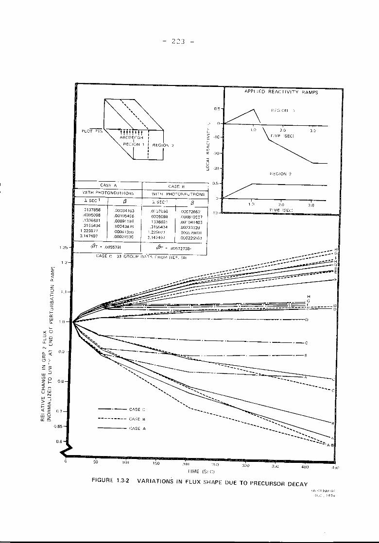
2~3
APPLIED REACTIVITY RAMPS
0.5
0
>-f-
> .10;:
2 '-'«wIX .20...J«u0 .30...J
f:EGION 2
I- 0.9CL «0:CJ >-
I-Z Zw ::J
CJ 0Z I- 0.8«I 0U w
Nw ->-'-«1-2«0: 0.7-'0i:!Z
0.65
0.6
0
3.0
400
2.0TIME (SEe)
1.n
:100
B
_-- R_----:.--- G
---- ----- F----:.:.-----------_.~.:::::..:.:::::::::.-_:.-:--_:.:::.- --- ~
--- E
------._--. -~----"'-":'----.....,c'""_-_-:. _ _ A C
------------- C
.. ~. -~-_. ----. ----. ----. -- B
----. ---- .----.-. ----. -- C
l!;O
CASE C
CASE A
H• __ G
~~~.'f::.===:=:=~=~~==:=:=:::~'.~----_:.~------;.----.r------- g---- ----_-.:.---a:----. -----.----.---- .---- .---- .----. -----0
HID
CASE C' 33 GROUP OAT.'" FfWM REF. (4)
50
0.5CASE A CAS[ B
VIITH PHOTONEUTRONS WITH PHOTONEUTRONS0A SEC.1 13 A SEC.1
!3
.0137856 .00034103 .0137856 .00012662 .llJ
.0305098 .00105496 0305098 .000819557
.1336881 .00091186 .1336881 .001041405
.3155434 .00243876 .3155434 .002335201.225077 00061309 1.225077 0005790313.147497 .00021930 3.147497 .000225563
(!3T .0055791 1/3r = 005727381
12
1.1
1.25
1.0
~2«0:z0I-«en0:::JI-0:WCL
LL
X 0::J 0-'LL Z
W
'"
FIGURE 1.3.2 VARIATIONS IN FLUX SHAPE DUE TO PRECURSOR DECAYtil, Ul lUll t\t;
DU: 1~174
- 224 -
the pre-event shape and subsequently a larger variation in shape isnecessary to reach the asymptotic shape.
For comparison, the results of the simulation usi~g the uncollapsed33 group data are also given in Fig. 1.3.2. After removal of the faster decayingprecursors, the variation in shape is negligible on the time scale shown.Fifteen percent of the photoneutrons precursors have decay constants ranging
-3 -7-ibetween 4.81 x 10 and 6.20 x 10 sec • These lie outside the rangesof the six decay constants of the collapsed groups. The retardation in fluxshape is increased when using 33 groups as both methods of col lapsingfavour the faster decaying precursors.
1.4 Photoneutron Production in Heavy Water
Approximately 17% of the delayed source in CANDU systems isdue to photoneutron production in heavy water. The effect of delayedsource on power shape and reactivity has been illustrated in Section 1.3.The contribution of photoneutrons to these effects has been calculatedto demonstrate their significance to CANDU space-time kinetics.
A 3-D model of a 600 MWe system was used in the calculations.Reactivity transient due to loss-of-coolant and subsequent asymmetricinsertion of reactivity devices was represented as discussed in section 1.1(See Figure 1.4-1 and 1.4-2).
Six delayed neutron groups and two energy groups were used.Delayed neutron data used is listed in Figure 1.4.1. Photonuetrons wereincluded by modifying data for groups 1 and 4. The changes to parametersfor groups 1 and 4 due to photoneutrons were obtained by collapsing thenine group photoneutron data given in reference (4). The methods used forcollapsing are discussed in Section 1.3. Power pulses calculated with andwithout the photoneutron source are compared in Figure 1.4.1. The peak powersin the two cases differ by 25%. Excluding photoneutrons changes the systemfrom prompt sub to prompt-super critical during the transient.
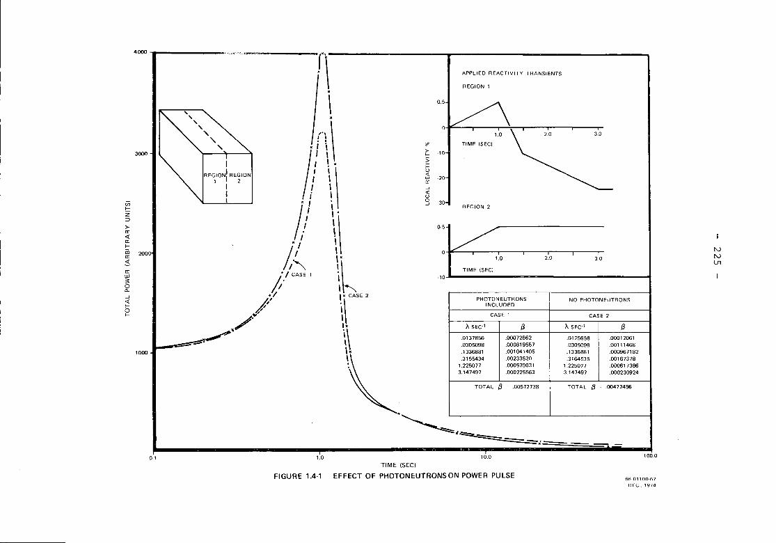
IVIVV1
{j.00012061.00111468.000967182.00167378.000617386.000230924
NO PHOTONEUTRONS
A SEC1
3.0
TOT A L {j .00472456
CASE 2
.01256580305098
.1336881
.31645351.2250773.147497
2.0
{j.00072662.000819557.001041405.00233520.000579031.000225563
TOT AL {j .00572738
1.0
PHOTONEUTRONSINCLUDED
CASE 1
TIME (SEC)
REGION 1
APPLIED REACTIVITY TRANSIENTS
A SEC-l
.0137856
.0305098
.1336881
.31554341.2250773.147497
o
-10
0.5
0
'">- .10!::>I-U<l:
-20w<I:...J<l:u
REGION 20 -30 _...J
0.5
.~.=-==- -, --
IREGION1
1
REGION1 2
III
r~. \
\,., \I I
• I
j. f i
: \.\I I! I
J. ; \" \"\. ,
i/ \//" I";/ "", il..,/ ,~
/' "CASE2
..;....~ .\,. I
_.-" \.\\I.I
1000
3000
4000
UlI-Z:::>>rr:<l:rr:I-m 200rr:~rr:w;;;0a....J«I-0I-
0.1 1.0 10.0 100.0
FIGURE '.4-'
TIME (SEe)
EFFECT OF PHOTONEUTRONSON POWER PULSE 66_0110067
DEC., 1974
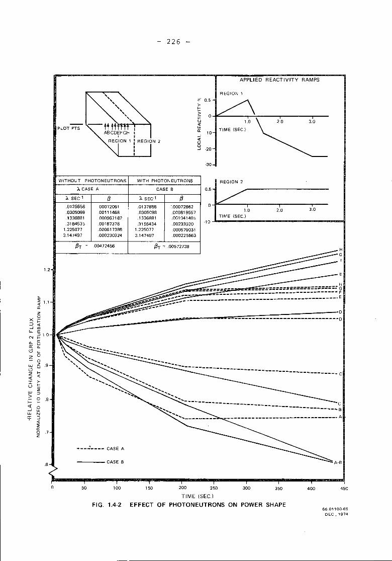
226
APPLIED REACTIVITY RAMPS
PLOT PTS
REGION 1
*' 0.5>-!::>;: 0u«wa: .10...J«Uo...J .20
.30
WITHOUT PHOTONEUTRONS
I.. CASE A
WITH PHOTONEUTRONS
CASE B
I.. SEC.1
.0125658
.0305098
.1336881
.31645351.2250773.147497
{3.00012061.00111468.000967182.00167378.000617386.000230924
I.. SEC.l
.0137856
.0305098
.1336881
.31554341.2250773.147497
{3'.00072662.000819557.001041405.00233520.000579031.000225563
REGION 2
0.5
o1.0
TIME (SEC.).10
2.0 3.0
1.2
.6
E
D--------------------------------D
H-===::::::_-_:::::::::::::::::::::::::::~E,
f3T = .00572738
CASE A
.00472456
-----CASE B
.--------
13T
.............. .._---------- .._-----------
--..---------------------------------------------C\\
"""","-........................
a..~ 1.1a:ZoX f=
::> «..J coLL a:N ~ 1.0
a.. ffia: a..19Z
Ll.
oo
lJJ iE .919Z I-<! «I >-U I-
2lJJ :;)
> 0f- I- .8<! 0..J wlJJ N
Cf ~::;;a:o .7Z
o 50 100 150 200 250 300 350 400 450
FIG. 1.4.2TIME (SEC.)
EFFECT OF PHOTONEUTRONS ON POWER SHAPE66.01100.65
DEC., 1974
- 227 -
The effect on power shape following completion of the perturbationramp is illustrated in Figure 1.4.2. The values plotted vs time foreach point is the deviation from the average of all points. The pointsare located on an axis chosen to demonstrate maximum shape change. Thecase with photoneutrons included shows larger variation in flux shapesubsequent to completion of the applied perturbations. The increase indelayed neutron source due to photoneutrons results in a shape that is closerto the pre-event shape and subsequently a larger variation in shape isnecessary to reach the asymptotic shape. On the time scale shown, the majorcontribution to this effect is from group I which has a decay constant of
-1.0138 sec •
1.5 Static Modeling
The dependence of the results on the simulation model is accentuatedby neutronic decoupl ing. In particular, larger flux gradients are encounteredin a system with higher neutronic decoupl ing which increases the number of
mesh lines required for calculation of the flux gradients to a given degreeof accuracy. In order to reduce mesh size without loss of accuracy, fuelchannels with adjacent reactivity devices are grouped into supercells. Cross-sections to be used in supercells are obtained by solution of the staticdiffusion equations using precalculated internal boundary conditions torepresent the fuel and reactivity devices. The supercell method is describedin Section 2 - 2.2. It allows significant reduction in problem size byelimination of the mesh Iines required to simulate the large flux gradientsencountered near the surface of reactivity devices.
Large flux gradients in the heavy water reflector make the resultsparticularly sensitive to the mesh structure in that vicinity. This isillustrated by comparing power shapes and reactivities obtai ned from solutionsof the static diffusion equations for two reflector models with a 600 MWesystem. In Figure 1.5.1 the integrated power of 12 radial planes is shownas a function of axial position with 26 shutoff rods inserted asymmetrical iyas discussed in Section 1. I.I. The difference in flux shape due to the removalof four mesh Iines in the radial plane accompanied with the change in therepresentation of the reflector produces significant changes in staticreactivities and power distributions.
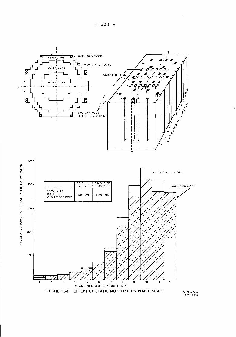
228
,8,''' JfT
1
2
3
4 ti:::
5 ,y6 ~
Qtv
8 ~9 f
10 J~11 ~~
,,-"
. "iii' 'I0041000
II /"oodooo",,1fT" , 81
R~fN~R~~~/' ~ r1l
ORIGINAL MODEL
SIMPLIFIED MODEL
~I
rt-
ORIGINAL SIMPLIFIEDMODEL MODEL
REACTIVITYWORTH OF -4 :,.05 Imkl -44.40 Imkl26 SHUT-OFF RODS
500(j)I-Z::l
>-c:<l:c: 400I-CDc:~UJZ<l:...JC>-u. 3000c:UJ
~0C>-
OUJI- 200<l:c:19UJI-Z
100
FIGURE '.5-'
8
IN Z DIRECTION
EFFECT OF STATIC MODELING ON POWER SHAPE
12
66.01100-55DEC., 1974
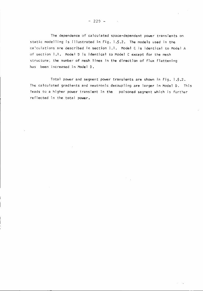
- 229 -
The dependence of calculated space-dependent power transients onstatic modelling is illustrated in Fig. 1.5.2. The models used in thecalculations are described in section 1.1. Model C is identical to Model Aof section 1.1. Model D is identical to Model C except for the meshstructure; the number of mesh 1ines in the direction of flux flatteninghas been increased in Model D.
Total power and segment power transients are shown in Fig. 1.5.2.The calculated gradients and neutronic decoupling are larger in Model D. Thisleads to a higher power transient in the poisoned segment which is furtherreflected in the total power.
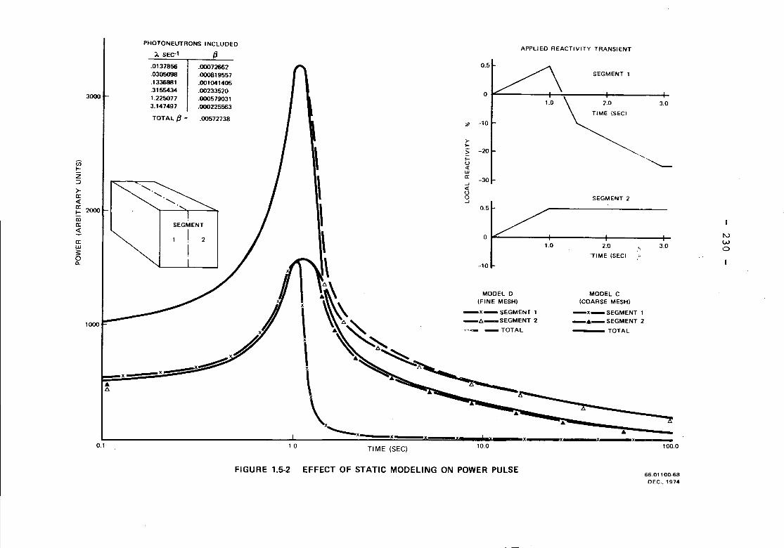
X~
"JWo
100.0
3.0
3.0~2.0
TIME (SECI
SEGMENT 2
..... "--
/';.
MOOEL C(COARSE MESH)
-X_ SEGMENT 1_._ SEGMENT 2
---- TOTAL
1.0
X, X x X, _
10.0
..
0.5
"" -10
--~.~-----~saz
o
o
APPLlEO REACTIVITY TRANSIENT
0.5
-E"'IIIIoor...- --~
>-r->r-u<{wa:...J<{Uo...J
MOOEL 0(FINE MESH)
-X-SEGMENT 1_/';._SEGMENT 2
;"~ _TOTAL
TIME (SEe)
<,.-----lX1.0
.00072662
.000819557
.001041405
.00233520
.000579031
.000225563
_X~
TOTAL fJ = .00572738
.0137856
.0305098
.1336881
.31554341.2250773.147497
PHOTONEUTRONS INCLUOEO
~ SEC-l fJI
x
•/';.
1000
0.1
3000
II:W:i=o"-
enr-z::J
>-II:<l:II:!:: 2000IIIII:<l:
FIGURE 1.5-2 EFFECT OF STATIC MODELING ON POWER PULSE66.01100-68
DEC.• 1974
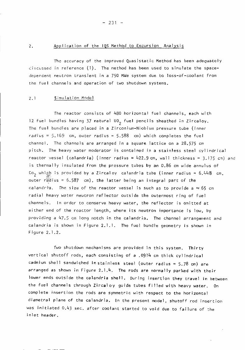
2.
- 231 -
Appl ication of the IQS Method to Excursion Analysis
The accuracy of the Improved Quasistatic Method has been adequatelydiscussed in reference (I). The method has been used to simulate the space-dependent neutron transient in a 750 MWe system due to loss-of-coolant fromthe fuel channels and operation of two shutdown systems.
2.1 Simulation Model
The reactor consists of 480 horizontal fuel channels, each with12 fuel bundles having 37 natural U02 fuel pencils sheathed in Zircaloy.The fuel bundles are placed in a Zirconium-Niobium pressure tube (innerradius = 5.169 cm, outer radius = 5.588 cm) which completes the fuelchannel. The channels are arranged in a square lattice on a 28.575 empitch. The heavy water moderator is contained in a stainless steel cyl indricalreactor vessel (calandria) (inner radius = 422.9cm, wall thickness = 3.175 cm) andis thermally insulated from the pressure tubes by an 0.86 cm wide annulus ofCO2 whi,~;r.is provided by a Zircaloy calandria tube (inner radius = 6.448 cm,outer r~Bius = 6.587 cm), the latter being an integral part of theca 1andri"a. The size of the reactor vessel is such as to prov ide a ~ 65 cmradial heavy water neutron reflector outside the outermost ring of fuelchannels. In order to conserve heavy water, the reflector is omitted ateither end of the reactor length, where its neutron importance is low, byproviding a 47.5 cm long notch in the calandria. The channel arrangement andcalandria is shown in Figure 2.1.1. The fuel bundle geometry is shown inFigure 2.1.2.
Two shutdown mechanisms are provided in this system. Thirtyvertical shutoff rods, each consisting of a .0914 cm thick cyl indricalcadmium shell sandwiched instainless steel (outer radius = 5.78 em) arearranged as shown in Figure 2.1.4. The rods are normally parked with theirlower ends outside the calandria shell. During insertion they travel in betweenthe fuel channels through Zircaloy guide tubes filled with heavy water. Oncomplete insertion the rods are symmetric with respect to the horizontaldiametral plane of the calandria. In the present model, shutoff rod insertion
was initiated 0.43 sec. after coolant started to void due to failure of theinlet header.
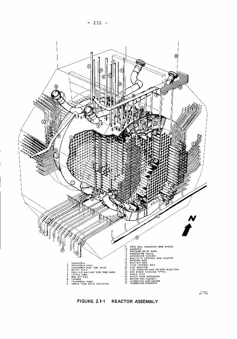
232
I CAlANDRIA Hell
2 CAlANDRIA ~IDE TUBE SHEETCAlANDRIA HEE:
3 BAFflE PLATE INE SIDE TUBE S4 FUELLING MACH5 lATTICE TUBE~ END FITTINGS8 FEEDERS f5
CAlANDRIA TU~lID SHIELDINGI~ SHIELD TANK S
~N
I. G (END SHIELDI11 STEEL BAll SHIElDIN
12 MANHOLE RElIEF PIPES13 PRESSURE R INLETS
14 MODER~igR OUTlETS 00 NOZZlES15 ~E~~~~VITY CONTROL R
:~ BOOSTER RO~
18 SHUT OF6NRT~Ol ROD
19 ~~U~E MCONITOR AND POISON INJECTION20 FLUX MONITOR OliNG PIPINGg END SHIELD CO
23 SHIELD TAN~ EXTENSION24 SHIELD TAN ASSEMBLY25 RUPTURE DISRCINlET HEADER26 MODERA TgR OVERflOW27 MODERAT
11 )1000.$U'" 1.1911
FIGURE 2.'-' REACTOR ASSEMBLY
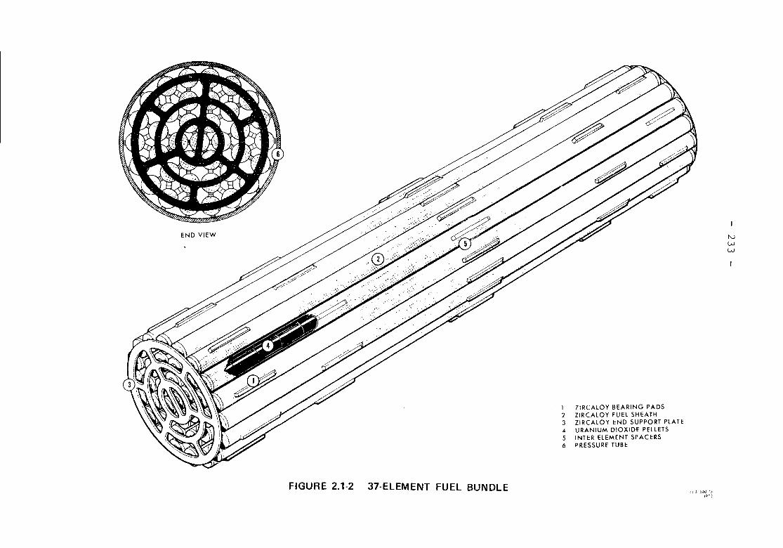
f\.)
ww
1 ZIRCALOY BEARING PADS2 ZIRCALOY FUEL SHEATH3 ZIRCALOY END SUPPORT PLATE4 URANIUM DIOXIDE PELLETS5 INTER ELEMENT SPACERS6 PRESSURE TUBE
END VIEW
FIGURE 2.1.2 37-ELEMENT FUEL BUNDLEJ . ~,)\) ':'
I""!
- 234 -
The second shutdown mechanism consists of seven horizontal injectionnozzles placed between fuel channels through which a concentrated solution ofgadol inium nitrate in heavy water is injected into the moderator at hispressure. Each nozzle is connected to a storage tank of polson and each tankis connected to a common reservoir of helium maintained at a pressure of1200 psia. The injection nozzles have four rows of 0.159 cm radii holes alongits length and each row extends over 16 lattice pitches (458 em). In thepresent model poison injection was initiated 0.53 sec. after coolant startedto void.
Two shutoff rods and one poison injection nozzle were assumedunoperational in the analysis. The locations of the omitted reactivitydevices is shown on Figure 2.1.4.
The relatively long cooling time of the U02 fuel (time constant~ .125 sec-l) compared with the time taken for reactivity device insertion
(~1.5 sec) results in, at most, a weak effect of the power transients onthe rate at which the coolant is lost from the core. The coolant voidingis, therefore, mainly a pressure driven phenomenon which allows pre-calculationof the voiding transient which is used as input to the IQS method.
The variation of the thermal neutron -cross-~-ections with fueltemperature is influenced by the presence of plutonium isotopes. The averagefuel composition in the core during nominal operating conditions is such thatthe negative reactivity coefficient of fuel temperature due to dopplerbroadening of the U238 resonances is largely compensated by the positive reactivitycoefficient of fuel temperature due to the temperature dependence of allother isotopes. In this analysis the fuel temperature changecorresponding to a 100% increase in power gave rise to a total reactivitychange of -3 milli-k. This change is considered small compared with theworth of the reactivity devices. Furthermore, the cool ing time of the fuel(time constant = .125 sec-l) is relatively long compared with the timetaken for reactivity device insertion. For these reasons temperature effectswere excluded from the model.
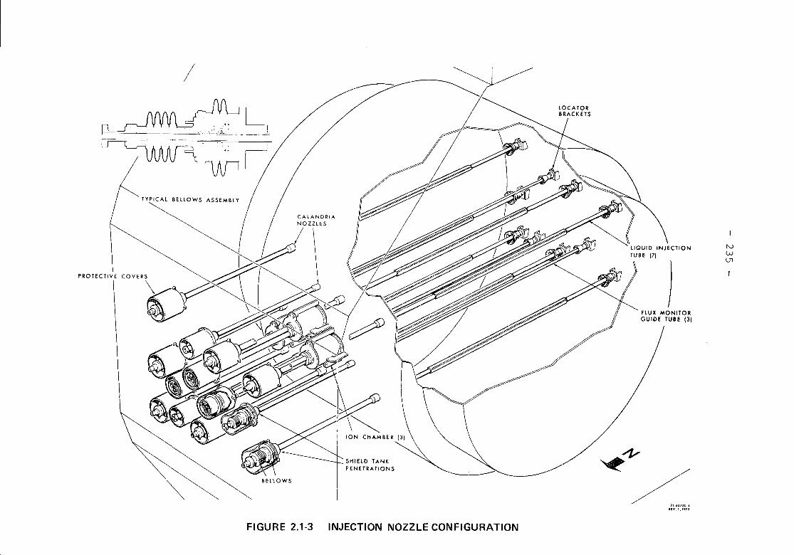
/
TYPICAL BEllOWS ASSEMBLY
PROTECTIVE COVERS
FIGURE 2.1-3 INJECTION NOZZLE CONFIGURATION
JflUX MONITORGUIDE TUBE (3)
~4'
/11,63130_.If". 1,1973
tvWlJl
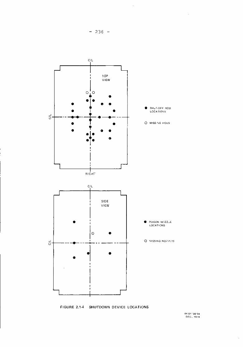
- 236 -
C/l
I TOPI
VIEW
I0.0 •- -1- • • • SHUT.OFF ROD- I - LOCATIONSI
....J --7---T .u - - ° MISSING RODS
•,
• •t.- •
RIGHT
C/l
I---+----~-- -----
SIDE
VIEW
•_ POISON NOZZLE
LOCATIONS
o MISSING NOZZLES
-••
-....J
U
FIGURE 2.1.4 SHUTDOWN DEVICE LOCATIONS
66.01100.54DEC .. 1974
- 237 -
The voiding of the coolant and movement of reactivity devices issimulated by changing various neutron cross-sections in space and time. Thecross-section changes produced by coolant voiding are calculated usingempirical lattice recipes which have been correlated with various latticemeasurements. The cross-section changes produced by reactivity devicemovement are obtained for regions termed as 'supercells' which include thefuel channels adjacent to the shutdown device. The method used in thiscalculation is outl ined beiow.
2.2 Static Modeling
As shown in Section 1.5 the mesh 1ine distribution in the simulationmodel affects the flux shape and reactivity. The number of mesh linesrequired for negl igible effect increases in regions of high flux gradients.In particular, at the shutoff rod surface mesh spacings of ~ 0.5 cm arenecessary for explicit representation of the shutoff rod in the simulationmodel. In order to reduce the size of the numerical computation to withinpractical limits the flux shape is calculated in two stages. The flux in theregion adjacent to reactivity devices including the ne~hboring fuel channelsis pre-calculated for various degrees of reactivity device insertion.
I. Internal boundary conditions are used to represent the surfaces offuel and reactivity devices. There are two options available forcalculating these. If the absorber rod is in the form of a black tubefilled with heavy water, the method of reference (2) is used. If theabsorber material is highly scattering or is grey, then the method ofreference 0) is used. In both cases the extrapolation distance forfast neutrons is obtained by assuming that neutrons thermalizedwithin the'rod are absorbed if the rod is black. Poison injectedinto the moderator is represented in the supercells by surfacesexperimentally observed in out-of-core test rigs. Resonanceabsorption in the fuel is included by modifying the fast extrapolationdistance.
- 238 -
20 A 3-D model of the superceTI is set up in rectangular geometry.The absorber rod and fuel are represented by an equivalent surfacesuch that the net current integrated over the surface is the sameas in actual geometry. Pressure, calandria and guide tubes areincluded ill the model. (See Fig. 2.2.1)
3. The thermal flux distribution within the cell is obtained bysolving the inhomogeneous 2 group diffusion equation with a fixedsource assuming that the fast flux is flat outside the absorberrod and fuel regions. The calculated extrapolation distances areused as internal boundary conditions. Reflection boundary conditionsare used on the outer surfaces of the cell.
4. From the thermal flux shape and reaction rates (including leakagerates in absorber rod and homogenized region) calculated in 3 averagesupercell cross-sections are obtained.
5. Using these cross-sections a check is made on the neutron spectrumused in 2 to obta in the cross-sect ions and extrapo 1at ion d istances. If
a large eno~9h discrepancy is found due to spectral hardening, thecross-sections are recalculated and procedures (1) to (5) repeated.
6. The average cell cross-sections are used to model the absorber rodsin the total system and a macroscopic flux distribution is obtainedby solving the time-independent neutron diffusion equations in3-dimensions.
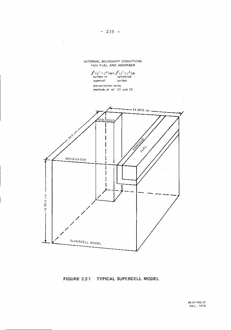
Eu
tDr--coN
""
- 239 -
INTERNAL BOUNDARY CONDITIONSFOR FUEL AND ABSORBER
f (j- - j+)ds= f(j- -j+)dssurface in cylindrical
supercell surface
pre-calculated usingmethods of ref. (2) and (3)
MODERATOR
SUPERCELL MODEL
FIGURE 2.2.' TYPICAL SUPERCELL MODEL
66.01100.53DEC., 1974
- 240 -
7. The macroscopic flux shape at the surface of the supercellsrepresenting the absorber rod IS used to check the boundarycondition used in (3) on the outer surface of the supercell. If thereflection boundary conditions are grossly incorrect, they arereplaced by the ones obtained from the macroscopic flux shape andprocedures (3) to (7) repeated.
For all shutoff rod simulations we have so far found it unnecessaryto repeat (3) with the inhomogeneous boundary conditions on the outer surfacesof the supercell.
The simulation model consisted of 26,136 regions of which 2,539 weresupercells. Two energy groups and six delayed neutron groups shown inFigure 1.3.1 were used. The six delayed neutron groups were obtained bycollapsing 33 neutron precursors, 9 of which were photoneutrons (see Section 1.3).
During reactivity device insertion the flux shape was calculated atintervals ranging from 0.1 to 0.4 secs. Relatively slow variations in fluxshape before and after reactivity device insertion allowed use of larger timeintervals in the shape calculation. In particular when the delayed source wascomprised mainly of photoneutrons time steps of 30 to 50 secs were adequate.
2.3 Static and Dynamic Reactivities
As illustrated in Section 1, the degree of neutronic decoupl ingencountered in CANDU systems accentuates the effect of the delayed neutronsource on the space-time behaviour of the system. The effect on reactivity(defined here a9 the excess neutron production over loss) is produced throughthe influence on dynamic flux shape and hence on the importance of the reactivitydevices. The system reactivity transient is shown in Figure 2.3.1. For comparisonthe static reactivity obtained by solution of the time-independent equations is
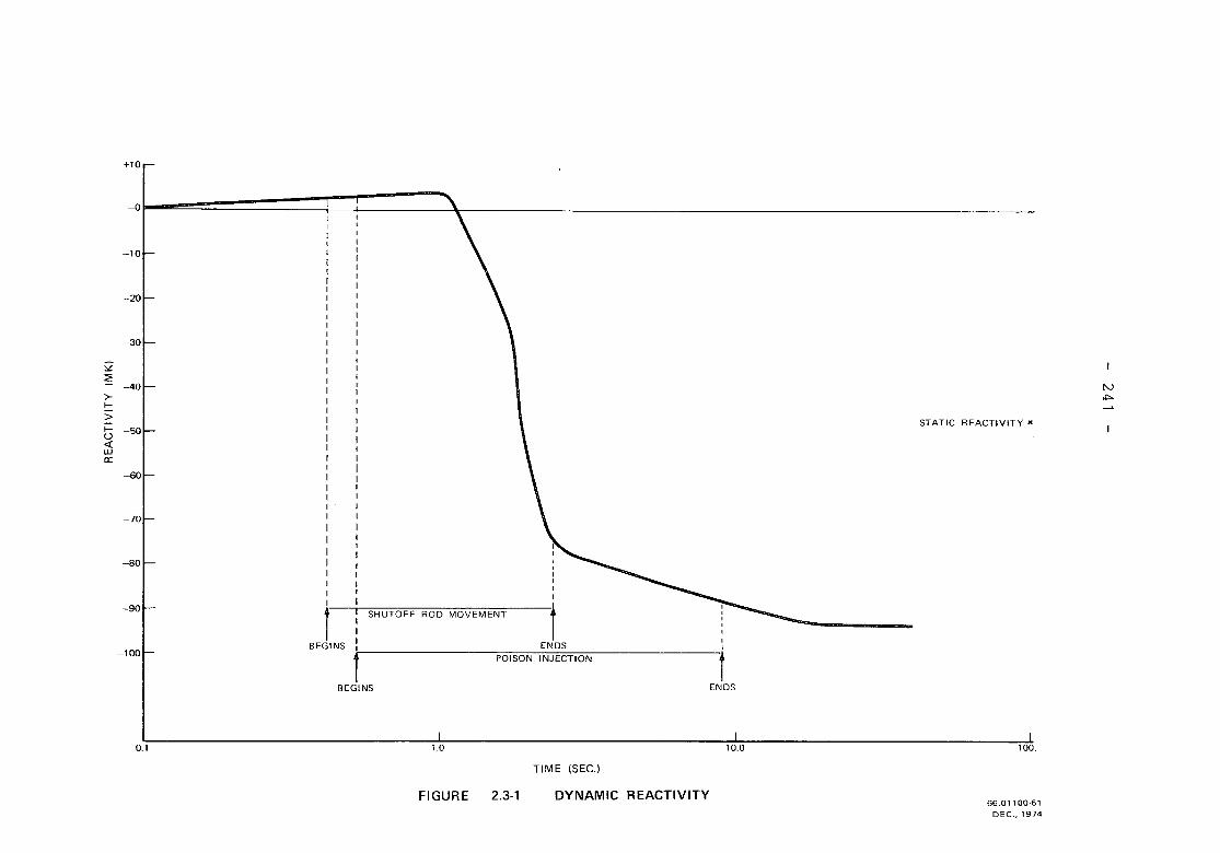
IV~
STATIC REACTIVITY x
IIII
I,
iENDS
",I,,,,I
tENDS
INJECTIONPOISON
SHUTOFF ROD MOVEMENT
BEGINS
BEGINS
+10
-0
-10
-20
-30
;;Z:?:
>-I->I-U<{wa::
-60
-70
-80
-90
-100
0.1 1.0 10.0 100.
TIME (SEC.)
FIGURE 2.3.' DYNAMIC REACTIVITY66.01100.61
DEC,,1974
- 242 -
indicated when voiding and reactivity device movement is complete. Thestatic and dynamic reactivity definitions are identical. In each case theneutron balance is taken with the balancing term of the equations excluded,i.e. the time derivatives of the flux shape and ampl itudes in the dynamiccase and the adjustment to the neutrons per fission in the static case. Asillustrated in Section 2.4 the effect of the delayed source is to retardthe change in flux shape produced by the reactivity devices which invariablyincreases their importance and reactivity worth. As precursor decayprogresses the dynamic shapes and reactivities approach their static values.The time scale of this process is determined by the slowest decaying photo-neutron precursors and is of the order of minutes.
The above results indicate that solutions of time-independentdiffusion equations are inadequate for the design of the reactivity deviceconfigurations in CANDU systems.
2.4 Shape Transient Retardation
Figures 2.4.1 to 2.4.6 show flux shapes at various times alongthree axes all passing through the reactor centre. The static flux shapes aregiven for times> 9 sec. For times greater than 9 secs the change in flux
shape is due to precursor decay alone. The approach to the asymptotic shapeand the extent to which the shape transient is retarded by the delayedneutron holdback is clearly seen.
2.5 Total Power Transient
The total power pulse is shown in Figure 2.5.1. The systemremains prompt sub-critical during the transient as seen in Figure 2.3.1.The values shown in Figure 2.5.1 are for neutron power~ Power produced byradiation from decay of fission produces predominates after 20 sec and isnot included.
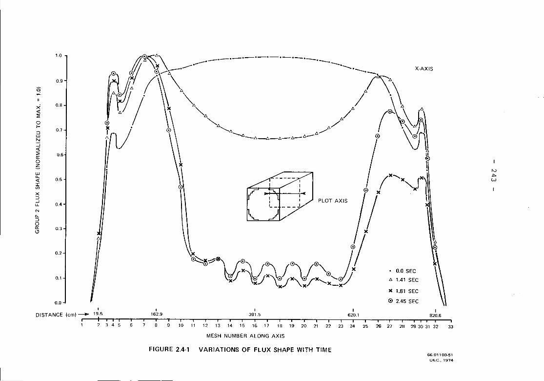
1.0 ., tr;\_.--.-~_._'_._._._._._.- ---.-- X-AXIS
I (\!)"\ I!/IV
0.9
0"11.£>.,(;)/11 :
~
-~ /- '. \~. I
0'] Ivl r\~~X~
£>.<l:
D./~0 ~\ "~D. //l- X iD
0.7 I ro,__ A _D.
UJN...J<l:~ 0.6a:0z ;
~ j IX--X"Ji\ IVUJ
"""C-0.5 W<l:
ICIl
X:::>
PLOT AXIS /...J0.4LL.
NC-:::>0a: 0.3
)((:J i/0.2 -l Ii
\~~:\ I':) /)V0"0 J. • 0.0 SEC
0.1-1 /I :,.'/\~:;\~.r,,~/"'-x'-1) D. 1.41 SEC
)( 1.81 SEC
r e 2.45 SECo.o~I I I I I
DISTANCE (em) -- 19.5 162.9 391.5 620.1 820.6I Iii i i i i i i i i i i i i i i i i i I i Iii t i i i i i i1 23456 7891011121314151617 181920212223242526272829303132 33
MESH NUMBER ALONG AXIS
FIGURE 2.4-' VARIATIONS OF FLUX SHAPE WITH TIME66.01100-51
DEC., 1974
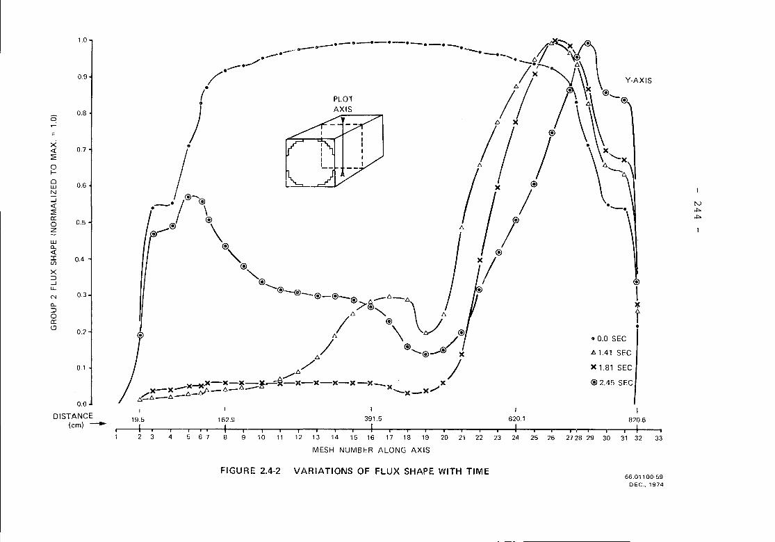
N.J::>.J::>
o
i~I
00.0 SEC
X 1.81 SEC
@2.45 SEC
'" 1.41 SEC
(
o
0_0
_0
-0
-0
-0_0_ I!~-X\'o-- 0- 1-""""':.---- • ---e... '/.-----.-- '~/7?-'"A V AXIS
o (\X @f PLOT /. A\ -co
) ~I /6/X@\\\• I , , / \~X
\ I"" d'V I " /-~ \. ;A I@" @
@,,@ j /"""-@'-@ -@-@_:/~::::6_\ 6
I @\ / @/
@ /6 '@-@ X
/6/ /-A .~-X-X-~~X-X-X-X-X-):(_ XX-X_X ".""_6_6- X X.......
/' A_6-cr-- ):(t5.-6-'-'
1.0
0.9
0.0
0.8
0.3
0.6
0.1
0.2
0.7
0.5
0.4
5
><«::2:oI-owN...J«::2:0:oZ
wa..«I(f)
><:::::>...Ju-N
a..:::::>oc:19
I
DISTANCE 19.5 162.9 391.5 620.1 820.6
(em) ----.., Iii i i i Iii i i ii' Iii i i i i i Iii i Iii i I j
1 2 3 4 5 6 7 8 9 10 11 12 13 14 15 16 17 18 19 20 21 22 23 24 25 26 2728 29 30 31 32 33
MESH NUMBER ALONG AXIS
FIGURE 2.4-2 VARIATIONS OF FLUX SHAPE WITH TIME66.01100"59
DEC., 1974
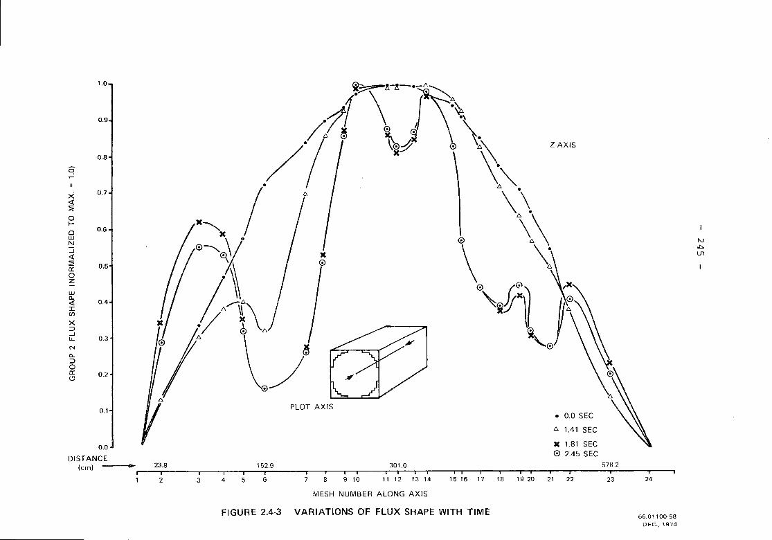
1'0oJ:>,lJl
Z-AXIS
PLOT AXIS
~ -.If\A A-.-~~~
\'0:f ~.• . X 0 "'\:\
/
6. ~
X -..... 6""-.0-----'\ · \ \
16~i I 6Y .. 0 /'"6 J, '6/ '- I,X' \,X
\~J ~ ~'0o
0.1
0.3
0.5
0.2
0.4
0.8
0.7
0.6
W0-~I(f)
X~-lLL
N
0-~oa:l'J
~
x~~oI-awN-l~~a:oz
• 0.0 SEC
/:, 1.41 SEe
0.0.1 )( 1.81 SEC
DISTANCE 0 2.45 SEC(em) .. 23.8 152.9 301.0 578.2
i i i i Iii i i i i i i i i i i i i i i i i i i
1 2 3 4 5 6 7 8 9 10 11 12 13 14 15 16 17 18 19 20 21 22 23 24
MESH NUMBER ALONG AXIS
FIGURE 2.4-3 VARIATIONS OF FLUX SHAPE WITH TIME66.01100.58
DEC., 1974
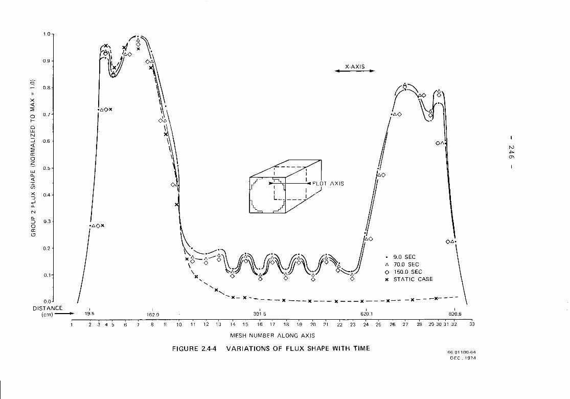
N~m
I820.6
OLI.o
o 9.0 SEC
'" 70.0 SECo 150.0 SEex STATIC CASE
''''0
I620.1
PLOT AXIS)
I
3915
f~~Oi~\ 01
-60 ~: ~l 06
X-AXIS'II ..
..... ..... x, )( _-)(-)(~----)( ---x---x---X---)(---x
o
~ J"'O\~~~i\j~\!i\j~\j~"~1Jx 0 <> <> <> <>'-
I162.9
)(~6'C6~ ~ ~ \\o~L/JlO 0
~~ OS
~~~
0"'0)( ~~
0"'0)(
I
19.5
0.5
0.7
0.8
0.6
0.2
~
0.1
1.0
0.0
DISTANCE(cmj-
0.9
wa..<!ICfl
~ 0.4...JLL
N
a..:J 0.3oa:c.9
x<!:2'oI-oWN
...J<!:2'a:oz
-----------------------~----~--I--~--~----~----~---------------1----~I--~---,-,1
1 2 3 4 5 6 7 8 9 10 11 12 13 14 15 16 17 18 19 20 21 22 23 24 25 26 27 28 293031 32 33
MESH NUMBER ALONG AXIS
FIGURE 2.4-4 VARIATIONS OF FLUX SHAPE WITH TIME66.01100.64
DEC .. 1974

IV
*""-..J
+X........
o 9.0 SEC....... 70.0 SECX 150.0 SEC+ STATIC CASE
X
x•(l'.~X.l'.Y.AXIS ,+,I , XI \ • X
,h, , \ "--...;,, , , .I \ , '+__' , II + PLOT II "" I AX'S I
:t---
A
ff,,""" ""l'. +( I / II \ i' I: II " I
l~ l'.).~\ ' "~ f~"""'X I I
0/. .\, "" /
'-~ • I.~\ .......X j f
'\ " I.......x j. I" '" I"," X I
\. "'" X I +\ " '" " "I~ "'. X j. I\ '-....-0_ '....... I /
\ '-".. ..~ .,....... X ," ~ ', . /
'+ X x. I
" ~....... X A::/ +''+",+ •.;::-.......-. ", ". -""'" I
' I' +'+'" I'+ /\ +""+--+"-+--'"
0.7
0.8
0.3
0.6
0.9
0.2
0.5
0.4
1.0
0.0
0.1
I I I I IDISTAN~I 19.5 162.9 391.5 620.1 870.6
(em) i r i i i I Iii i i I I i
1 2 3 4 5 67 8 9 10 11 12 13 14 15 16 17 18 19 20 21 22 23 24 25 26 272829 30 31 32 33
X<t:~oI-owN...J<t:~0::oZ
wCl.<t::cVl
X::>...JLL
N
Cl.::>o0::(:J
0:
MESH NUMBER ALONG AXIS
FIGURE 2.4.5 VARIATIONS OF FLUX SHAPE WITH TIME 66.01100.57DEC., 1974
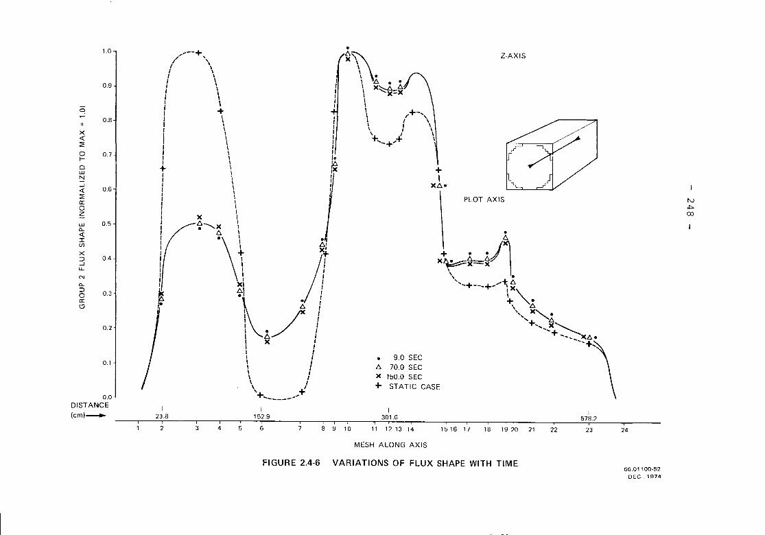
I23.8 152.9 301.0 578.2
I i I I , I I
1 2 3 4 5 6 7 8 9 10 11 12 13 14 15 16 17 18 19 20 21 22 23 24
tv~CO
Z-AXIS
PLOT AXIS
•~
.~~=/l,_+ +/~ 6.IX",+ •
\ '/::;.
" ~' .'+ '/::;.-', X ..............'+- ""-- X~.
-+~
+,X~.
• 9.0 SEC~ 70.0 SECX 150.0 SEC+ STATIC CASE
-~'\\X\\\ .\ '£, • t:,.-, )(~~-XI ....X-I
\\
\, I\ I\ ++,-+"
I.Ie,X
JIIII
,--+" ",; \
,; \I \
f \I \1 \' \, ,
\+\\I
\\\\I\+ \\\\\
\\\X I
~""""X I~\\j /f~I ,
.~I ~ f1//I II 1I. 1I ~ 1I X II 1I 1I II I\ 1' I\ I\ I
\ +'+,-----,;
0.1
1.0
0.9
0
"0.8
X<l:2:0 0.7~0wN-l<l: 0.62cr:0~w 0.50-<l::x:(f)
X:J 0.4-lU-
N
0-:J0 0.3cr:t:l
0.2
0.0DISTANCE(cm)_
MESH ALONG AXIS
FIGURE 2.4.6 VARIATIONS OF FLUX SHAPE WITH TIME66.01100-52
DEC., 1974
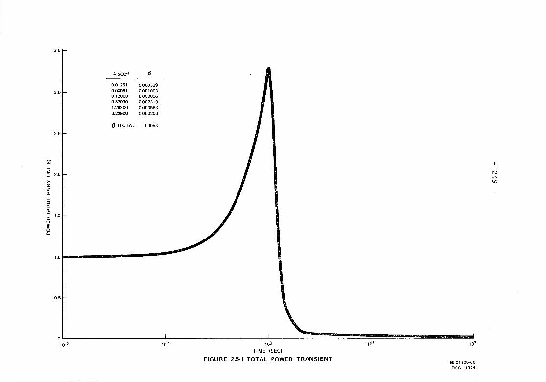
3.5
).. SEC-1 (3
3.0
0.012610.030510.120000.320901.262003.23900
0.0003290.0010030.0008560.0023190.0005830.000206
fJ (TOTAL) = 0.0053
2.5
1.0
iilI-
~ 2,Or I I IVol::>\D
a:<{a:I-ma:<{
;; 1.5w~0a.
0.5
o10-2 10-1 100
TIME (SEe)
FIGURE 2.5-1 TOTAL POWER TRANSIENT
101 102
66.01 100-60DEC .• 1974
3.
3. 1
- 250 -
Conclusions
Space dependent neutron transients in CANDU systems result from acomb inat ion of:
a) asymmetric insertion of reactivity devices,
b) neutronic decoupl ing of reactor segments produced partiallyby del iberate flattening of flux distribution,
c) increased effect of delayed source distribution due tomainly prompt sub-critical transients.
3.2 Neutronic decoupl ing accentuates the effect of asymmetric insertionof reactivity devices. As shown in Section 1.1 increased neutronicdecoupl ing due to power flattening significantly reduces thereactivity worth of shutdown devices.
3.3 Photoneutrons have a significant effect on the magnitude of thetotal power transient and on the variation of the power distributiondue to precursor decay. In some simulations when photoneutronswere included peak powers were 25% lower and flux shape variationfollowing completion of appl ied perturbations increased by 100%due to excess retardation.
3.4 Neutronic decoupl ing accentuates the effect of the delayed sourcedistribution on flux (power) distribution and reactivity. Theretardation of the flux shape during the approach to the asymptoticflux shape increases the importance and hence the worth of thereactivity devices by as I~luchas 80%. Solutions of the time-dependent diffusion equations with adequate representation ofdelayed neutron precursors are required for the design of reactivitydevice configurations.
- 251 -
ACKNOWLEDGEMENTS
Thanks are due to L. Pease, and A. A. Pasanen for helpful discussion;Special thanks are due to D. E. Meneley for detailed guidance on the improvedquasistatic method and on all aspects of space-time kinetics; to G. Kugler forproviding up-to-date delayed neutron and photoneutron data; to M. H. Guenzel,J. Howieson and T. L. Tang for model ing and input preparation for the CERBERUScode, to F. Sheldrake for typing and to the Computation Section for assistancein development and execution of the CERBERUS code.
- 252 -
REFERENCES
(1) Ott, K.O. and Meneley, D.A., l'Accuracy of the Quasistatic Treatment of
Spatial Reactor Kineticsl', Nuclear Science and Engineering: 36,402-411
(1969).
(2) Pease, L., "Tables of Neutron Transmission Probabil ities Through Purely
Absorbing Tubes", AECL-1504 (Parts I and II), April 1962.
0) Kushneriuk, S.A., "Neutron Capture by Long Cylindrical Bodies Surrounded
by Predominantly Scattering Media", AECL-462, April 1959.
(4) Keepin, G.R., 'IPhysics of Nuclear Kinetics'l, Addison-Wesley Publishing
Co. Inc., 1965.
- 253 -
DISCUSSION
A. Siebertz
I have two questions:
1) What do you mean by "neutronic decoupling of reactor seg-ments due to deliberate power flattening"?
2) What time integration methods do you use for the solu-tion of the amplitude equation, for the shape equationand for the thermohydraulic feedback equation? What isthe order of magnitude of the corresponding time steps?
A.R. Dastur
1) The coupling reactivity of a segment may be defined asthe fraction of neutrons born in the segment which resultfrom fissions produced by neutrons that were born outsidethe segment in the previous generation. Power flatteningreduces this quantity.
2) The amplitude equation is solved by expansion of the termgiving the time dependence of the flux and precursor con-centrations into matrix series.
3) The shape equation is solved using a finite differenceformulation.
4) There is no thermalhydraulic feedback included in themodel.
- 254 -
5) The size of the time step varies during the transient de-pending on the size of the shape variation. During reacti-vity device insertion, the shape is calculated approxi-mately every 0.1 sec. During precursor decay (after all"external" perturbations are complete) it can be as largeas 30 sec. The time step for the amplitude calculation isusually 1/100 of that used in the shape calculation.
G. Williams
Is there any governing philosophy which limits the cost ofa study even though the study is in support of a safety caseto the Regulatory Authority?
A.F. Henry
Machine running time is one practical limitation.
Very few computing machines will run for twenty straighthours without a fault. For an iterative procedure, such afault will require that the problem will have to begin itsconvergence process over again.
Aside from that, it seems to me some sort of cost benefitanalysis must be brought into consideration in deciding howmuch money should be spent for safety calculations.
H. Ktisters
This morning, we heard that large effort is being spent toimprove the calculational time without loss of too much ac-curacy. You have presented a full Candu-reactor representa-tion within a 3dimensional improved quasi-static method.Even without the inclusion of feedback, what is the amount
- 255 -
of time to produce the complete input (including cell cal-culation) and the amount of computing time, getting thisway a figure from which we may learn what can be gained byapproximate methods for 3d cases?
A.R. Dastur
1) To prepare the complete input, which consists of a) nor-mal lattice calculations, b) supercell calculations andc) reactor configuration in space and time, it would re-quire between 2 and 3 weeks of professional time.
2) For the problem described (25 000 mesh points, 2500 su-percells, 6 delayed neutron groups and 2 energy groups),it would require 200 sec of CP time on the CDC 6600 pershape calculation.

- 257 -
J.K. Fletcher, M.A. Perks
THE SPATIAL KINETICSPROGRM1SPARK AND ITS APPLICATION TOFAST REACTOR TRANSIENTS
UKAEA, Risley, Warrington, United Kingdom

- 259 -
The Spatial Kinetics Program SPARK and its Applicationto Fast Reactor Transients
J K FletcherM A Perks
UKAEA. Risley, Warrington. England
Introduction
This paper describes the one, two and three-dimensional fast reactor kinetics codeSPARK with space and energy dependence of the neutron flux. The solution of theequations is discussed and then a description of the neutronics, heat transfer andfeedback formulation is presented.
The program was used to calculate the two-dimensional fast reactor benchmark problem,the results of which are being presented at the conference. The program has alsobeen used to study several types of transients leading to can failure or fuel melt-ing and some typical examples are presented.
Discussion of the Method
Solutions used in other computer programs fall roughly into three groups:
a. Synthesis in which the time and space dependent behaviour is obtainedfrom a series of precalculated spacial flux distributions.
b. Splitting techniques where the flux is expressed as the product of twofactors, one time dependent only, the other called the shape function whichis space dependent with a comparatively small time variation. These areusually called quasistatic methods.
c. Methods in which the flux is derived as efHdt where H is a matrix, t thetime and approximation methods are used to evaluate the exponential.
The SPARK program was based on (b) because use could be made of existing programsand feedback could be incorporated fairly easily, also by increasing the number ofshape function calculations the exact solution of the equations can be approached.
Synthesis procedures have difficulty with temperature feedback and accuracy estimatesand some iteration and recalculation of the base functions may be necessary.
Method (c) is new and makes use of sophisticated mathematics which may prove not tobe suitable for practical problems especially if H depends on t.
Neutronics Solution
The multigroup space and time dependent diffusion equations are
1- a0::; = DVg at g
?'Vr!>
'g C1r0g + ~ L (l - Pm) ViT fmg' ~g' Xgm g'
(Tg'~ ~g'n
g = 1, NG
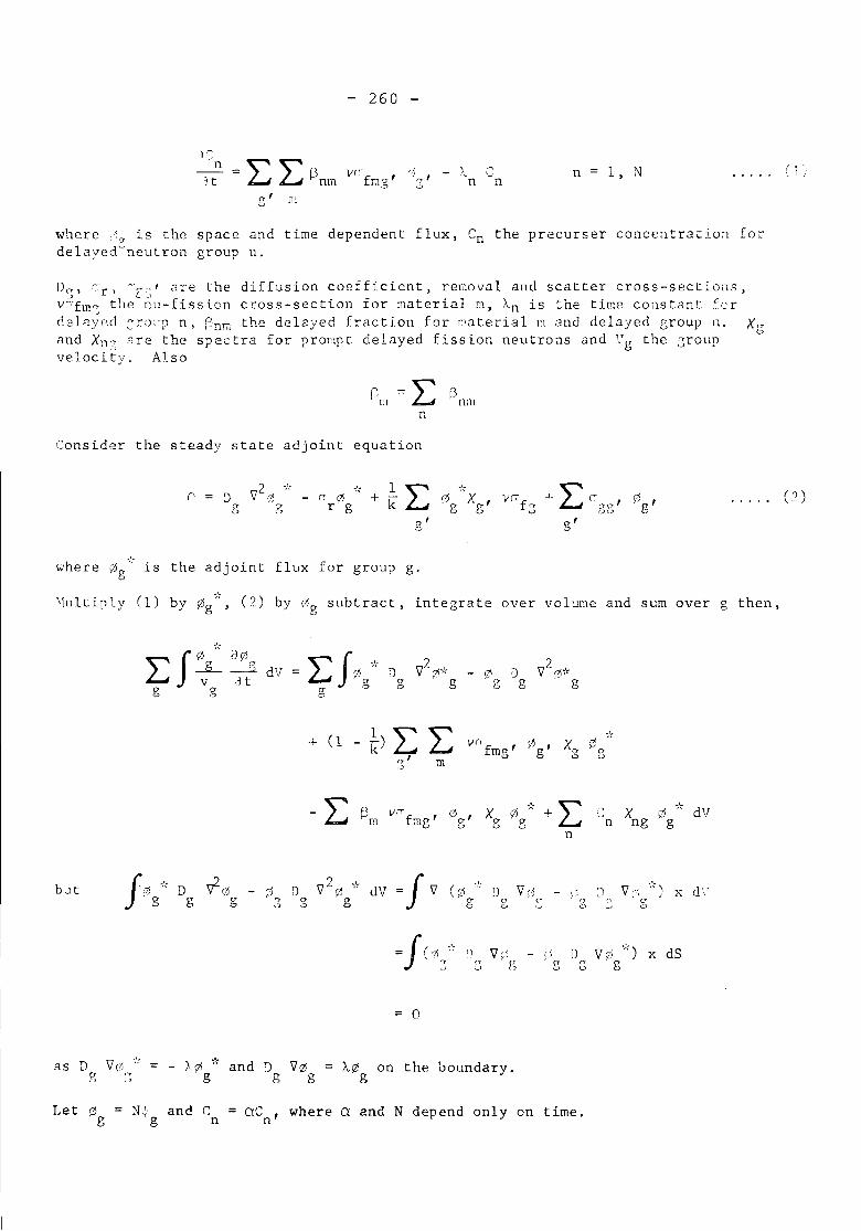
- 260 -
g' iL
Vfrfms'
:(',-,.' _ \. l-..l
,J n nn 1, N
where ry is the space and time dependent flux, Cn the precurser concentration fordelayed0neutron group n.
Do, cr' --~~, are the diffusion coefficient, removal and scatter cross-sections,vr~fma the~'~u-fissicn cross-section for material 8, An is the time constant fer22lR~pd ;ra~p n. fnm the delayed fraction for Raterial m and delayed group n. Xgand Xn~ 2re the spectra for prompt delayed fission neutrons and Vg the groupvelocity. Also
B, nmn
Consider the steady state adjoint equation
2 ,'- ...': 1 L ,'. +Lr, J 'I ,~ IT oj + k 0g X g' v"f" (;O('T'
o ,(t CY r g g0 ::, u .?< ..'0' g'CJ
..... en
where 0g~ is the adjoint flux for group g.
Hultiply (1) by 0g"', en by (~g subtract, integrate over volume and sum over g then,
L: f 0 ,', ;'].0.-iL -ll d'Jv~t
g g
(1 1)L L .,t:-+- - verf ' 0g, Xo 95k mg (t
'r' 0 '--',J m
L f3,'. +L: ;'~ dV- ll':'f ' 0g' XI" 9-\~ C Xng 95
ill mg u n gn
f~,', ;0 7 i': =f (>,~ ',', .'.D d f) '1- ~j dV 'I !,) 'Y ,0 J 'Y,' "~ d','~I/ 0 - - \ ; X, ry
"g g 0 g cr g <, 0 ~~ C'
'" '" 'J 0 '" ""
=Je0 ",', '1" "~J ':"'1
o
..., "V;<,(r
"
- dg
as D '1(1, ',',a /" rr.::-_> :.l
.'.!0g and 1) '10
g gA0 on the boundary.
g
N' and C = ac , where a and N depend only on time.-"g n n
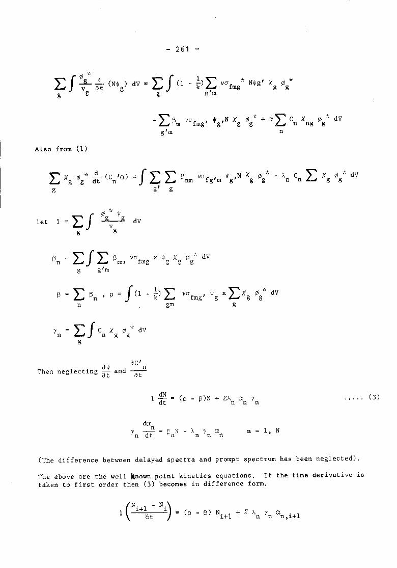
- 261 ....
,'.Lf 0!' ~~t (N1Vg) dV = L f (1 - ~)L vCYf * N\jIg'X o *mg g gg g g g'm
-L:~m VCY f ,\jI ,N X,',
+ a L: en X o ,'( dVmg g g 0g ng gg'm n
Also from (1)
L X o ,'( d (C 'a) = J L L: ~nm\If ,N X o * - Ie C 1: Xg
o of, dVvCYf 'g g dt n g m g g g n n gg g' g
"LJ o of, '.)I
let 1 = g g dVvg g
~n ~JL ~ VCY f x '.)I -'. dV= X 0nm mg a g goJ
g g'm
~ = L ~n ' P = J (1 ~)LVCYf ' \)J XLXgo ,'( dVmg g g
n gm g
LJ Cn X p ..,', dVI'n g gg
ac'(l\V d nThen neglecting at an at
1 dNdt ..... (3)
n = 1, N
(The difference between delayed spectra and prompt spectrum has been neglected).
The above are the well known point kinetics equations. If the time derivative istaken to first order then (3) becomes in difference form.
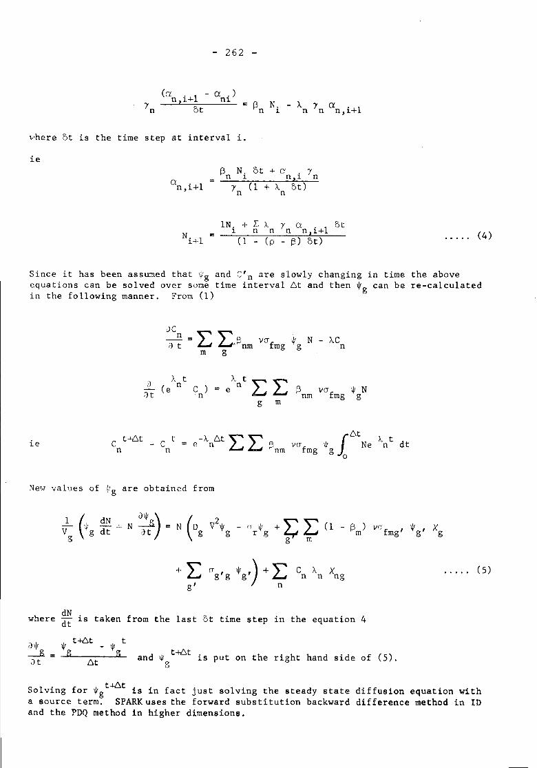
- 262 -
(('1 . 1 - a ,)n,1+ n15t = A N.I-'n 1
,.,here5t is the time step at interval i.
ie
a . 1 =n,1+~ N. 5t + a . yn 1 n,1 n
y (l + A at)n n
IN. + LAY a at1 n n n n,i+l(l - (p - ~) 5t) ..... (4)
Since it has been assumed that Wg and C'n are slowly changing in time the aboveequations can be solved over some time interval 6t and then .g can be re-calculatedin the following manner. From (1)
JC
= L: ~'~nmn
vcr f 'f N- AC--a t mg g nm g
A t A t L:L:d (e n C ) n~ W N= e vcrfat n nm mg gg m
ie C t+6tn
C tn
-- e-An6t '" '" Pnm 16t/..tLJ L.J I-' V(Jf.o Ne 'n dt
mg 0 0
New values of tg are obtained from
1.- (,jr dN _1_ N a.g) = N (D V2• - (T. + '\' '" (l - ~ ) vCTf
,., XgV g d t d t g g r g ~ LJ m mg g
g g m
h dN. k f h 1 ~ . h . 4were dt 1S ta en rom t east ot time step 1n t e equat10n
..... (5)
• t+6t _ • tg g
6t and W t~t is put on the right hand side of (5).g
t-+b.tSolving for .g is in fact just solving the steady state diffusion equation witha source term, SPARK uses the forward substitution backward difference method in IDand the PDQ method in higher dimensions.
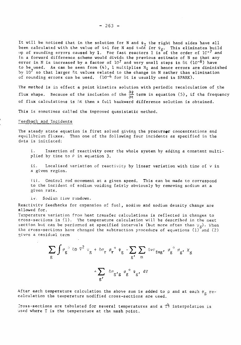
- 263 -
It will be noticed that in the solution for Nand *0 the right hand sides have all'"been calculated with the value of i+l for Nand tffit for *g. This eliminates build
up of rounding errors caused by 1. For fast reactors 1 is of the order of 10-7 andin a forward difference scheme would divide the previous estimate of N so that anyerror in N is increased by a factor of 107 and very small steps in ot (10-8) haveto be used. As can be seen from (4), 1 multiplies Ni and hence errors are diminishedby 107 so that larger ot values related to the change in N rather than eliminationof rounding errors can be used. (10-4 for ot is usually used in SPARK).
The method is in effect a point kinetics solution with periodic recalculation of theflux shape. Because of the inclusion of the a* term in equation (5), if the frequencyatof flux calculations is ot then a full backward difference solution is obtained.
This is sometimes called the improved quasistatic method.
Feedback and Incidents
The steady state equation is first solved g~v~ng the precurser concentrations andequilibrium fluxes. Then one of the following four incidents as specified in thedata is initiated:
i. Insertion of reactivity over the whole system by adding a constant multi-plied by time to P in equation 3.
ii. Localised variation of reactivity by linear variation with time of v ina given region.
iii. Control rod movement at a given speed. This can be made to correspondto the incident of sodium voiding fairly obviously by removing sodium at agiven rate.iv. Sodium flow rundown.
Reactivitv feedbacks for expansion of fuel, sodium and sodium density change areallowed for.Temperature variation from heat transfer calculations is reflected in changes tocross-sections in (1). The temperature calculation will be described in the nextsection but can be performed at specified intervals (but more often than *0)' Hhenthe cross-sections have changed the subtraction procedure of equations (l)"'and (2)gives a residual term
-LLg' m
";':
()VC1 fmg' ~g
g'
After each temperature calculation the above sum is added to p and at each ~g re-calculation the temperature modified cross-sections are used.
Cross-sections are tabulated for several temperatures and a T~ interpolation isused where T is the temperature at the mesh point.
- 264 -
Heat Transfer and Temperature Equations
For the purpose of calculating reactivity feedback ar1s1ng from temperature changes.the reactor is considered to be composed of a number of axial channels each of whichis divided into a number of discrete thermal regions.
If the flux calculation is in slab (Z) geometry then a single reactor channel isused and thermal regions correspond one-to-one with the mesh-boxes defined for theflux calculation.
If the flux calculation is in cylindrical (R) geometry then a number of axial reactorchannels overlay the radial flux-channel. and a fixed axial power profile is definedfor each reactor channel.
The equations determining the behaviour of material temperatures in each thermalregion are presented in Appendix 1. Thermal capacities and heat transfer coeffi-cients for each thermal region are defined by items of input data: the powerdistribution P(i.j) is obtained. in the slab (Z) case. directly from the fluxcalculation, or, in the cylindrical (R) case, by a synthesis of the results of theradial flux calculation together with the axial power profiles defined as inputdata.
A flow rundown disturbance may be specified which acts directly on the temperatureequations via the coolant axial heat transport term G and the can/coolant andstructure/coolant heat transfer coefficients.
Time Step Selection
It is assumed that the amplitude is the fastest changing variable followed by thetemperature and flux shape respectively. In SPARK a time step is selected for thepoint kinetics (usually 10-4) then in the data the number of time steps per tempera-ture calculation and number of temperature calculations per shape function is speci-fied (these could obviously both be 1). The selection of these is left to the userat present as there does not seem to be any time saving method of automatic adjust-ment.
SPARK is flexible in that after doing say 100 time steps between temperature calcula-tions and 20 temperature calculations between shape functions these can be alteredto 50 and 2 after a specified number of shape functions and so on.
Solution of Temperature Equations
The thermal equation for a general material i may be written as
dTidt aP + bT. 1 - cT, + dT. 1 + e1- 1 1+
where u, b. c. d and e are known and positive. In finite-difference form, this is
T,n- 1 (1 - 0) (apn+l + bT~+ll
1-cTn.+l + d x Tn+l + e)1 i+l
(a X Pn + b x n Tn n )+ e T1_l - c x i + d x Ti+l + e
where 8 is an integration parameter whose value is a matter of choice.
- 265 -
finite-difference formulation of their N
pn and pn+l are known, the finite-difference equation may be. . n+l n+l n+lrelat~onsh~p between the unknowns T. I' T. and T. l' In~- ~ ~+ n+l
e = 1 ('forward differencing'), the coefficients of T. 1 and~-is determined explicitly. More generally, if there are NT~+l
~thermal-region then the
n n nIf T. l' T., T. l'~- ~ ~+re-arranged to yield athe particular case of
n+l1. 1 are zero and~+materials in eachthermal equations yields a tri-diagonal N x N matrix whose inversion is necessaryto obtain l~+l, i = 1,2, ..... , N. Other frequent choices of e are ~ ('central
~differencing') and 0 ('backward differencing').
Forward differencing (e = 1)
a x 6t x pn + (b x 6t) T~ 1 + (1 - c6t) T~ + (d6t) Tn + e6t~- ~ i+l
Central differencing (0 ~)
+ c x ~t)T~_l -l. (1 -
(-b x ~t)T~~~.(.(1+ (b x ~t) 6t) n ( 6t) nc x ~ 1i + d x ~ Ti+l + e6t
Backward 4~fferencing (8 = 0)
(-b x 6t) n+l n= a x 6t x p + T. + e x 6t~
The apparent superiority of forward differencing ar~s~ng from its simplicity maywell be outweighed by the fact that a very small time increment 6t is necessary tosatisfy stability criteria. Moreover, central differencing, which is not thusrestricted, has a truncation error only of order (6t)3 compared to the order (6t)2of forward and backward differencing. A disadvantage of central differencing arisesfrom the extra arithmetic necessary in setting up the coefficients of the matrix.
An intermediate difference scheme, a compromise between the classical forward andbackward difference methods, is obtained by writing
n+l Tn.T. -~ ~6t
= n+l bTn+laP + i-I cT~+l + dT~ 1 + e~ ~+
yielding
Tn+l + (1 + c6t)i-In+l n na x 6t x P + T + d6t T + e6ti i+l

- 266 -
The method does not have the instability disadvantage of forward-differencing.and gains over backward-differencing in that the matrix obtained is now lower-diagonal and may be solved simply by forward substitution.
Another possibility arises from the observation that, on integrating across a time-step in which the true temperature derivative is of constant sign. the errors, whencompared to the true solution, of the forward difference solution and the backwarddifference solution are of opposite sign and similar magnitude. Thus the applica-tion of backward difference and forward difference methods in alternate time stepsresults in some cancellation of errors, yielding a solution method more accurateand faster than simple backward differencing and less liable to stability difficul-ties than forward differencing.
All five one-step difference methods (forward. central, backward. intermediate andalternate backward/forward) are available in the present version of SPARK. Thechoice of method, and the time-step employed in the one-step methods. are user-options. It is hoped that experience gained in using the program will lead toempirical rules to guide the user in his choice of solution method. A time-stepalgorithm may also be an advantage.
Programming Details and Running Times
The program is written completely in FORTRAN IV. There are no fixed dimensions sothat problem size is limited only by the amount of fast store available in thecomputer.
In order to reduce the running time. as little use as possible is made of peripheralstorage. In one and two dimensions disc storage is used for the finite differencecoefficients in the shape function calculation. In three dimensions some data trans-fers are used so that practical problems can be run. During the shape functioncalculation the adjoint, initial temperatures and point precursor values are putonto disc and read back for the amplitude calculation.
A one dimensional nine group problem takes about five minutes and ten minutes with-out and with shape functions respectively. Two dimensional problems take about 60minutes in 6 energy groups with shape function recalculation. Only a small problemin three dimensions has been done taking twenty minutes (900 mesh points threegroups).
Future Developments
Up to now SPARK has been used to predict the onset of fuel melting, can failure orcoolant boiling in a variety of transients. some examples of which are given laterin this paper. It is hoped to extend the program to deal with situations arisingafter coolant boiling and gross fuel movement have occurred. This will necessitatethe incorporation of sub routines dealing with detailed failure criteria, coolantexpulsion, fuel movement before and after clad failure and molten fuel-coolantinteraction. Typical examples of these are already available in the whole coreaccident code FRAX currently under development in the UK.
Application of SPARK Program to Fast Reactor Transients
The program has been used to study several types of transient in large fast reactorsleading to can failure or fuel melting. The results presented in this paper are forthe following incidents:

is an annular region containing absorber.fractions with absorber region situated within the innerand the absorber natural boron carbide. For the largestfraction of absorber was lower than for the other two inthe same flux depression in the steady state.
- 267 -
1. A range of localised reactivity ramp insertions in three sizes of fastreactor (by changing v) - cylindrical geometry.
2. The effect of control rod ejection (by movement of absorber) - RZ geometry.
3. The effect of channel voiding (by progressive removal of coolant) - RZgeometry.
4. The effect of multinode representation of the fuel pin for fast reactivityramps and coolant voiding - RZ geometry.
Test problems in three dimensions (XYZ geometry) have been successfully run for aflow run-down incident and a localised ramp (change of v). Some graphical resultswill be presented at the conference.
Local Ramp Insertion of Reactivity
A comparison has been made of the effect of local ramp insertion of reactivity inthree sizes of fast reactor. Details of the reactor models used, representativeof fast power reactors of 250 MW(E), 1,000 ~~(E) and 2,000 MW(E), are given inTable 1. One-dimensional (cylindrical) geometry was used and in each model there
PuThere are two zones of differing u + Puzone. The fuel is oxidereactor (type 3) theorder to produce about
Transients were induced by changing v for every fuel isotope linearly with time inthe absorber region only .. Calculations were made using an appropriate 9 energygroup condensation of the FD4 data set. For types 2 and 3 the rates of change of vwere selected to give reactivity ramps varying between 1 and 100 ~/sec. For type 1a ramp of 50 $/sec only was considered. All the transients were calculated usingboth the point kinetics and spatial kinetics options of SPARK.
Typical results for fuel temperature for a ramp rate of 50 $/sec in type 2 are shownin Fig 1. Similar results were found for type 3 but for ~ype 1 the differencesbetween point and spatial kinetics were small. The effect of the range of ramprate is shown in Figs 2 and 3 where the time for the maximum fuel temperature torise from 2,100oK (steady state) to 3,000oK (approximate melting point) is givenfor types 2 and 3. It can be seen that difference between point and spatialkinetics is largely independent of ramp rate but is much larger for reduced power.
The effect of the range of reactor sizes is shown in Fig 4 where the peak fueltemperature and power are given for a ramp of 50 S/sec. The general conclusion tobe drawn from this study is that it is difficult to induce spatial effects inreactors of the 250 MW(E) size but that they can be significant in reactors of1,000 MW(E) size and large in reactors of 2,000 MW(E) size. This conclusion refersto a comparison between spatial kinetics and point kinetics using the steady stateflux and adjoint distributions to calculate reactivity feedback. The obviousinadequacy of using point kinetics in this way when significant flux changes areanticipated can be avoided by the methods used in the next example.
Control Rod Ejection
The model used for this work was in RZ geometry with a core radius of 142 cm andheight 100 cm. The two zone fuel Pu fractions were 0.176 and 0.220. Both 3 group
- 268 -
and 9 group condensations of the FD4 data set were used and also a 3 group conden-sation of the FD5 data set.
The calculations were concerned with the ejection of a central control rod ofnatural boron carbide. Three speeds of removal were considered - 1,000 em/see,100 em/see and 10 em/sec. Calculations were made using the material movementfacility of SPARK to change 'rod in' composition to 'rod out' composition in acentral 7.6 em radius region. For a power of approximately 3,000 MW(H) the maximumfuel temperature in the steady state (rod in) was l,7000K occurring in the outercore zone.
Steady state and kinetics calculations of the reactivity change due to control rodmovement at 100 em/see in 3 groups and in 9 groups showed little difference so sub-sequent calculations were restricted to 3 groups. Steady state calculations gavethe \vorth of the central control rod as 0.50% or 1.6 S.
Kinetics calculations were made using SPARK in both the point mode (no flux shaperecalculations) and the spatial mode (usually employing about 10 flux shape re-calculations). Typical results (for rod speed of 100 em/see) for the reactivityand maximum fuel temperature are shown in Figs 5 and 6. Significant differencesare seen to exist between the two modes of calculation.
The '12~_nreason for these differences was assumed to be that in the point modeSPARK uses the steady state (rod in) flux and adjoint to calculate reactivitychanges. To test this the reactivity change between different steady state situa-tions as the rod \Vas withdrawn was calculated using three methods with the program~IAP~ :
a. direct k effective calculations
b. first order perturbation theory
c. exact perturbation theory for rod out (using adjoint flux with rod out).
The results are given in Fig 7 and show the same sort of difference between methods(a) and (b) as between point and spatial modes (Fig 5 - until significant Dopplerfeedback occurs).
The test was taken a stage further by setting up a point kinetics case with theprogram FUTURE-2 using the steady state keff curve of Fig 7 as a reactivity varia-tion for a rod speed of 100 em/sec. The Doppler constant, effective delayed frac-tion and prompt reaction lifetime used were obtained from 3 group MARC calculationfor the rod in condition. The resulting transient reactivity and fuel temperatureare shown in Figs 5 and 6. These are seen to agree well with the SPARK spatialkinetics calculations.
Results for rod speeds of 1,000 em/see and 10 em/see showed similar trends to thosefor 100 em/see, ie the fuel temperature rise calculated using the point mode wasabout half that using the spatial mode, but the use of FUTURE-2 with direct keffreactivity data gave results within 1000e of the spatial mode ones.
For the rod speed of 100 em/see calculations were also made at 10/0power and flow.Results obtained using the above (improved point kinetics) method were in pooreragreement with the SPARK spatial mode one. For this transient can failure (aboutl,2000K) occurs at about 2 see (well before fuel melting). Although the time toreach this failure criterion was within 0.3 see for the spatial kinetics and the
- 269 -
improved point kinetics methods, the temperature distributions were different.The variation of can temperature with radius at 2 see is shown in Fig 8, fromwhich it can be seen that most of the channels in the inner core are within 70Kof failure when this occurs in the outer core, whereas in the improved pointkinetics case these channels are 200K to 600K below failure.
Coolant Voiding
Calculations have been made of the effect of progressive loss of coolant in aradial channel in RZ geometry. The reactor model used was type 2 of table 1 (with-out absorber region) with a core height of 100 cm and axial blanket thickness of45 em. The boundary between 'sodium in' and 'sodium' regions moves linearly withtime starting from a specified height. When the boundary is between two meshpoints an arithmetic average of composition is used in that mesh box. A 9 groupcondensation of FD4 data was used with appropriate spectra for the voided andunvoided volumes.
Two cases were considered in which central regions of the core were voided at1,000 cm/sec from the bottom of the core. In the first case the radius of theregion was 42.5 cm (one eighth of the core) and in the second case the radius was85 cm (one half of the core - all the inner zone).
The resulting reactivity variations gave maximum rates of reactivity addition of32 S/sec and 61 S/sec for the two cases. The difference between point and spatialkinetics was small. The variation of peak fuel temperature is shown in Figs 9 and10 which show temperature differences between point and spatial kinetics of up to2000K for the first case and up to 1,000oK for the second case.
In an accident code context where the progress of voiding cannot easily be pre-determined the method of improving point kinetics used before is more difficult toapply and the effects found may be significant.
Multinode Representation of the Fuel Pin
In all the foregoing three studies the fuel pin was represented by a single meantemperature only. The effect of using several nodes in the pin has been consideredfor a reactivity ramp insertion of 100 S/sec and for a case of coolant voiding.For this work the model described previously for the control rod ejection studywas used.
For a uniform fast ramp of 100 S/sec cases with 1, 3 and 10 nodes in the fuel pinwere considered. It was found that there was negligible difference in the meanfuel temperature (across the pin) throughout the transient. However the peak fueltemperature, shown in Fig 11, reveals considerable difference between land 3 nodesbut little between 3 and 10 nodes. The effect of the latent heat of melting at3,040oC is clear.
Next a non-uniform rmnp equivalent to 100 S/sec was applied over an annular regionbetween radii 8 cm and 29 em by changing v. The cases were restricted to 1 and 3nodes and the results for fuel temperature are shown in Fig 12. It can be seenthat the error in using 1 node compared to 3 nodes is of similar magnitude to thatin using point kinetics compared to spatial kinetics.
The case of coolant voiding considered with multinode pin representation was theprogressive removal of coolant from the whole of the inner core zone at 1,000 cmlsecstarting at the bottom of the core. Fuel melting was found to start after about40 msec and in Fig 13 is shown the fraction of cross-sectional area molten in the

- 270 -
hottest pin. Cases with no flux recalculation (point kinetics) were run with 1,3 and 10 nodes and show a difference mainly between 1 and 3 nodes. Cases with 5flux recalculations (up to a molten fraction of unity) were run with 1 and 3 nodesonly.
In this case it can be seen that the error in using 1 node compared to 3 is of lesssignificance to that in using point kinetics.
Conclusions
The improved quasistatic method as used in SPARK has proved to be very suitable fordevelopment and programming into a one, two and three-dimensional spatial kineticssystem for fast reactor transients.
No difficulties in running the prograrrlhave been experienced over a wide range oftransients. There are no restrictions on number of mesh points or energy groupsother than those imposed by the size of computer store available. Running timesare reasonable considering the early stage of development.
The transients considered have shown that spatial effects will be significant inthe larger commercial fast reactors currently under consideration. Although animproved point kinetics scheme in which the reactivity input is pre-calculated canbe used to obtain accurate results for power level, it has also been shown thatdetailed temperature distributions can not be well calculated without a spatialkinetics capability.
The inclusion of SPARK into a whole core accident code is regarded as important inorder to be able to cope with the unpredictable reactivity and flux shape changeswhich are associated with events such as coolant voiding and fuel motion whichoccur under whole core accident conditions.
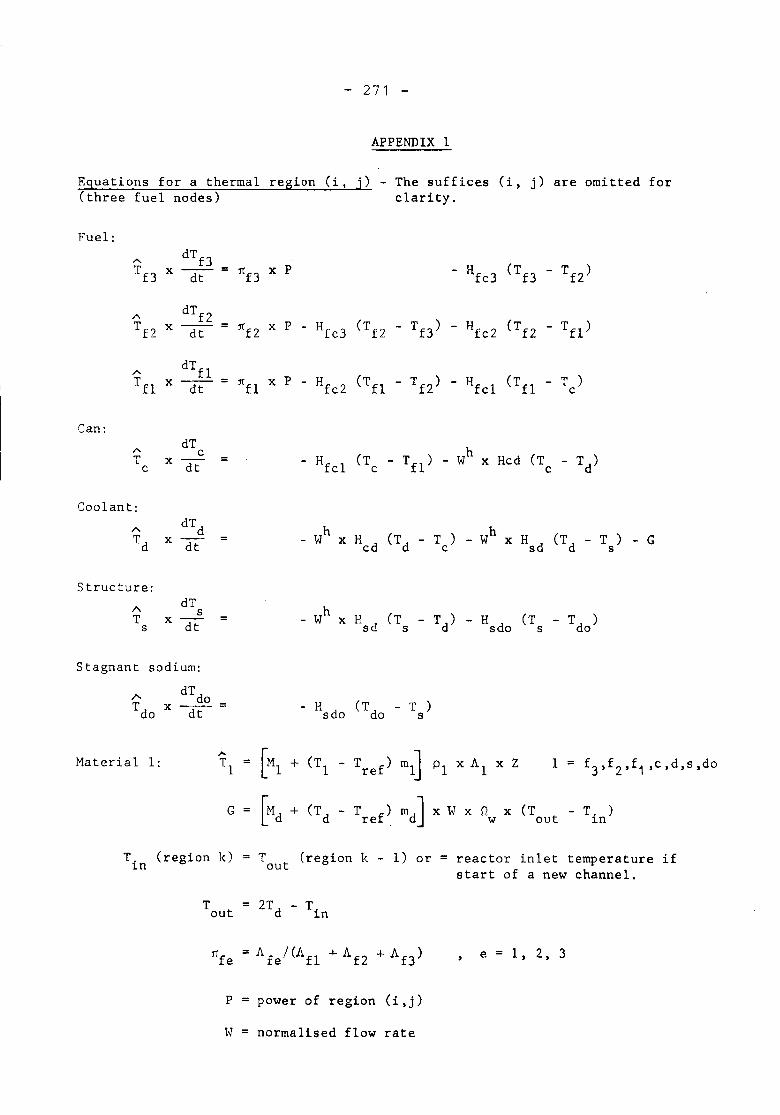
- 271 -
APPENDIX 1
Equations for a thermal region (i, j)(three fuel nodes)
Fuel:
The suffices (i. j) are omitted forclarity.
'"dTf2 (Tf2 - Tn) (Tf2Tf2 x dt rrf2 x P - Hfc3 - Hfc2 - Tn)
'"dTn
(Tn - Tf2) (Tn )T£1 x = 1ln x P - Hfc2 - Hfel - Tdt c
Can:dT h'" cT x = - Hfel (T - Tn) - W x Hcd (T - T )c dt c c d
Coolant:A dTd h hTd x dt - W x Hcd (Td - Tc) - W x Hsd (Td - Ts) - G
Structure:
'"dT hsT x = - W x Hsd (T - T ) - H (T - T )s dt 5 d sdo s do
Stagnant sodium:/'. dT doTdo x dt - H (T
d- T )sdo 0 s
Material 1:
G T. )~n
T.~n(region k) T (region k - 1) or =out reactor inlet temperature if
start of a new channel.
P = power of region (i,j)
W = normalised flow rate
e 1, 2. 3
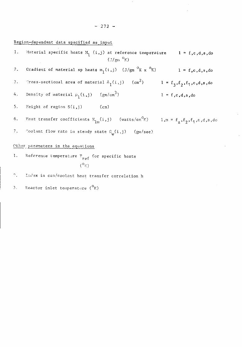
- 272 -
Region-dependant data specified as input
1.
2.
l'!aterialspecific heats HI (i ,j) at reference temperature(J/gm oK)
Gradient of material sp heats ml (i,j) (J/gm OK x OK)
I = f,c,d,s,do
I = f,c,d,s,do
3. ~ross-sectional area of material AI(i,j)
4.
5.
Density of material PI(i,j)
Height of region S(i,j)
3(gm/cm )
(em)
I f,c,d,s,do
6. Heat transfer coefficients HI (i,j)III
°(watts/em K) l,m
7. ~oolant flow rate in steady state D (i,j)\v
(gm/sec)
Other parameters in the equations
1. Reference temperature T for specific heatsref(on
~ Index in can/coolant heat transfer correlation h
J. Reactor inlet temperatdre (oK)
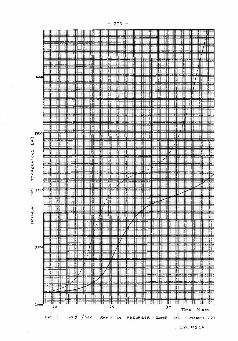
3600r'XV
.J +,-,III ,300:JU.
)(
<1:
-+
;4600
20
1- 50 ~ / SEe
273
IN
30
Z.ONE OF"
... It ..t""'". _i-t_.t ~
+++
MODE l- (~)
_ C Yl-INO ER
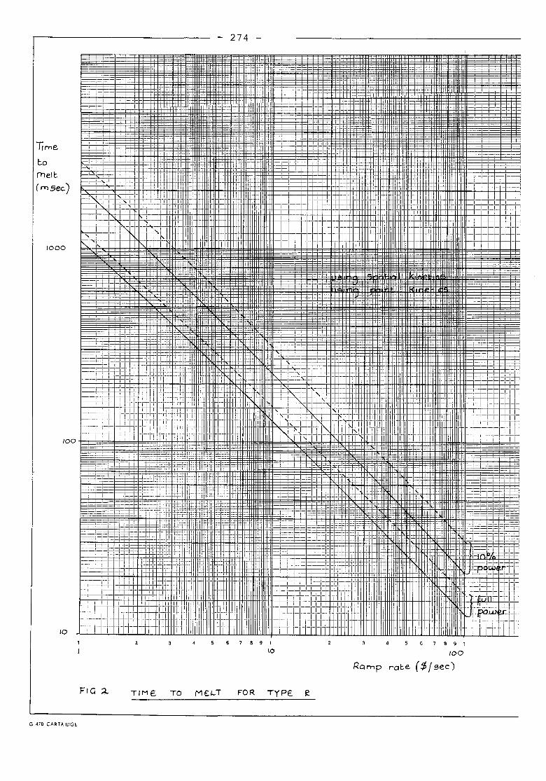
- 274 -
.__ .. '~t-
=1" .+;=
.. 1
, i
-rr
::r-:- -....-I~
: r
",:f.:\1: P
~fti=====r~81
__ .n:<-:r- . ~__. !
--1 _:j:
-. :
==--::-t-'--
=
If ~: .::f' ltmm-L-,rmEEl'll ' : II n ';
~ . . ~3=litl:illlIl.lJ1]. Iii-l--l.: • ~ ~.:. m'~~.Pi:j::tlr, .. tt E::-
, T .--:-, I i1 • 1. Hnl.i.1....1 I :~ I ~~ 1_ -1-' •;-.-+H-1 It' H t' - L ";'. .'. '11i.. f , ' : ;"':;--+-, i
. I I -f : -i+ TIttp~h-t- .. j ,f-~: I I: I : l-t+tH-l-ilFi- .. 1 I -, ::1~ II : I F
• , I , J+t+I--W-1-j. -l-!-I.HI.j-'. . __ -- '.1 I-f---j: " : : =i ~ I : lftf+ -H'H.ILri'1'I . I I nT Ti----Itri.~i.lr J -. ~+ -~~ iTI", -1+ti-111trr --. T -- I II~+ \: I~ 1- I-H'I--l .. f : i-H---' - ---
I--,---;-fF -- r- -lit ,. .. -I -I !I ----~I.; : r : T hh.-f I III IiIT -~-----.~I :,1 I I I .1 I-Tr1"f T -- IITT
1000
"Time1::.0melt::.("""sec)
100
10
~.:
=;=
5 6 7 8 9 1
105 6 7 8 9 1
100
~arnp rate ($jsec)
TIME. TO M~l-.T
G 470 CARTRIDGE
:t: ~:.
- 275 -
......,. -.
: ..~,r. ..1 -c-
:mf1_.1
lime 1:0
Meltrnlsee.
~=E-;-,-
r-:i=t= ~-=1-1.,::
...q.....1
.. _-- -:.
_.t,--T.
Ii1
t--
;,,t --- - _.:q. +.
-
"'1'"-;4
-
=R:'" :: +H-+T ++++
I I I, I
, I
II I '"i
i I I
I II I
I i II I II I i
.111, I II
I
I I
, ,,I.', I
I II I I II I,
~I
T,I
- - If-
r II -rHt 11
T-
1 I- - - - j:+-1 -- -:-r.:11
H-t-,
III I
I
I 11 1
I II I I! I II I I
,, ,,I
II
I
'1 !
f
~H{f,:. !r,-IT
1- iiij~I t
t .,
-=:
10
100
1000
7 8 9 1
10
4 7 8 9 1
100
Romp rote (1' see.)
FIG ..3 TIME. TO ME.I-.T FoR TYPE 3
G 470 CARTRIDGE
3000
i2i200
.500
k-DO
300
i200o 1000
- 276 -
~ooo
- 277 -
r-Eu~
r0u
0 't"0
f0
.IJA
::1:8E -......:
Ee 0u..
0u 0uca ....AI1ft «0
Q0tt..10«~z0u
UlIa::...zCI'U
<:JZ-t-u...h..0t-
W~Q
>-...->-I-Ua:\AIa::
U)
IJ'
U.
0
278
_¥.0
!.e... 00
0 c 0
u. .. ~ 0 0 0
E B nI10 @ .9~
:)0E ~- a..a ~
~.JJ
Eooo
...([
o~
..IoIt...Zou
w~t-1.CaJu
Ii.o
2o...uU).,'l>
u..
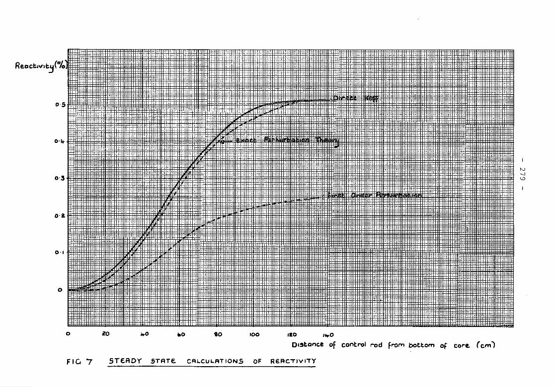
Reactivi tj(8/0
0.2
o
o lO ...0 610
.':It
10
'~.r
100 ,ao ,...0D'5l:.ance Of control rod From bott.om of cO"~ ( ern)
tv--J~
FIG 7 STEADY STATE. CAL.CUL.ATIONS of R£RCTIVI"TY
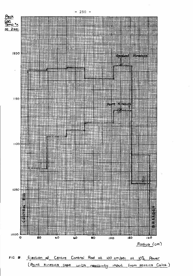
- 280 -
r~oo
1150
1100
1050
1000o 80 100 liO Iit-O
RadlU~ (em J
FIG 8 _Ejectton of Centre Control Rod at:. 100 cm/..sec. at 10% fbwe,r
(Point K,net.lcs case. wlt.h ,..egCCIVIt.~~pUt. From Sl:.at:.lC3 Coles.)
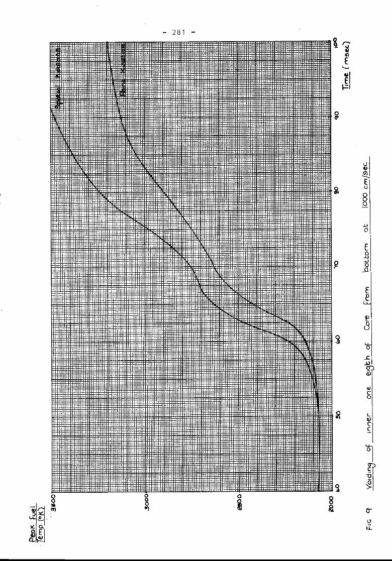
- 281 -
JI
~I-..........:El.J
.uo
Eo-U.oJo..a
Ee
aICo
<-IIICC
cr
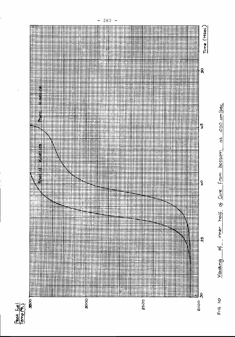
ooo
.Da
EeLL..:
LQJCC
ocru.
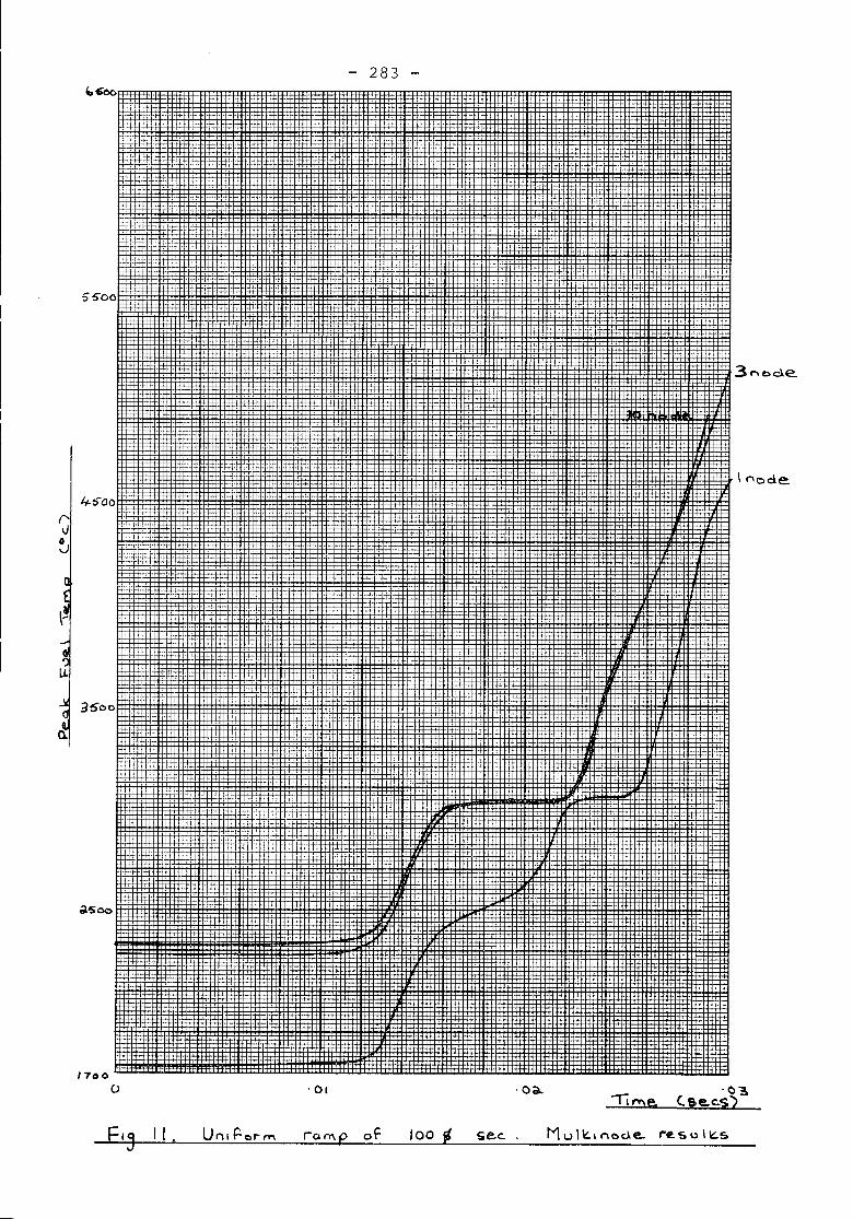
:.'i.
..1..+:
3500
1700o
Lt
- 283 -
lnode
100 l' se.e. .
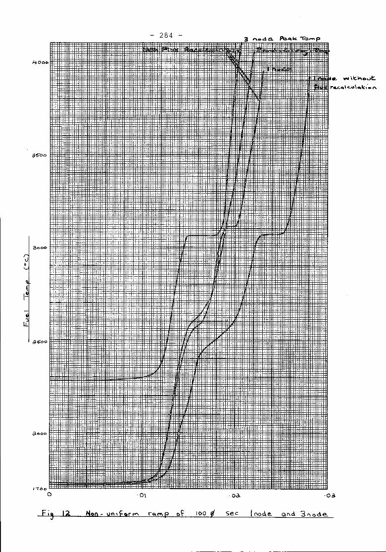
&. "'" i~""o",t:.r4LQ\ c..u\_Ic'.o"
.Oc3.
284
.0\
._-f- +-
',-:-'
J} , +
+
:i:
I-rOO
o
.--t--
(;1.600
~ooo
12. rCU'l'\ (? of: 100 f See lno~e and '3 node..
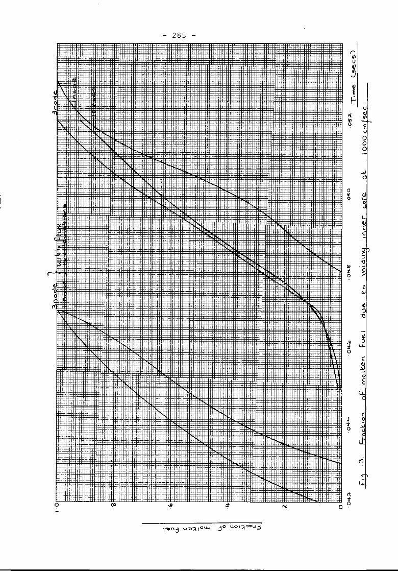
o
285
o
alL.-a..>
LIIIC,
ID)tIP:i 00 :>
cS
~-0
V'.)
u.
C
~
LLL
\.1..

- 286 -
DISCUSSION
A.F. Henry
How many energy groups are required for accurate spectrumrepresentation in the fast reactor transients you described?
M.A. Perks
For rod ejection problems we find 3 energy groups sufficient,but for coolant voiding problems, 9 groups are required foraccurate results. This was checked by one-dimensional calcu-lations in 3, 9, and 25 groups.
- 287 -
G. Dubois
THE IMPORTANCE OF FLUX SHAPE CHANGES IN SPACE-TIME KINETICSCALCULATIONS
Ecole Poly technique de Montreal, Quebec, Canada

- 289 -
TAB L E o F CON TEN T S
page
1. INTRODUCTION • • • • • • • • • • • • • • • • • • • • • 1
. . . . . . . . . . . . . . .
2.4 Reduction of the Calculational Model. . . .
REACTOR MATHEM.ATICAL REPRESENTATION
2.1 Time-Dependent Diffusion Model2.2 Perturbation Model2.3 Feedback Model
.......
..........
. . . .
3
3
4
5
6
3. CONSTRUCTION OF REDUCED KINETICS MODELS . . . . 8
4.
3.1 The X-Time Kinetics Model3.2 The Z-Time Kinetics Model3.3 The Point-Kinetics Model
NUMERICAL METIiODS OF, SOLUTION
.0. . . . . . . . .• • • • • 0 • • • • 0
.0. • • • • 0 • • •
. . . . . . . . . . . .
8
9
9
10
5. ACCIDENT SHIULATION AND ANALYSIS • • • 0 • • • • • • 11
6. SUMMARY AND CONCLUSION . . . . . . . . . . . . . . . 28
7. RE~CES 0 0 0 • 0 • • • • • • • • • • • • • • • • •30
-..1.
- 290 -
INTRODUCTION
The primary objective of the study was to determine whether or
not three-dimensional time-dependent diffusion calculations were essential
for obtaining ~onservative estimates of the reactor behavior when rapid
and localized perturbations are introduced into the core. This analysis1-3was jnitiated by the works of other authors who studied the dynamic
behavior of slab reactors by using point kinetics, models. These reports
clearly indicate the possibility of obtaining erroneous results with
simplified kinetics models.
A quite important advantage of reduced kinetics models is their
relatively low computational cost. If these models fail to adequately
simulate the ,ime-dependent behaviour of a perturbed assembly, one may
ask how useful they can be in safety studies? This is the second point
this study addresses itself.
This work is not a safety analysis of a given reactor system
but instead an evaluation of some hypothesis used in such studies. For
this reason, the reactor model used was kept as simple as possible. The
assembly is a bare, cubical. U-metal-fuelled, water-cooled and
moderated reactor. Diluted boron acts as the operational controller.
The uranium rods are fresh and enriched to 2.7%. The transient is
assumed adiabatic and all feedback effects are neglected except the
thermal expansion of the fuel pins. The perturbation is generated by
the rapid insertion of a bundle of fuel rods into the core.
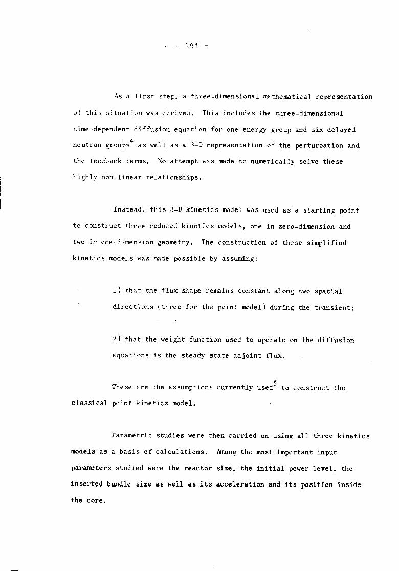
- 291 -
As a first step, a three-dimensional mathematical representation
of this situation was derived. This includes the three-dimensional
tin~-dependent diffusion equation for one energy group and six deldyed. 4neutron groups as well as a 3-D representation of the perturbation and
the feedback terms, No attempt ,vas made to numerically solve thesehighly non-linear relationships.
Instead, this 3-D kinetics model was used as a starting point
to construct three reduced kinetic s model s, one in zero-dimension and
two in one-dimension geometry. The construction of these simplifiedkinetics models was made possible by assuming:
1) that the flux ~hape remains constant along two spatial
direttions (three for the point model) during the transient;
2) that the weight function used to operate on the diffusion
equations is the steady state adjoint flux.
5These are the assumptions currently used to construct theclassical point kinetics model.
Parametric studies were then carried on using all three kinetics
models as a basis of calculations. Among the most important input
parameters studied were the reactor size, the initial power level, the
inserted bundle size as well as its acceleration and its position inside
the core.
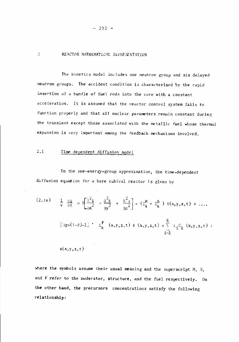
,)
- 292 -
REACTOR NATHEMATICAL Rbl'RESCXTATION
The kinetics model includes one neutron group and six delayed
neutron groups. The accident condition is characterized by the rapid
insertion of a bundle of fuel rods into the core with a constant
acceleration. It is asswned that the reactor control system fails to
function properly and that all nuclear parameters remain constant during
the transient except those associated with the metallic fuel whose thermal
expansion is very important among the feedback mechanisms involved.
2.1 Time dependent diffusion model
In the one-energy-group approximation, the time-dependent
diffusion equaJtion for a bare cubical reactor is given by
(2.1a) 1v +
')
o"~] _ (L'\f + i> ) ~(x, y, z, t) + ....OZ a a
s(x,y,z,t)
(x,y,z,t) <p
6(x,y,z,t) + '\
--"
i=l
Le. (x,y,z,t) +1 1
where the symbols asswne their usual meaning and the superscript H, S,
and F refer to the moderator, structure, and the fuel respectively. On
the other hand, the precursors concentrations satisfy the following
relationship:
- 293 -
~2.lb) :J C.1ot
F.=.: ~i l P € La (x,y,z,t). ~ (x,y,z,t) - \.C.(x,y,z,t)
J. 1 '
for i :-.1. 2 ~ . " 6. In these equations. v, D, ~ ' L= ' ~, p, E:, V, D.;;7J.
and ~. are all assumed constant both in space and time since the reactorJ.
is studied :it the beginning of its core life with a rmiform distributed
fuel. The source term s(x,y,z,t) vanishes at t '-= ° and models the reactor
perturbation for t > O. As for Z~ (x,y,z,t), it is appropriate to mention
that its spatial and temporal dependencies result from the feedback
mechanism. Since the assembly is initially critical, the reactor edge "2a"
satisfies the following relation:
(2.3)1D
~(~pE:-l).~ (0) - ~l a a -,-$;~a
where H2 is th~ critical buckling.
2.2 Perturbation Model
At time t c.= 0, the assembly is perturbed by the rapid insertion
of a bundle of fuel rods of the same composition as those present in the
core. The brmdle movement is downward, parallel to the Z-:lxisand the
insertion point in the X-Y plane is (x ,y ). Note that the bundle ml1yeso 0
with a constant acceleration. Assuming that the bundle size is negligible
compared to the reactor size, it can be shown that the source term in (~.la)
takes the following form:
(2.3) s(x, y, z, t) T)Pe: K Zl(t); (x,y,z,t)
o
5(x-xo)5(y-yo)~(x,y.z,t)for :.::;Zlfor z > Zl
- 294 -
where Zl is the distance travelled inside the core at time "t" by the
bundle, K is a constant proportional to the bundle size and 6(x-x ) iso
the Dirac delta function.
From a mathematical view-point, Zl(t) can take any positive
value which is the same as viewing the ramp insertion as unlimited.
Actually, however, the maximum value of Zl(t) should be equal to 2a, the
reactor edge. In such case, the ramp insertion becomes limited.
2.3 Feedback Model
The source term derived in the preceding section generates a
transient that changes the neutron density level by several orders of
magnitude in ~ess that 100 msec. For metallic fuels, an important
feedback is the change in,fuel density resulting fram the substantial
increase in temperature. Let CF and TF be the heat capacity and the
tempera ture of the fuel. Then~ assuming an adiabatic transient, one can
write:
(2 Aa)dTF (x,y,z,t) = Y LF
dt f(X,y,z,t) ~ (x,y,z,t)
where y is a constant of proportionality. On the other hand, the fuelFtemperature coefficient ~T is assumed constant and is defined as:
(2 Ab) I
LF (x,y,z,t)a
- 295 -
Combining these two relationships by eliminating TF yields:
(2.5 ) ; (x,y,z,t)t
1 + P2 Jo
r! (0)a
~(x,y,z,t) dt
where P2 is ~ positive constan~.
2 .4 Red uc tion of the Calcula tiona I Moo e1
Relations (2.1) thru (2.5) can be combined such that the source
term is (2.la) as well as the precursors concentrations can be e1imina.ted.
This rearrangement therefore yields the following relationship:
(Z.6a)'1 2 2
D i Clkq, I- ~ +- U +- H2 qi J_~ 2 2 2ux, cy a z
F tL (T)ps-l) 2::a (0) [R(x,y,::,t) - P2 Jo qi(x,y,z,T)dTJ qi(x,y,z,t)
where
6
- l1Ps 2::: (0) Li=l
-A. (t-r)e 1.
(2.6b) R(x,y,z,t) K Zl (t) . 5(x-x ) . 5(y-y )o 0
o
z
- 296 -
Note that (2.6a) is an integro-differential relationship which will be used
later to construct simplified kinetics models. Homogeneous boundary
conditions are associated with this equation. Since the reactor is initially
critical and operating at a power P, it foll~~s that:
(2.7) Hx,y,z,o) B B'Pocos (1f3x) cos (1f3) y) cos
where ~ is a constant related to the reactor power at steady state and Bo
is given by (2.2).
In constructing the simplified kinetics models, it was necessaryto approximate (2.6 b) because this function is singular and furthermore,it contains a time-dependent discontinuity along the z-axis. For thesereasons, the Dirac delta function was approximated by the followingexpression :
(2.8) ( )• ~ , -0'2 (y _ Y ) 25 Y - Yo = ~ e 0IfTT
where 0' takes on a large but finite value. Note that if 0' ~ 00 , (2.8) isexact. For the time-dependent discontinuity along the z-axis, a similarapproximation was used but this time, the approximating function was theerror function which in the limit becomes the step function.
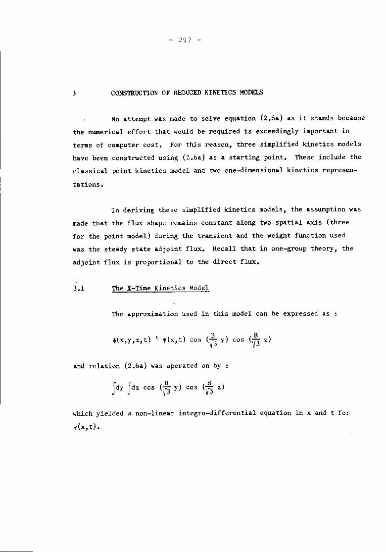
3
- 297 -
CONSmUCTION OF REDUCED KINETICS MODELS
No attempt was made to solve equation (2.6a) as it stands becausethe numerical effort that would be required is exceedingly important interms of computer cost. For this reason, three simplified kinetics modelshave been constructed using (2.6a) as a starting point. These include theclassical point kinetics model and two one-dimensional kinetics represen-tations.
In deriving these simplified kinetics models, the assumption wasmade that the flux shape remains constant along two spatial axis (threefor the point model) during the transient and the weight function usedwas the steady state adjoint flux. Recall that in one-group theory, theadjoint flux is proportional to the direct flux.
3.1 The X-Time Kinetics Model
The approximation used in this model can be expressed as
B~(x,y,z,t) ~ ~(x,t) cos (~3 y)
and relation (2.6a) was operated on by :
J" B Bdy Jdz cos (~3 y) cas (~3 z)
cos B(~3 z)
which yielded a non-linear integro-differential equation in x and t for'!'(x,t).
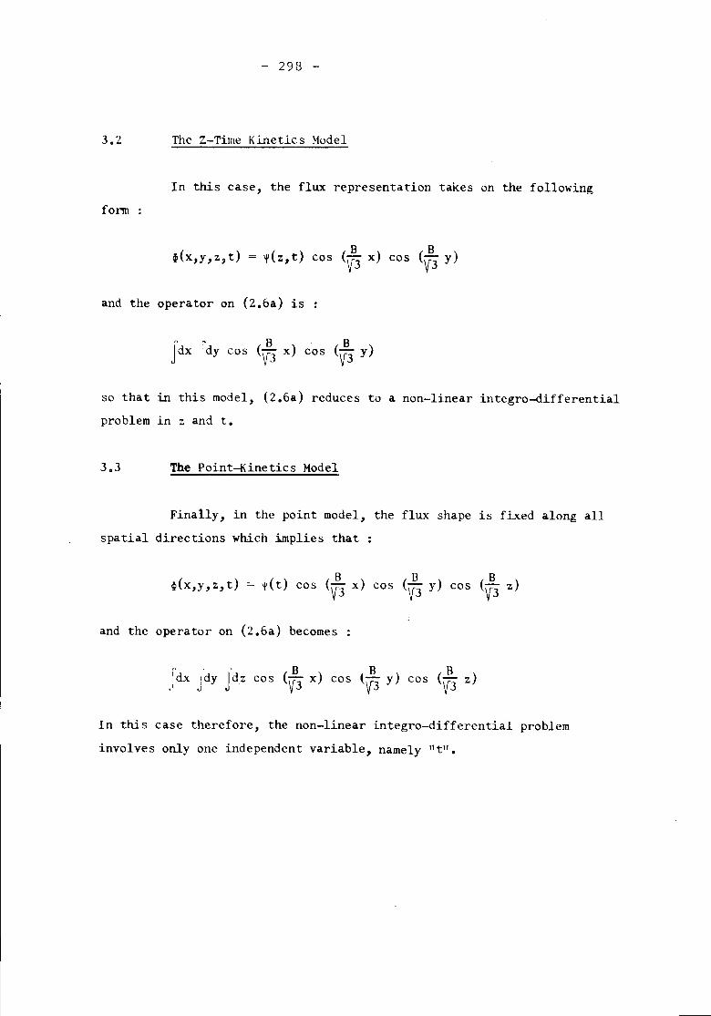
- 298 -
3.2 The Z-Time Kinetics Model
In this case, the flux representation takes on the followingform
~(x,y,z,t) ",(z,t) cos 8 8(1f3x) cos (1f3y)
and the operator on (Z.6a) is
Jdx:"' B 8dy cos (\[3x) cos (\[3y)
so that in this model, (Z.6a) reduces to a non-linear integro-differentialproblem in z and t.
3.3 The Point-Kinetics Model
Finally, in the point model, the flux shape is fixed along allspatial directions which implies that
4i(x,y,z,t) 8'¥( t) cos (V3 x) cos 8('f3 y) cos 8
(1f3z)
and the operator on (Z.6a) becomes
cos B(1f3y) cos
In this case therefore, the non-linear integro-differential probleminvolves only one independent variable, namely "t".
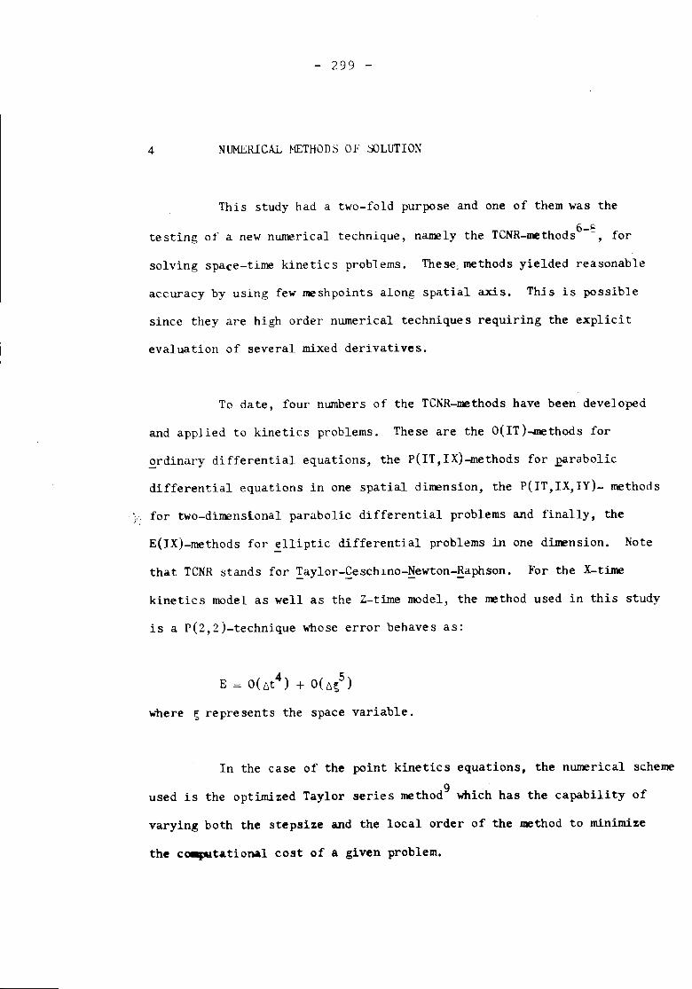
4
- 299 -
NUMERICAL METHOD'::;OF ~LUTION
This study had a two-fold purpose and one of them was the
testing of a new numerical technique, namely the TCNR_methods6-8., for
solving space-time kinetics problems. These;methods yielded reasonable
accuracy by using few rneshpoints along spatial axis. This is possible
since they are high order numerical techniques requiring the explicit
evaluation of several mixed derivatives.
To date, four numbers of the TCNR-rnethods have been developed
and applied to kinetics problems. These are the O(IT)-methods for
£rdinary differential equations, the P(IT,IX)-methods for ~rabolicdifferential equations in one spatial dimension, the P(IT,IX,IY)- methods
./ for two-dirnenslonal parabolic differential problems and finally, the
E(IX)-methods for ~lliptic differential problems in one dimension. Note
that TCNR stands for !aylor-~eschino-~ewton-~aphson. For the X-time
kinetics model as well as the Z-time model, the method used in this study
is a p(Z,Z)-technique whose error behaves as:
where S represents the space variable.
In the case of the point kinetics equations, the numerical scheme
used is the optimized Taylor series method9 which has the capability of
varying both the stepsize and the local order of the method to minimize
the cOBpUtatio.nal cost of a given problem.
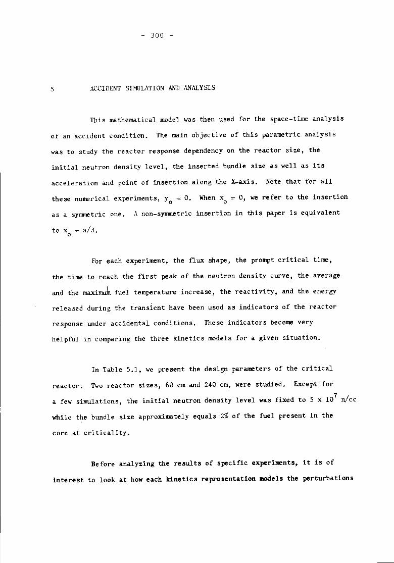
5
- 300 -
ACCIDENT SIMULATION AND ANALYSIS
This mathematical model was then used for the space-time analysis
of an accident condition. The main objective of this parametric analysiswas to study the reactor response dependency on the reactor size, theinitial neutron density level, the inserted bundle size as well as its
acceleration and point of insertion along the X-axis. Note that for allthese numerical experiments, y = O. When x = 0, we refer to the insertiono 0
as a symmetric one. A non-symmetric insertion in this paper is equivalent
to x = a/3.o
For each experiment, the flux shape, the prompt critical time,the time to reach the first peak of the neutron density curve, the average
and the maximuk fuel temperature increase, the reactivity, and the energyreleased during the transient have been used as indicators of the reactorresponse under accidental conditions. These indicators become veryhelpful in comparing the three kinetics models for a given situation.
In Table 5.1, we present the design parameters of the critical
reactor. Two reactor sizes, 60 cm and 240 cm, were studied. Except fora few simulations, the initial neutron density level was fixed to 5 x 10⁷ nlcc
while the bundle size approximately equals 2% of the fuel present in the
core at criticality.
Before analyzing the results of specific experiments, it is of
interest to look at how each kinetics representation models the perturbations
- 301 -
TABLE 5.1
Design Parameters of the Critical Reactor
Reactor Type
Coolant
fuelEnrichment (atomic)
Clad Material
Control Material
Clad Thickness (inches)
Fuel-Clad Gap (inches)Neutron Velocity (m/sec)Fuel Temp. Coefficient (l;oC)Fuel Heat Capacity (cal./gr.-oC)
IFuel Density (gr./cc)
Shutdown Coefficienta) Point Kinetics (cc/sec)zb) Space-time Kinetics (cm )
Metal-fuelled
Water
Uranium
2.7%
SS-304Boron
0.0240
0.00752200
-5-4.5 x 10
0.0276
19.1
? -127._9 x 10_178.81 x 10
function. A typical example appears in Figures 5.1 A, B, C for x = 0o
(i.e. symmetric insertion). For the X-time kinetics model, the perturbation
is always a local phenomenon while it is just the opposite for the point-
model.. In the case of the Z-time kinetics model, the perturbation is
always local and non-symmetric until the bundle has reached the bottom of
the core; then, the perturbation becomes uniform along the Z-axis.
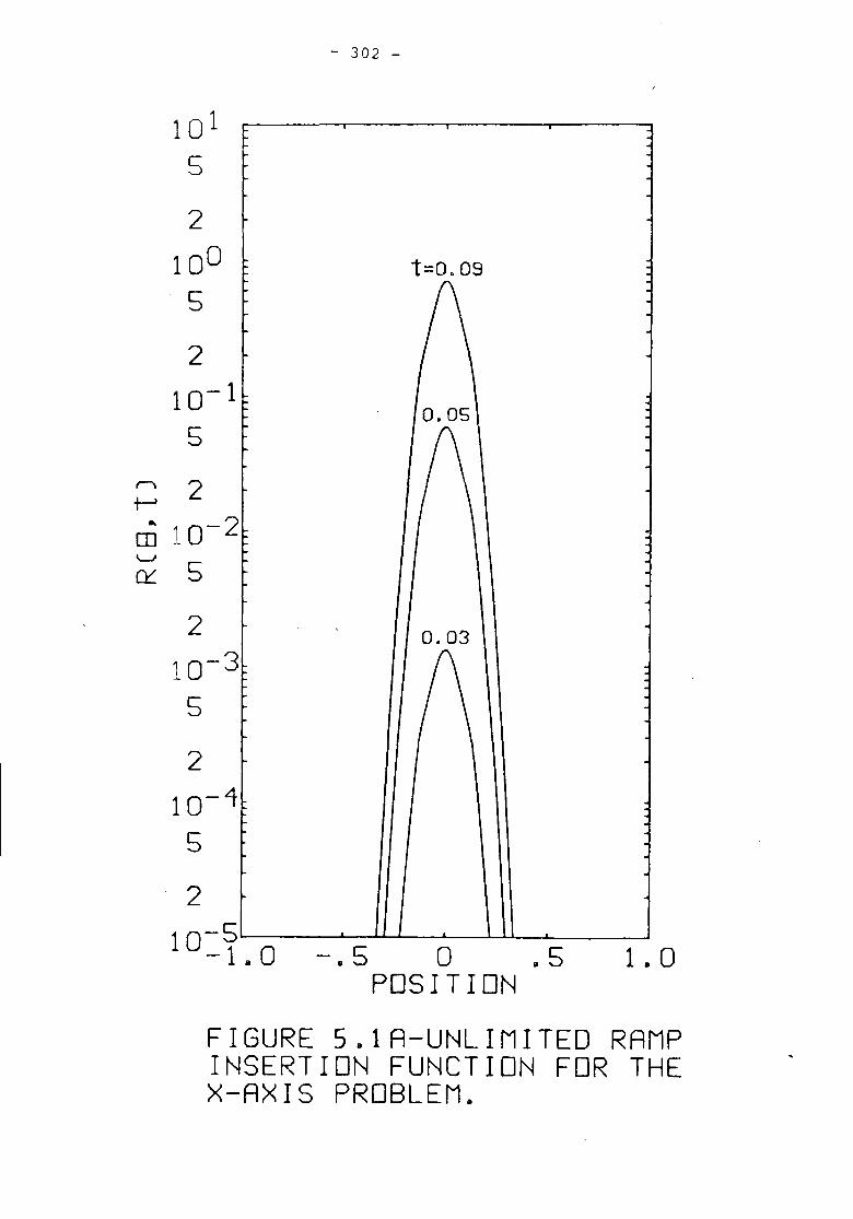
- 302 -
0.05
t=0.09
<l 2f--J.. 10-2rn .-
~ 5
0.03210-3
5
210-45
210-5-1.0 -.5 0 .5 1.0
POSITIONFIGURE 5.1A-UNLIMITED RAMPINSERTION FUNCTION FOR THEX-AXIS PROBLEM.
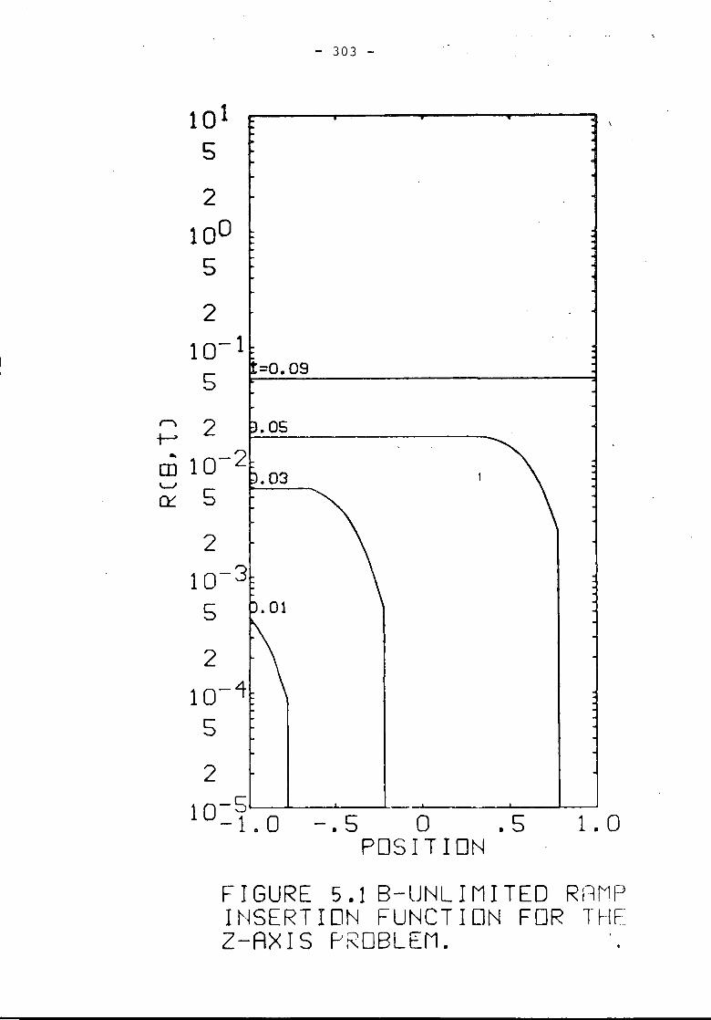
- 303 -
=0.09
210-35 .01
210-45
210-5-1.0 -.5 0 .5 1.0
POSITION
FIGURE 5.1 B-LJNL I MI TED RllMPI~~SERTION FUNCTION FOR THEZ-AXIS PROBLEM.
f"l 2 .05~
.. 10-2~ .03~ 5
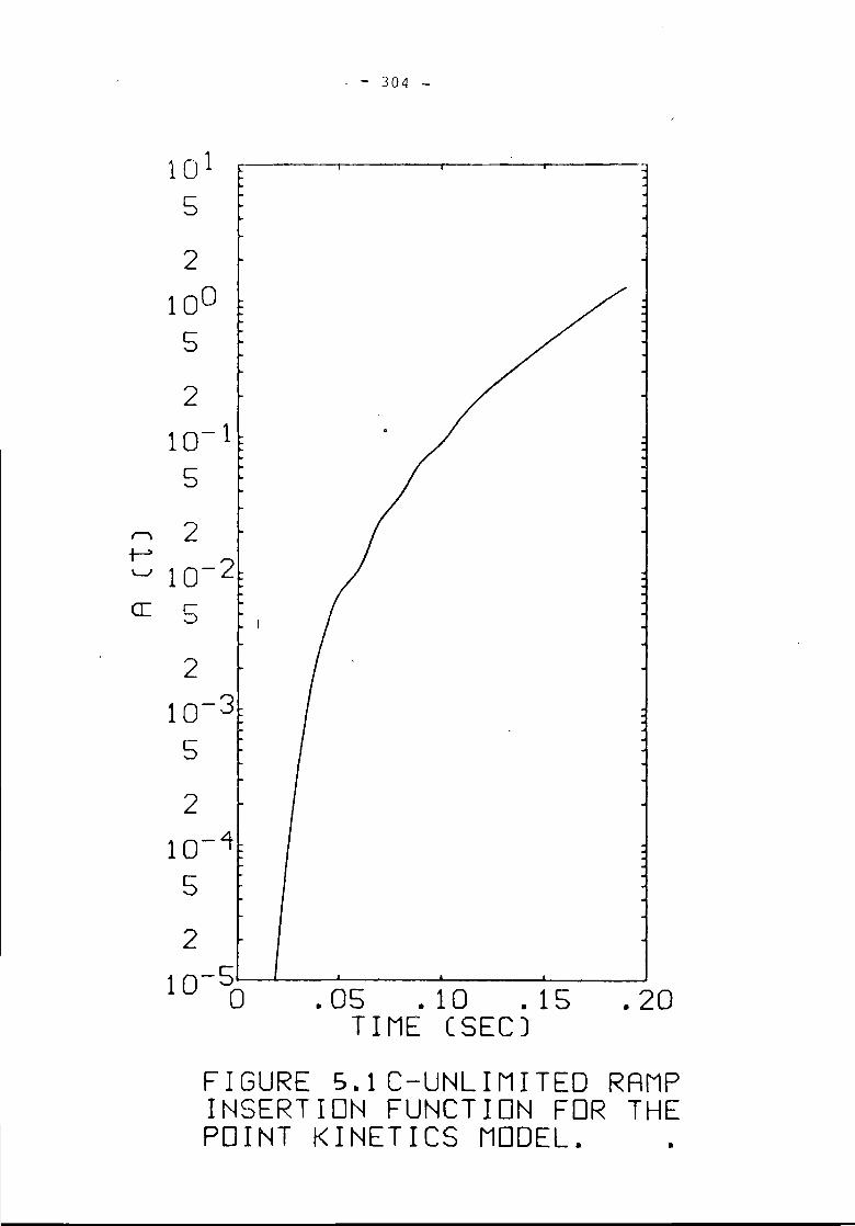
- - 304 -
. 05 II 10 . 15 . 20TIME (SEC)FIGURE S.lC-UNLIMITED RAMPINSERTION FUNCTION FOR THEPOINT KINETICS MODEL. .
101
5
2
1005
210-15
r) 2t-"'-' 10-2cr: r
::>
210-35
210-4
5
210-5
0
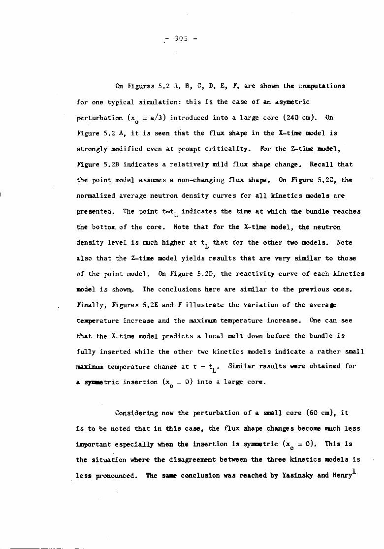
- 305 -
On Figures 5.2 A, B, C, D, E, F, are shown the computations
for one typical simulation: this is the case of an asymetric
perturbation (x = a/3) introduced into a large core (240 cm). On. 0
Figure 5.2 A, it is seen that the flux shape in the X-time model is
strongly modified even at prompt criticality. For the Z-time model,
Figure 5.2B indicates a relatively mild flux shape change. Recall that
the point model asswnes a non-changing flux shape. On Figure 5.2C, the
normalized average neutron density curves for all kinetics models are
presented. The point t=tL indicates the time at which the bundle reaches
the bottom of the core. Note that for the X-time model, the neutron
d~nsity level is much higher at tL that for the other two models. Note
also that the Z-time model yields results that are very similar to those
of the point modeL On Figure 5.2D, the reactivity curve of each kinetics
model is sho~. The conclusions here are similar to the previous ones.
Finally, Figures 5.2E and, F illustrate the variation of the averalr
temperature increase and the maximum temperature increase. One can see
that the X-time model predicts a local melt down before the bundle is
fully inserted while the other two kinetics models indicate a rather smallmaximum temperature change at t = ~. Similar results were obtained for
a ~tric insertion (x = 0) into a large core.o
Considering noW' the perturbation of a small core (60 em), it
is to be noted that in this case, the flux shape changes become IIllchl~ss
important especially when the insertion is sy_trie (x = 0). This isothe situation where the disagreement be~en the three kinetics models is
Ie 5S pronounced. The Sallie conclusion WI reached by Yasinsky and Henryl
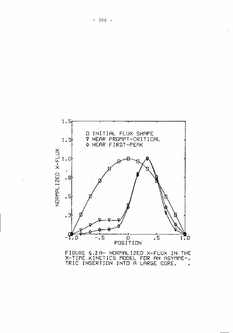
. - 306 -
1.5
o INITIAL FLUX SHAPE1.3 V NEAR PROMPT-CRITICAL
o NEAR FIRST-PEAKx::)
~ 1. aIxow .8Nt-1
-'a::I:a:: .5oz
.3
a .5POSITIONFIGURE S.2A- NORMALIZED X-FLUX IN THEX-TIME KINETICS MODEL FOR AN ASYMME-.TRIC INSERTION INTO A LARGE CORE.
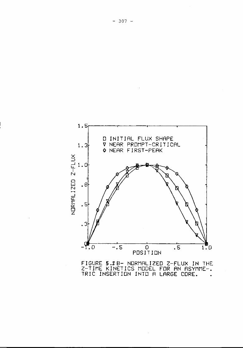
- 307 -
1.5
o INITIAL FLUX SHAPE1.3 V NEAR PROMPT-CRITICAL
o NEAR FIRST-PEAKX::;l
~ 1.0IN
oW .8N.........-Jcr:r::~ .5oz
-.5 0 .5POSITIONFIGURE 5.ZB- NORMALIZED Z-FLUX IN THEZ-TIME KINETICS MODEL FOR AN ASYMME-.TRIC INSERTION INTO A LARGE CORE.
- 308 -
- X-TIME KINETICSo Z-TIME KINETICS. POINT KINETICS
e. ~o.
o 0
o
•,
°I '
1'°
,°1,0 t=tL.
O. 0 I
.010 .080 .120 .160TIME (SEC)FIGURE 5.1C- NORMALIZED AVERAGENEUTRON DENSITY FOR AN ASYMME- ..TRIC INSERTION INTO A LARGE CORE
106
5
2
)- 105~'"""1 5(/)z~ 25 101
~ 5:::>~ 2
~ 103a:~ 5w::>a: 2 I
8 102N- 5..Ja:~ 2oz 101
5
2
10
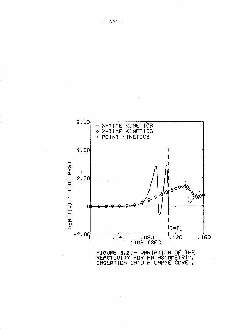
- 309 -
6.00 - X-TIME KINETICSo Z-TIME KINETICS· POINT KINETICS
1.00
r-'"I
CJ)~a:-J 2.00-J00'-'
>-t--~-t-Ua:wa:::
-2.000
I
It=t".010 .080 .120 .160TIME (SEC)
FIGURE 5.%D- VARIATION OF THEREACTIVITY FOR AN ASYMMETRIC.INSERTION INTO A LARGE CORE.
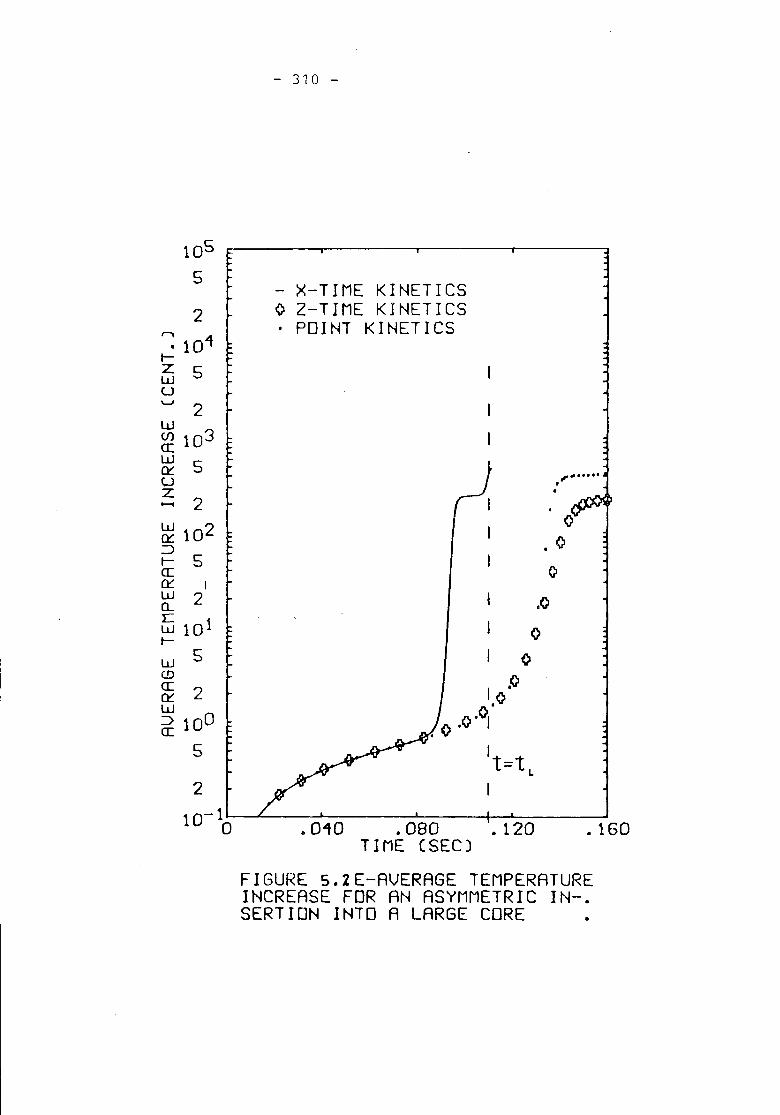
- 310 -
.160
I .0I 0
I <>.0
10• <> .0.01•
It=tL.
I
- X-TIME KINETICSo Z-TIME KINETICS. POINT KINETICS
.010 .080 .120TIME (SEC)FIGURE S.ZE-AVERAGE TEMPERATUREINCREASE FOR AN ASYMMETRIC IN-.SERTION INTO A LARGE CORE .
105
5
2
~ 101t-~ 5u\...J 2w~ 103
~ 5u~ 2~ 102.:)t- 5a:fr:~ 25 101t-w 5(!)
~ 2w::> 100a:
5
2
10-1a
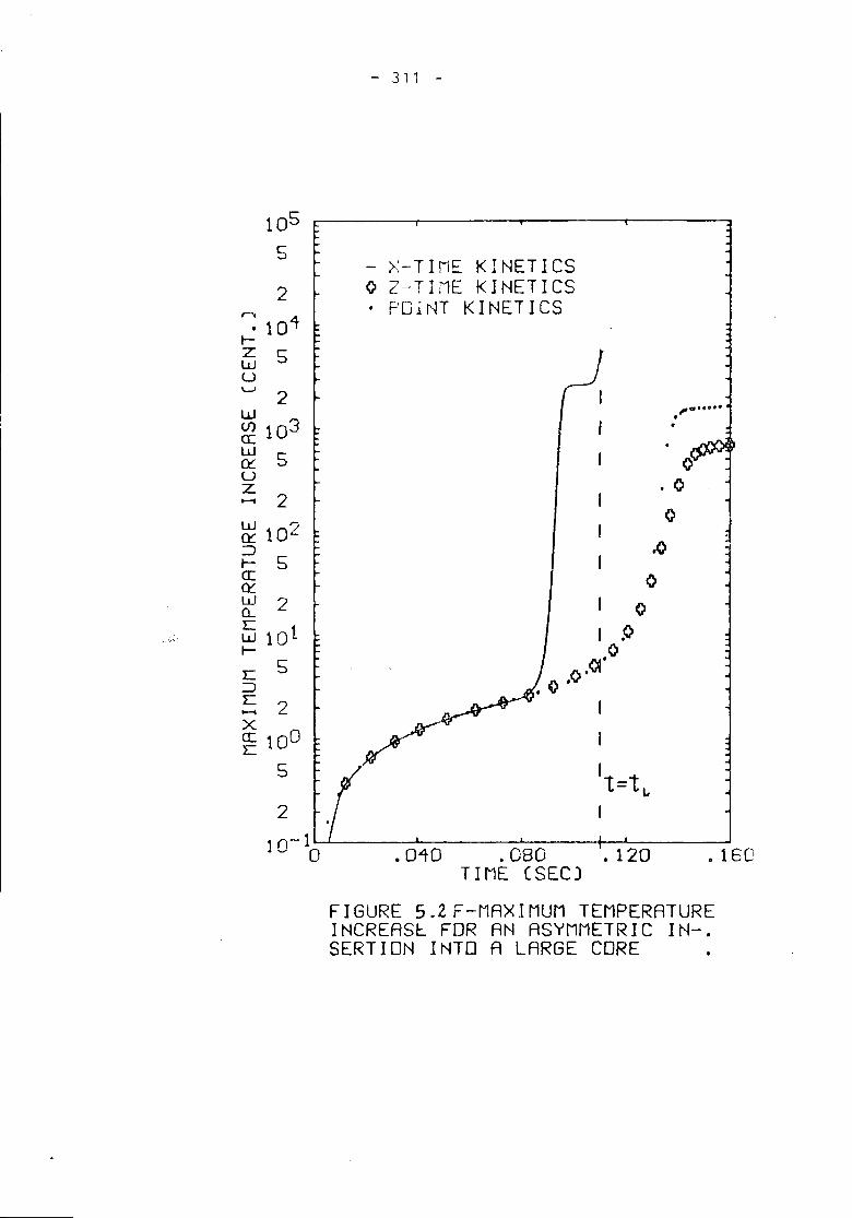
- 311 -
• 16e'
<>(}
, ,0,0
0,01, Q '
I
I
't=t L.
I
- X-TIME KINETICSo Z-TIME KINETICS, POiNT KINETICS
.040 .080 .120TIME (SEe)FIGURE 5.ZF-MAXIMUM TEMPERATUREINCREASl FOR AN ASYMMETRIC IN-.SERTION INTO A LARGE CORE
2
10-1~ 0
105
5
2
r-: 104I-
~ 5u'-'2w~ 103
~ 5uz.......2~ 102:JI- 5cr:fr:~ 2~ 101l-
I: 5:J
~ 2x~ 100
5
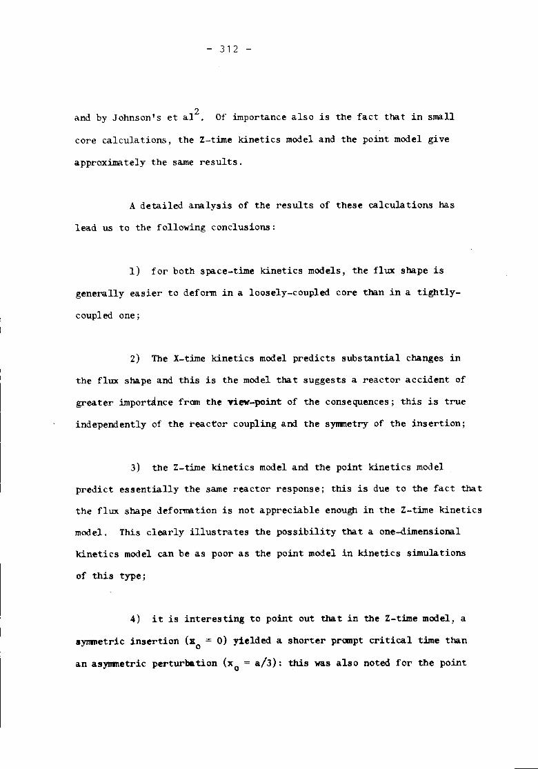
2and by Johnson's et al
- 312 -
Of importance also is the fact that in small
core calculations, the Z-time kinetics model and the point model give
approximately the same results.
A detailed analysis of the results of these calculations has
lead us to the following conclusions:
1) for both space-time kinetics models, the flux shape is
generally easier to deform in a loosely-coupled core than in a tightly-
coupled one;
2) The X-time kinetics model predicts substantial changes in
the flux shape and this is the model that suggests a reactor accident of
greater imporulnce from the view-point of the consequences; this is true
independently of the t'eac~or coupling and the synmetry of the insertion;
3) the Z-time kinetics model and the point kinetics modelpredict essentially the same reactor response; this is due to the fact that
the flux shape deformation is not appreciable enough in the Z-time kinetics
model. This clearly illustrates the possibility that a one-dimensional
kinetics model can be as poor as the point model in kinetics simulations
of this type;
4) it is interesting to point out that in the Z-time model, a
lyJ1IIletricinsertion (xo = 0) yielded a shorter prcnpt critical time than
an asynmetric perturbation (xo = a/3): this was also noted for the point
- 313 -
kinetics model;
5) at the time the bundle reaches the bottom of the core, the
normalized neutron density predicted by the X-time model can be several
orders of magnituie larger than the value predicted by the other two
kinetics models; this statement hold for both symmetric or asymmetric
insertion into a small or large core; the main consequence of the result
is the fact that the X-time model is the only one tha t predicts possible
core damage;
6) the magnitude of the first peak in the neutron density curves
depends primarily on the feedback model and flux shape changes;
7) lhe pranpt critical time as computed by the three models
vary appreciably (as much ~s 30%); as we shall see below, even the X-time
estimate is not conservative because flux shape changes along the y-axis
are neglected in this model; this suggests that the point model value as
well as the Z-time value may be wrong by a factor as large as two; this
statement holds also for the time at which the first peak of the neutron
density curve occurs;
8) in kinetics studies, the instanteneous power level depends
heavily on the perturbation model, the feedback model, and the control
mechanism (external correcti~e action) model; it appears highly desirable
in such analysis to extract the influence of each model on the simulation
results; this b bec&uae unless these models are very sophisticated and
- 314 -
accurate, parametric studies even in 3-D analysis could lead to erroneous
conclusions;
9) the comparative analysis of the simulations obtained for the
three kinetics models indicates that none of these models yield conservative
results because they all neglect flux shape changes along at least two
spatial dimensions; this is particularly important for the Y-flux shape;
consequently, for fast, localized perturbations, it appeared that 3-D
kinetics simulations are essential for reactor safety studies assuming
that the perturbation model, the feedback model am the control mechanismmodel are sophisticated and accurate;
10) the agreement between the three reduced kinetics models is
very good for Fimes smaller than the prompt critical time;
11) the three models yield approximately the same result for the
amount of energy released up to the first peak of the neutron density curves;
In addition to the computer simulations mentioned earlier,
parametric studies have been carried out for an asymmetric insertion into
a large core. The aim of these additional runs was to determine the
influence of the inserted bundle acceleration and its size as well as the
initial neutron density level on the transients. From these nunerical
experiments, we arrived at the following conclusions:
12) for all three kinetics models, the bundle acceleration "G"
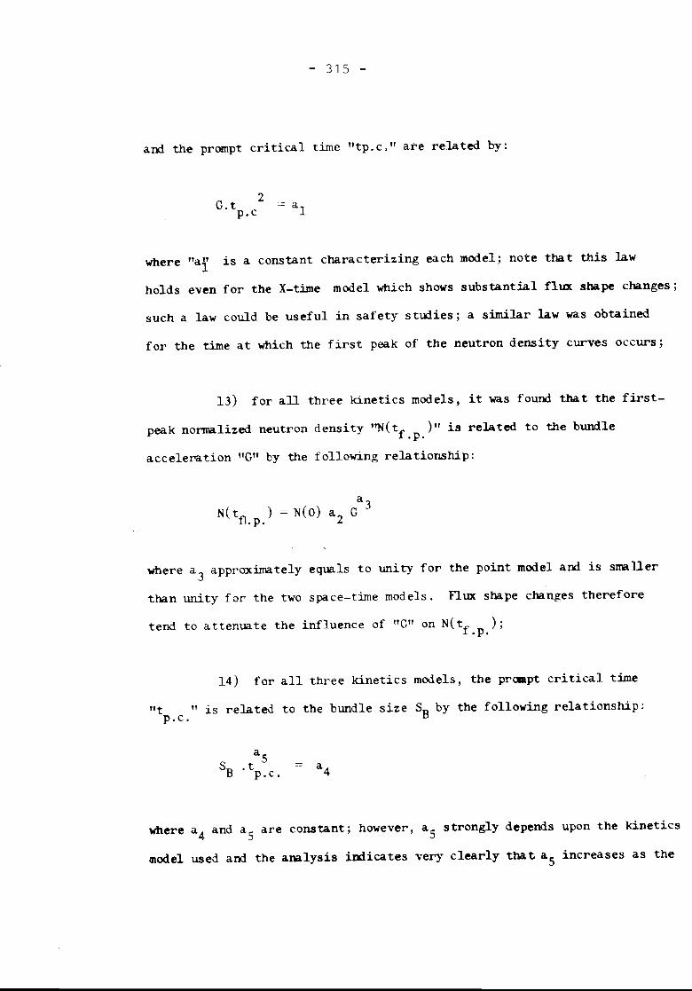
- 315 -
and the prompt critical time "tp.c." are related by:
ZG.t alp.c
..mere "at is a constant characterizing each model; note tha t this law
holds even for the X-time model 'Which shows substantial nux shape changes;
such a law could be useful in safety studies; a similar law was obtained
for the time at 'Which the first peak of the neutron density curves occurs;
13) for all three kinetics models, it was found that the first-
peak normalized neutron density ''N( tf )" is related to the bundle.p.
accelera tion "G" by the following relationship:
a3N(tfl
) = N(O) aZ G.p.
where a3
approximately equals to unity for the point model and is smaller
than unity for the two space-time models. Flux shape changes therefore
tend to attenua te the influence of "G" on N(tf ) ;.p.
14) for all three kinetics models, the prompt critical time
lit "is related to the bundle size 5B by the following relationship:p.c.
where a4
and as are constant; however, as strongly depends upon the kinetics
~odel used and the analysis indicates very clearly that as increases as the
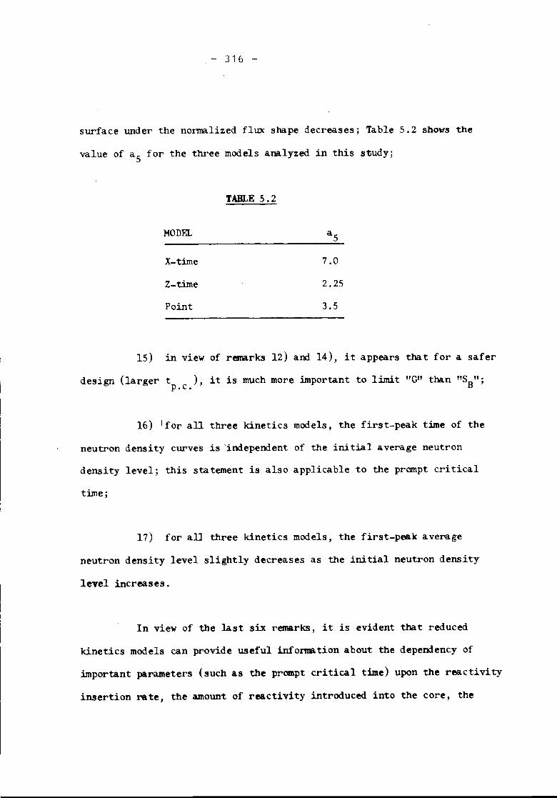
,-316-
surface under the normalized flux shape decreases; Table 5.2 shows the
value of as for the three models analyzed in this study;
TABLE 5.2
MODEL
X-time
Z-timePoint
7.0
2.25
3.5
15) in view of remarks 12) and 14), it appears that for a safer
design (larger t ), it is much more important to limit "G" than "SB";p.c.
16) Ifor all three kinetics models, the first-peak time of the
neutron density curves is 'independent of the initial average neutron
density level; this statement is also applicable to the prompt critical
time;
17) for all three kinetics models, the first-peak average
neutron density level slightly decreases as the initial neutron density
level increases.
In view of the last six remarks, it is evident that reduced
kinetics models can provide useful information about the dependency of
important parameters (such as the prompt critical time) upon the reactivity
insertion rate, the amount of reactivity introduced into the core, the

- 317 -
initial power level, ani flux shape changes.
6
- 318 -
SlMMARY AND roN CLUSION
The main conclusion to draw fram this study is that simplified
kinetics models present serious drawbacks in the analysis of super-prompt-
critical excursions. Except for a symmetric reactivity insertion into
a tightly-coupled core, the three kinetics models display substantial
disagreements. In addition, the analysis shows that a one-dimensional
kinetics model can be as poor as the point model in describing properly
this type of accident condition. In view of the important flux shape
changes, it appeared that both one-dimensional kinetics models were
inadequate for safety studies since they do not yield conservative
estimates of the reactor dynamic behavior.
DesPite serious disagreements on same points, the three kineticsmodels agree on others: 1) the prampt criti all time is nearly independent
of the initial neutron density; 2) the magnitude of the first peak of the
neutron density curves decreases as the initial power level increases;3) the amount of energy released up to the first peak of the neutron density
curve is approximately the same; 4) for reactivity insertions less than one
dollar, the three kinetics models essentially predicts the same power
excursion. It thus appears that reduced kinetics models could be useful
in carrying out sub-prompt-critical analysis as well as parametric
studies even though they can be erroneous in camputing the value of some
important parameters such as the prampt critical time and the reactivity
at any given time.

- 319 -
'Ibis study agrees with the recent findings of Birkhofer,
10Schmidt and Werner on the urgent need to solve three-dimensional
kinetics problems for super-proMpt-critical excursions. This implies the
development of much faster numerical techniques, capable of reasonable
accuracy. It would greatly enhance the reliability of reactor safety
studies.
7 REFERENCES
- 320 -
1. J.B. Yasinsky, &0 A.F. Henry, "SQIIleNumerical Experiments Concerning
Space-Time Reactor Kinetics Behavior", Trans. Am. Nucl. Soc., 22, 171
(1965) .
2. S.O. Johnson, E.P. Gyftopoulos, and M.E. Radd, "Effects of flux Shape
Changes in Power Excursion Behavior", Trans. Am. Nucl. Sac. 8, 221 (1965).
3. J.B. Yasinsky, "On the Use of Point Kinetics for the Analysis of Rod-
Ejection Accidents", Nuc1. Sc. Eng. 37, 241 (1970).
4. \II.M. Stacey, Jr., "Space-Time Nuclear Reactor Kinetics", Acadenic Press
(1969) •
5. J.B. Yasinsky, "Notes on Nuclear Reactor Kinetics", WAPD-'IM-960(1970).
6. G. Dubois, "Numerical Methods for Reactor Kinetics Problems", Ph. D.I
Dissertation, University of California (Berkeley).
7. G. Dubois and L.M. GrosRllUl, "'A New Method for Space-Time Kinetics and
Heat Flow Problems", Trans. Am. Nucl. Soc. 15, 2, 788 (1972).
8. G. Dubois, "A High Order Method for Two-Dimensional Space-Time Kinetics
Problems", Trans. Am. Nuc1. Soc., 17, 1, 253 (1973).
9. G. Dubois ami L.M. Grossman, ''Optimized Taylor Series Method in Point
Kinetics Calculations", Trans. Am. Nucl. Soc. 15, 1, 288 (1972).
10. A. Birkhofer, A. Schmidt, and W. Werner, "Comparison of Two- and Three-
Dimensional Calculations of Super-Prompt-Critical Excursions" Nucl.
Tech., 24, 7 (1974).
- 321 -
Session IV/1
REVIEW OF KINETICS BENCHMARK CALCULATIONS
Chairman: A.F. Henry, USA
D.E. Billington, G. Buffoni, E.H. ChildsD.K. Cooper, A. Galati, S. Gnattas,F.M. McDonnell, R. Masiello, A. Musco,F. Norelli, T. Otsuka, K. Porn, J. Sidell,S. Tsunoyana
SURVEY OF THE RESULTS OF A ONE-DIMENSIONALBENCHMARK PROBLEM TYP ICAL FOR A THERMAL REACTOR
P.S. Christensen, F.J. Fayers, S. Langenbuch,F.N. McDonnell, A. Schmidt, E. Vincenti,H. Yoshikawa, W. Werner
SURVEY OF THE RESULTS OF A TWO- AND THREE-DIMENSIONAL KINETICS BENCHMARK PROBLEMTYPICAL FOR A THERMAL REACTOR
323
413

- 323 -
D.E. Billington, G. Buffoni, E.H. Childs, D.K. Cooper,A. Galati, S. Gnattas, F.M. McDonnell, R. Mosiello,A. Musco, F. Norelli, T. Otsuka, K. Porn, J. Sidell,S. TsunoyanaSURVEY OF THE RESULTS OF A ONE-DIMENSIONAL KINETICBENCHMARK PROBLEM TYPICAL FOR A THERMAL REACTOR

I lliTRODUCTION
- 325 -
J SIDELL
United Kingdom Atomic Energy AuthorityAtomic Ener&y Establishment
YlinfrithDORCILSSTER
Dorset
AEEW - R 988
Th0re is a growing awareness of the need to improve representational detailsand a.ccuracy in computing the fault end operational transient behaviour ofnuclear power reactors. The problems involved, however, are significantsince the solutions of kinetic equations involving all the relevant feeCibackphenooena in a multi-dimensionnl representation of a whole reactor are notrea.dily achievable with current computer systems. In tl:.ese')ircumstancesthere is a need to pursue nunerical and computer techniques T.hic~ off~rimprovements in solution time aud cost. Furthermore, since this is a commonbasic goal of many national laboratories, the pooling vf relevan~ experienceand research is beneficial.
In or.der to stimulate mutual interest in this area., the Nuclear Energy- AgencyCommittee on Reactor Physic~ has assembled a series of 'bencr~rk' kineticproblems and has invited workers in the field to atte~pt their solution witha view to subsequent exchange of experience and inter-comparison of performancoof tbe co~uter models used.
This paper reviews the contributions submitted to n series of one-dimer~ionalproblems conceived as a starting point for subsequent rrv1ti-diLensionalproble~s. The aiD in setting the proble2S (~hich are detailed in theattached note) ~s been to focu3 attention on promising meth~s of solution50 that no 'real' reactor problem or siruulation is imFlicd. Th~ problemscontain a simplified form of reactivity feedback in an axial core representa-tion with reflectors and e. controller. The basi.s of the proble:n is tocc~,~te an initial steady ~tate and then to follow a transient caused eitherby moving the control rod or by varying cross-section.
In rosponse to this series of problems, nine submiBsions were r~turDed fromvarious interested parties solving some or all of the cases. Section II ofthe paper lists the submissions received and summarises the ccde~ and methodsused.
In Section III the quantit~tive results of the nine submissions are given.The results and methods used are compared and discussed in Section 'IV.
- 326 -
Many of the methods used for the Golution of the benchmark CRses are relativelynew, in the s€nse that either they incorporate some new feature, based on anexisting method or else they contain sorne improved method of 6~lving resulting sctsof equations. This introduction contains a brief summary of the basic methodsfrom which the benchmark set have been derived.
1) !inite DifferenceThis method, dating back to classical numerical analysis, attempts to approxim~tethe time dependc~t diffusion equation b)' representing the spacial and ti~e deviativesas a local su~ of flux values, which matches the Taylor series of the variablesup to some required order. In general. the srealler the spacing between the fluxvalues ~d the larger the ~umbcr of terms retained in the sum,< the more accuratethe representation will become.
The diffusion equation ultimately reduces to a set of algebraic e~uations, thesolution of which forms the basis of the codes.Points in favour of such methods are that the differences give a true representationof the equations in the sense that in t~e limit the exact solution will be 0otaincd,and that the method will work equally well on any reactor configul'ation. Point£> -against these methods are that in general many equations are requ~red to obtain anadequate representation of the physical situation and that the solution of theseequations may be costly in computer time.
2) Adiaba:ic MethodTaic method aS8Umes that at every instant, during a transient, the flux shepes canb~ obtained by static calculations. The Bpace-ti~Je flux can then be reprcsentedn~ a product of an amplitude fauction depending on time only and a spacial functionrepresenting the flux shapes at the particular time, produced by Rolving thesteady state equations of current conditions.
The diffusion equation ultimat~ly reduces to a set of ordinary differentialequations in time for the ~plitude functions, and a set of static equations,usually solved by finite difference methods, in the spacial co-ordinates.
This method is relatively ~qst in computing time but han the dra~back thct thestatic flux shapes may not in general be good approximations to the true flux shapesat any particular time, especially when feedback terres are present.
3) ~nthesis MethodsIn these methods the flux is decomposed into a sum of proc~cts of amplitude functionsand spacial functions. This has the advantage over the adiabatic method in thesense that all that is required of the spacial functions js that a linear cor;;bir:.2tioaof them be n good approximation to the true flux shape6. The diffLision equatioll
.ultimately reduces to a set of ordinary differential equations for the a~plitudefunctions. The trial spacial functions are chosen to satisfy reasonable esti::lo.tesof reactor conditions which bracket those ~ctual:y to be experienced.
The appeal of fl~x synthesis methods resides in their ability to partition a ~ulti.,dimensional problem into a sequence of simpler problems thus providing a means cfobtaining a multidimensional solution, albeit an approAimate onc, in a desree ofdetail which is impossible or economically imprac~icable with a ~irect solution.
The ques~ion of how many trial functions to use in the approximation frequentlyoccurs. The accuracy of the representation depends very strongly on which trialfunctions and how many, are chosen.
- 327 -
n SUBMISSIONS RETURNED
1 CEGB
SUBlJISSOR: D K CooperSa~ety Technology ~roupGDCCEGB
CASES SUBilITTED: A, C
COhIPtrrER: IBM 370/165
CODE: KINA! 3
KINAX is a one-dimensional cne-group reactor kinetic program. Up to sixdelayed neutron groups are included. Special facilities of the code includereactor tripping initiated by outlet tecperatures and an elaborate heat trans-{'er ILodel. Transient calculations can be continued ~rcm a previous runwitllout recomputation. The model incorporates a fixod optional tim3 stepbetween output points
METHODSThe ti.'lle-dependcnt~olutio1l3 of the diffusion and heat transfer equations a.recomputed usi~g the Cre.n}~-lU.cholsonfini ';;ed:;'ff~renc.etechnique to prcxluce tri-diagonal natrix difference equations which are solved directly. The delayedneutron precurRors aI'e treated differently. The precursor equations areintegrated by parts assu.mil".gthat the gradients of the prompt neutron,fluxesare constant over a time step, and tile resulting expressions are substitutedinto the dii'fl1sionequa,;ions. ~he values of the precursors are updated onlyonce for each time step after the prompt flux solution has converged.
REFERENCE
ELLIS J. The y~~~~ One-d~ensiono.l Reactor Kinetic Program KINAX 3.CD/NS/ll, NPCC/RKnP/P286, August 1963
2 N.AI~.SUB1HSSOR: T Otsuka, S Tsunoyana
Nippon Atomic Industry Group Co Ltd250 Suchi Rocho, Kawa&akikuKu~asaki KanagawaJapan
CASES sumcrrTED: J..., B, C, D
COMPUTER: TOSDAC 5600/170 (Factor 4 slower then IBM 370/165 f~or.:lcOr.:lpariscnof mean of arithr.:leti0~1o~erations)
CODE: NAKlN
NAKIN is a onc-dimension~l code for the solutivn of the tJ.~e deperAent multi-group neutron diffusion equations. The neutronic celcu~~tion is coupled withthe feedbacks due to the temperature effects on the cros3-sections. The codoincorporates an automatic adjustment of the ti~e step. There are options onthe nwnber of energy groups, nw::ber of mesh points, nUJ1lberof material regio1l8
- 328 -
and number of delayed neutrons, but is subject to maximum dimensions on all.
lJETllODS
There is no English write-up of this code but the numerical ID£thods are besedon those used in the code GAKIN.
The multi-group neutron diffusion equations are centrally finite differencedin the spacial dimensions and the set of differenced equa~i0ns is treated as alarge set of si~ultareous ordinary differential equntions ir ti~~, one equ~tionfor each flux and precursor eroup at each mesh point. The scattering andabsorption in £roup terms are collated with the ti~c derivative to impose a.pure exponential factor on the neutron group fluxes and presursors at eachsp~ce point.
The resulting p.quations nre integrated over El. time step by assuming that thenew variables b~have in a purely exponential form with a decay rate equal tothat of the therulal flux. This rate9 at each space point, is cODputed fromtwo adjacent tice values of the thermal flux. The resulting form is exactin the case of constlllltreactivity.
The c001ant temperature equations are solved by the Crank-Nicholson finitodifference sch0~0.
REFERENCEHANSEN R .p, JOHNSON S R. GAKIN: A One-dimensional liulti-group KinetiC3Code. USAECReport GA-7543, AUGUst 1967.
3 CEliS
SunllISSOR: S Gnatte.sService dfEtudes des Reacteurs et de Mathematiqucs Appliqu~p.sCBA, SaclayBP No 291190 GIF-SDR-YYETTEFrance
CASES SUB}HTTl~D: C
C 01tPU'l'ER :
CODE:IBM 360/91
CINTAX(Equivalent to IBM 370/165 at C:E:'1Se3tir~:lte)
cmTAX is a code to solve the one-dimensiona.l, twc-group, time ..depe:lient n'3'Jtrcndiffusion equation with fuel temperature feedback. l;t present CL;T.AX is stillin the sta.:;eof developr~eLt and is not as ;yet in its opti:nal foro. The te-nch-mark submission is by ~ay of a test on the code.
METHODS
As no write-up exists, there is little kno~ledge of the methods e~p~oyed inCINTAXo The only info~ation available is that it is a discontin~ous tim~synthesis model.
- 329 -
4 CRNL
SUBMISSOR: P M McDonnelApplied l!athema tics BranchChalk River Nuclear LaboratoriesCHALK RIVEROntario KOJ 130Canada
CASES SUB!HTTED: A, B, C, D
COMPUTER:
CODE:CDC 6600ADEP
(Comparable to IBM 370/165 at CRNL estlmatc)
ADZP is So 0110- or two-dilJensional code to solve the time-d.ependent few-groupneutron diffusion equations. A spec.ial feature of the code is full variabledimensioning on tho number of energy groups, nw~ber of delayed presursors,number of resions and number of mexh points.
A stea~ state subroutine is included and may be used to calculate the initi~lconditions, adjoint fluxes and point kinetics parameters for a given configura-tion.The time step size may be varied but the code does not have an automatic choice.
METHODS.
The time dependent diffusion equation is solved by the alternating directionexplicit method or, as an option, the exponentially transformed alternatingdirection:'explicit method.
The alternation occurs at each time step. The finite difference equationsare alTanged so that at oid time steps the flux values are fouud at each spacepoint one by one from the bottom of the reactor from those immediately pre-ceding at the same iime step and those immediately succeeding at the previoustime step. While at even time steps, the computation reycrses and pl'oceedsfrom the top of the reactor to the bottom. The prompt neutron group fluxesare centrally averaged in time and the multi-group equations are solved byGaussian elimination for each space Foint.
In order to cut down on the number of equations, the uelayed neutron precu~scr3retein the values held at the previous time step and ~hese ure updatp,d when thefluxes have been computed.
TLe temperature feedback 3~uations are solved exactly assuming that the powe~generated is constant at its mean value, over ea.ch ti.me step.
DENNn~G R S. ADEP: A One- and Two-dimensional Few Group Kinetics Cod"".BMI-1911, J~~y 1971.
- 330 -
5 UK-RISSUB1!ISSOR: .' D E Billington
Central Technical ServicesUKAEARisleyWARRINGTOULancs
CASES SUB1UTTED: A, C
COMPUTER:
CODE
ICL 4-70 (Factor 4 slower than ruM 370/165 at lJ.J\-RISestimate)
CYCLOPSCYCLOPSis a new cwo for the solution of tlie multi-group time G.c]Xnc1cntn0ut.rcndiffusion equations. There is as yet no write-up of the code, its facilitiesor method of use.
METHODS
The method of solution is an iwproved quasi-static method. The flux is decom-F0s0d into an uDplitude fu~ction of time ~~d a spacial flux sbape. The specialslnpc is initially computed &~d updated, ns necessary, by a ~ource ca1culaticn.The adjoint flux is r.0~puted nt the initial state and is then held for thefuture source ca1culatio~s. The time depcnaent a~plitude function is foundfrow a point kinetics model.
The teIT.'pCrCiture equati~n3 are solved by a piecewise polynomial rcpresen"ta tion.Tho te:r:pera ture equations are resolved in}~o tYro separable vectors hy a si:.lilr.ri tytr~sforwation, which ha s. a purely expunentia1 and inriopendent form.
6 JJ3A
S1JlJMISSOR : K P'ornJill Atol!JcnergiStu(lsvikFack8-611 01 NYKOPING-Sweden
CASES SUE!.a'J'?ED: A, B, C
CODE:
CDC 6600TPJJfS
(Equivalent to IBM 370/165 at CENLcstir:a t:e)
TRMlS i~ a code for the 501ution of the trro-group time dependent neutrondiffus~on cqu~tio~. The cede has been specially designed to proQuce accu!~~esolutions F.ith ~ ~0Q~~3.te calcul[;,tjo['~l {~ff0r't.
1ziE?F.ODS
At lJrcsent there is no report on the nUl!lericdl m~th(lds e~ploJed in TRAHS. Ingeneral e.11 ',;}:e differentie.l eqJ",:,3.tions e.re solved by unconciit:i.oD.:l.lly s~e.b1eimp1ic:it net1:ois rrith iterative sh.:l.rpenin::; of the acc.u.r~cy for ea.ch time step.All tirJ~ derivative terms are retained. in the 50lu~ion.
- 331 -
7 CSNSUBMISSORS: G Buf'foni, A ~alati, R Mosie110, Ii Musko, F Norel1i
Centro Studi Nuc1eari del1a Cassaccia Qe1 CHENVia Angui11areseKm 1+3005 Maria di ~aleriaROME
CASES SlBM IT TED : A, B, C, D
Cm!PUTE..li.: IBM 360/75 (Factor 2 slower than IBM 370/165; based onC&~ estinate of CDC 6600 and 13M Year Book 1970 esti~ateof IBM 370/165 a.."1dCDC 6600)
CODE: NADYF-ANADl'"P-Ais a two-d.imensiona1 code to solve the time dependent few group neutrondiffusion equations. The reactor is described in r,z geometry. The therrno-~n~mic model involves an appropriate subdivision of the reactor in any n~berof radial shells, anyone of which is described by n single channel model.
METHODS
Tho steaa~ state equations are solved by assuming that the fluxes are a sum oftrigonometric an~or Bessel functions.
The time dependent neutron diffusion equations are solved by the meb staticmethod. The metast~tic method is an offshoot of the adiabatic method. Itassumes th&t the group fluxes can be decomposed into the prodt.<ctof an ampli-tuda function depending only on time, and a shape fun~tion to be dete~mined bystatic cal~ulations. The static source ealeulation3 are a~~ieved by one ofan option of two fast converging iterative schemes, cne ol.~which always con-verges when the other diverges. The amplitude function is found fr0ID a pointkinetics model, which differs from the adiabatic model in that the unperturbedadjoint fluxes at the current time replace the aSJ~etric ones. Theseapproximations imply a lower limit on the size of step lel~th.
The heat equations are solved by tbe method of characteristics.REFEREnCE
~ALATI A. The Metastatic Method in Nuclear Reactor Core KineticsCalculations. Nuc Sci and Engg, 11, 1, pp 30-40, July 1969
8 UK-WlH
SUBMIcSOR: J SidelllJKAEAAE.E WinfrithDORCHESTERDorset
CASES SUb1~TTED: A, B, C, D
COMPUTER: ImF 9 (Factor 10 slower than ID~ 370/165 at UK-O"..l;estimate)
CODE: EXTRA
- 332 -
EXTRAis a code for the solution of a set of initial value ordinary differen-tial equations. The code incorporates an automatic choice of step length.
METHODSThe ti~e dependent neutron diffusion equations are centrally finite differencedin space. The coolant te~perature equation is bacl~;ard differenced and theresultins set of equations is treateQ as a large set of ordinary djfferentialequa tions. A pure exponentia.l transforCLation is made on each e q\..l3tion of theset, which is dcsi[;ned to miniUlise the sum of squares of eigenvalues of thesyr,tc~. The lilethod then uses a si~ple one step methoQ to cross an interval oftimo, which is then repassed v;ith halving time steps. The enrl intervaJ,.resul ts of these steps are extrapolated with Romberg-type extrapolat:i,ons.
9 UK-AN
SUBMISSOH: E H ChildsUYJ!.E.A.AEEWinfri thDORGHESTk"':"J:<Dorset
CASES SUBMITTED: A, D
COMf:rl'EH:
lJ1"THODS
PACEAnalogue (Real time comparison with IBM 370/J.(5)
All neutrnn l'lux and temperature e'luatic.ns were centrally finite differencedin f'IICl.ce. The resulting set of equations are then treB,ted. as a large set ofordin..'lry <lifferential equations. The delayed neutron precursor eq~J.tionswere condensed into Gyro grcups. The time dependent ~quations were theninteGra:.ed by analoGuo techr~ques~
The::steaa,)" state was computed by the progra.m,Sn~ES wbich treats the resultinGspacial difference eq'Jations as a Bet of algebr2.i') oq'J.a."tions and solves by theNewton-Raphson technique.
III CASE COHPARISON
In each of' cases A, C e.~,rt D, the tabular output from each eub:::lissor is lisbcl.The results have been rounded to the least accurato of' 'i;ilose quoted in orderto make co~p.3.rison ea.sier.
The best solution of the cases has been taken as the a.verage value of' thos~8uuillitteQ. Since the only available code which was capable of obta.ininganSi'lerS to a hibb degree ('If precision wes also one of' the subc.:.ssions, <lr:.yatt~~pt ~t obtaining an exact solution ~ust th~n have been biased tOnardsthe an,swers obtained., and. would therefore have giv-=n an UJ)f"air advant.age.The average va~ue is, of course, not the true solution, so percentaGe devia-tions froI:l the average, unle 58 large in masnitude, should not be in any 'tI'ayrelr.tod to the accuracy of' any code or solution but meroly act as a qualit[ ...tivcguide.
Similerly the relative t:kings must suffer from tho seme criticisms. Inter-conputer comparison is a ~ell known di~ficulty. The only true comparison of'
- 333 -
times 170uld be to run each code and case, uritten cotlp<'crablyefficiently in theBEHle languaee, t}:rough the S<1oe computer on the same machine to the sameaccuracy. In !n::J:;Y'C<lses the re13tive r.12chi:1eco~pa.risons ,,:eres'Jpplied by thesubr.iis[;ors,however, where omitted relative timinGs by other mc<:UlSwereobtained, ~h~se at times were severely inaccurate. Thus the relative timingsquoted may be a factor of two or perhaps three out either ,,'ayin magnitude.
For the submissicDs which did not conplcte the trwlsicnts in the cases, forvarious reasons, the times h,'3.\'e.been scaled up linearly to produce the relat::'vetiming. This, in fact, is a little harsh on these sub[ussions because incases A, C and D tbe transients are tending towards a steady state, so tha.t theaciual t~,e steps used can be lengthened as the approach is made. ThesetiE'.ir.bsmy then be read cnl;:,{8.S nn estiT:.2.tcdupper botlnd of the actu~l time
, which would have been taken to cOwplete the transient.
Tho aver~ge deviation of all submissions from the mean was ~ in Case A. Thisindicates that the majority of codes coped well with the slow Irlo7ingcontrol rod.
The fastest result was obt~ined by UK-Wnr but this appears to be a case of thequicl~r result producing the leasi accurate solution. Although t~e averagedeviation from the me[iIlwaS only 5.lio at the time of 50 seconds, when thecontrol rod is still movinG the average deviation becomes 11.0'}b with a maximumof 21. 770 on the therxal flux. The C03t of improving the accuracy all.this casewould be great for reasons which will be deferred to the discussions of theNA:G entry.
The CEGB one-group code shows up 'V.eryfavourably. However, the advantages infinite differenC0 solution in one group over two groups is well known •.Although the number of flux equations would only double, the tridiagor~.l struc-ture of the~pacial [;latrixwO'J.ldexpand into a five-band, t1'..ree-hlockstructurewhich is not amenable to the one-elimil12.tion-doiYl1and one-elimircZtion-upGaus~ian method of solution. There appears, ho~eyer, tobe a factor of twoin the time ratio be~~ecn this end the next soltltion time so allo~ing that thesmall 2.9% deviation fr':lmthe mean is at least some indication that fewer tiu:esteps cc,-~ldhave been take:2. It is far fr08 inconceiyuble th3.t a multi-groupcode based on these methods would be slo~er tllan the other multi-group entries.
There c~~~e ~o criticism nr defect in the next three fastest submisEions - uK-~IS,ABA and CSN. Th6 results tie in very closely tocether with tbe average 8y~ncm-erine only c,%.The UK-RIS reslut is the fa~test of the tr~ee but the ABA results lie nearerthe absolute mean &t only a fr&ction more time. As a general trend all thr~eresult s are higher than the mean for all variables, the :'I'..A result being thesnmlles t in maenitude. The solution tlj' JJ3A is by a fully stable implicit method.This would tend to sUGgest thn t since the trE:.nsientof t1'js case is risiq;, tr.t9fully implicit methods, if classical, tenc1.to overestll:-.tethe tLJ,e solution.(This is bOl'ne out by the mean value.) Therefore, if the steps of the J.J3Amethod are increased in ma~nitude the error would increase in a positive senseand the res:.lltter,d upwards t9Viards the tJL-nIS :""csultsat sooe less cost.
This sUGGests that the t~o codes of UK-RIS ~,d ABA ~avc producea re~u~tsboth in accurac;" and spend which are very comparable.
The C&~ time is approximately a factor of two up on t~e other two. There is noindication of the relevant steady state solution time, so how much is translentsolution canr.ot be estimated, but by comp2.rison with tho trends of the othercodes it would not appear to be any grent aoount. The metastatic method .requires an eigen-solution for the adjoint flux at points in the transient aswell as the neutron flux. The UK-RIS code requires only the neutron flux.
- 334 -
If one can guess that the flux calculations take up the bulk of the computationtime, and tr~t both UK-RIS and CSN have co~puted the flux solutions approxi-mately often, then the factor of two way be accounted for. It may well bethat this case has been too much over-simplified in that the adj0int flux atthe initial state could be a perfectly good enough-estimate for dll points ofthe transient and that recomputation during the transient is uunecessa~.For more complex configurations and transients the differences in accuraciesand timil)gs may well be direinished.
The analogue c~puter results (UK-t~)are, on average, farth3st away from themean value. This is probRbly due to an inadequate representation ofthe spacial mesh. Analogue integration is in general more efficient thandigital integration but the large digital memory stores are more readilyadaptable to the solution of large sets of equations.
The CTIlILresult; .ias surpri:_:;iI}glyslow. On paper it seemed that this code wouldpre,duce tte fastest step turn-round time of all. The methods are nesigncdfor a speedy solution so that it can only be surmised that a lot of time steps ormesh points were taken. The methods employed are purely explicit and thusshould undcrpredict the rising true solution. This is again borne out bycom~arison with the mean value. The CPJfL results are the most accurate ofthe under-predicted methods and thus the number of steps cr mesh points oouldbe reduced to produce comparable accuracies. However, a factor of nine or SC'
is probably asking far too much.
The NAI~ result ~as the slowest. In many ways this case was harsh on ri codeof this form. - The method employed is exponentially dOl'line.tedwith the factorbeing chosen from successive thermal flux values. This ~actor is ner.:essnrilyreal, however, as the driving eigenvalue of Case A is complex, producine smG~logcill~tions. The exponential factor computed by the code, therefore, willnot give any gain to the truncation error and in all probability will worsenthe effect, sO that shorter steps would have to be taken tr~n on a s~ilarcode without expo~er.tial tr8nsforIDetic~s. (This reasoning tends to suggestthat the UK-'NTIi entry' 3 time could well escalate when tighter accuracy isforced.) The NAIG node incorporates an auto~tic time step. However, sincecase A is strop~ly stable and the error after a lerge number of ste~s bearslittle relationship to the step by step error, ie whatever the step lene,1;hchosen, and hov.ever inaccurate the steady state solution is, the result fromany stable methods rou..Jtreach the steady state at :Llfinite time, siIriplybecausethere is nowhere else the transient can go. ~'heI'efore, in the ::J.e.in,a stepby step criterior r.ill only slow down the computation rate and iemand moresteps than n.re necessary for a. point to point comparison.
This case could well point out some of the dengers of exponentiF1lly basedmet.hoos. Ail interesting point to note is that the mctastati~ oethoo. does notfall dorm over this point. Since, although there is all expon~ntial weiE;htil2gon the eigenfunction flux, the corrplex eigenvalu2, which arises due to thefeedback effect between fluX and temperature, is retain3d tr~ough the poi~tkil~tics relationship and te~perature solution without the imposed exponentialfactor dominating.
Case C follows the saIne patterns as C2.se A. The CEGB one-group code was againtwice as fast as its nearest competitor and the saxe re~rk3 apply.. Theresults were very close to the mean value, as in Case A.
The co:;",parability in performance between UK-RIS and lJ3A is even more underlined.The similarity between results aud timings is very noticeable and they formalmost a perfect match.
- 335 -
'1'h1Btimethe CSN result vms 25% slower than the UK-IUS rez:ult but the deviation froll:the mean is twice that of the other two, and is practically the same as thatattained in Case A.The CENS submission takes the next place in time order. As this was the onlyentry from CENS, comments will have to be restricted to this case. The~esults quoted for t = 200 are in fact at t = 190 (the limit of their integra-tion) but as the transient at this stage is pra.ctically at its steady state thedifference should be negligible. Secondly, the time quoted for CE,S must beo.crinflated as the time step to cover the last 110 seco!1dscould be very 1&.rge.This therefore puts the C&~S code at a speed ccroparablo to cm~ a.t a similaraccuracy. Since the code is still in the development stage the resultn may bedescribed as very e~couraGing.
The CRliliresults are some way out of line compared with the others. Mostnoticeable are the flux values at t = 50 and 100, and the corresponding coolantoutlet temperatures. This would tend to suggest, contrary to Case A, that thestep lengths in space or time would have to be tightened up, but the timingsuggests that much computatior:al effort has been e:x:per;ded.It is difficultto believe that any step approrirr;ations InC'.dein the code could prvi'jJ~etrunca.tionerrors of this magnitude even thouGh the transient is rising rapidly.
The NAIG result was aCRin slow. This seems to be for the same :easonsa.s in Case A. The rr:axiruumvalue of Tf max at the steady state is noticeablydifferent from the other submissions. 'The stated value was transmttcd tot~e other cases. However, as Case C returns to its original stea.dy btate,whj.ch NAIr;.states as a different result, the initial value has ~~en taken as amiJ-ren~type rat~er than any inaccuracy.
The UK~r.nr result this time was the slo"est. Tbe values produced are a littlemore evenly near the avereee value although the fluxes seem on ave~age quite 8.bit hieh. The time taken has escalated rapidly suggesting that the exponen-tial method found some degree of difficulty in copir~ with the pronouncedoscillation.
Whereas in Cases A and C the mean value served some useful purpose, the samecannot be said about Ce.se D. Tho flux solutions are so widely dispersedand the s~b~ssio~s so few that the norm need not be ~n~here near the truesolution. It is a pity that this ease did net attract more entries as itgives such widespread resul ts. However, sinGe the transient was cau2ed byvarying a particular cross-section, rather than rod move~ent, the pau~jty ofcases j, was due to lack of facility, rather tbsn trouble with any of the r:e"tl:ods.Conzcquently, not too much may be said about accuracy of solution in tbis case.
The most rapid solution was obtained by csn who were also nearest to the !tiean ,if this can be indicative, and rounds off a very reliable set of resalts fere.11 cases.
The analogue real time solution produced temperature results close to the etherva.llles. The fluxes Viere not includ.ed in the '-'utputresults because the fallthrough :JSny decades produced the 10S3 of too oar.,y:fisures :.n the.solutio~.
The UK-WJll result Was quicker this time but it is noticeable t~2t the te~pera-tures are at all points higher tI~n the corresponding other entries.
The CrolL result was slow again in comparison •. The results, however, scemreasoooble.

- 336 -
The NAIG result ~as slowest. This time it is slightly surprlslng. Theequations still ha~~ the complex eigenvalue but from the graphical output itappears that the solution curves lack the oscillatory form of Ceses A and C.Therefore, one would suspect some gain in the NAIG result time over theirprevious cases, but the run time is slowest of all in r,ase D.
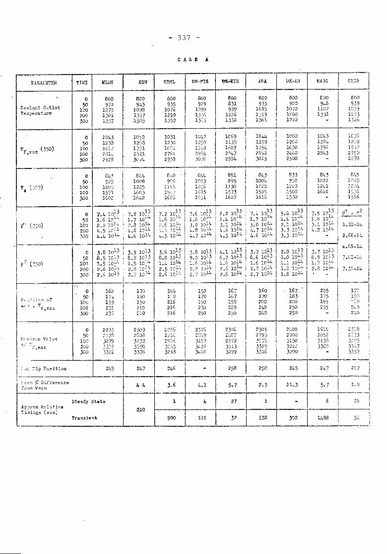
- 337 -
C J" 3 E A
rJ.RA1~ Tlv.3 cs!< C!lNL UK-Ll
CoollUlt OutlotTe::>!",,)'1l.t.'.lNl
-'_.-
o50
100200300
o50
100200300
800920
107513011337
101,3123$1(,[,72311.2923
BCO945
109813371385
105012G8175129213071~
800935
107612991352
1031123016[:127612953
BOO929
105013~01>::5
101,7J253114329S4YJ96
800831999
12361330
10691135ID072?472934
800935
10351)191;.61
104.4-1259175423:'23015
800900
10701;:001220
10CV120016)024402500
600943
11021333
10431231..171629J.)
800939
IGi112)3 I1;;;-6
:;.CS? I) 27215:;2 I2i'SJ I2670 I
!iI,i1
Ij
26
--I
21,7
...,- 0,"./J-0
2:3.33:::'53':/,7)-'157
,(.1 ~ (1'2 II1.23+14 I
I2.6E+14 I
i4.6S+U !7.C~;...::'J;. i
iI.
7.:;.:::.1.+ I17-)-'1::n Ii-; ()
:!!,Cl I2-'.,0 i
1
6
247
2051751952~:~
III
- II
1488
843102012U1610
1642JS-J;,l}3330:'
21+5
-.167.183200250250
?-'+Oo2900;'15032203200
11.3
8339r~./"
12(;')15C/O15.'.0
1
16017020024021+0
1~
230527933~7S33293316
843100412201535161::;
3 •., 10138.6 10131.6 10U.2.7 10142.7 10U.
..... ' ,...-L.i.-v,
237233::'33299
I,
3:'
16-;'167188229250
5.7
851895 J
113015731607
4.1
4
1»170) 90230250
110
841,1(':)31~~;?616151651
3.8 10139.0 10131.6 )0142.3 lOll,2.7 JOll•
1
u.8FG216211;216
32:',53293
2:'362734
8!;D9~G
11~'5l'".L-i160(;
3.*5 101~8.0 101)1.4 10U.2.5 10"42.6 lO"J.
8l;l~1008122516031hl.2
3.8 1013 3.9 10136.5 1013 8.9 1013l.5 loll, 1.5 lOll.2.6 )e:l• I 2.8 )0,1,.2.6 1015 I 2.7 1014
f--
o50
100200:'>-'Xl
-_ ..-o
50100200}.:I 0
o50
100200300
4-4
210
,0 162 lYJ50 1f'. 190
100 1)9 190200 231 210300 236 ZlO
o 2?33~;iJ950 2(78 280310C 3079 3132
~ ~~~; I ~~~
21,9 I 247
Ste!ldy State
1'ransio'lt
}~I.XJ ~,'JC Vclu~C~. '1'1' ,8'..8X
--
Ar~'rox Rehtive~i~ine3 (8~C;
L.! 1,- •
I (' ()50)
~.-III'" (~;,O)
I~--I
, y{ :...i_~lcn 0::"
I j ",J. Tip Po~ition
1---! ~'~fl.n ~ Differenco
f':"'O::J:I ~ec.n
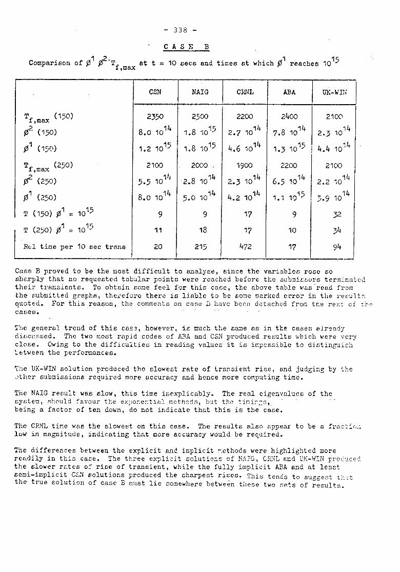
- 338 -
CASE B
Comparison of ~1 ~.Tf at t = 10 secs and times at which ~1 reaches 1015,max
CSN NAIG CRNL ABA UK-Wm
Tf (150) 2350 2500 2200 2400 2100,max
~ (150) 8.0 1014 1.8 1015 2.7 1014 7.8 1014 2.3 1014
~1 (150) 1.2 1015 1.8 1015 4.6 1014 1.3 1015 4.4 1014
Tf (250) 2100 2000 . 1900 2200 2100,max
~ (250) 5.5 1011t .2.8 1014 2.3 1014 6.5 1014 2.2 1014
911 (250) 8.0 1014 5.0 1014 4.2 1014 1.1 10~5I ;;.9 1014
T (150) .01= 1015 9 9 17 9 32
T (250) ~1 = 1015 11 18 17 10 34ReI time per 10 see trans I 20 215 472 17 94
Case B proved to be the most difficult to analyce, since the var~ables rose sosh~rply that no requested tabular points were reached before the 6ub~ic50r6 ter~inatedtheir transients. To ohtain 6o~e feel for this case, the above table was'read fromthe r:ubmitted graphs, thf::ceforethere is liable to be some marked croror in the rerJlt G
quot~d. For this.reason, the comments on case B have been detached from the rest of t~~caDes.
The general trend of this caE~, however, il;:t:mch the 6nme as in the cases elread:rdibCl!sscd. T11e two mOGt rapid codes of ABA and CSN produced reblllts \>'l::ich~ere veryclose. Owing to the difficulties in reading values it is impossible to distinguic~~~twepn t~e performances.
The UK-WIN solution produced the slowest rate of t.ransi.entrise, and judging by the.)ther submissions required more uccuracy aI!d hence more computing time.
Tile NAIG result was slow, this time inexplicably. The real eigenvalues of thesY6tem, !Should favour the ex;)onential methods, but the tini:--:::s,being a facto~ of ten down, do not indicate that this is the case.
The CP.NL time wa6 the slowe13t on this case. The results also appeat. to be a frac:i(,.~low in magnituue, indicating that Clore accuracy ....ould be required.
The differences between the explicit and implicit :.ethods were highlighted Clorereadily i.n this cace. T:J.eth~ee e)..-pliGit solutio:::!:::of !'lAW, CP":~Land t!K-W:!:Npro'.:'-lcr.'clthe slower rates 0: rise of transient, while the fully implicit ABA and at leastsemi-implicit C~~ solutions produced the sharpest rises. ~his tends to suggeGt t::~tthe true solution of case B must lie somewhere between t;lese two sets of results.
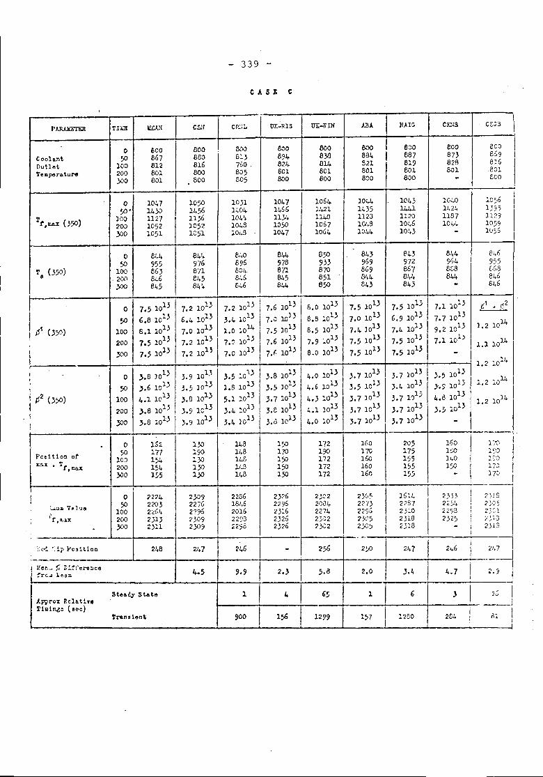
- 339 -
CASE C
CoolG.1ltOutletTe"porature
THE
o50
100200)00
o50"
100200)00
o50
100- 200
YJO
o50
100200}JO
o50
100200
})O
600867812801801
104714)0112710521051
841.955863846845
7.5 10136.8 10138.1 10137.5 10137.5 1013
-'.8 J.013
-,.6 10134.1 1013-'.8 1013
}.8 1013
CS:l
800880816800800
1050145611;.610521051
84'.9768-{l84584!t
7.2 10136.4 10137.0 10137.2 10137.2 101}
3.9 10133.5 1013,.8 10133.9 10133.9 1013
cn;:L
tx">J13137{,0.805805
10311404104',1048~Ol..'l
7.2 1013
3.4 1013
1.0 10l1,7.': 1013
7.0 1013
3.5 10131.B 1013
5.1 10133.4 :013
3.4 1013
I OT.-RIS
800894821.601800
104714.5611.)1,10501047
8W.9788n6458W.
7.6 101317.0 1013
7.5 10137.6 10137.r- 1013
3.8 10133.5 10133.7 ::'0133.e 1013
3.8 1013
6008313814801800
106411,21114010671064
850933870851850
6.0 1013
8.8 1013B.5 1013
7.9 :"013
8.0 1013
4.0 10134.6 10134.3 10134.1 10134.0 1013
ABA
llOO884-S21801800
lOW.14351123lOL.81044
B4396986981,4843
7.5 10137.0 10137.4- 1013
7.5 10137.5 1013
3.710133.5 10133.7 1013
3.7 10133.71013
NAIr;
800087819801800
101,3l44.l11201046104)
e4397286781,1.843
7.5 10136.9 10137.4 10137.5 10137.5 1013
3.71013I
3.4 10133.7 1,,1,5
3.7 ::'0133.71013
CEll3
800873828801
IG4D142411871041.
844-91)48Ul8W.
7.1 10137.7 10139.2 10137.1 101)
3.5 10137.~ 1013
4.8 10133.; 1013
C:::~B
eco£~98~6EClleoo
10:;-5153511291059I1J5~
1.2 10l1,
1.1 1014
I 1.2 1014
II Pcet tiO!! orI I:SX • Tr,ma%
1
I.-;:.u. V'.1'-l8
i'r,lE...1x
'::~ ':i:;> Position
! 1!et._ ~ Di~rerene8frc..J }.;ean
J,.pprox Rclllti1'8Th,in.es (see)
o 15~50 177
10:> 1)!.200 154)00 155
o 222450 2203
100 2:<GI.200 2}13}JO ua
248
Steady Stat/!
Transient
1}J1901)01)01.30
2)092276229023C'92)09
247
14311,814811.8148
2286181,620162293,298
1
900
150170150150150
23262295231623262326
4.
156
172190172172172
23::'22Cil4227423:>22)02
! 5.3
I 65
r-~299
16017'G160160160
230522/322~';2}J52)OJ
2.0
1
157
2051751551;'5155
1611,22S-'231023182)18
I
6
::'280
160EO1401';0
2;,3322)1,22532325
4.7
3
261.
I 'Ii
1-;':>l:,'"J!~0
I17J17:' I
I ~;-I2:;052;.;:,1
I"' ,- ~ ,L ..11.-:.>
2313
I 21>71-L__~I 2.7 I,I LC I. J
! in I, I
J
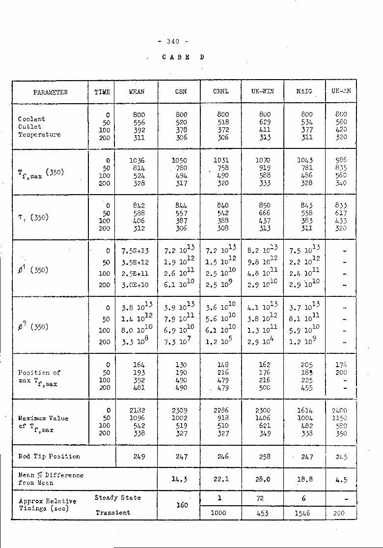
- 340 -
CASE D
PARA1fETER TIME 1lF..AN CSN CRNL UK-i'I'IN N.HG- UK~~':.N
-Coola.nt 0 800 800 800 8uO 800 800
50 556 520 518 629 534 580Outlet 100 392 378 372 411 377 420Temperature 200 311 .306 .306 313 311 320
0 10}6 1050 1031 10('0 1043 986Tf ,n:ax (350) 50 814 .780 758 919 781 835
100 524 494 490 588 486 560200 328 317 320 333 328 340
0 842 844 840 850 843 833T (350) 50 588 557 542 666 558 617
s 100 406 387 388 437 383 433200 312 306 308 313 311 320
- <.
0 7.5E+13 7.2 1013 7.2 1013 8.2 10:3 7.5 1013 -50 3.5E-t12 1.9 1012 1.5 1012 9.8 1012 2.2 1012 -
~1 (350) 100 2.5E+11 2.6 lOll 2.5 1010 4.8 lOll 112.4 10 -200 3.0E+I0 6.1 1010 2.5 109 2.9 1010 2.9 .1010 -
0 3.8 1013 3.9 1013 3.6 1010 4.1 1013 3.7 1013 -50 1.4 1012 7.9 loll 5.6 1010 3.8 1012 8.1 lOll -')
f;- (350) 100 8.0 1010 6.9 1010 6.1 1010 1.3 loll 5.9 1010 -200 3.3 108 7.3 107 1.2 105 2.9 104 1.2 109 -
J
0 164 1;<) 148 162 205 -~nPosition of 50 193 190 216 176 18' 2COmaxT 100 352 490 479 216 225f,max 200 481 490 479 50C 455 -
.1
0 2132 2309 2286 2300 1614 2480Maximum Value 50 1096 1002 918 1406 1004 115')of Tf 100 542 519 510 621 482 ~SO, IDa X 200 338 327 327 349 333 350
Bod T;.p Position 249 247 246 258 247 245
Mean % Difference 14.3 22.1 28.0 18.8 4.5from Mean 4
Approx Relative Steady State 1 72 6 -Timings (see) 160 I
Transient 1000 453 1546 I 2CO j
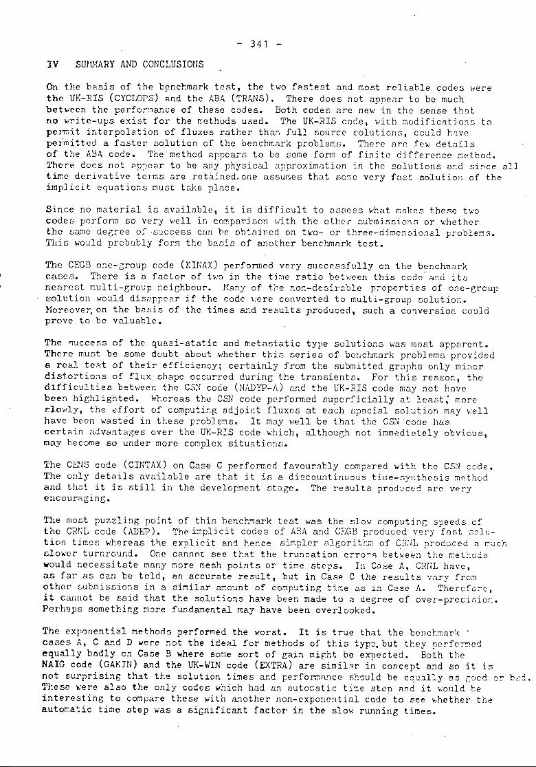
- 341 -
IV SmmARY AND CONCLUSIONS
On the basis of the b~nchmark test, the two fastest ond most reliable codes werethe UK-RIS (CYCLOPS) ;:md the fillA(TRANS). There does not appen.r to be muchbetween the perfoT::Janceof these codes. Both codes are new in the sense thatno write-ups exist for the methods used. The UK-RIS code, with ~odifications topel~it interpolation of fluxes rather tha~ full source solutions, could h~vepermitted a faster solution of the benchmark problems. There Clrc few detnilsof the ABA code. The method Clppcars to be some form of finite difference r.;ethod.'l'heredocs not ap:-;carto be any physical 3lJproxir.w,tionin the solutions and si!'ce alltime derivative terms are retained. one assumes that so::.every fast solution of theimplicit equations must take place.
Since no material is available, it is difficult to assess what rnnkes these twocodes perform so very \o.'ellin comparison \,:iththe otber sucmission" or \o.'hetherthe snme degree of success can Qe obtained on t ....o- or three-dimensional problems.Tlli.swould probCibly form the basis of another benchmark test.
The CEGB one-Group code (KINAX) performed very successfully on the benchmarkcases. There is a factor of two in the time ratio between this code'a~d itsnearest multi-group neighbour. Many of the non-desirable properties of one-groupsolution would disuppear if the code were converted to multi-group solution.Horeover, on the babis of the times and results produced. such a cO'1version couldprove to be valuable.
The ~ucceSG of the quasi-static and metastatic type solutions was most aj:'parent.There must be some doubt about \-,'hetherthiG series of benchmark problems provideda real teRt of their efficiency; certainly from the submitted gr~phs only mi~ordisto~tio~s of flux shape occurred during the transients. For this reason, thedifficu~.ties between the CS~ code (NADYP-A) and the UK-RIS code may not h11vebeen highlighted. 'tihereasthe CSN code performed superficially at le;:wt,'moreclowly. the €ffort of computing adjoint fluxes at each spacial solation may wellhave been wasted in these problems. It may vlell be that the CS1~code hCiS
certain advantages over the UK-R~S code \o.'hich,although not immediately obvious,may become so under more co~plex situations.
The CEtiS code (CINTAX) on Case C performed favourably cOr:1paredwith the CSl'-Icode.The only details available are that it is a discountinuous time-[)Yl:thesismethodand that it is still in the development stage. The results produced are veryencourrtgint;.
The most puzzling point of this bencr~'1arktest was the slow computi!1C speeds ofthe CRNL code (ADE?). The irr.plicitcodes of ABA a:ld CEGB produced very fast 301u-tion times whereas tl1eexplicit and hence simpler algoritr~";1of ~R:iL produced a TCClCh
slo~er turnround. One cannnt see that the truncation erro~s betwee!1 the ~ethGds....ould necessi tate marlY more mesh points or ti~e sters. In Case A, CmiL h;;ve.as far as can be told, an accurate result, but in Case C the results V<lry fro:!]other subrissions in a similar ar.ount of computing ti:!1eas i~ Cesc A. Thercfo~0,it cannot be said tllat the solutions have been made to a degree of over-precisio~.Perh~ps something more funda";1entalmay have been overlooked.
The exponential methoos p~rforMed the worst. It is true that the benct~ar~ .CB.ses A, C and D ....are :lot the ideal for methods of this typ:-,but they perfomedequally badly on Cane B where some sort of gain might be expected. Both theNAIG code (GAKIH) and the UK-WIN code (EXTRA) are simil"'r in concept and so it isnot surprising th~t the solution times and perfo~nnce should be cqu~lly DS rood or bo:~.These ~erc also the only codes which had an auto~alic ti'1estep And it ~ould beinteresting to cOr.1!Jarethese wHh a.'1othernon-expone:ltial code to see .,hether th~auto~atic time step was a siGnificant factor in the slo.: running times.

- 342 -
The analogue conputer, UK-.~, p!'Ovided an a.lternative slant to the methods ofsolution. Horrever, with the increase in size end coorlexity of reactormodelling it is unlikely that t~ size of the analogue co~puter would be ebleto cope on its own. The a.nswer to this problem could lie in hybric1 computa-tion.
The benchma:d: submissions did not give a.ny clear cut sign of which of thevarious classes of method is to be rreferred. Of the two most fa.voured, one1m3 quasi-static end the other finito difference (essu[iled). On average theflux shape methods perforr.:od better than the finite di:fft:t"cnce techniques, wbichmay be so~e indication that the more analytic type of me~hod3 are advantageous.
30 May 1974
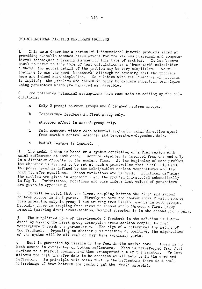
- 343 -
ONE-DIJ.rENSION.AL KINETICS BENCEMARK PROBLEMS
1 This note describes a series "of l-di~ensional kinetic problems ai~ed atprovidinG suitable testbed calculations for the various numerical and computa-tional techniques currently in use for this type of problem. It has becomeusual to refer to this type of test calc~ation ns a 'b~nchmark' calculational though the actual detail of tb.e problem may be very simplified. vre willcontinue to use the word 'benchmark' although recognising that the problerrshere are ind.eeo.much simplified. No relation with real reactors or proble:::J~.is implied; the problems are chosen in order to explore llUDerical techniquesusing paramete~s which are regarded as plausible.
2 The following principal assumptions have been made in setting up the cal-culations:
a Only 2 prompt neutron groups and 6 delayed neutron groups.
b Temperature feedback in first group only.
c Absorber effect in second group only.
d Data' constant within each material region in ~xial direction apartfrom movable control absorber and temperatu~e-dependent data.
e Radial leakage is ignored.
3 ~'he model chosen is based on a system consisting of a fuel regior. Tlithaxial reflectors nt both ends. Control absorber i.3 inserted from one end onlyin a. direction opposite to the coolant flow. At the beginning of each probler:lthe absorber i3 assurr.edto be set at such a penetration that k-cff = 1.0 andthe po';'Terlevel is defined by the inlet/outlet coolant teoperatures and. thehc~t transfer equations. Xenon variations are ignored. Equations definingthe probleo are given in Appeno.ix 1 and the probleo illustr~ted schematicallyin Fig 1. Definitions, notations and case independent v~lucs of para~etergare given in Appendix 2.
4 It will be noted that the direct coupling between the fj~st and secondneutron groups is in 2 parts. Firstly we have the conventional fission sourceterm appearing only in group I but arising from fission events in bottl groups.Seco-::d1ythere is coupling fron first to second group through a fj.rst erolJPrecoval (slowing down) cross-section. Control absorber is in the second ~'oup culy.
5 The si~plified form of time-dependent feedback in the solution is int~.o-duced by having the first group absorption cross-section coupled to fuelte~perature thro~5h the parameter a. The sign of a determine~ the nature ofthe feedback. DC"pending on whether a is negative or positive, the eigenvaL:e:::of the system will be all real or may have imaginary parts.
6 Heat is ger.erated by fission in the fuel in the active corcj "there is ~oheat source in either top or bottom reflectors. Heat is transferred fro~ fuelsurface to e. perfect coolant and then tr8r.srorted out of the n~:lctcr. Vfe f...'1veallo71ed the heat transfer data to be consta.nt at all heiehts in the core e.nd.reflector. In principle this ceans that in the reflectors there is a s;;;allinterchange of heat between the coolant Q.nd the 'fuel' material.
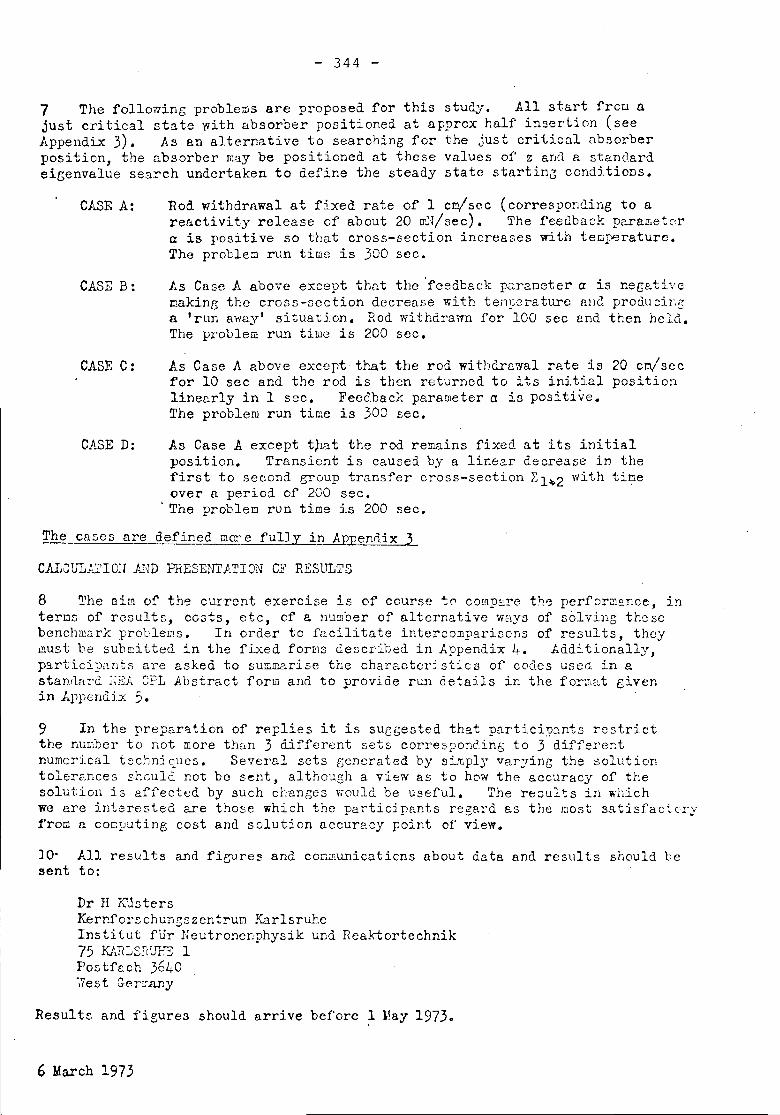
- 344 -
7 The folloning problems are proposed for this stu~. All start frc~ njust critical state with absorber positioned at apprcx half insertion (seeAppendix 3). As an alternative to searching for the just critical absorberposition, the absorber may be positioned at these values of z &ncla. stanclardei8envalue search undertaken to define the steady state startin3 conditions.
CASE A:
CASE B:
CASE C:
Rod withdra.wal at fixed rate of 1 c~/scc (corresponding to areactivity release of about 20 rnN/sec) • The feedback pararr.etcra is positive so that cross-section increases with teru["3raturc.The procleo run time is 300 sec.
As Case A a.bove except that the 'feedback parancter a is neg~tivemaking the cross-section decrease with tem~>3rature and produ cir,sa trtm away' situation. Rod withdrawn for 100 sec and then held.The problem rQ~ time is 200 sec.
As Case A above except that the rod withdrawal rate is 20 cn! seefor 10 sec and the rod is then returned to its initial positionlinearly in 1 sec. Feedback parameter a is positiVe.The problem run time is 300 sec.
CASE D: As Case A except tpat the rod remains fixed at its initialposition. Transient is caused by a linear decrease in thefirst to second group transfer cross-section ~1~2 with ti~eover a period of 200 sec •
. The problem run time is 200 sec.
The cases are defined ma:.:e ful1y in Appendix 3
CALCULATIW .AND PRESENTATION OF RESULTS
8 The aim of the current exercise is of course tC' corrrp::crethe perform~nce, interms of results, cests, etc, of a nu:nber of alternative ways of solving thesebenchrear};: problems. In order to facilitate interco:nparisons of results, theyL'lUSt be subI!:;itted in the fixed fon~3 described in Appendix Ih Additionally,ps.rticipants are asked to SUill..01?riECthe characteristics of codes used. in astanrlard ;;EA CPL J.bstract form and to provide run details in the format eivenin J.ppend.ix 5.
9 In the prepar~tion of replies it is suggested that particip~nts restrictthe nUL1bcrto not more th[ln 3 different sets correspond_ine; to 3 differentnumerical tec~nic:ues. Several sets generated by suply varying the ::.olutiontoler~Dces shGulc not be sent, altho~gh a view as to how the accuracy of thesolution is affected by such che.DGes would. be useful. The re3ults in whichwe are interested are thoE,e which the participants regard as the most s-'1.tisfac<,:cr;,'lfrom a cocputing cost and solution accuracy point of view.
]0- All results and figures and cOrlIEunicatiQns about data and results should besent to:
Dr H Kt1stersKerrSorschunsszent~un KarlsruheInstitut fUr Neutroncnphysik und Reaktortechnik75 K.UiLsnuJ-S 1Postfcch 3640.,7est Gerr:-.any
Resultz and figures should arrive before ,1 l~ay 1973.
6 March 197.3
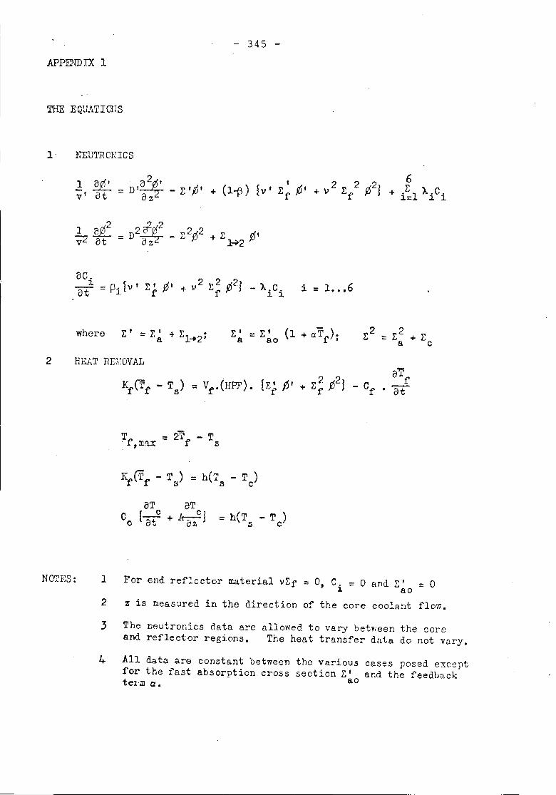
- 345 -APPENDIX 1
THE EQUNl'IOIIS
. aCi _p. fV' 1:' .i, + v2 ~2 ,,<21 _ A.C. i = 1 ••• 6ot - 1 ~ f 11 f P ~ 1.
1::' = 1::' (1 + aTf).,a ao2 HEAT RE1WVAL
a'TKfCTf - Ts) :;:Vf.(HPF). {l.;;J' + 1::~ ,02} - Cf • 0/
T = 2T - T.f ,max f 8
K (T - T ) = h(~ - T )r f B 8 C
aT aTc {a~C+~} = heT - T )c '" vZ S C
NOTES: 1 For end ref~cctor material vl::f = 0, C. = 0 and Z' = 01. ao
2 z is measured in the direction of the core coolant flow.
3 The neutrollics data are allowed to vary bet?ieen the coreand reflector regions. The heat transfer data do not vary.
4 All data are constant between the various cases posed exceptfor the fast absorption cross section Z' and the feedoacktel.J) Cl. ao
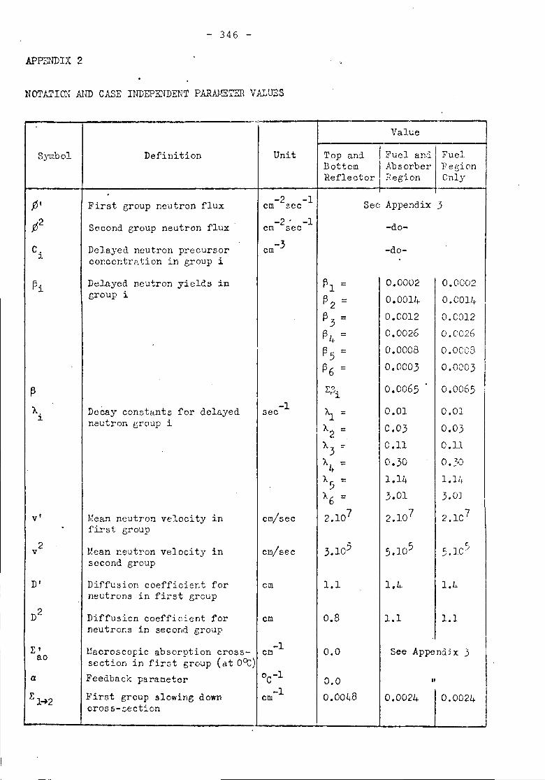
- 346 -
APP-&IDIX 2
NOTATlm AND CASE INDEPENDENT PAR.A1,!ETER V.A1UZS
Value lSymbol Definition Unit Top and
BottomReflector
Fuel and.Absorbernegion
FuelRegionOnly
C.~
First group neutron flux
Second group neutron flux
Delayed neutron precursorconcentration in group i
-2 -1em see-2' -1em see
See Appendix 3
-do-
-do-
See .Appendj x .3
f:li
V'
2v
D'
E Iaoa
Delayed neutron yields ingroup i
DeCay constants for delayedneutron group i
I,rean neutron velocity infirst group
Uean neutron velocity insecond group
Diffusion coefficient forneutrons in first group
Diffusion coefficient forneutrons in second group
Haeroseopie absorption cross-section in first group (at oct)Feedback parameterFirst group slowing downcross-::;eetion
-1see
em/see
em/see
em
em
-1el!l
o -1C-1cm
~l ::
(32 ::
(33 ::
(34 ::
(35 ::
136 ::l:f3.~
'1=i "2 ::
A3 ="4 ::).. ~ ::
:J
"6 ::
2.107
1.1
0.8
0.0
0,0
0.001;.8
0.0002O.OOlh0.00120.00260.00080.0003
0.0065
0.010.030.110.301.143.01
2.107
1.1
0.0024"
0.00020.00140.00120.00260.00030.0003
0.0065
0.010.030.11
0.301.1h
3.0J
2.107
1.1..
1.1
0.0024
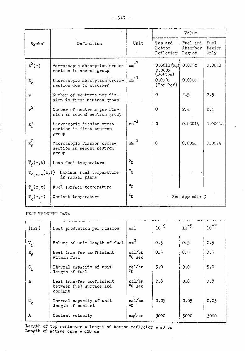
- 347 -
Value.
Symbol Definition Unit Top and Fuel and FuelBottom Absorber ReeionReflector Region Only
}:2( z) Macroscopic absorption cross- -1O.COII ~br)1 0.0050 0.0041em
section in second group 0.0002-1
(Bottom)}: Macroscopic absorption cross- em 0.0009 0.0009c section due to absorber (Top Ref).VI N~ber of neutrons per fis- 0 2.5 2.5
sion in first neutron groupv2 Nwnber of neutrons ~er fis- 0 2.4 2.4
sion in second neutron grcup
E' Macroscopic fission cross- -1 0 0.00014 0.00014emf section in first neutroni group
i:2 Macroscopic fission cross- -1 0 0.0024 0.0024emf section in second neutron
group
Tf( z,t) Mean fuel tem:?erature "c
Tf max(z,t) t:aximum fuel tCl.lperature °c ., in radial planeIT (zrt) }'uel surface teITIperature °cs
Tc(z,t) Coolant temperature °c See Appendix .:;.
HEAT 'TRAHSFER DATA
I
i (HPF) Heat production per fission cal 10-9 10-9 10-9
I .I Volume of unit length of fuel cm2 0.5 0.5 0.5. Vf II K
f Heat transfer coefficient cal/cm 0.5 0.5 0.5 Iwithin fuel °c see
II
Cf Thermal capacity of unit cal/cm 9.0 9.0 9.0length of fuel °c
h Heat transre~ coefficient ! cal/cM ' 0.8 0.8 0.8between fuel surface and °c seecoolant
C Ther~al capacity of unit cal/em 0.05 0.05 0.05c length of coolant OC
A Coolant velocity em/see 3000 3000 .3000
Length of top reflector = leneth of bottom refl~ctor = 40 emLength of active core = 420 em
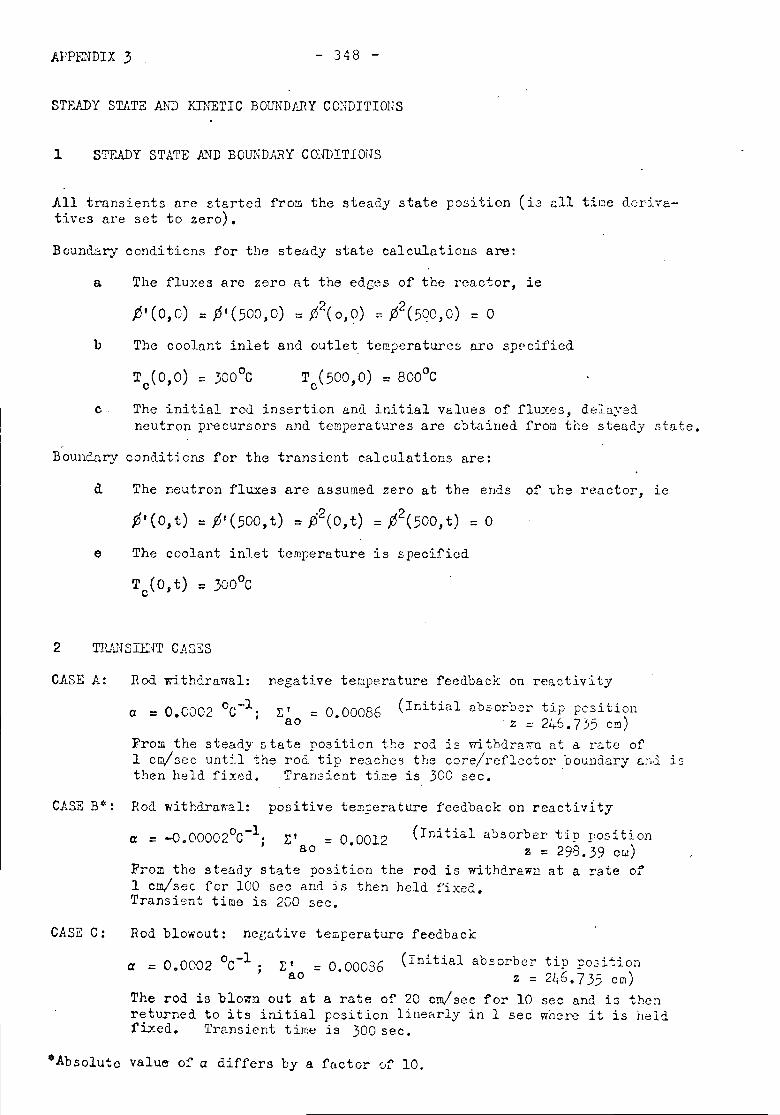
APPENDIX 3 - 348 -
STEADY STATE AND KINETIC BOUNDARY CWDITIOliS
1 STEADY STATE .AND BOUNDA.1iYCOlIDITIOHS
All transients tlrc started from the steady state position (i3 c:l1time dr:;rive.-tive3 are set to zero).
Bound.ary conditions for the steady state calculations are:
a The fluxes are zero at the edGes of the reactor, ie
b The coolant inlet and outlet temperatures are specified
T (500,0) = BOOoCc
c The initial rod insertion and initial values of flu.;:es,delayed.neutron pl~cursors and temperatures are ob~.ined frow the steady state.
-Boundnry conditions for the transient calculations are:
d The neutron fluxes are assumed zero at the ends of ~he reactor, 1e
~'(O,t) = ~'(500,t) = ~2(0,t) = ~2(500,t) = 0
e The coolant inlet temperature is specifiod
2 THlJ-ISffirr CAS~S
CASE A: Rod withdrawal: pegative temperature feedback on reactivitya = 0.0002 °C-l; ~' = 0.00086 (Initial absorb~r tip pcsition
ao -z = 246.735 cm)
From the steady 5 tate position the rod is wi thdr2->n1at d. rde ofI em/see until the roel tip reaches the core/reflector boundary end. isthen held fixed. Transient ti~e is 300 sec.
CASE B*: Rod withdrar.al: positive te:nferature feedback on reactivitya = -o.00002oC-l. r' = 0.0012 (rnitia.l absorber tip :position
J ao z = 298.39 ew)From the steady state position the rod is withdrawn at a rate ofI em/see for 100 see anelis then held fixed.Transien~ time is 200 sec,
CASE C: Rod blowout: nebative te~perature feedback
r' = 0,00036ao(Initial absorber tip p03i:ion
z = 246. 7 35 e [)J )
The rod is blo~n out at a rate of 20 em/see for 10 see and i3 thenreturned to its initial position line8.rly in 1 see where it is heldfixed. Transient tirr:eis 300 see,
.Absolute value of a differs by a factor 0f 10.
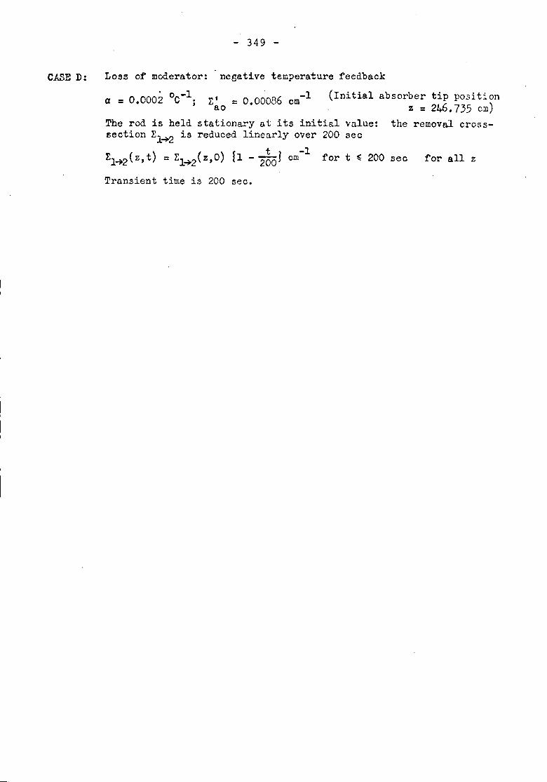
CASE D:
- 349 -
Loss of moderator: negative temperature feedback• 0 -1
a = 0.0002 C ; ~l = 0.00086 cm-lao
(Initial absorber tip positionz = 246.735 em)
The rod is held stationary at its initial value: the removal cross-section rl~2 is reduced linearly over 200 see
Transient time is 200 sec.
-1em for t ~ 200 sec for all z
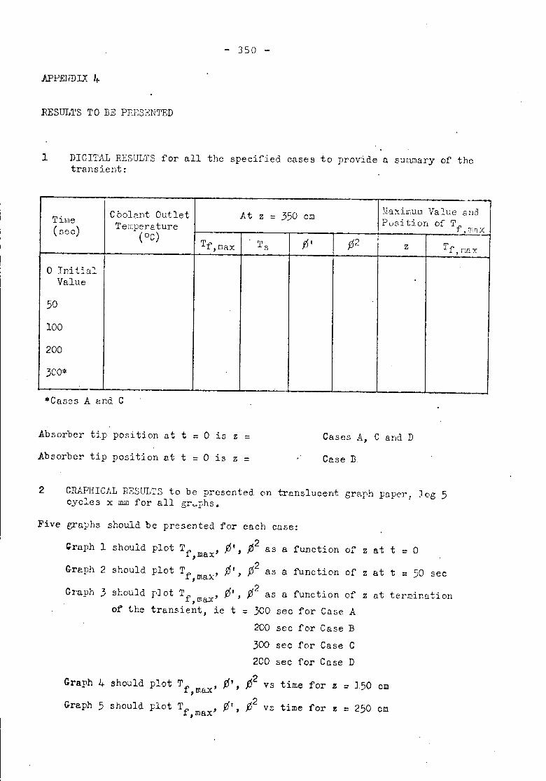
- 350 -
.APPEIIDlX 4
RESULTS TO BE PP.ESENTED
1 DIGIT/iL RESULTS for all the specified cases to provide a sU;:'1Hlaryof thetransient:
._-C aoIent Outlet At 350 MflximurnValue andTilne z = CD
P0si tion of T(sec) Temperature f-Jm'1~(°C) Tf,max Ts j5' >32 z Tf,rnn:x
0 TilltialValue
50
100
2003CO* .
•Cnses A and C
Absorber tip position at t = 0 is z =Absorber tip position at t = 0 is z =
Cases A, C and D
Case B
= 150 em= 250 em
2 GRAA{ICAL RESULTS to be presented on translucent graph paper: Jog 5cyc:es x mm for all gr~phs.
Five graphs should be presented for each case:(;.raph1 should plot T ;5' , ;52 as a function of' z at t = 0f,max'Greph 2 should plot '1' ~,, >32 as a function of z at t = 50 see-f,max'Graph 3 should plot T 15' , 152 as a function of z at terl!!inationf, max'
of the transient, ie t = 300 see for Case A200 see for Case B300 see for Case C200 see for Case D
Graph 4 should plot Tf ' ;5', ~2 vs time for z, ma.x
Greph 5 should plot T ~', ;52 vs time for zf,mex'
- 351 -
The scales to be used in these graphs are as follows:Abscissa - Time and space dimension
Time 10 mm E 20 see
Space 30 mID :: 100 cmOrdinate - Flux and Temperature
Flux lOll to 1016 over 5 cyclesTemperature 1 to 1050C over 5 cycles
NOTE: The accoopanying figures arc not meant to represent actual runsthey are for illustrative purposes only.
- 352 -
APPENDIX 5
RUN DETAILS
Participants nre asked to supply the following ip£orrnation concerning detailsof the individual co:nputer runs which form,the basis of their submittedresults:
1 DATA SPECIFICATIONGive det~ils of any respects in which the data used are necessarilydifferent from those specified. Hopefully zero return under this item.
2 STEADY STATE
a Give initial steady state eigenvalues for Cases A and B in term~of critical absorber penetration or eigenvalue (on v) for anabsorber tip position of
z = 246.735 (Case A)z = 298.39 (Case B)
NB: Because the temperature feedback term in Case A is positive(0.0002) and in Case B is negative (-0.00002), the steady statecondition will be different. This is reflected in the'different absorption ter:ns used and the different rod r~si-tions.
b state computer used and give cOQputer time for initial steadystate computation in terms of
CPU (see)I/O (see)
3 TRPj'iSIEi\"l'S
For each case provide the following details:
~PU tiffietaken (see)I/O ti~e taken (3ec)Core storage used (Kb, words etc)
4 COIr.FUTER PERFCR1.lP.lICE
Prcvi~e an es~i~~e of the performance of your computer relative to anIB)~ 370/165 COQI'U ter.
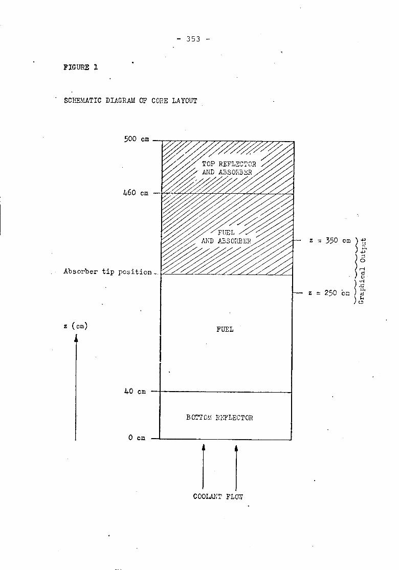
- 353 -
FIGURE 1
SCHEMATIC DIAGRAM OF CORE LAYOUT
500 em
460 em
Abso~ber tip position
z (em)
40 em
o em
FUEL
BOI'TOM RLFLECTOR
COOLANT FLOW
z = 350 em ~].
l;z = 250 co ~~
)~

- 355 -
CYCLOPS A Program for the solution of thefew group one dimensional neutron kinetics equations
with temperature feedback
By
D. E. BillingtonUKAEA Risley, England
December 1974
- 356 -
CONTENTS
1. Introduction
2. Method of Calculation
3. Results
4. Discussion
5. References
6. Tables
Figures
Appendix 1: Derivation of Improved Quasi-staticEquations.
Appendix 2: Solution of the Amplitude FunctionEquations.
Appendix 3: Solution of the Spatial Function Equations
Appendix 4: Temperature Calculation and ReactivityFeedback.
Appendix 5: Notation
PAGE
1
1
2
3
4
5
10
16
27
38
41
- 357 -
1. Introduction
There has been a considerable effort at a number of national centresto produce efficient computer methods for the solution of kinetics problemsin nuclear power reactors where flux distortions in space and energy have asignificant effect on the course of a transient.
The Nuclear Energy Agency Committee on Reactor Physics has assembleda series of 'benchmark' problems and has invited workers in the field toattempt a solution. A review of the solutions to a series of one-dimensionalproblems has been provided by Sidell (Reference 3).
One such solution was obtained by use of the UK code CYCLOPS, whichwas originally conceived for use with thermal reactors although the methodof solution used is not so limited. This paper details the procedures usedin the code and demonstrates the effect on results and computing time ofvariations in the time steps used in the solution.
2. Method of Calculation
The method used is the improved quasi-static. The space, energy andtime dependent flux is decomposed into a spatial function in one dimensionand an amplitude function. The spatial function contains all the space andenergy dependence but only depends on time through spatial distortions,whilst the amplitude function contains most of the temporal dependence and isindependent of space and energy. The obvious advantage is that the grosstime behaviour is calculated on a point basis and the space and energydistortions, which occur on a longer time-scale, can be calculated lessfrequently.
The derivation of the equations governing the behaviour of these twofunctions is given in Appendix 1. The spatial function is the solution of aneigenvalue problem which includes a spatial function independent source termderiving from the time history of the delayed neutron precursors and alsofrom a backward-difference representation of the time derivative of thespatial function. The solution of this problem is performed in a speciallywritten module described in Appendix 3.
The amplitude function is the solution of the familiar point kineticsequations. These equations are solved by the piecewise polynomials methodwith collocation weighting. The method has been modified to improve theconditioning, particularly in the case of small time-steps and is describedin Appendix 2.
The steady-state calculation proceeds by iteration between evaluationof the steady-state spatial function (Appendix 3) and the steady-statetemperature distribution (Appendix 4) in order to obtain the specified coolanttemperature rise and to allow for temperature feedback onto the spatialfunction. This procedure is taken to convergence and the steady-state adjointspatial function calculation (Appendix 3) completes the initia1isation ofthe problem.
Over one amplitude function time-step the procedure is as follows. Anestimate of the amplitude function over the time-step is obtained by linearextrapolation from the previous time-step. This estimate is combined with thecurrent spatial function in the calculation of the local linear heat ratingover the spatial mesh and the temperatures at the end of the time-step arecalculated (Appendix 4). The effect on cross-sections of the change in mean
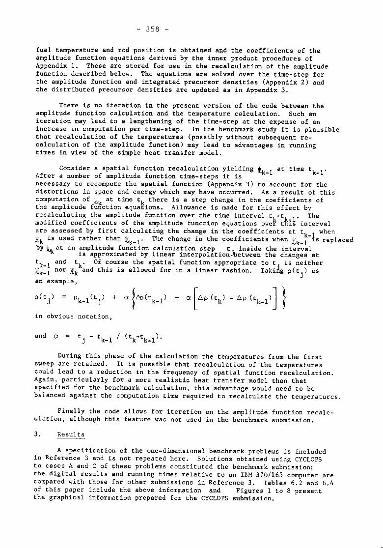
- 358 -
fuel temperature and rod position is obtained and the coefficients of theamplitude function equations derived by the inner product procedures ofAppendix 1. These are stored for use in the recalculation of the amplitudefunction described below. The equations are solved over the time-step forthe amplitude function and integrated precursor densities (Appendix 2) andthe distributed precursor densities are updated as in Appendix 3.
There is no iteration in the present version of the code between theamplitude function calculation and the temperature calculation. Such aniteration may lead to a lengthening of the time-step at the expense of anincrease in computaticn per time-step. In the benchmark study it is plausiblethat recalculation of the temperatures (possibly without subsequent re-calculation of the amplitude function) may lead to advantages in runningtimes in view of the simple heat transfer model.
Consider a spatial function recalculation yielding Ik-1 at time tk_1.After a number of amplitude function time-steps it isnecessary to recompute the spatial function (Appendix 3) to account for thedistortions in space and energy which may have occurred. As a result of thiscomputation of ~k at time tk there is a step change in the coefficients ofthe amplitude function equations. Allowance is made for this effect byrecalculating the amplitude function over the time interval tk-tk_1. Themodified coefficients of the amplitude function equations over this intervalare assessed by first calculating the change in the coefficients at tk_1 whenIk is used rather than Ik-1' The change in the coefficients when ~k-1 1S replacedby 114< at an amplitude function calculation step t ~ inside the interval
is approximated by linear interpo1ation~Detween the changes attk_1 and tk. Of course the spatial function appropriate to t
iis neither
Ik-1 nor Ik and this is allowed for in a linear fashion. Takirtg p(tj) as
an example,
p (t.)J
=
in obvious notation,
During this phase of the calculation the temperatures from the firstsweep are retained. It is possible that recalculation of the temperaturescould lead to a reduction in the frequency of spatial function recalculation.Again, particularly for a more realistic heat transfer model than thatspecified for the benchmark calculation, this advantage would need to bebalanced against the computation time required to recalculate the temperatures.
Finally the code allows for iteration on the amplitude function recalc-ulation, although this feature was not used in the benchmark submission.
3. Resul ts
A specification of the one-dimensional benchmark problems is includedin Reference 3 and is not repeated here. Solutions obtained using CYCLOPSto cases A and C of these problems constituted the benchmark submission;the digital results and running times relative to an IBM 370/165 computer arecompared with those for other submissions in Reference 3. Tables 6.2 and 6.4of this paper include the above information and Figures I to 8 presentthe graphical information prepared for the CYCLOPS submission.
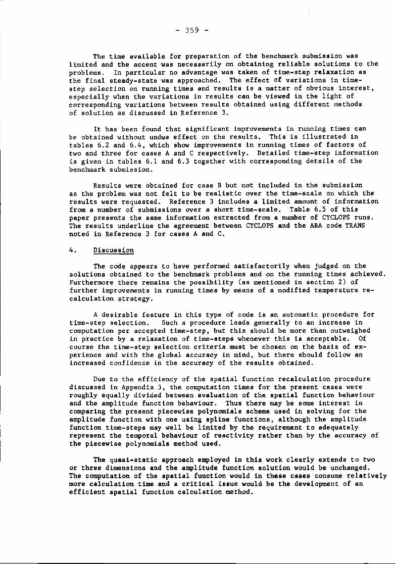
- 359 -
The time available for preparation of the benchmark submission waslimited and the accent was necessarily on obtaining reliable solutions to theproblems. In particular no advantage was taken of time-step relaxation asthe final steady-state was approached. The effect of variations in time-step selection on running times and results is a matter of obvious interest,especially when the variations in results can be viewed in the light ofcorresponding variations between results obtained using different methodsof solution as discussed in Reference 3.
It has been found that significant improvements in running times canbe obtained without undue effect on the results. This is illustrated intables 6.2 and 6.4, which show improvements in running times of factors oftwo and three for cases A and C respectively. Detailed time-step informationis given in tables 6.1 and 6.3 together with corresponding details of thebenchmark submission.
Results were obtained for case B but not included in the submissionas the problem was not felt to be realistic over the time-scale on which theresults were requested. Reference 3 includes a limited amount of informationfrom a number of submissions over a short time-scale. Table 6.5 of thispaper presents the same information extracted from a number of CYCLOPS runs.The results underline the agreement between CYCLOPS and the ABA code TRANSnoted in Reference 3 for cases A and C.
4. Discussion
The code appears to have performed satisfactorily when judged on thesolutions obtained to the benchmark problems and on the running times achieved.Furthermore there remains the possibility (as mentioned in section 2) offurther improvements in running times by means of a modified temperature re-calculation strategy.
A desirable feature in this type of code is an automatic procedure fortime-step selection. Such a procedure leads generally to an increase incomputation per accepted time-step, but this should be more than outweighedin practice by a relaxation of time-steps whenever this is acceptable. Ofcourse the time-step selection criteria must be chosen on the basis of ex-perience and with the global accuracy in mind, but there should follow anincreased confidence in the accuracy of the results obtained.
Due to the efficiency of the spatial function recalculation procedurediscussed in Appendix 3, the computation times for the present cases wereroughly equally divided between evaluation of the spatial function behaviourand the amplitude function behaviour. Thus there may be some interest incomparing the present piecewise polynomials scheme used in solving for theamplitude function with one using spline functions, although the amplitudefunction time-steps may well be limited by the requirement to adequatelyrepresent the temporal behaviour of reactivity rather than by the accuracy ofthe piecewise polynomials method used.
The quasi-static approach employed in this work clearly extends to twoor three dimensions and the amplitude function solution would be unchanged.The computation of the spatial function would in these cases consume relativelymore calculation time and a critical issue would be the development of anefficient spatial function calculation method.
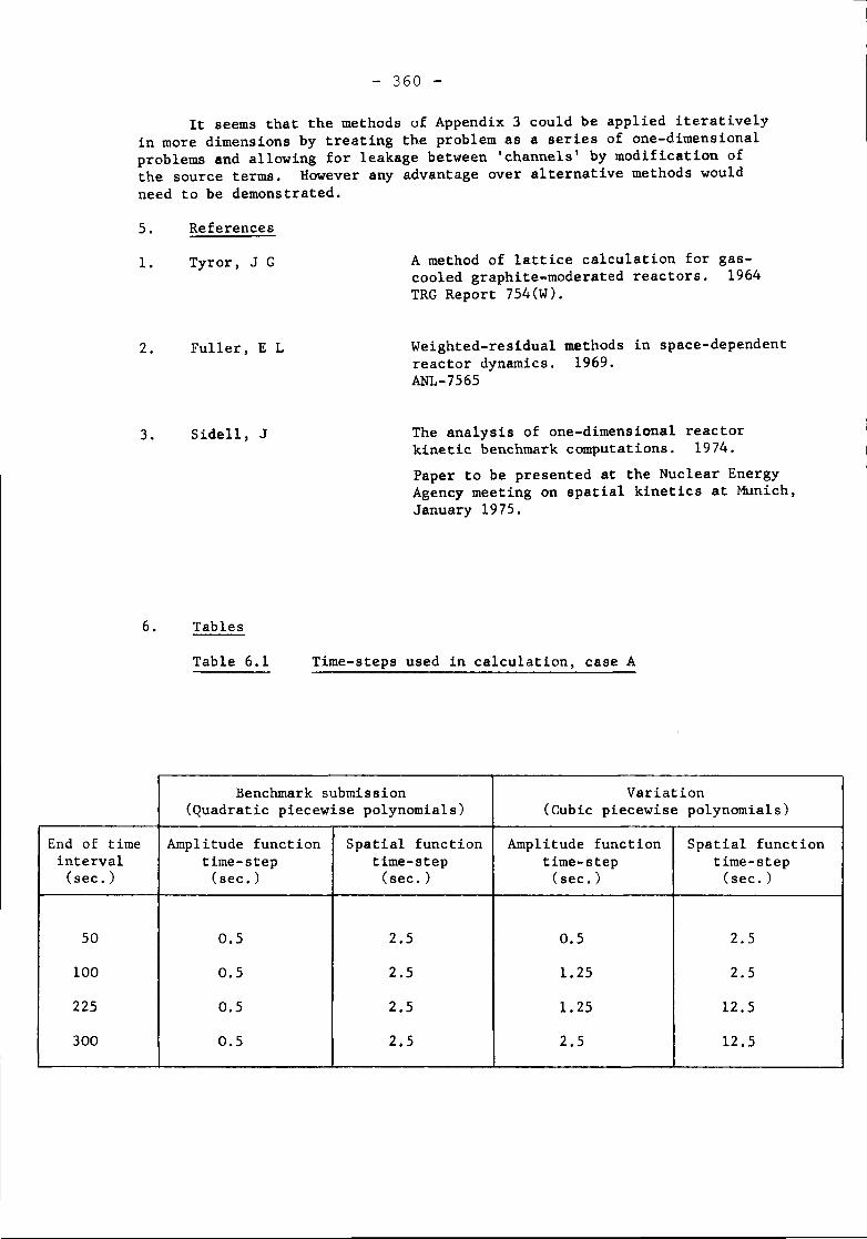
- 360 -
It seems that the methods of Appendix 3 could be applied iterativelyin more dimensions by treating the problem as a series of one-dimensionalproblems and allowing for leakage between 'channels' by modification ofthe source terms. However any advantage over alternative methods wouldneed to be demonstrated.
5. References
1.
2.
3.
Tyror, J G
Fuller, E L
Sidell, J
A method of lattice calculation for gas-cooled graphite-moderated reactors. 1964TRG Report 754(W).
Weighted-residual methods in space-dependentreactor dynamics. 1969.ANL-7565
The analysis of one-dimensional reactorkinetic benchmark computations. 1974.Paper to be presented at the Nuclear EnergyAgency meeting on spatial kinetics at Munich,January 1975.
6. Tables
Table 6.1 Time-steps used in calculation, case A
Benchmark submission Variation(Quadratic piecewise polynomials) (Cubic piecewise polynomials)
End of time Amplitude function Spatial function Amplitude function Spatial functioninterval time-step time-step time-step time-step
(sec.) (sec.) (sec.) (sec. ) (sec.)
50 0.5 2.5 0.5 2.5100 0.5 2.5 1.25 2.5225 0.5 2.5 1.25 12.5300 0.5 2.5 2.5 12.5
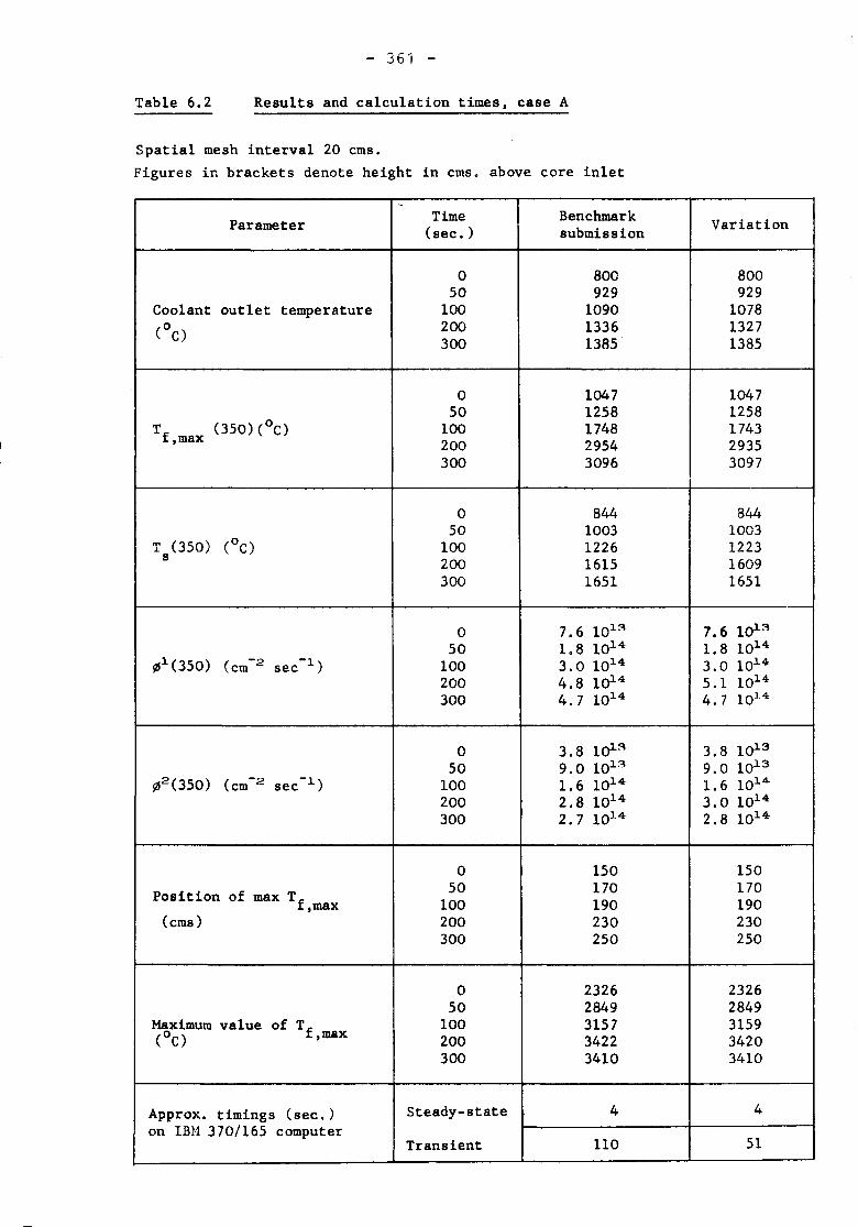
Table 6.2
- 361 -
Results and calculation times. case A
Spatial mesh interval 20 ems.Figures in brackets denote height in ems. above core inlet
-Parameter Time Benchmark Variation(sec. ) submission
0 800 80050 929 929
Coolant outlet temperature 100 1090 1078° 200 1336 1327( C) 300 1385 1385
0 1047 104750 1258 1258
T (350) (oC) 100 1748 1743f,max 200 2954 2935300 3096 3097
0 844 84450 1003 1003
T (350) (oC) 100 1226 1223s 200 1615 1609300 1651 1651
0 7.6 101::\ 7.6 101::\50 1.8 10.1.4 1. 8 10.1.4
l2S1(350) (cm-2 sec-.1.) 100 3.0 101.4 3.0 10.1.4200 4.8 lo.t4 5.1 1014300 4.7 10.1.4 4.7 1014
0 3.8 lo.t::\ 3.8 10.1.350 9.0 10.1.3 9.0 10.1.3
l2S2(350) (cm-2 sec-.1.) 100 1. 6 10.1.4 1.6 10.1.4
200 2.8 1014 3.0 10.1.4300 2.7 101.4 2.8 10.1.4
0 150 150Position of max Tf
50 170 170.max 100 190 190
(ems) 200 230 230300 250 250
0 2326 232650 2849 2849
Maximum value of Tf 100 3157 3159(oC) .max 200 3422 3420
300 3410 3410
Approx. timings (sec.) Steady-state 4 4on IBM 370/165 computer
Transient 110 51
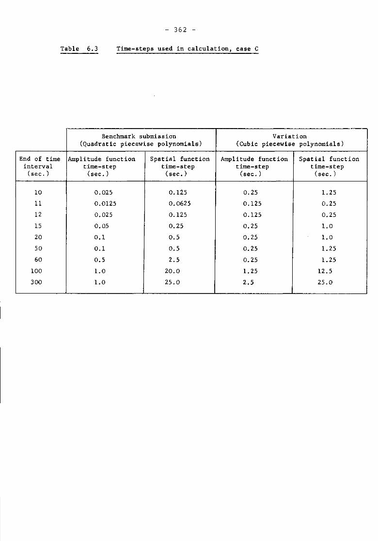
Table 6.3
- 362 -
Time-steps used in calculation. case C
Benchmark submission Variation(Quadratic piecewise polynomials) (Cubic piecewise polynomials)
End of time Amplitude function Spatial function Amplitude function Spatial functioninterval time-step time-step time-step time-step
(sec.) (sec. ) (sec.) (sec.) (sec.)
10 0.025 0.125 0.25 1.2511 0.0125 0.0625 0.125 0.2512 0.025 0.125 0.125 0.2515 0.05 0.25 0.25 1.020 0.1 0.5 0.25 1.050 0.1 0.5 0.25 1.2560 0.5 2.5 0.25 1.25
100 1.0 20.0 1.25 12.5300 1.0 25.0 2.5 25.0
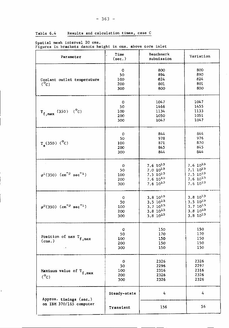
Table 6.4
- 363 -
Results and calculation times, case C
Spatial mesh interval 20 ems.Figures in brackets denote height in ems. above core inlet
Parameter - Time Benchmark Variation(sec.) submission
0 800 80050 894 890
Coolant outlet temperature 100 824 824(oC) 200 801 801
300 800 800
0 1047 104750 1466 1455
Tf (350) COC) 100 1134 1133,max 200 1050 1051300 1047 1047
0 844 84-450 978 976
T (350) (oC) 100 871 870s 200 845 845300 844 844
0 7.6 10~3 7.6 10~350 7.0 10~3 7.1 10~3
)Ill(350) (cm-2 sec-l) 100 7.5 1013 7.5 1013200 7.6 1013 7.6 1013300 7.6 1013 7.6 1013
0 3.8 1013 3.8 101350 3.5 1013 3.5 1013
)112(350)(cm-2 sec-l) 100 3.7 1013 3.7 10J.3
200 3.8 10J.3 3.8 10~3300 3.8 1013 3.8 lOl3
0 150 150Position of max Tf
50 170 170(ems.) ,max 100 150 150
200 150 150300 150 150
0 2326 2326SO 2296 2297
Maximum value of Tf 100 2316 2316(oC)
,max 200 2326 2326I300 2326 2326
Steady-state 4 4Approx. timings (sec.)on IBM 370/165 computer 156 56Transient
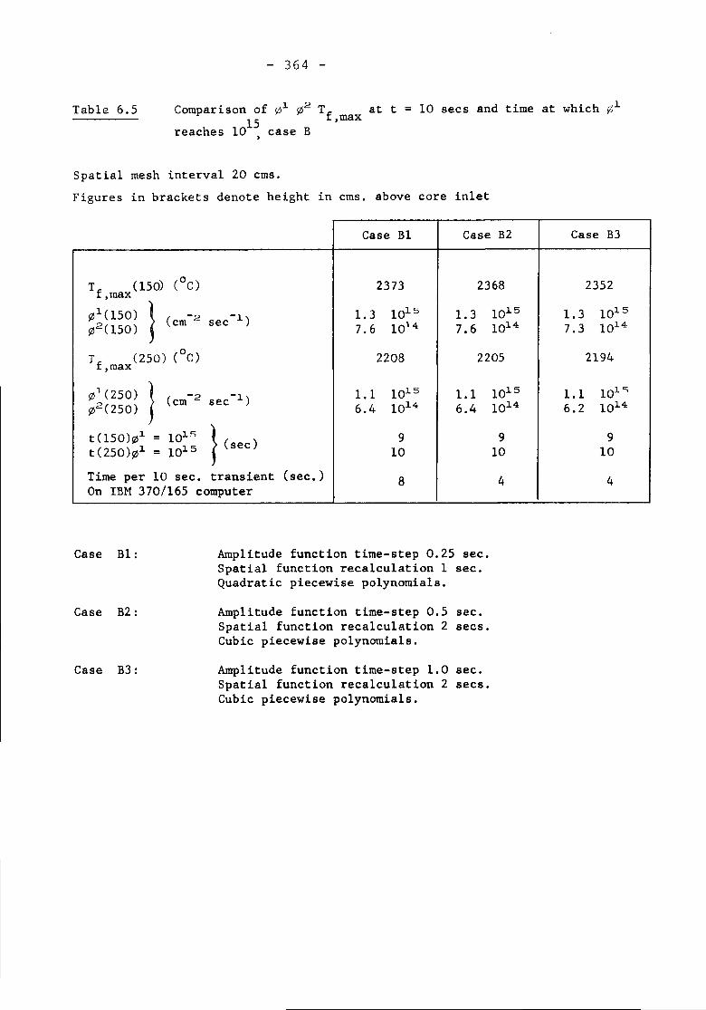
Table 6.5
- 364 -
Comparison of 01 ~2 Tf at t = 10 secs and time at which 01,max
reaches 1015 case B,
Spatial mesh interval 20 cms.Figures in brackets denote height in cms. above core inlet
Case Bl Case B2 Case B3
T (150) (oC) 2373 2368 2352f,max~1(l50) } (cm-2 sec-l) 1.3 1015 1.3 1015 1.3 1015~2(150) 7.6 10'4 7.6 1014 7.3 1014
Tf
(250) (oC) 2208 2205 2194,max
~'(250) } (cm-2 sec-l) 1.1 1015 1.1 1015 1.1 101c;
~2(250) 6.4 1014 6.4 1014 6.2 1014
t(150)~1 = 101" } (see) 9 9 9t(250)~1 = 1015 10 10 10Time per 10 sec. transient (sec.) 8 4 4On IBM 370/165 computer
Case Bl:
Case B2:
Case B3:
Amplitude function time-step 0.25 sec.Spatial function recalculation 1 sec.Quadratic piecewise polynomials.
Amplitude function time-step 0.5 sec.Spatial function recalculation 2 secs.Cubic piecewise polynomials.
Amplitude function time-step 1.0 sec.Spatial function recalculation 2 secs.Cubic piecewise polynomials.
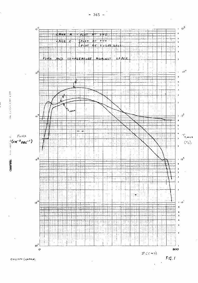
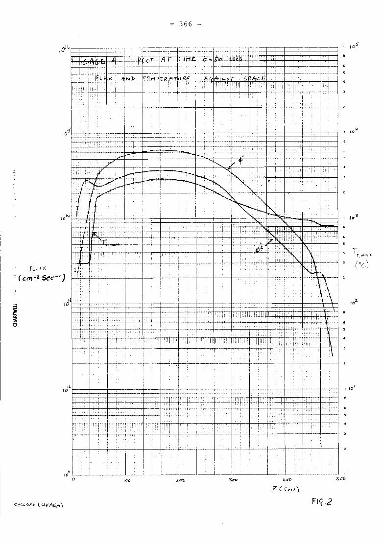
- 366 -
1 10'
4
.'
~--- I
SO'l>
6
II 1 1oJ.
, ,\
.,',"
~
.
. 1 1oS"
.
1
.--1-........,.---'-
I ij ..•.
II
10'",.
, ... ,
.., ,
'.
:t ,,' "',"" .... '; ,
.,
"':.
!t.
o ••••
, . "-'.' '.
--
, .
.
".: ::.:"
':": ""i': ::: : : ':
-:c-
,
.,
.
•
III
! ----
: "
•
.
.
::' ,I" "r ..
.
::',.:
:--c---T ......-,--c
II
I!
I.
, , i ' i I-~ 1---.
., :
. ,
I !---4.
100
I, rOoI' . .r-- -'-:-11
--""7--1-----.- -:- --_.
i
~--.---b:=-~-_-,,':~c::ci__.:.J :::::::::be: ~ .~.._,_~I, ,-': :::"::: i"::,": I" -. " : 'it" ..
--::"::
.
,-
, ! •. ' , '
I. "
'1': :
,'.'
'I
.
.. :.:. "..,
....
o
',it
'''i:, "
II:II
"10
Ii10
,2-iO
lOlL --:~~ +==-=-:t':-=--=f: :.--,-:=--+--=:::~=-,-:::--==~ -=t='::::-F> ,b!-~ ..tIn A"'" .'A=Y 'MJtI-_It-,,1 I"...:
......,.,.. ~ : T : I .
FL-~{X.::(em-I 5ec-' )
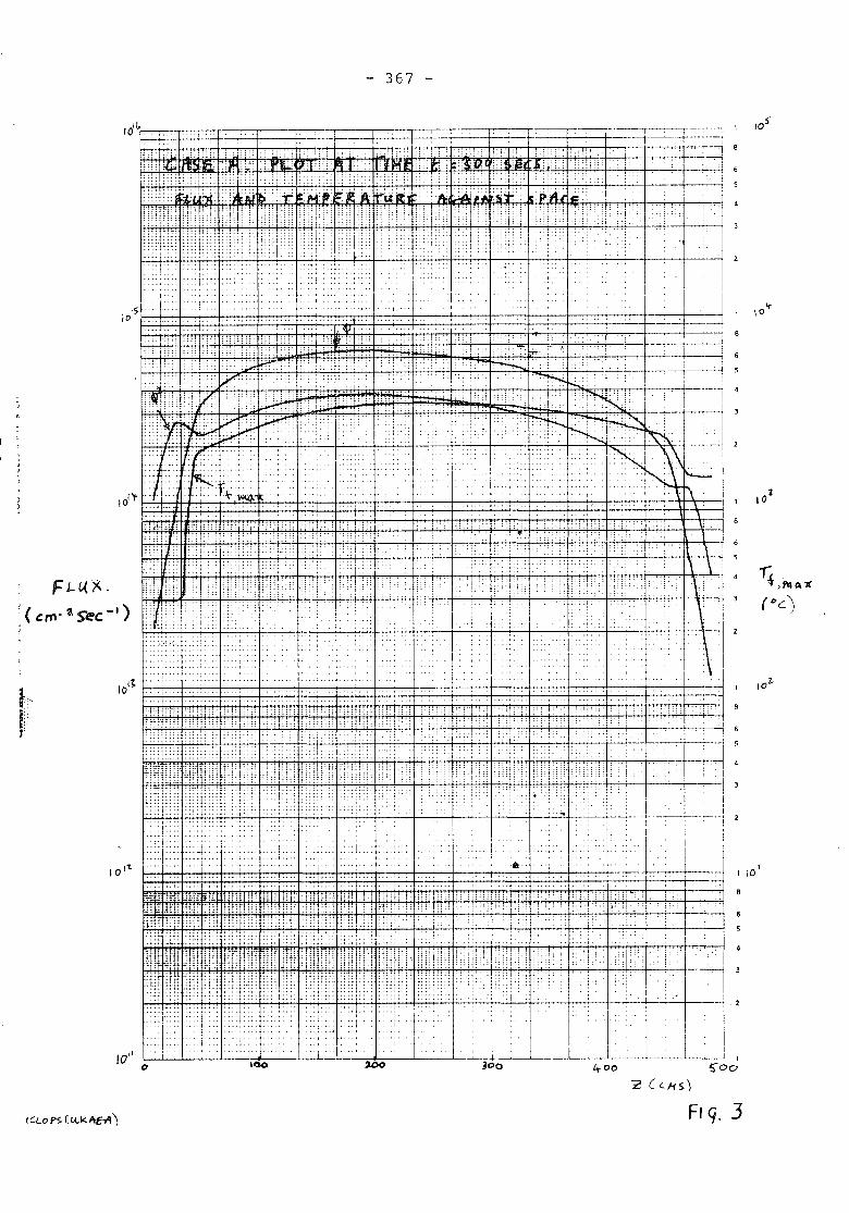
367
.
...
\0""
:~
.~ 4
: ,II 3
iI--'--j 2
iI
--
,Ii
. \'j,\ '
V-
.--~
---- +-,-
-'--
, .
:
. I "
::1:
.....
::" ','
.:: .... :'.I
, {..j,
!-~ .. ~._., --
..1
::
i"I
:
,
:
,:
:" ..!,'.,' i'!.". i'i, ", . :::' .
!'
. ..
. .
'f! :
, .
I,
: .
: I:
! i
,.:.
I':,
I ' ..I'
I I.:'
,,- .....
..
, iII
l:.,
'::::,:~~
, .
: : : ~ I : I : :
'~~&lii ..n: 'i !
... ,CCC
'-1" 'I': ,'" ':'
. f." ':::'
" '
: ..
'::
:.'
..
: ....
.: :
: : ::
I,' .:'::' I .. :
::i":::!::.
..,:.
'.
..
, I',
..'
I:'...
.. ,
! '
;'f',.i'
".:"::ii'.I'1:
::1 ' "::,' I:
:,' 1'1 ,..1 .: ',: ;;:,
... :
:[:
"
,
....
'I,
: .i
" I,'
.,
:.:'
, : I::: ::.::1:
::I .... : ..
. ': ':.......
"~I ,
,: j.,.~!
".: ! :l I :.,:! .
,", I
; np.t~J'~ i~Wl-' JJ:Tl; :PtJi>: :tJ~i!':;;;;; :i: .. ,.
:",~Ib:.,...~~bt" 'il +~~~::: I" ,II'" 'I"i
...
I
~!t
! .... .
:1:
:: I ::
:, i.'::i : ':: .:' : 1::.
n Hi! " " n:IH
:.ii'
l
: t :
: ~_i
i.
: : ".1'
Li:r: I
1,,: ."
;: i:~ti.;n... '{
: :1
\U :j
1510
1011.
FJ-(,{X.:( em' 2. See -I)
-:'.f'
.rmtH,: i I j.
:!:;1": ll:
J :i ".. ,..:'
I :: ! "f'
,I, '
,I ::
'I ":
I1
:1:::
i
' ...I
: :
;,
I: i i
lOti
1:1:, ,
io 100
II I
4-00
IQoPS (U.kPtEA') Flq. J
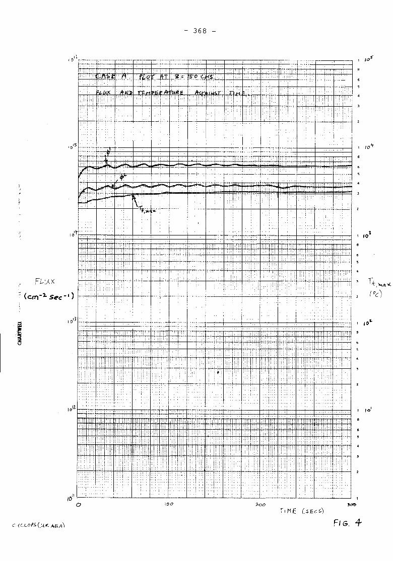
368
.._.. . . ...
' ..
..
.
i .
'I "'I'!
, ., :.'.
, i ; '. I ~ .
::.' .
.. ;
..
TI"':' ~::
>!:, ,i : 'i.'
.~ .. : .. ::.
i •:):
i'>. I
P/~ol!"' /!tT,'i:,. S"P(.iSj.'1 .
A.
...
~lri>, Ai~».
ii, >:', '!::':1
.
..
r)
1510
:CC' ,"'. .
"'1]>,,~ J..j"
~,"
-:-
.
.- ...
.,
, :j' , ~
i '
...
>.
.. :
"
i:
...
,
.
.. ,
"
:
1O't
. .
..
. .
..
..
'.:: ! :
;' I j:'
: .. '",
..
..
...
:1 :
.
••
:.:.,
I ...
',' ",'i,:
:.
ii' ,."t i
.. :,i ' I"~,
:1:
.. : .
!::::, .
' .., 'I, ,
'!' ,
", '':'
' ..
:1: ; i
':: .. i
.,
.....
:: .. I::,'
: ..
,,' , 'T ,!
II ili i
.'i
.
, ~;
I,
.'
:.:,".
....
'.
,. :
',i
,i,i :
..
.
','.'1>,";
": ,'": .,.
::: :::.. .. .
:",',.'
:: :
':
...
::,:1:
. ::TJ! :: I
, I
.. : ::
. " ''Ii' '
" .. ,' .::: .. ::... ::: ..
..
I
!',
..
..
1 ..
! .
Ii"
: :r~1
...IO't ..
. 1..i"CT
..TT
! I I:: : l
•i:
:.... ,-,
8Ii:
'T
...
I
3~
:1;, ....
'ii:' .
: :.. : i
: I: !
:::,!
/'I
..::
.. 11:.:
I...
: T ~ ; •• !: .: .; 'I:,
I I;,1:.:1:'
':i.:
Jt:
":::, ;
,) I'
ii,'I:.: :
,"
.. 01
..i I:;::
!
:1:!i! '
..., ,1.'1' "
" .L''!.. ,
'i::.i:,.:. I .
I
. , i'i.
... .
I'I:1: .
,,
!, '1: ,,' ; "...
100
I
: :t \PLi : i
, "T : i"::: ::
: :...
I: iI",
'I",'
j ~ 1 j t . I : t
Hi,!l!
i ':i.
I mnl, j,
"~i.
I::
FIG. +
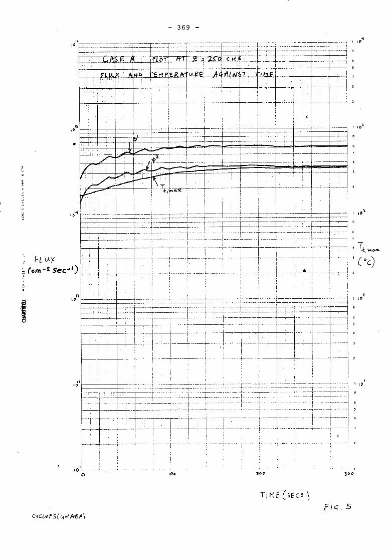
l~10 I
IS10
•
~u
~~
uu
<.J ''tS .0
.~.
..~
1110
.
..
.
.
.
- 369 -
1/10
I• !
TIME (SEcs.)
-- i
1 10'+
I ,~'\
.T:'1", """00 ....
t1 117
•1 10
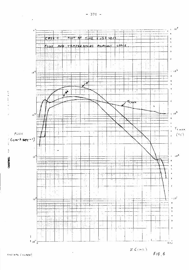
- 370 -
-----s.Pft( E.
". : .!
IO~
•••....
. I .
'i". ..
I .
10"
, 10 't
~-, 1 ,0
--_:
..
.---;- .. '
i! i
i:
..
:
.: II
, ..
" !'iT. : ..
". :
. ;;.
....", ,'1'
•••. t ••
.
.I ;-:-
I:
. : ..
......::;"1
'f,I
'.'J .'
:.,...,.- :
.".""•...•/7i 4f
.•::::/ I.,.....r-!- ~It.7".".IT
''1' J:.'10
I
-- __ ._ - ..~ _- .--- ."-- _- --"-"'-" -_ ..
10'
.... ::. I
! .. [.. ,,,
.:• !
I :
.' "
......I.
II
.... 1._-- __
I110
z {.(M '5)
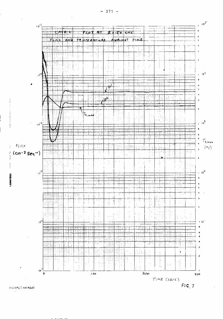
""' 371
10'"
--l~J! I
~..Ji 1
I iI
:: i'.
II
j!
:
, ;: ,
.
I
..
" ! ':.i' , ,
., R"
.. : ..::
"
., !
.- ...
..
I,
,:,
....
'l;.i;l'1" 'I:! I ' .......
:ic'" :f:ILUl1'i~j T1ll
..'cr \.:': ... I: :.. I.
t: ('\ '.!
, ,., 'i.,.
I1:\ ", ..
.... .
, 0'
\(,10
It
\1 ID
8
6
z..I 10
~\ 10
.'
: ..
, (""
'.
, .. '
,"
..,
"'C'
, I, '1'
" ..,>:::: ',' ~: " .
I ..
::,
.::.:':,,:.::
!
':
: ....
.
..
. '
:1 :
::.,..
:!:
.i
. : I,----[<I-'. I
:
'I.:',:
. ,
.,
,.T':'.
".'
..
....l--..:-I
Ii
'1iII
....
.
'.:
I: ~':"
, I i
,.i " 'i, .. :
':
...,,!::' ": !
. ., 'i'"i'
.
. ,
:: .::'::.: '
::.:
.','
.
I::
..I "Iii ..I'
:' "~,:
I
...
....! :
:::
I, "
~;
..... , " .... ..
... ::':11".., ! i r:!'
. :: :::-: .. :::;: II C
:[ :
..
.. ".
, .. !
. .I.
I::I.
:< '/:':1 .. "...,,::
i' iI' !i ,-
:.
I.X~: :::' .",
JU
I: ; ..
In!:
,~
10
FL-l,( I'
( em .:z SE'c -I )
"10o
,I
.1 ...... -f 00
TI ME (SEes.)
Fief 7
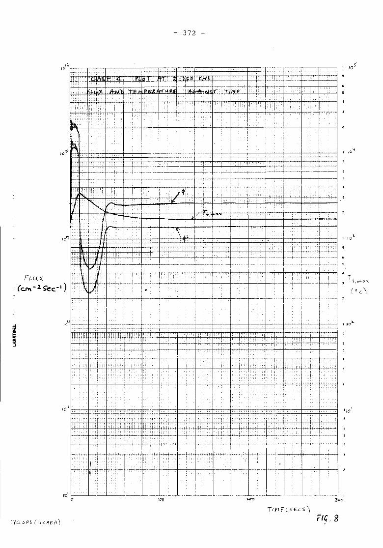
372
,I.10 IO~
i
, ::,.
"T' ii', ... '
I.I'
I:
. ,.:.. ::
.
, .. ..:
'11
..
.. ,
1 10 't
: :
. .. 1-.,
,.
::..
.
.
]" , , , .
-,--_. !
:'••.•:i,
,.;; ... :
-- -,
-- 1--'I .
..
i. '.:
,r.--'-r.---.--t-- "- ... ......
--f---: t-. --' -'-c+-~'-r-:7"-.': i'.:
,'r(.;;,
--_.
'.
......
I::.: ::
"~,. : .. '
~.. "'N('
15 "/0 ..
o't ....
.. . ..
1 10'Z-
.
.:.
. ..
:
,
: ::
,,: I ,: "
..'I .. :
':
..
, :'.
."
.
:
'T
••
:-- .- -I-- . -- !- ....-...-._.. -_.,_. +---.- -_.+--- .... -.+.._: --
• I---'--_...--....1_+-~~ 2
II I. I! I I
~ :
•.. "f--
", ,
.,
, , :,. ,:
;:: , ,, ,
.-
,
••. :
!... :
,
.,..
e---;.-
:, i
+-l 1I
'..:...
. :
","
--
, J'•_.-{
I
...
.
.'
. ..
: :.
: ::
.
.
:: ! :I '
','.'
..
...
::,::: .. :.::
I
I .'
I':'
T '1"':\ r..,t\01:'
:.:.
: :]::;:",.
,.
" "':
,.10
..
,.
'Ii ", '1'
, •• 1
, T': .
.. '
.. ,.:",l' :'
T .. ! ::::: ''''i '
1:::
: !
....
'. ::
.. .
...
! :"I''.'
I
:I
..;
I' ••:~. ~: ~: :., ....:
, :
~".~-r--':"~I : ' .
~-_._.~.
i'
.
"'0 o,.
10'lJ_ .. ~. __ ._ .. _--- I
'•• - '. L... ••.• _._ 1300
TlhflS£.CS~
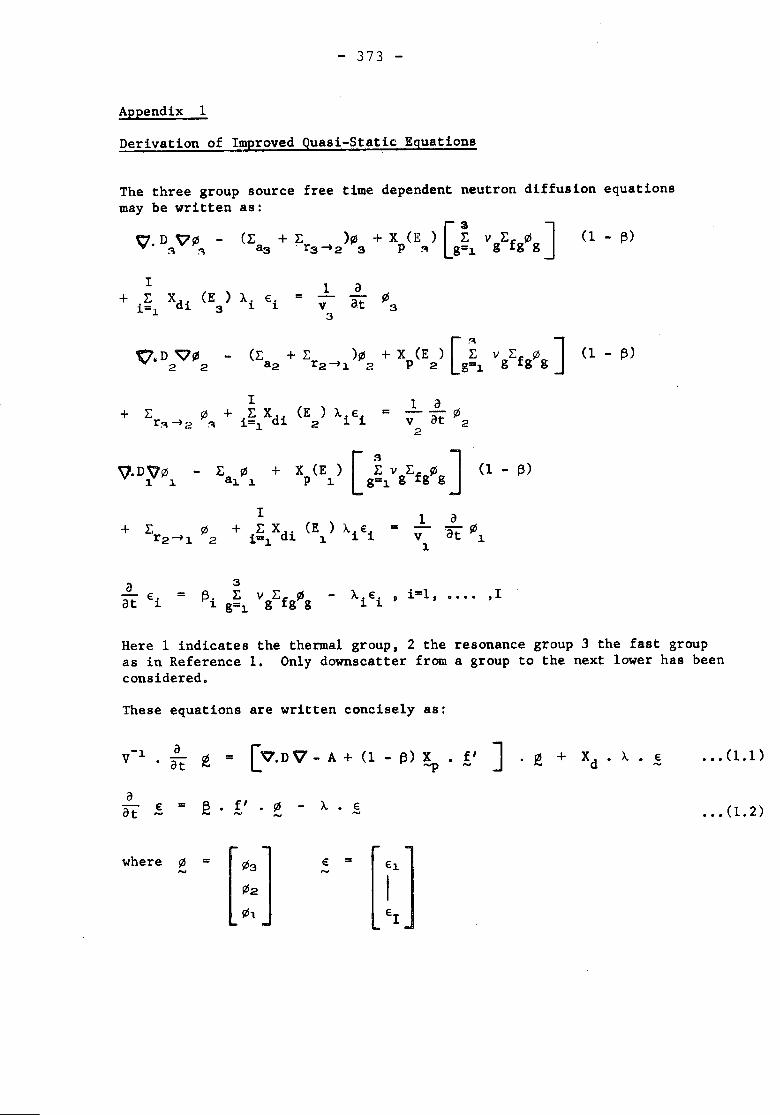
- 373 -
Appendix 1
Derivation of Improved Quasi-Static Equations
The three group source free time dependent neutron diffusion equationsmay be written as:
V'.D VIIS - 0:: + L )Ill+ X (E ) C ~ v gLfgllSg]::\ ~ a3 .r3~2 3 p ~ g=1.
I 1 a+ L Xdi (E ) Ai Ei = lISi=l 3 V at 3
3
(1 - 13)
1 a= --\I.lv at 22
t}.DV\I.l - L lIS + X (E ) [ ~ v Lf lIS ] (1 - 13)1. 1. a1.1. P 1. g=1. g g g
I+ L \I.l + L X (E) A. €
r2 ~ 1 2 1Cll11 di 1. i i= 1
v1.
=3
l3i g~l VgLfgllSg
Here 1 indicates the thermal group, 2 the resonance group 3 the fast groupas in Reference 1. Only downscatter from a group to the next lower has beenconsidered.
These equations are written concisely as:
f' ] . ~ + Xd• A. • ~ •••(l.1)
atz • £" • ~at € = A. • € ••• (l.2)..... ~
where lIS = [::] € = €1.....
€I
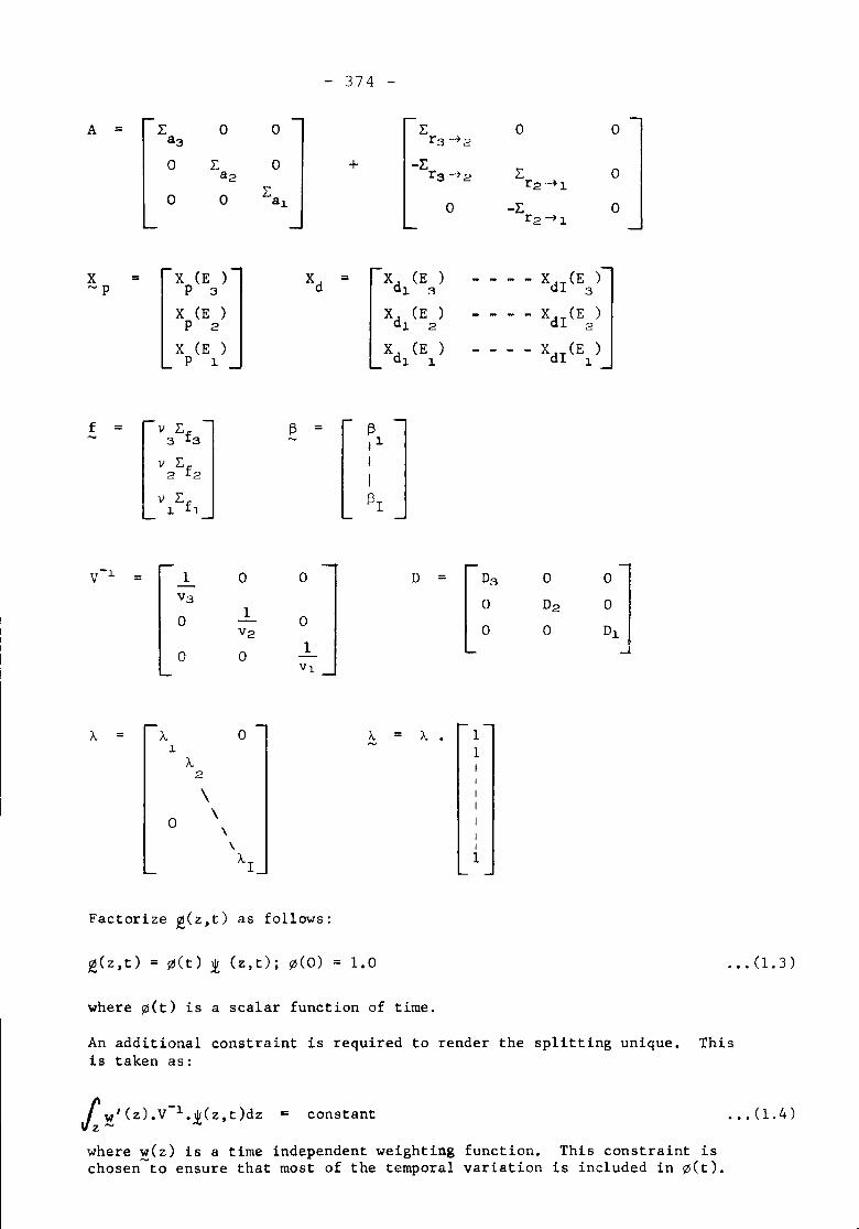
- 374 -
A = I: 0 0 I: 0 0a3 r3 -t2a I: 0 + -I:
I:82 r3 -t2 0I:
r2 -t10 0 a1 0 -I: 0r2 -t1
x = X (E ) Xd = Xd (E ) XdI(E3)~p p 3 1 ::\X (E ) Xd (E ) - - X (E)
p 2 1 2 dI 2X (E ) Xd (E ) - XdI(E1)
p 1 1 1
f = v I:f t3 = t33 3 ,1V l:f I2 2 Iv l:f t311 1
v-l 1 0 0V3
01
0V2
0 0 1Vl.
D = o
A = A 0 A = A . 11 - 1A I2
I
\ I
\ I
a I\ I\ I
AI 1
Factorize ~(z,t) as follows:
~(z,t) = ~(t) ,i (z,t); ~(O) = 1.0 .•• (1.3)
where ~(t) is a scalar function of time.
An additional constraint is required to render the splitting unique. Thisis taken as:
f w'(z).V-1.,i(z,t}dz = constantJz ~where w(z) is 8 time independent weighting function. This constraint ischosen~to ensure that most of the temporal variation is included in ~(t).
••• (1.4)
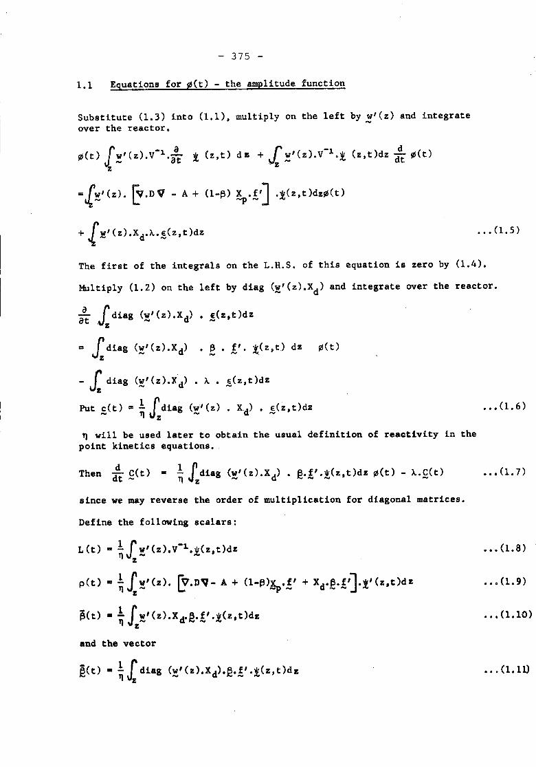
- 375 -
1.1 Equations for @(t) - the amplitude function
Substitute (1.3) into (1.1), multiply on the left by !'(z) and integrateover the reactor.
~(t) [!'(Z).v-l..aat 1 (z,t) dB + 1;!'(z).V-1'i (z,t)dz :t l/l(t)
= l'!' (z). ~. D V - A + (l-13) ;"!'] .i(z , t )dz~ (t )
•.• 0.5)
The first of the integrals on the L.R.S. of this equation is zero by (1.4).
Multiply (1.2) on the left by diag (!'(z).Xd) and integrate over the reactor.
aat .£diag (!'(z).Xd) • !(z,t)dz
= 1dbg ('!'(Z).xd) • ~ • !'. t(z,t) dz l/l(t)z
- 1:diag (!' (z).xd) • A. •
1J .Put c(t) = - diag (w'(z).... 1') z ....
~(z,t)dz
• •• (1.6)
1') will be used later to obtain the usual definition of reactivity in thepoint kinetics equations •.
d 1!Then dt C(t) = - diag (w'(z).xd) • R.f'.w(z,t)dz l/l(t)- A..C(t),..., Tl z I*V ~""'I ,.." -
since we may reverse the order of multiplication for diagonal matrices.
Define the following scalars:
L(t) ..~J:!'(z).v-l.1(z,t)dZz
p(t) ..~~!'(z). [y.D~- A + (l-13)~.!' + Xd,~,!'J.:t'(z,t)dZ
~(t> .. ~ L!' (z).Xd.ti!.!'.t(z.t)dz
and the vector
••• (1.7)
••• <l.8)
••• (1.9)
... (1.10)
... (1.11)
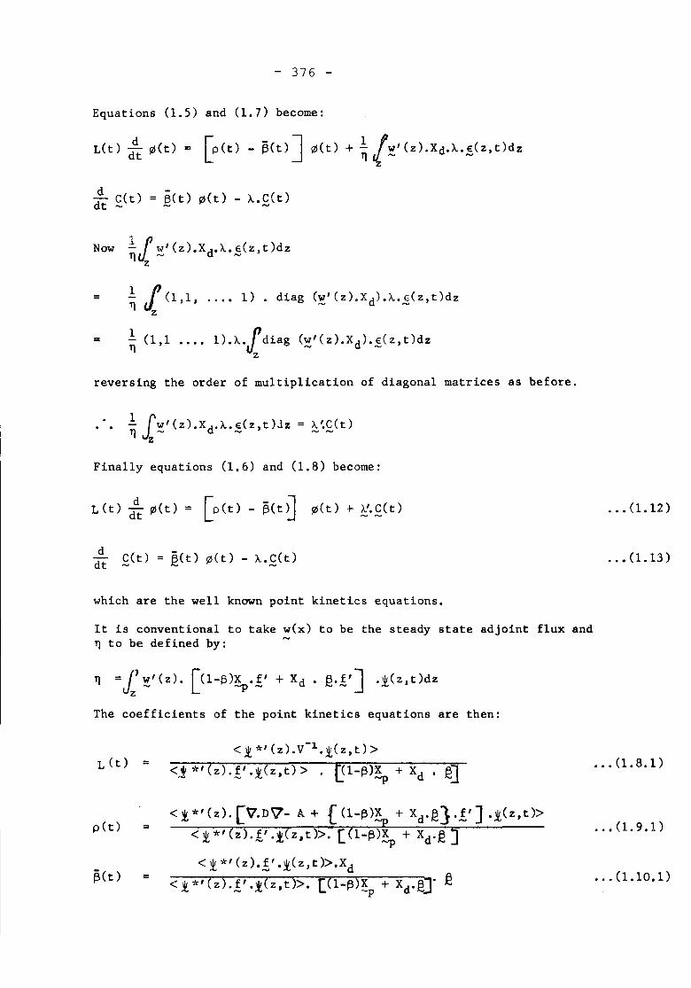
- 376 -
Equations (1.5) and (1.7) become:
Now 1:. (J \v'(z).Xd.Ldz,t)dzT)tL ~ ~z
= 1:. P(l,l, ..•• 1). diag (w'(z).Xd).LE(z,t)dzT) ~ ~ ~z
= 1:. (1,1 •••• l).A. Pdiag (w'(z).Xd).E(Z,t)dzT) ~ ~ ~z
reversing the order of multiplication of diagonal matrices as before .
••• 1:. Iw'(z).Xd.A.E(z,t)Jz = A~C(t)T) ~ ~ ~ ~z
Finally equations (1.6) and (1.8) become:
which are the well known point kinetics equations.
It is conventional to take w(x) to be the steady state adjoint flux andT) to be defined by: ~
The coefficients of the point kinetics equations are then:
••• (1.12)
.•• (1.13)
L(t) =
pet) ::I
~(t) =
< i'.*, (z) .V-1•i'.( z, t )><j *, (z).!'.i'.(z ,t) > . ~""'l--f3"")""';'-+-X-d-.-[2-0-
<t*'(Z)'[V.DV- A+ (1-f3)\ + Xd.[2}.!'] .i'.(z,t»<i'.*'(z).!.'.i(z,t}>. [(1-f3)\ + Xd.[2J< i'.*, (z).!' .i'.(z,t».Xd
< i'.*, (z).!' .1(z,t». [(l-t3)~p + Xd.[2J [2
••• (1.8.1)
••• (1.9.1)
•.• (1.10.1)
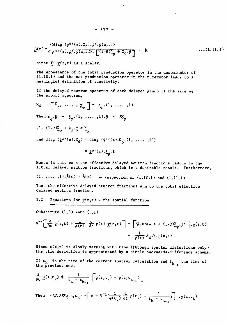
- 377 -
_ <diag (I*'(z)'Xd).!'.i(z,t»~(t) = <I *,(z ) •!'.i(z , t ». [( 1-t3 )!p + Xd• ~] •
since !"I(z,t) is a scalar.
The appearance of the total production operator in the denominator of(1.10.1) and the net production operator in the numerator leads to ameaningful definition of reactivity.
If the delayed neutron spectrum of each delayed group is the same asthe prompt spectrum,
•••(1.11.1)
X .(1, •••• ,1)""PThen X •Fl. = X •(1, •••• ,1).Fl. =d,l;;; "'p I;;;
(1-t3; + Xd.~ = 2lp
and diag (I*'(z).Xd) = diag (I*'(Z).x""P'C1,.... ,0)
= 1*' (z).X •I"'P
Hence in this case the effective delayed neutron fractions reduce to theactual delayed neutron fractions, which is a desirable result. Furthermore,
(1, .... ,1).~(t) = ~(t) by inspection of (1.10.1) and (1.11.1)Thus the effective delayed neutron fractions sum to the total effectivedelayed neutron fraction.
1.2 Equations for I(z,t) - the spatial function
Substitute (1.3) into (1.1)
V-~[aat I(z,t) + '/Jlt) ddt'/J(t)I(z,t) ] = [V.DV- A + (l-f3);,.!'] 'I(z,t)1
+ '/J(t)Xd.A.~(z,t)
Since I(z,t) is slowly varying with time (through spatial distortions only)the time derivative is approximated by a simple backwards-difference scheme.
If tk is the time of the current spatial calculation and tk the time ofthe previous one, -~
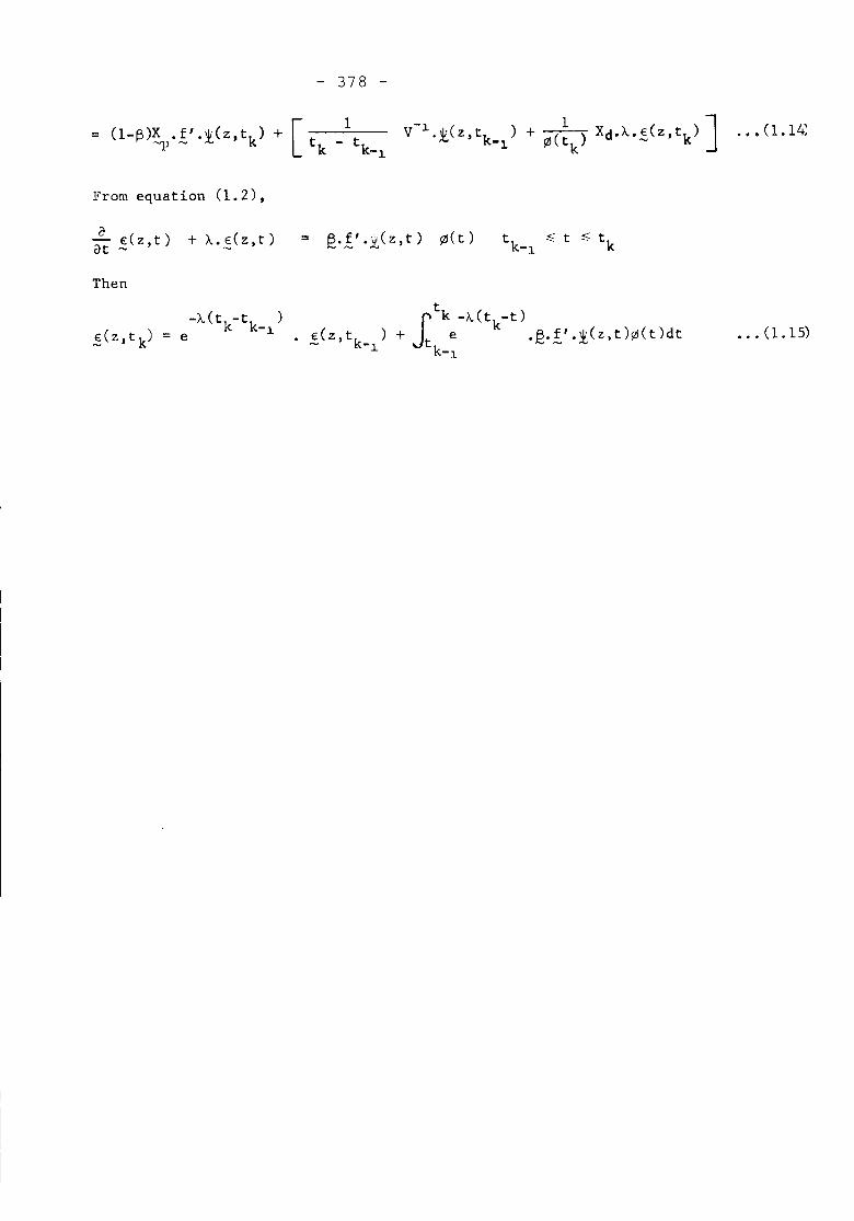
- 378 -
From equation (1.2),
aat ~(z,t) + A.~(Z,t) = ~.!'.!(z,t) ~(t)
Then
••• (1. 15)
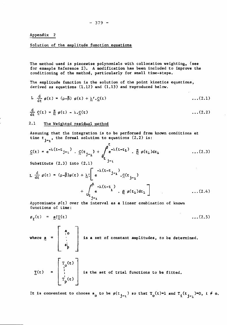
- 379 -
Appendix 2
Solution of the amplitude function equations
The method used is piecewise polynomials with collocation weighting, (seefor example Reference 2). A modification has been included to improve theconditioning of the method, particularly for small time-steps.
The amplitude function is the solution of the point kinetics equations,derived as equations (1.12) and (1.13) and reproduced below.
• •• (2.1)
••• (2.2)
••• (2.3)
• .. (2.4)
2.1 The Weighted residual method
Assuming that the integration is to be performed from known conditions attime tj_~' the formal solution to equations (2.2) is:
t
£(t) = .-A(t-tJ_,) • £(tJ-,) + ~.-A(t-t1) • ~ ~(t,)dt,
t .Substitute (2.3) into (2.1) J-1
. [-)"(t-t)L ddt16(t) = (p-~)16(t)+ ~~ e j-~ .£(tj_~)
t1-)..(t-t)+ e ~.
tj_
1
Approximate 16(t) over the interval as a linear combination of knownfunctions of time:
16f(t) = ~!I(t)
a,0
where a =-\a,p
T (t),0
I(t) I= I
IT (t)p
•••(2.5)
is a set of constant amplitudes, to be determined.
is the set of trial functions to be fitted.
It is convenient to choose a to be ~(tj ) so that T (t)=l and Ti(tj
)=0, i ; o.o -, 0 -1
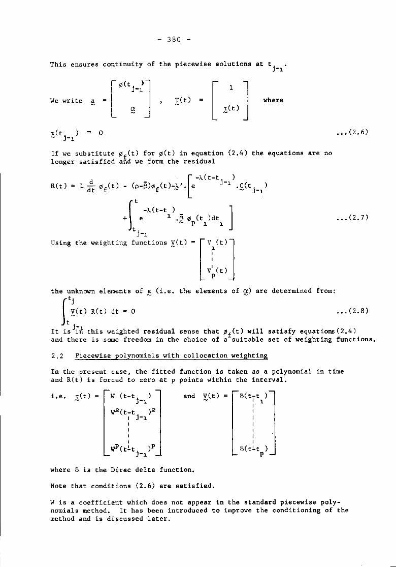
- 380 -
This ensures continuity of the piecewise solutions at tj .-l.
We write a-o
= where
... (2.6)
R( t)
If we substitute ~f(t) for ~(t) in equation (2.4) the equations are nolonger satisfied and we form the residual
. [-A.(t-t )(P-~)~f(t)-1'. e j-l. .£(t
j_
1)
~
t -A.(t-t ) ]+ e 1 .~ ~ (t )dt
p l. l.tj -l.
Using the weighting functions Vet) = V (t)- 1
I
II
V (t)p
... (2.7)
... (2.8)
the unknown elements of ~ (i.e. the elements of g) are determined from:
Itj
yet) R(t) dt = 0t .
It isJiJ this weighted residual sense that ~f(t) will satisfy equations (2.4)and there is some freedom in the choice of a suitable set of weighting functions.
2.2 Piecewise polynomials with collocation weighting
In the present case, the fitted function is taken as a polynomial in timeand R(t) is forced to zero at p points within the interval.
W (t-tj
)-1.
W2(t-t )2I j-l.IIII
WP(t.!.t )pj-1
and yet) = 5(t-t )I l.I
I
IIIII
f)(ti.t )p
where 5 is the Dirac delta function.
Note that conditions (2.6) are satisfied.
W is a coefficient which does not appear in the standard piecewise poly-nomials method. It has been introduced to improve the conditioning of themethod and is discussed later.
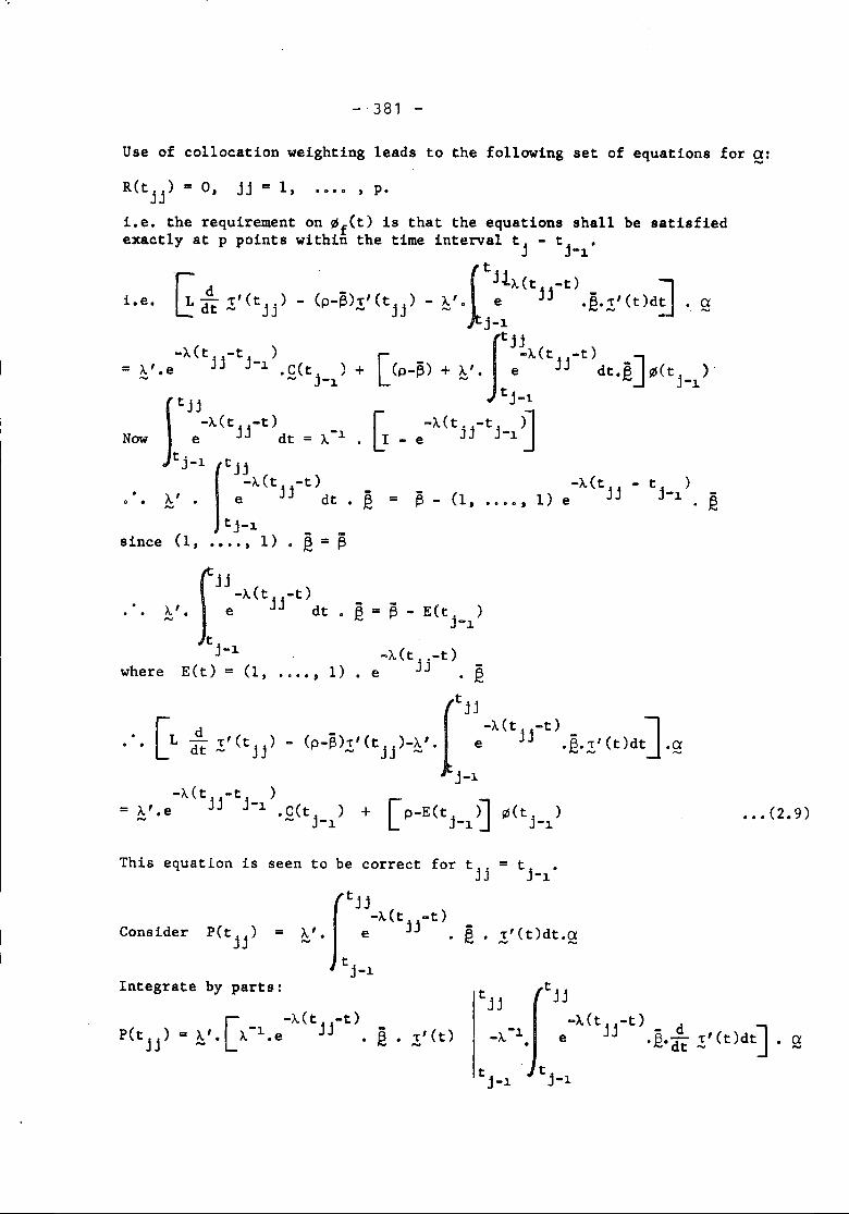
- 381 -
Use of collocation weighting leads to the following set of equations for g:R(tjj) = 0, jj = 1, •••• , p.
i.e. the requirement on ~f(t) is that the equations shall be satisfiedexactly at p points within the time interval tj - tj_
1•
1t11I d _ A(tjj-t) _ ~i.e. ~ dt l'(tjj) - (p-~)l'(tjj) - ~'. e •[email protected]'(t)d:J. g
j-1
-A(t. -t) [ Jtj~A(t -t)=A'.e ]j j-1.C(t )+ (p-~)+A'. e jj dt.~J~(t ).- - j-l - ~ j-1
Jt JJ t j-l
-A(tjj-t) _ r -A(t 'j-tj_ )lNow e dt = A 1 • LI - e ] 1J
tj
_1 ftjj
-A(t -t) -A(tjj - t )•• ~'. e jj dt ~ = ~ - (1, .•••, 1) e j-l ~
tj-1since (1, ••.• , 1) • ~ = ~
fJj -A(t -t)~'. e jj dt. ~ = ~ - E(t
j_
1)
t .j-1 -A(t. -t)
where E(t) = (1, ...•, 1) • e ]j . ~
[
tjj
[d -A(t. -t) J
••• L dt l'(tjj) - (P-~)l'(tjj)-~'. e ]j .~.l'(t)dt .gj-1
-A(t. -t )= A'.e ]j j-1 .C(t ) + [P-E(t )11 ~(t ) (2 9)- - j-l j-1 J)U j-1 ••. •
This equation is seen to be correct for tjj =
Integrate by parts:
Consider[
tjj-A(t -t)= ~'. e jj .
tj-1
~ • l'(t)dt.g
tjj tjj-A(t -t)
_A-1• e jj .~.d~ l'(t)dt] • gtj_
1tj_
1
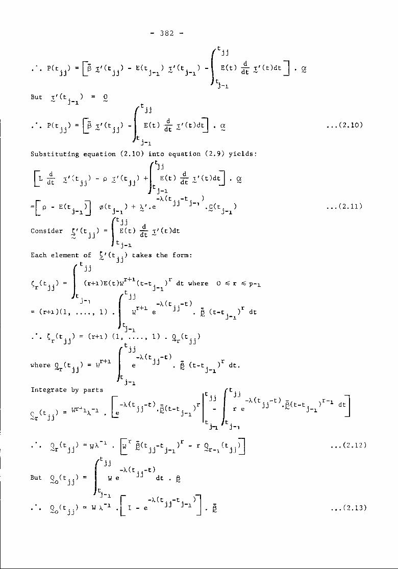
- 382 -
ddt!' (t)dt] • a
••• (2.10)
.•. O.ll)
But
itjj
P(tj j) = ~ 1:'(tj j) - E (t) d~ 1:'(t)d~ • ~t.J-1
Substituting equation (2.10) into equation (2.9) yields:
f,tj j
[L d~ 1:'Ctjj) - P l'(tjj) + E(t) d~ !'(t)dt] • £t j-1
[ J-,,(t .. -t. )= P _ E(t. ) ~(t ) + A'.e JJ J-, .C(t. )J-1 j-l ~ ~ J-1
Consider r'(t ..) = ft~it) dd .'(t)dt~ JJ t ~
tj_l.
Each element of ~'(t ..) takes the form:
it.. ~ JJJJ
S (t ..) = (r+1)E(t)\-Jr+l(t_t.)r dt where 0 ~r ~P-1
r JJ tj_, [tjj+ J~:(t .._t)_ ( ) C ) r 1 J J C )r- r+1 1, .... , 1. VJ e . f2 t-t. dt
J-1t.J-1. .. s Ct.j) = (r+l) (1, •••• , 1) • ~ (t ..)
Where
r
!), :t.j
) = Hr+l.f.tj~-'(tJj_t).r~ ::-t. )r de.r J J-1
t.J-1
Integrate by parts it ..
Ct.. JJ
JJ -A(t -t) - r-1\~+1 -1 -,,(tjj-t).~(t_t.)r _ r e jj .f2Ct-tj_1)
Q (t .. ) = ". e J-1~r JJt. t.
J~ J-,
r Q (tj.)l~r-1 J ~
••• (2.12)
C.JJ -A(t ..-t)But Q Ct ..) = W e JJ dt • f2~o JJ
t.J-l._ e-'CtjJ-tJ_,)].
goCtjj) = w ,-' • [ I ~ ••• (2.13)
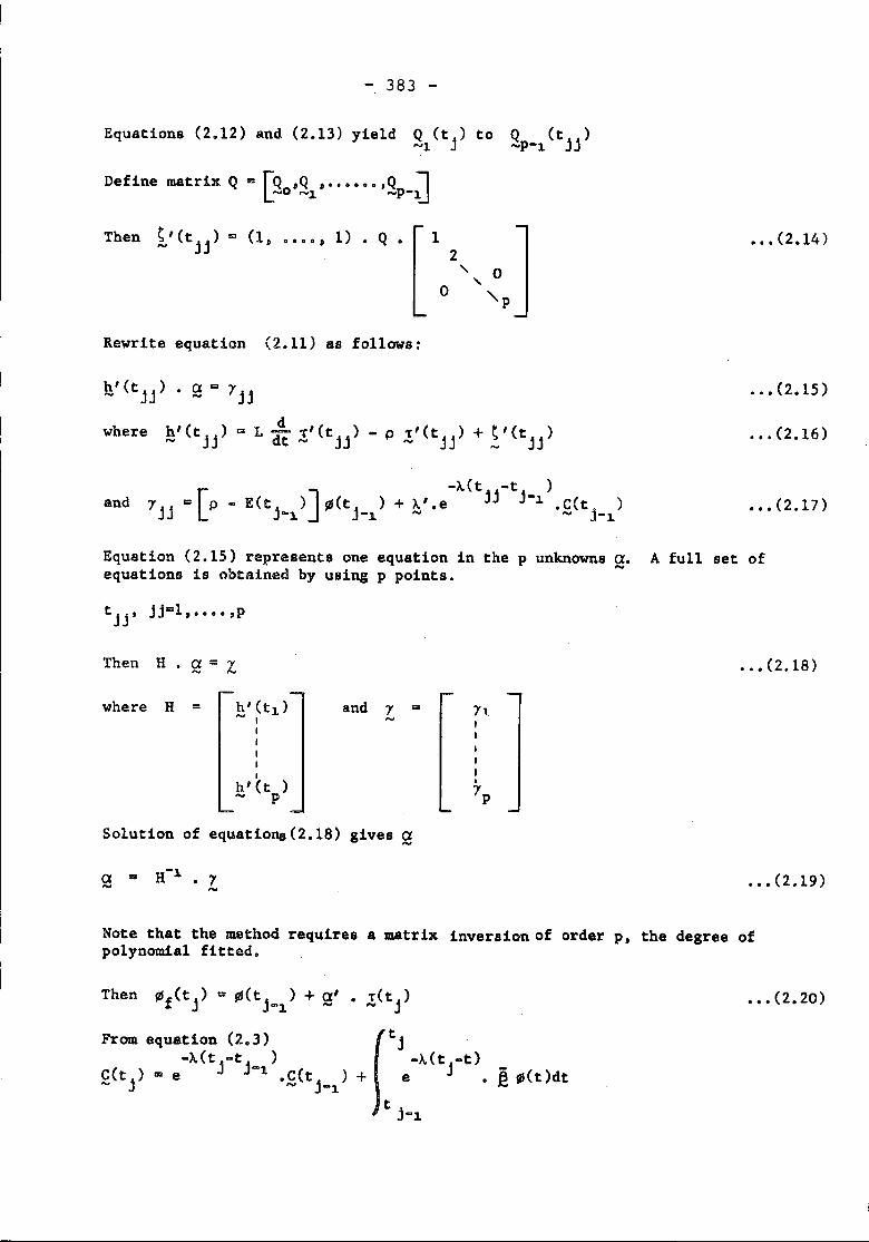
- 383 -
Equations (2.12) and (2.13) yield Q (tj) to Q (tjj)......1 ......P-l
Define matrix Q ...rQ ,Q ,•••••• ,Q IL...-0 ......~ ......p-~J
Then ~'(tjj) = (1, •••• , 1) • Q •
Rewrite equation (2.11) as follows:
1
o
2" 0"'p
•••(2.14)
where .••(2.16)
and ••• (2.17)
Equation (2.15) represents one equation in the p unknowns Q. A full set ofequations is obtained by using p points. -
tjj' jj=l, •••• ,p
Then H. ~ = Z ••• (2.18)
where H = h'(tl).......IIIII
h'(t )- p
and ., =...... "1I
IIIII
"p
Solution of equations(2.18) gives ~
•••(2.19)
Note that the method requires a matrix inversion of order p, the degree ofpolynomial fitted.
•••(2.20)
- 384 -
Replacing ~(t) by ~f(t) inside the integral,
f.t j
-~(t -t ) -~(t -t)C(t ) = e j j-, .C(t ) + e j dt~ j ~ j-,
ftj t.J-~
-~(t -t)+ e j • ~ . !'(t)dt . g
t.J-~-~(t -to ) {j J -1. 1 (Then f (tj) = e . C(tj ) + w- Qt.) ~ (t . )
- ~ -~ ~o J J-~
+ rQ (t.), Q (tj), •••., Q (tj)l. o:}L-1. J ~2 ~p J- ••• (2.21)
In the conventional formulation of the piecewise polynomials method withcollocation weighting the scaling factor W introduced in this paper does notappear and the Q , r = 0, ..•., p are derived from~r
=
and the recurrence relationship
-1. 0- r J= ~ • Q(t.j-t. ) - r Q (t.j)J J-1 ~r-, J
(Equations (2.12) and (2.13) with W = 1)
There is the possibility of rounding errors in this process, especially in thecase of small time-steps. The factor W is introduced to remove this difficulty.
With at = t -t and eat = t -t the modified equations (2.12) and (2.13)for Q and Qj mJyl.bewritten: jj j-l'
~r _0
3r = W ~-, • [wr~ eratr - r 3r-,J
30 = w ~-~ • [I - e-~eatJ. ~
2.3 Derivation of the Q-functions
The requirement on W implied by the analysis is that it should be independentof time over the time-step. That is not to say that it should be independentof the time-step.
Put
Then
W = 1at
= r -~at ~
•••(2.23)
- 385 -
Q (ot 9) Il:I .l >..-1 • [I _e->..90t ] • ~...0' ot .-Expanding the exponentials:
Q (et,S) = ~ I - ~ >..ot+ ~ (>..ot)2- ~ (>..8t)3+ - .... J .~.....0 L 2' 3. 4.
Q (ot,e) ...Oe~ I - ~ >..ot+ ~ (>..ot)2- 9~ (>"ot)3+ - ••••J . ~...~ 2. 3. 4. 5•
.[as- g6 852 96
3 J-Q (ot,9) III 2: .. I - -, >"8t+ .. (>..8t)- -, (>..8t)+ -.... • ~.....2 :5. 4. 5. 8.
Q (8t ,8) ... [ 9r+l 9r+2 8r+s (>..8t)2 ...] . ~r: (r+l)! I (r+2) ! >..ot + (r+3H - +.....r
r+l [ co ( ) i ( ), (90t )i>..iJie Q (at e) ... _9_._ I + E -~ r+, • . ~ ••• (2.22).....r' r+, i=l r+i+l)'
The series expansions for the Q-functions involved in equations (2.22) arerapidly convergent since they involve the relatively slow time constantsassociated with the delayed neutron groups. Further, powers of A involveonly scalar operations since A is diagonal.
Writing equation (2.21) in th~ new notation,->..ot {£(tj) = e • £(tj_~) + 2o(ot,1) ~(tj_1)
+ [S,(5t,l),~(5t.l), ••••• Sp(5t,l~. g } 5t
2.4 Behaviour of the Q-functions for small time-steps
Since ~~:o[~r (at,9) ] ... the Q-functions are well-behaved forsmall time-steps and from equations (2.23)
Lim5t-+O
... ( ) + QJ.+ f!2+ ~ }-~ t j-l 2 ::\ ..•• + P+1 ~
which corresponds with the limiting behaviour of equations (2.3) with ~(t)replaced by ~f(t). (Bearing in mind the slow time constants associated withdelayed neutrons).
The method does not require that the coefficients of the point kinetics equationsshould be constant over the time-step. Rather the vectors used in the calculationof ~ in Appendix I are taken as constant over the time-step, thus L is constant.The assumption is then made that p and ~ vary linearly over the time-step.
- 386 -
2.5 Numerical example
The procedures are best illustrated by means of a simple example such as thefitting of a quadratic in the case of one delayed group.
L = 5xlO-7 secs.r:. = 3xlO-3.
-~A. 0.3 sec .fIJ (t . ) 100
J-}
C(t. ) 0.5J-~The first two examples assume a constant reactivity over the time-steppet > 0) = 95 cents. In this case the solution for the amplitude function canbe obtained by evaluation of the eigenvalues and eigenvectors of the kineticsmatrix as:f/J(at)= 964.424e5.590l5 at _ 864.424 e-306.l08 at
Evaluating the series to order 3, we have:
f/J(at)= 100 + 26.9998xl04at - 0.40484lxloB5t2 + 0.004l3254xl012at3
... (2.24)
••.(2.25)
Hence for 5t = 10-4 sec. the solution should be well represented by a quadraticand this is the first example
Example 1. 5t = 10-4 sec., constant reactivity
Using equations (2.22),
It is interesting to check these values with the limiting behaviour of theQ-functions for small time-steps.
Using equations (2.14),
('(5xlO-5) = (0.499996,0.249998) r:.
= (0.999985,0.999990) ~
Naturally the unit vector in equations (2.14) becomes scalar unity for onedelayed group.
Using equations (2.16),
h'(5xlO-S)=5xlO-7 (104,104)-2.85xlO-3(0.5,O.25)+(O.499996,O.249998)3xlO-3
.'. ~'(5xlO-5)=(5.07499xl0-3,5.03749xl0-3)
- 387 -
E'(10-4)=5x10⁻⁷ (104,2x10⁴)-2.85xlO-3(1,1)+(0.999985,0.999990)3x10⁻³
.'. h'(10-4)a(5.14996xlO-3,l.01500xlO-2)-Using equations (2.17),
r ;:[ 0.135002]0.135005
[5.07499xlO-35.l4996x10-3
g = [0.135002]0.135005
(see equations (2.18»
Then g = [26.9937 ]-0.395230
C.f. equation (2.25)
Now ~f(10-4)=126.599, in exact agreement with (2.24).
In this example the time-step was chosen to be such that the series expansion(2.25) of (2.24) was well represented by the quadratic. The example confirmsthat the fitted polynomial is a good representation of (2.25) and that thesolution agrees well with (2.24). It is easy to see that for a time-step of10-2 sec. equation (2.25) is badly represented by the quadratic and the nextexample illustrates the behaviour of the method in this situation.
Example 2. ot = 10-2 sec., constant reactivity
Q (10-2,~) = 0.499963 ~ Q (10-2i~) = 0.124938 ~_0 -J.
go (10-2,1) ;:0.998502 ~ Q (l0-2,l) = 0.499500 ~-1
~'(5x10⁻³) = (0.499963,0.249876) ~
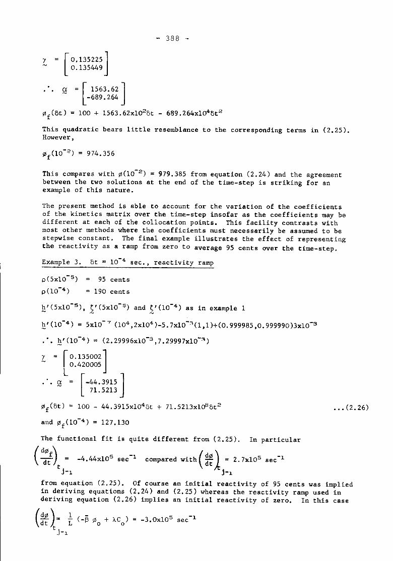
- 388 -
., = [0.135225J0.135449
~ = [ 1563.62 ]-689.264
~f(5t) = 100 + 1563.62xl025t - 689.264xl045t2
This quadratic bears little resemblance to the corresponding terms in (2.25).However,
This compares with ~(10-2) = 979.385 from equation (2.24) and the agreementbetween the two solutions at the end of the time-step is striking for anexample of this nature.
The present method is able to account for the variation of the coefficientsof the kinetics matrix over the time-step insofar as the coefficients may bedifferent at each of the collocation points. This facility contrasts withmost other methods where the coefficients must necessarily be assumed to bestepwise constant. The final example illustrates the effect of representingthe reactivity as a ramp from zero to average 95 cents over the time-step.Example 3. 5t = 10-4 sec. , reactivity ramp
p(5xlO-5) = 95 centsp(10-4) = 190 cents
£'(5xlO-5), ~'(5xlO-5) and ~'(10-4) as in example 1
£'(10-4) = 5xlO-7 (104,2x10⁴)-5.7xlO-3(1,1)+(0.999985,0.999990)3xlO-S
.'. £'(10-4) = (2.29996xlO-3,7.29997xlO-3)
., = r 0.135002]0.420005
L~ = [-44.3915 J71.5213
~f(5t) = 100 - 44.39l5xl045t + 7l.52l3xlaB5t2
and ~f(10-4) = 127.130•••(2.26)
+ >..c )o
The functional fit is quite different from (2.25). In particular
(d:tf)t = -4.44xl05 sec-' comparedWith( *1 = 2.7xl05 sec-'j-l j-l
from equation (2.25). Of course an initial reactivity of 95 cents was impliedin deriving equations (2.24) and (2.25) whereas the reactivity ramp used inderiving equation (2.26) implies an initial reactivity of zero. In this case
(*1- t (-~~ot.J-1

- 389 -
Hence the behaviour of (2.26) is plausible for the reactivity variation imposedon the solution, although the numerical value of the time derivative of theamplitude function at time t is not numerically exact. This feature isreadily understood as the j-1 start of the time-step is not a collocationpoint and so the corresponding reactivity 1s not imposed on the solution. Thismay be an argument in favour of the use of spline functions.
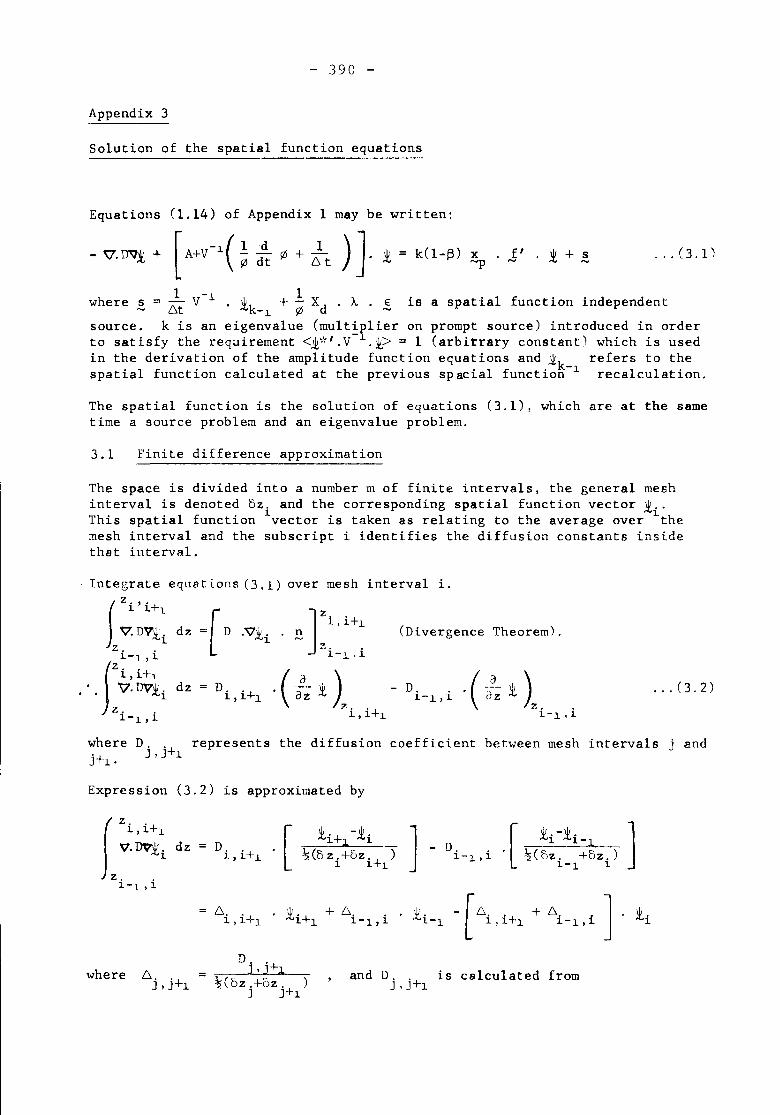
- 390 -
Appendix 3
Solution of the spatial function equations
Equations (1.14) of Appendix 1 may be written:
-~.~+ l' . .t + s ... (J.n
1 -1 1where s = -- V . \Ifk + - Xd . A . E is a spatial function independent~ 6t .:t, -1 fi1 ~source. k is an eigenvalue (multiplier on prompt source) introduced in orderto satisfy the requirement <i*'.V-1.t> = 1 (arbitrary constant) which is usedin the derivation of the amplitude function equations and ~k- refers to thespatial function calculated at the previous spacial function 1 recalculation.
The spatial function is the solution of equations (3.1), which are at the sametime a source problem and an eigenvalue problem.
3.1 Finite difference approximation
The space is divided into a number m of finite intervals, the general meshinterval is denoted Oz. and the corresponding spatial function vector .t ..This spatial function ~vector is taken as relating to the average over ~themesh interval and the subscript i identifies the diffusion constants insidethat interval.
Integrate equations C3.1)
(Zi'i+l [
J~D'Vli dz = Dzi .
jZ. -: ' ~1.,1.+,. '. \7. DV;ti dz
z. .1.-~,1.
over mesh interval i.
(Divergence Theorem).
... 0.2)
where D.. represents the diffusion coefficient between mesh intervals j andJ,J+1j+1.
Expression (3.2) is approximated by
r .[ ]1.,~+1 Ii+1-.ti ] [ 1i-1i-1V.DV;t. dz = Di . - D.~ ,1+1 ~(5zi+5zi+1) 1-1,i . ~(c)z. +5z.)~-1 ~z. .
~-l,~
6 .. 1 + 6i . Ii-l -[6.. + 6. i ] :ii~,~+l i+1 -1,1 ~.~+1 1.-1,
whereDj .
= • J+l.~(5z.+oz. )
J J+1and D.. is calculated from
J, J+1
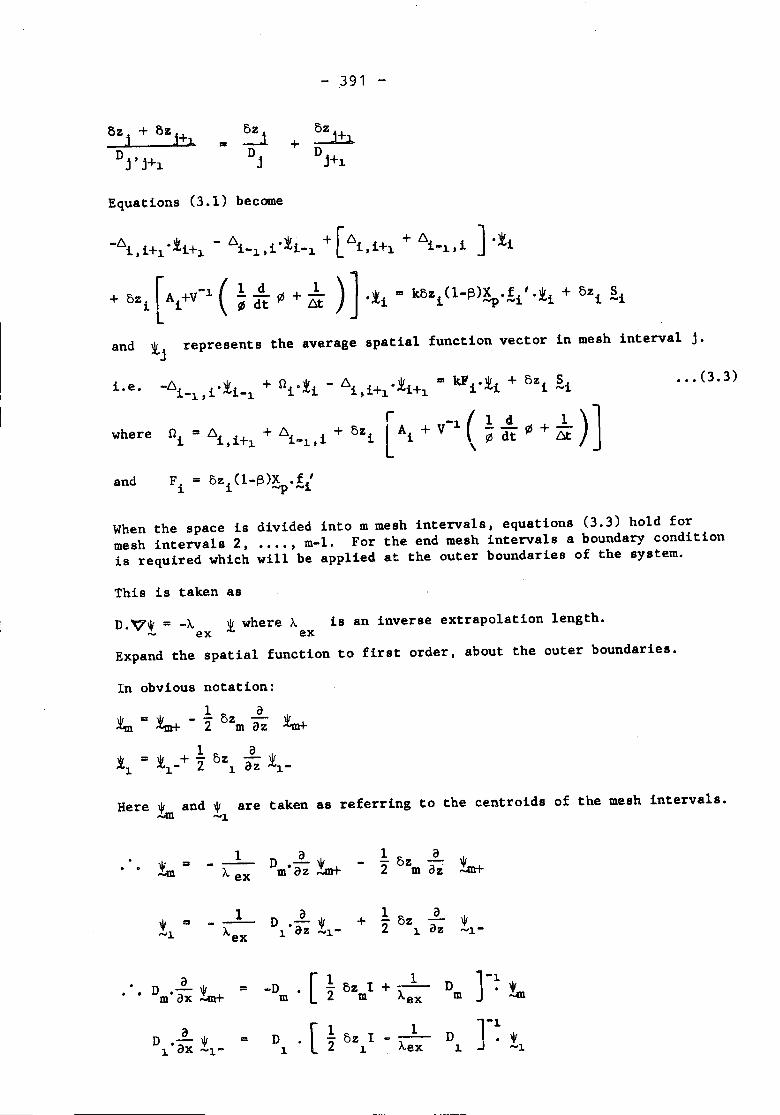
- 391 -
8zj + 8zj+3,D j' j+l
Equations (3.1) become
-6.i,i+3,.1i+1 - 6.i-1,i.1i-1 + [6.i,i+1.+ 6.1-1.,i] .li
+ 5°1 [A1+V->( i d~ ~ + ~ ) ] .11 = k501(1-~):;"!1' .11+ 5°1 4
and represents the average spatial function vector in mesh interval j.
i.e.
where
•.• (3.3)
When the space is divided into m mesh intervals, equations (3.3) hold formesh intervals 2, •••. , m-l. For the end mesh intervals a boundary conditionis required which will be applied at the outer boundaries of the system.
This is taken asD.~t= -~ 1where A is an inverse extrapolation length.
ex exExpand the spatial function to first order, about the outer boundaries.
In obvious notation:1 a
\It = 111 . - - 8z - \I{ .~ ~ 2 m oZ ~
Here !m and 11
are taken as referring to the centroids of the mesh intervals.
'if ... 1 a 1 aDm• oZ !m+ - 8z :tn+NIJ1 A ex 2 m ai
*1 D ...!., 1 a
*... + - 8z....l Aex 1.0Z ....1- 2 1 az ....3,-
D a -D [ 1 1 D ]-:m. ax !m+ ... - 8z I +-- !mm 2 m ~ex m
D •...!. * D .[1 1 D J-~... - 8z I If1 ax ....l- 1 2 1. Aex 1. ....1
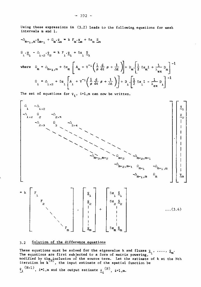
- 392 -
Using these expressions in (3.2) leads to the following equations for meshintervals m and 1.
-t:, .1jf + n .'li= k F.1jf + OZ Sm-1 ,m ....m-1 m NUl m NUl m .....m
n .'li - t:, .1jf = k F.1jI + OZ S1 ....1 1,2 ....2 1 ....1 1 ....1
]
-1+_l_D
A. mex
1 ]-1--DA.ex l.
ilm • "m-,.m + 5zm [ Am + V-,
(~ ddt " + it )J+ Dm{t 5zmI
il1 • ",.2 + 5", [A1 + V-10 :t " + it )} D1-[t 5", I
where
The set of equations for 'lii'i=l,m can now be written.
D -t:,1 1,2-t:, D -t:,
1'2 2 2,::\-t:, D -t:,2,3 3 3,4
"- .......... "-......... .................... .........
-t:,m-1,m Dm
1jI....2
IIIIIIIIIItn
= k F li1 DZ Sl. l. ....l.
F li2 OZ S2 2 ....2"- I + I
"- I I
"- I I
"- I I
"- I IF !tm OZ Sm m ""m
... (3.4)
3.2 Solution of the difference equations
These equations must be solved for the eigenvalue k and fluxes 1' ...., lim'The equations are first subjected to a form of matrix powering, 1modified by thtNtnclusion of the source term. Let the estimate of k at the Nthiteration be k ,the input estimate of the spatial function be~ (N-1), i=1,m and the output estimate !i (N), i=l,m.

- 393 -
The improved estimate of the spatial function is derivad from the set oflinear inhomogeneous equations
I(N-l)
(N-l)
r"'lIl
(N)= ! =
i (N)~IIIIIIIIII
.im(N)
"-"-
"-" "-
"-"- ,
:'6m-~,m
n2
"
n -6~ ~,2
-6~,2
"-"-
"- ,"-
"-"-,,,
-6 .,m-2,m-~
... (3.5)
(N) k(N) F * (N-l) 5z Swhere ! =~ .....~ I 1 .....~
" I I
" I
" I + I
"" I I
" 1m(N-l) IF 5z Sm m ""'m
Equations (3.5) are solved using the Choleski method modified to use matrixelements, ie the following transformation is performed .
I - s .i: (N) R (N-l)2 11 .....~ I
I - s I I3 I I" " I = I
" I
" I" I I" I
I - S I Im:tm(N) R (N-l)
I ""'m
- 394 -
where S n -1 62 1 1,2
S. ~[c - 6. . S. r 6.1 i-1 1-2,i-1 1-1 1-1,i i = 3,m
R (N-l)1
(N-l)r = S-1 2
61,2
(N-l)r-1
i =R (N-l) [ J-l[ (N-l) (N-l)]= n -6. . •S . • r. + 6. . .Rii i 1-1,1 1 -1 1-1,1 - -1
-1 [ (N-l) (N-l)]= S. .6.. . ri + 6. i.Ri ' i = 2,m1+1 1,1+1 - 1-1, --1
1m(N) is obtained directly and the remaining li(N) by back substitution.
In this phase of the calculation use is made of the lower triangular form ofthe matrices to be inverted. Furthermore the inversions need be performedonly once as the matrices are independent of the iterations.
The revised estimate of the eigenvalue is derived as follows.
~. (N) is the solution of the equations_1
[ Ai + V-' ( ~ ddt" + ,; t ) - V.Di~' i/N
) • PI~~::) (l-~)!Sp'!i" ii (N-1) +~i .• (3.6)
(N-l) * -1 (N-l)where the inner product PI = <.'1: '. V ..jJ, > and is a scalar dividedinto the output spatial function estimate from each iteration to ensure therequired property <jJ,*, .V-1.f> = 1.
It is convenient to define
E.1
= -1 (1 d 1) t""'7A. + V - -d lZl + -;::- - v. D . ~1 lZl t ~t 1
... (3.7)
In this notation, equations (3.6) become
E .• ,II. (N)1 .t.1
k(N)= ----(N-l)
PIF ,II (N-l) +i . .t.i ~i ... (3.8)
The estimate of .'1:i for input to the next iteration is
,Ii = 1 'II~(N).:Li --eN).:L ...
PI
Then (N+l)E .1jI.i _1
=k (N+l)p (N)I
.•. (3.9)
- 395 -
(N+l) * ( )k (N) <1' .F.1 N >PI
Now if 1i(N+l) is the required solution.
*+ <1'.~ •••(3.10)
= 1 lil (N)(N) ~i
PI••• (3.11)
Substitute (3.11) into (3.8)
E ,II (N+l)i .~i =
keN)(N-l) (N)
PI PI
.••(3.12)
Inspection of equations (3.10) and (3.12) yields:
ie k(N+l) = ..•(3.13)
-(N-1) 1 (N-l)where I = (N-1) 1 is the normalised spatial function output fromPIiteration (N-I).
3.3 Extrapolation procedure
The iterative procedure outlined above could be continued until the spatialfunction was determined to within the required accuracy. This might imply somehundreds of iterations and various extrapolation techniques have been developedto improve the rate of convergence in calculations of this nature. The approachadopted in the present work was suggested by the presence of the spatial functionindependent source and the fact that convergence of the eigenvalue (being anintegral parameter) is much faster than convergence of the spatial functionitself.When the eigenvalue has converged to within a prescribed accuracy. the currentestimate is used in (3.4) to form the set of inhomogeneous equations
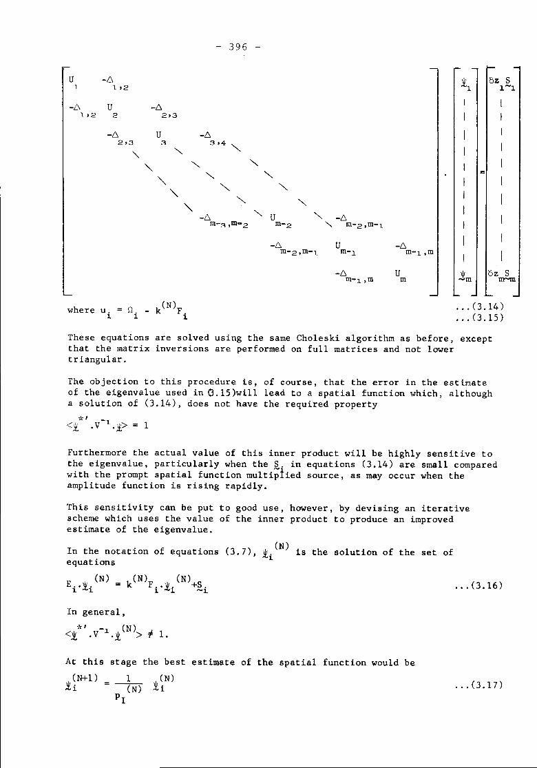
- 396 -
;£~ bZ S1-l.
I
I
III =IIII
I
1m bZ Sm-m
... 0.14)
... 0.15)
except
-6 U -62,3 3 3,4
"""- "'-
'" "'- "'-
'" "'- "'-"'- "" "'"
'" "'" "'"-6 "'- U "'- -6m-~,m-2 m-2 "- m-2,m-l
These equations are solved using the same Choleski algorithm as before,that the matrix inversions are performed on full matrices and not lowertriangular.
-6 Um-l,m m
U -61. 1,2
where u = n _ k(N)Fi i i
-6 U1. '2 2
The objection to this procedure is, of course, that the error in the estimateof the eigenvalue used in O.15)will lead to a spatial function which, althougha solution of (3.14), does not have the required property
Furthermore the actual value of this inner product will be highly sensitive tothe eigenvalue, particularly when the ~. in equations (3.14) are small comparedwith the prompt spatial function multiplied source, as may occur when theamplitude function is rising rapidly.
This sensitivity can be put to good use, however, by devising an iterativescheme which uses the value of the inner product to produce an improvedestimate of the eigenvalue.
'l'i(N)In the notation of equations (3.7), ~ is the solution of the set ofequations
... 0.16)
In general,
At this stage the best estimate of the spatial function would be
;£ iN+l) = ---tD liN)
PI... 0.17)
- 397 -
Substituting in (3.16),
E 111 (N+l)i •.l.i
Then
<"t*' . E."t (ltt-1» = k (N)<"t*' •F."t (ltt-1» + {PI ~N)-1}<:t *' •[> + <:t*' .[>
Similarly
.•• (3.18)
*, *,<1 .p + <~.p ... (3.19)
If the (N+l)th iteration produces the required solution,
From (3.19),
(N+l) *, (N+l) *,= k <1. F. 1 > + <1 .P .•. (3.20)
Comparing equations (3.18) and (3.20):
k(N+q = keN) +{_l __ l}. (N)
PI
*,<1 .p
<)t*,.F. )t (N+ 1»
ie ... 0.21)
using 0.17).
As would be expected, (3.21) is the special case of (3.13) with the inputestimate of the spatial function equal to the output estimate.
The above procedure (which we will call "direct iteration") is treated as anextrapolation procedure as a precaution against ill-conditioning. The eigen-value and spatial function estimates from the direct iteration scheme aresubmitted to the power iteration scheme, which is taken to convergence. Thisprocedure guards against a situation which could occur in a rapidly risingtransient where the precursor derived source term would become small. It wasthought that in this event it might have been necessary to switch the directiteration scheme to the modified version used in extrapolating the steadystate and adjoint calculations and described below.
In practice the direct iteration scheme has been well-conditioned in all casesattempted, despite rises in the amplitude function of many orders of magnitude.(Super prompt critical excursions in fast reactor situations without temperaturefeedback). This may be due to use of the improved quasi-static method, whichcontributes a source term which does not decay to zero with increase inamplitude function.
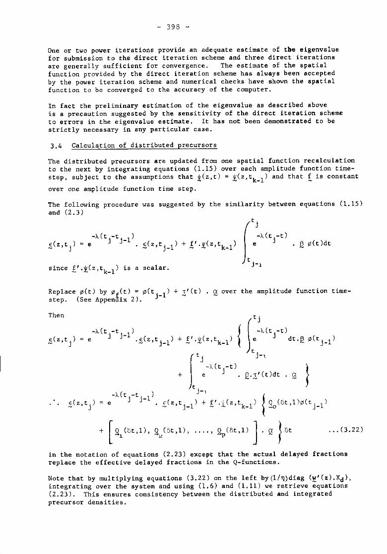
- 398 -
One or two power iterations provide an adequate estimate of the eigenvaluefor submission to the direct iteration scheme and three direct iterationsare generally sufficient for convergence. The estimate of the spatialfunction provided by the direct iteration scheme has always been acceptedby the power iteration scheme and numerical checks have shown the spatialfunction to be converged to the accuracy of the computer.
In fact the preliminary estimation of the eigenvalue as described aboveis a precaution suggested by the sensitivity of the direct iteration schemeto errors in the eigenvalue estimate. It has not been demonstrated to bestrictly necessary in any particular case.
3.4 Calculation of distributed precursors
The distributed precursors are updated from one spatial function recalculationto the next by integrating equations (1.15) over each amplitude function time-step, subject to the assumptions that ~(z,t) = ~(z,tk_l) and that f is constantover one amplitude function time step.
The following procedure was suggested by the similarity between equations (1.15)and (2.3)
• f2 (/J(t)dt
since !'.i(z,tk_l) is a scalar.
Replace (/J(t)by (/Jf(t)= (IJ(t._l)+ !'(t)step. (See Appenaix 2). J
~ over the amplitude function time-
... (3.22)
}
{( ~l. ( t .-t )
!'.~(z,tk_l) Jte J dt.f2 (/J(tj_l)
Jtj j-l
-\.(t.-t)+ e J • f2.!'(t)dt . ~
t.J -,
~(z,tJ_l) + t"1(z,tk_1) {So(5t,I).(tJ_1)
...•, ~ (5t,I) J . s! } 6t+ [g (at, 1), g (at, 1) ,1 2
-A.(t.-t. 1)J J-e .E(Z,t. 1) +
- J-
E(z,t.)- J
Then
in the notation of equations (2.23) except that the actual delayed fractionsreplace the effective delayed fractions in the Q-functions.
Note that by multiplying equations (3.22) on the left by(l/~)diag (~'(z).Xd)'integrating over the system and using (1.6) and (1.11) we retrieve equations(2.23). This ensures consistency between the distributed and integratedprecursor densities.
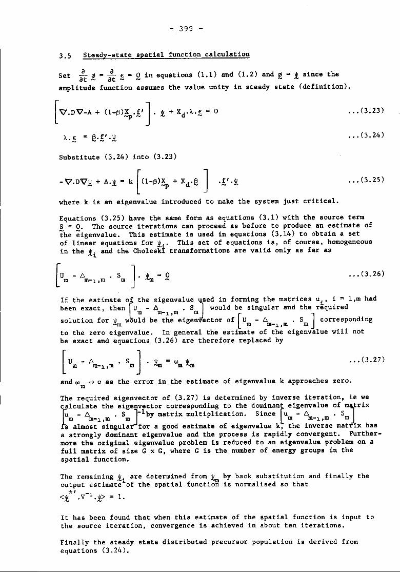
- 399 -
3.5 Steady-state spatial function calculation
a aSet at ~ = at ~ = Q in equations (1.1) and (1.2) and ~ = 1 since theamplitude function assumes the value unity in steady state (definition).
[~.DV-A + (l-D).;,'!' ] . :t: + Xd.L.!\ = a
A..~ = /2..£".1
Substitute (3.24) into (3.23)
... 0.23)
...(3.24)
- V.DV)i + A.)l. = k [(1-D)';' + Xd'~ ] .!' .)i ... (3.25)
where k is an eigenvalue introduced to make the system just critical.
Equations (3.25) have the same form as equations (3.1) with the source termS = O. The source iterations can proceed as before to produce an estimate ofthe eigenvalue. This estimate is used in equations (3.14) to obtain a setof linear equations for 1i. This set of equations is, of course, homogeneousin the ii and the CholeskI transformations are valid only as far as
• Sm... 0.26)
If the estimate o[ the eigenvalue used in forming the matrices ui' i = l,m hadbeen exact, then U - D. • S ] would be singular and the requiredm m-l,m msolution for 111 would be the eigenvector of [u - 6 • S ] corresponding
~ m m-~,m mto the zero eigenvalue. In general the estimate of the eigenvalue will notbe exact and equations (3.26) are therefore replaced by
... 0.27)[u -!:lm m-~,m
and !Ai ~ 0 asm
• Sm ] • :l'.. = "'m t"the error in the estimate of eigenvalue k approaches zero.
The required eigenvector of (3.27) is determined by inverse iteration, ie wecalculate the eigenvector corresponding to the dominant eigenvalue of mJtrix
t -6 • S ]-lbY matrix multiplication. Since [u - 6 • Sm m-1 ,m m m m-1 ,m ms almost singular for a good estimate of eigenvalue k, the inverse matrix has
a strongly dominant eigenvalue and the process is rapidly convergent. Further-more the original eigenvalue problem is reduced to an eigenvalue problem on afull matrix of size G x G, where G is the number of energy groups in thespatial function.
The remaining ii are determined from 1m by back substitution and finally theoutput estimate of the spatial function is normalised so that
*' -1<i .V .1> = 1.
It has been found that when this estimate of the spatial function is input tothe source iteration, convergence is achieved in about ten iterations.
Finally the steady state distributed precursor population is derived fromequations (3.24).

- 400 -
3.6 Steady-state adjoint function calculation
Transposition of the matrix operators in equations (3.25) destroys thelower triangular nature of the matrices inverted in the Choleski procedureof the source iterations. The elements of the adjoint function at eachspatial position are therefore symmetrically re-ordered in energy. Theadjoint matrix operators are then formed by transposing about the non-leading diagonal, thus retaining the lower triangular form where appropriate.
Since the eigenvalue is the same as in the direct spatial function problem,the extrapolation technique of the preceeding section is used without previousresource to source iteration. When the output estimate of the adjointfunction is submitted to source iteration it is immediately accepted.Finally the elements of the adjoint function solution are re-ordered.
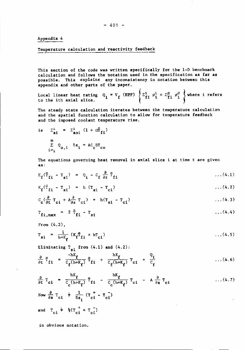
- 401 -
Appendix 4
Temperature calculation and reactivity feedback
This section of the code was written specifically for the l-D benchmarkcalculation and follows the notation used in the specification as far aspossible. This explains any inconsistency in notation between thisappendix and other parts of the paper.
Local linear heat rating Qi'" Vf (HPF) {L:~i (Zlt + L:~i (Zlf t where i refersto the ith axial slice. jThe steady state calculation iterates between the temperature calculationand the spatial function calculation to allow for temperature feedbackand the imposed coolant temperature rise.
ie =
OZi = AC oTc co
The equations governing heat removal in axial slice i at time t are givenas:
=
... (4.1)
... (4.2)
... (4.3)
Tf.~,max = ... (4.4)
From (4.2),1
= h+Kf... (4.5)
Eliminating Tsi from (4.1)i:) _ -hKf
at Tfi = Cf(h+Kf) Tfi +
and (4.2):hKf
----TCf(h+Kf) ci... (4.6)
... ... (4.7)
in obvious notation.
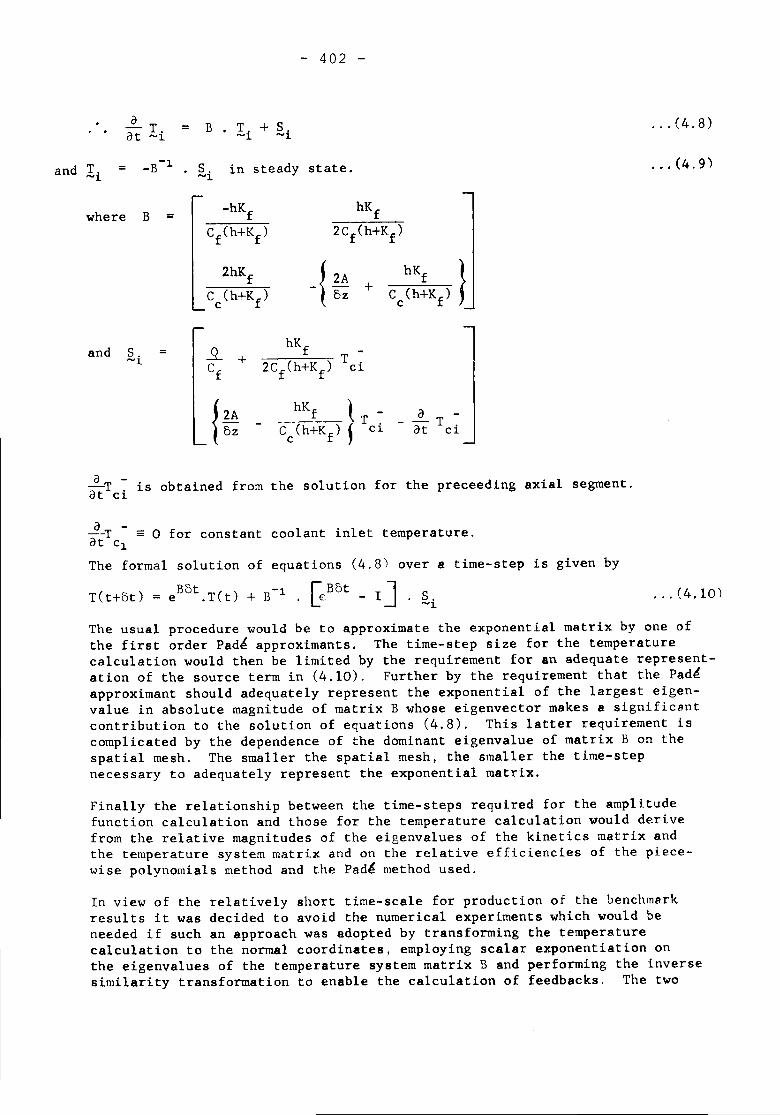
- 402 -
~T = B . T. + s.at ~i ~l ~l
and Ii = -~ S. in steady-B state.~l
... (4.8)
... (4.9)
where B =
and S. SLhKf T .~l + 2Cf(h+KfYCf Cl
{ 2AhKf t - a -
fT. -Toz Cc(h+Kf) Cl at ci
a -atTci is obtained from the solution for the preceeding axial segment.
a --T = 0 for constant coolant inlet temperature.at c~The formal solution of equations (4.8) over a time-step is given by
T(t+ot) = eBat.T(t) + B-~ . [eBat - I~ . ~i ... (4.10)
The usual procedure would be to approximate the exponential matrix by one ofthe first order Pad~ approximants. The time-step size for the temperaturecalculation would then be limited by the requirement for an adequate represent-ation of the source term in (4.10). Further by the requirement that the Pad~approximant should adequately represent the exponential of the largest eigen-value in absolute magnitude of matrix B whose eigenvector makes a significantcontribution to the solution of equations (4.8). This latter requirement iscomplicated by the dependence of the dominant eigenvalue of matrix B on thespatial mesh. The smaller the spatial mesh, the smaller the time-stepnecessary to adequately represent the exponential matrix.
Finally the relationship between the time-steps required for the amplitudefunction calculation and those for the temperature calculation would derivefrom the relative magnitudes of the eigenvalues of the kinetics matrix andthe temperature system matrix and on the relative efficiencies of the piece-wise polynomials method and the Pad~ method used.
In view of the relatively short time-scale for production of the benchmarkresults it was decided to avoid the numerical experiments which would beneeded if such an approach was adopted by transforming the temperaturecalculation to the normal coordinates, employing scalar exponentiation onthe eigenvalues of the temperature system matrix B and performing the inversesimilarity transformation to enable the calculation of feedbacks. The two
- 4.03 -
eigenvalues and the modal matrix were calculated by direct and inverse matrixmultiplication, which is efficient for widely separated eigenvalues as is thecase in the benchmark problems.
With the use of this approach it was felt to be adequate to calculate thetemperatures on the same time mesh as the amplitude function. This time-mesh is now dictated by the efficiency of the piecewise polynomials method,the need for an 'adequate representation of sources into the temperatureequations and the requirement for recalculation of reactivity feedbacks.
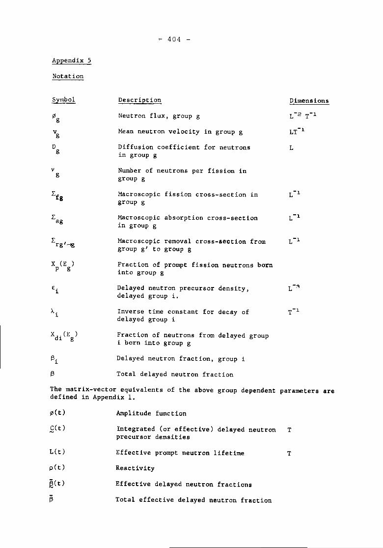
.,.. 404 -
Total delayed neutron fraction
Delayed neutron fraction, group i
Inverse time constant for decay ofdelayed group i
Dimensions
L
Mean neutron velocity in group g
Neutron flux, group g
Description
Diffusion coefficient for neutronsin group g
Number of neutrons per fission ingroup g
Fraction of prompt fission neutrons borninto group g
Macroscopic absorption cross-section L-1
in group g
Macroscopic removal cross-section from L-1
group g' to group g
Macroscopic fission cross-section in L-1
group g
Delayed neutron precursor density,delayed group i.
Fraction of neutrons from delayed groupi born into group g
Appendix 5
Notation
Symbol
>1lgvgDg
v g
Lfg
Lag
Lrg'-lg
X (E )P g
€i
A..I.
Xdi (Eg)
t3it3
The matrix-vector equivalents of the above group dependent parameters aredefined in Appendix 1.
Amplitude function
Integrated (or effective) delayed neutronprecursor densities
T
L(t) Effective prompt neutron lifetime T
Reactivity
Effective delayed neutron fractions
Total effective delayed neutron fraction
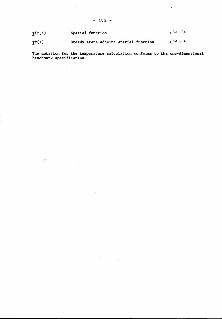
:t:(z.t)
i*(z)
- 405 -
Spatial function
Steady state adjoint spatial function
The notation for the temperature calculation conforms to the one-dimensionalbenchmark specification.
- 406 -
DISCUSSION
J. Devooght
The reason, why the time needed for codes using automatictime step selection is so great, can maybe simply be foundin the fact that it is necessary. There are two distinctproblems for time step selection. The first one is the e-valuation of the final global accuracy and the choice ofthe strategy, i.e. the variation of the time step to a-chieve such accuracy. The first problem is tractable, thesecond one is unsolved to my knowledge. May I ask Mr.Fayers if the submitted benchmarks did contain informationabout the influence of the time step? At least, we shouldhave results for the step halved and even if the resultis unchanged, I should not be completely convinced thatconvergence has been obtained.
F.J. Fayers
Contributors were asked to submit solutions which in theirexperience would represent a reasonable compromise betweenspeed and accuracy. Detailed information underlying theirchoice was not provided. Individual contributors may nowbe able to supply background results in this area.
A.F. Henry
How are the group fluxes calculated in ADEP?

-.407 -
F.N. McDonnell
The group fluxes at each mesh point at a given time stepare calculated simultaneously using a Gauss reduction me-thod. Dr. Ferguson has suggested that it might be betterto calculate the group fluxes separately since this appar-ently reduces the error.
A.F. Henry
Possible problems with 1-D benchmarks?
F.N. McDonnell
When these 1-D cases were carried out, the exponential trans-formation option was not available in ADEP. The cases shouldprobably use the exponential transformation. This is espec-ially so in caseB which behaves essentially exponentially.Another point with ADEP is that a coarser effective mesh isused for the feedback equation; this affects the temperaturecalculation.
A.F. Henry
What are the reasons for discrepancies between the resultsfor case B?
D.A. Meneley
The exact approximation (such as mesh spacing and means ofrepresentation of the moving control rod) used in each codecan strongly influence the results. Each contributor shoulddefine exactly what approximations are used.

- 408 -
A.F. Henry
The implications of discrepancies between results of caseB could be quite broad. What can be done to resolve thesediscrepancies?
D.A. Meneley
The ANS Benchmark Committee is moving in the direction ofdefining benchmark problems as standards, following the pre-cedent set by the US regulatory authorities' insistence thattwo reference thermal-hydraulics problems must be solved byeach applicant. If the participants find that the resultscan be published, it is my impression that the ANS BenchmarkCommittee would be happy to publish the verified results intheir standard format.
E. Infuehr
Automatic Time-Step Control: Adapting the method as used forO-D kinetics (DYN - Ein Dynamikprogramm fUr Kugelhaufenreak-toren; EURATOM 80) to the more-dimensional case by using anydiscrepancy encountered (e.g. violation of boundary condi-tions) as a criterion for accuracy; furthermore distinguish-ing between neutronic and feedback time step with differentcriteria (e.g. energy balance as to temperature) .
D.A. Meneley
See my answer to A.F. Henry titled "further comments on au-tomatic time step selection".
I agree that separation between neutronic and feedback timesteps is a valuable procedure. Care must be taken in the de-
- 409 -
sign of the overall control to recognize the interval overwhich all of the components must reach a common point intime.
A ..F. Henry
What are comments concerning automatic time step selection?
D.A. Meneley
QX1 has an automatic time step selector with reasonablytight convergence criteria built in as default values. Theuser may modify these values based on his own experience.This has been quite successful except for the low-accuracyend of the range, for the shape function time step. Theeffort involved in developing II intelligent II .time step con-trol was quite large.
A.F. Henry
Further comments regarding time step selection?
D.A. Meneley
The 2-dimensional code FX2 uses essentially the same auto-matic time step selector as QX1. The code decouples thetime step required by neutronic und feedback algorithms,so that each subset of the equation system uses its ownrequired time step. The step controller chooses the mini-mum step length on the basis of rates of change of systemparameters. Details are given in ANL-1169.

- 410 -
A. Siebertz
Everybody recognizes the importance but also the difficultyof the time step automatic adaptation. I should appreciatevery much the various contributors giving leading ideas con-cerning the automatic time step adaptation algorithms orgiving pertinent references related to this problem.
A.F. Henry
I believe that is an excellant suggestion, and I hope theparticipants will comply with it.
A.F. Henry
The differences between codes for case B could be due tomesh differences and the way in which the rod effect ischanged. Have we any information on this?
M.J. Bridge
Since his original submission, Cooper has run case B. Hisresults appear to be in reasonable agreement with the CYCLOPSresults just mentioned by Billington and the ABA results.These KINAX group calculations used 43 mesh points and rodchanges were "phased out" from each mesh in turn, using aquadratic function.
- 411 -
COMMENTS
O. Norinder
I should like to make some comments on TRANSPROGRAM. TRANSis made for BWRs and PWRs. TRANS has a neutronic, full tem-perature and hydraulic part. In the neutronic part, thetime derivative terms are added to the diffusion equation.This can be solved directly in the standard way for 1-Ddiffusion except for the delayed neutrons. That causes someiterations to arrive at an accurate solution. This methodcannot be extended to multi-D cases. - Time step is in gen-eral automatically selected, halved if number of iterationsgoes over a (small) number and time step doubled if one(or 2?) iterations are used. Time step is also kept withinvalues set in input.

- 413 -
P.S. Christensen, F.J. Fayers, S. Langenbuch,F.N. McDonnell, A. Schmidt, E. Vincenti, H. Yoshikawa,W. Werner
SURVEY OF THE RESULTS OF A TWO- AND THREE-DIMENSIONALKINETICS BENCHMARK PROBLEM TYPICAL FOR A THERMAL REACTOR

- 415 -
W. Werner
Laboratorium fUr Reaktorregelung und Anlagensicherung
I. Introduction
In 1973, NEACRP and CSNI posed a number of kinetic benchmarkproblems intended to be solved by different groups. Compari-son of the submitted results should lead to estimates on theaccuracy and efficiency of the employed codes. This was feltto be of great value since the codes involved become moreand more important in the field of reactor safety.
In this paper the results of the 2d and 3d benchmark problemfor a BWR are presented. The specification of the problemis included in the appendix of this survey. For the 2dbenchmark problem, 5 contributions have been obtained, forthe 3d benchmark problem 2 contributions habe been ob-tained.
Section II contains the list of participants and summariesof the methods employed in their codes.
In section III, some of the essential results of the 2d-contributions are presented.
Section IV contains graphs of characteristic quantities ofthe 2d-solutions.
Section V contains the discussion of 2d-results.
Section VI contains graphs of characteristic quantities ofthe 3d-solution.
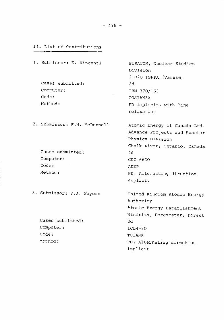
- 416 -
II. List of Contributions
1. Submissor: E. Vincenti
Cases submitted:Computer:Code:Method:
2. Submissor: F.N. McDonnell
Cases submitted:Computer:Code:Method:
3. Submissor: F.J. Fayers
Cases submitted:Computer:Code:Method:
EURATOM, Nuclear StudiesDivision21020 ISPRA (Varese)2dIBM 370/165COSTANZAFD implicit, with linerelaxation
Atomic Energy of Canada Ltd.Advance Projects and ReactorPhysics DivisionChalk River, Ontario, Canada2dCDC 6600ADEPFD, Alternating directionexplicit
United Kingdom Atomic EnergyAuthorityAtomic Energy EstablishmentWinfrith, Dorchester, Dorset2dICL4-70TUTANKFD, Alternating directionimplicit
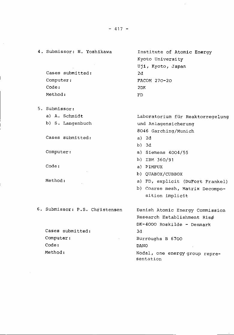
- 417 -
4. Submissor: H. Yoshikawa
Cases submitted:Computer:Code:Method:
5. Submissor:a) A. Schmidtb) S. Langenbuch
Cases submitted:
Computer:
Code:
Method:
6. Submissor: P.S. Christensen
Cases submitted:Computer:Code:Method:
Institute of Atomic EnergyKyoto UniversityUji, Kyoto, Japan2dFACOM 270-202DKFD
Laboratorium fur Reaktorregelungund Anlagensicherung8046 GarchingjMunicha) 2db) 3da) Siemens 4004/55b) IBM 360/91a) PIMFUXb) QUABOX/CUBBOXa) FD, explicit (DuFort Frankel)b) Coarse mesh, Matrix Decompo-
sition implicit
Danish Atomic Energy CommissionResearch Establishment Ris~DK-4000 Roskilde - Denmark3dBurroughs B 6700DANONodal, one energy group repre-sentation
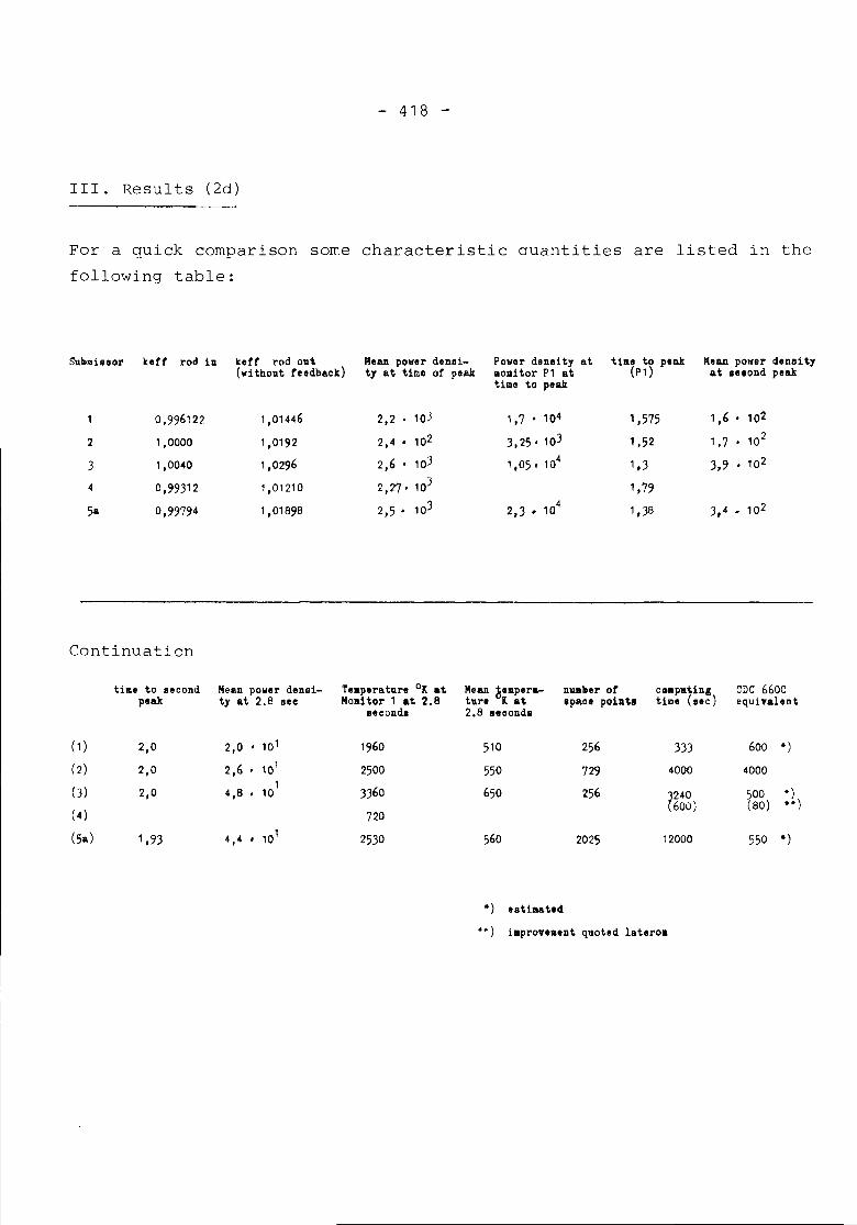
- 418 -
III. Results (2d)
For a quick comparison some characteristic auantities are listed in thefollowing table:
~u.Dilloor keff rod in keff rod out Mean pover denai- Powor denoity at till8 to peak Mean power denoity(without feedback) ty at time of peak 110 attor Plat (p1) at neond peak
timo to peak
0,996122 1,01446 2,2 103 1,7 • 104 ',575 1,6 • 102
2 1,0000 1,0192 2,4 • 102 3,25' 103 1,52 1,7 • 102
3 1,0040 1,0296 2,6 103 1,05. 104 1,3 3,9 • 102
4 0,99312 1,01210 2,27' 103 1,791,01898 103 4 1,38 3,4 • 1025a 0,99794 2,5 • 2,) • 10
Continuation
time to eecond Mean power denei- Te.perature °l at Mean ~.Ilper~ nUllDer of c...pat.ing CDC 6600peak ty at 2.8 see Moaitor 1 at 2.8 hr. K at opace point. tiae (IOC) equivalent
ucond. 2.8 second •
(1) 2,0 2,0 • 101 1960 510 256 3)) 600 .)(2) 2,0 2,6 • 101 2500 550 729 4000 4000()) 1 ))60 650 256 .)2,0 4,8 • 10 (240 500(4) 600) (80) ..)
720(5a) 1,93 4,4 • 101 25)0 560 2025 12000 550 .)
.) utima ted•• ) improvement quoted latera.

- 419 -
IV. Graphic Representation of Characteristic Quantities (2d)
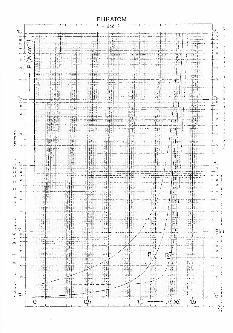
EURATOM
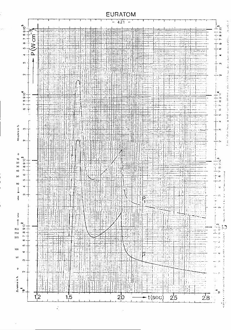
~~~ (')
.'E.c,.c.a
N<{
0M
10 CJ
20
~j:30
40
50
=t60 ~ -
1 (')-j-~~
,1NJ250 CO
"200<O-
"'"100~-
50(')
0N-
o~
S
"II
..'Il
~~ ...~ coN
EURATOM'4:21 i
,-+- ...I
I _TI
-.Lo;:-I, ~
-,-0..
1I
--,- C"'t
i
--~ :...
'-0 :;
OJ
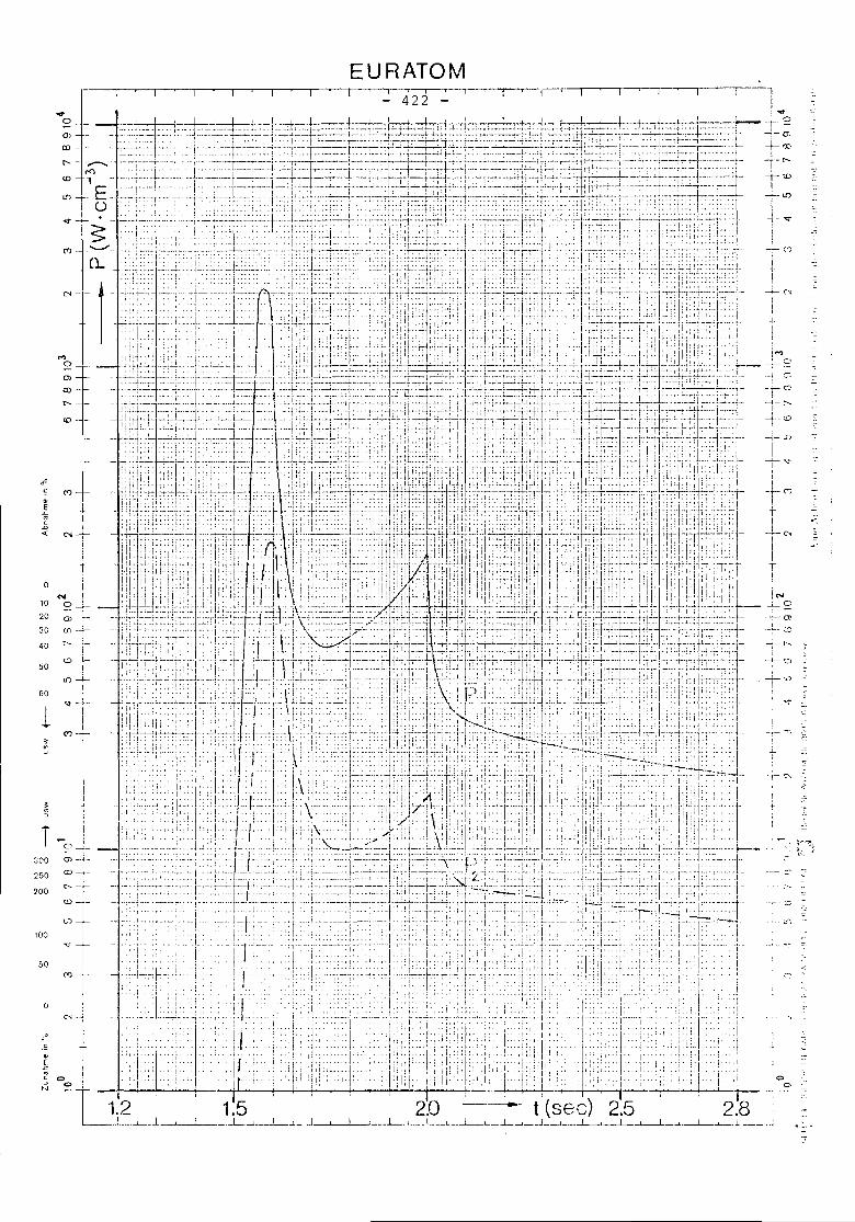
EURATOM
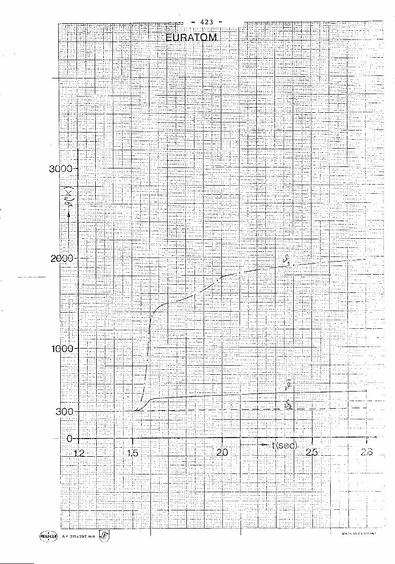
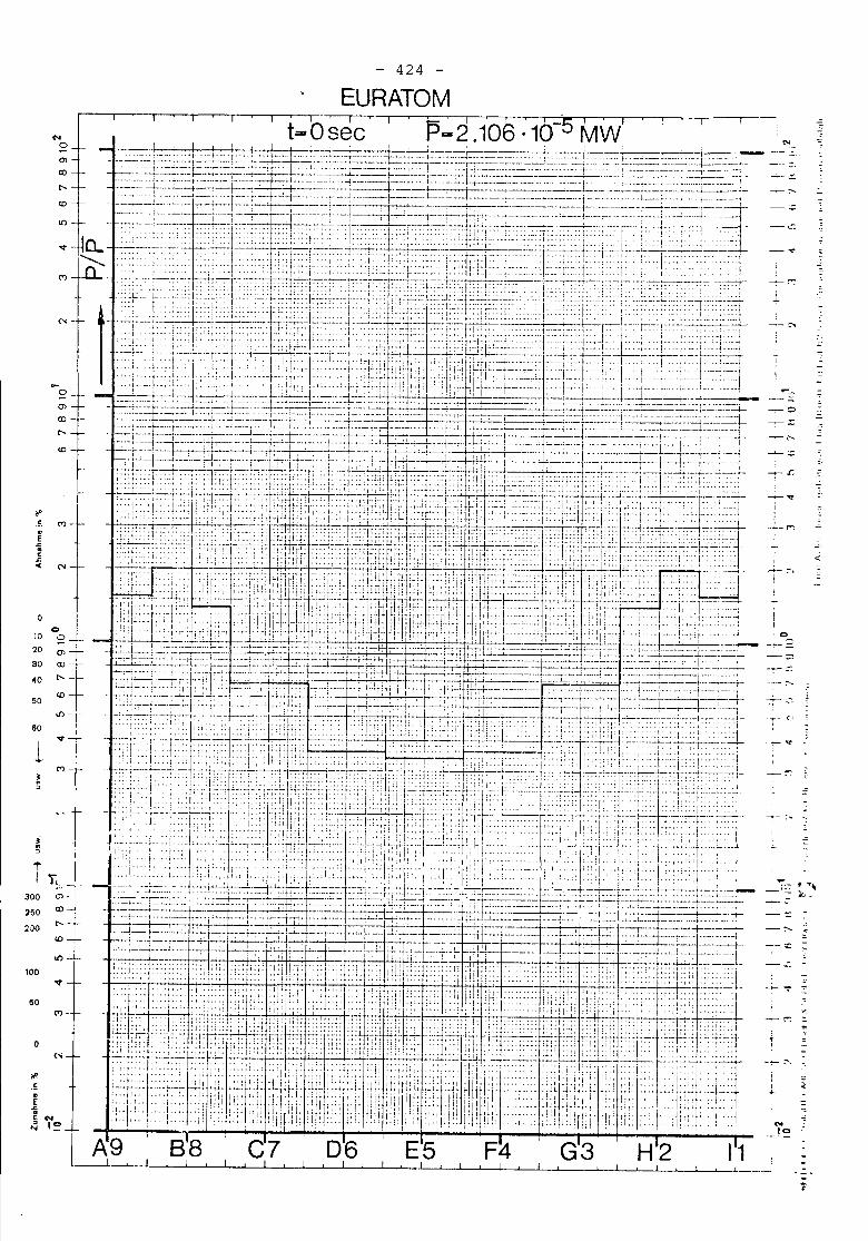
424
Nomco!'-
-~--
<
--
--.,-
mco - -
C>o
o
50
10
2030
40
It)
100'<t
50C')-
aC~
If!.~..i..c N~ I~N
T Ie I-'-I ~300 O'J -:-
250 ~+-i~VO
<D
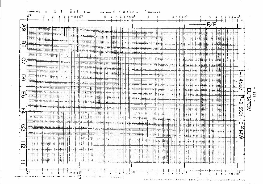
mC~JJ~~Ios:
5 6 7 8 91024326789101
Abna~me in %
2 3.; ::; 6 7 8910°
I I I I I I3
I I , -
uaw. U8W. t-- g g; ~ ~ ~ (5 0
.., ., ...8 g; 8 --t
5 6 7 8 910'1!-4
g4
g;
3
o
2
Zun.hme in %
102
»1 , II . I I' ' I 1 I' , ... """ I I
<.0 f-----:c T; ~+~----'-P" E:=' c:::: F=T I qi r" .:..=:t-~-cc~r--:::;.c~tr'-:--":r-mi~ ~::"""::::::f~~:,+L: :::--F -'r 1::;"'CH+(J-::;:"l;;: :;:: -rl+ !Il=~~::~t"=~.~...IJlff']I~@Jm'j-~ZTImr.-r jrIi~~~~5:iI.i';:".1[rI1 iH:rrnI~Uli';~ili~0,..•.•! 1!Ir
OJ 1----' j'-~.:" --:::::t:';::c~" --',. l 1 IHI~, ...,. __. -'~.',-Il ,.- :.:1.-- .•. i ..iil ----...~----------.-..,.",.Ci,,,--,,r1'-Ttti 1 ..L __::J:. 1+1 .... [,T,,, ',.,. '.~-'"--- .'. 1T.~- .. :':L- ~_.=:-+-~-~-:-: :.: :t- ._. :-.,~It.t.:"::::::-~.-:::-:":'::-~::=~:J:'~.~. ;'.l. .. -* :~: :._--+ <;"=:r-:::: ..:::- ~:_:: '::~:_~J-.~. :-.r:-~t.:-:t- r -f-~.r -.::--~:::.-: .:;.n _;..;;+:.;::+ i:r":~ :;~: .::_.' _ l-
ex> I .--...' _:.::.cr C:c:.t=-I ;.' ,: j ; --.-.:--:,~..~__-.------t._:: ..c""--' ':.~.:::I.'Tr:~~ .:'-----_:.::j::==-~.~"c:., ::t. :__.1 --,. '.j .Li::.::.-':.: .. : .:;~~t.nl:;:i: ",_.t",.:.;-::.:.: :jC 'm". t-'- ""'. '-:-:1.; t. --. '. -----------.. .~ ,.--.,"::::: __..4 trr. ,'=,::L_""j:== --.. + I" ".:i::'--" .: .. f t'., ,." ".t., ::tn - I::-t:-: ...- ..: -r- =:~ "'__. ~_I "t:: ~.... -t
o
• -~ •• ":~_='-':'~'==~.~_~.':':._;:~~---;'~?---' _ . __ ~ .. _~~.--t--~--~:~: "t-"~" - • t -.~~::::~~~., ....~~:.::~~ ~..._. ~.'.'"~-:;:::i=t: ---~c:::::::i:::':_ ...•.. "1 r I .f-'~ •. -"--." . ' .•. ~:::.r " ...• ., .";" .. - .. - --. __f , -.r~' -. _.--'---::::::: ,'., . .c: ' •• '.' ..... I rrt,.--,.~--.:cr .. r ",:.;1 •..-- ". j,-:". .. r----------- -- .. -': r:::=::::t::-:.:. ~'::'"::-.;.::-: ! ::".:f: -:/ j- :::t::.-:-:_; ,,=':,-~'!:~' .;::-:'_:+::'::: -;--::-;:::_ ':'t-:::,_.:t:. .' -r ...... --:-:t::t::t .. :-:::::j.'.4.- ..' :.:;:"r" ;.:':: -- '1. I fl _1;::- ~-~ :::;;:1:':-;; ~~"j:';'!'~.:~:' - , .-
:::,-::=.~~~~:.t:~t:;~~c;-:~JIlc:[<::l.Jr;:c~~~::-f~~:JT'I:i~~;)k:~~-L'+L VL~j~~L:-j~t!: ii: :! •. :::' ..' J. L r J)')l LJ iUJlt1liJ1L ~~.'. I_! l'-!J. () --~--t----'--.F:.::I-:-'" -~ .. _,--t. 1 f~1 ,;: 1':..iCh ,.tj..-, ~---~,.-.. t l' '1::F11'~~--'---' --'-- '---'::'iJ::: 'j, rl -J Ifl " ... :;['.r "'ir"""'''-- L",. ,t If,
['-J.~=:::i=~ =-~~~~~:~~~;~~: :_~~~'i~1.lFf'IJ:~-:ii.:.L~~:.t::' ;~~;;.,:~'~"~~~;'~'~.~;l~:.lr:f~~g~:;~¥.1~:::LiJil:tI.rJ:1 ~utJif;[0~.[i;~~_{t~~;1. T. ~'
- .' .. ::.::::(,.... -- .. . --cr' :'1 .t 1" ~----~.--::cr..:'. - 1--- ..--,1,.-.. =-t-L II! .~ • -.'-r-r .• L" .' --, .~,.,.E::':-':i- ".'--.' -+ d 1 , 1 '" ... , •• -- -, ... , '. ,IT.-:. ,,1.t~.:-c---".' r- ,.- ,.,.;;. 1 11 H-H-~--=::t:=~: -:::=::t;;:::~:::: ; ::-.- .j .... , ,::., t ::::::.::~-=::-:::; ::':-:::1:::::: ~c: "I'I!I t .:E:-l-.::i..:1~:-=.l:: :::-::::;:I::~Ei.+: t":J in: ':-=J:! Ti ii:; ;d~FtlTE j: I; =i. .--.-.:.:: :: ::-- "::':.' ':C:,' -' I ,i'. :'.1 : .'.1,. --_c.:' - I:.:' .:. .' '.. '; -:, . --'; ,. ::;.:.::;, :.'.;:::;.,.:c;... '.1 I ' I :r':: :::: ::': .:,;: ,., t: "" .' '!.'=.,., --.--..j.-- --' ,,, I, i I lle-:;'" 'I ,. "--1 ,.j t f I j"."J-:;':;:. -- "r"'" ;".i ..: . ",.:.-r- 'j I 1 ' ,.,. '.", ""1'--' I"'" ,':,. -.1 j'lft. D~ ! ::--:- ::.:':,:::::: :.:,:: :; - r !+j' .-:: :-1:-;': ., '" I-- . '. . '1' - ,- -: .:'; I.E.: : ::":::.:; .f:''' :~;:+~ '1 1 r'! -+'i----'- :-,-.,: :.:.~ :-;-:: ..-:-:-+:- -:cr+:+ r-r " tO ~ ~------. ~::...-----".---I' Ii'" .--:1--.--" .,.-- I I" 'r,L." ...... "" ,", ,--, ' II III' ,.--,.1.",1 "':!:'" --,,-, '''---- j' II •-_.::- .:.:t:---::.::~.: ;1::':.: .':.:.:- :.;':; -. _ ! ----:._~-:.j:-.:.;:; ':. .'i':::, .:" t- ,I •.. :_;-~- ••• : .• t-.:-~~.!.:.:~.;:::~:: .~~ :;~~ r : 1.1 ;-~-:::~.t::;; ~:J:,!;:;, ~.l:,: :-;.;;'- - L •
~ --,'~.f ,--.,.--..------.,,., "'-- ! I, + ' . ". , ' ,.. "".1'" ,. ',.. , ....• "---,, -- .". I",. -- --' .. " 'J! 1 ,--"1' . :r--J' --. ." '1" '" " '",. ffiVJ --.--- ~,.--.. -::::l.--.-- .. ,,--.-,. """. - - H. - ...-- -. ~". "." . '" .'" .- r . ,. ,,-~.~.~~.,--'--:;",. --,'j. "--[ 1 . j' __h ., •• , --' • i" ',., -- ,.~ ,.'., , .•.:--_-~_.~::::;~:~~:.:~Z~c:: i +11: ,'~-~~~~:,::::; :xi 'cc.-:':: ... : " .'. 4. ~~~ ~~~!~~W~~;::2.{UHte\- ~iL I ..~BH:.t++H ~Hr :+ t8 EFt .. ~",'~-~'.- • __~l:t:':" " .. --__., , .f .,." ..•.~ '----.-- . :1'1:; . ~~+- _ .. T. _ .fr: ._-----+---+--~'__'___'__ .. ,_ --.--.,1"" ., ""., •__'_'f'" __--I .1 . r __ • _.,.J:, ,.' .." _ . ," re.,. "." .. .1..... -------r-o-- - :!:.:l: ' -t - _- T_ -~ ..•...• -<- .• ,-~t::::.:.: ..__.~ .. ~:.~ 1::, - ,--+---+ ----'--.:....~_._ +~.. -f- -." •. f .t-t ~ "'! f- '!'.~ •. , ••.•• t.- .
-_.----~.-:---=---- ..__ --j... :.L:::......: .::: .. 1- - 'j .1 I : : .. --=-~l::-- ::.::-~,::-' ::::=. __:::::.r -:: .. li' -:8=--- 1-------.:J.~1t.::: ::;-;:::L~-i:c-t.. H I L :-~ I --:I; -": :':.1, I:!." r1-u .' ..' 1', t-=..-::;::::'''-_.,,,.. "1 ~ .. '. ---::::;:---I --'--'~--":t" -. i11 -"- +--.'-.----., '~ •. I:,L_i_ -, .1_ •. ~"l '''I 'Id.r__~r-t 'I, .....--~.::':-~' ..~:- :. :-:: :=:: I :-::: - ~.- -=::;: :-~- ... - - - -:-=:=-:._ ...-~~ .~:T-'2 r--;-;-il"'; - - ~ ~ _1;T"l frH-r-Hf ~+t."1~-:-r-ti ._~ . -m ._'!:E~' .---]=--- ----- .. _,t jft ~,._.--q:-::r,,,L,, r-d'::';.;. ---.I::I.--t ,,__ ~.::t:t., ""p,,, '--"ri.l I {'.1-"1' ",1+ It,r '." ~ i i~::=-._~:~:=:::~:.:_:4~.~_~:-'. I ::1" ~:.:--~~ 'I 7f:;-I-~:: ., __ -:r:,- -t.t :--~=~~:t~:~~:::~'t:::: r, - :-r--~_lj:: :::,::.: ,:L_l~:!: : '_H-_01 '''.::.;=J: ,- .., I ' 1.,--:. "'C'!' ! ! t '" t ' -I ':l '+'1'", IC~.Lc:~. ,.1. I! I -..- ,!=r.., 'Ltl: , -,' "" 1 I It--+.,, • I, j""" , •• " " i 11 1:-:::'--_.-,--:: .. _'_ •. ::'~:-::':-7,_ ... :! '_;_ too: -l.J'_~:"- ~ ~~::.I;-~.-~.' =.; I 1 ~ --:---t:------:- ...:r~: :.; __:.:...:.~:J_~ .....~......:. 'l-- . T~--.;.r;: t:'~ Jj' ~r_:' ;I~--: .r.- _ 1--' . --"'--)'---.-. t ,I -,-. ,,,,., I' --.. -. f- -T - _J ,-- .•. -- -,-"" 'n, ""f -- :j + t ~>--t, ---;71' ~.2+1' ,,, tlr. t:" 9
-- - 0-- 4_. --.--•• _.. .4' -~-- ~~ _. .,. t-~., _ _ _ 4--------... 4 _ 1, , _ _ 4 -l _+ -t :"';-1- ._, ,', _--------,-' . -"-,,,. ,--,,--'::::::f f I hfl' -- ! -'" ,1.--, -- •. -- "'-- -! -:I. t .-T-' .~,.[ _f,:+:., .--" -" :~:.--; 1 1 • -,.j:£:j:.' '~.r' t1::-l .,1+ _:t- __t .'" 1:---='--~":£:f:-:-'.~'~"-- :.,., :-~ -."--:: '-,: .. :-- ~:." --: ' - - --~'- "--;-': ';. ,:~;.: ;:. ' '.--,.:.-. -;.::~: ':~:~",;: -- '- fTf-.----------+--~. - ,- . --.• --. ,.. f-r- . t.. ,j J -- 'T -" -j' liT-' .- -- +- f - '=8-- "=;:H ._, 'lc", .-,:t, . ,.-.:::t. ,:;!: t ,t.t. --+ -+--q ~._,,' 'T-I-1; 1"" +-1 T' ,-It t It=-==--=::.:~ ~=:-..:--:::::::. ~~:::. :::' .t. "1' '~-:-.-',- .--=.:. ~~t+::_~~;:::':-: 1':;' ~ l' -:"':::-::'~.- :::::~4---+-:;'rS-: ':- 1 , ! -1-_:=:--.- :=-:~1~-::;: s" #fi :i-!-:~ -.- 1 ~1I1------------ .. ~ .- '---' . l.r!' ,.:~r -" "":: tj1-.~-~=_=__:~: "1",, --, I'" t +tl If-I., .. ,;1 "'''H ,," "" I
~;~~~~~~~~~-~~:l:.:~::.:~.. J I t ~~~;l.;-t~r ::: . i ~,t': ~:-~-.~-.:';: ..~~r~~~H-+~++,+:-;::;~;~F~+++~~:~~- 1'+--1r1----.~,--.":!" !-- . . I' II 'I ' I' " , I' I I I '-- -- " , '" 1: :: 'I I' I II 1, , " "I '" ,," ,'" j, I.:::....:...:....:.--=-.:~T~.:.:.:-t------------'--:.:. - .1 'rTLj.l: :=---::;::=---r- 1':.":-:' r '11~Jr' .:....::..::.:--:1-" - .l..:J_:--=-- I~:-J-LI- -I ~ I ll--i~::"':':'.' --,:,.1.:, ;_:..l.j ~ __: .• ~Ij I;::::.=-.,:-:.'.':,'" :::1:' t;: :'~:=--il' ,,' 1 Iii ,! ::':-:::•.'.:.'.: :j': I.' "'J I; li-:"::: .:. ':1,:'::,_ :,;,.111 il,.-., -.-.- ----+'" -- --,,' 1 iii' ,.----,--:.', .,., ,. --., I I , , ,t ~--, 1.• --, '--, '---- "- l' i ".,' ,. "'1'''' t"j .", I 1 I-- _~"_4. 4 ••. -+.__ ._ •• t ~ .. _ .:.1 ...• ! . __ .• . 1 l _ .•.. ,.,. _. __ j • + , ••••• ~. '" _ •• _4 _ ,
--- -_:---::'::. ::,:c',--:' - -- : .'.:1 ' .1 c:t 1 I •. ':, ::.:_- .:: r"--1 :-='-: ':::. • ~~' 1: ".:::;.;:'j-l:-:- ,": "'.: •. i::- 4l:.I----r' I 'J, -.: -: ': :::: ;:;1 ;;1; L'il ,';-: ..-~-.--~--:I-- .. ----- _. f:: t:j:t,-- .---.j::.-.-, '" -.-.---- 'f 111---.,--.'+-.--' ."I.:.~.;::-.-lTt:l" L ., "---'I-''''I'lPl-f' "" I===== =-J':'.~ -- _' -.-:~ -r -~ --;'+--==~- ..<--1 :_ -:.:: :::. ~:-l ~=;=-:-:-..~. - - - - _- - + -~~+- .~: ~:-. : ~ ..... i~--:-I • !-:~ - _ .:+: _l-_.; ~ __ ... : .. ~ t-l ... ,"-; : .:~ iG)~._-_. ---f=r-:-::':"'_. -----'f l-tJ j-'-;~----t------"'~-' '.' l r: &-11-,--~t-" ,o.:t, •. l't ~r~i- -'1 b t j:J:'tt ,r." L--t ~:; ,," " ... , I II-~-~_~l 4:=~~~~-:_~~-=~'.- fl.l r-'':'~-~~-'''~:--:~~~~~:j'::;:.; ,,=-:--:.-.~~::::~i~~:~'--'- ,1 .;~~~~ :s:~:~~~;;~::~':~;~;;._.-;. Ifc.u --------- .:+.------.~r;q~~f ] I---'-=t--.:-.-----, ..-,,--r:::-:.:::-- =--de1=' :.j::~-.---:.lc__-.- .. __.L... -.. " ',:::: j I .-.----- '1'';':1'''' ". t.rj, ,." "-=-~~-_~-:--~~~-~--_-.-~-~~~:: -._:~ _-- :-*-=_ .. -='~:--, -.-:-:-.--1 ..... ~.~::-.--:=.:J:: .. -:~-~:. I';', -t--~:_+ l__ .~~.p~:-;.-:-S-~;'t: - 4 H-- -.-- ---- --- .. 1----- .-. C-:f~.' , i-H---------.~:.=:C~. ; - .. --1--.-1 F ni1 I:t! ~;:++-- ;::::1 ..... ,,:!C., 1 - 11 .-+.+ ,L j, 'j'" ,,~, ''',' +~:--- "'--::; -:---:.::' _,c- '-, : ,1==----.--:-:::.I:.::::CL.,mIII.--" ."::":"" _' -1_ I'll --.,-=-:::t",,~: ': I :,:" ,,!. I ,.1 >_' ~i'. I'::':.:_~.:.. ;~...: i j L_
-'. , ---;---t--: I'" 1 ' ; , I • ,." --.,. , ,. -:-:-:-:r ' 1 r-I' I "'.,' I , , ' I I ,." ;'1" '1'1 I;:;' 'I ,:-: • : 4 ": • • • • •• : •• If' 1 I : .: ! r ~ : : .; ~, .: : ~ : fl'!! ; : :; :.: .'" I • ! ;' ,; 1 t i : 1 , .. : : : t I : ii' : :.~.. +7_;~-7~I"lr L trti'~T---' >--:-:--:- ~: ;-:- -.~., .t"-- jl.ll-ll I---r-, , t .:-:- ,-" '."1 c:'i ',', ' 11',"1-'" :1"1;1Tlt:~, ;t-"1 H-t:J 1 .I~Irl- '" I . h~s~ '4 I I ' I ,', ", , " I" ,,, , " I ", "t' " ! ' , 1 " I " I I'" 1 .rr 1'1' ,,, I -- ":.:.: ... t-: -- - _. ,_;_ L' .': 1 :t~ .. ' :1:" 1.:;' i:~ . i t-'- l.:...i:.' :: .' .::; .. ,1 I -1: i: ,j ,l,. :.~: ,~.: j~ •
• •••• • • ... I • • , •• ,' , 1 • , I... .... , " I • , • I" ". t ! I,' \ If,. I • Ir\) :.,,1':;' -- "H It'l ,"." '"I, --"'" I r"""""'" :i II"" "1'1'1"" '''''' J I. " ; , I ': 1II ' ::', " , I, "I I : ,: 'I ' , ' " '::, "I ',' I I I I, I I I ' ! I! I ' II:: I, ; : : I
~~
I ' I I I" , "I ' '" 'I' 'II l~'II.", I I'" 'I ' ," "1 I"I ' • • I ,,' , I, " I, "oil " I ' , , " " ,I, --_. , -.. -. :;:, ,,!. j I "ill -" - , --, . 1 ! ',,' • ,-. "--' ,'" I" . " " 1 I, I I : , I" '" I 't ,'.. I '1 I I,' " I II"" '" " ,r!, I' I" " , I I r I', I' " , " 'I I ' '" " '1'1'" 'I I "I "",,,,,,, , t' , ',I I I I: , I' , I I' ,'I 1 . ;: '. I I : Ii ,:: t' I' 1: I: 1 I t;,'''! I ';:' .,,1__ . I' I' ,I" I' "" 't ,,--,I. "1"1""",, 'II "I' "',./.,,'"'' " .. I I I,• :. " • ..: ' ~ ',. , l ' • I : I ' : ~ I ,:; : ' ; j : ::, : I j,:.', I " 1 •• j I ; i ;,.: I •
- ,. ,,, :I:':;!'" ,;1::::1,1 jillil" I ~"'" ,I" I Lll ;.;;:1::::1:;::, ",I:::: Ll.Li1iI1'j II "'1,:11::;1" ,,1. i Ii! 111....L 't : ~ ":":'::'~I 1 I I ,--:--' '1 'I'" I ' - I ~" , .i...L.:lP - t-4:. ,', '.utr.:.::"" .. , Lt~ 1. '
L.--f_-+--.-t--+-.t--+-+---.J--+ H i~1'---'----j-. +-. ~----+-t-l-H-~-.,,---;--+--+--t--+~t-+. +-f [-j-----.+- ..---!--+-. t ..... f----\ J- t i I l---JI\!2 ') 3 4 b tl '; 0 ~I !f) '} ~l 4 : II 7 e lJ 10° 2:i 4 [) Ij 'I B lJ 1111 ?:J '" tJ lJ 'I H ~J 1i11
1<'--."Jt,III""':141lIt'fll./'! ~1111:tli.llIlf.'.'II,~lIjl! .-,H/lill.'tll. ~" I' •.. 111, !~f;",'I.1 Il, .In'I' "l/';"''''h'',!I'''",','
1111,. !'.Il,,' I"'!II! 'If/I,d" Villi lIlli, 111"'111 ! Hdt"I! i,'.1 I, IIljll dill IllId"!I' 1'[ Illfll Illtll1tll"'"11II"dl\',fIlI.
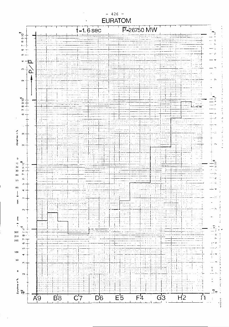
Nol;;;+CXl -t-,['.. -i--
I
426
EURATOM_, I I
t~1. 6 see P=r26750 MW ,.__.~------~ --"--+------'------ ---_. ---_.--_.------ j;....--1--- -~--_..
N
- ...;
--~
.. j .... : ..•.. j.
Ol
Q)
.... -
--,:.
::
c.,,
.",
'0
,!o
---00:::-
--::'""
_..L_ .....
IT~'
1
1i
.'
. ~ ., .. ......-i-
-'--
1 ' , , -1'1' I' ., ;,' II'J j , ,I l' I t -. , I' • l I I 1 r- I
_.__._1 -'-- ~--~'--_:t:-=-.--4-~--.__,~ :...:._.:-- -~.-:..._-;------'---- --' _.J ---- ----'-I I. 1 t j 'j I 1 ••---;'-~_:-.---;--.-i--~-!-:.--:--:--.J
I---:-- !---~iF~- ;-------~---.~.: ,- ~-- ----:--~-.--- __ l-
"I' ,., I, "~'I -1,,1 -:
+ .,r.~J-. T=.T-L. :;.-:.••••."1
]'._.::1.H. 1;1=:;+!ull,.j!'Ii.'!..ui" , , .. 1 ... 1. ,jl .... "":';':1".[ .. 11", .'\.,.!.I .... '.-,
. iI. ..,, !
- .-. i" • '-'1 _ ..~
"I" :.; I... 1..
I I ,: I I \ I '"-.::.-=== ==_.:--=~~- :~~_ -=,.: ~::=-:-::-==~:::-:::~~=-~:~:-~:::~~---t-.::::::=d::... _--~;.:::--~-:::.:....::
:u~f/~~C~-~lc-t<~"ji~~~fi:~~il~~T~~rn"f¥8t:;f=t, 'I ' I I I, I I I I 1, ,,' . ,'," I' " ' l I ' I' I 'Ii' " 'I'" 1 I 1J~----;- I ~---.;.--...:.~-~---+._...:.-b..:.........ri __ ._._+ __ ..1 __L__ --_: _L_L. __- .. --!..--_._-.: !' Ii':' 'I I I I' 'I: :, , 1 ., ' I . I "'"-'1':''' . :. -'I' '. - "1---' -'1'" . -'1'- I I ,1. I I -. I - . --I ",.-. i i 1--T- \ '\'1 i'-j
I ,. t..' \ \ . II I , j I I I I I I 1 I
. ; : : j. ~ : : : : ; '. ';'" :". l'..: i i I : 1 i . ;: 1 I: :, I I I ' I . ,. I I I I ' :. j' " , I I '. ,.. .. ...... -. -1- .. --I '1' -- . " "I --I ,. 'j'" . , 'I I ', I I I' ,.. ,. ,. I . I "'1 '1" .... 1 '1 I'" "! ,. J • I . i, .. ' ....... t. . . . 1" I
.. ,'j , ',.1 , " !'J"I .. II. '1,:". , I. I. j" "', I ... . .....j. "I .
A9 88 e'7 06 E5 Ht2
I
(N~ •
ICO -- -
N
u)
c.~..C NN I~ __
oo
10 ?-+20 cr,]-30 C!' -
~O .... t51 <::--,
60 C'/t<t+1 I
~t! ..+
o
50
100
300
250
200
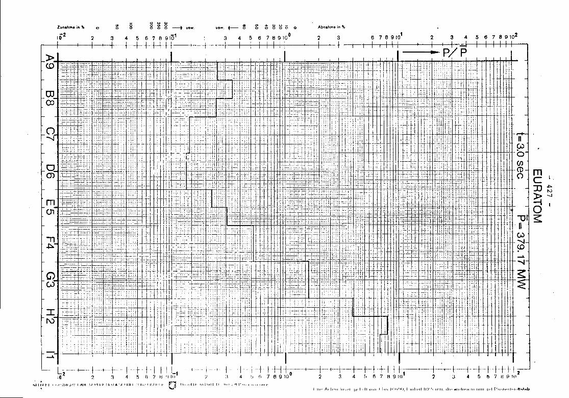
mc.JJ~»:-..Jd~
5 6 7 8 91024326 7 8 9101Abnahma in "
2 3
(JI .. W "" .....o 0 0 0 0 0
5 6 7 8 91004
uaw. +-- ~Ulw,'" '" '"8 ~ 8 ~5 6 7 8 9101
84
'"o3
o
2
Zunahme in ~
102
I - ~P/P ,» 1 1 : I ' I , , ' " , I<0
'
-::;--::.;::'::::1..;,,::::-;:' .:-. ::::::~.- ~'. C:1=:-t-::j::-~"1 .. ~cr::l:::.:,-~ -- -'.; -_::tete- I -:...--. '1-::.::-._- .• r, 1:_":1 - 1fT1-' I -I '~q.H':'-:1' ':'J' I .• 'II.-'--'+:-.: ....e.."1...,~,.~.-.- -,t.--t-t:: .... --=r-T;----- .... /,. - -t:::I::'::1-' - :::r=t=H-"'I"-Ti:;;,-~.tl::rl '}I' ]':'n'j .]~ ... !. '1.~_-~,L;:~:.;:~~::;:~t:;~':';-;:'-'_l! II ;:;::;1:;-' ._c:.':" :,.;: :::;-Ft-{ J!T->'I-;~'~'~' .,. . -r'1!+1';-'-;-:: i. ::': ';:11- ~-j II';
=-.=---=-,-f.:::':-:-:-: .. :-:::::::-t-:-:I::::-:i:'11 ii; ,-_::::='1.:_::: . \r:: ::~., :i1~l:L:LL I, ::,=_:_.; .. :-., ,l. :' II; 1 __l;';' .1"., . I ! . I.'..-. .... .. ,. '.- ., ,. ... .; ---...".---.-:-.....".,....,... ' .... ~ .'."-- , 'tf 'r"....-.---;:1:-- " ---.+:-::: ... Ii . 1'1' --. 'i'" ... , "I .. , + 'r - I"-}-~-'--" '''1' j-",,-I ..., .1. I 1--'" ,.,. " ..... , ,:: .:-=:~_~~-~~:~-:~:::-~:~~::-::. . ! 1 :--1-~~t~~. ',::~:: :-;~t~:~~-- ~ .~ ~~~:1~--:~-:+.:l.-:..:::~.+~-~;~;~~-~~k..-t: f t +-~i: -~::~:4:;4~; ~-::1 ~~~ -- -'. - -fOJH'-- -~-t,- ... - .Ct .- ~ --'I~~~-~-J:J.IT! IT,. ~ ...'- ,c __ .~ ""'f::j l '-t-- .• - ::FL . ~n.t--cl,-....r III .-S .P' 11':1,' ., I' .,. t 1 r-=--:-~:~-~:,.~.:~~=J.::~ .. - , ':-'if :.-:~:__::-~~:::~: .,:,. : ::':.; _,::':::--:1::t::: :.:::':::'I:':,:::ltl -I '~_.• , ' .. ; ,';:;;;:: :',: 1;:. " •.rY"I ~.:.-_. ~=-~:=;:::::: , L:t I I -+-- .. :1. .1:::-'1: ,,_:::,: .. ,. 1-' - .-1 -~-"-.-'-.--::::.:::::. '.T"I.~ ,--.-" ''';.' J [ .' ' •. , j -::.:-". ;1,1 J 11'1)VJ -=-=-=:=-r:-:': i:~'::~:':':;=::--~-_:"'-:: -~- t t-~.r-:.t-:~:":7_:.'~:_-:,:-:I._:-~--~:-~::_:..:: -:--.:--- -1- .--=t=.~-l:::_-::~-:':::::::~L.:~f':':::"-.:0-':',..:-;,.;' -- .:i t -;-:t.:l-~l':j~j .u!:~~.:; ~I .• j ::' I. I l~:
~... =i=!t:T I""" ='-'--":1:':.'''' .. ,,;::' 1 -~-~ +~.~ :.l::"J:-:,::< .. , , ,-r c ,.J 1 !1'f'I'-:=::=::.:.=::£:...:.:.::' ~'::::",::--l,/-t 1t "-'::":::--1_:,'-": ,:'1::; :::::.:r:c: -le "1 r--;-::::C::'I-:itllj>i::F:::; c- , i I :~~i i:;; ;'::!;.:' ;;~: .. , i 'i '.w.. • - '-' . ......- ;-::: I ' ~ I -- -. -.. ., -.. .:.. I I ' , 1 , •• -;: -. , • t "'1 ~ .-,. I'" I' '. .. - ....,'... "., .. I !-IE:-:=:-F--~:;. ::~;:::. ;".;:-:"':" !, :-~-'_+;.-' , ~:.l l.~l ,I I j ;-':::.t. :!.::.~:: 'i~;~';;:: ;;i": ' I : I:! 1-: ;1; :!i' i;l: :!~: t....-t..~-:-:.~f-'-'_T_'_'7.~-J ~ ,-I ' '-" .. ~.; ! 7.:1 -i-'L.::,C ;"';1 J t - ,: i -;... ~-:-t.. I:::; :-r:;':,::: j'" ' (I T... l ~t:t !t.1H!'ii r:-;' I':: I I IIIO ;-::: I;" ;:;.!. .. ;', ." I i I I".' .. hl''''':; :.' 1 I' ,:; :1'; .:; I'::: il;: ;1:: j , • i' I t' ,'I, 'I!: i": I'! ;J' I f• _ .. f" ., I" ,. I r' ",fl r ., ~ :::":. ",j ;., l.;~. ;.; •.• ':'. , •. II, ." ,11 1'1 Ill' l r-+-: • : :- .~. ; •• : ~. t, •• - I . •• --:-:-;-. ~ -:; . I' I I r j:-; ".':; :-.;.:; :'.; i! 1: ' j ~,. !' . ~ - I i j: .. : i : ;' :,~: ! -j ! ~ j:': .
~-;-l..;-' :-:+'-1-;-. -:=-:-=: T - , -' : ;- ...1 :--;. ,- ,: II:, r':':-; .:.:.. ~ -.'. '-+:-ioS- -:':2 ii:-ft:;:; . .t....-.... '!t+++; ;.-!; 1 !;~: ::11 -1-1;-; ::.: 1 . 1' .....:-:: ;'-:' t ,.. ..... ,. n. I I I ' 1.. I .. r ' 'I . .T' " .. , '., .. ' I' ,." i:: I I " " .:. 1 I' I ... I .. , .", I i I VJ
;~;~~~;,:' :~; .:" ~;. :r ! ~ 1 'r:-.~ ;:;~.;';,:.'i',' :: , .; ;~-:Y;ll:.;::: l~:::1 ••.. +~;:: :::: :;" ;::::::: :::;, (:).-.,.t.l .. ;;~ .... , ... 'I L'W" .'. I ........ I"':c. : .'-"" ~I , .. , ;:. T I I I"" ",. "1'1"" "',' I.'. I I llill~ ~ '. :~.; : :: .•. :':. -;-:'':'''-- ':"""0 -I -': + -:+. --,-;-> , ':";i~I-:-~~';" . • t - .,:..::,: ~- '.: ,1-;-;";'.-:-; '+ r.- __i_) •. 'j-:'''':--+.+ ~TH,L;.-H.':i;:+7-:'f- +1++ "j- ." IJ; n,o ~--;-,:::1=-""-;-:-c:";:::c,: ,I. fl' I;' ~;-; ~;';:.;:I:'ll;-i:~:. 1! __:+::_.._;:,L:t .:: :j:: ..,.~ :::::. 'i.l,IlI"'-'::,,-:" ;:::Ii:" ;;-11 h•. t.. - i VI(J)=:;;i~:~ ::~~~~~ii:,- :.t.-I:~, 1,1 :l~-jj:::~;E"'" ." Ill";: ,:::,: I ..- ... '::; __~:f~,c-"t:t~' ';;;i~;:::.'r. 11:~;i:,t~;~4;f) :~I~h:i~:i;~,;i-i;~' '. ,! .. j I CD
.. , " ~ ::..;.; ",: --:.j::. --1: t-':ji::;'r ;,;,. "e: -+-,:-1', .• -.. ..t. -,,":t:: ."",- .• ,...-1_1- ,.;,' - :1 .. ,.1' -: .. -. t.Ttn+~...:#i-1.:~t -1 :.1,:. l'l ()~~_~~~~0~ci-;-~:;F~n: .-!r!--~~~,::-:::~[:I;::::;j=::-~~:::i:':Ti:},;;~:~'. t:~~~q:F._ : !Yf~;::"P+f~:~;!~;!:-;-n~i!L j' ," ..l!1~'..,~£..._:-t: .....:::::,,, ..--4-' ,j:':f. I..,,. T:r "j' .... ..+ 1 11--,-.,-..,....... -.-".. ,I .." ,,~ I", ,1 ,,) ........ jj:! -I I '1111
m _f~~~~>;~~~!i!';.'_~;._'r-ft, T:-~=~"~'h~;n:llIr/~}:i r!~t1::i~,T:~.. ~iJ~i'. - - j t J,~q~t'~~;0ti!::: 1~2~:-I' ! llltt01 .--.----- ..-------F-- . .-:::::::::- ... -.-;.~.. 'I '. '-- .. -- .... -'~.r' ..... ,.7 .,....t .... 'ltS}:::-r i,'.p----:-:j:7..,"'-l'., .... :E+~-!.:.'.'.'."".f'" ! -'j::E:.....:L"::fr--:w; 1.. .. , ",' H 11nTI
;. _ :=~_;::-<¥~~:2:~~:~~~f~.•~j,f:~:~:.-::.':-:=~~_~-:.. ~~l~t]~__L~1~igf$~~~"::'-;IE -~(n ~',- -: : ==T-rt=,;~-tIii~~-l-~jtW ~rft~~i1-:.' ". - ~.-~=::r.:::': ~f1:-~'c:: "';' --I f j f'l -.:-'--;.~:,-,';';.,::.:::,:::-Id:;" -: :. :"j' r - , ill- iti!~'I ;,_..... r : ,,=. . .. ,' - ': _I Eri':j ;-;:1 tl: r :;r: .. t1.; 1:";1 rIll' t
-~-:~~~-::-~~~~~::.:;:;,:_~.~:::r,t:: t IV:;c::~=t+f.::ntl:H :~.::L+< ' t 1- ~ -+~::t:'~., ':1 ... . ." I )'+ffi -f:i--4- :~~ ~~~ +-F) ; :t+ -: t- f i :"J.- - ~ I 'I' . I -' r "., .,.. I --.... . .. -: f. . .-, _1.1 I'.; J ' .".,. I t I-II . I~l~~~~~o::;:~;~~~+:-<;~';;:;:i:1.:'1 -~ti;T;:;;r;>I:t;;,il< T , ;...:-~-,~,';:i .. ;', "",' -;j'1J "iH;.ii;::::;;Ji;~:;-:t1Tr1J.~--~------' . __.... _~.l .... -,,--- - - .. I '.::j.:=k ' Il~~--.-..'" .. -t-;::. ,-" =:- ... -, ..I ,I -+fLi.,~ ,;--1 -II -...=4-:;:-:;'- ''''~- " .. .1. ... "'1'" • 1 . - ,Tt-
- :::.- . =;-- c_:::. ::::::~~;- =;:,-,~:::C::i.F/;;:'- f + cl' J :,:,.-=:,~.::~~FT::1;S=FFf+r;:::i~1 =n T,I 'IE ; _::i' :.-f-, .._It:m~l::iJ~- ~HF!!Ft~Wf:m1=::::: :1.. 'II •--=--:.,....::.-~=: I : • .:-- .;-:.;; I " 1 : 1'(':; :"", ..:: _.; ::. 0__' 1-" , ,- i+I-- -.-., -=-- '!:C':''' :~:j:l :;1- - , l ",-:-t: ::..;, ;;:! :;;. ,P'l ;"1; - .: i I...-.-!".- .• ::::T -... "I I ... _.._.......... . I " --. "-;.. ..-!, 1'" - - 1", "'1 "r"I" "J'1 '11 !
-- •• _ ••••••••• '_->-'" :. ...__ _' ~ -T4~~--~-";"";'~:~":~: '_.,'+-: .. ~, ~7' l J _; :_~_; ...... " ;..;1. .~:_~~ .'L~_ .. _.L"_~,:- W'., '_,..-'_:'~'-:"J+ .... 1.' ..~.r"'W;:r .,' I 1 ' , , --. H' .,' ,., " li d I j, ..1."" ..'. iI,' ,d" "r 'biB ", .. i" T'tv ~_.~-~_;)~~.:~;;~==~:~I~~-;;r1'jl~~~~~'"~;£;:~1' I~~~ I ,;;;;' i:ff~;~;, ,: . ~"t:~i,;~:;10; :~' . ,f
-.---=+_ .. :?~::.- .... -t;.-:~=l:::l+" L .::::.:- -1=-'-=6'1.;::-.:::..:.::...:.:..:.111 . "'1''--' _,C' , , ,', +-: 1 ~ 1,':'JI '..i-:~:lh:~ ;:.l::.~:~._j J i--,:. • . . t . -. . . !:.... .. IF' t, "',' .. . II .. jl' + H .'I .. I • "I' c.. 1.. " ,. , . -+~:- . l' ",.: :' .. ':. :-:1':" , ... ; Int': . I ~ . " :. ':." I; ;',-":::, . '; , ; "L IT.;.'- :-;; :;1'1',. '; ::;. - I~';~:~~::,"'.: :: :: ,'--_.~- t;-'--'-F',:: ,:',.,.""i., i, ::~' ... I : ':- -I' ~.:i": :~:; ;':;':T1;--rTT-:-i':" - -t-.... I. L I ' " . I,. 1 I" .. , ,! " , .. ,. '. ,. "'1 1 ::r1hL1'I'1 , .. 1,,11: ,.1.~: ~~l:.~ .:-:-' .. t t!~. :~: -:-:-~-:~~-~.-~~~ ~f~- -L -~-: ~~ :~.~ -;-"8:--- -;--=:--:-. ~~ -. j t- :- "I':: :*~~ :t~ - o. 'r• __ • . . . . . _.I. •... . 11, n _. ..,. .... ,. ~ t- ,-,-. t .,,, .... .... 1 , • ' j 1. .... ", 11 , • I .•
I L- ':":::1 ~ :': :~::T ::-:::::: 'f I ! itUl~-;-.~'"J' j-HtH i i I Lc" "'ITfl~8~'"; J I J , ill; h!%, ',', .~.lli..'.""'I' --l' fIiL!.:I:, I I '.ii" ' .. ---"'-1" I '''1'~R' 111-'-'.' '., .. I., "., "1 t II II .. f, LII,. ",,1: .. " 1 t' 1IV :--.::--_t::;:~-:f:f'::_':: I II';:" ~"',.!.: '::":' I -.;-.'!-:- 't'l ,I, 'j !1~1;; .;' •. :;:,1 ;",' [--_. ~...:.:::.:.. '-' -I- --I- t r---1- -.; - --- t 1 ]J 1--.- r-" ..J." ----- - I 'j pru-"-. -'..--, -, 1.,~. - 1- .. l'............ "-' 1 I I •. . 1'1' '" j 1 1. ... 'I. ," I I ." L " . . , , , ': ':'" !.:. t ... ':: ! I' f II ( ,i " I' , • 1 , j 11 'I , ,. I,' I i I Ii':!' I,: I I:', ' ,j' ;: I 1 I. -. r ~ .-1- +-1- f rr-r--c'-'" --i- -,.....'---.!. - ., -I ' r [' t- ... -,-- - .. -. - ....... j-.- . t . ~--+ '. ~ . -11---~---c,.,-. ,... -. ---' 'T _I_..j - ~-
i :":;l : : :, . , : , : ! I ;!: l ~I : , ' ; i : : : . I : ~: : : . : : :! : : : . I : :,! i; t ! i : 1 : ; :. : ! : ~ j ~ :.:' I : . :: ,: . :::: I Ii; I I i 1::; ::!; !;,: I : : . : i::: ::::: . ! i \.. - 'r--- .+ -. _ ' iI-I t "'j' ,I _..~ 1'.: .~- .. :, IJt j '.~" "lllil---"-"--'" I~..jl.'. '.,l~':I 'WI I] ._ ~. ,-t •.,,,1 , ••. .1. j- .. \.I'j.jll'... , "1 " ,. .\ . .. .. .,....... .. . '4- ,. 1 '~. i.,.,..I' "., '1" .... .... . 'f .,'. ,., .1'11'" - I'" if ... I Ill' . "., ,....,., I' 1"'" I'" .,', "I ,." "'1 ; .. ,' Ij"" ,." ,I' .. ',--I.' '::;:' :,... ;::.. :::, :::: I' -"-tt..fF :,,: ::,:,::,! : ,,'" L~_ : I-I.: ,;" Ii;:: I:; , l., : I I ' i r. .. _ .' - I: ' 'I "',',::: "1' . ; I l I
L--- +--- t---+--t--, \ --+ ! 'I f I!_ 1--- I-I t .1. ;,j t +++----+-.+-1 ...+--+-+--++11 +'-+--+'~+-+'-"+-++I'+' j !-102 ?:1 -1 !'J (i 7 fl '11,,1 ~':l 4 I, n 'I B 0100 :2 3 4 f> f\ ., A 9101 :2 3 4 5 t) '/ II \1 1(12."'I f (t' : ,,!'nllt.1 f' I ,AHI ~111111 Ii.! lI!l" '..,,litH I .'j.I!I":! P Ii II (,I' 0" I 1" .. Jt,U Ilt •• I;"t~III'1 tll 'H,'II, Ii" "'.1'1 p, .,1""''''Il'
I 1111' AI IIHII 11I'ldl 1,ldlllll Vor" I 11111 flllllll), I 111111111 C\'J 'I 1I1111, dt" ., .. tinlli "' IlllIl IIliI r'IH""1111l1,IU~I .. kI
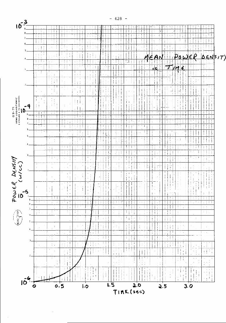
- 428 -
, .
I
i i
i iI :
! !i
,! I! II! I II ! !i i i
I ,i
: ;
I i I
Ii!, i i
! , :! : i •I __ ---'---:-: •• :_
1 i
i i :
'i I: I i I
,i I
I , Ii i I
i:
,: iI ii [
,
I I
I I
! :-i ! I
1 Ii 1
•
: i j
.
! '
; i.!
3.0
I : 1
r ;, ,
: j ';.i i !
: !i
: ! :
:
I ,: ' i i
I I i,
i :i '
! I I Ii i i I
IiiI I
, i II
I I I
Ii!
, ,, ,
I ! i
i I !
I ,
i ri I
I I
I-I! !
!I , ii ! '-IIii
I
! i i iI I I I
I i I ii i I I
, ,I
'I
I :
: ; i
: :! -,
: i I" i
! I
~..5
; i
I i
i I iI "i II 1
I I I
, ! j I- I )-1
; I ;
I, ' ,
II "!Iii, i 1
; ! i1 ~
: I 1 t.~i .~ 1
! i i .. i I I:i,: [:-I!-:i _1-.. f., ..j i
i [1_ r- -i 1,
j'-I
: i I' ! I
--! i. [ 1
~ i !
I : ! !
\ i
i
1 ! ! :
i ) ! :! I I i
;-:-! -i-Ii I i II I ! i
I :
I I :
I I ii I II i
I I ; \
II i i
i ,
! i iif! LI i I-
i : 1
Ii: I
i I
fiII
I 1
i!; i
I ! I j, I
i i
! i Ii i I
! "!. !
I t j !I
'I I• I I i
: i ! !! i : !
--!! iI_I 1 ,
I! t
i :1
! I I
! i i I!
I
: i ! i
f ~:! !I '
i. . j
,I i! i i
i I
i i I !! l ! i
i i I! i
I i, '
I ! I
i I !
: ! i :
! \ ; :
I Iii'I I
I Iiii'I .. : I
i I,- \
! I II ! i
! '!
,
1,1 i !I
i 1 - r
, :
IIi iII
i i! :
I II
: !
1 ! 1I I
I !I ,
I, ! !
, :I
:' I
I ' : I
I I
i ! !
: 1
: I
[ i ; i[ ) I---i
I, I I
I II
i 'Ii '
i i
I \ \ I
,
j ,
: 1I j
!I ,
j
~I !
, I I
: 1!
I Iil
i I I
; iI I i
1 '
: r
i I Ii i
I !I . • ._
: : ii i I !
! !!
I ii I,- i i I I-
I lit I! i !
I i II
IlL
l i ii I I ,
, ',i Ii i,
I 1I 'II Ii I, j
, I
i i I i
1.5 ~,oT I"i:.. ( 5ec)
, t: ! I ! i I! I
: i _ : .1 :! !!
, i ,
I
"I 1 [ 1
! Ii :
I I I Iiii! j [ !
i i -1- !~- -; i ! \I 1- 1 Ii I ti I ,t !-~I I i
I! !! j 'I! , I "
i i ! ,Iii I: i I !
: ! ' :illi I I
Iii I
I i, , '• I !!
-. f
I iII
I I
I I
i i
iI !
!
:i i
!
1 i
.
" I
I J:! II I, !
, !
i I I :i !
1.0
i !
!: ~
i !
) \
, :
; !
,; I
: '
! i
I I
ii'
, :
:
! !
ill
, i i
•
i
-------:--
,
,
: :
,
,
0.5
,
: : I
,,
•
.
! :
, '
,
-------:-
---- ---,-,--
-:-.-:_-,---- --
I
! i!
~ __.I-
•.. ,
i I! ',1:11 /;1
t-----r-~-----, k)1' !I ,
i I I i
"
! II I~' ,I illI I w..~i' "II i10
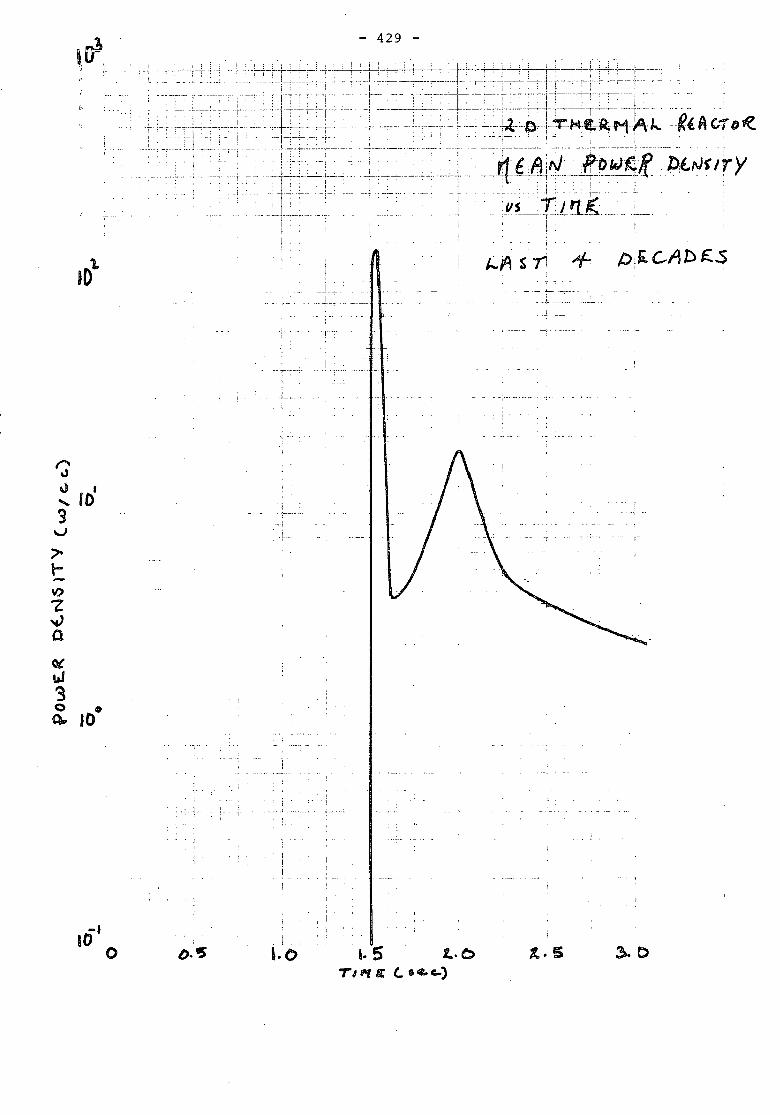
- 429 -
"•...F:~'-:f~_f'~L!+r~_lf=~~i~~t;_DijI-l=T-.. .-+- ;-;.. ,-;"-~-~--,-----:--,- -,--p-:-- ,---.;-. . i- ---- ----~-:-G_-!-~P\-& -a-t1-I'\- J... --~l A (,.,. () ~'. ,-. - ;-1- i - i ..- !-,-;- i- -:- . i ~ -: -:-; . ; c" '.. .
.--.-.....-.-...------,---..-- ... '''1--' -.~---- . -r-- ----.~-7------------:.....------.-,---.
:__;~_~i__c_~ •. _~ .c_'_c_: __ d. _.. q~€ l11ri._~Jfo~~fi .J)~~~ IT Yt~!-jc '!-iLrlrrt' .i
.. J
"J~ 10.3v~t-\I)
~'tJaotw3~ 10.
-,10 o
. .~. l-.. ,• ",- "1"
.1 ..
I__l _ ,
1.0 1. 5 1,.O7"'1 f'f ~ c.. &4I-e-)
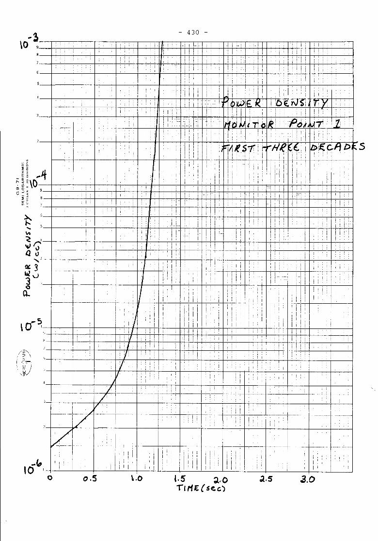
- 430 -
: ..
....
.
• :
: J
i : ,
, I
-! i 1-. I. 1 ~j 1 l_- l 1
!!: 'i' i-'i: Ie ~iii, l i i i i 1 'I: ' I ~ l "I" . i. !: .-- i! ' , i
i I
: !
i, .
.
.
.
•
: !i
:: ,.i i!
!
! ~ I
, :
.
. .c _
i :
:
. '
.:
: :
! I !
i . i ,.
i! I
ii, ::
TYI !":
J.O
: i IiJii ! 1
I -I !
I I i: I-i i i! i
j i
! I
i i,
1 :1 ii ' i
I ! I i
i i III! I
i I!i I i: i i •
_______ c_ . :_,
::. :!! i
j ;, ,
i
, 1 1
!, I
i I • I
I I iI Iii
i
! i !
: i 1 !
, • I
,I •
; i
: I I
: [ i ;"_
i ': I
: :
-----~ ------_._- --------.- - ----
~.5
,! I
! ~
I '
.
.
.!
! : !I Ii; !
,I :
, ,
I, !
1
j i!I !I I ii! Ii, i :
:
iI Ii:
I I
, .. i: : : I
!! . I
,i I
!
,
i !
[ i! i
! ! I I
i !
I '! ; I
i I I
Iii Ii IIii
il, iI i I ii Iii
! ,
, I'
1 ! I iIi! !
i! :i ! I
ill
: I [
ii-I :-! Iii; : '
. :
, I : !, I
., ; i,
: '. !
.
•
Ii : i-Ii I .•. !
l.5 ~.,OTIME{sec)
II i
'I I I
I I
ii !.
I,I
i, !
i r
i !i i
: !
! !.i.
! : I :
! : ;
I i:
:
: :
: :. :
i i
, :
i !! I"I
, ., .
i [I'ii ii i Ii!
I , ! i i!! I I
I: i I i r :: i '!' ii : I i Iii: i ii II i i !'! I
I I 1'1 'i i
! I I i I ii : i i I Iii I
; j i.! i iI 1<:.,.1 i i
: '
t.O
: '
I 1
,
: r I
I •
I I
II
I I
.
.
: .
.: • i
:
O.S
.
. i
.
. .
Ii I
.
I I I
i
-----------;------- _._--~-. I I'
I . I------- t-----.- .----tI I
--~------If I iI i
o
\(J~'I
u::E:t!::
- It!' .., II
ell 0
" :::E"''"
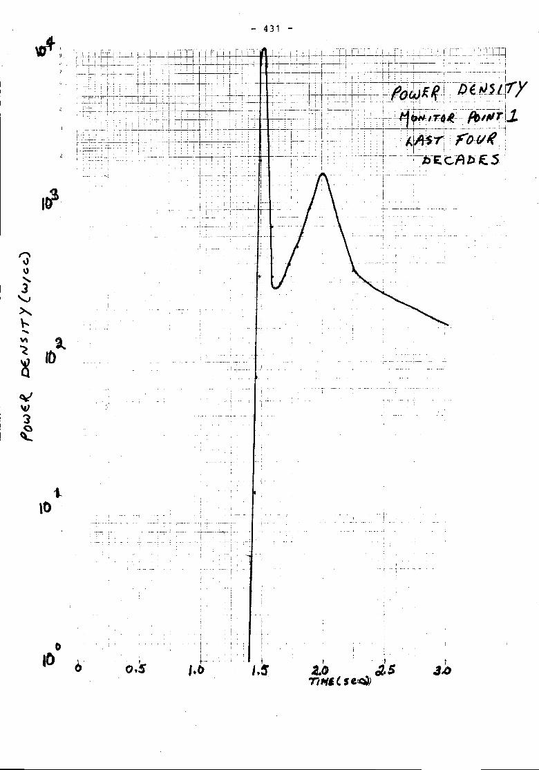
1""'\
"\)~'.J
""'""'" 2..~ 10~
Q,/\I)
3~
- 431 -
... ,
-f -~ -, ri-
,
0 I10
I i .
0 , ~.~ i- , t t0,5 '.0 I,~ .to t2.S .J,I)
Tt"ff, ( S e~
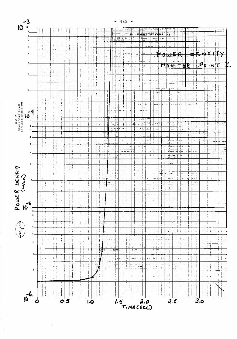
! !
; I
I! _.
, '
, , :
i !
I I i
fIN!:ill~l;I ii,
•
,
1 ! '
: I
,: :! I j
j i
--iH=II',I-11-1- - 1
I" 'i---I"
i
i :
i :
: I i
!I
i :1 !i :j
i i ;
, , ;
! I[ I ,
[ Ii'
Ii'
i
---
! i
, I
,
~ I r
I ,
i II
I
! !
, I ,
! Ii I : i! i, Iii ~cCl IC!,'=!~i- il,::; ~rL:-i':c II+i -II I I
I ! II ' : ' 'I - 1=i,:,1 ,_ - I-I i--'Ci-I ! i' ,[ fl I ! i
!: I I .I ...! r--- ;! _. ! : l-~~ -- -'.'::"'.---~ll i'-j-l-.- -ll-l! -I; 1 "j
; j! ! ..i j 1.! -~l:-~ j--~r-! !-_ -l~:L~ =-~ - -r-l~'.~-!-~ -j-~,J.1- i i i-.! ;;; .f -
, 1 I!!' I, I ['I:r I': "I i 1-- -, • i: ,!_I :: ii' , I, L.~;: r ! ; j.:! ]"! 1 - ~l ~:~-~.).:.!:. ! f .1 L 11); ~ ~ !:,ilr r.z' !~.~ ~.. \.-l<:' :~ 'J-
! I ' 1 I i,li--'II- Ii I : II 1111' i~j:~I,:T!"'i-' il, i 11- i'I~;, i ': i [ , I 1 ,-I! 1111,1-, I~I I, I I I I ,I i! : ,: 1. i: I I -_
j , " Ii i i',i--I il- lii- Ii! t1tPI'~:jll1T-O te,1 '~f):'I .. :r i'-o'";'=1.: : 1 i J ! L 1 ..-1 .j. i J, ' I,r:" 1: i! !.!
i T--=':-~;- -1--:] , , -1 ;~: _~!. t i i 1 •
: : : ' "! ' I' I ' '--: 1 " i, :!' ! j -: _-!.I - 1_ l~. 1 '1 ; -! . i _.j -1 .1 i [-,; i: i ! [i !
: ',: " _I, Iii i I I i I' i : 11::-1 i I-t 'I i ii' : \! I: ii ii,! i-I'. i -I .- \--\- ]- . f-) I Ii, ) i! j i i i !! [
i I: i!, -I 'I' I -.II' I -, II 1 1- 'i i Ii _[ I~ I H. I I I, I i I II i I'\ ' " i, I i I 'i il'!:i 'I I [I, I i Iii , ,: I: : II 'I' I I ' - I i - ! : II I ' Ii' 'I I Ii 'i iil'! - I i 1- - I :' i ,I i' Iii i I - 1 Iii I j I Ii':
:, ill i - i -1::.11
_- _II~ -fl~ II il-!I = -~Ijl-I, -![-III : i I I: I I-Il I IT l I iTII+ i i I;; 1[=
, ! i ii, j , I I i It'- ,'1"_ I 'i iT! : 1 i" :: Ii'II-Ii i Iii : i' >: H ! ' r!'-j I'! I i I' L j i, -i ,"'le-
i --I -~kr-, f \'.l! 1 I :: !~~~~-:-!1 1- !! i -j.: t -1.:-\ i r f-; r-i! ';: ;--:"[.1 ! .f:~~[;.! ~ !! \"J~:: t [ i-.:j=---i ':l~l:::_: ..1"-' II !-! ~! j.
! i.,1 i i ;,=1 =!:tL :1 =1i 1:-r,'~JTi-li - -i i! I I"! i 1---[
, ' i I:!! i -i-i i-~::- --:,:! ii-!l i I! i! ':f::~iH~!:lTf,:1 li- ~,:IIi 1,'1 'I 'i 1- : :' r--'-- 1-' -I I I ,I
i . i .. ~. t Iii Ii! ,. :-J, ,:!! 1!:- i. : i; i!
I .: i :-'1 J~:~r;' i! ~ I ! i:: I! I .__ .- I _ i ~ !! i') : i i - :i I - i i [" I 1-', I" i ill I: i I I ill 1,'- I,: - i I I'
i i ,.1 :; '].-= -1.1 i i Iii ! i : j:- ).. i Ii!. -.:! !i- i~.-- i i !: I. i !
, ; i il : i ! ' Ii,: : i 1 -1:1:1' ,i, i i j j ,: =j: ! i ii' ,i i ! l! ) !!! i i! -I I j---l .. i'1 ! i.. j--i' -i l-J-.l - i i i
, i I I -i i i: i i ! 1 I i .,i II i i'l' il.:.: 11~-1-1- i 'I i i i i i, j 1- i-' -! ' 1~ I i I I Ii: i - -,~I I: [ - i'I~I'=I- II i i I I 'I i i i :
~- , 'II '11,,11"-"1-1--11 '1
1"1,11
"11
1,1 1--1 1'1' ',i-il i i lLI - 'II+'I"~:::~'I-=II+T-:_II - Jl Iii:! I I f
Iii i -! -I- i -I i '1"-1--1 - I I Iii !: i i !i "l -~!._.i--i~i:-= t .! l . i i j 1 j 1 1 ! i ;! !!: 1 I - = ~ i-.j' i
I 1'1 11-:-]-! ;II=I-i!! ,I i t I I i I i I [ i
i i i i 11'1:1'1 i [Ii: I [ I: t i Iii I i Ii'I', ! i i j i I[ ,I, _: '!~- j.! i: i : .! i I! ! 1 r ; ',I 1 ~! ' , !! : 1 ! ii, J ! ! 1 J
: IIi I !.!' i; ! ! i j ( I! I: j I - j ~ j i i J
l : I!!!! I-j i j! 1_,1 -l 1 1-' \ \
: i I il II: 'Ii I! ' I i II Ii ',I 1'1 i .. Li-:::i' : II f: i 1 i J ~ -1. : i j !.- I I '.'f -,. ; '! j - '-_.J i ~-!-~j. ! r I I
! I I _ _ ; ! ~ Iii! i i: If --: I ; I Ii! i ! I I I-i,: ! L !:.::!:c, I! r'j 1_ Iii', : ! IL_ i :": - - I I I I !-_! i! 1- i ! ! !
"ii i~ !:!l::rl- i-i- II!i i ii-Iiil-i:!- I'--I-:r-rti- 1
1-1
1-:1-1-1 -!:! I
! : I' '1-: 11-1=/- I I 1:1 , Ii I I !: I I !! i I ! I i
I : i ,
i i i I t
Ii.
i I i
i I
i i
[ Iii,
: I! !
,
-
,
: :
:: ; '!,
,
,
:
i :
, '
I
I :
: : !
;
i i I I: i I I
•
,
;
- 432 -
/.5 ~.()-r'MI. 'S ec..)
;; i
1 i
Iiii: :
:
:
; ! I
I ! i:
! i
ii ,Ii !
, ,:
, !:
o
9
8
7
-3\0 10
9
8
7
.u z- 0:I ;;r -I- ~_ 0
::: II: 0" <t ,, CIOl 0 "'" .J ~- .J
:I u'" >Ul U
M
l::--
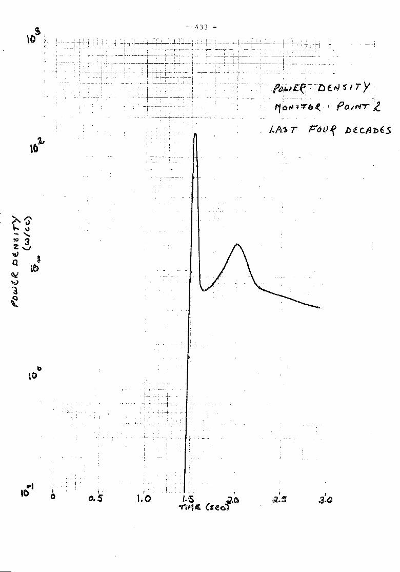
- 433 -
... -
~-~~ '- .~.~:-"~- ) ,-r----:r' .-., i ..
,. '.-_._-'--j-~--~-"--- ~.------- _....
i .
.........--1'-".-' '.,
_.-~
~- r
. . : .l' .._..---':' , "
"'bill lTO(: POINT l.
>'':J'" \J... ,w 3z-....)
'"QOJ\Q)
"1ei
-, ••• T .<-
i .. J..,
! .
. 1...: .
"I80!fo i.().s ,
1.0. ,
'.5 ~.t)-rl111£ (see'
. I
c2.5t
3,(;
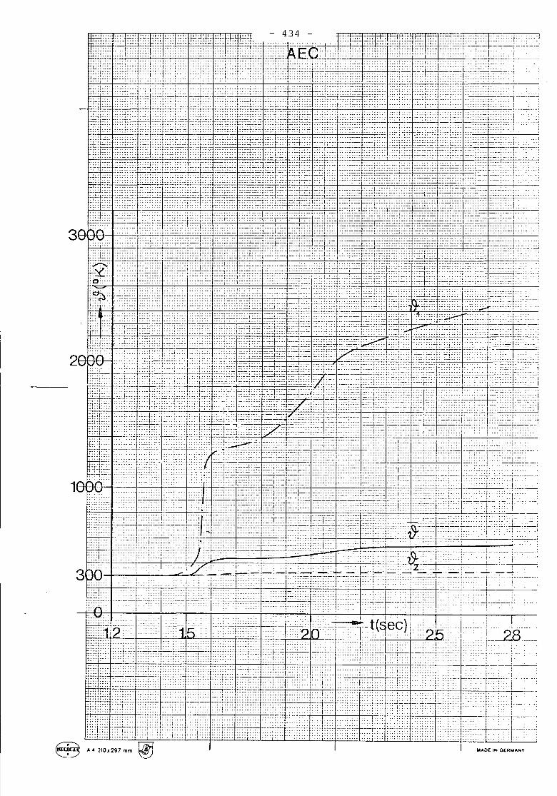
:--:-:-:-:-r---.. .1'::-_: t -----
.,~- - 1,... '-
,i- t-c:--:,:' i'I I
""DE IN GERWAHY'
u:::1 . ;.:rT:::j .... t... :-r":-:
: :.. :~: :. ; : : ::
2
3
=tr.;..;{:~: :::t:=:: :-:':,.1:11' ... :t:... E~ ~~!;t:::t~fF::..::::t - 434 - :,:t:-.:::~::,:j:!:.. ;;.~t::.::::.=rt;::: '":1:''' ...,.... ,,:(: I J~:=.:- ;.::1'... .:j::: l .... .1: .........:::: :':+':-==f:':::'::;:':li..~"" ."re._ ..::1::: . .:4=-- .:=t:~_:L_._ _ __ .....__,;;t':: :.l:'T': I: :: J ::: ::":::::do. Fu~:l: : : ::: :;:;:::i:::::>:::: : : .. . : ..
:~H.:::::::~.::~4..:..' :':: :~':~!:~T:.: : Mfo::; ...~:' ; ..: "::!' :~' ::-}-=-::. t-4.;. ' '..". - . I 4:' i. -- : .•,:;:::,p:.:::::" : j' 0: :~::"'" :.:' .:'; :: .• i.:::':: : : .:.~SJ.j=:'" :<~r "":'!" ...'~~~:-""):-:t' ::e;:~::j:~tA~~':':k. ... :=::r::: :=: .. ~C':-t~::', ::: .':L:-l.<-T' .... '
., . ' ..:,:r::::::]' ......, .. ... .. .. :.:::-:; . ..L::jr1::~f'1.::.: :. ;~::I:::~~:;~~~~\2:~-~~.p:t2;-:~::: .:r:~~~~"~.:;:21-~~=t~_.!,.,-:
"::jf: <;:: .. ~;;_ ,:. ~+:J::::;}~;:;:~::::-;~.. :~':+'~',:~A:'::~>'.._:~e~. .. <::-~~:i:~.......<:;:j~f:H+-c ..:;~~;-: ~~i:::: : ~;; 7~.'::;:+7 :qt-o' ::,:~:~::_::L~~:o~::~:~:~:f!_~=:::..-: =r~::-.::: .:~k~~~:..=.:~~~~8i~.:-0:~~]j~j:=:L::-;.i ::e~ :=rt::'-t#:.:~<~-..~~~:e:..i~:~~ ~+~:~:..~:~:~>~.::-.>" ~~~ :e::~:.,:=:.:..::-~:>_e-..-:.:::F ~ "--r~--. .." .. -, - . I • - -
"- -•...--,_.
- ; -::-:- : ~~ _~~ -=-:.:.E:
" " c::--- ----'tr: -- ,.. -- .-.~-~:.:::
.- _._. --.-..
:::: --....
: :':-: -~..
. , .
.1~~.<.T.••.- ':~~., .,,' ".:.: -- I<....~.::~.....=, ,..,...::.~.,'.~~: ~.:.'-.:~,::-.=--.:;:.:i!.t:.: ...:.r,:.::::=he ;~. ::::. - TO::: .. ', .; !,', I"j .... :, .. . ," .• .:. -:- .'~:;:--'
18[~";~tF I_:!~! .••'•••••U::; it- ._ :1~~_;.~~,.••.•.:H ~l.••:~••~•.
~:~jt:~~ft::H' _ uJ~:~:... ~-._U:;i:--I~--T:--.l:hft.J~-: >.~~~~_c .... ~_5~~~ .'. ---- +-::::::,~-:. ;iJiliV .. ':I~-:': '~ •• :".f••':.. :::.-: E.:":::! -:: ]~'Y~' .:' I .-: --~
::.:....: ':'/ I t'.......... . ~., .Y2: .... 1 I I
3 ?9. . Ii -:.T::i •.:~-:J:T:d+;. r::T=-:r:::J-4-::-j: ~j:~---r'.-::--! --.--":1}ir -:~--'c-i: :~i~jl- ):: --I:-} ..+-)-;W:: : :..-<+~~':+_~:c.:~----· +--~~.--j--:...:-1 :: --1.--- ,' .....
~,'J?c~U[Lih+r .••[ ..cc. ~~~i?~~r-.~ej _,?!"Ir.' 2~.. :::::: .. :. : :.: : r
ii.•J/ .' ~:~::.I i' ::!=" .':.::' Pt:::_:~~~'--:,i:~;: -~:-:---:::;,;1 :. :-:-~:i:t:.:-:+--- .. :: :::--...::: Hi>~..f:: :... : I.U::-: ::/...: ~++L"-:: .:---lh~ ::;;1- ..'.
..... :- i::-. I : I :... ,..
c:: .I:~ . . ., ." ":' .::_:..•.:•.,. _"._.1::.... ::=-_: .. (.. .. :.:.... ,:T:::: ;-:-.;-::-;:- : .... :... ::::- ... ..... -_. . . . :.;: .. 1::. ::::1::.
8 A' 210,297mm ~
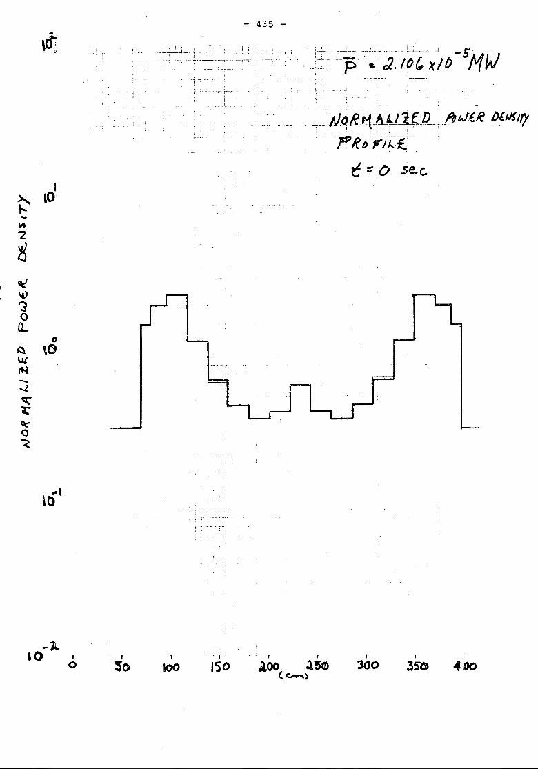
, ,
. , :
. -.... \
- 435 -
t._+_.~ : : : ; ,,~.~--+-...:--..;.+"'l--r .-; .'. 1 --'--':"'~-'. :'.' ~- -1 - 5 ..- <-- ..~':~:~::'-'-;- ' .. ;.' '--'15. ~1:J.IO'xlt; MW
. -1--:- .... -:-----:.. :. -;._- - .. --"' ._ ... - ...-._.:. _...~. ..: i •.
:JJqg~f~L¥.Q ..;.b tJ!/C /JbJ!''7,. 'PIC D Fii..'£.i' .,
t::O see.I
t:' LO-~-Z
~
Q('&>')0G-
oQ \0~
"'"-~q:~Qc'()
'<
... \\0
-16-.0 to. I
So.. , '
ISOt ,
.100 3050(~)
1
300t
3S'C,
400
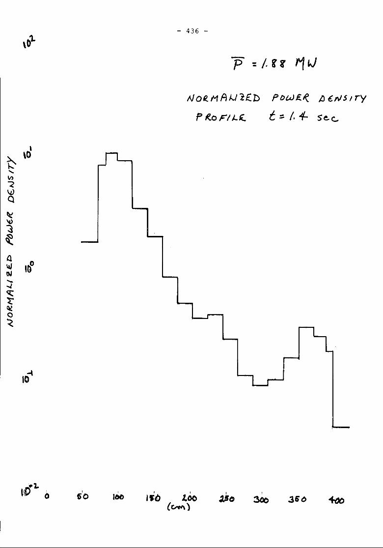
- 436 -
P ({o F I J.,. k... t. :::I. 4- 5eo c:.,
I60 I
IbOI I
"0 100(~)
I»0 36'0
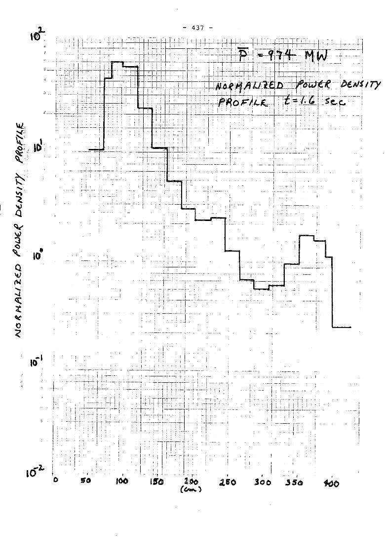
• •10
t ..
... i,
- 437 -
. ! .
---- ..r-II['I
--"':--1 -~..- ~_.~._~,-' - :-..+--_._----':-~-;:--r-c.- .... - ,' ...... ,'c--,' -
I !_.- "'-r--I
i --'~...._.1
,"'.'"-'---' -_ .._--~_..
..~-
T
. i!
; I; iI !
:,'
jIi
o
~,.. ;-~.-r--~- -;..: : . :: ' .._ r--r-:-~.-~.-:.
-1- '-r-':"
:r,"IJT~--)f'Ht ...
,16b
I 0
I
~ i : ':
-1'- "
1 . 1 ., • I:~lTr~-lI' II :I '
:~ J . 1 t
15'C ~.oo(~)
-,
.... ;. , : I i--.---!-~-'......'....T,.T-:- ..~
! ,.
f
300
.... !
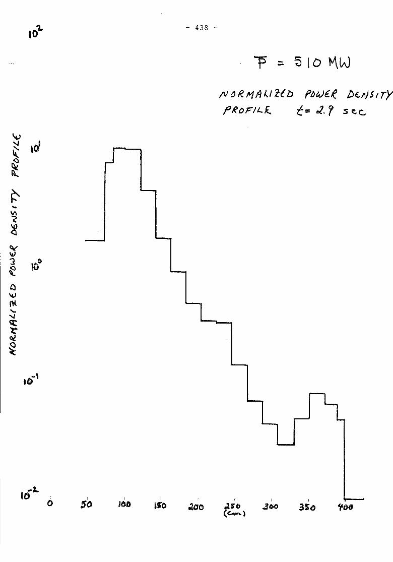
'01-- 438 -
1S - ~ 10 tv\W-IV 0 R. ~ A 1../ 1.(b ftJl,Je~ /)£rJ51 ryI'~OFI'-( t:= .2. r see
"" lO."-J
~
~~
~"\1\<~
cv\U'3 IOc~
Q\l)
~
"'-lq:1:Ql
~
...\to
,50 I
~ao,
35'4;
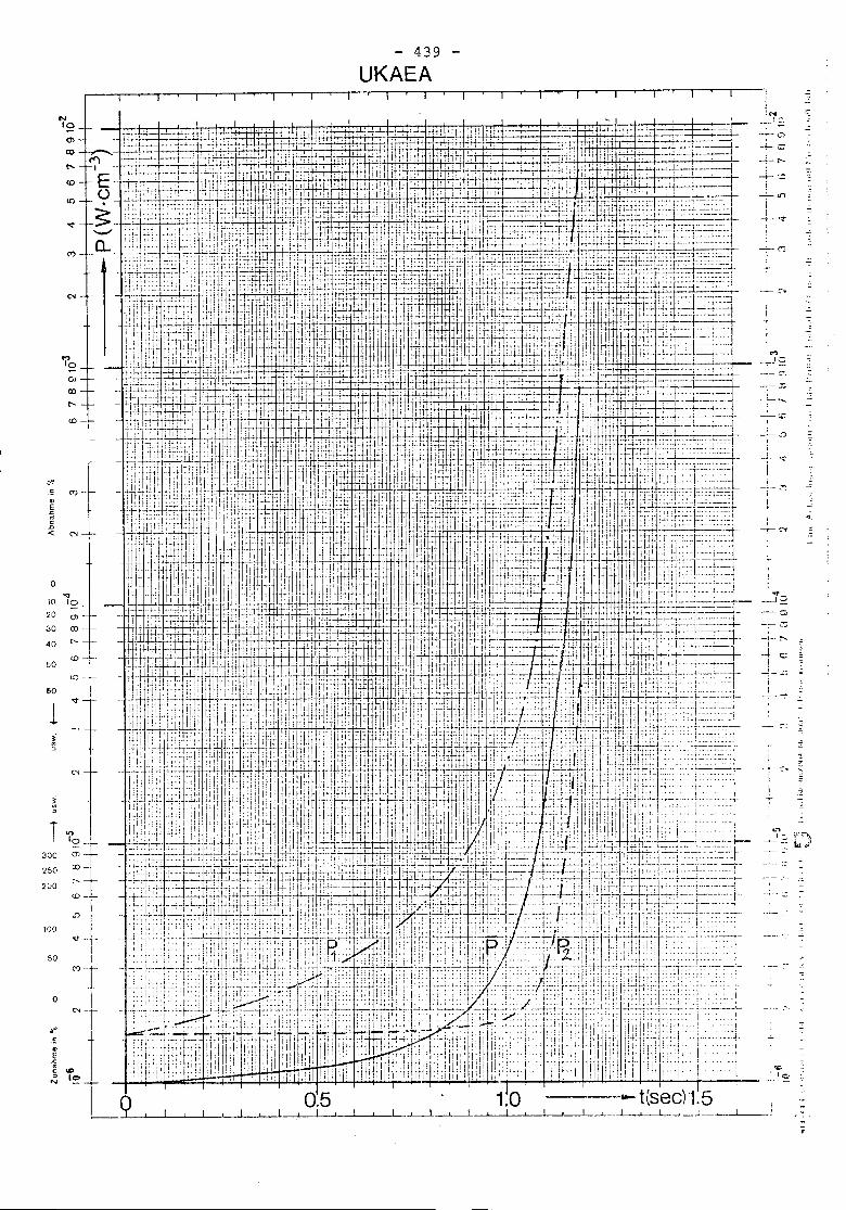
.,. -
iI -:i ::I -I •.
'M__ J'::
.s
010 ""10
20
3040 "-
50 CD
60
1v
~
o
.".s"]~ \QN Ie
- 439
UKAEA
-+-=Tt'-T'~-+-tr>
Ii-+..• 't"
:
,--- ~-i -I
I -.
~iT~I
!
--C":
T
":
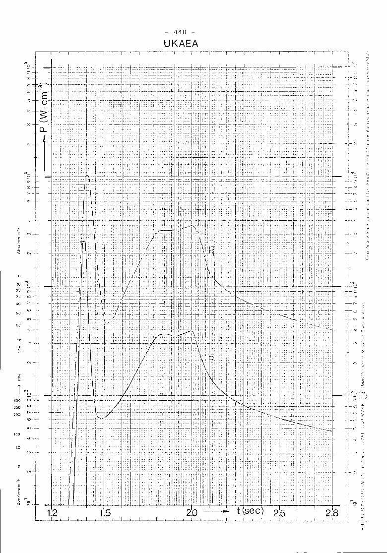
440
UKAEA
c...... -
o
---C"')
,-I
._; .. ~-: --
!-'!--' ('~
1.5I
1.2I
"ot~+"Tm--'r
I-I
C'~-
Ii N I
52 -rOJ --rco ]---['-.._ ... -
=l7T
1
;~ M~ A=38 CO - i .-
[iC'
40
,0
100
300
200
i
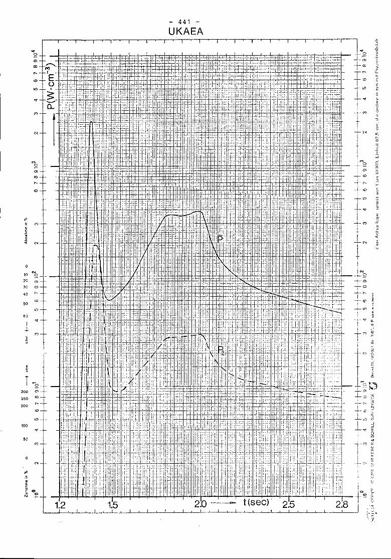
....oOl
lXl
"
'"o())
CO
"
".C')
"Jj..C
.D« N
0
10N
52 - -20 ())
30 CO
40 "ill
50
LO
60<:t
1C')~~
~~
T -0 __
300 ())
250 CO
200 "CO
LO
100'<T
50C')
0N
""-~.,E.c~ <:>~ <:>N
1.2 1.5
- 441UKAEA
2.0 --0- t (see) I 2.5
... .;;
T~-0>~-CXJ "
J,<--rco -Er: "E+~2
"'C
t" --""c-
'"---w
I'" g'--r-52TO> c-j-CXJ "'f: -'0
:::;;~~
-,--v C+~"-2<::
t" <~
:J.,;
IN_~O~;-LenI
t" z
TeD ~..LlC) !.
I ~~-+- ~ n.I '"'I
'"TO? "'"-'- ~
l--~g""~'-
T ~cE
-b~t,)-~~
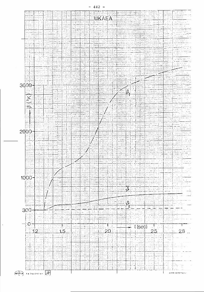
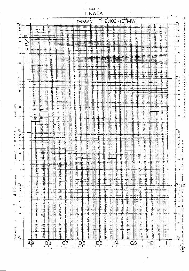
NoOlIX)
to-
(l)
IX)
l'-
1
~
T I~- -300 ~X250200 e--+~tIn100
~I-50
Ml0,,< --
<I'~"f~~ N"~ 10...
- 443 -UKAEA
P=2.106 .10 'iMW IN ""-LO .<
--1-- ;;
r ---<Q -
It) [~
r ~:.
~.
t N "'-..,..<;C
1:
};..;;0
~-t: --
r ..... '""
- ('J -t;.,:
I- .c
-+N <-..
i ~Ir!+o~f~Tl'- ~
tl0 ~
r: E;('.I ,-
I-;--C'? g..,1 ~I ~.I 5
T'" ""! ;:
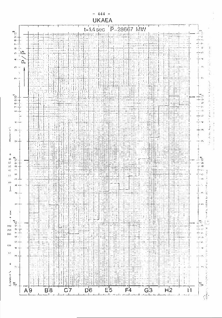
o
200
100
\00
o
N - ~
N-
'I'if
444
UKAEA
iI
_. .1
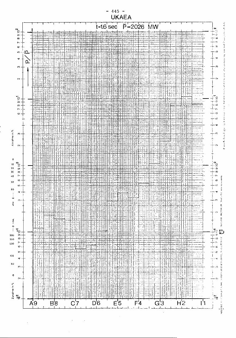
No
....o
"e~ C')
"]g
.D« N
00
10 0
20 O'l30 a:> --
~O "-
CD50
1O-60 ~1
C')-
~
~~
T 10300 O'l
250 a:>
200 "-CD
1O
100~
50C')
0N -
il>~"i'"5 NN I~
A9I
88I
C7I
06 F4 G3 H2 I 111! ....L-L- ..L..._~ __ "" J
__ I
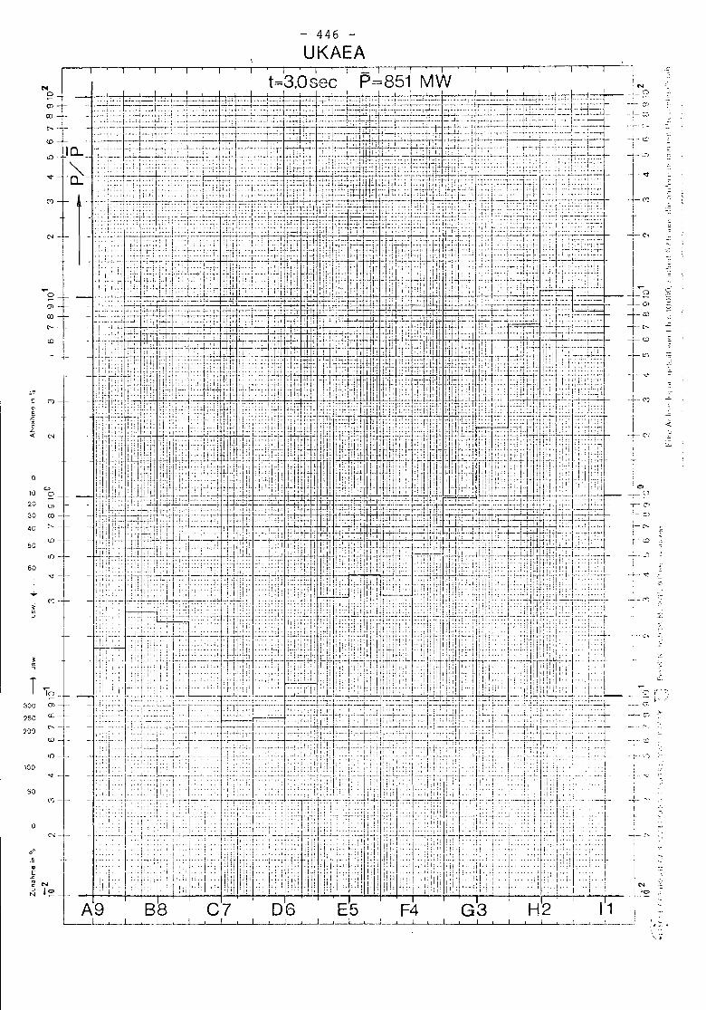
,:.
c
N<"")
_.\-_ .j
-1'-'" ~"~:-
~.,. "
-.- G
_~_:::: ?f-
l!
;-w
. :---j.-.,I. \
.\,.j-
I:1.',
1
':, ',: I," .;. . I .-ii; i. I::i'l ""0 .'c
06 E5 F4 G 3 H2 Ii1 I
~_L_~~_~~_~~_~I_...-i.-.-l---'_~ ~~_L_~ __ L._~_ .. ~_ •.. ,.,,' "._,._l_.J
--,- ,
1Cl..
-~ ..
01-
No(J)
CO
-0(J)
CO
r--to - -
0' jc
"!.0
""
0 "~110
20
30 CO -1'-
',0 ~tCD--50
L{) - -
60 't1(').
~
~~
T 10_300 Q).
250<0- _.
700 r--~-
"'+L{).L100
"50
(Y) -
001 - -
,,"c..i
N 6" i:
l~_ _ ' i.;
N
A9 88L__..4-_L~, .'
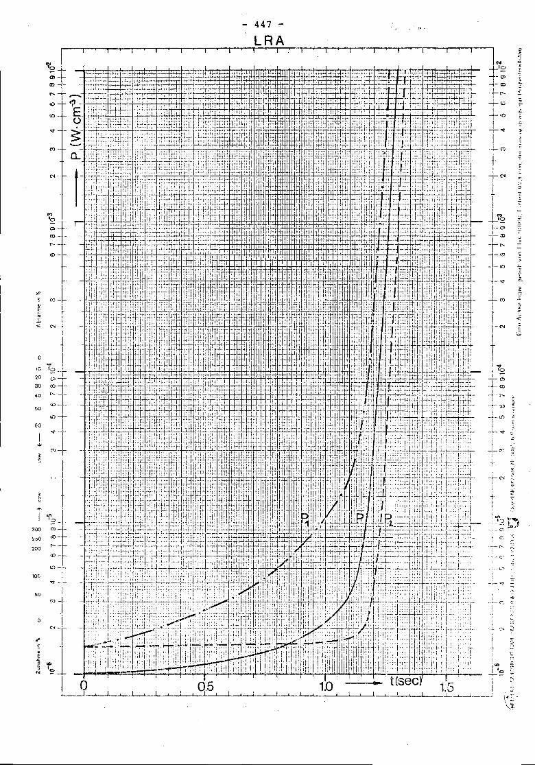
447LRA
" }e ~'"~
-Ola:l +co ~r--. -+-e-CD +~10- J-i.O ~t~ -~ ~
(') -l~iN --:;
--
1 '""':;
I --
.... l~'00> - -+-0 -
I '"co -c- :D
+r--.-e-
<D- r'o ~r: Co
?t? I -:: ~- +C'J~ I i~ -I- ""I <:.0« N iN -
tl:.i
0
70_L i..,.10 -4---19- I I20 Qi +~30 CO .
40 " -- !::1 ~50 I
I r: ~60 ,.
'<t'-t-I ~
(')-~I
.,....
'"-:-("1') ,,'::
~ I ,"
t + ;,:",'
-t- _ore-< 3
I.-.
I "~ +z
" I !..,.
~? -+-, ..ltr.l
l''''_.:__t:~;l>,'
300 00+ --- c,U)- "-t-c.- ~<250
200 e-l --;- " -<D- '-- (L'
lDJ_. I
-t ..l.:,)
10(, i~_!- -;.- ~
I50 I
i~)l >C'-f- ("~ ,-
!.i
0 i ~,
-'-, c" x
/I' 1 ~c
• T ,t;ci I
~ 'I' I~ 7, i "eN ~ ;- ..- .,
('iq.5 ..I ---I---l.-L-l ~---'- -i':; .
\):.
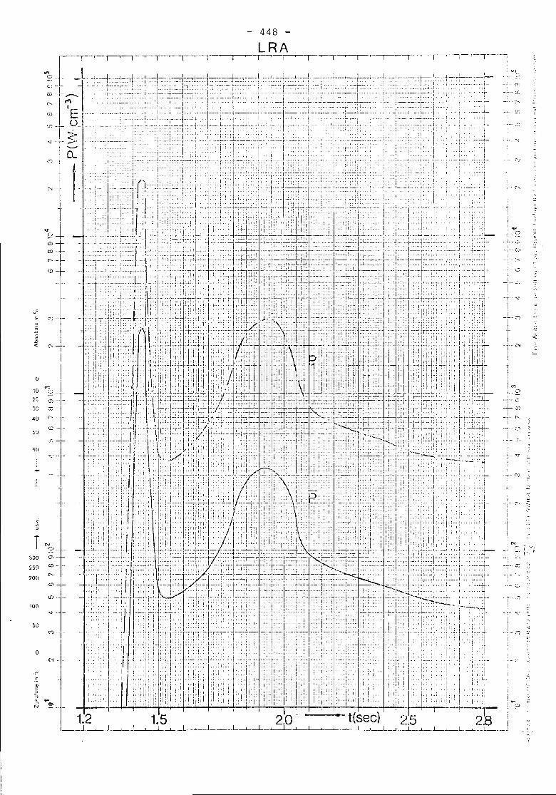
448 -LRA
.•. *''';
,'-
,
r, --.-
....c:,
: v~
"
-_ .. u:'
•. _~._L
200['--
C!).
l{)- ..
100v-- -
50~
0
"
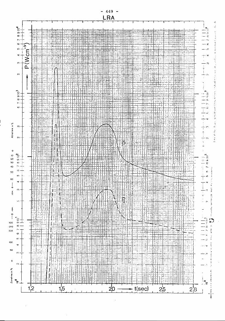
- 449 -
LRA
--
1--""c C').,E
~.0« N
0
10N0
20 OJ
30 Q)
40 c'
CO50
lD
60
1'<t
C')
~
~
T .....0
300 OJ
2fiO en
200 "'-
CO
lD
100'<t
50~)
0 t',
""c..1~ C>, eN
-
-
-
-
-
I I1,5
I I
--:"-
-"c
-.:::;
-:-';
-::".
=
-~ -
=-- .......
.-
:0C>
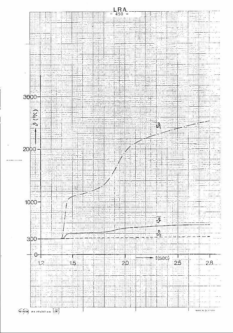
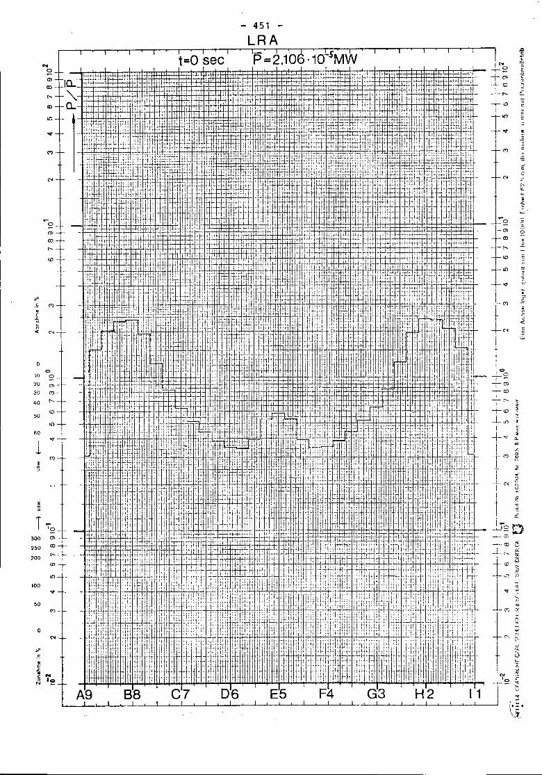
I
N
~ -m -ro -to- -<0
LD
'f
"'0 -0> -ro -... -CD
~o of.~
"~~
.D« C"l
00
10 0
2CJ C'>
30 (')
40 ...CD50to
60
1'<t"
C'j
~
~~
T 19_300 0>-
I
250 ~t200CD
LD
100'<t"
50C')-
0~
iI'.~..E'"..
Nc~ IeN
A9
I I I I -, I
t=O see
- 451
LRA'p=2.106.10LSMW I I I
I
[t1
f~
EE
.s
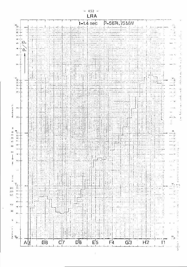
o10
20
30)
.?50
1U0
50
o
C"I ---
-~J~flol
L
MtNJ
452LRA
i___L.__
.. \
_._,:".
_._- >..
N'",
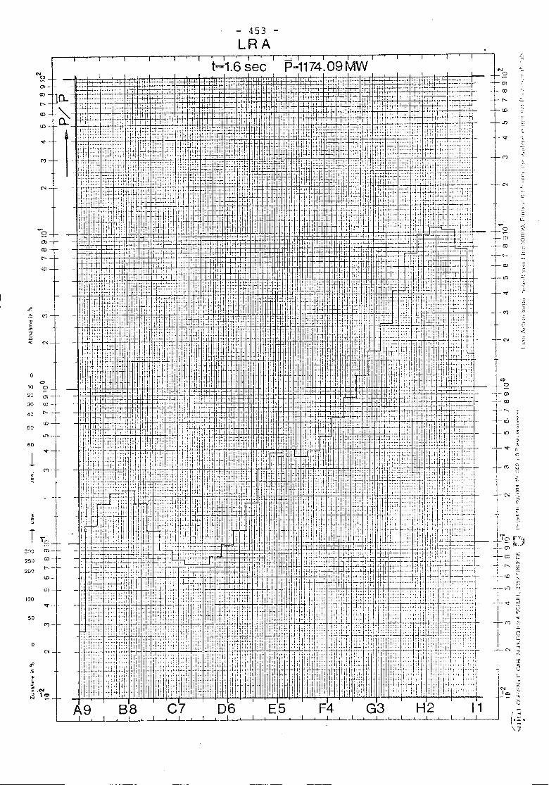
(j)
co
<0
<l)-
0>
cot---
'"
••c
~
T 'e310 01-
250 co
200t---
'"Ii)
100'<t
50M-
0N -
Ii"..£~E.c~.N, ., c>N
- 453 -
LRA
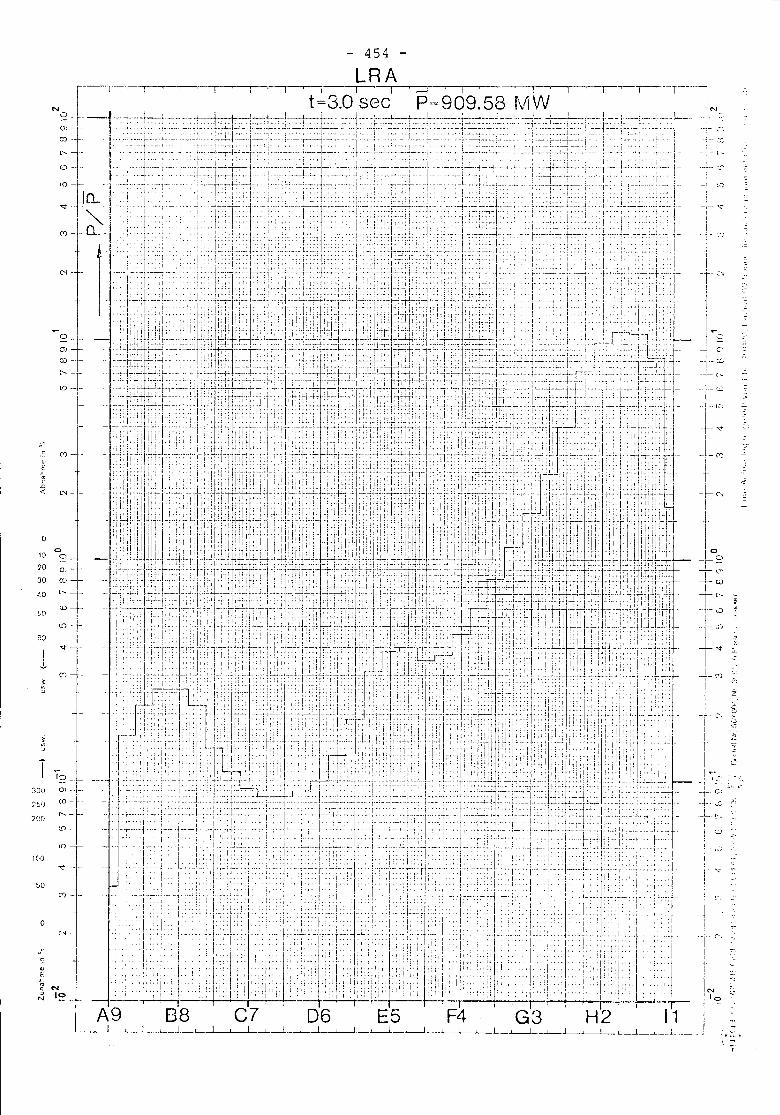
454
('oj _. -
01- -
00
I'N
._.;...- ::.
I
i - "",.!
r-,
,_L. c. ~
I ~
I ::I~
-; ':--:-1-' r;:--j_ .. c:; --
._~ ~~
II
+"i
.j!
I~+~-C-
-i- ::.:;t"-'[-~~{.-lD
It-"
I+cry
iT
-~("
ILI
_~oo
1- ("it.)T['-t.- \0
l--:T ~+") -,
! Z
cs - .-
C'I-
'"o
IJ.-
[') --
o
~--
~i~U) -l' _
tO~
:1~~-
It5 +
T 1~10> --1-0)+:llO
"E.-~,-.a<
10
?O
30:'0
1(,0
:nu
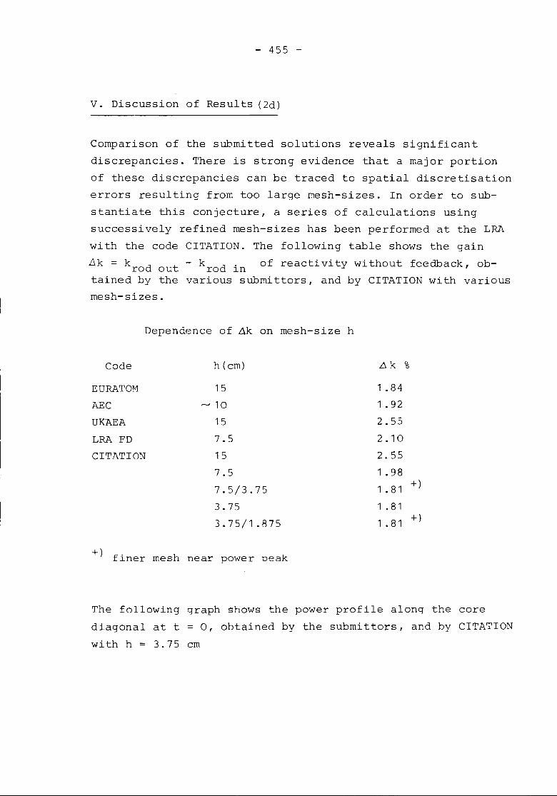
- 455 -
V. Discussion of Results (2d)
Comparison of the submitted solutions reveals significantdiscrepancies. There is strong evidence that a major portionof these discrepancies can be traced to spatial discretisationerrors resulting from too large mesh-sizes. In order to sub-stantiate this conjecture, a series of calculations usingsuccessively refined mesh-sizes has been performed at the LRAwith the code CITATION. The following table shows the gain~k = krod out - krod in of reactivity without feedback, ob-tained by the various submittors, and by CITATION with variousmesh-sizes.
Dependence of ~k on mesh-size h
Code
EURATOMAECUKAEALRA FDCITATION
h(cm)
15,-..J 10
15
7.515
7.57.5/3.75
3.75
3.75/1.875
L>k %
1 .84
1 .92
2.55
2.10
2.55
1 .98
1 .81 +)
1 .81
1 .81 +)
+) finer mesh near power peak
The following graph shows the power profile along the corediagonal at t = 0, obtained by the submittors, and by CITATIONwith h = 3. 75 cm
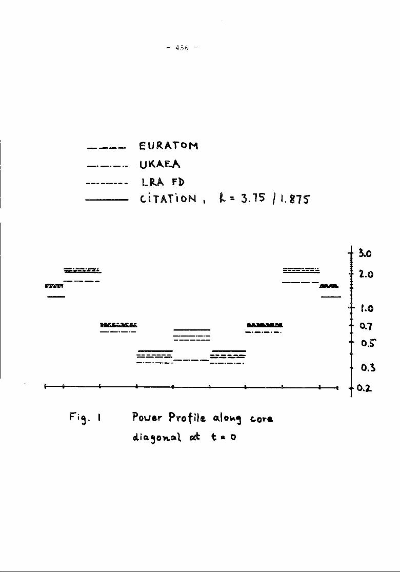
------- ---------- ---~----
- 456 -
EURATOMUKAE.~
LIl~ Fl>tiTAT"ON ,
M5553rFM
~ ~ 3.15 11.815"
--_ ..--------
........
~.o1,0
1.0
0.7o,~
O.!>I • I • I • • 02-.
F"i ~, PO\J6r Pro file. ~I O~~ ~OY'.
cli Q.~ Ol\,~l cd: t a 0
- 457 -
From these results it is obvious that the mesh sizes usedby the submittors have been too large. For this benchmarkproblem, FD-codes require a mesh size of h < 4 cm, at leastin some vicinity of the power maximum, in order to produceresults of acceptable accuracy.
Analysing the submitted transient solutions, one finds thattheir discrepancies are roughly speaking, consistent withthe errors in ~k. Since this effect presumably is much lar-ger than other causes of error, such as time integrationmethod or representation of feedback, it is at present im-possible to make a reasonable comparison of results.The conclusion reached during the discussion at the meetingwas, that the contributors should rerun the problem, employ-ing finer mesh spacing.


- 459 -
VI. GRAPHIC REPRESENTATION OF CHARACTERISTIC QUANTITIES (3d)

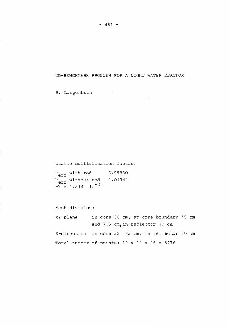
- 461 -
3D-BENCHMARK PROBLEM FOR A LIGHT WATER REACTOR
S. Langenbuch
static multiplication factor:
keff with rodkeff without rod6k = 1.814 10-2
Mesh division:
0.995301.01344
XY-plane
Z-direction
in core 30 cm, at core boundary 15 cmand 7.5 cm/in reflector 10 cm
in core 33 1/3 cm, in reflector 10 cm
Total number of points: 19 x 19 x 16 = 5776
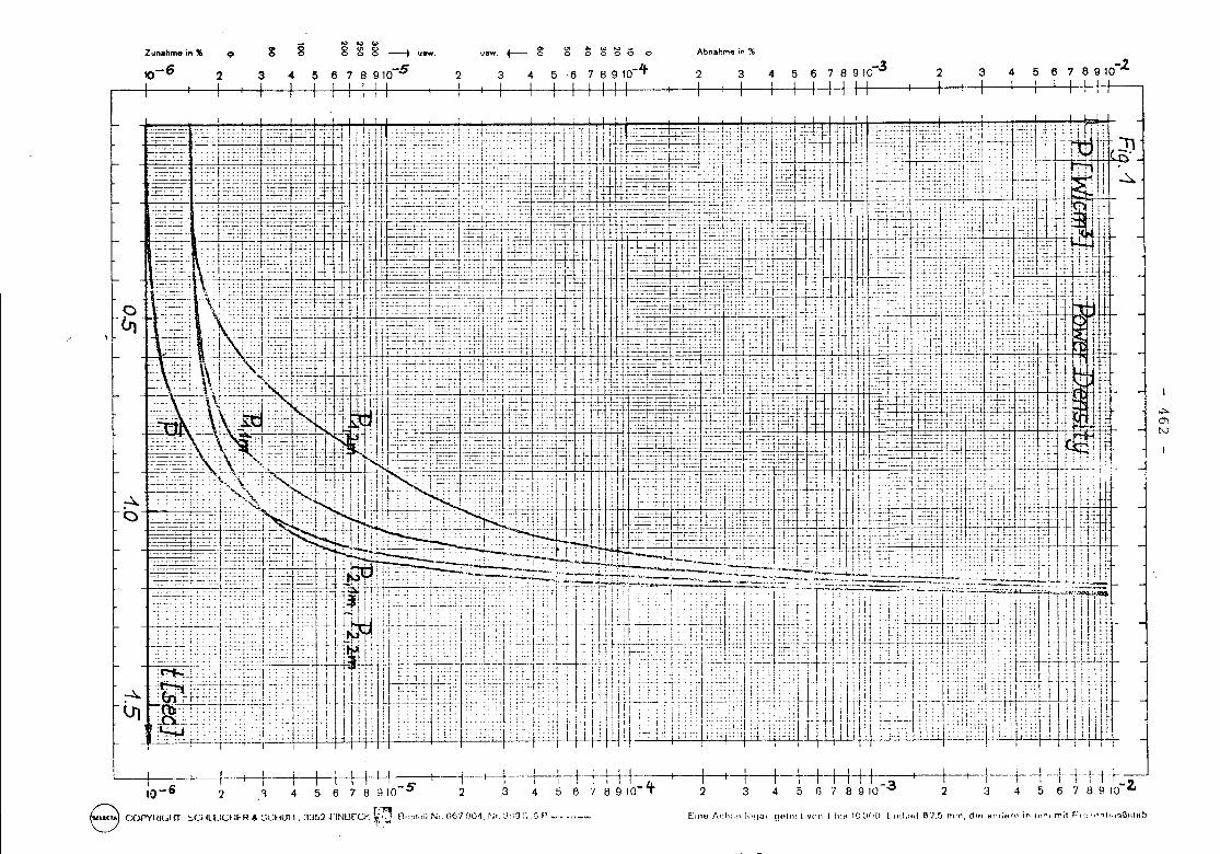
Zunahme in %
1()-6 2
o
3
g
4
8., ., Co>ggg--.
5 6 7 8 910-5uaw.
2
uaw. +--- g
3 4
(,71 ~ CU "" _o 0 0 0 0 0
56 7 8 91O-1tAbnahme in %
2 3 4 5 6 7 8 910-3 2 3 4 5 6 7 8 910-2
Einu f,f:h:-,!~ !\)qnl OUlodt "'(Ill 1 IIll. 10lJOO, [illhi.lt 67,!) mrn, dIn iHHitHP in 111""\mil f-'lil'."f'ltnl!l13nlHh
~b
i I t--+---t--+-t-+-r-++-\ I ---1--+--+--: i t-+++-+--10-6 2 .1 4 5 6 7 8 910-5 2 3 4 5 e '1 89 IO-it8 COP'YIlICiI-lT S0llLlU :ER & ~;CHUU,33~2 !INUreI': ~:jn, ,,1,.11N . no'?oo~. ~k ~".:'l~',Q P '.' .•"--'
I I I2
1-13 4
t-t-H++5 6 7 8 910-3
t--+2
f---+--r-+3 4 5 6
J
~
.,.mN
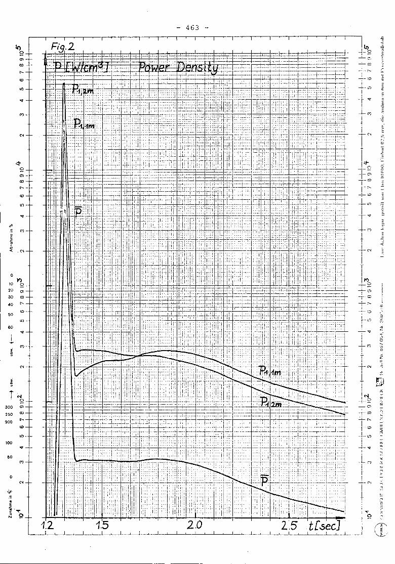
It)o(1)
CO
.::t-O
(1)
CO
C'-
<0
L{)-
'l"
*.~ C'1
"E-'=~.D
< . C'I
0I')
10 ~20 Ol30 CO
40 C'
<050L{)
60
1-.rC'1~
'"~
C'I
~
T ~0
300 Ol
250 CO
200 C'
<0
lO.100
'l"
50C'1
0C'I
.;f,e.~
C>E
-'=.. ~c~ QN
1.2 1-5
463
!!J)-<_ 0
I ---('!';
-CJ
---[""--
. ....;...L..")
I
-r- -.r!
J-.,.,l-.r1M
I.l-II---+- C'lI
iT
I~+~Ten-r-C)+""ii-O
I---
.::
~.
=
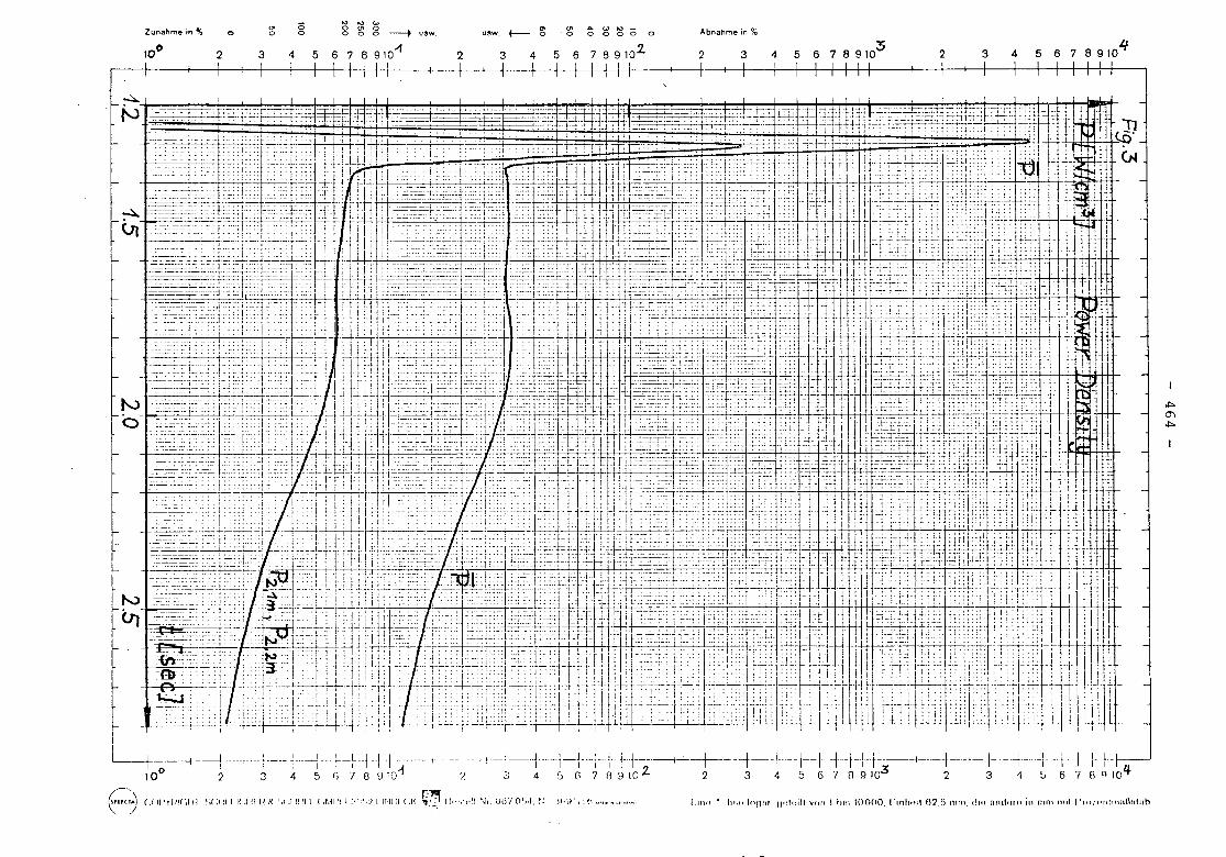
-::...
Zunahme in %
1002
o
3
'"o
4
oo
.., .., '"g~g--+
5678910""I
uSw.
2
U!!,w. +-- ~3 4
(J'l llo W f't>J _o 0 0 0 0 0
5 6 7 B 9102I
Abnahme in %
2 3 4 5 6 7 8 9103 2 3 4 5 678910'1
+--... ......•-.--- 1---'
r
II
L-t----+--1----,--f----~- ---1- - :--++-11-----1---:-- ,---j-+--j-1---H-j--j-----t--t---+---t--j---\-j +-H-+-- I 1--+-1-----+-+ -1-1 i- f-,100 '2 3450780;01 ~ 3 4 ~(i7ngI02 2 3456'10910.3 2 3,1 5678Q1OLt
>l'>m>l'>
c<:') (.()lITl.'!f~11I ~~(:,HJI(.:!fI-:'X.',1:1H!ll (:MJ~II.:l.l',)llr.H~I(:h ~~ 1~1",h.~INI,0()./()t),I,~~: ;j1'\)'J:~~"'''''~''''''''''''C'I'/-~ LillO" IplIlloHm \Ill1oill \lOll I hili 10000, l'ultlltll n7,~') mm, dill nndOltl ill mnl 11111l'IO:I'Il!l!latbtnh
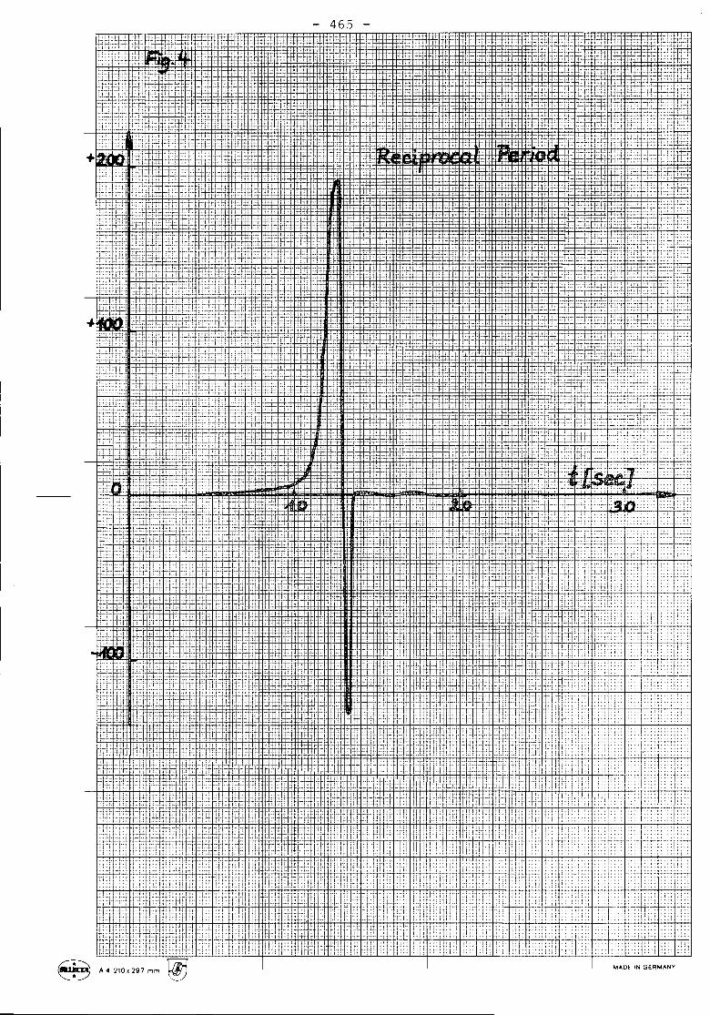
8 A4 210,297 mm @
465
,, .., ..
I'
; ;; ;;:
:::; ":: :::M"D~ IN GERMANY
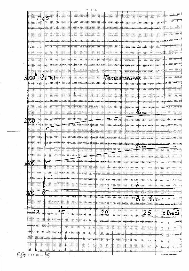
MADE IN GERM"""Y
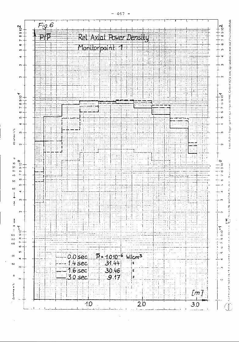
---'.
...Io
..:-:. c)- .....- C)
, ".! • ~
_1 - :c
--:.-- U;
i-,-'t
:.,!
. . . . . . .i . .
:.1... ::') ,. '
..!I
_.l __ .-l'
• j ••
~°(])-00
<---
CD
ll) -
't - '::I!:.ILJ "']:1 ,'.'j:, 1 .. :11,1, ;",1'1'1:: !.,~. . ." .' .... ,,1:1
C") -r - +F~.h--hf'-+-:~G~'~r-l-::-'--j~~:~__t":i::- :Clh~f--'-i-i~-i'-~T:.; .,:.:r+..'.<;: i i' '.--:T-h:-rrt-f-:Hj ..-.-..,. ,.---.,...-0--.1-----.-1".-.1--. '--1-- ... -'-.\' ..t ...-.-f- .,--+-. -.----1...1..-.,'.--- .."':, ....._,.........--'I-':'c" .~.
N -- - - :!f::;-'::)--h/::~r::"-~'H~-I-:-j.-+.-:-~-l~-,~-.LLl~+.•i'-J~.:_:..:Jj+;••.••! ..• '._:1 ..~~--:+~':.!!il .•. [ :1: ...~...,.... '; I "1' i ... r ••• r ... " ... ~... r •..••.• ; ..... : .... .]. "1:1 .. j ... / ''',' . I ,,!. I. :., ... , ., . . • ,. I' I . r.. ...:.. ...• • I....,... . . ! ' I. .. I . . . . . . , . . , ' '. ". ~.. ,.... . . . ••. •... ...,. I . ..+H~ft.'rT~-'I''':'''t~''''l' -~I;,.''''''''''''I'-I .·.'[
- 467 -
1f :r&~~:~-i~=J~~c~ch:~:~:~;~;=~n~CH,:==,'••:~:~cf:~~
oo
10 °20 (]) -
30 OJ
40 "-
<D50
ll)
60I 't
J.
~
50
N --
~~Ti. 0 .. _
100 01 -- --
!lJO Q) -t-
'00 "-+
100
oC'<--
(T'......0.,.
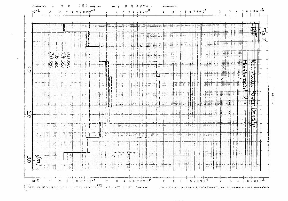
"'"0'100
5 6 7 B 91024325 6 7 8 910'"
+++-+-H--+-----I-t--~__+-+_t-l-1--i I
5 6 7 8 9 10 ..., 2 3 4 5 6 7 8 9 102.
4
I I II3 <1
Ab!18hme in %
2 3
I
+---i2
678910°
'" A. Co) 1'0 _o 0 0 GOOUS'N. +- g;
--t--+-----.-L-t - -H--t---t-i. I , . I I . , 02 ::1 <: cj 6 '7 8 ? 10
2
USw,
I .__ I I II I I I '
~ b '7 '3 9 :0-1
'"ooZur.ahme In % g g ~ g -----+4 5 5 7 8 910-1I I I I I I II I ~
~II! I I I~.--~---+--~-----. _.-t-
1'0-2 2 3
rI-
~Ir~IrI
lIr~~O-
(\\~~',A)(;(H')"f;:',,! IIr:~
~,(:!:: t '(.l n ~,' ..:' I !r'i~ t I,f.""i~ .:.\'.' i P1!'! (\" ~_;.:\ Ii.' .!~.[1 ~.;r lJ'.\./D~),I. ~!. ~V,')' ti ...,,,. F.,n!: Ac!,:H: !nqdr ~jt,:"dt 'I(ln 1 bi~, I()(~IOO, Einhell G~.:j fllm, d,I,4: nndoru In mm nut Pro.lt~nlma6slab
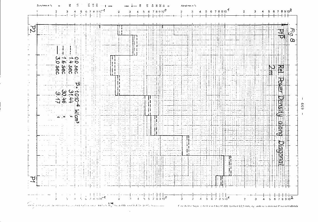
~m\0
JI
J
5 6 7 8 91024326 7 8 910154
Abnahme In %
2 3
A W '" _o 0 0 0 0
C'ot-- g;U8w.
2 3 4 5 6 7 8 9 100
I : I__ +_+-'! I
1 ;
: ~; ], ._i!. !-
i-I
, l" I il" I I.:.! ... ; - - : ; :: . : : . !. : I . • .! ; I .. : .ftl :r;T; 1*- ~I --. ~ ~.+-_.-_..~. ! •. _-.---._ •.- _-, -.-.-- .• -e.-r_. - -1'-:1TI \,1 Ii! :::::l!!:i :,.j:- i;i: ::'; '>i:':::.::;:'. ':::; i-Lul!
.' I 11'1 : : ;' ,II: ,I :.: ..• : :i I I: i: 1.11 i . :! _ .:':i .: I: : 11.;::1 I I I t:::::Ill:t I
.. I J i 1i: I:;:! j ~ ; 1 ;
i'i i
.1
g ~ g --+ usw
7 8 010-11-. , I
.. \ '1-7---
6o
4 5 6--j- ~.-\
'"o
!
:)
I'III
I. I
'1
____ 1
.i.
0J ~i.~O." •. i.. •. i Ib O"'l:-I::' p
----~ l/l. tn..~.: (l) (b ('\) rc
(')nOpi, . , - .
iI .
:"dl, ill
: · 6J .VJ~'-~.:O-~O~ ~r-'~~,.. ..,.,..-,-0N '(3) -+=-: I...e.
.- ~.
:-:::. .
:.::::.:::: ""~--:VI
ZUlldhme In '" 0
\:1-~
~
~-
123
,--+--+--i---+- !II,-~
t'-)
!-
I!,-
I
I~
LI,
'J. :JT .- j -_.
" l, I I: '.1-11)-'1 'J.! ----;--f -1-!1 ~ ~ G 7
f+ t-.---t.-+--+-/-----j-+-+-+ i-++------+-+-+ --\--t-+ --+-t+++-{3 9 !0 0 2 3 1\ 5 G 'l 8 0 10..-1 2 3 4 5 6 7 8 9 10 2.
/-f ' ., I: .: .' I~ ~)( , '; ! It .: I! j: ., •. ' (I 'I! I J 11 \j I 1 \' '.' I ~J 11\' \ h V,'} 1\.-. 1,.11 ~1, c' ~i 'I (; '...1 r~, :j!I'I', \) ..', l"l!11: I~l:h~;l' !\1~1;1I ~;,:l",11 VI III I hI:; Il'l)()(), Linht'll ('2,~) nlpl, .l!;: .mdt''-u i:l mm mil ~Ji('/ •.•nll'"!li1astab
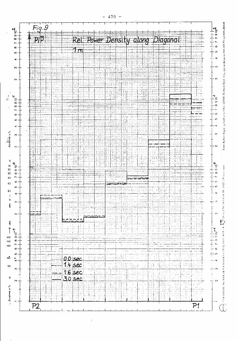
470
::-.-.
~C',
-~F~~ .. '
""I0- C',
-" .:r.~ r----
I<£
""_.- Ut
- ....-
i(") ::::
II
c"
l~.-;-- 0-'...Lc:;
!T:!t,n
---t--tI,lM+
toI""t~-r- ro
'1- "t.~r:I '
I-!- (")LiNt+?
-,-- r:lr~--"w
i
l:
C r;-. ~~T~~.+_-= ~~:=~_--t -i--~'l+-T'-'--
..- ~':r-+=I--'r'-'- "--=r-~:~ ~.;::;..:-.-,. .;;t:-~, I.' ~-;.-- ~~--: ~~:~~I-'--~~T~C~.-:~,:~:.T ~~::." -+ ~-:-I-
,.,'ii: •....~::I,h': 'I::r ~~t~fH4;>;+'::1:: .. : i ._L~~-~~'~~~I ..-~st+t~~:~f~T:¥rt~+~::<:::~H~W~f.:T.\_:t~*~~~t-"'~,. ---.... -1-.- .--.. 1... ,. +---"-- ~-"'-"I..:t~.--.l.: ...i_ .. EL._ ---.l--_ •.-- ....-~--_.-t----l----~
- <1:"'1:;: 1:'11 -.>.~~~¥¥!:.r-tT1I.-';': l:~:~-.~~I:':~ftj.~.~,r-;:~.,~;>.~11:~:;f,J1(r,L.I:)<~l.~II;.;~~.'1' !-'.:.;.j.;.j]" ~ . 1 - .. ,., ... '" ,.~ ' j" i"'" 'i' ... L"I...t'l I"
:-:fil:::~' -- .-.'~-l:..-:-~---r-.r~I--:--. --:, :-, .,,' .-:-..r:--::r:-::I '1' "1'" ;"""--1'-:1 .--;-:::: i --:1'-'1:---:-;-:'':T . '.1 i,! . ',' I !'" - ., -- ! I, :;::h,l ,I. "t,--l. -':12:1ii, I': .: ',' -, I. " I::," .... "1~'1 . ,'II' "-!""I ":)' .. ; ; .... ,; .... ' ... -.'1.. 'j'To:l -. : +~ __ L,jli . l~.~J-.."---~ . I' ,-; I' ._~' ,- :.!. ~~ I' _.t _ ~~-I --'--r-.•~l:~i::;',c'C..::'EEoI::"C:i:.=O~'i'~~"--'~-~~~~:~':~-.r==~::f:'~~~-::;2-:'~:~.-.~-
.,d:::-~.~=T:~~~~~~..:.:~ =.i=1-=-:~~~-:~__{~~:-:-..--:::~~t==:~~-':-+':~1:~T1",--::-~:-..:.::~~=]~::'~-""I->98~F". :.::~:::t-£:tt-:~l.:::r=i::"t:-----~:-:L:-:::ll":':"=;"+.J:.:-;.l':':::';:+~':"-~':~':"':::";:._. r -- -r.::!.=:~..:.--,:.L-1~.J..., .. - 1-'1. 'J"-','-- - -1--;';-"--" ;.- t'.._...---)..:..-[--h"'I' -'J' --1--j'-"(" ;['-'-t ...-.-- .--: ---~.-i- -1--, --I.::-!- ; :-i --r:T-t--:- ~ii~l--'~'-!'~~---J;-rT~~~n;~----:-~!':r!~"~~. -i' -r 0:-~r~1-
- :il~tl,:-tn-l-T-+-r--:,..-~+~~~-:G--::T--~~~,--~F-I-l~'~l,..T~I-;~~I-r:m~T-:~d-r~~i~t:-.~-Tt 0 :j;; -I :1 tit ::;:j. I' .', I. I I" , . J" I ,.. . t -I- 'i-'T~"-T-~- -::-':'1---
i'-~--:--!-r ..-I'-~~--I-.i:~,--; -~.:-t-;'--l--T- ~- I'-~~-i'-~-:-i-
.....- .. "",~""Iu ., ..... -.--. -- -.... -"-'" j ........ ""'--1' -~, --.. - .....- "'.od_.' -'t--- ;*-,.',I:'l"! I I ! ,,' ',,:i: ! .;, 1'''1'' .1,,: :: .~,_ .. I ! t' :-.
-- frr,'C':::"'--I: -: ... _~-.-t.:T: "11
;- 8-~ '---:-'--J'~~[;~'~I,:'II"-~'::.-~-;-~.....-----:f--7'"- : ---t:r-~ir'-,t , I. .! . t T r ...,.,: I • • T. • I 0 .' • I I j , I' I T tj , II I. 1:, ~ l. . . "
'i;: ~::: ':-:I~ '-;r"l' '1"- - :JI:'-J'"7-1---:~T-:~-l.~ !~~II-~.. :-:T--lll'-~:~,-"~f~~';}j.-"~"~T:tl':T!-;:.~'T-~r
:111:: ',: i' t : J!"I -: I, ", I',:l ',ll I I I ;:' "1 I,', ! i. :' I':' IJ- :~~:i~:;J:-:-~.:":F-~=~::b-r:'.-~~:._-J. ...,~~~_J--~!-~:---~:-~-;~;--_:;--:--:~-:i-.:..L~'-~:~~~~
~~ljl.~~~i=:~lYi~~.t~~[f:l~~;..~~~;J~f:ftf-{~~_+~__:'_'I__'_:_"_!' __ '~_~ __ L. -1----;--- - - -t.-:---+.-,----;-' ~!--r-.-I..----;----t--- :-t-'~F+-.,.;...-.l--.-~.-.. '- 1 -' ._L....!_ .. j- ....-1--'-.-- ....l.... !_ ---..1.----:--:-.--:.-.1--- L:1~- -'- : - _:__..1_ ~ __:L_ 1-1.,," -- - --~, I' I ,", I I ',.,.",I ~::.':..:::::"_;":;:-:--' I! I I ! I., ,'i,: i 1 :::-t~.-----:-_..- _._--;-t~:t~~-~----'-~l-~:~:1j---~.:-;-::~!:'-'i~:i:~":"--T~~.-----f--'-l=:-~-f
:... - i. • I I ,i' I ': I" j'" 1--1--'''' '1--:---- I! ;[i1":;;".;c;...- -:.--~-.-i.._.,""[ --T-- -1.~::~.1:~:..L-- .--T-----. -;-----.;-
'i,i i.1 ,i -'-:7- C11- ifi:1 i i .1'Ji-~----:III-::: _ --~..:~L_ ..:__:-.. l__--L~.-J-_,__~ 1. ~.. _.I :... ..L ..c,..._.l __. ~ j ~_-<_._. __
- ~ -;-----r
.1
"or 'r:
.. " .. ,:~.. l _..__ ._::_.__..._._L .0
::j ..I .. ..l ...I..:! .. !I"I .;:1: Jll,: .1.::,;;;-1 t..:'I' ." :: '1" I. . . .. :I' ! . I '1 Ii'" -I
~2 ... '.1 ....Iii P1' ~~- ~~..._'_J-----l..--.L-"--.L_L...... .l.........L...J.....~~1 __ ~.--,--_l--,--- L ...L_-' __ .J--L_-'-__LI •__ ,L.... .....__ .L.._ I__ L --'-__ 1.. .1 (jj
C'4o0> -
CD
0( ""oi 0
0>
CD
t'-
<0
L{)
'<t
o!?c C'J,~
~~N~
.D
"" N
00
10 920 0>-30 ro40 t'-
<050
L{)
60'<r
1C'J
J~N --
J~
T "t-
'9 -100 0>-
!50 ro
!OOt'-
<0
L{)
lOt! •'<r
50C'J--.
0N
,j>
~~~•c~N
- 471 -
DANISH ATO)UC ENERGY COi'1!HSSIONResearch EstablishmentReactor Department
Riso10 October -;973
PSC/rj
3D-BENCHMARK PROBLEMFOR A
LIGHT WATER REACTOR
by
P. Skjerk Christensen
RESEARCH ESTABLISHMENT RISO
- 472 -
1. INTRODUCTION
A benchmark problem concerning an example of a fast transientin a three dimensional reactor has been distributed by EACRP and theresults from some calculations are reported here.
The transient may be described as the time behaviour of thereactor when a control rod near the core-reflector boundary is with-drawn from the initial delayed critical reactor. The transient isregarded so fast that the reactor is assumed adiabatic and the powercontrolled by the Doppler effect solely.
In this report the original version of the benchmark problemis not duplicated which means that equations and constants are notrepeated.
The pro hI em has be en sol ve d vii th anodal code DANO vlhich isa spe cial vel'Si on 0 f a mm--Sil:Julator. As thi s code coul d not taJ,-einto account all features of the benchmark problem, the approach tothe proble~ is given here.
In this report the methods used are very shortly describedalong with the necessary cllanges of the original geometry and nu-clear constants. Next the results are presented in tables and fig-ures. At last some data concerning the computer ure given.
2. GEO;1E'PRY
In the appendix is shown the core lay-out as given by thebenchmark distributors. The core consists of various types offuel elements and in an unsymmetric positioll a movable control rodis situated.
As the core has no symmetric properties it was necessary torepresent each fuel elemellt explicit, that means 312 total, and itwas decided to divide the height in 18 sections making a total of5616 mesh points.
- 473 -
At the points 1 and 2 detectors are placed and certainquantities are to be followed here: local power density, tempera-ture, and reciprocal period.
As the code used contains a nodal model of the reactor thereflector is taken into account by albedo values, and thus theboundary of the problem is the interface between core and reflector.
3. NUCLEAR PARAMETERS
The code used here is based on a one energy group represen-tation. The neutron cross sections, however, may be given in twogroups hut are condensed to one group according to
and
where
The one group picture viill also neglect the speed of the fact neulrongroup whicll is assumed in equilibiium (infinite speed), whjle thethermal neutrons have a finite Gpeed.
The benchmark problem has a reflector with glven nuclearcOllstantc. In the code 'I however, the reflector is described l)yan albedo concept, and the albedo value',,;have been found by f:itt:inE';the po\-:erdistri bu tion 0 f thi c nodal model to the power gi ven by acode based on ordinary difference techrliyyc. 'filefitting has beendone with the movable rod full 1n and the accuracy obtained is about5% in the power distribution.
- 474 -
The movable control rod has to be represented by a poisoncross section and thus the equivalent poison cross section givenin' the problem has been used~
The nodal representation of a moving control rod gives riseto a ripple on the reactivity - and reciprocal period vs. time-functions which may be Eeen both on fig. 1 and 5. Althoughthe program contains a smoothing parameter, it has not been possibleto remove the ripples fully.
4. NU!1ERICAL EETIIODS AND ASSU!'lPTIONS
The steady state power distribution and effective multipli-cation factor are found by an iterative method.
The tempernture is assumed constant over the core.In the transient calculation the code assumes that the flux
distribution may be s~parated in an amplitude and a spacedepcndent(the last one slowly time dependent) part. Both are integrated bya predictor-corrector method in which the time step is determinedby the difference between predictor and corrector valucis and bythe number of iter;ltions necessary in th0 fluxdistribution corrector.
The code includes the delayed neutrons by the full equation
C. = ~.v~f~ - A.C .•1 1 ! 1 1
'rhe ternperature is in tegra tcd by a simple Euler me thod in wh ich thetruncation error is computed and co.mparcd with a given limit.
5. RESULTS
The results are given in the following tables and figures.As these areselfexplanatory only a' few remarks arc given.
- 475 -
Generaly it is seen that the local quantities in point 2differ very little between the two heights, thu5 only one curvehas been shown in several cases.
In table 2 the static multiplication factor is given withand without control rod.
6. COl1PUTER
'rhe calculations are performed on a Bourroughs B-6700 witha core size of ~8 K words of which the soft ware system occupiesthe half. There is a number of disk~ on which program and dataare stored. The program is segmented automatically and so aresome of the common blocks, in a way not ~overned by the programmer.Thus,as the program plus data exceed the available core, a heavyamount of disk transfer is necessary, and this makes the cost incomputer time high.
In table 3 the total a;~unt of computer time is given alongwith tIle equivalent CDc-6Goo computer time. The conversion ofB-6?00 central processor (CP) time to CDc-6600 CP-time is made byaf;pnversion factor of 10 found experimentally. The conversion ofinput/output (I/O) time is based on experience and a guess, a~ theprogram if it should be run economically on a CDc-6600, would haveto be fitted with an overlay structure and furthermore, a lot offile storage could be replaced by arrays thus reducing the I/O timesignificantly.
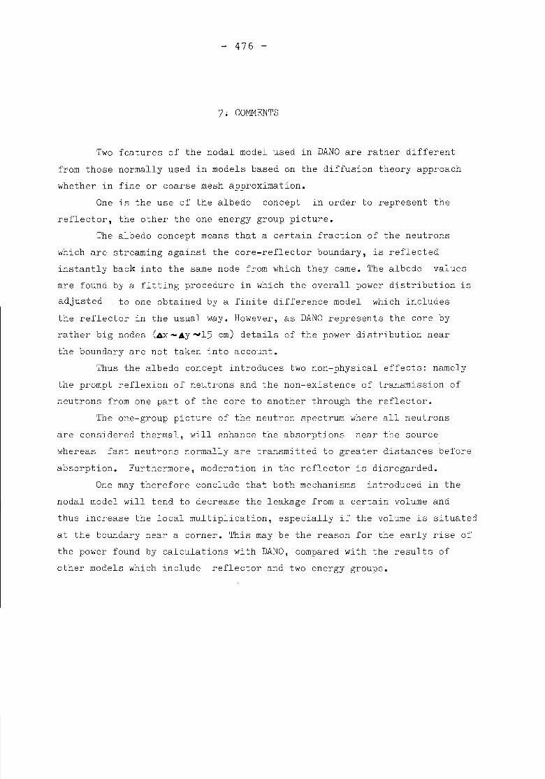
- 476 -
7. COMMENTS
Two features of the nodal model used in DANO are rather differentfrom those normally used in models based on the diffusion theory approachwhether in fine or coarse mesh approximation.
One is the use of the albedo concept in order to represent thereflector, the other the one energy group picture.
The albedo concept means that a certain fraction of the neutronswhich are streaming against the core-reflector boundary, is reflectedinstantly back into the same node from which they carne. The albedo valuesare found by a fitting procedure in which the overall power distribution isadjusted to one obtained by a finite difference model which includesthe reflector in the usual way. However, as DANO represents the core byrather big nodes (AX -4y ~15 cm) details of the power distribution nearthe boundary are not taken into account.
Thus the albedo concept introduces two non-physical effects: namelythe prompt reflexion of neutrons and the non-existence of transmission ofneutrons from one part of the core to another through the reflector.
The one-group picture of the neutron spectrum where all neutronsare considered thermal, will enhance the absorptions near the sourcewhereas fast neutrons normally are transmitted to greater distances beforeabsorption. Furthermore, moderation in the reflector is disregarded.
One may therefore conclude that both mechanisms introduced in thenodal model will tend to decrease the leakage from a certain volume andthus increase the local multiplication, especially if the volume is situatedat the boundary near a corner. This may be the reason for the early rise ofthe power found by calculations with DANO, compared with the results ofother models which include reflector and two energy groups.
Figures:
- 477 -
1A Total po ....er versus time, o. -0.8 seconds1B Total po ....er versus time, 0.8-3.0 seconds2A Local power versus time, o. -0.8 seconds2B Local po ....er versus time, 0.8-3.0 seconds2C Local power versus time, 0.8-3.0 seconds3 Average temperature versus time4 Local temperature versus time5 Reciprocal period, average6 Reciprocal period, local7A Diagonel po ....er trace, 1 m height7B Diagonel power trace, 2 m height8A Axial power trace, point 1
8B Axial power trace, point 2
Appendix 3 Core description.
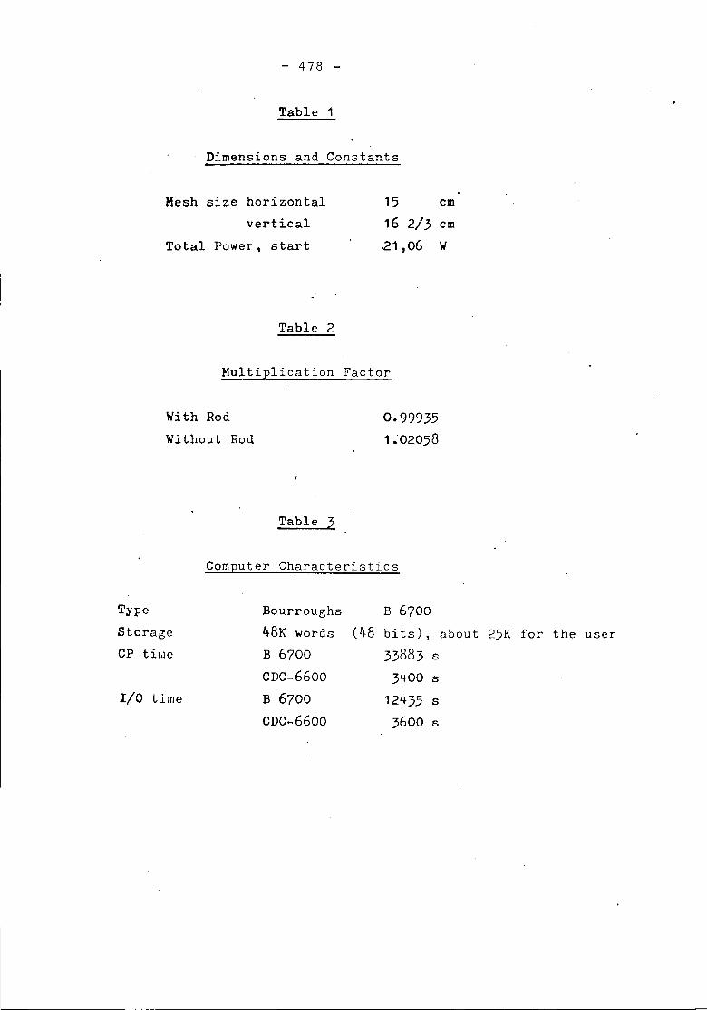
- 478 -
Table 1
Dimensions and Constants
Mesh size horizontalvertical
Total Power, start
Table 2
15 em
16 2/3 em.21,06 W
Multiplication Factor
With RodWithout Rod
Table :2
0.999351.02058
Computer Characteristics
Type
StorageCP tiwe
r/o time
Bourroughs48K wordsB 6700CDc-6600B 6700CDc-6600
B 6700(48 bits), about 25K for the user
33883 s
3400 s
12435 s
3600 s
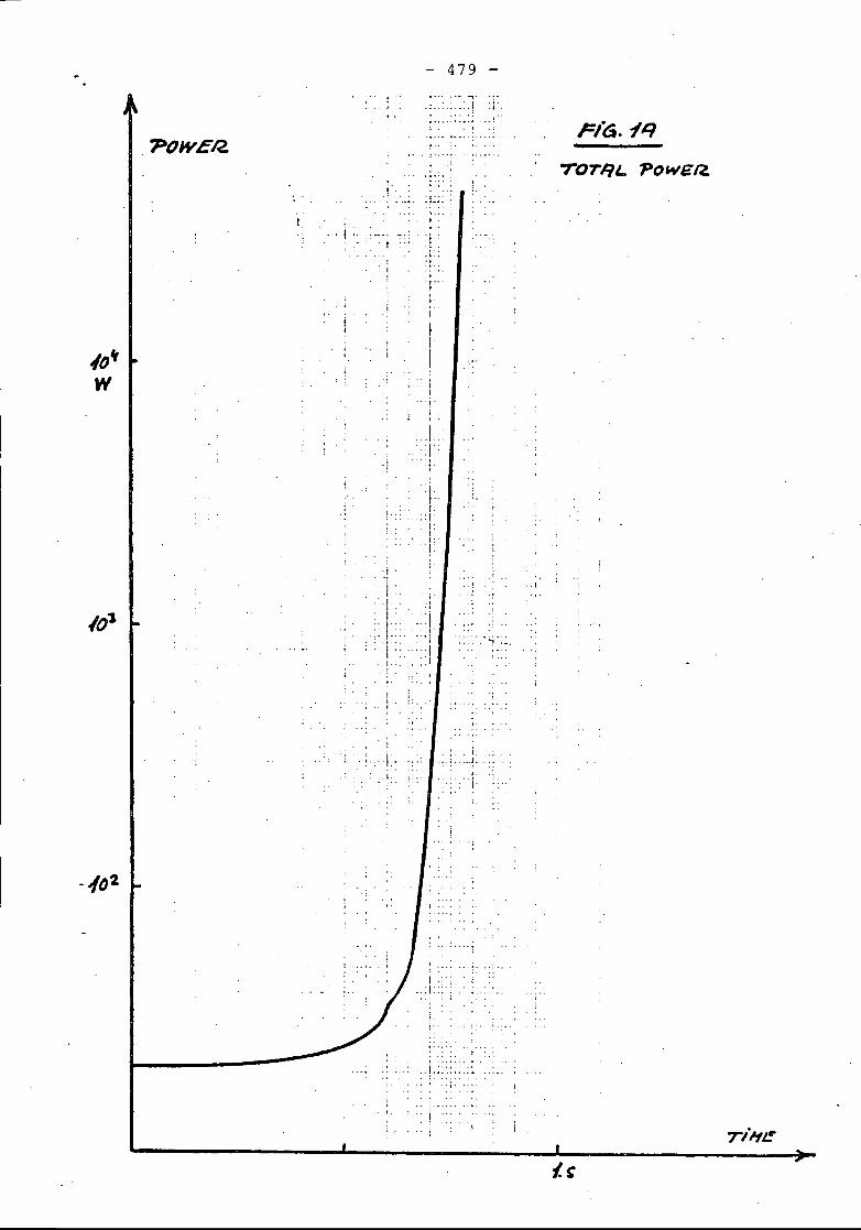
479
,OT/iL 'POWER.
,- .--...,.:.'.\ T'
;...... , ...•..I . . ~.. .. .... ~; ..
. ; ...;
: .. ,
, ,
-PoweR.I.I.
~!~::I ...j.
.' I .. '--, - :... I I'; .
.L:
.t ..
. i
Il-III ..i.t •
.. I1
...,
:1
.1 .<I .....i
I:r .
.. :1'• I
I:
Ti
. 'i
,o~.i.
. 'j
i; -
, ..t •
. I
•. J •••
It
.. 1. . i ... , .-J- ...
I.
.,J:>Ii,- I'.......
I....::. :
:.-::::-:-';i.
: i '.i
.,.
.1.i ..t
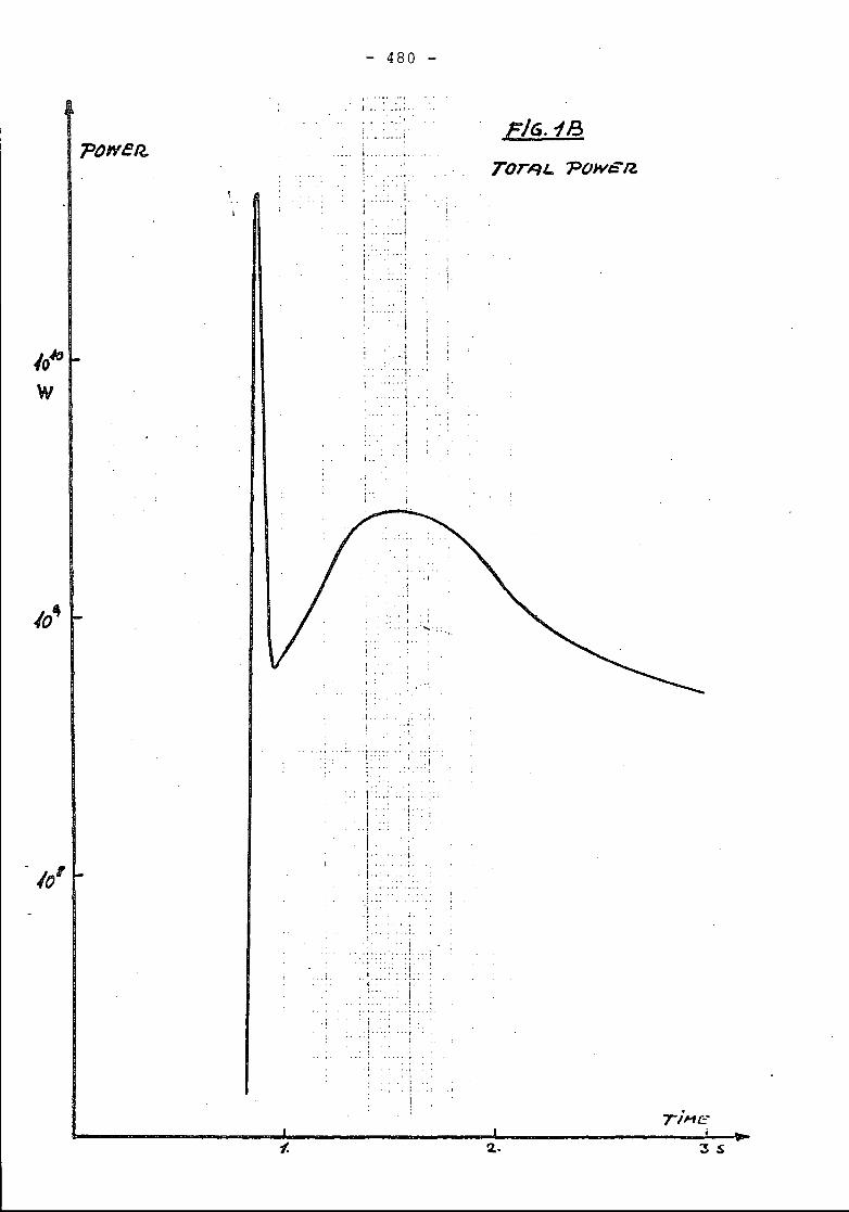
!oJoW
- 480 -
J .••••••• 1 ••
I ........•..
iI ..
;I ....•. to
:. . iI' ,
.. ...~.!, .,.i.iI.
I •••
I
-.'1I
F!G.1B
i ...
i. !
i
I ...1.!
•.. 1
- 10'
f.
. 1
..•• "'j-
:'1:'
,'1
. i
• • • •• • j • •
I.I .• ,
... 1.
i..• 1 •.....••:-! ":., t.
i .
.1.
2,.
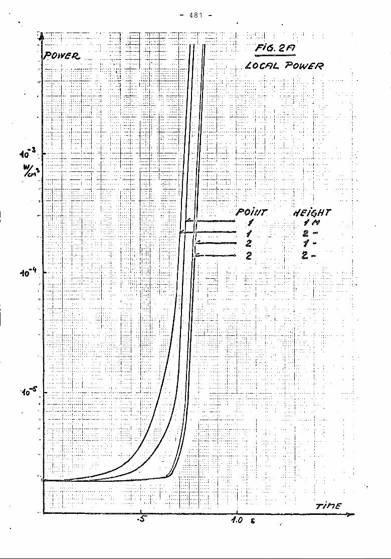
481
i
.:.1 ••., .
,.,
;, ..
.1.
!'0
i
I.
" .I.'
"i.. "
I
.,
'IIF/~HrI'Na-f-t-
,.,
I., ,. I
II.
t
I
i:j
I.
.... " .'1'1
I:
o.,
\'
i.
,~.., - , ..'
,.
,.0'
..-.i ..
.1.I
.. f. "I'
I'1.. ,
~:..~;.
I.I
I.
:~:I::,J'Pi6.2A
'.1.::o
I. :.,o
.1
pOillr.~
"22
:.1.
LOCFJl. POWER.,'j'",.
.::1:: :; 1.
i ..
i •...
..i, ..
.l .... ,
:1:
,".' "
.. ,'---1'
t.
-- -:; :; ;-
.::1:::" 'j'
._~~ .... :-+.::~---::',.:>
.•.. -t---,
'j
::.j..I
....~.-:-::;~. -~:.----,': .... 1.• __ •• 1
" 1.!'" • t L .••••• :!:"...~..i~ I • I .
i:::.: :: I i., .1. ... : " .. j .' I.: .... , ... '. I ;. "I "1 .1, ..I , '
I, , ..1.: :.j .. j ,:. ; i, ......::r:;:;:::J .C:~F;:::::.::. ..1..,--~-- .. -: I ! ,j""' .. r 0" I ...' .::;'-:::;':::,: I.,..!.:: /.
. 1 ..! ..:-:T~i':~l.l
.__~ L ~_~_... __•••• ; •••• 1 .1.
:::: I:: "._. ~--~ .. t.
_.-:.
__~ j~._i~_ !...
:.i :i-".r"._;: .Ii.:1::::-~--....; ..-.:.... . r . .. . ..-:T'~'
. 1._.,
1.>-1, __
YLl "'..
I. ;:..... I .•. ,.
:1: :\':> .I •• "
. - .. • I
I"I'
.i..I ..II.
"L.1
(.
'1.0 , ,'.
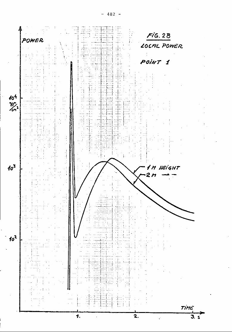
482
.. ; ......
; .. :
""I.,
. 1..
"
FiG. 28~O'I9L powt:R..
P()iNT :!
.. f
"
! I I.
-
.. I
.'
• j
.- ..... ; ...• !. .. ~.
I .t .
.:;-t.~1<!'..'; .. ':: .
. ..- - - _ ..-, ,<.J: , .
.. ; .. I' .1 .. ,... -I ••. ')" .• !
.1. I ::.. : I " . I.. .I
..: .... 1 • ..1. ::.... '.-.__J. :..:... '.:.:j:::.i ...1
.~:~:.~:~~:.:j..: .... i.
I"'1
I
1.
••• j., ... , "'1'" .... . , , .::I' :..i::.:,.~:::::., .... : ..... ,.:.
• I . . . . • • .•
i ri!1t:r3. s
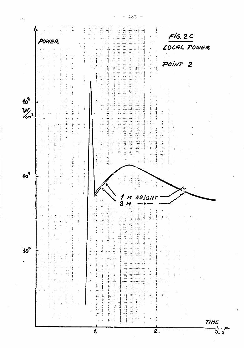
- 483
. jI
-_.!.
.• 1 .
, .
,..!
FiG.2CLOCRL POWE/l,
POiNT 2
,-
I :J..;I ,_
.1.II
.. ~
••• 1.j
I.1.
__,I I,': .. ~~:. !- .. j •..••..
2.
In2 1'1, - .. -
::j ... :'.:; j,.-_. . ..I.:'
!.
; .. -
j",.1
i
.: ..; .. ,-
!.
-I,--. ,
'y--
I.. _,
": .. ,,i:
.,
j.
..40
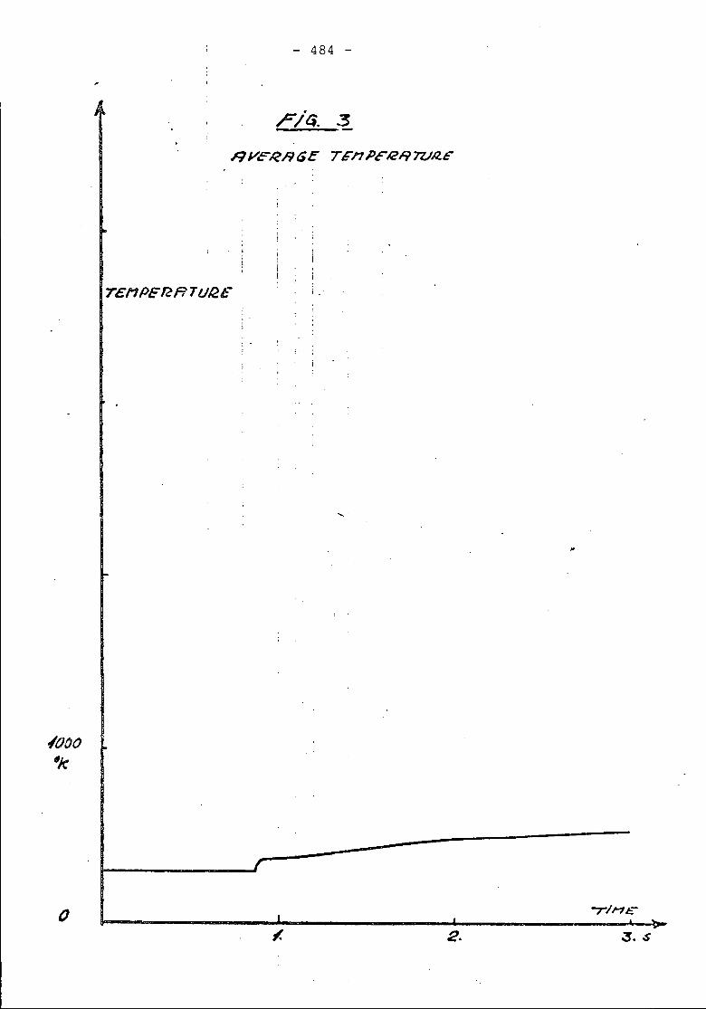
- 484 -
o
i _
2.
-rIHt:.-
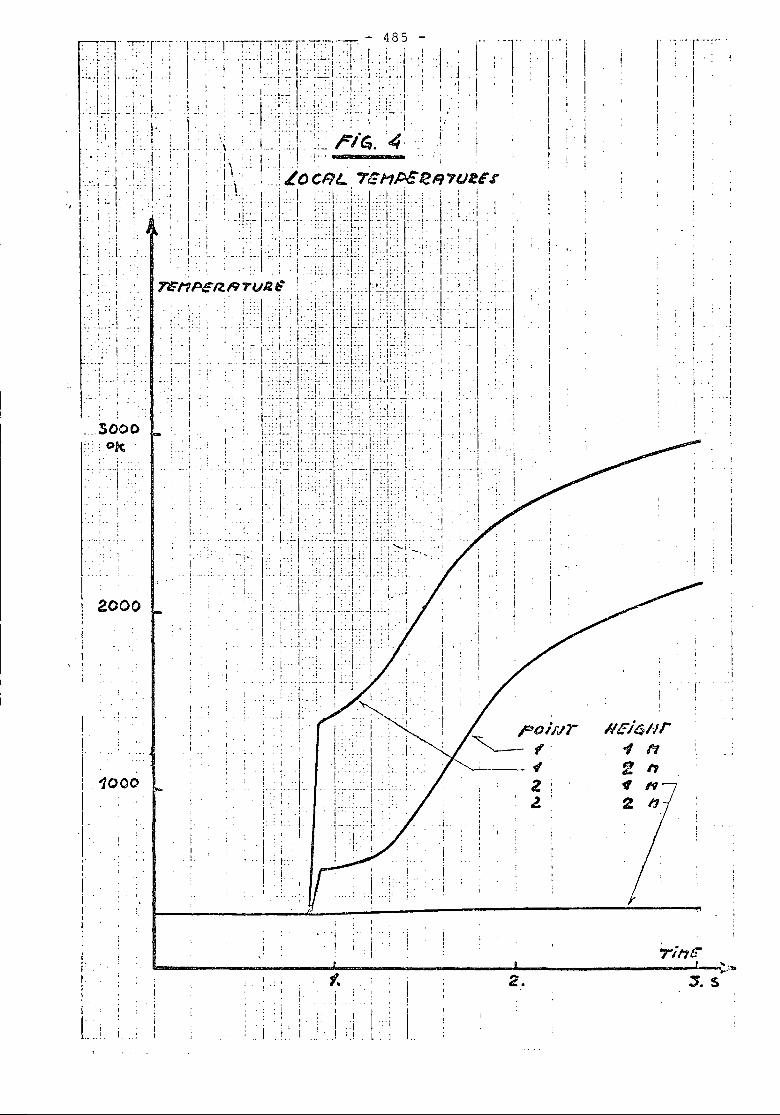
. , '
. ; ..
III
, 1
:1. S
. II
i. I
iIi
II
II
HEit;Nr., f1
2 "., If
2 11
, , ..
III
II
III
"
.i..I
'I
!
'i',
I: ..:. I.', I
-r I .•
I
,I.
iI
II
.. f. I 2.!,
I II
i I I :i I.1 .! l.
1I
: (.• i
i.,ii II
" :1' ~. ; ,
I
!
I'
I
iI
, i
. j.I
1000
,.I
iIIII!
III,I
I
I
I
! 2000
II
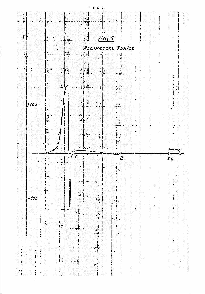
1 •
iI
.1
,.j
.. 1 ".'1I
I1I .. ,
i I I
IIi"I
..:"r--, I
II
riHG:-;:-.-
5$
,II,'.
II
.r,
!I!
.i
. I
I
.. J,
. i
. I
:. -+100
.' ,
. ,.'.-1'"
': I .. ..:. ~
, ...... J..
1
- 486 -.-FT -~~"'-l-~-rT;l:-l-~r-T--'r-;T"[-~T~T:-'l'l"i-T-'-'1'''' '1'- "I':. t I .!:. I I I 'li"" I" I "1 I:. ':' i I I . I.: (.: .. ' - ! ...!.. I :.. I "i :-.V: 1"+' !'~:~!l"-l,~+~..i ,.! j~ I I I I. :. I. I , .' I. I .It... I ... .'.., I • I I
: .l.'_1 !"'t'..: .... 1' ... : . 'II .- .. ,' .. 1. .... ~. .:L ',.:.:1-.1 .! I, i I I !.. : '1" . i.Oi: :,:j:. I, :'I:::r:I:: f: I '{"I ':n~;~.:5:' ,:;. I j". .: . i . I ' l j: .• ~ ,...... ,_ ..•. r ~ .• \ -_. 1 ' ' 1. •I.' ; Ii: '1.; ',>.' I ' ::1:'. . ':: ~ ,. ,I-.<-.t. :~j ..1 ~.~'_.f .. l: ' :'WcCiPR.OCAL. "PER/OO
I ; '. :. :iir1j:LIH-.:y! 'I. ,::1 _;I I .1. 1 ... ( ..... , ! ... "'r l ..:1.1•1 "1':.. , : t. .:. !
: ii' i I', . j. : j' I' Ii I;..,.. :!' i .'!
i: I; J __:1,1-1- il: . ~~:.::.'j . ,.-:l:.~ ..I. S,. ,~l:;~LLL.!.. ;:; ,.1
1,:,. 1
" . '.. ' . l: : I i'l " i .I. :: Ii .;.. I ''', .... _ I I. I'" I . ,
1" •• ••• '!;_!.+ ..1':+'" ,': .' .•.:.1.', iI, , . . .. : :../.:1: 1,:.'1. I.: i"':' i
','.' i', :',,' -'I." '!~<i+; -:(~I:;::"I':',.I::I, I .• : ': ••' ;:: I,>::::i. ,~:;" ••: ::, j
.' .'.: 'I"! ;. '1'.--::''\'':;''''/,:::1'''''': 1 ':"', .. :,I. i. : I. : .:: 'Ii :1:.: i '1 " I'. J ... I .. I .! ! .:'.,.:J "'1':' I,. ~ i :1 .. 1. ., . i' , " .:, ,I i' : ,I I'
.! I 'j' :; !:!'f':":; !:.':;' ::1 ':, . ":,: -t':c ;.,,:".'.:'1.' ~'If•.': .,'. ! .... I' :.I. I ....... ' '-,-' I!. . . i ..~....=----~ .'-,,"'p •• ~ •.. s.awt*
1:...... I,' ._.... 1. ii, i' Z. ,i. ' "'1 ' ... I .... T ' i
':',.1' '1": I" , .Jf' . 1
I . '1 "i', I
I" I :''ll' :.,',' , II'; I. ,':I:: i';'!): .1
..': .. I.... : ~~ i :: i II: :'!':Y":"-I' :; i
.:., -0' :~I'f ••-j !
, :i"I- :;' ['-T' --:-:.1- r .',
, I::: r :-:., ,''':i' :,'.i, I...... I•. 'J"":. '1"-1' : 1- ., J. 'I. : I. '!', . " . '.
::'-::[:;I( I- . ,I; i I.'.i" 'I : ,.. I~:.I. ;, i I
, I, ,I I I: I "; 'l"~"'I: --, I "'1 .. : '1' . i,
,," . I . I I, . f'~'. .~ I.... I~ I ~,f I'
I'. I I' i J. l' '.1
r" ~.! ,.: -1-. ,:" .i. I:i:; I,', '.J.. ! !
I' I 1:1 I II.. . . 1"'1.. I ': I. ;,1;d..:t.l.
.. .. ~ t,,
I. iII'
.11II
!I ! ,_ ..
I ,
I -100I . iI Ii; ,
I ; iII
I I • !I
1. I. II,
i
!i1 I II.
I,.. I,
. ; Ii :
.\ i
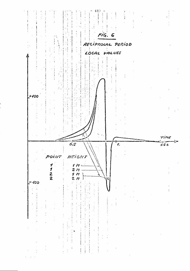
t_~~:.~>{,6"5-
1.
r;~.
I.
- 487,I
"
L.O~LI
I"
Ii!
iIII!
t
"
},
,,, 1
! IlEC;PROGIfL.
-I
- i!
fl'121111121-1
i ,- ... _.
II' .'I
II I
: . I -I,
I\ I
I I, II; ,
I ;I!
"1f~2
paiN""
,I
i , Ii i I I I'
I I
:1 I II .1i i .. '
j'._41 •..
1 I .. iI .j.
0#-«00 1 I : jI I I : jI- I ,
II -- :
III
i II
iII,
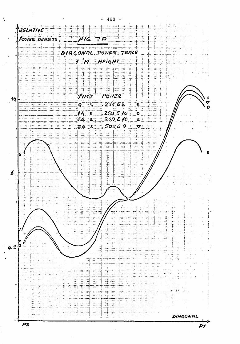
- 488
s
"jiI
I.'.1
..;:1
--I
l>iR<50ltlRL
I"
I'I
iI
.. I
0 .. :: .)( --.!:: .
._ ... "(1 ;.::::
. I •. •
. ;~~"';' ..... : 1:. :;: .. -' . ;...~:... , ... • :: : :. : : ~ I . • ,.~: . : : 1. ..;:::: J :. .' ':. i :;:~j' -.. :. ,I •
.1:+ tP1t:: '~l:••~!'.:~;.~.•::.
. :r::::.::: '''-''''':'i'
., .',:'f ••••[2l£;!•••+211cl.~•••Je.i•.. ....•.••!.•. . .. L.~:::~:::::.:::L~L::L~~:::.LI'. ! . .
•.. l:~~\_' . i~.__L~:!::•.::;~;~~~_:l:._II\\!..EL.l:.:X.:'1'. ,. : .... 1. . "j, .1. -- ... I ... 1.. : '1" --I" 1 i' .: i:' .i.' ,
.... 'l' .,t, .. j'
.. --_ .. 1. .. '_ .. ,..1
.. ~ j :. .,.. :!:. ..
... , ..,
. ! . '" [ I.... !. ..,....1.... I
1 .... 1
.c. ":'.1_:I",.
..'-r"; I
......... ,_ ...... --- ~-- ..
_..._.:L::~.:~;:I
1 ', 'r:r::;.1:.... .,
1
:~~i:~51~r:~~-~~stJ;j~:.~~t:-J.~~}"J?~•••i~.'!••..,..•' ....- :.L:.; !__..~~L_~':..L~~._ _ , _.~~.__ ~_.._u •••• L:.; ::.1::::(: .. :"
:; . :. ,'::: 1::' . i:. ::; .: ., I' ..•. J . i :. : .
~:.._.::..~ __l-::'_..::.:.L..'DIR~OfIRl.. 'PO£V~I?.: 7~J),c .... :...: .; ...:.....: I'. i':': '! .. :.: I . \:. .... . ... , : ; . . ; ..
•]t:I.~f~•••l-.I: .•i.• 1.~j.•I;:~lif~iillS:~f-~••~I'•••i••.•'•.•.!.•..,'.', j r j , --,'1' 'l .L---J_.,_._ .._t~,-_l--, I.J.u,u' I'" !,''':j i I'".. 1..• , , 1 ••• 1,." \ , .. ,j., 1.1 , .. I 1... 1 :;i , , I ..1.1.1" I ..I 1. I 1.. .. I. 1 !. ,...i ,' i..--I.. : .1 •. , ! .. t' .: I::... ~ .I ,I. ... I . ' .. !. I' .1.. I' . II
i . "L." "'11':;.;"":7/11:2' •.. 'po!uaR, .. l '.. ;... Ii., ,
. , .. :": 1:. .- j :"1::'- '.::. I ..I...". .• •. • •• I 1 ~. .' • •• , •• J - ~ I I • • I
10
i.
PI
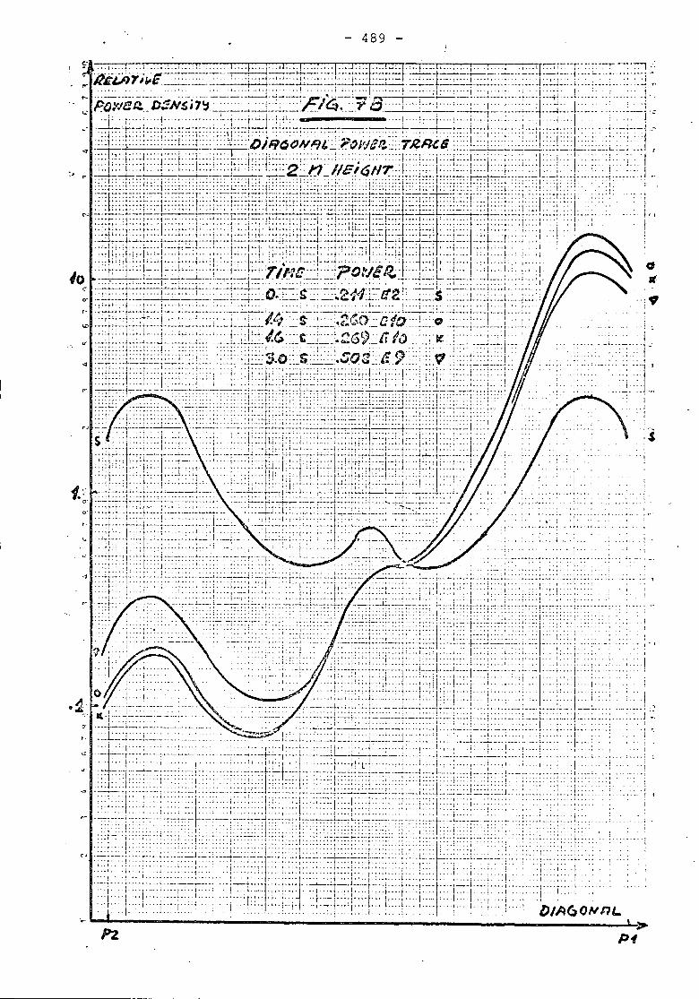
489
" ,
; - ...;$
.. lI
':j
.<i'f
'1 t
.. I').<0
........ J
i ..
I .1
.:j: .'1,..I.•. t .'. ~ - -
• :~ L ••
: ii#47j~E:"":~::. '~-':"'r:.j~:':~.":~~:~~=fu==J=~:~:+:~~J:~E:~r::~~:~F..:::8]:: koy,i!ii~iJ$Hs';i~--:-'~::~-:-:-'.E/4--':~'a~~~~;.:~~.f.' .~.-.L:~i ...l .:.. : ...: .1
: ••.ji~ttJ.H•••.i.-~;~-i.~~Jk~~::~L~~~~e~C-~;~~+.~.-i~I;j~f1~t-~••~.=i-~1.... ".I"~"J. .. , .. , ... :1.:.,.:.::,,:: J:.::L.:.,2 .n"lleiQIIT I '. I: :"~:"i ':r. I. j:: :I....; . I. :: .. : 1.. I:;MH+-mt. ~:T:;~~:~[~~...•~;~~f",~cgc;i,-,~).:-Jdt;,!-j ;;.-1 ...-: ......1B , 'r t r , •• ; I'.;.; , j , I. "8¥'" c.: , I 'j' r I' r .. ,. , . .'" 7.:;::.-t:.:::::': ::.""" ..:.. ;...:...:;:.:.:...~..:i:::.'= ..:.:..:.:::t::J:.::::::~ :::2t::-=l::C',:: :i '.. "::':' j.'Tf" I -j-":.' :.:.: ; ': .. , t i 'i ..1 1 .. -' ' 1. I .-~-.T.- --..":+tFf'.~~~::~~;.~:~t::~~~::l:~:\~£:~;j~~)~~4]~:+~~~~~f~:;I~:j~~~:~nLi.~~:~:::li:"T.::1'j"! :
...j, .... ,.+...1 t..1.1 , .. t....I. I "!' I';",' ..:.. " ~'I" .....1,.. ~ .... , .. ' .... 1. f ..':;Itl. ~'.I._.'I "t f'.!' .1.. I~1.~~:'~.I':~:I~..:~t'..t.;~I! .. : 1.::_ .... , . .1 , •• : '.-1 ..
1.,' ;10 [:+ -_._ I rlr~ :..'po ~"l' '~"I'..; / ,.1 ' , .
':~':r~'::J::~:S . [ 1 1.;I ;. I;' . ..Jl~,.:;.'/;~vr~~~~:l.:."::.:;f1): [::':j.::l::~l~)I:;::';::+"t :.:<,1:: ..;':';
t:: --~::.~~+~~-~~-+~_.! '"1''''!''' ! i"'" ...,l'T -.1- ...... i I ... ::¥t:;::-r~-+:~....::::t::~cf:~J~;:E::::,~~TF:"';"-..,-'r:--i---"'''_'''' L_.. ':.;L~.F~f:~:~~;':"jl__.::__~- '-:-:L~:E~r~~~:J:::~". 1" I . ; f. .: .. ,...:.' " , i ' "
'lfl'!:.1~TTj{::: L
I.- •.... !
_ .. J
:::i:-: 'i.:::i--'- i
P-t
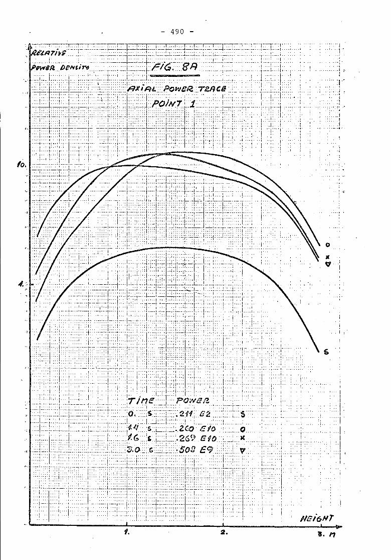
- 490
t.. .j,
_, .1..J __ .._ ,_._
!1
IIIrI
....! .I
i
....... ;
.. : ... ; ... J.f
oIt"1
.',
:1 ~.:.. T-
o • _ : ~ ~ _ ~ j"f
:1...... -1
, - ",', --~]'.....
. "
!
"!". . . . I . . .
.j ••
:1j •. : ..
; _.,l .•..i,
,'-. ,.:1: 'j
'f'
,1--'1' " I.. ! - ... j" .j •• ;
, I .1
:,1:I. :-:
'I ...,. ,
.,-- ,.., .. t.
'.
--1
. '1--" 1 -...... ._.1 , 1 '1 1.. +.."'.., ., '" . .. .. . . I . t.. .. ,.. ..... I. I' i ": i. . 1 • • •• t .. ,' ... I' .... I:
• 1 ,i. ! :::1 '''::::' -- I.' .. "i'
1. 2.
I ..
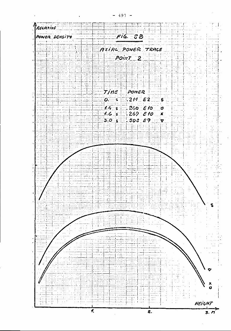
- 491
IIE/tiHT
,:i,., .
.. I
JI
"'j ....1
.0'
,! -"
'Coo
: ,,-
;
J.:,
'1
:.1
I.,
.j •.
.1,
i I
:i":'
I.... ' ... 1
. I.. ..... 1
' ..
::J"'I...
..-: i
.t ; ',
..1.
I
i~. .,
..I
'4' .•••• " ••
I.
_._." ......j.
.1 .
,,,i1.
. :i ..I
"1'
.. ~
.../::.
. ~1:,.,.-, "I. . ,,.: I
.I
'I'
. .••• i .•.
":i ,..:.::~:i:~::!::.~!
~: .; ....I,
.• - .,-_ .... _-_.j.
. , . . .... -! . _.. : ... ~:._... . .. - . ~. ~::~.
. ,.
..'.! 1..:.'.',~_ _~.,.: , .. ' 1-- ,. -.I.--j ••. 1.:..01 , 1. .. ; 1 ... ,.( .. , ... , .... ,' :, .. ' ., i .. I, . i '., .d,.' I". I. l. I I I '1" I
.. ,:": ,:.;,-- .i , : ., i"';::' I'" I ; 1'.It' i :.j ... J .. "'1 . ",
.:r:: :::Y'::::::':::l'.:'::::r:J:\':r:Tine:;::::i>OWEJa :.: : !
~'l-=£;~~~;:::::~=j'~'~:'::':~-~::\=~::~:,.~::..:~:=~:.: .. .:..:-::~::.........L..- .. --.---'--l .. -J" .. + ...L- .....u .,----------'--.Do. ..... ~ .......• 2 (1 E 2 S<J" ~+--t-~~.::.i::.+-+:>:~..~:;;:~.i..~~.I:+~-~.~~' ~ :•.. 1_ :- ..• --I--.._.j _.~_.J:.------l.. ,. .I.4.. $ .......•.(.;60 ..e 0 0
, , I .' I I' I I )'.. :.'.:'..'[.'.--i: "', :";.'. , !,' .. :::.'1'::. '1/. '.': --: ',.,2."'-0 ~AO' ".• •.•.. .••~.L. 1_ •• _ ••.. _.:.. __ .,...... ..L ,. ";,."'" ..
,
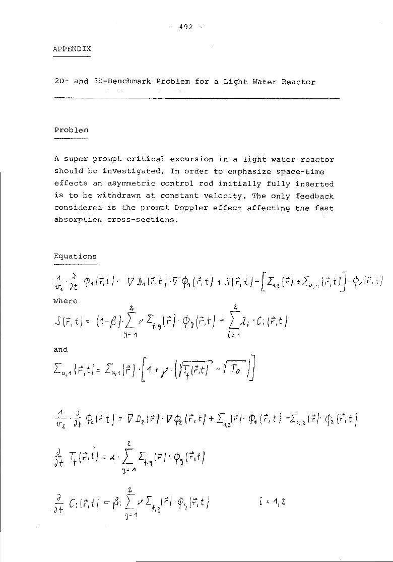
- 492 -
APPENDIX
2D- and 3D-Benchmark Problem for a Light Water Reactor
Problem
A super prompt critical excursion in a light water reactorshould be investigated. In order to emphasize space-timeeffects an asymmetric control rod initially fully insertedis to be withdrawn at constant velocity. The only feedbackconsidered is the prompt Doppler effect affecting the fastabsorption cross-sections.
Equations
where2.
(1-,g )- [ jl LT' ~ {r;' ep} (r,t) +~= 1
zL1j • C; (;=1 t )l:: "
1./t Tf (;, t I = A.' I~,~(;:I . cp~(~l f)~.:: /1
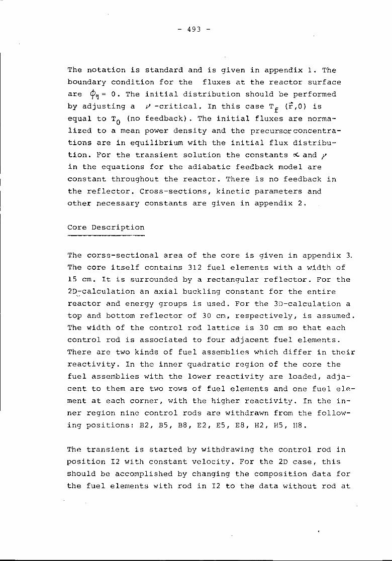
- 493 -
The notation is standard and is given in appendix 1. Theboundary condition for the fluxes at the reactor surfaceare ~~= O. The initial distribution should be performedby adjusting a ~ -critical. In this case Tf (r,O) isequal to TO (no feedback). The initial fluxes are norma-lized to a mean power density and the precursorconcentra-tions are in equilibrium with the initial flux distribu-tion. For the transient solution the constants ~ and fin the equations for the adiabatic feedback model areconstant throughout the reactor. There is no feedback inthe reflector. Cross-sections, kinetic parameters andother necessary constants are given in appendix 2.
Core Description
The corss-sectional area of the core is given in appendix 3.The core itself contains 312 fuel elements with a width of15 cm. It is surrounded by a rectangular reflector. For the2D-calculation an axial buckling constant for the entire
~I ,"
reactor and energy groups is used. For the 3D-calculation atop and bottom reflector of 30 cm, respectively, is assumed.The width of the control rod lattice is 30 cm so that eachcontrol rod is associated to four adjacent fuel elements.There are two kinds of fuel assemblies which differ in theirreactivity. In the inner quadratic region of the core thefuel assemblies with the lower reactivity are loaded, adja-cent to them are two rows of fuel elements and one fuel ele-ment at each corner, with the higher reactivity. In the in-ner region nine control rods are withdrawn from the follow-ing positions: B2, BS, B8, E2, ES, E8, H2, HS, H8.
The transient is started by withdrawing the control rod inposition 12 with constant velocity. For the 2D case, thisshould be accomplished by changing the composition data forthe fuel elements with rod in 12 to the data without rod at

- 494 -
a constant velocity or a poison cross-section should be de-ducted from the thermal absorption cross-section to representrod movement.
For the 3D case, the rod is moved only in the fuel zone; itdoes not penetrate into top or bottom reflector. For repre-sentation of the rod again a poison cross-section should bededucted from the thermal absorption cross-section.
Evaluation of Results
First, the static multiplication factors with and withoutrod (but without feedback) should be given.
The transient should be followed for about 3 seconds. Forbetter comparison of the results it is suggested to explic-itly represent the first three decades of the reactor powerseparately on logarithmic paper as well as the upper fourdecades where the maximum power will occur. For graphicaldisplay of temperatures 5 em per 1000 K is proposed.
For the 2D and 3D case mean values of power, temperature andreciprocal periods should be given. Local values of the samequantities in the monitoring points 1 and 2 (see appendix 3)should be given. The monitoring points for the 3D case are100 cm and 200 cm from top of the reactor fuel zone.
Of further interest are power profiles at different timesalong the diameter specified in appendix 3. The power pro-files should be evaluated at t1=0, t2=1.4, t3=1.6 and t4=3.0seconds. The power profiles for the 3D case should be speci-fied at the same heights as the local monitoring points.Furthermore for the 3D case the axial power shape in themonitoring points 1 and 2 should be given at the same times.

- 495 -
The power shapes should be normalized to the instantaneoustotal power. Also these total powers should be specified.
Additional information of type of computer, storage, CPUand I/O-times (sec.) are of interest. Computing timesshould be estimated relative to a CDC 6600 computer.
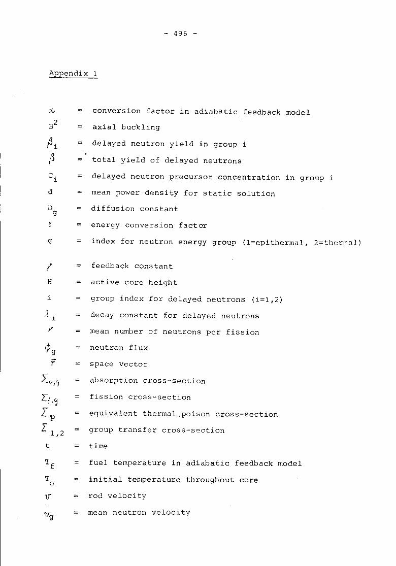
- 496 -
Appendix 1
d
Dg
G
g
rH
i
..-r
= conversion factor in adiabatic feedback model= axial buckling
= delayed neutron yield in group i
= total yield of delayed neutrons
= delayed neutron precursor concentration in group i
= mean power density for static solution= diffusion constant
= energy conversion factor
= index for neutron energy group (l=epithermal, 2=ther~ul)
= feedback constant
= active core height
= group index for delayed neutrons (i=1,2)
= decay constant for delayed neutrons
= mean number of neutrons per fission
= neutron flux
= space vector
= absorption cross-section
= fission cross-section
= equivalent thermal poison cross-section
= group transfer cross-section
= time
= fuel temperature in adiabatic feedback model
= initial temperature throughout core
= rod velocity
= mean neutron velocity
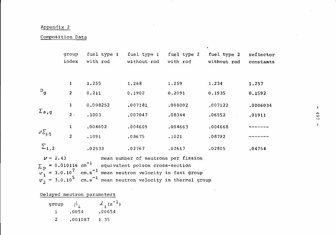
Appendix 2
Composition Data
groupindex
fuel type 1with rod
fuel type 1without rod
fuel type 2with rod
fuel type 2without rod
reflectorconstants
Dg
La,g
LlLf,9
[1,2
1 1.255 1.268 1.259 1.234 1.2572 0.211 0.1902 ,0.2091 0.1935 0.1592
1 0.008252 .007181 .008002 .007122 .0006034 ,
2, .1003 .007047 .08344 .06552 .01911 ~\.0---.J
,1 .004602 .004609 .004663 .004668 -------
2 .1091 .08675 .1021 .08792 -------
.02533 .02767 .02617 .02805 .04754
J,J= 2.43 mean number of neutrons per fissionL = 0.010116 cm-l equivalent poison cross-section
p 7 -1if1 = 3.0.10 cm.s mean neutron velocity in fast group~2 = 3.0.105 cm.s-1 mean neutron velocity in thermal groap
Delayed neutron parameters
group1
2
r~ •I 1
.0054
.001087
)..(s-l)1
.006541. 35
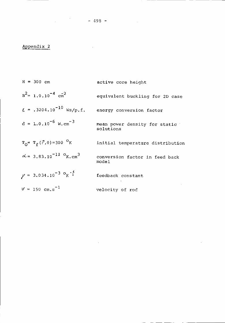
Appendix 2
H = 300 cm
B2= -4-21.0.10 cm
-10E = .3204.10 Wsjp.f.
-6 -3d = 1.0.10 W.cm
-11 0 3oL = 3. 83 • 10K. cm
-3 0 _.1-3.034.10 K 2
- 498 -
active core height
equivalent buckling for 2D case
energy conversion factor
mean power density for staticsolutions
initial temperature distribution
conversion factor in feed backmodel
feedback constant
1.1 = 150 -1crn. s velocity of rod
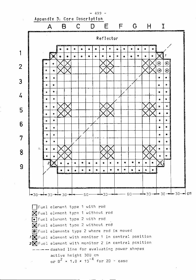
- 499 -AppendIx 3: Core DescrIptIon
A B c o E F G H I
type 1 'di th roo
type 1 without rod
type 2 \.J it h rod
type 2 vJi thout roo
1
2
3
4
5
6
7
8
9
Reflector
e e (D (I) e • It 0 • /• • • 0 •rx .. • (I) • • • • • (j) 0 • 0 0 • )Q 1
It 0 rxX XX X ~ @ (!)
• G. rx X [)(~ X[X @ @
• • /Cl •1/
• III 1// It It
• • 1// 0•• • /
1/ (I) Ii
• 0 X [X ~ lX ~ X 0 •• e X ~ ~ [X [>( ~ • •• III 1// 0 •
7Q • 1/ • •0 0
/V • e
• • v/ • •'.~. • • r.x[X XX XX • •
• • X[X XX X ~ • G
~ XIS!."III<lIIl
2 • • 0 " -. • 0 • • • • • • •l/ • • • 0 • • • \I e CD • 0 • •
- 30__ f-- 30 -.. -- 30 60 30 60 30 -9P1-. 30-- r--30-
DFuel element
~Fu8l element
0Fuel element~Fu8l element~Fuel elements type 2 where rod is moved
1~Fuel elerT18nt with monitor 1 in central position
2~Fuel element with monitor 2 in central position_____ dashed line for evaluating power shapes
active height 300 cmor 82 = 1.0 * 10-4 for 20 - case
cm
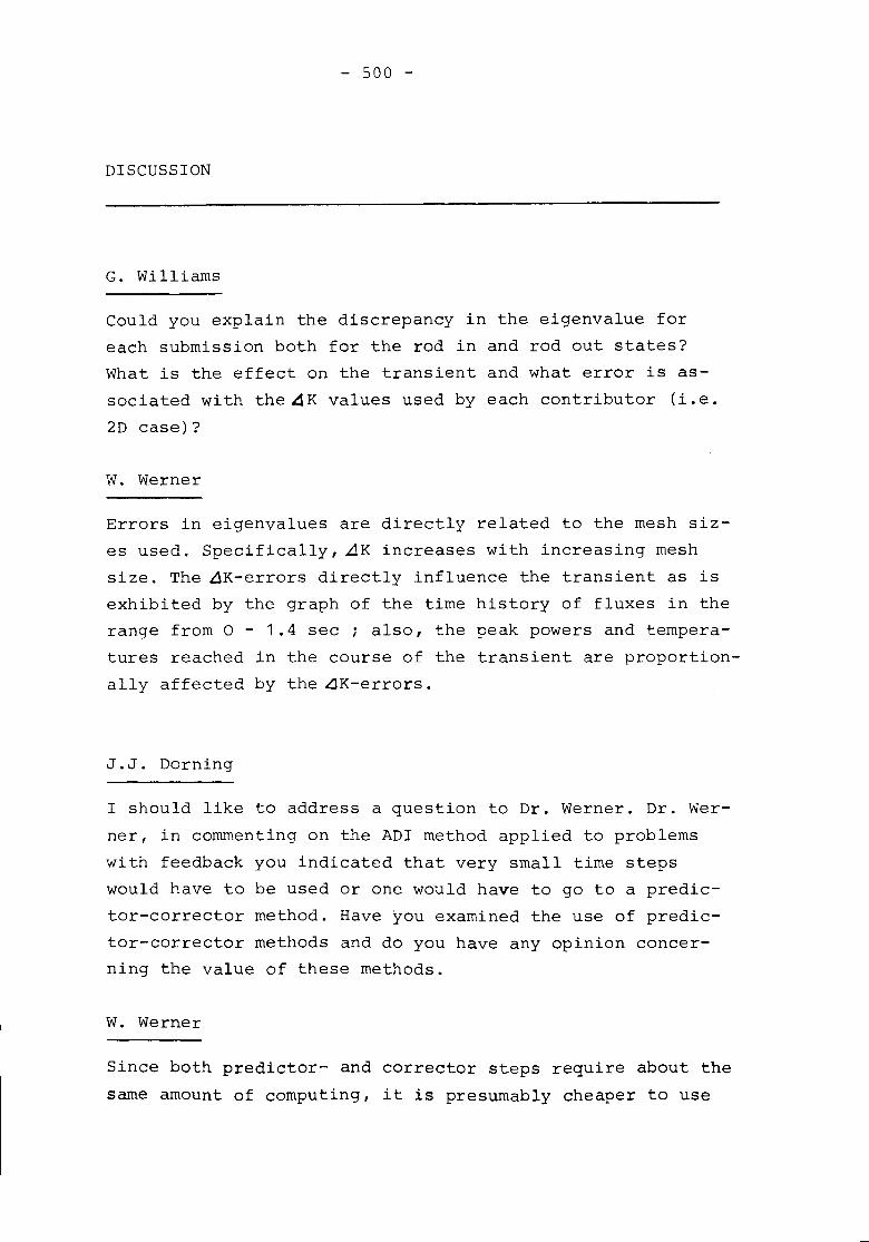
- 500 -
DISCUSSION
G. Williams
Could you explain the discrepancy in the eigenvalue foreach submission both for the rod in and rod out states?What is the effect on the transient and what error is as-sociated with theAK values used by each contributor (i.e.2D case)?
W. Werner
Errors in eigenvalues are directly related to the mesh siz-es used. Specifically, AK increases with increasing meshsize. The ~K-errors directly influence the transient as isexhibited by the graph of the time history of fluxes in therange from 0 - 1.4 see; also, the peak powers and tempera-tures reached in the course of the transient are proportion-ally affected by the ~K-errors.
J.J. Darning
I should like to address a question to Dr. Werner. Dr. Wer-ner, in commenting on the ADI method applied to problemswith feedback you indicated that very small time stepswould have to be used or one would have to go to a predic-tor-corrector method. Have you examined the use of predic-tor-corrector methods and do you have any opinion concer-ning the value of these methods.
W. Werner
Since both predictor- and corrector steps require about thesame amount of computing, it is presumably cheaper to use

- 501 -
anly predictars, tagether with a smaller step size.
J.J. Darning
I shauld like to. suggest a mare detailed discussian af theinitial static K-calculatian. I believe that the transientcalculatians will be very much affected by this renarmali-zatian af K. Perhaps, the cantributars cauld state whetherthey have dane any systematic canvergence studies in theirstatic calculatians, what the canvergence criteria an theirsaurce iteratian calculatian af K was, etc., and, in gener-al, their awn subjective view af the credibility af theirstatic calculatian. I believe that the inadequate canver-gence af same af the K-calculatians might accaunt far sameaf the discrepancies in the transient calculatians.
w. Werner
There is strong evidence that the discrepancy can be ex-plained by mesh size effects, rather than by paar canver-gence af static calculatians. The mesh size effect is ex-hibited very strikingly by CITATION-calculatians whichshawed acceptable accuracy anly when the mesh size camedawn to. 3.5 cm.
M.J. Bridge
I have naticed that there are significant differences be-tween the reactivity warth shape when paisan crass-sectianis changed linearly between cell-centred and interstitialmesh cades. Cauld this accaunt far same af the differencesabserved?
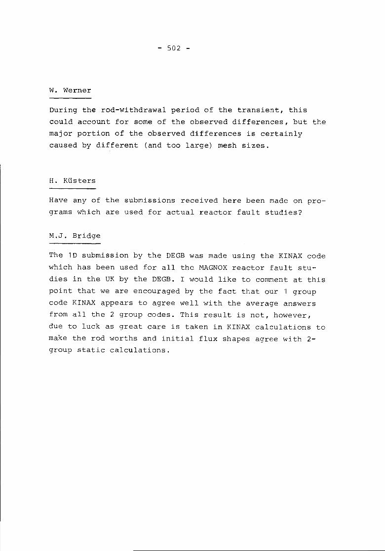
- 502 -
W. Werner
During the rod-withdrawal period of the transient, thiscould account for some of the observed differences, but themajor portion of the observed differences is certainlycaused by different (and too large) mesh sizes.
H. Klisters
Have any of the submissions received here been made on pro-grams which are used for actual reactor fault studies?
M.J. Bridge
The 1D submission by the DEGB was made using the KINAX codewhich has been used for all the MAGNOX reactor fault stu-dies in the UK by the DEGB. I would like to comment at thispoint that we are encouraged by the fact that our groupcode KINAX appears to agree well with the average answersfrom all the 2 group codes. This result is not, however,due to luck as great care is taken in KINAX calculations tomake the rod worths and initial flux shapes agree with 2-group static calculations.
- 503 -
COMMENTS
A.R. Dastur
The correlation between ~~ and mesh size used in the CITA-TION calculation would perhaps be more understandable ifthe mesh size is expressed in units of absorption and/ortransport mean face paths, or some other convenient neu-tronic parameter in case of multigroup formulations.
W. Werner
At first sight, we have found considerable disagreement be-tween the solutions of the various contributors.
There is strong evidence that a major portion of the dis-agreement may be traced down to the spatial discretisationerror.
I would like to suggest that the contributors rerun theirproblems using refined meshes. Hopefully, these solutionsshould converge and should provide a better estimation ofthe correctness of the solutions.

- 505 -
Session IV/2
REVIEW OF KINETICS BENCHMARK CALCULATIONS
Chairman: D.A. Meneley, Canada
A. Buffoni, J.K. Fletcher, A. Galati,F.N. McDonnell, A. Musco, L. Vath
SURVEY OF THE RESULTS OF A TWO-DIMENSIONALKINETIC BENCHMARK PROBLEM TYPICAL FOR A FASTREACTOR
505

- 507 -
L. VathInstitut fUr Neutronenphysik und ReaktortechnikGesellschaft fUr Kernforschung m.b.H., Karlsruhe
I. Introduction
In 1973 the NEACRP posed a number of kinetic bench-mark problems intended to be solved by different groups.The results were to be compared leading to estimateson the accuracy and efficiency of the different codes.This was felt to be of great value since the codes in-volved become more and more important in the field ofreactor safety.
Most of the benchmark problems are typical for thermalreactors, but it was deemed necessary to include oneproblem typical for a fast reactor. The results for thistwo-dimensional reactor kinetics benchmark problem areanalyzed in this paper.
In formulating the problem two aims were followed.First, the problem was intended to be sufficientlyeasy to be solved by a large number of codes, puttinga strong weight to the neutronics and using a verysimple feedback model, which could be easily incorporatedin any code. The feedback is therefore independent of
- 508 -
space, using a mean core temperature for computingthe Doppler effect. Two nearly equivalent feedbackversions were submitted, one acting on the crosssections, the other directly changing the reactivity.A 2-group formulation was chosen so that typical 2-group thermal reactor codes could be used, but further-more, a more realistic 6-group formulation was submitted,too. Thus the 4 benchmark problems are, in reality,only one problem.
The second aim was to have reactor dimensions and atransient typical for the fast reactor predisassemblyphase of a hypothetical core disruptive accident. Thereactor geometry and group constants were derived fromthe German SNR-300 design with a number of simplifications.The very high ramp rate is typical for the rates producedby slumping or fuel-coolant interaction. The totalreactivity inserted was limited to less than 3 $ soas to stay within reasonable bounds for the fuel tempera-ture. Therefore, it was not attempted to model one ofthe feedback phenomena just mentioned, which result ina much bigger total reactivity. Instead the ramp wasproduced by a simulation of control rod movement. Forfurther information on the benchmark, see appendix.
Unluckily, the effort at producing a relatively simpleproblem did not bring the desired result in the formof a great number of contributions. There are only four,none of which is able to act as a reference solution.Thus, there is no standard against which to compare thesolutions, and one is not able to obtain a picture ofthe state of the art, since a big number of methodsdifferent of the ones employed by the participantsexist.
- 509 -
In section II of this paper a list of the participantsand sununaries of the methods employed in their codes isgiven. In section III, the results are presented andcompared. The final conclusions will be sununarized inchapter IV.
II. List of Contributions
1. UK - RIS
Submissor:
Cases submitted:
Computer:
Code:
Methods:
P.eference:
2. CRNL
Submissor:
J.K. FletcherCentral Technical ServiceUKAEARisleyWarringtonLancsEngland
1,2,3,4
ICL 470
SPARK
SPARK uses the improvedquasistatic method
FRCMV1P P (72) 71
F.N. McDonnellApplied Mathematics BranchChalk P.iver NuclearLaboratoriesChalk RiverOntarioCanada
- 510 -
Cases submitted:
Computer:
Code:
I~ethods:
Reference;
3. CSN
Submissor:
Cases submitted:
Computer:
Code:
CDC 6600
ADEP
The alternating directionexplicit method is used. Inaddition, an exponentialtransformation of the fluxis used. The program calledADEP was written at BatelleColuITbus Labs. It has beenmodified at CRNL to incorporatea variety of feedback models.Automatic time-step size isnot used in this program
R.S. Denning: ADEP: A One-and Two-dimensional Few Grou?Kinetics Code.BMI - 1 91 1 ( 1 97 1 )
G. Buffoni, A. Galati, A. ;'uscoCentro Studi Nucleari delIaCasaccia C.N.E.~.Via Anguillarese k~ 1 + 300S. Maria di GaleriaRomaItaly
1, 2
IBI") 37'J/ 16 5
NADYP-A
- 511 -
Methods:
References:
This program provides for thecalculation of neutron fluxesand temperature distributionduring an operating or accidentaltransient. The reactor isdescribed in r-z geometryand few-groups (~5) diffusionmodel, the macroscopic crosssections depending on theDoppler temperature and coolantdensity. The thermodraulicmodel involves an appropriatesubdivision of reactor in anynumber of radial shells, anyone of which is described bya single channel model. Themass, energy and momentum con-servation equations in the fuel,clad and coolant are solved foreach channel, where the materialproperties are temperature de-pendent.
The stationary diffusion equationsare solved by assuming fluxesas sum of trigonometric and/orBessel functions; the time-dependent diffusion equationsare solved by the metastaticmethod; finally, the heatequations are solved by thecharacteristics method.
A. Galati - N.S.E. 37, 30-40(1969)
4. GfK
- 512 -
G.Buffoni, A.Galati, A.Musco:"DIFF-2, un programma di diffusionea 2 dimensioni" CNEN RT I(FCR) (74)8
G.Buffoni, A.Galati, R.Mosiello,A.Musco, F.Norelli, C.D.Stanescu:"NADYP, un codice di dinamica perreattori veloci: descrizione delmodello fisico matematico" - CNENRT/FI(74)8
Submissor: L. VEith
Institut fur Neutronenphysikund ReaktortechnikGesellschaft fUr KernforschungD-7500 KarlsruhePostfach 3640West Germany
Cases submitted: 1, 2, 3, 4
Computer:
Code:
Methods:
Reference:
IBM 370/168
KINTIC-1
KINTIC-l may use the normal quasi-static, adiabatic or point kineticsmethod and has a detailed thermo-hydraulics part.For the benchmark calculations,the adiabatic model has been usedand the simple feedback model wasincorporated.L. Mayer, H.Bachmann: KINTIC-1A program for the calculation oftwo-dimensional reactor dynamicsof fast reactors with the quasi-static method. KrK 1627 (1972).

- 513 -
III. Results and Comparison
Case 1
Benchmark case 1 will be analyzed in some detail, sincethis is the only case which has been solved by allcontributors. Furthermore, comparison of the other casesyields similar results requiring only a few additionalremarks.
-.~
Some of the main results are depicted in fig's 1-5.The development of power vs. time is shown in fig's 2and 2.1 with good qualitative agreement of UK-RIS, CRNL,and GfK, but markedly different results from CSN. Thisis astonishing since UK-RIS, GfK and CSN all employfactorizing methods. Nevertheless, there are somepeculiarities to the metastatic method which may accountfor the differences:
1. The method uses different iteration schemes dependingon whether the reactor is above or below promptcritical. The marked deviation occurs at 6 msec, thepoint around which the reactor should go promptcritical, and is finished at 15 msec, the point atwhich the ramp ends and the reactor goes below promptcritical.
2. There is no information about time step lengths andthe way time dependent cross sections are handled.Errors could occur if big time steps are combined withstepwise alterations of the cross sections or if nosufficient iteration between power development andcross section alteration is assured.
The other three solutions (fig.2) agree qualitatively, butthe heights of maxima and minima vary about 25 %, theirposition on the time scale about 10 % or more. The
- 514 -
difference in the initial ramp rates (fig. 1) is 10%.The resulting temperature behaviour is shown in fig.3.In an attempt to find out possible reasons for this,initial and final flux shapes and spectra have beeninvestigated. Fig's 4 and 5 show that small but distinctdifferences exist in the radial flux distribution nearthe reactor midplane. Especially these differences canbe found in the region of the movable absorber and thusmay account for the different ramp rates. As an indicatorfor the time dependent flux shaDe the quotient 0q (r=20,z=88.25,t)/0 (r=38, z=88.25,t), r=20 and r=38 being theaposition of the initial total flux minimum resp. maximum,has been calculated for each group and different times(table 2). It shows small but marked differences in theinitital value as well as in iLs time dependent change.The time dependent 2-group spectra at two points in thereactor, one of which is located in the movable absorberregion, has been evaluated too. There is no differencebetween the results of all three contributors withinthe available accuracy (table 1).
The use of different numerical methods in the transientpart may play a role in explaining the difference betweenthe CRNL results and the other two contributions in thefeedback Dart of the transient (t > 8 msec). Thisassumption is supported by the initial contributionof CRNL, which had used larger time steps with farworse results (see fig. 2.2). Smaller time steps sub-sequently produced the better results presented, butit is not clear whether these steps are fully adequatesince CRNL employs no automatic steD adjustment.
The difference of the UK-RIS and GfK results cannot beexnlaineu by the different numerical methods. The twomethods - the improved quasistatic and the adiabatic
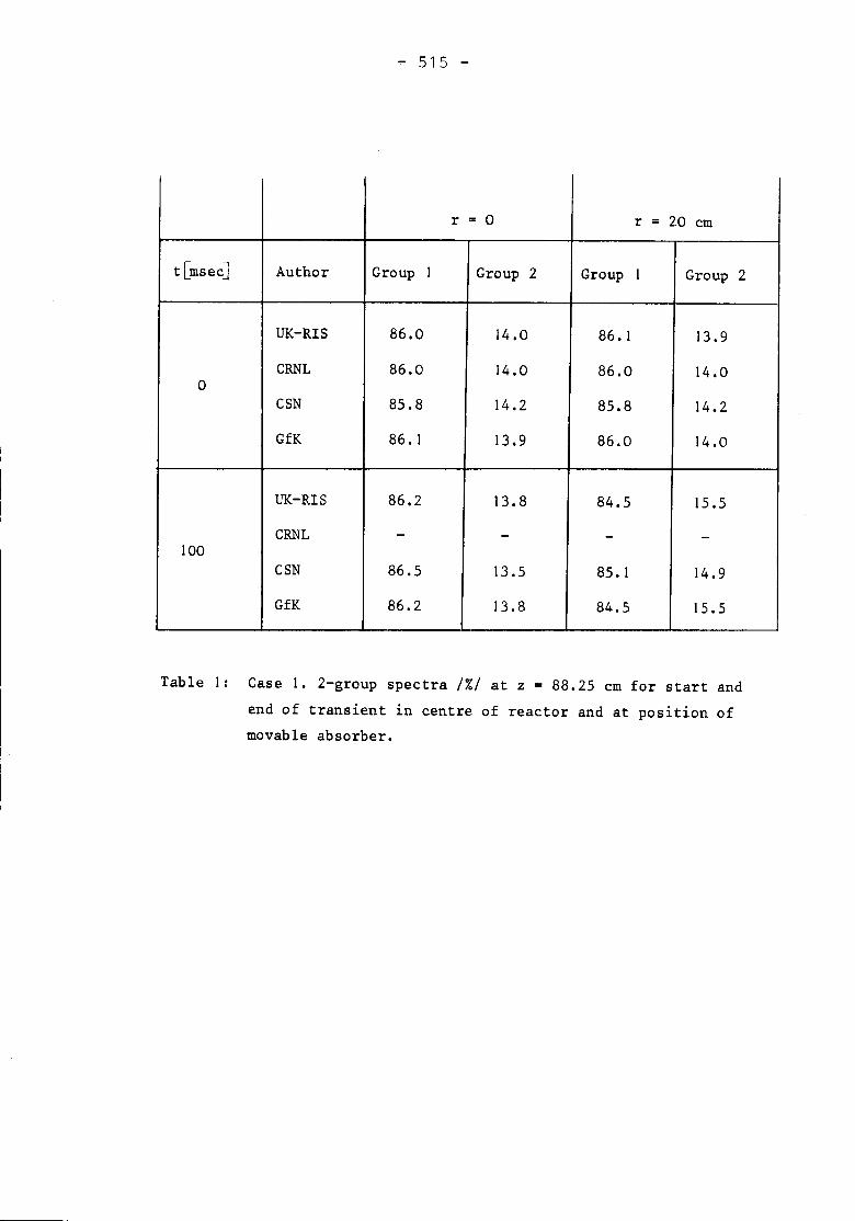
.,.. 515 -
r = 0 r = 2.0 cm
t[msecJ Author Group 1 Group 2 Group 1 Group 2
UK-RIS 86.0 14.0 86. 1 13.9CRNL 86.0 14.0 86.0 14.00CSN 85.8 14.2 85.8 14.2GfK 86.1 13.9 86.0 14.0
UK-RIS 86.2 13.8 84.5 15.5CRNL - - - -100CSN 86.5 13.5 85.1 14.9GfK 86.2 13.8 84.5 15.5
Table 1: Case 1. 2-group spectra /%/ at z = 88.25 cm for start andend of transient in centre of reactor and at position ofmovable absorber.
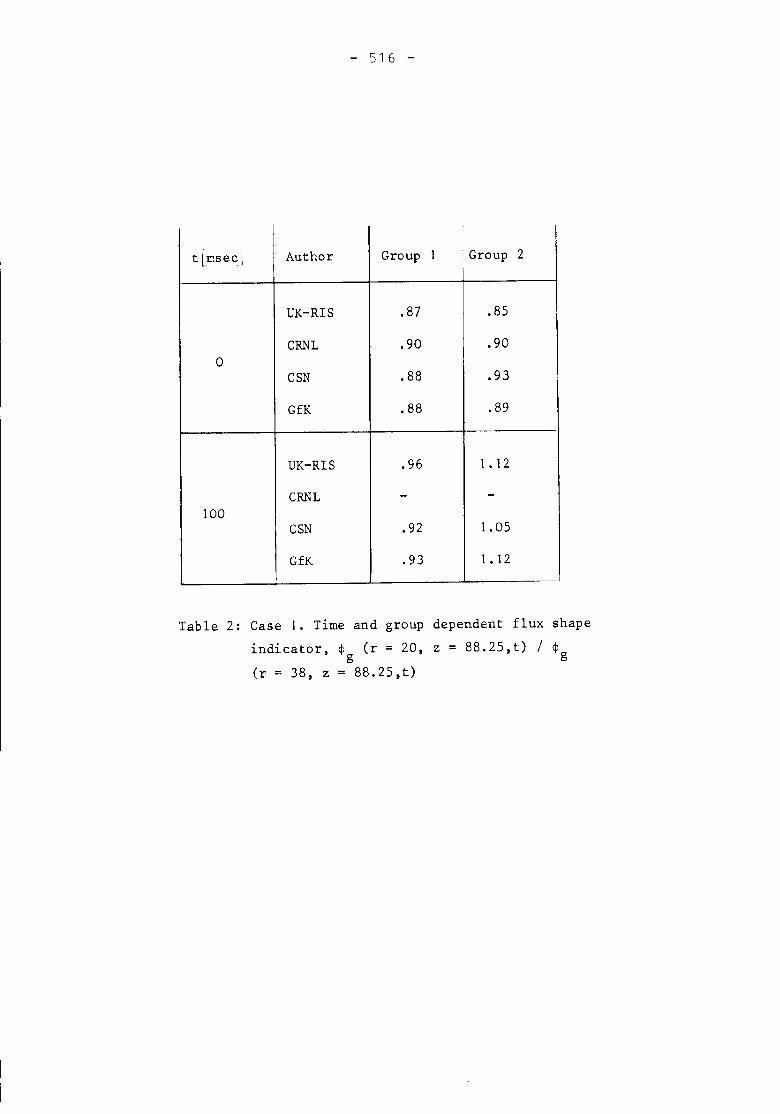
- 516 -
I II
t [msecj Author Group I Group 2
UK-RIS .87 .85
CRNL .90 .90a
CSN .88 .93
GfK .88 .89
UK-RIS .96 I. 12
CRNL - -100
CSN .92 1.05
GfK .93 I. 12
Table 2: Case 1. Time and group dependent flux shapeindicator, ~ (r = 20, z = 88.25,t) / ~g g(r ~ 38, z = 88.25,t)
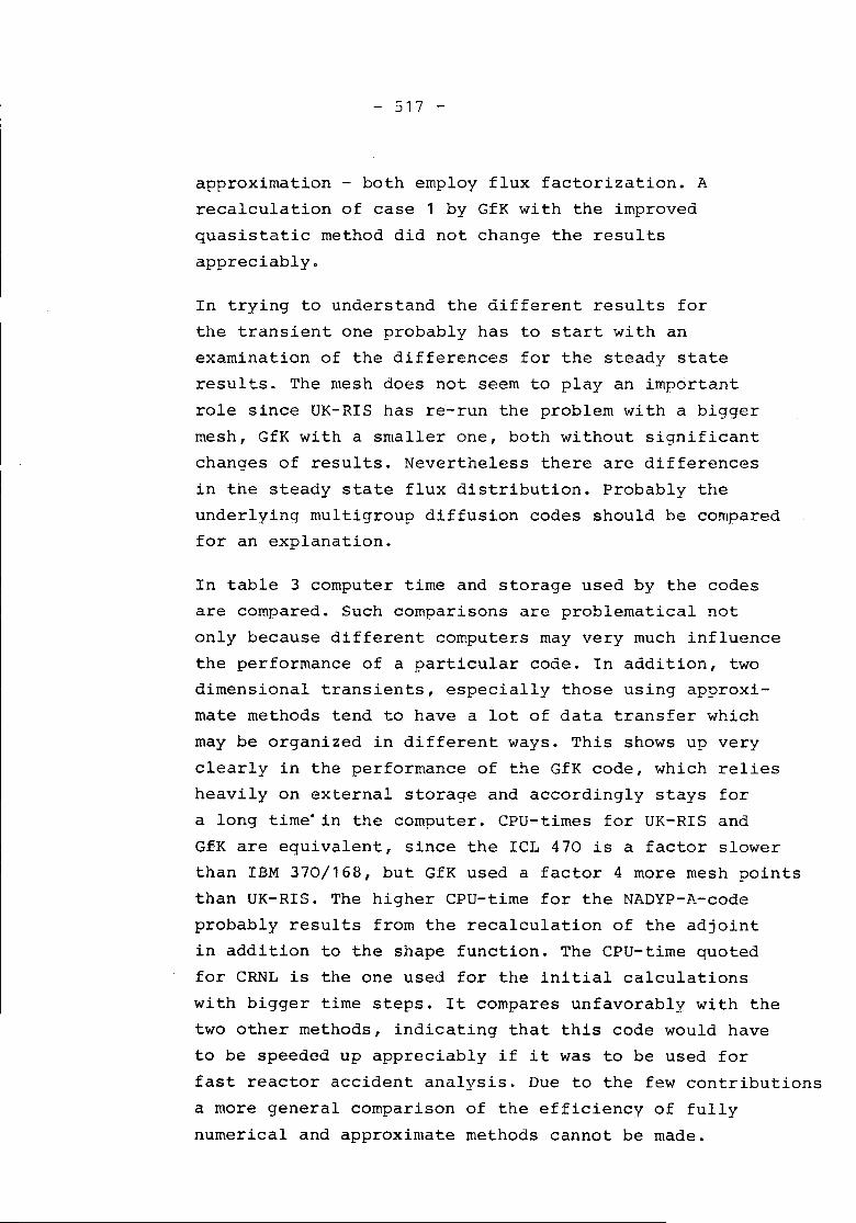
- 517 -
approximation - both employ flux factorization. Arecalculation of case 1 by GfK with the improvedquasistatic method did not change the resultsappreciably.
In trying to understand the different results forthe transient one probably has to start with anexamination of the differences for the steady stateresults. The mesh does not seem to play an importantrole since UK-RIS has re-run the problem with a biggermesh, GfK with a smaller one, both without significantchanges of results. Nevertheless there are differencesin the steady state flux distribution. Probably theunderlying multigroup diffusion codes should be comparedfor an explanation.
In table 3 computer time and storage used by the codesare compared. Such comparisons are problematical notonly because different computers may very much influencethe performance of a particular code. In addition, twodimensional transients, especially those using approxi-mate methods tend to have a lot of data transfer whichmay be organized in different ways. This shows up veryclearly in the performance of the GfK code, which reliesheavily on external storage and accordingly stays fora long time. in the computer. CPU-times for UK-RIS andGfK are equivalent, since the ICL 470 is a factor slowerthan IBM 370/168, but GfK used a factor 4 more mesh pointsthan UK-RIS. The higher CPU-time for the NADYP-A-codeprobably results from the recalculation of the adjointin addition to the shape function. The CPU-time quotedfor CRNL is the one used for the initial calculationswith bigger time steps. It compares unfavorably with thetwo other methods, indicating that this code would haveto be speeded up appreciably if it was to be used forfast reactor accident analysis. Due to the few contributionsa more general comparison of the efficiency of fullynumerical and approximate methods cannot be made.
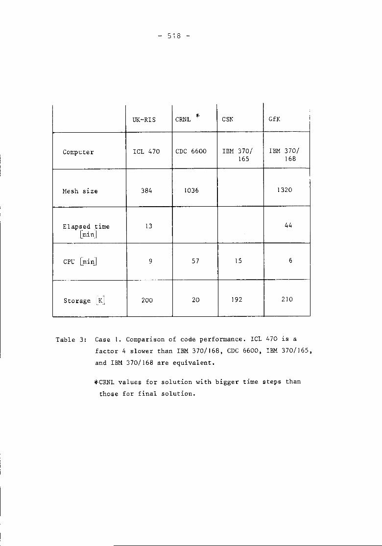
- 518 -
UK-RIS CRNL f CSN GfK
Computer ICL 470 CDC 6600 IBH 370/ IBM 370/165 168
Hesh size 384 1036 1320
Elapsed time 13 44[minJ
CPU [minJ 9 57 15 6
Storage [KJ 200 20 192 210
Table 3: Case 1. Comparison of code performance. ICL 470 ~s afactor 4 slower than IBM 370/168t CDC 6600t IBM 370/165t
and IBM 370/168 are equivalent.
*CRNL values for solution with bigger time steps thanthose for final solution.
- 519 -
Case 2
Cases 2 - 4 have been calculated by UK-RIS and GfKonly. The difference between case 1 and case 2 isin the feedback only, which in case 2 directly altersthe reactivity. It is dimensioned in such a way that thefeedback effect is approximately the same as in case1. Fig.6 shows the time dependent reactivity forcase 2 • The picture is nearly identical with fig.1for case 1 and does not lead to any new conclusions.
Case 3
This case is the 6-group version of case 1 and givesqualitatively the same, but quantitatively slightlydifferent results. This shows up in fig's 7 - 9. Theinitial ramp rates of UK-RIS and GfK agree excellently,but later on slight differences in reactivity turn up.This leads to differences in the power and, consequently,a quite sizable difference of the temperatures at theend of the transient.
As in case 1, spectra and flux distributions have beencompared and some details are given in tables 4 and 5.
The spectra at the centre of the reactor agreeexcellently within the limits of accuracy (table 4).The same holds true for the spectra at initial timein the region of the movable absorber, whereas thechange of the spectra in this region shows a markeddifference in group 5. Furthermore, table 5 showsdifferences in the flux distributions at initial timeand at the end of the transient with GfK consistentlyproducing higher values of ~~r = 20, z = 88.25,t) I~g (r = 38, z = 88.25,t)
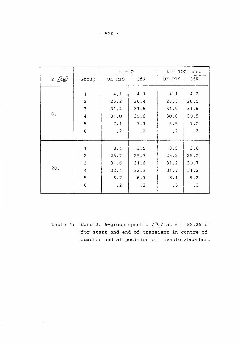
- 520 _.
It = 0 t = 100 msec
__4'
U~~RIS j'. -- ! -- ..". __ ... --_.
r (Cf.!)/ Group GfK UK-RIS I GfKI
!1 4.1
\4.1 I
4.1 4.22 26.2 26.4 26.3 26.53 31.4 31.6 31 .9 31.6
o. 4 31.0 30.6 30.6 30.55 7. 1 7 .1 6.9 7.06 .2 I .2 : .2 .2
I II
II,
1 3.4 3.5 ! 3.5 3.6i2 25.7 25.7 25.2 25.0
3 31.6 31 .6 i 31.2 30.7i20. I
4 32.4 32.3 i 31 .7 31.2
I 5 6.7 6.7
I8.1 9.2
I6 .2 .2 .3 .3
II
Table 4: Case 3. 6-group spectra L-~/ at z = 88.25 cmfor start and end of transient in centre ofreactor and at position of movable absorber.
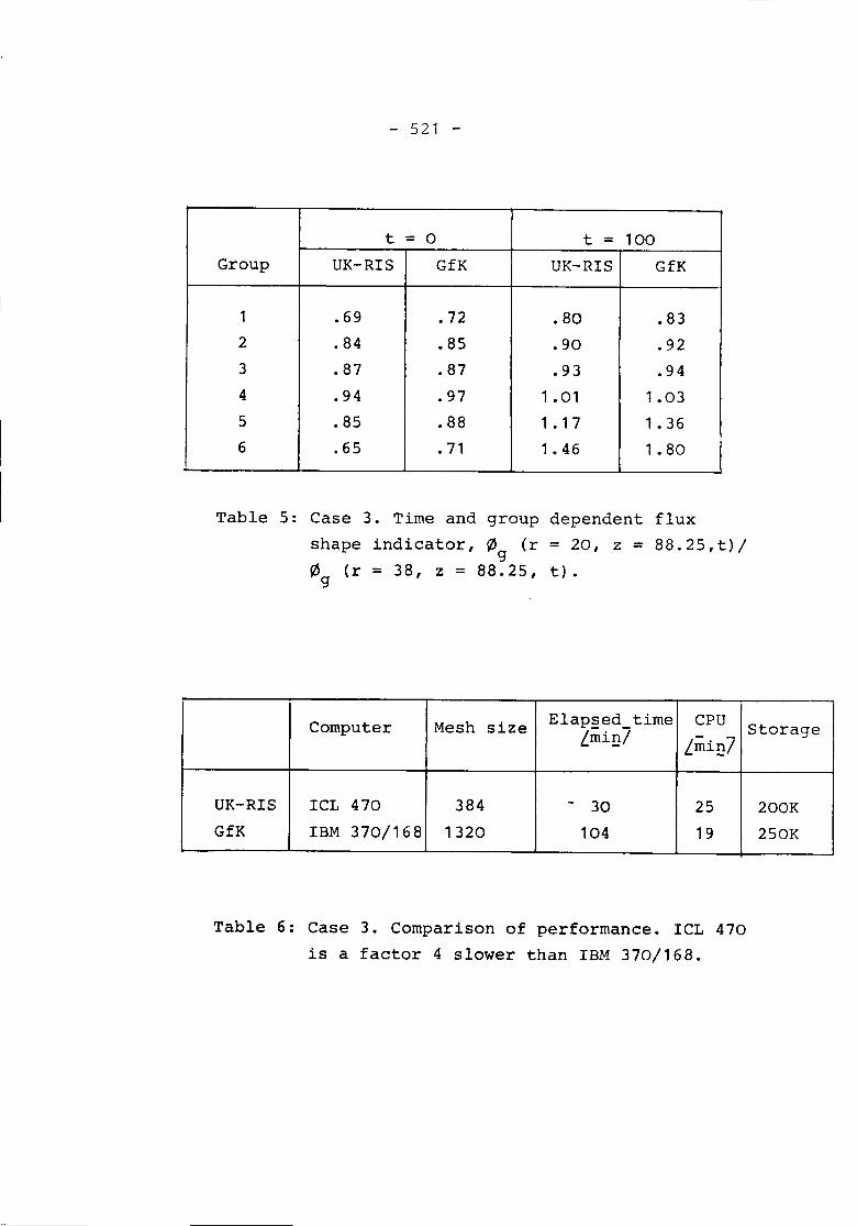
- 521 -
t = 0 t = 100Group UK-RIS GfK UK-RIS GfK
1 .69 .72 .80 .832 .84 .85 .90 .923 .87 .87 .93 .944 .94 .97 1.01 1.035 .85 .88 1.17 1.366 .65 .71 1.46 1.80
Table 5: Case 3. Time and group dependent fluxshape indicator, ~ (r = 20, z = 88.25,t)/g~ (r = 38, z = 88.25, t).g
Computer Mesh size Elap~ed_time CPU StorageLmi!}/ Lmi!}!
UK-RIS ICL 470 384 - 30 25 200KGfK IBM 370/168 1320 104 19 250K
Table 6: Case 3. Comparison of performance. ICL 470is a factor 4 slower than IBM 370/168.
- 522 -
than UK-RIS. Taking into account the results of thecomparison for case 1, it seems that the excellentagreement of the initial ramp rates for case 3 isfortuitous. As in case 1, one should examine thedifferences of the steady state results for clues tothe discrepancies in the transient.
Table 6 shows a comparison of storage and computertime for case 3. The pattern is the same as in case 1.
Case 4The time dependent reactivity as calculated by UK-RISand GfK is shown in fig. 10 and is nearly identical tocase 3 (fig.6). Since case 4 is related to case 3 inthe same way as case 2 is related to case 1, no furtherdiscussion of the results mneeded.
IV. ConclusionsWith only a few contributions it is very difficult toreach definite and many conclusions. Nevertheless, twomay be ventured:1. The performance of the approximate methods looks very
good compared to the only finite difference method.A comparison with other finite difference methodswould be very desirable, especially with one thatcould act as a reference solution.
- 523 -
2. A more detailed analysis of the steady statediffusion codes is warranted to find out aboutcauses and effects of the differences in spatialflux distributions.
3. A second 2d fast reactor benchmark problem withmore realistic feedback should not be submittedbefore the differences of the solutions to thisfirst benchmark have been fully understood.
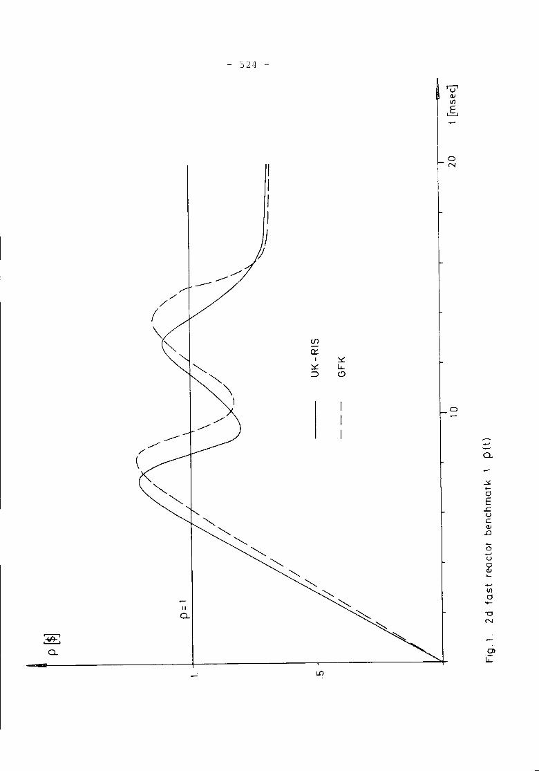
- 524 -
o
oN
.....-a.
~...0E
L:.uC(l)
.D...a--'u0(l)........Ul0
II......
a. ""0N
:~:a. 01
G:
-
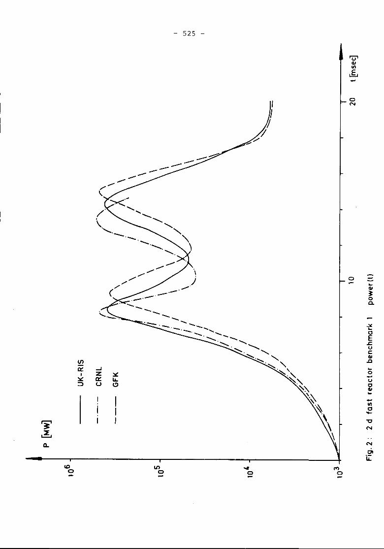
CDo
/.\ ..........
--'-.- . ......... ............
IIIo
- 525 -
......
....
oN
0 ....-~QI
~0a.
oX~0E~uCQI.0~0....u0QI~-II)0....'0N
N
CliL:

I I 1 , .-
14 16 18 20 t (msec)12108642o103
lOS
Fig. 2.1: 2d fast reactor benchmark 1 power(t)
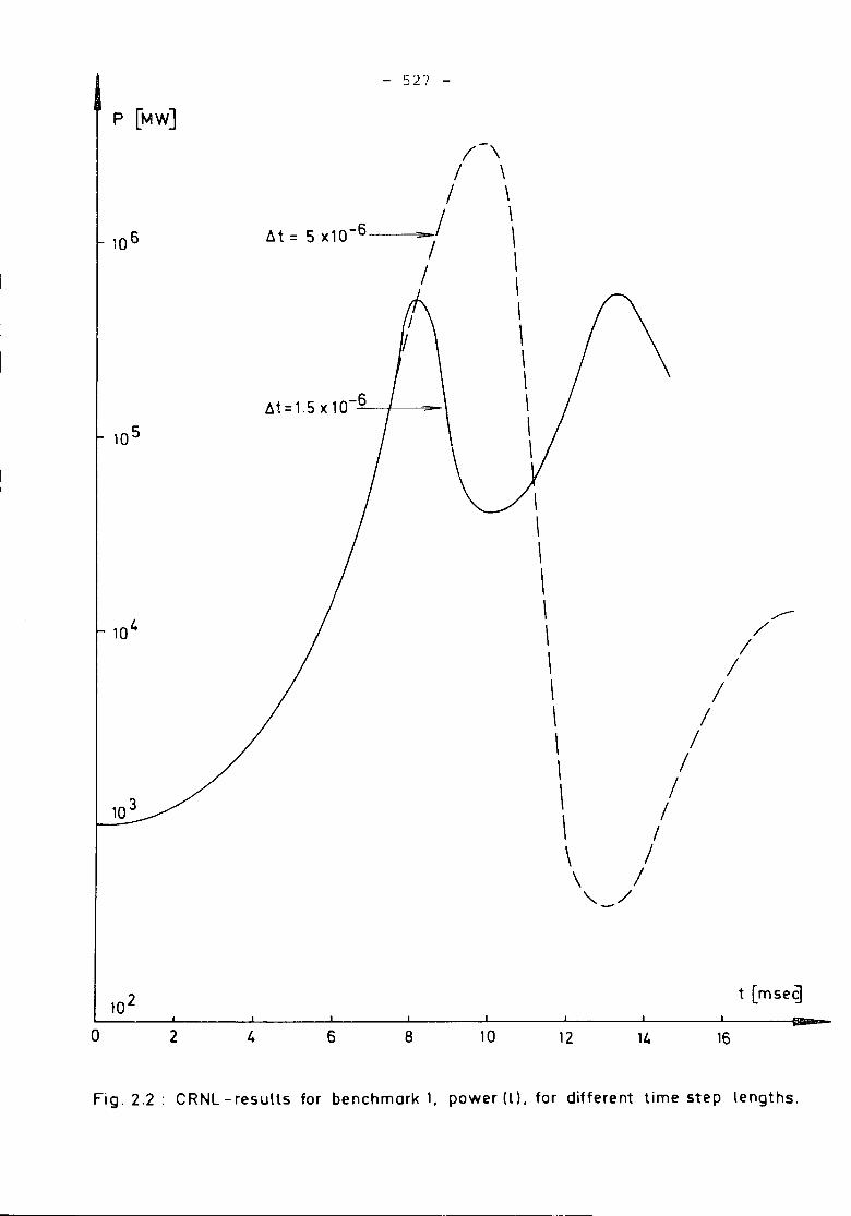
P [MWJ
- 5'27 -
I'/
/Llt = 5 X10⁻⁶----/
//
Llt=1.5 x 10⁻⁶
\\\\\\\\\\\\\\
\\\\\ ----\ /\ II\ /\ /\ /\ /\ /\ /\ /\ /,,_/
t [mseg
o 2 6 8 10 12 14 16
Fig. 2.2 : CRNL-results for benchmark 1, power (t), for different time step lengths.
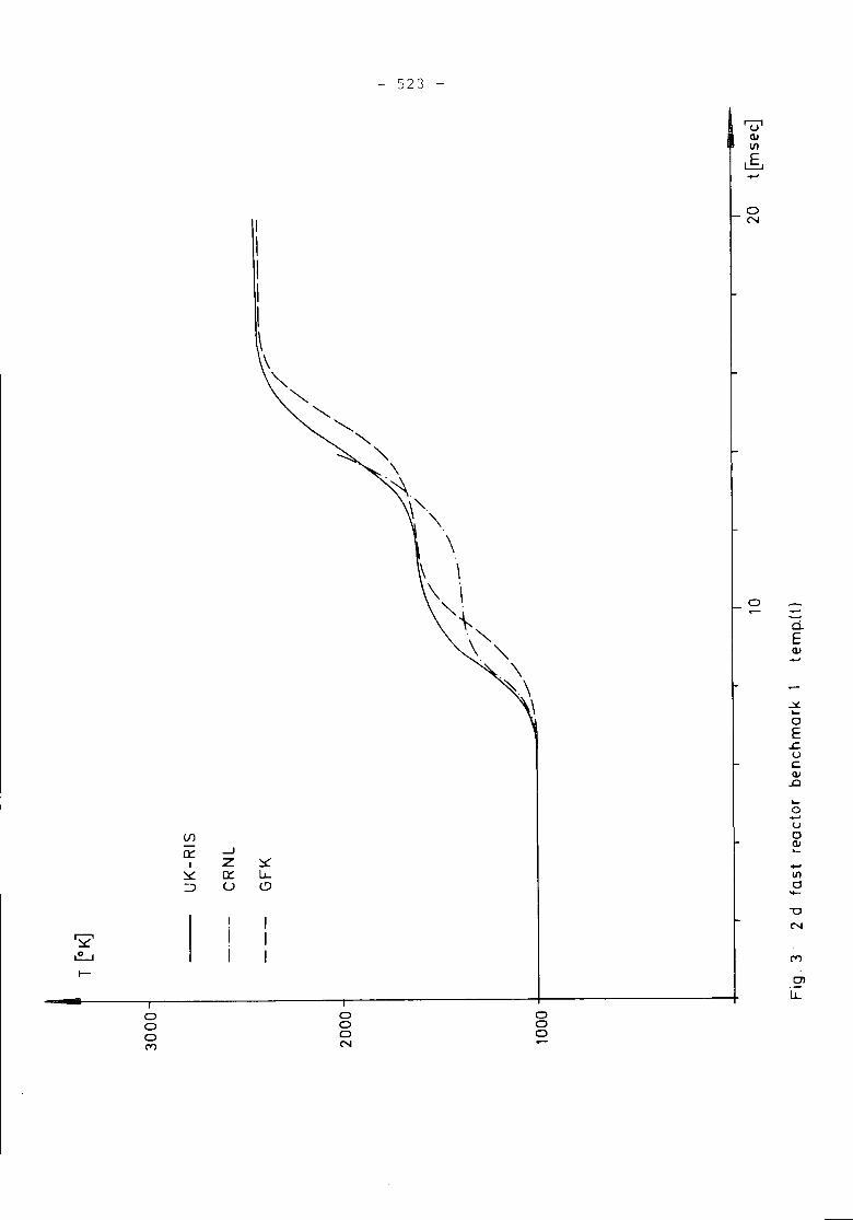
- 523 -
oN
o
d.EQ)
.::£....oE.cucQ)
.D
....o......uoQ)....+"C/lo.......
enlL..
ooo("I')
oooN
ooo
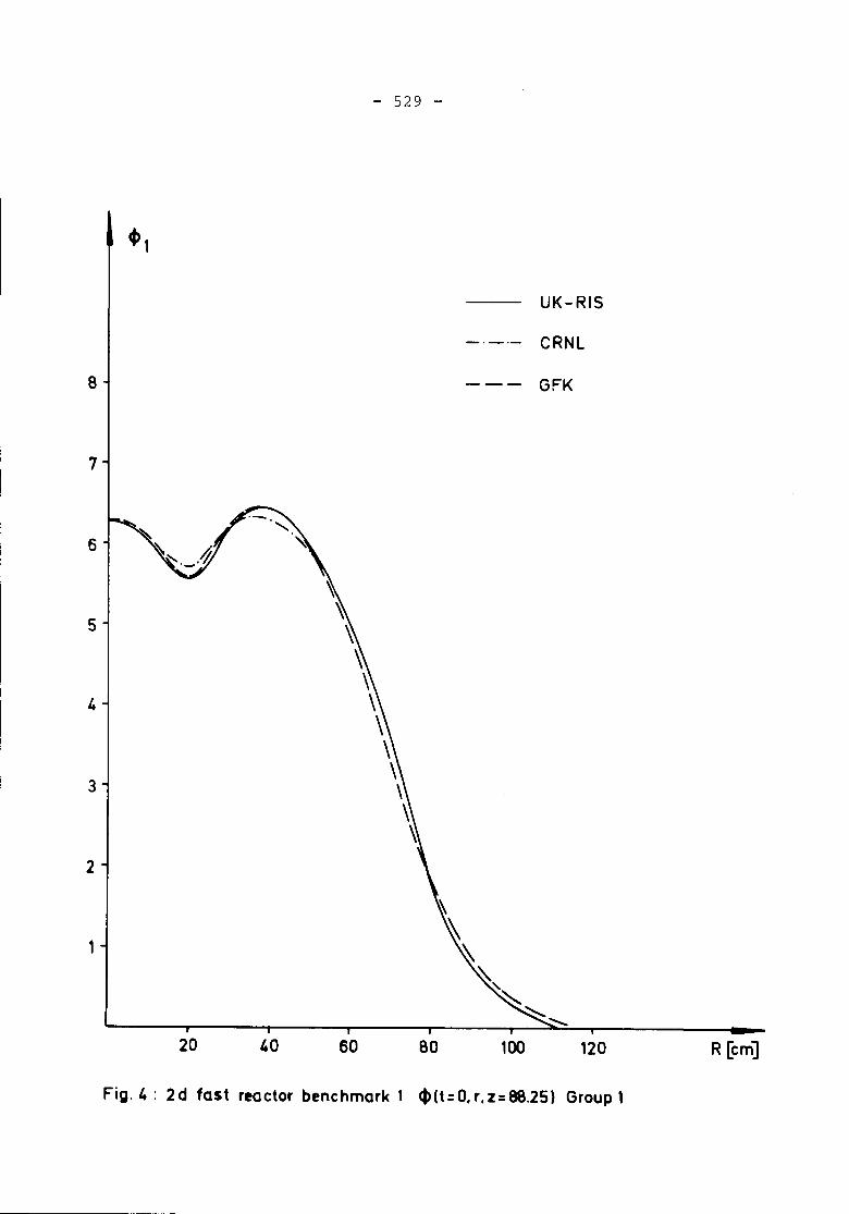
8
7
6
- 529 -
~1
UK-RIS
-'-'- CRNl
--- GFK
5
4
3
2
20 40 R [em]
Fig.4: 2d fast reactor benchmark 1 <I>(t=O,r,z=88.25) Group 1
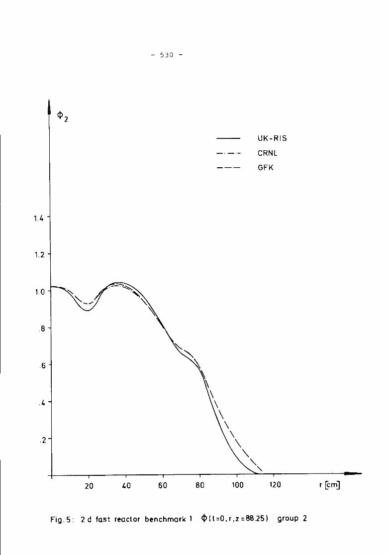
1.4
1.2
1.0
.8
.6
.4
.2
- 530 -
<1>2
UK-RIS
CRNL
GFK
20 40 60 80 100 120 r [em]
Fig. 5: 2 d fast reactor benchmark 1 <p (t =0. r, Z = 88.25) group 2
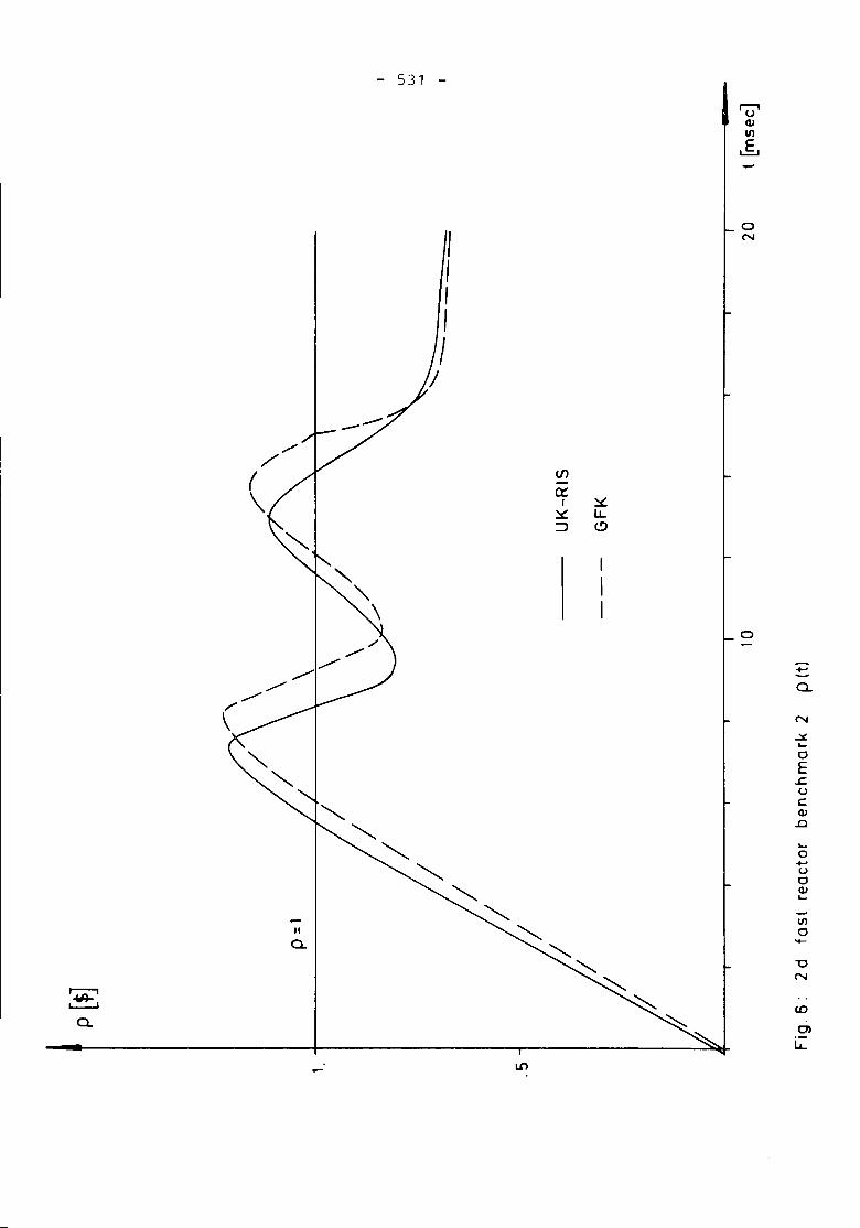
- 531 -
oN
0
...0-
N
.:x...0E
.J::.0CQI
.Q
...0...00QI....-III0
'+-
"UN
CD
01L;:
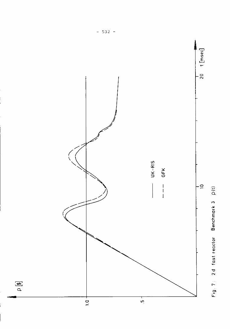
- 532 -
oN
(/')
0::~I
~ ~:::> C)
0I --IQ.I('I")
~0E~uC<1J
1Il
~0--u0<1J~-VI0-
"t:JN
c---
01
LL
i~iL..=..:..J
Q.
LJ')0
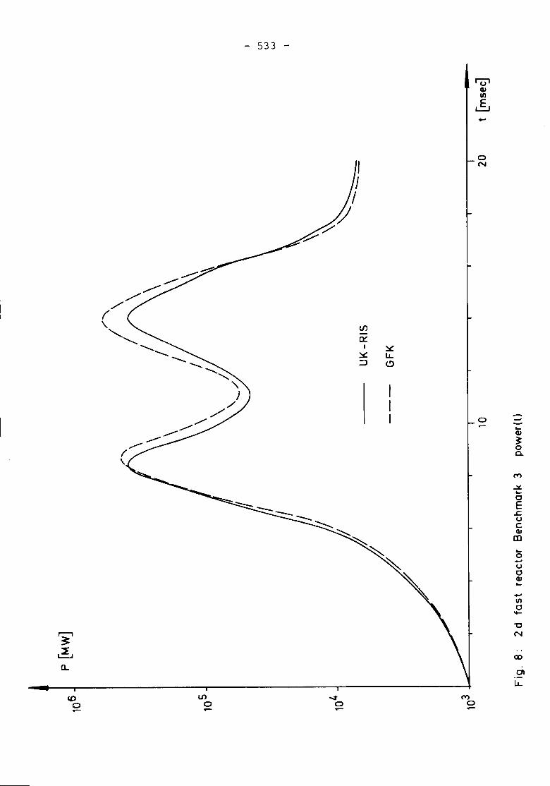
CDo- U')
o
- 533 -
-oN
0 --~QI~0a.
(Y)
.::£~0E
L:.UCQI(II
~0-u0QI~-IIICl-"0N
ex>
atu...
(Y)0-
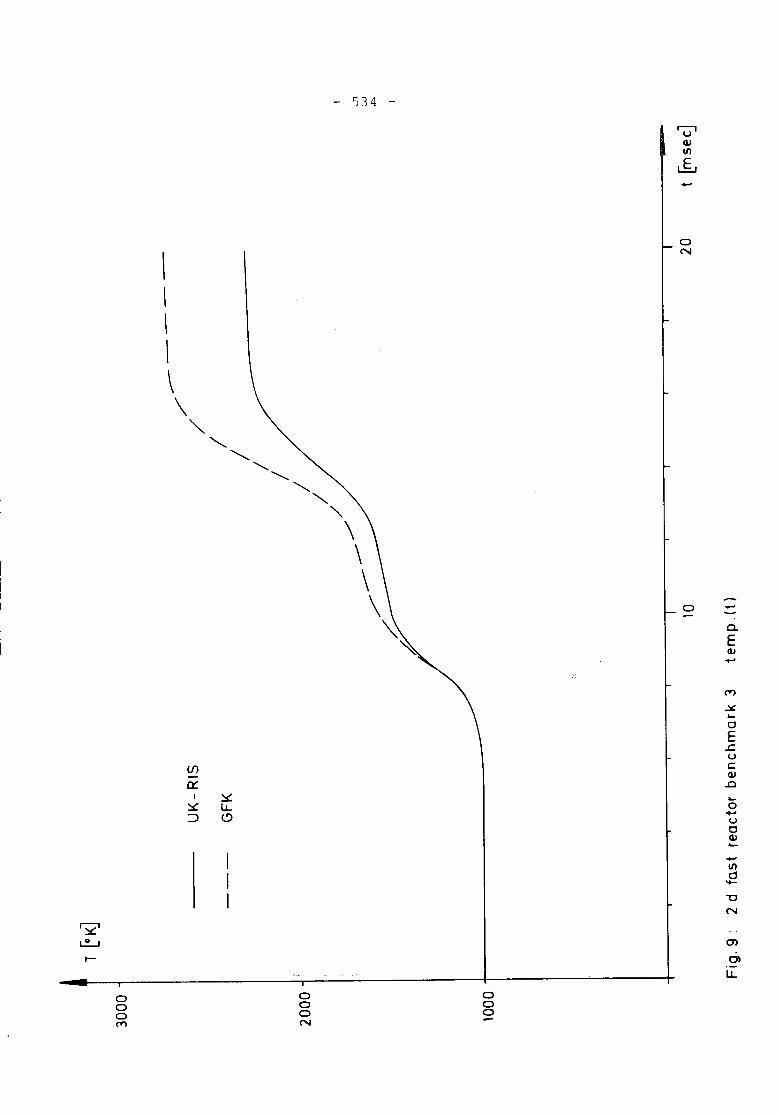
- 534 -
0 -a.Ecv+-'
rt')
.::s:~0E.cuccv.0~0-u0cv~
+-'IIId--CN
a>01
LL
oN
\
\
\
I\\'""-
.......................
............."-"-"-\
\\\
~~
ooort')
oooN
obo
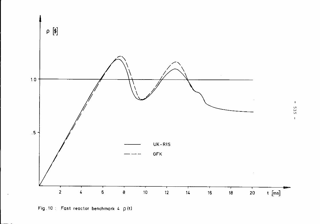
1.0
p [$J
U1WU1
.5
UK- RIS
--- GFK
2 4 6 8 10 12 14 16 18 20 t ems]
Fig. 10: Fast reactor benchmark 4 p (t)
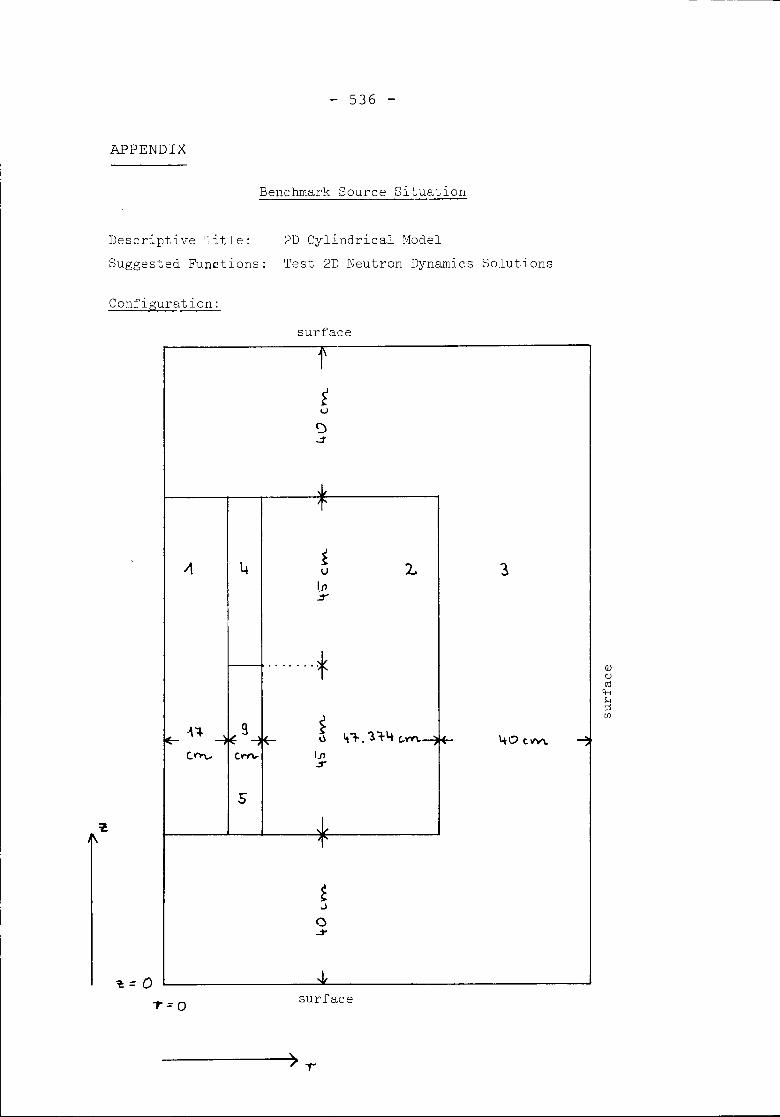
- 536 -
APPENDIX
Benchmark Source Situation
Descriptive Title: 2D Cylindrical ModelSuggested Functions: Test 2D Neutron Dynamics Solutions
Configuration:
surface
2.
....... +
5
~:::O
40 t.VV\.
""=0surface
>..,..
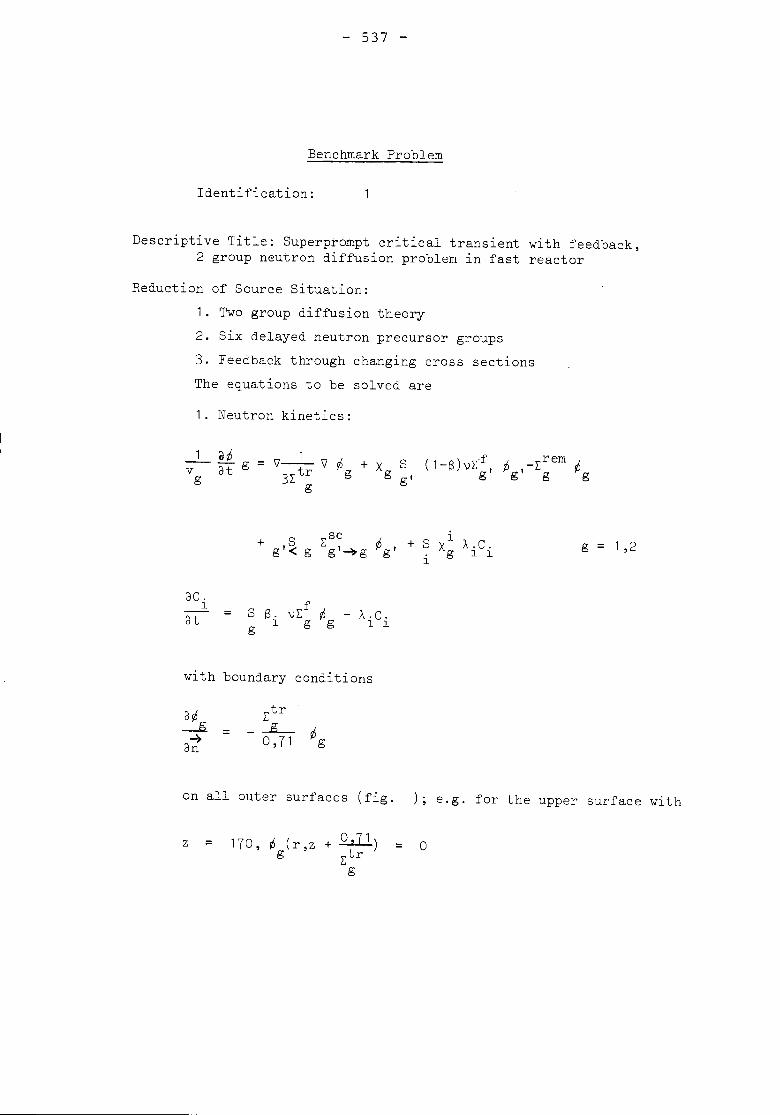
- 537 -
Benchmark Problem
Identification:
Descriptive Title: Superprompt critical transient with feedback,2 group neutron diffusion problem in fast reactor
Reduction of Source Situation:1. Two group diffusion theory2. Six delayed neutron precursor groups3. Feedback through changing cross sectionsThe equations to be solved are
1. Neutron kinetics:
1/_1_ 1/ ~g + X S (l-S) vl;f', ~ _L:rem ~3L:tr g g' g g' g g
g
ac.lat =
S ~sc ~ l+ It..., 'fJ I + S Xg A. C .g < g g ~g g ill
S S. vL:f
~ - A.C.l g g l lg
g = 1,2
with boundary conditions
=
on all outer surfaces (fig. ); e.g. for the upper surface with
z = 170, ~ (r,z +~) = 0g L: tr
g
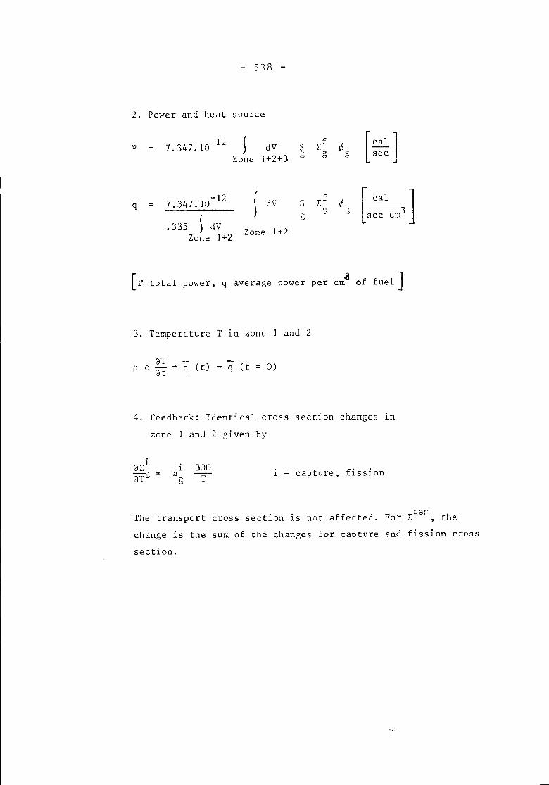
- 538 -
2. Pm.rer and heat source
P 7. 347. 10-12 ) dV S L:f ~ [~]g 0' g secZone 1+2+3 "
7. 347. 10-12~
dV S L:f ~ [ cal ]q0' 0' sec cm3(.:- u '"
~u
.335 dV Zone 1+2Zone 1+2
[p total power, q average power per cm.g of fuel]
3. Temperature T ln zone 1 and 2
aTP c at q (t) - q (t 0)
4. Feedback: Identical cross section changes lnzone 1 anJ 2 given by
l 300a Tg
l capture, fission
The transport cross section lS not affected. For L:rem, the
change is the sum of the changes for capture and fission crosssection.
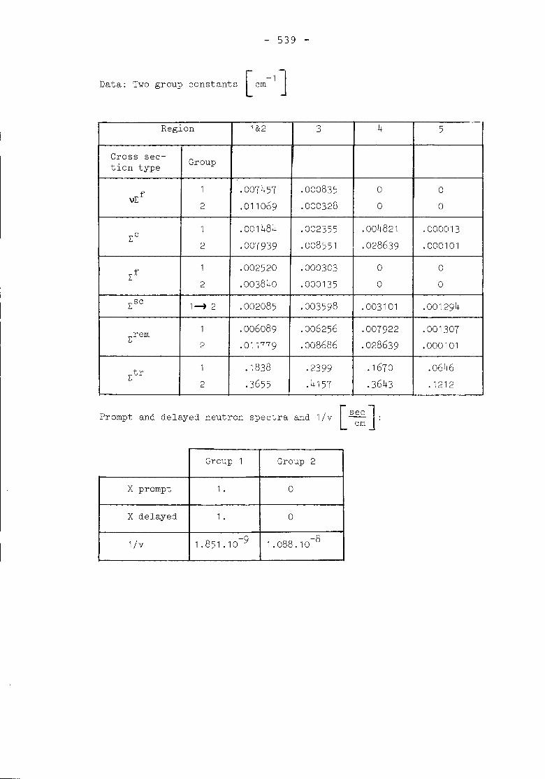
- 539 -
Data: Two group constants [cm-1JRegion 1&2 3 4 5
Cross sec- Grouption type
VL:f1 .007457 .000835 0 02 .011069 .000328 0 0
1 .001484 .002355 .004821 .000013L:c .008551 .0286392 .007939 .000101
L:f1 .002520 .000303 0 02 .003840 .000135 0 0
L:sc 1~ 2 .002085 .003598 .003101 .001294
1 .006089 .006256 .007922 .001307L:rem
2 .011779 .008686 .028639 .000101
L:tr 1 .1838 .2399 .1670 .06462 .3655 .4157 .3643 .1212
[ sec ]Prompt and delayed neutron spectra and l/v cm:
Group 1 Group 2
X prompt 1. 0
X delayed 1. 0
l/v -9 -81.851.10 1.088.10
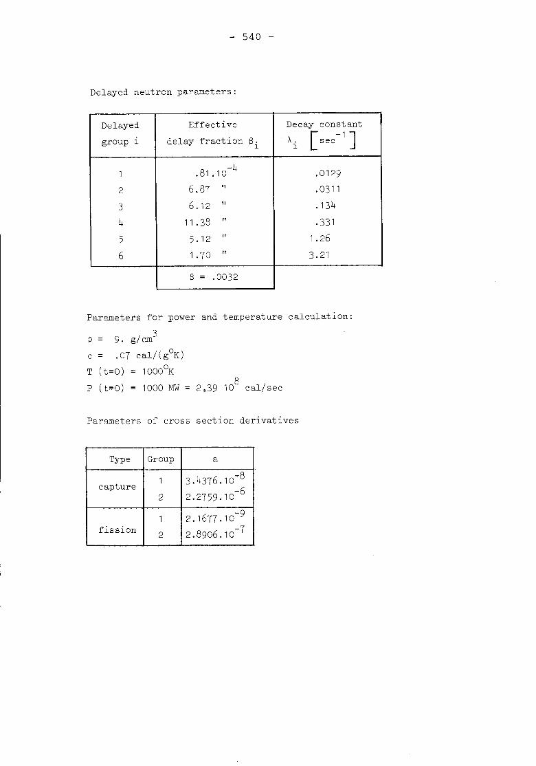
- 540 -
Delayed neutron parameters:
Delayed Effective Decay constantgroup l delay fraction B. A. [sec-1]
l l
-41 .81 .10 .01292 6.87 " .03113 6.12 " .1344 11 .38 " .3315 5.12 " 1.266 1.70 " 3.21
B = .0032
Parameters for power and temperature calculation:
p = 9. g/cm3
c = .07 cal/(gOK)T (t=o) = 10000KP (t=O) = 1000 MW = 82,39 10 cal/sec
Parameters of cross section derivatives
Type Group a
1 6 -8capture 3.437 .10
-62 2.2759.10-91 2.1677.10
fission -72 2.8906.10
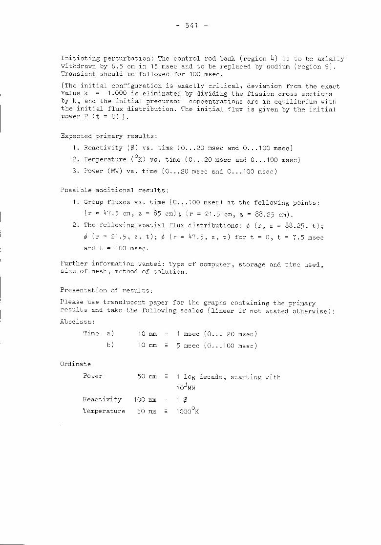
- 541 -
Initiating perturbation: The control rod bank (region 4) is to be axiallywithdrawn by 6.5 cm in 15 msec and to be replaced by sodium (region 5).Transient should be followed for 100 msec.(The initial configuration is exactly critical, deviation from the exactvalue k = 1.000 is eliminated by dividing the fission cross sectionsby h, and the initial prec~rsor concentrations are in equilibrium withthe initial flux distribution. The initial flux is given by the initialpower P (t = 0) ).
Expected prlmary results:1. Reactivity ($) vs. time (0 20 msec and O 100 msec)2. Temperature (oK) vs. time (0 20 msec and 0 100 msec)3. Power (MW) vs. time (0 ...20 msec and 0 ...100 msec)
Possible additional results:1. Group fluxes vs. time (0 ...100 msec) at the following points:
(r = 47.5 cm, z = 85 cm); (r = 21.5 cm, Z = 88.25 cm).2. The following spatial flux distributions: p (r, z = 88.25, t);
p (r = 21.5, z, t); p (r = 47.5, z, t) for t = 0, t = 7.5 msecand t = 100 msec.
Further information wanted: Type of computer, storage and time used,size of mesh, method of solution.
Presentation of results:Please use translucent paper for the graphs containing the primaryresults and take the following scales (linear if not stated otherwise):Abscissa:
Time a)b)
OrdinatePower
ReactivityTemperature
10 mID
10 mID
50 mID
100 mID
50 rnm
msec (0 20 msec)5 msec (0 100 msec)
1 log decade, starting with103M\-T
1 $
10000K
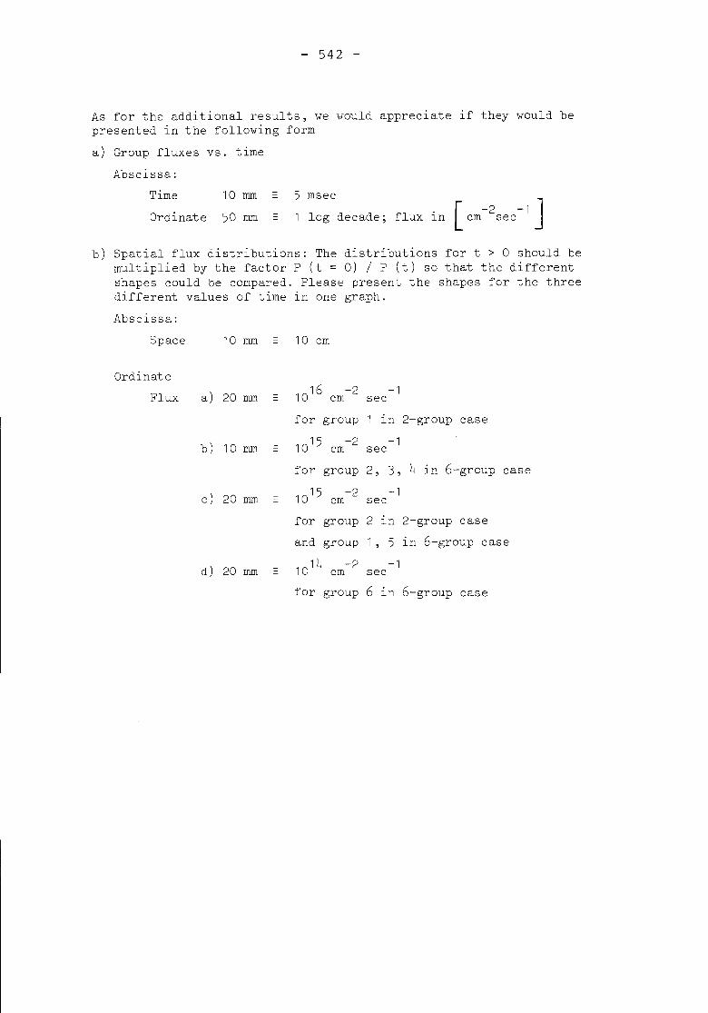
- 542 -
As for the additional results, we would appreciate if they would bepresented in the following forma) Group fluxes vs. time
Abscissa:TimeOrdinate
10 mID
50 mID
5 mseclog decade; flux In [
-2 -1 Jem see
b) Spatial flux distributions: The distributions for t > 0 should bemultiplied by the factor P (t = 0) / P (t) so that the differentshapes could be compared. Please present the shapes for the threedifferent values of time in one graph.Abscissa:
Space 10 mID 10 em
OrdinateFlux a) 20 mID 1016 -2 -1
- em seefor group 1 in 2-group case
b) 10 mID 1015 -2 -1- em see
for group 2, 3, 4 In 6-group case
c) 20 mm 1015 -2 -1- em see
for group 2 In 2-group caseand group 1, 5 In 6-group case
d) 20 mm 1014 -2 -1- em see
for group 6 In 6-group case
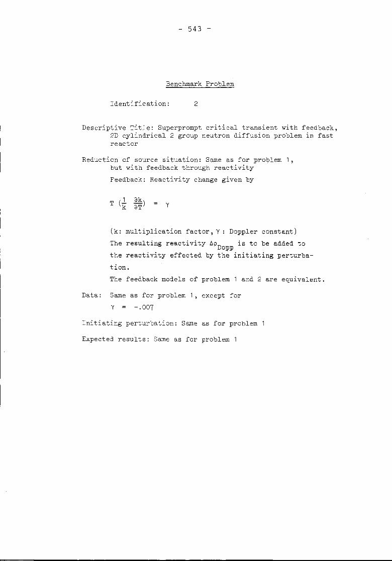
- 543 -
Benchmark Problem
Identification: 2
Descriptive Title: Superprompt critical transient with feedback,2D cylindrical 2 group neutron diffusion problem in fastreactor
Reduction of source situation: Same as for problem 1,but with feedback through reactivityFeedback: Reactivity change given by
= y
(k: multiplication factor, Y: Doppler constant)The resulting reactivity 6PD is to be added to
oppthe reactivity effected by the initiating perturba-tion.The feedback models of problem 1 and 2 are equivalent.
Data: Same as for problem 1, except forY = -.007
Initiating perturbation: Same as for problem
Expected results: Same as for problem 1
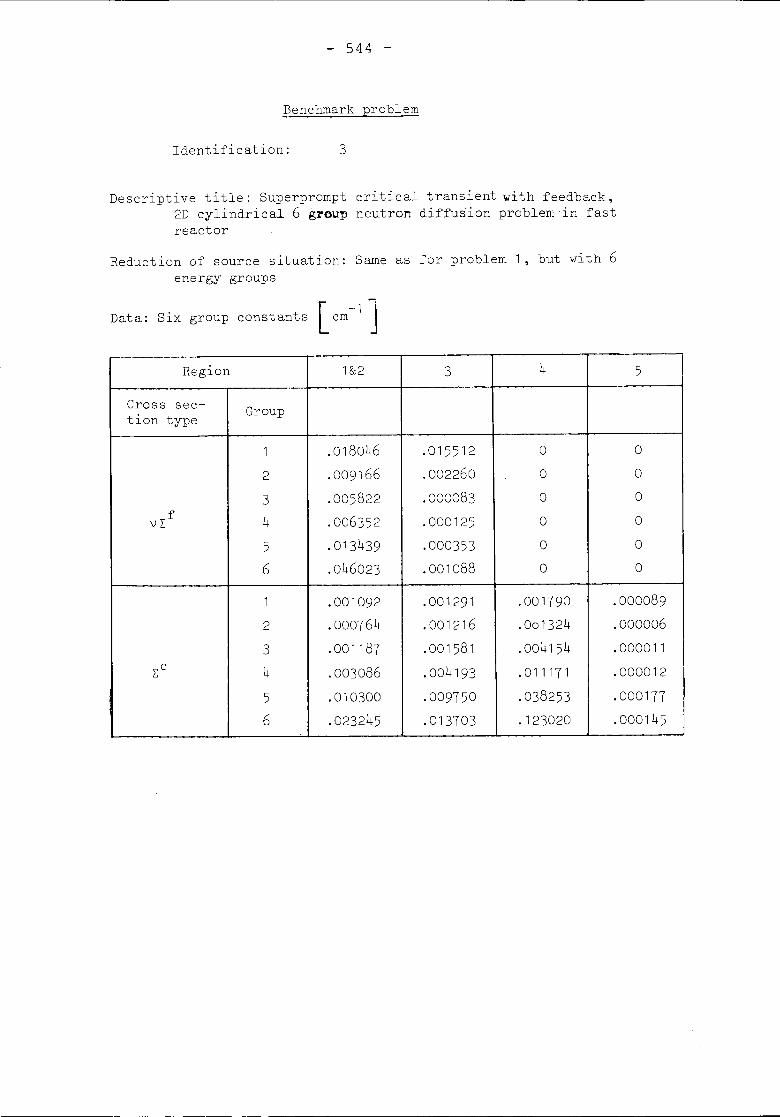
- 544 -
Benchmark problem
Identification: 3
Descriptive title: Superprompt critical transient with feedback,2D cylindrical 6 group neutron diffusion problem in fastreactor
Reduction of source situation: Same as for problem 1, but with 6energy groups
Data: Six group constants [cm -1 JRegion 1&2 3 4 5
Cross sec- Grouption type
1 .018046 .015512 0 02 .009166 .002260 0 03 .005822 .000083 0 0
VL:f 4 .006352 .000125 0 0
5 .013439 .000353 0 06 .046023 .001088 0 0
1 .001092 .001291 .001790 .0000892 .000764 .001216 .001324 .0000063 .001187 .001581 .004154 .000011
L:c 4 .003086 .004193 .011171 .0000125 .010300 .009750 .038253 .0001776 .023245 .013703 .123020 .000145 !
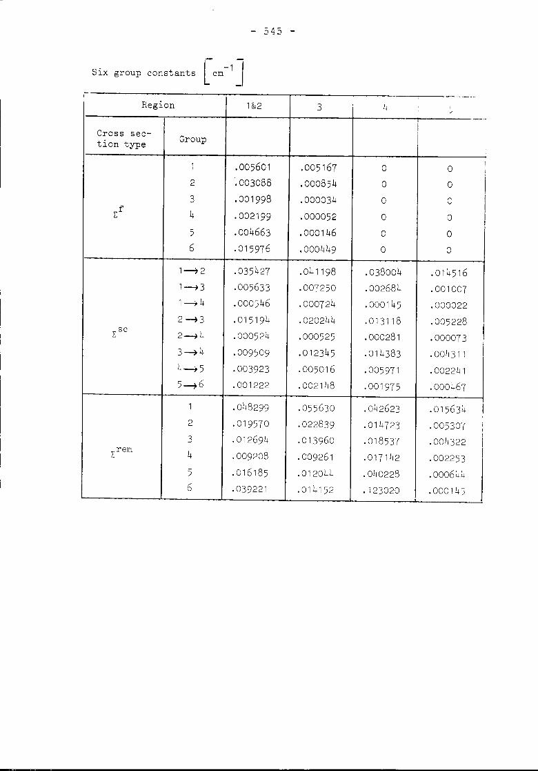
l-cm-1_1Six group constants
- 545 -
I- "-_ ...
Region 1&2 3 )1 ,/
I -_.-ICross sec- Group ition type ,
.005601 ,005167 0 0 I1
i2 ,003088 .000854 0 03 .001998 .000034 0 0
~f 4 .002199 .000052 0 05 .004663 ,000146 0 06 .015976 ,000449 0 0
1..-, 2 .035427 .041198 .038004 .0145161~3 ,005633 .007250 .002684 ,0010071~4 .000546 .000724 .000145 ,0000222~3 .015194 .020244 .013118 .005228
IL: sc 2~4 ,000524 .000525 .000281 .0000733 ---? 4 .009509 .012345 .014383 ,0043114-15 .003923 .005016 .005971 ,0022415~6 .001222 ,002148 ,001975 .000467
1 .048299 ,055630 ,042623 .0156342 .019570 .022839 .014723 .0053073 .012694 .013960 .018537 .004322
L:rem 4 ,009208 ,009261 .017142 .002253
5 .016185 .012044 ,040228 .0006446 ,039221 ,014152 .123020 .000145
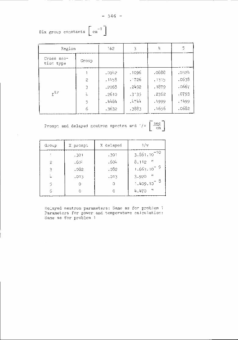
- 546 -
[ cm-1 J-Six group constants
Region 1&2 3 4 5
Cross sec- Grouption type
1 .0942 .1096 .0888 .03242 .1458 .1126 .1315 .06383 .2068 .2492 .1819 .0661
z:tr 4 .2610 .3135 .2362 .0193
I5 .4484 .4144 .4999 .1)-\996 .3632 .3883 .4656 .0682
- ]secPrompt and delayed neutron spectra and 1Iv l cm
Group X prompt X delayed 11v
1 .301 .301 3.861.10-10
2 .604 .604 8. 112 "3 .082 .082 1.663.10 - 9
4 .013 .013 3.920 "5 0 0 1.409.10 - 86 0 0 4.470 "
Delayed neutron parameters: Same as for problem 1Parameters for power and temperature calculation:Same as for problem 1
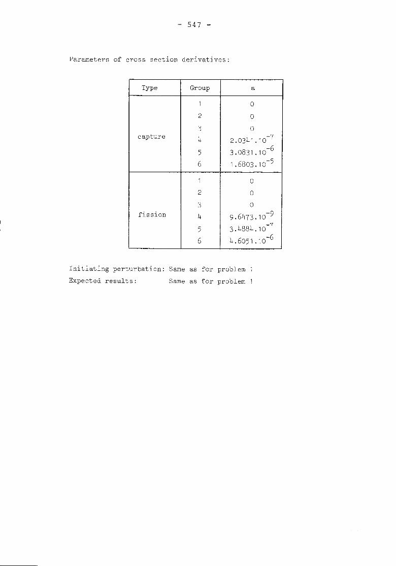
- 547 -
Parameters of cross section derivatives:
Type Group a
1 0
2 0'~ 0-'
capture 4 -12.0341.10-6
5 3.0831.10
6 -51.6803.10
1 0
2 0
3 0fission 4 -99.6413.10
-15 3.4884.10
6 -64.6051.10
Initiating perturbation: Same as for problemExpected results: Same as for problem
- 548 -
Benchmark Problem
Identification: 4
Descriptive Title: Superprompt critical transient with feedback,2D cylindrical 6 group neutron diffusion problem infast reactor
Reduction of source situation: Same as for problem 2, but with6 energy groups. The feedback models of problem 3 and4 are nearly equivalent.
Data: Same as for problem 3, except fory = -.001
Initiating perturbation: Same as for problem
Expected results: Same as for problem 1

- 549 -
DISCUSSION
A. Siebertz
1) Could some discrepancies between the results given bycodes using QS or IQS method be explained with the dif-ference in reactivity history?
2) Could the difference, if any, in reactivity history beexplained by the differences in the way of calculatingthe reactivity (use of a unique weighting adjoint func-tion calculated once at initial time or use at each timestep of a recalculated time independent asymptotic ad-joint weighting function)?
D.A. Meneley
1) Yes. They could be resolved by reduction of time stepsif the different methods are internally consistent.
2) The differences in "reactivity" values can be explainedin this way, differences in total power cannot.
A.F. Henry
The use of what is in effect a time dependent weight func-tion requires that changes in the conventional point kine-tics equations (extra terms) be made.
G. Forti
The weighting by the right adjoint fluxes seems to me animportant point in the reactivity history determinationand, to be more precise, the lifetimes parameters are of
- 550 -
the same importance - the transient evaluation may be ef-fected remarkably by these factors, and Galati's approachto the problem has many advantages from this point of view.
J.J. Dorning
I believe that Prof. Henry was refering to the problem ofthe additional term which arises in the point kineticsequations when a time-dependent adjoint function (or anytime-dependent weight function) is used. In the case athand, you effectively have piecewise constant adjointweighting functions which when inserted into the time de-rivative of the inner product of the adjoint function andthe shape function will lead to delta-function terms attime corresponding to the time points at which the adjointfunctions are changed (recalculated). I think it is thequestion of whether these terms were accounted for in yourcalculation which Prof. Henry was raising rather than therecalculations of lifetimes, reactivity, etc.
COMMENTS
J.K. Fletcher
Although the agreement between SPARK and KINTIC is satis-factory on the 2D FR benchmark calculations it is not asgood as one would expect. Therefore over the next few weeksthe benchmark problems will be further investigated and anysignificant results will be communicated to Dr. Vath.

... 551 ...
As a general comment on the meeting; the impression is thatthe quasi-static method will continue, over the next fewyears at least to be as good a way of solving neutron kine-tics problems as any other.


LIST OF PARTICIPANTS
- 553 -

AUSTRIA
- 555 -
F. Putz Osterreichische Studiengesellschaft fUrAtomenergie, Wien
BELGIUM
J.E.A.
DevooghtHundSiebertz
Universite libre de BruxellesUniversite libre de BruxellesCentre d'Etudes de l'Energie, Mol
CANADA
A.R. Dastur
M.G. DuboisA.A. HarmsF.N. McDonnellD.A. Meneley
DENMARK
P.S. Christensen
EEC
Atomic Energy of Canada Limited,MississaugaUniversite de MontrealMcMaster University, Hamilton, ant.Atomic Energy of Canada, Chalk River, ant.Ontario Hydro, Toronto
Danish Atomic Energy Commission, Roskilde
G.E.
FortiVincenti
Euratom, IspraEuratom, Ispra
FINLAND
M.K. Rajamaeki Technical Research Center of Finland,Otaniemi

- 556 -
FRANCE
P. Reuss CEN, Saclay
F.R. GERMANY
R. Bieselt
H. FinnemannE. InfuehrH. KustersS. LangenbuchJ. LanghansJ. LockauS. RehkerD. StruweL. Viith
M.R. WagnerW. Werner
NETHERLANDS
T.D. Oei
NORWAY
Babcock-Brown Boveri Reaktor GmbH,MannheimKraftwerk Union, ErlangenHochtemperatur-Reaktorbau, MannheimGfK, KarlsruheLRA, GarchingIRS, KolnKraftwerk Union, FrankfurtInstitut fur Plasmaphysik, GarchingGfK, KarlsruheGfK, KarlsruheKraftwerk Union, ErlangenLRA, Garching
Reactor Centrum Nederland, Pet ten
K. Haugset Institutt for Atomenergi, Kjeller
SWEDEN
E.O. Norinder AB Atomenergi, Studsvik, Nykoping

TURKEY
- 557 -
U. Adalioglu Cekmece Nuclear Research Centre
UNITED KINDGOM
D.E. BillingtonM.J. BrigdeF.J. FayersJ.K. FletcherR.N. McMillanM. PerksG. Hilliams
UNITED STATES
J.J. DorningA.F. Henry
NEA
N. De BoerJ. Royen
UKAEA, RisleyCEGB, BerkeleyUKAEA, WinfrithUKAEA, RisleyUKAEA SRD, Culcheth, WarringtonUKAEA, RisleyNIl Safety & Health Commission, London
University of Illinois, UrbanaMIT, Cambridge
NEA, ParisNEA, Paris
- I -
VERTEILERLISTE
Ministerien, Technische Uberwachungsvereine
Arbeitsministerium des Landes Baden-Wurttemberg, Stuttgart,Dipl.-Ing. Gunther
Arbeits- und Sozialministerium des Landes Nordrhein-West-falen, Dusseldorf
Bayerisches Staatsministerium fur Landesentwicklung und Um-weltfragen, Munchen, Ministerialdirigent Wochinger
Bayerisches Staatsministerium fur Landesentwicklung und Um-weltfragen, Munchen, Ministerialrat R. Mauker
Bundesministerium fur Forschung und Technologie, Bonn,Dipl.-Ing. H. Seipel
Bundesministerium des Innern, Bonn, Dr. Berg
Hessisches Ministerium fur Wirtschaft und Technik, Wiesba-den, Ministerialrat H. Wagner
Ministerium fur Arbeit, Soziales und Vertriebene des LandesSchleswig-Holstein, Kiel
Niedersachsisches Sozialministerium, Hannover
Institut fur Reaktorsicherheit der Technischen Uberwachungs-vereine e.V., Kaln
Rhein.-Westfalischer Technischer Uberwachungs-Verein e.V.Essen
Technischer Uberwachungs-Verein Baden e.V., MannheimDr. Fendler
Technischer Uberwachungs-Verein Bayern e.V., Munchen
Technischer Uberwachungs-Verein Berlin e.V., Berlin
- II -
Technischer Uberwachungs-Verein Hannover e.V., Hannover
Technischer Uberwachungs-Verein Hessen e.V., Eschborn
Technischer Uberwachungs-Verein Norddeutschland e.V.,HamburgTechnischer Uberwachungs-Verein Pfalz e.V., Kaiserslautern
Technischer Uberwachungs-Verein Rheinland e.V., Kaln
Technischer Uberwachungs-Verein Saarland e.V., Saarbrucken
Technischer Uberwachungs-Verein Stuttgart e.V., Stuttgart
Vereinigung der Technischen Uberwachungsvereine e.V., Essen
Wirtschaftsministerium des Landes Baden-WUrttemberg, Stutt-gart
Deutsche Firmen, Institute, Kernkraftwerke, Bibliotheken
Allianz AG, MUnchen, Dipl.-Ing. J. Feldmann
Atombibliothek der Technischen Universit~t MUnchen
Battelle Institut, Frankfurt, B. RUdiger
Bayernwerk AG, MUnchen, Dr. Knoerzer
BBR GmbH, Mannheim, Dr. Loth
BBR GmbH, Mannheim, Dr. A. Schatz
Dr. Brosche, Bayernwerke AG, MUnchen
Dr. F. Fischer, Gesellschaft f. Kernforschung, ProjektNukleare Sicherheit, Karlsruhe
Hartmann & Braun AG, MUnchen
Hochtemperatur-Reaktorbau GmbH, Mannheim, G. Mieze
Gesellschaft fUr Kernforschung, Institut fUr Neutronenphysikund Reaktortechnik, Karlsruhe, Prof. Dr. K. Wirtz
- III -
Gesellschaft fur Kernforschung, Literaturabteilung, Karlsruhe
Gesellschaft fur Kernforschung, Karlsruhe, Dr. Schikarski
Gesellschaft fur Kernforschung, Versuchsanlagen, Leopoldshafen
Gesellschaft fur Kernenergieverwertung in Schiffbau und Schiff-fahrt mbH, Institut fur Reaktorphysik, Geesthacht-Tesperhude
GutehoffnungshUtte Sterkrade AG, Oberhausen
Hahn-Meitner-Institut fUr Kernforschung, Berlin, Bibliothek
Handelsblatt GmbH, Atomwirtschaft, DUsseldorf, W.D. MUller
Institut fur Kerntechnik der TU Berlin, Prof. Dr.-Ing. Memmert
Institut fUr Kerntechnik der TU Hannover, Prof. Dr.-Ing.D. Stegemann
Institut fur Nukleare Sicherheitsforschung, Julich
Institut fur Reaktortechnik der TH Darmstadt, Prof. Dr. Humbach
Interatom, Bensberg, Dr. Harde und Abt. Systemanalyse
Prof. Dr.-lng. T. Jaeger, Bundesanstalt fUr Materialprufung,Berlin
Kernkraftwerk Lingen GmbH, Darme
Kernkraftwerk Niederaichbach GmbH, MUnchen
Kernkraftwerk Obrigheim, Direktor Dr. H. Schenk
Kernkraftwerk RWE-Bayernwerk GmbH, Gundremmingen, DirektorDr. A. ~"1eckesser
Dipl.-Phys. Korber, Institut fUr Kernenergetik, Stuttgart-Vaihingen
KWU, Abt. RZR, Erlangen, Dr. W. Braun
Kw~, Abt. Reaktorentwicklung, Erlangen, v. Haebler
KWU, Abt. R1, Erlangen, Dr. Markl
KWU, Abt. R11, Erlangen, F. Winkler

- IV -
KWU, Offenbach, Dir. Dr. Kornbichler
KWU, Abt. E3 R3, Offenbach, Dr. SchruferK~m, Abt. E3 R3, Offenbach, Dipl.-Ing. Voigt
K~m, GroBwelzheim, Prof. Dr. A. Kirchenmeyer
KWU, Abt. V 697, Offenbach, H ..Repke
Prof. Dr.-Ing. F. Mayinger, Institut fur Verfahrenstechnikder TU Hannover
Norddeutsche Kraftwerke AG, Hamburg
NUKEM GmbH, Hanau
Physikalisch-Technische Bundesanstalt, Braunschweig,H. Blechschmidt
Preussische Elektrizitats AG, Hannover
RWE, Biblis, Dr. Eisermann
RWE, Essen, Abt. KW
Prof. Dr.-Ing. W. Schutze, Institut fur Kernphysik derUniversitat Frankfurt
Prof. Dr. J. Schwibach, Bundesgesundheitsamt, Abt. furStrahlenhygiene, Neuherberg
Prof. Dr. D. Smidt, Institut fur Reaktorentwicklung, Ge-sellschaft fur Kernforschung, Karlsruhe
Universitatsbibliothek der TU Berlin
Universitatsbibliothek und TIB, Hannover
Vereinigte Elektrizitats-Werke AG, Dortmund, Dr. Schwarz
Versuchsatomkraftwerk Kahl GmbH, Kahl
Dir. Prof. Dr. J. Wengler, Farbwerke Hoechst AG, Frankfurt-Hoechst
ZAED, Leopoldshafen, Fr. Alt-Felix

- v -
Zentralbibliothek der Kernforschungsanlage Julich
Dr. K. Zuelke, Gesellschaft fur Kernforschung, Karlsruhe
Auslandische Firmen, Institutionen, Bibliotheken
Aktiebolaget Atomenergi, Studsvik, Nykoping, Sweden
Battelle Northwest, Richland, Washington, R.T. Allemann, USA
Dr. Benedek, Forschungsinstitut fur Elektrische Energie,Budapest, Hungary
Dr. Carangelos, Public Power Corporation (PPC), Athens, Greece
CEA Cadarache, Saint-Paul-lez-Durance, France
CEN Saclay, Gif-sur-Yvette, J. Bourgeois, France
CNEN, E. Iansiti, Roma, Italy
Dr. Chrysochoidis, Greek Atomic Research Center "Democritos",Athens, Greece
Delegationen for Atomenergifragor, Mr. Hedgran, Stockholm,Sweden
ETH-Bibliothek, Zurich, Switzerland
Institut fur Strahlenphysik, T. Eurola, Helsinki, Finland
Institutt for Atomenergi, Library, Mrs. Opheim, Kjeller, Norway
Junta de Energia Nuclear, H. Alonso, Madrid, Spain
KEMA, R.M. van Kuyk, Arnhem, The Netherlands
Kommission der Europaischen Gemeinschaften,
W. Vinck, Bruxelles, Belgium
Laboratory for Nuclear Engineering, Prof. ir. D.G.H. Latzko,Delft University of Technology, Delft, The Netherlands
Dr. K.B. Misra, University of Roorkee, Roorkee, India

- VI -
National Lending, Library for Science and Technology,Miss Douglas, Yorkshire, UK
NEA/OECD, Dipl.-Ing. K.B. Stadie, Paris, France
Osterreichische Studiengesellschaft fur Atomenergie, Wien,Austria
Technical University Helsinki, Mrs. M. Kuula, Otaniemi, Finland
UKAEA, Authority Health & Safety Branch, F.R. Farmer, Risley,Warrington, UK
University of Washington, Prof. Dr. K.L. Garlid, Seattle, USA
U.S. Nuclear Regulatory Commission, Division of ReactorDevelopment, Washington, USA
U.S. Nuclear Regulatory Commission, Office of Nuclear ReactorRegulation, R.S. Boyd and R.L. Tedesco, Washington, USA
U.S. Nuclear Regulatory Commission, Office of InternationalPrograms, Washington, USA
U.S. Nuclear Regulatory Commission, Technical InformationCenter, Oak Ridge, USA
Stand: Marz 1975


