Embed Size (px)
Citation preview

Kestler, Berg, Miller, Steinert, Eaton, Larson, and Haddock
Keeping Springtime Low-Volume Road Damage to a Minimum; A Toolkit of Practical Low-Cost Methods for Road Managers
March 21, 2010Effective Word Count = 6688; (4938 Words, 4 Figures = 1000, 3 Tables = 750)
Maureen A. Kestler – Corresponding AuthorUSDA Forest Service, San Dimas Technology & Development Center
444 E. Bonita Ave.San Dimas, CA 91773
Tel : 603-455-1157, Fax: 909-592-2309 [email protected]
Richard L. Berg FROST Associates6 Floyd Ave.
West Lebanon, NH 03784Tel: 603-298-5698, Fax: 603-298-5698
Heather J. MillerDepartment of Civil Engineering, UMass Dartmouth,
285 Old Westport RoadN. Dartmouth, MA 02747
Tel: 508-999-8481, Fax: [email protected]
Bryan C. SteinertEngineer, Haley & Aldrich, Inc.
75 Washington Avenue Suite 203Portland, Maine 04101-2617
Tel: 207-482-4607, Fax: [email protected]
Robert EatonNHDOT District 2
8 Eastman Hill RoadEnfield, NH 03748
Tel: 603-448-2654, Fax: 603-448-2059 [email protected]
Gregg LarsonApplied Research Associates
505 W. UniversityChampaign, IL 61820
Tel: 217-356-4500, Fax: [email protected]
John HaddockSchool of Civil Engineering
Civil Engineering Building, Room G229550 Stadium Mall Dr.
West Lafayette, IN 47907-2051Tel: 765-494-0697, Fax: 765-496-1364
Kestler, Berg, Miller, Steinert, Eaton, Larson, and Haddock
ABSTRACTThere are approximately three million miles of low-volume roads in the United States (1), and approximately half of them are located in seasonal frost areas. Limiting or prohibiting loads during spring thaw can keep damage to a minimum. However methods of determining when to place and remove spring load restrictions, particularly on low-volume roads, are often highly subjective, and that is if restrictions are imposed at all.
In partnership with several other agencies, the USDA Forest Service has been compiling a toolkit of practical low-cost diagnostic techniques for determining conditions under which spring load restrictions should be placed and removed. This paper both expands upon techniques reported upon in a previous Transportation Research Board Low-Volume Roads Conference paper and reports on further developments of additional methods.
Techniques discussed herein include subsurface instrumentation, lightweight deflectometer, thaw index, and a climatic thaw predictor model. Requirements and equipment needed to utilize each of the techniques are described, strengths and weaknesses of each are outlined, and recommendations on various combinations of methods are provided enabling road managers to optimize placement of spring load restrictions.
SCOPEThis paper serves as a sequel to and update of a Transportation Research Board (TRB) Low-Volume Roads Conference paper by several of the same authors (2). It can serve as a practitioner’s guide for using a variety of low-cost techniques to determine when to place spring load restrictions (SLRs), often referred to as road bans, with only limited discussion of analysis and theory. The paper first reviews the thawing phenomenon and loss of road strength. Backcalculation, used as an analysis technique to calculate road stiffness, is also briefly reviewed. The paper then proceeds to outline four diagnostic techniques that have been developed or evaluated as methods of determining when to place and remove SLRs: The first two methods, subsurface instrumentation and lightweight deflectometer (LWD), are covered only briefly, as details and analysis techniques have been previously reported (2); however recommendations on types of instrumentation, equipment, and methods have been added here. The third, a thaw index technique where road surface temperatures are fit to a sine curve, is expanded upon based upon recent field testing. The fourth, a climatic thaw predictor model, based upon a stand-alone version of the Enhanced Integrated Climatic Model (EICM) (the climatic component of the Mechanistic Empirical Pavement Design Guide), is also outlined herein. This thaw predictor model is currently undergoing further development, and is being tested at a few locations. The paper concludes with recommendations on use for each of the four low-cost techniques.
INTRODUCTIONRoads in seasonal frost areas are highly susceptible to damage from trafficking during spring thaw. As freezing occurs from the surface downward, moisture is drawn toward the freezing front, and ice lenses are formed. When the ice lenses, which are above still frozen underlying layers, melt, the material is left in an undrained, unconsolidated condition, thus the structure is highly susceptible to damage during springtime trafficking.
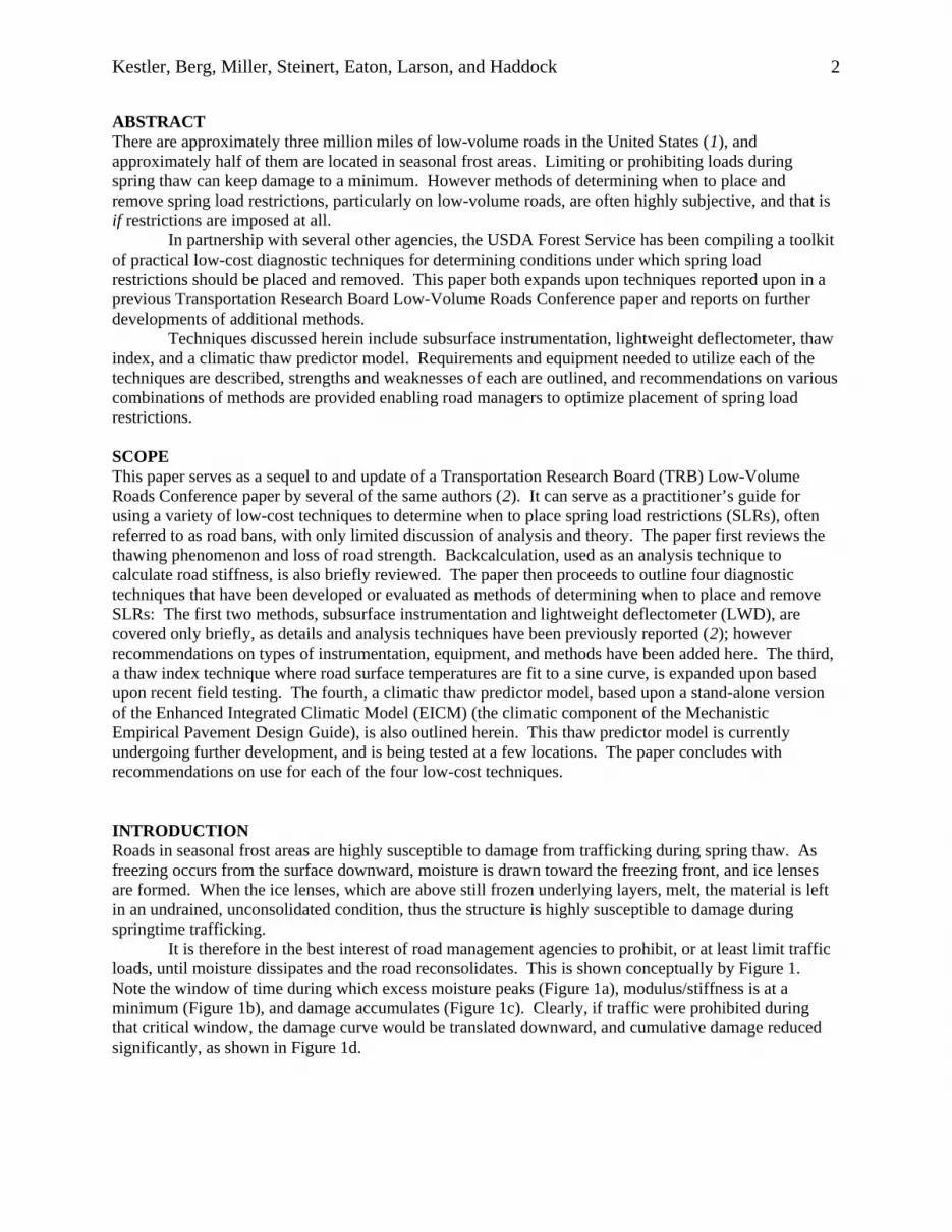
It is therefore in the best interest of road management agencies to prohibit, or at least limit traffic loads, until moisture dissipates and the road reconsolidates. This is shown conceptually by Figure 1. Note the window of time during which excess moisture peaks (Figure 1a), modulus/stiffness is at a minimum (Figure 1b), and damage accumulates (Figure 1c). Clearly, if traffic were prohibited during that critical window, the damage curve would be translated downward, and cumulative damage reduced significantly, as shown in Figure 1d.
2
Kestler, Berg, Miller, Steinert, Eaton, Larson, and Haddock
FIGURE 1 Moisture, modulus, and damage as functions of time during spring thaw and recovery. Note damage with trafficking throughout the spring season = d3, whereas damage on that same date = d3-d2 if a spring load restriction were placed.
It should be noted that, although spring load restrictions do keep road damage to a minimum, the spring load restrictions themselves adversely affect companies whose livelihood depends on trucking. For some construction companies and timber industries, this interruption in hauling lasts for as long as 25% of an entire year. Processing facilities are forced to operate for extended periods from stockpiled inventory, and the resulting economic impact on those facilities, trucks, and others down the line, is significant. Therefore, it is equally important for road management agencies to minimize their period of restricted haul as it is for them to maximize the length restricted hauling to reduce road damage. The
3

Kestler, Berg, Miller, Steinert, Eaton, Larson, and Haddock
diagnostic techniques discussed herein will aid in defining that very highly damage-susceptible condition such that a balance between maximizing local economy and minimizing road damage can be attained.
ANALYSIS TECHNIQUES USED
EverseriesSpring load restrictions should be in place when pavement modulus is low and rate of damage accumulation is high. Thus FWD testing was used to determine baseline metrics to which output from the other techniques could be compared. Pavement layer moduli were backcalculated using Evercalc, a mechanistic-based pavement backcalculation program based on CHEVRON, and part of the Everseries Suite of pavement analysis programs developed for the State of Washington (3) (4). Evercalc uses an iterative approach to match measured and theoretical surface deflections calculated from assumed moduli, and root mean square (RMS) value is minimized. Additionally, stress and strain were computed, and then damage factor, or ratio of the number of loads to reach failure under normal summertime conditions to the number of loads to reach failure under freeze-thaw conditions, was determined by Everpave, also in the Everseries suite.
It should be noted that, in contrast to standard (non-spring thaw) backcalculation, thaw depth progression causes changing layer thicknesses through time for any one section. Consequently: For days on which a road was thawed to some depth in the base, layers would typically comprise:
Asphalt layer (if present) Thawed base Frozen material (frozen base is typically combined with frozen subgrade)
If thaw had progressed to some depth in the subgrade, then layers would typically comprise: Asphalt layer (if present) Base Thawed subgrade Frozen subgradeThawed materials were typically subdivided to account for drainage/recovery differences.Computed damage factors were used for analysis of subsurface sensor techniques, and backcalculated
moduli, computed using Evercalc, were used for comparisons to direct readings of modulus from the LWD.
Everseries output was also used, but to a lesser degree, for the remaining two SLR techniques -- thaw index, and EICM thaw predictor.
Enhanced Integrated Climatic Model (EICM)The EICM was used as the primary analysis tool for development of the thaw predictor. The EICM is a one-dimensional coupled heat and moisture flow climatic model that is currently a primary component of the Mechanistic-Empirical Pavement Design Guide (MEPDG), or soon-to-be AASHTO pavement design guide (5). It comprises three major components:
Infiltration and Drainage Model – developed at Texas A&M University (6). Climatic Materials Structural Model – Developed at the University of Illinois. Frost Heave & Thaw Settlement Model – Developed at CRREL (7)The Integrated Climatic Model was originally developed at Texas A&M, revised by Larson and
Dempsey (8), and most recently underwent significant revisions under NCHRP1-37A (5). The EICM computes changes in both behavior and characteristics of unbound materials as a function of environmental conditions over time. More specifically, it computes:
temperature resilient modulus pore water pressure
4

Kestler, Berg, Miller, Steinert, Eaton, Larson, and Haddock
water content frost and thaw depths, and frost heave
throughout the entire road structure throughout timeThe EICM will be further discussed in the section specifically on the EICM thaw predictor
method.
DIAGNOSTIC TECHNIQUES
Subsurface InstrumentationSeveral National Forests in the Northwestern United States have installed thermistors to monitor temperatures under paved roads to determine thaw-weakened conditions. Current practice is to impose spring load restrictions when near-surface temperatures rise to 0oC (32oF) (9). This practice proves effective in determining when to start the load restriction window. However, the timing for strength recovery and restriction removal is less well-defined. In this regard, analysis of field data collected at several National Forests showed a close correlation between unfrozen soil moisture and the inverse of road stiffness, and a dissipation of moisture when roads are no longer highly damage susceptible (10).
This relationship is exemplified by Figure 2. The figure shows thaw depth and corresponding damage factor values calculated by the Everseries suite (3) (4). As shown by the moisture and damage curves in the figure, by the time excess moisture dissipates, the road damage factor levels out. Thus moisture sensors can serve as a surrogate indicator of pavement stiffness, and the leveling out of moisture, an end to rapidly occurring damage.
5
Kestler, Berg, Miller, Steinert, Eaton, Larson, and Haddock
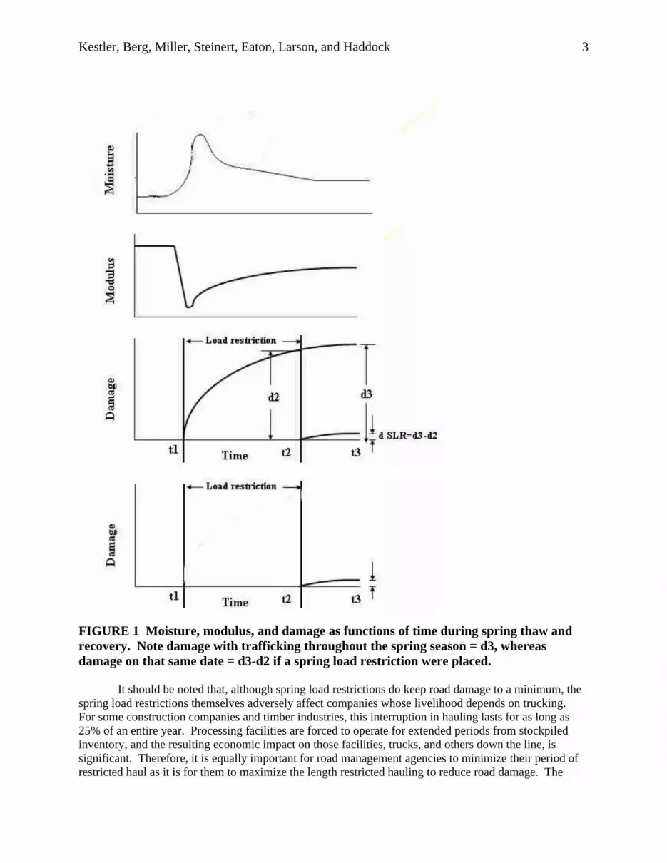
FIGURE 2 Damage factor relative to moisture dissipation; Kootenai National Forest.
Since damage occurs only after the subsurface increases to 0 ºC (32 ºF), and rate of damage becomes minimal once moisture has dissipated, a coupling of permanently installed subsurface temperature with moisture sensors strategically located on a forest road network can provide an affordable method for quantitatively determining both the start and end of critical periods of pavement weakening associated with spring thaw (10).
Table 1 provides a list of typical instrumentation and equipment that can be used for determining when to place and remove SLRs. Additional devices can be used, but these have been used by the authors, and have proven to be cost effective and relatively reliable.
TABLE 1 Typical Subsurface Instrumentation for Aiding in Placing and Removing Spring Load Restrictions Instrumentation or Sensors
Primary SLR Parameter Measured 1
Ref. Approx. Cost Remarks
Thermocouples Temperature (2)(11) (12)(13)(14)
Inexpensive if manually read. Materials for a string of 12 are probably under $100. Manual reader approx $300.
Can be easily fabricated in-house. Typically read manually using a digital thermometer reader or thermocouple reader, or can readily be hooked up to automated data-logger. Be cautious of reference junction temperature.
Thermistors Temperature (9)(10)(15) (16)
More expensive than thermo-couples, but still relatively inexpensive. Purchasing an assembly of 12 from a company may cost approx. $1000. Manual thermistors reader approx $300.
Sensors can be purchased and assemblies of several can be fabricated in-house, although significantly more difficult to fabricate than thermocouples, so the authors recommend purchasing.Typically read manually using a thermistors reader, or can readily be hooked up to automated data-logger.
Temperature sensors encased in small enclosures with mini dataloggers
Temperature (17)(18)
More expensive than thermistors with manual reader, but significantly less expensive than thermistors with automated data acquisition system. Approx $60 per sensor including mini-datalogger for that one sensor.
Individual sensors in canisters can be purchased, then assembled in-house in concentric PVC pipes, with spacers separating sensor locations, and installed vertically in road sub-structure. Need to cap with removable traffic-supporting lid for removal and downloading. Safety issue: traffic control is required as person removing PVC pipe with canisters for downloading is in the path of traffic. Safety issue: need to keep checking that cover does not work its way up out of pavement.
6
Kestler, Berg, Miller, Steinert, Eaton, Larson, and Haddock
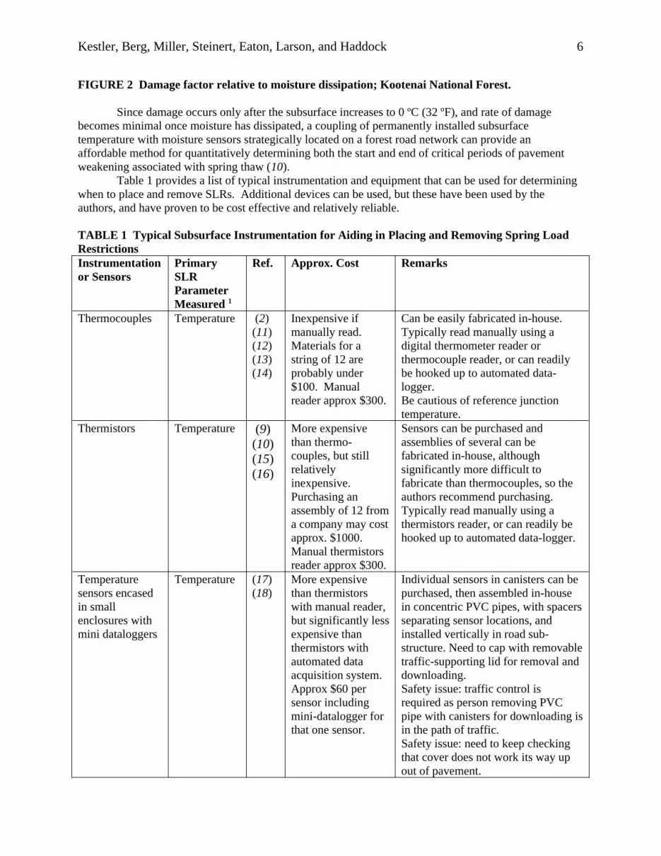
Frost Tubes State of ground (frozen / thawed)
(19)(20)
State of ground at depth – frozen or unfrozen. Can fabricate for under $50.
Can be easily fabricated in-house. Install vertically in road substructure. Need to cap with removable traffic-supporting lid for removal and downloading.Read manually. Safety issue: traffic control is required as person removing frost tube is in the path of traffic.Safety issue: need to keep checking that cover does not work its way up out of pavement.
Resistivity probes
State of ground (frozen / thawed)
(21) State of ground at depth – frozen or unfrozen
Can be fabricated in-house.
Time Domain Reflectometer (TDR)
Unfrozen moisture content
(10)(14)(22) (23)(24)
Individual probes approx $100 ea, or probes with electronics in the head approx $300 ea.
Although possible to fabricate, authors highly recommend purchasing ready-made TDR probes from a distributor. Can be either read manually or hooked up to an automated data-logger.
Radio Frequency soil moisture sensor
Unfrozen moisture content
(10)(25)(26)
Individual probes in the range of $60-$300 each.
Can be purchased from distributor. Can be read either manually or via automated data-logger.
Other soil moisture sensors
(14)(27)
Same as above Same as above
1 Some sensors provide other info than primary listed below, such as TDR shows if frozen or thawed, but recommended primary use here is for measuring parameter listed, such as unfrozen moisture content for TDR
All the instrumentation in Table 1 can be readily retro-fit in existing roads. If installing
instrumentation from the surface down to significant depths, the recommended technique is to drill, insert dowels into drill hole (or individual sensors into the side wall), replace the same material at the same depths in drill hole, and tamp to obtain adequate compaction. If installing sensors in only the upper three ft of the pavement structure, a backhoe can dig a small trench, and instrumentation can be placed into the sides, (or in the case of sensors encased in dowels, a short probe placed vertically in the trench), and backfill of the same material at the same depth is compacted during replacement. Typical installation details are available in Hanek et al (10).
Subsurface instrumentation has proven to work well for the FS, primarily in the Northwest, as a low-cost method for placing and removing SLRs, but is site specific.
Lightweight DeflectometerThe light weight deflectometer (LWD) was developed to estimate in-situ soil stiffness modulus of soils. It had been used outside the United States for some time, but is now rapidly gaining popularity in the United States. Am ASTM standard is now available (28), and a comprehensive literature review, equipment description, and background are provided by Steinert et al. (29). The device is most frequently used for quality control/quality assurance and structural evaluation of compacted earthwork and pavement construction. However, because it measures stiffness, it can also be used as a tool to determine when to place and remove SLRs from low-volume roads (2) (29) (30) (31).
7
Kestler, Berg, Miller, Steinert, Eaton, Larson, and Haddock
The LWD measures deflection, generally from a center geophone, and, using linear-elastic half space theory, calculates a composite modulus for the road/pavement structure. Several LWD manufacturers have added radial geophones, however, to date, only limited publications discuss analysis of radial sensor deflections (32) (33).
The composite modulus measured is that of only the upper reaches of the road structure. A very approximate depth of influence is 1-1/2 times the diameter of the plate onto which the load is applied.
A few US distributors now carry the device. As of 2010, the device cost anywhere from approximately $10,000 to $18,000, depending on options and accessories. Features of various LWD include variable load / drop height, variable plate size, center sensor plus radial sensors, and load cell. The authors recommend an LWD with these features.
Spring thaw testing was conducted by the Univ of Maine, the FS, and numerous other partnering agencies (2) (29). Funding was provided primarily by the FS and New England Transportation. Paved and unpaved test sites were located in ME, NH, VT, MN, MT, ID, and WA. Comparisons were made between the LWD and traditional falling weight deflectometer (FWD). It was shown that the LWD followed seasonal stiffness variations and compared well with FWD-derived moduli on LVRs. Recommendations for using a PFWD to determine when to place and remove SLRs (29) include using the following:
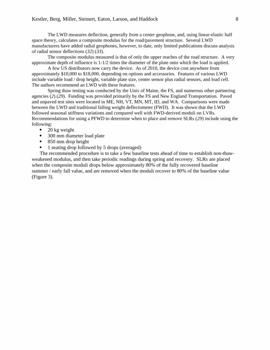
20 kg weight 300 mm diameter load plate 850 mm drop height 1 seating drop followed by 5 drops (averaged)The recommended procedure is to take a few baseline tests ahead of time to establish non-thaw-
weakened modulus, and then take periodic readings during spring and recovery. SLRs are placed when the composite moduli drops below approximately 80% of the fully recovered baseline summer / early fall value, and are removed when the moduli recover to 80% of the baseline value (Figure 3).
8
Kestler, Berg, Miller, Steinert, Eaton, Larson, and Haddock
FIGURE 3 Moduli measured with the LWD and backcalculated from conventional FWD; Crosstown Road, Berlin, Vermont.
Thaw IndexThe original ‘thaw index method,’ developed in Washington State (34) (35) and revised for use in Minnesota (36) (37), enables a simple estimation of the date when thawing commences by using just current air temperature. The technique works well for those specific locations, but it requires different reference temperatures, some of which themselves vary over time, for different geographic locations. Because the FS has roads scattered across the US, a limited budget, and few people to make detailed calculations, it is necessary to have a simple method that can be applied quickly and readily adapted to national forests across the country. A method developed by Berg (38) enables estimation of pavement surface temperatures on a daily basis, and subsequent estimation of the date of the start of thaw.
A relatively simple thaw index spreadsheet is available from Richard Berg, or from San Dimas Technology and Development Center. Historical mean or average monthly air temperatures at the closest representative weather station, obtainable from the internet, are entered on the spreadsheet and fit to an annual sinusoidal temperature variation that approximates average monthly temperatures. Factors are applied to this curve to obtain an average surface temperature curve. The daily temperature differences between the air and pavement surface temperature curves
9
Kestler, Berg, Miller, Steinert, Eaton, Larson, and Haddock
are added to the observed/measured and forecast air temperatures to obtain daily pavement surface temperatures for the winter /spring of observation. Summing these values, the onset of thaw can be estimated to occur on the date that the value of cumulative degree-days reaches a particular value.
The method was tested at several field sites. For sites in the East and Central US, calculated and measured dates for the start of thaw coincided well, even when relatively distant weather stations were used, and SLRs can be placed shortly after the pavement starts to thaw based on Thaw Index spreadsheet predictions. However, for mountainous terrain of the Fremont-Winema National Forests of Oregon, for sites where the nearest weather station is not relatively close, the estimation of the start of thaw fell short of accurate. Attempts were made to correct for temperature using standard temperature corrections with elevation, but microclimates did not allow for the correction to significantly improve estimated thaw dates. It should be noted that the developers of the FHWA air temperature data base for use with the EICM also cautioned about interpolating data for a given location from nearby weather stations in mountainous areas.
Other than for mountainous remote locations, using this modified sinusoidal thaw index technique to predict the start of thawing worked well. The beauty of this method is that it is inexpensive; it is neither limited to specific predetermined sites, as is the case with instrumented sites, nor might it require a few different reference temperatures, as the original thaw index method does when used at different sites. Rather, 0C (32F) can be used as a baseline temperature at all locations. This variation of the classic thaw index method appears to be promising for estimating onset of thaw and placement of SLRs, and it appears that a duration of time, yet to be fine-tuned at the time of this paper, may be recommended for estimating complete thaw and subsequent SLR removal dates for various pavement structures and subgrade materials. Climatic Thaw PredictorGeneralThrough a cooperative effort funded by NHDOT, the FS, and Applied Research Associates (ARA), ARA has been converting the EICM (5) to a prediction model, so, based on general road structure and other climatic data, road managers can, at any location, run the model to determine when to place SLRs. The work is to be applicable primarily on national forests, e.g., nationwide, but there was also a specific focus in NH.
Input parameters to the modified thaw predictor include general pavement structure including subgrade material, location, estimated water table depth, and general snowpack on wear surface or wear surface clear of snow (as many forest roads typically have a few inches of packed snow as opposed to clear surfaces of most higher volume non-forest roads). Many of the otherwise required EICM input parameters are defaulted based upon soil types, location, etc. If the model is scheduled for use in the spring as a prediction model for a forest road on which timber hauling is planned for a known timber sale, an added recommendation is for the local forest to place just one or two sensors near the road surface, and these near-surface temperatures can optionally be periodically input manually, or hooked up to transmit remotely, improving the accuracy of the prediction model significantly.
The EICM requires local climatic information on an hourly basis to calculate temperature and moisture at all depths through time. This climatic data is obtained from the National Climatic Data Center (NCDC) from 851 stations located across the United States (39). Although stations exist in each of the 50 states, the closest stations, which are frequently at airports and cities, are not necessarily representative of local climatic conditions of remote FS sites (as was the case for the thaw predictor program when tested in the Winema-Fremont National Forest in Oregon). Therefore, one of the first
10
Kestler, Berg, Miller, Steinert, Eaton, Larson, and Haddock
modifications to the stand-alone EICM to facilitate thaw predictions at national forests nationwide was the addition of a second climatic database consisting of approximately 2000 remote automated weather stations (RAWS) (40) (41). In contrast to typical / NCDC stations, RAWS are often located in isolated areas accessible only by all-terrain vehicles, helicopters, snowmobiles, or by backpacking to them – typically geographically closer to and more representative of remote forest road locations, particularly in the western USA.
An additional modification to the stand-alone EICM to enable thaw prediction includes the thaw predictor program regularly seeking internet-based weather forecasts. Current and predicted thermal and moisture regime are calculated for the upcoming week, and probabilities provided ranging from 0%, implying no need to place SLRs within the upcoming week, to 100% thaw expected, implying SLRs should be imposed to prevent LVR damage.
An option for specific use on NH roads allows for an increased number of automated input parameters, thus a more accurate prediction of commencement of thaw. Further, but similar, program modification would be required for similar improved accuracy for other States/locations if so desired by another agency.
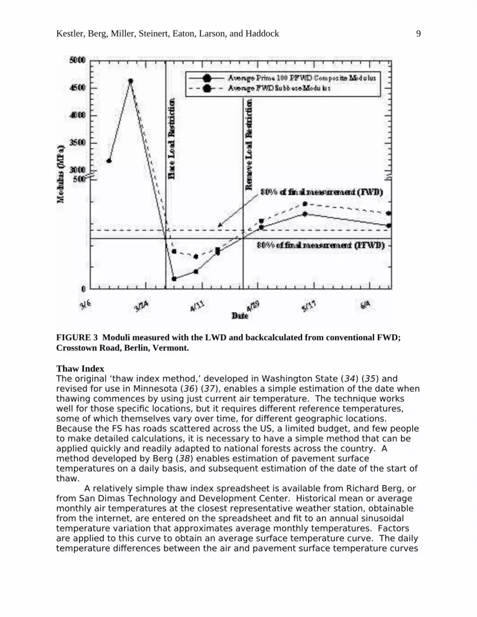
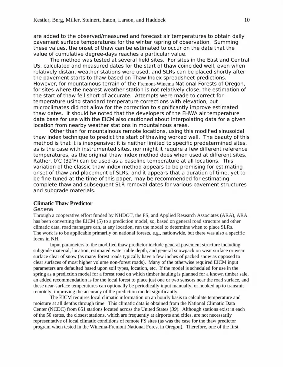
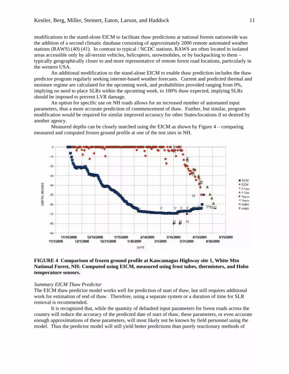
Measured depths can be closely matched using the EICM as shown by Figure 4 – comparing measured and computed frozen ground profile at one of the test sites in NH.
FIGURE 4 Comparison of frozen ground profile at Kancamagus Highway site 1, White Mtn National Forest, NH: Computed using EICM, measured using frost tubes, thermistors, and Hobo temperature sensors.
Summary EICM Thaw PredictorThe EICM thaw predictor model works well for prediction of start of thaw, but still requires additional work for estimation of end of thaw. Therefore, using a separate system or a duration of time for SLR removal is recommended.
It is recognized that, while the quantity of defaulted input parameters for forest roads across the country will reduce the accuracy of the predicted date of start of thaw, these parameters, or even accurate enough approximations of these parameters, will most likely not be known by field personnel using the model. Thus the predictor model will still yield better predictions than purely reactionary methods of
11

Kestler, Berg, Miller, Steinert, Eaton, Larson, and Haddock
imposing SLRs, and damage will be reduced significantly from what would have been the case without the aid of the predictor model. CONCLUSIONS AND RECOMMENDATIONSA variety of low-cost techniques have been developed, refined, modified, and or evaluated by the FS and others for determining when to place and remove SLRs.
Each exhibits strengths and weaknesses for various conditions, but overall, the techniques are relatively inexpensive, reliable, easy-to-use, e.g., little to no training is required, and can aid significantly in saving road maintenance dollars if used to place and remove SLRs on asphalt surfaced and gravel-surfaced low-volume roads. Table 2 summarizes several of the advantages and disadvantages discussed for the various techniques. The authors believe that low-volume road maintenance agencies can capitalize on the strengths of the individual techniques, by using them in combination with each other, as summarized in Table 3. Some agencies are currently keeping SLRs in place for a specific length of time rather than quantitatively determine conditions for LVR removal, and in this regard, additional evaluations (at numerous locations across the nations, to enable national forests anywhere to use the methods) are proposed for validating implementation of a specified length of time after SLR placement that removal should take place for various combinations of pavement structures and subgrade materials.
TABLE 2 Summary of Strengths and Weaknesses / Advantages and Disadvantages of Various Techniques
Diagnostic Technique
Strengths / Advantages Weaknesses / Disadvantages
Subsurface sensors
With coupling of temperature and moisture sensors, can predict when to both place and remove spring load restrictions.
Site specific. Requires field visits to manually read or download unless a remote automated data acquisition system is installed.Difficult to install if a rocky subgrade.
Lightweight Deflectometer
Can be used anywhere – not site specific as are subsurface sensors.Works well for both placement and removal of load restrictions.
LWD provides modulus for the upper reaches of a road; It is only good for paved roads with up to 4-5 in. max of asphalt. Composite modulus. Not all LWDs have a load cell -- The authors do not necessarily recommend LWDs without a load cell.
Thaw Index Does not require field visit; can be used from office. Simple to use once spreadsheet is set up (following first year).
First year of use requires additional time to set up historical temp data. Does not appear to work as well in mountainous locations if there is not a very nearby weather station for historical and current climatic data.Not as good for removal of load restrictions as it is for placement.
EICM Thaw Predictor
Does not require field visit; can be used from office.Takes into account materials/road structure.
Works better if there is a temperature sensor in the road with which the prediction can be calibrated. Good for determining start of thaw, but still needs work for predicting completion of thaw.
12

Kestler, Berg, Miller, Steinert, Eaton, Larson, and Haddock
TABLE 3 Recommendations for Combinations of Techniques for Placing and Removing Spring Load Restrictions
If Spring Load Restriction is Placed Using this Method:
1,2 Recommended method(s) for Removing Spring Load Restriction:
Subsurface temperature sensors Subsurface moisture sensors Lightweight Deflectometer
Lightweight Deflectometer Lightweight DeflectometerThaw Index Lightweight DeflectometerEICM Thaw Predictor Lightweight Deflectometer1 A length of time, referenced in above text, serves as an alternative method to remove SLRs. Although not a quantitative technique, times are based on past observations, and the method will still keep damage to a minimum. 2 It is possible to shorten the SLR window further, if approved by the agency under which jurisdiction the road is, by using reduced tire pressure methods (42). Use reduced tire pressure for approx. the last two weeks of estimated standard SLR window, then continue using reduced tire pressure for two to three weeks following estimated SLR window. Resulting road damage is approximately the same as for standard SLR window with standard tire pressure.
Low-volume road management agencies interested in using these methods for imposing SLRs need only purchase and install subsurface instrumentation or purchase and use a LWD if planning on using one or both of the first two methods. For the second two, the modified sinusoidal thaw index spreadsheet and instructions for use are available from Richard Berg or from San Dimas Technology and Development Center, and the EICM thaw predictor and instructions for use are available from Gregg Larson, ARA; San Dimas Technology and Development Center; or NHDOT. Contact information for each is shown on the title sheet accompanying this paper.
ACKNOWLEDGMENTSThe authors would like to thank Gordon Hanek, Mark Truebe, Dave Katagiri J. Sylvester, Alan Yamada, Bill Vischer, Barry Collins, John Freetly, and many others currently or formerly USDA Forest Service; Dana Humphrey and Chris Helstrom (currently or formerly Univ. of Maine, Orono); the New England Transportation Consortium; Meghan Amatrudo (UMass-Dartmouth); Andy Hall, Alan Hanscom, Denis Boisvert, Glenn Roberts and Alan Rawson (NH Dept of Transportation); Gary Evans (Western Federal Lands Highway Division FHWA); Mike Santi (Idaho Transportation Department); Rajib Mallick (Worcester Polytechnic Institute); Greg Johnson, John Siekmeier, and Rebecca Embacher (MN DOT); Jeff Uhleymer and Chuck Kinne (WA DOT); Charlie Smith and Edel Cortez (CRREL): Steve Saboundjian (AK DOT&PF); Al Bradley (FERIC); and many others for their assistance with various spring load restriction projects leading to this SLR diagnostic techniques guide.
REFERENCES
(1) Road Management & Engineering Journal, 1997, TranSafety, Inc., http://www.usroads.com/journals/rej/9702/re970204.htm (accessed March 2010).
(2) Kestler, Maureen A., Richard L. Berg, Bryan C. Steinert, Gordon L. Hanek, Mark A. Truebe, and Dana N. Humphrey, Determining When to Place and Remove Spring Load Restrictions on Low-Volume Roads: Three Low-Cost Techniques , 2007, Transportation Research Record No 1989, LVR Conference, Austin TX, pp. 219-229.
13

Kestler, Berg, Miller, Steinert, Eaton, Larson, and Haddock
(3) WSDOT. Pavement Guide, Volume 2: Pavement Notes for Design, Evaluation, and Rehabilitation. 1995.
(4) WSDOT Pavement Guide, Volume 3: Pavement Analysis Computer Software and Case Studies, 1995. (5) Guide for Mechanistic-Empirical Design of New and Rehabilitated Pavement Structures. Final Report, 2004. NCHRP Project 1-37A. http://onlinepubs.trb.org/onlinepubs/archive/mepdg/home.htm (accessed Mar 2010).
(6) 10. Richter, C. A., Seasonal Variations in the Moduli of Unbound Pavement Layers. Publication FHWA-HRT-04-079. FHWA, U.S. Department of Transportation, 2006.
(7) Guymon, Gary L., Berg, Richard L. and Hromadka II, Theodore V., 1993, Mathematical Model of Frost Heave and Thaw Settlement in Pavements, CRREL Special Report #93-2, Hanover, NH.
(8) 12. Larson, G., and B. J. Dempsey. Enhanced Integrated Climatic Model. Version 2.0, FinalReport. Contract DTFA MN/DOT 72114. Department of Civil Engineering, University of Illinois at Urbana-Champaign, 1997.
(9) Barcomb, Joe. 1989. Use of Thermistors for Spring Road Management. Transportation Research Board 1252.
(10) Hanek, Gordon L., Mark A. Truebe, Maureen A. Kestler. Using Time Domain Reflectometry (TDR) and Radio Frequency (RF) Devices to Monitor Seasonal Moisture Variation in Forest Road Subgrade and Base Materials. 0077 1805P. San Dimas, CA: U.S. Department of Agriculture, Forest Service, San Dimas Technology and Development Center. 2001.
(11) Omega Engineering Technical Reference. Thermocouples – An Introduction http://www.omega.com/thermocouples.html (accessed March 2010).
(12) Dataforth Introduction to Thermocouples AN106, https://www.dataforth.com/catalog/pdf/an106.pdf (accessed March 2010), Tuscon, AZ. Sept 2006.
(13) Janoo, Vincent, Lynne Irwin, and Robert Haehnel Pavement Subgrade Performance Study Project Overview. ERDC/CRREL TR-03-05, Hanover, NH. March 2003.
(14) Willis, J. Richard. A Synthesis of Practical and Appropriate Instrumentation Use forAccelerated Pavement Testing in the United States, International Conference on Accelerated Pavement Testing, Madrid, Spain. 2008.
(15) Baichtal, J.F. (1990) “Monitoring Subgrade Frost Penetration Using Constant Data Loggers with Thermistor Installations.” Engineering Field Notes, USFS, WA, D.C., V22.
(16) Esch, David C. (1989) Temperature and Thaw Depth Monitoring of Pavement Structures, State of the Art of Pavement Response Monitoring Systems for Roads and Airfields, Hanover, NH.
(17) Department Of Transportation Federal Highway Administration Western Federal Lands Highway Division, Warm Lake Road, Frost Heave Monitoring Report; Boise National Forest, Valley County, Id, Idaho Forest Highway 22, March 2010.
14
Kestler, Berg, Miller, Steinert, Eaton, Larson, and Haddock
(18) Onset website http://www.onsetcomp.com/products/data-loggers/ua-002-64 (accessed Mar 2010).
(19) McCool, D. K. McCool and Myron Molnau, Measurement of Frost Depth, Proceedings Western Snow Conference 52:33-42.1984, Sun Valley, Idaho, http://snow.cals.uidaho.edu/Publications/frost/frost.html (accessed March 2010).
(20) All About Frozen Ground: Studying Frozen Ground, Frost Tube Program ,UAF, Students guide to frost tube fabrication and observation http://www.uaf.edu/water/projects/permafrost/frost_tube.htm (accessed March 2010).
(21) Atkins, Ronald T. Frost resistivity Gages: Assembly and Installation TechniquesCRREL Technical Note, Hanover, NH, Oct 1990.
(22) Topp, G.C., S.J. Zegelin, and I. White (1994) Monitoring soil water content using TDR: An overview of Progress, In Proceedings Symposium and Workshop on Time Domain Reflectometry in Environmental, Infrastructure, and Mining Applications, pp. 67-80, Northwestern University, Evanston, Illinois. September.
(23) Kestler, Maureen A.; Bull, Dale; Wright, Brenda; Hanek, Gordon; Truebe, Mark. 1997. Freeze-thaw testing of time domain reflectometry (TDR) and radio frequency (RF) sensors. Proceedings: international seasonally frozen soils symposium; June; Fairbanks, AK.
(24) Campbell Scientific TDR-Time Domain Reflectometry website http://www.campbellsci.com/tdr (accessed Mar 2010).
(25) Atkins, Ronald T., Timothy Pangburn, Roy E. Bates, and Bruce E. Brockett. Soil Moisture Determinations Using capacitance Probe Technology, CRREL Special Report 98-02, Hanover, NH, January 1998.
(26) Stevens Soil Moisture Sensors website, http://www.stevenswater.com/soil_moisture_sensors/index.aspx (accessed Mar 2010).
(27) Decagon Devices Soil Moisture Systems http://www.decagon.com/soil_moisture/ (accessed Mar 2010).
(28) ASTM (2007) Standard Test Method for Measuring Deflections with a Light WeightDeflectometer, ASTM E 2583-07, American Society for Testing and Materials, WestConshohocken, PA, USA.
(29) Steinert, B. C., D. N. Humphrey, and M. A. Kestler. Field and LaboratoryEvaluation of the Portable Falling Weight Deflectometer: A Study for the New England Transportation Consortium. Department of Civil and Environmental Engineering, University of Maine, Orono, 2005.
(30) Davies, Tom (1997) Assessing the Suitability of the Loadman Single-Point Falling Weight Deflectometer to Tracking the Change in Strength in Thin Asphalt Roads Through Spring Thaw in Saskatchewan. UNB International Symposium on Thin Pavements, Surface Treatments, and Unbound Roads, New Brunswick, Canada. 117-124.
(31) Baiz, Sarah, Susan L. Tighe, Brian Mills, Carl T. Haas, and Ken Huen. Using Road Weather
15
Kestler, Berg, Miller, Steinert, Eaton, Larson, and Haddock
Information Systems (RWIS) to Control Load Restrictions on Gravel and Surface-Highways, Ministry of Transportation of Ontario (MTO) / Highway Innovation Infrastructure Funding Program (HIIFP), November 2007.
(32) Horak, E., J. Maina, D. Guiamba, and A. Hartman. Correlation Study with Light Weight Deflectometer in South Africa. Proc., 27th Southern African Transport Conference, Pretoria, South Africa, 2008.
(33) Senseney, Maj. Christopher T. and Michael A. Mooney, Ph.D., P.E Characterization of a Two-Layer Soil System Using a Lightweight Deflectometer with Radial Sensors, TRB 2010, WA, DC.
(34) Rutherford, M. S. Pavement Response and Load Restrictions on Spring Thaw–Weakened Flexible Pavements. In Transportation Research Record 1252, TRB, National Research Council, Washington, D.C., 1989, pp. 1–11.
(35) Rutherford, M. S., J. P. Mahoney, R. G. Hicks, and T. Rwebingira. Recommended Guidelines for Imposing and Lifting Springtime Restrictions. Report FHWA-RD-86-501. Washington State Department of Transportation and FHWA, U.S. Department of Transportation, 1985. (36) Van Deusen, D. A. Improved Spring Load Restriction Guidelines Using Mechanistic Analysis. Proc., Ninth International Conference on Cold Regions Engineering, Duluth, Minn., Sept. 27–30, American Society of Civil Engineers, Reston, Va., 1998, pp. 188–199.
(37) Van Deusen, D., C. Schrader, D. Bullock, and B. Worel. Springtime Thaw Weakening and Load Restrictions in Minnesota. In Transportation Research Record 1615, TRB National Research Council, Washington, D.C., 1998, pp. 21–28.
(38) Berg, Richard L, Maureen A. Kestler, Robert A. Eaton, and Christopher C. Benda. Estimating When to Apply and Remove Spring Load Restrictions, Proceedings ASCE Cold Regions Engineering Conference ,Bangor, ME, July 2006.
(39) Johanneck, Luke and Lev Khazanovich, A Comprehensive Evaluation of The Effect Of Climate In MEPDG Predictions, Transportation Research Board, WA ,DC, 2010.
(40) USDA Forest Service Remote Automated Weather Stations http://www.fs.fed.us/raws/ (accessed Mar 2010).
(41) Desert Research Institute, RAWS USA Climate Archive, Remote Automated Weather Stations, http://www.raws.dri.edu/documents/RAWS.pdf (accessed Mar 2010).
(42) Maureen A. Kestler, Richard L. Berg, and John E. Haddock . Can Spring Load Restrictions on Low-Volume Roads Be Shortened Without Increasing Road Damage? Transportation Research Record: Journal of the Transportation Research Board Volume 1913. WA, DC. 2005.
16


