July 2016 - socet

GUJARAT TEGHNOLOGIGAL UNIUERSITY(Estabfished by Government of Gujarat under Gujarat Act No.: 20 of 20071

1g"r"rd 2 s-iLcr[o gcil. 11fi..[f.a(g're.ra aegt?-u g%?rcr utf\hqq grrig : ?o/?ooe erer wrr[\a)

MESSAGE OF THE VICE CHANCELLOR

Silver Oak has been doing good work in generating

innovative ideas. This has inspired many students to

take up creative and relevant projects. lt is in order, that

these ideas are disseminated to all stake holders.

I congratulate the Principal and faculty for publishing

these ideas in Sarjan- 2Ot6

Date: 7tn July 2016

Winnersof:ICTEnabledUniversityAwardE-India-20A9*ManthsnAwurd-2009*ensUewuyd-2011* ntgitut tearning WES - 2011 Award te ,aUUtS tnternutional Innovstive Llniversity Award - 2013

'\Ghandkheda l Nr. Campus of Vishwakarma Government Engineering College, Sabarmati - Koba Highway, Nr. Visat Three Roads,

Chandkheda, Ahmedabad - 382 424. Gujarat, India Ph. :079 - 232 67 500 Fax : +91 - 79 232 67 580Ahmedabad : 2nd Floor, ACPC Building, L. D. College of Engineering Campus, Navrangpura, Ahmedabad, (Gujarat) lndia - 380 015.

Knowledge is not a power but its implementation is a power.

With that concept in mind, 5th issue of SARJAN is launched which showcases innovative ideas of

experienced technocrats along with budding engineers. A remarkable point for this particular issue lies

in the fact that 5th issue of SARJAN also involves participation of authors from colleges other than Silver

Oak Group of Institutes. One more innovative idea was that reviewing of research articles was done by

experts of respective branches of engineering of college other than Silver Oak Group of Institutes. I want

to thank Reviewers for giving their valuable time in review process. I also want to thank all the authors

for contributing their research and review articles to SARJAN.

I am thankful to Ms. Upama Vachhani for assisting me in designing of front and back cover page of our

journal. I express my deep gratitude towards my dear friends for helping me out in every phase.

I also want to extend my sincere thanks to Dr. Saurin Shah – Principal, SOCET for giving me this

wonderful opportunity to work for SARJAN. I wish to extend my words of thanks to my coordinating

team without whom this venture could never have been accomplished.

Editor

Dr. Roshni Dave

Co-ordinators

Ms. Rewati Marathe Mr. Hardik Shukla Mr. Ravi Raval Ms. Darshana Ahir Ms. Dimple Agarwal Ms. Puja Bavra Ms. Ritika Sharma

Our Reviewers

Captain Dr. C.S. Sanghavi

Assistant Professor L.D. College of Engineering Ahmedabad [email protected]

Dr. V.K. Bhatt

Professor Mechanical Department Specialization in Tribology machine design Indus University Ahmedabad [email protected]

Dr. Sharnil Pandya

Associate Professor, I.T Dept. Parul University Research Area: Embedded Systems, Cloud Computing, Internet of Things, Wireless Sensor Networks, Web and Mobile Technology Membership: ISTE, IEEE, CSI [email protected]

Dr. Bhavik Suthar Assistant Professor L.D.College of Engineering Ahmedabad, Gujarat [email protected]

Mr. Kalpesh Joshi Assistant Professor IIT Gandhinagar Gandhinagar Gujarat [email protected]

Dr. R. A. Thakker

Professor Electronics & Communication Department Vishwakarma Govt. Eng. College, Chandkheda Ahmedabad [email protected]

mailto:[email protected]


CL01: Analysis of Underground Tank With Reference to IS 3370……………………...1 Rahul Patel, Rishi Dave, Rahul Shah

School of Science & Engineering, Navrachana University, Vadodara.

CL02: Analyzing an urban over bridge. A case study of Odhav Junction Bridge……….5 Kaushik Khunt, Rewati S. Marathe

Silver Oak College of Engineering & Technology, Ahmedabad.

CL03: Problem Occur during Construction of Pile foundation of fly over. A Case study

of Bopal Fly Over………………………………………………………………………..13 Ram Dhankani, Tark Patel, Deep Amin, Varun Bhavsar, Rewati S. Marathe


CL04: Design and Construction of an affordable housing scheme……………………..16

Shruti Patel


ME01: Minimizing Driving Constraints with Respect to the Driving seat of a Car and

Accessibility to the overall Dashboard…………………………………………………..29 AjinkyaRatnaparkhi, Kannan Srinivasan

VIT University, Chennai.

ME02: A Review of thermal effects on the IC engine exhaust valve for design

optimization……………………………………………………………………………...34 Karan Soni, Ripen Shah, UmangVora


ME03: Design procedure of monorail runway beam as per CMAA 74………………....38 Shashi Sagar


ME04: Design and Development of Duster Cleaning Machine…………………………50

Chirag Patel, Sameer Kambad, SahilkumarParmar, Pavankumar

Prajapati


ME05: Design and development of hydraulic rod bending machine……………………54

Chirag Patel , Vijay Patel, Harsh Pathak, Malav Gandhi, PrashilPatele,

Kishan Patel


ME06:Design and development of Valve Plate Testing Fixtureto detect air

leakage……………………………………...……………………………………………58 Chirag Patel, SudhirParmar, KeyurParmar, Nirav Patel, MoshakirPatel


ME07: Effect of frequency on Inertance Tube Pulse Tube Refrigerator (IPTR)

Performance .…………………………………………………………………………….62 Nikul Patel


ME08: Effect of Injection Pressure on the Performance of Single Cylinder CI Engine

Fueled with the Blend of 30% Plastic Pyrolysis Oil and 70% Diesel ………………......68

DhruvinKagdi


ME09: Mechanism for Garbage disposal vehicle ……………………………..……......78 Hardik Shukla, Raj Padhiyar


ME10:IC engine Exhaust Valve design optimization using finite element analysis……84 Karan Soni, Ripen Shah, UmangVora


ME11: Improving the Efficiency of Knitting Machine………………………………….89

Chirag Patel, MayurShrivas, Prerak Rathod


ME12: Quad-copter Stabilization Using Perceptron Assisted Proportional Control……95 Hardik D. Gangadia, Markand P. Pathak, Keval P. Kelawala


ME13: Finite Element Based Static Structural Analysis of IC Engine Piston…………101 NamrataSengar Abhishek Shah , Swati Saini


ME14: Thermal Analysis of Diesel Engine Cylinder liner & Design Modification Using

Finite Element Analysis …………………………………………………………….....106 Abhishek Shah, Swati Saini ,NamrataSengar


ME15:CFD Analysis for Heat Transfer Augmentation by Changing Profiles of Air

Cooled Fins ……………………………………………………………………...……..114

Swati Saini, DhruvinKagdi ,NamrataSengar , Abhishek Shah


EEE01: Simulation of Induction Motor Pump supplied by Photovolatic generator…...121

PiyushP. Tandel

MGITER, Navsari.

EE01: A Review: Optimal Sizing and Cost Assessment of Roof Top PV Systems for

Aditya Silver Oak Institute of Technology……………………………………………..128 Darshna V. Ahir, Ashish Khatik

Aditya Silver Oak College Institute of Technology, Ahmedabad.

EE02: A Review Article on Distributed Generation

Technology…………………………………………………………………………......134 Manan Pathak, DarshnaAhir

Aditya Silver Oak College Institute of Technology, Ahmedabad.

EE03:VoltageStability improvement in Multi-Machine Power system by Static Var

Compensator (SVC) FACTS Controller stability ......……………………….................140 Mitul Vekaria

Silver Oak College of Engineering & Technology, Ahmedabad

EE04:Simulation of Speed Control of Induction Motor using Voltage/frequency (V/F)

Ratio ………………………………………………………………...………………….150

Mitul Vekaria


EE05:Problem Associated with Inverter Driven Induction Motor and its Solution .….158

DarshanThakar


EC01:Analysis of Micro strip Patch Antenna for WiMAX Application .…………...…168

AnshuToshniwal


EC02:Review onClassical planning ………………………………………………...…176

Kevin Naik, Maulik Swaminarayan, Aayushi Kothari


EC03:AReview on CMOS Operational Trans-conductance Amplifier…………..……183

Bhoomi P. Patel, Kaushani H. Shah, Mohammed G. Vayada


EC04:Low Pass Filter using Evolutionary Algorithms ………………………........…..191

Bhoomi N. Thakkar, Vimal H. Nayak


EC05:Implementation of CCII based on Current Mirror Pair and Differential Pair ..…195 Kaushani H. Shah, Bhoomi P. Patel, Mohammed G. Vayada


EC06:Satellite image classification using fuzzy logic ...…………………..…………..202

Pranali Shah, Mohammed G. Vayada


EC07:Comparsion between m0 and m3 for single dc stepper motor into servo motor 209

Patel Kuldeep J, Dimple Agrawal


CE01: Survey on Different Auto Scaling Techniques in Cloud Computing Environment

.........................………………………………………………………………………….214

PranaliGajjar


CE02:Development of data retrieval and scientific data- presentation platform ..……224

SrideviRamya, GayatriYellamraju


CE03:A survey on Performance Improvement in Media file using CDN Cloud

Computing ..……………………………………………………………………………231

Dhwani Modi


CE04:Agent Based Network Surveillance System ..…………………………………..237

Gunjan Bhatt, Chandrashekhar T R


CE05:Securing MANET against Wormhole Attack ..…………………………………241

Pooja Bavarva


IT01:ZAPTRO an inter communication tool for Organizations ...…………………….248

ShnansheDiksha, KrimaRokadiya


IT02:A Review on wireless sensor network attacks ..…………………………………256

Nikhil Patel


1

Analysis of Underground Tank With Reference to IS 3370

Rahul Patel, Rishi Dave, Rahul Shah

[email protected]

Civil Engineering Department, School of Science & Engineering, Navrachana University, Vadodara

Abstract: Water tanks are used to store water for various household and commercial works thus, the tanks are designed as

crack free structures, to eliminate any leakage. In this paper analysis of underground water tank is presented. Such tanks are

designed as per IS 3370:2009 Part I&II where the vertical wall is subjected to hydrostatic pressure and soil pressure and the

base is subjected to weight of water and soil pressure & uplift. To set up a relationship between varying capacity and the base

moment will be a helping hand at the time of design.

This paper gives an idea of designing the rectangular underground water tank using working stress method. The analysis and the

design of rectangular underground water tank is done with the help of spreadsheet program and a relationship between varying

tank capacities with moment capacity is derived.

Keywords

RCC water tank, Working stress method, Tank capacity, Moment capacity, Design

1. Introduction:

Rectangular water tanks are provided where small capacity tanks are required. For small capacities circular tanks prove

uneconomical as the formwork for circular tank is very costly. Square plan water tanks are economical than the rectangular

water tank. In rectangular water tank the longer side should not be greater than twice the smaller side.

In rectangular tanks moment are caused in two directions. The exact analysis is very difficult, so we can design it by an

approximate method.

For rectangular tanks, we can design all walls as continuous frame subjected to pressure varying from zero at top to maximum at

H/4 or 1m from base slab, whichever is more. The bottom part of H/4 or 1 m is designed as cantilever.

In addition to bending, walls are subjected to direct tension caused by hydrostatic pressure on the walls. We need to design it for

both direct tension and bending moment. The bending moment in the walls are found by moment distribution method.

Direct tension in long walls (TL) = [ Γw(H-h)*B] / 2

Direct tension in short wall (Ts) = [ Γw(H-h)*L]/2

If the ratio between length and breadth of a tank is greater than 2 means than the long walls are designed as cantilever and short

walls as slabs supported on long walls.

1.1 General Requirements According to IS: 3370

IS: 3370 is the Indian code of practice for concrete structures for the storage of liquids

In IS: 3370

Part 1(2009): General Requirements

Part 2(2009): Reinforced concrete structures

Part 3(1967): Prestressed concrete structures

Part 4(1967): Design tables

Correct placing of reinforcement, use of small-sized and use of deformed bars lead to a diffused distribution of cracks. A crack

width of 0.1 mm has been accepted in liquid retaining structures.

1.2 Stresses in the Reinforcement:-

To reduce any possible tensile cracking of concrete of the tank wall the following working stresses are adopted in the

reinforcement.

Reinforcement

Permissible tensile stress in the reinforcement

Plain round mild steel bars High strength deformed bars

Tensile stress in members under 115 N/mm2 130 N/mm

2


2

direct tension, bending and shear

Compressive stress in columns

subjected to direct load 125 N/mm

2 140 N/mm

2

For a design of underground water tank, we should have two things in our mind; our designed water tank must be safe in

following cases:

Case 1: Tank is full and no earth pressure.

Case 2: Tank is empty and active earth pressure acting from outside.

Underground water tanks need roof slab to keep water clean. Hence the designer must design the roof slab which is similar to

design of slabs in buildings. Here the design criterion is as follows:

1. Determination Of Dimension Of The Tank

Assuming length is equal to the three times of breadth.

Area of the tank = Q / H

B =√ (area of tank / 3)

L=3B

2. Design Of Long Walls

i. First considering that pressure of saturated soil acting from outside and no water pressure from inside, calculate the

depth and over all depth of the walls.

ii. Calculate the maximum bending moment at base of long wall.

iii. Calculate the area of steel and provide it on the outer face of the walls.

iv. Now considering water pressure acting from inside and no earth pressure acting from outside, calculate the maximum

water pressure at base.

v. Calculate the maximum bending moment due to water pressure at base.

vi. Calculate the area of steel and provide it on the inner face of the walls.

vii. Distribution steel provided = (0.3 - 0.1 * (t - 100) / 350) * t * 10

3. Design Of Short Walls

i. Bottom 1m acts as cantilever and remaining 3m acts as slab supported on long walls.

ii. Calculate the water pressure at a depth of (H-1) m from top.

iii. Calculate the maximum bending moment at support and centre.

iv. Calculate the corresponding area of steel required and provide on the

v. Outer face of short wall respectively.

vi. Then the short walls are designed for condition pressure of saturated soil acting from outside and no earth pressure

from inside.

4. Base Slab Is Checked Against Uplift.

5. Design Of Base Is Done.

2. Design of Underground Tank

DESCRIPTION VALUE

Capacity 24000l

Depth of the tank 3.55 m

Compressive strength of concrete 25 MPa

Free board 0.3 m

Diameter of bars used 8 mm, 10 mm, 12 mm

Angle of repose of soil 30°

3

Unit weight of soil 16 kN/m3

Unit weight of water 9.8 kN/m3

3. Result and Discussion The result values are computed to determine the graph of moment v/s capacity of tank. With increase of capacity in tank the

moment increases.

DESCRIPTION VALUE

Length (m) [Input value] 6 m

Breadth (m) [Input value] 2 m

Height (m) [Input value] 2 m

Thickness of wall (mm)

IS: 3370 (Part II) 250 mm

Long wall

Steel along inner side (mm2)

M= Ast*σst*j*d 532.74 mm2

Steel along outer side (mm2)

M= Ast*σst*j*d 1353 mm2

Distribution steel (mm2)

Ast= (πd2/4)/S*1000

S- spacing between bars

335 mm2 Each Face

Short wall

Steel along inner side at support (mm2)

M= Ast*σst*j*d

80.64 mm2

Steel along inner side at center (mm2)

M= Ast*σst*j*d

80.64 mm2

Base thickness (mm) 250 mm

Reinforcement in base (mm2)

Ast= (πd2/4)/S*1000 1340 mm

2

Roof slab thickness (mm)

D= depth+(dia./2)+c/c 200 mm

Reinforcement in roof slab (mm2)

Ast= (πd2/4)/S*1000 107 mm

2

4

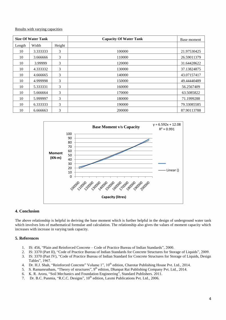
Results with varying capacities

Size Of Water Tank Capacity Of Water Tank Base moment

Length Width Height

10 3.333333 3 100000 21.97530425

10 3.666666 3 110000 26.59011379

10 3.99999 3 120000 31.64428622

10 4.333332 3 130000 37.13824875

10 4.666665 3 140000 43.07157417

10 4.999998 3 150000 49.44440489

10 5.333331 3 160000 56.2567409

10 5.666664 3 170000 63.5085822

10 5.999997 3 180000 71.1999288

10 6.333333 3 190000 79.33085585

10 6.666663 3 200000 87.90113788

4. Conclusion

The above relationship is helpful in deriving the base moment which is further helpful in the design of underground water tank

which involves lots of mathematical formulae and calculation. The relationship also gives the values of moment capacity which

increases with increase in varying tank capacity.

5. References

1. IS: 456, ―Plain and Reinforced Concrete – Code of Practice Bureau of Indian Standards‖, 2000.

2. IS: 3370 (Part II), ―Code of Practice Bureau of Indian Standards for Concrete Structures for Storage of Liquids‖, 2009.

3. IS: 3370 (Part IV), ―Code of Practice Bureau of Indian Standard for Concrete Structures for Storage of Liquids, Design

Tables‖, 1967.

4. Dr. H.J. Shah, ―Reinforced Concrete‖ Volume 1‖, 10th

edition, Charotar Publishing House Pvt. Ltd., 2014.

5. S. Ramamrutham, ―Theory of structures‖, 9th

edition, Dhanpat Rai Publishing Company Pvt. Ltd., 2014.

6. K. R. Arora, ―Soil Mechanics and Foundation Engineering‖, Standard Publishers. 2011.

7. Dr. B.C. Punmia, ―R.C.C. Designs‖, 10th

edition, Laxmi Publications Pvt. Ltd., 2006.

y = 6.592x + 12.08R² = 0.991

0102030405060708090

100

Moment (KN-m)

Capacity (litres)

Base Moment v/s Capacity

Linear ()

http://www.amazon.in/s/ref=dp_byline_sr_book_1?ie=UTF8&field-author=Dr.+B.C.+Punmia&search-alias=stripbooks

5

Analyzing An Urban Over Bridge: A Case Study Of Odhav

Junction Bridge

Kaushik Khunt and Rewati S. Marathe

[email protected],[email protected]

Civil Engineering Department, Silver Oak College of Engineering & Technology, Gujarat Technological

University, India

Abstract:- Traffic is big nuisance in our country. As population is increasing, the requirement of road facility is also in increasing. The aim

of our project is to study economic analysis of bridge. For this purpose transportation surveys like delay survey, spot speed

survey is to be carried out. Due to construction of bridge and cost of fuel, if delay in terms of money is reduced, then we can say

that it is eco-friendly and feasible. For this purpose, signal design at intersection or an over bridge or under pass structure at the

location, is possible alternate. Over bridge or under pass type structures are provided after prior studies at any intersection

considering the geographical and the traffic condition of that location. Even after the renewed design at any location, it may be

possible that at the end of project, user might not be able to get desired outcome as envisage at the time of its recommendation.

This research work tries to evaluate over bridge performance at the ODHAV intersection in context to traffic congestion

reduction as well as economic benefits. For this purpose we are concentrating on surveys at intersection like CVC survey,

stopped delay survey and spot speed survey.

Keywords: Over Bridge, Intersection, delay, pollution, CV Count.

1. Introduction

Transportation is world-wide and our government provides best facilities for transportation. At the present, there are all country

having transportation facilities and without transportation. We cannot envision our routine life because it‘s a need of each and

every people.

A transportation system may be defined as a planned network of elements or physical components that play different roles in the

transportation of goods and persons from one place to another.

It is very useful for public transportation when there is some obstruction like river, rail lines, junctions (cross road). It is a big

factor for reducing highway traffics and helps to bypass town cross roads which saves time and fuel as well for all types of

vehicles including heavy loading vehicles as flyover saves much of their time and wages.

While the construction of a bridge or anything related to transportation there are disturbance and noise has been created.

Through this construction pedestrian and vehicle has been disturbed and they are delay to reach his destination. So we can focus

on the economic analysis on bridge and do some surveys for collecting data and easy to understand the problem faced by the

transporter.Due to continuous increase in number of vehicles, massive traffic problem arises in mega cities. To reduce the

problems arise due to traffic in the big cities, there are different alternate options available to transport planner. Alternate may be

signalised intersection or an over bridge. According to traffic condition and land availability appropriate structure is provided at

the affected places. User benefit is most important criteria in any transportation project. Any project should fulfil its user‘s need

or purpose for which it is designed. For this purpose prior studies and surveys are carried out. But sometimes due to

unavailability of data, misinterpretation of data or due to false assumptions project may not give true result. To assess benefits

obtained from project, economic evaluation of project is carried out. From economic evaluation benefits can be converted into

monetary value. From that value viability or feasibility of project can be checked. In case if the project fails to fulfil the

objectives then alternative arrangement can be provided and it will also give base data for future work of similar type.


6

2. Study Area and Methodology

Ahmedabad is the largest city in the whole state of Gujarat. Ahmedabad is the hub of trade and commerce in Gujarat. The

commercial importance of Ahmedabad makes the city an important travel destination in India. Besides being home to a number

of important industries, Ahmedabad also has a number of majestic monuments, which remind us of the great historical and

cultural past of the city. There are numerous places in Ahmedabad which are suffering from the problem of congestion. Among

them I choose ODHAV cross road (Sardar Patel Ring Road) as my study area, at which over bridge is constructed in order to

reduce traffic congestion. This flyover is running perpendicular to 150 feet ring road. Every day, during office hours, this stretch

becomes a major traffic bottleneck. According to a traffic survey, ODHAV crossroads get extremely congested with traffic, to

cop up with this traffic over bridge was provided. The bridge measure 866 meters in length and 30 meters wide.

2.1 Problem Definition

In present scenario due to heavy traffic volume, the existing roads are insufficient to maintain the design speed. With the help of

spot speed studies we can manage the traffic volume by diversion or by designing signal cycle time.

2.2 Objectives

To establish speed limit in an Odhav Bridge, Ahmedabad. (2)To recommend Zebra crossing or pedestrian signal if

necessary. (3)To recommend caution signs in the school zone

3. Data Collection

Data collection in the transportation engineering is one of the time consuming, costly as well as very laborious activity, which

requires too much patience as well as through planning in order to get the factual data. Not only this but necessary permission as

well as documentation from the authority is one of the big impediments in the data collection.

In order to collect the volume data, speed, delay at the ODHAV intersection is carried out by the support and cooperation

students of Silver Oak College of engineering. The data for speed was collected on the week day ( Monday ) 19th

February 2016

between 10:30 AM – 11:30 AM at all the four leg of ODHAV intersection. The data for traffic volume was collected on the

week day (Tuesday) 3rd

February between 10:45AM-12:30PM in the morning session and 5:45-7:30 PM in the evening session

by using conventional technique of pen and paper method. Along with the volume data queue length at the intersection on all the

four leg was also collected. The data is represented in this chapter along with its interpretation.

3.1 CVC Survey.

The hourly volume data consisting morning and evening time period as mentioned above for Odhav intersection is analyzed in

the following tables and figures. Table 3.1, and 3.2 shows observed traffic volume data for different leg of the intersection.

The traffic volume composition observed at Odhav intersection is presented in the Table 3.1, and 3.2 which lead to the

information related to the turning traffic at different leg. The Figure 3.1 also shows that ca count at Odhav intersection.

Table 3.1 Evening classified volume count through the intersection only

Direction

From Dastan circle From Vastral From Odhav From Kathwada

( In Vehicle) ( In Vehicle) ( In Vehicle) ( In Vehicle)

TW 4715 1462 5269 696

3W 468 174 403 251

Car 1737 1264 1678 251

LCV 60 18 92 3

Bus/Truck 114 15 83 13

Cycle 292 100 835 99

Total 7386 3033 8360 1313

Table 3.2: Summary of vehicles at intersection in evening session

Time Period

(p.m.)

Number of vehicles Total

Vehicles

TW 3W Car LCV Bus / Truck Cycle Vehicles

5:45 - 7:30 12143 1296 4930 173 225 1326 20093

7

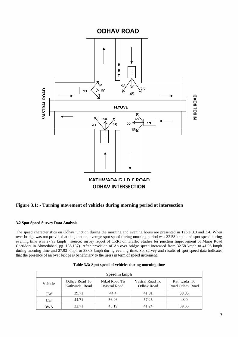
Figure 3.1: - Turning movement of vehicles during morning period at intersection

3.2 Spot Speed Survey Data Analysis

The speed characteristics on Odhav junction during the morning and evening hours are presented in Table 3.3 and 3.4. When

over bridge was not provided at the junction, average spot speed during morning period was 32.58 kmph and spot speed during

evening time was 27.93 kmph ( source: survey report of CRRI on Traffic Studies for junction Improvement of Major Road

Corridors in Ahmedabad, pg. 136,137). After provision of An over bridge speed increased from 32.58 kmph to 41.96 kmph

during morning time and 27.93 kmph to 38.08 kmph during evening time. So, survey and results of spot speed data indicates

that the presence of an over bridge is beneficiary to the users in term of speed increment.

Table 3.3: Spot speed of vehicles during morning time

Speed in kmph

Vehicle Odhav Road To

Kathwada Road

Nikol Road To

Vastral Road

Vastral Road To

Odhav Road

Kathwada To

Road Odhav Road

TW 39.71 44.4 41.91 39.03

Car 44.71 56.96 57.25 43.9

3WS 32.71 45.19 41.24 39.35

67

94

KATHWADA G.I.D.C ROAD

ODHAV INTERSECTION

BRTS

VA

STR

AL

RO

AD

NIK

OL

RO

AD

ODHAV ROAD

62

3 8

1147

1781

768 45

02

986

1572

4809 41

3 656

901 22

4

609 3

45

193

FLYOVER

8

LCV/HCV 31.51 44.46 41.23 27.88

Average 37.16 47.75 45.4 37.54

Table 3.4: Spot speed of vehicles during evening time

Speed in kmph

Vehicle Odhav Road To

Kathwada Road

Nikol Road To

Vastral Road

Vastral Road To

Odhav Road

Kathwada To

Road Odhav Road

TW 36.48 38.01 43.56 35.7

Car 39.97 46.23 37.42 34.77

3W 38.44 38.83 36.12 39.27

LCV/HCV 34.87 37.09 39.12 33.5

Average 37.44 40.04 39.05 35.81

3.3 Delay Data Collection

Delay survey was carried out during peak hour in the morning between 10:45 to 11:45 and 6:30 to 7:30 in the evening. Analysis

is summarized as shown in tables.

Table 3.5: Average delay at all leg per vehicle

Direction

Delay during total survey time (in seconds)

Morning Evening

From Vastral 101 100

From Odhav 83 82

From Nikol 96 100

From Kathwada 82 82

3.4 Economic Analysis

The Traffic volume at Odhav intersection was continuously increasing day by day prior to the ROB. Also there was tremendous

accident hazard during peak hour due to the heavy traffic in that area.

To overcome this problem an over bridge is constructed. In order to understand the impact of ROB on traffic condition as well

as on delay reduction, an attempt has been made to evaluate the cost and benefits in terms of reduction in fuel consumption and

travel time delay.

Analysis of collected data converts user travel time saving and fuel consumption into monetary terms. This has been done based

on the volume count and simultaneous delay survey carried out during total survey time of 3.5 hours during morning and

evening session.

There are two alternatives for evaluating performance of Odhav over bridge. One alternative is to compare it with the past

condition with present condition of traffic scenario at intersection and another alternative is to judge the effect on travel time

and fuel consumption saving if the over bridge would be constructed parallel to 200 feet ring road.

3.5 Analysis of data results

The following average occupancy for different modes as per observation. (Table 3.6)

Table 3.6: Vehicle Occupancy Table

Type of Vehicle Occupancy

TW 1.6

3W 2.4

Car 1.8

LCV 1.2

Bus 52

(Source: By an observation)

9

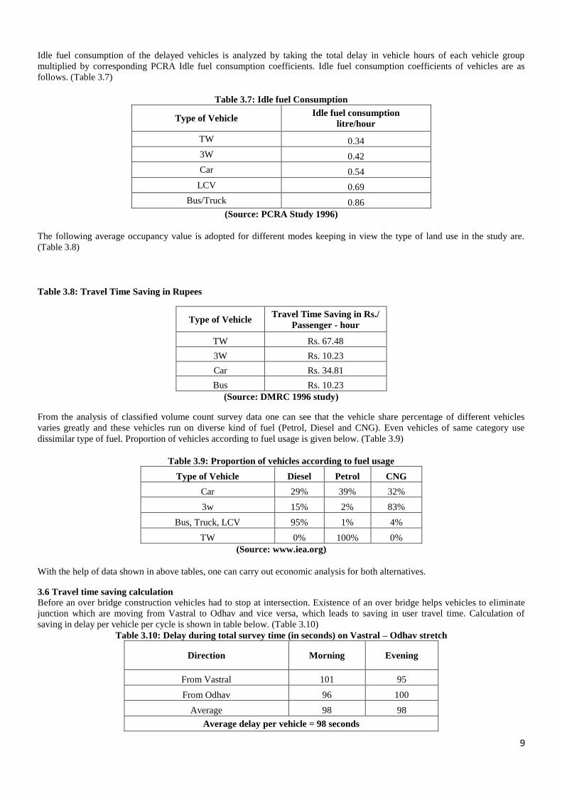
Idle fuel consumption of the delayed vehicles is analyzed by taking the total delay in vehicle hours of each vehicle group

multiplied by corresponding PCRA Idle fuel consumption coefficients. Idle fuel consumption coefficients of vehicles are as

follows. (Table 3.7)

Table 3.7: Idle fuel Consumption

Type of Vehicle Idle fuel consumption

litre/hour

TW 0.34

3W 0.42

Car 0.54

LCV 0.69

Bus/Truck 0.86

(Source: PCRA Study 1996)

The following average occupancy value is adopted for different modes keeping in view the type of land use in the study are.

(Table 3.8)

Table 3.8: Travel Time Saving in Rupees

Type of Vehicle Travel Time Saving in Rs./

Passenger - hour

TW Rs. 67.48

3W Rs. 10.23

Car Rs. 34.81

Bus Rs. 10.23

(Source: DMRC 1996 study)

From the analysis of classified volume count survey data one can see that the vehicle share percentage of different vehicles

varies greatly and these vehicles run on diverse kind of fuel (Petrol, Diesel and CNG). Even vehicles of same category use

dissimilar type of fuel. Proportion of vehicles according to fuel usage is given below. (Table 3.9)

Table 3.9: Proportion of vehicles according to fuel usage

Type of Vehicle Diesel Petrol CNG

Car 29% 39% 32%

3w 15% 2% 83%

Bus, Truck, LCV 95% 1% 4%

TW 0% 100% 0%

(Source: www.iea.org)

With the help of data shown in above tables, one can carry out economic analysis for both alternatives.

3.6 Travel time saving calculation

Before an over bridge construction vehicles had to stop at intersection. Existence of an over bridge helps vehicles to eliminate

junction which are moving from Vastral to Odhav and vice versa, which leads to saving in user travel time. Calculation of

saving in delay per vehicle per cycle is shown in table below. (Table 3.10)

Table 3.10: Delay during total survey time (in seconds) on Vastral – Odhav stretch

Direction Morning Evening

From Vastral 101 95

From Odhav 96 100

Average 98 98

Average delay per vehicle = 98 seconds

10

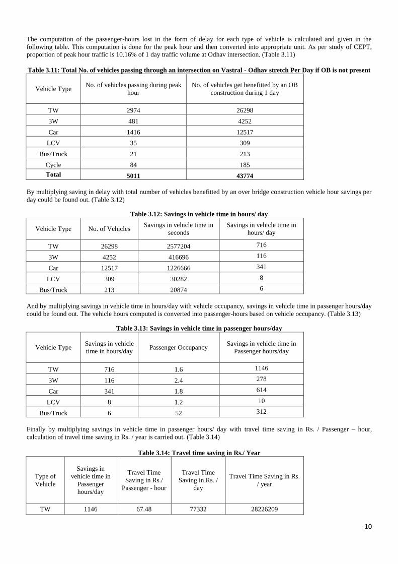
The computation of the passenger-hours lost in the form of delay for each type of vehicle is calculated and given in the

following table. This computation is done for the peak hour and then converted into appropriate unit. As per study of CEPT,

proportion of peak hour traffic is 10.16% of 1 day traffic volume at Odhav intersection. (Table 3.11)

Table 3.11: Total No. of vehicles passing through an intersection on Vastral - Odhav stretch Per Day if OB is not present

Vehicle Type No. of vehicles passing during peak

hour

No. of vehicles get benefitted by an OB

construction during 1 day

TW 2974 26298

3W 481 4252

Car 1416 12517

LCV 35 309

Bus/Truck 21 213

Cycle 84 185

Total 5011 43774

By multiplying saving in delay with total number of vehicles benefitted by an over bridge construction vehicle hour savings per

day could be found out. (Table 3.12)

Table 3.12: Savings in vehicle time in hours/ day

Vehicle Type No. of Vehicles Savings in vehicle time in

seconds

Savings in vehicle time in

hours/ day

TW 26298 2577204 716

3W 4252 416696 116

Car 12517 1226666 341

LCV 309 30282 8

Bus/Truck 213 20874 6

And by multiplying savings in vehicle time in hours/day with vehicle occupancy, savings in vehicle time in passenger hours/day

could be found out. The vehicle hours computed is converted into passenger-hours based on vehicle occupancy. (Table 3.13)

Table 3.13: Savings in vehicle time in passenger hours/day

Vehicle Type Savings in vehicle

time in hours/day Passenger Occupancy

Savings in vehicle time in

Passenger hours/day

TW 716 1.6 1146

3W 116 2.4 278

Car 341 1.8 614

LCV 8 1.2 10

Bus/Truck 6 52 312

Finally by multiplying savings in vehicle time in passenger hours/ day with travel time saving in Rs. / Passenger – hour,

calculation of travel time saving in Rs. / year is carried out. (Table 3.14)

Table 3.14: Travel time saving in Rs./ Year

Type of

Vehicle

Savings in

vehicle time in

Passenger

hours/day

Travel Time

Saving in Rs./

Passenger - hour

Travel Time

Saving in Rs. /

day

Travel Time Saving in Rs.

/ year

TW 1146 67.48 77332 28226209

11

3W 278 10.23 2844 1038038

Car 614 34.81 21373 7801269

LCV 10 10.23 102 37340

Bus/Truck 312 10.23 3192 1164992

Total

3,82,67,848 Rs.

3.7 Fuel consumption saving calculation

To find out money saving due to fuel consumption saving, first of all vehicles benefitted by an over bridge construction is to be

found out. Then from idle fuel consumption litre / hour and delay time saving, fuel consumption saving is calculated. Fuel

saving is then divided with respect to vehicle fuel usage type and multiplied by respective fuel price (as on date 14/05/2015).

(Table 3.15)

Table 3.15: Money saving in Rs. in 1 year

Vehicle

Type

No. of

Vehicles

benefitted by

an OB

construction

in 1 day

Fuel

saving

during 1

day in

litres

Saving

in

Petrol

(litre)

Saving

in

Diesel

(litre)

Saving

in

CNG

(kg)

Money

saving in 1

day as per

respective

fuel price

Money saving in

Rs. in 1 year

TW 26298 243 243 0 0 16164 5899860

3W 4252 49 1 7 41 2369 864685

Car 12517 184 72 53 59 10471 3821915

LCV 309 6 0 6 0 331 120815

Bus/

Truck 213 5 0 5 0 276 100740

Total

1,08,08,015 Rs.

3.8 Total money saving during 1 year

Summation of fuel consumption saving and travel time saving in rupees indicates total money saving during 1 year.

(Table 3.16)

Table 3.16: Total saving of money during period of 1 year

Sr. No. Saving Amount in Rs.

1 Travel Time Savings 3,82,67,848

2 Fuel Savings 1,08,08,015

Total 4,90,75,863 Rs.

4. Conclusion From the data supplied by AMC, the cost of the ROB construction was 20 crores in March 2013 while at present the savings as

per the alternative 1 comes out to be 4,90,75,863 Rs., which comes out to be about 24.5% of construction cost of ROB. For the

second alternative, parallel to 132 feet ring road the savings as per the present data comes out to be 7,66,15,843 Rs., which is far

more than the alternative 1 and it is also an effective solution for the intersection into the above case study. In this case

construction cost would be 34 crores (source: HCP feasibility report, September 2012) and saving would be about 22.5% of

construction cost of ROB. So as per ROR concern, 1st alternative is good option.

Study conducted at ODHAV intersection revealed that in the absence of an over bridge users were facing numerous problems

like congestion, delay, accident and air and noise pollution resulting in heavy economic losses.

At this place traffic studies were conducted to determine the traffic volume, spot speed and delay. From the collected data

economic analysis is carried out as well as impact of an over bridge on traffic characteristic is studied.

Following are the important observations from the surveys, study and analysis.

Total number of vehicles benefitted by an over bridge construction in one day are 43774

The reduction in the vehicle delay occurs even though the traffic volume increases after the over bridge construction at

Odhav intersection.

12

By implementation of an OB following indirect benefits are achieved.

The reduction in the vehicle delay has also made the benefit of improving the environmental degradation due to noise

as well as by air pollution.

Saving in cost of vehicle idling.

Increase in aesthetic of the area.

Increase in safety.

The accident hazards at level crossing are eliminated.

Increase in convenience and comfort of passengers.

4.1 Scope of Work

There are some areas which can be studied from the above research work.

Impact on accident cost

Impact on environmental characteristics

Impact on social characteristics

This analysis and study of data provide basic information for the work of similar type to be carried out in order to understand

and evaluate the similar type of transportation infrastructure project.

5. REFERENCES

[1] Jiang,Y.G. Zhaoand S. Li"An Economic Analysis Methodology for Project Evaluation and Programming"Publication

FHWA/IN/JTRP– 2013/17.JointTransportation Research Program, Indiana Department of Transportation and Purdue University, West

Lafayette, Indiana, 2013.doi:10.5703/1288284315219-2013. [2] Patel A. M. ―EconomicEvaluation for Proposed Highway Railway overBridge:ACase Study of Naroda RailCrossing‖ Vol.1,issue:

7, December 2012, ISSN No. 2277-8160, Pg.86-88-2012.

[3] Transport infrastructure project evaluation using cost-benefit analysis Heather Jonesa,*,Filipe Mouraa,Tiago Domingosb

Heather Jones et al.

[4] Prasnna Kumar S. M. and Mahajan S.K."Economical Applications of GPS in Road Projects in India"-13thCOTAInternational

Conference of Transportation Professionals (CICTP2013), Procedia-Social and Behavioral Sciences 96(2013)2800–

2810.doi:10.1016/j.sbspro.2013.08.31-2013.

[5]Economic Evaluation for Transportation Project Guideline ―Socio-Economic and Financial Evaluation OfTransportation

Project‖Ref.PT-2001-001-02IAPP-2010.

[6]Corotis R. B. "Highway User Travel Time Evaluation" Journal of Transportation

engineering,Vol.133,No.12,December1,2007.©ASCE,ISSN0733-947X/2007/12-663–669,DOI:10.1061/(ASCE)0733-

947X(2007)133:12(663)-2007

[7] Boadway R."The Economic Evaluation of Project" pg.1-51-1992.

13

Problems Occur During Construction of Pile Foundation of Flyover: A case

study of Bopal Flyover

Ram Dhankani, Tark Patel, Deep Amin, Varun Bhavsar, Rewati S. Marathe

[email protected],[email protected],[email protected],[email protected]

[email protected]

Civil Engineering Department, Silver Oak College of Engineering & Technology, Gujarat Technological University, India

Abstract Over bridges are the backbones of Indian Highways. The construction of over bridges involves various steps. The main

construction component is foundation. Considering different soil strata and requirement of superstructure different types of

foundation are constructed. Now a day‘s pile foundation is used all over. During construction many difficulties and problems

have to face. Our aim is to overcome such problems during construction of pile foundation and give their solution.

Keywords: Pile, Pile cap,Pile Foundation,Soil expansion, Flyover

1. Introduction Now a day‘s entire world is expanding at super-fast speed, in each and every corner of world, human kinds is expanding his

horizon in the field of construction. In today‘s world construction industry most required one of the growing. Infrastructure

development is increasing its importance day by day.

As transportation is main part of the life, so infrastructure development is must done without it is not possible for everyone to

carried out trade.

A Pile is a slender structural member made of steel, concrete, wood or composite material. A Pile is either driven into the soil or

formed in-site by excavating a hole and filling it with concrete.

Pile Foundation is the types of deep foundation. Casinos and Cofferdams are also types of deep foundation. But we focus on pile

foundation.

2. Industrial problem During our visit at construction site Bopal Junction Flyover, There are mainly two problems during construction of pile

foundation.

Obstruction of Water pipe line below the ground

Soil expansion problem

1.1 Obstruction of water pipe line below the ground

Figure: 1Problem of Water Pipe Line below the Ground

The water pipe line problem is occur at the far of the Bopal junction.Due to water pipeline problem in existing road is become a

major problem on site for construction of road and bridges.This is the basically an obstruction in pile foundation of a bridge and

main prospect is how to cover it with best economical trick/method to do it in regular time management of our project.





14

1.2 Soil expansion problem

Figure: 2 Soil Expansion/Shrinkage

Soil expands when water is added and shrinks when it dries out. This change in soil volume can cause shifting and cracking in

structures.These soils typically contain clay minerals that attract and absorb the water.Depending upon the supply of soggy in

the ground, Expansive soils will experience changes in volume of up to thirty percent or more. Foundation soils which are

expansive will ―heave‖ and can cause lifting of a building or other structure during periods of high humid. On the other hand

during periods of falling soil damp, expansive soil will ―collapse‖ and can result in building settlement. Although, damage can

be broad, in order for expansive soil to cause foundation problems, there must be fluctuations in the amount of wetness

contained in the foundation soils.

3. Solution for Problems

3.1 Solution of Water pipe line problem

Pile cap taken 2.5 m. Below Pipe.

Square pile cap is provided instead of rectangular pile cap.

Figure: 3Solution of Water Pipe Line below the Ground

3.2 Solution of soil expansion problem

For soil expansion problem, sand cushion method is suggested in our project.

15

Figure: 4 Solution of Expansive soil

Satya Narayana (1969) has suggested that the entire depth of the expansive soil layer or a part there of may be separate and

replaced with a sand cushion, compacted to the wanted density and thickness. Swelling pressure varies inversely as the thickness

of the sand stratum and straight as its density.

Therefore, usually sand cushions are shaped in their loosest possible state without, however, violating the bearing capacity

criterion. The sand cushion method has several limitations particularly when it is adopted in deep strata.

The mixture of sand and soft clayey soil is used as a cushion material.

4. Conclusion During the construction of pile foundation there are two major problems on our site such as Soil expansion and obstruction of

Water pipe line. The best solution for Bopal Flyover:

For obstruction of water pipe line, square pile cap is provided instead of rectangular pile cap at 2.5m below the ground.

For soil expansion problem, sand cushion method is suggested in our project.

5. References

[1] Bhattacharya Subhamoy & Bolton Malcolm ―Errors in design leading to Pile Failures during Seismic

Liquefaction‖2004.

[2] Bles Thomas et al ―A Risk Model for Pile Foundations‖2003.

[3] Murali Krishna et al. ―Seismic Design of Pile foundation for Different Ground Conditions‖2012.

[4] B. Surya Prakash Rao ―Geoelectrical investigations for flyover bridge construction in marine Environment of

Vishakhapatnam‖2005.

[5] Horne John & Kramer Steven ―Effects of Liquefaction on Pile Foundation‖1998.

[6] Satyamurthy Ranjan ―Investigations of Pile Foundations in Brownfields‖2005.

[7] Amiri Sharid Khan ―The Earthquake Response of Bridge Pile Foundations to Liquefaction InducedLateral Spread

Displacement Demands‖2008.

[8] Maheshwari BAL Krishna & Hiroyuki Watanabe ―Dynamic Analysis of Pile Foundations: Effects of Material Nonlinearity

of Soil‖2007.

[9]WEI Xiao et al. ―Damage Patterns and Failure Mechanisms of Bridge Pile Foundation underEarthquake‖2008.

[10] J. David Rogers and Robert B. Rogers ―Damage foundations from expansive soil‖2002.

[11]Eric P. Koehler & David W. Fowler ―Measuring the Workability of High Fines Concrete‖2003.

[12] Frank Rausche, Garland Likins and Mohammad Hussein): ―Design and Testing of Pile Foundation‖1998.

[13] http://www.designingbuildings.co.uk/wiki/Pile_foundations

[14] https://en.wikipedia.org/wiki/Pile_driver

[15]http://www.aboutcivil.org/types-classification-of-piles.html

http://www.aboutcivil.org/types-classification-of-piles.html

16

Design And Construction Of An Affordable Housing Scheme

Shruti Patel

[email protected]

Civil Engineering Department, Silver Oak College of Engineering & Technology, Gujarat Technological University, India

Abstract:- Autoclaved Aerated Concrete (AAC) is a light weight building material produced from the natural resources available all around

the world. It has several useful structural and architectural characteristics that make it a good choice for a wide variety of

structural application. This paper firstly presents the materials for production and properties of AAC. It has a good thermal

insulation and fire resistance in comparison with conventional concrete masonry unit. The production procedure and the

structural design methodology of AAC are then explained. No toxic material is produced during the manufacturing process and

energy consumption during production is less than that of some other building materials. Finally the applicability of AAC in the

Canadian construction industry is investigated.

Among the factors that make the design of AAC different than CMU, the two most import ones are: compressive strength and

tensile strength. In CMU, compressive strength is much higher than in AAC units. This will force some limitations in some

cases for AAC. On the other hand, tensile strength in CMU is lower than in AAC and this will make AAC a good choice for

some other cases as will be explained more in this section.

In this project we are performing a seismic check of the building and behavior of the building during earthquake. We are going

to compare the seismicity of a RC frame structure containing brick wall also known as CMU (Clay Masonry Unit) and AAC

Blocks (Autoclaved Aerated Concrete) using ETABS software.

Keywords: AAC Block, CMU (Clay Masonry Unit), ETABS software, G+14

1. Introduction As one of the oldest construction methods in human history, masonry has become a major competitor in modern construction.

The renewed interest in its practice around the world is largely due to its transformation from a brittle and fragile material to one

that can successfully endure dynamic loading from earthquake and wind forces. This construction technique underwent its first

measure modification since roman times with the introduction of reinforced concrete slab as floor and roof system in building

construction, allowing the formation of rigid structures. It became apparent that future improvements had to be made when the

after math of the long beach earthquake (California, USA) in 1933 revealed wide spread damaged to unreinforced masonry

structures(Casaubon, 2000). With the incorporation of steel reinforcement into walls, tensile resistance increased significantly.

These two advances, coupled with accessibility to quality, controlled masonry unit with increased compressive strength, enable

the construction of taller structures and reduction in wall thickness which substantially increased the efficiency of masonry

construction. Over the last 40 years in North America, and more recently in Latin American countries, renewed interest in

masonry has made this material the object of extensive research to understand its behavior, define its mechanical properties and

improve its safety and seismic performance. During this process, masonry expanded beyond its aesthetic applications into a

viable structural system that exhibits a greater degree of ductility.

2. OVERVIEW

2.1 Overview of ETABS: Structural Engineering is a science which understands behavior of various structures under different loads, analyzing and

designing these structures to withstand any/all anticipated loads.

A good structural engineer walks over a thin line between safety and economy. The role of a structural engineer today involves a

significant understanding of both static and dynamic loading, and the structures that are available to resist them. The complexity

of a modern structure often requires a great deal of creativity from the engineer in order to ensure the structures support and

resist the loads they are subjected to.

Analysis is the study of behavior of structure under different loads. There are three approaches to the analysis: strength of

materials, the elasticity theory approach, and the finite element approach. Matrix methods are more accurate method and they

tend to get complex with more number of structural elements.

Since the 1990s, specialist software has become available to aid in the design of structures, with the functionality to assist in the

drawing, analyzing and designing of structures with maximum precision; examples include AutoCAD, STAADPro, ETABS,

Prokon, Rivet Structure etc. such software may also take into consideration environmental loads, such as from earthquakes and

winds.

The structural system must also be designed to resist loading conditions associated with wind, seismic and live loads. Live loads

typically result from human occupants acting either as a seismic or dynamic load on the structures.

2.2 Overview of AAC:

In developing country masonry is still the most prevalent housing material, while a renewed interest in the developed world has

helped transformed this Asian system into an innovative engineering material with a variety of structural applications. Due to

17

the time-critical nature of the modern construction industry, there is a need to improve into traditional masonry constructions

which are labor and time intensives. The pursuit of this had led to the development of several nonconventional methods of

masonry construction, including a variety of mortar less systems.

Masonry performs simultaneous functions of carrying load and enclosing space, while possessing strong properties for fire

resistance, thermal and sound insulation and protection against environmental exposure. As a result, masonry is a cost effective

and low energy alternative when design appropriately. However, its main shortcoming is that its construction is slow and labor

intensive. Furthermore, conventional masonry construction, especially for smaller units, leads to a large number of mortar joints.

In order to limit the stresses induced in these joints during construction, the rate at which height of a wall increases in somewhat

restricted.

2.3 Overview of CMU: CMU has more density and it is very bulky. This will force some limitations in some cases for AAC.

3 AAC FEATURES

3.1 What is AAC? The autoclaved aerated concrete material was developed in 1924 in Sweden. It has become one of the most used building

materials in Europe and is rapidly growing in many other countries around the world.

Autoclaved aerated concrete is a light weight, load bearing, high insulating, durable building product which is produced in a

wide range of sizes and strengths.

AAC offers incredible opportunities to increase building quality and at the same time reduced cost at the construction site.

AAC is produced out of mixed of quartz, sand and/or pulverized Fly ash (PFA), lime, cement, gypsum, water and aluminum and

is hardened by steam curing in autoclaves. As a result of its excellent properties, AAC is used in many building constructions,

for example in residential homes, commercial and industrial buildings, schools, hospitals, hotels and many other applications.

The construction materials AAC contain 60% to 80% air by volume.

3.2 Advantages of AAC Excellent thermal insulation: AAC has very low thermal conductivity and therefore very light thermal energy efficiency is

achieved. This result is cost saving for heating and cooling

Lightweight: AAC possesses cellular structure creating during manufacturing process. Millions of tiny air cells impact AAC a

very lightweight structure. Density of AAC usually ranges between 550 to 650 kg/m3and hence is lighter than the water

Faster Construction: AAC is very easy to handle and can be cut and aligned using ordinary tools such as the drill, band saws,

etc. Moreover, AAC blocks can be produced in large variety of sizes, thus reducing the number of joints. This ultimately result

faster construction work as the installation time is significantly reduced due to fewer amount ofblocks. The masonry amount

involved is also lowered resulting in to reduced time-to-finish

Sound Insulation and Absorption: The porous structure of AAC result into enhanced sound absorption. Thus, AAC has been

the most ideal material of the construction of the walls in auditorium, hotels, hospitals, studios etc.

Environment Friendly: Energy consumed in the production process of AAC is only a fraction compared to the production of

other building material. The manufacturing process emits no pollutants and creates no by-products or toxic waste products. AAC

is manufactured from natural raw material. The finished product is thrice the volume of the raw material used, making it

extremely resource efficient and environment friendly

Perfect Size and Shape: The process of manufacturing AAC ensures constant and consistent dimensions. Factory finish AAC

provides a uniform base for economical application of variety of finishing systems. Internal walls can be finished by direct

P.O.P, thus eliminating the need of plastering

Superior fire resistance: Depending upon the thickness, AAC offer fire resistance for about 2 to 6 hours. AAC highly suitable

for the areas where fire safety of great priority

Earthquake resistance: The light weight property of AAC results into higher steadiness in the structure of buildings as the

impact of the earthquake is directly proportional to the weight of the building, construction done using AAC are more reliable

and safer

High compressive strength: AAC has an average compressive strength of (3 to 4.5) N/mm3 Which is superior as compared to

other light weight building material and 25% stronger than other products of the same density

High resistance to water penetration: AAC products possess cellular and discontinuous micro structure which resists water

penetrability superior resistance to moisture penetration than the traditional clay bricks

Paste resistance: AAC is an inorganic, insect resistant and solid wall construction material. Termites and ants do not eat or nest

in AAC products preventing/ avoiding damages or losses

Versatile: AAC has an attractive appearance and is readily adaptable to any style of architecture. Almost any design can be

achieved with AAC

Non-toxic: AAC products do not contain any toxic gas substances. The product does not harbor encourage vermin

18

Table 1.1 Comparison between AAC block and clay brick:

Parameter AAC Block Clay Brick

Structural cost Steel saving up to 15% No saving

Cement mortar for

plaster and masonry.

Required less due to flat, even surface and

less number of joint.

Required more due to irregular surface

and more number of joints.

Breakage Less than 5% Average 10% to 20%

Construction speed Speedy construction due to its big size, light

weight and easy to cut any size or shape.

Comparatively slow.

Quality Uniform and consistent Normally varies

Fitting and chasing All kind of fitting and chasing possible All kind of fitting and chasing possible

Carpet area More due to less thickness of walling

material

Comparatively low

Availability Any time Shortage in monsoon

Energy saving Approx. 30% reduction in air conditioned

load

No such saving

Chemical composition Sand/flash around 60 to 70% which react

with lime and cement to form AAC

Soil used contents many inorganic

impurities like sulphates etc. resulting

in efflorescence.

4. ETABS

Computer and structures, Inc. (CSI) is a structural and earthquake engineering Software Company found in 1975 and based in

Berkeley, California. The structural analysis and software CSI produce include SAP2000, CSiBridge, ETABS, SAFE,

PERFORM-3D, and CSiCOL. ETABS: Enhanced three dimensional Analysis of building system version 9.7.4.

In use for 30 years developed by computers and structures Inc. (CSI).ETABS is the ultimate integrated software package for the

structural analysis of design of buildings. Basic or advanced system under static or dynamic conditions may be evaluated using

ETABS. ETABS offers unmatched 3D object basic modeling and visualization tool, linear and nonlinear analytical power,

sophisticated and compressive design capabilities for a wide range of materials, and insightful graphic displace, reports, and

schematic drawing that allow user to quickly and easily decipher and understand analysis and design results.

ETABS provides unequal suite of tools for structural engineers designing buildings, whether they are working on one story

industrial structures or tallest commercial high rises. ETABS was used to create the mathematical model of the Burj Khalifa,

currently the world‘s tallest buildings, design by Chicago, Illinois-based Skidmore, owing sand Merrill LLP (SOM). Gravity,

wind, and seismic response were all characterized using ETABS.

From the start of design conception through the production of schematic drawings, ETABS integrates every aspect of the

engineering design process. Creative of models has never been easier-intuitive drawing commands allow for the rapid

generation o floor and elevation framing. CAD drawings can be converted directly into ETABS models or used as templates

onto which ETABS objects may be overlaid. The concept of special programmer for building type structures was introduced

over 30 years ago and resulted in the development of the ETABS series of computer programmer.

5. MODELING OF BUILDING USING ETABS

5.1 Modeling of structure using ETABS

The building is modeled using the software‘s ETABS nonlinear v9.7.4. Different elements of building are modeled as below.

Beams and Columns are modeled as two nodded beam elements with six degree of freedom at each node.

Slab is modeled as four nodded shell element with six DOF at each node for RCC and Membrane element for steel and

composite structure. Shell element has both in plane and out of plane stiffness while membranes element has only out of plane

stiffness.

19

5.2 Fixing of Member Size:

First of all building with RCC frame is modeled. Size of beam, column, slab and wall is chosen by normal practicing rule. Size

of AAC wall is taken similar to size of brick wall or composite wall i.e., ratio of elastic modulus of steel and concrete.

For composite structure same procedure is followed as above. 5.3 Stepwise Procedure for modeling of building using ETABS:

Step 1: Define storey data like storey height, no of storey etc.

Step 2: Select Code preference from option and then define material properties from define Menu

Step 3: Define Frame Section from Define menu like column, beam

Step 4: Define slab section

Step 5: Draw building Elements from draw menu

Step 6: Give support conditions

Step 7: Define load cases and load combinations

Step 8: Assign load

Step 9: Define mass Source

Step 10: Give structure auto line constraint

Step 11: Give renumbering to the whole structure

Step 12: Select analysis option and Run analysis

5.4 Modeling of Building for current problem in ETABS:

Concrete of grade M25 and M35 and steel of Fe 415 grade are taken. Material properties are assigned as shown in

fig. 5.1 and fig.5.2.

Fig. 5.1: Material Property Data Fig. 5.2: Material Property Data

The design of the structural members like beam and column is as shown in fig 5.3 and fig 5.4

20

Fig. 5.3: Design of structural member column

Fig. 5.4: Design of structural member beam

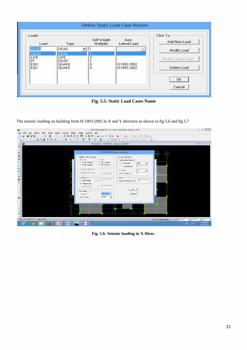
For loading purpose live load, dead load is applied as area load while wall load is applied as line load. Earthquake load is

applied as per IS 1893-2002. For defining load only once in dead load case self-weight multiplier is taken one. Application of

various loads including seismic loads is shown here in fig. 5.5. Table shows load cases on building while using brick masonry

and AAC blocks. All loads are in kN/cu. M

Table 5.1 Load cases on building

Load Case Brick Masonry AAC Blocks

Dead Load 1 1

Live Load 3 3

Floor Finish 1 1

Earthquake Force in X As Per IS: 1893-2000 As Per IS 1893-2000

Earthquake Force in Y As Per IS 1893-2000 As Per IS 1893-2000

Wall Load 9.8 3.43

21

Fig. 5.5: Static Load Cases Name

The seismic loading on building from IS 1893:2002 in X and Y direction as shown in fig 5.6 and fig 5.7

Fig. 5.6: Seismic loading in X-Direc.

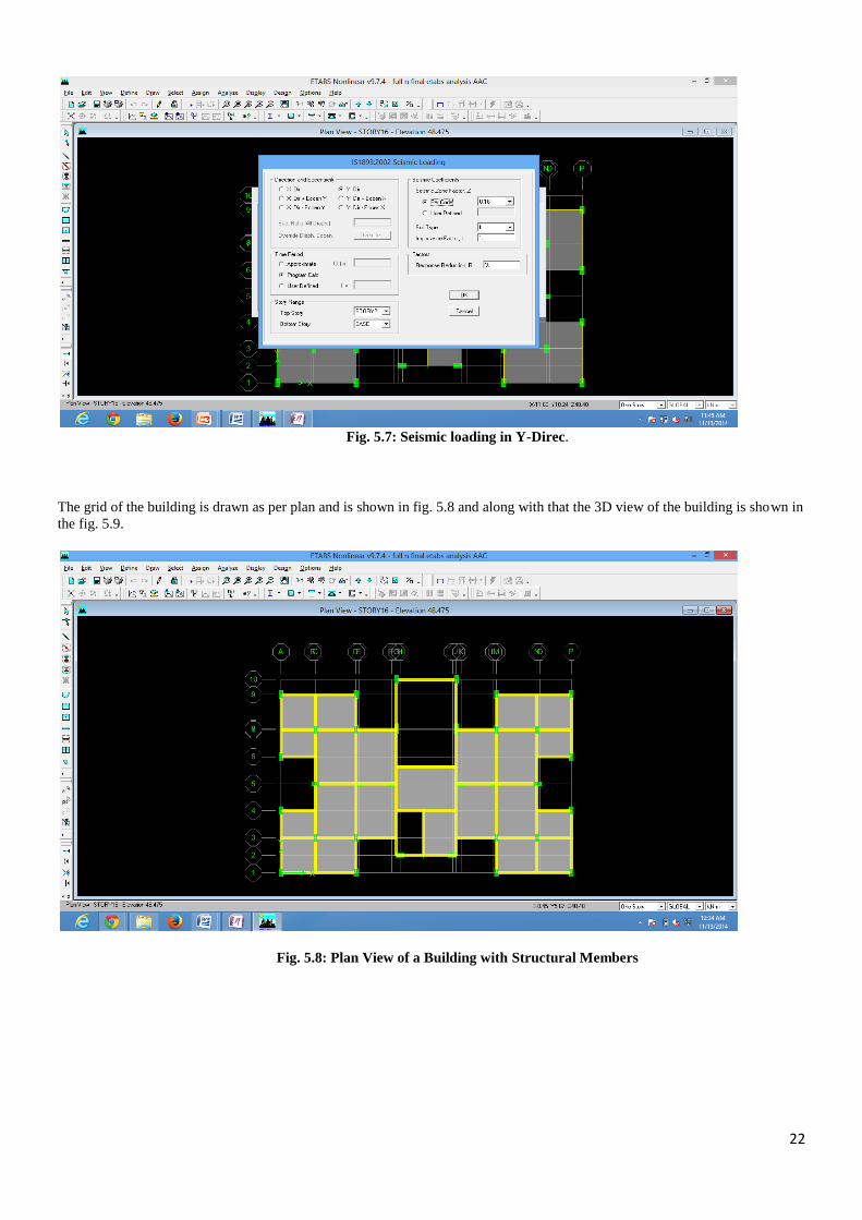
22

Fig. 5.7: Seismic loading in Y-Direc.

The grid of the building is drawn as per plan and is shown in fig. 5.8 and along with that the 3D view of the building is shown in

the fig. 5.9.

Fig. 5.8: Plan View of a Building with Structural Members

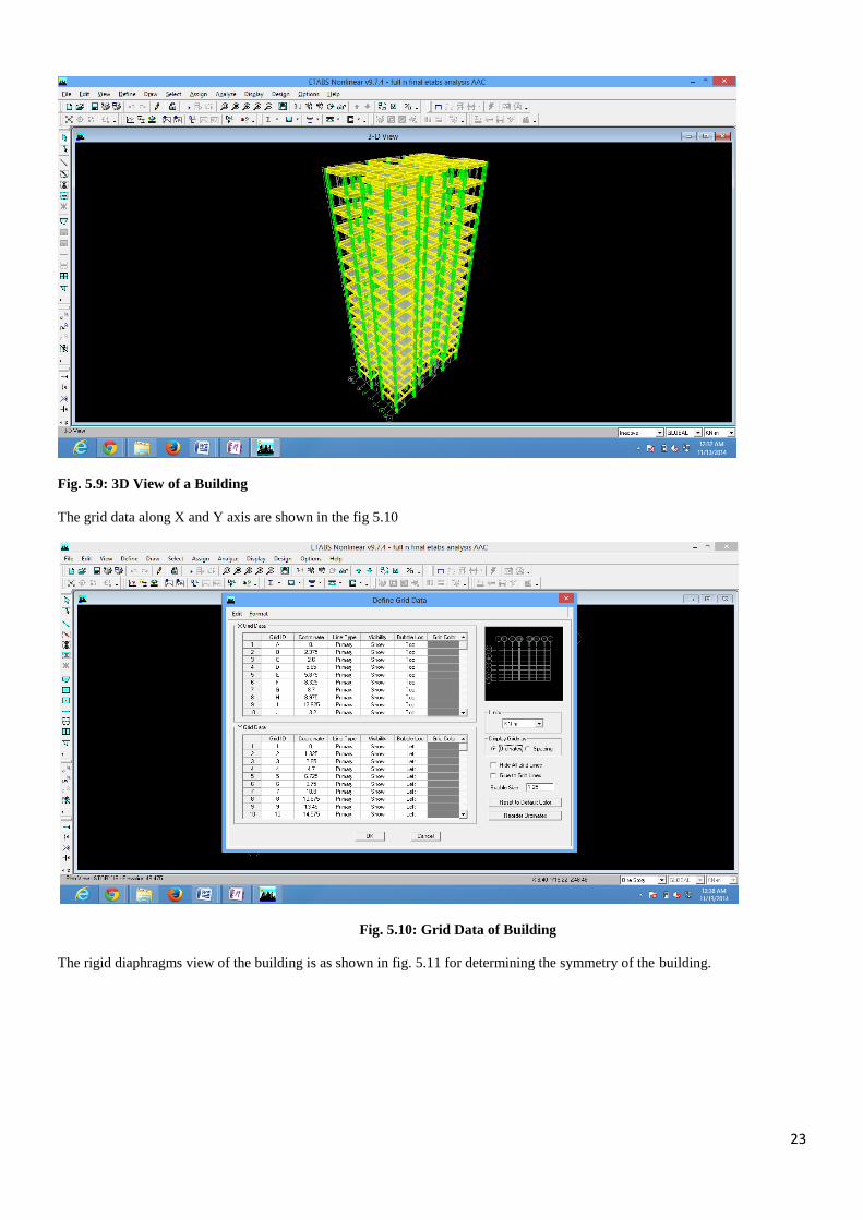
23

Fig. 5.9: 3D View of a Building

The grid data along X and Y axis are shown in the fig 5.10

Fig. 5.10: Grid Data of Building

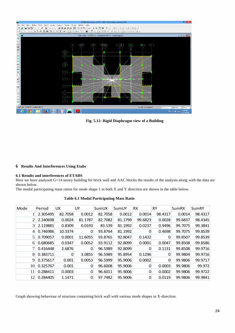
The rigid diaphragms view of the building is as shown in fig. 5.11 for determining the symmetry of the building.

24

Fig. 5.11: Rigid Diaphragm view of a Building

6 Results And Interferences Using Etabs

6.1 Results and interferences of ETABS

Here we have analysed G+14 storey building for brick wall and AAC blocks the results of the analysis along with the data are

shown below.

The modal participating mass ratios for mode shape 1 in both X and Y direction are shown in the table below.

Table 6.1 Modal Participating Mass Ratio

Mode Period UX UY SumUX SumUY RX RY SumRX SumRY

1 2.305495 82.7058 0.0012 82.7058 0.0012 0.0014 98.4317 0.0014 98.4317

2 2.240698 0.0024 81.1787 82.7082 81.1799 99.6823 0.0028 99.6837 98.4345

3 2.119881 0.8309 0.0193 83.539 81.1992 0.0237 0.9496 99.7075 99.3841

4 0.746986 10.3374 0 93.8764 81.1992 0 0.4698 99.7075 99.8539

5 0.709057 0.0001 11.6055 93.8765 92.8047 0.1432 0 99.8507 99.8539

6 0.680685 0.0347 0.0052 93.9112 92.8099 0.0001 0.0047 99.8508 99.8586

7 0.416448 2.6876 0 96.5989 92.8099 0 0.1131 99.8508 99.9716

8 0.383711 0 3.0855 96.5989 95.8954 0.1296 0 99.9804 99.9716

9 0.375617 0.001 0.0053 96.5999 95.9006 0.0002 0 99.9806 99.9717

10 0.325767 0.001 0 96.6008 95.9006 0 0.0003 99.9806 99.972

11 0.288411 0.0003 0 96.6011 95.9006 0 0.0002 99.9806 99.9722

12 0.284405 1.1471 0 97.7482 95.9006 0 0.0119 99.9806 99.9841

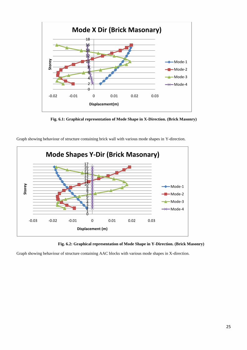
Graph showing behaviour of structure containing brick wall with various mode shapes in X-direction.

25

Fig. 6.1: Graphical representation of Mode Shape in X-Direction. (Brick Masonry)

Graph showing behaviour of structure containing brick wall with various mode shapes in Y-direction.

Fig. 6.2: Graphical representation of Mode Shape in Y-Direction. (Brick Masonry)

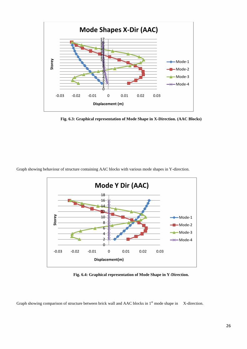
Graph showing behaviour of structure containing AAC blocks with various mode shapes in X-direction.

0

2

4

6

8

10

12

14

16

18

-0.02 -0.01 0 0.01 0.02 0.03

Sto

rey

Displacement(m)

Mode X Dir (Brick Masonary)

Mode-1

Mode-2

Mode-3

Mode-4

0123456789

1011121314151617

-0.03 -0.02 -0.01 0 0.01 0.02 0.03

Sto

rey

Displacement (m)

Mode Shapes Y-Dir (Brick Masonary)

Mode-1

Mode-2

Mode-3

Mode-4

26

Fig. 6.3: Graphical representation of Mode Shape in X-Direction. (AAC Blocks)

Graph showing behaviour of structure containing AAC blocks with various mode shapes in Y-direction.

Fig. 6.4: Graphical representation of Mode Shape in Y-Direction.

Graph showing comparison of structure between brick wall and AAC blocks in 1st mode shape in X-direction.

0123456789

1011121314151617

-0.03 -0.02 -0.01 0 0.01 0.02 0.03

Sto

rey

Displacement (m)

Mode Shapes X-Dir (AAC)

Mode-1

Mode-2

Mode-3

Mode-4

0

2

4

6

8

10

12

14

16

18

-0.03 -0.02 -0.01 0 0.01 0.02 0.03

Sto

rey

Displacement(m)

Mode Y Dir (AAC)

Mode-1

Mode-2

Mode-3

Mode-4

27

Fig. 6.5: Graphical representation of Mode Shape Comparing (Brick Masonry & AAC Blocks) in X-Direction.

Graph showing comparison of structure between brick wall and AAC blocks in 1st mode shape in Y-dirc.

Fig. 6.6: Graphical representation of Mode Shape Comparing (Brick Masonry & AAC Blocks) in Y-Direction.

7. Conclusion

From the above project we concluded that the construction joint gap of 200 mm that is provided between two buildings is

sufficient. The building will deflect from its original position under the deflection of Earthquake force. Here we have seen that

the stability and stiffness of Brick masonry structure is more as compared to the AAC Blocks structure because the mass of the

brick structure is large as compared to the AAC block structure which affects the flexibility of the structure. But still even

though AAC blocks due to its due advantages of light weight, less material consumption, heat resistant properties etc. it is a far

better material that can be used in the construction industry. Also it helps in reducing cost of construction and time of

construction. By using ETABS software to perform seismic analysis of a RC frame structure we concluded that the deflection of

the structure is under the desired range that is set as a minimum criteria for minimum spacing between two structures.

8. REFERENCES

[1]U. H. Varnayi second edition of ―Design of Structures‖

[2]S.K. Duggal ―Earth quake resistant design of structures‖ pg. no: 305 on flexural strength 8.14.1 case 1 & 2

[3]H J Shah in his ―Advanced Concrete Design‖ Vol 1 & 2

[4]S B Junarkar in his ―Mechanics of Structure‖

0

5

10

15

20

0 0.005 0.01 0.015 0.02 0.025

Sto

rey

Displacement(m)

1st Mode X Dir (Comparison Brick & AAC)

Brick

AAC

0123456789

1011121314151617

0 0.005 0.01 0.015 0.02 0.025

Sto

rey

Displacement (m)

1st Mode Shapes Y-Dir (Brick Masonary)

Brick

AAC

28

[5]IS Code 456-2000:1993

[6]IS Code 456:2000

[7]IS Code 1893IS Code 875 Part-1

[8]IS Code 875 Part 2IS Code 875 Part-3

[9]Matthys, J. and Barnett, R. ―New Masonry Product for the US Designer Emerges - Autoclaved Aerated Concrete Structures‖

2004: pp. 1-11. Doi: 10.1061/40700(2004)109-2004.

[10]Hamed, E. and Rabinovitch, O. ―Lateral Out-of-Plane Strengthening of Masonry Walls with Composite Materials.‖J.

Compos. Constr., 14(4), 376–387. Volume 14, Issue 4-2010.

[11]Tena-Colunga, A. and Martínez-Becerril, L―Approximations of Lateral Displacements of Reinforced Concrete Frames with

Symmetric Haunched Beams in the Elastic Range of Response Using Commercial Software‖ Pract.Period.Struct.Des. Constr.,

18(2), 92–100.Volume 18, Issue 2-May 2013.

[12]Warszawski, A., Gluck, J., and Segal, D. (1996). ―Economic Evaluation of Design Codes—Case of Seismic Design.‖ J.

Struct. Eng., 122(12), 1400–1408. Volume 122, Issue 12-1996.

29

Minimizing Driving Constraints with Respect to the Driving seat of a Car

and Accessibility to the overall Dashboard

Ajinkya Ratnaparkhi, Kannan Srinivasan

VIT University, Chennai-600127, Tamilnadu

[email protected], [email protected]

Abstract –

With the increasing dependability on one‘s private vehicle it is likely that the future adaptations in ‗car‘s driving seat design‘

will be linked in some part to the physical infirmities often faced by the car driving population. This paper offers a bridge

between the conventional design followed almost in all cars and the design which is comfortable mainly for the elderly driving

people.

In this work, a questionnaire was prepared consisting of questions related to car seat, human body parts, accessibility to

dashboard and ‗entry and exit‘ of the car. Based on the responses received, statistical analysis was done. A five-point scale is

used to access the comfort of the driver. The validity of the questionnaire was checked with the help of Cronbach Alpha test.

The correlation studies were performed to understand the correlation between

1. Age and comfort score

2. BMI and comfort score

3. Body segments and comfort score

4.

Keywords - Car Seat Design, Driving constraints, Ergonomic considerations, Car Seat comfort, BMI, Cronbach alpha,

correlation coefficient, Comparison of comforts for different cars, seating system.

I. INTRODUCTION Currently in India, whenever the ergonomic considerations in car seat design are focused on, the age group targeted is

of young drivers. But, a considerable segment of population is elder drivers (above 50 yrs of age). At this age, major changes

take place in a person with respect to its anatomy, physique and psychology. All these changes prove responsible in variable

extents for a poor driving experience.

Due to rapidly changing lifestyle, the number of such elder drivers will go on increasing every year. Thus, it is much

needed to that we take them into account whenever we design the car‘s driving seat. This will ensure a design which is suitable

for both, young as well as the old population. 1.1. LITERATURE REVIEW

As the name suggests, it explains about the driving hindrances faced by the elder population usually above 50 years of

age. Thus, a firm relationship has to be established between the ages, BMI, comfort level, ergonomy etc. For this each aspect has

to be viewed with different perspectives. We referred several papers for entire study and a few out of those prominently

dominated our research. The Research papers include wide variety and mainly can be classified as follows:

1. Papers related to human factors

2. Papers related to ergonomy in particular

3. Papers related to design aspect of car

4. Papers related to general and allied aspects of the concerned study

2. METHODOLOGY As the study is directly related to the customer end, it is mandatory that the feedbacks of the owners or drivers of the

cars have to be recorded.

A questionnaire designed and developed for the same. The questionnaire consists of the questions related to different

parts of a human body, either directly or indirectly. From the observer‘s perspective, the human body had to be divided into

three main segments i.e. Upper body, Back and Lower body. This made the further analysis easy. To include the car design

aspect, the existing system design of the parts included in our study had to be examined. This study allows knowing the

modifications required in the car seat design and dashboard accessibility. Further, the system which is studied had to be analysed

scientifically and statistically to make it as a concrete base to arrive at conclusions. The questionnaire needed to be checked for

reliability with the help of some techniques. In this study, ‗Cronbach Alpha test‘ was used. This step justifies the statistical

approach of the study. As a part of the results achieved from the calculations, certain comfort scores of each user were obtained.

Further, a relation between BMI and age, age and comfort were established and results were plotted graphically.



30

3. DATA COLLECTION

To implement the changes in the existing design of the car seat, it is necessary on engineer‘s part that he/she must examine the

existing design in depth. For this purpose, one must know the experiences of the people who drive at least one vehicle regularly

enough to sense the difficulties with reference to comfort while driving.

The real time data or precisely the ‗responses‘ of the driving population can be collected in many ways or many sources, but the

most effective method being the Questionnaire-method wherein several questions pertaining to various aspects of the car yet

affecting the comfort of the users to different extents, can be covered.

The questionnaire on the basis of the body parts and car design aspects was hence designed. It consisted of 18-questions and has

covered almost all the human and car related aspects. 3.1. CHECKING THE RELIABILITY OF THE QUESTIONNAIRE

Once the questionnaire is prepared it is mandatory to prove mathematically that it is reliable. Statistically, there are many ways

to achieve this but the easiest and yet efficient way to prove it was chosen. Thus, the questionnaire was put through a test called

Cronbach Alpha test, and fairly good results after few modifications in the questionnaire are obtained. As per the test conducted,

70% reliability on the questionnaire was obtained. To get maximum responses, it was developed into a format of ‗Google form‘

and was floated on social networking platforms. Besides, various taxi stands in Chennai were visited to get responses of the full

time drivers. The locations included Airport taxi stand, Tambaram and Chennai central. We got 103 responses in all from

various age groups, different physiques (BMI), different lifestyles etc. These included 42 full-time drivers and rest included

students, office-going class etc.

PARAMETER READING

Sum of Variances 22.686

Number of Variances 14

Cronbach‘s Aplha 0.70

SEM 4.41

Alternative SEM 4.41

SEM* 4.76

Table 1: Cronbach Alpha test for 25 Users and 18 Questions

3.2. QUANTIFYING THE DATA The data available was in text format and mainly opinion based. For further statistical calculations, the data ought to

be a numeric value. Thus, different scores were assigned to the responses received, in a proportionate manner. For eg. If the

response for a particular parameter say ‗high‘, then it was assigned score of 5 and if it had reading low then it was assigned the

score 1. After assigning the scores, the mean had to be calculated for each body segment and each different type of car, as it is

cumbersome and unproductive to calculate each data individually.

Fig. no.1: Dividing human body into segments

3.3. PLOTTING THE DATA GRAPHICALLY The data obtained was plotted graphically to enhance clarity about the variance and other parameters.

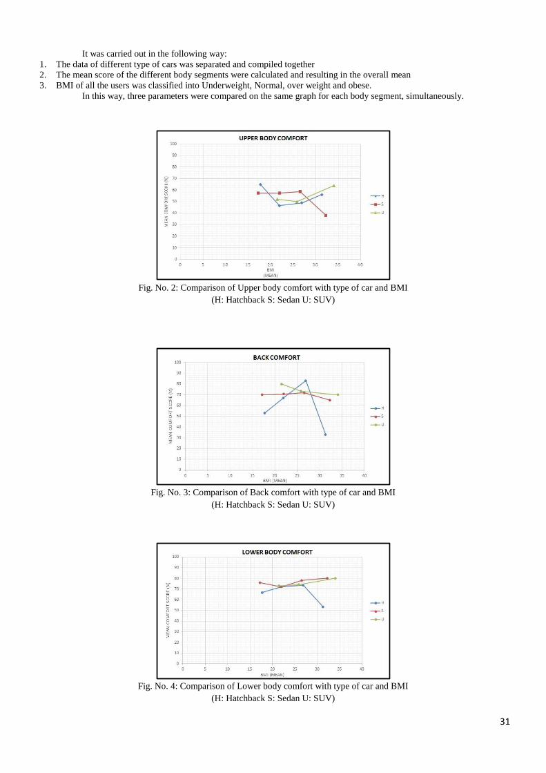
31

It was carried out in the following way:

1. The data of different type of cars was separated and compiled together

2. The mean score of the different body segments were calculated and resulting in the overall mean

3. BMI of all the users was classified into Underweight, Normal, over weight and obese.

In this way, three parameters were compared on the same graph for each body segment, simultaneously.

Fig. No. 2: Comparison of Upper body comfort with type of car and BMI

(H: Hatchback S: Sedan U: SUV)

Fig. No. 3: Comparison of Back comfort with type of car and BMI


Fig. No. 4: Comparison of Lower body comfort with type of car and BMI


32

Fig. No. 5: Comparison of Overall mean comfort of body segments with type of car and BMI


3.4. OBSERVATIONS POST GRAPHICAL REPRESENTATION After plotting the graphs shown in fig. no.2, fig. no.3, fig. no.4, fig. no.5, following observations were made:

1. For higher BMI values, Upper body comfort varies closely for hatchback and SUVs whereas it varies widely for

sedan and either of the other types.

2. For different values of BMI, back comfort changes steeply for hatchback type and are most comfortable at BMI

value of 27, whereas for SUV and sedan, change in BMI values does not result in appreciable change in back

comfort.

3. For different values of BMI, the line of sedan and hatchback type follows approximately a straight line with minor

variations for lower body comfort. For SUV type the lower body comforts decreases steeply after certain BMI

value (27).

4. For different values of BMI, the overall body comfort varies widely for SUV type whereas for the other two types

it is more or less the same.

3.5. ESTABLISHING THE RELATIONSHIP BETWEEN THE BMI AND THE COMFORT SCORE

BMI is the parameter that influences ergonomic consideration to a greater extent. Thus, it goes without saying that it

affects the comfort level of any person driving the car. But, again it has to be proven that the variances we get fit approximately

in single line (Regression analysis) and also that BMI and comfort is correlated (Correlation analysis).

df SS MS F Significance

Regression 1 8.456 8.456

5 0.04509

Residual

12

20.291 1.690

Total 13 28.747

Table 2: Regression analysis

Mean comfort

score

BMI

Mean comfort score 1

BMI 0.576 1

Table 3: Correlation analysis

33

4. CONCLUSION Hence, it has been proved that the comfort with respect to the driving seat of the car for the person seated in it is

affected majorly by his/her BMI (Body Mass Index), Type of usage, Age and Type of car. Moreover, it also means that the

design of the seats available currently in the market is not universally efficient and needs to be revised.

FUTURE SCOPE OF WORK This paper talks about the statistical analysis of the driving activity and factors related to it that influence the comfort.

However, to propose the changes in the design of the driving seat in a more rigid format, modeling of the same is necessary.

Besides, the type of changes required to be made need to be chosen wisely between mechanical or electronic in order to

maintain economy-performance balance.

5. REFERENCES

[1]Smith, DannionR.Andrews, David M.Wawrow, Peter T.,‘Development and evaluation of theAutomotive Seating Discomfort

Questionnaire (ASDQ)‘International Journal of Industrial Ergonomics, 2006.

[2] Leonardis, Doreen M De Ferguson, Susan a Pantula, Janella F, ‗Survey of Driver Seating Positions in Relation to the

Steering Wheel‘, 2000

[3] Prasad Kumbhar, PeijunXu, James Yang, ‗Evaluation of Human Body response for different vehicle seats using multibody

Biodynamic Model‘, SAE international, 2013.[4] Park, Se-jin,Lee, Jung-woo, Kim, Jin-sun, ‗Seating Physical Characteristics

and Subjective Comfort : Design Considerations‘, SAE International

[5] Kyung, Gyouhyung Nussbaum, Maury a. Babski-Reeves, Kari, ‗Driver sitting comfort and discomfort (part I): Use of

subjective ratings in discriminating car seats and correspondence among ratings‘, International Journal of Industrial Ergonomics,

2008.

[6] Andreoni, Giuseppe Santambrogio, Giorgio C. Rabuffetti, Marco Pedotti, Antonio, ‗Method for the analysis of posture and

interface pressure of car drivers‘, Applied Ergonomics, 2002.

[7] Jain, RavindraPandey, Rachit, ‗A Study on the Role of Body Posture on Static Seating Comfort, 2009.

[8] Res, Korea Park, Se Jin Min, Seung Nam Subramaniyam, Murali Lee, Dong-hoon Lee, Heeran Kim, Dong Gyun, ‗Analysis

of Body Pressure Ratio for Evaluation of Automotive Seating Comfort‘, 2014.

[9] Demontis, Salvatore Giacoletto, Monica, ‗SAE TECHNICAL Prediction of Car Seat Comfort from Human-Seat Interface

Pressure Distribution‘, 2002.

[10] Bove, Robert T Fisher, Jacob L Ciccarelli, Lauren Ii, Robert S Cargill Moore, Tara L a, ‗The Effects of Anthropometry on

Driver Position and Clearance Measures, 2006.

[11] Kolich, Mike, ‗Automobile seat comfort: Occupant preferences vs. anthropometric accommodation, Applied Ergonomics,

2003.

[12] Oudenhuijzen, Aernout Tan, Koen, ‗The Relationship between Comfort and Knee Angles‘, 2013

34

A Review of Thermal Effects on the IC Engine Exhaust Valve for Design

Optimization

Karan Soni, Ripen Shah, Umang Vora

[email protected],[email protected],[email protected]

Mechanical Engineering Department, Silver Oak College of Engineering & Technology, Gujarat Technological University,

India

Abstract:-

Exhaust valves are utilized in 4-stroke internal combustion engines to allow the exhaust gases to escape into the exhaust

manifold. Due to the exposure to high temperature gases, exhaust valve design is of a crucial interest. Apart from high thermal

stresses, these valves are also exposed to cyclic mechanical stresses during opening and closing, causing them to fail

prematurely. As such, factors such as temperature, fatigue life, material strength and manufacturing processes are to be

considered in order to design a valve that operates without premature failure. The use of modern computational techniques such

as finite element analysis is extremely beneficial to evaluate and optimize the engine valve design, requiring least amount of

development time. The objective of this review is to figure out the potential parameters that affect the valve design and possible

ways to eliminate them. There has been significant research already done in the areas of material, fatigue strength and thermal

effects for exhaust valves which are reviewed here and served as a reference to identify and define the problem.

Keywords: Engine Exhaust Valve, Thermal Analysis Exhaust Valve, Finite Element Analysis, Design Optimization.

1. Introduction

Modern engines are required to perform well under critical loading conditions and also ensure least environmental

footprints. This requires the engine to be downsized and at the same time provide equal output. As such, design optimization is a

key driver towards sustainable design of the engine and its components. Since the role of the exhaust valve is to allow the

exhaust gases to escape from the engine cylinder, it has a prominent role in engine performance. A poorly designed exhaust

valve can fail prematurely due to high temperature fatigue effects, and increase exhaust emissions. There are several factors on

which the exhaust valve design is based upon; studying those can help in devising an exhaust valve that can perform its tasks

better. Numerous research works have been carried out to study and optimize the design of exhaust valves using finite element

methods. The use of this technique is increasingly becoming common among design engineers, as it significantly reduces the

number of physical test trials required.

2. General Review

Singaiah Gali et al. [1] designed an exhaust valve for a four cylinder diesel engine using theoretical calculations and later

performed structural and thermal analysis based on steady state conditions. Material optimization was undertaken considering

EN52 and EN59 materials. Based on the material properties and exhaust temperature data, thermal analysis using ANSYS

Mechanical was performed. Information such as temperature contour, thermal flux and thermal stresses were plotted to identify

critical regions in the valve geometry.

Based on the thermal analysis, the best suitable material for the valve was identified considering good chemical and physical

properties such as hot forming temperature, thermal conductivity, specific heat capacity & co-efficient of thermal expansion.

35

Fig.1 Contour Plot Thermal Stresses Fig.2 Thermal Flux

Goli Uday Kumar et al. [2] performed failure analysis of internal combustion engine valves using ANSYS. Their research is

focused on different failure modes of internal combustion engine valves such as failure due to fatigue, high temperature effects,

and impact load that depends on load and time. For the study of fatigue life, a combined S-N (max. stress v/s number of cycles)

curve was prepared, which helped in comparing the fatigue failure for different materials at different high temperatures. For

achieving these goals, couple –field, fatigue and transient analysis were performed on valves to determine structural and thermal

behavior in working condition.

Fig.3 Stress values after 5000 cycles Fig.4 S-N Curve (5000*1e7 loading cycles)

The findings from the paper conclude that valve with Mg alloy fin is the right choice for maximum life.

V. Bala Sundaram [3] performed coupled field (structural-thermal) analysis on exhaust valves made up of different materials.

In this study, the steady state thermal analysis of the exhaust valve for the different materials such as 21 4N, Nimonic 80A and

Nimonic105A have been performed. ANSYS software is applied to the steady state thermal analysis problem with outer and

inner surface temperature as thermal boundary conditions. To obtain the simulation of thermal behavior appearing in different

valve material, the basic governing equation for the heat conduction is solved with the initial boundary conditions with thermal

conductivity as the property is solved for the two materials. It is evident from the analysis, the best material for the valve is

Nimonic105A as far as thermal and structural behavior is concerned.

Ram MS [4] found that modifying the exhaust valve by varying its position size and shape and with particular thermal and

structural considerations, helps in increasing the rate of heat transfer from the seat portion of the exhaust valve, thereby reducing

the possibility of knocking. In addition, the increased size of the exhaust valve pushes large amount of exhaust gas outside

through the manifold which reduces the dilution inside the engine‘s combustion chamber. The reduced dilution reduces the

amount of unburnt mixture/charge inside the chamber which reduces the hydrocarbon emissions coming out of the engine. The

reduced emissions help in development of the emission standards. Reduction in unburnt fuel inside the chamber results in

increased power with less consumption of fuel thereby increasing its fuel efficiency. Large amount of gas escapes due to larger

size of the exhaust valve and hence the heat energy coming out will be more which can be completely utilized for turbochargers

thereby increasing its turbine efficiency.

The measurements of the exhaust valve of Hero Honda CD100 are taken and the modifications are made. Exhaust Seat

Diameter is 2 centimeters and the length of the stem is 66 centimeters. The diameter is modified to 2.35 centimeters (inlet

36

valve‘s diameter of the same vehicle) and length is same. Due to the increase in cross sectional area and increase in thermal

conductivity, the rate of heat transfer is increased which in turn reduced the hot spot- high temperature region on the valve seat

there by reducing knocking possibilities.

Fig.5 Nodal analysis for large E.V. Fig.6 Nodal analysis for small E.V.

Naresh Kr. Raghuvanshi et al [5] identified possible causes of valve failure by considering different materials, effects of high

temperature, corrosion and wear. From their study, it is found that the predominant cause of failure of valves of internal

combustion engine is fatigue. The valves are subjected to high temperature, cyclic loading, impact loading, erosion-corrosion

and high pressure inside the cylinder, thus making it critically important to know about fatigue under these conditions.

Thet T. Mon et al. [6] utilized simplified finite element model of spark ignition engine to analyze combustion heat transfer.

Finite element model of the gasoline SI engine was developed in general-purpose FE code. The model was simplified into 2D

geometry with its computational domain comprising one cylinder and its major components including combustion chamber,

water jacket, piston head, cylinder head with inlet/outlet manifolds, and intake/exhaust valves. The finite element prediction has

indicated that thermal effect in the combustion chamber is influenced by major parameters such as combustion flame

temperature, convection of cooling system, and thermal properties of engine component materials. Apparently, the choice of

material for part component in the combustion chamber is one of the solutions in order to improve engine performance and

efficiency. In addition, the geometry and dimension of the engine parts also can be considered in order to improve the engine

performance.

C. M. Sonsino [7] presented basic relationships concerning the fatigue behavior of the structural Al2O3 and Si3N4 ceramics

and subsequently described the fatigue design of Si3N4 intake and exhaust valves. It has been observed that up to 1000 °C the

static and fatigue strengths of structural ceramics like Al2O3 and Si3N4 are not affected by temperature. However, at

temperatures above 1000 °C, the softening of the glass phase decreases the fatigue strength.

The paper also presented the design methodology for Si3N4 intake and exhaust valves to gain advantages over conventional

steel valves such as: Weight reduction by about 60%, Improvement of valve dynamics and valve train efficiency by about 20%,

Smoothing of engine torque behavior by changing the cam profile ,increasing the valve acceleration as well as the volumetric

efficiency and Saving of fuel consumption by 3–4% and reduction of CO emission by 20%.

Ajay Pandey et al. [8] discussed failures of automobile valves due to the effect of high temperature in the engine combustion

chamber. The changes in microstructures of valves were studied and analyzed with the aid of a Scanning Electron Microscope

(SEM). Specimens were prepared out of failed engine valves whereas new valves were also analyzed for the sake of

comparison. The paper discusses that valves operate at very high temperatures and are subjected to cyclic loading. The failure of

the contact conical surface is mainly caused due to elastic and plastic deformation. Exhaust valve stem generally fails by

overheating which manifests itself in terms of significant hardness loss and extensive surface oxidation and fretting / galling on

the valve stem. The temperature the exhaust valve is subjected to is about 750ºC to 950ºC.

A comparison of the microstructure of failed valves and new valves reveals that the size of grains, grain boundaries, and

distribution of carbide particles is affected by high temperature operating conditions and has a serious impact on the useful life

of the valves by not only adding to crack initiation and its propagation but by influencing the wear pattern also.

Subodh Kumar Sharma et al. [9] presented a theoretical investigation to study operating temperatures, heat fluxes and radial

thermal stresses in the valves of a modern diesel engine with and without air-cavity. Temperatures, heat fluxes and radial

thermal stresses were measured theoretically for both cases under four thermal loading conditions. By creating an air cavity

inside the valves stem, it acts as an insulating medium and prevents the heat flow; hence the need of providing insulation coating

on valves is minimized. The main motive of this is to reduce the weight of engine and cost associated with thermal coating.

Results observed in the engine valves revealed that after creating an optimized air cavity in the valve, thermal stresses and

temperatures at all nodal points decrease lightly. The weight of the valve decreased up to 11% without losing its strength. In

37

addition to heat transferred by convection and radiation from combustion gases, the temperature and heat flux distributions are

considerably affected by heat conduction from valve seat. The temperature field, heat transfer rate and thermal stresses were

investigated with numerical simulation models using FORTRAN FE (finite element) software.

P. Venubabu et al [10] designed the diesel engine exhaust valve using design formulas and developed the valve model using

Pro/Engineer software. The paper discusses about the transient thermal analysis conducted at closing and opening condition

using Bimetal and Single metal for the valve. A thermal analysis was also performed to determine temperature distribution

across the valve geometry. Thermal analysis of the exhaust valve showed that the maximum temperature of the exhaust valve

occurs at the stem of the valve. By observing the transient thermal analysis results, the results were found same for closed and

open conditions using Bimetal and Single metal. By comparing the closed and open conditions, the heat transfer rate was found

good in the closed condition than in open condition.

3. Review Conclusion

The literature survey conducted reveal important information related to valve design and provide insights on aspects that can

be considered to optimize the design further an achieve weight reduction. Following points can be concluded from the literature

described above:

Exhaust valves with better material strength can provide significant benefits in cost reduction while also reducing its weight.

Changing the valve material can provide better strength against structural thermal loads.

Modifying the exhaust valve by varying its position size and shape and with particular thermal and structural considerations

helps in increasing the rate of heat transfer.

Valves are subjected to high temperature, cyclic loading, impact loading, erosion-corrosion and high pressure inside the

cylinder, thus making it critically important to know about fatigue under these conditions.

Thermal analysis using finite element method provides details on stress concentration and deformation in critical regions.

Using finite element analysis, it is possible to achieve reduction in weight of the valve, while keeping the structural and

thermal strength intact.

REFERENCES

[1] Diesel Engine Exhaust Valve Design, Analysis and Manufacturing Processes, Singaiah Gali, T.N. Charyulu, Indian

Stream Research Journal, Vol.2, Issue 7, ISSN 2230-7850, Aug. 2012

[2] Failure Analysis of Internal Combustion Engine Valves By Using ANSYS, Goli Uday Kumar, Venkata Ramesh

Mamilla, American Int. Journal of Research in Science, Technology, Engineering & Mathematics. Vol. 14, Issue 183, ISSN

2328-3580, 2014.

[3] V. Bala Sundaram ,‖Coupled Field Analysis of Exhaust Valve Using ANSYS‖.

[4] Design Modification in Engine Exhaust, Ram M.S., International Journal of Scientific & Engineering Research Volume

2, Issue 12, ISSN 2229-5518, Dec-2011.

[5] Failure Analysis of Internal Combustion Engine Valves: A Review, Naresh Kr. Raghuwanshi, Ajay Pandey, R. K.

Mandloi, International Journal of Innovative Research in Science, Engineering & Technology, Vol 1, Issue 2, , ISSN 2319-

8753, Dec-2012.

[6] Thermal Analysis of SI-Engine Using Simplified Finite Element Model, Thet T Mon, Rizalman Mamat, Nazri Kamsah,

Proceedings of the World Congress on Engineering 2011, Vol. III, Jul 6-8, London, UK, ISSN 2078-0966, 2011.

[7] Fatigue Design of Structural Ceramic Parts by the Example of Automotive Intake and Exhaust Valves, C.M. Sonsino,

International Journal of Fatigue, Vol. 25, Issue 2, ISSN 0142-1123, 2003.

[8] Effects of High Temperature on the Microstructure of Automotive Engine Valves, Ajay Pandey, R.K. Mandloi,

International Journal of Engineering Research and Applications, Vol. 4, Issue 3 March-2014, ISSN 2248-9622

[9] Modeling and Analysis of Radial Thermal Stresses and Temperature Field in Diesel Engine Valves with and without

Air Cavity, Subodh Kr. Sharma, P.K. Saini, N.K. Samria, International Journal of Engineering, Science and Technology, Vol.5

Issue 3, 2013

[10] Design and Transient Thermal Analysis of a Diesel Engine Outlet Bi-Metal Valve for Open and Closed Conditions, P.

Venubabu, S. Chandrasekhar Reddy, International Journal & Magazine of Engineering, Technology, Management and

Research, Vol. 1, Issue 9, Sept 2014, ISSN 2348-4845

38

Design procedure of monorail runway beam as per CMAA 74

ShashiSagar

[email protected]

Silver Oak College of Engineering and Technology, Gujarat Technological University, Ahmedabad, 382481

Abstract: Material handling is very important aspect in industry. Appropriate material handling system in any industry

minimizes space utilization, manual handling of object that leads to effective production and cost minimization. Generally for

handling medium and heavy sized material in processing or manufacturing industry, they are using overhead and monorail

crane. Our aim is to build a basic approach for designing such system through mathematical and analytical method. During

course of design we have tried to taking in consideration all the possible loading conditions those may or may not be

significantly affecting the structural strength and rigidity. Bottom flange bending, local capacity check, fatigue check and

deflection check is carried out for monorail runway beam design and deciding support position.

Keywords: Monorail crane, Runway beam, Bottom flange bending, CMAA 74.

1. Introduction

Materials handling is loading, moving and unloading of materials, i.e. raw material, semi/finished good, etc. To do it safely and

economically, different types of tackles, gadgets and equipment are used, for mechanical handling of materials. Material

handling systems utilize resources to move entities from one location to another. Monorail systems come in a variety of styles

and are used with a number of attachments to facilitate load lift.

Monorails is a continuous run of fixed, overhead track on which carriers or trolleys equipped with trolley hoists to lift, lower

and suspend the load travel. A series of carriers in a row is called a trolley conveyor. Hand trolleys are propelled manually;

alternately, trolley movement can be by pneumatic or electric-powered tractor drive, as is the case with an automated electrified

monorail. [3]

2. Design Methodology

Some basic initial information and design criteria needed for the design of a monorail system includes [2]

:

Design load rating or lift load

Safety, load, or impact factors to use

Design codes or other specifications

Minimum clearances required

Special requirements specific to the project like path of travel, space availability etc.

Minimum or Maximum hook height

Path of monorail

Preferred method of support

Connection types: welded or bolted

Understanding of final use

Prior to design of monorail, the required monorail system must be classified based on the maximum load capacity and load

cycles and that is also used to check the fatigue criteria of monorail system.

2.1 Monorail Classification

The different class of the monorail is having different criteria for fatigue. CMAA Specification No. 74 has four (4)

classifications that are based on the level of service of the system.

The classifications are [5]

:


39

Class A Stand-by or Infrequent Service Capacity load handled during installation and

during infrequent maintenance

Class B Light Service

Load varies from no load to the rated load and is

lifted 2 to 5 times per hour and averaging 10 feet

per lift

Class C Moderate Service Lifts 50% of rated load 5 to 10 times per hour and

averaging 15 feet per lift.

Class D Heavy Service Lifts 50% of rated load more than 10 times per

hour.

Table 2.1 Monorail Classification

In many cases, the classification can easily be determined; however, the code also provides a table that can used to determine the

classification based on more detailed information: load classes and load cycles.

The four (4) load classes as per the code are [5]

:

L1 Hoist normally lifts with very light loads and very rarely the rated load.

L2 Hoist normally lifts loads at 1/3 the rated load and rarely the rated load

L3 Hoist normally lifts loads 1/3 to 2/3 the rated load and lifts the rated load fairly frequently.

L4 Hoist regularly lifts close to the rated load.

Table 2.1 Load classes of monorail

The four (4) load cycles per the code are [5]

:

N1 20,000 to 100,000 cycles Irregular use followed by long idle periods.

N2 100,000 to 500,000 cycles Regular use in intermittent operations.

N3 500,000 to 2,000,000 cycles Regular use in continuous operations.

N4 over 2,000,000 cycles Regular use in severe continuous operations.

Table 2.2: Classification of load cycles of monorail

2.2 Support locations

Support locations are determined based on (and not limited to) the following [3]

:

Combined axial and bending stresses

Fatigue allowable stress range

Deflection limitations

The design of the monorail beam along with the supports and connections can be an iterative procedure.

2.3 Connections

Bolted and/or welded connections can be used on a monorail [5]

. The type of Connection may be driven by the owner‘s

specification, costs, and constructability.

40

2.4 Loads Definitions

The loads as defined by the CMAA specification are as follows [5]

:

Dead Load (DL) The weight of the monorail beam and any other fixed item supported by the

beam.

Trolley Load (TL) The weight of the trolley and any other equipment attached to the trolley.

Lifted Load (LL) The weight of the item lifted along with all associated lift devices such as

slings, shackles, spreader beams, etc.

Collision Forces (CF) Loading resulting from the collision with another trolley or bumper stop. The

velocity and mass of the objects are required to determine the kinetic energy

released during the collision.

Inertia Forces from

Drives (IFD)

Forces occurring during the acceleration, deceleration, and motions of the

monorail.

Operating Wind Load

(WLO)

The loading on the projected area exposed to the wind. The wind velocity at

which a safe lift should be used as specified by the owner/specifier.

Stored Wind Load

(WLS)

The maximum wind applied to the monorail when the system is not in use.

Table 2.4 Load definitions

2.4.1 Additional loads

In addition to the loads defined in table 4.4, the monorail beam should also be designed for in-line (axial) and out-of plane

(lateral) loading. IS 875 states that a minimum of 5% of the load shall be applied in-line or longitudinally and a minimum of

10% of the load shall be applied normal to or perpendicular to the beam [6]

. The load used in the calculations should be based on

the lift load and the trolley weight with all load factors applied.

Torsional moment caused by the eccentric loading should also be accounted for in the design. The moment is determined by

multiplying the lateral load by the vertical distance between the beam shear center and the centerline of the load.

The load is generally assumed to be applied at the bottom flange for bottom running trolleys; therefore, for a standard S-beam or

I-beam, the distance is one half (1/2) the beam depth. The stresses are determined using the section modulus of one flange only

[2].

2.4.2 Load factors

Dead load factor[5]

This factor covers only the dead loads of the monorail, trolley and its associated equipment and shall be taken. According to:

Dead load factor, …….(2.1)

Hoist load factor [5]

This factor applies to the motion of the rated load in the vertical direction, and covers inertia forces, the mass forces due to the

sudden lifting of the hoist load and the uncertainties in allowing for other influences.

……..(2.2)

2.4.3 Load Combinations

The CMAA specification requires that combined stresses be checked for three different stress levels. The three (3) load

combinations requiring evaluation are [5]

:

41

Case 1: Monorail in regular use under principle loading (Stress Level 1).

(DL × DLF) + (TL × DLF) + (LL × HLF) + IFD

Case 2: Monorail in regular use under principle loading additional loading (Stress Level 2).

(DL × DLF) + (TL × DLF) + (LL × HLF) + IFD + WLO + SK

Case 3: Monorail under extraordinary loading (Stress Level 3). There are two conditions evaluated for this case.

I. Monorail not in use and Stored Wind Load

DL + TL +WLS

II. Crane in collision

DL+TL+LL+CF

2.5 Allowable stresses

The design of monorail runway beam is checked for different stresses. The stresses developed must be in permissible range

recommended by CMAA 74. σy is yield strength of beam material.

Stress level and cases

Allowable compression

stress

Allowable tension

stress Allowable shear stress

1 0.60σy 0.60σy 0.35σy

2 0.66σy 0.66σy 0.375σy

3 0.75σy 0.75σy 0.43σy

Table 2.3 Allowable stresses for monorail design [5]

2.6 Fatigue design

Fatigue problems occur in monorails due to the repeated loading and unloading of the system. A Class A monorail will likely

not have fatigue problems due to infrequent usage. On the other hand, a Class D monorail design could possibly be governed by

fatigue since its usage is very frequent [21]

.

Fatigue is checked by determining the maximum stress range encountered by the beam and checking if it does not exceed the

allowable stress range [2]

.

………(2.3)

Maximum stress range = (maximum bending stress at loading condition) – (maximum bending stress in unloading condition)

2.7 Local Bending of Flanges Due to Wheel Loads

Each wheel load shall be considered as a concentrated load applied at the center of wheel contact with the flange. Each

individual wheel load will include a portion of the lifted load (in its most critical position), the dead loads, and the impact.

Trolley

wheel

42

Figure 2.1 Stress point 5 Figure 2.2. Wheel loading

5

Flange bending depends on thelocation of the wheels with respect to beam. Local flange bending stresses in the lateral (x) and

longitudinal (y) direction at certain critical points may be calculated from the following formulas [5]

:

Underside of flange at flange-to-web transition -Point 0:

; ……..(2.4)

Underside of flange directly beneath wheel contact point-Point 1:

; ……..(2.5)

Topside of flange at flange-to-web transition-Point 2:

; ……..(2.6)

For tapered flange section [25]

:

……..(2.7)

……...(2.8)

……...(2.9)

…….(2.10)

…….(2.11)

Where tf is flange thickness [5]

.

For parallel flange section

…...(2.12)

……(2.13)

……(2.14)

I beam

43

..…..(2.15)

For single web symmetrical sections

…...(2.16)

Where, b = section width across flanges.

P = load per wheel including HLF.

ta = flange thickness at point of load application.

tw= web thickness.

a = distance from edge of flange to point of wheel load application

The localized stresses due to local bending effects imposed by wheel loads calculated at points 0 and1 are to be combined with

the stresses due to the Case 2 loading.

2.8 Runway beam design

In order to determine the rated capacity, the capacity of monorail section is first calculated using three different criteria, each of

which imposes a maximum load limit, and the minimum of these three calculated values.

1. The maximum allowable tensile stress

2. The maximum allowable compression stress

3. The maximum allowable deflection In practice, the actual load is usually suspended from one or more monorail trolleys and is therefore transmitted to the

supporting monorail, at two or more points. Therefore, it is necessary to convert the actual distributed load into an equivalent

centre load, ECL.

2.8.1 Determination of Equivalent centre load & Maximum hanger load

The first step in determining the ECL is to calculate the total design load P imposed on monorail by the loaded trolley.

Total design load is determined with load factors according to CMAA74 as discussed earlier.

Calculation of ECL is grouped into three categories [1]

.

a) Equal wheel loading , Four wheel Trolley

b) Equal wheel loading , Eight wheel Trolley

c) Unequal wheel loading, general solution

Here, first two conditions are discussed.

Case a: Equal wheel loading, Four wheels Trolley [1]

Figure 2.3 Maximum bending moments with four wheel trolley

Four wheel trolley

44

In fig. 2.3 the four wheel trolley is shown in the position that will produce the maximum bending moment in the runway beam.

In the fig 2.3:

P = Maximum design load

L= Rail span between supports

A = wheel base of trolley

To determine the ECL, the design load P is multiplied by the coefficient C, so that

…….(4.17)

In which C = coefficient due to load distribution.

When the wheelbase is relatively short with respect to the span, i.e. a ≤ L/4, then the approximate value of C may be calculated

by the use of a very simple equation. Although the result is an approximation, the error is on the order of 2% or less, and

because of its simplicity the following equation is widely used within the monorail industry [3]

.

……(4.18)

When greater accuracy is necessary, or desired, then the exact value of C may be determined by the following:

…….(4.19)

The above equation applies for all values of ‗a’ up to and including a = 0.586 L. For values of a greater than 0.586 L, C = 0.50.

Case b: Equal wheel loading, Eight wheels Trolley [1]

:

In fig. 2.4 the eight wheel trolley is shown in the position that will produce the bending moment in runway beam. In the figure

2.4:

P = maximum design load (equally distributed)

L = rail span between supports

a = principal wheel base of trolley

t = wheel base of auxiliary four wheel trolleys

As in case 1, C may be calculated by use of,

When a ≤ L/4, and t ≤ a/4. After which

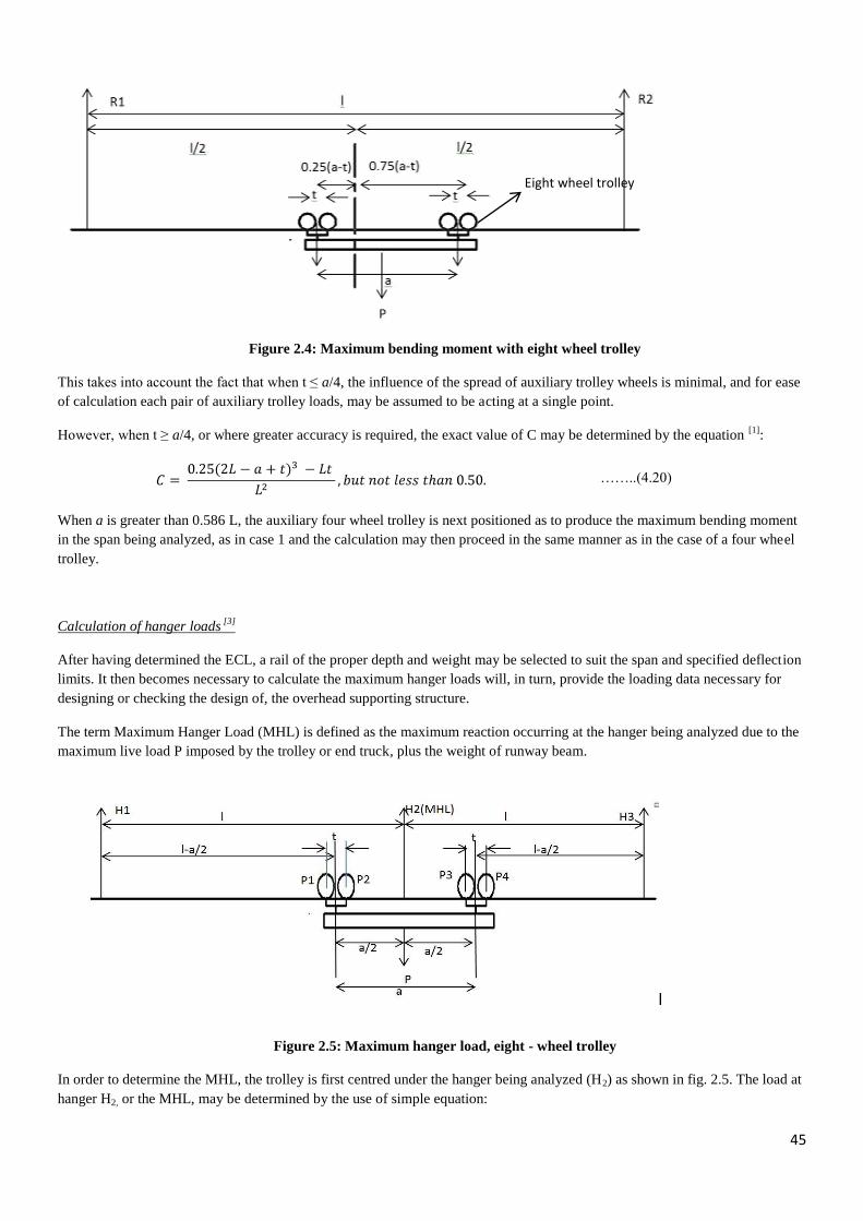
45

Figure 2.4: Maximum bending moment with eight wheel trolley

This takes into account the fact that when t ≤ a/4, the influence of the spread of auxiliary trolley wheels is minimal, and for ease

of calculation each pair of auxiliary trolley loads, may be assumed to be acting at a single point.

However, when t ≥ a/4, or where greater accuracy is required, the exact value of C may be determined by the equation [1]

:

……..(4.20)

When a is greater than 0.586 L, the auxiliary four wheel trolley is next positioned as to produce the maximum bending moment

in the span being analyzed, as in case 1 and the calculation may then proceed in the same manner as in the case of a four wheel

trolley.

Calculation of hanger loads [3]

After having determined the ECL, a rail of the proper depth and weight may be selected to suit the span and specified deflection

limits. It then becomes necessary to calculate the maximum hanger loads will, in turn, provide the loading data necessary for

designing or checking the design of, the overhead supporting structure.

The term Maximum Hanger Load (MHL) is defined as the maximum reaction occurring at the hanger being analyzed due to the

maximum live load P imposed by the trolley or end truck, plus the weight of runway beam.

Figure 2.5: Maximum hanger load, eight - wheel trolley

In order to determine the MHL, the trolley is first centred under the hanger being analyzed (H2) as shown in fig. 2.5. The load at

hanger H2, or the MHL, may be determined by the use of simple equation:

Eight wheel trolley

46

MHL= KP + rail weight ……..(2.21)

Where: P= total design load

K= distribution factor

……..(2.22)

The factor K is applicable to either four wheel or eight wheel trolleys so long as all of the stipulated conditions have been met [1]

.

2.8.2 Support Conditions:

The two ends of the runway beam are assumed to be simply supported, in the sense that the flexural displacements and twisting

rotation of the beam are restrained at the supports.

Consider two cases of support,

1. Single span is designed considering simply supported.

2. Simply supported continuous beam

Comparative bending moment diagram under both cases shown in fig. 2.6,

Figure 2.6. Comparative bending moment diagram

In second case for design, if one span failed by some reason it may cause failure of full system. So we prefer to design by

considering the single span as simply supported to avoid the collapse of structure.

3. Design Example Design the monorail runway beam to convey the material weighed maximum of 6 ton with speed of 1m/min on a track of 24 m

with the help of trolley running on bottom flange of overhead monorail structure.

3.1 Monorail classification:

Speed of monorail = 1m/min

Minimum distance for 1 cycle = 25m

Time taken to complete one cycle = 25 min

Maximum lifts per hour = 3

According to CMAA classification of monorail, our system is come under Class B.

47

3.2. Trolley selection

Two monorail trolleys are selected of the capacity of 3 ton each from JDN Trolleys. catalogue distance between them is 2.5 m.

Specification of one trolley:

No. Of wheels: 4

Capacity: 3 ton

Weight of trolley: 33 kg

Wheel base of trolley (a): 0.14 m

Width of trolley (t): 0.1 m

3.3. Beam selection

According to trolley wheel diameter, for better strength and rigidity ISMB 250 is selected for monorail runway beam.(IS

808:1989).

3.4. Load FactorsDetermination

3.4.1. Dead Load Factor (DLF)

By using eq.

Travel speed is in feet/min.

1m/min= 3.281 feet/min

DLF= 1.05+0.0016=1.0516

DLF= 1.1

3.4.2Hoist Load Factor (HLF)

By using equation 4.2, for low speed trolleys, hoist load factor is taken as 1.15.

3.4.3. Additional load factor[26]

In case of monorail, there is lateral load and axial load because of breaking and starting torque of trolley. As per

recommendation from IS 875[27]

, for this case

Axial load factor= 0.05; Lateral load factor= 0.1

5.5. Design of runway beam

5.5.1. Load calculations

The uniform load is the weight of the runway beam with applied load factor.

W= self-weight of beam

= 37.3× DLF

= 41.03 kg/m

= 402.5 N/m (g= 9.81 m/s2)

Maximum Load by each trolley on runway beam with load factor

48

Ptrolley = DLF × trolley weight + HLF × capacity of trolley

=1.10×323.73+1.15×30000

= 34856.103 N

Lateral and Axial load

Paxial = 0.05×P = 1742.80 N

Plateral = 0.1 × P = 3485.60 N

Wheel load, Pwheel= Ptrolley / No. of wheel = 8714.026 N

5.5.2. Summary of Results

To find the optimum span for runway beam the design is checked for both the cases:

i. a<0.586 L ii. a>0.586 L

It is found that for 3 m span length, the design is safe in local bending of bottom flange, local capacity and deflection.

Span

Length

Bending stress

(in MPa)

(σpermissible = 150 MPa)

Interaction

ratio

Bottom flange bending

stress (in MPa)

(σpermissible=165MPa)

Deflection

(in mm)

Major axis

bending stress

Minor axis

bending stress Point 0 Point 1 Point 2

3.5 m 72.85 70.39 0.96 164.45 181.69 100.57 3

3.4 m 70.65 68.76 0.94 160.66 177.89 96.87 2.8

3.3 m 68.44 67.13 0.91 156.88 174.11 93.82 2.5

3.2 m 66.24 65.5 0.88 153.1 170.32 89.5 2.3

3.1 m 64 63.08 0.86 149.33 166.54 89.43 2.1

3.0 m 61.8 62.2 0.84 145.57 162.76 82.199 1.9

Table: Iteration results for straight runway beam for different span length

3.6. Validation of Result

The straight runway beam of span length 3m is analyzed with simply supported end and under calculated loading condition. The

comparison between calculated result and software result is given in table below:

49

Figure: Design of straight runway beam in STAAD Pro.

The comparison of result for 3m span:

Calculated STAAD Pro % Deviation

Major axis bending moment 25389.58 Nm 26594.51 Nm 4.5 %

Minor axis bending moment 2614.2 Nm 2614.2 Nm 0 %

Deflection 1.94mm 1.94 mm

0 %

Table: Comparison of calculated result and STAAD Pro result for straight runway beam

4. Conclusions It is concluded that for the design of monorail system the effect of moving loads must be considered in design. The loading in

bottom flange causes local bending stress developed in the I beam.Support locations must be found by considering Runway

beam as simply supported beam. Thus whole monorail system designed and checked for strength and rigidity by interaction

ratio.

5. References: 1. Raymond a. Kulweic, Material Handling Handbook, 2

nd Edition John Wiley & Sons Publication

2. Tomas H Orihuela,"Design of Monorail Systems".

3. Monorail Manufacturers Association, Inc (MMA) website.

4. Material Handling Industry of America (MHIA) website.

5. Crane Manufacturers Association of America, Inc. (CMAA) Specification No. 74, Revised, Specifications for Top Running

and Under Running Single Girder Electric Overhead Cranes Utilizing Under Running Trolley Hoists,2000.

6. IS 875 part 2 Code of practice for design loads. (Second revision).

7. A D Anjikar and C C Handa, Design Procedure Of Overhead Monorail For Material Handling System For Food Processing

Industry, Int. J. Mech. Eng. & Rob. Res. ISSN 2278 – 0149 Vol. 2, No. 4, October 2013

8. A. D. Anjikar, Design, Development of Overhead Monorail for Material Handling System For food Processing

Industry(International Journal of Research in Mechanical Engineering & Technology Vol. 3, Issue 2, ISSN : 2249-5762

(Online) ISSN : 2249-5770 (Print), May - Oct 2013.

50

Design and Development of Duster Cleaning Machine

Chirag Patel, Sameer Kambad, Sahilkumar Parmar, Pavankumar Prajapati


Mechanical Engineering Department, Silver Oak College of Engineering and Technology, Gujarat Technological University,

Ahmedabad, 382481, Gujarat, India.

Abstract

The aim to design and develop a machine based on mechanically controlled automotive duster cleaning machine for black board

duster called ―Automatic Duster Cleaner‖. We have pleasure in introducing our innovative project, which is an automated

machine keep our environment clean and give a royal status to our colleges and schools. It also gives best sincere environment

to sincere students. It‘s a project which designed to keep clean and dust free environment.

Keywords: Base, Motor, Crank, Crank Shaft, Connecting Rod, Duster Plate, Duster Box, Duster.

1. Introduction:

Our project is based on mechanically controlled automotive duster cleaning machine for black board duster to clean dirty duster

called ―Automatic Duster Cleaner‖. This is a machine that has some mechanism by in which we put the dirty duster and we get

clean duster after five to six seconds. It also stores the dust and provide clean environment to students, teachers and whole

educational firm. In the educational system we can see that teachers write on the black board by chalk than clean the board by

duster and go outside of the class to clean the dirty duster and clean it on the wall and some of them clean duster inside the class.

That disturbs the other classes and same class also. The students who have allergy they are also get unsafe environment and start

sneezing in class that make other disturb. So by cleaning the duster without a safe small automatic machine is creates so much

disturbance and produce insincere environment to educational system. Automatic Blackboard Duster has been made by Tiwari

Amit [1] and Real-Time Automatic Blackboard Eraser using Embedded System done by Rubhini B1, Mrunalini T

2 [2].

2. Conceptual Design When written black-board clean by duster, it will be too dirty to clean it, put it In the Duster-box of machine. After supplying electricity by on/off switch the motor starts Rotary motion. Than by the rotary to reciprocating mechanism piston moves up and down reciprocal motion. Piston is connected with a metal pad it slapped on the dirty duster and cleans it. Dust catch by vacuum fan which is connected directly by belt and pulley with motor. Thus, duster cleaner works.



51

Figure1. Conceptual design of duster cleaner

3. Experiment for Find out Required Force

For Find out needed force on the duster we have done an experiment. The photos , calculations And details written as under, First we put 1000gm force on the duster that was too large that may brake duster so it create problem. Then apply 500 N on duster, by this force on duster, slapping 26 times duster will be clean but till now it is too large force for duster. After it we put 300gm force it will clean duster in 33 times of slapping and give accurate result also.

NOTE:-Here velocity =9.81m/s and height is 15 cm.

Table 1. Model estimation results

WEIGHT (gm.) No of Slapping

1000gm 10 (Too Large)

500gm 26 (Not satisfy )

300gm. 33 (Perfect)

250 36( Too Less)

From The Table and Experiment We Conclude that the Resultant Force what we required is 300gf.

4. Design Calculation

4.1 Velocity The velocity required for metal pad is considered as the gravity acceleration because of no external force used on pad. So, we

considered to take 9.81 m/s velocity of metal pad.

4.2 Rotor Speed The Rotor Speed Calculate by defining time of cleaning the duster in the machine that we considered as 5 sec. If we considerer

5 sec. For cleaning a duster our rpm of rotor can be calculated by this Way

RPM = (60 * 33) / 5 =396 rpm So, our required RPM For rotor is 400 revolutions per minute for clean the duster in 5 to 6 seconds.

52

4.3 Motor [3] Required torque, Inertia, Load and HP of motor can calculate as under,

4.3.1 Load Torque: Load torque required is:

TL = F*D

Where, TL =Load torque,

F = Required force,

D = Distance

TL = 2.94 * 0.15 = 0.441 Nm

4.3.2 Accelerating Torque: Ta = ( JM * i² + JL) * (Nm ) 9.55 t1

Where, JM = Rotor Inertia = 6.36 * 10 ˉ

7 Kgm²

J1 = Inertia of piston = 2.13 * 10ˉ7 Kgm²

J2 = Inertia of CR. = 4.167 * 10 ˉ8 Kgm²

JL = J1+ J2 =Total inertia = 2.55 * 10 ˉ7 Kgm² [4]

t1= thickness of connecting rod

From calculation,

Ta =3.732 * 10ˉ4 Nm

4.3.3 Total Torque:

T = (TL + Ta ) * FOS

Where, FOS = 6 [4]

T= 0.88 Nm

4.3.4 Required HP of Motor

HP = [4]

HP = 0.06 hp [5]

4.7 Thickness of Connecting Rod [6]

Buckling load,

Wb = F * FOS

= 17.64 N

For I section,

Ixx = -

= 3.94 x 10-7

m4

Iyy = = 9.85 x 10-8

m4

Bearing capacity of connecting rod,

So thickness of connecting rod,

t = 6.49 mm ≈ 6.5 mm

4. Experimental Model

53

Figure2. Experimental Model

5. Results and Conclusion

Through the experiment with fabricated model following results were found,

Table 2. Results from fabricated model

Force required 2.94 N

Motor HP 0.06HP

RPM of motor 400 rpm

Average Time required to clean the duster 7 sec

Overall cost of machine 3000 Rs

Result shows that designed duster cleaner is very useful device that can reduce adverse effect of cleaning duster manually. The

machine is also economical for the cost point of view that small educational institutes can afford it.

6. REFRENCES

[1] Automatic Blackboard Duster1st Amit Tiwari, Assistant Professor, Mechanical Engineering Department, Dungerpur

College of Engineering and Technology( Dugarpur), India, IJETIE, ISSN: 2394 – 6598 Volume 1, issue 2, February 2015.

[2] Real-Time Automatic Blackboard Eraser using Embedded System , Rubhini B1,Mrunalini T

2,Associated Software engineer,

Robert Bosch Engineering & Business Solution, Coimbatore,India, Vol 3, Issue 8, August 2014.

[3] Bureau of Energy Efficiency, BEE, Chapter 2 Electric Motor.

[4] Machine Design Book R.S. Khurmi, j. K. Gupta, ISBN: 81-219-2537-1 First Edition 1979.

[6] Technical Reference, Technical Support, Oriental Motor General Catalogue Publish 2012.

[5] Design and Analysis of Connecting Rod, Leela Krishna Vegi1, Venu Gopal Vegi2, Department of Mechanical Engineering,

Jawaharlal Nehru Technological University, Kakinada, AP, INDIA Volume 4, Issue 6, June-2013.

54

Design and development of hydraulic rod bending machine

Chirag Patel, Vijay Patel, Harsh Pathak, Malav Gandhi, Prashil Patel, Kishan Patel

[email protected], [email protected], [email protected]



Abstract

Nowadays the world is focusing into automation. Each and every work of human is reduced by a machine, but few areas like

construction the usage of machines for bending rods for stirrups which are used to withstand loads in beams and columns are not

done by machine because the cost of machine is high and need skilled labors to operate it. So this project is aimed to do bending

operation for stirrups using hydraulics and named as hydraulic rod bending machine. The main objective of our project is to

implement the hydraulic rod bending machine in the construction sites with less cost compared to the existing bending

machines, and increasing the productivity of the stirrups.

Keywords: Hydraulic Rod Bending Machine, Hydraulic Operation, Stirrups maker

1. Introduction

This project is to bend the rod at the specified dimensions which is used in the building construction which called as Stirrups.

Stirrup is an important reinforced element which acts as a shear reinforcement. Presently, stirrups are made manually which

suffers from many drawbacks like lack of accuracy, low productivity and resulting into severe fatigue in the operator. In manual

stirrup making process, operators not only subjecting their hands to hours of repetitive motion, but in many occasions it results

into several musculoskeletal disorders (MSDs). The project is designed based on the principle of Hydraulic system. The

hydraulic load has more power compare to the other type of loads like pneumatic and electric. By using heavy loads we can

increase the productivity of the product. The manual stirrup making process suffers from the many drawbacks. The construction

worker not only subject their hands to hours of repetitive motion but also sometimes suffers internal injury to his body organ i.e.

disorder carpal tunnel syndrome CTS, slipped disc problem etc.

1.1. Working principle

In the beginning of the process of rod bending, electric motor runs the pump, which is connected to hydraulic oil tank

and increases the pressure of hydraulic fluid by hydraulic pump [1]. This high pressure fluid is passes through pressure

relief valve where high pressure of fluid is returned to hydraulic oil tank. After that fluid passes from direction control

valve where it gives direction to fluid to reach at hydraulic cylinder. But between the hydraulic cylinder and direction

control valve, there is flow control valve which is used for control the required flow of fluid to hydraulic cylinder.

Direction control valve direct the fluid to the hydraulic cylinders which

moves the piston in forward direction to bend the rod. This fluid is

returned to hydraulic oil tank when hydraulic cylinders piston return to

its position. This process is continued until the stirrups making is done

and after the making of stirrups this stirrups are removed from machine

and this process is continued for making stirrups.

Figure 1: Hydraulic assembly:

1 Hydraulic Oil Tank

2 Pump

3 Check Valve

4 Pressure Relief Valve




55

5 Direction Control Valve

6 Hydraulic Cylinder

The Hydraulic oil employed in this process is initially stored in a tank of 20 liters capacity. A filter air breather is mounted on

the tank for filling the air passing into the reservoir and straining the oil while filling the reservoir. An electrical motor of 1.5 HP

is coupled to external gear pump to drive the fluid. When the motor runs, coupling that connects motor and the pump causes the

rotation of the pump in turn. Depending upon the speed of the rotation of the pump, a vacuum is created which make the oil to

be sucked and raised into the system. The pressurized oil passes through an inline check valve that prevents the return flow of

the oil into the pump. This is followed by a pressure line filter to filter the oil from dust partials. A Pressure Relief Valves is

connected parallel to the output line of the filter. This relief valve is used to prevent the system from the effect caused by excess

pressure this limit, the valve get activated and releases the excess pressure. The flow from these valves is measured using a

pressure gauge mounted on the pipe line and it can be adjusted. The pressurized oil then enters the Directional Control Valve. At

other end of DCV is connected to a Double acting cylinder. This cylinder is involved in the bending operation. When the left

spool is activated, the oil flows into the piston end of the cylinder causing the extension of the cylinder. The extension force of

the cylinder is used for bending operation. Once the bending is completed, the right spool is activated. This causes the retraction

of the cylinder. This process is repeated for bending stirrups controlled manually [2], [3].

1.2. Design calculation:

Pressure of external gear pump = 150 bar pressure

Flow of the external gear pump = 4 LPM

Now we have to bend the 16 mm diameter rod which material is mild steel.

Bending stress(S) of mild steel = 165 = 1683

Pressure of pump = 150 bar = 150

Calculation for force:

Where, Ad = area of rod

d = diameter of rod = 12 mm

= 1.1304

So,

F = 3804.93 kg = 37326.32 N = 37.32 KN

Now,

F = PA

So,

A = F/P

A = 3804.93/150

A = 25.37

Now,

Where, A = Area of Piston rod

D = Bore Diameter, R = Radius of bore

56

So,

R = 28.42 mm OR D = 56.84 mm

Standard 63 mm Bore diameter of hydraulic cylinder is taken [4].

Cylinder specification:

Bore diameter = 63 mm

Rod diameter = 36 mm

Stroke length = 200 mm

Pump specification: Max. Pressure = 150 bar

Force calculation: Area, A = 31.16

Force or load = PA= 150*31.16 = 4673.5 kg = 45847.01 N =45.85 KN

1.3. Geometric Model:

Figure2.

Geometric

Model

2. Fabricated

Model:

3. Results and

Conclusion

Through the

experiment

with fabricated

model following results were found,

Table1. Results from fabricated model

57

Sr. No. Diameter of rod to be bend Required Pressure

1 8 mm 50 bar

2 12 mm 80 bar

It was observed that to bend 16mm diameter rod 150bar pressure was enough but the structure was not capable to take that much

force so it could not be used for 16mm diameter. It was also observed that by changing the fixture in the table and the pulley on

piston rod, we can produce various sizes of the stirrups. At end of each bend we observed that rod spring back about 1-2 degree

due to its elasticity. Design force was capable to bend 12 mm diameter rod. During the bending process piston rod is rotating on

its axis so the pulley joint with it also rotate about its axis at time of bending.

REFERENCES

[1] Dr.R.K.Bansal (Ninth edition) ―Fluid Mechanics and Hydraulic Machines‖ Laxmi Publications

[2] REXROTH BOSCH GROUP COMPANY, ―Hydraulic, Basic, Principles and Components‖

[3] http://hydraulicspneumatics.com/search/results/hydraulic%20tank

[4] Kongu Engineering College, ―Design and Fabrication of Hydraulic Rod Bending Machine‖, Tamilnadu, India, 2014

http://hydraulicspneumatics.com/search/results/hydraulic%20tank

58

Design and Development of Valve Plate Testing Fixture to Detect Air

Leakage

Chirag Patel, Sudhir Parmar, Keyur Parmar, Nirav Patel, Moshakir Patel




Abstract

It is not possible to identify improper functioning of an air compressor valve plate before assemble it into air compressor.

Improper functioning valve plate leading to the leakage of valve plate so require function cannot be performing by an air

compressor because air compressor is used to produce high pressure air. But due to leakage in Valve Plate the high pressure of

air cannot maintain as it is. It reduces frequently and required function cannot achieve from an air compressor. And in order to

fulfil the require task it is necessary to dismantle all the components of an air compressor. During dismantling certain

components are damaged which required to repurchase them so identification of leakage in valve plate after complete assembly

leading to the loss of time and money.

Keywords: - Air Compressor, Valve plate, Leakage, Assembling, Disassembling of Air compressor

1. Introduction

In an air compressor manufacturing industries, they have high work load to manufacture huge quantity of an air compressor in

specific time to meet the customer demand. They required supplying the product of good quality in order to satisfy the customer

need. It results in to increase in organization reputation in market. But for that purpose they need to check the product before it

is supply to customer. If they identify any leakage in an air compressor they required to dismantle all the component of an air

compressor. During disassembly certain component are damaged which result into Loss of time and money. This fixture helps

the worker in identification of leakage in valve plate before it is assemble in an air compressor. It results in reduction of time

consumption of manufacturing and overall cost of production [1].

2. Problem Identification

In the industry when worker carried out assembly of an High Pressure Reciprocating (Working At Pressure of 8 bar) air

compressor they don‘t know that there is any leakage in it or not. When an air compressor is sent to Q/C Department then they

check the compressor for any leakage. If there is any leakage find in an air compressor then they send it again to assembly

department for its dismantling. During dismantling there is a chance of damage to certain component which is required to

purchase new component from store this which results in to west of time and money. These things are happen frequently in an

organization. [2][3]

Valve Plate of

Air compressor

is fitted here



59

Figure1. High Pressure Reciprocating Air Compressor [4]

3. Design of Fixture

Conceptual Design

Figure2.Conceptual Design

Design Calculation

Casing Thickness: - It is taken as a flat circular plate whose thickness (th).

th =

=

(Take C= 0.1, D=90, σc = Between 30 to 40 MPa ≈ 40 MPa [5])

th = 4.14 mm≈5 mm

Design of Flange:-

Flange thickness should be taken as 1.2t to 1.4t

t = thickness of cylinder wall

here we take 1.3t = 1.3 6

tf = 7.8 mm

Design of stud:-

No. of studs:-

Ns = 0.02D+4

= 5.7 ≈ 6 (max.)

Stud dia.:-

= ns

(Assume between 50 to 70 [6]

= 50 N/mm2)

dc = 4.79 mm

dc = dia. Of the root of the thread in mm

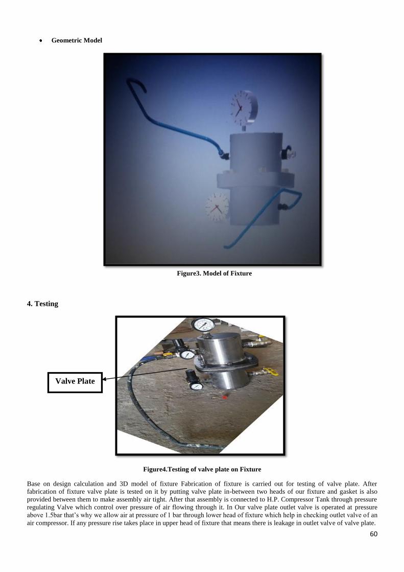
60

Geometric Model

Figure3. Model of Fixture

4. Testing

Figure4.Testing of valve plate on Fixture

Base on design calculation and 3D model of fixture Fabrication of fixture is carried out for testing of valve plate. After

fabrication of fixture valve plate is tested on it by putting valve plate in-between two heads of our fixture and gasket is also

provided between them to make assembly air tight. After that assembly is connected to H.P. Compressor Tank through pressure

regulating Valve which control over pressure of air flowing through it. In Our valve plate outlet valve is operated at pressure

above 1.5bar that‘s why we allow air at pressure of 1 bar through lower head of fixture which help in checking outlet valve of an

air compressor. If any pressure rise takes place in upper head of fixture that means there is leakage in outlet valve of valve plate.

Valve Plate

61

The valve used in valve plate is non return type valve if we apply pressure higher than 1.5bar in upper head of fixture it does not

allow to pass it through lower casing due to non return valve. If any pressure rise is indicated in lower head of fixture this

indicate leakage in inlet valve of fixture.

5. Conclusion After fabrication of our fixture worker can test valve plate before assembly in an air compressor. Which result in reduction of

west of time and money which is result due to identification of leakage in valve plate after assembly.

In industry they identify one or two faulty valve plate a week. It costs 1200Rs if it requires to completely replacing. Waste of

time in Disassembly and repairing if it is repairable. After use of Our Fixture worker can identify leakage in valve plate in

advance that result in saving of time and money.

Also in industry it is require keeping Air Compressor in running position for half an hour to identify any leakage in valve plate.

But after using our fixture they can identify any leakage in valve plate in 10minutes which results in saving of time and money.

REFERENCES [1] Namdeo, Rajeev; Manepatil, Smita; and Saraswat, Suvandan, "Detection of Valve Leakage in Reciprocating Compressor

Using Artificial Neural Network (ANN)" (2008). International Compressor Engineering Conference. Paper 1939.

[2] http://valveproducts.net/relief-valve/operation-principle-of-relief-valve

[3] https://www.google.co.in/search?q=Regulating+valve+of+air+compressor

[4] Marcus, RD, Pneumatic Conveying of Bulk Solids, Notes for Short Course on Pneumatic Conveying of Bulk Solids,

University of Newcastle, 1983.

[5] DINT TECH CONTROL Pvt. Ltd. Company Manual

[6] www.pneumofore.com/regulating-valve

http://valveproducts.net/relief-valve/operation-principle-of-relief-valve

https://www.google.co.in/search?q=Regulating+valve+of+air+compressor

http://www.pneumofore.com/regulating-valve

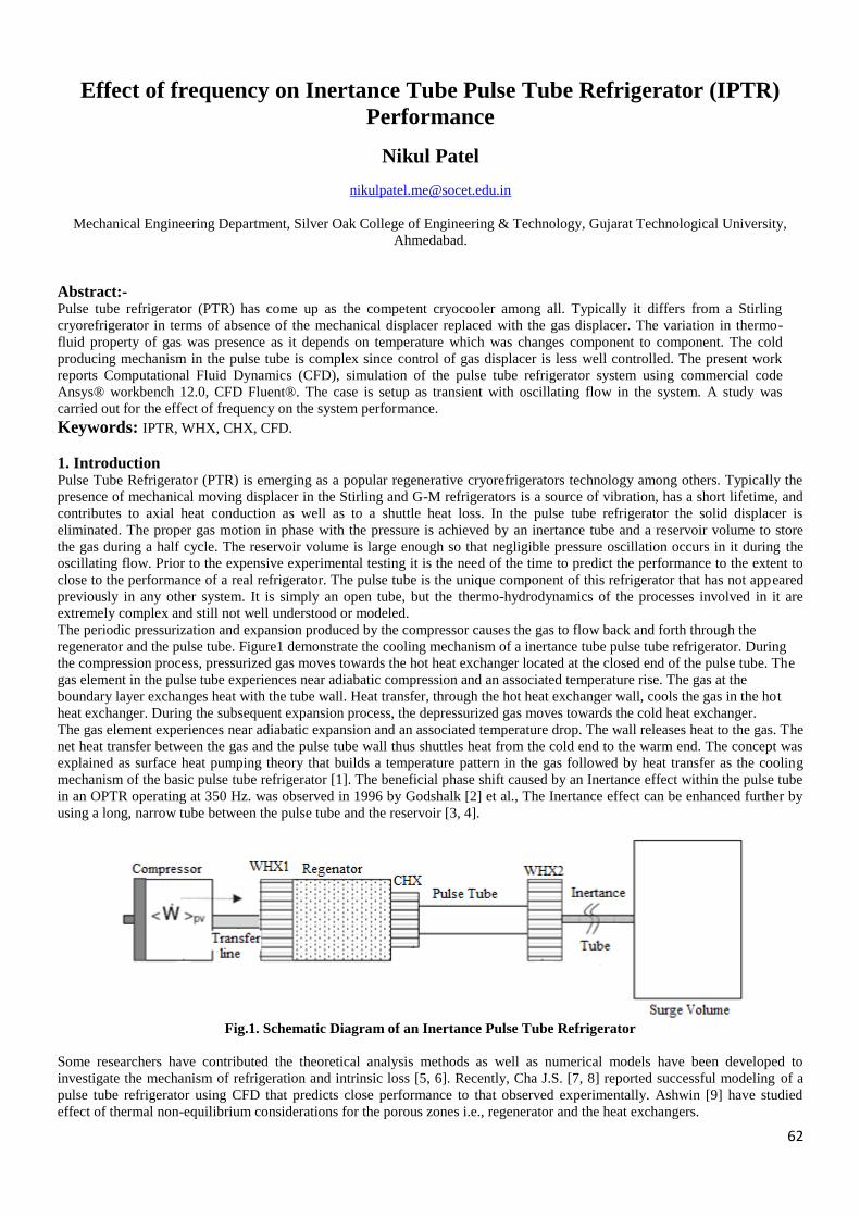
62

Effect of frequency on Inertance Tube Pulse Tube Refrigerator (IPTR)

Performance

Nikul Patel

[email protected]


Ahmedabad.

Abstract:- Pulse tube refrigerator (PTR) has come up as the competent cryocooler among all. Typically it differs from a Stirling

cryorefrigerator in terms of absence of the mechanical displacer replaced with the gas displacer. The variation in thermo-

fluid property of gas was presence as it depends on temperature which was changes component to component. The cold

producing mechanism in the pulse tube is complex since control of gas displacer is less well controlled. The present work

reports Computational Fluid Dynamics (CFD), simulation of the pulse tube refrigerator system using commercial code

Ansys® workbench 12.0, CFD Fluent®. The case is setup as transient with oscillating flow in the system. A study was

carried out for the effect of frequency on the system performance.

Keywords: IPTR, WHX, CHX, CFD.

1. Introduction Pulse Tube Refrigerator (PTR) is emerging as a popular regenerative cryorefrigerators technology among others. Typically the

presence of mechanical moving displacer in the Stirling and G-M refrigerators is a source of vibration, has a short lifetime, and

contributes to axial heat conduction as well as to a shuttle heat loss. In the pulse tube refrigerator the solid displacer is

eliminated. The proper gas motion in phase with the pressure is achieved by an inertance tube and a reservoir volume to store

the gas during a half cycle. The reservoir volume is large enough so that negligible pressure oscillation occurs in it during the

oscillating flow. Prior to the expensive experimental testing it is the need of the time to predict the performance to the extent to

close to the performance of a real refrigerator. The pulse tube is the unique component of this refrigerator that has not appeared

previously in any other system. It is simply an open tube, but the thermo-hydrodynamics of the processes involved in it are

extremely complex and still not well understood or modeled.

The periodic pressurization and expansion produced by the compressor causes the gas to flow back and forth through the

regenerator and the pulse tube. Figure1 demonstrate the cooling mechanism of a inertance tube pulse tube refrigerator. During

the compression process, pressurized gas moves towards the hot heat exchanger located at the closed end of the pulse tube. The

gas element in the pulse tube experiences near adiabatic compression and an associated temperature rise. The gas at the

boundary layer exchanges heat with the tube wall. Heat transfer, through the hot heat exchanger wall, cools the gas in the hot

heat exchanger. During the subsequent expansion process, the depressurized gas moves towards the cold heat exchanger.

The gas element experiences near adiabatic expansion and an associated temperature drop. The wall releases heat to the gas. The

net heat transfer between the gas and the pulse tube wall thus shuttles heat from the cold end to the warm end. The concept was

explained as surface heat pumping theory that builds a temperature pattern in the gas followed by heat transfer as the cooling

mechanism of the basic pulse tube refrigerator [1]. The beneficial phase shift caused by an Inertance effect within the pulse tube

in an OPTR operating at 350 Hz. was observed in 1996 by Godshalk [2] et al., The Inertance effect can be enhanced further by

using a long, narrow tube between the pulse tube and the reservoir [3, 4].

Fig.1. Schematic Diagram of an Inertance Pulse Tube Refrigerator

Some researchers have contributed the theoretical analysis methods as well as numerical models have been developed to

investigate the mechanism of refrigeration and intrinsic loss [5, 6]. Recently, Cha J.S. [7, 8] reported successful modeling of a

pulse tube refrigerator using CFD that predicts close performance to that observed experimentally. Ashwin [9] have studied

effect of thermal non-equilibrium considerations for the porous zones i.e., regenerator and the heat exchangers.


63

The present work is aimed at elaborating the inherent details of modeling of a PTR and performance prediction using

commercial CFD code Fluent®. Finally, study was carried out for the effect of frequency on the system performance. As a

result, there is always existence of optimum value of frequency for the same boundary condition and operating parameter.

2. Simulation Model 2.1 Description of different components of IPTR

The dimensions and material for different components of IPTR was mention in table 3.1 [7, 8]. The geometry of the system is

same as that. Cha [7, 8] reported and mesh model was generated from that geometry shown in figure 2. In entire IPTR domain,

5081 nodes were generated approximately. A two-dimensional axi symmetric model is developed and simulated for a pulse tube

refrigerator with inertance tube phase shifting mechanism.

Table 1: Dimensions and Material for different component of IPTR

Component Radius (m) Length (m) Material

A (Compressor) 9.54E-03 7.5E-03 S.S 304

B (Transfer Line) 1.55E-03 1.01E-01 S.S 304

C (WHX 1) 4.00E-03 2E-02 OFHC Copper

D (Regenerator) 4.00E-03 5.8E-02 S.S 304

E (CHX) 3.00E-03 5.7E-03 OFHC Copper

F (Pulse tube) 2.50E-03 6E-02 S.S 304

G (WHX 2) 4.00E-03 1E-02 OFHC Copper

H (Inertance tube) 4.25E-04 0.6841 S.S 304

I (Surge Volume) 0.013 0.13 S.S 304

Fig.2. Mesh model of IPTR (Inertance tube Pulse Tube Refrigerator)

2.2 Operating and boundary condition for IPTR components

The model is defined with all real boundary conditions, which restrict the necessity of arbitrary assumptions, hence lead to the

realistic analysis. WHX1 and WHX2 are defined with isothermal condition 293K while other components of IPTR except CHX

defined with adiabatic boundary condition. The CHX is defined with appropriate boundary condition in order to achieve lowest

temperature at specific heat load.

The externally imposed boundary conditions are a cyclically moving piston wall at one end of the tube and constant temperature

or heat flux boundaries at the external walls of the hot end and cold end heat exchangers. The compressor work can better way

model with dynamic meshing function in Fluent. To use the dynamic mesh model, it is required to provide a starting volume

mesh and the description of the motion. The fluid mesh motion is set to update by dynamic layering and local remeshing

method. In order to model the piston and cylinder, a user defined function (UDF) was hooked to Fluent, developed in C

programming language to simulate the piston cylinder effect. Where the piston head motion is assigned as:

piston

piston

dX=ωX cos ωt

dt (1)

Where, ω= angular velocity,

Xpiston = piston displacement = 4.511e-3 m.

Simulation was initiated with 3.1 MPa charge pressure and 300 K temperature, and it is performed until steady-periodic state

achieved.

2.3 Properties of material and gas

The compressible laminar flow model is adopted to investigate flow and heat transfer inside the system. The working fluid,

helium-4 gas is modeled as an ideal gas. The viscosity, specific heat and thermal conductivity of helium at constant pressure are

all temperature-dependent. Piecewise-polynomial form is used to define thermo-fluid properties of gas as shown in table 3.2.

Similarly thermal properties of different solid material for different components were also assigned as temperature dependent.

Table 2: Piecewise-Polynomial Equations for Helium-4 gas Property at 3.1MPa

Sr.

No.

Property

(S.I Unit)

Temperature

Range

(S.I. unit)

Piecewise-Polynomial equation

1 Thermal

conductivity

80-140 0.024225956+(0.0005824735812*T)

+(-0.0000005364383562*T^2)

64

141-220 0.027398818+(0.0005310187526*T)

+(-0.0000003300442478*T^2)

221-320 0.071013029+(0.0002069573374*T)

+(0.0000002741790512*T^2)

2 Specific heat 80-110 5573.83+(-5.724*T)+(0.023*T^2)

111-150 5358.965+(-1.8265*T)+0.00525*T^2

151-320 5269.548571+(-0.659142857*T)

+(0.001428571429*T^2)

3 Viscosity 80-150 0.000004981088435+(0.00000004941496599*T)

+(1.360544218E-11*T^2)

151-220 0.0000400878988+(-.0000003310470238*T)

+(0.000000001028630952*T^2)

221-320 (-0.00003259813338)+(0.0000003314257576*T)

+(-0.0000000005186363636*T^2)

2.4 Numerical Scheme and Convergence criteria

Once the model is set to appropriate boundary conditions, Fluent solve the continuum-based conservation equations for mass,

momentum and energy. The after cooler (WHX1), cold heat exchanger (CHX), hot heat exchanger (WHX2) and the regenerator

are modeled as porous media, assuming that there is local thermodynamic equilibrium between the fluid and solid structure in

these components. The required parameter for defining porous zone such as viscous resistance, inertial resistance and porosity

for regenerator and other heat exchangers are same as that of Cha [7, 8].

Fluent solves the continuum based continuity, momentum and energy equations using control volume method. These are non-

linear partial differential equations which are linearized using appropriate numerical technique. IPTR is case of complicated

fluid flow and heat transfer phenomena occurring at low temperature. Pressure based segregated solver was set with First order

implicit formulation. Solution controls are set as second order upwind for pressure, density, momentum and first order upwind

for energy for the desired numerical discretization. For better convergence of transient problem, PISO algorithm is selected

because process is time dependant for transient analysis. Convergence criteria are set for continuity and momentum as 1e-5 and

for energy 1e-7.

3. Description of different simulated case CFD technology is used to analyze the multi-dimensional PTR system that solve the conservation equations of mass, momentum

and energy for fluid flow based on space and time. Different cases are simulated in order to study complex thermo-fluidic

process in IPTR and effect of frequency on the system performance. Case 1 is simulated using adiabatic boundary condition at

CHX with 34Hz frequency. While case 2, 3 and 4 is simulated using constant heat load 1 watt with 30, 34 and 40Hz frequency.

Simulation was initiated with 3.1 MPa charge pressure and 300 K temperature, and it is performed until steady-periodic state

achieved.

4. Results and discussion The CFD assisted numerical simulations are carried out for no load test that will predict minimum attainable temperature and

load test at constant heat load of 1 Watt with different operating frequency.

In order to determine the accuracy of the algorithm and the method of solution, a validation study is conducted against the

previously published work. Figure 3 shows that the present cool down curve is almost identical with that reported by Cha [7].

Moreover, the no load steady state temperature of 87 K reached with the present model using 5081 grid points, a times step of

0.00073529 second and 5 inner iterations per time step compares favorably with the lowest temperature of 87K reported by Cha.

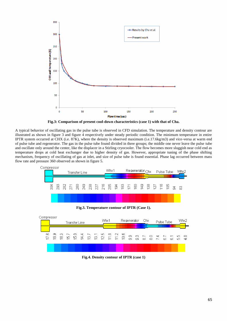
65

Fig.3: Comparison of present cool-down characteristics (case 1) with that of Cha.

A typical behavior of oscillating gas in the pulse tube is observed in CFD simulation. The temperature and density contour are

illustrated as shown in figure 3 and figure 4 respectively under steady periodic condition. The minimum temperature in entire

IPTR system occurred at CHX (i.e. 87K), where the density is observed maximum (i.e.17.6kg/m3) and vice-versa at warm end

of pulse tube and regenerator. The gas in the pulse tube found divided in three groups; the middle one never leave the pulse tube

and oscillate only around the center, like the displacer in a Stirling cryocooler. The flow becomes more sluggish near cold end as

temperature drops at cold heat exchanger due to higher density of gas. However, appropriate tuning of the phase shifting

mechanism, frequency of oscillating of gas at inlet, and size of pulse tube is found essential. Phase lag occurred between mass

flow rate and pressure 360 observed as shown in figure 5.

Fig.3. Temperature contour of IPTR (Case 1).

Fig.4. Density contour of IPTR (case 1)

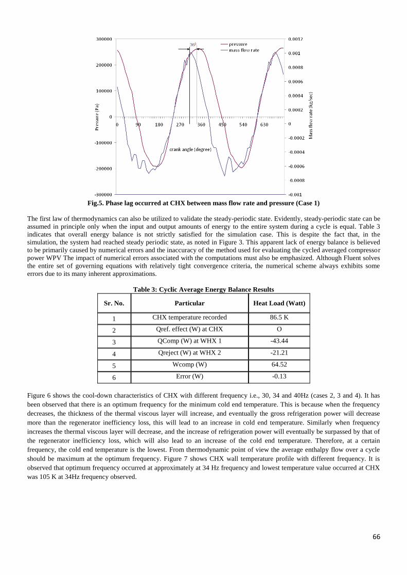
66

Fig.5. Phase lag occurred at CHX between mass flow rate and pressure (Case 1)

The first law of thermodynamics can also be utilized to validate the steady-periodic state. Evidently, steady-periodic state can be

assumed in principle only when the input and output amounts of energy to the entire system during a cycle is equal. Table 3

indicates that overall energy balance is not strictly satisfied for the simulation case. This is despite the fact that, in the

simulation, the system had reached steady periodic state, as noted in Figure 3. This apparent lack of energy balance is believed

to be primarily caused by numerical errors and the inaccuracy of the method used for evaluating the cycled averaged compressor

power WPV The impact of numerical errors associated with the computations must also be emphasized. Although Fluent solves

the entire set of governing equations with relatively tight convergence criteria, the numerical scheme always exhibits some

errors due to its many inherent approximations.

Table 3: Cyclic Average Energy Balance Results

Sr. No. Particular Heat Load (Watt)

1 CHX temperature recorded 86.5 K

2 Qref. effect (W) at CHX O

3 QComp (W) at WHX 1 -43.44

4 Qreject (W) at WHX 2 -21.21

5 Wcomp (W) 64.52

6 Error (W) -0.13

Figure 6 shows the cool-down characteristics of CHX with different frequency i.e., 30, 34 and 40Hz (cases 2, 3 and 4). It has

been observed that there is an optimum frequency for the minimum cold end temperature. This is because when the frequency

decreases, the thickness of the thermal viscous layer will increase, and eventually the gross refrigeration power will decrease

more than the regenerator inefficiency loss, this will lead to an increase in cold end temperature. Similarly when frequency

increases the thermal viscous layer will decrease, and the increase of refrigeration power will eventually be surpassed by that of

the regenerator inefficiency loss, which will also lead to an increase of the cold end temperature. Therefore, at a certain

frequency, the cold end temperature is the lowest. From thermodynamic point of view the average enthalpy flow over a cycle

should be maximum at the optimum frequency. Figure 7 shows CHX wall temperature profile with different frequency. It is

observed that optimum frequency occurred at approximately at 34 Hz frequency and lowest temperature value occurred at CHX

was 105 K at 34Hz frequency observed.

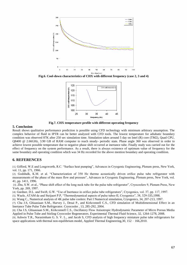
67

Fig.6. Cool-down characteristics of CHX with different frequency (case 2, 3 and 4)

Fig.7. CHX temperature profile with different operating frequency

5. Conclusion Result shows qualitative performance prediction is possible using CFD technology with minimum arbitrary assumption. The

complex behavior of fluid in IPTR can be better analyzed with CFD tools. The lowest temperature for adiabatic boundary

condition was observed 87K after 250 sec simulation time. Simulation takes around 5 day on Intel (R) core (TM2), Quad CPU,

Q8400 @ 2.66GHz, 3.90 GB of RAM computer to reach steady- periodic state. Phase angle 360 was observed in order to

achieve lowest possible temperature due to negative phase shift occurred at inertance tube. Finally study was carried out for the

effect of frequency on the system performance. As a result, there is always existence of optimum value of frequency for the

same boundary and operating condition which was 34 Hz recorded for the above mention boundary and operating condition.

6. REFERENCES

[1]. Gifford, W.E and Longsworth, R.C. ―Surface heat pumping‖, Advances in Cryogenic Engineering, Plenum press, New York,

vol. 11, pp. 171, 1966.

[2]. Godshalk, K.M. et al. ―Characterization of 350 Hz thermo acoustically driven orifice pulse tube refrigerator with

measurements of the phase of the mass flow and pressure‖, Advances in Cryogenic Engineering, Plenum press, New York, vol.

41, pp. 1411, 1996.

[3]. Zhu, S.W. et al., ―Phase shift effect of the long neck tube for the pulse tube refrigerator‖, Cryocoolers 9, Plenum Press, New

York, pp. 269, 1997.

[4]. Gardner, D.L. and Swift, G.W. ―Use of Inertance in orifice pulse tube refrigerators‖, Cryogenics, vol. 37, pp. 117, 1997.

[5]. Waele, ATAM de and Steijaert P.P, ―Thermodynamical aspects of pulse tubes-II, Cryogenics‖, 38, 329-335,1998.

[6]. Wang C., Numerical analysis of 4K pulse tube coolers: Part I Numerical simulation, Cryogenics, 34, 207-213, 1997.

[7]. Cha J.S, Ghiaasiaan S.M., Harvey J., Desai P., and Kirkconnell C.S., CFD simulation of Multidimensional Effect in an

Inertance Tube Pulse Tube Refrigerator. Cryocooler , 13, 285-292, 2004.

[8]. Cha J.S, Ghiaasiaan S.M., Kirkconnell C.S., Oscillatory Flow Anisotropic Hydrodynamic Parameter of Micro Porous Media

Applied in Pulse Tube and Stirling Cryocooler Regenerators. Experimental Thermal Fluid Science, 32, 1264-1278, 2008.

[9]. Ashwin T.R., Narasimham G. S. V. L., and Jacob S, CFD analysis of high frequency miniature pulse tube refrigerators for

space applications with thermal non-equilibrium model, Applied Thermal Engineering,30, 152 – 166,2010.

68

Effect of Injection Pressure on the Performance of Single Cylinder CI

Engine Fueled with the Blend of 30% Plastic Pyrolysis Oil and 70% Diesel

Dhruvin Kagdi

[email protected]

Mechanical Engineering Department, Silver oak college of Engineering & Technological Gujarat Technological University,

India

Abstract:- Depleting quantity of Conventional Fuel has been focused as a greater problem these days. Day by day, quantity of Petroleum,

Crude Oil has more utilization and lesser production. Increasing use of Petrol & Diesel has made the people of the world to

think for some alternative way for energy resources. At the same time. Other rising problem against the people of the world is

increase in plastic waste and recycling of the same. Both of the issues are focused and efforts are made to get optimum solution.

An experimental setup has been prepared for Blended Fuel of 30% Plastic Pyrolysis oil and 70% Diesel Fuel to be used in single

cylinder, 4-stroke CI engine. Plastic Pyrolysis oil is obtained from plastic waste by pyrolysis process. Pyrolysis process is a

thermo-chemical decomposition of organic matter in absence of oxygen. Blending of pyrolysis oil with diesel helps to reduce

the consumption of diesel fuel. The variation in the Injection Pressure of the Engine, fueled with above stated Blended Fuel,

affects the engine performance as well as exhaust emission data. To understand the variation in Engine performance,

Experiments were performed by setting different values of injection pressure individually on single cylinder CI Engine, fueled

with above stated blended fuel, at different loading conditions. Selected Injection Pressures were 160 bar, 180 bar, 200 bar and

220 bar. Effect of Engine performance of each was compared by Graphical representation of different performance parameters.

It was found to have increase in Engine Performance with increase in Injection Pressure. HC and CO2 emissions were found to

be decreased, while NOX were found to be increased with increase in Injection Pressure.

Keywords: Pyrolysis, Diesel, Engine, Injection, Pressure, Blend

1. Introduction Use of plastic in our daily activities seemed to be increased from years. In an online article, dated April 4, 2013 of the daily

newspaper The Times of India of the author Dhananjay Mahapatra it was stated that ‗"We are sitting on a plastic time bomb,"

the Supreme Court said on Wednesday after the Central Pollution Control Board (CPCB) informed it that India generates 56

lakh tonnes of plastic waste annually, with Delhi accounting for a staggering 689.5 tonnes a day. "Total plastic waste which is

collected and recycled in the country is estimated to be 9,205 tonnes per day (approximately 60% of total plastic waste) and

6,137 tonnes remain uncollected and littered," the CPCB said. [1]

The energy crisis as well as the environmental degradation is the major problems mankind is facing today. Demand of energy

has been increased day by day because of the increased population on the earth. By the year 2100, the world population is

expected to be in excess of 12 billion and it is essential that the demand of energy will be increased by five times of what it is

now. According to the world energy report, we get around 80% of our energy from conventional fossil fuels like oil (36%),

natural gas (21%), and coal (23%). It is well known that the time is not so far when all these sources will be completely

exhausted.

To overcome both of the issues stated above, the alternative fuel i.e. Plastic Pyrolysis Oil can be used in CI Engine. As the CI

Engine generally available are designed to work effectively with Diesel Fuel only, to use Plastic Pyrolysis Oil in the CI Engine,

one need to blend it with Diesel Fuel. Past work related to Plastic Pyrolysis Oil shows that this fuel does not give as comparable

performance as Diesel Fuel or other Pyrolysis Oil like Tyre Pyrolysis Oil. So, one need to either improve in Engine Design or

make changes in Engine parameter to get noticeable performance of Engine with Plastic Pyrolysis Oil blends with Diesel Fuel.

To achieve that, experimentations have been carried out with variation in Injection Pressure in this research.

2. Literature Survey 2.1 Research work regarding performance and emissions of engine with the blended fuel of Plastic Pyrolysis Oil along

with other parametric variation has been stated below.

C. Wongkhorsub & N. Chindaprasert[2]

made a comparison of the use of pyrolysis oils (Pyrolysis oils from waste tire and waste

plastic) in diesel engine in the assessment of engine performance, and feasibility analysis. It was concluded that with Engine

modification tire pyrolysis oil gives better performance than the diesel fuel, while plastic pyrolysis oil was found to be have high

heating value. On economical aspect it was found that plastic pyrolysis oil could have much efficient if it‘s price is not more

than 85% of diesel fuel and it can reduce a great amount of solid plastic waste, which is advantageous on environmental aspects,

too. M. Mani et al[3]

performed an experimental investigation on four stroke, single cylinder, and direct-injection (DI) diesel

engine using 100% waste plastic with cooled exhaust gas recirculation. Experiments showed a comparative reduction in NOX,


69

smoke, HC, CO along with comparable Brake Thermal Efficiency with 20% EGR level. M. Mani & G. Nagarajan[4]

studied the

influence of injection timing on performance, emission and combustion characteristics of a DI diesel engine running on waste

plastic oil at four injection timings (23°, 20°, 17° and 14° bTDC). Compared to standard injection timing of 23° bTDC, the

injection timing of 14° bTDC was having reduction in NOX, CO and HC emissions with increase in brake thermal efficiency,

CO2 and smoke.

2.2 Effect of variation in Injection Pressure on Engine with different Fuels has been stated in following research work

Avinash Kumar Agarwal et al [5]

used a single cylinder diesel fueled CI engine to experimentally determine the effects Avinash

Kumar Agarwal et al [5]

used a single cylinder diesel fueled CI engine to experimentally determine the effects of fuel injection

strategies and injection timings on engine combustion, performance and emission characteristics at constant speed (2500 rpm)

with two FIPs (500 and 1000 bars respectively) and different start of injection (SOI) timings. Cylinder pressure, rate of heat

release (ROHR), exhaust gas temperature and brake mean effective pressure (BMEP) were found to be higher for lower FIPs

(i.e. 500 bars), while Brake Thermal Efficiency (BTE) increases at higher FIPs. For advanced SOI, ROHR, BMEP and BTE

increased, while brake specific fuel consumption (BSFC) and exhaust gas temperature reduced significantly. Wenming Yang et

al[6]

researched with fuel injection strategies to strike an optimum solution between engine performance and emissions in CI

engines. They concluded that increasing the fuel injection pressure can improve the fuel atomization and thus improving

combustion process with a higher brake thermal efficiency, producing less HC, CO, PM emissions, but more NOx emission.

Pilot injection help in reducing combustion noise and NOx emissions and immediate post injection may help in soot oxidation

and late post injection helps in regeneration of diesel particulate filter. Kyunghyun Ryu[7]

observed the effects of pilot injection

pressure on the combustion and emissions characteristics in a diesel engine using biodiesel–CNG dual fuel. In a Dual Fuel

Combustion (DFC) mode, with increase in pilot-fuel injection pressure, the combustion begins and ends earlier with reduce in

ignition delay, exhaust smoke and CO emissions. While the same increases NOX emissions. Özer Cana et al[8]

observed the

effects of ethanol addition (10% and 15% in volume) with 1% isopropanol on performance and emissions of a turbocharged

indirect injection Diesel engine running at different injection pressures(150, 200 and 250 bar) at full load. It was found that the

ethanol addition reduces CO, soot and SO2 emissions, with increase in NOx emission and approximately 12.5% (for 10%

ethanol addition) and 20% (for 15% ethanol addition) power reductions. It was also found reduction in CO, smoke emissions

and in Power with increase in injection pressure especially between 1500 and 2500 rpm. R. Anand and G.R. Kannan[9]

used a

blend of 30% waste cooking palm oil (WCO) methyl ester, 60% diesel and 10% ethanol (called as Diestrol) in the experimental

evaluation of DI diesel engine at varying injection pressure and injection timing. Maximum brake thermal efficiency of 31.3%

was obtained at an injection pressure of 240 bar and injection timing of 25.5° before TDC. Compared to diesel, diestrol fuel

showed reduction in CO, CO2, NOx and smoke emission by 33%, 6.3%, 4.3% and 27.3% respectively with increase in unburnt

hydrocarbon (UHC), cylinder gas pressure and heat release rate. Minimum ignition delay of 12.7° CA was observed with

diestrol fuel which was similar to diesel at same operating condition.

3. Plastic Pyrolysis Oil Pyrolysis is a thermochemical decomposition of organic material at elevated temperatures in the absence of oxygen (or any

halogen). It involves the simultaneous change of chemical composition and physical phase, and is irreversible. The word is

coined from the Greek-derived elements pyro "fire" and lysis "separating".

Pyrolysis differs from other high-temperature processes like combustion and hydrolysis in that it usually does not involve

reactions with oxygen, water, or any other reagents. In practice, it is not possible to achieve a completely oxygen-free

atmosphere. Because some oxygen is present in any pyrolysis system, a small amount of oxidation occurs.Bio-oil is produced

via pyrolysis, a process in which biomass is rapidly heated to 450–500°C in an oxygen-free environment and then quenched,

yielding a mix of liquid fuel (pyrolysis oil), gases, and solid char. Variations in the pyrolysis method, biomass characteristics,

and reaction specifications will produce varying percentages of these three products. Several technologies and methodologies

can be used for pyrolysis, including circulating fluid beds, entrained flow reactors, multiple hearth reactors, or vortex reactors.

The process can be performed with or without a catalyst or reductant.

The original biomass feedstock and processing conditions affect the chemical properties of the pyrolysis oil, but it typically

contains a significant amount of water (15%–30% by weight), has a higher density than conventional fuel oils, and exhibits a

lower pH (2–4). The heating value of pyrolysis oil is approximately half that of conventional fuel oils, due in part to its high

water and oxygen content, which can make it unstable until it undergoes further processing. Bio-oil can be hydro-treated to

remove the oxygen and produce a liquid feedstock resembling crude oil (in terms of its carbon/hydrogen ratio), which can be

further hydro-treated and cracked to create renewable hydrocarbon fuels and chemicals. Hydro-treating stabilizes the bio-oil

preventing molecule-to-molecule and molecule-to-surface reactions and eventually produces a finished blend-stock for fuels.

Bio-oil can be deoxygenated from its high initial oxygen content of 35-45 percent by weight (wt%) on a dry basis all the way

down to 0.2 wt%. [10]

70

Donglei Wu et al.[11]

produced experimental setup for low temperature conversion of plastic waste into light hydrocarbons. For

this purpose 1 litre volume, energy efficient batch reactor was manufactured locally and tested for pyrolysis of waste plastic.

The feedstock for reactor was 50 g waste polyethylene. The average yield of the pyrolytic oil, wax, pyrogas and char from

pyrolysis of PW were 48.6, 40.7, 10.1 and 0.6%, respectively, at 275 C with non-catalytic process. Using catalyst the average

yields of pyrolytic oil, pyrogas, wax and residue (char) of 50 g of PW was 47.98, 35.43, 16.09 and 0.50%, respectively, at

operating temperature of 250 C.

The steps involved in conversion of plastic waste into liquid fuel are given below:

Mechanical segregation of plastic waste from mixed MSW dump yard/storage.

Transportation of segregated plastic waste through conveyor belt for optical segregation. Optical segregation of plastic

waste is done (only HD, LD, PP and multilayer packaging except PVC). Shredding of plastic waste and dislodging dust and

impurities.

Transportation of segregated (100% plastic waste) into feeding hopper (reactor). Feeding of plastic waste into reactor for

random depolymerisation in presence of additives.

Produced raw gases are sent to char collector where solid char particles are separated from gases. Char collector contains a

cyclone coil to separate char particles from gases.

After that, raw gases are sent to quench system or condenser to separate recycled gases and Pyrolysis oil.

Following Figure shows all the processes of production of Plastic Pyrolysis Oil.

Fig. 1 Production of Plastic Pyrolysis Oil

Plastic Pyrolysis Oil used for this research work was tested in certified laboratory for its properties and test results are

stated in the table 1 given below.

Table 1 Properties of Plastic Pyrolysis Oil

SR

NO TEST TYPE

TEST

RESULT UNIT

1 Acidity, Inorganic NIL N/A 2 Appearance DARK RED Visual

3 Kinematic Viscosity

cSt at 40 ᵒc

1.69cSt cSt

4 Flash point ᵒC 22 ᵒC

5 Fire Point ᵒC 26 ᵒC

6 Gross Calorific Value 10980 Cal/kg

7 Density 0.788 gm/ml

8 Oil Impurity 0.01% % by Wt.

9 Water % 40 ppm % by Wt.

10 Pour Point Above -2 ᵒC

11 Sulphur 0.01 % by mass

12 Ash 0.001 % by mass

13 Sediment 0.001 % by Wt.

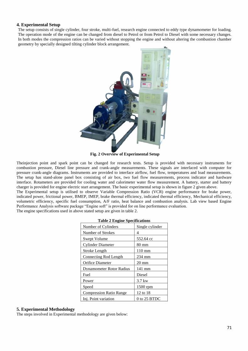
71

4. Experimental Setup The setup consists of single cylinder, four stroke, multi-fuel, research engine connected to eddy type dynamometer for loading.

The operation mode of the engine can be changed from diesel to Petrol or from Petrol to Diesel with some necessary changes.

In both modes the compression ratios can be varied without stopping the engine and without altering the combustion chamber

geometry by specially designed tilting cylinder block arrangement.

Fig. 2 Overview of Experimental Setup

Theinjection point and spark point can be changed for research tests. Setup is provided with necessary instruments for

combustion pressure, Diesel line pressure and crank-angle measurements. These signals are interfaced with computer for

pressure crank-angle diagrams. Instruments are provided to interface airflow, fuel flow, temperatures and load measurements.

The setup has stand-alone panel box consisting of air box, two fuel flow measurements, process indicator and hardware

interface. Rotameters are provided for cooling water and calorimeter water flow measurement. A battery, starter and battery

charger is provided for engine electric start arrangement. The basic experimental setup is shown in figure 2 given above.

The Experimental setup is utilised to observe Variable Compression Ratio (VCR) engine performance for brake power,

indicated power, frictional power, BMEP, IMEP, brake thermal efficiency, indicated thermal efficiency, Mechanical efficiency,

volumetric efficiency, specific fuel consumption, A/F ratio, heat balance and combustion analysis. Lab view based Engine

Performance Analysis software package ―Engine soft‖ is provided for on line performance evaluation.

The engine specifications used in above stated setup are given in table 2.

Table 2 Engine Specifications

Number of Cylinders Single cylinder

Number of Strokes 4

Swept Volume 552.64 cc

Cylinder Diameter 80 mm

Stroke Length 110 mm

Connecting Rod Length 234 mm

Orifice Diameter 20 mm

Dynamometer Rotor Radius 141 mm

Fuel Diesel

Power 3.7 kw

Speed 1500 rpm

Compression Ratio Range 12 to 18

Inj. Point variation 0 to 25 BTDC

5. Experimental Methodology The steps involved in Experimental methodology are given below:

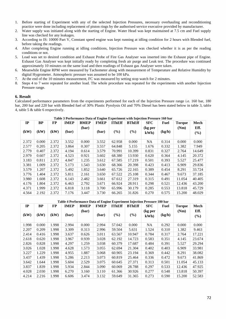
72

1. Before starting of Experiment with any of the selected Injection Pressures, necessary overhauling and reconditioning

practice were done including replacement of piston rings by the authorised service executive provided by manufacturer.

2. Water supply was initiated along with the starting of Engine. Water Head was kept maintained at 7.5 cm and Fuel supply

line was checked for any leakages.

3. According to IS: 10000 Part V, Constant speed engine was kept running at idling condition for 2 hours with Blended fuel,

before taking the readings.

4. After completing Engine running at idling conditions, Injection Pressure was checked whether it is as per the reading

conditions or not.

5. Load was set to desired condition and Exhaust Probe of Fire Gas Analyser was inserted into the Exhaust pipe of Engine.

Exhaust Gas Analyser was kept initially ready by completing fresh air purge and Leak test. The procedure was continued

approximately 10 minutes on the same load and then readings of Exhaust gas Analyser were taken.

6. Meanwhile Engine RPM were measured by Tachometer along with measurement of Temperature and Relative Humidity by

digital Hygrometer. Atmospheric pressure was assumed to be 100 kPa.

7. At the end of the 10 minutes measurement, FC was measured by setting stop watch for 2 minutes.

8. Steps 4 to 7 were repeated for another load. The whole procedure was repeated for the experiments with another Injection

Pressure range.

6. Result Calculated performance parameters from the experiments performed for each of the Injection Pressure range i.e. 160 bar, 180

bar, 200 bar and 220 bar with Blended fuel of 30% Plastic Pyrolysis Oil and 70% Diesel has been stated below in table 3, table

4, table 5 & table 6 respectively.

Table 3 Performance Data of Engine Experiment with Injection Pressure 160 bar

IP

(kW)

BP

(kW)

FP

(kW)

IMEP

(bar)

BMEP

(bar)

FMEP

(bar)

IThEff

(%)

BThEff

(%)

SFC

(kg per

kWh)

Fuel

(kg/h)

Torque

(Nm)

Mech

Eff.

(%)

2.372 0.000 2.372 3.552 0.000 3.552 62.958 0.000 NA 0.314 0.000 0.000

2.577 0.205 2.372 3.864 0.307 3.557 64.848 5.155 1.676 0.332 1.382 7.949

2.779 0.407 2.372 4.194 0.614 3.579 70.991 10.399 0.831 0.327 2.764 14.649

2.979 0.607 2.372 4.523 0.921 3.602 68.380 13.930 0.620 0.364 4.145 20.372

3.183 0.811 2.372 4.847 1.235 3.612 67.585 17.219 0.501 0.393 5.527 25.477

3.381 1.009 2.372 5.173 1.543 3.630 68.366 20.398 0.423 0.413 6.909 29.836

3.579 1.207 2.372 5.492 1.852 3.640 65.726 22.165 0.389 0.454 8.291 33.724

3.776 1.404 2.372 5.811 2.161 3.650 67.522 25.108 0.344 0.467 9.673 37.185

3.980 1.608 2.372 6.143 2.482 3.661 67.612 27.319 0.315 0.491 11.054 40.405

4.176 1.804 2.372 6.463 2.792 3.671 66.924 28.911 0.298 0.521 12.436 43.200

4.371 1.999 2.372 6.818 3.118 3.700 65.996 30.179 0.285 0.553 13.818 45.729

4.564 2.192 2.372 7.176 3.447 3.730 66.265 31.826 0.270 0.575 15.200 48.029

Table 4 Performance Data of Engine Experiment Injection Pressure 180 bar

IP

(kW)

BP

(kW)

FP

(kW)

IMEP

(bar)

BMEP

(bar)

FMEP

(bar)

IThEff

(%)

BThEff

(%)

SFC

(kg per

kWh)

Fuel

(kg/h)

Torque

(Nm)

Mech

Eff.

(%)

1.998 0.000 1.998 2.994 0.000 2.994 57.042 0.000 NA 0.292 0.000 0.000

2.207 0.209 1.998 3.309 0.313 2.996 59.504 5.631 1.524 0.310 1.382 9.463

2.414 0.416 1.998 3.637 0.626 3.011 63.567 10.947 0.784 0.317 2.764 17.221

2.618 0.620 1.998 3.967 0.939 3.028 62.192 14.723 0.583 0.351 4.145 23.674

2.826 0.828 1.998 4.297 1.259 3.038 60.379 17.687 0.484 0.391 5.527 29.294

3.026 1.028 1.998 4.628 1.573 3.055 62.694 21.304 0.402 0.403 6.909 33.981

3.227 1.229 1.998 4.955 1.887 3.068 60.905 23.194 0.369 0.442 8.291 38.082

3.437 1.439 1.998 5.286 2.213 3.073 60.819 25.464 0.336 0.472 9.673 41.869

3.642 1.644 1.998 5.604 2.529 3.075 60.645 27.371 0.313 0.501 11.054 45.133

3.837 1.839 1.998 5.934 2.844 3.090 60.069 28.788 0.297 0.533 12.436 47.925

4.028 2.030 1.998 6.270 3.160 3.110 61.366 30.926 0.277 0.548 13.818 50.397

4.214 2.216 1.998 6.606 3.474 3.132 59.649 31.365 0.273 0.590 15.200 52.583

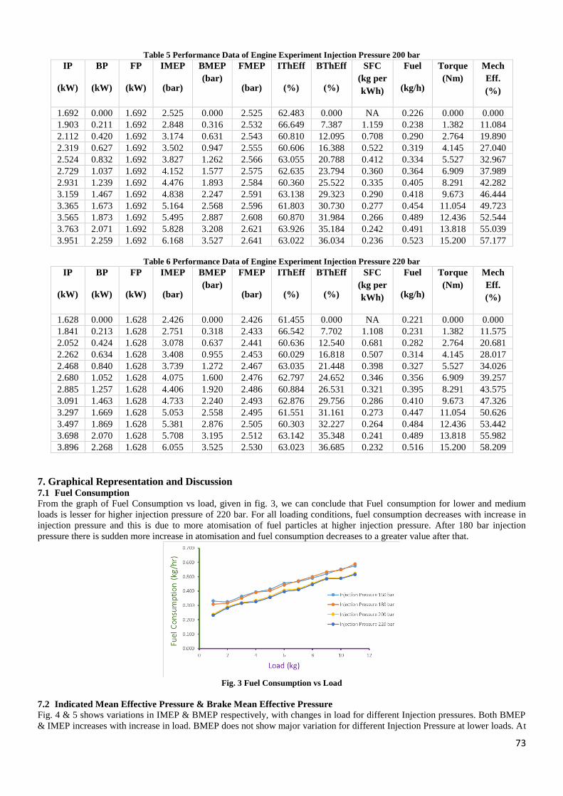
73


IP

(kW)

BP

(kW)

FP

(kW)

IMEP

(bar)

BMEP

(bar)

FMEP

(bar)

IThEff

(%)

BThEff

(%)

SFC

(kg per

kWh)

Fuel

(kg/h)

Torque

(Nm)

Mech

Eff.

(%)

1.692 0.000 1.692 2.525 0.000 2.525 62.483 0.000 NA 0.226 0.000 0.000

1.903 0.211 1.692 2.848 0.316 2.532 66.649 7.387 1.159 0.238 1.382 11.084

2.112 0.420 1.692 3.174 0.631 2.543 60.810 12.095 0.708 0.290 2.764 19.890

2.319 0.627 1.692 3.502 0.947 2.555 60.606 16.388 0.522 0.319 4.145 27.040

2.524 0.832 1.692 3.827 1.262 2.566 63.055 20.788 0.412 0.334 5.527 32.967

2.729 1.037 1.692 4.152 1.577 2.575 62.635 23.794 0.360 0.364 6.909 37.989

2.931 1.239 1.692 4.476 1.893 2.584 60.360 25.522 0.335 0.405 8.291 42.282

3.159 1.467 1.692 4.838 2.247 2.591 63.138 29.323 0.290 0.418 9.673 46.444

3.365 1.673 1.692 5.164 2.568 2.596 61.803 30.730 0.277 0.454 11.054 49.723

3.565 1.873 1.692 5.495 2.887 2.608 60.870 31.984 0.266 0.489 12.436 52.544

3.763 2.071 1.692 5.828 3.208 2.621 63.926 35.184 0.242 0.491 13.818 55.039

3.951 2.259 1.692 6.168 3.527 2.641 63.022 36.034 0.236 0.523 15.200 57.177


IP

(kW)

BP

(kW)

FP

(kW)

IMEP

(bar)

BMEP

(bar)

FMEP

(bar)

IThEff

(%)

BThEff

(%)

SFC

(kg per

kWh)

Fuel

(kg/h)

Torque

(Nm)

Mech

Eff.

(%)

1.628 0.000 1.628 2.426 0.000 2.426 61.455 0.000 NA 0.221 0.000 0.000

1.841 0.213 1.628 2.751 0.318 2.433 66.542 7.702 1.108 0.231 1.382 11.575

2.052 0.424 1.628 3.078 0.637 2.441 60.636 12.540 0.681 0.282 2.764 20.681

2.262 0.634 1.628 3.408 0.955 2.453 60.029 16.818 0.507 0.314 4.145 28.017

2.468 0.840 1.628 3.739 1.272 2.467 63.035 21.448 0.398 0.327 5.527 34.026

2.680 1.052 1.628 4.075 1.600 2.476 62.797 24.652 0.346 0.356 6.909 39.257

2.885 1.257 1.628 4.406 1.920 2.486 60.884 26.531 0.321 0.395 8.291 43.575

3.091 1.463 1.628 4.733 2.240 2.493 62.876 29.756 0.286 0.410 9.673 47.326

3.297 1.669 1.628 5.053 2.558 2.495 61.551 31.161 0.273 0.447 11.054 50.626

3.497 1.869 1.628 5.381 2.876 2.505 60.303 32.227 0.264 0.484 12.436 53.442

3.698 2.070 1.628 5.708 3.195 2.512 63.142 35.348 0.241 0.489 13.818 55.982

3.896 2.268 1.628 6.055 3.525 2.530 63.023 36.685 0.232 0.516 15.200 58.209

7. Graphical Representation and Discussion 7.1 Fuel Consumption

From the graph of Fuel Consumption vs load, given in fig. 3, we can conclude that Fuel consumption for lower and medium

loads is lesser for higher injection pressure of 220 bar. For all loading conditions, fuel consumption decreases with increase in

injection pressure and this is due to more atomisation of fuel particles at higher injection pressure. After 180 bar injection

pressure there is sudden more increase in atomisation and fuel consumption decreases to a greater value after that.

Fig. 3 Fuel Consumption vs Load

7.2 Indicated Mean Effective Pressure & Brake Mean Effective Pressure

Fig. 4 & 5 shows variations in IMEP & BMEP respectively, with changes in load for different Injection pressures. Both BMEP

& IMEP increases with increase in load. BMEP does not show major variation for different Injection Pressure at lower loads. At

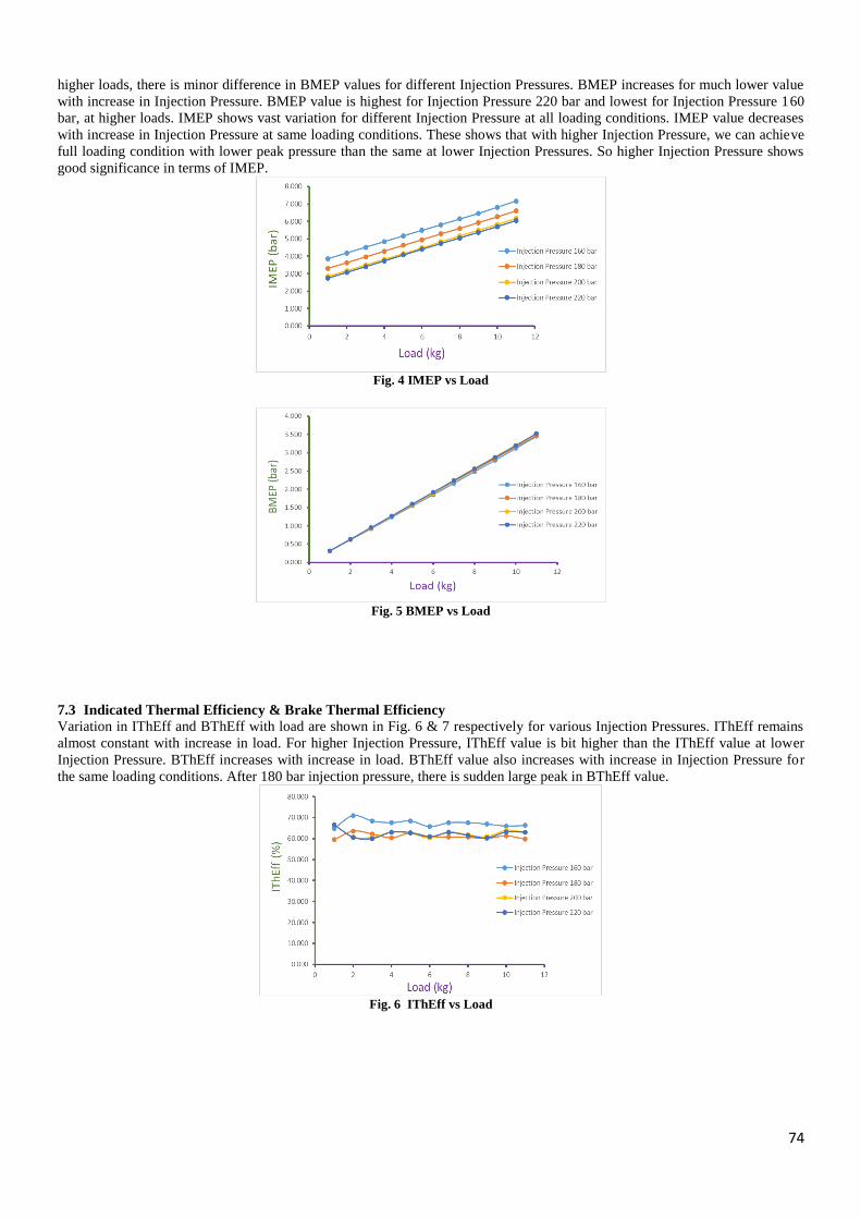
74

higher loads, there is minor difference in BMEP values for different Injection Pressures. BMEP increases for much lower value

with increase in Injection Pressure. BMEP value is highest for Injection Pressure 220 bar and lowest for Injection Pressure 160

bar, at higher loads. IMEP shows vast variation for different Injection Pressure at all loading conditions. IMEP value decreases

with increase in Injection Pressure at same loading conditions. These shows that with higher Injection Pressure, we can achieve

full loading condition with lower peak pressure than the same at lower Injection Pressures. So higher Injection Pressure shows

good significance in terms of IMEP.

Fig. 4 IMEP vs Load

Fig. 5 BMEP vs Load

7.3 Indicated Thermal Efficiency & Brake Thermal Efficiency

Variation in IThEff and BThEff with load are shown in Fig. 6 & 7 respectively for various Injection Pressures. IThEff remains

almost constant with increase in load. For higher Injection Pressure, IThEff value is bit higher than the IThEff value at lower

Injection Pressure. BThEff increases with increase in load. BThEff value also increases with increase in Injection Pressure for

the same loading conditions. After 180 bar injection pressure, there is sudden large peak in BThEff value.

Fig. 6 IThEff vs Load

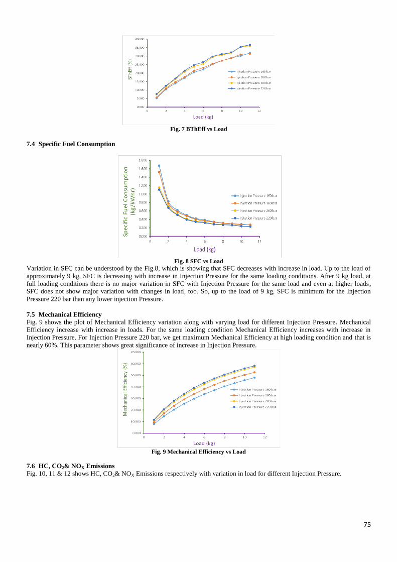
75

Fig. 7 BThEff vs Load

7.4 Specific Fuel Consumption

Fig. 8 SFC vs Load

Variation in SFC can be understood by the Fig.8, which is showing that SFC decreases with increase in load. Up to the load of

approximately 9 kg, SFC is decreasing with increase in Injection Pressure for the same loading conditions. After 9 kg load, at

full loading conditions there is no major variation in SFC with Injection Pressure for the same load and even at higher loads,

SFC does not show major variation with changes in load, too. So, up to the load of 9 kg, SFC is minimum for the Injection

Pressure 220 bar than any lower injection Pressure.

7.5 Mechanical Efficiency

Fig. 9 shows the plot of Mechanical Efficiency variation along with varying load for different Injection Pressure. Mechanical

Efficiency increase with increase in loads. For the same loading condition Mechanical Efficiency increases with increase in

Injection Pressure. For Injection Pressure 220 bar, we get maximum Mechanical Efficiency at high loading condition and that is

nearly 60%. This parameter shows great significance of increase in Injection Pressure.

Fig. 9 Mechanical Efficiency vs Load

7.6 HC, CO2& NOX Emissions

Fig. 10, 11 & 12 shows HC, CO2& NOX Emissions respectively with variation in load for different Injection Pressure.

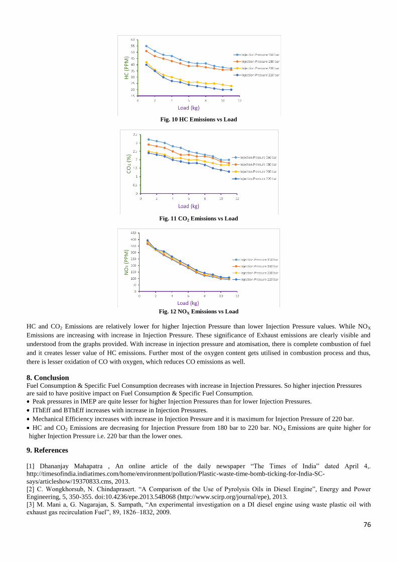
76

Fig. 10 HC Emissions vs Load

Fig. 11 CO2 Emissions vs Load

Fig. 12 NOX Emissions vs Load

HC and CO2 Emissions are relatively lower for higher Injection Pressure than lower Injection Pressure values. While NOX

Emissions are increasing with increase in Injection Pressure. These significance of Exhaust emissions are clearly visible and

understood from the graphs provided. With increase in injection pressure and atomisation, there is complete combustion of fuel

and it creates lesser value of HC emissions. Further most of the oxygen content gets utilised in combustion process and thus,

there is lesser oxidation of CO with oxygen, which reduces CO emissions as well.

8. Conclusion Fuel Consumption & Specific Fuel Consumption decreases with increase in Injection Pressures. So higher injection Pressures

are said to have positive impact on Fuel Consumption & Specific Fuel Consumption.

Peak pressures in IMEP are quite lesser for higher Injection Pressures than for lower Injection Pressures.

IThEff and BThEff increases with increase in Injection Pressures.

Mechanical Efficiency increases with increase in Injection Pressure and it is maximum for Injection Pressure of 220 bar.

HC and CO2 Emissions are decreasing for Injection Pressure from 180 bar to 220 bar. NOX Emissions are quite higher for

higher Injection Pressure i.e. 220 bar than the lower ones.

9. References

[1] Dhananjay Mahapatra , An online article of the daily newspaper ―The Times of India‖ dated April 4,.

http://timesofindia.indiatimes.com/home/environment/pollution/Plastic-waste-time-bomb-ticking-for-India-SC-

says/articleshow/19370833.cms, 2013.

[2] C. Wongkhorsub, N. Chindaprasert. ―A Comparison of the Use of Pyrolysis Oils in Diesel Engine‖, Energy and Power

Engineering, 5, 350-355. doi:10.4236/epe.2013.54B068 (http://www.scirp.org/journal/epe), 2013.

[3] M. Mani a, G. Nagarajan, S. Sampath, ―An experimental investigation on a DI diesel engine using waste plastic oil with

exhaust gas recirculation Fuel‖, 89, 1826–1832, 2009.

77

[4] M. Mani, G. Nagarajan, ― Influence of injection timing on performance, emission and combustion characteristics of a DI

diesel engine running on waste plastic oil Energy, 34, 1617–1623, 2009.

[5] Avinash Kumar Agarwala, Dhananjay Kumar Srivastavaa, Atul Dhara, Rakesh Kumar Mauryaa, Pravesh Chandra Shuklab,

Akhilendra Pratap Singha,‖ Effect of fuel injection timing and pressure on combustion, emissions and performance

characteristics of a single cylinder diesel engine Fuel‖, Volume 111, Pages 374–383, March 2013.

[6] Balaji Mohan, Wenming Yang, Siaw kiang Chou, ―Fuel injection strategies for performance improvement and emissions

reduction in compression ignition engines - A review‖. Renewable and Sustainable Energy Reviews, Vol. 28, pp. 664–676,

2013.

[7] Kyunghyun Ryu, ―Effects of pilot injection pressure on the combustion and emissions characteristics in a diesel engine using

biodiesel–CNG dual fuel. Energy Conversion and Management‖, Volume 76, pp 506–516, 2013.

[8] Özer Cana, İsmet Çeliktenb, Nazım Ustac. ―Effects of ethanol addition on performance and emissions of a turbocharged

indirect injection Diesel engine running at different injection pressures‖, Energy Conversion and Management, Volume 45,

Issues 15–16, Pages 2429–2440, 2004.

[9] G.R. Kannan, R. Anand, ―Experimental evaluation of DI diesel engine operating with diesel at varying injection pressure and

injection timing‖, Fuel Processing Technology, Volume 92, Issue 12, pp.2252–2263, 2011.

[10] A report on Technical Information Exchange on Pyrolysis Oil: Potential for a Renewable Heating Oil Substitution Fuel in

New England, Report prepared by Energetics Incorporated Columbia, Maryland For Bioenergy, Technologies Office

Washington, DC Contact Info: Bioenergy Technologies Office Energy Efficiency and Renewable Energy U.S. Department of

Energy 1000 Independence Avenue, SW Washington, DC 20585. eere.energy.gov/biomass, May 9-10, 2012.

[11] Sajid Hussain Shah, Zahid Mahmood Khan, Iftikhar Ahmad Raja, Qaisar Mahmood, Zulfiqar Ahmad Bhatti, Jamil Khan,

Ather Farooq, Naim Rashid, Donglei Wub, Low temperature conversion of plastic waste into light hydrocarbons. Journal of

Hazardous Materials 179, 15–20, 2010.

78

Mechanism for Garbage disposal vehicle

Hardik Shukla,Hardik Gangadia, Raj Padhiyar


Mechanical Department, Silver Oak College of Engineering and Technology, Gujarat Technological University,

Ahmedabad, 382481, Ahmedabad

Abstract:- Now a day‘s cleanliness is the major concern. Truck typed vehicles are used to convey garbage to street to disposal site. While filling garbage into truck, some sort of garbage fall outside the tuck to avoid this easy and efficient mechanism is developed. Also a mechanism provide bucket at lower height so that anyone can fill garbage vary easy way. These systems collect the garbage for the proper collection and loading of garbage in the garbage disposal vehicle. Generally these vehicles are provided by the Municipal Corporation which required two people to fill garbage in the container and this system is very handy to operate, required only one person to operate without any heavy effort. This mechanism serves efficiently to reduce the human effort and also neglect the outflow of garbage while filling it into the container of the truck.

Keywords: Bucket, Rope & pulley drive, Winding drum, Shaft, Bearing

1. Introduction It is very important to clean ones surrounding to prevent illness of the human being. Government plays an important role for the

cleanliness from the society. For that they have provided garbage collection truck that collect garbage from the society and

dump it in the disposal place [1]. Fig. 1 shows the garbage disposal truck.

Fig. 1 Garbage Disposal Truck

As we can clearly see that it‘s just a large garbage container loaded on the truck and there is no loading facility available hence

the workers have to load the garbage by their effort. Due to high height of garbage container, people do not dump the garbage

easily, minimum two people required to dump the garbage into the container. Sometimes the garbage bucket suddenly fall from

the people or such type of hazards occurs. During such process required much time that increase the wastage of time of workers.



79

In every morning of day, municipal worker collect the garbage from residential area, commercial area, industrial area or road

side garbage [3]. As worker is working in all the weather condition, it will be difficult to dump

garbage into container on daily basis. Sometimes, it may happen that while dumping the garbage in container some amount of

garbage fall down on the floor and to produced dirtiness in surrounding the medium.

Various type of interaction occurs while dumped the garbage in the container.

The Automated Garbage Disposal [6] Vehicles available are very expensive and they operate on hydraulics, fuel,

pneumatics and other non renewable resource for hauling of the garbage and these resources are already declining. The vehicles

mostly used in India as mentioned earlier have no system to haul and dump the garbage.

To come out such difficulties present work is carried out by designing such a mechanical system for the proper collection and

loading of garbage in the garbage disposal vehicle that is operated manually.

2. Development of mechanism For the development of mechanism first the dimension of the AMC garbage truck container is selected. The container shown in

fig 2 is actually working in the municipal corporation. Mechanism is designed is such a way that it will be fitted on outer surface

of the existing container.

Fig. 2 AMC container

By considering above container dimensions conceptual mechanism is developed that includes components like shaft, Bucket for

garbage, Bearing, rope & pulley, drum. Such design is developed in the software CREO. Fig 3 shows final design of the

mechanism.

80

Fig. 3 Conceptual Design

3. Designing of Mechanism Garbage truck mechanism have many component that affected by the amount of load acting on it and designing of such

component is explained below.

3.1 Bucket

In the bucket [4] garbage will be filled and transfer to the container. The length and width of the bucket is exact size of the

container window. At the end of the bucket specific L shaped is developed that will avoid the falling of the bucket inside the

window. By considering the dimension of length, breadth and height as 73, 58 and 20 respectively, total volume of bucket is

determined as 78880 cm3.

Fig. 4 Bucket for dumping garbage

3.2 Shaft[2]

Shaft is used to lift three of the bucket simultaneously with the help of the external force. Bearing is used to support the shaft.

Stresses developed in shaft are shear stresses due to the transmission of torque and Bending stresses.

Mass that carry by shaft = mass of bucket + mass of wastage

= 12kg+ 17kg

= 30kg

Total Weight of bucket, W = 30 * 9.81 = 294.3N

81

Fig. 5 shaft force analysis

Two joining are there so weight is divided by 2.

Consider only one bucket and taking moment@ point A,

(147.1*24)+(147.1*48) = (Rb*72)

Rb = 147.1N

Ra+Rb =147.1+147.1

Ra=147.1N

Moment at mid points,

M = Ra*24 = 35304 Nmm

σbt = 0.6 σy

For our case σbt = σb

For mild steel yield stress y= 248Mpa

Moment equation;

M = (3.14* σb *d3)/32

Putting M and σb we get d = 14mm

For hollow shaft outer diameter do = 14mm

Moment equation is given by,

M = (3.14* σb *(do4-di

4))/(32*do)

di = 8.21mm

3.3 Bearing

Bearing is used to support the rotating shaft and selection criteria majorly depend upon the application where it is used. Rolling

contact bearing is used and dimension is selected as per availability in the market. Dimension of the bearing are, Bore = 20mm,

Outer diameter = 47mm, Width = 14mm.

3.4 Pulley & Rope

Rope [7] is selected according to the load to be carried and the standard ropes available in the market. When a large amount of

power is to be transmitted over long distances from one pulley to another (i.e. when the pulleys are upto 150 metres apart), then

wire ropes are used. The wire ropes are widely used in elevators, mine hoists, cranes, conveyors, hauling devices and suspension

bridges.

Pulley is selected according to the rope to be wound and the standard pulleys available accordingly. Dimensions for the pulley

and rope are as follows, Rope: Diameter = 3mm*5mm (7*19); Length = 300mm and for Pulley (sheave): Outer diameter =

70mm; Inner diameter = 12mm; Slot thickness = 10mm; Slot height = 10mm.

3.5 Drum

The drum is used to winding the rope at the end. Drum is make by any material but for cost saving in the final model wooden is

selected. For the drum handle you need some pedal type part for easily rotate. The distance from winding drum center to holding

center is more than torque is more and working is easily.

Otherwise we can use more number of pulleys for minimizing the load.

4. Working Model Working modal is developed by considering the half scale of the dimensions. Wood is selected for making the container due to

its availability. Also galvanized sheet is used for making bucket of a required size. By considering such materials manufacturing

cost is decreased and modal gives conceptual idea for the same as actual. Below table 1 gives actual weight of the individual

component that is used in the mechanism.

Sr. No. Component Weight(gm)

1 Shaft 132

2 Bearing 30

3 Pulley 76

4 Rope 548

82

5 Clamp of rope 20

6 Drum 18

7 Bucket 1102

Table 1 Actual weight of the component

Fig.6 shows the actual working modal of the garbage disposal mechanism which is developed by considering half scale of the

dimensions.

Fig 6 Actual working Modal of mechanism

5. Results and discussion The amount of force required to lift the load is near about 10 kg, so it is very easy to lift the load by the human for dumping

garbage into the container. As drum is rotated rope is wound on it and bucket which is connected to the rope will go upward

with the garbage. Experiment shows that mechanism serves its purpose correctly.

During the running condition of the truck bucket will rest on the container so that it will not affect any regular running condition

of garbage truck.

6. Conclusion Experiment shows that mechanism serves its purpose correctly. Similar way one can able to developed for the three bucket.

Such mechanism will reduce the human effort as well as time for collecting the garbage. Also only single man can able to

perform the given task like dumping garbage into the container, driving truck to different places and less amount of wastage is

occur. One can also make automated [5] mechanism but that increase the cost of the mechanism so that in the present work only

mechanical component is used in order to make it cost efficient.

7. References [1]. Vitus M. Tabie, Yesuenyeagbe A. K. Fiagbe, ‖Weight Optimization Of A Lift-Tipping Mechanism For Small Solid Waste

Collection Truck‖, International Journal of Scientific & Technology Research, volume 3, issue 7, ISSN 2277-8616, 2014.

[2]. R. S. Khurmi and J. K. Gupta Machine design by published at. A Textbook for the Students of B.E. / B.Tech., U.P.S.C.

(Engg. Services); Section ‗B‘ of A.M.I.E. (I), 2005.

[3].Geroux, Zachary; Voytko, Eric. "The Ever Expanding History of the Front Load Refuse Truck".

http://www.classicrefusetrucks.com/albums/FL/FL01.html. "Heil Expands Operate-At-Idle Offering". 4 February 2005.

Retrieved 10 September, 2014.

http://www.classicrefusetrucks.com/albums/FL/FL01.html

http://www.classicrefusetrucks.com/albums/FL/FL01.html

http://fleetowner.com/news/heil_idle_system_020405

83

[4]."Waste Truck Collection Systems". TruckWorld.com.au. 11 February 2015. Retrieved12 May, 2015.

[5]. Marc J. Rogoff. "Solid waste collection automation in the United States" , Retrieved 10 September, 2014.

[6].http://www.madehow.com/Volume-3/Garbage-Truck.html.Sean, Murphy, "Automated Garbage Collection"3 April, 2014.

[7] Design data book PSG publication.

http://www.truckworld.com.au/Blogs/Waste-Truck-Collection-Systems

http://www.scsengineers.com/Papers/Rogoff_Solid_Waste_Collection_Automation_in_the_United_States.pdf

http://www.madehow.com/Volume-3/Garbage-Truck.html

http://eagledumpsterrental.com/automated-garbage-collection.html

84

IC Engine Exhaust Valve Design Optimization Using Finite Element

Analysis

Karan Soni, Ripen Shah, Umang Vora

[email protected], [email protected],[email protected]


India

Abstract:-

In order to develop an exhaust valve with high thermal and structural strength, experimental investigations are often costly and

time consuming, affecting manufacturing time as well as time-to-market. An alternative approach is to utilize computational

methods such as Finite Element Analysis, which provides greater insights on temperature distribution across the valve geometry

as well as possible deformation due to structural and thermal stresses. This method significantly shortens the design cycle by

reducing the number of physical tests required. Utilizing the computational capability, this research aims to identify possible

design optimization of the exhaust valve for material and weight reduction, without affecting the thermal and structural strength.

Keywords: Design Optimization, Exhaust Valve, Finite Element Analysis, Structural Analysis, Thermal Analysis

1. Introduction

Exhaust valves are utilized in 4-stroke internal combustion engines to allow the exhaust gases to escape into the exhaust

manifold. Due to the exposure to high temperature gases, exhaust valve design is of a crucial interest. Apart from high thermal

stresses, these valves are also exposed to cyclic mechanical stresses during opening and closing, causing them to fail

prematurely. It is quite evident that a common cause of valve fracture is fatigue. Valves fail due to cyclic loading at high

temperatures. High temperature is also responsible for decrease in hardness and yield strength of valve material, and also causes

corrosion of exhaust valves [5]. As such, factors such as temperature, fatigue life, material strength and manufacturing processes

are to be considered in order to design a valve that operates without premature failure. Exhaust valves with better material

strength can provide significant benefits in cost reduction while also reducing its weight [1]. Several material studies show that

Magnesium alloy [2] and Nimonic105A [3] are some of the best suitable materials for exhaust valves. Modifying the exhaust

valve by varying its position size and shape and with particular thermal and structural considerations, helps in increasing the rate

of heat transfer from the seat portion of the exhaust valve, thereby reducing the possibility of knocking [4]. Utilizing finite

element analysis, exhaust valve design can be optimized without affecting its thermal and structural strength [6]. A study is

carried out on exhaust valve with and without air cavity using finite element approach.

By creating an air cavity inside the valves stem, it acts as an insulating medium and prevents the heat flow; hence the need of

providing insulation coating on valves is minimized. The main motive of this is to reduce the weight of engine and cost

associated with thermal coating. Results observed in the engine valves revealed that after creating an optimized air cavity in the

valve, thermal stresses and temperatures at all nodal points decrease lightly.

2. Model Selection

In order to carry out thermal and structural analysis, exhaust valve from a single-cylinder engine is selected. The details of the

valve model are as shown in the table.

Table 1: Engine specifications for exhaust valve selection

Engine Type Single Cylinder, 4-Stroke

Cylinder Bore Dia. 50 mm

Displacement 97.2 cc

Max. Power 7.2bhp/8000 rpm

The calculated dimensions of the valve for a single cylinder engine application are tabulated below:


85

Table 2: Valve dimensions

Valve Head Diameter 20 mm

Valve Stem Diameter 5 mm

Stem Length 65.30 mm

Valve face angle 450

Thickness of Valve Head 5 mm

The material of the valve is an Aluminum Alloy EN52 consisting of following mechanical properties.

Table 3: Material Properties

Yield Strength @ 6000C 250 N/mm

2

Tensile Strength @ 6000C 240 N/mm

2

Modulus of Elasticity 210 KN/mm2

Thermal Conductivity 21 W/mK

Specific Heat Capacity 500 J/Kg K

Co-efficient of Thermal Expansion 24.5 x 10-6

3. Assumptions

1. Under normal operation, when the valve is properly seating at the cam ramp, stresses arising from seating are quite

moderate. They can become very high when the valve train is improperly engineered so that the valve bounce occurs,

or when the engine is over speeded or the valve lash is improperly set. In this analysis the stresses due to valve seating

has been not taken into account assuming a normal operation.

2. The distortion stresses in a valve arise due to misalignment of valve with the seat. The valve head must deflect to

accommodate to the seat, and this causes bending stresses in the stem. Under most conditions, gas pressures and spring

loads will be sufficient to bring the valve head into conformity with a mildly distorted seat.

3. The engine considered for the analysis is a medium range engine ( 500 kW). It is assumed that it is air cooled.

4. The heat generated inside the chamber is taken away by water chamber around cylinder liner and in the cylinder head.

5. The valve keeps popping up and down. The analysis has been done for a stationary valve assuming that the fatigue life

of the valve is very high and the stress arising due to that has been neglected.

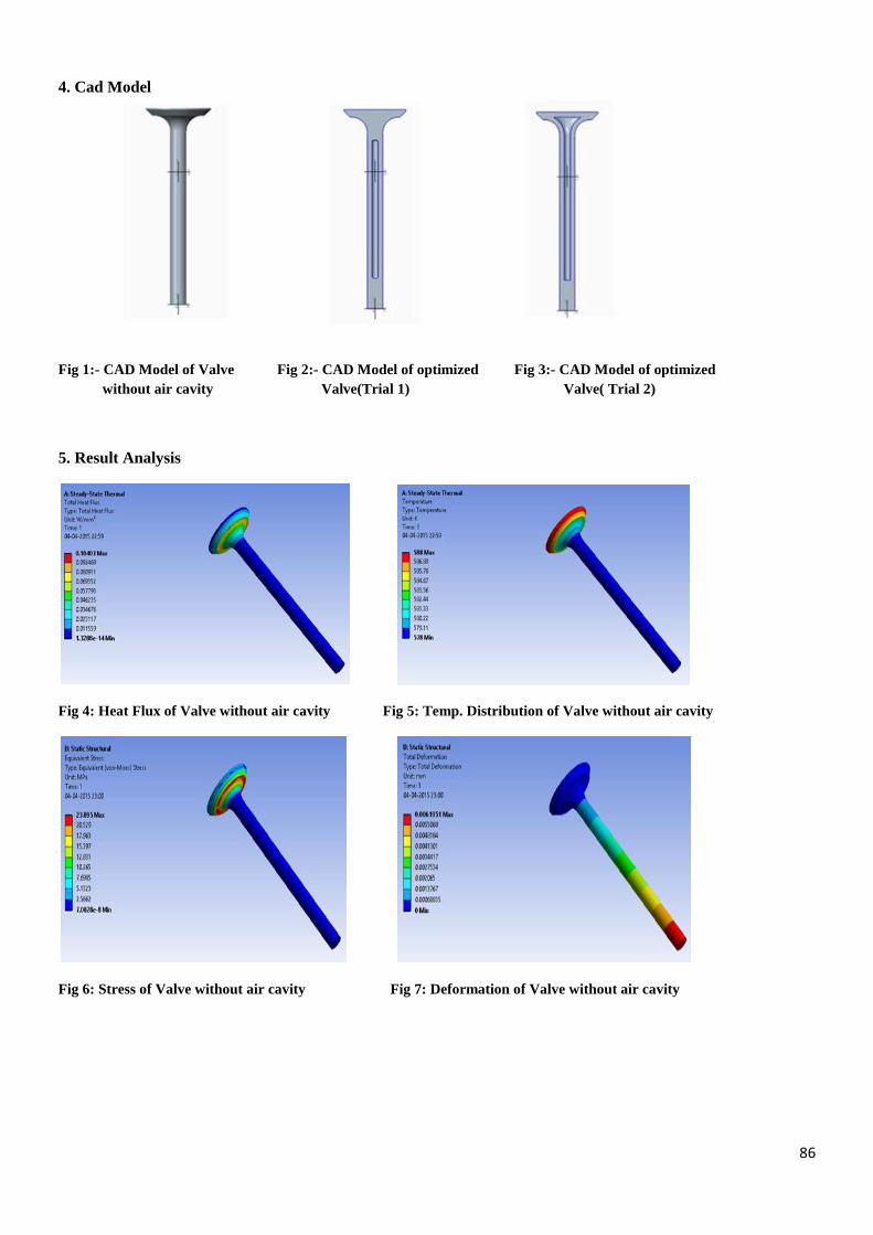
86

4. Cad Model

Fig 1:- CAD Model of Valve Fig 2:- CAD Model of optimized Fig 3:- CAD Model of optimized

without air cavity Valve(Trial 1) Valve( Trial 2)

5. Result Analysis

Fig 4: Heat Flux of Valve without air cavity Fig 5: Temp. Distribution of Valve without air cavity

Fig 6: Stress of Valve without air cavity Fig 7: Deformation of Valve without air cavity

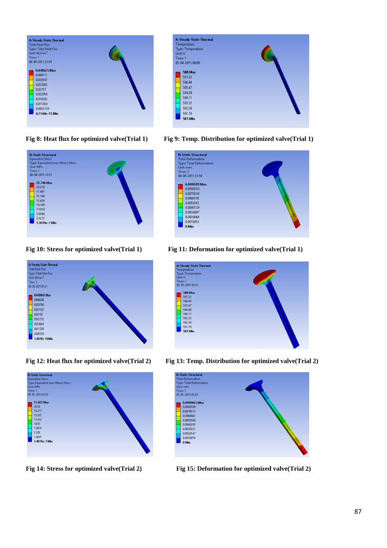
87

Fig 8: Heat flux for optimized valve(Trial 1) Fig 9: Temp. Distribution for optimized valve(Trial 1)

Fig 10: Stress for optimized valve(Trial 1) Fig 11: Deformation for optimized valve(Trial 1)

Fig 12: Heat flux for optimized valve(Trial 2) Fig 13: Temp. Distribution for optimized valve(Trial 2)

Fig 14: Stress for optimized valve(Trial 2) Fig 15: Deformation for optimized valve(Trial 2)

88

Table 4: Result Comparison for Valve with and without cavity

6. Conclusion

The results obtained through numerical analysis suggest that the valve design can be optimized to reduce its weight, without

affecting permissible stress and deformation values. The weight of the valve is reduced by 15%, which can be further reduced

using the same procedure. Considering mass production, significant amount of material can be saved, helping in reduction of the

manufacturing costs.

7. References

[1] Singaiah Gali, T.N. Charyulu, ―Diesel Engine Exhaust Valve Design, Analysis and Manufacturing Processes‖, Indian Stream

Research Journal, Vol.2, Issue 7, ISSN 2230-7850, 2012.

[2] Goli Uday Kumar, Venkata Ramesh Mamilla, ―Failure Analysis of Internal Combustion Engine Valves By Using ANSYS‖,

American Int. Journal of Research in Science, Technology, Engineering & Mathematics. Vol. 14, Issue 183, ISSN 2328-3580,

2014.

[3] V. BalaSundaram, Coupled Field Analysis of Exhaust Valve Using ANSYS.

[4] Ram M.S., ―Design Modification in Engine Exhaust‖, International Journal of Scientific & Engineering Research, Volume 2,

Issue 12, Dec-, ISSN 2229-5518, 2011.

[5] Naresh Kr. Raghuwanshi, Ajay Pandey, R. K. Mandloi, ―Failure Analysis of Internal Combustion Engine Valves: A Review,

International Journal of Innovative Research in Science‖, Engineering & Technology, Vol.1, Issue 2, ISSN 2319-8753, 2012.

Parameters Weight

(gm)

Heat Flux

(W)

Stress

(Mpa)

Temperature

(0K)

Deformation

(mm)

Without Air

Cavity

15.90 0.1043 23.095 588 0.0062

With Air Cavity

(Trial 1)

14.80 0.0496 22.746 588 0.0090

With Air Cavity

(Trial 2)

13.5 0.04984 23.422 588 0.0090

89

Improving the Efficiency of Knitting Machine by Modifying the Needle

Chirag Patel, Mayur Shrivas, Prerak Rathod




Abstract

This project deals with problem of major concern to the Textile industry, which is machine defect and fabric defect. When a

defect occurs, the Knitting machine has to be stopped and the fault corrected, thus result in time loss which is uneconomic.

Eventually the knitted fabric may be rejected if quality requirements are not met. An effective monitoring of the knitting

machine is required in order to avoid or detect and locate a defect and its causes as soon as possible, for avoiding the

productivity and quality loss.

Keyword: Knitting Machine, Yarn, Needle, Creel, Knot Catcher

1. Introduction 1.1 Circular knitting machine [1] Circular knitting machine is widely used through out the knitting industry to produce fabric. This machine can be built in almost

any reasonable diameter and the small diameter of up to five, which are used for wear.

Machine for outerwear and under wear may vary from 12 inch to 60 inch in diameter according to manufactures requirement.

This machine can be used either as fabric or for making garments completely with fancy stitch. Latch needle are commonly

employed in all modern circular machines because of their simple action and also their ability to process more types of yarns.

Figure 1: Circular Knitting Machine Figure 2: Needles

Needle: It is a principal element of the knitting machine. Its help the yarn to create a loop. And by this way fabric are produce.

Prior to yarn feeding the needle is raised to clear the old loop from the hook, and received the new loop above it on needle stem.

The new loopis then enclosed in the needle hook as the needle starts to descend. [2]

The needles are the most important stitch forming elements. They are displaced vertically up and down and are mounted into

tricks or cuts of knitting cylinder. There are types of needles namely:

1. Latch Needle [3]

2. Spring Bearded Needle, and

3. Compound Needle

mailto:[email protected],%[email protected],%[email protected]

90

Figure 3: Components of needles

1.2 Problems and Limitations of Circular Knitting Machines Problems associated in knitting machine which reduces production and increases consumption of time & electricity. One major

problem amount of heat generation is more. Fabric and Machine defects are listed below:

Table 4: Problems and limitations [4] [5]

Codes REASONS (For Loss Of Production) Reasons for Stoppage(Problems )

01 Yarn lot changed Needle breakage

02 Needle changed Program change

03 M/C setting Star mark

04 Maintenance Hole mark

05 Mech. Breakdown Sinker Mark

06 Electrical breakdown Needle mark

07 Yarn Rewinding Maintenance

08 Yarn short Hole Mark

09 Air problem RPM Oil & belt check

10 App. Pending Power failure

11 Press of Problem Yarn Breakage

12 Holes Problem Fabric Handling

13 Other Prob. Yarn Breakage

1.3 Possible Solution

The above Reasons reduce production and increases time consumption. The defects can be due to fabric and machine. So

below list of Possible Solution:

Table 5: List of possible solutions

No Possible Solutions:

1 Needle Modification (latch needle) Major Issue

2 Yarn Guide Tube

3 Control Of Quality and Rpm by VDQ Pulley

4 Size Modification of Note Catcher

5 Increase in Floor Space Area

1.4 Geometric Modeling Of Modified Needle

Modified latch needle is a newly designed needle on which the shapes of the main body and rear area have been

modified to reduce the amount of contact with the cylinder slot. This new design makes it possible to greatly reduce both the

amount of energy required for operation and the amount of heat generated by friction. Dimensions of the Needle has been taken

from [5]

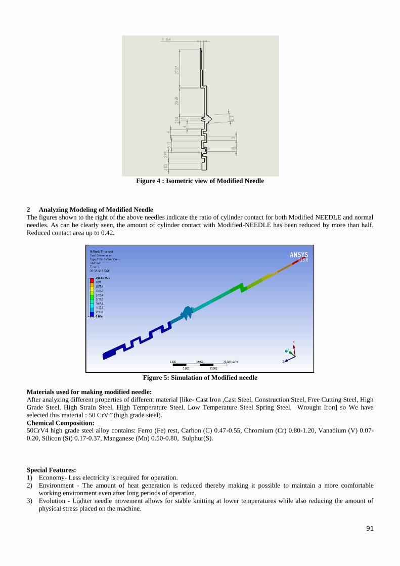
91

Figure 4 : Isometric view of Modified Needle

2 Analyzing Modeling of Modified Needle

The figures shown to the right of the above needles indicate the ratio of cylinder contact for both Modified NEEDLE and normal

needles. As can be clearly seen, the amount of cylinder contact with Modified-NEEDLE has been reduced by more than half.

Reduced contact area up to 0.42.

Figure 5: Simulation of Modified needle

Materials used for making modified needle: After analyzing different properties of different material [like- Cast Iron ,Cast Steel, Construction Steel, Free Cutting Steel, High

Grade Steel, High Strain Steel, High Temperature Steel, Low Temperature Steel Spring Steel, Wrought Iron] so We have

selected this material : 50 CrV4 (high grade steel).

Chemical Composition: 50CrV4 high grade steel alloy contains: Ferro (Fe) rest, Carbon (C) 0.47-0.55, Chromium (Cr) 0.80-1.20, Vanadium (V) 0.07-

0.20, Silicon (Si) 0.17-0.37, Manganese (Mn) 0.50-0.80, Sulphur(S).

Special Features:

1) Economy- Less electricity is required for operation.

2) Environment - The amount of heat generation is reduced thereby making it possible to maintain a more comfortable

working environment even after long periods of operation.

3) Evolution - Lighter needle movement allows for stable knitting at lower temperatures while also reducing the amount of

physical stress placed on the machine.

92

4) The amount of consumed energy and generated heat with Modified Needle and Normal needles was compared after 3000

machine revolutions.

5) To summarize, an average heat reduction of approximately 15% in the cam holder and sinker cap area as well as an

approximate energy savings of 10% was achieved on the machine running with Modified Needle.

6) The strength of the standard fukuhara needles has been maintained on modified needle.

7) Thus, all of the mentioned improvements have been made without compromising durability. Modified needle is available in

a wide range of gauges and is yet another easy to use and reliable fukuhara product.

3 Production Calculation of Circular Knitting Machine

Let us consider a circular Single Jersey knitting machines, having F no of Feeder and N no of needles, is running with a speed of

n r.p.m and producing fabrics of loop length ‗l‘ mm.

No. of courses produced in 1 rev. = F

No. of courses produced in n rev. = F x n

No. of courses produced in 1 min. = F x n

No. of courses produced in 1 hr = F x n x 60

yarn consumed by 1 needle from 1 course = l mm

yarn consumed by 1 needle from 1 hr = F x n x 60 x l mm

yarn consumed by N needle from 1 hr = F x n x 60 x l x N mm = F x n x 60 x l x N /1000 meter

Total yarn consumed by the m/c in 1 hr = F.n.60.l.N/1000 meter

If yarn count is N- m, then the weight of above yarn = F.n.60.l.N/1000.Nm.1000 Kg

Problem For 1st line:

Feeder=84

Diameter=30 inch

Gauge=24/inch

Cylinder rpm =18

Yarn count=30Ne

Efficiency=90%

Stitch length=2 mm

Solution:

length of yarn = (3.14x30x24x2x84x24x60x24x60)/(1000x100)

=7875831.39 meter

=7875.83

now 20NE = NE x tex = 590.6….. [6]

So, tex=590.6/20 = 29.58

Again 1 Km Yarn Weight=29.58

7875.83 km yarn weight = (29.58x7875.83)

Total yarn weight =232.967 kg

Table 3: Estimated Production Rate

M/c

Ga

uge

[6]

Prod

uct

No.

[6]

K. Qty

Machine

Capacity

(kg)

Current

Knitted

Producti

on (kg)

Calculated and

Assumed Prod.

By Modified

needle (kg)

87 48.4 330 192.7 232.96

88 107.7 370 107.7 302

83 612.2 785 612.2 720

70 435.2 2510 1371.3 1800

69 125.7 402 146.2 298

96 116 384 158.6 326

81 762.4 12000 4190.42 6002

93

4 Results and Conclusion

The results indicate approximately 0.17kw less electricity was consumed on the machine running with Modified Needle. This

calculates to a CO2 reduction of 30 liters.

Figure 6: Comparison of Amount of Energy Consumed with Normal Needle and Modified Needle

Average temperature at cam holder and sinker cap area least conducted at room temperature 24.6 degree Celsius .heat reduction

is 15%.

Figure 7: Comparison of Temperature generation with Normal Needle and Modified Needle

With the use of modified needle in knitting machine it will give more production in less time and less maintenance cost.

Modified needle is cost effective and after material modification its weight is maintained 670 milligrams as weight of normal

needle but still it is as more durable than normal needle. Furthermore electricity consumption is reduced and heat generation is

reduced by reducing the contact area coefficient compared to normal needle decreased by more than 55%. From production

sheet we can say that efficiency of machine is increased by 30%.

REFERENCES

[1] Anbumani N., P.S.G. College of Technology, Coimbatore, Tamil Nadu, ―Knitting Fundamentals, Machines, Structures and

Developments‖, 2014.

Amount of

energy

consumed

kwh

20G /Sf900 30rpm/30

Temp 0c

http://www.newagepublishers.com/servlet/nadispinfo?offset=0&searchtype=Author&text1=Anbumani,%20N.&ordby=Publication%20Year

94

[2] Hodder, Stoughton, ―Mary Thomas's Knitting Book (1938) reprinted‖, 1985.

[3] Textilelearner.blogspot.in

[4] Catarino A. P., Rocha A. M., Monterio J.L., ―Monitoring Systems for Fault Detection on Circular Knitting Machines

Through Yarn Input Tension‖, ICOM 2003-International Conference on Mechatronics, ISBN 1 86058 420 9.

[5] Fundamentals and Advances in Knitting Technology, Wood head Publishing India Pvt. Ltd., New-Delhi, India, October,

2011.

[6] Arvind Polycot Limited, Manual.

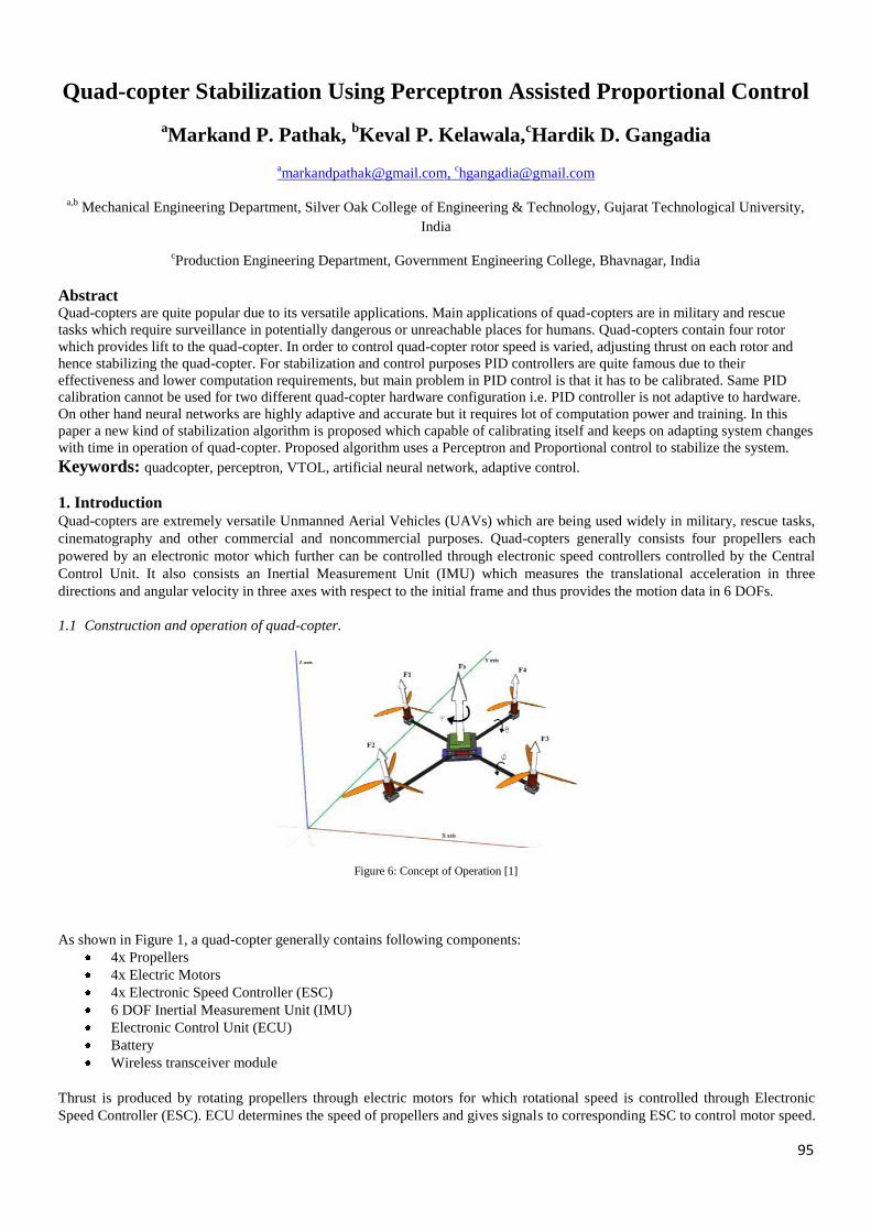
95

Quad-copter Stabilization Using Perceptron Assisted Proportional Control

aMarkand P. Pathak,

bKeval P. Kelawala,

cHardik D. Gangadia

[email protected],

[email protected]

a,b Mechanical Engineering Department, Silver Oak College of Engineering & Technology, Gujarat Technological University,

India

cProduction Engineering Department, Government Engineering College, Bhavnagar, India

Abstract Quad-copters are quite popular due to its versatile applications. Main applications of quad-copters are in military and rescue

tasks which require surveillance in potentially dangerous or unreachable places for humans. Quad-copters contain four rotor

which provides lift to the quad-copter. In order to control quad-copter rotor speed is varied, adjusting thrust on each rotor and

hence stabilizing the quad-copter. For stabilization and control purposes PID controllers are quite famous due to their

effectiveness and lower computation requirements, but main problem in PID control is that it has to be calibrated. Same PID

calibration cannot be used for two different quad-copter hardware configuration i.e. PID controller is not adaptive to hardware.

On other hand neural networks are highly adaptive and accurate but it requires lot of computation power and training. In this

paper a new kind of stabilization algorithm is proposed which capable of calibrating itself and keeps on adapting system changes

with time in operation of quad-copter. Proposed algorithm uses a Perceptron and Proportional control to stabilize the system.

Keywords: quadcopter, perceptron, VTOL, artificial neural network, adaptive control.

1. Introduction Quad-copters are extremely versatile Unmanned Aerial Vehicles (UAVs) which are being used widely in military, rescue tasks,

cinematography and other commercial and noncommercial purposes. Quad-copters generally consists four propellers each

powered by an electronic motor which further can be controlled through electronic speed controllers controlled by the Central

Control Unit. It also consists an Inertial Measurement Unit (IMU) which measures the translational acceleration in three

directions and angular velocity in three axes with respect to the initial frame and thus provides the motion data in 6 DOFs.

1.1 Construction and operation of quad-copter.

Figure 6: Concept of Operation [1]

As shown in Figure 1, a quad-copter generally contains following components:

4x Propellers

4x Electric Motors

4x Electronic Speed Controller (ESC)

6 DOF Inertial Measurement Unit (IMU)

Electronic Control Unit (ECU)

Battery

Wireless transceiver module

Thrust is produced by rotating propellers through electric motors for which rotational speed is controlled through Electronic

Speed Controller (ESC). ECU determines the speed of propellers and gives signals to corresponding ESC to control motor speed.

mailto:[email protected]?subject=QUERY%20REGARDING%20PAPC%20CONTROL

96

Thrust produced by all four propellers lifts the quad-copter. However the quad-copters are very unstable without constant

monitoring and applying corrections through propeller speed. To monitor behavior of quad-copter Inertial Measurement Units

(IMU) are employed which gives 6 DOF motion data to ECU. Based on IMU data ECU applies correction to the motor speed.

Correction is calculated using PID algorithm in most of the cases.

1.2 PID control and its limitations

Figure 7: PID Control

Nomenclature

System response

Error signal

Time

KP Coefficient of proportionality

KI Coefficient of Integrator

KD Coefficient of Differentiator

ix Input signals to perceptron

X Input value vector 0[ ]Tx a dt

nx Count of input values per iteration

nd Difference in speed of propellers in percentage

iw Weights of perceptron inputs

W Weight vector

kb Bias for perceptron

ky Perceptron output

Perceptron activation function

( )J w Error energy

Perceptron learning rate

Basic flow diagram of a PID controller is shown in the Figure 2. PID is abbreviation of Proportional-Integrator-Derivative. As

name suggests it contains three gain block. Mathematically PID control system can be represented as following:

0

( )( ) ( ) ( ) D

t

P Iu t K e tde t

e td

t KKt

d …(1)

There are three main problems associated with three blocks of PID control [2]. Proportionality block tends to have steady state

errors. The integrator term accumulates the errors from the starting of operation and hence value of integrator term increases

with every iteration. Theoretically it does not possess any problem but in actual practice value of integrator term saturates in

very short time and leads to a situation called integrator windup [3]. The differentiator term is not immune to high frequency

noise. The output of D block increases rapidly with increase in frequency of noise and hence it makes system unstable.

Another major disadvantage of using PID is that it requires precise tuning before it can be used regularly. Once tuned the PID is

not adaptive to the changes occurs in environment and quad-copter hardware itself as these changes may change physics of

quad-copter to a great extent. Weight distribution of quad-copter should be well balanced to minimize the effort required for

tuning of PID. It also restricts the weight/payload can be carried by quad-copter because as weight increases it also changes the

behavior of the quad-copter to which PID is not immune.

97

2. Perceptron A perceptron is the most basic artificial neuron and important element of Artificial Neural Network (ANN) and widely used for

classification problems using supervised learning approach. General structure of a perceptron is shown in the Figure 3.

As shown in Figure 3, perceptron can be represented in mathematical terms as following:

1

m

k i i k

i

y x w b …(2)

Here activation function () can be any activation function and selection of activation function is dependent on problem and

applications. It can be a threshold function or a sigmoid function with variable slopes. If we consider the bias value provided in

perceptron as an input to the neuron then input signal provided to that node will be unit value.

Figure 8: An artificial neuron

Rewriting the equation of perceptron

0

m

k i i

i

wy x

To apply the perceptron in quad-copter it is necessary that perceptron is used to find hyperplane in Euclidian space instead of

classifying the input data. To do so activation functions is considered as a unit function.

0

m

k i i

i

wy x …(3)

Weights of the neuron can be adjusted using proper training algorithm.

3. Perceptron Assisted Proportional Control for Quad-Copter To apply perceptron to quad-copters, a factor which affects the quad-copter system should be considered and a hypothesis

function should be generated. For stabilization in translational movement mainly acceleration in three direction and time of

program iteration are the main factors. Now to combine perceptron with proportional control, gain for each factor should be

summed up and it can be called a hypothesis function which once trained incorporates physics of quad-copter in any one

direction. Now for translational motion in X and Y direction from Figure 1, hypothesis function for motion in X direction can be

written as

0 0 1 2( )x xxh w w a tx w d …(4)

( ) T

xh X X W …(5)

Where 0 1x and 0 kw b which acts as a bias input to the perceptron.

Now to train the algorithm real time data is captured from inertial measurement unit [4]. Now consider only one directional

motion in quad which is mainly due to two opposite propellers. Now if both of the propellers are rotating at same speed then

both will produce same thrust and hence system will be stable. If there will be any speed difference between two propellers then

98

there will be a net thrust in translational direction. So the system will start moving in direction opposite to thrust [5]. Now speed

difference is directly controlled by the ECU and hence it can be concluded that there is an unknown relation between speed

difference in propellers and acceleration produced in system, which can be incorporated in hypothesis function through

perceptron training. Now due to inertia of the quad-copter system acceleration is not constant between two consecutive program

iteration on ECU so it is necessary to measure time between two program iteration which indirectly incorporates inertia of quad-

copter system in perceptron. To train perceptron Least-Mean-Square (LMS) is used to calculate total error energy and Gradient

descent algorithm is employed to adjust weights of perceptron. Mathematically total error energy can be written as following.

2

1

( ) (1

2( ) )

k

x n n

n

J w h x d …(6)

Now using stochastic- update rule the gradient descent algorithm can be written as following

( ) ( 1)

( 1)

i

i t i t

i t

wd

ww …(7)

Simplifying Equations 3 and 4

( ) ( 1) ( 1)( )( )i t i t nn x t iw dw h X x …(8)

Now these calculated weights can be placed in hypothesis function and it will be approximately equal to the percentage speed

deference in propellers.

( )n x nd h X …(9)

Now assume that, there is a disturbance to the quad-copter and due to that disturbance quad-copter starts moving with any

acceleration a . Now to stabilize that disturbance reverse acceleration should be applied by adjusting propeller speed. From

Equation 9, required difference in propeller speed can be calculated in terms of percentage by putting value of acceleration and

dt . This percentage value is defined in terms of maximum allowed difference between propeller speeds to eliminate complete

roll of the system. Once calculated required propeller speed difference it should be applied such that reverse acceleration is

produced. The learning algorithm should be performed with every program- iteration to constantly adapt the environment and

quad-copter system changes. Learning rate should be selected in range of 0.1 to 0.9. If the selected learning rate is too high

then system will adapt to every minor change and makes the quad-copter very sensitive to minor disturbance and if learning rate

is kept low then quad will take too much time to adapt the situation. So learning rate should be selected such that perceptron

remains invariant for small changes in quad-behaviour.

Figure 4 shows graphical representation of Perceptron Assisted Proportional Control (PAPC). Here for simplicity purpose

control of only single direction is given. Same procedure can be applied for all the directions in quad-copter system. Initial

weights of perceptron can be taken random and it is trained it automatically converges towards optimum value. There is no need

to calibrate the system initially, as shown in Figure 4 output is fed into the perceptron and due to that as system starts from

scratch and starts flying it also trains itself in real time.

Figure 9: Perceptron Assisted Proportional Control

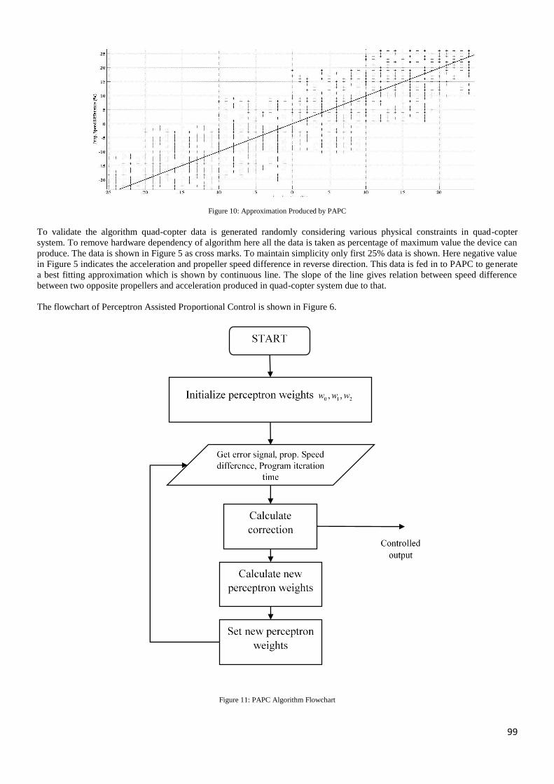
99

Figure 10: Approximation Produced by PAPC

To validate the algorithm quad-copter data is generated randomly considering various physical constraints in quad-copter

system. To remove hardware dependency of algorithm here all the data is taken as percentage of maximum value the device can

produce. The data is shown in Figure 5 as cross marks. To maintain simplicity only first 25% data is shown. Here negative value

in Figure 5 indicates the acceleration and propeller speed difference in reverse direction. This data is fed in to PAPC to generate

a best fitting approximation which is shown by continuous line. The slope of the line gives relation between speed difference

between two opposite propellers and acceleration produced in quad-copter system due to that.

The flowchart of Perceptron Assisted Proportional Control is shown in Figure 6.

Figure 11: PAPC Algorithm Flowchart

100

4. Additional Advanced Capabilities Due to PAPC Following additional capabilities are added in quad-copter resulting from Perceptron Assisted Proportional Control:

PID controlled quad-copters are vulnerable to weight distribution on the quad-copter body. Extreme care has to be

taken for balancing of weight. In PAPC control, during training weight unbalance becomes a part of the physics of the

quad-copter and hence it is not necessary that the payload carried by the quad-copter is balanced. Any payload having

uneven weight distribution can be carried and no extra effort will be required from operator side to control the quad

with uneven weight distribution.

Any quad-copter experiences changes in its performance over time due to degradation in battery capacity, wear of parts

and due to accidental damage. This all changes are not incorporated in PID controller. However the PAPC is constantly

adaptive it incorporates all these changes over time and hence maintains the performance at optimum value.

As PID controller is calibrated using trial and error method it is almost impossible to converge towards most optimum

solution. While PAPC automatically calibrates itself and hence it uses mathematical methods to converge towards

optimum solution, the performance always converges towards optimum.

As the time passes mathematical approximation as described in hypothesis function gets more and more accurate.

Hence it also helps in optimizing power consumption because PAPC will use only required amount of power to balance

the system.

5. Conclusion By using this control algorithm, the quadcopters can be made immune to the change in environment and change in the system

itself. By using this algorithm there is no need to calibrate onboard control system on quadcopters according to the hardware of

drone. Instead of calibration the drone is operated in safe conditions for first few minutes to avoid accidental damage, while the

algorithm adapts to the physics of drone. Once adapted it will continue to improve operation of drone. This algorithm also

permits use of unbalanced payload up to certain limit without compromising the control of the drone. The limit of unbalanced

load depends on the hardware of the drone.

6. Acknowledgements The authors would like to thank Asst. Prof. Subhash Padmanabhan and Asst. Prof. Rohit Sahu, Ex. Faculty Members of

Department of Mechanical Engineering, Silver Oak College of Engineering and Technology, Ahmedabad, Gujarat, India, for

inspiring us and for many insightful discussions on era of Quad-Copter. We also like to thank Mr. Raj Hakani and Mr. Hemal

Nayak at CIC3 for guiding us throughout the development of the system.

7. REFERENCES [1] Patel D. C., Gabhawala G. S., Kapadia A. K., Desai N. H.and Sheth S. M., Design of Quadcopter in Reconnaissance, , DOI:

10.13140/RG.2.1.3775.0564/1 [2] Yun li, kiam heong ang, and gregory c.y. Chong, pid control system analysis and design problems, remedies, and future

directions, IEEE Control Systems Magazine 26(1):pp. 32-41 [3] Liu Luoren, Luo Jinling, Research of PID Control Algorithm Based on Neural Network, ESEP 2011: 9-10 December 2011,

Singapore [4] Robin Ritz and RaffaelloD‘Andrea, An On-Board Learning Scheme for Open-Loop Quadrocopter Maneuvers Using Inertial

Sensors and Control Inputs from an External Pilot, IEEE International Conference on Robotics & Automation (ICRA), Hong Kong Convention and Exhibition Center, May 31 - June 7, 2014. Hong Kong, China, 2014.

[5] Marcelo De Lellis Costa de Oliveira, Modeling, Identication and Control of a Quadrotor Aircraft, MA Thesis, Czech Technical University, Prague, June 2011

101

Finite Element Based Static Structural Analysis of IC Engine Piston

Namrata Sengar, Abhishek Shah, Swati Saini


Mechanical Engineering Department, Silver Oak College of Engineering and Technology, Gujarat Technological

University, India

Abstract The thermal and structural analyses are carried out for three different materials for IC engine piston and the results are

compared. Based on the results, a material with better resistance to stress and deformation is selected for the piston design, to

investigate further weight reduction opportunities. Results obtained suggest that weight of the piston can be reduced

considerably without affecting its structural strength.

Keywords: Engine Piston-thermal and Structural Analysis-weight optimization

1. Introduction:

A piston is a crucial component of reciprocating engines, pumps, compressors and pneumatic cylinders, and other similar

reciprocating mechanisms. It is one of the moving components contained inside the engine cylinder and is surrounded by

piston rings that act as a seal against the combustion gases from leaking to the crankcase. In IC engines, the purpose of

piston is to transfer compressive force from combustion gases to the crankshaft through connecting rod. Modern day pistons

are made up of Aluminum alloys that have the advantages of light weight and high heat transfer rates. However, through the use

of computer aided tools, it is possible to further optimize the geometry of the piston by using different materials that are light in

weight. Through simulation, it is possible to evaluate the materials within short time and hence the design can be finalized

quickly.

2. Problem Definition Research suggests that design optimization can be performed on the piston considering thermal parameters. Finite element

approach can be utilized to identify critical stress regions and subsequent deformation. [1,8] However, study on the effect of

temperature on the piston geometry made up of different materials will provide further room for design optimization. [2,6,7] The

design parameters such as crown thickness, land thickness, skirt length & thickness and piston pin area can be studied

individually for thermal sensitivity and further optimization can be achieved.[3,4]

3. Model Selection A. Engine Specifications Piston is considered to be used in Four Stroke Bike, the engine performance data are as under:

TABLE I

ENGINE SPECIFICATIONS [5]

Induction Air Cooled Type

Bore Size 51.00 mm

Stroke Length 48.80 mm

Length of Connecting Rod 97.60 mm

Displacement Volume 99.27 cm3

Compression Ratio 8.4

Maximum Power 6.03 KW at 7500 RPM

Maximum Torque 8.05 Nm at 5500 RPM

Number of Revolutions/Cycle 2

Mechanical Efficiency (η) 0.8

Higher Calorific Value (HCV) 47000 KJ/Kg



102

The dimension of the piston is calculated from the design calculation. Initially, the design calculation is initiated by selecting the

piston material, which in this case is an AL6061 Aluminum alloy. The material properties of AL6061 alloy is mentioned in the

table below:

TABLE II

AL6061 MATERIAL PROPERTIES [5]

Elastic Modulus 69100 MPa

Ultimate Tensile Strength 627 MPa

0.20% Yield Strength 635 MPa

Poissons Ratio 0.33

Thermal Conductivity 147 W/m0C

Co-eff. of Thermal Expansion 25.9 x 10-6

Density 2770 Kg/m3

Factor of Safety (FOS) 2.25

Engine type Air cooled 4-stroke

Bore × Stroke (mm) 50×49.5

Displacement 97.2CC

Maximum Power 5.5KW@8000rpm

Maximum Torque 7.95Nm @ 5000rpm

Compression Ratio 9.0:1

B. Piston Dimensions

The dimensions of the piston are calculated theoretically using standard empirical relations based on the material properties and

engine specifications. The values obtained are as mentioned in the table below:

TABLE III

PISTON DIMENSIONS

Thickness of Piston Head (th) 5.72mm

Piston Ring Radial Width (b) 1.33mm

Axial thickness of the piston ring (h) 1.07mm

Width of Top land (h1) 5.72mm

Width of ring land (h2) 0.80mm

Thickness of Piston Barrel at the top (t1) 7.76mm

Thickness of piston barrel at the open end (t2) 2.72mm

Length of Skirt ( ls) 30.60mm

Length of Piston pin in the connecting rod

bushing (l1)

22.95mm

Piston pin diameter (d0) 14.28mm

Similar calculations were done for ALGHS1300 and Mild Steel material and the difference in the dimensions was compared as

shown below:

103

Fig. 1 Comparison of Basic Geometry of Piston

4. FINITE ELEMENT ANALYSIS The model of the piston was developed using Creo and was imported to ANSYS Mechanical. Meshing was applied on the

geometry as shown in the figure below:

Fig. 2 Mesh model of AL6061 Piston

To study the effects of thermal loads, boundary conditions at different regions of the piston were applied as shown in the figure:

Fig. 3 Thermal Boundary Conditions

104

Fig. 4 Heat Flux on AL6061 Piston Model

Fig. 5 Structural boundary conditions on AL6061 Piston

Fig. 6 Equivalent Von-Mises Stress on AL6061 Piston

Fig. 7 Total deformation on AL6061 Piston

Similar analyses were performed for ALGHS1300 and Mild Steel pistons and the results found are compared in the

table below:

105

TABLE IV

RESULT COMPARISON

Mate

rial

Max. Temp.

(0C)

Max. Stress

(Mpa)

Max. Deformation

(mm)

Sensit

ive

Regions

AL6061 623 413.88 0.256 Piston

Crown,

Ring

Grooves,

Skirt

ALGHS

1300

623 431.48 0.179 Crown,

Piston

Pin, Skirt

Bottom

Mild

Steel

623 541.69 0.100 Crown,

Skirt

Bottom,

Piston Pin

5. CONCLUSION Results from the analysis suggest that the maximum effect of temperature is seen on piston crown, which is likely because of

direct exposure of the crown to combustion gases. Piston pin, grooves and bottom skirt portion are also exposed to high stress

and deformation.

Out of the three different materials used to perform thermal analysis, it can be concluded that maximum stress and deformation

occurs in ALGHS1300, while AL6061 can be considered an ideal material to carry out optimization.

Design optimization of the piston model can be performed by utilizing less thermally sensitive regions to avoid excessive stress

and deformation.

6. REFERENCES 1. Wu-Shung Fu, Sin-Hong Lian, Liao-Ying Hao, ―An investigation of heat transfer of reciprocating piston‖, International

Journal of Heat & Mass Transfer, 49, 4360–4371, 2006.

2. Gudimetal P., Gopinath C.V, AIJSTPME, ―Finite Element Analysis of Reverse Engineered Internal Combustion Engine

Piston‖, Vol. 2, Issue 4, 2009.

3. Shuoguo Zhao, ― Design the Piston of Internal Combustion Engine by Pro\ENGEER‖, 2nd International Conference on

Electronic & Mechanical Engineering and Information Technology

4. Ch. Venkata rajam, P. V. K. Murthy & M. V. S. Murali Krishna, ―Linear static structural analysis of optimized piston

for bio-fuel using ANSYS‖, International Journal of Mechanical and Production Engineering Research and

Development (IJMPERD) ISSN 2249-6890 Vol. 3, Issue 2, 2013.

5. Gayatri Vaishnav, K. K. Jain, ―Optimization of I.C. Engine Piston Using Finite Element Method‖ , International

Journal of Engineering Analysis (IJEA), Vol.1, Issue.4

6. M. Cerit, V. Ayhan, A. Parlak, H. Yasar ,‖Thermal analysis of a partially ceramic coated piston: Effect on cold start HC

emission in a spark ignition engine‖, Applied Thermal Engineering

7. Vinod Junju, M.V. Mallikarjun and Venkata Ramesh Mamilla, ―Thermo mechanical analysis of diesel engine piston

using ceramic crown‖, International Journal of Emerging trends in Engineering and Development

8. Hongyuan Zhang, Jian Xing and Chang Guo, ―Thermal analysis of diesel engine piston‖, Journal of Chemical and

Pharmaceutical Research

106

Thermal Analysis of Diesel Engine Cylinder liner & Design Modification

Using Finite Element Analysis

Abhishek Shah, Swati Saini , Namrata Sengar


Mechanical Engineering Silver Oak College of Engineering and Technology, Gujarat Technological University,

Ahmedabad, India

Abstract: This paper aims to utilize alternative approach of computational methods such as Finite Element Analysis, to understand

behavior of cylinder liner subjected to high temperature and gas pressure. Utilizing this capability, the paper aims to identify

possible design optimization of cylinder liner with alternative material and gain weight reduction, without affecting the

structural and thermal strength.

Keywords: - computational methods - Finite Element Analysis - cylinder liner-design optimization

1. Introduction: Improving engine life and performance remain critical for the present automotive industry scenario. Increasing pressure from

regulatory authorities to bring down emission levels and improvise fuel economy points to developing better, efficient engines

for the future. Cylinder liner being a part of engine is exposed to high temperatures and is directly related to the overall

performance. Better heat carrying capacity, light weight and cost-effective design are some of the features required for the IC

engine of today and the future. To further study the effects and importance of cylinder liners, and possible ways to optimize the

design to meet performance goals, an exhaustive research was conducted across diverse areas

2. Problem Definition: Previous research from several scholars suggests that design optimization can be performed on the cylinder liner considering

thermal and structural parameters [1,5].Finite element approach can be utilized to identify critical stress regions and subsequent

deformation [3,4]. It is possible to optimize liner using alternative material to make it light weight [2]. Also, it is possible to use

FEA technique to further reduce material without affecting stress and deformation values to obtain weight reduction. .

3. Methodology

To conduct FEA on the cylinder liner, following methodology is adopted:

1. Selecting the liner model and material

2. Performing necessary experimental calculations

3. Developing CAD model of the cylinder liner 4. Importing the geometry to ANSYS environment

5. Applying boundary conditions

6. Performing structural and thermal analysis

7. Comparing the results of different materials

8. Selecting the best material for optimization

9. Performing design changes for weight reduction

10. Finalizing the design

4. MODEL SELECTION

4.1 Engine Specifications

To perform the thermal studies using finite element analysis, the cylinder liner from the following engine is selected [7]:




107

TABLE I

ENGINE SPECIFICATIONS

Type 4 stroke, Single Cylinder

Diesel Engine

Max. output 3.5 KW

Compression

Ratio

16.5 :1

Bore 87.5 mm

Stroke Length 110 mm

Cooling Medium Water

Engine rpm 1500 rpm

Model Dimensions

The geometrical dimensions of the cylinder liner model are as mentioned in the table below [7]:

TABLE II

CYLINDER LINER DIMENSIONS

Inner Diameter 87.6 mm

Outer Diameter 102 mm

Thickness 14.4 mm

Length of the liner 204 mm

Material Grey Cast Iron

4.2 Material Properties

The material for the liner is grey cast iron grade 60 with following physical properties [6]:

TABLE III

PHSYICAL PROPERTIES OF GREY CAST IRON GRADE 60

Density 7100 kg/m3

Specific Heat 0.46 kJ/kg 0C

Thermal Conductivity 46 W/m 0C

Tensile Strength 430 MPa

Yield Strength 276 Mpa

Young‘s Modulus 206 Gpa

Max. Service Temperature 551oC

108

5. DIESEL ENGINE TEST RIG SETUP

5.1. Experimental Setup

The setup consists of single cylinder, four stroke, Multi-fuel, research engine connected to eddy current type dynamometer for

loading. The operation mode of the engine can be changed from diesel to Petrol or from Petrol to Diesel with some necessary

changes. In both modes the compression ratio can be varied without stopping the engine and without altering the combustion

chamber geometry by specially designed tilting cylinder block arrangement. Setup is provided with necessary instruments for

combustion pressure, Diesel line pressure and crank-angle measurements [7].

Fig.1 4-Stroke, Single Cylinder Diesel Engine Test Rig

To measure the readings, the engine was made to operate for 30 minutes first. Following data were found from the test setup:

TABLE 4

TEST RIG OBSERVATION

Load 11.26 N-m

Speed 1464 rpm

Fuel Rate 1.38 kg/Hr

Air Rate 22 m3/Hr

Water Flow 37.7 cc/sec

tw1, water inlet to Calorie meter 39.7 0C

tw2, water outlet from Engine Jacket 34.7 0C

tw3, water outlet from Calorie meter 55.9 0C

te4, exhaust Gas inlet to Calorie meter 199 0C

te5, exhaust Gas outlet from Calorie meter 190.8 0C

t1, ambient Temperature 36.1 0C

Air Fuel Ratio, AFR 17.87

5.2 Analytical Calculations

Following empirical relations were used to calculate required cylinder wall temperature-

1) Air is considered as ideal gas, from ideal gas the isentropic compression is given by-

2) Heat release by the combustion (Q)

109

3) Stoichiometric combustion equation of fuel-

4) Mass Fraction (Ym)

5) Gas Temperature (Tg)

6) Woschni‘s Equation for Heat Transfer Co-efficient (h)

7) Cylinder Wall Temperature (Tw)

8) Mean Piston Speed (Sp)

9) Surface Area of the cylinder (A)

Based on the above empirical relations, following data was calculated:

TABLE 5

ANALYTICAL CALCULATION RESULTS

Mass flow rate of fuel for one cycle, mf 3.006× 10-5

kg/s

Volumetric flow rate of air 22 m3/hr

Mass flow rate of air for one cycle , ma 5.69 × 10-4

kg/ s

Temperature at the end of compression stroke, T2 948.31 K

Heat release by the combustion for one cycle, Q 1303 J/ s

Temperature of the gas, Tg 1142.82 K

Heat transfer coefficient for one cycle, h 97.30 W/m2K

Cylinder wall temperature, Tw 903.68 K

6. FEA ANALYSIS 6.1 CAD Modelling

The CAD model for the cylinder liner was developed using PTC Creo 2.0 for further investigation using finite element analysis.

110

Fig. 2 CAD Model for Cylinder Liner

6.2. Thermal and Structural Analysis

Fig. 3 Applying thermal boundary conditions

Fig. 4 Applying structural boundary conditions

111

Fig. 5 Equivalent Von-Mises Stress for CI Liner

Fig. 6 Total Deformation for CI Liner

7. Results 7.1 Alternative Material Selection

For a comparative study, three different materials are selected i.e. Cast Stainless Steel, NiAlBr Alloy and Carbon Steel [6]. The

comparative results are as shown in the table 6.

TABLE 6

CYLINDER LINER MATERIAL COMPARISON

Material Heat Flux

(W/mm2)

Stress

(MPa)

Deformation

(mm)

Cast Iron 0.0801 59.52 0.0010

Carbon Steel 0.1047 64.76 0.0012

Cast Stainless Steel 0.0329 92.69 0.0017

NiAlBr Alloy 0.0329 65.52 0.0018

7.2 DESIGN OPTIMIZATION

Based on the material comparison, it is observed that Cast Iron is suitable material for further optimization as it develops

minimum stress and deformation. The optimization trials are performed thus with Cast Iron with an objective to reduce the

weight without compromising with excessive stress and deformation.

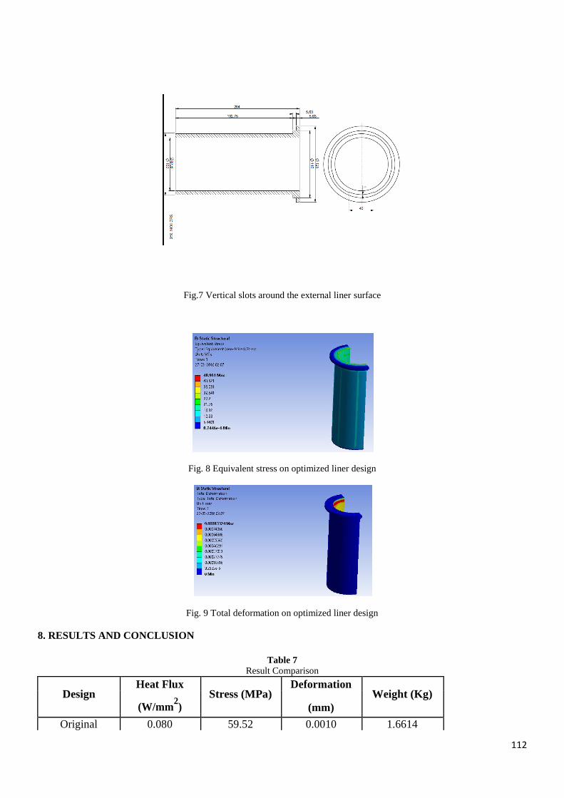
112

Fig.7 Vertical slots around the external liner surface

Fig. 8 Equivalent stress on optimized liner design

Fig. 9 Total deformation on optimized liner design

8. RESULTS AND CONCLUSION

Table 7

Result Comparison

Design Heat Flux

Stress (MPa) Deformation

Weight (Kg)

(W/mm2) (mm)

Original 0.080 59.52 0.0010 1.6614

113

Trial 1 0.051 48.96 0.0008 1.5489

Based on the trials performed, it is observed that cylinder liner design can be optimized for weight reduction opportunities. By

applying vertical slots on the external surface of the liner, the weight of the liner was reduced to approximately 7% and no

significant change in the stress and deformation was observed.

Hence, with the methodology discussed here, it is possible to reduce the weight of the liner without generating excessive stress

and deformation. The methodology outlined in this paper provides opportunities to carry out future work to improve the overall

performance of the IC engine. Some of the possible opportunities are highlighted below:

Performing fatigue life estimation for the proposed design

Utilizing the methodology to optimize other IC engine components

Evaluating the engine performance and emission with new liner design

9. REFERENCES [1] P. Gustof, A. Hornik, ―Determination of the temperature distribution in the wet cylinder sleeve in turbo diesel engine‖,

Journal of Achievements in Materials and Manufacturing Engineering, Vol. 27, Issue 2, Apr. 2008

[2] Pari, Hariharan, Raj, Rajendran, Pandiarajan, Ganesh, Rasu, Elansezhian, ―Study On The Performance Of Electroless Nickel

Coating On Aluminium For Cylinder Liners‖, On behalf of IP Rings Ltd, Maraimalainagar

[3] Amir Malakizadi, Hamidreza Chamani, ―Thermo-mechanical Fatigue Life Prediction Of A Heavy Duty Diesel Engine

Liner‖, Proceedings of the ASME Internal Combustion Engine Division, Fall Technical Conference, 2007.

[4] Satya Thrinadh Balla, Panchumarthy Phani Kumar‖Finite Element Analysis of a Diesel Generator Cylinder‖, International

Journal of Engineering Research & Technology, Vol 3, Issue 3, Mar 2014.

[5] Lutfi Y. Zeidan, Mohammed KH. Abbass, Ali Z. Asker, Diyala, ―The study of temperature distribution on a Cylinder of

Suzuki 250gsx engine fuelled with Gasoline blends using finite element analysis‖, Journal of Engineering Sciences, Vol. 07,

Issue No. 02, June 2014.

[6] Dineshkumar. S, Sriprashanth.V, ―Liner Material Thermal Analysis for Diesel Engines‖, International Journal of

Engineering Research and General Science, Volume 3, Issue 2, Part 2, March-April, 2015.

[7] Research engine test set up 1 cylinder, 4 stroke, multi-fuel, VCR (Computerized) Instruction manual Apex Innovations.

114

CFD Analysis for Heat Transfer Augmentation by Changing Profiles of Air

Cooled Fins

Swati Saini, Dhruvin Kagdi , Namrata Sengar , Abhishek Shah

[email protected], kagdidhruvin.me@

socet.edu.in,[email protected],[email protected]

Mechanical Engineering Department, Silver Oak College of Engineering and Technology, Gujarat Technological

University, India

Abstract

The main of aim of this work is to study various researches done in past to improve heat transfer rate of cooling fins by

changing cylinder block fin geometry and climate condition. Based on the research done, a model is selected to perform heat

transfer analysis and identify possible increase in the rate by changing the fin profile. To perform the study, virtual simulation

by CFD approach is proposed.

Keywords: catalytic CFD, I C Engine Fins, Heat Transfer Augmentation

1. Introduction: Engine life and effectiveness can be improved with effective cooling. The cooling mechanism of the air cooled engine is mostly

dependent on the fin design of the cylinder head and block. Insufficient removal of heat from engine will lead to high thermal

stresses and lower engine efficiency. The cooling fins allow the wind and air to move the heat away from the engine. Low rate

of heat transfer through cooling fins is the main problem in this type of cooling. The main of aim of this work is to study various

researches done in past to improve heat transfer rate of cooling fins by changing cylinder block fin geometry and climate

condition.

2. Problem Definition From several researches done in the past, it is evident that the fin geometry can be optimized to improve heat transfer rate. Finite

volume approach can be utilized to identify temperature distribution and heat transfer rate from the engine cylinder. Changing

the fin geometry with elliptical or wavy shapes and increasing number of fins can yield altogether different thermal behaviour of

the IC engine. 3. Model Selection 3.1 Model Selection for Analysis

The finned cylinder geometry is selected based on the research and experiments conducted by researchers as described in the

table:

TABLE I

MODEL SELECTION

Thornhill et al Gibson Bierman et al.

Cylinder Diameter[mm] 100 32-95 118.364

Fin Pitch [mm] 8-14 4-19 1.448-15.240

Fin Length mm] 10-50 16-41 9.398-37.338

Material Aluminium alloy Copper, Steel, Aluminium Steel

Wind Velocity [km/hr] 7.2-72 32-97 46.8-241.2

3.2 Boundary Conditions

TABLE II

BOUNDARY CONDITIONS

Wind velocity 30, 40, 50, 60 & 70 km/hr


mailto:kagdidhruvin.me@%20socet.edu.in,




115

Air Temperature Ambient Temperature 300K

Atmospheric Pressure 101.325 kPa

Flow Direction Left to Right

Outer Cylinder Surface Wall Boundary Condition

Cylinder Inside Wall Temperature 150 0C

Fig. 1 Experimental Cylinder

3.3 Mathematical Model for CFD Analysis

To successfully obtain results through CFD analysis, there are several important factors required to be considered, these are-

Developing ―watertight‖ geometry. i.e. Solid geometry without holes/gaps

Enclosing the geometry with substantially large fluid domain to accurately capture fluid flow behaviour

Selecting proper boundary conditions both for solid and fluid domains

Using the right turbulence model

Running the simulation for adequate number of iterations to ensure minimum residuals

The mathematical model used for solving the flow problems in ANSYS Fluent is based on finite volume method.

In this case, the standard Navier - Stokes equations of fluid flow in three dimensions is solved for finding the pressure and

velocity at domain points. SIMPLE method for pressure velocity coupling was implemented for pressure correction. The

following momentum conservation was used along with the continuity equation:

For modeling heat transfer, the energy equation is solved in the following form:

3.4 CFD Simulation Methodology To perform fluid flow and conjugate heat transfer analysis, following methodology is adopted:

Import finned cylinder geometry to ANSYS Design Modeler

Develop fluid domain around the cylinder geometry to capture flow physics

Generate mesh and create name selection for relevant faces in the geometry

Setup model details in Fluent environment

Select material (Air and Aluminum)

Apply velocity inlet, pressure outlet and cylinder wall temperature as boundary conditions

Initialize the solution

Calculate the solution by gradually increasing the number of iterations while monitoring the residuals

Determine the results through CFD Post-processing

116

4. CFD Analysis For CFD analysis, CAD model of the cylinder was developed using Creo and was imported to ANSYS Fluent. To reduce

computational power, the geometry is considered symmetric and the surrounding fluid domain is developed to capture the flow

physics.

Fig. 2 Symmetry Cylinder with Surrounding Fluid Domain

Fig. 3 Inlet Boundary at Left Face of Fluid Domain

Fig. 4 Outlet Boundary at Right Face of Fluid Domain

Fig. 5 Mesh for Fluid and Solid Domains

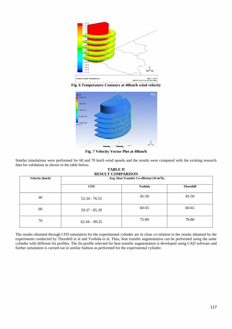
117

Fig. 6 Temperature Contours at 40km/h wind velocity

Fig. 7 Velocity Vector Plot at 40km/h

Similar simulations were performed for 60 and 70 km/h wind speeds and the results were compared with the existing research

data for validation as shown in the table below:

TABLE II

RESULT COMPARISON Velocity (km/h) Avg. Heat Transfer Co-efficient (W/m2K)

CFD Yoshida Thornhill

40 52.34 - 76.53 45-50 45-50

60 59.37 - 85.39 60-65 60-65

70 62.44 – 89.25 75-80 78-80

The results obtained through CFD simulation for the experimental cylinder are in close co-relation to the results obtained by the

experiments conducted by Thornhill et al and Yoshida et al. Thus, heat transfer augmentation can be performed using the same

cylinder with different fin profiles. The fin profile selected for heat transfer augmentation is developed using CAD software and

further simulation is carried out in similar fashion as performed for the experimental cylinder.

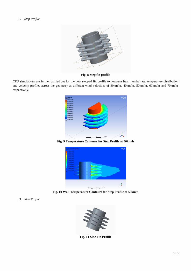
118

C. Step Profile

Fig. 8 Step fin profile

CFD simulations are further carried out for the new stepped fin profile to compute heat transfer rate, temperature distribution

and velocity profiles across the geometry at different wind velocities of 30km/hr, 40km/hr, 50km/hr, 60km/hr and 70km/hr

respectively.

Fig. 9 Temperature Contours for Step Profile at 50km/h

Fig. 10 Wall Temperature Contours for Step Profile at 50km/h

D. Sine Profile

Fig. 11 Sine Fin Profile

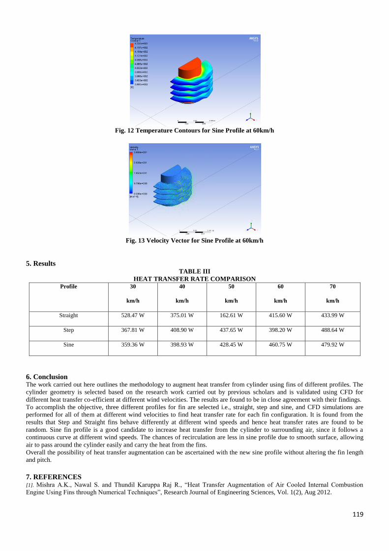
119

Fig. 12 Temperature Contours for Sine Profile at 60km/h

Fig. 13 Velocity Vector for Sine Profile at 60km/h

5. Results TABLE III

HEAT TRANSFER RATE COMPARISON

Profile 30

km/h

40

km/h

50

km/h

60

km/h

70

km/h

Straight 528.47 W 375.01 W 162.61 W 415.60 W 433.99 W

Step 367.81 W 408.90 W 437.65 W 398.20 W 488.64 W

Sine 359.36 W 398.93 W 428.45 W 460.75 W 479.92 W

6. Conclusion The work carried out here outlines the methodology to augment heat transfer from cylinder using fins of different profiles. The

cylinder geometry is selected based on the research work carried out by previous scholars and is validated using CFD for

different heat transfer co-efficient at different wind velocities. The results are found to be in close agreement with their findings.

To accomplish the objective, three different profiles for fin are selected i.e., straight, step and sine, and CFD simulations are

performed for all of them at different wind velocities to find heat transfer rate for each fin configuration. It is found from the

results that Step and Straight fins behave differently at different wind speeds and hence heat transfer rates are found to be

random. Sine fin profile is a good candidate to increase heat transfer from the cylinder to surrounding air, since it follows a

continuous curve at different wind speeds. The chances of recirculation are less in sine profile due to smooth surface, allowing

air to pass around the cylinder easily and carry the heat from the fins.

Overall the possibility of heat transfer augmentation can be ascertained with the new sine profile without altering the fin length

and pitch.

7. REFERENCES [1]. Mishra A.K., Nawal S. and Thundil Karuppa Raj R., ―Heat Transfer Augmentation of Air Cooled Internal Combustion

Engine Using Fins through Numerical Techniques‖, Research Journal of Engineering Sciences, Vol. 1(2), Aug 2012.

120

[2]. R. Arularasan, “Modeling and simulation of engine cylinder fins by using FEA‖, Int. Journal for Research in Applied

Science and Engg. & Technology, Vol.2 (4), April 2014.

[3]. Mohsin A. Ali1, Prof. (Dr.) S.M Kherde, ―Design modification and analysis of two wheeler cooling fins-a review‖,

International Journal of Engineering and Applied Sciences, Vol.5 (1), June 2014.

[4]. K. Ashok Reddy, T. V. Seshi Reddy and S Satpagiri,‖Heat Flux and Temperature Distribution Analysis of I C Engine

Cylinder Head Using ANSYS‖, International Journal of Advanced Research Foundation, Vol. 2(5), May 2015.

[5] Polidas Varalakshmi,‖Steady State Thermal Analysis of Engine Cylinder Fin by Changing Geometry and Material‖, Int.

Journal & Magazine of Engineering, Technology, Management & Research, Vol. 2(8), August 2015.

[5]. Pulkit Agarwal, Mayur Shrikhande and P. Srinivasan,‖Heat Transfer Simulation by CFD from Fins of an Air Cooled

Motorcycle Engine under Varying Climatic Conditions‖, Proceedings of the World Congress on Engineering 2011, Vol. III, July

6 - 8, London, U.K, 2011.

121

SIMULATION OF INDUCTION MOTOR-PUMP SUPPLIED BY

PHOTOVOLTAIC GENERATOR

Tandel Piyush N.

[email protected]

Department of Electrical Engineering, MGITER, Navsari, Gujarat, India

Abstract -This paper deals with the modeling of a centrifugal pump system driven by a three-phase induction

motor, which is supplied by a photovoltaic generator. The system includes solar panel, a DC / DC converter

equipped with its maximum power control, a the three-phase Pulse Width Modulation voltage inverter and a

centrifugal pump driven by a three phase induction motor. Several algorithms of maximum power point tracking are

presented in literature; the Perturb & Observe (P&O) method is studied in this paper. In order to regulate the flow of

the centrifugal pump, a direct torque of the induction machine is used for controlling the speed. The simulation

results are carried out using Matlab/Simulink.

Keywords: Photovoltaic generators; Maximum power point tracking (MPPT); DC/DC converters; Induction motor.

1. Introduction

Photovoltaic energy is a renewable energy source, inexhaustible and non-polluting. To be used for different

applications and to meet the economic constraints, the design and implementation of PV systems are necessary and

currently facing many problems. The PV system must be made robust, reliable and with high efficiency. PV systems

require little maintenance, are quiet and do not emit pollutants. These PV systems, electricity generators, can be

operated in different places: electrification of remote sites, installation in buildings, direct connection to the network,

pumping water.

The use of solar energy for water pumping is particularly well suited to rural areas where water is lacking. The

growing demand for water in these areas is a great interest in the use of solar panels as a source of energy groups.

The major part of the pumping systems currently implemented as electric actuator using the DC motor or brushless

motor. The problems of cost and maintenance have contributed to the induction motor which thus constitutes a new

alternative.

The point, called the maximum power point (MPP) is dependent on the intensity of illumination. The adaptation of

the PV panels to the load is therefore necessary to extract the PV module maximum power. This is done through the

DC-DC energy converters controlled by a control command called MPPT (Maximum Power Point Tracking). In the

literature, several types of analog and digital MPPT control have been proposed. These commands are characterized

by their high costs and implementation difficulties. In our work, we used the Perturbation and observation method.

The induction motor is used more and more for photovoltaic pumping systems. The low cost of the engine, the low

maintenance requirements and the increased efficiency for solar pumping systems make it particularly major

problem with the use of PV panels is their non-linear nature. The PV module has an optimum operating attractive

where the additional cost of the inverter is less significant. In recent years, the advent of efficient inverter to control

the speed of these motors has allowed used for solar pumping applications.

In this paper, the pump used is the centrifugal type driven by a three phase asynchronous motor which is powered by

a three-phase inverter.


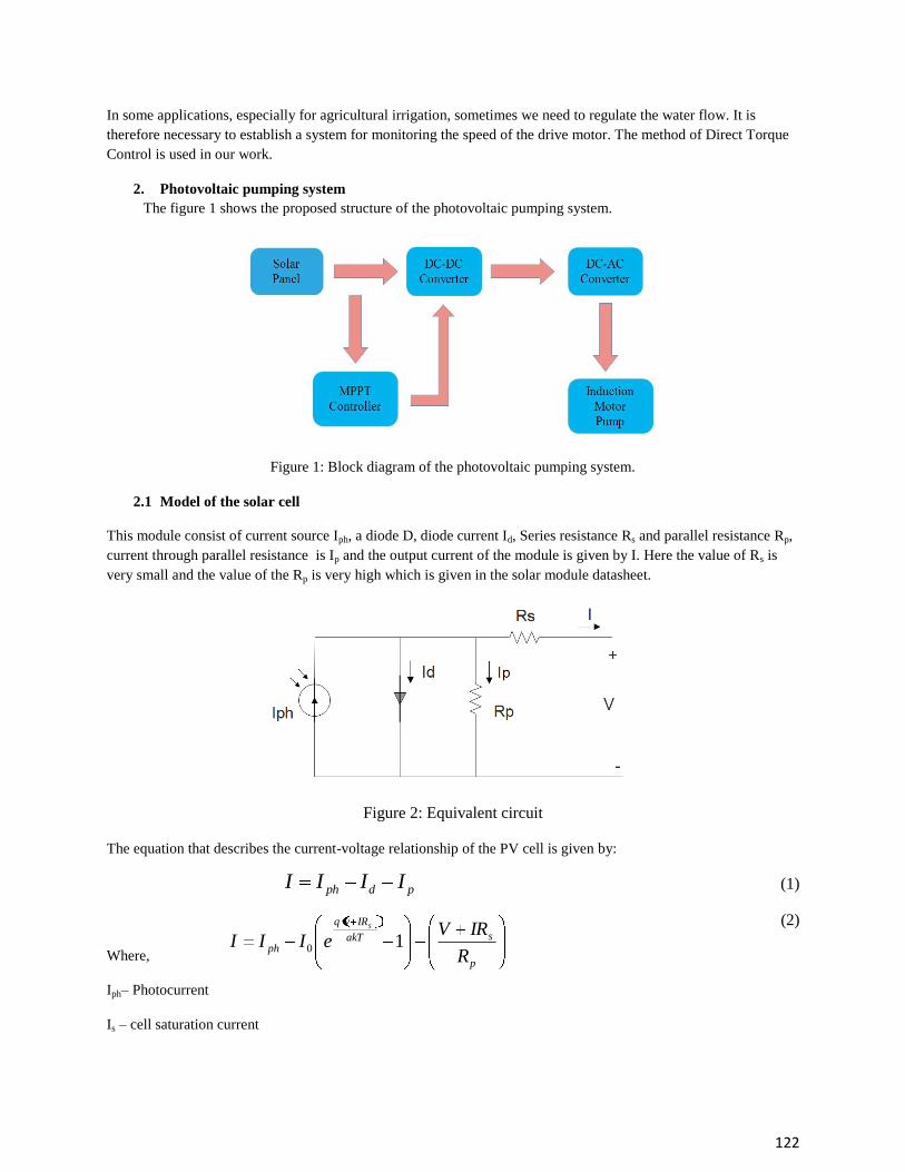
122

In some applications, especially for agricultural irrigation, sometimes we need to regulate the water flow. It is

therefore necessary to establish a system for monitoring the speed of the drive motor. The method of Direct Torque

Control is used in our work.

2. Photovoltaic pumping system

The figure 1 shows the proposed structure of the photovoltaic pumping system.

Figure 1: Block diagram of the photovoltaic pumping system.

2.1 Model of the solar cell

This module consist of current source Iph, a diode D, diode current Id, Series resistance Rs and parallel resistance Rp,

current through parallel resistance is Ip and the output current of the module is given by I. Here the value of Rs is

very small and the value of the Rp is very high which is given in the solar module datasheet.

Figure 2: Equivalent circuit

The equation that describes the current-voltage relationship of the PV cell is given by:

(1)

(2)

Where,

Iph– Photocurrent

Is – cell saturation current

pdph IIII

p

sakT

IRvq

phR

IRVeIII

s

10

123

q – Electron charge (1.6×10-19

C)

k – Boltzman‘s constant – 1.38×10-23

J/K

A – Ideal factor which depend on PV characteristic

Rp – shunt resistance

Rs – Series resistance

2.2 MPPT based on DC-DC Boost converter

To extract at each time the maximum power available at the terminals of the PV and transfer it to the load, the

technique conventionally used is to use a stage adaptation between the PV and the load. This stage plays the role of

an interface between the two elements ensuring through control action, the transfer of maximum power supplied by

the generator to make it as close as possible to PMAX.

DC-DC converters, as voltages elevators, are also used in photovoltaic applications, especially in photovoltaic

pumping system. In our study we use a boost converter which is a power converter with an output voltage greater

than its input voltage.

MPPT control varies the duty cycle of the converter so that the power supplied by the PV is equal to PMAX

provided at its terminals. The MPPT algorithm can be more or less complicated to find the MPP, but generally it is

based on the variation of the duty cycle of the converter to be placed on the MPP in terms of changes in input

parameters converter (IPV and VPV).

Many MPPT algorithms have been proposed in literature. The P&O method is the most commonly used MPPT in

commercial PV products. It has a simple feedback structure and a fewer measured parameters. Figure 3 shows the

flowchart of this algorithm.

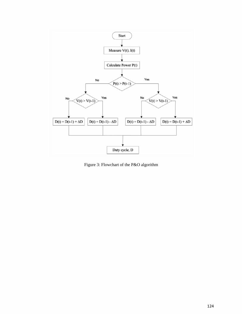
124

Figure 3: Flowchart of the P&O algorithm

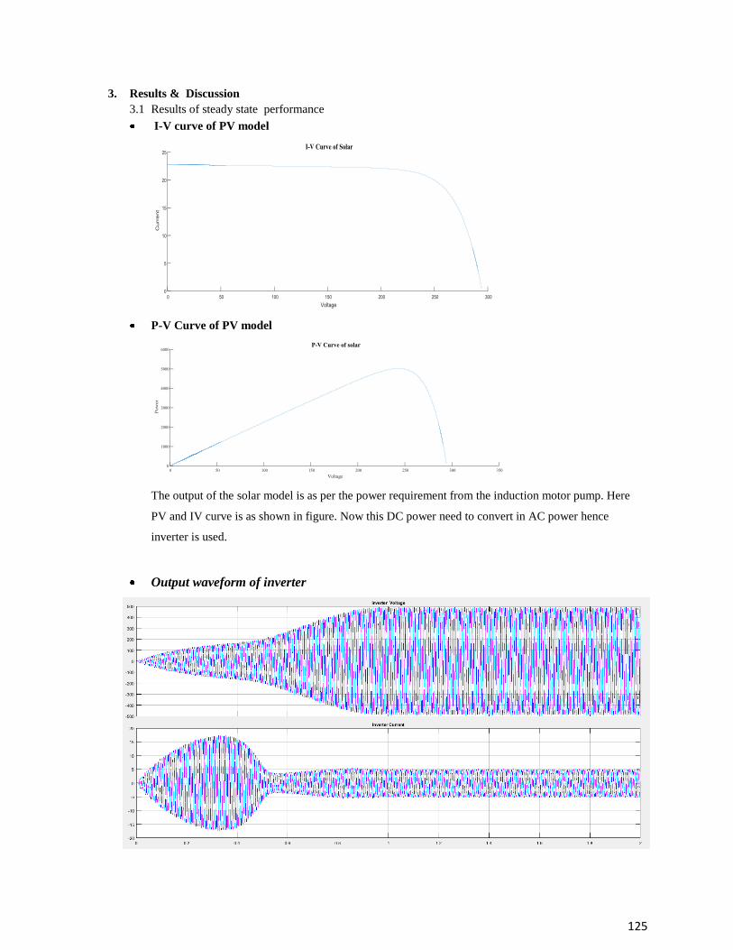
125

3. Results & Discussion

3.1 Results of steady state performance

I-V curve of PV model

P-V Curve of PV model

The output of the solar model is as per the power requirement from the induction motor pump. Here

PV and IV curve is as shown in figure. Now this DC power need to convert in AC power hence

inverter is used.

Output waveform of inverter

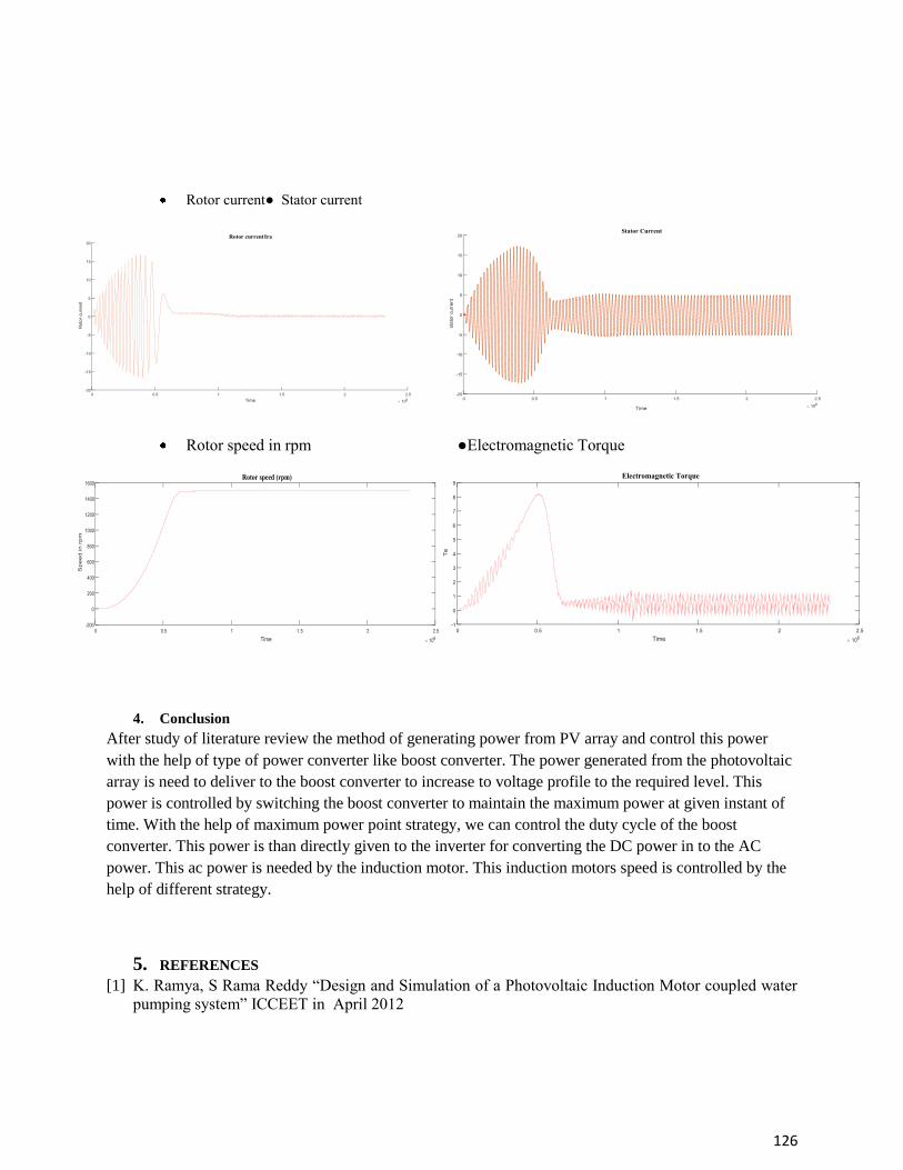
126

Rotor current Stator current

Rotor speed in rpm Electromagnetic Torque

4. Conclusion

After study of literature review the method of generating power from PV array and control this power

with the help of type of power converter like boost converter. The power generated from the photovoltaic

array is need to deliver to the boost converter to increase to voltage profile to the required level. This

power is controlled by switching the boost converter to maintain the maximum power at given instant of

time. With the help of maximum power point strategy, we can control the duty cycle of the boost

converter. This power is than directly given to the inverter for converting the DC power in to the AC

power. This ac power is needed by the induction motor. This induction motors speed is controlled by the

help of different strategy.

5. REFERENCES [1] K. Ramya, S Rama Reddy ―Design and Simulation of a Photovoltaic Induction Motor coupled water

pumping system‖ ICCEET in April 2012

127

[2] Pawan Kumar, Ankit Gupta, Rupendra Kumar Pachauri, Yogesh K. Chauhan ―Utilization of Energy

Sources in Hybrid PV/FCPower Assisted Water Pumping System‖ IEEE International Conference

2015

[3] Amrutha Rose Thomas and Shinosh Mathew ―Solar Powered Single Phase Induction Motor using

Single Source Five Level Inverter‖ International Conference on Magnetics, Machines & Drives2014

[4] H. Bouzeria, C. Fetha, T. Bahi, L. Rachedi ―Speed Control of Induction Moto Pump Supplied by

Photovoltaic Generator‖ Proceedings of the 3rd International Conference on October, 2013

[5] P.Abarnaa, Mrs.S.P.G.Bhavani ― A Solar Powered PV Based Induction Motor Drive in Water

Pumping System Using Flc‖ International Journal of Scientific & Engineering Research,5(4), April-

2014

[6] Rajiv K. Varma and Shah Arifur Rahman Vinay Sharma Tim Vanderheide ―Novel Control Of A PV

Solar System as Statcom (Pv-Statcom) For Preventing Instability of Induction Motor Load‖ 25th

IEEE Canadian Conference on Electrical and Computer Engineering, 2012

[7] Nafisa Binte Yousuf, Khosru M. Salim, Rafid Haider, Md. Rajin Alam, Fatima Binte Zia

―Development of a Three Phase Induction Motor ontroller for Solar Powered Water Pump‖ IEEE

conference Aug. 2012

[8] Montie ales Vitorino, Mauricio Beltraode RossitterCorrea.Cursino Brandao Jacobina,"An Effective

InductionMotor Control For Phtovoltaic Pumping "IEEE Trans. Ind.Electron., vol. 58, April 2011

128

A Review: Optimal Sizing and Cost Assessment of Roof Top PV

Systems for Aditya Silver Oak Institute of Technology

Manan Pathak, Darshna V. Ahir

[email protected]@socet.edu.in

Electrical Engineering Department, Aditya Silver Oak Institute of Technological

Gujarat Technological University, India

Abstract— Fast depleting reserves of fossil fuels, increasingcost of fuel for conventional power generation in

recent times,along with a regulatory framework to minimize the carbonfootprint worldwide, the use of

Renewable sources of powergeneration has become an inevitable reality. The paper makes afeasibility

assessment of Renewable Energy Sources) as a possible source for electrification for a education institution

namely Aditya Silver Oak Institute of Technology located at Ahmedabad, Gujarat,India (23.50 °N, 72.31 °E). A

use of renewable source like photovoltaic (PV) either instandalone or grid connected mode with energy storage

capacitybased energy systems are investigated in this paper. The objectiveof the study is to optimize the size and

cost of renewable energysystem at the selected site to meet the electrical demand of a loadof 24kWh/day having

a peak load of 6.5 kW. The modelling,optimization and analysis of the Roof top PV system is carried outusing

HOMER software produced by National RenewableEnergy Laboratory (NREL), Colorado USA. The

Photovoltaic systemsare evaluated on the basis of Net Present Cost (NPC), LevelisedCost of Energy (COE),

Initial Cost, Operating Cost, andRenewable Fraction obtained on the basis of computation results.The results are

favorable for the use of renewable energy basedsource at the selected site with PV-Grid connected

systememerging as the most economic RES with COE equal to 0.209$/kWh.

Keywords— Renewable Energy system, PV, Wind, Grid,HOMER, Cost analysis, Optimal Sizing

I. Introduction

Renewable energy has the prospective to act as a feasiblesource to improve energy security with moderate

dependence on imported fuels and electricity, in addition to end evoking to meet the requirements of the world

scenario for energy demand [1, 2, 3]. Harnessing the available renewableenergy sources provides an opportunity

to produce energy in aclean and environmentally friendly way [4]. A Solar Photovoltaic powersystem

comprising of renewable generations andenergy storage may alleviate the reliability issues concerningresource

intermittency of renewable power sources [5]. The application of these sourcesincludes the very small to large

isolated, grid connected hybridpower systems. Increasing the RES penetration demands theintegration of energy

storage systems, which in turn counterbalancesthe inherent fluctuations of RES power supplyleading to its

adaptation to the load profile [7]. The demand sideflexibility can counterbalance renewable supplyvariations and

efficiently integrate renewable generation [8].In the present world scenario, the trend towards

increasingsustainable power penetration in modern power systemimposes a very serious requirement to consider

their effect onthe system adequacy [9]. Moreover the solar photovoltaic power systemsexhibit higher adequacy

of the generation system incomparison to the use of a single source as a renewable supplyof energy.

The proper care has to be taken whiledesigning a system that meets the load demand in accordancewith all the

above mentioned parameters as limitingconditions. Renewablepower generation and comprehensive sequential

load modelsare both time-dependent due to their strong connection withvarying time and weather-related

variables [10]. Thus thedesigning of new analytical models and tools are needed inorder to resourcefully deal

with time-dependent systems.This paper investigates the renewable energypotential for an educational

institution based on energy costanalysis. Feasibility investigation is also carried out toevaluate the possibility of

utilizing solar energy atthe selected site to meet the power requirements as a standalonesystem and in

conjunction with the grid connectedsystem. Micro power optimization program HOMER is usedin this study for

evaluation of technical and economicparameters [13]. The optimization results obtained from thestudy indicates

the possibility of utilization of PV/basedRES for Aditya Silver Oak Institute of Technology.



129

2. Methodology

HOMER decides whether renewable energy sources can orcannot satisfy the electric demand for every hour of

the year.In case the sources considered are inadequate, HOMERensures that secondary sources (diesel generator

or gridconnection) are available to meet the required demand. Theoptimization program simulates the operation

of the system bymaking energy balance calculations for each of the 8760 hoursin one year. The optimization

compares the energy demandthat the system can supply in an hour and calculates the relatedenergy flow towards

and from each component [1]. HOMERexpresses the economics of controllable energy sources withtwo values:

fixed cost per hour and energy cost per kWh.These costs represent the cost for the generating energy at anytime

for a power source. HOMER searches for thecombinations of sources meeting the load and then finds thesystem

that achieves the goal with minimum cost [11,14]. Theeconomic analysis is generally carried out on the basis of

NetPresent Cost (NPC), Level zed Cost of Energy (COE) and theenvironmental assessment based on the

Renewable Fraction(RF). These indicators are discussed in brief under thefollowing heads:

A. Net present cost (NPC) The net present cost, which indicates the present value ofinstalling and operating the system over its lifetime of

theproject, also referred to as life cycle cost. HOMER givesoptimization results of simulation, ranked andbased

on thetotal NPC which is calculated according to Eqs. (1) and(2).

Eqs. (1) & (2)

Where, Cann,totis the total annualized cost ($/year) whichincludes the capital, replacement, annual operating and

maintenance, and fuel costs. CRF is the capital recoveryfactor, used to calculate the present value of a series of

equal annual cash flows, i is the real interest rate (%) andN is the project lifetime (in number of years).

B. Levelized cost of energy (COE) The Levelized cost of energy is the average cost perkilowatt hour ($/kWh) of useful electrical energy produced

by the system. It is calculated as given in equation (3):

Eqs. (3)

where, Cann,totis the total annualized cost ($/year), Eprim,ACis the AC primary load served (kWh/year) and

Eprim,DCisthe DC primary load served (kWh/year).

C. Renewable Fraction (RF) In a hybrid PV-Wind energy system, the renewable fractionspecifies the contribution from different sources. PV

fractionfpvand wind fraction fwtare given by the following equations(4) and (5):

Eqs. (4) & (5)

WhereEpvandEwtrepresent the electricity generated from PVand Wind source.

3. Resource Potential at Selected Site

Aditya Silver Oak Institute of Technology Engineering College (ASOIT), was established in the year 2013. It is

situated at Gota in the center part of Ahmedabad, which is a landmark in the colourful and chequered history of

Gujarat [15]. The institution faces a serious deterrentin meeting the adequate power requirement in the

summerseason due to inadequate supply of power from utility. A 5kWp PV system designed for the site in

MATLAB/SIMULINK showed that the possible yield of PV based renewable power from the site lie within the

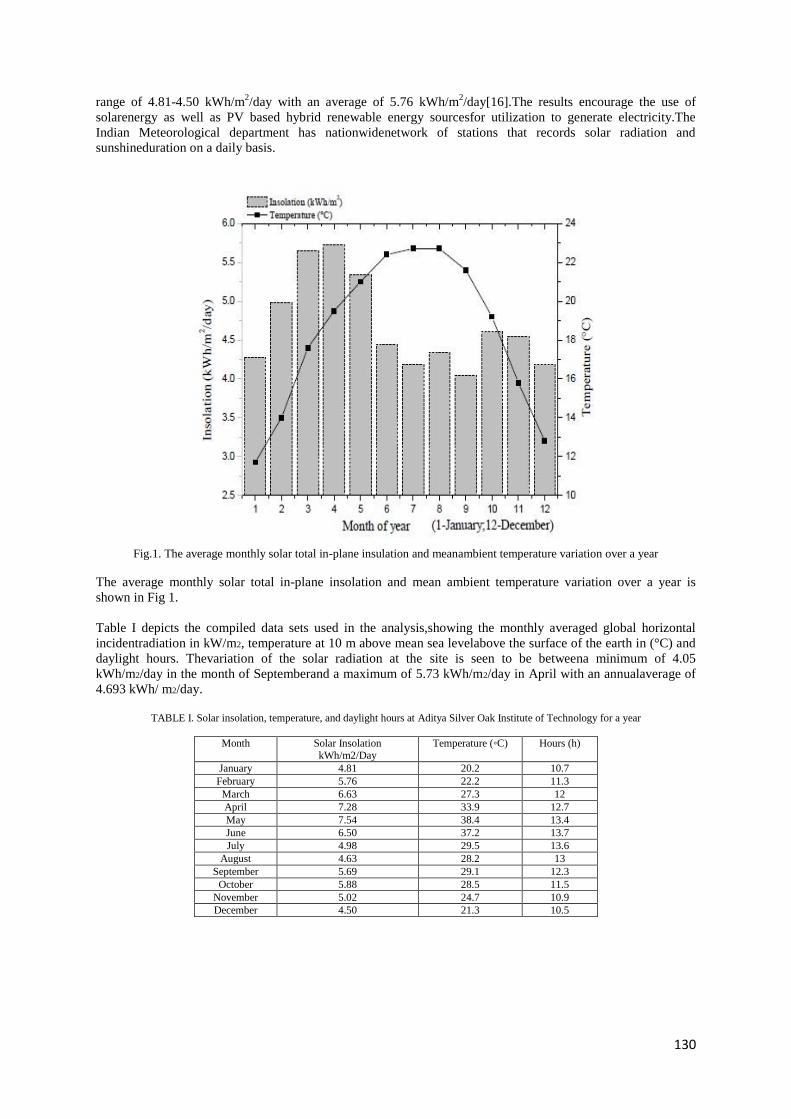
130

range of 4.81-4.50 kWh/m2/day with an average of 5.76 kWh/m

2/day[16].The results encourage the use of

solarenergy as well as PV based hybrid renewable energy sourcesfor utilization to generate electricity.The

Indian Meteorological department has nationwidenetwork of stations that records solar radiation and

sunshineduration on a daily basis.

Fig.1. The average monthly solar total in-plane insulation and meanambient temperature variation over a year

The average monthly solar total in-plane insolation and mean ambient temperature variation over a year is

shown in Fig 1.

Table I depicts the compiled data sets used in the analysis,showing the monthly averaged global horizontal

incidentradiation in kW/m2, temperature at 10 m above mean sea levelabove the surface of the earth in (°C) and

daylight hours. Thevariation of the solar radiation at the site is seen to be betweena minimum of 4.05

kWh/m2/day in the month of Septemberand a maximum of 5.73 kWh/m2/day in April with an annualaverage of

4.693 kWh/ m2/day.

TABLE I. Solar insolation, temperature, and daylight hours at Aditya Silver Oak Institute of Technology for a year

Month Solar Insolation kWh/m2/Day

Temperature (C) Hours (h)

January 4.81 20.2 10.7

February 5.76 22.2 11.3

March 6.63 27.3 12

April 7.28 33.9 12.7

May 7.54 38.4 13.4

June 6.50 37.2 13.7

July 4.98 29.5 13.6

August 4.63 28.2 13

September 5.69 29.1 12.3

October 5.88 28.5 11.5

November 5.02 24.7 10.9

December 4.50 21.3 10.5

131

4. System Components

A. Load Profile B. The Solar Photovoltaic modelling in this paper is carried out for the Aditya Silver Oak Institute of

Technology Type classrooms of the institution. In addition to theregular classes, the institute functions

as a nodal center for different government examination like GPSC, UPSC during the year on holidays.

The considered loads are 410 fans of 75 Watts each,516 incandescent lamps of 40 W each and 30 CFL

of 10Weach. The load is operated only on weekdays and duringcollege hours, i.e. from 9:30 a.m. to

3.45 p.m. The summermonths (March to October) see the highest demand in the loadrequirement (3460

W) on account of the operation of the fans.The winter months (November, December and January)

areseen to have the lowest requirement in the loads (1060 W)while the transitional months of October

and February sees arequirement of a load of 2260 W assuming that half the totalnumber of the fans are

operational. The scaled annual averageenergy demand at the site as simulated in HOMER is24kWh/day

with a peak of 6.5 kW. The average load for theentire year is shown in Fig 2. Table III gives a break-up

of theload considered in the simulation study.

Table III. Load Composition Data considered for the Institution

Summer load profile

Electrical Load Watts (W) Quantity Total kWatts

CFL 10 30*10 0.3

Incandescent lamp 40 516*40 20.64

Fan 75 410*75 30.75

Air Conditioner 1200 1200*10 12.0

Lab Equipments 250 10*250 2.50

Total 66.19

Winter Load

Electrical Load Watts (W) Quantity Total kWatts

CFL 10 30*10 0.3

Incandescent lamp 40 516*10 20.64

Lab Equipments 250 10*250 2.5

Total 23.44

C. PV MODULE

The per kW capital cost of the PV module is considered to beequal to $2800 (187782 Rs) and the replacement

cost is assumed to be $2800 (187782 Rs), with zero operation and maintenance cost (O&M) [19-21]. The

lifetime of the PV system is considered to be 20 yearswith a de-rating factor of 80%, ground reflectance of 15%

anddevoid of any tracking equipment.

D. BATTERY

The study takes into consideration storage elements in theform of battery. The reference battery for modelling

insimulation is taken to be the Vision 6FM200D manufacturedby Vision Battery. The reference model has a

nominal voltageof 12V and nominal capacity of 200Ah and the capital costand replacement cost of one unit is

assumed to be $145 (9724.42 Rs) with an annual maintenance of $2 (134.13 Rs). A number of units of

thebattery is considered for the simulation process to account fora definite number of days of autonomy.

E. CONVERTER

A systems consisting of both ac and dc sources and elementsrequires a power converter (either a rectifier or a

inverter). Theconverter per kW capital cost , replacement cost and O&Mcost is assumed to be $700 (46945.5

Rs), $700 (46945.5 Rs) and $2 (134.13 Rs) for this study[15,17].The life time of the converter is assumed to be

15years while the efficiency is considered to be 90% and 85%for the inversion and rectification process.


132

In order to ascertain the best possible combination of (RES) for the selected site anumber of possible

combinations of PV without gridconnectivity, PV with grid connectivity and PV with batteryas the sole source

are simulated in HOMER software platform.While carrying out the simulation a few of the assumptionsmade

are listed here below:

A minimum renewable fraction for all thecombinations is considered to be 50% and apermissible

capacity shortage is assumed to be 10%.

The cost of electricity from the grid is assumed to be $0.1/kWh (6.71 Rs/kWh) for the simulation

study.

The simulation was carried out by assuming that inthe hybrid system the PV capacity comprises 4,8,12

and 16 kW PV inputs, 1, 2 and 5 kW Wind turbine,variable number (8-32) of strings in a battery bank

and converter of capacity 2kW, 5kW and 6 kW.

The simulation was carried out for a project lifetime of 25 years with an annual rate of interest taken as

6%.

The results of the simulation study are tabulated onthe basis of the Initial Cost, Operating Cost, Total

Net Present Cost, Cost of Energy and RenewableFraction and also on the basis of optimal size of the

RES configuration.

As shown in the table IV, the Net present cost (NPC) obtainedfor the PV based system without grid connectivity

is $59,556 (3994123.14 Rs) while for a PV with grid connectivity it is observed to be $23,352 (Rs 1566101.8).

PV instandalone configuration the NPC is found out fromsimulation to be equal to $ 31,047 (Rs 2082167.05)

and $40,089 (Rs 2688568.78) respectively. On the other hand the COE obtained for the PV basedsystem

without grid connectivity is 0.576 $/kWh (38.67 Rs/kWh), for a PV with grid connectivity it is observed to be

0.209 $/kWh (14.02 Rs/kWh). PV-Grid based system has the COE equal to 0.270 $/kWh (18011 Rs/kWh). The

operating cost is minimum (578 $/yr or 38763.57 Rs/yr) for the PV in standalone. Therenewable faction is high

in case of PV without gridconnection and PV in the standalone configuration.

Table IV. Summary of cost composition of different HRES configuration

RES

CONFIGURATION

Initial

Cost

($)

Operating

Cost

($/yr)

Total

NPC

($)

COE

($/kWh)

Renewable

Fraction

PV-Grid 20 480 751 30 087 0.270 0.56 20 480 751 30

PV

standalone

32 700 578 40 089 0.383 1.00 32 700 578 40

Table V shows the optimal size of the PV, battery andconverter for the different system configurations. PV

system when it is not connected to the grid is seen to require aconfiguration of 16kW for PV, 32 no. Ofbatteries

and a 6kW converter. The requirement is seen todecrease for grid connected systems, as in such a

situationmajority of the load is supplied by the grid. For the PVsystem with grid connectivity, it is observed that

the optimalsize of the system consists of a PV source of 4 kW, 8 no of batteries and a converter of size 2kW.For

a PV-Grid connected system the optimal size as seen fromthe computation is consisting of a PV source of 8 kW,

abattery bank containing 8 batteries and a converter of 2kW. The results suggest making use of grid

connectedsystems for economic considerations. However from anenvironmental point of view it can be

suggested that the PVstandalone and PVwithout grid connectivity can also beconsidered as an alternate and

viable source for the selectedsite.

Table V. Optimal sizing of different HRES configuration

HRESConfiguration PV (kW) No. of

batteries

Converter

(kW)

PV GRID 8 8 2 PV standalone 12 16 5

6. Conclusion

133

This paper presents an approach for modelling andoptimization of Solar Roof top PV renewable energy systems

for aneducational institution namely ASOIT.With the renewable sources acting in stand-alone mode, theCOE is

observed to be high in comparison with a Gridconnected PV system. However as the fossil fuelreserves are a

limited resource and with a possible gradualincrease in the cost of energy from use of fossil fuels in thefuture, a

balanced utilization of renewable and grid connectedsystem is seen to be the optimum configuration for

theselected site. This phenomenon is substantiated from theresults obtained in the simulation, which indicates

that themost economically viable system configuration for theselected site is found to be the PVGrid

connectedsystem with COE equal to 0.209 $/kWh. Moreover the studyshows promising results that encourage

the use of PV systemsin standalone mode (COE 0.270 $/kWh) as well as PVstandalone system (COE 0.576

$/kWh) at the site consideringenvironmental issues of greenhouse emission. This is a significant development as

the use of PVbased HRES increase the possibility of conservation of gridelectricity immensely. The economics

of generation aside,such a HRES system is obviously environment friendly andclimate benign.

7. References

1. B. E. Turkay, A. Y., A.Y. Telli, “Economic analysis of standalone and grid connected hybrid system”,

Renewable Energy, Elsevier Inc.,vol 36, issue 7, pp 1931-1943, July 2011.

2. I BaniasadAskariab& M. Ameriab,“Techno-economic Feasibility Analysis of Stand-alone Renewable

Energy Systems (PV/wind/bat) inKerman, Iran” Energy Sources, Part B: Economics, Planning and

Policy, vol 7, issue 1, pp 45-60,2012.

3. F Cucchiella, I D’Adamo,“Feasibility study of developing photovoltaic power projects in Italy: An

integrated approach”, Renewable and Sustainable Energy Reviews, Elsevier Inc., vol 16, issue 3, pp

1562- 1576, April 2012.

4. Setaiwan, A.A Chem, Y.Z., Nayar V., “Design , Economic Analysis and Environmental Considerations

of Mini-Grid Hybrid Power System with Reverse Osmosis Desalination Plant for Remote Areas”,

Renewable Energ, Elsevier Inc., vol 34, pp 374-383, 2009

5. S. Rehman, M.M. Alam, J.P. Meyer, L.M. Al-Hadhrami, “Feasibility study of a Wind-PV-Diesel

Hybrid Power System for a Village.”Renewable Energy Elsevier Inc., vol 38, pp 258-268 2012.

6. Arabali, A.; Ghofrani, M.; Etezadi-Amoli, M.; Fadali, M.S., "Stochastic Performance Assessment and

Sizing for a Hybrid Power System of Solar/Wind/Energy Storage," IEEE Transactions on Sustainable

Energy, vol.5, no.2, pp.363-371, April 2014

7. Vrettos, E.I.; Papathanassiou, S.A., "Operating Policy and Optimal Sizing of a High Penetration RES-

BESS System for Small IsolatedGrids," Energy Conversion, IEEE Transactions on, vol.26, no.3,

pp.744- 756, Sept. 2011

8. Arabali, A.; Ghofrani, M.; Etezadi-Amoli, M.; Fadali, M.S.; Baghzouz, Y., "Genetic-Algorithm-Based

Optimization Approach for Energy Management," IEEE Transactions on Power Delivery, vol.28, no.1,

pp.162-170, Jan. 2013

9. Atwa, Y.M.; El-Saadany, E.F.; Salama, M.M.A.; Seethapathy, R.; Assam, M.; Conti, S., "Adequacy

Evaluation of Distribution SystemIncluding Wind/Solar DG During Different Modes of Operation,"

IEEE Transactions on Power Systems, vol.26, no.4, pp.1945-1952, Nov. 2011

10. Gonzalez-Fernandez, R.A.; Leite da Silva, A.M., "Reliability Assessment of Time-Dependent Systems

via Sequential Cross-EntropyMonte Carlo Simulation," IEEE Transactions on Power Systems, vol.26,

no.4, pp.2381-2389, Nov. 2011

11. Lambert T, Gilman P, Lilienthal P, Micropowersytemmodeling with HOMER, John Wiley&Sons, Inc.

Available at:http://www.mistya.ca/software/docs/MicrropowerSystemModelingWith HOMER.pdf

12. Elhadidy MA, Shaahid SM, “Parametric study of hybrid (wind+solar+diesel) power generation

systems.” Renewable EnergyElsevier Inc., vol. 21, no. 2, pp.129-39. October 2000.

13. HOMER Publications, NREL (National Renewable Energy Laboratory) available

at:https://analysis.nrel.gov/homer/includes/downloads/HOMERPublication s.pdf

14. Koutroulis E, Kolokotsa D, Potirakis A, Kalaitzakis K. “Methodology for optimal sizing of stand-alone

photovoltaic /wind generator systems using genetic algorithms.” Solar Energy Elsevier Inc., vol 80, pp-

1072- 1088. 2006

15. B.J. Saharia, B.K. Talukdar, “Theroetical assessment of PV Energy Potential At Assam Engineering

College using PV Indices.”International Journal of Engineering Research & Technology, Vol 3, issue

8, pp 1230-1233, August 2014.

http://www.mistya.ca/software/docs/MicrropowerSystemModelingWith

https://analysis.nrel.gov/homer/includes/downloads/HOMERPublication

134

A review article on Distributed Generation Technologies

Darshna V. Ahir, Ashish Khatik


Electrical Engineering Department, Aditya Silver Oak Institute of Technological


Abstract:-

The Energy demand is increasing because of a growing rate of urbanization, economic growth, increasing prosperity

and rising per capita energy consumption. To fulfil the increasing energy demand India need better cost effective

and environment friendly solution Renewable energy source based Distributed Power Generation is environment

friendly solution to fulfil the demand. Small scale Distributed Generation is connected to distribution systems. It is

difficult to achieve the good quality power with wind power generation because of vacillating behaviour of wind

speed, which affects the voltage and active power output of electrical machine connected to wind turbine. Similarly

solar power generation affects the voltage profile and frequency response of the system .This paper presents a

review of Distributed power generation technologies and benefits

Keywords: Distributed Generation, Distribution System, wind energy, fuel cell.

1. Introduction

India is fourth largest electricity producer with 1052 terrawatthour (TWH) and fourth largest electricity

consumer in the world. As of October 2014 India has 255GW installed capacity and it is 5th largest in the world at

Compound Annual Growth Rate (CAGR) of 10.4 per cent in FY09-Oct-14.Electricity production in India is 1173.8

TWH during FY14.The production increases with CAGR of 6.3 per cent during FY08-14. Total Thermal installed

capacity is 177.4GW while hydro and renewable energy installed capacity totalled 40.8GW & 31.7GW respectively.

[1]

Demand for electricity is expected to increase 1915 TWH over FY07-22 with CAGR of 9 percent. Indian Govt. is

enthusiastic for promotion of hydro, renewable and gas based power generation. Renewable energy is fast emerging

as major source of power. Renewable energy capacity addition to 41GW is planned till 2017 to meet the growing

energy demand. [1]

Fig- 1: Yearly total Electricity Production in India Fig- 2: Installed Power generation capacity in India as

of OCT -14

To meet increasing energy demand fast emerging source of power are Renewable energy sources based Distributed

Generation (DG). DG has few more advantages then conventional power generation. DG is reliable and it has

reduced fuel cost. DG can improve power quality and reduced emissions. DG is capable of providing constant,

uninterrupted power. By reducing the flicker and voltage regulation problems DG can improve power quality.



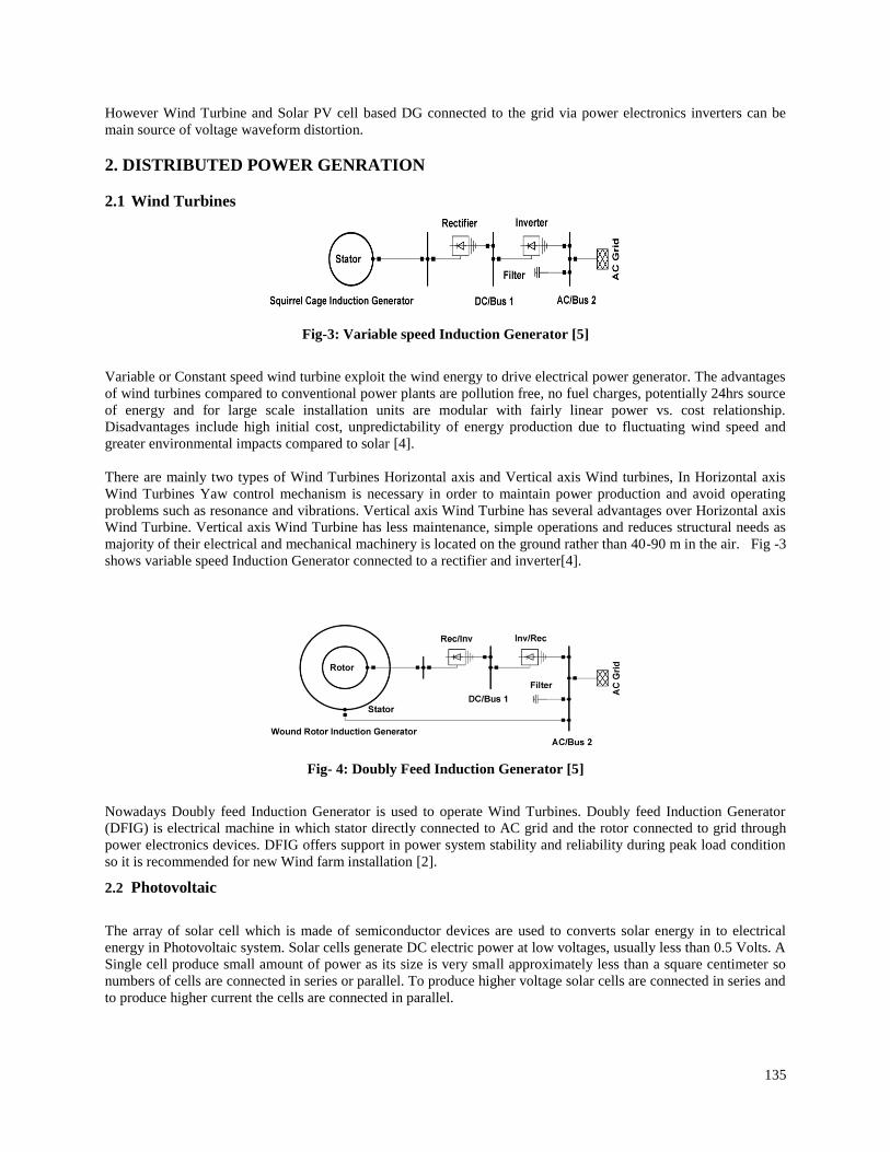
135

However Wind Turbine and Solar PV cell based DG connected to the grid via power electronics inverters can be

main source of voltage waveform distortion.

2. DISTRIBUTED POWER GENRATION

2.1 Wind Turbines

Fig-3: Variable speed Induction Generator [5]

Variable or Constant speed wind turbine exploit the wind energy to drive electrical power generator. The advantages

of wind turbines compared to conventional power plants are pollution free, no fuel charges, potentially 24hrs source

of energy and for large scale installation units are modular with fairly linear power vs. cost relationship.

Disadvantages include high initial cost, unpredictability of energy production due to fluctuating wind speed and

greater environmental impacts compared to solar [4].

There are mainly two types of Wind Turbines Horizontal axis and Vertical axis Wind turbines, In Horizontal axis

Wind Turbines Yaw control mechanism is necessary in order to maintain power production and avoid operating

problems such as resonance and vibrations. Vertical axis Wind Turbine has several advantages over Horizontal axis

Wind Turbine. Vertical axis Wind Turbine has less maintenance, simple operations and reduces structural needs as

majority of their electrical and mechanical machinery is located on the ground rather than 40-90 m in the air. Fig -3

shows variable speed Induction Generator connected to a rectifier and inverter[4].

Fig- 4: Doubly Feed Induction Generator [5]

Nowadays Doubly feed Induction Generator is used to operate Wind Turbines. Doubly feed Induction Generator

(DFIG) is electrical machine in which stator directly connected to AC grid and the rotor connected to grid through

power electronics devices. DFIG offers support in power system stability and reliability during peak load condition

so it is recommended for new Wind farm installation [2].

2.2 Photovoltaic

The array of solar cell which is made of semiconductor devices are used to converts solar energy in to electrical

energy in Photovoltaic system. Solar cells generate DC electric power at low voltages, usually less than 0.5 Volts. A

Single cell produce small amount of power as its size is very small approximately less than a square centimeter so

numbers of cells are connected in series or parallel. To produce higher voltage solar cells are connected in series and

to produce higher current the cells are connected in parallel.

136

Fig -5: Photovoltaic system connected to a grid

To obtain Maximum Power Point Tracking (MPPT) using photovoltaic cells a DC/DC converter must be used at the

output end of Fig – 5. This will extract maximum available power through a given insulation level, It means the

voltage level will be maintained as close as possible to the maximum power point [10]. As there is not any moving

parts so PV system required less maintenance.

2.3 Fuel Cells

Basically Fuel cell is energy conversation technology which converts chemical energy in to electrical energy

directly. All the fuel cell technologies consume hydrogen which is received from fossil fuel and the oxygen from air.

In the presence of catalyst, under monitored and controlled condition the hydrogen inside the fuel cell is oxidized.

Then combine the hydrogen and oxygen to produce water. Fuel cell has many advantages with respect to fossil fuel

generation including high efficiency, low pollution, very low noise, quick installation and re-usable heat output [7].

However fuel cell has many drawbacks including high initial cost, maintenance skills required, fuel sensitivity and

unproven track record. Mainly five types of Fuel cells are available which include phosphoric acid fuel cell

(PAFC), proton exchange membrane fuel cell (PEMFC), alkaline fuel cells (AFC), molten carbonate fuel cells

(MCFC) and solid oxide fuel cells (SOFC) [7]. Fig -6.Shows the basic structure of fuel cell.

Fig - 6. Fuel Cell Electrolyte membrane [5]

2.4 Micro-Gas Turbines

As Micro-gas turbines are simple, robust and compact devices so it can be used as distributed generation system. It

uses gas instead of steam to rotate the rotor of turbine and produce electricity. Most micro-gas turbines acquire their

intake air from a recuperator. It is a device which manages heat from the turbines exhaust to pre-heat the intake air

also raise the turbine internal temperature [7].The recuperator is type of heat exchanger or radiator that transfers heat

from the exhaust to the incoming air. Micro-gas turbine systems are equipped with air bearings to run at speeds

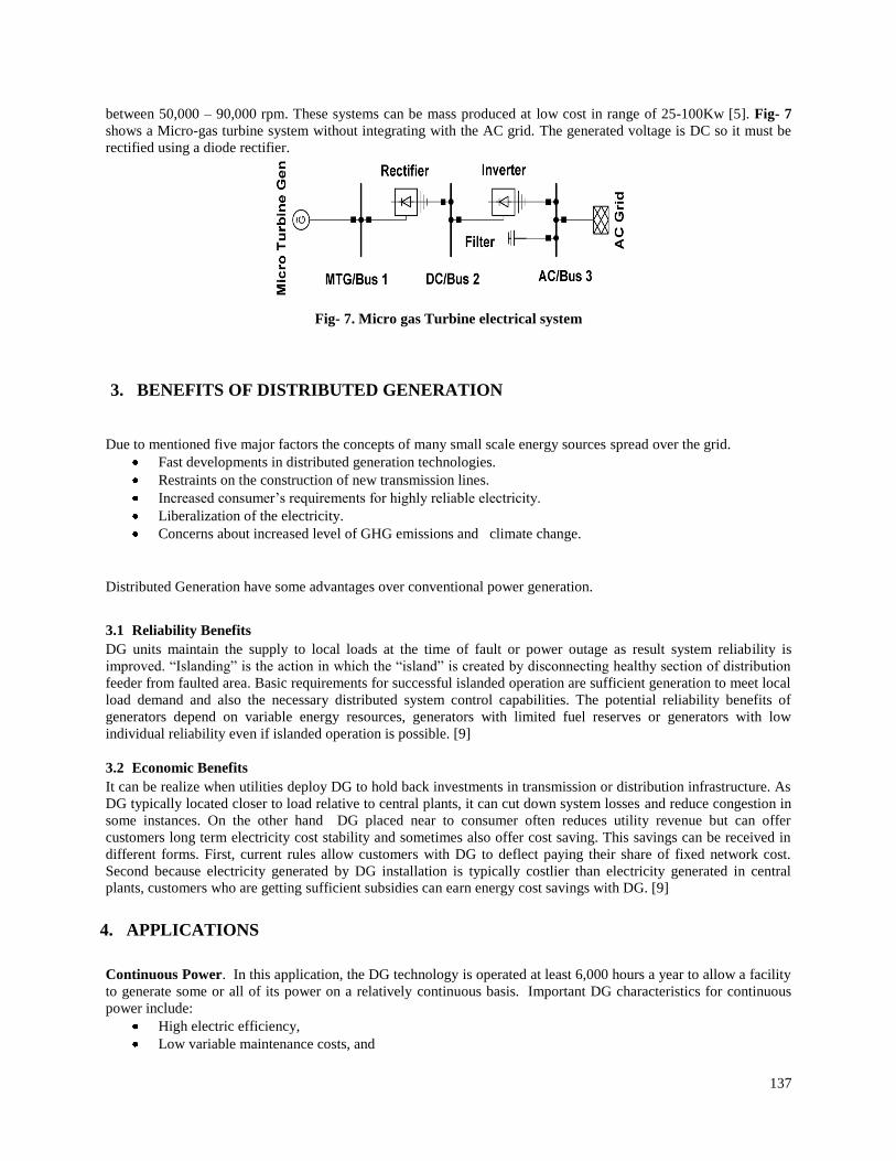
137

between 50,000 – 90,000 rpm. These systems can be mass produced at low cost in range of 25-100Kw [5]. Fig- 7

shows a Micro-gas turbine system without integrating with the AC grid. The generated voltage is DC so it must be

rectified using a diode rectifier.

Fig- 7. Micro gas Turbine electrical system

3. BENEFITS OF DISTRIBUTED GENERATION

Due to mentioned five major factors the concepts of many small scale energy sources spread over the grid.

Fast developments in distributed generation technologies.

Restraints on the construction of new transmission lines.

Increased consumer’s requirements for highly reliable electricity.

Liberalization of the electricity.

Concerns about increased level of GHG emissions and climate change.

Distributed Generation have some advantages over conventional power generation.

3.1 Reliability Benefits

DG units maintain the supply to local loads at the time of fault or power outage as result system reliability is

improved. “Islanding” is the action in which the “island” is created by disconnecting healthy section of distribution

feeder from faulted area. Basic requirements for successful islanded operation are sufficient generation to meet local

load demand and also the necessary distributed system control capabilities. The potential reliability benefits of

generators depend on variable energy resources, generators with limited fuel reserves or generators with low

individual reliability even if islanded operation is possible. [9]

3.2 Economic Benefits

It can be realize when utilities deploy DG to hold back investments in transmission or distribution infrastructure. As

DG typically located closer to load relative to central plants, it can cut down system losses and reduce congestion in

some instances. On the other hand DG placed near to consumer often reduces utility revenue but can offer

customers long term electricity cost stability and sometimes also offer cost saving. This savings can be received in

different forms. First, current rules allow customers with DG to deflect paying their share of fixed network cost.

Second because electricity generated by DG installation is typically costlier than electricity generated in central

plants, customers who are getting sufficient subsidies can earn energy cost savings with DG. [9]

4. APPLICATIONS

Continuous Power. In this application, the DG technology is operated at least 6,000 hours a year to allow a facility

to generate some or all of its power on a relatively continuous basis. Important DG characteristics for continuous

power include:

High electric efficiency,

Low variable maintenance costs, and

138

Low emissions

Currently, DG is being utilized most often in a continuous power capacity for industrial applications in facilities

with low thermal demands. Commercial sector usage, while a fraction of total industrial usage, includes sectors

such as grocery stores, hotels, and hospitals, usually in facilities where the building has a heating, ventilating, and air

conditioning system that makes cogeneration installation costly [14].

Combined Heat and Power (CHP). Also referred to as Cooling, Heating, and Power or cogeneration, this DG

technology allows a facility to generate some or all of its power. A portion of the DG waste heat is used for water

heating, space heating, steam generation or other thermal needs. In some instances this thermal energy can also be

used to operate special cooling equipment. Important DG characteristics for combined heat and power include:

High useable thermal output (leading to high overall efficiency),

Low variable maintenance costs, and

Low emissions.

CHP characteristics are similar to those of continuous power, and thus the two applications have almost identical

customer profiles, though the high thermal demand necessary here is not a requisite for continuous power

applications. As with Continuous Power, CHP is most commonly used by industry clients, with a small portion of

overall installations in the commercial sector. Because of their superior life-cycle economics, CHP applications are

much more common than continuous power applications [14].

Peaking Power. In a peaking power application, DG is operated between 200-3000 hours per year to reduce

overall electricity costs. Units can be operated to reduce the utility’s demand charges, to defer buying electricity

during high-price periods, or to allow for lower rates from power providers by smoothing site demand. Important

DG characteristics for peaking power include:

Low installed cost,

Quick startup, and

Low fixed maintenance costs.

Peaking power applications can be offered by energy companies to clients who want to reduce the cost of buying

electricity during high-price periods. Currently DG peaking units are being used mostly in the commercial sector as

load factors in the industrial sector are relatively flat. The most common applications are in educational facilities,

lodging, miscellaneous retail sites and some industrial facilities with peaky load profiles.

Green Power. DG units can be operated by a facility to reduce environmental emissions from generating its power

supply. Important DG characteristics for green power applications include:

Low emissions,

High efficiency, and

Low variable maintenance costs.

Green power could also be used by energy companies to supply customers who want to purchase power generated

with low emissions, although this does not truly fit the strict definition of DG unless the green power is located close

to the customer site [14].

Premium Power. DG is used to provide electricity service at a higher level of reliability and/or power quality than

typically available from the grid. The growing premium power market presents utilities with an opportunity to

provide a value-added service to their clients [11]. Customers typically demand uninterrupted power for a variety of

applications, and for this reason, premium power is broken down into three further categories:

139

Emergency Power System - This is an independent system that automatically provides electricity within a specified

time frame to replace the normal source if it fails. The system is used to power critical devices whose failure would

result in property damage and/or threatened health and safety. Customers include apartment, office and commercial

buildings, hotels, schools, and a wide range of public gathering places [14].

Standby Power System - This independent system provides electricity to replace the normal source if it fails and

thus allows the customer’s entire facility to continue to operate satisfactorily. Such a system is critical for clients like

airports, fire and police stations, military bases, prisons, water supply and sewage treatment plants, natural gas

transmission and distribution systems and dairy farms [14].

True Premium Power System - Clients who demand uninterrupted power, free of all power quality problems such

as frequency variations, voltage transients, dips, and surges, use this system. Power of this quality is not available

directly from the grid – it requires both auxiliary power conditioning equipment and either emergency or standby

power. Alternatively, a DG technology can be used as the primary power source and the grid can be used as a

backup. Premium power systems are used by mission critical systems like airlines, banks, insurance companies,

communications stations, hospitals and nursing homes [14].

Important DG characteristics for premium power (emergency and standby) applications include:

Quick start-up,

Low installed cost, and


Transmission and Distribution Deferral. In some cases, placing DG units in strategic locations can help delay the

purchase of new transmission or distribution systems and equipment such as distribution lines and substations. A

thorough analysis of the life-cycle costs of the various alternatives is critical and contractual issues relating to

equipment deferrals must also be examined closely. Important DG characteristics for transmission and distribution

deferral (when used as a “peak deferral”) include:

Low installed cost, and


Ancillary Service Power. DG is used by an electric utility to provide ancillary services (interconnected operations

necessary to affect the transfer of electricity between purchaser and seller) at the transmission or distribution

level. The market for ancillary services is still unfolding in the U.S., but in markets where the electric industry has

been deregulated and ancillary services unbundled (in the United Kingdom, for example), DG applications offer

advantages over currently employed technologies. Ancillary services include spinning reserves (unloaded

generation, which is synchronized and ready to serve additional demand) and non-spinning, or supplemental,

reserves (operating reserve is not connected to the system but is capable of serving demand within a specific time or

interruptible demand that can be removed from the system within a specified time). Other potential services range

from transmission market reactive supply and voltage control, which uses generating facilities to maintain a proper

transmission line voltage, to distribution level local area security, which provides back-up power to end users in the

case of a system fault. The characteristics that may influence the adoption of DG technologies for ancillary service

applications will vary according to the service performed and the ultimate shape of the ancillary service market

[14].

5. CONCLUSION Distributed Generation is beneficial to the society as electricity generated near the place of consumption, reduction

of power losses in the network, reduction of green house gas emissions, creating the more competitive market, it

increase reliability of power system, but It is not always economically viable. The economic viability of Distributed

Generation is depends on energy prices and measures taken by the national governments to stimulate Distributed

Generation

140

6. REFERENCES

[1]www.ibf.org

[2] MIT Study on the Future of the Electric Grid Chapter 5 “The Impact of Distributed Generation and Electrical

Vehicles”

[3].ErMamthaSandhu, Dr Tilak Thakur “Issues, Challenges , Causes, Impact and Utilization of Renewable Energy

sources –Grid Integration” IJERA Vol.4 issue 3 pp 636-643 March 2014.

[4]. Anil Gupta, Dr ArunShandilya “Challenges of Integration of Wind Power on Power System Grid: A Review”

IJETAE Vol. 4 Issue 4 April 2014

[5]. AkhtarKalam,N A Hidayatullah, BlagojceStojecevski “Analysis of Distributed Generation Systems ,Smart Grid

Technology and Future Motivators Influencing Change in the Electricity Sector” Smart Grid and Renewable energy

, 2001

[6] MihailAbrudean, Lucian IoanDulau, DorinBica “Effects of Distributed Generation on electric Power Systems”

International conference INTER-ENG 2013

[7]. H.L Wills and W. G. Scott, “Distributed Power Generation –Planning and Evaluation,” Marcel Dekker, New

York 2000.

[8] Sweta, Mohamed Samir “A Generalized Overview of Distributed Generation” IJERMT Vol. 2 Issue 2 DEC 2013

[9] Anees, A.S “Grid Integration of renewable energy sources: Challenges, issues and possible solutions” 5th IEEE

International Conference on Power Electronics (IICPE), 2012 Page 1-6.

[10] N.Hatziargyriou “Modeling New Forms of Generation and storage” CIGRE technical broucher, TF 38.01.10,

November 2000.

[11] Singh S. N, et al “Distributed Generation in Power systems: An overview and Key issues, Indian Engineering

Congress 2009.

[12] Rangan Banerjee “ Comparison of option for distributed generation in India” Elsevier journal of energy policy.

[13] U.S.Department of Energy, The Potential Benefits of Distributed Generation and Rate Related Issues that May

Impede their Expansion: A Study Pursuant to Section 1817 of Energy Policy Act of 2005.

[14] http://www.distributed-generation.com

140

Voltage Stability improvement in Multi-Machine Power

System by Static Var Compensator (SVC) FACTS

Controller

Mitul Vekaria

[email protected]

Electrical Engineering Department, Silver oak college of Engineering & Technology, Gujarat Technological

University, India

Abstract

This paper presents the implication of adding FACTS controller in multi-machine power system environment in

coordinated control manner for enhancement of voltage stability requires an appropriate mathematical model of the

power system and the FACTs controllers such as a Static Var Compensator (SVC). The DAE (Differential Algebraic

Equation) methodology for multi-machine system has been is used in this paper. The model developed have been

utilized for Eigen-value analysis of IEEE 9-bus 3-machine power systems. There are many commercial packages

available for transient simulation and analysis of power systems. The transient simulation packages (e.g.

EMTDC/PSCAD) allow incorporation of FACTS controller models. This facility is however not available in the small

signal stability analysis packages. The objective of this paper is to develop a methodology to incorporate FACTS

controllers in a modular fashion to facilitate Eigen-value and voltage stability analysis using MATLAB toolbox.

Key Words: Flexible AC Transmission Systems (FACTS), FACTS Controllers, SVC, Voltage Stability

1. Introduction

DAE (Differential Algebraic Equation) methodology for multi-machine system has been presented in [1] is used in

this paper. Event tough the SVC model has been incorporated in DAE model [2]. So the purpose of this paper is to

derive SVC model such that it can be incorporated in DAE model. Further in a large power system there may be more

than one FACTS controllers, therefore it is important to put FACTS controller that can be incorporated in the DAE

model in Modular fashion. The models developed have been utilized for eigen-value analysis of IEEE 9-bus power

systems. This paper is organized as follows, Fist we discuss the DAE model of multi-machine power system without

FACTS controllers & then introduces the DAE model of multi-machine power system with SVC & later introduces

the results, discussions and conclusions of the paper.

2. DAE Model of Multi-Machine Power System without FACTS Controllers

The methodology given in [1] describes dynamic modeling of a general m-machine, n-bus system. This model

represents each machine by a two-axis model and the excitation system is chosen as the IEEE type-I rotating exciter.

The transmission system has been modeled by static equations. The DAE model utilizes power balance form. The

equations are written as

x f ( x, y, u)

x(0) xo

(1)

0 g(x, y, u) y(0) yo

(2)



141

j

A

j

T

AE

Where x is a vector of state variables y

is vector of algebraic variables and u is a vector of inputs and parameters.

Equation (1) consists of the differential equations of the mechanical system, field winding, q-axis damper winding,

and the electrical equations of the exciter. Equation (2) consists of the stator algebraic equations and the network

power balance equations. Various vectors are defined as [1]

xT , , E

' qi , E

' di , E

,V , R i i

yT V ,

, I di , I qi

fdi Ri Fi (3)

u TMi

,VREFi

, PLi

, QLi

i 1,.....m;

j 1,.......n (4)

Based on the methodology described in [1], the linearized model is given as

X

A1mo d A2 n ew A3n ew X E

0

K 2

K1n ew C4 n ew z

0 U

0

G1 D1n ew D2 n ew v 0

J

K1n ew

C4 n ew

(5)

AE D D

Where

D2 new , load flow Jacobian J LF

and 1n ew 2n ew is the algebraic Jacobian.

zT , V ,........., V

vT

, ,....., , V

,........., V The vectors 1 1 m and 2 3 m m1 n

The system matrix

Asys can be obtained as

X AsysX EU

(6)

K A

sys A

1mo d

2 n ew A

3n ew .J 1

. 2

Where G1

The details of DAE model are given in [1]. This DAE model for multi-machine system can be used for studying steady

state stability, voltage stability and low frequency electro-mechanical oscillations. Based on this methodology, a small

signal stability program has been developed using MATLAB. The developed program is tested for 9-bus WSCC test

system and its results are corrected with the results published in [1] as shown below.

3. DAE Model of Multi-Machine Power System with FACTS Controller

3.1 Case Study (WSCC 9 bus System):

In order to ensure that the developed small signal stability program gives satisfactory results, eigen-value analysis is

performed for the Western System Coordinating Council (WSCC) 9-bus system shown in Fig. 1. This WSCC system

comprises three generators and nine buses. Loads are connected at buses 5, 6, and 8 as shown in Fig.1. At base case

loading condition of the system, the generator 2 and 3 are supplying 163 MW and 85MW power respectively. The

base MVA is 100, and system frequency is 60Hz. Table 1 shows the eigen-values of WSCC system. Column 1 of

table 1 shows the eigen-values reported in [1] while column 2 depicts the eigen-values obtained from developed

142

MATLAB program. It is evident that eigen-values obtained from developed MATLAB program correlate very well

with those reported in [1]. This validates the developed MATLAB program.

Fig.1. WSCC (9-bus, 3-machine) power system

3.2 Mathematical model of SVC

:

Static VAR Compensator (SVC) is a shunt connected FACTS controller whose main functionality is to regulate the

voltage at a given bus by controlling its equivalent reactance. Basically it consists of a fixed capacitor (FC) and a

thyristor controlled reactor (TCR). Generally they are two configurations of the SVC.

a) SVC total susceptance model. A changing susceptance Bsvc represents the fundamental frequency equivalent

susceptance of all shunt modules making up the SVC as shown in Fig. 2(a).

b) SVC firing angle model. The equivalent reactance XSVC, which is function of a changing firing angle α, is made

up of the parallel combination of a thyristor controlled reactor (TCR) equivalent admittance and a fixed capacitive

reactance as shown in Fig. 2 (b).

c) This model provides information on the SVC firing angle required to achieve a given level of compensation.

143

𝐿

QSVC

-jXC

Bus

Th2

V Bus

BSVC

Th1

SVC

Fig. 2(a) SVC firing angle model Fig. 2(b) SVC total susceptance model

Figure 3 shows the steady-state and dynamic voltage-current characteristics of the SVC. In the active control range,

current/susceptance and reactive power is varied to regulate voltage according to a slope (droop) characteristic. The

slope value depends on the desired voltage regulation, the desired sharing of reactive power production between

various sources, and other needs of the system. The slope is typically 1-5%. At the capacitive limit, the SVC

becomes a shunt capacitor. At the inductive limit, the SVC becomes a shunt reactor (the current or reactive power

may also be limited).

Fig.3. steady-state and dynamic voltage/current Characteristics of the SVC

SVC firing angle model is implemented in this paper. Thus, the model can be developed with respect to a sinusoidal

voltage, differential and algebraic equations can be written as I S VC jBS VCVk .The fundamental frequency TCR

equivalent reactance

X TCR

X L

sin , Where 2( ), X

L L

Firing angle

X TCR X L

2( ) sin 2

(7)

and are conduction and firing angles respectively. At

900

, TCR conducts fully and the equivalent

reactance X TCR becomes 𝑋 , while at 1800

, TCR is blocked and its equivalent reactance becomes infinite. The

SVC effective reactance X

S VC is determined by the parallel combination of X

C

and

X TCR

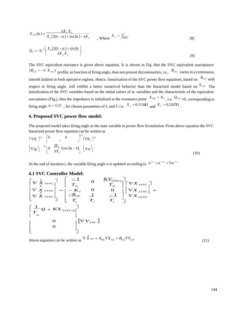
144

X

C L

X ( ) X

C X

L

S VC X

C [2( ) sin 2 ] X

L

, Where 1

C C

(8)

2 X [2( ) sin 2 Q V

C

k k

X X

(9)

The SVC equivalent reactance is given above equation. It is shown in Fig. that the SVC equivalent susceptance

(BS VC

1/ X S VC

) profile, as function of firing angle, does not present discontinuities, i.e.,

BS VC

varies in a continuous,

smooth fashion in both operative regions. Hence, linearization of the SVC power flow equations, based on B

S VC with

respect to firing angle, will exhibit a better numerical behavior than the linearized model based on X S VC

The

initialization of the SVC variables based on the initial values of ac variables and the characteristic of the equivalent

susceptance (Fig.), thus the impedance is initialized at the resonance point X TCR X C , i.e.

QS VC =0, corresponding to

firing angle 1150

, for chosen parameters of L and C i.e. X L 0.1134

and X C 0.2267 .

4. Proposed SVC power flow model:

The proposed model takes firing angle as the state variable in power flow formulation. From above equation the SVC

linearized power flow equation can be written as

Pk ( i ) 0 0

2

(i )

k (i )

Q

0 2V

k [cos 2 1]

k X

L

(10)

At the end of iteration i, the variable firing angle α is updated according to (i ) (i 1) (i )

4.1 SVC Controller Model:

X 1S VC

1 KV

S VC o 0 X

2

Tm

0

Tm

0

1S VC

X S VC K

I X

2 S VC

X 3 S VC K

P 1 1 X 3 S VC

1 (1

Tc

Tc

Tc

T KX

3 S VC o)

m

0 VS VC

0

Above equation can be written as X S VC A

AVC X

S VC B

S VCV

S VC

(11)

145

E U

1 KVS VCo

1 (1 KX

T

0 T

T 3 S VCo )

m m m A

S VC K

I

K P

0

1

0 1

BS VC

0 0

Where Tc

Tc

Tc and

5. Incorporation of SVC in multi-machine power systems:

In its simplest form SVC is composed of FC-TCR configuration as shown in Fig.2. The SVC is connected to a coupling

transformer that is connected directly to the ac bus whose voltage is to be regulated. The effective reactance of the

FC-TCR is varied by firing angle control of the thyristor. The firing angle can be controlled through a PI controller in

such a way that the voltage of the bus where the SVC is connected is maintained at the desired reference value. The

SVC can be connected at either the existing load bus or at a new bus that is created between two buses. As DAE model

is based on power-balance, rewriting of the power-balance equations at the buses with SVC connected in the system

requires modification of D

2 n ew .When SVC is connected at specified load buses, and gets modified as given below

n

PS VCi

PLi

(Vi ) V

iV

k Y

ik cos(

i

k

ik ) 0

k 1

i m 1,................,n

n

QS VCi

QLi

(Vi ) V

iV

k Y

ik sin(

i

k

ik ) 0

k 1

i m 1,......................n

Obtained state equations after linearization of above equation

CS VC V

l D

S VCX

S VC D

1V

g D

2 V

l 0

or

DS VC X

S VC D

1V

g D

2 S VC V

l 0

Where

D

2 S VC C

S VC D

2

(12)

The incorporation of the SVC into DAE model of multi-machine power system is done on the same lines as explained

in [2] given by Incorporation of (11), (12), and (5) gives DAE model of multi -machine power system with SVC

incorporated in the system. After reordering, final form of DAE model with SVC is given as

X

A1 mo d P

1S VC A

2 n ew A

3 n ew X E

X S VC

P2 S VC A

S VC P3 svc B

svcn ew X

S VC

0 U

0 K

2

P4 svc

K1n ew

C4 n ew

z 0

0 G1

DS VC D

1n ew _ svc D2 n ew _ svc v 0

The state equation for the system with SVC is then given as follows

X sys _ svc Asys svc

X sys

svc S VC

(13)

146

2

The System matrix with SVC given as A

S YS _ S VC A

SV1 ( A

SV 2 * (inv( A

SV 4 ) * A

SV 3 )

(14)

A P A

SV1

1 mo d 1svc

P2 svc

A

AS VC

A A

SV 2

2 n ew 3 n ew

P3 svc

K

Bsvcn ew

P A

SV 3

4 svc

G1 D

S VC

A

SV 4

K

1n ew C

4 n ew

D1n ew _ svc D

2 n ew _ svc

6. Results & Discussions

After incorporating FACTS controller into DAE model of multi-machine system, voltage stability of 9-bus system is

carried out at various loading conditions. However results are presented for maximum loading condition. Table 2 show

that without any FACTS controllers the system is unstable. In table 1 Eigen-values of WSCC (9-bus, 3-machine)

power and Table 2 Eigen-values of WSCC (9-bus, 3-machine) power system with SVC

Eigen-values from [1] Eigen-values from developed MATLAB program

0.7209 j12.7486 0.7198 j12.7456

0.1908 j8.3672 0.1906 j8.3660

5.4875 j7.9487 5.6867 j7.9663

5.3236 j7.9220 5.3644 j7.9311

5.2218 j7.8161 5.2287 j7.8263

5.1761 5.1779

3.3995 3.3993

0.4445 j1.2104 0.4513 j1.1997

0.4394 j0.7392 0.4481 j0.7291

0.4260 j0.4960 0.4366 j0.4868

0.0000 0.0000

0.0000 0.0000

3.2258 3.2258

Table 1:- Eigen-values of WSCC (9-bus, 3-machine) power

147

However the system become stable when SVC is connected. At maximum loading condition, there is a need for a

shunt device at bus 5. Table 2 shows eigen-values of the 9-bus system at maximum loading conditions for without

any FACTS device, with an SVC connected at bus 5.

In the similar fashion multiple FACTS controllers can also be added to DAE model of multi-machine power systems

for enhancement of voltage stability of the systems in coordinated control manner

Without any FACTS device With SVC

90.9053 92.8398

45.3014 0.5511 j50.3889

2.8938 j12.3353 0.5840 j12.6211

10.8806 j5.8904 0.1256 j8.0372

1.2151 j8.8486 9.8966 j7.0805

6.3982 j7.4235 7.3482 j7.9374

7.1865 5.2924 j7.8977

5.1023 5.3210

2.1747 3.9843

1.6763 0.5010 j1.1119

0.728 4 j0.3533 0.6142 j0.6468

0.022 9 j0.2268 0.7376 j0.2042

0.0000 j0.0000 0.0000 j0.0000

3.2258 3.2258

Table 2:- Eigen-values of WSCC (9-bus, 3-machine) power system with SVC

7. Conclusions

This paper presents a systematic modular approach to incorporate shunt FACTS controller in DAE model of multi -

machine power systems in coordinated control manner for enhancement of voltage stability of the systems. This

proposed approach is general and can be applied to any large power system environments. With the proposed approach

it is possible to connect any number and any type (series and shunt) of FACTS controllers. The results of the proposed

modular approach are illustrated for 9-bus 3-machine WSCC system.

8. References

[1] Peter W. Sauer and M. A. Pai, Power System Dynamics and Stability, Prentice Hall, 1998.

[2] M. J. Laufenberg, M. A. Pai, and K. R. Padiyar, “Hopf Bifurcation control in Power System with Static Var

Compensators, “Electric Power & Energy Systems, Vol. 19, No.5, pp. 339-347, 1997 .

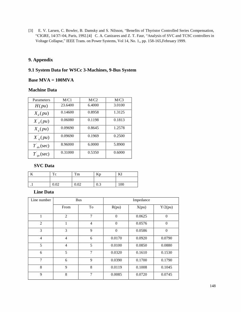
148

[3] E. V. Larsen, C. Bowler, B. Damsky and S. Nilsson, “Benefits of Thyristor Controlled Series Compensation,

“CIGRE, 14/37/-04, Paris, 1992.[4] C. A. Canizares and Z. T. Faur, “Analysis of SVC and TCSC controllers in

Voltage Collapse,” IEEE Trans. on Power Systems, Vol 14, No. 1,, pp. 158-165,February 1999.

9. Appendix

9.1 System Data for WSCc 3-Machines, 9-Bus System

Base MVA = 100MVA

Machine Data

Parameters M/C1 M/C2 M/C3

H ( pu) 23.6400 6.4000 3.0100

X d ( pu) 0.14600 0.8958 1.3125

X '

( pu) d 0.06080 0.1198 0.1813

X q ( pu) 0.09690 0.8645 1.2578

X '

( pu) q 0.09690 0.1969 0.2500

T '

(sec) do 8.96000 6.0000 5.8900

T '

(sec) qo 0.31000 0.5350 0.6000

SVC Data

K Tc Tm Kp KI

.1 0.02 0.02 0.3 100

Line Data

Line number Bus Impedance

From To R(pu) X(pu) Y/2(pu)

1 2 7 0 0.0625 0

2 1 4 0 0.0576 0

3 3 9 0 0.0586 0

4 4 6 0.0170 0.0920 0.0790

5 4 5 0.0100 0.0850 0.0880

6 5 7 0.0320 0.1610 0.1530

7 6 9 0.0390 0.1700 0.1790

8 9 8 0.0119 0.1008 0.1045

9 8 7 0.0085 0.0720 0.0745

149

Load Flow Results for Base Case of WSCC 9Bus System

Bus Type Angles Voltages PL QL PG QG

1 SL 0 1.0400 0 0 0.7164 0.2705

2 PV 9.2800 1.0250 0 0 1.6300 0.0665

3 PV 4.6648 1.0250 0 0 0.8500 -0.1086

4 PQ -2.2168 1.0258 0 0 0 0

5 PQ -3.9888 0.9956 1.2500 0.5000 0 0

6 PQ -3.6874 1.0127 0,9000 0.3000 0 0

7 PQ 3.7197 1.0258 0 0 0 0

8 PQ 0.7275 1.0159 1.0000 0.3500 0 0

9 PQ 1.9667 1.0324 0 0 0 0

150

Simulation of Speed Control of Induction Motor using

Voltage/frequency (V/F) Ratio

1Mitul Vekaria, 2Darshan Thakar


Electrical Engineering Department, Silver oak College of Engineering & Technology,


Abstract

This paper presents the need of Speed Control in Induction Motors. Out of the various methods of controlling Induction

motors, V/f Control has proven to be the most versatile. The overall scheme of implementing V/f control has been

presented. One of the basic requirements of this scheme is the PWM Inverter. In this, PWM Inverters outputs fed to the

Induction Motor drives. The uncontrolled transient and steady state response of the Induction Motor has been obtained

and analyzed. A MATLAB code was developed to successfully implement Open Loop V/f Control on a PWM-Inverter

fed 3-phase Induction Motor, and the Torque was found to be constant for various rotor speeds. This was followed by a

MATLAB model for Closed-Loop V/f Control on a PWM-Inverter fed 3-phase Induction Motor. It was observed that

using a Closed-Loop scheme with a Proportional Controller gave a very superior way of controlling the speed of an

Induction motor while maintaining a constant maximum torque.

Key Words: V/F, Speed Control of Induction Motor, PWM, Open loop V/F, Close loop V/F.

1. Introduction

Induction Motors are often termed the “Workhorse of the Industry”. This is because it is one of the most widely used

motors in the world. It is used in transportation and industries, and also in household appliances, and laboratories. The

major reasons behind the popularity of the Induction Motors are Induction Motors are cheap compared to DC and

Synchronous Motors. In this age of competition, this is a prime requirement for any machine. Due to its economy of

procurement, installation and use, the Induction Motor is usually the first choice for an operation. Squirrel-Cage

Induction Motors are very rugged in construction. There robustness enables them to be used in all kinds of environments

and for long durations of time. Induction Motors have high efficiency of energy conversion. Also they are very reliable.

Owing to their simplicity of construction, Induction Motors have very low maintenance costs. Induction Motors have

very high starting torque. This property is useful in applications where the load is applied before starting the motor.

Another major advantage of the Induction Motor over other motors is the ease with which its speed can be controlled.

Different applications require different optimum speeds for the motor to run at. Speed control is a necessity in Induction

Motors because of the .It ensures smooth operation. It provides torque control and acceleration control. Different

processes require the motor to run at different speeds. It compensates for fluctuating process parameters. During

installation, slow running of the motors is required. All these factors present a strong case for the implementation of

speed control or variable speed drives in Induction Motors.



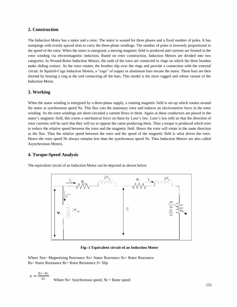
151

2. Construction

The Induction Motor has a stator and a rotor. The stator is wound for three phases and a fixed number of poles. It has

stampings with evenly spaced slots to carry the three-phase windings. The number of poles is inversely proportional to

the speed of the rotor. When the stator is energized, a moving magnetic field is produced and currents are formed in the

rotor winding via electromagnetic induction. Based on rotor construction, Induction Motors are divided into two

categories. In Wound-Rotor Induction Motors, the ends of the rotor are connected to rings on which the three brushes

make sliding contact. As the rotor rotates, the brushes slip over the rings and provide a connection with the external

circuit. In Squirrel-Cage Induction Motors, a “cage” of copper or aluminum bars encase the stator. These bars are then

shorted by brazing a ring at the end connecting all the bars. This model is the more rugged and robust variant of the

Induction Motor.

3. Working

When the stator winding is energized by a three-phase supply, a rotating magnetic field is set-up which rotates around

the stator at synchronous speed Ns. This flux cuts the stationary rotor and induces an electromotive force in the rotor

winding. As the rotor windings are short-circuited a current flows in them. Again as these conductors are placed in the

stator’s magnetic field, this exerts a mechanical force on them by Lenz’s law. Lenz’s law tells us that the direction of

rotor currents will be such that they will try to oppose the cause producing them. Thus a torque is produced which tries

to reduce the relative speed between the rotor and the magnetic field. Hence the rotor will rotate in the same direction

as the flux. Thus the relative speed between the rotor and the speed of the magnetic field is what drives the rotor.

Hence the rotor speed Nr always remains less than the synchronous speed Ns. Thus Induction Motors are also called

Asynchronous Motors.

4. Torque-Speed Analysis

The equivalent circuit of an Induction Motor can be depicted as shown below

Fig:-1 Equivalent circuit of an Induction Motor

Where Xm= Magnetizing Reactance Xs= Stator Reactance Xr= Rotor Reactance

Rs= Stator Resistance Rr= Rotor Resistance S= Slip

Where Ns= Synchronous speed, Nr = Rotor speed

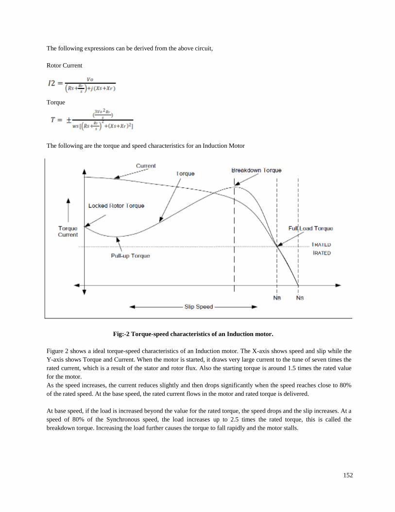
152

The following expressions can be derived from the above circuit,

Rotor Current

Torque

The following are the torque and speed characteristics for an Induction Motor

Fig:-2 Torque-speed characteristics of an Induction motor.

Figure 2 shows a ideal torque-speed characteristics of an Induction motor. The X-axis shows speed and slip while the

Y-axis shows Torque and Current. When the motor is started, it draws very large current to the tune of seven times the

rated current, which is a result of the stator and rotor flux. Also the starting torque is around 1.5 times the rated value

for the motor.

As the speed increases, the current reduces slightly and then drops significantly when the speed reaches close to 80%

of the rated speed. At the base speed, the rated current flows in the motor and rated torque is delivered.

At base speed, if the load is increased beyond the value for the rated torque, the speed drops and the slip increases. At a

speed of 80% of the Synchronous speed, the load increases up to 2.5 times the rated torque, this is called the

breakdown torque. Increasing the load further causes the torque to fall rapidly and the motor stalls.

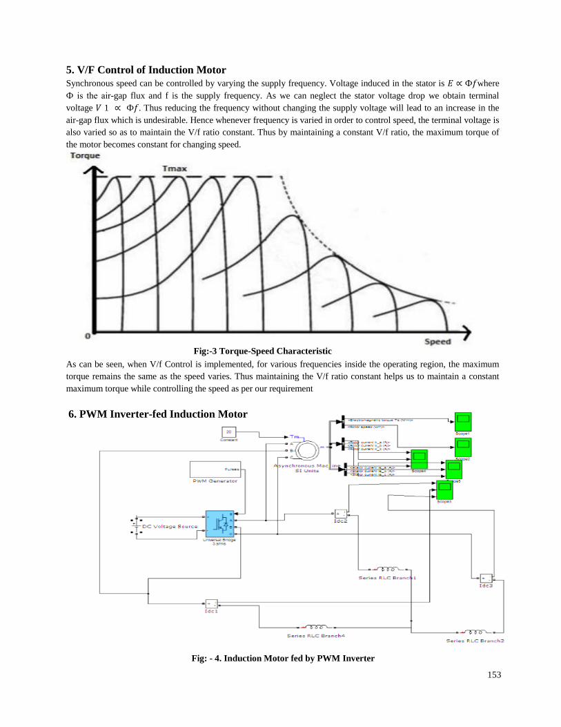
153

5. V/F Control of Induction Motor

Synchronous speed can be controlled by varying the supply frequency. Voltage induced in the stator is 𝐸 ∝ Ф𝑓where

Ф is the air-gap flux and f is the supply frequency. As we can neglect the stator voltage drop we obtain terminal

voltage 𝑉 1 ∝ Ф𝑓. Thus reducing the frequency without changing the supply voltage will lead to an increase in the

air-gap flux which is undesirable. Hence whenever frequency is varied in order to control speed, the terminal voltage is

also varied so as to maintain the V/f ratio constant. Thus by maintaining a constant V/f ratio, the maximum torque of

the motor becomes constant for changing speed.

Fig:-3 Torque-Speed Characteristic

As can be seen, when V/f Control is implemented, for various frequencies inside the operating region, the maximum

torque remains the same as the speed varies. Thus maintaining the V/f ratio constant helps us to maintain a constant

maximum torque while controlling the speed as per our requirement

6. PWM Inverter-fed Induction Motor

Fig: - 4. Induction Motor fed by PWM Inverter

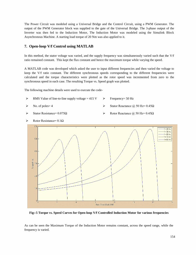
154

The Power Circuit was modeled using a Universal Bridge and the Control Circuit, using a PWM Generator. The

output of the PWM Generator block was supplied to the gate of the Universal Bridge. The 3-phase output of the

Inverter was then fed to the Induction Motor, The Induction Motor was modeled using the Simulink Block

Asynchronous Machine. A starting load torque of 20 Nm was also applied to it.

7. Open-loop V/f Control using MATLAB

In this method, the stator voltage was varied, and the supply frequency was simultaneously varied such that the V/f

ratio remained constant. This kept the flux constant and hence the maximum torque while varying the speed.

A MATLAB code was developed which asked the user to input different frequencies and then varied the voltage to

keep the V/f ratio constant. The different synchronous speeds corresponding to the different frequencies were

calculated and the torque characteristics were plotted as the rotor speed was incremented from zero to the

synchronous speed in each case. The resulting Torque vs. Speed graph was plotted.

The following machine details were used to execute the code-

RMS Value of line-to-line supply voltage = 415 V

No. of poles= 4

Stator Resistance= 0.075Ω

Rotor Resistance= 0.1Ω

Frequency= 50 Hz

Stator Reactance @ 50 Hz= 0.45Ω

Rotor Reactance @ 50 Hz= 0.45Ω

Fig:-5 Torque vs. Speed Curves for Open-loop V/f Controlled Induction Motor for various frequencies

As can be seen the Maximum Torque of the Induction Motor remains constant, across the speed range, while the

frequency is varied.

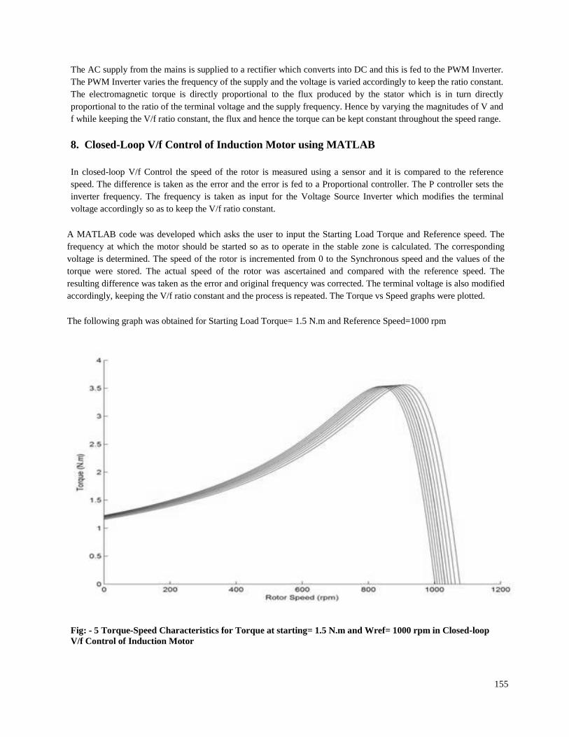
155

The AC supply from the mains is supplied to a rectifier which converts into DC and this is fed to the PWM Inverter.

The PWM Inverter varies the frequency of the supply and the voltage is varied accordingly to keep the ratio constant.

The electromagnetic torque is directly proportional to the flux produced by the stator which is in turn directly

proportional to the ratio of the terminal voltage and the supply frequency. Hence by varying the magnitudes of V and

f while keeping the V/f ratio constant, the flux and hence the torque can be kept constant throughout the speed range.

8. Closed-Loop V/f Control of Induction Motor using MATLAB

In closed-loop V/f Control the speed of the rotor is measured using a sensor and it is compared to the reference

speed. The difference is taken as the error and the error is fed to a Proportional controller. The P controller sets the

inverter frequency. The frequency is taken as input for the Voltage Source Inverter which modifies the terminal

voltage accordingly so as to keep the V/f ratio constant.

A MATLAB code was developed which asks the user to input the Starting Load Torque and Reference speed. The

frequency at which the motor should be started so as to operate in the stable zone is calculated. The corresponding

voltage is determined. The speed of the rotor is incremented from 0 to the Synchronous speed and the values of the

torque were stored. The actual speed of the rotor was ascertained and compared with the reference speed. The

resulting difference was taken as the error and original frequency was corrected. The terminal voltage is also modified

accordingly, keeping the V/f ratio constant and the process is repeated. The Torque vs Speed graphs were plotted.

The following graph was obtained for Starting Load Torque= 1.5 N.m and Reference Speed=1000 rpm

Fig: - 5 Torque-Speed Characteristics for Torque at starting= 1.5 N.m and Wref= 1000 rpm in Closed-loop

V/f Control of Induction Motor

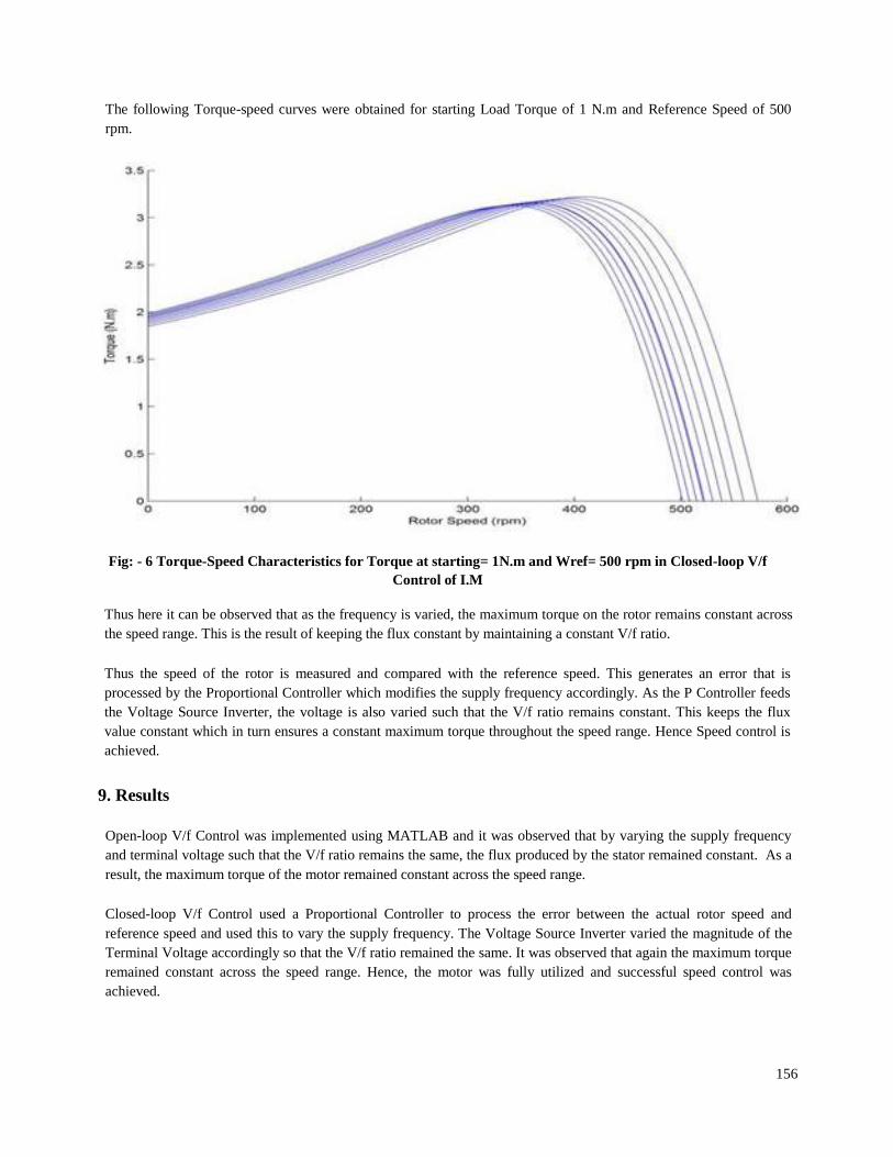
156

The following Torque-speed curves were obtained for starting Load Torque of 1 N.m and Reference Speed of 500

rpm.

Fig: - 6 Torque-Speed Characteristics for Torque at starting= 1N.m and Wref= 500 rpm in Closed-loop V/f

Control of I.M

Thus here it can be observed that as the frequency is varied, the maximum torque on the rotor remains constant across

the speed range. This is the result of keeping the flux constant by maintaining a constant V/f ratio.

Thus the speed of the rotor is measured and compared with the reference speed. This generates an error that is

processed by the Proportional Controller which modifies the supply frequency accordingly. As the P Controller feeds

the Voltage Source Inverter, the voltage is also varied such that the V/f ratio remains constant. This keeps the flux

value constant which in turn ensures a constant maximum torque throughout the speed range. Hence Speed control is

achieved.

9. Results

Open-loop V/f Control was implemented using MATLAB and it was observed that by varying the supply frequency

and terminal voltage such that the V/f ratio remains the same, the flux produced by the stator remained constant. As a

result, the maximum torque of the motor remained constant across the speed range.

Closed-loop V/f Control used a Proportional Controller to process the error between the actual rotor speed and

reference speed and used this to vary the supply frequency. The Voltage Source Inverter varied the magnitude of the

Terminal Voltage accordingly so that the V/f ratio remained the same. It was observed that again the maximum torque

remained constant across the speed range. Hence, the motor was fully utilized and successful speed control was

achieved.

157

10. References

[1]. Dr. P.S. Bimbhra, “Electrical Machinery”, 7th Edition, Khanna Publishers, New Delhi, 2010.

[2]. Gopal K. Dubey, “Fundamentals of Electrical Drives”, 2nd Edition, Narosa Publishing House, New Delhi, 2011.

[3]. M.C. Trigg and C.V. Nayar, “Matlab Simulink Modelling of a Single-Phase Voltage Controlled Voltage Source

Inverter”, Dept. of Electrical Engineering, Curtin University of Technology.

[4]. M Harsha Vardhan Reddy and V. Jegathesan, “Open loop V/f Control of Induction Motor based on hybrid PWM

with Reduced Torque Ripple”, ICETECT 2011, Karunya University.

[5]. Sharad S. Patil, R.M. Holmukhe, P.S. Chaudhari, “Steady State Analysis of PWM inverter fed Cage Induction

Motor Drive”, Department of Electrical Engineering, College of Engineering, Pune, India.

[6]. Neelashetty Kashappa and Ramesh Reddy K., “Performance of Voltage Source Multilevel Inverter-fed

Induction Motor Drive using Simulink”, ARPN Journal of Engineering and Applied Sciences, vol. 6, No. 6, June

2011.

[7]. A. E. Fitzgerald, Charles Kingsley, Jr. And Stephan D. Umans, “Electrical Machinery”, McGraw- Hills

Publications, Year 2002.

[8]. Scott Wade, Matthew W. Dunnigan, and Barry W. Williams, “Modelling and Simulation of Induction Machine

Vector Control with Rotor Resistance Identification”, IEEE transactions on power electronics, vol. 12, no. 3, may

1997.

[9]. “IEEE Standard Test Procedure for Polyphase Induction Motors and Generators”, volume 112,

issue 1996 of IEEE, by IEEE Power Engineering Society.

158

Problems Associated with Inverter Driven Induction Motor and it’s

Solution Darshan Thakar

[email protected]

Electrical Engineering Department, Silver oak college of Engineering & Technological Gujarat Technological

University, India

Abstract:-

In this paper, first the operation of inverter driven induction motor is presented and then the problems associated

with inverter driven induction motor is presented. A variable frequency drive using inverter controls the operating

speed of an AC motor by controlling the frequency and voltage of the power supplied to the motor. Thus, it has

extended the use of induction motor in variable speed drive applications. The performance of the induction motor is

affected due to the high Total Harmonic Distortion (THD) produced by the conventional two level inverters.

Keywords: induction Motor ,inverter ,variable frequency drive(VFD) ,total harmonic distortion(THD) ,pulse width

modulation(PWM) .

1. Introduction Three phase induction motors are the most widely used motors for industrial control and automation.

Hence they are often called the workhorse of the motion industries. They are robust, reliable, less maintenance and of

high durability. When power is supplied to an induction motor with recommended specified voltage and frequency, it

runs at its rated speed. However many applications need variable speed variations to improve the quality of the

product. The development of power electronic devices and control systems has to mature to allow these components

to be used for speed control of AC motors control in place of conventional methods. This type of control not only

controls the speed of AC motors, but can improve the motor’s dynamic and steady state characteristics.

Pulse Width Modulation (PWM) variable speed drives are increasingly applied in many new industrial

applications that require superior performance. Three phase voltage-fed PWM inverters are recently showing growing

popularity for multi-megawatt industrial drive applications.

Power electronic inverter is a circuit that converts direct power to alternative power. Inverters are commonly

used to supply AC power from DC sources. It is widely used in industrial power conversion systems both for utility

and drives applications .

Variable frequency inverter-fed induction motor drives are used in ratings up to hundreds of kilowatts. Standard

50 Hz or 60 Hz motors are often used (though as we will see later this limits performance), and the inverter output

frequency typically covers the range from around 5–10 Hz up to perhaps 120 Hz. This is sufficient to give at least a

10:1 speed range with a top speed of twice the normal (mains frequency) operating speed. The majority of inverters

are 3-phase input and 3-phase output, but single-phase input versions are available up to about 5 kW, and some very

small inverters (usually less than 1 kW) are specifically intended for use with single-phase motors. The general

arrangement of inverter driven induction motor is shown in below figure.[1]

159

Fig.1. General arrangement of inverter fed variable frequency induction motor speed controlled drive

2. Induction Motor Operation With Variable Speed Drive For an induction motor, rotor speed, frequency of the voltage source, number of poles and slip are interrelated

according to the following equation:

120(1 ) (1)

fn s

P

Where:

n : mechanical speed (rpm)

f : fundamental frequency of the input voltage.

p : number of poles.

s : slip

The analysis of the formula above shows that the mechanical speed of an induction motor is a function of three

parameters. Thus the change of any of those parameters will cause the motor speed to vary . The utilization of static

frequency converters comprehends currently the most efficient method to control the speed of induction motors.

Converters transform a constant frequency-constant amplitude voltage into a variable (controllable) frequency-

variable (controllable) amplitude voltage. The variation of the power frequency supplied to the motor leads to the

variation of the rotating field speed, which modifies the mechanical speed of the machine.

The torque developed by the induction motor follows the equation below:

1 2 (2)mT k I

Where:

T : torque available on the shaft (N.m)

Øm : magnetizing flux (Wb)

I2 : rotor current (A)

V1 : stator voltage (V)

k1: constants à depend on the material and on the machine design.

Considering a constant torque load and admitting that the current depends on load (therefore practically constant

current), then varying proportionally amplitude and frequency of the voltage supplied to the motor results in constant

flux and therefore constant torque while the current remains unchanged. So the motor provides continuous

adjustments of speed and torque with regard to the mechanical load. The curves below are obtained from the

equations above. The ratio V1/f1 is kept constant up to the motor base (rated) frequency. From this frequency upwards

the voltage is kept constant at its base (rated) value, while the frequency applied on the stator windings keeps

growing, as shown next.

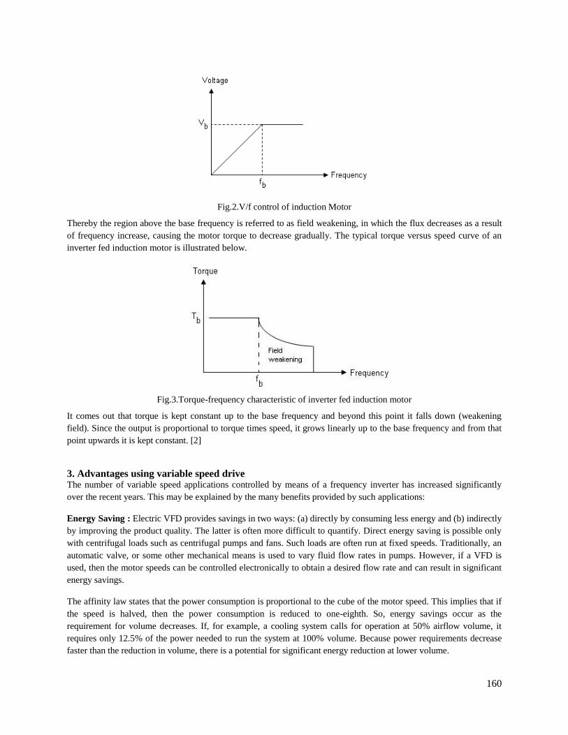
160

Fig.2.V/f control of induction Motor

Thereby the region above the base frequency is referred to as field weakening, in which the flux decreases as a result

of frequency increase, causing the motor torque to decrease gradually. The typical torque versus speed curve of an

inverter fed induction motor is illustrated below.

Fig.3.Torque-frequency characteristic of inverter fed induction motor

It comes out that torque is kept constant up to the base frequency and beyond this point it falls down (weakening

field). Since the output is proportional to torque times speed, it grows linearly up to the base frequency and from that

point upwards it is kept constant. [2]

3. Advantages using variable speed drive The number of variable speed applications controlled by means of a frequency inverter has increased significantly

over the recent years. This may be explained by the many benefits provided by such applications:

Energy Saving : Electric VFD provides savings in two ways: (a) directly by consuming less energy and (b) indirectly

by improving the product quality. The latter is often more difficult to quantify. Direct energy saving is possible only

with centrifugal loads such as centrifugal pumps and fans. Such loads are often run at fixed speeds. Traditionally, an

automatic valve, or some other mechanical means is used to vary fluid flow rates in pumps. However, if a VFD is

used, then the motor speeds can be controlled electronically to obtain a desired flow rate and can result in significant

energy savings.

The affinity law states that the power consumption is proportional to the cube of the motor speed. This implies that if

the speed is halved, then the power consumption is reduced to one-eighth. So, energy savings occur as the

requirement for volume decreases. If, for example, a cooling system calls for operation at 50% airflow volume, it

requires only 12.5% of the power needed to run the system at 100% volume. Because power requirements decrease

faster than the reduction in volume, there is a potential for significant energy reduction at lower volume.

161

Improved Process Control: Using VFDs to improve process control results in more efficient operating systems. The

throughput rates of most industrial processes are functions of many variables. For example, throughput in continuous

metal annealing depends on, amongst other factors, the material characteristics, the cross-sectional area of the

material being processed and the temperature of one or more heat zones. If constant speed motors are used to run

conveyors on the line, it must either run without material during the time required to change temperature in a heat

zone or produce scrap during this period. Both choices waste energy or material. With VFDs, however, the time

needed to change speed is significantly less than the time it takes to change heat-zone temperature. By adjusting the

material flow continuously to match the heat zone conditions, a production line can operate continuously. The results

are less energy use and less scrap metal.

Reduced Mechanical Stress (Soft Starts): Starting a motor on line-power increases stress on the mechanical system

e.g. belts and chains. Direct on-line start-up of an induction motor is always associated with high inrush current with

poor power factor. VFD can improve the operating conditions for a system by giving a smooth, controlled start and by

saving some energy during starting and running. Smoother start-up operation will prolong life and reduce

maintenance. The benefits are that the power wasted by current inrush is eliminated and that the life of the motor and

the driven machine are prolonged by the gentle, progressive application of torque.

Improved Electrical System Power Factors : When a diode supply bridge is used for rectification, electric variable

speed drives operate at near unity power factor over the whole speed range (the supply delivers mostly real power).

When a fully controlled thyristor supply bridge is used (as in DC, Cyclo and current source drives) the power factor

starts at around 0.9 at full speed, and proportionately worsens as speed declines due to front-end thyristor (typically

0.45 at 50% speed and 0.2 at 25% speed). Modern pulse width modulated (PWM) drives convert the three phases AC

line voltage to a fixed-level DC voltage. They do this regardless of inverter output speed and power. The PWM

inverters, therefore, provide a constant power factor regardless of the power factor of the load machine and the

controller installation configuration, for example, by adding a reactor or output filter between the VSD and the motor.

4. Problems associated with inverter driven induction motor and its Solutions The problems associated with inverter driven induction motor with solutions are explained below.

Thermal stress : Employing a VFD with a motor will necessarily increase the amount of heat the motor must

dissipate. Thermal stress is because of the nature of the current produced from the PWM voltage input to the motor,

numerous harmonics of various magnitudes are present. Although not contributing to torque production, these

harmonic currents produce I2R heat in the motor .The typical voltage and current waveforms for inverter fed induction

motor is shown in fig.4.

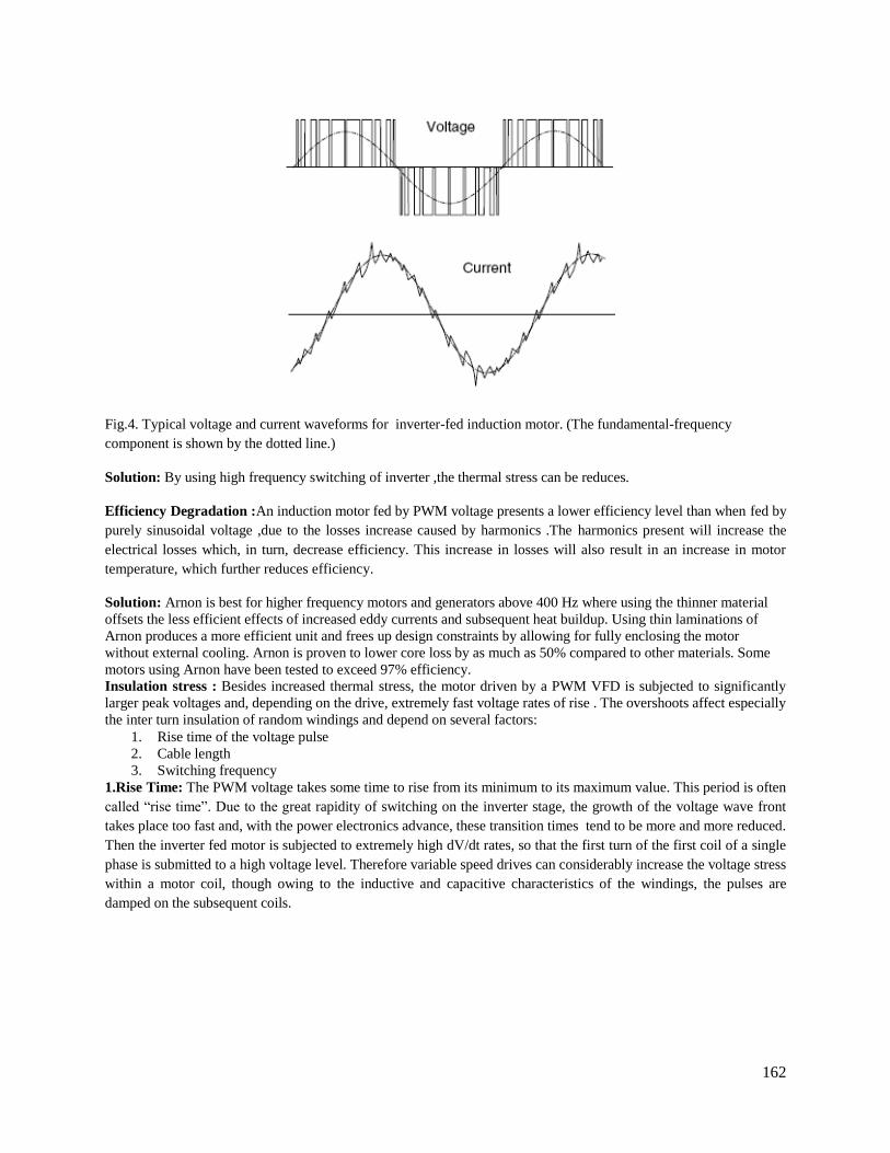
162

Fig.4. Typical voltage and current waveforms for inverter-fed induction motor. (The fundamental-frequency

component is shown by the dotted line.)

Solution: By using high frequency switching of inverter ,the thermal stress can be reduces.

Efficiency Degradation :An induction motor fed by PWM voltage presents a lower efficiency level than when fed by

purely sinusoidal voltage ,due to the losses increase caused by harmonics .The harmonics present will increase the

electrical losses which, in turn, decrease efficiency. This increase in losses will also result in an increase in motor

temperature, which further reduces efficiency.

Solution: Arnon is best for higher frequency motors and generators above 400 Hz where using the thinner material

offsets the less efficient effects of increased eddy currents and subsequent heat buildup. Using thin laminations of

Arnon produces a more efficient unit and frees up design constraints by allowing for fully enclosing the motor

without external cooling. Arnon is proven to lower core loss by as much as 50% compared to other materials. Some

motors using Arnon have been tested to exceed 97% efficiency.

Insulation stress : Besides increased thermal stress, the motor driven by a PWM VFD is subjected to significantly

larger peak voltages and, depending on the drive, extremely fast voltage rates of rise . The overshoots affect especially

the inter turn insulation of random windings and depend on several factors:

1. Rise time of the voltage pulse

2. Cable length

3. Switching frequency

1.Rise Time: The PWM voltage takes some time to rise from its minimum to its maximum value. This period is often

called “rise time”. Due to the great rapidity of switching on the inverter stage, the growth of the voltage wave front

takes place too fast and, with the power electronics advance, these transition times tend to be more and more reduced.

Then the inverter fed motor is subjected to extremely high dV/dt rates, so that the first turn of the first coil of a single

phase is submitted to a high voltage level. Therefore variable speed drives can considerably increase the voltage stress

within a motor coil, though owing to the inductive and capacitive characteristics of the windings, the pulses are

damped on the subsequent coils.

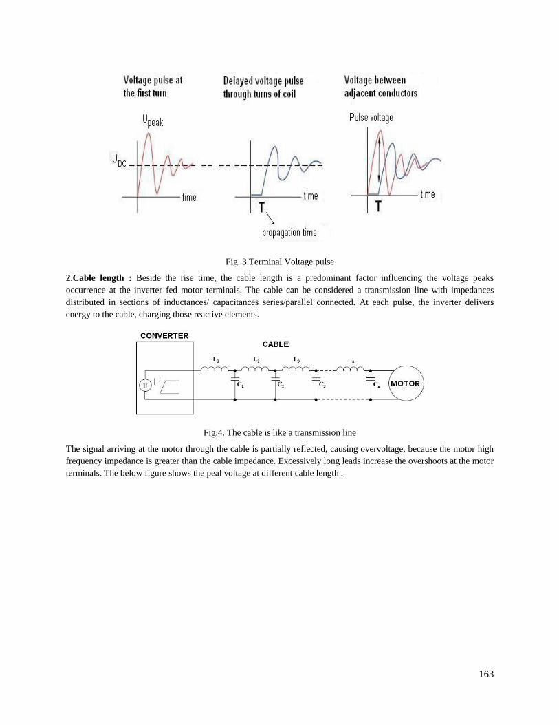
163

Fig. 3.Terminal Voltage pulse

2.Cable length : Beside the rise time, the cable length is a predominant factor influencing the voltage peaks

occurrence at the inverter fed motor terminals. The cable can be considered a transmission line with impedances

distributed in sections of inductances/ capacitances series/parallel connected. At each pulse, the inverter delivers

energy to the cable, charging those reactive elements.

Fig.4. The cable is like a transmission line

The signal arriving at the motor through the cable is partially reflected, causing overvoltage, because the motor high

frequency impedance is greater than the cable impedance. Excessively long leads increase the overshoots at the motor

terminals. The below figure shows the peal voltage at different cable length .

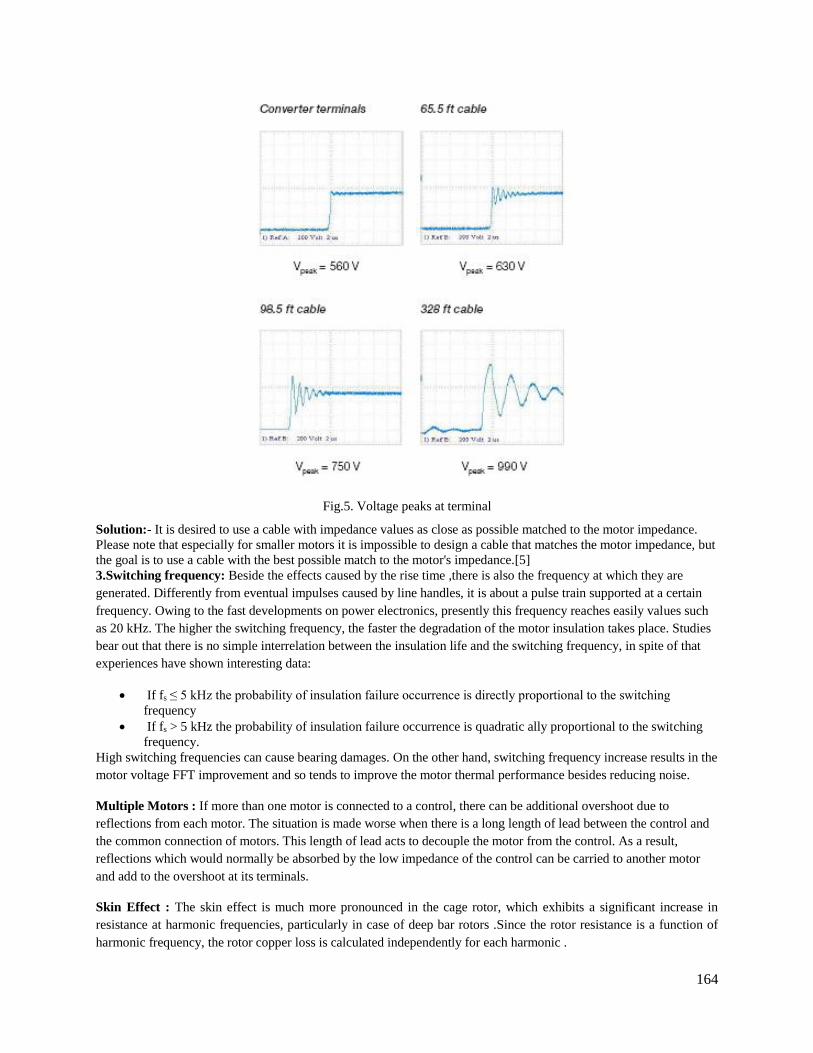
164

Fig.5. Voltage peaks at terminal

Solution:- It is desired to use a cable with impedance values as close as possible matched to the motor impedance.

Please note that especially for smaller motors it is impossible to design a cable that matches the motor impedance, but

the goal is to use a cable with the best possible match to the motor's impedance.[5]

3.Switching frequency: Beside the effects caused by the rise time ,there is also the frequency at which they are

generated. Differently from eventual impulses caused by line handles, it is about a pulse train supported at a certain

frequency. Owing to the fast developments on power electronics, presently this frequency reaches easily values such

as 20 kHz. The higher the switching frequency, the faster the degradation of the motor insulation takes place. Studies

bear out that there is no simple interrelation between the insulation life and the switching frequency, in spite of that

experiences have shown interesting data:

If fs ≤ 5 kHz the probability of insulation failure occurrence is directly proportional to the switching

frequency

If fs > 5 kHz the probability of insulation failure occurrence is quadratic ally proportional to the switching

frequency.

High switching frequencies can cause bearing damages. On the other hand, switching frequency increase results in the

motor voltage FFT improvement and so tends to improve the motor thermal performance besides reducing noise.

Multiple Motors : If more than one motor is connected to a control, there can be additional overshoot due to

reflections from each motor. The situation is made worse when there is a long length of lead between the control and

the common connection of motors. This length of lead acts to decouple the motor from the control. As a result,

reflections which would normally be absorbed by the low impedance of the control can be carried to another motor

and add to the overshoot at its terminals.

Skin Effect : The skin effect is much more pronounced in the cage rotor, which exhibits a significant increase in

resistance at harmonic frequencies, particularly in case of deep bar rotors .Since the rotor resistance is a function of

harmonic frequency, the rotor copper loss is calculated independently for each harmonic .

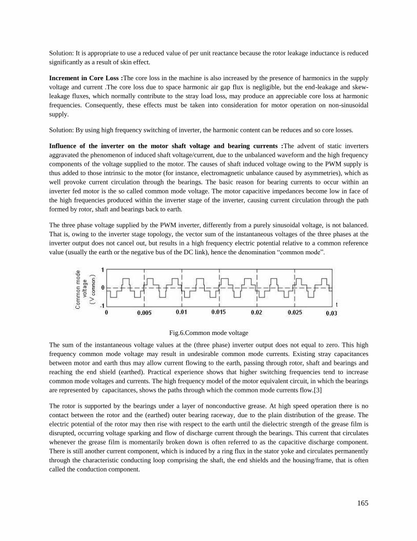
165

Solution: It is appropriate to use a reduced value of per unit reactance because the rotor leakage inductance is reduced

significantly as a result of skin effect.

Increment in Core Loss :The core loss in the machine is also increased by the presence of harmonics in the supply

voltage and current .The core loss due to space harmonic air gap flux is negligible, but the end-leakage and skew-

leakage fluxes, which normally contribute to the stray load loss, may produce an appreciable core loss at harmonic

frequencies. Consequently, these effects must be taken into consideration for motor operation on non-sinusoidal

supply.

Solution: By using high frequency switching of inverter, the harmonic content can be reduces and so core losses.

Influence of the inverter on the motor shaft voltage and bearing currents :The advent of static inverters

aggravated the phenomenon of induced shaft voltage/current, due to the unbalanced waveform and the high frequency

components of the voltage supplied to the motor. The causes of shaft induced voltage owing to the PWM supply is

thus added to those intrinsic to the motor (for instance, electromagnetic unbalance caused by asymmetries), which as

well provoke current circulation through the bearings. The basic reason for bearing currents to occur within an

inverter fed motor is the so called common mode voltage. The motor capacitive impedances become low in face of

the high frequencies produced within the inverter stage of the inverter, causing current circulation through the path

formed by rotor, shaft and bearings back to earth.

The three phase voltage supplied by the PWM inverter, differently from a purely sinusoidal voltage, is not balanced.

That is, owing to the inverter stage topology, the vector sum of the instantaneous voltages of the three phases at the

inverter output does not cancel out, but results in a high frequency electric potential relative to a common reference

value (usually the earth or the negative bus of the DC link), hence the denomination “common mode”.

Fig.6.Common mode voltage

The sum of the instantaneous voltage values at the (three phase) inverter output does not equal to zero. This high

frequency common mode voltage may result in undesirable common mode currents. Existing stray capacitances

between motor and earth thus may allow current flowing to the earth, passing through rotor, shaft and bearings and

reaching the end shield (earthed). Practical experience shows that higher switching frequencies tend to increase

common mode voltages and currents. The high frequency model of the motor equivalent circuit, in which the bearings

are represented by capacitances, shows the paths through which the common mode currents flow.[3]

The rotor is supported by the bearings under a layer of nonconductive grease. At high speed operation there is no

contact between the rotor and the (earthed) outer bearing raceway, due to the plain distribution of the grease. The

electric potential of the rotor may then rise with respect to the earth until the dielectric strength of the grease film is

disrupted, occurring voltage sparking and flow of discharge current through the bearings. This current that circulates

whenever the grease film is momentarily broken down is often referred to as the capacitive discharge component.

There is still another current component, which is induced by a ring flux in the stator yoke and circulates permanently

through the characteristic conducting loop comprising the shaft, the end shields and the housing/frame, that is often

called the conduction component.

166

Fig.8.Equilent circuit of high frequency induction motor

Where,

Cer : Capacitor formed by the stator winding and the rotor lamination (Dielectric = airgap + slot insulation + wire

insulation)

Crc : Capacitor formed by the rotor and the stator cores (Dielectric = airgap)

Cec : Capacitor formed by the stator winding and the frame (Dielectric = slot insulation + wire insulation)

Cmd and Cmt : Capacitances of the DE (drive end) and the NDE (non-drive end) bearings, formed by the inner and

the outer bearing raceways, with the metallic rolling elements in the inside. (Dielectric = gaps between the raceways

and the rolling elements + bearing grease)

ICM : Total common mode current

Ier : Capacitive discharge current flowing from the stator to the rotor

Ic : Capacitive discharge current flowing through the bearings

These discontinuous electric discharges wear the raceways and erode the rolling elements of the bearings, causing

small superimposing punctures. Long term flowing discharge currents result in furrows (fluting), which reduce

bearings life and may cause the machine to fail precociously.

Noise : The rotating electrical machines have basically three noise sources:

The ventilation system

The rolling bearings

Fig.7.High frequency model of induction motor

167

Electromagnetic excitation

Bearings in perfect conditions produce practically despicable noise, in comparison with other sources of the noise

emitted by the motor. In motors fed by sinusoidal supply, especially those with reduced pole numbers (higher speeds),

the main source of noise is the ventilation system. On the other hand, in motors of higher polarities and lower

operation speeds often stands out the electromagnetic noise. However, in variable speed drive systems, especially at

low operating speeds when ventilation is reduced, the electromagnetically excited noise can be the main source of

noise whatever the motor polarity, owing to the harmonic content of the voltage.

Solution:-Following are the solution of bearing current.

1. Faraday shield

2. Insulated bearings

3. Ceramic bearings

4. Grounding brush

5. Shaft grounding ring (SGR)[4]

Mechanical Vibration of the motor : Interactions between currents and flux harmonics may result in stray forces

actuating over the motor causing mechanical vibration and further contributing to increase the overall noise levels.

This mechanism gains importance especially when amplified natural frequencies of the motor, the forces produced

can excite vibration modes by mechanical resonances within the motor or the driven machine.

5. Conclusion Variable frequency drives applied on industrial motors represent an exciting increase in speed control and energy

savings. However, by virtue of the sophisticated electronics now available with pulse width modulated technology,

certain characteristics affecting the motor's insulation and cooling systems must be considered .In this paper the

operation of inverter driven induction motor is discussed then the advantages using inverter driven induction motor is

discussed.. The problems associated with inverter driven induction motor is discussed in details and solutions are also

suggested.

6. REFERENCES

[1]Steven L. Mecker, Member IEEE Siemens Energy & Automation, Inc “Considerations In Derating Induction

Motors For Applications On Variable Frequency Drives“CH3142-719210000-0191 1992 IEEE

[2] Singh, G.K.. "A research survey of induction motor operation with non-sinusoidal supply wave forms", Electric

Power Systems Research, 2005.

[3]Gao Qiang, Xu Dianguo, "A New Approach to Mitigate CM and DM Voltage dv/dt Value in PWM Inverter

Drive Motor Systems", Applied Power Electronics Conference, APEC 2007 - Twenty Second Annual IEEE-2007

[4] H. William Oh ,Adam Will werth "Shaft Grounding-A Solution to Motor Bearing Currents",American Society of

Heating, Refrigerating and Air-Conditioning(ASHRAE) Transactions Vol. 114, Part 2,2008,pp. 246-251.

[5] John. M. Bentley Patrick J. Link,"Evaluation of Motor Power Cables for PWM AC Drive",Pulp and Paper

Industry Technical Conference-1996,Vol 33 , Issue: 2, pp. 55-69.

168

Analysis of Microstrip Patch Antenna for WiMAX Application

Anshu Mundra

[email protected]

Electronics & Communication Engineering Department, Silver Oak College of Engineering & Technology


Abstract: This paper discusses an analysis of multi band square microstrip patch antenna loaded with a pair of horizontal and

vertical slits. Here, impedance bandwidth of the conventional microstrip patch antenna is increased to 42.05% by

introducing vertical and horizontal slits in the patch. The proposed designed antenna resonates at three frequencies

namely 3.02GHz, 4.81GHz & 6.8GHz. The antenna proposed is designed and simulated using IE3D virtual platform

and results like VSWR, radiation pattern, return loss, gain & impedance matching are presented. Proposed design may

be utilized for multi band application appropriate for numerous wireless communication systems like WiMAX,

WLAN etc.

Keywords: Microstrip, Impedance Bandwidth, Return Loss.

1. Introduction The demand of microstrip antennas still persists due to its light weight, low profile, low cost and ease of integration

with microwave circuit and no other antenna still could replace its features and hence it is being used in the wireless

and other applications [1-2]. The traditional microstrip patch antenna in general has a narrow band structure. However

bandwidth enhancements usually demanded for practical applications. Application‟s in present day mobile

communication systems usually require smaller antenna size in order to meet the miniaturization requirements of

mobile unit. Thus size reduction and bandwidth enhancement are becoming major design considerations for practical

applications of microstrip antennas. There are numerous methods to increase the bandwidth of antennas, including

increase of the substrate thickness, the use of a low dielectric substrate, the use of multiple resonators; edge coupled

parasitic patches, fractal patch and the use of slot antenna geometry [3-4]. However, the bandwidth and the size of an

antenna are generally conflicting each other, that is, improvement of one of the characteristics normally results in

degradation of the other [5-6].

Patch antennas are receiving interest in various Mobile communication systems since they can provide advantages

over traditional antennas in terms of high efficiency, low EM coupling to the human head and increased mechanical

reliability. In many applications the requirements on both bandwidth and physical size are quite stringent. In some

applications it is desired to have a dual band or multiband characteristics [7]. These characteristics can be obtained by

coupling multiple radiating elements or by using tuning devices. However these methods make antenna more

complicated. A simple method to achieve the dual band characteristics in a microstrip antenna is inserting slot in the

patch as the structure proposed here in which the radiating patch includes a pair of step slots. Inserting a slot on the

patch can reduce the resonating frequency while reducing the dimensions of the antenna. Antenna dimensions can be

reduced by creating appropriate slots making antenna useful for wideband and multiband frequency application [8-10].

Recent development on the multiband microstrip antenna progressed rapidly especially the IEEE 802.16 Worldwide

Interoperability for Microwave Access (WiMAX) application. In practical application, narrow bandwidth is a major

disadvantage of microstrip patch antenna. Based on the IEEE 802.16 standard, the WiMAX operations are in 2.5 GHz

band (2.5 GHz - 2.69 GHz), 3.5 GHz band (3.3 GHz - 3.8GHz) and 5.5GHz band (5.25 GHz - 5.85 GHz)[11-12]. In

this paper wider bandwidth which is a major concern for practical implementation of WiMAX application is discussed.

The proposed antenna is simulated using virtual platform IE3D [13]. This paper consists of IV sections. Brief

introduction is discussed in section I. Section II describes proposed antenna design. Result analysis and performance

comparison with conventional patch antenna and the modify patch antenna loaded with one, two and three pair of

vertical and horizontal slits is discussed in section III. Section IV concludes the paper.


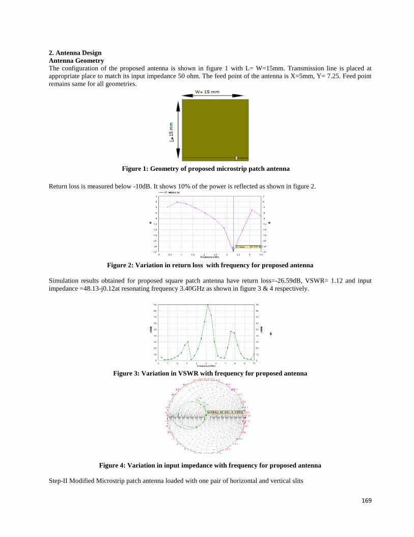
169

2. Antenna Design

Antenna Geometry

The configuration of the proposed antenna is shown in figure 1 with L= W=15mm. Transmission line is placed at

appropriate place to match its input impedance 50 ohm. The feed point of the antenna is X=5mm, Y= 7.25. Feed point

remains same for all geometries.

Figure 1: Geometry of proposed microstrip patch antenna

Return loss is measured below -10dB. It shows 10% of the power is reflected as shown in figure 2.

Figure 2: Variation in return loss with frequency for proposed antenna

Simulation results obtained for proposed square patch antenna have return loss=-26.59dB, VSWR= 1.12 and input

impedance =48.13-j0.12at resonating frequency 3.40GHz as shown in figure 3 & 4 respectively.

Figure 3: Variation in VSWR with frequency for proposed antenna

Figure 4: Variation in input impedance with frequency for proposed antenna

Step-II Modified Microstrip patch antenna loaded with one pair of horizontal and vertical slits

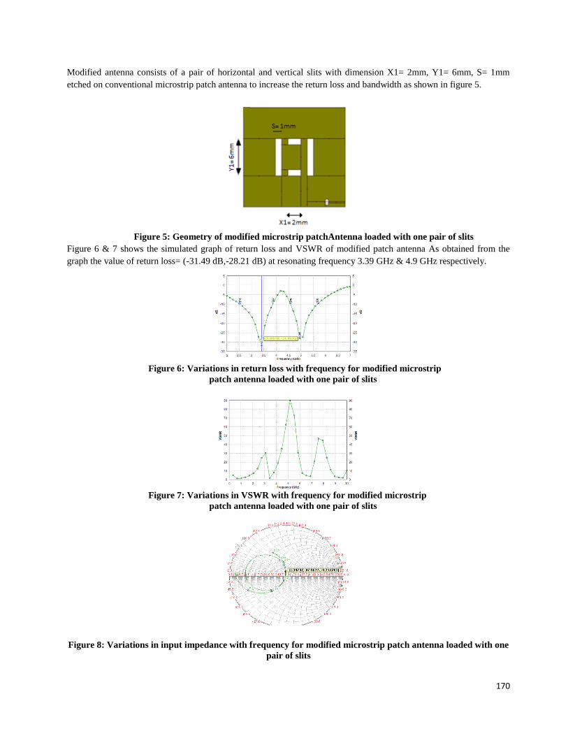
170

Modified antenna consists of a pair of horizontal and vertical slits with dimension X1= 2mm, Y1= 6mm, S= 1mm

etched on conventional microstrip patch antenna to increase the return loss and bandwidth as shown in figure 5.

Figure 5: Geometry of modified microstrip patchAntenna loaded with one pair of slits

Figure 6 & 7 shows the simulated graph of return loss and VSWR of modified patch antenna As obtained from the

graph the value of return loss= (-31.49 dB,-28.21 dB) at resonating frequency 3.39 GHz & 4.9 GHz respectively.

Figure 6: Variations in return loss with frequency for modified microstrip

patch antenna loaded with one pair of slits

Figure 7: Variations in VSWR with frequency for modified microstrip

patch antenna loaded with one pair of slits

Figure 8: Variations in input impedance with frequency for modified microstrip patch antenna loaded with one

pair of slits

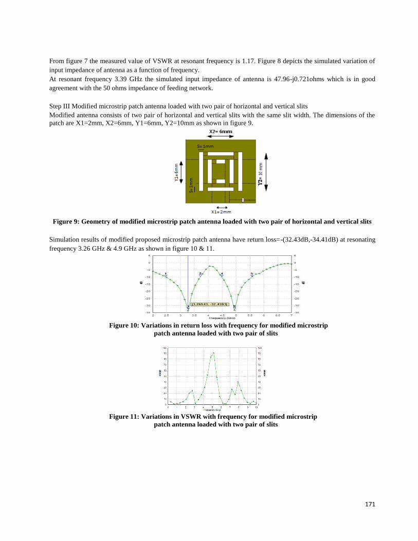
171

From figure 7 the measured value of VSWR at resonant frequency is 1.17. Figure 8 depicts the simulated variation of

input impedance of antenna as a function of frequency.

At resonant frequency 3.39 GHz the simulated input impedance of antenna is 47.96-j0.721ohms which is in good

agreement with the 50 ohms impedance of feeding network.

Step III Modified microstrip patch antenna loaded with two pair of horizontal and vertical slits

Modified antenna consists of two pair of horizontal and vertical slits with the same slit width. The dimensions of the

patch are X1=2mm, X2=6mm, Y1=6mm, Y2=10mm as shown in figure 9.

Figure 9: Geometry of modified microstrip patch antenna loaded with two pair of horizontal and vertical slits

Simulation results of modified proposed microstrip patch antenna have return loss=-(32.43dB,-34.41dB) at resonating

frequency 3.26 GHz & 4.9 GHz as shown in figure 10 & 11.


patch antenna loaded with two pair of slits



172

Figure 12: Variations in input impedance with frequency for modified microstrip


The simulated variation of VSWR and input impedance with frequency is shown in figure 11 & 12 respectively. From

the simulated plots the value of VSWR & input impedance is 1.09 & 48.07-j0.69 ohms respectively.

Step IV Modified microstrip patch antenna loadedwith three pair of horizontal and vertical slits

Modifed antenna consists of three pair of horizontal and vertical slits with dimension X1=2mm, X2=6mm, Y1=6mm,

Y2=10mm, X3=10mm, Y3=14mm etched on conventional microstrip patch antenna as shown in figure 13.

Figure 13: Geometry of Modified microstrip patch Antenna loaded with three pair of horizontal and vertical slits

Simulation results of modified proposed microstrip patch antenna have return loss=(-32.20dB, -27.12dB, -21.20dB)

at resonating frequency 3.02 GHz , 4.81GHz & 6.8 GHz as shown in figure 13.


patch antenna loaded with three pair of slits

173



Figure 16: Variations in input impedance with frequency for modified microstrip


The variation of VSWR with frequency as shown in figure 13 indicates that VSWR is close to 1 at resonant frequency

which indicates an excellent matching between the antenna and the feed network. The input impedance variation with

frequency is shown in figure 14 with a value of 48.37-j1.64 ohms.


Result obtained for all steps of modified antenna is presented in figure 17. It can be seen that resonant frequency

decreases as the number of slits increases. Figure 16 depicts the input impedance loci using smith chart, as input

impedance curve is passing through unit impedance circle which shows perfect matching of input.

Figure 14 shows the variation of return loss (-32.20dB, -27.12dB, -21.20dB) at three resonating frequencies 3.02GHz,

4.81GHz & 6.8GHz respectively. The input impedance of antenna is near to 49Ω which shows perfect matching

between antenna and feed network. These antennas show a good matching between antenna and feed network as the

value of VSWR is close to unity.

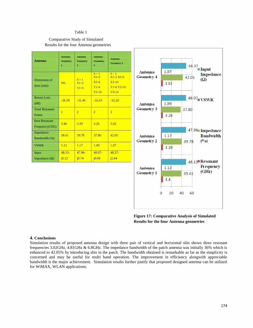
174

Table 1

Comparative Study of Simulated

Results for the four Antenna geometries

Antenna

Antenna

Geometry

1

Antenna

Geometry

2

Antenna

Geometry

3

Antenna

Geometry 4

Dimension of

slots (mm) NIL

S = 1

X1=2

Y1=6

S = 1

X1=2

X2=6

Y1=6

Y2=10

S = 1

X1=2 X2=6

X3=10

Y1=6 Y2=10

Y3=14

Return Loss

(dB) -26.59 -31.49 -32.43 -32.20

Total Resonant

Points 1 2 2 3

Best Resonant

Frequency(GHz) 3.40 3.39 3.26 3.02

Impedance

Bandwidth (%) 39.41 39.78 37.80 42.05

VSWR 1.12 1.17 1.09 1.07

Input

Impedance (Ω)

48.13-

j0.12

47.96-

j0.74

48.07-

j0.69

48.37-

j1.64

Figure 17: Comparative Analysis of Simulated

Results for the four Antenna geometries

4. Conclusions

Simulation results of proposed antenna design with three pair of vertical and horizontal slits shows three resonant

frequencies 3.02GHz, 4.81GHz & 6.8GHz. The impedance bandwidth of the patch antenna was initially 36% which is

enhanced to 42.05% by introducing slits in the patch. The bandwidth obtained is remarkable as far as the simplicity is

concerned and may be useful for multi band operation. The improvement in efficiency alongwith appreciable

bandwidth is the major achievement. Simulation results further justify that proposed designed antenna can be utilized

for WiMAX, WLAN applications.

175

5. REFERENCES

[1].Wing Chi Mok, Sai Hoi Wong, Kwai Man Luk, Kai Fong Lee, “Single-Layer Single-Patch Dual-Band and Triple-

Band Patch Antennas”, IEEE Transactions On Antennas And Propagation, Vol. 61, Issue 8, pp. 4341-4344, August

2013.

[2].C.A.Balanis “Antenna Theory, Analysis and Design”, John Wiley & Sons, Inc, New York 1997.

[3]. Tapan Nahar and O. P. Sharma, “Bandwidth Enhancement of Corporate fed Bowties Antenna Array operating in L

Band by Changing the substrate material and Ground Plane Length”, International Journal of Computer Applications,

ISSN: 0975-8887, Vol. 107, Issue .4, pp. 16-19, December 2014.

[4].Khushboo Gupta and O. P. Sharma “Parametric Performance Analysis of Slotted, Stacked and Conventional

Microstrip Patch Antenna”, International Journal of Enhanced Research in Science Technology & Engineering, ISSN:

2319-7463, Vol. 2, Issue 3, pp. 1-9, March 2013.

[5].Ruchi Singhal and Om Prakash Sharma , “Bandwidth Enhancement of Hybrid tri-rect Slotted Microstrip Patch

Antenna”, International Journal of Latest Technology in Engineering, Management & Applied Science”, ISSN: 2278-

2540, Vol. 4, Issue 5, pp. 48-50, June 2015.

[6]. Manoj Dubey, D. Bharadwaj, J.S. Saini, V.K. Saxena, Rajesh Jain and D. Bhatnagar, “Dual frequency rectangular

patch antenna with a rectangular notch for improved bandwidth performance”, Proceedings of International

Conference on Microwave 08, Vol. 3, Issue 5, pp. 809-811, August 2008.

[7].Douglas H. Werner and Suman Ganguly, “An overview of Fractal Antenna Engineering Research”, IEEE

Antennas and Propagation Magazine Vol. 45, Issue 1, pp. 2451-2455, February 2003

[8]. Amit Kumar, Prof. P. R. Chadha, “U Shaped Multiband Microstrip Patch Antenna for Wireless Communication

System and Parametric Variational Analysis”, International Conference on Wireless & Optical Communication

Networks”, ISSN: 1811-3923, Vol. 4, Issue 5, pp. 1-4, March 2013.

[9]. S Kaushik Mandal and Partha Prtim Sarkar, “High Gain Wide-Band U-Shaped Patch Antennas with Modified

Ground Planes”,IEEE Transactions on Antennas And Propagation, Vol. 61, Issue 4, pp. 2279-2281, April 2013.

[10]. N.A. Saidatul, A.A.H. Azremi, P.J. Soh, “A Hexgonal Fractal Antenna for Multiband Application”, International

Conference on Intelligent and Advanced Systems”, Vol. 4, Issue 4, pp. 12-15, March 2007.

[11].H. Nornikman1, F. Malek, N. Saudin, M. Md. Shukor, N. A. Zainuddin, M. Z. A. Abd Aziz, B. H. Ahmad, M. A.

Othman, “Design of Rectangular Stacked Patch Antenna with Four L-Shaped Slots and CPW-Fed for WiMAX

Application”, 3rd International Conference on Instrumentation, Communications, Information Technology, and

Biomedical Engineering (ICICI-BME) Bandung, Vol.2, Issue 4, pp.39-43, November 7-8, 2013.

[12]. Nihal F. F. Areed, “Low Profile Dual band Slotted-Patch Antenna For WIMAX Applications”, 28th National

Radio Science Conference (NRSC 2011), National Telecommunication Institute, Egypt, April 2011.

[13]. IE3D Simulation Software, Zealand, version 14.05.2008.

176

Review on Classical Planning with examples and application

Kevin Naik, Maulik Swaminarayan , Aayushi Kothari

[email protected] , [email protected] , [email protected]

Electronics & Communication Engineering Department, Silver oak college of Engineering & Technological


Abstarct :

Artificial intelligence is compact incarnation block of logic,function and implementation of machine. An upcoming

technology is now replacing human efficiency into machine intelligence. It is carried by either software or machine to

increase its performance,quality and accuracy. This paper gives the idea about the techniques which can be adapted

while designing any machine or software in more desirable manner by pre-planning the problems from the current

state. Classical planning constructs the sequence of actions that are computed if an algorithm is correctly implemented.

It undertakes the problem and solve them in polinomial time.

1. Introduction AI Search technique is problem solving technique which has formulated problems, a set of operators, an initial state

and goal state. To explain search problem let‟s take an example of London underground[1]

. Person wants to travel for

X location to Z location than in this case X is initial sate and Z is goal state. Now there can be many way of reaching

Z. The question that arises is which tube to take to reach Z as there may be many ways to reach Z. When you are

traveling on tube you cannot change. This constraint helps in simplifying the search problem by mapping out all

possibility[10]

.

Problem discussed above can be classified as systematic search. But the question is if person wants to walk to location

Z it is very difficult to map complex route. So some search techniques is required to solve the problem. The next

section is describing one such Technique called A* Search.

1.1. A* Search:

A* is one of the extended version of the Best first Search. A* is hybrid of uniform cost search and heuristic search.

This technique is used to shortest path[15]

.

Let n be the nodes

f(n) is Cost function

g(n) is the cost of the path from the initial state to node n

h(n) is heuristic function

f(n)=g(n)+h(n)

from the above equation f(n) will estimate the lowest cost. The best part of the A* is that it expands all the nodes it

does not stop as soon as goal is achieved [1]

.

Create a search graph G, consisting solely of the start node, no. Put no on a list called OPEN.

Create a list called CLOSED that is initially empty.

If OPEN is empty, exit with failure.

Select the first node on OPEN, remove it from OPEN, and put it on CLOSED. Called this node n.

If n is a goal node, exit successfully with the solution obtained by tracing a path along the pointers from n to

no in G. (The pointers define a search tree and are established in Step 7.)

Expand node n, generating the set M, of its successors that are not already ancestors of n in G. Install these

members of M as successors of n in G.

Establish a pointer to n from each of those members of M that were not already in G (i.e., not already on

either OPEN or CLOSED). Add these members of M to OPEN. For each member, m, of M that was already

on OPEN or CLOSED, redirect its pointer to n if the best path to m found so far is through n. For each

member of M already on CLOSED, redirect the pointers of each of its descendants in G so that they point

backward along the best paths found so far to these descendants.

Reorder the list OPEN in order of increasing f values. (Ties among minimal f values are resolved in favor of

the deepest node in the search tree.)

Go to Step 3.




177

Expanding the above example to show how A* works.

Table 1.1 : Nodes value

Fig 1.1.1: Flowchart of nodes

Now using f(n)

f(d) = h(d) + g(d) = 5 + 10 =15

f(a) = h(a) + g(a) = 5 +20 = 25

f(y) = h(y) + g(y) = 30 + 30 = 60

here the lowest is picked which is node d in this case. Similarly finding for other nodes the final answer can be

achieved. In above case the answer would be X-d-c-z.

Example :

The “four-queens puzzle" is a puzzle whose objective is to place 4 queens on a 4x4 grid in a such a way that none can

capture each other. Assume the grid is initially empty and consider the problem of placing the queens one by one at

each step so as to avoid that any of them is under attack (i.e., in the same row, column or diagonal of another queen).[2]

Queen is represented by

Node

name

Value

(h(n))

Link Value

X 10 X-a 20

A 5 X-d 10

B 20 X-y 30

C 10 d-c 10

D 5 d-b 5

y 30 c-z 5

z 10 b-z 5

X

y

z

a

b c

d

Empty Grid

Here both queens will capture each other

This is also wrong configure

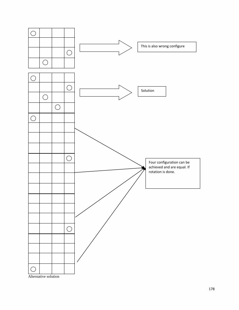
178

Alternative solution

Solution

Four configuration can be achieved and are equal. If rotation is done.

This is also wrong configure

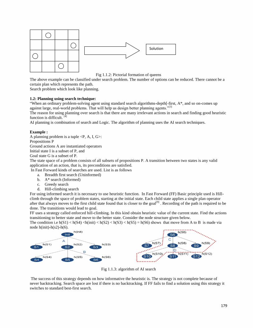
179

Fig 1.1.2: Pictorial formation of queens

The above example can be classified under search problem. The number of options can be reduced. There cannot be a

certain plan which represents the path.

Search problem which look like planning.

1.2: Planning using search technique:

“When an ordinary problem-solving agent using standard search algorithms-depth[-first, A*, and so on-comes up

against large, real-world problems. That will help us design better planning agents.”[3]

The reason for using planning over search is that there are many irrelevant actions in search and finding good heuristic

function is difficult. [4]

AI planning is combination of search and Logic. The algorithm of planning uses the AI search techniques.

Example : A planning problem is a tuple <P, A, I, G>:

Propositions P

Ground actions A are instantiated operators

Initial state I is a subset of P, and

Goal state G is a subset of P.

The state space of a problem consists of all subsets of propositions P. A transition between two states is any valid

application of an action, that is, its preconditions are satisfied.

In Fast Forward kinds of searches are used. List is as follows

a. Breadth first search (Uninformed)

b. A* search (Informed)

c. Greedy search

d. Hill-climbing search

For using informed search it is necessary to use heuristic function. In Fast Forward (FF) Basic principle used is Hill-

climb through the space of problem states, starting at the initial state. Each child state applies a single plan operator

after that always moves to the first child state found that is closer to the goal[9]

. Recording of the path is required to be

done. The transitions would lead to goal.

FF uses a strategy called enforced hill-climbing. In this kind obtain heuristic value of the current state. Find the actions

transitioning to better state and move to the better state. Consider the node structure given below.

The condition i.e h(S1) < h(S4) <h(init) < h(S2) < h(S3) < h(S5) = h(S6) shows that move from A to B is made via

node h(init)-h(s2)-h(6).

Fig 1.1.3: algorithm of AI search

The success of this strategy depends on how informative the heuristic is. The strategy is not complete because of

never backtracking. Search space are lost if there is no backtracking. If FF fails to find a solution using this strategy it

switches to standard best-first search.

Solution

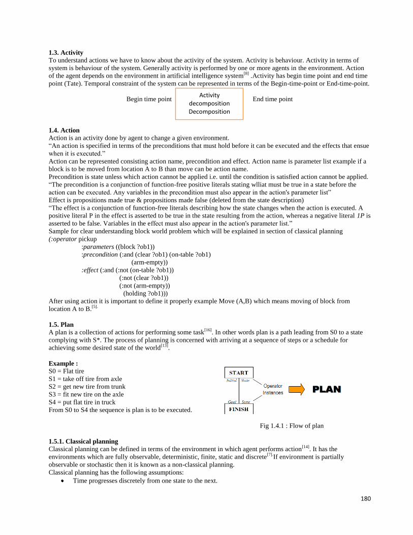
180

1.3. Activity

To understand actions we have to know about the activity of the system. Activity is behaviour. Activity in terms of

system is behaviour of the system. Generally activity is performed by one or more agents in the environment. Action

of the agent depends on the environment in artificial intelligence system[8]

.Activity has begin time point and end time

point (Tate). Temporal constraint of the system can be represented in terms of the Begin-time-point or End-time-point.

Begin time point End time point

1.4. Action Action is an activity done by agent to change a given environment.

“An action is specified in terms of the preconditions that must hold before it can be executed and the effects that ensue

when it is executed.”

Action can be represented consisting action name, precondition and effect. Action name is parameter list example if a

block is to be moved from location A to B than move can be action name.

Precondition is state unless which action cannot be applied i.e. until the condition is satisfied action cannot be applied.

“The precondition is a conjunction of function-free positive literals stating wlliat must be true in a state before the

action can be executed. Any variables in the precondition must also appear in the action's parameter list”

Effect is propositions made true & propositions made false (deleted from the state description)

“The effect is a conjunction of function-free literals describing how the state changes when the action is executed. A

positive literal P in the effect is asserted to be true in the state resulting from the action, whereas a negative literal 1P is

asserted to be false. Variables in the effect must also appear in the action's parameter list.”

Sample for clear understanding block world problem which will be explained in section of classical planning

(:operator pickup

:parameters ((block ?ob1))

:precondition (:and (clear ?ob1) (on-table ?ob1)

(arm-empty))

:effect (:and (:not (on-table ?ob1))

(:not (clear ?ob1))

(:not (arm-empty))

(holding ?ob1)))

After using action it is important to define it properly example Move (A,B) which means moving of block from

location A to B.[5].

1.5. Plan

A plan is a collection of actions for performing some task[16]

. In other words plan is a path leading from S0 to a state

complying with S*. The process of planning is concerned with arriving at a sequence of steps or a schedule for

achieving some desired state of the world[13]

.

Example :

S0 = Flat tire

S1 = take off tire from axle

S2 = get new tire from trunk

S3 = fit new tire on the axle

S4 = put flat tire in truck

From S0 to S4 the sequence is plan is to be executed.

Fig 1.4.1 : Flow of plan

1.5.1. Classical planning

Classical planning can be defined in terms of the environment in which agent performs action[14]

. It has the

environments which are fully observable, deterministic, finite, static and discrete[7].

If environment is partially

observable or stochastic then it is known as a non-classical planning.

Classical planning has the following assumptions:

Time progresses discretely from one state to the next.

Activity decomposition Decomposition

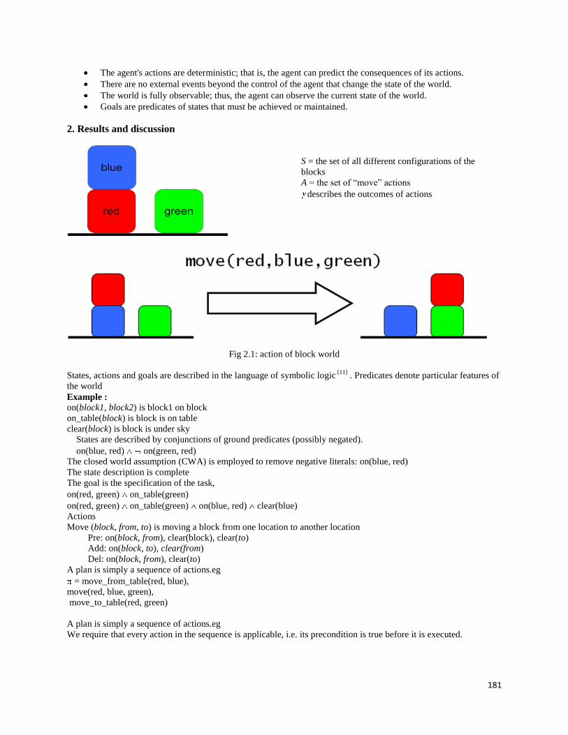
181

The agent's actions are deterministic; that is, the agent can predict the consequences of its actions.

There are no external events beyond the control of the agent that change the state of the world.

The world is fully observable; thus, the agent can observe the current state of the world.

Goals are predicates of states that must be achieved or maintained.

2. Results and discussion

S = the set of all different configurations of the

blocks

A = the set of “move” actions

describes the outcomes of actions

Fig 2.1: action of block world

States, actions and goals are described in the language of symbolic logic [11]

. Predicates denote particular features of

the world

Example :

on(block1, block2) is block1 on block

on_table(block) is block is on table

clear(block) is block is under sky

States are described by conjunctions of ground predicates (possibly negated).

on(blue, red) on(green, red)

The closed world assumption (CWA) is employed to remove negative literals: on(blue, red)

The state description is complete

The goal is the specification of the task,

on(red, green) on_table(green)

on(red, green) on_table(green) on(blue, red) clear(blue)

Actions

Move (block, from, to) is moving a block from one location to another location

Pre: on(block, from), clear(block), clear(to)

Add: on(block, to), clear(from)

Del: on(block, from), clear(to)

A plan is simply a sequence of actions.eg

= move_from_table(red, blue),

move(red, blue, green),

move_to_table(red, green)

A plan is simply a sequence of actions.eg

We require that every action in the sequence is applicable, i.e. its precondition is true before it is executed.

182

Fig 2.2: Representation of blocks

4. Conclusion Artificial intelligence gives the easiest and shortest outcome for movement from one place to another. It gives

opportunity to the machine to think analytically using the concepts [6]

of classical planning. It ensures the progressive

and profitable results if proper planning of customised design of machine is attempted[12]

. We conclude that further

research in this area will threaten the survival of humanity and effective growth of stimulated thinking will encounter.

4. References

[1] Adapted from Nilson,” Principles of Artificial Intelligence”, 1982.

[2] Stuart Russell Peter Norvig, “Artificial Intelligence A modern Approaches”, 2016.

[3] S.N. Deepa, B. Aruna Devi, “A survey on artificial intelligence approaches for medical image classification”,

Indian Journal of Science and Technology, Vol. 4 No. 11 (Nov 2011).

[4] Nils Nilsson, ” Artificial Intelligence: A New Synthesis “ ,1998

[5] Charles Weddle, Graduate Student, Florida State University “Artificial Intelligence and Computer Games”,

unpublished.

[6] Holland JH, “Adaptation in Natural and Artificial Systems”, 1975.

[7] Mahdiyeh EslamiI, Hussain Shaareef, Azah Mohamed, “Application of artificial intelligent techniques in PSS

design: a survey of the state-of-the-art methods”.

[8] Oscar Firschein, Martin A. Fischler, L.Stephen Coles, Jay M. Tenenbaum, “Forecasting and Assessing the

Impact of Artificial Intelligence on Society”, unpublished.

[9] N.P. Padhya “Artificial Intelligence and Intelligent Systems”, April 2005.

[10] Philip C. Jackson, Philip C. Jackson, “Introduction to Artificial Intelligence” June 1985.

[11] Hank Mishkoff, “The Emotion Machine: Commonsense Thinking, Artificial Intelligence, and the Future of

the Human Mind” 1985.

[12] George F. Luger, “Artificial Intelligence: Structures and Strategies for Complex Problem Solving”,

September 1987.

[13] Malte Helmert, “Understanding Planning Tasks: Domain Complexity and Heuristic Decomposition”, March

2008.

[14] Alexander Nareyek, “Local Search for Planning and Scheduling”, December 2001.

[15] Michael Negnevitsky, “Artificial Intelligence: A Guide to Intelligent Systems”, 2001.

[16] James Hendler “Artificial Intelligence Planning Systems: Proceedings of the First Conference”, June 1992.

183

A Review on CMOS Operational Trans-conductance Amplifier

Bhoomi P. Patel, Kaushani H. Shah, Mohammed G. Vayada


Electronics and Communication Engineering Department, Silver oak college of Engineering & Technological Gujarat

Technological University, India

Abstract:-

An operational transconductunce amplifier (OTA) is voltage controlled current source. The operational

transconductance are used in analog circuits and systems which were implemented by operational amplifier previously.

Present time is about development of VLSI technology and everything is related to size of transistor and decreasing

power supply in a circuit. Operational transconductance amplifier is mostly used for analog circuitry for example

instrumentation amplifier, converters and filters. This paper represents design concept and review on different types of

OTA such as single input single output OTA, differential input single output OTA, differential input differential output

OTA and differential input balanced output OTA. Here also reviewed two types of techniques.

Keywords: Operational Tran conductance amplifier, Gain, Rail to Rail, Tran conductance

1. Introduction

Recently Operational transconductance amplifier (OTA) has been widely used in filter design and electronic circuits.

Operational transconductance amplifiers (OTA) have been one of the most important building blocks in analog and

mix-mode circuits, such as transconductance-C filter (Gm-C filter), variable gain amplifiers (VGAs), voltage-

controlled oscillators (VCOs) and data converters [1]. The main concept is to produce an output current which is

proportional to the differential input voltage. In recent few years the design of integrated circuits has gone in the

direction of low supply voltage and low power consumption, such as portable applications that their power is given

even by a single cell battery. For this reason, OTA should be designed for low supply voltage and low power

consumption with proper linearity and noise performance.

Fig. 1 Evolution of OTA(Operational transconductance amplifier)[2]

The bipolar OTA was commercially introduced in 1969. CMOS OTA has become vital component in number of

electronic circuits both in open loop and close loop applications. The continues time filters with OTA and capacitors

are known as Gm-C or OTA-C are very popular as application of OTA.

2. Types of OTA

There are four different types of Operational Transconductance Amplifier based on its input and output.

1. Single input Single output OTA

2. Differential input single Output OTA

3. Differential input differential Output OTA

4. Differential input balanced Output OTA.



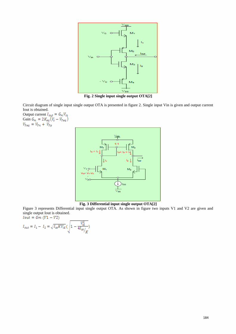
184

Fig. 2 Single input single output OTA[2]

Circuit diagram of single input single output OTA is presented in figure 2. Single input Vin is given and output current

Iout is obtained.

Output current

Gain

Fig. 3 Differential input single output OTA[2]

Figure 3 represents Differential input single output OTA. As shown in figure two inputs V1 and V2 are given and

single output Iout is obtained.

185

Fig. 4 Differential input differential output OTA[2]

Figure 4 represents circuit diagram of Differential input differential output OTA. It means two inputs and two outputs.

Here two different inputs are given and based on the inputs V1 and V2, we will gain two different outputs Iout1 and

Iout2.

Fig. 5 Differential input balanced output OTA[2]

Circuit diagram of simple Differential input balanced output OTA is presented in figure 5. It is same as the differential

input differential output OTA. The only difference is, in single input balanced output OTA, the output currents are

same in magnitude but different is direction i.e. Iout1 = -Iout2. Which are different in magnitude in differential input

differential output OTA.

3. TECHNIQUES OF OTA There are two types of techniques of OTA.

3.1 Gate driven OTA

In MOS there are total four terminals Gate, Drain, Source and Bulk. In Gate driven technique input is given to

gate terminal of MOS and the bulk terminal is fixed to a specific bias voltage.

3.2 Bulk driven OTA

In bulk driven technique, the input is given to bulk terminal and the gate terminal is fixed to a specific voltage.

186

4. Literature Review

Shahabi, Mehdi[1] in their research paper on low power high CMRR OTA, have proposed a gate driven

CMOS OTA using CMFF (common mode feedforward technique). This design is carried out in 0.18 µm technology.

Common Mode Rejection

Ratio

110 db

Gain 46 db

Phase margin 85°

Bandwidth 14 MHz

Capacitive Load 2pf

Power consumption 28µW

Supply Voltage 1.2 V

Table 1. Different parameters of proposed OTA[1]

In this paper input voltage range is not considered as this design is of gate driven technology and maximum possible

input range is VDD- 2VDSAT.

Lee, Dong-Soo, Ali Dadashi, and Kang-Yoon Lee [3] in their research paper have proposed high DC gain Modified

CMOS OTA. This paper represents design of Gate driven CMOS OTA in 0.35µm Technology. In this paper,

conventional triple folded cascade structure is presented. In this paper enhancement in gain without affecting phase

margin, bandwidth and output voltage is achieved. It provides high linearity of the output in larger output swing.

Supply Voltage 3.3 v

Gain 87db

Phase margin 70°

Bandwidth 485 MHz

Output Voltage Swing Vdd – 6Vsat

Power consumption 8 mv


In this paper as input power supply is 3.3v, this OTA cannot be used for low power application. The power

consumption is 8 mv which is high compare to bulk driven OTA. Unity gain bandwidth is good. The gain of this OTA

is 87db which is good compare to bulk driven OTA. Phase margin is good. In this paper PVT (Process-Voltage-

Temperature) analysis is carried out. Output voltage swing is Vdd – 6Vsat, which is not good.

Yodtean, Apiradee[4] in their research paper have proposed Bulk driven OTA having high gain. This OTA is designed

in 0.18µm Technology. In this paper the trans-conductance is tuned electronically. Symmetric structure is used. Using

this OTA, Gm-C Biquard filter application is tasted.


Gain 76db

Phase margin 86°

Bandwidth 423 KHz

CMRR 148 db

Power consumption 4.58 µw

Area 0.4 mm2


The input voltage range is very low so this OTA can be used in low supply voltage applications. Power consumption is

also very low. The gain is high compare to other bulk drive OTA and low compare to gate driven OTA.

Abdelfattah, Omar, et al have presented 0.35 v Bulk driven self biased OTA with rail to rail iput range in 65 nm

technology. In this paper common mode feed forward circuit is used.


Gain 46 db

Phase margin 56°

Bandwidth 3.6 MHz

CMRR 17 µW


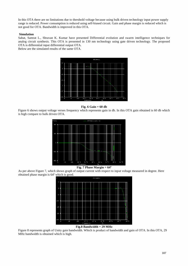
187

In this OTA there are no limitations due to threshold voltage because using bulk driven technology input power supply

range is reduced. Power consumption is reduced using self-biased circuit. Gain and phase margin is reduced which is

not good for OTA. Bandwidth is improved in this OTA.

Simulation Sabat, Samrat L., Shravan K. Kumar have presented Differential evolution and swarm intelligence techniques for

analog circuit synthesis. This OTA is presented in 130 nm technology using gate driven technology. The proposed

OTA is differential input differential output OTA.

Below are the simulated results of the same OTA.

Fig. 6 Gain = 60 db

Figure 6 shows output voltage verses frequency which represents gain in db. In this OTA gain obtained is 60 db which

is high compare to bulk driven OTA.

Fig. 7 Phase Margin = 64º

As per above Figure 7, which shows graph of output current with respect to input voltage measured in degree. Here

obtained phase margin is 64º which is good.

Fig.8 Bandwidth = 29 MHz

Figure 8 represents graph of Unity gain bandwidth. Which is product of bandwidth and gain of OTA. In this OTA, 29

MHz bandwidth is obtained which is high.

188

Fig. 9 ICMR = -0.5 To 0.5 = 1 V

The graph of Input voltage versus output voltage is represented in figure 9 which is called as input common mode

rejection ratio (ICMR).As shown in fig. obtained ICMR is -0.5 to 0.5 v which is not rail to rail as the OTA is gate

driven OTA.

5. Conclusion

This paper describes types of OTA and different techniques for implementation of OTA. Literature survey is carried

out on OTA design technique and about its applications. Bulk driven technique is quite useful to deal with low power

and low voltage application [4][5][9][11]. Using bulk driven technology, the threshold voltage of MOSFET can be

reduced or even removed from signal path [4][5][9][11]. Bulk driven technology does not suggest any change in

existing technology[4][5][9][11]. This technique reduces the threshold voltage[4][5][9][11], thus low voltage and low

power design is possible. Drawback of bulk driven technique is this technique provides relatively small DC gain[1]-

[12] and requires complex calculations.

6. References

[1]. Shahabi, Mehdi, et al."A novel low power high CMRR pseudo-differential CMOS OTA with common-mode

feedforward technique." Electrical Engineering (ICEE), 2015 23rd Iranian Conference on. IEEE, 2015.

[2]. Dr. Soliman Mahmoud, “Microelectronics” German Univercity of Cario, 2006

[3]. Lee, Dong-Soo, Ali Dadashi, and Kang-Yoon Lee. "A high DC-gain modified CMOS OTA." SoC Design

Conference (ISOCC), 2013 International. IEEE, 2013.

[4]. Yodtean, Apiradee."A CMOS OTA and Implementation" Intelligent Signal Processing and Communication

Systems (ISPACS), 2014 International Symposium on. IEEE, 2014.

[5]. Abdelfattah, Omar, et al. "A 0.35-V bulk-driven self-biased OTA with rail-to-rail input range in 65 nm CMOS."

Circuits and Systems (ISCAS), 2015 IEEE International Symposium on. IEEE, 2015.

[6]. Sabat, Samrat L., Shravan K. Kumar, and Siba K. Udgata. "Differential evolution and swarm intelligence

techniques for analog circuit synthesis."Nature & Biologically Inspired Computing, 2009. NaBIC 2009. World

Congress on. IEEE, 2009.

[7]. Ferreira, Luis HC, and Sameer R. Sonkusale. "A 60-dB gain OTA operating at 0.25-V power supply in 130-nm

digital CMOS process." Circuits and Systems I: Regular Papers, IEEE Transactions on 61.6 (2014): 1609-1617.

[8]. Linares-Barranco, Bernabé, et al. "CMOS OTA-C high-frequency sinusoidal oscillators." Solid-State Circuits,

IEEE Journal of 26.2 (1991): 160-165

[9].Haga, Yasutaka, et al. "Design of a 0.8 Volt fully differential CMOS OTA using the bulk-driven technique."

Circuits and Systems, 2005. ISCAS 2005. IEEE International Symposium on. IEEE, 2005.

[10]. De Carvalho, Luís Henrique, and Ferreira E. Pimenta. "An ultra low-voltage ultra low power rail-to-rail CMOS

OTA Miller." Circuits and Systems, 2004. Proceedings. The 2004 IEEE Asia-Pacific Conference on. Vol. 2. IEEE,

2004.

[11]. Rosenfeld, Jonathan, Mücahit Kozak, and Eby G. Friedman. "A bulk-driven CMOS OTA with 68 dB DC gain."

Electronics, Circuits and Systems, 2004. ICECS 2004. Proceedings of the 2004 11th IEEE International Conference on.

IEEE, 2004.

[12]. Duangmalai, Danupat, and Khanittha Kaewdang. "A linear tunable wide input range CMOS OTA." TENCON

2014-2014 IEEE Region 10 Conference. IEEE, 2014.

189

Low Pass Filter Design Using Evolutionary Algorithms

Bhoomi N. Thakkar, Vimal H. Nayak

Electronics and Communication Engineering Department, Silver Oak College of Engineering & Technology,


Abstract:-

In this paper, PSO Algorithm and HPSO Algorithm are used for the optimization of RC Filter and the results of both

the algorithms are compared. By using these algorithms on sphere and rosenbrock benchmark functions the best values

of RC filter parameters are achieved in such a way that it minimizes error between simulated output and optimized

output. With the help of this parameters the circuit simulator gives the cut off frequency (1.000000e + 03) which is

much closer to the standard cut off frequency i.e.1k.

Keywords: Automatic Analog Circuit Design, Analog Circuit Synthesis, Hierarchical Particle Swarm Optimization,

Particle Swarm Optimization.

1. Introduction

Technology scaling, high performance demands, and system-on-chip applications force analog modules to be

implemented in the same technology nodes as that of digital circuits or at most few nodes behind digital technology

nodes.As technology is scaled down, the physical models of analog circuits have become complex due to various short-

channel effects. These factors have led to the manual design of analog circuits to be a challenging and time wasting

task and hence efficient automatic design techniques are required. There are various optimization techniques have been

reported previously for automatic design of analog circuits.

The classical optimization methods need to calculate derivatives and require good initial guess for the design

variables. In the absence of first guess close to the globally optimum solution, these algorithms would generally stuck

at a locally optimum solution. The evolutionary algorithms, which can be used to solve multimodal optimization

problems, do not suffer from problems associated with the gradient-based methods. The Genetic Algorithm (GA),

developed by Holland. Particle swarm optimization (PSO), another evolutionary algorithm, was proposed by Kennedy

and Eberhart. It is reported in literature that withincreasing in particle number PSO algorithms will improves its

performance. The hierarchical PSO algorithm, a recent variant of PSO algorithm, has been explored for automatic

analog circuit design applications.

In this paper, we propose and demonstrate the PSO algorithm and a hierarchical PSO algorithm (HPSO) are

proposed for automatic analog circuit design. In this paper, the RC filter is considered as a design problem. The design

results obtained with the PSO algorithm and HPSO algorithm on two benchmark functions and are also compared with

each other. It is shown that the results are almost same.

2. PSO Algorithm and its implementation

The PSO is inspired by the social behaviour of a flock of migrating birds trying to get a place of an unknown

destination. In PSO, each solution is a „bird‟ in the flock and is referred to as a „particle‟. The birds in the population

only change their social behaviour and accordingly their movement towards a destination. Physically, this mimics a

group of birds that communicate together as they fly. Each bird looks in a specific path, and then when communicating

together, they identify the bird that is in the best location.

Accordingly, each bird speeds in the direction of the best bird using a velocity that depends on its current

position. Each bird, then investigates the search space from its new local place and the process repeats until the flock

reaches a desired destination. It is vital to note that the process involves both social interaction and Intelligence so that

birds learn from their own experience (local search) and also from the experience of others round them (global search)

[1].

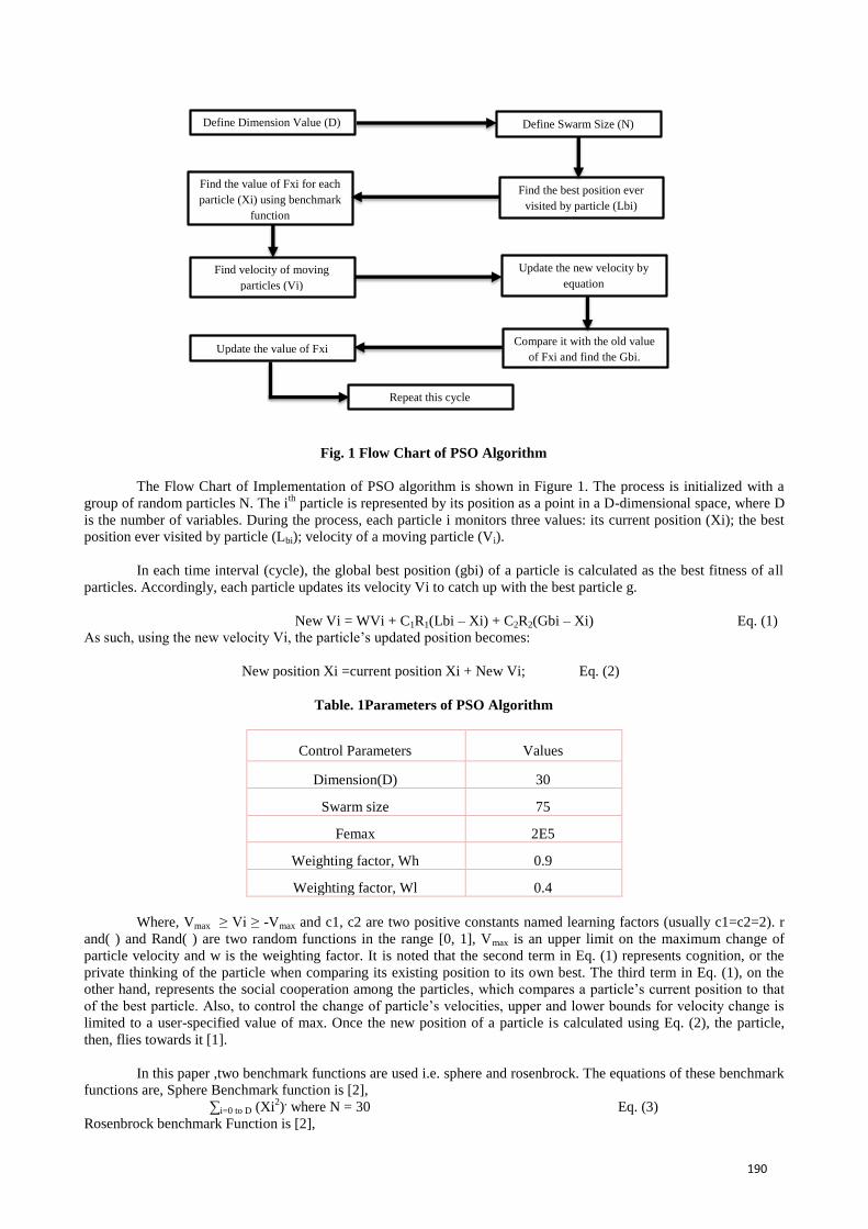
190

Define Dimension Value (D)

Define Swarm Size (N)

Find the value of Fxi for each

particle (Xi) using benchmark

function

Find the best position ever

visited by particle (Lbi)

Find velocity of moving

particles (Vi)

Update the new velocity by

equation

Update the value of Fxi Compare it with the old value

of Fxi and find the Gbi.

Repeat this cycle

Fig. 1 Flow Chart of PSO Algorithm

The Flow Chart of Implementation of PSO algorithm is shown in Figure 1. The process is initialized with a

group of random particles N. The ith

particle is represented by its position as a point in a D-dimensional space, where D

is the number of variables. During the process, each particle i monitors three values: its current position (Xi); the best

position ever visited by particle (Lbi); velocity of a moving particle (Vi).

In each time interval (cycle), the global best position (gbi) of a particle is calculated as the best fitness of all

particles. Accordingly, each particle updates its velocity Vi to catch up with the best particle g.

New Vi = WVi + C1R1(Lbi – Xi) + C2R2(Gbi – Xi) Eq. (1)

As such, using the new velocity Vi, the particle‟s updated position becomes:

New position Xi =current position Xi + New Vi; Eq. (2)

Table. 1Parameters of PSO Algorithm

Control Parameters Values

Dimension(D) 30

Swarm size 75

Femax 2E5

Weighting factor, Wh 0.9

Weighting factor, Wl 0.4

Where, Vmax ≥ Vi ≥ -Vmax and c1, c2 are two positive constants named learning factors (usually c1=c2=2). r

and( ) and Rand( ) are two random functions in the range [0, 1], Vmax is an upper limit on the maximum change of

particle velocity and w is the weighting factor. It is noted that the second term in Eq. (1) represents cognition, or the

private thinking of the particle when comparing its existing position to its own best. The third term in Eq. (1), on the

other hand, represents the social cooperation among the particles, which compares a particle‟s current position to that

of the best particle. Also, to control the change of particle‟s velocities, upper and lower bounds for velocity change is

limited to a user-specified value of max. Once the new position of a particle is calculated using Eq. (2), the particle,

then, flies towards it [1].

In this paper ,two benchmark functions are used i.e. sphere and rosenbrock. The equations of these benchmark

functions are, Sphere Benchmark function is [2],

∑i=0 to D (Xi2)

, where N = 30 Eq. (3)

Rosenbrock benchmark Function is [2],

191

∑i=0 to D-1 100 (Xi2 – Xi+1)

2 + (1 – xi

2) Eq. (4)

3. HPSO Algorithm and its implementation

In the HPSO algorithm, the particles are divided into many groups with each group having a “local leader” and

particles within a group follow their local leader. This feature of the HPSO algorithm enables enhanced exploration of

the search space and shows better consistency in finding the optimum solution. The organization of particles in HPSO

is described below. The organization of particles in HPSO is described below. Let us assume that the total number of

particles is N. In HPSO, these particles are first arranged in ascending order according to their fitness, with the globally

best particle (the “global leader”) at position N, as shown in below Figure 4.The next M best particles are designated as

the “local leaders.” The remaining (N −M −1) particles are divided into M groups. The M local leaders are assigned to

the M groups as shown in Figure 4.

Fig.4: Arrangement of particles in the HPSO algorithm [1].

The common particles follow their local leader and the local leaders follow the global leader. Any particle is

permissible to become a local leader or the global leader, depending upon its fitness relative to the other particles [1].

4. Comparison of PSO and HPSO Algorithm

Result for mean values of both the functions using PSO and HPSO algorithms are listed in below table.

Table 1: Mean values of PSO and HPSO Algorithms

Algorithms Mean Values of different functions

Sphere Rosenbrock

PSO 0.691767090299 1.04290779626

HPSO 424.14899671 29.8275602641

In above section II and III implementation of PSO and HPSO algorithm is done. By using above mean

valuesthe comparison graphs of error versus function evolutions for sphere and rosenbrock function can be plot which

is in the below Figures. In these graphs the inaccuracy will be reduceas increasing in the function evolutions.

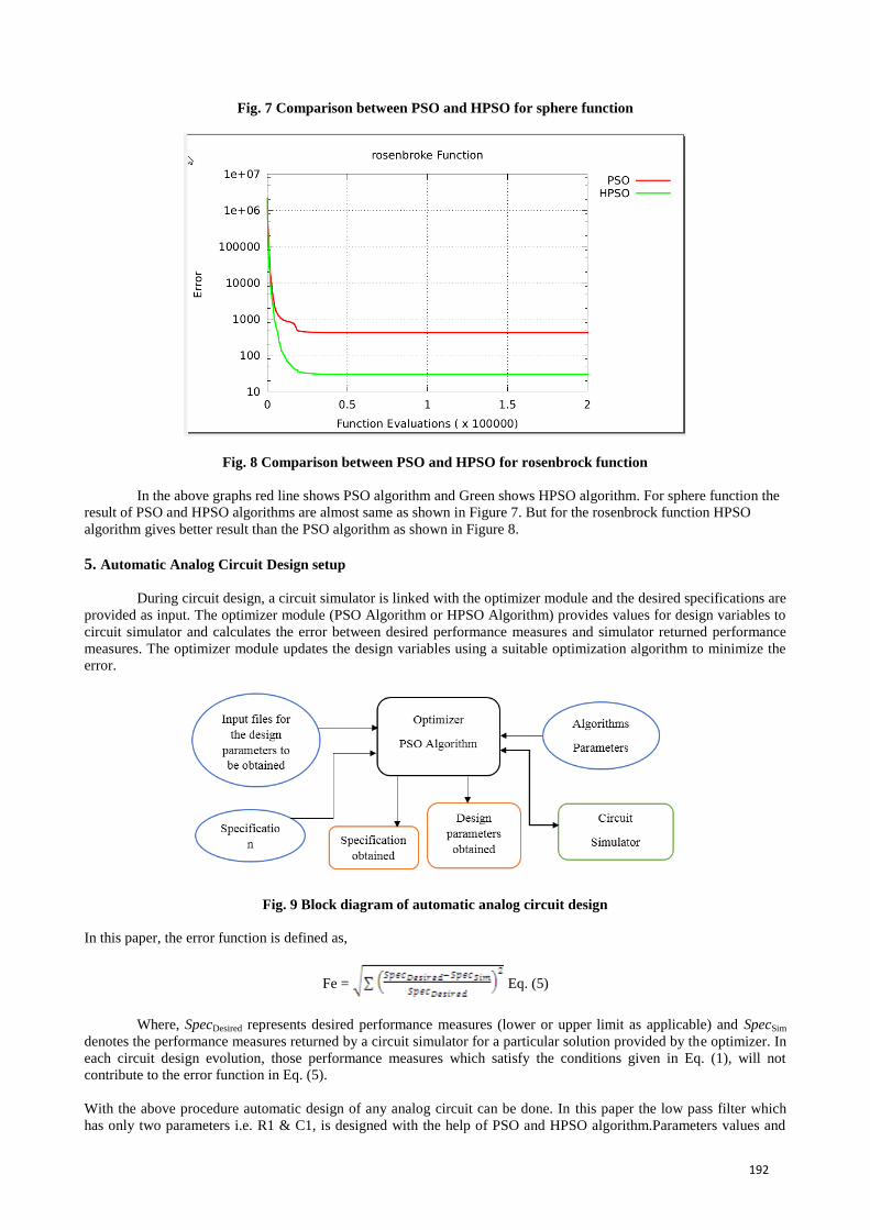
192

Fig. 7 Comparison between PSO and HPSO for sphere function

Fig. 8 Comparison between PSO and HPSO for rosenbrock function

In the above graphs red line shows PSO algorithm and Green shows HPSO algorithm. For sphere function the

result of PSO and HPSO algorithms are almost same as shown in Figure 7. But for the rosenbrock function HPSO

algorithm gives better result than the PSO algorithm as shown in Figure 8.

5. Automatic Analog Circuit Design setup

During circuit design, a circuit simulator is linked with the optimizer module and the desired specifications are

provided as input. The optimizer module (PSO Algorithm or HPSO Algorithm) provides values for design variables to

circuit simulator and calculates the error between desired performance measures and simulator returned performance

measures. The optimizer module updates the design variables using a suitable optimization algorithm to minimize the

error.

Fig. 9 Block diagram of automatic analog circuit design

In this paper, the error function is defined as,

Fe = Eq. (5)

Where, SpecDesired represents desired performance measures (lower or upper limit as applicable) and SpecSim

denotes the performance measures returned by a circuit simulator for a particular solution provided by the optimizer. In

each circuit design evolution, those performance measures which satisfy the conditions given in Eq. (1), will not

contribute to the error function in Eq. (5).

With the above procedure automatic design of any analog circuit can be done. In this paper the low pass filter which

has only two parameters i.e. R1 & C1, is designed with the help of PSO and HPSO algorithm.Parameters values and

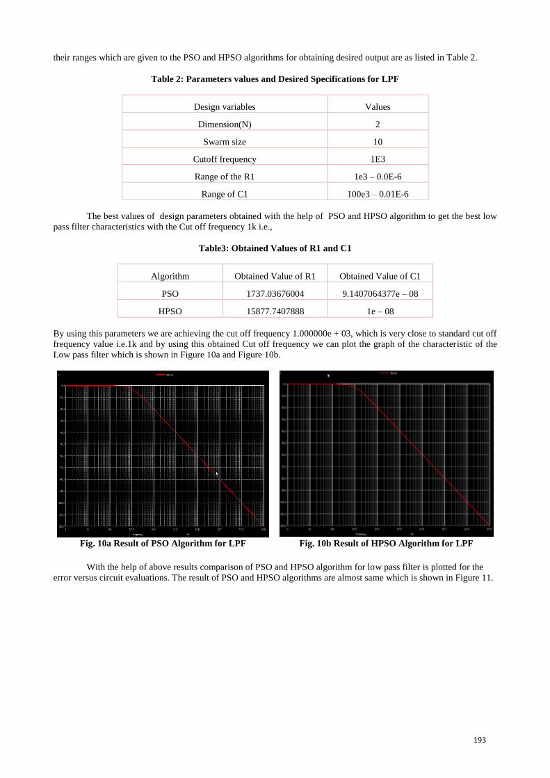
193

their ranges which are given to the PSO and HPSO algorithms for obtaining desired output are as listed in Table 2.

Table 2: Parameters values and Desired Specifications for LPF

Design variables Values

Dimension(N) 2

Swarm size 10

Cutoff frequency 1E3

Range of the R1 1e3 – 0.0E-6

Range of C1 100e3 – 0.01E-6

The best values of design parameters obtained with the help of PSO and HPSO algorithm to get the best low

pass filter characteristics with the Cut off frequency 1k i.e.,

Table3: Obtained Values of R1 and C1

Algorithm Obtained Value of R1 Obtained Value of C1

PSO 1737.03676004 9.1407064377e – 08

HPSO 15877.7407888 1e – 08

By using this parameters we are achieving the cut off frequency 1.000000e + 03, which is very close to standard cut off

frequency value i.e.1k and by using this obtained Cut off frequency we can plot the graph of the characteristic of the

Low pass filter which is shown in Figure 10a and Figure 10b.

Fig. 10a Result of PSO Algorithm for LPF Fig. 10b Result of HPSO Algorithm for LPF

With the help of above results comparison of PSO and HPSO algorithm for low pass filter is plotted for the

error versus circuit evaluations. The result of PSO and HPSO algorithms are almost same which is shown in Figure 11.

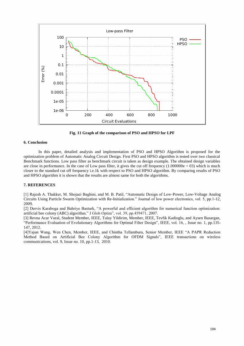
194

Fig. 11 Graph of the comparison of PSO and HPSO for LPF

6. Conclusion

In this paper, detailed analysis and implementation of PSO and HPSO Algorithm is proposed for the

optimization problem of Automatic Analog Circuit Design. First PSO and HPSO algorithm is tested over two classical

Benchmark functions. Low pass filter as benchmark circuit is taken as design example. The obtained design variables

are close in performance. In the case of Low pass filter, it gives the cut off frequency (1.000000e + 03) which is much

closer to the standard cut off frequency i.e.1k with respect to PSO and HPSO algorithm. By comparing results of PSO

and HPSO algorithm it is shown that the results are almost same for both the algorithms.

7. REFERENCES

[1] Rajesh A. Thakker, M. Shojaei Baghini, and M. B. Patil, “Automatic Design of Low-Power, Low-Voltage Analog

Circuits Using Particle Swarm Optimization with Re-Initialization.” Journal of low power electronics, vol. 5, pp.1-12,

2009.

[2] Dervis Karaboga and Bahriye Basturk, “A powerful and efficient algorithm for numerical function optimization:

artificial bee colony (ABC) algorithm.” J Glob Optim”, vol. 39, pp.459471, 2007.

[3] Revna Acar Vural, Student Member, IEEE, Tulay Yildirim, Member, IEEE, Tevfik Kadioglu, and Aysen Basargan,

“Performance Evaluation of Evolutionary Algorithms for Optimal Filter Design”, IEEE, vol. 16, , Issue no. 1, pp.135-

147, 2012.

[4]Yajun Wang, Wen Chen, Member, IEEE, and Chintha Tellambura, Senior Member, IEEE “A PAPR Reduction

Method Based on Artificial Bee Colony Algorithm for OFDM Signals”, IEEE transactions on wireless

communications, vol. 9, Issue no. 10, pp.1-13, 2010.

195

Implementation of CCII based on Current Mirror Pair and

Differential Pair Kaushani H.Shah, Bhoomi P.Patel

, Mohammed G. Vayada

[email protected]

Electronics and Communication Engineering Department, Silver oak college of Engineering & Technological Gujarat

Technological University, India

Abstract:

Now a day current mode circuits have been receiving significant attention in analog signal processing. In many cases

the conveyor-based implementation offers improved performance to the voltage op-amp-based implementation in terms

of accuracy, bandwidth and convenience. Current mode circuits do not have the limitation of dynamic range. Various

topologies are used to implement current conveyor circuit. In this paper two topologies are used which are current

mirror based topology and differential pair based topology. Major applications are available based on current conveyor

which are capacitance multiplier, negative impedance conveyor and V to I converters. This paper gives the comparison

of both topologies in terms of gain, bandwidth, linearity, power consumption. In the end results of different simulations

are compared to conclude that differential pair based topology gives better results.

Keywords: Bandwidth, CCII, CMOS, Current Conveyor, Gain, Linearity, VLSI.

1. Introduction

The current conveyor is a three terminal device performing many useful analog signal processing functions when the

device is connected with other electronic elements in specific circuit configurations. The current conveyor has evolved

from first generation to third generation. the first generation current conveyor (CCI) was proposed by Smith and Sedra

in 1968 [1] and the more versatile second generation current conveyor (CCII) was introduced by the same authors in

1970 [2] as an extension of their first generation conveyor.

There has been substantial emphasis on the development of current mode signal processing circuits such as filters and

oscillators. This is due to increased bandwidth, simple circuitry, better linearity, dynamic range performances and

lower power consumption as compared to their voltage mode circuitry. A variety of current mode building blocks are

developed with current mode circuits. The current conveyor (CCII) is one among such blocks which has received

significant attention. It is hybrid block and has basic construction containing a voltage follower (VF) interconnected

with either current mirror or current follower. Two topologies of the current conveyor are used. The first is based on

current mirror and the second is based on differential pair.

2. Literature Review

This paper gives the comparison between two topologies. The first method is inverter based current conveyor

and the second method is current mirror based current conveyor. Second generation current conveyor is used

for both the methods. Table gives the comparison of both topologies. [5]

Table 1: Comparison of Topologies

Sr No. Parameters Inverter based CCII Current mirror based CCII

1 Bandwidth Twice than Translinear loop based

CCII+ Half of the Inverter based CCII+

2 Third Harmonic Distortion Less More

3 Output Noise Less than Inverter based CCII+ More than Inverter based CCII+

4 Area of silicon required Half Twice

5 Synthesized by Analog and Digital Only Analog


196

Even through inverter based topology performs better for certain performance measure, it may fail at input voltage

dynamic range. The input voltage dynamic range for the CMOS inverter for using in linear application is very narrow;

this may lead very small dynamic range. Current mirror based topology has very high input voltage dynamic range.

This paper is based on the second method which is differential pair based CCII. This paper represents that NMOS

differential pair works, when voltage is greater than 2vdsat and PMOS differential pair works, when voltage is less than

2vdsat. So using both type of MOSFET, increase in voltage dynamic range is possible. If CCII use only NMOS pair

then necessary voltage required is 2vdat to run the circuit. If CCII use only PMOS pair then necessary voltage required,

which is less than 2vdat to run the circuit.In this paper, a new circuit is proposed low-voltage low power CMOS rail-to-

rail second generation current conveyor. [3]

Drawback: No of transistors increases so power consumption is increases. Power consumption are not compared,

however the power consumption for the proposed design seems to be higher because there are two differential pairs and

thus requirement of two separate current sources.

3. Circuit Description

Fig1: Basic CCII+ current conveyor voltages and currents

If a voltage is applied to terminal Y, an equi-potential will appear on the input terminal X. An input current I being

forced into terminal X will result an equal amount of current flowing into terminal Y. The current I will be conveyed to

output terminal such that terminal Z has the characteristics of a current source, of value I with high output impedance.

Potential of X being set by that of Y, is independent of the current being forced into port X. Current through port Y

being fixed by X is independent of the voltage applied to Y. Terminal Y exhibits an infinite input Impedance.

It is a three port device. Three terminals X, Y, Z are used to satisfy all the conditions which CCII needed. Fig2 shows

the all conditions which are required for CCII.

Fig 2: Matrix Representation of CCII

Vx = Vy,

Iy = 0,

Iz = Ix

4. Current Mirror Based Topology

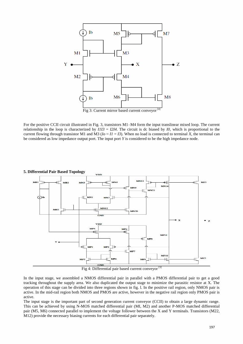
197

Fig 3: Current mirror based current conveyor

[4]

For the positive CCII circuit illustrated in Fig. 3, transistors M1–M4 form the input translinear mixed loop. The current

relationship in the loop is characterized by I1I3 = I2I4. The circuit is dc biased by I0, which is proportional to the

current flowing through transistor M1 and M3 (Io ≈ I1 = I3). When no load is connected to terminal X, the terminal can

be considered as low impedance output port. The input port Y is considered to be the high impedance node.

5. Differential Pair Based Topology

Fig 4: Differential pair based current conveyor

[3]

In the input stage, we assembled a NMOS differential pair in parallel with a PMOS differential pair to get a good

tracking throughout the supply area. We also duplicated the output stage to minimize the parasitic resistor at X. The

operation of this stage can be divided into three regions shown in fig. l. In the positive rail region, only NMOS pair is

active. In the mid-rail region both NMOS and PMOS are active, however in the negative rail region only PMOS pair is

active.

The input stage is the important part of second generation current conveyor (CCII) to obtain a large dynamic range.

This can be achieved by using N-MOS matched differential pair (MI, M2) and another P-MOS matched differential

pair (M5, M6) connected parallel to implement the voltage follower between the X and Y terminals. Transistors (M22,

M12) provide the necessary biasing currents for each differential pair separately.

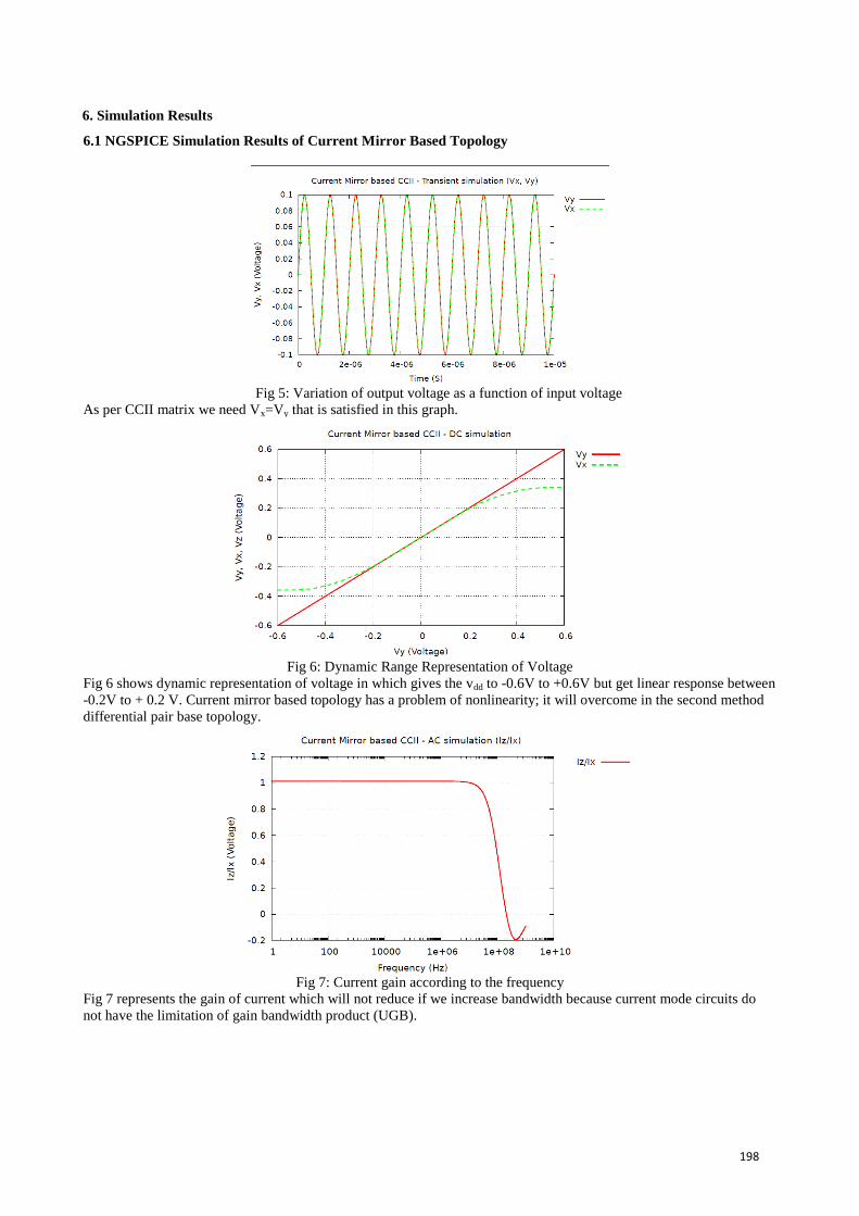
198

6. Simulation Results

6.1 NGSPICE Simulation Results of Current Mirror Based Topology

Fig 5: Variation of output voltage as a function of input voltage

As per CCII matrix we need Vx=Vy that is satisfied in this graph.

Fig 6: Dynamic Range Representation of Voltage

Fig 6 shows dynamic representation of voltage in which gives the vdd to -0.6V to +0.6V but get linear response between

-0.2V to + 0.2 V. Current mirror based topology has a problem of nonlinearity; it will overcome in the second method

differential pair base topology.

Fig 7: Current gain according to the frequency

Fig 7 represents the gain of current which will not reduce if we increase bandwidth because current mode circuits do

not have the limitation of gain bandwidth product (UGB).

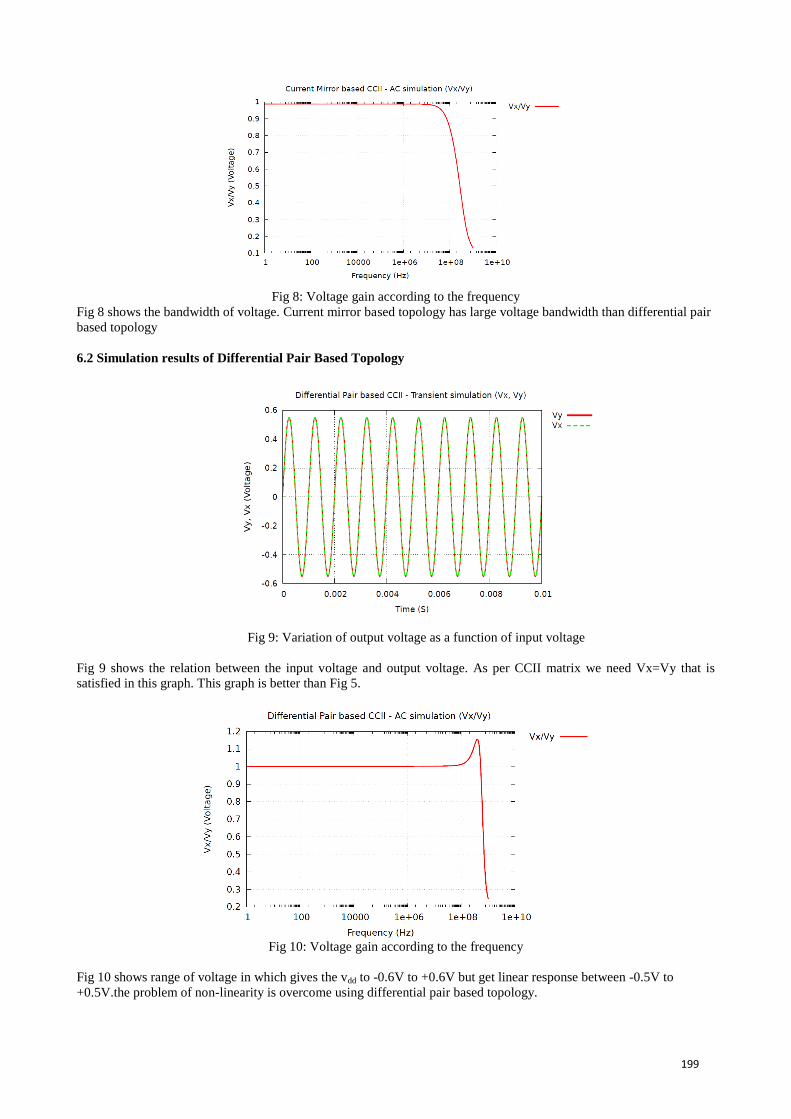
199

Fig 8: Voltage gain according to the frequency

Fig 8 shows the bandwidth of voltage. Current mirror based topology has large voltage bandwidth than differential pair

based topology

6.2 Simulation results of Differential Pair Based Topology

Fig 9: Variation of output voltage as a function of input voltage

Fig 9 shows the relation between the input voltage and output voltage. As per CCII matrix we need Vx=Vy that is

satisfied in this graph. This graph is better than Fig 5.

Fig 10: Voltage gain according to the frequency

Fig 10 shows range of voltage in which gives the vdd to -0.6V to +0.6V but get linear response between -0.5V to

+0.5V.the problem of non-linearity is overcome using differential pair based topology.

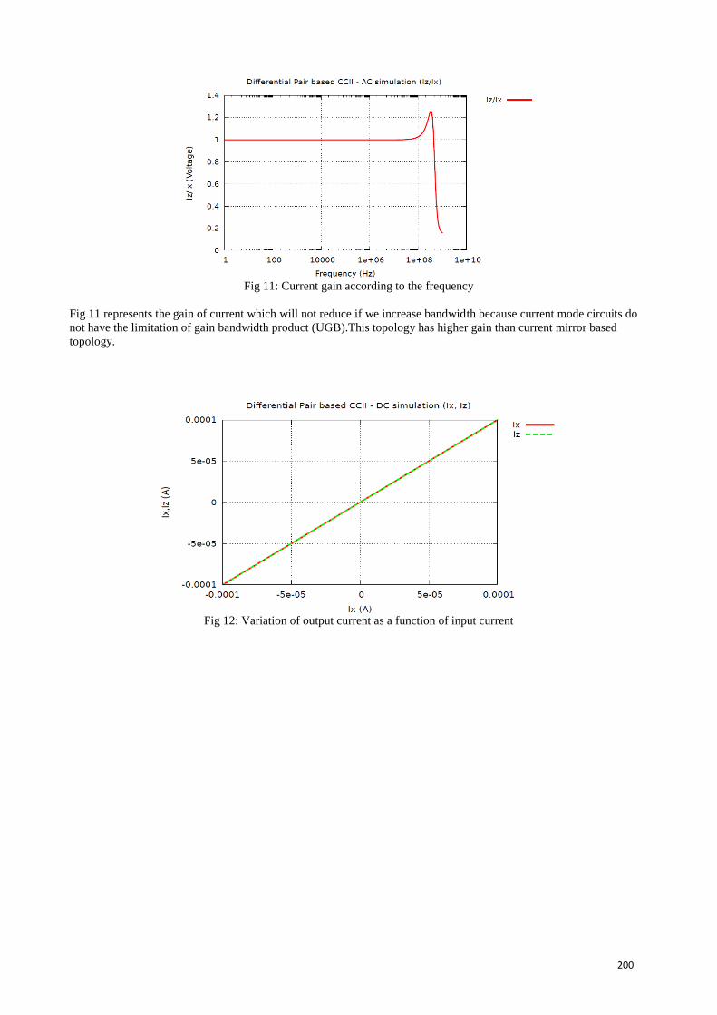
200

Fig 11: Current gain according to the frequency

Fig 11 represents the gain of current which will not reduce if we increase bandwidth because current mode circuits do

not have the limitation of gain bandwidth product (UGB).This topology has higher gain than current mirror based

topology.

Fig 12: Variation of output current as a function of input current

201

Fig 12 shows the bandwidth of voltage. Current mirror based topology has large voltage bandwidth than differential

pair based topology.

7. Conclusion

The effect of CCII topologies performance is evaluated on the basis of gain, bandwidth and linear characteristics.

Bandwidth response for voltage transfer is found to be higher in current mirror based topology than differential pair

based topology. But in case of linearity and dynamic range differential pair based topology gives better performance

than current mirror based topology. Simulations results are compared for both topologies.

8. REFERENCES

[1] SEDRA, A.S., and SMITH. K.C.: “A second-generation current conveyor and its applications”, IEEE

Trans. Circuit Theory, Vol-17, pp. 132-134, 1970.

[2] Sedra, A. S., Gordon W. Roberts, and F. Gohh. "The current conveyor: history, progress and new

results." IEEE Proceedings G (Circuits, Devices and Systems) 137.2, pp.78-87, 1990.

[3] Ettaghzouti, T., Hassen, N., &Besbes, K. “Novel CMOS second generation current conveyor CCII with

rail-to-rail input stage and filter application. In Multi-Conference on Systems”, Signals & Devices (SSD),

Vol 11, pp. 1-6, 2014.

[4] Ashenafi, E., &Chowdhury, M. H. (2013, December). “Active on-chip voltage regulator based on second

generation current conveyor”. In Electronics, Circuits, and Systems (ICECS),Vol 20,pp. 605-608,2013

[5] Varshney, G., Pandey, N., Pandey, R., & Bhattacharyya, A. (2013, December). “Performance comparison

of filter circuits based on two different current conveyor topologies”. In Signal Processing and

Communication (ICSC), International Conference on ,pp. 419-423, 2013.

[6] MazharulHuqChowdhury. "Active on-chip voltage regulator based on second generation current

conveyor." Electronics, Circuits, and Systems (ICECS), Vol 20, pp.605-608, 2013.

[7] Abolila, Ahmed HM, Hesham FA Hamed, and El-Sayed AM Hasaneen. "New±0.75 V low voltage low

power CMOS current conveyor." Microelectronics (ICM), International Conference on. IEEE, pp. 220-223,

2010.

[8] Varshney, Garima, et al. "Performance comparison of filter circuits based on two different current conveyor

topologies." Signal Processing and Communication (ICSC), Conference on. IEEE, pp. 419-423, 2013.

[9] Cha, H-W., and K. Watanabe. "Wideband CMOS current conveyor.”Electronics Letters 32.14, pp.1245-12.

202

Satellite image classification using fuzzy logic

Pranali Shah, Mohammed G. Vayada


Electronics and Communication Engineering Department, Silver Oak College of Engineering & Technology Gujarat Technological University, India

Abstract:-

In present day classification of image plays an important role in engineering and computer vision applications like

image processing in remote sensing image. The classification of image is a challenging and important task

nowadays. Image classification techniques have three approaches: Spatial domain, transform domain and

classification approaches. The main problems in satellite image classification are uncertainties in position of object

borders and multiple similarities of segments to different classes. To solve this problem fuzzy logic is used, as it

efficiently handles uncertainty. Different techniques are reviewed for image classification is done using Gaussian

distribution (supervised) and fuzzy (unsupervised) classification. Keywords: Fuzzy logic, Image classification, Different techniques, Satellite image.

1. Introduction Image processing is used to convert an image into digital form and perform some operations on it, in order to get an enhanced image or to extract some useful information from it. The various purpose of image processing is image sharpening and restoration, image retrieval, image recognition, visualization and measurement of pattern. Image processing is used in remote sensing, biomedical imaging techniques, moving object tracking, intelligent transportation system etc.

Classification is a process in which individual items (objects/patterns/image regions/pixels) are grouped based on the similarity between the item and the description of the group. Classification is needed to group together of alike things according to common qualities or characteristics. The principle application of classified images is to display meaningful pattern in form of classes [1].Image classification is an important and challenging task in various application domains like remote sensing, biometry, video surveillance, vehicle navigation, industrial visual inspection, robot navigation, and biomedical imaging.

Classification of remote sensing image is an important part of pattern recognition and will partitions the images into homogenous regions, each of which corresponds to some particular type. The images that are classified are used in various applications like urban planning, forestry, geology, land cover/use etc.

In classification remote sensing domain plays an important role because environmental and socioeconomic study is

based on results of classified images [1]. The main problems in satellite image classification are the uncertainties in

the position of object borders in satellite images and also multiplex resemblance of the segments to different classes.

Traditional methods like supervised and unsupervised classifications were used for classification but have certain

disadvantages. In order to solve this problem fuzzy logic is used for image classification since it provides the

possibility of image analysis using multiple parameters without requiring inclusion of certain thresholds in the class

assignment process and efficiently handles uncertainty. Basic objective of satellite image classification is used to

categorize the image into forest, land, water resources, vegetation, etc

2. Image classification Classification is used to classify an image into similar categories. Classification includes image sensors, image pre-processing, object detection, object segmentation, feature extraction and object classification [6]. Classification system basically consists of database that contains predefined patterns that compares with detected object to classify in to proper category. In case of satellite image, classification is a difficult task as we are not able to see the different regions from an image clearly.

Image classification is contextual information in images. Contextual means it will focus on the relationship of the


203

nearby pixels. The objective of image classification is to automatically categorize all pixels in an image

3. Literature survey Four supervised classification techniques such as mahalanobis, maximum likelihood classification, minimum

distance and parallelepiped are classified with different time period of satellite images. Comparison of all supervised

classification is done with different Land sat satellite images of different time period. [1]

Object based image analysis method is used which is also known as image analysis method based on image

segment. Initial classification is done through semantic based analysis method. Then the result of initial

classification will be modified based on qualitative matching and classification is done. [2]

In object oriented classification the image is divided into series of image object adopting fuzzy classification to

achieve classification and information extraction. The classification is done using object oriented and maximum

likelihood classification. Comparisons are made between object oriented and maximum likelihood classification. [3]

Proposed method shows how an image can be classified from given large image data base. Artificial neural network and k nearest neighbour methods are used for classification and comparison is done between them in terms of training data and testing data

[4].

4. Different classification techniques There are mainly two types of classification strategies

Supervised classification Unsupervised classification

4.1 Supervised classification

Supervised classification is a method in which the analyst defines small areas called training sites on the image,

which contain the predictor variables measured in each sampling unit, and assigns prior classes to the sampling

unit [8].The delineation of training areas representative of a cover type is most effective when an image analyst has

knowledge of the geography of a region and experience with the spectral properties of the cover classes.

Common classifiers in supervised classification are

Parallelepiped

Minimum distance to mean Maximum likelihood

4.2 Unsupervised classification

In unsupervised classification, the spectral data imposes constraints on our interpretation [8] Rather than

defining training sets and carving out pieces of n-dimensional space, no classes are defined beforehand and

instead use Statistical approaches to divide the n-dimensional space into clusters with the best separation. Clustering algorithms used are

K- means

Fuzzy logic

5. Fuzzy logic

Fuzzy logic is a problem solving control system method that lends itself to implementation in system which is

ranging from small, simple, embedded micro controllers to large networked multi channel PC or workstation based

acquisition and control systems. It can be implemented in software, hardware or a combination of both. It provides a

simple way to arrive at a definite conclusion which depends upon noisy, imprecise, inaccurate, or missing input

information. In fuzzy classification various stochastic associations are determined to describe characteristics of an

image. The various types of stochastic are combined and members of this set of properties are fuzzy in nature. It

provides description of different categories of stochastic characteristics which are in similar form [5] .Fuzzy logic is

204

used in different areas of applications like management and decision making, process control, operation research,

pattern recognition and classification. The major advantage of fuzzy logic is that it provides natural description of

problems in linguistic terms and not in terms of relationships between precise numerical value [7] .It is user defined

function. It efficiently handles uncertainty so more accurate results are obtained. Properties are described by

identifying various stochastic relationships. In traditional classification methods each pixel in the image will have an

attribute equal to 1 or 0 whether a pixel belongs to a certain class or not. In fuzzy classification instead of using a

binary decision making the possibility of each pixel belonging to a specific class is considered and is defined using

membership function. A membership function offers membership degree values ranging from 0 to 1, where 1 means

fully belonging to the class and 0 means it does not belongs to the class.

5.1 Fuzzy sets

Fuzzy logic mainly starts with the concept of a fuzzy set. A fuzzy set is a set which is a clearly defined boundary

without a crisp. It is a set whose elements are having degrees of membership. Its element can be a full member or a

partial member. The membership value assigned to an element is not limited to two values i.e. 0 and 1 but can be

any value in between [7].

5.2 MATLAB’s Fuzzy Logic Tool Box

Fuzzy logic tool box is used as precise mathematical model. It allows using logic if then rules to describe the

behaviour of the system. The toolbox is a collection of functions which are built on the MATLAB numeric

computing environment and provides tools for creating and editing fuzzy inference systems within the framework of

MATLAB [6]. The toolbox provides three categories of tools: A command line functions, a graphical interactive

tools, Simulink blocks and examples. Fuzzy logic toolbox allows two types of system building: Fuzzy Inference

System (FIS) and adaptive Neuro-fuzzy inference system (ANFIS).

5.3. Fuzzy inference system

It is the process of formulating the mapping from a given input to an output using fuzzy logic. The fuzzy inference

process mainly involves: membership functions, fuzzy logic operators and if- then rules. There are two types of

fuzzy inference systems which can be implemented: Sugeno type and Mamdani type. Mamdani‟s fuzzy inference

method is most common method which is used in fuzzy methodology and it expects the output membership

functions to be fuzzy sets. There is a fuzzy set for each output variable which needs defuzzification after the

aggregation process. Sugeno - type systems is used to model any inference system where the output membership

functions are either constant or linear.

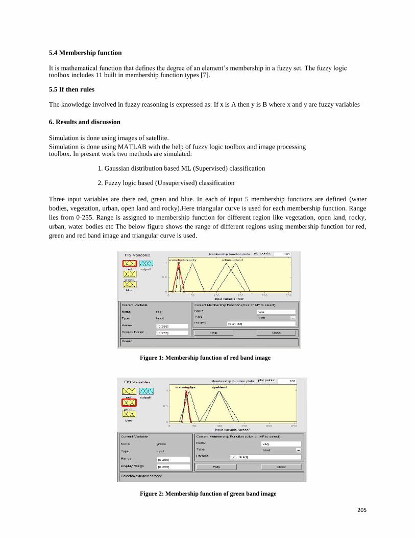
205

5.4 Membership function

It is mathematical function that defines the degree of an element‟s membership in a fuzzy set. The fuzzy logic toolbox includes 11 built in membership function types [7]. 5.5 If then rules The knowledge involved in fuzzy reasoning is expressed as: If x is A then y is B where x and y are fuzzy variables

6. Results and discussion

Simulation is done using images of satellite. Simulation is done using MATLAB with the help of fuzzy logic toolbox and image processing toolbox. In present work two methods are simulated:

1. Gaussian distribution based ML (Supervised) classification

2. Fuzzy logic based (Unsupervised) classification

Three input variables are there red, green and blue. In each of input 5 membership functions are defined (water

bodies, vegetation, urban, open land and rocky).Here triangular curve is used for each membership function. Range

lies from 0-255. Range is assigned to membership function for different region like vegetation, open land, rocky,

urban, water bodies etc The below figure shows the range of different regions using membership function for red,

green and red band image and triangular curve is used.

Figure 1: Membership function of red band image

Figure 2: Membership function of green band image

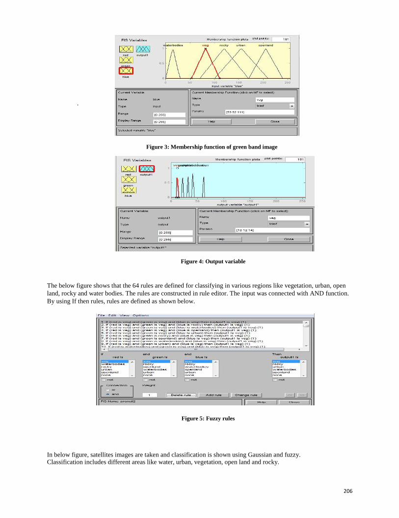
206

.

Figure 3: Membership function of green band image

Figure 4: Output variable

The below figure shows that the 64 rules are defined for classifying in various regions like vegetation, urban, open

land, rocky and water bodies. The rules are constructed in rule editor. The input was connected with AND function.

By using If then rules, rules are defined as shown below.

Figure 5: Fuzzy rules

In below figure, satellites images are taken and classification is shown using Gaussian and fuzzy. Classification includes different areas like water, urban, vegetation, open land and rocky.

207

6

5

4

3

2

1

0 0 2000 4000 6000 8000 10000 12000

Figure 8: Fuzzy classification Figure 9: Fuzzy classification

7. Conclusion The existing literature shows that till date the satellite image classification was done with the help of various

methods. Literature survey of existing methods has been done and it has been observed that fuzzy logic efficiently

handles uncertainties and increases accuracy in case of image classification. Detailed concept regarding image

classification approach is described in detail along with the classification steps. The proposed method is explained in

detail and its concept is explained. Also classification of image is shown using Gaussian distribution which is

supervised classification and using fuzzy classification which is unsupervised classification for various satellite

images. In future comparisons can be shown between different methods.

8. REFERENCES

[1]. Sisodia, P. S., Tiwari, V., & Kumar, A., A comparative analysis of remote sensing image classification techniques”, Advances in Computing, Communications and Informatics (ICACCI, International Conference. IEEE, pp. 1418-1421, 2014. [2]. Zhang, L., Xu, T., Zhang, J., & Yu, Y., “A knowledge-based procedure for remote sensing image classification. In Fuzzy Systems and Knowledge Discovery (FSKD)”, 11th International Conference, pp. 72-76, IEEE, 2014. [3]. Patidar, D., Jain, N., & Parikh, A., “Performance analysis of artificial neural network and K Nearest neighbour‟s image classification techniques with wavelet features”, Computer Communication and Systems, International Conference on (pp. 191-194). IEEE, 2014.

208

[4].Zhang, C., Zhao, Y., Zhang, D., & Zhao, N. (2011, July). Application and evaluation of object-oriented technology in high-resolution remote sensing image classification. In Control, Automation and Systems Engineering (CASE), 2011 International Conference on (pp. 1-4). IEEE. [5].Al-Tamimi, S., & Al-Bakri, J. T. (2005). Comparison between supervised and unsupervised classifications for mapping land use/cover in Ajloun area. [6].Kamavisdar, P., Saluja, S., & Agrawal, S. (2013). A survey on image classification approaches and techniques. International Journal of Advanced Research in Computer and Communication Engineering, 2(1), 1005-1009. [7].Nedeljkovic, I. (2004). Image classification based on fuzzy logic. The International Archives of the Photogrammetry, Remote Sensing and Spatial Information Sciences, 34(Part XXX). [8].Al-Doski, J., Mansor, S. B., & Shafri, H. Z. M. (2013). Image Classification in Remote Sensing. Journal of Environment and Earth Science, 3(10), 141-147. [9].Akgün, A., Eronat, A. H., & TÜRK, N. (2004). Comparing Different Satellite Image Classification Methods: An Application In Ayvalýk District, Western Turkey. In XXth International Congress for Photogrammetry and Remote Sensing, Istanbul, Turkey. [10].Li, M., Zang, S., Zhang, B., Li, S., & Wu, C. (2014). A review of remote sensing image classification techniques: The role of spatio-contextual information. European Journal of Remote Sensing, 47, 389-411. [11].Lu, D., & Weng, Q. (2007). A survey of image classification methods and techniques for improving classification performance. International journal of Remote sensing, 28(5), 823-870. [12].Jabari, S., & Zhang, Y. (2013). Very high resolution satellite image classification using Fuzzy rule-based systems. Algorithms, 6(4), 762-7. [13].Prasad, S. V. S., Savithri, T. S., & Krishna, I. V. M. (2015). Techniques In Image Classification; A Survey. Global Journal of Researches In Engineering, 15(6).

209

Comparison between M0 and M3 for Single Dc/Stepper Motor Into

Servo Motor

Patel Kuldeep J, Dimple Agrawal


Electronics and Communication Engineering Department, Silver Oak College of Engineering & Technology


Abstract: The objective of this paper is to design the transfer the function of stepper/dc motor into servo motor in

discrete time system and comparison between M0 and M3 controller. In motion control system the stepper motor is

widely used as it is an electromechanical device which converts electrical pulses into discrete mechanical a

movement with the use of cortex M0 and Arduino M3. The stepper drivers are used for compatible as the motor

description but take input voltage according to TTL voltage of microcontroller and control the rotation of the motor

and provide more flexibility.

Keywords: PSoC Chip, Stepper driver, Stepper Motor, Arduino M3.

Introduction

The many huge industrial technologies use the motor in heavy machinery for the operation of plant as it converts

the electrical energy into the mechanical energy. The motor is operating through the interaction between an electric

motor's magnetic field and winding currents to generate force within the motor. The components of motor are rotor,

stator, air gap, winding, and commutator. The operation of motor is either by DC supply or AC supply.

There are two type of DC/Stepper (i) Brushless DC motor (BLDC) (ii) Permanent DC motor (PMDC). In BLDC the

rotation of motor is done with the help of field magnet generated while in PMDC the rotation of motor is done with

the help of permanent magnet inside the motor.

The Stepper motor is part of DC motor as it has permanent magnet, synchronous electric motor that converts digital

pulses into mechanical shaft rotation. There are two type of stepper (i) unipolar (ii) bipolar. The unipolar motor

operates with one winding with a center tap per phase. Each section of the winding is switched on for each direction

of the magnetic field. While the bipolar motor operates as there is only a single winding per phase. The driving

circuit needs to be more complicated to reverse the magnetic pole; this is done to reverse the current in the winding.

Literature Review

Paper-1:

Title: Design of Control Unit for CNC Machine Tool using Arduino based Embedded System [4]

Author: Dev P. Desai and Dr. D.M. Patel

Publication: International Conference on smart technologies and management, May 2015

Conclusion: This paper describes the study of Digital Differential Analyser (DDA) and designing of the

software DDA and core working of CNC machine and interpreter for decoding Electronic Industries

Association (EIA) machine. During machining large amount of torque and power is required and therefore AC

servo motors are required as actuators. For economizing the work, unipolar stepper motors are selected for

driving the X, Y and Z axes & driver cards are designed accordingly. As the stepper motors are having low

capacity of load carrying, the machining is demonstrated using engraving tools with light cut using low depth of

cut. [4]

https://en.wikipedia.org/wiki/Magnetic_field



https://en.wikipedia.org/wiki/Electrical_conductor



210

Paper-2:

Title: Fast and Cheap Stepper Motor Drive [7]

Author: Mohamed Y. Tarnini

Publication: 4th

international conference on renewable energy research and application, November 2015

Conclusion: This paper describes the speed control of the stepper motor is possible by controlling the terminal

voltage by using a timer 555 or Microcontroller. In small stepping mode the stator flux can be considered

smoother than other modes like as half or full steps hence less vibration, noiseless stepping possible down to

near zero Hz hence the motor speed can change smoothly with short settling time and rise in voltage. [7]

Paper- 3:

Title: Speed Control of Brushless DC Motor Using Intelligent Controller [8]

Author: Md Mustafa Kamal, Lini Mathew and S.Chatterji

Publication: Intelligence Systems in Electrical Engineering Journal, 4th

year, No. 4, January 2014

Conclusion: This paper describes the PID design of controller using genetic algorithm. The dynamic behaviour

of BLDCM has been studied with the conventional controllers as well as fuzzy PID controller. It is observed

that from the conventional controller the results can be better to an extent. By using fuzzy logic controller,

results can be further better than conventional controllers. The proposed GA-PID controller not only eliminates

the overshoot of the response but also shows better improvement in term of rise time, settling time and peak

overshoot. Thus it is concluded that for the speed control of BLDCM, GA-PID provided far better response. [8]

Paper- 4:

Title: A PSoC Controller for a NASA Robotic Arm [9]

Author: Erik Goodman, Daniel Baker, Patrick Kane, Michael Shanblatt

Publication: Microelectronic Systems Education, 2007. IEEE International Conference on, June 2007

Conclusion: This paper describes the implement of a success, allowing joystick control of the arm and

providing both position data and a video feed to the computer program's GUI. [9]

Hardware and Software

PSoC: It most closely resembles a microcontroller combined with a PLD and programmable analog. Code is

executed to interact with the user-specified peripheral functions (called "Components"), using automatically

generated APIs and interrupt routines. Both APIs that initialize the user selected components upon the user‟s needs

in a Visual-Studio-like GUI [2]. There are two types of digital blocks, Digital Building Blocks (DBBxx) and Digital

Communication Blocks (DCBxx) [2].

These chips include a CPU core and mixed-signal arrays of configurable integrated analog and digital peripherals.

PSoC architecture that provides the industry‟s lowest-power 32-bit ARM Cortex-M0 based System on-Chip, with

unmatched ability to integrate analog and digital ICs. It offers larger devices with up to 128KB of Flash and 55

GPIOs and new peripherals including RTC, CAN and DMA, while supporting the AEC-Q100 standard - enabling

designers to reduce system BOM cost while quickly developing product variants [1].

Stepper Motor: The shaft or spindle of a stepper motor rotates in discrete step increments when electrical command

pulses are applied to it in the proper sequence. Figure 1 describe the motors rotation has several direct relationships

http://ieeexplore.ieee.org/xpl/mostRecentIssue.jsp?punumber=4599591






https://en.wikipedia.org/wiki/Microcontroller



https://en.wikipedia.org/wiki/Visual_studio






211

to these applied input pulses. The sequence of the applied pulses is directly related to the direction of motor shafts

rotation. The speed of the motor shafts rotation is directly related to the frequency of the input pulses and the length

of rotation is directly related to the number of input pulses applied [3].

Operation: We know that like poles of a magnet repel and unlike poles attract shows a typical cross-sectional view

of the rotor and stator of a stepper motor. Figure 1 describe the stator has eight poles, and the rotor has six poles [3].

The rotor will require 24 pulses of electricity to move the 24 steps to make one complete revolution. Another way to

say this is that the rotor will move precisely 15° for each pulse of electricity that the motor receives. The number of

degrees the rotor will turn when a pulse of electricity is delivered to the motor can be calculated by dividing the

number of degrees in one revolution of the shaft by the number of poles he rotor. In this stepper motor 360° is

divided by 24 to get 15° [3].

Figures: 1 Schematic of Motor [3]

Stepper Driver: The stepper driver is used to control the rotation of shaft of the motor. The encoder sends the error

signal to the driver and according it will acceleration or deceleration the speed of the motor. Figure 2 show the

RMCS-1106 is Rhino Motion Controls new and improved DSP based micro-stepping drive for 1.8deg Bipolar

Stepper Motors. It is designed for smooth and quiet operation without compromising on torque and control at higher

speeds. It has short-circuited protection for the motor outputs, over-voltage and under-voltage protection. The

RMCS-1106 achieves micro-stepping using a synchronous PWM output drive and high precision current feedback

and this is absolutely silent when the motor is stopped or turning slowly. It virtually eliminates stopped-motor

heating regardless of power supply voltage using a DSP based PID current control loop [5].

Figure: 2stepper driver [5]

Arduino M3: The Arduino Due is a microcontroller board based on the Atmel SAM3X8E ARM Cortex-M3 CPU.

It is the first Arduino board based on a 32-bit ARM core microcontroller. It has 54 digital input/output pins (of

which 12 can be used as PWM outputs), 12 analog inputs, 4 UARTs (hardware serial ports), an 84 MHz clock, an

USB OTG capable connection, 2 DAC (digital to analog), 2 TWI, a power jack, an SPI header, a JTAG header, a

reset button and an erase button [6].

The board contains everything needed to support the microcontroller simply connect it to a computer with a

microUSB cable or power it with an AC-to-DC adapter or battery to get started. The Arduino Due is compatible

with all Arduino shields that work at 3.3V and are compliant with the 1.0 Arduino pin out [6].

http://www.atmel.com/Images/Atmel-11057-32-bit-Cortex-M3-Microcontroller-SAM3X-SAM3A_Datasheet.pdf





212

Arduino IDE: The Arduino board will need to upload some kind of program to it. By writing a program and

uploading it to the Arduino‟s processor, we can instruct it to do lots of useful and interesting things. In order to get

the programs onto the Arduino, we need to install the Arduino IDE (Integrated Development Environment) on

another computer. This software compiles (converts) the code that we write into instructions that the Arduino can

understand, then transfers it through the USB to the Arduino‟s ATMega 386 processor.

Figure: 3 Arduino IDE

Figure 3 describe the Ardiuno IDE initial setup after software were we can start the new program according to the

programmer required and boot loader is used to load the program into the chip and working of the program is seen

on the hardware.

Result Analysis

After set up of the software PSoC Creator and after created a project file and program it in main.c file according

per requirement we load the program in to chip hardware with the help of boot loader for stimulation. For loading

the PSoC chip is connected to device with the help of the USB as in PSoC chip have serial communication

facility and serial is internally connected to the parallel communication. Hence the program can be done parallel

communication. Figure 4 show the rotation of the motor is depending upon the frequency applied hence to

increase the rotation the value of pulse throw the driver is reduced by 16 times or 32 times the original pulse

applied hence the run off problem is get overcome and can handle the load easily.

Figure: 4Circuit Diagram

The reason for changing to M0 to M3 is less controlling space and drawback faced in M0 are requirement of digital

block is more for counter size, counter resolution, index input, glitch filtering, quadrature A and B of encoder so

need to upgrade to M3.

The new project is created in ardiuno M3 and program of DC motor driver is done with the help of predefined

library along with the software like PWM and clock block. The predefined block is blank just need to enter the value

213

of pin for pulse and staring and stop of the block in program file. Another new project is created and program of

Stepper motor driver is done with the help of predefined library along with the software like PWM and clock block.

The predefined block is blank just need to enter the value of pin for pulse and staring and stop of the block in

program file as shown in figure 5.

Figure: 5 Circuit Diagram

Conclusion

Hence, conclude that with the help of PSoC M0 and ardiuno M3, which is programmable can make

program according to the requirement and try to implement the rotation of the stepper motor on the chip with the

help of the stepper driver and try to implementation of real time encoder position of the motor for calculating the

rotation of the shaft as per the pulse given by the driver and load balancing tuning for industrial precise machine application.

REFERENCES

[1]. http://www.cypress.com/video-library

[2]. http://www.cypress.com/products/psoc-4

[3]. http://robokits.co.in/motors/nema34-stepper-motor-85kgcm-torque?cPath=2_4&

[4]. Dev P. Desai and Dr. D.M. Patel, “Design of Control Unit for CNC Machine Tool using Arduino based

Embedded

System”, IEEE Transaction onSmart Technologies and Management for Computing, Communication, Controls,

Energy and Materials (ICSTM), PP.443-448, 2015

[5]. http://robokits.co.in/motor-drives/stepper/micro-stepping-stepper-motor-drive-12-40v-2amp?cPath=73

[6]. https://www.arduino.cc/en/Main/ArduinoBoardDue

[7]. Mohamed Y. Tarnini, “Fast and Cheap Stepper Motor Drive”, IEEE Transaction on on Renewable Energy

Research and Applications (ICRERA), PP.689-693, 2015

[8]. Md Mustafa Kamal, Lini Mathew and S.Chatterji,“Speed Control of Brushless DC Motor Using Intelligent

Controller” IEEE Transaction on Engineering and Systems (SCES), PP.1-5, 2014.

[9]. Erik Goodman, Daniel Baker, Patrick Kane, Michael Shanblatt, “A PSoC Controller for a NASA Robotic Arm”,

IEEE Transaction on Microelectronic Systems Education, PP.129-130, 2007.

http://www.cypress.com/products/psoc-4








http://robokits.co.in/motors/nema34-stepper-motor-85kgcm-torque?cPath=2_4&

























http://robokits.co.in/motor-drives/stepper/micro-stepping-stepper-motor-drive-12-40v-2amp?cPath=73





























https://www.arduino.cc/en/Main/ArduinoBoardDue








214

Survey on Different Auto Scaling Techniques in Cloud Computing

Environment

Pranali Gajjar

[email protected]

Computer Engineering Department, Silver Oak College of Engineering & Technology, Gujarat Technological

University, India Abstract:- Cloud computing is a recent technology trending that help companies in providing their services in a scalable

manner. Hence, used this service capabilities required many procedures in order to get better performance. Cloud

computing environments allow customers to dynamically scale their applications. The key problem is how to lease

the right amount of resources, on a pay-as-you-go basis. The objective of this paper was to present a comprehensive

study about the auto-scaling mechanisms available today. Auto-scaling techniques are diverse, and involve various

components at the infrastructure, platform and software levels. Many techniques have been proposed for auto-

scaling. We propose a classification of these techniques into five main categories: static threshold-based rules,

control theory, reinforcement learning, queuing theory and time series analysis.

Keywords: Cloud Computing, Auto scaling, Auto scaling techniques

1. Introduction Cloud computing is in its infant form and numerous definitions have been proposed by many scientists. Some of the definitions are, Buy et al. defines, “A Cloud is a type of parallel and distributed system consisting of a collection of

inter-connected and virtualized computers that are dynamically provisioned and presented as one or more unified

computing resource(s) based on service-level agreements established through negotiation between the service provider and consumers” [1].

The National Institute of Standards and Technology (NIST) defines, “A model for enabling convenient, on-demand network access to a shared pool of configurable computing resources (e.g., networks, servers, storage, applications,

and services) that can be rapidly provisioned and released with minimal management effort or service provider

interaction. This cloud model promotes availability and is composed of five essential characteristics, three service models, and four deployment models” [2].

Figure 1: Cloud Computing

215

In brief cloud is essentially a bunch of commodity computers networked together in same or different geographical

locations, operating together to serve a number of customers with different need and workload on demand basis with

the help of virtualization. Cloud services are provided to the cloud users as utility services like water, electricity,

telephone using pay-as-you-use business model. These utility services are generally described as XaaS (X as a

Service) where X can be Software or Platform or Infrastructure etc. Cloud users use these services provided by the

cloud providers and build their applications in the internet and thus deliver them to their end users. So the cloud

users don‟t have to worry about installing, maintaining hardware and software needed. And they also can afford

these services as they have to pay as much they use. So the cloud users can reduce their expenditure and effort in the

field of IT using cloud services instead of establishing IT infrastructure themselves [3].

1.1 Characteristics of Cloud On Demand Self Service: On demand self-service refers to services requested by the customers to manage

their own computing resources. These services are provided over the internet by a cloud provider to a customer

who has requested for services and can manage their own computing resources. Resource Pooling: Cloud computing provides shared pool of resources that can be rapidly provisioned and can

be released with minimal effort. Customers draw resources from remote data centers. Broad Network Access: To avail cloud computing services, internet works as a backbone of cloud computing.

All services are available over the network and are also accessible through standard protocols using web

enabled devices viz. computers, laptops, mobile phones etc. Rapid Elasticity: As cloud computing provides services over the internet. These services can be managed or

can be requested from cloud providers as per customer‟s requirement. Rapid elasticity refers to services which

can be smaller or larger as per user requirement. Measured Service: These are services which are billed according to customer demand for definite services. As

customers can request for services as per their own requirement, services are billed according to customer‟s

demand.

1.2 Service Models of Cloud Computing

Cloud computing is a computational process in which services are delivered over a network using computing

resources.

There are three main types of service models:

Software as a Service (SaaS) Platform as a Service (PaaS) Infrastructure as a Service (IaaS)

1.2.1 Software-as-a-Service (SaaS):

In this multitenant service model, the consumers use application running on a cloud infrastructure. The cloud

infrastructure including (servers, OS, Network or application etc.) is managed and controlled by the service provider

with the user not having any control over the infrastructure. Some of the popular examples are SalesForce.com, Net

Suite, IBM, Microsoft and Oracle etc.

Example for SaaS Company:

Athena health Concur Technologies E2open

216

1.2.2 Platform-as-a-Service (PaaS):

With this model, the provider delivers to user a platform including all the systems and environments comprising

software development life cycle viz. testing, deploying, required tools and applications. The user does not have any

control over network, servers, operating system and storage but it can manage and control the deployed application

and hosting environments configurations. Some popular PaaS providers are GAE, Microsoft‟s Azure etc.

Example for PaaS Company:

Apprenda IBM Open shift

1.2.3 Infrastructure-as-a-Service (IaaS):

In this service model, the provider delivers to user the infrastructure over the internet. With this model, the user is

able to deploy and run various software‟s including system or application softwares. The user has the ability to

provision computing power, storage, networks. The consumers have control over operating systems, deployed

applications, storage and partial control over network. The consumer has no control over underlying infrastructure.

Some important IaaS providers are GoGrid, Flexiscale, Joyent, Rackspace etc.

Example for IaaS Company:

Amazon web service At & t Ca technologies

1.3 Deployment models

Cloud systems can be deployed in four forms viz. private, public, community and hybrid cloud as per the access

allowed to the users and are classified as follows:

1.3.1 Private cloud:

This deployment model is implemented solely for an organization and is exclusively used by their employees at

organizational level and is managed and controlled by the organization or third party. The cloud infrastructure in this

model is installed on premise or off premise. In this deployment model, management and maintenance are easier,

security is very high and organization has more control over the infrastructure and accessibility.

Examples of Private Cloud:

Eucalyptus Ubuntu Enterprise Cloud - UEC (powered by Eucalyptus) Amazon VPC (Virtual Private Cloud) VMware Cloud Infrastructure Suite Microsoft ECI data center.

1.3.2 Public cloud:

This deployment model is implemented for general users. It is managed and controlled by an organization selling

cloud services. The users can be charged for the time duration they use the services. Public clouds are more

vulnerable to security threats than other cloud models because all the application and data remains publicly available

217

to all users making it more prone to malicious attacks. The services on public cloud are provided by proper

authentication.

Examples of Public Cloud:

Google App Engine Microsoft Windows Azure IBM Smart Cloud Amazon EC2

1.3.3 Community cloud:

This cloud model is implemented jointly by many organizations with shared concerns viz. security requirements,

mission, and policy considerations. This cloud is managed by one or more involved organizations and can be

managed by third party. The infrastructure may exist on premise to one of the involved organization or it may exist

off premise to all organizations.

Examples of Community Cloud:

Google Apps for Government Microsoft Government Community Cloud

1.3.4 Hybrid cloud:

This deployment model is an amalgamation of two or more clouds (private, community, public or hybrid). The

participating clouds are bound together by some standard protocols. It enables the involved organization to serve its

needs in their own private cloud and if some critical needs (cloud bursting for load-balancing) occur they can avail

public cloud services. Examples of Hybrid Cloud:

Windows Azure (capable of Hybrid Cloud) VMware vs Cloud (Hybrid Cloud Services)

1.4 Advantages of Cloud Computing

Cloud computing offers many benefits and flexibility to its users. User can operate from anywhere at any time in a

secure way. With the increasing number of web-enabled devices used now-a-days (e.g. tablets, smart phones etc.),

access to one‟s information and data must be quick and easier. Some of these relevant benefits in respect to the

usage of a cloud can be as follows:

Reduces up-front investment, Total Cost of Ownership (TCO), Total Operational Cost (TOC) and minimizes

business risks. Provides a dynamic infrastructure that provides reduced cost and improved services with less development and

maintenance cost. Provides on-demand, flexible, scalable, improved and adaptable services on pay-as-you go model. Provides consistent availability and performance with automatically provisioned peak loads. Can recover rapidly and has improved restore capabilities for improved business resiliency. Provides unlimited processing, storage, networking etc. in an elastic way. Offers automatic software updates, Improved Document Format Compatibility and improved compatibility

between different operating systems.

218

Offers easy group collaboration i.e. flexibility to its users on global scale to work on the same project. Offers increased return on investment of existing assets, freeing capital to deploy strategically. Provides environment friendly computing as it only uses the server space required by the application which in

turn reduces the carbon footprints.

1.5 Disadvantages of Cloud Computing

Every coin has two faces. That‟s not to say, of course, cloud computing is without disadvantages. Some of the

disadvantages while using a cloud can be summarized as:

Requires high speed network and connectivity constantly. Privacy and security is not good. The data and application on a public cloud might not be very secure. Disastrous situation are unavoidable and recovery is not possible always. If the cloud loses one‟s data, the user

and the service provider both gets into serious problems. Users have external dependency for mission critical applications. Requires constantly monitoring and enforcement of service level agreements (SLAs).

2. Defining Scalability

André B. Bondi of AT&T Labs defined scalability as “The concept connotes the ability of a system to accommodate

an increasing number of elements or objects, to process growing volumes of work gracefully, and/or to be

susceptible to enlargement”[4]. He further proceeds to give an initial taxonomy consisting of four types of

scalability:

1. Load scalability: It describes a system that is capable of operating graceful different loads while making good

use of available resources. Some of the factors that may hamper load scalability is scheduling of a shared

resource, scheduling of a class of resources in a manner that increases its own usage, and inadequate

exploitation of parallelism.

2. Space scalability: It refers to the growth of memory usage compared to the scale of the system. Many different

approaches like space efficient algorithms and compression can help with space scalability, but the effects (like

added CPU time of compression) might reduce other types of scalability like load scalability.

3. Space-time scalability: It regards the ability of a system functions gracefully when the number of items it

handles increase by an order of magnitude. Space-time scalability may be related to both load scalability and

space scalability in that the amount of items might stem from an increased load, and the presence of these

objects may use more memory and affect data structures. 4. Structural scalability: It refers to the implementation or standards of the system and how they limit the

number of item the system may handle. The prime example of structural scalability concerns the addressing of

the items, for instance will a fixed addressing space put a limit on the systems scalability.

3. Types of Scaling

In cloud three way of scaling is done horizontal scaling, vertical scaling, auto scaling. Auto scaling is the ability to

scale up and scale down the application server‟s capacity automatically according to customer defines. To maintain

the performance when demand is huge it increases the number of instance and decrease automatically when demand

reduces to minimize cost [5].

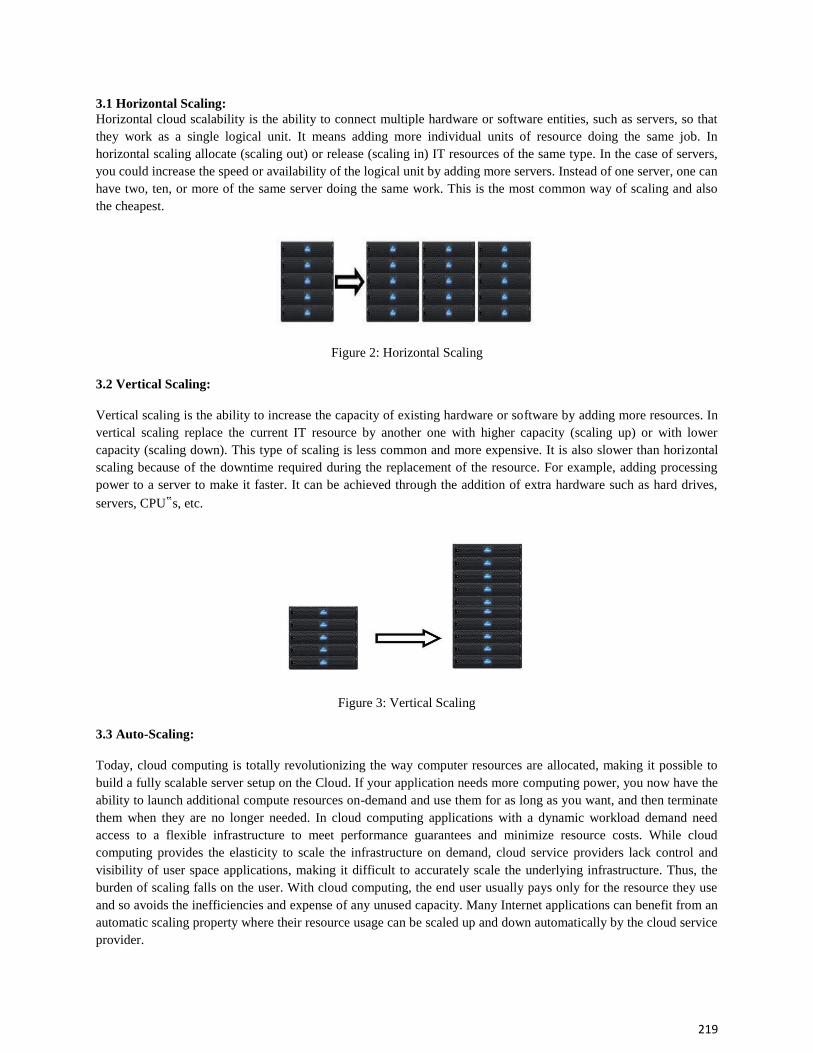
219

3.1 Horizontal Scaling: Horizontal cloud scalability is the ability to connect multiple hardware or software entities, such as servers, so that

they work as a single logical unit. It means adding more individual units of resource doing the same job. In

horizontal scaling allocate (scaling out) or release (scaling in) IT resources of the same type. In the case of servers,

you could increase the speed or availability of the logical unit by adding more servers. Instead of one server, one can

have two, ten, or more of the same server doing the same work. This is the most common way of scaling and also

the cheapest.

Figure 2: Horizontal Scaling

3.2 Vertical Scaling:

Vertical scaling is the ability to increase the capacity of existing hardware or software by adding more resources. In

vertical scaling replace the current IT resource by another one with higher capacity (scaling up) or with lower

capacity (scaling down). This type of scaling is less common and more expensive. It is also slower than horizontal

scaling because of the downtime required during the replacement of the resource. For example, adding processing

power to a server to make it faster. It can be achieved through the addition of extra hardware such as hard drives,

servers, CPU‟s, etc.

Figure 3: Vertical Scaling

3.3 Auto-Scaling:

Today, cloud computing is totally revolutionizing the way computer resources are allocated, making it possible to

build a fully scalable server setup on the Cloud. If your application needs more computing power, you now have the

ability to launch additional compute resources on-demand and use them for as long as you want, and then terminate

them when they are no longer needed. In cloud computing applications with a dynamic workload demand need

access to a flexible infrastructure to meet performance guarantees and minimize resource costs. While cloud

computing provides the elasticity to scale the infrastructure on demand, cloud service providers lack control and

visibility of user space applications, making it difficult to accurately scale the underlying infrastructure. Thus, the

burden of scaling falls on the user. With cloud computing, the end user usually pays only for the resource they use

and so avoids the inefficiencies and expense of any unused capacity. Many Internet applications can benefit from an

automatic scaling property where their resource usage can be scaled up and down automatically by the cloud service

provider.

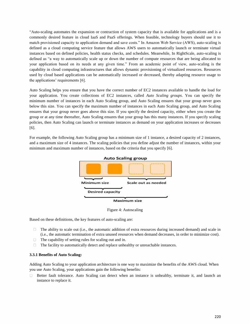
220

“Auto-scaling automates the expansion or contraction of system capacity that is available for applications and is a

commonly desired feature in cloud IaaS and PaaS offerings. When feasible, technology buyers should use it to

match provisioned capacity to application demand and save costs.” In Amazon Web Service (AWS), auto-scaling is

defined as a cloud computing service feature that allows AWS users to automatically launch or terminate virtual

instances based on defined policies, health status checks, and schedules. Meanwhile, In RightScale, auto-scaling is

defined as “a way to automatically scale up or down the number of compute resources that are being allocated to

your application based on its needs at any given time.” From an academic point of view, auto-scaling is the

capability in cloud computing infrastructures that allows dynamic provisioning of virtualized resources. Resources

used by cloud based applications can be automatically increased or decreased, thereby adapting resource usage to

the applications‟ requirements [6].

Auto Scaling helps you ensure that you have the correct number of EC2 instances available to handle the load for

your application. You create collections of EC2 instances, called Auto Scaling groups. You can specify the

minimum number of instances in each Auto Scaling group, and Auto Scaling ensures that your group never goes

below this size. You can specify the maximum number of instances in each Auto Scaling group, and Auto Scaling

ensures that your group never goes above this size. If you specify the desired capacity, either when you create the

group or at any time thereafter, Auto Scaling ensures that your group has this many instances. If you specify scaling

policies, then Auto Scaling can launch or terminate instances as demand on your application increases or decreases

[6].

For example, the following Auto Scaling group has a minimum size of 1 instance, a desired capacity of 2 instances,

and a maximum size of 4 instances. The scaling policies that you define adjust the number of instances, within your

minimum and maximum number of instances, based on the criteria that you specify [6].

Figure 4: Autoscaling

Based on these definitions, the key features of auto-scaling are:

The ability to scale out (i.e., the automatic addition of extra resources during increased demand) and scale in

(i.e., the automatic termination of extra unused resources when demand decreases, in order to minimize cost). The capability of setting rules for scaling out and in. The facility to automatically detect and replace unhealthy or unreachable instances.

3.3.1 Benefits of Auto Scaling:

Adding Auto Scaling to your application architecture is one way to maximize the benefits of the AWS cloud. When

you use Auto Scaling, your applications gain the following benefits: Better fault tolerance. Auto Scaling can detect when an instance is unhealthy, terminate it, and launch an

instance to replace it.

221

Better availability. You can configure Auto Scaling to use multiple Availability Zones. If one Availability Zone

becomes unavailable, Auto Scaling can launch instances in another one to compensate. Better cost management. Auto Scaling can dynamically increase and decrease capacity as needed. Because you

pay for the EC2 instances you use, you save money by launching instances when they are actually needed and

terminating them when they aren't needed.

4. Classification of Auto scaling Techniques

It is difficult to work out a proper classification of auto-scaling techniques, due to the wide diversity of approaches

found in the literature that are sometimes hybridizations of two or more methods. Considering the anticipation

capacity as the main criteria, techniques could be divided into two main classes: reactive (the system reacts to

changes but does not anticipate them) or predictive (the system tries to predict future resource requirements in order

to ensure sufficient resource are available ahead of time) [7].

4.1 Reactive Scaling:

Reactive scaling is also implemented. When a company begins running applications in cloud resources, some

unexpected changes in the workload may occur. A reactive scaling strategy can meet this demand by adding or

removing scaling up or down resources. Periodic acquisition of performance data is important both to the cloud

provider and to the cloud agencies for maintaining QoS. In addition, reactive scaling enables a provider to react

quickly to unexpected demand. In other words, when CPU or RAM or another resource reaches a certain level of

utilization, the provider adds more of that resource to the environment.

4.2 Proactive Scaling:

Proactive scaling is usually done in a cloud by scaling at predictable, fixed intervals or when big surges of traffic

requests are expected. Proactive scaling is also known as predictive scaling. A well-designed proactive scaling

system enables providers to schedule capacity changes that match the expected changes in application demand. To

perform proactive scaling, they should first understand expected traffic flow. This simply means that they should

understand (roughly) how much normal traffic deviates from agency expectations. The most efficient use of

resources is just below maximum agency capacity, but scheduling things that way can create problems when

expectations are wrong.

4.3 Auto Scaling Techniques:

Auto-scaling techniques grouped into these categories [8, 9]:

1. Static Threshold Based Rules 2. Reinforcement Learning 3. Queuing Theory 4. Control Theory 5. Time-series Analysis

4.3.1 Static Threshold-based Rules

Threshold based techniques are widely used in the commercial auto-scaling systems. The popularity of these

approaches is due to their simplicity and intuitive nature. To implement a threshold based auto-scaling environment,

the first step is to monitor one or more performance metrics. In this approach, number of VMs varies based on the

measures of performance metrics and thresholds which are set by the operator. Typically there are two rules, once

for scaling up and another for scaling down. These rules usually have a time variable e.g. bring up an instance if the

%processor time > 85 over a 15 minute period. There is usually a cooling down period associated with a rule (post

222

invocation) where a node is not shut down for a defined period. This is a reactive strategy; an instance is added only

when a flag (threshold reached) is raised. The most significant drawback of the threshold based techniques is the

difficulty of setting suitable threshold values.

4.3.2 Reinforcement Learning

Auto-scaling based on reinforcement learning is a predictive approach to auto-scaling. VM instantiation is predicted

via learned behavior. It makes decisions based on interaction between the auto-scaling agent and the scalable

application. In the cloud provisioning problem domain, the auto-scaling component is the agent that interacts with

the scalable application environment and decides whether to add or remove resources to gain the maximum award

(i.e., minimize response time). The main drawbacks of these approaches are bad initial performance, long training

time and the problem to handle sudden bursts in input workload.

4.3.3 Queuing Theory

Queuing theory can be utilized to add capacity by analyzing and making decisions based on a queue i.e. requests

queued at the load balancer. Classical queuing theory has been extensively used to model Internet applications and

traditional servers, in order to estimate performance metrics such as the queue length or the average waiting time for

requests. Approaches based on queuing theory, monitor system parameters and apply specific performance laws (i.e., Little‟s law and utilization law) to estimate system‟s performance metrics. Since queuing theory only provides

an estimation of performance metrics, most of the authors, have combined it with another approaches (i.e., threshold

based policies, control theory, and reinforcement learning) to deal with auto-scaling problem. There are two

important obstacles to using queuing theory approaches in auto-scaling systems. First, they impose non-realistic

assumptions which are not valid in real scenarios; and second, they are not efficient for complex systems.

4.3.4 Control Theory

Control systems use a feedback loop by modifying the controller input to influence the normative output. Control

systems are mainly reactive, but there are also some proactive approximations such as Model Predictive Control, or

even combining a control system with a predictive model. Control theory has been applied to automate management

of resources in various engineering fields, such as storage systems, data centers and cloud computing platforms. The

main objective of a controller is to maintain the output of the target system (e.g., performance of a cloud

environment) to a desired level by adjusting the control input (e.g. number of VMs). Similar to queuing theory

approaches, control theory based techniques mostly use other provisioning approaches (such as threshold based

approach) to perform decision making.

4.3.5 Time-series Analysis

Time-series analysis uses historical data to predict future usage. Time series are used in many domains including

finance, engineering, economics and bioinformatics, generally to represent the change of a measurement over time.

A time-series is a sequence of data points, measured typically at successive time instants spaced at uniform time

intervals. An example is the number of requests that reaches an application, taken at one-minute intervals. The time-

series analysis could be used to find repeating patterns in the input workload or to try to forecast future values.

5. Conclusion

One of the conclusions that can be extracted from this survey is that auto scaling is the ability to scale up or down

the capacity automatically according to conditions of the user defines. With Auto Scaling ensure that the number of

instances is increasing seamlessly during demand to maintain performance, and decreases automatically during

demand reduce to minimize costs. The system should be able to adapt to the customer request so as to increase

resources or decrease the resources, so as to maintain the balance between performance and cost effectiveness. We

223

discussed various types of scaling. Here we have discussed the auto scaling techniques. Improving the performance

and utilization of the cloud systems are gained by the auto-scaling of the applications; this is because of the fact that,

some approaches have been proposed for auto scaling.

6. REFERENCES

[1] R. Buyya, C. S. Yeo, S. Venugopal, J. Broberg and I. Brandic, “Cloud computing and emerging IT platforms:

Vision, hype, and reality for delivering computing as the 5th

utility”, Future generation computer systems, vol. 25,

no. 6, pp. 599–616, June 2009.

[2] L. Badger, T Grance, R. P. Comer and J. Voas, DRAFT cloud computing synopsis and recommendations,

Recommendations of National Institute of Standards and Technology (NIST), May-2012.

[3] Mohammad Sajid, Zahid Raza, Cloud Computing: Issues & Challenges, International Conference on Cloud, Big

Data and Trust, Nov 13-15, RGPV, 2013.

[4] André B. Bondi, “Characteristics of scalability and their impact on performance, In Proceedings of the 2Nd

International Workshop on Software and Performance”, WOSP ‟00, pages 195–203, New York, NY, USA, 2000.

ACM. ISBN 1-58113- 195-X. doi: 10.1145/350391.350432. URL http://doi.acm.org/10.1145/350391.350432.

[5] M.Kriushanth, L. Arockiam, and G. Justy Mirobi, “Auto Scaling in Cloud Computing: An Overview”, July 2013

[6] “Amazon Auto Scaling in Cloud Computing”,http://aws.amazon.com/autoscaling/30.05.2012

[7] Laura R. Moore, Kathryn Bean and Tariq Ellahi, ”A Coordinated Reactive and Predictive Approach to Cloud

Elasticity”

[8] Brian C. Carroll, “Auto-Scaling in the Cloud: Evaluating a Control Based Technique”

[9] T. Lorido-Botrán, J. Miguel-Alonso and J. A. Lozano, “Auto-scaling Techniques for Elastic Applications in

Cloud Environments. Technical Report EHU-KAT-IK-09-12”, University of the Basque Country, Sept. 2012.

[10] R. Pragaladan, P. Suganthi, “A Study on Challenges of Cloud Computing in Enterprise Perspective”, July 2004.

[11] D. A. Menasce and P. Ngo, “Understanding cloud computing: Experimentation and capacity planning,” in

Proc. of computer measurement group conf.”, pp. 1-11, December 2009.

[12] IBM Global Services, “Cloud computing: defined and demystified explore public, private and hybrid cloud

approaches to help accelerate innovative business solutions”, April-2009.

[13] Lijun Mei, W.K. Chan and T.H. Tse, "A Tale of Clouds: Paradigm Comparisons and Some Thoughts on

Research Issues", IEEE Asia-Pacific Services Computing Conference, 2008, pp 464-469.

http://doi.acm.org/10.1145/350391.350432

224

Development of data retrieval and scientific data-

presentation platform

Sridevi Ramya, Gayatri Yellamraju

[email protected]

Computer Engineering Department, Silver Oak College of Engineering & Technology, Gujarat Technological

University, India Abstract:-

LIGO-India, or INDIGO, is a planned collaborative project between the LIGO Laboratory and the Indian

government‟s Initiative in Gravitational-wave Observations (IndIGO) to create a world-class gravitational-wave

detector in India. Gravitational waves carry information about their dramatic origins and about the nature of gravity

that cannot otherwise be obtained. Direct detection of gravitational waves has long been sought. Their discovery

would launch a new branch of astronomy to complement electromagnetic telescopes and neutrino observatories.

Joseph Weber pioneered the effort to detect gravitational waves in the 1960s through his work on resonant mass bar

detectors. Bar detectors continue to be used at six sites worldwide. By the 1970s, scientists including Rainer Weiss

realized the applicability of laser interferometer to gravitational wave measurements.

This research paper involves in developing a typical Graphical User Interface which will provide interface for data retrieval from remote machine. It also facilitates scientific data plotting and signal processing environment for basic

operations. These plots are used by the observers to interpret the gravitational phenomena. The intensity of the research paper lies in the option of acquiring the real time data and plotting it simultaneously.

Keywords: Data retrieval, graphical user interface, gravitational waves, data plotting and graphs.

1. Introduction

Gravitational observations need a platform to plot and interpret. The constraints are real time acquisition of

data and simultaneous operation on acquired data. The dynamic files are not supported by most of the data plotting

software platforms and to provide each and every user with offline software platform to plot the data. The silver

lining of the paper is about process to fetch data from remote machine, then plot pulse as well as continuous graph.

Further, if user wants to see down sampled plot then down sampling for both pulse and continuous data is to be

presented.

This paper involves in developing a Graphical User Interface (GUI) using Python language. The GUI prompts the user to enter details of data to be fetched from remote machine while requesting for scientific presentation of data. The basic modules include the data retrieval parameters‟ input, plotting of existing data set (pulse) and at real time (continuous) along with down sampling. Directories and files required for signal processing reside at a remote

machine which are fetched and processed. In a nut shell, this project involves in programming a GUI to retrieve data and plot the received data for analysis.

2. Plotting algorithm

In order to retrieve data from remote machine, initially user needs to find appropriate parameters to fetch

data. Then one can follow the hierarchy given in parameters to obtain the raw data set. The plotting of data set algorithm mainly has three steps

Take parameters from user of which the graph is to be drawn. Search the respective matches in remote machine and fetch the available raw data into local machine. Draw the graph for acquired data set in canvas.


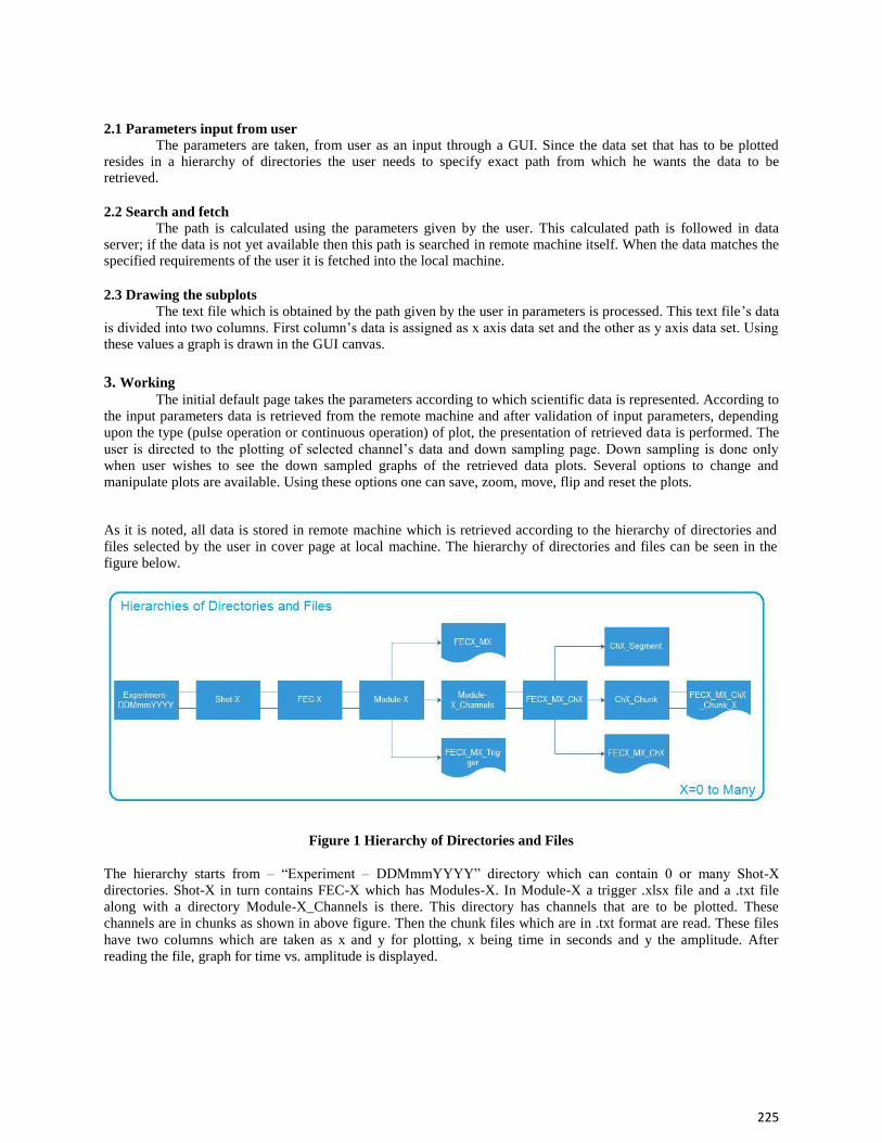
225

2.1 Parameters input from user The parameters are taken, from user as an input through a GUI. Since the data set that has to be plotted

resides in a hierarchy of directories the user needs to specify exact path from which he wants the data to be retrieved.

2.2 Search and fetch The path is calculated using the parameters given by the user. This calculated path is followed in data

server; if the data is not yet available then this path is searched in remote machine itself. When the data matches the specified requirements of the user it is fetched into the local machine.

2.3 Drawing the subplots The text file which is obtained by the path given by the user in parameters is processed. This text file‟s data

is divided into two columns. First column‟s data is assigned as x axis data set and the other as y axis data set. Using these values a graph is drawn in the GUI canvas.

3. Working The initial default page takes the parameters according to which scientific data is represented. According to

the input parameters data is retrieved from the remote machine and after validation of input parameters, depending

upon the type (pulse operation or continuous operation) of plot, the presentation of retrieved data is performed. The

user is directed to the plotting of selected channel‟s data and down sampling page. Down sampling is done only

when user wishes to see the down sampled graphs of the retrieved data plots. Several options to change and

manipulate plots are available. Using these options one can save, zoom, move, flip and reset the plots.

As it is noted, all data is stored in remote machine which is retrieved according to the hierarchy of directories and

files selected by the user in cover page at local machine. The hierarchy of directories and files can be seen in the

figure below.

Figure 1 Hierarchy of Directories and Files

The hierarchy starts from – “Experiment – DDMmmYYYY” directory which can contain 0 or many Shot-X

directories. Shot-X in turn contains FEC-X which has Modules-X. In Module-X a trigger .xlsx file and a .txt file

along with a directory Module-X_Channels is there. This directory has channels that are to be plotted. These

channels are in chunks as shown in above figure. Then the chunk files which are in .txt format are read. These files

have two columns which are taken as x and y for plotting, x being time in seconds and y the amplitude. After

reading the file, graph for time vs. amplitude is displayed.

226

Figure 2 Default setting page

This page has all parameters that are considered for plotting graph. Plot channel data tab where graphs according to

input parameters are displayed. The down sampling tab is initially disabled along with the down sampling factor.

When down sampling checkbox is checked the down sampling factor entry box and down sampling tab both are

enabled. The drive and date are taken as input. The Shot, FEC and Module are selected from dropdown. The channel

selection is disabled as well initially. It is enabled if number of channels in Module-X is more than 8 otherwise all 8

channels are displayed. Then whether continuous plot is to be drawn or pulse is selected by radio buttons. The down

sampling plot will skip as many rows in chunk directory for plotting as mentioned in down sampling factor.

Validation button validates the inputs provided. Proceed button is enabled only when validation is done. Quit button

and quit tab both close the GUI window.

The channel details are updated according to the selection in Module dropdown menu. Maximum number of

channels to be displayed in plot section is always eight. The number of channels for plot section will show how

many channels are present at given path. According to the selections in drive, date, shot, FEC and module, channel

dropdown menu for all 8 plots is showed in which channels whose plot is to be showed are selected. Channels for all

8 paths can be selected or only certain plots can be selected. Plots are displayed according to the menu selection.

When pulse is selected the data set that is already present at given path is displayed chunk by chunk. Down sampling

is checked hence down sampling factor and down sampling tab are enabled. And down sampling factor of 10 is

taken. Thus number of rows skipped in chunks for plotting in down sampling tab starting from the first row is ten as

provided in down sampling factor.

Inputs are validated and proceed button is enabled to move further and plot the graphs. After proceeding further the

user can either go to the plot channel data tab or to down sampling tab depending on his interest. The user can also stay on the same page and modify some inputs if he wishes to do so or completely come out of GUI by clicking either the Quit button provided at the Access Button section or Quit tab provided along with other tabs at the top.

As shown in following Fig 3 the pulse plot is shown for all chunks in the selected channels one after the other. The

plots that are not selected are left blank. X axis represents time in seconds and Y the amplitude. A stop button is provided to stop the plotting till start button is clicked, after which potting beings again. Interactive navigation toolbar is also provided at the bottom for easy analysis of subplots by user.

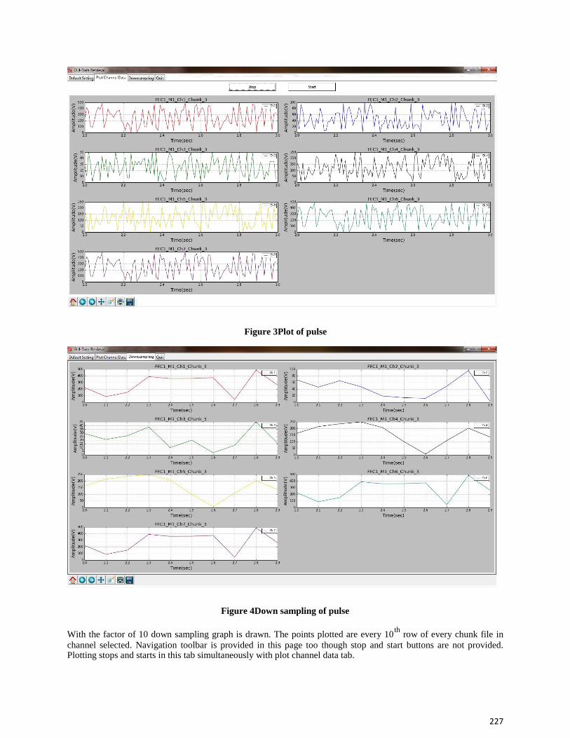
227

Figure 3Plot of pulse

Figure 4Down sampling of pulse

With the factor of 10 down sampling graph is drawn. The points plotted are every 10th

row of every chunk file in

channel selected. Navigation toolbar is provided in this page too though stop and start buttons are not provided. Plotting stops and starts in this tab simultaneously with plot channel data tab.

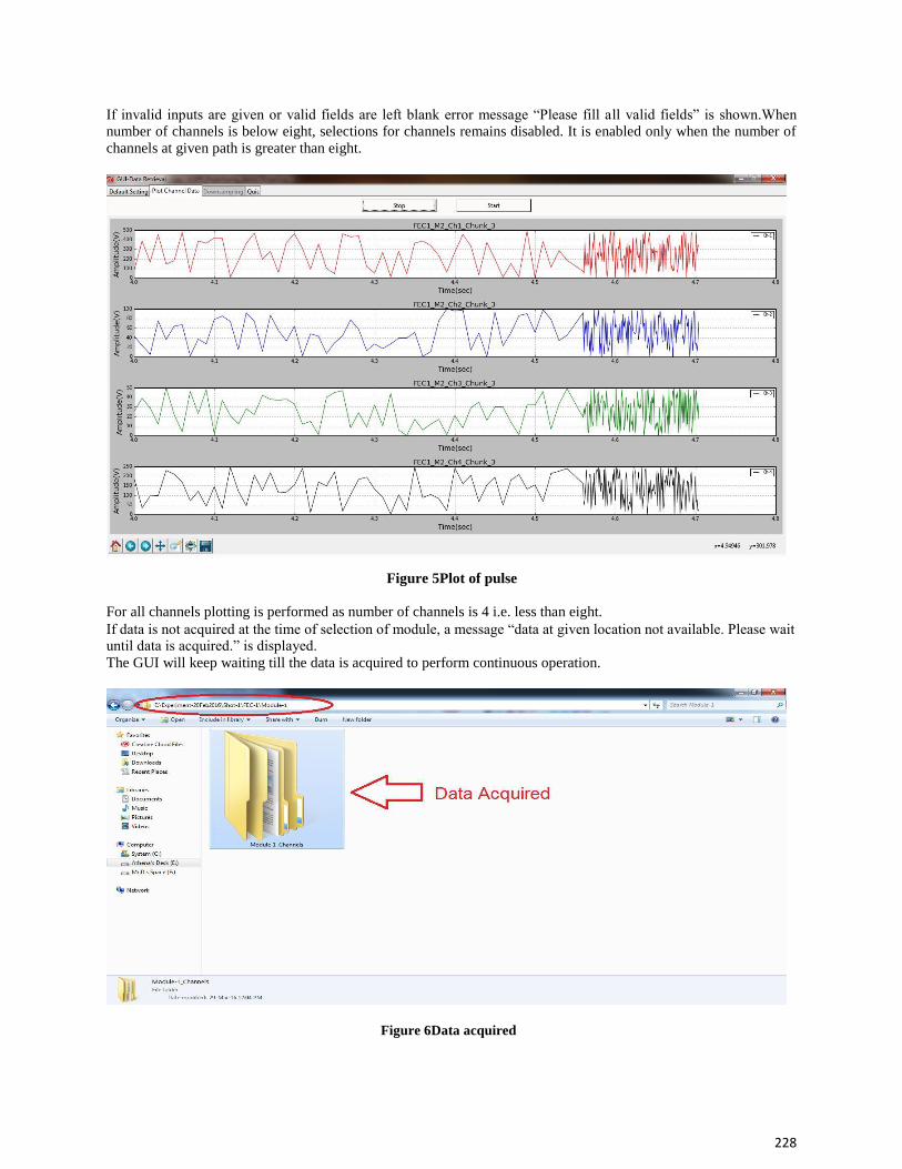
228

If invalid inputs are given or valid fields are left blank error message “Please fill all valid fields” is shown.When number of channels is below eight, selections for channels remains disabled. It is enabled only when the number of

channels at given path is greater than eight.

Figure 5Plot of pulse

For all channels plotting is performed as number of channels is 4 i.e. less than eight. If data is not acquired at the time of selection of module, a message “data at given location not available. Please wait until data is acquired.” is displayed.

The GUI will keep waiting till the data is acquired to perform continuous operation.

Figure 6Data acquired

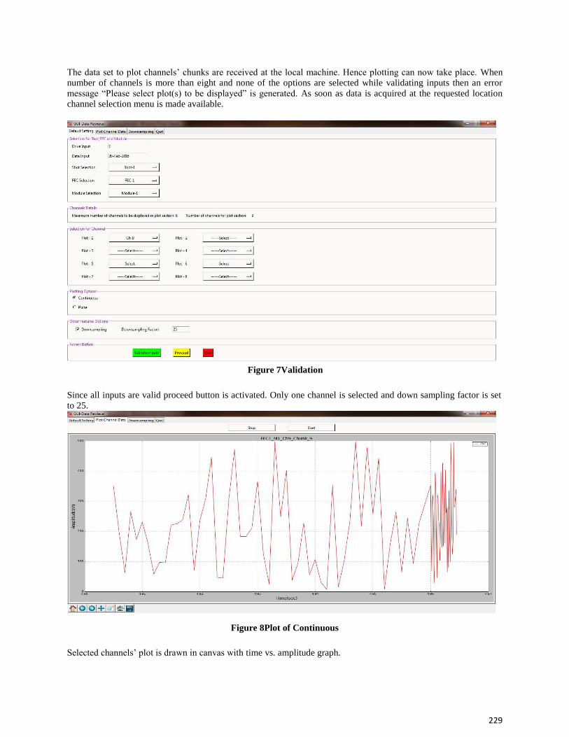
229

The data set to plot channels‟ chunks are received at the local machine. Hence plotting can now take place. When number of channels is more than eight and none of the options are selected while validating inputs then an error

message “Please select plot(s) to be displayed” is generated. As soon as data is acquired at the requested location channel selection menu is made available.

Figure 7Validation

Since all inputs are valid proceed button is activated. Only one channel is selected and down sampling factor is set to 25.

Figure 8Plot of Continuous

Selected channels‟ plot is drawn in canvas with time vs. amplitude graph.

230

Figure 9Down sampled plot of Continuous

With down sampling factor of 25 plotting has been done.

4. Conclusion The developed software platform for the data retrieval and scientific data presentation has been

successfully tested with mapping server data on client machine. The codes were tested for pulse mode operation as

well as continuous operation through data server. The developed program was tested for raw data plotting and

processed data plotting. The implemented algorithm for data plotting can be operated at different client machines on the network.

5. REFERENCES [1] Flynt, Clifton. Tcl/Tk for Real Programmers. Academic Press (AP Professional), ISBN: 0-12261-205-1, 1998. [2] Foster-Johnson, Eric. “Graphical Applications with Tcl and Tk”, 2nd edition. M&T Books. ISBN: 1-55851-569-0, 1997. 1.2.2 Harrison, Mark and Michael J. McLennan. “Effective Tcl/Tk Programming: Writing Better Programs in Tcl and Tk.” Addison Wesley Longman, 1997. [3] Ousterhout, John. Tcl and the Tk Toolkit. Addison-Wesley, 1994. ISBN: 0-20163-337-X. [4] Raines, Paul. Tcl/Tk Pocket Reference. O‟Reilly & Associates, 1998. ISBN: 1-56592-498-3.

231

CE03: A Survey on Performance Improvement in Media file

using CDN Cloud Computing

Dhwani Modi

[email protected]

Computer Department, Silver Oak College of Engineering & Technology, Ahmedabad, India Abstract- Cloud Computing becomes a popular tendency in recent years. Content delivery network has been used

for many years to distribute content over the world. The relative between Cloud computing and content delivery

network is exciting. In this paper, we discuss about the content delivery network architectures and advantages of it.

Then discuss about P2P architectures and grouping of both. We proposed a cloud based content delivery network. It

provides better performance and reliable web serving platform. Content providers could place content to nearest

node from the end user. Thus Cloud-CDN and hybrid cloud will become the next generation of content distribution

network. Keyword: Content Delivery Network, P2P, Cloud I. Introduction

With the rapid development of the Internet, Some problems such as latency, package loss, network

congestion occurs when they access the internet. To solve the problem Content distribution technology appears. So

it can optimize the network performance, such as maximizing bandwidth, improving accessibility, maintaining

correctness, by distributing the replication to edge cache server located closest to user.

The reminder of this paper is organized as follows: in the second and third part, we analyze the architecture

of CDN and P2P, and conclude the advantages and disadvantages of them. And in the fourth part we discuss CDN-

P2P hybrid architecture. Finally we introduce the concept of CDN-Cloud. And it will be the next generation of

content distribution network.

The most promising approaches are trying to bridge the success and reliability of CDNs with the scalability and cost effectiveness of peer-to-peer (P2P) protocols, where the end users contribute their own upload capacity thus reducing the load on the CDN servers. 2. Cdn Architecture

A CDN, or Content Delivery Network, is a means of distribution that both large-scale and small-scale

websites incorporate into their website‟s data transfer structure. This technology allows content, usually website

files, to be replicated on various data centers around the world. This is, essentially, a means of caching files close to

the visitor‟s physical location.

The Typical functionality of CDN is: 1) Request redirection service- To redirect a request to end user that

are closest to CDN cache server. 2) Content delivery service- To deliver a replica of content to the end user through

the origin server. 3) Content distribution service- content is distributed to web servers from the origin server. 4)

Management service- To manage network content, to handle accounting, and to monitor content usage.

232

Fig.1 Abstract architecture of content delivery network[3]

The basic idea of CND is guiding the users to the nearest server and achieving load balancing through

effective management mechanism. It constitutes a layer of intelligent virtual network based on the traditional

Internet by placing network node servers in different places. The traditional CDN consists of center nodes and edge

nodes. Center nodes include the global load balancing DNS server and source server. The source server stores

source content and it can be viewed as content provider origin server. It pushes content to the edge nodes directly

and the edge nodes serve the users.

A CDN provider installs their servers at key location across the internet. Each server contains large amount

of local storage plus copies of its data with other servers on the content network through a process called replication.

These servers act as data caches. In order to apply caches data to client around the world most efficiency, CDN

providers install their servers at geographically- dispersed edge location places that directly connected to internet,

typically in the data centers near large Internet Service Providers (ISPs) [5].

The principle of CDN is: replicate the desired content to some mirrored servers which are strategically

placed in different locations; therefore users are redirected to the nearest servers in order to fetch the required

content. These approaches can efficiently optimizing network bandwidth and improving content delivery

performance. And also reduce user‟s response time. Benefits of CDN:

It can improve publisher‟s quality of service. Client users enjoy much faster downloads for CDN enable content like videos and much more. And

generally better responsive for internet applications. It can improve network latency and greater response time.

233

3. P2P Architecture

Peer-to-Peer Architecture (P2P Architecture) is commonly used computer networking architecture in which

each node has the same capability and responsibility.

P2P networks have many applications, but most common is content distribution. This includes content

delivery, media streaming, software distribution, which all are on-demand content delivery.

Fig 3: P2P network Architecture [6]

There are three models of unstructured P2P computer network architecture, and that is Pure P2P, Hybrid P2P,

and Centralized P2P. In structured P2P computer network architecture, workstations (nodes), and sometimes

resources as well, are organized according to specific criteria and algorithms. This leads to overlays with specific

topologies and properties.

Advantages of P2P:

1.2.3 In P2P network, all clients provide resources, including bandwidth, storage space, and computing

power. Thus total capacity of the system is increase with client.

1.2.4 The distributed P2P network increase robustness in case of failures by replicating data over

multiple peers.

1.2.5 Pure P2P networks have find data without need for any centralized index server.

Limitations to P2P and CDN:

CDN and P2p are two leading architecture of content distribution network. It can reduce the end users

perceive latency, and decrease the deployment cost. But there are some disadvantages of its architecture. 1) Network

cost: with increase the total network cost, it increases the network traffic. 2) Economic cost: The cost of service rate

for web content distribution increases, resulting in increasing the running and investment cost of CDN. 3) Social

cost: Content distribution has been centralized to CDN providers.

4. Limitations to P2p and Cdn CDN and P2P are two dominant architectures of content distribution network. The former can reduce end-

users‟ perceive latency, and the latter can decrease deployment cost. However, there are still some disadvantages of

its architecture in our research. 1) Network cost: With the increase of total network cost, servers and corresponds

increase in network traffic. 2) Economic cost: The cost of service rate for Web content distribution increases,

resulting in the increase in initial investment and running cost of CDN. 3) Social cost: Content distribution has been

centralized to CDN providers and revenue monopolization in this area. The huge financial cost relates to CDN

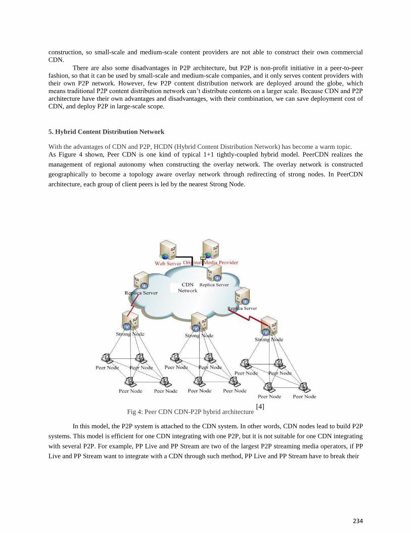
234

construction, so small-scale and medium-scale content providers are not able to construct their own commercial CDN.

There are also some disadvantages in P2P architecture, but P2P is non-profit initiative in a peer-to-peer

fashion, so that it can be used by small-scale and medium-scale companies, and it only serves content providers with

their own P2P network. However, few P2P content distribution network are deployed around the globe, which

means traditional P2P content distribution network can‟t distribute contents on a larger scale. Because CDN and P2P

architecture have their own advantages and disadvantages, with their combination, we can save deployment cost of

CDN, and deploy P2P in large-scale scope.

5. Hybrid Content Distribution Network With the advantages of CDN and P2P, HCDN (Hybrid Content Distribution Network) has become a warm topic.

As Figure 4 shown, Peer CDN is one kind of typical 1+1 tightly-coupled hybrid model. PeerCDN realizes the

management of regional autonomy when constructing the overlay network. The overlay network is constructed

geographically to become a topology aware overlay network through redirecting of strong nodes. In PeerCDN

architecture, each group of client peers is led by the nearest Strong Node.

Fig 4: Peer CDN CDN-P2P hybrid architecture [4]

In this model, the P2P system is attached to the CDN system. In other words, CDN nodes lead to build P2P

systems. This model is efficient for one CDN integrating with one P2P, but it is not suitable for one CDN integrating

with several P2P. For example, PP Live and PP Stream are two of the largest P2P streaming media operators, if PP

Live and PP Stream want to integrate with a CDN through such method, PP Live and PP Stream have to break their

235

current overlay construction and data transmission mechanisms to adapt to the CDN, which will increase the

integration difficulty.

6. The Architecture of Cdn Cloud

From the above, the CDN system can reduce user response time and provide better browsing experience.

But with the increase of users and more network traffic, CDN need to constantly increase its IT infrastructure to

meet user‟s requirements. Thus the advantage of cloud computing make it become an effective solution for the

current CDN. It reduces the cloud export congestion and user access delay.

The Architecture of CDN cloud system is shown in Figure 5. Content provider puts content in the cloud,

the master is responsible for content distribution. It allocates the location for content and saves the copies in other

area. Content provider doesn‟t have to maintain the origin server. Master will be responsible for all data grouping

after being store in the cloud. According different geographical location, the CDN is divided into different area.

Each has one authority server and one cache server. CDN cloud adds a DNS server to realize the DNS redistribution

mechanism.

Fig 5: Overview of cloud CDN architecture [2]

Cloud storage is an important application of cloud computing, and many websites uses private cloud

storage to distribute their content. Many cloud storage provider, such as METACDN, Cloud Front, and it has low

cost, faster response time. Many cloud storage suppliers can provide basic storage services, such as load balancing,

load redirection, and monitoring.

236

7. Conclusion

In this paper, we describe the CDN technology and its advantage for retrieving the contents from the

internet. Then we discuss P2P technology and it has become an important part of content distribution network. CDN

and P2P grouping is more useful over the internet. We describe the limitation of CDN and P2P architecture. Then

merging CDN with cloud is most effective to receive the content from the website, it has low cost, greater response

time and better performance. CDN cloud is become next generation of content distribution network.

8. REFERENCES

[1] Chia-feng Lin, Muh-Chyi Leu, Chih-wei chang, Shyan-ming Yuan,”The Study and Methods for cloud based

CDN”. In IEEE International Conference on Cyber-Enabled Distributed computing and Knowledge Discovery,

October 2011

[2] Li Ling, Ma Xiaozhen, Huang Yulan. CDN Cloud: “A Novel Scheme for Combining CDN and Cloud

Computing”, IEEE 2nd

International Conference on Measurement, Information and Control, August 2013. [3] http://www.cloudbus.org/cdn/RD/CDNs_files/CDN_1.JPG [4] http://www.jocm.us/uploadfile/2013/0416/20130416034901618.pdf [5] http://compnetworking.about.com/od/internetaccessproviders/fl/Introduction-to-Content-Delivery-

and-Distribution-Networks-CDN.htm

[6]http://www.google.co.in/imgres?imgurl=https://www.gigatribe.com/images/p2p-

networks.jpg&imgrefurl=https://www.gigatribe.com/en/help-p2p-

intro&h=305&w=616&tbnid=BRsiD92NW2fhM:&docid=kEj20qEzKm7sxM&ei=rshSVqirJouCjwP67aqYDg

&tbm=isch&ved=0ahUKEwiouqr1iqbJAhULwWMKHfq2CuMQMwgrKA8wD

http://www.jocm.us/uploadfile/2013/0416/20130416034901618.pdf

http://compnetworking.about.com/od/internetaccessproviders/fl/Introduction-to-Content-Delivery-%20%20%20and-



237

Agent Based Network Surveillance System

Gunjan Bhatt, Chandrashekar TR


Computer Engineering Department, Silver Oak College of Engineering & Technology, Gujarat Technological University, India

Abstract: - In a world which is moving forward at a great pace, Information sharing and communication with others is very vital

to sustain the development of the human kind. Networking provided us a great platform for this and has since

become an irreplaceable tool of communication whose need is only going to increase as we move forward. Increase

in networking also means increase of burden on a network administration. So to cope with this growing burden a

network admin will need all the tools which can make his work a little simpler. Agent Based Network Surveillance

System is one such tool. It has been implemented using raspberry as gateway though which is aimed to provide an

affordable system to small Startup Companies and home users. We are trying to provide a network admin a single

application which will monitor, analyze and control network traffic exactly as he wants.

Keywords: Network Monitoring, Access control, Raspberry pi as gateway.

1. Introduction

Agent Based Network Surveillance System is a centralized application to monitor and manage networked

systems using Java-based packet capturing and manipulating over LAN & WAN both. The GUI of any system is

very important and so we are using Java FX 8with N-tier architecture for a dynamic and responsive UI. The

increasing use of communication networks has raised the demand for advanced network management. A network

management system handles problems related to the reliability, efficiency, security and accountability of networked

systems. This application is concerned with monitoring, analysis, security, file sharing and control of network

performance to ensure effortless network operations. Accurate and effective monitoring is vital for network

management, and is the main focus of our work. The program captures all the packets moving inside and outside

around the network to extract useful information from it and represent it all. This information obtained from the

packets will be helpful for controlling the network with more precision. Also one can analyze and manage

bandwidth utilization, keep track of all activities occurring in the network and be sure that the network performance

is maintained at optimal levels. The security of the resources and data available on our network is of paramount

importance. File and message transferring will also be provided through our software. This application will contain a

server side and a client side program. The Server program is installed on the Raspberry Pi and is operated by the

network admin. It provides all the above mentioned functionalities to the network admin. The client program is

installed on the entire PC in the network. The clients are differentiated on the basis of Privilege level set by the

admin during account creation. The client side can also be used to monitor all the activities done by that particular

client himself. The main purpose of this project is to provide a wide array of functionalities at as low a cost as

possible. To make this possible we chose raspberry pi a low cost mini-PC to act as our Server agent which controls

the whole network. The project also provides a network administrator all the tools needed to manage the network

efficiently in one software. This makes collecting and managing the data much more easy and effective. This

application hence tries to cover a lot of ground when it comes to easing the work of a network administrator and so

acts as a complete solution to for most of his/her problems.

2. Study of current system

There are many network monitor systems today which give a host of functionalities but not any one offer what can be considered as a complete solution. Most functionality found in this software are complex and hence special

care has to be taken in UI to make the system understandable.



238

2.1 Problems in existing systems The current systems found in the market are either too costly or don‟t have even the basic required

functionalities. The open source software like wires hark have a complex and non-user friendly User interface or are very basic

and don‟t give more functionalities. The paid software like PRTG, even though provide a lot of functionalities, are too costly to be bought by small

startups. The need is to find the right balance between both functionalities and cost.

3. Network Setup Used In order for the program work properly it is mandatory for the network to be setup properly. The Raspberry

Pi on which the server program is implemented has to be set as the gateway for all the PCs in the network so that all the packets pass through it. To enable that Feature in Raspberry pi it is mandatory to Follow a bunch of procedure and that are:-

1.2.6 IPV4 Forwarding Must be enabled. 1.2.7 In all the Client pc the gateway must be set to the ip address of Raspberry Pi. 1.2.8 Network Address Translation is must be enabled.

3.1 Physical Setup of the network The below image show the physical setup of the network. This is how all the components are connected

with each other.

Fig 3.1 physical setup of network In, fig 3.1 the user pc and the raspberry pi is connected through the router and the router is connect to the internet. Here all the clients get their internet through the raspberry pi. The role of router is only to switching the packets from internetwork to wide Area network.

3.2 Logical Setup of the network The below image shows how the packet travels logically in the network.

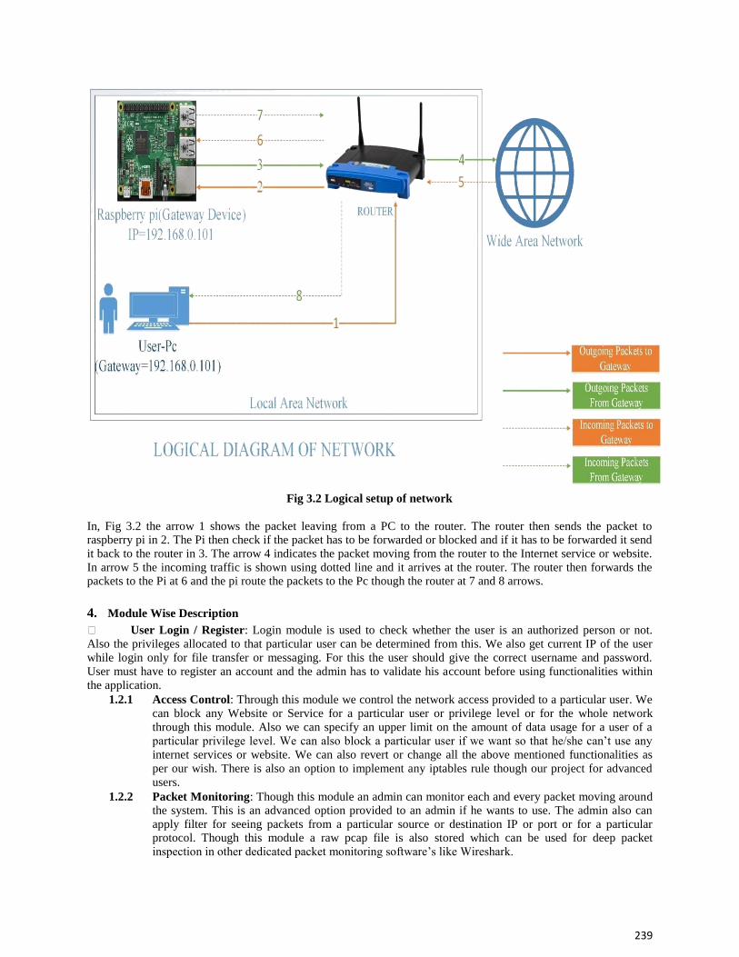
239

Fig 3.2 Logical setup of network

In, Fig 3.2 the arrow 1 shows the packet leaving from a PC to the router. The router then sends the packet to raspberry pi in 2. The Pi then check if the packet has to be forwarded or blocked and if it has to be forwarded it send

it back to the router in 3. The arrow 4 indicates the packet moving from the router to the Internet service or website.

In arrow 5 the incoming traffic is shown using dotted line and it arrives at the router. The router then forwards the packets to the Pi at 6 and the pi route the packets to the Pc though the router at 7 and 8 arrows.

4. Module Wise Description User Login / Register: Login module is used to check whether the user is an authorized person or not.

Also the privileges allocated to that particular user can be determined from this. We also get current IP of the user

while login only for file transfer or messaging. For this the user should give the correct username and password.

User must have to register an account and the admin has to validate his account before using functionalities within

the application. 1.2.1 Access Control: Through this module we control the network access provided to a particular user. We

can block any Website or Service for a particular user or privilege level or for the whole network

through this module. Also we can specify an upper limit on the amount of data usage for a user of a

particular privilege level. We can also block a particular user if we want so that he/she can‟t use any

internet services or website. We can also revert or change all the above mentioned functionalities as

per our wish. There is also an option to implement any iptables rule though our project for advanced

users. 1.2.2 Packet Monitoring: Though this module an admin can monitor each and every packet moving around

the system. This is an advanced option provided to an admin if he wants to use. The admin also can

apply filter for seeing packets from a particular source or destination IP or port or for a particular protocol. Though this module a raw pcap file is also stored which can be used for deep packet

inspection in other dedicated packet monitoring software‟s like Wireshark.

240

1.2.4 Mail Notification: Through this module an admin can select to get mail updates of all the ongoing

activities periodically. He can add multiple email Id of different members to send them all the periodic updates. He

can set the time interval between mails and also select what all the contents that has to be mailed. 1.2.5 File Transfer and Messaging: Through this module the users can do file transferring and messaging inside

the network among themselves. The Client can do file transfer or unicast messaging while the Server can do

multicast and broadcast messages too. As the Server Side of the application will be running on a raspberry pi

dedicated only for this software keeping File transfer module in the server side seemed redundant and hence it will

not be available on the server side of the project. 1.2.6 Manage User Account: The admin can change all the details of a client except his username and password

through this module he can also upgrade the user‟s privilege level or block or unblock him using this module. 1.2.7 Bandwidth Usage and System (Pi) Temperature Monitoring: Through this module live updates of Bandwidth Usage and Pi‟s Temperature is displayed on the home tab of the server side.

5. Results and discussion Though the raspberry pi is a very capable device it can only be used for a small scale networks only

without being lag free. The following results were obtained when the memory was split 30-70 % between GPU and RAM

RAM

GPU

Network utilization

State of PI memory Threads CPU usage (%) used(MB)

used(MB)

Before program

150-200 <50 Depends on Internet Speed 20-30 10 starts

When program is 250-270 =<150 Same as Above 50-60 70-75

idle

When program is in 300-350 150-200 54 Mbps 65-80 76-99

Usage

Table 4.1 Raspberry Pi Statistics

In,table 4.1 it is seen that when program is in full usage the CPU usage can reach up to 99%.Hence in large Scale Systems the pi has to be used in cluster Architecture to work lag free.

5. Conclusion The growth in the previous 4-5 decades is mainly due to the networks (internet) which has enabled sharing

of information at never before speed and ease. This makes networks indispensable tool and a network admin a very

essential person and he would require all help he gets to manage the flow of information at a desirable level.With the

growing responsibilities and burden on a network admin, our project will surely play a constructive role in easing his

burden and better manage his responsibilities thereby increasing the efficiency of the network and of the

organization too.

6. References [1] http://qcktech.blogspot.in/2012/08/raspberry-pi-as-router.html [2] https://code.google.com/archive/p/iotsys/wikis/groupCommunication.wiki

[3] http://www.rpiblog.com/2014/03/installing-oracle-jdk-8-on-raspberry-pi.html

[4] http://docs.gluonhq.com/javafxports/#_setting_up [5] https://www.raspberrypi.org/forums/viewtopic.php?f=63&t=35826 [6] http://stackoverflow.com/questions/17830333/start-raspberry-pi-without-login [7] http://elinux.org/R-Pi_Troubleshooting# [8] https://forum.pfsense.org/index.php [9]http://www.developer.com/java/ent/article.php/1356891/A-PatternFramework-for-ClientServer-Programming-in-Java.htm [10]http://stackoverflow.com/questions/2627706/how-to-icmps-and-traceroutes-in-java

http://qcktech.blogspot.in/2012/08/raspberry-pi-as-router.html

https://code.google.com/archive/p/iotsys/wikis/groupCommunication.wiki

http://www.rpiblog.com/2014/03/installing-oracle-jdk-8-on-raspberry-pi.html

http://docs.gluonhq.com/javafxports/#_setting_up

https://www.raspberrypi.org/forums/viewtopic.php?f=63&t=35826

http://stackoverflow.com/questions/17830333/start-raspberry-pi-without-login

https://forum.pfsense.org/index.php

http://stackoverflow.com/questions/2627706/how-to-icmps-and-traceroutes-in-java

241

Securing MANET against Wormhole Attack

Pooja Bavarva

[email protected]

Computer Engineering Department, Silver Oak College of Engineering & Technology Gujarat Technological

University, India Abstract:-

In mobile ad hoc networks (MANETs) security is of major concern because of its inherent liabilities. The

characteristics of MANETs like infrastructure less network with dynamic topology pose a number of challenges to

security design. There is an increasing threat of attacks in MANET. Wormhole attack is one of the security attacks

on mobile ad hoc networks in which a pair of colluding nodes make a tunnel using a high speed network. This paper

focuses on providing a solution for secure transmission through the network and proposes a neighbor node analysis

approach to identify wormhole attack and removes wormhole link in MANET. The proposed work is simulated

using NS-2 and is analyzed using certain parameters such as throughput, loss rate, delay rate.

Keywords: Wormhole Attack, AODV, Routing, Network Security, MANET

1. Introduction

Due to technological advances in laptop computers and wireless communication devices such as wireless

phone and wireless LANs, wireless communication between the mobile users is becoming more popular than ever.

An ad hoc network is the cooperative engagement of a collection of mobile nodes without the required intervention

of any centralized access point or existing infrastructure. There is an increasing trend to adopt ad hoc networking for

commercial usage. However, their main applications lie in military, tactical and other security sensitive operations.

In these and other applications of ad hoc networking, secure routing is an important issue. Designing a foolproof

security for ad hoc network is a challenging task due to its unique characteristics such as, lack of central authority,

frequent topology changes, rapid node mobility, shared radio channel and limited availability of resources.

Wireless ad hoc networks can be classified into three sub networks wireless sensor networks, wireless

meshnetworks and mobile ad hoc networks. Mobile ad hoc networks consist of auto configuring nodes such as

laptop computers, PDAs and wireless phones that use wireless communication with each other. A mobile ad hoc

network with four nodes is shown in Figure 1. The nodes at the same time may act as both host and router i.e. each

node participates in routing by forwarding data for other nodes and deciding to which node data must be forwarded

next, based on network connectivity. The routers are to move randomly and organize themselves without any

centralized administration. Thus the network topology may change rapidly and unpredictably. Such a network may

be an independent network or may be connected to internet. Applications of ad hoc networks range from military

operations and emergency disaster relief to commercial usage such as community networking and communication


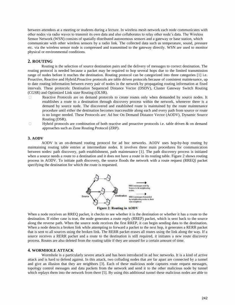
242

between attendees at a meeting or students during a lecture. In wireless mesh network each node communicates with

other nodes via radio waves to transmit its own data and also collaborates to relay other node‟s data. The Wireless Sensor Network (WSN) consists of spatially distributed autonomous sensors and a gateway or base station, which communicate with other wireless sensors by a radio link. The collected data such as temperature, sound, pressure etc. via the wireless sensor node is compressed and transmitted to the gateway directly. WSN are used to monitor

physical or environmental conditions.

2. ROUTING Routing is the selection of source destination pairs and the delivery of messages to correct destination. The

routing protocol is needed because a packet may be required to hop several hops due to the limited transmission

range of nodes before it reaches the destination. Routing protocol can be categorized into three categories [1] i.e.

Proactive, Reactive and Hybrid.Proactive protocols are table driven protocols because of consistent maintenance, up

to date routing information between every pair of nodes in the network by propagating routing information at fixed

intervals. These protocols: Destination Sequenced Distance Vector (DSDV), Cluster Gateway Switch Routing

(CGSR) and Optimized Link state Routing (OLSR). Reactive Protocols are on demand protocols to create routes only when demanded by source nodes. It

establishes a route to a destination through discovery process within the network, whenever there is a

demand by source node. The discovered and established route is maintained by the route maintenance

procedure until either the destination becomes inaccessible along each and every path from source or route

is no longer needed. These Protocols are: Ad hoc On Demand Distance Vector (AODV), Dynamic Source

Routing (DSR). Hybrid protocols are combination of both reactive and proactive protocols i.e. table driven & on demand

approaches such as Zone Routing Protocol (ZRP).

3. AODV AODV is an on-demand routing protocol for ad hoc networks. AODV uses hop-by-hop routing by

maintaining routing table entries at intermediate nodes. It involves three main procedures for communication

between nodes: path discovery, path establishment, path maintenance [1]. The path discovery process is initiated

when a source needs a route to a destination and it does not have a route in its routing table. Figure 2 shows routing

process in AODV. To initiate path discovery, the source floods the network with a route request (RREQ) packet

specifying the destination for which the route is requested.

When a node receives an RREQ packet, it checks to see whether it is the destination or whether it has a route to the

destination. If either case is true, the node generates a route reply (RREP) packet, which is sent back to the source

along the reverse path. When the source node receives the first RREP, it can begin sending data to the destination.

When a node detects a broken link while attempting to forward a packet to the next hop, it generates a RERR packet

that is sent to all sources using the broken link. The RERR packet erases all routes using the link along the way. If a

source receives a RERR packet and a route to the destination is still required, it initiates a new route discovery

process. Routes are also deleted from the routing table if they are unused for a certain amount of time.

4. WORMHOLE ATTACK Wormhole is a particularly severe attack and has been introduced in ad hoc networks. It is a kind of active

attack and is hard to defend against. In this attack, two colluding nodes that are far apart are connected by a tunnel

and give an illusion that they are neighbors [3]. Each of these malicious node captures route request messages,

topology control messages and data packets from the network and send it to the other malicious node by tunnel

which replays them into the network from there [5]. By using this additional tunnel these malicious nodes are able to

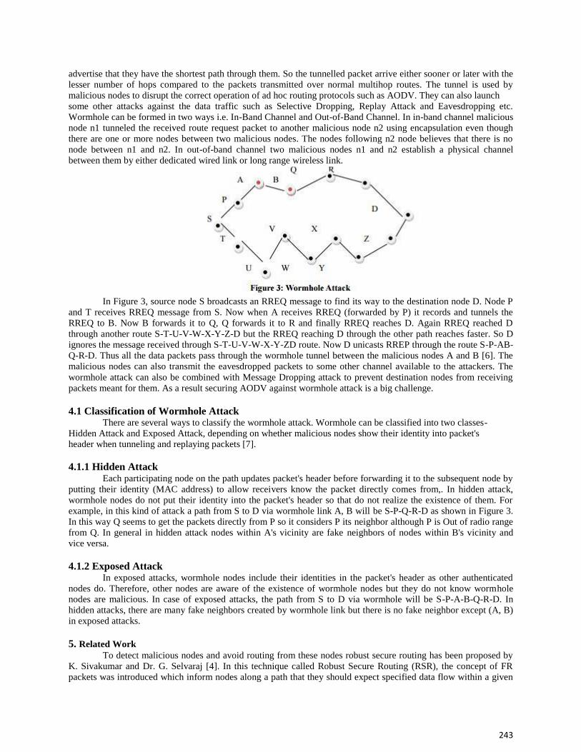
243

advertise that they have the shortest path through them. So the tunnelled packet arrive either sooner or later with the

lesser number of hops compared to the packets transmitted over normal multihop routes. The tunnel is used by

malicious nodes to disrupt the correct operation of ad hoc routing protocols such as AODV. They can also launch

some other attacks against the data traffic such as Selective Dropping, Replay Attack and Eavesdropping etc.

Wormhole can be formed in two ways i.e. In-Band Channel and Out-of-Band Channel. In in-band channel malicious

node n1 tunneled the received route request packet to another malicious node n2 using encapsulation even though

there are one or more nodes between two malicious nodes. The nodes following n2 node believes that there is no

node between n1 and n2. In out-of-band channel two malicious nodes n1 and n2 establish a physical channel

between them by either dedicated wired link or long range wireless link.

In Figure 3, source node S broadcasts an RREQ message to find its way to the destination node D. Node P

and T receives RREQ message from S. Now when A receives RREQ (forwarded by P) it records and tunnels the

RREQ to B. Now B forwards it to Q, Q forwards it to R and finally RREQ reaches D. Again RREQ reached D

through another route S-T-U-V-W-X-Y-Z-D but the RREQ reaching D through the other path reaches faster. So D

ignores the message received through S-T-U-V-W-X-Y-ZD route. Now D unicasts RREP through the route S-P-AB-

Q-R-D. Thus all the data packets pass through the wormhole tunnel between the malicious nodes A and B [6]. The

malicious nodes can also transmit the eavesdropped packets to some other channel available to the attackers. The

wormhole attack can also be combined with Message Dropping attack to prevent destination nodes from receiving

packets meant for them. As a result securing AODV against wormhole attack is a big challenge.

4.1 Classification of Wormhole Attack There are several ways to classify the wormhole attack. Wormhole can be classified into two classes-

Hidden Attack and Exposed Attack, depending on whether malicious nodes show their identity into packet's header when tunneling and replaying packets [7].

4.1.1 Hidden Attack Each participating node on the path updates packet's header before forwarding it to the subsequent node by

putting their identity (MAC address) to allow receivers know the packet directly comes from,. In hidden attack,

wormhole nodes do not put their identity into the packet's header so that do not realize the existence of them. For

example, in this kind of attack a path from S to D via wormhole link A, B will be S-P-Q-R-D as shown in Figure 3.

In this way Q seems to get the packets directly from P so it considers P its neighbor although P is Out of radio range

from Q. In general in hidden attack nodes within A's vicinity are fake neighbors of nodes within B's vicinity and

vice versa.

4.1.2 Exposed Attack In exposed attacks, wormhole nodes include their identities in the packet's header as other authenticated

nodes do. Therefore, other nodes are aware of the existence of wormhole nodes but they do not know wormhole nodes are malicious. In case of exposed attacks, the path from S to D via wormhole will be S-P-A-B-Q-R-D. In

hidden attacks, there are many fake neighbors created by wormhole link but there is no fake neighbor except (A, B)

in exposed attacks.

5. Related Work To detect malicious nodes and avoid routing from these nodes robust secure routing has been proposed by

K. Sivakumar and Dr. G. Selvaraj [4]. In this technique called Robust Secure Routing (RSR), the concept of FR

packets was introduced which inform nodes along a path that they should expect specified data flow within a given

244

time frame. The path elements can therefore be on the lookout for the given data flow, and in the event that they do

not receive the traffic flow, they can transmit info to the source informing it that the data flow they expected did not

arrive. A path tracing algorithm for detection and prevention of wormhole attack has been proposed by P. Anitha and M. Sivaganesh [11]. The PT algorithm runs on each node in a path during the AODV route discovery process. It calculates per hop distance based on the RTT value and wormhole link using frequency appearance count. The

corresponding node detects the wormhole if per hop distance exceeds the maximum threshold range.

An effort return based trust model to detect and evade wormhole attack is proposed by Shalini Jain and Dr.Satbir

Jain in [12] where each node executing the trust model, measures the accuracy and sincerity of the immediate

neighboring nodes by monitoring their participation in the packet forwarding mechanism. The sending node verifies

the different fields in the forwarded IP packet for requisite modifications through a sequence of integrity checks. If

the integrity checks succeed, it confirms that the node has acted in a benevolent manner and so its direct trust

counter is incremented. Similarly, if the integrity checks fail or the forwarding node does not transmit the packet at

all, its corresponding direct trust measure is decremented. This derived trust is then used to influence the routing

decisions, which in turn guide a node to avoid communication through the wormholes.

For detection and prevention of attack in MANET an efficient multipath algorithm was proposed by Waseem Ahad

and Manju Sharma [10]. This algorithm will randomly generate a number in between 0 to maximum number of

nodes and make the node with same number as transmitter node as wormhole attack is done by transmitter and

receiver so have to decide the transmitter and receiver. Then generate the route from selected transmitting node to

any destination node with specified average route length. After this it will send packet according to selected

destination and start timer to count hops and delay. By repeating the whole process up to this point will be required

as to store routes and their hops and delay. Now for detection of malicious node, if the hop count for a particular

route decreases abruptly for average hop count then at least one node in the route must be attacker. Algorithm will

check the delay of all previous routes which involve any on node of the suspicious route. The node not encounter

previously should be malicious.

An end-to-end detection of wormhole attack (EDWA) in wireless ad hoc networks is proposed by Xia Wang and

Johnny Wong [8]. Authors first presented the wormhole detection which is based on the smallest hop count

estimation between source and destination. If the hop count of a received shortest route is much smaller than the

estimated value an alert of wormhole attack is raised at the source node. Then the source node will start a wormhole

tracing procedure to identify the two end points of the wormhole. Finally, a legitimate route is selected for data

communication

An Approach to Defend against Wormhole Attack in Ad hoc Network Using Digital Signature is proposed by

Pallavi Sharma and Aditya Trivedi [9]. This paper presented a mechanism which is helpful in prevention of

wormhole attack in ad hoc network is verification of digital signatures of sending nodes by receiving node because

each legitimate node in the network contains the digital signature of every other legitimate nodes of same network.

In proposed solution, if sender wants to send the data to destination, firstly it creates a secure path between sender

and receiver with the help of verification of digital signature. If there is presence of any malicious node in between

the path then it is identified because malicious node does not have its own legal digital signature.

6. Proposed Work We are presenting a novel approach to secure AODV against wormhole attack in MANET using neighbor

node analysis. In our work, neighbor node analysis approach analyze the neighboring nodes so as to check the

authenticity of the nodes for secure transmission of data over the network. According to this approach a node will

request to its neighboring nodes and perform a request and response mechanism. The node will maintain the table to

track the timeout. If the reply time is not accurate there is an attack in the network. All the intermediate nodes are

analyzed to detect the presence of wormhole attack using AODV protocol in MANET. The steps of proposed

algorithm are:

Step 1: As transmission initiates, source node search for the neighbor nodes and form a neighbor list. Step 2: Source node then generates RREQ packet and encrypt it using the public keys of neighboring nodes and distribute it all around. Step 3: If the neighboring node receiving RREQ packet, decrypt it using their private key then the node is

authenticated otherwise, remove the node from neighbor list and report node as bad node.

245

Step 4: If node is authenticated it will send the RREP message to the source node. Step 5: Source node will record the response time of RREP message. Step 6: Compare the response time of RREP message with response time of actual message sent. If Response Time (Actual Message) > Response Time (RREP) + Threshold Then

1.2.9 Wormhole link is present in that route. 1.2.10 Block that route and update it in routing table. 1.2.11 Fetch another route from the routing table.

Step 7: The process is repeated for each node in the neighbor list till the destination is reached.

7. Simulation Based Performance Analysis In our experiment we simulated 50 nodes distributed over 670m x 670m terrain on NS-2. The initial

positions of nodes are random. The implementation used 802.11 MAC layer and CBR traffic type. The AODV protocol is used which is an on demand routing protocol and is given in Table 1

In Figure 4, the comparison between the existing (with wormhole attack) and proposed approach (without wormhole attack) was made on basis of throughput. Here the simulation is carried out for 10 seconds. The given graph shows

the throughput for both the scenarios (existing and proposed). Initially the throughput was zero at the time of start.

After the TCP (Transmission Control Protocol) connection was build, we can see that the throughput increased in

the proposed system.

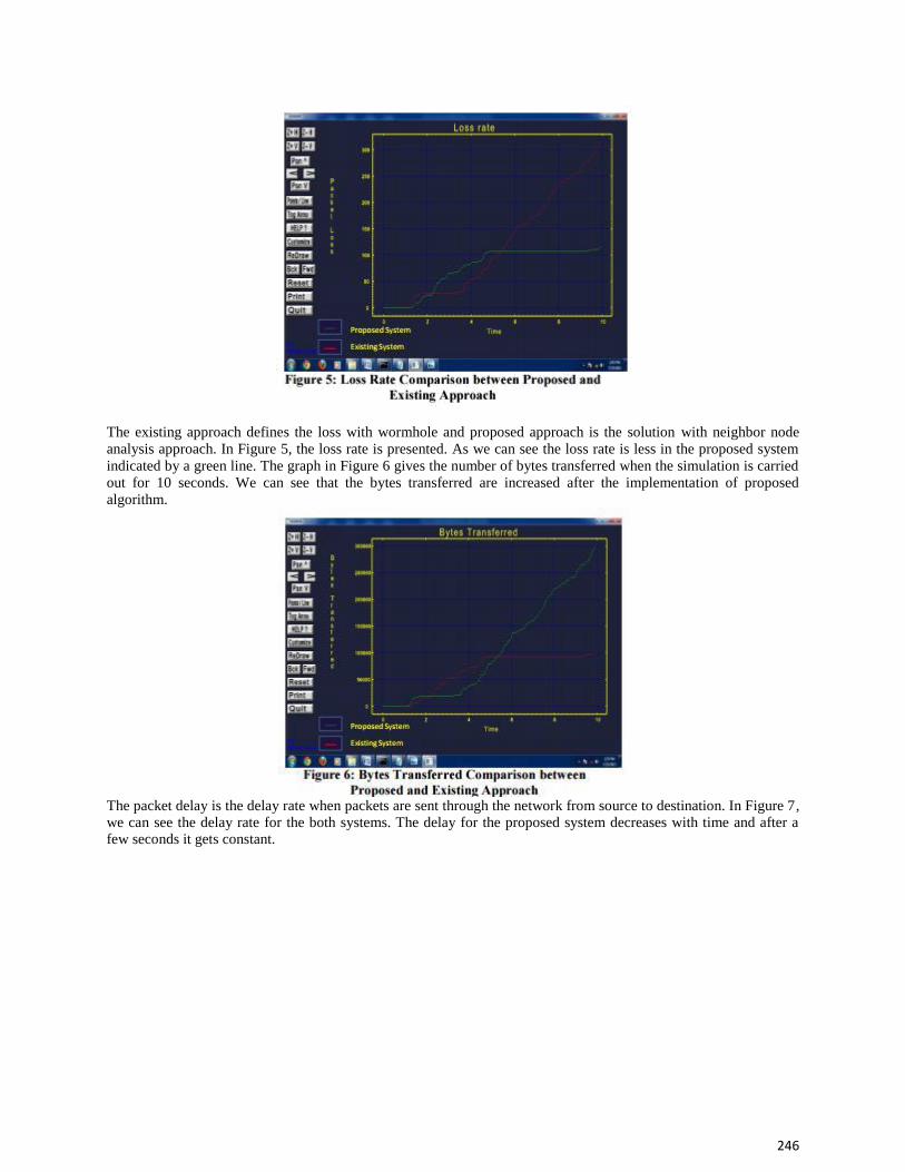
246

The existing approach defines the loss with wormhole and proposed approach is the solution with neighbor node

analysis approach. In Figure 5, the loss rate is presented. As we can see the loss rate is less in the proposed system

indicated by a green line. The graph in Figure 6 gives the number of bytes transferred when the simulation is carried

out for 10 seconds. We can see that the bytes transferred are increased after the implementation of proposed

algorithm.

The packet delay is the delay rate when packets are sent through the network from source to destination. In Figure 7, we can see the delay rate for the both systems. The delay for the proposed system decreases with time and after a few seconds it gets constant.

247

8. Conclusion Wormhole attack is one of the most serious attacks in MANETs. Many solutions have been proposed to detect

and remove the attack but are not perfect in terms of efficiency or any special hardware, the proposed approach is

based on neighbor node analysis and provides a solution for detection of wormhole attack and removal of wormhole

link from the network. The proposed technique gives a better solution for wormhole attack in the network. The

proposed work with respect to four parameters throughput, loss rate, bytes transferred and delay rate has been

simulated. Simulation results shows that the proposed approach is successful in detecting wormhole attack and locating

wormhole link thus avoiding wormhole link in route discovery process providing better efficiency.

9. REFERENCES [1] Achint Gupta, Priyanka V J, Saurabh Upadhyay, “Analysis of wormhole Attack in AODV based MANET Using Opnet Simulator”, International Journal of Computing, Communications and Networking Vol. 1,October 2012. [2] Jatin D. Parmar, Ashish D. Patel, Rutvij H. Jhaveri1, Bhavin I. Shah, “ MANET Routing Protocols and Wormhole Attack against AODV”, IJCSNS International Journal of Computer Science and Network Security, Vol. 10, No.4, April 2010.

[3] Reshmi Maulik, Nabendu Chaki, “A Study on Wormhole Attacks in MANET”, International Journal of Computer Information Systems and Industrial Management Applications ISSN 2150-7988 Vol. 3, pp. 271-279, 2011. [4] K. Sivakumar, Dr. G. Selvaraj, “Analysis of Worm Hole Attack In MANET And Avoidance Using Robust Secure Routing Method”, International Journal of Advanced Research in Computer Science and Software

Engineering, Vol. 3, No. 1, January 2013. [5] Yashpalsinh Gohil, Sumegha Sakhreliya, Sumitra Menaria, “A Review on Detection and Prevention of Wormhole Attcaks in MANET”, International Journal of Scientific and Research Publications, Vol. 3, No.

2, February 2013. [6] Abari Bhattacharya, Himadri Nath Saha, “A Study of Secure Routing in MANET various attacks and their countermeasures”, IEMCON organized in collaboration with IEEE in January 2011. [7] Susheel Kumar, Vishal Pahal, Sachin Garg, “Wormhole Attack in Mobile Ad Hoc Networks: A Review”, IRACST, Vol. 2, April 2012. [8]Xia Wang, Johnny Wong, “An End-to-end Detection of Wormhole Attack in Wireless Ad hoc Networks”, 31st Annual International Computer Software and Applications Conference IEEE, 2007. [9] Pallavi Sharma, Prof. Aditya Trivedi, “An Approach to Defend Against Wormhole Attack in Ad Hoc Network Using Digital Signature”, IEEE, 2011. [10] Waseem Ahad, Manju Sharma, “Efficient Multipath Algorithm in MANETs to Prevent Wormhole Attack”, CT International Journal of Information &Communication Technology Vol. 1, No. 1, 2013.

[11] P. Anitha, M. Sivaganesh, “Detection And Prevention Of Wormhole Attacks In Manets Using Path Tracing”, International Journal of Communications Networking System, Vol. 01, No. 02, December 2012. [12] Shalini Jain, Dr.Satbir Jain, “ Detection and prevention of wormhole attack in mobile adhoc networks” , International Journal of Computer Theory and Engineering, Vol. 2, No. 1 February, 2010.

248

Zaptro-an inter communication tool for Organizations

Shnanshe Diksha, Krima Rokadiya

[email protected] , [email protected]

Information Technology Department, Silver Oak College of Engineering & Technology, Gujarat Technological

University, India

Abstract:- Spanning three nations, tool can afford opportunities for a wide variety of business and customers, from retail,

finance to insurance and Non Government Organization. The portal will provide secure way of exchanging

messages, text docs and images. Here again internal chat on one to one basis and group chat is provided to better

communication channel. The automation of task in this way without wasting time is becoming possible. Secure

space for inter communication that encourages employees in an organization to exchange knowledge, documents,

task management, contact data. The intranet has evolved to companies‟ needs of today. The main purpose of inter-

communication software is developing the communication with all person of the same organization on the net. We

can compare the Inter-communication software with the telephonic communication. Normally in Telephone

Conference there will be more than two users connected at a time and all the users are able to hear word from any

one of the users. Social clubs for a brand, company, event, team, community, goal... that allow members to interact

privately and exclusively, becoming an active part of a group connected by a common purpose or interest that

transcends the virtual community itself. Communities are for companies, idea management, support, training,

recruitment.

Keywords: Project management, Risk Management, Effort Estimation

1. Introduction Communication has a major role to play for the well being and growth of an organization. Sometimes

communication alone can be responsible for rescuing an organization out of distressed times while the lack of it can

be the sole cause for its debacle. Communication has evolved into one of the key factors in the aspects of

organizational operations that as even a few years back not given enough importance. Communication serves four

major functions within a group or an organization, control, motivation, emotional, expression and information.

Communication acts to control member behavior in more ways than many. Communication acts to control member

behavior in several ways. Organizations acts to control member Organizations have authority hierarchies and formal

guidelines that employees are required follow. When employees for instance, are required to first communicate any

job related grievance to their immediate boss to follow their job description, or to comply with company policies,

communication is performing a control function .But informal communication also controls behavior. When work

groups tease or harass a member who produces too much and makes the rest of the group look bad .They are

informally communicating with and controlling the member‟s behavior.[1][2]

No group can exist without communication. However communication is thought to be the transference and

the transmission of the meaning of information and ideas. But this interpretation of communication is not always

considered as proper. This can be concluded because if in an organization two people, having the knowledge about

two different languages have to interact then there is no utility of the transference of meanings .Therefore

communication must include a dual process of transference and the understanding of meanings. An idea no matter

how great it might be is of no practical use Communication, thus is not only about imparting the meaning of a

particular idea.



249

An idea, however great it might be has no practical use without unless it is transmitted and interpreted by others.

Perfect communication, if there was such a thing would exist when the idea pictured by the sender would be exactly

the same as that envisioned by the sender. [1]

This tool is a social (and mobile) business platform with an array of customization options for internal collaboration

and communication. Through the site, you can create file management, task assignments and execution, and a

contacts directory. Spanning 3 nations, tool should afford opportunities for a wide variety of businesses and

customers, from retail and finance to insurance and NGO sectors. The Scope of this tool is developing the

communication with all persons of the same organization on the net. We can compare the Intra-communication s/w

with the Telephonic Communication. Normally in Telephone Conference there will be more than two users

connected at a time and all the users are able to here word from any one of the users. So implementing the same

concept on the Net is nothing but Intra-Communication Software.

Project management is the application of knowledge, skills, tools, and techniques to project activities to meet project

requirements. Managing projects is not the same as managing ongoing operations. This work that is unique and

temporary requires different management disciplines.

Project management is accomplished through the use of the following 5 processes:

1. Initiation

2.Planning

3. Execution

4.Controlling and

5.Closure

The term “project management” is sometimes used to describe an organizational approach to the management of ongoing operations. This approach treats many aspects of ongoing operations as projects to apply project

management techniques to them. A detailed discussion of the approach itself is outside the scope of this document.

Project Management: The Managerial Process, 4e is distinguished by its balanced treatment of both the technical

and behavioral issues in project management as well as by its coverage of a broad range of industries to which

project management principles can be applied. It focuses on how project management is integral to the organization

as a whole. The 4th edition reflects the latest changes found in the practice. The core of PLM (product lifecycle

management) is in the creations and central management of all product data and the technology used to across this

information and knowledge PLM as a discipline emerged from tools such as CAD, CAM and PDM, but can be

viewed as the integration of these tools with methods, people and the processes through all stages of a product‟s life.

It is not just about software technology but is also a business strategy.

Project planning is part of project management, which relates to the use of schedules such as Gantt charts to plan

and subsequently report progress within the project environment. Initially, the project scope is defined and the

appropriate methods for completing the project are determined. Following this step, the durations for the various

tasks necessary to complete the work are listed and grouped into a work breakdown structure. The logical

dependencies between tasks are defined using an activity network diagram that enables identification of the critical

path. Float or slack time in the schedule can be calculated using project management software. Then the necessary

resources can be estimated and costs for each activity can be allocated to each resource, giving the total project cost.

At this stage, the project schedule may be optimized to achieve the appropriate balance between resource usage and

project duration to comply with the project objectives. Once established and agreed, the project schedule becomes

what is known as the baseline schedule. Progress will be measured against the baseline schedule throughout the life

of the project. Analyzing progress compared to the baseline schedule is known as earned value management.

The inputs of the project planning phase include the project charter and the concept proposal. The outputs of the

project planning phase include the project requirements, the project schedule, and the project management plan.

250

2. Estimation

Estimation is the process of finding an estimate, or approximation, which is a value that is usable for some purpose

even if input data may be incomplete, uncertain, or unstable The value is nonetheless usable because it is derived

from the best information available. Estimation involves "using the value of a statistic derived from a Sample to

estimate the value of a corresponding population parameter". The sample provides information that can be projected,

through various formal or informal processes, to determine a range most likely to describe the missing information.

An estimate that turns out to be incorrect will be an overestimate if the estimate exceeded the actual result and an

underestimate if the estimate fell short of the actual result. Approximation, prediction, or projection of a quantity

based on experience and/or information available at the time, with the Recognition that other pertinent facts are

unclear or unknown. An estimate is almost the same as an educated guess, and the cheapest type of modeling.

Estimation is finding a number that is close enough to the right answer. The process is of forecasting or

approximating the time and cost of completing project deliverables.

Estimation is often done by sampling which is counting a small number of examples something, and projecting that

number onto a larger population. An example of estimation would be determining how many candies of a given size

are in a glass jar. Because the distribution of candies inside the jar may vary, the observer can count the number of

candies visible through the glass, consider the size of the jar, and presume that a similar distribution can be found in

the parts that cannot be seen, thereby making an estimate of the total number of candies that could be in the jar if

that presumption were true. Estimates can similarly be generated by projecting results from polls or surveys on to

the entire population.

3. Implementation Environment

Zaptro-an inter communication is an advanced java based web application, so appropriate IDE is required for the

development of application, actual devices are necessary for testing, running, and debugging it like netbens 8.0. As

the database plays very important role in the application, it is essential to use efficient database service providing

software. My SQL is an add-on in Google chrome browser, which is highly preferred and recommended in the area

of well web site development

Hardware: Customer Side:

Processer: Pentium dual core.

RAM: 4GB (128 SD-RAM).

Hard Disk: 500GB or above.

Monitor: 14”VGA.

Mouse

DVD Writer

Developer Side:

Operating System : Window

Technology : Java/J2EE (JDBC, Servlets, JSP,JSTL)

Web Technologies : Html, JavaScript, CSS,JQUERY,AJAX,JSON

IDE : Eclipse/NetBeans

Hardware:

Customer Side:




Monitor: 14”VGA.

Mouse

DVD Writer

251

Developer Side:





Hardware:

Customer Side:




Monitor: 14”VGA.

Mouse

DVD Writer

Developer Side:





Web Server : Tomcat/Glassfish

Database : MySQL& /Hibernate

4. Modules Specification

The modules involved in the application are:

User Login / Register

Manage Administration

Assign projects and take review

Conduct meeting and conference

Create chat room

Module wise Description:

User Login/Register: Login module is used to check whether the user is an authorized person or not.

For this the user should give the correct username and password. User must have to register an account

before using functionalities within the application.

Manage Administration: Administration module is used to manage the user, log, session, user team.

Administrative managers oversee the support operations of an organization. They ensure that there is

effective information flow and that resources are employed efficiently throughout a system

Assign projects and take review: This module explains how to staff a project based on the skills and

availability of worker resources. By using resource-based scheduling, you can deploy your

organization's workers efficiently and effectively when they are needed. You can review the capacity

of each worker and see whether the worker is being adequately scheduled, and then assign the worker

to a project or activity based on the project requirements and the worker‟s qualification.

252

Conduct meeting and conference: Conduct conferences with their employee. So they can get online

decisions from employee from the different branches of the company. The advantage is that the

company is having branches throughout the country. So this will help them to communicate business

affairs of the company and live meetings and conferences between their directors. They can conduct

board of directors meeting. It will give On-line solutions from the superiors to the employees.

Create chat room: By using this module administrator can create chat rooms, they can login in to chat

rooms and also they can view all chat rooms which are available in this portal. By using this

functionality employee can create chat rooms, they can login in to chat rooms and also they can view

all chat rooms which are available in this portal.

SECURITY FEATURES

Securing an open platform requires robust security architecture and rigorous security programs.java base web

application was designed with multi-layered security that provides the flexibility required for an open platform,

while providing protection for all users of the platform.

Java is designed to both reduce the probability of these attacks and greatly limit the impact of the attack in

the event it was successful.

Java is a high security that seeks to be the most secure and usable operating system for web sites platforms

by re-purposing traditional operating system security controls to:

Protect user data

Protect system resources (including the network)

Mandatory application sandbox for all applications

Secure inter-process communication

Application signing

Application-defined and user-granted permission

4. Results and Discussion

Write the actual input data to be provided and the expected output for your actual working product. You must

provide the actual input data values, not just a description. Often the test data can be shown in tabular form, with a

column of input items and the corresponding column of expected outputs.

1) Test case For Log In

Project: - Zaptro-an inter communication system. Objective: - To check whether user name & Password valid or invalid.

Prepared By: Group-10

Page: -Sign In

Sr.no. Steps Expected Data Status

1 Enter user Email , Password and press Sign

In button

Should navigate user to dashboard

Pass

2 Enter Email only and press Sign In button. Should Display message ―password is required” Invalid

3 Enter Password and press Sign In button Should display message "Email is required? Invalid

4 Enter blank Email and blank Password and

press Sign In button.

Should display message ―Email is required & ― Password is required!

Invalid

5 Enter wrong Email And password Should display a message ―Invalid Email or

password

Invalid

253

1 Log in-team leader

Fig. 2 Home page of team leader

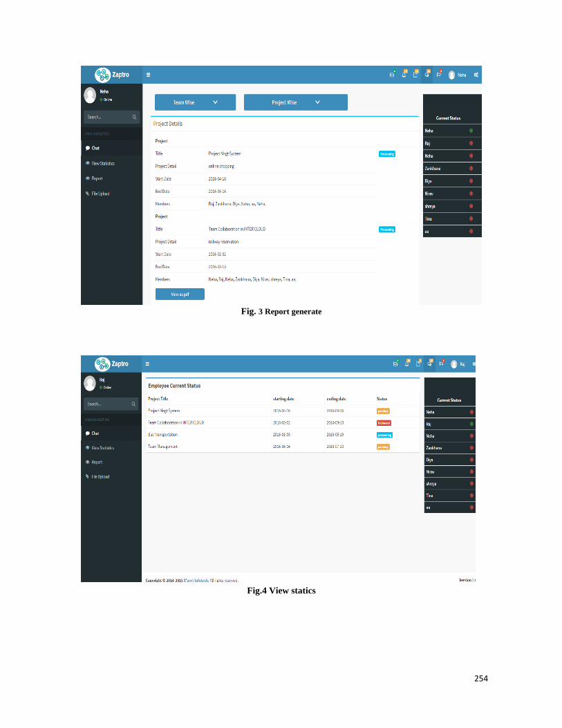
254

Fig. 3 Report generate

Fig.4 View statics

255

Fig.5 Manage Employee

Fig [1] is representing the Login page of the tool & fig [2, 3, 4, 5] are the remaining images of the tool.

5. Limitation and Future Enhancement

Though we tried best in developing this Tool but as limitation are more part of any tool are of our tool.

Some limitations are as follow.

As we are not aware of how to use different compression algorithm for compressing the tool, the size of

tool is comparatively large. The application is complex in size, so the execution time & time required to load the

maps is high. Enhancements are the perquisite for development of an tool. Every existing tool‟s module has

proposed enhancements which make it better and easier to use and more secure. The enhancements that have been

proposed for this website are listed here. Our tool is running successfully and we are looking for the solution to

improve the size of the application. We are finding the solution to improve the execution time and fetching time

from the maps. Though the UI of application is good, we are looking to make it better. So the user can easily handle

it. We are planning to add some new modules and features in the application. We are planning to upload our

application on Google play store after some improvements on tool.

6. Conclusion:

We have successfully deployed our application on online sites .The provides information about nearby places, trips

followed by other users and many more. Customers can make their own questions and can share it with other

Customers; Customers can ask Questions many more. Tool will be help in shared the documents to desire

Employee. It could also be done by doing generating printed document format (pdf). It will run on a laptop or pc

which using online websites.

7. REFERENCES

[1] http://smallenterpriseindia.com/index.php/knowledage-center/hr/498-business-communication-its-needs-and-

characteristics

[2] https://www.localenterprise.ie/DublinCity/Start-or-Grow-your-Business/Knowledge-Centre/General-Business-

Issues/The-Right-Tools-for-Communication/.

[3] http://www.dzone.com

[4] http://www.javased.com

[5] http://leetcode.com

[6] http://docs.oracle.com/javase/

[7] http://www.javaworld.com

[8] http://stackoverflow.com

http://smallenterpriseindia.com/index.php/knowledage-center/hr/498-business-communication-its-needs-and-

http://www.localenterprise.ie/DublinCity/Start-or-Grow-your-Business/Knowledge-Centre/General-Business-

http://www.dzone.com/

http://www.javased.com/

http://leetcode.com/

http://docs.oracle.com/

http://www.javaworld.com/

http://stackoverflow.com/

256

A REVIEW ON WIRELESS SENSOR NETWORK ATTACKS

Nikhil Patel

[email protected]

Information Technology Department, Silver Oak College of Engineering & Technology, Gujarat Technological

University, India

Abstract

Due to vast improvement in the wireless communication technology, wireless sensor plays a vital role in the areas

like military applications, environmental monitoring. But such networks always a big security threats due to some

routing attacks like battery life is low, memory is limited and radio link for communication is insure. In this paper,

the survey was undertaken among various attacks like Black hole attack, Worm hole attack, Sybil attack, Gray hole

attack, Denial of Service attack, Hello flood attack. The detection techniques of these attacks are surveyed in this

paper and the comparison of the severity of these attacks are undertaken.

Keywords: wireless communication, security threats, attack, detection techniques.

1. Introduction

Wireless sensor network is a wireless network consists of a spatially distributed sensor devices to monitor

physical or environmental conditions [1]. Some of the resource constraints involved in wireless sensor network is

low battery life, small memory storage, and radio links for communication are insecure [2]. While a Wireless

network is more versatile than a wired network; it is also more vulnerable to attacks. This is due to very nature of

radio transmissions which are made on the air. The paper mainly deals towards the security threats in the wireless

sensor network and various detection techniques available. The paper is structured as Section 2 discusses about the

security issues and attacks in wireless sensor network. Section 3 discusses about the types of attacks. Section 4

discusses about the literature survey taken regarding the various attacks. Section 5 concludes the paper.

2. Security Issues and Attacks in Wireless Sensor Network

Security issues include the safety goals covers each the conventional network desires and the dreams suited

totally to the wi-fi sensor network. Some of the security goals are,

1) Confidentiality: Confidentiality guarantees that the records may be accessed simplest through the

authorized man or woman. Hence this revelation entails hike in charge.

2) Authentication: Allow the communicating parties to be confident of the alternative identity.

3) Integrity: The message should not be altered during the transmission of data from sender to receiver.

4) Availability: Whenever the request for message is sent from sender to receiver the network should be

available to send the message otherwise it leads to failure of the network availability.

Attacks in wireless sensor network are classified into internal and external attacks.

A. Internal attack: Internal attack, in which the adversary wants to gain the normal access to the network and

participate in the network activities, either by some malicious impersonation to get the access to the network as a

new node, or by directly compromising a current node and using it as a basis to conduct its malicious behaviors.

B. External attack: External attack, in which the attacker aims to cause congestion, propagates fake routing

facts or disturbs nodes from presenting services.

Attacks can also be classified as active attack and passive attack.


257

A. Active attack:

Active attack involves monitoring, listening change of the information stream with the aid of the malicious nodes

prevailing interior or outside the network. Active attack causes direct harm to the network due to the fact they can

manage the data circulation.

B. Passive attack:

Passive attack is also an attack involves monitoring and listening of the data stream but do not involve modification

of data stream. It does not cause direct harm to the network as they cannot modify the data. Attacks against privacy

are a passive attack.

a. Attacks against privacy:

Sensor network allows the availability of large volume of data through remote access. This causes a privacy problem

as the malicious nodes can easily obtain available to maintain surveillance.

3. Types of Attacks

The various routing attacks involved in wireless sensor networks are,

1) Black hole attack:

It is a malicious node uses its routing protocol in order to advertise itself for having the shortest path to the

destination node or to the packet it wants to intercept. This hostile node advertises its availability of fresh routes

irrespective of checking its routing table. In this way attacker node will always have the availability in replying to

the route request and thus interrupt the data packet and retain it.

2) Gray hole attack:

In this kind of attack, the attacker misleads the network by agreeing to forward the packets in the network. As soon

as it receive the packets from the neighboring node, the attacker drop the packets. In the beginning the attacker

nodes behaves normally or reply true RREP messages to the nodes that started RREP messages when it receives the

packets it starts dropping the packets.

3) Sybil attack:

The Sybil attack is defined as a malicious device illegitimately taking on multiple identities. The malicious node can

claim false identities, or impersonate other legitimate nodes in a network. The protocols affected by Sybil attack

includes data aggregation, voting, routing protocols. To attack routing protocols a Sybil attack would rely on a

malicious node taking on the identity of multiple nodes, thus routing multiple paths through a single malicious node.

4) Worm hole attack:

It is one of the severe attacks on MANET routing where attackers record the wireless data and replay the packets at

the other end of the network. Once the worm hole attacker has the control of a link he drop the packets to be

forwarded by the link. Basically, all packets are dropped, a random portion of packets, or specifically targeted

packets are dropped. Attacker can also send packets out of order or on and off „switch‟ of its link. By disturbing the

routing of packets worm hole corrupt the whole path and hamper the transfer of data from source to destination.

5) Denial of Service attack:

A Denial of Service attack is one that attempts to prevent the victim from being able to use all or part of his/her

network connection. DoS attack allows an adversary to subvert, disrupt, or destroy a network and also to diminish a

258

network‟s capability to provide a service. DoS attack extends to all the layers of the protocol stack. They are usually

very difficult to prevent because they exist in many forms inside the network.

6) Hello flood attack:

Many routing protocols use HELLO packet to discover neighboring nodes and thus to establish a topology of the

network. The simplest attack for an attacker consists in sending a flood of such messages to flood the network and to

prevent other messages from being exchanged.

4. Literature Survey

The various detection techniques involved in detecting the attacks in wireless sensor networks are,

1) Prototype application:

A prototype machine turned into built on this technique to simulate the black hole attack in MANET. This allows to

show the concept concerning defend MANET from black hollow attacks. This method proposed the use of java

programming language. Java SWING API is used to provide intuitive user interface.

2) Signature based approach:

In this approach, the detection of attacks includes black hole attack, worm hole attack, Sybil attack. For every

known attack, certain signature is assigned based on the rules designed with the rule base which was used to detect

the above attacks. In this approach, simulation results show the improvement of reliability of data by measuring the

parameters such as throughput and packet delivery ratio while detecting the routing attacks. This approach is

implemented in Network Simulator 2. Hence in this approach the three attacks were detected and data are reliably

transferred.

3) AODV based MANET with authentication based scheme:

In this paper, the network was safeguard the data from its own sender or receiver by denying involving sending or

receiving a data supply using Zero Knowledge Protocol as the authentication structure. In this system the black hole

attack, gray hole attack and cloning attack can be detected. The detection and reduction of destructive attacks using

Extended Data Routing Information (EDRI) table along with the routing table of AODV. In this system, it also

maintains the history of earlier malicious node with regard to gray actions.

4) AOMDV protocol:

In this paper, Ad hoc on demand multipath distance vector routing algorithm is used for routing purpose. This

algorithm reduces the end to end delay by utilizing several parallel paths. In this, worm hole attack is detected in the

multipath routing. Security and Authentication was provided to each and every node using the public and private

keys. This paper was simulated using the NS 2 software.

5) ANAP:

An Anonymous Authentication protocol enhanced with distributed reputation system. The objective is to provide

mechanisms concealing a real identity of the communicating nodes with an ability of resist to known attacks. The

distributed reputation system is incorporated for a trust management and malicious behavior detection in the

network. The end-to-end anonymous authentication is conducted in three-pass handshake based on an asymmetric

and symmetric key cryptography. Hence, in this paper an example for protocol implementation is done.

6) Routing Attacks:

In this paper, the various attacks like black hole attack, worm hole attack, gray hole attack, Sybil attack, Denial of

Service attack are surveyed and the comparison of these attacks packet loss and packet corruption are done. Various

papers are surveyed and based on those methods the comparison was done.

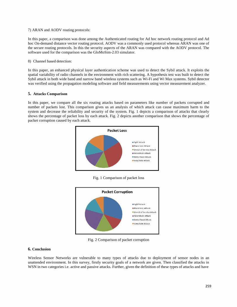
259

7) ARAN and AODV routing protocols:

In this paper, a comparison was done among the Authenticated routing for Ad hoc network routing protocol and Ad

hoc On-demand distance vector routing protocol. AODV was a commonly used protocol whereas ARAN was one of

the secure routing protocols. In this the security aspects of the ARAN was compared with the AODV protocol. The

software used for the comparison was the GloMoSim-2.03 simulator.

8) Channel based detection:

In this paper, an enhanced physical layer authentication scheme was used to detect the Sybil attack. It exploits the

spatial variability of radio channels in the environment with rich scattering. A hypothesis test was built to detect the

Sybil attack in both wide band and narrow band wireless systems such as Wi-Fi and Wi Max systems. Sybil detector

was verified using the propagation modeling software and field measurements using vector measurement analyzer.

5. Attacks Comparison

In this paper, we compare all the six routing attacks based on parameters like number of packets corrupted and

number of packets lost. This comparison gives us an analysis of which attack can cause maximum harm to the

system and decrease the reliability and security of the system. Fig. 1 depicts a comparison of attacks that clearly

shows the percentage of packet loss by each attack. Fig. 2 depicts another comparison that shows the percentage of

packet corruption caused by each attack.

Fig. 1 Comparison of packet loss

Fig. 2 Comparison of packet corruption

6. Conclusion

Wireless Sensor Networks are vulnerable to many types of attacks due to deployment of sensor nodes in an

unattended environment. In this survey, firstly security goals of a network are given. Then classified the attacks in

WSN in two categories i.e. active and passive attacks. Further, given the definition of these types of attacks and have

260

also given the known defenses and countermeasures against them. Hope that this survey will help future

researches in developing a good knowledge about the attacks and their countermeasures.

7. References

[1] André weimerskirch, “Authentication in ad-hoc and sensor networks”, Electrical Engineering and Information

Technology, Ruhr-University Bochum, 2004.

[2]Liang Xiao, Larry J. Greenstein, Narayan B. Mandayam, “Channel-based detection of Sybil attacks in

wireless networks”, IEEE transactions on Information Forensics and Security, vol. 4, no. 3, September 2009.

[3] Virendra Pal Singh, Sweta Jain and Jyoti singhai, “Hello flood attack and its countermeasures in wireless

sensor networks”, International journal of computer science issues, vol. 7, issue 3, no 11, may 2010.

[4] V.Umadevi Chezhian, Ramar, Zaheer Uddin Khan, “Security requirements in mobile Ad hoc networks”,

International journal of advanced research in computer and communication engineering vol. 1, issue 2, April

2012.

[5] Atishay Bansal, Dinesh Sharma, Gajendra Singh, Tumpa Roy, “New approach for wireless communication

security protocol by using mutual authentication”, advanced computing: An International journal, vol.3, no.3,

May 2012.

[6] B. Manzoor, N. Javaid, O. Rehman, M. Akbar, Q. Nadeem, A. Iqbal, M. Ishfaq, “Q-LEACH: A new routing

protocol for WSNs”, Procedia computer science 2013.

[7] Deepali Virmani, Ankita Soni, Shringarica Chandel, Manas Hemrajani, “Routing attacks in wireless sensor

networks: a survey”, International journal of computer science and information technologies, vol. 5 (2), 2014.

[8] Neetika Dhardwaj, Rajdeep Singh,“Detection and Avoidance of black hole attack in AOMDV protocol in

MANETS”, International journal of application or innovation in engineering & management volume 3, issue 5,

May 2014.

[9] Arti Tiwari, Nilmani Verma, “Intrusion detection and Prevention of Denial of service attacks in AODV based

MANET with authentication based Scheme”, International journal of engineering research and technology, vol 3,

issue 4, April 2014.

[10] Heena Dhawan, Sandeep Waraich, “Comparative study on LEACH routing protocol and its variants in

wireless sensor networks: a survey”, Journal of computer applications vol 95– no.8, June 2014.

[11] Amanpreet Kaur, Manjotkaur Sidhu, “Mitigation of black hole and grey hole attack in mobile ad hoc

networks”, International journal of innovative science, engineering & technology, vol. 1 issue 4, June 2014.

[12] Kanu Geete, Piyush Kumar Shukla, Anjana Jayant Deen, “A survey on gray hole attack in wireless mesh

networks”, International journal of computer applications, volume 95– no.23, June 2014.

[13] Richa Gulati, Savita Shivani, “Implementing security algorithm to worm hole attack using AOMDV

protocol & comparison using ns2 simulator”, IOSR journal of computer engineering, volume 16, issue 5, ver. iv

(Sep – Oct. 2014).

[14] Marpu Devadas, k. Vinay Kumar, “Protecting mobile Ad hoc networks from black hole attacks”,

International journal of computer science and mobile computing, vol.3 issue.12, December- 2014.

[15] Chris Karlof David Wagner, University Of California at Berkeley, “Secure routing in wireless sensor

networks: attacks and untermeasures”.

Documents

July 2016 - socet