İSTANBUL TECHNICAL UNIVERSITY INSTITUTE OF SCIENCE AND TECHNOLOGY

TOWARDS THE CLASSIFICATION OF SCALAR INTEGRABLE EVOLUTION EQUATIONS IN (1+1)-

DIMENSIONS

Ph.D. Thesis by

Eti MİZRAHİ, M.Sc.

Department : Mathematics Engineering Programme: Mathematics Engineering

Supervisor : Prof. Dr. Ayşe H. BİLGE

JUNE 2008

İSTANBUL TECHNICAL UNIVERSITY INSTITUTE OF SCIENCE AND TECHNOLOGY

TOWARDS THE CLASSIFICATION OF SCALAR INTEGRABLE EVOLUTION EQUATIONS IN (1+1)-

DIMENSIONS

Ph.D. Thesis by Eti MİZRAHİ, M.Sc.

(509012002)

Date of submission : 19 February 2008

Date of defence examination: 18 June 2008

Supervisor (Chairman): Prof. Dr. Ayşe Hümeyra BİLGE

Members of the Examining Committee Prof.Dr. Mevlut TEYMUR (İTÜ)

Prof.Dr. Hasan GÜMRAL (YÜ)

Prof.Dr. Faruk GÜNGÖR (İTÜ)

Prof.Dr. Avadis S. HACINLIYAN (YÜ)

JUNE 2008

İSTANBUL TEKNİK ÜNİVERSİTESİ FEN BİLİMLERİ ENSTİTÜSÜ

SINIFLANDIRMA YOLUNDA (1+1)-BOYUTTA İNTEGRE EDİLEBİLİR SKALER EVRİM DENKLEMLERİ

DOKTORA TEZİ Y. Müh. Eti MİZRAHİ

(509012002)

Tezin Enstitüye Verildiği Tarih : 19 Şubat 2008 Tezin Savunulduğu Tarih : 18 Haziran 2008

Tez Danışmanı : Prof.Dr. Ayşe Hümeyra BİLGE

Diğer Jüri Üyeleri Prof.Dr. Mevlut TEYMUR (İ.T.Ü.)

Prof.Dr. Hasan GÜMRAL (Y.Ü.)

Prof.Dr. Faruk GÜNGÖR (İ.T.Ü.)

Prof.Dr. Avadis S. HACINLIYAN (Y.Ü.)

HAZİRAN 2008

ACKNOWLEDGEMENTS

I would like to express my heartfelt thanks to my supervisor Prof. Ayse H. Bilge,for her continuous support, encouragement and assistance in every stage of thethesis.

I would also like to express my heartfelt thanks to Professor Avadis Hacınlıyan,for his help and support in programming languages.

I owe my deepest gratitude to my husband Jeki for his caring throughout my lifeand for encouraging me in everything I decided to do.

I also wish to give my very special thanks to my daughter Leyla, my son Vedatand my daughter in law Suzi for living with the thesis as well as me and givingme love and support all through the years.

June 2008 Eti Mizrahi

ii

TABLE OF CONTENTS

LIST OF THE TABLES iv

LIST OF SYMBOLS vSUMMARY viOZET viii

1. INTRODUCTION 1

1.1 Introduction 1

2. PRELIMINARIES 62.1 Notation and Basic Definitions 6

2.2 Integrability Tests 7

2.3 Symmetries and Recursion Operators 9

3. BASIC ALGEBRAIC STRUCTURES 11

3.1 Basic Definitions 11

3.2 The Structure of The Graded Algebra 14

3.3. The Ring of Polynomials and “Level-Grading” 15

4. CLASSIFICATION OF EVOLUTION EQUATIONS 17

4.1 Notation and Terminology, Conserved Densities 17

4.2 General Results on Classification 20

4.3 Polynomiality Results in top Three Derivatives 23

5. SPECIAL CASES 31

5.1 Classification of 7th order evolution equation 31

5.1.1 First Method 31

5.1.2 Second Method 45

5.2 Classification of 9th order evolution equation 47

6. DISCUSSIONS AND CONCLUSIONS 60

APPENDIX A 62

APPENDIX B 69

APPENDIX C 72

APPENDIX D 78

REFERENCES 80

VITA 83

iii

LIST OF THE TABLES

Page No.

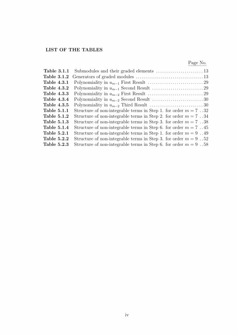
Table 3.1.1 Submodules and their graded elements . . . . . . . . . . . . . . . . . . . . . . . 13Table 3.1.2 Generators of graded modules . . . . . . . . . . . . . . . . . . . . . . . . . . . . . . . . . 13Table 4.3.1 Polynomiality in um−1 First Result . . . . . . . . . . . . . . . . . . . . . . . . . . . 29Table 4.3.2 Polynomiality in um−1 Second Result . . . . . . . . . . . . . . . . . . . . . . . . . 29Table 4.3.3 Polynomiality in um−2 First Result . . . . . . . . . . . . . . . . . . . . . . . . . . . 29Table 4.3.4 Polynomiality in um−2 Second Result . . . . . . . . . . . . . . . . . . . . . . . . . 30Table 4.3.5 Polynomiality in um−2 Third Result . . . . . . . . . . . . . . . . . . . . . . . . . . 30Table 5.1.1 Structure of non-integrable terms in Step 1. for order m = 7 . .32Table 5.1.2 Structure of non-integrable terms in Step 2. for order m = 7 . .34Table 5.1.3 Structure of non-integrable terms in Step 3. for order m = 7 . .38Table 5.1.4 Structure of non-integrable terms in Step 6. for order m = 7 . .45Table 5.2.1 Structure of non-integrable terms in Step 1. for order m = 9 . .49Table 5.2.2 Structure of non-integrable terms in Step 3. for order m = 9 . .52Table 5.2.3 Structure of non-integrable terms in Step 6. for order m = 9 . .58

iv

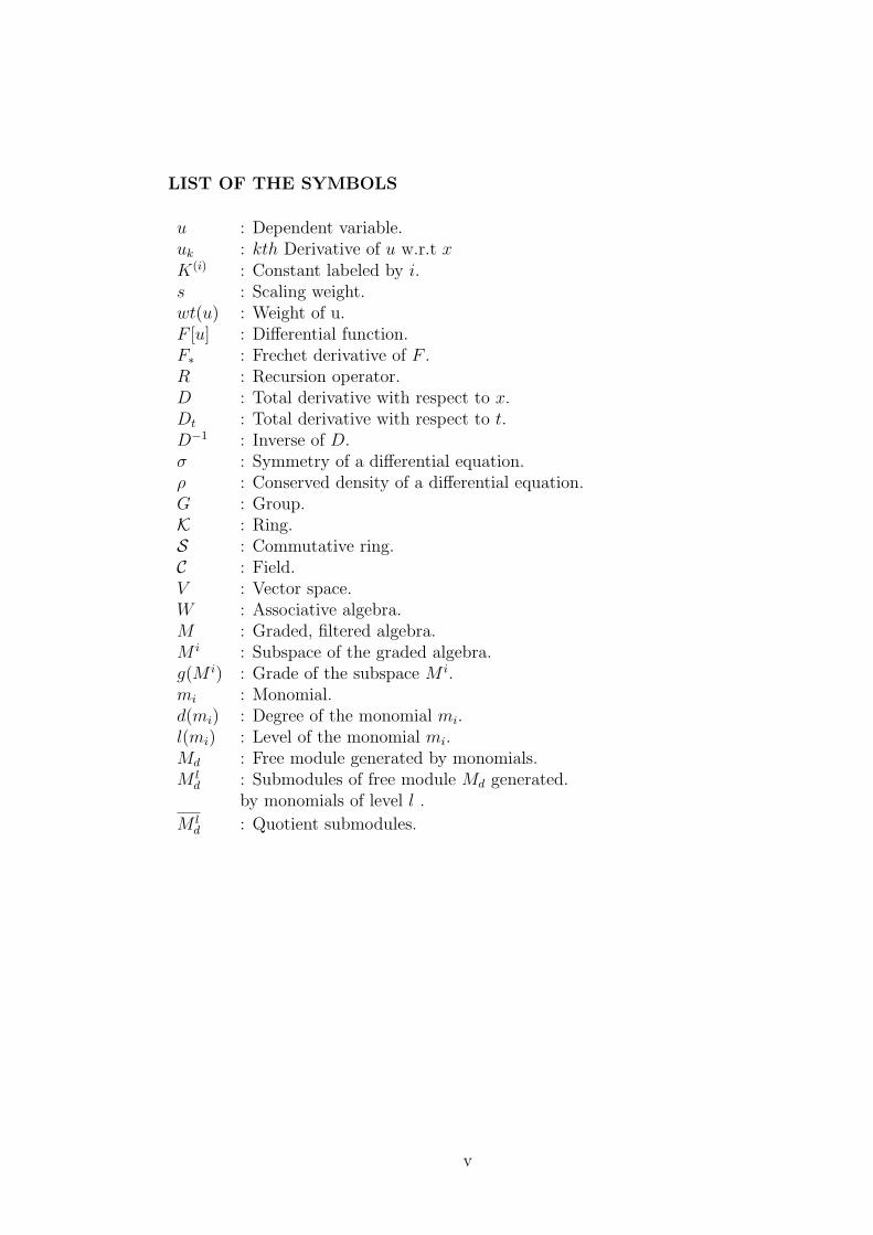
LIST OF THE SYMBOLS

u : Dependent variable.uk : kth Derivative of u w.r.t xK(i) : Constant labeled by i.s : Scaling weight.wt(u) : Weight of u.F [u] : Differential function.F∗ : Frechet derivative of F .R : Recursion operator.D : Total derivative with respect to x.Dt : Total derivative with respect to t.D−1 : Inverse of D.σ : Symmetry of a differential equation.ρ : Conserved density of a differential equation.G : Group.K : Ring.S : Commutative ring.C : Field.V : Vector space.W : Associative algebra.M : Graded, filtered algebra.M i : Subspace of the graded algebra.g(M i) : Grade of the subspace M i.mi : Monomial.d(mi) : Degree of the monomial mi.l(mi) : Level of the monomial mi.Md : Free module generated by monomials.M l

d : Submodules of free module Md generated.by monomials of level l .

M ld : Quotient submodules.

v

TOWARDS THE CLASSIFICATION OF SCALAR INTEGRABLEEVOLUTION EQUATIONS IN (1+1)-DIMENSIONS

SUMMARY

In the literature, integrable equations are meant to be non-linear equationswhich are solvable by a transformation to a linear equation or by an inversespectral transformation [22]. The difficulty in constructing an inverse spectraltransformation had motivated the search for other methods which would identifythe equations expected to be solvable by an inverse spectral transformation.These methods which consist of finding a property shared by all knownintegrable equations are called “integrability tests”. The existence of an infinitenumber of conserved quantities, infinite number of symmetries, soliton solutions,Hamiltonian and bi-Hamiltonian structures, Lax pairs, Painleve property, arewell known integrability tests.

“The classification problem” is defined as the classification of families ofintegrable differential equations. Recently Wang and Sanders used the existenceof infinitely many symmetries to solve this problem for polynomial scale invariant,scalar equations, by proving that scale invariant scalar integrable evolutionequations of order greater than seven are symmetries of third and fifth orderequations [3].

The first result towards a classification for arbitrary m’th order evolutionequations is obtained in [1] where it is shown that scalar evolution equationsut = F [u], of order m = 2k + 1 with k ≥ 3, admitting a nontrivial conserveddensity ρ = Pu2

n + Qun + R of order n = m + 1, are quasi-linear. This resultindicates that essentially non-linear classes of integrable equations arising atthe third order are absent for equations of order larger than 7 and one mayhope to give a complete classification in the non-polynomial case. This is themotivation of the present work where the problem of classification of scalarintegrable evolution equations in (1+1) (1 spatial and 1 temporal)-dimensions isfurther analyzed.

In this thesis, we use the existence of a formal symmetry introduced by Mikhailovet al. as the integrability test [2]. We introduce a graded algebra structure “thelevel grading” on the derivatives of differential polynomials. Our main result isthe proof that arbitrary (non-polynomial) scalar, integrable evolution equationsof order m, are polynomial in top three derivatives, namely um−i, i = 0, 1, 2. Inthe proof of this result, explicit computations are needed at lower orders andcomputations for equations of order 7 and 9 are given as examples.

In our computations we used three conserved densities, ρ(1), ρ(2), ρ(3) obtained in[1]. Computations for the general case and for the lower orders showed that it isimpossible to obtain polynomiality in um−3 by using only these three conserved

vi

densities. Thus the investigation of polynomials beyond um−3 is postponed tofuture work.

The first section is devoted to a general introduction with a literature review, onconservation laws, symmetries, integrability and classification, beginning fromthe discovery of the soliton.

Notation used in this study, basic definitions and preliminary notions aboutintegrability tests, symmetries and recursion operators with examples on KdVequations are given in the second section.

Main results are gathered in sections three and four. In section three, we givebasic definitions and properties of graded and filtered algebras, and define the“level grading” while in section four we present the polynomiality results.

In section three, a graded algebra structure on the polynomials in the derivativesuk+i over the ring of functions depending on x, t, u, . . . , uk is introduced. Thisgrading, called “level grading”, is motivated by the fact that derivatives of afunction depending on x, t, u, . . . , uk are polynomial in higher order derivativesand have a natural scaling by the order of differentiation above the “base level k”.The crucial point is that, equations relevant for obtaining polynomiality resultsinvolve only the term with top scaling weight with respect to level grading. Thisenables to consider top level term only, disregarding the lower ones, and to reducesymbolic computations to a feasible range.

Polynomiality results on the classification of scalar integrable evolution equationsof order m are given in section four. In our computations we proved thatarbitrary scalar integrable evolution equations of order m ≥ 7 are polynomial inthe derivatives um−i for i = 0, 1, 2.

Section five is devoted to explicit computations for the classification of 7thand 9th order evolution equations. The purpose of this section is to give aninformation about explicit computations and compare with the solutions forgeneral m. In particular, at order 7, it is shown that no further informationis obtained by the use of all conserved densities ρ(i), i = −1, 1, 2, 3.

The discussion of the results and directions for future research are given in sectionsix.

Appendices A,B,C,D, give respectively the submodules and quotient submoduleswith their generating monomials, used in the classification of 7th and 9th orderevolution equations. One can derive easily the monomials for evolution equationsof order higher than nine using these lists.

vii

SINIFLANDIRMA YOLUNDA (1+1)-BOYUTTA INTEGREEDILEBILIR SKALER EVRIM DENKLEMLERI

OZET

Literaturde, “integre edilebilen denklemler”, lineer denklemlere donusturulebilenya da ters spektral donusum ile cozulebilen denklemler olarak tanımlanır [22].Ters spektral donusumlerin insaasının cok zor olması, ters spektral donusumile cozulmeye aday denklemleri belirleyebilecek yontemlerin gelistirilmesineyolacmıstır. Bilinen tum integre edilebilen denklemlerin ortak bir ozelliginibulmaya dayalı bu yontemlere “integrabilite testleri” adı verilir. Sonsuz sayıdakorunan nicelikler, sonsuz sayıda simetriler, soliton cozumleri, Hamiltonyenve bi-Hamiltonyen yapı, Lax ciftleri veya Painleve ozelliginin varlıgı, yaygınkullanılan integrabilite testleri olarak bilinir.

“Sınıflandırma problemi”, integre edilebilir diferansiyel denklem ailelerininsınıflandırılması olarak bilinir. Yakın gecmiste Wang ve Sanders, sonsuzsayıda simetrilerin varlıgını kullanarak, olcek bagımsız skaler integre edilebilir,7 inci mertebeden buyuk, evrim denklemlerinin, 3 uncu ve 5 inci mertebedendenklemlerin simetrileri oldugunu gostererek sınıflandırma problemini, polinomolcek bagımsız skaler denklemler icin cozmuslerdir. [3].

Keyfi m inci mertebeden evrim denklemlerinin sınıflandırılması hakkında, ilksonuc, [1]’de elde edilmisir. Bu sonuc, n = m + 1 mertebeden, trivial olmayankorunan yogunluk (conserved density) olarak ρ = Pu2

n + Qun + R yu kabuleden, m = 2k + 1, ve k ≥ 3 mertebeden, ut = F [u] evrim denklemlerininkuazilineer olmasıdır. Elde edilen sonuca gore ozellikle 3 uncu mertebedeortaya cıkan, lineer olmayan, integre edilebilir evrim denklemlerinin sınıfları,7 den buyuk mertebelerde gozukmez. Bu nedenle polinom olmayan durumlaricin bir sınıflandırma yapılabilecegi dusunulebilir. Bu dusunceden yola cıkarak,bu calısmada, (1+1) boyutta (1 uzaysal 1 zamansal ) integre edilebilir evrimdenklemlerinin sınıflandırılması problemi ele alınmıstır.

Bu tezde, integrabilite testi olarak, Mikhailov ve digerleri tarafından ortayakonan, bicimsel simetrilerinin varlıgı kabul edilmistir [2]. Ayrıca “Level grading”adı verilen, diferansiyel polinomların turevleri uzerine bir kademeli cebir (gradedalgebra) yapısı tanımlanmıstır. Bu calısmanın esas sonucu, keyfi polinomolmayan skaler integre edilebilir m inci mertebeden evrim denklemlerinin um−i,i = 0, 1, 2 olmak uzere, en ust uc mertebeden tureve gore polinom oldugununispatıdır. Bu sonucun ispatı, dusuk mertebelerde acık hesaplamaların yapılmasınıgerektirdiginden, 7 inci ve 9 uncu mertebeden keyfi skaler evrim denklemleri,ornek olarak, acık sekilde hesaplanmıstır.

Bu calısmada, [1]’de hesaplanan ve bicimsel simetrinin varlıgının bir sonucuolan, uc korunan yogunluk, ρ(1), ρ(2), ρ(3) (conserved densities) kullanılmıstır.

viii

Genel m ve m ≤ 19 icin yapılan hesaplamalarda, sadece bu uc korunanyogunluk kullanılarak, daha alt mertebeler (ornegin um−3) icin polinomlugunelde edilmesinin imkansız oldugu gorulmustur. Boylece problem ile ilgili bundanbaska yapılacak olan tartısmalar ileriki calısmalara ertelenmistir.

Birinci bolumde genel bir giris ile birlikte, soliton dalgaların kesfi ile baslayanve gunumuze dek gelen, korunum yasaları, simetriler, integre edilebilirlik vesınıflandırma ile ilgili literatur ozeti verilmistir.

Ikinci bolum, calısmada kullanılan notasyon, temel tanımlar, integre edilebilirliktestleri, simetriler ve rekursyon operatorleri hakkında on bilgilere ve KdVdenklemleri ile ilgili orneklere ayrılmıstır.

Esas sonuclar ucuncu ve dorduncu bolumde toplanmıstır. Ucuncu bolumde,kademeli (graded) ve filtrelenmis (filtered) cebir ile ilgili temel tanımlar veozellikler ile birlikte “level grading” in tanımı yapılmıstır. Dorduncu bolumdeise polinom sonuclar verilmistir.

Katsayıları, x, t, u, . . . , uk ya baglı fonksiyonlar halkası uzerinde, turevleri uk+i

olan polinomlara kademeli cebir (graded algebra) yapısı oturtulmustur. “Levelgrading” olarak adlandıracagımız bu yapının olusma nedeni; x, t, u, . . . , uk yabaglı fonksiyonların turevlerinin yuksek mertebe turevlerde polinom olması veturevlenme sırasına gore baz seviye k uzerinde dogal bir olceklemeye sahipolmasıdır. Bu yapının olusmasındaki can alıcı nokta, polinom sonuclar icerendenklemlerin “level grading”’e gore, sadece en yuksek mertebeden olceklemeagırlıgına sahip terimleri icermesidir. Bu durum, dusuk seviyedeki terimlerigozardı ederek ve sadece yuksek seviyedeki terimleri dikkate alarak sembolikhesaplamaların yapılabilir bir seviyeye indirgenmesini saglamıstır.

Skaler, integre edilebilir m inci mertebeden evrim denklemlerinin sınıflandırılmasıuzerine polinom sonuclar dorduncu bolumde verilmistir. Hesaplamalarda, keyfiskaler integre edilebilir m ≥ 7 mertebe evrim denklemlerinin um−i, i = 0, 1, 2turevlerine gore polinom oldugu ispatlanmıstır.

Besinci bolum ise 7 inci ve 9 uncu mertebeden evrim denklemlerininsınıflandırılması icin yapılan acık hesaplamalara ayrılmıstır. Bu bolumunamacı, acık hesaplamaların sonuclarını genel m icin elde edilen sonuclarlakarsılastırmak olmustur. Ozel olarak 7 inci mertebede, bilinen tumkorunan yogunlukların, ρ(i), i = −1, 1, 2, 3, kullanılmasının elde edilen sonucudegistirmedigi gosterilmistir.

Altıncı bolumde sonuclar uzerine tartısmalar ve ileriki arastırmalar icinyonlendirmeler verilmistir.

A,B,C ve D, eklerinde sırasıyla, 7 inci ve 9uncu mertebeden evrim denklemlerininhesaplamalarında kullanılan alt modul ve kalan alt modulleri ureten monomlarınlisteleri verilmistir. Bu listelerin yardımı ile dokuzuncu mertebeden buyuk evrimdenklemleri icin monomialların kolaylıkla turetilebildigi gorulmustur.

ix

1 INTRODUCTION

1.1 Introduction

In the literature, integrable equations refer to non-linear equations for whichexplicit solutions can be obtained by means of a transformation to linearequations or by the inverse scattering method. Burgers’ and Korteweg de Vries(KdV) equations are respectively prototypes for these two cases. For examplethe Cole-Hopf transformation vx = uv, which is local, linearizes the Burgersequation ut − 2uux − uxx = 0, to the heat equation vt = vxx, while the KdVequation requires an inverse spectral transformation [29], [28].

Investigations of the solutions of nonlinear partial differential equationsmotivated the discovery of mathematical “soliton” known as solitary wave whichasymptotically preserves its shape and velocity upon nonlinear interaction withother solitary waves [6]. In 1834 J. Scott Russel was the first who observes, ridingon horse back beside a narrow canal, the formation of a solitary wave. In 1895Korteweg and de Vries derived the equation for water waves in shallow channelswhich bears their name and which confirmed the existence of solitary waves.The discovery of additional properties of solitons began with the appearance ofcomputers followed by the numerical calculations carried out on the Maniac Icomputer by Fermi, Pasta and Ulam in 1955. They took a chain of harmonicoscillators coupled with a quadratic nonlinearity and investigated how the energyin one mode would spread to the rest. They found the system cycled periodically,implying it was much more integrable than they had thought. The continuumlimit of their model was the KdV equation [30].

The exact solutions of the KdV equation were the solitary wave and cnoidal wavesolutions. While the exact solution of the KdV equation ut + 6uux + uxxx = 0subject to the initial condition u(x, 0) = f(x) where f(x) decays sufficientlyrapidly as |x| → ∞, was developed by Gardner, Green, Kruakal and Miurain 1967. The basic idea for this solution is to relate the KdV equation tothe time-independent Schrodinger scattering problem [10]. Gardner, Miura andKruskal found out that the eigenvalues of the Schrodinger operator are integralsof the Korteweg-de Vries equation. This discovery were succeeded by Laxs’principle which associates nonlinear equations of evolutions with linear operatorsso that the eigenvalues of the linear operator are integrals of the nonlinearequation [24].

The interest to the integrability problem increased by the discovery of solitonbehavior of the KdV equation and of the inverse spectral transformation forits analytical solution. In 1965 Zabusky and Kruskal, in numerical studies,re-derived the KdV equation and they found the remarkable property of solitary

1

waves [21]. They give the conjecture that the double wave solutions of the KdVequation with large |t| behave as the superposition of two solitary waves travellingat different speeds [24]. These numerical results lead them to search someanalytic explanation. They found out that this behavior can be explained by theexistence of many conservation laws. Therefore the search for the conservationlaws for the KdV equation started. A conservation law has the following formwhere U is the conserved density and F is the conserved flux.

DtU + DxF = 0.

First Zabusky and Kruskal found conserved densities of order 2 and 3, afterMiura found a conserved density of order 8. Finally it is proved that there existan infinite number of conservation laws and conserved densities at each order [7].

Methods for selecting equations that are considered to be “integrable” among ageneral class are called “integrability tests”. Integrability tests use the fact thatintegrable equations have a number of remarkable properties such as the existenceof an infinite number of conserved quantities, infinite number of symmetries,soliton solutions, Hamiltonian and bi-Hamiltonian structure, conserved covariant(co-symmetries), Lax pairs, Painleve property, conservation laws etc. Usuallythe requirement of sharing a certain property with known integrable equationsleads to the selection of a finite number of equations from a general class andthe selected equations are expected to be integrable. This method leads to a“classification” and the criterion used in is called an “integrability test”.

The Korteweg-deVries (KdV) equation

ut = u3 + uu1 (1.1)

is the prototype of integrable evolution equations. There are a number of otherequations related to it involving first order derivatives. These are called the“modified KdV” or “potential KdV” equations and they are also integrable.Miura found that the Modified Korteweg de Vries equation

vt = v3 + v2v1 (1.2)

turn to KdV equation under the transformation

u = v2 +√−6v1.

Therefore he proved that if v(x, t) is a solution of (1.2), u(x, t) is a solution of(1.1).

Miura transformations map symmetries to symmetries hence those equationsthat are related to a known integrable equation by Miura transformations arealso considered integrable and belonging to the same class.

Sophus Lie was the first who studied the symmetry groups of differentialequations. A symmetry group of a system can be defined as the geometrictransformations of its dependent and independent variables which leave thesystem invariant. Geometric transformations on the space of independent anddependent variables of the system are called geometric symmetries. In 1918

2

Emmy Noether proved the one-to-one correspondence between one-parametersymmetry groups and conservation laws for the Euler Lagrange equations [12].This result can not explain the existence of infinitely many conserved densitiesfor the KdV equation which possessed only a four-parameter symmetry group.This observation leads to reinterpret higher order analogs of the KdV equationas “higher order symmetries”. Then the search began for the hidden symmetriescalled “generalized symmetries”, which are groups whose infinitesimal generatorsdepend not only on the dependent and independent variables of the system butalso the derivatives of the dependent variables [5].

In the classical theory, the “symmetry of a differential equation” is definedin terms of the invariance groups of the differential equation. This definitionis essentially equivalent to defining symmetries as solutions of the linearizedequation. That is if σ is a symmetry of the evolution equation ut =F (x, t, u, ux, . . . , ux...x), then

σt = F∗σ (1.3)

where F∗ is the Frechet derivative of F . A function f(x, t, u, ux, ut, . . .) is calledsymmetry of the partial differential equation H(x, t, u, ux, ut, uxx, uxt, utt, . . .) =0, if it satisfies the following “linearization”:

∂H

∂u+

∂H

∂ux

∂

∂x+

∂H

∂ut

∂

∂t+

∂H

∂uxx

(∂

∂x

)2

+∂H

∂uxt

∂

∂t

∂

∂x+

∂H

∂utt

(∂

∂t

)2

+ . . .

(f) = 0 (1.4)

For a nonlinear evolution equation ut = F (x, t, u, ux, . . . , ux...x), symmetries ofthe form σ = σ(x, t, u, ux, ut), linear in ux, ut are called “classical symmetries”,while symmetries depending on higher order derivatives of the dependent variableu with respect to x are called “generalized symmetries”. For example one of thesimplest general symmetries of the KdV equation ut = uxxx + 6uux

is: f = uxxxxx + 10uuxxx + 20uxuxx + 30u2ux [2].The existence of infinitely many generalized symmetries is tied to the existenceof a recursion operator which maps symmetries to symmetries [9].

The recursion operator is in general an integro-differential operator say R suchthat Rσ is a symmetry whenever σ is a symmetry, i.e.,

ut = F [u] . (1.5)

(Rσ)t = F∗(Rσ). It follows that for any symmetry σ,

(Rt + [R,F∗]) σ = 0. (1.6)

where F∗, is the Frechet derivative of F. Given a recursion operator R, one mayexpand the integral terms in R in an infinite formal series in terms of the inversepowers of the operator D=d/dx. A “formal recursion operator” is defined asa formal series in inverse powers of D satisfying the operator equation (1.6).A truncation of the formal series satisfying equation (1.6) for a given evolutionequation or F∗ is defined to be a formal symmetry in [2].

3

The solvability of the coefficients of R in the class of local functions requiresthat certain quantities denoted as ρ(i) be conserved densities. The existence ofone higher symmetry permits to construct not one but many conservation laws.These conservation laws contain a lot of knowledge about the equation underconsideration.

A function ρ = ρ(x, t, u, u1, u2, . . . , un) is called a density of a conservation law ofut = F (x, t, u, ux, . . .), if there exists a local function σ such that d

dt(ρ) = D(σ).

If ρ = D(h) for any h and σ = ht then σ is a trivial conserved density. Theseconserved density conditions give over-determined systems of partial differentialequations for F and lead to a classification.

Integrability tests based on the existence of a formal symmetry has lead to manystrong results on the classification of 3th and 5th order equations [14] [15]. Amongpolynomial equations, at the third order the KdV class is unique, while at thefifth order there are in addition the Sawada-Kotera and Kaup equations [2].

The classification problem for scalar integrable equations is solved in the work ofWang and Sanders [3], for the polynomial scale invariant case. Their method isbased on the search of higher symmetries and uses number theoretical techniques.They proved that if λ homogeneous (with respect to the scaling xux + λu, withλ > 0) equations of the form ut = um + f(u, . . . , um−1) have one generalizedsymmetry, they have infinitely many and these can be found using recursionoperators or master symmetries [3]. They proved also that if an equation has ageneralized symmetry, it is enough to be able to solve the symmetry equation uptill quadratic terms to find other symmetries [3]. They showed also that if theorder of the symmetry is > 7, there exists a nontrivial symmetry of order ≤ 7[3].Their main result is that scale invariant, scalar integrable evolution equations oforder greater than seven are symmetries of third and fifth order equations [3] andsimilar results are obtained in the case where negative powers are involved [4].The problem of classification of arbitrary evolution equations is thus reduced toproving that such equations have desired polynomiality and scaling properties.In a recent work, the non-polynomial case is studied in [1] and it is shown thatthe existence of a conserved density of order m + 1 leads to quasi-linearity. Thisis a first step in proving polynomiality, and our motivation is to prove stepby step further polynomiality results and give a complete classification in thenon-polynomial case.

We shall summarize recent works done on the similar field. In 1993 RobertoCamassa and Darryl Holm derive a new completely integrable dispersive shallowwater equation

ut + 2κux − uxxt + 3uux = 2uxuxx + uxxx

where u is the fluid velocity in the x direction and κ is a constant related tothe critical shallow water wave speed. The equation is obtained by using anasymptotic expansion directly in the Hamiltonian for Euler’s equation. Thisequation is bi-Hamiltonian it can be expressed in Hamiltonian form in twodifferent ways. The ration of its two Hamiltonian operators is a recursionoperator that produces an infinite sequence of conservation laws [31]. In 2001Artur Sergyeyev extended the recursion operators with nonlocal terms of specialform for evolution systems in (1+1)-dimensions, to well-defined operators on

4

the space of nonlocal symmetries and showed that these extended recursionoperators leave this space invariant [33]. Another study of Sergyeyev publishedin 2002 is about conditionally integrable evolution systems. They describe all(1+1)-dimensional evolution systems that admit a generalized (Lie-Backlund)vector field satisfying certain non-degeneracy assumptions, as a generalizedconditional symmetry [34]. Two of several studies about systems of evolutionequations are produced by Wolf. With Sokolov they extend the simplest versionof the symmetry approach to the classification of integrable evolution equationsfor (1+1)-dimensional nonlinear PDEs., to the case of vector evolution equations.They considered systems of evolution equations with one or two vector unknownsand systems with one vector and one scalar unknown. They gave the list of allequations having the simplest higher symmetry for these classes [32]. Tsuchidaand Wolf performed a classification of integrable systems mixed scalar and vectorevolution equations with respect to higher symmetries. They consider polynomialsystems that are homogeneous under suitable weighting of variables. Theygave the complete lists of second order systems with a third order or fourthorder symmetry and third order systems with a fifth order symmetry using theKdV, the Burgers, the Ibrahimov-Shabat and two unfamiliar weightings [35].Partial differential equations of second order (in time) that possess a hierarchyof infinitely many higher symmetries are studied in [36]. The classification ofhomogeneous integrable evolution equations of fourth and sixth order (in thespace derivative) equations has been done applying the perturbative symmetryapproach in symbolic representation. Three new tenth order integrable equationshas been found. The integrability condition has been proved providing thecorresponding bi-Hamiltonian structures and recursion operators [36]. Recentlynumber theory results on factorization of polynomials has been used to classifysymmetries of integrable equations [37].

In the present work, the classification of quasi-linear evolution equations of orderm ≥ 7, using the existence of a “formal symmetry” as an integrability testproposed in [2], is studied.

The presentation is organized as follows: Notation used in this study, basicdefinitions and preliminary notions about integrability tests, symmetries andrecursion operators with examples on KdV equations are given in Section 2.A new structure called “level grading” based on the structure of graded andfiltered algebra accompanied by related definitions, properties and examplesare introduced in Section 3. Polynomiality results in top three derivatives onclassification of scalar integrable evolution equations of order m are given inSection 4. Section 5 is devoted to the classification of 7th and 9th order evolutionequations. Two different methods are given for the computations of evolutionequation of order 7. Discussions and conclusions are given in Section 6. Thesubmodules and quotient submodules with their generating monomials, used inthe classification of 7th and 9th order evolution equations are respectively givenin Appendices A,B,C and D.

5

2 PRELIMINARIES

The purpose of this section is to introduce notations used in this study. Wealso give a brief knowledge about integrability tests, symmetries and recursionoperators which constitute the fundamental part of this study.

2.1 Notation and Basic Definitions

In this study we work with scalar evolution equations in one space dimensionwhere the independent space and time variables are respectively x and t whilethe dependent variable is u = u(x, t).

Definition 2.1.1. A differential function F[u] is a smooth function of x,t, u andof the derivatives of u with respect to x, up to an arbitrary but finite order.

Evolution equations are of the form

∂

∂tu(x, t) = F [u] (2.1.1)

where F[u] is a differential function.

We simplify the notation for the derivatives of differential polynomials as follows:

The partial derivative of u with respect to t is denoted by ut = ∂u∂t

. The partial

derivatives with respect to x are denoted by ui = ∂iu∂xi .

This agreement emphasizes that these quantities are considered as independentvariables.If F [u] = F (x, t, u, u1, ..., um) is a differential function, the total derivative withrespect to t denoted by Dt is

Dt(F ) =m∑

i=0

∂F

∂ui

∂ui

∂t+

∂F

∂t, (2.1.2)

and the total derivative with respect to x denoted by D is

DF =m∑

i=0

∂F

∂ui

ui+1 +∂F

∂x(2.1.3)

We agree on the convention that the operator inverse of D is D−1 defined asD−1ϕ =

∫ϕ.

6

Definition 2.1.2. The differential polynomial F [u] is said to have fixed scalingweight s if it transforms as F [u] → λsF [u] under the scaling (x, u) → (λ−1x, λdu),where d is called the weight of u and denote it as wt(u).

Definition 2.1.3. A differential polynomial is called KdV-like if it is a sumof polynomials with odd scaling weight s, with wt(u) = 2.

Definition 2.1.4. . A Laurent series in D is a formal series

L =n∑

i=1

LiDi +

∞∑

i=1

L−iD−i (2.1.4)

and it is called a pseudo-differential operator. The order of the operator is thehighest index n with Ln 6= 0. The operators given in closed form that involveintegral operations will be called integro-differential operators.In order to define the products of pseudo-differential operators, we need to definethe operator

D−1ϕ = ϕD−1 −DϕD−2 + D2ϕD−3 + ...

=m∑

i=0

(−1)i(Diϕ

)D−i−1 + (−1)m+1 D−1

[(Dm+1ϕ

)D−m−1

](2.1.5)

this formula is just the expression of integration by parts, for example

D−1(ϕDkψ

)=

∫ϕDkψ = ϕDk−1ψ −

∫DϕDk−1ψ

= ϕDk−1ψ −DϕDk−2ψ +∫

D2ϕDk−2ψ (2.1.6)

The action of D−k is computed by repeated applications of (2.1.6), up to anydesired order.

2.2 Integrability Tests

In this part we shall briefly discuss integrability tests. First of all oneneeds a definition of “integrability” for nonlinear partial differential evolutionequations, in order to understand the integrability of known equations, to testthe integrability of new equations and to obtain new integrable equations. Thissubject has been discussed in several papers gathered on the book “What isintegrability?”[23]. “There is no precise definition besides the two notions of“C-integrability” and “S-integrability” ” as stated by Calogero in [22]. Thefirst one corresponds to the possibility of linearization via an appropriate“change of variables”, while the second denotes solvability via the “Spectraltransform technique” or the “inverse Scattering method”. The transformation ofa nonlinear equation via an invertible change of coordinates into a linear equationcan also be defined as “C-integrability” [38]. Indirect methods are used to identifythe equations expected to be solvable by an inverse spectral transformation andthey are commonly called “integrability tests”.

7

A well known example for equations solvable by an inverse spectraltransformation is the Korteweg de Vries equation. Integrability tests areinspired by the remarkable properties of the KdV equation such as an infinitenumber of conserved quantities, infinite number of symmetries, soliton solutions,Hamiltonian and bi-Hamiltonian structure, Lax pairs and Painleve property.

The existence of an infinite set of conservation laws for the KdV equation suggeststhat certain nonlinear partial differential evolution equations might have similarproperties. The existence of the infinite set of conservation laws motivated thesearch for a simple way of generating the conserved quantities[11]. This searchled to the Miura-Gardner one parameter family of Backlaund transformationsbetween the solutions of KdV and of the modified KdV equations. Therefore theinverse scattering transform for directly linearizing the equation was developed.In 1968 Lax put the inverse scattering method for solving the KdV equation intoa more general form and found the Lax pair [24].

The Backlaund transformation was an important key to check a given equationfor symmetries. The nonexistence of an infinite number of conservation lawsdoes not obstruct integrability. There exist integrable equations which have afinite number of conservation laws, which are not Hamiltonian and which aredissipative. An appropriate example is the Burgers equation which has only oneconservation law, although an infinite number of symmetries. It can be integratedusing the one parameter family of Backlaund transformation between solutionsof the heat and Burgers equation.

In 1971 Hirota developed a direct method, known as Bilinear Representation,for finding N-soliton solutions of nonlinear evolution equations [6]. It is shownthat KdV-like equations with non-zero 3rd order part, viewed as perturbationsof the KdV equations can be transformed to the KdV equations up to a certainorder provided that the coefficients satisfy certain conditions. These conditionsare obtained by requiring that the conserved densities of the KdV equations beextended to higher orders [26], [27].

Kruskal and Zabusky after the re-derivation of the KdV equation discovered theinteraction properties of the soliton and they explain the existence of infinitelymany conservation laws by suggesting the existence of hidden symmetries in thisequation. In 1987, Fokas proposed the existence of one generalized symmetryas an integrability test [25]. MSS develop a new symmetry, called “formalsymmetry”, using as a base, the locality concept of the Sophus Lie classical theoryof contact transformations and the inverse scattering transform. The existenceof formal symmetries of sufficiently high order is proposed as an integrabilitytest [2]. A formal symmetry is a pseudo-differential operator which agrees up toa certain order with some fractional power of a recursion operator expanded ininverse powers of D, which is the total derivative with respect to x. The existenceof a formal symmetry gives certain conserved density conditions which in turnlead to a classification. The Painleve method, which can be applied to systemsof ordinary and partial differential equations alike, is one of the methods used toidentify integrable systems. The basic idea is to expand each dependent variablein the system of equations as a Laurent series about a pole manifold [8].

8

2.3 Symmetries and Recursion Operators

In this section we shall give the definitions and interrelations between symmetries,recursion operators conserved densities and discuss the formal symmetry method.

Definition 2.3.1. A local one parameter group of transformations acting on thespace of variables (x, t, u) is called a symmetry group of the equation ut = F [u],if it transforms all solutions to solutions.

Definition 2.3.2. The Frechet derivative denoted by F∗ is a linearized operatorassociated with the differential function F [u] and is defined as

F∗ =m∑

i=0

(∂F

∂ui

)Di (2.3.1)

where ui =(

∂iu∂ix

)

Definition 2.3.3. A differential function σ is called a symmetry of the equationut = F [u] if it satisfies the linearized equation, σt = F∗σ.

Definition 2.3.4. The symmetries depending linearly on the first derivatives ofthe unknown function are called classical symmetries or Lie-point symmetries.All other symmetries are called non Lie-point or generalized symmetries.

Definition 2.3.5. A differential function ρ is called a conserved density, if thereexists a differential polynomial ϕ such that ρt = Dϕ.

In the solution of the KdV equation via the inverse spectral transformation, itappears that not only the KdV equation, but the sequence of odd order equationscalled the KdV hierarchy are all solvable by the same method. These equationsare symmetries of the KdV equation and they can be defined recursively.

Definition 2.3.6. A recursion operator is a linear operator R such that Rσ is asymmetry whenever σ is a symmetry. It can also be defined as a solution of theoperator equation Rt + [R,F∗] = 0.

Assuming that σ is a symmetry and using the equation above we have

(Rσ)t = Rtσ + RF∗σ

= (−RF∗σ + F∗Rσ) + RF∗σ

= F∗Rσ (2.3.2)

hence Rσ is a symmetry. We can conclude that R sends symmetries tosymmetries.

9

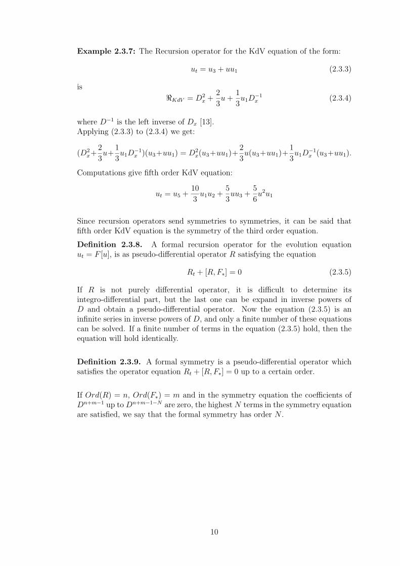
Example 2.3.7: The Recursion operator for the KdV equation of the form:

ut = u3 + uu1 (2.3.3)

is

<KdV = D2x +

2

3u +

1

3u1D

−1x (2.3.4)

where D−1 is the left inverse of Dx [13].Applying (2.3.3) to (2.3.4) we get:

(D2x+

2

3u+

1

3u1D

−1x )(u3+uu1) = D2

x(u3+uu1)+2

3u(u3+uu1)+

1

3u1D

−1x (u3+uu1).

Computations give fifth order KdV equation:

ut = u5 +10

3u1u2 +

5

3uu3 +

5

6u2u1

Since recursion operators send symmetries to symmetries, it can be said thatfifth order KdV equation is the symmetry of the third order equation.

Definition 2.3.8. A formal recursion operator for the evolution equationut = F [u], is as pseudo-differential operator R satisfying the equation

Rt + [R,F∗] = 0 (2.3.5)

If R is not purely differential operator, it is difficult to determine itsintegro-differential part, but the last one can be expand in inverse powers ofD and obtain a pseudo-differential operator. Now the equation (2.3.5) is aninfinite series in inverse powers of D, and only a finite number of these equationscan be solved. If a finite number of terms in the equation (2.3.5) hold, then theequation will hold identically.

Definition 2.3.9. A formal symmetry is a pseudo-differential operator whichsatisfies the operator equation Rt + [R,F∗] = 0 up to a certain order.

If Ord(R) = n, Ord(F∗) = m and in the symmetry equation the coefficients ofDn+m−1 up to Dn+m−1−N are zero, the highest N terms in the symmetry equationare satisfied, we say that the formal symmetry has order N .

10

3 BASIC ALGEBRAIC STRUCTURES

In this section we give the algebraic structures that will be used in our problem.In the first part we give basic algebraic definitions with some examples, in thesecond and third part we give respectively the structure of the graded algebraand the “level grading” structure that we introduce in this study.

3.1 Basic Definitions

In this part we give fundamental definitions concerning the graded and filteredalgebra.

Definition 3.1.1 A ring 〈K, +, .〉 is a set K together with two binary operations(+, .), which we call addition and multiplication, defined on K such that thefollowing axioms are satisfied:1) 〈K, +〉 is an abelian group.2) Multiplication is associative.3) For all a, b, c,∈ K, the left distributive law, a (b + c) = (ab) + (ac) and4)The right distributive law, (a + b) c = (ac) + (bc), hold [17].

Definition 3.1.2. Let K be a ring. A (left) K-module consists of an abeliangroup G together with an operation of external multiplication of each element ofG by each element of K on the left such that for all α, β,∈ G and r, s,∈ K, thefollowing conditions are satisfied:1) (rα) ∈ G.2) r(α + β) = rα + rβ.3) (r + s)α = rα + sα.4) (rs)α = r(sα).

A K-module is very much like a vector space except that the scalars need onlyform a ring [17]. In any left K-module, a family of elements x1, x2, ..., xn is calledlinearly independent if for any αi ∈ K the relation

∑αixi = 0 holds only when

α1 = ... = αn = 0. A linearly independent generating set is called a basis.

Definition 3.1.3. A module is said to be free if it has a basis.It is clear that any basis of a free module is a minimal generating set, i.e. agenerating set such that no proper subset generates the whole module [19].

11

Definition 3.1.4. An algebra consists of a vector space V over a field C,together with a binary operation of multiplication on the set V of vectors, suchthat for all a ∈ C and α, β, γ ∈ V , the following conditions are satisfied:1)(aα)β = a(αβ) = α(aβ).2)(α + β)γ = αγ + βγ.3)α(β + γ) = αβ + αγ.W is an associative algebra over C if, in addition to the preceding threeconditions:4)(αβ)γ = α(βγ) for all α, β, γ ∈ W [17].

Definition 3.1.5. If for a field C a positive integer n exists such that n.a = 0for all a ∈ C, then the least such positive integer is the characteristic of thefield C. If no such positive integer exists, then C is of characteristic 0 [17].

Definition 3.1.6. Let C be a field of characteristic 0. A vector space V over Cis called a Lie Algebra over C if there is a map(X,Y ) 7→ [X,Y ], (X,Y, [X, Y ] ∈ V )of V × V into V with the following properties:(i)(X, Y ) 7→ [X, Y ] is bilinear(ii)[X, Y ] + [Y,X] = 0, (X,Y ∈ V )(iii)[X, [Y, Z]] + [Y, [Z, X]] + [Z, [Y, X]] = 0, (X,Y, Z ∈ V ) [20].

The following definitions of the graded and filtered algebra are based on theprevious preliminary definitions.

Definition 3.1.7. Let M be an associative algebra over a field C of characteristic0. M is said to be graded if for each integer n ≥ 0 there is a subspace Mn of Msuch that(i)1 ∈ M(0) and M is the direct sum of the Mn,(ii)M(ni)M(nj) ⊆ M(ni+nj)

for all ni, nj ≥ 0In this case the elements of

⋃∞ni=0 Mni

are called homogeneous, and those of Mn

are called homogeneous of degree n; if v =∑

n≥0 vn(vn ∈ Mn, v ∈ M), then vn iscalled the homogeneous component of v of degree n [20].

Definition 3.1.8. M is said to be filtered if for each integer n ≥ 0 there is asubspace M (n) of M such that:(i)1 ∈ M (0), M0 ⊆ M1 ⊆ ...,

⋃∞n=0 M (n) = M and

(ii)M (ni)M (nj) ⊂ M (ni+nj) for all ni, nj ≥ 0.It is convenient to use the convention that M (−1) = ∅. For v ∈ M, the integers ≥ 0 such that M ∈ M (s) but /∈ M (s−1) is called the degree of v, and writtendeg(v). For n ≥ 0, M (n) is then the set of all v ∈ M with deg(v) ≤ n [20].We give now certain examples of gradings on polynomial rings. The polynomialsin a single variable x over a field C is a standard example of graded and filteredalgebra.

12

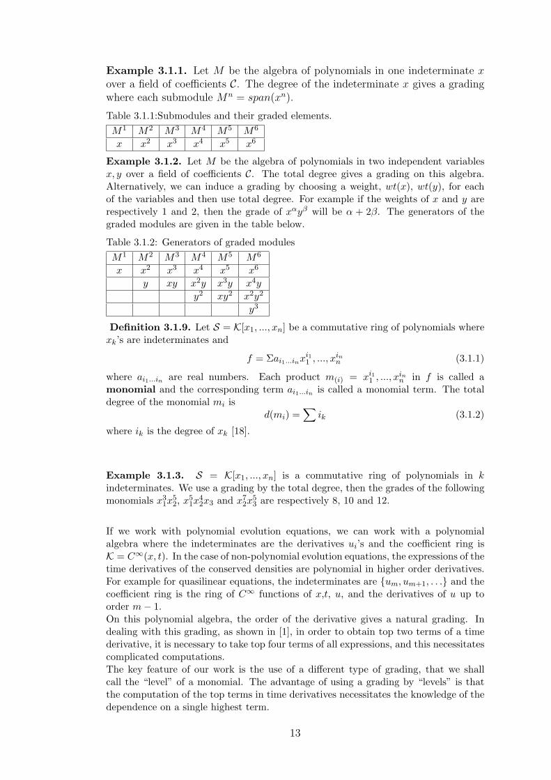
Example 3.1.1. Let M be the algebra of polynomials in one indeterminate xover a field of coefficients C. The degree of the indeterminate x gives a gradingwhere each submodule Mn = span(xn).

Table 3.1.1:Submodules and their graded elements.M1 M2 M3 M4 M5 M6

x x2 x3 x4 x5 x6

Example 3.1.2. Let M be the algebra of polynomials in two independent variablesx, y over a field of coefficients C. The total degree gives a grading on this algebra.Alternatively, we can induce a grading by choosing a weight, wt(x), wt(y), for eachof the variables and then use total degree. For example if the weights of x and y arerespectively 1 and 2, then the grade of xαyβ will be α + 2β. The generators of thegraded modules are given in the table below.

Table 3.1.2: Generators of graded modulesM1 M2 M3 M4 M5 M6

x x2 x3 x4 x5 x6

y xy x2y x3y x4y

y2 xy2 x2y2

y3

Definition 3.1.9. Let S = K[x1, ..., xn] be a commutative ring of polynomials wherexk’s are indeterminates and

f = Σai1...inxi11 , ..., xin

n (3.1.1)

where ai1...in are real numbers. Each product m(i) = xi11 , ..., xin

n in f is called amonomial and the corresponding term ai1...in is called a monomial term. The totaldegree of the monomial mi is

d(mi) =∑

ik (3.1.2)

where ik is the degree of xk [18].

Example 3.1.3. S = K[x1, ..., xn] is a commutative ring of polynomials in kindeterminates. We use a grading by the total degree, then the grades of the followingmonomials x3

1x52, x5

1x42x3 and x7

2x53 are respectively 8, 10 and 12.

If we work with polynomial evolution equations, we can work with a polynomialalgebra where the indeterminates are the derivatives ui’s and the coefficient ring isK = C∞(x, t). In the case of non-polynomial evolution equations, the expressions of thetime derivatives of the conserved densities are polynomial in higher order derivatives.For example for quasilinear equations, the indeterminates are {um, um+1, . . .} and thecoefficient ring is the ring of C∞ functions of x,t, u, and the derivatives of u up toorder m− 1.On this polynomial algebra, the order of the derivative gives a natural grading. Indealing with this grading, as shown in [1], in order to obtain top two terms of a timederivative, it is necessary to take top four terms of all expressions, and this necessitatescomplicated computations.The key feature of our work is the use of a different type of grading, that we shallcall the “level” of a monomial. The advantage of using a grading by “levels” is thatthe computation of the top terms in time derivatives necessitates the knowledge of thedependence on a single highest term.

13

3.2 The Structure of The Graded Algebra

Let K(k) be the ring of C∞ functions of x, t, u, . . . , uk and M (k) be the polynomialalgebra over K(k) generated by S(k) = {uk+1, uk+2, . . .}. A monomial mi in M (k) is aproduct of a finite number of elements of S(k). Monomials are of the form

mi =n∏

j=1

um−1+kj (3.2.1)

We shall call m − 1 as the “base level” and the “level of a derivative term un will bethe number of derivatives above the base level, i.e., n− (m− 1).

Let’s now fix a base level d and denote the submodules generated by elements of levelj above this base level by M j

d . Then the polynomial algebra Md over K will be a directsum of these modules given as

Md =⊕

l≥0

M ld (3.2.2)

or explicitly asMd = M0

d

⊕M1

d

⊕M2

d

⊕M3

d

⊕M4

d . . .

The first few submodules can be expressed in terms of their generators as follows.

Md = K⊕〈um〉

⊕〈um+1, u

2m〉

⊕〈um+2, um+1um, u3

m〉⊕

. . . .

Full sets of generators are given in the Appendices.

The differentiation with respect to x induces a map on these modules compatible withthe grading as follows. For example, a general term in M1

d is of the form φud+1 whereφ is a function of x, t, u and the ui’s for i ≤ d. Then

D(φud+1) = φud+2 + Dφud+1 (3.2.3)= φud+2 + ud+1[φdud+1 + φd−1ud + . . .]

Thus it has parts in M1d and inM2

d . Similarly it can be seen that

π : M id → M i

d

⊕M i+1

d

andπj : M i

d → M id

⊕M i+1

d

⊕. . .

⊕M i+j

d

Note that not all monomials appear in a total derivative, i.e, in each submodule mid

there are monomials that are not in the image of π. These will be the ”non-integrable”terms that we shall be searching for. It can be seen that a monomial is non-integrableif and only if it is nonlinear in the highest derivative. We describe the structure asfollows. Let

R = Im(πj)⋂

M i+jd

and define the quotient submodule Mi+jd by

Mi+jd = M i+j

d /R.

It can be seen that the quotient module is generated by the the non-integrablemonomials. These are listed in the Appendices.

The most important feature of this grading is that in the intersection of the image ofπj with the top module only the dependencies on ud appear. That is practically if wework on the top module, we may assume that our functions depend on ud only. Thisallows a considerable reduction in the computational requirements.

14

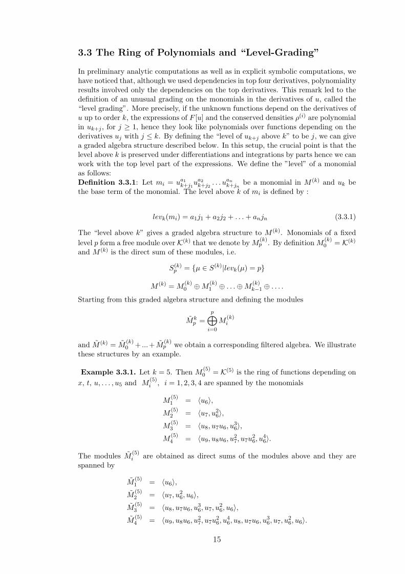
3.3 The Ring of Polynomials and “Level-Grading”

In preliminary analytic computations as well as in explicit symbolic computations, wehave noticed that, although we used dependencies in top four derivatives, polynomialityresults involved only the dependencies on the top derivatives. This remark led to thedefinition of an unusual grading on the monomials in the derivatives of u, called the“level grading”. More precisely, if the unknown functions depend on the derivatives ofu up to order k, the expressions of F [u] and the conserved densities ρ(i) are polynomialin uk+j , for j ≥ 1, hence they look like polynomials over functions depending on thederivatives uj with j ≤ k. By defining the “level of uk+j above k” to be j, we can givea graded algebra structure described below. In this setup, the crucial point is that thelevel above k is preserved under differentiations and integrations by parts hence we canwork with the top level part of the expressions. We define the ”level” of a monomialas follows:Definition 3.3.1: Let mi = ua1

k+j1ua2

k+j2. . . uan

k+jnbe a monomial in M (k) and uk be

the base term of the monomial. The level above k of mi is defined by :

levk(mi) = a1j1 + a2j2 + . . . + anjn (3.3.1)

The “level above k” gives a graded algebra structure to M (k). Monomials of a fixedlevel p form a free module over K(k) that we denote by M

(k)p . By definition M

(k)0 = K(k)

and M (k) is the direct sum of these modules, i.e.

S(k)p = {µ ∈ S(k)|levk(µ) = p}

M (k) = M(k)0 ⊕M

(k)1 ⊕ . . .⊕M

(k)k−1 ⊕ . . . .

Starting from this graded algebra structure and defining the modules

Mkp =

p⊕

i=0

M(k)i

and M (k) = M(k)0 + ...+M

(k)p we obtain a corresponding filtered algebra. We illustrate

these structures by an example.

Example 3.3.1. Let k = 5. Then M(5)0 = K(5) is the ring of functions depending on

x, t, u, . . . , u5 and M(5)i , i = 1, 2, 3, 4 are spanned by the monomials

M(5)1 = 〈u6〉,

M(5)2 = 〈u7, u

26〉,

M(5)3 = 〈u8, u7u6, u

36〉,

M(5)4 = 〈u9, u8u6, u

27, u7u

26, u

46〉.

The modules M(5)i are obtained as direct sums of the modules above and they are

spanned by

M(5)1 = 〈u6〉,

M(5)2 = 〈u7, u

26, u6〉,

M(5)3 = 〈u8, u7u6, u

36, u7, u

26, u6〉,

M(5)4 = 〈u9, u8u6, u

27, u7u

26, u

46, u8, u7u6, u

36, u7, u

26, u6〉.

15

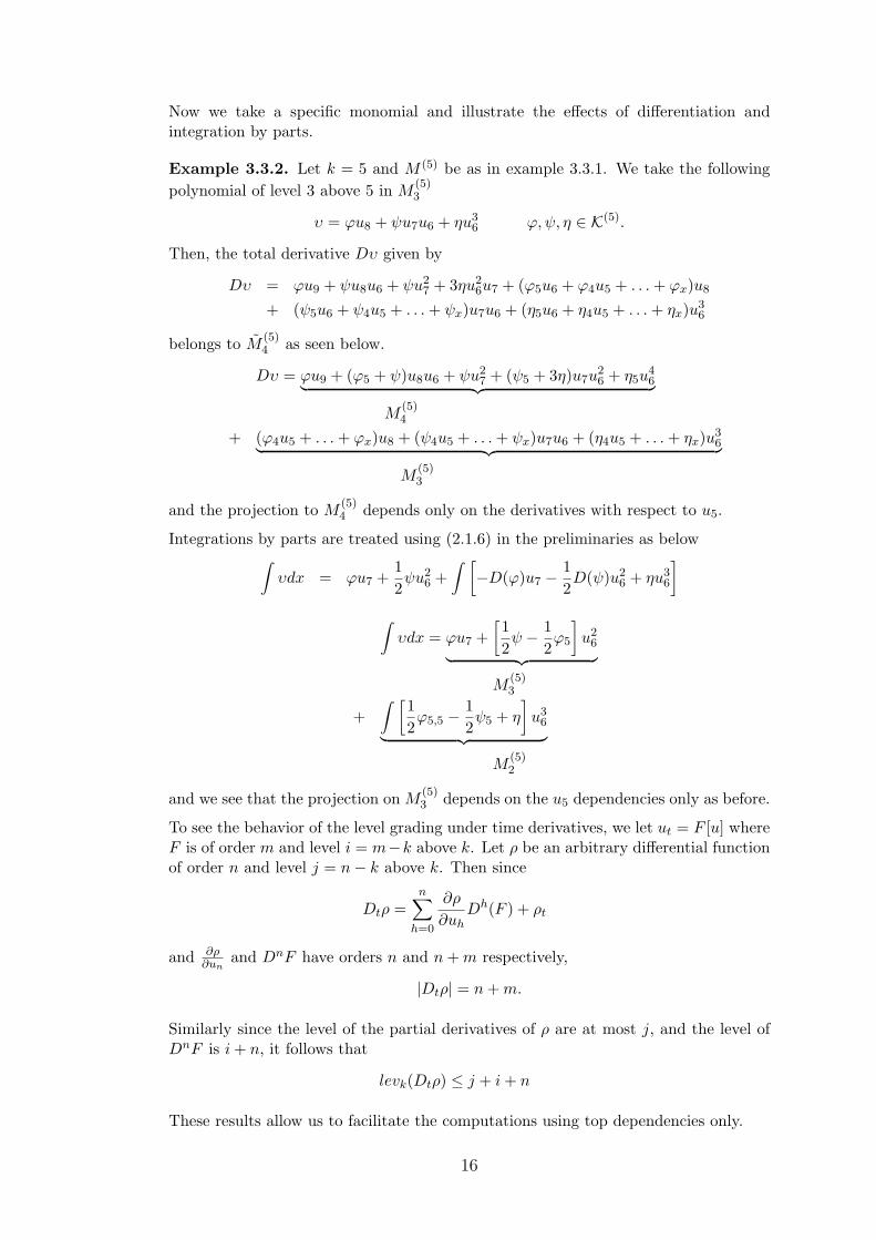
Now we take a specific monomial and illustrate the effects of differentiation andintegration by parts.

Example 3.3.2. Let k = 5 and M (5) be as in example 3.3.1. We take the followingpolynomial of level 3 above 5 in M

(5)3

υ = ϕu8 + ψu7u6 + ηu36 ϕ,ψ, η ∈ K(5).

Then, the total derivative Dυ given by

Dυ = ϕu9 + ψu8u6 + ψu27 + 3ηu2

6u7 + (ϕ5u6 + ϕ4u5 + . . . + ϕx)u8

+ (ψ5u6 + ψ4u5 + . . . + ψx)u7u6 + (η5u6 + η4u5 + . . . + ηx)u36

belongs to M(5)4 as seen below.

Dυ = ϕu9 + (ϕ5 + ψ)u8u6 + ψu27 + (ψ5 + 3η)u7u

26 + η5u

46︸ ︷︷ ︸

M(5)4

+ (ϕ4u5 + . . . + ϕx)u8 + (ψ4u5 + . . . + ψx)u7u6 + (η4u5 + . . . + ηx)u36︸ ︷︷ ︸

M(5)3

and the projection to M(5)4 depends only on the derivatives with respect to u5.

Integrations by parts are treated using (2.1.6) in the preliminaries as below∫

υdx = ϕu7 +12ψu2

6 +∫ [

−D(ϕ)u7 − 12D(ψ)u2

6 + ηu36

]

∫υdx = ϕu7 +

[12ψ − 1

2ϕ5

]u2

6

︸ ︷︷ ︸M

(5)3

+∫ [

12ϕ5,5 − 1

2ψ5 + η

]u3

6

︸ ︷︷ ︸M

(5)2

and we see that the projection on M(5)3 depends on the u5 dependencies only as before.

To see the behavior of the level grading under time derivatives, we let ut = F [u] whereF is of order m and level i = m−k above k. Let ρ be an arbitrary differential functionof order n and level j = n− k above k. Then since

Dtρ =n∑

h=0

∂ρ

∂uhDh(F ) + ρt

and ∂ρ∂un

and DnF have orders n and n + m respectively,

|Dtρ| = n + m.

Similarly since the level of the partial derivatives of ρ are at most j, and the level ofDnF is i + n, it follows that

levk(Dtρ) ≤ j + i + n

These results allow us to facilitate the computations using top dependencies only.

16

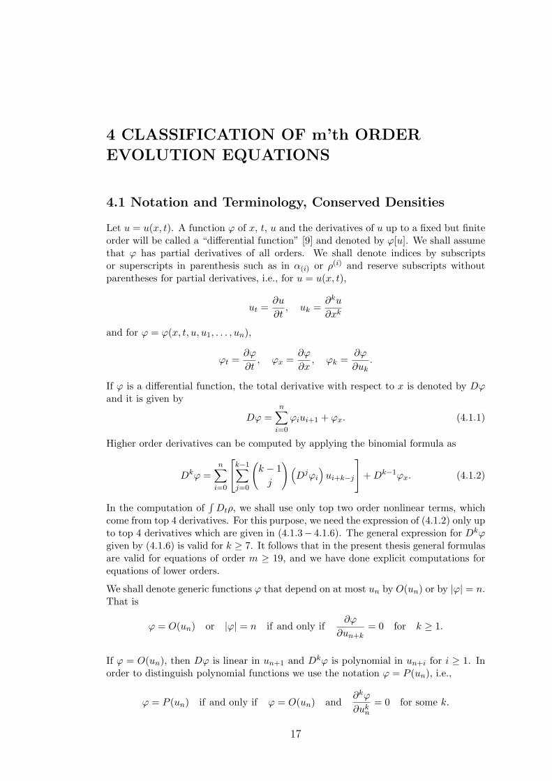
4 CLASSIFICATION OF m’th ORDER

EVOLUTION EQUATIONS

4.1 Notation and Terminology, Conserved Densities

Let u = u(x, t). A function ϕ of x, t, u and the derivatives of u up to a fixed but finiteorder will be called a “differential function” [9] and denoted by ϕ[u]. We shall assumethat ϕ has partial derivatives of all orders. We shall denote indices by subscriptsor superscripts in parenthesis such as in α(i) or ρ(i) and reserve subscripts withoutparentheses for partial derivatives, i.e., for u = u(x, t),

ut =∂u

∂t, uk =

∂ku

∂xk

and for ϕ = ϕ(x, t, u, u1, . . . , un),

ϕt =∂ϕ

∂t, ϕx =

∂ϕ

∂x, ϕk =

∂ϕ

∂uk.

If ϕ is a differential function, the total derivative with respect to x is denoted by Dϕand it is given by

Dϕ =n∑

i=0

ϕiui+1 + ϕx. (4.1.1)

Higher order derivatives can be computed by applying the binomial formula as

Dkϕ =n∑

i=0

k−1∑

j=0

(k − 1

j

) (Djϕi

)ui+k−j

+ Dk−1ϕx. (4.1.2)

In the computation of∫

Dtρ, we shall use only top two order nonlinear terms, whichcome from top 4 derivatives. For this purpose, we need the expression of (4.1.2) only upto top 4 derivatives which are given in (4.1.3− 4.1.6). The general expression for Dkϕgiven by (4.1.6) is valid for k ≥ 7. It follows that in the present thesis general formulasare valid for equations of order m ≥ 19, and we have done explicit computations forequations of lower orders.

We shall denote generic functions ϕ that depend on at most un by O(un) or by |ϕ| = n.That is

ϕ = O(un) or |ϕ| = n if and only if∂ϕ

∂un+k= 0 for k ≥ 1.

If ϕ = O(un), then Dϕ is linear in un+1 and Dkϕ is polynomial in un+i for i ≥ 1. Inorder to distinguish polynomial functions we use the notation ϕ = P (un), i.e.,

ϕ = P (un) if and only if ϕ = O(un) and∂kϕ

∂ukn

= 0 for some k.

17

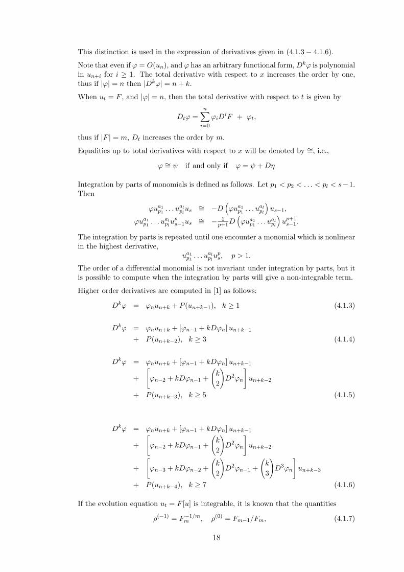
This distinction is used in the expression of derivatives given in (4.1.3− 4.1.6).

Note that even if ϕ = O(un), and ϕ has an arbitrary functional form, Dkϕ is polynomialin un+i for i ≥ 1. The total derivative with respect to x increases the order by one,thus if |ϕ| = n then |Dkϕ| = n + k.

When ut = F , and |ϕ| = n, then the total derivative with respect to t is given by

Dtϕ =n∑

i=0

ϕiDiF + ϕt,

thus if |F | = m, Dt increases the order by m.

Equalities up to total derivatives with respect to x will be denoted by ∼=, i.e.,

ϕ ∼= ψ if and only if ϕ = ψ + Dη

Integration by parts of monomials is defined as follows. Let p1 < p2 < . . . < pl < s−1.Then

ϕua1p1

. . . ualpl

us∼= −D

(ϕua1

p1. . . ual

pl

)us−1,

ϕua1p1

. . . ualpl

ups−1us

∼= − 1p+1D

(ϕua1

p1. . . ual

pl

)up+1

s−1.

The integration by parts is repeated until one encounter a monomial which is nonlinearin the highest derivative,

ua1p1

. . . ualpl

ups, p > 1.

The order of a differential monomial is not invariant under integration by parts, but itis possible to compute when the integration by parts will give a non-integrable term.

Higher order derivatives are computed in [1] as follows:

Dkϕ = ϕnun+k + P (un+k−1), k ≥ 1 (4.1.3)

Dkϕ = ϕnun+k + [ϕn−1 + kDϕn] un+k−1

+ P (un+k−2), k ≥ 3 (4.1.4)

Dkϕ = ϕnun+k + [ϕn−1 + kDϕn] un+k−1

+

[ϕn−2 + kDϕn−1 +

(k

2

)D2ϕn

]un+k−2

+ P (un+k−3), k ≥ 5 (4.1.5)

Dkϕ = ϕnun+k + [ϕn−1 + kDϕn] un+k−1

+

[ϕn−2 + kDϕn−1 +

(k

2

)D2ϕn

]un+k−2

+

[ϕn−3 + kDϕn−2 +

(k

2

)D2ϕn−1 +

(k

3

)D3ϕn

]un+k−3

+ P (un+k−4), k ≥ 7 (4.1.6)

If the evolution equation ut = F [u] is integrable, it is known that the quantities

ρ(−1) = F−1/mm , ρ(0) = Fm−1/Fm, (4.1.7)

18

where

Fm =∂F

∂um, Fm−1 =

∂F

∂um−1(4.1.8)

are conserved densities for equations of any order [2].

Higher order conserved densities are computed in [1] as below, with the followingnotation

a = F 1/mm , α(i) =

Fm−i

Fm, i = 1, 2, 3, 4 (4.1.9)

ρ(1) = a−1(Da)2 − 12m(m + 1)

Daα(1)

+ a

[12

m2(m + 1)α2

(1)

− 24m(m2 − 1)

α(2)

], (4.1.10)

ρ(2) = a(Da)[Dα(1) +

3m

α2(1) −

6(m− 1)

α(2)

]

+ 2a2[− 1

m2α3

(1) +3

m(m− 1)α(1)α(2)

− 3(m− 1)(m− 2)

α(3)

], (4.1.11)

ρ(3) = a(D2a)2 − 60m(m + 1)(m + 3)

a2D2aDα(1)

+14a−1(Da)4 + 30a(Da)2

[(m− 1)

m(m + 1)(m + 3)Dα(1)

+1

m2(m + 1)α2

(1) −2

m(m2 − 1)α(2)

]

+120

m(m2 − 1)(m + 3)a2Da

[−(m− 1)(m− 3)

mα(1)Dα(1)

+ (m− 3)Dα(2) −(m− 1)(2m− 3)

m2α3

(1)

+6(m− 2)

mα(1)α(2) − 6α(3)

]

+60

m(m2 − 1)(m + 3)a3

[(m− 1)

m(Dα(1))

2

− 4m

Dα(1)α(2) +(m− 1)(2m− 3)

m3α4

(1)

− 4(2m− 3)

m2α2

(1)α(2) +8m

α(1)α(3)

+4m

α2(2) −

8(m− 3)

α(4)

]. (4.1.12)

19

4.2 General Results on Classification

In [1], the criterion for integrability is the existence of a formal symmetry in the senseof [2]. The existence of a formal symmetry requires the existence of certain conserveddensities ρ(i), i = −1, 0, 1, . . .. It is well known that for any m, the first two conserveddensities are

ρ(−1) = F−1/mm and ρ(0) = Fm−1/Fm.

The explicit expressions of ρ(1) and ρ(2) for m ≥ 5 and of ρ(3) for m ≥ 7 obtainedin [1] are given in Appendix A. In our computations we shall use only conserveddensities which look like ρ(1), ρ(2) and ρ(3), but all conserved densities have been usedin computer algebra computations at lower orders for cross checking purposes.

The coefficients of top two nonlinear terms in Dtρ(1) give a linear homogeneous system

of equations for ∂2F∂u2

mand ∂2ρ(1)

∂u2n

, with coefficients depending on m. The coefficientmatrix is nonsingular for m 6= 5, hence it follows that for m ≥ 7, an evolutionequation of order m admitting a nontrivial conserved density of order m + 1 has tobe quasi-linear. In [1], it is shown that u2

3k+l+1 is the top nonlinear term in∫

Dtρ,for ρ = ρ(x, t, u, . . . , un) and ut = F (x, t, u, . . . , um) where m = 2k + 1, n ≥ m andn = 2k + l + 1.

In this section first we shall show that the contribution to the top two nonlinearterms, come from the top 4 derivatives in the expansion of

∫Dtρ. Then we shall give

the expression of the coefficients of top two nonlinearities u23k+l+1 and u2

3k+l in theexpansion of

∫Dtρ.

This result is based on the expression of the derivatives as in [1].

Proposition 4.2.1. Let ρ = ρ(x, t, u, . . . , un) and ut = F (x, t, u, . . . , um) wherem = 2k + 1, n = 2k + l + 1 and k + l − 1 ≥ 0. Then

(−1)k+1Dtρ ∼= [Dk+1ρn −Dkρn−1]Dk+lF − [Dkρn−2 −Dk−1ρn−3]Dk+l−1F

+ O(u3k+l−1). (4.2.1)

Proof:

Dtρ =n∑

i=0

ρiDiF + ρt (4.2.2)

In Dtρ, the highest order derivative comes from ρnDnF , where ρn and DnF are oforders 2k + 1 + l and 4k + 2 + l respectively. If we integrate by parts k + 1 times weobtain

ρnDnF ∼= (−1)k+1Dk+1ρn Dk+lF

where Dk+1ρ and Dk+lF are now respectively of orders 3k + 2 + l and 3k + 1 + l. Onemore integration by parts gives a term nonlinear in u3k+1+l. Similarly one can see thatin ρn−1D

n−1F , ρn−1 and Dn−1F are of orders 2k + 1 + l and 4k + 1 + l. This time,integrating by parts k times, we have

ρn−1Dn−1F ∼= (−1)kDkρn Dk+lF,

where Dkρn−1 and Dk+lF are both of orders 3k + 1 + l. Thus the highest ordernonlinear term, in u3k+l+1, comes from top two derivatives in ρnDn and ρn−1D

n−1F .

20

By similar counting arguments, one can easily see that top two nonlinear terms areobtained from top four derivatives and the remaining terms are of order 3k + l − 1.

ρn−2pDn−2pF + ρn−2p−1D

n−2p−1F = ρ2k+l+1−2pD2k+l+1−2pF

+ ρ2k+l−2pD2k+l−2pF (4.2.3)

with 2k + l − 2p > 0. We integrate by parts until the order of the product differ byone and we get:

(−1)k+1−p[Dk+1−pρn−2p −Dk−pρn−2p−1]Dk+l−pF (4.2.4)

Here, the first and the second term in the brackets are of orders 3k + l + 2 − p and3k + l + 1 − p respectively, and Dk+l−pF has order 3k + l + 1 − p. Thus afterintegration by parts again we get the term u2

3k+l+1−p. It follows that the top twononlinear terms for p = 0, and p = 1 come from ρn, ρn−1, ρn−2 and ρn−3. 2

Remark 4.2.2 As the general expressions for the derivatives given in (4.1.3 − 4.1.6)are valid for large k, there are restrictions on the validity of the formula (4.2.1). Sincethe top four terms of Dk+lF and Dk+1ρn are needed in (4.2.1), from (4.1.6) it followsthat k + 1 and k + l should be both larger than or equal to 7. On the other hand, atmost top two terms of the expressions in the second bracket in (4.2.1) contribute tothe top nonlinearities and it turns out that the restrictions coming from (4.1.3, 4.1.4)are always satisfied and the crucial restriction is k + 1 ≥ 7 and k + l ≥ 7. Thus forl = 1, 0, −1 and −2, we need respectively k ≥ 6, 7, 8 and 9 hence m ≥ 13, 15, 17 and19.

We shall now give the explicit expressions of the coefficients of top two nonlinear termsfor m ≥ 19 and k + l ≥ 7.

Proposition 4.2.3Let ut = F (x, t, u, . . . , um), m = 2k + 1, be an evolution equationand ρ = ρ(x, t, u, . . . , un) with n = m + l, −2 ≤ l ≤ 2, be a conserved density forut = F . For m ≥ 13 and k + l ≥ 7, the coefficients of the top two nonlinear termsu2

3k+l+1 for k + l > 0 and u23k+l for k + l − 1 > 0 are respectively as follows

(k +12)FmDρn,n − (k + l +

12)DFmρn,n − Fm−1ρn,n = 0, (4.2.5)

ρn,n D3Fm

[112

(2k3 + 6k2l + 6kl2 + 2l3 + 3k2 + 3l2 + 6kl + k + l)]

+ ρn,n D2Fm−1

[12

(k2 + 2kl + 2k + 2l + l2 + 1)]

+ ρn,n DFm−2

[12

(3 + 2k + 2l)]

+ ρn,n Fm−3

+ Dρn,n D2Fm

[14

(−2k3 − 4k2l − 2kl2 + k2 + l2 + 2kl + k + l)]

+ Dρn,n DFm−1

[12

(1 + l − 2k2 − 2kl)]

+ Dρn,n Fm−2

[12

(1− 2k)]

+ D2ρn,n DFm

[14(2k3 + 2k2l − k2 − k)

]

21

+ D2ρn,n Fm−1

[12

k2]

+ D3ρn,n Fm

[112

(−2k3 − 3k2 − k)]

+ Dρn,n−1 DFm

[12

(−1 + 2k + 2l)]

+ Dρn,n−1 Fm−1

+ D2ρn,n−1 Fm

[12

(−1− 2k)]

+ ρn,n−2 DFm [2k + 2l − 1]+ ρn,n−2 Fm−1 [2]+ Dρn,n−2 Fm [−2k − 1]

+ ρn−1,n−1 DFm

[12

(1− 2k − 2l)]

+ ρn−1,n−1 Fm−1 [−1]

+ Dρn−1,n−1 Fm

[12

(1 + 2k)]

= 0. (4.2.6)

Proof. The proof is a straightforward computation of the integrations indicated inProposition 4.2.1. Writing the first four terms in Dtρ and keeping only the termswhich contribute to the nonlinearities u2

3k+l+1, u23k+l, we get

(−1)k+1Dtρ ∼= ρn,n Fmu3k+l+1 u3k+l+2

+ ρn,n [Fm−1 + (k + l)DFm] u3k+l u3k+l+2

+ ρn,n

[Fm−2 + (k + l)DFm−1 +

(k + l

2

)D2Fm

]u3k+l−1 u3k+l+2

+ ρn,n

[Fm−3 + (k + l)DFm−2 +

(k + l

2

)D2Fm−1

+

(k + l

3

)D3Fm

]u3k+l−2 u3k+l+2

+ (k + 1) Dρn,n Fm u3k+l+1 u3k+l+1

+ (k + 1) Dρn,n [Fm−1 + (k + l)DFm] u3k+l u3k+l+1

+ (k + 1) Dρn,n [Fm−2 + (k + l)DFm−1

+

(k + l

2

)D2Fm

]u3k+l−1 u3k+l+1

+

[ρn,n−2 + Dρn,n−1 +

(k + 1

2

)D2ρn,n

− ρn−1,n−1] Fmu3k+l+1 u3k+l

+

[ρn,n−2 + Dρn,n−1 +

(k + 1

2

)D2ρn,n − ρn−1,n−1

]

× [Fm−1 + (k + l)DFm] u3k+l u3k+l

+

[ρn,n−3 + (k + 1)Dρn,n−2 + kD2ρn,n−1 +

(k + 1

3

)D3ρn,n

− ρn−1,n−2 − kDρn−1,n−1] Fm u3k+l+1 u3k+l−1

− ρn−2,n Fm u3k+l u3k+l+1

− ρn−2,n [Fm−1 + (k + l − 1)DFm] u3k+l−1 u3k+l+1

22

− [ρn−2,n−1 + kDρn−2,n − ρn−3,n] Fm u3k+l u3k+l. (4.2.7)

After integrations by parts we get (4.2.5) as the coefficient of the first nonlinear termu2

3k+l+1 and (4.2.6) as the coefficient of the second nonlinear term u23k+l. 2

From equation (4.2.5) we can easily get a number of results pertaining the form ofthe conserved densities. In particular we can see that higher order conserved densitiesshould be quadratic in the highest derivative and top coefficients of the conserveddensities at every order are proportional to each other [1].

Corollary 4.2.4 Let ρ = ρ(x, t, u, . . . , un) and ut = F (x, t, u, . . . , um), m ≥ 7 andn > m. Then

ρn,n,n = 0 (4.2.8)

Proof. It can be seen that (4.2.5) uses only top two terms and for l > 0 it is valid fork + 1 ≥ 3. Writing it in the form

(k +12)Dρn,n

ρn,n− (k + l +

12)DFm

Fm=

Fm−1

Fm, (4.2.9)

we can see that for n > m the highest order term is Dρn,n and it follows that ρn,n,n = 0.2

Remark 4.2.5 From (4.2.9) one can easily see that if ρ and η are both conserveddensities of order n, with ρn,n = P and ηn,n = Q, then DP

P = DQQ , hence the ratio of

the top coefficients is independent of x. If ρ and η are conserved densities of consecutiveorders say, |ρ| = n and |η| = n + 1 with ρn,n = P and ηn+1,n+1 = Q, then

(k +12)(

DQ

Q− DP

P

)=

DFm

Fm,

hence Q = F2/mm P .

Remark 4.2.6 If the partial derivatives of F and ρ in (4.2.5) and (4.2.6) depend atmost on uj , then these equations are polynomial in uj+i, i > 0. In all the subsequentcomputations we have used only the coefficient of the top order derivatives.

4.3 Polynomiality Results in Top Three Derivatives

In this section we give our final results which are the polynomiality in top threederivatives. We apply Proposition 4.2.3 either directly to a canonical density ρ(i),i = 1, 2, 3(step 3 and 6), or to generic conserved densities ρ, ν. We also give Tablesshowing that at least one of the canonical densities is of the generic form (Tables(4.3.1)− (4.3.5))

We used generic conserved densities in steps one, two and four. The first step isto obtain the quasilinearity result for m > 5, which follows from the fact that thecoefficient matrix of a homogeneous system is non-singular for m > 5. At the secondand fourth steps we have a similar structure; we show that the coefficient of um isindependent of um−1 and um−2 respectively, by obtaining nonsingular homogeneoussystems of linear equations.

The third and sixth steps are based on relatively straightforward computations usingthe canonical densities. At the third step we complete polynomiality in um−1 whileat the fifth and sixth steps we complete polynomiality in um−2, by using the explicitform of the canonical densities ρ(1) and ρ(3).

23

Step 0:Quasilinearity Fm,m = 0

First we obtain again the quasilinearity result given in [1], for m > 5. Thanks to thegeneral expressions in Proposition 4.2.3, applying (4.2.5) to ρ(1) the proof given hereis very neat.

Proposition 4.3.1 Let ut = F (x, t, u, . . . , um), m = 2k + 1 > 13, |F | = m, bean arbitrary evolution equation and ρ(1) = P (0)u2

m+1 + Q(0)um+1 + R(0), l = 1,|P (0)| = |Q(0)| = |R(0)| = m, P (0) 6= 0 its conserved density, then Fm,m = 0

Proof: The coefficient of um+1 in (4.2.5) and the coefficient of um+3 in (4.2.6) arerespectively as follows:

(2k + 1)P

(0)m

P (0)− (2k + 3)

Fm,m

Fm= 0 (4.3.1)

(2k + 1)(k2 + k + 6)P

(0)m

P (0)− (2k + 3)(k + 1)(k + 2)

Fm,m

Fm= 0 (4.3.2)

From (4.3.1) and (4.3.2) we get:[

1 −1(k2 + k + 6) −(k2 + 3k + 2)

]

P(0)m

P (0)

Fm,m

Fm

=

[00

](4.3.3)

Since k 6= 2 from (4.3.3) we conclude that

Fm,m = P (0)m = 0 (4.3.4)

2

The following steps are valid for m ≥ 19

The aim of the first and second steps is to investigate the dependency on um−1 of thecoefficients A and B in the quasi-linear integrable evolution equation ut = Aum + B.For this purpose we use the coefficients of the top two nonlinearities in

∫Dtρ which are

respectively equations 4.2.5 and 4.2.6. The results with their proof are given below.

Step 1:Polynomiality in um−1 1st Result Am−1 = Pm−1 = 0

Proposition 4.3.2 Letut = Aum + B,

with A = am and |A| = |B| = m− 1. Then the canonical density ρ(1) reduces to

ρ(1) = P (1)u2m + Q(1)um + R(1),

with |P (1)| = |Q(1)| = |R(1)| = m− 1, And if ρ(1) is conserved density then

Am−1 = P(1)m−1 = 0 (4.3.5)

Proof: Substituting ut = Aum + B in (4.1.10) and integrating by parts if necessarywe get ρ(1) with

P (1) =a2

m−1

a(4.3.6)

24

The coefficient of um in (4.2.5) is:

(2k + 1)P

(1)m−1

P (1)− (2k + 3)

Am−1

A= 0 (4.3.7)

While the coefficient of um+2 in (4.2.6) is:

2P (1)Am−1112

[2k3 + 9k2 + 13k + 6

]− 2P

(1)m−1A

112

[2k3 + 3k2 + 13k + 6

]= 0

[2k3 + 9k2 + 13k + 6

] Am−1

A−

[2k3 + 3k2 + 13k + 6

] P(1)m−1

P (1)= 0 (4.3.8)

From (4.3.7) and (4.3.8) we get:

[2k + 1 −(2k + 3)2k3 + 3k2 + 13k + 6 −(2k3 + 9k2 + 13k + 6)

]

P(1)m−1

P (1)

Am−1

A

=

[00

](4.3.9)

Since k 6= 2, Am−1 = P(1)m−1 = 0. 2

Now we shall see that the existence of a conserved density determines the form of B.

Step 3:Polinomiality in um−1 2nd Result Bm−1,m−1,m−1 = 0

Proposition 4.3.3 Letut = Aum + B,

with |A| = m− 2, |B| = m− 1 and the canonical densities

ρ(1) = P (1)u2m−1 + Q(1)um−1 + R(1)

ρ(3) = P (3)u2m + Q(3)um + R(3)

with |P (1)| = m−2 and |P (3)| = m−1 And if ρ(1) and ρ(3) are conserved densities,then

Bm−1,m−1,m−1 = 0 (4.3.10)

Proof: We substitute ut = Aum +B and Am−1 = 0 in (4.1.10), (4.1.12) and integrateby parts then we get the coefficients P (1) and P (3) respectively:

P (1) =24

m2 − 1am−2,m−2 + a2

m−2a−1(m2 − 1) (4.3.11)

P (3) =a

m3 + 3m2 −m− 3

[a2

m−2

(m3 + 3m2 − 121m + 597

)

+ a−m+1am−2Bm−1,m−1

(180m

− 60)

+ a−2m+2B2m−1,m−1

(60m− 60

m2

)](4.3.12)

We compute (4.2.5) using ρ(1) where l = −1 and the top dependency of P (1) is um−2

and we get:

(k +12)2AP

(1)m−2um−1 − (k − 1

2)2P (1)Am−2um−1 − 2P (1)Bm−1 = 0 (4.3.13)

25

We compute also (4.2.5) using ρ(3) where l = 0 and the top dependency of P (3) is um−1

and we get:

(k +12)2AP

(3)m−1um − (k +

12)2P (3)Am−2um−1 − 2P (3)Bm−1 = 0 (4.3.14)

Differentiating twice (4.3.13) with respect to um−1 we obtain:

2P (1)Bm−1,m−1,m−1 = 0 (4.3.15)

On the other hand the coefficient of um in (4.3.14) gives:

(k +12)2AP

(3)m−1 = 0 (4.3.16)

and P(3)m−1 can be written as

Bm−1,m−1,m−1(p1Am−2 + p2Bm−1,m−1) (4.3.17)

where p1 and p2 are independent from um−1. Then from (4.3.15) and (4.3.17) weconclude that:

Bm−1,m−1,m−1 = 0. (4.3.18)

2

Here is the form of the integrable evolution equation that we obtain which is polynomialin um−1. ut = Aum + Cu2

m−1 + Dum−1 + E. The following three steps investigate thepolynomiality in um−2.

Step 4:Polinomiality in um−2 1st Result Am−2 = Pm−2 = C = 0

Proposition 4.3.4 Let ut = Aum + Cu2m−1 + Dum−1 + E, where a = A

1m and the

canonical densitiesρ(1) = P (1)u2

m−1 + Q(1)um−1 + R(1) (4.3.19)

andρ(2) = P (2)u2

m + Q(2)um + R(2) (4.3.20)

where A,C, D,E, P (1), P (2), a depend on x, t, u, . . . , um−2,. If ρ(1) and ρ(2) areconserved densities, then

Am−2 = P(1)m−2 = C = 0 (4.3.21)

Proof: We substitute ut = Aum +Cu2m−1 +Dum−1 +E, in (4.1.10) and (4.1.12q) and

notice that ρ(1) and ρ(3) have the same form as ρ(1) and ρ(2). We recomputed (4.2.5),and (4.2.6) for l = −1, 0 and we get respectively:The coefficient of um−1 in (4.2.5) for ρ(1), l = −1

4C − (2k + 1) am P(1)m−2

P (1)+

(4k2 − 1

)am−1am−2 = 0 (4.3.22)

The coefficient of um+1 in (4.2.6) for ρ(1), l = −1

12k2C −(2k3 + 3k2 + 13k + 6

)am P

(1)m−2

P (1)

+(4k4 − 4k3 + 23k2 + 25k + 6

)am−1am−2 = 0 (4.3.23)

26

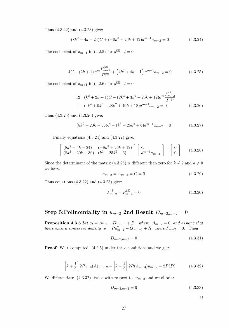
Thus (4.3.22) and (4.3.23) give:

(8k2 − 4k − 24)C + (−8k3 + 26k + 12)am−1am−2 = 0 (4.3.24)

The coefficient of um−1 in (4.2.5) for ρ(2), l = 0

4C − (2k + 1) am P(2)m−2

P (2)+

(4k2 + 4k + 1

)am−1am−2 = 0 (4.3.25)

The coefficient of um+1 in (4.2.6) for ρ(2), l = 0

12 (k2 + 2k + 1)C − (2k3 + 3k2 + 25k + 12)am P(2)m−2

P (2)

+ (4k4 + 9k3 + 28k2 + 49k + 18)am−1am−2 = 0 (4.3.26)

Thus (4.3.25) and (4.3.26) give:

(8k2 + 20k − 36)C + (k3 − 25k2 + 6)am−1am−2 = 0 (4.3.27)

Finally equations (4.3.24) and (4.3.27) give:[

(8k2 − 4k − 24) (−8k3 + 26k + 12)(8k2 + 20k − 36) (k3 − 25k2 + 6)

] [Cam−1am−2

]=

[00

](4.3.28)

Since the determinant of the matrix (4.3.28) is different than zero for k 6= 2 and a 6= 0we have:

am−2 = Am−2 = C = 0 (4.3.29)

Thus equations (4.3.22) and (4.3.25) give:

P(1)m−2 = P

(2)m−2 = 0 (4.3.30)

Step 5:Polinomiality in um−2 2nd Result Dm−2,m−2 = 0

Proposition 4.3.5 Let ut = Aum + Dum−1 + E, where Am−2 = 0, and assume thatthere exist a conserved density ρ = Pu2

m−1 + Qum−1 + R, where Pm−2 = 0. Then

Dm−2,m−2 = 0 (4.3.31)

Proof: We recomputed (4.2.5) under these conditions and we get:

[k +

12

]2Pm−3(A)um−2 −

[k − 1

2

]2P (Am−3)um−2 = 2P (D) (4.3.32)

We differentiate (4.3.32) twice with respect to um−2 and we obtain:

Dm−2,m−2 = 0 (4.3.33)

2

27

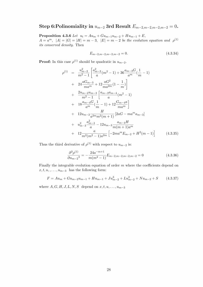
Step 6:Polinomiality in um−2 3rd Result Em−2,m−2,m−2,m−2 = 0.

Proposition 4.3.6 Let ut = Aum + Gum−1um−2 + Hum−1 + E,A = am, |A| = |G| = |H| = m − 3, |E| = m − 2 be the evolution equation and ρ(1)

its conserved density. Then

Em−2,m−2,m−2,m−2 = 0. (4.3.34)

Proof: In this case ρ(1) should be quadratic in um−2.

ρ(1) =u2

m−2

m2 − 1

[a2

m−3

a(m2 − 1) + 36

am−3G

am(

1m− 1)

+ 24aGm−3

mam+ 12

aG2

ma2m(1− 1

m)

]

+2um−2um−3

m2 − 1

[am−3am−4

a(m2 − 1)

+ 18am−4G

am(

1m− 1) + 12

Gm−4a

mam

]

+ 12um−2H

a2mm2(m + 1)[2aG−mamam−3]

+ u2m−3

a2m−4

a− 12um−3

am−4H

m(m + 1)am

+ 12a

m2(m2 − 1)a2m

[−2mamEm−2 + H2(m− 1)

](4.3.35)

Thus the third derivative of ρ(1) with respect to um−2 is:

∂3ρ(1)

∂um−23

= − 24a−m+1

m(m2 − 1)Em−2,m−2,m−2,m−2 = 0 (4.3.36)

Finally the integrable evolution equation of order m where the coefficients depend onx, t, u, , . . . , um−3 has the following form:

F = Aum + Gum−2um−1 + Hum−1 + Ju3m−2 + Lu2

m−2 + Num−2 + S (4.3.37)

where A, G,H, J, L, N, S depend on x, t, u, . . . , um−3

28

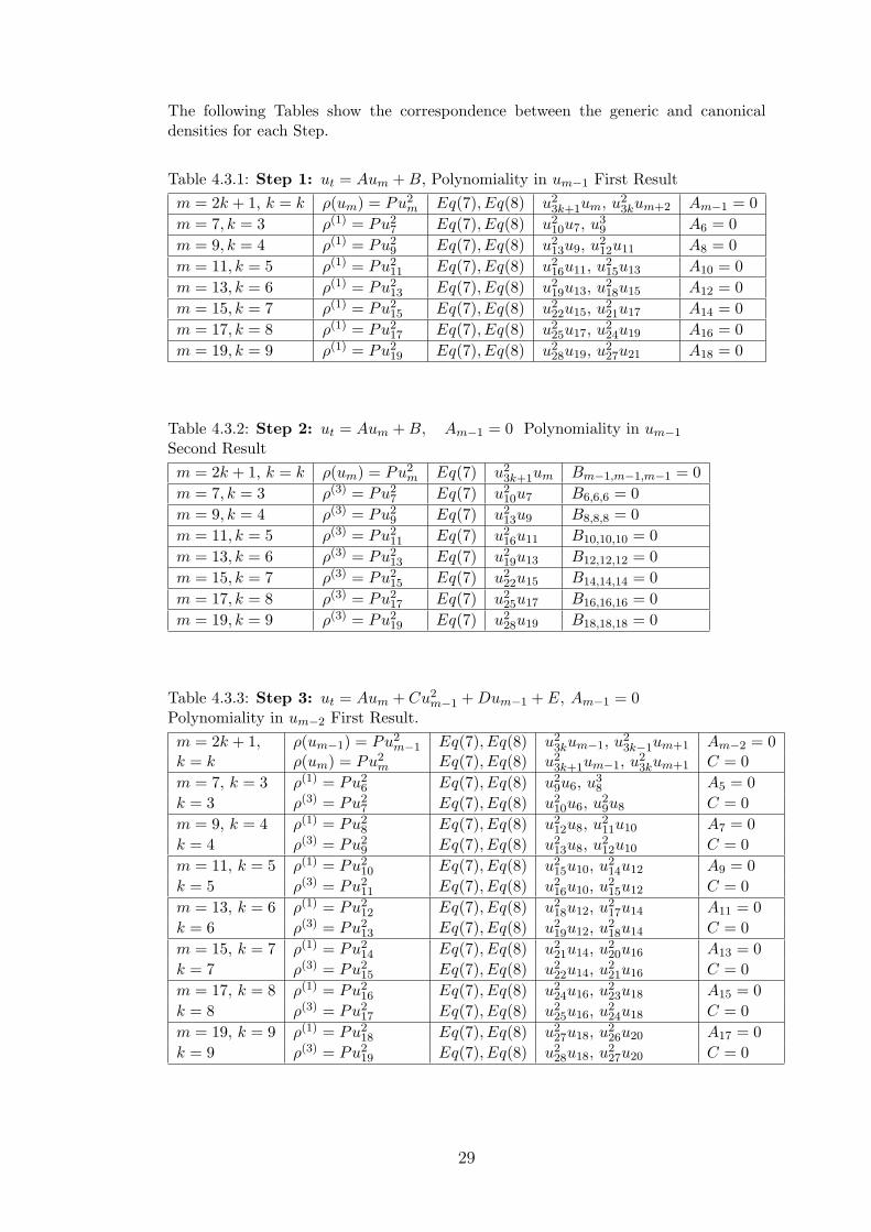
The following Tables show the correspondence between the generic and canonicaldensities for each Step.

Table 4.3.1: Step 1: ut = Aum + B, Polynomiality in um−1 First Resultm = 2k + 1, k = k ρ(um) = Pu2

m Eq(7), Eq(8) u23k+1um, u2

3kum+2 Am−1 = 0m = 7, k = 3 ρ(1) = Pu2

7 Eq(7), Eq(8) u210u7, u3

9 A6 = 0m = 9, k = 4 ρ(1) = Pu2

9 Eq(7), Eq(8) u213u9, u2

12u11 A8 = 0m = 11, k = 5 ρ(1) = Pu2

11 Eq(7), Eq(8) u216u11, u2

15u13 A10 = 0m = 13, k = 6 ρ(1) = Pu2

13 Eq(7), Eq(8) u219u13, u2

18u15 A12 = 0m = 15, k = 7 ρ(1) = Pu2

15 Eq(7), Eq(8) u222u15, u2

21u17 A14 = 0m = 17, k = 8 ρ(1) = Pu2

17 Eq(7), Eq(8) u225u17, u2

24u19 A16 = 0m = 19, k = 9 ρ(1) = Pu2

19 Eq(7), Eq(8) u228u19, u2

27u21 A18 = 0

Table 4.3.2: Step 2: ut = Aum + B, Am−1 = 0 Polynomiality in um−1

Second Resultm = 2k + 1, k = k ρ(um) = Pu2

m Eq(7) u23k+1um Bm−1,m−1,m−1 = 0

m = 7, k = 3 ρ(3) = Pu27 Eq(7) u2

10u7 B6,6,6 = 0m = 9, k = 4 ρ(3) = Pu2

9 Eq(7) u213u9 B8,8,8 = 0

m = 11, k = 5 ρ(3) = Pu211 Eq(7) u2

16u11 B10,10,10 = 0m = 13, k = 6 ρ(3) = Pu2

13 Eq(7) u219u13 B12,12,12 = 0

m = 15, k = 7 ρ(3) = Pu215 Eq(7) u2

22u15 B14,14,14 = 0m = 17, k = 8 ρ(3) = Pu2

17 Eq(7) u225u17 B16,16,16 = 0

m = 19, k = 9 ρ(3) = Pu219 Eq(7) u2

28u19 B18,18,18 = 0

Table 4.3.3: Step 3: ut = Aum + Cu2m−1 + Dum−1 + E, Am−1 = 0

Polynomiality in um−2 First Result.m = 2k + 1, ρ(um−1) = Pu2

m−1 Eq(7), Eq(8) u23kum−1, u2

3k−1um+1 Am−2 = 0k = k ρ(um) = Pu2

m Eq(7), Eq(8) u23k+1um−1, u2

3kum+1 C = 0m = 7, k = 3 ρ(1) = Pu2

6 Eq(7), Eq(8) u29u6, u3

8 A5 = 0k = 3 ρ(3) = Pu2

7 Eq(7), Eq(8) u210u6, u2

9u8 C = 0m = 9, k = 4 ρ(1) = Pu2

8 Eq(7), Eq(8) u212u8, u2

11u10 A7 = 0k = 4 ρ(3) = Pu2

9 Eq(7), Eq(8) u213u8, u2

12u10 C = 0m = 11, k = 5 ρ(1) = Pu2

10 Eq(7), Eq(8) u215u10, u2

14u12 A9 = 0k = 5 ρ(3) = Pu2

11 Eq(7), Eq(8) u216u10, u2

15u12 C = 0m = 13, k = 6 ρ(1) = Pu2

12 Eq(7), Eq(8) u218u12, u2

17u14 A11 = 0k = 6 ρ(3) = Pu2

13 Eq(7), Eq(8) u219u12, u2

18u14 C = 0m = 15, k = 7 ρ(1) = Pu2

14 Eq(7), Eq(8) u221u14, u2

20u16 A13 = 0k = 7 ρ(3) = Pu2

15 Eq(7), Eq(8) u222u14, u2

21u16 C = 0m = 17, k = 8 ρ(1) = Pu2

16 Eq(7), Eq(8) u224u16, u2

23u18 A15 = 0k = 8 ρ(3) = Pu2

17 Eq(7), Eq(8) u225u16, u2

24u18 C = 0m = 19, k = 9 ρ(1) = Pu2

18 Eq(7), Eq(8) u227u18, u2

26u20 A17 = 0k = 9 ρ(3) = Pu2

19 Eq(7), Eq(8) u228u18, u2

27u20 C = 0

29

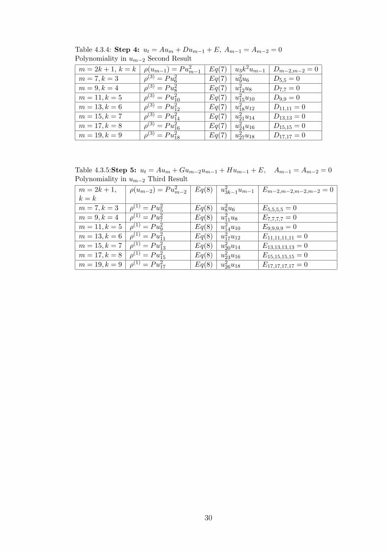
Table 4.3.4: Step 4: ut = Aum + Dum−1 + E, Am−1 = Am−2 = 0Polynomiality in um−2 Second Resultm = 2k + 1, k = k ρ(um−1) = Pu2

m−1 Eq(7) u3k2um−1 Dm−2,m−2 = 0

m = 7, k = 3 ρ(3) = Pu26 Eq(7) u2

9u6 D5,5 = 0m = 9, k = 4 ρ(3) = Pu2

8 Eq(7) u212u8 D7,7 = 0

m = 11, k = 5 ρ(3) = Pu210 Eq(7) u2

15u10 D9,9 = 0m = 13, k = 6 ρ(3) = Pu2

12 Eq(7) u218u12 D11,11 = 0

m = 15, k = 7 ρ(3) = Pu214 Eq(7) u2

21u14 D13,13 = 0m = 17, k = 8 ρ(3) = Pu2

16 Eq(7) u224u16 D15,15 = 0

m = 19, k = 9 ρ(3) = Pu218 Eq(7) u2

27u18 D17,17 = 0

Table 4.3.5:Step 5: ut = Aum + Gum−2um−1 + Hum−1 + E, Am−1 = Am−2 = 0Polynomiality in um−2 Third Resultm = 2k + 1, ρ(um−2) = Pu2

m−2 Eq(8) u23k−1um−1 Em−2,m−2,m−2,m−2 = 0

k = k

m = 7, k = 3 ρ(1) = Pu25 Eq(8) u2

8u6 E5,5,5,5 = 0m = 9, k = 4 ρ(1) = Pu2

7 Eq(8) u211u8 E7,7,7,7 = 0

m = 11, k = 5 ρ(1) = Pu29 Eq(8) u2

14u10 E9,9,9,9 = 0m = 13, k = 6 ρ(1) = Pu2

11 Eq(8) u217u12 E11,11,11,11 = 0

m = 15, k = 7 ρ(1) = Pu213 Eq(8) u2

20u14 E13,13,13,13 = 0m = 17, k = 8 ρ(1) = Pu2

15 Eq(8) u223u16 E15,15,15,15 = 0

m = 19, k = 9 ρ(1) = Pu217 Eq(8) u2

26u18 E17,17,17,17 = 0

30

5 SPECIAL CASES

In the application of the integrations by parts to Dtρ we use the expression of thekth derivatives given by (4.1.6). This expression, which involves top 4 derivativesis valid for k ≥ 7. In our computations Dk+l−1F for l = −2,−1, 0, 1, 2 appears in(4.2.1). Although at this place only top 2 derivatives are used, we assume that thegeneral results obtained in the previous section are valid for k ≥ 9, i.e, for m ≥ 19,and treat m = 7, 9, 11, 13, 15, 17, 19 as special cases and conserved density conditionsare computed directly, without using 4.2.5 and 4.2.6. The derivations for m = 7 andm = 9 are given in some detail below. At all other orders, computations are carriedout explicitly. One can compute it using the tables below (Tables 5.1.1−5.1.4) where ithas been shown the steps and quadratic terms to be considered on each computation.

5.1 Classification of 7th order evolution equation

5.1.1 First Method

In this section we give the explicit computations for m = 7 using all canonical densitiesρ(i), i = −1, 1, 2, 3 computed in [1].

Step 1. We start with the quasilinear case where

ut = A(x, t, u, . . . , u6)u7 + B(x, t, u, . . . , u6).

Recalling that in the grading by levels we need only the dependency on u6 we write

ut ∼ A(u6)u7 + B(u6).

In the following ∼ will denote equality using the dependency on the top base levelonly.

The conserved densities areρ(−1) = a−1 = A−1/7 (5.1.1.1)

ρ(1) = u27a

26a−1 +

314

u7a6B6a−7 +

398

B26a−13, (5.1.1.2)

ρ(2) = u27a6a

−7 [−7a6B6 + B6a]− 37u7a6B

26a−13

− 249

B36a−19, (5.1.1.3)

ρ(3) = u28a

26a + u4

7

[−2

3a666a6a +

13a2

66a−23a66a

26 +

14a4

6a−1

]

+ u37a−6

[356

a66B66a +928

a26B66 − 3

56a6B666a

]

+ u27a−13

[16598

a26B

26 −

3398

a6B66B6a +3

196B2

66a2]

+33686

u7a6B36a−19 +

339604

B46a−25. (5.1.1.4)

31

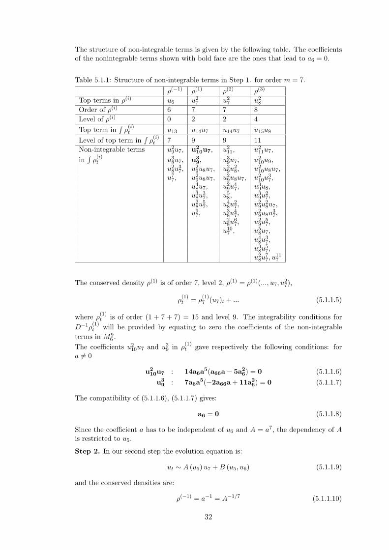
The structure of non-integrable terms is given by the following table. The coefficientsof the nonintegrable terms shown with bold face are the ones that lead to a6 = 0.

Table 5.1.1: Structure of non-integrable terms in Step 1. for order m = 7.

ρ(−1) ρ(1) ρ(2) ρ(3)

Top terms in ρ(i) u6 u27 u2

7 u28

Order of ρ(i) 6 7 7 8Level of ρ(i) 0 2 2 4Top term in

∫ρ(i)t u13 u14u7 u14u7 u15u8

Level of top term in∫

ρ(i)t 7 9 9 11

Non-integrable terms u29u7, u2

10u7, u211, u2

11u7,

in∫

ρ(i)t u3

8u7, u39, u3

9u7, u210u9,

u28u

37, u2

9u8u7, u29u

28, u2

10u8u7,u7

7, u29u8u7, u2

9u8u7, u210u

37,

u48u7, u2

9u47, u3

9u8,u3

8u37, u5

8, u39u

27,

u28u

57, u4

8u27, u2

9u28u7,

u97, u3

8u47, u2

9u8u37,

u28u

67, u2

9u57,

u107 , u5

8u7,u4

8u37,

u38u

57,

u28u

77, u

117

The conserved density ρ(1) is of order 7, level 2, ρ(1) = ρ(1)(..., u7, u27),

ρ(1)t = ρ

(1)7 (u7)t + ... (5.1.1.5)

where ρ(1)t is of order (1 + 7 + 7) = 15 and level 9. The integrability conditions for

D−1ρ(1)t will be provided by equating to zero the coefficients of the non-integrable

terms in M96 .

The coefficients u210u7 and u3

9 in ρ(1)t gave respectively the following conditions: for

a 6= 0

u210u7 : 14a6a5(a66a− 5a2

6) = 0 (5.1.1.6)u3

9 : 7a6a5(−2a66a + 11a26) = 0 (5.1.1.7)

The compatibility of (5.1.1.6), (5.1.1.7) gives:

a6 = 0 (5.1.1.8)

Since the coefficient a has to be independent of u6 and A = a7, the dependency of Ais restricted to u5.

Step 2. In our second step the evolution equation is:

ut ∼ A (u5) u7 + B (u5, u6) (5.1.1.9)

and the conserved densities are:

ρ(−1) = a−1 = A−1/7 (5.1.1.10)

32

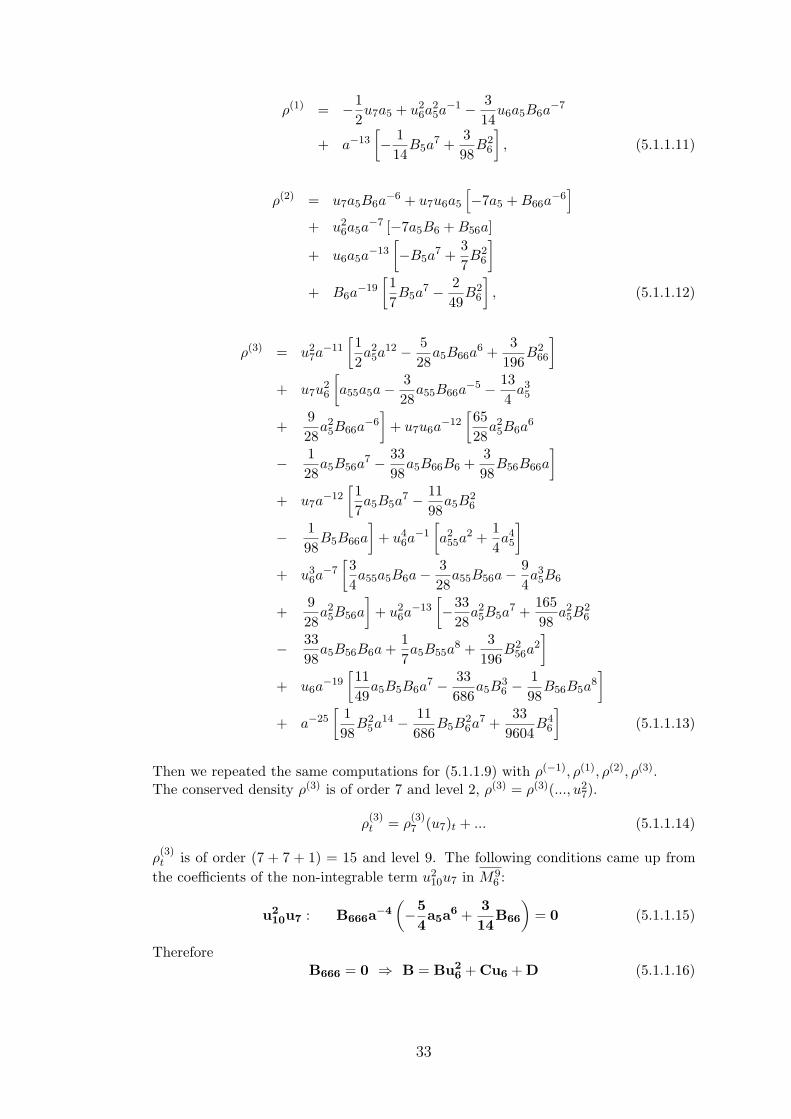
ρ(1) = −12u7a5 + u2

6a25a−1 − 3

14u6a5B6a

−7

+ a−13[− 1

14B5a

7 +398

B26

], (5.1.1.11)

ρ(2) = u7a5B6a−6 + u7u6a5

[−7a5 + B66a

−6]

+ u26a5a

−7 [−7a5B6 + B56a]

+ u6a5a−13

[−B5a

7 +37B2

6

]

+ B6a−19

[17B5a

7 − 249

B26

], (5.1.1.12)

ρ(3) = u27a−11

[12a2

5a12 − 5

28a5B66a

6 +3

196B2

66

]

+ u7u26

[a55a5a− 3

28a55B66a

−5 − 134

a35

+928

a25B66a

−6]

+ u7u6a−12

[6528

a25B6a

6

− 128

a5B56a7 − 33

98a5B66B6 +

398

B56B66a

]

+ u7a−12

[17a5B5a

7 − 1198

a5B26

− 198

B5B66a

]+ u4

6a−1

[a2

55a2 +

14a4

5

]

+ u36a−7

[34a55a5B6a− 3

28a55B56a− 9

4a3

5B6

+928

a25B56a

]+ u2

6a−13

[−33

28a2

5B5a7 +

16598

a25B

26

− 3398

a5B56B6a +17a5B55a

8 +3

196B2

56a2]

+ u6a−19

[1149

a5B5B6a7 − 33

686a5B

36 −

198

B56B5a8]

+ a−25[

198

B25a14 − 11

686B5B

26a7 +

339604

B46

](5.1.1.13)

Then we repeated the same computations for (5.1.1.9) with ρ(−1), ρ(1), ρ(2), ρ(3).The conserved density ρ(3) is of order 7 and level 2, ρ(3) = ρ(3)(..., u2

7).

ρ(3)t = ρ

(3)7 (u7)t + ... (5.1.1.14)

ρ(3)t is of order (7 + 7 + 1) = 15 and level 9. The following conditions came up from

the coefficients of the non-integrable term u210u7 in M9

6 :

u210u7 : B666a−4

(−5

4a5a6 +

314

B66

)= 0 (5.1.1.15)

ThereforeB666 = 0 ⇒ B = Bu2

6 + Cu6 + D (5.1.1.16)

33

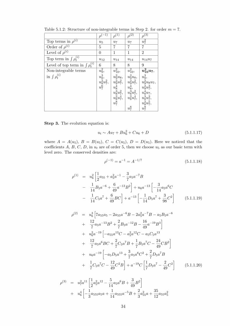
Table 5.1.2: Structure of non-integrable terms in Step 2. for order m = 7.

ρ(−1) ρ(1) ρ(2) ρ(3)

Top terms in ρ(i) u5 u7 u7 u27

Order of ρ(i) 5 7 7 7Level of ρ(i) 0 1 1 2Top term in

∫ρ(i)t u12 u14 u14 u14u7

Level of top term in∫

ρ(i)t 6 8 8 9

Non-integrable terms u29, u2

10, u210, u2

10u7,

in∫

ρ(i)t u3

8, u29u8, u2

9u8, u39,

u28u

27, u2

9u27, u2

9u27, u2

9u8u7,u6

7 u48 u4

8, u29u

37,

u38u

27, u3

8u27, u4

8u7,u2

8u47, u2

8u47, u3

8u37,

u87 u2

8u57,

u87 u9

7

Step 3. The evolution equation is:

ut ∼ Au7 + Bu26 + Cu6 + D (5.1.1.17)

where A = A(u5), B = B(u5), C = C(u5), D = D(u5). Here we noticed that thecoefficients A, B, C, D, in ut are of order 5, then we choose u5 as our basic term withlevel zero. The conserved densities are:

ρ(−1) = a−1 = A−1/7 (5.1.1.18)

ρ(1) = u26

[12a55 + a2

5a−1 − 3

7a5a

−7B

− 114

B5a−6 +

649

a−13B2]

+ u6a−13

[− 3

14a5a

6C

− 114

C5a7 +

649

BC

]+ a−13

[− 1

14D5a

7 +398

C2]

(5.1.1.19)

ρ(2) = u36

[7a55a5 − 2a55a

−6B − 2a25a−7B − a5B5a

−6

+127

a5a−13B2 +

27B5a

−12B − 1649

a−19B3]

+ u26a−19

[−a55a

13C − a25a

12C − a5C5a13

+127

a5a6BC +

27C5a

7B +17B5a

7C − 2449

CB2]

+ u6a−19

[−a5D5a

13 +37a5a

6C2 +27D5a

7B

+17C5a

7C − 1249

C2B

]+ a−19C

[17D5a

7 − 249

C2]

(5.1.1.20)

ρ(3) = u27a

11[12a2

5a12 − 5

14a5a

6B +349

B2]

+ u46

[−1

3a555a5a +

114

a555a−5B +

23a2

55a +3512

a55a25

34

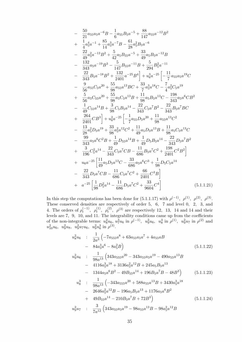
− 5021

a55a5a−6B − 1

6a55B5a

−5 +88147

a55a−12B2

+14a4

5a−1 +

8514

a35a−7B − 61

28a2

5B5a−6

− 2249

a25a−13B2 +

542

a5B55a−5 +

3349

a5B5a−12B

− 132343

a5a−19B3 − 5

147B55a

−11B +5

294B2

5a−11

− 22343

B5a−18B2 +

1322401

a−25B4]

+ u36a−25

[−11

7a55a5a

19C

− 956

a55C5a20 +

5598

a55a13BC +

337

a35a

18C − 74a2

5C5a19

+556

a5C55a20 +

5598

a5C5a13B +

1198

a5B5a13C − 198

343a5a

6CB2

− 149

C55a14B +

398

C5B5a14 − 22

343C5a

7B2 − 22343

B5a7BC

+2642401

CB3]

+ u26a−25

[−1

7a55D5a

20 +1198

a55a13C2

− 1328

a25D5a

19 +3398

a25a

12C2 +1149

a5D5a13B +

1198

a5C5a13C

− 99343

a5a6C2B +

149

D55a14B +

149

D5B5a14 − 22

343D5a

7B2

+3

196C2

5a14 − 22343

C5a7CB − 11

686B5a

7C2 +1982401

C2B2]

+ u6a−25

[1149

a5D5a13C − 33

686a5a

6C3 +198

D5C5a14

− 22343

D5a7CB − 11

686C5a

7C2 +66

2401C3B

]

+ a−25[

198

D25a

14 − 11686

D5a7C2 +

339604

C4]

(5.1.1.21)

In this step the computations has been done for (5.1.1.17) with ρ(−1), ρ(1), ρ(2), ρ(3).These conserved densities are respectively of order 5, 6, 7 and level 0, 2, 3, and4. The orders of ρ

(−1)t , ρ

(1)t , ρ

(2)t , ρ(3) are respectively 12, 13, 14 and 14 and their

levels are 7, 9, 10, and 11. The integrability conditions came up from the coefficientsof the non-integrable terms: u2

8u6, u37u6 in ρ(−1), u2

9u6, u38 in ρ(1), u2

9u7 in ρ(2) andu2

10u6, u29u8, u2

9u7u6, u29u

36 in ρ(3).

u28u6 :

12a3

(−7a555a

8 + 63a55a5a7 + 4a55aB

− 84a35a

6 − 8a25B

)(5.1.1.22)

u29u6 :

198a13

(343a555a

20 − 343a55a5a19 − 490a55a

13B

− 4116a35a

18 + 3136a25a

12B + 245a5B5a13

− 1344a5a6B2 − 49B55a

14 + 196B5a7B − 48B3

)(5.1.1.23)

u38 :

198a13

(−343a555a

20 + 588a55a13B + 3430a3

5a18

− 2646a25a

12B − 196a5B5a13 + 1176a5a

6B2

+ 49B55a14 − 210B5a

7B + 72B3)

(5.1.1.24)

u29u7 :

37a12

(343a55a5a

19 − 98a55a13B − 98a2

5a12B

35

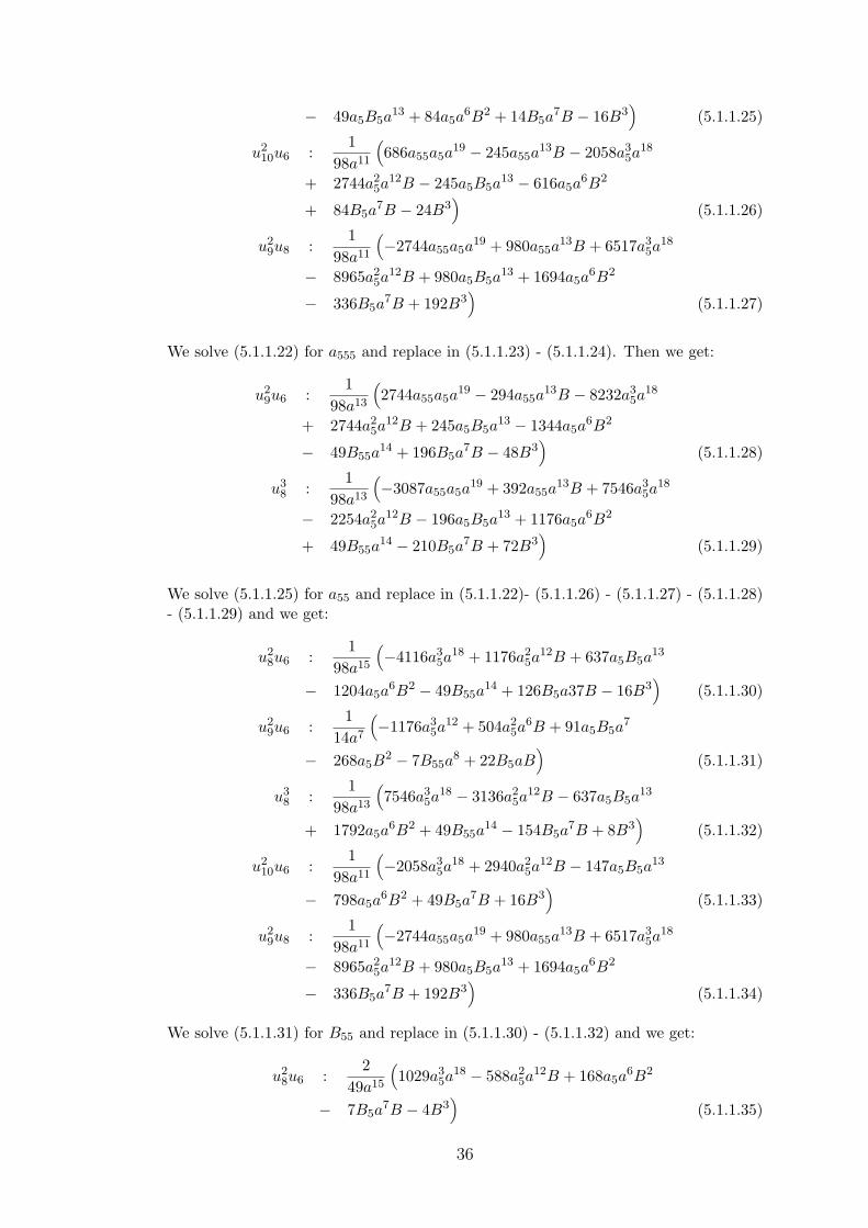
− 49a5B5a13 + 84a5a

6B2 + 14B5a7B − 16B3

)(5.1.1.25)

u210u6 :

198a11

(686a55a5a

19 − 245a55a13B − 2058a3

5a18

+ 2744a25a

12B − 245a5B5a13 − 616a5a

6B2

+ 84B5a7B − 24B3

)(5.1.1.26)

u29u8 :

198a11

(−2744a55a5a

19 + 980a55a13B + 6517a3

5a18

− 8965a25a

12B + 980a5B5a13 + 1694a5a

6B2

− 336B5a7B + 192B3

)(5.1.1.27)

We solve (5.1.1.22) for a555 and replace in (5.1.1.23) - (5.1.1.24). Then we get:

u29u6 :

198a13

(2744a55a5a

19 − 294a55a13B − 8232a3

5a18

+ 2744a25a

12B + 245a5B5a13 − 1344a5a

6B2

− 49B55a14 + 196B5a

7B − 48B3)

(5.1.1.28)

u38 :

198a13

(−3087a55a5a

19 + 392a55a13B + 7546a3

5a18

− 2254a25a

12B − 196a5B5a13 + 1176a5a

6B2

+ 49B55a14 − 210B5a

7B + 72B3)

(5.1.1.29)

We solve (5.1.1.25) for a55 and replace in (5.1.1.22)- (5.1.1.26) - (5.1.1.27) - (5.1.1.28)- (5.1.1.29) and we get:

u28u6 :

198a15

(−4116a3

5a18 + 1176a2

5a12B + 637a5B5a

13

− 1204a5a6B2 − 49B55a

14 + 126B5a37B − 16B3)

(5.1.1.30)

u29u6 :

114a7

(−1176a3

5a12 + 504a2

5a6B + 91a5B5a

7

− 268a5B2 − 7B55a

8 + 22B5aB)

(5.1.1.31)

u38 :

198a13

(7546a3

5a18 − 3136a2

5a12B − 637a5B5a

13

+ 1792a5a6B2 + 49B55a

14 − 154B5a7B + 8B3

)(5.1.1.32)

u210u6 :

198a11

(−2058a3

5a18 + 2940a2

5a12B − 147a5B5a

13

− 798a5a6B2 + 49B5a

7B + 16B3)

(5.1.1.33)

u29u8 :

198a11

(−2744a55a5a

19 + 980a55a13B + 6517a3

5a18

− 8965a25a

12B + 980a5B5a13 + 1694a5a

6B2

− 336B5a7B + 192B3

)(5.1.1.34)

We solve (5.1.1.31) for B55 and replace in (5.1.1.30) - (5.1.1.32) and we get:

u28u6 :

249a15

(1029a3

5a18 − 588a2

5a12B + 168a5a

6B2

− 7B5a7B − 4B3

)(5.1.1.35)

36

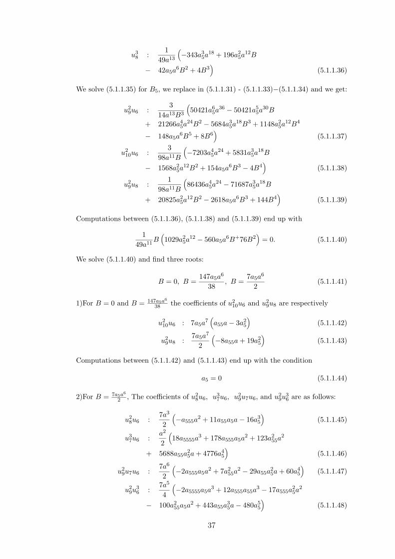
u38 :

149a13

(−343a3

5a18 + 196a2

5a12B

− 42a5a6B2 + 4B3

)(5.1.1.36)

We solve (5.1.1.35) for B5, we replace in (5.1.1.31) - (5.1.1.33)−(5.1.1.34) and we get:

u29u6 :

314a13B3

(50421a6

5a36 − 50421a5

5a30B

+ 21266a45a

24B2 − 5684a35a

18B3 + 1148a25a

12B4

− 148a5a6B5 + 8B6

)(5.1.1.37)

u210u6 :

398a11B

(−7203a4

5a24 + 5831a3

5a18B

− 1568a25a

12B2 + 154a5a6B3 − 4B4

)(5.1.1.38)

u29u8 :

198a11B

(86436a4

5a24 − 71687a3

5a18B

+ 20825a25a

12B2 − 2618a5a6B3 + 144B4

)(5.1.1.39)

Computations between (5.1.1.36), (5.1.1.38) and (5.1.1.39) end up with

149a11

B(1029a2

5a12 − 560a5a

6B+76B2)

= 0. (5.1.1.40)

We solve (5.1.1.40) and find three roots:

B = 0, B =147a5a

6

38, B =

7a5a6

2(5.1.1.41)

1)For B = 0 and B = 147a5a6

38 the coefficients of u210u6 and u2

9u8 are respectively

u210u6 : 7a5a

7(a55a− 3a2

5

)(5.1.1.42)

u29u8 :

7a5a7

2

(−8a55a + 19a2

5

)(5.1.1.43)

Computations between (5.1.1.42) and (5.1.1.43) end up with the condition

a5 = 0 (5.1.1.44)

2)For B = 7a5a6

2 , The coefficients of u28u6, u3

7u6, u29u7u6, and u2

9u36 are as follows:

u28u6 :

7a3

2

(−a555a

2 + 11a55a5a− 16a35

)(5.1.1.45)

u37u6 :

a2

2

(18a5555a

3 + 178a555a5a2 + 123a2

55a2

+ 5688a55a25a + 4776a4

5

)(5.1.1.46)

u29u7u6 :

7a6

2

(−2a555a5a

2 + 7a255a

2 − 29a55a25a + 60a4

5

)(5.1.1.47)

u29u

36 :

7a5

4

(−2a5555a5a

3 + 12a555a55a3 − 17a555a

25a

2

− 100a255a5a

2 + 443a55a35a− 480a5

5

)(5.1.1.48)

37

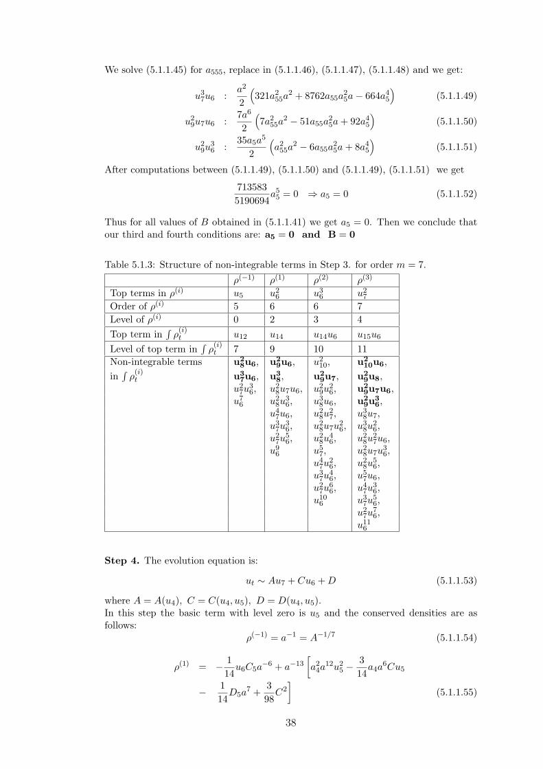
We solve (5.1.1.45) for a555, replace in (5.1.1.46), (5.1.1.47), (5.1.1.48) and we get:

u37u6 :

a2

2

(321a2

55a2 + 8762a55a

25a− 664a4

5

)(5.1.1.49)

u29u7u6 :

7a6

2

(7a2

55a2 − 51a55a

25a + 92a4

5

)(5.1.1.50)

u29u

36 :

35a5a5

2

(a2

55a2 − 6a55a

25a + 8a4

5

)(5.1.1.51)

After computations between (5.1.1.49), (5.1.1.50) and (5.1.1.49), (5.1.1.51) we get

7135835190694

a55 = 0 ⇒ a5 = 0 (5.1.1.52)

Thus for all values of B obtained in (5.1.1.41) we get a5 = 0. Then we conclude thatour third and fourth conditions are: a5 = 0 and B = 0

Table 5.1.3: Structure of non-integrable terms in Step 3. for order m = 7.

ρ(−1) ρ(1) ρ(2) ρ(3)

Top terms in ρ(i) u5 u26 u3

6 u27

Order of ρ(i) 5 6 6 7Level of ρ(i) 0 2 3 4Top term in

∫ρ(i)t u12 u14 u14u6 u15u6

Level of top term in∫

ρ(i)t 7 9 10 11

Non-integrable terms u28u6, u2

9u6, u210, u2

10u6,

in∫

ρ(i)t u3

7u6, u38, u2

9u7, u29u8,

u27u

36, u2

8u7u6, u29u

26, u2

9u7u6,u7

6 u28u

36, u3

8u6, u29u

36,

u47u6, u2

8u27, u3

8u7,u3

7u36, u2

8u7u26, u3

8u26,

u27u

56, u2

8u46, u2

8u27u6,

u96 u5

7, u28u7u

36,

u47u

26, u2

8u56,

u37u

46, u5

7u6,u2

7u66, u4

7u36,

u106 u3

7u56,

u27u

76,

u116

Step 4. The evolution equation is:

ut ∼ Au7 + Cu6 + D (5.1.1.53)

where A = A(u4), C = C(u4, u5), D = D(u4, u5).In this step the basic term with level zero is u5 and the conserved densities are asfollows:

ρ(−1) = a−1 = A−1/7 (5.1.1.54)

ρ(1) = − 114

u6C5a−6 + a−13

[a2

4a12u2

5 −314

a4a6Cu5

− 114

D5a7 +

398

C2]

(5.1.1.55)

38

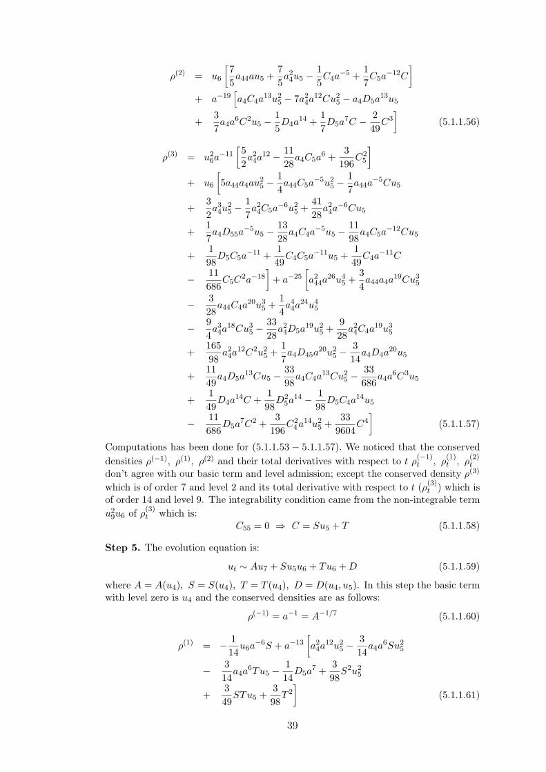
ρ(2) = u6

[75a44au5 +

75a2

4u5 − 15C4a

−5 +17C5a

−12C

]

+ a−19[a4C4a

13u25 − 7a2

4a12Cu2

5 − a4D5a13u5

+37a4a

6C2u5 − 15D4a

14 +17D5a

7C − 249

C3]

(5.1.1.56)

ρ(3) = u26a−11

[52a2

4a12 − 11

28a4C5a

6 +3

196C2

5

]

+ u6

[5a44a4au2

5 −14a44C5a

−5u25 −

17a44a

−5Cu5

+32a3

4u25 −

17a2

4C5a−6u2

5 +4128

a24a−6Cu5

+17a4D55a

−5u5 − 1328

a4C4a−5u5 − 11

98a4C5a

−12Cu5

+198

D5C5a−11 +

149

C4C5a−11u5 +

149

C4a−11C

− 11686

C5C2a−18

]+ a−25

[a2

44a26u4

5 +34a44a4a

19Cu35

− 328

a44C4a20u3

5 +14a4

4a24u4

5

− 94a3

4a18Cu3

5 −3328

a24D5a

19u25 +

928

a24C4a

19u35

+16598

a24a

12C2u25 +

17a4D45a

20u25 −

314

a4D4a20u5

+1149

a4D5a13Cu5 − 33

98a4C4a

13Cu25 −

33686

a4a6C3u5

+149

D4a14C +

198

D25a

14 − 198

D5C4a14u5

− 11686

D5a7C2 +

3196

C24a14u2

5 +33

9604C4

](5.1.1.57)

Computations has been done for (5.1.1.53 − 5.1.1.57). We noticed that the conserveddensities ρ(−1), ρ(1), ρ(2) and their total derivatives with respect to t ρ

(−1)t , ρ

(1)t , ρ

(2)t

don’t agree with our basic term and level admission; except the conserved density ρ(3)

which is of order 7 and level 2 and its total derivative with respect to t (ρ(3)t ) which is

of order 14 and level 9. The integrability condition came from the non-integrable termu2

9u6 of ρ(3)t which is:

C55 = 0 ⇒ C = Su5 + T (5.1.1.58)

Step 5. The evolution equation is:

ut ∼ Au7 + Su5u6 + Tu6 + D (5.1.1.59)

where A = A(u4), S = S(u4), T = T (u4), D = D(u4, u5). In this step the basic termwith level zero is u4 and the conserved densities are as follows:

ρ(−1) = a−1 = A−1/7 (5.1.1.60)

ρ(1) = − 114

u6a−6S + a−13

[a2

4a12u2

5 −314

a4a6Su2

5

− 314

a4a6Tu5 − 1

14D5a

7 +398

S2u25

+349

STu5 +398

T 2]

(5.1.1.61)

39

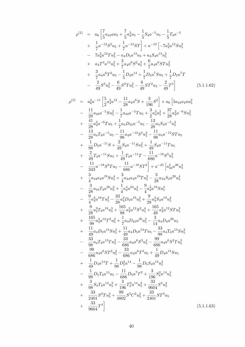
ρ(2) = u6

[75a44au5 +

75a2

4u5 − 15S4a

−5u5 − 15T4a

−5

+17a−12S2u5 +

17a−12ST

]+ a−19

[−7a2

4a12Su3

5

− 7a24a

12Tu25 − a4D5a

13u5 + a4S4a13u3

5

+ a4T4a13u2

5 +37a4a

6S2u35 +

67a4a

6STu25

+37a4a

6T 2u5 − 15D4a

14 +17D5a

7Su5 +17D5a

7T

− 249

S3u35 −

649

S2Tu25 −

649

ST 2u5 − 249

T 3]

(5.1.1.62)

ρ(3) = u26a−11

[52a2

4a12 − 11

28a4a

6S +3

196S2

]+ u6

[5a44a4au2

5

− 1128

a44a−5Su2

5 −17a44a

−5Tu5 +32a3

4u25 +

3728

a24a−6Su2

5

+4128

a24a−6Tu5 +

17a4D55a

−5u5 − 1328

a4S4a−5u2

5

− 1328

a4T4a−5u5 − 11

98a4a

−12S2u25 −

1198

a4a−12STu5

+198

D5a−11S +

249

S4a−11Su2

5 +149

S4a−11Tu5

+249

T4a−11Su5 +

149

T4a−11T − 11

686a−18S3u2

5

− 11343

a−18S2Tu5 − 11686

a−18ST 2]

+ a−25[a2

44a26u4

5

+34a44a4a

19Su45 +

34a44a4a

19Tu35 −

328

a44S4a20u4

5

− 328

a44T4a20u3

5 +14a4

4a24u4

5 −94a3

4a18Su4

5

− 94a3

4a18Tu3

5 −3328

a24D5a

19u25 +

928

a24S4a

19u45

+928

a24T4a

19u35 +

16598

a24a

12S2u45 +

16549

a24a

12STu35

+16598

a24a

12T 2u25 +

17a4D45a

20u25 −

314

a4D4a20u5

+1149

a4D5a13Su2

5 +1149

a4D5a13Tu5 − 33

98a4T4a

13Su35

− 3398

a4T4a13Tu2

5 −33686

a4a6S3u4

5 −99686

a4a6S2Tu3

5

− 99686

a4a6ST 2u2

5 −33686

a4a6T 3u5 +

149

D4a14Su5

+149

D4a14T +

198

D25a

14 − 198

D5S4a14u2

5

− 198

D5T4a14u5 − 11

686D5a

7T 2 +3

196S2

4a14u45

+398

S4T4a14u3

5 +3

196T 2

4 a14u25 +

339604

S4u45

+33

2401S3Tu3

5 +99

4802S2C2u2

5 +33

2401ST 3u5

+33

9604T 4

](5.1.1.63)

40

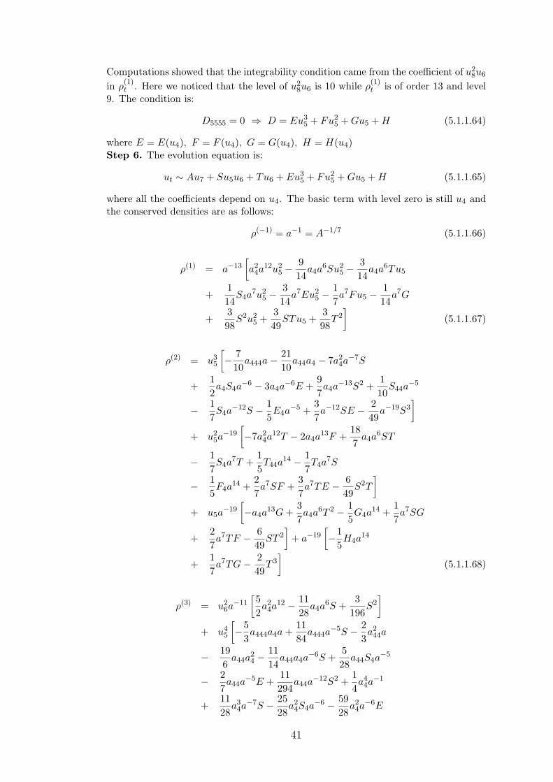
Computations showed that the integrability condition came from the coefficient of u28u6

in ρ(1)t . Here we noticed that the level of u2

8u6 is 10 while ρ(1)t is of order 13 and level

9. The condition is:

D5555 = 0 ⇒ D = Eu35 + Fu2

5 + Gu5 + H (5.1.1.64)

where E = E(u4), F = F (u4), G = G(u4), H = H(u4)Step 6. The evolution equation is:

ut ∼ Au7 + Su5u6 + Tu6 + Eu35 + Fu2

5 + Gu5 + H (5.1.1.65)

where all the coefficients depend on u4. The basic term with level zero is still u4 andthe conserved densities are as follows:

ρ(−1) = a−1 = A−1/7 (5.1.1.66)

ρ(1) = a−13[a2

4a12u2

5 −914

a4a6Su2

5 −314

a4a6Tu5

+114

S4a7u2

5 −314

a7Eu25 −

17a7Fu5 − 1

14a7G

+398

S2u25 +

349

STu5 +398

T 2]

(5.1.1.67)

ρ(2) = u35

[− 7

10a444a− 21

10a44a4 − 7a2

4a−7S

+12a4S4a

−6 − 3a4a−6E +

97a4a

−13S2 +110

S44a−5

− 17S4a

−12S − 15E4a

−5 +37a−12SE − 2

49a−19S3

]

+ u25a−19

[−7a2

4a12T − 2a4a

13F +187

a4a6ST

− 17S4a

7T +15T44a

14 − 17T4a

7S

− 15F4a

14 +27a7SF +

37a7TE − 6

49S2T

]

+ u5a−19

[−a4a

13G +37a4a

6T 2 − 15G4a

14 +17a7SG

+27a7TF − 6

49ST 2

]+ a−19

[−1

5H4a

14

+17a7TG− 2

49T 3

](5.1.1.68)

ρ(3) = u26a−11

[52a2

4a12 − 11

28a4a

6S +3

196S2

]

+ u45

[−5

3a444a4a +

1184

a444a−5S − 2

3a2

44a

− 196

a44a24 −

1114

a44a4a−6S +

528

a44S4a−5

− 27a44a

−5E +11294

a44a−12S2 +

14a4

4a−1

+1128

a34a−7S − 25

28a2

4S4a−6 − 59

28a2

4a−6E

41

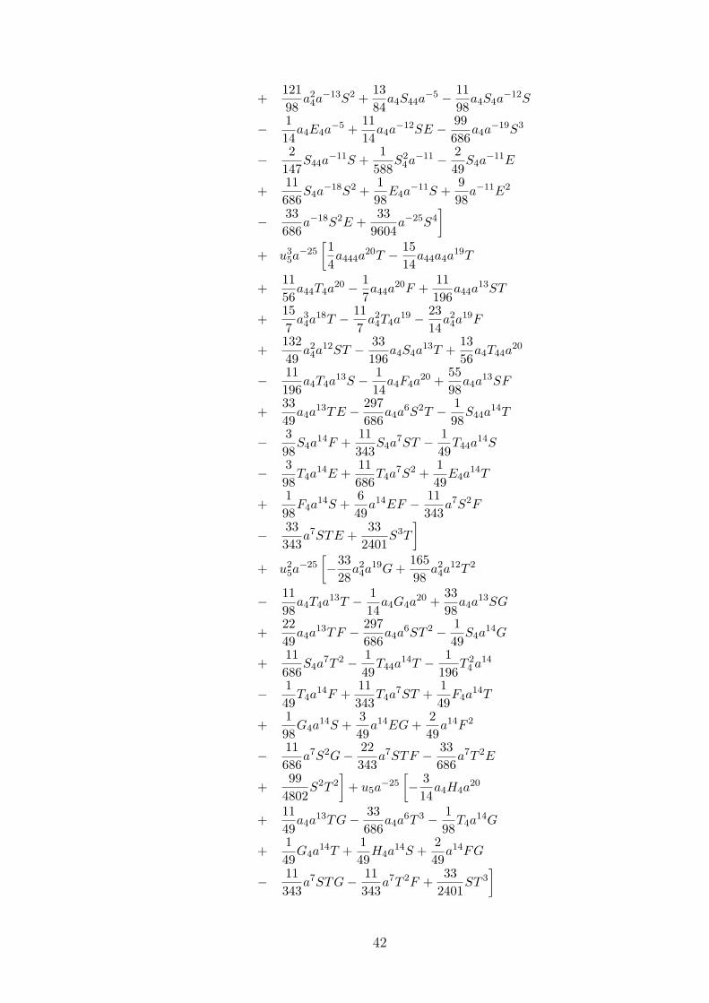
+12198

a24a−13S2 +

1384

a4S44a−5 − 11

98a4S4a

−12S

− 114

a4E4a−5 +

1114

a4a−12SE − 99

686a4a

−19S3

− 2147

S44a−11S +

1588

S24a−11 − 2

49S4a

−11E

+11686

S4a−18S2 +

198

E4a−11S +

998

a−11E2

− 33686

a−18S2E +33

9604a−25S4

]

+ u35a−25

[14a444a

20T − 1514

a44a4a19T

+1156

a44T4a20 − 1

7a44a

20F +11196

a44a13ST

+157

a34a

18T − 117

a24T4a

19 − 2314

a24a

19F

+13249

a24a

12ST − 33196

a4S4a13T +

1356

a4T44a20

− 11196

a4T4a13S − 1

14a4F4a

20 +5598

a4a13SF

+3349

a4a13TE − 297

686a4a

6S2T − 198

S44a14T

− 398

S4a14F +

11343

S4a7ST − 1

49T44a

14S

− 398

T4a14E +

11686

T4a7S2 +

149

E4a14T

+198

F4a14S +

649

a14EF − 11343

a7S2F

− 33343

a7STE +33

2401S3T

]

+ u25a−25

[−33

28a2

4a19G +

16598

a24a

12T 2

− 1198

a4T4a13T − 1

14a4G4a

20 +3398

a4a13SG

+2249

a4a13TF − 297

686a4a

6ST 2 − 149

S4a14G

+11686

S4a7T 2 − 1

49T44a

14T − 1196

T 24 a14

− 149

T4a14F +

11343

T4a7ST +

149

F4a14T

+198

G4a14S +

349

a14EG +249

a14F 2

− 11686

a7S2G− 22343

a7STF − 33686

a7T 2E

+99

4802S2T 2

]+ u5a

−25[− 3

14a4H4a

20

+1149

a4a13TG− 33

686a4a

6T 3 − 198

T4a14G

+149

G4a14T +

149

H4a14S +

249

a14FG

− 11343

a7STG− 11343

a7T 2F +33

2401ST 3

]

42

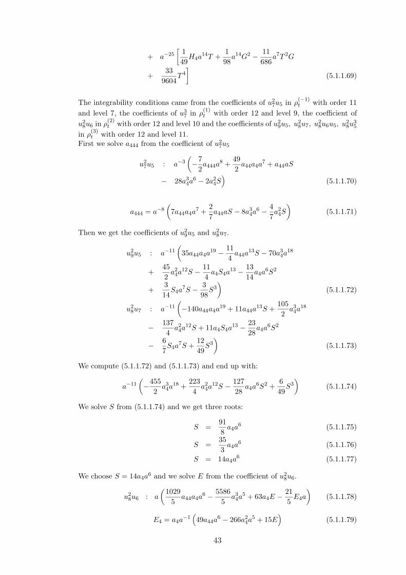
+ a−25[

149

H4a14T +

198

a14G2 − 11686

a7T 2G

+33

9604T 4

](5.1.1.69)

The integrability conditions came from the coefficients of u27u5 in ρ

(−1)t with order 11

and level 7, the coefficients of u37 in ρ

(1)t with order 12 and level 9, the coefficient of

u28u6 in ρ

(2)t with order 12 and level 10 and the coefficients of u2

9u5, u28u7, u2

8u6u5, u28u

35

in ρ(3)t with order 12 and level 11.

First we solve a444 from the coefficient of u27u5

u27u5 : a−3

(−7

2a444a

8 +492

a44a4a7 + a44aS

− 28a34a

6 − 2a24S

)(5.1.1.70)

a444 = a−8(

7a44a4a7 +

27a44aS − 8a3

4a6 − 4

7a2

4S

)(5.1.1.71)

Then we get the coefficients of u29u5 and u2

8u7.

u29u5 : a−11

(35a44a4a

19 − 114

a44a13S − 70a3

4a18

+452

a24a

12S − 114

a4S4a13 − 13

14a4a

6S2

+314

S4a7S − 3

98S3

)(5.1.1.72)

u28u7 : a−11

(−140a44a4a

19 + 11a44a13S +

1052

a34a

18

− 1374

a24a

12S + 11a4S4a13 − 23

28a4a

6S2

− 67S4a

7S +1249

S3)

(5.1.1.73)

We compute (5.1.1.72) and (5.1.1.73) and end up with:

a−11(−455

2a3

4a18 +

2234

a24a

12S − 12728

a4a6S2 +

649

S3)

(5.1.1.74)

We solve S from (5.1.1.74) and we get three roots:

S =918

a4a6 (5.1.1.75)

S =353

a4a6 (5.1.1.76)

S = 14a4a6 (5.1.1.77)

We choose S = 14a4a6 and we solve E from the coefficient of u2

8u6.

u28u6 : a

(1029

5a44a4a

6 − 55865

a34a

5 + 63a4E − 215

E4a

)(5.1.1.78)

E4 = a4a−1

(49a44a

6 − 266a24a

5 + 15E)

(5.1.1.79)

43

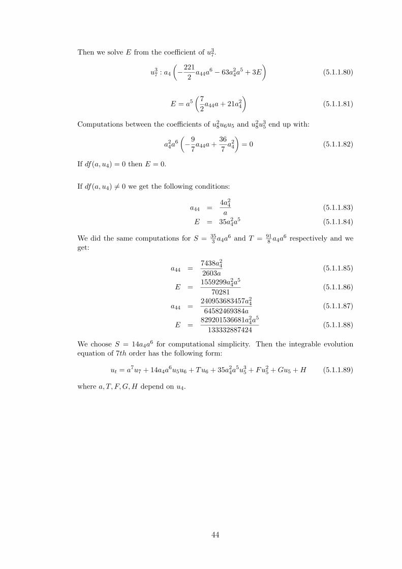
Then we solve E from the coefficient of u37.

u37 : a4

(−221

2a44a

6 − 63a24a

5 + 3E

)(5.1.1.80)

E = a5(

72a44a + 21a2

4

)(5.1.1.81)

Computations between the coefficients of u28u6u5 and u2

8u35 end up with:

a24a

6(−9

7a44a +

367

a24

)= 0 (5.1.1.82)

If df(a, u4) = 0 then E = 0.

If df(a, u4) 6= 0 we get the following conditions:

a44 =4a2

4

a(5.1.1.83)

E = 35a24a

5 (5.1.1.84)

We did the same computations for S = 353 a4a

6 and T = 918 a4a

6 respectively and weget:

a44 =7438a2

4

2603a(5.1.1.85)

E =1559299a2

4a5

70281(5.1.1.86)

a44 =240953683457a2

4

64582469384a(5.1.1.87)

E =829201536681a2

4a5

133332887424(5.1.1.88)

We choose S = 14a4a6 for computational simplicity. Then the integrable evolution

equation of 7th order has the following form:

ut = a7u7 + 14a4a6u5u6 + Tu6 + 35a2

4a5u3

5 + Fu25 + Gu5 + H (5.1.1.89)

where a, T, F, G, H depend on u4.

44

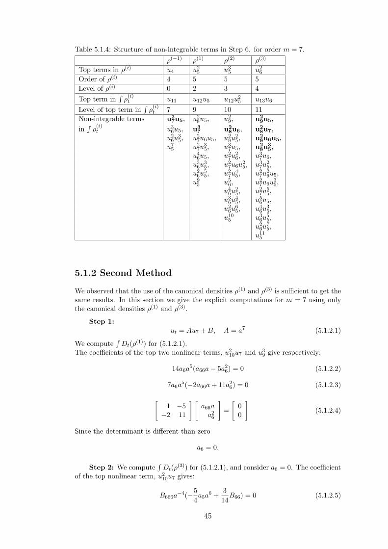
Table 5.1.4: Structure of non-integrable terms in Step 6. for order m = 7.

ρ(−1) ρ(1) ρ(2) ρ(3)

Top terms in ρ(i) u4 u25 u3

5 u26

Order of ρ(i) 4 5 5 5Level of ρ(i) 0 2 3 4Top term in

∫ρ(i)t u11 u12u5 u12u

25 u13u6

Level of top term in∫

ρ(i)t 7 9 10 11

Non-integrable terms u27u5, u2

8u5, u29, u2

9u5,

in∫

ρ(i)t u3

6u5, u37 u2

8u6, u28u7,

u26u

35, u2

7u6u5, u28u

25, u2

8u6u5,u7

5 u27u

35, u3

7u5, u28u

35,

u46u5, u2

7u26, u3

7u6,u3

6u35, u2

7u6u25, u3

7u25,

u26u

55, u2

7u45, u2

7u26u5,

u95 u5

6, u27u6u

35,

u46u

25, u2

7u55,

u36u

45, u5

6u5,u2

6u65, u4

6u35,

u105 u3

6u55,

u26u

75,

u115

5.1.2 Second Method

We observed that the use of the canonical densities ρ(1) and ρ(3) is sufficient to get thesame results. In this section we give the explicit computations for m = 7 using onlythe canonical densities ρ(1) and ρ(3).

Step 1:ut = Au7 + B, A = a7 (5.1.2.1)

We compute∫

Dt(ρ(1)) for (5.1.2.1).The coefficients of the top two nonlinear terms, u2

10u7 and u39 give respectively:

14a6a5(a66a− 5a2

6) = 0 (5.1.2.2)

7a6a5(−2a66a + 11a2

6) = 0 (5.1.2.3)

[1 −5

−2 11

] [a66a

a26

]=

[00

](5.1.2.4)

Since the determinant is different than zero

a6 = 0.

Step 2: We compute∫

Dt(ρ(3)) for (5.1.2.1), and consider a6 = 0. The coefficientof the top nonlinear term, u2

10u7 gives:

B666a−4(−5

4a5a

6 +314

B66) = 0 (5.1.2.5)

45

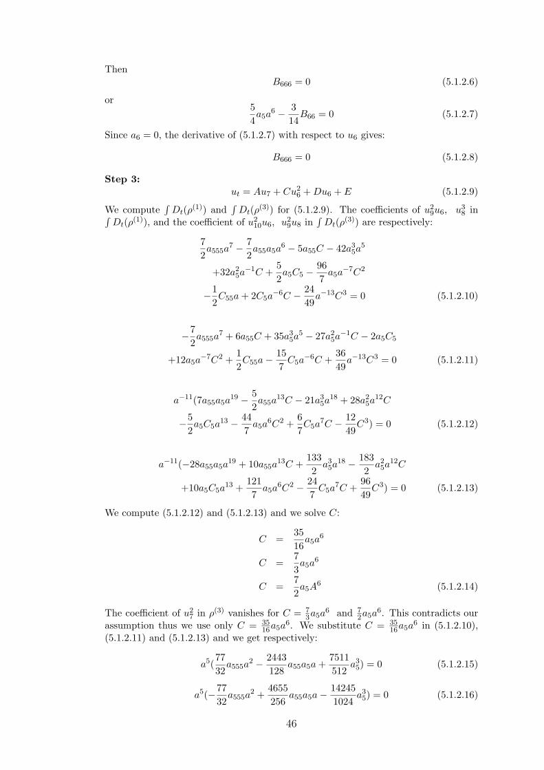
ThenB666 = 0 (5.1.2.6)

or54a5a

6 − 314

B66 = 0 (5.1.2.7)

Since a6 = 0, the derivative of (5.1.2.7) with respect to u6 gives:

B666 = 0 (5.1.2.8)

Step 3:ut = Au7 + Cu2

6 + Du6 + E (5.1.2.9)

We compute∫

Dt(ρ(1)) and∫

Dt(ρ(3)) for (5.1.2.9). The coefficients of u29u6, u3

8 in∫Dt(ρ(1)), and the coefficient of u2

10u6, u29u8 in

∫Dt(ρ(3)) are respectively:

72a555a

7 − 72a55a5a

6 − 5a55C − 42a35a

5

+32a25a−1C +

52a5C5 − 96

7a5a

−7C2

−12C55a + 2C5a

−6C − 2449

a−13C3 = 0 (5.1.2.10)

−72a555a

7 + 6a55C + 35a35a

5 − 27a25a−1C − 2a5C5

+12a5a−7C2 +

12C55a− 15

7C5a

−6C +3649

a−13C3 = 0 (5.1.2.11)

a−11(7a55a5a19 − 5

2a55a

13C − 21a35a

18 + 28a25a

12C

−52a5C5a

13 − 447

a5a6C2 +

67C5a

7C − 1249

C3) = 0 (5.1.2.12)

a−11(−28a55a5a19 + 10a55a

13C +1332

a35a

18 − 1832

a25a

12C

+10a5C5a13 +

1217

a5a6C2 − 24

7C5a

7C +9649

C3) = 0 (5.1.2.13)

We compute (5.1.2.12) and (5.1.2.13) and we solve C:

C =3516

a5a6

C =73a5a

6

C =72a5A

6 (5.1.2.14)

The coefficient of u27 in ρ(3) vanishes for C = 7

3a5a6 and 7

2a5a6. This contradicts our

assumption thus we use only C = 3516a5a

6. We substitute C = 3516a5a

6 in (5.1.2.10),(5.1.2.11) and (5.1.2.13) and we get respectively:

a5(7732

a555a2 − 2443

128a55a5a +

7511512

a35) = 0 (5.1.2.15)

a5(−7732

a555a2 +

4655256

a55a5a− 142451024

a35) = 0 (5.1.2.16)

46

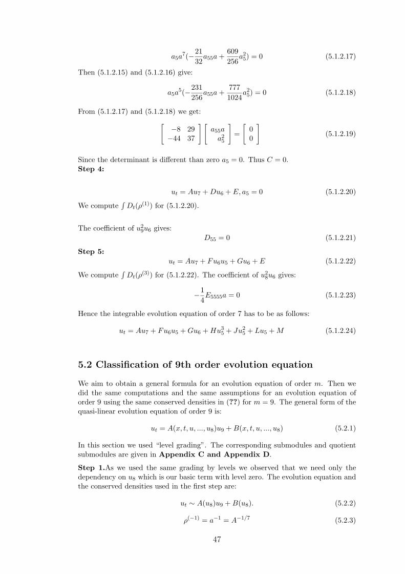
a5a7(−21

32a55a +

609256

a25) = 0 (5.1.2.17)

Then (5.1.2.15) and (5.1.2.16) give:

a5a5(−231

256a55a +

7771024

a25) = 0 (5.1.2.18)

From (5.1.2.17) and (5.1.2.18) we get:[

−8 29−44 37

] [a55a

a25

]=

[00

](5.1.2.19)

Since the determinant is different than zero a5 = 0. Thus C = 0.Step 4:

ut = Au7 + Du6 + E, a5 = 0 (5.1.2.20)

We compute∫

Dt(ρ(1)) for (5.1.2.20).

The coefficient of u29u6 gives:

D55 = 0 (5.1.2.21)

Step 5:ut = Au7 + Fu6u5 + Gu6 + E (5.1.2.22)

We compute∫

Dt(ρ(3)) for (5.1.2.22). The coefficient of u28u6 gives:

−14E5555a = 0 (5.1.2.23)

Hence the integrable evolution equation of order 7 has to be as follows:

ut = Au7 + Fu6u5 + Gu6 + Hu35 + Ju2

5 + Lu5 + M (5.1.2.24)

5.2 Classification of 9th order evolution equation

We aim to obtain a general formula for an evolution equation of order m. Then wedid the same computations and the same assumptions for an evolution equation oforder 9 using the same conserved densities in (??) for m = 9. The general form of thequasi-linear evolution equation of order 9 is:

ut = A(x, t, u, ..., u8)u9 + B(x, t, u, ..., u8) (5.2.1)

In this section we used “level grading”. The corresponding submodules and quotientsubmodules are given in Appendix C and Appendix D.

Step 1.As we used the same grading by levels we observed that we need only thedependency on u8 which is our basic term with level zero. The evolution equation andthe conserved densities used in the first step are:

ut ∼ A(u8)u9 + B(u8). (5.2.2)

ρ(−1) = a−1 = A−1/7 (5.2.3)

47

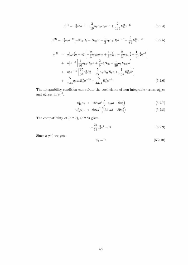
ρ(1) = u29a

28a−1 +

219

u9a8B8a−9 +

2135

B28a−17 (5.2.4)

ρ(2) = u29a8a

−9 [−9a8B8 + B88a]− 13u9a8B

28a−17 − 2

81B3

8a−25 (5.2.5)

ρ(3) = u210a

28a + u4

9

[−2

3a888a8a +

13a2

88a−23a88a

28 +

14a4

8a−1

]

+ u39a−8

[136

a88B88a +29a2

8B88 − 136

a8B888a

]

+ u29a−17

[6554

a28B

28 −

527

a8B88B8a +1

162B2

88a2]

+5

243u9a8B

38a−25 +

54374

B48a−33 (5.2.6)

The integrability condition came from the coefficients of non-integrable terms, u213u9

and u212u11 in ρ

(1)t .

u213u9 : 18a8a

7(−a88a + 6a2

8

)(5.2.7)

u212u11 : 6a8a

7(13a88a− 89a2

8

)(5.2.8)

The compatibility of (5.2.7), (5.2.8) gives:

−2413

a38a

7 = 0 (5.2.9)

Since a 6= 0 we get:a8 = 0 (5.2.10)

48

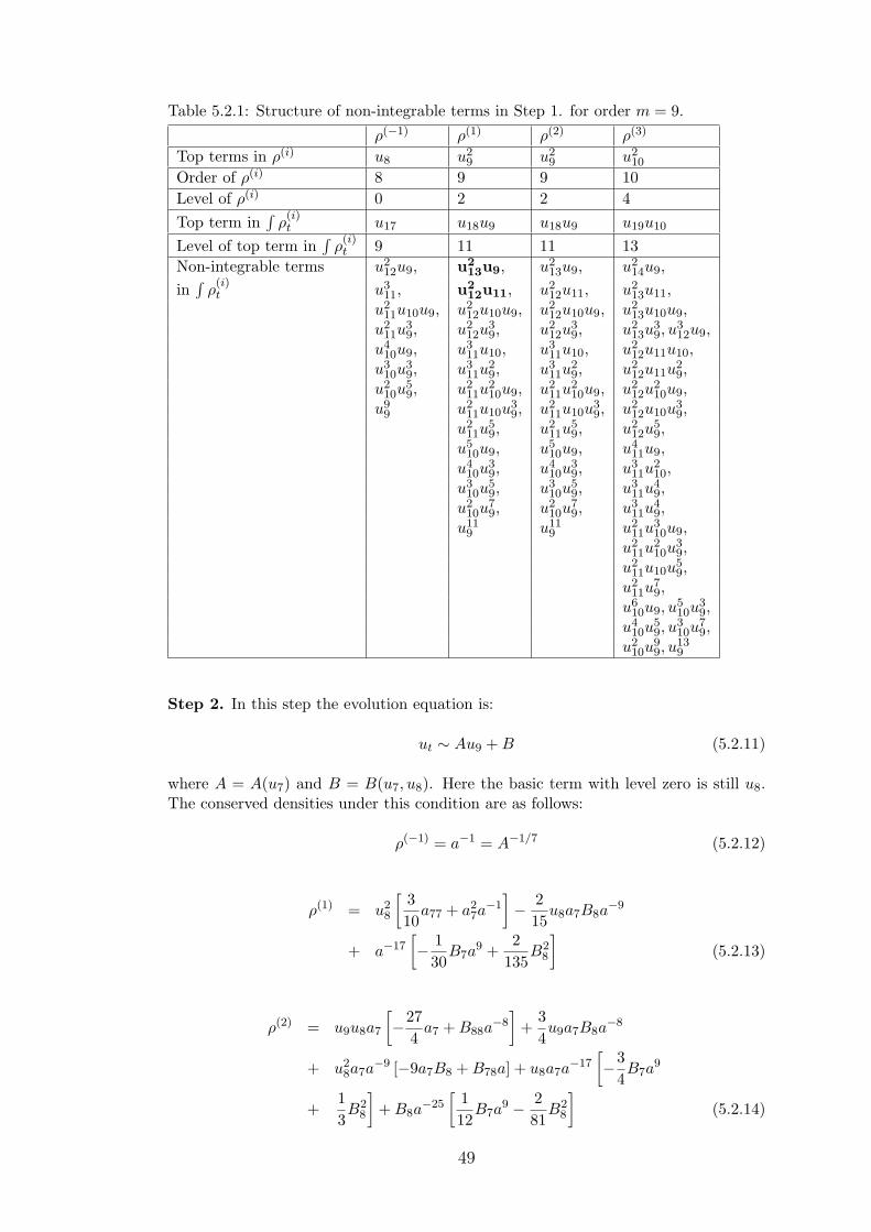
Table 5.2.1: Structure of non-integrable terms in Step 1. for order m = 9.

ρ(−1) ρ(1) ρ(2) ρ(3)

Top terms in ρ(i) u8 u29 u2

9 u210

Order of ρ(i) 8 9 9 10Level of ρ(i) 0 2 2 4Top term in

∫ρ(i)t u17 u18u9 u18u9 u19u10

Level of top term in∫

ρ(i)t 9 11 11 13

Non-integrable terms u212u9, u2

13u9, u213u9, u2

14u9,

in∫

ρ(i)t u3

11, u212u11, u2

12u11, u213u11,

u211u10u9, u2

12u10u9, u212u10u9, u2

13u10u9,u2

11u39, u2

12u39, u2

12u39, u2

13u39, u

312u9,

u410u9, u3

11u10, u311u10, u2

12u11u10,u3

10u39, u3

11u29, u3

11u29, u2

12u11u29,

u210u

59, u2

11u210u9, u2

11u210u9, u2

12u210u9,

u99 u2

11u10u39, u2

11u10u39, u2

12u10u39,

u211u

59, u2

11u59, u2

12u59,

u510u9, u5

10u9, u411u9,

u410u

39, u4

10u39, u3

11u210,

u310u

59, u3

10u59, u3

11u49,

u210u

79, u2

10u79, u3

11u49,

u119 u11

9 u211u

310u9,

u211u

210u

39,

u211u10u

59,

u211u

79,

u610u9, u

510u

39,

u410u

59, u

310u

79,

u210u

99, u

139

Step 2. In this step the evolution equation is:

ut ∼ Au9 + B (5.2.11)

where A = A(u7) and B = B(u7, u8). Here the basic term with level zero is still u8.The conserved densities under this condition are as follows:

ρ(−1) = a−1 = A−1/7 (5.2.12)

ρ(1) = u28

[310

a77 + a27a−1

]− 2

15u8a7B8a

−9

+ a−17[− 1

30B7a

9 +2

135B2

8

](5.2.13)

ρ(2) = u9u8a7

[−27

4a7 + B88a

−8]

+34u9a7B8a

−8

+ u28a7a

−9 [−9a7B8 + B78a] + u8a7a−17

[−3

4B7a

9

+13B2

8

]+ B8a

−25[

112

B7a9 − 2

81B2

8

](5.2.14)

49

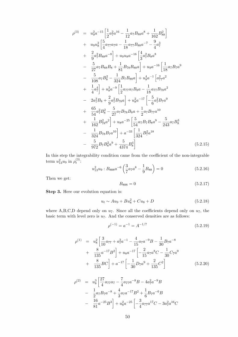
ρ(3) = u29a−15

[12a2

7a16 − 1

12a7B88a

8 +1

162B2

88

]

+ u9u28

[54a77a7a− 1

18a77B88a

−7 − 94a3

7

+29a2

7B88a−8

]+ u9u8a

−16[43a2

7B8a8

− 527

a7B88B8 +181

B78B88a

]+ u9a

−16[

118

a7B7a9

− 5108

a7B28 −

1324

B7B88a

]+ u4

8a−1

[a2

77a2

+14a4

7

]+ u3

8a−9

[12a77a7B8a− 1

18a77B78a

2

− 2a37B8 +

29a2

7B78a

]+ u2

8a−17

[−5

6a2

7B7a9

+6554

a27B

28 −

527

a7B78B8a +12a7B77a

10

+1

162B2

78a2]

+ u8a−25

[554

a7B7B8a9 − 5

243a7B

38

− 1324

B78B7a10

]+ a−33

[1

324B2

7a18

− 5972

B7B28a9 +

54374

B48

](5.2.15)

In this step the integrability condition came from the coefficient of the non-integrableterm u2

13u9 in ρ(3)t :

u213u9 : B888a

−6(

37a7a

8 − 19B88

)= 0 (5.2.16)

Then we get:B888 = 0 (5.2.17)

Step 3. Here our evolution equation is:

ut ∼ Au9 + Bu28 + Cu8 + D (5.2.18)

where A,B,C,D depend only on u7. Since all the coefficients depend only on u7, thebasic term with level zero is u7. And the conserved densities are as follows:

ρ(−1) = a−1 = A−1/7 (5.2.19)

ρ(1) = u28

[310

a77 + a27a−1 − 4

15a7a

−9B − 130

B7a−8

+8

135a−17B2

]+ u8a

−17[− 2

15a7a

8C − 130

C7a9

+8

135BC

]+ a−17

[− 1

30D7a

9 +2

135C2

](5.2.20)

ρ(2) = u38

[274

a77a7 − 74a77a

−8B − 4a27a−9B

− 12a7B7a

−8 +43a7a

−17B2 +16B7a

−6B

− 1681

a−25B3]

+ u28a−25

[−3

4a77a

17C − 3a27a

16C

50

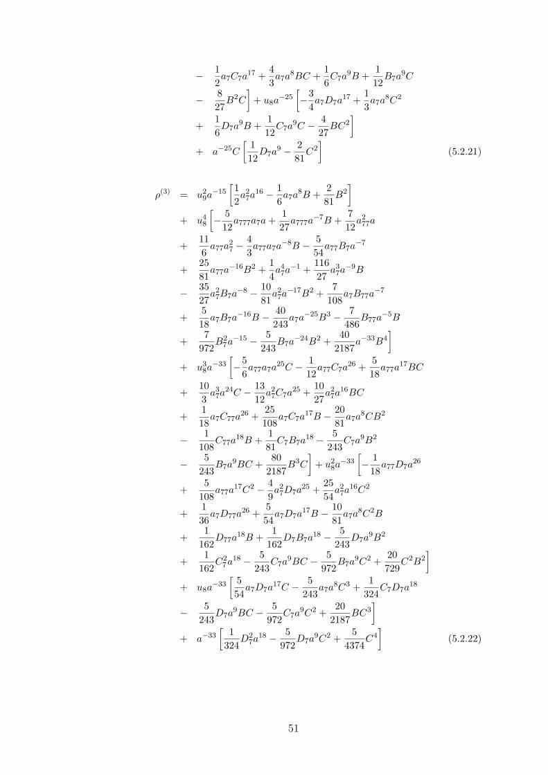
− 12a7C7a

17 +43a7a

8BC +16C7a

9B +112

B7a9C

− 827

B2C

]+ u8a

−25[−3

4a7D7a

17 +13a7a

8C2

+16D7a

9B +112

C7a9C − 4

27BC2

]

+ a−25C

[112

D7a9 − 2

81C2

](5.2.21)

ρ(3) = u29a−15

[12a2

7a16 − 1

6a7a

8B +281

B2]

+ u48

[− 5

12a777a7a +

127

a777a−7B +

712

a277a

+116

a77a27 −

43a77a7a

−8B − 554

a77B7a−7

+2581

a77a−16B2 +

14a4

7a−1 +

11627

a37a−9B

− 3527

a27B7a

−8 − 1081

a27a−17B2 +

7108

a7B77a−7

+518

a7B7a−16B − 40

243a7a

−25B3 − 7486

B77a−5B

+7

972B2

7a−15 − 5243

B7a−24B2 +

402187

a−33B4]

+ u38a−33

[−5

6a77a7a

25C − 112

a77C7a26 +

518

a77a17BC

+103

a37a

24C − 1312

a27C7a

25 +1027

a27a

16BC

+118

a7C77a26 +

25108

a7C7a17B − 20

81a7a

8CB2

− 1108

C77a18B +

181

C7B7a18 − 5

243C7a

9B2

− 5243

B7a9BC +

802187

B3C

]+ u2

8a−33

[− 1

18a77D7a

26

+5

108a77a

17C2 − 49a2

7D7a25 +

2554

a27a

16C2

+136

a7D77a26 +

554

a7D7a17B − 10

81a7a

8C2B

+1

162D77a

18B +1

162D7B7a

18 − 5243

D7a9B2

+1

162C2

7a18 − 5243

C7a9BC − 5

972B7a

9C2 +20729

C2B2]

+ u8a−33

[554

a7D7a17C − 5

243a7a

8C3 +1

324C7D7a

18

− 5243

D7a9BC − 5

972C7a

9C2 +20

2187BC3

]

+ a−33[

1324

D27a

18 − 5972

D7a9C2 +

54374

C4]

(5.2.22)

51

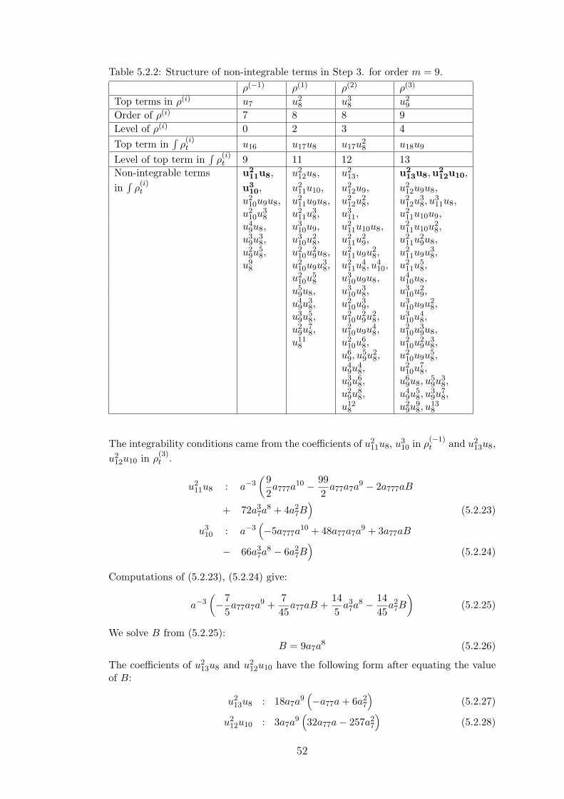
Table 5.2.2: Structure of non-integrable terms in Step 3. for order m = 9.

ρ(−1) ρ(1) ρ(2) ρ(3)

Top terms in ρ(i) u7 u28 u3

8 u29

Order of ρ(i) 7 8 8 9Level of ρ(i) 0 2 3 4Top term in

∫ρ(i)t u16 u17u8 u17u

28 u18u9

Level of top term in∫

ρ(i)t 9 11 12 13

Non-integrable terms u211u8, u2

12u8, u213, u2

13u8,u212u10,

in∫

ρ(i)t u3

10, u211u10, u2

12u9, u212u9u8,

u210u9u8, u2

11u9u8, u212u

28, u2

12u38, u

311u8,

u210u

38 u2

11u38, u3

11, u211u10u9,

u49u8, u3

10u9, u211u10u8, u2

11u10u28,

u39u

38, u3

10u28, u2

11u29, u2

11u29u8,

u29u

58, u2

10u29u8, u2

11u9u28, u2

11u9u38,

u98 u2

10u9u38, u2

11u48, u

410, u2

11u58,

u210u

58 u3

10u9u8, u410u8,

u59u8, u3

10u38, u3

10u29,

u49u

38, u2

10u39, u3

10u9u28,

u39u

58, u2

10u29u

28, u3

10u48,

u29u

78, u2

10u9u48, u2

10u39u8,

u118 u2

10u68, u2

10u29u

38,

u69, u

59u

28, u2

10u9u58,

u49u

48, u2

10u78,

u39u

68, u6

9u8, u59u

38,

u29u

88, u4

9u58, u

39u

78,

u128 u2

9u98, u

138

The integrability conditions came from the coefficients of u211u8, u3

10 in ρ(−1)t and u2

13u8,u2

12u10 in ρ(3)t .

u211u8 : a−3

(92a777a

10 − 992

a77a7a9 − 2a777aB

+ 72a37a

8 + 4a27B

)(5.2.23)

u310 : a−3

(−5a777a

10 + 48a77a7a9 + 3a77aB

− 66a37a

8 − 6a27B

)(5.2.24)

Computations of (5.2.23), (5.2.24) give:

a−3(−7

5a77a7a

9 +745

a77aB +145

a37a

8 − 1445

a27B

)(5.2.25)

We solve B from (5.2.25):B = 9a7a

8 (5.2.26)

The coefficients of u213u8 and u2

12u10 have the following form after equating the valueof B:

u213u8 : 18a7a

9(−a77a + 6a2

7

)(5.2.27)

u212u10 : 3a7a

9(32a77a− 257a2

7

)(5.2.28)

52

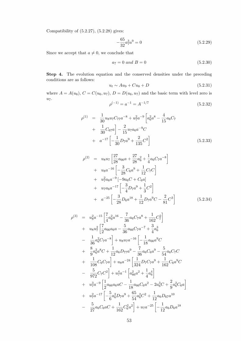
Compatibility of (5.2.27), (5.2.28) gives:

−6532

a37a

9 = 0 (5.2.29)

Since we accept that a 6= 0, we conclude that

a7 = 0 and B = 0 (5.2.30)

Step 4. The evolution equation and the conserved densities under the precedingconditions are as follows:

ut ∼ Au9 + Cu8 + D (5.2.31)

where A = A(u6), C = C(u6, u7), D = D(u6, u7) and the basic term with level zero isu7.

ρ(−1) = a−1 = A−1/7 (5.2.32)

ρ(1) =130

u8u7C77a−8 + u2

7a−9

[a2

6a8 − 4

15a6C7

+130

C67a

]− 2

15u7a6a

−9C

+ a−17[− 1

30D7a

9 +2

135C2

](5.2.33)

ρ(2) = u8u7

[2728

a66a +2728

a26 +

14a6C7a

−8]

+ u8a−16

[− 3

28C6a

9 +112

C7C

]

+ u27a6a

−9 [−9a6C + C6a]

+ u7a6a−17

[−3

4D7a

9 +13C2

]

+ a−25[− 3

28D6a

18 +112

D7a9C − 2

81C3

](5.2.34)

ρ(3) = u28a−15

[74a2

6a16 − 7

36a6C7a

8 +1

162C2

7

]

+ u8u27

[72a66a6a− 5

36a66C7a

−7 +34a3

6

− 136

a26C7a

−8]

+ u8u7a−16

[− 1

18a66a

9C

+89a2

6a8C +

112

a6D77a9 − 7

36a6C6a

9 − 554

a6C7C

+1

108C6C7a

]+ u8a

−24[

1324

D7C7a9 +

1162

C6a9C

− 5972

C7C2]

+ u47a−1

[a2

66a2 +

14a4

6

]

+ u37a−9

[12a66a6aC − 1

18a66C6a

2 − 2a36C +

29a2

6C6a

]

+ u27a−17

[−5

6a2

6D7a9 +

6554

a26C

2 +112

a6D67a10

− 527

a6C6aC +1

162C2

6a2]

+ u7a−25

[− 1

12a6D6a

18

53

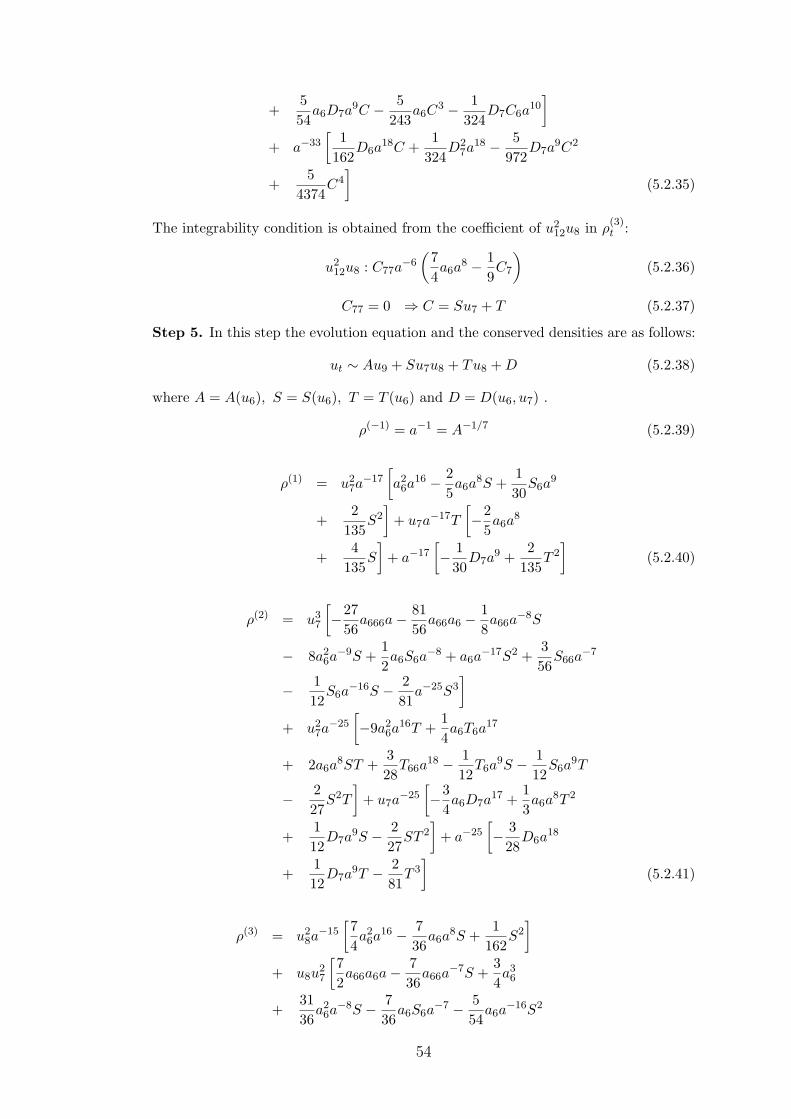
+554

a6D7a9C − 5

243a6C

3 − 1324

D7C6a10

]

+ a−33[

1162

D6a18C +

1324

D27a

18 − 5972

D7a9C2

+5

4374C4

](5.2.35)

The integrability condition is obtained from the coefficient of u212u8 in ρ

(3)t :

u212u8 : C77a

−6(

74a6a

8 − 19C7

)(5.2.36)

C77 = 0 ⇒ C = Su7 + T (5.2.37)

Step 5. In this step the evolution equation and the conserved densities are as follows:

ut ∼ Au9 + Su7u8 + Tu8 + D (5.2.38)

where A = A(u6), S = S(u6), T = T (u6) and D = D(u6, u7) .

ρ(−1) = a−1 = A−1/7 (5.2.39)

ρ(1) = u27a−17

[a2

6a16 − 2

5a6a

8S +130

S6a9

+2

135S2

]+ u7a

−17T

[−2

5a6a

8

+4

135S

]+ a−17

[− 1

30D7a

9 +2

135T 2

](5.2.40)

ρ(2) = u37

[−27

56a666a− 81

56a66a6 − 1

8a66a

−8S

− 8a26a−9S +

12a6S6a

−8 + a6a−17S2 +

356

S66a−7

− 112

S6a−16S − 2

81a−25S3

]

+ u27a−25

[−9a2

6a16T +

14a6T6a

17

+ 2a6a8ST +

328

T66a18 − 1

12T6a

9S − 112

S6a9T

− 227

S2T

]+ u7a

−25[−3

4a6D7a

17 +13a6a

8T 2

+112

D7a9S − 2

27ST 2

]+ a−25

[− 3

28D6a

18

+112

D7a9T − 2

81T 3

](5.2.41)

ρ(3) = u28a−15

[74a2

6a16 − 7

36a6a

8S +1

162S2

]

+ u8u27

[72a66a6a− 7

36a66a

−7S +34a3

6

+3136

a26a−8S − 7

36a6S6a

−7 − 554

a6a−16S2

54

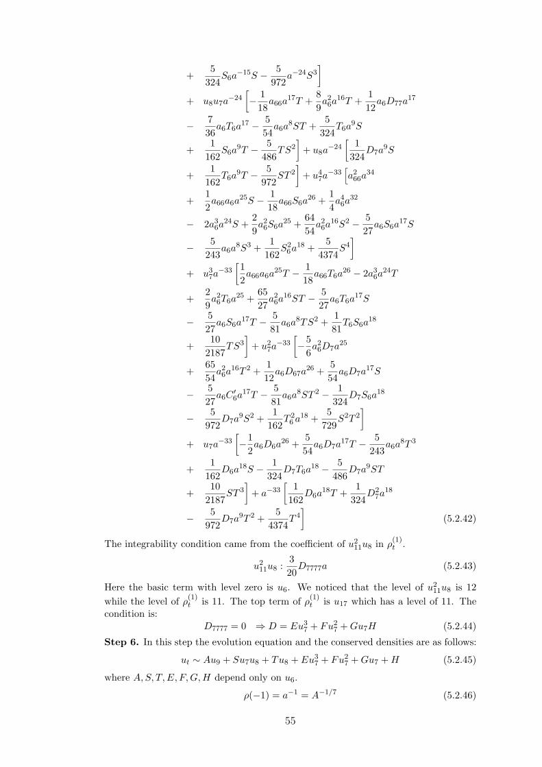
+5

324S6a

−15S − 5972

a−24S3]

+ u8u7a−24

[− 1

18a66a

17T +89a2

6a16T +

112

a6D77a17

− 736

a6T6a17 − 5

54a6a

8ST +5

324T6a

9S

+1

162S6a

9T − 5486

TS2]

+ u8a−24

[1

324D7a

9S

+1

162T6a

9T − 5972

ST 2]

+ u47a−33

[a2

66a34

+12a66a6a

25S − 118

a66S6a26 +

14a4

6a32

− 2a36a

24S +29a2

6S6a25 +

6454

a26a

16S2 − 527

a6S6a17S

− 5243

a6a8S3 +

1162

S26a18 +

54374

S4]

+ u37a−33

[12a66a6a

25T − 118

a66T6a26 − 2a3

6a24T

+29a2

6T6a25 +

6527

a26a

16ST − 527

a6T6a17S

− 527

a6S6a17T − 5

81a6a

8TS2 +181

T6S6a18

+10

2187TS3

]+ u2

7a−33

[−5

6a2

6D7a25

+6554

a26a

16T 2 +112

a6D67a26 +

554

a6D7a17S

− 527

a6C′6a

17T − 581

a6a8ST 2 − 1

324D7S6a

18

− 5972

D7a9S2 +

1162

T 26 a18 +

5729

S2T 2]

+ u7a−33

[−1

2a6D6a

26 +554

a6D7a17T − 5

243a6a

8T 3

+1

162D6a

18S − 1324

D7T6a18 − 5

486D7a

9ST

+10

2187ST 3

]+ a−33

[1

162D6a

18T +1

324D2

7a18

− 5972

D7a9T 2 +

54374

T 4]

(5.2.42)

The integrability condition came from the coefficient of u211u8 in ρ

(1)t .

u211u8 :

320

D7777a (5.2.43)

Here the basic term with level zero is u6. We noticed that the level of u211u8 is 12

while the level of ρ(1)t is 11. The top term of ρ

(1)t is u17 which has a level of 11. The

condition is:D7777 = 0 ⇒ D = Eu3

7 + Fu27 + Gu7H (5.2.44)

Step 6. In this step the evolution equation and the conserved densities are as follows:

ut ∼ Au9 + Su7u8 + Tu8 + Eu37 + Fu2

7 + Gu7 + H (5.2.45)

where A, S, T,E, F, G, H depend only on u6.

ρ(−1) = a−1 = A−1/7 (5.2.46)

55

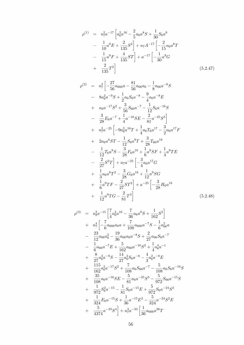
ρ(1) = u27a−17

[a2

6a16 − 2

5a6a

8S +130

S6a9

− 110

a9E +2

135S2

]+ u7A

−17[− 2

15a6a

8T

− 115

a9F +4

135ST

]+ a−17

[− 1

30a9G

+2

135T 2

](5.2.47)

ρ(2) = u37

[−27

56a666a− 81

56a66a6 − 1

8a66a

−8S

− 8a26a−9S +

12a6S6a

−8 − 94a6a

−8E

+ a6a−17S2 +

356

S66a−7 − 1

12S6a

−16S

− 328

E6a−7 +

14a−16SE − 2

81a−25S3

]

+ u27a−25

[−9a2

6a16T +

14a6T6a

17 − 32a6a

17F

+ 2a6a8ST − 1

12S6a

9T +328

T66a18

− 112

T6a9S − 3

28F6a

18 +16a9SF +

14a9TE

− 227

S2T

]+ u7a

−25[−3

4a6a

17G

+13a6a

8T 2 − 328

G6a18 +

112

a9SG

+16a9TF − 2

27ST 2

]+ a−25

[− 3

28H6a

18

+112

a9TG− 281

T 3]

(5.2.48)

ρ(3) = u28a−15

[74a2

6a16 − 7

36a6a

8S +1

162S2

]

+ u47

[−7

6a666a6a +

7108

a666a−7S − 1

6a2

66a

− 2312

a66a26 −

1936

a66a6a−8S +

227

a66S6a−7

− 16a66a

−7E +5

162a66a

−16S2 +14a4

6a−1

+827

a36a−9S − 14

27a2

6S6a−8 − 4

3a2

6a−8E

+115162

a26a−17S2 +

7108

a6S66a−7 − 5

108a6S6a

−16S

+35108

a6a−16SE − 5

81a6a

−25S3 − 5972

S66a−15S

+1

972S2

6a−15 − 181

S6a−15E +

5972

S6a−24S2

+1

324E6a

−15S +136

a−15E2 − 5324

a−24S2E

+5

4374a−33S4

]+ u3

7a−33

[136

a666a26T

56

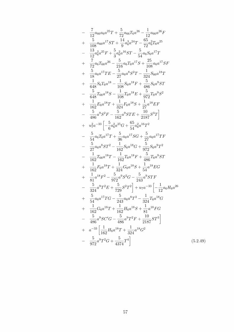
− 712

a66a6a25T +

572

a66T6a26 − 1

12a66a

26F

+5

108a66a

17ST +149

a36a

24T − 6572

a26T6a

25

− 1312

a26a

25F +53a2

6a16ST − 5

54a6S6a

17T

+772

a6T66a26 − 5

216a6T6a

17S +25108

a6a17SF

+518

a6a17TE − 5

27a6a

8S2T − 1324

S66a18T

+1

648S6T6a

18 − 1108

S6a18F +

5486

S6a9ST

− 5648

T66a18S − 1

108T6a

18E +5

972T6a

9S2

+1

162E6a

18T +1

324F6a

18S +127

a18EF

− 5486

a9S2F − 5162

a9STE +10

2187S3T

]

+ u27a−33

[−5

6a2

6a25G +

6554

a26a

16T 2

− 554

a6T6a17T +

536

a6a17SG +

527

a6a17TF

− 527

a6a8ST 2 − 1

162S6a

18G +5

972S6a

9T 2

− 1162

T66a18T − 1

162T6a

18F +5

486T6a

9ST

+1

162F6a

18T +1

324G6a

18S +154

a18EG

+181

a18F 2 − 5972

a9S2G− 5243

a9STF

− 5324

a9T 2E +5

729S2T 2

]+ u7a

−33[− 1

12a6H6a

26

+554

a6a17TG− 5

243a6a

8T 3 − 1324

T6a18G

+1

162G6a

18T +1

162H6a

18S +181

a18FG

− 5486

a9SC ′G− 5486

a9T 2F +10

2187ST 3

]

+ a−33[

1162

H6a18T +

1324

a18G2

− 5972

a9T 2G +5

4374T 4

](5.2.49)

57

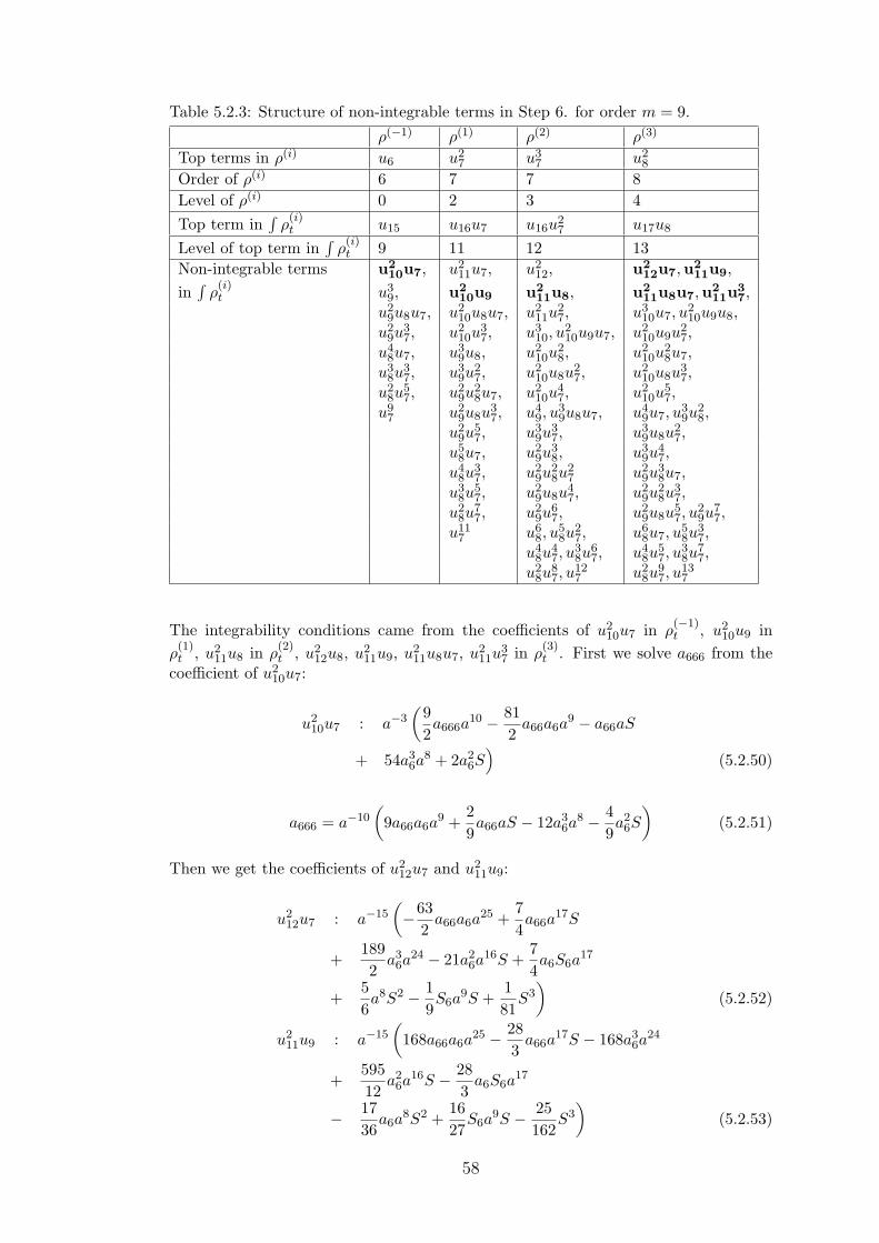
Table 5.2.3: Structure of non-integrable terms in Step 6. for order m = 9.

ρ(−1) ρ(1) ρ(2) ρ(3)

Top terms in ρ(i) u6 u27 u3

7 u28

Order of ρ(i) 6 7 7 8Level of ρ(i) 0 2 3 4Top term in

∫ρ(i)t u15 u16u7 u16u

27 u17u8

Level of top term in∫

ρ(i)t 9 11 12 13

Non-integrable terms u210u7, u2

11u7, u212, u2

12u7,u211u9,

in∫

ρ(i)t u3

9, u210u9 u2

11u8, u211u8u7,u2

11u37,

u29u8u7, u2

10u8u7, u211u

27, u3

10u7, u210u9u8,

u29u

37, u2

10u37, u3

10, u210u9u7, u2

10u9u27,

u48u7, u3

9u8, u210u

28, u2

10u28u7,

u38u

37, u3

9u27, u2

10u8u27, u2

10u8u37,

u28u

57, u2

9u28u7, u2

10u47, u2

10u57,

u97 u2

9u8u37, u4

9, u39u8u7, u4

9u7, u39u

28,

u29u

57, u3

9u37, u3

9u8u27,

u58u7, u2

9u38, u3

9u47,

u48u

37, u2

9u28u

27 u2

9u38u7,

u38u

57, u2

9u8u47, u2

9u28u

37,

u28u

77, u2

9u67, u2

9u8u57, u

29u

77,

u117 u6

8, u58u

27, u6

8u7, u58u

37,

u48u

47, u

38u

67, u4

8u57, u

38u

77,

u28u

87, u

127 u2

8u97, u

137

The integrability conditions came from the coefficients of u210u7 in ρ

(−1)t , u2

10u9 inρ(1)t , u2

11u8 in ρ(2)t , u2

12u8, u211u9, u2

11u8u7, u211u

37 in ρ

(3)t . First we solve a666 from the

coefficient of u210u7:

u210u7 : a−3

(92a666a

10 − 812

a66a6a9 − a66aS

+ 54a36a

8 + 2a26S

)(5.2.50)

a666 = a−10(

9a66a6a9 +

29a66aS − 12a3

6a8 − 4

9a2

6S

)(5.2.51)

Then we get the coefficients of u212u7 and u2

11u9:

u212u7 : a−15

(−63

2a66a6a

25 +74a66a

17S

+1892

a36a

24 − 21a26a

16S +74a6S6a

17

+56a8S2 − 1

9S6a

9S +181

S3)

(5.2.52)

u211u9 : a−15

(168a66a6a

25 − 283

a66a17S − 168a3

6a24

+59512

a26a

16S − 283

a6S6a17

− 1736

a6a8S2 +

1627

S6a9S − 25

162S3

)(5.2.53)

58

We compute (5.2.52), (5.2.53) and we get:

a−15(

2a36a

24 − 107288

a26a

16S +1436048

a6a8S2 − 43

81648S3

)(5.2.54)

We solve S from (5.2.54) and choose one of the three roots:

S =57643

a6a8 (5.2.55)

We solve E6 form the coefficient of u211u8 and E from the coefficient of u2

10u9 :

u211u8 : a

(−865323

3698a66a6a

8 +73670553159014

a36a

7

− 5103172

a6E +8128

E6a

)(5.2.56)

E6 = a6a−1

(1495621849

a66a8 − 12733182

79507a2

6a7 +

44143

E

)(5.2.57)

u210u9 : a6

(−782997

9245a66a

8 − 111425793397535

a26a

7

+4071215

E

)(5.2.58)

E = a7(

26099958351

a66a +371419312509093

a26

)(5.2.59)

Finally we get from the computations between the coefficients of u211u8u7 and u2

11u37:

u211u8u7 : a14

(1563582247953404839201

a266a

2

+91566976338255146408085643

a66a26a

− 235137525820554156295547682649

a46

)(5.2.60)

u211u

37 : a14

(305455811181333

292816171286a2

66a2

− 554967112707269712591095365298

a66a26a

− 3351976543600422032707078550353907

a46

)(5.2.61)

a26a−2

(K(1)a66a−K(2)a2

6

)= 0 (5.2.62)

where K(1) and K(2) are constants. Assuming that a6 6= 0

a66 = K(3)a26a−1 (5.2.63)

where K(3) = K(2)/K(1), andE = K(4)a2

6a7 (5.2.64)

where K(4) is a constant. In conclusion, integrable evolution equations of order 9 havethe following form:

ut = a9u9 +57643

a6a8u7u8 + Tu8 + K(4)a2

6a7u3

7 + Fu27 + Gu7 + H (5.2.65)

where a, T, F, G, H depend on u6.

59

6 DISCUSSIONS AND CONCLUSIONS

The aim of this thesis is to classify scalar integrable evolution equations. Theconstraints of the integrable equations, to be classified, are to be scalar andevolutionary. Non-evolutionary equations i.e. utt = F [u], and integrable evolutionsystems or vector evolution equations are excluded. The problem is based on anarbitrary evolution equation ut = F [u] without any functional and scaling assumption.

The integrability test that we used is Mikhailov-Shabat-Sokolov’s “formal symmetrymethod”. This integrability test is based on the existence of a truncated expansion ofa formal pseudo-differential operator R, satisfying the operator equation

Rt + [R, F∗] = 0,

where F∗ is the Frechet derivative of F . The solvability of the coefficients in R requiresthe existence of canonical conserved densities, denoted as ρ(i), i = −1, 0, 1, 2, 3, . . .

We worked with mth order equations. The order m = 2k + 1 is odd because theconserved densities of even order equations are trivial [1].

It is known that there are essentially nonlinear integrable 3rd order equations [2]which need special techniques [16]. There exist also essentially nonlinear fifth orderequations which are not quasi-linear. Since 3rd and 5th order equations remain stillas open problems, our results are valid for m ≥ 7.

The integrability of homogeneous and non-polynomial scalar evolution equations hasbeen discussed in [3] and [4]. In the former one it has been shown that scale invariantpolynomial evolution equations of order greater than seven are symmetries of thirdand fifth order equations, while in the latter similar results are obtained using negativepowers. Thus the problem of classification of arbitrary evolution equations is reducedto prove the polynomiality and scaling properties of such equations.

We proved that arbitrary (non-polynomial) scalar evolution equations of order m ≥ 7,that are integrable in the sense of admitting the canonical conserved densities ρ(1),ρ(2) and ρ(3), introduced in [2], and computed in [1] are polynomial in the derivativesum−i for i = 0, 1, 2. By the use of these conserved densities we did actually some morecomputations and we obtained that the coefficient of um is independent of um−3 andthe coefficient of um−2um−1 is zero. But as it was not possible to obtain polynomialityin um−3, we didn’t present these in the thesis. The similarity of the results obtainedin explicit computations for m = 7, m = 9 and symbolic computations for generalm assure the consistence of our results. In computations for arbitrary m, we haven’tused ρ(−1) and ρ(0), while for m = 7 we did the computations in two methods whererespectively we used ρ(−1), ρ(0), ρ(1), ρ(2), ρ(3) and only the conserved densities, ρ(1) andρ(3). These two methods showed that ρ(−1) and ρ(0) didn’t give any further information.We did not use ρ(2) in the computations of 7th order whereas we needed it for thecomputations of the general m.

For future work the computation of few more conserved densities is necessary to settlethe classification problem at low orders. But is there any end for the computations of

60

the conserved densities? The explicit computations of the conserved densities for 7thorder evolution equations will give an idea.

The use of the graded algebra structure named as “level grading” that we introducedin this thesis and the scale invariance property seems to be promising for an explicitformula for general m. The use of “level grading” will be a tool for the assumption of afixed level and the form of the conserved densities ρ(k), without explicit computations.These assumptions will give the proof of the independence of A from uk, ( ∂A

∂uk= 0)

which will be sufficient for the polynomiality case.

61

Appendix A

The submodules M ld and their generating monomials with level l(mi), where d =

6, 5, 4, 3 and l = 1, 2, 3, ..., 11 used in classification of 7th order evolution equations:

Submodules with base level 6

M16 = 〈u7〉

M26 = 〈u8, u

27〉

M36 = 〈u9, u8u7, u

37〉

M46 = 〈u10, u9u7, u

28, u8u

27, u

47〉

M56 = 〈u11, u10u7, u9u8, u9u

27, u

28u7, u8u

37, u

57〉

M66 = 〈u12, u11u7, u10u8, u10u

27, u

29, u9u8u7, u9u

37,

u38, u

28u

27, u8u

47, u

67〉

M76 = 〈u13, u12u7, u11u8, u11u

27, u10u9, u10u8u7, u10u

37,

u29u7, u9u

28, u9u8u

27, u9u

47,

u38u7, u

28u

37, u8u

57, u

77〉

M86 = 〈u14, u13u7, u12u8, u12u

27, u11u9, u11u8u7, u11u

37,

u210, u10u9u7, u10u

28, u10u8u

27, u10u

47,

u29u8, u

29u

27, u9u

28u7, u9u8u

37, u9u

57,

u48, u

38u

27, u

28u

47, u8u

67, u

87〉

M96 = 〈u15, u14u7, u13u8, u13u

27,

u12u9, u12u8u7, u12u37,

u11u10, u11u9u7, u11u28, u11u8u

27, u11u

47,

u210u7, u10u9u8, u10u9u

27, u10u

28u7, u10u8u

37, u10u

57,

u39, u

29u8u7, u

29u

37, u9u

38, u9u

28u

27, u9u8u

47, u9u

67,

u48u7, u

38u

37, u

28u

57, u8u

77, u

97〉

M106 = 〈u16, u15u7, u14u8, u14u

27,

u13u9, u13u8u7, u13u37,

u12u10, u12u9u7, u12u28, u12u8u

27, u12u

47,

u211, u11u10u7, u11u9u8, u11u9u

27, u11u

28u7, u11u8u

37, u11u

57,

u210u8, u

210u

27, u10u

29, u10u9u8u7, u10u9u

37,

u10u38, u10u

28u

27, u10u8u

47, u10u

67,

u39u7, u

29u

28, u

29u8u

27, u

29u

47, u9u

38u7, u9u

28u

37, u9u8u

57, u9u

77,

u58, u

48u

27, u

38u

47, u

28u

67, u8u

87, u

107 〉

M116 = 〈u17, u16u7, u15u8, u15u

27,

u14u9, u14u8u7, u14u37,

u13u10, u13u9u7, u13u28, u13u8u

27, u13u

47,

u12u11, u12u10u7, u12u9u8, u12u9u27, u12u

28u7, u12u8u

37, u12u

57

u211u7, u11u10u8, u11u10u

27, u11u

29, u11u9u8u7, u11u9u

37,

u11u38, u11u

28u

27, u11u8u

47, u11u

67,

62

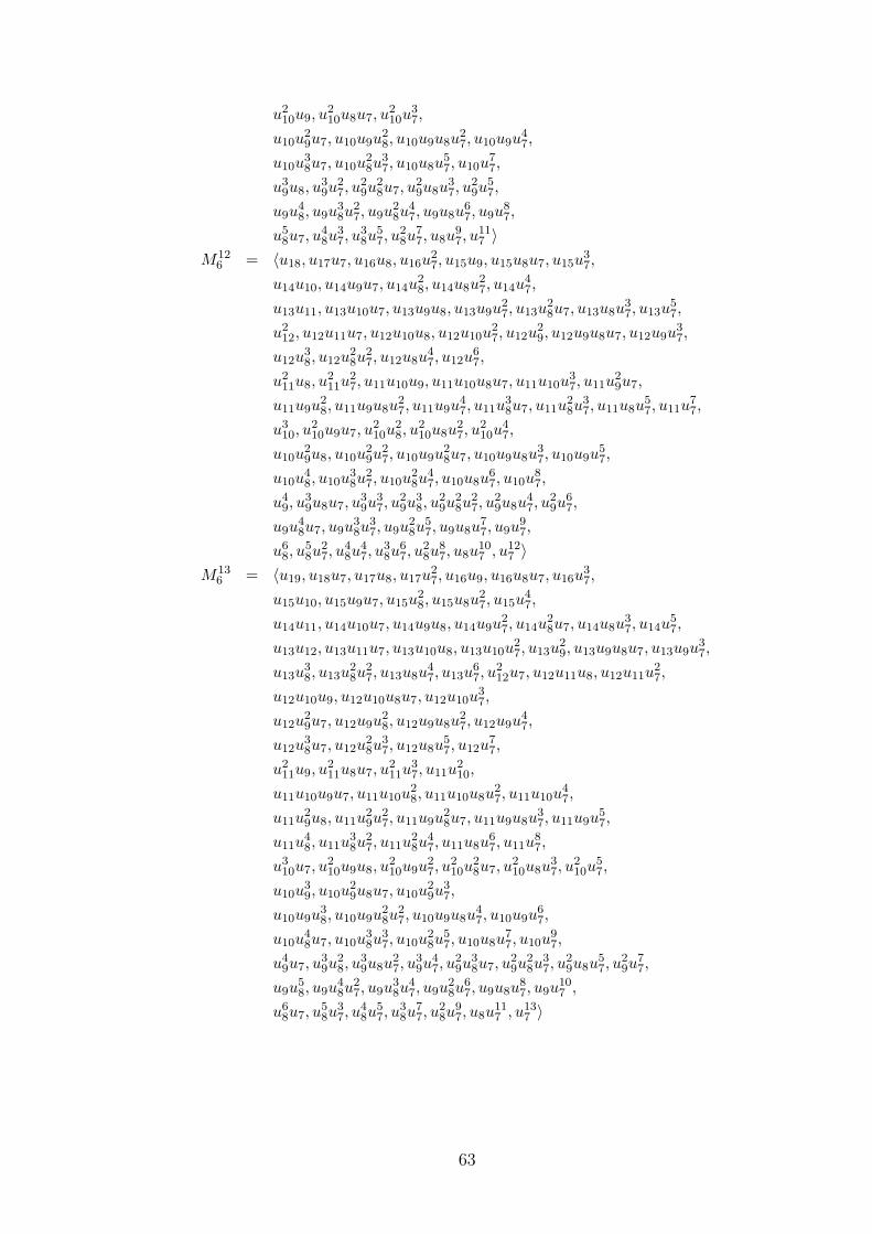
u210u9, u

210u8u7, u

210u

37,

u10u29u7, u10u9u

28, u10u9u8u

27, u10u9u

47,

u10u38u7, u10u

28u

37, u10u8u

57, u10u

77,

u39u8, u

39u

27, u

29u

28u7, u

29u8u

37, u

29u

57,

u9u48, u9u

38u

27, u9u

28u

47, u9u8u

67, u9u

87,

u58u7, u

48u

37, u

38u

57, u

28u

77, u8u

97, u

117 〉

M126 = 〈u18, u17u7, u16u8, u16u

27, u15u9, u15u8u7, u15u

37,

u14u10, u14u9u7, u14u28, u14u8u

27, u14u

47,

u13u11, u13u10u7, u13u9u8, u13u9u27, u13u

28u7, u13u8u

37, u13u

57,

u212, u12u11u7, u12u10u8, u12u10u

27, u12u

29, u12u9u8u7, u12u9u

37,

u12u38, u12u

28u

27, u12u8u

47, u12u

67,

u211u8, u

211u

27, u11u10u9, u11u10u8u7, u11u10u

37, u11u

29u7,

u11u9u28, u11u9u8u

27, u11u9u

47, u11u

38u7, u11u

28u

37, u11u8u

57, u11u

77,

u310, u

210u9u7, u

210u

28, u

210u8u

27, u

210u

47,

u10u29u8, u10u

29u

27, u10u9u

28u7, u10u9u8u

37, u10u9u

57,

u10u48, u10u

38u

27, u10u

28u

47, u10u8u

67, u10u

87,

u49, u

39u8u7, u

39u

37, u

29u

38, u

29u

28u

27, u

29u8u

47, u

29u

67,

u9u48u7, u9u

38u

37, u9u

28u

57, u9u8u

77, u9u

97,

u68, u

58u

27, u

48u

47, u

38u

67, u

28u

87, u8u

107 , u12

7 〉M13

6 = 〈u19, u18u7, u17u8, u17u27, u16u9, u16u8u7, u16u

37,

u15u10, u15u9u7, u15u28, u15u8u

27, u15u

47,

u14u11, u14u10u7, u14u9u8, u14u9u27, u14u

28u7, u14u8u

37, u14u

57,

u13u12, u13u11u7, u13u10u8, u13u10u27, u13u

29, u13u9u8u7, u13u9u

37,

u13u38, u13u

28u

27, u13u8u

47, u13u

67, u

212u7, u12u11u8, u12u11u

27,

u12u10u9, u12u10u8u7, u12u10u37,

u12u29u7, u12u9u

28, u12u9u8u

27, u12u9u

47,

u12u38u7, u12u

28u

37, u12u8u

57, u12u

77,

u211u9, u

211u8u7, u

211u

37, u11u

210,

u11u10u9u7, u11u10u28, u11u10u8u

27, u11u10u

47,

u11u29u8, u11u

29u

27, u11u9u

28u7, u11u9u8u

37, u11u9u

57,

u11u48, u11u

38u

27, u11u

28u

47, u11u8u

67, u11u

87,

u310u7, u

210u9u8, u

210u9u

27, u

210u

28u7, u

210u8u

37, u

210u

57,

u10u39, u10u

29u8u7, u10u

29u

37,

u10u9u38, u10u9u

28u

27, u10u9u8u

47, u10u9u

67,

u10u48u7, u10u

38u

37, u10u

28u

57, u10u8u

77, u10u

97,

u49u7, u

39u

28, u

39u8u

27, u

39u

47, u

29u

38u7, u

29u

28u

37, u

29u8u

57, u

29u

77,

u9u58, u9u

48u

27, u9u

38u

47, u9u

28u

67, u9u8u

87, u9u

107 ,

u68u7, u

58u

37, u

48u

57, u

38u

77, u

28u

97, u8u

117 , u13

7 〉

63

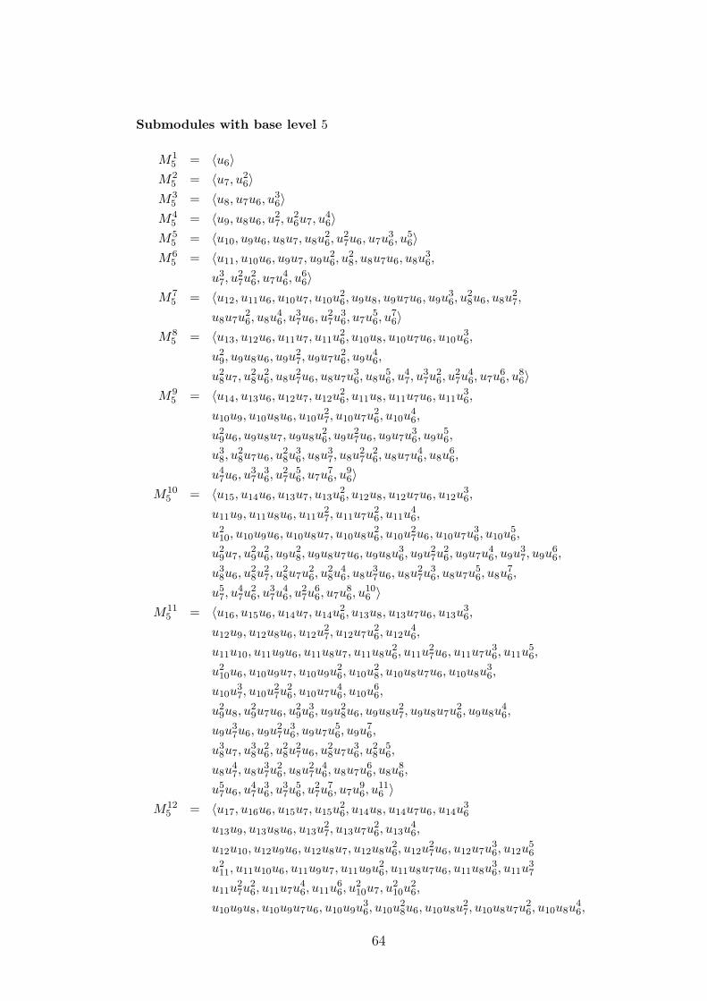
Submodules with base level 5

M15 = 〈u6〉

M25 = 〈u7, u

26〉

M35 = 〈u8, u7u6, u

36〉

M45 = 〈u9, u8u6, u

27, u

26u7, u

46〉

M55 = 〈u10, u9u6, u8u7, u8u

26, u

27u6, u7u

36, u

56〉

M65 = 〈u11, u10u6, u9u7, u9u

26, u

28, u8u7u6, u8u

36,

u37, u

27u

26, u7u

46, u

66〉

M75 = 〈u12, u11u6, u10u7, u10u

26, u9u8, u9u7u6, u9u

36, u

28u6, u8u

27,

u8u7u26, u8u

46, u

37u6, u

27u

36, u7u

56, u

76〉

M85 = 〈u13, u12u6, u11u7, u11u

26, u10u8, u10u7u6, u10u

36,

u29, u9u8u6, u9u

27, u9u7u

26, u9u

46,

u28u7, u

28u

26, u8u

27u6, u8u7u

36, u8u

56, u

47, u

37u

26, u

27u

46, u7u

66, u

86〉

M95 = 〈u14, u13u6, u12u7, u12u

26, u11u8, u11u7u6, u11u

36,

u10u9, u10u8u6, u10u27, u10u7u

26, u10u

46,

u29u6, u9u8u7, u9u8u

26, u9u

27u6, u9u7u

36, u9u

56,

u38, u

28u7u6, u

28u

36, u8u

37, u8u

27u

26, u8u7u

46, u8u

66,

u47u6, u

37u

36, u

27u

56, u7u

76, u

96〉

M105 = 〈u15, u14u6, u13u7, u13u

26, u12u8, u12u7u6, u12u

36,

u11u9, u11u8u6, u11u27, u11u7u

26, u11u

46,

u210, u10u9u6, u10u8u7, u10u8u

26, u10u

27u6, u10u7u

36, u10u

56,

u29u7, u

29u

26, u9u

28, u9u8u7u6, u9u8u

36, u9u

27u

26, u9u7u

46, u9u

37, u9u

66,

u38u6, u

28u

27, u

28u7u

26, u

28u

46, u8u

37u6, u8u

27u

36, u8u7u

56, u8u

76,

u57, u

47u

26, u

37u

46, u

27u

66, u7u

86, u

106 〉

M115 = 〈u16, u15u6, u14u7, u14u

26, u13u8, u13u7u6, u13u

36,

u12u9, u12u8u6, u12u27, u12u7u

26, u12u

46,

u11u10, u11u9u6, u11u8u7, u11u8u26, u11u

27u6, u11u7u

36, u11u

56,

u210u6, u10u9u7, u10u9u

26, u10u

28, u10u8u7u6, u10u8u

36,

u10u37, u10u

27u

26, u10u7u

46, u10u

66,

u29u8, u

29u7u6, u

29u

36, u9u

28u6, u9u8u

27, u9u8u7u

26, u9u8u

46,

u9u37u6, u9u

27u

36, u9u7u

56, u9u

76,

u38u7, u

38u

26, u

28u

27u6, u

28u7u

36, u

28u

56,

u8u47, u8u

37u

26, u8u

27u

46, u8u7u

66, u8u

86,

u57u6, u

47u

36, u

37u

56, u

27u

76, u7u

96, u

116 〉

M125 = 〈u17, u16u6, u15u7, u15u

26, u14u8, u14u7u6, u14u

36

u13u9, u13u8u6, u13u27, u13u7u

26, u13u

46,

u12u10, u12u9u6, u12u8u7, u12u8u26, u12u

27u6, u12u7u

36, u12u

56

u211, u11u10u6, u11u9u7, u11u9u

26, u11u8u7u6, u11u8u

36, u11u

37

u11u27u

26, u11u7u

46, u11u

66, u

210u7, u

210u

26,

u10u9u8, u10u9u7u6, u10u9u36, u10u

28u6, u10u8u

27, u10u8u7u

26, u10u8u

46,

64

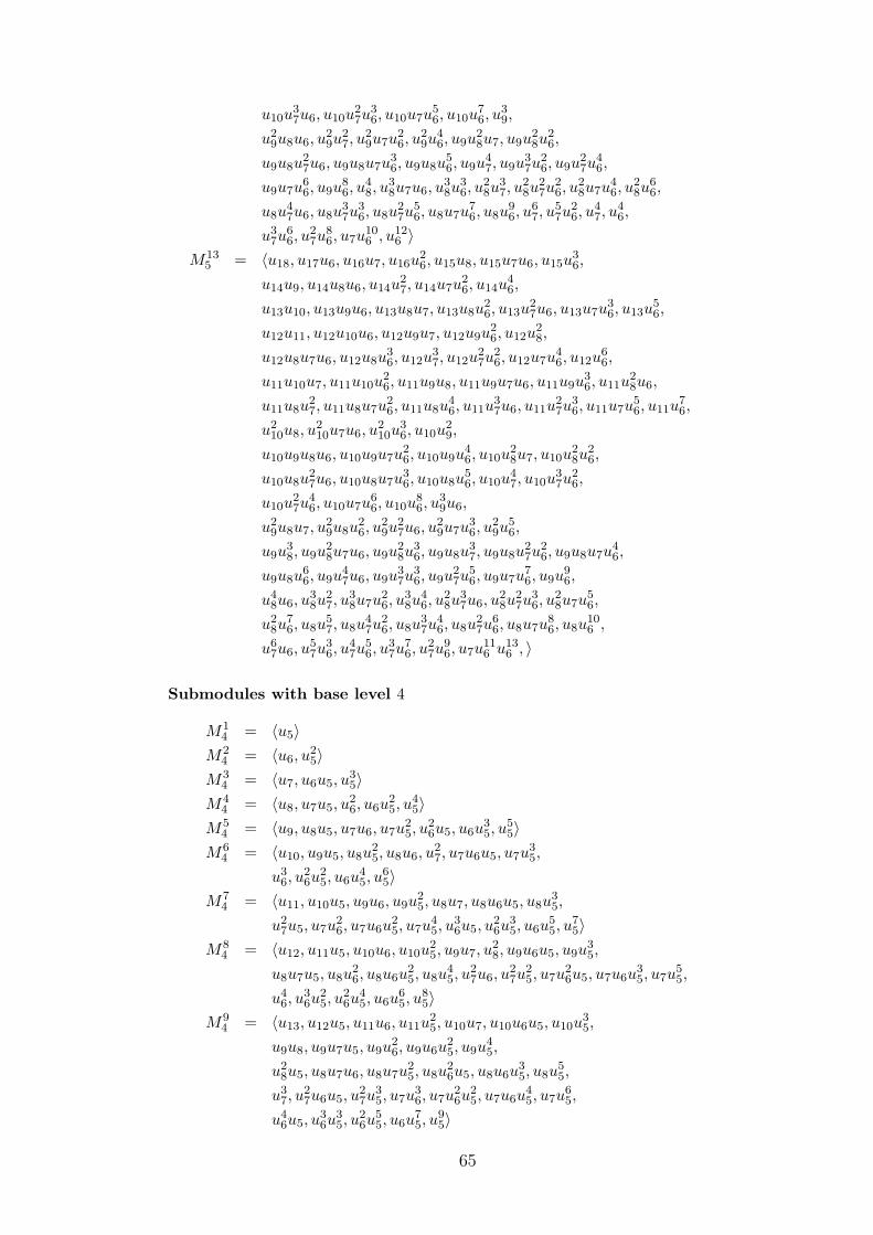
u10u37u6, u10u

27u

36, u10u7u

56, u10u

76, u

39,

u29u8u6, u

29u

27, u

29u7u

26, u

29u

46, u9u

28u7, u9u

28u

26,

u9u8u27u6, u9u8u7u

36, u9u8u

56, u9u

47, u9u

37u

26, u9u

27u

46,

u9u7u66, u9u

86, u

48, u

38u7u6, u

38u

36, u

28u

37, u

28u

27u

26, u

28u7u

46, u

28u

66,

u8u47u6, u8u

37u

36, u8u

27u

56, u8u7u

76, u8u

96, u

67, u

57u

26, u

47, u

46,

u37u

66, u

27u

86, u7u

106 , u12

6 〉M13

5 = 〈u18, u17u6, u16u7, u16u26, u15u8, u15u7u6, u15u

36,

u14u9, u14u8u6, u14u27, u14u7u

26, u14u

46,

u13u10, u13u9u6, u13u8u7, u13u8u26, u13u

27u6, u13u7u

36, u13u

56,

u12u11, u12u10u6, u12u9u7, u12u9u26, u12u

28,

u12u8u7u6, u12u8u36, u12u

37, u12u

27u

26, u12u7u

46, u12u

66,

u11u10u7, u11u10u26, u11u9u8, u11u9u7u6, u11u9u

36, u11u

28u6,

u11u8u27, u11u8u7u

26, u11u8u

46, u11u

37u6, u11u

27u

36, u11u7u

56, u11u

76,

u210u8, u

210u7u6, u

210u

36, u10u

29,

u10u9u8u6, u10u9u7u26, u10u9u

46, u10u

28u7, u10u

28u

26,

u10u8u27u6, u10u8u7u

36, u10u8u

56, u10u

47, u10u

37u

26,

u10u27u

46, u10u7u

66, u10u

86, u

39u6,

u29u8u7, u

29u8u

26, u

29u

27u6, u

29u7u

36, u

29u

56,

u9u38, u9u

28u7u6, u9u

28u

36, u9u8u

37, u9u8u

27u

26, u9u8u7u

46,

u9u8u66, u9u

47u6, u9u

37u

36, u9u

27u

56, u9u7u

76, u9u

96,

u48u6, u

38u

27, u

38u7u

26, u

38u

46, u

28u

37u6, u

28u

27u

36, u

28u7u

56,

u28u

76, u8u

57, u8u

47u

26, u8u

37u

46, u8u

27u

66, u8u7u

86, u8u

106 ,

u67u6, u

57u

36, u

47u

56, u

37u

76, u

27u

96, u7u

116 u13

6 , 〉

Submodules with base level 4

M14 = 〈u5〉

M24 = 〈u6, u

25〉

M34 = 〈u7, u6u5, u

35〉

M44 = 〈u8, u7u5, u

26, u6u

25, u

45〉

M54 = 〈u9, u8u5, u7u6, u7u

25, u

26u5, u6u

35, u

55〉

M64 = 〈u10, u9u5, u8u

25, u8u6, u

27, u7u6u5, u7u

35,

u36, u

26u

25, u6u

45, u

65〉

M74 = 〈u11, u10u5, u9u6, u9u

25, u8u7, u8u6u5, u8u

35,

u27u5, u7u

26, u7u6u

25, u7u

45, u

36u5, u

26u

35, u6u

55, u

75〉

M84 = 〈u12, u11u5, u10u6, u10u

25, u9u7, u

28, u9u6u5, u9u

35,

u8u7u5, u8u26, u8u6u

25, u8u

45, u

27u6, u

27u

25, u7u

26u5, u7u6u

35, u7u

55,

u46, u

36u

25, u

26u

45, u6u

65, u

85〉

M94 = 〈u13, u12u5, u11u6, u11u

25, u10u7, u10u6u5, u10u

35,

u9u8, u9u7u5, u9u26, u9u6u

25, u9u

45,

u28u5, u8u7u6, u8u7u

25, u8u

26u5, u8u6u

35, u8u

55,

u37, u

27u6u5, u

27u

35, u7u

36, u7u

26u

25, u7u6u

45, u7u

65,

u46u5, u

36u

35, u

26u

55, u6u

75, u

95〉

65

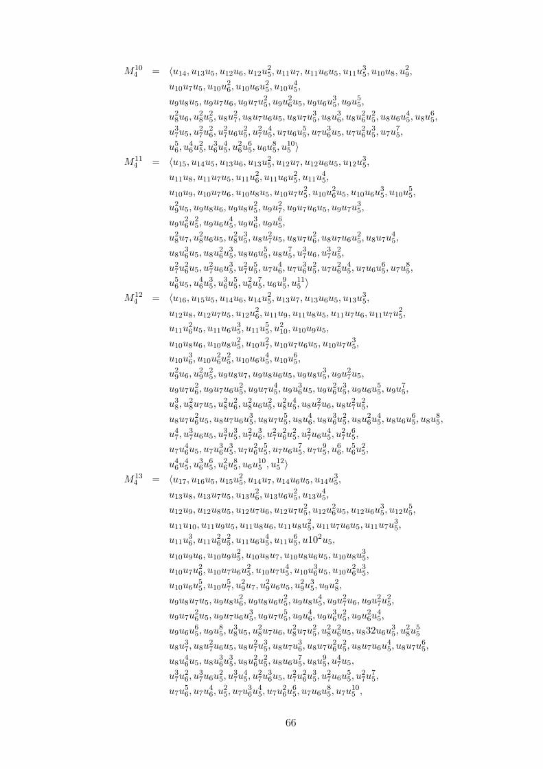
M104 = 〈u14, u13u5, u12u6, u12u

25, u11u7, u11u6u5, u11u

35, u10u8, u

29,

u10u7u5, u10u26, u10u6u

25, u10u

45,

u9u8u5, u9u7u6, u9u7u25, u9u

26u5, u9u6u

35, u9u

55,

u28u6, u

28u

25, u8u

27, u8u7u6u5, u8u7u

35, u8u

36, u8u

26u

25, u8u6u

45, u8u

65,

u37u5, u

27u

26, u

27u6u

25, u

27u

45, u7u6u

55, u7u

36u5, u7u

26u

35, u7u

75,

u56, u

46u

25, u

36u

45, u

26u

65, u6u

85, u

105 〉

M114 = 〈u15, u14u5, u13u6, u13u

25, u12u7, u12u6u5, u12u

35,

u11u8, u11u7u5, u11u26, u11u6u

25, u11u

45,

u10u9, u10u7u6, u10u8u5, u10u7u25, u10u

26u5, u10u6u

35, u10u

55,

u29u5, u9u8u6, u9u8u

25, u9u

27, u9u7u6u5, u9u7u

35,

u9u26u

25, u9u6u

45, u9u

36, u9u

65,

u28u7, u

28u6u5, u

28u

35, u8u

27u5, u8u7u

26, u8u7u6u

25, u8u7u

45,

u8u36u5, u8u

26u

35, u8u6u

55, u8u

75, u

37u6, u

37u

25,

u27u

26u5, u

27u6u

35, u

27u

55, u7u

46, u7u

36u

25, u7u

26u

45, u7u6u

65, u7u

85,

u56u5, u

46u

35, u

36u

55, u

26u

75, u6u

95, u

115 〉

M124 = 〈u16, u15u5, u14u6, u14u

25, u13u7, u13u6u5, u13u

35,

u12u8, u12u7u5, u12u26, u11u9, u11u8u5, u11u7u6, u11u7u

25,

u11u26u5, u11u6u

35, u11u

55, u

210, u10u9u5,

u10u8u6, u10u8u25, u10u

27, u10u7u6u5, u10u7u

35,

u10u36, u10u

26u

25, u10u6u

45, u10u

65,

u29u6, u

29u

25, u9u8u7, u9u8u6u5, u9u8u

35, u9u

27u5,

u9u7u26, u9u7u6u

25, u9u7u

45, u9u

36u5, u9u

26u

35, u9u6u

55, u9u

75,

u38, u

28u7u5, u

28u

26, u

28u6u

25, u

28u

45, u8u

27u6, u8u

27u

25,

u8u7u26u5, u8u7u6u

35, u8u7u

55, u8u

46, u8u

36u

25, u8u

26u

45, u8u6u

65, u8u

85,

u47, u

37u6u5, u

37u

35, u

27u

36, u

27u

26u

25, u

27u6u

45, u

27u

65,

u7u46u5, u7u

36u

35, u7u

26u

55, u7u6u

75, u7u

95, u

66, u

56u

25,

u46u

45, u

36u

65, u

26u

85, u6u

105 , u12

5 〉M13

4 = 〈u17, u16u5, u15u25, u14u7, u14u6u5, u14u

35,

u13u8, u13u7u5, u13u26, u13u6u

25, u13u

45,

u12u9, u12u8u5, u12u7u6, u12u7u25, u12u

26u5, u12u6u

35, u12u

55,

u11u10, u11u9u5, u11u8u6, u11u8u25, u11u7u6u5, u11u7u

35,

u11u36, u11u

26u

25, u11u6u

45, u11u

65, u102u5,

u10u9u6, u10u9u25, u10u8u7, u10u8u6u5, u10u8u

35,

u10u7u26, u10u7u6u

25, u10u7u

45, u10u

36u5, u10u

26u

35,

u10u6u55, u10u

57, u

29u7, u

29u6u5, u

29u

35, u9u

28,

u9u8u7u5, u9u8u26, u9u8u6u

25, u9u8u

45, u9u

27u6, u9u

27u

25,

u9u7u26u5, u9u7u6u

35, u9u7u

55, u9u

46, u9u

36u

25, u9u

26u

45,

u9u6u65, u9u

85, u

38u5, u

28u7u6, u

28u7u

25, u

28u

26u5, u832u6u

35, u

28u

55

u8u37, u8u

27u6u5, u8u

27u

35, u8u7u

36, u8u7u

26u

25, u8u7u6u

45, u8u7u

65,

u8u46u5, u8u

36u

35, u8u

26u

25, u8u6u

75, u8u

95, u

47u5,

u37u

26, u

37u6u

25, u

37u

45, u

27u

36u5, u

27u

26u

35, u

27u6u

55, u

27u

75,

u7u56, u7u

46, u

25, u7u

36u

45, u7u

26u

65, u7u6u

85, u7u

105 ,

66

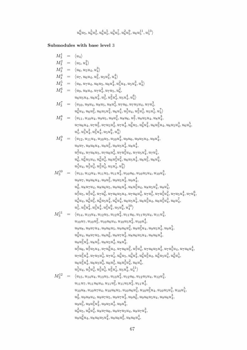
u66u5, u

56u

35, u

46u

55, u

36u

75, u

26u

95, u6u

115 , u13

5 〉

Submodules with base level 3

M13 = 〈u4〉

M23 = 〈u5, u

24〉

M33 = 〈u6, u5u4, u

34〉

M43 = 〈u7, u6u4, u

25, u5u

24, u

44〉

M53 = 〈u8, u7u4, u6u5, u6u

24, u

25u4, u5u

34, u

54〉

M63 = 〈u9, u8u4, u7u

24, u7u5, u

26,

u6u5u4, u6u34, u

35, u

25u

24, u5u

44, u

64〉

M73 = 〈u10, u9u4, u8u5, u8u

24, u7u6, u7u5u4, u7u

34,

u26u4, u6u

25, u6u5u

24, u6u

44, u

35u4, u

25u

34, u5u

54, u

74〉

M83 = 〈u11, u10u4, u9u5, u9u

24, u8u6, u

27, u8u5u4, u8u

34,

u7u6u4, u7u25, u7u5u

24, u7u

44, u

26u5, u

26u

24, u6u

25u4, u6u5u

34, u6u

54,

u45, u

35u

24, u

25u

44, u5u

64, u

84〉

M93 = 〈u12, u11u4, u10u5, u10u

24, u9u6, u9u5u4, u9u

34,

u8u7, u8u6u4, u8u25, u8u5u

24, u8u

44,

u27u4, u7u6u5, u7u6u

24, u7u

25u4, u7u5u

34, u7u

54,

u36, u

26u5u4, u

26u

34, u6u

25u

24, u6u5u

44, u6u

35, u6u

64,

u45u4, u

35u

34, u

25u

54, u5u

74, u

94〉

M103 = 〈u13, u12u4, u11u5, u11u

24, u10u6, u10u5u4, u10u

34,

u9u7, u9u6u4, u9u25, u9u5u

24, u9u

44,

u28, u8u7u4, u8u6u5, u8u6u

24, u8u

25u4, u8u5u

34, u8u

54,

u27u5, u

27u

24, u7u

26, u7u6u5u4, u7u6u

34, u7u

35, u7u

25u

24, u7u5u

44, u7u

64,

u36u4, u

26u

25, u

26u5u

24, u

26u

44, u6u5u

54, u6u

35u4, u6u

25u

34, u6u

74,

u55, u

45u

24, u

35u

44, u

25u

64, u5u

84, u

104 〉

M113 = 〈u14, u13u4, u12u5, u12u

24, u11u6, u11u5u4, u11u

34,

u10u7, u10u25, u10u6u4, u10u5u

24, u10u

44,

u9u8, u9u7u4, u9u6u5, u9u6u24, u9u

25u4, u9u5u

34, u9u

54,

u28u4, u8u7u5, u8u

26, u8u7u

24, u8u6u5u4, u8u6u

34,

u8u25u

24, u8u

35, u8u5u

44, u8u

64,

u27u6, u

27u5u4, u7u

26u4, u7u6u

25, u

27u

34, u7u6u5u

24, u7u

35u4, u7u6u

44,

u7u25u

34, u7u5u

54, u7u

74, u

36u5, u

36u

24, u

26u

25u4, u

26u5u

34, u

26u

54,

u6u25u

44, u6u5u

64, u6u

45, u6u

35u

24, u6u

84,

u55u4, u

45u

34, u

35u

54, u

25u

74, u5u

94, u

114 〉

M123 = 〈u15, u14u4, u13u5, u13u

24, u12u6, u12u5u4, u12u

34,

u11u7, u11u6u4, u11u25, u11u5u

24, u11u

44,

u10u8, u10u7u4, u10u6u5, u10u6u24, u10u

25u4, u10u5u

34, u10u

54,

u29, u9u8u4, u9u7u5, u9u7u

24, u9u

26, u9u6u5u4, u9u6u

34,

u9u35, u9u

25u

24, u9u5u

44, u9u

64,

u28u5, u

28u

24, u8u7u6, u8u7u5u4, u8u7u

34,

u8u26u4, u8u6u5u

24, u8u6u

25, u8u6u

44,

67

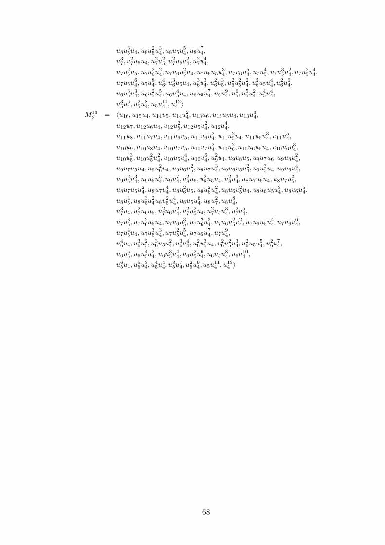
u8u35u4, u8u

25u

34, u8u5u

54, u8u

74,

u37, u

27u6u4, u

27u

25, u

27u5u

24, u

27u

44,

u7u26u5, u7u

26u

24, u7u6u

25u4, u7u6u5u

34, u7u6u

54, u7u

45, u7u

35u

24, u7u

25u

44,

u7u5u64, u7u

84, u

46, u

36u5u4, u

36u

34, u

26u

35, u

26u

25u

24, u

26u5u

44, u

26u

64,

u6u35u

34, u6u

25u

54, u6u

45u4, u6u5u

74, u6u

94, u

65, u

55u

24, u

45u

44,

u35u

64, u

25u

84, u5u

104 , u12

4 〉M13

3 = 〈u16, u15u4, u14u5, u14u24, u13u6, u13u5u4, u13u

34,

u12u7, u12u6u4, u12u25, u12u5u

24, u12u

44,

u11u8, u11u7u4, u11u6u5, u11u6u24, u11u

25u4, u11u5u

34, u11u

54,

u10u9, u10u8u4, u10u7u5, u10u7u24, u10u

26, u10u6u5u4, u10u6u

34,

u10u35, u10u

25u

24, u10u5u

44, u10u

64, u

29u4, u9u8u5, u9u7u6, u9u8u

24,

u9u7u5u4, u9u26u4, u9u6u

25, u9u7u

34, u9u6u5u

24, u9u

35u4, u9u6u

44,

u9u25u

34, u9u5u

54, u9u

74, u

28u6, u

28u5u4, u

28u

34, u8u7u6u4, u8u7u

25,

u8u7u5u24, u8u7u

44, u8u

26u5, u8u

26u

24, u8u6u

25u4, u8u6u5u

34, u8u6u

54,

u8u45, u8u

35u

24u8u

25u

44, u8u5u

64, u8u

27, u8u

84,

u37u4, u

27u6u5, u

27u6u

24, u

27u

25u4, u

27u5u

34, u

27u

54,

u7u36, u7u

26u5u4, u7u6u

35, u7u

26u

34, u7u6u

25u

24, u7u6u5u

44, u7u6u

64,

u7u45u4, u7u

35u

34, u7u

25u

54, u7u5u

74, u7u

94,

u46u4, u

36u

25, u

36u5u

24, u

36u

44, u

26u

35u4, u

26u

25u

34, u

26u5u

54, u

26u

74,

u6u55, u6u

45u

24, u6u

35u

44, u6u

25u

64, u6u5u

84, u6u

104 ,

u65u4, u

55u

34, u

45u

44, u

35u

74, u

25u

94, u5u

114 , u13

4 〉

68

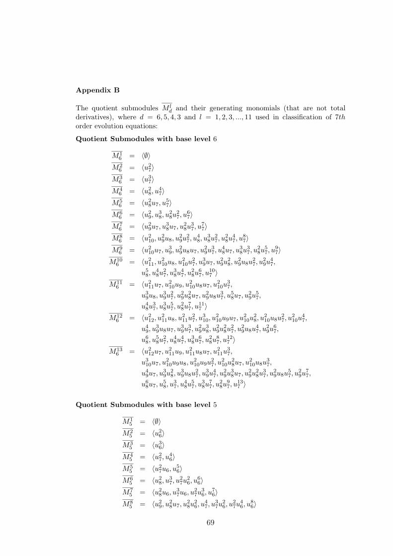
Appendix B

The quotient submodules M ld and their generating monomials (that are not total

derivatives), where d = 6, 5, 4, 3 and l = 1, 2, 3, ..., 11 used in classification of 7thorder evolution equations:

Quotient Submodules with base level 6

M16 = 〈∅〉

M26 = 〈u2

7〉M3

6 = 〈u37〉

M46 = 〈u2

8, u47〉

M56 = 〈u2

8u7, u57〉

M66 = 〈u2

9, u38, u

28u

27, u

67〉

M76 = 〈u2

9u7, u38u7, u

28u

37, u

77〉

M86 = 〈u2

10, u29u8, u

29u

27, u

48, u

38u

27, u

28u

47, u

87〉

M96 = 〈u2

10u7, u39, u

29u8u7, u

29u

37, u

48u7, u

38u

37, u

28u

57, u

97〉

M106 = 〈u2

11, u210u8, u

210u

27, u

39u7, u

29u

28, u

29u8u

27, u

29u

47,

u58, u

48u

27, u

38u

47, u

28u

67, u

107 〉

M116 = 〈u2

11u7, u210u9, u

210u8u7, u

210u

37,

u39u8, u

39u

27, u

29u

28u7, u

29u8u

37, u

58u7, u

29u

57,

u48u

37, u

38u

57, u

28u

77, u

117 〉

M126 = 〈u2

12, u211u8, u

211u

27, u

310, u

210u9u7, u

210u

28, u

210u8u

27, u

210u

47,

u49, u

39u8u7, u

39u

37, u

29u

38, u

29u

28u

27, u

29u8u

47, u

29u

67,

u68, u

58u

27, u

48u

47, u

38u

67, u

28u

87, u

127 〉

M136 = 〈u2

12u7, u211u9, u

211u8u7, u

211u

37,

u310u7, u

210u9u8, u

210u9u

27, u

210u

28u7, u

210u8u

37,

u49u7, u

39u

28, u

39u8u

27, u

39u

47, u

29u

38u7, u

29u

28u

37, u

29u8u

57, u

29u

77,

u68u7, u

58, u

37, u

48u

57, u

38u

77, u

28u

97, u

137 〉

Quotient Submodules with base level 5

M15 = 〈∅〉

M25 = 〈u2

6〉M3

5 = 〈u36〉

M45 = 〈u2

7, u46〉

M55 = 〈u2

7u6, u56〉

M65 = 〈u2

8, u37, u

27u

26, u

66〉

M75 = 〈u2

8u6, u37u6, u

27u

36, u

76〉

M85 = 〈u2

9, u28u7, u

28u

26, u

47, u

37u

26, u

27u

46, u

86〉

69

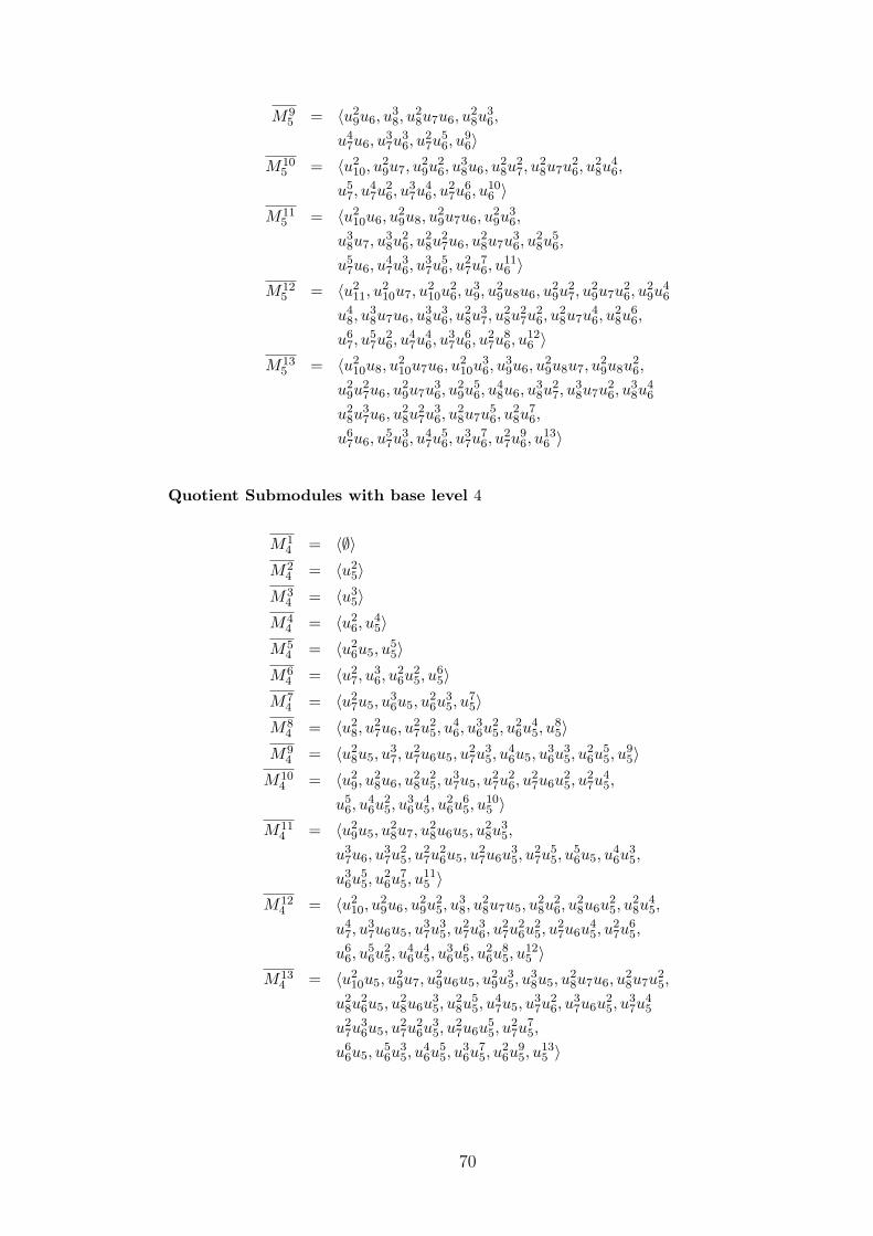
M95 = 〈u2

9u6, u38, u

28u7u6, u

28u

36,

u47u6, u

37u

36, u

27u

56, u

96〉

M105 = 〈u2

10, u29u7, u

29u

26, u

38u6, u

28u

27, u

28u7u

26, u

28u

46,

u57, u

47u

26, u

37u

46, u

27u

66, u

106 〉

M115 = 〈u2

10u6, u29u8, u

29u7u6, u

29u

36,

u38u7, u

38u

26, u

28u

27u6, u

28u7u

36, u

28u

56,

u57u6, u

47u

36, u

37u

56, u

27u

76, u

116 〉

M125 = 〈u2

11, u210u7, u

210u

26, u

39, u

29u8u6, u

29u

27, u

29u7u

26, u

29u

46

u48, u

38u7u6, u

38u

36, u

28u

37, u

28u

27u

26, u

28u7u

46, u

28u

66,

u67, u

57u

26, u

47u

46, u

37u

66, u

27u

86, u

126 〉

M135 = 〈u2

10u8, u210u7u6, u

210u

36, u

39u6, u

29u8u7, u

29u8u

26,

u29u

27u6, u

29u7u

36, u

29u

56, u

48u6, u

38u

27, u

38u7u

26, u

38u

46

u28u

37u6, u

28u

27u

36, u

28u7u

56, u

28u

76,

u67u6, u

57u

36, u

47u

56, u

37u

76, u

27u

96, u

136 〉

Quotient Submodules with base level 4

M14 = 〈∅〉

M24 = 〈u2

5〉M3

4 = 〈u35〉

M44 = 〈u2

6, u45〉

M54 = 〈u2

6u5, u55〉

M64 = 〈u2

7, u36, u

26u

25, u

65〉

M74 = 〈u2

7u5, u36u5, u

26u

35, u

75〉

M84 = 〈u2

8, u27u6, u

27u

25, u

46, u

36u

25, u

26u

45, u

85〉

M94 = 〈u2

8u5, u37, u

27u6u5, u

27u

35, u

46u5, u

36u

35, u

26u

55, u

95〉

M104 = 〈u2

9, u28u6, u

28u

25, u

37u5, u

27u

26, u

27u6u

25, u

27u

45,

u56, u

46u

25, u

36u

45, u

26u

65, u

105 〉

M114 = 〈u2

9u5, u28u7, u

28u6u5, u

28u

35,

u37u6, u

37u

25, u

27u

26u5, u

27u6u

35, u

27u

55, u

56u5, u

46u

35,

u36u

55, u

26u

75, u

115 〉

M124 = 〈u2

10, u29u6, u

29u

25, u

38, u

28u7u5, u

28u

26, u

28u6u

25, u

28u

45,

u47, u

37u6u5, u

37u

35, u

27u

36, u

27u

26u

25, u

27u6u

45, u

27u

65,

u66, u

56u

25, u

46u

45, u

36u

65, u

26u

85, u

125 〉

M134 = 〈u2

10u5, u29u7, u

29u6u5, u

29u

35, u

38u5, u

28u7u6, u

28u7u

25,

u28u

26u5, u

28u6u

35, u

28u

55, u

47u5, u

37u

26, u

37u6u

25, u

37u

45

u27u

36u5, u

27u

26u

35, u

27u6u

55, u

27u

75,

u66u5, u

56u

35, u

46u

55, u

36u

75, u

26u

95, u

135 〉

70

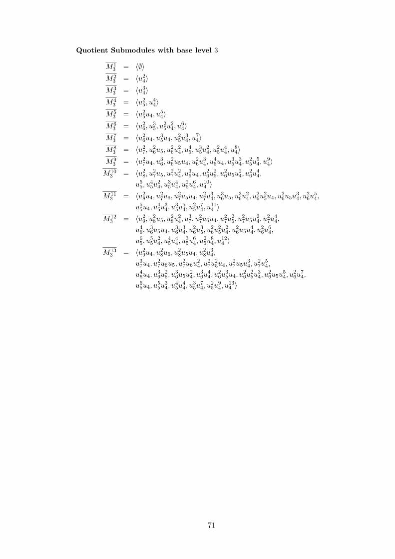
Quotient Submodules with base level 3

M13 = 〈∅〉

M23 = 〈u2

4〉M3

3 = 〈u34〉

M43 = 〈u2

5, u44〉

M53 = 〈u2

5u4, u54〉

M63 = 〈u2

6, u35, u

25u

24, u

64〉

M73 = 〈u2

6u4, u35u4, u

25u

34, u

74〉

M83 = 〈u2

7, u26u5, u

26u

24, u

45, u

35u

24, u

25u

44, u

84〉

M93 = 〈u2

7u4, u36, u

26u5u4, u

26u

34, u

45u4, u

35u

34, u

25u

54, u

94〉

M103 = 〈u2

8, u27u5, u

27u

24, u

36u4, u

26u

25, u

26u5u

24, u

26u

44,

u55, u

45u

24, u

35u

44, u

25u

64, u

104 〉

M113 = 〈u2

8u4, u27u6, u

27u5u4, u

27u

34, u

36u5, u

36u

24, u

26u

25u4, u

26u5u

34, u

26u

54,

u55u4, u

45u

34, u

35u

54, u

25u

74, u

114 〉

M123 = 〈u2

9, u28u5, u

28u

24, u

37, u

27u6u4, u

27u

25, u

27u5u

24, u

27u

44,

u46, u

36u5u4, u

36u

34, u

26u

35, u

26u

25u

24, u

26u5u

44, u

26u

64,

u65, u

55u

24, u

45u

44, u

35u

64, u

25u

84, u

124 〉

M133 = 〈u2

9u4, u28u6, u

28u5u4, u

28u

34,

u37u4, u

27u6u5, u

27u6u

24, u

27u

25u4, u

27u5u

34, u

27u

54,

u46u4, u

36u

25, u

36u5u

24, u

36u

44, u

26u

35u4, u

26u

25u

34, u

26u5u

54, u

26u

74,

u65u4, u

55u

34, u

45u

44, u

35u

74, u

25u

94, u

134 〉

71

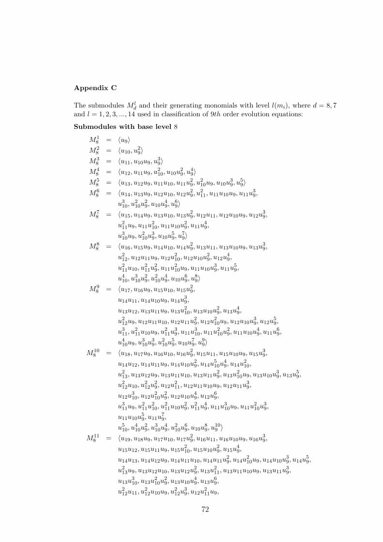
Appendix C

The submodules M ld and their generating monomials with level l(mi), where d = 8, 7

and l = 1, 2, 3, ..., 14 used in classification of 9th order evolution equations:

Submodules with base level 8

M18 = 〈u9〉

M28 = 〈u10, u

29〉

M38 = 〈u11, u10u9, u

39〉

M48 = 〈u12, u11u9, u

210, u10u

29, u

49〉

M58 = 〈u13, u12u9, u11u10, u11u

29, u

210u9, u10u

39, u

59〉

M68 = 〈u14, u13u9, u12u10, u12u

29, u

211, u11u10u9, u11u

39,

u310, u

210u

29, u10u

49, u

69〉

M78 = 〈u15, u14u9, u13u10, u13u

29, u12u11, u12u10u9, u12u

39,

u211u9, u11u

210, u11u10u

29, u11u

49,

u310u9, u

210u

39, u10u

59, u

79〉

M88 = 〈u16, u15u9, u14u10, u14u

29, u13u11, u13u10u9, u13u

39,

u212, u12u11u9, u12u

210, u12u10u

29, u12u

49,

u211u10, u

211u

29, u11u

210u9, u11u10u

39, u11u

59,

u410, u

310u

29, u

210u

49, u10u

69, u

89〉

M98 = 〈u17, u16u9, u15u10, u15u

29,

u14u11, u14u10u9, u14u39,

u13u12, u13u11u9, u13u210, u13u10u

29, u13u

49,

u212u9, u12u11u10, u12u11u

29, u12u

210u9, u12u10u

39, u12u

59,

u311, u

211u10u9, u

211u

39, u11u

310, u11u

210u

29, u11u10u

49, u11u

69,

u410u9, u

310u

39, u

210u

59, u10u

79, u

99〉

M108 = 〈u18, u17u9, u16u10, u16u

29, u15u11, u15u10u9, u15u

39,

u14u12, u14u11u9, u14u10u29, u14u

510u

49, u14u

210,

u213, u13u12u9, u13u11u10, u13u11u

29, u13u

210u9, u13u10u

39, u13u

59,

u212u10, u

212u

29, u12u

211, u12u11u10u9, u12u11u

39,

u12u310, u12u

210u

29, u12u10u

49, u12u

69,

u311u9, u

211u

210, u

211u10u

29, u

211u

49, u11u

310u9, u11u

210u

39,

u11u10u59, u11u

79,

u510, u

410u

29, u

310u

49, u

210u

69, u10u

89, u

109 〉

M118 = 〈u19, u18u9, u17u10, u17u

29, u16u11, u16u10u9, u16u

39,

u15u12, u15u11u9, u15u210, u15u10u

29, u15u

49,

u14u13, u14u12u9, u14u11u10, u14u11u29, u14u

210u9, u14u10u

39, u14u

59,

u213u9, u13u12u10, u13u12u

29, u13u

211, u13u11u10u9, u13u11u

39,

u13u310, u13u

210u

29, u13u10u

49, u13u

69,

u212u11, u

212u10u9, u

212u

39, u12u

211u9,

72

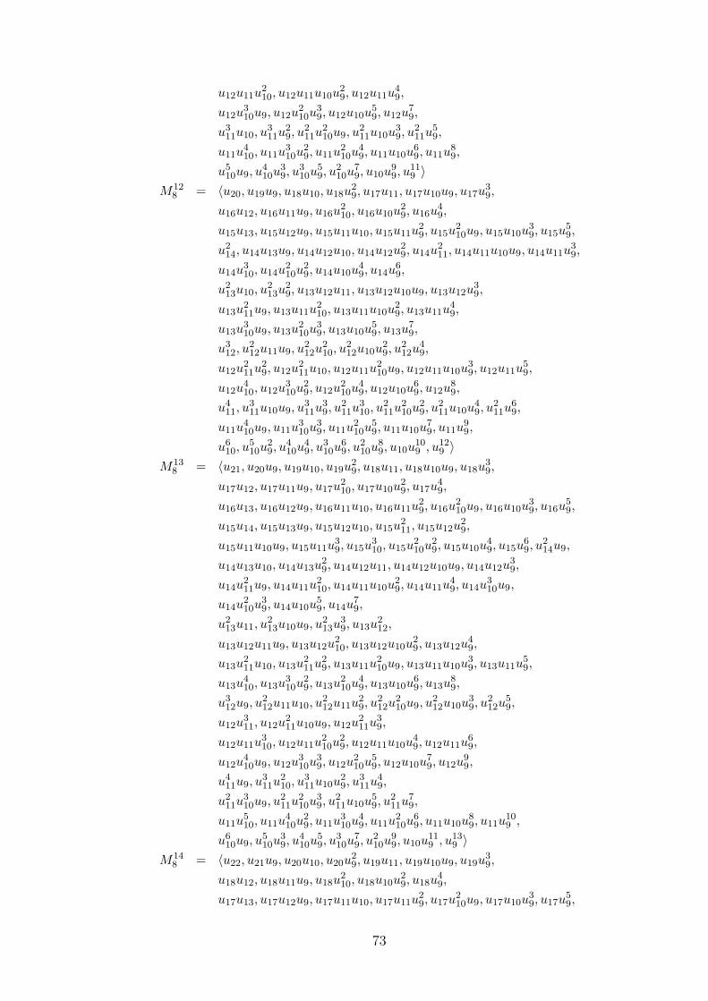
u12u11u210, u12u11u10u

29, u12u11u

49,

u12u310u9, u12u

210u

39, u12u10u

59, u12u

79,

u311u10, u

311u

29, u

211u

210u9, u

211u10u

39, u

211u

59,

u11u410, u11u

310u

29, u11u

210u

49, u11u10u

69, u11u

89,

u510u9, u

410u

39, u

310u

59, u

210u

79, u10u

99, u

119 〉

M128 = 〈u20, u19u9, u18u10, u18u

29, u17u11, u17u10u9, u17u

39,

u16u12, u16u11u9, u16u210, u16u10u

29, u16u

49,

u15u13, u15u12u9, u15u11u10, u15u11u29, u15u

210u9, u15u10u

39, u15u

59,

u214, u14u13u9, u14u12u10, u14u12u

29, u14u

211, u14u11u10u9, u14u11u

39,

u14u310, u14u

210u

29, u14u10u

49, u14u

69,

u213u10, u

213u

29, u13u12u11, u13u12u10u9, u13u12u

39,

u13u211u9, u13u11u

210, u13u11u10u

29, u13u11u

49,

u13u310u9, u13u

210u

39, u13u10u

59, u13u

79,

u312, u

212u11u9, u

212u

210, u

212u10u

29, u

212u

49,

u12u211u

29, u12u

211u10, u12u11u

210u9, u12u11u10u

39, u12u11u

59,

u12u410, u12u

310u

29, u12u

210u

49, u12u10u

69, u12u

89,

u411, u

311u10u9, u

311u

39, u

211u

310, u

211u

210u

29, u

211u10u

49, u

211u

69,

u11u410u9, u11u

310u

39, u11u

210u

59, u11u10u

79, u11u

99,

u610, u

510u

29, u

410u

49, u

310u

69, u

210u

89, u10u

109 , u12

9 〉M13

8 = 〈u21, u20u9, u19u10, u19u29, u18u11, u18u10u9, u18u

39,

u17u12, u17u11u9, u17u210, u17u10u

29, u17u

49,

u16u13, u16u12u9, u16u11u10, u16u11u29, u16u

210u9, u16u10u

39, u16u

59,

u15u14, u15u13u9, u15u12u10, u15u211, u15u12u

29,

u15u11u10u9, u15u11u39, u15u

310, u15u

210u

29, u15u10u

49, u15u

69, u

214u9,

u14u13u10, u14u13u29, u14u12u11, u14u12u10u9, u14u12u

39,

u14u211u9, u14u11u

210, u14u11u10u

29, u14u11u

49, u14u

310u9,

u14u210u

39, u14u10u

59, u14u

79,

u213u11, u

213u10u9, u

213u

39, u13u

212,

u13u12u11u9, u13u12u210, u13u12u10u

29, u13u12u

49,

u13u211u10, u13u

211u

29, u13u11u

210u9, u13u11u10u

39, u13u11u

59,

u13u410, u13u

310u

29, u13u

210u

49, u13u10u

69, u13u

89,

u312u9, u

212u11u10, u

212u11u

29, u

212u

210u9, u

212u10u

39, u

212u

59,

u12u311, u12u

211u10u9, u12u

211u

39,

u12u11u310, u12u11u

210u

29, u12u11u10u

49, u12u11u

69,

u12u410u9, u12u

310u

39, u12u

210u

59, u12u10u

79, u12u

99,

u411u9, u

311u

210, u

311u10u

29, u

311u

49,

u211u

310u9, u

211u

210u

39, u

211u10u

59, u

211u

79,

u11u510, u11u

410u

29, u11u

310u

49, u11u

210u

69, u11u10u

89, u11u

109 ,

u610u9, u

510u

39, u

410u

59, u

310u

79, u

210u

99, u10u

119 , u13

9 〉M14

8 = 〈u22, u21u9, u20u10, u20u29, u19u11, u19u10u9, u19u

39,

u18u12, u18u11u9, u18u210, u18u10u

29, u18u

49,

u17u13, u17u12u9, u17u11u10, u17u11u29, u17u

210u9, u17u10u

39, u17u

59,

73

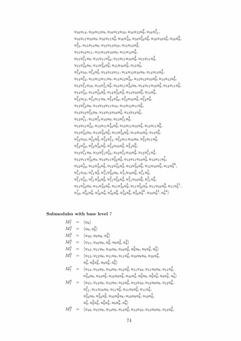
u16u14, u16u13u9, u16u12u10, u16u12u29, u16u

211,

u16u11u10u9, u16u11u39, u16u

310, u16u

210u

29, u16u10u

49, u16u

69,

u215, u15u14u9, u15u13u10, u15u13u

29,

u15u12u11, u15u12u10u9, u15u12u39,

u15u211u9, u15u11u

210, u15u11u10u

29, u15u11u

49,

u15u310u9, u15u

210u

39, u15u10u

59, u15u

79,

u214u10, u

214u

29, u14u13u11, u14u13u10u9, u14u13u

39,

u14u212, u14u12u11u9, u14u12u

210, u14u12u10u

29, u14u12u

49,

u14u211u10, u14u

211u

29, u14u11u

210u9, u14u11u10u

39, u14u11u

59,

u14u410, u14u

310u

29, u14u

210u

49, u14u10u

69, u14u

89,

u213u12, u

213u11u9, u

213u

210, u

213u10u

29, u

213u

49,

u13u212u9, u13u12u11u10, u13u12u11u

29,

u13u12u210u9, u13u12u10u

39, u13u12u

59,

u13u311, u13u

211u10u9, u13u

211u

39,

u13u11u310, u13u11u

210u

29, u13u11u10u

49, u13u11u

69,

u13u410u9, u13u

310u

39, u13u

210u

59, u13u10u

79, u13u

99,

u312u10, u

312u

29, u

212u

211, u

212u11u10u9, u

212u11u

39,

u212u

310, u

212u

210u

29, u

212u10u

49, u

212u

69,

u12u311u9, u12u

211u

210, u12u

211u10u

29, u12u

211u

49,

u12u11u310u9, u12u11u

210u

39, u12u11u10u

59, u12u11u

79,

u12u510, u12u

410u

29, u12u

310u

49, u12u

210u

69, u12u10u

89, u12u

109 ,

u411u10, u

411u

29, u

311u

210u9, u

311u10u

39, u

311u

59,

u211u

410, u

211u

310u

29, u

211u

210u

49, u

211u10u

69, u

211u

89,

u11u510u9, u11u

410u

39, u11u

310u

59, u11u

210u

79, u11u10u

99, u11u

119 ,

u710, u

610u

29, u

510u

49, u

410u

69, u

310u

89, u

210u

109 , u10u

129 , u14

9 〉

Submodules with base level 7

M17 = 〈u8〉

M27 = 〈u9, u

28〉

M37 = 〈u10, u9u8, u

38〉

M47 = 〈u11, u10u8, u

29, u9u

28, u

48〉

M57 = 〈u12, u11u8, u10u9, u10u

28, u

29u8, u9u

38, u

58〉

M67 = 〈u13, u12u8, u11u9, u11u

28, u10u9u8, u10u

38,

u39, u

29u

28, u9u

48, u

68〉

M77 = 〈u14, u13u8, u12u9, u12u

28, u11u10, u11u9u8, u11u

38,

u210u8, u10u

29, u10u9u

28, u10u

48, u

39u8, u

29u

38, u9u

58, u

78〉

M87 = 〈u15, u14u8, u13u9, u13u

28, u12u10, u12u9u8, u12u

38,

u211, u11u10u8, u11u

29, u11u9u

28, u11u

48,

u210u9, u

210u

28, u10u

29u8, u10u9u

38, u10u

58,

u49, u

39u

28, u

29u

48, u9u

68, u

88〉

M97 = 〈u16, u15u8, u14u9, u14u

28, u13u10, u13u9u8, u13u

38,

74

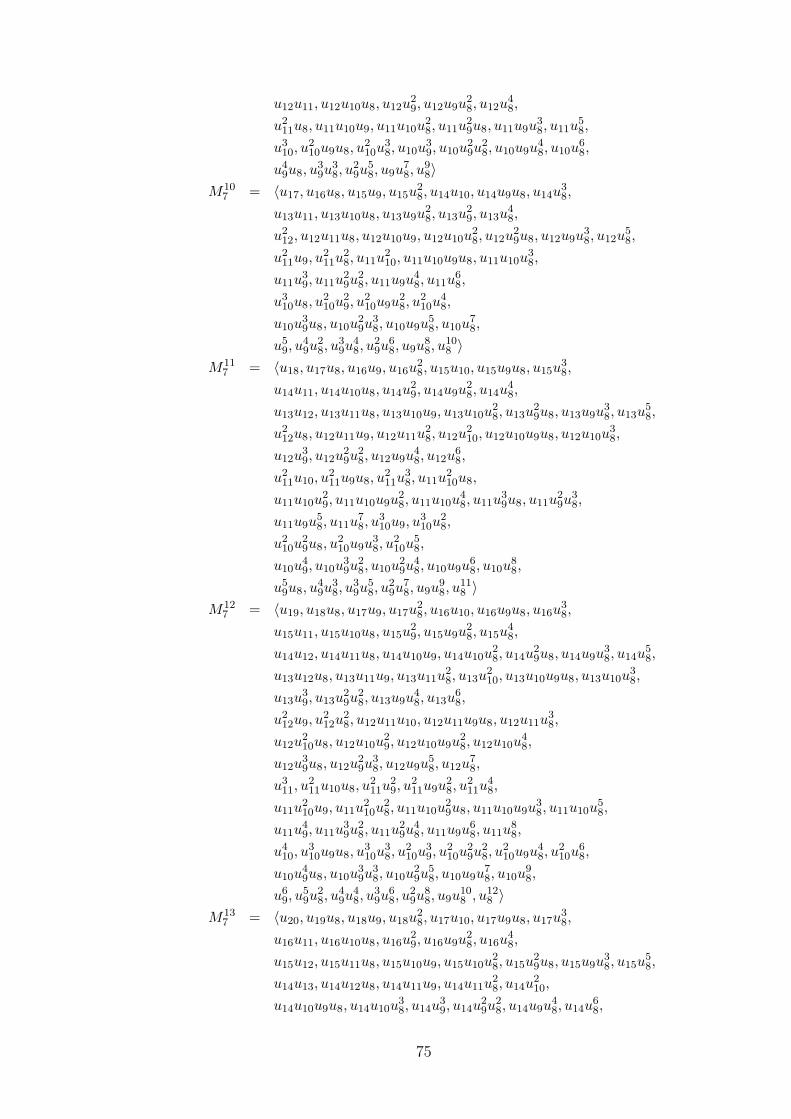
u12u11, u12u10u8, u12u29, u12u9u

28, u12u

48,

u211u8, u11u10u9, u11u10u

28, u11u

29u8, u11u9u

38, u11u

58,

u310, u

210u9u8, u

210u

38, u10u

39, u10u

29u

28, u10u9u

48, u10u

68,

u49u8, u

39u

38, u

29u

58, u9u

78, u

98〉

M107 = 〈u17, u16u8, u15u9, u15u

28, u14u10, u14u9u8, u14u

38,

u13u11, u13u10u8, u13u9u28, u13u

29, u13u

48,

u212, u12u11u8, u12u10u9, u12u10u

28, u12u

29u8, u12u9u

38, u12u

58,

u211u9, u

211u

28, u11u

210, u11u10u9u8, u11u10u

38,

u11u39, u11u

29u

28, u11u9u

48, u11u

68,

u310u8, u

210u

29, u

210u9u

28, u

210u

48,

u10u39u8, u10u

29u

38, u10u9u

58, u10u

78,

u59, u

49u

28, u

39u

48, u

29u

68, u9u

88, u

108 〉

M117 = 〈u18, u17u8, u16u9, u16u

28, u15u10, u15u9u8, u15u

38,

u14u11, u14u10u8, u14u29, u14u9u

28, u14u

48,

u13u12, u13u11u8, u13u10u9, u13u10u28, u13u

29u8, u13u9u

38, u13u

58,

u212u8, u12u11u9, u12u11u

28, u12u

210, u12u10u9u8, u12u10u

38,

u12u39, u12u

29u

28, u12u9u

48, u12u

68,

u211u10, u

211u9u8, u

211u

38, u11u

210u8,

u11u10u29, u11u10u9u

28, u11u10u

48, u11u

39u8, u11u

29u

38,

u11u9u58, u11u

78, u

310u9, u

310u

28,

u210u

29u8, u

210u9u

38, u

210u

58,

u10u49, u10u

39u

28, u10u

29u

48, u10u9u

68, u10u

88,

u59u8, u

49u

38, u

39u

58, u

29u

78, u9u

98, u

118 〉

M127 = 〈u19, u18u8, u17u9, u17u

28, u16u10, u16u9u8, u16u

38,

u15u11, u15u10u8, u15u29, u15u9u

28, u15u

48,

u14u12, u14u11u8, u14u10u9, u14u10u28, u14u

29u8, u14u9u

38, u14u

58,

u13u12u8, u13u11u9, u13u11u28, u13u

210, u13u10u9u8, u13u10u

38,

u13u39, u13u

29u

28, u13u9u

48, u13u

68,

u212u9, u

212u

28, u12u11u10, u12u11u9u8, u12u11u

38,

u12u210u8, u12u10u

29, u12u10u9u

28, u12u10u

48,

u12u39u8, u12u

29u

38, u12u9u

58, u12u

78,

u311, u

211u10u8, u

211u

29, u

211u9u

28, u

211u

48,

u11u210u9, u11u

210u

28, u11u10u

29u8, u11u10u9u

38, u11u10u

58,

u11u49, u11u

39u

28, u11u

29u

48, u11u9u

68, u11u

88,

u410, u

310u9u8, u

310u

38, u

210u

39, u

210u

29u

28, u

210u9u

48, u

210u

68,

u10u49u8, u10u

39u

38, u10u

29u

58, u10u9u

78, u10u

98,

u69, u

59u

28, u

49u

48, u

39u

68, u

29u

88, u9u

108 , u12

8 〉M13

7 = 〈u20, u19u8, u18u9, u18u28, u17u10, u17u9u8, u17u

38,

u16u11, u16u10u8, u16u29, u16u9u

28, u16u

48,

u15u12, u15u11u8, u15u10u9, u15u10u28, u15u

29u8, u15u9u

38, u15u

58,

u14u13, u14u12u8, u14u11u9, u14u11u28, u14u

210,

u14u10u9u8, u14u10u38, u14u

39, u14u

29u

28, u14u9u

48, u14u

68,

75

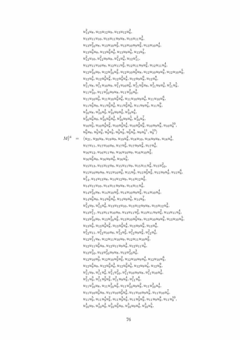
u213u8, u13u12u9, u13u12u

28,

u13u11u10, u13u11u9u8, u13u11u38,

u13u210u8, u13u10u

29, u13u10u9u

28, u13u10u

48,

u13u39u8, u13u

29u

38, u13u9u

58, u13u

78,

u212u10, u

212u9u8, u

212u

38, u12u

211,

u12u11u10u8, u12u11u29, u12u11u9u

28, u12u11u

48,

u12u210u9, u12u

210u

28, u12u10u

29u8, u12u10u9u

38, u12u10u

58,

u12u49, u12u

39u

28, u12u

29u

48, u12u9u

68, u12u

88,

u311u8, u

211u10u9, u

211u10u

28, u

211u

29u8, u

211u9u

38, u

211u

58,

u11u310, u11u

210u9u8, u11u

210u

38,

u11u10u39, u11u10u

29u

28, u11u10u9u

48, u11u10u

68,

u11u49u8, u11u

39u

38, u11u

29u

58, u11u9u

78, u11u

98,

u410u8, u

310u

29, u

310u9u

28, u

310u

48,

u210u

39u8, u

210u

29u

38, u

210u9u

58, u

210u

78,

u10u59, u10u

49u

28, u10u

39u

48, u10u

29u

68, u10u9u

88, u10u

108 ,

u69u8, u

59u

38, u

49u

58, u

39u

78, u

29u

98, u9u

118 , u13

8 〉M14

7 = 〈u21, u20u8, u19u9, u19u28, u18u10, u18u9u8, u18u

38,

u17u11, u17u10u8, u17u29, u17u9u

28, u17u

48,

u16u12, u16u11u8, u16u10u9, u16u10u28,

u16u29u8, u16u9u

38, u16u

58,

u15u13, u15u12u8, u15u11u9, u15u11u28, u15u

210,

u15u10u9u8, u15u10u38, u15u

39, u15u

29u

28, u15u9u

48, u15u

68,

u214, u14u13u8, u14u12u9, u14u12u

28,

u14u11u10, u14u11u9u8, u14u11u38,

u14u210u8, u14u10u

29, u14u10u9u

28, u14u10u

48,

u14u39u8, u14u

29u

38, u14u9u

58, u14u

78,

u213u9, u

213u

28, u13u12u10, u13u12u9u8, u13u12u

38,

u13u211, u13u11u10u8, u13u11u

29, u13u11u9u

28, u13u11u

48,

u13u210u9, u13u

210u

28, u13u10u

29u8, u13u10u9u

38, u13u10u

58,

u13u49, u13u

39u

28, u13u

29u

48, u13u9u

68, u13u

88,

u212u11, u

212u10u8, u

212u

29, u

212u9u

28, u

212u

48,

u12u211u8, u12u11u10u9, u12u11u10u

28,

u12u11u29u8, u12u11u9u

38, u12u11u

58,

u12u310, u12u

210u9u8, u12u

210u

38,

u12u10u39, u12u10u

29u

28, u12u10u9u

48, u12u10u

68,

u12u49u8, u12u

39u

38, u12u

29u

58, u12u9u

78, u12u

98,

u311u9, u

311u

28, u

211u

210, u

211u10u9u8, u

211u10u

38,

u211u

39, u

211u

29u

28, u

211u9u

48, u

211u

68,

u11u310u8, u11u

210u

29, u11u

210u9u

28, u11u

210u

48,

u11u10u39u8, u11u10u

29u

38, u11u10u9u

58, u11u10u

78,

u11u59, u11u

49u

28, u11u

39u

48, u11u

29u

68, u11u9u

88, u11u

108 ,

u410u9, u

410u

28, u

310u

29u8, u

310u9u

38, u

310u

58,

76

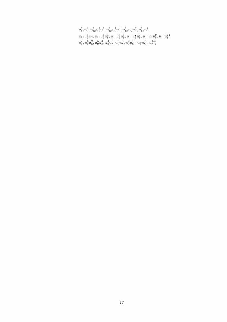
u210u

49, u

210u

39u

28, u

210u

29u

48, u

210u9u

68, u

210u

88,

u10u59u8, u10u

49u

38, u10u

39u

58, u10u

29u

78, u10u9u

98, u10u

118 ,

u79, u

69u

28, u

59u

48, u

49u

68, u

39u

88, u

29u

108 , u9u

128 , u14

8 〉

77

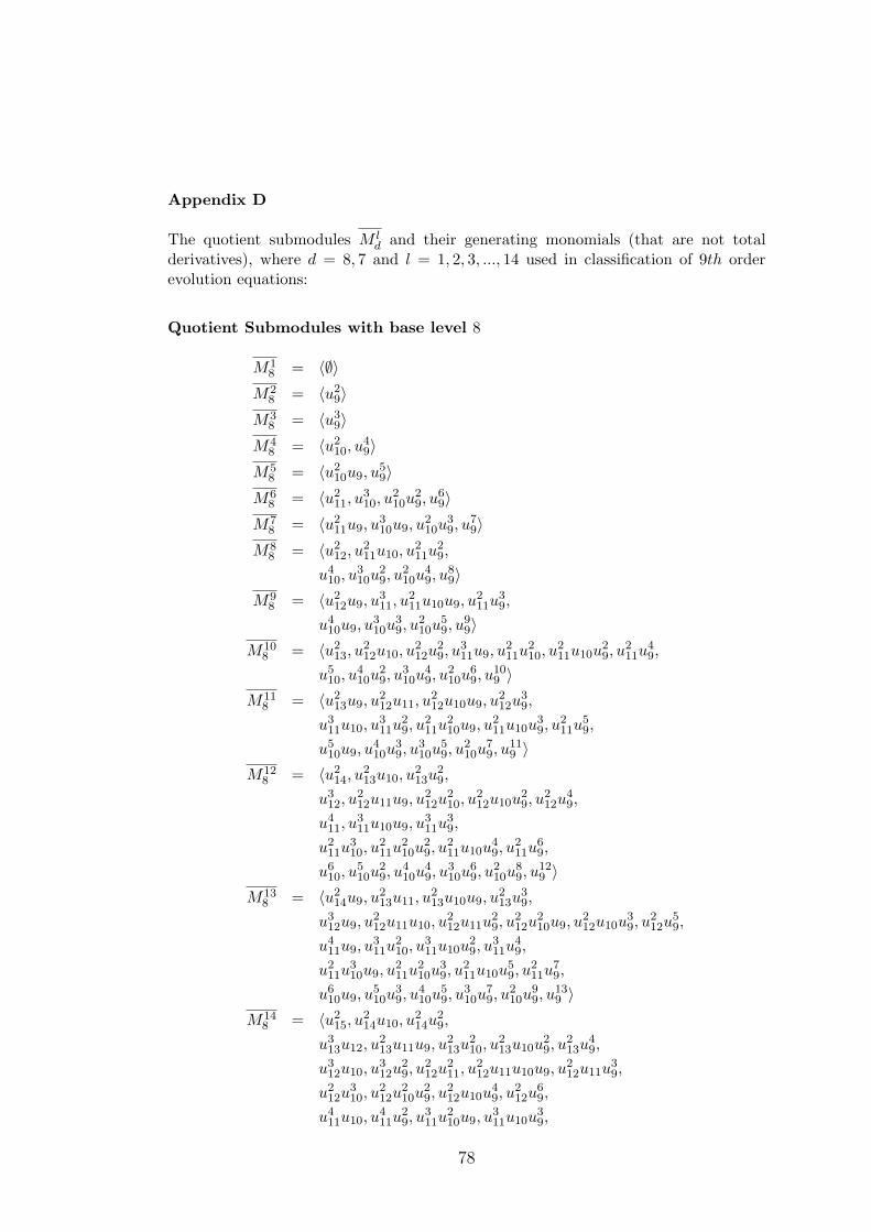
Appendix D

The quotient submodules M ld and their generating monomials (that are not total

derivatives), where d = 8, 7 and l = 1, 2, 3, ..., 14 used in classification of 9th orderevolution equations:

Quotient Submodules with base level 8

M18 = 〈∅〉

M28 = 〈u2

9〉M3

8 = 〈u39〉

M48 = 〈u2

10, u49〉

M58 = 〈u2

10u9, u59〉

M68 = 〈u2

11, u310, u

210u

29, u

69〉

M78 = 〈u2

11u9, u310u9, u

210u

39, u

79〉

M88 = 〈u2

12, u211u10, u

211u

29,

u410, u

310u

29, u

210u

49, u

89〉

M98 = 〈u2

12u9, u311, u

211u10u9, u

211u

39,

u410u9, u

310u

39, u

210u

59, u

99〉

M108 = 〈u2

13, u212u10, u

212u

29, u

311u9, u

211u

210, u

211u10u

29, u

211u

49,

u510, u

410u

29, u

310u

49, u

210u

69, u

109 〉

M118 = 〈u2

13u9, u212u11, u

212u10u9, u

212u

39,

u311u10, u

311u

29, u

211u

210u9, u

211u10u

39, u

211u

59,

u510u9, u

410u

39, u

310u

59, u

210u

79, u

119 〉

M128 = 〈u2

14, u213u10, u

213u

29,

u312, u

212u11u9, u

212u

210, u

212u10u

29, u

212u

49,

u411, u

311u10u9, u

311u

39,

u211u

310, u

211u

210u

29, u

211u10u

49, u

211u

69,

u610, u

510u

29, u

410u

49, u

310u

69, u

210u

89, u

129 〉

M138 = 〈u2

14u9, u213u11, u

213u10u9, u

213u

39,

u312u9, u

212u11u10, u

212u11u

29, u

212u

210u9, u

212u10u

39, u

212u

59,

u411u9, u

311u

210, u

311u10u

29, u

311u

49,

u211u

310u9, u

211u

210u

39, u

211u10u

59, u

211u

79,

u610u9, u

510u

39, u

410u

59, u

310u

79, u

210u

99, u

139 〉

M148 = 〈u2

15, u214u10, u

214u

29,

u313u12, u

213u11u9, u

213u

210, u

213u10u

29, u

213u

49,

u312u10, u

312u

29, u

212u

211, u

212u11u10u9, u

212u11u

39,

u212u

310, u

212u

210u

29, u

212u10u

49, u

212u

69,

u411u10, u

411u

29, u

311u

210u9, u

311u10u

39,

78

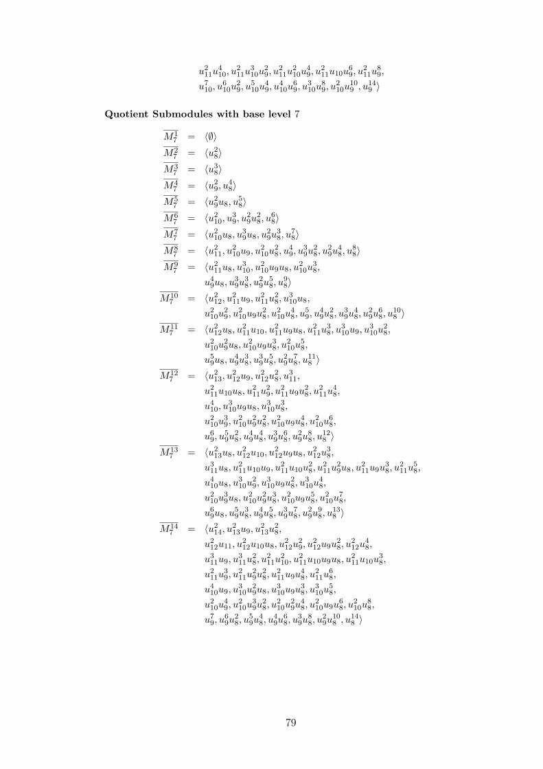
u211u

410, u

211u

310u

29, u

211u

210u

49, u

211u10u

69, u

211u

89,

u710, u

610u

29, u

510u

49, u

410u

69, u

310u

89, u

210u

109 , u14

9 〉

Quotient Submodules with base level 7

M17 = 〈∅〉

M27 = 〈u2

8〉M3

7 = 〈u38〉

M47 = 〈u2

9, u48〉

M57 = 〈u2

9u8, u58〉

M67 = 〈u2

10, u39, u

29u

28, u

68〉

M77 = 〈u2

10u8, u39u8, u

29u

38, u

78〉

M87 = 〈u2

11, u210u9, u

210u

28, u

49, u

39u

28, u

29u

48, u

88〉

M97 = 〈u2

11u8, u310, u

210u9u8, u

210u

38,

u49u8, u

39u

38, u

29u

58, u

98〉

M107 = 〈u2

12, u211u9, u

211u

28, u

310u8,

u210u

29, u

210u9u

28, u

210u

48, u

59, u

49u

28, u

39u

48, u

29u

68, u

108 〉

M117 = 〈u2

12u8, u211u10, u

211u9u8, u

211u

38, u

310u9, u

310u

28,

u210u

29u8, u

210u9u

38, u

210u

58,

u59u8, u

49u

38, u

39u

58, u

29u

78, u

118 〉

M127 = 〈u2

13, u212u9, u

212u

28, u

311,

u211u10u8, u

211u

29, u

211u9u

28, u

211u

48,

u410, u

310u9u8, u

310u

38,

u210u

39, u

210u

29u

28, u

210u9u

48, u

210u

68,

u69, u

59u

28, u

49u

48, u

39u

68, u

29u

88, u

128 〉

M137 = 〈u2

13u8, u212u10, u

212u9u8, u

212u

38,

u311u8, u

211u10u9, u

211u10u

28, u

211u

29u8, u

211u9u

38, u

211u

58,

u410u8, u

310u

29, u

310u9u

28, u

310u

48,

u210u

39u8, u

210u

29u

38, u

210u9u

58, u

210u

78,

u69u8, u

59u

38, u

49u

58, u

39u

78, u

29u

98, u

138 〉

M147 = 〈u2

14, u213u9, u

213u

28,

u212u11, u

212u10u8, u

212u

29, u

212u9u

28, u

212u

48,

u311u9, u

311u

28, u

211u

210, u

211u10u9u8, u

211u10u

38,

u211u

39, u

211u

29u

28, u

211u9u

48, u

211u

68,

u410u9, u

310u

29u8, u

310u9u

38, u

310u

58,

u210u

49, u

210u

39u

28, u

210u

29u

48, u

210u9u

68, u

210u

88,

u79, u

69u

28, u

59u

48, u

49u

68, u

39u

88, u

29u

108 , u14

8 〉

79

REFERENCES

[1] Bilge, A.H., (2005). Towards the Classification of Scalar Non-PolinomialEvolution Equations: Quasilinearity, Computers and

Mathematics with Applications, 49, 1837-1848.

[2] Mikhailov, A.V., Shabat, A.B., and Sokolov, V.V., (1991). TheSymmetry Approach To The Classification of IntegrableEquations,in, What is integrability?, Ed. Zakharov, V.E.Springer-Verlag,Berlin.

[3] Sanders, J.A. and Wang, J.P., (1998). On the Integrabilityof Homogenous Scalar Evolution Equations, Journal

of Differential Equations, 147(2), 410-434.

[4] Sanders, J.A. and Wang, J.P., (2000). On the integrabilityof non-polynomial scalar evolution equations, Journal

of Differential Equations, 166,(1), 132-150.

[5] Wang, J.P., (1998). Symmetries and Conservation Laws of EvolutionEquations, Thomas Stieltjes Institute for Mathematics,

Amsterdam.

[6] Ablowitz, M.J. and Clarkson, P.A., (1991). Solitons, NonlinearEvolution Equations and Inverse Scattering, Cambridge

University Press, Cambridge.

[7] Miura, R.M., Gardner, C.S. and Kruskal, M.D.,(1968).Korteweg-de Vries equation and generalizations. II.Existenceof conservation laws and constants of motion, Journal ofMathematical Physics, 9(8), 1204-1209.

[8] Flaschka, H., Newell, A.C., and Tabor, M., (1991). Integrability,in,What is integrability?, Ed. Zakharov,V.E. Springer-

Verlag,Berlin.

[9] Olver, P.J., (1977). Evolution equations possessing infinitelymany symmetries, Journal of Mathematical Physics, 18(6),1212-1215.

[10] Gardner, C.S., Greene, J.M., Kruskal, M.D., and Miura, R.M.,(1967). Method for solving the Korteweg-de Vries equationPhys. Rev. Lett., 19, 1095-1097.

80

[11] Gardner, C.S., Greene, J.M., Kruskal, M.D., and Miura, R.M.,(1974). Koteweg-de Vries equation and generalizations.VI.Methods for exact solution, Communications on Pure andApplied Mathematics, 27, 97-133.

[12] Noether, E., (1918). Invariante variationsprobleme, Nachr.v.d. Ges.d.Wiss. zu Gottingen, Math.-Phys., Kl.2, 235-257.

[13] Olver, P.J., (1986). Application of Lie Groups to Differential Equations,Springer-Verlag, New York.

[14] Sokolov, V.V., Shabat, A.B., (1984). Classification of IntegrableEvolution Equations, Mathematical Physics Reviews, SovietSci.Rev.Sect.C Math. Phys.Rev.,Harwood Academic Publ.,4 221-280, Chur.

[15] Svinolupov, S.L., Sokolov, V.V., (1985). Classification ofFifth-Order Evolution Equations Having an Infinite Seriesof Conservation Laws,(Russian,English summary), Dokl. ofUkrain Akad., Ser. A, 10, 7-10, Ukrain.

[16] Heredero, R.H., Sokolov, V.V., and Svinolupov, S.I., (1995).Classification of 3rd Order Integrable Evolution Equations,Physica D, 87 (1-4), 32-36.

[17] Fraleigh, John B., (1982). A First Course in Abstract Algebra,Addison-Wesley Publishing Company, USA.

[18] Cohn, P.M., (1982). Algebra Volume 1, John Wiley and Sons, Chichester.

[19] Cohn, P.M., (1989). Algebra Volume 2, John Wiley and Sons, Chichester.

[20] Varadarajan, V.S., (1974). Lie Groups, Lie Algebras, and TheirRepresentations, Springer-Verlag , New York.

[21] Zabuski, N.J., Kruskal, M.D., (1965). Interaction of solitonsin a collisionless plasma and the recurrence of initial

states, Phys.Rev.Lett., 15 240.

[22] Calogero, F., (1991). Why Are Certain Nonlinear PDEs Both WidelyApplicable and Integrable? What is integrability?, Ed.

Zakharov, V.E. Springer-Verlag,Berlin.

[23] Zakharov, V.E., (1991). What is integrability?, Springer-Verlag, Berlin.

[24] Lax, P.D., (1968) Integrals of non-linear equations of evolution andsolitary waves. Communications on Pure and Applied

Mathematics, 21 467-490.

[25] Fokas, A.S., (1987). Symmetries and integrability, Studies in AppliedMathematics, 77 253-299.

81

[26] Kodama, Y., (1985). On integrable systems with higher order corrections,Phys.Lett., 107A 245.

[27] Kodama, Y., (1985). Nearly integrable systems, Physica, 16D 14.

[28] Cole, J.D., (1951). On a quasi-linear parabolic equation occuring inaerodynamics, Q. Appl. Math.,9 225-236.

[29] Hopf, E., (1950). The partial differential equations ut + uux = µuxx,Commun. Pure Appl. Math., 3 201-230.

[30] Fermi, A., Pasta, J., Ulam, S. (1955). Studies of nonlinear problems I,Los Alamos Report LA 1940,1955. Reproduced in “NonlinearWave Motion,” proceedings, Postdam, New York,1972, ed.A.C. Newell, Lect. Appl. Math., 15 143-156.

[31] Camassa, R., Holm, D.D. (1993). An integrable shallow water equationwith peaked solitons, Phys.Rev.Lett. 71 1661-1664.

[32] Sokolov, V.V., Wolf, T. (2001). Classification of integrable polynomialvector evolution equations, J.Phys. A:Math. Gen. 34 1113911148.

[33] Sergyeyev, A. (2000) On recursion operators and nonlocal symmetriesof evolution equations, Math. Publ. Ed. Krupka,D. SilesianUniv.,Opava 2 159-173.

[34] Sergyeyev, A. (2002) Constructing conditionally integrable evolutionsystems in (1+1)-dimensions: a generalization of invariantmodules approach, J. Phys. A:Math. Gen. 35 7653-7660.

[35] Tsuchida, T., Wolf, T. (2005). Classification of polynomial integrablesystems of mixed scalar and vector evolution eqautions:IJ.Phys A:Math. Gen. 38 7691-7733.

[36] Mikhailov, A.V., Wang, J.P. (2007). On classification of integrablenon-evolutionary equations, Studies in Applied Mathematics118 4 419-457.

[37] Sanders, J.A., Wang, J.P. (2008). Number Theory and SymmetryClassification of Integrable Systems, Lecture Notes in PhysicsEd. Mikhailov, A.V. Springer.

[38] Gaeta, G. (1994) Nonlinear symmetries and nonlinear equations,Ed. Hazewinkel, M. Kluwer Academic Publishers, Dordrecht.

82

VITA

Eti Mizrahi was born in Istanbul, in 1956, with the surname Benarditi. Shegraduated from Notre Dame de Sion Fransız Kız Lisesi in 1975. She enteredIstanbul Technical University in 1995 where she graduated as a MathematicalEngineer in 1999. She received her M.Sc. degree in Mathematical Engineeringfrom the Institute of Science and Technology of the same university. She enrolledthe Ph.D program of the same institute in 2001. She has been working asa research and teaching assistant at the Mathematics Department of IstanbulTechnical University since 1999. She is married and has two children.

83