Embed Size (px)
Citation preview

UNCORRECTEDPROOF
Chapter 17 1
Is It Significant? Guidelines for Reporting BCI 2
Performance 3
Martin Billinger, Ian Daly, Vera Kaiser, Jing Jin, Brendan Z. Allison, 4
Gernot R. Muller-Putz, and Clemens Brunner 5
Abstract Recent growth in brain-computer interface (BCI) research has increased 6
pressure to report improved performance. However, different research groups report 7
performance in different ways. Hence, it is essential that evaluation procedures are 8
valid and reported in sufficient detail. 9
In this chapter we give an overview of available performance measures such as 10
classification accuracy, cohen’s kappa, information transfer rate (ITR), and written 11
symbol rate (WSR). We show how to distinguish results from chance level using 12
confidence intervals for accuracy or kappa. Furthermore, we point out common 13
pitfalls when moving from offline to online analysis and provide a guide on how 14
to conduct statistical tests on BCI results. 15
17.1 Introduction 16
Brain–computer interface (BCI) research is expanding in many ways. Within the 17
academic research community, new articles, events, and research groups emerge 18
increasingly quickly. Research labs have developed BCIs for communication [7,19, 19
27, 34, 43–45, 67], for control of wheelchairs [24, 53] and neuroprosthetic devices 20
M. Billinger (�) � I. Daly � V. Kaiser � B.Z. Allison � G.R.Muller-Putz � C. BrunnerAQ1Institute for Knowledge Discovery, Graz University of Technology, Austriae-mail: [email protected]; [email protected]; [email protected]; [email protected];[email protected]; [email protected]
C. BrunnerSwartz Center for Computational Neuroscience, INC, UCSD, San Diego, CA, USAe-mail: [email protected]
J. JinKey Laboratory of Advanced Control and Optimization for Chemical Processes, Ministryof Education, East China University of Science and Technology, Chinae-mail: [email protected]
B. Allison et al. (eds.), Towards Practical Brain-Computer Interfaces, Biologicaland Medical Physics, Biomedical Engineering, DOI 10.1007/978-3-642-29746-5 17,© Springer-Verlag Berlin Heidelberg 2012
333

UNCORRECTEDPROOF
334 M. Billinger et al.
[31, 46]. Although BCI research has been conducted for more than 20 years now, 21
only some research labs have successfully applied BCIs to patient use [30, 36– 22
38,47,49,51,52,65]. The popular media has also shown increased interest in BCIs, 23
with BCIs featured prominently in science fiction as well as in the mainstream. 24
Additionally, new businesses are gaining attention with various products sold as 25
BCIs for entertainment. 26
Hence, there is growing attention in performance, and increased pressure to 27
report improved performance. Recent articles that developed fast BCIs openly noted 28
this feat [6, 12, 63]. Articles routinely highlight methods and results that improve 29
accuracy or reduce illiteracy relative to earlier work [3,4,10,11,33,55,62]. However, 30
different groups use different methods for reporting performance, and it is essential 31
that (1) the evaluation procedure is valid from a statistical and machine learning 32
point of view, and (2) this procedure is described in sufficient detail. 33
It is also important to distinguish any reported BCI performance from the chance 34
level, the expected best performance obtainable by chance alone. Depending on 35
the performance measure, the number of classes in the BCI task, and the number of 36
available trials, the chance level varies and should be considered in every study [48]. 37
In this chapter, we provide an introduction to common performance measures 38
(such as classification accuracy, Cohen’s kappa, and information transfer rate). 39
Furthermore, we discuss confidence intervals of the classification accuracy and 40
Cohen’s kappa to estimate the associated chance level. We also summarize state 41
of the art offline procedures to estimate performance on a pre-recorded data set 42
and discuss common cross-validation pitfalls. In the last two sections, we describe 43
statistical tests often used in BCI studies, such as t-tests, repeated measures 44
ANOVA, and suitable post-hoc tests. We also mention the need to correct for 45
multiple comparisons. 46
17.2 Performance Measures 47
17.2.1 Confusion Matrix 48
A number of metrics may be used to measure the performance of a BCI. These 49
include the number of correct classifications and the number of mistakes made 50
by the classifier. The most straightforward classification example is binary classi- 51
fication, in which the classifier need only differentiate two classes. For example, 52
this might be the case in the popular P300 speller first presented by Farwell and 53
Donchin [22]. The task of the classifier is to determine if there is a P300 event 54
present in a particular time segment of the EEG. Therefore, the two classes are either 55
“yes, there is a P300 present” or “no, there is no P300 present.” When considering 56
such binary classification problems, four classification results are possible: 57
(1) A trial is classified as containing a P300 when a P300 is present (true 58
positive, TP). 59
UNCORRECTEDPROOF
17 Is It Significant? Guidelines for Reporting BCI Performance 335
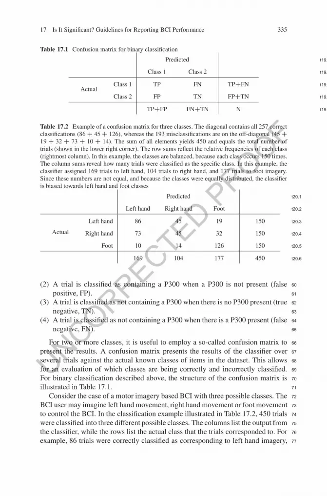
Table 17.1 Confusion matrix for binary classification
t19.Predicted
t19.Class 1 Class 2
t19.Actual
Class 1 TP FN TPCFN
t19.Class 2 FP TN FPCTN
t19.TPCFP FNCTN N
Table 17.2 Example of a confusion matrix for three classes. The diagonal contains all 257 correctclassifications (86 C 45 C 126), whereas the 193 misclassifications are on the off-diagonal (45 C19 C 32 C 73 C 10 C 14). The sum of all elements yields 450 and equals the total number oftrials (shown in the lower right corner). The row sums reflect the relative frequencies of each class(rightmost column). In this example, the classes are balanced, because each class occurs 150 times.The column sums reveal how many trials were classified as the specific class. In this example, theclassifier assigned 169 trials to left hand, 104 trials to right hand, and 177 trials to foot imagery.Since these numbers are not equal, and because the classes were equally distributed, the classifieris biased towards left hand and foot classes
t20.1Predicted
t20.2Left hand Right hand Foot
t20.3
Actual
Left hand 86 45 19 150
t20.4Right hand 73 45 32 150
t20.5Foot 10 14 126 150
t20.6169 104 177 450
(2) A trial is classified as containing a P300 when a P300 is not present (false 60
positive, FP). 61
(3) A trial is classified as not containing a P300 when there is no P300 present (true 62
negative, TN). 63
(4) A trial is classified as not containing a P300 when there is a P300 present (false 64
negative, FN). 65
For two or more classes, it is useful to employ a so-called confusion matrix to 66
present the results. A confusion matrix presents the results of the classifier over 67
several trials against the actual known classes of items in the dataset. This allows 68
for an evaluation of which classes are being correctly and incorrectly classified. 69
For binary classification described above, the structure of the confusion matrix is 70
illustrated in Table 17.1. 71
Consider the case of a motor imagery based BCI with three possible classes. The 72
BCI user may imagine left hand movement, right hand movement or foot movement 73
to control the BCI. In the classification example illustrated in Table 17.2, 450 trials 74
were classified into three different possible classes. The columns list the output from 75
the classifier, while the rows list the actual class that the trials corresponded to. For 76
example, 86 trials were correctly classified as corresponding to left hand imagery, 77

UNCORRECTEDPROOF
336 M. Billinger et al.
whereas 45 trials that corresponded to left hand imagery were misclassified as 78
corresponding to right hand imagery. From this example, it is clear that the number 79
of correct classifications for each class are found along the diagonal of the confusion 80
matrix. The row sums reflect the a priori distribution of the classes, that is, the 81
relative frequency of each class. Conversely, the column sums reveal a potential 82
bias of the classifier towards one (or more) classes. 83
While the confusion matrix contains all information on the outcome of a 84
classification procedure, it is difficult to compare two or more confusion matrices. 85
Therefore, most studies usually report scalar performance measures, which can be 86
derived from the confusion matrix. Metrics commonly used in reporting BCI results 87
include classification accuracy, Cohen’s kappa �, sensitivity and specificity, positive 88
and negative predictive value, the F -measure and the r2 correlation coefficient [57]. 89
17.2.2 Accuracy and Error Rate 90
The accuracy p is the probability of performing a correct classification. It can be 91
estimated from dividing the number of correct classifications by the total number of 92
trials 93
p DP
Ci;i
N: (17.1)
Ci;i is the i th diagonal element of the confusion matrix, and N is the total number of 94
trials. The error rate or misclassification rate e D 1 � p is the probability of making 95
an incorrect classification. 96
Accuracy and error rate do not take class balance into account. If one class occurs 97
more frequently than the other, accuracy may be high even for classifiers that cannot 98
discriminate between classes. See Tables 17.3 and 17.4 for examples. 99
17.2.3 Cohen’s Kappa 100
Cohen’s kappa (�) is a measure for the agreement between nominal scales [15]. As 101
such � can be used to measure the agreement between true class labels and classifier 102
output. It is scaled between 1 (perfect agreement) and 0 (pure chance agreement). 103
Equation (17.2) shows how to obtain � from accuracy p and chance level p0. 104
� D p � p0
1 � p0
(17.2)
The chance level p0 is the accuracy under the assumption that all agreement 105
occurred by chance (see Sect. 17.3.1). p0 can be estimated from the confusion 106
matrix by 107
p0 DP
Ci;WCW;iN 2
: (17.3)

UNCORRECTEDPROOF
17 Is It Significant? Guidelines for Reporting BCI Performance 337
Table 17.3 Confusion matrix for binary classification when the two classes are not balanced(class 1 occurs more often than class 2). Left: The classifier selected the classes with a probabilityof 50 %. Right: The classifier always selected the first class
t21.1
Predicted
1 2
Actual1 45 45 90
2 5 5 10
50 50 100
p D 0:5 � D 0
Predicted
1 2
Actual1 90 0 90
2 10 0 10
100 0 100
p D 0:9 � D 0
Table 17.4 Confusion matrix for binary classification when the two classes are not balanced(class 1 occurs more often than class 2). Left: The classifier selected the first class with 90 %probability and the second class with 10 % probability. Right: The classifier classified all trialscorrectly
t22.1
Predicted
1 2
Actual1 81 9 90
2 9 1 10
90 10 100
p D 0:82 � D 0
Predicted
1 2
Actual1 90 0 90
2 0 10 10
90 10 100
p D 1 � D 1
Ci;W and CW;i are the i th row and column of the confusion matrix, and N is the total 108
number of trials. 109
For both confusion matrices in Table 17.3 � D 0, indicating classification at 110
chance level. Neither of these confusion matrices represents a meaningful classifier, 111
although accuracies are 0:5 and 0:9 respectively. 112
17.2.4 Sensitivity and Specificity 113
Alternative metrics reported in BCI studies include the sensitivity and specificity 114
(see for example [5,21,25,60]), which measure the proportion of correctly identified 115
positive results (true positives) and the proportion of correctly identified negative 116
results (true negatives). Sensitivity is defined as 117
H D Se D TP
TP C FN: (17.4)
Specificity is then defined as 118
Sc D TN
TN C FP: (17.5)

UNCORRECTEDPROOF
338 M. Billinger et al.
The sensitivity is alternately referred to as the true positive rate (TPR) or the 119
recall. The false positive rate (FPR) is then equal to 1—specificity. 120
The false detection rate F may be calculated as 121
F D FP
TP C FP: (17.6)
From this, the positive predictive value (also referred to as the precision) may be 122
calculated as 1 � F . The HF difference (H � F ), as developed in [32], may then be 123
derived. 124
These metrics may also be used to measure the receiver operator characteristic 125
(ROC) curve [18, 29, 41]. This is a plot of how the true positive rate varies against 126
the false positive rate for a binary classifier as the classification threshold is varied 127
between its smallest and largest limit. The x axis of the ROC curve is the false 128
positive rate (1—specificity), while the y axis is the true positive rate (sensitivity). 129
The larger the area under the ROC curve, the larger the true positive rate and the 130
smaller the false positive rate for a greater number of threshold values. Thus, an 131
ROC curve that forms a diagonal from the bottom left corner of the plot to the top 132
right is at theoretical chance level, whereas an ROC plot that reaches the top left 133
corner is reporting perfect classification. 134
17.2.5 F -Measure 135
The terms precision and recall (sensitivity) may be used to describe the accuracy 136
of classification results. Precision (also referred to as the positive predictive value) 137
measures the fraction of classifications which are correct while recall measures the 138
fraction of true positive classifications. 139
As the precision is increased, the recall decreases, and vice-versa. Therefore, 140
for a given classifier, it is useful to have a measure of the harmonic mean of both 141
measures. The F -measure is used to do this and is defined as 142
F˛ D .1 C ˛/ � .1 � F / � H
˛ � .1 � F / C H; (17.7)
where ˛ is the significance level of the measure and may be varied between 0 and 1. 143
Thus, the F-measure may be analogous to the ROC curve, in that it provides a 144
measure of the classifier performance across different significance levels. 145
17.2.6 Correlation Coefficient 146
The correlation coefficient may be used for either feature extraction or validation 147
of classification results (see for example [13, 41, 60]). It is defined—via Pearson’s 148
correlation coefficient—as 149

UNCORRECTEDPROOF
17 Is It Significant? Guidelines for Reporting BCI Performance 339
r DP
i .yi � Ny/.xi � Nx/p.P
i .yi � Ny/2/.P
i .xi � Nx/2/; (17.8)
where xi denotes output values, yi the class labels, Nx the mean of x and Ny the mean 150
of the labels y. 151
Pearson’s correlation should be used for Gaussian data, while for non-Gaussian 152
data the rank correlation is recommended. The rank correlation is defined as above 153
with the difference that xi and yi values are replaced by rank.xi / and rank.yi /. 154
The correlation varies between �1 and 1, with a 0 indicating no correlation 155
between the classifier results and a 1 indicating perfect positive correlation. 156
A correlation of �1 indicates perfect negative correlation and may be discounted 157
if the squared correlation measure is chosen (as used in [13]). 158
17.3 Significance of Classification 159
Reporting classification results by providing performance measures alone is often 160
not enough. Even accuracies as high as 90 % can be meaningless if the number of 161
trials is too low or classes are not balanced (see Table 17.3). 162
The practical level of chance [48] provides a convenient tool to quickly verify if 163
an accuracy value lies significantly above chance level. This practical level of chance 164
is defined as the upper confidence interval of a random classifier’s accuracy. Given 165
the number of trials, the resulting accuracy of a BCI experiment must be higher 166
than the practical level of chance. Then the BCI can be said to perform significantly 167
better than chance. 168
The original publication assumes that classes are balanced [48]. In this section, 169
we describe a more general approach that can handle arbitrary class distributions. 170
17.3.1 Theoretical Level of Random Classification 171
In order to test classification results for randomness, a sound definition of random 172
classification is required: A random classifier’s output is statistically independent 173
from the true class labels.1 More formally, 174
P.ce D c j ct / D P.ce D c/; (17.9)
where ce is the estimated class label and ct is the true class label. 175
1Such randomness is not necessarily caused by the classifier alone. The BCI user failing at thetask, electrode failures or inadequate features may all decrease the degree of agreement betweenthe estimated and true class labels. The actual source of randomness is not relevant for this analysis.

UNCORRECTEDPROOF
340 M. Billinger et al.
The probability of such a random classifier correctly classifying a trial is 176
p0 DXc2C
P.ce D c/ � P.ct D c/; (17.10)
where C is the set of all available class labels. 177
While the probability P.ct D c/ of a trial belonging to class c is determined 178
by the experimental setup, the probability P.ce D c/ of the classifier returning 179
class c needs to be carefully considered. The most conservative approach is to find 180
the highest possible p0 for a given experiment. This is the case for a classifier that 181
always returns the class that occurs most often. Intuitively, such a classifier would 182
not be considered random since its output is purely deterministic, but the output is 183
independent from the true class labels, thus (17.9) applies. 184
Alternatively, the values for P.ce D c/ can be calculated from the experimental 185
results using the confusion matrix (17.3). This yields the same p0 that is used for the 186
calculation of Cohen’s �, which is the theoretical chance level of an actual classifier. 187
This approach is less conservative as the chance level no longer depends on the 188
experimental setup alone, but also on the probability of each class to be selected 189
by the classifier. However, this approach can only be applied after classification has 190
been performed. 191
17.3.2 Confidence Intervals 192
Can a BCI identify the user’s intended message or command more accurately than 193
chance? This question can be formally defined with a statistical test, in which the 194
null hypothesis H0 represents the hypothesis that the BCI’s classification is not more 195
accurate than a random classifier. As discussed later, performing above chance is a 196
necessary, but not sufficient, condition for an effective BCI. BCIs typically must 197
perform well above chance to be useful. For example, a speller that identifies one of 198
36 targets with 50 % accuracy would perform much better than chance, but would 199
not allow useful communication. Formally, the hypothesis test can be written as 200
H0 W p � p0
H1 W p > p0;
where p is the true classification accuracy, and p0 is the classification accuracy of 201
a random classifier. We compare the one-sided confidence interval of p against the 202
theoretical level of chance, p0. If p0 lies outside the confidence interval of p, we can 203
reject H0 in favor of H1, thereby indicating that the classifier performs significantly 204
better than chance, at the chosen level of significance. 205
Regardless of the number of classes, classification can be reduced to either of 206
two outcomes: correct or wrong classification. The correct classification of a trial is 207

UNCORRECTEDPROOF
17 Is It Significant? Guidelines for Reporting BCI Performance 341
called “success.” When the probability of success is p, then the probability of getting 208
exactly K successes from N independent trials follows the binomial distribution: 209
f .KI N; p/ D
N
K
!pK .1 � p/N �K : (17.11)
In a BCI experiment, the classification accuracy is an estimate of p, the true prob- 210
ability of correctly classifying a trial. Given the observed classification accuracy Op, 211
a confidence interval can be calculated that contains the true p with a probability of 212
1 � ˛. 213
Different confidence intervals have been proposed in the literature. The Clopper– 214
Pearson “exact” interval, as well as the Wald interval are too conservative and should 215
not be used in favor of the adjusted Wald interval or the Wilson score interval [8]. 216
We will focus on the adjusted Wald interval because of its simplicity. 217
17.3.2.1 Adjusted Wald Confidence Interval for Classification Accuracy 218
Consider the situation where we have N independent trials, of which K are correctly 219
classified. Adding two successes and two failures to the experimental result leads to 220
an unbiased estimator for the probability Op of correct classification (17.12). Upper 221
and lower confidence limits of Op are given by (17.13) and (17.14) respectively. 222
Op D K C 2
N C 4(17.12)
pu D Op C z1�˛=2
sOp.1 � Op/
N C 4(17.13)
pl D Op � z1�˛=2
sOp.1 � Op/
N C 4(17.14)
z1�˛=2 is the 1 � ˛=2 quantile of the standard normal distribution. For a one-sided 223
confidence interval z1�˛ can be used instead of z1�˛=2. 224
17.3.2.2 Adjusted Wald Confidence Interval for Cohen’s Kappa 225
Kappa is calculated by transforming accuracy values from the interval Œp0; 1� 226
to the interval Œ0; 1� according to (17.2). Similarly, a confidence interval of the 227
classification accuracy can be transformed, resulting in a confidence interval for � 228
�l=u D pl=u � p0
1 � p0
: (17.15)

UNCORRECTEDPROOF
342 M. Billinger et al.
This results in a modified null hypothesis that tests � and associated confidence 229
intervals against zero 230
H0 W � � 0
H1 W � > 0:
The original publication introducing � [15] proposes a confidence interval that is 231
derived from the Wald interval, which is too conservative according to [8]. Applying 232
the adjusted Wald interval instead results in (17.16)–(17.19) 233
Op D K C 2
N C 4(17.16)
O� D Op � p0
1 � p0
(17.17)
�l D O� � z1�˛=2
p Op.1 � Op/
.N C 4/.1 � p0/(17.18)
�u D O� C z1�˛=2
p Op.1 � Op/
.N C 4/.1 � p0/; (17.19)
where O� is the value of kappa that follows from the unbiased estimator in (17.16). 234
17.3.3 Summary 235
It is important not only to consider point estimators of performance measures but 236
also to use appropriate statistics to validate experimental results. In this section we 237
showed how to test estimates of classification accuracy and Cohen’s � against results 238
expected from random classification. 239
Care has to be taken to chose an appropriate model of random classification. 240
Without knowledge of the classifier’s behavior conservative assumptions have to be 241
made about chance classification. When classification results are available a less 242
conservative chance level can be estimated from the classifier output. 243
17.4 Performance Metrics Incorporating Time 244
Another critical factor in any communication system is speed—the time required 245
to accomplish a goal, such as spelling a sentence or navigating a room. BCIs often 246
report performance in terms of ITR or bit rate, a common metric for measuring 247
the information sent within a given time [58, 66]. We will measure ITR in bits per 248

UNCORRECTEDPROOF
17 Is It Significant? Guidelines for Reporting BCI Performance 343
minute, and bit rate in bits per trial, which can be calculated via 249
B D log2 C C Op log2 Op C .1 � Op/ log2
1 � OpC � 1
; (17.20)
where Op is the estimated classification accuracy and C is the total number of classes 250
(i.e. possible selections). This equation provides the amount of information (in bits) 251
communicated with a single selection. Many BCI articles multiply B by the number 252
of selections per unit time to attain the ITR, measured in bits per minute. In a trial 253
based BCI this is accomplished by multiplying the ITR by the actual number of 254
trials performed per minute. 255
However, in a typical BCI speller, users correct errors through a “backspace” 256
function, which may be activated manually or automatically via detection of a 257
neuronal error potential [56]. In contrast to the ITR, the WSR (17.21)–(17.22) 258
incorporates such error correction functionality [23]. 259
SR D B
log2 C(17.21)
WSR D�
.2SR � 1/=T SR > 0:5
0 SR � 0:5; (17.22)
where SR is referred to as symbol rate, and T is the trial duration in minutes 260
(including eventual delays). 261
The WSR incorporates correction of an error by two additional selections 262
(backspace and new selection). However, another error may happen during the 263
correction process. This has been addressed by the practical bit rate (PBR) [61], 264
calculated via 265
PBR D�
B.2p � 1/=T Op > 0:5
0 Op � 0:5: (17.23)
However, WSR or PBR may not be suitable for systems that use other mecha- 266
nisms to correct errors [1, 17], or if the user chooses to ignore some or all errors. 267
ITR calculation may seem to rest on a few simple formulae. However, ITR 268
is often misreported, partly to exaggerate a BCI’s performance and partly due to 269
inadequate understanding of many assumptions underlying ITR calculation. Articles 270
that only report the time required to convey a single message or command might 271
ignore many delays that are inevitable in realworld BCI operation. BCIs often entail 272
delays between selections for many reasons. A BCI system might need time to 273
process data to reach a classification decision, present feedback to the user, clear 274
the screen, allow the user to choose a new target, and/or provide a cue that the next 275
trial will begin. Delays also occur if a user decides to correct errors. 276
Moreover, various factors could affect the effective information transfer rate [2], 277
which incorporates advanced features that could help users attain goals more quickly 278
UNCORRECTEDPROOF
344 M. Billinger et al.
without improving the raw bit rate. Some BCIs may feature automatic tools to 279
correct errors or complete words or sentences. These tools may introduce some 280
delays, which are presumably welcome because they avoid the greater delays that 281
might be necessary to manually correct errors complete their messages. Similarly, 282
some BCIs may focus on goal-oriented selections rather than process-oriented 283
selections [1,64]. Consider two BCIs that allow a user to choose one of eight items 284
with perfect accuracy every ten seconds. Each BCI has a raw ITR of 18 bits/min. 285
However, the first BCI allows a user to move a wheelchair one meter in one of eight 286
directions with each selection, and a second BCI might instead let users choose a 287
target room (leaving the system to work out the details necessary to get there). Other 288
BCIs might incorporate context in various ways. BCIs might change the mapping 289
from brain signals to outcomes. For example, if a robot is in an open space, then 290
imagining left hand movement could move the robot left, but if a wall is to the 291
robot’s left, then the same mental command could instruct the robot to follow the 292
wall [42]. BCIs could also use context to change the options available to a user. For 293
example, if a user turns a light off, or if the light bulb burns out, then the option of 294
turning on a light might simply not be available [1]. 295
Moreover, ITR has other limitations [4]. For example, ITR is only meaningful 296
for some types of BCIs. ITR is best suited to synchronous BCIs. Self-paced BCIs, 297
in which the user can freely choose when to make selections or refrain from 298
communicating, are not well suited to ITR estimation. ITR also does not account for 299
different types of errors, such as false positives vs. misses, which could influence 300
the time needed for error correction. Reporting ITR might encourage developers to 301
focus on maximizing ITR, even though some users may prefer higher accuracy, even 302
if it reduces ITR. 303
In summary, ITR calculation is more complicated than it may seem. Articles that 304
report ITR should include realworld delays, account for tools that might increase 305
effective ITR, and consider whether ITR is the best metric. In some cases, articles 306
present different ITR calculation methods such as practical bit rate or raw bit 307
rate [33, 63]. In such cases, authors should clearly specify the differences in ITR 308
calculation methods and explain why different methods were explored. 309
17.5 Estimating Performance Measures on Offline Data 310
BCI researchers often perform initial analysis on offline data to test out a new 311
approach, e.g. a new signal processing method, a new control paradigm etc. For 312
example, [4, 10] report on offline results of a hybrid feature set before they apply it 313
in an online BCI [11]. 314
Because the data is available offline it may be manipulated in a way that is not 315
possible with online data. Common manipulations used in the analysis of offline data 316
include, but are not limited to, cross validation, iteration over a parameter space and 317
the use of machine learning techniques. When applying any offline analysis method, 318

UNCORRECTEDPROOF
17 Is It Significant? Guidelines for Reporting BCI Performance 345
it is important to consider firstly the statistical significance of the reported results 319
and secondly how well the results translate to online BCI operation. 320
Statistical significance must be reported on the results of classifying a dataset 321
which is separate from the dataset used to train the classification function. The 322
dataset the results are reported on is referred to as the verification (or testing) 323
set while the dataset the classifier is trained on is referred to as the training 324
set. Separating training and verification sets allows us to estimate the expected 325
performance of the trained classifier on unseen data. 326
The ability to translate offline analysis results to online BCI operation depends 327
on a number of factors including the effects of feedback in online analysis, any 328
temporal drift effects in the signal and how well the offline analysis method 329
is constructed to ensure that the results generalize well. These issues will be 330
considered further in the subsequent sections. 331
17.5.1 Dataset Manipulations 332
In online BCI operation any parameters (e.g. classifier weights, feature indices) must 333
be learned first before operation of the BCI begins. However with offline data the 334
trials within the dataset may be manipulated freely. 335
The most straightforward approach is to simply split the dataset into a training 336
and validation set. This could be done with or without re-sorting the trials. If no 337
re-sorting is used and the trials at the beginning of the session are used for training, 338
this is analogous to online analysis. On the other hand it may be desirable to remove 339
serial regularities from the dataset via re-sorting the trial order prior to splitting into 340
training and validation sets. 341
A common approach taken is to use either k-fold or leave 1 out cross validation. 342
In k-fold cross validation the dataset is split into K subsets. One of these subsets 343
(subset l) is omitted (this is denoted as the “hold out” set), the remainder are used 344
to train the classifier function. The trained function is then used to classify trials in 345
the l th hold out set. This operation is repeated K times with each set being omitted 346
once. Leave 1 out cross validation is identical, except that each hold out set contains 347
just one trial. Thus, every trial is omitted from the training set once. 348
Cross validation requires trials to be independent. In general this is not the case 349
due to slowly varying baseline, background activity and noise influence. Trials 350
recorded close to each other are likely to be more similar than trials recorded further 351
apart in time. This issue is addressed through h-block cross validation [39]. h trials 352
closest to each trial in the validation set are left out of the training set, in order to 353
avoid overfitting due to temporal similarities in trials. 354
Another approach taken, particularly in situations where the size of the available 355
dataset is small, is to use bootstrapping. The training (and possibly the validation) set 356
is created from bootstrap replications of the original dataset. A bootstrap replication 357
is a new trial created from the original dataset in such a way that it preserves 358
some statistical or morphological properties of the original trial. For example, [40] 359

UNCORRECTEDPROOF
346 M. Billinger et al.
describes a method to increase the training set for BCI operation by randomly 360
swapping features between a small number of original trials to create a much larger 361
set of bootstrap replications. 362
17.5.2 Considerations 363
Ultimately, the results reported from offline analysis should readily translate to 364
online BCI operation. Therefore when deciding on any data manipulations and/or 365
machine learning techniques the following considerations should be made: 366
1. Temporal drift in the dataset. During online BCI operation, factors such as 367
fatigue, learning and motivation affect the ability of the BCI user to exert control. 368
If trials are randomly re-sorted in offline analysis the effect of such temporally 369
dependent changes in the signal are destroyed. 370
2. The effects of feedback. During online BCI operation the classifier results are fed 371
back to the user via exerted control. This affects the users’ motivation and hence 372
the signals recorded from them. 373
3. Overlearning and stability. Classification methods should be stable when applied 374
to large datasets recorded over prolonged periods of time. Thus, efforts must be 375
made to ensure manipulations made to datasets during offline analysis do not 376
lead to an overlearning effect resulting in poor generalisation and performance 377
instability. 378
17.6 Hypothesis Testing 379
Statistical significance of the results obtained in a study is reported via testing 380
against a null hypothesis (H0), which corresponds to a general or default position 381
(generally the opposite of an expected or desired outcome). For example, in 382
studies reporting classification accuracies, the null hypothesis is that classification 383
is random, i. e. the classification result is uncorrelated with the class labels (see 384
Sect. 17.3). In Sect. 17.3 we discussed the use of confidence intervals in testing 385
against the null hypothesis. This section will elaborate further on additional 386
approaches to testing against the null hypothesis, issues that may arise, and how 387
to properly report results. 388
Many BCI papers present new or improved methods such as new signal 389
processing methods, new pattern recognition methods, or new paradigms, aiming 390
to improve overall BCI performance. From a scientific point of view, the statement 391
that one method is better than another method is only justifiable if it is based on a 392
solid statistical analysis. 393
A prerequisite for all statistical tests described in the following subsections is a 394
sufficiently large sample size. The optimal sample size depends on the level of the 395

UNCORRECTEDPROOF
17 Is It Significant? Guidelines for Reporting BCI Performance 347
˛ (type I) and ˇ (type II) error and the effect size [9]. The effect size refers to 396
the magnitude of the smallest effect in the population which is still of substantive 397
significance (given the alternate hypothesis H1 is valid). For smaller effect sizes, 398
bigger sample sizes are needed and vice versa. Cohen suggested values for small, 399
medium, and large effect sizes and their corresponding sample sizes [16]. 400
The following guidelines are a rough summary of commonly used statistical tests 401
for comparing different methods and should help in finding an appropriate method 402
for the statistical analysis of BCI performance. 403
17.6.1 Student’s t-Test vs. ANOVA 404
To find out if there is a significant difference in performance between two methods, 405
a Student’s t-test is the statistic of choice. However, this does not apply to the case 406
where more than two methods should be compared. The reason for this is that every 407
statistical test has a certain probability of producing an error of Type I—that is, 408
incorrectly rejecting the null hypothesis. In the case of the t-test, this would mean 409
that the test indicates a significant difference, although there is no difference in the 410
population (this is referred to as the type I error, false positives, or ˛ error). For t- 411
test we establish an upper bound on the probability of producing an error of Type I. 412
This is the significance level of the test, denoted by the p-value. For instance, a test 413
with p � 0:04 indicates the probability of a Type I error is no greater than 4 %. If 414
more than one t-test is calculated, this Type I (˛) error probability accumulates over 415
independent tests. 416
There are two ways to cope with this ˛-error accumulation. Firstly, a cor- 417
rection for multiple testing such as Bonferroni correction could be applied (see 418
Sect. 17.6.3). Secondly, an analysis of variances (ANOVA) with an adequate post- 419
hoc test avoids the problem of ˛-error accumulation. The advantage of an ANOVA 420
is that it does not perform multiple tests, and in case of more than one factor or 421
independent variable interactions between these variables can also be revealed (see 422
Sect. 17.6.2). 423
17.6.2 Repeated Measures 424
There are different ways to study the effects of new methods. One way is to compare 425
the methods by applying each method to a separate subgroup of one sample, 426
meaning every participant is only tested with one method. Another way is to apply 427
each method to every participant, meaning that each participant is tested repeatedly. 428
For statistical analysis, the way the data has been collected must be considered. 429
In case of repeated measures, different statistical tests must be used as compared 430
to separated subgroups. For a regular t-test and an ANOVA, it is assumed that the 431
samples are independent, which is not fulfilled if the same participants are measured 432

UNCORRECTEDPROOF
348 M. Billinger et al.
repeatedly. A t-test for dependent samples and an ANOVA for repeated measures 433
take the dependency of the subgroups into account and are therefore the methods of 434
choice for repeated measurements. 435
In a repeated measures ANOVA design, the data must satisfy the sphericity 436
assumption. This has to be verified (i.e. Mauchly’s test for sphericity), and if the 437
assumption is violated, a correction method such as Greenhouse Geisser correction 438
must be applied. Most statistical software packages provide tests for sphericity and 439
possible corrections. 440
In summary, comparing different methods on the same data set also requires 441
repeated measures tests, which is the classical setting for most offline analyses. 442
17.6.3 Multiple Comparisons 443
Section 17.3.2 showed how to test a single classification result against the null 444
hypothesis of random classification. This approach is adequate when reporting a 445
single classification accuracy. However, consider the case when multiple classifi- 446
cations are attempted simultaneously. For example, if one has a dataset containing 447
feature sets spanning a range of different time-frequency locations, one may train a 448
classifier on each feature independently and report significantly better then chance 449
performance, at a desired significance level (e.g. p < 0:05), if at least one of 450
these classifiers perform better then chance. In this case, the probability of us 451
falsely reporting better then chance performance for a single classifier is 5 % (the 452
Type 1 error rate). However, if we have 100 classifiers each being trained on an 453
independent feature, then we would expect on average five (5 %) of these classifiers 454
to falsely appear to perform significantly better than chance. Thus, if fewer than six 455
of our classifiers independently perform better than chance, we cannot reject the 456
null hypothesis of random classification at the 5 % significance level. 457
To adjust for this multiple comparisons problem, Bonferroni correction is 458
commonly applied. This is an attempt to determine the family-wise error rate 459
(the probability of making a type 1 error when multiple hypotheses are tested 460
simultaneously). For n comparisons, the significance level is adjusted by 1=n. Thus, 461
if 100 independent statistical tests are carried out simultaneously, the significance 462
level for each test is multiplied by 1/100. In our previous example, our original 463
significance level of 0.05 (5 %) would thus be reduced to 0:05=100 D 0:0005. 464
If we were then to select any single classifier which performs significantly better 465
than chance at this adjusted significance level, we may be confident that in practical 466
application it could be expected to perform better than chance at the 5 % significance 467
level. 468
BCI studies often report features identified in biosignals which may be useful 469
for BCI control. These signals produce very high-dimensional feature spaces due to 470
the combinatorial explosion of temporal, spatial or spectral dimensions. Traditional 471
analysis methods suggest that it is necessary to correct for multiple comparisons. 472

UNCORRECTEDPROOF
17 Is It Significant? Guidelines for Reporting BCI Performance 349
However, often in biomedical signal processing such corrections prove to be too 473
conservative. 474
For example, in a plethora of studies from multiple labs, features derived from 475
the event related desynchronization (ERD) have been successfully shown to reliably 476
allow control of BCIs via imagined movement (see for example [20,35,41,50,54]). 477
However, if one attempts to report the statistical significance of the ERD 478
effect in the time-frequency spectra—treating every time-frequency location as an 479
independent univariate test—using Bonferroni correction, the effect may not pass 480
the test of statistical significance. Say, for example, we observe an ERD effect in 481
a set of time-frequency features spanning a 2 s interval (sampled as 250 Hz) and 482
a frequency range of 1–40 Hz, in 1 Hz increments. Say also we have 100 trials, 483
50 of which contain the ERD effect and 50 of which do not. Our dataset contains 484
250 � 2 � 40 features and we are interested in which of them contain a statistically 485
significant difference between the 50 trials in which an ERD is observed and the 486
50 trials in which an ERD is not observed. We are making 20,000 comparisons, 487
therefore the Bonferroni adjustment to our significance level is 1/20,000. With 488
such a large adjustment, we find that classifiers trained on those time-frequency 489
features encompassing the ERD do not exhibit performance surpassing this stringent 490
threshold for significance. In fact, with this many comparisons, if we wished to 491
continue using Bonferroni correction, we would need a much larger number of trials 492
before we began to see a significant effect. 493
This highlights a fundamental issue with applying Bonferroni correction to 494
BCI features. Namely, the Bonferroni correction assumes independence of the 495
comparisons. This is an adequate assumption when considering coin tosses (and a 496
number of other more interesting experimental paradigms). However, the biosignals 497
used for BCI classification features, typically derived from co-dependent temporal, 498
spatial, and spectral dimensions of the signal, cannot be assumed to be independent. 499
This must be taken into account when correcting for multiple comparisons. 500
The false discovery rate (FDR) has been proposed to allow multiple comparison 501
control that is less conservative than the Bonferroni correction, particularly in cases 502
where the individual tests may not be independent. This comes at the risk of 503
increased likelihood of Type 1 errors. The proportion of false positives is controlled 504
instead of the probability of a single false positive. This approach is routinely 505
used to control for Type I errors in functional magnetic resonance tomography 506
(fMRI) maps, EEG/MEG, and functional near infrared spectroscopy (fNIRS) (see 507
for example [14, 26, 28]). However, dependencies between time, frequency and 508
spatial locations may not be adequately accounted for. 509
A new hierarchical significance testing approach proposed in [59] may provide a 510
solution. The EEG is broken into a time-frequency hierarchy. For example, a family 511
of EEG features at different time-frequency locations may be broken into frequency 512
band sub-families (child hypothesis). Each of these frequency families may be 513
further deconstructed into time sub-families. Hypothesis testing proceeds down the 514
tree with pruning at each node of the tree if we fail to reject the null hypothesis at that 515
node. Child hypotheses are recursively checked if their parents’ null hypothesis is 516

UNCORRECTEDPROOF
350 M. Billinger et al.
rejected. This pruning approach prevents the multiple comparisons correction from 517
being overly conservative while accounting for time-frequency dependencies. 518
17.6.4 Reporting Results 519
To correctly report the results of a statistical analysis, the values of the test statistic 520
(t-test: t-value, ANOVA: F -value), the degrees of freedom (subscripted to values 521
of test statistic, e. g. tdf, Fdf1;df2, where df1 stands for in between degrees of freedom 522
and df2 equals within degrees of freedom), and the significance level p (e.g. p D 523
0:0008, p < 0:05; p < 0:01; p < 0:001; or n. s. for not significant results) must be 524
provided. If tests for the violation of assumptions (such as sphericity or normality) 525
are applied, results of these tests and adequate corrections should be reported too. 526
17.7 Conclusion 527
A BCI is applied for online control of a computer or device. Yet, offline analysis, 528
including preliminary analyses and parameter optimization, remains an important 529
tool in successful development of online BCI technology. Special care must be taken 530
so that offline analysis readily translates to accurate online BCI operation. Effects 531
from temporal drift in the data, feedback which may not be available in training 532
data, and the possibility of overfitting have to be considered. 533
A number of different metrics for reporting classification performance are 534
available. From these, classification accuracy is probably the most comprehensible, 535
as it directly corresponds to the probability of performing a correct classification. 536
However, reporting only the accuracy is not sufficient. Depending on the number 537
and distribution of classes, even bad performance can lead to high accuracy values. 538
Therefore, the theoretical chance level and confidence interval should always be 539
reported along with accuracy metrics. Additionally, confusion matrices or ROC 540
curves may provide a more complete picture of classification performance. 541
When reporting performance metrics that incorporate time, one should always 542
take into account the actual time required to reach a certain goal. This includes 543
trial duration, repetitions, error correction, delays in processing or feedback, and 544
even breaks between trials. Furthermore, this time may be reduced by application 545
specific tools. For instance, consider a BCI spelling system. The time required to 546
spell a complete sentence is likely to be the most important criteria for the BCI user. 547
The bit rate measures the amount of information provided by a single trial, and bit 548
rate multiplied by the rate at which trials are repeated allows one to determine the 549
speed at which individual letters can be spelled. Finally, automatic word completion 550
may reduce the time required to complete words and sentences. 551
Ultimately, as in almost every other applied science, results of a BCI study will 552
need to be subject to a statistical test. Researchers often seek to demonstrate that 553

UNCORRECTEDPROOF
17 Is It Significant? Guidelines for Reporting BCI Performance 351
a BCI can operate at a particular performance level. Or to demonstrate improved 554
performance of a new method over a previously published method, or compare 555
BCI performance in one population to that of a control group. An appropriate 556
statistic, such as a t-test or ANOVA with or without repeated measures design 557
must be chosen, and when necessary, care should be taken to account for multiple 558
comparisons. 559
Acknowledgements The views and the conclusions contained in this document are those of the 560
authors and should not be interpreted as representing the official policies, either expressed or 561
implied, of the corresponding funding agencies. 562
The research leading to these results has received funding from the European Union Seventh 563
Framework Programme FP7/2007-2013 under grant agreement 248320. In addition, the authors 564
would like to acknowledge the following projects and funding sources: 565
• Coupling Measures for BCIs, FWF project P 20848-N15 566
• TOBI: Tools for Brain–Computer Interaction, EU project D-1709000020 567
• Grant National Natural Science Foundation of China, grant no. 61074113. 568
We would like to express our gratitude towards the reviewers, who provided invaluable 569
thorough and constructive feedback to improve the quality of this chapter. 570
References 571
1. Allison, B.Z.: Human-Computer Interaction: Novel Interaction Methods and Techniques, chap 572
The I of BCIs: next generation interfaces for brain - computer interface systems that adapt to 573
individual users (2009)AQ2 5742. Allison, B.Z.: Toward Ubiquitous BCIs. Brain–Computer Interfaces. The Frontiers Collection, 575
pp. 357–387 (2010) 576
3. Allison, B.Z., Neuper, C.: Could anyone use a BCI? In: Tan, D.S., Nijholt, A. (eds.) (B+H)CI: 577
The Human in Brain–Computer Interfaces and the Brain in Human–Computer Interaction 578
(2010)AQ3 5794. Allison, B.Z., Brunner, C., Kaiser, V., Muller-Putz, G.R., Neuper, C., Pfurtscheller, G.: Toward 580
a hybrid brain–computer interface based on imagined movement and visual attention. J. Neural 581
Eng. 7, 026,007 (2010). DOI 10.1088/1741-2560/7/2/026007 582
5. Atum, Y., Gareis, I., Gentiletti, G., Ruben, A., Rufiner, L.: Genetic feature selection to 583
optimally detect P300 in brain computer interfaces. In: 32nd Annual International Conference 584
of the IEEE EMBS (2010) 585
6. Bin, G., Gao, X., Wang, Y., Li, Y., Hong, B., Gao, S.: A high-speed BCI based on code 586
modulation VEP. J. Neural Eng. 8, 025,015 (2011). DOI 10.1088/1741-2560/8/2/025015 587
7. Birbaumer, N., Ghanayim, N., Hinterberger, T., Iversen, I., Kotchoubey, B., Kubler, A., 588
Perelmouter, J., Taub, E., Flor, H.: A spelling device for the paralysed. Nature 398, 297–298 589
(1999). DOI 10.1038/18581 590
8. Boomsma, A.: Confidence intervals for a binomial proportion. Unpublished manuscript, 591
university of Groningen, Department of Statistics & Measurement Theory (2005) 592
9. Bortz, J.: Statistik fur Sozialwissenschaftler. Springer, Berlin, Heidelberg, New York (1999) 593
10. Brunner, C., Allison, B.Z., Krusienski, D.J., Kaiser, V., Muller-Putz, G.R., Pfurtscheller, G., 594
Neuper, C.: Improved signal processing approaches in an offline simulation of a hybrid brain– 595
computer interface. J. Neurosci. Methods 188, 165–173 (2010). DOI 10.1016/j.jneumeth.2010. 596
02.002 597

UNCORRECTEDPROOF
352 M. Billinger et al.
11. Brunner, C., Allison, B.Z., Altstatter, C., Neuper, C.: A comparison of three brain–computer 598
interfaces based on event-related desynchronization, steady state visual evoked potentials, 599
or a hybrid approach using both signals. J. Neural Eng. 8, 025,010 (2011a). DOI 10.1088/ 600
1741-2560/8/2/025010 601
12. Brunner, P., Ritaccio, A.L., Emrich, J.F., Bischof, H., Schalk, G.: Rapid communication with 602
a “P300” matrix speller using electrocorticographic signals (ECoG). Front. Neurosci. 5, 5 603
(2011b) 604
13. Cabestaing, F., Vaughan, T.M., Mcfarland, D.J., Wolpaw, J.R.: Classification of evoked 605
potentials by Pearson’s correlation in a brain–computer interface. Matrix 67, 156–166 (2007) 606
14. Chumbley, J.R., Friston, K.J.: False discovery rate revisited: FDR and topological inference 607
using gaussian random fields. NeuroImage 44(1), 62–70 (2009). DOI 10.1016/j.neuroimage. 608
2008.05.021, http://www.ncbi.nlm.nih.gov/pubmed/18603449 609
15. Cohen, J.: A coefficient of agreement for nominal scales. Psychol. Meas. 20, 37–46 (1960) 610
16. Cohen, J.: A power primer. Psychol. Bull. 112(1), 155–159 (1992) 611
17. Dal Seno, B., Matteucci, M., Mainardi, L.: Online detection of P300 and error potentials in a 612
BCI speller. Comput. Intell. Neurosci. (2010)AQ4 61318. Daly, I., Nasuto, S., Warwick, K.: Single tap identification for fast BCI control. Cogn. 614
Neurodyn. 5, 21–30 (2011) 615
19. Dornhege, G., del R Millan, J., Hinterberger, T., McFarland, D.J., Muller, K.R.: (eds.) Towards 616
Brain–Computer Interfacing. MIT Press (2007) 617
20. Eskandari, P., Erfanian, A.: Improving the performance of brain–computer interface through 618
meditation practicing. In: Engineering in Medicine and Biology Society, 2008. EMBS 2008. 619
30th Annual International Conference of the IEEE, pp. 662–665 (2008). DOI 10.1109/IEMBS. 620
2008.4649239 621
21. Falk, T., Paton, K., Power, S., Chau, T.: Improving the performance of NIRS-based brain– 622
computer interfaces in the presence of background auditory distractions. In: Acoustics Speech 623
and Signal Processing (ICASSP), 2010 IEEE International Conference on, pp. 517–520 (2010). 624
DOI 10.1109/ICASSP.2010.5495643 625
22. Farwell, L.A., Donchin, E.: Talking off the top of your head: toward a mental prosthesis 626
utilizing event-related brain potentials. Electroencephalogr. Clin. Neurophysiol. 70, 510–523 627
(1988) 628
23. Furdea, A., Halder, S., Krusienski, D.J., Bross, D., Nijboer, F., Birbaumer, N., Kubler, A.: An 629
auditory oddball (P300) spelling system for brain–computer interfaces. Psychophysiology 46, 630
1–9 (2009). DOI 10.1111/j.1469-8986.2008.00783.x 631
24. Galan, F., Nuttin, M., Lew, E., Ferrez, P.W., Vanacker, G., Philips, J., del R Millan, J.: A brain- 632
actuated wheelchair: asynchronous and non-invasive brain–computer interfaces for continuous 633
control of robots. Clin. Neurophysiol. 119, 2159–2169 (2008). DOI 10.1016/j.clinph.2008.06. 634
001 635
25. Gareis, I., Gentiletti, G., Acevedo, R., Rufiner, L.: Feature extraction on brain computer 636
interfaces using discrete dyadic wavelet transform: preliminary results. J. Phys. Conf. Ser. 637
(2010) 638
26. Genovese, C., Wasserman, L.: Operating characteristics and extensions of the false discovery 639
rate procedure. J. R. Stat. Soc. Series B Stat. Methodol. 64(3), 499–517 (2002). DOI 10.1111/ 640
1467-9868.00347, http://doi.wiley.com/10.1111/1467-9868.00347 641
27. Guger, C., Ramoser, H., Pfurtscheller, G.: Real-time EEG analysis with subject-specific spatial 642
patterns for a brain–computer interface (BCI). IEEE Trans. Neural Syst. Rehabil. Eng. 8, 447– 643
450 (2000). DOI 10.1109/86.895947 644
28. Hemmelmann, C., Horn, M., Susse, T., Vollandt, R., Weiss, S.: New concepts of multiple tests 645
and their use for evaluating high-dimensional EEG data. J. Neurosci. Methods 142(2), 209–17 646
(2005). DOI 10.1016/j.jneumeth.2004.08.008, http://ukpmc.ac.uk/abstract/MED/15698661/ 647
reload=1 648
29. Hild II, K.E., Kurimo, M., Calhoun, V.D.: The sixth annual MLSP competition, 2010. Machine 649
Learning for Signal Proc (MLSP ’10) (2010) 650

UNCORRECTEDPROOF
17 Is It Significant? Guidelines for Reporting BCI Performance 353
30. Hoffmann, U., Vesin, J.M., Ebrahimi, T., Diserens, K.: An efficient P300-based brain– 651
computer interface for disabled subjects. J. Neurosci. Methods 167, 115–125 (2008). 652
DOI 10.1016/j.jneumeth.2007.03.005 653
31. Horki, P., Solis-Escalante, T., Neuper, C., Muller-Putz, G.: Combined motor imagery and 654
SSVEP based BCI control of a 2 DoF artificial upper limb. Med. Biol. Eng. Comput. (2011). 655
DOI 10.1007/s11517-011-0750-2 656
32. Huggins, J.E., Levine, S.P., BeMent, S.L., Kushwaha, R.K., Schuh, L.A., Passaro, E.A., Rohde, 657
M.M., Ross, D.A., Elisevich, K.V., Smith, B.J.: Detection of event-related potentials for 658
development of a direct brain interface. J. Clin. Neurophysiol. 16(5), 448 (1999) 659
33. Jin, J., Allison, B., Sellers, E., Brunner, C., Horki, P., Wang, X., Neuper, C.: Optimized stimulus 660
presentation patterns for an event-related potential EEG-based brain–computer interface. Med. 661
Biol. Eng. Comput. 49, 181–191 (2011). doi:10.1007/s11517-010-0689-8 662
34. Kalcher, J., Flotzinger, D., Neuper, C., Golly, S., Pfurtscheller, G.: Graz brain–computer 663
interface II: towards communication between humans and computers based on online clas- 664
sification of three different EEG patterns. Med. Biol. Eng. Comput. 34, 382–388 (1996). 665
DOI 10.1007/BF02520010 666
35. Karrasch, M., Laine, M., Rapinoja, P., Krause, C.M.: Effects of normal aging on event-related 667
desynchronization/synchronization during a memory task in humans. Neurosci. Lett. 366(1), 668
18–23 (2004). DOI 10.1016/j.neulet.2004.05.010, http://dx.doi.org/10.1016/j.neulet.2004.05. 669
010 670
36. Krausz, G., Ortner, R., Opisso, E.: Accuracy of a brain computer interface (p300 spelling 671
device) used by people with motor impairments. Stud. Health Technol. Inform. 167, 182–186 672
(2011) 673
37. Kubler, A., Birbaumer, N.: Brain-computer interfaces and communication in paralysis: extinc- 674
tion of goal directed thinking in completely paralysed patients? Clin. Neurophysiol. 119, 675
2658–2666 (2008). DOI 10.1016/j.clinph.2008.06.019 676
38. Kubler, A., Nijboer, F., Mellinger, J., Vaughan, T.M., Pawelzik, H., Schalk, G., McFar- 677
land, D.J., Birbaumer, N., Wolpaw, J.R.: Patients with ALS can use sensorimotor rhythms 678
to operate a braincomputer interface. Neurology 64, 1775–1777 (2005) 679
39. Lemm, S., Blankertz, B., Dickhaus, T., Muller, K.R.: Introduction to machine learning for brain 680
imaging. NeuroImage (2011, in press). DOI 10.1016/j.neuroimage.2010.11.004AQ5 68140. Lotte, F.: Generating artificial EEG signals to reduce BCI calibration time. In: Proceedings of 682
the 5th International Brain–Computer Interface Conference 2011, pp. 176–179 (2011) 683
41. Mason, S.G., Birch, G.E.: A brain-controlled switch for asynchronous control applications. 684
IEEE Trans. Biomed. Eng. 47, 1297–1307 (2000) 685
42. Millan, J., Mourino, J.: Asynchronous BCI and local neural classifiers: an overview of the 686
adaptive brain interface project. IEEE Trans. Neural Syst. Rehabil. Eng. 11, 159–161 (2003) 687
43. Millan, J., Mourino, J., Franze M., Cincotti, F., Varsta, M., Heikkonen, J., Babiloni, F.: A local 688
neural classifier for the recognition of EEG patterns associated to mental tasks. IEEE Trans. 689
Neural Netw. 13, 678–686 (2002) 690
44. Muller, K.R., Anderson, C.W., Birch, G.E.: Linear and nonlinear methods for brain–computer 691
interfaces. IEEE Trans. Neural Syst. Rehabil. Eng. 11, 165–169 (2003) 692
45. Muller, K.R., Tangermann, M., Dornhege, G., Krauledat, M., Curio, G., Blankertz, B.: Machine 693
learning for real-time single-trial EEG analysis: from brain–computer interfacing to mental 694
state monitoring. J. Neurosci. Meth. 167, 82–90 (2008). DOI 10.1016/j.jneumeth.2007.09.022 695
46. Muller-Putz, G.R., Pfurtscheller, G.: Control of an electrical prosthesis with an SSVEP-based 696
BCI. IEEE Trans. Biomed. Eng. 55, 361–364 (2008). DOI 10.1109/TBME.2007.897815 697
47. Muller-Putz, G.R., Scherer, R., Pfurtscheller, G., Rupp, R.: EEG-based neuroprosthesis 698
control: a step towards clinical practice. Neurosci. Lett. 382, 169–174 (2005) 699
48. Muller-Putz, G.R., Scherer, R., Brunner, C., Leeb, R., Pfurtscheller, G.: Better than random? A 700
closer look on BCI results. Int. J. Bioelectromagn. 10, 52–55 (2008) 701
49. Neuper, C., Muller, G.R., Kubler, A., Birbaumer, N., Pfurtscheller, G.: Clinical application 702
of an EEG-based brain–computer interface: a case study in a patient with severe motor 703
impairment. Clin. Neurophysiol. 114, 399–409 (2003) 704

UNCORRECTEDPROOF
354 M. Billinger et al.
50. Pfurtscheller, G., Neuper, C.: Motor imagery and direct brain–computer communication. Proc. 705
IEEE 89, 1123–1134 (2001). DOI 10.1109/5.939829 706
51. Pfurtscheller, G., Muller, G.R., Pfurtscheller, J., Gerner, H.J., Rupp, R.: “Thought”-control of 707
functional electrical stimulation to restore handgrasp in a patient with tetraplegia. Neurosci. 708
Lett. 351, 33–36 (2003). DOI 10.1016/S0304-3940(03)00947-9 709
52. Piccione, F., Giorgi, F., Tonin, P., Priftis, K., Giove, S., Silvoni, S., Palmas, G., Beverina, F.: 710
P300-based brain computer interface: reliability and performance in healthy and paralysed 711
participants. Clin. Neurophysiol. 117, 531–537 (2006). DOI 10.1016/j.clinph.2005.07.024 712
53. Rebsamen, B., Guan, C., Zhang, H., Wang, C., Teo, C., Ang, M.H., Burdet, E.: A brain 713
controlled wheelchair to navigate in familiar environments. IEEE Trans. Neural Syst. Rehabil. 714
Eng. 18(6), 590–598 (2010). DOI 10.1109/TNSRE.2010.2049862, http://dx.doi.org/10.1109/ 715
TNSRE.2010.2049862 716
54. Roberts, S., Penny, W., Rezek, I.: Temporal and spatial complexity measures for electroen- 717
cephalogram based brain–computer interfacing. Med. Biol. Eng. Comput. 37, 93–98 (1999). 718
doi:10.1007/BF02513272 719
55. Ryan, D.B., Frye, G.E., Townsend, G., Berry, D.R., Mesa-G, S., Gates, N.A., Sellers, 720
E.W.: Predictive spelling with a P300-based brain–computer interface: Increasing the rate of 721
communication. Int. J. Hum. Comput. Interact. 27, 69–84 (2011). DOI 10.1080/10447318. 722
2011.535754 723
56. Schalk, G., Wolpaw, J.R., McFarland, D.J., Pfurtscheller, G.: EEG-based communication: 724
presence of an error potential. Clin. Neurophysiol. 111, 2138–2144 (2000) 725
57. Schlogl, A., Kronegg, J., Huggins, J.E., Mason, S.G.: Evaluation criteria for BCI research. In: 726
Toward brain–computer interfacing. MIT Press (2007) 727
58. Shannon, C.E., Weaver, W.: A mathematical theory of communication. University of Illinois 728
Press (1964) 729
59. Singh, A.K., Phillips, S.: Hierarchical control of false discovery rate for phase locking 730
measures of EEG synchrony. NeuroImage 50(1), 40–47 (2010). DOI 10.1016/j.neuroimage. 731
2009.12.030, http://dx.doi.org/10.1016/j.neuroimage.2009.12.030 732
60. Sitaram, R., Zhang, H., Guan, C., Thulasidas, M., Hoshi, Y., Ishikawa, A., Shimizu, K., 733
Birbaumer, N.: Temporal classification of multichannel near-infrared spectroscopy signals of 734
motor imagery for developing a brain–computer interface. NeuroImage 34, 1416–1427 (2007) 735
61. Townsend, G., LaPallo, B.K., Boulay, C.B., Krusienski, D.J., Frye, G.E., Hauser, C.K., 736
Schwartz, N.E., Vaughan, T.M., Wolpaw, J.R., Sellers, E.W.: A novel P300-based brain– 737
computer interface stimulus presentation paradigm: Moving beyond rows and columns. Clin. 738
Neurophysiol. 121, 1109–1120 (2010) 739
62. Vidaurre, C., Blankertz, B.: Towards a cure for BCI illiteracy. Brain Topogr. 23, 194–198 740
(2010). DOI 10.1007/s10548-009-0121-6 741
63. Volosyak, I.: SSVEP-based Bremen-BCI interface – boosting information transfer rates. 742
J. Neural Eng. 8, 036,020 (2011). DOI 10.1088/1741-2560/8/3/036020 743
64. Wolpaw, J.R.: Brain-computer interfaces as new brain output pathways. J. Physiol. 579, 623– 744
619 (2007). DOI 10.1113/jphysiol.2006.125948 745
65. Wolpaw, J.R., Flotzinger, D., Pfurtscheller, G., McFarland, D.J.: Timing of EEG-based cursor 746
control. J. Clin. Neurophysiol. 14(6), 529–538 (1997) 747
66. Wolpaw, J.R., Birbaumer, N., Heetderks, W.J., McFarland, D.J., Peckham, P.H., Schalk, G., 748
Donchin, E., Quatrano, L.A., Robinson, C.J., Vaughan, T.M.: Brain-computer interface 749
technology: a review of the first international meeting. IEEE Trans. Rehabil. Eng. 8, 164–173 750
(2000). DOI 10.1109/TRE.2000.847807 751
67. Wolpaw, J.R., Birbaumer, N., McFarland, D.J., Pfurtscheller, G., Vaughan, T.M.: Brain- 752
computer interfaces for communication and control. Clin. Neurophysiol. 113, 767–791 (2002). 753
DOI 10.1016/S1388-2457(02)00057-3 754

UNCORRECTEDPROOF
AUTHOR QUERIES
AQ1. First author has been considered as corresponding author. Please suggest.AQ2. Please provide complete information for ref. [1]AQ3. Pelase provide publisher and location details for ref. [3]AQ4. Please provide volume number and page range for refs. [17, 25]AQ5. Kindly update ref. [39]


