MNRAS 000, 1–15 (2015) Preprint 24 November 2015 Compiled using MNRAS LATEX style file v3.0

Investigating Cepheid `Carinae’s Cycle-to-cycle Variations viaContemporaneous Velocimetry and Interferometry?

R. I. Anderson,1,2† A. Mérand,3 P. Kervella,4,5 J. Breitfelder,3,4 J.-B. LeBouquin,6

L. Eyer,7 A. Gallenne,8 L. Palaversa,7 T. Semaan,7 S. Saesen,7 and N. Mowlavi7

1 Physics and Astronomy Department, The Johns Hopkins University, 3400 N. Charles St, Baltimore, MD 21218, USA2 Swiss National Science Foundation Fellow3 European Southern Observatory, Alonso de Córdova 3107, Casilla 19001, Santiago 19, Chile4 LESIA (UMR 8109), Observatoire de Paris, PSL, CNRS, UPMC, Univ. Paris-Diderot, 5 pl. Jules Janssen, 92195 Meudon, France5 Unidad Mixta Internacional Franco-Chilena de Astronomía (UMI 3386), CNRS/INSU, France and

Departamento de Astronomía, Universidad de Chile, Camino El Observatorio 1515, Las Condes, Santiago, Chile6 UJF-Grenoble 1 / CNRS-INSU, Institut de Planétologie et d’Astrophysique de Grenoble (IPAG) UMR 5274, F-38041 Grenoble, France7 Observatoire de Genève, Université de Genève, 51 Ch. des Maillettes, 1290 Versoix, Switzerland8 Departamento de Astronomía, Universidad de Concepción, Casilla 160-C, Concepción, Chile

Accepted 2015 October 17. Received 2015 October 16; in original form 2015 September 21

ABSTRACTBaade-Wesselink-type (BW) techniques enable geometric distance measurements of Cepheidvariable stars in the Galaxy and the Magellanic clouds. The leading uncertainties involvedconcern projection factors required to translate observed radial velocities (RVs) to pulsationalvelocities and recently discovered modulated variability.

We carried out an unprecedented observational campaign involving long-baseline inter-ferometry (VLTI/PIONIER) and spectroscopy (Euler/Coralie) to search for modulated vari-ability in the long-period (P ∼ 35.5 d) Cepheid `Carinae. We determine highly precise an-gular diameters from squared visibilities and investigate possible differences between twoconsecutive maximal diameters, ∆maxΘ. We characterize the modulated variability along theline-of-sight using 360 high-precision RVs.

Here we report tentative evidence for modulated angular variability and confirm cycle-to-cycle differences of `Carinae’s RV variability. Two successive maxima yield ∆maxΘ =13.1± 0.7(stat.) µas for uniform disk models and 22.5± 1.4(stat.) µas (4% of the total angularvariation) for limb darkened models. By comparing new RVs with 2014 RVs we show mod-ulation to vary in strength. Barring confirmation, our results suggest the optical continuum(traced by interferometry) to be differently affected by modulation than gas motions (tracedby spectroscopy). This implies a previously unknown time-dependence of projection factors,which can vary by 5% between consecutive cycles of expansion and contraction.

Additional interferometric data are required to confirm modulated angular diameter vari-ations. By understanding the origin of modulated variability and monitoring its long-termbehavior, we aim to improve the accuracy of BW distances and further the understanding ofstellar pulsations.

Key words: techniques: radial velocities; techniques: high angular resolution; stars: oscilla-tions; stars: variables: Cepheids; stars: individual: `Carinae = HD 84810; distance scale

? Based on observations collected with PIONIER at the ESO Very LargeTelescope Interferometer located at ESO Paranal Observatory under pro-gramme number 094.D-0584 and on observations collected with the Coralieechelle spectrograph mounted to the Swiss 1.2m Euler telescope located atLa Silla Observatory, Chile.† E-mail:ria@jhu.edu

1 INTRODUCTION

Classical Cepheid variable stars are excellent probes of stellar evo-lution and pulsation physics. Moreover, they are crucial calibratorsof cosmic distances and hold the key for determining the Hubbleconstant to within a couple of percent accuracy (e.g. Riess et al.2011; Freedman et al. 2012) , aiding in the interpretation of the cos-

c© 2015 The Authors

arX

iv:1

511.

0708

9v1

[as

tro-

ph.S

R]

23

Nov

201

5

2 R.I. Anderson et al.

mic microwave background for cosmology. (Hinshaw et al. 2013;Planck Collaboration et al. 2014)

Large efforts are currently under way to push the accuracy ofa measurement of the local Hubble constant, H0, to 1% (Suyu et al.2012). Improved Cepheid distances are a crucial element in pursuitof such extreme cosmological precision. Extragalactic Cepheid dis-tances are typically determined using period-luminosity relations(PLRs, Leavitt 1908; Leavitt & Pickering 1912) whose calibrationis achieved more locally, e.g. in the Galaxy (Feast & Catchpole1997; van Leeuwen et al. 2007; Benedict et al. 2007), the LargeMagellanic Cloud (e.g. Soszynski et al. 2008; Groenewegen 2013;Macri et al. 2015), the mega-maser galaxy NGC 4258 (Macri et al.2006; Humphreys et al. 2013; Hoffmann & Macri 2015), or combi-nations of these (e.g. Riess et al. 2011). One remaining key issue inthis context is how chemical composition affects the calibration ofPLRs.

An investigation into the impact of metallicity on slope andzero-point of PLRs requires distance measurements to individ-ual Cepheids of different metallicities. While ESA’s space missionGaia will soon provide an unprecedented data set of extremely ac-curate Cepheid parallaxes, the metallicity range spanned by thissample will be relatively small. Extending the sample to Cepheidsin the Magellanic clouds would provide a stronger handle on metal-licity. However, even Gaia will not be able to measure individualCepheid parallaxes at such great distances with the accuracy re-quired to separate depth effects inside the LMC from metallicity ef-fects on PLRs. This point is particularly difficult for the Small Mag-ellanic Cloud (Scowcroft et al. 2015), which provides the greatestlever for metallicity.

Fortunately, variants of the Baade-(Becker-)Wesselink (BW;Lindemann 1918; Baade 1926; Becker 1940; Wesselink 1946) tech-nique afford a homogeneous methodology for determining individ-ual geometric distances to Cepheids in the Galaxy, LMC, and SMC(e.g. Storm et al. 2004; Groenewegen 2008; Storm et al. 2011;Groenewegen 2013). However, BW distances have suffered fromsystematic difficulties related to the calibration of the projectionfactor as described below. This has limited their ability to revealhow metallicity affects the PLR. It is therefore important to im-prove the accuracy of BW distances, and new observational oppor-tunities such as long-baseline near-infrared (NIR) interferometry(e.g. Fouqué & Gieren 1997; Nordgren et al. 2000; Kervella et al.2001, 2004a,b) and infrared surface brightness relations (Kervellaet al. 2004c) are providing ever higher precision.

BW techniques exploit pulsational motion to measure geomet-ric distances. In essence, distance

d [pc] = 9.3095 · ∆R[R�]/∆Θ[mas] , (1)

where ∆R denotes the linear radius variation in R� (usingR�=696, 342 ± 65 km from Emilio et al. 2012) as measured fromradial velocities (RVs) and ∆Θ the angular diameter variation inmilliarcseconds. The method’s accuracy rests to a large extent onthe empirically calibrated projection factor p (see Breitfelder et al.,in preparation), since p is required to translate observed line-of-sight velocities (which integrate over a limb-darkened disk) to thepulsational velocity as seen from the star’s center. The linear equiv-alent to ∆Θ is thus obtained by computing

∆R = p ·∫ t2

t1

vrdt . (2)

Nardetto et al. (2007) decomposed this projection factor as

p = po fgrad fo−g , (3)

where geometric aspects of limb darkening and disk integration areincluded in po, velocity differences between the optical and gasphotospheric layers are represented by fo−g, and velocity gradientsacting over the line forming region by fgrad.

Sabbey et al. (1995) and Nardetto et al. (2004) investi-gated how the characteristic, variable spectral line asymmetry ofCepheids introduces a (repeating) phase-dependence of projectionfactors. It is generally assumed, however, that these variations of pcancel out when integrating over an entire pulsation cycle.

Recently, Anderson (2014) demonstrated an additional diffi-culty for determining BW distances. Four Cepheids were shown toexhibit modulated RV curves, where modulation refers to differ-ences in RV curve shape that occur on time-scales from weeks toyears. RV curve modulation can lead to significant differences in

∆R/p =

∫ t2

t1

vrdt (4)

determined from consecutive pulsation cycles for long periodCepheids; short-period (likely overtone) Cepheids exhibit modula-tion on longer time-scales. Specifically, `Carinae exhibited a sys-tematic difference of 5 − 6% between consecutive pulsation cy-cles. We stress that this effect is notably different from the phase-dependent p-factors discussed by Sabbey et al. (1995). Anderson(2014) discussed RV curve modulation in terms of a systematic un-certainty for BW distances, since ∆R/p linearly enters d in Eq. 1.It remained unclear, however, how ∆Θ relates to cycle-to-cyclechanges in ∆R/p.

To answer this question, we started a monitoring campaign in-volving contemporaneous long-baseline interferometric and spec-troscopic observations that operated between 2014 December 20and 2015 May 22. `Carinae was chosen as the target for this cam-paign, since it subtends the largest angular size of any knownCepheid on the sky and since previous observations by Kervellaet al. (2004d) and Davis et al. (2009) indicated that the instrumen-tal precision of modern optical/NIR interferometers may be suffi-cient to reveal cycle-to-cycle differences at the order or magnitudeindicated by the RV modulations.

In this paper, we investigate whether cycle-to-cycle differ-ences are present in both the angular motion of optical layerstraced by interferometry, and the line-of-sight or linear motion ofgas layers traced by RVs, cf. Eq. 3. We describe our new observa-tions in Sect. 2. Using these new observations, we first determineangular diameters from squared visibility curves in Sect. 3.1. Wethen study the RV variability in Sect. 3.2 using RVs determined bycross-correlation. We discuss our findings and their implications inSect. 4 and conclude in Sect. 5. We provide supporting materials inAppendix A available in the electronic version of the journal.

2 OBSERVATIONS

We have gathered an unprecedented data set comprising 360 high-precision RVs derived from optical spectra and 15 high-precisionangular diameters from NIR long-baseline interferometry. In thissection, we describe the observations and resulting data sets.

2.1 VLTI/PIONIER High-precision Long-baseline Near-IRInterferometry

We carried out interferometric observations with the four-beamcombiner PIONIER (Le Bouquin et al. 2011) at the Very LargeTelescope Interferometer (VLTI, cf. Mérand et al. 2014) during

MNRAS 000, 1–15 (2015)

The Modulated Pulsations of `Carinae 3

three observing runs in 2015 January and February (ESO ProgramID 094.D-0583). The observations were taken near three epochs ofpredicted extremal diameter comprising two maxima and one min-imum. We refer to these as max1, min1, and max2 in the remainderof this paper.

Our observations were aimed at determining angular diam-eters at successive extrema to test whether consecutive extremawould be significantly different, and how the full amplitude of an-gular diameter variations would behave if closely monitored. Themotivation to carry out this investigation was given by observedcycle-to-cycle differences in the RV variability of four Cepheids(Anderson 2014).

We carried out all observations using all four 1.8 m AuxiliaryTelescopes (ATs) placed to achieve the longest available baselines(up to 140 m, referred to here in units of mega-λ), aiming for thehighest spatial frequencies to enable maximal spatial resolution.This was crucial for achieving the precision required for this pro-gram, since the longest baselines are just about capable of resolvingthe first zero of the visibility curves of `Carinae near its maximaldiameter.

All measurements were taken with the recently installedRAPID detector1, which is optimized for fainter targets. In themedium sensitivity setting, we employed typical read-out times of0.5 ms, which enabled up to 100 science object observations perhalf-night. All observations were taken in the new GRISM disper-sion mode, which supplies six spectral channels in the H band(1.53, 1.58, 1.63, 1.68, 1.73, and 1.78 µm) with a spectral resolvingpower R ∼ 45. Our typical (nightly) visibility curves for `Carinaecontain approximately 500 data points.

We applied this extreme strategy in order to achieve thehighest possible sensitivity to even the most minute cycle-to-cycle differences in the angular diameters. We followed the well-established observing strategy of alternating between observationsof the science target and calibrator stars. During the first observ-ing run (run A), this sequence was Cal1, Sci, Cal2, Sci,Cal1, etc. During later observing runs, we added additionalcalibrator stars. The calibrators common to all observations areHD 81502 and HD 89805. We calibrate our science observationsusing only the calibrator stars in common to all three observingruns, namely HD 81502 and HD 89805, and employ two other cal-ibrators, namely HD 74088 and HD 81011, as standard stars, seethe online Appendix A. Standard star observations are crucial fordemonstrating that the precision and instrumental stability achievedare sufficient for identifying apparent cycle-to-cycle differences asfeatures of the pulsations.

Table 1 lists all calibrator stars observed during our pro-gram. These were selected using the SearchCal tool (Bonneauet al. 2006, 2011) and/or taken from the catalog by Mérandet al. (2005) based on proximity on the sky, similar magni-tude, and (where possible) accurately known diameters. CalibratorsHD 90853, HD 102461, HD 102964, and HD 110458 are not usedin this work, as they were observed only sporadically and/or vari-able stars.

The data reduction and calibration was performed using thePIONIER pipeline pndrs, adapted for the new detector. We cleanedthe nightly time series, rejecting data that were obviously affectedby meteorological conditions or technical problems such as the fail-ing delay line DL4 (night of 2015 January 12) or if fringe track-ing was temporarily lost. We removed a total of 700 of 10238

1 http://www.eso.org/public/usa/announcements/ann15042/

HD Sep mH SpTyp ΘUD σ(ΘUD) Run[deg] [mag] [mas] [mas]

74088† 7.65 3.15 K4III 1.493a 0.019 C81101† 2.81 2.67 G6III 1.394b 0.099 B,C81502 3.42 3.24 K1.5II-III 1.230a 0.016 A,B,C89805 4.61 2.87 K2II 1.449a 0.019 A,B,C908531 6.46 2.96 F2II 1.025b 0.072 B1024612 16.2 1.66 K5III 2.93c 0.034 B102964‡ 26.7 1.69 K3III 2.51c 0.039 B110458‡ 30.1 2.38 K0III 1.65c 0.018 B

Table 1. Stars of known angular diameter observed contemporaneouslywith `Carinae. The two stars listed in bold font, HD 81502 and HD 89805,were observed during each observing run and are used to calibrate the mea-surements of `Carinae and any standard stars identified by †. CalibratorsHD 102964 and HD 110458 (marked with ‡) were disregarded due to theirsmall number of observations. Notes on individual stars. 1: s Carinae (not tobe confused with variable star S Carinae) is a possible low-amplitude vari-able star (Stoy 1959) of unknown type. 2: V918 Centauri, a variable star ofunknown type with (Hipparcos-band) amplitude 0.0216 mag and frequencyf = 0.05517 (Koen & Eyer 2002). Origin of literature diameters: a Mérandet al. (2005), b Lafrasse et al. (2010), c Bordé et al. (2002).

UV points2. Once we completed outlier rejection, we used the PI-ONIER pipeline to compute squared visibilities V2, triple prod-uct amplitudes, and triple product closure phases. In this work,we focus mainly on the derived squared visibilities. We studied`Carinae’s closure phase data using the python tool CANDID3 (Gal-lenne et al. 2015) to search for a close companion or signs of asym-metry, cf. Sect. 4.1. We also inspected closure phase stability of thecalibrators and standard stars to ensure that these objects did notshow any signs of companions.

Figure 1 shows the calibrated squared visibilities against pro-jected baseline for the measurements of this program. Each rowrepresents one epoch near an extremal diameter (max1, min1,max2) and the UV-plane coverage is shown in the top right cor-ner of each night. Fig. 1 demonstrates the exquisite data qualityachieved and helps to identify nights of better and worse quality.Uninterrupted observations and densely-covered UV-planes iden-tify the better nights. The most crucial nights for comparing maxi-mal radii were the three nights from 2015-01-09 through 2015-01-11 (marked max1) and 2015-02-14 through 2015-02-16 (markedmax2).

Figure 1 also shows that the baseline configurations used aresufficient to resolve the first zero of the squared visibility curve dur-ing epochs near maximal diameter. Near minimal diameter, how-ever, the first zero is not fully resolved.

We were extremely lucky not to suffer any completely lostnight over the entirety of our 15 night observing program, witha total of 5 hours lost due to weather. Nevertheless, our data areof course subject to ambient conditions and other circumstancessuch as technical issues. We also note the failure of delay line 4during observations on the night of 12 January. Inspection of theV2 curve from that night and the resulting diameter indicates thatthis night’s measurements are offset (biased) with respect to theother nights. While we cannot trace the reason for this outlier, wenote a peculiar bifurcation in the visibility curve (Fig. 1) and thesystematically higher χ2 values (compared to the other nights of

2 Each observation supplies six UV points3 https://github.com/amerand/CANDID

MNRAS 000, 1–15 (2015)

4 R.I. Anderson et al.

Night BL Sky Seeing τcoh tl,W Tech[arcsec] [ms] [h]

9 Jan A1-G1-K0-I1 TN 0.7 − 1 1 − 210 Jan A1-G1-K0-I1 TK 1 − 1.5 ∼ 111 Jan A1-G1-K0-I1 CY-TN 0.8 − 1.5 2 − 1 312 Jan A1-G1-K0-I1 TN 0.7 − 1.5 < 2 DL413 Jan A1-G1-K0-I1 TK > 1 ∼ 1 2

26 Jan A1-G1-K0-I1 CL-WI 0.5 − 0.8 4 − 827 Jan A1-G1-K0-I1 CL-PH 1.5 − 2.5 ∼ 128 Jan A1-G1-K0-I1 CL 0.5 − 1.2 2 − 329 Jan A1-G1-K0-I1 TN-CL 1 − 1.5 < 230 Jan A1-G1-K0-I1 TK-CL 0.5 − 1.3 ∼ 2

12 Feb A1-G1-K0-J3 PH ∼ 1 ∼ 214 Feb A1-G1-K0-J3 PH 1.7 − 1 2 − 415 Feb A1-G1-K0-J3 PH 0.5 − 1 4.5 − 316 Feb A1-G1-K0-J3 PH 1.3 − 1 2 − 418 Feb A1-G1-K0-J3 HU CL 1 − 2 < 1

Table 2. Observation log for our VLTI/PIONIER program. Col-umn BL lists the baseline configuration of the ATs, see http://www.eso.org/sci/facilities/paranal/telescopes/vlti/configuration/P94.html.html for more details. The informationgiven for sky quality, seeing, etc. is given in chronological order pernight. Sky quality is abbreviated as follows: TN = thin clouds, TK= thick clouds, CL = clear, CY = cloudy, WI = strong winds, PH =

photometric, HU = high humidity. Column Seeing gives the range ofDIMM seeing measured over the course of our observations. τcoh isthe coherence time-scale of the atmosphere, tl,W lists the time lost dueto weather in hours, and Column Tech indicates nights with technicaldifficulties. Additional details are available through the ESO archive athttp://archive.eso.org/asm/ambient-server.

this run) returned by the diameter fitting procedures (cf. Sect. 3.1).This does not constitute a problem for the present work, however,since we investigate primarily the three nights closest to maximum,see below. Table 2 provides an observing log for each night.

MNRAS 000, 1–15 (2015)

TheM

odulatedP

ulsationsof`

Carinae

5

0.0

0.2

0.4

0.6

0.8

2015-01-09

max1

2015-01-10

max1

2015-01-11

max1

2015-01-12 2015-01-13

0.0

0.2

0.4

0.6

0.8

V2

2015-01-26 2015-01-27 2015-01-28 2015-01-29 2015-01-30

0 20 40 60 80

0.0

0.2

0.4

0.6

0.8

2015-02-12

0 20 40 60 80

2015-02-14

max2

0 20 40 60 80

Projected Baseline [Mλ]

2015-02-15

max2

0 20 40 60 80

2015-02-16

max2

0 20 40 60 80

2015-02-18

Figure 1. Squared visibilities against projected baselines in mega-λ and UV plane coverage for all nights of program 094.D-0583. The axis range is 0 − 95 Mλ on the x-axis and −0.02 to unity on the y-axis. Thelocal date of the beginning of each night is shown in the bottom left. The top panels show the epoch near the first maximum, followed by the epoch near minimal radius in the center panels, and the second maximumin the bottom row. The best-fitting uniform disk diameter fit is shown as a solid red curve. Nights near the first and second maximum are marked as max1 and max2, respectively. The UV-plane polar circles indicate12.5, 25, 50, 75, and 100 Mλ.

MN

RA

S000,1–15

(2015)

6 R.I. Anderson et al.

BJD −2 400 000 vr σ(vr)d [km s−1] [km s−1]

57012.630987 19.603 0.00557012.688859 19.623 0.00457012.754012 19.636 0.00457012.790623 19.630 0.00457012.866436 19.628 0.00457013.686595 19.259 0.00457013.736319 19.221 0.00457013.787895 19.174 0.00457013.834101 19.106 0.00357013.865421 19.069 0.004

. . .57158.496217 4.944 0.00457158.641075 3.316 0.00457159.494445 -4.971 0.00457159.628088 -5.962 0.00457160.493287 -10.866 0.00457160.668815 -11.552 0.00457162.489324 -15.003 0.00457162.629240 -15.042 0.00457164.525810 -14.314 0.00457164.623180 -14.228 0.012

Table 3. Example data from our new (2014-2015) Coralie RV campaign.The first and last 10 measurements are shown. The full data set is madepublicly available in the electronic version of the journal and through theCDS.

2.2 Coralie High-resolution Optical Spectra

We conducted optical high-resolution spectroscopic observationsof `Carinae using the Coralie spectrograph (Queloz et al. 2001)at the Swiss 1.2 m Euler telescope located at La Silla Observa-tory, Chile. These observations served three primary purposes: (a)to quantify the line-of-sight component of `Carinae’s pulsations,i.e., ∆R/p (cf. Eq. 4), contemporaneously with the interferometricmeasurements; (b) to confirm the cycle-to-cycle modulations seenin 2014; (c) to provide precise timings for each cycle of contrac-tion, expansion or full pulsation cycle (contraction and expansion).We typically aimed for three measurements per night, spaced outover the visibility of the object from La Silla Observatory to limitphase gaps introduced by the day/night cycle. Steeper and extremalparts of the RV curve were monitored more closely, with up to 10observations in a given night. Our Coralie monitoring campaignbegan on 20 December 2014 and ended on 22 May 2015.

The raw data were reduced using the Coralie pipeline, whichincludes pre- and over-scan bias corrections, flat-fielding usinghalogen lamps, cosmic-clipping, and order extraction. The wave-length calibration is provided by thorium-argon lamp referencespectra. All observations were made in the OBTH observing mode,wherein a Th-Ar spectrum is interlaced between the orders of thescience target via a secondary fiber to provide simultaneous correc-tions for RV zero-point drifts. This observing mode offers the high-est precision. We determine RVs via the cross-correlation technique(Baranne et al. 1996; Pepe et al. 2003) using a numerical line maskrepresentative of a solar spectral type. Table 3 shows a subset of ournew RV measurements of `Carinae. The full data set is available inthe electronic version of the journal as well as via the CDS.

Coralie received an upgrade in November 2014, before ourmonitoring began. During this upgrade, octagonal fibers were in-stalled to replace the previously installed fibers with circular cross-sections, and a double-scrambler was reintroduced (F. Pepe 2014,

private communication). Octagonal fibers have been shown to yieldhigher precision RVs than circular ones (Bouchy et al. 2013), whichis primarily attributed to better light scrambling as the light passesthrough the fiber into the spectrograph. The realignment of the opti-cal path and the new optical fiber are expected to introduce a smallzero-point offset with respect to Coralie RVs measured prior to theupgrade. Based on a monitoring of RV standard stars, this offset ison the order of 15 m s−1, but may depend on spectral type (F. Pepeprivate communication), and thus, may vary slightly as a functionof pulsation phase. Since the upgrade was carried out before the RVmonitoring campaign began, we expect no significant zero-pointdifferences among the observations taken for this program. Theremay, however, exist small (∼ 15 m s−1), possibly phase-dependent,differences between the Coralie RVs published by Anderson (2014)and the present ones.

RV uncertainties are determined by the Coralie pipeline andtake into account photon noise as well as the shape of the CCF. Inthe case of the very bright (〈mV〉 ∼ 3.75 mag, Fernie et al. 1995)star `Carinae, the derived uncertainty is limited by photon noise(Bouchy et al. 2001). The resulting typical uncertainties are on theorder of a few m s−1, with median 3.14 m s−1. This is five timesbetter than the measurements published in Anderson (2014), owingprimarily to the different observing mode (OBTH).

We note that Cepheid atmospheres are much more complexthan the atmospheres of stars to which this level of instrumentalprecision is usually applied, being subject to velocity gradients, tur-bulence, large scale convection, granulation, and possibly shock. Inlight of this, the above-stated uncertainties should not be mistakenfor estimates of accuracy (cf. Lindegren & Dravins 2003), both be-cause the measurement is biased and because no unique velocityapplies to the entire atmosphere of the star.

In this work, we aim to determine differences in the behaviorof pulsation cycles, i.e., we aim for the utmost precision. To thisend, we adopt the definition that leads to the most precise estimateof (a weighted atmospheric average) RV. As shown by Anderson(2013) and reflected by the low scatter (during a single pulsationcycle) of the RV data presented here, so-called Gaussian RVs de-termined with the cross-correlation technique yield the most pre-cise estimation of such mean velocities. We therefore adopt – as isalso common practice – Gaussian RVs in this work. Further work(Anderson, in preparation) will provide additional insight into thesequestions.

3 RESULTS

We report the results of our observational program in this section,starting with the interferometric part in Sect. 3.1, followed by theresults from spectroscopy in Sect. 3.2.

3.1 Modulated Interferometric Variability

The primary purpose of our observations for this paper is to ob-tain a differential measurement of `Carinae’s diameter determinednear two consecutive maxima. To achieve the greatest possible pre-cision, we obtained an unprecedented amount of observations witha state-of-the-art instrument, and aimed at avoiding observationalbiases as much as possible, e.g. by using the same calibrator starsfor all observations.

We determined angular diameters Θ by fitting squared visibil-ity curves assuming both uniform disk (ΘUD) and limb-darkenedmodels. We determine ΘUD as well as diameters assuming linear

MNRAS 000, 1–15 (2015)

The Modulated Pulsations of `Carinae 7

limb darkening ΘLD,lin using LITpro (Tallon-Bosc et al. 2008), atool made freely available by the JMMC4. We adopt the fixed coeffi-cient in the H band uLD,H = 0.29 for models assuming linear limbdarkening (Neilson & Lester 2013).

We also determine limb darkened (Rosseland) diameters,ΘSATLAS, based on spherical SATLAS models (Neilson & Lester2013), adopting a temperature range of 4700−5300 K for the phasescovered by our observations (Luck et al. 2011). To this end, wecompute V2 profiles using a numerical Hankel transform, takinginto account bandwidth smearing effects. These limb-darkened di-ameters are likely the most accurate ever determined for a Cepheidvariable star, given the amount of high-quality data used, mainlylimited by assumptions on limb darkening and the wavelength so-lution. While we do adopt phase-dependent limb darkening laws(by adopting a range of Teff), we do not assume a cycle-dependentlimb darkening law, since cycle-to-cycle differences in temperatureat fixed pulsation phase are at least an order of magnitude smallerand will not significantly impact the result.

Table 4 lists the time series of the diameters we determined,as well as two measurements taken in between our program’s runs,when `Carinae was observed as a backup target5 The uncertaintieslisted in Tab. 4 are formal statistical uncertainties, i.e., do not takeinto account systematics such as the uncertainty of the wavelengthcalibration.

Since observations taken during the three nights closest tothe maximal diameter do not vary significantly, we average theseto determine more precise mean maximal diameters 〈Θmax1〉 and〈Θmax2〉, cf. Tab. 5. We determine the standard mean error from thedispersion around that value, divided by

√3. Figure 2 shows the

angular diameters from Tab. 4 versus time relative to the closesttime of maximal linear radius as determined from the RV curve,see Sect. 3.2.1. The enlarged inlays show the clearly offset, largerdiameters of the second epoch near maximal diameter.

We thus determine a larger mean maximal diameter for thesecond epoch, differing by approximately 22.5 ± 1.4(stat.) µas, or0.7% of the second epoch’s diameter. We note that the cycle-to-cycle difference in maximal diameter is also apparent for UD di-ameters and diameters determined using a linear limb darkeninglaw. While this difference is much larger than the squared sum ofthe scatter, we caution that other effects such as ablation due torotation, small companions, or lack of instrumental stability couldin principle introduce effects of this order. While we carried outseveral investigations into the robustness of this result, we unfor-tunately cannot demonstrate the long-term stability due to a lackof standard star observations during run A. We therefore conserva-tively consider this result tentative evidence for modulated angularvariability.

At the extreme level of precision aimed for in this work, allpossible sources of bias and instrumental effects must be taken intoaccount (e.g. Kervella et al. 2004e). These include non-linear andtime-dependent effects that can introduce unknown, albeit possi-bly significant, bias. Both types of systematics can in principle betraced by observations of standard stars. Time-dependent effectsinclude shorter (intra-run) and longer (inter-run) effects. We per-formed the following tests to investigate whether the cycle-to-cycledifferences are likely to be real. None of these tests indicated a spu-rious detection, i.e., they are all consistent with our result being a

4 http://www.jmmc.fr/litpro_page.htm5 We thank F. Anthonioz for observing `Carinae as a backup target duringESO programme ID 094.C-0884(A).

true detection of cycle-to-cycle differences in the angular variabil-ity (see the online Appendix A for details). Specifically, we testedfor:

(i) the impact of the slightly different quadruplet baselines usedat the two epochs near maximal diameter, since one station differedbetween run A (I1) and run C (J3), cf. Tab. 2;

(ii) the impact of an asymmetric circumstellar envelope (CSE;Kervella et al. 2009). To this end, we discarded short baselines(V2 > 0.5) and re-determined diameters;

(iii) the impact of the wavelength calibration. We investigate theintra-run stability for run C using HD 74088 and the intra-run sta-bility (run B to C) using HD 81101. Since no standard stars wereobserved during run A, we unfortunately cannot demonstrate thestability of the inferred diameters over the full pulsation cycle.However, UD diameters of HD 81101 exhibit no systematic dif-ference between run B and C;

(iv) the impact of the fitting routine applied. We determine ΘUD

and ΘLD,lin using LITpro and ΘSATLAS using an independent pythonroutine as well as CANDID’s (Gallenne et al. 2015) functionalityto determine diameters. While the face values of diameters de-termined with a given software may differ numerically, the clearcycle-to-cycle difference remains;

(v) We test for companions of `Carinae (cf. Sect. 4.1) as well ascalibrator/standard stars by inspecting closure phases;

Other possible sources of systematic effects are listed in AppendixA. Future observing runs will include additional standard star ob-servations to monitor the stability of inferred diameters.

A real cycle-to-cycle difference between the two consecutivemaximal diameters of `Carinae should lead to differences in bright-ness and color at the corresponding pulsation phase, since lumi-nosity, radius, and temperature are linked to each other via theStefan−Boltzmann law. We estimate the effect on both brightnessand color while adopting a fixed value for the other. For an un-changed temperature, luminosity will vary by ∼ 5%, leading toa difference of approximately 10 mmag in the bolometric mag-nitude. For constant luminosity, the change in radius would leadto a decrease of 10 − 15 K in effective temperature, which willbe challenging to detect spectroscopically. However, such a dif-ference is likely detectable photometrically with the BRITE nano-satellites6, since it corresponds to a color difference of approxi-mately ∆(B − V) ≈ 5 mmag. Magnitude fluctuations on this or-der of magnitude have previously been reported using photometryfrom the MOST satellite (Evans et al. 2015) and, at a lower level,for V1154 Cygni with Kepler (Derekas et al. 2012), while Porettiet al. (2015) report only tentative detections of modulation basedon CoRoT photometry of seven Cepheids. This illustrates the diffi-culty of detecting cycle-to-cycle differences, even with high-qualityinstruments due to the need for high instrumental stability over thetime-scales of at least two pulsation cycles (more than two monthsfor `Carinae).

3.2 Modulated Spectroscopic Variability

3.2.1 Radial Velocities

`Carinae was among the targets for which Anderson (2014) discov-ered the modulated nature of Cepheid RV curves. Our new (2015)

6 http://brite-constellation.at/

MNRAS 000, 1–15 (2015)

8 R.I. Anderson et al.

MJD ΘUD σ(ΘUD) χ2r,UD ΘLDlin σ(ΘLDlin) χ2

r,LDlin ΘSATLAS σ(ΘSATLAS) χ2r,SATLAS

[mas] [mas] [mas] [mas] [mas] [mas]

57032.304901 3.09757 0.00029 2.13 3.1878 0.00037 3.10 3.2484† 0.0004 4.15357033.295435 3.09717 0.00026 1.48 3.1873 0.00032 2.12 3.2480† 0.0004 2.93057034.347907 3.09695 0.00031 1.49 3.1872 0.00036 1.85 3.2482† 0.0004 2.60657035.282871 3.10028 0.00036 2.89 3.1948 0.00044 3.89 3.2588† 0.0005 5.58957036.252418 3.08485 0.00052 1.33 3.1751 0.00060 1.62 3.2359† 0.0007 2.089

57049.298269 2.63828 0.00028 0.82 2.7076 0.00030 0.91 2.7313‡ 0.0003 0.96357050.260437 2.60085 0.00092 2.03 2.6687 0.00095 2.02 2.6918‡ 0.001 2.01957051.304289 2.59989 0.00036 1.29 2.6675 0.00039 1.43 2.6905‡ 0.0004 1.49857052.301669 2.60375 0.00026 0.76 2.6716 0.00027 0.81 2.6947‡ 0.0003 0.84457053.308108 2.61558 0.00038 1.10 2.6829 0.00040 1.15 2.7058‡ 0.0004 1.183

57058.348365 2.84296 0.00247 0.91 2.9106 0.00255 0.92 2.9390∗ 0.0026 0.92357059.356773 2.89133 0.00353 1.14 2.9599 0.00363 1.14 2.9887∗ 0.0037 1.137

57066.101811 3.09287 0.00021 2.66 3.1883 0.00026 3.74 3.2531† 0.0003 5.12857068.216931 3.11169 0.00030 3.10 3.2044 0.00034 3.76 3.2672† 0.0004 4.85457069.127975 3.10887 0.00019 3.01 3.2064 0.00025 4.35 3.2726† 0.0003 6.18657070.147921 3.11036 0.00027 3.62 3.2067 0.00034 4.85 3.2723† 0.0004 6.5557072.109906 3.08883 0.00031 1.54 3.1813 0.00041 2.44 3.2438† 0.0005 3.418

Table 4. Angular diameters determined from our PIONIER observations. MJD is modified Julian date, i.e., JD −2 400 000.5. Subscripts UD and LD indicateuniform disk and limb darkened disk models, uncertainties given are the (underestimated, see the text in Sect. 3.1) statistical uncertainties, and all χ2 valueshave been divided by the number of degrees of freedom. The measurements are grouped according to the epochs (max1, min1, in between, max2). Valuesshown in italics should be considered unreliable due to a technical problem with delay line 4. We adopt the following Teff for the SATLAS models (Neilson &Lester 2013): †: 4700 K, ∗: 5100 K, and ‡: 5300 K (Luck et al. 2011).

−10 −5 0 5 10 15 20

time since closest Rmax from RVs [d]

2.6

2.7

2.8

2.9

3.0

3.1

3.2

3.3

ΘUD [

mas]

max1

min1

max2

−3−2−1 0 1 2 3 43.08

3.09

3.10

3.11

3.12

−10 −5 0 5 10 15 20

time since closest Rmax from RVs [d]

2.6

2.7

2.8

2.9

3.0

3.1

3.2

3.3

ΘLD,SATLAS [

mas]

−3−2−1 0 1 2 3 43.233.243.253.263.273.28

Figure 2. Tentative evidence for modulated nature of `Carinae’s variable angular diameters. We show diameters against time since the closest maximal linearradius as measured from the RV curve. Measurements near minimal, average, and maximal diameters are plotted as downward triangles, circles, and upwardtriangles, respectively. Open symbols denote earlier measurements. We show uniform disk diameters ΘUD in the left-hand panel and limb-darkened diameters(based on SATLAS models, cf. Tab. 4) in the right-hand panel. The measurements near maximum diameter suggest a systematic difference between the twoconsecutive observed maxima. The inlays in the center right of each panel are close-ups near maximum Θ. The mean of the three measurements near eachmaximum is overplotted at time 0 as a red filled circle with the standard mean uncertainty determined from the dispersion of the points. The upward-offsetopen triangle near time 2 should be given low weight due to technical problems during that night, cf. Tabs. 2 and 4.

Coralie data presented here are approximately five times more pre-cise than the 2014 data, owing mainly to contemporaneous RV driftcorrections and to a lesser extent to an instrumental upgrade, cf.Sect. 2.2. As a result, our new data are particularly sensitive to RVcurve modulation.

Figure 3 shows the new Coralie RV data obtained for

`Carinae. The top panel shows the RV with respect to the Solarsystem barycenter against observation date and illustrates the un-precedented time sampling achieved over a period of 3 full months.We label epochs of extremal radii (min0, max1, min1, max2, min2,max3), which we use for timing purposes in this work. We computeresiduals as RV minus a best-fitting 12-th order Fourier series (fit-

MNRAS 000, 1–15 (2015)

The Modulated Pulsations of `Carinae 9

−14

−7

0

7

14

21

RV

[km/s]

min0 min1 min2max1 max2 max3

57020 57040 57060 57080 57100 57120 57140 57160

BJD - 2,400,000 [d]

−0.8

−0.4

0.0

0.4

O-C

[km/s]

10 σ:

Figure 3. The 2015 RV curve recorded for `Carinae against observation date. The top shows the barycentric RVs determined via the cross-correlationtechnique, with a color coding that traces the observation date (same in other related figures). Times near extremal diameters are indicated by min0, max1,min1, max2, min2, to inform the discussion in the text. A 12th-order Fourier series fit is shown as a black solid line, assuming pulsation period P = 35.5578 d.The 10-fold median uncertainty is shown in the top right of the bottom panel. The bottom panel shows the residuals (data minus Fourier series fit), indicatinga linear decrease in average RV during the continuously sampled part of the RV curve. This trend is not reproduced by the later, separate epoch observed nearBJD 2457160.

−15

−10

−5

0

5

10

15

20

RV

-drift

[km/s]

0.0 0.2 0.4 0.6 0.8 1.0

Phase (min0 to min1)

-0.02

-0.01

0.0

0.01

0.02

Residuals

[km/s]

0.0 0.2 0.4 0.6 0.8 1.0

Phase (max1 to max2)

0.0 0.2 0.4 0.6 0.8 1.0

Phase (min1 to min2)

Figure 4. The 2015 RV curve of `Carinae split into three separate parts, from min0 to min1 (left-hand panels), from max1 to max2 (center panels), and frommin1 to min2 (right-hand panels). The linear drift shown in Fig. 3 was removed to determine times when the RV curve intersects the average velocity. Toppanels show the RV data minus the drift as function of phase (within a given cycle). Bottom panels show the residuals of these data minus a cubic spline fit(shown as solid line in upper panels). The rms of the three residual panels is 3.0 m s−1, 3.3 m s−1, and 3.0 m s−1(the median RV uncertainty is 3.14 m s−1) ,respectively.

ted following Anderson et al. 2013). These residuals exhibit a lineartrend over the duration of the continuous monitoring campaign. Itis common to interpret such a linear variation in average RV as ev-idence for spectroscopic binarity (e.g. Anderson et al. 2015). Wetherefore obtained additional measurements in May 2015 to testwhether the trend would continue. As the residuals demonstrate,

the additional (May) data are not consistent with a spectroscopiccompanion and show that the linear trend had stopped. We notethat changes in pulsation period cannot explain this behavior. Therecorded spectra exhibit cycle-to-cycle differences in the line pro-file variations that appear to be the leading origin of RV curve mod-ulation, consistent with the interpretation that the apparent linear

MNRAS 000, 1–15 (2015)

10 R.I. Anderson et al.

Epoch 〈ΘUD〉 σ(〈ΘUD〉) 〈ΘSATLAS〉 σ(〈ΘSATLAS〉)[mas] [mas] [mas] [mas]

max1 3.0972 0.0001 3.2482 0.0001max2 3.1103 0.0007 3.2707 0.0014

∆maxΘ 0.0131 0.0007 0.0225 0.0014

Table 5. Mean UD and limb-darkened diameters (based on SATLAS mod-els, cf. Tab. 4) determined from the three nights closest to the maximalepoch together with their respective standard mean errors. The bottom rowlists the difference in maximal diameter (max2 − max1) and the square-summed standard mean errors. The standard mean uncertainties do not re-flect possible additional systematic uncertainty, see text. The difference inmaximal limb-darkened diameters translates to a cycle-to-cycle differenceof 1.2 R�.

Extremum BJD - 2 400 000[d]

min0 57016.386006max1 57033.608096min1 57051.957192max2 57069.171281min2 57087.491377max3† 57104.522379

Table 6. Epochs of extremal radius determined from the (trend-corrected)RV curve. † indicates that the epoch for max3 was determined by linearextrapolation over less than 1 d.

trend is not due to an unseen companion. An in-depth discussion ofthis effect will be presented separately (Anderson, in prep.).

To precisely determine epochs near extremal radii, knowledgeof the intersection points of the RV curve and its average is re-quired. Since the average velocity, usually referred to as vγ, is ap-parently changing over the duration of our contemporaneous in-terferometric and spectroscopic observing campaign, we deem itappropriate to account for a time-variable vγ when determiningtimes of extremal radii. To this end, we represent the RV data be-fore epoch max3 by a 12-th order Fourier series and a linear trend(slope mdrift = −8.0 m s−1 d−1). We subtract this trend from the RVdata and from thereon treat the time series as having a constantvγ = 3.500 km s−1.

We determine epochs of extremal radius from a cubic B-spline representation of the RV curve sampled at intervals of 10−6 d(0.086 s), which corresponds to the timing precision with whichthe spectra are recorded. Table 6 lists the timings of the extremalepochs thus determined. We note that subtracting the linear trendfrom the RV curve before determining epochs of extremal radiusyields significantly smaller scatter in the cycle-to-cycle behavior ofthe pulsation period.

Figure 4 shows the RV curve of individual pulsation cyclesbetween extrema min0 and max2, defined as running from eitherminimal radius to minimal radius or maximal to maximal radiusover the duration of the VLTI campaign (ran from max1 to max2).The residuals in the lower panel have rms of approximately 3 m s−1

and show the excellent fit quality achieved by the spline model7.

7 We chose spline models here, since Fourier series models exhibit ringingthat overall yields a slightly less credible representation of the RV curve.While this effect is small, with a typical rms of 6 m s−1 when using Fourierseries, we prefer the spline representation.

-0.005mean

+0.005

∆R/p [R⊙]

0

250

500

750

Count

min0-max1σ =0.001

-0.005mean

+0.005

∆R/p [R⊙]

max1-min1σ =0.001

-0.005mean

+0.005

∆R/p [R⊙]

0

250

500

750

Count

min1-max2σ =0.001

-0.005mean

+0.005

∆R/p [R⊙]

0

250

500

750

Count

max2-min2σ =0.0013

-0.005mean

+0.005

∆R/p [R⊙]

0

250

500

750

Count

min2-max3σ =0.0014

Figure 5. Distributions of ∆R/p from 10000 Monte Carlo trials, centeredon the respective means listed in Tab. 7. Standard deviations are indicatedinside each panel.

We list the most relevant information regarding RV curvemodulation in Table 7. We provide durations of consecutive expan-sion/contraction cycles, their RV amplitudes8, as well as the inte-gral of the RV curve, i.e., ∆R/p (Eq. 4), determined using the tim-ings from Tab. 6. We determine ∆t and ∆R/p as well as their uncer-tainties by means of a Monte Carlo experiment with 10 000 trials.We show the distributions for ∆R/p thus determined in Fig. 5, cen-tered on the mean of the distribution. We determine RV amplitudesfrom the spline fit and list as a conservative uncertainty estimatethe rms of the residuals rounded up to the next 5 m s−1.

The values of ∆t in Tab. 7 indicate that `Carinae contracts dur-ing ∼ 51.5% of its pulsation cycle. The durations also exhibit clearcycle-to-cycle variations. Such ‘jitter’ in pulsation periods has alsobeen identified using space-based photometry of certain short pe-riod Cepheids, see Derekas et al. (2012) and Evans et al. (2015). Wecaution that the duration of the last expansion cycle (min2 to max3)appears to be significantly affected by the upturning RV residualsin Fig. 3, where the linear drift adds bias.

In addition to period jitter, Tab. 7 also clearly shows varyingpulsation amplitudes, albeit at a much lower level than the oneshown in Anderson (2014, ∆Avr = 0.51 km s−1 between two con-secutive cycles). We illustrate this by plotting two well-sampledsets of two consecutive pulsation cycles from 2014 and 2015 inFig. 6, demonstrating the irregular and unpredictable nature of RVcurve modulation. We point out that RV zero-point offsets (of order0.015 km s−1) due to the instrumental upgrade are not responsiblefor this difference in amplitude. While all values of ∆R/p deter-

8 We refer to expansion and contraction cycles separately, since these enterBW distances via ∆R and ∆Θ. The amplitudes of expansion and contractioncycles have to be added to obtain the total peak-to-peak amplitude of a fullpulsation cycle.

MNRAS 000, 1–15 (2015)

The Modulated Pulsations of `Carinae 11

From Mean JD-2.4M ∆t σ(∆t) Nmeas ARV σ(ARV) ∆R/p σ(∆R/p)[d] [d] [d] [km s−1] [km s−1] [R�] [R�]

min0 to max1 57023.222701 17.2211 0.0014 66 18.391 0.005 -24.0306 0.0095

max1 to min1 57045.413951 18.3521 0.0014 81 15.704 0.005 23.9752 0.0010

min1 to max2 57058.037466 17.2118 0.0013 85 18.181 0.005 -23.7519 0.0010

max2 to min2 57079.597885 18.3197 0.0013 57 15.651 0.005 23.6587 0.0013

min2 to max3† 57092.907763 17.07 0.015 32 18.297 0.010 -23.7910 0.0020

Table 7. RV (semi-)amplitudes ARV and RV curve integrals ∆R/p determined from new Coralie data. The mean Julian date is that of the observations betweenconsecutive extrema. The duration between extrema ∆t and ∆R/p as well as their uncertainties are determined from a Monte Carlo analysis with 10000repetitions. RV (semi-)amplitudes ARV are estimated from a spline fit (cf. Fig. 3 with a fixed adopted uncertainty of 5 m s−1, for an rms of approximately3 m s−1. We used R� = 696 342 ± 65 km (Emilio et al. 2012). The † indicates that a linear extrapolation was used to determine the values for the last epoch(min2-max3), see Sect. 3.2.

0.0 0.2 0.4 0.6 0.8 1.0

Phase

−15

−10

−5

0

5

10

15

20

RV

[km/s]

2014a

2014b

2015a

2015b

−0.10−0.05 0.00 0.05

Phase

−15

−14

−13

−12

−11

−10

RV

[km/s]

10σ:

0.6 0.7 0.8

Phase

13

14

15

16

17

18

19

20

RV

[km/s]

10σ:

Figure 6. Comparison between 2014 and 2015 behavior of RV curve mod-ulation. Data from two consecutive pulsation cycles from 2014 and 2015.2014 data are shown as blue circles and cyan squares, data from 2015 asblue crosses (min0-min1) and yellow dots (min1-min2). In 2014, overall RVcurve amplitudes were lower, but cycle-to-cycle differences were greaterthan in 2015. 10-fold median uncertainties shown in bottom panels.

mined from 2015 data are consistently larger than the ones from theyear before, we note that the cycle-to-cycle variations were weakerin 2015.

Summing up the values for ∆R/p determined in 2015, wefind that RVs indicate an overall decrease in stellar radius of0.223 ± 0.001 R� between the epochs with contemporaneous inter-ferometric measurements (max1 and max2), cf. Sect. 3.1, in con-trast with the interferometric results. Taken at face value, the mod-ulated RV curve indicates9 a decrease of 4.2 µas between epochsmax1 and max2, i.e., an effect of different sign and amplitude com-pared to the angular diameter variability investigated above. Oneway to reconcile such a difference is by introducing a dependenceof projection factors on pulsation cycles, cf. Sect. 4.2.

9 assuming a “true" d = 497.5 pc (value from Benedict et al. 2007) andp = 1.22 from Breitfelder et al. (in preparation)

4 DISCUSSION

We now discuss these findings. First, we investigate whether thediameters we determine for `Carinae may be biassed due to anunseen companion, finding no indication of this. Then, we discussthe implications of modulated angular and linear variability on BWdistances.

4.1 Possible companion stars to `Carinae

Based on the interferometric observations, we determine a detec-tion limit of 0.15%, i.e., ∆mH ≈ 7 mag, for any companions within∼ 50 mas of `Carinae using the CANDID tool (Gallenne et al. 2015).At a distance of ∼ 500 pc this excludes bright companions with rel-ative semimajor axis arel . 25 AU.

Based on this detection limit and Geneva stellar evolutionmodels (Ekström et al. 2012; Georgy et al. 2013; Anderson et al.2014) of solar metallicity and average rotation, we estimate that`Carinae does not have a companion with mass greater than5 M�(assuming 9 M� for `Carinae). The models predict MH ≈

−7.6 mag for such a Cepheid on the third crossing of the insta-bility strip, which is consistent with observations of rates of pe-riod change (Breitfelder et al. in prep.) and the absolute magnitudemeasured by Benedict et al. (2007). This provides an age estimateof approximately 35 Myr, which we use to inform the upper masslimit for a main sequence (MS) companion.

Possible companions with contrast ratios higher than 0.05%could in principle bias our result, while being undetectable in theinterferometric data. This contrast ratio corresponds to a ∼ 3.5 M�MS star. Adopting an orbit with arel = 25 AU (the detection win-dow for CANDID), and a circular orbit, we find that such a hypo-thetical companion would have a semi-amplitude of > 1 km s−1 forinclination i > 10 deg (e.g. 2 km s−1 at i ∼ 20 deg) and orbital pe-riod of ∼ 35 yr. However, such a companion would be unlikelyto bias the diameter estimate. Closer-in orbits would be more eas-ily detectable due to higher RV semi-amplitude and shorter orbitalperiods. For instance, a semimajor axis of 3.5 AU (∼ 5 times theradius of `Carinae) would have Porb ∼ 1.9 yr, and orbital RV semi-amplitude in excess of 1 km s−1 for almost all possible inclinations(i > 4 deg.)

If one were to adopt the residual drift in RVs seen in Fig. 3 as asign of spectroscopic binarity, then this would yield an estimate ofthe orbital period in the range of approximately 160 d. We estimatea minimum mass of approximately 0.05 M� for an edge-on orbitwith this period and K1 ∼ 400 m s−1. For a companion star of moresignificant mass, the orbit would have to be seen nearly face on for

MNRAS 000, 1–15 (2015)

12 R.I. Anderson et al.

combination ΘLD,max ΘLD,min ∆Θ ∆R/p p[mas] [mas] [mas] [R�]

max1 to min1 3.2482 2.6905 0.5577 23.9752 1.24min1 to max2 3.2707 2.6905 0.5802 23.7519 1.31max1 to max2 1.1379 47.7271 1.2741

Table 8. p−factors calculated separately for contraction and expansion, andfor the full pulsation cycle (sum of the two) based on our fully contempo-raneous data set. We here adopt d = 497.5 pc as true distance to showcasethe impact of modulated variability on p-factors. We use the limb-darkeneddiameters based on SATLAS models, cf. Tab. 4. The accuracy of p−factorsis currently limited by errors on distance (∼ 10%).

this not to cause enormous RV variations. Within the range of theresiduals, only inclinations < 1 deg would be allowed. However,such an orbit would result in significant tidal forces that would sig-nificantly distort `Carinae, leading to hotter polar regions. Due tothe (hypothetical) low inclination, one would thus expect `Carinaeas an abnormally hot Cepheid. Contrastingly, `Carinae is amongthe coolest known Cepheids, i.e., this prediction is inconsistent withthe available evidence.

It is thus highly unlikely that our diameter measurements of`Carinae are biased by an unseen companion. Low-mass compan-ions on long-period orbits remain possible, however. Gaia’s ongo-ing observations of `Carinae will be useful for further exploringthe parameter space of possible companions to `Carinae.

4.2 Importance for Baade-Wesselink distances

As described above, we find tentative evidence for `Carinae’s dif-ferent maximal angular diameters measured from two consecutivepulsation cycles. Contemporaneously, we have confirmed its mod-ulated variability in RV. While interferometric measurements sug-gest (at face value) an increase in maximal diameter from the firstto the second maximum (by approximately 22.5 µas for limb dark-ened diameters), the modulated RV curve suggests a variation withopposite sign and smaller amplitude.

If confirmed by further interferometric measurements, thisdiscrepancy could be explained by differences in the motion of gaslayers (traced by RVs) and optical layers (interferometry traces mo-tion of the continuum). Following Nardetto et al. (2007), this dif-ference enters into the definition of the projection factor, which isused to translate measured line-of-sight velocities to pulsation ve-locities, cf. the factor fo−g in Eq. 3. Our result would thus imply atime-dependence in the differential motion between the optical andgas motions, rendering fo−g time-dependent, i.e., differing betweenone contraction or expansion cycle and the following expansion orcontraction.

To quantify the possible difference in p−factor caused by dif-ferentially moving layers, we consider the following scenarios inwhich we determine p using (a “true” distance of) d = 497.5 pc(Benedict et al. 2007, the uncertainty of approximately 10% is ne-glected for this thought experiment), and the three possible combi-nations of ∆Θ and ∆R/p measured contemporaneously. We list theresults in Tab. 8.

These examples illustrate how cycle-to-cycle variations in ∆Θ

and the integrated RV curve lead to differences in p of up to 5%,even between successive contractions and expansions. This signifi-cant difference must be overcome to enable BW distances accurateto 1%, since BW distances depend linearly on p. However, cycle-to-cycle variations in `Carinae thus far appear to be stochastic

(based on the 2014 and 2015 RV data). It therefore seems likely thatsuch effects largely cancel out when using data covering a largertemporal baseline. This is the approach used in analyses based onthe SPIPS code (Mérand et al. in press; Breitfelder et al. in prep.).

If not somehow avoided or corrected for, the modulated vari-ability of `Carinae and other Cepheids could lead to an increasedscatter of PLRs calibrated using BW distances. Decreasing the scat-ter of PLRs is, however, crucial for separating luminosity differ-ences due to line-of-sight and metallicity effects in Cepheids lo-cated in the Magellanic clouds.

5 CONCLUSIONS

We have carried out an unprecedented 3-month-long interferomet-ric (VLTI/PIONIER) and spectroscopic (Coralie) monitoring cam-paign aimed at characterizing the modulated variability of the long-period Cepheid `Carinae.

The following summarizes our key results.

(i) We find the first tentative evidence of cycle-to-cycle dif-ferences in the angular diameter variability of a pulsating star.The two maximal (limb-darkened) angular diameters determinedfrom two consecutive epochs spanning maximal diameters differby 22.4 ± 1.4(stat.) µas. Our results suggest the second maximumto subtend a larger angle. While certain systematic effects couldrender this result spurious, none of the tests that we were able tocarry out indicated such bias.

(ii) If real, this difference in maximal angular diameter canlead to photometric variations at this pulsation phase on the or-der of ∼ 10 mmag in bolometric magnitude, or 5 mmag in (B − V)color. Fluctuations on this order have been detected in short-periodCepheids by Derekas et al. (2012) and Evans et al. (2015).

(iii) We confirm the presence of RV curve modulation reportedby Anderson (2014). Our new observations have approximately fivetimes higher precision. We find a lower level of RV curve modula-tion than in 2014, although overall RV amplitudes are larger, indi-cating an irregular modulation. We find that RV curve modulationcan under certain circumstances be misinterpreted as evidence forspectroscopic binarity.

(iv) Our results suggest that angular diameter and linear radiusvariations are modulated at different amplitudes and (in this case)with opposite sign. Such behavior is likely indicative of the dif-ferent motion undergone by the optical continuum traced inter-ferometrically and the gas traced via RVs. This different motionenters the definition of the projection factor as a factor fo−g, seeNardetto et al. (2007) and Eq. 3. Our result thus suggests that fo−g

is time-dependent, varying by approximately 5% between succes-sive expansion and contraction cycles. The irregular behavior ofthe RV curve modulation suggests a complex time-dependence ofp-factors.

(v) We use interferometric measurements to set an upper limitof 5 M� for any potential companion stars.

Our detailed spectro-interferometric investigation reveals pre-viously hidden complexities of Cepheid pulsations that open a newwindow for understanding the variability of classical Cepheids. Ad-ditional observations are required to investigate the long-term be-havior of the modulated variability as well as any possible period-icity. To this end, high-quality interferometric, multi-band photo-metric, and high-precision velocimetric data are needed.

Greater angular resolution, enabled by larger interferomet-ric baselines such as those offered by the CHARA array or high-

MNRAS 000, 1–15 (2015)

The Modulated Pulsations of `Carinae 13

precision instruments such as the future GRAVITY instrument atESO VLTI provide access to expanding this kind of study to ad-ditional Cepheids. High-quality photometry will soon be providedby the BRITE nano-satellites. Optical spectrographs capable of de-livering m s−1 precision are becoming more common thanks to thedevelopments driven by the search for extra-solar planets. Finally,Gaia and Hubble Space Telescope (Riess et al. 2014) will soon de-liver Cepheid parallaxes of unprecedented accuracy. This fortuitouscombination of instruments delivering unprecedented data qual-ity will enable significant improvements for Baade-Wesselink dis-tances in the near future, which will enable detailed investigationsof the effect of chemical composition on the period-luminosity re-lation.

ACKNOWLEDGMENTS

We thank the anonymous referee for her/his report. We acknowl-edge the Euler team at Geneva Observatory and La Silla Obser-vatory for ensuring smooth operations and the Geneva exoplanetgroup for providing support. We thank (in chronological order)A.H.M.J. Triaud, S. Péretti, J. Cerda, D. Martin, V. Mégevand, L.Weber, J. Jenkins, and V. Bonvin for carrying out observations aspart of the RV monitoring campaign. We also thank the directorof Geneva Observatory, S. Udry for agreeing to such a dedicated,long-term effort. We greatly appreciated the friendly and competentassistance by ESO staff at ESO La Silla and Paranal Observatories.

RIA acknowledges funding from the Swiss National ScienceFoundation. PK, AM, JB, and AG acknowledge financial supportfrom the “Programme National de Physique Stellaire" (PNPS) ofCNRS/INSU, France. PK and AG acknowledge support of theFrench-Chilean exchange program ECOS-Sud/CONICYT. AG ac-knowledges support from FONDECYT grant 3130361. This re-search received the support of PHASE, the partnership betweenONERA, Observatoire de Paris, CNRS and University DenisDiderot Paris 7. The Euler telescope is supported by the Swiss Na-tional Science Foundation.

This research has made use of the following services providedJean-Marie Mariotti Center services Aspro10 and SearchCal11,co-developed by FIZEAU and LAOG/IPAG, as well as of the CDSAstronomical Databases SIMBAD and VizieR catalogue accesstool12 and NASA’s Astrophysics Data System.

REFERENCES

Anderson R. I., 2013, PhD thesis, Université de GenèveAnderson R. I., 2014, A&A, 566, L10Anderson R. I., Eyer L., Mowlavi N., 2013, MNRAS, 434, 2238Anderson R. I., Ekström S., Georgy C., Meynet G., Mowlavi N., Eyer L.,

2014, A&A, 564, A100Anderson R. I., Sahlmann J., Holl B., Eyer L., Palaversa L., Mowlavi N.,

Süveges M., Roelens M., 2015, ApJ, 804, 144Baade W., 1926, Astronomische Nachrichten, 228, 359Baranne A., et al., 1996, A&AS, 119, 373Becker W., 1940, ZAp, 19, 289Benedict G. F., et al., 2007, AJ, 133, 1810Bonneau D., et al., 2006, A&A, 456, 789

10 Available at http://www.jmmc.fr/aspro11 Available at http://www.jmmc.fr/searchcal12 Available at http://cdsweb.u-strasbg.fr/

Bonneau D., Delfosse X., Mourard D., Lafrasse S., Mella G., Cetre S.,Clausse J.-M., Zins G., 2011, A&A, 535, A53

Bordé P., Coudé du Foresto V., Chagnon G., Perrin G., 2002, A&A, 393,183

Bouchy F., Pepe F., Queloz D., 2001, A&A, 374, 733Bouchy F., Díaz R. F., Hébrard G., Arnold L., Boisse I., Delfosse X., Per-

ruchot S., Santerne A., 2013, A&A, 549, A49Davis J., Jacob A. P., Robertson J. G., Ireland M. J., North J. R., Tango

W. J., Tuthill P. G., 2009, MNRAS, 394, 1620Derekas A., et al., 2012, MNRAS, 425, 1312Ekström S., et al., 2012, A&A, 537, A146Emilio M., Kuhn J. R., Bush R. I., Scholl I. F., 2012, ApJ, 750, 135Evans N. R., et al., 2015, MNRAS, 446, 4008Feast M. W., Catchpole R. M., 1997, MNRAS, 286, L1Fernie J. D., Evans N. R., Beattie B., Seager S., 1995, Information Bulletin

on Variable Stars, 4148, 1Fouqué P., Gieren W. P., 1997, A&A, 320, 799Freedman W. L., Madore B. F., Scowcroft V., Burns C., Monson A., Persson

S. E., Seibert M., Rigby J., 2012, ApJ, 758, 24Gallenne A., et al., 2015, A&A, 579, A68Georgy C., Ekström S., Granada A., Meynet G., Mowlavi N., Eggenberger

P., Maeder A., 2013, A&A, 553, A24Groenewegen M. A. T., 2008, A&A, 488, 25Groenewegen M. A. T., 2013, A&A, 550, A70Hinshaw G., et al., 2013, ApJS, 208, 19Hoffmann S. L., Macri L. M., 2015, AJ, 149, 183Humphreys E. M. L., Reid M. J., Moran J. M., Greenhill L. J., Argon A. L.,

2013, ApJ, 775, 13Kervella P., Coudé du Foresto V., Perrin G., Schöller M., Traub W. A., La-

casse M. G., 2001, A&A, 367, 876Kervella P., Nardetto N., Bersier D., Mourard D., Coudé du Foresto V.,

2004a, A&A, 416, 941Kervella P., Bersier D., Mourard D., Nardetto N., Coudé du Foresto V.,

2004b, A&A, 423, 327Kervella P., Bersier D., Mourard D., Nardetto N., Fouqué P., Coudé du

Foresto V., 2004c, A&A, 428, 587Kervella P., Fouqué P., Storm J., Gieren W. P., Bersier D., Mourard D.,

Nardetto N., du Coudé Foresto V., 2004d, ApJ, 604, L113Kervella P., Coudé du Foresto V., Segransan D., di Folco E., 2004e, in Traub

W. A., ed., Society of Photo-Optical Instrumentation Engineers (SPIE)Conference Series Vol. 5491, New Frontiers in Stellar Interferometry.p. 741

Kervella P., Mérand A., Gallenne A., 2009, A&A, 498, 425Koen C., Eyer L., 2002, MNRAS, 331, 45Lafrasse S., Mella G., Bonneau D., Duvert G., Delfosse X., Ches-

neau O., Chelli A., 2010, in Society of Photo-Optical Instrumenta-tion Engineers (SPIE) Conference Series. p. 4 (arXiv:1009.0137),doi:10.1117/12.857024

Le Bouquin J.-B., et al., 2011, A&A, 535, A67Leavitt H. S., 1908, Annals of Harvard College Observatory, 60, 87Leavitt H. S., Pickering E. C., 1912, Harvard College Observatory Circular,

173, 1Lindegren L., Dravins D., 2003, A&A, 401, 1185Lindemann F. A., 1918, MNRAS, 78, 639Luck R. E., Andrievsky S. M., Kovtyukh V. V., Gieren W., Graczyk D.,

2011, AJ, 142, 51Macri L. M., Stanek K. Z., Bersier D., Greenhill L. J., Reid M. J., 2006,

ApJ, 652, 1133Macri L. M., Ngeow C.-C., Kanbur S. M., Mahzooni S., Smitka M. T., 2015,

AJ, 149, 117Mérand A., Bordé P., Coudé du Foresto V., 2005, A&A, 433, 1155Mérand A., et al., 2014, in Society of Photo-Optical Instrumenta-

tion Engineers (SPIE) Conference Series. p. 0 (arXiv:1407.2785),doi:10.1117/12.2057150

Nardetto N., Fokin A., Mourard D., Mathias P., Kervella P., Bersier D.,2004, A&A, 428, 131

Nardetto N., Mourard D., Mathias P., Fokin A., Gillet D., 2007, A&A, 471,661

MNRAS 000, 1–15 (2015)

14 R.I. Anderson et al.

Neilson H. R., Lester J. B., 2013, A&A, 554, A98Nordgren T. E., Armstrong J. T., Germain M. E., Hindsley R. B., Hajian

A. R., Sudol J. J., Hummel C. A., 2000, ApJ, 543, 972Pepe F., Bouchy F., Queloz D., Mayor M., 2003, in Deming D., Seager S.,

eds, Astronomical Society of the Pacific Conference Series Vol. 294,Scientific Frontiers in Research on Extrasolar Planets. pp 39–42

Planck Collaboration et al., 2014, A&A, 571, A16Poretti E., Le Borgne J.-F., Rainer M., Baglin A., Benko J., Debosscher J.,

Weiss W. W., 2015, preprint, (arXiv:1508.07639)Queloz D., et al., 2001, The Messenger, 105, 1Riess A. G., et al., 2011, ApJ, 730, 119Riess A. G., Casertano S., Anderson J., MacKenty J., Filippenko A. V.,

2014, ApJ, 785, 161Sabbey C. N., Sasselov D. D., Fieldus M. S., Lester J. B., Venn K. A., Butler

R. P., 1995, ApJ, 446, 250Scowcroft V., Freedman W. L., Madore B. F., Monson A., Persson S. E.,

Rich J., Seibert M., Rigby J. R., 2015, preprint, (arXiv:1502.06995)Soszynski I., et al., 2008, Acta Astron., 58, 163Storm J., Carney B. W., Gieren W. P., Fouqué P., Latham D. W., Fry A. M.,

2004, A&A, 415, 531Storm J., et al., 2011, A&A, 534, A94Stoy R. H., 1959, Monthly Notes of the Astronomical Society of South

Africa, 18, 48Suyu S. H., et al., 2012, preprint, (arXiv:1202.4459)Tallon-Bosc I., et al., 2008, in Society of Photo-Optical Instrumentation

Engineers (SPIE) Conference Series. p. 1, doi:10.1117/12.788871Wesselink A. J., 1946, Bull. Astron. Inst. Netherlands, 10, 91van Leeuwen F., Feast M. W., Whitelock P. A., Laney C. D., 2007, MNRAS,

379, 723

APPENDIX A: SUPPORTING EVIDENCE FORMODULATED ANGULAR VARIABILITY

This appendix provides details of the tests we carried out to investi-gate the precision of the diameters inferred from our interferomet-ric measurements and the instrumental stability. This is a crucialstep in determining whether the minute cycle-to-cycle differencesbetween the maximal diameters subtended by `Carinae are real orexplained by systematics. While the accuracy of angular diametermeasurements is dominated by the accuracy of the wavelength cal-ibration and the treatment of limb darkening, significantly higherprecision may be achieved by eliminating sources of bias via adifferential measurement. The tentative evidence for such cycle-to-cycle variations presented here relies on such a differential mea-surement involving the mean maximal diameters determined duringthe consecutive runs A and C.

The following elements involved in the observation affect theprecision of this differential measurement. These can be separatedinto effects acting on intra-run time-scales (< 10 d) and inter-runtime-scales (> 10 d). Intra-run effects include

(i) nightly wavelength calibrations (can be traced via standardstars);

(ii) choice of calibrator stars (avoided by using common set ofcalibrator stars);

(iii) sampling of UV-plane, i.e., projected baselines;(iv) telescope or instrument vibrations (should mainly cancel

out over half-nights of observations);(v) pupil stability (affects baseline stability).

Any biases introduced by such effects should affect all starsobserved during a given night in the same way. Standard star obser-vations, i.e., treating calibrator stars of known high stability as sci-ence targets, thus provide a means to monitor the stability and the

precision that can be achieved during a given observing run. If thesame standard star was observed during multiple observing runs,this information can be used to track instrumental stability over alonger timeframe. We perform such a test in Appendix A1 below,finding excellent inter-run precision for standard star HD 74088and no significant offsets between runs B and C for standard starHD 81101.

Inter-run effects (mainly introduced by observations at differ-ent azimuthal angles) include the following.

(i) All intra-run effects listed above.(ii) Stellar companions to `Carinae although Sect. 4.1 excludes

this possibility.(iii) Stellar companions to calibrator stars, in analogy with the

effect stated above for the science target. Using more than one cal-ibrator per run (as we did) reduces the impact of such an effect. Weadditionally inspect the closure phase measurements for all stan-dard stars in Appendix A4 below.

(iv) Stellar ablation due to rotation (calibrators and science tar-get) can yield similar intra-run differences due to different viewingangles. However, rotation is expected to be very slow for all cal-ibrator stars used (late-type giant stars) as well as for `Carinae.Nevertheless, `Carinae’s v sin i ≈ 7 km s−1 may lead to a flatteningon the order of 0.2−0.3% (assuming a Roche model with 8 M� and180 R�), i.e., around 7.5 µas.

(v) Possible surface inhomogeneities (spots).(vi) Changes in the instrumental setup: mirror coatings (ageing

effects, re-coatings of individual mirrors), optical defects, polariza-tion.

(vii) asymmetric circumstellar envelopes (CSE). CSEs mainlyaffect short baseline and the top part of the V2 curve. We there-fore discarded short baselines and re-determined diameters withonly long baselines, but found virtually no difference with the resultbased on all baselines, cf. Appendix A2.

(viii) Different baseline configurations used. One AT was lo-cated at different stations during runs A (station I1) and C (stationJ3). We investigate whether this result might introduce a bias inAppendix A3, and find no sign of a bias.

Unfortunately, no standard star observations are available forrun A, precluding a final assessment of any inter-run differencesbetween run A and run C. While all of our tests indicate that thereis no cause for alarm13, we acknowledge that there remains roomfor systematics that can lead to a spurious result, since we cannotdemonstrate the absence of inter-run biases between run A and C.We thus conservatively consider the evidence for modulated angu-lar diameter variability as tentative and call for prudence in the in-terpretation of this result. To improve this situation in the future, weplan to observe the standard stars HD 74088, HD 81011 during allfuture observing runs in order to identify and monitor instrumentaleffects and distinguish them clearly from real modulated variability.

A1 Intra- and Inter-run Stability of Inferred Diametersdetermined using Standard stars

Using the calibrator star HD 74088 as a standard14 star, we inves-tigate the stability of UD diameters over the timespan of one run,specifically run C. Figure A1 shows the UD diameters determined

13 This one is for VLT observers14 i.e., we treated it as a science object, calibrating the visibilities with thesame stars that were used for `Carinae.

MNRAS 000, 1–15 (2015)

The Modulated Pulsations of `Carinae 15

50 55 60 65 70 75

BJD - 2457000 [d]

1.34

1.36

1.38

1.40

1.42

1.44

1.46

1.48

1.50

ΘUD [

mas]

HD 74088

HD 81101

run B run C

Figure A1. Time series of angular diameters for standard stars. HD 74088 isplotted as black pluses and indicates excellent intra-run stability (∼ 0.0015mas). HD 81101 is plotted as black open circles and can be used to traceinter-run stability. There is no significant difference between runs B andC for HD 81101 and HD 74088 and this demonstrates excellent intra-runstability.

with LITPro as black pluses. We find 〈Θ〉 = 1.4746 ± 0.0015 masover the five nights. This indicates excellent intra-run stability andcorroborates the use of mean diameters for investigating the modu-lated variability of `Carinae.

Analogously, we use HD 81101 (observed during runs B andC) to test the inter-run stability of UD diameters. Figure A1 showsthese diameters as open circles. We find no significant differencebetween the diameters determined during runs B and C, with a dif-ference of 0.0004±0.0068. The absence of any inter-run differencescorroborates the apparent cycle-to-cycle difference of the maximaldiameters.

Unfortunately, we do not have a sufficient number of calibra-tor stars available to perform this test for runs A and C. We did,however, perform a test where we calibrated each calibrator withthe other and checked for the stability of the result. Of course, theresults of this test are not independent, since a bias in either calibra-tor will directly affect the ‘science’ target. Nevertheless, we find noclear signs of systematic differences between runs A and C; the off-sets between both runs are each approximately 8 µas, with oppositesign. We find standard mean errors during each run of 3 − 5 µas forboth stars. This example shows the importance of observing addi-tional calibrator stars as standards to trace the instrumental stability.

A2 Removing short baselines with V2 > 0.5 for `Carinae

Here we test the sensitivity to a possible circumstellar environmentby discarding measurements at short baselines. We list the inferredUD diameters in Tab. A1 and show the V2 curves in Fig. A2. Weobtain results that are virtually identical to the UD diameters inTab. 4 and find a clear (formal) difference between the diameters atthe two maxima.

A3 Discarding stations I1 and J3 for `Carinae

One of the ATs was positioned at station I1 during run A and at sta-tion J3 during run C. Here we remove all baselines involving thattelescope to test whether this difference could bias our result. We

Night 01-09 01-10 01-11 02-14 02-15 02-16

ΘUD [mas] 3.0979 3.0974 3.0970 3.1118 3.1089 3.1105σ(ΘUD) [mas] 0.0003 0.0003 0.0003 0.0003 0.0002 0.0003χ2

r 2.533 1.763 1.847 3.363 3.204 3.896

〈ΘUD〉 [mas] 3.0974 ± 0.0002 3.1104 ± 0.0006∆〈ΘUD〉 [mas] 0.013 ± 0.001

Table A1. Uniform disk diameters determined for nights near maximumwith short baseline removed. The three-night averages are nearly identicalto the results in Tab. 5 and indicate a larger second maximum.

0.00.10.20.30.40.50.6

V2

2015-01-09 2015-01-10 2015-01-11

0.00.10.20.30.40.50.6

V2

2015-02-14

20 40 60 80

Projected Baseline [Mλ]

2015-02-15 2015-02-16

Figure A2. Visibility curves with short baselines removed for nights nearmaximum diameter.

Night 01-09 01-10 01-11 02-14 02-15 02-16

ΘUD [mas] 3.0999 3.0978 3.0976 3.1066 3.1080 3.1106σ(ΘUD) [mas] 0.0004 0.0003 0.0004 0.0003 0.0002 0.0003χ2

r 2.603 1.868 2.152 1.853 2.623 3.140

〈ΘUD〉 [mas] 3.0985 ± 0.0006 3.1084 ± 0.0010∆〈ΘUD〉 [mas] 0.010 ± 0.001

Table A2. Uniform disk diameters determined for nights near maximumwith all I1 (run A) and J3 (run C) baselines removed. The three-night aver-ages show a clear difference, indicating a larger second maximum.

show the resulting V2 curves in Fig. A3 and list the UD diameters inTab. A2. The resulting diameters are in agreement with the resultsincluding all baselines, and the difference between the maximal di-ameters remains clear.

A4 Closure phase stability

Figures A5 through A7 present the stability of closure phases forall calibrator stars. To within the precision of PIONIER, none of thecalibrator/standard stars shows signs of asymmetry or companions(known binaries were rejected by Lafrasse et al. 2010, and noneof the calibrators are listed as multiples in Mérand et al. 2005).The absence of time-dependent changes suggests that the changingazimuthal angle of the observations does not introduce a bias forthe diameter determination.

MNRAS 000, 1–15 (2015)

16 R.I. Anderson et al.

0.00.10.20.30.40.50.6

V2

2015-01-09 2015-01-10 2015-01-11

0.00.10.20.30.40.50.6

V2

2015-02-14

20 40 60 80

Projected Baseline [Mλ]

2015-02-15 2015-02-16

Figure A3. Visibility curves with baselines I1 (run A) and J3 (run C) re-moved for nights near maximum diameter.

-8

-4

0

4

8

2015-02-12 σ =1.11 deg

-8

-4

0

4

8

2015-02-14 σ =1.14 deg

-8

-4

0

4

8

Closu

rephase

[deg

]2015-02-15 σ =0.59 deg

-8

-4

0

4

8

2015-02-16 σ =0.87 deg

50 55 60 65 70 75 80 85

Projected baseline [Mλ]

-8

-4

0

4

8

2015-02-18 σ =1.23 deg

Figure A4. Closure phases versus projected baseline for standard starHD 74088. All panels have identical axis ranges. The dotted lines indicate0 degrees and the 1σ range, which is also given in the bottom right of eachpanel. The night of observation is printed in the bottom left of each panel.Different colors represent different spectral channels.

MNRAS 000, 1–15 (2015)

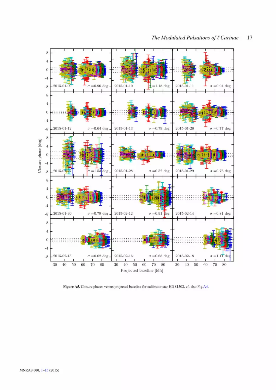
The Modulated Pulsations of `Carinae 17

-8

-4

0

4

8

2015-01-09 σ =0.96 deg 2015-01-10 σ =1.18 deg 2015-01-11 σ =0.94 deg

-8

-4

0

4

8

2015-01-12 σ =0.64 deg 2015-01-13 σ =0.79 deg 2015-01-26 σ =0.77 deg

-8

-4

0

4

8

Closu

rephase

[deg

]

2015-01-27 σ =1.53 deg 2015-01-28 σ =0.52 deg 2015-01-29 σ =0.76 deg

-8

-4

0

4

8

2015-01-30 σ =0.79 deg 2015-02-12 σ =0.91 deg 2015-02-14 σ =0.81 deg

30 40 50 60 70 80

-8

-4

0

4

8

2015-02-15 σ =0.62 deg

30 40 50 60 70 80

Projected baseline [Mλ]

2015-02-16 σ =0.68 deg

30 40 50 60 70 80

2015-02-18 σ =1.11 deg

Figure A5. Closure phases versus projected baseline for calibrator star HD 81502, cf. also Fig.A4.

MNRAS 000, 1–15 (2015)

18 R.I. Anderson et al.

-8

-4

0

4

8

2015-01-09 σ =0.81 deg 2015-01-10 σ =1.19 deg 2015-01-11 σ =0.91 deg

-8

-4

0

4

8

2015-01-12 σ =0.66 deg 2015-01-13 σ =1.4 deg 2015-01-26 σ =0.68 deg

-8

-4

0

4

8

Closu

rephase

[deg

]

2015-01-27 σ =2.06 deg 2015-01-28 σ =0.7 deg 2015-01-29 σ =1.11 deg

-8

-4

0

4

8

2015-01-30 σ =0.86 deg 2015-02-12 σ =0.87 deg 2015-02-14 σ =0.67 deg

30 40 50 60 70 80

-8

-4

0

4

8

2015-02-15 σ =0.73 deg

30 40 50 60 70 80

Projected baseline [Mλ]

2015-02-16 σ =0.84 deg

30 40 50 60 70 80

2015-02-18 σ =1.6 deg

Figure A6. Closure phases versus projected baseline for calibrator star HD 89805, cf. also Fig.A4.

MNRAS 000, 1–15 (2015)

The Modulated Pulsations of `Carinae 19

-8

-4

0

4

8

2015-01-27 σ =1.0 deg 2015-01-28 σ =0.72 deg 2015-01-29 σ =1.22 deg

-8

-4

0

4

8

Closu

rephase

[deg

]

2015-01-30 σ =0.95 deg 2015-02-12 σ =1.41 deg 2015-02-14 σ =0.64 deg

40 50 60 70 80

-8

-4

0

4

8

2015-02-15 σ =0.62 deg

40 50 60 70 80

Projected baseline [Mλ]

2015-02-16 σ =0.69 deg

40 50 60 70 80

2015-02-18 σ =1.27 deg

Figure A7. Closure phases versus projected baseline for standard star HD 81101, cf. also Fig.A4.

MNRAS 000, 1–15 (2015)