Embed Size (px)
Citation preview

Scott M. Lynch
Introduction to Applied BayesianStatistics and Estimation forSocial Scientists
c©2006 SPRINGER SCIENCE+BUSINESS MEDIA, LLC. All rights
reserved. No part of this work may be reproduced in any form without the written
permission of SPRINGER SCIENCE+BUSINESS MEDIA, LLC.
April 24, 2007
Springer
Berlin Heidelberg NewYorkHongKong LondonMilan Paris Tokyo


For my Barbara

Preface
This book was written slowly over the course of the last five years. Duringthat time, a number of advances have been made in Bayesian statistics andMarkov chain Monte Carlo (MCMC) methods, but, in my opinion, the marketstill lacks a truly introductory book written explicitly for social scientiststhat thoroughly describes the actual process of Bayesian analysis using thesemethods. To be sure, a variety of introductory books are available that coverthe basics of the Bayesian approach to statistics (e.g., Gill 2002 and Gelmanet al. 1995) and several that cover the foundation of MCMC methods (e.g.,beginning with Gilks et al. 1996). Yet, a highly applied book showing how touse MCMC methods to complete a Bayesian analysis involving typical socialscience models applied to typical social science data is still sorely lacking. Thegoal of this book is to fill this niche.
The Bayesian approach to statistics has a long history in the discipline ofstatistics, but prior to the 1990s, it held a marginal, almost cult-like status inthe discipline and was almost unheard of in social science methodology. Theprimary reasons for the marginal status of the Bayesian approach include (1)philosophical opposition to the use of “prior distributions” in particular andthe subjective approach to probability in general, and (2) the lack of com-puting power for completing realistic Bayesian analyses. In the 1990s, severalevents occurred simultaneously to overcome these concerns. First, the explo-sion in computing power nullified the second limitation of conducting Bayesiananalyses, especially with the development of sampling based methods (e.g.,MCMC methods) for estimating parameters of Bayesian models. Second, thegrowth in availability of longitudinal (panel) data and the rise in the use ofhierarchical modeling made the Bayesian approach more appealing, becauseBayesian statistics offers a natural approach to constructing hierarchical mod-els. Third, there has been a growing recognition both that the enterprise ofstatistics is a subjective process in general and that the use of prior distribu-tions need not influence results substantially. Additionally, in many problems,the use of a prior distribution turns out to be advantageous.
viii Preface
The publication of Gelfand and Smith’s 1990 paper describing the use ofMCMC simulation methods for summarizing Bayesian posterior distributionswas the watershed event that launched MCMC methods into popularity instatistics. Following relatively closely on the heels of this article, Gelman etal.’s (1995) book, Bayesian Data Analysis, and Gilks et al.’s (1996) book,Markov Chain Monte Carlo in Practice, placed the Bayesian approach ingeneral, and the application of MCMC methods to Bayesian statistical models,squarely in the mainstream of statistics. I consider these books to be classicsin the field and rely heavily on them throughout this book.
Since the mid-1990s, there has been an explosion in advances in Bayesianstatistics and especially MCMC methodology. Many improvements in the re-cent past have been in terms of (1) monitoring and improving the performanceof MCMC algorithms and (2) the development of more refined and complexBayesian models and MCMC algorithms tailored to specific problems. Theseadvances have largely escaped mainstream social science.
In my view, these advances have gone largely unnoticed in social science,because purported introductory books on Bayesian statistics and MCMCmethods are not truly introductory for this audience. First, the mathematicsin introductory books is often too advanced for a mainstream social scienceaudience, which begs the question: “introductory for whom?” Many social sci-entists do not have the probability theory and mathematical statistics back-ground to follow many of these books beyond the first chapter. This is not tosay that the material is impossible to follow, only that more detail may beneeded to make the text and examples more readable for a mainstream socialscience audience.
Second, many examples in introductory-level Bayesian books are at bestforeign and at worst irrelevant to social scientists. The probability distribu-tions that are used in many examples are not typical probability distributionsused by social scientists (e.g., Cauchy), and the data sets that are used in ex-amples are often atypical of social science data. Specifically, many books usesmall data sets with a limited number of covariates, and many of the modelsare not typical of the regression-based approaches used in social science re-search. This fact may not seem problematic until, for example, one is facedwith a research question requiring a multivariate regression model for 10,000observations measured on 5 outcomes with 10 or more covariates. Nonethe-less, research questions involving large-scale data sets are not uncommon insocial science research, and methods shown that handle a sample of size 100measured on one or two outcomes with a couple of covariates simply may notbe directly transferrable to a larger data set context. In such cases, the ana-lyst without a solid understanding of the linkage between the model and theestimation routine may be unable to complete the analysis. Thus, some dis-cussion tailored to the practicalities of real social science data and computingis warranted.
Third, there seems to be a disjunction between introductory books onBayesian theory and introductory books on applied Bayesian statistics. One
Preface ix
of the greatest frustrations for me, while I was learning the basics of Bayesianstatistics and MCMC estimation methods, was (and is) the lack of a bookthat links the theoretical aspects of Bayesian statistics and model develop-ment with the application of modern estimation methods. Some examples inextant books may be substantively interesting, but they are often incompletein the sense that discussion is truncated after model development withoutadequate guidance regarding how to estimate parameters. Often, suggestionsare made concerning how to go about implementing only certain aspects ofan estimation routine, but for a person with no experience doing this, thesesuggestions are not enough.
In an attempt to remedy these issues, this book takes a step back fromthe most recent advances in Bayesian statistics and MCMC methods and triesto bridge the gap between Bayesian theory and modern Bayesian estimationmethods, as well as to bridge the gap between Bayesian statistics books writ-ten as “introductory” texts for statisticians and the needs of a mainstreamsocial science audience. To accomplish this goal, this book presents very littlethat is new. Indeed, most of the material in this book is now “old-hat” instatistics, and many references are a decade old (In fact, a second edition ofGelman et al.’s 1995 book is now available). However, the trade-off for not pre-senting much new material is that this book explains the process of Bayesianstatistics and modern parameter estimation via MCMC simulation methods ingreat depth. Throughout the book, I painstakingly show the modeling processfrom model development, through development of an MCMC algorithm to es-timate its parameters, through model evaluation, and through summarizationand inference.
Although many introductory books begin with the assumption that thereader has a solid grasp of probability theory and mathematical statistics, Ido not make that assumption. Instead, this book begins with an exposition ofthe probability theory needed to gain a solid understanding of the statisticalanalysis of data. In the early chapters, I use contrived examples applied to(sometimes) contrived data so that the forest is not lost for the trees: Thegoal is to provide an understanding of the issue at hand rather than to getlost in the idiosyncratic features of real data. In the latter chapters, I show aBayesian approach (or approaches) to estimating some of the most commonmodels in social science research, including the linear regression model, gen-eralized linear models (specifically, dichotomous and ordinal probit models),hierarchical models, and multivariate models.
A consequence of this choice of models is that the parameter estimatesobtained via the Bayesian approach are often very consistent with those thatcould be obtained via a classical approach. This may make a reader ask,“then what’s the point?” First, there are many cases in which a Bayesianapproach and a classical approach will not coincide, but from my perspective,an introductory text should establish a foundation that can be built upon,rather than beginning in unfamiliar territory. Second, there are additionalbenefits to taking a Bayesian approach beyond the simple estimation of model
x Preface
parameters. Specificially, the Bayesian approach allows for greater flexibility inevaluating model fit, comparing models, producing samples of parameters thatare not directly estimated within a model, handling missing data, “tweaking”a model in ways that cannot be done using canned routines in existing software(e.g., freeing or imposing constraints), and making predictions/forecasts thatcapture greater uncertainty than classical methods. I discuss each of thesebenefits in the examples throughout the latter chapters.
Throughout the book I thoroughly flesh out each example, beginningwith the development of the model and continuing through to developing anMCMC algorithm (generally in R) to estimate it, estimating it using the algo-rithm, and presenting and summarizing the results. These programs should bestraightforward, albeit perhaps tedious, to replicate, but some programmingis inherently required to conduct Bayesian analyses. However, once such pro-gramming skills are learned, they are incredibly freeing to the researcher andthus well worth the investment to acquire them. Ultimately, the point is thatthe examples are thoroughly detailed; nothing is left to the imagination orto guesswork, including the mathematical contortions of simplifying posteriordistributions to make them recognizable as known distributions.
A key feature of Bayesian statistics, and a point of contention for oppo-nents, is the use of a prior distribution. Indeed, one of the most complex thingsabout Bayesian statistics is the development of a model that includes a priorand yields a “proper” posterior distribution. In this book, I do not concentratemuch effort on developing priors. Often, I use uniform priors on most param-eters in a model, or I use “reference” priors. Both types of priors generallyhave the effect of producing results roughly comparable with those obtainedvia maximum likelihood estimation (although not in interpretation!). My goalis not to minimize the importance of choosing appropriate priors, but insteadit is not to overcomplicate an introductory exposition of Bayesian statisticsand model estimation. The fact is that most Bayesian analyses explicitly at-tempt to minimize the effect of the prior. Most published applications to datehave involved using uniform, reference, or otherwise “noninformative” priorsin an effort to avoid the “subjectivity” criticism that historically has beenlevied against Bayesians by classical statisticians. Thus, in most Bayesian so-cial science research, the prior has faded in its importance in differentiatingthe classical and Bayesian paradigms. This is not to say that prior distribu-tions are unimportant—for some problems they may be very important oruseful—but it is to say that it is not necessary to dwell on them.
The book consists of a total of 11 chapters plus two appendices covering(1) calculus and matrix algebra and (2) the basic concepts of the Central LimitTheorem. The book is suited for a highly applied one-semester graduate levelsocial science course. Each chapter, including the appendix but excludingthe introduction, contains a handful of exercises at the end that test theunderstanding of the material in the chapter at both theoretical and appliedlevels. In the exercises, I have traded quantity for quality: There are relativelyfew exercises, but each one was chosen to address the essential material in
Preface xi
the chapter. The first half of the book (Chapters 1-6) is primarily theoreticaland provides a generic introduction to the theory and methods of Bayesianstatistics. These methods are then applied to common social science modelsand data in the latter half of the book (Chapters 7-11). Chapters 2-4 caneach be covered in a week of classes, and much of this material, especially inChapters 2 and 3, should be review material for most students. Chapters 5and 6 will most likely each require more than a week to cover, as they formthe nuts and bolts of MCMC methods and evaluation. Subsequent chaptersshould each take 1-2 weeks of class time. The models themselves should befamiliar, but the estimation of them via MCMC methods will not be and maybe difficult for students without some programming and applied data analysisexperience. The programming language used throughout the book is R, afreely available and common package used in applied statistics, but I introducethe program WinBugs in the chapter on hierarchical modeling. Overall, R andWinBugs are syntactically similar, and so the introduction of WinBugs is notproblematic. From my perspective, the main benefit of WinBugs is that somederivations of conditional distributions that would need to be done in orderto write an R program are handled automatically by WinBugs. This featureis especially useful in hierarchical models. All programs used in this book, aswell as most data, and hints and/or solutions to the exercises can be foundon my Princeton University website at: www.princeton.edu/∼slynch.
Acknowledgements
I have a number of people to thank for their help during the writing of thisbook. First, I want to thank German Rodriguez and Bruce Western (both atPrinceton) for sharing their advice, guidance, and statistical knowledge withme as I worked through several sections of the book. Second, I thank myfriend and colleague J. Scott Brown for reading through virtually all chap-ters and providing much-needed feedback over the course of the last severalyears. Along these same lines, I thank Chris Wildeman and Steven Shafer forreading through a number of chapters and suggesting ways to improve ex-amples and the general presentation of material. Third, I thank my statisticsthesis advisor, Valen Johnson, and my mentor and friend, Ken Bollen, for allthat they have taught me about statistics. (They cannot be held responsiblefor the fact that I may not have learned well, however). For their constanthelp and tolerance, I thank Wayne Appleton and Bob Jackson, the seniorcomputer folks at Princeton University and Duke University, without whosesupport this book could not have been possible. For their general supportand friendship over a period including, but not limited to, the writing of thisbook, I thank Linda George, Angie O’Rand, Phil Morgan, Tom Espenshade,Debby Gold, Mark Hayward, Eileen Crimmins, Ken Land, Dan Beirute, TomRice, and John Moore. I also thank my son, Tyler, and my wife, Barbara, forlistening to me ramble incessantly about statistics and acting as a sounding

xii Preface
board during the writing of the book. Certainly not least, I thank Bill Mc-Cabe for helping to identify an egregious error on page 364. Finally, I want tothank my editor at Springer, John Kimmel, for his patience and advice, andI acknowledge support from NICHD grant R03HD050374-01 for much of thework in Chapter 10 on multivariate models.
Despite having all of these sources of guidance and support, all the errorsin the book remain my own.
Princeton University Scott M. LynchApril 2007
Contents
Preface . . . . . . . . . . . . . . . . . . . . . . . . . . . . . . . . . . . . . . . . . . . . . . . . . . . . . . . . vii
Contents . . . . . . . . . . . . . . . . . . . . . . . . . . . . . . . . . . . . . . . . . . . . . . . . . . . . . . .xvii
List of Figures . . . . . . . . . . . . . . . . . . . . . . . . . . . . . . . . . . . . . . . . . . . . . . . . . xxv
List of Tables . . . . . . . . . . . . . . . . . . . . . . . . . . . . . . . . . . . . . . . . . . . . . . . . . .xxviii
1 Introduction . . . . . . . . . . . . . . . . . . . . . . . . . . . . . . . . . . . . . . . . . . . . . . . 11.1 Outline . . . . . . . . . . . . . . . . . . . . . . . . . . . . . . . . . . . . . . . . . . . . . . . . 31.2 A note on programming . . . . . . . . . . . . . . . . . . . . . . . . . . . . . . . . . . 51.3 Symbols used throughout the book . . . . . . . . . . . . . . . . . . . . . . . . 6
2 Probability Theory and Classical Statistics . . . . . . . . . . . . . . . . 92.1 Rules of probability . . . . . . . . . . . . . . . . . . . . . . . . . . . . . . . . . . . . . . 92.2 Probability distributions in general . . . . . . . . . . . . . . . . . . . . . . . . 12
2.2.1 Important quantities in distributions . . . . . . . . . . . . . . . . . 172.2.2 Multivariate distributions . . . . . . . . . . . . . . . . . . . . . . . . . . 192.2.3 Marginal and conditional distributions . . . . . . . . . . . . . . . 23
2.3 Some important distributions in social science . . . . . . . . . . . . . . . 252.3.1 The binomial distribution . . . . . . . . . . . . . . . . . . . . . . . . . . 252.3.2 The multinomial distribution . . . . . . . . . . . . . . . . . . . . . . . 272.3.3 The Poisson distribution . . . . . . . . . . . . . . . . . . . . . . . . . . . 282.3.4 The normal distribution . . . . . . . . . . . . . . . . . . . . . . . . . . . . 292.3.5 The multivariate normal distribution . . . . . . . . . . . . . . . . . 302.3.6 t and multivariate t distributions . . . . . . . . . . . . . . . . . . . . 33
2.4 Classical statistics in social science . . . . . . . . . . . . . . . . . . . . . . . . . 332.5 Maximum likelihood estimation . . . . . . . . . . . . . . . . . . . . . . . . . . . 35
2.5.1 Constructing a likelihood function . . . . . . . . . . . . . . . . . . . 362.5.2 Maximizing a likelihood function . . . . . . . . . . . . . . . . . . . . 382.5.3 Obtaining standard errors . . . . . . . . . . . . . . . . . . . . . . . . . . 39
xiv Contents
2.5.4 A normal likelihood example . . . . . . . . . . . . . . . . . . . . . . . . 412.6 Conclusions . . . . . . . . . . . . . . . . . . . . . . . . . . . . . . . . . . . . . . . . . . . . . 442.7 Exercises . . . . . . . . . . . . . . . . . . . . . . . . . . . . . . . . . . . . . . . . . . . . . . . 44
2.7.1 Probability exercises . . . . . . . . . . . . . . . . . . . . . . . . . . . . . . . 442.7.2 Classical inference exercises . . . . . . . . . . . . . . . . . . . . . . . . . 45
3 Basics of Bayesian Statistics . . . . . . . . . . . . . . . . . . . . . . . . . . . . . . . 473.1 Bayes’ Theorem for point probabilities . . . . . . . . . . . . . . . . . . . . . 473.2 Bayes’ Theorem applied to probability distributions . . . . . . . . . . 50
3.2.1 Proportionality . . . . . . . . . . . . . . . . . . . . . . . . . . . . . . . . . . . 513.3 Bayes’ Theorem with distributions: A voting example . . . . . . . . 53
3.3.1 Specification of a prior: The beta distribution . . . . . . . . . 543.3.2 An alternative model for the polling data: A gamma
prior/ Poisson likelihood approach . . . . . . . . . . . . . . . . . . . 603.4 A normal prior–normal likelihood example with σ2 known . . . . 62
3.4.1 Extending the normal distribution example . . . . . . . . . . . 653.5 Some useful prior distributions . . . . . . . . . . . . . . . . . . . . . . . . . . . . 68
3.5.1 The Dirichlet distribution . . . . . . . . . . . . . . . . . . . . . . . . . . 693.5.2 The inverse gamma distribution . . . . . . . . . . . . . . . . . . . . . 693.5.3 Wishart and inverse Wishart distributions . . . . . . . . . . . . 70
3.6 Criticism against Bayesian statistics . . . . . . . . . . . . . . . . . . . . . . . 703.7 Conclusions . . . . . . . . . . . . . . . . . . . . . . . . . . . . . . . . . . . . . . . . . . . . . 733.8 Exercises . . . . . . . . . . . . . . . . . . . . . . . . . . . . . . . . . . . . . . . . . . . . . . . 74
4 Modern Model Estimation Part 1: Gibbs Sampling . . . . . . . . 774.1 What Bayesians want and why . . . . . . . . . . . . . . . . . . . . . . . . . . . . 774.2 The logic of sampling from posterior densities . . . . . . . . . . . . . . . 784.3 Two basic sampling methods . . . . . . . . . . . . . . . . . . . . . . . . . . . . . . 80
4.3.1 The inversion method of sampling . . . . . . . . . . . . . . . . . . . 814.3.2 The rejection method of sampling . . . . . . . . . . . . . . . . . . . 84
4.4 Introduction to MCMC sampling . . . . . . . . . . . . . . . . . . . . . . . . . . 884.4.1 Generic Gibbs sampling . . . . . . . . . . . . . . . . . . . . . . . . . . . . 884.4.2 Gibbs sampling example using the inversion method . . . 894.4.3 Example repeated using rejection sampling . . . . . . . . . . . 934.4.4 Gibbs sampling from a real bivariate density . . . . . . . . . . 964.4.5 Reversing the process: Sampling the parameters given
the data . . . . . . . . . . . . . . . . . . . . . . . . . . . . . . . . . . . . . . . . . . 1004.5 Conclusions . . . . . . . . . . . . . . . . . . . . . . . . . . . . . . . . . . . . . . . . . . . . . 1034.6 Exercises . . . . . . . . . . . . . . . . . . . . . . . . . . . . . . . . . . . . . . . . . . . . . . . 105
5 Modern Model Estimation Part 2: Metroplis–HastingsSampling . . . . . . . . . . . . . . . . . . . . . . . . . . . . . . . . . . . . . . . . . . . . . . . . . . 1075.1 A generic MH algorithm . . . . . . . . . . . . . . . . . . . . . . . . . . . . . . . . . . 108
5.1.1 Relationship between Gibbs and MH sampling . . . . . . . . 113
Contents xv
5.2 Example: MH sampling when conditional densities aredifficult to derive . . . . . . . . . . . . . . . . . . . . . . . . . . . . . . . . . . . . . . . . 115
5.3 Example: MH sampling for a conditional density with anunknown form . . . . . . . . . . . . . . . . . . . . . . . . . . . . . . . . . . . . . . . . . . 118
5.4 Extending the bivariate normal example: The fullmultiparameter model . . . . . . . . . . . . . . . . . . . . . . . . . . . . . . . . . . . . 1215.4.1 The conditionals for µx and µy . . . . . . . . . . . . . . . . . . . . . . 1225.4.2 The conditionals for σ2
x, σ2y, and ρ . . . . . . . . . . . . . . . . . . . 123
5.4.3 The complete MH algorithm . . . . . . . . . . . . . . . . . . . . . . . . 1245.4.4 A matrix approach to the bivariate normal distribution
problem . . . . . . . . . . . . . . . . . . . . . . . . . . . . . . . . . . . . . . . . . . 1265.5 Conclusions . . . . . . . . . . . . . . . . . . . . . . . . . . . . . . . . . . . . . . . . . . . . . 1285.6 Exercises . . . . . . . . . . . . . . . . . . . . . . . . . . . . . . . . . . . . . . . . . . . . . . . 129
6 Evaluating Markov Chain Monte Carlo (MCMC)Algorithms and Model Fit . . . . . . . . . . . . . . . . . . . . . . . . . . . . . . . . . 1316.1 Why evaluate MCMC algorithm performance? . . . . . . . . . . . . . . 1326.2 Some common problems and solutions . . . . . . . . . . . . . . . . . . . . . . 1326.3 Recognizing poor performance . . . . . . . . . . . . . . . . . . . . . . . . . . . . 135
6.3.1 Trace plots . . . . . . . . . . . . . . . . . . . . . . . . . . . . . . . . . . . . . . . 1356.3.2 Acceptance rates of MH algorithms . . . . . . . . . . . . . . . . . . 1416.3.3 Autocorrelation of parameters . . . . . . . . . . . . . . . . . . . . . . 1466.3.4 “R” and other calculations . . . . . . . . . . . . . . . . . . . . . . . . . 147
6.4 Evaluating model fit . . . . . . . . . . . . . . . . . . . . . . . . . . . . . . . . . . . . . 1536.4.1 Residual analysis . . . . . . . . . . . . . . . . . . . . . . . . . . . . . . . . . . 1546.4.2 Posterior predictive distributions . . . . . . . . . . . . . . . . . . . . 155
6.5 Formal comparison and combining models . . . . . . . . . . . . . . . . . . 1596.5.1 Bayes factors . . . . . . . . . . . . . . . . . . . . . . . . . . . . . . . . . . . . . 1596.5.2 Bayesian model averaging . . . . . . . . . . . . . . . . . . . . . . . . . . 161
6.6 Conclusions . . . . . . . . . . . . . . . . . . . . . . . . . . . . . . . . . . . . . . . . . . . . . 1636.7 Exercises . . . . . . . . . . . . . . . . . . . . . . . . . . . . . . . . . . . . . . . . . . . . . . . 163
7 The Linear Regression Model . . . . . . . . . . . . . . . . . . . . . . . . . . . . . . 1657.1 Development of the linear regression model . . . . . . . . . . . . . . . . . 1657.2 Sampling from the posterior distribution for the model
parameters . . . . . . . . . . . . . . . . . . . . . . . . . . . . . . . . . . . . . . . . . . . . . 1687.2.1 Sampling with an MH algorithm . . . . . . . . . . . . . . . . . . . . 1687.2.2 Sampling the model parameters using Gibbs sampling . . 169
7.3 Example: Are people in the South “nicer” than others? . . . . . . . 1747.3.1 Results and comparison of the algorithms . . . . . . . . . . . . 1757.3.2 Model evaluation . . . . . . . . . . . . . . . . . . . . . . . . . . . . . . . . . . 178
7.4 Incorporating missing data . . . . . . . . . . . . . . . . . . . . . . . . . . . . . . . 1827.4.1 Types of missingness . . . . . . . . . . . . . . . . . . . . . . . . . . . . . . . 1827.4.2 A generic Bayesian approach when data are MAR:
The “niceness” example revisited . . . . . . . . . . . . . . . . . . . . 186
xvi Contents
7.5 Conclusions . . . . . . . . . . . . . . . . . . . . . . . . . . . . . . . . . . . . . . . . . . . . . 1917.6 Exercises . . . . . . . . . . . . . . . . . . . . . . . . . . . . . . . . . . . . . . . . . . . . . . . 192
8 Generalized Linear Models . . . . . . . . . . . . . . . . . . . . . . . . . . . . . . . . 1938.1 The dichotomous probit model . . . . . . . . . . . . . . . . . . . . . . . . . . . . 195
8.1.1 Model development and parameter interpretation . . . . . . 1958.1.2 Sampling from the posterior distribution for the model
parameters . . . . . . . . . . . . . . . . . . . . . . . . . . . . . . . . . . . . . . . 1988.1.3 Simulating from truncated normal distributions . . . . . . . 2008.1.4 Dichotomous probit model example: Black–white
differences in mortality . . . . . . . . . . . . . . . . . . . . . . . . . . . . . 2068.2 The ordinal probit model . . . . . . . . . . . . . . . . . . . . . . . . . . . . . . . . . 217
8.2.1 Model development and parameter interpretation . . . . . . 2188.2.2 Sampling from the posterior distribution for the
parameters . . . . . . . . . . . . . . . . . . . . . . . . . . . . . . . . . . . . . . . 2208.2.3 Ordinal probit model example: Black–white differences
in health . . . . . . . . . . . . . . . . . . . . . . . . . . . . . . . . . . . . . . . . . 2238.3 Conclusions . . . . . . . . . . . . . . . . . . . . . . . . . . . . . . . . . . . . . . . . . . . . . 2288.4 Exercises . . . . . . . . . . . . . . . . . . . . . . . . . . . . . . . . . . . . . . . . . . . . . . . 229
9 Introduction to Hierarchical Models . . . . . . . . . . . . . . . . . . . . . . . 2319.1 Hierarchical models in general . . . . . . . . . . . . . . . . . . . . . . . . . . . . . 232
9.1.1 The voting example redux . . . . . . . . . . . . . . . . . . . . . . . . . . 2339.2 Hierarchical linear regression models . . . . . . . . . . . . . . . . . . . . . . . 240
9.2.1 Random effects: The random intercept model . . . . . . . . . 2419.2.2 Random effects: The random coefficient model . . . . . . . . 2519.2.3 Growth models . . . . . . . . . . . . . . . . . . . . . . . . . . . . . . . . . . . . 256
9.3 A note on fixed versus random effects models and otherterminology . . . . . . . . . . . . . . . . . . . . . . . . . . . . . . . . . . . . . . . . . . . . . 264
9.4 Conclusions . . . . . . . . . . . . . . . . . . . . . . . . . . . . . . . . . . . . . . . . . . . . . 2689.5 Exercises . . . . . . . . . . . . . . . . . . . . . . . . . . . . . . . . . . . . . . . . . . . . . . . 269
10 Introduction to Multivariate Regression Models . . . . . . . . . . . 27110.1 Multivariate linear regression . . . . . . . . . . . . . . . . . . . . . . . . . . . . . 271
10.1.1 Model development . . . . . . . . . . . . . . . . . . . . . . . . . . . . . . . . 27110.1.2 Implementing the algorithm . . . . . . . . . . . . . . . . . . . . . . . . 275
10.2 Multivariate probit models . . . . . . . . . . . . . . . . . . . . . . . . . . . . . . . 27710.2.1 Model development . . . . . . . . . . . . . . . . . . . . . . . . . . . . . . . . 27810.2.2 Step 2: Simulating draws from truncated multivariate
normal distributions . . . . . . . . . . . . . . . . . . . . . . . . . . . . . . . 28310.2.3 Step 3: Simulation of thresholds in the multivariate
probit model . . . . . . . . . . . . . . . . . . . . . . . . . . . . . . . . . . . . . . 28910.2.4 Step 5: Simulating the error covariance matrix . . . . . . . . 29510.2.5 Implementing the algorithm . . . . . . . . . . . . . . . . . . . . . . . . 297
Contents xvii
10.3 A multivariate probit model for generating distributions ofmultistate life tables . . . . . . . . . . . . . . . . . . . . . . . . . . . . . . . . . . . . . 30310.3.1 Model specification and simulation . . . . . . . . . . . . . . . . . . 30710.3.2 Life table generation and other posterior inferences . . . . 310
10.4 Conclusions . . . . . . . . . . . . . . . . . . . . . . . . . . . . . . . . . . . . . . . . . . . . . 31510.5 Exercises . . . . . . . . . . . . . . . . . . . . . . . . . . . . . . . . . . . . . . . . . . . . . . . 317
11 Conclusion . . . . . . . . . . . . . . . . . . . . . . . . . . . . . . . . . . . . . . . . . . . . . . . . 319
A Background Mathematics . . . . . . . . . . . . . . . . . . . . . . . . . . . . . . . . . . 323A.1 Summary of calculus . . . . . . . . . . . . . . . . . . . . . . . . . . . . . . . . . . . . . 323
A.1.1 Limits . . . . . . . . . . . . . . . . . . . . . . . . . . . . . . . . . . . . . . . . . . . 323A.1.2 Differential calculus . . . . . . . . . . . . . . . . . . . . . . . . . . . . . . . . 324A.1.3 Integral calculus . . . . . . . . . . . . . . . . . . . . . . . . . . . . . . . . . . . 326A.1.4 Finding a general rule for a derivative . . . . . . . . . . . . . . . . 329
A.2 Summary of matrix algebra . . . . . . . . . . . . . . . . . . . . . . . . . . . . . . . 330A.2.1 Matrix notation . . . . . . . . . . . . . . . . . . . . . . . . . . . . . . . . . . . 330A.2.2 Matrix operations . . . . . . . . . . . . . . . . . . . . . . . . . . . . . . . . . 331
A.3 Exercises . . . . . . . . . . . . . . . . . . . . . . . . . . . . . . . . . . . . . . . . . . . . . . . 335A.3.1 Calculus exercises . . . . . . . . . . . . . . . . . . . . . . . . . . . . . . . . . 335A.3.2 Matrix algebra exercises . . . . . . . . . . . . . . . . . . . . . . . . . . . . 335
B The Central Limit Theorem, Confidence Intervals, andHypothesis Tests . . . . . . . . . . . . . . . . . . . . . . . . . . . . . . . . . . . . . . . . . . 337B.1 A simulation study . . . . . . . . . . . . . . . . . . . . . . . . . . . . . . . . . . . . . . 337B.2 Classical inference . . . . . . . . . . . . . . . . . . . . . . . . . . . . . . . . . . . . . . . 338
B.2.1 Hypothesis testing . . . . . . . . . . . . . . . . . . . . . . . . . . . . . . . . . 339B.2.2 Confidence intervals . . . . . . . . . . . . . . . . . . . . . . . . . . . . . . . 342B.2.3 Some final notes . . . . . . . . . . . . . . . . . . . . . . . . . . . . . . . . . . . 344
References . . . . . . . . . . . . . . . . . . . . . . . . . . . . . . . . . . . . . . . . . . . . . . . . . . . . . 347
Index . . . . . . . . . . . . . . . . . . . . . . . . . . . . . . . . . . . . . . . . . . . . . . . . . . . . . . . . . . 355


List of Figures
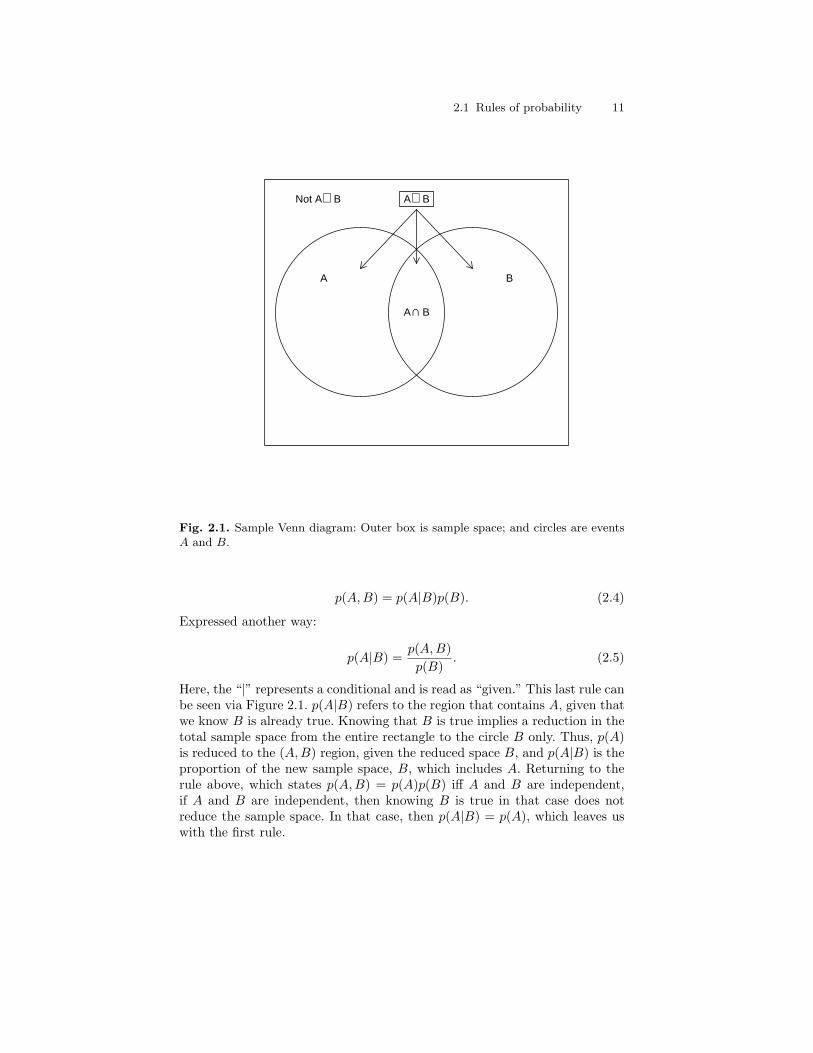
2.1 Sample Venn diagram: Outer box is sample space; and circlesare events A and B. . . . . . . . . . . . . . . . . . . . . . . . . . . . . . . . . . . . . . . 11
2.2 Two uniform distributions. . . . . . . . . . . . . . . . . . . . . . . . . . . . . . . . . 152.3 Histogram of the importance of being able to express
unpopular views in a free society (1 = Not very important...6= One of the most important things). . . . . . . . . . . . . . . . . . . . . . . . 16
2.4 Sample probability density function: A linear density. . . . . . . . . . 172.5 Sample probability density function: A bivariate plane density. . 202.6 Three-dimensional bar chart for GSS data with “best” planar
density superimposed. . . . . . . . . . . . . . . . . . . . . . . . . . . . . . . . . . . . . . 222.7 Representation of bivariate cumulative distribution function:
Area under bivariate plane density from 0 to 1 in bothdimensions. . . . . . . . . . . . . . . . . . . . . . . . . . . . . . . . . . . . . . . . . . . . . . . 23
2.8 Some binomial distributions (with parameter n = 10). . . . . . . . . . 272.9 Some Poisson distributions. . . . . . . . . . . . . . . . . . . . . . . . . . . . . . . . . 292.10 Some normal distributions. . . . . . . . . . . . . . . . . . . . . . . . . . . . . . . . . 312.11 Two bivariate normal distributions. . . . . . . . . . . . . . . . . . . . . . . . . . 322.12 The t(0, 1, 1), t(0, 1, 10), and t(0, 1, 120) distributions (with an
N(0, 1) distribution superimposed). . . . . . . . . . . . . . . . . . . . . . . . . . 342.13 Binomial (top) and Bernoulli (bottom) likelihood functions
for the OH presidential poll data. . . . . . . . . . . . . . . . . . . . . . . . . . . . 372.14 Finding the MLE: Likelihood and log-likelihood functions for
the OH presidential poll data. . . . . . . . . . . . . . . . . . . . . . . . . . . . . . . 39
3.1 Three beta distributions with mean α/(α + β) = .5. . . . . . . . . . . 563.2 Prior, likelihood, and posterior for polling data example: The
likelihood function has been normalized as a density for theparameter K. . . . . . . . . . . . . . . . . . . . . . . . . . . . . . . . . . . . . . . . . . . . . 58
3.3 Posterior for polling data example: A vertical line at K = .5 isincluded to show the area needed to be computed to estimatethe probability that Kerry would win Ohio. . . . . . . . . . . . . . . . . . . 59
xx List of Figures
3.4 Some examples of the gamma distribution. . . . . . . . . . . . . . . . . . . 61
4.1 Convergence of sample means on the true beta distributionmean across samples sizes: Vertical line shows sample size of5,000; dashed horizontal lines show approximate confidenceband of sample estimates for samples of size n = 5, 000; andsolid horizontal line shows the true mean. . . . . . . . . . . . . . . . . . . . 81
4.2 Example of the inversion method: Left-hand figures show thesequence of draws from the U(0, 1) density (upper left) andthe sequence of draws from the density f(x) = (1/40)(2x + 3)density (lower left); and the right-hand figures show thesedraws in histogram format, with true density functionssuperimposed. . . . . . . . . . . . . . . . . . . . . . . . . . . . . . . . . . . . . . . . . . . . 83
4.3 The three-step process of rejection sampling. . . . . . . . . . . . . . . . . . 864.4 Sample of 1,000 draws from density using rejection sampling
with theoretical density superimposed. . . . . . . . . . . . . . . . . . . . . . . 874.5 Results of Gibbs sampler using the inversion method for
sampling from conditional densities. . . . . . . . . . . . . . . . . . . . . . . . . 924.6 Results of Gibbs sampler using the inversion method for
sampling from conditional densities: Two-dimensional viewafter 5, 25, 100, and 2,000 iterations. . . . . . . . . . . . . . . . . . . . . . . . . 93
4.7 Results of Gibbs sampler using rejection sampling to samplefrom conditional densities. . . . . . . . . . . . . . . . . . . . . . . . . . . . . . . . . . 97
4.8 Results of Gibbs sampler using rejection sampling to samplefrom conditional densities: Two-dimensional view after 5, 25,100, and 2,000 iterations. . . . . . . . . . . . . . . . . . . . . . . . . . . . . . . . . . . 98
4.9 Results of Gibbs sampler for standard bivariate normaldistribution with correlation r = .5: Two-dimensional viewafter 10, 50, 200, and 2,000 iterations. . . . . . . . . . . . . . . . . . . . . . . . 100
4.10 Results of Gibbs sampler for standard bivariate normaldistribution: Upper left and right graphs show marginaldistributions for x and y (last 1,500 iterations); lower leftgraph shows contour plot of true density; and lower rightgraph shows contour plot of true density with Gibbs samplessuperimposed. . . . . . . . . . . . . . . . . . . . . . . . . . . . . . . . . . . . . . . . . . . . 101
4.11 Samples from posterior densities for a mean and varianceparameter for NHIS years of schooling data under two Gibbssampling approaches: The solid lines are the results for themarginal-for-σ2-but conditional-for-µ approach; and thedashed lines are the results for the full conditionals approach. . . 104
5.1 Example of symmetric proposals centered over the previousand candidate values of the parameters. . . . . . . . . . . . . . . . . . . . . . 110
5.2 Example of asymmetric proposals centered at the mode overthe previous and candidate values of the parameters. . . . . . . . . . . 111

List of Figures xxi
5.3 Example of asymmetry in proposals due to a boundaryconstraint on the parameter space. . . . . . . . . . . . . . . . . . . . . . . . . . 113
5.4 Trace plot and histogram of m parameter from linear densitymodel for the 2000 GSS free speech data. . . . . . . . . . . . . . . . . . . . . 117
5.5 Trace plot and histogram of ρ parameter from bivariatenormal density model for the 2000 GSS free speech andpolitical participation data. . . . . . . . . . . . . . . . . . . . . . . . . . . . . . . . . 120
5.6 Trace plot and histogram of ρ from bivariate normal model forthe 2000 GSS free speech and political participation data. . . . . . 126
6.1 Trace plot for first 1,000 iterations of an MH algorithmsampling parameters from planar density for GSS free speechand political participation data. . . . . . . . . . . . . . . . . . . . . . . . . . . . . 136
6.2 Trace plot for first 4,000 iterations of an MH algorithmsampling parameters from planar density for GSS free speechand political participation data. . . . . . . . . . . . . . . . . . . . . . . . . . . . . 137
6.3 Trace plot for all 50,000 iterations of an MH algorithmsampling parameters from planar density for GSS free speechand political participation data with means superimposed. . . . . . 138
6.4 Trace plot of cumulative and batch means for MH algorithmsampling parameters from planar density for GSS free speechand political participation data. . . . . . . . . . . . . . . . . . . . . . . . . . . . . 139
6.5 Trace plot of cumulative standard deviation of m2 from MHalgorithm sampling parameters from planar density for GSSfree speech and political participation data. . . . . . . . . . . . . . . . . . . 140
6.6 Posterior density for m2 parameter from planar density MHalgorithm and two proposal densities: U(−.0003, .0003) andU(−.003, .003). . . . . . . . . . . . . . . . . . . . . . . . . . . . . . . . . . . . . . . . . . . 142
6.7 Trace plot of the first 1,000 iterations of an MH algorithm forthe planar density with a (relatively) broad U(−.003, .003)proposal density. . . . . . . . . . . . . . . . . . . . . . . . . . . . . . . . . . . . . . . . . . 143
6.8 Posterior density for m2 parameter from planar density MHalgorithm and two proposal densities: U(−.003, .003) andN(0, .00085). . . . . . . . . . . . . . . . . . . . . . . . . . . . . . . . . . . . . . . . . . . . . 144
6.9 Two-dimensional trace plot for initial run of MH algorithmsampling parameters from planar density for GSS free speechand political participation data: Two possible bivariate normalproposal densities are superimposed. . . . . . . . . . . . . . . . . . . . . . . . . 145
6.10 Trace plot for 5000 iterations of an MH algorithm samplingparameters from planar density for GSS free speech andpolitical participation data: Bivariate normal proposal densitywith correlation −.9. . . . . . . . . . . . . . . . . . . . . . . . . . . . . . . . . . . . . . . 146
xxii List of Figures
6.11 Autocorrelation plots of parameter m2 from MH algorithmsfor the planar density: Upper figure is for the MH algorithmwith independent uniform proposals for m1 and m2; andlower figure is for the MH algorithm with a bivariate normalproposal with correlation −.9. . . . . . . . . . . . . . . . . . . . . . . . . . . . . . . 148
6.12 Histogram of marginal posterior density for m2 parameter:Dashed reference line is the posterior mean. . . . . . . . . . . . . . . . . . . 149
6.13 Trace plot of first 600 sampled values of ρ from MH algorithmswith three different starting values (GSS political participationand free speech data). . . . . . . . . . . . . . . . . . . . . . . . . . . . . . . . . . . . . . 151
6.14 Two-dimensional trace plot of sampled values of σ2x and σ2
y
from MH algorithms with three different starting values (GSSpolitical participation and free speech data). . . . . . . . . . . . . . . . . . 152
6.15 Trace plot of the scale reduction factor R for ρ, σ2x, and σ2
y
across the first 500 iterations of the MH algorithms. . . . . . . . . . . 1536.16 Posterior predictive distributions for the ratio of the mean to
the median in the bivariate normal distribution and planardistribution models: Vertical reference line is the observedvalue in the original data. . . . . . . . . . . . . . . . . . . . . . . . . . . . . . . . . . 158
6.17 Correlations between observed cell counts and posteriorpredictive distribution cell counts for the bivariate normal andplanar distribution models. . . . . . . . . . . . . . . . . . . . . . . . . . . . . . . . . 160
7.1 Scale reduction factors by iteration for all regressionparameters. . . . . . . . . . . . . . . . . . . . . . . . . . . . . . . . . . . . . . . . . . . . . . 176
7.2 Trace plot of error variance parameter in three differentMCMC algorithms. . . . . . . . . . . . . . . . . . . . . . . . . . . . . . . . . . . . . . . 177
7.3 Posterior predictive distributions: (1) The distribution of allreplicated samples and the distribution of the original data;(2) the distribution of the ratio of the sample mean of y tothe median, with the observed ratio superimposed; and (3)the distribution of the ranges of predicted values with theobserved range superimposed. . . . . . . . . . . . . . . . . . . . . . . . . . . . . . . 180
7.4 Posterior predictive distributions (solid lines) and observedvalues (dashed vertical lines) for persons 1,452 and 1,997. . . . . . . 181
7.5 Distribution of age, education, and income for entire sampleand for 31 potential outliers identified from posteriorpredictive simulation (reference lines at means). . . . . . . . . . . . . . . 183
7.6 Examples of types of missingness: No missing, missing are notOAR, and missing are not MAR. . . . . . . . . . . . . . . . . . . . . . . . . . . . 185
8.1 Depiction of simulation from a truncated normal distribution. . . 2018.2 Depiction of rejection sampling from the tail region of a
truncated normal distribution. . . . . . . . . . . . . . . . . . . . . . . . . . . . . . 203
List of Figures xxiii
8.3 Trace plot and autocorrelation function (ACF) plot forintercept parameter in dichotomous probit model example(upper plots show samples thinned to every 10th sample; lowerplot shows the ACF after thinning to every 24th post-burn-insample). . . . . . . . . . . . . . . . . . . . . . . . . . . . . . . . . . . . . . . . . . . . . . . . . . 209
8.4 Sampled latent health scores for four sample members fromthe probit model example. . . . . . . . . . . . . . . . . . . . . . . . . . . . . . . . . 211
8.5 Model-predicted traits and actual latent traits for fourobservations in probit model (solid line = model-predictedlatent traits from sample values of β; dashed line = latenttraits simulated from the Gibbs sampler). . . . . . . . . . . . . . . . . . . . 212
8.6 Latent residuals for four observations in probit model(reference line at 0). . . . . . . . . . . . . . . . . . . . . . . . . . . . . . . . . . . . . . 213
8.7 Distribution of black and age-by-black parameters (Cases 2and 3 = both values are positive or negative, respectively;Cases 1 and 4 = values are of opposite signs. Case 4 is thetypically-seen/expected pattern). . . . . . . . . . . . . . . . . . . . . . . . . . . 215
8.8 Distribution of black-white crossover ages for ages > 0 and <200 (various summary measures superimposed as referencelines). . . . . . . . . . . . . . . . . . . . . . . . . . . . . . . . . . . . . . . . . . . . . . . . . . . 216
8.9 Depiction of latent distribution for Y ∗ and Y with thresholdssuperimposed. . . . . . . . . . . . . . . . . . . . . . . . . . . . . . . . . . . . . . . . . . . . 220
8.10 Trace plot for threshold parameters in ordinal probit model. . . . 2248.11 Distributions of latent health scores for five persons with
different observed values of y. . . . . . . . . . . . . . . . . . . . . . . . . . . . . . . 2258.12 Distributions of R2 and pseudo-R2 from OLS and probit
models, respectively. . . . . . . . . . . . . . . . . . . . . . . . . . . . . . . . . . . . . . . 228
9.1 Two-dimensional trace plot of α(0) and α(1) parameters(dashed lines at posterior means for each parameter). . . . . . . . . . 249
9.2 Scatterplots of four persons’ random intercepts and slopesfrom growth curve model of health (posterior meanssuperimposed as horizontal and vertical dashed lines). . . . . . . . . . 261
9.3 Predicted trajectories and observed health for four persons:The solid lines are the predicted trajectories based on theposterior means of the random intercepts and slopes fromFigure 9.2; and the dashed lines are the predicted trajectoriesbased on the individuals’ covariate profiles and posteriormeans of the parameters in Table 9.4 . . . . . . . . . . . . . . . . . . . . . . . 265
xxiv List of Figures
10.1 Depiction of a bivariate outcome space for continuous latentvariables Z1 and Z2: The observed variables Y1 and Y2 areformed by the imposition of the vectors of thresholds in eachdimension; and the darkened area is the probability that anindividual’s response falls in the [2, 3] cell, conditional on thedistribution for Z. . . . . . . . . . . . . . . . . . . . . . . . . . . . . . . . . . . . . . . . . 282
10.2 Comparison of truncated bivariate normal simulation usingnaive simulation and conditional/decomposition simulation:Upper plots show the true contours (solid lines) of the bivariatenormal distribution with sampled values superimposed (dots);and lower plots show histograms of the values sampled fromthe two dimensions under the two alternative samplingapproaches. . . . . . . . . . . . . . . . . . . . . . . . . . . . . . . . . . . . . . . . . . . . . . . 287
10.3 Truncated bivariate normal distribution: Marginal distributionfor x1 when truncation of x2 is ignored. . . . . . . . . . . . . . . . . . . . . . 288
10.4 Comparison of truncated bivariate normal distributionsimulation using naive simulation and two iterations of Gibbssampling: Upper plots show the true contours (solid lines)of the bivariate normal distribution with sampled valuessuperimposed (dots); and lower plots show histograms ofthe values sampled from the two dimensions under the twoalternative approaches to sampling. . . . . . . . . . . . . . . . . . . . . . . . . 290
10.5 Gibbs sampling versus Cowles’ algorithm for samplingthreshold parameters. . . . . . . . . . . . . . . . . . . . . . . . . . . . . . . . . . . . . . 293
10.6 Posterior predictive distributions for the probability a30-year-old white male from the South self-identifies as aconservative Republican across time. . . . . . . . . . . . . . . . . . . . . . . . . 304
10.7 Representation of state space for a three state model. . . . . . . . . . 30510.8 Two-dimensional outcome for capturing a three-state state
space. . . . . . . . . . . . . . . . . . . . . . . . . . . . . . . . . . . . . . . . . . . . . . . . . . . . 30610.9 Trace plots of life table quantities computed from Gibbs
samples of bivariate probit model parameters. . . . . . . . . . . . . . . . . 31510.10Histograms of life table quantitities computed from Gibbs
samples of bivariate probit model parameters. . . . . . . . . . . . . . . . . 316
A.1 Generic depiction of a curve and a tangent line at an arbitrarypoint. . . . . . . . . . . . . . . . . . . . . . . . . . . . . . . . . . . . . . . . . . . . . . . . . . . . 324
A.2 Finding successive approximations to the area under a curveusing rectangles. . . . . . . . . . . . . . . . . . . . . . . . . . . . . . . . . . . . . . . . . . 328
B.1 Distributions of sample means for four sample sizes (n = 1, 2,30, and 100). . . . . . . . . . . . . . . . . . . . . . . . . . . . . . . . . . . . . . . . . . . . . 339
B.2 Empirical versus theoretical standard deviations of samplemeans under the CLT. . . . . . . . . . . . . . . . . . . . . . . . . . . . . . . . . . . . . 340
B.3 Sampling distributions of variances in the simulation. . . . . . . . . . 341

List of Figures xxv
B.4 z-based confidence intervals for the mean. . . . . . . . . . . . . . . . . . . . 343

List of Tables
1.1 Some Symbols Used Throughout the Text . . . . . . . . . . . . . . . . . . . 7
2.1 Cross-tabulation of importance of expressing unpopular viewswith importance of political participation. . . . . . . . . . . . . . . . . . . . 21
3.1 CNN/USAToday/Gallup 2004 presidential election polls. . . . . . . 57
4.1 Cell counts and marginals for a hypothetical bivariatedichotomous distribution. . . . . . . . . . . . . . . . . . . . . . . . . . . . . . . . . . 94
6.1 Posterior predictive tests for bivariate normal and planardistribution models. . . . . . . . . . . . . . . . . . . . . . . . . . . . . . . . . . . . . . . 159
7.1 Descriptive statistics for variables in OLS regression example(2002 and 2004 GSS data, n = 2, 696). . . . . . . . . . . . . . . . . . . . . . . 175
7.2 Results of linear regression of measures of “niceness” on threemeasures of region. . . . . . . . . . . . . . . . . . . . . . . . . . . . . . . . . . . . . . . . 178
7.3 Results of regression of empathy on region with and withoutmissing data: Missing data assumed to be MAR. . . . . . . . . . . . . . 190
8.1 Link functions and corrresponding generalized linear models(individual subscripts omitted). . . . . . . . . . . . . . . . . . . . . . . . . . . . . 194
8.2 Descriptive statistics for NHANES/NHEFS data used indichotomous probit model example (baseline n = 3, 201). . . . . . . 207
8.3 Gibbs sampling results for dichotomous probit modelpredicting mortality. . . . . . . . . . . . . . . . . . . . . . . . . . . . . . . . . . . . . . . 214
8.4 Maximum likelihood and Gibbs sampling results for ordinalprobit model example. . . . . . . . . . . . . . . . . . . . . . . . . . . . . . . . . . . . . 226
8.5 Various summary measures for the black-white healthcrossover age. . . . . . . . . . . . . . . . . . . . . . . . . . . . . . . . . . . . . . . . . . . . . 229
xxviii List of Tables
9.1 Results of hierarchical model for voting example underdifferent gamma hyperprior specifications. . . . . . . . . . . . . . . . . . . . 240
9.2 Results of hierarchical model for two-wave panel of incomeand Internet use data. . . . . . . . . . . . . . . . . . . . . . . . . . . . . . . . . . . . . 247
9.3 Results of “growth” model for two-wave panel of income andInternet use data. . . . . . . . . . . . . . . . . . . . . . . . . . . . . . . . . . . . . . . . . 257
9.4 Results of growth curve model of health across time. . . . . . . . . . . 262
10.1 Results of multivariate regression of measures of “niceness” onthree measures of region. . . . . . . . . . . . . . . . . . . . . . . . . . . . . . . . . . . 277
10.2 Political orientation and party affiliation. . . . . . . . . . . . . . . . . . . . . 27910.3 Multivariate probit regression model of political orientation
and party affiliation on covariates (GSS data, n = 37, 028). . . . . 30010.4 Results of multivariate probit regression of health and
mortality on covariates. . . . . . . . . . . . . . . . . . . . . . . . . . . . . . . . . . . . 310
B.1 Percentage of confidence intervals capturing the true mean insimulation. . . . . . . . . . . . . . . . . . . . . . . . . . . . . . . . . . . . . . . . . . . . . . . 343
1
Introduction
The fundamental goal of statistics is to summarize large amounts of data witha few numbers that provide us with some sort of insight into the process thatgenerated the data we observed. For example, if we were interested in learn-ing about the income of individuals in American society, and we asked 1,000individuals “What is your income?,” we would probably not be interested inreporting the income of all 1,000 persons. Instead, we would more likely beinterested in a few numbers that summarized this information—like the mean,median, and variance of income in the sample—and we would want to be ableto use these sample summaries to say something about income in the popu-lation. In a nutshell, “statistics” is the process of constructing these samplesummaries and using them to infer something about the population, and itis the inverse of probabilistic reasoning. Whereas determining probabilitiesor frequencies of events—like particular incomes—is a deductive process ofcomputing probabilities given certain parameters of probability distributions(like the mean and variance of a normal distribution), statistical reasoning isan inductive process of “guessing” best choices for parameters, given the datathat have been observed, and making some statement about how close our“guess” is to the real population parameters of interest. Bayesian statisticsand classical statistics involving maximum likelihood estimation constitutetwo different approaches to obtaining “guesses” for parameters and for mak-ing inferences about them. This book provides a detailed introduction to theBayesian approach to statistics and compares and contrasts it with the clas-sical approach under a variety of statistical models commonly used in socialscience research.
Regardless of the approach one takes to statistics, the process of statisticsinvolves (1) formulating a research question, (2) collecting data, (3) developinga probability model for the data, (4) estimating the model, and (5) summa-rizing the results in an appropriate fashion in order to answer the researchquestion—a process often called “statistical inference.” This book generallyassumes that a research question has been formulated and that a randomsample of data has already been obtained. Therefore, this book focuses on
2 1 Introduction
model development, estimation, and summarization/inference. Under a clas-sical approach to statistics, model estimation is often performed using cannedprocedures within statistical software packages like SAS R©, STATA R©, andSPSS R©. Under the Bayesian approach, on the other hand, model estimationis often performed using software/programs that the researcher has developedusing more general programming languages like R, C, or C++. Therefore, asubstantial portion of this book is devoted to explaining the mechanics ofmodel estimation in a Bayesian context. Although I often use the term “es-timation” throughout the book, the modern Bayesian approach to statisticstypically involves simulation of model parameters from their “posterior dis-tributions,” and so “model estimation” is actually a misnomer.
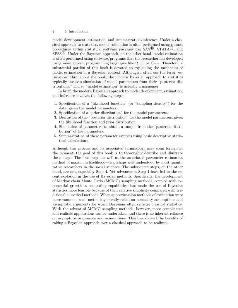
In brief, the modern Bayesian approach to model development, estimation,and inference involves the following steps:
1. Specification of a “likelihood function” (or “sampling density”) for thedata, given the model parameters.
2. Specification of a “prior distribution” for the model parameters.3. Derivation of the “posterior distribution” for the model parameters, given
the likelihood function and prior distribution.4. Simulation of parameters to obtain a sample from the “posterior distri-
bution” of the parameters.5. Summarization of these parameter samples using basic descriptive statis-
tical calculations.
Although this process and its associated terminology may seem foreign atthe moment, the goal of this book is to thoroughly describe and illustratethese steps. The first step—as well as the associated parameter estimationmethod of maximum likelihood—is perhaps well understood by most quanti-tative researchers in the social sciences. The subsequent steps, on the otherhand, are not, especially Step 4. Yet advances in Step 4 have led to the re-cent explosion in the use of Bayesian methods. Specifically, the developmentof Markov chain Monte Carlo (MCMC) sampling methods, coupled with ex-ponential growth in computing capabilities, has made the use of Bayesianstatistics more feasible because of their relative simplicity compared with tra-ditional numerical methods. When approximation methods of estimation weremore common, such methods generally relied on normality assumptions andasymptotic arguments for which Bayesians often criticize classical statistics.With the advent of MCMC sampling methods, however, more complicatedand realistic applications can be undertaken, and there is no inherent relianceon asymptotic arguments and assumptions. This has allowed the benefits oftaking a Bayesian approach over a classical approach to be realized.

1.1 Outline 3
1.1 Outline
For this book, I assume only a familiarity with (1) classical social sciencestatistics and (2) matrix algebra and basic calculus. For those without sucha background, or for whom basic concepts from these subjects are not freshin memory, there are two appendices at the end of the book. Appendix Acovers the basic ideas of calculus and matrix algebra needed to understandthe concepts of, and notation for, mathematical statistics. Appendix B brieflyreviews the Central Limit Theorem and its importance for classical hypothesistesting using a simulation study.
The first several chapters of this book lay a foundation for understandingthe Bayesian paradigm of statistics and some basic modern methods of esti-mating Bayesian models. Chapter 2 provides a review of (or introduction to)probability theory and probability distributions (see DeGroot 1986, for an ex-cellent background in probability theory; see Billingsley 1995 and Chung andAitSahlia 2003, for more advanced discussion, including coverage of Measuretheory). Within this chapter, I develop several simple probability distributionsthat are used in subsequent chapters as examples before jumping into morecomplex real-world models. I also discuss a number of real univariate andmultivariate distributions that are commonly used in social science research.
Chapter 2 also reviews the classical approach to statistical inference fromthe development of a likelihood function through the steps of estimating theparameters involved in it. Classical statistics is actually a combination of atleast two different historical strains in statistics: one involving Fisherian maxi-mum likelihood estimation and the other involving Fisherian and Neyman andPearsonian hypothesis testing and confidence interval construction (DeGroot1986; Edwards 1992; see Hubbard and Bayarri 2003 for a discussion of theconfusion regarding the two approaches). The approach commonly followedtoday is a hybrid of these traditions, and I lump them both under the term“classical statistics.” This chapter spells out the usual approach to derivingparameter estimates and conducting hypothesis tests under this paradigm.
Chapter 3 develops Bayes’ Theorem and discusses the Bayesian paradigmof statistics in depth. Specifically, I spend considerable time discussing theconcept of prior distributions, the classical statistical critique of their use,and the Bayesian responses. I begin the chapter with examples that use apoint-estimate approach to applying Bayes’ Theorem. Next, I turn to morerealistic examples involving probability distributions rather than points es-timates. For these examples, I use real distributions (binomial, poisson, andnormal for sampling distributions and beta, gamma, and inverse gamma forprior distributions). Finally, in this chapter, I discuss several additional prob-ability distributions that are not commonly used in social science research butare commonly used as prior distributions by Bayesians.
Chapter 4 introduces the rationale for MCMC methods, namely that sam-pling quantities from distributions can help us produce summaries of themthat allow us to answer our research questions. The chapter then describes

4 1 Introduction
some basic methods of sampling from arbitrary distributions and then de-velops the Gibbs sampler as a fundamental method for sampling from high-dimensional distributions that are common in social science research.
Chapter 5 introduces an alternative MCMC sampling method that canbe used when Gibbs sampling cannot be easily employed: the Metropolis-Hastings algorithm. In both Chapters 4 and 5, I apply these sampling methodsto distributions and problems that were used in Chapters 2 and 3 in order toexemplify the complete process of performing a Bayesian analysis up to, butnot including, assessing MCMC algorithm performance and evaluating modelfit.
Chapter 6 completes the exemplification of a Bayesian analysis by showing(1) how to monitor and assess MCMC algorithm performance and (2) how toevaluate model fit and compare models. The first part of the chapter is al-most entirely devoted to technical issues concerning MCMC implementation.A researcher must know that his/her estimation method is performing ac-ceptably, and s/he must know how to use the output to produce appropriateestimates. These issues are generally nonissues for most classical statisticalanalyses, because generic software exists for most applications. However, theyare important issues for Bayesian analyses, which typically involve softwarethat is developed by the researcher him/herself. A benefit to this additionalstep in the process of analysis—evaluating algorithm performance—is that itrequires a much more intimate relationship with the data and model assump-tions than a classical analysis, which may have the potential to lull researchersinto a false sense of security about the validity of parameter estimates andmodel assumptions.
The second part of the chapter is largely substantive. All researchers, clas-sical or Bayesian, need to determine whether their models fit the data at handand whether one model is better than another. I attempt to demonstrate thatthe Bayesian paradigm offers considerably more information and flexibilitythan a classical approach in making these determinations. Although I cannotand do not cover all the possibilities, in this part of the chapter, I introducea number of approaches to consider.
The focus of the remaining chapters (7-10) is substantive and applied.These chapters are geared to developing and demonstrating MCMC algo-rithms for specific models that are common in social science research. Chap-ter 7 shows a Bayesian approach to the linear regression model. Chapter 8shows a Bayesian approach to generalized linear models, specifically the di-chotomous and ordinal probit models. Chapter 9 introduces a Bayesian ap-proach to hierarchical models. Finally, Chapter 10 introduces a Bayesian ap-proach to multivariate models. The algorithms developed in these chapters,although fairly generic, should not be considered endpoints for use by re-searchers. Instead, they should be considered as starting points for the devel-opment of algorithms tailored to user-specific problems.
In contrast to the use of sometimes contrived examples in the first sixchapters, almost all examples in the latter chapters concern real probability

1.2 A note on programming 5
distributions, real research questions, and real data. To that end, some ad-ditional beneficial aspects of Bayesian analysis are introduced, including theability to obtain posterior distributions for parameters that are not directlyestimated as part of a model, and the ease with which missing data can behandled.
1.2 A note on programming
Throughout the text, I present R programs for virtually all MCMC algo-rithms in order to demystify the linkage between model development andestimation. R is a freely available, downloadable programming package and isextremely well suited to Bayesian analyses (www.r-project.org). However, Ris only one possible programming language in which MCMC algorithms canbe written. Another package I use in the chapter on hierarchical modeling isWinBugs. WinBugs is a freely available, downloadable software package thatperforms Gibbs sampling with relative ease (www.mrc-bsu.cam.ac.uk/bugs).I strongly suggest learning how to use WinBugs if you expect to routinelyconduct Bayesian analyses. The syntax of WinBugs is very similar to R, andso the learning curve is not steep once R is familiar. The key advantage toWinBugs over R is that WinBugs derives conditional distributions for Gibbssampling for you; the user simply has to specify the model. In R, on the otherhand, the conditional distributions must be derived mathematically by theuser and then programmed. The key advantage of R over WinBugs, however,is that R—as a generic programming language—affords the user greater flex-ibility in reading data from files, modeling data, and writing output to files.For learning how to program in R, I recommend downloading the variousdocumentation available when you download the software. I also recommendVenables and Ripley’s books for S and S-Plus R© programming (1999, 2000).The S and S-Plus languages are virtually identical to R, but they are notfreely available.
I even more strongly recommend learning a generic programming languagelike C or C++. Although I show R programs throughout the text, I haveused UNIX-based C extensively in my own work, because programs tend torun much faster in UNIX-based C than in any other language. First, UNIXsystems are generally faster than other systems. Second, C++ is the languagein which many software packages are written. Thus, writing a program in asoftware package’s language when that language itself rests on a foundationin C/C++ makes any algorithm in that language inherently slower than itwould be if it were written directly in C/C++.
C and C++ are not difficult languages to learn. In fact, if you can pro-gram in R, you can program in C, because the syntax for many commandsis close to identical. Furthermore, if you can program in SAS or STATA, youcan learn C very easily. The key differences between database programminglanguages like SAS and generic programming languages like C are in terms
6 1 Introduction
of how elements in arrays are handled. In C, each element in an array mustbe handled; in database and statistics programming languages, commandstypically apply to an entire column (variable) at once. For example, recodinggender in a database or statistics package requires only a single commandthat is systematically applied to all observations automatically. In a genericprogramming language, on the other hand, one has to apply the commandrepeatedly to every row (usually using a loop). R combines both features, asI exemplify throughout the examples in the text: Elements in arrays may behandled one-at-a-time, or they may be handled all at once.
Another difference between generic programming languages like C anddatabase packages is that generic languages do not have many functions builtinto them. For example, simulating variates from normal distributions in R,SAS, and STATA is easy because these languages have built-in functions thatcan be used to do so. In a generic language like C, on the other hand, one musteither write the function oneself or find a function in an existing library. Onceagain, although this may seem like a drawback, it takes very little time toamass a collection of functions which can be used in all subsequent programs.
If you choose to learn C, I recommend two books: Teach Yourself C in 24Hours (Zhang 1997) and Numerical Recipes in C (Press et al. 2002). TeachYourself C is easy to read and will show you practically everything you needto know about the language, with the exception of listing all the built-infunctions that C-compilers possess. Numerical Recipes provides a number ofalgorithms/functions for conducting various mathematical operations, such asCholesky decomposition, matrix inversion, etc.
1.3 Symbols used throughout the book
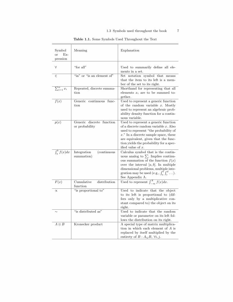
A number of mathematical symbols that may be unfamiliar are used through-out this book. The meanings of most symbols are discussed upon their firstappearance, but here I provide a nonexhaustive summary table for reference.Parts of this table may not be helpful until certain sections of the book havebeen read; the table is a summary, and so some expressions/terms are usedhere but are defined within the text (e.g., density function).
As for general notation that is not described elsewhere, I use lowercaseletters, generally from the end of the alphabet (e.g., x), to represent randomvariables and uppercase versions of these letters to represent vectors of randomvariables or specific values of a random variable (e.g., X). I violate this generalrule only in a few cases for the sake of clarity. Greek letters are reserved fordistribution parameters (which, from a Bayesian view, can also be viewed asrandom variables). In some cases, I use p() to represent probabilities; in othercases, for the sake of clarity, I use pr().
1.3 Symbols used throughout the book 7
Table 1.1. Some Symbols Used Throughout the Text
Symbolor Ex-pression
Meaning Explanation
∀ “for all” Used to summarily define all ele-ments in a set.
∈ “in” or “is an element of” Set notation symbol that meansthat the item to its left is a mem-ber of the set to its right.Pn
i=1 xi Repeated, discrete summa-tion
Shorthand for representing that allelements xi are to be summed to-gether.
f(x) Generic continuous func-tion
Used to represent a generic functionof the random variable x. Mostlyused to represent an algebraic prob-ability density function for a contin-uous variable.
p(x) Generic discrete functionor probability
Used to represent a generic functionof a discrete random variable x. Alsoused to represent “the probability ofx.” In a discrete sample space, theseare equivalent, given that the func-tion yields the probability for a spec-ified value of x.R b
af(x)dx Integration (continuous
summation)Calculus symbol that is the contin-uous analog to
P. Implies continu-
ous summation of the function f(x)over the interval [a, b]. In multipledimensional problems, multiple inte-gration may be used (e.g.,
R b
a
R d
c. . .).
See Appendix A.
F (x) Cumulative distributionfunction
Used to representR X
−∞ f(x)dx.
∝ “is proportional to” Used to indicate that the objectto its left is proportional to (dif-fers only by a multiplicative con-stant compared to) the object on itsright.
∼ “is distributed as” Used to indicate that the randomvariable or parameter on its left fol-lows the distribution on its right.
A⊗B Kronecker product A special type of matrix multiplica-tion in which each element of A isreplaced by itself multiplied by theentirety of B : AijB, ∀i, j.

2
Probability Theory and Classical Statistics
Statistical inference rests on probability theory, and so an in-depth under-standing of the basics of probability theory is necessary for acquiring a con-ceptual foundation for mathematical statistics. First courses in statistics forsocial scientists, however, often divorce statistics and probability early withthe emphasis placed on basic statistical modeling (e.g., linear regression) inthe absence of a grounding of these models in probability theory and prob-ability distributions. Thus, in the first part of this chapter, I review somebasic concepts and build statistical modeling from probability theory. In thesecond part of the chapter, I review the classical approach to statistics as itis commonly applied in social science research.
2.1 Rules of probability
Defining “probability” is a difficult challenge, and there are several approachesfor doing so. One approach to defining probability concerns itself with thefrequency of events in a long, perhaps infinite, series of trials. From that per-spective, the reason that the probability of achieving a heads on a coin flip is1/2 is that, in an infinite series of trials, we would see heads 50% of the time.This perspective grounds the classical approach to statistical theory and mod-eling. Another perspective on probability defines probability as a subjectiverepresentation of uncertainty about events. When we say that the probabilityof observing heads on a single coin flip is 1/2, we are really making a seriesof assumptions, including that the coin is fair (i.e., heads and tails are infact equally likely), and that in prior experience or learning we recognize thatheads occurs 50% of the time. This latter understanding of probability groundsBayesian statistical thinking. From that view, the language and mathematicsof probability is the natural language for representing uncertainty, and thereare subjective elements that play a role in shaping probabilistic statements.
Although these two approaches to understanding probability lead to dif-ferent approaches to statistics, some fundamental axioms of probability are
10 2 Probability Theory and Classical Statistics
important and agreed upon. We represent the probability that a particularevent, E, will occur as p(E). All possible events that can occur in a single trialor experiment constitute a sample space (S), and the sum of the probabilitiesof all possible events in the sample space is 11:∑
∀E∈S
p(E) = 1. (2.1)
As an example that highlights this terminology, a single coin flip is atrial/experiment with possible events “Heads” and “Tails,” and therefore hasa sample space of S = Heads, Tails. Assuming the coin is fair, the probabil-ities of each event are 1/2, and—as used in social science—the record of theoutcome of the coin-flipping process can be considered a “random variable.”
We can extend the idea of the probability of observing one event in one trial(e.g., one head in one coin toss) to multiple trials and events (e.g., two headsin two coin tosses). The probability assigned to multiple events, say A andB, is called a “joint” probability, and we denote joint probabilities using thedisjunction symbol from set notation (∩) or commas, so that the probabilityof observing events A and B is simply p(A,B). When we are interested in theoccurrence of event A or event B, we use the union symbol (∪), or simply theword “or”: p(A ∪B) ≡ p(A or B).
The “or” in probability is somewhat different than the “or” in commonusage. Typically, in English, when we use the word “or,” we are referringto the occurrence of one or another event, but not both. In the language oflogic and probability, when we say “or” we are referring to the occurrence ofeither event or both events. Using a Venn diagram clarifies this concept (seeFigure 2.1).
In the diagram, the large rectangle denotes the sample space. Circles Aand B denote events A and B, respectively. The overlap region denotes thejoint probability p(A,B). p(A or B) is the region that is A only, B only, andthe disjunction region. A simple rule follows:
p(A or B) = p(A) + p(B)− p(A,B). (2.2)
p(A,B) is subtracted, because it is added twice when summing p(A) and p(B).There are two important rules for joint probabilities. First:
p(A,B) = p(A)p(B) (2.3)
iff (if and only if) A and B are independent events. In probability theory,independence means that event A has no bearing on the occurrence of eventB. For example, two coin flips are independent events, because the outcomeof the first flip has no bearing on the outcome of the second flip. Second, if Aand B are not independent, then:
1 If the sample space is continuous, then integration, rather than summation, isused. We will discuss this issue in greater depth shortly.
2.1 Rules of probability 11
A B
A∩B
A∪BNot A∪B
Fig. 2.1. Sample Venn diagram: Outer box is sample space; and circles are eventsA and B.
p(A,B) = p(A|B)p(B). (2.4)
Expressed another way:
p(A|B) =p(A,B)p(B)
. (2.5)
Here, the “|” represents a conditional and is read as “given.” This last rule canbe seen via Figure 2.1. p(A|B) refers to the region that contains A, given thatwe know B is already true. Knowing that B is true implies a reduction in thetotal sample space from the entire rectangle to the circle B only. Thus, p(A)is reduced to the (A,B) region, given the reduced space B, and p(A|B) is theproportion of the new sample space, B, which includes A. Returning to therule above, which states p(A,B) = p(A)p(B) iff A and B are independent,if A and B are independent, then knowing B is true in that case does notreduce the sample space. In that case, then p(A|B) = p(A), which leaves uswith the first rule.
12 2 Probability Theory and Classical Statistics
Although we have limited our discussion to two events, these rules gener-alize to more than two events. For example, the probability of observing threeindependent events A, B, and C, is p(A,B,C) = p(A)p(B)p(C). More gener-ally, the joint probability of n independent events, E1, E2 . . . En, is
∏ni=1 p(Ei),
where the∏
symbol represents repeated multiplication. This result is veryuseful in statistics in constructing likelihood functions. See DeGroot (1986)for additional generalizations. Surprisingly, with basic generalizations, thesebasic probability rules are all that are needed to develop the most commonprobability models that are used in social science statistics.
2.2 Probability distributions in general
The sample space for a single coin flip is easy to represent using set notationas we did above, because the space consists of only two possible events (headsor tails). Larger sample spaces, like the sample space for 100 coin flips, orthe sample space for drawing a random integer between 1 and 1,000,000,however, are more cumbersome to represent using set notation. Consequently,we often use functions to assign probabilities or relative frequencies to allevents in a sample space, where these functions contain “parameters” thatgovern the shape and scale of the curve defined by the function, as well asexpressions containing the random variable to which the function applies.These functions are called “probability density functions,” if the events arecontinuously distributed, or “probability mass functions,” if the events arediscretely distributed. By continuous, I mean that all values of a randomvariable x are possible in some region (like x = 1.2345); by discrete, I meanthat only some values of x are possible (like all integers between 1 and 10).These functions are called “density” and “mass” functions because they tell uswhere the most (and least) likely events are concentrated in a sample space.We often abbreviate both types of functions using “pdf,” and we denote arandom variable x that has a particular distribution g(.) using the genericnotation: x ∼ g(.), where the “∼” is read “is distributed as,” the g denotes aparticular distribution, and the “.” contains the parameters of the distributiong.
If x ∼ g(.), then the pdf itself is expressed as f(x) = . . . , wherethe “. . .” is the particular algebraic function that returns the relative fre-quency/probability associated with each value of x. For example, one of themost common continuous pdfs in statistics is the normal distribution, whichhas two parameters—a mean (µ) and variance (σ2). If a variable x has prob-abilities/relative frequencies that follow a normal distribution, then we sayx ∼ N(µ, σ2), and the pdf is:
f(x) =1√
2πσ2exp
− (x− µ)2
2σ2
.
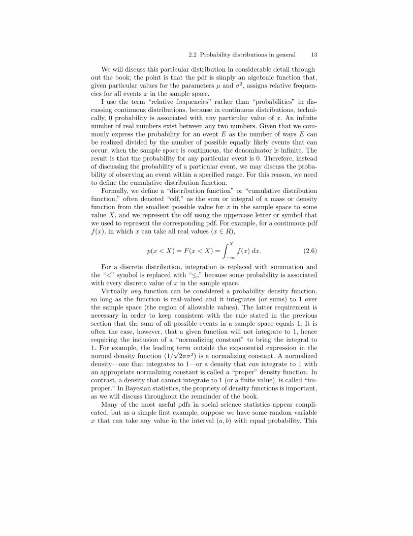
2.2 Probability distributions in general 13
We will discuss this particular distribution in considerable detail through-out the book; the point is that the pdf is simply an algebraic function that,given particular values for the parameters µ and σ2, assigns relative frequen-cies for all events x in the sample space.
I use the term “relative frequencies” rather than “probabilities” in dis-cussing continuous distributions, because in continuous distributions, techni-cally, 0 probability is associated with any particular value of x. An infinitenumber of real numbers exist between any two numbers. Given that we com-monly express the probability for an event E as the number of ways E canbe realized divided by the number of possible equally likely events that canoccur, when the sample space is continuous, the denominator is infinite. Theresult is that the probability for any particular event is 0. Therefore, insteadof discussing the probability of a particular event, we may discuss the proba-bility of observing an event within a specified range. For this reason, we needto define the cumulative distribution function.
Formally, we define a “distribution function” or “cumulative distributionfunction,” often denoted “cdf,” as the sum or integral of a mass or densityfunction from the smallest possible value for x in the sample space to somevalue X, and we represent the cdf using the uppercase letter or symbol thatwe used to represent the corresponding pdf. For example, for a continuous pdff(x), in which x can take all real values (x ∈ R),
p(x < X) = F (x < X) =∫ X
−∞f(x) dx. (2.6)
For a discrete distribution, integration is replaced with summation andthe “<” symbol is replaced with “≤,” because some probability is associatedwith every discrete value of x in the sample space.
Virtually any function can be considered a probability density function,so long as the function is real-valued and it integrates (or sums) to 1 overthe sample space (the region of allowable values). The latter requirement isnecessary in order to keep consistent with the rule stated in the previoussection that the sum of all possible events in a sample space equals 1. It isoften the case, however, that a given function will not integrate to 1, hencerequiring the inclusion of a “normalizing constant” to bring the integral to1. For example, the leading term outside the exponential expression in thenormal density function (1/
√2πσ2) is a normalizing constant. A normalized
density—one that integrates to 1—or a density that can integrate to 1 withan appropriate normalizing constant is called a “proper” density function. Incontrast, a density that cannot integrate to 1 (or a finite value), is called “im-proper.” In Bayesian statistics, the propriety of density functions is important,as we will discuss throughout the remainder of the book.
Many of the most useful pdfs in social science statistics appear compli-cated, but as a simple first example, suppose we have some random variablex that can take any value in the interval (a, b) with equal probability. This
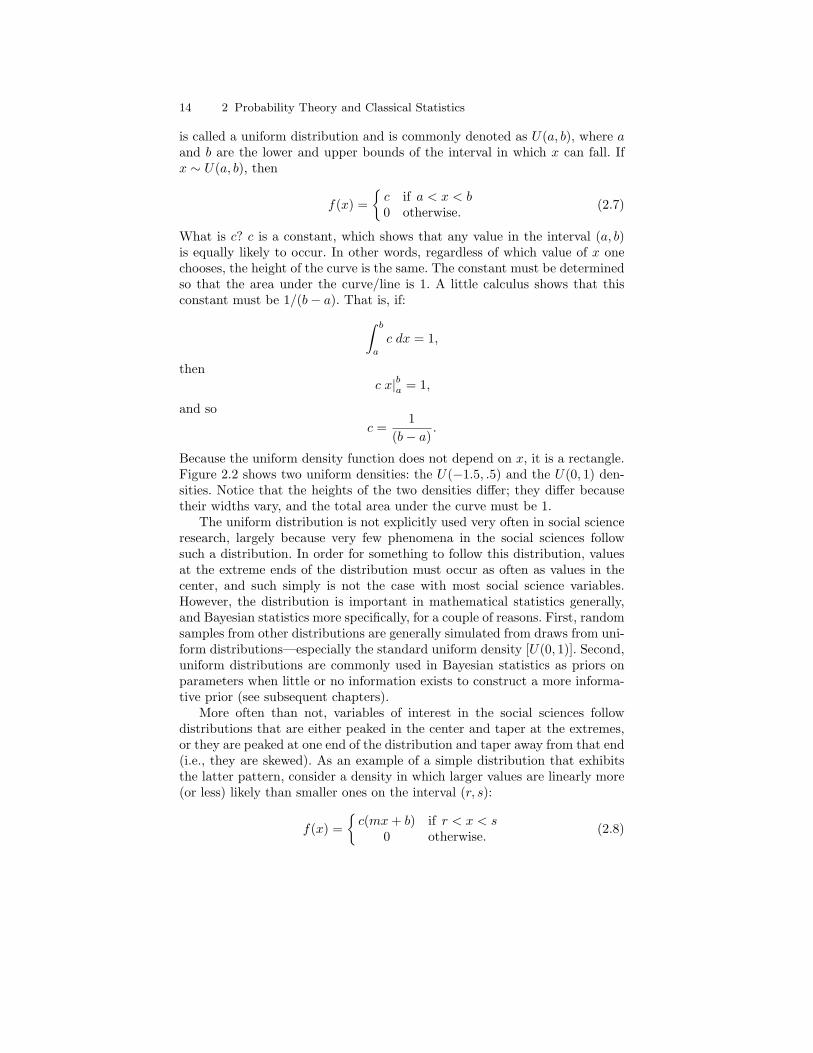
14 2 Probability Theory and Classical Statistics
is called a uniform distribution and is commonly denoted as U(a, b), where aand b are the lower and upper bounds of the interval in which x can fall. Ifx ∼ U(a, b), then
f(x) =
c if a < x < b0 otherwise. (2.7)
What is c? c is a constant, which shows that any value in the interval (a, b)is equally likely to occur. In other words, regardless of which value of x onechooses, the height of the curve is the same. The constant must be determinedso that the area under the curve/line is 1. A little calculus shows that thisconstant must be 1/(b− a). That is, if:∫ b
a
c dx = 1,
thenc x|ba = 1,
and soc =
1(b− a)
.
Because the uniform density function does not depend on x, it is a rectangle.Figure 2.2 shows two uniform densities: the U(−1.5, .5) and the U(0, 1) den-sities. Notice that the heights of the two densities differ; they differ becausetheir widths vary, and the total area under the curve must be 1.
The uniform distribution is not explicitly used very often in social scienceresearch, largely because very few phenomena in the social sciences followsuch a distribution. In order for something to follow this distribution, valuesat the extreme ends of the distribution must occur as often as values in thecenter, and such simply is not the case with most social science variables.However, the distribution is important in mathematical statistics generally,and Bayesian statistics more specifically, for a couple of reasons. First, randomsamples from other distributions are generally simulated from draws from uni-form distributions—especially the standard uniform density [U(0, 1)]. Second,uniform distributions are commonly used in Bayesian statistics as priors onparameters when little or no information exists to construct a more informa-tive prior (see subsequent chapters).
More often than not, variables of interest in the social sciences followdistributions that are either peaked in the center and taper at the extremes,or they are peaked at one end of the distribution and taper away from that end(i.e., they are skewed). As an example of a simple distribution that exhibitsthe latter pattern, consider a density in which larger values are linearly more(or less) likely than smaller ones on the interval (r, s):
f(x) =
c(mx + b) if r < x < s0 otherwise. (2.8)

2.2 Probability distributions in general 15
−2 −1 0 1 2
0.0
0.5
1.0
1.5
2.0
x
f(x)
U(−1.5,.5) density
U(0,1) density
Fig. 2.2. Two uniform distributions.
This density function is a line, with r and s as the left and right bound-aries, respectively. As with the uniform density, c is a constant—a normalizingconstant—that must be determined in order for the density to integrate to 1.For this generic linear density, the normalizing constant is (see Exercises):
c =2
(s− r)[m(s + r) + 2b].
In this density, the relative frequency of any particular value of x depends onx, as well as on the parameters m and b. If m is positive, then larger valuesof x occur more frequently than smaller values. If m is negative, then smallervalues of x occur more frequently than larger values.
What type of variable might follow a distribution like this in social sci-ence research? I would argue that many attitudinal items follow this sort ofdistribution, especially those with ceiling or floor effects. For example, in the2000 General Social Survey (GSS) special topic module on freedom, a ques-tion was asked regarding the belief in the importance of being able to expressunpopular views in a democracy. Figure 2.3 shows the histogram of responsesfor this item with a linear density superimposed. A linear density appears to
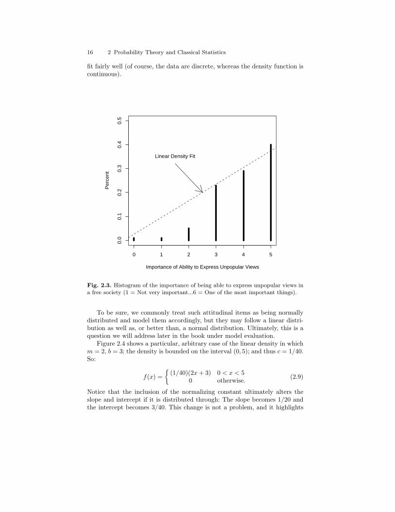
16 2 Probability Theory and Classical Statistics
fit fairly well (of course, the data are discrete, whereas the density function iscontinuous).
0 1 2 3 4 5
0.0
0.1
0.2
0.3
0.4
0.5
Importance of Ability to Express Unpopular Views
Per
cent
Linear Density Fit
Fig. 2.3. Histogram of the importance of being able to express unpopular views ina free society (1 = Not very important...6 = One of the most important things).
To be sure, we commonly treat such attitudinal items as being normallydistributed and model them accordingly, but they may follow a linear distri-bution as well as, or better than, a normal distribution. Ultimately, this is aquestion we will address later in the book under model evaluation.
Figure 2.4 shows a particular, arbitrary case of the linear density in whichm = 2, b = 3; the density is bounded on the interval (0, 5); and thus c = 1/40.So:
f(x) =
(1/40)(2x + 3) 0 < x < 50 otherwise. (2.9)
Notice that the inclusion of the normalizing constant ultimately alters theslope and intercept if it is distributed through: The slope becomes 1/20 andthe intercept becomes 3/40. This change is not a problem, and it highlights
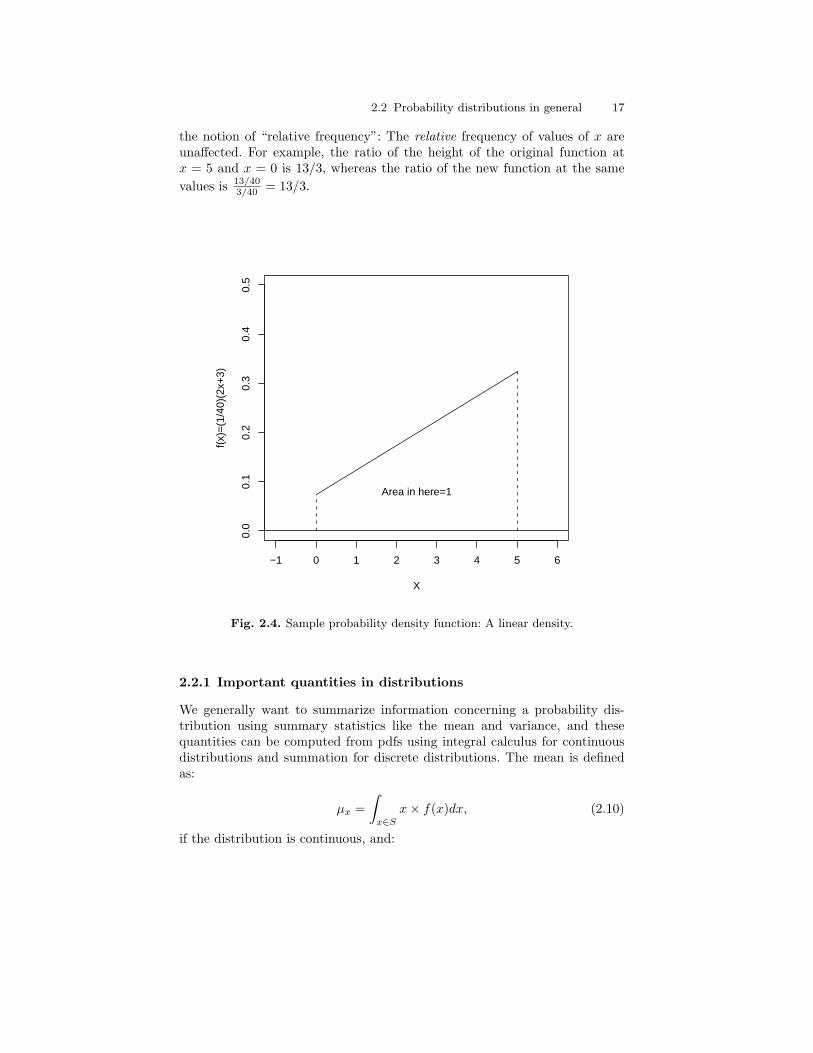
2.2 Probability distributions in general 17
the notion of “relative frequency”: The relative frequency of values of x areunaffected. For example, the ratio of the height of the original function atx = 5 and x = 0 is 13/3, whereas the ratio of the new function at the samevalues is 13/40
3/40 = 13/3.
−1 0 1 2 3 4 5 6
0.0
0.1
0.2
0.3
0.4
0.5
X
f(x)
=(1
/40)
(2x+
3)
Area in here=1
Fig. 2.4. Sample probability density function: A linear density.
2.2.1 Important quantities in distributions
We generally want to summarize information concerning a probability dis-tribution using summary statistics like the mean and variance, and thesequantities can be computed from pdfs using integral calculus for continuousdistributions and summation for discrete distributions. The mean is definedas:
µx =∫
x∈S
x× f(x)dx, (2.10)
if the distribution is continuous, and:

18 2 Probability Theory and Classical Statistics
µx =∑x∈S
x× p(x), (2.11)
if the distribution is discrete. The mean is often called the “expectation” orexpected value of x and is denoted as E(x). The variance is defined as:
σ2x =
∫x∈S
(x− µx)2 × f(x)dx, (2.12)
if the distribution is continuous, and:
σ2x =
1n
∑x∈S
(x− µx)2, (2.13)
if the distribution is discrete. Using the expectation notation introduced forthe mean, the variance is sometimes referred to as E((x − µx)2); in otherwords, the variance is the expected value of the squared deviation from themean.2
Quantiles, including the median, can also be computed using integral cal-culus. The median of a continuous distribution, for example, is obtained byfinding Q that satisfies:
.5 =∫ Q
−∞f(x)dx. (2.14)
Returning to the examples in the previous section, the mean of the U(a, b)distribution is:
E(x) = µx =∫ b
a
x×(
1b− a
)dx =
b + a
2,
and the variance is:
E((x− µx)2) =∫ b
a
1b− a
(x− µx)2 dx =(b− a)2
12.
For the linear density with the arbitrary parameter values introduced inEquation 2.9 (f(x) = (1/40)(2x + 3)), the mean is:
µx =∫ 5
0
x× (1/40)(2x + 3)dx = (1/240)(4x3 + 9x2)dx
∣∣∣∣50
= 3.02.
The variance is:
2 The sample mean, unlike the population distribution mean shown here, is esti-mated with (n − 1) in the denominator rather than with n. This is a correctionfactor for the known bias in estimating the population variance from sample data.It becomes less important asymptotically (as n →∞.)
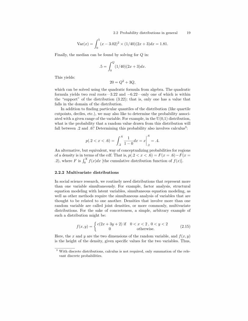
2.2 Probability distributions in general 19
Var(x) =∫ 5
0
(x− 3.02)2 × (1/40)(2x + 3)dx = 1.81.
Finally, the median can be found by solving for Q in:
.5 =∫ Q
0
(1/40)(2x + 3)dx.
This yields:20 = Q2 + 3Q,
which can be solved using the quadratic formula from algebra. The quadraticformula yields two real roots—3.22 and −6.22—only one of which is withinthe “support” of the distribution (3.22); that is, only one has a value thatfalls in the domain of the distribution.
In addition to finding particular quantiles of the distribution (like quartilecutpoints, deciles, etc.), we may also like to determine the probability associ-ated with a given range of the variable. For example, in the U(0,1) distribution,what is the probability that a random value drawn from this distribution willfall between .2 and .6? Determining this probability also involves calculus3:
p(.2 < x < .6) =∫ .6
.2
11− 0
dx = x
∣∣∣∣.6.2
= .4.
An alternative, but equivalent, way of conceptualizing probabilities for regionsof a density is in terms of the cdf. That is, p(.2 < x < .6) = F (x = .6)−F (x =.2), where F is
∫X
0f(x)dx [the cumulative distribution function of f(x)].
2.2.2 Multivariate distributions
In social science research, we routinely need distributions that represent morethan one variable simultaneously. For example, factor analysis, structuralequation modeling with latent variables, simultaneous equation modeling, aswell as other methods require the simultaneous analysis of variables that arethought to be related to one another. Densities that involve more than onerandom variable are called joint densities, or more commonly, multivariatedistributions. For the sake of concreteness, a simple, arbitrary example ofsuch a distribution might be:
f(x, y) =
c(2x + 3y + 2) if 0 < x < 2 , 0 < y < 20 otherwise. (2.15)
Here, the x and y are the two dimensions of the random variable, and f(x, y)is the height of the density, given specific values for the two variables. Thus,
3 With discrete distributions, calculus is not required, only summation of the rele-vant discrete probabilities.
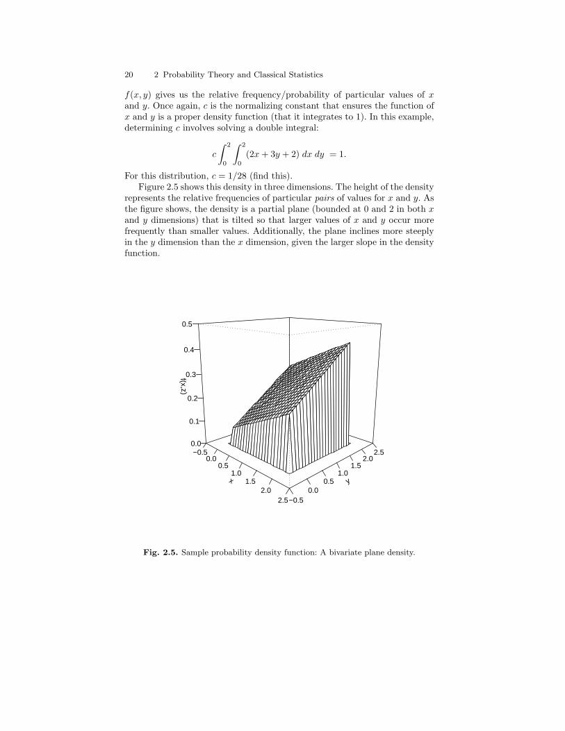
20 2 Probability Theory and Classical Statistics
f(x, y) gives us the relative frequency/probability of particular values of xand y. Once again, c is the normalizing constant that ensures the function ofx and y is a proper density function (that it integrates to 1). In this example,determining c involves solving a double integral:
c
∫ 2
0
∫ 2
0
(2x + 3y + 2) dx dy = 1.
For this distribution, c = 1/28 (find this).Figure 2.5 shows this density in three dimensions. The height of the density
represents the relative frequencies of particular pairs of values for x and y. Asthe figure shows, the density is a partial plane (bounded at 0 and 2 in both xand y dimensions) that is tilted so that larger values of x and y occur morefrequently than smaller values. Additionally, the plane inclines more steeplyin the y dimension than the x dimension, given the larger slope in the densityfunction.
x
−0.50.0
0.51.0
1.52.0
2.5
y
−0.50.0
0.51.0
1.52.0
2.5
f(x,z)
0.0
0.1
0.2
0.3
0.4
0.5
Fig. 2.5. Sample probability density function: A bivariate plane density.
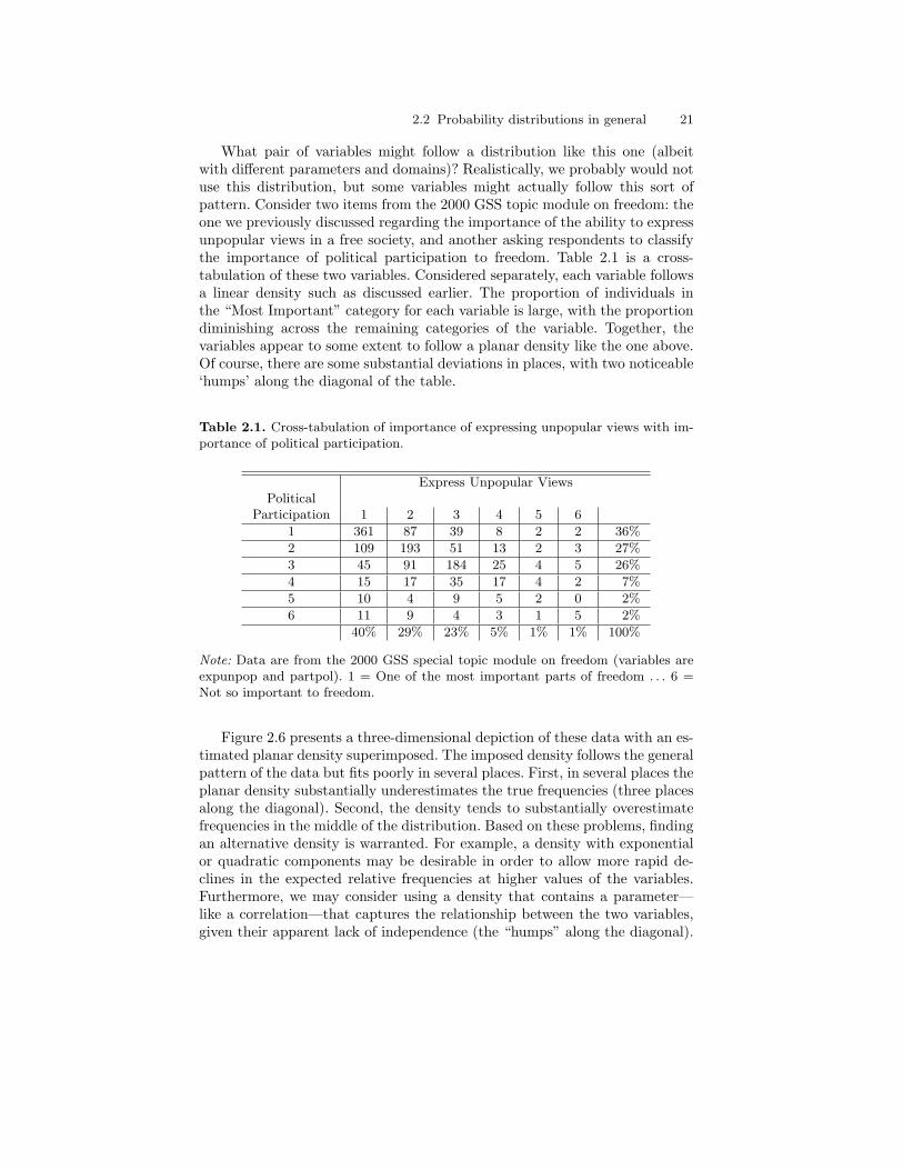
2.2 Probability distributions in general 21
What pair of variables might follow a distribution like this one (albeitwith different parameters and domains)? Realistically, we probably would notuse this distribution, but some variables might actually follow this sort ofpattern. Consider two items from the 2000 GSS topic module on freedom: theone we previously discussed regarding the importance of the ability to expressunpopular views in a free society, and another asking respondents to classifythe importance of political participation to freedom. Table 2.1 is a cross-tabulation of these two variables. Considered separately, each variable followsa linear density such as discussed earlier. The proportion of individuals inthe “Most Important” category for each variable is large, with the proportiondiminishing across the remaining categories of the variable. Together, thevariables appear to some extent to follow a planar density like the one above.Of course, there are some substantial deviations in places, with two noticeable‘humps’ along the diagonal of the table.
Table 2.1. Cross-tabulation of importance of expressing unpopular views with im-portance of political participation.
Express Unpopular ViewsPolitical
Participation 1 2 3 4 5 6
1 361 87 39 8 2 2 36%
2 109 193 51 13 2 3 27%
3 45 91 184 25 4 5 26%
4 15 17 35 17 4 2 7%
5 10 4 9 5 2 0 2%
6 11 9 4 3 1 5 2%
40% 29% 23% 5% 1% 1% 100%
Note: Data are from the 2000 GSS special topic module on freedom (variables areexpunpop and partpol). 1 = One of the most important parts of freedom . . . 6 =Not so important to freedom.
Figure 2.6 presents a three-dimensional depiction of these data with an es-timated planar density superimposed. The imposed density follows the generalpattern of the data but fits poorly in several places. First, in several places theplanar density substantially underestimates the true frequencies (three placesalong the diagonal). Second, the density tends to substantially overestimatefrequencies in the middle of the distribution. Based on these problems, findingan alternative density is warranted. For example, a density with exponentialor quadratic components may be desirable in order to allow more rapid de-clines in the expected relative frequencies at higher values of the variables.Furthermore, we may consider using a density that contains a parameter—like a correlation—that captures the relationship between the two variables,given their apparent lack of independence (the “humps” along the diagonal).
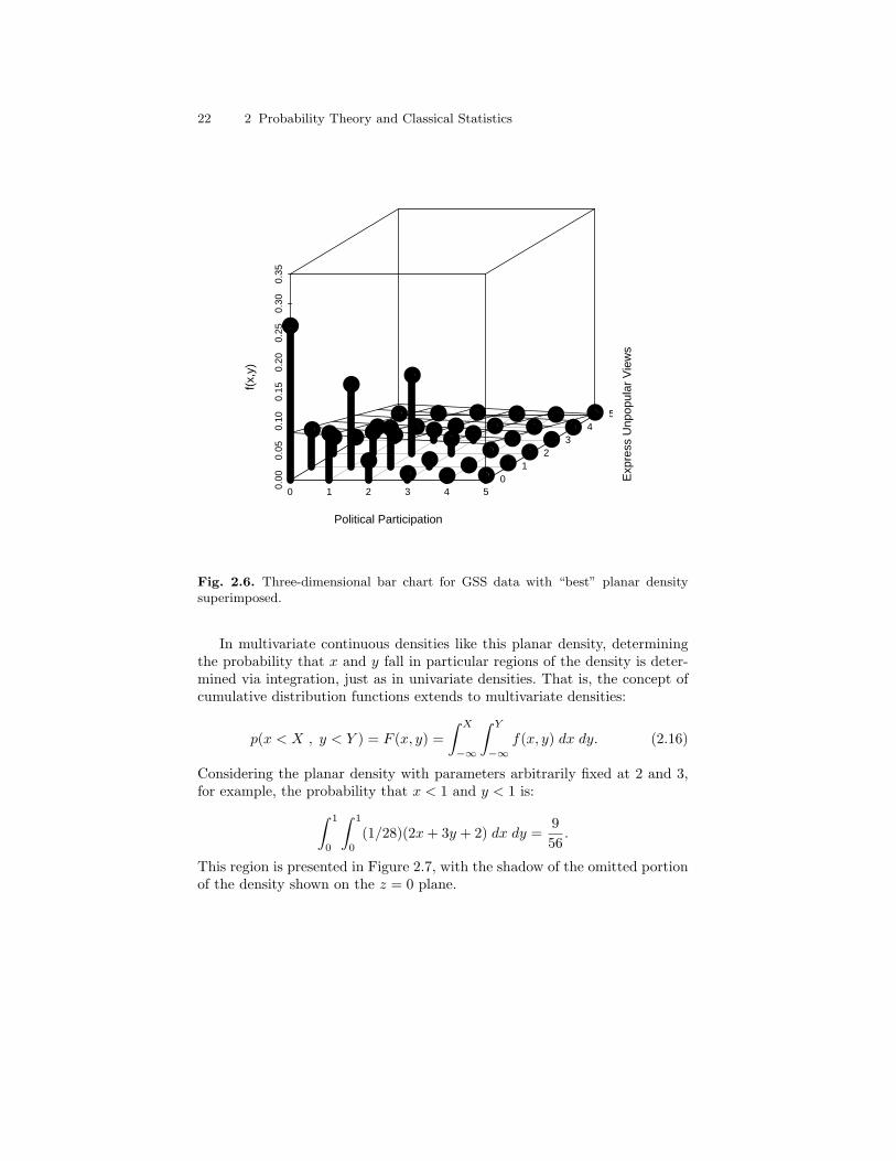
22 2 Probability Theory and Classical Statistics
0 1 2 3 4 50.00
0.05
0.10
0.15
0.20
0.25
0.30
0.35
01
23
45
Political Participation
Exp
ress
Unp
opul
ar V
iew
s
f(x,
y)
Fig. 2.6. Three-dimensional bar chart for GSS data with “best” planar densitysuperimposed.
In multivariate continuous densities like this planar density, determiningthe probability that x and y fall in particular regions of the density is deter-mined via integration, just as in univariate densities. That is, the concept ofcumulative distribution functions extends to multivariate densities:
p(x < X , y < Y ) = F (x, y) =∫ X
−∞
∫ Y
−∞f(x, y) dx dy. (2.16)
Considering the planar density with parameters arbitrarily fixed at 2 and 3,for example, the probability that x < 1 and y < 1 is:∫ 1
0
∫ 1
0
(1/28)(2x + 3y + 2) dx dy =956
.
This region is presented in Figure 2.7, with the shadow of the omitted portionof the density shown on the z = 0 plane.

2.2 Probability distributions in general 23
x
−0.50.0
0.51.0
1.52.0
2.5
y
−0.50.0
0.51.0
1.52.0
2.5
f(x,z)
0.0
0.1
0.2
0.3
0.4
0.5
Fig. 2.7. Representation of bivariate cumulative distribution function: Area underbivariate plane density from 0 to 1 in both dimensions.
2.2.3 Marginal and conditional distributions
Although determining the probabilities for particular regions of multivariatedensities is important, we may be interested in only a subset of the dimen-sions of a multivariate density. Two types of “subsets” are frequently needed:marginal distributions and conditional distributions. The data contained inTable 2.1 help differentiate these two types of distributions.
The marginal distribution for the “Express unpopular views” item is therow at the bottom of the table: It is the distribution of this variable summingacross the categories of the other variable (or integrating, if the density werecontinuous). The conditional distribution of this item, on the other hand,is the row of the table corresponding to a particular value for the politicalparticipation variable. For example, the conditional distribution for expressingunpopular views, given the value of “1” for political participation, consists ofthe data in the first row of the table (361, 87, 39, 8, 2, and 2, or in renormalizedpercents: 72%, 17%, 8%, 2%, .4%, and .4%).

24 2 Probability Theory and Classical Statistics
Thus, we can think of marginal distributions for a variable as being theoriginal distribution “flattened” in one dimension, whereas the conditionaldistribution for a variable is a “slice” through one dimension.
Finding marginal and conditional distributions mathematically is concep-tually straightforward, although often difficult in practice. Although Equa-tion 2.5 was presented in terms of discrete probabilities, the rule also appliesto density functions. From Equation 2.5, a conditional distribution can becomputed as:
f(x|y) =f(x, y)f(y)
(2.17)
This equation says that the conditional distribution for x given y is equal tothe joint density of x and y divided by the marginal distribution for y, where amarginal distribution is the distribution of one variable, integrating/summingover the other variables in the joint density. Thus:
f(y) =∫
x∈S
f(x, y)dx. (2.18)
In terms of our bivariate distribution above (f(x, y) = (1/28)(2x+3y+2)),the marginal distributions for x and y can be found as:
f(x) =∫ 2
y=0
(1/28)(2x + 3y + 2)dy = (1/28)(4x + 10)
and
f(y) =∫ 2
x=0
(1/28)(2x + 3y + 2)dx = (1/28)(6y + 8).
The conditional distributions can then be found as:
f(x|y) =(1/28)(2x + 3y + 2)∫ 2
x=0(2x + 3y + 2)dx
=(1/28)(2x + 3y + 2)
(1/28)(6y + 8)
and
f(y|x) =(1/28)(2x + 3y + 2)∫ 2
y=0(2x + 3y + 2)dy
=(1/28)(2x + 3y + 2)
(1/28)(4x + 10).
Observe how the marginal distributions for each variable exclude the othervariable (as they should), whereas the conditional distributions do not. Once aspecific value for x or y is chosen in the conditional distribution, however, theremaining function will only depend on the variable of interest. Once again,in other words, the conditional distribution is akin to taking a slice throughone dimension of the bivariate distribution.
As a final example, take the conditional distribution f(x|y), where y = 0,so that we are looking at the slice of the bivariate distribution that lies on thex axis. The conditional distribution for that slice is:
2.3 Some important distributions in social science 25
f(x|y = 0) =2x + 3(y = 0) + 2
6(y = 0) + 8= (1/8)(2x + 2).
With very little effort, it is easy to see that this result gives us the formulafor the line that we observe in the x, z plane when we set y = 0 in the originalunnormalized function and we exclude the constant 1/8. In other words:
(1/8)(2x + 2) ∝ (1/28)(2x + 3y + 2)
when y = 0. Thus, an important finding is that the conditional distributionf(x|y) is proportional to the joint distribution for f(x, y) evaluated at a par-ticular value for y [expressed f(x|y) ∝ f(x, y)], differing only by a normalizingconstant. This fact will be useful when we discuss Gibbs sampling in Chap-ter 4.
2.3 Some important distributions in social science
Unlike the relatively simple distributions we developed in the previous sec-tion, the distributions that have been found to be most useful in social scienceresearch appear more complicated. However, it should be remembered that,despite their sometimes more complicated appearance, they are simply alge-braic functions that describe the relative frequencies of occurence for partic-ular values of a random variable. In this section, I discuss several of the mostimportant distributions used in social science research. I limit the discussionat this point to distributions that are commonly applied to random variablesas social scientists view them. In the next chapter, I discuss some additionaldistributions that are commonly used in Bayesian statistics as “prior distri-butions” for parameters (which, as we will see, are also treated as randomvariables by Bayesians). I recommend Evans, Hastings, and Peacock (2000)for learning more about these and other common probability distributions.
2.3.1 The binomial distribution
The binomial distribution is a common discrete distribution used in socialscience statistics. This distribution represents the probability for x successesin n trials, given a success probability p for each trial. If x ∼ Bin(n, p), then:
pr(x|n, p) =(
nx
)px(1− p)n−x. (2.19)
Here, I change the notation on the left side of the mass function to “pr”to avoid confusion with the parameter p in the function. The combinatorial,(
nx
), at the front of the function, compensates for the fact that the x suc-
cesses can come in any order in the n trials. For example, if we are interested
26 2 Probability Theory and Classical Statistics
in the probability of obtaining exactly 10 heads in 50 flips of a fair coin [thus,pr(x = 10 | n = 50, p = .5)], the 10 heads could occur back-to-back, or severalmay appear in a row, followed by several tails, followed by more heads, etc.This constant is computed as n!/(x!(n − x)!) and acts as a normalizing con-stant to ensure the mass under the curve sums to 1. The latter two terms inthe function multiply the independent success and failure probabilities, basedon the observed number of successes and failures. Once the parameters n andp are chosen, the probability of observing any number x of successes can becomputed/deduced. For example, if we wanted to know the probability of ex-actly x = 10 heads out of n = 50 flips, then we would simply substitute thosenumbers into the right side of the equation, and the result would tell us theprobability. If we wanted to determine the probability of obtaining at least 10heads in 50 flips, we would need to sum the probabilities from 10 successes upto 50 successes. Obviously, in this example, the probability of obtaining moreheads than 50 or fewer heads than 0 is 0. Hence, this sample space is boundedto counting integers between 0 and 50, and computing the probability of atleast 10 heads would require summing 41 applications of the function (forx = 10, x = 11, ..., x = 50).
The mean of the binomial distribution is np, and the variance of the bi-nomial distribution is np(1 − p). When p = .5, the distribution is symmetricaround the mean. When p > .5, the distribution is skewed to the left; whenp < .5, the distribution is skewed to the right. See Figure 2.8 for an example ofthe effect of p on the shape of the distribution (n = 10). Note that, althoughthe figure is presented in a histogram format for the purpose of appearance(the densities are presented as lines), the distribution is discrete, and so 0probability is associated with non-integer values of x.
A normal approximation to the binomial may be used when p is close to.5 and n is large, by setting µx = np and σx =
√np(1− p). For example,
in the case mentioned above in which we were interested in computing theprobability of obtaining 10 or more heads in a series of 50 coin flips, computing41 probabilities with the function would be tedious. Instead, we could setµx = 25, and σx =
√50(.5)(1− .5) = 3.54, and compute a z-score as z =
(10−25)/(3.54) = −4.24. Recalling from basic statistics that there is virtually0 probability in the tail of the z distribution to the left of −4.24, we wouldconclude that the probability of obtaining at least 10 heads is practically 1,using this approximation. In fact, the actual probability of obtaining at least10 heads is .999988.
When n = 1, the binomial distribution reduces to another important dis-tribution called the Bernoulli distribution. The binomial distribution is oftenused in social science statistics as a building block for models for dichotomousoutcome variables like whether a Republican or Democrat will win an upcom-ing election, whether an individual will die within a specified period of time,etc.

2.3 Some important distributions in social science 27
0 2 4 6 8 10
0.0
0.1
0.2
0.3
0.4
0.5
x
pr(x
)
Bin(p=.2) Bin(p=.5) Bin(p=.8)
Fig. 2.8. Some binomial distributions (with parameter n = 10).
2.3.2 The multinomial distribution
The multinomial distribution is a generalization of the binomial distributionin which there are more than two outcome categories, and thus, there aremore than two “success” probabilities (one for each outcome category). Ifx ∼ Multinomial(n, p1, p2, . . . , pk), then:
pr(x1 . . . xk | n, p1 . . . pk) =n!
x1! x2! . . . xk!px11 px2
2 . . . pxk
k , (2.20)
where the leading combinatorial expression is a normalizing constant,∑k
i=1 pi =1, and
∑ki=1 xi = n. Whereas the binomial distribution allows us to compute
the probability of obtaining a given number of successes (x) out of n trials,given a particular success probability (p), the multinomial distribution allowsus to compute the probability of obtaining particular sets of successes, givenn trials and given different success probabilities for each member of the set.To make this idea concrete, consider rolling a pair of dice. The sample space
28 2 Probability Theory and Classical Statistics
for possible outcomes of a single roll is S = 2, 3, 4, 5, 6, 7, 8, 9, 10, 11, 12, andwe can consider the number of occurrences in multiple rolls of each of theseoutcomes to be represented by a particular x (so, x1 represents the numberof times a 2 is rolled, x2 represents the number of times a 3 is rolled, etc.).The success probabilities for these possible outcomes vary, given the fact thatthere are more ways to obtain some sums than others. The vector of prob-abilities p1 . . . p11 is 1
36 , 236 , 3
36 , 436 , 5
36 , 636 , 5
36 , 436 , 3
36 , 236 , 1
36. Suppose we rollthe pair of dice 36 times. Then, if we want to know the probability of obtain-ing one “2”, two “3s”, three “4s”, etc., we would simply substitute n = 36,p1 = 1
36 , p2 = 236 , . . . , p11 = 1
36 , and x1 = 1, x2 = 2, x3 = 3, . . . into thefunction and compute the probability.
The multinomial distribution is often used in social science statistics tomodel variables with qualitatively different outcomes categories, like religiousaffiliation, political party affiliation, race, etc, and I will discuss this distribu-tion in more depth in later chapters as a building block of some generalizedlinear models and some multivariate models.
2.3.3 The Poisson distribution
The Poisson distribution is another discrete distribution, like the binomial,but instead of providing the probabilities for a particular number of successesout of a given number of trials, it essentially provides the probabilities for agiven number of successes in an infinite number of trials. Put another way,the Poisson distribution is a distribution for count variables. If x ∼ Poi(λ),then:
p(x|λ) =e−λλx
x!. (2.21)
Figure 2.9 shows three Poisson distributions, with different values for the λparameter. When λ is small, the distribution is skewed to the right, with mostof the mass concentrated close to 0. As λ increases, the distribution becomesmore symmetric and shifts to the right. As with the figure for the binomialdistribution above, I have plotted the densities as if they were continuous forthe sake of appearance, but because the distribution is discrete, 0 probabilityis associated with non-integer values of x
The Poisson distribution is often used to model count outcome variables,(e.g., numbers of arrests, number of children, etc.), especially those with lowexpected counts, because the distributions of such variables are often skewedto the right with most values clustered close to 0. The mean and variance of thePoisson distribution are both λ, which is often found to be unrealistic for manycount variables, however. Also problematic with the Poisson distribution isthe fact that many count variables, such as the number of times an individualis arrested, have a greater frequency of 0 counts than the Poisson densitypredicts. In such cases, the negative binomial distribution (not discussed here)and mixture distributions (also not discussed) are often used (see Degroot 1986
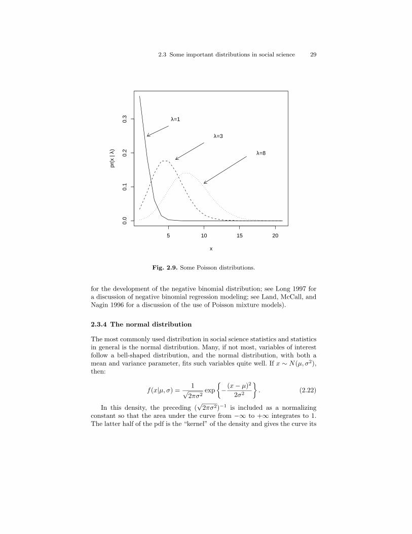
2.3 Some important distributions in social science 29
5 10 15 20
0.0
0.1
0.2
0.3
x
pr(x
| λ)
λ=1
λ=3
λ=8
Fig. 2.9. Some Poisson distributions.
for the development of the negative binomial distribution; see Long 1997 fora discussion of negative binomial regression modeling; see Land, McCall, andNagin 1996 for a discussion of the use of Poisson mixture models).
2.3.4 The normal distribution
The most commonly used distribution in social science statistics and statisticsin general is the normal distribution. Many, if not most, variables of interestfollow a bell-shaped distribution, and the normal distribution, with both amean and variance parameter, fits such variables quite well. If x ∼ N(µ, σ2),then:
f(x|µ, σ) =1√
2πσ2exp
− (x− µ)2
2σ2
. (2.22)
In this density, the preceding (√
2πσ2)−1 is included as a normalizingconstant so that the area under the curve from −∞ to +∞ integrates to 1.The latter half of the pdf is the “kernel” of the density and gives the curve its
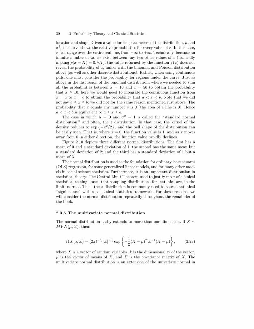
30 2 Probability Theory and Classical Statistics
location and shape. Given a value for the parameters of the distribution, µ andσ2, the curve shows the relative probabilities for every value of x. In this case,x can range over the entire real line, from −∞ to +∞. Technically, because aninfinite number of values exist between any two other values of x (ironicallymaking p(x = X) = 0,∀X), the value returned by the function f(x) does notreveal the probability of x, unlike with the binomial and Poisson distributionabove (as well as other discrete distributions). Rather, when using continuouspdfs, one must consider the probability for regions under the curve. Just asabove in the discussion of the binomial distribution, where we needed to sumall the probabilities between x = 10 and x = 50 to obtain the probabilitythat x ≥ 10, here we would need to integrate the continuous function fromx = a to x = b to obtain the probability that a < x < b. Note that we didnot say a ≤ x ≤ b; we did not for the same reason mentioned just above: Theprobability that x equals any number q is 0 (the area of a line is 0). Hencea < x < b is equivalent to a ≤ x ≤ b.
The case in which µ = 0 and σ2 = 1 is called the “standard normaldistribution,” and often, the z distribution. In that case, the kernel of thedensity reduces to exp
−x2/2
, and the bell shape of the distribution can
be easily seen. That is, where x = 0, the function value is 1, and as x movesaway from 0 in either direction, the function value rapidly declines.
Figure 2.10 depicts three different normal distributions: The first has amean of 0 and a standard deviation of 1; the second has the same mean buta standard deviation of 2; and the third has a standard deviation of 1 but amean of 3.
The normal distribution is used as the foundation for ordinary least squares(OLS) regression, for some generalized linear models, and for many other mod-els in social science statistics. Furthermore, it is an important distribution instatistical theory: The Central Limit Theorem used to justify most of classicalstatistical testing states that sampling distributions for statistics are, in thelimit, normal. Thus, the z distribution is commonly used to assess statistical“significance” within a classical statistics framework. For these reasons, wewill consider the normal distribution repeatedly throughout the remainder ofthe book.
2.3.5 The multivariate normal distribution
The normal distribution easily extends to more than one dimension. If X ∼MV N(µ,Σ), then:
f(X|µ,Σ) = (2π)−k2 |Σ|− 1
2 exp−1
2(X − µ)T Σ−1(X − µ)
, (2.23)
where X is a vector of random variables, k is the dimensionality of the vector,µ is the vector of means of X, and Σ is the covariance matrix of X. Themultivariate normal distribution is an extension of the univariate normal in
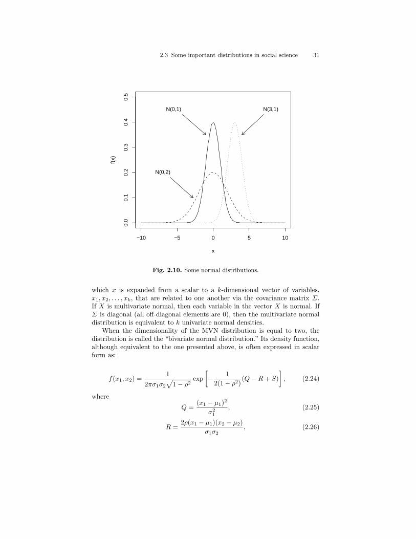
2.3 Some important distributions in social science 31
−10 −5 0 5 10
0.0
0.1
0.2
0.3
0.4
0.5
x
f(x)
N(0,2)
N(0,1) N(3,1)
Fig. 2.10. Some normal distributions.
which x is expanded from a scalar to a k-dimensional vector of variables,x1, x2, . . . , xk, that are related to one another via the covariance matrix Σ.If X is multivariate normal, then each variable in the vector X is normal. IfΣ is diagonal (all off-diagonal elements are 0), then the multivariate normaldistribution is equivalent to k univariate normal densities.
When the dimensionality of the MVN distribution is equal to two, thedistribution is called the “bivariate normal distribution.” Its density function,although equivalent to the one presented above, is often expressed in scalarform as:
f(x1, x2) =1
2πσ1σ2
√1− ρ2
exp[− 1
2(1− ρ2)(Q−R + S)
], (2.24)
where
Q =(x1 − µ1)2
σ21
, (2.25)
R =2ρ(x1 − µ1)(x2 − µ2)
σ1σ2, (2.26)
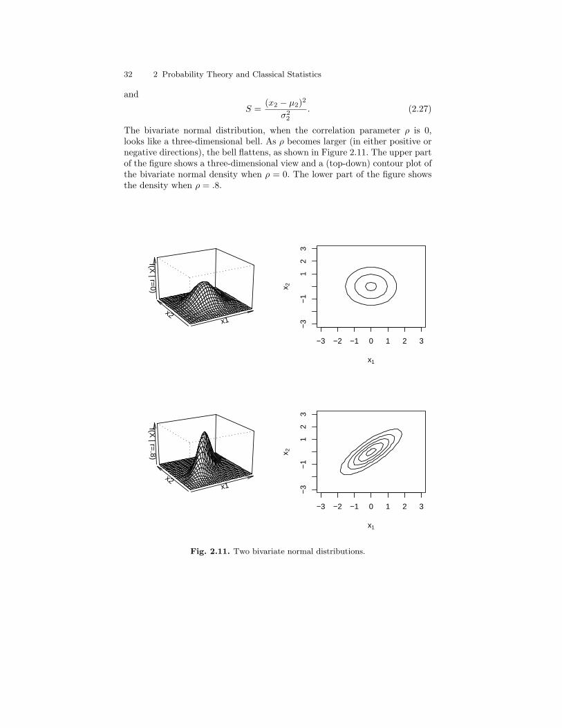
32 2 Probability Theory and Classical Statistics
and
S =(x2 − µ2)2
σ22
. (2.27)
The bivariate normal distribution, when the correlation parameter ρ is 0,looks like a three-dimensional bell. As ρ becomes larger (in either positive ornegative directions), the bell flattens, as shown in Figure 2.11. The upper partof the figure shows a three-dimensional view and a (top-down) contour plot ofthe bivariate normal density when ρ = 0. The lower part of the figure showsthe density when ρ = .8.
x1x2
f(X | r=
0)
x1
x 2
−3 −2 −1 0 1 2 3
−3
−1
12
3
x1x2
f(X | r=
.8)
x1
x 2
−3 −2 −1 0 1 2 3
−3
−1
12
3
Fig. 2.11. Two bivariate normal distributions.
2.4 Classical statistics in social science 33
The multivariate normal distribution is used fairly frequently in socialscience statistics. Specifically, the bivariate normal distribution is used tomodel simultaneous equations for two outcome variables that are known tobe related, and structural equation models rely on the full multivariate normaldistribution. I will discuss this distribution in more depth in later chaptersdescribing multivariate models.
2.3.6 t and multivariate t distributions
The t (Student’s t) and multivariate t distributions are quite commonly usedin modern social science statistics. For example, when the variance is un-known in a model that assumes a normal distribution for the data, with thevariance following an inverse gamma distribution (see subsequent chapters),the marginal distribution for the mean follows a t distribution (consider testsof coefficients in a regression model). Also, when the sample size is small, thet is used as a robust alternative to the normal distribution in order to com-pensate for heavier tails in the distribution of the data. As the sample sizeincreases, uncertainty about σ decreases, and the t distribution converges ona normal distribution (see Figure 2.12). The density functions for the t dis-tribution appears much more complicated than the normal. If x ∼ t(µ, σ, v),then:
f(x) =Γ ((v + 1)/2)Γ (v/2)σ
√vπ
(1 + v−1
(x− µ
σ
)2)−(v+1)/2
, (2.28)
where µ is the mean, σ is the standard deviation, and v is the “degrees offreedom.” If X is a k-dimensional vector of variables (x1 . . . xk), and X ∼mvt(µ, Σ, v), then:
f(X) =Γ ((v + d)/2)
Γ (v/2)vk/2πk/2| Σ |−1/2
(1 + v−1(X − µ)T Σ−1(X − µ)
)−(v+k)/2,
(2.29)where µ is a vector of means, and Σ is the variance-covariance matrix of X.
We will not explicitly use the t and multivariate t distributions in thisbook, although a number of marginal distributions we will be working withwill be implicitly t distributions.
2.4 Classical statistics in social science
Throughout the fall of 2004, CNN/USAToday/Gallup conducted a numberof polls attempting to predict whether George W. Bush or John F. Kerrywould win the U.S. presidential election. One of the key battleground stateswas Ohio, which ultimately George Bush won, but all the polls leading up

34 2 Probability Theory and Classical Statistics
−4 −2 0 2 4
0.0
0.1
0.2
0.3
0.4
0.5
x
f(x)
t(1 df)t(2 df)t(10 df)t(120 df)
N(0,1) [solid line]
Fig. 2.12. The t(0, 1, 1), t(0, 1, 10), and t(0, 1, 120) distributions (with an N(0, 1)distribution superimposed).
to the election showed the two candidates claiming proportions of the votesthat were statistically indistinguishable in the state. The last poll in Ohioconsisted of 1,111 likely voters, 46% of whom stated that they would vote forBush, and 50% of whom stated that they would vote for Kerry, but the pollhad a margin of error of ±3%.4
In the previous sections, we discussed probability theory, and I statedthat statistics is essentially the inverse of probability. In probability, once weare given a distribution and its parameters, we can deduce the probabilitiesfor events. In statistics, we have a collection of events and are interested in
4 see http://www.cnn.com/ELECTION/2004/special/president/showdown/OH/polls.html for the data reported in this and the next chapter. Additional polls aredisplayed on the website, but I use only the CNN/USAToday/Gallup polls, giventhat they are most likely similar in sample design. Unfortunately, the proportionsare rounded, and so my results from here on are approximate. For example, inthe last poll, 50% planned to vote for Kerry, and 50% of 1,111 is 556. However,the actual number could range from 550 to 561 given the rounding.
2.5 Maximum likelihood estimation 35
determining the values of the parameters that produced them. Returning tothe polling data, determining who would win the election is tantamount todetermining the population parameter (the proportion of actual voters whowill vote for a certain candidate) given a collection of events (a sample ofpotential votes) thought to arise from this parameter and the probabilitydistribution to which it belongs.
Classical statistics provides one recipe for estimating this population pa-rameter; in the remainder of this chapter, I demonstrate how. In the nextchapter, I tackle the problem from a Bayesian perspective. Throughout thissection, by “classical statistics” I mean the approach that is most commonlyused among academic researchers in the social sciences. To be sure, the clas-sical approach to statistics in use is a combination of several approaches,involving the use of theorems and perspectives of a number of statisticians.For example, the most common approach to model estimation is maximumlikelihood estimation, which has its roots in the works of Fisher, whereas thecommon approach to hypothesis testing using p-values has its roots in theworks of both Neyman and Pearson and Fisher—each of whom in fact devel-oped somewhat differing views of hypothesis testing using p-values (again, seeHubbard and Bayarri 2003 or see Gill 2002 for an even more detailed history).
2.5 Maximum likelihood estimation
The classical approach to statistics taught in social science statistics coursesinvolves two basic steps: (1) model estimation and (2) inference. The first stepinvolves first determining an appropriate probability distribution/model forthe data at hand and then estimating its parameters. Maximum likelihood(ML) is the most commonly used method of estimating parameters and de-termining the extent of error in the estimation (steps 1 and 2, respectively) insocial science statistics (see Edwards 1992 for a detailed, theoretical discus-sion of likelihood analysis; see Eliason 1993 for a more detailed discussion ofthe mechanics of ML estimation).
The fundamental idea behind maximum likelihood estimation is that agood choice for the estimate of a parameter of interest is the value of theparameter that makes the observed data most likely to have occurred. To dothis, we need to establish some sort of function that gives us the probabilityfor the data, and we need to find the value of the parameter that maximizesthis probability. This function is called the “likelihood function” in classicalstatistics, and it is essentially the product of sampling densities—probabilitydistributions—for each observation in the sample. The process of estimationthus involves the following steps:
1. Construct a likelihood function for the parameter(s) of interest.2. Simplify the likelihood function and take its logarithm.3. Take the partial derivative of the log-likelihood function with respect to
each parameter, and set the resulting equation(s) equal to 0.
36 2 Probability Theory and Classical Statistics
4. Solve the system of equations to find the parameters.
This process seems complicated, and indeed it can be. Step 4 can be quitedifficult when there are lots of parameters. Generally, some sort of iterativemethod is required to find the maximum. Below I detail the process of MLestimation.
2.5.1 Constructing a likelihood function
If x1, x2 . . . xn are independent observations of a random variable, x, in a dataset of size n, then we know from the multiplication rule in probability theorythat the joint probability for the vector X is:
f(X|θ) ≡ L(θ | x) =n∏
i=1
f(xi | θ). (2.30)
This equation is the likelihood function for the model. Notice how theparameter and the data switch places in the L(.) notation versus the f(.)notation. We denote this as L(.), because from a classical standpoint, theparameter is assumed to be fixed. However, we are interested in estimatingthe parameter θ, given the data we have observed, so we use this notation.The primary point of constructing a likelihood function is that, given the dataat hand, we would like to solve for the value of the parameter that makesthe occurence of the data most probable, or most “likely” to have actuallyoccurred.
As the right-hand side of the equation shows, the construction of the like-lihood function first relies on determining an appropriate probability distri-bution f(.) thought to generate the observed data. In our election pollingexample, the data consist of 1,111 potential votes, the vast majority of whichwere either for Bush or for Kerry. If we assume that candidates other thanthese two are unimportant—that is, the election will come down to whomamong these two receives more votes—then the data ultimately reduce to 556potential votes for Kerry and 511 potential votes for Bush. An appropriatedistribution for such data is the binomial distribution. If we are interestedin whether Kerry will win the election, we can consider a vote for Kerry a“success,” and its opposite, a vote for Bush, a “failure,” and we can set upour likelihood function with the goal of determining the success probabilityp. The likelihood function in this case looks like:
L(p|X) =(
1067556
)p556(1− p)511.
As an alternative view that ultimately produces the same results, we can con-sider that, at the individual level, each of our votes arises from a Bernoulli dis-tribution, and so our likelihood function is the product of n = 1, 067 Bernoullidistributions. In that case:
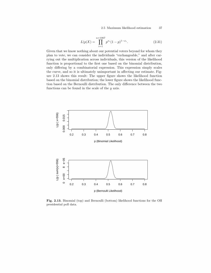
2.5 Maximum likelihood estimation 37
L(p|X) =n=1067∏
i=1
pxi(1− p)1−xi . (2.31)
Given that we know nothing about our potential voters beyond for whom theyplan to vote, we can consider the individuals “exchangeable,” and after car-rying out the multiplication across individuals, this version of the likelihoodfunction is proportional to the first one based on the binomial distribution,only differing by a combinatorial expression. This expression simply scalesthe curve, and so it is ultimately unimportant in affecting our estimate. Fig-ure 2.13 shows this result: The upper figure shows the likelihood functionbased on the binomial distribution; the lower figure shows the likelihood func-tion based on the Bernoulli distribution. The only difference between the twofunctions can be found in the scale of the y axis.
0.2 0.3 0.4 0.5 0.6 0.7 0.8
0.00
00.
015
p (Binomial Likelihood)
L(p
| x=
556)
0.2 0.3 0.4 0.5 0.6 0.7 0.8
0 e
+00
8 e
−05
p (Bernoulli Likelihood)
L(p
| sum
(x)=
556)
Fig. 2.13. Binomial (top) and Bernoulli (bottom) likelihood functions for the OHpresidential poll data.
38 2 Probability Theory and Classical Statistics
2.5.2 Maximizing a likelihood function
How do we obtain the estimates for the parameters after we set up the like-lihood function? Just as many pdfs are unimodal and slope away from themode of the distribution, we expect the likelihood function to look about thesame. So, what we need to find is the peak of this curve. From calculus weknow that the slope of the curve should be 0 at its peak. Thus, we shouldtake the derivative of the likelihood function with respect to the parameter,set it equal to 0, and find the x coordinate (the parameter value) for whichthe curve reaches a maximum.
We generally take the logarithm of the likelihood function before we dif-ferentiate, because the log function converts the repeated multiplication torepeated addition, and repeated addition is much easier to work with. Thelog-likelihood reaches a maximum at the same point as the original function.Generically:
Log-Likelihood ≡ LL(θ | X) =n∑
i=1
log(f(xi | θ)). (2.32)
For our specific problem:
LL(p|x) ∝ 556 ln p + 511 ln(1− p).
To find the value of p where this log-likelihood function reaches a maximum,we need to take the derivative of the function with respect to p, set it equalto 0, and solve for p. Generically, the derivative of a binomial log-likelihoodfunction is:
dLL
dp=∑
xi
p− n−
∑xi
1− p. (2.33)
If we set this derivative equal to 0 and solve for p, we obtain:
n−∑
xi
1− p=∑
xi
p.
Simplifying yields:
p =∑
xi
n. (2.34)
This result shows that the maximum likelihood estimate for p is simply theobserved proportion of successes. In our example, this is the proportion ofpotential votes for Kerry, out of those who opted for either Kerry or Bush(here, 556/1067 = .521). Given that this value for p is an estimate, we typicallydenote it p, rather than p.
Figure 2.14 displays this process of estimation graphically. The figureshows that both the likelihood function and the log-likelihood functions peakat the same point. The horizontal lines are the tangent lines to the curve
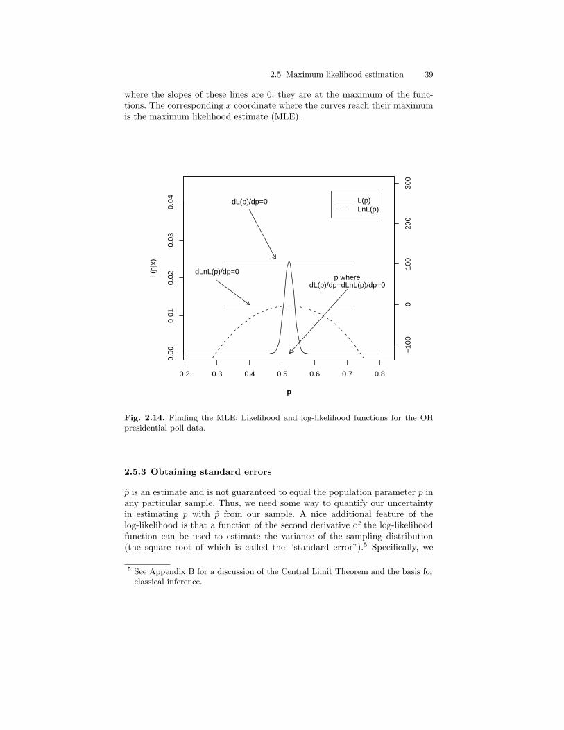
2.5 Maximum likelihood estimation 39
where the slopes of these lines are 0; they are at the maximum of the func-tions. The corresponding x coordinate where the curves reach their maximumis the maximum likelihood estimate (MLE).
0.2 0.3 0.4 0.5 0.6 0.7 0.8
0.00
0.01
0.02
0.03
0.04
p
L(p|
x)
dL(p)/dp=0
p wheredL(p)/dp=dLnL(p)/dp=0
p
−10
00
100
200
300
dLnL(p)/dp=0
L(p)LnL(p)
Fig. 2.14. Finding the MLE: Likelihood and log-likelihood functions for the OHpresidential poll data.
2.5.3 Obtaining standard errors
p is an estimate and is not guaranteed to equal the population parameter p inany particular sample. Thus, we need some way to quantify our uncertaintyin estimating p with p from our sample. A nice additional feature of thelog-likelihood is that a function of the second derivative of the log-likelihoodfunction can be used to estimate the variance of the sampling distribution(the square root of which is called the “standard error”).5 Specifically, we
5 See Appendix B for a discussion of the Central Limit Theorem and the basis forclassical inference.
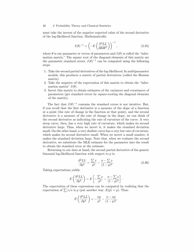
40 2 Probability Theory and Classical Statistics
must take the inverse of the negative expected value of the second derivativeof the log-likelihood function. Mathematically:
I(θ)−1 =(−E
(∂2LL
∂θ∂θT
))−1
, (2.35)
where θ is our parameter or vector of parameters and I(θ) is called the “infor-mation matrix.” The square root of the diagonal elements of this matrix arethe parameter standard errors. I(θ)−1 can be computed using the followingsteps:
1. Take the second partial derivatives of the log-likelihood. In multiparametermodels, this produces a matrix of partial derivatives (called the Hessianmatrix).
2. Take the negative of the expectation of this matrix to obtain the “infor-mation matrix” I(θ).
3. Invert this matrix to obtain estimates of the variances and covariances ofparameters (get standard errors by square-rooting the diagonal elementsof the matrix).
The fact that I(θ)−1 contains the standard errors is not intuitive. But,if you recall that the first derivative is a measure of the slope of a functionat a point (the rate of change in the function at that point), and the secondderivative is a measure of the rate of change in the slope, we can think ofthe second derivative as indicating the rate of curvature of the curve. A verysteep curve, then, has a very high rate of curvature, which makes its secondderivative large. Thus, when we invert it, it makes the standard deviationsmall. On the other hand, a very shallow curve has a very low rate of curvature,which makes its second derivative small. When we invert a small number, itmakes the standard deviation large. Note that, when we evaluate the secondderivative, we substitute the MLE estimate for the parameter into the resultto obtain the standard error at the estimate.
Returning to our data at hand, the second partial derivative of the genericbinomial log-likelihood function with respect to p is:
∂2LL
∂p2=∑
x
p2− n−
∑x
(1− p)2. (2.36)
Taking expectations yields:
E
(∂2LL
∂p2
)= E
[−∑
x
p2− n−
∑x
(1− p)2
].
The expectation of these expressions can be computed by realizing that theexpectation of
∑x/n is p (put another way: E(p) = p). Thus:
E
(∂2LL
∂p2
)= −np
p2− n− np
(1− p)2.
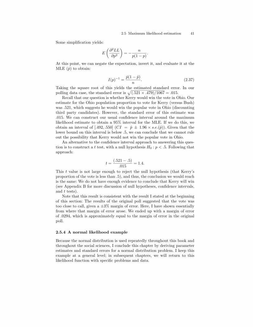
2.5 Maximum likelihood estimation 41
Some simplification yields:
E
(∂2LL
∂p2
)= − n
p(1− p).
At this point, we can negate the expectation, invert it, and evaluate it at theMLE (p) to obtain:
I(p)−1 =p(1− p)
n. (2.37)
Taking the square root of this yields the estimated standard error. In ourpolling data case, the standard error is
√(.521× .479)/1067 = .015.
Recall that our question is whether Kerry would win the vote in Ohio. Ourestimate for the Ohio population proportion to vote for Kerry (versus Bush)was .521, which suggests he would win the popular vote in Ohio (discountingthird party candidates). However, the standard error of this estimate was.015. We can construct our usual confidence interval around the maximumlikelihood estimate to obtain a 95% interval for the MLE. If we do this, weobtain an interval of [.492, .550] (CI = p ± 1.96 × s.e.(p)). Given that thelower bound on this interval is below .5, we can conclude that we cannot ruleout the possibility that Kerry would not win the popular vote in Ohio.
An alternative to the confidence interval approach to answering this ques-tion is to construct a t test, with a null hypothesis H0 : p < .5. Following thatapproach:
t =(.521− .5)
.015= 1.4.
This t value is not large enough to reject the null hypothesis (that Kerry’sproportion of the vote is less than .5), and thus, the conclusion we would reachis the same: We do not have enough evidence to conclude that Kerry will win(see Appendix B for more discussion of null hypotheses, confidence intervals,and t tests).
Note that this result is consistent with the result I stated at the beginningof this section: The results of the original poll suggested that the vote wastoo close to call, given a ±3% margin of error. Here, I have shown essentiallyfrom where that margin of error arose. We ended up with a margin of errorof .0294, which is approximately equal to the margin of error in the originalpoll.
2.5.4 A normal likelihood example
Because the normal distribution is used repeatedly throughout this book andthroughout the social sciences, I conclude this chapter by deriving parameterestimates and standard errors for a normal distribution problem. I keep thisexample at a general level; in subsequent chapters, we will return to thislikelihood function with specific problems and data.
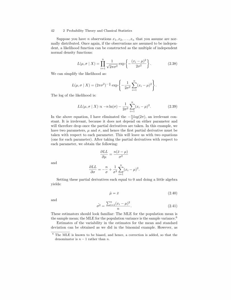
42 2 Probability Theory and Classical Statistics
Suppose you have n observations x1, x2, . . . , xn that you assume are nor-mally distributed. Once again, if the observations are assumed to be indepen-dent, a likelihood function can be constructed as the multiple of independentnormal density functions:
L(µ, σ | X) =n∏
i=1
1√2πσ2
exp− (xi − µ)2
2σ2
. (2.38)
We can simplify the likelihood as:
L(µ, σ | X) = (2πσ2)−n2 exp
− 1
2σ2
n∑i=1
(xi − µ)2
.
The log of the likelihood is:
LL(µ, σ | X) ∝ −n ln(σ)− 12σ2
n∑i=1
(xi − µ)2. (2.39)
In the above equation, I have eliminated the −n2 log(2π), an irrelevant con-
stant. It is irrelevant, because it does not depend on either parameter andwill therefore drop once the partial derivatives are taken. In this example, wehave two parameters, µ and σ, and hence the first partial derivative must betaken with respect to each parameter. This will leave us with two equations(one for each parameter). After taking the partial derivatives with respect toeach parameter, we obtain the following:
∂LL
∂µ=
n(x− µ)σ2
and∂LL
∂σ= −n
σ+
1σ3
n∑i=1
(xi − µ)2.
Setting these partial derivatives each equal to 0 and doing a little algebrayields:
µ = x (2.40)
and
σ2 =∑n
i=1(xi − µ)2
n. (2.41)
These estimators should look familiar: The MLE for the population mean isthe sample mean; the MLE for the population variance is the sample variance.6
Estimates of the variability in the estimates for the mean and standarddeviation can be obtained as we did in the binomial example. However, as
6 The MLE is known to be biased, and hence, a correction is added, so that thedenominator is n− 1 rather than n.

2.5 Maximum likelihood estimation 43
noted above, given that we have two parameters, our second derivate matrixwill, in fact, be a matrix. For the purposes of avoiding taking square rootsuntil the end, let τ = σ2, and we’ll construct the Hessian matrix in terms ofτ . Also, let θ be a vector containing both µ and τ . Thus, we must compute:
∂2LL
∂θ∂θT=
∂2LL∂µ2
∂2LL∂µ∂τ
∂2LL∂τ∂µ
∂2LL∂τ2
. (2.42)
Without showing all the derivatives (see Exercises), the elements of the Hes-sian matrix are then:
∂2LL
∂θ∂θT=
−nτ −n(x−µ)
τ2
−n(x−µ)τ2
n2τ2 −
Pni=1(xi−µ)2
τ3
.
In order to obtain the information matrix, which can be used to compute thestandard errors, we must take the expectation of this Hessian matrix and takeits negative. Let’s take the expectation of the off-diagonal elements first. Theexpectation of x− µ is 0 (given that the MLE is unbiased), which makes theoff-diagonal elements of the information matrix equal to 0. This result shouldbe somewhat intuitive: There need be no relationship between the mean andvariance in a normal distribution.
The first element, (−n/τ), is unchanged under expectation. Thus, aftersubstituting σ2 back in for τ and negating the result, we obtain n/σ2 for thiselement of the information matrix.
The last element, (n/2τ2) − (∑n
i=1(xi − µ)2)/τ3, requires a little con-sideration. The only part of this expression that changes under expecta-tion is
∑ni=1(xi − µ)2. The expectation of this expression is nτ . That is,
E(xi − µ)2 = τ , and we are taking this value n times (notice the summa-tion). Thus, this element, after a little algebraic manipulation, negation, andsubstitution of σ2 for τ , becomes: n/2σ4. So, our information matrix appearsas:
I(θ) =[
nσ2 00 n
2σ4
]. (2.43)
To obtain standard errors, we need to (1) invert this matrix, and (2) takethe square root of the diagonal elements (variances) to obtain the standarderrors. Matrix inversion in this case is quite simple, given that the off-diagonalelements are equal to 0. In this case, the inverse of the matrix is simply theinverse of the diagonal elements.
Once we invert and square root the elements of the information matrix,we find that the estimate for the standard error for our estimate µ is σ/
√n,
and our estimate for the standard error for σ2 is σ2√
2/n. The estimate forthe standard error for µ should look familiar: It is the standard deviation of
44 2 Probability Theory and Classical Statistics
the sampling distribution for a mean based on the Central Limit Theorem(see Appendix B).
2.6 Conclusions
In this chapter, we have reviewed the basics of probability theory. Importantly,we have developed the concept of probability distributions in general, and wehave discussed a number of actual probability distributions. In addition, wehave discussed how important quantities like the mean and variance can bederived analytically from probability distributions. Finally, we reviewed themost common approach to estimating such quantities in a classical setting—maximum likelihood estimation—given a collection of data thought to arisefrom a particular distribution. As stated earlier, I recommend reading De-Groot (1986) for a more thorough introduction to probability theory, and Irecommend Billingsley (1995) and Chung and AitSahlia (2003) for more ad-vanced and detailed expositions. For a condensed exposition, I suggest Rudas2004. Finally, I recommend Edwards (1992) and Gill (2002) for detailed dis-cussions of the history and practice of maximum likelihood (ML) estimation,and I suggest Eliason (1993) for a highly applied perspective on ML estima-tion. In the next chapter, we will discuss the Bayesian approach to statisticsas an alternative to this classical approach to model building and estimation.
2.7 Exercises
2.7.1 Probability exercises
1. Find the normalizing constant for the linear density in Equation 2.8.2. Using the binomial mass function, find the probability of obtaining 3 heads
in a row with a fair coin.3. Find the probability of obtaining 3 heads in a row with a coin weighted
so that the probability of obtaining a head is .7.4. What is the probability of obtaining 3 heads OR 3 tails in a row with a
fair coin?5. What is the probability of obtaining 3 heads and 1 tail (order irrelevant)
on four flips of a fair coin?6. Using a normal approximation to the binomial distribution, find the prob-
ability of obtaining 130 or more heads in 200 flips of a fair coin.7. Plot a normal distribution with parameters µ = 5 and σ = 2.8. Plot a normal distribution with parameters µ = 2 and σ = 5.9. Plot the t(0, 1, df = 1) and t(0, 1, df = 10) distributions. Note: Γ is a
function. The function is: Γ (n) =∫∞0
e−uun−1du. For integers, Γ (n) =(n − 1)! Thus, Γ (4) = (4 − 1)! = 6. However, when the argument to thefunction is not an integer, this formula will not work. Instead, it is easierto use a software package to compute the function value for you.

2.7 Exercises 45
10. Show that the multivariate normal density function reduces to the univari-ate normal density function when the dimensionality of the distributionis 1.
2.7.2 Classical inference exercises
1. Find the MLE for p in a binomial distribution representing a sample inwhich 20 successes were obtained out of 30 trials.
2. Based on the binomial sample in the previous question, if the trials in-volved coin flips, would having 20 heads be sufficient to question the fair-ness of the coin? Why or why not?
3. Suppose a sample of students at a major university were given an IQ test,which resulted in a mean of 120 and a standard deviation of 10. If weknow that IQs are normally distributed in the population with a mean of100 and a standard deviation of 16, is there sufficient evidence to suggestthat the college students are more intelligent than average?
4. Suppose a single college student were given an IQ test and scored 120. Isthere sufficient evidence to indicate that college students are more intelli-gent than average based on this sample?
5. What is the difference (if any) between the responses to the previous twoquestions?
6. Derive the Hessian matrix for the normal distribution example at the endof the chapter.
7. Derive the MLE for λ from a sample of n observations from a Poissondistribution.
8. Derive the standard error estimate for λ from the previous question.

3
Basics of Bayesian Statistics
Suppose a woman believes she may be pregnant after a single sexual encounter,but she is unsure. So, she takes a pregnancy test that is known to be 90%accurate—meaning it gives positive results to positive cases 90% of the time—and the test produces a positive result.1 Ultimately, she would like to know theprobability she is pregnant, given a positive test (p(preg | test +)); however,what she knows is the probability of obtaining a positive test result if she ispregnant (p(test + |preg)), and she knows the result of the test.
In a similar type of problem, suppose a 30-year-old man has a positiveblood test for a prostate cancer marker (PSA). Assume this test is also ap-proximately 90% accurate. Once again, in this situation, the individual wouldlike to know the probability that he has prostate cancer, given the positivetest, but the information at hand is simply the probability of testing positiveif he has prostate cancer, coupled with the knowledge that he tested positive.
Bayes’ Theorem offers a way to reverse conditional probabilities and,hence, provides a way to answer these questions. In this chapter, I first showhow Bayes’ Theorem can be applied to answer these questions, but then Iexpand the discussion to show how the theorem can be applied to probabilitydistributions to answer the type of questions that social scientists commonlyask. For that, I return to the polling data described in the previous chapter.
3.1 Bayes’ Theorem for point probabilities
Bayes’ original theorem applied to point probabilities. The basic theoremstates simply:
p(B|A) =p(A|B)p(B)
p(A). (3.1)
1 In fact, most pregnancy tests today have a higher accuracy rate, but the accuracyrate depends on the proper use of the test as well as other factors.
48 3 Basics of Bayesian Statistics
In English, the theorem says that a conditional probability for event Bgiven event A is equal to the conditional probability of event A given eventB, multiplied by the marginal probability for event B and divided by themarginal probability for event A.
Proof: From the probability rules introduced in Chapter 2, we know thatp(A,B) = p(A|B)p(B). Similarly, we can state that p(B,A) = p(B|A)p(A).Obviously, p(A,B) = p(B,A), so we can set the right sides of each of theseequations equal to each other to obtain:
p(B|A)p(A) = p(A|B)p(B).
Dividing both sides by p(A) leaves us with Equation 3.1.The left side of Equation 3.1 is the conditional probability in which we
are interested, whereas the right side consists of three components. p(A|B)is the conditional probability we are interested in reversing. p(B) is the un-conditional (marginal) probability of the event of interest. Finally, p(A) is themarginal probability of event A. This quantity is computed as the sum ofthe conditional probability of A under all possible events Bi in the samplespace: Either the woman is pregnant or she is not. Stated mathematically fora discrete sample space:
p(A) =∑
Bi∈SB
p(A | Bi)p(Bi).
Returning to the pregnancy example to make the theorem more concrete,suppose that, in addition to the 90% accuracy rate, we also know that thetest gives false-positive results 50% of the time. In other words, in cases inwhich a woman is not pregnant, she will test positive 50% of the time. Thus,there are two possible events Bi: B1 = preg and B2 = not preg. Additionally,given the accuracy and false-positive rates, we know the conditional probabil-ities of obtaining a positive test under these events: p(test +|preg) = .9 andp(test +|not preg) = .5. With this information, combined with some “prior”information concerning the probability of becoming pregnant from a singlesexual encounter, Bayes’ theorem provides a prescription for determining theprobability of interest.
The “prior” information we need, p(B) ≡ p(preg), is the marginal probabil-ity of being pregnant, not knowing anything beyond the fact that the womanhas had a single sexual encounter. This information is considered prior infor-mation, because it is relevant information that exists prior to the test. We mayknow from previous research that, without any additional information (e.g.,concerning date of last menstrual cycle), the probability of conception for anysingle sexual encounter is approximately 15%. (In a similar fashion, concerningthe prostate cancer scenario, we may know that the prostate cancer incidencerate for 30-year-olds is .00001—see Exercises). With this information, we candetermine p(B | A) ≡ p(preg|test +) as:
3.1 Bayes’ Theorem for point probabilities 49
p(preg | test +) =p(test + | preg)p(preg)
p(test + | preg)p(preg) + p(test + | not preg)p(not preg).
Filling in the known information yields:
p(preg | test +) =(.90)(.15)
(.90)(.15) + (.50)(.85)=
.135.135 + .425
= .241.
Thus, the probability the woman is pregnant, given the positive test, is only.241. Using Bayesian terminology, this probability is called a “posterior prob-ability,” because it is the estimated probability of being pregnant obtainedafter observing the data (the positive test). The posterior probability is quitesmall, which is surprising, given a test with so-called 90% “accuracy.” How-ever, a few things affect this probability. First is the relatively low probabilityof becoming pregnant from a single sexual encounter (.15). Second is the ex-tremely high probability of a false-positive test (.50), especially given the highprobability of not becoming pregnant from a single sexual encounter (p = .85)(see Exercises).
If the woman is aware of the test’s limitations, she may choose to repeat thetest. Now, she can use the “updated” probability of being pregnant (p = .241)as the new p(B); that is, the prior probability for being pregnant has now beenupdated to reflect the results of the first test. If she repeats the test and againobserves a positive result, her new “posterior probability” of being pregnantis:
p(preg | test +) =(.90)(.241)
(.90)(.241) + (.50)(.759)=
.135.135 + .425
= .364.
This result is still not very convincing evidence that she is pregnant, but if sherepeats the test again and finds a positive result, her probability increases to.507 (for general interest, subsequent positive tests yield the following prob-abilities: test 4 = .649, test 5 = .769, test 6 = .857, test 7 = .915, test 8 =.951, test 9 = .972, test 10 = .984).
This process of repeating the test and recomputing the probability of in-terest is the basic process of concern in Bayesian statistics. From a Bayesianperspective, we begin with some prior probability for some event, and we up-date this prior probability with new information to obtain a posterior prob-ability. The posterior probability can then be used as a prior probability ina subsequent analysis. From a Bayesian point of view, this is an appropriatestrategy for conducting scientific research: We continue to gather data to eval-uate a particular scientific hypothesis; we do not begin anew (ignorant) eachtime we attempt to answer a hypothesis, because previous research providesus with a priori information concerning the merit of the hypothesis.
50 3 Basics of Bayesian Statistics
3.2 Bayes’ Theorem applied to probability distributions
Bayes’ theorem, and indeed, its repeated application in cases such as the ex-ample above, is beyond mathematical dispute. However, Bayesian statisticstypically involves using probability distributions rather than point probabili-ties for the quantities in the theorem. In the pregnancy example, we assumedthe prior probability for pregnancy was a known quantity of exactly .15. How-ever, it is unreasonable to believe that this probability of .15 is in fact thisprecise. A cursory glance at various websites, for example, reveals a wide rangefor this probability, depending on a woman’s age, the date of her last men-strual cycle, her use of contraception, etc. Perhaps even more importantly,even if these factors were not relevant in determining the prior probabilityfor being pregnant, our knowledge of this prior probability is not likely to beperfect because it is simply derived from previous samples and is not a knownand fixed population quantity (which is precisely why different sources maygive different estimates of this prior probability!). From a Bayesian perspec-tive, then, we may replace this value of .15 with a distribution for the priorpregnancy probability that captures our prior uncertainty about its true value.The inclusion of a prior probability distribution ultimately produces a poste-rior probability that is also no longer a single quantity; instead, the posteriorbecomes a probability distribution as well. This distribution combines theinformation from the positive test with the prior probability distribution toprovide an updated distribution concerning our knowledge of the probabilitythe woman is pregnant.
Put generally, the goal of Bayesian statistics is to represent prior uncer-tainty about model parameters with a probability distribution and to updatethis prior uncertainty with current data to produce a posterior probability dis-tribution for the parameter that contains less uncertainty. This perspectiveimplies a subjective view of probability—probability represents uncertainty—and it contrasts with the classical perspective. From the Bayesian perspective,any quantity for which the true value is uncertain, including model param-eters, can be represented with probability distributions. From the classicalperspective, however, it is unacceptable to place probability distributions onparameters, because parameters are assumed to be fixed quantities: Only thedata are random, and thus, probability distributions can only be used to rep-resent the data.
Bayes’ Theorem, expressed in terms of probability distributions, appearsas:
f(θ|data) =f(data|θ)f(θ)
f(data), (3.2)
where f(θ|data) is the posterior distribution for the parameter θ, f(data|θ)is the sampling density for the data—which is proportional to the Likeli-hood function, only differing by a constant that makes it a proper densityfunction—f(θ) is the prior distribution for the parameter, and f(data) is the
3.2 Bayes’ Theorem applied to probability distributions 51
marginal probability of the data. For a continuous sample space, this marginalprobability is computed as:
f(data) =∫
f(data|θ)f(θ)dθ,
the integral of the sampling density multiplied by the prior over the samplespace for θ. This quantity is sometimes called the “marginal likelihood” for thedata and acts as a normalizing constant to make the posterior density proper(but see Raftery 1995 for an important use of this marginal likelihood). Be-cause this denominator simply scales the posterior density to make it a properdensity, and because the sampling density is proportional to the likelihoodfunction, Bayes’ Theorem for probability distributions is often stated as:
Posterior ∝ Likelihood× Prior, (3.3)
where the symbol “∝” means “is proportional to.”
3.2.1 Proportionality
As Equation 3.3 shows, the posterior density is proportional to the likelihoodfunction for the data (given the model parameters) multiplied by the prior forthe parameters. The prior distribution is often—but not always—normalizedso that it is a true density function for the parameter. The likelihood function,however, as we saw in the previous chapter, is not itself a density; instead, it isa product of densities and thus lacks a normalizing constant to make it a truedensity function. Consider, for example, the Bernoulli versus binomial speci-fications of the likelihood function for the dichotomous voting data. First, theBernoulli specification lacked the combinatorial expression to make the like-lihood function a true density function for either the data or the parameter.Second, although the binomial representation for the likelihood function con-stituted a true density function, it only constituted a true density for the dataand not for the parameter p. Thus, when the prior distribution for a parameteris multiplied by the likelihood function, the result is also not a proper densityfunction. Indeed, Equation 3.3 will be “off” by the denominator on the rightside of Equation 3.2, in addition to whatever normalizing constant is neededto equalize the likelihood function and the sampling density p(data | θ).
Fortunately, the fact that the posterior density is only proportional to theproduct of the likelihood function and prior is not generally a problem inBayesian analysis, as the remainder of the book will demonstrate. However,a note is in order regarding what proportionality actually means. In brief, ifa is proportional to b, then a and b only differ by a multiplicative constant.How does this translate to probability distributions? First, we need to keep inmind that, in a Bayesian analysis, model parameters are considered randomquantities, whereas the data, having been already observed, are consideredfixed quantities. This view is completely opposite that assumed under the
52 3 Basics of Bayesian Statistics
classical approach. Second, we need to recall from Chapter 2 that potentialdensity functions often need to have a normalizing constant included to makethem proper density functions, but we also need to recall that this normalzingconstant only has the effect of scaling the density—it does not fundamentallychange the relative frequencies of different values of the random variable.As we saw in Chapter 2, the normalizing constant is sometimes simply atrue constant—a number—but sometimes the constant involves the randomvariable(s) themselves.
As a general rule, when considering a univariate density, any term, sayQ (no matter how complicated), that can be factored away from the randomvariable in the density—so that all the term(s) involving the random variableare simply multiples of Q—can be considered an irrelevant proportionalityconstant and can be eliminated from the density without affecting the results.
In theory, this rule is fairly straightforward, but it is often difficult to applyfor two key reasons. First, it is sometimes difficult to see whether a term canbe factored out. For example, consider the following function for θ:
f(θ) = e−θ+Q.
It may not be immediately clear that Q here is an arbitrary constant withrespect to θ, but it is. This function can be rewritten as:
f(θ) = e−θ × eQ,
using the algebraic rule that ea+b = eaeb. Thus, if we are considering f(θ)as a density function for θ, eQ would be an arbitrary constant and could beremoved without affecting inference about θ. Thus, we could state withoutloss of information that:
f(θ) ∝ e−θ.
In fact, this particular function, without Q, is an exponential density for θwith parameter β = 1 (see the end of this chapter). With Q, it is proportionalto an exponential density; it simply needs a normalizing constant of e−Q sothat the function integrates to 1 over the sample space S = θ : θ > 0:∫ ∞
0
e−θ+Q dθ = − 1e∞−Q
+ eQ = eQ.
Thus, given that this function integrates to eQ, e−Q renormalizes the integralto 1.
A second difficulty with this rule is that multivariate densities sometimesmake it difficult to determine what is an irrelevant constant and what is not.With Gibbs sampling, as we will discuss in the next chapter and throughoutthe remainder of the book, we generally break down multivariate densities intounivariate conditional densities. When we do this, we can consider all termsnot involving the random variable to which the conditional density applies to
3.3 Bayes’ Theorem with distributions: A voting example 53
be proportionality constants. I will show this shortly in the last example inthis chapter.
3.3 Bayes’ Theorem with distributions: A votingexample
To make the notion of Bayes’ Theorem applied to probability distributionsconcrete, consider the polling data from the previous chapter. In the previouschapter, we attempted to determine whether John F. Kerry would win thepopular vote in Ohio, using the most recent CNN/USAToday/Gallup pollingdata. When we have a sample of data, such as potential votes for and against acandidate, and we assume they arise from a particular probability distribution,the construction of a likelihood function gives us the joint probability of theevents, conditional on the parameter of interest: p(data|parameter). In theelection polling example, we maximized this likelihood function to obtain avalue for the parameter of interest—the proportion of Kerry voters in Ohio—that maximized the probability of obtaining the polling data we did. Thatestimated proportion (let’s call it K to minimize confusion) was .521. Wethen determined how uncertain we were about our finding that K = .521.To be more precise, we determined under some assumptions how far K mayreasonably be from .521 and still produce the polling data we observed.
This process of maximizing the likelihood function ultimately simply tellsus how probable the data are under different values for K—indeed, that isprecisely what a likelihood function is —but our ultimate question is reallywhether Kerry will win, given the polling data. Thus, our question of interestis “what is p(K > .5),” but the likelihood function gives us p(poll data |K)—that is, the probability of the data given different values of K.
In order to answer the question of interest, we need to apply Bayes’ The-orem in order to obtain a posterior distribution for K and then evaluatep(K > .5) using this distribution. Bayes’ Theorem says:
f(K|poll data) ∝ f(poll data|K)f(K),or verbally: The posterior distribution for K, given the sample data, is propor-tional to the probability of the sample data, given K, multiplied by the priorprobability for K. f(poll data|K) is the likelihood function (or sampling den-sity for the data). As we discussed in the previous chapter, it can be viewedas a binomial distribution with x = 556 “successes” (votes for Kerry) andn − x = 511 “failures” (votes for Bush), with n = 1, 067 total votes betweenthe two candidates. Thus,
f(poll data|K) ∝ K556(1−K)511.What remains to be specified to complete the Bayesian development of themodel is a prior probability distribution for K. The important question is:How do we do construct a prior?
54 3 Basics of Bayesian Statistics
3.3.1 Specification of a prior: The beta distribution
Specification of an appropriate prior distribution for a parameter is the mostsubstantial aspect of a Bayesian analysis that differentiates it from a classi-cal analysis. In the pregnancy example, the prior probability for pregnancywas said to be a point estimate of .15. However, as we discussed earlier, thatspecification did not consider that that prior probability is not known withcomplete certainty. Thus, if we wanted to be more realistic in our estimate ofthe posterior probability of pregnancy, we could compute the posterior prob-ability under different values for the prior probability to obtain a collectionof possible posterior probabilities that we could then consider and compareto determine which estimated posterior probability we thought was more rea-sonable. More efficiently, we could replace the point estimate of .15 with aprobability distribution that represented (1) the plausible values of the priorprobability of pregnancy and (2) their relative merit. For example, we maygive considerable prior weight to the value .15 with diminishing weight tovalues of the prior probability that are far from .15.
Similarly, in the polling data example, we can use a distribution to repre-sent our prior knowledge and uncertainty regarding K. An appropriate priordistribution for an unknown proportion such as K is a beta distribution. Thepdf of the beta distribution is:
f(K | α, β) =Γ (α + β)Γ (α)Γ (β)
Kα−1(1−K)β−1,
where Γ (a) is the gamma function applied to a and 0 < K < 1.2 The param-eters α and β can be thought of as prior “successes” and “failures,” respec-tively. The mean and variance of a beta distribution are determined by theseparameters:
E(K | α, β) =α
α + β
andVar(K | α, β) =
αβ
(α + β)2(α + β + 1).
This distribution looks similar to the binomial distribution we have alreadydiscussed. The key difference is that, whereas the random variable is x and thekey parameter is K in the binomial distribution, the random variable is K andthe parameters are α and β in the beta distribution. Keep in mind, however,from a Bayesian perspective, all unknown quantities can be considered randomvariables.
2 The gamma function is the generalization of the factorial to nonintegers. Forintegers, Γ (a) = (a − 1)!. For nonintegers, Γ (a) =
R∞0
xa−1 e−x dx. Most soft-ware packages will compute this function, but it is often unnecessary in practice,because it tends to be part of the normalizing constant in most problems.
3.3 Bayes’ Theorem with distributions: A voting example 55
How do we choose α and β for our prior distribution? The answer to thisquestion depends on at least two factors. First, how much information priorto this poll do we have about the parameter K? Second, how much stockdo we want to put into this prior information? These are questions that allBayesian analyses must face, but contrary to the view that this is a limitationof Bayesian statistics, the incorporation of prior information can actually bean advantage and provides us considerable flexibility. If we have little or noprior information, or we want to put very little stock in the information wehave, we can choose values for α and β that reduce the distribution to auniform distribution. For example, if we let α = 1 and β = 1, we get
f(p|α = 1, β = 1) ∝ K1−1=0(1−K)1−1=0 = 1,
which is proportional to a uniform distribution on the allowable interval forK ([0,1]). That is, the prior distribution is flat, not producing greater a prioriweight for any value of K over another. Thus, the prior distribution will havelittle effect on the posterior distribution. For this reason, this type of prior iscalled “noninformative.”3
At the opposite extreme, if we have considerable prior information and wewant it to weigh heavily relative to the current data, we can use large values ofα and β. A little algebraic manipulation of the formula for the variance revealsthat, as α and β increase, the variance decreases, which makes sense, becauseadding additional prior information ought to reduce our uncertainty about theparameter. Thus, adding more prior successes and failures (increasing bothparameters) reduces prior uncertainty about the parameter of interest (K).Finally, if we have considerable prior information but we do not wish for it toweigh heavily in the posterior distribution, we can choose moderate values ofthe parameters that yield a mean that is consistent with the previous researchbut that also produce a variance around that mean that is broad.
Figure 3.1 displays some beta distributions with different values of α andβ in order to clarify these ideas. All three displayed beta distributions havea mean of .5, but they each have different variances as a result of having αand β parameters of different magnitude. The most-peaked beta distributionhas parameters α = β = 50. The least-peaked distribution is actually flat—uniform—with parameters α = β = 1. As with the binomial distribution, thebeta distribution becomes skewed if α and β are unequal, but the basic ideais the same: the larger the parameters, the more prior information and thenarrower the density.
Returning to the voting example, CNN/USAToday/Gallup had conductedthree previous polls, the results of which could be treated as prior information.
3 Virtually all priors, despite sometimes being called “noninformative,” impartsome information to the posterior distribution. Another way to say this is thatclaiming ignorance is, in fact, providing some information! However, flat priorsgenerally have little weight in affecting posterior inference, and so they are callednoninformative. See Box and Tiao 1973; Gelman et al. 1995; and Lee 1989.
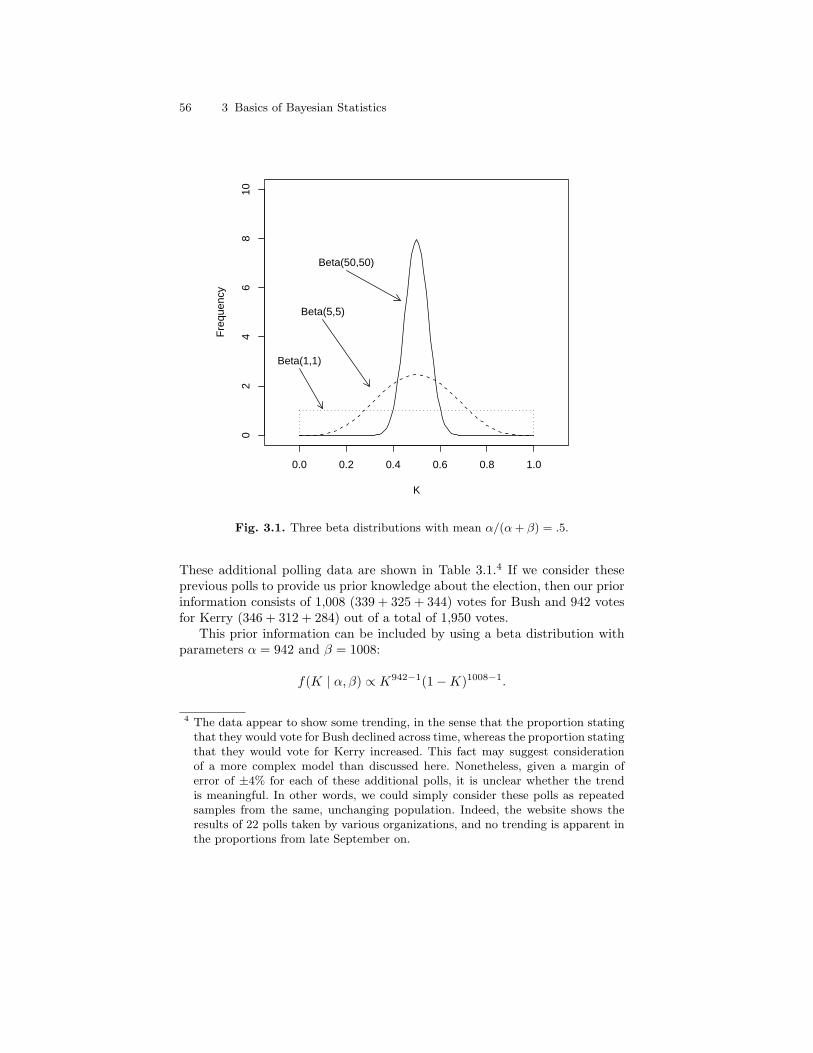
56 3 Basics of Bayesian Statistics
0.0 0.2 0.4 0.6 0.8 1.0
02
46
810
K
Fre
quen
cy
Beta(1,1)
Beta(5,5)
Beta(50,50)
Fig. 3.1. Three beta distributions with mean α/(α + β) = .5.
These additional polling data are shown in Table 3.1.4 If we consider theseprevious polls to provide us prior knowledge about the election, then our priorinformation consists of 1,008 (339 + 325 + 344) votes for Bush and 942 votesfor Kerry (346 + 312 + 284) out of a total of 1,950 votes.
This prior information can be included by using a beta distribution withparameters α = 942 and β = 1008:
f(K | α, β) ∝ K942−1(1−K)1008−1.
4 The data appear to show some trending, in the sense that the proportion statingthat they would vote for Bush declined across time, whereas the proportion statingthat they would vote for Kerry increased. This fact may suggest considerationof a more complex model than discussed here. Nonetheless, given a margin oferror of ±4% for each of these additional polls, it is unclear whether the trendis meaningful. In other words, we could simply consider these polls as repeatedsamples from the same, unchanging population. Indeed, the website shows theresults of 22 polls taken by various organizations, and no trending is apparent inthe proportions from late September on.
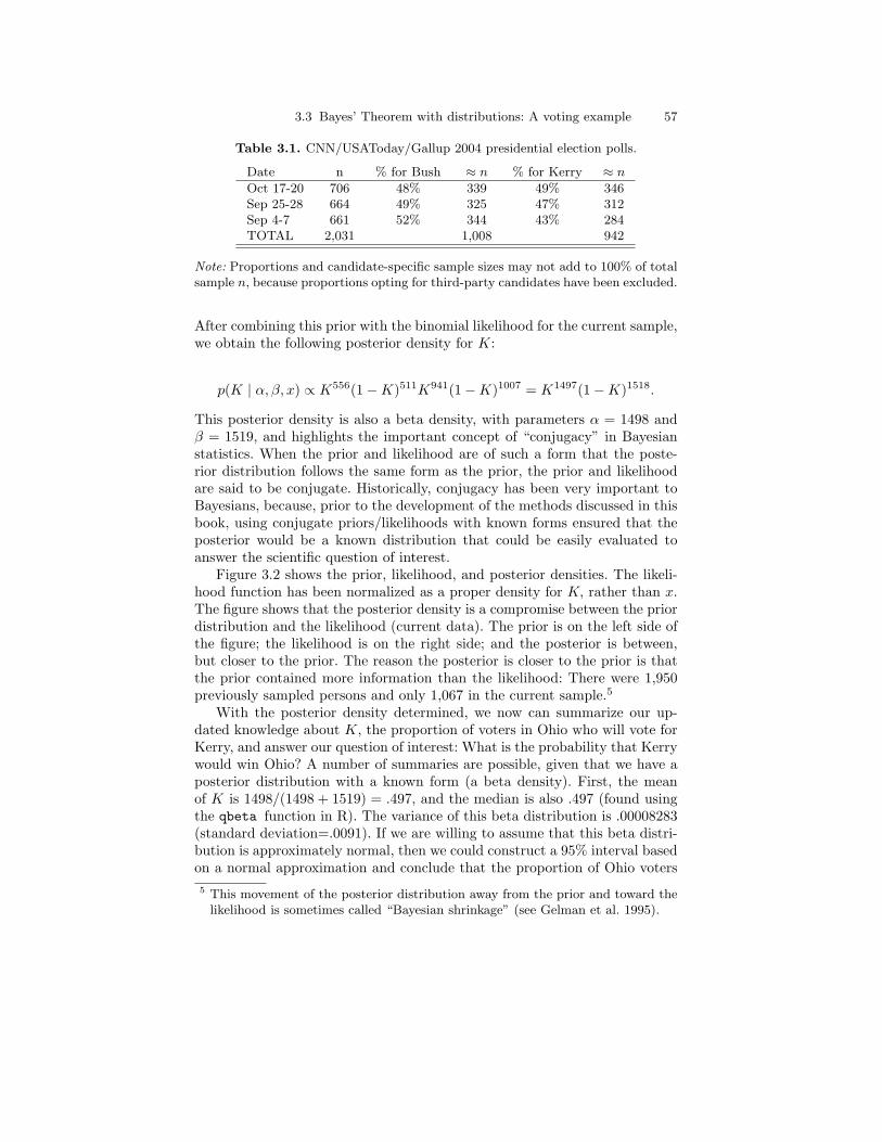
3.3 Bayes’ Theorem with distributions: A voting example 57
Table 3.1. CNN/USAToday/Gallup 2004 presidential election polls.
Date n % for Bush ≈ n % for Kerry ≈ n
Oct 17-20 706 48% 339 49% 346Sep 25-28 664 49% 325 47% 312Sep 4-7 661 52% 344 43% 284TOTAL 2,031 1,008 942
Note: Proportions and candidate-specific sample sizes may not add to 100% of totalsample n, because proportions opting for third-party candidates have been excluded.
After combining this prior with the binomial likelihood for the current sample,we obtain the following posterior density for K:
p(K | α, β, x) ∝ K556(1−K)511K941(1−K)1007 = K1497(1−K)1518.
This posterior density is also a beta density, with parameters α = 1498 andβ = 1519, and highlights the important concept of “conjugacy” in Bayesianstatistics. When the prior and likelihood are of such a form that the poste-rior distribution follows the same form as the prior, the prior and likelihoodare said to be conjugate. Historically, conjugacy has been very important toBayesians, because, prior to the development of the methods discussed in thisbook, using conjugate priors/likelihoods with known forms ensured that theposterior would be a known distribution that could be easily evaluated toanswer the scientific question of interest.
Figure 3.2 shows the prior, likelihood, and posterior densities. The likeli-hood function has been normalized as a proper density for K, rather than x.The figure shows that the posterior density is a compromise between the priordistribution and the likelihood (current data). The prior is on the left side ofthe figure; the likelihood is on the right side; and the posterior is between,but closer to the prior. The reason the posterior is closer to the prior is thatthe prior contained more information than the likelihood: There were 1,950previously sampled persons and only 1,067 in the current sample.5
With the posterior density determined, we now can summarize our up-dated knowledge about K, the proportion of voters in Ohio who will vote forKerry, and answer our question of interest: What is the probability that Kerrywould win Ohio? A number of summaries are possible, given that we have aposterior distribution with a known form (a beta density). First, the meanof K is 1498/(1498 + 1519) = .497, and the median is also .497 (found usingthe qbeta function in R). The variance of this beta distribution is .00008283(standard deviation=.0091). If we are willing to assume that this beta distri-bution is approximately normal, then we could construct a 95% interval basedon a normal approximation and conclude that the proportion of Ohio voters5 This movement of the posterior distribution away from the prior and toward the
likelihood is sometimes called “Bayesian shrinkage” (see Gelman et al. 1995).

58 3 Basics of Bayesian Statistics
0.40 0.45 0.50 0.55 0.60
010
2030
4050
60
K
f(K
)
Prior (Normalized)Likelihood
Posterior
Fig. 3.2. Prior, likelihood, and posterior for polling data example: The likelihoodfunction has been normalized as a density for the parameter K.
who would vote for Kerry falls between .479 and .515 (.497±1.96×.0091). Thisinterval is called a “credible interval,” a “posterior probability interval,” or a“probability interval,” and it has a simpler interpretation than the classicalconfidence interval. Using this interval, we can say simply that the proportionK falls in this interval with probability .95.
If, on the other hand, we are not willing to assume that this posteriordensity is approximately normal, we can directly compute a 95% probabilityinterval by selecting the lower and upper values of this beta density thatproduce the desired interval. That is, we can determine the values of this betadensity below which 2.5% of the distribution falls and above which 2.5% ofthe distribution falls. These values are .479 and .514, which are quite close tothose under the normal approximation.
These results suggest that, even with the prior information, the electionmay have been too close to call, given that the interval estimate for K captures.5. However, the substantive question—what is the probability that Kerrywould win—can also be answered within the Bayesian framework. This prob-ability is the probability that Kerry will get more than half of the votes, which
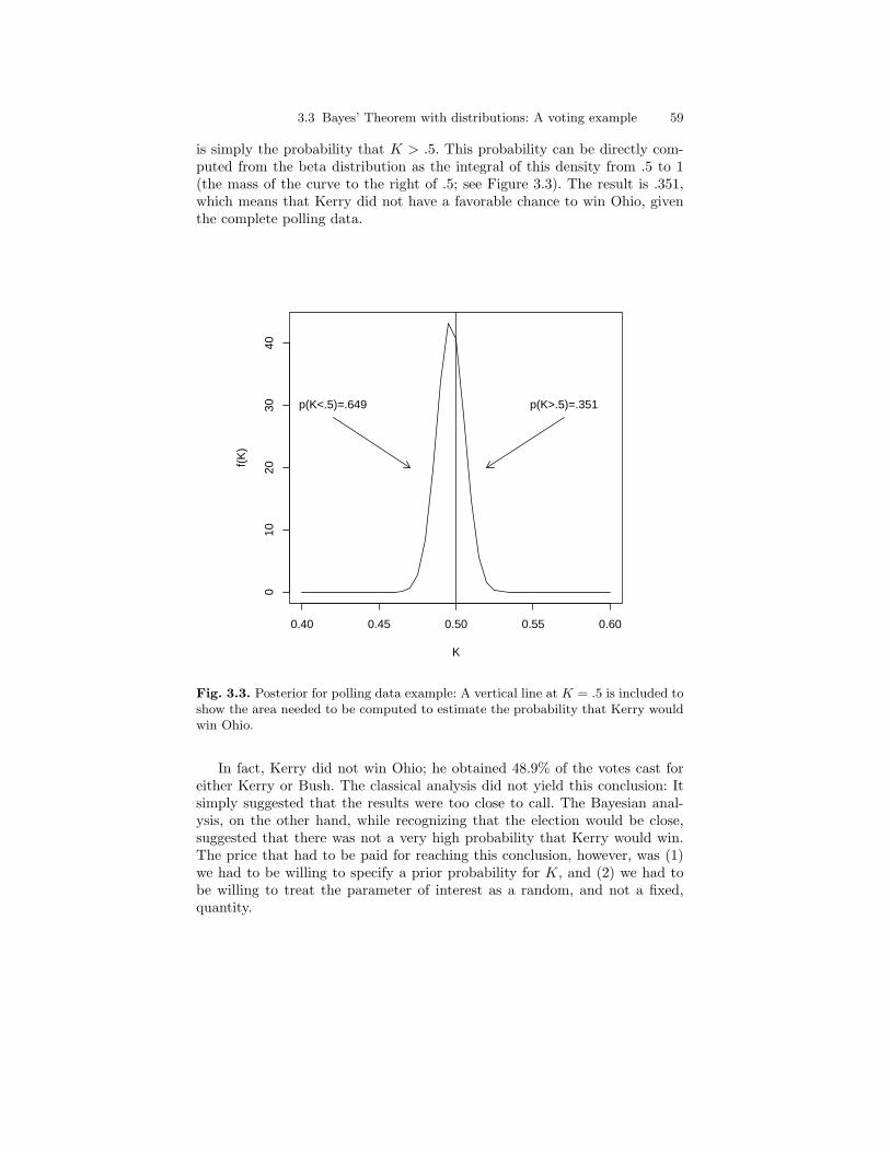
3.3 Bayes’ Theorem with distributions: A voting example 59
is simply the probability that K > .5. This probability can be directly com-puted from the beta distribution as the integral of this density from .5 to 1(the mass of the curve to the right of .5; see Figure 3.3). The result is .351,which means that Kerry did not have a favorable chance to win Ohio, giventhe complete polling data.
0.40 0.45 0.50 0.55 0.60
010
2030
40
K
f(K
)
p(K>.5)=.351p(K<.5)=.649
Fig. 3.3. Posterior for polling data example: A vertical line at K = .5 is included toshow the area needed to be computed to estimate the probability that Kerry wouldwin Ohio.
In fact, Kerry did not win Ohio; he obtained 48.9% of the votes cast foreither Kerry or Bush. The classical analysis did not yield this conclusion: Itsimply suggested that the results were too close to call. The Bayesian anal-ysis, on the other hand, while recognizing that the election would be close,suggested that there was not a very high probability that Kerry would win.The price that had to be paid for reaching this conclusion, however, was (1)we had to be willing to specify a prior probability for K, and (2) we had tobe willing to treat the parameter of interest as a random, and not a fixed,quantity.
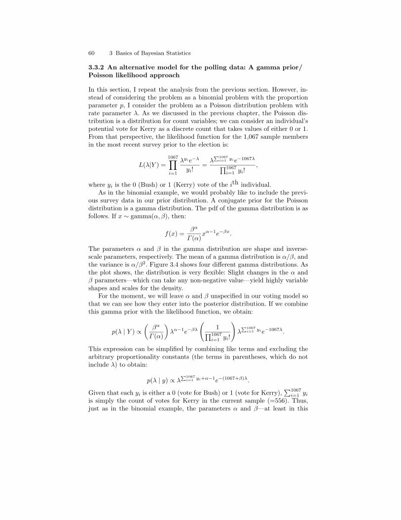
60 3 Basics of Bayesian Statistics
3.3.2 An alternative model for the polling data: A gamma prior/Poisson likelihood approach
In this section, I repeat the analysis from the previous section. However, in-stead of considering the problem as a binomial problem with the proportionparameter p, I consider the problem as a Poisson distribution problem withrate parameter λ. As we discussed in the previous chapter, the Poisson dis-tribution is a distribution for count variables; we can consider an individual’spotential vote for Kerry as a discrete count that takes values of either 0 or 1.From that perspective, the likelihood function for the 1,067 sample membersin the most recent survey prior to the election is:
L(λ|Y ) =1067∏i=1
λyie−λ
yi!=
λP1067
i=1 yie−1067λ∏1067i=1 yi!
,
where yi is the 0 (Bush) or 1 (Kerry) vote of the ith individual.As in the binomial example, we would probably like to include the previ-
ous survey data in our prior distribution. A conjugate prior for the Poissondistribution is a gamma distribution. The pdf of the gamma distribution is asfollows. If x ∼ gamma(α, β), then:
f(x) =βα
Γ (α)xα−1e−βx.
The parameters α and β in the gamma distribution are shape and inverse-scale parameters, respectively. The mean of a gamma distribution is α/β, andthe variance is α/β2. Figure 3.4 shows four different gamma distributions. Asthe plot shows, the distribution is very flexible: Slight changes in the α andβ parameters—which can take any non-negative value—yield highly variableshapes and scales for the density.
For the moment, we will leave α and β unspecified in our voting model sothat we can see how they enter into the posterior distribution. If we combinethis gamma prior with the likelihood function, we obtain:
p(λ | Y ) ∝(
βα
Γ (α)
)λα−1e−βλ
(1∏1067
i=1 yi!
)λ
P1067i=1 yie−1067λ.
This expression can be simplified by combining like terms and excluding thearbitrary proportionality constants (the terms in parentheses, which do notinclude λ) to obtain:
p(λ | y) ∝ λP1067
i=1 yi+α−1e−(1067+β)λ.
Given that each yi is either a 0 (vote for Bush) or 1 (vote for Kerry),∑1067
i=1 yi
is simply the count of votes for Kerry in the current sample (=556). Thus,just as in the binomial example, the parameters α and β—at least in this
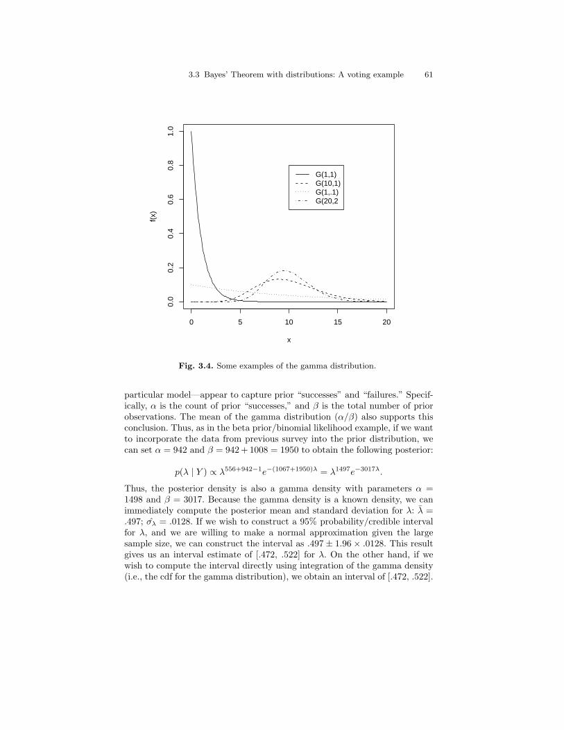
3.3 Bayes’ Theorem with distributions: A voting example 61
0 5 10 15 20
0.0
0.2
0.4
0.6
0.8
1.0
x
f(x)
G(1,1)G(10,1)G(1,.1)G(20,2
Fig. 3.4. Some examples of the gamma distribution.
particular model—appear to capture prior “successes” and “failures.” Specif-ically, α is the count of prior “successes,” and β is the total number of priorobservations. The mean of the gamma distribution (α/β) also supports thisconclusion. Thus, as in the beta prior/binomial likelihood example, if we wantto incorporate the data from previous survey into the prior distribution, wecan set α = 942 and β = 942 + 1008 = 1950 to obtain the following posterior:
p(λ | Y ) ∝ λ556+942−1e−(1067+1950)λ = λ1497e−3017λ.
Thus, the posterior density is also a gamma density with parameters α =1498 and β = 3017. Because the gamma density is a known density, we canimmediately compute the posterior mean and standard deviation for λ: λ =.497; σλ = .0128. If we wish to construct a 95% probability/credible intervalfor λ, and we are willing to make a normal approximation given the largesample size, we can construct the interval as .497± 1.96× .0128. This resultgives us an interval estimate of [.472, .522] for λ. On the other hand, if wewish to compute the interval directly using integration of the gamma density(i.e., the cdf for the gamma distribution), we obtain an interval of [.472, .522].
62 3 Basics of Bayesian Statistics
In this case, the normal-theory interval and the analytically derived intervalare the same when rounded to three decimal places.
How does this posterior inference compare with that obtained using thebeta prior/binomial likelihood approach? The means for K in the beta/binomialapproach and for λ in the gamma/Poisson approach are identical. The inter-vals are also quite comparable, but the interval in this latter approach iswider—about 42% wider. If we wish to determine the probability that Kerrywould win Ohio, we simply need to compute p(λ > .5), which equals .390.Thus, under this model, Kerry had a probability of winning of .390, which isstill an unfavorable result, although it is a slightly greater probability thanthe beta/binomial result of .351.
Which model is to be preferred? In this case, the substantive conclusionwe reached was comparable for the two models: Kerry was unlikely to winOhio. So, it does not matter which model we choose. The fact that the twomodels produced comparable results is reassuring, because the conclusion doesnot appear to be very sensitive to choice of model. Ultimately, however, weshould probably place greater emphasis on the beta/binomial model, becausethe Poisson distribution is a distribution for counts, and our data, whichconsisted of dichotomous outcomes, really does not fit the bill. Consider theparameter λ: There is no guarantee with the gamma/Poisson setup that λ willbe less than 1. This lack of limit could certainly be problematic if we had lessdata, or if the underlying proportion favoring Kerry were closer to 1. In sucha case, the upper bound on the interval for λ may have exceeded 1, and ourresults would therefore be suspect. In this particular case, however, we hadenough data and prior information that ultimately made the interval widthvery narrow, and so the bounding problem was not an issue. Nonetheless, thebeta/binomial setup is a more natural model for the voting data.
3.4 A normal prior–normal likelihood example with σ2
known
The normal distribution is one of the most common distributions used instatistics by social scientists, in part because many social phenomena in factfollow a normal distribution. Thus, it is not uncommon for a social scientistto use a normal distribution as the basis for a likelihood function for a set ofdata. Here, I develop a normal distribution problem, but for the sake of keepingthis example general for use in later chapters, I used a contrived scenario andkeep the mathematics fairly general. The purpose at this point is simply toillustrate a Bayesian approach with a multivariate posterior distribution.6
6 The normal distribution involves two parameters: the mean (µ) and variance (σ2).When considered as a density for x, it is univariate, but when a normal likelihoodand some prior for the parameters are combined, the result is a joint posteriordistribution for µ and σ2, which makes the posterior a multivariate density.
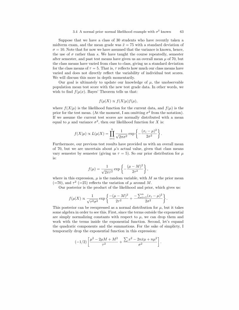
3.4 A normal prior–normal likelihood example with σ2 known 63
Suppose that we have a class of 30 students who have recently taken amidterm exam, and the mean grade was x = 75 with a standard deviation ofσ = 10. Note that for now we have assumed that the variance is known, hence,the use of σ rather than s. We have taught the course repeatedly, semesterafter semester, and past test means have given us an overall mean µ of 70, butthe class means have varied from class to class, giving us a standard deviationfor the class means of τ = 5. That is, τ reflects how much our class means havevaried and does not directly reflect the variability of individual test scores.We will discuss this more in depth momentarily.
Our goal is ultimately to update our knowledge of µ, the unobservablepopulation mean test score with the new test grade data. In other words, wewish to find f(µ|x). Bayes’ Theorem tells us that:
f(µ|X) ∝ f(X|µ)f(µ),
where f(X|µ) is the likelihood function for the current data, and f(µ) is theprior for the test mean. (At the moment, I am omitting σ2 from the notation).If we assume the current test scores are normally distributed with a meanequal to µ and variance σ2, then our likelihood function for X is:
f(X|µ) ∝ L(µ|X) =n∏
i=1
1√2πσ2
exp− (xi − µ)2
2σ2
.
Furthermore, our previous test results have provided us with an overall meanof 70, but we are uncertain about µ’s actual value, given that class meansvary semester by semester (giving us τ = 5). So our prior distribution for µis:
f(µ) =1√
2πτ2exp
− (µ−M)2
2τ2
,
where in this expression, µ is the random variable, with M as the prior mean(=70), and τ2 (=25) reflects the variation of µ around M .
Our posterior is the product of the likelihood and prior, which gives us:
f(µ|X) ∝ 1√τ2σ2
exp−(µ−M)2
2τ2+−∑n
i=1(xi − µ)2
2σ2
.
This posterior can be reexpressed as a normal distribution for µ, but it takessome algebra in order to see this. First, since the terms outside the exponentialare simply normalizing constants with respect to µ, we can drop them andwork with the terms inside the exponential function. Second, let’s expandthe quadratic components and the summations. For the sake of simplicty, Itemporarily drop the exponential function in this expression:
(−1/2)[µ2 − 2µM + M2
τ2+∑
x2 − 2nxµ + nµ2
σ2
].
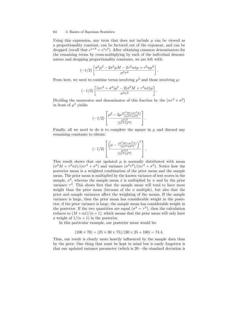
64 3 Basics of Bayesian Statistics
Using this expression, any term that does not include µ can be viewed asa proportionality constant, can be factored out of the exponent, and can bedropped (recall that ea+b = eaeb). After obtaining common denominators forthe remaining terms by cross-multiplying by each of the individual denomi-nators and dropping proportionality constants, we are left with:
(−1/2)[σ2µ2 − 2σ2µM − 2τ2nxµ + τ2nµ2
σ2τ2
].
From here, we need to combine terms involving µ2 and those involving µ:
(−1/2)[(nτ2 + σ2)µ2 − 2(σ2M + τ2nx)µ
σ2τ2
].
Dividing the numerator and denominator of this fraction by the (nτ2 + σ2)in front of µ2 yields:
(−1/2)
µ2 − 2µ (σ2M+nτ2x)(nτ2+σ2)
σ2τ2
(nτ2+σ2)
.
Finally, all we need to do is to complete the square in µ and discard anyremaining constants to obtain:
(−1/2)
(µ− (σ2M+nτ2x)
(nτ2+σ2)
)2
σ2τ2
(nτ2+σ2)
.
This result shows that our updated µ is normally distributed with mean(σ2M + τ2nx)/(nτ2 + σ2) and variance (σ2τ2)/(nτ2 + σ2). Notice how theposterior mean is a weighted combination of the prior mean and the samplemean. The prior mean is multiplied by the known variance of test scores in thesample, σ2, whereas the sample mean x is multiplied by n and by the priorvariance τ2. This shows first that the sample mean will tend to have moreweight than the prior mean (because of the n multiple), but also that theprior and sample variances affect the weighting of the means. If the samplevariance is large, then the prior mean has considerable weight in the poste-rior; if the prior variance is large, the sample mean has considerable weight inthe posterior. If the two quantities are equal (σ2 = τ2), then the calculationreduces to (M +nx)/(n+1), which means that the prior mean will only havea weight of 1/(n + 1) in the posterior.
In this particular example, our posterior mean would be:
(100× 70) + (25× 30× 75)/(30× 25 + 100) = 74.4.
Thus, our result is clearly more heavily influenced by the sample data thanby the prior. One thing that must be kept in mind but is easily forgotten isthat our updated variance parameter (which is 20—the standard deviation is
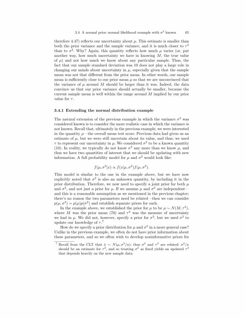
3.4 A normal prior–normal likelihood example with σ2 known 65
therefore 4.47) reflects our uncertainty about µ. This estimate is smaller thanboth the prior variance and the sample variance, and it is much closer to τ2
than to σ2. Why? Again, this quantity reflects how much µ varies (or, putanother way, how much uncertainty we have in knowing M , the true valueof µ) and not how much we know about any particular sample. Thus, thefact that our sample standard deviation was 10 does not play a large role inchanging our minds about uncertainty in µ, especially given that the samplemean was not that different from the prior mean. In other words, our samplemean is sufficiently close to our prior mean µ so that we are unconvinced thatthe variance of µ around M should be larger than it was. Indeed, the dataconvince us that our prior variance should actually be smaller, because thecurrent sample mean is well within the range around M implied by our priorvalue for τ .
3.4.1 Extending the normal distribution example
The natural extension of the previous example in which the variance σ2 wasconsidered known is to consider the more realistic case in which the variance isnot known. Recall that, ultimately in the previous example, we were interestedin the quantity µ—the overall mean test score. Previous data had given us anestimate of µ, but we were still uncertain about its value, and thus, we usedτ to represent our uncertainty in µ. We considered σ2 to be a known quantity(10). In reality, we typically do not know σ2 any more than we know µ, andthus we have two quantities of interest that we should be updating with newinformation. A full probability model for µ and σ2 would look like:
f(µ, σ2|x) ∝ f(x|µ, σ2)f(µ, σ2).
This model is similar to the one in the example above, but we have nowexplicitly noted that σ2 is also an unknown quantity, by including it in theprior distribution. Therefore, we now need to specify a joint prior for both µand σ2, and not just a prior for µ. If we assume µ and σ2 are independent—and this is a reasonable assumption as we mentioned in the previous chapter;there’s no reason the two parameters need be related—then we can considerp(µ, σ2) = p(µ)p(σ2) and establish separate priors for each.
In the example above, we established the prior for µ to be µ ∼ N(M, τ2),where M was the prior mean (70) and τ2 was the measure of uncertaintywe had in µ. We did not, however, specify a prior for σ2, but we used σ2 toupdate our knowledge of τ .7
How do we specify a prior distribution for µ and σ2 in a more general case?Unlike in the previous example, we often do not have prior information aboutthese parameters, and so we often wish to develop noninformative priors for7 Recall from the CLT that x ∼ N(µ, σ2/n); thus σ2 and τ2 are related: σ2/n
should be an estimate for τ2, and so treating σ2 as fixed yields an updated τ2
that depends heavily on the new sample data.
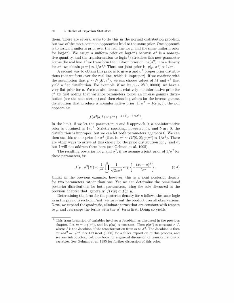
66 3 Basics of Bayesian Statistics
them. There are several ways to do this in the normal distribution problem,but two of the most common approaches lead to the same prior. One approachis to assign a uniform prior over the real line for µ and the same uniform priorfor log(σ2). We assign a uniform prior on log(σ2) because σ2 is a nonega-tive quantity, and the transformation to log(σ2) stretches this new parameteracross the real line. If we transform the uniform prior on log(σ2) into a densityfor σ2, we obtain p(σ2) ∝ 1/σ2.8 Thus, our joint prior is: p(µ, σ2) ∝ 1/σ2.
A second way to obtain this prior is to give µ and σ2 proper prior distribu-tions (not uniform over the real line, which is improper). If we continue withthe assumption that µ ∼ N(M, τ2), we can choose values of M and τ2 thatyield a flat distribution. For example, if we let µ ∼ N(0, 10000), we have avery flat prior for µ. We can also choose a relatively noninformative prior forσ2 by first noting that variance parameters follow an inverse gamma distri-bution (see the next section) and then choosing values for the inverse gammadistribution that produce a noninformative prior. If σ2 ∼ IG(a, b), the pdfappears as:
f(σ2|a, b) ∝ (σ2)−(a+1)e−β/(σ2).
In the limit, if we let the parameters a and b approach 0, a noninformativeprior is obtained as 1/σ2. Strictly speaking, however, if a and b are 0, thedistribution is improper, but we can let both parameters approach 0. We canthen use this as our prior for σ2 (that is, σ2 ∼ IG(0, 0); p(σ2) ∝ 1/σ2). Thereare other ways to arrive at this choice for the prior distribution for µ and σ,but I will not address them here (see Gelman et al. 1995).
The resulting posterior for µ and σ2, if we assume a joint prior of 1/σ2 forthese parameters, is:
f(µ, σ2|X) ∝ 1σ2
n∏i=1
1√2πσ2
exp− (xi − µ)2
2σ2
. (3.4)
Unlike in the previous example, however, this is a joint posterior densityfor two parameters rather than one. Yet we can determine the conditionalposterior distributions for both parameters, using the rule discussed in theprevious chapter that, generally, f(x|y) ∝ f(x, y).
Determining the form for the posterior density for µ follows the same logicas in the previous section. First, we carry out the product over all observations.Next, we expand the quadratic, eliminate terms that are constant with respectto µ and rearrange the terms with the µ2 term first. Doing so yields:
8 This transformation of variables involves a Jacobian, as discussed in the previouschapter. Let m = log(σ2), and let p(m) ∝ constant. Then p(σ2) ∝ constant× J ,where J is the Jacobian of the transformation from m to σ2. The Jacobian is thendm/dσ2 = 1/σ2. See DeGroot (1986) for a fuller exposition of this process, andsee any introductory calculus book for a general discussion of transformations ofvariables. See Gelman et al. 1995 for further discussion of this prior.
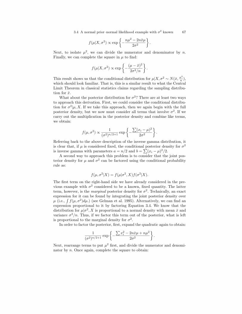
3.4 A normal prior–normal likelihood example with σ2 known 67
f(µ|X, σ2) ∝ exp−nµ2 − 2nxµ
2σ2
.
Next, to isolate µ2, we can divide the numerator and denominator by n.Finally, we can complete the square in µ to find:
f(µ|X, σ2) ∝ exp− (µ− x)2
2σ2/n
.
This result shows us that the conditional distribution for µ|X, σ2 ∼ N(x, σ2
n ),which should look familiar. That is, this is a similar result to what the CentralLimit Theorem in classical statistics claims regarding the sampling distribu-tion for x.
What about the posterior distribution for σ2? There are at least two waysto approach this derivation. First, we could consider the conditional distribu-tion for σ2|µ,X. If we take this approach, then we again begin with the fullposterior density, but we now must consider all terms that involve σ2. If wecarry out the multiplication in the posterior density and combine like terms,we obtain:
f(µ, σ2) ∝ 1(σ2)n/2+1
exp−∑
(xi − µ)2
2σ2
.
Referring back to the above description of the inverse gamma distribution, itis clear that, if µ is considered fixed, the conditional posterior density for σ2
is inverse gamma with parameters a = n/2 and b =∑
(xi − µ)2/2.A second way to approach this problem is to consider that the joint pos-
terior density for µ and σ2 can be factored using the conditional probabilityrule as:
f(µ, σ2|X) = f(µ|σ2, X)f(σ2|X).
The first term on the right-hand side we have already considered in the pre-vious example with σ2 considered to be a known, fixed quantity. The latterterm, however, is the marginal posterior density for σ2. Technically, an exactexpression for it can be found by integrating the joint posterior density overµ (i.e.,
∫f(µ, σ2)dµ.) (see Gelman et al. 1995). Alternatively, we can find an
expression proportional to it by factoring Equation 3.4. We know that thedistribution for µ|σ2, X is proportional to a normal density with mean x andvariance σ2/n. Thus, if we factor this term out of the posterior, what is leftis proportional to the marginal density for σ2.
In order to factor the posterior, first, expand the quadratic again to obtain:
1(σ2)n/2+1
exp−∑
x2i − 2nxµ + nµ2
2σ2
.
Next, rearrange terms to put µ2 first, and divide the numerator and denomi-nator by n. Once again, complete the square to obtain:
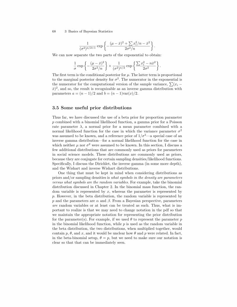
68 3 Basics of Bayesian Statistics
1(σ2)n/2+1
exp− (µ− x)2 +
∑x2
i /n− x2
2σ2/n
.
We can now separate the two parts of the exponential to obtain:
1σ
exp− (µ− x)2
2σ2/n
× 1
(σ2)n/2exp
∑x2
i − nx2
2σ2
.
The first term is the conditional posterior for µ. The latter term is proportionalto the marginal posterior density for σ2. The numerator in the exponential isthe numerator for the computational version of the sample variance,
∑(xi −
x)2, and so, the result is recognizable as an inverse gamma distribution withparameters a = (n− 1)/2 and b = (n− 1)var(x)/2.
3.5 Some useful prior distributions
Thus far, we have discussed the use of a beta prior for proportion parameterp combined with a binomial likelihood function, a gamma prior for a Poissonrate parameter λ, a normal prior for a mean parameter combined with anormal likelihood function for the case in which the variance parameter σ2
was assumed to be known, and a reference prior of 1/σ2—a special case of aninverse gamma distribution—for a normal likelihood function for the case inwhich neither µ nor σ2 were assumed to be known. In this section, I discuss afew additional distributions that are commonly used as priors for parametersin social science models. These distributions are commonly used as priors,because they are conjugate for certain sampling densities/likelihood functions.Specifically, I discuss the Dirichlet, the inverse gamma (in some more depth),and the Wishart and inverse Wishart distributions.
One thing that must be kept in mind when considering distributions aspriors and/or sampling densities is what symbols in the density are parametersversus what symbols are the random variables. For example, take the binomialdistribution discussed in Chapter 2. In the binomial mass function, the ran-dom variable is represented by x, whereas the parameter is represented byp. However, in the beta distribution, the random variable is represented byp and the parameters are α and β. From a Bayesian perspective, parametersare random variables or at least can be treated as such. Thus, what is im-portant to realize is that we may need to change notation in the pdf so thatwe maintain the appropriate notation for representing the prior distributionfor the parameter(s). For example, if we used θ to represent the parameter pin the binomial likelihood function, while p is used as the random variable inthe beta distribution, the two distributions, when multiplied together, wouldcontain p, θ, and x, and it would be unclear how θ and p were related. In fact,in the beta-binomial setup, θ = p, but we need to make sure our notation isclear so that that can be immediately seen.
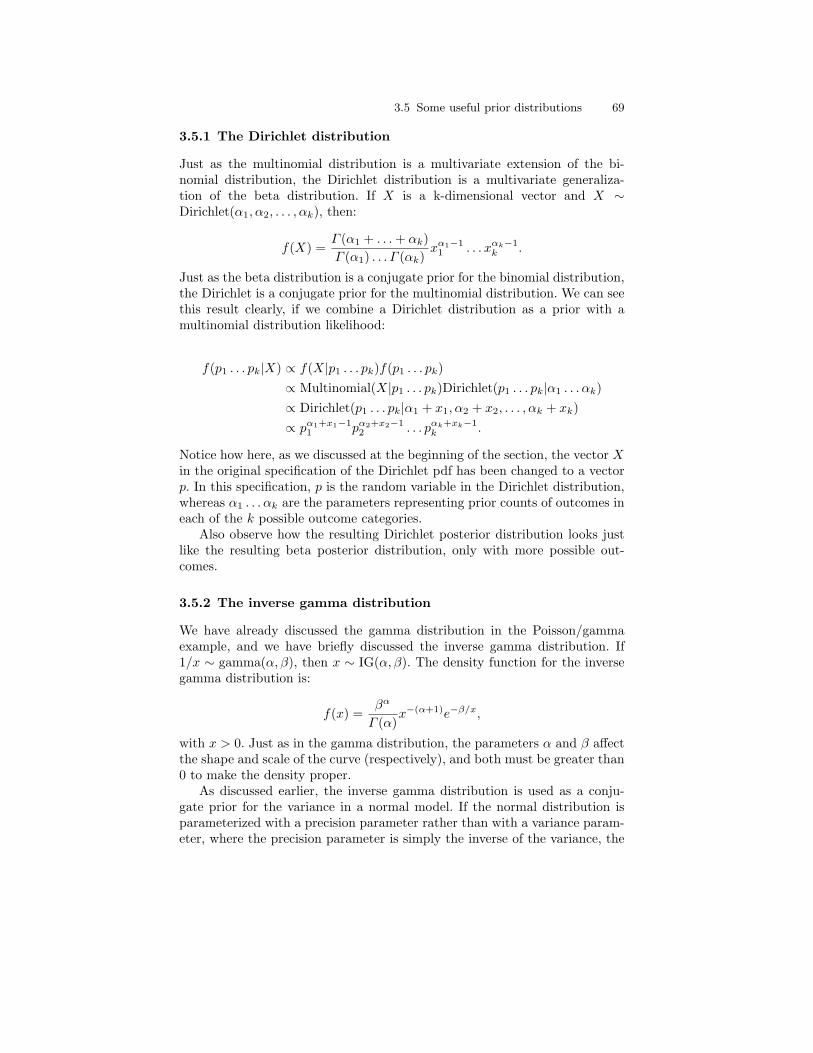
3.5 Some useful prior distributions 69
3.5.1 The Dirichlet distribution
Just as the multinomial distribution is a multivariate extension of the bi-nomial distribution, the Dirichlet distribution is a multivariate generaliza-tion of the beta distribution. If X is a k-dimensional vector and X ∼Dirichlet(α1, α2, . . . , αk), then:
f(X) =Γ (α1 + . . . + αk)Γ (α1) . . . Γ (αk)
xα1−11 . . . xαk−1
k .
Just as the beta distribution is a conjugate prior for the binomial distribution,the Dirichlet is a conjugate prior for the multinomial distribution. We can seethis result clearly, if we combine a Dirichlet distribution as a prior with amultinomial distribution likelihood:
f(p1 . . . pk|X) ∝ f(X|p1 . . . pk)f(p1 . . . pk)∝ Multinomial(X|p1 . . . pk)Dirichlet(p1 . . . pk|α1 . . . αk)∝ Dirichlet(p1 . . . pk|α1 + x1, α2 + x2, . . . , αk + xk)∝ pα1+x1−1
1 pα2+x2−12 . . . pαk+xk−1
k .
Notice how here, as we discussed at the beginning of the section, the vector Xin the original specification of the Dirichlet pdf has been changed to a vectorp. In this specification, p is the random variable in the Dirichlet distribution,whereas α1 . . . αk are the parameters representing prior counts of outcomes ineach of the k possible outcome categories.
Also observe how the resulting Dirichlet posterior distribution looks justlike the resulting beta posterior distribution, only with more possible out-comes.
3.5.2 The inverse gamma distribution
We have already discussed the gamma distribution in the Poisson/gammaexample, and we have briefly discussed the inverse gamma distribution. If1/x ∼ gamma(α, β), then x ∼ IG(α, β). The density function for the inversegamma distribution is:
f(x) =βα
Γ (α)x−(α+1)e−β/x,
with x > 0. Just as in the gamma distribution, the parameters α and β affectthe shape and scale of the curve (respectively), and both must be greater than0 to make the density proper.
As discussed earlier, the inverse gamma distribution is used as a conju-gate prior for the variance in a normal model. If the normal distribution isparameterized with a precision parameter rather than with a variance param-eter, where the precision parameter is simply the inverse of the variance, the

70 3 Basics of Bayesian Statistics
gamma distribution is appropriate as a conjugate prior distribution for theprecision parameter. In a normal model, if an inverse gamma distribution isused as the prior for the variance, the marginal distribution for the mean is at distribution.
The gamma and inverse gamma distributions are general distributions;other distributions arise by fixing the parameters to specific values. For ex-ample, if α is set to 1, the exponential distribution results:
f(x) = (1/β)e−x/β ,
or, more commonly f(x) = βe−βx, where β is an inverse scale parameter.Under this parameterization, βinverse scale = 1/βscale.
If α is set to v/2, where v is the degrees of freedom, and β is set to 1/2, thechi-square distribution results. Setting the parameters equal to the same valuein the inverse-gamma distribution yields an inverse-chi-square distribution.
3.5.3 Wishart and inverse Wishart distributions
The Wishart and inverse Wishart distributions are complex in appearance;they are multivariate generalizations of the gamma and inverse gamma dis-tributions, respectively. Thus, just as the inverse gamma is a conjugate priordensity for the variance in a univariate normal model, the inverse Wishartis a conjugate prior density for the variance-covariance matrix in a multi-variate normal model. With an inverse Wishart distribution for the variance-covariance matrix in a multivariate normal model, the marginal distributionfor the mean vector is multivariate t.
If X ∼ Wishart(S), where S is a scale matrix of dimension d, then
f(X) ∝| X |(v−d−1)/2 exp−1
2tr(S−1X)
,
where v is the degrees of freedom.If X ∼ inverse Wishart(S−1), then:
f(X) ∝| X |−(v+d+1)/2 exp−1
2tr(SX−1)
.
The assumption for both the Wishart and inverse Wishart distributions isthat X and S are both positive definite; that is, zT Xz > 0 and zT Sz > 0 forany non-zero vector z of length d.
3.6 Criticism against Bayesian statistics
As we have seen in the examples, the development of a Bayesian model re-quires the inclusion of a prior distribution for the parameters in the model.The notion of using prior research or other information to inform a current
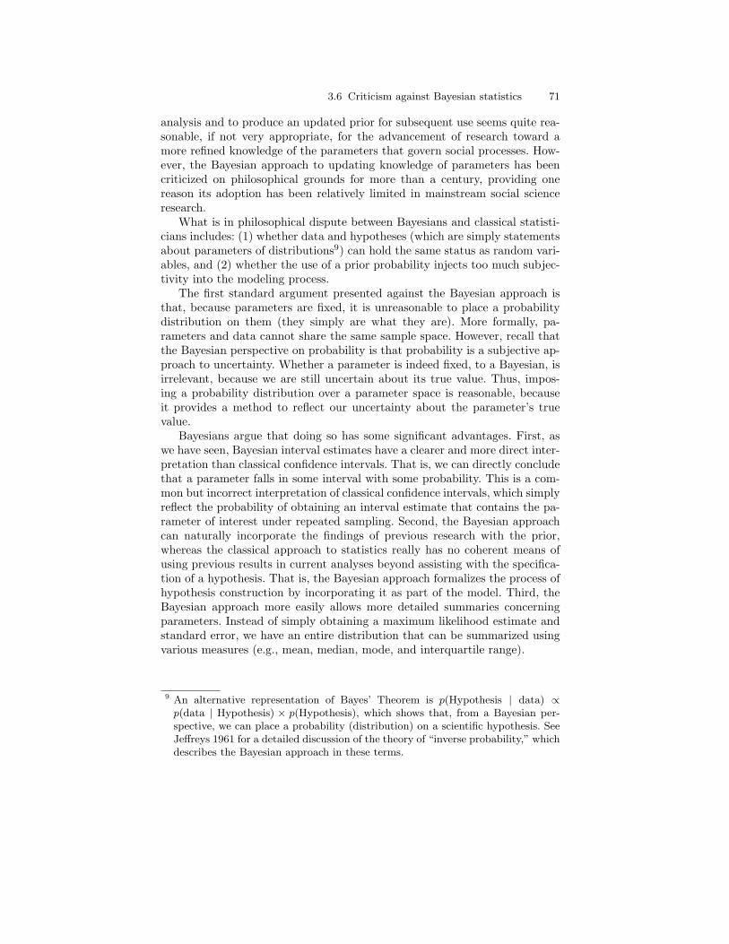
3.6 Criticism against Bayesian statistics 71
analysis and to produce an updated prior for subsequent use seems quite rea-sonable, if not very appropriate, for the advancement of research toward amore refined knowledge of the parameters that govern social processes. How-ever, the Bayesian approach to updating knowledge of parameters has beencriticized on philosophical grounds for more than a century, providing onereason its adoption has been relatively limited in mainstream social scienceresearch.
What is in philosophical dispute between Bayesians and classical statisti-cians includes: (1) whether data and hypotheses (which are simply statementsabout parameters of distributions9) can hold the same status as random vari-ables, and (2) whether the use of a prior probability injects too much subjec-tivity into the modeling process.
The first standard argument presented against the Bayesian approach isthat, because parameters are fixed, it is unreasonable to place a probabilitydistribution on them (they simply are what they are). More formally, pa-rameters and data cannot share the same sample space. However, recall thatthe Bayesian perspective on probability is that probability is a subjective ap-proach to uncertainty. Whether a parameter is indeed fixed, to a Bayesian, isirrelevant, because we are still uncertain about its true value. Thus, impos-ing a probability distribution over a parameter space is reasonable, becauseit provides a method to reflect our uncertainty about the parameter’s truevalue.
Bayesians argue that doing so has some significant advantages. First, aswe have seen, Bayesian interval estimates have a clearer and more direct inter-pretation than classical confidence intervals. That is, we can directly concludethat a parameter falls in some interval with some probability. This is a com-mon but incorrect interpretation of classical confidence intervals, which simplyreflect the probability of obtaining an interval estimate that contains the pa-rameter of interest under repeated sampling. Second, the Bayesian approachcan naturally incorporate the findings of previous research with the prior,whereas the classical approach to statistics really has no coherent means ofusing previous results in current analyses beyond assisting with the specifica-tion of a hypothesis. That is, the Bayesian approach formalizes the process ofhypothesis construction by incorporating it as part of the model. Third, theBayesian approach more easily allows more detailed summaries concerningparameters. Instead of simply obtaining a maximum likelihood estimate andstandard error, we have an entire distribution that can be summarized usingvarious measures (e.g., mean, median, mode, and interquartile range).
9 An alternative representation of Bayes’ Theorem is p(Hypothesis | data) ∝p(data | Hypothesis) × p(Hypothesis), which shows that, from a Bayesian per-spective, we can place a probability (distribution) on a scientific hypothesis. SeeJeffreys 1961 for a detailed discussion of the theory of “inverse probability,” whichdescribes the Bayesian approach in these terms.
72 3 Basics of Bayesian Statistics
The second general argument that has been advanced against Bayesiananalysis is that incorporating a prior injects too much subjectivity into statis-tical modeling. The Bayesian response to this argument is multifaceted. First,all statistics is subjective. The choice of sampling density (likelihood) to usein a specific project is a subjective determination. For example, when facedwith an ordinal outcome, some choose to use a normal likelihood function,leading to the ordinary least squares (OLS) regression model. Others choose abinomial likelihood with a link function, leading to an ordinal logit or probitregression model. These are subjective choices.
Second, the choice of cut-point (α) at which to declare a result “statisti-cally significant” in a classical sense is a purely subjective determination. Also,similarly, the decision to declare a statistically significant result substantivelymeaningful is a subjective decision.
A third response to the subjectivity criticism is that priors tend to beoverwhelmed by data, especially in social science research. The prior distribu-tion generally contributes to the posterior once, whereas data enter into thelikelihood function multiple times. As n → ∞, the prior’s influence on theposterior often becomes negligible.
Fourth, priors can be quite noninformative, obviating the need for largequantities of data to “outweigh” them. In other words, a prior can be madeto contribute little information to the posterior. That is, given that the pos-terior density is simply a weighted likelihood function, where the weightingis imposed by the prior, we can simply choose a prior distribution for theparameters that assigns approximately equal weight to all possible values ofthe parameters. The simplest noninformative prior that is often used is thus auniform prior. Use of this prior yields a posterior density that is proportionalto the likelihood function. In that case, the mode of the likelihood function(the maximum likelihood estimate) is the same as the Bayesian maximum aposteriori (MAP) estimate, and the substantive conclusions reached by bothapproaches may be similar, only differing in interpretation.
In defense of the classical criticism, although uniform densities for param-eters are often used as priors, transformation from one parameterization ofa parameter to another may yield an informative prior. However, alternativeapproaches have been developed for generating noninformative priors, includ-ing the development of Jeffreys priors and other priors. These noninformativepriors tend to be based on the information matrix and are invariant under pa-rameter transformation. An in-depth discussion of such priors is beyond thescope of this book, given the goal of a general introduction to estimation. Formore details, see Gelman et al. (1995) or see Gill (2002) for a more in-depthdiscussion of the history of the use and construction of noninformative priors.
A fourth response is that the influence of priors can be evaluated aftermodeling the data to determine whether posterior inference is reasonable. Ul-timately, the results of any statistical analysis, whether Bayesian or classical,must be subjectively evaluated to determine whether they are reasonable, andso, the use of informative priors cannot introduce any more subjectivity than
3.7 Conclusions 73
could be included via other means in any analysis. Another response alongthese lines is that we can use priors to our advantage to examine how pow-erful the data are at invalidating the prior. For example, we may establisha conservative prior for a regression coefficient that claims that the a prioriprobability for a regression coefficient is heavily concentrated around 0 (i.e.,the covariate has no effect on the outcome). We can then examine the strengthof the data in rejecting this prior, providing a conservative test of a covariate’seffect.
In general, the historical criticisms of Bayesian statistics are philosophicalin nature and cannot be conclusively adjudicated. Instead, the rise in theuse of Bayesian statistics over the last few decades has largely occurred forpragmatic reasons, including (1) that many contemporary research questionsreadily lend themselves to a Bayesian approach, and (2) that the developmentof sampling methods used to estimate model parameters has increased theirease of use. The remaining chapters attempt to demonstrate these points.
3.7 Conclusions
In this chapter, we have developed the basics of the Bayesian approach tostatistical inference. First, we derived Bayes’ Theorem from the probabilityrules developed in the previous chapter, and we applied Bayes’ Theorem toproblems requiring point estimates for probabilities. We then extended theBayesian approach to handle prior distributions for parameters rather thansimply point estimates for prior probabilties. The result was that our posteriorprobability became a distribution, rather than a point estimate. Next, we dis-cussed how to summarize posterior probability distributions, and we demon-strated how to do so using several common examples. Finally, we discussedsome common criticisms of the Bayesian approach that have been advancedover the last century, and we reviewed some common Bayesian responses tothem. Although the material presented in this chapter is sufficient for gaininga basic understanding of the Bayesian approach to statistics, I recommendseveral additional sources for more in-depth coverage. I recommend Lee 1989for an extremely thorough but accessible exposition of the Bayesian paradigm,and I recommend Box and Tiao (1973) for a more advanced exposition.
In the next chapter, we will continue exploring the Bayesian approachto posterior summarization and inference, but we will ultimately focus onmultivariate posterior distributions—the most common type of posterior dis-tribution found in social science research—where the multivariate posteriordistribution may not be as easy to summarize directly as the univariate pos-terior densities shown in this chapter.
74 3 Basics of Bayesian Statistics
3.8 Exercises
1. In your own words, state what Bayes’ Theorem for point probabilities ac-tually does. For example, refer to Chapter 2 where I defined conditionalprobability, and use the same sort of discussion to describe how the the-orem works.
2. The pregnancy example was completely contrived. In fact, most pregnancytests today do not have such high rates of false positives. The “accuracyrate” is usually determined by computing the percent of correct answersthe test gives; that is, the combined percent of positive results for positivecases and negative results for negative cases (versus false positives andfalse negatives). Recompute the posterior probability for being pregnantbased on an accuracy rate of 90% defined in this manner. Assume thatfalse positives and false negatives occur equally frequently under this 90%rate. What changes in the calculation?
3. Determine the posterior probability that a 30-year-old male has prostatecancer, given (1) a positive PSA test result; (2) a 90% accuracy rate (asdefined in the pregnancy example), coupled with a 90% false positive rate;and (3) a prior probability of .00001 for a 30-year-old male having prostatecancer. Based on the result, why might a physician consider not testing a30-year-old male using the PSA test?
4. Find and plot the posterior distribution for a binomial likelihood withx = 5 successes out of n = 10 trials using at least three different beta priordistributions. Does the prior make a large difference in the outcome—when?
5. Find and plot the posterior distribution for a normal distribution likeli-hood with a sample mean x = 100 and variance var(x) = 144 (assumen = 169) using at least three different normal priors for the mean. Whendoes the prior make the largest difference in the outcome—when the priormean varies substantially from the sample mean, or when the prior vari-ance is small or large?
6. Reconsider the pregnancy example from the beginning of the chapter. Ishowed the posterior probabilities for the second through the tenth sub-sequent tests. Reproduce these results, using the posterior obtained fromthe kth test as the prior for the (k + 1)st test. Next, assume the originalprior (p = .15) and assume the 10 tests were taken simultaneously andall yielded a positive result. What is the posterior probability for preg-nancy? Finally, reconduct the pregnancy example with the 10 positivetests treated simultaneously as the current data, and use a beta priordistribution. Interpret the results.
7. In the 2004 U.S. presidential election, surveys throughout the fall con-stantly reversed the projected victor. As each survey was conducted, wouldit have been appropriate to incorporate the results of previous surveys aspriors and treat the current survey as new data to update the prior ina Bayesian fashion? If so, do you think a more consistent picture of the
3.8 Exercises 75
winner would have emerged before the election? If a Bayesian approachwould not have been appropriate, why not?
8. Give two simple examples showing a case in which a prior distributionwould not be overwhelmed by data, regardless of the sample size.
9. Show how the multinomial likelihood and Dirichlet prior are simply amultivariate generalization of the binomial likelihood and beta prior.
10. Show how the Wishart distribution reduces to the gamma distributionwhen the number of dimensions of the random variable is 1.
11. I said throughout the chapter that the inverse gamma distribution was theappropriate distribution for a variance parameter. It could be said thatvariance parameter could be considered to be distributed as an inversechi-square random variable. Both of these statements are true. How?
12. Why can a prior distribution that equals a constant be considered pro-portional to a uniform distribution?

4
Modern Model Estimation Part 1: GibbsSampling
The estimation of a Bayesian model is the most difficult part of undertakinga Bayesian analysis. Given that researchers may use different priors for anyparticular model, estimation must be tailored to the specific model underconsideration. Classical analyses, on the other hand, often involve the useof standard likelihood functions, and hence, once an estimation routine isdeveloped, it can be used again and again.
The trade-off for the additional work required for a Bayesian analysis isthat (1) a more appropriate model for the data can be constructed than extantsoftware may allow, (2) more measures of model fit and outlier/influential casediagnostics can be produced, and (3) more information is generally availableto summarize knowledge about model parameters than a classical analysisbased on maximum likelihood (ML) estimation provides. Along these samelines, additional measures may be constructed to test hypotheses concerningparameters not directly estimated in the model.
In this chapter, I first discuss the goal of model estimation in the Bayesianparadigm and contrast it with that of maximum likelihood estimation. Then,I discuss modern simulation/sampling methods used by Bayesian statisticiansto perform analyses, including Gibbs sampling. In the next chapter, I discussthe Metropolis-Hastings algorithm as an alternative to Gibbs sampling.
4.1 What Bayesians want and why
As the discussion of ML estimation in Chapter 2 showed, the ML approachfinds the parameter values that maximize the likelihood function for the ob-served data and then produces point estimates of the standard errors of theseestimates. A typical classical statistical test is then conducted by subtractinga hypothesized value for the parameter from the ML estimate and dividingthe result by the estimated standard error. This process yields a standardizedestimate (under the hypothesized value). The Central Limit Theorem statesthat the sampling distribution for a sample statistic/parameter estimate is

78 4 Modern Model Estimation Part 1: Gibbs Sampling
asymptotically normal, and so we can use the z (or t) distribution to evalu-ate the probability of observing the sample statistic we observed under theassumption that the hypothesized value for it were true. If observing the sam-ple statistic we did would be an extremely rare event under the hypothesizedvalue, we reject the hypothesized value.
In contrast to the use of a single point estimate for a parameter and itsstandard error and reliance on the Central Limit Theorem, a Bayesian analysisderives the posterior distribution for a parameter and then seeks to summarizethe entire distribution. As we discussed in Chapter 2, many of the quantitiesthat may be of interest in summarizing knowledge about a distribution areintegrals of it, like the mean, median, variance, and various quantiles. Obtain-ing such integrals, therefore, is a key focus of Bayesian summarization andinference.
The benefits of using the entire posterior distribution, rather than point es-timates of the mode of the likelihood function and standard errors, are several.First, if we can summarize the entire posterior distribution for a parameter,there is no need to rely on asymptotic arguments about the normality of thedistribution: It can be directly assessed. Second, as stated above, having theentire posterior distribution for a parameter available allows for a considerablenumber of additional tests and summaries that cannot be performed under aclassical likelihood-based approach. Third, as discussed in subsequent chap-ters, distributions for the parameters in the model can be easily transformedinto distributions of quantities that may be of interest but may not be di-rectly estimated as part of the original model. For example, in Chapter 10,I show how distributions for hazard model parameters estimated via Markovchain Monte Carlo (MCMC) methods can be transformed into distributionsof life table quantities like healthy life expectancy. Distributions of this quan-tity cannot be directly estimated from data but instead can be computed as afunction of parameters from a hazard model. A likelihood approach that pro-duces only point estimates of the parameters and their associated standarderrors cannot accomplish this.
Given the benefits of a Bayesian approach to inference, the key questionthen is: How difficult is it to integrate a posterior distribution to producesummaries of parameters?
4.2 The logic of sampling from posterior densities
For some distributions, integrals for summarizing posterior distributions haveclosed-form solutions and are known, or they can be easily computed usingnumerical methods. For example, in the previous chapter, we determined theexpected proportion of—and a plausible range for—votes for Kerry in the2004 presidential election in Ohio, as well as the probability that Kerry wouldwin Ohio, using known information about integrals of the beta distribution.We also computed several summaries using a normal approximation to the
4.2 The logic of sampling from posterior densities 79
posterior density, and of course, integrals of the normal distribution are well-known.
For many distributions, especially multivariate ones, however, integralsmay not be easy to compute. For example, if we had a beta prior distribu-tion on the variance of a normal distribution, the posterior distribution forthe variance would not have a known form. In order to remedy this problem,Bayesians often work with conjugate priors, as we discussed in the previouschapter. However, sometimes conjugate priors are unrealistic, or a model mayinvolve distributions that simply are not amenable to simple computation ofquantiles and other quantities. In those cases, there are essentially two ba-sic approaches to computing integrals: approximation methods and samplingmethods.
Before modern sampling methods (e.g., MCMC) were available or com-putationally feasible, Bayesians used a variety of approximation methods toperform integrations necessary to summarize posterior densities. Using thesemethods often required extensive knowledge of advanced numerical methodsthat social scientists generally do not possess, limiting the usefulness of aBayesian approach. For example, quadrature methods—which involve eval-uating weighted points on a multidimensional grid—were often used. As an-other example, Bayesians often generated Taylor series expansions around themode of the log-posterior distribution, and then used normal approximationsto the posterior for which integrals are known. For multimodal distributions,Bayesians would often use approximations based on mixtures of normals. Allof these approaches were methods of approximation and, hence, formed a foun-dation for criticizing Bayesian analysis. Of course, it is true that a BayesianCentral Limit Theorem shows that asymptotically most posterior distributionsare normal (see Gelman et al. 1995 for an in-depth discussion of asymptoticnormal theory in a Bayesian setting), but reliance on this theorem underminesa key benefit of having a complete posterior distribution: the lack of need to—and, in small samples, the inability to—rely on asymptotic arguments. I donot focus on these methods in this book.
Sampling methods constitute an alternative to approximation methods.The logic of sampling is that we can generate (simulate) a sample of sizen from the distribution of interest and then use discrete formulas appliedto these samples to approximate the integrals of interest. Under a samplingapproach, we can estimate a mean by:∫
xf(x)dx ≈ 1n
∑x
and the variance by: ∫(x− µ)2f(x)dx ≈ 1
n
∑(x− µ)2.
Various quantiles can be computed empirically by noting the value of x forwhich Q% of the sampled values fall below it.
80 4 Modern Model Estimation Part 1: Gibbs Sampling
Thus, modern Bayesian inference typically involves (1) establishing amodel and obtaining a posterior distribution for the parameter(s) of interest,(2) generating samples from the posterior distribution, and (3) using discreteformulas applied to the samples from the posterior distribution to summarizeour knowledge of the parameters. These summaries are not limited to a singlequantity but instead are virtually limitless. Any summary statistic that wecommonly compute to describe a sample of data can also be computed for asample from a posterior distribution and can then be used to describe it!
Consider, for example, the voting example from the previous chapter inwhich we specified a beta prior distribution for K, coupled with a binomiallikelihood for the most recent polling data. In that example, the posteriordensity for K was a beta density with parameters α = 1498 and β = 1519.Given that the beta density is a known density, we computed the posteriormean as 1498/(1498 + 1519) = .497, and the probability that K > .5 as.351. However, assume these integrals could not be computed analytically. Inthat case, we could simulate several thousand draws from this particular betadensity (using x=rbeta(5000,1498,1519)in R, with the first argument beingthe desired number of samples), and we could then compute the mean, median,and other desired quantities from this sample. I performed this simulation andobtained a mean of .496 for the 5,000 samples (obtained by typing mean(x)in R) and a probability of .351 that Kerry would win (obtained by typingsum(x>.5)/5000).
Notice that the mean obtained analytically (via integration of the posteriordensity) and the mean obtained via sampling are identical to almost threedecimal places, as are the estimated probabilities that Kerry would win. Thereason that these estimates are close is that sampling methods, in the limit,are not approximations; instead, they provide exact summaries equivalentto those obtained via integration. A sample of 5,000 draws from this betadistribution is more than sufficient to accurately summarize the density. Asa demonstration, Figure 4.1 shows the convergence of the sample-estimatedmean for this particular beta distribution as the sample size increases from1 to 100,000. At samples of size n = 5, 000, the confidence band around themean is only approximately .0005 units wide. In other words, our error inusing simulation rather than analytic integration is extremely small. As thesample size increases, we can see that the simulation error diminishes evenfurther.
4.3 Two basic sampling methods
In the example shown above, it was easy to obtain samples from the desiredbeta density using a simple command in R. For many distributions, thereare effective routines in existence for simulating from them (some of whichultimately rely on the inversion method discussed below). For other distribu-tions, there may not be an extant routine, and hence, a statistician may need
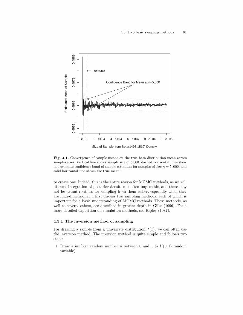
4.3 Two basic sampling methods 81
0 e+00 2 e+04 4 e+04 6 e+04 8 e+04 1 e+05
0.49
550.
4965
0.49
750.
4985
Size of Sample from Beta(1498,1519) Density
Est
imat
ed M
ean
of S
ampl
e
n=5000
Confidence Band for Mean at n=5,000
Fig. 4.1. Convergence of sample means on the true beta distribution mean acrosssamples sizes: Vertical line shows sample size of 5,000; dashed horizontal lines showapproximate confidence band of sample estimates for samples of size n = 5, 000; andsolid horizontal line shows the true mean.
to create one. Indeed, this is the entire reason for MCMC methods, as we willdiscuss: Integration of posterior densities is often impossible, and there maynot be extant routines for sampling from them either, especially when theyare high-dimensional. I first discuss two sampling methods, each of which isimportant for a basic understanding of MCMC methods. These methods, aswell as several others, are described in greater depth in Gilks (1996). For amore detailed exposition on simulation methods, see Ripley (1987).
4.3.1 The inversion method of sampling
For drawing a sample from a univariate distribution f(x), we can often usethe inversion method. The inversion method is quite simple and follows twosteps:
1. Draw a uniform random number u between 0 and 1 (a U(0, 1) randomvariable).
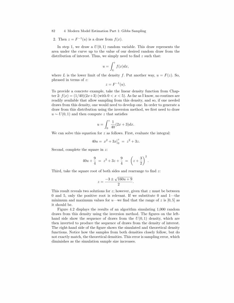
82 4 Modern Model Estimation Part 1: Gibbs Sampling
2. Then z = F−1(u) is a draw from f(x).
In step 1, we draw a U(0, 1) random variable. This draw represents thearea under the curve up to the value of our desired random draw from thedistribution of interest. Thus, we simply need to find z such that:
u =∫ z
L
f(x)dx,
where L is the lower limit of the density f . Put another way, u = F (z). So,phrased in terms of z:
z = F−1(u).
To provide a concrete example, take the linear density function from Chap-ter 2: f(x) = (1/40)(2x+3) (with 0 < x < 5). As far as I know, no routines arereadily available that allow sampling from this density, and so, if one neededdraws from this density, one would need to develop one. In order to generate adraw from this distribution using the inversion method, we first need to drawu ∼ U(0, 1) and then compute z that satisfies
u =∫ z
0
140
(2x + 3)dx.
We can solve this equation for z as follows. First, evaluate the integral:
40u = x2 + 3x∣∣z0
= z2 + 3z.
Second, complete the square in z:
40u +94
= z2 + 3z +94
=(
z +32
)2
.
Third, take the square root of both sides and rearrange to find z:
z =−3±
√160u + 92
.
This result reveals two solutions for z; however, given that z must be between0 and 5, only the positive root is relevant. If we substitute 0 and 1—theminimum and maximum values for u—we find that the range of z is [0, 5] asit should be.
Figure 4.2 displays the results of an algorithm simulating 1,000 randomdraws from this density using the inversion method. The figures on the left-hand side show the sequence of draws from the U(0, 1) density, which arethen inverted to produce the sequence of draws from the density of interest.The right-hand side of the figure shows the simulated and theoretical densityfunctions. Notice how the samples from both densities closely follow, but donot exactly match, the theoretical densities. This error is sampling error, whichdiminishes as the simulation sample size increases.
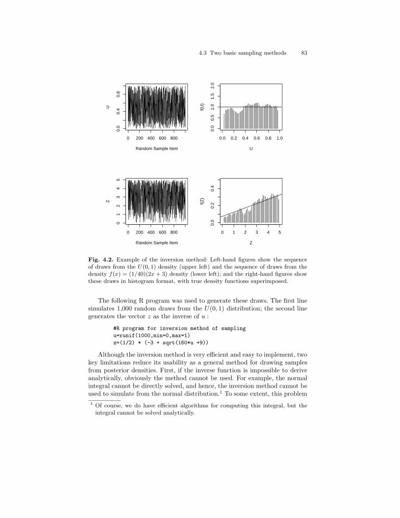
4.3 Two basic sampling methods 83
0 200 400 600 800
0.0
0.4
0.8
Random Sample Item
U
0.0 0.2 0.4 0.6 0.8 1.0
0.0
0.5
1.0
1.5
2.0
U
f(U
)
0 200 400 600 800
01
23
45
Random Sample Item
Z
0 1 2 3 4 5
0.0
0.2
0.4
Z
f(Z
)
Fig. 4.2. Example of the inversion method: Left-hand figures show the sequenceof draws from the U(0, 1) density (upper left) and the sequence of draws from thedensity f(x) = (1/40)(2x + 3) density (lower left); and the right-hand figures showthese draws in histogram format, with true density functions superimposed.
The following R program was used to generate these draws. The first linesimulates 1,000 random draws from the U(0, 1) distribution; the second linegenerates the vector z as the inverse of u :
#R program for inversion method of sampling
u=runif(1000,min=0,max=1)
z=(1/2) * (-3 + sqrt(160*u +9))
Although the inversion method is very efficient and easy to implement, twokey limitations reduce its usability as a general method for drawing samplesfrom posterior densities. First, if the inverse function is impossible to deriveanalytically, obviously the method cannot be used. For example, the normalintegral cannot be directly solved, and hence, the inversion method cannot beused to simulate from the normal distribution.1 To some extent, this problem1 Of course, we do have efficient algorithms for computing this integral, but the
integral cannot be solved analytically.

84 4 Modern Model Estimation Part 1: Gibbs Sampling
begs the question: If we can integrate the density as required by the inversionmethod, then why bother with simulation? This question will be addressedshortly, but the short answer is that we may not be able to perform integrationon a multivariate density, but we can often break a multivariate density intounivariate ones for which inversion may work.
The second problem with the inversion method is that the method willnot work with multivariate distributions, because the inverse is generally notunique beyond one dimension. For example, consider the bivariate planar den-sity function discussed in Chapter 2:
f(x, y) =128
(2x + 3y + 2),
with 0 < x, y < 2. If we draw u ∼ U(0, 1) and attempt to solve the doubleintegral for x and y, we get:
28u = yx2 +3xy2
2+ 2xy,
which, of course, has infinitely many solutions (one equation with two un-knowns). Thinking ahead, we could select a value for one variable and thenuse the inversion method to draw from the conditional distribution of theother variable. This process would reduce the problem to one of samplingfrom univariate conditional distributions, which is the basic idea of Gibbssampling, as I discuss shortly.
4.3.2 The rejection method of sampling
When F−1(u) cannot be computed, other methods of sampling exist. A veryimportant one is rejection sampling. In rejection sampling, sampling from adistribution f(x) for x involves three basic steps:
1. Sample a value z from a distribution g(x) from which sampling is easyand for which values of m× g(x) are greater than f(x) at all points (m isa constant).
2. Compute the ratio R = f(z)m×g(z) .
3. Sample u ∼ U(0, 1). If R > u, then accept z as a draw from f(x). Other-wise, return to step 1.
In this algorithm, m×g(x) is called an “envelope function,” because of therequirement that the density function g(x) multiplied by some constant m begreater than the density function value for the distribution of interest [f(x)]at the same point for all points. In other words, m × g(x) envelops f(x). Instep 1, we sample a point z from the pdf g(x).
In step 2, we compute the ratio of the envelope function [m × g(x)] eval-uated at z to the density function of interest [f(x)] evaluated at the samepoint.
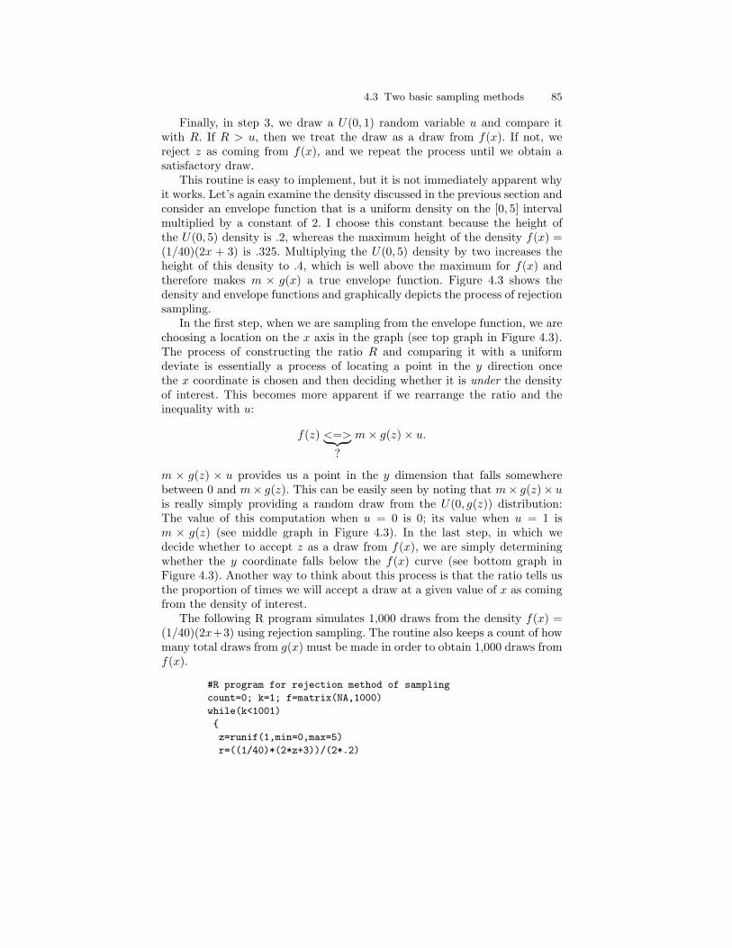
4.3 Two basic sampling methods 85
Finally, in step 3, we draw a U(0, 1) random variable u and compare itwith R. If R > u, then we treat the draw as a draw from f(x). If not, wereject z as coming from f(x), and we repeat the process until we obtain asatisfactory draw.
This routine is easy to implement, but it is not immediately apparent whyit works. Let’s again examine the density discussed in the previous section andconsider an envelope function that is a uniform density on the [0, 5] intervalmultiplied by a constant of 2. I choose this constant because the height ofthe U(0, 5) density is .2, whereas the maximum height of the density f(x) =(1/40)(2x + 3) is .325. Multiplying the U(0, 5) density by two increases theheight of this density to .4, which is well above the maximum for f(x) andtherefore makes m × g(x) a true envelope function. Figure 4.3 shows thedensity and envelope functions and graphically depicts the process of rejectionsampling.
In the first step, when we are sampling from the envelope function, we arechoosing a location on the x axis in the graph (see top graph in Figure 4.3).The process of constructing the ratio R and comparing it with a uniformdeviate is essentially a process of locating a point in the y direction oncethe x coordinate is chosen and then deciding whether it is under the densityof interest. This becomes more apparent if we rearrange the ratio and theinequality with u:
f(z) <=>︸ ︷︷ ︸ m× g(z)× u.
?
m × g(z) × u provides us a point in the y dimension that falls somewherebetween 0 and m× g(z). This can be easily seen by noting that m× g(z)× uis really simply providing a random draw from the U(0, g(z)) distribution:The value of this computation when u = 0 is 0; its value when u = 1 ism × g(z) (see middle graph in Figure 4.3). In the last step, in which wedecide whether to accept z as a draw from f(x), we are simply determiningwhether the y coordinate falls below the f(x) curve (see bottom graph inFigure 4.3). Another way to think about this process is that the ratio tells usthe proportion of times we will accept a draw at a given value of x as comingfrom the density of interest.
The following R program simulates 1,000 draws from the density f(x) =(1/40)(2x+3) using rejection sampling. The routine also keeps a count of howmany total draws from g(x) must be made in order to obtain 1,000 draws fromf(x).
#R program for rejection method of sampling
count=0; k=1; f=matrix(NA,1000)
while(k<1001)
z=runif(1,min=0,max=5)
r=((1/40)*(2*z+3))/(2*.2)
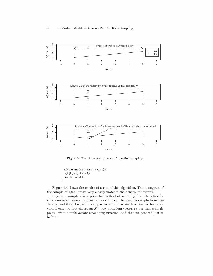
86 4 Modern Model Estimation Part 1: Gibbs Sampling
−1 0 1 2 3 4 5 6
0.0
0.3
0.6
Step 1
f(x)
and
g(x
) Choose z from g(x) [say this point is '*']
f(x)g(x)
−1 0 1 2 3 4 5 6
0.0
0.3
0.6
Step 2
f(x)
and
g(x
) Draw u~U(0,1) and multiply by m*g(z) to locate vertical point [say '*']
−1 0 1 2 3 4 5 6
0.0
0.3
0.6
Step 3
f(x)
and
g(x
) Is u*(m*g(z)) above (reject) or below (accept) f(z)? [here, it is above, so we reject]
Fig. 4.3. The three-step process of rejection sampling.
if(r>runif(1,min=0,max=1))
f[k]=z; k=k+1
count=count+1
Figure 4.4 shows the results of a run of this algorithm. The histogram ofthe sample of 1,000 draws very closely matches the density of interest.
Rejection sampling is a powerful method of sampling from densities forwhich inversion sampling does not work. It can be used to sample from anydensity, and it can be used to sample from multivariate densities. In the multi-variate case, we first choose an X—now a random vector, rather than a singlepoint—from a multivariate enveloping function, and then we proceed just asbefore.
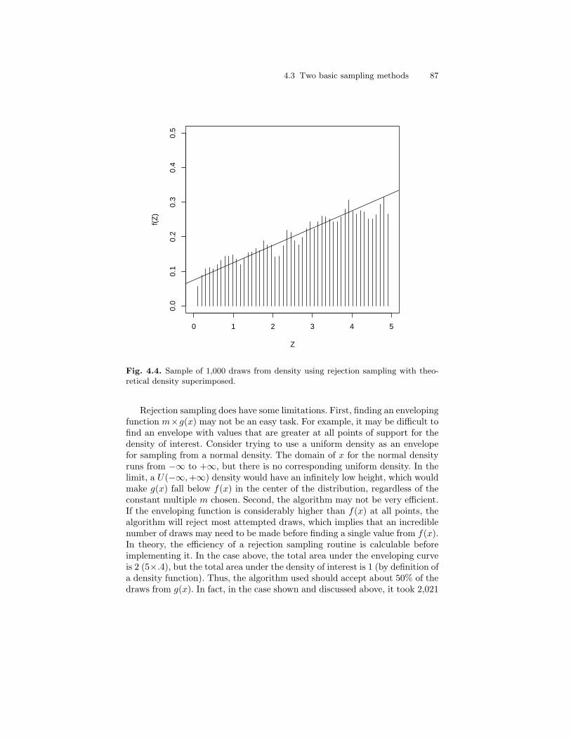
4.3 Two basic sampling methods 87
0 1 2 3 4 5
0.0
0.1
0.2
0.3
0.4
0.5
Z
f(Z
)
Fig. 4.4. Sample of 1,000 draws from density using rejection sampling with theo-retical density superimposed.
Rejection sampling does have some limitations. First, finding an envelopingfunction m×g(x) may not be an easy task. For example, it may be difficult tofind an envelope with values that are greater at all points of support for thedensity of interest. Consider trying to use a uniform density as an envelopefor sampling from a normal density. The domain of x for the normal densityruns from −∞ to +∞, but there is no corresponding uniform density. In thelimit, a U(−∞,+∞) density would have an infinitely low height, which wouldmake g(x) fall below f(x) in the center of the distribution, regardless of theconstant multiple m chosen. Second, the algorithm may not be very efficient.If the enveloping function is considerably higher than f(x) at all points, thealgorithm will reject most attempted draws, which implies that an incrediblenumber of draws may need to be made before finding a single value from f(x).In theory, the efficiency of a rejection sampling routine is calculable beforeimplementing it. In the case above, the total area under the enveloping curveis 2 (5×.4), but the total area under the density of interest is 1 (by definition ofa density function). Thus, the algorithm used should accept about 50% of thedraws from g(x). In fact, in the case shown and discussed above, it took 2,021
88 4 Modern Model Estimation Part 1: Gibbs Sampling
attempts to obtain 1,000 draws from f(x), which is a rejection rate of 50.5%.These two limitations make rejection sampling, although possible, increasinglydifficult as the dimensionality increases in multivariate distributions.
4.4 Introduction to MCMC sampling
The limitations of inversion and rejection sampling make the prospects ofusing these simple methods daunting in complex statistical analyses involv-ing high-dimensional distributions. Although rejection sampling approachescan be refined to be more efficient, they are still not very useful in and ofthemselves in real-world statistical modeling. Fortunately, over the last fewdecades, MCMC methods have been developed that facilitate sampling fromcomplex distributions. Furthermore, aside from allowing sampling from com-plex distributions, these methods provide several additional benefits, as wewill be discussing in the remaining chapters.
MCMC sampling provides a method to sample from multivariate densitiesthat are not easy to sample from, often by breaking these densities downinto more manageable univariate or multivariate densities. The basic MCMCapproach provides a prescription for (1) sampling from one or more dimensionsof a posterior distribution and (2) moving throughout the entire support of aposterior distribution. In fact, the name “Markov chain Monte Carlo” impliesthis process. The “Monte Carlo” portion refers to the random simulationprocess. The “Markov chain” portion refers to the process of sampling a newvalue from the posterior distribution, given the previous value: This iterativeprocess produces a Markov chain of values that constitute a sample of drawsfrom the posterior.
4.4.1 Generic Gibbs sampling
The Gibbs sampler is the most basic MCMC method used in Bayesian statis-tics. Although Gibbs sampling was developed and used in physics prior to1990, its widespread use in Bayesian statistics originated in 1990 with its in-troduction by Gelfand and Smith (1990). As will be discussed more in the nextchapter, the Gibbs sampler is a special case of the more general Metropolis-Hastings algorithm that is useful when (1) sampling from a multivariate pos-terior is not feasible, but (2) sampling from the conditional distributions foreach parameter (or blocks of them) is feasible. A generic Gibbs sampler followsthe following iterative process (j indexes the iteration count):
4.4 Introduction to MCMC sampling 89
0. Assign a vector of starting values, S, to the parameter vector:Θj=0 = S.
1. Set j = j + 1.2. Sample (θj
1 | θj−12 , θj−1
3 . . . θj−1k ).
3. Sample (θj2 | θ
j1, θj−1
3 . . . θj−1k ).
......
k. Sample (θjk | θ
j1, θj
2, . . . , θjk−1).
k+1. Return to step 1.
In other words, Gibbs sampling involves ordering the parameters and samplingfrom the conditional distribution for each parameter given the current value ofall the other parameters and repeatedly cycling through this updating process.Each “loop” through these steps is called an “iteration” of the Gibbs sampler,and when a new sampled value of a parameter is obtained, it is called an“updated” value.
For Gibbs sampling, the full conditional density for a parameter needs onlyto be known up to a normalizing constant. As we discussed in Chapters 2 and3, this implies that we can use the joint density with the other parametersset at their current values. This fact makes Gibbs sampling relatively simplefor most problems in which the joint density reduces to known forms for eachparameter once all other parameters are treated as fixed.
4.4.2 Gibbs sampling example using the inversion method
Here, I provide a simple example of Gibbs sampling based on the bivariateplane distribution developed in Chapter 2 f(x, y) = (1/28)(2x + 3y + 2). Theconditional distribution for x was:
f(x | y) =f(x, y)f(y)
=2x + 3y + 2
6y + 8,
and the conditional distribution for y was:
f(y | x) =f(x, y)f(x)
=2x + 3y + 2
4x + 10.
Thus, a Gibbs sampler for sampling x and y in this problem would followthese steps:
1. Set j = 0 and establish starting values. Here, let’s set xj=0 = −5 andyj=0 = −5.
2. Sample xj+1 from f(x | y = yj).3. Sample yj+1 from f(y | x = xj+1).4. Increment j = j + 1 and return to step 2 until j = 2000.
90 4 Modern Model Estimation Part 1: Gibbs Sampling
How do we sample from these conditional distributions? We know what theyare, but they certainly are not standard distributions. Since they are notstandard distributions, but since these conditionals are univariate and F−1()can be calculated for each one, we can use an inversion subroutine to samplefrom each conditional density. How do we find the inverses in this bivariatedensity? Recall that inversion sampling requires first drawing a u ∼ U(0, 1)random variable and then inverting this draw using F−1. Thus, to find theinverse of the conditional density for y|x, we need to solve:
u =∫ z
0
2x + 3y + 24x + 10
for z. Given that this is the conditional density for y, x is fixed and can betreated as a constant, and we obtain:
u(4x + 10) = (2x + 2)y + (3/2)y2∣∣z0.
Thus:
u(4x + 10) = (2x + 2)z + (3/2)z2.
After multiplying through by (2/3) and rearranging terms, we get:
(2/3)u(4x + 10) = z2 + (2/3)(2x + 2)z.
We can then complete the square in z and solve for z to obtain:
z =√
(2/3)u(4x + 10) + ((1/3)(2x + 2))2 − (1/3)(2x + 2).
Given a current value for x and a random draw u, z is a random draw fromthe conditional density for y|x. A similar process can be undertaken to findthe inverse for x|y (see Exercises).
Below is an R program that implements the Gibbs sampling:
#R program for Gibbs sampling using inversion method
x=matrix(-5,2000); y=matrix(-5,2000)
for(i in 2:2000)
#sample from x | y
u=runif(1,min=0, max=1)
x[i]=sqrt(u*(6*y[i-1]+8)+(1.5*y[i-1]+1)*(1.5*y[i-1]+1))
-(1.5*y[i-1]+1)
#sample from y | x
u=runif(1,min=0,max=1)
y[i]=sqrt((2*u*(4*x[i]+10))/3 +((2*x[i]+2)/3)*((2*x[i]+2)/3))
- ((2*x[i]+2)/3)

4.4 Introduction to MCMC sampling 91
This program first sets the starting values for x and y equal to −5. Then,x is updated using the current value of y. Then, y is updated using the just-sampled value of x. (Notice how x[i] is computed using y[i-1], whereasy[i] is sampled using x[i].) Both are updated using the inversion methodof sampling discussed above.
This algorithm produces samples from the marginal distributions for bothx and y, but we can also treat pairs of x and y as draws from the joint density.We will discuss the conditions in which we can do this in greater depth shortly.Generally, however, of particular interest are the marginal distributions forparameters, since we are often concerned with testing hypotheses concerningone parameter, net of the other parameters in a model. Figure 4.5 shows a“trace plot” of both x and y as well as the marginal densities for both variables.The trace plot is simply a two-dimensional plot in which the x axis representsthe iteration of the algorithm, and the y axis represents the simulated valueof the random variable at each particular iteration. Heuristically, we can thentake the trace plot, turn it on its edge (a 90 degree clockwise turn), and allowthe “ink” to fall down along the y-axis and “pile-up” to produce a histogramof the marginal density. Places in the trace plot that are particularly darkrepresent regions of the density in which the algorithm simulated frequently;lighter areas are regions of the density that were more rarely visited by thealgorithm. Thus, the “ink” will pile-up higher in areas for which the variableof interest has greater probability. Histograms of these marginal densities areshown to the right of their respective trace plots, with the theoretical marginaldensities derived in Chapter 2 superimposed. Realize that these marginals areunnormalized, because the leading 1/28 normalizing constant cancels in boththe numerator and the denominator.
Notice that, although the starting values were very poor (−5 is not a validpoint in either dimension of the density), the algorithm converged very rapidlyto the appropriate region—[0, 2]. It generally takes a number of iterations foran MCMC algorithm to find the appropriate region—and, more theoretically,for the Markov chain produced by the algorithm to sample from the appro-priate “target” distribution. Thus, we generally discard a number of earlyiterations before making calculations (called the “burn-in”). The marginaldensities, therefore, are produced from only the last 1,500 iterations of thealgorithm.
The histograms for the marginal densities show that the algorithm samplesappropriately from the densities of interest. Of course, there is certainly someerror—observe how the histograms tend to be a little too low or high hereand there. This reflects sampling error, and such error is reduced by samplingmore values (e.g., using 5,000 draws, rather than 2,000); we will return to thisissue in the next chapter.
Aside from examining the marginal distributions for x and y, we can alsoexamine the joint density. Figure 4.6 shows a two-dimensional trace plot, takenat several stages. The upper left figure shows the state of the algorithm after5 iterations; the upper right figure shows the state after 25 iterations; the

92 4 Modern Model Estimation Part 1: Gibbs Sampling
0 500 1000 1500 2000
−5
05
10
Iteration
Sam
pled
X
−0.5 0.5 1.5 2.5
0.0
0.4
0.8
x
f(x)
0 500 1000 1500 2000
−5
05
10
Iteration
Sam
pled
Y
−0.5 0.5 1.5 2.5
0.0
0.4
0.8
y
f(y)
Fig. 4.5. Results of Gibbs sampler using the inversion method for sampling fromconditional densities.
lower left figure shows it after 100 iterations; and the lower right figure showsit after the 2,000 iterations. Here again, we see that the algorithm, althoughstarting with poor starting values, converged rapidly to the appropriate two-dimensional, partial plane region represented by f(x, y).
After sampling from the distribution for x and y, we can now summarizeour knowledge of the density. The theoretical mean for x can be found bytaking the marginal for x (f(x) = (1/28)(4x + 10)) and by integrating acrossall values for x:
µx =∫ 2
0
x× f(x)dx = 1.095.
A similar calculation for y yields a theoretical mean of 1.143. The empiricalestimates of the means, based on the last 1,500 draws from the marginaldistributions for the variables (discarding the first 500 as the burn-in) are

4.4 Introduction to MCMC sampling 93
−5 0 5 10
−5
−3
−1
12
x
y
−5 0 5 10
−5
−3
−1
12
x
y
−5 0 5 10
−5
−3
−1
12
x
y
−5 0 5 10
−5
−3
−1
12
x
y
Fig. 4.6. Results of Gibbs sampler using the inversion method for sampling fromconditional densities: Two-dimensional view after 5, 25, 100, and 2,000 iterations.
x = 1.076 and y = 1.158. The discrepancy between the theoretical and theempirical means is attributable to sampling error in the MCMC algorithm. Alonger run would reduce the error, although, even with 1,500 simulated draws,the discrepancies here are minimal (less than 2% for both x and y).
4.4.3 Example repeated using rejection sampling
In the Gibbs sampling algorithm we just discussed, we used the inversionmethod for sampling from the conditional distributions of x and y. It is oftenthe case that using the inversion method may not be feasible, for several rea-sons. First, the conditionals in the Gibbs sampler may not be univariate. Thatis, we do not have to break our conditional distributions into univariate con-ditional densities; we may choose multivariate conditional densities, as we willsee in Chapter 7. Second, F ()−1 may not be calculable, even in one dimension.
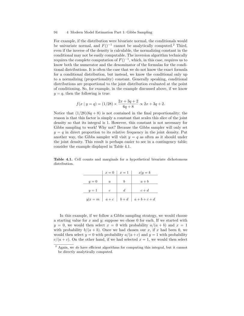
94 4 Modern Model Estimation Part 1: Gibbs Sampling
For example, if the distribution were bivariate normal, the conditionals wouldbe univariate normal, and F ()−1 cannot be analytically computed.2 Third,even if the inverse of the density is calculable, the normalizing constant in theconditional may not be easily computable. The inversion algorithm technicallyrequires the complete computation of F ()−1, which, in this case, requires us toknow both the numerator and the denominator of the formulas for the condi-tional distributions. It is often the case that we do not know the exact formulafor a conditional distribution, but instead, we know the conditional only upto a normalizing (proportionality) constant. Generally speaking, conditionaldistributions are proportional to the joint distribution evaluated at the pointof conditioning. So, for example, in the example discussed above, if we knowy = q, then the following is true:
f(x | y = q) = (1/28)× 2x + 3q + 26q + 8
∝ 2x + 3q + 2.
Notice that (1/28)(6q + 8) is not contained in the final proportionality; thereason is that this factor is simply a constant that scales this slice of the jointdensity so that its integral is 1. However, this constant is not necessary forGibbs sampling to work! Why not? Because the Gibbs sampler will only sety = q in direct proportion to its relative frequency in the joint density. Putanother way, the Gibbs sampler will visit y = q as often as it should underthe joint density. This result is perhaps easier to see in a contingency table;consider the example displayed in Table 4.1.
Table 4.1. Cell counts and marginals for a hypothetical bivariate dichotomousdistribution.
x = 0 x = 1 x|y = k
y = 0 a b a + b
y = 1 c d c + d
y|x = m a + c b + d a + b + c + d
In this example, if we follow a Gibbs sampling strategy, we would choosea starting value for x and y; suppose we chose 0 for each. If we started withy = 0, we would then select x = 0 with probability a/(a + b) and x = 1with probability b/(a + b). Once we had chosen our x, if x had been 0, wewould then select y = 0 with probability a/(a+ c) and y = 1 with probabilityc/(a + c). On the other hand, if we had selected x = 1, we would then select
2 Again, we do have efficient algorithms for computing this integral, but it cannotbe directly analytically computed.
4.4 Introduction to MCMC sampling 95
y = 0 with probability b/(b + d) and y = 1 with probability d/(b + d). Thus,we would be selecting y = 0 with total probability
p(y = 0) = p(y = 0 | x = 0)p(x = 0) + p(y = 0 | x = 1)p(x = 1).
So,
p(y = 0) =(
a
a + c
)(a + c
a + b + c + d
)+(
b
b + d
)(b + d
a + b + c + d
)=
a + b
a + b + c + d.
This proportion reflects exactly how often we should choose y = 0, giventhe marginal distribution for y in the contingency table. Thus, the normalizingconstant is not relevant, because the Gibbs sampler will visit each value ofone variable in proportion to its relative marginal frequency, which leads us tothen sample the other variable, conditional on the first, with the appropriaterelative marginal frequency.
Returning to the example at hand, then, we simply need to know whatthe conditional distribution is proportional to in order to sample from it.Here, if we know y = q, then f(x | y = q) ∝ 2x + 3q + 2. Because we do notnecessarily always know this normalizing constant, using the inversion methodof sampling will not work.3 However, we can simulate from this density usingrejection sampling. Recall from the discussion of rejection sampling that weneed an enveloping function g(x) that, when multiplied by a constant m,returns a value that is greater than f(x) for all x. With an unnormalizeddensity, only m must be adjusted relative to what it would be under thenormalized density in order to ensure this rule is followed. In this case, if wewill be sampling from the joint density, we can use a uniform density on the[0, 2] interval multiplied by a constant m that ensures that the density doesnot exceed m × .5 (.5 is the height of the U(0,2) density). The joint densityreaches a maximum where x and y are both 2; that peak value is 12. Thus,if we set m = 25, the U(0, 2) density multiplied by m will always be abovethe joint density. And, we can ignore the normalizing constants, includingthe leading (1/28) in the joint density and the 1/(6y + 8) in the conditionalfor x and the 1/(4x + 10) in the conditional for y. As exemplified above, theGibbs sampler will sample from the marginals in the correct proportion totheir relative frequency in the joint density. Below is a Gibbs sampler thatsimulates from f(x, y) using rejection sampling:3 The normalizing constant must be known one way or another. Certainly, we can
perform the integration we need to compute F−1 so long as the distribution isproper. However, if we do not know the normalizing constant, the integral willdiffer from 1, which necessitates that our uniform draw representing the areaunder the curve be scaled by the inverse of the normalizing constant in order torepresent the area under the unnormalized density fully.
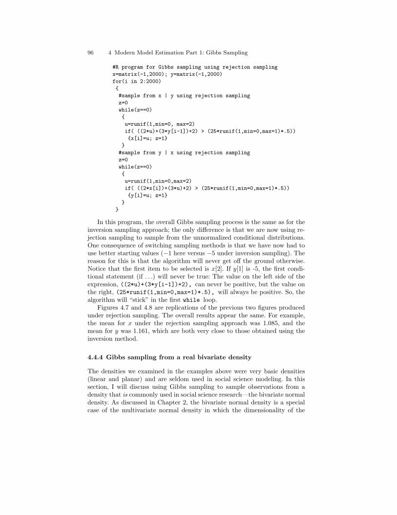
96 4 Modern Model Estimation Part 1: Gibbs Sampling
#R program for Gibbs sampling using rejection sampling
x=matrix(-1,2000); y=matrix(-1,2000)
for(i in 2:2000)
#sample from x | y using rejection sampling
z=0
while(z==0)
u=runif(1,min=0, max=2)
if( ((2*u)+(3*y[i-1])+2) > (25*runif(1,min=0,max=1)*.5))
x[i]=u; z=1
#sample from y | x using rejection sampling
z=0
while(z==0)
u=runif(1,min=0,max=2)
if( ((2*x[i])+(3*u)+2) > (25*runif(1,min=0,max=1)*.5))
y[i]=u; z=1
In this program, the overall Gibbs sampling process is the same as for theinversion sampling approach; the only difference is that we are now using re-jection sampling to sample from the unnormalized conditional distributions.One consequence of switching sampling methods is that we have now had touse better starting values (−1 here versus −5 under inversion sampling). Thereason for this is that the algorithm will never get off the ground otherwise.Notice that the first item to be selected is x[2]. If y[1] is -5, the first condi-tional statement (if . . .) will never be true: The value on the left side of theexpression, ((2*u)+(3*y[i-1])+2), can never be positive, but the value onthe right, (25*runif(1,min=0,max=1)*.5), will always be positive. So, thealgorithm will “stick” in the first while loop.
Figures 4.7 and 4.8 are replications of the previous two figures producedunder rejection sampling. The overall results appear the same. For example,the mean for x under the rejection sampling approach was 1.085, and themean for y was 1.161, which are both very close to those obtained using theinversion method.
4.4.4 Gibbs sampling from a real bivariate density
The densities we examined in the examples above were very basic densities(linear and planar) and are seldom used in social science modeling. In thissection, I will discuss using Gibbs sampling to sample observations from adensity that is commonly used in social science research—the bivariate normaldensity. As discussed in Chapter 2, the bivariate normal density is a specialcase of the multivariate normal density in which the dimensionality of the
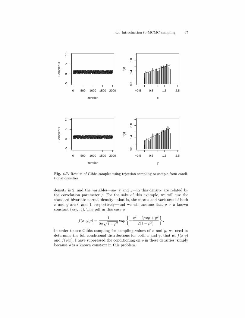
4.4 Introduction to MCMC sampling 97
0 500 1000 1500 2000
−5
05
10
Iteration
Sam
pled
X
−0.5 0.5 1.5 2.5
0.0
0.4
0.8
x
f(x)
0 500 1000 1500 2000
−5
05
10
Iteration
Sam
pled
Y
−0.5 0.5 1.5 2.5
0.0
0.4
0.8
y
f(y)
Fig. 4.7. Results of Gibbs sampler using rejection sampling to sample from condi-tional densities.
density is 2, and the variables—say x and y—in this density are related bythe correlation parameter ρ. For the sake of this example, we will use thestandard bivariate normal density—that is, the means and variances of bothx and y are 0 and 1, respectively—and we will assume that ρ is a knownconstant (say, .5). The pdf in this case is:
f(x, y|ρ) =1
2π√
1− ρ2exp
−x2 − 2ρxy + y2
2(1− ρ2)
.
In order to use Gibbs sampling for sampling values of x and y, we need todetermine the full conditional distributions for both x and y, that is, f(x|y)and f(y|x). I have suppressed the conditioning on ρ in these densities, simplybecause ρ is a known constant in this problem.

98 4 Modern Model Estimation Part 1: Gibbs Sampling
−5 0 5 10
−5
−3
−1
12
x (after 5 iterations)
y
−5 0 5 10
−5
−3
−1
12
x (after 25 iterations)
y
−5 0 5 10
−5
−3
−1
12
x (after 100 iterations)
y
−5 0 5 10
−5
−3
−1
12
x (after 2000 iterations)
y
Fig. 4.8. Results of Gibbs sampler using rejection sampling to sample from condi-tional densities: Two-dimensional view after 5, 25, 100, and 2,000 iterations.
As we discussed above, Gibbs sampling does not require that we knowthe normalizing constant; we only need to know to what density each con-ditional density is proportional. Thus, we will drop the leading constant(1/(2π
√1− ρ2)). The conditional for x then requires that we treat y as
known. If y is known, we can reexpress the kernel of the density as
f(x|y) ∝ exp−x2 − x(2ρy)
2(1− ρ2)
exp
− y2
2(1− ρ2)
,
and we can drop the latter exponential containing y2, because it is simply aproportionality constant with respect to x. Thus, we are left with the left-handexponential. If we complete the square in x, we obtain
f(x|y) ∝ exp− (x2 − x(2ρy) + (ρy)2 − (ρy)2)
2(1− ρ2)
,
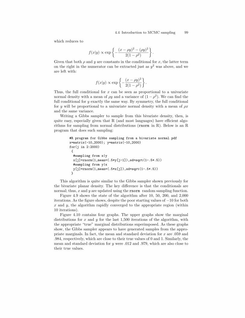
4.4 Introduction to MCMC sampling 99
which reduces to
f(x|y) ∝ exp− (x− ρy)2 − (ρy)2
2(1− ρ2)
.
Given that both ρ and y are constants in the conditional for x, the latter termon the right in the numerator can be extracted just as y2 was above, and weare left with:
f(x|y) ∝ exp− (x− ρy)2
2(1− ρ2)
.
Thus, the full conditional for x can be seen as proportional to a univariatenormal density with a mean of ρy and a variance of (1− ρ2). We can find thefull conditional for y exactly the same way. By symmetry, the full conditionalfor y will be proportional to a univariate normal density with a mean of ρxand the same variance.
Writing a Gibbs sampler to sample from this bivariate density, then, isquite easy, especially given that R (and most languages) have efficient algo-rithms for sampling from normal distributions (rnorm in R). Below is an Rprogram that does such sampling:
#R program for Gibbs sampling from a bivariate normal pdf
x=matrix(-10,2000); y=matrix(-10,2000)
for(j in 2:2000)
#sampling from x|y
x[j]=rnorm(1,mean=(.5*y[j-1]),sd=sqrt(1-.5*.5))
#sampling from y|x
y[j]=rnorm(1,mean=(.5*x[j]),sd=sqrt(1-.5*.5))
This algorithm is quite similar to the Gibbs sampler shown previously forthe bivariate planar density. The key difference is that the conditionals arenormal; thus, x and y are updated using the rnorm random sampling function.
Figure 4.9 shows the state of the algorithm after 10, 50, 200, and 2,000iterations. As the figure shows, despite the poor starting values of −10 for bothx and y, the algorithm rapidly converged to the appropriate region (within10 iterations).
Figure 4.10 contains four graphs. The upper graphs show the marginaldistributions for x and y for the last 1,500 iterations of the algorithm, withthe appropriate “true” marginal distributions superimposed. As these graphsshow, the Gibbs sampler appears to have generated samples from the appro-priate marginals. In fact, the mean and standard deviation for x are .059 and.984, respectively, which are close to their true values of 0 and 1. Similarly, themean and standard deviation for y were .012 and .979, which are also close totheir true values.
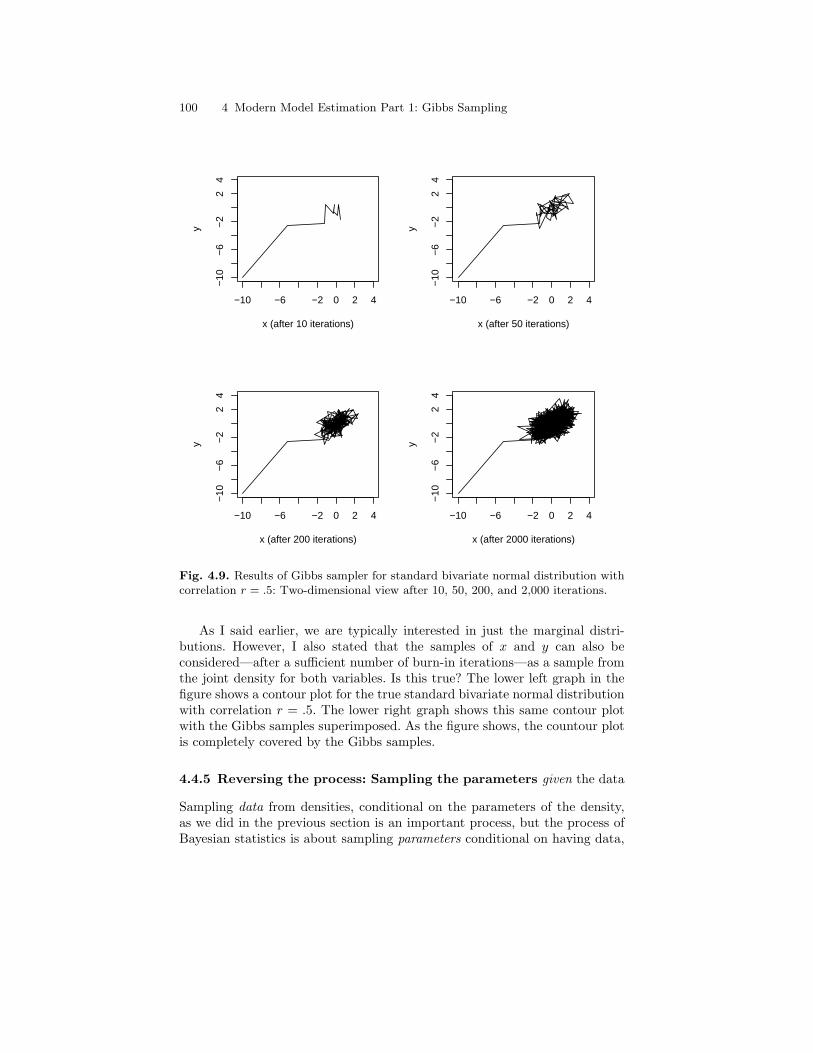
100 4 Modern Model Estimation Part 1: Gibbs Sampling
−10 −6 −2 0 2 4
−10
−6
−2
24
x (after 10 iterations)
y
−10 −6 −2 0 2 4
−10
−6
−2
24
x (after 50 iterations)
y
−10 −6 −2 0 2 4
−10
−6
−2
24
x (after 200 iterations)
y
−10 −6 −2 0 2 4
−10
−6
−2
24
x (after 2000 iterations)
y
Fig. 4.9. Results of Gibbs sampler for standard bivariate normal distribution withcorrelation r = .5: Two-dimensional view after 10, 50, 200, and 2,000 iterations.
As I said earlier, we are typically interested in just the marginal distri-butions. However, I also stated that the samples of x and y can also beconsidered—after a sufficient number of burn-in iterations—as a sample fromthe joint density for both variables. Is this true? The lower left graph in thefigure shows a contour plot for the true standard bivariate normal distributionwith correlation r = .5. The lower right graph shows this same contour plotwith the Gibbs samples superimposed. As the figure shows, the countour plotis completely covered by the Gibbs samples.
4.4.5 Reversing the process: Sampling the parameters given the data
Sampling data from densities, conditional on the parameters of the density,as we did in the previous section is an important process, but the process ofBayesian statistics is about sampling parameters conditional on having data,
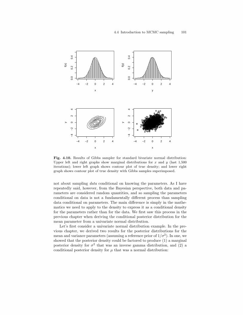
4.4 Introduction to MCMC sampling 101
−4 −2 0 2 4
0.0
0.2
0.4
x
f(x)
−4 −2 0 2 4
0.0
0.2
0.4
y
f(y)
x
y
−4 −2 0 2 4
−4
−2
02
4
x
y
−4 −2 0 2 4
−4
−2
02
4
Fig. 4.10. Results of Gibbs sampler for standard bivariate normal distribution:Upper left and right graphs show marginal distributions for x and y (last 1,500iterations); lower left graph shows contour plot of true density; and lower rightgraph shows contour plot of true density with Gibbs samples superimposed.
not about sampling data conditional on knowing the parameters. As I haverepeatedly said, however, from the Bayesian perspective, both data and pa-rameters are considered random quantities, and so sampling the parametersconditional on data is not a fundamentally different process than samplingdata conditional on parameters. The main difference is simply in the mathe-matics we need to apply to the density to express it as a conditional densityfor the parameters rather than for the data. We first saw this process in theprevious chapter when deriving the conditional posterior distribution for themean parameter from a univariate normal distribution.
Let’s first consider a univariate normal distribution example. In the pre-vious chapter, we derived two results for the posterior distributions for themean and variance parameters (assuming a reference prior of 1/σ2). In one, weshowed that the posterior density could be factored to produce (1) a marginalposterior density for σ2 that was an inverse gamma distribution, and (2) aconditional posterior density for µ that was a normal distribution:
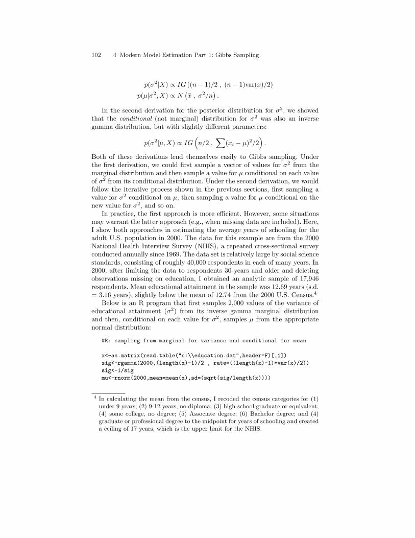
102 4 Modern Model Estimation Part 1: Gibbs Sampling
p(σ2|X) ∝ IG ((n− 1)/2 , (n− 1)var(x)/2)
p(µ|σ2, X) ∝ N(x , σ2/n
).
In the second derivation for the posterior distribution for σ2, we showedthat the conditional (not marginal) distribution for σ2 was also an inversegamma distribution, but with slightly different parameters:
p(σ2|µ,X) ∝ IG(n/2 ,
∑(xi − µ)2/2
).
Both of these derivations lend themselves easily to Gibbs sampling. Underthe first derivation, we could first sample a vector of values for σ2 from themarginal distribution and then sample a value for µ conditional on each valueof σ2 from its conditional distribution. Under the second derivation, we wouldfollow the iterative process shown in the previous sections, first sampling avalue for σ2 conditional on µ, then sampling a value for µ conditional on thenew value for σ2, and so on.
In practice, the first approach is more efficient. However, some situationsmay warrant the latter approach (e.g., when missing data are included). Here,I show both approaches in estimating the average years of schooling for theadult U.S. population in 2000. The data for this example are from the 2000National Health Interview Survey (NHIS), a repeated cross-sectional surveyconducted annually since 1969. The data set is relatively large by social sciencestandards, consisting of roughly 40,000 respondents in each of many years. In2000, after limiting the data to respondents 30 years and older and deletingobservations missing on education, I obtained an analytic sample of 17,946respondents. Mean educational attainment in the sample was 12.69 years (s.d.= 3.16 years), slightly below the mean of 12.74 from the 2000 U.S. Census.4
Below is an R program that first samples 2,000 values of the variance ofeducational attainment (σ2) from its inverse gamma marginal distributionand then, conditional on each value for σ2, samples µ from the appropriatenormal distribution:
#R: sampling from marginal for variance and conditional for mean
x<-as.matrix(read.table("c:\\education.dat",header=F)[,1])
sig<-rgamma(2000,(length(x)-1)/2 , rate=((length(x)-1)*var(x)/2))
sig<-1/sig
mu<-rnorm(2000,mean=mean(x),sd=(sqrt(sig/length(x))))
4 In calculating the mean from the census, I recoded the census categories for (1)under 9 years; (2) 9-12 years, no diploma; (3) high-school graduate or equivalent;(4) some college, no degree; (5) Associate degree; (6) Bachelor degree; and (4)graduate or professional degree to the midpoint for years of schooling and createda ceiling of 17 years, which is the upper limit for the NHIS.
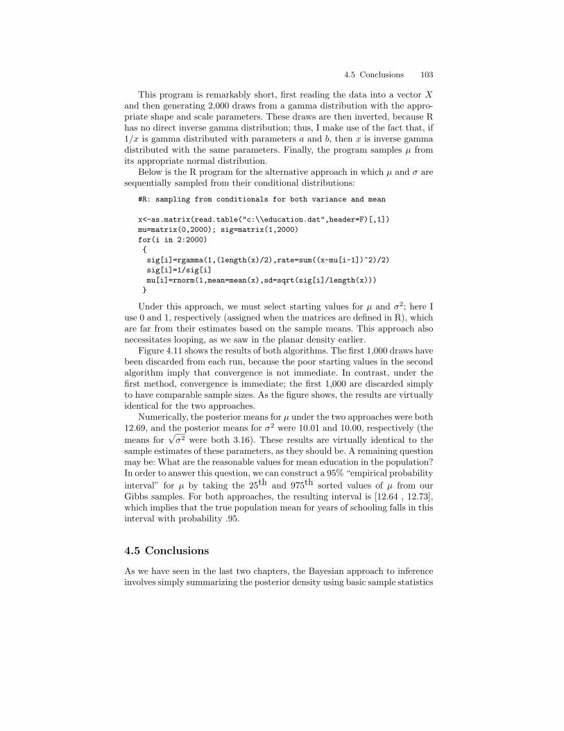
4.5 Conclusions 103
This program is remarkably short, first reading the data into a vector Xand then generating 2,000 draws from a gamma distribution with the appro-priate shape and scale parameters. These draws are then inverted, because Rhas no direct inverse gamma distribution; thus, I make use of the fact that, if1/x is gamma distributed with parameters a and b, then x is inverse gammadistributed with the same parameters. Finally, the program samples µ fromits appropriate normal distribution.
Below is the R program for the alternative approach in which µ and σ aresequentially sampled from their conditional distributions:
#R: sampling from conditionals for both variance and mean
x<-as.matrix(read.table("c:\\education.dat",header=F)[,1])
mu=matrix(0,2000); sig=matrix(1,2000)
for(i in 2:2000)
sig[i]=rgamma(1,(length(x)/2),rate=sum((x-mu[i-1])^2)/2)
sig[i]=1/sig[i]
mu[i]=rnorm(1,mean=mean(x),sd=sqrt(sig[i]/length(x)))
Under this approach, we must select starting values for µ and σ2; here Iuse 0 and 1, respectively (assigned when the matrices are defined in R), whichare far from their estimates based on the sample means. This approach alsonecessitates looping, as we saw in the planar density earlier.
Figure 4.11 shows the results of both algorithms. The first 1,000 draws havebeen discarded from each run, because the poor starting values in the secondalgorithm imply that convergence is not immediate. In contrast, under thefirst method, convergence is immediate; the first 1,000 are discarded simplyto have comparable sample sizes. As the figure shows, the results are virtuallyidentical for the two approaches.
Numerically, the posterior means for µ under the two approaches were both12.69, and the posterior means for σ2 were 10.01 and 10.00, respectively (themeans for
√σ2 were both 3.16). These results are virtually identical to the
sample estimates of these parameters, as they should be. A remaining questionmay be: What are the reasonable values for mean education in the population?In order to answer this question, we can construct a 95% “empirical probabilityinterval” for µ by taking the 25th and 975th sorted values of µ from ourGibbs samples. For both approaches, the resulting interval is [12.64 , 12.73],which implies that the true population mean for years of schooling falls in thisinterval with probability .95.
4.5 Conclusions
As we have seen in the last two chapters, the Bayesian approach to inferenceinvolves simply summarizing the posterior density using basic sample statistics

104 4 Modern Model Estimation Part 1: Gibbs Sampling
12.5 12.6 12.7 12.8 12.9
05
15
µ
f(µ)
9.5 10.0 10.5
02
4
σ2
f(σ2 )
Fig. 4.11. Samples from posterior densities for a mean and variance parameterfor NHIS years of schooling data under two Gibbs sampling approaches: The solidlines are the results for the marginal-for-σ2-but conditional-for-µ approach; and thedashed lines are the results for the full conditionals approach.
like the mean, median, variance, and various quantiles of the distribution.When posterior densities are such that these integral-based statistics cannotbe directly computed—e.g., when they are multivariate—modern Bayesianstatistics turns to sampling from the posterior density and to computing thesequantities just as we would when we have a sample of data.
Gibbs sampling provides a fairly easy method for sampling from multivari-ate densities, so long as we can derive the appropriate conditional densities.In most problems, this reduces simply to (1) treating other variables as fixedin the joint density, and (2) determining how to sample from the resultingconditional density. Sometimes, the conditional densities take known forms,as they did in our normal distribution example. Other times, the conditionaldensities may be derivable, but they may take unknown forms, as they did inour linear and planar distributions examples. In the latter case, we may turnto inversion or rejection sampling for sampling from the conditionals withunknown forms.
4.6 Exercises 105
In some cases, however, inversion of a conditional density may not be pos-sible, and rejection sampling may be difficult or very inefficient. In those cases,Bayesians can turn to another method—the Metropolis-Hastings algorithm.Discussion of that method is the topic of the next chapter. For alternative andmore in-depth and theoretical expositions of the Gibbs sampler, I recommendthe entirety of Gilks, Richardson, and Spiegelhalter 1996 in general and Gilks1996 in particular. I also recommend a number of additional readings in theconcluding chapter of this book.
4.6 Exercises
1. Find the inverse distribution function (F−1) for y|x in the bivariate planardensity; that is, show how a U(0, 1) sample must be transformed to be adraw from y|x.
2. Develop a rejection sampler for sampling data from the bivariate planardensity f(x) ∝ 2x + 3y + 2.
3. Develop an inversion sampler for sampling data from the linear densityf(x) ∝ 5x + 2. (Hint: First, find the normalizing constant, and then findthe inverse function).
4. Develop an appropriate routine for sampling the λ parameter from thePoisson distribution voting example in the previous chapter.
5. Develop an appropriate routine for sampling 20 observations (data points)from an N(0, 1) distribution. Then, reverse the process using these datato sample from the posterior distribution for µ and σ2. Use the noninfor-mative prior p(µ , σ2) ∝ 1/σ2, and use either Gibbs sampler describedin the chapter. Next, plot the posterior density for µ, and superimposean appropriate t distribution over this density. How close is the match?Discuss.
6. As we have seen throughout this chapter, computing integrals (e.g., themean and variance) using sampling methods yields estimates that are notexact in finite samples but that become better and better estimates as thesample size increases. Describe how we might quantify how much samplingerror is involved in estimating quantities using sampling methods (Hint:Consider the Central Limit Theorem).

5
Modern Model Estimation Part 2:Metroplis–Hastings Sampling
Gibbs sampling is a very powerful tool, and to date, it has been used by statis-ticians performing Bayesian analyses perhaps more than any other Markovchain Monte Carlo (MCMC) method. However, Gibbs sampling has severallimitations. First, there are cases in which a conditional distribution cannotbe easily derived or determined from the joint density. Such cases are rare,as we discussed previously: Conditional densities are proportional to the jointdensity. Nonetheless, consider the simple generic linear density discussed be-fore:
f(x|m, b) =2(mx + b)
(s− r)[m(s + r) + 2b].
With the boundaries s and r as known constants, the likelihood function form and b would be:
L(m, b|X) ∝n∏
i=1
mxi + b
m(s + r) + 2b. (5.1)
Even ignoring the denominator, the repeated multiplication of the numeratorbecomes messy. For example, consider just the first two terms:
L(m, b|X) ∝2∏
i=1
(mxi + b)
= (mx1 + b)(mx2 + b)
= m2x1x2 + mx1b + mx2b + b2.
Given that almost every term contains both m and b, and given that theseterms are additive, it would be extremely difficult (if not impossible) to deter-mine the conditionals for either parameter, almost regardless of what type ofprior density one chose for the parameters. Fortunately, the most common dis-tributions used in social science research are exponential family distributions

108 5 Modern Model Estimation Part 2: Metroplis–Hastings Sampling
(e.g., the normal and Poisson distributions) that do not generally present thistype of problem.
A second, more common case in which Gibbs sampling may not be optimalis if a conditional density is not of a known form, inversion sampling from itis impossible, or it is difficult to find an appropriate envelope for rejectionsampling. For example, determining the maximum value of a density in amultivariate model may be analytically difficult. We will discuss this case ingreater depth below.
A third case in which Gibbs sampling may be limited in its usefulness is ifGibbs sampling is simply inefficient for the problem at hand. We will discussthis case in the next chapter and in Chapter 10, but essentially, there arecases in which sampling from the conditional distributions may lead to veryslow “mixing” of the algorithm. That is, rather than converging rapidly to thecenter of the distribution of interest and sampling rapidly throughout it, thealgorithm may stick in a low-density area, moving slowly to the main supportof the density and moving slowly within it once it reaches it.
In each of these cases, an alternative to Gibbs sampling is the more genericMetropolis-Hastings (MH) algorithm. In this chapter, I first describe the MHalgorithm in some detail. I then apply it to two generic examples in whichGibbs sampling would difficult to implement.
5.1 A generic MH algorithm
The MH algorithm is an algorithm that generates samples from a probabilitydistribution, using the full joint density function (see Hastings 1970 for theoriginal exposition; see Gilks, Richardson, and Spiegelhalter 1996 for a pre-sentation of various MH algorithms). A key advantage to the MH algorithmover other methods of sampling, like inversion and rejection sampling, is thatit will work with multivariate distributions (unlike inversion sampling), andwe do not need an enveloping function (as in rejection sampling).
A basic MH algorithm consists of the following steps:
1. Establish starting values S for the parameter: θj=0 = S. Set j = 1.2. Draw a “candidate” parameter, θc from a “proposal density,” α(.).3. Compute the ratio R = f(θc)α(θj−1|θc)
f(θj−1)α(θc|θj−1) .
4. Compare R with a U(0, 1) random draw u. If R > u, then set θj = θc.Otherwise, set θj = θj−1.
5. Set j = j + 1 and return to step 2 until enough draws are obtained.
In the first step, one must establish starting values for the parameters, justas in Gibbs sampling. Starting values can be obtained via maximum likelihoodestimation or via some other (even arbitrary) method. MCMC theory saysthat the algorithm’s stationary distribution—that is, the distribution to whichthe Markov chain produced by the algorithm converges—will be the posterior
5.1 A generic MH algorithm 109
distribution of interest, regardless of the starting values chosen (Tierney 1996).However, particularly poor starting values may cause the algorithm to rejectmany candidates and hence not move quickly toward the main support of theposterior, leading to extremely long run times. We will discuss how to assessand address this problem, as well as others, in the next chapter.
In step 2, a candidate value for the parameter (θc) is obtained by sim-ulating a value for it from a proposal density [α(.)]. The simulated value isconsidered a “candidate,” because it is not automatically accepted as a drawfrom the distribution of interest; it must be evaluated for acceptance just as inrejection sampling. Indeed, this step is somewhat akin to drawing a candidatefrom an enveloping function in rejection sampling, except that the proposaldensity need not actually envelop the posterior distribution. Instead, a pro-posal density can take any form that is easy to sample from (normal, uniform,etc.). Given that the proposal density is not the density of interest, we mustcheck to determine whether the candidate parameter can be considered to befrom the target distribution, just as we did in rejection sampling.
Often, we may use a symmetric proposal density (e.g., a normal or uni-form) centered over the current value of the parameter (θj−1). For example,using a normal proposal density, the candidate would be drawn from a normaldistribution with a mean equal to θj−1 and some variance: θc = θj−1+N(0, c),where c is a constant (more on the choice for c later). This approach yieldsa “random walk Metropolis algorithm,” which is the main algorithm dis-cussed/used in this book because of its simplicity and effectiveness.
The use of symmetric proposals centered over the previous value of theparameter is not necessary, but understanding asymmetry in the context ofMH algorithms requires some discussion. In the MH algorithm, asymmetrymeans that α(θc|θj−1) 6= α(θj−1|θc). In other words, there is greater proba-bility that either the candidate would be proposed when the chain is in stateθj−1 than θj−1 would be proposed when the chain is in state θc, or vice versa.To clarify this point, see Figure 5.1. The figure shows normal proposal densi-ties centered over both the candidate and the previous values. Because thesedensities themselves are symmetric and centered over the candidate and pre-vious values, the height of the proposal density at the candidate value, whenthe proposal is centered over the previous value, is the same as the height ofthe proposal density at the previous value, when the proposal is centered overthe candidate value. This result implies that the chain is just as likely to movefrom the candidate to the previous value as it is to move from the previousvalue to the candidate.
When might a proposal density be asymmetric, or how may asymme-try arise? First, we can use proposals that are asymmetric densities, likethe lognormal distribution. We have not discussed this distribution, but ifln(x) ∼ N(µ, σ2), then x ∼ LogN(µ, σ2). The distribution is therefore skewedright (consider the distribution of income and ln(income), for instance). Con-
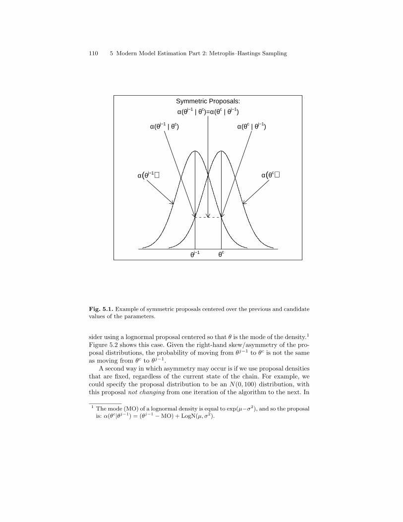
110 5 Modern Model Estimation Part 2: Metroplis–Hastings Sampling
θj−1 θc
α(θc | θj−1)α(θj−1 | θc)
Symmetric Proposals:
α(θj−1 | θc)=α(θc | θj−1)
α(θc)α(θj−1)
Fig. 5.1. Example of symmetric proposals centered over the previous and candidatevalues of the parameters.
sider using a lognormal proposal centered so that θ is the mode of the density.1
Figure 5.2 shows this case. Given the right-hand skew/asymmetry of the pro-posal distributions, the probability of moving from θj−1 to θc is not the sameas moving from θc to θj−1.
A second way in which asymmetry may occur is if we use proposal densitiesthat are fixed, regardless of the current state of the chain. For example, wecould specify the proposal distribution to be an N(0, 100) distribution, withthis proposal not changing from one iteration of the algorithm to the next. In
1 The mode (MO) of a lognormal density is equal to exp(µ−σ2), and so the proposalis: α(θc|θj−1) = (θj−1 −MO) + LogN(µ, σ2).
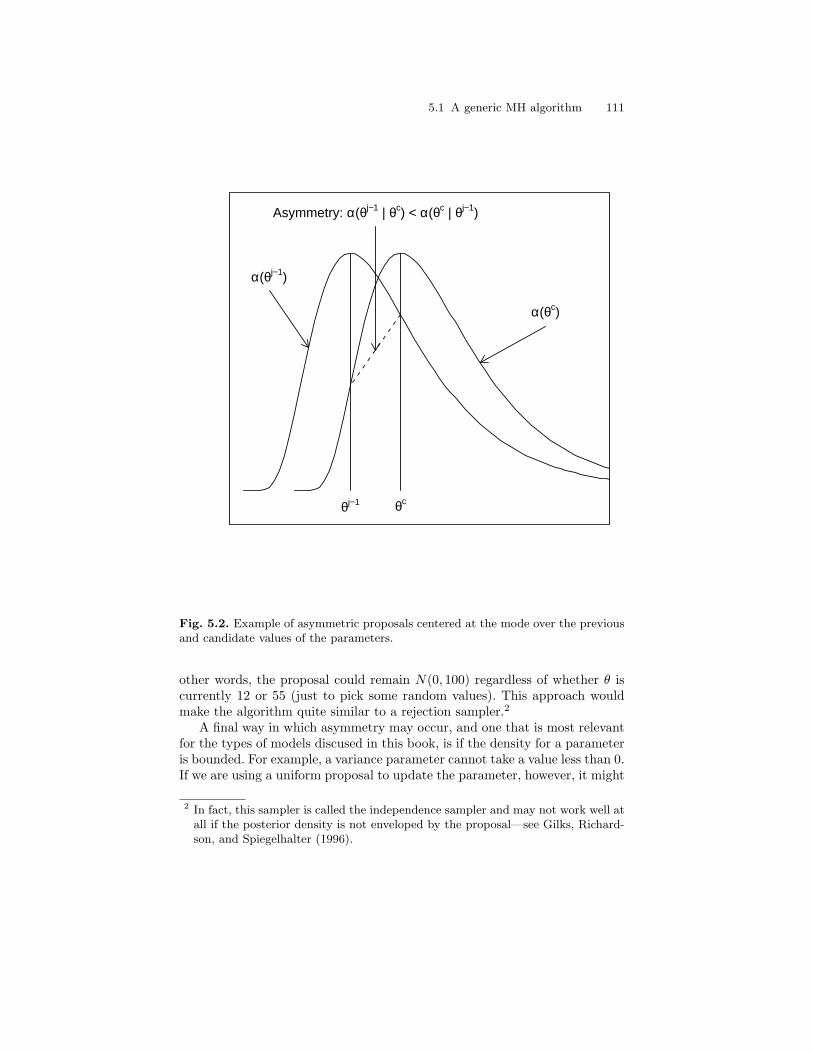
5.1 A generic MH algorithm 111
θj−1 θc
Asymmetry: α(θj−1 | θc) < α(θc | θj−1)
α(θc)
α(θj−1)
Fig. 5.2. Example of asymmetric proposals centered at the mode over the previousand candidate values of the parameters.
other words, the proposal could remain N(0, 100) regardless of whether θ iscurrently 12 or 55 (just to pick some random values). This approach wouldmake the algorithm quite similar to a rejection sampler.2
A final way in which asymmetry may occur, and one that is most relevantfor the types of models discused in this book, is if the density for a parameteris bounded. For example, a variance parameter cannot take a value less than 0.If we are using a uniform proposal to update the parameter, however, it might
2 In fact, this sampler is called the independence sampler and may not work well atall if the posterior density is not enveloped by the proposal—see Gilks, Richard-son, and Spiegelhalter (1996).
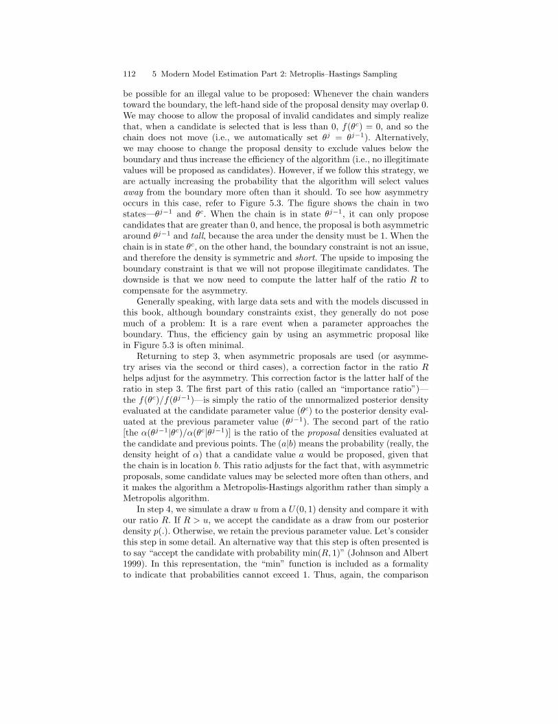
112 5 Modern Model Estimation Part 2: Metroplis–Hastings Sampling
be possible for an illegal value to be proposed: Whenever the chain wanderstoward the boundary, the left-hand side of the proposal density may overlap 0.We may choose to allow the proposal of invalid candidates and simply realizethat, when a candidate is selected that is less than 0, f(θc) = 0, and so thechain does not move (i.e., we automatically set θj = θj−1). Alternatively,we may choose to change the proposal density to exclude values below theboundary and thus increase the efficiency of the algorithm (i.e., no illegitimatevalues will be proposed as candidates). However, if we follow this strategy, weare actually increasing the probability that the algorithm will select valuesaway from the boundary more often than it should. To see how asymmetryoccurs in this case, refer to Figure 5.3. The figure shows the chain in twostates—θj−1 and θc. When the chain is in state θj−1, it can only proposecandidates that are greater than 0, and hence, the proposal is both asymmetricaround θj−1 and tall, because the area under the density must be 1. When thechain is in state θc, on the other hand, the boundary constraint is not an issue,and therefore the density is symmetric and short. The upside to imposing theboundary constraint is that we will not propose illegitimate candidates. Thedownside is that we now need to compute the latter half of the ratio R tocompensate for the asymmetry.
Generally speaking, with large data sets and with the models discussed inthis book, although boundary constraints exist, they generally do not posemuch of a problem: It is a rare event when a parameter approaches theboundary. Thus, the efficiency gain by using an asymmetric proposal likein Figure 5.3 is often minimal.
Returning to step 3, when asymmetric proposals are used (or asymme-try arises via the second or third cases), a correction factor in the ratio Rhelps adjust for the asymmetry. This correction factor is the latter half of theratio in step 3. The first part of this ratio (called an “importance ratio”)—the f(θc)/f(θj−1)—is simply the ratio of the unnormalized posterior densityevaluated at the candidate parameter value (θc) to the posterior density eval-uated at the previous parameter value (θj−1). The second part of the ratio[the α(θj−1|θc)/α(θc|θj−1)] is the ratio of the proposal densities evaluated atthe candidate and previous points. The (a|b) means the probability (really, thedensity height of α) that a candidate value a would be proposed, given thatthe chain is in location b. This ratio adjusts for the fact that, with asymmetricproposals, some candidate values may be selected more often than others, andit makes the algorithm a Metropolis-Hastings algorithm rather than simply aMetropolis algorithm.
In step 4, we simulate a draw u from a U(0, 1) density and compare it withour ratio R. If R > u, we accept the candidate as a draw from our posteriordensity p(.). Otherwise, we retain the previous parameter value. Let’s considerthis step in some detail. An alternative way that this step is often presented isto say “accept the candidate with probability min(R, 1)” (Johnson and Albert1999). In this representation, the “min” function is included as a formalityto indicate that probabilities cannot exceed 1. Thus, again, the comparison
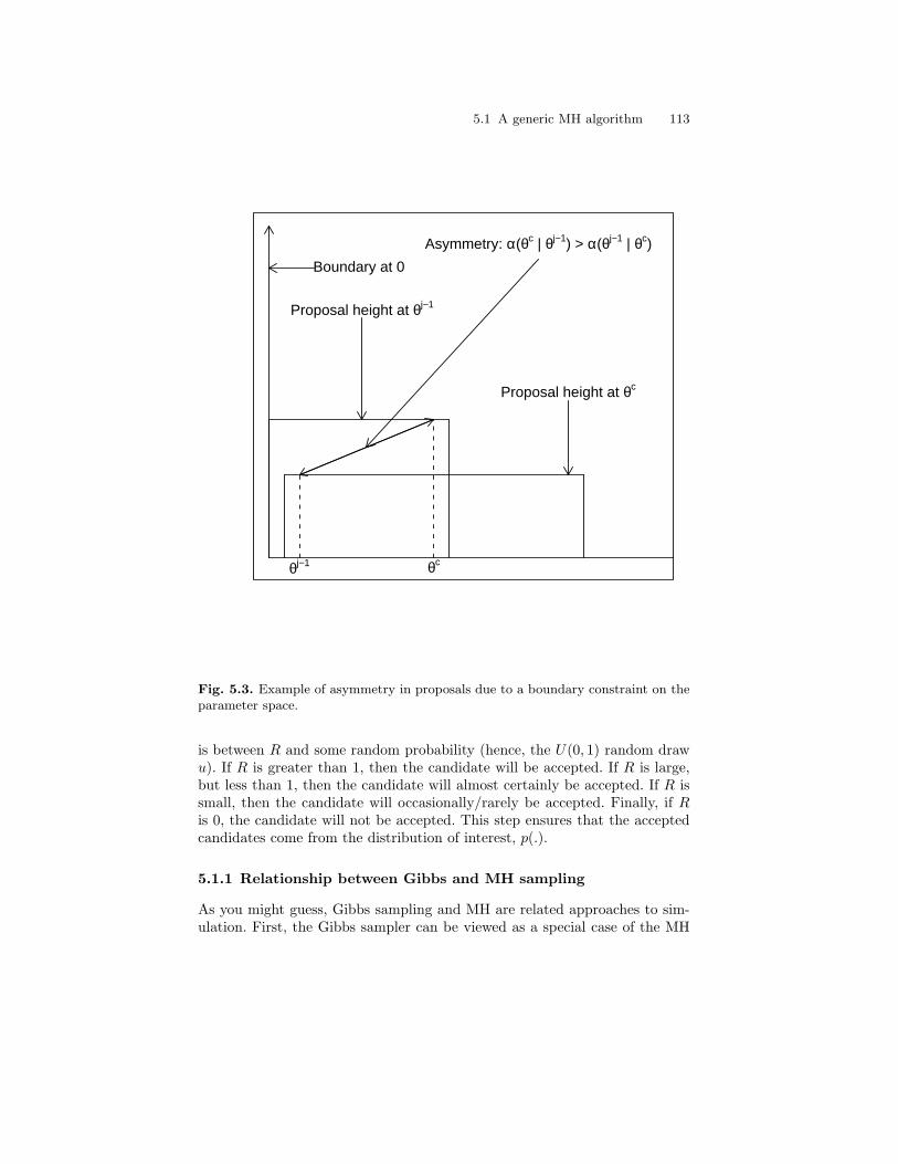
5.1 A generic MH algorithm 113
θj−1 θc
Proposal height at θj−1
Proposal height at θc
Asymmetry: α(θc | θj−1) > α(θj−1 | θc)
Boundary at 0
Fig. 5.3. Example of asymmetry in proposals due to a boundary constraint on theparameter space.
is between R and some random probability (hence, the U(0, 1) random drawu). If R is greater than 1, then the candidate will be accepted. If R is large,but less than 1, then the candidate will almost certainly be accepted. If R issmall, then the candidate will occasionally/rarely be accepted. Finally, if Ris 0, the candidate will not be accepted. This step ensures that the acceptedcandidates come from the distribution of interest, p(.).
5.1.1 Relationship between Gibbs and MH sampling
As you might guess, Gibbs sampling and MH are related approaches to sim-ulation. First, the Gibbs sampler can be viewed as a special case of the MH
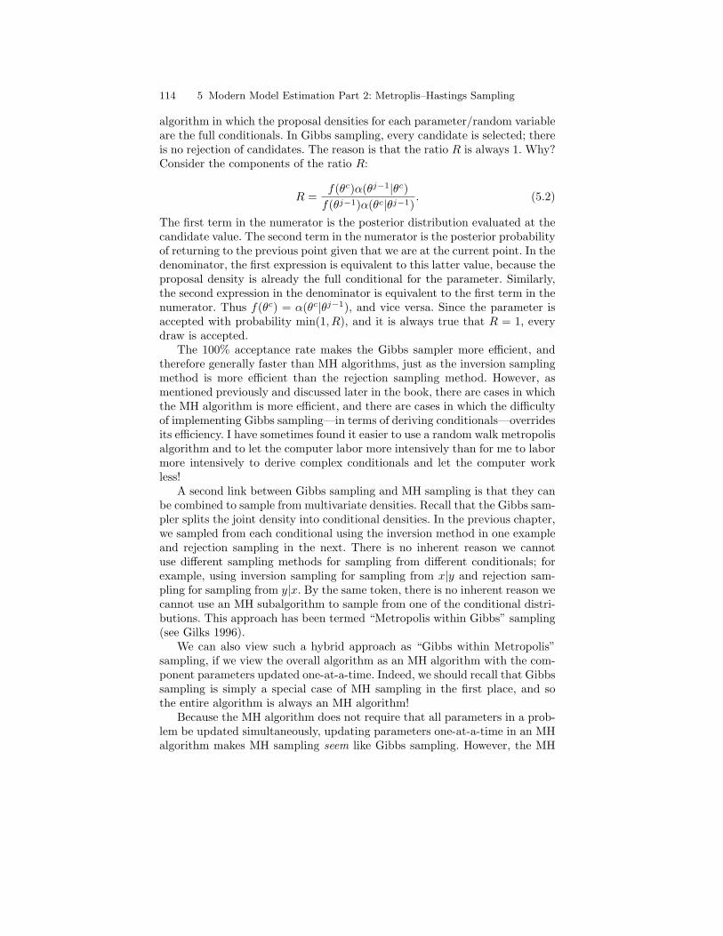
114 5 Modern Model Estimation Part 2: Metroplis–Hastings Sampling
algorithm in which the proposal densities for each parameter/random variableare the full conditionals. In Gibbs sampling, every candidate is selected; thereis no rejection of candidates. The reason is that the ratio R is always 1. Why?Consider the components of the ratio R:
R =f(θc)α(θj−1|θc)
f(θj−1)α(θc|θj−1). (5.2)
The first term in the numerator is the posterior distribution evaluated at thecandidate value. The second term in the numerator is the posterior probabilityof returning to the previous point given that we are at the current point. In thedenominator, the first expression is equivalent to this latter value, because theproposal density is already the full conditional for the parameter. Similarly,the second expression in the denominator is equivalent to the first term in thenumerator. Thus f(θc) = α(θc|θj−1), and vice versa. Since the parameter isaccepted with probability min(1, R), and it is always true that R = 1, everydraw is accepted.
The 100% acceptance rate makes the Gibbs sampler more efficient, andtherefore generally faster than MH algorithms, just as the inversion samplingmethod is more efficient than the rejection sampling method. However, asmentioned previously and discussed later in the book, there are cases in whichthe MH algorithm is more efficient, and there are cases in which the difficultyof implementing Gibbs sampling—in terms of deriving conditionals—overridesits efficiency. I have sometimes found it easier to use a random walk metropolisalgorithm and to let the computer labor more intensively than for me to labormore intensively to derive complex conditionals and let the computer workless!
A second link between Gibbs sampling and MH sampling is that they canbe combined to sample from multivariate densities. Recall that the Gibbs sam-pler splits the joint density into conditional densities. In the previous chapter,we sampled from each conditional using the inversion method in one exampleand rejection sampling in the next. There is no inherent reason we cannotuse different sampling methods for sampling from different conditionals; forexample, using inversion sampling for sampling from x|y and rejection sam-pling for sampling from y|x. By the same token, there is no inherent reason wecannot use an MH subalgorithm to sample from one of the conditional distri-butions. This approach has been termed “Metropolis within Gibbs” sampling(see Gilks 1996).
We can also view such a hybrid approach as “Gibbs within Metropolis”sampling, if we view the overall algorithm as an MH algorithm with the com-ponent parameters updated one-at-a-time. Indeed, we should recall that Gibbssampling is simply a special case of MH sampling in the first place, and sothe entire algorithm is always an MH algorithm!
Because the MH algorithm does not require that all parameters in a prob-lem be updated simultaneously, updating parameters one-at-a-time in an MHalgorithm makes MH sampling seem like Gibbs sampling. However, the MH

5.2 Example: MH sampling when conditional densities are difficult to derive 115
algorithm differs from the Gibbs sampler in two important ways. First, thecandidate parameter is not automatically accepted, because it comes from aproposal density and not from the appropriate conditional distribution. Sec-ond, the proposal density is not an enveloping function as in the rejectionsampling routine discussed above. In short, all Gibbs sampling is MH sam-pling, but not all MH sampling is Gibbs sampling.
Some of the algorithms discussed in the later chapters of this book willinvolve mixtures of Gibbs and MH steps, so it is important to realize that theircombination is possible and sometimes even a desirable alternative to one orthe other approach. For the models presented in the later chapters, virtuallyall of the algorithms that involve MH steps technically will be random walkmetropolis algorithms involving symmetric proposals.
5.2 Example: MH sampling when conditional densitiesare difficult to derive
In Chapter 2 I suggested that a linear density may fit the 2000 GSS itemregarding the importance of expressing unpopular views (“free speech”) betterthan some other distribution. As we discussed at the beginning of this chapter,it would be quite difficult to determine the conditional distributions for thelinear density parameters, m and b, and so Gibbs sampling would not bea good option for sampling from the posterior density. For that matter, aclassical analysis involving finding the maximum likelihood estimate of theseparameters would be difficult also. Therefore, here I develop an MH algorithmfor sampling from the posterior density for m and b. First, I assume uniformprior distributions for the parameters such that p(m) ∝ U(−∞,∞) and p(b) ∝U(0,∞). Although these priors are improper (they cannot integrate to 1), theposterior distribution is proper, subject to an important constraint: m andb must be perfectly related. The possible responses to the free speech itemrange from 0 to 5.3 Thus, if b = 0, m must equal 2 in order for the areaunder the (sampling) density to equal 1. Similarly, if b = 5, m must be −2.More generally, b = (2 − (s − r)2m)/2(s − r), (find this) and so, once m isknown, b is automatically determined. This finding makes an MH algorithm asimple one-parameter process. Below is a random walk metropolis algorithmthat samples from the posterior distribution for m (and by default, b):
#R program for Random Walk Metropolis algorithm
m<-matrix(0,5000); b<-matrix(.2,5000); z<-matrix(0,1377)
z[1:17]=0; z[18:32]=1; z[33:103]=2
z[104:425]=3; z[426:826]=4; z[827:1337]=5
3 The original metric was integers ranging from 1 to 6, but I have recoded to the(0,5) interval and have made a standard assumption that responses are continu-ously, rather than discretely, distributed for simplicity.

116 5 Modern Model Estimation Part 2: Metroplis–Hastings Sampling
acctot=0
for(i in 2:5000)
m[i]=m[i-1]+rnorm(1,mean=0,sd=.002)
b[i]=(2-25*m[i])/10
acc=tot=1
for(j in 1:1377)
tot=tot*((z[j]*m[i]+b[i])/(z[j]*m[i-1]+b[i-1]))
if(runif(1,min=0,max=1)>tot || b[i]<0)
m[i]=m[i-1]; b[i]=b[i-1]; acc=0
acctot=acctot+acc
if(i%%10==0)print(c(i,m[i],b[i],acctot/i))
The first line of this program establishes (1) the vectors and starting valuesfor the slope (m) and intercept (b) parameters (step 1 of the general MHalgorithm described above), and (2) the vector for the data (z). The nexttwo lines constitute the data, with 17/1337 persons responding “0”, 15/1337persons responding “1,” and so on. The third line sets a variable acctot equalto 0; this variable keeps a tally of the number of candidate parameter valuesthat are accepted over the course of the algorithm. (We will discuss the needfor this quantity in some depth later).
The subsequent lines of the program constitute the iterative looping forthe MH algorithm. First, at each iteration, a candidate parameter value form is generated using a normal proposal density centered over the previousvalue for m (m[i]=m[i-1]+rnorm(1,mean=0,sd=.005) ), and b is computed(b[i]=(2-25*m[i])/10 ), given the candidate value for m (step 2 of thegeneral MH algorithm). The next line sets variables acc and tot equal to1. acc is an indicator for whether a candidate is accepted. By default, thealgorithm assumes the candidate is accepted; acc is set to 0 later in theevent the candidate is rejected. tot is initialized at 1; this variable is used totabulate the ratio R.
The next two lines loop over the data in generating the unnormalizedposterior density value at the current and previous values for the parameters.This is the ratio R from step 3 of the general MH algorithm.4
In accordance with Step 4 of the general MH algorithm, the following lines(1) compare this ratio to a U(0, 1) draw (say u), and (2) set the values of mand b to their previous values if R < u or b < 0 (the prior constraint on b).
4 As written, the program computes this ratio one person at a time and sequentiallymultiplies the results together, because computing the entire posterior density ateither the candidate or previous value yields a number too large for the computerto handle. That is,
Qni=1 Ai/
Qni=1 Bi =
Qni=1 Ai/Bi, but the former leads to
overflows in the numerator and denominator, whereas the latter does not.
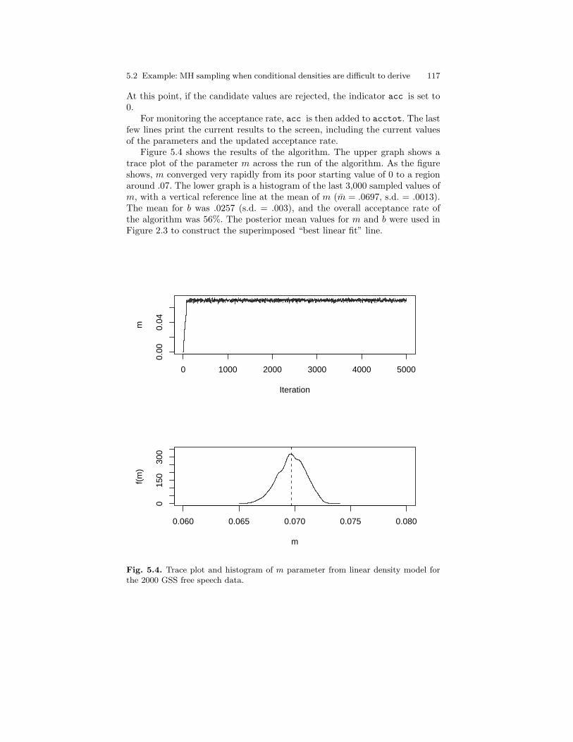
5.2 Example: MH sampling when conditional densities are difficult to derive 117
At this point, if the candidate values are rejected, the indicator acc is set to0.
For monitoring the acceptance rate, acc is then added to acctot. The lastfew lines print the current results to the screen, including the current valuesof the parameters and the updated acceptance rate.
Figure 5.4 shows the results of the algorithm. The upper graph shows atrace plot of the parameter m across the run of the algorithm. As the figureshows, m converged very rapidly from its poor starting value of 0 to a regionaround .07. The lower graph is a histogram of the last 3,000 sampled values ofm, with a vertical reference line at the mean of m (m = .0697, s.d. = .0013).The mean for b was .0257 (s.d. = .003), and the overall acceptance rate ofthe algorithm was 56%. The posterior mean values for m and b were used inFigure 2.3 to construct the superimposed “best linear fit” line.
0 1000 2000 3000 4000 5000
0.00
0.04
Iteration
m
0.060 0.065 0.070 0.075 0.080
015
030
0
m
f(m
)
Fig. 5.4. Trace plot and histogram of m parameter from linear density model forthe 2000 GSS free speech data.
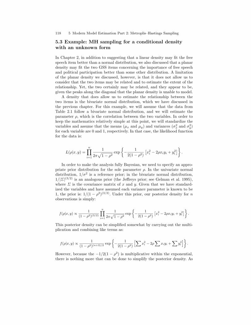
118 5 Modern Model Estimation Part 2: Metroplis–Hastings Sampling
5.3 Example: MH sampling for a conditional densitywith an unknown form
In Chapter 2, in addition to suggesting that a linear density may fit the freespeech item better than a normal distribution, we also discussed that a planardensity may fit the two GSS items concerning the importance of free speechand political participation better than some other distribution. A limitationof the planar density we discussed, however, is that it does not allow us toconsider that the two items may be related and to estimate the extent of therelationship. Yet, the two certainly may be related, and they appear to be,given the peaks along the diagonal that the planar density is unable to model.
A density that does allow us to estimate the relationship between thetwo items is the bivariate normal distribution, which we have discussed inthe previous chapter. For this example, we will assume that the data fromTable 2.1 follow a bivariate normal distribution, and we will estimate theparameter ρ, which is the correlation between the two variables. In order tokeep the mathematics relatively simple at this point, we will standardize thevariables and assume that the means (µx and µy) and variances (σ2
x and σ2y)
for each variable are 0 and 1, respectively. In that case, the likelihood functionfor the data is:
L(ρ|x, y) =n∏
i=1
1
2π√
1− ρ2exp
− 1
2(1− ρ2)[x2
i − 2ρxiyi + y2i
].
In order to make the analysis fully Bayesian, we need to specify an appro-priate prior distribution for the sole parameter ρ. In the univariate normaldistribution, 1/σ2 is a reference prior; in the bivariate normal distribution,1/|Σ|(3/2) is an analogous prior (the Jeffreys prior; see Gelman et al. 1995),where Σ is the covariance matrix of x and y. Given that we have standard-ized the variables and have assumed each variance parameter is known to be1, the prior is: 1/(1 − ρ2)(3/2). Under this prior, our posterior density for nobservations is simply:
f(ρ|x, y) ∝ 1
(1− ρ2)(3/2)
nYi=1
1
2πp
1− ρ2exp
− 1
2(1− ρ2)
ˆx2
i − 2ρxiyi + y2i
˜ff.
This posterior density can be simplified somewhat by carrying out the multi-plication and combining like terms as:
f(ρ|x, y) ∝ 1
(1− ρ2)(n+3)/2exp
− 1
2(1− ρ2)
hXx2
i − 2ρX
xiyi +X
y2i
iff.
However, because the −1/2(1 − ρ2) is multiplicative within the exponential,there is nothing more that can be done to simplify the posterior density. As

5.3 Example: MH sampling for a conditional density with an unknown form 119
it stands, this posterior density for ρ is not a known form, and so Gibbssampling is not a straightforward option (but see Albert 1992 for an approachto using Gibbs sampling to sample a correlation parameter via transformationof variables in an unrelated model).5 Below is an R program that uses MHsampling to sample from the posterior density for ρ. To save space, I haveomitted a number of initial lines that define the data (from Table 2.1):
#MH algorithm for sampling a correlation parameter
#x and y are the data, already stored in memory
lnpost<-function(r)
-690*log(1-r^2)-.5*(sum(x^2)-2*r*sum(x*y)+sum(y^2))/(1-r^2)
corr=matrix(0,10000); acctot=0
for(i in 2:10000)
corr[i]=corr[i-1]+runif(1,min=-.07,max=.07)
acc=1
if(abs(corr[i])>1)acc=0; corr[i]=corr[i-1]
if((lnpost(corr[i])-lnpost(corr[i-1]))
<log(runif(1,min=0,max=1)))
corr[i]=corr[i-1]; acc=0
acctot=acctot+acc
if(i%%100==0)print(c(i,corr[i],acctot/i))
The first line of this program creates a function (lnpost) that evaluatesthe log of the posterior density, given the data and a specified value for thecorrelation coefficient (r). Here, I have introduced a new approach—using thelog of the posterior density rather than the posterior density. With a sampleas large as this one (n = 1, 377), evaluating the posterior itself would generatean underflow problem because of the large negative exponents involved in theposterior. Evaluating the log of the posterior resolves this problem. However,it requires a change later in the program as I will discuss.
After the matrix corr[] is created to store the samples of ρ, and theacceptance rate total is established, the main loop begins. As with the lineardensity example in the previous section, the parameter is first updated usinga uniform proposal density. The candidate is assumed to be accepted (acc=1),but it is then evaluated twice for rejection. It is first evaluated to determinewhether it is a legitimate value for a correlation (within the [−1, 1] interval).Next, it is evaluated using the standard step 3 of the generic MH algorithm:If R < u, the candidate is rejected. However, given that we are comparing logposterior values, the ratio R becomes a subtraction, and it must be comparedwith the log of a uniform draw, rather than simply a uniform draw. As before,5 In fact, univariate sampling is really not Gibbs sampling, but this finding—that
the conditional is an unknown form—would hold if the mean and variance pa-rameters were being estimated rather than assumed to be known quantities.
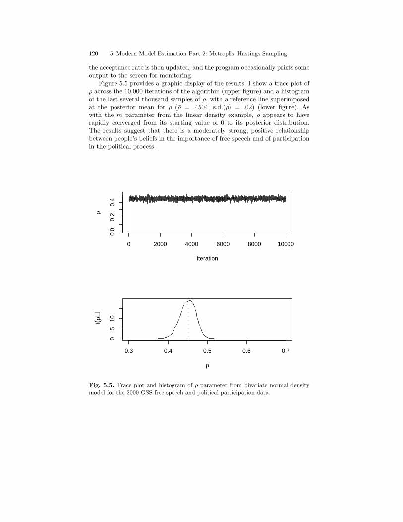
120 5 Modern Model Estimation Part 2: Metroplis–Hastings Sampling
the acceptance rate is then updated, and the program occasionally prints someoutput to the screen for monitoring.
Figure 5.5 provides a graphic display of the results. I show a trace plot ofρ across the 10,000 iterations of the algorithm (upper figure) and a histogramof the last several thousand samples of ρ, with a reference line superimposedat the posterior mean for ρ (ρ = .4504; s.d.(ρ) = .02) (lower figure). Aswith the m parameter from the linear density example, ρ appears to haverapidly converged from its starting value of 0 to its posterior distribution.The results suggest that there is a moderately strong, positive relationshipbetween people’s beliefs in the importance of free speech and of participationin the political process.
0 2000 4000 6000 8000 10000
0.0
0.2
0.4
Iteration
ρ
0.3 0.4 0.5 0.6 0.7
05
10
ρ
f(ρ)
Fig. 5.5. Trace plot and histogram of ρ parameter from bivariate normal densitymodel for the 2000 GSS free speech and political participation data.
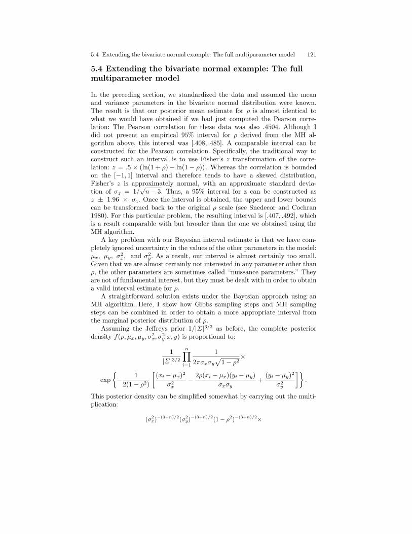
5.4 Extending the bivariate normal example: The full multiparameter model 121
5.4 Extending the bivariate normal example: The fullmultiparameter model
In the preceding section, we standardized the data and assumed the meanand variance parameters in the bivariate normal distribution were known.The result is that our posterior mean estimate for ρ is almost identical towhat we would have obtained if we had just computed the Pearson corre-lation: The Pearson correlation for these data was also .4504. Although Idid not present an empirical 95% interval for ρ derived from the MH al-gorithm above, this interval was [.408, .485]. A comparable interval can beconstructed for the Pearson correlation. Specifically, the traditional way toconstruct such an interval is to use Fisher’s z transformation of the corre-lation: z = .5 × (ln(1 + ρ)− ln(1− ρ)) . Whereas the correlation is boundedon the [−1, 1] interval and therefore tends to have a skewed distribution,Fisher’s z is approximately normal, with an approximate standard devia-tion of σz = 1/
√n− 3. Thus, a 95% interval for z can be constructed as
z ± 1.96 × σz. Once the interval is obtained, the upper and lower boundscan be transformed back to the original ρ scale (see Snedecor and Cochran1980). For this particular problem, the resulting interval is [.407, .492], whichis a result comparable with but broader than the one we obtained using theMH algorithm.
A key problem with our Bayesian interval estimate is that we have com-pletely ignored uncertainty in the values of the other parameters in the model:µx, µy, σ2
x, and σ2y. As a result, our interval is almost certainly too small.
Given that we are almost certainly not interested in any parameter other thanρ, the other parameters are sometimes called “nuissance parameters.” Theyare not of fundamental interest, but they must be dealt with in order to obtaina valid interval estimate for ρ.
A straightforward solution exists under the Bayesian approach using anMH algorithm. Here, I show how Gibbs sampling steps and MH samplingsteps can be combined in order to obtain a more appropriate interval fromthe marginal posterior distribution of ρ.
Assuming the Jeffreys prior 1/|Σ|3/2 as before, the complete posteriordensity f(ρ, µx, µy, σ2
x, σ2y|x, y) is proportional to:
1|Σ|3/2
n∏i=1
1
2πσxσy
√1− ρ2
×
exp− 1
2(1− ρ2)
[(xi − µx)2
σ2x
− 2ρ(xi − µx)(yi − µy)σxσy
+(yi − µy)2
σ2y
].
This posterior density can be simplified somewhat by carrying out the multi-plication:
(σ2x)−(3+n)/2(σ2
y)−(3+n)/2(1− ρ2)−(3+n)/2×

122 5 Modern Model Estimation Part 2: Metroplis–Hastings Sampling
exp
− 1
2(1− ρ2)
» P(xi − µx)2
σ2x
− 2ρP
(xi − µx)(yi − µy)
σxσy+
P(yi − µy)2
σ2y
–ff.
(5.3)
5.4.1 The conditionals for µx and µy
In order to develop a Gibbs sampling routine (with MH steps for simulating σ2x,
σ2y, and ρ), we need to derive the conditionals for the parameters in the model.
This process is tedious, although not fundamentally difficult. In deriving theconditional for µx, as before we can eliminate multiplicative terms that areconstant with respect to µx. The remaining terms are:
p(µx|µy, σ2x, σ2
y, ρ, x, y) ∝
exp− 1
2(1− ρ2)
[∑(xi − µx)2
σ2x
− 2ρ∑
(xi − µx)(yi − µy)σxσy
].
This result can be simplified by expanding the quadratic expressions andagain eliminating terms that do not involve µx as proportionality constants.Following this strategy leaves us with:
p(µx|µy, σ2x, σ2
y, ρ, x, y) ∝
exp− 1
2(1− ρ2)
[n
σ2x
(µ2x − 2xµx)− 2nρ
σxσy(µxµy − yµx)
].
In order to conserve space, I do not elaborate on all the remaining steps.However, if we take this expression, (1) factor an n from the numerator, (2)multiply through by σ2
xσy to eliminate the denominator, and (3) rearrangeterms, we obtain:
exp(
− n
2σ2x(1− ρ2)
)[µ2
x − 2µx
(x +
σxρ
σy(µy − y)
)].
As in the previous chapter, we can now complete the square in µx, but evenwithout doing this, we may recognize that the conditional for µx is:
µx|µy, σx, σy, ρ, x, y ∼ N
(x +
σx
σyρ(µy − y) ,
σ2x(1− ρ2)
n
).
Suppose, momentarily that we know ρ = 0. In that case, the conditionalposterior for µx would reduce to the posterior for the mean in the previouschapter:
µx|ρ = 0 ∼ N(x , σ2
x/n).
By symmetry, we can obtain a comparable conditional distribution for µy;only the x and y subscripts must be changed. What remains is determining theconditional distributions for the two variance parameters and the correlation.
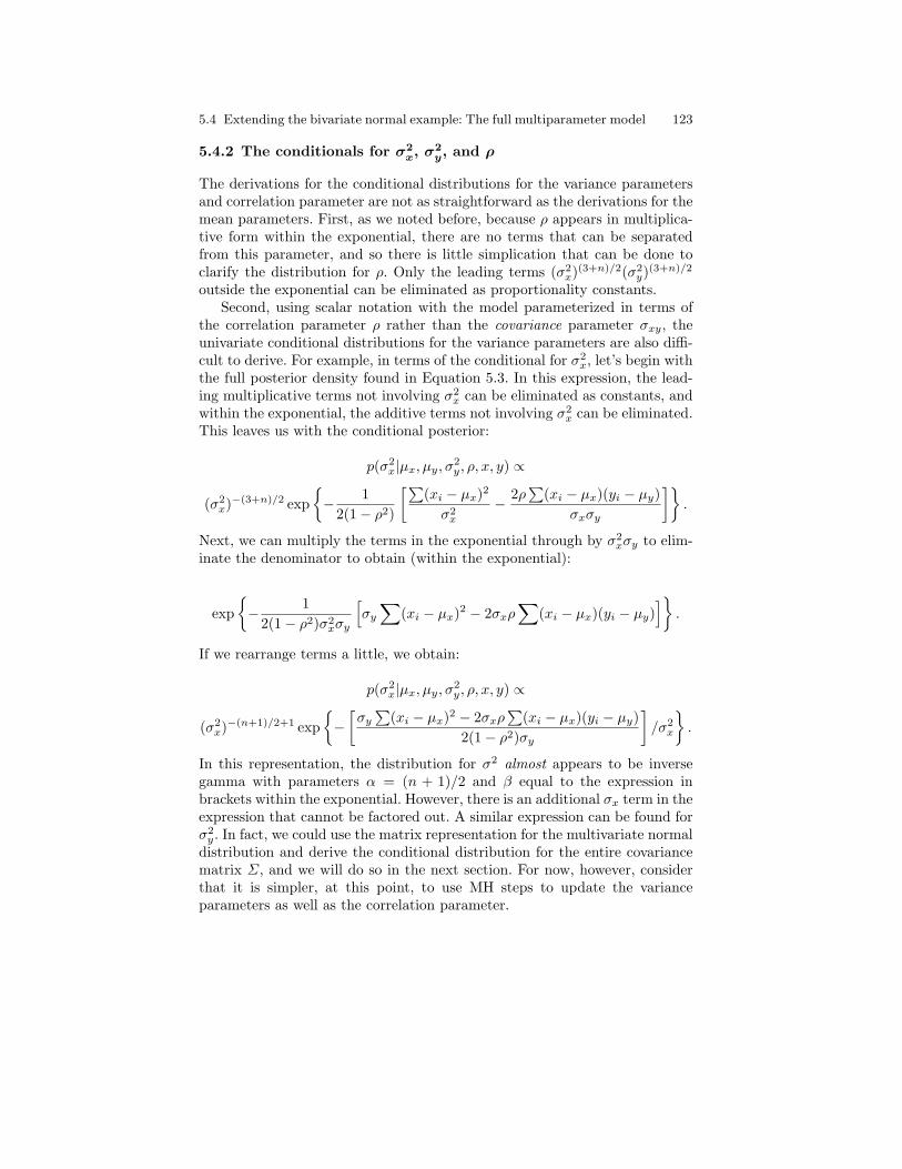
5.4 Extending the bivariate normal example: The full multiparameter model 123
5.4.2 The conditionals for σ2x, σ2
y, and ρ
The derivations for the conditional distributions for the variance parametersand correlation parameter are not as straightforward as the derivations for themean parameters. First, as we noted before, because ρ appears in multiplica-tive form within the exponential, there are no terms that can be separatedfrom this parameter, and so there is little simplication that can be done toclarify the distribution for ρ. Only the leading terms (σ2
x)(3+n)/2(σ2y)(3+n)/2
outside the exponential can be eliminated as proportionality constants.Second, using scalar notation with the model parameterized in terms of
the correlation parameter ρ rather than the covariance parameter σxy, theunivariate conditional distributions for the variance parameters are also diffi-cult to derive. For example, in terms of the conditional for σ2
x, let’s begin withthe full posterior density found in Equation 5.3. In this expression, the lead-ing multiplicative terms not involving σ2
x can be eliminated as constants, andwithin the exponential, the additive terms not involving σ2
x can be eliminated.This leaves us with the conditional posterior:
p(σ2x|µx, µy, σ2
y, ρ, x, y) ∝
(σ2x)−(3+n)/2 exp
− 1
2(1− ρ2)
[∑(xi − µx)2
σ2x
− 2ρ∑
(xi − µx)(yi − µy)σxσy
].
Next, we can multiply the terms in the exponential through by σ2xσy to elim-
inate the denominator to obtain (within the exponential):
exp− 1
2(1− ρ2)σ2xσy
[σy
∑(xi − µx)2 − 2σxρ
∑(xi − µx)(yi − µy)
].
If we rearrange terms a little, we obtain:
p(σ2x|µx, µy, σ2
y, ρ, x, y) ∝
(σ2x)−(n+1)/2+1 exp
−[σy
∑(xi − µx)2 − 2σxρ
∑(xi − µx)(yi − µy)
2(1− ρ2)σy
]/σ2
x
.
In this representation, the distribution for σ2 almost appears to be inversegamma with parameters α = (n + 1)/2 and β equal to the expression inbrackets within the exponential. However, there is an additional σx term in theexpression that cannot be factored out. A similar expression can be found forσ2
y. In fact, we could use the matrix representation for the multivariate normaldistribution and derive the conditional distribution for the entire covariancematrix Σ, and we will do so in the next section. For now, however, considerthat it is simpler, at this point, to use MH steps to update the varianceparameters as well as the correlation parameter.

124 5 Modern Model Estimation Part 2: Metroplis–Hastings Sampling
5.4.3 The complete MH algorithm
Below is a hybrid algorithm with Gibbs sampling steps for updating the meanparameters µx and µy and with MH steps for updating σ2
x and σ2y:
# R program for simulating parameters from BVN distribution
# x and y are the data, already stored in memory
lnpost<-function(ar,amx,amy,asx,asy,ax,ay,axy)
return(-690*log((1-ar^2)*asx*asy)
+(-.5/(1-ar^2))*(ax/asx - 2*ar*axy/sqrt(asx*asy) + ay/asy))
mnx=mean(x); mny=mean(y); accr=0; accx=0; accy=0
mx=matrix(0,10000); my=matrix(0,10000);
sx=matrix(1,10000); sy=matrix(1,10000); r=matrix(0,10000)
for(i in 2:10000)
#sample mx from normal
mx[i]<-rnorm(1,mean=mnx+(r[i-1]*sx[i-1]*(my[i-1]-mny))/sy[i-1]
,sd=sqrt(sx[i-1]*(1-r[i-1]^2)/1377))
#sample my from normal
my[i]<-rnorm(1,mean=mny+(r[i-1]*sy[i-1]*(mx[i]-mnx))/sx[i-1]
,sd=sqrt(sy[i-1]*(1-r[i-1]^2)/1377))
#update sums of squares
sx2=sum((x-mx[i])^2); sy2=sum((y-my[i])^2);
sxy=sum((x-mx[i])*(y-my[i]))
#sample sx
sx[i]=sx[i-1]+runif(1,min=-.1,max=.1); acc=1
if(sx[i]<0)acc=0; sx[i]=sx[i-1]
if((lnpost(r[i-1],mx[i],my[i],sx[i],sy[i-1],sx2,sy2,sxy)
-lnpost(r[i-1],mx[i],my[i],sx[i-1],sy[i-1],sx2,sy2,sxy))
<log(runif(1,min=0,max=1)))
acc=0; sx[i]=sx[i-1]
accx=accx+acc
#sample sy
sy[i]=sy[i-1]+runif(1,min=-.1,max=.1); acc=1
if(sy[i]<0)acc=0; sy[i]=sy[i-1]
if((lnpost(r[i-1],mx[i],my[i],sx[i],sy[i],sx2,sy2,sxy)
-lnpost(r[i-1],mx[i],my[i],sx[i],sy[i-1],sx2,sy2,sxy))
<log(runif(1,min=0,max=1)))
acc=0; sy[i]=sy[i-1]
accy=accy+acc
#sample r from full posterior using MH step
5.4 Extending the bivariate normal example: The full multiparameter model 125
r[i]=r[i-1]+runif(1,min=-.05,max=.05); acc=1
if(abs(r[i])>1)acc=0; r[i]=r[i-1]
if((lnpost(r[i],mx[i],my[i],sx[i],sy[i],sx2,sy2,sxy)
-lnpost(r[i-1],mx[i],my[i],sx[i],sy[i],sx2,sy2,sxy))
<log(runif(1,min=0,max=1)))
acc=0; r[i]=r[i-1]
accr=accr+acc
if(i%%100==0)print(c(i,accr/i,accx/i,accy/i,
mx[i],my[i],sx[i],sy[i],r[i]),digits=4)
This program is intimidatingly long. However, if we consider each sectionof the program separately, it is really fairly simple. For the sake of brevity, Iwill not discuss the entire program line-by-line; instead, I will briefly describethe separate sections.
At the very beginning of the program, I define the various variables to beused in the program, and I create a function (lnpost) that is used in the MHsteps for updating the variance and correlation parameters. This function isthe log posterior density, which is evaluated at established values of the dataand parameters. Once again, I use the log posterior density, because evaluatingthe density itself (in this form) produces computational underflow issues.
The next two sections simply sample the mean parameters from appropri-ate normal distributions derived in the previous section, conditional on thecurrent values of all other parameters in the model. The next, brief sectionupdates the sums of squares (sums of the square deviations of the data fromthe current values of the mean parameters). The next three sections updatethe variances and correlation, given the current values for the means, sumsof squares, and other remaining parameters. These sections are remarkablysimilar, except that (1) the candidate generation step changes, and (2) thelnpost function is fed different variables. Notice that I have created separateacceptance rate variables—one for each variance and correlation—and that Iuse a logged value of a uniform random number to compare with the ratio ofthe logged posterior densities.
Figure 5.6 shows a trace plot and histogram of the samples from themarginal posterior distribution of the correlation parameter—the key param-eter of interest in the model. As the figure shows, the algorithm rapidly con-verged to the .45 region (the Pearson correlation). Overall, the posterior meansfor all parameters were very close to their sample counterparts: µx = x = 2.19;µy = y = 2.02; σ2
x = s2x = 1.43; σ2
y = s2y = 1.14; and ρ = r = .450. Finally,
we can construct a new interval estimate for ρ that reflects our uncertaintyin all the parameters. This interval is [.406 , .491], which is about 10% largerthan the estimate we obtained when we assumed the other parameters werefixed at their sample values, and this estimate more closely matches the oneobtained using the z transformation of the Pearson correlation.
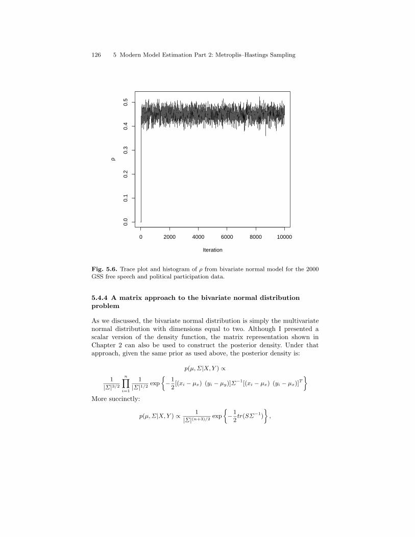
126 5 Modern Model Estimation Part 2: Metroplis–Hastings Sampling
0 2000 4000 6000 8000 10000
0.0
0.1
0.2
0.3
0.4
0.5
Iteration
ρ
Fig. 5.6. Trace plot and histogram of ρ from bivariate normal model for the 2000GSS free speech and political participation data.
5.4.4 A matrix approach to the bivariate normal distributionproblem
As we discussed, the bivariate normal distribution is simply the multivariatenormal distribution with dimensions equal to two. Although I presented ascalar version of the density function, the matrix representation shown inChapter 2 can also be used to construct the posterior density. Under thatapproach, given the same prior as used above, the posterior density is:
p(µ, Σ|X, Y ) ∝
1
|Σ|3/2
nYi=1
1
|Σ|1/2exp
−1
2[(xi − µx) (yi − µy)]Σ−1[(xi − µx) (yi − µx)]T
ffMore succinctly:
p(µ, Σ|X, Y ) ∝ 1
|Σ|(n+3)/2exp
−1
2tr(SΣ−1)
ff,
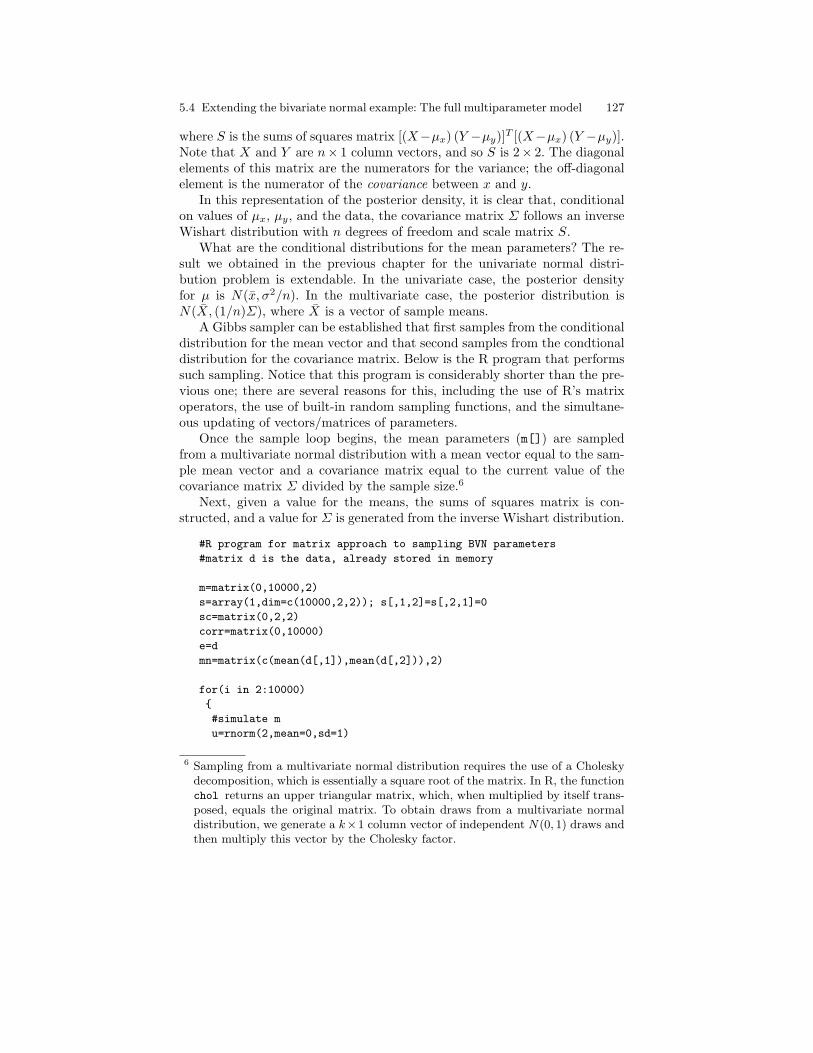
5.4 Extending the bivariate normal example: The full multiparameter model 127
where S is the sums of squares matrix [(X−µx) (Y −µy)]T [(X−µx) (Y −µy)].Note that X and Y are n× 1 column vectors, and so S is 2× 2. The diagonalelements of this matrix are the numerators for the variance; the off-diagonalelement is the numerator of the covariance between x and y.
In this representation of the posterior density, it is clear that, conditionalon values of µx, µy, and the data, the covariance matrix Σ follows an inverseWishart distribution with n degrees of freedom and scale matrix S.
What are the conditional distributions for the mean parameters? The re-sult we obtained in the previous chapter for the univariate normal distri-bution problem is extendable. In the univariate case, the posterior densityfor µ is N(x, σ2/n). In the multivariate case, the posterior distribution isN(X, (1/n)Σ), where X is a vector of sample means.
A Gibbs sampler can be established that first samples from the conditionaldistribution for the mean vector and that second samples from the condtionaldistribution for the covariance matrix. Below is the R program that performssuch sampling. Notice that this program is considerably shorter than the pre-vious one; there are several reasons for this, including the use of R’s matrixoperators, the use of built-in random sampling functions, and the simultane-ous updating of vectors/matrices of parameters.
Once the sample loop begins, the mean parameters (m[]) are sampledfrom a multivariate normal distribution with a mean vector equal to the sam-ple mean vector and a covariance matrix equal to the current value of thecovariance matrix Σ divided by the sample size.6
Next, given a value for the means, the sums of squares matrix is con-structed, and a value for Σ is generated from the inverse Wishart distribution.
#R program for matrix approach to sampling BVN parameters
#matrix d is the data, already stored in memory
m=matrix(0,10000,2)
s=array(1,dim=c(10000,2,2)); s[,1,2]=s[,2,1]=0
sc=matrix(0,2,2)
corr=matrix(0,10000)
e=d
mn=matrix(c(mean(d[,1]),mean(d[,2])),2)
for(i in 2:10000)
#simulate m
u=rnorm(2,mean=0,sd=1)
6 Sampling from a multivariate normal distribution requires the use of a Choleskydecomposition, which is essentially a square root of the matrix. In R, the functionchol returns an upper triangular matrix, which, when multiplied by itself trans-posed, equals the original matrix. To obtain draws from a multivariate normaldistribution, we generate a k×1 column vector of independent N(0, 1) draws andthen multiply this vector by the Cholesky factor.
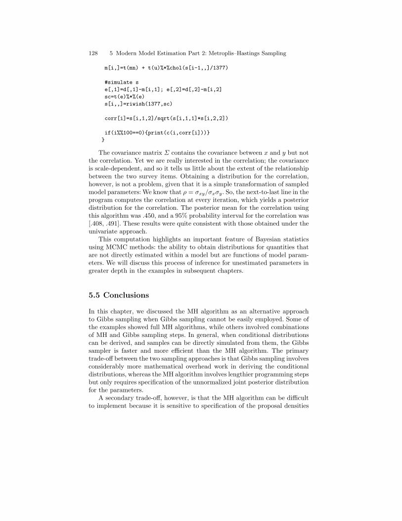
128 5 Modern Model Estimation Part 2: Metroplis–Hastings Sampling
m[i,]=t(mn) + t(u)%*%chol(s[i-1,,]/1377)
#simulate s
e[,1]=d[,1]-m[i,1]; e[,2]=d[,2]-m[i,2]
sc=t(e)%*%(e)
s[i,,]=riwish(1377,sc)
corr[i]=s[i,1,2]/sqrt(s[i,1,1]*s[i,2,2])
if(i%%100==0)print(c(i,corr[i]))
The covariance matrix Σ contains the covariance between x and y but notthe correlation. Yet we are really interested in the correlation; the covarianceis scale-dependent, and so it tells us little about the extent of the relationshipbetween the two survey items. Obtaining a distribution for the correlation,however, is not a problem, given that it is a simple transformation of sampledmodel parameters: We know that ρ = σxy/σxσy. So, the next-to-last line in theprogram computes the correlation at every iteration, which yields a posteriordistribution for the correlation. The posterior mean for the correlation usingthis algorithm was .450, and a 95% probability interval for the correlation was[.408, .491]. These results were quite consistent with those obtained under theunivariate approach.
This computation highlights an important feature of Bayesian statisticsusing MCMC methods: the ability to obtain distributions for quantities thatare not directly estimated within a model but are functions of model param-eters. We will discuss this process of inference for unestimated parameters ingreater depth in the examples in subsequent chapters.
5.5 Conclusions
In this chapter, we discussed the MH algorithm as an alternative approachto Gibbs sampling when Gibbs sampling cannot be easily employed. Some ofthe examples showed full MH algorithms, while others involved combinationsof MH and Gibbs sampling steps. In general, when conditional distributionscan be derived, and samples can be directly simulated from them, the Gibbssampler is faster and more efficient than the MH algorithm. The primarytrade-off between the two sampling approaches is that Gibbs sampling involvesconsiderably more mathematical overhead work in deriving the conditionaldistributions, whereas the MH algorithm involves lengthier programming stepsbut only requires specification of the unnormalized joint posterior distributionfor the parameters.
A secondary trade-off, however, is that the MH algorithm can be difficultto implement because it is sensitive to specification of the proposal densities
5.6 Exercises 129
from which candidate parameters are simulated. The consequence is that mon-itoring the performance of an MH algorithm—and making adjustments—is, inmany ways, more important than monitoring the performance of a Gibbs sam-pling routine. To be sure, both types of algorithms require careful monitoringto ensure that they are “converging” and “mixing” appropriately. The nextchapter discusses how to conduct such monitoring and then describes someapproaches to evaluating overall model fit before constructing summaries ofindividual model parameters.
5.6 Exercises
1. In the final example, I introduced a possibly unfamiliar matrix algebraidentity in showing the posterior density for Σ. Let A be a k × 1 columnvector, and let B be a k × k matrix. Show that AT BA = tr(AB) whenk = 3.
2. Derive the relationship shown between m and b in the linear density asshown in Section 5.2, and show how m can also be represented as a func-tion of b (the opposite approach to that shown in the example). Run thealgorithm as it is presented in the text, and then set up the MH algorithmto sample from the posterior for b, rather than m. Compare the resultsand discuss.
3. Rerun the MH algorithm for the linear density in Section 5.2, but firstattempt to allow m and b to both be updated independently. That is, ignorethe constraint that b is completely determined by m. What happens?Next, continue to allow both parameters to be updated, but change theposterior density by adopting a proper prior distribution. Try independentbeta distributions for both parameters, and then try a bivariate normaldistribution with correlation ρ = .5. What happens? Discuss.
4. Return to the final bivariate normal distribution example. Instead of de-riving the conditional distributions for some of the parameters, developan MH algorithm to sample all the parameters.
5. Develop an MH algorithm to sample the parameters mx, my, and b fromthe planar density using the data from Table 2.1. Note that a constraintsimilar to the one imposed in the linear density example needs to be en-forced. That is, once two parameters are determined, the third parameteris fixed.
6. The last bivariate normal algorithm presented (the Gibbs sampler) is themultivariate analog to the univariate Gibbs sampler for sampling the meanand variance parameters from a univariate normal distribution. In Chap-ter 4, I also presented a Gibbs sampler using the marginal distribution(not the conditional distribution) for σ2. In that algorithm, we generateda sequence of draws for σ2, and then we simulated values for µ condi-tional on these samples for σ2. A similar process can be performed in themultivariate case; the only changes include (1) that the scale matrix S

130 5 Modern Model Estimation Part 2: Metroplis–Hastings Sampling
is constructed once, using the sample means rather than the parametersµx and µy, and (2) the degrees of freedom for the inverse Wishart distri-bution are one fewer. Construct this Gibbs sampler and compare resultswith those obtained using the algorithm presented in the chapter.

6
Evaluating Markov Chain Monte Carlo(MCMC) Algorithms and Model Fit
In the previous two chapters, we used Gibbs sampling and Metropolis-Hastings(MH) sampling to make inference for parameters. Making inference, however,should come after (1) we have determined that the algorithm worked cor-rectly, and (2) we have decided that the model we chose is acceptable for ourpurposes. These two issues are the focus of this chapter.
The first part of this chapter addresses the first concern in discussing theconvergence and mixing of MCMC algorithms. This part should not be con-sidered an exhaustive exposition of the topic; as I stated, many of the recentadvances in MCMC methods have been in this area. However, the approachesI present to evaluating algorithm performance are the most common onesused (see Liu 2001 and Robert and Casella 1999). In the previous chapters,I showed the basics of MCMC implementation, but I left these technical is-sues unaddressed. However, because software development is largely left tothe researcher estimating Bayesian models, assessing how well an MCMC al-gorithm performs is crucial to conducting a responsible Bayesian analysis andto making appropriate inferences.
The second part of the chapter discusses three approaches to evaluating thefit of models and to selecting a model as “best.” Specifically, I discuss posteriorpredictive distributions, Bayes factors, and Bayesian model averaging. I devoterelatively little attention to the latter two methods. Bayes factors require thecomputation of the marginal likelihood of the data (the denominator of Bayes’full formula for probability distributions), which is a complex integral thatis not a by-broduct of MCMC estimation and is generally quite difficult tocompute. Hence, additional methods are needed to compute it, and such isbeyond the scope of this book (see Chen, Shao, and Ibrahim 2000). Bayesianmodel averaging (BMA) avoids the need for selecting models essentially bycombining the results of multiple models into a single model. BMA thereforemay not be used often in a social science setting in which we are generallyinterested in testing a single, specific model to evaluate a hypothesis.
132 6 Evaluating Markov Chain Monte Carlo (MCMC) Algorithms and Model Fit
6.1 Why evaluate MCMC algorithm performance?
In classical statistics, the estimation routines that are used to produce max-imum likelihood or other (e.g., least squares) estimates have already beendeveloped, debugged, tested, and retested, and they are largely out of viewof the researcher who uses them. For example, if a researcher is using SASor STATA to estimate an ordinary least squares (OLS) regression model, theresearcher does not need to know how to compute (XT X)−1(XT Y ) to use thesoftware and obtain the OLS estimates. In contrast, in a Bayesian analysisinvolving MCMC methods, the researcher does need to know this informa-tion. Thus, the researcher must be attuned to programming errors and otherissues that are involved in constructing estimation routines. The trade-off forthis extra work is that there is much more flexibility in model development,inference, and evaluation of model fit than a classical analysis generally canoffer without the researcher investing considerable programming effort.
Aside from basic programming mistakes that can render an MCMC al-gorithm useless, there are two primary concerns with the implementation ofany MCMC algorithm: convergence and mixing. We must make sure that thealgorithm produces a Markov chain that “converges” to the appropriate den-sity (the posterior density) and that “mixes” well throughout the support ofthe density. Unlike routines used to find maximum likelihood estimates, whichconverge to a point, MCMC algorithms must converge to, and sample thor-oughly from, a density. Thus, even if an MCMC algorithm converges to theappropriate region, we must also be sure that the algorithm “moves around”throughout the density once it has converged and samples from all areas ofthe density as it should before the run of the algorithm ends.
6.2 Some common problems and solutions
Convergence and mixing may be affected by a number of factors, includingespecially the following:
• The starting values for the parameters.• The shape of the posterior distribution.• The choice of proposal density in an MH algorithm.
As with maximum likelihood estimation algorithms, starting values maymake a difference in the performance of an MCMC algorithm. AlthoughMCMC theory shows that an MCMC algorithm will, in the limit, convergeon the posterior distribution of interest, there is no guarantee that it will inany run of finite length (see Tierney 1996 for discussion of theory relevant toMCMC methods; see Bremaud 1999 for a broader theoretical exposition). Forexample, if it takes 10,000 iterations for an MCMC algorithm to converge, butthe algorithm is only run for 1,000 iterations, the algorithm certainly will nothave converged. Furthermore, the algorithm obviously will not have mixed
6.2 Some common problems and solutions 133
well, either. In brief, if the starting values are particularly poor (e.g., far fromthe center of the target distribution), the run may end before convergence iseven obtained, let alone before the algorithm has thoroughly sampled fromthe target distribution. In some cases, particularly poor starting values mayproduce an algorithm that never even “gets off the ground.” For example,as I mentioned in the last chapter, the second Gibbs sampler for the planardensity required reasonable starting values in order for the algorithm to beginsampling; without a good starting value, the algorithm could not simulate asingle legitimate value for x.
An obvious solution to the problem of having poor starting values is sim-ply to find better ones! This may be easier said than done; however, for mostmodels common in the social sciences, we can generally use maximum likeli-hood estimates from similar models as our starting values. For example, in themultivariate probit models discussed later in the book, we could use maximumlikelihood estimates from univariate probit models as our starting values. Asecond solution to the problem may be to run the algorithm for more itera-tions. In the limit, the algorithm should converge on the target distribution.
The shape of the posterior distribution may also affect convergence andmixing. If the posterior is multimodal, for example, an MCMC algorithm mayconverge rapidly on one mode, but it may not mix well across modes. There area number of solutions to this problem (some more complicated than others); asimple one might be to expand the width/variance of the proposal density sothat it is possible to jump from one mode to another. A second solution may beto find a better model, that is, to incorporate better predictors (assuming themodel is a regression model). One cause of multimodality may be the omissionof an important variable (like gender). Theoretically, posterior distributionstend to be asymptotically normal, and with the models discussed in this book,multimodality may seldom be a problem if most or all relevant variables areincluded.
Another feature of a posterior distribution that may slow convergence andmixing is strong posterior correlation of the model parameters. In a simpleregression model, for example, the intercept and slope parameters will oftenbe highly negatively correlated. Strong correlations between parameters maycause slow convergence, because it may be difficult—especially when the pro-posal densities are broad—for the algorithm to move from its starting values.Similarly, if the starting values are very good (e.g., at the maximum likelihoodestimates), the algorithm may not mix well, because it may be difficult for thealgorithm to move away from them. This problem is often easy to diagnose,because it will yield a very low acceptance rate (see below), but it may notbe very easy to remedy. There are essentially three solutions to the problemof highly correlated parameters: transforming the data, reparameterizing themodel, and modifying the proposal densities.
In the simple regression model example mentioned above, an easy solu-tion is to transform the data by centering the variables, where centering issimply the process of subtracting the mean of each variable from all of the
134 6 Evaluating Markov Chain Monte Carlo (MCMC) Algorithms and Model Fit
observations on that variable. Centering often works to reduce posterior cor-relation of the parameters in regression models as well as hierarchical/growthmodels. However, in a regression model, centering will only reduce the corre-lation between the intercept and the slope parameters (and not between slopeparameters).
The latter two solutions to the problem of strong posterior correlationsbetween parameters are essentially flip sides of the same coin. Reparameter-ization is the process of transforming the model parameters so that they areuncorrelated. For example, Gilks and Roberts (1996) show that transformingtwo highly correlated parameters X1 and X2 by constructing new variablesY1 = X1 +X2 and Y2 = 3(X1X2), simulating from the distribution for Y1 andY2, and then transforming the simulated samples back to get samples fromthe distributions for the original variables, leads to more rapid convergenceand mixing. Alternative reparameterizations are possible, of course, so longas the new parameters are uncorrelated or weakly correlated.
Reparameterization may be quite difficult. First, if we are estimating aregression model with a large number of predictors, transforming all the re-gression coefficients may be extremely tedious, and finding a transformationthat reduces or eliminates strong posterior correlations may be a hit-or-missproposition. Second, when we transform a distribution from one parameter-ization to another, we must include the Jacobian of the transformation inthe new distribution, where the Jacobian is essentially a scalar or matrix thatrepresents how the variables in one space relate to one another relative to howthe variables in the original space related to one another. The Jacobian in ahigh-dimensional transformation will be a matrix, and its derivation may becomplex, especially when compared with simply changing the proposal den-sities (see DeGroot 1986 and/or a calculus text discussing transformations ofmultivariable equations).
The final solution I discuss—modifying the proposal densities—is mucheasier than reparameterizing the model. One reason that a model may notconverge rapidly or mix well when there are strong posterior correlations be-tween the parameters is that the proposal densities do not closely match theshape of the posterior density, and so the algorithm produces a large numberof rejected candidates. Finding a multivariate proposal density with correla-tions that match those in the set of parameters that are highly correlated willgenerally lead to more rapid convergence and better mixing, because havinga similar shape for the proposal and posterior allows the proposals to havegreater density where they should: at regions where the posterior is moredense. Ultimately, altering the proposal densities is an equivalent strategyto reparameterization: Under reparameterization, the proposals remain con-stant, while the posterior is modified to more closely match the shape of theproposals; under proposal modification, the posterior remains constant, whilethe proposals are changed to more closely match the shape of the posterior.I personally prefer the latter approach, because it is simpler and does not re-
6.3 Recognizing poor performance 135
quire additional steps at the end to transform the samples back to the originalparameterization.
Finally, the choice of proposal density may affect convergence and mixingeven when strong posterior correlations are not present. The general rule isthat, the less similar the proposal density is to the posterior density, the worsethe convergence and mixing problems. In my own experience, using randomwalk metropolis algorithms (often with some Gibbs sampling steps) to esti-mate basic models that are commonly used in the social sciences, changing theproposal density is usually not necessary when strong posterior correlationsbetween parameters are not evident. When it is necessary to change the pro-posal, it is usually not because of the fundamental shape of the proposal butrather the scale, in terms of its width or variance. This problem—having toonarrow or too wide of a proposal density—is usually quite easy to diagnose,because the acceptance rate of the algorithm will either be too small or toolarge.
6.3 Recognizing poor performance
In the previous section, I described some common problems that produce non-convergence and poor mixing and discussed some relatively simple approachesto improving performance. But, how do we diagnose when convergence andmixing problems are present?
Since the original development of MCMC methods, a number of methodshave been proposed to evaluate the convergence (and mixing) of MCMC algo-rithms. I will discuss several that appear to be most useful. It is important tonote at the outset, however, that there is no definitive way of assessing conver-gence and mixing for problems that involve analytically intractable densities,and thus, a combination of methods should be employed to satisfy a researcherthat convergence has been obtained. As with any statistical enterprise, MCMCestimation is to a large extent an art that is helped with experience.
6.3.1 Trace plots
The first, and probably most common, method of assessing convergence andmixing is the use of the trace plot. Trace plots were introduced earlier, andas discussed, they are simply plots of the sampled values from an algorithmat each iteration, with the x axis referencing the iteration of the algorithmand the y axis referencing the sampled value (parameter or data point). Witha trace plot, a lack of convergence is evidenced by trending in the sampledvalues such that the algorithm never levels-off to a stable, stationary state.
As an example, I constructed an MH algorithm for sampling the slopeparameters m1 and m2 and the intercept parameter b from a planar den-sity applied to the free speech and political participation items described inChapter 2. Figure 6.1 shows a trace plot of the first 1000 samples for the m2

136 6 Evaluating Markov Chain Monte Carlo (MCMC) Algorithms and Model Fit
parameter (the slope parameter for the free speech item). The algorithm doesnot appear to have converged prior to the 400th iteration; instead, clear down-ward trending is present from the starting value of 0 down to approximately−.012. The algorithm may have converged somewhere around the 400th iter-ation (reference the dotted vertical line). Notice that the sampled values forthe m2 parameter do not evidence any clear, general trending from iteration400 or so through iteration 1,000.
0 200 400 600 800 1000
−0.
012
−0.
008
−0.
004
0.00
0
Iteration
m2
Possible convergence here
Certainly not converged yet
Fig. 6.1. Trace plot for first 1,000 iterations of an MH algorithm sampling param-eters from planar density for GSS free speech and political participation data.
I say that the algorithm may have converged, because we do not haveenough evidence to conclude that it has. Figure 6.2 is a trace plot of the first4,000 iterations, with vertical lines referencing iterations 400-1,000 shown inthe previous figure. From this view, especially given the upward trending inthe last few hundred iterations, it is unclear whether the algorithm, in fact,had converged by iteration 400.
The figure also demonstrates that, even if the algorithm had convergedby iteration 400 or so, it certainly had not thoroughly mixed through the
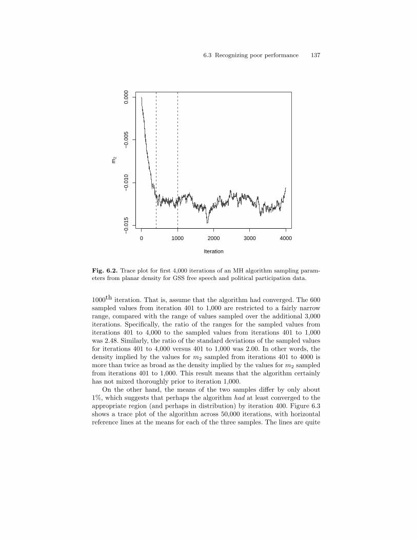
6.3 Recognizing poor performance 137
0 1000 2000 3000 4000
−0.
015
−0.
010
−0.
005
0.00
0
Iteration
m2
Fig. 6.2. Trace plot for first 4,000 iterations of an MH algorithm sampling param-eters from planar density for GSS free speech and political participation data.
1000th iteration. That is, assume that the algorithm had converged. The 600sampled values from iteration 401 to 1,000 are restricted to a fairly narrowrange, compared with the range of values sampled over the additional 3,000iterations. Specifically, the ratio of the ranges for the sampled values fromiterations 401 to 4,000 to the sampled values from iterations 401 to 1,000was 2.48. Similarly, the ratio of the standard deviations of the sampled valuesfor iterations 401 to 4,000 versus 401 to 1,000 was 2.00. In other words, thedensity implied by the values for m2 sampled from iterations 401 to 4000 ismore than twice as broad as the density implied by the values for m2 sampledfrom iterations 401 to 1,000. This result means that the algorithm certainlyhas not mixed thoroughly prior to iteration 1,000.
On the other hand, the means of the two samples differ by only about1%, which suggests that perhaps the algorithm had at least converged to theappropriate region (and perhaps in distribution) by iteration 400. Figure 6.3shows a trace plot of the algorithm across 50,000 iterations, with horizontalreference lines at the means for each of the three samples. The lines are quite
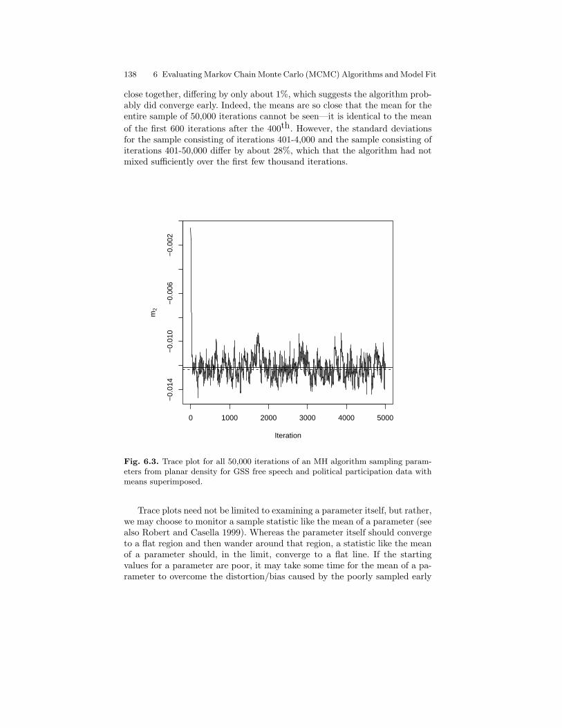
138 6 Evaluating Markov Chain Monte Carlo (MCMC) Algorithms and Model Fit
close together, differing by only about 1%, which suggests the algorithm prob-ably did converge early. Indeed, the means are so close that the mean for theentire sample of 50,000 iterations cannot be seen—it is identical to the meanof the first 600 iterations after the 400th. However, the standard deviationsfor the sample consisting of iterations 401-4,000 and the sample consisting ofiterations 401-50,000 differ by about 28%, which that the algorithm had notmixed sufficiently over the first few thousand iterations.
0 1000 2000 3000 4000 5000
−0.
014
−0.
010
−0.
006
−0.
002
Iteration
m2
Fig. 6.3. Trace plot for all 50,000 iterations of an MH algorithm sampling param-eters from planar density for GSS free speech and political participation data withmeans superimposed.
Trace plots need not be limited to examining a parameter itself, but rather,we may choose to monitor a sample statistic like the mean of a parameter (seealso Robert and Casella 1999). Whereas the parameter itself should convergeto a flat region and then wander around that region, a statistic like the meanof a parameter should, in the limit, converge to a flat line. If the startingvalues for a parameter are poor, it may take some time for the mean of a pa-rameter to overcome the distortion/bias caused by the poorly sampled early
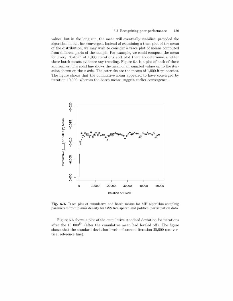
6.3 Recognizing poor performance 139
values, but in the long run, the mean will eventually stabilize, provided thealgorithm in fact has converged. Instead of examining a trace plot of the meanof the distribution, we may wish to consider a trace plot of means computedfrom different parts of the sample. For example, we could compute the meanfor every “batch” of 1,000 iterations and plot them to determine whetherthese batch means evidence any trending. Figure 6.4 is a plot of both of theseapproaches. The solid line shows the mean of all sampled values up to the iter-ation shown on the x axis. The asterisks are the means of 1,000-item batches.The figure shows that the cumulative mean appeared to have converged byiteration 10,000, whereas the batch means suggest earlier convergence.
0 10000 20000 30000 40000 50000
0.00
0−
0.00
5−
0.01
0−
0.01
5−
0.02
0
Iteration or Block
Cum
ulat
ive
(___
) or
Bat
ch (
*) M
ean
Fig. 6.4. Trace plot of cumulative and batch means for MH algorithm samplingparameters from planar density for GSS free speech and political participation data.
Figure 6.5 shows a plot of the cumulative standard deviation for iterationsafter the 10, 000th (after the cumulative mean had leveled off). The figureshows that the standard deviation levels off around iteration 25,000 (see ver-tical reference line).
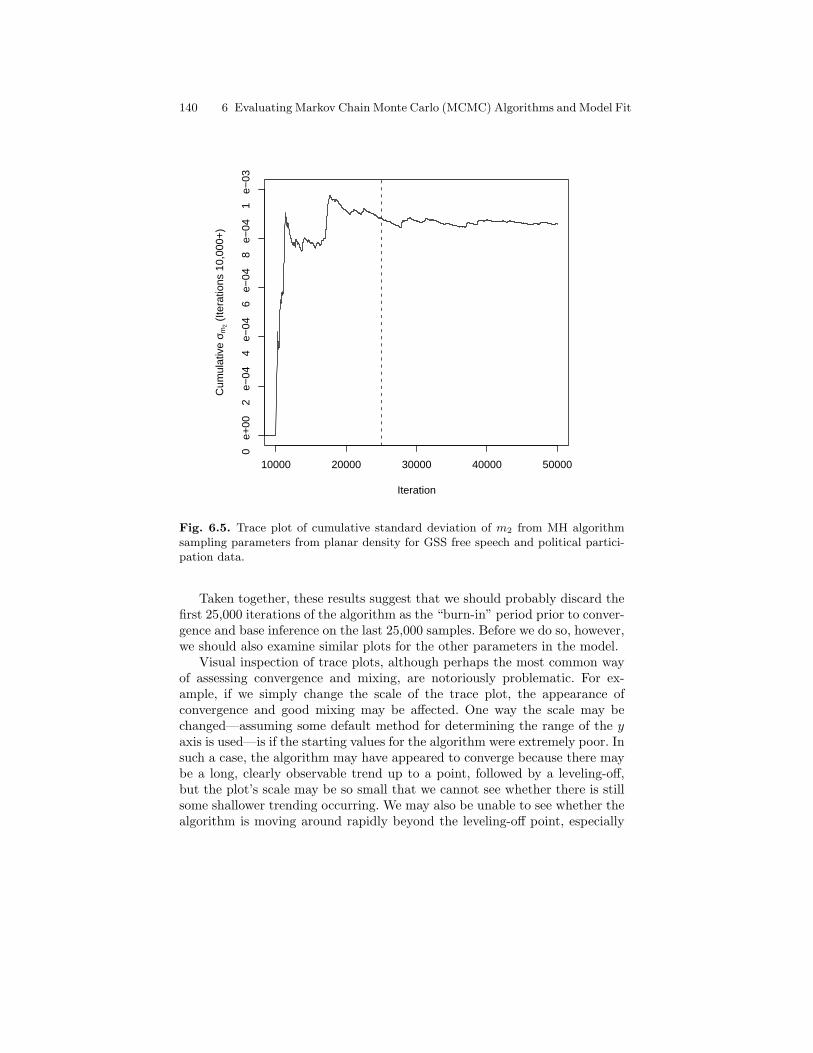
140 6 Evaluating Markov Chain Monte Carlo (MCMC) Algorithms and Model Fit
10000 20000 30000 40000 50000
0 e
+00
2 e
−04
4 e
−04
6 e
−04
8 e
−04
1 e
−03
Iteration
Cum
ulat
ive
σ m2 (
Itera
tions
10,
000+
)
Fig. 6.5. Trace plot of cumulative standard deviation of m2 from MH algorithmsampling parameters from planar density for GSS free speech and political partici-pation data.
Taken together, these results suggest that we should probably discard thefirst 25,000 iterations of the algorithm as the “burn-in” period prior to conver-gence and base inference on the last 25,000 samples. Before we do so, however,we should also examine similar plots for the other parameters in the model.
Visual inspection of trace plots, although perhaps the most common wayof assessing convergence and mixing, are notoriously problematic. For ex-ample, if we simply change the scale of the trace plot, the appearance ofconvergence and good mixing may be affected. One way the scale may bechanged—assuming some default method for determining the range of the yaxis is used—is if the starting values for the algorithm were extremely poor. Insuch a case, the algorithm may have appeared to converge because there maybe a long, clearly observable trend up to a point, followed by a leveling-off,but the plot’s scale may be so small that we cannot see whether there is stillsome shallower trending occurring. We may also be unable to see whether thealgorithm is moving around rapidly beyond the leveling-off point, especially
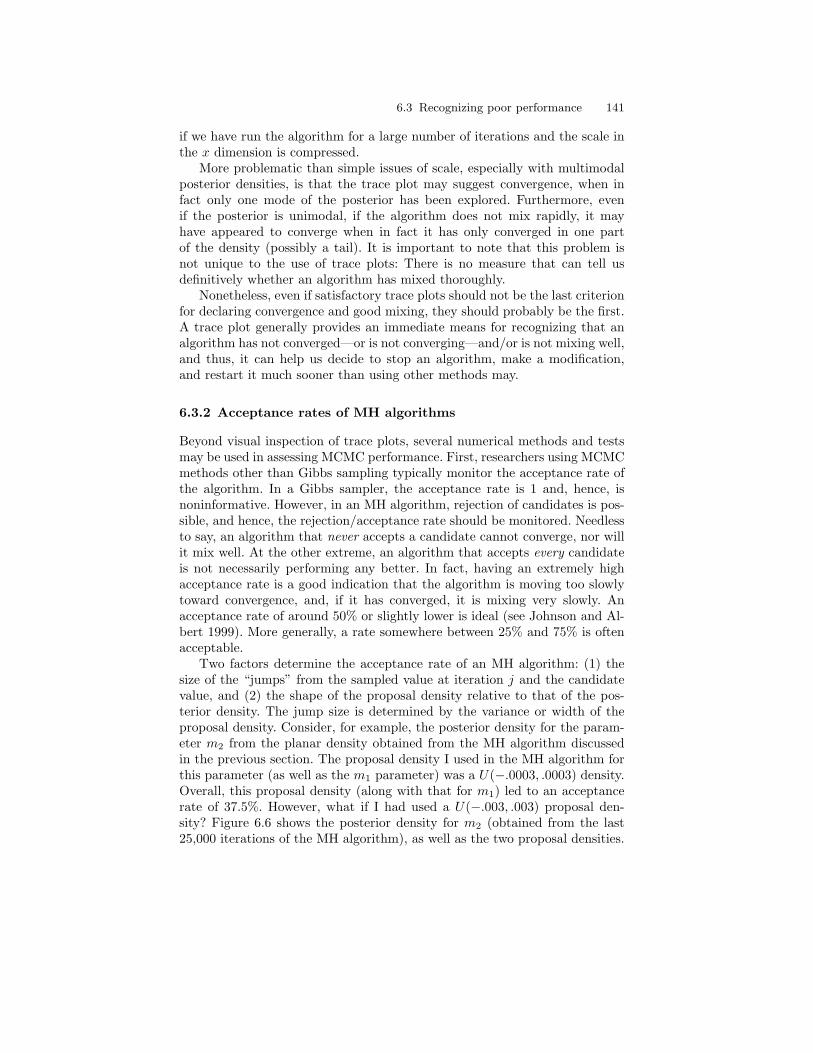
6.3 Recognizing poor performance 141
if we have run the algorithm for a large number of iterations and the scale inthe x dimension is compressed.
More problematic than simple issues of scale, especially with multimodalposterior densities, is that the trace plot may suggest convergence, when infact only one mode of the posterior has been explored. Furthermore, evenif the posterior is unimodal, if the algorithm does not mix rapidly, it mayhave appeared to converge when in fact it has only converged in one partof the density (possibly a tail). It is important to note that this problem isnot unique to the use of trace plots: There is no measure that can tell usdefinitively whether an algorithm has mixed thoroughly.
Nonetheless, even if satisfactory trace plots should not be the last criterionfor declaring convergence and good mixing, they should probably be the first.A trace plot generally provides an immediate means for recognizing that analgorithm has not converged—or is not converging—and/or is not mixing well,and thus, it can help us decide to stop an algorithm, make a modification,and restart it much sooner than using other methods may.
6.3.2 Acceptance rates of MH algorithms
Beyond visual inspection of trace plots, several numerical methods and testsmay be used in assessing MCMC performance. First, researchers using MCMCmethods other than Gibbs sampling typically monitor the acceptance rate ofthe algorithm. In a Gibbs sampler, the acceptance rate is 1 and, hence, isnoninformative. However, in an MH algorithm, rejection of candidates is pos-sible, and hence, the rejection/acceptance rate should be monitored. Needlessto say, an algorithm that never accepts a candidate cannot converge, nor willit mix well. At the other extreme, an algorithm that accepts every candidateis not necessarily performing any better. In fact, having an extremely highacceptance rate is a good indication that the algorithm is moving too slowlytoward convergence, and, if it has converged, it is mixing very slowly. Anacceptance rate of around 50% or slightly lower is ideal (see Johnson and Al-bert 1999). More generally, a rate somewhere between 25% and 75% is oftenacceptable.
Two factors determine the acceptance rate of an MH algorithm: (1) thesize of the “jumps” from the sampled value at iteration j and the candidatevalue, and (2) the shape of the proposal density relative to that of the pos-terior density. The jump size is determined by the variance or width of theproposal density. Consider, for example, the posterior density for the param-eter m2 from the planar density obtained from the MH algorithm discussedin the previous section. The proposal density I used in the MH algorithm forthis parameter (as well as the m1 parameter) was a U(−.0003, .0003) density.Overall, this proposal density (along with that for m1) led to an acceptancerate of 37.5%. However, what if I had used a U(−.003, .003) proposal den-sity? Figure 6.6 shows the posterior density for m2 (obtained from the last25,000 iterations of the MH algorithm), as well as the two proposal densities.
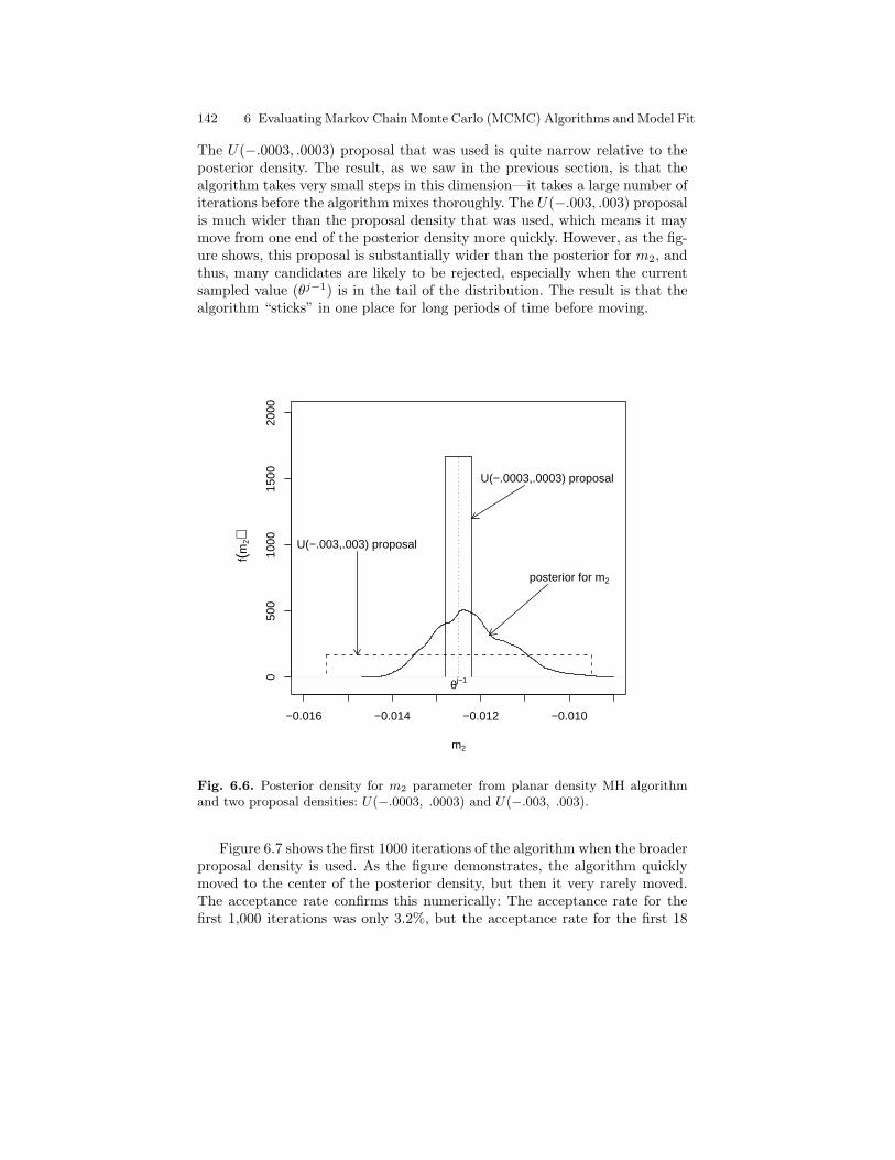
142 6 Evaluating Markov Chain Monte Carlo (MCMC) Algorithms and Model Fit
The U(−.0003, .0003) proposal that was used is quite narrow relative to theposterior density. The result, as we saw in the previous section, is that thealgorithm takes very small steps in this dimension—it takes a large number ofiterations before the algorithm mixes thoroughly. The U(−.003, .003) proposalis much wider than the proposal density that was used, which means it maymove from one end of the posterior density more quickly. However, as the fig-ure shows, this proposal is substantially wider than the posterior for m2, andthus, many candidates are likely to be rejected, especially when the currentsampled value (θj−1) is in the tail of the distribution. The result is that thealgorithm “sticks” in one place for long periods of time before moving.
−0.016 −0.014 −0.012 −0.010
050
010
0015
0020
00
m2
f(m2)
posterior for m2
U(−.0003,.0003) proposal
U(−.003,.003) proposal
θj−1
Fig. 6.6. Posterior density for m2 parameter from planar density MH algorithmand two proposal densities: U(−.0003, .0003) and U(−.003, .003).
Figure 6.7 shows the first 1000 iterations of the algorithm when the broaderproposal density is used. As the figure demonstrates, the algorithm quicklymoved to the center of the posterior density, but then it very rarely moved.The acceptance rate confirms this numerically: The acceptance rate for thefirst 1,000 iterations was only 3.2%, but the acceptance rate for the first 18
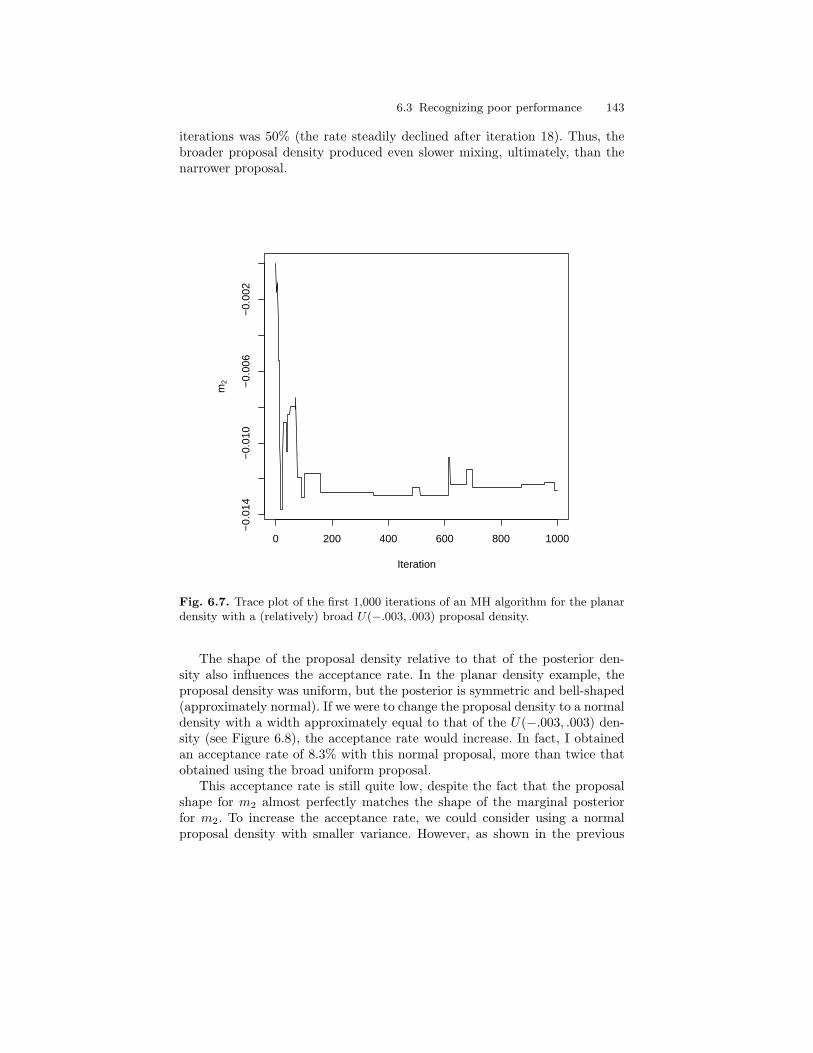
6.3 Recognizing poor performance 143
iterations was 50% (the rate steadily declined after iteration 18). Thus, thebroader proposal density produced even slower mixing, ultimately, than thenarrower proposal.
0 200 400 600 800 1000
−0.
014
−0.
010
−0.
006
−0.
002
Iteration
m2
Fig. 6.7. Trace plot of the first 1,000 iterations of an MH algorithm for the planardensity with a (relatively) broad U(−.003, .003) proposal density.
The shape of the proposal density relative to that of the posterior den-sity also influences the acceptance rate. In the planar density example, theproposal density was uniform, but the posterior is symmetric and bell-shaped(approximately normal). If we were to change the proposal density to a normaldensity with a width approximately equal to that of the U(−.003, .003) den-sity (see Figure 6.8), the acceptance rate would increase. In fact, I obtainedan acceptance rate of 8.3% with this normal proposal, more than twice thatobtained using the broad uniform proposal.
This acceptance rate is still quite low, despite the fact that the proposalshape for m2 almost perfectly matches the shape of the marginal posteriorfor m2. To increase the acceptance rate, we could consider using a normalproposal density with smaller variance. However, as shown in the previous
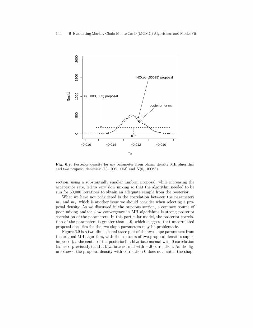
144 6 Evaluating Markov Chain Monte Carlo (MCMC) Algorithms and Model Fit
−0.016 −0.014 −0.012 −0.010
050
010
0015
0020
00
m2
f(m2)
posterior for m2
N(0,sd=.00085) proposal
U(−.003,.003) proposal
θj−1
Fig. 6.8. Posterior density for m2 parameter from planar density MH algorithmand two proposal densities: U(−.003, .003) and N(0, .00085).
section, using a substantially smaller uniform proposal, while increasing theacceptance rate, led to very slow mixing so that the algorithm needed to berun for 50,000 iterations to obtain an adequate sample from the posterior.
What we have not considered is the correlation between the parametersm1 and m2, which is another issue we should consider when selecting a pro-posal density. As we discussed in the previous section, a common source ofpoor mixing and/or slow convergence in MH algorithms is strong posteriorcorrelation of the parameters. In this particular model, the posterior correla-tion of the parameters is greater than −.9, which suggests that uncorrelatedproposal densities for the two slope parameters may be problematic.
Figure 6.9 is a two-dimensional trace plot of the two slope parameters fromthe original MH algorithm, with the contours of two proposal densities super-imposed (at the center of the posterior): a bivariate normal with 0 correlation(as used previously) and a bivariate normal with −.9 correlation. As the fig-ure shows, the proposal density with correlation 0 does not match the shape
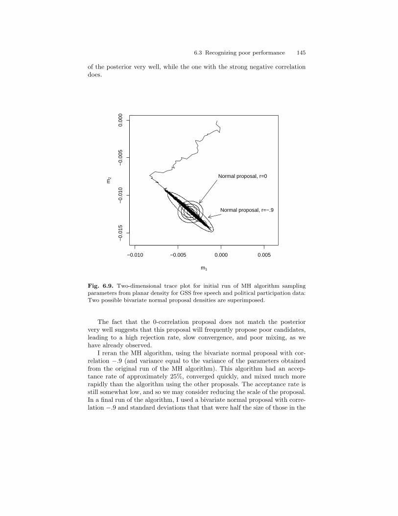
6.3 Recognizing poor performance 145
of the posterior very well, while the one with the strong negative correlationdoes.
−0.010 −0.005 0.000 0.005
−0.
015
−0.
010
−0.
005
0.00
0
m1
m2 Normal proposal, r=0
Normal proposal, r=−.9
Fig. 6.9. Two-dimensional trace plot for initial run of MH algorithm samplingparameters from planar density for GSS free speech and political participation data:Two possible bivariate normal proposal densities are superimposed.
The fact that the 0-correlation proposal does not match the posteriorvery well suggests that this proposal will frequently propose poor candidates,leading to a high rejection rate, slow convergence, and poor mixing, as wehave already observed.
I reran the MH algorithm, using the bivariate normal proposal with cor-relation −.9 (and variance equal to the variance of the parameters obtainedfrom the original run of the MH algorithm). This algorithm had an accep-tance rate of approximately 25%, converged quickly, and mixed much morerapidly than the algorithm using the other proposals. The acceptance rate isstill somewhat low, and so we may consider reducing the scale of the proposal.In a final run of the algorithm, I used a bivariate normal proposal with corre-lation −.9 and standard deviations that that were half the size of those in the
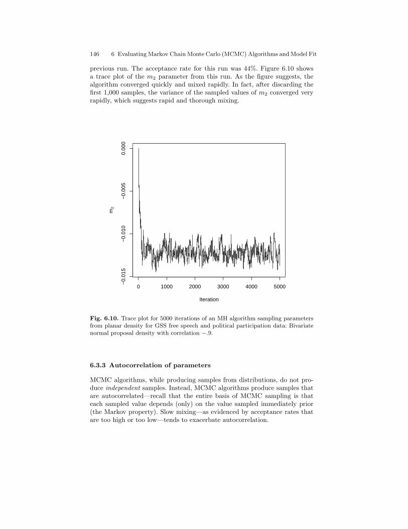
146 6 Evaluating Markov Chain Monte Carlo (MCMC) Algorithms and Model Fit
previous run. The acceptance rate for this run was 44%. Figure 6.10 showsa trace plot of the m2 parameter from this run. As the figure suggests, thealgorithm converged quickly and mixed rapidly. In fact, after discarding thefirst 1,000 samples, the variance of the sampled values of m2 converged veryrapidly, which suggests rapid and thorough mixing.
0 1000 2000 3000 4000 5000
−0.
015
−0.
010
−0.
005
0.00
0
Iteration
m2
Fig. 6.10. Trace plot for 5000 iterations of an MH algorithm sampling parametersfrom planar density for GSS free speech and political participation data: Bivariatenormal proposal density with correlation −.9.
6.3.3 Autocorrelation of parameters
MCMC algorithms, while producing samples from distributions, do not pro-duce independent samples. Instead, MCMC algorithms produce samples thatare autocorrelated—recall that the entire basis of MCMC sampling is thateach sampled value depends (only) on the value sampled immediately prior(the Markov property). Slow mixing—as evidenced by acceptance rates thatare too high or too low—tends to exacerbate autocorrelation.
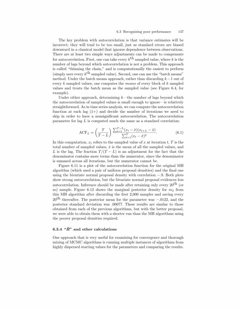
6.3 Recognizing poor performance 147
The key problem with autocorrelation is that variance estimates will beincorrect; they will tend to be too small, just as standard errors are biaseddownward in a classical model that ignores dependence between observations.There are at least two simple ways adjustments can be made to compensatefor autocorrelation. First, one can take every kth sampled value, where k is thenumber of lags beyond which autocorrelation is not a problem. This approachis called “thinning the chain,” and is computationally the easiest to perform(simply save every kth sampled value). Second, one can use the “batch means”method. Under the batch means approach, rather than discarding k−1 out ofevery k sampled values, one computes the means of every block of k sampledvalues and treats the batch mean as the sampled value (see Figure 6.4, forexample).
Under either approach, determining k—the number of lags beyond whichthe autocorrelation of sampled values is small enough to ignore—is relativelystraightforward. As in time series analysis, we can compute the autocorrelationfunction at each lag (1+) and decide the number of iterations we need toskip in order to have a nonsignificant autocorrelation. The autocorrelationparameter for lag L is computed much the same as a standard correlation:
ACFL =(
T
T − L
) ∑T−Lt=1 (xt − x)(xt+L − x)∑T
t=1(xt − x)2. (6.1)
In this computation, xt refers to the sampled value of x at iteration t, T is thetotal number of sampled values, x is the mean of all the sampled values, andL is the lag. The fraction T/(T − L) is an adjustment for the fact that thedenominator contains more terms than the numerator, since the denominatoris summed across all iterations, but the numerator cannot be.
Figure 6.11 is a plot of the autocorrelation function for the original MHalgorithm (which used a pair of uniform proposal densities) and the final oneusing the bivariate normal proposal density with correlation −.9. Both plotsshow strong autocorrelation, but the bivariate normal proposal evidences lessautocorrelation. Inference should be made after retaining only every 20th (orso) sample. Figure 6.12 shows the marginal posterior density for m2 fromthis MH algorithm after discarding the first 2,000 samples and saving every20th thereafter. The posterior mean for the parameter was −.0122, and theposterior standard deviation was .00077. These results are similar to thoseobtained from each of the previous algorithms, but with the better proposal,we were able to obtain them with a shorter run than the MH algorithms usingthe poorer proposal densities required.
6.3.4 “R” and other calculations
One approach that is very useful for examining for convergence and thoroughmixing of MCMC algorithms is running multiple instances of algorithms fromhighly dispersed starting values for the parameters and comparing the results.
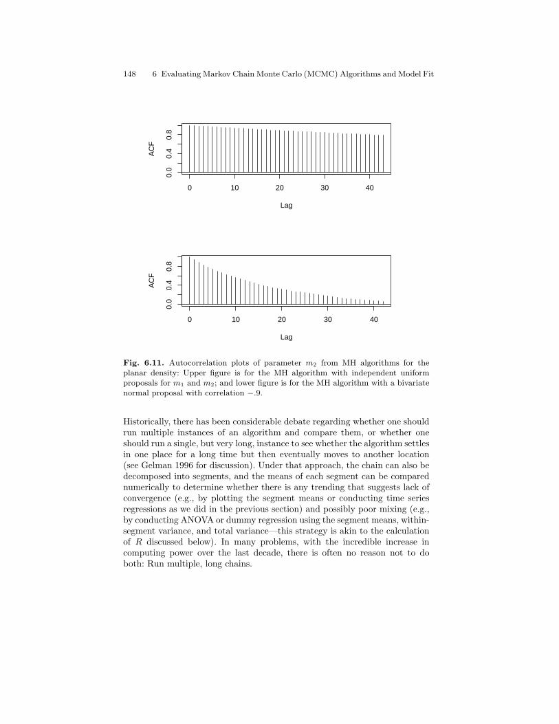
148 6 Evaluating Markov Chain Monte Carlo (MCMC) Algorithms and Model Fit
0 10 20 30 40
0.0
0.4
0.8
Lag
AC
F
0 10 20 30 40
0.0
0.4
0.8
Lag
AC
F
Fig. 6.11. Autocorrelation plots of parameter m2 from MH algorithms for theplanar density: Upper figure is for the MH algorithm with independent uniformproposals for m1 and m2; and lower figure is for the MH algorithm with a bivariatenormal proposal with correlation −.9.
Historically, there has been considerable debate regarding whether one shouldrun multiple instances of an algorithm and compare them, or whether oneshould run a single, but very long, instance to see whether the algorithm settlesin one place for a long time but then eventually moves to another location(see Gelman 1996 for discussion). Under that approach, the chain can also bedecomposed into segments, and the means of each segment can be comparednumerically to determine whether there is any trending that suggests lack ofconvergence (e.g., by plotting the segment means or conducting time seriesregressions as we did in the previous section) and possibly poor mixing (e.g.,by conducting ANOVA or dummy regression using the segment means, within-segment variance, and total variance—this strategy is akin to the calculationof R discussed below). In many problems, with the incredible increase incomputing power over the last decade, there is often no reason not to doboth: Run multiple, long chains.

6.3 Recognizing poor performance 149
−0.015 −0.014 −0.013 −0.012 −0.011 −0.010 −0.009
010
020
030
040
050
0
m2
f(m2)
Fig. 6.12. Histogram of marginal posterior density for m2 parameter: Dashed ref-erence line is the posterior mean.
How do we determine starting values for multiple chains? One approach isto start all parameters at 0 for one chain (if such is sensible—e.g., for regressionparameters, this approach may be reasonable; for a variance parameter, it maynot be), use maximum likelihood estimates from a similar (or identical) modelas starting values in another, and use wildly inappropriate starting values forthe parameters for a third. If all three chains converge to the same location,it may indicate convergence.
What else can we do besides simply using different starting values? We canoften do more than simply modify starting values in an MCMC algorithm.For example, we can modify the proposal densities (either their form or theirwidth/variance) used in each algorithm. If we are updating parameters se-quentially and not all simultaneously, we can switch the order of updating.In other words, we can play around with the fundamentals of the programconducting the simulation. Ultimately, the point is that, if the algorithms areconverging and mixing well, they should all yield similar results.
How do we detect convergence from the results? Once a set of chains hasbeen produced, we need to have some tools for evaluting the results. One way

150 6 Evaluating Markov Chain Monte Carlo (MCMC) Algorithms and Model Fit
to compare multiple chains is to overlay all of them on a single trace plot. Ifthe traces are indistinguishable, then the algorithm may have converged andmixed throughout the density of interest.
As an example, let’s consider again the MH algorithm for the bivariatenormal model for the free speech/political participation data. In the originalMH model, we simulated µx and µy from their full conditional distributions(Gibbs sampling steps), but we simulated the variance parameters σ2
x and σ2y
as well as the correlation parameter ρ using MH steps with uniform proposaldensities. I have rerun the MH algorithm three times, using different sets ofstarting values for the variance and correlation parameters. In the first run,I used σ2
x = σ2y = 1 and ρ = 0 as starting values. In the second, I used
σ2x = σ2
y = 10 and ρ = −.99. In the third, I used σ2x = σ2
y = .01 and ρ = .99.These starting values are highly dispersed: The starting values for ρ span thepossible range for this parameter, and the starting values for the varianceparameters span a large range of possible values, starting near the lowestpossible value (0).
Figure 6.13 shows a trace plot of the sampled values of ρ for the first600 iterations of the MH algorithm under each set of starting values. As thefigure reveals, all three runs of the algorithm converge to a common regionwithin little more than 400 iterations. Beyond 400 iterations, the simulationsequences become indistinguishable.
Figure 6.14 shows a two-dimensional trace plot of the sampled values ofthe variance parameters. This figure provides a picture consistent with thatfor ρ: Regardless of starting values for the variances, the algorithms convergedrapidly to a common bivariate region for these parameters.
The acceptance rates for the three parameters, across the three algorithms,were quite stable at 55%, 64%, and 57% after the first 1,000 iterations (dif-fering across runs by less than one percentage point), providing additionalevidence that convergence had been reached relatively early, and that thor-ough mixing had occurred after the first 1,000 or so iterations.
Another approach involving multiple chains is to compare numerical re-sults: Are means, variances, etc. similar across the different chains? They arealmost certain to not be identical, but are they within the limits of MCMCsampling error?1 In the current example, the means for ρ for the three runswere .4504, .4495, and .4490, with posterior standard deviations of .0215,
1 MCMC algorithms produce samples from a distribution. Running an algorithmmultiple times will produce different samples and, thus, different means, vari-ances, and other statistics. The classical Central Limit Theorem says that thesestatistics will be normally distributed with a mean equal to the population meanand a standard deviation equal to the population standard deviation divided bythe square root of the sample size. Thus, we can estimate MCMC error by com-puting the posterior standard deviation and dividing it by the square root of theMCMC sample size. The posterior mean should vary by a factor of this quantity.Specifically, 95% of MCMC runs should produce posterior means within ±1.96standard errors.
6.3 Recognizing poor performance 151
0 100 200 300 400 500 600
−1.
0−
0.5
0.0
0.5
1.0
Iteration
ρ
Chain 1 Start: ρ=0
Chain 3 Start: ρ=0.99
Chain 2 Start: ρ=− 0.99
Fig. 6.13. Trace plot of first 600 sampled values of ρ from MH algorithms withthree different starting values (GSS political participation and free speech data).
.0214, and .0209, respectively. Thus, the posterior means are all within MCMCsampling fluctuation of each other, providing some indication that the algo-rithm converged and mixed thoroughly.
A common aproach used to determine convergence and adequate mix-ing is the calculation of the “Scale reduction factor” R (often called the“Gelman-Rubin convergence diagnostic.” This is not the ratio R from theMH algorithm!) (see Gelman 1996). When m chains are run, each of lengthn, we can compute the mean of a parameter θ for each chain (θj), the overallmean of the parameter if we combined all chains (θ), the within-chain vari-ance [(1/(m(n − 1))
∑mi=1
∑nj=1(θij − θi)2], and the between-chain variance
[n/(m− 1)∑m
i=1(θi − θ)2]. Gelman (1996) shows that the total variance of θ,then, is (n− 1)/n× within variance + (1/n)× between variance.
As the chains converge, the variance between the chains should decrease,implying that the within variance approaches the total variance. Thus, thescale reduction factor can be computed as:
√R =
√Total/Within. This fac-
tor should be close to 1 when convergence has been reached. Continuing with
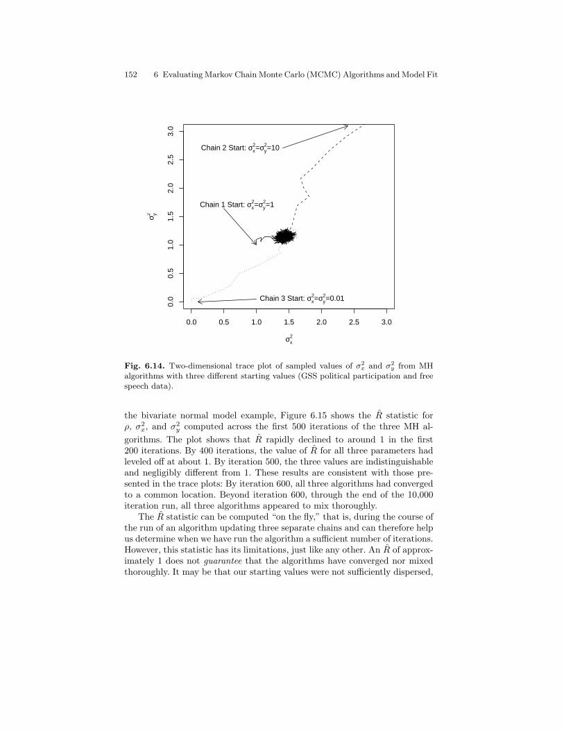
152 6 Evaluating Markov Chain Monte Carlo (MCMC) Algorithms and Model Fit
0.0 0.5 1.0 1.5 2.0 2.5 3.0
0.0
0.5
1.0
1.5
2.0
2.5
3.0
σx2
σ y2Chain 2 Start: σx
2=σy2=10
Chain 3 Start: σx2=σy
2=0.01
Chain 1 Start: σx2=σy
2=1
Fig. 6.14. Two-dimensional trace plot of sampled values of σ2x and σ2
y from MHalgorithms with three different starting values (GSS political participation and freespeech data).
the bivariate normal model example, Figure 6.15 shows the R statistic forρ, σ2
x, and σ2y computed across the first 500 iterations of the three MH al-
gorithms. The plot shows that R rapidly declined to around 1 in the first200 iterations. By 400 iterations, the value of R for all three parameters hadleveled off at about 1. By iteration 500, the three values are indistinguishableand negligibly different from 1. These results are consistent with those pre-sented in the trace plots: By iteration 600, all three algorithms had convergedto a common location. Beyond iteration 600, through the end of the 10,000iteration run, all three algorithms appeared to mix thoroughly.
The R statistic can be computed “on the fly,” that is, during the course ofthe run of an algorithm updating three separate chains and can therefore helpus determine when we have run the algorithm a sufficient number of iterations.However, this statistic has its limitations, just like any other. An R of approx-imately 1 does not guarantee that the algorithms have converged nor mixedthoroughly. It may be that our starting values were not sufficiently dispersed,
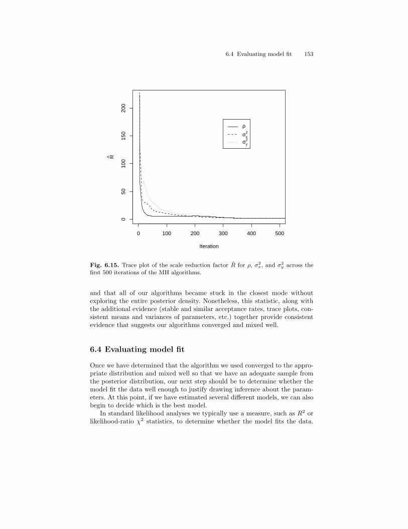
6.4 Evaluating model fit 153
0 100 200 300 400 500
050
100
150
200
Iteration
R
ρσx
2
σy2
Fig. 6.15. Trace plot of the scale reduction factor R for ρ, σ2x, and σ2
y across thefirst 500 iterations of the MH algorithms.
and that all of our algorithms became stuck in the closest mode withoutexploring the entire posterior density. Nonetheless, this statistic, along withthe additional evidence (stable and similar acceptance rates, trace plots, con-sistent means and variances of parameters, etc.) together provide consistentevidence that suggests our algorithms converged and mixed well.
6.4 Evaluating model fit
Once we have determined that the algorithm we used converged to the appro-priate distribution and mixed well so that we have an adequate sample fromthe posterior distribution, our next step should be to determine whether themodel fit the data well enough to justify drawing inference about the param-eters. At this point, if we have estimated several different models, we can alsobegin to decide which is the best model.
In standard likelihood analyses we typically use a measure, such as R2 orlikelihood-ratio χ2 statistics, to determine whether the model fits the data.
154 6 Evaluating Markov Chain Monte Carlo (MCMC) Algorithms and Model Fit
We can use such measures in a Bayesian setting as well, but the Bayesianapproach offers a broader range of possibilities in addition to these, as we willdiscuss briefly here but more in depth in the remaining chapters of the book.
6.4.1 Residual analysis
One way we can evaluate model fit is to conduct residual analyses muchas we would if we were conducting a classical analysis. The only differencebetween a Bayesian and a classical analysis of residuals is that, whereas theclassical approach produces a point estimate for parameters, and thus a pointestimate for the residual for each observation, the Bayesian approach producesa distribution of the parameters and thus a distribution of residuals for eachobservation in the data set. The distribution of residuals provides us withmore information with which to assess the model, because we can examinethe distribution of errors for each observation: We can construct “tests” todetermine whether the distribution of errors for each case is “significantly”different from 0. Cases for which the distribution of errors is far from 0 indicatethat the observation is not fit well by the model. Thus, we do not have to relyon a simple examination of how different a case’s error is from the rest of thesample’s errors—we can concentrate on each case itself. Furthermore, we canconstruct sample-level tests to determine the probability that some proportionof the errors exceeds some value. For example, in a sample of size n = 100,with an MCMC sample of 1,000 draws from the posterior distribution forthe parameters, we could compute, iteration by iteration, the proportion oferrors that exceed some value q, collect these proportions into a distributionof 1,000 proportions, and evaluate this distribution. A model that producesa relatively high average proportion of errors exceeding the criterion q maythen be deemed a poorly fitting model.
Ultimately, Bayesian residual analysis provides greater flexibility in evalu-ating the fit of the model to the data than does a classical analysis. This factwill be even more evident when we discuss generalized linear models (GLMs).In GLMs, the classical approach is limited to using ad hoc tests of residualsthat are based on ordinary least squares (OLS) regression residual analysis;however, these tests are not well suited to models in which the outcome is notmeasured at the interval level. The data-augmentation/latent data approachused by Bayesians, on the other hand, allows us to compute “latent residuals”that are continuously distributed, and thus allows us to follow the same formatfor residual analyses as OLS regression without stretching assumptions (seeJohnson and Albert 1999 for an in-depth exposition of this topic in ordinaldata models).
Because residual analyses are very similar, ultimately, to using poste-rior predictive simulation, and because they are primarily only useful in aregression-model setting, which we have yet to discuss, I do not discuss resid-ual analysis further at this point. We will discuss this topic more in depth inthe remaining chapters when we develop regression models.
6.4 Evaluating model fit 155
6.4.2 Posterior predictive distributions
One of the best and most flexible approaches to examining model fit is theuse of posterior predictive distributions. The posterior predictive distributionfor a model is the distribution of future observations that could arise fromthe model under consideration. The posterior predictive distribution takesinto account both (1) parametric uncertainty and (2) sampling uncertaintyfrom the original model. Parametric uncertainty is captured via the posteriordistribution for the parameters, a sample of which is the result of simulationusing MCMC methods. Sampling uncertainty is captured via the specificationof the sampling density for the data. Recall that the posterior density forthe parameters is a product of the prior distribution for parameters and thelikelihood function (sampling density for the data):
p(θ | data) ∝ p(data | θ)p(θ).
Once this posterior density is obtained, future observations should be expectedto arise from the sampling distribution for the data in the original model; theparameters for this sampling distribution, however, are no longer weightedbased on the prior from the original model, but rather they are weighted bythe posterior distribution for the parameters. Formally, if we use yrep to denotefuture observations, the probability density for future observations, given theobserved sample data is:
p(yrep | y) =∫
p(yrep | θ)p(y | θ)p(θ)dθ. (6.2)
The latter two terms on the right side of this equation (not counting the dθ)constitute the posterior distribution of the parameters. The first term on theright side is the probability density for a future observation that could bedrawn from its sampling distribution, which, of course, is governed by theparameter θ.
If a model fits the current data well—that is, we have adequately capturedthe data-generation process—future data simulated from the model shouldlook much like the current data. Thus, we can simulate data from the pos-terior predictive distribution, compare it with the observed data, and, if thesimulated data are similar to the observed data, we may conclude the modelfits well. In order to determine whether the simulated and observed data aresimilar, we can conduct formal tests using Bayesian p-values. If we define T (y)to be a function of the data (a test statistic) and T (yrep) to be the same func-tion applied to the replicated data, then we can compute a Bayesian p-valueas:
p-value = p(T (yrep) ≥ T (y)|y). (6.3)
In English, the p-value is the proportion of replicated future data sets whosefunction values T (yrep) exceed that of the function T (y) applied to the original
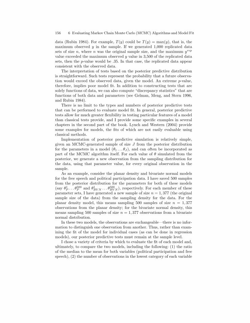
156 6 Evaluating Markov Chain Monte Carlo (MCMC) Algorithms and Model Fit
data (Rubin 1984). For example, T (y) could be T (y) = max(y), that is, themaximum observed y in the sample. If we generated 1,000 replicated datasets of size n, where n was the original sample size, and the maximum yrep
value exceeded the maximum observed y value in 3,500 of the replicated datasets, then the p-value would be .35. In that case, the replicated data appearconsistent with the observed data.
The interpretation of tests based on the posterior predictive distributionis straightforward. Such tests represent the probability that a future observa-tion would exceed the observed data, given the model. An extreme p-value,therefore, implies poor model fit. In addition to constructing tests that aresolely functions of data, we can also compute “discrepancy statistics” that arefunctions of both data and parameters (see Gelman, Meng, and Stern 1996,and Rubin 1984).
There is no limit to the types and numbers of posterior predictive teststhat can be performed to evaluate model fit. In general, posterior predictivetests allow for much greater flexibility in testing particular features of a modelthan classical tests provide, and I provide some specific examples in severalchapters in the second part of the book. Lynch and Western (2004) providesome examples for models, the fits of which are not easily evaluable usingclassical methods.
Implementation of posterior predictive simulation is relatively simple,given an MCMC-generated sample of size J from the posterior distributionfor the parameters in a model (θ1 . . . θJ), and can often be incorporated aspart of the MCMC algorithm itself. For each value of θ simulated from theposterior, we generate a new observation from the sampling distribution forthe data, using that parameter value, for every original observation in thesample.
As an example, consider the planar density and bivariate normal modelsfor the free speech and political participation data. I have saved 500 samplesfrom the posterior distribution for the parameters for both of these models(say θ1
P . . . θ500P and θ1
BV N . . . θ500BV N ), respectively. For each member of these
parameter sets, I have generated a new sample of size n = 1, 377 (the originalsample size of the data) from the sampling density for the data. For theplanar density model, this means sampling 500 samples of size n = 1, 377observations from the planar density; for the bivariate normal density, thismeans sampling 500 samples of size n = 1, 377 observations from a bivariatenormal distribution.
In these two models, the observations are exchangeable—there is no infor-mation to distinguish one observation from another. Thus, rather than exam-ining the fit of the model for individual cases (as can be done in regressionmodels), our posterior predictive tests must remain at the sample level.
I chose a variety of criteria by which to evaluate the fit of each model and,ultimately, to compare the two models, including the following: (1) the ratioof the median to the mean for both variables (political participation and freespeech), (2) the number of observations in the lowest category of each variable
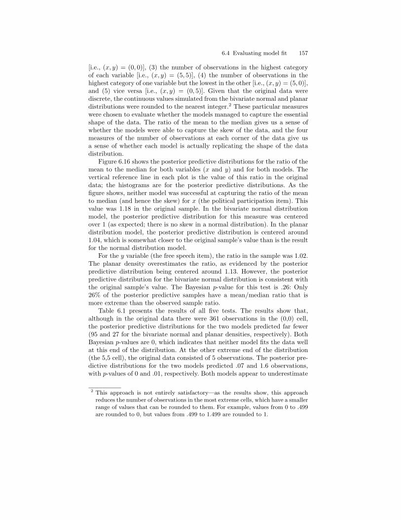
6.4 Evaluating model fit 157
[i.e., (x, y) = (0, 0)], (3) the number of observations in the highest categoryof each variable [i.e., (x, y) = (5, 5)], (4) the number of observations in thehighest category of one variable but the lowest in the other [i.e., (x, y) = (5, 0)],and (5) vice versa [i.e., (x, y) = (0, 5)]. Given that the original data werediscrete, the continuous values simulated from the bivariate normal and planardistributions were rounded to the nearest integer.2 These particular measureswere chosen to evaluate whether the models managed to capture the essentialshape of the data. The ratio of the mean to the median gives us a sense ofwhether the models were able to capture the skew of the data, and the fourmeasures of the number of observations at each corner of the data give usa sense of whether each model is actually replicating the shape of the datadistribution.
Figure 6.16 shows the posterior predictive distributions for the ratio of themean to the median for both variables (x and y) and for both models. Thevertical reference line in each plot is the value of this ratio in the originaldata; the histograms are for the posterior predictive distributions. As thefigure shows, neither model was successful at capturing the ratio of the meanto median (and hence the skew) for x (the political participation item). Thisvalue was 1.18 in the original sample. In the bivariate normal distributionmodel, the posterior predictive distribution for this measure was centeredover 1 (as expected; there is no skew in a normal distribution). In the planardistribution model, the posterior predictive distribution is centered around1.04, which is somewhat closer to the original sample’s value than is the resultfor the normal distribution model.
For the y variable (the free speech item), the ratio in the sample was 1.02.The planar density overestimates the ratio, as evidenced by the posteriorpredictive distribution being centered around 1.13. However, the posteriorpredictive distribution for the bivariate normal distribution is consistent withthe original sample’s value. The Bayesian p-value for this test is .26: Only26% of the posterior predictive samples have a mean/median ratio that ismore extreme than the observed sample ratio.
Table 6.1 presents the results of all five tests. The results show that,although in the original data there were 361 observations in the (0,0) cell,the posterior predictive distributions for the two models predicted far fewer(95 and 27 for the bivariate normal and planar densities, respectively). BothBayesian p-values are 0, which indicates that neither model fits the data wellat this end of the distribution. At the other extreme end of the distribution(the 5,5 cell), the original data consisted of 5 observations. The posterior pre-dictive distributions for the two models predicted .07 and 1.6 observations,with p-values of 0 and .01, respectively. Both models appear to underestimate
2 This approach is not entirely satisfactory—as the results show, this approachreduces the number of observations in the most extreme cells, which have a smallerrange of values that can be rounded to them. For example, values from 0 to .499are rounded to 0, but values from .499 to 1.499 are rounded to 1.
158 6 Evaluating Markov Chain Monte Carlo (MCMC) Algorithms and Model Fit
0.8 0.9 1.0 1.1 1.2
05
1015
Mean(x)/Median(x) (BVN model)
PP
D fr
eque
ncy
0.8 0.9 1.0 1.1 1.2
05
1015
Mean(x)/Median(x) (Planar model)
PP
D fr
eque
ncy
0.8 0.9 1.0 1.1 1.2
05
1015
Mean(y)/Median(y) (BVN model)
PP
D fr
eque
ncy
0.8 0.9 1.0 1.1 1.2
05
1015
Mean(y)/Median(y) (Planar model)
PP
D fr
eque
ncy
Fig. 6.16. Posterior predictive distributions for the ratio of the mean to the me-dian in the bivariate normal distribution and planar distribution models: Verticalreference line is the observed value in the original data.
the number of observations in this cell, but the planar model underestimatesless. The final two tests suggest that the bivariate normal distribution con-sistently underestimates the counts in the tails of the distribution, but theplanar distribution does only slightly better.
We could conduct a similar test on each cell of the bivariate table, butas a simple summary, I computed the correlation between the observed andthe posterior predictive distribution cell counts for both models. Figure 6.17shows the distributions of these correlations. The mean correlation betweenobserved and predictive cell counts for the planar distribution model was .32,

6.5 Formal comparison and combining models 159
which is a low to moderate correlation, while the mean correlation for thebivariate normal distribution model was .75.
Table 6.1. Posterior predictive tests for bivariate normal and planar distributionmodels.
Bivariate Normal PlanarSample
Test Value µPPD p-value µPPD p-value
Mean(x)/Median(x) 1.18 1.00 0.0 1.04 0.0Mean(y)/Median(y) 1.02 0.99 0.26 1.13 0.# of (0,0) Observations 361.0 94.7 0.0 26.5 0.0# of (5,5) Observations 5.0 0.07 0.0 1.6 0.01# of (5,0) Observations 11.0 0.17 0.0 20.3 0.03# of (0,5) Observations 2.0 0.1 0.01 7.0 0.05
Note: Data are from the 2000 GSS special topic module on freedom (variables areexpunpop and partpol).
Overall, the results of the posterior predictive simulation indicate thatneither model fits these data particularly well. The normal distribution con-sistently underpredicts the number of observations in the tails of the distri-bution, and the planar distribution fails to match the overall shape of thedata distribution. The results suggest that, of the two models, the bivariatenormal should be preferred. However, this result is not particularly surprising.The planar density model involved three parameters and did not allow for arelationship between the two variables. The bivariate normal model, on theother hand, had five parameters, including one that captures the relationshipbetween the two variables.
6.5 Formal comparison and combining models
6.5.1 Bayes factors
We are often interested in comparing two or more models to determine whichis “best.” Sometimes, choosing the best model may be our strategy for de-termining which of two competing theories or hypotheses provides a betterexplanation for the data at hand. Occasionally, the models we would like tocompare are nested; that is, one model is a special case of another. In suchcases, the classical approach using maximum likelihood methods provides aprescription for testing for “significant” differences between two models. Moreoften, however, we need to compare models that are not nested. An informal,
160 6 Evaluating Markov Chain Monte Carlo (MCMC) Algorithms and Model Fit
0.0 0.2 0.4 0.6 0.8 1.0
05
1015
Correlation between Observed & PPD Cell Counts
Fre
quen
cyBivariate NormalPlanar
Fig. 6.17. Correlations between observed cell counts and posterior predictive dis-tribution cell counts for the bivariate normal and planar distribution models.
yet flexible and multifaceted approach to comparing models is the use ofposterior predictive simulation as described in the previous section. That is,we could establish a number of criteria (e.g., test statistics) along which tocompare models and choose the model that bests meets the criteria. Indeed,ultimately, model comparison rests on comparing how well two models fit thesame data, and residual analysis and posterior predictive simulation tell ushow well a model fits the data.
The Bayesian approach to statistics also offers more formal means forcomparing models. The use of Bayes factors is one tool for doing so (see Kassand Raftery 1995, and Raftery 1995, for more extensive discussion of modelselection and the Bayes Factor in general, but also see Gelman and Rubin1995).
Suppose we have two models M1 and M2 with parameters θ1 and θ2 that wewould like to compare. Ultimately, what we would like to know is the posteriorprobability of each model, given the data we have observed—P (M | data). Acomparison of the two models, given the posterior probabilities for each wouldthen be straightforward:
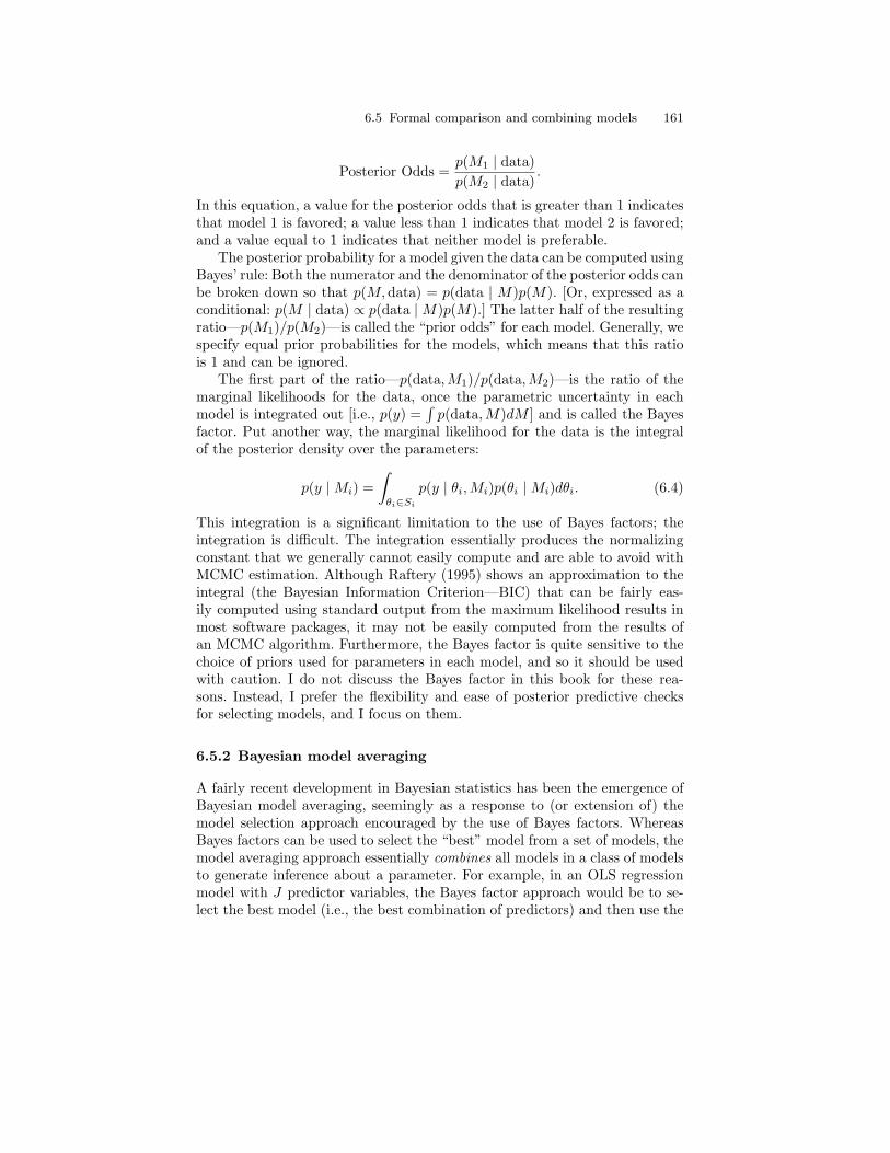
6.5 Formal comparison and combining models 161
Posterior Odds =p(M1 | data)p(M2 | data)
.
In this equation, a value for the posterior odds that is greater than 1 indicatesthat model 1 is favored; a value less than 1 indicates that model 2 is favored;and a value equal to 1 indicates that neither model is preferable.
The posterior probability for a model given the data can be computed usingBayes’ rule: Both the numerator and the denominator of the posterior odds canbe broken down so that p(M,data) = p(data | M)p(M). [Or, expressed as aconditional: p(M | data) ∝ p(data | M)p(M).] The latter half of the resultingratio—p(M1)/p(M2)—is called the “prior odds” for each model. Generally, wespecify equal prior probabilities for the models, which means that this ratiois 1 and can be ignored.
The first part of the ratio—p(data,M1)/p(data,M2)—is the ratio of themarginal likelihoods for the data, once the parametric uncertainty in eachmodel is integrated out [i.e., p(y) =
∫p(data,M)dM ] and is called the Bayes
factor. Put another way, the marginal likelihood for the data is the integralof the posterior density over the parameters:
p(y | Mi) =∫
θi∈Si
p(y | θi,Mi)p(θi | Mi)dθi. (6.4)
This integration is a significant limitation to the use of Bayes factors; theintegration is difficult. The integration essentially produces the normalizingconstant that we generally cannot easily compute and are able to avoid withMCMC estimation. Although Raftery (1995) shows an approximation to theintegral (the Bayesian Information Criterion—BIC) that can be fairly eas-ily computed using standard output from the maximum likelihood results inmost software packages, it may not be easily computed from the results ofan MCMC algorithm. Furthermore, the Bayes factor is quite sensitive to thechoice of priors used for parameters in each model, and so it should be usedwith caution. I do not discuss the Bayes factor in this book for these rea-sons. Instead, I prefer the flexibility and ease of posterior predictive checksfor selecting models, and I focus on them.
6.5.2 Bayesian model averaging
A fairly recent development in Bayesian statistics has been the emergence ofBayesian model averaging, seemingly as a response to (or extension of) themodel selection approach encouraged by the use of Bayes factors. WhereasBayes factors can be used to select the “best” model from a set of models, themodel averaging approach essentially combines all models in a class of modelsto generate inference about a parameter. For example, in an OLS regressionmodel with J predictor variables, the Bayes factor approach would be to se-lect the best model (i.e., the best combination of predictors) and then use the
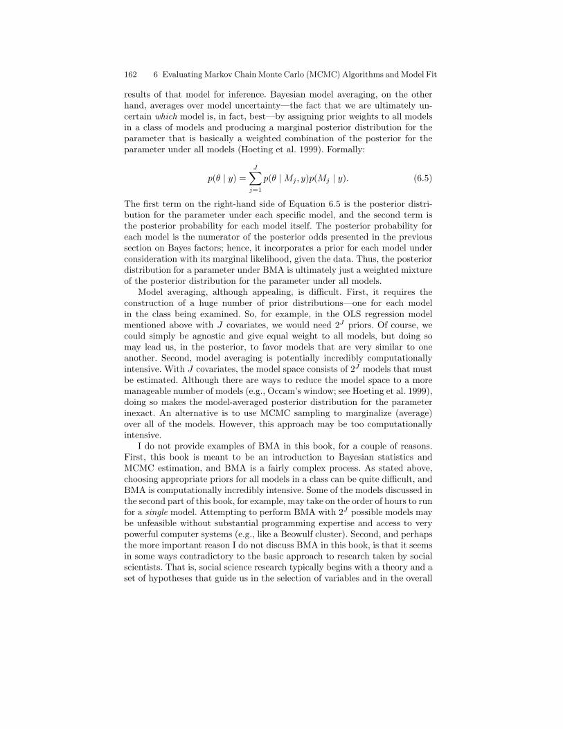
162 6 Evaluating Markov Chain Monte Carlo (MCMC) Algorithms and Model Fit
results of that model for inference. Bayesian model averaging, on the otherhand, averages over model uncertainty—the fact that we are ultimately un-certain which model is, in fact, best—by assigning prior weights to all modelsin a class of models and producing a marginal posterior distribution for theparameter that is basically a weighted combination of the posterior for theparameter under all models (Hoeting et al. 1999). Formally:
p(θ | y) =J∑
j=1
p(θ | Mj , y)p(Mj | y). (6.5)
The first term on the right-hand side of Equation 6.5 is the posterior distri-bution for the parameter under each specific model, and the second term isthe posterior probability for each model itself. The posterior probability foreach model is the numerator of the posterior odds presented in the previoussection on Bayes factors; hence, it incorporates a prior for each model underconsideration with its marginal likelihood, given the data. Thus, the posteriordistribution for a parameter under BMA is ultimately just a weighted mixtureof the posterior distribution for the parameter under all models.
Model averaging, although appealing, is difficult. First, it requires theconstruction of a huge number of prior distributions—one for each modelin the class being examined. So, for example, in the OLS regression modelmentioned above with J covariates, we would need 2J priors. Of course, wecould simply be agnostic and give equal weight to all models, but doing somay lead us, in the posterior, to favor models that are very similar to oneanother. Second, model averaging is potentially incredibly computationallyintensive. With J covariates, the model space consists of 2J models that mustbe estimated. Although there are ways to reduce the model space to a moremanageable number of models (e.g., Occam’s window; see Hoeting et al. 1999),doing so makes the model-averaged posterior distribution for the parameterinexact. An alternative is to use MCMC sampling to marginalize (average)over all of the models. However, this approach may be too computationallyintensive.
I do not provide examples of BMA in this book, for a couple of reasons.First, this book is meant to be an introduction to Bayesian statistics andMCMC estimation, and BMA is a fairly complex process. As stated above,choosing appropriate priors for all models in a class can be quite difficult, andBMA is computationally incredibly intensive. Some of the models discussed inthe second part of this book, for example, may take on the order of hours to runfor a single model. Attempting to perform BMA with 2J possible models maybe unfeasible without substantial programming expertise and access to verypowerful computer systems (e.g., like a Beowulf cluster). Second, and perhapsthe more important reason I do not discuss BMA in this book, is that it seemsin some ways contradictory to the basic approach to research taken by socialscientists. That is, social science research typically begins with a theory and aset of hypotheses that guide us in the selection of variables and in the overall

6.7 Exercises 163
design of a model. The logic of BMA seems to run counter to this approach:BMA allows the data to tell us whether particular variables are important. Ofcourse, we can incorporate our prior expectations for which variables/modelsare most important in a class via our prior specifications for the models, butif we do so, why not simply specify the model we are interested in testing inthe first place! This strategy is akin to conducting BMA and assigning a priorprobability of 0 for all models in the class of models we are evaluating exceptfor the one that our theory leads us to believe is the appropriate one—andgiving it a prior probability of 1.
6.6 Conclusions
In this chapter we have discussed (1) assessing the performance of MCMCalgorithms and (2) assessing model fit. The assessment of MCMC algorithmperformance is an important process, because, if the model has not convergedand mixed well, the results cannot be used for making inference about modelparameters. As we discussed, algorithm assessment requires a multifacetedapproach, because no single approach constitutes a sufficient test for deter-mining whether the routine has converged and mixed well. Indeed, developingbetter ways of assessing performance, as well as developing better performingalgorithms for specific problems has been a key area of research in MCMCmethods over the last decade. In this chapter, we have covered the most com-monly used methods of assessing performance, and we have discussed severalstrategies for improving performance if it is found to be lacking.
Once we have determined that our MCMC algorithm sampled thoroughlyfrom the posterior distribution of interest, our next step should be to assesswhether the model in fact fits the data well. In this chapter, we discussedseveral methods for assessing model fit and comparing models, but the primaryfocus was on posterior predictive checks. I limited the in-depth discussion tothis approach, because posterior predictive simulation is easy to perform, andit is a highly flexible approach to assessing how well the model fits any featureof the data we are concerned about.
Our coverage of these two topics has been relatively basic and limitedlargely to contrived examples. In the remaining chapters, we will employ avariety of strategies for assessing MCMC performance and evaluating modelfit using common social science models and real social science data.
6.7 Exercises
1. How are residual analysis and posterior predictive simulation similar toone another?
2. How can posterior predictive simulation be considered a method to com-pare models and not simply a method to evaluate a single model?

164 6 Evaluating Markov Chain Monte Carlo (MCMC) Algorithms and Model Fit
3. Reconduct the bivariate normal distribution example from the last chap-ter, using an MH algorithm to estimate the parameters, but select ex-tremely poor starting values for them. Run the algorithm five times withdifferent sets of such poor starting values and compute the scale reductionfactor R. Also construct trace plots. Does the R calculation lead you toa different conclusion concerning where to consider the burn-in to haveended than the trace plots?
4. Reconduct the final normal distribution example again with an MH al-gorithm. Use good starting values this time, but run the algorithm atleast seven times using different widths for the proposal distribution forthe means. Can you develop a rule (for this model) for determining theappropriate proposal density width/variance given a desired acceptancerate?
5. Generate 100 observations from a normal distribution with a mean of 5and variance of 4, as in the example. Now square these values, assumethey come from a normal distribution, and estimate the parameters forthis normal distribution using either a Gibbs sampler or an MH algorithm.Next, use posterior predictive simulation to determine whether the modelfits the data. Does it?

7
The Linear Regression Model
The first six chapters of this book have developed statistical modeling from amathematical view of probability, introduced the Bayesian approach to dataanalysis, shown how to sample from Bayesian posterior distributions in or-der to make statistical inference, and demonstrated the basics for evaluatingMCMC algorithm performance, evaluating model fit, and comparing models.So far, the models have been relatively simple; yet statistical modeling in so-cial science research generally involves singling-out one or more variables asoutcomes for which we would like to evaluate the influence of a set of theo-retically important predictors and controls. In short, most social science dataanalysis involves some form of regression modeling. The remaining chapters ofthis book are geared to showing how to perform such analyses in a Bayesianframework. The basic models themselves should be quite familiar, and so thenew content will be the Bayesian implementation of them. In the process ofdemonstrating how a Bayesian might approach these models, I will show someof the advantages of a Bayesian approach, including the ease of handling miss-ing data, the ability to make statistical inference for functions of parametersin models, and the breadth of possible methods for evaluating model fit.
7.1 Development of the linear regression model
The linear regression model—often called the “ordinary least squares (OLS)Regression Model”—is the fundamental model of all social scientific research.Although over the last few decades it has been supplanted by more compli-cated models, especially generalized linear models and models that can handleserial correlation between errors (e.g., fixed and random effects models), thebasic assumption that an outcome variable y (or a function thereof) can beexpressed as a linear combination of predictor variables and some stochasticerror is the foundation of virtually all parametric models in social sciencetoday.
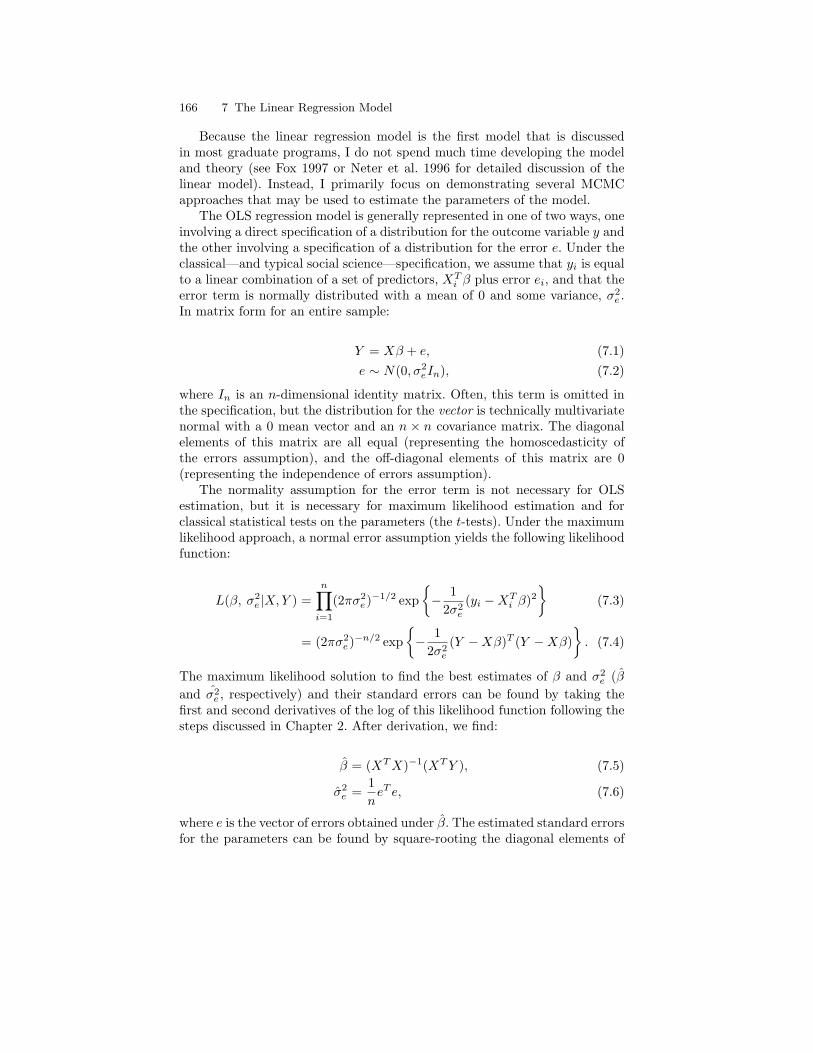
166 7 The Linear Regression Model
Because the linear regression model is the first model that is discussedin most graduate programs, I do not spend much time developing the modeland theory (see Fox 1997 or Neter et al. 1996 for detailed discussion of thelinear model). Instead, I primarily focus on demonstrating several MCMCapproaches that may be used to estimate the parameters of the model.
The OLS regression model is generally represented in one of two ways, oneinvolving a direct specification of a distribution for the outcome variable y andthe other involving a specification of a distribution for the error e. Under theclassical—and typical social science—specification, we assume that yi is equalto a linear combination of a set of predictors, XT
i β plus error ei, and that theerror term is normally distributed with a mean of 0 and some variance, σ2
e .In matrix form for an entire sample:
Y = Xβ + e, (7.1)e ∼ N(0, σ2
eIn), (7.2)
where In is an n-dimensional identity matrix. Often, this term is omitted inthe specification, but the distribution for the vector is technically multivariatenormal with a 0 mean vector and an n × n covariance matrix. The diagonalelements of this matrix are all equal (representing the homoscedasticity ofthe errors assumption), and the off-diagonal elements of this matrix are 0(representing the independence of errors assumption).
The normality assumption for the error term is not necessary for OLSestimation, but it is necessary for maximum likelihood estimation and forclassical statistical tests on the parameters (the t-tests). Under the maximumlikelihood approach, a normal error assumption yields the following likelihoodfunction:
L(β, σ2e |X, Y ) =
n∏i=1
(2πσ2e)−1/2 exp
− 1
2σ2e
(yi −XTi β)2
(7.3)
= (2πσ2e)−n/2 exp
− 1
2σ2e
(Y −Xβ)T (Y −Xβ)
. (7.4)
The maximum likelihood solution to find the best estimates of β and σ2e (β
and σ2e , respectively) and their standard errors can be found by taking the
first and second derivatives of the log of this likelihood function following thesteps discussed in Chapter 2. After derivation, we find:
β = (XT X)−1(XT Y ), (7.5)
σ2e =
1n
eT e, (7.6)
where e is the vector of errors obtained under β. The estimated standard errorsfor the parameters can be found by square-rooting the diagonal elements of
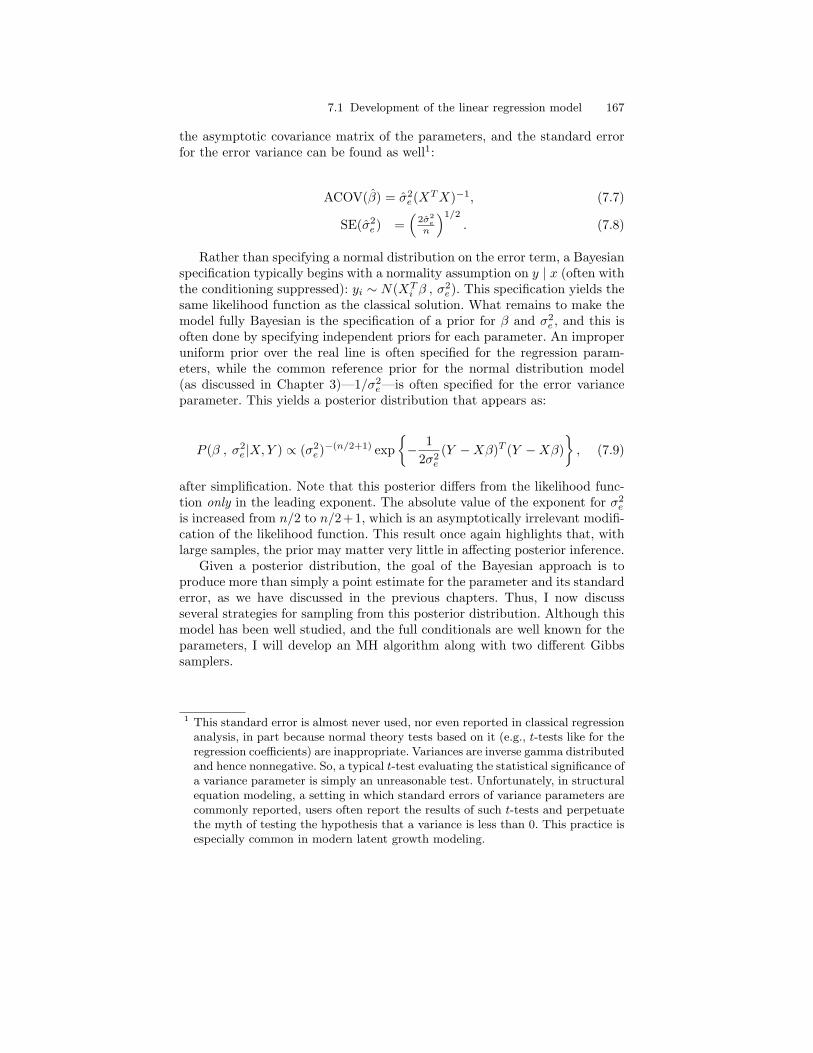
7.1 Development of the linear regression model 167
the asymptotic covariance matrix of the parameters, and the standard errorfor the error variance can be found as well1:
ACOV(β) = σ2e(XT X)−1, (7.7)
SE(σ2e) =
(2σ2
e
n
)1/2
. (7.8)
Rather than specifying a normal distribution on the error term, a Bayesianspecification typically begins with a normality assumption on y | x (often withthe conditioning suppressed): yi ∼ N(XT
i β , σ2e). This specification yields the
same likelihood function as the classical solution. What remains to make themodel fully Bayesian is the specification of a prior for β and σ2
e , and this isoften done by specifying independent priors for each parameter. An improperuniform prior over the real line is often specified for the regression param-eters, while the common reference prior for the normal distribution model(as discussed in Chapter 3)—1/σ2
e—is often specified for the error varianceparameter. This yields a posterior distribution that appears as:
P (β , σ2e |X, Y ) ∝ (σ2
e)−(n/2+1) exp− 1
2σ2e
(Y −Xβ)T (Y −Xβ)
, (7.9)
after simplification. Note that this posterior differs from the likelihood func-tion only in the leading exponent. The absolute value of the exponent for σ2
e
is increased from n/2 to n/2+1, which is an asymptotically irrelevant modifi-cation of the likelihood function. This result once again highlights that, withlarge samples, the prior may matter very little in affecting posterior inference.
Given a posterior distribution, the goal of the Bayesian approach is toproduce more than simply a point estimate for the parameter and its standarderror, as we have discussed in the previous chapters. Thus, I now discussseveral strategies for sampling from this posterior distribution. Although thismodel has been well studied, and the full conditionals are well known for theparameters, I will develop an MH algorithm along with two different Gibbssamplers.
1 This standard error is almost never used, nor even reported in classical regressionanalysis, in part because normal theory tests based on it (e.g., t-tests like for theregression coefficients) are inappropriate. Variances are inverse gamma distributedand hence nonnegative. So, a typical t-test evaluating the statistical significance ofa variance parameter is simply an unreasonable test. Unfortunately, in structuralequation modeling, a setting in which standard errors of variance parameters arecommonly reported, users often report the results of such t-tests and perpetuatethe myth of testing the hypothesis that a variance is less than 0. This practice isespecially common in modern latent growth modeling.
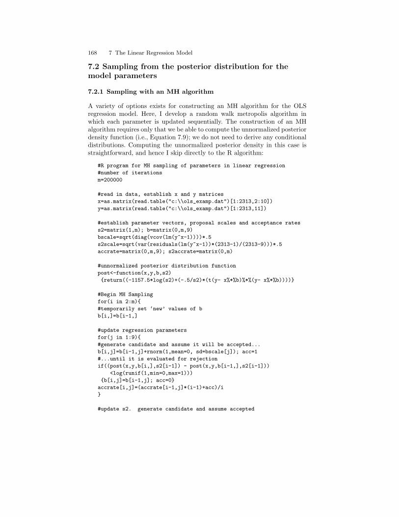
168 7 The Linear Regression Model
7.2 Sampling from the posterior distribution for themodel parameters
7.2.1 Sampling with an MH algorithm
A variety of options exists for constructing an MH algorithm for the OLSregression model. Here, I develop a random walk metropolis algorithm inwhich each parameter is updated sequentially. The construction of an MHalgorithm requires only that we be able to compute the unnormalized posteriordensity function (i.e., Equation 7.9); we do not need to derive any conditionaldistributions. Computing the unnormalized posterior density in this case isstraightforward, and hence I skip directly to the R algorithm:
#R program for MH sampling of parameters in linear regression
#number of iterations
m=200000
#read in data, establish x and y matrices
x=as.matrix(read.table("c:\\ols_examp.dat")[1:2313,2:10])
y=as.matrix(read.table("c:\\ols_examp.dat")[1:2313,11])
#establish parameter vectors, proposal scales and acceptance rates
s2=matrix(1,m); b=matrix(0,m,9)
bscale=sqrt(diag(vcov(lm(y~x-1))))*.5
s2scale=sqrt(var(residuals(lm(y~x-1))*(2313-1)/(2313-9)))*.5
accrate=matrix(0,m,9); s2accrate=matrix(0,m)
#unnormalized posterior distribution function
post<-function(x,y,b,s2)
return((-1157.5*log(s2)+(-.5/s2)*(t(y- x%*%b)%*%(y- x%*%b))))
#Begin MH Sampling
for(i in 2:m)
#temporarily set ‘new’ values of b
b[i,]=b[i-1,]
#update regression parameters
for(j in 1:9)
#generate candidate and assume it will be accepted...
b[i,j]=b[i-1,j]+rnorm(1,mean=0, sd=bscale[j]); acc=1
#...until it is evaluated for rejection
if((post(x,y,b[i,],s2[i-1]) - post(x,y,b[i-1,],s2[i-1]))
<log(runif(1,min=0,max=1)))
b[i,j]=b[i-1,j]; acc=0
accrate[i,j]=(accrate[i-1,j]*(i-1)+acc)/i
#update s2. generate candidate and assume accepted
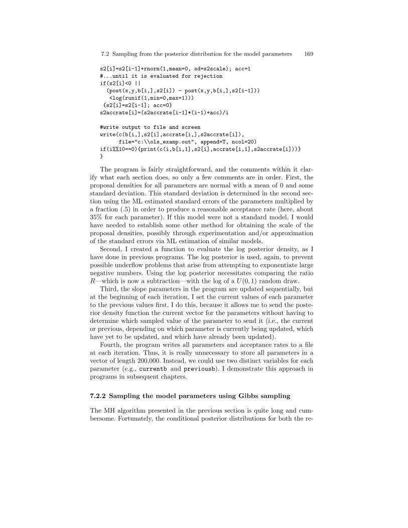
7.2 Sampling from the posterior distribution for the model parameters 169
s2[i]=s2[i-1]+rnorm(1,mean=0, sd=s2scale); acc=1
#...until it is evaluated for rejection
if(s2[i]<0 ||
(post(x,y,b[i,],s2[i]) - post(x,y,b[i,],s2[i-1]))
<log(runif(1,min=0,max=1)))
s2[i]=s2[i-1]; acc=0
s2accrate[i]=(s2accrate[i-1]*(i-1)+acc)/i
#write output to file and screen
write(c(b[i,],s2[i],accrate[i,],s2accrate[i]),
file="c:\\ols_examp.out", append=T, ncol=20)
if(i%%10==0)print(c(i,b[i,1],s2[i],accrate[i,1],s2accrate[i]))
The program is fairly straightforward, and the comments within it clar-ify what each section does, so only a few comments are in order. First, theproposal densities for all parameters are normal with a mean of 0 and somestandard deviation. This standard deviation is determined in the second sec-tion using the ML estimated standard errors of the parameters multiplied bya fraction (.5) in order to produce a reasonable acceptance rate (here, about35% for each parameter). If this model were not a standard model, I wouldhave needed to establish some other method for obtaining the scale of theproposal densities, possibly through experimentation and/or approximationof the standard errors via ML estimation of similar models.
Second, I created a function to evaluate the log posterior density, as Ihave done in previous programs. The log posterior is used, again, to preventpossible underflow problems that arise from attempting to exponentiate largenegative numbers. Using the log posterior necessitates comparing the ratioR—which is now a subtraction—with the log of a U(0, 1) random draw.
Third, the slope parameters in the program are updated sequentially, butat the beginning of each iteration, I set the current values of each parameterto the previous values first. I do this, because it allows me to send the poste-rior density function the current vector for the parameters without having todetermine which sampled value of the parameter to send it (i.e., the currentor previous, depending on which parameter is currently being updated, whichhave yet to be updated, and which have already been updated).
Fourth, the program writes all parameters and acceptance rates to a fileat each iteration. Thus, it is really unnecessary to store all parameters in avector of length 200,000. Instead, we could use two distinct variables for eachparameter (e.g., currentb and previousb). I demonstrate this approach inprograms in subsequent chapters.
7.2.2 Sampling the model parameters using Gibbs sampling
The MH algorithm presented in the previous section is quite long and cum-bersome. Fortunately, the conditional posterior distributions for both the re-
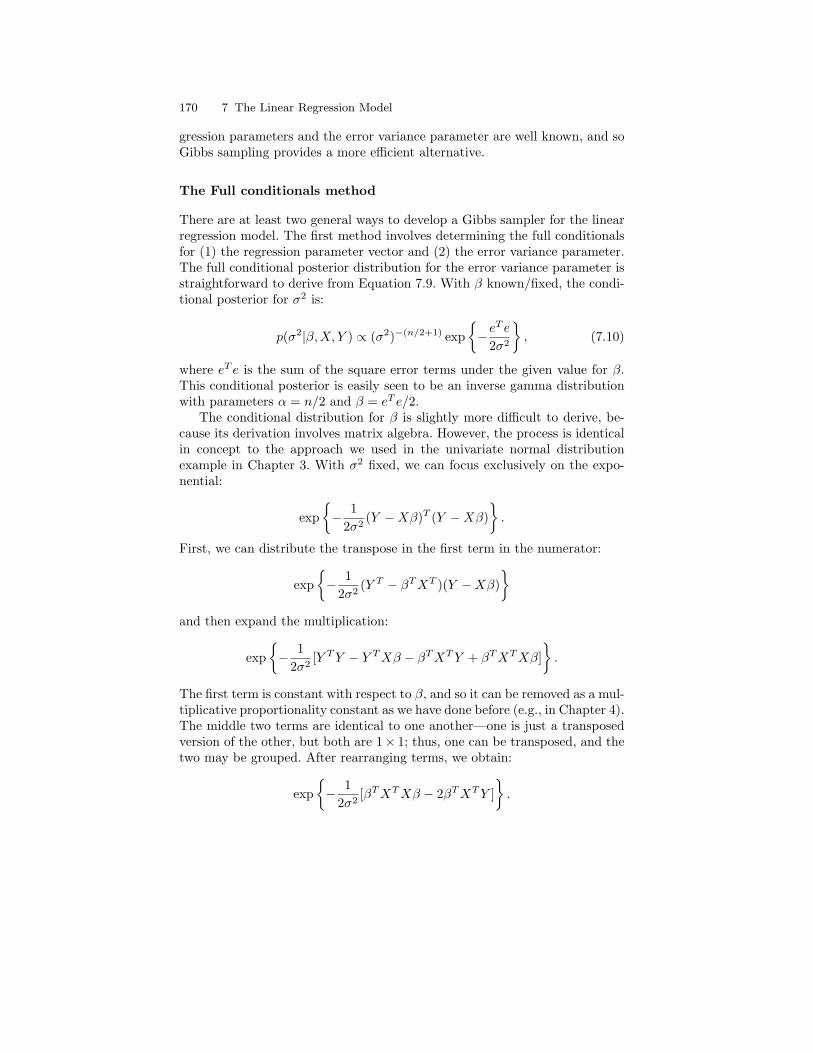
170 7 The Linear Regression Model
gression parameters and the error variance parameter are well known, and soGibbs sampling provides a more efficient alternative.
The Full conditionals method
There are at least two general ways to develop a Gibbs sampler for the linearregression model. The first method involves determining the full conditionalsfor (1) the regression parameter vector and (2) the error variance parameter.The full conditional posterior distribution for the error variance parameter isstraightforward to derive from Equation 7.9. With β known/fixed, the condi-tional posterior for σ2 is:
p(σ2|β, X, Y ) ∝ (σ2)−(n/2+1) exp−eT e
2σ2
, (7.10)
where eT e is the sum of the square error terms under the given value for β.This conditional posterior is easily seen to be an inverse gamma distributionwith parameters α = n/2 and β = eT e/2.
The conditional distribution for β is slightly more difficult to derive, be-cause its derivation involves matrix algebra. However, the process is identicalin concept to the approach we used in the univariate normal distributionexample in Chapter 3. With σ2 fixed, we can focus exclusively on the expo-nential:
exp− 1
2σ2(Y −Xβ)T (Y −Xβ)
.
First, we can distribute the transpose in the first term in the numerator:
exp− 1
2σ2(Y T − βT XT )(Y −Xβ)
and then expand the multiplication:
exp− 1
2σ2[Y T Y − Y T Xβ − βT XT Y + βT XT Xβ]
.
The first term is constant with respect to β, and so it can be removed as a mul-tiplicative proportionality constant as we have done before (e.g., in Chapter 4).The middle two terms are identical to one another—one is just a transposedversion of the other, but both are 1× 1; thus, one can be transposed, and thetwo may be grouped. After rearranging terms, we obtain:
exp− 1
2σ2[βT XT Xβ − 2βT XT Y ]
.

7.2 Sampling from the posterior distribution for the model parameters 171
If we now multiply the numerator and denominator through by (XT X)−1
appropriately,2 we get:
exp− 1
2σ2(XT X)−1[βT β − 2βT (XT X)−1(XT Y )]
.
At this point, we can complete the square in β, or we can simply recognizethat doing so will yield a distribution for β that is normal with a mean equalto (XT X)−1(XT Y ) and a variance of σ2
e(XT X)−1.With the conditionals derived, we can implement Gibbs sampling from
the full conditionals by (1) establishing starting values for the parameters, (2)sampling β from its multivariate normal distribution with σ2
e fixed, and (3)sampling σ2
e from its inverse gamma distribution with β (and hence e) fixed.The following is an R program that implements this process:
#R program for Gibbs sampling from full conditionals in OLS example
#number of iterations
m=5000
#read only observations with complete information, n=2313
x=as.matrix(read.table("c:\\ols_examp.dat")[1:2313,2:10])
y=as.matrix(read.table("c:\\ols_examp.dat")[1:2313,11])
#establish parameter vectors and constant quantities
s2=matrix(1,m); b=matrix(0,m,9)
xtxi=solve(t(x)%*%x)
pars=coefficients(lm(y~x-1))
#Gibbs sampling begins
for(i in 2:m)
#simulate beta from its multivariate normal conditional
b[i,]=pars+t(rnorm(9,mean=0,sd=1))%*%chol(s2[i-1]*xtxi)
#simulate sigma from its inverse gamma distribution
s2[i]=1/rgamma(1,2313/2,.5*t(y-x%*%(b[i,]))%*%(y-x%*%(b[i,])))
#write output to file and screen
write(c(b[i,],s2[i]),file="c:\\ols_examp.out", append=T, ncol=10)
if(i%%50==0)print(c(i,b[i,1],s2[i]))
This program is remarkably shorter than the MH algorithm and requiresvery little explanation. Before the Gibbs sampling begins, I compute the
2 Technically, we cannot “divide” by (XT X)−1. Instead, we can multiply the nu-merator through by (XT X)(XT X)−1 and just distribute the inverse term. Then,the inverse variance of the distribution for β is (XT X)/σ2
e . Inverting this quantitygives us the variance.
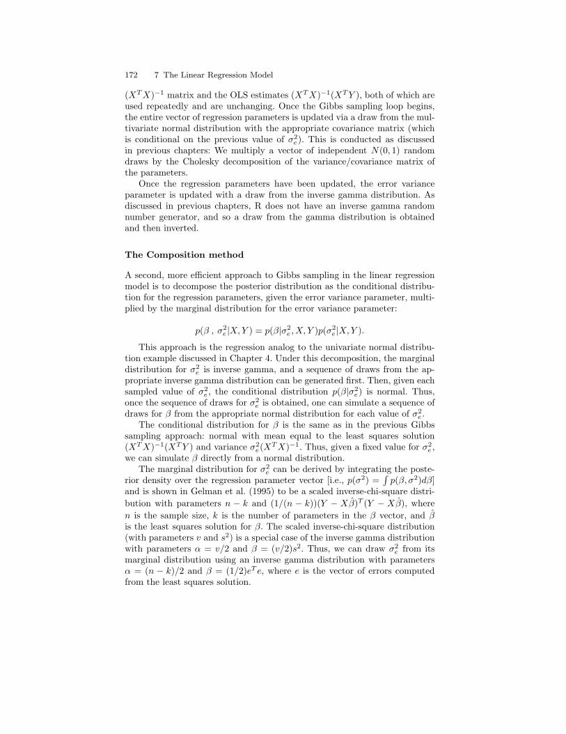
172 7 The Linear Regression Model
(XT X)−1 matrix and the OLS estimates (XT X)−1(XT Y ), both of which areused repeatedly and are unchanging. Once the Gibbs sampling loop begins,the entire vector of regression parameters is updated via a draw from the mul-tivariate normal distribution with the appropriate covariance matrix (whichis conditional on the previous value of σ2
e). This is conducted as discussedin previous chapters: We multiply a vector of independent N(0, 1) randomdraws by the Cholesky decomposition of the variance/covariance matrix ofthe parameters.
Once the regression parameters have been updated, the error varianceparameter is updated with a draw from the inverse gamma distribution. Asdiscussed in previous chapters, R does not have an inverse gamma randomnumber generator, and so a draw from the gamma distribution is obtainedand then inverted.
The Composition method
A second, more efficient approach to Gibbs sampling in the linear regressionmodel is to decompose the posterior distribution as the conditional distribu-tion for the regression parameters, given the error variance parameter, multi-plied by the marginal distribution for the error variance parameter:
p(β , σ2e |X, Y ) = p(β|σ2
e , X, Y )p(σ2e |X, Y ).
This approach is the regression analog to the univariate normal distribu-tion example discussed in Chapter 4. Under this decomposition, the marginaldistribution for σ2
e is inverse gamma, and a sequence of draws from the ap-propriate inverse gamma distribution can be generated first. Then, given eachsampled value of σ2
e , the conditional distribution p(β|σ2e) is normal. Thus,
once the sequence of draws for σ2e is obtained, one can simulate a sequence of
draws for β from the appropriate normal distribution for each value of σ2e .
The conditional distribution for β is the same as in the previous Gibbssampling approach: normal with mean equal to the least squares solution(XT X)−1(XT Y ) and variance σ2
e(XT X)−1. Thus, given a fixed value for σ2e ,
we can simulate β directly from a normal distribution.The marginal distribution for σ2
e can be derived by integrating the poste-rior density over the regression parameter vector [i.e., p(σ2) =
∫p(β, σ2)dβ]
and is shown in Gelman et al. (1995) to be a scaled inverse-chi-square distri-bution with parameters n − k and (1/(n − k))(Y − Xβ)T (Y − Xβ), wheren is the sample size, k is the number of parameters in the β vector, and βis the least squares solution for β. The scaled inverse-chi-square distribution(with parameters v and s2) is a special case of the inverse gamma distributionwith parameters α = v/2 and β = (v/2)s2. Thus, we can draw σ2
e from itsmarginal distribution using an inverse gamma distribution with parametersα = (n − k)/2 and β = (1/2)eT e, where e is the vector of errors computedfrom the least squares solution.
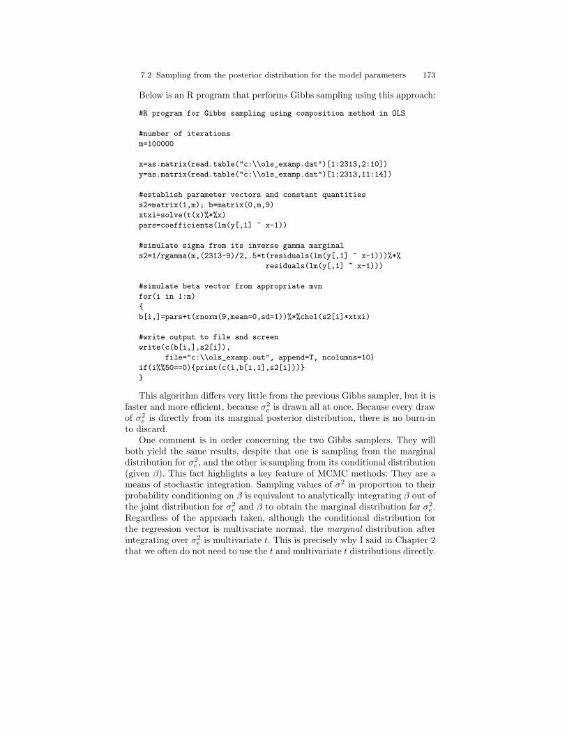
7.2 Sampling from the posterior distribution for the model parameters 173
Below is an R program that performs Gibbs sampling using this approach:
#R program for Gibbs sampling using composition method in OLS
#number of iterations
m=100000
x=as.matrix(read.table("c:\\ols_examp.dat")[1:2313,2:10])
y=as.matrix(read.table("c:\\ols_examp.dat")[1:2313,11:14])
#establish parameter vectors and constant quantities
s2=matrix(1,m); b=matrix(0,m,9)
xtxi=solve(t(x)%*%x)
pars=coefficients(lm(y[,1] ~ x-1))
#simulate sigma from its inverse gamma marginal
s2=1/rgamma(m,(2313-9)/2,.5*t(residuals(lm(y[,1] ~ x-1)))%*%
residuals(lm(y[,1] ~ x-1)))
#simulate beta vector from appropriate mvn
for(i in 1:m)
b[i,]=pars+t(rnorm(9,mean=0,sd=1))%*%chol(s2[i]*xtxi)
#write output to file and screen
write(c(b[i,],s2[i]),
file="c:\\ols_examp.out", append=T, ncolumns=10)
if(i%%50==0)print(c(i,b[i,1],s2[i]))
This algorithm differs very little from the previous Gibbs sampler, but it isfaster and more efficient, because σ2
e is drawn all at once. Because every drawof σ2
e is directly from its marginal posterior distribution, there is no burn-into discard.
One comment is in order concerning the two Gibbs samplers. They willboth yield the same results, despite that one is sampling from the marginaldistribution for σ2
e , and the other is sampling from its conditional distribution(given β). This fact highlights a key feature of MCMC methods: They are ameans of stochastic integration. Sampling values of σ2 in proportion to theirprobability conditioning on β is equivalent to analytically integrating β out ofthe joint distribution for σ2
e and β to obtain the marginal distribution for σ2e .
Regardless of the approach taken, although the conditional distribution forthe regression vector is multivariate normal, the marginal distribution afterintegrating over σ2
e is multivariate t. This is precisely why I said in Chapter 2that we often do not need to use the t and multivariate t distributions directly.
174 7 The Linear Regression Model
7.3 Example: Are people in the South “nicer” thanothers?
Conventional wisdom holds that Southern (US) culture is very different fromNortheastern, Western, and even Midwestern culture. This is perhaps onereason why so many regression models in social science, when they includeregion as a control variable, include only an indicator variable for “South.”Three important ways that the South is considered different from other regionsin the US are (1) the pace of life is assumed to be slower than especially thatof the Northeast and West, (2) people are assumed to be friendlier and morecompassionate than persons from other regions, and (3) people are assumedto be poorer, less sophisticated, and perhaps even less intelligent than peoplefrom other regions.3
In 2002 and 2004, the General Social Survey (GSS) conducted a specialtopics module on “altruism,” which allows us to examine item 2, the assump-tion that people in the South are more compassionate. For this example, Iexamine four outcome variables: (1) a summed scale of seven items that as-sesses individuals’ feelings of empathy, (2) a single item measuring toleranceof others, (3) a summed scale of four items assessing selfless attitude, and (4)a summed scale of actual altruistic behavior.
I use age, sex, race, education, and family income as control variables.I measure region using a series of three dummy variables constructed fromthe region the respondent lived in at age 16 and the region the respondentcurrently lives in: continuous resident of the South, South in-migrant, Southout-migrant.4 I choose this measure, because, although the culture of theSouth may be indigenous to that region, individuals internalize culture overtime. Thus, individuals who move into a region do not immediately adopt thecultural practices of the region, and individuals who move out of a region donot immediately shed their previous cultural identity.
The original sample size for the two years in which this topic module wasused was n = 2, 712. Sixteen persons (.6%) were missing on either age or edu-cation; they were deleted. An additional 257 persons (9.5%) were missing onincome only, and an additional 127 persons (4.7%) were missing on an out-
3 These assumptions probably stem largely from the agricultural history of theSouth, where/when time was measured by daylight, rather than by a clock,most workers were physical (agricultural) laborers lacking in formal educationbeyond elementary school, and the closed nature of rural communities produced“gemeinschaft-like” relations that made empathy and compassion more viablethan in urban communities in which individuals were less similar to one another(i.e., where “gesellschaft-like” relations predominated) and thus less able to em-pathize with the plight of others. My goal here is not to develop a sociologicaltheory of South/non-South differences. See Durkheim (1984) for the foundationof such sociological theory.
4 Of course, this measure is not perfect. Individuals may have moved many times;this measure only captures residence at two points in time.
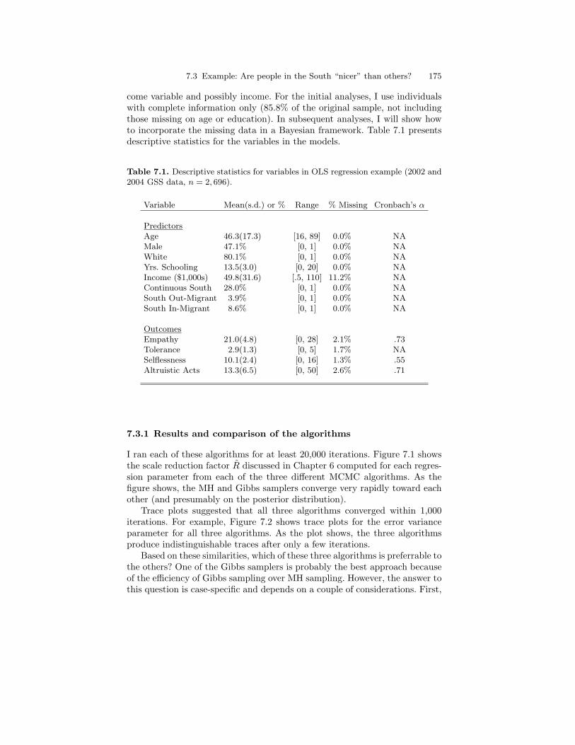
7.3 Example: Are people in the South “nicer” than others? 175
come variable and possibly income. For the initial analyses, I use individualswith complete information only (85.8% of the original sample, not includingthose missing on age or education). In subsequent analyses, I will show howto incorporate the missing data in a Bayesian framework. Table 7.1 presentsdescriptive statistics for the variables in the models.
Table 7.1. Descriptive statistics for variables in OLS regression example (2002 and2004 GSS data, n = 2, 696).
Variable Mean(s.d.) or % Range % Missing Cronbach’s α
PredictorsAge 46.3(17.3) [16, 89] 0.0% NAMale 47.1% [0, 1] 0.0% NAWhite 80.1% [0, 1] 0.0% NAYrs. Schooling 13.5(3.0) [0, 20] 0.0% NAIncome ($1,000s) 49.8(31.6) [.5, 110] 11.2% NAContinuous South 28.0% [0, 1] 0.0% NASouth Out-Migrant 3.9% [0, 1] 0.0% NASouth In-Migrant 8.6% [0, 1] 0.0% NA
OutcomesEmpathy 21.0(4.8) [0, 28] 2.1% .73Tolerance 2.9(1.3) [0, 5] 1.7% NASelflessness 10.1(2.4) [0, 16] 1.3% .55Altruistic Acts 13.3(6.5) [0, 50] 2.6% .71
7.3.1 Results and comparison of the algorithms
I ran each of these algorithms for at least 20,000 iterations. Figure 7.1 showsthe scale reduction factor R discussed in Chapter 6 computed for each regres-sion parameter from each of the three different MCMC algorithms. As thefigure shows, the MH and Gibbs samplers converge very rapidly toward eachother (and presumably on the posterior distribution).
Trace plots suggested that all three algorithms converged within 1,000iterations. For example, Figure 7.2 shows trace plots for the error varianceparameter for all three algorithms. As the plot shows, the three algorithmsproduce indistinguishable traces after only a few iterations.
Based on these similarities, which of these three algorithms is preferrable tothe others? One of the Gibbs samplers is probably the best approach becauseof the efficiency of Gibbs sampling over MH sampling. However, the answer tothis question is case-specific and depends on a couple of considerations. First,
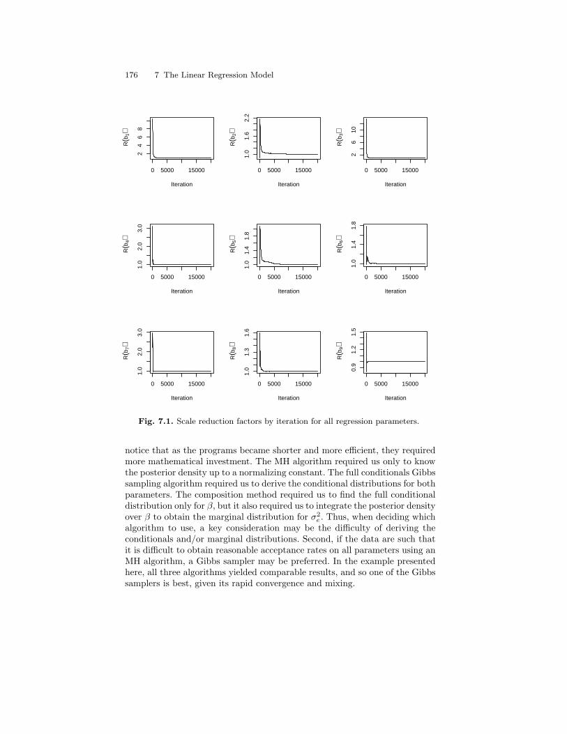
176 7 The Linear Regression Model
0 5000 15000
24
68
Iteration
R(b
1)
0 5000 15000
1.0
1.6
2.2
Iteration
R(b
2)
0 5000 15000
26
10
Iteration
R(b
3)
0 5000 15000
1.0
2.0
3.0
Iteration
R(b
4)
0 5000 15000
1.0
1.4
1.8
Iteration
R(b
5)
0 5000 15000
1.0
1.4
1.8
Iteration
R(b
6)
0 5000 15000
1.0
2.0
3.0
Iteration
R(b
7)
0 5000 15000
1.0
1.3
1.6
Iteration
R(b
8)
0 5000 15000
0.9
1.2
1.5
Iteration
R(b
9)
Fig. 7.1. Scale reduction factors by iteration for all regression parameters.
notice that as the programs became shorter and more efficient, they requiredmore mathematical investment. The MH algorithm required us only to knowthe posterior density up to a normalizing constant. The full conditionals Gibbssampling algorithm required us to derive the conditional distributions for bothparameters. The composition method required us to find the full conditionaldistribution only for β, but it also required us to integrate the posterior densityover β to obtain the marginal distribution for σ2
e . Thus, when deciding whichalgorithm to use, a key consideration may be the difficulty of deriving theconditionals and/or marginal distributions. Second, if the data are such thatit is difficult to obtain reasonable acceptance rates on all parameters using anMH algorithm, a Gibbs sampler may be preferred. In the example presentedhere, all three algorithms yielded comparable results, and so one of the Gibbssamplers is best, given its rapid convergence and mixing.
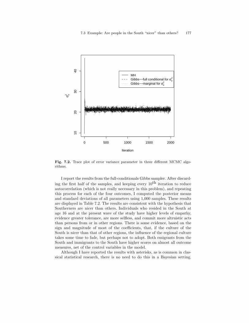
7.3 Example: Are people in the South “nicer” than others? 177
0 500 1000 1500 2000
1020
3040
Iteration
σ e2
MHGibbs−−full conditional for σe
2
Gibbs−−marginal for σe2
Fig. 7.2. Trace plot of error variance parameter in three different MCMC algo-rithms.
I report the results from the full-conditionals Gibbs sampler. After discard-ing the first half of the samples, and keeping every 10th iteration to reduceautocorrelation (which is not really necessary in this problem), and repeatingthis process for each of the four outcomes, I computed the posterior meansand standard deviations of all parameters using 1,000 samples. These resultsare displayed in Table 7.2. The results are consistent with the hypothesis thatSoutherners are nicer than others. Individuals who resided in the South atage 16 and at the present wave of the study have higher levels of empathy,evidence greater tolerance, are more selfless, and commit more altruistic actsthan persons from or in other regions. There is some evidence, based on thesign and magnitude of most of the coefficients, that, if the culture of theSouth is nicer than that of other regions, the influence of the regional culturetakes some time to fade, but perhaps not to adopt. Both emigrants from theSouth and immigrants to the South have higher scores on almost all outcomemeasures, net of the control variables in the model.
Although I have reported the results with asterisks, as is common in clas-sical statistical research, there is no need to do this in a Bayesian setting.

178 7 The Linear Regression Model
Instead, we could directly discuss the probabilities that say, immigrants tothe South are nicer than persons who have never lived in the South. For ex-ample, the probability that immigrants have greater empathy than personswho have never lived in the South is .821. This probability was obtainedsimply by computing the proportion of sampled regression parameter valuesthat exceed 0. Thus, although this parameter was not considered “significant”from a classical standpoint, the Bayesian approach suggests that immigrantsare quite likely to be nicer (by this measure) than persons who have neverlived in the South.
The bottom of the table reports interval estimates for the model R2. Giventhat we have complete distributions for the regression parameters and errorvariance parameter, and not simply point estimates, we can compute the R2
implied by each sample of the parameters, thereby obtaining a sample fromthe posterior distribution for the model R2. Once this sample is sorted, wecan then select the 2.5th and 97.5th percentile values as the end points for a95% interval estimate.
Table 7.2. Results of linear regression of measures of “niceness” on three measuresof region.
Outcome
Variable Empathy Tolerance Selflessness Altruistic Acts
Intercept 19.62(.57)*** 3.16(.15)*** 8.71(.30)*** 9.17(.76)***Age 0.018(.006)** −0.008(.002)*** 0.01(.003)*** −0.03(.01)***Male −2.42(.19)*** −0.35(.05)*** −0.87(.10)*** 0.32(.26)White 0.55(.26)* 0.09(.07)# 0.17(.13)# 0.01(.33)Yrs. Schooling 0.06(.04)* 0.004(.01) 0.07(.02)*** 0.32(.05)***Income ($1,000s) 0.003(.003) 0.0006(.0009) 0.001(.002) 0.02(.005)***Continuous South 0.65(.21)** 0.22(.06)*** 0.25(.11)* 0.41(.30)#South Out-Migrant 0.39(.50) 0.11(.14) −0.33(.25)# 0.01(.70)South In-Migrant 0.34(.35) 0.24(.10)** 0.17(.17) −0.01(.45)p
σ2e 4.61 1.22 2.31 6.23
R2 .07[.066,.072] .03[.029,.036] .05[.047,.054] .055[.051,.057]
Note: The Bayesian estimates are posterior means. The Bayesian p-values are basedon one-sided tail probabilities that the parameter exceeds 0 truncated to the classicalcut-points of #p < .1, *p < .05, **p < .01, ***p < .001. The R2 reported are basedon the posterior mean estimates for the parameters; a 95% interval estimate is alsoreported.
7.3.2 Model evaluation
Although I modeled the tolerance outcome variable as if it were a continuousmeasure, in fact it is a single ordinal item with five categories. Thus, we shouldevaluate the fit of the model and verify that it fits the data. The R2 presentedin the table is quite low (3%), which suggests poor fit, but R2 reveals only one
7.3 Example: Are people in the South “nicer” than others? 179
aspect of how well the model fits the data in this problem. Some remainingquestions include: (1) How well does the model fit various aspects of thedata? and (2) Are there particularly poorly fitted cases that contribute tothe model’s poor fit? As discussed in earlier chapters, a Bayesian approachallows us many more options to address these questions than the classicalapproach, and it allows us to take into account both sampling and parametricuncertainty in doing so.
In order to begin to address these questions, I used posterior predictivesimulation. For each person in the sample, I generated 1,000 posterior predic-tive cases with the same covariate structure, using every sampled value of βand σ2
e . This approach requires two steps:
1. Compute yji = xT
i βj , ∀ individuals, i, and all sampled values of the re-gression coefficients βj .
2. Simulate a predictive score yji = yj
i + N(0, σ2(j)e ), for each case.
If you visualize the original data set, with 2,313 rows representing theoriginal sample members with complete data and 10 columns representing the9 predictors plus the outcome variable, these predictive cases can be viewed asexpanding the column space of the data array by an additional 1,000 columns.For any row, i, each new column (j) represents a future observation withoutcome yj as a function of the jth sampled value of β and σ2
e , and thecovariate profile of the ith person. Thus, each new complete column can beconsidered a replicated sample, whereas the new 1,000 elements of each rowcan be considered replications of individual i under different parameter values.This means we can examine how well a model fits various features of theoriginal sample (like the ratio of the mean of y to its median) by examiningthe column-wise collection of these values in repeated samples. Plus, we canexamine how well a model fits particular cases by examining the row-wisedistributions for each observation in the sample.
For this particular example, I considered three posterior predictive dis-tribution features of the first type—sample level features. First, I examinedthe extent to which the distribution of replicated values of y matched thedistribution of the original y. The top plot in Figure 7.3 shows this result.In general, the distribution of replicated data appears to match that of theobserved data fairly well. Second, I computed the ratio of the mean of y toits median. The second plot in the figure shows that the distribution of theratio of the mean to the median in the replicated samples is centered over 1(as it should be, given that the error distribution is assumed normal), whilethe observed ratio was .95. As the plot shows, the Bayesian p-value associatedwith a test of this statistic (the mean/median ratio) would be 0 (or 1), whichindicates very poor fit of the model to the data. Third I computed the range ofy from each posterior predictive sample. The third plot in the figure reinforcesthat the model has poor fit. This plot shows the distribution of the range ofvalues in the replicated data with a vertical reference line for the range in the
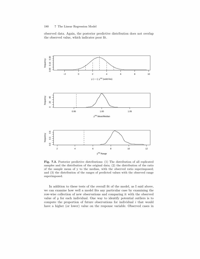
180 7 The Linear Regression Model
observed data. Again, the posterior predictive distribution does not overlapthe observed value, which indicates poor fit.
−2 0 2 4 6 8 10
0.00
0.15
0.30
y (−−−); yrep (solid line)
freq
uenc
y
0.95 1.00 1.05
020
40
yrep Mean/Median
freq
uenc
y
2 4 6 8 10 12
0.0
0.3
0.6
yrep Range
freq
uenc
y
Fig. 7.3. Posterior predictive distributions: (1) The distribution of all replicatedsamples and the distribution of the original data; (2) the distribution of the ratioof the sample mean of y to the median, with the observed ratio superimposed;and (3) the distribution of the ranges of predicted values with the observed rangesuperimposed.
In addition to these tests of the overall fit of the model, as I said above,we can examine how well a model fits any particular case by examining therow-wise collection of new observations and comparing it with the observedvalue of y for each individual. One way to identify potential outliers is tocompute the proportion of future observations for individual i that wouldhave a higher (or lower) value on the response variable. Observed cases in
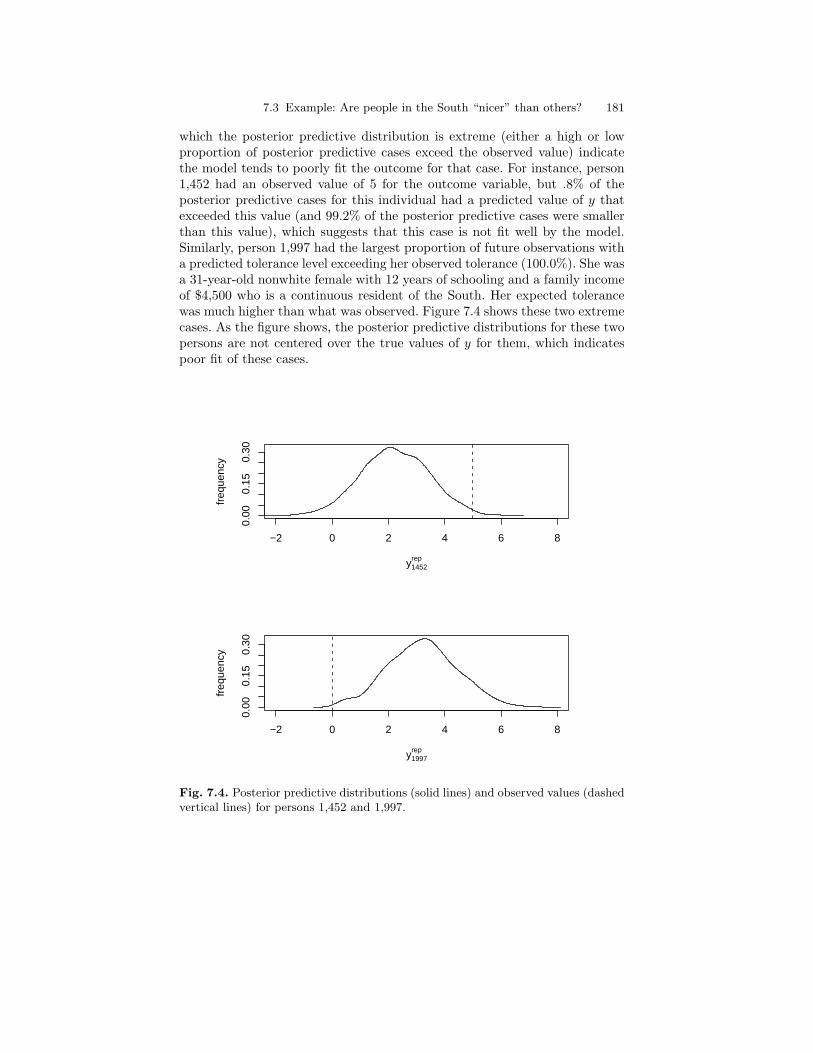
7.3 Example: Are people in the South “nicer” than others? 181
which the posterior predictive distribution is extreme (either a high or lowproportion of posterior predictive cases exceed the observed value) indicatethe model tends to poorly fit the outcome for that case. For instance, person1,452 had an observed value of 5 for the outcome variable, but .8% of theposterior predictive cases for this individual had a predicted value of y thatexceeded this value (and 99.2% of the posterior predictive cases were smallerthan this value), which suggests that this case is not fit well by the model.Similarly, person 1,997 had the largest proportion of future observations witha predicted tolerance level exceeding her observed tolerance (100.0%). She wasa 31-year-old nonwhite female with 12 years of schooling and a family incomeof $4,500 who is a continuous resident of the South. Her expected tolerancewas much higher than what was observed. Figure 7.4 shows these two extremecases. As the figure shows, the posterior predictive distributions for these twopersons are not centered over the true values of y for them, which indicatespoor fit of these cases.
−2 0 2 4 6 8
0.00
0.15
0.30
y1452rep
freq
uenc
y
−2 0 2 4 6 8
0.00
0.15
0.30
y1997rep
freq
uenc
y
Fig. 7.4. Posterior predictive distributions (solid lines) and observed values (dashedvertical lines) for persons 1,452 and 1,997.

182 7 The Linear Regression Model
To determine whether such persons are outliers or whether the modelsimply is not fitting particular covariates well, we can examine collectionsof possible outliers and determine whether they share similar characteristics.For example, in these data, although there is only one person (1,452) whosetolerance is substantially underpredicted, there are 31 observations for whomthe proportion of replicated outcomes exceeding the observed outcome is atleast 99%. If these individuals are substantially similar to one another onone or more covariates, then the implication would be that the model doesnot fit those covariates well. Figure 7.5 shows the sample distribution of age,education, and income with the distribution of these variables for the 31 po-tential outlying cases superimposed. The figure shows quite clearly that theseindividuals do not appear to differ from the overall sample on these threecharacteristics. Thus, it is reasonable to conclude that these cases are prob-ably simply outliers, at least in the context of the current model. We shouldprobably consider including additional covariates that may help explain theirlow tolerance levels.
All in all, the posterior predictive checks suggest that the OLS regressionmodel does not fit the tolerance item well, and so perhaps an alternative modelshould be considered for this item. Specifically, we may consider treating thisoutcome as an ordinal measure and model it using a generalized linear modelas discussed in the next chapter. If we were to estimate a new model, wecould apply similar tests and decide which model fits better either formallyor informally. For example, formally, we could begin with a test of the pro-portion of values of R2 for the new model exceeded the maximum value ofR2 for the first model. This proportion would be a measure of the probabilitythat the new model fit the data better than the original model and wouldtherefore serve as a basis for deciding which model to prefer. Note that thistype of comparison does not require that the models be nested, because, froma Bayesian perspective, any two probability distributions can be compared ifit makes sense to compare them.
7.4 Incorporating missing data
In the previous sections I discussed the results of models in which the caseswith missing data were simply listwise deleted, leaving us with 85.8% of theoriginal sample (14.2% missing). Conventional wisdom in the social sciencesclaims that this amount of missing data is unacceptable, and so some alterna-tive to listwise deletion of observations with missing data should be considered.The Bayesian paradigm using MCMC simulation offers some relatively simple,yet appropriate methods for handling missing data.
7.4.1 Types of missingness
Before determining how to handle missing data, we should decide whetherthe missing data mechanism—that is, the process that generated the missing
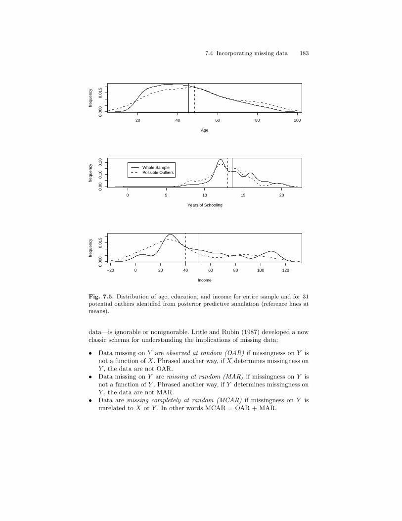
7.4 Incorporating missing data 183
20 40 60 80 100
0.00
00.
015
Age
freq
uenc
y
0 5 10 15 20
0.00
0.10
0.20
Years of Schooling
freq
uenc
y
Whole SamplePossible Outliers
−20 0 20 40 60 80 100 120
0.00
00.
015
Income
freq
uenc
y
Fig. 7.5. Distribution of age, education, and income for entire sample and for 31potential outliers identified from posterior predictive simulation (reference lines atmeans).
data—is ignorable or nonignorable. Little and Rubin (1987) developed a nowclassic schema for understanding the implications of missing data:
• Data missing on Y are observed at random (OAR) if missingness on Y isnot a function of X. Phrased another way, if X determines missingness onY , the data are not OAR.
• Data missing on Y are missing at random (MAR) if missingness on Y isnot a function of Y . Phrased another way, if Y determines missingness onY , the data are not MAR.
• Data are missing completely at random (MCAR) if missingness on Y isunrelated to X or Y . In other words MCAR = OAR + MAR.
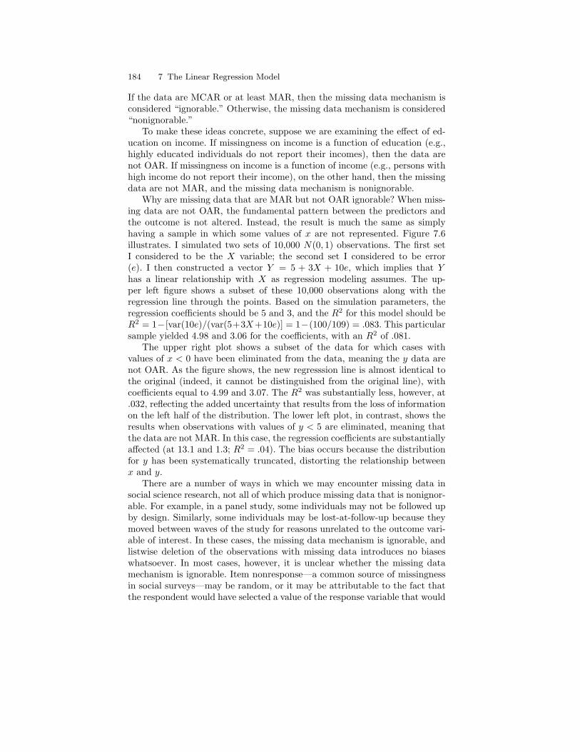
184 7 The Linear Regression Model
If the data are MCAR or at least MAR, then the missing data mechanism isconsidered “ignorable.” Otherwise, the missing data mechanism is considered“nonignorable.”
To make these ideas concrete, suppose we are examining the effect of ed-ucation on income. If missingness on income is a function of education (e.g.,highly educated individuals do not report their incomes), then the data arenot OAR. If missingness on income is a function of income (e.g., persons withhigh income do not report their income), on the other hand, then the missingdata are not MAR, and the missing data mechanism is nonignorable.
Why are missing data that are MAR but not OAR ignorable? When miss-ing data are not OAR, the fundamental pattern between the predictors andthe outcome is not altered. Instead, the result is much the same as simplyhaving a sample in which some values of x are not represented. Figure 7.6illustrates. I simulated two sets of 10,000 N(0, 1) observations. The first setI considered to be the X variable; the second set I considered to be error(e). I then constructed a vector Y = 5 + 3X + 10e, which implies that Yhas a linear relationship with X as regression modeling assumes. The up-per left figure shows a subset of these 10,000 observations along with theregression line through the points. Based on the simulation parameters, theregression coefficients should be 5 and 3, and the R2 for this model should beR2 = 1−[var(10e)/(var(5+3X+10e)] = 1−(100/109) = .083. This particularsample yielded 4.98 and 3.06 for the coefficients, with an R2 of .081.
The upper right plot shows a subset of the data for which cases withvalues of x < 0 have been eliminated from the data, meaning the y data arenot OAR. As the figure shows, the new regresssion line is almost identical tothe original (indeed, it cannot be distinguished from the original line), withcoefficients equal to 4.99 and 3.07. The R2 was substantially less, however, at.032, reflecting the added uncertainty that results from the loss of informationon the left half of the distribution. The lower left plot, in contrast, shows theresults when observations with values of y < 5 are eliminated, meaning thatthe data are not MAR. In this case, the regression coefficients are substantiallyaffected (at 13.1 and 1.3; R2 = .04). The bias occurs because the distributionfor y has been systematically truncated, distorting the relationship betweenx and y.
There are a number of ways in which we may encounter missing data insocial science research, not all of which produce missing data that is nonignor-able. For example, in a panel study, some individuals may not be followed upby design. Similarly, some individuals may be lost-at-follow-up because theymoved between waves of the study for reasons unrelated to the outcome vari-able of interest. In these cases, the missing data mechanism is ignorable, andlistwise deletion of the observations with missing data introduces no biaseswhatsoever. In most cases, however, it is unclear whether the missing datamechanism is ignorable. Item nonresponse—a common source of missingnessin social surveys—may be random, or it may be attributable to the fact thatthe respondent would have selected a value of the response variable that would
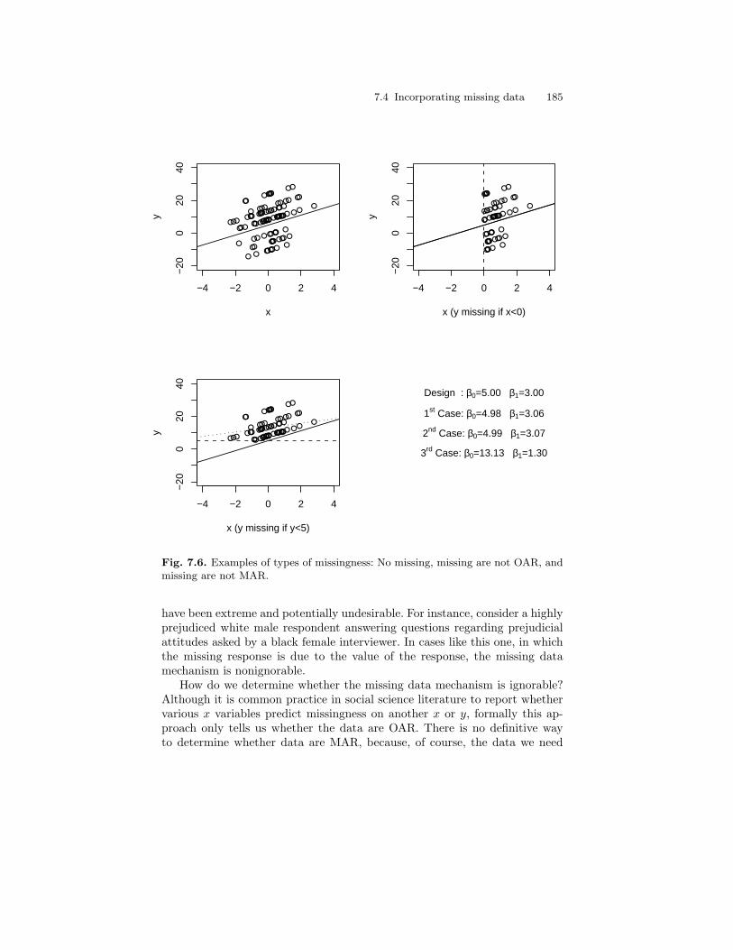
7.4 Incorporating missing data 185
−4 −2 0 2 4
−20
020
40
x
y
−4 −2 0 2 4
−20
020
40
x (y missing if x<0)
y
−4 −2 0 2 4
−20
020
40
x (y missing if y<5)
y
Design : β0=5.00 β1=3.00
1st Case: β0=4.98 β1=3.06
2nd Case: β0=4.99 β1=3.07
3rd Case: β0=13.13 β1=1.30
Fig. 7.6. Examples of types of missingness: No missing, missing are not OAR, andmissing are not MAR.
have been extreme and potentially undesirable. For instance, consider a highlyprejudiced white male respondent answering questions regarding prejudicialattitudes asked by a black female interviewer. In cases like this one, in whichthe missing response is due to the value of the response, the missing datamechanism is nonignorable.
How do we determine whether the missing data mechanism is ignorable?Although it is common practice in social science literature to report whethervarious x variables predict missingness on another x or y, formally this ap-proach only tells us whether the data are OAR. There is no definitive wayto determine whether data are MAR, because, of course, the data we need
186 7 The Linear Regression Model
to make this determination are missing. Thus, ultimately, we must rely onsome sort of prior, out-of-sample, knowledge to decide whether the missingdata mechanism is ignorable or nonignorable. For example, in the GSS data,there were 302 persons missing on income. Suppose income had been our out-come variable, and we estimated a probit model with education predictingmissingness on the income item. The result of that analysis (not presentedhere) showed that education was strongly related to missingness on income,such that more educated persons were less likely to be missing on income(conversely, less educated persons are more likely to be missing on income).This result simply tells us that income is not OAR. However, if we have prior(out-of-sample) information indicating that more educated individuals tendto have higher incomes, then we might infer that the missing data on incomeis not MAR: Lower income predicts missingness on income.
If we decide that the missing data mechanism is ignorable, then the onlycost of listwise deletion—that is, deletion of an entire case when one or morevariable is missing—is the reduction in sample size and the correspondinginefficiency in estimating standard errors (or posterior standard deviations)of parameters. Indeed, if we attempt to perform some sort of imputation inthis setting, we are more likely to produce biases or underestimate uncertaintyin the parameters (see Allison 2003).
If, on the other hand, the missing data mechanism is nonignorable, list-wise deletion will produce biased parameter estimates, but so will most formsof simple imputation or modeling strategies that fail to accurately capturethe process that generates the missing data. For example, so-called “full-information maximum likelihood” (FIML) estimation (sometimes also called“direct maximum likelihood estimation”), estimation based on the EM algo-rithm, multiple imputation methods, and other popular contemporary meth-ods do not resolve the nonignorability of the missing data mechanism. Instead,in their typical application, these approaches simply assume the missing datafollow the same distribution (or pattern) as the observed data. Therefore,these methods are ultimately of little use when the missing data are notMAR, despite their growth in popularity.
7.4.2 A generic Bayesian approach when data are MAR: The“niceness” example revisited
The Bayesian paradigm (coupled with MCMC methods) offers a simple ap-proach to handling missing data when the missing data mechanism is ignor-able, one that is generally easier to implement than (1) switching softwareor estimators when the package you are using does not have a missing datamethod (e.g., switching from one structural equation modeling package to an-other that can handle missing data) or (2) performing multistep proceduresto compute parameters and adjust standard errors for missing data models(e.g., using a secondary package to adjust standard errors when performingmultiple imputation).
7.4 Incorporating missing data 187
As an example demonstrating the ease with which the Gibbs sampler canhandle missing data, I return to the first outcome (empathy) in the previousexample. Recall that the original sample size was 2,696, but that a numberof persons were missing on either income or one of the outcome variables,leaving us with 2,313 persons with complete information. We will continue toignore persons missing on income for the moment, but suppose we wished toinclude persons missing on the empathy item. There were 34 such persons inthe sample. Focusing on this outcome only allows us to incorporate individualswho were missing on the other outcomes, and so our sample size is 2,394.
Let Y be the observed outcome data, and let Z be the missing outcomedata. In the OLS regression model without missing data, the posterior dis-tribution we sought included the regression parameter vector β and the errorvariance parameter σ2
e . However, when we have missing data, the missingdata can also be treated as unknown, and hence, the posterior distributionmay involve Z as well. Thus (suppressing dependence on X), our posteriorbecomes:
p(β, σ2e , Z|Y ) ∝ p(Y |β, σ2
e , Z)p(β, σ2e , Z).
The latter term in this posterior is a joint prior probability for the missingdata, the regression parameters, and the error variance, and it can be decom-posed as:
p(β, σ2e , Z) ∝ p(Z|β, σ2
e)p(β, σ2e).
Furthermore, just as the observed cases are assumed to be independent, wemay also assume that the observed and missing cases are independent, andso the first term in the posterior reduces to p(Y |β, σ2
e). The full posteriordistribution, then, is:
p(β, σ2e , Z|Y ) ∝ p(Y |β, σ2
e)p(Z|β, σ2e)p(β, σ2
e),
where the latter term is simply the joint prior for the regression parametersand error variance. Let’s assume the same reference prior as we did in theexample with complete data (1/σ2
e).A Gibbs sampler for sampling from this posterior distribution simply in-
volves sequentially sampling from the conditional posterior distributions forβ, σ2
e , and Z. The conditional posterior distribution for β|Z, σ2e , Y is straight-
forward, given values for Z. Indeed, assume we have values for Z, so thatY ∗ = [Y,Z] is a set of complete data. In that case:
(β| Y ∗, σ2e) ∼ N((XT X)−1(XT Y ∗), σ2
e(XT X)−1),
which is a result identical to that we obtained previously, only now we haveincorporated the missing data.
Similarly, given Y ∗, the conditional posterior for the error variance is:
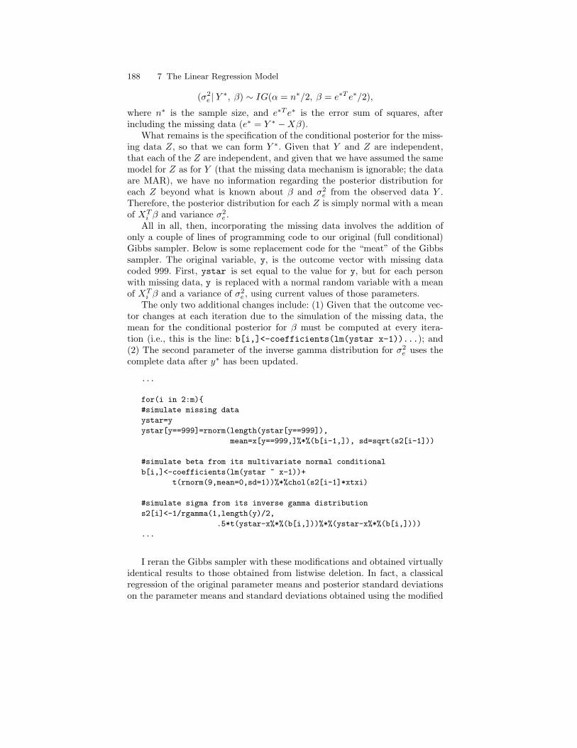
188 7 The Linear Regression Model
(σ2e | Y ∗, β) ∼ IG(α = n∗/2, β = e∗T e∗/2),
where n∗ is the sample size, and e∗T e∗ is the error sum of squares, afterincluding the missing data (e∗ = Y ∗ −Xβ).
What remains is the specification of the conditional posterior for the miss-ing data Z, so that we can form Y ∗. Given that Y and Z are independent,that each of the Z are independent, and given that we have assumed the samemodel for Z as for Y (that the missing data mechanism is ignorable; the dataare MAR), we have no information regarding the posterior distribution foreach Z beyond what is known about β and σ2
e from the observed data Y .Therefore, the posterior distribution for each Z is simply normal with a meanof XT
i β and variance σ2e .
All in all, then, incorporating the missing data involves the addition ofonly a couple of lines of programming code to our original (full conditional)Gibbs sampler. Below is some replacement code for the “meat” of the Gibbssampler. The original variable, y, is the outcome vector with missing datacoded 999. First, ystar is set equal to the value for y, but for each personwith missing data, y is replaced with a normal random variable with a meanof XT
i β and a variance of σ2e , using current values of those parameters.
The only two additional changes include: (1) Given that the outcome vec-tor changes at each iteration due to the simulation of the missing data, themean for the conditional posterior for β must be computed at every itera-tion (i.e., this is the line: b[i,]<-coefficients(lm(ystar x-1))...); and(2) The second parameter of the inverse gamma distribution for σ2
e uses thecomplete data after y∗ has been updated.
...
for(i in 2:m)
#simulate missing data
ystar=y
ystar[y==999]=rnorm(length(ystar[y==999]),
mean=x[y==999,]%*%(b[i-1,]), sd=sqrt(s2[i-1]))
#simulate beta from its multivariate normal conditional
b[i,]<-coefficients(lm(ystar ~ x-1))+
t(rnorm(9,mean=0,sd=1))%*%chol(s2[i-1]*xtxi)
#simulate sigma from its inverse gamma distribution
s2[i]<-1/rgamma(1,length(y)/2,
.5*t(ystar-x%*%(b[i,]))%*%(ystar-x%*%(b[i,])))
...
I reran the Gibbs sampler with these modifications and obtained virtuallyidentical results to those obtained from listwise deletion. In fact, a classicalregression of the original parameter means and posterior standard deviationson the parameter means and standard deviations obtained using the modified
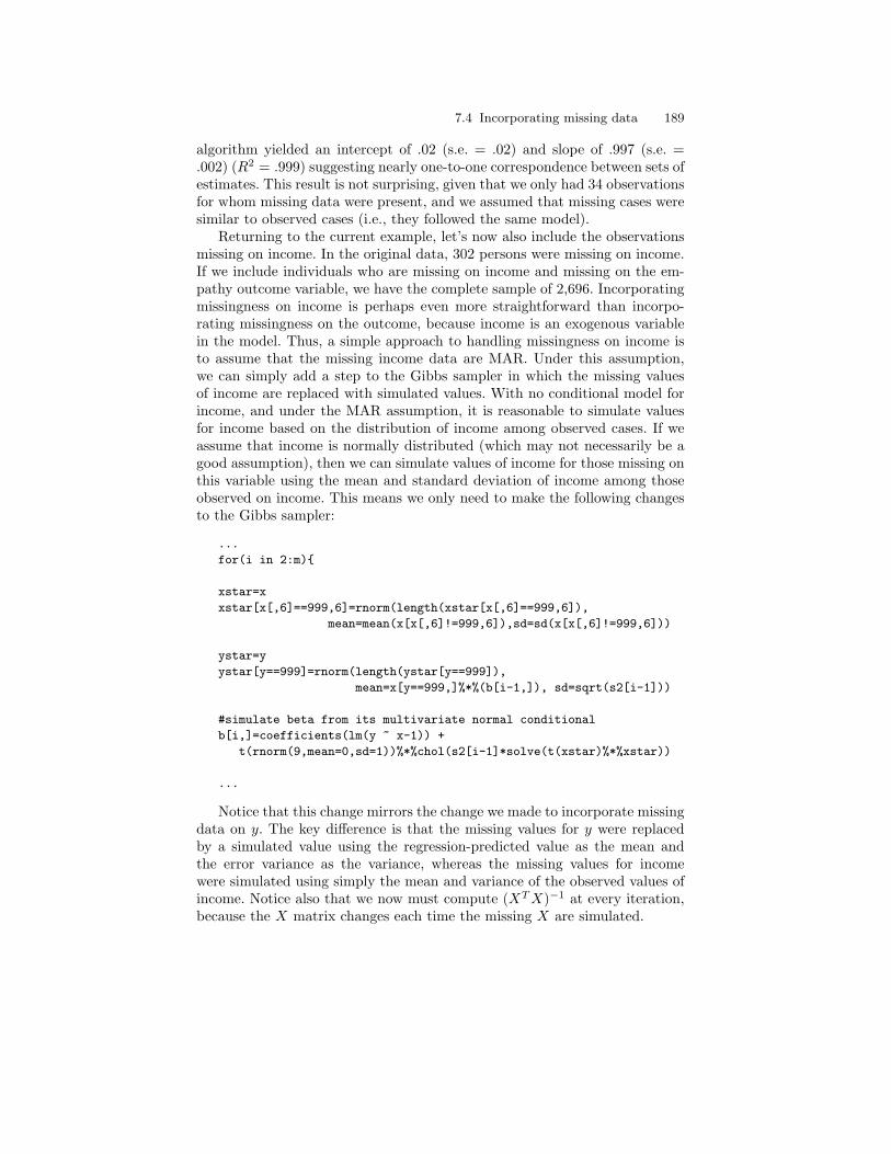
7.4 Incorporating missing data 189
algorithm yielded an intercept of .02 (s.e. = .02) and slope of .997 (s.e. =.002) (R2 = .999) suggesting nearly one-to-one correspondence between sets ofestimates. This result is not surprising, given that we only had 34 observationsfor whom missing data were present, and we assumed that missing cases weresimilar to observed cases (i.e., they followed the same model).
Returning to the current example, let’s now also include the observationsmissing on income. In the original data, 302 persons were missing on income.If we include individuals who are missing on income and missing on the em-pathy outcome variable, we have the complete sample of 2,696. Incorporatingmissingness on income is perhaps even more straightforward than incorpo-rating missingness on the outcome, because income is an exogenous variablein the model. Thus, a simple approach to handling missingness on income isto assume that the missing income data are MAR. Under this assumption,we can simply add a step to the Gibbs sampler in which the missing valuesof income are replaced with simulated values. With no conditional model forincome, and under the MAR assumption, it is reasonable to simulate valuesfor income based on the distribution of income among observed cases. If weassume that income is normally distributed (which may not necessarily be agood assumption), then we can simulate values of income for those missing onthis variable using the mean and standard deviation of income among thoseobserved on income. This means we only need to make the following changesto the Gibbs sampler:
...
for(i in 2:m)
xstar=x
xstar[x[,6]==999,6]=rnorm(length(xstar[x[,6]==999,6]),
mean=mean(x[x[,6]!=999,6]),sd=sd(x[x[,6]!=999,6]))
ystar=y
ystar[y==999]=rnorm(length(ystar[y==999]),
mean=x[y==999,]%*%(b[i-1,]), sd=sqrt(s2[i-1]))
#simulate beta from its multivariate normal conditional
b[i,]=coefficients(lm(y ~ x-1)) +
t(rnorm(9,mean=0,sd=1))%*%chol(s2[i-1]*solve(t(xstar)%*%xstar))
...
Notice that this change mirrors the change we made to incorporate missingdata on y. The key difference is that the missing values for y were replacedby a simulated value using the regression-predicted value as the mean andthe error variance as the variance, whereas the missing values for incomewere simulated using simply the mean and variance of the observed values ofincome. Notice also that we now must compute (XT X)−1 at every iteration,because the X matrix changes each time the missing X are simulated.
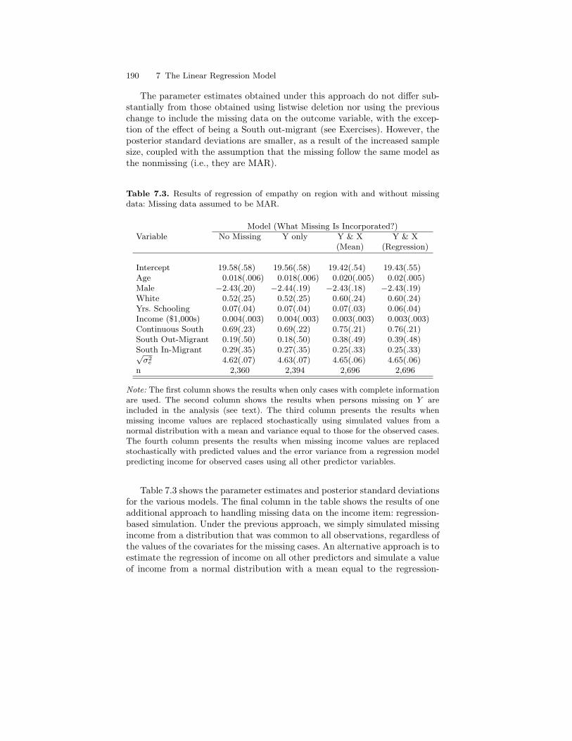
190 7 The Linear Regression Model
The parameter estimates obtained under this approach do not differ sub-stantially from those obtained using listwise deletion nor using the previouschange to include the missing data on the outcome variable, with the excep-tion of the effect of being a South out-migrant (see Exercises). However, theposterior standard deviations are smaller, as a result of the increased samplesize, coupled with the assumption that the missing follow the same model asthe nonmissing (i.e., they are MAR).
Table 7.3. Results of regression of empathy on region with and without missingdata: Missing data assumed to be MAR.
Model (What Missing Is Incorporated?)Variable No Missing Y only Y & X Y & X
(Mean) (Regression)
Intercept 19.58(.58) 19.56(.58) 19.42(.54) 19.43(.55)Age 0.018(.006) 0.018(.006) 0.020(.005) 0.02(.005)Male −2.43(.20) −2.44(.19) −2.43(.18) −2.43(.19)White 0.52(.25) 0.52(.25) 0.60(.24) 0.60(.24)Yrs. Schooling 0.07(.04) 0.07(.04) 0.07(.03) 0.06(.04)Income ($1,000s) 0.004(.003) 0.004(.003) 0.003(.003) 0.003(.003)Continuous South 0.69(.23) 0.69(.22) 0.75(.21) 0.76(.21)South Out-Migrant 0.19(.50) 0.18(.50) 0.38(.49) 0.39(.48)South In-Migrant 0.29(.35) 0.27(.35) 0.25(.33) 0.25(.33)√
σ2e 4.62(.07) 4.63(.07) 4.65(.06) 4.65(.06)
n 2,360 2,394 2,696 2,696
Note: The first column shows the results when only cases with complete informationare used. The second column shows the results when persons missing on Y areincluded in the analysis (see text). The third column presents the results whenmissing income values are replaced stochastically using simulated values from anormal distribution with a mean and variance equal to those for the observed cases.The fourth column presents the results when missing income values are replacedstochastically with predicted values and the error variance from a regression modelpredicting income for observed cases using all other predictor variables.
Table 7.3 shows the parameter estimates and posterior standard deviationsfor the various models. The final column in the table shows the results of oneadditional approach to handling missing data on the income item: regression-based simulation. Under the previous approach, we simply simulated missingincome from a distribution that was common to all observations, regardless ofthe values of the covariates for the missing cases. An alternative approach is toestimate the regression of income on all other predictors and simulate a valueof income from a normal distribution with a mean equal to the regression-
7.5 Conclusions 191
based predicted score for income and a variance equal to the residual variance.5
I leave the modification of the Gibbs sampler to handle this approach as anexercise. This set of results is virtually identical to those obtained using theprevious approach for handling missingness on income.
Overall, the results reveal more similarities than differences between pa-rameter estimates, but the latter two approaches show a substantial reductionin the posterior standard deviations of the parameters. The reason is that thesample size is increased by retaining observations that would have been deleteddue to having missing data. Is this reduction in the standard error legitimate;that is, should we see smaller posterior standard deviations despite the factthat our models recognize the uncertainty the missing data present? Yes—infact, the posterior standard deviations are reduced proportional to the gain inthe square root of the sample size obtained by incorporating the observationswith missing data, just as the Central Limit Theorem suggests. However, it isimportant to recognize that, if we had taken the common approach of simplyimputing a single fixed value for the missing data (either using regression im-putation or mean imputation), the uncertainty presented by the missing datawould have been ignored, and the posterior standard deviations would havebeen even smaller (and inappropriately so).
Does the fact that the parameter estimates are consistent across thesemodels reassure us of the robustness of the results to missing data? The answerto this question is “absolutely not,” although it is tempting to believe that suchconsistency of results demonstrates robustness. Each of the approaches thatwe have taken has assumed that the missing data are MAR (but possibly notOAR). So long as that assumption is maintained in our missing data strategy,the results will be consistently similar.
In order to obtain different results, we would need to make adjustments tothe model that compensate for possible violations of the MAR assumption. Ofcourse, in that case, we have no way to know whether the results we obtain atthat point are realistic or not: That determination rests on our prior knowledgeregarding the missing data generation mechanism. In brief, there is no freelunch when it comes to violations of the MAR assumption. If the data arenot MAR, we cannot know from the data at hand how to obtain unbiasedparameter estimates.
7.5 Conclusions
In this chapter, we demonstrated the Bayesian approach to the multiple re-gression model using a Metropolis-Hastings sampling algorithm and two Gibbssamplers. In this process, I used several of the techniques discussed in the pre-vious chapter for assessing how well the algorithms performed, as well as for
5 Allison (2003) argues that y should also be included in imputing the missingvalues of x, but I have used only other x variables in this example.

192 7 The Linear Regression Model
assessing how well the models fit the data. Finally, I showed how Gibbs sam-pling can be adapted easily to handle missing data that are MAR. In the nextchapter, we will consider some basic generalized linear models that are usefulwhen the outcome variable is not continuous.
7.6 Exercises
1. Derive the maximum likelihood estimate for the regression vector (β) inthe linear regression model (i.e., Equation 7.5).
2. Develop an MH algorithm for the linear regression model that samples allregression parameters simultaneously. How difficult is it to find a proposaldensity that yields a reasonable acceptance rate? What are some possiblestrategies for finding a good proposal density?
3. How can we work with the original posterior density (not the logged ver-sion) without worrying about overflow/underflow problems. Hint: Con-sider computing the ratio case by case. Write the R code and test it.
4. Develop a Gibbs sampler that handles missingness on income via regression-based simulation of income on all other covariates.
5. We discovered, under the various missing data approaches that assumedthe data to be MAR, that the only coefficients that changed substantiallywere some of the region coefficients. Why did they change?
6. Using your own data, treat the outcome variable as missing for everytenth case and rerun the Gibbs sampler that handles missingness on theoutcome. Repeat the process with every fifth case treated as missing.Finally, repeat the process with every other case missing (50% missing).What happens to the posterior means and standard deviations of theparameters?
8
Generalized Linear Models
In the last chapter, we discussed the linear regression model. A requirementfor using that model is that the outcome variable must be continuous andnormally distributed. In social science research, having a continuous outcomevariable is rare. More often, we tend to have dichotomous, ordinal, or nom-inal outcomes. In these cases, the linear regression model discussed in theprevious chapter is inappropriate for several reasons. First, heteroscedasticityand nonnormal errors are guaranteed when the outcome is not continuous,nullifying the justification for statistical tests on the parameters (see Long1997). Second, the linear model will often predict values that are impossible.For example, although the tolerance item in the last chapter had a range of 5,nothing in the model prevents predicted values from falling outside the [0,5]interval.1 Third, the functional form specified by the linear model will oftenbe incorrect. For example, we should doubt that increases in a covariate willyield the same returns on the dependent variable at the extremes as wouldbe obtained toward the middle. Although we did not explore this issue in theprevious chapter, it seems clear that the effect of education on tolerance, say,would be greatest in the middle of the education distribution than at eitherend. Adding a few years of education beyond a college degree or adding a fewyears but maintaining a grade level below 8 will probably not be as influentialas transitioning from 11 to 12 years of education or from 12 to 16 years ininfluencing an individual’s tolerance.
Generalized linear models (GLMs) provide a way to handle these problems.Recall that the basic OLS regression model can be expressed as:
µi = XTi β,
1 As it turns out, no combination of covariates will actually produce predictedvalues outside the allowable range, but this is because the model fits poorly—thecovariates as specified do not have much influence on the outcome.
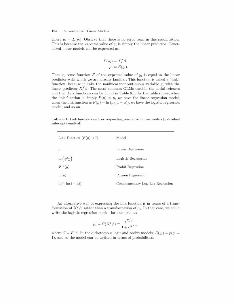
194 8 Generalized Linear Models
where µi = E(yi). Observe that there is no error term in this specification:This is because the expected value of yi is simply the linear predictor. Gener-alized linear models can be expressed as:
F (µi) = XTi β,
µi = E(yi).
That is, some function F of the expected value of yi is equal to the linearpredictor with which we are already familiar. This function is called a “link”function, because it links the nonlinear/noncontinuous variable yi with thelinear predictor XT
i β. The most common GLMs used in the social sciencesand their link functions can be found in Table 8.1. As the table shows, whenthe link function is simply F (µ) = µ, we have the linear regression model;when the link function is F (µ) = ln (µ/(1− µ)), we have the logistic regressionmodel; and so on.
Table 8.1. Link functions and corrresponding generalized linear models (individualsubscripts omitted).
Link Function (F (µ) is ?) Model
µ Linear Regression
ln“
µ1−µ
”Logistic Regresssion
Φ−1(µ) Probit Regression
ln(µ) Poisson Regression
ln(− ln(1− µ)) Complementary Log–Log Regression
An alternative way of expressing the link function is in terms of a trans-formation of XT
i β, rather than a transformation of µi. In that case, we couldwrite the logistic regression model, for example, as:
µi = G(XTi β) ≡ eXT
i β
1 + eXTi β
,
where G = F−1. In the dichotomous logit and probit models, E(yi) = p(yi =1), and so the model can be written in terms of probabilities:
8.1 The dichotomous probit model 195
p(yi = 1) = G(XTi β).
In this notation, G is the link function.For a logistic regression model, G is the cumulative standard logistic dis-
tribution function, whereas for a probit model, G is the cumulative standardnormal distribution function.
8.1 The dichotomous probit model
One of the first generalized linear regression models to achieve popularity inthe social sciences was the logistic regression model for dichotomous outcomevariables (Hosmer and Lemeshow 1989). Dichotomous outcomes are prevalentin social science research, but prior to the 1980s, the computing power requiredto estimate the parameters of generalized linear regression models exceededcapacity. As a result, many social science researchers estimated parametersusing OLS regression, which, as we discussed above, is an undesirable approachfor several reasons. With the development of the iteratively reweighted leastsquares algorithm, coupled with an increase in computing power, the use oflogistic regression rapidly replaced OLS regression as the preferred methodfor handling dichotomous outcomes. The logistic regression model obtainedpopularity primarily because of the relative ease of interpretation of the modelparameters, as I show below. Nonetheless, in this chapter, my examples involveonly the dichotomous probit model and its extension to the ordinal probitmodels.
The choice of the probit model over the logistic regression model or othermodels (e.g., the complementary log-log model) is largely for convenience: Aswe will see, the probit model, from a probability standpoint is often easier towork with, because it involves use of the normal distribution. Nonetheless, theextensions to logistic and complementary log-log models are straightforward.For a classical approach to these models, I recommend Long (1997) and Powersand Xie (2000). For an in-depth Bayesian exposition to dichotomous andordinal outcome models, I recommend Johnson and Albert (1999).
8.1.1 Model development and parameter interpretation
If our outcome variable in a regression model is dichotomous (0,1), then an ap-propriate likelihood function for the data is based on the binomial or Bernoullidistribution. The likelihood function can be expressed as:
L(P |y) ∝n∏
i=1
pyi
i (1− pi)1−yi , (8.1)
where yi is the observed dichotomous outcome for person i. For a person witha “1” on the outcome, the contribution to the likelihood reduces to the first

196 8 Generalized Linear Models
term; for a person with a 0, the contribution to the likelihood reduces to thesecond term.
As written, this likelihood function has no regression parameters, but wewould like to link pi—the probability of a “1” response—to the linear combi-nation XT
i β. As discussed at the beginning of the chapter, this is problematicbecause an identity link [i.e., pi = XT
i β] can predict illegitimate values forpi. Cumulative distribution functions constitutes a class of functions that canmap the predictor from the entire real line onto the interval [0, 1], becausecdfs are naturally constrained to produce values that fall in this range (referto Chapter 2). In the probit model case, we allow pi = Φ(XT
i β), where Φ(.) is
the cumulative normal distribution function (i.e.,∫XT
i β
−∞ N(0, 1)). Regardlessof the value of XT
i β, pi will fall in the acceptable range. To obtain a logisticregression model, one would simply need to set pi = eXT
i β/(1 + eXTi β) (the
cumulative logistic distribution function).Another way to think about dichotomous probit and logistic regression
models—one that is useful for setting up a Gibbs sampler—is in terms oflatent variables. We could express the probit or logistic regression model asa linear model for a continuously distributed unobserved trait or propensityscore, y∗i as:
y∗i = XTi β + ei (8.2)
using the link:
yi =
1 iff y∗i > 00 iff y∗i ≤ 0.
(8.3)
From this perspective, although y∗i is continuous, crude measurement lim-its our observation to the dichotomous individual response yi. If the individ-ual’s propensity is great enough (i.e., it falls above the threshold of 0), weobserve a 1 on y; otherwise, we observe a 0.
Given this set up, we need to rearrange the model somewhat to allow esti-mation of the regression parameters of interest. We can combine Equations 8.2and 8.3 such that:
If yi =
1, ei > −XTi β
0, ei < −XTi β.
(8.4)
If we assume a standard normal distribution for e, then we obtain the probitmodel:
p(yi = 1) = p(ei > −XTi β) = p(ei < XT
i β) =∫ XT
i β
−∞N(0, 1). (8.5)
Observe that this is the same expression we placed into the likelihoodfunction above in Equation 8.1. If we assume a logistic distribution for the
8.1 The dichotomous probit model 197
error instead of a normal distribution, then we obtain the logistic regressionmodel discussed above.
To make the probit model fully Bayesian, we need to specify priors on theregression parameters in the model. For that purpose, we could use improperuniform priors over the real line, as we did in the previous chapter, we could usevery vague normal priors [e.g., β ∼ N(0, 10000)], or we could use somethingcalled “conditional means priors.” Under this approach, we would specifyprior expected probabilities for several combinations of covariates, invert theseprobabilities into the regression coefficient scale, and combine this informationwith the likelihood function to obtain the posterior (see Johnson and Albert1999 for examples). In the examples, I simply use uniform priors so thatcomparisons can be made with estimates obtained via maximum likelihoodestimation.
With priors established, and Φ(XTi β) substituted for pi, the posterior dis-
tribution is:
p(β|Y,X) ∝n∏
i=1
Φ(XTi β)yi(1− Φ(XT
i β))1−yi . (8.6)
The interpretation of the parameters in this model—and all GLMs—is notas easy as the interpretation of parameters in the OLS regression model (seeLiao 1994). Because the link function is nonlinear (an integral of a nonlinearfunction), the model itself is nonlinear in the probabilities, even though thepredictor is linear. This nonlinearity complicates interpretation, because theeffects of each variable is no longer independent of the effects of other variables.The probit model is linear, however, in z (standard normal) units. That is,given that Xβ implies a particular upper limit for the integral of the standardnormal distribution, each β can be viewed in terms of its expected effect onthe z score for a one-unit increase in its corresponding covariate. The logisticregression model, on the other hand, is linear in log-odds units. Recall thatodds are computed as the ratio of p
1−p . The logistic link function, then, is alog-odds function. The coefficients from the model can be interpreted in termsof their linear effect on the log-odds, but this is not much help. Instead, if weexponentiate the model, we obtain:
exp(
ln(
pi
1− pi
))= exp
(XT
i β)
= eβ0eβ1xi1 . . . eβkxik . (8.7)
This result says that the odds are equal to the multiple of the exponenti-ated coefficients. Suppose we had an exponentiated coefficient of 2 for sex(measured as a dummy variable in which male = 1). This exponentiated coef-ficient would imply that the odds for a male responding “1” on the outcomevariable are twice as great as the odds for a female responding “1,” net ofthe other variables in the model. This ease of interpretation has made thelogistic regression model popular in the social sciences. The limitations, how-ever, include (1) that this interpretation tells us nothing about absolute risk,
198 8 Generalized Linear Models
only relative risk; and (2) the odds ratios are commonly interpreted as if theywere ratios of probabilities.2 In fact, there is not one-to-one correspondencebetween absolute risk measured by a ratio of probabilities and relative riskmeasured by a ratio of odds. For example, if groups A and B have absoluterisks of .1 and .01, respectively, the odds ratio representing the relative risk forgroup A versus B is the same as if the probabilities were .99 and .9: The oddsratio is 11, but certainly the absolute risks are substantially different. Theratio of probabilities conveys this information about the absolute risk. Theratio of probabilities is 10 under the first set of probabilities and is 1.1 underthe second, which indicates a substantially larger difference in the absoluteprobabilities for the first pair than for the second pair.
For both the logistic and the probit models, model probabilities can beobtained by (1) evaluating the linear predictor, and (2) applying the linkfunction to obtain p.
8.1.2 Sampling from the posterior distribution for the modelparameters
With the posterior distribution established in Equation 8.6, MCMC samplingrelies either on using this posterior as written for an MH algorithm or onderiving the conditional distribution for β for Gibbs sampling. Developing anMH algorithm for this model is straightforward using the pnorm function inR (or its equivalent in other languages), and I leave doing so as an exercise(see Exercises).
As written in Equation 8.6, the posterior cannot be simplified further, mak-ing the construction of a Gibbs sampler appear to be a daunting process. How-ever, as I mentioned above, the latent variable approach makes the process ofGibbs sampling simple. The unknown quantities in the model are the vector βand the vector Y ∗. We know from the initial specification that Y ∗ ∼ N(Xβ, 1),subject to the constraint that each y∗i > 0 iff yi = 1 and y∗i < 0 iff yi = 0.Together, these specifications imply that y∗i |yi, Xi, β ∼ TN(XT
i β, 1), whereTN is the truncated normal distribution. The point of truncation is 0, and theside of the distribution that is truncated is determined by yi: For individualswith y = 0, the distribution is truncated above 0; for individuals with y = 1,the distribution is truncated below 0 (see Albert and Chib 1993).
What is the distribution for β? Because the vector Y ∗ is normally dis-tributed, given Y ∗, the conditional distribution for β is the same as for the OLSregression model (with σ2 = 1): β|X, Y ∗ ∼ N
((XT X)−1(XT Y ∗), (XT X)−1
).
Thus, a Gibbs sampler can be specified in four steps:
1. Establish starting values for β.2. Simulate Y ∗|X, Y, β ∼ TN(Xβ, 1).2 Researchers commonly say that an odds ratio of 2 implies that one group is “twice
as likely” as another to have a “1” on the outcome, but this language implies thatthe odds ratio is a ratio of two probabilities, and it is not.
8.1 The dichotomous probit model 199
3. Simulate β|X, Y ∗, Y ∼ N((XT X)−1(XT Y ∗), (XT X)−1
).
4. Return to step 2 (repeat).
An R program for implementing this Gibbs sampler is as follows:
#R program for dichotomous probit model
#read the data
x=as.matrix(read.table("c:\\bookdead.dat")[,3:9])
y=as.matrix(read.table("c:\\bookdead.dat")[,10])
#create variables, set values, and write out starting values
b=matrix(0,7); vb=solve(t(x)%*%x); ch<-chol(vb)
write(c(i,t(b)), file="c:\\dprob_gibbs.out", append=T, ncol=8)
#begin MCMC simulation
for(i in 2:5000)
#simulate latent data from truncated normal distributions
u=as.matrix(runif(length(y),min=0,max=1))
xb=as.matrix(x%*%b)
ystar=qnorm(y*u + u*(-1)^y*pnorm(0,mean=xb,sd=x[,1]) +
y*pnorm(0,mean=xb,sd=1), mean=xb, sd=x[,1])
#simulate beta vector from appropriate mvn distribution
b<-vb%*%(t(x)%*%ystar) + t((rnorm(7,mean=0,sd=1))%*%ch)
write(c(i,t(b))), file="c:\\dprob_gibbs.out", append=T, ncolumns=8)
if(i%%10==0)print(c(i,t(b))),digits=2)
This program is similar to the Gibbs samplers for the OLS regression modelin the previous chapter, with four key differences. First, there is no simulationof σ2
e in this program, because this parameter is fixed at 1 in the probit model(i.e., the error is assumed to be standard normal). Second, latent data (ystar)are simulated to replace the observed dichotomous y. Third, the regressionparameter vector mean changes at every iteration. This change is attributableto the fact that the latent data, ystar, change at every iteration, and thus(XT X)−1(XT Y ∗) changes. Fourth, because I am saving the results to a file, Ido not need to double-subscript b (the regression parameter vector) to reflectthe iteration of the algorithm. Instead, the current value of the vector, afterit is sampled, is written to the file.
I have written this program to be quite compact—with many statementsI have used separately in previous programs now being combined into a sin-gle line—but only one section of this program requires some discussion: thesimulation of the latent data from truncated normal distributions.
200 8 Generalized Linear Models
8.1.3 Simulating from truncated normal distributions
Simulation from truncated normal distributions can be quite simple but inef-ficient, or it can be very fast but mathematically challenging. In this and thefollowing sections, I discuss three ways to perform such simulation: a naivebut simple way, a rejection sampling approach, and an inversion sampling ap-proach. Ultimately, I use the inversion sampling approach, but I have oftenused the naive approach. I describe the rejection sampling approach largelyto motivate thinking about sampling from uncommon distributions in a morepractical setting than in previous chapters.
The naive approach
A “naive” way of simulating from truncated normal distributions, as Robertand Casella (1999) call it, is to repeatedly simulate draws from a full normaldistribution with the specified mean until a draw is obtained in the appropriatepart of the distribution. This approach is very simple to implement but hasone serious drawback: It is extremely inefficient. If an individual is an outlier,that is, his/her XT
i β is large (small) but s/he reported a 0 (1), most of themass of the normal distribution from which we would be simulating possiblevalues will be centered well away from the region from which the latent scoremust be drawn. This fact implies that it may take hundreds or even thousandsof simulated scores before obtaining just one that falls in the right region.For a general example, see Figure 8.1. The figure shows a complete normaldistribution with a mean of 1.645 and a standard deviation of 1. If a personwith XT
i β = 1.645 happened to respond “0” on the outcome variable, his/herlatent score would need to be simulated to the left of the point of truncation(0), which is 1.645 standard deviations away from the mean. It is well knownthat only 5% of the mass of a normal density lies to the left of 1.645 standarddeviations from the mean, and so it would take an expected 20 draws beforewe would sample this person’s latent score at that particular iteration of thealgorithm (5 out of every 100 draws should come from that region). Simulatingan expected 20 draws to obtain one valid value is highly inefficient, consideringthat we may need to draw from a tail region for many cases (e.g., if the modeldoes not fit the data well and/or has many outliers), and we need to do thisfor thousands of iterations. If one has chosen particularly poor starting valuesfor the parameters, an algorithm may not even begin to simulate parameters,because it may find itself stuck indefinitely attempting to simulate latentscores at the first iteration!
In all fairness, this naive sampling scheme often works well and may be fastenough despite its inefficiency if one has access to very powerful computing.However, it may not be satisfactory. Fortunately, alternative approaches tosimulating values from truncated normal distributions can be constructed.
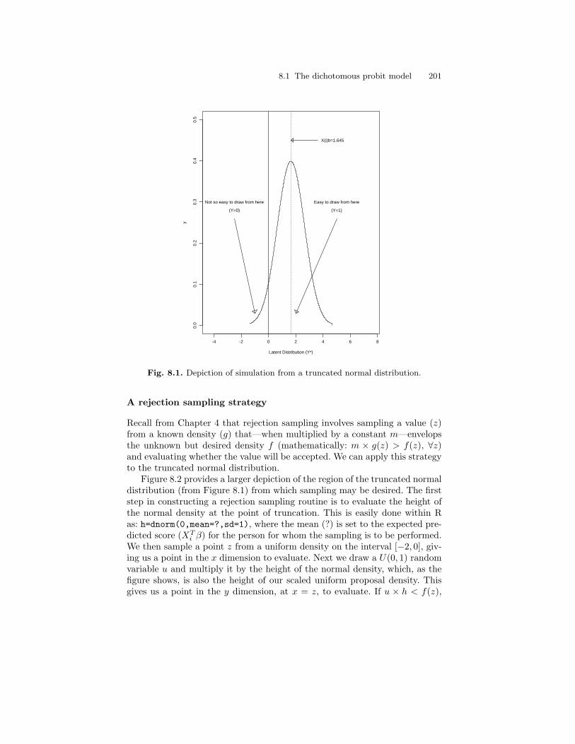
8.1 The dichotomous probit model 201
Latent Distribution (Y*)
y
-4 -2 0 2 4 6 8
0.0
0.1
0.2
0.3
0.4
0.5
Not so easy to draw from here
(Y=0)
Easy to draw from here
(Y=1)
X(i)b=1.645
Fig. 8.1. Depiction of simulation from a truncated normal distribution.
A rejection sampling strategy
Recall from Chapter 4 that rejection sampling involves sampling a value (z)from a known density (g) that—when multiplied by a constant m—envelopsthe unknown but desired density f (mathematically: m × g(z) > f(z), ∀z)and evaluating whether the value will be accepted. We can apply this strategyto the truncated normal distribution.
Figure 8.2 provides a larger depiction of the region of the truncated normaldistribution (from Figure 8.1) from which sampling may be desired. The firststep in constructing a rejection sampling routine is to evaluate the height ofthe normal density at the point of truncation. This is easily done within Ras: h=dnorm(0,mean=?,sd=1), where the mean (?) is set to the expected pre-dicted score (XT
i β) for the person for whom the sampling is to be performed.We then sample a point z from a uniform density on the interval [−2, 0], giv-ing us a point in the x dimension to evaluate. Next we draw a U(0, 1) randomvariable u and multiply it by the height of the normal density, which, as thefigure shows, is also the height of our scaled uniform proposal density. Thisgives us a point in the y dimension, at x = z, to evaluate. If u × h < f(z),
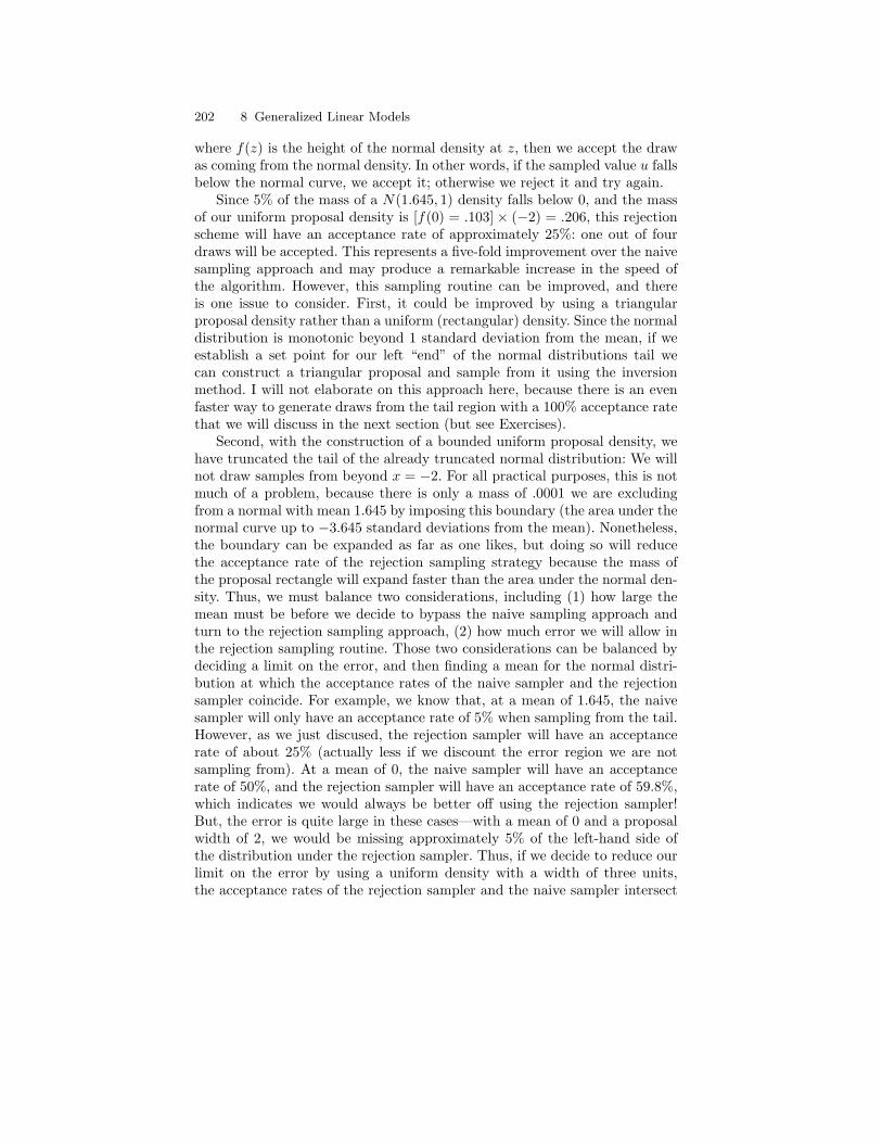
202 8 Generalized Linear Models
where f(z) is the height of the normal density at z, then we accept the drawas coming from the normal density. In other words, if the sampled value u fallsbelow the normal curve, we accept it; otherwise we reject it and try again.
Since 5% of the mass of a N(1.645, 1) density falls below 0, and the massof our uniform proposal density is [f(0) = .103]× (−2) = .206, this rejectionscheme will have an acceptance rate of approximately 25%: one out of fourdraws will be accepted. This represents a five-fold improvement over the naivesampling approach and may produce a remarkable increase in the speed ofthe algorithm. However, this sampling routine can be improved, and thereis one issue to consider. First, it could be improved by using a triangularproposal density rather than a uniform (rectangular) density. Since the normaldistribution is monotonic beyond 1 standard deviation from the mean, if weestablish a set point for our left “end” of the normal distributions tail wecan construct a triangular proposal and sample from it using the inversionmethod. I will not elaborate on this approach here, because there is an evenfaster way to generate draws from the tail region with a 100% acceptance ratethat we will discuss in the next section (but see Exercises).
Second, with the construction of a bounded uniform proposal density, wehave truncated the tail of the already truncated normal distribution: We willnot draw samples from beyond x = −2. For all practical purposes, this is notmuch of a problem, because there is only a mass of .0001 we are excludingfrom a normal with mean 1.645 by imposing this boundary (the area under thenormal curve up to −3.645 standard deviations from the mean). Nonetheless,the boundary can be expanded as far as one likes, but doing so will reducethe acceptance rate of the rejection sampling strategy because the mass ofthe proposal rectangle will expand faster than the area under the normal den-sity. Thus, we must balance two considerations, including (1) how large themean must be before we decide to bypass the naive sampling approach andturn to the rejection sampling approach, (2) how much error we will allow inthe rejection sampling routine. Those two considerations can be balanced bydeciding a limit on the error, and then finding a mean for the normal distri-bution at which the acceptance rates of the naive sampler and the rejectionsampler coincide. For example, we know that, at a mean of 1.645, the naivesampler will only have an acceptance rate of 5% when sampling from the tail.However, as we just discused, the rejection sampler will have an acceptancerate of about 25% (actually less if we discount the error region we are notsampling from). At a mean of 0, the naive sampler will have an acceptancerate of 50%, and the rejection sampler will have an acceptance rate of 59.8%,which indicates we would always be better off using the rejection sampler!But, the error is quite large in these cases—with a mean of 0 and a proposalwidth of 2, we would be missing approximately 5% of the left-hand side ofthe distribution under the rejection sampler. Thus, if we decide to reduce ourlimit on the error by using a uniform density with a width of three units,the acceptance rates of the rejection sampler and the naive sampler intersect

8.1 The dichotomous probit model 203
(with the rejection samplers rate being better) for distributions with a meanaround .6.
Tail region of normal distribution, Mean=1.645, S.D.=1
f(x)
-6 -4 -2 0 2 4
0.0
0.05
0.10
0.15
0.20 Point of Truncation
Ht. of density at truncation
Scaled uniform density for rejection sampling
25% acceptance rate
w/ rejection sampling
Fig. 8.2. Depiction of rejection sampling from the tail region of a truncated normaldistribution.
A better strategy: Inversion sampling
For sampling from univariate truncated normal distributions, there is no in-herent reason to use the rejection sampling approach we just discussed forsimulating. The inversion method, when the truncated region of the normaldistribution is renormalized, is much faster and has an acceptance rate of100%. We discussed the inversion method of sampling in Chapter 4. Theinversion method involves (1) drawing a U(0, 1) random variable that repre-sents the area under the distribution of interest, and (2) using the inverse-distribution function to find the value x from the distribution that yields thatarea below it. For example, if we were attempting to draw samples from astandard normal distribution and we drew a .5 from the uniform distribution,
204 8 Generalized Linear Models
the inversion method would produce x = 0 as our sample from the N(0, 1)distribution. If we drew a .025 from the uniform distribution, the inversionmethod would produce x = −1.96, etc.
The inversion method can be adapted to sample from truncated nor-mal distributions. I will first show how to simulate from the left-hand sideof the distribution. In the first step, we must “renormalize” the truncatedregion; that is, we must multiply the density by a constant so that thearea of the truncated region integrates to 1. This renormalization step in-volves simply determining the area of the normal distribution that falls inthe truncated region and hence just involves using the distribution functionΦµ,σ(T ) =
∫ T
−∞N(µ, σ), with a given mean µ, standard deviation σ, and trun-cation point T . For the probit model, we have already stated the mean is theexpected value for the given observation/case, the standard deviation is 1, andthe truncation point is x = 0. Thus, in R we use: A=pnorm(0,xb,1), where 0is the truncation point, xb is the mean, and 1 is the standard deviation. Ourconstant for renormalizing is then 1/A.
In the next step, we draw a U(0, 1) random variable u, just as in theoriginal inversion routine. Finally, we multiply u by A, and we then applythe inverse-normal distribution function to this draw to obtain the draw fromthe truncated region. Why do we multiply u by A? In the original inversionapproach, we let u = Φ(x), where u is our uniform draw and x is our sampledvalue of interest. In order to find x, we take Φ−1(u) = Φ−1(Φ(x)) = x. Inthe truncated distribution, however, our area is determined by the integralfrom −∞ to T . Φ must then be rescaled to produce an area no bigger thanA, and so we use: u = (1/A)Φ(x). To solve for x, we move A to the left sideof this equation: uA = Φ(x). Since u can be no bigger than 1, uA can be nobigger than A. So, Φ(x) will be limited between 0 and A and hence Φ−1 willbe limited to the interval [−∞, T ].
Sampling from the right-hand side of the normal distribution is onlyslightly more tedious. We can do this in one of two ways: (1) use the factthat the normal distribution is symmetric and reverse the sign of the meanand then reverse the sign of x once it is computed using Φ−1, or (2) keep themean as is and simply add the appropriate constant before applying Φ−1 tokeep x from falling below the truncation point. I discuss the latter approachhere, because it is easier to understand, and because it is easier to use in theordinal probit model to be discussed later.
As before, when sampling from the right-hand side of a truncated normaldistribution, we first need to renormalize the area to the right of the trun-cation point. Given that the area under the normal curve totals 1, this canbe computed easily as: B = 1 − Φ(T ). Now, in this case, we need x to bebounded between T and ∞. We know from before that uA provides the areafor which x = T , and so, we need Φ to yield a minimum value of uA. We alsoneed Φ to yield a maximum value of 1. For Φ to yield A at a minimum, wetherefore need Φ−1(A + C), where C must range from 0 to 1 − A (or B) toensure that x falls in the appropriate region. Thus, we let C = uB, and we
8.1 The dichotomous probit model 205
have x = Φ−1(A + uB) as our solution. When u is 0, the function returns T ;when u = 1, the function returns ∞, because A + B = 1.
Another way to perform inversion sampling, rather than renormalizingthe appropriate area (left or right side of the distribution), is to set theminimum and maximum values of the uniform random number functionto the appropriate values. For example, if we are sampling from the leftside of a normal distribution, we could set the minimum value for the uni-form density to Φ(−∞) = 0 and the maximum to Φ(0) for the normaldensity with mean xb and standard deviation 1 [e.g., in R, we would use:u=runif(1,min=0,max=pnorm(0,mean=xb,sd=1)]. This approach is mathe-matically equivalent to the previous one. In the first one, we leave the uniformdensity as U(0, 1) but multiply it to rescale its maximum value; in the sec-ond, we simply resize the uniform density. Under either approach, we wouldneed to apply the inverse normal distribution function (qnorm in R) to u toobtain our latent y∗. Both approaches involve the same number of “steps,”but one approach may be easier to implement than another, depending on theprogramming language being used.
Returning to the Gibbs sampler presented earlier, the truncated normalsampling code was:
u=as.matrix(runif(length(y),min=0,max=1))xb=as.matrix(x%*%b)
ystar=qnorm(y*u + u*(-1)^y*pnorm(0,mean=xb,sd=1) +y*pnorm(0,mean=xb,sd=1), mean=xb, sd=1)
The first line simply generates an n-length vector of U(0, 1) random numbers.The second line generates an n-length vector of predicted values/expectedmeans. The remaining code performs all the truncated normal simulationsteps discussed above, but simultaneously handles (1) all cases in one step,relying on R’s ability to handle operations to entire vectors at once, and (2)simulation for y = 0 and y = 1. Feature (1) is straightforward: y, u, and xbare all vectors, and so ystar also is a vector. The second feature is a littlemore difficult to see. Suppose, for an individual, y = 0. In that case, the firstargument within the qnorm function reduces to:
u*pnorm(0,mean=xb,sd=1)
This is the appropriate argument for cases in which y = 0, as shown above.In the event y = 1, the first argument reduces to:
u - u*pnorm(0,mean=xb,sd=1) + pnorm(0,mean=xb,sd=1)
Rearranging terms and factoring u reveals that this is, indeed, the correctargument for cases in which y = 1.
An alternative argument, based on the second strategy listed above—adjusting the minimum and maximum arguments to the uniform randomdraw—can be implemented as:
206 8 Generalized Linear Models
ystar=qnorm(mean=xb,sd=1,runif(length(y),
min=(y*pnorm(0,xb,1)), max=(pnorm(0,xb,1)^(1-y))))
Notice here that when y = 0, the min=0 and the max=pnorm(0,xb,1); wheny = 1, min=pnorm(0,xb,1) and max=1.(Also notice that I have shuffledaround the arguments to the qnorm function—the order of arguments is ir-relevant to R for most functions).
8.1.4 Dichotomous probit model example: Black–white differencesin mortality
Racial differences in mortality—especially black-white differences—are an im-portant concern for mortality demographers and health researchers. It is wellknown that blacks have higher levels of mortality than whites. A commongoal in the literature has been to try to understand why this health advan-tage for whites exists (see Markides and Black 1996). Interestingly, this whiteadvantage, however, does not exist across the entire age range. Instead, at ad-vanced ages (usually over 75 years of age), a crossover is observed such blackmortality rates fall below those of whites. Although a relatively large demo-graphic literature has emerged over the last few decades suggesting possibleexplanations for the crossover (e.g., see Elo and Preston 1994; Lynch, Brownand Harmsen 2003; Preston et al. 1996), very few studies have attempted toquantify uncertainty in the age at which the crossover occurs, largely becausethe crossover age is a quantity for which the standard error is difficult to de-rive using classical methods. The example of the dichotomous probit model(and ordinal probit model) I use here seeks to quantify this uncertainty.
A standard approach to modeling racial differences in mortality is to usedichotomous probit or logistic regression models, often in a discrete-timeformat, when individual-level longitudinal data are used. In a discrete-timespecification, each person contributes more than one observation to the fi-nal dataset—one record for every year observed (Allison 1984; Hosmer andLemeshow 1999; Yamaguchi 1991). I construct such a data set here, using datafrom the National Health and Nutrition Examination Survey (NHANES) andits follow-ups, the National Epidemiologic Follow-up Surveys (NHEFS). TheNHANES was a cross-sectional survey designed to assess the nation’s healthusing a sample of roughly 34,000 individuals ages 24-77 beginning in 1971. Ofthese, roughly 7,000 sample members were administered a physical exam bya physician, as well as a health care supplemental survey measuring self-ratedhealth, and were then followed-up on at least three occasions: in 1982, 1987,and 1992. Using individuals who (1) survived to 1975 (the last year of thebaseline study), (2) were at least 40 years of age in 1975, (3) had no missingdata on variables used in the analyses, and (4) were either white or black,I created an analytic sample of 3,201 persons, of which 685 died during theobservation period. The resulting person-year file consisted of 55,173 records,
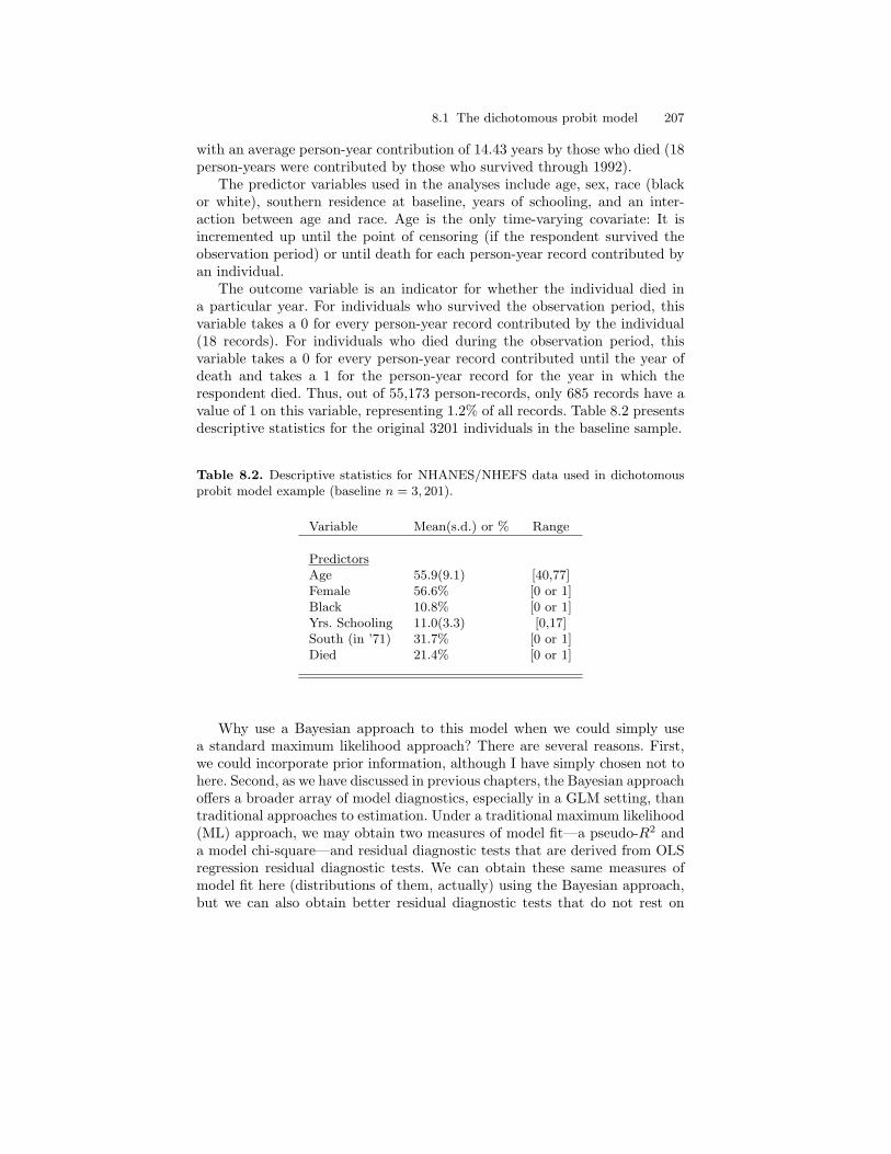
8.1 The dichotomous probit model 207
with an average person-year contribution of 14.43 years by those who died (18person-years were contributed by those who survived through 1992).
The predictor variables used in the analyses include age, sex, race (blackor white), southern residence at baseline, years of schooling, and an inter-action between age and race. Age is the only time-varying covariate: It isincremented up until the point of censoring (if the respondent survived theobservation period) or until death for each person-year record contributed byan individual.
The outcome variable is an indicator for whether the individual died ina particular year. For individuals who survived the observation period, thisvariable takes a 0 for every person-year record contributed by the individual(18 records). For individuals who died during the observation period, thisvariable takes a 0 for every person-year record contributed until the year ofdeath and takes a 1 for the person-year record for the year in which therespondent died. Thus, out of 55,173 person-records, only 685 records have avalue of 1 on this variable, representing 1.2% of all records. Table 8.2 presentsdescriptive statistics for the original 3201 individuals in the baseline sample.
Table 8.2. Descriptive statistics for NHANES/NHEFS data used in dichotomousprobit model example (baseline n = 3, 201).
Variable Mean(s.d.) or % Range
PredictorsAge 55.9(9.1) [40,77]Female 56.6% [0 or 1]Black 10.8% [0 or 1]Yrs. Schooling 11.0(3.3) [0,17]South (in ’71) 31.7% [0 or 1]Died 21.4% [0 or 1]
Why use a Bayesian approach to this model when we could simply usea standard maximum likelihood approach? There are several reasons. First,we could incorporate prior information, although I have simply chosen not tohere. Second, as we have discussed in previous chapters, the Bayesian approachoffers a broader array of model diagnostics, especially in a GLM setting, thantraditional approaches to estimation. Under a traditional maximum likelihood(ML) approach, we may obtain two measures of model fit—a pseudo-R2 anda model chi-square—and residual diagnostic tests that are derived from OLSregression residual diagnostic tests. We can obtain these same measures ofmodel fit here (distributions of them, actually) using the Bayesian approach,but we can also obtain better residual diagnostic tests that do not rest on
208 8 Generalized Linear Models
assumptions that the dichotomous data cannot meet (see Johnson and Albert1999 for more discussion).
Assessing model fit is important in a discrete time setting. Something thatis often overlooked in discrete time analyses is that the dilution of the originaldata via construction of a person-year file reduces the “success” proportion inthe outcome variable. For example, here, 21% of the respondents died over theobservation period (685/3201), yet deaths represent only 1.2% of the recordsin the person-year data. Logit and probit models tend to fare best when the“success” proportion is close to .5, and thus we should carefully consider modelfit when using discrete time models.3
A third reason for taking a Bayesian approach is that, although the black-white crossover is an important phenomenon to mortality demographers at-tempting to understand racial heterogeneity and inequality, the ML approachoffers no simple approach to testing hypotheses about it. The Bayesian ap-proach, on the other hand, does. The crossover age can be computed by settingthe regression equations equal for blacks and whites and solving for age to findthe point of intersection. With only age, race, and an interaction between themin the model, the model is:
y∗ = b0 + b1Age + b2Black + b3Age× Black. (8.8)
For blacks, Black = 1, and so the right-hand side reduces to (b0 + b2) + (b1 +b3)Age. For whites, Black = 0, and so the right-hand side reduces to b0+b1Age.Setting these equal, we find:
b2 + b3Age = 0, (8.9)
and so the age at which the crossover occurs is −b2/b3. This estimate canbe found with the ML approach to estimation, but there is no simple way toquantify our uncertainty in it using the estimated standard errors of the con-tributing parameters—the product of normally distributed random variableshas no known distribution, and so the standard error of a product of normalvariables is not defined. In the Bayesian setting, however, we can constructthis crossover age for every sampled value of the contributing parametersproduced by the Gibbs sampler and thereby obtain a distribution for thisquantity. Doing so allows us to answer important questions like: What is theprobability that the crossover age lies outside reasonable bounds on the lifespan?
I ran the Gibbs sampler presented in Section 8.1.2 several times, usingdifferent starting values for the parameters for each run. Figure 8.3 shows atrace plot of the intercept parameter, along with a plot of the autocorrelation3 One issue that is problematic when the success proportion is extreme (either high
or low) is that a model that simply predicts success or failure for every observationwill tend to predict the observed outcome very well. In this particular example, amodel that simply predicts that no one died would seem to explain 98.8% of theobserved responses! See Hosmer and Lemeshow for more discussion of this issue.
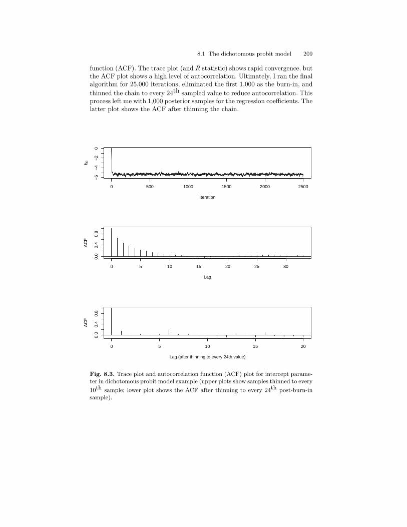
8.1 The dichotomous probit model 209
function (ACF). The trace plot (and R statistic) shows rapid convergence, butthe ACF plot shows a high level of autocorrelation. Ultimately, I ran the finalalgorithm for 25,000 iterations, eliminated the first 1,000 as the burn-in, andthinned the chain to every 24th sampled value to reduce autocorrelation. Thisprocess left me with 1,000 posterior samples for the regression coefficients. Thelatter plot shows the ACF after thinning the chain.
0 500 1000 1500 2000 2500
−6
−4
−2
0
Iteration
b 0
0 5 10 15 20 25 30
0.0
0.4
0.8
Lag
AC
F
0 5 10 15 20
0.0
0.4
0.8
Lag (after thinning to every 24th value)
AC
F
Fig. 8.3. Trace plot and autocorrelation function (ACF) plot for intercept parame-ter in dichotomous probit model example (upper plots show samples thinned to every
10th sample; lower plot shows the ACF after thinning to every 24th post-burn-insample).
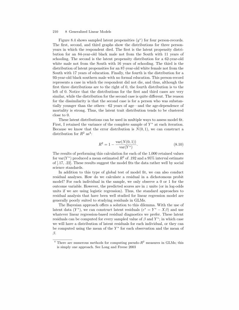
210 8 Generalized Linear Models
Figure 8.4 shows sampled latent propensities (y∗) for four person-records.The first, second, and third graphs show the distributions for three person-years in which the respondent died. The first is the latent propensity distri-bution for an 84-year-old black male not from the South with 11 years ofschooling. The second is the latent propensity distribution for a 62-year-oldwhite male not from the South with 16 years of schooling. The third is thedistribution of latent propensities for an 87-year-old white female not from theSouth with 17 years of education. Finally, the fourth is the distribution for a93-year-old black southern male with no formal education. This person-recordrepresents a case in which the respondent did not die, and thus, although thefirst three distributions are to the right of 0, the fourth distribution is to theleft of 0. Notice that the distributions for the first and third cases are verysimilar, while the distribution for the second case is quite different. The reasonfor the dissimilarity is that the second case is for a person who was substan-tially younger than the others—62 years of age—and the age-dependence ofmortality is strong. Thus, the latent trait distribution tends to be clusteredclose to 0.
These latent distributions can be used in multiple ways to assess model fit.First, I retained the variance of the complete sample of Y ∗ at each iteration.Because we know that the error distribution is N(0, 1), we can construct adistribution for R2 as4:
R2 = 1− var(N(0, 1))var(Y ∗)
. (8.10)
The results of performing this calculation for each of the 1,000 retained valuesfor var(Y ∗) produced a mean estimated R2 of .192 and a 95% interval estimateof [.17, .22]. These results suggest the model fits the data rather well by socialscience standards.
In addition to this type of global test of model fit, we can also conductresidual analyses. How do we calculate a residual in a dichotomous probitmodel? For each individual in the sample, we only observe a 0 or 1 for theoutcome variable. However, the predicted scores are in z units (or in log-oddsunits if we are using logistic regression). Thus, the standard approaches toresidual analysis that have been well studied for linear regression model aregenerally poorly suited to studying residuals in GLMs.
The Bayesian approach offers a solution to this dilemma. With the use oflatent data (Y ∗), we can construct latent residuals (e∗ = Y ∗ −Xβ) and usewhatever linear regression-based residual diagnostics we prefer. These latentresiduals can be computed for every sampled value of β and Y ∗; in which casewe will have a distribution of latent residuals for each individual, or they canbe computed using the mean of the Y ∗ for each observation and the mean ofβ.
4 There are numerous methods for computing pseudo-R2 measures in GLMs; thisis simply one approach. See Long and Freese 2003
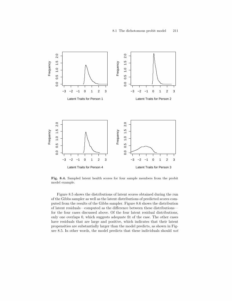
8.1 The dichotomous probit model 211
−3 −2 −1 0 1 2 3
0.0
0.5
1.0
1.5
2.0
Latent Traits for Person 1
Fre
quen
cy
−3 −2 −1 0 1 2 3
0.0
0.5
1.0
1.5
2.0
Latent Traits for Person 2
Fre
quen
cy
−3 −2 −1 0 1 2 3
0.0
0.5
1.0
1.5
2.0
Latent Traits for Person 4
Fre
quen
cy
−3 −2 −1 0 1 2 3
0.0
0.5
1.0
1.5
2.0
Latent Traits for Person 3
Fre
quen
cy
Fig. 8.4. Sampled latent health scores for four sample members from the probitmodel example.
Figure 8.5 shows the distributions of latent scores obtained during the runof the Gibbs sampler as well as the latent distributions of predicted scores com-puted from the results of the Gibbs sampler. Figure 8.6 shows the distributionof latent residuals—computed as the difference between these distributions—for the four cases discussed above. Of the four latent residual distributions,only one overlaps 0, which suggests adequate fit of the case. The other caseshave residuals that are large and positive, which indicates that their latentpropensities are substantially larger than the model predicts, as shown in Fig-ure 8.5. In other words, the model predicts that these individuals should not

212 8 Generalized Linear Models
have died, but in fact they did, which leads to values for Y ∗ that are positive(but predicted values that are negative).
−3 −2 −1 0 1 2 3
01
23
4
Person 1
Fre
quen
cy
−3 −2 −1 0 1 2 3
02
46
810
Person 2
Fre
quen
cy
−3 −2 −1 0 1 2 3
02
46
8
Person 3
Fre
quen
cy
−3 −2 −1 0 1 2 3
0.0
1.0
2.0
3.0
Person 4
Fre
quen
cy
Fig. 8.5. Model-predicted traits and actual latent traits for four observations inprobit model (solid line = model-predicted latent traits from sample values of β;dashed line = latent traits simulated from the Gibbs sampler).
I selected these cases for this particular reason: As I discussed above, ina model with a proportion of “successes” that is substantially far from .5, amodel that predicts that all cases are either successes or failures will appear,on its face, to fit the data well. In this particular model, we have very fewdeaths, and so the model tends to predict that no one dies. In order to beconvinced that the model fits well, we might consider investigating the latent
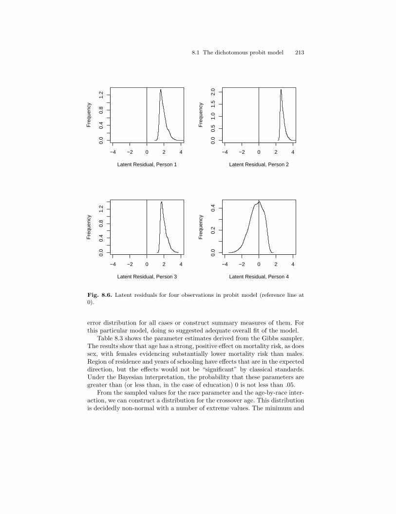
8.1 The dichotomous probit model 213
−4 −2 0 2 4
0.0
0.4
0.8
1.2
Latent Residual, Person 1
Fre
quen
cy
−4 −2 0 2 4
0.0
0.5
1.0
1.5
2.0
Latent Residual, Person 2
Fre
quen
cy
−4 −2 0 2 4
0.0
0.4
0.8
1.2
Latent Residual, Person 3
Fre
quen
cy
−4 −2 0 2 4
0.0
0.2
0.4
Latent Residual, Person 4
Fre
quen
cy
Fig. 8.6. Latent residuals for four observations in probit model (reference line at0).
error distribution for all cases or construct summary measures of them. Forthis particular model, doing so suggested adequate overall fit of the model.
Table 8.3 shows the parameter estimates derived from the Gibbs sampler.The results show that age has a strong, positive effect on mortality risk, as doessex, with females evidencing substantially lower mortality risk than males.Region of residence and years of schooling have effects that are in the expecteddirection, but the effects would not be “significant” by classical standards.Under the Bayesian interpretation, the probability that these parameters aregreater than (or less than, in the case of education) 0 is not less than .05.
From the sampled values for the race parameter and the age-by-race inter-action, we can construct a distribution for the crossover age. This distributionis decidedly non-normal with a number of extreme values. The minimum and

214 8 Generalized Linear Models
Table 8.3. Gibbs sampling results for dichotomous probit model predicting mor-tality.
Variable Parameter
Intercept −5.37(.15)***Age 0.047(.002)***Female −0.24(.03)***Black 0.81(.36)*Yrs. Schooling −0.003(.005)South (in ’71) 0.03(.04)Age × Black −0.0099(.005)*
Note: The Bayesian estimates are posterior means. The p-values are based on one-sided tail probabilities that the parameter exceeds 0 truncated to the classical cut-points of #p < .1, *p < .05, **p < .01, **p < .001.
maximum values for the crossover age, for example, were −13, 226.38 and393.33, respectively. These extreme values are a product of the fact that wehave uncertainty in both of the contributing parameters. Figure 8.7 shows thebivariate distribution for these contributing parameters, with horizontal andvertical reference lines at 0 dividing the distribution into four “cases.” In Case1, the main effect parameter is negative, and the interaction effect parameteris positive. This combination produces crossover ages that are positive. How-ever, under this scenario blacks begin life advantaged over whites and slowlysee this advantage erode. In Case 2, the main and interaction effect parametersare both positive, which produces crossover ages that are negative. Through-out the observed life span, the black-white gap expands. In Case 3, the mainand interaction effect parameters are both negative, producing crossover agesthat also occur outside the life span (negative). In these cases, blacks evi-dence lower mortality than whites throughout life with the gap expandingacross age. Finally, in Case 4, the main effect is positive and the interactioneffect is negative, producing crossover ages that are positive and generallyconsistent with expectation. That is, the white advantage erodes across age.
As the figure shows, the vast majority of the sampled parameter values—97.3% of them—fall under scenario 4. Overall, 1.6% of the sample parametervalues fall under scenario 1, while 1.1% of the sample parameter values fallunder scenario 2, and none fall under scenario 3. Thus, from a Bayesian view,there is a large probability that a crossover exists, and that the age patternof mortality is consistent with theory—that is, blacks are disadvantaged inearly life, but the white advantage decreases across age. In contrast, there is0 probability that blacks actually experience a large and growing advantagein mortality across age (cases 3), and very low probabilities that whites expe-rience a growing advantage across age (case 2) or that blacks begin life withan advantage that declines across age (case 1).

8.1 The dichotomous probit model 215
−1.5 −1.0 −0.5 0.0 0.5 1.0 1.5 2.0
−0.
025
−0.
015
−0.
005
0.00
00.
005
Black Parameter
Age
−by
−B
lack
Par
amet
er (+) crossover ages
(Case 4)
(Case 2)
(Case 3)
(Case 1)
Fig. 8.7. Distribution of black and age-by-black parameters (Cases 2 and 3 = bothvalues are positive or negative, respectively; Cases 1 and 4 = values are of oppositesigns. Case 4 is the typically-seen/expected pattern).
We can consider the crossover in more detail by summarizing its distribu-tion, rather than considering the contributing parameters. Figure 8.8 shows atrace plot as well as a histogram of the distribution for crossover ages between0 years of age and 200 years of age. The trace plot shows a seemingly stationarydistribution of crossover ages, with periodically very high or very low sampledvalues. The histogram shows several summary statistics for the crossover, in-cluding the mean age based on all sampled values of the crossover age, themedian crossover age based on all sampled values, the mean age based on onlyvalues falling between ages 0 and 200, and the typical maximum likelihood-estimated crossover age. This latter age is found by taking the maximumlikelihood estimates for the contributing parameters, substituting them intoEquation 8.9, and solving for age.
In general, the various measures of the crossover age vary substantially.The posterior mean when all sampled values for the crossover age are con-sidered is 69.04, but the posterior mean when only those values falling in theinterval [0,200] are considered was 84.1. The median age, when all values are
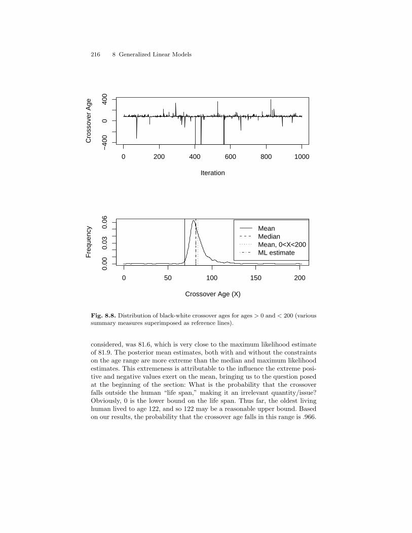
216 8 Generalized Linear Models
0 200 400 600 800 1000
−40
00
400
Iteration
Cro
ssov
er A
ge
0 50 100 150 200
0.00
0.03
0.06
Crossover Age (X)
Fre
quen
cy MeanMedianMean, 0<X<200ML estimate
Fig. 8.8. Distribution of black-white crossover ages for ages > 0 and < 200 (varioussummary measures superimposed as reference lines).
considered, was 81.6, which is very close to the maximum likelihood estimateof 81.9. The posterior mean estimates, both with and without the constraintson the age range are more extreme than the median and maximum likelihoodestimates. This extremeness is attributable to the influence the extreme posi-tive and negative values exert on the mean, bringing us to the question posedat the beginning of the section: What is the probability that the crossoverfalls outside the human “life span,” making it an irrelevant quantity/issue?Obviously, 0 is the lower bound on the life span. Thus far, the oldest livinghuman lived to age 122, and so 122 may be a reasonable upper bound. Basedon our results, the probability that the crossover age falls in this range is .966.
8.2 The ordinal probit model 217
The probability that the crossover age is negative is .011; the probability thatthe crossover age is greater than 122 is .023. These results suggest that thecrossover most likely occurs during the life span.
As an alternative to using 122 as the upper boundary, we may considerlife expectancy at birth to be a more reasonable upper bound, given that itrepresents (in theory) an age around which most deaths cluster in a popu-lation.5 Life expectancy at birth is approximately 78. The probability thatthe crossover occurs before this age (but after age 0!) is: .258, a relativelysmall probability. However, research has argued that the crossover is an arti-fact of within-population heterogeneity in mortality rates (Lynch, Brown, andHarmsen 2003), and thus, we may not expect the crossover to occur until afterhalf the population has died. Approximately half of individuals born todaycan expect to live to age 80, and so we may consider the probability that thecrossover age falls between 80 and 100, the age at which only approximately1-2% of the population remains alive. Thus, if the crossover occurs after thisage, it has little substantive importance. The probability that the crossoverage falls between 80 and 100 is .506.
In addition to these specific probabilities, we may consider constructingprobability intervals for the crossover age. A 95% probability interval for thecrossover age is [57.1,120.2], and a 90% interval is [72.1,108.0]. All of theseresults taken together provide a much more detailed summary of the crossoverage than the maximum likelihood approach can offer. Substantively, fromthese results, we might conclude that the crossover exists and that it occurswithin the normal life span of individuals within a population.6
8.2 The ordinal probit model
The dichotomous probit model is easily generalizable in the event our outcomevariable is ordinal rather than dichotomous. In the event the outcome variableis ordinal with numerous categories (e.g., more than five), we may consider anOLS regression model. However, by definition ordinal variables have rankableoutcome categories with unequal spacing between categories, which makesOLS regression theoretically inappropriate. For example, in health research,a four-category self-rated health measure—with categories Excellent, Good,Fair, and Poor—is a commonly used outcome variable. Although the order ofthe categories reflects an unmistakable progression from best health to worst5 Technically, it is the expected value for the age of death distribution, but in most
modern societies, deaths increasingly cluster around this point.6 In all fairness, a key reason the crossover is assumed not to exist is that it is an
artifact of age misreporting among older persons (see Elo and Preston 1994). Agemisreporting is less problematic in a longitudinal study in which most individualsare observed at a younger age than we typically expect to find such misreporting.Nonetheless, we cannot easily control for such measurement error with the modelwe have used.

218 8 Generalized Linear Models
health, the interval between, say, Excellent and Good is not necessarily com-parable with the interval between Fair and Poor. Thus, OLS regression, whichrequires an interval level outcome, is an inappropriate model. Nonetheless, asthe number of categories increases—and thus the interval width between anytwo categories shrinks—the difference between interval widths may becomenegligible and potentialize the legitimate use of OLS regression. We will con-sider this possibility in the example.
8.2.1 Model development and parameter interpretation
Whereas the likelihood function for the dichotomous probit model relied onthe binomial distribution, the likelihood function for the ordinal probit modelrelies on the multinomial distribution. As we discussed in Chapter 2, themultinomial distribution is simply an extension of the binomial distributionfor the case in which there are multiple p parameters being modeled ratherthan simply one. Thus, the likelihood function for the ordinal probit modelis:
L(P |Y ) ∝n∏
i=1
J∏j=1
pI(yi=j)ij
. (8.11)
This representation may at first appear confusing, but it is a straightfor-ward extension of the binomial likelihood function in Equation 8.1. First, inthe ordinal probit case, p is replaced by P to represent the fact that we arenow dealing with more than simply the probability of an individual falling inone category versus its complement (e.g., Healthy versus Not): Now we havemultiple possible categories (e.g., Excellent health, Good health, Fair health,Poor health). Second, we have two product symbols. The first constructs thejoint sampling density for all individuals in the sample, just as the productin the binomial likelihood. The second is an extension to handle the fact thatwe now have J outcome categories rather than two. In the binomial likeli-hood function, a given individual’s contribution is pyi
i (1 − pi)1−yi , where pi
represents the probability the individual registers a “1” (versus a 0) on theoutcome. An individual who registers a “1” ends up only contributing the for-mer term, whereas an individual who registers a “0” ends up only contributingthe latter term. In the multinomial version, the individual’s contribution isp
I(yi=1)i1 p
I(yi=2)i2 . . . p
I(yi=J)iJ , where I(yi = j) is an indicator function indicat-
ing that the individual’s response is in category j. Thus, the individual onlyultimately contributes one term to the likelihood (all others drop, because theindicator function takes a value of 0).
How do we incorporate the regression parameters (and X) into this model?As before, the pij correspond to integrals of the standard normal distribution.Consider the latent variable approach discussed above. If we assume onceagain that a latent variable y∗i underlies our observed ordinal measure, thenwe can expand the link equation presented earlier (see Equation 8.3) to:
8.2 The ordinal probit model 219
yi =
1 iff −∞ = τ1 ≤ y∗i < τ2
2 iff τ2 ≤ y∗i < τ3
...k iff τk ≤ y∗i < τk+1 = ∞.
(8.12)
Figure 8.9 presents a graphic depiction of the process outlined in the equa-tion. The latent distribution (y∗) is divided by thresholds (τ), with individuals’observed values of y determined by the location of their y∗ and the placementof the thresholds. For example, an individual whose value of y∗ is small enoughto fall between τ1 and τ2 will respond “1” to the measured item.7
As before, the link equation, given a distributional specification for theerror term, implies an integral over the error distribution, but now the integralis bounded by thresholds that divide the latent y∗ into the observed ordinal“bins”:
p(yi = j) = P (τj−1 −XTi β < ei < τj −XT
i β) =∫ τj−XT
i β
τj−1−XTi β
N(0, 1). (8.13)
This result allows us to write the likelihood more succinctly as:
L(β, τ |y) ∝n∏
i=1
∫ τyi−XT
i β
τyi−1−XTi β
N(0, 1) ≡n∏
i=1
Φ(τyi−XT
i β)− Φ(τyi−1 −XTi β).
(8.14)To make the model fully Bayesian, we simply need to specify priors for theregression parameters and thresholds. Once again, I opt to use improper uni-form priors for all parameters, and so the posterior distribution is proportionalto the likelihood.
The interpretation of parameters from this model poses the same difficul-ties as described in the previous section. The metric for the coefficients inthe ordinal probit model, just as in the dichotomous probit model, is the zscale, and thus the interpretation of the effect of the parameters is in terms ofshifting the z score for an individual up or down β units for each unit increasein the corresponding variable. Alternative interpretations in terms of deter-mining the probability an individual falls in a particular category—or in aparticular category or higher—can be derived (see Johnson and Albert 1999),although interest generally centers simply on the sign, relative magnitude, andstatistical significance of the coefficient.
As with the dichotomous logistic regression model, an ordinal logistic re-gression model coefficient can be exponentiated to reflect the change in the
7 Although many texts begin their threshold subscripts at 0, I begin the thresholdnumbering at 1 for ease of translation into R, which does not allow 0 subscripts.
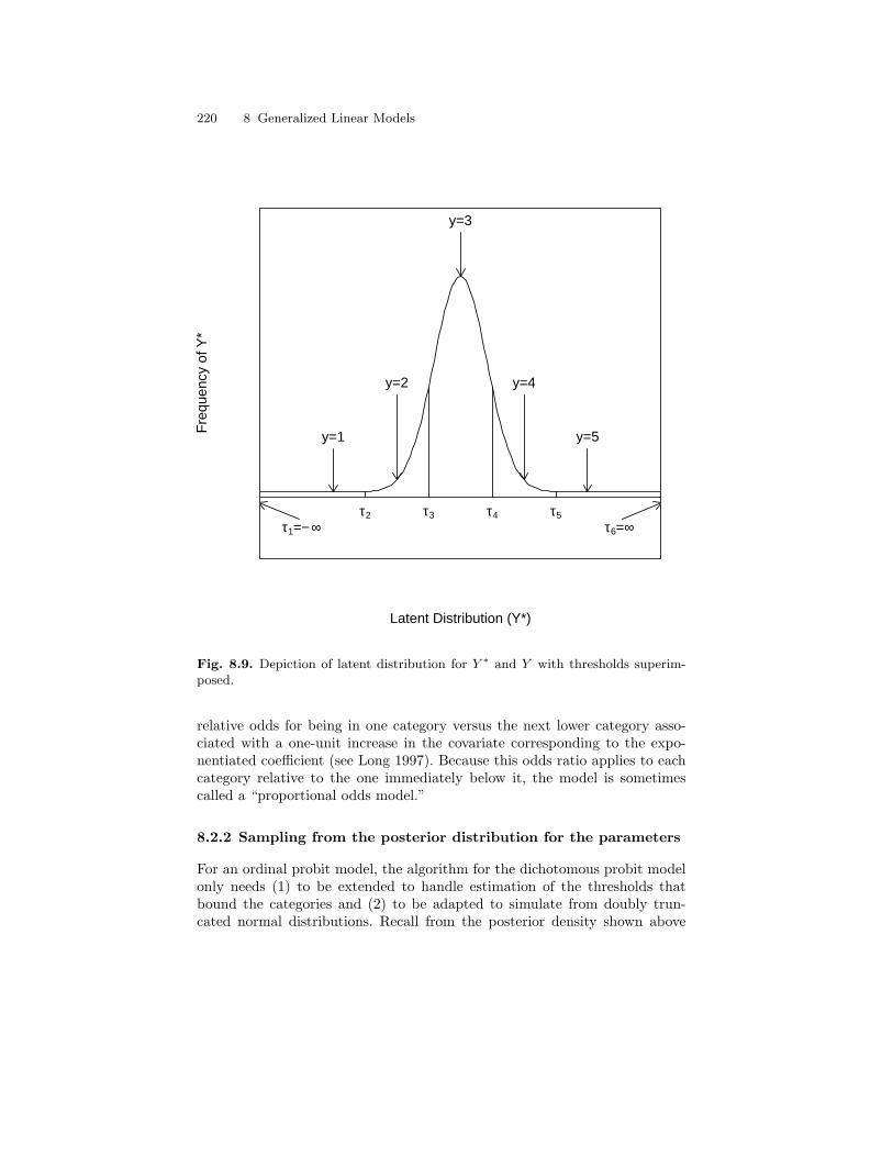
220 8 Generalized Linear Models
Latent Distribution (Y*)
Fre
quen
cy o
f Y*
τ1=− ∞τ2 τ3 τ4 τ5
τ6=∞
y=1
y=2
y=3
y=4
y=5
Fig. 8.9. Depiction of latent distribution for Y ∗ and Y with thresholds superim-posed.
relative odds for being in one category versus the next lower category asso-ciated with a one-unit increase in the covariate corresponding to the expo-nentiated coefficient (see Long 1997). Because this odds ratio applies to eachcategory relative to the one immediately below it, the model is sometimescalled a “proportional odds model.”
8.2.2 Sampling from the posterior distribution for the parameters
For an ordinal probit model, the algorithm for the dichotomous probit modelonly needs (1) to be extended to handle estimation of the thresholds thatbound the categories and (2) to be adapted to simulate from doubly trun-cated normal distributions. Recall from the posterior density shown above
8.2 The ordinal probit model 221
that the parameters of the model include not only the regression coefficients,but also the category thresholds that “slice up” the latent distribution intothe observed ordinal bins. In the dichotomous probit model, we fixed the solethreshold at 0. This constraint is necessary for the intercept to be identified;if the threshold is allowed to vary, the intercept can simply change withoutaffecting the likelihood. In the ordinal probit model, we need to constrain onethreshold parameter, but we can estimate the remainder of them (but seeJohnson and Albert, 1999, who discuss using a proper prior on the thresh-olds to allow estimation of all of them). Thus, our Gibbs sampling algorithmmust be extended to include simulating the thresholds from their conditionalposterior distribution. Assuming uniform priors for the thresholds, the con-ditional distribution for threshold j is a uniform distribution on the intervalbetween the maximum latent propensity (Y ∗) drawn for an individual in cat-egory j − 1 and the minimum latent propensity drawn for an individual incategory j. Thus, the algorithm is extended as:
1. Establish starting values for all parameters. Now the parameter vectoralso includes thresholds, which need some reasonable starting values. Asimple approach to obtaining starting values for threshold j is to use theinverse normal cumulative distribution function (CDF) for the proportionof observations in category j or below.
2. Sample latent propensities (Y ∗) from truncated normal distributions.Whereas with the dichotomous probit in which the propensities were sam-pled from above 0 if the response was a 1 and below 0 if the response wasa 0, the truncation points in the ordinal probit model are the thresholdsthat bound the ordinal category in which the response falls.
3. Sample threshold j(∀j) from uniform densities on the interval [max(y :y ∈ j − 1),min(y : y ∈ j)].
4. Sample regression coefficients from their conditional distribution: β ∼(X ′X)−1(X ′Y ∗).
5. Repeat until enough draws are obtained.
Notice that the only two differences between this algorithm and the onefor the dichotomous probit model are (1) the inclusion of the step in whichthe thresholds are sampled, and (2) the sampling of the latent propensitiesfrom doubly truncated normal distributions implied by the introduction ofadditional thresholds.
Sampling from doubly-truncated normal distributions using the inversionmethod requires relatively little change from the inversion method discussedin the previous section. In the polytomous case, we need to renormalize thearea between thresholds rather than simply computing the area from −∞ to0 or from 0 to ∞. Thus, determining the bounded area requires two calls tothe function that computes Φ. To sample from a particular category k theappropriate renormalized density is:
z[τk,τk+1] ∼ Φ−1 [u (Φ(τk+1)− Φ(τk)) + Φ(τk)] , (8.15)
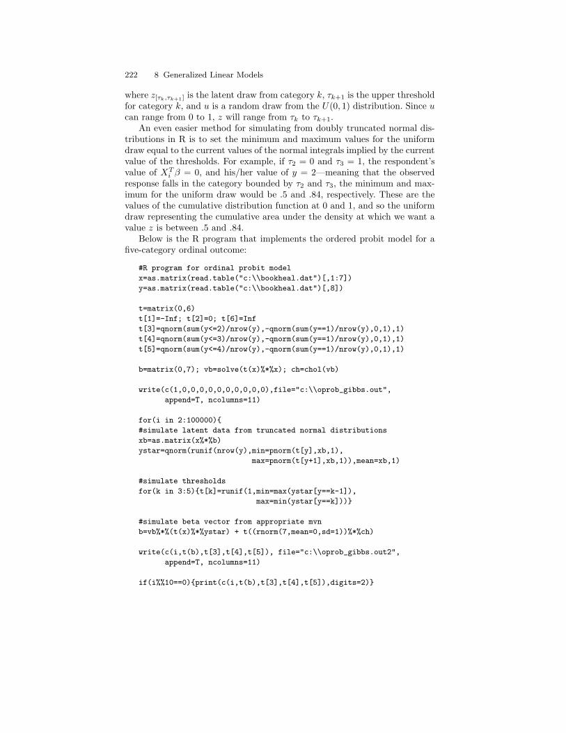
222 8 Generalized Linear Models
where z[τk,τk+1] is the latent draw from category k, τk+1 is the upper thresholdfor category k, and u is a random draw from the U(0, 1) distribution. Since ucan range from 0 to 1, z will range from τk to τk+1.
An even easier method for simulating from doubly truncated normal dis-tributions in R is to set the minimum and maximum values for the uniformdraw equal to the current values of the normal integrals implied by the currentvalue of the thresholds. For example, if τ2 = 0 and τ3 = 1, the respondent’svalue of XT
i β = 0, and his/her value of y = 2—meaning that the observedresponse falls in the category bounded by τ2 and τ3, the minimum and max-imum for the uniform draw would be .5 and .84, respectively. These are thevalues of the cumulative distribution function at 0 and 1, and so the uniformdraw representing the cumulative area under the density at which we want avalue z is between .5 and .84.
Below is the R program that implements the ordered probit model for afive-category ordinal outcome:
#R program for ordinal probit model
x=as.matrix(read.table("c:\\bookheal.dat")[,1:7])
y=as.matrix(read.table("c:\\bookheal.dat")[,8])
t=matrix(0,6)
t[1]=-Inf; t[2]=0; t[6]=Inf
t[3]=qnorm(sum(y<=2)/nrow(y),-qnorm(sum(y==1)/nrow(y),0,1),1)
t[4]=qnorm(sum(y<=3)/nrow(y),-qnorm(sum(y==1)/nrow(y),0,1),1)
t[5]=qnorm(sum(y<=4)/nrow(y),-qnorm(sum(y==1)/nrow(y),0,1),1)
b=matrix(0,7); vb=solve(t(x)%*%x); ch=chol(vb)
write(c(1,0,0,0,0,0,0,0,0,0,0),file="c:\\oprob_gibbs.out",
append=T, ncolumns=11)
for(i in 2:100000)
#simulate latent data from truncated normal distributions
xb=as.matrix(x%*%b)
ystar=qnorm(runif(nrow(y),min=pnorm(t[y],xb,1),
max=pnorm(t[y+1],xb,1)),mean=xb,1)
#simulate thresholds
for(k in 3:5)t[k]=runif(1,min=max(ystar[y==k-1]),
max=min(ystar[y==k]))
#simulate beta vector from appropriate mvn
b=vb%*%(t(x)%*%ystar) + t((rnorm(7,mean=0,sd=1))%*%ch)
write(c(i,t(b),t[3],t[4],t[5]), file="c:\\oprob_gibbs.out2",
append=T, ncolumns=11)
if(i%%10==0)print(c(i,t(b),t[3],t[4],t[5]),digits=2)
8.2 The ordinal probit model 223
The program follows the same general structure as the one for the di-chotomous probit model. First, the data are read from the file, variables aredefined and initiated, and the starting values for all parameters are writtento the output file. Notice that there are six thresholds defined. The first andlast are set to +∞ and −∞, respectively, and the second threshold is set to0 to identify the model. The remaining three thresholds are initialized basedon the proportion of the sample falling in each category of the outcome. Themean argument to the qnorm function is -qnorm(sum(y==1)/nrow(y),0,1)because the normal distribution must be shifted so that the proportion ofcases falling below the second threshold of 0 is equal to the proportion ofindividuals who fall in the first category of the outcome variable.
After all variables are initialized, the Gibbs sampler begins. First, giventhe current values of the regression parameters and thresholds, latent dataare simulated to replace the observed ordinal outcome. As we did in the di-chotomous probit model program, we make use of R’s ability to handle entirevectors simultaneously, and so the latent data simulation is performed in onestep. Notice that I use the second method for simulating from the doublytruncated normal distribution: The minimum and maximum values for thelatent data for an individual are determined by applying the qnorm functionto the thresholds that bound the observed response.
Once the latent data have been simulated, the three free thresholds aresimulated from uniform distributions on the interval between the largest latentvalue simulated for the category below the threshold and the smallest latentvalue simulated for the category above the threshold. Finally, given a completeset of latent data, the regression parameters are simulated as before.
8.2.3 Ordinal probit model example: Black–white differences inhealth
For an example of the ordinal probit model, I extend the example in the pre-vious section using self-rated health as the outcome measure. Additionally,rather than using a person-year file, I use only the 1992 wave of the study.I ran the Gibbs sampler above several times for 100,000 iterations each timeusing different starting values for the threshold parameters. Although therewas no need to run the Gibbs sampler for so many iterations, the algorithmis extremely fast, and thus there is little cost to doing so. The results of thethree runs suggested that the regression parameters converged quickly, butthe threshold parameters converged slowly. Figure 8.10 shows trace plots ofthe three estimated threshold parameters from the first run of the algorithmin which the thresholds were initialized at values that were higher than theyshould be. As the figure indicates, the threshold parameters did not convergeuntil after 20,000 or so iterations. Slow convergence—and mixing—of thresh-old parameters occurs when the sample size is large enough that the minimum
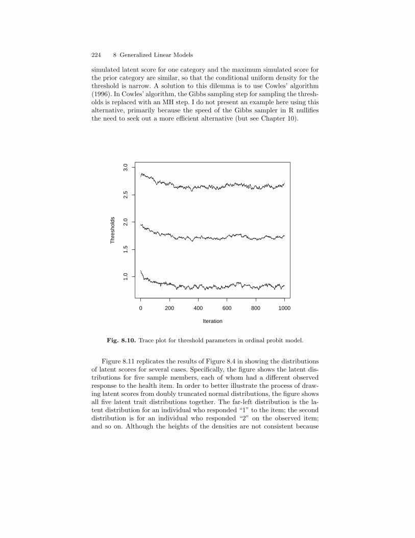
224 8 Generalized Linear Models
simulated latent score for one category and the maximum simulated score forthe prior category are similar, so that the conditional uniform density for thethreshold is narrow. A solution to this dilemma is to use Cowles’ algorithm(1996). In Cowles’ algorithm, the Gibbs sampling step for sampling the thresh-olds is replaced with an MH step. I do not present an example here using thisalternative, primarily because the speed of the Gibbs sampler in R nullifiesthe need to seek out a more efficient alternative (but see Chapter 10).
0 200 400 600 800 1000
1.0
1.5
2.0
2.5
3.0
Iteration
Thr
esho
lds
Fig. 8.10. Trace plot for threshold parameters in ordinal probit model.
Figure 8.11 replicates the results of Figure 8.4 in showing the distributionsof latent scores for several cases. Specifically, the figure shows the latent dis-tributions for five sample members, each of whom had a different observedresponse to the health item. In order to better illustrate the process of draw-ing latent scores from doubly truncated normal distributions, the figure showsall five latent trait distributions together. The far-left distribution is the la-tent distribution for an individual who responded “1” to the item; the seconddistribution is for an individual who responded “2” on the observed item;and so on. Although the heights of the densities are not consistent because
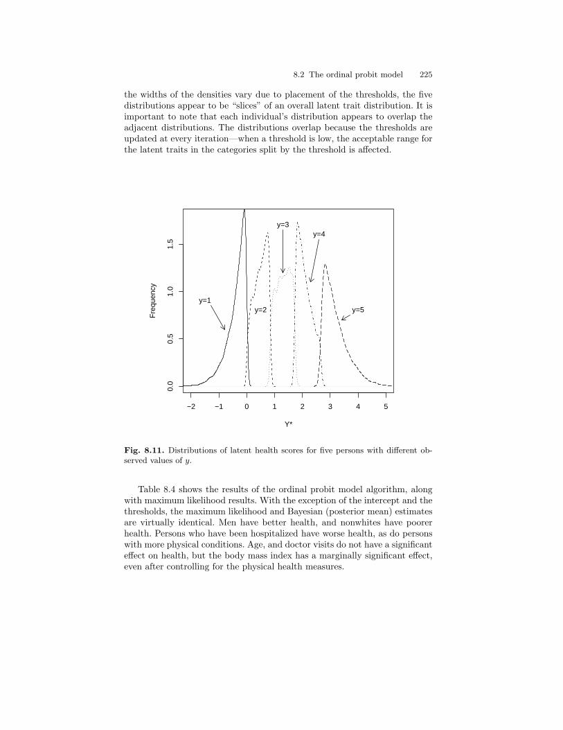
8.2 The ordinal probit model 225
the widths of the densities vary due to placement of the thresholds, the fivedistributions appear to be “slices” of an overall latent trait distribution. It isimportant to note that each individual’s distribution appears to overlap theadjacent distributions. The distributions overlap because the thresholds areupdated at every iteration—when a threshold is low, the acceptable range forthe latent traits in the categories split by the threshold is affected.
−2 −1 0 1 2 3 4 5
0.0
0.5
1.0
1.5
Y*
Fre
quen
cy
y=1y=2
y=3y=4
y=5
Fig. 8.11. Distributions of latent health scores for five persons with different ob-served values of y.
Table 8.4 shows the results of the ordinal probit model algorithm, alongwith maximum likelihood results. With the exception of the intercept and thethresholds, the maximum likelihood and Bayesian (posterior mean) estimatesare virtually identical. Men have better health, and nonwhites have poorerhealth. Persons who have been hospitalized have worse health, as do personswith more physical conditions. Age, and doctor visits do not have a significanteffect on health, but the body mass index has a marginally significant effect,even after controlling for the physical health measures.
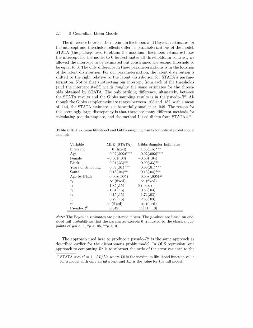
226 8 Generalized Linear Models
The difference between the maximum likelihood and Bayesian estimates forthe intercept and thresholds reflects different parameterizations of the model.STATA (the package used to obtain the maximum likelihood estimates) fixesthe intercept for the model to 0 but estimates all thresholds. In contrast, weallowed the intercept to be estimated but constrained the second threshold tobe equal to 0. The only difference in these parameterizations is in the locationof the latent distribution: For our parameterization, the latent distribution isshifted to the right relative to the latent distribution for STATA’s parame-terization. Notice that subtracting our intercept from each of the thresholds(and the intercept itself) yields roughly the same estimates for the thresh-olds obtained by STATA. The only striking difference, ultimately, betweenthe STATA results and the Gibbs sampling results is in the psuedo-R2. Al-though the Gibbs sampler estimate ranges between .105 and .182, with a meanof .144, the STATA estimate is substantially smaller at .049. The reason forthis seemingly large discrepancy is that there are many different methods forcalculating pseudo-r-square, and the method I used differs from STATA’s.8
Table 8.4. Maximum likelihood and Gibbs sampling results for ordinal probit modelexample.
Variable MLE (STATA) Gibbs Sampler Estimates
Intercept 0 (fixed) 1.86(.15)***Age −0.02(.002)*** −0.02(.002)***Female −0.001(.03) −0.001(.04)Black −0.91(.33)** −0.90(.33)**Years of Schooling 0.09(.01)*** 0.09(.01)***South −0.13(.04)** −0.13(.04)***Age-by-Black 0.008(.005) 0.008(.005)#τ1 −∞ (fixed) −∞ (fixed)τ2 −1.85(.15) 0 (fixed)τ3 −1.04(.15) 0.83(.03)τ4 −0.15(.15) 1.72(.03)τ5 0.79(.15) 2.65(.03)τ6 ∞ (fixed) −∞ (fixed)Pseudo-R2 0.049 .14[.11, .18]
Note: The Bayesian estimates are posterior means. The p-values are based on one-sided tail probabilities that the parameter exceeds 0 truncated to the classical cut-points of #p < .1, *p < .05, **p < .01.
The approach used here to produce a pseudo-R2 is the same approach asdescribed earlier for the dichotomous probit model. In OLS regression, oneapproach to computing R2 is to subtract the ratio of the error variance to the8 STATA uses r2 = 1−LL/L0, where L0 is the maximum likelihood function value
for a model with only an intercept and LL is the value for the full model.
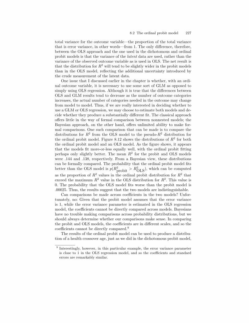
8.2 The ordinal probit model 227
total variance for the outcome variable—the proportion of the total variancethat is error variance, in other words—from 1. The only difference, therefore,between the OLS approach and the one used in the dichotomous and ordinalprobit models is that the variance of the latent data are used, rather than thevariance of the observed outcome variable as is used in OLS. The net result isthat the distribution for R2 will tend to be slightly wider in the probit modelsthan in the OLS model, reflecting the additional uncertainty introduced bythe crude measurement of the latent data.
One issue that I discussed earlier in the chapter is whether, with an ordi-nal outcome variable, it is necessary to use some sort of GLM as opposed tosimply using OLS regression. Although it is true that the differences betweenOLS and GLM results tend to decrease as the number of outcome categoriesincreases, the actual number of categories needed in the outcome may changefrom model to model. Thus, if we are really interested in deciding whether touse a GLM or OLS regression, we may choose to estimate both models and de-cide whether they produce a substantially different fit. The classical approachoffers little in the way of formal comparison between nonnested models; theBayesian approach, on the other hand, offers unlimited ability to make for-mal comparisons. One such comparison that can be made is to compare thedistributions for R2 from the OLS model to the pseudo-R2 distribution forthe ordinal probit model. Figure 8.12 shows the distributions of R2 for boththe ordinal probit model and an OLS model. As the figure shows, it appearsthat the models fit more-or-less equally well, with the ordinal probit fittingperhaps only slightly better. The mean R2 for the probit and OLS modelswere .144 and .138, respectively. From a Bayesian view, these distributionscan be formally compared. The probability that the ordinal probit model fitsbetter than the OLS model is p(R2
probit > R2OLS), which can be computed
as the proportion of R2 values in the ordinal probit distribution for R2 thatexceed the maximum R2 value in the OLS distribution for R2. This value is0. The probability that the OLS model fits worse than the probit model is.00025. Thus, the results suggest that the two models are indistinguishable.
Can comparisons be made across coefficients in the two models? Unfor-tunately, no: Given that the probit model assumes that the error varianceis 1, while the error variance parameter is estimated in the OLS regressionmodel, the coefficients cannot be directly compared across models. Bayesianshave no trouble making comparisons across probability distributions, but weshould always determine whether our comparisons make sense. In comparingthe probit and OLS models, the coefficients are in different scales, and so thecoefficients cannot be directly compared.9
The results of the ordinal probit model can be used to produce a distribu-tion of a health crossover age, just as we did in the dichotomous probit model,
9 Interestingly, however, in this particular example, the error variance parameteris close to 1 in the OLS regression model, and so the coefficients and standarderrors are remarkably similar.
228 8 Generalized Linear Models
0.05 0.10 0.15 0.20
05
1015
20
R−Square
Fre
quen
cyOLSProbit
Fig. 8.12. Distributions of R2 and pseudo-R2 from OLS and probit models, respec-tively.
using the distributions for the “black” parameter and the age-by-black inter-action parameter. Table 8.5 provides a number of summaries for the healthcrossover age. The central age (mean or median) for the health crossover issubstantially higher than the mortality crossover age. In fact, the various sum-mary measures suggest that there is a low probability that a health crossoveroccurs during the normal human life span. Taken together, the results of thedichotomous probit and ordinal probit models indicate that, although mor-tality rates for blacks fall below those for whites in later life, blacks havepoorer health at all ages. A stronger approach to reaching this conclusionwould require a model that simultaneously considers health and mortality—amultivariate model. Multivariate models are the subject of Chapter 10.
8.3 Conclusions
In this chapter we have covered two commonly used generalized linearmodels—the dichotomous probit model and the ordinal probit model. For

8.4 Exercises 229
Table 8.5. Various summary measures for the black-white health crossover age.
Description of Summary Measure Summary (Age)
Maximum Likelihood estimate of crossover age 113.8Posterior Mean (all values) 157.7Posterior Median (all values included) 112.2Posterior Mean (of values 0-200) 117.195% Interval [-236.0, 680.0]90% Interval [75.7, 370.6]p(0 < Age < 200) .831p(0 < Age < 120) .535p(0 < Age < 78) .003p(80 < Age < 100) .264
each model, we discussed a single Gibbs sampler. A key difference betweenthese samplers and that for the linear regression model in the last chapter isthe need to sample latent data from truncated normal distributions. Thus, wediscussed three strategies for performing such simulation.
We also spent considerable time in this chapter demonstrating how to makeuse of the Gibbs sampler to generate samples from distributions of quantitiesnot directly included in the model (e.g., the crossover age), as well as howto perform basic residual analyses in the probit model. We will continue dis-cussing the benefits of the Bayesian approach in the remaining two chapters,but in the next chapter—which covers hierarchical modeling—we will pri-marily focus on the ease with which the Bayesian approach can incorporatehierarchical structure to the data and model.
8.4 Exercises
1. Develop an MH algorithm for the dichotomous probit model.2. Develop a rejection sampler for simulating from a truncated normal dis-
tribution using a triangular density, rather than a uniform density, asdiscussed in Section 8.1.3.
3. Starting with the Gibbs sampler shown earlier for the dichotomous probitmodel, modify it to make it a hybridized Gibbs-MH algorithm. That is,continue to sample the latent data at each iteration (a Gibbs samplingstep), but update the parameters using MH steps.
4. Write an algorithm to estimate the parameters in the dichotomous probitmodel using the binomial likelihood function-with link function. The like-lihood function will contain normal integrals. Compare results betweenthis algorithm and the Gibbs sampler. Are there any differences in thespeed of convergence? Are the parameter estimates and standard errorscomparable?

230 8 Generalized Linear Models
5. Construct an MH algorithm to estimate the parameters in the ordinalprobit model.
6. There are several alternative methods for calculating pseudo-R2 values inGLMs. One such approach in a dichotomous probit model is to constructa two-by-two table of observed and predicted outcomes, where individualswith Xβ > 0 assigned to have a predicted score of “1” (otherwise theyreceive a predicted score of “0”). The R2 is then simply the proportionof correctly classified individuals. Under a Bayesian approach, we wouldobtain multiple values for β and, hence, multiple possible R2 values. Per-form this process and compare the result with what is obtained usingthe method I described in the chapter. How does the distribution of theoutcome variable influence the difference between these two types of R2s?
7. Develop a strategy for handling missing data in the probit model (dichoto-mous or ordinal). Assume the data are MAR.
9
Introduction to Hierarchical Models
One of the important features of a Bayesian approach is the relative easewith which hierarchical models can be constructed and estimated using Gibbssampling. In fact, one of the key reasons for the recent growth in the use ofBayesian methods in the social sciences is that the use of hierarchical modelshas also increased dramatically in the last two decades.
Hierarchical models serve two purposes. One purpose is methodological;the other is substantive. Methodologically, when units of analysis are drawnfrom clusters within a population (communities, neighborhoods, city blocks,etc.), they can no longer be considered independent. Individuals who comefrom the same cluster will be more similar to each other than they will beto individuals from other clusters. Therefore, unobserved variables may in-duce statistical dependence between observations within clusters that maybe uncaptured by covariates within the model, violating a key assumptionof maximum likelihood estimation as it is typically conducted when indepen-dence of errors is assumed. Recall that a likelihood function, when observationsare independent, is simply the product of the density functions for each ob-servation taken over all the observations. However, when independence doesnot hold, we cannot construct the likelihood as simply. Thus, one reason forconstructing hierarchical models is to compensate for the biases—largely inthe standard errors—that are introduced when the independence assumptionis violated. See Ezell, Land, and Cohen (2003) for a thorough review of theapproaches that have been used to correct standard errors in hazard model-ing applications with repeated events, one class of models in which repeatedmeasurement yields hierarchical clustering.
In addition to the methodological need for hierarchical models, substan-tively we may believe that there are differences in how predictors in a regres-sion model influence an outcome of interest across clusters, and we may wishto model these differences. In other words, the influence of predictors maybe context-dependent, a notion that is extremely important and relevant to asocial scientific—especially sociological—understanding of the world. For ex-ample, the emergence of hierarchical modeling in education research occurred
232 9 Introduction to Hierarchical Models
because there is a natural nesting of students within classes (and classes withinschools, schools within communities, and so on), and grades, test performance,etc. may be dependent on teacher quality, making students in one class dif-ferent from those in another class. In other words, student performance maybe dependent on the teacher—the environmental context of classes.
In this chapter, I discuss simple hierarchical models in general as well as hi-erarchical linear regression models. I conclude the chapter with a brief discus-sion of terminological issues that make hierarchical modeling seem mysteriousand complicated. I recommend Gelman et al. (1995) for an in-depth exposi-tion of the Bayesian approach to a variety of hierarchical models, both thesimple hierarchical models discussed in the next section as well as hierarchicalregression models discussed later in the chapter. I recommend Raudenbushand Bryk (2002) and Snijders and Bosker (1999) for thorough coverage of theclassical approach to hiearchical linear regression models.
9.1 Hierarchical models in general
Hierarchical models are models in which there is some sort of hierarchicalstructure to the parameters and potentially to the covariates if the model isa regression model. I begin by discussing the simpler case in which the modelof interest is not a regression model with covariates, but rather is simplyhierarchical in the parameters.
Recall that Bayes’ Theorem is often expressed as:
p(θ | data)︸ ︷︷ ︸ ∝ p(data | θ)︸ ︷︷ ︸ × p(θ)︸︷︷︸posterior ∝ likelihood × prior
This equation itself reveals a simple hierarchical structure in the parameters,because it says that a posterior distribution for a parameter is equal to aconditional distribution for data under the parameter (first level) multipliedby the marginal (prior) probability for the parameter (a second, higher, level).Put another way, the posterior distribution is the prior distribution weightedby the observed information.
This hierarchical structure of the parameters need not stop at one higherlevel; instead, the conditioning structure in theory can continue ad infini-tum. For instance, suppose we have a model that contains an added layerof hierarchy. Suppose we have J observations within each of G groups:y11, . . . , yJ1, y12, . . . , yJ2, . . . , y1G, . . . , yJG, and we assume that the data aredistributed within groups according to some distribution Q with parameterθ, but that each group has its own parameter (θg). Thus:
yig ∼ Q(θg).
9.1 Hierarchical models in general 233
Suppose we assume further that these parameters θg arise from a common dis-tribution W with parameter γ (this parameter is called a “hyperparameter”).So:
θg ∼ W (γ).
Finally, assume γ has some vague distribution like a uniform:
γ ∼ U(−100, 100).
A posterior distribution for all unknown parameters would then be (aftersubstituting the densities Q and W into the conditional structure below):
p(γ, θ|y) ∝ p(y | θ, γ)p(θ | γ)p(γ).
To see how this hierarchical structure “works,” notice that the last two termshere [p(θ | γ)p(γ)], when multiplied together, yield a joint distribution for γand θ [p(θ , γ)]. Thus, we are left with a marginal joint distribution for thetwo parameters, which is then multiplied by a sampling density for the data[p(y | θ , γ)]. Bayes’ theorem tells us that the multiple of this marginal jointdensity for the parameters and the sampling density for the data, given theparameters, yields a posterior density for all of the parameters.
Ultimately we might not be interested much in the posterior distributionsfor the group level parameters (θg), but rather in the posterior distributionfor the hyperparameter γ that structures the distribution of the group levelparameters. In other words, we may be interested only in the marginal distri-bution for γ:
p(γ|y) ∝∫
p(y|θ, γ)p(θ|γ)p(γ)dθ.
As we have discussed throughout the last several chapters, this integration isperformed stochastically via MCMC methods as we sample from the condi-tional posterior distributions for each parameter.
This result demonstrates the simplicity with which a Bayesian approachcan handle hierarchical structure in data or parameters. We could very easily,if desired, add subsequent layers to the structure, and we can also break eachlayer of the structure into regression components.
9.1.1 The voting example redux
In Chapter 3, I illustrated Bayes’ Theorem with a voting example from 2004pre-election polls. In that example, we considered the posterior probabilitythat Kerry would win the election in Ohio using the most recent poll asthe current data and data from three previous polls as prior information.We assumed a binomial likelihood function/sampling density for the currentpolling data (x) given the proportion of voters who would vote for Kerry (K),
234 9 Introduction to Hierarchical Models
and we used a beta distribution as the prior for K, with the number of votesfor Kerry and Bush in the previous polls being represented by the parametersα and β, respectively. To summarize, our posterior density was:
p(K|α, β, X) ∝ K556(1−K)511︸ ︷︷ ︸ K941(1−K)1007︸ ︷︷ ︸ .
current data previous poll data(likelihood) (prior)
In the original example I noted that, although the four polls we usedappeared to show some trending, complete data from all available polls fromvarious polling organizations did not suggest any trending, justifying our com-bination of the previous pollng data into a single prior distribution for α andβ. As an alternative approach, without trending, the polls could be consideredas separate samples drawn from the same population, each one providing con-ditionally independent information regarding the parameters α and β. In thatcase, we could consider that each poll’s results were the result of a unique,poll-specific parameter Ki, with the Ki being random realizations from thebeta distribution with hyperparameters α and β. This approach recasts thevoting example as a hierarchical model with the following structure:
p(α, β, K|X) ∝ p(X|K)︸ ︷︷ ︸ p(K|α, β)︸ ︷︷ ︸ p(α, β)︸ ︷︷ ︸ .
likelihood prior hyperprior
Here, and throughout the remainder of the chapter, I suppress notation inthe conditional distributions when a particular quantity does not directlydepend on a higher level parameter. For example, the likelihood function hereultimately depends on the hyperparameters α and β; however, it only dependson these parameters through the prior for K, and so, I do not spell out thecomplete likelihood as p(X|K, α, β).
The likelihood portion of the model is the product of the sampling densitiesfor the four polls:
p(X|K) ∝4∏
i=1
Kxii (1−Ki)ni−xi .
The prior densities for each K (K1 . . .K4) are beta densities; their product isthe full prior density:
p(K|α, β) ∝4∏
i=1
(Γ (α + β)Γ (α)Γ (β)
)Kα−1
i (1−Ki)β−1.
Finally, we must establish hyperpriors for the hyperparameters α and β. How-ever, before we consider the form of the hyperprior, let’s consider the fullexpression for the posterior density:
9.1 Hierarchical models in general 235
p(α, β, K|x) ∝(∏4i=1 Kxi
i (1−Ki)ni−xi
)(∏4i=1
(Γ (α+β)
Γ (α)Γ (β)
)Kα−1
i (1−Ki)β−1)
p(α, β).
We can simplify this posterior distribution by combining like products asfollows:
p(α, β, K|x) ∝(Γ (α+β)
Γ (α)Γ (β)
)4 (∏4i=1 Kxi+α−1
i (1−Ki)ni−xi+β−1)
p(α, β).(9.1)
The key difference between the current approach and as it was presented inthe original example in Chapter 3 is that the current data were assumed tobe simply the most recent polling data, and the previous three polls werecombined and assumed to be fixed quantities representing the values of αand β. Under the current approach, in contrast, the previous polling data—rather than being treated as fixed prior information—are also considered toarise from a random process governed by the hyperparameters α and β. Whenthese parameters were assumed to be fixed, the posterior density only involvedthe single parameter K. Now, however, the full posterior involves each Ki inaddition to α and β. Before, the leading expression involving the gammafunction [Γ (α + β)/(Γ (α)Γ (β))] could be dropped as a normalizing constant,because α and β were, in fact, constant. However, under the hierarchicalapproach they are now considered random variables, and terms involving themcannot simply be dropped. Indeed, although the individual K parameters arestill of interest, interest centers primarily on α and β, which are thought tobe the population parameters governing the proportion of voters who wouldvote for Kerry and which drive each individual poll result.
A Gibbs sampling strategy, then, should involve sampling the α, β, andeach K from their conditional posterior distributions. The conditional pos-terior distributions for each K, after eliminating terms in the posterior inEquation 9.1 that do not involve them, are easily seen to be beta distribu-tions with parameters A = xi + α and B = ni − xi + β:
p(Ki|α, β, xi) ∝ Kxi+α−1i (1−Ki)ni−xi+β−1.
The conditional posterior distributions for α and β are not as simple. Con-sider the posterior for α. If we eliminate terms not involving α, the posteriorfor α is: (
Γ (α + β)Γ (α)Γ (β)
)4 4∏i=1
Kxi+α−1i p(α, β).
This posterior can be simplified considerably if we use a “trick” to allow thecombination of the exponents. If we take the log and exponentiate simultane-ously, we obtain:
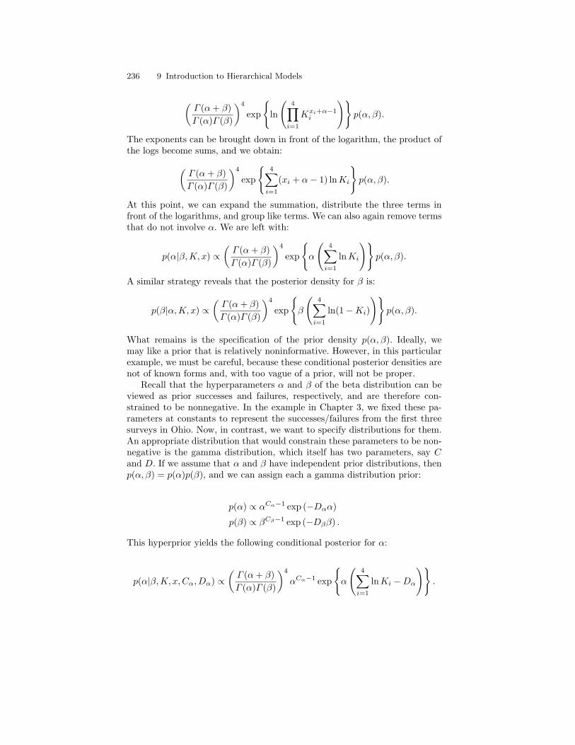
236 9 Introduction to Hierarchical Models
(Γ (α + β)Γ (α)Γ (β)
)4
exp
ln
(4∏
i=1
Kxi+α−1i
)p(α, β).
The exponents can be brought down in front of the logarithm, the product ofthe logs become sums, and we obtain:(
Γ (α + β)Γ (α)Γ (β)
)4
exp
4∑
i=1
(xi + α− 1) ln Ki
p(α, β).
At this point, we can expand the summation, distribute the three terms infront of the logarithms, and group like terms. We can also again remove termsthat do not involve α. We are left with:
p(α|β, K, x) ∝(
Γ (α + β)Γ (α)Γ (β)
)4
exp
α
(4∑
i=1
lnKi
)p(α, β).
A similar strategy reveals that the posterior density for β is:
p(β|α, K, x) ∝(
Γ (α + β)Γ (α)Γ (β)
)4
exp
β
(4∑
i=1
ln(1−Ki)
)p(α, β).
What remains is the specification of the prior density p(α, β). Ideally, wemay like a prior that is relatively noninformative. However, in this particularexample, we must be careful, because these conditional posterior densities arenot of known forms and, with too vague of a prior, will not be proper.
Recall that the hyperparameters α and β of the beta distribution can beviewed as prior successes and failures, respectively, and are therefore con-strained to be nonnegative. In the example in Chapter 3, we fixed these pa-rameters at constants to represent the successes/failures from the first threesurveys in Ohio. Now, in contrast, we want to specify distributions for them.An appropriate distribution that would constrain these parameters to be non-negative is the gamma distribution, which itself has two parameters, say Cand D. If we assume that α and β have independent prior distributions, thenp(α, β) = p(α)p(β), and we can assign each a gamma distribution prior:
p(α) ∝ αCα−1 exp (−Dαα)
p(β) ∝ βCβ−1 exp (−Dββ) .
This hyperprior yields the following conditional posterior for α:
p(α|β, K, x,Cα, Dα) ∝(
Γ (α + β)Γ (α)Γ (β)
)4
αCα−1 exp
α
(4∑
i=1
lnKi −Dα
).
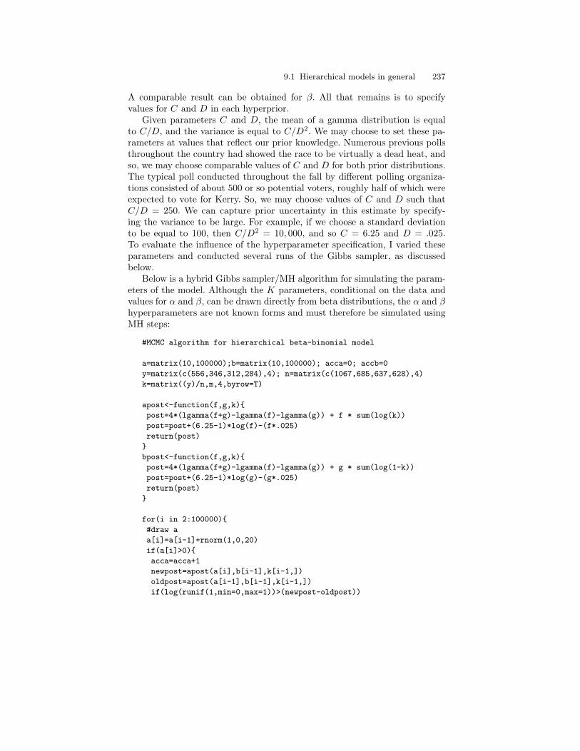
9.1 Hierarchical models in general 237
A comparable result can be obtained for β. All that remains is to specifyvalues for C and D in each hyperprior.
Given parameters C and D, the mean of a gamma distribution is equalto C/D, and the variance is equal to C/D2. We may choose to set these pa-rameters at values that reflect our prior knowledge. Numerous previous pollsthroughout the country had showed the race to be virtually a dead heat, andso, we may choose comparable values of C and D for both prior distributions.The typical poll conducted throughout the fall by different polling organiza-tions consisted of about 500 or so potential voters, roughly half of which wereexpected to vote for Kerry. So, we may choose values of C and D such thatC/D = 250. We can capture prior uncertainty in this estimate by specify-ing the variance to be large. For example, if we choose a standard deviationto be equal to 100, then C/D2 = 10, 000, and so C = 6.25 and D = .025.To evaluate the influence of the hyperparameter specification, I varied theseparameters and conducted several runs of the Gibbs sampler, as discussedbelow.
Below is a hybrid Gibbs sampler/MH algorithm for simulating the param-eters of the model. Although the K parameters, conditional on the data andvalues for α and β, can be drawn directly from beta distributions, the α and βhyperparameters are not known forms and must therefore be simulated usingMH steps:
#MCMC algorithm for hierarchical beta-binomial model
a=matrix(10,100000);b=matrix(10,100000); acca=0; accb=0
y=matrix(c(556,346,312,284),4); n=matrix(c(1067,685,637,628),4)
k=matrix((y)/n,m,4,byrow=T)
apost<-function(f,g,k)
post=4*(lgamma(f+g)-lgamma(f)-lgamma(g)) + f * sum(log(k))
post=post+(6.25-1)*log(f)-(f*.025)
return(post)
bpost<-function(f,g,k)
post=4*(lgamma(f+g)-lgamma(f)-lgamma(g)) + g * sum(log(1-k))
post=post+(6.25-1)*log(g)-(g*.025)
return(post)
for(i in 2:100000)
#draw a
a[i]=a[i-1]+rnorm(1,0,20)
if(a[i]>0)
acca=acca+1
newpost=apost(a[i],b[i-1],k[i-1,])
oldpost=apost(a[i-1],b[i-1],k[i-1,])
if(log(runif(1,min=0,max=1))>(newpost-oldpost))
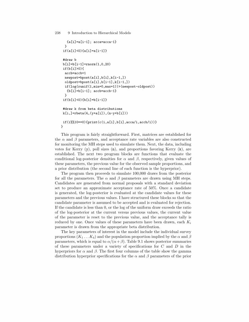
238 9 Introduction to Hierarchical Models
a[i]=a[i-1]; acca=acca-1
if(a[i]<0)a[i]=a[i-1]
#draw b
b[i]=b[i-1]+rnorm(1,0,20)
if(b[i]>0)
accb=accb+1
newpost=bpost(a[i],b[i],k[i-1,])
oldpost=bpost(a[i],b[i-1],k[i-1,])
if(log(runif(1,min=0,max=1))>(newpost-oldpost))
b[i]=b[i-1]; accb=accb-1
if(b[i]<0)b[i]=b[i-1]
#draw k from beta distributions
k[i,]=rbeta(4,(y+a[i]),(n-y+b[i]))
if(i%%10==0)print(c(i,a[i],b[i],acca/i,accb/i))
This program is fairly straightforward. First, matrices are established forthe α and β parameters, and acceptance rate variables are also constructedfor monitoring the MH steps used to simulate them. Next, the data, includingvotes for Kerry (y), poll sizes (n), and proportions favoring Kerry (k), areestablished. The next two program blocks are functions that evaluate theconditional log-posterior densities for α and β, respectively, given values ofthese parameters, the previous value for the observed sample proportions, anda prior distribution (the second line of each function is the hyperprior).
The program then proceeds to simulate 100,000 draws from the posteriorfor all the parameters. The α and β parameters are drawn using MH steps.Candidates are generated from normal proposals with a standard deviationset to produce an approximate acceptance rate of 50%. Once a candidateis generated, the log-posterior is evaluated at the candidate values for theseparameters and the previous values. I have structured these blocks so that thecandidate parameter is assumed to be accepted and is evaluated for rejection.If the candidate is less than 0, or the log of the uniform draw exceeds the ratioof the log-posterior at the current versus previous values, the current valueof the parameter is reset to the previous value, and the acceptance tally isreduced by one. Once values of these parameters have been drawn, each Ki
parameter is drawn from the appropriate beta distribution.The key parameters of interest in the model include the individual survey
proportions (K1 . . .K4) and the population proportion implied by the α and βparameters, which is equal to α/(α+β). Table 9.1 shows posterior summariesof these parameters under a variety of specifications for C and D in thehyperpriors for α and β. The first four columns of the table show the gammadistribution hyperprior specifications for the α and β parameters of the prior

9.1 Hierarchical models in general 239
distribution. These values for the hyperpriors were chosen to examine howsensitive the posterior inferences are to prior specification.
The first two columns show the mean and standard deviation of the gammahyperprior distribution for α, respectively; the third and fourth columns showthe mean and standard deviation of the hyperprior for β. Recall from abovethat the mean of the gamma distribution for α can be considered as previousvotes for Kerry, and the variance/standard deviation of this distribution canbe viewed as a measure of our uncertainty in this number of previous votes.Similarly, the mean of the gamma distribution for β can be considered asprevious votes for Bush, and its standard deviation reflects our uncertaintyin this number. Thus, the first specification implies that previous polls haveshown an equal—and small—number of votes for both candidates, and therelatively large standard deviation of each (10) suggests that we are not verycertain of these numbers.
Thus, the first row shows the posterior inference when the prior informa-tion is fairly weak. That is, this hyperprior specification implies that we haveprior information equivalent to 10 previous votes for Kerry and 10 for Bush,with a fairly large standard deviation reflecting considerable uncertainty aboutthese numbers of votes. In contrast, the final hyperprior specification impliesthat we have prior information equivalent to 2,500 votes for Kerry and 500votes for Bush, and that our confidence in these numbers is relatively strong(standard deviation of only 50, compared with the number of prior votes).
The bottom two rows of the table show the results under two alternativeapproaches to the hierarchical approach discussed here. The first row at thebottom shows the results obtained if the four polls are analyzed independently;the second shows the results obtained if the data from all polls are pooled andgiven a noninformative prior distribution—an equivalent approach to treatingthe most recent polling data as the current data and the earlier three polls asprior information (see Chapter 3).
Overall, all the hyperprior specifications lead to similar posterior inferencefor the prior distribution mean α/(α + β) and for each of the polls, with theexception of the most informative specification which shows heavy favoritismfor Kerry (2,500 prior votes versus 500). Under that specification, the posteriormean for the second level beta prior distribution is pulled strongly away fromthe mean implied by the polling data and toward the prior.
A couple of comments are warranted regarding these results. First, noticethat pooling the data led to a posterior mean of .497 for Kerry’s proportionof the vote, and that a similar proportion was obtained using α/(α+β) in thehierarchical model, except for the final one with the strongest and most un-balanced hyperprior. However, although the posterior means are comparable,the posterior standard deviation for this proportion tended to be much largerunder the hierarchical approach. The reason for this result is that, under thehierarchical approach, the distribution for α/(α+β) captures the range of thesurvey specific Ki parameters, each of which contains its own variability. Un-der the pooled-data approach, on the other hand, three of the Ki are assumed
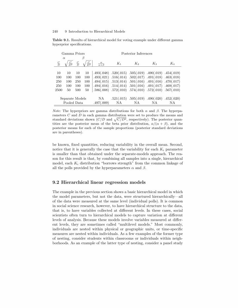
240 9 Introduction to Hierarchical Models
Table 9.1. Results of hierarchical model for voting example under different gammahyperprior specifications.
Gamma Priors Posterior Inferencesα β
CD
qC
D2CD
qC
D2α
α+βK1 K2 K3 K4
10 10 10 10 .493(.048) .520(.015) .505(.019) .490(.019) .454(.019)100 100 100 100 .493(.021) .516(.014) .502(.017) .491(.018) .463(.018)250 100 250 100 .494(.015) .513(.014) .501(.016) .491(.016) .470(.017)250 100 100 100 .494(.016) .514(.014) .501(.016) .491(.017) .469(.017)2500 50 500 50 .586(.008) .572(.010) .574(.010) .572(.010) .567(.010)
Separate Models NA .521(.015) .505(.019) .490(.020) .452(.020)Pooled Data .497(.009) NA NA NA NA
Note: The hyperpriors are gamma distributions for both α and β. The hyperpa-rameters C and D in each gamma distribution were set to produce the means andstandard deviations shown (C/D and
pC/D2, respectively). The posterior quan-
tities are the posterior mean of the beta prior distribution, α/(α + β), and theposterior means for each of the sample proportions (posterior standard deviationsare in parentheses).
be known, fixed quantities, reducing variability in the overall mean. Second,notice that it is generally the case that the variability for each Ki parameteris smaller than that obtained under the separate-models approach. The rea-son for this result is that, by combining all samples into a single, hierarchicalmodel, each Ki distribution “borrows strength” from the common linkage ofall the polls provided by the hyperparameters α and β.
9.2 Hierarchical linear regression models
The example in the previous section shows a basic hierarchical model in whichthe model parameters, but not the data, were structured hierarchically—allof the data were measured at the same level (individual polls). It is commonin social science research, however, to have hierarchical structure to the data,that is, to have variables collected at different levels. In these cases, socialscientists often turn to hierarchical models to capture variation at differentlevels of analysis. Because these models involve variables measured at differ-ent levels, they are sometimes called “multilevel models.” Most commonly,individuals are nested within physical or geographic units, or time-specificmeasures are nested within individuals. As a few examples of the former typeof nesting, consider students within classrooms or individuals within neigh-borhoods. As an example of the latter type of nesting, consider a panel study

9.2 Hierarchical linear regression models 241
in which individuals are measured repeatedly across time. In such a case, the“group” is the individual, and the time-specific measures are nested withinthe individual. The examples here will follow this latter format—time-specificmeasures nested within individuals—although the underlying concepts of hi-erarchy are identical.
I discuss several types of such hierarchical regression models, beginningwith an example that evaluates the extent to which Internet usage influencesincome using a two-wave panel study.1 These data are from the 2000 and 2001Current Population Survey Computer Use and Internet Supplement. This sup-plement measured, among other variables, individual use of computers and theInternet in 2000 and again in 2001 and allows us to examine the relationshipbetween Internet usage and wages across a brief, but important, period of timewhen availability of broadband Internet connectivity was exploding. Wages inthese examples have been transformed to 1982 dollars and are recoded intolog-dollars per hour for additional analyses not presented here.
At the end of the chapter, I turn to an example that examines factors thatinfluence health trajectories for individuals across age using a four-wave study(the National Health Epidemiologic Follow-up Surveys) discussed in previouschapters.
9.2.1 Random effects: The random intercept model
Generally, the goal of hierarchical modeling is to determine the extent towhich factors measured at different levels influence an outcome using a typicalregression modeling framework. OLS regression, however, is inappropriate,because of the lack of independence of errors for observations within groups.Thus, an alternative model must be developed to compensate for this lack ofindependence.
The foundation for the hierarchical regression model is the simple randomeffects model. Assume, as an example, that we observe a collection of indi-viduals twice over a two-year period and ask their income at each point intime. It is most likely the case that each individual’s income changes onlyslightly over the time period, and so, we could model the data such that eachindividual receives his/her own intercept (or mean). In equation form:
yit = αi + eit,
with αi ∼ N(α, τ2) and eit ∼ N(0, σ2). This specification shows that the out-come of interest (income; y) is considered a function of “variables” measuredat two different levels: αi is an individual (group) level variable, and eit is atime-specific (individual) random error term.
An alternative, but equivalent, way to specify this model is to use proba-bility notation. This approach clarifies the hierarchical nature of the model:1 I thank Bart Bonikowski and Paul DiMaggio for allowing me to use their Inter-
net/income data in the examples.

242 9 Introduction to Hierarchical Models
yit ∼ N(αi, σ2)
αi ∼ N(α, τ2)
α ∼ N(m, s2)
τ2 ∼ IG(a, b)
σ2 ∼ IG(c, d).
This specification says that an individual’s time-specific income is a ran-dom normal variable with a mean equal to an individual-specific mean andsome variance. The second equation shows that the individual-specific meansthemselves come from a (normal) distribution with a mean equal to somepopulation mean and some variance. Finally, the last three equations spec-ify hyperprior distributions for the population grand mean α, the populationvariance (around the mean) τ2, and the error variance σ2. The hyperpriordistribution for the population mean is specified here to be normal, with pa-rameters m and s2; Without prior knowledge, these parameters should bespecified to make the hyperprior vague (e.g., say m = 0 and s2 = 10, 000).The hyperprior distributions for the population variance and the error vari-ance are inverse gamma distributions, with parameters a and b and c and d,respectively. Once again, without prior information, these parameters shouldbe fixed to make the hyperprior vague.
In addition to being a simple random effects model, this model is some-times called a “random intercept model,” because the model can be viewedas a regression model with each αi considered a group-specific intercept termarising from a (normal) probability distribution (at this point, with no covari-ates included).
To implement a Gibbs sampler for this model, we first need to construct theposterior distribution. The posterior distribution for this model is straightfor-ward to derive following the hierarchical modeling structure using conditionaldistributions presented at the beginning of the chapter. The parameters of in-terest in the posterior distribution are the individual αi, the population meanα, its variance τ2, and the residual variance σ2, and so our posterior densityis:
p(α, τ2, αi, σ2|Y ) ∝ p(Y |αi, σ
2)p(αi|α, τ2)p(α|m, s2)p(τ2|c, d)p(σ2|a, b).
To complete the specification of the posterior distribution, we simply need toreplace each term with its actual distribution. As discussed above, the dataare assumed to be normally distributed, and so the likelihood term is:
p(Y |αi, σ2) ∝
n∏i=1
2∏t=1
1√σ2
exp− (yit − αi)2
2σ2
.
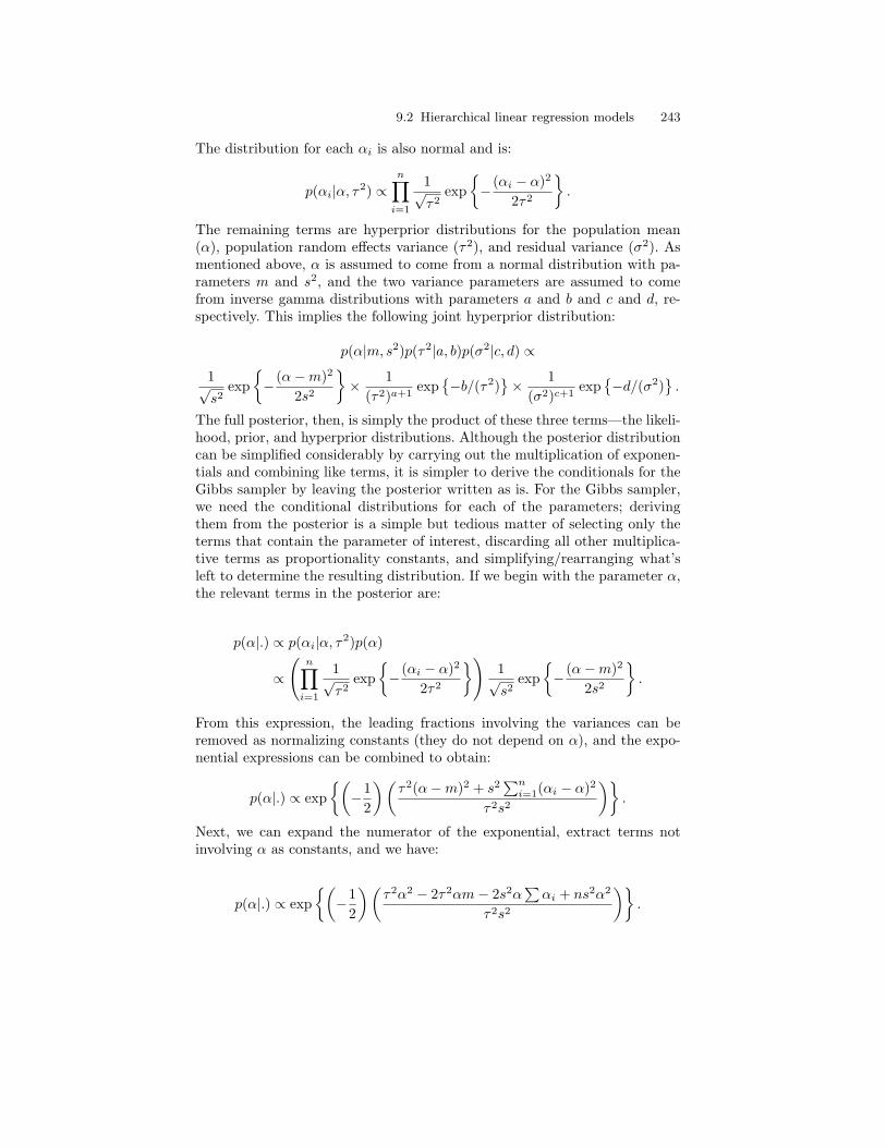
9.2 Hierarchical linear regression models 243
The distribution for each αi is also normal and is:
p(αi|α, τ2) ∝n∏
i=1
1√τ2
exp− (αi − α)2
2τ2
.
The remaining terms are hyperprior distributions for the population mean(α), population random effects variance (τ2), and residual variance (σ2). Asmentioned above, α is assumed to come from a normal distribution with pa-rameters m and s2, and the two variance parameters are assumed to comefrom inverse gamma distributions with parameters a and b and c and d, re-spectively. This implies the following joint hyperprior distribution:
p(α|m, s2)p(τ2|a, b)p(σ2|c, d) ∝
1√s2
exp− (α−m)2
2s2
× 1
(τ2)a+1exp
−b/(τ2)
× 1
(σ2)c+1exp
−d/(σ2)
.
The full posterior, then, is simply the product of these three terms—the likeli-hood, prior, and hyperprior distributions. Although the posterior distributioncan be simplified considerably by carrying out the multiplication of exponen-tials and combining like terms, it is simpler to derive the conditionals for theGibbs sampler by leaving the posterior written as is. For the Gibbs sampler,we need the conditional distributions for each of the parameters; derivingthem from the posterior is a simple but tedious matter of selecting only theterms that contain the parameter of interest, discarding all other multiplica-tive terms as proportionality constants, and simplifying/rearranging what’sleft to determine the resulting distribution. If we begin with the parameter α,the relevant terms in the posterior are:
p(α|.) ∝ p(αi|α, τ2)p(α)
∝
(n∏
i=1
1√τ2
exp− (αi − α)2
2τ2
)1√s2
exp− (α−m)2
2s2
.
From this expression, the leading fractions involving the variances can beremoved as normalizing constants (they do not depend on α), and the expo-nential expressions can be combined to obtain:
p(α|.) ∝ exp(
−12
)(τ2(α−m)2 + s2
∑ni=1(αi − α)2
τ2s2
).
Next, we can expand the numerator of the exponential, extract terms notinvolving α as constants, and we have:
p(α|.) ∝ exp(
−12
)(τ2α2 − 2τ2αm− 2s2α
∑αi + ns2α2
τ2s2
).
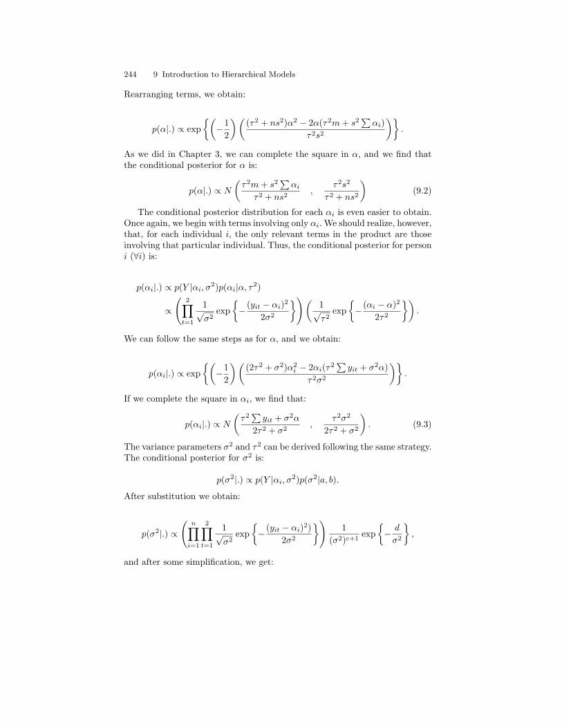
244 9 Introduction to Hierarchical Models
Rearranging terms, we obtain:
p(α|.) ∝ exp(
−12
)((τ2 + ns2)α2 − 2α(τ2m + s2
∑αi)
τ2s2
).
As we did in Chapter 3, we can complete the square in α, and we find thatthe conditional posterior for α is:
p(α|.) ∝ N
(τ2m + s2
∑αi
τ2 + ns2,
τ2s2
τ2 + ns2
)(9.2)
The conditional posterior distribution for each αi is even easier to obtain.Once again, we begin with terms involving only αi. We should realize, however,that, for each individual i, the only relevant terms in the product are thoseinvolving that particular individual. Thus, the conditional posterior for personi (∀i) is:
p(αi|.) ∝ p(Y |αi, σ2)p(αi|α, τ2)
∝
(2∏
t=1
1√σ2
exp− (yit − αi)2
2σ2
)(1√τ2
exp− (αi − α)2
2τ2
).
We can follow the same steps as for α, and we obtain:
p(αi|.) ∝ exp(
−12
)((2τ2 + σ2)α2
i − 2αi(τ2∑
yit + σ2α)τ2σ2
).
If we complete the square in αi, we find that:
p(αi|.) ∝ N
(τ2∑
yit + σ2α
2τ2 + σ2,
τ2σ2
2τ2 + σ2
). (9.3)
The variance parameters σ2 and τ2 can be derived following the same strategy.The conditional posterior for σ2 is:
p(σ2|.) ∝ p(Y |αi, σ2)p(σ2|a, b).
After substitution we obtain:
p(σ2|.) ∝
(n∏
i=1
2∏t=1
1√σ2
exp− (yit − αi)2)
2σ2
)1
(σ2)c+1exp
− d
σ2
,
and after some simplification, we get:

9.2 Hierarchical linear regression models 245
p(σ2|.) ∝(σ2)−(n+c+1)
exp
−(∑n
i=1
∑2t=1(yit − αi)2 + 2d
)2σ2
.
This result shows that the conditional posterior for σ2 is an inverse gammadistribution:
p(σ2|.) ∝ IG
(n + c ,
∑ni=1
∑2t=1(yit − αi)2 + 2d
2
). (9.4)
The conditional posterior for τ can be derived similarly. The posterior is:
p(τ2|.) ∝ p(αi|α, τ2)p(τ2)
∝
(n∏
i=1
1√τ2
exp− (αi − α)2
2τ2
)1
(τ2)a+1exp
− b
τ2
.
After simplification, we obtain:
p(τ2|.) ∝ IG
(n/2 + a + 1 ,
∑ni=1(αi − α)2 + 2b
2
)(9.5)
(see Exercises).Given a complete set of conditional posterior distributions, we can im-
plement a Gibbs sampler for the model by sequentially drawing from theseconditionals. Below is an R program that conducts the Gibbs sampling:
#R program for simple random effects model
#read data
y=as.matrix(read.table("c:\\internet_examp.dat")[,3:4])
m=0; s2=10000; a=c=.001; b=d=.001; tau2=1; sigma2=1; malpha=0
n=nrow(y)
for(i in 1:20000)
#draw alpha_i
alpha= rnorm(n,
mean=(((tau2*(y[,1]+y[,2]))+sigma2*malpha)/(2*tau2+sigma2)),
sd=sqrt((tau2*sigma2)/(2*tau2+sigma2)))
#draw malpha
malpha=rnorm(1,
mean=(tau2*m+s2*sum(alpha))/((tau2+n*s2)),
sd=sqrt((tau2*s2)/((tau2+n*s2))))
#draw tau2
tau2=rgamma(1, shape=(n/2+a), rate=(sum((alpha-malpha)^2)+2*b)/2)
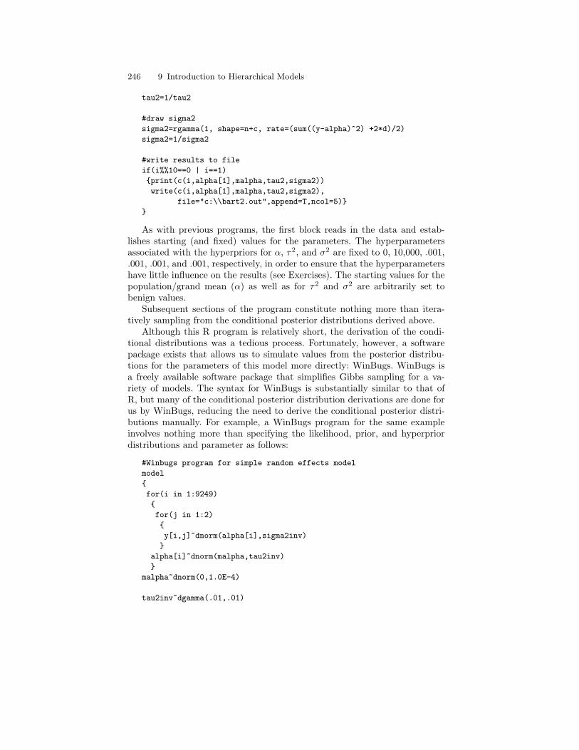
246 9 Introduction to Hierarchical Models
tau2=1/tau2
#draw sigma2
sigma2=rgamma(1, shape=n+c, rate=(sum((y-alpha)^2) +2*d)/2)
sigma2=1/sigma2
#write results to file
if(i%%10==0 | i==1)
print(c(i,alpha[1],malpha,tau2,sigma2))
write(c(i,alpha[1],malpha,tau2,sigma2),
file="c:\\bart2.out",append=T,ncol=5)
As with previous programs, the first block reads in the data and estab-lishes starting (and fixed) values for the parameters. The hyperparametersassociated with the hyperpriors for α, τ2, and σ2 are fixed to 0, 10,000, .001,.001, .001, and .001, respectively, in order to ensure that the hyperparametershave little influence on the results (see Exercises). The starting values for thepopulation/grand mean (α) as well as for τ2 and σ2 are arbitrarily set tobenign values.
Subsequent sections of the program constitute nothing more than itera-tively sampling from the conditional posterior distributions derived above.
Although this R program is relatively short, the derivation of the condi-tional distributions was a tedious process. Fortunately, however, a softwarepackage exists that allows us to simulate values from the posterior distribu-tions for the parameters of this model more directly: WinBugs. WinBugs isa freely available software package that simplifies Gibbs sampling for a va-riety of models. The syntax for WinBugs is substantially similar to that ofR, but many of the conditional posterior distribution derivations are done forus by WinBugs, reducing the need to derive the conditional posterior distri-butions manually. For example, a WinBugs program for the same exampleinvolves nothing more than specifying the likelihood, prior, and hyperpriordistributions and parameter as follows:
#Winbugs program for simple random effects model
model
for(i in 1:9249)
for(j in 1:2)
y[i,j]~dnorm(alpha[i],sigma2inv)
alpha[i]~dnorm(malpha,tau2inv)
malpha~dnorm(0,1.0E-4)
tau2inv~dgamma(.01,.01)
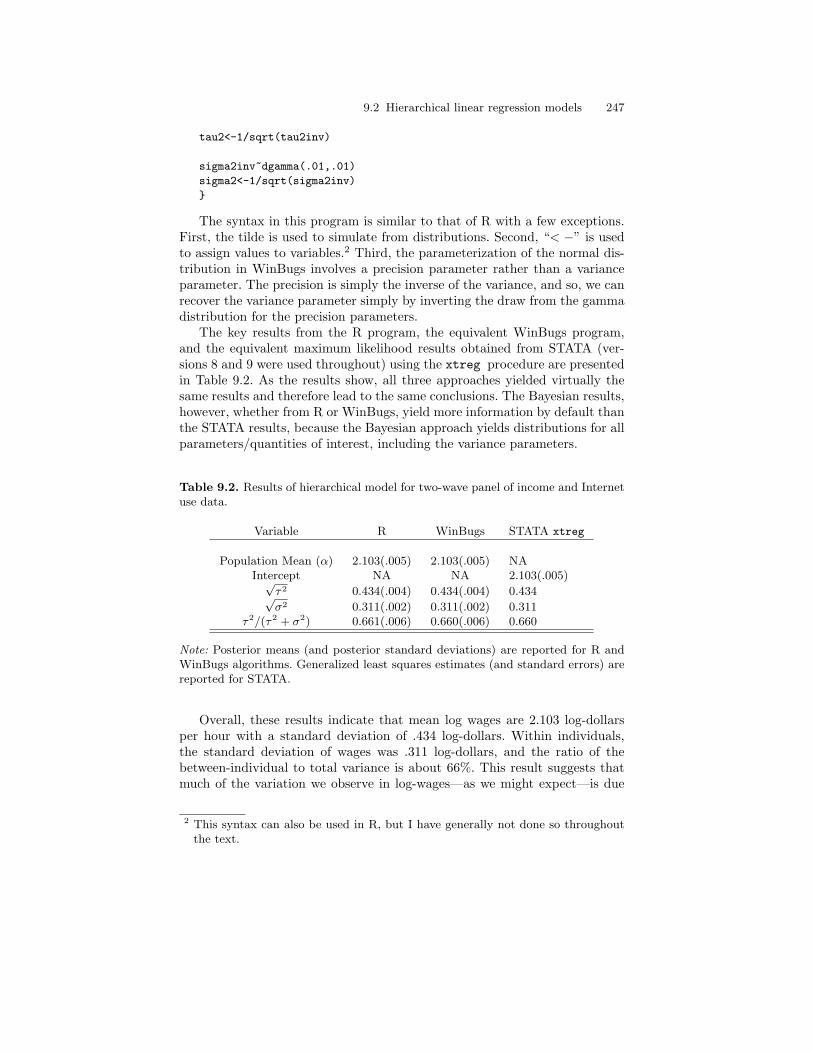
9.2 Hierarchical linear regression models 247
tau2<-1/sqrt(tau2inv)
sigma2inv~dgamma(.01,.01)
sigma2<-1/sqrt(sigma2inv)
The syntax in this program is similar to that of R with a few exceptions.First, the tilde is used to simulate from distributions. Second, “< −” is usedto assign values to variables.2 Third, the parameterization of the normal dis-tribution in WinBugs involves a precision parameter rather than a varianceparameter. The precision is simply the inverse of the variance, and so, we canrecover the variance parameter simply by inverting the draw from the gammadistribution for the precision parameters.
The key results from the R program, the equivalent WinBugs program,and the equivalent maximum likelihood results obtained from STATA (ver-sions 8 and 9 were used throughout) using the xtreg procedure are presentedin Table 9.2. As the results show, all three approaches yielded virtually thesame results and therefore lead to the same conclusions. The Bayesian results,however, whether from R or WinBugs, yield more information by default thanthe STATA results, because the Bayesian approach yields distributions for allparameters/quantities of interest, including the variance parameters.
Table 9.2. Results of hierarchical model for two-wave panel of income and Internetuse data.
Variable R WinBugs STATA xtreg
Population Mean (α) 2.103(.005) 2.103(.005) NAIntercept NA NA 2.103(.005)√
τ2 0.434(.004) 0.434(.004) 0.434√σ2 0.311(.002) 0.311(.002) 0.311
τ2/(τ2 + σ2) 0.661(.006) 0.660(.006) 0.660
Note: Posterior means (and posterior standard deviations) are reported for R andWinBugs algorithms. Generalized least squares estimates (and standard errors) arereported for STATA.
Overall, these results indicate that mean log wages are 2.103 log-dollarsper hour with a standard deviation of .434 log-dollars. Within individuals,the standard deviation of wages was .311 log-dollars, and the ratio of thebetween-individual to total variance is about 66%. This result suggests thatmuch of the variation we observe in log-wages—as we might expect—is due
2 This syntax can also be used in R, but I have generally not done so throughoutthe text.
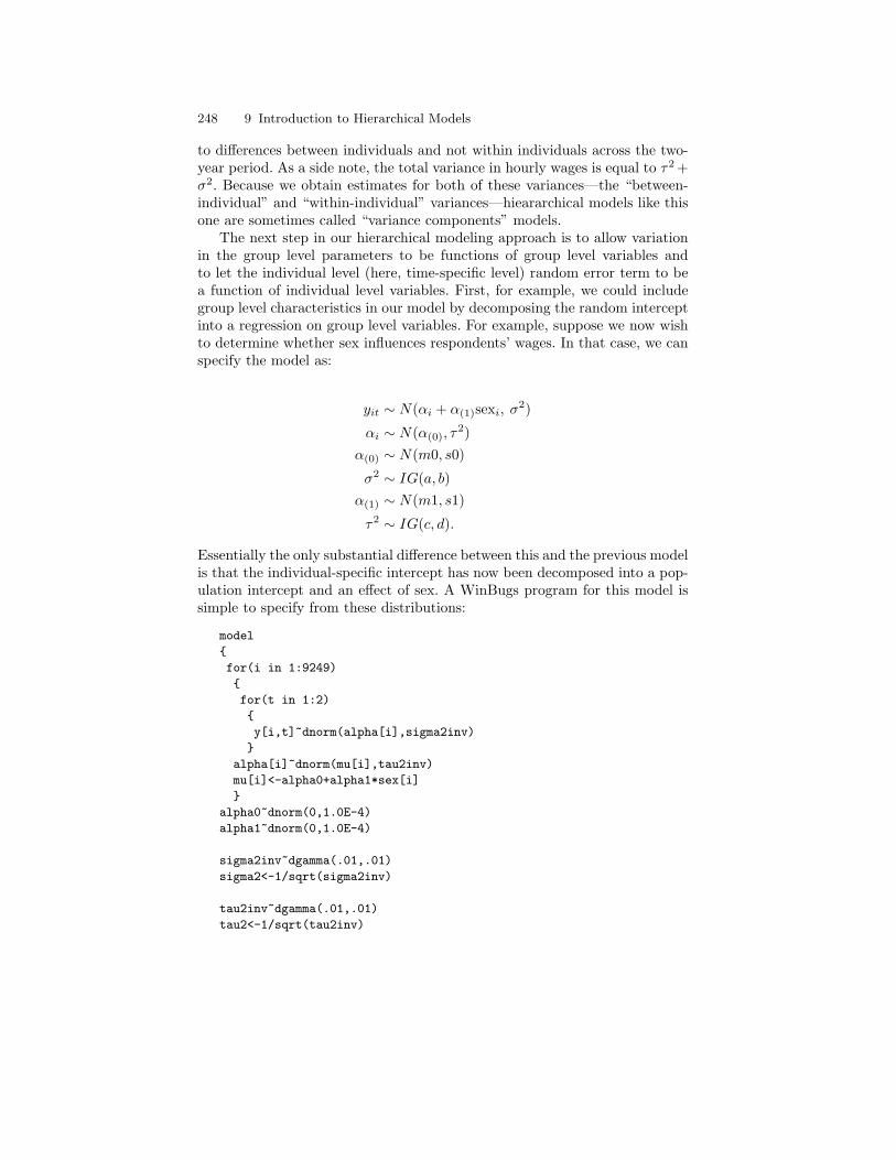
248 9 Introduction to Hierarchical Models
to differences between individuals and not within individuals across the two-year period. As a side note, the total variance in hourly wages is equal to τ2 +σ2. Because we obtain estimates for both of these variances—the “between-individual” and “within-individual” variances—hieararchical models like thisone are sometimes called “variance components” models.
The next step in our hierarchical modeling approach is to allow variationin the group level parameters to be functions of group level variables andto let the individual level (here, time-specific level) random error term to bea function of individual level variables. First, for example, we could includegroup level characteristics in our model by decomposing the random interceptinto a regression on group level variables. For example, suppose we now wishto determine whether sex influences respondents’ wages. In that case, we canspecify the model as:
yit ∼ N(αi + α(1)sexi, σ2)
αi ∼ N(α(0), τ2)
α(0) ∼ N(m0, s0)
σ2 ∼ IG(a, b)α(1) ∼ N(m1, s1)
τ2 ∼ IG(c, d).
Essentially the only substantial difference between this and the previous modelis that the individual-specific intercept has now been decomposed into a pop-ulation intercept and an effect of sex. A WinBugs program for this model issimple to specify from these distributions:
model
for(i in 1:9249)
for(t in 1:2)
y[i,t]~dnorm(alpha[i],sigma2inv)
alpha[i]~dnorm(mu[i],tau2inv)
mu[i]<-alpha0+alpha1*sex[i]
alpha0~dnorm(0,1.0E-4)
alpha1~dnorm(0,1.0E-4)
sigma2inv~dgamma(.01,.01)
sigma2<-1/sqrt(sigma2inv)
tau2inv~dgamma(.01,.01)
tau2<-1/sqrt(tau2inv)
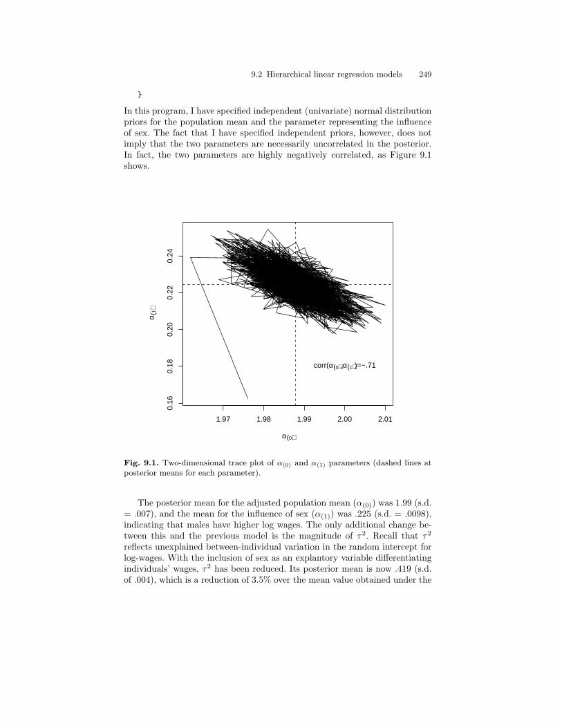
9.2 Hierarchical linear regression models 249
In this program, I have specified independent (univariate) normal distributionpriors for the population mean and the parameter representing the influenceof sex. The fact that I have specified independent priors, however, does notimply that the two parameters are necessarily uncorrelated in the posterior.In fact, the two parameters are highly negatively correlated, as Figure 9.1shows.
1.97 1.98 1.99 2.00 2.01
0.16
0.18
0.20
0.22
0.24
α(0)
α (1)
corr(α(0),α(1))=−.71
Fig. 9.1. Two-dimensional trace plot of α(0) and α(1) parameters (dashed lines atposterior means for each parameter).
The posterior mean for the adjusted population mean (α(0)) was 1.99 (s.d.= .007), and the mean for the influence of sex (α(1)) was .225 (s.d. = .0098),indicating that males have higher log wages. The only additional change be-tween this and the previous model is the magnitude of τ2. Recall that τ2
reflects unexplained between-individual variation in the random intercept forlog-wages. With the inclusion of sex as an explantory variable differentiatingindividuals’ wages, τ2 has been reduced. Its posterior mean is now .419 (s.d.of .004), which is a reduction of 3.5% over the mean value obtained under the
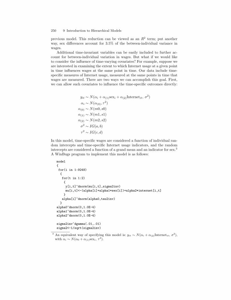
250 9 Introduction to Hierarchical Models
previous model. This reduction can be viewed as an R2 term; put anotherway, sex differences account for 3.5% of the between-individual variance inwages.
Additional time-invariant variables can be easily included to further ac-count for between-individual variation in wages. But what if we would liketo consider the influence of time-varying covariates? For example, suppose weare interested in examining the extent to which Internet usage at a given pointin time influences wages at the same point in time. Our data include time-specific measures of Internet usage, measured at the same points in time thatwages are measured. There are two ways we can accomplish this goal. First,we can allow such covariates to influence the time-specific outcomes directly:
yit ∼ N(αi + α(1)sexi + α(2)Internetit, σ2)
αi ∼ N(α(0), τ2)
α(0) ∼ N(m0, s0)α(1) ∼ N(m1, s1)α(2) ∼ N(m2, s2)
σ2 ∼ IG(a, b)
τ2 ∼ IG(c, d)
In this model, time-specific wages are considered a function of individual ran-dom intercepts and time-specific Internet usage indicators, and the randomintercepts are considered a function of a grand mean and an indicator for sex.3
A WinBugs program to implement this model is as follows:
model
for(i in 1:9249)
for(t in 1:2)
y[i,t]~dnorm(mu[i,t],sigma2inv)
mu[i,t]<-(alpha[i]+alpha1*sex[i])+alpha2*internet[i,t]
alpha[i]~dnorm(alpha0,tau2inv)
alpha0~dnorm(0,1.0E-4)
alpha1~dnorm(0,1.0E-4)
alpha2~dnorm(0,1.0E-4)
sigma2inv~dgamma(.01,.01)
sigma2<-1/sqrt(sigma2inv)
3 An equivalent way of specifying this model is: yit ∼ N(αi + α(2)Internetit, σ2),with αi ∼ N(α0 + α(1)sexi, τ2).

9.2 Hierarchical linear regression models 251
tau2inv~dgamma(.01,.01)
tau2<-1/sqrt(tau2inv)
This program is only slightly more complicated than the previous pro-grams. The only substantial differences are that (1) we have included the newparameter (α(2)) within the double loop (i, t), and (2) we have incorporated aprior distribution for it. The results of this model suggest that Internet usagedoes, in fact, influence income. The posterior mean for the influence of Inter-net usage is .18 (s.d. = .0075), and the intercept (α(0)) falls to 1.86 (s.d. =.009).
9.2.2 Random effects: The random coefficient model
As written, the last model in the previous section forces the effect of Internetusage to be constant across time: There was only a single parameter repre-senting the effect of Internet usage on wages. This constraint may introduceerror into the model if, in fact, the influence of Internet usage on wages variesacross time. Thus, a second way we can include this time-varying variable isto allow the influence of Internet usage to vary across time. This model is:
yit ∼ N(αi + α(1)sexi + α(2t)Internetit, σ2)
αi ∼ N(α(0), τ2)
α(0) ∼ N(m0, s0)α(1) ∼ N(m1, s1)
α(21) ∼ N(m2, s2)α(22) ∼ N(m3, s3)
σ2 ∼ IG(a, b)
τ2 ∼ IG(c, d)
The alterations of the WinBugs program to accommodate this new param-eter are very slight: The alpha2 parameter must be subscripted appropriately(i.e., alpha2[t]), and an additional hyperprior distribution must be incorpo-rated. By some terminologies, we can now call the model a random coefficientmodel, because a slope—and not simply an intercept—is now considered afunction of other variables.4
4 It may be easier to recognize that allowing alpha2 to vary across time impliesthat alpha2 is now a slope, and not simply an intercept, if we consider that ourcurrent representation is equivalent to specifying α2 to be a function of a dummyvariable reflecting time of measurement: α2 = β0 + β1I(t = 2), where β1 is aregression slope.
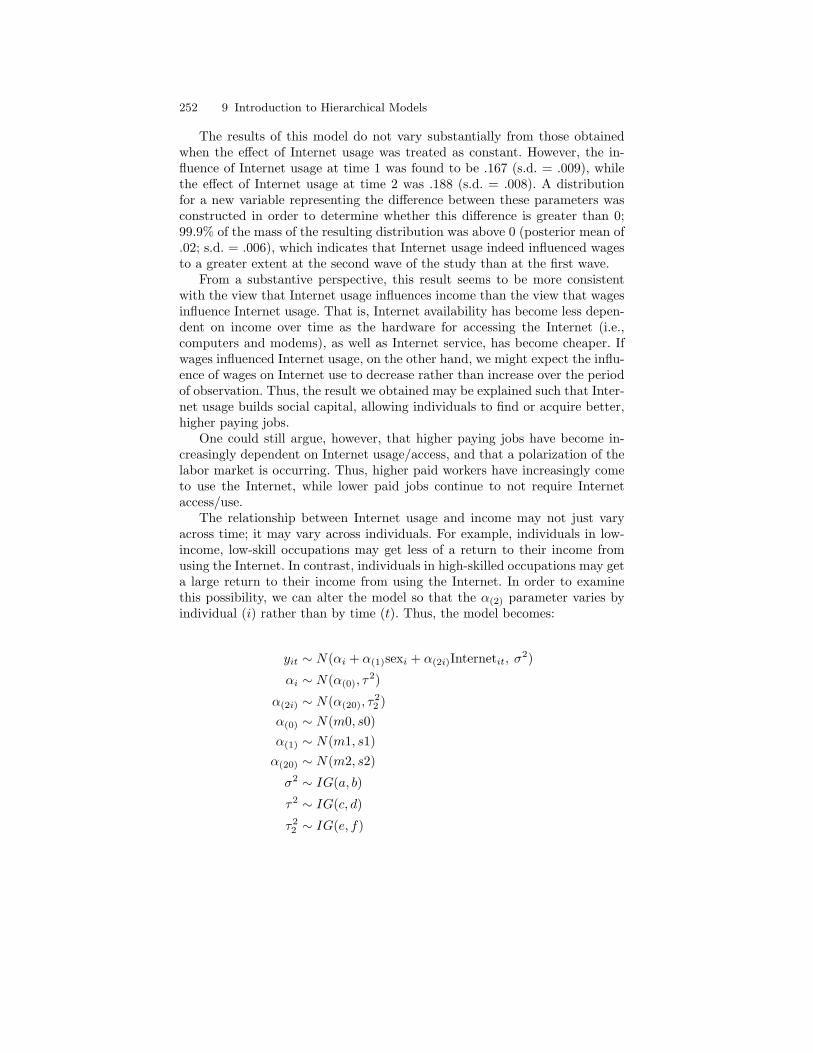
252 9 Introduction to Hierarchical Models
The results of this model do not vary substantially from those obtainedwhen the effect of Internet usage was treated as constant. However, the in-fluence of Internet usage at time 1 was found to be .167 (s.d. = .009), whilethe effect of Internet usage at time 2 was .188 (s.d. = .008). A distributionfor a new variable representing the difference between these parameters wasconstructed in order to determine whether this difference is greater than 0;99.9% of the mass of the resulting distribution was above 0 (posterior mean of.02; s.d. = .006), which indicates that Internet usage indeed influenced wagesto a greater extent at the second wave of the study than at the first wave.
From a substantive perspective, this result seems to be more consistentwith the view that Internet usage influences income than the view that wagesinfluence Internet usage. That is, Internet availability has become less depen-dent on income over time as the hardware for accessing the Internet (i.e.,computers and modems), as well as Internet service, has become cheaper. Ifwages influenced Internet usage, on the other hand, we might expect the influ-ence of wages on Internet use to decrease rather than increase over the periodof observation. Thus, the result we obtained may be explained such that Inter-net usage builds social capital, allowing individuals to find or acquire better,higher paying jobs.
One could still argue, however, that higher paying jobs have become in-creasingly dependent on Internet usage/access, and that a polarization of thelabor market is occurring. Thus, higher paid workers have increasingly cometo use the Internet, while lower paid jobs continue to not require Internetaccess/use.
The relationship between Internet usage and income may not just varyacross time; it may vary across individuals. For example, individuals in low-income, low-skill occupations may get less of a return to their income fromusing the Internet. In contrast, individuals in high-skilled occupations may geta large return to their income from using the Internet. In order to examinethis possibility, we can alter the model so that the α(2) parameter varies byindividual (i) rather than by time (t). Thus, the model becomes:
yit ∼ N(αi + α(1)sexi + α(2i)Internetit, σ2)
αi ∼ N(α(0), τ2)
α(2i) ∼ N(α(20), τ22 )
α(0) ∼ N(m0, s0)α(1) ∼ N(m1, s1)
α(20) ∼ N(m2, s2)
σ2 ∼ IG(a, b)
τ2 ∼ IG(c, d)
τ22 ∼ IG(e, f)
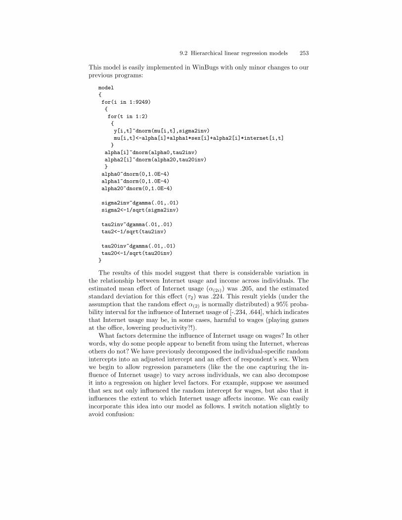
9.2 Hierarchical linear regression models 253
This model is easily implemented in WinBugs with only minor changes to ourprevious programs:
model
for(i in 1:9249)
for(t in 1:2)
y[i,t]~dnorm(mu[i,t],sigma2inv)
mu[i,t]<-alpha[i]+alpha1*sex[i]+alpha2[i]*internet[i,t]
alpha[i]~dnorm(alpha0,tau2inv)
alpha2[i]~dnorm(alpha20,tau20inv)
alpha0~dnorm(0,1.0E-4)
alpha1~dnorm(0,1.0E-4)
alpha20~dnorm(0,1.0E-4)
sigma2inv~dgamma(.01,.01)
sigma2<-1/sqrt(sigma2inv)
tau2inv~dgamma(.01,.01)
tau2<-1/sqrt(tau2inv)
tau20inv~dgamma(.01,.01)
tau20<-1/sqrt(tau20inv)
The results of this model suggest that there is considerable variation inthe relationship between Internet usage and income across individuals. Theestimated mean effect of Internet usage (α(2i)) was .205, and the estimatedstandard deviation for this effect (τ2) was .224. This result yields (under theassumption that the random effect α(2) is normally distributed) a 95% proba-bility interval for the influence of Internet usage of [-.234, .644], which indicatesthat Internet usage may be, in some cases, harmful to wages (playing gamesat the office, lowering productivity?!).
What factors determine the influence of Internet usage on wages? In otherwords, why do some people appear to benefit from using the Internet, whereasothers do not? We have previously decomposed the individual-specific randomintercepts into an adjusted intercept and an effect of respondent’s sex. Whenwe begin to allow regression parameters (like the the one capturing the in-fluence of Internet usage) to vary across individuals, we can also decomposeit into a regression on higher level factors. For example, suppose we assumedthat sex not only influenced the random intercept for wages, but also that itinfluences the extent to which Internet usage affects income. We can easilyincorporate this idea into our model as follows. I switch notation slightly toavoid confusion:
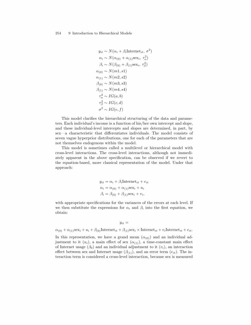
254 9 Introduction to Hierarchical Models
yit ∼ N(αi + βiInternetit, σ2)
αi ∼ N(α(0) + α(1)sexi, τ2α)
βi ∼ N(β(0) + β(1)sexi, τ2β)
α(0) ∼ N(m1, s1)α(1) ∼ N(m2, s2)β(0) ∼ N(m3, s3)β(1) ∼ N(m4, s4)
τ2α ∼ IG(a, b)
τ2β ∼ IG(c, d)
σ2 ∼ IG(e, f)
This model clarifies the hierarchical structuring of the data and parame-ters. Each individual’s income is a function of his/her own intercept and slope,and these individual-level intercepts and slopes are determined, in part, bysex—a characteristic that differentiates individuals. The model consists ofseven vague hyperprior distributions, one for each of the parameters that arenot themselves endogenous within the model.
This model is sometimes called a multilevel or hierarchical model withcross-level interactions. The cross-level interactions, although not immedi-ately apparent in the above specification, can be observed if we revert tothe equation-based, more classical representation of the model. Under thatapproach:
yit = αi + βiInternetit + eit
αi = α(0) + α(1)sexi + ui
βi = β(0) + β(1)sexi + vi,
with appropriate specifications for the variances of the errors at each level. Ifwe then substitute the expressions for αi and βi into the first equation, weobtain:
yit =
α(0) + α(1)sexi + ui + β(0)Internetit + β(1)sexi× Internetit + viInternetit + eit.
In this representation, we have a grand mean (α(0)) and an individual ad-justment to it (ui), a main effect of sex (α(1)), a time-constant main effectof Internet usage (β0) and an individual adjustment to it (vi), an interactioneffect between sex and Internet usage (β(1)), and an error term (eit). The in-teraction term is considered a cross-level interaction, because sex is measured
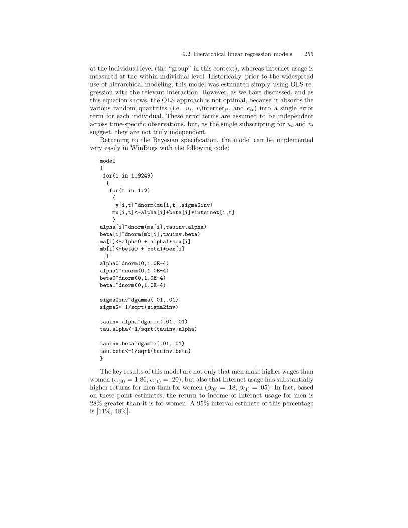
9.2 Hierarchical linear regression models 255
at the individual level (the “group” in this context), whereas Internet usage ismeasured at the within-individual level. Historically, prior to the widespreaduse of hierarchical modeling, this model was estimated simply using OLS re-gression with the relevant interaction. However, as we have discussed, and asthis equation shows, the OLS approach is not optimal, because it absorbs thevarious random quantities (i.e., ui, viinternetit, and eit) into a single errorterm for each individual. These error terms are assumed to be independentacross time-specific observations, but, as the single subscripting for ui and vi
suggest, they are not truly independent.Returning to the Bayesian specification, the model can be implemented
very easily in WinBugs with the following code:
model
for(i in 1:9249)
for(t in 1:2)
y[i,t]~dnorm(mu[i,t],sigma2inv)
mu[i,t]<-alpha[i]+beta[i]*internet[i,t]
alpha[i]~dnorm(ma[i],tauinv.alpha)
beta[i]~dnorm(mb[i],tauinv.beta)
ma[i]<-alpha0 + alpha1*sex[i]
mb[i]<-beta0 + beta1*sex[i]
alpha0~dnorm(0,1.0E-4)
alpha1~dnorm(0,1.0E-4)
beta0~dnorm(0,1.0E-4)
beta1~dnorm(0,1.0E-4)
sigma2inv~dgamma(.01,.01)
sigma2<-1/sqrt(sigma2inv)
tauinv.alpha~dgamma(.01,.01)
tau.alpha<-1/sqrt(tauinv.alpha)
tauinv.beta~dgamma(.01,.01)
tau.beta<-1/sqrt(tauinv.beta)
The key results of this model are not only that men make higher wages thanwomen (α(0) = 1.86; α(1) = .20), but also that Internet usage has substantiallyhigher returns for men than for women (β(0) = .18; β(1) = .05). In fact, basedon these point estimates, the return to income of Internet usage for men is28% greater than it is for women. A 95% interval estimate of this percentageis [11%, 48%].
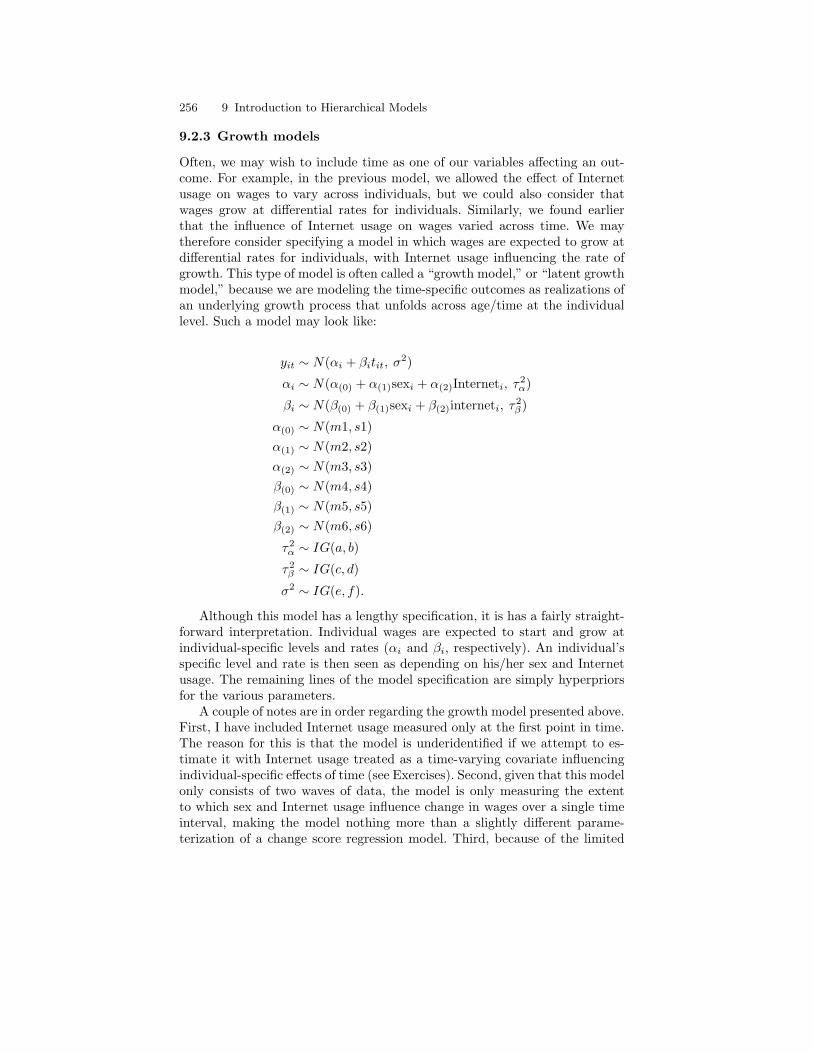
256 9 Introduction to Hierarchical Models
9.2.3 Growth models
Often, we may wish to include time as one of our variables affecting an out-come. For example, in the previous model, we allowed the effect of Internetusage on wages to vary across individuals, but we could also consider thatwages grow at differential rates for individuals. Similarly, we found earlierthat the influence of Internet usage on wages varied across time. We maytherefore consider specifying a model in which wages are expected to grow atdifferential rates for individuals, with Internet usage influencing the rate ofgrowth. This type of model is often called a “growth model,” or “latent growthmodel,” because we are modeling the time-specific outcomes as realizations ofan underlying growth process that unfolds across age/time at the individuallevel. Such a model may look like:
yit ∼ N(αi + βitit, σ2)
αi ∼ N(α(0) + α(1)sexi + α(2)Interneti, τ2α)
βi ∼ N(β(0) + β(1)sexi + β(2)interneti, τ2β)
α(0) ∼ N(m1, s1)α(1) ∼ N(m2, s2)α(2) ∼ N(m3, s3)β(0) ∼ N(m4, s4)β(1) ∼ N(m5, s5)β(2) ∼ N(m6, s6)
τ2α ∼ IG(a, b)
τ2β ∼ IG(c, d)
σ2 ∼ IG(e, f).
Although this model has a lengthy specification, it is has a fairly straight-forward interpretation. Individual wages are expected to start and grow atindividual-specific levels and rates (αi and βi, respectively). An individual’sspecific level and rate is then seen as depending on his/her sex and Internetusage. The remaining lines of the model specification are simply hyperpriorsfor the various parameters.
A couple of notes are in order regarding the growth model presented above.First, I have included Internet usage measured only at the first point in time.The reason for this is that the model is underidentified if we attempt to es-timate it with Internet usage treated as a time-varying covariate influencingindividual-specific effects of time (see Exercises). Second, given that this modelonly consists of two waves of data, the model is only measuring the extentto which sex and Internet usage influence change in wages over a single timeinterval, making the model nothing more than a slightly different parame-terization of a change score regression model. Third, because of the limited
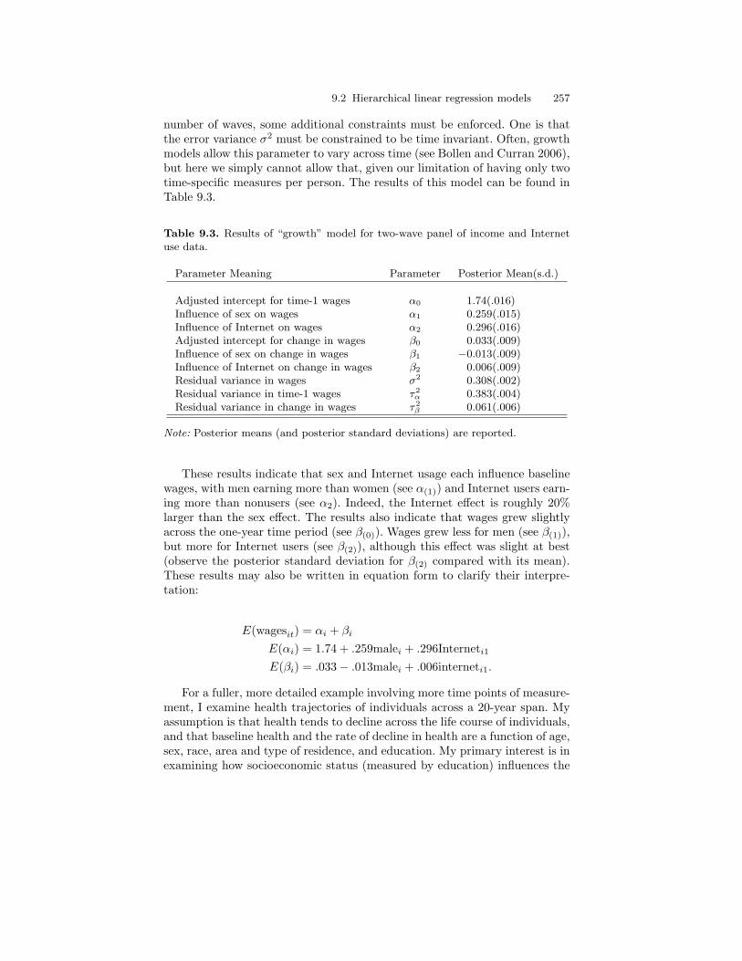
9.2 Hierarchical linear regression models 257
number of waves, some additional constraints must be enforced. One is thatthe error variance σ2 must be constrained to be time invariant. Often, growthmodels allow this parameter to vary across time (see Bollen and Curran 2006),but here we simply cannot allow that, given our limitation of having only twotime-specific measures per person. The results of this model can be found inTable 9.3.
Table 9.3. Results of “growth” model for two-wave panel of income and Internetuse data.
Parameter Meaning Parameter Posterior Mean(s.d.)
Adjusted intercept for time-1 wages α0 1.74(.016)Influence of sex on wages α1 0.259(.015)Influence of Internet on wages α2 0.296(.016)Adjusted intercept for change in wages β0 0.033(.009)Influence of sex on change in wages β1 −0.013(.009)Influence of Internet on change in wages β2 0.006(.009)Residual variance in wages σ2 0.308(.002)Residual variance in time-1 wages τ2
α 0.383(.004)Residual variance in change in wages τ2
β 0.061(.006)
Note: Posterior means (and posterior standard deviations) are reported.
These results indicate that sex and Internet usage each influence baselinewages, with men earning more than women (see α(1)) and Internet users earn-ing more than nonusers (see α2). Indeed, the Internet effect is roughly 20%larger than the sex effect. The results also indicate that wages grew slightlyacross the one-year time period (see β(0)). Wages grew less for men (see β(1)),but more for Internet users (see β(2)), although this effect was slight at best(observe the posterior standard deviation for β(2) compared with its mean).These results may also be written in equation form to clarify their interpre-tation:
E(wagesit) = αi + βi
E(αi) = 1.74 + .259malei + .296Interneti1
E(βi) = .033− .013malei + .006interneti1.
For a fuller, more detailed example involving more time points of measure-ment, I examine health trajectories of individuals across a 20-year span. Myassumption is that health tends to decline across the life course of individuals,and that baseline health and the rate of decline in health are a function of age,sex, race, area and type of residence, and education. My primary interest is inexamining how socioeconomic status (measured by education) influences the

258 9 Introduction to Hierarchical Models
health differential across time. One hypothesis in the literature—the cumula-tive advantage hypothesis—argues that the health gap between high and lowSES groups widens across age as a function of the cumulative disadvantagethat low SES generates across the life course (see Lynch 2003). At young ages,risk factors like smoking and lack of health care access matter little, becausemost young adults are quite healthy. However, across age, exposure to riskfactors accumulates and produces a larger health differential. An alternatehypothesis is the age-as-leveler hypothesis. This hypothesis argues that thehealth gap narrows across age because age overwhelms all risk factors—thebiological effect of aging supercedes any socially based risk factor (see Houseet al. 1994). Often a selective mortality argument is also advanced to supportthis hypothesis: that the observed health gap at a particular age is ultimatelya between-individual measure, and only the health of survivors is observed.Thus, those with the poorest health have been eliminated from the observedpopulation, and the gap is simply a comparison of a robust subset of lowerSES individuals with higher SES individuals. In other words, there are differ-ent populations being compared at young and older ages (see Lynch 2003 forextensive discussion).
A life course perspective suggests that we should examine trajectories ofhealth for individuals, and that selective mortality should be “controlled out.”One way to do this is to allow decedents to be included in the model, ratherthan to exclude them, as cross-sectional analyses must do (because only sur-vivors can be observed in a cross-section). A Bayesian growth model can easilyhandle the unbalanced data that result from mortality, and health trajecto-ries can even be estimated for individuals for whom we only observe a sin-gle measure. Their trajectories become a compromise between their observedmeasures and those of persons with similar covariate profiles who do survive.Ultimately, this approach underestimates the rate of decline in health, becausesurviving low-SES individuals drive the estimate of the mean growth rate, andsurely decedents have/had steeper—but unobserved—rates of health decline.However, this argument implies that the finding with regard to the cumulativeadvantage hypothesis are conservative.
For this example, I again use the data from the National Health and Nutri-tion Examination Survey (NHANES) and its follow-ups, the National HealthEpidemiologic Follow-up Surveys (NHEFS) (see Chapter 8 for a description).After eliminating individuals who were missing on one or another variablein the analyses and individuals whose final status in 1992 was unknown, theanalytic sample consisted of 6,403 persons.
In this example, I include only individuals who were between 30 and 34years of age at baseline, because age presents a problem in these analyses:The variable “age” represents both age and cohort. Research has shown thata common pattern for the health gap between individuals with low versus highSES across age is divergent until midlife and then convergent after (see Houseet al. 1994). This pattern is a function of two things: selective mortality andcohort change in the importance of education in affecting health (see Lynch

9.2 Hierarchical linear regression models 259
2003). Thus, for the sake of simplicity in this example, I restrict the analysesto the 608 individuals who fall in this age range, eliminating cohort effects.
I include age (mean = 32.0, s.d. = 1.4), sex (male = 1, 41.6%), race (non-white = 1, 12.3%), region (south = 1, 28.1%), urban residence (urban = 1,23.2%), and education (in years, mean = 12.6, s.d. = 2.6, minimum = 0,maximum = 17) as second-level covariates that may influence the random in-tercept and slope factors. The outcome measure is self-rated health measuredon a 5-point Likert scale ranging from excellent health (5) to poor health (1).Health measured on a 5-point scale is known to be a reliable and valid indica-tor of health (especially at younger ages), and the data are fairly symmetric,with a slight skew toward excellent health. I expect that individuals randomintercepts are relatively high, and that in general, health declines between30 and 55—the age range covered by the study. Furthermore, I expect thateducation differentiates health at baseline, with higher educated individualshaving better health than lower educated ones. Finally, if the cumulative ad-vantage hypothesis is true at least prior to age 55, education serves to reducethe rate of decline in health. This hypothesis implies that the growth ratein health is negative in general, but that education’s influence on the growthrate is positive.
Below is the WinBugs program specifying the growth model:
model
for(i in 1:608)
for(t in 1:pyrs[i])
h[i,t]~dnorm(mu[i,t],sigma2inv)
mu[i,t]<-alpha[i]+beta[i]*yr[i,t]
alpha[i]~dnorm(ma[i],tauinv.alpha)
beta[i]~dnorm(mb[i],tauinv.beta)
ma[i]<-alpha0 + alpha1*age[i] + alpha2*male[i] + alpha3*nonw[i] +
alpha4*south[i] + alpha5*urban[i] + alpha6*educ[i]
mb[i]<-beta0 + beta2*male[i] + beta3*nonw[i] +
beta4*south[i] + beta5*urban[i] + beta6*educ[i]
alpha0~dnorm(0,1.0E-4)
alpha1~dnorm(0,1.0E-4)
alpha2~dnorm(0,1.0E-4)
alpha3~dnorm(0,1.0E-4)
alpha4~dnorm(0,1.0E-4)
alpha5~dnorm(0,1.0E-4)
alpha6~dnorm(0,1.0E-4)
beta0~dnorm(0,1.0E-4)
beta2~dnorm(0,1.0E-4)
beta3~dnorm(0,1.0E-4)
beta4~dnorm(0,1.0E-4)

260 9 Introduction to Hierarchical Models
beta5~dnorm(0,1.0E-4)
beta6~dnorm(0,1.0E-4)
sigma2inv~dgamma(.01,.01)
sigma2<-1/sqrt(sigma2inv)
tauinv.alpha~dgamma(.01,.01)
tau.alpha<-1/sqrt(tauinv.alpha)
tauinv.beta~dgamma(.01,.01)
tau.beta<-1/sqrt(tauinv.beta)
This program, although longer than our previous growth model programbecause of the inclusion of additional level 2 covariates, is only slightly differ-ent from it. In order for WinBugs to handle unbalanced data—that is, datacollected at different times and on different numbers of occasions for differentrespondents—I include a variable called pyrs, which tells the program at howmany occasions the respondent was interviewed, and time of measurementis treated as a time-specific, individual-level variable. Individuals who die—or are lost—before the first follow-up (after baseline) contribute only a singleperson-year record and single measure of time. Persons who die—or are lost—before the second follow-up contribute two person-year records, etc. In thesedata, there are 16 persons who contribute one person-year record, 7 personswho contribute two records, 6 who contribute three, and 579 who contributethe maximum of four. These data provide some initial indication that thereis some education-based selective mortality: The mean for education amongpersons who contribute 4 person-records is 12.7, whereas the mean for thosewho contribute fewer records is 10.9. In other words, the less-educated dieearlier than the more-educated.
The remainder of the model is virtually identical to the one presentedearlier, only with more covariates and therefore more hyperprior distributions.One note is in order: I do not include the effect of respondent’s age on growth.The reason for this is that for age to influence the growth rate, either (1) theunderlying latent health trajectories must be assumed to be nonlinear or (2)there are cohort differences in growth rates (see Mehta and West 2000).
I ran the program for 10,000 iterations and retained the last 1,000 samplesfor inference. Figure 9.2 shows 200 sampled values for the random interceptsand random slopes for four individuals. Person 1 only survived through thefirst wave of the study; person 17 survived through two waves; person 24survived through three waves; and person 35 survived through all four waves.As the figure shows, the scatter of points is widest for person 1, reflectingthe lack of certainty about this individual’s true random intercept and slopevalues due to the existence of only one observed measure for his health. Asthe number of time points observed increases, the variance in the randomintercept and slope for each individual decreases. For example, in the bottom
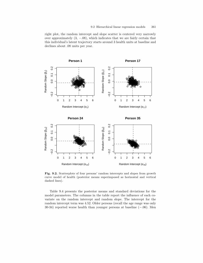
9.2 Hierarchical linear regression models 261
right plot, the random intercept and slope scatter is centered very narrowlyover approximately (3, −.08), which indicates that we are fairly certain thatthis individual’s latent trajectory starts around 3 health units at baseline anddeclines about .08 units per year.
0 1 2 3 4 5 6
−0.
20.
00.
10.
2
Person 1
Random Intercept (α1)
Ran
dom
Slo
pe (
β 1)
0 1 2 3 4 5 6
−0.
20.
00.
10.
2
Person 17
Random Intercept (α17)
Ran
dom
Slo
pe (
β 17)
0 1 2 3 4 5 6
−0.
20.
00.
10.
2
Person 24
Random Intercept (α24)
Ran
dom
Slo
pe (
β 24)
0 1 2 3 4 5 6
−0.
20.
00.
10.
2
Person 35
Random Intercept (α35)
Ran
dom
Slo
pe (
β 35)
Fig. 9.2. Scatterplots of four persons’ random intercepts and slopes from growthcurve model of health (posterior means superimposed as horizontal and verticaldashed lines).
Table 9.4 presents the posterior means and standard deviations for themodel parameters. The columns in the table report the influence of each co-variate on the random intercept and random slope. The intercept for therandom intercept term was 4.52. Older persons (recall the age range was only30-34) reported worse health than younger persons at baseline (−.06). Men
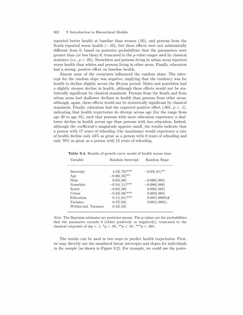
262 9 Introduction to Hierarchical Models
reported better health at baseline than women (.05), and persons from theSouth reported worse health (−.05), but these effects were not substantiallydifferent from 0, based on posterior probabilities that the parameters weregreater than (or less than) 0, truncated to the p-value ranges used by classicalstatistics (i.e., p < .05). Nonwhites and persons living in urban areas reportedworse health than whites and persons living in other areas. Finally, educationhad a strong, positive effect on baseline health.
Almost none of the covariates influenced the random slope. The inter-cept for the random slope was negative, implying that the tendency was forhealth to decline slightly across the 20-year period. Males and nonwhites hada slightly steeper decline in health, although these effects would not be sta-tistically significant by classical standards. Persons from the South and fromurban areas had shallower declines in health than persons from other areas,although, again, these effects would not be statistically significant by classicalstandards. Finally, education had the expected positive effect (.001, p < .1),indicating that health trajectories do diverge across age (for the range fromage 30 to age 55), such that persons with more education experience a shal-lower decline in health across age than persons with less education. Indeed,although the coefficient’s magnitude appears small, the results indicate thata person with 17 years of schooling (the maximum) would experience a rateof health decline only 43% as great as a person with 0 years of schooling andonly 76% as great as a person with 12 years of schooling.
Table 9.4. Results of growth curve model of health across time.
Variable Random Intercept Random Slope
Intercept 4.52(.70)*** −0.03(.01)**Age −0.06(.02)**Male 0.05(.08) −0.006(.005)Nonwhite −0.54(.11)*** −0.006(.008)South −0.05(.08) 0.003(.005)Urban −0.23(.08)*** 0.003(.005)Education 0.11(.01)*** 0.001(.0009)#Variance 0.37(.03) 0.001(.0001)Within-ind. Variance 0.42(.02)
Note: The Bayesian estimates are posterior means. The p-values are the probabilitiesthat the parameter exceeds 0 (either positively or negatively), truncated to theclassical cutpoints of #p < .1, *p < .05, **p < .01, ***p < .001.
The results can be used in two ways to predict health trajectories. First,we may directly use the simulated latent intercepts and slopes for individualsin the sample (as shown in Figure 9.2). For example, we could use the poste-

9.2 Hierarchical linear regression models 263
rior means for these simulated intercepts and slopes to construct an expectedtrajectory: yit = µαi
+ µβi× t. Second, we may use the posterior distribu-
tions for the model parameters—the covariate effects—to compute predictedlatent intercepts and slopes for persons with particular covariate profiles. Thisapproach allows us to predict trajectories for individuals out of the sample,in addition to those in the sample. Person 1 shown in Figure 9.2 was a 31-year-old nonwhite male living in a non-southern, urban area with 11 years ofschooling. Based on the posterior means for the effects of the covariates, thisindividual would have a predicted intercept of 3.22 for his health trajectoryand a predicted slope of −.022.
Figure 9.3 shows these two types of predicted trajectories for the fourindividuals shown in the previous figure, along with their observed healthmeasures. The solid line in each graph shows the predicted trajectory basedon the posterior means of the simulated, individual-specific random interceptsand slopes (i.e., the simulated values from Figure 9.2). The dashed line in eachgraph shows the model predicted trajectory based on the posterior means ofthe parameters applied to each individual’s covariate profile.
There is a substantial difference between these two trajectories, as well asbetween either trajectory and the observed health measures. This variationreflects the different types of (error) variance captured by the model. Thediscrepancies between the solid-line trajectories and the observed health mea-sures are captured by the within-individual error variance parameter σ2. Inbrief, we do not expect each individual’s health measure to fall exactly on thesolid line, because a number of unobserved factors may “bump” an individualoff of his/her expected, latent health trajectory at any point in time. Instead,what the model has attempted to capture is the best fitting line for the ob-served health measures. This error may be reduced by including time-specificmeasures into the model as we did in the previous section in the model inwhich we included Internet usage as a time-varying covariate.
The discrepancies between the solid and dashed-line trajectories, on theother hand, reflect the extent of between-individual variation captured (ornot!) by the covariates in the model. Put another way, if the covariates per-fectly explained all differences between individuals’ health trajectories, thesolid and dashed lines would perfectly coincide. The fact that these lines arenot overlapping suggests that our covariates do a poor job differentiating indi-viduals in the sample. This conclusion is foretold by the lack of strong resultsin Table 9.4, especially with respect to the general lack of effect of covari-ates on the latent growth rate. Indeed, if we consider the estimated rate ofdecline in health for each individual in Figure 9.3, all four individuals areexpected to have similar, shallow rates of health decline that obviously donot match the observed health declines (or those predicted by the simulatedindividual-specific random effects). In contrast, the estimated intercepts forthese trajectories show greater variability, reflecting the stronger effects of thecovariates in predicting baseline health. In an additional model (not shown),I re-estimated this growth model with no covariates to obtain estimates of
264 9 Introduction to Hierarchical Models
the variance of the mean latent intercept and slope. An R2 for the effectsof the covariates on the estimated latent intercept was found by computing1− τ2
α,cov/τ2α,nocov, using the posterior means for these variance parameters
from the two models. A similar calculation was performed for the variance ofthe latent slope (τ2
β). The results indicated that the covariates reduced thebetween-individual variance in the latent intercept by 29% (i.e., R2 = .29),but the covariates reduced the between-individual variance in the latent slopeby only 10%. These results confirm that our covariates have little effect on thelatent slope, and therefore, it is no surprise that our two types of predictedtrajectories differ substantially.
As a final note on growth modeling, the use of growth models has beenrapidly expanding in psychology and sociology over the last decade, in partbecause the growing availability of longitudinal (panel) data has enabled theinvestigation of life course processes for which growth modeling is well suited.Additionally, growth models have become increasingly popular, because theycan be estimated via a variety of software packages, including HLM and var-ious structural equation modeling packages (see Willett and Sayer 1994; seealso McArdle and Epstein 1987, Meredith and Tisak 1990 and Rogosa andWillett 1985). The HLM approach closely resembles the modeling strategydeveloped in this section. The structural equation modeling approach, on theother hand, is in some ways more intuitive, although it is mathematicallyequivalent to the Bayesian and HLM approaches.5 However, that approachtypically requires balanced data—that is, data that have been collected atthe same time and at all times for all individuals in the sample. This lat-ter requirement can be relaxed by assuming that individuals who are missingat one or more occasions are missing at random and estimating the modelusing a full information maximum likelihood (FIML) estimator. The formerrestriction, however, is not easily relaxed. However, estimating the model us-ing a Bayesian approach or using other hierarchical modeling packages offer astraightforward way to handling unbalanced data. For more details on latentgrowth modeling within a structural equation modeling framework, I highlyrecommend Bollen and Curran (2006).
9.3 A note on fixed versus random effects models andother terminology
One issue that makes understanding hierarchical models difficult is the ter-minology that different disciplines and statistical paradigms use to describevarious features of the models. In this section, I hope to clarify some of theterminology, although there is certain to be some disagreement regarding my
5 In fact, for each growth model example presented here, I estimated the equivalentmodel using a structural equation approach. The results were nearly identical.
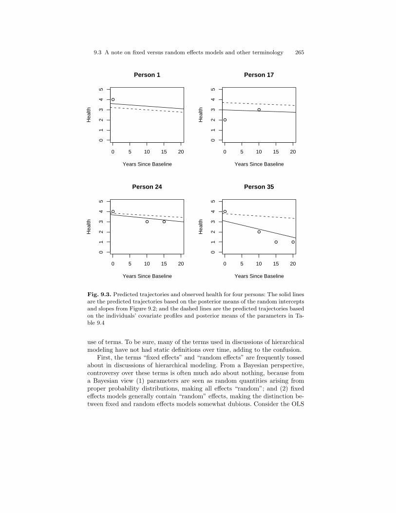
9.3 A note on fixed versus random effects models and other terminology 265
0 5 10 15 20
01
23
45
Person 1
Years Since Baseline
Hea
lth
0 5 10 15 20
01
23
45
Person 17
Years Since Baseline
Hea
lth
0 5 10 15 20
01
23
45
Person 24
Years Since Baseline
Hea
lth
0 5 10 15 20
01
23
45
Person 35
Years Since Baseline
Hea
lth
Fig. 9.3. Predicted trajectories and observed health for four persons: The solid linesare the predicted trajectories based on the posterior means of the random interceptsand slopes from Figure 9.2; and the dashed lines are the predicted trajectories basedon the individuals’ covariate profiles and posterior means of the parameters in Ta-ble 9.4
use of terms. To be sure, many of the terms used in discussions of hierarchicalmodeling have not had static definitions over time, adding to the confusion.
First, the terms “fixed effects” and “random effects” are frequently tossedabout in discussions of hierarchical modeling. From a Bayesian perspective,controversy over these terms is often much ado about nothing, because froma Bayesian view (1) parameters are seen as random quantities arising fromproper probability distributions, making all effects “random”; and (2) fixedeffects models generally contain “random” effects, making the distinction be-tween fixed and random effects models somewhat dubious. Consider the OLS
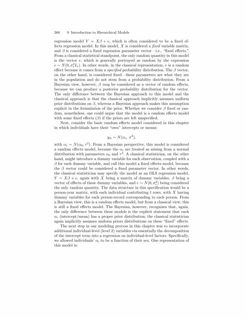
266 9 Introduction to Hierarchical Models
regression model Y = Xβ + e, which is often considered to be a fixed ef-fects regression model. In this model, X is considered a fixed variable matrix,and β is considered a fixed regression parameter vector—i.e., “fixed effects.”From a classical statistical standpoint, the only random quantity in this modelis the vector e, which is generally portrayed as random by the expressione ∼ N(0, σ2
eIn). In other words, in the classical representation, e is a randomeffect because it comes from a specified probability distribution. The β vector,on the other hand, is considered fixed—these parameters are what they arein the population and do not stem from a probability distribution. From aBayesian view, however, β may be considered as a vector of random effects,because we can produce a posterior probability distribution for the vector.The only difference between the Bayesian approach to this model and theclassical approach is that the classical approach implicitly assumes uniformprior distributions on β, whereas a Bayesian approach makes this assumptionexplicit in the formulation of the prior. Whether we consider β fixed or ran-dom, nonetheless, one could argue that the model is a random effects modelwith some fixed effects (β) if the priors are left unspecified.
Next, consider the basic random effects model considered in this chapterin which individuals have their “own” intercepts or means:
yit ∼ N(αi, σ2),
with αi ∼ N(α0, τ2). From a Bayesian perspective, this model is considered
a random effects model, because the αi are treated as arising from a normaldistribution with parameters α0 and τ2. A classical statistician, on the otherhand, might introduce a dummy variable for each observation, coupled with aβ for each dummy variable, and call this model a fixed effects model, becausethe β vector could be considered a fixed parameter vector. In other words,the classical statistician may specify the model as an OLS regression model,Y = Xβ + e, again with X being a matrix of dummy variables, β being avector of effects of these dummy variables, and e ∼ N(0, σ2
e) being consideredthe only random quantity. The data structure in this specification would be aperson-year matrix, with each individual contributing t rows, with X havingdummy variables for each person-record corresponding to each person. Froma Bayesian view, this is a random effects model, but from a classical view, thisis still a fixed effects model. The Bayesian, however, recognizes that, again,the only difference between these models is the explicit statement that eachαi (intercept/mean) has a proper prior distribution; the classical statisticianagain implicitly assumes uniform priors distributions on these “fixed” effects.
The next step in our modeling process in this chapter was to incorporateadditional individual-level (level 2) variables via essentially the decompositionof the intercept term into a regression on individual-level factors. Specifically,we allowed individuals’ αi to be a function of their sex. One representation ofthis model is:

9.3 A note on fixed versus random effects models and other terminology 267
yit ∼ N(αi, σ2)
αi ∼ N(α(0) + α(1)sexi, τ2),
along with appropriate (vague) hyperpriors for the hyperparameters α(0), α(1),σ2, and τ2. Alternatively, but equivalently, the model may be specified as wedid earlier:
yit ∼ N(αi + α(1)sexi, σ2)
αi ∼ N(α0, τ2),
again with appropriate priors for α(0), α(1), σ2, and τ2. A Bayesian thenwould call this a random intercept model. The classical statistician, on theother hand, would write this model as:
yit = αi + α1sexi + eit
eit ∼ N(0, σ2)αi = α0 + ui
uit ∼ N(0, τ2).
After substituting the third equation into the first, we would obtain:
yit = α0 + ui + α1sexi + eit.
Under this representation, the classical statistician would claim that α0 andα1 are fixed effects, and that the only random effects are ui and eit. If ui
is considered a component of α0, then the model could be called a randomintercept model with fixed effects. Once again, however, the Bayesian wouldargue that the explicit assignment of proper priors for α0 and α1 makes themodel a random effects model: The classical approach is implicitly assuminguniform priors on these parameters.
In subsequent steps of our modeling building process, we included Internetusage as a time-varying (level 1) variable, and we eventually allowed the influ-ence of Internet usage on wages to vary across individuals and we allowed theindividual-specific influence of Internet usage to be a function of individuals’sex:
yit ∼ N(αi + βiInternetit, σ2)
αi ∼ N(α0 + α1sexi, τ2α)
βi ∼ N(β0 + β1sexi, τ2β),
once again with appropriate hyperprior distributions for the higher level hy-perparameters. Using Bayesian terminology, this model is a “random coeffi-cients” model, because the regression coefficient βi is allowed to vary acrossindividuals. The classical approach, however, would find
268 9 Introduction to Hierarchical Models
yit = α0 + α1sexi + ui + β0Internetit + β1sexiInternetit + viInternetit + eit
after subsitution and might call the model a fixed effects model with randomintercepts, random coefficients, and cross-level interactions.
To make a long story short, all of these models are considered hierarchi-cal models because there is a hierarchical structure to the parameters. Theymay also be called multilevel models because the variables in the models aremeasured at different levels (time-specific measures and individual-level mea-sures). Additionally, all the models contain random effects and may thereforebe called random effects models, despite the fact that the classical statisticianmay prefer to include the term “fixed effects” in describing them. When theregression parameters—and not simply the intercepts—are allowed to varyacross individuals, they may be called “random coefficient models.” Whentime is included as a variable and its influence—a random coefficient—is al-lowed to vary across individuals, the model may be called a “(latent) growth(curve) model.” Finally, all of these models are sometimes called “mixed mod-els,” because they generally include both fixed and random effects when theterms “fixed” and “random” are applied to distinguish between effects thathave implicit versus explicit prior distributions.
9.4 Conclusions
In this chapter, we have covered considerable ground. We began by discussinghow we can use the conditional probability rule to produce hierarchical struc-ture in the parameters and obtain a posterior distribution for all parametersin a simple model without covariates. We then discussed how hierarchical re-gression models can easily be constructed to capture hierarchical structure inboth the parameters and the data with variables measured at different lev-els. Finally, we showed how the general hiearchical linear regression modelcan be specialized to examine growth in the outcome over time by includingtime in the model as a covariate. As the chapter demonstrated, the Bayesianapproach is naturally suited to hierarchical modeling. Indeed, the Bayesianapproach handles hierarchicality so easily that virtually no text on Bayesianstatistics omits hierarchical modeling, and I can find no Bayesian text thatonly covers hierarchical modeling. For further reading on Bayesian hierarchi-cal modeling, as I said at the beginning of the chapter, I recommend Gelmanet al. (1995). I also recommend Gill (2002) for an introductory exposition,and I suggest Spiegelhalter et al. (1996) for an illustrative example of growthmodeling.

9.5 Exercises 269
9.5 Exercises
1. Show the steps in the derivation of the conditional posterior distributionfor τ in Equation 9.5.
2. Explain why the values chosen to complete the hyperprior specification inSection 9.2.1 are noninformative.
3. Explain in your own words why the first growth model presented in Sec-tion 9.2.3 cannot allow Internet usage to be a time-varying variable in themodel as it is specified.
4. Using your own data, write an R routine to estimate a growth model.Then write a WinBugs routine to estimate the same model. Are the resultssimilar?


10
Introduction to Multivariate RegressionModels
In the social sciences, we commonly use multiple outcome variables in an-swering a research question rather than a single outcome variable. In thesecases, we may prefer to construct “multivariate models” rather than a seriesof univariate models like those presented in the previous three chapters. Typ-ically, when social scientists refer to multivariate models, they mean simplythat they are estimating a model with more than one variable; however, fora statistician, the term “multivariate model” generally implies that a modelhas more than one outcome/response variable. A variety of different types ofmultivariate response models exists; in this chapter, we will consider only twoof them: the multivariate linear regression model and the multivariate probitmodel. My goal in this chapter is not to provide an exhaustive account ofmultivariate models, a task that would require an entire book. Instead, mygoal is to present the basic ideas of multivariate modeling.
There are two primary reasons for constructing a multivariate model inplace of a set of univariate ones: (1) to eliminate biases or improve efficiencyover using a set of univariate models, and (2) to facilitate the use of modelparameters from a joint model in making inference for unestimated parame-ters/quantities. We will consider the first reason first in reconsidering the or-dinary least squares (OLS) regression models for “niceness” from Chapter 7.Then we will consider the latter reason in an example for the multivariateprobit model.
10.1 Multivariate linear regression
10.1.1 Model development
The most basic type of multivariate regression model is the extension of theOLS regression model to handle an M -length vector of responses Y for eachindividual in a sample, rather than a single response outcome (i.e., M = 1).For example, reconsidering the example from Chapter 7 in which we evaluated

272 10 Introduction to Multivariate Regression Models
whether Southerners are “nicer” than persons who have always lived in otherregions of the country, we could have treated the four outcomes—empathy,selflessness, tolerance, and altruistic acts—as a vector of responses for eachindividual rather than as separate responses. The result would have been asingle model, rather than four separate ones. In that case, the X variableswould have been the same for each equation, but each X would have beenallowed to have a different effect on each outcome. This model can be expressedjust as the OLS regression model:
Y = Xβ + e,
but the dimensions of the model matrices are expanded to handle the addi-tional responses. In this representation, Y and e are now n×M, rather thann× 1, with the additional columns representing the additional dimensions ofresponse. X is still n× k, but now β is expanded to be k ×M to allow eachX to have a distinct influence on each outcome. Thus, the expanded matrixrepresentation appears as:
y11 . . . y1M
.... . .
...yn1 . . . ynM
=
x11 . . . x1k
.... . .
...xn1 . . . xnk
β11 . . . β1M
.... . .
...βk1 . . . βkM
+
e11 . . . e1M
.... . .
...en1 . . . enM
n×M n× k k ×M n×M
,
(10.1)When the errors from each regression equation are unrelated, i.e., (eT e)ij =0,∀i 6= j, the model is equivalent to running independent univariate OLSregression models. In that case, the OLS solution of β = (XT X)−1(XT Y ) isstill the optimal classical solution—only the dimensionality of the solution haschanged—and, under uniform priors, this solution is still the posterior meanfor β. That is, p(β|X, Y ) ∼ N(βOLS, σ2
e(XT X)−1), where σ2e is a diagonal
matrix of error variances.However, when errors are correlated across equations, the univariate and
multivariate approaches are not necessarily equivalent. It can be shown that,when the cross-equation errors are correlated, the independent OLS solutionswill not be the same as the multivariate solution if (1) the covariate vectors arenot identical across equations; that is, if the X vectors differ across equations,or (2) if cross-equation constraints are imposed. For example, suppose weallowed education to influence the empathy outcome but not the other threeoutcomes. Alternatively, suppose we forced education’s influence on empathyand altruistic acts to be the same, or we fixed its effect to be some constant. Inthese cases, this model is called the “seemingly-unrelated regression model”in econometrics (see Zellner 1962), and the OLS solution will no longer be“best”—it will be less efficient than the multivariate solution.
To obtain the multivariate solution, we begin with construction of a mul-tivariate likelihood function. Whereas with the univariate linear regression
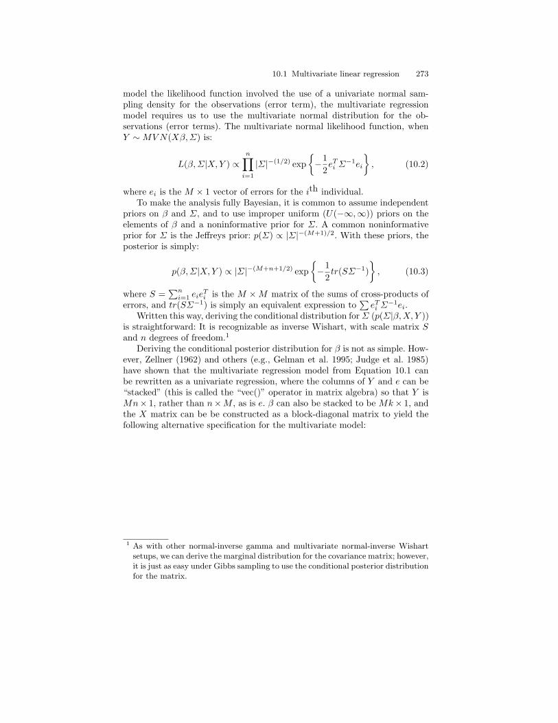
10.1 Multivariate linear regression 273
model the likelihood function involved the use of a univariate normal sam-pling density for the observations (error term), the multivariate regressionmodel requires us to use the multivariate normal distribution for the ob-servations (error terms). The multivariate normal likelihood function, whenY ∼ MV N(Xβ, Σ) is:
L(β, Σ|X, Y ) ∝n∏
i=1
|Σ|−(1/2) exp−1
2eTi Σ−1ei
, (10.2)
where ei is the M × 1 vector of errors for the ith individual.To make the analysis fully Bayesian, it is common to assume independent
priors on β and Σ, and to use improper uniform (U(−∞,∞)) priors on theelements of β and a noninformative prior for Σ. A common noninformativeprior for Σ is the Jeffreys prior: p(Σ) ∝ |Σ|−(M+1)/2. With these priors, theposterior is simply:
p(β, Σ|X, Y ) ∝ |Σ|−(M+n+1/2) exp−1
2tr(SΣ−1)
, (10.3)
where S =∑n
i=1 eieTi is the M ×M matrix of the sums of cross-products of
errors, and tr(SΣ−1) is simply an equivalent expression to∑
eTi Σ−1ei.
Written this way, deriving the conditional distribution for Σ (p(Σ|β, X, Y ))is straightforward: It is recognizable as inverse Wishart, with scale matrix Sand n degrees of freedom.1
Deriving the conditional posterior distribution for β is not as simple. How-ever, Zellner (1962) and others (e.g., Gelman et al. 1995; Judge et al. 1985)have shown that the multivariate regression model from Equation 10.1 canbe rewritten as a univariate regression, where the columns of Y and e can be“stacked” (this is called the “vec()” operator in matrix algebra) so that Y isMn× 1, rather than n×M , as is e. β can also be stacked to be Mk× 1, andthe X matrix can be be constructed as a block-diagonal matrix to yield thefollowing alternative specification for the multivariate model:
1 As with other normal-inverse gamma and multivariate normal-inverse Wishartsetups, we can derive the marginal distribution for the covariance matrix; however,it is just as easy under Gibbs sampling to use the conditional posterior distributionfor the matrix.
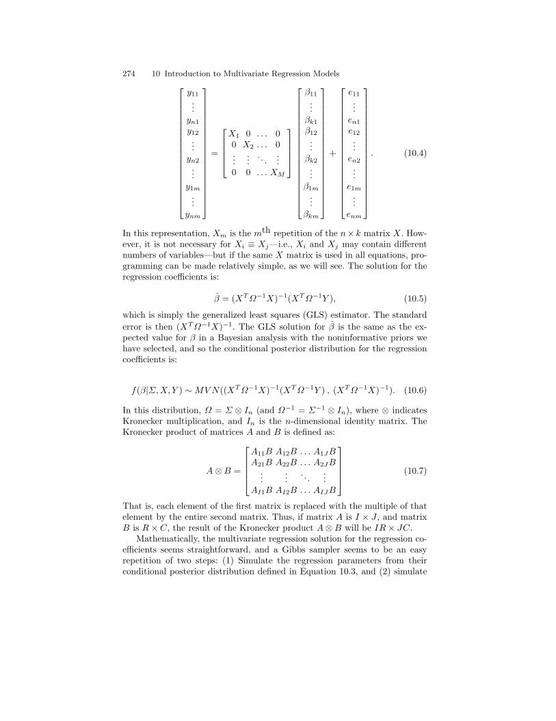
274 10 Introduction to Multivariate Regression Models
y11
...yn1
y12
...yn2
...y1m
...ynm
=
X1 0 . . . 00 X2 . . . 0...
.... . .
...0 0 . . . XM
β11
...βk1
β12
...βk2
...β1m
...βkm
+
e11
...en1
e12
...en2
...e1m
...enm
. (10.4)
In this representation, Xm is the mth repetition of the n× k matrix X. How-ever, it is not necessary for Xi ≡ Xj—i.e., Xi and Xj may contain differentnumbers of variables—but if the same X matrix is used in all equations, pro-gramming can be made relatively simple, as we will see. The solution for theregression coefficients is:
β = (XT Ω−1X)−1(XT Ω−1Y ), (10.5)
which is simply the generalized least squares (GLS) estimator. The standarderror is then (XT Ω−1X)−1. The GLS solution for β is the same as the ex-pected value for β in a Bayesian analysis with the noninformative priors wehave selected, and so the conditional posterior distribution for the regressioncoefficients is:
f(β|Σ,X, Y ) ∼ MV N((XT Ω−1X)−1(XT Ω−1Y ) , (XT Ω−1X)−1). (10.6)
In this distribution, Ω = Σ ⊗ In (and Ω−1 = Σ−1 ⊗ In), where ⊗ indicatesKronecker multiplication, and In is the n-dimensional identity matrix. TheKronecker product of matrices A and B is defined as:
A⊗B =
A11B A12B . . . A1JBA21B A22B . . . A2JB
......
. . ....
AI1B AI2B . . . AIJB
(10.7)
That is, each element of the first matrix is replaced with the multiple of thatelement by the entire second matrix. Thus, if matrix A is I × J , and matrixB is R× C, the result of the Kronecker product A⊗B will be IR× JC.
Mathematically, the multivariate regression solution for the regression co-efficients seems straightforward, and a Gibbs sampler seems to be an easyrepetition of two steps: (1) Simulate the regression parameters from theirconditional posterior distribution defined in Equation 10.3, and (2) simulate
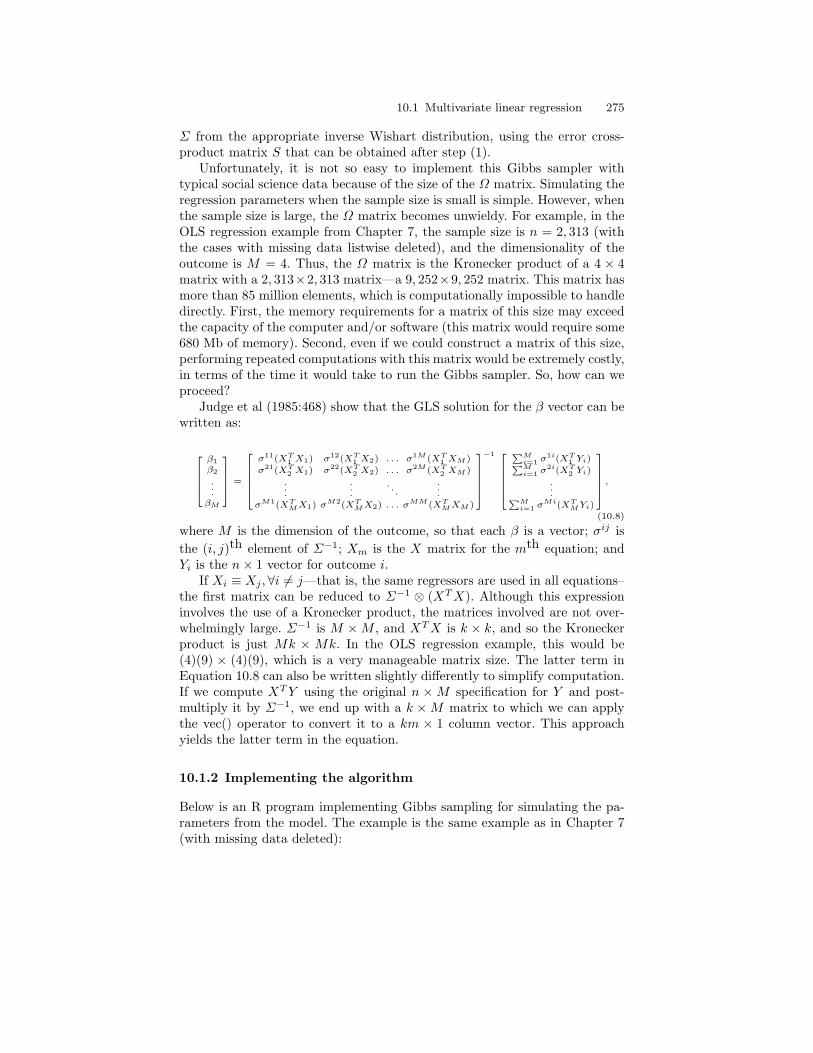
10.1 Multivariate linear regression 275
Σ from the appropriate inverse Wishart distribution, using the error cross-product matrix S that can be obtained after step (1).
Unfortunately, it is not so easy to implement this Gibbs sampler withtypical social science data because of the size of the Ω matrix. Simulating theregression parameters when the sample size is small is simple. However, whenthe sample size is large, the Ω matrix becomes unwieldy. For example, in theOLS regression example from Chapter 7, the sample size is n = 2, 313 (withthe cases with missing data listwise deleted), and the dimensionality of theoutcome is M = 4. Thus, the Ω matrix is the Kronecker product of a 4 × 4matrix with a 2, 313×2, 313 matrix—a 9, 252×9, 252 matrix. This matrix hasmore than 85 million elements, which is computationally impossible to handledirectly. First, the memory requirements for a matrix of this size may exceedthe capacity of the computer and/or software (this matrix would require some680 Mb of memory). Second, even if we could construct a matrix of this size,performing repeated computations with this matrix would be extremely costly,in terms of the time it would take to run the Gibbs sampler. So, how can weproceed?
Judge et al (1985:468) show that the GLS solution for the β vector can bewritten as:
26664β1β2
.
.
.βM
37775 =
266664σ11(XT
1 X1) σ12(XT1 X2) . . . σ1M (XT
1 XM )
σ21(XT2 X1) σ22(XT
2 X2) . . . σ2M (XT2 XM )
.
.
....
. . ....
σM1(XTM X1) σM2(XT
M X2) . . . σMM (XTM XM )
377775−1 266664
PMi=1 σ1i(XT
1 Yi)PMi=1 σ2i(XT
2 Yi)
.
.
.PMi=1 σMi(XT
M Yi)
377775 ,
(10.8)
where M is the dimension of the outcome, so that each β is a vector; σij isthe (i, j)th element of Σ−1; Xm is the X matrix for the mth equation; andYi is the n× 1 vector for outcome i.
If Xi ≡ Xj ,∀i 6= j—that is, the same regressors are used in all equations–the first matrix can be reduced to Σ−1 ⊗ (XT X). Although this expressioninvolves the use of a Kronecker product, the matrices involved are not over-whelmingly large. Σ−1 is M ×M , and XT X is k × k, and so the Kroneckerproduct is just Mk × Mk. In the OLS regression example, this would be(4)(9) × (4)(9), which is a very manageable matrix size. The latter term inEquation 10.8 can also be written slightly differently to simplify computation.If we compute XT Y using the original n ×M specification for Y and post-multiply it by Σ−1, we end up with a k ×M matrix to which we can applythe vec() operator to convert it to a km × 1 column vector. This approachyields the latter term in the equation.
10.1.2 Implementing the algorithm
Below is an R program implementing Gibbs sampling for simulating the pa-rameters from the model. The example is the same example as in Chapter 7(with missing data deleted):

276 10 Introduction to Multivariate Regression Models
#R program for multivariate regression
x<-as.matrix(read.table("c:\\mvn_examp.dat")[,2:10])
y<-as.matrix(read.table("c:\\mvn_examp.dat")[,11:14])
d=4;k=9
b<-matrix(0,(d*k)); s<-diag(d)
for(i in 2:1000)
#draw b from mvn
vb=solve(solve(s)%x%(t(x)%*%x))
mn=vb%*%(as.vector(t(x)%*%y%*%t(solve(s))))
b=mn+t(rnorm((d*k),0,1)%*%chol(vb))
#draw s from inverse wishart
e=matrix((as.vector(y)-(diag(d)%x%x%*%b)),nrow(y),d)
v=t(e)%*%e
s=riwish(nrow(y)-1,v)
print(c(b[1],b[10],b[19],b[28],s[1,1],s[2,2],s[3,3],s[4,4]))
write(c(t(b),t(s)),file="c:\\mvn2.out",ncolumns=52,append=T)
The program first reads the data into two matrices x and y and assignsthe number of dimensions of the outcome (d=4) and covariate vector (k=9). Itthen creates a vector for the regression coefficients and a matrix for the errorcovariance and assigns starting values for each—all regression coefficients areassumed to be 0; the error covariance matrix is set to an identity.
The Gibbs sampler begins first with the construction of the variance matrixfor the parameters (vb), which is also the first part of the regression vectormean. The remainder of the regression vector mean is then computed (mn), andthen the regression vector is drawn from its multivariate normal conditionaldistribution. Once the regression vector is drawn, the matrix of errors—asin the original model specification in Equation 10.1—is computed, and thecross-product matrix of the errors is computed (v). This matrix is used asthe scale matrix S in the inverse Wishart distribution for drawing the errorcovariance matrix Σ.
Table 10.1 shows the results of the multivariate regression model. If youcompare these results with those of Table 7.2 in Chapter 7, you will see that theresults are substantially similar. Indeed, only a few coefficients and posteriorstandard deviations change at all, and those that do change do not changesubstantially. That is, if one considers the implied posterior distributions forthe parameters, their overlap overshadows their slight differences.
As I stated above, when the X matrix is the same for all equations as it isin this example, there is nothing gained—beyond elegance—by using a multi-variate model rather than a series of univariate OLS regressions. However, if
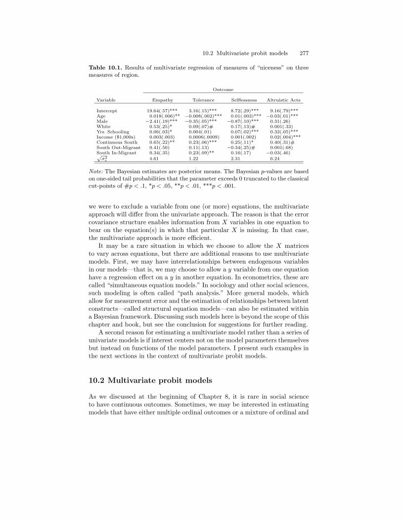
10.2 Multivariate probit models 277
Table 10.1. Results of multivariate regression of measures of “niceness” on threemeasures of region.
Outcome
Variable Empathy Tolerance Selflessness Altruistic Acts
Intercept 19.64(.57)*** 3.16(.15)*** 8.72(.29)*** 9.16(.79)***Age 0.018(.006)** −0.008(.002)*** 0.01(.003)*** −0.03(.01)***Male −2.41(.19)*** −0.35(.05)*** −0.87(.10)*** 0.31(.26)White 0.53(.25)* 0.09(.07)# 0.17(.13)# 0.001(.33)Yrs. Schooling 0.06(.03)* 0.004(.01) 0.07(.02)*** 0.32(.05)***Income ($1,000s) 0.003(.003) 0.0006(.0009) 0.001(.002) 0.02(.004)***Continuous South 0.65(.22)** 0.23(.06)*** 0.25(.11)* 0.40(.31)#South Out-Migrant 0.41(.50) 0.11(.13) −0.34(.25)# 0.001(.68)South In-Migrant 0.34(.35) 0.23(.09)** 0.16(.17) −0.03(.46)p
σ2e 4.61 1.22 2.31 6.24
Note: The Bayesian estimates are posterior means. The Bayesian p-values are basedon one-sided tail probabilities that the parameter exceeds 0 truncated to the classicalcut-points of #p < .1, *p < .05, **p < .01, ***p < .001.
we were to exclude a variable from one (or more) equations, the multivariateapproach will differ from the univariate approach. The reason is that the errorcovariance structure enables information from X variables in one equation tobear on the equation(s) in which that particular X is missing. In that case,the multivariate approach is more efficient.
It may be a rare situation in which we choose to allow the X matricesto vary across equations, but there are additional reasons to use multivariatemodels. First, we may have interrelationships between endogenous variablesin our models—that is, we may choose to allow a y variable from one equationhave a regression effect on a y in another equation. In econometrics, these arecalled “simultaneous equation models.” In sociology and other social sciences,such modeling is often called “path analysis.” More general models, whichallow for measurement error and the estimation of relationships between latentconstructs—called structural equation models—can also be estimated withina Bayesian framework. Discussing such models here is beyond the scope of thischapter and book, but see the conclusion for suggestions for further reading.
A second reason for estimating a multivariate model rather than a series ofunivariate models is if interest centers not on the model parameters themselvesbut instead on functions of the model parameters. I present such examples inthe next sections in the context of multivariate probit models.
10.2 Multivariate probit models
As we discussed at the beginning of Chapter 8, it is rare in social scienceto have continuous outcomes. Sometimes, we may be interested in estimatingmodels that have either multiple ordinal outcomes or a mixture of ordinal and

278 10 Introduction to Multivariate Regression Models
continuous outcomes. On other occasions, we may be interested in a modelthat has a single, but nominal-level, outcome. In the former cases, we sim-ply need an extension of the multivariate regression model discussed in theprevious section combined with a generalization that allows us to work withnon-continuous outcomes, as discussed in Chapter 8—called a multivariateprobit model. In the latter case, we need a similar, but more constrained,model in which the outcome variable is converted into a series of dichotomousoutcomes that are treated as mutually exclusive in the model—called a multi-nomial probit model. Algorithms to estimate these two different models differprimarily in this mutual-exclusivity criterion.
A model with multiple ordinal outcomes (including possibly multiple di-chotomous outcomes) is relatively straightforward to construct and estimate.We can use an algorithm similar to that for the multivariate linear modelwith only three alterations. First, we must include a Gibbs sampling step inwhich we sample latent data underlying the observed ordinal responses, justas we did in the generalized linear model (GLM) extension of the OLS regres-sion model. However, the latent data now must be sampled from truncatedmultivariate normal distributions rather than from truncated univariate nor-mal distributions, and such truncated multivariate normal simulation is notnearly as simple as truncated univariate normal simulation. Second, the er-ror covariance matrix can technically no longer be simulated from an inverseWishart distribution. In order to identify the multivariate probit model, wemust constrain the variances of the latent variables to be 1. This constraintmakes simulating from the inverse Wishart distribution difficult or impossible;instead, we may use a Metropolis step to simulate the free parameters of theerror correlation matrix. Third, as in the ordinal probit model in Chapter 8,when there are more than two outcome categories for a particular variable,the model will include free thresholds that must be estimated. In the followingsections, I present two examples. The first example shows the basic approachto handling multivariate ordinal data. The second example shows how we canexpand the model to handle “missing” data and use the results to constructdistributions of quantities not directly estimated within the model that are afunction of parameters from the multivariate equations.
10.2.1 Model development
Before we address the issues raised in the previous section, let’s consider thegeneral multivariate probit model (see also Chib and Greenberg 1998). In theexamples, I will limit the outcome to two dimensions, but there is no inherentneed to do so. As a generic example, suppose we want to determine whetherpolitical views and party affiliations have changed over time (see DiMaggio,Evans, and Bryson 1996, who tackle a similar question of interest). The GSShas asked at least two relevant questions since 1972. One asks whether respon-dents view themselves as liberal or conservative, while the other asks respon-dents whether they consider themselves to be Democrats or Republicans. Both
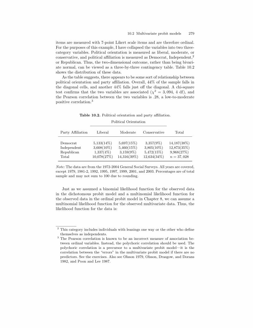
10.2 Multivariate probit models 279
items are measured with 7-point Likert scale items and are therefore ordinal.For the purposes of this example, I have collapsed the variables into two three-category variables. Political orientation is measured as liberal, moderate, orconservative, and political affiliation is measured as Democrat, Independent,2
or Republican. Thus, the two-dimensional outcome, rather than being bivari-ate normal, can be viewed as a three-by-three contingency table. Table 10.2shows the distribution of these data.
As the table suggests, there appears to be some sort of relationship betweenpolitical orientation and party affiliation. Overall, 44% of the sample falls inthe diagonal cells, and another 44% falls just off the diagonal. A chi-squaretest confirms that the two variables are associated (χ2 = 3, 094, 4 df), andthe Pearson correlation between the two variables is .28, a low-to-moderatepositive correlation.3
Table 10.2. Political orientation and party affiliation.
Political Orientation
Party Affiliation Liberal Moderate Conservative Total
Democrat 5,133(14%) 5,697(15%) 3,357(9%) 14,187(38%)Independent 3,608(10%) 5,460(15%) 3,805(10%) 12,873(35%)Republican 1,337(4%) 3,159(9%) 5,472(15%) 9,968(27%)Total 10,078(27%) 14,316(39%) 12,634(34%) n = 37, 028
Note: The data are from the 1972-2004 General Social Surveys. All years are covered,except 1979, 1981-2, 1992, 1995, 1997, 1999, 2001, and 2003. Percentages are of totalsample and may not sum to 100 due to rounding.
Just as we assumed a binomial likelihood function for the observed datain the dichotomous probit model and a multinomial likelihood function forthe observed data in the ordinal probit model in Chapter 8, we can assume amultinomial likelihood function for the observed multivariate data. Thus, thelikelihood function for the data is:
2 This category includes individuals with leanings one way or the other who definethemselves as independents.
3 The Pearson correlation is known to be an incorrect measure of association be-tween ordinal variables. Instead, the polychoric correlation should be used. Thepolychoric correlation is a precursor to a multivariate probit model—it is thecorrelation between the “errors” in the multivariate probit model if there are nopredictors. See the exercises. Also see Olsson 1979, Olsson, Drasgow, and Dorans1982, and Poon and Lee 1987.
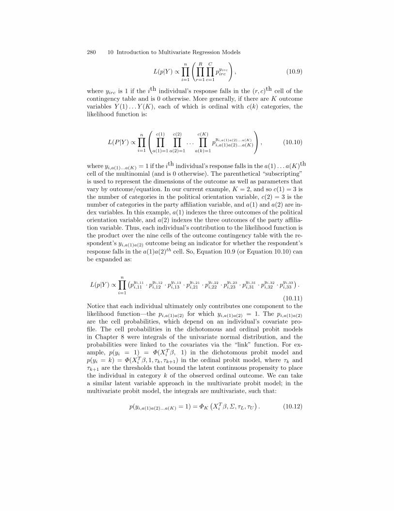
280 10 Introduction to Multivariate Regression Models
L(p|Y ) ∝n∏
i=1
(R∏
r=1
C∏c=1
pyirc
irc
), (10.9)
where yirc is 1 if the ith individual’s response falls in the (r, c)th cell of thecontingency table and is 0 otherwise. More generally, if there are K outcomevariables Y (1) . . . Y (K), each of which is ordinal with c(k) categories, thelikelihood function is:
L(P |Y ) ∝n∏
i=1
c(1)∏a(1)=1
c(2)∏a(2)=1
. . .
c(K)∏a(k)=1
pyi,a(1)a(2)...a(K)
i,a(1)a(2)...a(K)
, (10.10)
where yi,a(1)...a(K) = 1 if the ith individual’s response falls in the a(1) . . . a(K)th
cell of the multinomial (and is 0 otherwise). The parenthetical “subscripting”is used to represent the dimensions of the outcome as well as parameters thatvary by outcome/equation. In our current example, K = 2, and so c(1) = 3 isthe number of categories in the political orientation variable, c(2) = 3 is thenumber of categories in the party affiliation variable, and a(1) and a(2) are in-dex variables. In this example, a(1) indexes the three outcomes of the politicalorientation variable, and a(2) indexes the three outcomes of the party affilia-tion variable. Thus, each individual’s contribution to the likelihood function isthe product over the nine cells of the outcome contingency table with the re-spondent’s yi,a(1)a(2) outcome being an indicator for whether the respondent’sresponse falls in the a(1)a(2)th cell. So, Equation 10.9 (or Equation 10.10) canbe expanded as:
L(p|Y ) ∝n∏
i=1
(p
yi,11i,11 · pyi,12
i,12 · pyi,13i,13 · pyi,21
i,21 · pyi,22i,22 · pyi,23
i,23 · pyi,31i,31 · pyi,32
i,32 · pyi,33i,33
).
(10.11)Notice that each individual ultimately only contributes one component to thelikelihood function—the pi,a(1)a(2) for which yi,a(1)a(2) = 1. The pi,a(1)a(2)
are the cell probabilities, which depend on an individual’s covariate pro-file. The cell probabilities in the dichotomous and ordinal probit modelsin Chapter 8 were integrals of the univariate normal distribution, and theprobabilities were linked to the covariates via the “link” function. For ex-ample, p(yi = 1) = Φ(XT
i β, 1) in the dichotomous probit model andp(yi = k) = Φ(XT
i β, 1, τk, τk+1) in the ordinal probit model, where τk andτk+1 are the thresholds that bound the latent continuous propensity to placethe individual in category k of the observed ordinal outcome. We can takea similar latent variable approach in the multivariate probit model; in themultivariate probit model, the integrals are multivariate, such that:
p(yi,a(1)a(2)...a(K) = 1) = ΦK
(XT
i β, Σ, τL, τU
). (10.12)
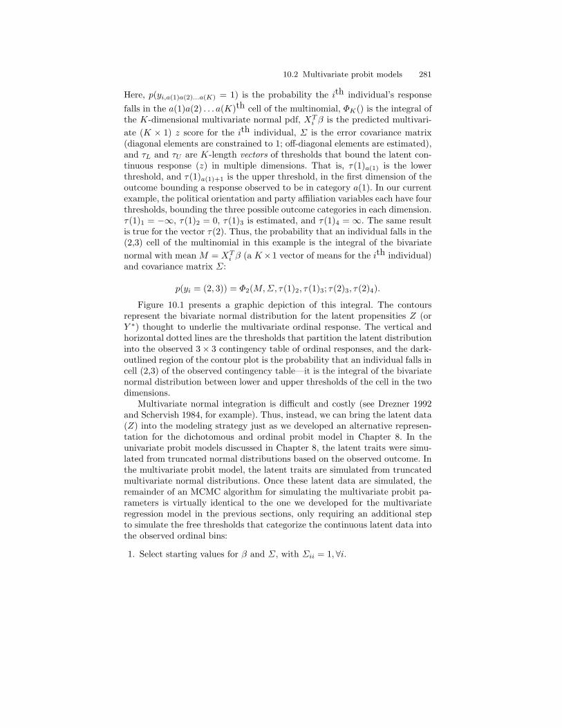
10.2 Multivariate probit models 281
Here, p(yi,a(1)a(2)...a(K) = 1) is the probability the ith individual’s responsefalls in the a(1)a(2) . . . a(K)th cell of the multinomial, ΦK() is the integral ofthe K-dimensional multivariate normal pdf, XT
i β is the predicted multivari-ate (K × 1) z score for the ith individual, Σ is the error covariance matrix(diagonal elements are constrained to 1; off-diagonal elements are estimated),and τL and τU are K-length vectors of thresholds that bound the latent con-tinuous response (z) in multiple dimensions. That is, τ(1)a(1) is the lowerthreshold, and τ(1)a(1)+1 is the upper threshold, in the first dimension of theoutcome bounding a response observed to be in category a(1). In our currentexample, the political orientation and party affiliation variables each have fourthresholds, bounding the three possible outcome categories in each dimension.τ(1)1 = −∞, τ(1)2 = 0, τ(1)3 is estimated, and τ(1)4 = ∞. The same resultis true for the vector τ(2). Thus, the probability that an individual falls in the(2,3) cell of the multinomial in this example is the integral of the bivariatenormal with mean M = XT
i β (a K×1 vector of means for the ith individual)and covariance matrix Σ:
p(yi = (2, 3)) = Φ2(M,Σ, τ(1)2, τ(1)3; τ(2)3, τ(2)4).
Figure 10.1 presents a graphic depiction of this integral. The contoursrepresent the bivariate normal distribution for the latent propensities Z (orY ∗) thought to underlie the multivariate ordinal response. The vertical andhorizontal dotted lines are the thresholds that partition the latent distributioninto the observed 3× 3 contingency table of ordinal responses, and the dark-outlined region of the contour plot is the probability that an individual falls incell (2,3) of the observed contingency table—it is the integral of the bivariatenormal distribution between lower and upper thresholds of the cell in the twodimensions.
Multivariate normal integration is difficult and costly (see Drezner 1992and Schervish 1984, for example). Thus, instead, we can bring the latent data(Z) into the modeling strategy just as we developed an alternative represen-tation for the dichotomous and ordinal probit model in Chapter 8. In theunivariate probit models discussed in Chapter 8, the latent traits were simu-lated from truncated normal distributions based on the observed outcome. Inthe multivariate probit model, the latent traits are simulated from truncatedmultivariate normal distributions. Once these latent data are simulated, theremainder of an MCMC algorithm for simulating the multivariate probit pa-rameters is virtually identical to the one we developed for the multivariateregression model in the previous sections, only requiring an additional stepto simulate the free thresholds that categorize the continuous latent data intothe observed ordinal bins:
1. Select starting values for β and Σ, with Σii = 1,∀i.
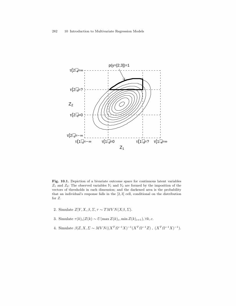
282 10 Introduction to Multivariate Regression Models
τ(1)1=− ∞ τ(1)2=0 τ(1)3=? τ(1)4=∞τ(2)1=− ∞
τ(2)2=0
τ(2)3=?
τ(2)4=∞p(y=[2,3])=1
Z1
Z2
Fig. 10.1. Depiction of a bivariate outcome space for continuous latent variablesZ1 and Z2: The observed variables Y1 and Y2 are formed by the imposition of thevectors of thresholds in each dimension; and the darkened area is the probabilitythat an individual’s response falls in the [2, 3] cell, conditional on the distributionfor Z.
2. Simulate Z|Y, X, β,Σ, τ ∼ TMV N(Xβ, Σ).
3. Simulate τ(k)c|Z(k) ∼ U(max Z(k)c,minZ(k)c+1),∀k, c.
4. Simulate β|Z,X, Σ ∼ MV N((XT Ω−1X)−1(XT Ω−1Z) , (XT Ω−1X)−1).
10.2 Multivariate probit models 283
5. Simulate Σ|Z, β, X ∼ IW (S, n), where S =∑n
i=1(Z −Xiβ)(Z −Xiβ)T ,subject to the constraint the Σii = 1,∀i.
6. Return to Step 2.
The first step, finding starting values, is straightforward. I generally startall regression parameters at 0 and the error covariance matrix Σ as an identitymatrix. The fourth step—simulation of the regression coefficients—requiresvery little discussion. Once the latent data Z replace the observed ordinaldata Y and an appropriate Σ matrix is available, the conditional distributionfor the regression parameters is identical to that of the multivariate regressionmodel presented in the previous section. The second, third, and fifth steps,on the other hand, require some discussion.
10.2.2 Step 2: Simulating draws from truncated multivariatenormal distributions
Simulating draws from truncated multivariate normal distributions is sub-stantially more complicated than simulating draws from truncated univariatenormal distributions. One method for simulating such draws is the naive ap-proach we discussed in Chapter 8: We simulate from untruncated normaldistributions until we obtain a draw from the appropriate region. For exam-ple, using the current example, if we wished to simulate a latent score fora person with an observed y = (2, 3) response, we would simulate from theentire bivariate normal distribution exemplified in Figure 10.1 until we ob-tained a draw that fell in the dark-outlined region. It is easy to see that thisnaive approach is extremely inefficient, and becomes increasingly so as the di-mensionality of the problem increases and as the number of categories in theordinal variables increases. Basically, anything that reduces the ratio of thearea under the multivariate normal curve in one cell relative to the total areaunder the multivariate normal curve reduces the naive approach’s efficiency.
We have already discussed how to simulate from truncated univariate nor-mal distributions, and so, if we can break simulation from our truncated mul-tivariate normal distribution into a series of truncated univariate normal dis-tribution simulations, it seems our problem is solved. One way that we canbreak the multivariate simulation problem into a series of univariate ones is todecompose the joint density function f(x1, x2, . . . , xK−1, xK) into the prod-uct of conditional distributions (as we did to construct hierarchical models inChapter 9) using the conditional probability rule that f(A,B) = f(A|B)f(B).We can carry this decomposition out beyond two variables as:
f(x1, x2, . . . , xK) = f(xK |xK−1, . . . , x1) . . . f(x3|x1, x2)f(x2|x1)f(x1).(10.13)
That this decomposition is correct can be seen by starting from the right endand recognizing that the first marginal times the first conditional leads to

284 10 Introduction to Multivariate Regression Models
a joint distribution for two variables. This joint distribution is then a newmarginal distribution, which, when multiplied by the next conditional distri-bution, yields a joint distribution for three variables, and so on:
f(x1, x2, . . . , xK) = . . . f(x4|x1, x2, x3) f(x3|x1, x2) f(x2|x1) f(x1)
f(x1, x2)
f(x1, x2, x3)
f(x1, x2, x3, x4)...
Thus, we can first draw x1 from its appropriate univariate normal distribu-tion. Then, conditional on this draw, we can draw x2 from f(x2|x1). Then,conditional on these draws, we can draw x3 from f(x3|x1, x2), and so on.Earlier, we discussed that the conditional distribution for one variable (e.g.,x2) from a standard bivariate normal distribution given the other (e.g., x1)is univariate normal with a mean of ρx1 and variance 1 − ρ2. More gener-ally, it is known that the conditional distribution for a single variable in amultivariate normal distribution is itself normal. If Z ∼ MV N(µ,Σ), then(Za|µ(−a) = M) ∼ N(µ∗, Σ∗), where:
µ∗ = µa + Σa.Σ−1(−a)
(µ(−a) −M
)(10.14)
Σ∗ = Σaa −Σa.Σ−1(−a)Σ.a. (10.15)
In these expressions, Σ(−a) is the multivariate covariance matrix obtained byomitting row and column a, Σa. is the ath row of Σ (similarly, Σ.a is the ath
column of Σ), and M is the current value of the normal draws for the other(i.e., −a) dimensions.
Thus, sampling from a multivariate normal distribution involves simplysampling the first variable from its univariate marginal distribution; then sam-pling the second variable from its univariate conditional distribution, whichdepends only on the first variable, then sampling the third variable from itsunivariate conditional distribution, which depends only on the first and sec-ond variables; and so on. Below is an R subroutine that samples 10,000 drawsfrom a five-dimensional normal distribution with mean vector µT = [1 2 3 4 5]and covariance matrix with all covariances equal to .5 and the variancesσ2
ii = [5 4 3 2 1]. The sampling begins with the last element (x5) and sam-ples from the appropriate conditional distribution moving backward to x1.Thus, as the fourth element is being sampled from its conditional distribu-tion, the relevant covariance matrix is the 2 × 2 matrix for variables x4 andx5. As the third element is being sampled, the relevant covariance matrix isthe 3× 3 covariance matrix for variables x3, x4, and x5, etc.:
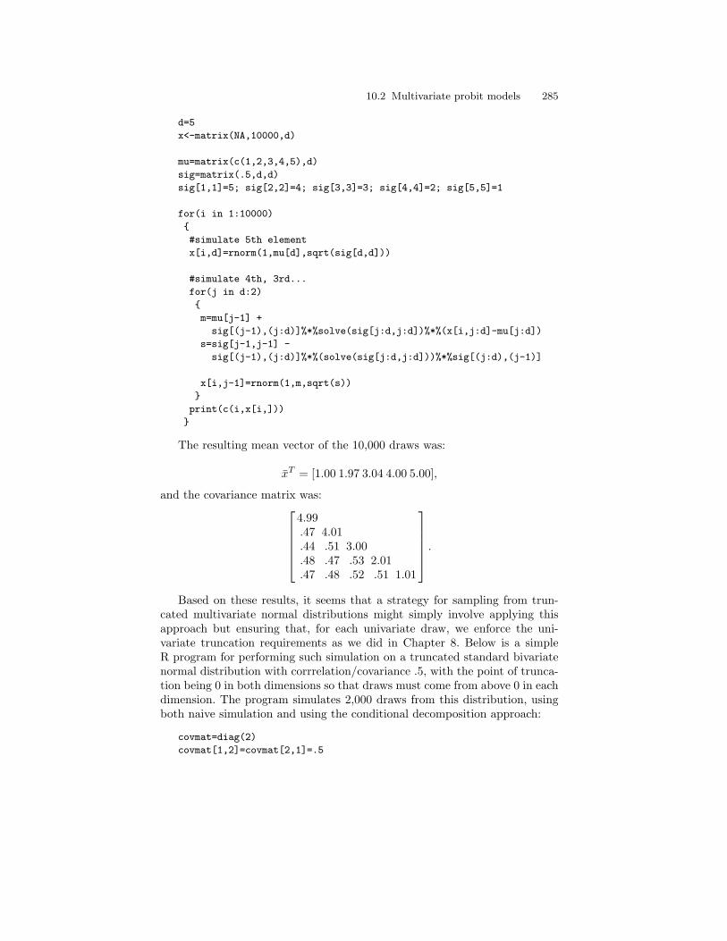
10.2 Multivariate probit models 285
d=5
x<-matrix(NA,10000,d)
mu=matrix(c(1,2,3,4,5),d)
sig=matrix(.5,d,d)
sig[1,1]=5; sig[2,2]=4; sig[3,3]=3; sig[4,4]=2; sig[5,5]=1
for(i in 1:10000)
#simulate 5th element
x[i,d]=rnorm(1,mu[d],sqrt(sig[d,d]))
#simulate 4th, 3rd...
for(j in d:2)
m=mu[j-1] +
sig[(j-1),(j:d)]%*%solve(sig[j:d,j:d])%*%(x[i,j:d]-mu[j:d])
s=sig[j-1,j-1] -
sig[(j-1),(j:d)]%*%(solve(sig[j:d,j:d]))%*%sig[(j:d),(j-1)]
x[i,j-1]=rnorm(1,m,sqrt(s))
print(c(i,x[i,]))
The resulting mean vector of the 10,000 draws was:
xT = [1.00 1.97 3.04 4.00 5.00],
and the covariance matrix was:4.99.47 4.01.44 .51 3.00.48 .47 .53 2.01.47 .48 .52 .51 1.01
.
Based on these results, it seems that a strategy for sampling from trun-cated multivariate normal distributions might simply involve applying thisapproach but ensuring that, for each univariate draw, we enforce the uni-variate truncation requirements as we did in Chapter 8. Below is a simpleR program for performing such simulation on a truncated standard bivariatenormal distribution with corrrelation/covariance .5, with the point of trunca-tion being 0 in both dimensions so that draws must come from above 0 in eachdimension. The program simulates 2,000 draws from this distribution, usingboth naive simulation and using the conditional decomposition approach:
covmat=diag(2)
covmat[1,2]=covmat[2,1]=.5
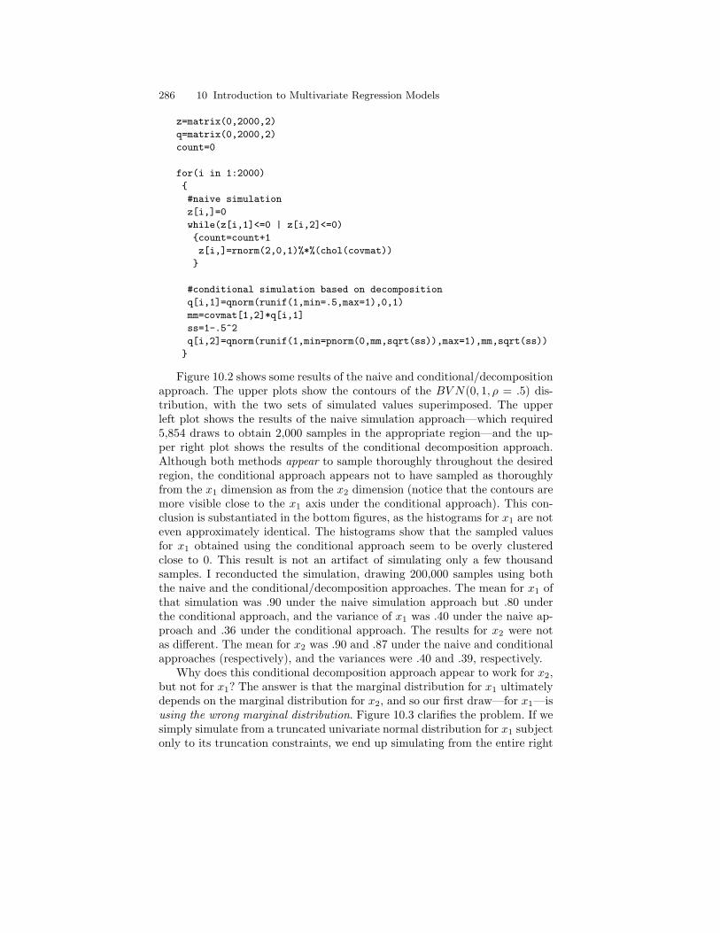
286 10 Introduction to Multivariate Regression Models
z=matrix(0,2000,2)
q=matrix(0,2000,2)
count=0
for(i in 1:2000)
#naive simulation
z[i,]=0
while(z[i,1]<=0 | z[i,2]<=0)
count=count+1
z[i,]=rnorm(2,0,1)%*%(chol(covmat))
#conditional simulation based on decomposition
q[i,1]=qnorm(runif(1,min=.5,max=1),0,1)
mm=covmat[1,2]*q[i,1]
ss=1-.5^2
q[i,2]=qnorm(runif(1,min=pnorm(0,mm,sqrt(ss)),max=1),mm,sqrt(ss))
Figure 10.2 shows some results of the naive and conditional/decompositionapproach. The upper plots show the contours of the BV N(0, 1, ρ = .5) dis-tribution, with the two sets of simulated values superimposed. The upperleft plot shows the results of the naive simulation approach—which required5,854 draws to obtain 2,000 samples in the appropriate region—and the up-per right plot shows the results of the conditional decomposition approach.Although both methods appear to sample thoroughly throughout the desiredregion, the conditional approach appears not to have sampled as thoroughlyfrom the x1 dimension as from the x2 dimension (notice that the contours aremore visible close to the x1 axis under the conditional approach). This con-clusion is substantiated in the bottom figures, as the histograms for x1 are noteven approximately identical. The histograms show that the sampled valuesfor x1 obtained using the conditional approach seem to be overly clusteredclose to 0. This result is not an artifact of simulating only a few thousandsamples. I reconducted the simulation, drawing 200,000 samples using boththe naive and the conditional/decomposition approaches. The mean for x1 ofthat simulation was .90 under the naive simulation approach but .80 underthe conditional approach, and the variance of x1 was .40 under the naive ap-proach and .36 under the conditional approach. The results for x2 were notas different. The mean for x2 was .90 and .87 under the naive and conditionalapproaches (respectively), and the variances were .40 and .39, respectively.
Why does this conditional decomposition approach appear to work for x2,but not for x1? The answer is that the marginal distribution for x1 ultimatelydepends on the marginal distribution for x2, and so our first draw—for x1—isusing the wrong marginal distribution. Figure 10.3 clarifies the problem. If wesimply simulate from a truncated univariate normal distribution for x1 subjectonly to its truncation constraints, we end up simulating from the entire right
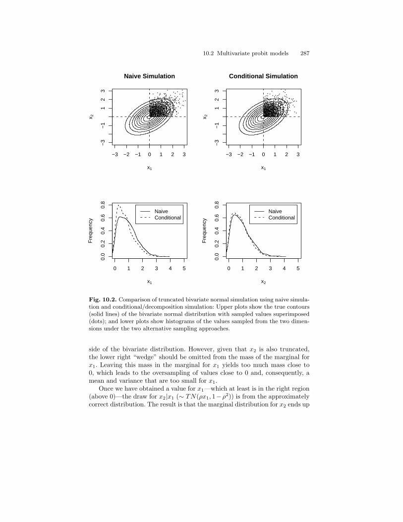
10.2 Multivariate probit models 287
Naive Simulation
x1
x 2
−3 −2 −1 0 1 2 3
−3
−1
12
3
Conditional Simulation
x1
x 2
−3 −2 −1 0 1 2 3
−3
−1
12
3
0 1 2 3 4 5
0.0
0.2
0.4
0.6
0.8
x1
Fre
quen
cy
NaiveConditional
0 1 2 3 4 5
0.0
0.2
0.4
0.6
0.8
x2
Fre
quen
cyNaiveConditional
Fig. 10.2. Comparison of truncated bivariate normal simulation using naive simula-tion and conditional/decomposition simulation: Upper plots show the true contours(solid lines) of the bivariate normal distribution with sampled values superimposed(dots); and lower plots show histograms of the values sampled from the two dimen-sions under the two alternative sampling approaches.
side of the bivariate distribution. However, given that x2 is also truncated,the lower right “wedge” should be omitted from the mass of the marginal forx1. Leaving this mass in the marginal for x1 yields too much mass close to0, which leads to the oversampling of values close to 0 and, consequently, amean and variance that are too small for x1.
Once we have obtained a value for x1—which at least is in the right region(above 0)—the draw for x2|x1 (∼ TN(ρx1, 1−ρ2)) is from the approximatelycorrect distribution. The result is that the marginal distribution for x2 ends up
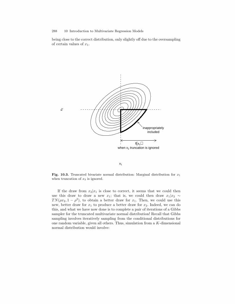
288 10 Introduction to Multivariate Regression Models
being close to the correct distribution, only slightly off due to the oversamplingof certain values of x1.
x1
x 2
f(x1)when x2 truncation is ignored
inappropriatelyincluded
Fig. 10.3. Truncated bivariate normal distribution: Marginal distribution for x1
when truncation of x2 is ignored.
If the draw from x2|x1 is close to correct, it seems that we could thenuse this draw to draw a new x1; that is, we could then draw x1|x2 ∼TN(ρx2, 1 − ρ2), to obtain a better draw for x1. Then, we could use thisnew, better draw for x1 to produce a better draw for x2. Indeed, we can dothis, and what we have now done is to complete a pair of iterations of a Gibbssampler for the truncated multivariate normal distribution! Recall that Gibbssampling involves iteratively sampling from the conditional distributions forone random variable, given all others. Thus, simulation from a K-dimensionalnormal distribution would involve:
10.2 Multivariate probit models 289
1. Simulate x1|x2, x3, x4, . . . , xK−1, xK .2. Simulate x2|x1, x3, x4, . . . , xK−1, xK .3. Simulate x3|x1, x2, x4, . . . , xK−1, xK ....
...K − 1. Simulate xK−1|x1, x2, x3, . . . , xK−2, xK .
K. Simulate xK |x1, x2, x3, . . . , xK−2, xK−1.
If we follow this Gibbs sampling strategy, simulating each variable from itsconditional distribution subject to its univariate truncation constraints, theGibbs sampler will produce a sample from the truncated multivariate normaldistribution within a few iterations. To perform the Gibbs sampling, eachconditional distribution can be derived using Equations 10.14 and 10.15.
Figure 10.4 shows the results of 2,000 samples if we follow this Gibbssampling strategy for only two iterations per sample.4 As the histograms show,the distributions for both x1 and x2 now closely match those obtained fromthe less efficient naive sampling approach. The means for x1 and x2 underthis approach were .89 and .90, respectively—both close to the means of .90and .90 obtained via naive sampling—and the variances were .40 and .40,respectively—both almost indistinguishable from the variances of .40 and .40obtained via naive sampling (see Robert 1995 who presents a more detailedand theoretical discussion of this approach).
In conclusion, although simulating from truncated multivariate normal dis-tributions is more complex than simulating from truncated univariate normaldistributions, we can perform such simulation using a Gibbs sampler withfew iterations, suggesting that we can simulate our latent data in a multi-variate probit model algorithm fairly efficiently—a Gibbs-sampler-within-a-Gibbs-sampler approach!
10.2.3 Step 3: Simulation of thresholds in the multivariate probitmodel
As we discussed in Chapter 8, the conditional distributions for the free thresh-olds are straightforward to derive: The conditionals in the univariate probitmodel are simply uniform on the interval between the largest latent scoresimulated for a person in the category below the threshold of interest and thesmallest latent score simulated for a person in the category above the thresh-old of interest. The thresholds in the multivariate probit are equally easy toderive. For the sake of simplicity of notation, let’s assume a bivariate probitmodel with uniform prior distributon for all parameters. The latent variablerepresentation of the posterior distribution then is:
p(τ, β,Σ, Z|X, Y ) ∝
4 The last three lines of the algorithm, in which mm and ss and q[i,?] are derived,are repeated twice: q[i,1] is drawn; then q[i,2] is drawn again.

290 10 Introduction to Multivariate Regression Models
Naive Simulation
x1
x 2
−3 −2 −1 0 1 2 3
−3
−1
12
3
Conditional Simulation
x1
x 2
−3 −2 −1 0 1 2 3
−3
−1
12
3
0 1 2 3 4 5
0.0
0.2
0.4
0.6
0.8
x1
Fre
quen
cy
NaiveConditional
0 1 2 3 4 5
0.0
0.2
0.4
0.6
0.8
x2
Fre
quen
cyNaiveConditional
Fig. 10.4. Comparison of truncated bivariate normal distribution simulation usingnaive simulation and two iterations of Gibbs sampling: Upper plots show the truecontours (solid lines) of the bivariate normal distribution with sampled values su-perimposed (dots); and lower plots show histograms of the values sampled from thetwo dimensions under the two alternative approaches to sampling.
n∏i=1
(R∑
r=1
C∑c=1
φ2(Zi −XTi β, Σ)I(τr < zi1 < τr+1)I(τc < zi2 < τc+1)
),
where Zi is the two-dimensional latent variable for individual i, with zi1 andzi2 representing the specific elements, φ2(a, b) is the bivariate normal densityfunction with mean a and covariance matrix b, τr is the rth threshold in thefirst dimension, and τc is the cth threshold in the second dimension. Thisposterior can be expanded as in Equation 10.11, but as in that example,
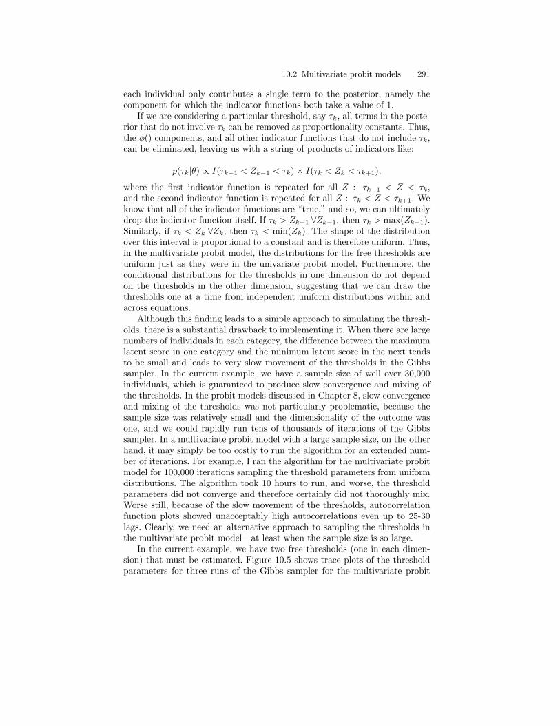
10.2 Multivariate probit models 291
each individual only contributes a single term to the posterior, namely thecomponent for which the indicator functions both take a value of 1.
If we are considering a particular threshold, say τk, all terms in the poste-rior that do not involve τk can be removed as proportionality constants. Thus,the φ() components, and all other indicator functions that do not include τk,can be eliminated, leaving us with a string of products of indicators like:
p(τk|θ) ∝ I(τk−1 < Zk−1 < τk)× I(τk < Zk < τk+1),
where the first indicator function is repeated for all Z : τk−1 < Z < τk,and the second indicator function is repeated for all Z : τk < Z < τk+1. Weknow that all of the indicator functions are “true,” and so, we can ultimatelydrop the indicator function itself. If τk > Zk−1 ∀Zk−1, then τk > max(Zk−1).Similarly, if τk < Zk ∀Zk, then τk < min(Zk). The shape of the distributionover this interval is proportional to a constant and is therefore uniform. Thus,in the multivariate probit model, the distributions for the free thresholds areuniform just as they were in the univariate probit model. Furthermore, theconditional distributions for the thresholds in one dimension do not dependon the thresholds in the other dimension, suggesting that we can draw thethresholds one at a time from independent uniform distributions within andacross equations.
Although this finding leads to a simple approach to simulating the thresh-olds, there is a substantial drawback to implementing it. When there are largenumbers of individuals in each category, the difference between the maximumlatent score in one category and the minimum latent score in the next tendsto be small and leads to very slow movement of the thresholds in the Gibbssampler. In the current example, we have a sample size of well over 30,000individuals, which is guaranteed to produce slow convergence and mixing ofthe thresholds. In the probit models discussed in Chapter 8, slow convergenceand mixing of the thresholds was not particularly problematic, because thesample size was relatively small and the dimensionality of the outcome wasone, and we could rapidly run tens of thousands of iterations of the Gibbssampler. In a multivariate probit model with a large sample size, on the otherhand, it may simply be too costly to run the algorithm for an extended num-ber of iterations. For example, I ran the algorithm for the multivariate probitmodel for 100,000 iterations sampling the threshold parameters from uniformdistributions. The algorithm took 10 hours to run, and worse, the thresholdparameters did not converge and therefore certainly did not thoroughly mix.Worse still, because of the slow movement of the thresholds, autocorrelationfunction plots showed unacceptably high autocorrelations even up to 25-30lags. Clearly, we need an alternative approach to sampling the thresholds inthe multivariate probit model—at least when the sample size is so large.
In the current example, we have two free thresholds (one in each dimen-sion) that must be estimated. Figure 10.5 shows trace plots of the thresholdparameters for three runs of the Gibbs sampler for the multivariate probit
292 10 Introduction to Multivariate Regression Models
model (to be discussed in the next section), as well as autocorrelation func-tion plots for the threshold parameter in the first equation/dimension of theoutcome (τ13). The first two plots in the first column of the 3-by-3 figureshows the trace plots for the two threshold parameters from a 10,000 iter-ation run of the Gibbs sampler, with every tenth sample saved. From thefigures, it is not clear that the threshold parameters’ samples have mixedwell, nor is it clear whether the algorithm has even converged. The bottomplot in the column is the autocorrrelation function plot for τ13. Even afterthinning the Gibbs samples to every tenth sample, the threshold parametershows extremely high autocorrelation. The second column of the figure showsthe results of extending the algorithm another 90,000 iterations (still savingevery tenth). Once again, it is not clear that the algorithm has mixed wellnor converged. Furthermore, the autocorrelation plot at the bottom of thecolumn shows extremely high autocorrelation. The third column, in contrast,shows the results for the thresholds when Cowles’ (1996) algorithm is used tosample them. This algorithm was run for 6,000 iterations, with the samplesthinned to every fifth iteration. The upper two plots show rapid convergenceand thorough mixing. Furthermore, the autocorrelation function plot showslittle autocorrrelation beyond one lag.
What is Cowles’ algorithm? Cowles’ algorithm is a Metropolis–Hastings(MH) step that replaces the Gibbs sampling step for simulating the thresh-olds from uniform distributions (Cowles 1996). Rather than simulating thethresholds from narrow uniform distributions, Cowles’ algorithm generatescandidate thresholds over the entire interval between adjacent thresholds andthen uses the standard MH accept/reject criterion for determining whether toaccept the candidate. The result is that the thresholds, even though all candi-dates are not accepted, make larger “jumps” when they move, leading to morerapid convergence, faster mixing, and less autocorrelation between successivesamples of the thresholds. I describe Cowles’ algorithm for one dimension—i.e., one vector of thresholds—but the algorithm is extendable to multivariatemodels, as I show in Section 10.2.5.
Consider a vector of thresholds, τ for a one-dimensional ordinal variablewith K categories:
τ = [(τ1 = −∞) (τ2 = 0) . . . (τK−1) (τK) (τK+1 = ∞)].
Cowles’ algorithm begins by simulating candidate parameters for each freeelement of τ from normal distributions centered over the current value ofeach τ truncated at the current values of the thresholds below and above thethreshold being simulated:
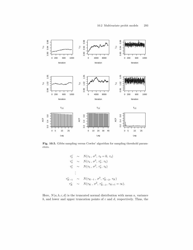
10.2 Multivariate probit models 293
0 200 600 1000
0.90
0.94
0.98
Iteration
τ 13
0 4000 8000
0.90
0.94
0.98
Iteration
τ 13
0 200 600 1000
0.90
0.94
0.98
Iteration
τ 13
0 200 600 1000
0.99
1.02
1.05
Iteration
τ 23
0 4000 8000
0.99
1.02
1.05
Iteration
τ 23
0 200 600 1000
0.99
1.02
1.05
Iteration
τ 23
0 5 15 25
0.0
0.4
0.8
Lag
AC
F
τ13
0 10 20 30 40
0.0
0.4
0.8
Lag
AC
F
τ13
0 5 15 25
0.0
0.4
0.8
Lag
AC
F
τ13
Fig. 10.5. Gibbs sampling versus Cowles’ algorithm for sampling threshold param-eters.
τ c3 ∼ N(τ3 , σ2, τ2 = 0, τ4)
τ c4 ∼ N(τ4 , σ2, τ c
3 , τ5)
τ c5 ∼ N(τ5 , σ2, τ c
4 , τ6)...
τ cK−1 ∼ N(τK−1 , σ2, τ c
K−2, τK)
τ cK ∼ N(τK , σ2, τ c
K−1, τK+1 = ∞).
Here, N(a, b, c, d) is the truncated normal distribution with mean a, varianceb, and lower and upper truncation points of c and d, respectively. Thus, the

294 10 Introduction to Multivariate Regression Models
generation of candidate values for the vector τ is sequential, with the lowertruncation point for τk being determined by the candidate threshold below(i.e., τ c
k−1), and the upper truncation point being determined by the currentvalue of the threshold above.
In our current political orientation/party affiliation example, only onethreshold is freely estimated in each dimension, and so, τ c
13 ∼ N(τ13, σ, τ12 =0, τ14 = ∞) and τ c
23 ∼ N(τ23, σ, τ22 = 0, τ24 = ∞).Once a set of candidates is generated, the next step in the MH algorithm
is to compute the ratio R. In this case, given the truncation of the normal pro-posal densities, the proposals are asymmetric, and hence, the full ratio mustbe computed. Given that the posterior distributions for the threshold param-eters are independent across equations, p(τ |β, Σ, Z, Y,X) ∝ p(τ |β, X, Y ), andso:
R =f(τ c|β, X, Y )g(τ |τ c)f(τ |β, X, Y )g(τ c|τ)
,
where f(a|b) is the posterior density evaluated at τ (or τ c) and g(c|d) is thevalue of the proposal density at c when the proposal is centered over d. Theposterior for the thresholds is:
p(τ |β, X, Y ) ∝n∏
i=1
Φ(XTi β, τyi , τyi+1),
where Φ(a, b, c) is the integral of the normal density function with mean a andvariance 1 between thresholds b and c. Thus, the first half of the ratio R is:
n∏i=1
Φ(βT Xi, τ cyi
, τ cyi+1)
Φ(βT Xi, τyi, τyi+1),
.
The latter half of the ratio corrects for the asymmetry in the proposals andis:
K∏j=3
Φ(τj , σ, τ cj−1, τj+1)
Φ(τ cj , σ, τj−1, τ c
j+1),
where in this case Φ(a, b, c, d) is the integral of the normal distribution withmean a and standard deviation b between the thresholds c and d. The standarddeviation b is chosen to produce an acceptance rate around 50%.
The product of these components constitutes the full ratio R. Once thisratio is computed, we follow the usual MH steps: We compare this ratio to au ∼ U(0, 1) random draw, and we accept τ c if R > u.
In the example at hand, we have a two-dimensional outcome, each dimen-sion of which only requires simulation of one threshold. As discussed in greaterdetail in Section 10.2.5, I perform a separate MH step for each dimension ofthe outcome.
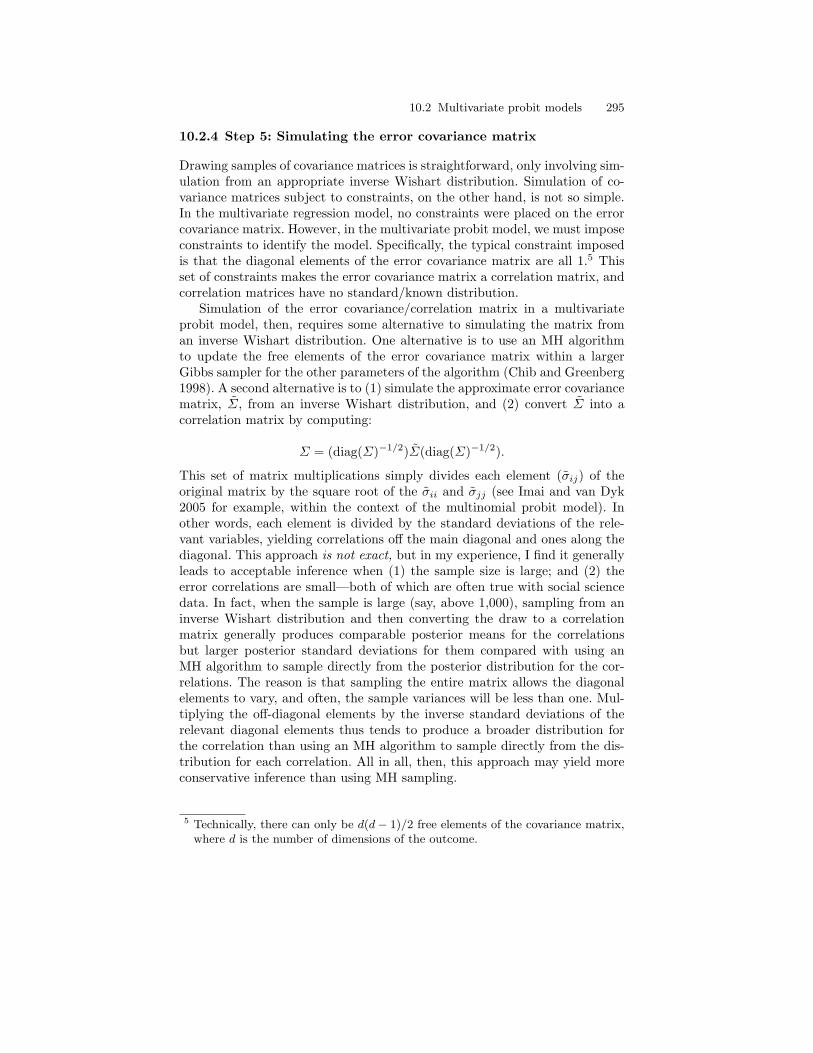
10.2 Multivariate probit models 295
10.2.4 Step 5: Simulating the error covariance matrix
Drawing samples of covariance matrices is straightforward, only involving sim-ulation from an appropriate inverse Wishart distribution. Simulation of co-variance matrices subject to constraints, on the other hand, is not so simple.In the multivariate regression model, no constraints were placed on the errorcovariance matrix. However, in the multivariate probit model, we must imposeconstraints to identify the model. Specifically, the typical constraint imposedis that the diagonal elements of the error covariance matrix are all 1.5 Thisset of constraints makes the error covariance matrix a correlation matrix, andcorrelation matrices have no standard/known distribution.
Simulation of the error covariance/correlation matrix in a multivariateprobit model, then, requires some alternative to simulating the matrix froman inverse Wishart distribution. One alternative is to use an MH algorithmto update the free elements of the error covariance matrix within a largerGibbs sampler for the other parameters of the algorithm (Chib and Greenberg1998). A second alternative is to (1) simulate the approximate error covariancematrix, Σ, from an inverse Wishart distribution, and (2) convert Σ into acorrelation matrix by computing:
Σ = (diag(Σ)−1/2)Σ(diag(Σ)−1/2).
This set of matrix multiplications simply divides each element (σij) of theoriginal matrix by the square root of the σii and σjj (see Imai and van Dyk2005 for example, within the context of the multinomial probit model). Inother words, each element is divided by the standard deviations of the rele-vant variables, yielding correlations off the main diagonal and ones along thediagonal. This approach is not exact, but in my experience, I find it generallyleads to acceptable inference when (1) the sample size is large; and (2) theerror correlations are small—both of which are often true with social sciencedata. In fact, when the sample is large (say, above 1,000), sampling from aninverse Wishart distribution and then converting the draw to a correlationmatrix generally produces comparable posterior means for the correlationsbut larger posterior standard deviations for them compared with using anMH algorithm to sample directly from the posterior distribution for the cor-relations. The reason is that sampling the entire matrix allows the diagonalelements to vary, and often, the sample variances will be less than one. Mul-tiplying the off-diagonal elements by the inverse standard deviations of therelevant diagonal elements thus tends to produce a broader distribution forthe correlation than using an MH algorithm to sample directly from the dis-tribution for each correlation. All in all, then, this approach may yield moreconservative inference than using MH sampling.
5 Technically, there can only be d(d− 1)/2 free elements of the covariance matrix,where d is the number of dimensions of the outcome.
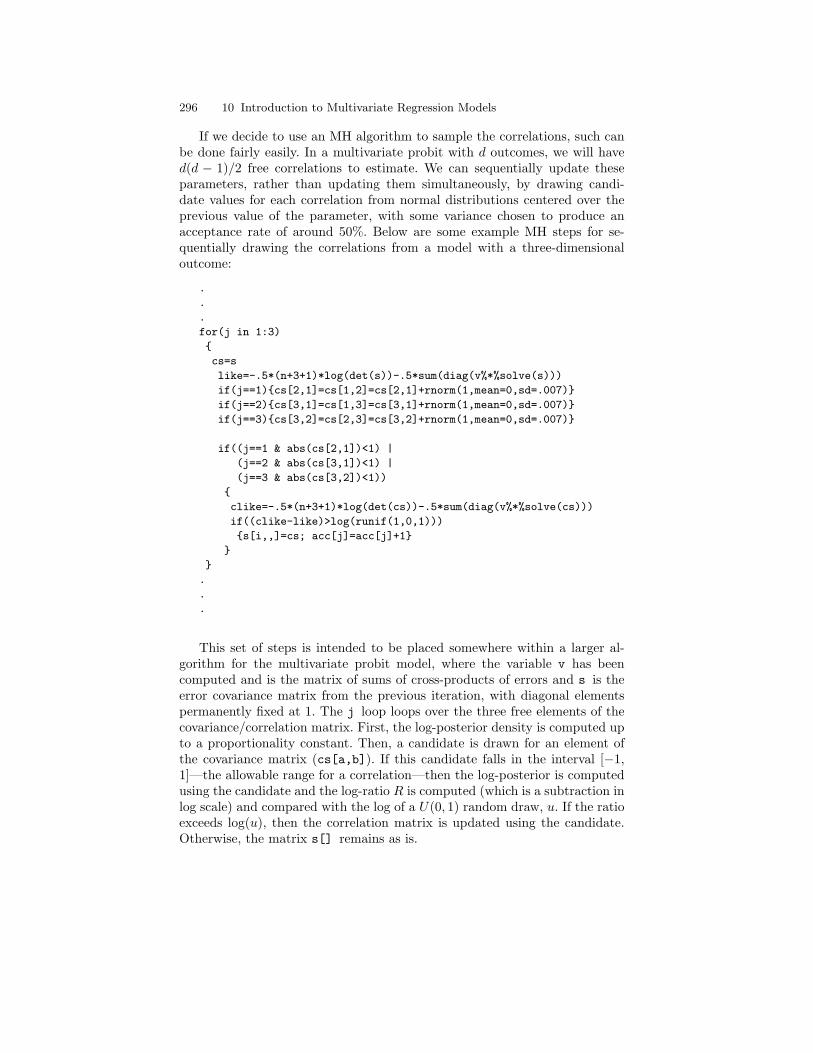
296 10 Introduction to Multivariate Regression Models
If we decide to use an MH algorithm to sample the correlations, such canbe done fairly easily. In a multivariate probit with d outcomes, we will haved(d − 1)/2 free correlations to estimate. We can sequentially update theseparameters, rather than updating them simultaneously, by drawing candi-date values for each correlation from normal distributions centered over theprevious value of the parameter, with some variance chosen to produce anacceptance rate of around 50%. Below are some example MH steps for se-quentially drawing the correlations from a model with a three-dimensionaloutcome:
.
.
.
for(j in 1:3)
cs=s
like=-.5*(n+3+1)*log(det(s))-.5*sum(diag(v%*%solve(s)))
if(j==1)cs[2,1]=cs[1,2]=cs[2,1]+rnorm(1,mean=0,sd=.007)
if(j==2)cs[3,1]=cs[1,3]=cs[3,1]+rnorm(1,mean=0,sd=.007)
if(j==3)cs[3,2]=cs[2,3]=cs[3,2]+rnorm(1,mean=0,sd=.007)
if((j==1 & abs(cs[2,1])<1) |
(j==2 & abs(cs[3,1])<1) |
(j==3 & abs(cs[3,2])<1))
clike=-.5*(n+3+1)*log(det(cs))-.5*sum(diag(v%*%solve(cs)))
if((clike-like)>log(runif(1,0,1)))
s[i,,]=cs; acc[j]=acc[j]+1
.
.
.
This set of steps is intended to be placed somewhere within a larger al-gorithm for the multivariate probit model, where the variable v has beencomputed and is the matrix of sums of cross-products of errors and s is theerror covariance matrix from the previous iteration, with diagonal elementspermanently fixed at 1. The j loop loops over the three free elements of thecovariance/correlation matrix. First, the log-posterior density is computed upto a proportionality constant. Then, a candidate is drawn for an element ofthe covariance matrix (cs[a,b]). If this candidate falls in the interval [−1,1]—the allowable range for a correlation—then the log-posterior is computedusing the candidate and the log-ratio R is computed (which is a subtraction inlog scale) and compared with the log of a U(0, 1) random draw, u. If the ratioexceeds log(u), then the correlation matrix is updated using the candidate.Otherwise, the matrix s[] remains as is.

10.2 Multivariate probit models 297
10.2.5 Implementing the algorithm
We have already discussed the steps involved in the Gibbs sampler for themultivariate probit model, and in the previous sections, we have discussedvarious issues that must be handled in the algorithm that differentiate it fromthe algorithm we discussed for the multivariate linear regression model. Allthat remains is to integrate these. Below is the complete R algorithm for thecurrent party affiliation/political orientation example:
#R program for multivariate probit model
x=as.matrix(read.table("c:\\mvnprob.dat1")[,1:7])
z=as.matrix(read.table("c:\\mvnprob.dat1")[,8:9])
#create variables and starting values
zstar=matrix(0,nrow(z),2)
d=2;k=7
b<-matrix(0,(d*k))
s=cs=diag(d)
tz=matrix(0,d,4)
tz[,1]=-Inf; tz[,2]=0; tz[,4]=Inf
tz[1,3]=qnorm(sum(z[,1]<=2)/nrow(z),
mean=-qnorm(sum(z[,1]==1)/nrow(z),mean=0,sd=1),
sd=1)
tz[2,3]=qnorm(sum(z[,2]<=2)/nrow(z),
mean=-qnorm(sum(z[,2]==1)/nrow(z),mean=0,sd=1),
sd=1)
ctz=tz
acc1=acc2=acctot=0;
write(c(0,t(b),t(s),tz[1,3],tz[2,3]),
file="c:\\mvprob.res",ncolumns=(d*k+k*k +3),append=T)
#begin Gibbs sampling
for(i in 2:6000)
#draw latent data: one-iteration gibbs sampler for tmvn simulation
bb=matrix(b,k,2)
m=x%*%bb
for(j in 1:d)
mm=m[,j] + t(s[j,-j])%*%solve(s[-j,-j])%*%(zstar[,-j]-m[,-j])
ss=s[j,j] - t(s[j,-j])%*%solve(s[-j,-j])%*%s[j,-j]
zstar[,j]=qnorm(runif(nrow(z),
min=pnorm(tz[j,z[,j]],mm,sqrt(ss)),

298 10 Introduction to Multivariate Regression Models
max=pnorm(tz[j,(z[,j]+1)],mm,sqrt(ss))),
mean=mm,sd=sqrt(ss))
#draw thresholds using Cowles’ algorithm
ctz[1,3]=qnorm(runif(1,min=pnorm(0,mean=tz[1,3],sd=.01),max=1),
mean=tz[1,3],sd=.01)
r=as.matrix((pnorm(ctz[1,z[,1]+1]-m[,1],0,1)
-pnorm(ctz[1,z[,1]]-m[,1],0,1))
/
(pnorm(tz[1,z[,1]+1]-m[,1],0,1)
-pnorm(tz[1,z[,1]]-m[,1],0,1)))
r= t(log(r))%*%matrix(1,nrow(z))
+log((1-pnorm(-tz[1,3]/.01,0,1))/(1-pnorm(-ctz[1,3]/.01,0,1)))
if(r>log(runif(1,0,1)))tz[1,3]=ctz[1,3]; acc1=acc1+1
ctz[2,3]=qnorm(runif(1,min=pnorm(0,mean=tz[2,3],sd=.01),max=1),
mean=tz[2,3],sd=.01)
r=as.matrix((pnorm(ctz[2,z[,2]+1]-m[,2],0,1)
-pnorm(ctz[2,z[,2]]-m[,2],0,1))
/
(pnorm(tz[2,z[,2]+1]-m[,2],0,1)
-pnorm(tz[2,z[,2]]-m[,2],0,1)))
r=t(log(r))%*%matrix(1,nrow(z))
+log((1-pnorm(-tz[2,3]/.01,0,1))/(1-pnorm(-ctz[2,3]/.01,0,1)))
if(r>log(runif(1,0,1)))tz[2,3]=ctz[2,3]; acc2=acc2+1
#draw b from mvn
vb=solve(solve(s)%x%(t(x)%*%x))
mn=vb%*%(as.vector(t(x)%*%zstar%*%t(solve(s))))
b=mn+t(rnorm((d*k),0,1)%*%chol(vb))
#use metropolis-hastings sampling to draw sigma
e=matrix((as.vector(zstar)-(diag(d)%x%x%*%b)),nrow(z),d)
v=t(e)%*%e
like=-.5*((d+nrow(z)+1)*log(det(s)) + sum(diag(v%*%solve(s))))
cs[1,2]=cs[2,1]=s[1,2]+rnorm(1,mean=0,sd=.01)
if(abs(cs[1,2])<1)
cslike=-.5*((d+nrow(z)+1)*log(det(cs)) + sum(diag(v%*%solve(cs))))
if((cslike-like)>log(runif(1,0,1)))
s[1,2]=s[2,1]=cs[1,2]; acctot=acctot+1

10.2 Multivariate probit models 299
if(i%%10==0)print(i)
if(i%%5==0)write(c(i,t(b),t(s),tz[1,3],tz[2,3]),
file="c:\\mvprob.res",ncolumns=(d*k+k*k+3),append=T)
This algorithm is certainly the longest algorithm in the book thus far, butit is not inherently difficult to follow if it is considered in parts. As with otheralgorithms in the book, we first read the covariates and outcome variables intotwo matrices (x and z, respectively). Next, we establish matrices and startingvalues for the various parameters in the algorithm. Here, I created a variableto store the latent variables in (zstar), started each regression coefficient at0, and started the error covariance matrix as an identity matrix. I createdtwo matrices for the error covariance matrix—s and cs. One (cs) is a storagevariable for candidate parameters, and the other (s) holds the previous value.Next, I created two sets of threshold parameters—one for the candidates,and one for the previous values, just as with the covariance matrix—and Iinitialized them as in Chapter 8 based on the proportion of respondents ineach category of the original variable z. Finally, I created three acceptancerate variables in which to monitor the parameters being updated with MHsteps.
Once the Gibbs sampler begins, the latent data are simulated using theGibbs sampling approach described in Section 10.2.2. The only difference be-tween the algorithm as written here versus in Section 10.2.2 is that it appearsthat I am only performing one iteration of the Gibbs sampler to obtain a drawfor each zstar. In fact, this algorithm does only iterate the Gibbs sampler onetime: It samples each latent trait (for each person) conditional on the valuesof the latent variable in the other dimensions. Whereas we needed to performat least two iterations to produce a legitimate draw from the truncated mul-tivariate normal distribution in Section 10.2.2, here, I rely on the value of thelatent variable stored from the previous iteration of the overall Gibbs samplerfor the model. As the overall Gibbs sampler for the model converges, so shouldthe simulations from the truncated multivariate normal distribution within.
After these latent vectors are drawn, the two free thresholds are updatedusing Cowles’ algorithm, as described in Section 10.2.3. This section of theprogram is repeated: The first instance is for the threshold in the latent distri-bution for the first dimension/equation; the second is for the the threshold inthe latent distribution for the second dimension/equation. Next, the regres-sion parameters are updated as in the original multivariate regression model atthe beginning of this chapter. Finally, the free element in the error covariancematrix—the error correlation between the two dimensions of the outcome—issimulated using an MH step as described in the previous section.
The algorithm took approximately 45 minutes to run 6,000 iterations onmy (average) desktop computer. Although this length of time is long compared
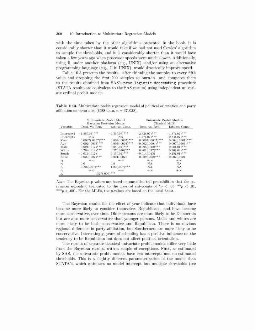
300 10 Introduction to Multivariate Regression Models
with the time taken by the other algorithms presented in the book, it isconsiderably shorter than it would take if we had not used Cowles’ algorithmto sample the thresholds, and it is considerably shorter than it would havetaken a few years ago when processor speeds were much slower. Additionally,using R under another platform (e.g., UNIX), and/or using an alternativeprogramming language (e.g., C in UNIX), would drastically improve speed.
Table 10.3 presents the results—after thinning the samples to every fifthvalue and dropping the first 200 samples as burn-in—and compares themto the results obtained from SAS’s proc logistic descending procedure(STATA results are equivalent to the SAS results) using independent univari-ate ordinal probit models.
Table 10.3. Multivariate probit regression model of political orientation and partyaffiliation on covariates (GSS data, n = 37, 028).
Multivariate Probit Model Univariate Probit ModelsBayesian Posterior Means Classical MLE
Variable Dem. vs. Rep. Lib. vs. Cons. Dem. vs. Rep. Lib. vs. Cons.
Intercept1 −1.55(.07)*** −0.35(.07)*** −2.52(.07)*** −1.37(.07)***Intercept2 NA NA −1.57(.07)*** −0.34(.07)***Year 0.0097(.0007)*** 0.004(.0007)*** 0.0097(.0007)*** 0.004(.0007)***Age −0.002(.0003)*** 0.007(.0003)*** −0.002(.0004)*** 0.007(.0003)***Male 0.094(.012)*** 0.08(.01)*** 0.095(.012)*** 0.08(.01)***White 0.798(.018)*** 0.27(.016)*** 0.801(.017)*** 0.26(.02)***South −0.014(.012) 0.15(.01)*** −0.014(.013) 0.15(.01)***Educ 0.029(.002)*** −0.001(.002) 0.029(.002)*** −0.002(.002)τ1 −∞ −∞ −∞ −∞τ2 0.0 0.0 NA NAτ3 0..96(.007)*** 1.03(.007)*** NA NAτ4 +∞ +∞ +∞ +∞ρe .327(.006)***
Note: The Bayesian p-values are based on one-sided tail probabilities that the pa-rameter exceeds 0 truncated to the classical cut-points of *p < .05, **p < .01,***p < .001. For the MLEs, the p-values are based on the usual t-test.
The Bayesian results for the effect of year indicate that individuals havebecome more likely to consider themselves Republicans, and have becomemore conservative, over time. Older persons are more likely to be Democratsbut are also more conservative than younger persons. Males and whites aremore likely to be both conservative and Republican. There is no obviousregional difference in party affiliation, but Southerners are more likely to beconservative. Interestingly, years of schooling has a positive influence on thetendency to be Republican but does not affect political orientation.
The results of separate classical univariate probit models differ very littlefrom the Bayesian results, with a couple of exceptions. First, as estimatedby SAS, the univariate probit models have two intercepts and no estimatedthresholds. This is a slightly different parameterization of the model thanSTATA’s, which estimates no model intercept but multiple thresholds (see

10.2 Multivariate probit models 301
Chapter 8), and it is clearly a different parameterization than our modelwith one intercept and one estimated threshold. However, if we consider ourintercept as SAS’s “Intercept 2”, we can subtract the estimated thresholdfrom this intercept to obtain SAS’s “Intercept 1.” Given that these thresholdparameters are nuissance parameters, the parameterization of the model withrespect to them has no substantive implications.
Second, the multivariate probit model results include an additional param-eter, ρe, that was not estimated (obviously) in the univariate probit models.Our result for this parameter indicates that the errors are moderately andpositively correlated (ρ = .33), meaning that unobserved factors that influ-ence party affiliation tend to be positively correlated with unobserved factorsthat influence political orientation.
If the results of the multivariate probit model are generally indistinct fromthose of the separate univariate probit models estimated via maximum like-lihood by extant software packages, then what is the advantage of the multi-variate approach specifically and the Bayesian approach more generally? Aswe discussed at the beginning of the chapter, the main advantages to adopt-ing a multivariate modeling strategy include (1) the elegance of using a singlemodel, rather than multiple models; and (2) the gain in efficiency if the covari-ate vectors differ across equations. Additionally, if interest centers on makinginference regarding functions of parameters rather than on the parametersthemselves, a multivariate Bayesian approach can provide more informationmore simply than a classical approach.
In assessing this latter claim, using the current example, suppose our in-terest lay in understanding change in the concurrence of party affiliation andpolitical orientation over time, and not on change in each independently. Forinstance, suppose our question is whether there has been a shift over timein the propensity for individuals to self-identify as conservative Republicans.This question requires us to examine the influence of time on a bivariatepropensity—a two-dimensional integral in this model. Refer again to Fig-ure 10.1—this probabiilty is the area above the third threshold in each di-mension. This integral depends on the error correlation between equations aswell as the model parameters applied to a set of specified covariate values.A set of univariate models lacks the error correlation and therefore cannothelp us address this question. A classically estimated bivariate probit model,on the other hand, can help us obtain a point estimate of the probability ahypothetical individual (with a given set of covariate values) will self-identifyas a conservative Republican. However, producing an interval estimate of thisprobability is not straightforward, because it would involve using some com-bination of the standard errors of the model parameters across the equations,plus incorporating the standard error of the error correlation, plus consideringhow these standard errors translate through the bivariate normal integral.
Under the Bayesian approach, we can easily produce a posterior distri-bution for the probability of self-identifying as a conservative Republican byusing posterior predictive simulation. Throughout the book, we have used and

302 10 Introduction to Multivariate Regression Models
discussed posterior predictive simulation as a tool for evaluating how well amodel fits the data at hand; this is still true. However, posterior predictivesimulation can also be used to make inference beyond that which can be madedirectly from the estimated model parameters. Specifically, we can make in-ference about change over time in the probability an individual with givencharacteristics will self-identify as a conservative Republican. The R programbelow shows how we can accomplish this:
g=as.matrix(read.table("c:\\mvprob1.out")[201:1200,])
summ=matrix(0,31,4)
#loop across all years
for(m in 1:31)
x=matrix(c(1,m+73,30,1,1,1,12),7)
cellsum=matrix(0,1000)
#loop over 1000 post-burnin samples of parameters
for(i in 1:1000)
s=matrix(c(1,g[i,17],g[i,17],1),2,2)
b=matrix(g[i,2:15],7,2)
t1=g[i,20]; t2=g[i,21]
xb=t(b)%*%x
#generate 1000 ppd samples to compute probabilities
#this step is equivalent to integration over desired cell
for(j in 1:1000)
zz=xb+t(rnorm(2,0,1)%*%chol(s))
if(zz[1]>t1 & zz[2]>t2)cellsum[i]=cellsum[i]+1
if(i%%5==0)print(c(m,i))
summ[m,1]=mean(cellsum/1000)
summ[m,2]=sd(cellsum/1000)
summ[m,3]=sort(cellsum)[25]
summ[m,4]=sort(cellsum)[975]
The R program first reads in the 1,000 post-burn-in parameter samplesfrom the multivariate probit output file and creates a matrix to store summarystatistics about the posterior predictive distributions for 31 individuals. Thefirst loop (over m) is across the years of observation (1974 to 2004, a 31-year period). The vector x is then defined so that the posterior predictivesimulation will be for a 30-year-old white male from the south with 12 yearsof education, for each year from 1974 through 2004.
10.3 A multivariate probit model for generating distributions of multistate life tables 303
Once the error correlation matrix (s), regression parameter matrix (b), andthresholds (t1 and t2) have been defined, a predicted score (xb) is computed.Next, 1,000 samples from a bivariate normal distribution with this predictedmean and given error covariance matrix are generated, and a tally of thenumber of these samples that fall above the appropriate threshold in eachdimension is kept (cellsum). This step is equivalent to computing the integralof the bivariate normal distribution with the given mean and covariance overits upper right tail.
Once we have computed this tally for the current sample of the modelparameters, we repeat the process for all 1,000 post-burn-in values of theparameters. The end result of this process is that, for each year, we obtainsummaries of the distribution for the probability of self-identifying as a con-servative Republican.
Figure 10.6 is a plot of the 95% probability intervals for being a conser-vative Republican from 1974 to 2004. As the figure shows, this probabilityhas increased substantially over the 31-year period. In 1974, the probability a30-year-old white Southern male with a high-school diploma would considerhimself a conservative Republican was about .136 (95% interval of [.11, .16]).By 2004, this probability had increased to .197 (95% interval of [.17, .22]),which is a 45% increase in the probability.
In this example, I have shown how to answer only one question using pos-terior predictive simulation from the multivariate model results. Nonetheless,it should be clear that the approach is flexible and can be used for making anynumber of additional inferences. In the next section, I provide a more detailedand realistic use of the Bayesian approach to making inference to parametersnot directly estimated in a multivariate setting.
10.3 A multivariate probit model for generatingdistributions of multistate life tables
The life table is a basic tool of demography that has been used for centuries.The basic measure produced by a life table—life expectancy—is the expectednumber of years of life remaining for individuals at given ages and is pro-duced using age-specific probabilities (or rates) of mortality in a specific year(see Preston, Heuveline, and Guillot 2001; Schoen 1988). In the early 1970s,researchers began using hazard regression models (e.g., the discrete time pro-bit model discussed in Chapter 8) to produce smoothed (parametric and pre-dicted) mortality probabilities for life table estimation (see Cox 1972; Menkenet al. 1981). Using hazard models allowed researchers to produce life tablesfor specific subpopulations, because estimated age-specific mortality rates fora subpopulation could be obtained from the hazard model by (1) applyingthe estimated model parameters to a given covariate profile (e.g., a specificvalue for age, sex, race, etc.) to obtain a predicted score and (2) transformingthis value into a probability by inverting the link function used in the hazard
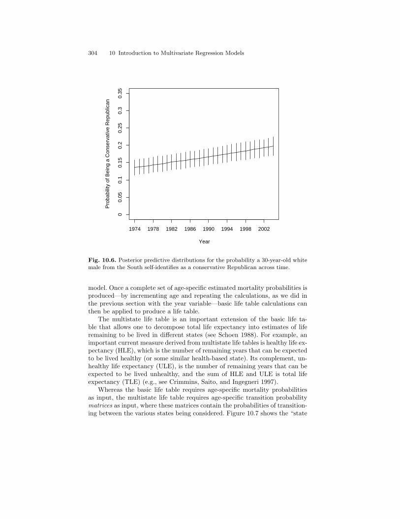
304 10 Introduction to Multivariate Regression Models
Year
Pro
babi
lity
of B
eing
a C
onse
rvat
ive
Rep
ublic
an
1974 1978 1982 1986 1990 1994 1998 2002
00.
050.
10.
150.
20.
250.
30.
35
Fig. 10.6. Posterior predictive distributions for the probability a 30-year-old whitemale from the South self-identifies as a conservative Republican across time.
model. Once a complete set of age-specific estimated mortality probabilities isproduced—by incrementing age and repeating the calculations, as we did inthe previous section with the year variable—basic life table calculations canthen be applied to produce a life table.
The multistate life table is an important extension of the basic life ta-ble that allows one to decompose total life expectancy into estimates of liferemaining to be lived in different states (see Schoen 1988). For example, animportant current measure derived from multistate life tables is healthy life ex-pectancy (HLE), which is the number of remaining years that can be expectedto be lived healthy (or some similar health-based state). Its complement, un-healthy life expectancy (ULE), is the number of remaining years that can beexpected to be lived unhealthy, and the sum of HLE and ULE is total lifeexpectancy (TLE) (e.g., see Crimmins, Saito, and Ingegneri 1997).
Whereas the basic life table requires age-specific mortality probabilitiesas input, the multistate life table requires age-specific transition probabilitymatrices as input, where these matrices contain the probabilities of transition-ing between the various states being considered. Figure 10.7 shows the “state

10.3 A multivariate probit model for generating distributions of multistate life tables 305
space” for a simple three-state model in which individuals can be healthy(state 1), unhealthy (state 2), or dead (state 3), and the allowable transitionsare from the healthy state to healthy, unhealthy, or dead states, and from theunhealthy state to either the healthy, unhealthy, or dead states. Thus, thereare six required transition probabilities (at each age).
Healthy(Stay=p11)
Unhealthy(Stay=p22)
Dead
p21
p12
p13 p23
Fig. 10.7. Representation of state space for a three state model.
Figure 10.8 shows that the necessary age-specific transition probabilitiesmay be estimated with a bivariate dichotomous probit model, with healthyversus unhealthy being one outcome variable, and alive versus dead being theother. In order to actually capture transition probabilities, we need two-wavepanel data, so that we may know both the state in which individuals begin atime interval and the state in which individuals end the interval. If we havesuch data, then age and the starting state can be included as covariates, alongwith any other variables desired.
Age-specific transition probabilities can then be produced from the modelparameters by computing the linear combination of parameters and desiredcovariate values. To obtain the complete age range, this linear combination
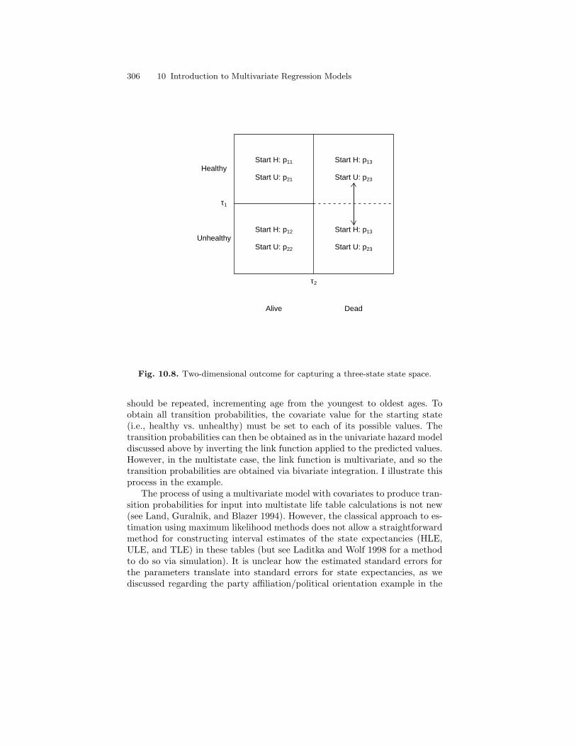
306 10 Introduction to Multivariate Regression Models
Alive Dead
Healthy
Unhealthy
τ2
τ1
Start H: p11
Start U: p21
Start H: p12
Start U: p22
Start H: p13
Start U: p23
Start H: p13
Start U: p23
Fig. 10.8. Two-dimensional outcome for capturing a three-state state space.
should be repeated, incrementing age from the youngest to oldest ages. Toobtain all transition probabilities, the covariate value for the starting state(i.e., healthy vs. unhealthy) must be set to each of its possible values. Thetransition probabilities can then be obtained as in the univariate hazard modeldiscussed above by inverting the link function applied to the predicted values.However, in the multistate case, the link function is multivariate, and so thetransition probabilities are obtained via bivariate integration. I illustrate thisprocess in the example.
The process of using a multivariate model with covariates to produce tran-sition probabilities for input into multistate life table calculations is not new(see Land, Guralnik, and Blazer 1994). However, the classical approach to es-timation using maximum likelihood methods does not allow a straightforwardmethod for constructing interval estimates of the state expectancies (HLE,ULE, and TLE) in these tables (but see Laditka and Wolf 1998 for a methodto do so via simulation). It is unclear how the estimated standard errors forthe parameters translate into standard errors for state expectancies, as wediscussed regarding the party affiliation/political orientation example in the
10.3 A multivariate probit model for generating distributions of multistate life tables 307
previous section. Thus, to date, most researchers using multistate life tablesproduced from hazard model results have simply reported point estimates forlife table quantities. Yet, given that the data used for model estimation typ-ically come from samples, and are not population data, we need to be ableto quantify at a minimum the uncertainty inherent in using sample data tomake inference to populations. The Bayesian approach offers a straightforwardway of doing so (see Lynch and Brown 2005 for a more in-depth discussionthan what is presented below for single decrement, multiple decrement, andmultistate life tables using Gibbs samplers and MH algorithms).
10.3.1 Model specification and simulation
The data for this example are from the 1987 and 1992 NHEFS. As describedearlier, the NHEFS is a series of at least four surveys, begun in 1971 andcontinuing in 1982, 1987, and 1992. The original sample size was 14,407 per-sons. After elminating persons who died or dropped out of the survey by1987, restricting the age range to persons 45 years of age or older in 1987,and eliminating individuals who were missing on one or more variables of in-terest, I obtained a sample of n = 3, 495 persons. I include age in 1987, sex,race, region of residence, marital status (both measured in 1987), education,and self-rated health in 1987 and 1992 in the analyses. Self-rated health isdichotomized as “Excellent” or “Good” health versus “Fair” or “Poor” healthin both 1987 and 1992, and the 1987 measure is included as a covariate. Ageis measured in five-year intervals (i.e., 45-49 = 0, 50-54 = 1, . . ., 85+ = 8).Sex, race, region, and marital status are measured as dummy variables (male= 1, nonwhite = 1, South = 1, married = 1), and education is measured asyears of schooling.
A bivariate probit model for predicting health status (unhealthy vs.healthy) and survival status (dead vs. alive) in 1992 is constructed, withhealth status in 1987, and an interaction between age and health status in1987, included as predictors, along with sex, race, region, marital status, andeducation. The bivariate probit model for predicting health and survival statusin 1992 does not differ substantially from the bivariate probit model discussedin the previous section, and so I do not repeat the general model here (referto the previous section).
One feature of the model, however, does differ and requires some discus-sion. Given the outcome space shown in Figure 10.8, it is clear that we canobserve health status among survivors but not among decedents. For indi-viduals who died between the 1987 and 1992 waves, health status in 1992 isnot observed, because the respondent, of course, could not be interviewed in1992. This dilemma constitutes a missing data problem of sorts and is easilyhandled via Gibbs sampling. The only change in the model—and really, inthe Gibbs sampler—is that latent data for the health outcome for decedentsmust be simulated without the truncation constraint. Below is the R programfor the model after making this adjustment:
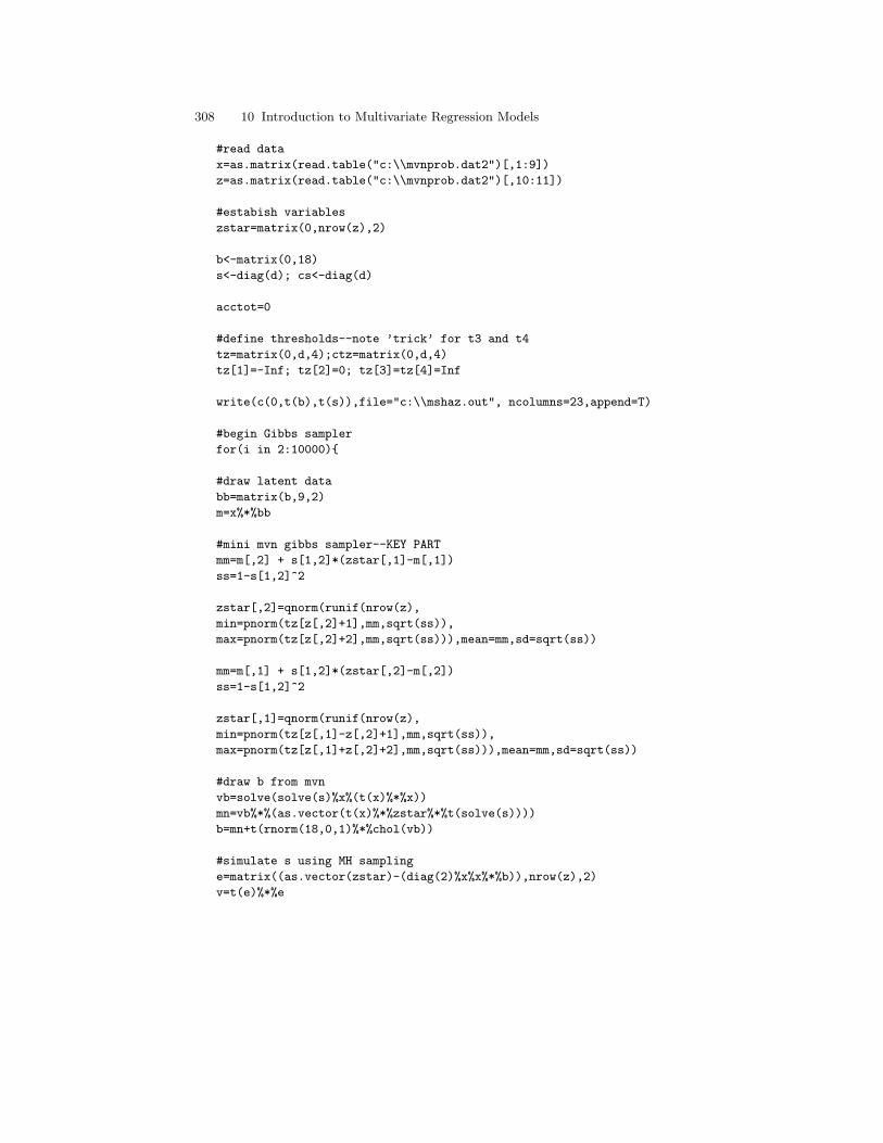
308 10 Introduction to Multivariate Regression Models
#read data
x=as.matrix(read.table("c:\\mvnprob.dat2")[,1:9])
z=as.matrix(read.table("c:\\mvnprob.dat2")[,10:11])
#estabish variables
zstar=matrix(0,nrow(z),2)
b<-matrix(0,18)
s<-diag(d); cs<-diag(d)
acctot=0
#define thresholds--note ’trick’ for t3 and t4
tz=matrix(0,d,4);ctz=matrix(0,d,4)
tz[1]=-Inf; tz[2]=0; tz[3]=tz[4]=Inf
write(c(0,t(b),t(s)),file="c:\\mshaz.out", ncolumns=23,append=T)
#begin Gibbs sampler
for(i in 2:10000)
#draw latent data
bb=matrix(b,9,2)
m=x%*%bb
#mini mvn gibbs sampler--KEY PART
mm=m[,2] + s[1,2]*(zstar[,1]-m[,1])
ss=1-s[1,2]^2
zstar[,2]=qnorm(runif(nrow(z),
min=pnorm(tz[z[,2]+1],mm,sqrt(ss)),
max=pnorm(tz[z[,2]+2],mm,sqrt(ss))),mean=mm,sd=sqrt(ss))
mm=m[,1] + s[1,2]*(zstar[,2]-m[,2])
ss=1-s[1,2]^2
zstar[,1]=qnorm(runif(nrow(z),
min=pnorm(tz[z[,1]-z[,2]+1],mm,sqrt(ss)),
max=pnorm(tz[z[,1]+z[,2]+2],mm,sqrt(ss))),mean=mm,sd=sqrt(ss))
#draw b from mvn
vb=solve(solve(s)%x%(t(x)%*%x))
mn=vb%*%(as.vector(t(x)%*%zstar%*%t(solve(s))))
b=mn+t(rnorm(18,0,1)%*%chol(vb))
#simulate s using MH sampling
e=matrix((as.vector(zstar)-(diag(2)%x%x%*%b)),nrow(z),2)
v=t(e)%*%e

10.3 A multivariate probit model for generating distributions of multistate life tables 309
like=-.5*(2+nrow(z)+1)*log(det(s))-.5*sum(diag(v%*%solve(s)))
cs[1,2]=cs[2,1]=s[1,2]+rnorm(1,mean=0,sd=.03)
if(abs(cs[1,2])<1)
cslike=-.5*(2+nrow(z)+1)*log(det(cs))-.5*sum(diag(v%*%solve(cs)))
if((cslike-like)>log(runif(1,0,1)))
s[1,2]=s[2,1]=cs[1,2]; acctot=acctot+1
if(i%%10==0)print(c(i,b[1],b[1+k],s[1,2],acctot/i),digits=5)
if(i%%5==0)
write(c(i,t(b),t(s)),file="c:\\mshaz.out",ncolumns=23,append=T)
This algorithm is remarkably similar to the longer algorithm presented inthe previous section with only a few exceptions. First, there is no estimationof thresholds. Given that both dimensions of the outcome are dichotomous,there are only three thresholds in each dimension, and these are fixed at −∞,0, and ∞ in each dimension to identify the model. Second, I have added afourth threshold in each dimension; these thresholds are set equal to ∞—like the third threshold in each dimension—and are used as a computingconvenience.
Third, and most importantly, the simulation of the latent data imposesslightly different truncation requirements (see the lines after the KEY PARTcomment). The outcome variables are coded so that the mortality outcometakes a 1 or 0 value, and the health outcome takes a 1 or 0 value for sur-vivors and a 1 for decedents. With this coding, simulation of the latent dataunderlying the observed dichotomous outcomes is as follows:
Observed outcome Latent health trait Latent mortality traitalive and healthy below 0 below 0alive and unhealthy above 0 below 0dead no truncation above 0
The specifc snippets of code that perform the last simulation are:
...min=pnorm(tz[z[,1]-z[,2]+1]...
max=pnorm(tz[z[,1]+z[,2]+2]...
For individuals who die, the first snippet reduces to tz[1], and the secondreduces to tz[4]. Thus, the latent trait for health is simulated from −∞ to∞. For persons who remain alive and are healthy in 1992, in contrast, thesesnippets reduce to t[1] and t[2](−∞ to 0). Finally, for persons who remainalive but are unhealthy in 1992, these snippets reduce to t[2] and t[3] (0to ∞).

310 10 Introduction to Multivariate Regression Models
It is important to realize that, although these are minor changes to themodel/program, handling this missing data could not be easily done withouta multivariate model. If we were using separate univariate probit models forhealth and mortality, decedents would be treated as missing observations andwould, by default, be listwise deleted by most software packages. Even if aunivariate model were employed that used a FIML estimator or some othermethod to compensate for the missing outcome data, it would be less efficientthan the multivariate approach, which can use the error correlation betweenequations, as well as the covariate effects in the mortality dimension, to informinference regarding the missing data.
10.3.2 Life table generation and other posterior inferences
As the program indicates, I ran this Gibbs sampler for 10,000 iterations, savingevery fifth sample. All parameters converged very rapidly and mixed very thor-oughly, and I retained the last 1,000 samples for posterior inference. Table 10.4shows the posterior means and posterior standard deviations for model param-eters. Age and poor health in 1987 had expected positive effects on both poorhealth and mortality. Also, as expected, males, nonwhites, and Southernershad generally poorer health and greater mortality risk than females, whites,and nonsoutherners, while education and marriage had protective effects.
Table 10.4. Results of multivariate probit regression of health and mortality oncovariates.
Outcome
Variable Poor Health Mortality
Intercept −0.65(.15)*** −2.50(.18)***Age 0.069(.02)*** 0.34(.02)***Unhealthy in ’87 1.44(.12)*** 0.77(.16)***Age×Unhealthy in ’87 −0.03(.03) −0.04(.03)#Male 0.13(.06)* 0.38(.07)***Nonwhite 0.35(.09)*** 0.05(.10)South 0.04(.06) 0.09(.07)#Married −0.20(.07)** −0.16(.07)*Yrs. Schooling −0.05(.01)*** −0.02(.01)*σ12 −0.10(.17)
Note: The Bayesian estimates are posterior means. The Bayesian p-values are basedon one-sided tail probabilities that the parameter exceeds 0 truncated to the classicalcut-points of #p < .1, *p < .05, **p < .01.
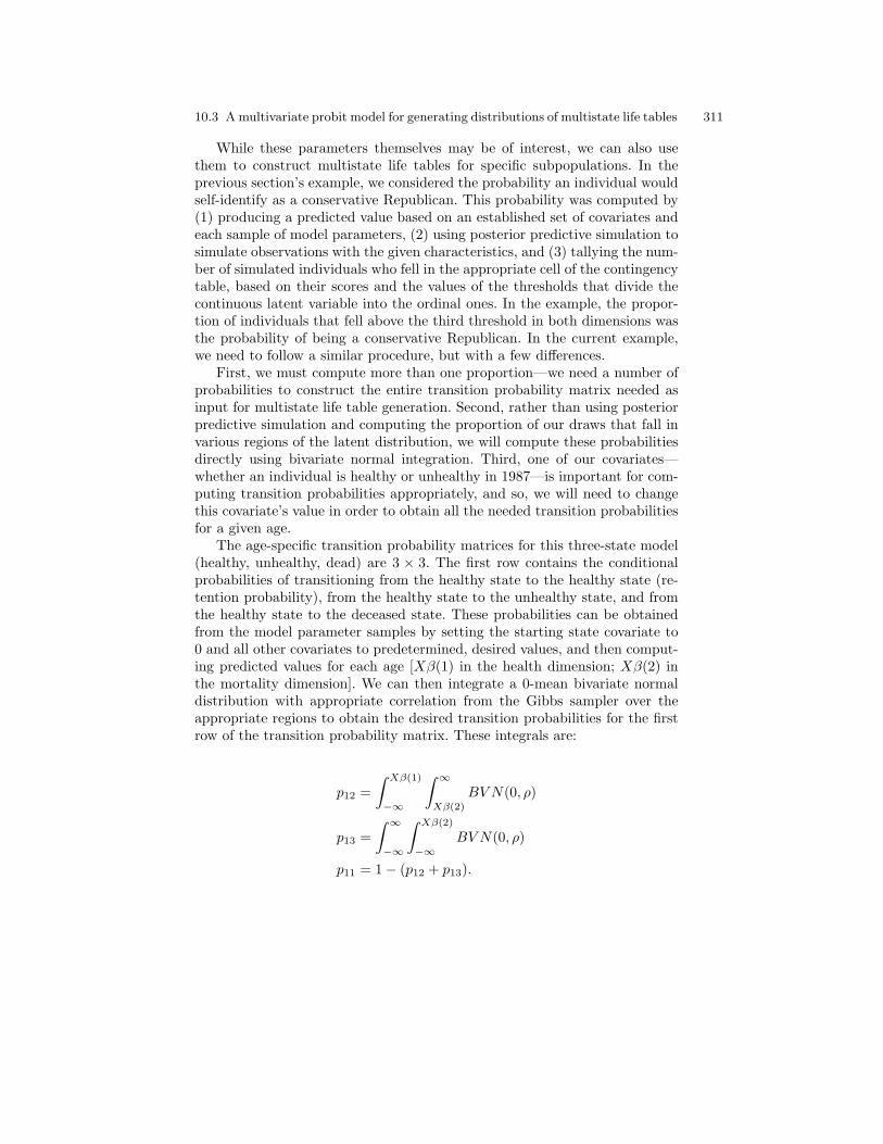
10.3 A multivariate probit model for generating distributions of multistate life tables 311
While these parameters themselves may be of interest, we can also usethem to construct multistate life tables for specific subpopulations. In theprevious section’s example, we considered the probability an individual wouldself-identify as a conservative Republican. This probability was computed by(1) producing a predicted value based on an established set of covariates andeach sample of model parameters, (2) using posterior predictive simulation tosimulate observations with the given characteristics, and (3) tallying the num-ber of simulated individuals who fell in the appropriate cell of the contingencytable, based on their scores and the values of the thresholds that divide thecontinuous latent variable into the ordinal ones. In the example, the propor-tion of individuals that fell above the third threshold in both dimensions wasthe probability of being a conservative Republican. In the current example,we need to follow a similar procedure, but with a few differences.
First, we must compute more than one proportion—we need a number ofprobabilities to construct the entire transition probability matrix needed asinput for multistate life table generation. Second, rather than using posteriorpredictive simulation and computing the proportion of our draws that fall invarious regions of the latent distribution, we will compute these probabilitiesdirectly using bivariate normal integration. Third, one of our covariates—whether an individual is healthy or unhealthy in 1987—is important for com-puting transition probabilities appropriately, and so, we will need to changethis covariate’s value in order to obtain all the needed transition probabilitiesfor a given age.
The age-specific transition probability matrices for this three-state model(healthy, unhealthy, dead) are 3 × 3. The first row contains the conditionalprobabilities of transitioning from the healthy state to the healthy state (re-tention probability), from the healthy state to the unhealthy state, and fromthe healthy state to the deceased state. These probabilities can be obtainedfrom the model parameter samples by setting the starting state covariate to0 and all other covariates to predetermined, desired values, and then comput-ing predicted values for each age [Xβ(1) in the health dimension; Xβ(2) inthe mortality dimension]. We can then integrate a 0-mean bivariate normaldistribution with appropriate correlation from the Gibbs sampler over theappropriate regions to obtain the desired transition probabilities for the firstrow of the transition probability matrix. These integrals are:
p12 =∫ Xβ(1)
−∞
∫ ∞
Xβ(2)
BV N(0, ρ)
p13 =∫ ∞
−∞
∫ Xβ(2)
−∞BV N(0, ρ)
p11 = 1− (p12 + p13).
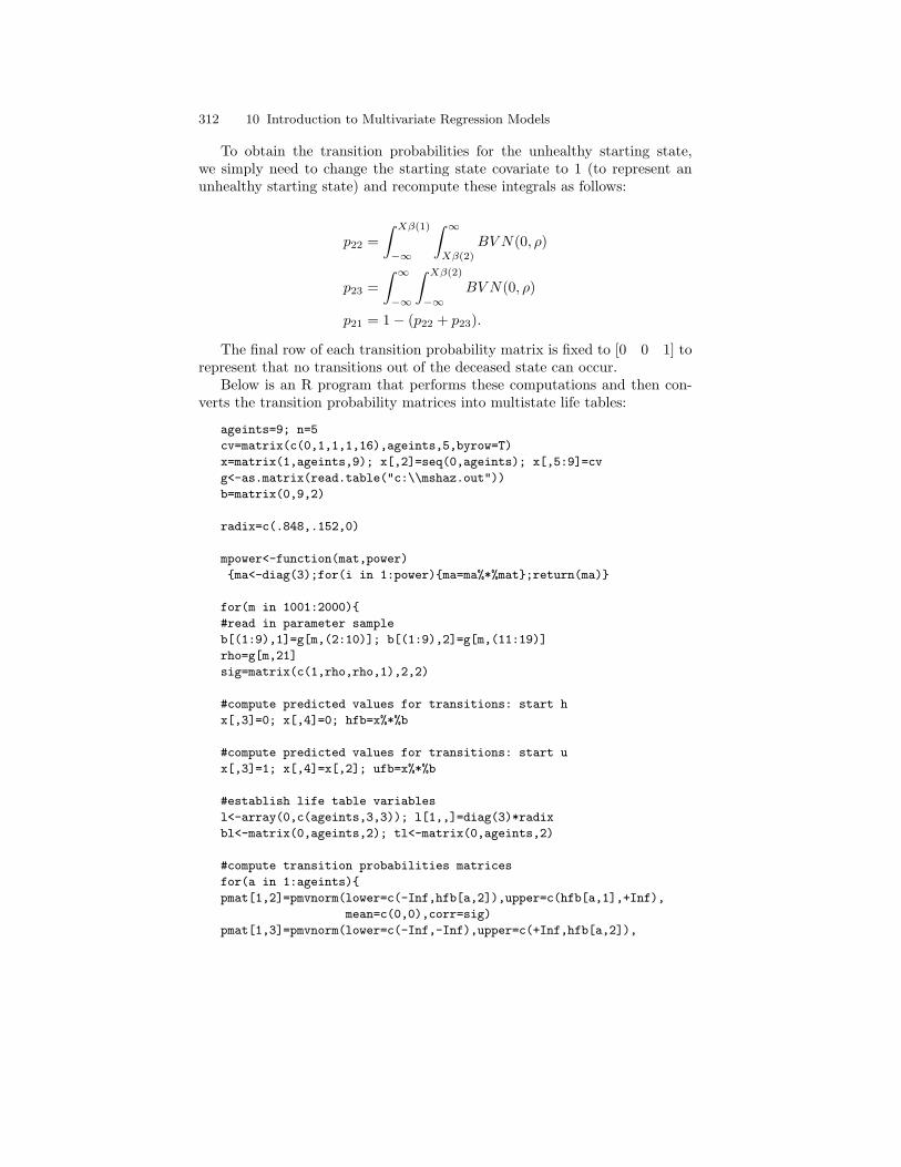
312 10 Introduction to Multivariate Regression Models
To obtain the transition probabilities for the unhealthy starting state,we simply need to change the starting state covariate to 1 (to represent anunhealthy starting state) and recompute these integrals as follows:
p22 =∫ Xβ(1)
−∞
∫ ∞
Xβ(2)
BV N(0, ρ)
p23 =∫ ∞
−∞
∫ Xβ(2)
−∞BV N(0, ρ)
p21 = 1− (p22 + p23).
The final row of each transition probability matrix is fixed to [0 0 1] torepresent that no transitions out of the deceased state can occur.
Below is an R program that performs these computations and then con-verts the transition probability matrices into multistate life tables:
ageints=9; n=5
cv=matrix(c(0,1,1,1,16),ageints,5,byrow=T)
x=matrix(1,ageints,9); x[,2]=seq(0,ageints); x[,5:9]=cv
g<-as.matrix(read.table("c:\\mshaz.out"))
b=matrix(0,9,2)
radix=c(.848,.152,0)
mpower<-function(mat,power)
ma<-diag(3);for(i in 1:power)ma=ma%*%mat;return(ma)
for(m in 1001:2000)
#read in parameter sample
b[(1:9),1]=g[m,(2:10)]; b[(1:9),2]=g[m,(11:19)]
rho=g[m,21]
sig=matrix(c(1,rho,rho,1),2,2)
#compute predicted values for transitions: start h
x[,3]=0; x[,4]=0; hfb=x%*%b
#compute predicted values for transitions: start u
x[,3]=1; x[,4]=x[,2]; ufb=x%*%b
#establish life table variables
l<-array(0,c(ageints,3,3)); l[1,,]=diag(3)*radix
bl<-matrix(0,ageints,2); tl<-matrix(0,ageints,2)
#compute transition probabilities matrices
for(a in 1:ageints)
pmat[1,2]=pmvnorm(lower=c(-Inf,hfb[a,2]),upper=c(hfb[a,1],+Inf),
mean=c(0,0),corr=sig)
pmat[1,3]=pmvnorm(lower=c(-Inf,-Inf),upper=c(+Inf,hfb[a,2]),

10.3 A multivariate probit model for generating distributions of multistate life tables 313
mean=c(0,0),corr=sig)
pmat[2,2]=pmvnorm(lower=c(-Inf,ufb[a,2]),upper=c(ufb[a,1],+Inf),
mean=c(0,0),corr=sig)
pmat[2,3]=pmvnorm(lower=c(-Inf,-Inf),upper=c(+Inf,ufb[a,2]),
mean=c(0,0),corr=sig)
pmat[1,1]=1-(pmat[1,2]+pmat[1,3])
pmat[2,1]=1-(pmat[2,2]+pmat[2,3])
#convert tp to m via Sylvester’s formula
mmat=0
lam2=(pmat[2,2]+pmat[1,1]+
sqrt((pmat[2,2]+pmat[1,1])^2-
4*(pmat[1,1]*pmat[2,2]-pmat[1,2]*pmat[2,1])))/2
lam3=(pmat[2,2]+pmat[1,1]-
sqrt((pmat[2,2]+pmat[1,1])^2-
4*(pmat[1,1]*pmat[2,2]-pmat[1,2]*pmat[2,1])))/2
mmat= (log(lam2)/((lam2-1)*(lam2-lam3)))*
((pmat-diag(3))%*%(pmat-lam3*diag(3)))+
(log(lam3)/((lam3-1)*(lam3-lam2)))*
((pmat-diag(3))%*%(pmat-lam2*diag(3)))
mmat=-mmat
#compute lx and Lx for next age group
if(a<ageints)
expm=diag(3);pyr=diag(3)
for(j in 1:20)
expm=expm + ((-1)^j)*mpower(mmat,j)/factorial(j);
pyr=pyr + ((-1)^j)*mpower(mmat,j)/factorial(j+1);
lx=l[a,,]%*%(expm)
l[a+1,1,1]=sum(lx[,1]); l[a+1,2,2]=sum(lx[,2]); l[a+1,3,3]=0;
blx=n*(l[a,,]%*%pyr)
bl[a,1]=sum(blx[,1]); bl[a,2]=sum(blx[,2])
if(a==ageints)
blx=l[a,1:2,1:2]%*%solve(mmat[1:2,1:2])
bl[a,1]=sum(blx[,1]); bl[a,2]=sum(blx[,2])
le<-matrix(NA,ageints,2)
for(a in 1:ageints)
tl[a,1]=sum(bl[a:ageints,1]); tl[a,2]=sum(bl[a:ageints,2])
le[a,]=tl[a,]/sum(l[a,,])

314 10 Introduction to Multivariate Regression Models
write(c(t(le)),file="c:\\lifetab.out",append=T,ncolumns=(2*ageints))
print(c(m,le[1,1],le[1,2]))
This program is fairly lengthy, and I will not discuss it in great depth.A number of variables are defined at the beginning, including the number ofage intervals (9), the number of years in each age interval (5), and the valuesof the five fixed covariates (male, nonwhite, South, married, and years ofschooling). These covariate values are repeated for nine lines in the x matrix,which contains incremented values of age. Next, the parameter file is read.Finally, the radix is established. The radix is the number or proportion ofindividuals in each state at the beginning of the first age in the life table.
After defining a function that computes a matrix raised to a specifiedpower, the loop begins to generate a life table for each post-burn-in samplefrom the Gibbs sampler. The parameters are read in one sample at a time andare combined with the covariate matrix, first with the starting state set to 0(to produce hfb) and then with the starting state set to 1 (to produce ufb).
After obtaining these two 9 × 2 matrices of predicted values, several lifetable variables are established before the computation of the life tables begins.A loop across age is established to produce the life table. First, the age-specifictransition probability matrix is computed. Second, this matrix is transformedinto the hazard rate matrix using Sylvester’s formula to compute its log (seeSinger and Spilerman 1976). The remainder of the program proceeds withtypical steps in computing the number of individuals transitioning betweenstates over the age interval and the number of person-years lived in each stateduring the interval (see Schoen 1988).
As an example, I ran this program to produce life tables for married non-white females from the South with 16 years of education. The radix was es-tablished by predicting the starting state (healthy/unhealthy) using age, sex,race, region, marital status, and education, and then computing the predictedscore, based on the covariate profile just described. Figure 10.9 shows traceplots of HLE, ULE, TLE, and the proportion of remaining life that can beexpected to be lived healthy (HLE/TLE). These trace plots suggest that thelife table quantities converged and mixed thoroughly, just as the parametersin the original Gibbs sampler did. Figure 10.10 shows histograms of thesesame quantities; all appear approximately normal.
The samples of life table quantities can be summarized just as we wouldsummarize other sample data. Mean TLE at age 45 for a person with thegiven covariate profile is 33.1 years, with a standard deviation of 1.5 years;an empirical interval estimate is [30.0, 35.9] years. The expected number ofyears remaining health was 25.4 years, with a standard deviation of 1.9 years;an empirical interval estimate is [21.7, 29.2] years. The remaining proportionof life to be spent healthy, based on these results, is .77, with an empiricalinterval estimate of [.68, .84]. If we wished to compare these results with thosefor a person with a different covariate profile, we would simply rerun the R

10.4 Conclusions 315
0 200 400 600 800
2024
28
Sample
HLE
0 200 400 600 800
46
810
12
Sample
ULE
0 200 400 600 800
2832
36
Sample
TLE
0 200 400 600 800
0.65
0.75
0.85
Sample
HLE
/TLE
Fig. 10.9. Trace plots of life table quantities computed from Gibbs samples ofbivariate probit model parameters.
program for a different covariate profile and then perform whatever sort ofcomparison we would like, treating the samples of life table quantities as wewould a sample of parameters or a sample of data.
10.4 Conclusions
In this chapter, I have described the multivariate linear regression model andthe multivariate probit model, perhaps two of the most important multivariatemodels that may be used in social science. Multivariate models are mathe-matically and computationally more complex than univariate models, and soI have paid particular attention to the reasons for using such models. As I
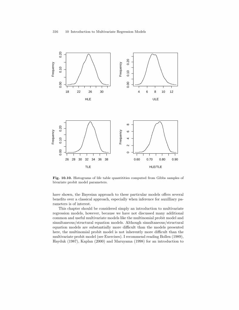
316 10 Introduction to Multivariate Regression Models
18 22 26 30
0.00
0.10
0.20
HLE
Fre
quen
cy
4 6 8 10 12
0.00
0.10
0.20
ULE
Fre
quen
cy
26 28 30 32 34 36 38
0.00
0.10
0.20
TLE
Fre
quen
cy
0.60 0.70 0.80 0.90
02
46
8
HLE/TLE
Fre
quen
cy
Fig. 10.10. Histograms of life table quantitities computed from Gibbs samples ofbivariate probit model parameters.
have shown, the Bayesian approach to these particular models offers severalbenefits over a classical approach, especially when inference for auxilliary pa-rameters is of interest.
This chapter should be considered simply an introduction to multivariateregression models, however, because we have not discussed many additionalcommon and useful multivariate models like the multinomial probit model andsimultaneous/structural equation models. Although simultaneous/structuralequation models are substantially more difficult than the models presentedhere, the multinomial probit model is not inherently more difficult than themultivariate probit model (see Exercises). I recommend reading Bollen (1989),Hayduk (1987), Kaplan (2000) and Maruyama (1998) for an introduction to
10.5 Exercises 317
these models from a classical perspective. I recommend Lee and Zhu (2000)and Song and Lee (2002) for a Bayesian approach.
10.5 Exercises
1. Develop a simple rejection sampling scheme for sampling from selectedregions of the three-dimensional (trivariate) normal distribution.
2. Develop a Gibbs sampler for a multivariate model in which some of theoutcomes are continuous and some are ordinal. How difficult is this processrelative to constructing a full multivariate probit sampling algorithm?
3. A polychoric correlation matrix is the correlation matrix between the la-tent variables in a multivariate probit model with no covariates. This typeof matrix is commonly used as input for structural equation models whenordinal data are present. How could the Gibbs sampler for the multivari-ate probit model be modified to obtain the polychoric correlation matrixrather than regression coefficients and an error correlation matrix?
4. The multinomial probit model differs only slightly from the multivari-ate probit model. In the multinomial probit model, the outcomes in eachdimension are all dichotomous and are mutually exclusive; that is, an in-dividual can only take a 1 on (at most) a single outcome variable. Themodel is generally used in social sciences for predicting a nominal leveloutcome—the outcome variable is broken into a series of dummy variableswith one omitted as the reference. The mutual exclusivity constraint leadsto only two differences between the multinomial probit and the multivari-ate probit we have already discussed. First, a slightly different approachto sampling the latent data thought to underlie the observed responsemust be undertaken. Second, only one of the diagonal elements of theerror covariance matrix must be constrained to 1 to identify the model.Regarding the simulation of the latent data, individuals are assumed tohave latent traits, the maximum of which is the one for which the respon-dent’s observed outcome is “1.” That latent trait must be above 0. Latenttraits for the other outcomes may also be above 0 but cannot be largerthan that one. If an individual does not take a “1” value on any of theoutcomes (i.e., his/her response is the reference outcome), all latent traitsmust be sampled from below 0. Develop a multinomial probit model al-gorithm and compare the results with those obtained using a multinomiallogit procedure in another software package (see Imai and van Dyk 2005for an in-depth consideration of various extant MCMC approaches to thismodel).

11
Conclusion
The goal of this book has been to describe a Bayesian approach to statis-tics, including the process of estimating parameters via Markov chain MonteCarlo (MCMC) methods, applied to models that are relatively common in so-cial science research. Throughout the text, I have referenced a small portionof a much larger body of literature on Bayesian theory, Bayesian modeling,and MCMC methodology that has emerged over the last two decades. I havelargely limited these references to sources that I have found to be invaluablein my studies and that were the most important and directly relevant sourcesto the topic being addressed. Yet, I have barely scratched the surface of po-tential sources. In this concluding chapter, I present a number of books andarticles that I recommend reading to gain a more in-depth understanding ofthe topics I have discussed throughout the book, as well as some topics thatI have not addressed. Some of these references I have presented in previouschapters; some I have not. Here, I provide a condensed summary.
As we have seen, the Bayesian approach to statistics involves (1) settingup a research question; (2) establishing a probability model for the data weintend to use to answer the question; (3) incorporating prior knowledge via thedevelopment of a prior distribution; (4) deriving the posterior distribution forthe parameters, given the data and prior knowledge; (5) simulating samples ofmodel parameters using MCMC methods; (6) evaluating the fit of the modeland perhaps choosing a “best” model from among a variety of models; and(7) summarizing the parameter samples—including some that were derivedfrom the original parameters—using basic descriptive statistics.
From these steps it is clear that understanding the Bayesian approachand implementing it requires a solid understanding of probability theory, andso the second chapter of this book covered the foundations of probabilitytheory and the mathematical approach to statistics required to complete aBayesian analysis. As I stated in Chapter 2, my coverage of this materialwas sufficient for our purposes, but I recommend DeGroot (1986) and Rudas(2004) for a more in-depth presentation. Both of these texts are thorough, yet
320 11 Conclusion
very readable, and present a much broader view of probability theory thancovered in this text.
The latter part of Chapter 2 reviewed the classical approach to statistics,from a probability-theory standpoint, involving maximum likelihood estima-tion. Most graduate statistics courses and books present the basics of thisestimation method, but I recommend Edwards (1992) for a more theoreticaldiscussion of this approach (and a rejection of the Bayesian one!) and Eliason(1993) for greater detail on the actual mechanics involved in producing MLestimates.
Chapter 3 provided a detailed presentation of Bayes’ Theorem for bothpoint probabilities and probability distributions. In this process, I coveredsome of the key arguments that have been presented historically against theBayesian approach to statistics. I am personally convinced that many of thesearguments have been adquately resolved over the last few decades, if not thelast century. Nonetheless, I recommend reading Jeffreys (1961) and, again, Ed-wards (1992) for the theoretical bases for and against the Bayesian paradigm.One of the key arguments against the Bayesian approach has centered on theuse of prior distributions. I strongly recommend Gelman et al. (1995) andGill (2002) for lengthier discussions of prior distributions, including how tomake them noninformative so as to avoid the argument that priors corruptresults by introducing too much subjectivity into the model. In this book, Ihave largely avoided using highly informative priors. As I said in Chapter 3,most Bayesian analyses to date, especially in social science research, have usedsuch noninformative priors to avoid the subjectivity criticism. I think this isan appropriate strategy, but I also believe that the use of informative priorswill be useful in the future in formalizing the current state of knowledge andincorporating it into the model so as to make social science research truly cu-mulative. From my view, social science research currently incorporates priorknowledge informally via the literature review in the hypothesis constructionand model selection process, but we often see the same hypotheses testedagain and again, leading to a broadening of research questions and findingsrather than an accumulation of them.
Once one has decided to undertake a Bayesian analysis and has obtaineda posterior distribution, the next step in the analysis is to summarize it. Thesummarization process is the primary area in which tremendous advanceshave been made in Bayesian statistics in the last few decades. Prior to 1990,Bayesian analyses often required extensive knowledge of numerical methodsto approximate integrals necessary for adequately summarizing posterior den-sities. The emergence of the use of MCMC methods in statistics replaced theneed for a stong background in numerical methods with a need for a back-ground in simulation methods. The goal of Chapters 4 through 6 was to pro-vide an introduction to these methods, specifically the Gibbs sampler and therandom walk Metropolis algorithm. For an introduction to general simula-tion methods, I first recommend Ripley (1987). Next, I strongly recommendGilks, Richardson, and Spiegelhalter (1996), the first major book introducing
11 Conclusion 321
MCMC methods in great detail. A number of additional books have appearedsince then providing much more technical and theoretical detail specificallyregarding the implementation of MCMC (and related) methods. Along theselines, I recommend Chen, Shao, and Ibrahim (2000), Liu (2001), and Robertand Casella (1999). These books are extremely detailed and provide advanceddiscussion of simulation approaches for various models. I also recommendCasella and George (1992) and Smith and Gelfand (1992) for concise, read-able discussions of MCMC methods.
The actual summarization of the posterior distribution for the model pa-rameters, once a sample from it has been obtained or it has been determinedthat the density is a known form from which integrals can be analyticallyderived, is a straightforward process. In this book, we began describing thesummarization of the posterior distribution in Chapter 3, and we continuedthroughout the remainder of the book as we covered some of the most commonclasses of models used in social science research.
There is a large and growing market of introductory books on Bayesianstatistics, and every one of them covers the process of Bayesian analysis fromBayesian model development through the process of summarization of theposterior distribution. Each introductory book, however, tends to have a dif-ferent selection of models covered as well as a slightly different emphasis. Inthis book, I have attempted to cover models that are most likely to be usedby social science researchers using observational data on humans collectedthrough social surveys. Nonetheless, such are not the only data analyzed bysocial scientists, and the models I discussed do not constitute an exhaustiveset. Additionally, this book does not exhaust the possible approaches to in-troducing Bayesian statistics, and therefore, I suggest a number of additionalintroductory books.
First, I recommend Gill (2002), which, to my knowledge is the only otherextant book written for social scientists. Second, I cannot recommend Gelmanet al. (1995) strongly enough. That book is now a classic text on Bayesianstatistics and covers much more ground than I covered here, albeit at a moreadvanced level. I recommend Box and Tiao (1973) as a classic introductorybook written at an advanced level focused primarily on Bayesian theory.Along those lines, I recommend Lee (1989), and Robert (1994), which arealso somewhat theoretical but written at a less advanced level. In addition tothese books, I suggest Congdon (2001 and 2003) for highly applied introduc-tions written at an advanced level. Finally, I recommend Leonard and Hsu(1999) and Sivia (1996), both of which are very readable introductions to theBayesian approach to statistics.
Noticeably absent from this book is an introduction to time series analysis,despite the fact that several of my examples suggested (if not begged for) atime series modeling approach. With the growth in the availability of longi-tudinal data, both in terms of panel data and repeated cross-sectional data,time series analyses have become increasingly important in social science overthe last several decades. I recommend Hamilton (1994) for an exposition of
322 11 Conclusion
the classical approach to time series analysis. Additionally, I recommend Alhoand Spencer (2005) for a statistical demographic approach to time series, andI suggest Pole, West, and Harrison (1994) for a Bayesian appproach to timeseries models.
Although this book has been written as an introduction to Bayesian statis-tics, many of the models presented can be—and generally are!—estimated viamaximum likelihood. In many cases I have compared Bayesian results withthose that would be obtained via maximum likelihood approaches. The pointof the book has been to show the flexibility and advantages of the Bayesianapproach using models that are familiar to social scientists. As we have seen,the primary advantages of a Bayesian approach to modeling include the flexi-bility of altering the model to suit your needs, the ease of estimating quantitiesthat are not directly estimated in the model, the ease of conducting inferenceand interpreting the results, and the ability to diagnose problems in modelsin which maximum likelihood solutions are neither satisfactory nor sufficient.I hope that now, after having read this book, you will agree with these con-clusions and begin to explore the vast and growing literature on Bayesianstatistics and consider using a Bayesian approach in your own research.
A
Background Mathematics
Although mathematics and statistics are different disciplines, a general back-ground in mathematics and mathematical concepts is important for a solidunderstanding of statistics. In this appendix, I summarize the basic conceptsfrom calculus and matrix algebra that are necessary to understand mathemat-ical statistics. In addition to the basic summary of calculus presented below,I recommend Thompson 1946, a classic, condensed calculus text. In additionto my summary of matrix algebra, I recommend Harville 1997. For additionalmath commonly used throughout the book, I recommend Hagle 1996.
A.1 Summary of calculus
Calculus can be divided into two halves: differential and integral calculus. Ina nutshell, differential calculus is concerned with slopes of curves and ratesof change. Integral calculus, on the other hand, is concerned with area underand between curves.
A.1.1 Limits
Central to both branches of calculus is the notion of “limits.” A limit is theresult a function returns as some quantity in the function approaches somevalue. For example, the limit of the function f(x) = 1/x as x approachesinfinity is 0. In calculus notation we write this expression as:
limx→∞
1x
= 0. (A.1)
The concept of a limit is fairly intuitive. If we imagine in this example thatx = 1, then the function value is 1. If x = 2, then the function value is smaller,at 1/2. As x gets larger, the fraction gets smaller, so that, as x approachesthe largest value possible (∞), the fraction’s value approaches 0. Evaluatinglimits can be quite difficult, and a good part of a first course in calculus is
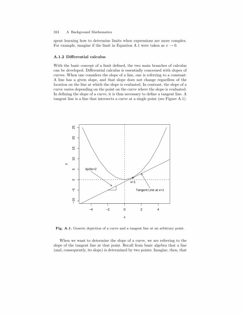
324 A Background Mathematics
spent learning how to determine limits when expressions are more complex.For example, imagine if the limit in Equation A.1 were taken as x → 0.
A.1.2 Differential calculus
With the basic concept of a limit defined, the two main branches of calculuscan be developed. Differential calculus is essentially concerned with slopes ofcurves. When one considers the slope of a line, one is referring to a constant:A line has a given slope, and that slope does not change regardless of thelocation on the line at which the slope is evaluated. In contrast, the slope of acurve varies depending on the point on the curve where the slope is evaluated.In defining the slope of a curve, it is thus necessary to define a tangent line. Atangent line is a line that intersects a curve at a single point (see Figure A.1).
−4 −2 0 2 4
−10
−5
05
1015
2025
x
y
Tangent Line at x=1
x=1
dy/dx=2
Fig. A.1. Generic depiction of a curve and a tangent line at an arbitrary point.
When we want to determine the slope of a curve, we are referring to theslope of the tangent line at that point. Recall from basic algebra that a line(and, consequently, its slope) is determined by two points. Imagine, then, that
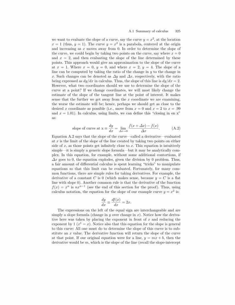
A.1 Summary of calculus 325
we want to evaluate the slope of a curve, say the curve y = x2, at the locationx = 1 (thus, y = 1). The curve y = x2 is a parabola, centered at the originand increasing as x moves away from 0. In order to determine the slope ofthe curve, we could begin by taking two points on the curve, say where x = 0and x = 2, and then evaluating the slope of the line determined by thesepoints. This approach would give an approximation to the slope of the curveat x = 1. Where x = 0, y = 0, and where x = 2, y = 4. The slope of aline can be computed by taking the ratio of the change in y to the change inx. Such changes can be denoted as ∆y and ∆x, respectively, with the ratiobeing expressed as dy/dx in calculus. Thus, the slope of this line is dy/dx = 2.However, what two coordinates should we use to determine the slope of thecurve at a point? If we change coordinates, we will most likely change theestimate of the slope of the tangent line at the point of interest. It makessense that the further we get away from the x coordinate we are examining,the worse the estimate will be; hence, perhaps we should get as close to thedesired x coordinate as possible (i.e., move from x = 0 and x = 2 to x = .99and x = 1.01). In calculus, using limits, we can define this “closing in on x”as:
slope of curve at x ≡ dy
dx= lim
∆x→0
f(x + ∆x)− f(x)∆x
. (A.2)
Equation A.2 says that the slope of the curve—called a derivative—evaluatedat x is the limit of the slope of the line created by taking two points on eitherside of x, as those points get infinitely close to x. This equation is intuitivelysimple—it is simply a generic slope formula—but it may be analytically com-plex. In this equation, for example, without some additional contortions, if∆x goes to 0, the equation explodes, given the division by 0 problem. Thus,a fair amount of differential calculus is spent learning “tricks” to manipulateequations so that this limit can be evaluated. Fortunately, for many com-mon functions, there are simple rules for taking derivatives. For example, thederivative of a constant C is 0 (which makes sense, because y = C is a flatline with slope 0). Another common rule is that the derivative of the functionf(x) = xn is nxn−1 (see the end of this section for the proof). Thus, usingcalculus notation, the equation for the slope of our example curve y = x2 is:
dy
dx≡ df(x)
dx= 2x.
The expressions on the left of the equal sign are interchangeable and aresimply a slope formula (change in y over change in x). Notice how the deriva-tive here was taken by placing the exponent in front of x and reducing theexponent by 1 (x1 = x). Notice also that this equation for the slope is generalto this curve: All one must do to determine the slope of this curve is to sub-stitute an x value. The derivative function will return the slope of the curveat that point. If our original equation were for a line, y = mx + b, then thederivative would be m, which is the slope of the line (recall the slope-intercept

326 A Background Mathematics
form from algebra), and the m is constant across all values of x. This resultshould be intuitive: As stated above, the slope of a line is constant regardlessof where it is evaluated.
This “first” derivative of a curve can not only be considered a slope ofthe curve, but it can also be considered a rate of change, since the slopetells the rate of change in y per unit change in x. There are higher orderrates of change (i.e., change in the rate of change—also called acceleration).Differential calculus involves not only first derivatives, but also higher orderderivatives, which are computed by taking the derivative of a derivative. Intheory, there is virtually no limit to the number of derivatives of a functionthat can be taken, except often second, third, and higher order derivatives areconstant.
Differential calculus in dimensions greater than two is also concerned with“partial” derivatives, or the slope of a curve in one of the multiple dimen-sions. Partial derivatives tend to be fairly simple to compute, because whentaking a partial derivative, one treats the variables representing other dimen-sions as constants. Whereas full derivatives are denoted using dy/dx, partialderivatives are denoted using the ∂ symbol: ∂y/∂x.
Derivatives are a fundamental part of likelihood analysis in statistics. Max-imizing a likelihood function requires finding the point at which the likelihoodcurve’s derivative is 0, because a tangent line with slope 0 indicates a flat line,implying a point on the curve that is either a maximum or a minimum. In theparabola example, the minimum is reached where x = 0.
Second derivatives are also useful in classical statistics. The second deriva-tive represents the rate of curvature in a curve. Given that the density func-tion for a probability distribution is simply a mathematical curve, the secondderivative reveals whether the curve has steep or shallow curvature, implyingeither smaller or greater variance (see Chapter 2).
A.1.3 Integral calculus
The other branch of calculus, integral calculus, is concerned in general withfinding area under and between curves. In probability modeling, finding thearea under curves is crucial. Indeed, the key requirement for a mathematicalcurve to constitute a probability density function is that the area under theentire curve totals 1.
Finding the area under a line segment is easy, because there are simpleformulas for computing areas of rectangles and triangles. However, findingthe area under a curve is more difficult, because there are no simple algebraicformulas for areas involving most curves. Imagine, for example, that one ispresented with the curve y = −x2 + 3 and wishes to find the area under it.This curve is an inverted parabola, with its vertex located at (0,3). The curveintersects the x axis in two places (where y = 0, x = ±
√3 ≈ 1.73).
We could divide the curve into two halves, create rectangles that closelyfit the area under the curve, and approximate the area under the curve using

A.1 Summary of calculus 327
the area of the rectangles (see Figure A.2 for a depiction of this curve). Thisestimated area would approximate the area under the curve, but there wouldbe considerable error. The rectangles, if they joined at x = 0 with a height of3, would include a considerable amount of area that is above the curve wherex < 0 and x > 0. Thus, an alternative might be to consider breaking thecurve into more than two sections and adjusting the height of each rectangleto more closely match the height of the curve at the rectangle’s position onthe x axis. However, unless the rectangles are infinitely small, there wouldalways been some overestimation or underestimation of the area. Again, referto Figure A.2. The upper plot shows this inverted parabola with its area underthe curve being approximated using two rectangles. With two rectangles, thereis considerable overestimation of the area under the curve. The middle plotshows the approximation with four rectangles; here there is substantially lessoverestimation. Finally, the bottom plot shows the approximation with eightrectangles. There is substantially less overestimation of the area with eightrectangles than with four.
Once again, the notion of a limit is crucial. If we let the rectangles getinfinitely small, then we can reduce the error in approximation to 0. Hence, asolution to finding the area under the curve is to use the following formula:
limn→∞
n∑i=1
Ai,
where Ai is the area of the ith rectangle under the curve.1 In this expression,as n approaches infinity, the sum becomes called an “integral,” and is denotedwith the symbol
∫. Thus, integrals can be considered the continuous analog
of discrete summation using∑
. Area under curves can be computed for theentire curve, or they can be computed for only sections of a curve. For example,the expression: ∫ √
3
0
(−x2 + 3)dx
implies that we are interested in the area under the curve between the limits ofx = 0 and x =
√3. Notice the “dx” placed at the end of the expression—this
quantity is the width of the rectangles being summed, and the remainder ofthe expression is the height.
The fundamental theorem of calculus relates integrals and derivatives,showing that they are inverse functions of one another. In brief, the theo-rem says:
d∫
f(x)dx
= f(x). (A.3)
1 In fact, one can achieve closer approximation with a finite n if one uses trapezoidsor other shapes that more closely match the shape of the curve at x.
328 A Background Mathematics
−3 −2 −1 0 1 2 3
−1
13
5
2 rectangles
yerror
−3 −2 −1 0 1 2 3
−1
13
5
4 rectangles
y
reduction in error
−3 −2 −1 0 1 2 3
−1
13
5
8 rectangles
y
even more reduction in error
Fig. A.2. Finding successive approximations to the area under a curve using rect-angles.
In other words, the derivative of an integral of a function is simply thefunction itself. Thus, if we know the derivative of some function, we alsoknow the integral of some other function. For example, above we saw that thederivative of xn was nxn−1. Using the fundamental theorem, we can invertthis process and find that the integral of xn is xn+1/(n + 1). Technically, theintegral also involves adding a constant C, because, given that the derivative ofa constant is 0, we never know what constant should be added when invertingthe derivative (that is, taking an integral).
A.1 Summary of calculus 329
Without going into all the details of integration, we evaluate integralsby (1) taking the integral and (2) evaluating the integral at the limits ofintegration. In our current example:
∫ √3
0
(−x2 + 3
)dx =
−x3
3+ 3x
∣∣∣∣√
3
0
=−(√
3)3
3+ 3
(√3)− 0
= 2√
3.
The first line shows the integral of the function. The bar to the rightindicates that these are the limits at which to evaluate this integral. Thethird expression shows the value of the function after evaluating it at theselimits, and the final expression is the area under the curve between 0 andthe
√3. Notice how the function value at the lower limit of integration is
subtracted from the value of the function at the upper limit of integration.This result should make sense: If you imagine taking all the area under thecurve to the left of
√3 and then subtracting all the area under the curve to
the left of 0, what remains is the area between the two points. This resultshould be somewhat familiar, if you have taken a basic statistics course andworked with finding the area (or probability) under the standard normal (z)curve between two points via subtraction.
Integrals can become very complex, especially when dealing with curvesof high dimension (e.g., as are used in multivariate probability distributions).Just as there are partial derivatives, there are partial integrals. Integrals canalso become complex when there is not a simple expression for the integral.Indeed, some curves have no analytically tractable integrals (for example, thenormal distribution curve has no closed form solution for its integral). In thesecases, other methods must be used to evaluate the integral, including usingsums of the area of tiny rectangles (or trapezoids).
A.1.4 Finding a general rule for a derivative
Above, I said that the derivative of y = xn is nxn−1. We know this result istrue generally by applying Equation A.2. Suppose our equation is y = xn +C,where C is an arbitrary constant. Derivatives of sums are equal to the sumof the derivatives, so we can take the derivative of xn separately from that ofC. Since the derivative of a constant is 0, we can disregard it and focus onlyon xn. Following Equation A.2, we have:
dy
dx= lim
∆x→0
(x + ∆x)n − xn
∆x. (A.4)
Using the rule for binomial expansion, (x + ∆x)n can be expanded as:
330 A Background Mathematics
(n0
)xn∆x0 +
(n1
)xn−1∆x1 + . . . +
(n
n− 1
)x1∆xn−1 +
(nn
)x0∆xn.
Notice that the first term of this expression reduces to xn, and thus, whenit is included in Equation A.4, it cancels the xn that is subtracted at the endin the numerator. So, we are left with a series of terms containing powers of∆x:
dy
dx= lim
∆x→0
(n1
)xn−1∆x1 + . . . +
(nn
)x0∆xn
∆x.
Because all the terms in the numerator contain at least one ∆x, we can factorout one from each part of the numerator and cancel it with the denominator,and we are left with:
dy
dx= lim
∆x→0
(n1
)xn−1 + . . . +
(nn
)x0∆xn−1. (A.5)
Allowing ∆x to go to 0 in Equation A.5 eliminates all the terms in theequation except for the first term, which is nxn−1, the rule presented above.Other general rules for derivatives are derived in a similar fashion and areusually presented in a table in a calculus text.
A.2 Summary of matrix algebra
Matrix algebra is a form of mathematics that allows compact notation for, andmathematical manipulation of, high-dimensional expressions and equations.For the purposes of this book, only a relatively simple exposition is required inorder to understand the notation for multivariate equations and calculations.
A.2.1 Matrix notation
The basic unit in matrix algebra is a matrix, generally expressed as:
A =
a11 a12 a13
a21 a22 a23
a31 a32 a33
.
Here, the matrix A is denoted as a matrix by the boldfaced type. Through-out the text, however, I use capitalized letters to denote matrices, rather thanboldface, for the sake of appearance. Matrices can be of any dimension; inthis example, the matrix is a “3-by-3” or “3× 3” matrix. The number of rowsis listed first; the number of columns is listed second. The subscripts of thematrix elements (a’s) clarify this: The third item in the second row is element
A.2 Summary of matrix algebra 331
a23. A matrix with only one element (i.e., 1×1 dimension) is called a “scalar.”A matrix with only a single column is called a column vector; a matrix withonly a single row is called a row vector. The term “vector” also has meaningin analytic geometry, referring to a line segment that originates at the origin(0, 0, . . . , 0) and terminates at the coordinates listed in the k dimensions. Forexample, you are already familiar with the Cartesian coordinate (4, 5), whichis located 4 units from 0 in the x dimension and 5 units from 0 in the y dimen-sion. The vector [4, 5], then, is the line segment formed by taking a straightline from (0, 0) to (4, 5).
A.2.2 Matrix operations
The first important operation that can be performed on a matrix (or vector) isthe transpose function, which is denoted as: A′ or AT . The transpose functionreverses the rows and columns of a matrix so that if B = AT :
bij = aji,∀ i, j. (A.6)
This equation says that the ijth element of the transposed matrix is the jith
element of the original matrix for all i = 1 . . . I and j = 1 . . . J elements.The dimensionality of a transposed matrix, therefore, is the opposite of theoriginal matrix. For example, if matrix B is 3× 2, then matrix BT will be ofdimension 2× 3. The transpose of the multiple of two matrices, say (AB)T , issimply the multiple of the transposes of the original matrices, only in reverse.Thus, (AB)T = BT AT .
With this basic function developed, we can now discuss other matrix oper-ations, including matrix addition, subtraction, and multiplication (includingdivision). Matrix addition and subtraction are relatively simple. Provided twomatrices have the same dimensionality (i.e., they “conform” for addition),adding or subtracting two matrices is performed by simply adding and sub-tracting corresponding elements in the two matrices:
A + B =[
a11 a12
a21 a22
]+[
b11 b12
b21 b22
]=[
(a11 + b11) (a12 + b12)(a21 + b21) (a22 + b22)
]. (A.7)
The commutative property of addition and subtraction that holds in scalaralgebra also holds in matrix algebra: The order in which matrices are added (orsubtracted) makes no difference to the outcome, so that A+B+C = C+B+A.
Matrix multiplication is slightly more difficult than addition and subtrac-tion, unless one is multiplying a matrix by a scalar. In that case, the scalaris distributed to each element in the matrix, and multiplication is carried outelement by element:
k
[a11 a12
a21 a22
]=[
ka11 ka12
ka21 ka22
]. (A.8)
332 A Background Mathematics
In the event two matrices are being multiplied, before multiplying, onemust make sure the matrices conform for multiplication, where “conform”means that the number of columns in the first matrix must equal the numberof rows in the second matrix. For example, one cannot post-multiply a 2× 3matrix A by another 2 × 3 matrix B, because the number of columns in Ais 3, while the number of rows in B is 2. One could, however, multiply A bya 3 × 2 matrix C. The matrix that results from multiplying A and C wouldhave dimension 2 × 2 (the same number of rows as the first matrix and thesame number of columns as the second matrix).
The general rule for matrix multiplication is as follows: If one is multiplyingA× C to obtain matrix D, then:
dij =K∑
k=1
aikckj , ∀ i, j. (A.9)
That is, the ijth element of matrix D is equal to the sum of the multipleof the elements in row i of A and the column j of C. Matrix multiplication istherefore a fairly tedious process. As an example, assume A is 2× 3 and C is3× 2, with the following elements:
A =[
1 2 34 5 6
], C =
1 23 45 6
.
Then, element d11 = (1 × 1) + (2 × 3) + (3 × 5) = 22, and the entire Dmatrix is (solve this yourself):
D =[
22 2849 64
].
Notice that matrix D is 2× 2.Unlike matrix addition and subtraction, in which the order of the matrices
is irrelevant, order matters for multiplication. Obviously, given the conforma-bility requirement, reversing the order of matrices may make multiplicationimpossible (e.g., although a 3 × 2 matrix can be post-multiplied by a 2 × 4matrix, the 2×4 matrix cannot be post-multiplied by the 3×2 matrix). How-ever, even if matrices are conformable for multiplication after reversing theirorder, the resulting matrices will not generally be identical. For example, a1×k row vector multiplied by a k×1 column vector will yield a scalar (1×1),but if we reverse the order of multiplication, we will obtain a k × k matrix.
Some additional functions that apply to matrices and are commonly usedin statistics include the trace operator [the trace of A is denoted as tr(A)],the determinant, and the inverse. The trace of a matrix is simply the sumof the diagonal elements of the matrix. The determinant is more difficult.Technically, the determinant is the sum of the signed multiples of all thepermutations of a matrix, where the term “permutations” refers to the unique
A.2 Summary of matrix algebra 333
combinations of a single element from each row and column, for all rowsand columns. If d denotes the dimensionality of a matrix, then there are d!permutations for the matrix. For example, in a 3 × 3 matrix, there are atotal of 6 permutations (3! = 3 × 2 × 1 = 6): (a11, a22, a33), (a12, a23, a31),(a13, a21, a32), (a13, a22, a31), (a11, a23, a32), (a12, a21, a33). Notice howfor each combination, there is one element from each row and column. Thesigning of each permutation is determined by the column position of eachelement in all the pairs that can be constructed using the elements of thepermutation, and the subscript of element at each position in each pair. Forexample, the permutation (a11, a22, a33) has elements from columns 1, 2,and 3. The possible ordered (i, j) pairs that can come from this permutationinclude (1, 2), (1, 3), and (2, 3) (based on the column position). If there are aneven number of (i, j) pairs in which i > j, then the permutation is considered“even” and takes a positive sign. Otherwise, the permutation is considered“odd” and takes a negative sign. In this example, there are 0 pairs in whichi > j, so the permutation is even (0 is even). However, in the permutation(a13, a22, a31), the pairs are (3, 2), (3, 1), and (2, 1). In this set, all three pairsare such that i > j; hence this permutation is odd and takes a negative sign.The determinant is denoted using absolute value bars on either side of thematrix name: for instance, the determinant of A is denoted as |A|, or often,det(A).
For 2× 2 and 3× 3 matrices, determinants can be calculated fairly easily.For example, the determinant of a 2 × 2 matrix A is: det(A) = a11a22 −a12a21. However, for larger matrices, the number of permutations becomeslarge rapidly. Fortunately, several rules simplify the process. First, if any rowor column in a matrix is a vector of 0, then the determinant is 0. In thatcase, the matrix is said not to be of full rank. Second, the same is true ifany two rows or columns is identical. Third, for a diagonal matrix (i.e., thereare 0’s everywhere but the main diagonal—the 11, 22, 33,... positions), thedeterminant is only the multiple of the diagonal elements. There are additionalrules, but they are not necessary for this brief introduction. I note that thedeterminant is essentially a measure of the area/volume/hypervolume spannedby the vectors of the matrix. This helps, I think, to clarify why matrices with0 vectors in them have determinant 0: Just as in two dimensions a line hasno area, when we have a 0 vector in a matrix, the dimensionality of the figurespanned by the vectors of a matrix is reduced by a dimension (because onevector does not pass the origin), and hence the hypervolume is necessarily 0.
Finally, a very important function in matrix algebra is the inverse function.The inverse function allows the matrix equivalent of division. In a sense, justas 5 times its inverse 1/5 = 1, a matrix A times its inverse—denoted A−1—equals I, where I is the “identity matrix.” An identity matrix is a diagonalmatrix with ones along the diagonal, and it is the matrix equivalent of “1.”Some simple algebraic rules follow from the discussion of inverses and theidentity matrix:
334 A Background Mathematics
AA−1 = A−1A = I. (A.10)
Furthermore,
AI = IA = A. (A.11)
Given the commutability implicit in the above rules, it stands that in-verses only exist for square matrices, and that all identity matrices are squarematrices. For that matter, the determinant function can only apply to squarematrices also.
Computing the inverse of matrices is a difficult task, and there are severalmethods by which to derive them. The simplest method to compute an inverseis to use the following formula:
A−1 =1|A|
adj A (A.12)
The only new element in this formula is “adj A,” which means “adjoint ofA.” The adjoint of a matrix is the transpose of its matrix of cofactors, wherea cofactor is the signed determinant of the “minor” of an element of a matrix.The minor of element i, j is the matrix the remains after deleting the ith rowand jth column of the original matrix. For example, the minor of element a11
of the matrix A shown at the beginning of this matrix algebra summary is:[a22 a23
a32 a33
].
Taking its determinant leaves one with a scalar that is then multipliedby −1i+j . This latter process is called “signing.” In this case, we obtain(−1)2(a22a33 − a23a32) as the cofactor for element a11. If one replaces ev-ery element in matrix A with its cofactor (called “expansion by cofactors,”)then transposes the result, one will obtain the adjoint of A. Multiplying thisby 1/|A| (a scalar) will yield the inverse of A.
Cofactors can also be used to find determinants. Simply take each elementin any row or column and multiply it by its cofactor, and then sum theseresults together for all the elements in the row/column. Obviously, effort issaved if one chooses a row or column with several 0’s, because the determinantsof those elements’ minors do not need to be calculated. (They will ulitmatelybe multiplied by 0 and will drop from the calculation).
Even using cofactors, the process of finding determinants and inverses istedious. Fortunately, computer packages tend to have determinant and inver-sion routines built into them, and there are plenty of inversion algorithmsavailable if you are designing your own software, so that we generally neednot worry. It is worth mentioning that, if a matrix has a 0 determinant, itdoes not have an inverse. There are many additional matrix algebra rules andtricks that one may need to know; however, they are also beyond the scope ofthis introduction.

A.3 Exercises 335
A.3 Exercises
A.3.1 Calculus exercises
Evaluate the following limits. If a limit does not exist, indicate such. Youshould graph the expression to see whether the limit exists.
1. limx→∞1x .
2. limx→01x .
3. limx→∞x2+5
3 .4. limx→0
x2−15 .
5. limx→∞ exp(−x).6. limx→0 exp(−x).7. limx→∞
x2x .
8. limσ→∞1
σ√
2πexp
−(x−µ)2
2σ2
.
Using the following rules for derivatives, find the slope of the curve below atx = 3.
(power rule) (constant rule) (addition rule)
ddx [un] = nun−1du d
dx [cu] = c× ddx [u]du d
dx [u + v] = ddx [u]du + d
dx [v]dv
9. y = 3x3 + 5x2 + 2x + 10.10. Using the fundamental theorem of calculus and the rules above, find thearea under the curve (the integral) of the curve above between 0 and 5.
A.3.2 Matrix algebra exercises
Perform the various calculations on the matrices below. If an operation isnot possible for an item, indicate this and explain why. Don’t forget steps:Expansion by cofactors involves a sign function that depends on i and j, wherei and j index the rows and columns. Also, the adjoint matrix is the transposeof the matrix of cofactors.
A B C D E
[3 2−1 3
] 3 1 −14 3 510 4 1
[1 7 4]
293
4 1 37 1 86 8 7

336 A Background Mathematics
1. Find B + E.2. Find E −B.3. Find AB.4. Find CD.5. Find DC.6. Find DE.7. Find ET .8. Find det(A).9. Find det(B).
10. Find E−1 (Hint: Use expansion by cofactors).11. Find tr(B).12. If the determinant represents area, volume, or hypervolume from a ge-
ometric perspective, then what is the hypervolume of a six-dimensionalidentity matrix?
B
The Central Limit Theorem, ConfidenceIntervals, and Hypothesis Tests
The classical approach to statistical inference relies heavily on the CentralLimit Theorem (CLT), a key result of which is:
f(x|µx, σx, n)asy∼ N
(µx,
σx√n
). (B.1)
In English, this expression says that, as sample sizes get larger, the samplingdistribution f() for a statistic, here x, approaches a normal distribution with amean equal to the population mean of x (µx) and a standard deviation equalto the population standard deviation of x (σx) divided by the square rootof the sample size (n) used to compute x. It is important to note that thetheorem does not require the distribution of the original variable x from whichthe statistic x was generated to be normal: Regardless of the distribution ofthe data, the asymptotic sampling distribution of a statistic will be normal.
What is a sampling distribution? Consider that, when we take a randomsample of size n individuals, this sample is only one of many possible samplesof size n that could be drawn from the population. Certainly, if we took asecond random sample of the same size, we would not end up with the samecollection of respondents, and consequently, the value of any statistic (likethe mean) we calculate from one sample will most likely differ from the valueobtained in another. The CLT, however, says that, if we were to take allpossible random samples of a given size from the population and compute thevalue of the statistic of interest (e.g., the mean) for each one, the distributionof these statistics—the sampling distribution—would be normal, assuming thesample size is large enough.
B.1 A simulation study
To demonstrate the theorem, I display the results of a brief simulation thatfollowed the following structure:
338 B The Central Limit Theorem, Confidence Intervals, and Hypothesis Tests
1. I drew 1,000 samples each of sizes n = 1, 2, 30, and 100 from a U(0, 1)distribution. The mean and standard deviation of a U(a, b) distribution
are b+a2 and
√(b−a)2
12 , respectively. Here, those values are .5 and .2887(variance = .0833).
2. I computed the mean for each of the 1,000 samples for each sample size andcomputed the standard deviation for each sample also. The collection ofthe means from each of the 1,000 samples of a given sample size representsthe sampling distribution of the mean for that sample size.
3. I computed the mean of all the sample means computed from Step 2 foreach sample size, and I computed the standard deviation (and variances)of these distributions of means.
Figure B.1 shows the distribution of these 1, 000 sample means (the sam-pling distribution) for all four sample sizes. The figure shows that the meansare distributed across the [0, 1] interval for samples size n = 1, basically re-flecting that samples of this size are nothing more than draws from the originaldistribution. As the sample size increases, the means become more clusteredaround the true mean of .5.
Figure B.2 shows what happens to the standard deviation of the samplingdistribution of the mean as the sample sizes get larger. The figure depictsthe empirical standard deviation of the sampling distribution for each of thesample sizes (the standard deviation of the 1,000 sample means), as well as thetheoretical standard deviation claimed by the CLT. Notice how the empiricaland theoretical standard deviations almost perfectly coincide, illustrating thetheorem.
Figure B.3 shows the distribution of the variances for samples size n = 2,n = 30, and n = 100. (Note: The variances for the samples of size n = 1are 0, which is why they are not plotted.) The sampling distribution for thevariances at n = 2 is truncated at 0 and highly right-skewed (in fact, thedistribution of variances is an inverse gamma distribution; see Chapter 3). Thedistribution is also very broad. As the sample sizes increase, the distributionbecomes more and more symmetric in shape and narrower. The mean of eachof these distributions of the variance is equal to approximately .08, the correctvariance (
√1/12
2). These results suggest that larger samples are also better
at pinpointing the true population variance/standard deviation.
B.2 Classical inference
Classical statistical inference relies on the CLT as exemplified by the simula-tion results. When we draw a random sample of size n from a population, wecan imagine that we are really sampling a sample mean, variance, regressionparameter, or some other statistic from its sampling distribution. From thatperspective, if we know that large samples have a normal sampling distribu-tion for a statistic (θ), and we let the sample statistic (e.g., mean, variance,
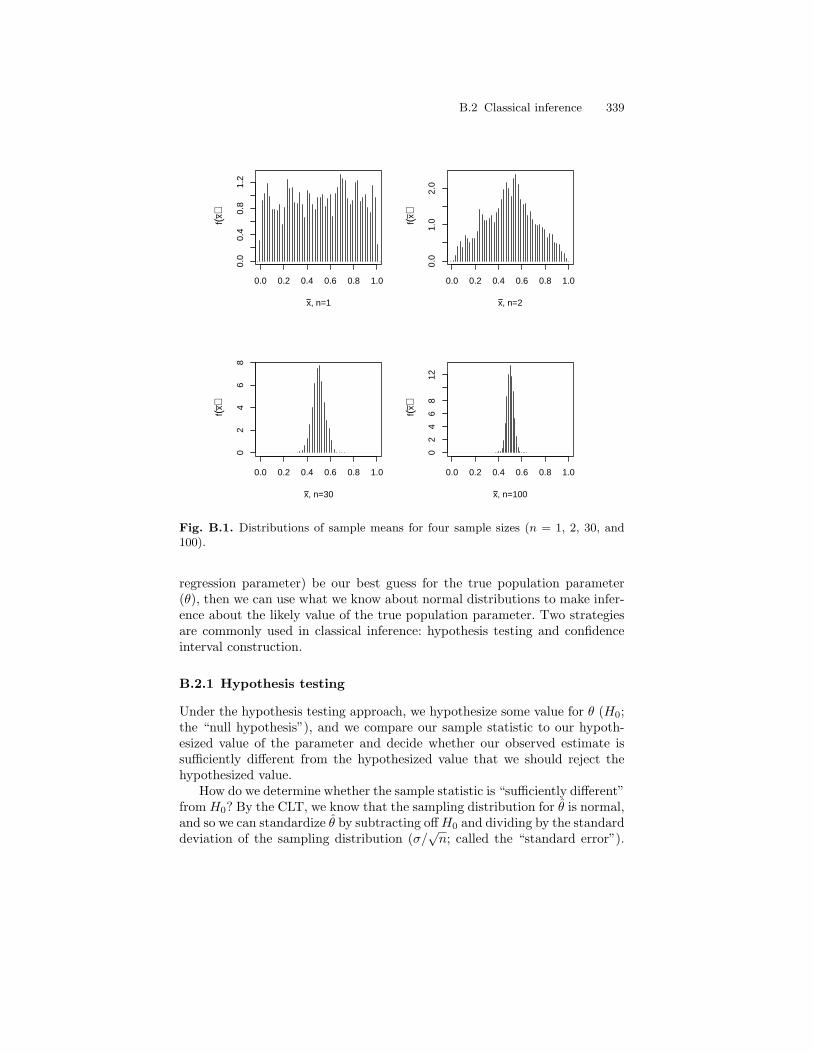
B.2 Classical inference 339
0.0 0.2 0.4 0.6 0.8 1.0
0.0
0.4
0.8
1.2
x, n=1
f(x)
0.0 0.2 0.4 0.6 0.8 1.0
0.0
1.0
2.0
x, n=2
f(x)
0.0 0.2 0.4 0.6 0.8 1.0
02
46
8
x, n=30
f(x)
0.0 0.2 0.4 0.6 0.8 1.0
02
46
812
x, n=100
f(x)
Fig. B.1. Distributions of sample means for four sample sizes (n = 1, 2, 30, and100).
regression parameter) be our best guess for the true population parameter(θ), then we can use what we know about normal distributions to make infer-ence about the likely value of the true population parameter. Two strategiesare commonly used in classical inference: hypothesis testing and confidenceinterval construction.
B.2.1 Hypothesis testing
Under the hypothesis testing approach, we hypothesize some value for θ (H0;the “null hypothesis”), and we compare our sample statistic to our hypoth-esized value of the parameter and decide whether our observed estimate issufficiently different from the hypothesized value that we should reject thehypothesized value.
How do we determine whether the sample statistic is “sufficiently different”from H0? By the CLT, we know that the sampling distribution for θ is normal,and so we can standardize θ by subtracting off H0 and dividing by the standarddeviation of the sampling distribution (σ/
√n; called the “standard error”).
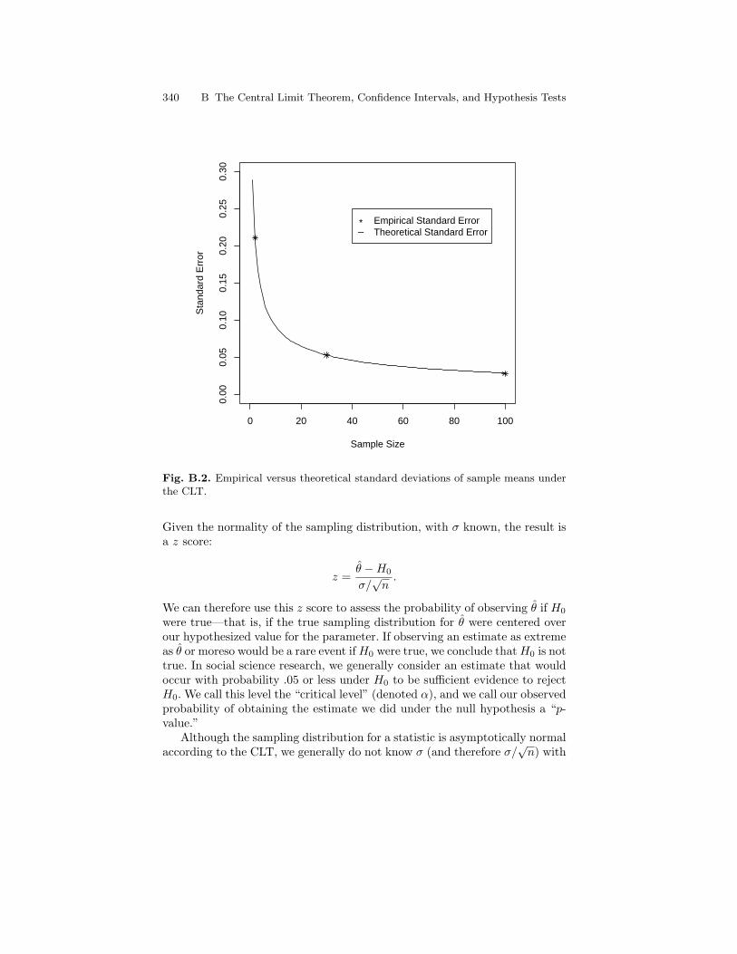
340 B The Central Limit Theorem, Confidence Intervals, and Hypothesis Tests
0 20 40 60 80 100
0.00
0.05
0.10
0.15
0.20
0.25
0.30
Sample Size
Sta
ndar
d E
rror
*_Empirical Standard ErrorTheoretical Standard Error
Fig. B.2. Empirical versus theoretical standard deviations of sample means underthe CLT.
Given the normality of the sampling distribution, with σ known, the result isa z score:
z =θ −H0
σ/√
n.
We can therefore use this z score to assess the probability of observing θ if H0
were true—that is, if the true sampling distribution for θ were centered overour hypothesized value for the parameter. If observing an estimate as extremeas θ or moreso would be a rare event if H0 were true, we conclude that H0 is nottrue. In social science research, we generally consider an estimate that wouldoccur with probability .05 or less under H0 to be sufficient evidence to rejectH0. We call this level the “critical level” (denoted α), and we call our observedprobability of obtaining the estimate we did under the null hypothesis a “p-value.”
Although the sampling distribution for a statistic is asymptotically normalaccording to the CLT, we generally do not know σ (and therefore σ/
√n) with
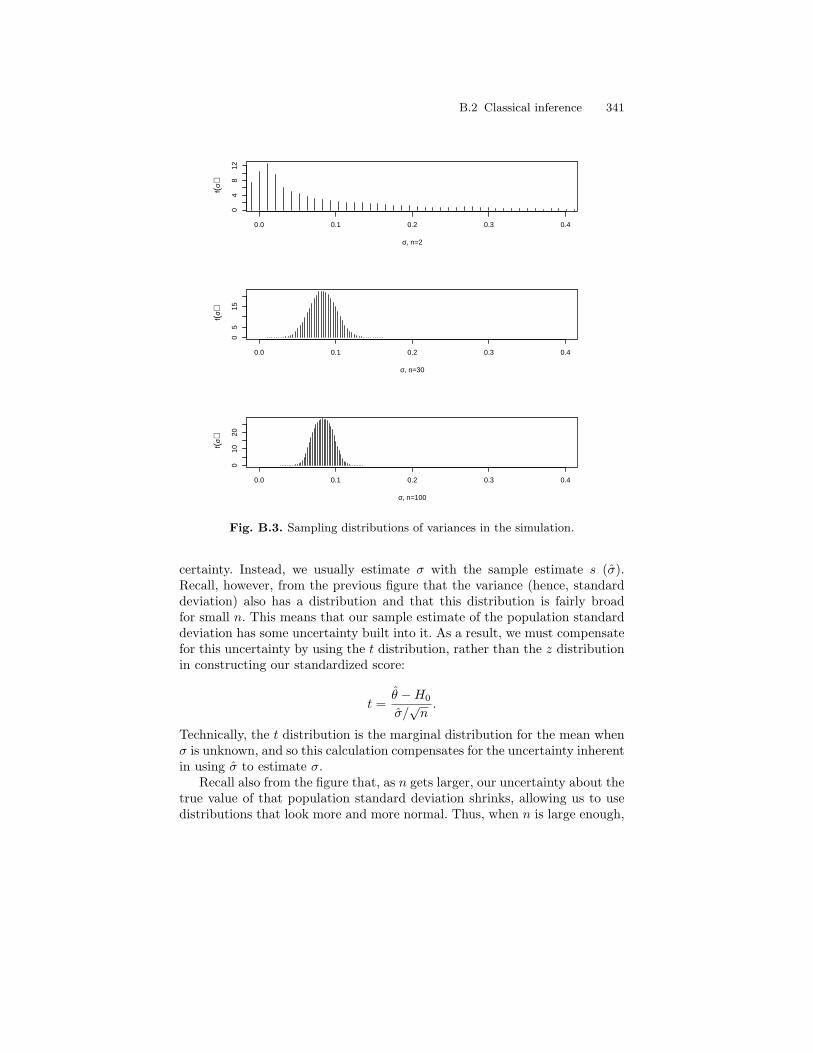
B.2 Classical inference 341
0.0 0.1 0.2 0.3 0.40
48
12σ, n=2
f(σ)
0.0 0.1 0.2 0.3 0.4
05
15
σ, n=30
f(σ)
0.0 0.1 0.2 0.3 0.4
010
20
σ, n=100
f(σ)
Fig. B.3. Sampling distributions of variances in the simulation.
certainty. Instead, we usually estimate σ with the sample estimate s (σ).Recall, however, from the previous figure that the variance (hence, standarddeviation) also has a distribution and that this distribution is fairly broadfor small n. This means that our sample estimate of the population standarddeviation has some uncertainty built into it. As a result, we must compensatefor this uncertainty by using the t distribution, rather than the z distributionin constructing our standardized score:
t =θ −H0
σ/√
n.
Technically, the t distribution is the marginal distribution for the mean whenσ is unknown, and so this calculation compensates for the uncertainty inherentin using σ to estimate σ.
Recall also from the figure that, as n gets larger, our uncertainty about thetrue value of that population standard deviation shrinks, allowing us to usedistributions that look more and more normal. Thus, when n is large enough,

342 B The Central Limit Theorem, Confidence Intervals, and Hypothesis Tests
the t distribution converges on the normal distribution, and we often simplyuse the normal distribution for inference.
B.2.2 Confidence intervals
An alternative method of performing statistical inference is to construct a“confidence interval” around a sample estimate in order to state, with somelevel of “confidence,” where we suspect the parameter θ falls. When σ isknown, we compute intervals using the z distribution; when σ is not known,we compute intervals using the t distribution, for the same reason discussedin the previous section. These intervals are computed as:
(1− α)%C.I. = θ ± zα2
(σ√n
),
and
(1− α)%C.I. = θ ± tα2
(σ√n
),
respectively, where (1 − α)% is the level of confidence, zα2
(or tα2) is the
number of standard errors we must add/subtract from our sample estimate θto obtain the desired level of confidence, and σ/
√n (or σ/
√n) is the size of
the standard error. Just as we commonly use a critical level of α = .05 underthe hypothesis testing approach to inference, we often construct 95% (1-.05)confidence intervals, and so I will discuss such intervals here.
The correct interpretation of a 95% confidence interval is that 95% of theconfidence intervals that could be drawn from the sampling distribution forθ would capture θ. In order to understand why, consider, once again, thatthe sampling distribution for θ is normal and centered over θ with a standarddeviation of σ/
√n. Then (assuming σ is known), 95% of all possible values
of θ will fall within 1.96 standard errors of θ. If this is true, then if we add(and subtract) 1.96 standard errors to (from) all possible estimates θ, 95%of the resulting intervals would contain θ. The ones that do not will be theintervals constructed around values of θ that fall in the tails of the samplingdistribution. As before, if σ is not known and is estimated with σ, our intervalshould be constructed using the t distribution.
Figure B.4 shows a collection of 95% confidence intervals based on thez distribution for the simulated samples of size n = 2, n = 30, and n =100. The intervals are vertical, with the true population parameter value (.5)represented by a horizontal line. Notice how these intervals are much moreconsistent in width and generally narrower for the larger size samples than then = 2 sized samples. Also notice that some of the confidence intervals for thesamples sized n = 2 are extremely narrow. This result reflects the uncertaintyin σ2 (and thus σ2/n) inherent in having small samples.
Table B.1 shows the percent of the confidence intervals (out of 1,000 foreach sample size) that, in fact, capture the true mean. In the table, I have
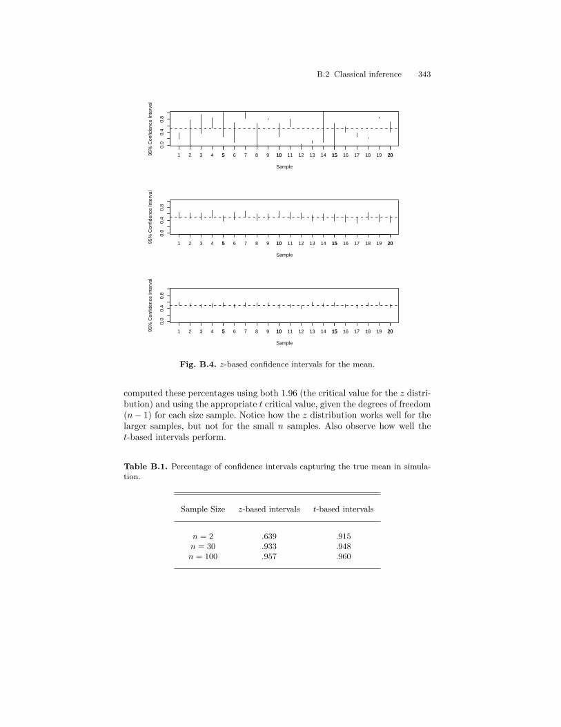
B.2 Classical inference 343
5 10 15 200.
00.
40.
8Sample
95%
Con
fiden
ce In
terv
al1 2 3 4 5 6 7 8 9 10 11 12 13 14 15 16 17 18 19 20
5 10 15 20
0.0
0.4
0.8
Sample
95%
Con
fiden
ce In
terv
al
1 2 3 4 5 6 7 8 9 10 11 12 13 14 15 16 17 18 19 20
5 10 15 20
0.0
0.4
0.8
Sample
95%
Con
fiden
ce In
terv
al
1 2 3 4 5 6 7 8 9 10 11 12 13 14 15 16 17 18 19 20
Fig. B.4. z-based confidence intervals for the mean.
computed these percentages using both 1.96 (the critical value for the z distri-bution) and using the appropriate t critical value, given the degrees of freedom(n− 1) for each size sample. Notice how the z distribution works well for thelarger samples, but not for the small n samples. Also observe how well thet-based intervals perform.
Table B.1. Percentage of confidence intervals capturing the true mean in simula-tion.
Sample Size z-based intervals t-based intervals
n = 2 .639 .915n = 30 .933 .948n = 100 .957 .960
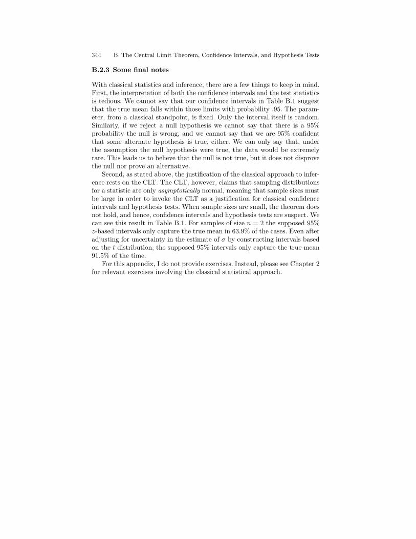
344 B The Central Limit Theorem, Confidence Intervals, and Hypothesis Tests
B.2.3 Some final notes
With classical statistics and inference, there are a few things to keep in mind.First, the interpretation of both the confidence intervals and the test statisticsis tedious. We cannot say that our confidence intervals in Table B.1 suggestthat the true mean falls within those limits with probability .95. The param-eter, from a classical standpoint, is fixed. Only the interval itself is random.Similarly, if we reject a null hypothesis we cannot say that there is a 95%probability the null is wrong, and we cannot say that we are 95% confidentthat some alternate hypothesis is true, either. We can only say that, underthe assumption the null hypothesis were true, the data would be extremelyrare. This leads us to believe that the null is not true, but it does not disprovethe null nor prove an alternative.
Second, as stated above, the justification of the classical approach to infer-ence rests on the CLT. The CLT, however, claims that sampling distributionsfor a statistic are only asymptotically normal, meaning that sample sizes mustbe large in order to invoke the CLT as a justification for classical confidenceintervals and hypothesis tests. When sample sizes are small, the theorem doesnot hold, and hence, confidence intervals and hypothesis tests are suspect. Wecan see this result in Table B.1. For samples of size n = 2 the supposed 95%z-based intervals only capture the true mean in 63.9% of the cases. Even afteradjusting for uncertainty in the estimate of σ by constructing intervals basedon the t distribution, the supposed 95% intervals only capture the true mean91.5% of the time.
For this appendix, I do not provide exercises. Instead, please see Chapter 2for relevant exercises involving the classical statistical approach.

B.2 Classical inference 345
*********************************************************


References
Albert, J.H. (1992). “Bayesian Estimation of the Polychoric Correlation Co-efficient.” Journal of Computation and Simulation 44:47-61.
Albert, J.H. and S. Chib. (1993). “Bayesian Analysis of Binary and Polychoto-mous Response Data.” Journal of the American Statistical Association88(422):669-679.
Alho, J.M. and B.D. Spencer. (2005). Statistical Demography and Forecasting.New York: Springer.
Allison, P.D. (1984). Event History Analysis: Regression for LongitudinalEvent Data. Sage University Paper Series on Quantitative Applicationsin the Social Sciences, 07-46. Thousand Oaks, CA: Sage.
Allison, P.D. (2003). Missing Data. Sage University Paper Series on Quanti-tative Applications in the Social Sciences, 07-136. Thousand Oaks, CA:Sage.
Billingsley, P. (1995). Probability and Measure. 3rd ed. New York: Wiley.Bollen, K.A. (1989). Structural Equations with Latent Variables. New York:
Wiley.Bollen, K.A. and P.J. Curran. (2006). Latent Curve Models: A Structural
Equation Perspective. Hoboken, NJ: Wiley.Box, G.E.P. and G.C. Tiao. (1973). Bayesian Inference in Statistical Analysis.
Reading, MA: Addison-Wesley.Bremaud, P. (1999). Markov Chains, Gibbs Fields, Monte Carlo Simulation,
and Queues. New York: Springer-Verlag.Carlin, B.P. and T.A. Louis. (2000). Bayes and Empirical Bayes Methods for
Data Analysis. 2nd ed. Boca Raton, FL: Chapman & Hall/CRC.Casella, G. and E.I. George. (1992). “Explaining the Gibbs Sampler.” The
American Statistician 46(3):167-174.Chen, M-H., Q-M. Shao, and J.G. Ibrahim. (2000) Monte Carlo Methods in
Bayesian Computation. New York: Springer-Verlag.

348 B The Central Limit Theorem, Confidence Intervals, and Hypothesis Tests
Chib, S. and E. Greenberg. (1998). “Analysis of Multivariate Probit Models.”Biometrika 85(2):347-361.
Chung, K.L. and F. AitSahlia. (2003). Elementary Probability Theory: WithStochastic Processes and an Introduction to Mathematical Finance. 4thed. New York: Springer-Verlag.
Congdon, P. (2003). Applied Bayesian Modelling. West Sussex, England: Wi-ley.
Congdon, P. (2001). Bayesian Statistical Modeling. West Sussex, England:Wiley.
Cowles, M.K. (1996). “Accelerating Monte Carlo Markov Chain Convergencefor Cumulative-Link Generalized Linear Models.” Statistics and Com-puting 6:101-110.
Cox, D.R. (1972). “Regression Models and Life Tables.” Journal of the RoyalStatistical Society, Series B34:187-220.
Crimmins, E.M., Y. Saito, and D. Ingegneri. (1997). “Trends in Disability-Free Life Expectancy in the United States, 1970-90.” Population andDevelopment Review 23(3):555-572.
DeGroot, M.H. (1986). Probability and Statistics. (Second Ed.) Reading, MA:Addison-Wesley.
DiMaggio, P., J. Evans, and B. Bryson. (1996). “Have Americans’ SocialAttitudes Become More Polarized?” American Journal of Sociology102(3):690-755.
Drezner, Z. (1992). “Computation of the Multivariate Normal Integral.” ACMTransactions on Mathematical Software 18(4):470-480.
Durkheim, E. (1984). The Division of Labor in Society. New York: The FreePress.
Edwards, A.W.F. (1992). Likelihood. Expanded Edition. Baltimore: JohnsHopkins University University Press.
Eliason, S.R. (1993). Maximum Likelihood Estimation: Logic and Practice.Sage University Paper Series on Quantitative Applications in the SocialSciences, 07-96. Thousand Oaks, CA: Sage.
Elo, I.T. and S.H. Preston. (1994). “Estimating African-American Mortalityfrom Inaccurate Data.” Demography 31(3):427-458.
Evans, M., N. Hastings, and B. Peacock. (2000). Statistical Distributions. 3rded. New York: Wiley.
Ezell, M.E., K.C. Land, and L.E. Cohen. (2003). “Modeling Multiple Fail-ure Time Data: A Survey of Variance-Corrected Proportional Haz-ards Models with Empirical Applications to Arrest Data.” SociologicalMethodology 33:111-167.
Fox, J. (1997). Applied Regression Analysis, Linear Models, and Related Meth-ods. Thousand Oaks, CA: Sage.

B.2 Classical inference 349
Gelfand, A.E. and A.F.M. Smith. (1990). “Sampling-Based Approaches toCalculating Marginal Densities.” Journal of the American StatisticalAssociation 85:398-409.
Gelman, A. (1996). “Inference and Monitoring Convergence.” Pp. 131-144 inGilks, W.R., S. Richardson, and D.J. Spiegelhalter (eds.) Markov ChainMonte Carlo in Practice. London: Chapman and Hall.
Gelman, A., J.B. Carlin, H.S. Stern, and D.B. Rubin. (1995). Bayesian DataAnalysis. London: Chapman and Hall.
Gelman, A. and D.B. Rubin. (1995). “Avoiding Model Selection in BayesianSocial Research.” Sociological Methodology 25:165–74.
Gelman, A., X-L. Meng, and H.S. Stern. (1996). “Posterior Predictive Assess-ment of Model Fitness via Realized Discrepancies.” Statistica Sinica6:733–807.
Gilks, W.R. (1996). “Full Conditional Distributions.” Pp. 59-88 in Gilks,W.R., S. Richardson, and D.J. Spiegelhalter (eds.). Markov ChainMonte Carlo in Practice. London: Chapman and Hall.
Gilks, W.R., S. Richardson, and D.J. Spiegelhalter (eds.). (1996). MarkovChain Monte Carlo in Practice. London: Chapman and Hall.
Gilks, W.R. and G.O. Roberts. (1996). “Strategies for Improving MCMC.”Pp. 89-110 in Gilks, W.R., S. Richardson, and D.J. Spiegelhalter (eds.).Markov Chain Monte Carlo in Practice. London: Chapman and Hall.
Gill, J. (2002). Bayesian Methods: A Social and Behavioral Sciences Approach.Boca Raton, FL: Chapman & Hall/CRC.
Hagle, T.M. (1996) Basic Math for Social Scientists: Problems and Solutions.Sage University Paper Series on Quantitative Applications in the SocialSciences, 07-108. Thousand Oaks, CA: Sage.
Hamilton, J.D. (1994). Time Series Analysis. Princeton: Princeton UniversityPress.
Harville, D.A. (1997). Matrix Algebra from a Statisticians Perspective. NewYork: Springer-Verlag.
Hastings, W.K. (1970). “Monte Carlo Sampling Methods Using MarkovChains and Their Applications.” Biometrika 57:97-109.
Hayduk, L.A. (1987). Structural Equation Modeling with LISREL. Baltimore,MD: The Johns Hopkins University Press.
Heckman, J.J. (1979). “Sample Selection Bias as a Specification Error.”Econometrica 47(1):153-161.
Hoeting, J.A., D. Madigan, A.E. Raftery, and C.T. Volinsky. (1999). “BayesianModel Averaging: A Tutorial.” Statistical Science 14(4):382-417.
Hosmer, D.W. and S. Lemeshow. (1989). Applied Logistic Regression. NewYork: Wiley.
Hosmer, D.W. and S. Lemeshow. (1999). Applied Survival Analysis: Regres-sion Modeling of Time to Event Data. New York: Wiley.

350 B The Central Limit Theorem, Confidence Intervals, and Hypothesis Tests
House, J.S., J.M. Lepkowski, A.M. Kinney, R.P. Mero, R.C. Kessler, andA.R. Herzog. (1994). “The Social Stratification of Aging and Health.”Journal of Health and Social Behavior 35(September):213-234.
Hubbard, R. and M.J. Bayarri. (2003). “Confusion Over Measures of Evi-dence (p’s) Versus Errors (α’s) in Classical Stastistical Testing.” TheAmerican Statistician 57(3):171-182.
Imai, K. and D.A. van Dyk. (2005). “A Bayesian Analysis of the Multino-mial Probit Model Using Marginal Data Augmentation.” Journal ofEconometrics 124:311-334.
Jeffreys, Sir H.. (1961). Theory of Probability. 3rd ed. New York: Oxford Uni-versity Press.
Johnson, V.E. and J.H. Albert. (1999). Ordinal Data Modeling. New York:Springer-Verlag.
Judge, G.G., W.E. Griffiths, R.C. Hill, H. Lutkepoohl, and T-C. Lee. (1985).The Theory and Practice of Econometrics. 2nd ed. New York: Wiley.
Kaplan, D. (2000). Structural Equation Modeling: Foundations and Exten-sions. Thousands Oaks, CA: Sage.
Kass, R.E. and A.E. Raftery. (1995). “Bayes Factors.” Journal of the Ameri-can Statistical Association 90(430):773-795.
Laditka, S.B. and D.A. Wolf. (1998). “New Methods for Analyzing Active LifeExpectancy.” Journal of Aging and Health 10(2):214-241.
Land, K.C., J.M. Guralnik, and D.G. Blazer. (1994). “Estimating Increment-Decrement Life Tables with Multiple Covariates from Panel Data: TheCase of Active Life Expectancy.” Demography 31(2):297-319.
Land, K.C., P.L. McCall, and D.S. Nagin. (1996). “A Comparison of Pois-son, Negative Binomial, and Semiparametric Mixed Poisson RegressionModels with Empirical Applications to Criminal Careers Research.” So-ciological Methods & Research 24:387-442.
Lee, P.M. (1989). Bayesian Statistics: An Introduction. New York: OxfordUniversity Press.
Lee, S-Y. and H-T. Zhu. (2000). “Statistical Analysis of Nonlinear Struc-tural Equation Models with Continuous and Polytomous Data.” BritishJournal of Mathematical and Statistical Psychology 53:209-232.
Leonard, T. and J.S.J. Hsu. (1999). Bayesian Methods: An Analysis for Statis-ticians and Interdisciplinary Researchers. Cambridge, UK: CambridgeUniversity Press.
Liao, T.F. (1994). Interpreting Probability Models: Logit, Probit, and OtherGeneralized Linear Models. Sage University Paper Series on Quantita-tive Applications in the Social Sciences, 07-101. Thousand Oaks, CA:Sage.
Little, R.J.A. and D.B. Rubin. (1987). Statistical Analysis with Missing Data.New York: Wiley.

B.2 Classical inference 351
Liu, J.S. (2001). Monte Carlo Strategies in Scientific Computing. New York:Springer-Verlag.
Long, J.S. (1997). Regression Models for Categorical and Limited DependentVariables. Thousand Oaks, CA: Sage.
Long, J.S. and J. Freese. (2003). Regression Models for Categorical DependentVariables Using Stata. College Station, TX: Stata Press.
Lynch, S.M. (2003). “Cohort and Life Course Patterns in the Relationship Be-tween Education and Health: A Hierarchical Approach.” Demography40(2):309-331.
Lynch, S.M. and J.S. Brown. (2005). “A New Approach to Estimating Life Ta-bles with Covariates and Constructing Interval Estimates of Life TableQuantities.” Sociological Methodology 35:177-225.
Lynch, S.M., J.S. Brown, and K.G. Harmsen. (2003). “Black-White Differ-ences in Mortality Deceleration and Compression and the MortalityCrossover Reconsidered.” Research on Aging 25(5):456-483.
Lynch, S.M. and B. Western. (2004). “Bayesian Posterior Predictive Checksfor Complex Models.” Sociological Methods & Research 32(3):301-335.
Markides, K.S. and S.A. Black. (1996). “Race, Ethnicity and Aging: The Im-pact of Inequality.” Pp. 153-170 in R.H. Binstock and L.K. George(eds.). Handbook of Aging and the Social Sciences 4th ed. San Diego,CA: San Diego Academic Press.
Maruyama, G.M. (1998). Basics of Structural Equation Modeling. ThousandOaks, CA: Sage.
McArdle, J.J. and D. Epstein. (1987). “Latent Growth Curves within Devel-opmental Structural Equation Models.” Child Development 58:110-133.
Mehta, P.D. and S.G. West. (2000). “Putting the Individual Back into Indi-vidual Growth Curves.” Psychological Methods 5(1):23-43.
Menken, J., J. Trussell, D. Stempel, and O. Babakol. (1981). “Propor-tional Hazards Life Table Models: An Illustrative Analysis of Socio-Demographic Influences on Marriage Dissolution in the United States.”Demography 18(2):181-200.
Meredith, W. and J. Tisak. (1990). “Latent Curve Analysis.” Psychometrika31:59-72.
Neter, J., M.H. Kutner, C.J. Nachtsheim, and W. Wasserman. (1996). AppliedLinear Regression Models. 3rd ed. Chicago: Irwin.
Olsson, U. (1979). “Maximum Likelihood Estimation of the Polychoric Cor-relation Coefficient.” Psychometrika 44(4):443-458.
Olsson, U., F. Drasgow, and N. J. Dorans. (1982). “The Polyserial CorrelationCoefficient.” Psychometrika 47(3):337-347.
Pole, A., M. West, and J. Harrison. (1994). Applied Bayesian Forecasting andTime Series Analysis. Boca Raton, FL: Chapman & Hall/CRC.
352 B The Central Limit Theorem, Confidence Intervals, and Hypothesis Tests
Poon, W-Y. and S-Y. Lee. (1987). “Maximum Likelihood Estimation of Multi-variate Polyserial and Polychoric Correlation Coefficients.” Psychome-trika 52(3):409-430.
Powers, D.A. and Y. Xie. (2000). Statistical Models for Categorical Data Anal-ysis. San Diego, CA: Academic Press.
Press, W.H., S.A. Teukolsky, W.T. Vetterling, and B.P. Flannery. (2002).Numerical Recipes in C: The Art of Scientific Computing. 2nd ed. NewYork: Cambridge University Press.
Preston, S.H., I.T. Elo, I. Rosenwaike, and M. Hill. (1996). “African-AmericanMortality at Older Ages: Results of a Matching Study.” Demography33:193-209.
Preston, S.H., P. Heuveline, and M. Guillot. (2001). Demography: Measuringand Modeling Population Processes. Oxford: Blackwell.
Raftery, A.E. (1995). “Bayesian Model Selection in Social Research.” Socio-logical Methodology 25:111-164.
Raudenbush, S.W. and A.S. Bryk. (2002). Hierarchical Linear Models: Ap-plications and Data Analysis Methods. 2nd ed. Thousand Oaks, CA:Sage.
Ripley, B.D. (1987). Stochastic Simulation. New York: Wiley.Robert, C.P. (1994). The Bayesian Choice: A Decision-Theoretic Motivation.
New York: Springer.Robert, C.P. (1995). “Simulation of Truncated Normal Variables.” Statistics
and Computing 5(2):121-125.Robert, C.P. and G. Casella. (1999). Monte Carlo Statistical Methods. New
York: Springer-Verlag.Rogosa, D.R. and J.B. Willett. (1985). “Understanding Correlates of Change
by Modeling Individual Differences in Growth.” Psychometrika 50:203-228.
Rubin, D.B. 1984. “ Bayesianly Justifiable and Relevant Frequency Calcula-tions for the Applied Statistician.” Annals of Statistics 12:1151–1172.
Rudas, T. (2004). Probability Theory: A Primer. Sage University Paper Serieson Quantitative Applications in the Social Sciences, 07-142. ThousandOaks, CA: Sage.
Schervish, M.J. (1984). “Multivariate Normal Probabilities with Error Bound.”Applied Statistics 33:81-94.
Schoen, R. (1988). Modeling Multigroup Populations. New York: Plenum.Singer, B. and Spilerman, S. (1976), “The Representation of Social Processes
by Markov Models.” American Journal of Sociology 82:1-54.Sivia, D.S. (1996). Data Analysis: A Bayesian Tutorial. New York: Oxford
University Press.

B.2 Classical inference 353
Smith, A.F.M. and A.E. Gelfand. (1992). “Bayesian Statistics without Tears:A Sampling-Resampling Perspective.” The American Statistician 46(2):84-88.
Snedecor, G.W. and W.G. Cochran. (1980). Statistical Methods 7th ed. Ames,IA: The Iowa State University Press.
Snijders, T. and R. Bosker. (1999). Multilevel Analysis: An Introduction toBasic and Advanced Multilevel Modeling. London: Sage.
Song, X-Y. and S-Y. Lee. (2002). “Bayesian Estimation and Model Selection ofMultivariate Linear Models with Polytomous Variables.” MultivariateBehavioral Research 37(4):453-477.
Spiegelhalter, D.J., N.G. Best, W.R. Gilks, and H. Inskip. (1996). “HepatitisB: A Case Study in MCMC Methods.” Pp. 21-43 in W.R. Gilks, S.Richardson, and D.J. Spiegelhalter (eds.). Markov Chain Monte Carloin Practice. Boca Raton, FL: Chapman and Hall/CRC.
Thompson, S.P. (1946). Calculus Made Easy. 3rd ed. Hong Kong: MacMillanPress Ltd.
Tierney, L. 1996. “Introduction to General State-Space Markov Chain The-ory.” Pp. 59-74 in W.R. Gilks, S. Richardson, and D.J. Spiegelhalter(eds.). Markov Chain Monte Carlo in Practice. Boca Raton, FL: Chap-man and Hall/CRC.
Venables, W.N. and B.D. Ripley. (1999). Modern Applied Statistics with S-Plus. 3rd ed. New York: Springer-Verlag.
Venables, W.N. and B.D. Ripley. (2000). S Programming. New York: Springer-Verlag.
Willett, J.B. and A.G. Sayer. (1994). “Using Covariance Structure Analysisto Detect Correlates and Predictors of Individual Change Over Time.”Psychological Bulletin 16:363-381.
Yamaguchi, K. (1991). Even History Analysis.. Newbury Park, CA: Sage.Zellner, A. (1962). “An Efficient Method of Estimating Seemingly Unrelated
Regressions and Tests for Aggregation Bias.” Journal of the AmericanStatistical Association 57(298):348-368.
Zhang, T. (1997). Sams Teach Yourself C in 24 Hours. Indianapolis, IN: SamsPublishing.


Index
acceptance rate, MH, 141–146autocorrelation function, 147
batch means, 146Bayes factors, 159–161Bayes’ Theorem, 47–48, 50–51Bayesian p-value, 155Bayesian model averaging, 161Bayesian shrinkage, 57Bayesian updating, 49–50Bayesian vs. classical statistics, 1Bernoulli distribution, see probability
distributionsbeta distribution, see probability
distributionsbeta prior, 54–57binomial distribution, see probability
distributionsnormal approximation to, 26
black-white crossover, 206, 208,213–217, 227
borrowing strength, 239burn-in, 91, 139Bush, defined as failure, 36
candidate, 109Central Limit Theorem, 43, 337–338
MCMC sampling error, 150change score, 256chi-square distribution, see probability
distributionsCholesky decomposition, 127classical statistics, 9, 33–44
classical vs. Bayesian statistics, 1, 50,51
CNN/USA Today/Gallup polls, 33, 34,56
completing the square, 64, 67composition method
normal distribution model, 68OLS regression, 172
conditional distribution, 23–25conditional probability, 11confidence interval, 342
election polling example, 41conjugate prior, 57, 60continuous distribution, 12convergence, MCMC, 132–135Cowles’ algorithm, 289–294credible interval, 58cumulative distribution function, 13
as GLM link function, 194
data augmentation, 198deduction vs. induction, 1density, see probability distributionsDirichlet distribution, see probability
distributionsdiscrete distribution, 12discrete time probit model, 206distribution, see probability distribu-
tionsdistribution function, 13
education and health, 257educational attainment, U.S., 102empirical interval, 103

356 Index
envelope function, 84exchangeability, 36expectation, 17exponential distribution, see probability
distributions
Fisher’s z transformation (of correla-tion), 121
fixed effects, 264full information maximum likelihood
(FIML), 186
gamma distribution, see probabilitydistributions
gamma function, 54gamma prior, 60–62Gelman-Rubin convergence diagnostic,
151General Social Survey data
free speech, 15–16free speech/political participation,
20–21niceness example, 174–178, 276–277political affiliation and orientation
example, 278–283, 300–303generalized linear models, defined, 193Gibbs sampling
defined, 88rationale, 93–95relationship with MH, 113–115
Gibbs within Metropolis, 114growth model, 257–264
Healthy Life Expectancy, 304, 314–315Hessian matrix, 40hierarchical model, purposes of, 231hyperparameter, 232, 234hyperprior, 234, 236, 267
identificationin multivariate probit model, 278,
295, 309ignorability, 183importance ratio, 112improper density, 13imputation, 186independence sampler, 111induction vs. deduction, 1information matrix, 40
Internet use example, 251–257inverse chi-square distribution, see
probability distributionsinverse gamma distribution, see
probability distributionsinverse probability, 71inverse Wishart distribution, see
probability distributionsinversion sampling, 81–83
limitations, 83item nonresponse, 184iteration, defined, 89
Jacobian, 66, 134Jeffreys prior (normal model), 118joint distribution, 19joint probability, 10
kernel (of a density), 29Kronecker product, 274
latent data augmentation, 198latent growth model, see growth modellatent propensities, 209–210latent residuals, 210latent traits, see latent propensitieslatent variable, 196life tables, 303likelihood function, 36–37
Bernoulli, 36binomial, 36multinomial (multivariate probit
model), 279multinomial (ordinal probit model),
218normal, 63Poisson, 60
linear distribution, see probabilitydistributions
link function, 194log odds, 197log posterior, use of in MH, 119, 125log-likelihood function, 38logistic regression, 197
marginal distribution, 23–25marginal likelihood, 51, 161Markov chain Monte Carlo, defined, 88Markov property, 146
Index 357
mass function, see probabilitydistributions
mathematical notation, 6
maximum a posteriori (MAP) estimate,72
maximum likelihood estimate, 38–39
normal distribution, 42
mean, formal definition, 17
median
formal definition, 18
Metropolis algorithm, 112
Metropolis within Gibbs, 114
Metropolis-Hastings algorithm
defined, 108–113
relationship with Gibbs, 113–115
missing at random (MAR), 182
missing completely at random (MCAR),182
missing data, 182–191
mixed models, 268
mixing, MCMC, 132–135
model averaging, 161
model selection (via Bayes factors), 159
multilevel model, 240
multinomial distribution, see probabil-ity distributions
multinomial likelihood function
multivariate probit model, 279
ordinal probit model, 218
multiple imputation, 186
multistate life table example, 303–315
multivariate t distribution, seeprobability distributions
multivariate model, defined, 271
multivariate normal distribution, seeprobability distributions
multivariate normal integration, 281
nonignorability, 183
noninformative prior, 55, 72
normal distribution, see probabilitydistributions
normal likelihood example, 41–44,62–68
normal prior, 62–68
normalizing constant, 13, 51–53
notation, see mathematical notation
nuissance parameter, 121
observed at random (OAR), 182odds ratio, 197ordinal probit likelihood, 219
p-value, 340parameters vs. variables in distributions,
68path analysis, 277planar distribution, see probability
distributionsPoisson distribution, see probability
distributionsPoisson likelihood function, 60polychoric correlation, 279posterior, 48–51posterior predictive distribution,
155–156OLS regression example, 179–182
precision parameter, 69, 247pregnancy example
Bayes’ rule for point estimates, 47–49presidential election example, 33–34,
41, 53–62, 233–240presidential poll data, 33–34, 56prior, x, 48–51
dichotomous probit, 197nonformative, see noninformative
priorprobability density function, 12probability distributions
t, 33Bernoulli, 26beta, 54–55binomial, 25–26bivariate normal, 30, 96–103chi-square, 69–70Dirichlet, 69exponential, 52–53, 69–70gamma, 69–70in general, 12–17inverse chi-square, 69–70inverse gamma, 69–70inverse Wishart, 70, 127, 295–296linear, 14–18, 115multinomial, 27–28multivariate, 19–22multivariate t, 33multivariate normal, 30–33normal, 29–30

358 Index
planar, 19–20Poisson, 28–29standard normal, 30t, 33uniform, 13–14, 18Wishart, 70z, 30
probability interval, 58probability mass function, 12probability rules, 9–12programming languages, 5–6
R, 5WinBugs, 5, 246–247
proper density, 13proportional odds model, 219proportionality, 51–53proposal density, 109–112pseudo-R2, 225, 226
quantiles, 18median, 18
R programselection data, hierarchical model, 237Gibbs sampler for OLS model, 171,
173Gibbs sampler using inversion, planar
density, 90Gibbs sampler using rejection, planar
density, 95Gibbs sampler, bivariate normal
density, 99Gibbs sampler, bivariate normal
density, matrix approach, 127Gibbs sampler, dichotomous probit
model, 199Gibbs sampler, mean and variance of
education, 102, 103Gibbs sampler, ordinal probit model,
222Gibbs sampler, simple random effects
model, 245Gibbs/MH for BVN model, 124inversion sampling, linear density, 83MH algorithm for OLS model, 168MH for ρ in BVN density, 119MH for linear density, 115MH steps for correlation matrix, 296multistate life tables, 312
multivariate probit model, health andmortality, 307
multivariate probit model, ppdsimulation, 302
multivariate regression model, 275political affiliation/orientation,
multivariate probit model, 297rejection sampling, linear density, 85simulation from multivariate normal,
284truncated multivariate normal
simulation, 285race and health example, 223–228race and mortality example, 206–217random coefficient model, 251random effects, 264random intercept model, 241–242,
248–249random variable, 10random walk Metropolis, 109reference prior, xregression modeling, briefly defined, 165rejection sampling, 84–86
limitations, 86relative frequency, 13, 16relative risk, 197reparameterization, 134
vs. changing proposal, 134
sample space, defined, 9sampling distribution, 337sampling methods, logic of, 78scale reduction factor (R), 147–153
OLS regression example, 175seemingly-unrelated regression, 272simultaneous equation models, 277stacked regression, 273standard errors, 39–41, 338–340state space, 304statistics, process of, 1structural equation models, 277subjectivity, criticism and response, 71support (of distribution), 19symbols, 6symmetry (in proposal density), 109
t distribution, see probability distribu-tions
t-test, 41

Index 359
target distribution, 91thinning the chain, 146threshold, 219trace (tr) of a matrix, 332trace plot, 91, 135transformation of variables, see
reparameterizationtransition probability, 311transpose of a matrix, 331truncated normal distribution
multivariate simulation, 283–289univariate simulation, 200–206, 221
uniform distribution, see probabilitydistributions
update, defined, 89
variable transformation, see reparame-terization
variables vs. parameters in distributions,68
variance components, 247variance, formal definition, 18vec operator, 273
wages, 241WinBugs, see programming languages
and Chapter 9WinBugs programs
growth curve model of health, 259Internet use, random coefficient
model, 253, 255Internet use, random intercept model,
248, 250simple random effects model, 246
Wishart distribution, see probabilitydistributions


