JAVAN MULENGA CHITEMBO

AUD16377BEC24087

COURSE NAME

APPLIED STATISTICS FOR ECONOMIC ANALYSIS

STUDENT PROFILE

THE APPLICATION OF STATISTICS IN DECISIONMAKING

LEVEL OF DEGREE

DOCTORATE

MARCH 2014Page 1 of 46

ATLANTIC INTERNATIONAL UNIVERSITY – AIU

HONOLULU HAWAII – USA

TABLE OF CONTENTS

I. Definitions.....................................................................................................3

II. Introduction...................................................................................................3

III. Statistics.......................................................................................................3

IV. Descriptivevariable......................................................................................3

V. Inferentialstatistics.......................................................................................3

VI. Sampling and datacollection........................................................................3

Page 2 of 46

VII. Probabilitydistribution...................................................................................3

VIII. Confidenceintervals.....................................................................................3

IX. Hypothesistesting........................................................................................3

X. Correlationanalysis......................................................................................3

XI. Simple regressionanalysis...........................................................................3

XII. Conclusion....................................................................................................3

Page 3 of 46

Introduction

On developing this compendium on statistics in economics, I

am particularly interested in appreciating the value of

applying statistics to decision making in our daily given

situations. It is thus undeniable that statistics are all

around us, gaining sound knowledge of the mechanics of

statistics moves us to a level where mankind can efficiently

command resources in order to achieve optimal results.

Although, statistics is one of the new fields that have

gained prominence, over the last few decades, in the

academic realm, it has attracted significant interest from

many scholars around the globe. To that effect, statistics

should be viewed as a science of numeric and non-numeric

which is applicable to all known fields, and as the tool

that helps us to gain deep understanding of the dynamics of

any given event.

Page 4 of 46

Singpurwalla, M. (2013) defined statistics as a science of

data. He further contended that it involves collecting,

classifying, summarizing, analyzing, and interpreting

numeric information.

Shayid, M, (2013) epitomized that statistics is that branch

of science which deals with; collection of data, organizing

and summarizing the data, analysis of data and making

inferences or decisions and predictions. He further argued

that the last point is the objective of statistics that is

making inferences about the population based on information

contained in a representative sample taken from that

population.

The learning and application of statistics in our daily

situations is mirrored from two angles, this is why many

pundits on this subject have distinctively dissected the

subject into two major branches that is descriptive

statistics and inferential statistics. It is in this light

that the discourse of this paper shall follow a similar

paradigm.

However, before I proceed with the above, it is important

that I define the commonly used terminologies in statisticsPage 5 of 46

in order to provide a solid background upon which the

audience of this paper can easily be acquainted with since

they shall appear most oftenly through out the dialogue.

Population: in statistics the word population does not

necessarily refer to people only as it is used in its

lateral meaning. Instead, in the statistics’ world, it is

referred to as a set of objects or elements that share

certain common properties and it is of interest to our

study, for example, a population of students of economics at

Atlantic International University.

Sample: This is a representative subset of a population. A

sample is very useful in situations where it apparently

appear to be practically impossible to deal with all the

elements in a population, for instance, a committee of five

(5) students in an economics class forms a sample of that

class.

Experimental unit: an individual object or element in a

population or sample from which data is being collected, for

instance, a student in a committee of an economics class

Page 6 of 46

Variable: underlines the characteristics or property of each

experimental unit. Emanating from the example above, the

variable will be economics since the population or sample is

about students who are studying economics at AIU.

Descriptive statistics

The focus of descriptive statistics is to describe a data

set. It achieves this by exploiting numerical and graphical

methods to unearth patterns that lie in a data set. The

revealed information is summarized and presented in a very

convenient manner for other users to make educated

decisions.

In short, descriptive statistics includes both numerical

measures and graphical display of data.

Since we already know what a population is, in certain

situations it is highly impractical to collect data from all

experimental units in a population. When we are in such a

given situation, we turn to consider a smaller and highly

representative part of that particular population we are

interested to study. This implies that we develop a sample

which becomes a subset of the population, for example, a

Page 7 of 46

committee of 5 students selected randomly from an economics

class.

Many scholars refer to these elements in a population or

sample differently while meaning the same thing. Some calls

them observations, measurements, scores or just data. In

this paper I will call the elements as measurements.

Shayib, M. (2013) argued that there are four measurements.

He called these as follows

Nominal data: this is a form of measurements in statistics

which does not follow any natural ordering. In other words,

a statician cannot perform arithmetic calculation on nominal

data the good examples of such data are names, labels,

gender or even major at college.

Ordinal data: At least this form of data can be arranged in

a particular order but still no arithmetic is performed on

ordinal data.

Interval data: Quite similar to ordinal data, however,

subtractions maybe performed on interval data and it has no

natural zero

Page 8 of 46

Ratio data: Quite similar to interval data, but natural zero

exists in a ratio data and also division is performed on

ratio data.

To this end, it is important to go a step further and

discuss different types of variables since they play a

crucial role in statistical research. You recall at this

juncture, that I defined variables in my earlier remarks as

characteristics or properties of individual measurement or

experimental unit in a population or sample. I must

emphasize that these variables comes in various values, some

can be in the form of numbers while others can be in

categories. It is with this respect that variables can be

analyzed from two perspectives, that is, category or

qualitative and numbers or quantitative variables.

Now let me explore them distinctively, beginning with

qualitative variables, but before I proceed any further on

this matter, I would like to make a clarification that some

scholars prefer calling them as qualitative data and

quantitative data while other scholar call them qualitative

variables and quantitative variables. This marked difference

in seen in many books for example Singpurwalla (2013) refers

Page 9 of 46

to them as variables while Shayib, M. (2013) refers to them

as data, also Lewis et al,. (2005) called them as data. No

one should torment their brains they all mean the same

thing. So, I have also adopted the term variable and I shall

proceed as such.

Category or qualitative variables

These are variables that cannot be measured on a natural

numerical scale but they can only be listed into one or more

categories. They have no order and the best way to study

qualitative variables is by the use of graphs. For example,

in an attempt to know the gender balance of students at AIU,

names of students can only be listed into categories of

Males/ Females. The most recommendable graphs for describing

qualitative variables are:

Pie chart

Bar graph

Pereto chart

Page 10 of 46

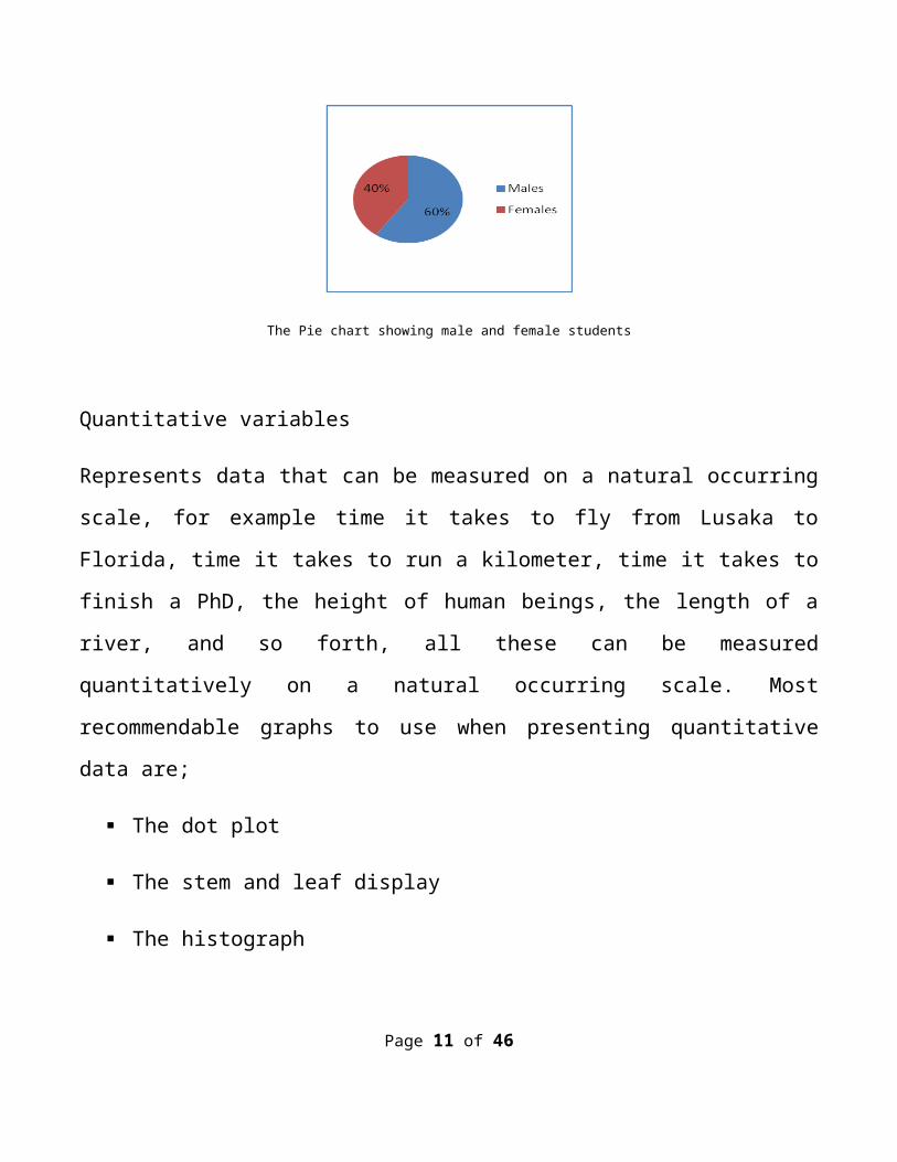
The Pie chart showing male and female students

Quantitative variables

Represents data that can be measured on a natural occurring

scale, for example time it takes to fly from Lusaka to

Florida, time it takes to run a kilometer, time it takes to

finish a PhD, the height of human beings, the length of a

river, and so forth, all these can be measured

quantitatively on a natural occurring scale. Most

recommendable graphs to use when presenting quantitative

data are;

The dot plot

The stem and leaf display

The histograph

Page 11 of 46

The presentation of information graphically and numerically

helps us to communicate our research findings in an accurate

and unambiguous fashion to others users. Absolutely,

arithmetic operations are carried out in quantitative

variables and this provides a far more meaningful results.

You can now agree that nominal data and ordinal data can be

taken care of by qualitative variables, interval and ratio

is measured by quantitative variables.

To take the debate further, quantitative variable is

classified into two types these are discrete or continuous

variables.

Under discrete variable, quantitative variable assumes a

finite or a countable set of values. On the contrary,

discrete variable does not embrace every possible value in

an interval on a real line. An example of a discrete

variable would be a number of children a family can have.

Consequently, continuous variable is a exact opposite of

discrete, it assumes an infinite number of values between

two points in an interval on a real line. For instance, the

awarding of GPA from 0.0 to 4.0 is a continuous variable

Page 12 of 46

Inferential statistics

The other type of statistics is inferential statistics. When

discussing descriptive statistics I alluded that its major

goal is to describe a data set. In inferential statistics,

our ultimate goal is to draw a conclusion about a population

based on the sample of experimental units from that

particular population. While in descriptive statistics we

use mostly numeric and graphical techniques, in inferential

statistics we exploit the hypothesis testing techniques.

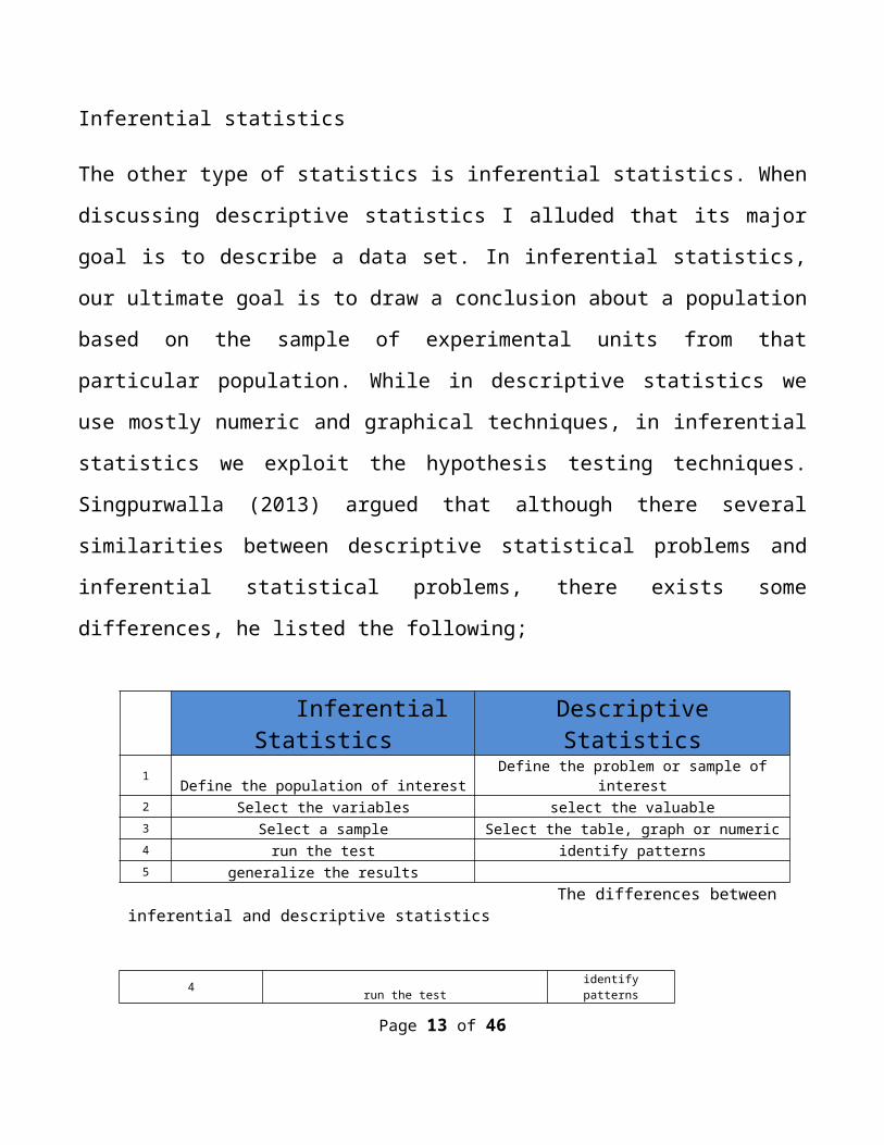
Singpurwalla (2013) argued that although there several

similarities between descriptive statistical problems and

inferential statistical problems, there exists some

differences, he listed the following;

InferentialStatistics

DescriptiveStatistics

1 Define the population of interestDefine the problem or sample of

interest2 Select the variables select the valuable3 Select a sample Select the table, graph or numeric4 run the test identify patterns5 generalize the results

The differences betweeninferential and descriptive statistics

4 run the testidentifypatterns

Page 13 of 46

5 generalise the results The differences between inferential and descriptive statistics

SAMPLING METHODS

Data collection and sampling

Mankind’s life depends on data, every day we gather data

because it is a crucial raw material input to our decision

making. We make decisions about what to buy, where to go for

vacation, how is the traffic situation? How the weather will

be, what will be the effect following the government policy

and so forth. All these we need data to help us make well

informed decision.

In this section I would specifically like to address how

these data are collected. Data is not information, but

information comes from the analysis, summarizing and

evaluation of data, in short, information is interpreted

data, pure and refined data is called information and the

two cannot be used interchangeably therefore care must be

Page 14 of 46

taken when using this two terminologies in order to show the

distinction.

To that effect, we gather data from various sources with the

use of data collection tools, such as survey.

Data collection is classified into two categories;

Primary data collection

Secondary data collection

Thus, interrogating sources in both categories is crucial to

gathering good data that once refined will enable us make

well informed decisions.

While the names to these categories maybe misleading to many

people, it is the secondary data collection exercise that is

conducted first before venturing into the primary data

collection exercise.

Secondary data collection is data done by other researchers

for a different purpose. The advantage is that it is readily

available and cost less to get, however, in this time and

age of internet, secondary data tends to be bulk in nature

posing danger of data overload and the fact that it was

Page 15 of 46

generated for a different purpose. Such examples of

secondary data, is one that is generated by A. Nielsen,

Satch & Satch, blackdot, government departments, newspapers

and so forth.

Primary data collection is virgin data that has not been

collected and is specifically being collected for the

purposes of the matter at hand. Here we use a survey; a

survey is a way of collecting data from experimental units.

Below are means through which primary research is conducted;

Focus group

In-depth interviews

Personal interviews: Is another method of collecting data.

It is mostly used when subjects are not likely to respond to

other survey methods such as online. They are in-depth and

very comprehensive.

Phones

Internet

Postal mails

Sampling method

Page 16 of 46

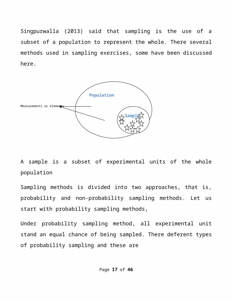
Singpurwalla (2013) said that sampling is the use of a

subset of a population to represent the whole. There several

methods used in sampling exercises, some have been discussed

here.

Measurements or elements

A sample is a subset of experimental units of the whole

population

Sampling methods is divided into two approaches, that is,

probability and non-probability sampling methods. Let us

start with probability sampling methods,

Under probability sampling method, all experimental unit

stand an equal chance of being sampled. There deferent types

of probability sampling and these are

Page 17 of 46

Population

Sample

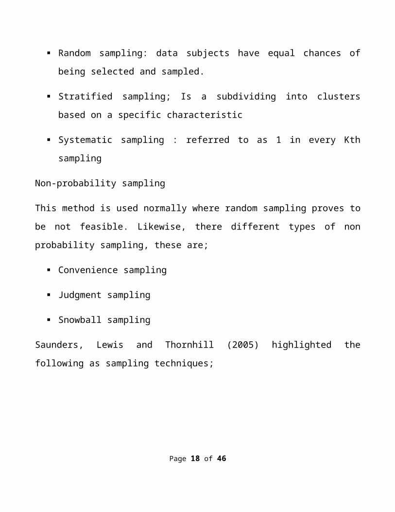
Random sampling: data subjects have equal chances of

being selected and sampled.

Stratified sampling; Is a subdividing into clusters

based on a specific characteristic

Systematic sampling : referred to as 1 in every Kth

sampling

Non-probability sampling

This method is used normally where random sampling proves to

be not feasible. Likewise, there different types of non

probability sampling, these are;

Convenience sampling

Judgment sampling

Snowball sampling

Saunders, Lewis and Thornhill (2005) highlighted the

following as sampling techniques;

Page 18 of 46

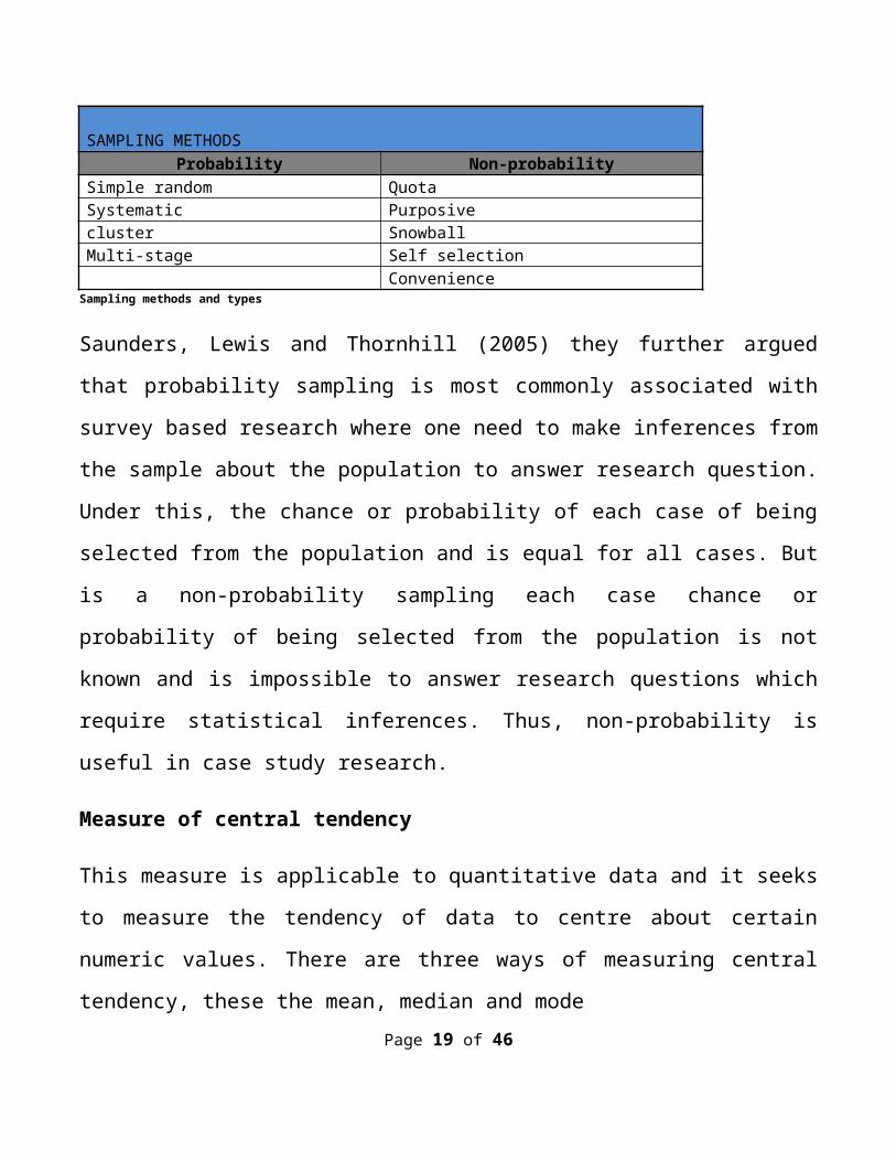
SAMPLING METHODS

Probability Non-probabilitySimple random QuotaSystematic Purposivecluster SnowballMulti-stage Self selection Convenience

Sampling methods and types

Saunders, Lewis and Thornhill (2005) they further argued

that probability sampling is most commonly associated with

survey based research where one need to make inferences from

the sample about the population to answer research question.

Under this, the chance or probability of each case of being

selected from the population and is equal for all cases. But

is a non-probability sampling each case chance or

probability of being selected from the population is not

known and is impossible to answer research questions which

require statistical inferences. Thus, non-probability is

useful in case study research.

Measure of central tendency

This measure is applicable to quantitative data and it seeks

to measure the tendency of data to centre about certain

numeric values. There are three ways of measuring central

tendency, these the mean, median and modePage 19 of 46

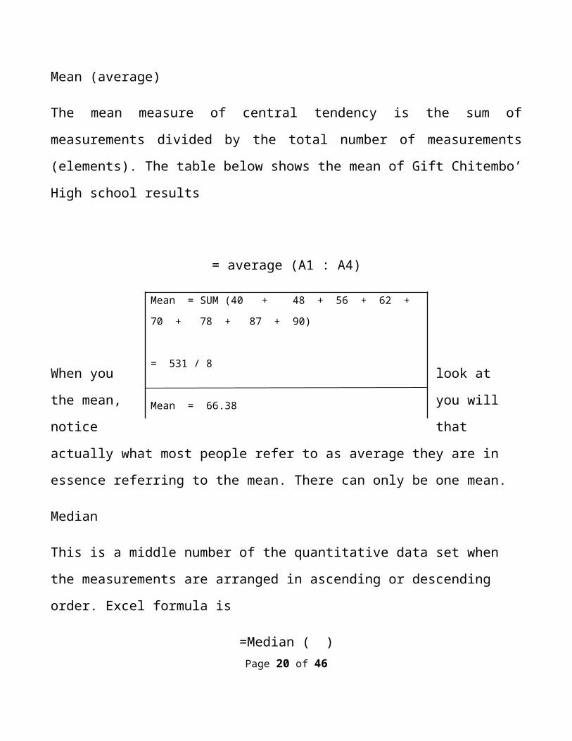
Mean (average)

The mean measure of central tendency is the sum of

measurements divided by the total number of measurements

(elements). The table below shows the mean of Gift Chitembo’

High school results

= average (A1 : A4)

When you look at

the mean, you will

notice that

actually what most people refer to as average they are in

essence referring to the mean. There can only be one mean.

Median

This is a middle number of the quantitative data set when

the measurements are arranged in ascending or descending

order. Excel formula is

=Median ( )Page 20 of 46

Mean = SUM (40 + 48 + 56 + 62 +

70 + 78 + 87 + 90)

= 531 / 8

Mean = 66.38

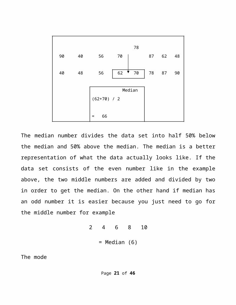
The median number divides the data set into half 50% below

the median and 50% above the median. The median is a better

representation of what the data actually looks like. If the

data set consists of the even number like in the example

above, the two middle numbers are added and divided by two

in order to get the median. On the other hand if median has

an odd number it is easier because you just need to go for

the middle number for example

2 4 6 8 10

= Median (6)

The mode

Page 21 of 46

90 40 56 70

78

87 62 48

40 48 56 62 70 78 87 90

Median

(62+70) / 2

= 66

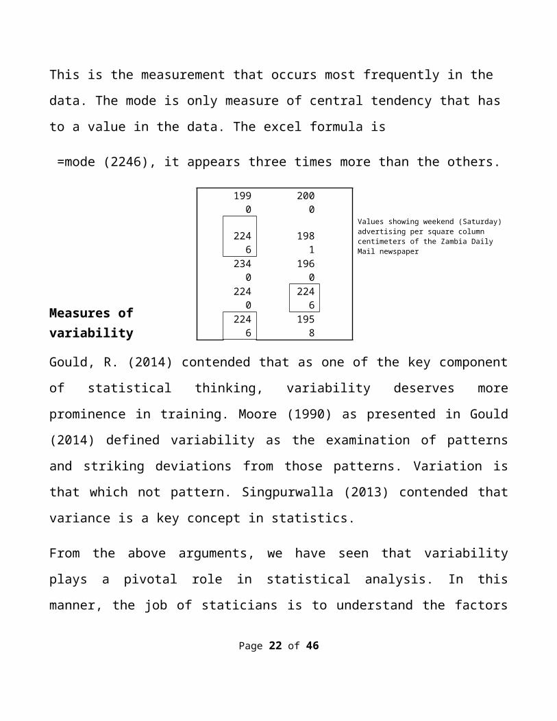
This is the measurement that occurs most frequently in the

data. The mode is only measure of central tendency that has

to a value in the data. The excel formula is

=mode (2246), it appears three times more than the others.

Measures ofvariability

Gould, R. (2014) contended that as one of the key component

of statistical thinking, variability deserves more

prominence in training. Moore (1990) as presented in Gould

(2014) defined variability as the examination of patterns

and striking deviations from those patterns. Variation is

that which not pattern. Singpurwalla (2013) contended that

variance is a key concept in statistics.

From the above arguments, we have seen that variability

plays a pivotal role in statistical analysis. In this

manner, the job of staticians is to understand the factors

Page 22 of 46

1990

2000

2246

1981

Values showing weekend (Saturday)advertising per square column centimeters of the Zambia Daily Mail newspaper

2340

1960

2240

2246

2246

1958

that cause variance and how it can be controlled. For

example, in HIV research, scientists have been amused by the

desire to understand why some people do not get HIV when

exposed it at first exposure while other do at first

exposure? Or Staticians tries to explain exactly what causes

these differences and develop drugs that may make all people

resistant to HIV virus.

There many ways of measuring variability but the commonest

ones are;

Variance

Standard deviation

Under the variance measure, we consider the average squared

distance of each point from the mean (Singpurwalla, 2013).

In other words we can say that variance is a measure of how

far data are spread out from the average (mean).

Excel formula to calculate variance is = ver. p(XX) XXX

On the other hand, standard deviation measures how much, on

average, each of the values in the distribution deviates

from the centre of the distribution.

Page 23 of 46

In excel this can be worked as follows

Excel formula to calculate variance is = stdev.p( XXX) $XXX

In both example, you can that Standard deviations carries a

unit of the data set it is due to this fact that people like

discussing data in terms of standard deviations. To sum up

on the measure of variability, standard deviations is a

simply the square root of the variance. On the other hand

the variance does not carry any unit of the data because it

is merely the measure of how spread data is thus it is unit

free.

The application of variance and standard deviations in

statistical analysis is very important in gaining insight

into the data set. This can be achieve when data is analyzed

from the angle of combined mean and standard deviation, the

combination adds up impetus to the statician to delve into

more underlying insights of the data set. But again,

analyzing further literature on this subject, we find that

standard deviation is not immune to outliers and normally

when they exists, the standard deviation get inflated,

notwithstanding, standard deviation is a positive number.

Probability, Random sampling and distributionPage 24 of 46

Earlier in this compendium I defined inferential statistics

and under sampling methodology, I did discuss probability.

But here, I want to specifically present probability and its

invaluable place in statistics. If we appreciate that

variability concept is key to statistics, probability is a

foundation of inferential statistics.

Consequently, failure to develop solid understanding of the

concept, it will relegate any work we shall do in

inferential statistics to yielding nothing. Thus, at this

point I am simply delving into the intuitive that lies

behind probability as it relates to inferential statistics.

What is probability? It is likelihood, prospects,

possibility. The probability of something to occur is its

chances, possibility, likelihood and prospect of it

happening. For example, the probability of an imminent

market crush is its likelihood of happening. Here, we see

that probability is somehow futuristic. But how can we

enhance our understanding of probability especially in light

of inferential statistics?

Before I define it, it is important that I hold it here and

quickly introduce a new concept in line with the subject atPage 25 of 46

hand. Uncertainty, for us to have a sound grasp of

probability, it is significantly vital to acquaint ourselves

with the concept of uncertainty. Uncertainty can be defined

as the study of something we do not know. Unfortunately, in

our daily lives we all encounter uncertainty. This is due to

the fact that we assess the future differently.

So some investors would deny that there is going to be a

market crush while other would say the market crush is

imminent. Since uncertainty is the study of something we do

not know, this sounds rather punitive to our minds, but even

the future must be quantified.

Singpurwalla (2013) spiced it up that by quantifying

uncertainty we are attempting to discuss the matter in a

more precise terms, but, what precise this mean? It is hard

to say without putting umbers behind the statements.

Scholars have most oftenly used probability as the measure

of uncertainty. To this end, I confidently argue that the

definition for probability is a measure of uncertainty.

Probability is the likelihood that something will happen and

it is expressed in percentage format.

Page 26 of 46

What qualifies the discussion of uncertainty is the idea

behind statistical experiment. By definition as statistical

experiment is a process or act of observation that leads to

a single outcome that cannot be predicted with certainty

where outcome is known as sample event. A collection of all

sample event is known as sample space, which is denoted in

set annotation as a set containing the sample event

S:

E2......E2

Then we assign a probability to each sample event in our

sample space.

This is done based on three factors

Previous knowledge of the experiment

Subjectively assigning probabilities

Experimentation

Need examples here

The technical of probability concept

Union and intersection of events

Page 27 of 46

Normally these events are categorized in two ways, that is,

unions and intersections. A union of two events A and B is

the event that occurs if either A or B or both occur on a

simple performance of the experiment, denoted by “U”. In

this case, AUB consists of all sample points that belong to

A or B or both.

The case of intersection occurs when A and B occurs on a

single performance of the experiment and it is denoted by A

intersect B the intersection consists of all sample points

that belongs to both A and B.

The additive rule of probability

This rule simply tells us how to calculate the probability

of the union of two events. The rule states that the

probability of the union of A and B is the sum of the

probability of events A and B minus A and B

Conditional probability

An example of condition probability is what would be the

probability of interest rates dropping, given that Bank of

Zambia ha just cut rates? The key word here “given”, that

Page 28 of 46

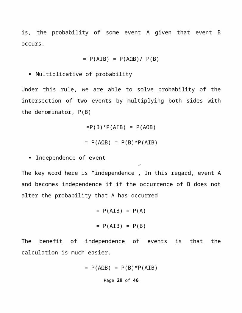
is, the probability of some event A given that event B

occurs.

= P(AIB) = P(AΩB)/ P(B)

Multiplicative of probability

Under this rule, we are able to solve probability of the

intersection of two events by multiplying both sides with

the denominator, P(B)

=P(B)*P(AIB) = P(AΩB)

= P(AΩB) = P(B)*P(AIB)

Independence of event

The key word here is “independence”, In this regard, event A

and becomes independence if if the occurrence of B does not

alter the probability that A has occurred

= P(AIB) = P(A)

= P(AIB) = P(B)

The benefit of independence of events is that the

calculation is much easier.

= P(AΩB) = P(B)*P(AIB)

Page 29 of 46

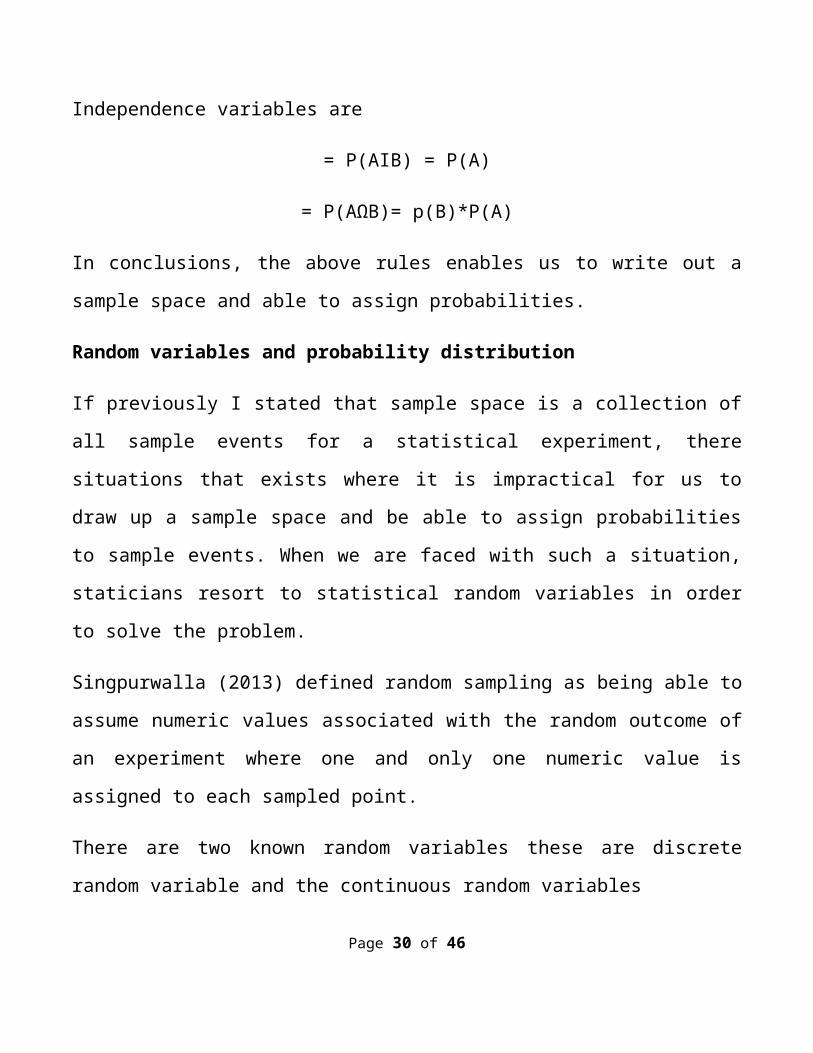
Independence variables are

= P(AIB) = P(A)

= P(AΩB)= p(B)*P(A)

In conclusions, the above rules enables us to write out a

sample space and able to assign probabilities.

Random variables and probability distribution

If previously I stated that sample space is a collection of

all sample events for a statistical experiment, there

situations that exists where it is impractical for us to

draw up a sample space and be able to assign probabilities

to sample events. When we are faced with such a situation,

staticians resort to statistical random variables in order

to solve the problem.

Singpurwalla (2013) defined random sampling as being able to

assume numeric values associated with the random outcome of

an experiment where one and only one numeric value is

assigned to each sampled point.

There are two known random variables these are discrete

random variable and the continuous random variables

Page 30 of 46

Earlier in this compendium, I discussed the two variables

but just to recap on them, discrete random variable is on

that assumes a finite value, such as 0,1,2,3,4 and so forth

thus you can see that they are often counts. While the

continuous random variable is the exact opposite of discrete

random variable which assumes an infinite value that are

uncountable for example, height, weight and time are good

examples of continuous random variables.

Let us go a step further and look at first the discrete

random variable and later the continuous random variable as

we expound the concept of probability distribution.

1. Probability distribution of the discrete random variable

You recall that the discrete random variable specifies the

probability associated with each possible value the random

variable can assume. Thus, the probability distribution of

the discrete random variable is represented in either as a

table or as a graph. But our dialogue on this matter will be

incomplete without a good analysis of the binomial

distribution.

Binomial distribution

Page 31 of 46

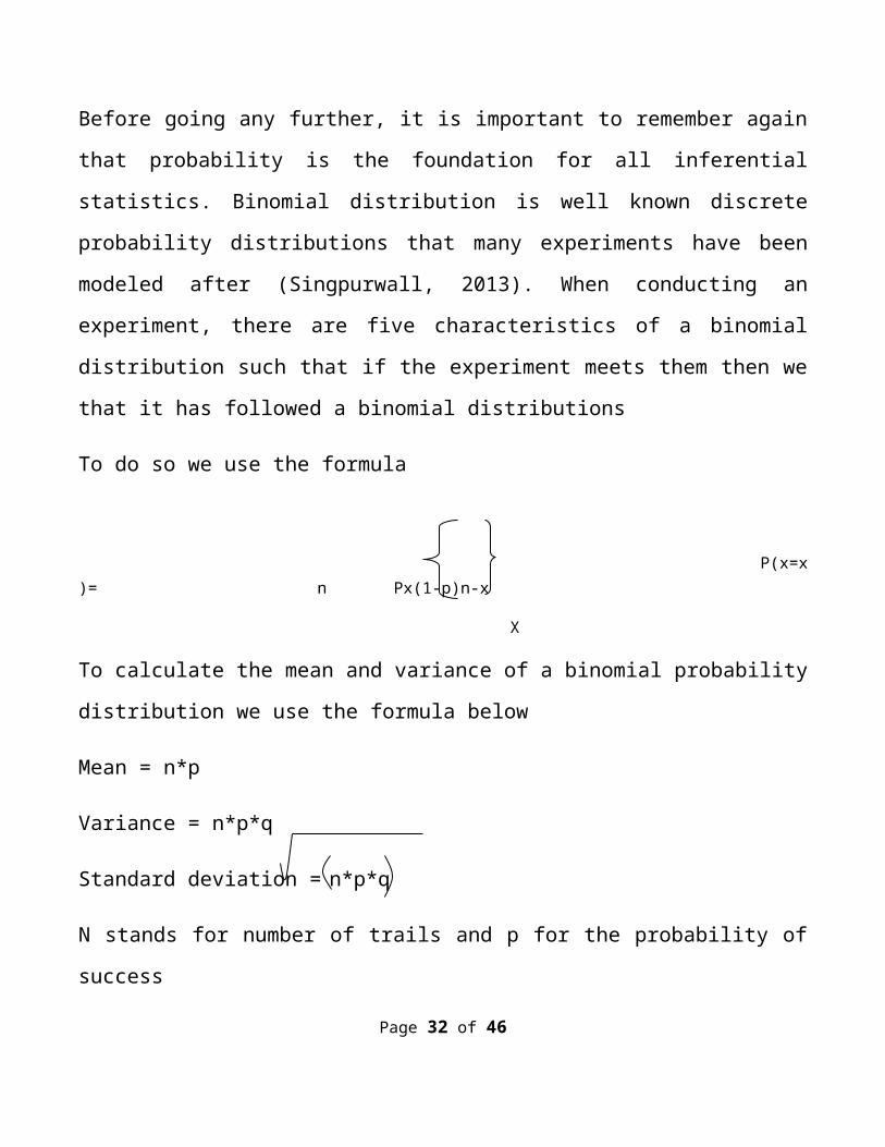
Before going any further, it is important to remember again

that probability is the foundation for all inferential

statistics. Binomial distribution is well known discrete

probability distributions that many experiments have been

modeled after (Singpurwall, 2013). When conducting an

experiment, there are five characteristics of a binomial

distribution such that if the experiment meets them then we

that it has followed a binomial distributions

To do so we use the formula

P(x=x)= n Px(1-p)n-x

X

To calculate the mean and variance of a binomial probability

distribution we use the formula below

Mean = n*p

Variance = n*p*q

Standard deviation = n*p*q

N stands for number of trails and p for the probability of

success

Page 32 of 46

As you can see from the standard deviation formula, it

justifies my assertion that standard deviation is a square

root of the variance, thus by recognizing the properties of

binomial experiments we can calculate specific probabilities

as well as the mean and variance (Singpurwalla, 2013). In

this way, solving problems related to statistical

experiments can effectively be dealt with by recognizing

probability distribution.

Normal distribution

This is another famous statistical distribution in use among

staticians. If the binomial distribution is a discrete

probability distribution, the normal distribution follows a

continuous probability distribution, for example, the height

of Lola, the level of hemoglobin in blood and so forth which

are all normally distributed. Therefore you can deduce that

normal distribution applies to random variable that are

measurable but not countable, for instance, one cannot count

height, or the level of blood such as o,1,2,3,4 as in the

binomial probability distribution. In the discrete discourse

I said we can calculate the mean, variance and the standard

Page 33 of 46

deviations, in the normal distribution, it is defined by its

own mean and standard deviation.

Further questions can be posed here, for instance, How

normal probabilities using normal distribution be

calculated? It is important to understand that the standard

normal distribution which is the most inference distribution

in statistics is very helpful in solving the problems that

arises when using normal distributions while solving normal

probabilities. Standard normal distribution has a mean, 0.

On the other hand, most normal distribution do not have the

mean 0 nor standard deviation of 1, worry not because by

standardizing the variables, this problem is being taken

care of.

To this end, recognizing probability distribution is

extremely helpful in solving problems related to statistical

experiments.

The sampling distribution

Page 34 of 46

Let us deal first with two issues here in order to put the

discussion into perspective, that is, a parameter and a

sample statistics

A parameter is defined as the numerical distributive measure

of a population. The fact that its measure is on the basis

of observations in the population, its value is unknown and

thus we estimate it.

Sample statistics: this is numeric distributive measure of a

sample that is calculated from the observations in the

sample, for instance, mean, variance etc.

To that, effect, can confidently infer that the sampling

distribution of a sample statistics, calculated from a

sample population of n measurements is the probability

distribution of the statistics

This discourse takes us to another yet important matter, the

sampling distribution of the mean of the data set. In order

to us to build a strong grasp of the concept, it important

that first appreciate its properties.

The first one states that: if a random sample of n

observation is selected from a population with a normal

Page 35 of 46

distribution, the sample distribution of x-bar a normal

distribution.

The second one states that for sufficiently large (n>30)

random sample, the sampling of x-bar will be approximately

normal with mean mu and standard error of sigma/sqrt(n). The

larger the sample size, the better will be the normal

approximation to the sampling distribution of x-bar.

The central limit theorem here is very crucial as it is in

statistics. So far, we have seen that we always sample from

a population whose underlying distribution we do not know,

central limit theorem states that if the sample size is more

than 30, we obtain a sampling distribution which is

approximately normal.

Confidence intervals

In statistics, the perceived level of confidence in the

information we generate is crucial to decision making. In

the previous dialogue, we learnt that the central limit

theorem stated that the population distribution has a mean

and a standard deviation. For sufficiently large the

Page 36 of 46

sampling distribution of the x-bar has mean and standard

deviations.

The idea behind the confidence interval is that instead of

estimating the parameter by a point estimate, a whole

interval of likely estimates is given. The confidence level

gives the probability that the interval will capture the

true parameter value in related samples. So far, a given

sample, mean, standard deviation, sample size and a

specified alpha level, we can calculate the confidence

interval in excel. Therefore, it gives us the margin of

error, we add or subtract from the sample mean to get the

confidence interval. Furthermore, the confidence level is

the confidence coefficient expressed as a percentage.

The proper deduction of confidence interval includes the

idea that the numbers were arrived at by a process that

gives the correct result 95% of the time and key to this is

the philosophy of repeated process.

In an event that you have a sample size of less than 30 it

simply means that you have less information upon to base

your conclusions about the mean. In this case the central

limit theorem can suffice. To that effect, a normalPage 37 of 46

distribution to make estimates about the margin of error

cannot be relied upon. When faced with such situations, the

t-distribution the only answer to negotiate statistical

hiccup.

The t-distribution

In conclusion confidence interval measures a population

parameter. This consists of a point estimate with some

measure of reliability that is estimate +-margin of error.

Hypothesis testing

What is statistical hypothesis? A statistical hypothesis is

a belief about a population parameter such as its mean,

proportion or variance. Thus, a hypothesis test is a

procedure which is applied to test the belief. For example,

we may believe that average weight loss for a population of

dieters is equal to 2lbs in one week. We need to run a

hypothesis test to prove whether this is true of false.

Although the steps the calculation for hypothesis testing is

the same as the one for confidence interval, there is a huge

difference in what we want to accomplish with hypothesis

testing than confidence interval. Furthermore, in confidence

Page 38 of 46

interval we do not posses any knowledge of what the

population parameter is and we rely on the data to estimate

it. While in hypothesis test we use data to confirm a priori

belief about it.

The null hypothesis and the alternative hypothesis

To every hypothesis test, there is a null hypothesis and the

alternative hypothesis. The null hypothesis is a statement

about a population parameter being equal to some value. It

actually represents that which is being tested. It is worth

mentioning that the null hypothesis carries a equality sign

always to underlie what the belief is and you want to test

it.

On the flip side of the coin, is the alternative hypothesis,

if the null hypothesis turns out to be false, absolutely the

alternative hypothesis is accepted thus alternative

hypothesis becomes a true alternative hypothesis. In other

words, alternative hypothesis is the exact opposite of the

null hypothesis. The alternative hypothesis carries sign

such as <, >, or an inequality sign therefore care must be

Page 39 of 46

applied when denoting your conclusions in alternative

hypothesis.

One or two side hypothesis

The above hypotheses occurs as follows

In the case of one sided hypothesis will happen if the

statician poses no priori of expectation of the outcome of

the test or indeed there no concern in understanding whether

the alternative hypothesis will be higher or lower. Then you

will get a two sided hypothesis carrying an inequality sign.

But when you are interested in knowing whether it is higher

or lower in the testing, the outcome will be a one sided

hypothesis and will have signs like <, >

The test statistics

So far, it appears that there is no end to statistical

creativity, there is another very important component to

hypothesis testing which is the test statistics, this one is

premised on the statistics that premises the parameter. Z=X-

u/root n this random variable has the standard normal

distribution N(0,1)

The P-valuePage 40 of 46

This is another very important concept to our understanding

of hypothesis testing in statistics. Calculating and

interpreting the p-value. The test of hypothesis quantifies

the chance of obtaining a particular random sample result if

the null hypothesis were true. It is a way of assessing the

accuracy or how believable the null hypothesis is given the

evidence provided by the sample mean.

A small P- value implies that random variation due to

sampling is not likely to account for the observed

difference. In this case, a small p-value simply signifies

that we reject the null hypothesis. But how small is small?

In many time , a p-value of 0.05 is considered significant.

So if the p-value is equal or less than the significant

alpha, then we reject the null hypothesis in favor of the

alternative hypothesis.

If the p-value is greater than the significance level then

fail to reject the null hypothesis.

Hypothesis of the mean

How do we test hypothesis of the mean based on the sample

random sample size from a normal population with unknown

Page 41 of 46

mean and known standard deviation? Here we have to rely on

the population of the sampling deviation. The P-value is the

area under the sampling distribution for values at least as

extreme in the direction of the alternative hypothesis as

that od our random sample.

In this case, we first use the test statistic to calculate

the z-values and then use excel to find the p-value

associated with the value.

The following are steps for conducting a hypothesis testing

State the null and alternative hypothesis

State a significance level

Calculate attest statistic

Find the p-value for the observed data

State your conclusion based on comparing the

significance level to the P-value

There is a difference between practical significance

statistical significance. Statistical significance only

shows that the observed effect is due to random sampling or

not. This does not mean that it practically important . With

Page 42 of 46

a large enough sample size, significance can be reached even

for the tiniest effects.

Correlation and regression

These are different ways of studying the relationships

between two variables. The most basic way of doing this is

by using a scatter plot graph and then observes for an

overall pattern and study the deviation from the pattern.

Put differently, it is the study of the relationship between

quantitative variable measured on the same individual. Here

we are referring to dependent and independent variables

In the scatter plot the independent variables are plotted on

the x-axis and the dependent variables are plotted on the y-

axis. Every individual in the data appear as a point in the

plot. Once this is achieved, our interest is to study the

relationship between the two, how is one affected by the

changes in the other.

Therefore, dependent variables are defined as those which

represent the effect being tested.

Page 43 of 46

And the independent variable represents the inputs to the

dependent variable or the variable that can be manipulated

to see if they are the cause.

The use of a scatter plot helps us to understand trends in

the data and also pinpointing out those points that are not

obeying the pattern.

Furthermore, with the scatter plot we can as well identify

the form, direction and the strength of that association

between two variables. The graph helps us to answer

questions such as

Is the form linear or curved?

Is there no pattern?

Is the direction positive or negative?

Or there is no direction at all

How closely do the points fit

Correlation

Correlation is denoted ‘r’ and is the most widely accepted

measure of association between two variable. In this

respect, correlation can be defined as the measure of thePage 44 of 46

direction and strength of a linear relationship between two

quantitative variables. Correlation is always between -1 to

1 from this one can quickly deduce that a negative value

symbolizes that the association between the variables is

negative. Likewise, a positive value of the association

between the variables means that it is positive.

Excel formula is correl (x,y)

Where x, y are the arrays of data you wish to calculate the

correlation on. Correlation does not concern with dependent

and independent variable so in excel it is not necessary to

belabor making the distinction. However, as one variable

grow the other one also grows thereby rendering the

relationship strong.

Simple linear regression

We can see that correlation only tells us about the

direction and strength of the linear relationship between

two quantitative variables. But is also important to

understand how both variables vary together. For example

what is the rate of decrease in the other is increasing?

Linear regression is one way we can quantify this.

Page 45 of 46

Here drawing up a linear regression line is very important.

The line describes how the dependent variables changes with

respect to an independent variable. Remember that under

correlation dependent and independent variables were not a

concern of correlation, but here the tow variable are

extreme crucial. It is with this line that statisticians are

able to explain the changes in a dependent variable in terms

of the independent variable and also to predict the value of

the independent variable for a given dependent variable.

In conclusion, the intuition behind the regression line is

that it attempts to quantify the relationship. By putting a

straight line through the data in a way that it minimizes

the sum of the vertical distances between the points of the

data set and the fitted line. The best line is the one that

minimizes these distances. The key to regression is proper

interpretation of the slope and the intercept of the line.

The interpretation of the intercepts is what the value of

the dependent variable would be if there was no effect of

the independent variables

Page 46 of 46