Embed Size (px)
Citation preview

www.jutaacademic.co.za T R E V O R W E G N E R
Applied BusinessStatistics
METHODS AND EXCEL-BASED APPLICATIONS4 th E d i t i o n
SOLUTIONS MANUAL
Applied Business Statistics METHODS AND EXCEL-BASED APPLICATIONS 4th Edition
TR
EV
OR
WE
GN
ER

Applied Business Statistics: Methods and Excel-based Applications: Solutions Manual Print edition first published in 1993 Reprinted 2000 and 2003 Second Edition 2008 Third Edition 2012 Fourth edition 2015 (Web PDF) Juta and Company (Pty) Ltd First Floor Sunclare Building 21 Dreyer Street Claremont 7708 PO Box 14373, Lansdowne 7779, Cape Town, South Africa © 2015 Juta & Company (Pty) Ltd ISBN 978 1 48511 788 9 (Web PDF) All rights reserved. No part of this publication may be reproduced or transmitted in any form or by any means, electronic or mechanical, including photocopying, recording, or any information storage or retrieval system, without prior permission in writing from the publisher. Subject to any applicable licensing terms and conditions in the case of electronically supplied publications, a person may engage in fair dealing with a copy of this publication for his or her personal or private use, or his or her research or private study. See section 12(1)(a) of the Copyright Act 98 of 1978. The author and the publisher believe on the strength of due diligence exercised that this work does not contain any material that is the subject of copyright held by another person. In the alternative, they believe that any protected pre-existing material that may be comprised in it has been used with appropriate authority or has been used in circumstances that make such use permissible under the law.

CHAPTER 1
STATISTICS IN MANAGEMENT
1.1 It is a decision support tool. It generates evidence based information through analysis of data to inform management decision making. 1.2 Descriptive statistics summarises (profiles) sample data; inferential statistics generalises sample findings to a broader population (to estimate values or confirm relationships). 1.3 Statistical modelling is explores and quantifies relationships between variables for estimation or prediction purposes. 1.4 Data quality is influenced by: (i) Data source; (ii) Data collection method; and (iii) Data type 1.5 Different statistical methods are valid for different data types. 1.6 In data preparation, consider (i) Data relevancy; (ii) Data cleaning; and (iii) Data enrichment. 1.7 (a) Random variable: Performance appraisal system used (b) Population: All JSE companies (c) Sample: The 68 HR managers surveyed (d) Sampling unit: a JSE-listed company (e) 46% is a sample statistic (f) Random sampling is necessary to allow valid inferences to be drawn based on the sample evidence. 1.8 (a) Random variable: Female magazine readership (b) Population: All female magazine readers (c) Sample: The 2000 randomly selected female magazine readers (d) Sampling unit: a female reader of a female magazine (e) 35% (700/2000) is a sample statistic (f) Inferential statistics – as its purpose is to test the belief that market share = 38% 1.9 (a) Three (3) random variables. They are: (i) weekly sales volume; (ii) number of ads placed per week; (iii) advertising media used. (b) Dependent variable = weekly sales volume (c) Independent variables = number of ads placed per week; advertising media used. (d) Statistical model building (predict sales volume from ads placed and media used)
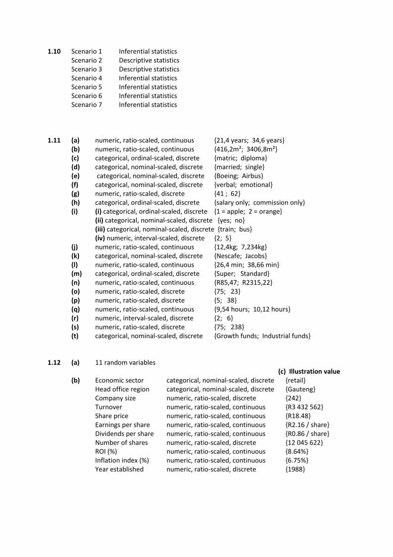
1.10 Scenario 1 Inferential statistics Scenario 2 Descriptive statistics Scenario 3 Descriptive statistics Scenario 4 Inferential statistics Scenario 5 Inferential statistics Scenario 6 Inferential statistics Scenario 7 Inferential statistics 1.11 (a) numeric, ratio-scaled, continuous {21,4 years; 34,6 years} (b) numeric, ratio-scaled, continuous {416,2m²; 3406,8m²} (c) categorical, ordinal-scaled, discrete {matric; diploma} (d) categorical, nominal-scaled, discrete {married; single} (e) categorical, nominal-scaled, discrete {Boeing; Airbus} (f) categorical, nominal-scaled, discrete {verbal; emotional} (g) numeric, ratio-scaled, discrete {41 ; 62} (h) categorical, ordinal-scaled, discrete {salary only; commission only} (i) (i) categorical, ordinal-scaled, discrete {1 = apple; 2 = orange} (ii) categorical, nominal-scaled, discrete {yes; no} (iii) categorical, nominal-scaled, discrete {train; bus} (iv) numeric, interval-scaled, discrete {2; 5} (j) numeric, ratio-scaled, continuous {12,4kg; 7,234kg} (k) categorical, nominal-scaled, discrete {Nescafe; Jacobs} (l) numeric, ratio-scaled, continuous {26,4 min; 38,66 min} (m) categorical, ordinal-scaled, discrete {Super; Standard} (n) numeric, ratio-scaled, continuous {R85,47; R2315,22} (o) numeric, ratio-scaled, discrete {75; 23} (p) numeric, ratio-scaled, discrete {5; 38} (q) numeric, ratio-scaled, continuous {9,54 hours; 10,12 hours} (r) numeric, interval-scaled, discrete {2; 6} (s) numeric, ratio-scaled, discrete {75; 238} (t) categorical, nominal-scaled, discrete {Growth funds; Industrial funds} 1.12 (a) 11 random variables (c) Illustration value (b) Economic sector categorical, nominal-scaled, discrete {retail} Head office region categorical, nominal-scaled, discrete {Gauteng} Company size numeric, ratio-scaled, discrete {242} Turnover numeric, ratio-scaled, continuous {R3 432 562} Share price numeric, ratio-scaled, continuous {R18.48} Earnings per share numeric, ratio-scaled, continuous {R2.16 / share} Dividends per share numeric, ratio-scaled, continuous {R0.86 / share} Number of shares numeric, ratio-scaled, discrete {12 045 622} ROI (%) numeric, ratio-scaled, continuous {8.64%} Inflation index (%) numeric, ratio-scaled, continuous {6.75%} Year established numeric, ratio-scaled, discrete {1988}

1.13 (a) 13 random variables (c) Illustration value (b) Gender categorical, nominal-scaled, discrete {female} Home language categorical, nominal-scaled, discrete {Xhosa} Position categorical, ordinal-scaled, discrete {middle manager} Join date numeric, ratio-scaled, discrete {1998} Status categorical, ordinal-scaled, discrete {gold status} Claimed categorical, nominal-scaled, discrete {yes} Problems categorical, nominal-scaled, discrete {yes} Yes problem categorical, nominal-scaled, discrete {online access difficult} Services - airlines numeric, interval-scaled, discrete {2} Services – car rentals numeric, interval-scaled, discrete {5} Services - hotels numeric, interval-scaled, discrete {4} Services – financial numeric, interval-scaled, discrete {2} Services – telecomms numeric, interval-scaled, discrete {2} 1.14 Financial Analysis data: mainly numeric (quantitative), ratio-scaled. Voyager Services Quality data: mainly categorical (qualitative); but when rating scales are used, such as in Question 8, the data is numeric, but interval-scaled and discrete.
---ooOoo---

CHAPTER 2
EXPLORATORY DATA ANALYSIS
SUMMARISING DATA SUMMARY TABLES AND GRAPHS
Exercise 2.1 A picture is worth a thousand words.
Exercise 2.2 (a) bar (or pie) chart(b) multiple (or stacked) bar chart
(c) histogram(d) scatter plot
Exercise 2.3 Cross-tabulation table (or joint frequency table; or two-way pivot table).
Exercise 2.4 Bar chart (i) displays data on a categorical variable(ii) categories can be displayed in any order(iii) width of bars is arbitrary (but all of equal widths)
Histogram (i) displays numerical data only(ii) intervals must be continuous (and constant width) and sequential(iii) width of bars is determined by interval width
Exercise 2.5 Line graph

Exercise 2.6 File: X2.6 - magazines.xlsx
(a) Magazine preferences by female teenagers
Magazine Count %True Love 95 19%Seventeen 146 29%Heat 118 24%Drum 55 11%You 86 17%Total 500 100%
(b) Interpretation
Seventeen is the most popular teenager magazine (29% of female teenager prefer it). Almost a quarter of the female readers surveyed prefer reading Heat (24%), while the leastpreferred magazine is Drum with only 11% of female magazine readers preferring it.
19%
29%24%
11%
17%
Percent of Female Teenagers
True Love
Seventeen
Heat
Drum
You

Exercise 2.7 File: X2.6 - magazines.xlsx
(a) Magazine preferences by female teenagers
Magazine Count %True Love 95 19%Seventeen 146 29%Heat 118 24%Drum 55 11%You 86 17%Total 500 100%
(b) Heat is preferred by 24% of all female teenager readers.
19%
29%
24%
11%
17%
0%
5%
10%
15%
20%
25%
30%
35%
% of Female Teenagers per Magazine

Exercise 2.8 File: X2.8 - job grades.xlsx
(a) and (b) Categorical Frequency Table - Job Grades
Job grade Data TotalA Count 14
% 35% Job Grade %B Count 11 A 35
% 27.5% B 27.5C Count 6 C 15
% 15% D 22.5D Count 9 Total 100
% 22.5%Total Count 40Total % 100%
(c) 22.5% of employees are in job grade D
(d) Bar Chart and Pie Chart - Job Grades
35
27.5
15
22.5
0
5
10
15
20
25
30
35
40
A B C D
% Employees per Job Grade
A35%
B27%
C15%
D23%
% of Employees per Job Grade
A
B
C
D

Exercise 2.9 File: X2.9 - office rentals.xlsx
(a) and (b) Numerical Frequency Distribution and Cumulative Frequency Distribution
Rentals Count % Count Cum %
≤ 200 4 13.3 13.3%
201 - ≤250 8 26.7 40.0%
251 - ≤300 9 30 70.0%
301 - ≤350 6 20 90.0%
351 - ≤400 3 10 100.0%
More 0 0 100.0%
Total 30 100
(c) (i) 13.3% of all office space costs less than or equal to R200 / m2
(ii) 70% of all office space costs at most R300 / m²(iii) 10% of all office space costs more than R350 / m²(iv) 9 office buildings have rentals between R300 and R400 / m²

Exercise 2.10 File: X2.10 - storage dams.xlsx
Cape Town water storage dams capacities
(a) Storage Dam Capacity (Ml) % Wemmershoek 158644 16.9Steenbras 95284 10.2Voelvlei 244122 26Theewaterskloof 440255 46.9Total capacity 938305 100
(b) (i) Voelvlei dam supplies 26% of Cape Town's water.(ii) Wemmershoek and Steenbras dams together provide 27.1% of Cape Town's water.
17%
10%
26%
47%
Capacity of Cape Town Storage Dams (in Million litre)
Wemmershoek
Steenbras
Voelvlei
Theewaterskloof
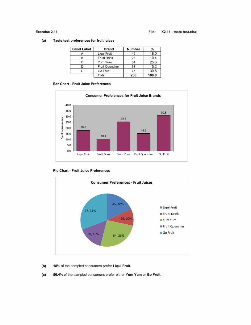
Exercise 2.11 File: X2.11 - taste test.xlsx
(a) Taste test preferences for fruit juices
Blind Label Brand Number %A Liqui Fruit 45 18.0B Fruiti Drink 26 10.4C Yum Yum 64 25.6D Fruit Quencher 38 15.2E Go Fruit 77 30.8
Total 250 100.0
Bar Chart - Fruit Juice Preferences
Pie Chart - Fruit Juice Preferences
(b) 18% of the sampled consumers prefer Liqui Fruit.
(c) 56.4% of the sampled consumers prefer either Yum Yum or Go Fruit.
18.0
10.4
25.6
15.2
30.8
0.0
5.0
10.0
15.0
20.0
25.0
30.0
35.0
40.0
Liqui Fruit Fruiti Drink Yum Yum Fruit Quencher Go Fruit
% o
f con
sum
ers
Consumer Preferences for Fruit Juice Brands
45, 18%
26, 10%
64, 26%38, 15%
77, 31%
Consumer Preferences - Fruit Juices
Liqui Fruit
Fruiti Drink
Yum Yum
Fruit Quencher
Go Fruit

Exercise 2.12 File: X2.12 - annual car sales.xlsx
Manufacturer Annual Sales % SalesToyota 96959 19.4Nissan 63172 12.6
Volkswagen 88028 17.6Delta 62796 12.6Ford 74155 14.8
MBSA 37268 7.5BMW 51724 10.4MMI 25354 5.1
Total Sales 499456 100.0
(a) Bar Chart - Annual Car Sales by Manufacturer
(b) Percentage Pie Chart - Annual Car Sales by Manufacturer
(c) Total % held by top three manufacturers - Toyota (19.4%), Volkswagen (17.6%)and Ford (14.8%) - represents 51.8% of the total passenger car market.
96959
63172
88028
6279674155
37268
51724
25354
0
20000
40000
60000
80000
100000
120000
Annual Sales of Passenger Cars by Manufacturer
Toyota, 19.4
Nissan, 12.6
Volkswagen, 17.6Delta, 12.6
Ford, 14.8
MBSA, 7.5
BMW, 10.4
MMI, 5.1% Annual Sales of Passenger Cars by Manufacturer
Toyota
Nissan
Volkswagen
Delta
Ford
MBSA
BMW
MMI

Exercise 2.13 File: X2.13 - half-yearly car sales.xlsx
Manufacturer First half Second half % ChangeToyota 42661 54298 27.3Nissan 35376 27796 -21.4VW 45774 42254 -7.7Delta 26751 36045 34.7Ford 32628 41527 27.3MBSA 19975 17293 -13.4BMW 24206 27518 13.7MMI 14307 11047 -22.8
(a) Multiple bar chart - Car Sales by Half-Year and Manufacturer
(b) First half-year best performers: Nissan; Volkswagen; MBSA and MMI
(c) Delta showed the largest % increase from the first half to the second half of 34.7%.Refer to the above Table for the % Change between First and Second Half-Year Sales.
Toyota Nissan VW Delta Ford MBSA BMW MMIFirst half 42661 35376 45774 26751 32628 19975 24206 14307Second half 54298 27796 42254 36045 41527 17293 27518 11047
0
10000
20000
30000
40000
50000
60000
Half-yearly Car Sales by Manufacturer
First half
Second half

Exercise 2.14 File: X2.14 - television brands.xlsx
(a) Categorical Frequency Table - Television Brands Owned
Count of BrandsBrands TotalDaewoo 16%LG 30.4%Philips 10.4%Sansui 24%Sony 19.2%Grand Total 100%
(b) Percentage Bar Chart - Television Brands Owned
Brands TotalDaewood 16%LG 30.4%Philips 10.4%Sansui 24%Sony 19.2%Total 100%
(c) Philips is the least preferred brand (preferred by only 10.4% of households surveyed).
(d) The most popular brand is LG that is owned by 30.4% of the households surveyed.
16%
30.4%
10.4%
24%
19.2%
0%
5%
10%
15%
20%
25%
30%
35%
Daewood LG Philips Sansui Sony
% of TV Brands Owned

Exercise 2.15 File: X2.15 - estate agents.xlsx
(a) Frequency Count TableCount of House sales
House sales Total3 124 155 66 77 58 3
Grand Total 48
(b) Histogram - Residential Properties Sold per Estate Agent
(c) The most frequently sold number of properties per estate agent was 4. 4 properties each were sold by (15/48) 31.3% of all estate agents
(d) The same frequency count table (a) and histogram (b) is produced.
3 4 5 6 7 8Total 12 15 6 7 5 3
1215
6 75
30
2
4
6
8
10
12
14
16
Histogram of Residential Properties Sold per Agent
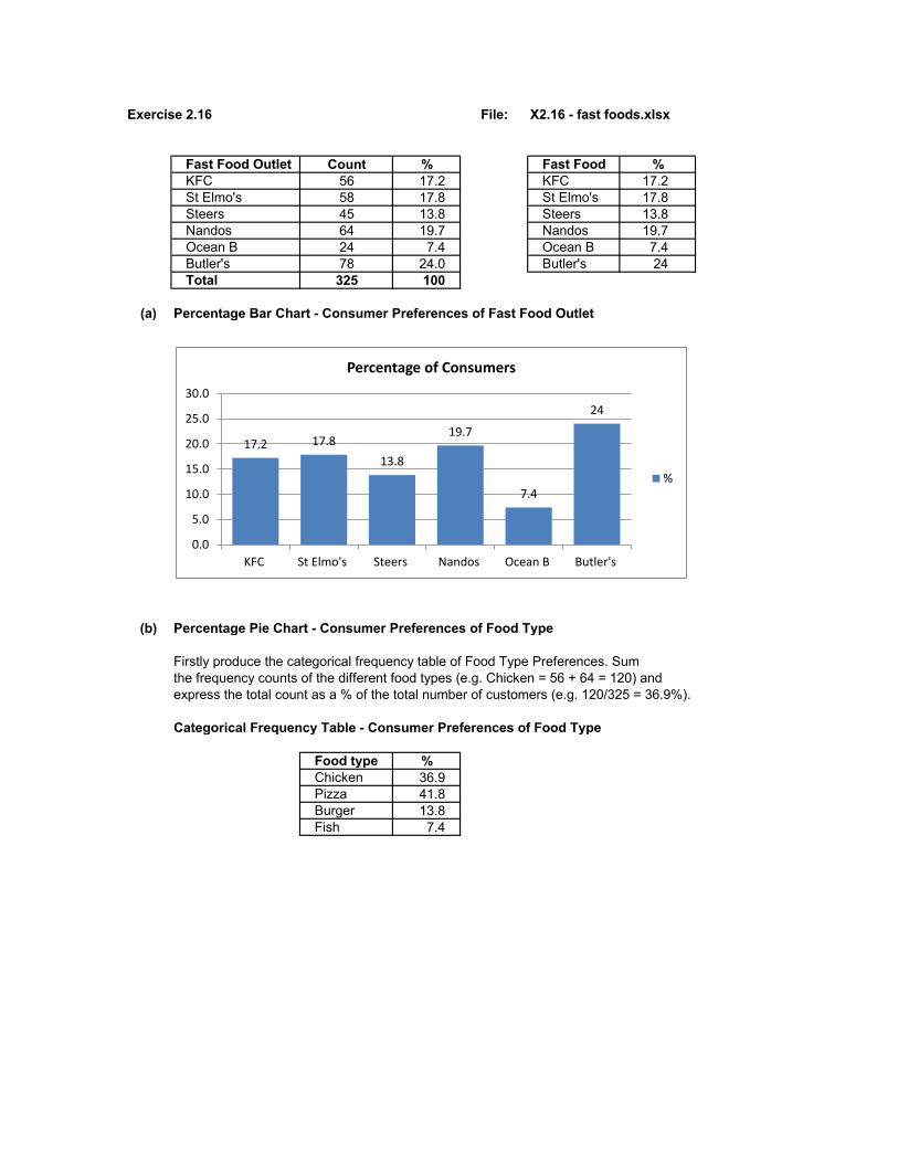
Exercise 2.16 File: X2.16 - fast foods.xlsx
Fast Food Outlet Count % Fast Food %KFC 56 17.2 KFC 17.2St Elmo's 58 17.8 St Elmo's 17.8Steers 45 13.8 Steers 13.8Nandos 64 19.7 Nandos 19.7Ocean B 24 7.4 Ocean B 7.4Butler's 78 24.0 Butler's 24Total 325 100
(a) Percentage Bar Chart - Consumer Preferences of Fast Food Outlet
(b) Percentage Pie Chart - Consumer Preferences of Food Type
Firstly produce the categorical frequency table of Food Type Preferences. Sumthe frequency counts of the different food types (e.g. Chicken = 56 + 64 = 120) and express the total count as a % of the total number of customers (e.g. 120/325 = 36.9%).
Categorical Frequency Table - Consumer Preferences of Food Type
Food type %Chicken 36.9Pizza 41.8Burger 13.8Fish 7.4
17.2 17.8
13.8
19.7
7.4
24
0.0
5.0
10.0
15.0
20.0
25.0
30.0
KFC St Elmo's Steers Nandos Ocean B Butler's
Percentage of Consumers
%

(c) Brief ReportPizza (42%) and Chicken (37%) dominate almost 80% of the fast food market with Pizzas being slightly more favoured by fast food consumers.
Chicken, 36.9
Pizza, 41.8
Burger, 13.8
Fish, 7.4
Consumer preference (%) by Food Type
Chicken
Pizza
Burger
Fish

Exercise 2.17 File: X2.17 - airlines.xlsx
(a) Two-way Pivot Table - Counts, Row % (by Airline), Column % (by Passenger)
PassengerAirline Data Business Tourist Grand TotalComair Count of Passenger 12 8 20
Row % 60.0% 40.0% 100%Column % 33.3% 23.5% 28.6%Total % 17.1% 11.4% 28.6%
Kulula Count of Passenger 4 16 20Row % 20.0% 80.0% 100.0%Column % 11.1% 47.1% 28.6%Total % 5.7% 22.9% 28.6%
SAA Count of Passenger 20 10 30Row % 66.7% 33.3% 100.0%Column % 55.6% 29.4% 42.9%Total % 28.6% 14.3% 42.9%
Total Count of Passenger 36 34 70Total Row % 51.4% 48.6% 100%Total Column % 100% 100% 100%Total Total % 51.4% 48.6% 100%
(b) Two-way Pivot table - Row Percentage by Airline
Count of Passenger PassengerAirline Business Tourist Grand TotalComair 60.0% 40.0% 100.0%Kulula 20.0% 80.0% 100.0%SAA 66.7% 33.3% 100.0%Grand Total 51.4% 48.6% 100.0%
(c) Multiple Bar Chart - Passenger Type by Airline
(d) 42.9% of passengers prefer to fly with SAA.
Comair Kulula SAABusiness 0.6 0.2 0.666666667Tourist 0.4 0.8 0.333333333
0.6
0.2
0.67
0.4
0.8
0.33
0%
10%
20%
30%
40%
50%
60%
70%
80%
90%
% o
f pas
seng
er p
er a
irlin
e
Multiple Bar Chart - Airline by Passenger Type
Business
Tourist

(e) Kulula is most preferred by tourists (47.1% of tourists prefer Kulula).
(f) Not true. Most business travellers prefer SAA (55.6%). More than half (55.6%) of all business travellers prefer SAA.
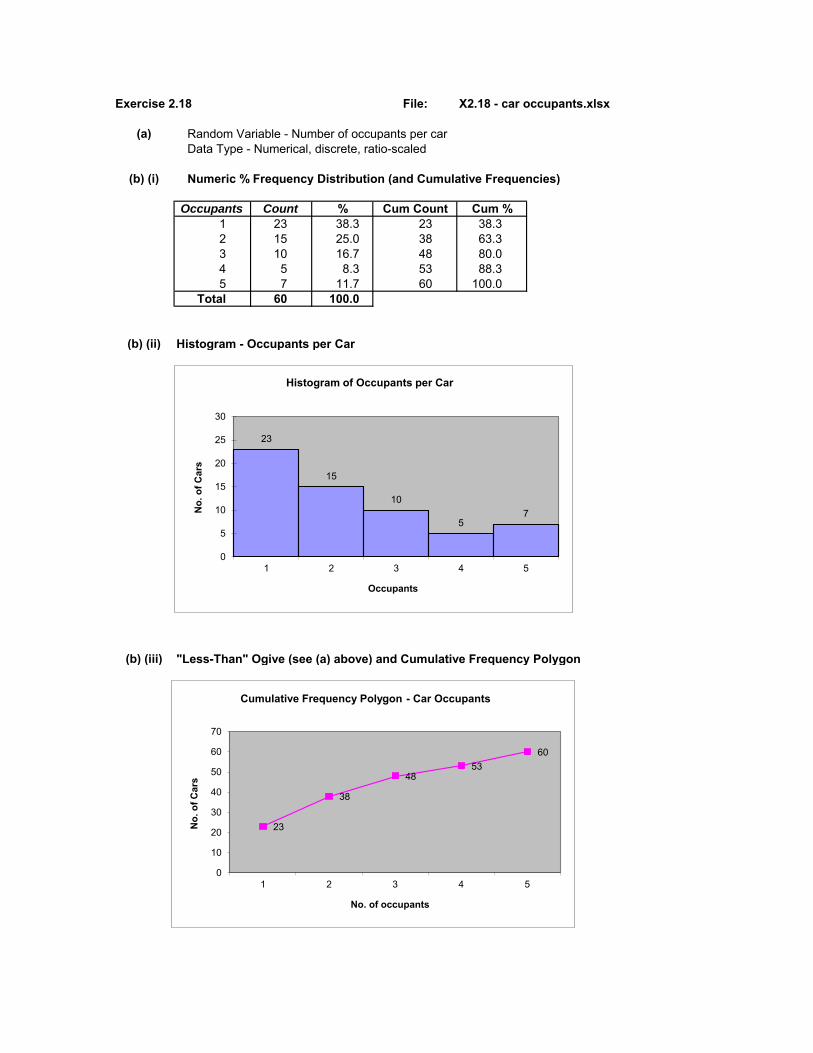
Exercise 2.18 File: X2.18 - car occupants.xlsx
(a) Random Variable - Number of occupants per carData Type - Numerical, discrete, ratio-scaled
(b) (i) Numeric % Frequency Distribution (and Cumulative Frequencies)
Occupants Count % Cum Count Cum %1 23 38.3 23 38.32 15 25.0 38 63.33 10 16.7 48 80.04 5 8.3 53 88.35 7 11.7 60 100.0
Total 60 100.0
(b) (ii) Histogram - Occupants per Car
(b) (iii) "Less-Than" Ogive (see (a) above) and Cumulative Frequency Polygon
23
15
10
57
0
5
10
15
20
25
30
1 2 3 4 5
No.
of C
ars
Occupants
Histogram of Occupants per Car
23
38
4853
60
0
10
20
30
40
50
60
70
1 2 3 4 5
No. o
f Car
s
No. of occupants
Cumulative Frequency Polygon - Car Occupants

(c) (i) 38.3% of motorists travel alone.(ii) 36.7% of vehicles have 3 or more occupants(iii) 63.3% of vehicles have no more than 2 occupants.

Exercise 2.19 File: X2.19 - courier trips.xlsx
(a) Random variable - distance travelled (in kms) per courier tripData type - numerical, continuous, ratio-scaled
(b) (i) (ii) Numeric % Frequency Distribution (and Cumulative Frequencies)
Distance Count % Cum Count Cum %≤10 4 8 4 8
11 - ≤15 7 14 11 2216 - ≤20 15 30 26 5221 - ≤25 12 24 38 7626 - ≤30 9 18 47 9431 - ≤35 3 6 50 100Total 50 100
(b) (iii) Histogram - Courier Travelling Distances per Trip
Distance Cum %10 815 2220 5225 7630 9435 100
4
7
15
12
9
3
0
2
4
6
8
10
12
14
16
18
≤10 11 - ≤15 16 - ≤20 21 - ≤25 26 - ≤30 31 - ≤35
No. o
f trip
s
Distance (in km)
Histogram of Courier Travelling Distances
8
22
52
76
94100
0
20
40
60
80
100
10 15 20 25 30 35
Perc
ent o
f trip
s
Distance (in km)
Cumulative % Frequency Polygon Distances Travelled per Trip

(c) (i) 18% of deliveries (9 trips) were between 25 km and 30 km.(ii) 76% of deliveries (38 trips) were within a 25 km radius. (iii) 48% of deliveries (24 trips) were beyond a 20 km radius.
(iv) Reading off the Cumulative % Frequency Table (or Polygon) above52% of trips were no more than 20 km from the depot.
(v) The longest 24% of trips were above 25 km.
(d) The percentage of trips above 30 km is only 6%. Hence there is adherance to the company policy.

Exercise 2.20 File: X2.20 - fuel bills.xlsx
(a) Random variable - monthly fuel expenditure (in Rands)Data type - numerical, continuous, ratio-scaled
(b) (i) (ii) Numeric % Frequency Distribution (and (d) the Ogive)
Fuel bill Count % Count Cum Count Cum %
≤300 7 14 7 14301 - 400 15 30 22 44401 - 500 13 26 35 70501 - 600 7 14 42 84601 - 700 5 10 47 94701 - 800 2 4 49 98
800+ 1 2 50 100Total 50 100
(b) (iii) Histogram of Fuel costs / motorist (Rand)
(c) 14% (7 motorists) spend between R500 and R600 per month on fuel.
(d) Cumulative % Frequency Polygon - Motorist fuel bills per month. (See the Ogive in (b) for Cumulative Frequencies)
7
15
13
7
5
21
0
2
4
6
8
10
12
14
16
≤300 301 - 400 401 - 500 501 - 600 601 - 700 701 - 800 800+
no. o
f mot
oris
ts
Fuel bill (in Rands)
Histogram of Motorists' Monthly Fuel Costs

(e) From (d), approx. 77% of motorists spend less than R550 per month on fuel.
(f) From (a) (and (d)), 30% (15 motorists) spend more than R500 per month on fuel.
14
44
70
84
9498 100
0
10
20
30
40
50
60
70
80
90
100
110
≤300 301 - 400 401 - 500 501 - 600 601 - 700 701 - 800 800+
Cumulative % Frequency Polygon - Fuel Bills per Month
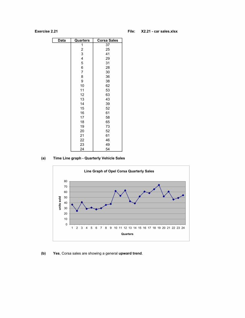
Exercise 2.21 File: X2.21 - car sales.xlsx
Data Quarters Corsa Sales1 372 253 414 295 316 287 308 369 3810 6211 5312 6313 4314 3915 5216 6117 5818 6519 7320 5221 6122 4623 4924 54
(a) Time Line graph - Quarterly Vehicle Sales
(b) Yes, Corsa sales are showing a general upward trend.
0
10
20
30
40
50
60
70
80
1 2 3 4 5 6 7 8 9 10 11 12 13 14 15 16 17 18 19 20 21 22 23 24
units
sol
d
Quarters
Line Graph of Opel Corsa Quarterly Sales

Exercise 2.22 File: X2.22 - market shares.xlsx
Data Year VW Toyota
1 13.4 9.92 11.6 9.63 9.8 11.24 14.4 12.05 17.4 11.66 18.8 13.17 21.3 11.78 19.4 14.29 19.6 16.0
10 19.2 16.9
(a) Trend Line graphs of Market Shares (%) per car type (VW, Toyota)
Legend: Top graph - VW; Bottom graph - Toyota
(b) VW shows a higher sales level but at a declining growth rate. Toyota shows a lower sales level, but at a rising growth rate.
(c) Choice of franchise is not clearcut, but suggest choosing Toyota because of its more consistent (steady) growth rate.
0
5
10
15
20
25
1 2 3 4 5 6 7 8 9 10
% m
arke
t sha
re
year
Market Share (%) Line Graphs

Exercise 2.23 File: X2.23 - defects.xlsx
(a) Scatter graph - Inspection time (x) vs Defects found (y)
(b) Yes, there appears to be a moderate to strong positive linear relationship between the inspection time of a batch and the no. of defects found per batch.
0
2
4
6
8
10
12
14
16
18
20
20 30 40 50 60 70
no. o
f def
ects
foun
d pe
r bat
ch
inspection time (minutes)
Scatter Graph of Defects against Inspection time
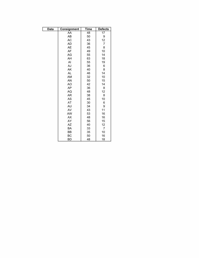
Data Consignment Time DefectsAA 48 17AB 50 9AC 43 12AD 36 7AE 45 8AF 49 10AG 55 14AH 63 18AI 55 19AJ 36 6AK 40 8AL 46 14AM 32 10AN 50 15AO 42 14AP 36 8AQ 48 12AR 38 8AS 45 10AT 30 6AU 34 9AV 43 11AW 53 16AX 48 16AY 56 15AZ 40 12BA 33 7BB 35 10BC 50 16BD 48 18

Exercise 2.24 File: X2.24 - leverage.xlsx
(a) Scatter Graph - Profit Growth (y) vs Leverage Ratio (x)
(b) Yes, there is a clear moderate to strong positive linear relationship betweenthe leverage ratio of a company and its profit growth.
Data Leverage Profit Growth40.8 11142.3 11643.2 13237.9 10536.2 6935.6 4036.4 5839.5 11842.6 10442.1 12537.8 9734.4 7636.5 9838.3 10039.3 7536.4 8833.5 2032.4 2535.4 7835.4 6535.7 8435.2 8835.3 8644.9 11535.9 5038.0 9236.7 11039.2 7241.1 12838.7 86
020406080
100120140160
30 32 34 36 38 40 42 44 46
prof
it gr
owth
leverage ratio
Scatter Graph Profit Growth (y) and Leverage Ratio (x)

Exercise 2.25 File: X2.25 - roi%.xlsx
(a) Sector Average Std devMining 9.87 4.58Services 11.33 2.99Grand Total 10.70 3.78
(b) Service companies have a higher average ROI% (11.33%) than mining companies (9.87%).The volatility of ROI% amongst service companies (2.99%) is far lower than amongst mining companies (4.58%)By inspection, there is a high overlap of ROI% between the two sectors (based on a two-standard deviationinterval around each sample mean). Thus it is likely that there is no statistically significant difference in mean ROI% between the two sectors.
Exercise 2.26 File: X2.26 - product location.xlsx
(a)Aisle Middle Top TotalFront Average 6.08 5.08 5.58
Std dev 0.890 0.622 0.895Middle Average 4.24 2.74 3.49
Std dev 1.387 0.297 1.232Back Average 4.66 4.1 4.38
Std dev 1.193 0.648 0.952Average 4.99 3.97 4.48Std dev 1.359 1.114 1.327
(b)
(c)
In combination however, sales volumes show highest variability when the product is positioned in a middle shelf position in a middle-of-store location (1.387) while the lowest variability in sales volumes occur when positioned in a top shelf position in a middle-of-store aisle location (0.297).
The large differences in average sales volumes (ranging from R6.08 to R2.74) is evidence of a likley statistically significant difference in sales volumes due to choice of aisle location and shelf positioning.
Recommendation:
Shelf position
A middle shelf position in a front-of-store ailse location is the most preferred product display location.
Based on shelf position alone, middle shelf positions generate higher average sales (R4.99) than top shelf positions (R3.97).Based on aisle location alone, a front-of-store aisle location generates the highest average sales (R5.58), followed by a back-of-store aisle location (R4.38).The lowest average sales occur when the product is displayed in a middle-of-store aisle location (R3.49). In combination, a front-of-store aisle location on a middle shelf position generates the highest average sales (R6.08), while a top shelf position in a middle-of-store aisle is the least desirable product location with an average sales volume of only R2.74.Sales variability is relatively consistent across aisle locations (0.895 to 1.232) as well as between shelf positions (1.114 to 1.359).

Exercise 2.27 File: X2.27 - property portfolio.xlsx
(a) Numeric Frequency Distribution and Cumulative % of NP%
Intervals Count Cumulative %
-5 0 0.0%
-2.5 4 1.2%
0 7 3.4%
2.5 4 4.6%
5 22 11.4%
7.5 87 38.3%
10 109 71.9%
12.5 46 86.1%
15 31 95.7%
17.5 12 99.4%
20 1 100%
More 1 100%
324 100%
(b) and (c)
Region Commercial Industrial Retail Total
A Average 7.5 4.9 10.2 7.9
Std dev 2.5 3.1 3.6 3.5
Minimum -2.4 -4.2 0.8 -4.2
Maximum 14.6 8.1 18.4 18.4
Count 104 40 70 214
B Average 12.3 6.8 8.5 9.8
Std dev 3.1 4.2 1.8 3.5
Minimum 2.7 -3.4 4.4 -3.4
Maximum 20.3 10.2 13.2 20.3
Count 46 16 48 110
Average 9.0 5.4 9.5 8.6
Std dev 3.5 3.5 3.1 3.6
Minimum -2.4 -4.2 0.8 -4.2
Maximum 20.3 10.2 18.4 20.3
Count 150 56 118 324
(d) Profile of property portfolio:
The company has almost twice as many properties in region A (214 or 66%) compared to region B (110 or 34%).
Almost half of their properties are commercial (46%) followed by retail (37%) and then industrial (17%).
Of all the prpoperties in the portfolio, the majority are commercial properties in region A (104 or 32%).
followed by retail properties in region A (70 or 22%).
The smallest component of their property portfolio consists of industrial properties in region B (only 16 or 5%).
Type of business usage
0 4 7 4
22
87
109
46
31
121 1
0.0%
20.0%
40.0%
60.0%
80.0%
100.0%
120.0%
0
20
40
60
80
100
120
-5 -2.5 0 2.5 5 7.5 10 12.5 15 17.5 20 More
Fre
qu
en
cy
Bin NP%
Histogram - Net Profit %

(e) Portfolio performance :
Net profit % across the entire portfolio is normally distributed (histogram) with an average return of 8.6% and a
standard deviation of 3/6%. NP% ranged from the lowest of -4.2% to the highest of 20.3%.
From the cumulative % distribution, 75% of all properties (cumulative 86.1% - cumulative 11.4%) earned a NP% of
between 5% and 12.5% p.a.
Region B (9.8%) has outperformed region A (7.9%) by almost 2% on average, while commercial (9.0%) and retail (9.5%)
have significantly outperformed industrial properties (5.4%).
The worst performing segment is industrial properties in region A (4.9%) while the best performing properties are
commercial properties in region B (12.3%).
There are 15 (4.6%) properties that are under-performing (with less than a 5% net profit % p.a.).(see histogram).
Volatility of NP% is fairly consistent across the segments (approx. 3.5%), except for higher variability noted in the
industrial properties of region B (4.2%).
Growth potential (high NP% p.a. segments) is mainly in commercial properties in region B which represents only 14% of the current portfolio
retail properties in region A (currently only constitute 22% of the current portfolio).
(f) Recommendations: Dispose of the worst performing industrial properties in both regions A and B and
purchase more commercial properties in region B followed by retail properties in region A.

CHAPTER 3
EXPLORATORY DATA ANALYSIS - DESCRIBING DATA
NUMERIC DESCRIPTIVE STATISTICS
Exercise 3.1 (a) median (b) mode (c) mean
Exercise 3.2 Upper quartile
Exercise 3.3 Statements (c) and (f). The mode would be more appropriate (both are categorical)
Exercise 3.4 (a) False (b) False (c) True (d) False (e) FalseThe new median mass will depend only on the masses of parcels in the 3rd and 4th
ordered positions out of the 6 positions (after adding the extra parcel). Also, the rank order position of this extra parcel's mass is unknown. It could be the 4th, 5th or 6th ranked mass, but this depends on the masses of parcels that are heavier than the current median mass.
If the 4th ranked mass is also equal to 6.5 kg, then the new median will not increase. If, on the other hand, the 4th ranked mass is greater than 6.5 kg, then the median will increase. Therefore the only statement that can be made with complete certainty is (c),(i.e. that it is impossible for the new median mass to be less than it was.)
Exercise 3.5 Correct method is (b). Use the formula for the arithmetic mean (Formula 3.1)
By definition, Mean = Σx / n
Given Mean = 4.1 and n = 9245, it is possible to
compute Σx (total number of persons) = Mean x n .i.e. total no. persons in Mossel Bay = 4.1 x 9245 = 37905 (rounded)

Exercise 3.6 File: X3.6 - equity returns.xls
General Equity Unit Trust % Returns
% Returns Deviation Deviation2
9.2 -0.1 0.01
8.4 -0.9 0.81
10.2 0.9 0.81
9.6 0.3 0.09
8.9 -0.4 0.16
10.5 1.2 1.44
8.3 -1 1
Sum 65.1 4.32
n 7
Using Excel
Mean 65.1/7 = 9.3 '=AVERAGE(9.2,...,8.3)
Std Dev √[4.32/(7-1)] = 0.8485 '=STDEV(9.2,...,8.3)

Exercise 3.7 File: X3.7 - luggage weights.xls
Mass (kg) Deviation Deviation2
11 0.43 0.1849
12 1.43 2.0449
8 -2.57 6.6049
10 -0.57 0.3249
13 2.43 5.9049
11 0.43 0.1849
9 -1.57 2.4649
Sum 74 17.7143
n 7
Using Excel
(a) Mean 74/7 = 10.57 '=AVERAGE(11,...,9)
Std Dev √[17.7143/(7-1)] = 1.7183 '=STDEV(11,...,9)
(b) On average, each passenger's hand luggage weighs 10.57 kg.
68.3% of all hand luggage is likely to weigh between 8.85 kg and 12.29 kg.
(This corresponds to one standard deviation limits about the mean).
(c) Coefficient of Variation 1.7183/10.57% = 16.26%
(d) The variation in hand luggage weights is moderate (close together).

Exercise 3.8 File: X3.8 - bicycle sales.xls
Bicycles sold Deviation Deviation2Sorted data
25 1.4 1.96 16
18 -5.6 31.36 18
30 6.4 40.96 18
36 12.4 153.76 19
18 -5.6 31.36 20
20 -3.6 12.96 24
16 -7.6 57.76 25
24 0.4 0.16 30
30 6.4 40.96 30
19 -4.6 21.16 36
Sum 236 392.4
n 10
(a) Mean = 236/10 = 23.6
On average, 23.6 bicycles are sold each month.
Median = (20 + 24)/2 = 22 (Median sales lies in the 5.5th position)
For half of the months (i.e. 5 months), bicycles sales were
less than 22 bicycles per month.
(b) Range = 36 - 16 = 20
The range of sales between the worst and best months was 20 bicycles.
(i.e. In the worst sales month, 16 were sold; in the best month, 36 were sold.
Variance = 392.4/(10-1) = 43.6
Standard deviation = √43.6 = 6.603
68.3% of all monthly bicycle sales are likely to lie between 17 and 30.2.
(c) Lower Quartile (Q1) = 18 (2.5th position)
25% of monthly bicycle sales were less than or equal to 18.
Or: No more than 18 bicycles per month were sold in 25% of the months.
Note: Using Excel : QUARTILE(data values,1) = 18.25
Upper Quartile (Q3) = 27.5 (7.5th position)
25% of monthly bicycle sales were above 27.5.
Or: More than 28 (27.5) bicycles per month were sold in 25% of the months.
Note: Using Excel : QUARTILE(data values,3) = 28.75
(d) Approximate Skewness = 3x(23.6 - 22)/6.603 = 0.7269
There is moderate positive skewness in monthly bicycle sales.
(i.e. There are one / two months with relative high bicycle sales)

(e) Box plot of monthly bicycle sales
Interpretation
Monthly bicycle sales range between 16 and 36.
The median monthly sales is 22. The positive skewness shows a wider spread
of monthly sales toward the months of high sales.
(f) Opening monthly stock level = 23.6 + 6.603 = 30.2 bicycles in stock
If orders = 30, then the dealer will have sufficient bicycle stock to meet demand.
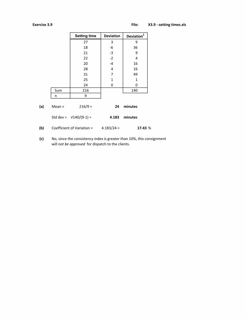
Exercise 3.9 File: X3.9 - setting times.xls
Setting time Deviation Deviation2
27 3 9
18 -6 36
21 -3 9
22 -2 4
20 -4 16
28 4 16
31 7 49
25 1 1
24 0 0
Sum 216 140
n 9
(a) Mean = 216/9 = 24 minutes
Std dev = √140/(9-1) = 4.183 minutes
(b) Coefficient of Variation = 4.183/24 = 17.43 %
(c) No, since the consistency index is greater than 10%, this consignment
will not be approved for dispatch to the clients.

Exercise 3.10 File: X3.10 - wage increases.xls
% Increases Deviation Deviation2 Sorted %
5.6 -0.83 0.6910 3.47.3 0.87 0.7547 4.84.8 -1.63 2.6610 5.36.3 -0.13 0.0172 5.68.4 1.97 3.8760 5.83.4 -3.03 9.1885 5.87.2 0.77 0.5910 5.85.8 -0.63 0.3985 6.28.8 2.37 5.6110 6.36.2 -0.23 0.0535 7.27.2 0.77 0.5910 7.25.8 -0.63 0.3985 7.37.6 1.17 1.3660 7.47.4 0.97 0.9385 7.65.3 -1.13 1.2797 8.45.8 -0.63 0.3985 8.8
Sum 102.9 28.8144
n 16
Using manual computations
(a) Mean = 102.9/16 6.43 %
Median = (6.2+6.3)/2 = 6.25 % (lies in the 8.5th position)
(b) Variance = [28.8144/(16-1)] = 1.921
Std dev = √28.8144/(16-1) = 1.386 %
(c) Lower limit = 6.43-2*(1.386) 3.66
Upper limit = 6.43+2*(1.386) 9.20
95.5% of all agreed wage increases lie between 3.66% and 9.2%.
(d) CV = (1.386/6.43) % = 21.56 %
Agreed wage increases are only moderately consistent.

Using Excel
Excel 's Data Analysis option Excel 's Function Keys
(a) Mean 6.43 '=AVERAGE(data values)
Standard Error 0.346
Median 6.25 '=MEDIAN(data values)
Mode 5.8
(b) Standard Deviation 1.386 '=STDEV(data values)
Sample Variance 1.921 '=VAR(data values)
Kurtosis 0.196
Skewness -0.286
Range 5.4
Minimum 3.4
Maximum 8.8
Sum 102.9
Count 16
(c) and (d) must be computed manually.
Wage increases

Exercise 3.11 Bank Trainee Exam Performance
Group 1 Group 2
Mean 76 64
Variance 110 88
Sample size 34 26
Std deviation √110 = √88 =
10.488 9.381
Group 1 Group 2
Coefficient (10.488/76)% (9.381/64)%
of Variation = 13.8 14.66
Interpretation
Both groups performed consistently well. The difference in CV% measures is marginal. However, group 1 trainees performed marginally more consistently than group 2 trainees.

Exercise 3.12 File: X3.12 - meal values.xls
(a) Random variable - value of a restaurant meal (in Rand)Data type - numerical, continuous, ratio-scaled (Using Data Analysis in Excel )
(b) Mean 1119/20 = = R55.95 Mean 55.95Standard Error 3.20
∑(deviation)² = 3902.95 Median 53n = 20 Mode 44
Standard Deviation 14.33Variance = 3902.95/(20-1) = 205.42 Sample Variance 205.42Std deviation = √205.42 = 14.33 Kurtosis 0.26
Skewness 0.74Range 55
(c) Median Minimum 35Average the Rand values in 10th and 11th positions. Maximum 90 = (51+55)/2 = R53 Sum 1119Half off the meals were valued at R53 or less. Count 20
Ranked MealPosition Value
1 352 363 444 445 446 477 488 489 5010 51 Median is midpoint between 11 55 these two middle values (R51 and R55)12 5613 5814 6215 6516 6517 6918 7219 8020 90
(d) Mode R44 occurs 3 times (see grouped ranked values in (c) above).
(e) There is moderate positive skewness caused by two high meal values (i.e. R80 and R90).
Hence recommend the median as the most representative central location meal value.
Meal values

Exercise 3.13 File: X3.13 - days absent.xls
(a) Mean = 237/23 10.3 days absent (Using Data Analysis in Excel )
Median Median is found in the (23+1)/2th position
i.e. 12th position Mean 10.30Standard Error 1.33
Median = 9 days absent Median 9Mode 5
Position Days absent Standard Deviation 6.361 2 Sample Variance 40.492 4 Skewness 1.383 4 Range 284 5 Minimum 25 5 Q1 position Maximum 306 5 and value Sum 2377 6 Count 238 69 6 Q1 5.5
10 8 Q3 1511 912 9 Median position and value13 1014 1015 1016 1217 15 Q3 position
18 15 and value19 1520 1621 1722 1823 30
Mode There are 4 possible modal values (5; 6; 10 and 15 days). All occur with a frequency of 4. Note: Only the first modal value is reported in Excel . The mode is an unreliable measure of central location in this study.
InterpretationOn average, an employee is absent for 10.3 days over this 9-month period. Half the employees were absent for up to 9 days.The most common number of days absent was 5 (or 6, or 10 or 15) days
(b) Lower Quartile (approximated manually)Q1 position = (23/4) = 5.75th position
Q1 value in this position is = 5+(0.75*(5 - 5) = 5 days absentUsing Excel 5.5 days absent =QUARTILE(data range,1)
25% of employees were absent for no more than 5 (or 5.5) days altogether.
days absent
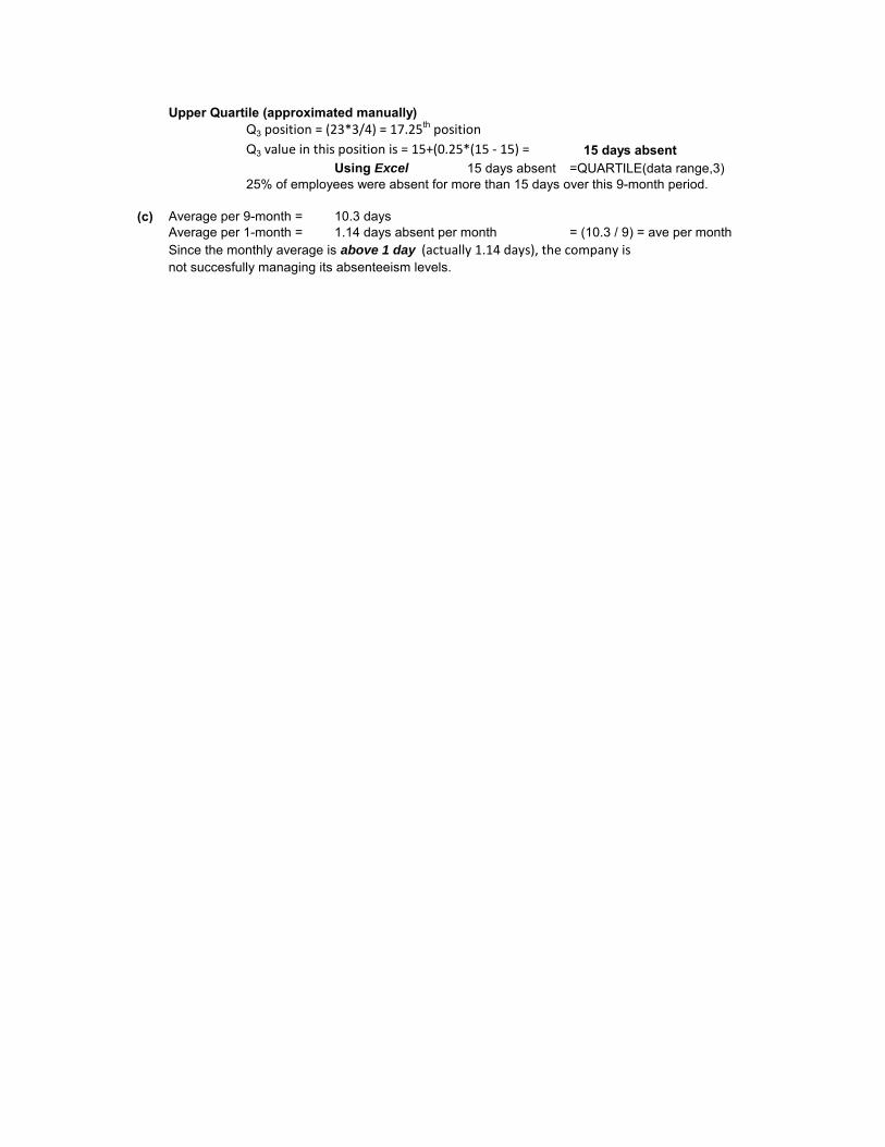
Upper Quartile (approximated manually)Q3 position = (23*3/4) = 17.25th position
Q3 value in this position is = 15+(0.25*(15 - 15) = 15 days absentUsing Excel 15 days absent =QUARTILE(data range,3)
25% of employees were absent for more than 15 days over this 9-month period.
(c) Average per 9-month = 10.3 daysAverage per 1-month = 1.14 days absent per month = (10.3 / 9) = ave per monthSince the monthly average is above 1 day (actually 1.14 days), the company is not succesfully managing its absenteeism levels.

Exercise 3.14 File: X3.14 - bad debts.xls
(a) Average = 79.3/17 4.665% (Using Data Analysis in Excel )
∑(deviation)² = 54.85882 bad debts %
n = 17 Mean 4.665Standard Error 0.45
Variance = 54.85882/(17-1) = 3.43 Median 5.4Std deviation = √(3.43) = 1.85 Mode 2.2
Standard Deviation 1.85Sample Variance 3.43
(b) Median Median is found in the (17+1)/2th position Kurtosis -1.49i.e. 9th position Skewness -0.35Median = 5.40% Range 5.4
Minimum 1.8Rank Ordered Maximum 7.2
Position bad debts % Sum 79.31 1.8 Count 172 2.23 2.2 Q1 2.64 2.4 Lower Quartile position Q3 6.15 2.6 and value6 3.47 4.48 4.79 5.4 Median position and value
10 5.711 5.712 5.8 Upper Quartile position 13 6.1 and value14 6.315 6.616 6.817 7.2
(c) Average: On average, each furniture retailer has a bad debt % of 4.665%.
Median: 50% of furniture retailers have a bad debt % of 5.4% or less. Since the mean < median, there is evidence of negative skewness.Hence propose the use of the median as the representative central value.
(d) There are two modal values (2.2% and 5.7%) both occurring with frequency of 2. This makes the mode an unreliable measure of central location.
(e) Skewness coefficient Values required for Formula 3.14(Formula 3.14) ∑(x - x(bar))3 = -31.2227
n = 17s (std dev) = 1.85
Then Skp = -0.35
Since the skewness coefficient is close to zero, there is only There is evidence of moderate negative skewness in the data on bad debts % (i.e. only a few fairly low bad debt % values - the majority are higher).
(17*(-31.2227))/((17-1)*(17-2)*1.853) =

(f) Lower Quartile (approximated manually)Q1 position = (17/4) = 4.25th position
Q1 value in this position is = (2.4*+(0.25*(2.6 - 2.4)) = 2.45%Using Excel = 2.6% =QUARTILE(data range,1)
25% of furniture retailers have a bad debts % of no more than 2.45% (or 2.6%).
Upper Quartile (approximated manually)Q3 position = (17*3/4) = 12.75th position
Q3 value in this position is = (5.8*+(0.75*(6.1 - 5.8)) = 6.025%Using Excel = 6.1% =QUARTILE(data range,3)
25% of furniture retailers have a bad debts % of more than 6.025% (or 6.1%).
(g) The average % bad debts is 4.665% while the median % bad debts is 5.4%. Sincethere is moderate negative skewness (Skp = -0.35), the median should be used
as the representative central value. Thus, since the median % of bad debts, is above 5% (median = 5.4%), an advisory note should be sent out.
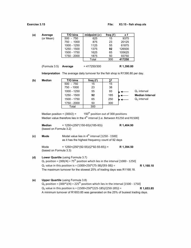
Exercise 3.15 File: X3.15 - fish shop.xls
(a) Average T/O bins midpoint (x ) freq (f ) x f
(or Mean) 500 - 750 625 15 9375750 - 1000 875 23 201251000 - 1250 1125 55 618751250 - 1500 1375 92 1265001500 - 1750 1625 65 1056251750 - 2000 1875 50 93750
Total 300 417250
(Formula 3.5) Average = 417250/300 R 1,390.80
Interpretation The average daily turnover for the fish shop is R1390.80 per day.
(b) Median T/O bins freq (f ) ∑f
500 - 750 15 15750 - 1000 23 381000 - 1250 55 93 Q1 interval
1250 - 1500 92 185 Median Interval1500 - 1750 65 250 Q3 interval
1750 - 2000 50 300Total 300
Median position = (300/2) = 150th position out of 300 positions
Median value therefore lies in the 4th interval [i.e. Between R1250 and R1500]
Median = 1250+(250*(150-93)/(185-93)) R 1,404.90(based on Formula 3.2)
(c) Mode Modal value lies in 4th interval [1250 - 1500]as it has the highest frequency count of 92 days
Mode = 1250+(250*(92-55)/(2*92-55-65)) = R 1,394.50(based on Formula 3.3)
(d) Lower Quartile (using Formula 3.7)Q1 position = (300/4) = 75th position which lies in the interval [1000 - 1250]
Q1 value in this position is = (1000+250*(75-38)/(93-38)) = R 1,168.18The maximum turnover for the slowest 25% of trading days was R1168.18.
(e) Upper Quartile (using Formula 3.8)Q3 position = (300*3/4) = 225th position which lies in the interval [1500 - 1750]
Q3 value in this position is = (1500+250*(225-185)/(250-185)) = R 1,653.85A minimum turnover of R1653.85 was generated on the 25% of busiest trading days.

Exercise 3.16 File: X3.16 - grocery spend.xls
(a) Average % Spend midpoint (x ) freq (f ) x f
(Mean) 10 - 20 15 6 9020 - 30 25 14 35030 - 40 35 16 56040 - 50 45 10 45050 - 60 55 4 220
Total 50 1670
(Formula 3.5) Average = 1670/50 33.4%
Interpretation On average, a family spends 33.4% of their income on groceries.
(b) (i) Median % Spend freq (f ) ∑f
10 - 20 6 620 - 30 14 20 Q1 interval
30 - 40 16 36 Median Interval40 - 50 10 46 Q3 interval
50 - 60 4 50Total 50
Median position = (50/2) = 25th
Median value therefore lies in the 3rd interval [30 - 40]
(Formula 3.2) Median = 30+(10*(25-20)/(36-20)) 33.125%
Interpretation 50% of families spend no more than 33.125% of their income on groceries.
(b) (ii) Lower Quartile (Q1) (using Formula 3.7)Q1 position = (50/4) = 12.5th position which lies in the interval [20 - 30]
Q1 value in this position is = 20+(10*(12.5-6)/(20-6)) = 24.64%
Interpretation 25% of families spend no more than 24.64% of their income on groceries.
(c) Upper Quartile (Q3) (using Formula 3.8)Q3 position = (50*3/4) = 37.5th position which lies in the interval [40 - 50]
Q3 value in this position is = 40+(10*(37.5-36)/(46-36)) = 41.5%
Interpretation 25% of families spend more than 41.5% of their income on groceries.

Exercise 3.17 File: X3.17 - equity portfolio.xls
Shares Price Value40 15 60010 20 2005 40 200
50 10 500105 Total 1500
Average value / equity = 1500/105 R 14.29(This is a weighted average measure)(Using Formula 3.5)
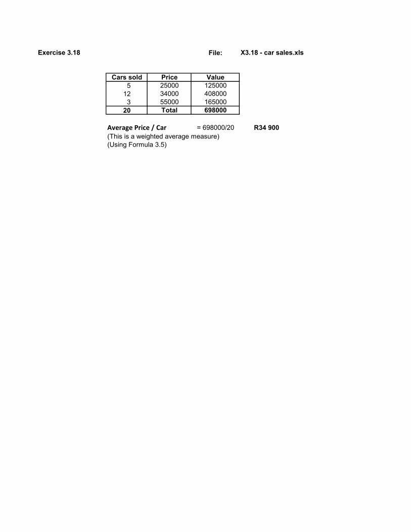
Exercise 3.18 File: X3.18 - car sales.xls
Cars sold Price Value5 25000 125000
12 34000 4080003 55000 165000
20 Total 698000
Average Price / Car = 698000/20 R34 900(This is a weighted average measure)(Using Formula 3.5)

Exercise 3.19 File: X3.19 - rental increases.xls
(Use Formula 3.4)Geometric mean = 4√(1.16*1.14*1.1*1.08) - 1 = 0.11955
InterpretationThe average annual % escalation rate in office rentals is 11.955%
Using Excel =GEOMEAN(1.16,1,14,1,1,1,08) - 1 = 0.11955

Exercise 3.20 File: X3.20 - sugar increases.xls
(a) (Using Formula 3.4)Geometric mean = 6√(1,05*1,12*1,06*1,04*1,09*1,03) - 1 = 0.06456
InterpretationThe average annual % increase in the sugar price (per kg) has been 6.456%
Using Excel =GEOMEAN(1.05,1.12,1.06,1.04,1.09,1.03) - 1 = 0.06456
(b) The geometric mean is more appropriate since the base value of each percentage change is different . Each year's percentage change is based on the previous year's sugar price.
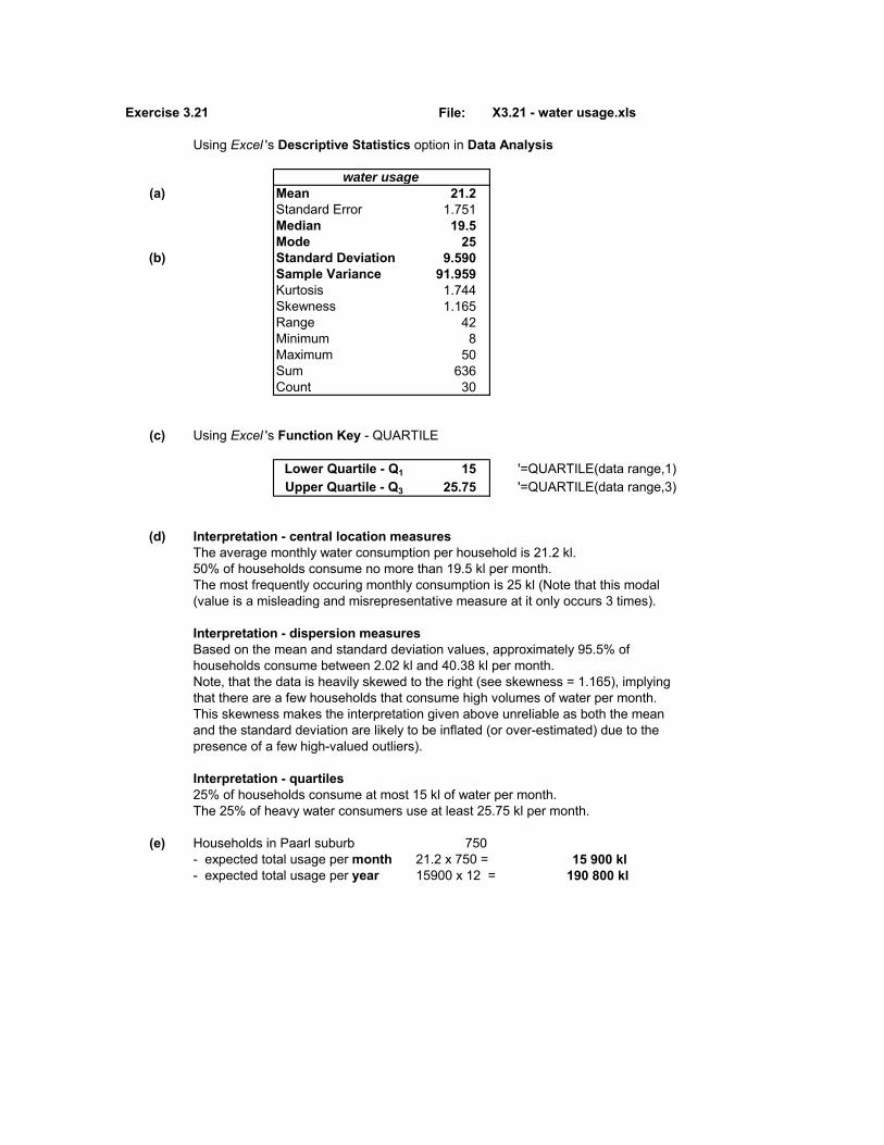
Exercise 3.21 File: X3.21 - water usage.xls
Using Excel 's Descriptive Statistics option in Data Analysis
water usage
(a) Mean 21.2Standard Error 1.751Median 19.5Mode 25
(b) Standard Deviation 9.590Sample Variance 91.959Kurtosis 1.744Skewness 1.165Range 42Minimum 8Maximum 50Sum 636Count 30
(c) Using Excel 's Function Key - QUARTILE
Lower Quartile - Q1 15 '=QUARTILE(data range,1)Upper Quartile - Q3 25.75 '=QUARTILE(data range,3)
(d) Interpretation - central location measuresThe average monthly water consumption per household is 21.2 kl.50% of households consume no more than 19.5 kl per month. The most frequently occuring monthly consumption is 25 kl (Note that this modal(value is a misleading and misrepresentative measure at it only occurs 3 times).
Interpretation - dispersion measuresBased on the mean and standard deviation values, approximately 95.5% of households consume between 2.02 kl and 40.38 kl per month. Note, that the data is heavily skewed to the right (see skewness = 1.165), implying that there are a few households that consume high volumes of water per month. This skewness makes the interpretation given above unreliable as both the mean and the standard deviation are likely to be inflated (or over-estimated) due to the presence of a few high-valued outliers).
Interpretation - quartiles25% of households consume at most 15 kl of water per month.The 25% of heavy water consumers use at least 25.75 kl per month.
(e) Households in Paarl suburb 750- expected total usage per month 21.2 x 750 = 15 900 kl- expected total usage per year 15900 x 12 = 190 800 kl

Exercise 3.22 File: X3.22 - veal dishes.xls
(a) Random variable - cost of a veal cordon bleu meal at a Durban restaurantData type - numerical, continuous, ratio-scaled.
(b) Using Excel 's Descriptive Statistics option in Data Analysis
Mean 61.25Standard Error 1.99Median 59Mode 48Standard Deviation 10.54Sample Variance 111.08Kurtosis 0.62Skewness 0.78Range 45Minimum 45Maximum 90Sum 1715Count 28
InterpretationOn average, a patron can expect to pay R61.25 for a veal cordon bleu meal
at a Durban restaurant.50% of Durban restaurants charge no more than R59 for a veal cordon bleu meal.
(c) There are two modal values (R48 and R55). Both occur with a frequency of 3. It is a misleading value because of its low frequency of occurrence.Note: Excel only shows the first occurrence of a modal value (i.e. R48) in its output.
(d) Standard deviation = R 10.54This means that 68.3% of Durban restaurants are likely to charge between R50.71 (61.25 - 10.54) and R71.79 (61.25 + 10.54) for a veal cordon bleu meal.
(e) Skewness Coefficient = 0.78 Formula 3.14Skewness coefficient (approx) = 0.64 Formula 3.15The relative high positive skewness is caused by two Durban restaurants charging high prices (R80 and R90) for a veal cordon bleu meal.
(f) Both measures indicate that there is moderate-to-high positive skewness, hence the median cost of R59 would be a more representative measure of central location.
(g) Upper Quartile (Q3) R68 =QUARTILE(data range,3)25% of Durban restaurants charge at least R68 for a veal cordon bleu meal.
(h) Lower Quartile (Q1) R 54.75 =QUARTILE(data range,1)25% of Durban restaurants charge no more than R54.75 for a veal cordon bleu meal.
(i) 90th percentile value R 72.90 =PERCENTILE(data range,0.9)
cordon bleu meal price
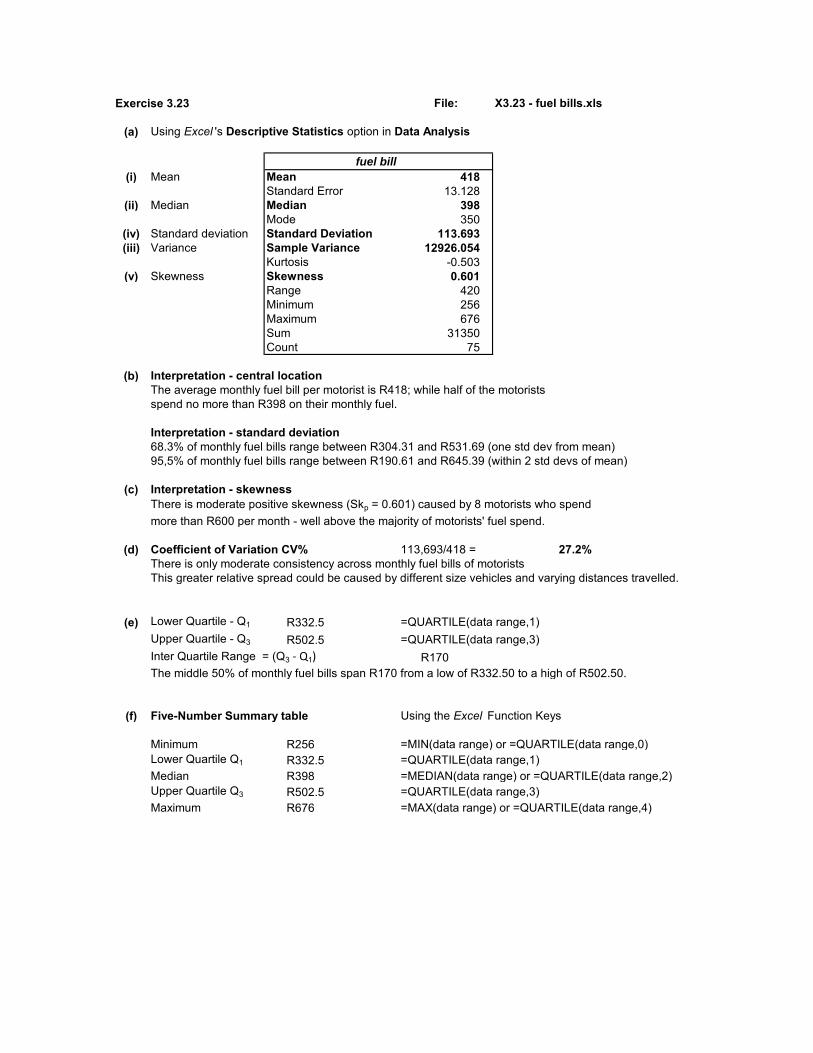
Exercise 3.23 File: X3.23 - fuel bills.xls
(a) Using Excel 's Descriptive Statistics option in Data Analysis
(i) Mean Mean 418Standard Error 13.128
(ii) Median Median 398Mode 350
(iv) Standard deviation Standard Deviation 113.693(iii) Variance Sample Variance 12926.054
Kurtosis -0.503(v) Skewness Skewness 0.601
Range 420Minimum 256Maximum 676Sum 31350Count 75
(b) Interpretation - central locationThe average monthly fuel bill per motorist is R418; while half of the motoristsspend no more than R398 on their monthly fuel.
Interpretation - standard deviation68.3% of monthly fuel bills range between R304.31 and R531.69 (one std dev from mean)95,5% of monthly fuel bills range between R190.61 and R645.39 (within 2 std devs of mean)
(c) Interpretation - skewnessThere is moderate positive skewness (Skp = 0.601) caused by 8 motorists who spend more than R600 per month - well above the majority of motorists' fuel spend.
(d) Coefficient of Variation CV% 113,693/418 = 27.2%There is only moderate consistency across monthly fuel bills of motoristsThis greater relative spread could be caused by different size vehicles and varying distances travelled.
(e) Lower Quartile - Q1 R332.5 =QUARTILE(data range,1)Upper Quartile - Q3 R502.5 =QUARTILE(data range,3)Inter Quartile Range = (Q3 - Q1) R170The middle 50% of monthly fuel bills span R170 from a low of R332.50 to a high of R502.50.
(f) Five-Number Summary table Using the Excel Function Keys
Minimum R256 =MIN(data range) or =QUARTILE(data range,0)Lower Quartile Q1 R332.5 =QUARTILE(data range,1)Median R398 =MEDIAN(data range) or =QUARTILE(data range,2)Upper Quartile Q3 R502.5 =QUARTILE(data range,3)Maximum R676 =MAX(data range) or =QUARTILE(data range,4)
fuel bill

(g) Box plot
(h) Interpretation of Box PlotThere is clear evidence of moderate positive skewness (skewed-to-the-right) in fuel bills. There are a few motorists who spend a large amount on fuel a month.
(i) Total amount of fuel consumed monthly by Paarl motorists for commuting to work:
Expected total monthly fuel bill = R418 * 25000 R 10,450,000(average bill / motorist x no.motorists)
Expected Total fuel consumed (in litres) = R10450000/10 = 1 045 000 litres(Expected total monthly cost / cost per litre)

Exercise 3.24 File: X3.24 - service periods.xls
(a) Using Excel 's Descriptive Statistics option in Data Analysis
service periods
(i) Mean Mean 7Standard Error 0.384
(ii) Median Median 6Mode 6
(iii) Std Dev Standard Deviation 3.838Sample Variance 14.727Kurtosis -0.437
(iv) Skewness Skewness 0.553Range 15Minimum 1Maximum 16Sum 700Count 100
(b) Interpretation - central locationOn average, each engineer has 7 years of service with a companyHalf of all engineers spend no more than 6 years with a company
Interpretation - standard deviation68.3% of engineers spend between 3.16 and 10.84 years with a company. Similar intervals can be computed for 2 and 3 std devs from the mean.Note: when the lower limit is computed to be negative, in practice it is zero.
Interpretation - skewnessThere is a moderate positive skewness (Skp = 0.553) in length of service periods, meaning that a few engineers have long service periods with their company.
(c) Using Excel 's Histogram option in Data Analysis
Frequency Distribution - Years of Service
Years of Service Count0 - 3 213 - 6 306 - 9 249 - 12 1512 - 15 815 - 18 2

(d) Lower limit = 7 - 3.838 = 3,16 yearsUpper limit = 7 + 3.838 = 10,84 years
68.3% of engineers spend between 3.16 years and 10.84 years with a company.
(e) Percent of members with less than 3 years of serviceCumulative % up to 3 years = 21/100 = 21%
Percent of members with more than 12 years of serviceCumulative % above 12 years = 10/100 = 10%
They meet the guidelines for "new blood" (21,2%) ,but havefar fewer "experienced" members (only 10%) than their guidelines require.

Exercise 3.25 File: X3.25 - dividend yields.xls
(a) Random variable dividend yield (%) of a company
Data type numeric, ratio-scaled
(b) Using Excel 's Descriptive Statistics option in Data Analysis
Dividend yields
(i) Mean Mean 4.273Standard Error 0.218
(ii) Median Median 4.1(iii) Mode Mode 2.8(iv) Std Dev Standard Deviation 1.444
Sample Variance 2.084
Kurtosis -0.359
(v) Skewness Skewness 0.259Range 6.1
Minimum 1.5
Maximum 7.6
Sum 188
Count 44
(c) Mean The average dividend yield per company is 4.273%
Median Half of the dividend yields are at or below 4.1%
Mode A misleading measure because there are 4 dividend yield values
(viz. 2,8, 3,6; 4,1; 5,1) of equal modal frequency (of 3)
Std dev 68.3% of all dividend yields lie between 2.83% and 5.72%
Similarly for 2 and 3 std devs from the mean
Skewness There is very slight positive (right) skewness (Skp = 0.259).
The histogram can be assumed to be normally distributed.
(d) the Mean (Average) as there is minimal skewness present in the data.
(e) Bin yields FrequencyBelow 2% 3
2 - 3.5% 11
3.5 - 5% 16
5 - 6.5% 11
6.5 - 8% 3

(f) Five-Number Summary TableMinimum 1.5 =QUARTILE(data range,0)
Lower Quartile Q1 3.175 =QUARTILE(data range,1)
Median 4.1 =QUARTILE(data range,2)Upper Quartile Q3 5.15 =QUARTILE(data range,3)
Maximum 7.6 =QUARTILE(data range,4)
(g) Box plot Dividend Yield %
The very slight positive skewness can be seen from the longer tail
on the right of the box plot. It implies a few companies have achieved
significantly higher dividend yields than the majority of the sample.
(h) Minimum dividend yield achieved by the top performing 10% of companies
6.17% =PERCENTILE(data range,0.90)
The top 10% of companies achieved at least a dividend yield of 6.17%
(i) % of companies who did not declare more than a 3.5% dividend yield
Cumulative frequency up to upper limit of 3.5 = (3 + 11) = 14.
% Cumulative = 14 / 44 % = 31.8%Almost 1/3 (31.8%) of companies did not declare more than a 3.5% dividend yield.

Exercise 3.26 File: rosebuds.xls
(a) Random variable - the unit price of a rosebud (in cents)Data type - numerical, continuous, ratio-scaled
(b) Using Excel 's Descriptive Statistics option in Data Analysis
selling price
(i) Mean 60.312Standard Error 0.319
(iii) Median 59.95Mode 60.6
(ii) Standard Deviation 3.188Sample Variance 10.160Kurtosis 1.770
(iv) Skewness 0.932Range 18.3Minimum 55.2Maximum 73.5Sum 6031.2Count 100
InterpretationMean: The average selling price of rosebuds is 60.312 cents.Median: 50% of rosebuds sold for no more than 59.95c. Std dev: 68.3% of rosebud unit prices are likely to lie between 57.12c and 63.5c.
Skewness: There is excessive positive skewness (one very high unit price)
(c) Coefficient of Variation CV% 3.188/60.312% = 5.3%
There is very low variability amongst unit selling prices of rose buds
(d) Lower Quartile Q1 57.7 cents =QUARTILE(data range,1)
Upper Quartile Q3 62.45 cents =QUARTILE(data range,3)
(e) The highest unit selling price of the cheapest 25% of sales is 57.7 cents (i.e. Q1)
(f) The minimum unit selling price of the highest-priced 25% of sales is 62.45 cents (i.e. Q3)Overall interpretation of (a), (d), (e) and (f)Unit selling prices ranged from 55.2c to 73.5c where 50% of the selling prices were above 59.95c. 25% of sales were below 57.7c while the most expensive 25% of unit selling prices were above 62.45c.
(g) 90th percentile 64.6c =PERCENTILE(data range,0.9)
(h) 10th percentile 56.6c =PERCENTILE(data range,0.1)
(i) Five-Number Summary Table and Boxplot
Minimum 55.2 =QUARTILE(data range,0)
Lower Quartile Q1 57.7 =QUARTILE(data range,1)
Median 59.95 =QUARTILE(data range,2)
Upper Quartile Q3 62.45 =QUARTILE(data range,3)
Maximum 73.5 =QUARTILE(data range,4)

Boxplot
Interpretation
The distribution of unit selling prices of rosebuds is skewed to the right.
There is also one extremely high unit selling price of 73.5c which can be
considered an outlier.
Overall, unit selling prices of rosebuds ranged between 55.2c and 73.5c.
25% of unit selling prices lay below 57.7 c (i.e. lower quartile); while
the middle 50% of unit selling prices ranged from 57.7c to 62.45c.
The "best" 25% of unit selling prices achieved were above 62.45c (Q3).
Finally, the median (middle) unit selling price achieved was 59.95c.

Mini Case Study 3.27 File: X3.27 - savings balances.xlsx
1 (a) Frequency Distribution
Savings Intervals Frequency0 - ≤ 200 21
201 - ≤ 400 71401 - ≤ 600 56601 - ≤ 800 19801 - ≤1000 4More 4
1 (b) Descriptive Statistics
Savings Balance (R10's)Mean 421.86 266.5Standard Error 16.247 520.5Median 385Mode 326Standard Deviation 214.93Sample Variance 46195.1765Kurtosis 4.727Skewness 1.634Range 1383Minimum 85Maximum 1468Sum 73826Count 175
1 (c ) Married Single Grand TotalFemale 23 41 64Male 83 28 111Grand Total 106 69 175
1 (d) Married Single Grand TotalFemale 512.6 563.7 545.3Male 368.0 299.3 350.7Grand Total 399.4 456.4 421.9
2 (a) Gender Categorical Nominal-scaledMarital status Categorical Nominal-scaledMonth-end balances Numeric Ratio-scaled
2 (b) Refer to 1 (a) (Histogram) and 1 (b) (Descriptive Statistics)
The average savings balance of bank clients is R421.86.50% of these clients have month-end balances of less than R385 (median). From the histogram, 21 clients have month-end balances of less than R200 and 8 are above R800. The 8 banking clients with relatively high month-end savings balances (skewness = 1.643 > 1.0) skew the average towards these higher balances and distorts the overall picture. Therefore the median month-end balance of R385 is a more representative indicator of savings balances. 25% of their clients have month-end balances of less than R266.6, while the top 25% of savers have month-end balances in excess R520.5 with 4 clients above R1000 (maximum = R1468).
Refer to 1 (c) (Count of Gender and Marital Status)
Amongst the female clients, the majority (64%) are single (41/64), while amongst the male clients, the majority (75%) are married. Thus they are attracting mainly single females; and married males.
Refer to 1 (d) (Breakdown Table of Average Savings by Gender and Marital Status)
Single females are saving the most (average of R563,7) while single males are the worst savers withan average savings balance of only R299.3 (compared to the overall average of R421.9).Also females save more, on average (R545) than males (R350). Single bank clients save more, on average (R456.4) than married bank clients (R399.4).
Lower QuartileUpper Quartile
21
71
56
19
4 4
0
10
20
30
40
50
60
70
80
0 - ≤ 200 201 - ≤ 400 401 - ≤ 600 601 - ≤ 800 801 - ≤1000 More
Nu
mb
er
of
Clie
nts
Savings Intervals
Histogram of Savings Balances (R10's)

2 (c) Plan of Action by BankBank should target females in general (as they comprise only 37%) of the current client basebut have the largest average balances of all clients. Single females (23%) in particular should be targetted to attract more high savers to the bank. They should encourage their main client base - married males - to save more.

Mini Case Study 3.28 File: X3.28 - medical claims.xlsx
1 (a) Frequency Distribution
Claims Ratio Count %
Below 0.1 6 4.0
0.1 - 0.5 35 23.3
0.5 - 0.9 26 17.3
0.9 - 1.3 36 24.0
1.3 - 1.7 30 20.0
1.7 - 2.1 14 9.3
2.1 - 2.5 2 1.3
Above 2.5 1 0.7
150 100
1 (b) Descriptive Statistics
Mean 0.974 0.460Median 0.996 1.421Mode #N/A
Standard Deviation 0.594
Sample Variance 0.353
Skewness 0.242
Range 2.672
Minimum 0.013
Maximum 2.685
Sum 146.1
Count 150
1(c) and (d) Cross-tabulation Table / Breakdown table
Marital 26 - 35 36 - 45 46 - 55 Row totalsMarried average 1.326 0.915 1.123 1.112
std dev 0.552 0.589 0.629 0.610minimum 0.147 0.051 0.013 0.013maximum 2.685 1.989 2.408 2.685count 23 27 35 85
Single average 0.919 0.474 0.947 0.793std dev 0.543 0.356 0.500 0.524minimum 0.014 0.024 0.218 0.014maximum 1.905 1.262 1.814 1.905count 36 19 10 65average 1.078 0.733 1.084 0.974
Column totals std dev 0.577 0.547 0.602 0.594minimum 0.014 0.024 0.013 0.013maximum 2.685 1.989 2.408 2.685count 59 46 45 150
2 (a) Marital Status Qualitative / Categoric NominalAge Group (bands) Qualitative / Categoric Ordinal Claims Ratio Quantitative / Numeric Ratio, Continuous
2 (b) Claims Ratio Pattern of MembersThe average claims ratio is 0.974. This means that, on average, members are claimingas much as they contribute. The median claims ratio is a similar value (0.996). This means that at least half the members are claiming more than they contribute. The distribution (see histogram) appears to be bi-modal showing a low claims ratio (i.e. less than half their contributions) by at least a quarter of members (Q1 = 0.46) and a high claims ratio by at least half of the members (50% greater than median claims ratio of 0.996). At least 25% of members areclaiming significantly more than they contribute (Q3 = 1.42).Only 4% of members claim less than 10% of their contributions (first interval of histogram). Also at least 11% (top three intervals of histogram) are claiming at least twice as much as they contribute.
Refer to 1(c) and (d)It would appear that married members claim significantly more (1.112) than single members (0.793). Married members also make up the majority of members (85/150 = 57%).
Claims Ratio
Lower QuartileUpper Quartile
Age
6
35
26
36
30
14
2 1
0
5
10
15
20
25
30
35
40
No
. of
Me
mb
ers
Claims Ratio Intervals
Histogram of Claims Ratios
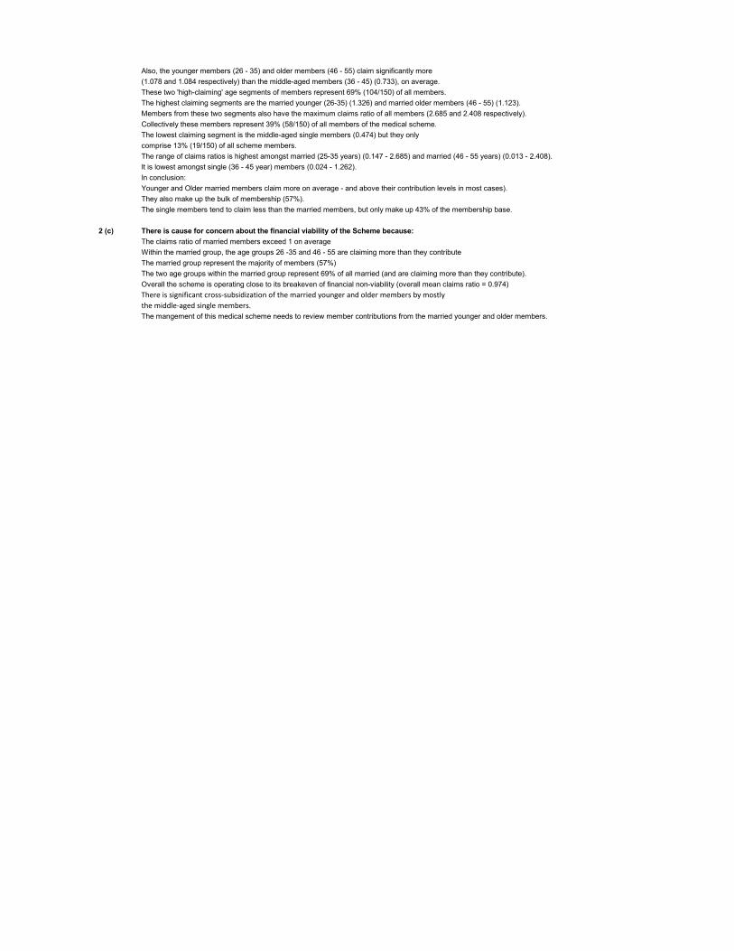
Also, the younger members (26 - 35) and older members (46 - 55) claim significantly more (1.078 and 1.084 respectively) than the middle-aged members (36 - 45) (0.733), on average. These two 'high-claiming' age segments of members represent 69% (104/150) of all members. The highest claiming segments are the married younger (26-35) (1.326) and married older members (46 - 55) (1.123). Members from these two segments also have the maximum claims ratio of all members (2.685 and 2.408 respectively). Collectively these members represent 39% (58/150) of all members of the medical scheme. The lowest claiming segment is the middle-aged single members (0.474) but they only comprise 13% (19/150) of all scheme members. The range of claims ratios is highest amongst married (25-35 years) (0.147 - 2.685) and married (46 - 55 years) (0.013 - 2.408).It is lowest amongst single (36 - 45 year) members (0.024 - 1.262). In conclusion:Younger and Older married members claim more on average - and above their contribution levels in most cases). They also make up the bulk of membership (57%). The single members tend to claim less than the married members, but only make up 43% of the membership base.
2 (c) There is cause for concern about the financial viability of the Scheme because:The claims ratio of married members exceed 1 on averageWithin the married group, the age groups 26 -35 and 46 - 55 are claiming more than they contributeThe married group represent the majority of members (57%) The two age groups within the married group represent 69% of all married (and are claiming more than they contribute). Overall the scheme is operating close to its breakeven of financial non-viability (overall mean claims ratio = 0.974)There is significant cross-subsidization of the married younger and older members by mostly
the middle-aged single members.
The mangement of this medical scheme needs to review member contributions from the married younger and older members.

CHAPTER 4
BASIC PROBABILITY CONCEPTS
Exercise 4.1 P(A) = 0.2 means that an event has a 20% chance of occurring.
Exercise 4.2 Mutually exclusive events.
Exercise 4.3 The outcome of one event does not influence / nor is influencedby / the outcome of the other event.
Exercise 4.4 P(A or B) = P(A) + P(B) - P(A ∩ B) = 0.26 + 0.35 - 0.14 = 0.47
Exercise 4.5 P(X / Y) = P(X ∩ Y) / P(Y) = 0.27 / 0.36 = 0.75P(Y / X) = P(Y ∩ X) / P(X) = 0.27 / 0.54 = 0.50Thus P(X / Y) ≠ P(Y / X)

Exercise 4.6 File: X4.6 - economic sectors.xls
(a) Sector Count % countMining 45 18.0Financial 72 28.8IT 32 12.8Production 101 40.4Total 250 100
(b) P(Financial) = 28.8%
(c) P(Not Production) = 100 - 40.4 = 59.6%
(d) P(Mining or IT) = 18 + 12.8 = 30.8%
(e) In (b), the marginal probability was computed. In (c), used the Complementary probability ruleIn (d), used the Addition rule for mutually exclusive events.
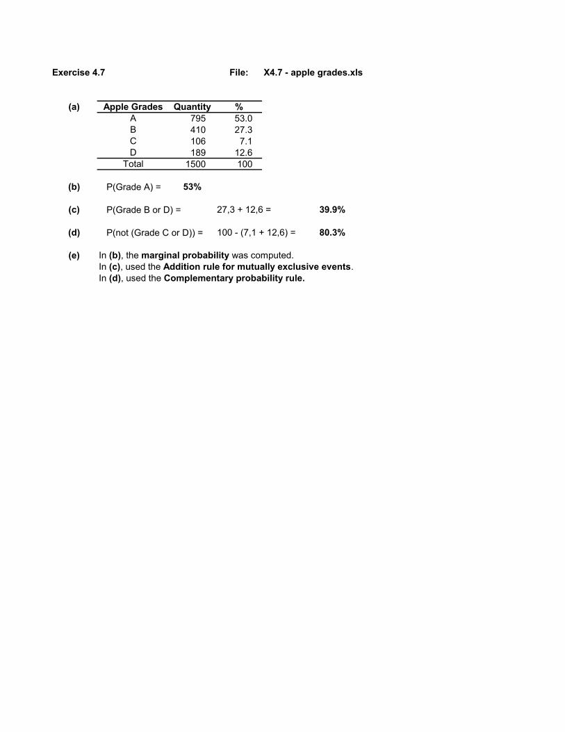
Exercise 4.7 File: X4.7 - apple grades.xls
(a) Apple Grades Quantity %A 795 53.0B 410 27.3C 106 7.1D 189 12.6
Total 1500 100
(b) P(Grade A) = 53%
(c) P(Grade B or D) = 27,3 + 12,6 = 39.9%
(d) P(not (Grade C or D)) = 100 - (7,1 + 12,6) = 80.3%
(e) In (b), the marginal probability was computed. In (c), used the Addition rule for mutually exclusive events.In (d), used the Complementary probability rule.
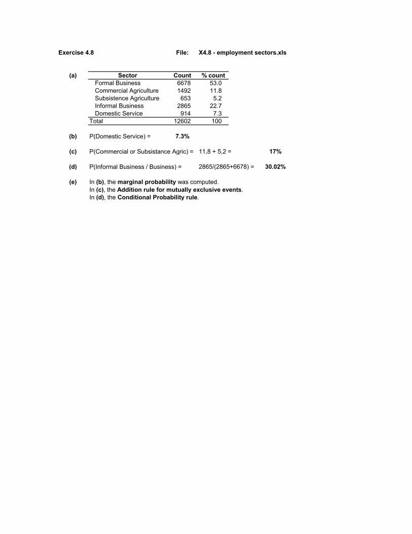
Exercise 4.8 File: X4.8 - employment sectors.xls
(a) Sector Count % countFormal Business 6678 53.0Commercial Agriculture 1492 11.8Subsistence Agriculture 653 5.2Informal Business 2865 22.7Domestic Service 914 7.3
Total 12602 100
(b) P(Domestic Service) = 7.3%
(c) P(Commercial or Subsistance Agric) = 11,8 + 5,2 = 17%
(d) P(Informal Business / Business) = 2865/(2865+6678) = 30.02%
(e) In (b), the marginal probability was computed. In (c), the Addition rule for mutually exclusive events.In (d), the Conditional Probability rule.

Exercise 4.9 File: X4.9 - qualification levels.xls
(a) Random variable 1 Managerial level (categorical, ordinal-scaled and discrete) Random variable 2 Qualification level (categorical, ordinal-scaled and discrete)
(b)Qualification Section Head Dept Head Division Head TotalMatric 28 14 8 50Diploma 20 24 6 50Degree 5 10 14 29Total 53 48 28 129
(c)(i) P(Matric) = 50/129 = 38.76%(ii) P(Section head ∩ Degree) = 5/129 = 3.88%(iii) P(Dept head / Diploma) = 24/50 = 48%(iv) P(Division head) = 28/129 = 21.71%(v) P(Division head U Section head) = (53+28)/129 = 62.79%(vi) P(Matric U Diploma U Degree) = (50+50+29)/129 = 100%(vii) P(Degree / Dept head) = 10/48 = 20.83%(viii) P(Division head U Diploma U both) = (28+50-6)/129 = 55.81%
(d) Probability Types and Rules(i) Marginal probability(ii) Joint probability and Multiplication rule(iii) Conditional probability(iv) Marginal probability(v) Addition rule for mutually exclusive events(vi) Collectively exhaustive set of events and Addition rule for mutually exclusive events(vii) Conditional probability(viii) Addition rule for non-mutually exclusive events
(e) Yes, since these outcomes cannot occur simultaneously.
Managerial Level
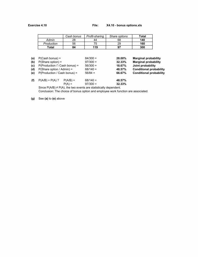
Exercise 4.10 File: X4.10 - bonus options.xls
Cash bonus Profit-sharing Share options TotalAdmin 28 44 68 140
Production 56 75 29 160Total 84 119 97 300
(a) P(Cash bonus) = 84/300 = 28.00% Marginal probability(b) P(Share option) = 97/300 = 32.33% Marginal probability(c) P(Production ∩ Cash bonus) = 56/300 = 18.67% Joint probability(d) P(Share option / Admin) = 68/140 = 48.57% Conditional probability(e) P(Production / Cash bonus) = 56/84 = 66.67% Conditional probability
(f) P(A/B) = P(A) ? P(A/B) = 68/140 = 48.57%P(A) = 97/300 = 32.33%
Since P(A/B) ≠ P(A), the two events are statistically dependent. Conclusion: The choice of bonus option and employee work function are associated.
(g) See (a) to (e) above

Exercise 4.11 File: X4.11 - age profile.xls
Age Production Sales Administration Total<30 60 25 18 103
30-50 70 29 25 124>50 30 8 35 73Total 160 62 78 300
(a) (i) P(< 30 years) = 103/300 = 34.33% Marginal probability (ii) P(Production) = 160/300 = 53.33% Marginal probability (iii) P(Sales ∩ (30-50) years) = 29/300 = 9.67% Joint probability (iv) P(>50 / Admin) = 35/78 = 44.87% Conditional probability (v) P(Production U <30 U both) = (160+103-60)/300 = 67.67% Conditional probability
(b) No, since outcomes of these two events can occur simultaneously.
(c) Let A = >50 and B = Admin.Is P(A/B) = P(A) ? P(A/B) = 35/78 = 44.87%
P(A) = 73/300 = 24.33%Since P(A/B) ≠ P(A), the two events are statistically dependent. Conclusion: There is an association between the Age of an employee and the Department in which they are employed (e.g. younger employees tend to be in Production).
(d) See (a) above
Department
Exercise 4.12 File: X4.12 - digital cameras.xls
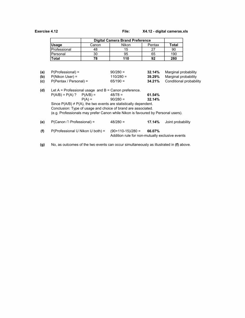
Usage Canon Nikon Pentax TotalProfessional 48 15 27 90Personal 30 95 65 190Total 78 110 92 280
(a) P(Professional) = 90/280 = 32.14% Marginal probability(b) P(Nikon User) = 110/280 = 39.29% Marginal probability(c) P(Pentax / Personal) = 65/190 = 34.21% Conditional probability
(d) Let A = Professional usage and B = Canon preference.P(A/B) = P(A) ? P(A/B) = 48/78 = 61.54%
P(A) = 90/280 = 32.14%Since P(A/B) ≠ P(A), the two events are statistically dependent. Conclusion: Type of usage and choice of brand are associated. (e.g. Professionals may prefer Canon while Nikon is favoured by Personal users).
(e) P(Canon ∩ Professional) = 48/280 = 17.14% Joint probability
(f) P(Professional U Nikon U both) = (90+110-15)/280 = 66.07%Addition rule for non-mutually exclusive events
(g) No, as outcomes of the two events can occur simultaneously as illustrated in (f) above.
Digital Camera Brand Preference

Exercise 4.13
(a) Probability Tree
(Fail) P(F2) = 0.15 P(F1 ∩ F2) = 0.20 x 0.15 = 0.03
P(F1) = 0.20(Fail)
(Not fail) P(S2) = 0.85 P(F1 ∩ S2) = 0.20 x 0.85 = 0.17
(Fail) P(F2) = 0.15 P(S1 ∩ F2) = 0.80 x 0.15 = 0.12(Not fail)P(S1) = 0.80
(Not fail) P(S2) = 0.85 P(S1 ∩ S2) = 0.80 x 0.85 = 0.68
1.00
Component A Component B Joint outcomes

Exercise 4.13
(b) P(A) = 0.20 P(B) = 0.15P(A ∩ B) = P(A) x P(B) = 0.2 * 0.15 = 0.03 (3% chance)
(c) P(Fail) = P(A U B)P(A U B) = P(A) + P(B) - P(A∩B) = 0.2+0.15-0.03 0.32Hence P(not Fail) = 1 - P(A U B) = 1 - 0.32 = 0.68 (68% chance)
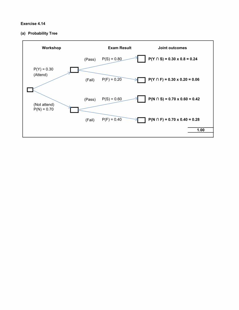
Exercise 4.14
(a) Probability Tree
(Pass) P(S) = 0.80 P(Y ∩ S) = 0.30 x 0.8 = 0.24
P(Y) = 0.30(Attend)
(Fail) P(F) = 0.20 P(Y ∩ F) = 0.30 x 0.20 = 0.06
(Pass) P(S) = 0.60 P(N ∩ S) = 0.70 x 0.60 = 0.42(Not attend)P(N) = 0.70
(Fail) P(F) = 0.40 P(N ∩ F) = 0.70 x 0.40 = 0.28
1.00
Workshop Exam Result Joint outcomes

Exercise 4.14
(b) Refer to the end nodes of the Probability Tree to answer question 4.14 (b)
(i) P(Pass and Attended workshop) = P(Y ∩ S) = 0.30 x 0.8 = 0.24 24%
(ii) P(Pass) = P(S) = P(S ∩ Y) + P(S ∩ N)
Reading off the Probability Tree P(S ∩ Y) = 0.30 x 0.8 = 0.24P(S ∩ N) = 0.70 x 0.60 = 0.42
Thus P(S) = 0.24 + 0.42 = 0.66 66%
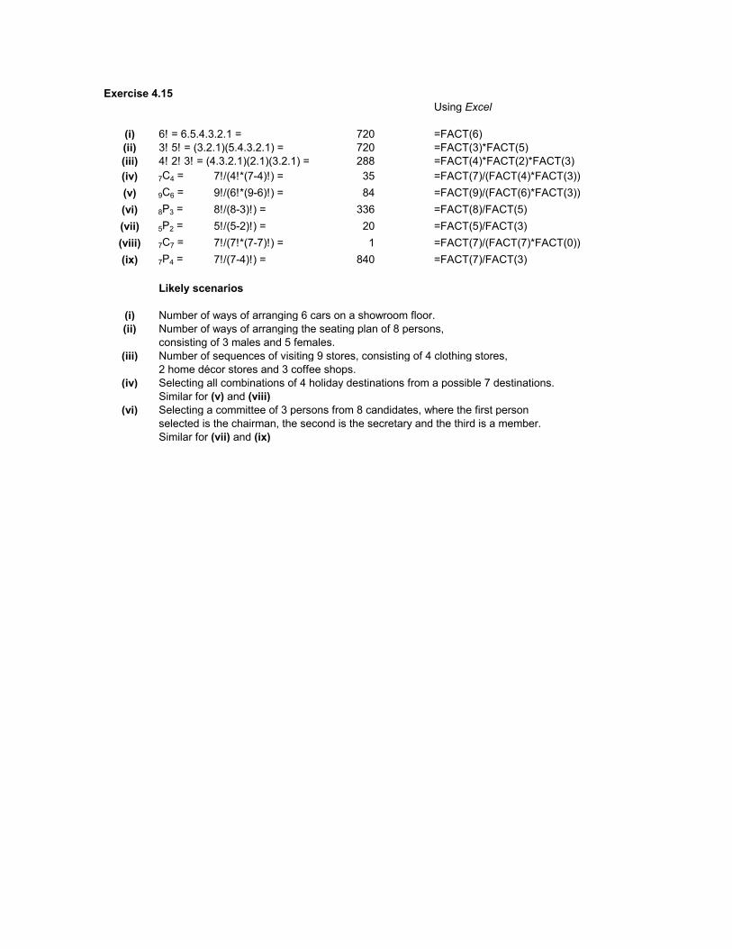
Exercise 4.15 Using Excel
(i) 6! = 6.5.4.3.2.1 = 720 =FACT(6)(ii) 3! 5! = (3.2.1)(5.4.3.2.1) = 720 =FACT(3)*FACT(5)(iii) 4! 2! 3! = (4.3.2.1)(2.1)(3.2.1) = 288 =FACT(4)*FACT(2)*FACT(3)(iv) 7C4 = 7!/(4!*(7-4)!) = 35 =FACT(7)/(FACT(4)*FACT(3))(v) 9C6 = 9!/(6!*(9-6)!) = 84 =FACT(9)/(FACT(6)*FACT(3))(vi) 8P3 = 8!/(8-3)!) = 336 =FACT(8)/FACT(5)(vii) 5P2 = 5!/(5-2)!) = 20 =FACT(5)/FACT(3)(viii) 7C7 = 7!/(7!*(7-7)!) = 1 =FACT(7)/(FACT(7)*FACT(0))(ix) 7P4 = 7!/(7-4)!) = 840 =FACT(7)/FACT(3)
Likely scenarios
(i) Number of ways of arranging 6 cars on a showroom floor.(ii) Number of ways of arranging the seating plan of 8 persons,
consisting of 3 males and 5 females.(iii) Number of sequences of visiting 9 stores, consisting of 4 clothing stores,
2 home décor stores and 3 coffee shops. (iv) Selecting all combinations of 4 holiday destinations from a possible 7 destinations.
Similar for (v) and (viii)(vi) Selecting a committee of 3 persons from 8 candidates, where the first person
selected is the chairman, the second is the secretary and the third is a member. Similar for (vii) and (ix)

Exercise 4.16
Assume each advertisement contains a different combination of 7 out of 12 products.
12C7 = 12!/(7!*(12-7)!) = 792 different combinations
=FACT(12)/(FACT(7)*FACT(5)) (Using Excel )

Exercise 4.17
A different permutation of 3 soup brands on 5 shelves is required.
5P3 = 5!/(5-3)! = 60 distinct ordering of 3 soup brands on 5 shelves.
=FACT(5)/FACT(2) (Using Excel )

Exercise 4.18
(a) 9C4 = 9!/(4!*(9-4)!) = 126 separate portfolios of 4 equities. =FACT(9)/(FACT(4)*FACT(5)) (Using Excel )
(b) P(3,5,7,8) = 1/126 = 0.007937 0,794% chance of getting this combination.

Exercise 4.19
No. of permutations of 5 screws = 5! 5.4.3.2.1 = 120
Thus the probability of replacing them in exactly the same order = 1/120 = 0.00833 (0,833% chance)

Exercise 4.20
(a) 10C3 = 10!/(3!*(10-3)!) = 120 different selections of 3 tourist attractions from 10 options. =FACT(10)/(FACT(3)*FACT(7)) (Using Excel )
(b) P(a given combination of 3 out of 10) = 1/120 = 0.0083 (0,833% chance)

Exercise 4.21
(a) 4C2 x 7C4 = (4!/(2!*2!))*(7!/(4!*3!)) = 210 different committees
=FACT(4)/(FACT(2)*FACT(2))*FACT(7)/(FACT(4)*FACT(3))(Using Excel )
(b) (4C2 x 7C4) x 2 = (4!/(2!*2!))*(7!/(4!*3!)) x 2 = 420 different committees
=2*FACT(4)/(FACT(2)*FACT(2))*FACT(7)/(FACT(4)*FACT(3))(Using Excel )

Exercise 4.22
APPROACH 1
T On time S Scope changeL Late NS No scope change
Marginal probabilities Conditional probabilities Joint probabilities
P(S/T) = 0.4 P(S and T) = 0.28P(T) = 0.7
On time P(NS/T) = 0.6 P(NS and T) = 0.42
Late P(S/L) = 0.8 P(S and L) = 0.24P(L) 0.3
P(NS/L) = 0.2 P(NS and L) = 0.06
1
Bayes Application Using the Joint Probabilities from the Probability Tree
Given P(T) = 0.7 Prior ProbabilityFind P(T/S) = P(T and S)/P(S) = Posterior Probability
(i) P(S) = P(S and T) + P(S and L) = 0.52(ii) P(T and S) = 0.28
Then P(T/S) = P(T and S)/P(S) = 0.5385
There is a 53.85% chance that a 'scope-changed' project will be completed on time.
---ooOoo---
APPROACH 2
S NST 0.28 0.42 0.7 P(T/S) = P(T and S)/P(S)L 0.24 0.06 0.3 =0.28/(0.28+0.24)
0.52 0.48 1 0.5385
---ooOoo---
Project Scoping Study Bayes Theorem
Using a PROBABILITY TREE
Using TABLE FORMAT (Applying Marginals and Conditional Probabilities)
Additional Information
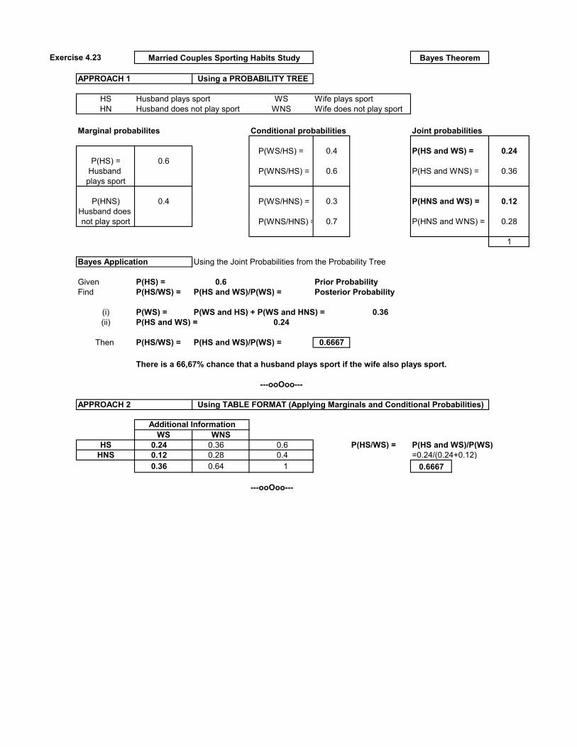
Exercise 4.23
APPROACH 1
HS Husband plays sport WS Wife plays sportHN Husband does not play sport WNS Wife does not play sport
Marginal probabilites Conditional probabilities Joint probabilities
P(WS/HS) = 0.4 P(HS and WS) = 0.24P(HS) = 0.6
Husband P(WNS/HS) = 0.6 P(HS and WNS) = 0.36plays sport
P(HNS) 0.4 P(WS/HNS) = 0.3 P(HNS and WS) = 0.12Husband does not play sport P(WNS/HNS) = 0.7 P(HNS and WNS) = 0.28
1
Bayes Application Using the Joint Probabilities from the Probability Tree
Given P(HS) = 0.6 Prior ProbabilityFind P(HS/WS) = P(HS and WS)/P(WS) = Posterior Probability
(i) P(WS) = P(WS and HS) + P(WS and HNS) = 0.36(ii) P(HS and WS) = 0.24
Then P(HS/WS) = P(HS and WS)/P(WS) = 0.6667
There is a 66,67% chance that a husband plays sport if the wife also plays sport.
---ooOoo---
APPROACH 2
WS WNSHS 0.24 0.36 0.6 P(HS/WS) = P(HS and WS)/P(WS)
HNS 0.12 0.28 0.4 =0.24/(0.24+0.12)0.36 0.64 1 0.6667
---ooOoo---
Married Couples Sporting Habits Study Bayes Theorem
Using a PROBABILITY TREE
Using TABLE FORMAT (Applying Marginals and Conditional Probabilities)
Additional Information
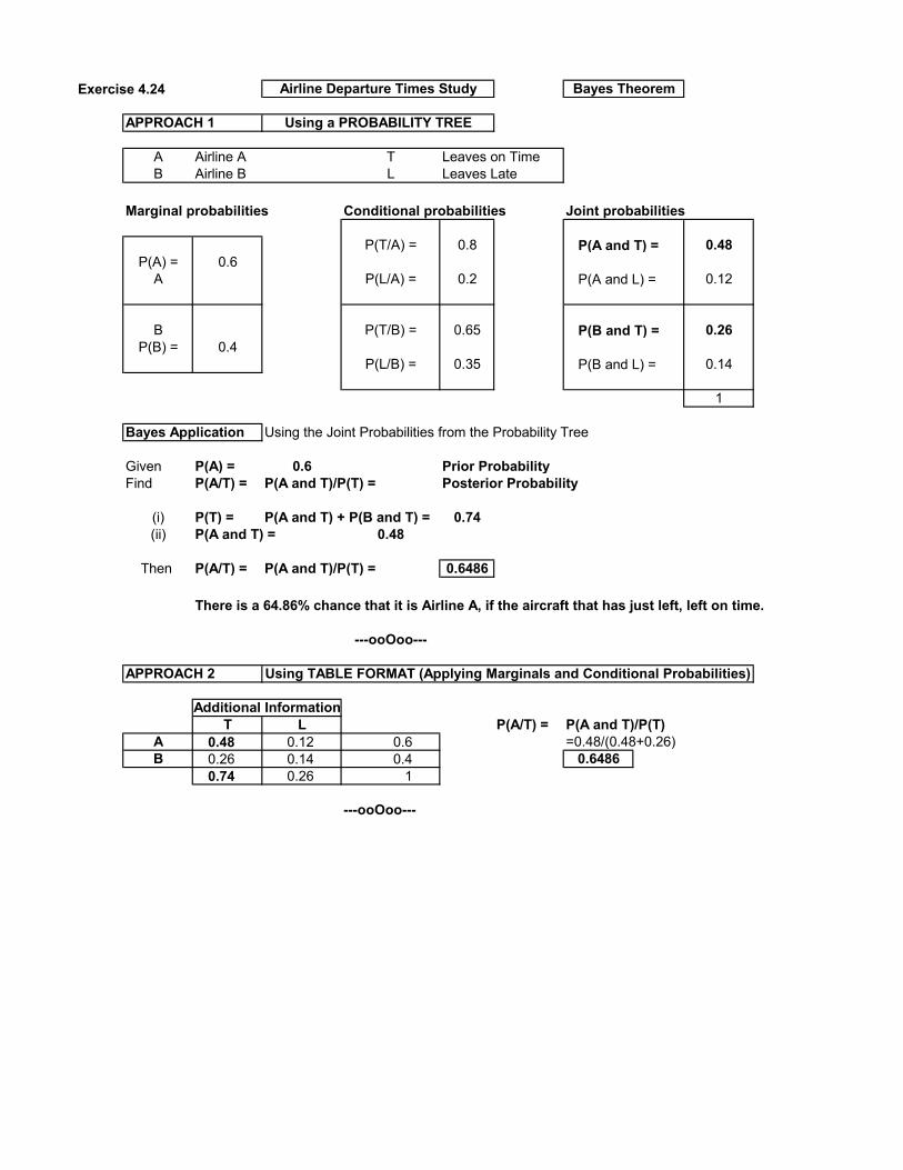
Exercise 4.24
APPROACH 1
A Airline A T Leaves on TimeB Airline B L Leaves Late
Marginal probabilities Conditional probabilities Joint probabilities
P(T/A) = 0.8 P(A and T) = 0.48P(A) = 0.6
A P(L/A) = 0.2 P(A and L) = 0.12
B P(T/B) = 0.65 P(B and T) = 0.26P(B) = 0.4
P(L/B) = 0.35 P(B and L) = 0.14
1
Bayes Application Using the Joint Probabilities from the Probability Tree
Given P(A) = 0.6 Prior ProbabilityFind P(A/T) = P(A and T)/P(T) = Posterior Probability
(i) P(T) = P(A and T) + P(B and T) = 0.74(ii) P(A and T) = 0.48
Then P(A/T) = P(A and T)/P(T) = 0.6486
There is a 64.86% chance that it is Airline A, if the aircraft that has just left, left on time.
---ooOoo---
APPROACH 2
T L P(A/T) = P(A and T)/P(T) A 0.48 0.12 0.6 =0.48/(0.48+0.26)B 0.26 0.14 0.4 0.6486
0.74 0.26 1
---ooOoo---
Airline Departure Times Study Bayes Theorem
Using a PROBABILITY TREE
Using TABLE FORMAT (Applying Marginals and Conditional Probabilities)
Additional Information

Exercise 4.25
APPROACH 1
G NBV started by Graduate S SuccessfulNG NBV started by non-Graduate F Failure
Marginal probabilities Conditional probabilities Joint probabilities
P(S/G) = 0.8 P(G and S) = 0.48P(G) = 0.6
Graduate P(F/G) = 0.2 P(G and F) = 0.12
Nongraduate P(S/NG) = 0.65 P(NG and S) = 0.26P(NG) = 0.4
P(F/NG) = 0.35 P(NG and F) = 0.14
1
Bayes Application Using the Joint Probabilities from the Probability Tree
Given P(G) = 0.6 Prior ProbabilityFind P(G/F) = P(G and F)/P(F) = Posterior Probability
(i) P(F) = P(G and F) + P(NG and F) = 0.26(ii) P(G and F) = 0.12
Then P(G/F) = P(G and F)/P(F) = 0.4615
There is a 46.15% chance that a NBV was started by a Graduate given that it has failed.
---ooOoo---
APPROACH 2
S FG 0.48 0.12 0.6 P(G/F) = P(G and F)/P(F)
NG 0.26 0.14 0.4 =0.12/(0.12+0.14)0.74 0.26 1 0.4615
---ooOoo---
New Business Venture Study Bayes Theorem
Using a PROBABILITY TREE
Using TABLE FORMAT (Applying Marginals and Conditional Probabilities)
Additional Information

Exercise 4.26
APPROACH 1
E e-Ticket purchase B Business TravellerNE non e-Ticket purchase NB non-Business Traveller
Marginal probabilities Conditional probabilities Joint probabilities
P(B/E) = 0.8 P(E and B) = 0.32P(E) = 0.4
e-Ticket P(NB/E) = 0.2 P(E and NB) = 0.08
non-e-Ticket P(B/NE) = 0.45 P(NE and B) = 0.27P(NE) = 0.6
P(NB/NE) = 0.55 P(NB and NB) = 0.33
1Bayes Application Using the Joint Probabilities from the Probability Tree
Given P(E) = 0.4 Prior ProbabilityFind P(E/B) = P(E and B)/P(B) = Posterior Probability
(i) P(B) = P(E and B) + P(NE and B) = 0.59(ii) P(E and B) = 0.32
Then P(E/B) = P(E and B)/P(B) = 0.5424
There is a 54.24% chance that an e-ticket was bought given that it was bought by a business traveller.
---ooOoo---
APPROACH 2
B NBE 0.32 0.08 0.4 P(E/B) = P(E and B)/P(B)
NE 0.27 0.33 0.6 =0.32/(0.32+0.27)0.59 0.41 1 0.5424
---ooOoo---
On-line Airline Tickets Purchase Study Bayes Theorem
Using a PROBABILITY TREE
Using TABLE FORMAT (Applying Marginals and Conditional Probabilities)
Additional Information

CHAPTER 5
PROBABILITY DISTRIBUTIONS
Exercise 5.1 Binomial probability distributionPoisson probability distribution
Exercise 5.2 (a) continuous (e.g. 35.142 gm)(b) discrete (e.g. 132 employees)(c) discrete (e.g. 7046 households)(d) continuous (e.g. 514.68 km)

Exercise 5.3
(a) (i) n = 7; p = 0,2; x = 3 P(x = 3) = 7C3 (0.2)3(0.8)(7-3) =0.1147 11.47%
(a) (ii) n = 10; p = 0,2; x = 4 P(x = 4) = 10C4 (0.2)4(0.8)(10-4) = 0.0881 8.81%
(a) (iii) n = 12; p = 0,3; x ≤ 4 P(x = 0) + P(x = 1) + P(x = 2) + P(x = 3) + P(x = 4)0.01384+0.07118+0.16779+0.2397+0.23114 = 0.7237 72.37%
(a) (iv) n = 10; p = 0,05; x = 2 or 3 P(x = 2) + P(x = 3)0.07464+0.01048 = 0.0851 8.51%
(a) (v) n = 8; p = 0,25; x ≥ 3 1 - (P(x = 0) + P(x = 1) + P(x = 2))1 - (0.10011+0.26697+0.31146) = 0.3215 32.15%
(b) (i) =BINOMDIST(3,7,0.2,0) 0.1147(b) (ii) =BINOMDIST(4,10,0.2,0) 0.0881(b) (iii) =BINOMDIST(4,12,0.3,1) 0.7237(b) (iv) =BINOMDIST(2,10,0.05,0)+BINOMDIST(3,10,0.05,0) 0.0851(b) (v) =1-BINOMDIST(2,8,0.25,1) 0.3215

Exercise 5.4
(a) Binomial distribution There are only two possible outcomes (in-stock; out-of-stock)This outcome is observed 6 times (n = 6 stores)The probability of observing the "out-of-stock" outcome, p = 0.20, is constant.The stores (trials) are independent of each other
(b) P(x = 1) = 6C1 (0.2)1 (0.8)(6-1) = 0.3932 39.32% =BINOMDIST(1,6,0.2,0)
(c) P(x ≤ 2) = P(x = 0) + P(x = 1) + P(x = 2) 0.2621 + 0.3932 + 0.2458 = 0.9011 90.11% =BINOMDIST(2,6,0.2,1)
(d) P(x = 0) = 6C0 (0.2)0 (0.8)(6-0) = 0.2621 26.21% =BINOMDIST(0,6,0.2,0)
(e) Mean (binomial) = 6 x 0.2 = 1.2On average, 1,2 stores out the 6 stores surveyed can be expected to be out of stock in a week.

Exercise 5.5
(a) Binomial distributionn = 12 p = 0.15P(x = 0) = 12C0 (0.15)0 (0.85)(12-0) = 0.1422 =BINOMDIST(0,12,0.15,0)
(b) n = 15 p = 0.15P(x < 3) = P(x = 0) + P(x = 1) + P(x = 2) =
= 0.0874 + 0.2312 + 0.2857 = 0.6042 =BINOMDIST(2,15,0.15,1)

Exercise 5.6
(a) Binomial distributionn = 10 p = 0.30 (probability of preferring the deluxe model)P(x = 3) = 10C3 (0.30)3 (0.70)(10-3) = 0.2668 =BINOMDIST(3,10,0.3,0)
(b) n = 10 p = 0.70 (probability of preferring the standard model)P(x > 2) = 1 - P(x ≤ 2) = 1 - (P(x = 0) + P(x = 1) + P(x = 2)) == 1 - (0.0000059 + 0.000138 + 0.00145) = 0.9984 =1-BINOMDIST(2,10,0.7,1)

Exercise 5.7
(a) Binomial distributionn = 8 p = 0.05 (probability of a defective Tata truck)P(x = 1) = 8C1 (0.05)
1 (0.95)
(8-1) = 0.2793 =BINOMDIST(1,8,0.05,0)
(b) n = 8 p = 0.05 (probability of a defective Tata truck)P(x ≤ 2) = P(x = 0) + P(x = 1) + P(x = 2) =
= 0.66342 + 0.27934 + 0.05146 = 0.9942 =BINOMDIST(2,8,0.05,1)
(c) n = 8 p = 0.05 (probability of a defective Tata truck)P(x = 0) = 8C0 (0.05)
0 (0.95)
(8-0) = 0.6634 =BINOMDIST(0,8,0.05,0)
(d) Mean(binomial) = 64 x 0.05 = 3.2Based on 64 sales, the dealer can expect 3.2 trucks to be returned for assemby defective repairs
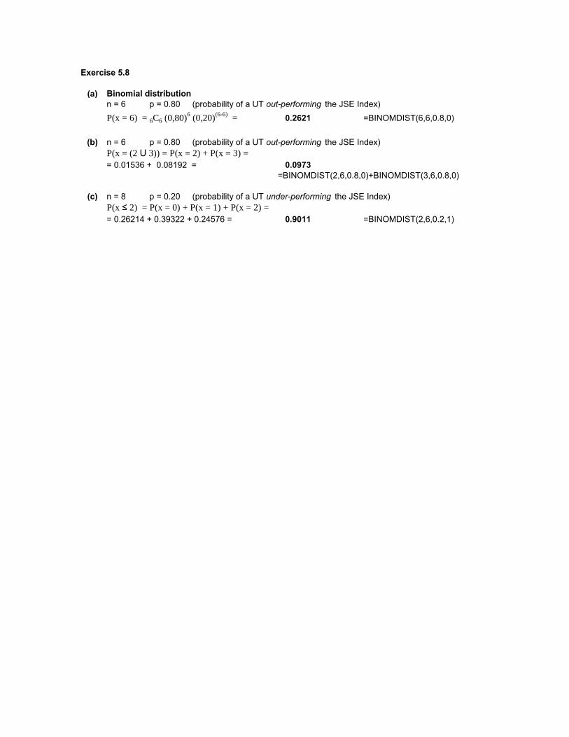
Exercise 5.8
(a) Binomial distributionn = 6 p = 0.80 (probability of a UT out-performing the JSE Index)P(x = 6) = 6C6 (0,80)
6 (0,20)
(6-6) = 0.2621 =BINOMDIST(6,6,0.8,0)
(b) n = 6 p = 0.80 (probability of a UT out-performing the JSE Index)P(x = (2 U 3)) = P(x = 2) + P(x = 3) =
= 0.01536 + 0.08192 = 0.0973=BINOMDIST(2,6,0.8,0)+BINOMDIST(3,6,0.8,0)
(c) n = 8 p = 0.20 (probability of a UT under-performing the JSE Index)P(x ≤ 2) = P(x = 0) + P(x = 1) + P(x = 2) =
= 0.26214 + 0.39322 + 0.24576 = 0.9011 =BINOMDIST(2,6,0.2,1)

Exercise 5.9
(a) Binomial distributionn = 12 p = 0.20 (probability of a person participating in a focus group)P(x = 2) = 12C2 (0.20)
2 (0.80)
(12-2) = 0.2835
=BINOMDIST(2,12,0.2,0)
(b) n = 12 p = 0.20 (probability of a person participating in a focus group)P(x = 5) = 12C5 (0.20)
5 (0.80)
(12-5) = 0.5320
=BINOMDIST(5,12,0.2,0)
(c) n = 12 p = 0.20 (probability of a person participating in a focus group)P(x ≥ 6) = 1 - P(x ≤ 5) = 1 - (P(x=0)+P(x=1)+P(x=2)+P(x=3)+P(x=4)+P(x=5)) =
= 1 - (0.0687 + 0.2062 + 0.2835 + 0.2362 + 0.1329 + 0.0532) = 0.0194=1 - BINOMDIST(5,12,0.2,1)

Exercise 5.10
(a) (i) Binomial distributionn = 10 p = 0.10 (probability of a general population person being a heavy reader )P(x < 2) = P(x=0)+P(x=1) = 10C0(0.10)0(0.90)(10-0) + 10C1(0.10)1(0.90)(10-1)
= 0.34868 + 0.38742 = 0.7361
P(x < 2) = =BINOMDIST(1,10,0.1,1)
(a) (ii) n = 10 p = 0.35 (probability of a pensioner person being a heavy reader )P(x < 2) = P(x=0)+P(x=1) = 10C0(0.35)0(0.65)(10-0) + 10C1(0.35)1(0.65)(10-1)
= 0.01346 + 0.07249 = 0.0860
P(x < 2) = =BINOMDIST(1,10,0.35,1)
(b) n = 280 p = 0.65 (probability of a pensioner person not being a heavy reader )Expected number (mean) of "non-heavy" readers = 280 x 0.65 = 182

Exercise 5.11
(a) Poisson distributionP(x = 5 / a = 3) = e-3 35 / 5! = 0.1008 10.08% =POISSON(5,3,0)
(b) P(x ≥ 4 / a = 3) = 1 - P(x ≤ 3) = 1 - (P(x=0)+P(x=1)+P(x=2)+P(x=3))= 1 - (e-3 30 / 0! +e-3 31 / 1! + e-3 32/ 2! + e-3 33 / 3!)= 1 - (0.04979 + 0.14936 + 0.22404 + 0.22404)= 1 - 0.64723 = 0.3528 35.28% =1-POISSON(3,3,1)
(c) P(x = 0 / a = 3) = e-3 30 / 0! = 0.0498 4.98% =POISSON(0,3,0)

Exercise 5.12
(a) Poisson distributionP(x ≤ 2 / a = 4) = P(x=0)+P(x=1)+P(x=2)
= e-4 40 / 0! +e-4 41 / 1! + e-4 42/ 2! = 0,01832 + 0,07326 + 0,14653 = 0.2381 23.81% =POISSON(2,4,1)
(b) P(x ≥ 4 / a = 4) = 1 - P(x ≤ 3) = 1 - (P(x=0)+P(x=1)+P(x=2)+P(x=3))= 1 - (0,2381 (from (i) above) + e-3 43 / 4!)= 1 - (0,2381 + 0,19537)= 1 - 0,43347 = 0.5665 56.65% =1-POISSON(3,4,1)
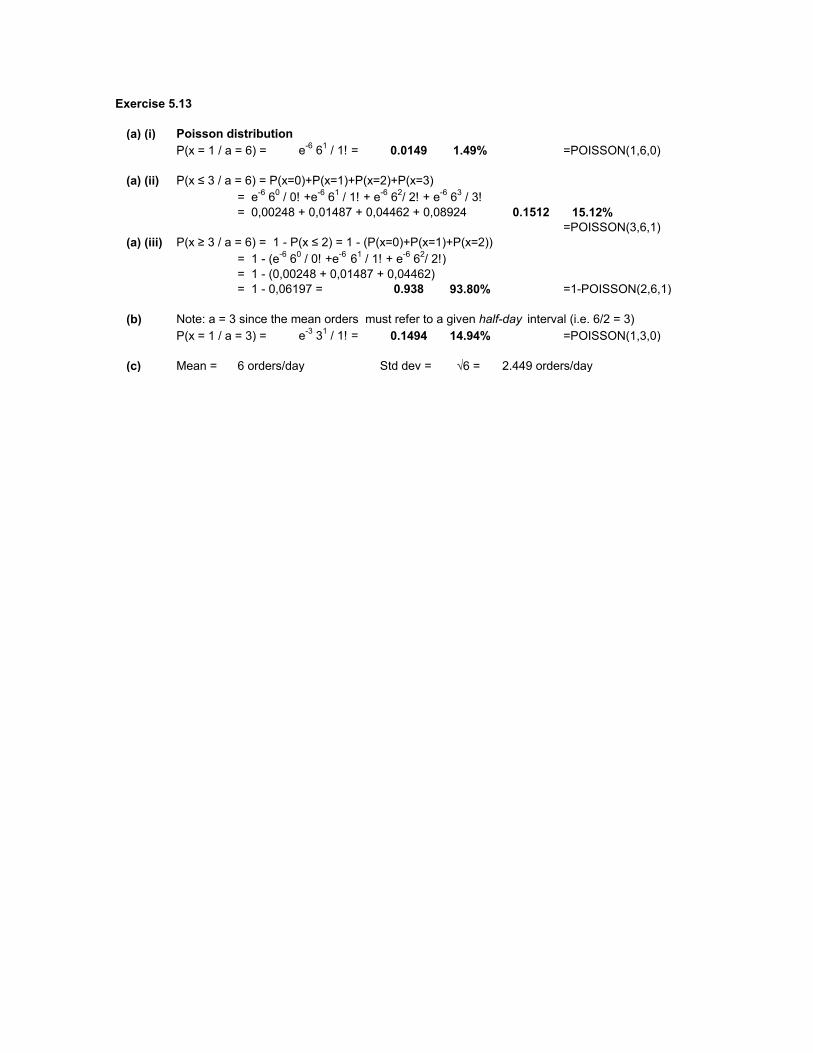
Exercise 5.13
(a) (i) Poisson distributionP(x = 1 / a = 6) = e-6 61 / 1! = 0.0149 1.49% =POISSON(1,6,0)
(a) (ii) P(x ≤ 3 / a = 6) = P(x=0)+P(x=1)+P(x=2)+P(x=3)= e-6 60 / 0! +e-6 61 / 1! + e-6 62/ 2! + e-6 63 / 3!= 0,00248 + 0,01487 + 0,04462 + 0,08924 0.1512 15.12%
=POISSON(3,6,1)(a) (iii) P(x ≥ 3 / a = 6) = 1 - P(x ≤ 2) = 1 - (P(x=0)+P(x=1)+P(x=2))
= 1 - (e-6 60 / 0! +e-6 61 / 1! + e-6 62/ 2!)= 1 - (0,00248 + 0,01487 + 0,04462)= 1 - 0,06197 = 0.938 93.80% =1-POISSON(2,6,1)
(b) Note: a = 3 since the mean orders must refer to a given half-day interval (i.e. 6/2 = 3)P(x = 1 / a = 3) = e-3 31 / 1! = 0.1494 14.94% =POISSON(1,3,0)
(c) Mean = 6 orders/day Std dev = √6 = 2.449 orders/day

Exercise 5.14
(a) Poisson distributionP(x ≥ 3 / a = 1.8) = 1 - P(x ≤ 2) = 1 - (P(x = 0) + P(x = 1) + P(x = 2))
= 1 - (e-1.8 1.80 / 0! + e-1.8 1.81 / 1! + e-1.8 1.82/ 2!)= 1 - (0.1653 + 0.29754 + 0.26778)= 1 - 0.7306 = 0.2694 26.94% =1-POISSON(2,1.8,1)
(b) P(x < 4 / a = 1.8) = P(x ≤ 3) = P(x = 0) + P(x = 1) + P(x = 2) + P(x = 3)= e-1.8 1.80 / 0! + e-1.8 1.81 / 1! + e-1.8 1.82/ 2! + e-1.8 1.83/ 3! = 0.1653 + 0.29754 + 0.26778 + 0.1607 = 0.8913 89.13%
=POISSON(3,1.8,1)

Exercise 5.15
(a) Poisson distributionP(x ≤ 5 / a = 7) = P(x = 0) + P(x = 1) + P(x = 2) + P(x = 3) + P(x = 4) + P(x = 5)= e-7 70 / 0! + e-7 71 / 1! + e-7 72/ 2! + e-7 73/ 3! + e-7 74 / 4! + e-7 75 / 5!= 0.00091 + 0.00638 + 0.02234 + 0.05213 + 0.09123 +0.12772 =
0.3007 30.07% =POISSON(5,7,1)
(b) P(x = 6 or x = 9 / a = 7) = P(x=6) + P(x=9)= e-7 76 / 6! + e-7 79 / 9! = 0.1490 + 0.1014 = 0.2504 25.04%
=POISSON(6,7,0)+POISSON(9,7,0)
(c) Note: a = 14 since the time interval is a given two-day period (i.e. 7 x 2 = 14)P(x > 20 / a = 14) = 1 - P(x ≤ 20) = 1 - (P(x = 0) + P(x = 1) + P(x = 2) + …… + P(x = 19) + P(x = 20))Use Excel only. =1 - POISSON(20,14,1) = = 1 - 0.9521 = 0.0479 4.79%

Exercise 5.16
Normal distribution Use the Standard Normal (z) table(a)
(i) P(0 < z < 1.83) = 0.4664(ii) P(z > -0.48) = 0.5 + P(0 < z < 0.48) = 0.5 + 0.1844 = 0.6844(iii) P(-2.25 < z < 0) = P(0 < z < 2.25) = 0.4878(iv) P(1.22 < z ) = 0.5 - P(0 < z < 1.22) = 0.5 - 0.3888 = 0.1112(v) P(-2.08< z < 0.63) = P(0 < z < 2.08)+P(0 < z < 0.63) = 0,4812 + 0,2357 = 0.7169(vi) P(z < -0.68) = 0.5 - P(0 < z < 0.68) = 0,5 - 0,2517 = 0.2483(vii) P(0.33 < z < 1.5) = P(0 < z < 1.5) - P(0 < z < 0.33) = 0.4332 - 0.1293 = 0.3039
(b) Using Excel(i) =NORMSDIST(1.83)-0.5 0.4664(ii) =1-NORMSDIST(-0.48) 0.6844(iii) =0.5-NORMSDIST(-2.25) 0.4878(iv) =1-NORMSDIST(1.22) 0.1112(v) =NORMSDIST(0.63)-NORMSDIST(-2.08) 0.7169(vi) =NORMSDIST(-0.68) 0.2483(vii) =NORMSDIST(1.5)-NORMSDIST(0.33) 0.3039

Exercise 5.17
Normal distribution Use the Standard Normal (z) table
(a) Look up area z-value(i) P(z < ?) = 0.9147 0.9147 - 0.5 = 0.4147 1.37(ii) P(z > ?) = 0.5319 0.5319 - 0.5 = 0.0319 -0.08
Since area to right of z is greater than 0.5, z must be negative. (iii) P(0 < z < ?) = 0.4015 0.4015 1.29(iv) P(? < z < 0) = 0.4803 0.4803 -2.06(v) P(? < z ) = 0.0985 0.5 - 0.0985 = 0.4015 1.29(vi) P(z < ?) = 0.2517 0.5 - 0.2517 = 0.2483 -0.67
Since area to left of z is less than 0.5, z must be negative. (vii) P(? < z ) = 0.6331 0.6331 - 0.5 = 0.1331 -0.34
Since area to right of z is greater than 0.5, z must be negative.
(b) Using Excel(i) =NORMSINV(0.9147) 1.3703(ii) =NORMSINV(1-0.5319) -0.0800(iii) =NORMSINV(0.5+0.4015) 1.2901(iv) =NORMSINV(0.5-0.4803) -2.0600(v) =NORMSINV(1-0.0985) 1.2901(vi) =NORMSINV(0.2517) -0.6691(vii) =NORMSINV(1-0.6331) -0.3401

Exercise 5.18
Use the Standard normal (z) table μ = 64 σ = 2.5(a)
(i) P(x < 62) = P(z < (62-64)/2.5) = P(z < -0.08) = 0.5 - 0.2881 = 0.2119(ii) P(x > 67.4) = P(z > (67.4-64)/2.5) = P(z > 1.36) = 0.5 - 0.4131 = 0.0869(iii) P(59.6 < x < 62.8) = P((59.6-64)/2.5 < z < (62.8-64)/2.5) = P(-1.76 < z < -0.48) =
0.4608 - 0.1844 = 0.2764(iv) P(x > ?) = 0.1026 Look up area = 0.3974 giving z ≈ 1.267
then x = 64+1.267*2.5 = 67.168 min(v) P(x > ?) = 0.9772 Look up area = 0.9772 - 0.5 = 0.4772 giving z = -2.00
then x = 64-2.00*2.5 = 59 min(vi) P(60.2 < x < ?) = 0.6652 Find P(60.2 < x < 64) = P(-1.52 < z < 0)
giving area = 0.4357. Look up area = 0.6652 - 0.4357 = 0.2295 giving z ≈ 0.611
then x = 64+0.611*2.5 = 65.528 min
(b) Using Excel NORMDIST and NORMINV
(i) =NORMDIST(62,64,2.5,1) 0.2119(ii) =1-NORMDIST(67.4,64,2.5,1) 0.0869(iii) =NORMDIST(62.8,64,2.5,1)-NORMDIST(59.6,64,2.5,1) 0.2764(iv) =NORMINV(1-0.1026,64,2.5) 67.167(v) =NORMINV(1-0.9772,64,2.5) 59.002(vi) =NORMDIST(60.2,64,2.5,1)+0.6652 0.729455
Apply area = 0.729455 to '=NORMINV(0.729455,64,2.5) 65.528

Exercise 5.19 Gym Attendance Duration
Normal distribution x ≡ N(80, 20)
(a) P(x > 120) = P(z > (120-80)/20) = P(z > 2) = 0.5 - 0.4772 = 0.0228 2.28%
(b) P(x < 60) = P(z (60-80)/20) = P(z < -1) = 0.5 - 0.3413 = 0.1587 15.87%
(c) P(x > k) = 0.60 Look up area = 0.60 - 0.50 = 0.10 giving z ≈ -0.253Then x = 80 - 0.253*20 ≈ 74.94 min
Using Excel NORMDIST or NORMINV
(a) =1-NORMDIST(120,80,20,1) 0.0228
(b) =NORMDIST(60,80,20,1) 0.1587
(c) =NORMINV(1-0.6,80,20) 74.93 minutes

Exercise 5.20 Automatic Washing Machine Lifespan
Normal distribution x ≡ N(3.1; 1.1)
(a) P(x < 1) = P(z < (1-3.1)/1.1) = P(z < -1.9091) = 0.5 - 0.4719 = 0.0281 2.81%
(b) (i) P(x > 4) = P(z > (4-3.1)/1.1) = P(z > 0.819) = 0.5 - 0.2939 = 0.2061 20.61%
(b) (ii) P(x > 5.5) = P(z > (5.5-3.1)/1.1) = P(z > 2.182) = 0.5 - 0.4854 = 0.0146 1.46%
(c) P(x < k) = 0.05 Look up area = 0.50 - 0.05 = 0.45 giving z ≈ -1.645Then x = 3.1 - 1.645*1.1 ≈ 1.29 years
Using Excel NORMDIST or NORMINV
(a) =NORMDIST(1,3.1,1.1,1) 0.0281
(b) (i) =1-NORMDIST(4,3.1,1.1,1) 0.2061
(b) (ii) =1-NORMDIST(5.5,3.1,1.1,1) 0.0146
(c) =NORMINV(0.05,3.1,1.1) 1.29 years
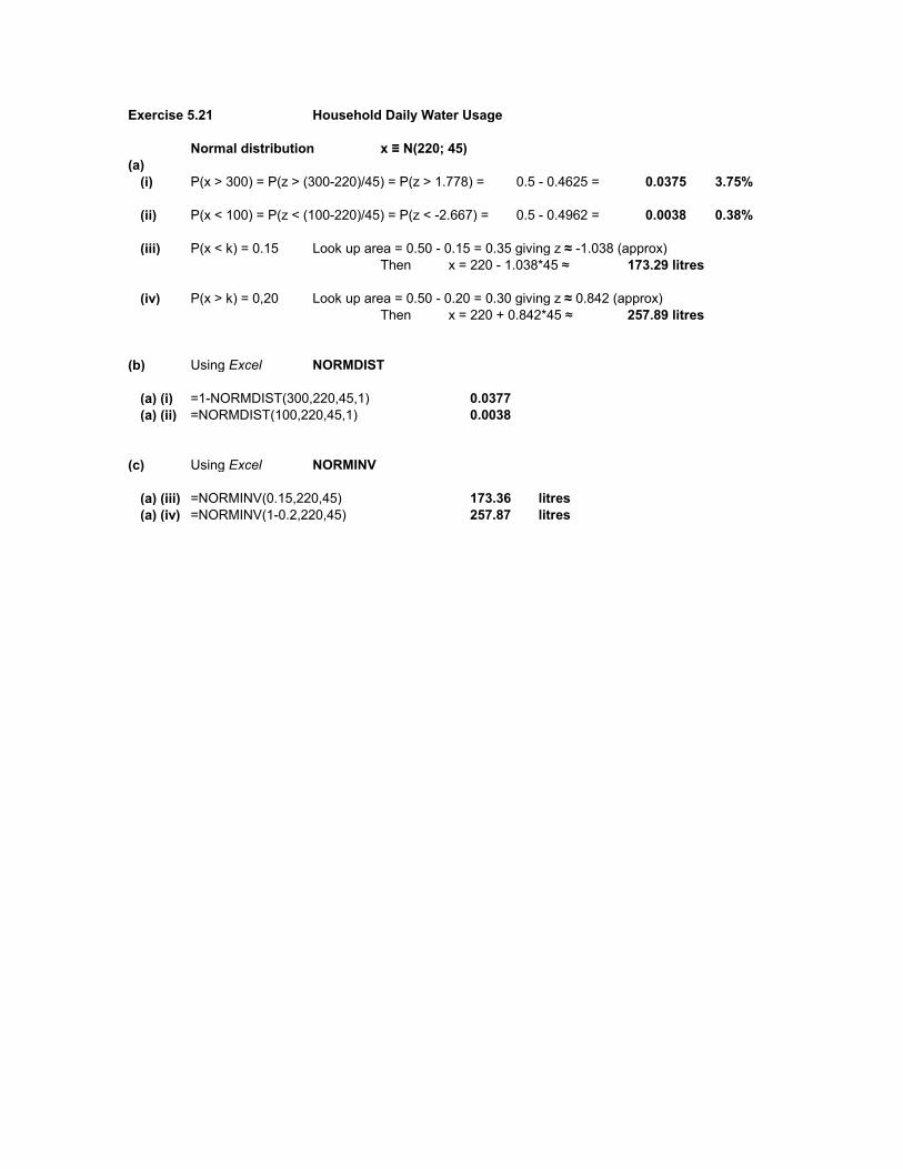
Exercise 5.21 Household Daily Water Usage
Normal distribution x ≡ N(220; 45)(a)
(i) P(x > 300) = P(z > (300-220)/45) = P(z > 1.778) = 0.5 - 0.4625 = 0.0375 3.75%
(ii) P(x < 100) = P(z < (100-220)/45) = P(z < -2.667) = 0.5 - 0.4962 = 0.0038 0.38%
(iii) P(x < k) = 0.15 Look up area = 0.50 - 0.15 = 0.35 giving z ≈ -1.038 (approx)Then x = 220 - 1.038*45 ≈ 173.29 litres
(iv) P(x > k) = 0,20 Look up area = 0.50 - 0.20 = 0.30 giving z ≈ 0.842 (approx)Then x = 220 + 0.842*45 ≈ 257.89 litres
(b) Using Excel NORMDIST
(a) (i) =1-NORMDIST(300,220,45,1) 0.0377(a) (ii) =NORMDIST(100,220,45,1) 0.0038
(c) Using Excel NORMINV
(a) (iii) =NORMINV(0.15,220,45) 173.36 litres(a) (iv) =NORMINV(1-0.2,220,45) 257.87 litres

Exercise 5.22 Long-distance Truck Drivers' Reaction Times
(a) Normal distribution x ≡ N(1.4; 0.25) Variance = 0.0625 Std dev = 0.25
(i) P(x > 2) = P(z > (2-1.4)/0.25) = P(z > 2.4) = 0.5 - 0.4918 =0.0082 0.82%
(ii) P(1.2 < x < 1.4) = P((1.2-1.4)/0.25 < z < (1.4-1.4)/0.25) = P(-0.80 < z < 0) = 0.2881 28.81%
(iii) P(x < 0.9) = P(z < (0.9-1.4)/0.25) = P(z < -2.00) = 0.5 - 0.4772 =0.0228 2.28%
(iv) P(0.5 < x < 1.0) = P((0.5-1.4)/0.25 < z < (1.0-1.4)/0.25) = P(-3.6 < z < -1.6) = 0.49984 - 0.4452 =0.0546 5.46%
(b) P(x > 1.8) = P(z > (1.8-1.4)/0.25) = P(z > 1.6) = 0.5 - 0.4452 =0.0548 5.48%
No. of truck drivers = 120 * 0,0548 = 6,576 drivers 7 drivers (approx)
(c) P(x > 1.7) = P(z > (1.7-1.4)/0.25) = P(z > 1.2) = 0.5 - 0.3849 =0.1151 11.51%
No. of truck drivers = 360 * 0.1151 = 41.436 drivers 42 drivers (approx)
(a) Using Excel NORMDIST
(i) =1-NORMDIST(2,1.4,0.25,1) 0.0082 0.82%(ii) =0.5-NORMDIST(1.2,1.4,0.25,1) 0.2881 28.81%(iii) =NORMDIST(0.9,1.4,0.25,1) 0.0228 2.28%(iv) =NORMDIST(1,1.4,0.25,1)-NORMDIST(0.5,1.4,0.25,1) 0.0546 5.46%
(b) =1-NORMDIST(1.8,1.4,0.25,1) 0.0548 5.48%truck drivers 6.576 7
(c) =1-NORMDIST(1.7,1.4,0.25,1) 0.115truck drivers 41.425 42
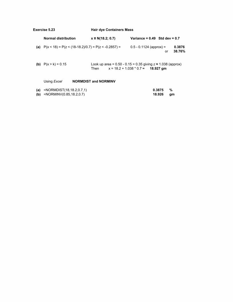
Exercise 5.23 Hair dye Containers Mass
Normal distribution x ≡ N(18.2; 0.7) Variance = 0.49 Std dev = 0.7
(a) P(x < 18) = P(z < (18-18.2)/0.7) = P(z < -0.2857) = 0.5 - 0.1124 (approx) = 0.3876or 38.76%
(b) P(x > k) = 0.15 Look up area = 0.50 - 0.15 = 0.35 giving z ≈ 1.038 (approx)Then x = 18.2 + 1.038 * 0.7 ≈ 18.927 gm
Using Excel NORMDIST and NORMINV
(a) =NORMDIST(18,18.2,0.7,1) 0.3875 %(b) =NORMINV(0.85,18.2,0.7) 18.926 gm

Exercise 5.24 Motor Vehicle Service Time
Normal distribution x ≡ N(70; 9) Variance = 81 Std dev = 9
(a) P(x < 60) = P(z < (60-70)/9) = P(z < -1.11) = 0.5 - 0.3665 = 0.1335 13.35%
(b) P(x > 90) = P(z > (90-70)/9) = P(z > 2.22) = 0.5 - 0.4868 = 0.0132 1.32%
(c) P(50 < x < 60) = P((50-70)/9 < z < (60-70)/9) = P(-2.22 < z < -1.11) = 0.4868 - 0.3665 = 0.1203 12.03%
(d) P(x > 80) = P(z > (80-70)/9) = P(z > 1.11) = 0.5 - 0.3665 = 0.1335 13.35%No. of customers = 0.1335 * 80 = 10.68 customers
(e) P(z > (80-μ)/9) = 0.05 Look up area = 0.50 - 0.05 = 0.45 giving z ≈ 1.645 Then 1.645 = (80 - μ)/9 giving μ = 80 - 1.645 * 9 = 65.195 min
Using Excel NORMDIST
(a) =NORMDIST(60,70,9,1) 0.13326 13.33%
(b) =1-NORMDIST(90,70,9,1) 0.013134 1.31%
(c) =NORMDIST(60,70,9,1)-NORMDIST(50,70,9,1) 0.120126 12.01%
(d) =1-NORMDIST(80,70,9,1) 0.13326 13.33%
(e) This answer cannot be computed from the Excel function NORMDIST.
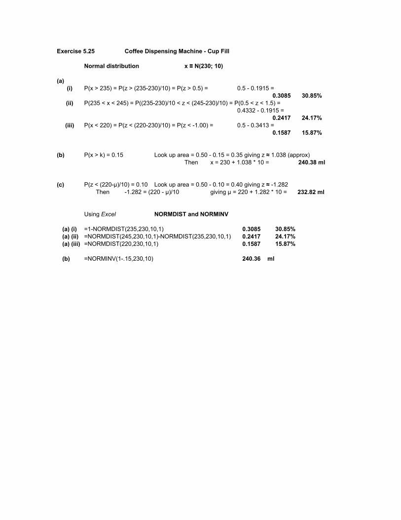
Exercise 5.25 Coffee Dispensing Machine - Cup Fill
Normal distribution x ≡ N(230; 10)
(a)(i) P(x > 235) = P(z > (235-230)/10) = P(z > 0.5) = 0.5 - 0.1915 =
0.3085 30.85%(ii) P(235 < x < 245) = P((235-230)/10 < z < (245-230)/10) = P(0.5 < z < 1.5) =
0.4332 - 0.1915 = 0.2417 24.17%
(iii) P(x < 220) = P(z < (220-230)/10) = P(z < -1.00) = 0.5 - 0.3413 =0.1587 15.87%
(b) P(x > k) = 0.15 Look up area = 0.50 - 0.15 = 0.35 giving z ≈ 1.038 (approx)Then x = 230 + 1.038 * 10 = 240.38 ml
(c) P(z < (220-μ)/10) = 0.10 Look up area = 0.50 - 0.10 = 0.40 giving z ≈ -1.282 Then -1.282 = (220 - μ)/10 giving μ = 220 + 1.282 * 10 = 232.82 ml
Using Excel NORMDIST and NORMINV
(a) (i) =1-NORMDIST(235,230,10,1) 0.3085 30.85%(a) (ii) =NORMDIST(245,230,10,1)-NORMDIST(235,230,10,1) 0.2417 24.17%(a) (iii) =NORMDIST(220,230,10,1) 0.1587 15.87%
(b) =NORMINV(1-.15,230,10) 240.36 ml

Exercise 5.26 Car Battery Lifespan
Normal distribution x ≡ N(28; 4)
(a) P(30 < x < 34) = P((30-28)/4 < z < (34-28)/4) = P(0.50 < z < 1.50) = 0.4332 - 0.1915 = 0.2417
or 24.17%
(b) P(x < 24) = P(z < (24-28)/4) = P(z < -1.00) = 0.5 - 0.3413 = 0.1587or 15.87%
(c) P(x > k) = 0.60 Look up area = 0.60 - 0.50 = 0.10 giving z ≈ -0.253 (approx)Then x = 28 - 0.253 * 4 ≈ 26.988 months
(d) P(z < (x-28)/4) = 0.05 Look up area = 0.50 - 0.05 = 0.45 giving z ≈ -1.645 Then -1.645 = (x - 28)/4 giving x = 28 - 1.645 * 4 = 21.42 months
Using Excel NORMDIST and NORMINV
(a) =NORMDIST(34,28,4,1) - NORMDIST(30,28,4,1) 0.2417 24.17%(b) =NORMDIST(24,28,4,1) 0.1587 15.87%(c) =NORMINV(0.4,28,4) 26.987 26.987 mths(d) =NORMINV(.05,28,4) 21.421 21.421 mths

CHAPTER 6
SAMPLING AND SAMPLING DISTRIBUTIONS
6.1 To generalise sample findings to the target population.
6.2 Sampling methods; Concept of the sampling distribution.
6.3 subset.
6.4 representative.
6.5 Non-probability sampling: sample members are chosen using non-random criteria meaning
that some members of the target population are excluded from being included in the
sample.
Probability sampling: sample members are chosen using random selection processes so that
each target population member stands a chance of being included in the sample.
6.6 Random (probability) sampling methods. Every member of the target population has a
chance of being included in the sample. This is likely to result in a more representative
sample than if a non-probability sampling method was used.
6.7 Unrepresentativeness of the target population;
Not possible to measure sampling error.
6.8 random (chance)
6.9 equal
6.10 Simple random sampling
6.11 Systematic random sampling
6.13 Stratified random sampling
6.14 Cluster random sampling
6.15 It results in a smaller sampling error
6.16 sample statistic; population parameter
6.17 standard error
6.18 95.5%
6.19 Normal
6.20 n = 30 or larger
6.21 Central Limit Theorem.
6.22 Sampling error is the error made when estimating the true population parameter (e.g.
population mean) when using the sample statistic (e.g. sample mean).

CHAPTER 7
CONFIDENCE INTERVAL ESTIMATION
Exercise 7.1 To estimate a population parameter value by defining an Interval within which the true population value is likely to fall at a stated level of confidence.
Exercise 7.2 Use the z-statistic since the population standard deviation, σ is known (Given σ = 8)
Standard error = 8/√64 = 195% Confidence level z(0.95) = 1.96 Use NORMSINV(0.975)Margin of error z x SE 1.96
Lower 95% confidence limit 85 - 1.96(1) 83.04Upper 95% confidence limit 85 + 1.96(1) 86.96
Exercise 7.3 t statistic
Exercise 7.4 Use the t -statistic since the population standard deviation, σ is unknown (Given s = 6)
Standard error (approx) = 6/√25 = 1.2Degrees of freedom = 25 - 1 2490% Confidence level t (0.10,24) = 1.711 Use TINV(0.10,24)Margin of error t x SE 2.91 Note: TINV requires tail probability
Lower 90% confidence limit 54 - 1.711(1.2) 51.95Upper 90% confidence limit 54 + 1.711(1.2) 56.05

Exercise 7.5
(a) Manuallyx(bar) = 24.4 σ = 10.8 n = 144
std error = 10.8/√144 = 0.9z crit (95%) = 1.9695% Confidence level = 1.96 *0.9 = 1.764
Lower 95% confidence limit 24.4 - 1.764 = 22.636Upper 95% confidence limit 24.4 + 1.764 = 26.164
Interpretation There is a 95% chance that the interval (22.636 to 26.164) covers the actual average number of employees per SME in Gauteng.
(b) z-crit (0.95) =NORMSINV(0.975) = 1.96
(c) 95% Confidence level =CONFIDENCE(0.05,10.8,144) 1.764

Exercise 7.6
(a) Manuallyx(bar) = 131.6 σ = 25 n = 87
std error = 2.68 25/√87 = 2.68z crit (90%) = 1.64590% Confidence level = 1.645*2.68 4.409
Lower 90% confidence limit 131.6 - 4.409 = 127.191Upper 90% confidence limit 131.6 + 4.409 = 136.009
InterpretationThere is a 90% chance that the interval (127.191 to 136.009) covers theactual average no. of palettes per order received by a sugar mill in Durban.
(b) z-crit (0.90) =NORMSINV(0.95) 1.645
(c) 90% Confidence level =CONFIDENCE(0.10,131.6,87) 4.409
(d) 90% confidence limits of total palettes shipped in a year
Lower 90% limit 127.191*720 = 91577.52 palettesUpper 90% limit 136.009*720 = 97926.48 palettes
InterpretationTotal palettes shipped in a year, on average, is likely to be between 91 577 and 97 926 palettes, with 90% confidence.

Exercise 7.7
(a) Manuallyx(bar) = R356 σ = R44 n = 256
std error = 44/√256 = 2.75z crit (95%) = 1.9695% Confidence level = 1.96 * 2.75 = 5.39
Lower 95% confidence limit 356 - 5.39 = R350.61Upper 95% confidence limit 356 + 5.39 = R361.39
InterpretationThere is a 95% chance that the interval (R350.61 to R361.39) covers theactual average monthly car insurance premium of medium-sized cars.
(b) z crit (90%) = 1.64590% Confidence level = 1.645*2.75 = 4.524
Lower 90% confidence limit 356 - 4,524 = R351.48Upper 90% confidence limit 356 + 4,524 = R360.52
InterpretationThere is a 90% chance that the interval (R351.48 to R360.52) covers theactual average monthly car insurance premium of medium-sized cars.
The 90% confidence interval limits are closer together than the 95% confidence interval limits.The lower confidence results in a more precise set of interval limits (narrower).
(c) z-crit (0.95) =NORMSINV(0.975) 1.96
(d) 95% Confidence level =CONFIDENCE(0.05,44,256) 5.3899
(e) 95% confidence limits of total monthly premium income
Lower 95% confidence limit 350.61*3000 R1 051 830Upper 95% confidence limit 361.39*3000 R1 084 170
InterpretationTotal monthly premium income, on average, is likely to be between R1 051 830 and R1 084 170 with 95% confidence.

Exercise 7.8
(a) Manuallyx(bar) = 4.985 σ = 0.04 n = 50
std error = 0.04/√50 = 0.005657z crit (99%) = 2.5899% Confidence level = 2.58 * 0.005657 = 0.01460
Lower 99% confidence limit 4.985 - 0.0146 = 4.9704Upper 99% confidence limit 4.985 + 0.0146 = 4.9996
InterpretationThere is a 99% chance that the interval (4.97 litres to 4.9996 litres)covers the actual average volume of paint in all five-litre cans.
(b) Yes, the store owner has statistical evidence to confirm that the average volume of paint in 5-litre cans is most likely to be below 5 litres.
(c) z-crit (0.99) =NORMSINV(0.995) 2.576
(d) 99% Confidence level =CONFIDENCE(0.01,0.04,50) 0.0146

Exercise 7.9
(a) Manuallyx(bar) = 3.8 σ = 0.6 n = 24
std error = 0,122474 0.6/√24 = 0.122474z crit (90%) = 1.64590% Confidence level = 0.20147
Lower 90% confidence limit 3.8 - 0.20147 = 3.599Upper 90% confidence limit 3.8 + 0.20147 = 4.001
InterpretationThere is a 90% chance that the interval (3.599 to 4.001) coversthe actual average inventory turnover rate of all convenience stores.
(b) z-crit (0.90) =NORMSINV(0.95) 1.645
(c) 90% Confidence level =CONFIDENCE(0.10,0.6,24) 0.20145

Exercise 7.10
(a) Manuallyx(bar) = 166.2 s = 22.8 n = 21
std error (estimated) = 22.8/√21 = 4.975368t crit (95%,20) 2.08695% Confidence level = 10.3786
Lower 95% confidence limit 166.2 - 10.3786 155.82Upper 95% confidence limit 166.2 + 10.3786 176.58
Interpretation There is a 95% chance that between 155.8 and 176.6 calls, onaverage, will be received by the call centre daily.
(b) Manuallyx(bar) = 166.2 s = 22.8 n = 21
std error (estimated) = 22.8/√21 = 4.975368t crit (99%,20) 2.84599% Confidence level = 14.1549
Lower 99% confidence limit 166.2 - 14.1549 152.05Upper 99% confidence limit 166.2 + 14.1550 180.35
Interpretation There is a 99% chance that between 152.1 and 180.4 calls, onaverage, will be received by the call centre daily.
(c) The 95% confidence interval is more precise (narrower), but less reliable than the 99% confidence interval which is less precise (wider), but more reliable.
(d) t-crit (0.95, 20) =TINV(0.05,20) 2.0860
(e) Over a 30 day period Lower 95% confidence limit 155.82*30 = 4674.60Upper 95% confidence limit 176.58*30 = 5297.40
Interpretation There is a 95% chance that between 4675 and 5298 calls, onaverage, will be received over a 30-day period.

Exercise 7.11
(a) Manuallyx(bar) = 12.5 s = 3.4 n = 28
std error (estimated) = 3.4/√28 = 0.64254t crit (90%, 27) 1.70390% Confidence level = 1.0943
Lower 90% confidence limit 12.5 - 1.0943 = 11.406Upper 90% confidence limit 12.5 + 1.0943 = 13.594
Interpretation There is a 90% chance that the actual mean dividend yield of all JSE-listed companies lies between 11.41% and 13.59%.
(b) t-crit (0.90, 27) =TINV(0.10,27) 1.7033

Exercise 7.12
(a) Manuallyx(bar) = 0.981 s = 0.052 n = 18
std error (estimated) = 0.052/√18 = 0.01226t crit (99%, 17) = 2.898299% Confidence level = 0.0355
Lower 99% confidence limit 0.981 - 0.0355 = 0.9455Upper 99% confidence limit 0.981 + 0.0355 = 1.0165
Interpretation There is a 99% chance that the average fill of 1-litre cartonsof milk lies between 0.9455 litres and 1.0165 litres.
Since the interval covers 1 litre, it can be concluded thatthe cartons do contain one litre of milk on average.
(b) Manuallyx(bar) = 0.981 s = 0.052 n = 18
std error (estimated) = 0.052/√18 = 0.01226t crit (95%, 17) = 2.109895% Confidence level = 0.0259
Lower 95% confidence limit 0.981 - 0.0259 = 0.9551Upper 95% confidence limit 0.981 + 0.0259 = 1.0069
Interpretation There is a 95% chance that the average fill of 1-litre cartonsof milk lies between 0.9551 litres and 1.0069 litres.
The 95% confidence interval is more precise (narrower), but less reliable than the 99% confidence interval which is less precise (wider), but more reliable.
(c) t-crit (0.99, 17) =TINV(0.01,17) 2.8982t-crit (0.95, 17) =TINV(0.05,17) 2.1098

Exercise 7.13
(a) Manuallyx(bar) = 1420 s = 160 n = 50
std error (estimated) = 160/√50 = 22.62742t crit (90%, 49) = 1.676 (use df = 50 from Table 2, Appendix)90% Confidence level = 37.9235
Lower 90% confidence limit 1420 - 37.9235 = 1382.08Upper 90% confidence limit 1421 + 37.9235 = 1457.92
Interpretation There is a 90% chance that the average monthly wage of union members lies between R1382.08 and R1457.92.
(b) Manuallyx(bar) = 1420 s = 160 n = 50
std error (estimated) = 160/√50 = 22.62742t crit (99%, 49) = 2.678 (use df = 50 from Table 2, Appendix)99% Confidence level = 60.5962
Lower 99% confidence limit 1420 - 60.5962 = 1359.4Upper 99% confidence limit 1420 + 60.5962 = 1480.6
Interpretation There is a 99% chance that the average monthly wage of union members lies between R1359.40 and R1480.60.
(c) The 90% confidence interval is more precise (narrower), but less reliable than the 99% confidence interval which is less precise (wider), but more reliable.
(d) t-crit (0.90, 49) =TINV(0.10,49) 1.6766t-crit (0.99, 49) =TINV(0.01,49) 2.6800
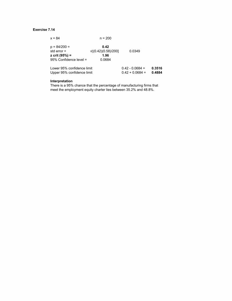
Exercise 7.14
x = 84 n = 200
p = 84/200 = 0.42std error = √[(0.42)(0.58)/200] 0.0349z crit (95%) = 1.9695% Confidence level = 0.0684
Lower 95% confidence limit 0.42 - 0.0684 = 0.3516Upper 95% confidence limit 0.42 + 0.0684 = 0.4884
InterpretationThere is a 95% chance that the percentage of manufacturing firms thatmeet the employment equity charter lies between 35.2% and 48.8%.

Exercise 7.15
x = 68 n = 160
p = 68/160 = 0.425std error = √[(0.425)(0.575)/160] = 0.03908z crit (95%) = 1.9695% Confidence level = 0.0766
Lower 95% confidence limit 0.425 - 0.0766 = 0.3484Upper 95% confidence limit 0.425 + 0.0766 = 0.5016
InterpretationThere is a 95% chance that the percentage of cash-paying customerslies between 34.8% and 50.2%.

Exercise 7.16
x = (365-78) = 287 n = 365
p = 287/365 = 0.786std error = √[(0.786)*(0.214)/365] = 0.021467z crit (90%) = 1.64590% Confidence level = 0.03532
Lower 90% confidence limit 0.786 - 0.0353 = 0.7507Upper 90% confidence limit 0.786 + 0.0353 = 0.8213
InterpretationThere is a 90% chance that the percentage of non-overdrawn cheque accountsat the Tshwane branch lies between 75.1% and 82.1%.

Exercise 7.17
x = 120 n = 300
p = 120/300 = 0.4std error = √[(0.4)*(0.6)/300] = 0.02828z crit (90%) = 1.64590% Confidence level = 0.04652
Lower 90% confidence limit 0.4 - 0.04652 = 0.3535Upper 90% confidence limit 0.4 + 0.04652 = 0.4465
InterpretationThere is a 90% chance that the percentage of shoppers who frequent a shoppingmall primarily because of its store mix lies between 35.4% and 44.7%.

Exercise 7.18 File: X7.18 - cashier absenteeism.xlsx
(a) Descriptive Statistics - Absent Days (Using Data Analysis in Excel )
Absent Days
Mean 9.379Standard Error 0.625Median 9Mode 7Standard Deviation 3.364Sample Variance 11.315Kurtosis -0.919Skewness -0.009Range 12Minimum 3Maximum 15Sum 272Count 29Confidence Level (95.0%) 1.280
The average number of days absent was 9.4 days. 68% of employees were absent between 6 and 12.7 days (within 1 std dev). The data is symmetrical about the mean (skewness = -0.009). Absenteeism per employee ranged between 3 (min) and 15 days (max) last year.
(b) Lower 95% Confidence Limit 9.379 - 1.28 = 8.10Upper 95% Confidence Limit 9.379 + 1.28 = 10.66
InterpretationThere is a 95% chance that the average number of days absent last year by all cashiers in a supermarket was between 8.1 days and 10.7 days.
(c) Since the 95% confidence interval covers 10 days (8.1 < μ < 10.66), it is possible that the mean number of days absent per employee does exceed 10 days. Thus the company's policy is not being strictly adhered to.
(d) t-crit (0.95, 28) =TINV(0.05,28) 2.0484Given standard error = 0.6250Confidence level (95%) = 0.625 * 2.0484 = 1.2803
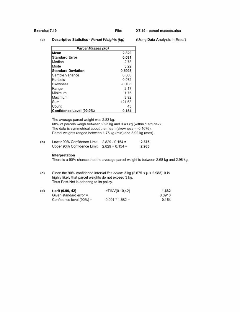
Exercise 7.19 File: X7.19 - parcel masses.xlsx
(a) Descriptive Statistics - Parcel Weights (kg) (Using Data Analysis in Excel )
Mean 2.829Standard Error 0.091Median 2.78Mode 3.22Standard Deviation 0.5998Sample Variance 0.360Kurtosis -0.972Skewness -0.108Range 2.17Minimum 1.75Maximum 3.92Sum 121.63Count 43Confidence Level (90.0%) 0.154
The average parcel weight was 2.83 kg. 68% of parcels weigh between 2.23 kg and 3.43 kg (within 1 std dev). The data is symmetrical about the mean (skewness = -0.1076). Parcel weights ranged between 1.75 kg (min) and 3.92 kg (max).
(b) Lower 90% Confidence Limit 2.829 - 0.154 = 2.675Upper 90% Confidence Limit 2.829 + 0.154 = 2.983
InterpretationThere is a 90% chance that the average parcel weight is between 2.68 kg and 2.98 kg.
(c) Since the 90% confidence interval lies below 3 kg (2.675 < μ < 2.983), it is highly likely that parcel weights do not exceed 3 kg.Thus Post-Net is adhering to its policy.
(d) t-crit (0.90, 42) =TINV(0.10,42) 1.682Given standard error = 0.0910Confidence level (90%) = 0.091 * 1.682 = 0.154
Parcel Masses (kg)
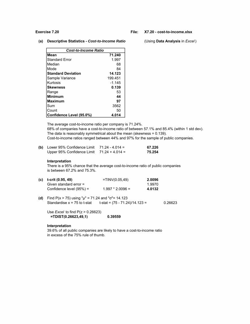
Exercise 7.20 File: X7.20 - cost-to-income.xlsx
(a) Descriptive Statistics - Cost-to-Income Ratio (Using Data Analysis in Excel )
Mean 71.240Standard Error 1.997Median 68Mode 84Standard Deviation 14.123Sample Variance 199.451Kurtosis -1.145Skewness 0.139Range 53Minimum 44Maximum 97Sum 3562Count 50Confidence Level (95.0%) 4.014
The average cost-to-income ratio per company is 71.24%.68% of companies have a cost-to-income ratio of between 57.1% and 85.4% (within 1 std dev). The data is reasonably symmetrical about the mean (skewness = 0.139). Cost-to-income ratios ranged between 44% and 97% for the sample of public companies.
(b) Lower 95% Confidence Limit 71.24 - 4.014 = 67.226Upper 95% Confidence Limit 71.24 + 4.014 = 75.254
InterpretationThere is a 95% chance that the average cost-to-income ratio of public companies is between 67.2% and 75.3%.
(c) t-crit (0.95, 49) =TINV(0.05,49) 2.0096Given standard error = 1.9970Confidence level (95%) = 1.997 * 2.0096 = 4.0132
(d) Find P(x > 75) using "μ" = 71.24 and "σ"= 14.123Standardise x = 75 to t-stat t-stat = (75 - 71.24)/14.123 = 0.26623
Use Excel to find P(z > 0.26623) =TDIST(0.26623,49,1) 0.39559
Interpretation39.6% of all public companies are likely to have a cost-to-income ratioin excess of the 75% rule of thumb.
Cost-to-Income Ratio
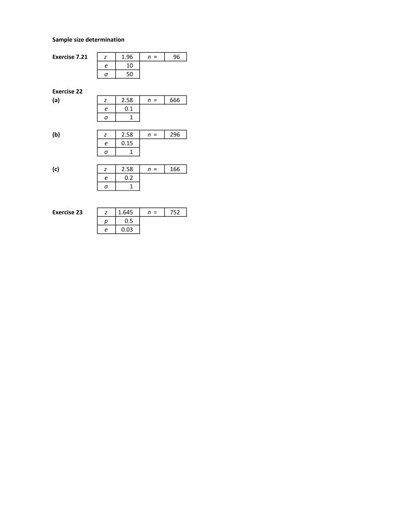
Sample size determination
Exercise 7.21 z 1.96 n = 96
e 10
σ 50
Exercise 22
(a) z 2.58 n = 666
e 0.1
σ 1
(b) z 2.58 n = 296
e 0.15
σ 1
(c) z 2.58 n = 166
e 0.2
σ 1
Exercise 23 z 1.645 n = 752
p 0.5
e 0.03

CHAPTER 8
HYPOTHESIS TESTS
SINGLE POPULATION (MEANS, PROPORTIONS AND VARIANCES)
Exercise 8.1 To test whether a claim / statement made about a population parameter
value is probably true or false, based on sample evidence.
Exercise 8.2 The “closeness” of the sample statistics to the claimed population parameter value.
Exercise 8.3 The Five Steps of Hypothesis TestingStep 1: Define the statistical hypotheses (the null and alternative hypotheses).Step 2: Determine the region of acceptance of the null hypothesis. Step 3: Compute the sample test statistic.Step 4: Compare the sample test statistic to the region of acceptance.Step 5: Draw the statistical and management conclusions.
Exercise 8.4 Level of significance (α)
(and sample size when the population standard deviation is unknown)
Exercise 8.5 Reject H0 in favour of H1 at the 5% level of significance.

Exercise 8.6
(i) H0: µ ≤ 560 H1: µ > 560x (bar) = 577 σ = 86 n = 120 α = 0.05
(a) One-sided upper tailed test Use z test statistic since σ is known.
Area of Acceptance z ≤ 1.645 Read off 0.45 from z-table; or =NORMSINV(0.95) [using Excel ]
(b) z-stat = (577-560)/(86/√(120) = 2.165
Since z-stat (2.165) > z-crit (1.645), there is sufficient sample evidence at the 5% level of significance to reject H0 in favour of H1. (i.e. Reject H0)Conclude that the population mean value is significantly larger than 560.
(c) p -value = P(z > 2.165) = 0.5 - 0.4848 = 0.0152 From z-table; or=1-NORMSDIST(2.165)
(ii) H0: π ≥ 0.72 H1: π < 0.72x = 216 n = 330 α = 0.10 Derive p = 216/330 = 0,6545
(a) One-sided lower tailed test Use z test statistic for proportions
Area of Acceptance z ≥ -1.28 Read off 0.4 from z-table; or=NORMSINV(0.9) [using Excel ]
(b) z-stat = (0.6545 - 0.72)/√[(0.72)(1-0.72)/330] = -2.65
Since z-stat (-2.65) < z-crit (-1.28), there is sufficient sample evidence at the 10% level of significance to reject H0 in favour of H1. (i.e. Reject H0)Conclude that the true population proportion is significantly less than 0.72.
(c) p -value = P(z < -2.65) = 0.5 - 0.496 = 0.0040 From z-table; or=NORMSDIST(-2.65)
(iii) H0: µ = 8.2 H1: µ ≠ 8.2x (bar) = 9.6 s = 2.9 n = 30 α = 0.01
(a) Two-sided test Use t test statistic since σ is unknown (only given the sample standard deviation, s and n is small (n < 30))
Area of Acceptance -2.756 ≤ t ≤ +2.756 Read off T(0.005,29) from t-table;or '=TINV(0.01,29) [using Excel ]
(b) t-stat = (9.6 - 8.2)/(2.9)/√(30) = 2.644
Since t-stat (2.644) falls within the area of acceptance, there is insufficient sampleevidence at the 1% level of significance to reject H0 in favour of H1. (i.e. Accept H0)Conclude that the true mean value is equal to 8.2.
(c) p -value = 2 x P(t > 2.644) = 0.0131 =TDIST(2.644,29,2)

(iv) H0: µ ≥ 18 H1: µ < 18x (bar) = 14.6 s = 3.4 n = 12 α = 0.01
(a) One-sided lower tailed test Use t test statistic since σ is unknown (only have the sample stardard deviation, s and n is small (n < 30))
Area of Acceptance t ≥ -2.718 Read off T(0.01,11) from t-table;or '=TINV(0.02,11) [using Excel ]
(b) t-stat = (14.6 - 18)/(3.4)/√(12) = -3.464
Since t-stat (-3.464) < t-crit (-2.718), there is sufficient sample evidence at the 1% level of significance to reject H0 in favour of H1. (Reject H0)Conclude that the true mean value is significantly below 18.
(c) p -value = P(t < -3.464) = 0.0026 '=TDIST(-(-3.464),11,1)
(v) H0: π = 0.32 H1: π ≠ 0.32x = 68 n = 250 α = 0.05 Derive p = 68/250 = 0.272
(a) Two-sided test Use z test statistic for proportions
Area of Acceptance -1.96 ≤ z ≤ +1.96 Read off z(0.975) from z-table; or=NORMSINV(0.975) [Excel ]
(b) z-stat = (0.272 - 0.32)/√[(0.32)(1-0.32)/250] = -1.627
Since z-stat (-1.627) falls within the area of acceptance, there is insufficient sample evidence at the 5% level of significance to reject H0 in favour of H1. (i.e. Accept H0)Conclude that the true population proportion is equal to 0.32.
(c) p -value = 2 x P(z < -1.627) = 0.1037 '=2*NORMSDIST(-1.627)

Exercise 8.7
(a) H0: µ = 85 H1: µ ≠ 85 Two-sided test
(b) Use the z test statistic since σ is known (σ = 25 min (given))
(c) Use α = 0.05Area of Acceptance -1.96 ≤ z ≤ 1.96 Read off 0.475 from z-table; or
=NORMSINV(0.975) [using Excel]
z-stat = (80.5 - 85)/(25/√(132) = -2.068
Statistical conclusionSince z-stat (-2.068) lies below -z-crit (-1.96), there is sufficient sample evidence at the 5% level of significance to reject H0 in favour of H1. (i.e. Reject H0).
Management conclusionConclude that the population mean value is significantly different from 85 minutes.Visitors to the Knysna shopping mall do not spend 85 minutes on average in the mall.
(d) p -value = 2 x P(z < -2.068) = 0.0386 =NORMSDIST(-2.068) x 2
(e) Since p -value (0.0386) < α (0.05), there is strong sample evidence to conclude that visitors to the Knysna shopping mall do not spend 85 minutes, on average, in the mall.
By inspection of the sample mean, it appears that visitors to the Knysa shopping mall spend significantly less than 85 minutes in the mall.

Exercise 8.8
(a) H0: µ ≥ 30 min H1: µ < 30 min One-sided lower tailed test
(b) Use the z test statistic since σ is known (σ = 10.5 min (given))
(c) Use α = 0.01Area of Acceptance z ≥ -2.33 Read off 0.49 from z-table; or
=NORMSINV(0.01) [using Excel]
z-stat = (27.9 - 30)/(10.5/√(86)) = -1.855
Statistical conclusionSince z-stat (-1.855) lies above z-crit (-2.33), there is insufficient sample evidence at the 1% level of significance to reject H0 in favour of H1 (Do not reject H0).
Management conclusionConclude that the population mean value is at least 30 minutes.The supermarket manager's belief is therefore valid.
(d) p -value = P(z < -1.855) = 0.0318 =NORMSDIST(-1.855)Since p -value (0.0318) > α (0.01) the sample evidence does not refute H0.
The sample evidence is not strong enough to refute the belief that customersspend 30 minutes or more, on average, doing their purchases at the supermarket. Hence conclude that customers are likely to spend at least half-an-hour, on average, in the supermarket doing their grocery shopping.

Exercise 8.9
(a) H0: µ ≤ 72 hours H1: µ > 72 hours One-sided upper tailed test
(b) Use the z test statistic since σ is known (σ = 18 hours (given))
Use α = 0.10Area of Acceptance z ≤ 1.28 Read off 0.40 from z-table; or
=NORMSINV(0.90) [using Excel]
z-stat = (75.9 - 72)/(18/√(46)) = 1.470
Statistical conclusionSince z-stat (1.47) > z-crit (1.28), there is sufficient sample evidence at the 10% level of significance to reject H0 in favour of H1 (Reject H0).
Management conclusionConclude that the local importer's claim is valid.Consignments are taking significantly longer than 72 hours to clear customs.
(c) p -value = P(z > 1.47) = 0.0708 =1-NORMSDIST(1.47)Since p -value (0.0708) < α (0.10) this confirms support for H1.
There is moderate sample evidence (relative to α = 0.10) to conclude that consignment clearance times, on average, are significantly longer than 72 hours.
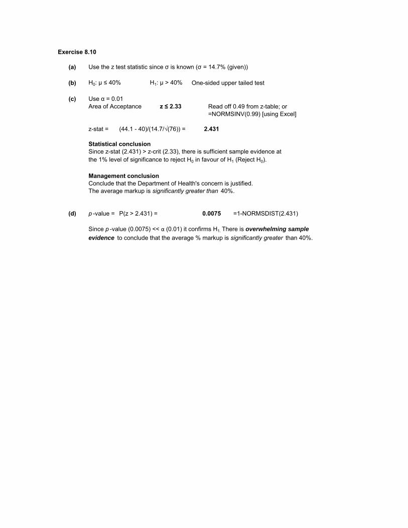
Exercise 8.10
(a) Use the z test statistic since σ is known (σ = 14.7% (given))
(b) H0: µ ≤ 40% H1: µ > 40% One-sided upper tailed test
(c) Use α = 0.01Area of Acceptance z ≤ 2.33 Read off 0.49 from z-table; or
=NORMSINV(0.99) [using Excel]
z-stat = (44.1 - 40)/(14.7/√(76)) = 2.431
Statistical conclusionSince z-stat (2.431) > z-crit (2.33), there is sufficient sample evidence at the 1% level of significance to reject H0 in favour of H1 (Reject H0).
Management conclusionConclude that the Department of Health's concern is justified.The average markup is significantly greater than 40%.
(d) p -value = P(z > 2.431) = 0.0075 =1-NORMSDIST(2.431)
Since p -value (0.0075) << α (0.01) it confirms H1. There is overwhelming sample
evidence to conclude that the average % markup is significantly greater than 40%.

Exercise 8.11
(a) Use the t test statistic since σ is unknown (only s = 21 gms is given)
H0: µ = 700 gms H1: µ ≠ 700 gms Two-sided test
Use α = 0.05 with degrees of freedom = (n -1) = 63Area of Acceptance -2.00 ≤ t ≤ 2.00 Read off t(0.025,63) from t-table; or
'=TINV(0.05,63) [using Excel]
t-stat = (695 - 700)/(21/√(64)) = -1.905
Statistical conclusionSince t-stat (-1,905) lies within the acceptance area, there is insufficient sample evidence at the 5% level of significance to reject H0 in favour of H1 (i.e. Accept H0)
Management conclusionConclude that Ryeband Bakery is both legally compliant and not wasting ingredients.The average weight of all white loaves produced by Ryeband Bakery is 700 gms.
(b) p -value = 2 x P(t < -1.905) = 0.0613 =TDIST(-(-1.905),63,2)
Since p -value (0.0613) > α (0.05) H0 cannot be rejected as the sample evidenceis weak in favour of H1. Hence it can be concluded that, on average, the weight of white bread loaves produced by the Ryeband Bakery is 700 gm.
(c) H0: µ ≥ 700 gms H1: µ < 700 gms One-sided lower tailed test
Use α 0.05 with degrees of freedom = (n -1) = 63Area of Acceptance t ≥ -1.671 Read off t(0.05,63) from t-table; or
=TINV(0.10,63) [using Excel]
t-stat = (695 - 700)/(21/√(64)) = -1.905
Statistical conclusionSince t-stat (-1.905) < t-crit (-1.671), there is sufficient sample evidence atthe 5% level of significance to reject H0 in favour of H1 (i.e. Reject H0).
Management conclusionConclude that Ryeband Bakery is not legally compliant.The average weight of all white bread loaves produced by Ryeband Bakery is significantly below 700 gms.

Exercise 8.12
(a) Use the t test statistic since σ is unknown (only s = R788 is given)
H0: µ ≥ 5500 H1: µ < 5500 One-sided lower tailed test
Use α = 0.10 with degrees of freedom = (n -1) = 17Area of Acceptance t ≥ -1.33 Read off t(0.10,17) from t-table; or
=TINV(0.20,17) [using Excel]
t-stat = (5275 - 5500)/(788/√(18)) = -1.211
Statistical conclusionSince t-stat (-1.211) lies within the acceptance area, there is insufficient sample evidence at the 10% level of significance to reject H0 in favour of H1 (i.e. Accept H0)
Management conclusionConclude that mean weekly sales of the new pudding flavour is not less than R5500.The company should therefore not withdraw the product at this stage.
(b) p -value = P(t < -1.211) = 0.1212 =TDIST(-(-1.211),17,1)
Since p -value (0.1212) > α (0.10), H0 cannot be rejected as the sample evidence is weak in favour of H1. Hence it can be concluded that, on average, the weekly sales of the new puddingflavour is not less than R5500 and the product should not be withdrawn.
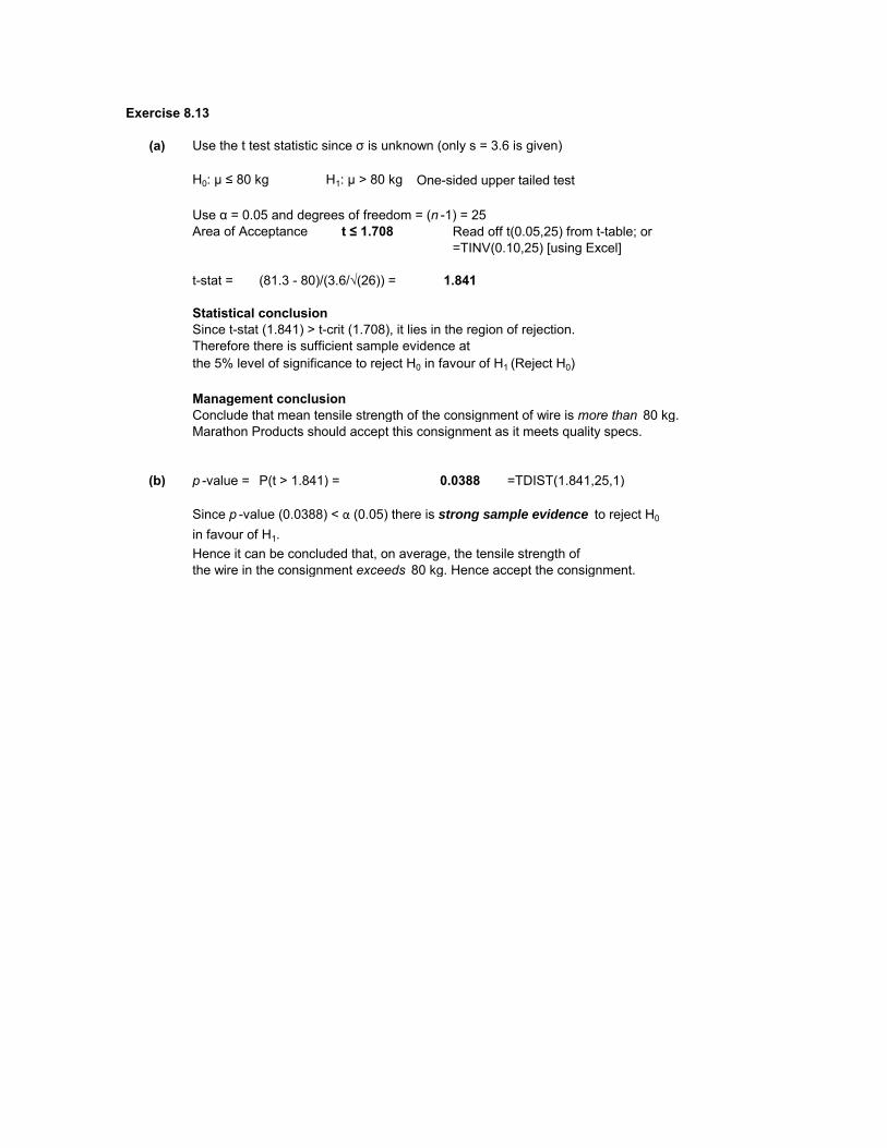
Exercise 8.13
(a) Use the t test statistic since σ is unknown (only s = 3.6 is given)
H0: µ ≤ 80 kg H1: µ > 80 kg One-sided upper tailed test
Use α = 0.05 and degrees of freedom = (n -1) = 25Area of Acceptance t ≤ 1.708 Read off t(0.05,25) from t-table; or
=TINV(0.10,25) [using Excel]
t-stat = (81.3 - 80)/(3.6/√(26)) = 1.841
Statistical conclusionSince t-stat (1.841) > t-crit (1.708), it lies in the region of rejection. Therefore there is sufficient sample evidence atthe 5% level of significance to reject H0 in favour of H1 (Reject H0)
Management conclusionConclude that mean tensile strength of the consignment of wire is more than 80 kg.Marathon Products should accept this consignment as it meets quality specs.
(b) p -value = P(t > 1.841) = 0.0388 =TDIST(1.841,25,1)
Since p -value (0.0388) < α (0.05) there is strong sample evidence to reject H0
in favour of H1. Hence it can be concluded that, on average, the tensile strength of the wire in the consignment exceeds 80 kg. Hence accept the consignment.
Exercise 8.14
(a) Use the t test statistic since σ is unknown (only s = 0.068 is given)
H0: µ ≥ 1 H1: µ < 1 One-sided lower tailed test
Use α = 0.05 and degrees of freedom = (n -1) = 19Area of Acceptance t ≥ -1.729 Read off t(0.05,19) from t-table; or
=TINV(0.10,19) [using Excel]
std error = 0.068/√(20) = 0.0152t-stat = (0.982 - 1)/(0.0152) = -1.1842
Statistical conclusionSince t-stat (-1.1842) > t-crit (-1.729), it lies within the region of acceptance. There is therefore insufficient sample evidence at the 5% level of significance to reject H0 in favour of H1 (i.e. Accept H0)
Management conclusionConclude that the mean fill of one-litre milk containers is not less than 1 litre.The Consumer Council's claim that containers are being underfilled is not valid.
(b) p -value = P(t < -1.1842) = 0.1255 =TDIST(-(-1.1842),19,1)
Since p -value (0.1255) > α (0.05), H0 cannot be rejected as there is no sample evidence to support H1. Hence it can be concluded that, on average, the mean fill of milk containers is at least one 1 lite. Thus there is no statistical support for the claim.

Exercise 8.15
(a) Use the z test statistic for proportions
H0: π ≥ 0.30 H1: π < 0.30 One sided lower tailed test
Use α = 0.05 Area of Acceptance z ≥ -1.645 Read off z(0.45) from z-table; or
=NORMSINV(0.05) [using Excel ]
n = 400 x = 106p = 106/400 = 0,265std error = √(0.3*0.7)/400 = 0,0229z-stat = (0.265 - 0.3)/(0.0229) = -1.5284
Statistical conclusionSince z-stat (-1.5284) > z-crit (-1.645) there is insufficient sample evidence atthe 5% level of significance to reject H0 in favour of H1 (i.e. Accept H0)
Management conclusionConclude that 30% or more of listeners tune into the news broadcast of this station.The company should advertise in this radio station's news timeslots.
(b) p -value = P(z < -1.5284) = 0.0632 '=NORMSDIST(-1.5284)
Since p-value (0.0633) > α (0.05), there is weak sample evidence to reject H0 in favour of H1. (i.e. Accept H0)The company can accept the radio station's claim as valid.
(c) p -value = P(z < -1.5284) = 0.0632 =NORMDIST(0.265,0.3,0.0229,1)
Exercise 8.16
(a) Use the z test statistic for proportions
H0: π ≤ 0.60 H1: π > 0.60
Use α = 0.05 Area of Acceptance z ≤ 1.645 Read off z(0.45) from z-table; or
=NORMSINV(0.95) [using Excel ]
n = 150 x = 54p = (150-54)/150 = 0.64std error = √(0.6*0.4)/150 = 0.04z-stat = (0.64 - 0.6)/(0.04) = 1.000
Statistical conclusionSince z-stat (1.00) < z-crit (1.645) there is insufficient sample evidence atthe 5% level of significance to reject H0 in favour of H1 (i.e. Accept H0)
Management conclusionConclude that not more than 60% of Cape Town motorists do not have vehicle insurance.The motor vehicle advisor's claim is not valid.
(b) p -value = P(z > 1.000) = 0.1587 =1-NORMSDIST(1)
Since p -value (0.1587) > α (0.05), the sample evidence does not support H1.
Hence the insurance advisor's claim has no statistical validity.

Exercise 8.17
(a) Use the z test statistic for proportions
H0: π ≤ 0.15 H1: π > 0.15
Use α = 0.10 Area of Acceptance z ≤ 1.28 Read off z(0.40) from z-table; or
=NORMSINV(0.90) [using Excel]
n = 560 x = 96p = 96/560 = 0.1714std error = √(0,15*0,85)/560 = 0.0151z-stat = (0,1714 - 0,15)/(0,0151) = 1.417
Statistical conclusionSince z-stat (1.417) > z-crit (1.28) there is sufficient sample evidence atthe 10% level of significance to reject H0 in favour of H1 (i.e. Reject H0)
Management conclusionConclude that the churn rate in the telecommunications industry exceeds 15%.
(b) p -value = P(z > 1.417) = 0.0782 =1-NORMSDIST(1.417)Since p -value (0.0782) > α (0.10), there is moderate sample evidence to reject H0 in favour of H1.
The same management conclusion applies as in (a) above.
(c) p -value = P(z > 1.417) = 0,0782 =1-NORMDIST(0.1714,0.15,0.0151,1)

Exercise 8.18
(a) Use the z test statistic for proportions
H0: π ≥ 0.90 H1: π < 0.90
Use α = 0.01 Area of Acceptance z ≥ -2.33 Read off z(0.49) from z-table; or
=NORMSINV(0.01) [using Excel]
n = 300 x = 260p = 260/300 = 0.8667std error = √(0.9*0.1)/300 = 0.0173z-stat = (0.8667 - 0.9)/(0.0173) = -1.9249
Statistical conclusionSince z-stat (-1.9249) > z-crit (-2.33) there is insufficient sample evidence atthe 1% level of significance to reject H0 in favour of H1 (i.e. Do not reject H0)
Management conclusionConclude that the germination rate of the barley seed is at least 90%.The cooperative can justify buying the barley seed from this merchant. The cooperative can accept the seed merchant's claim.
(b) p -value = P(z < -1.9249) = 0.0271 =NORMSDIST(-1.9249)Since p -value (0.0271) > α (0.01), there is weak sample evidence at the 1% level of signficance to reject H0 in favour of H1. Hence do not reject H0. The same management conclusion applies as in (a) above.
(c) p -value = P(z < -1.9249) = 0.0271 =NORMDIST(0.8667,0.9,0.0173,1)

Exercise 8.19 File: X8.19 - cost-to-income.xlsx
Use the t test statistic since σ is unknown Cost-to-income (%)
H0: µ ≥ 75% H1: µ < 75% Mean 71.24Standard Error 1.9973
Use α = 0.05 and degrees of freedom = (n -1) = 49 Median 68Read off t(0.05,49) from t-table; or Mode 84=TINV(0.10,49) [using Excel] Standard Deviation 14.1227
Sample Variance 199.451Area of Acceptance t ≥ -1.676 Kurtosis -1.1450
Skewness 0.1391std error = 1.9973 Range 53
Minimum 44t-stat = (71.24 - 75)/(1.9973) = -1.8825 Maximum 97
Sum 3562Count 50
Statistical conclusionSince t-stat (-1.8825) < t-crit (-1.676) there is sufficient sample evidence atthe 5% level of significance to reject H0 in favour of H1 (i.e. Reject H0)
Management conclusionConclude that the mean cost-to-income ratio of JSE companies is less than 75%.JSE companies are therefore adhering to the rule of thumb.

Exercise 8.20 File: X8.20 - kitchenware.xlsx
(a) Normality assumption check
Count568119641
The distribution appears to be normal.
(b) Use the t test statistic since σ is unknown Sales Transaction value
Mean 137.12H0: µ ≥ R150 H1: µ < R150 Standard Error 6.657
Median 138.5Use α = 0.05 and degrees of freedom = (n -1) = 49 Mode 184
Read off t(0.05,49) from t-table; or Standard Deviation 47.074=TINV(0.10,49) [using Excel] Sample Variance 2215.944
Kurtosis -0.741Area of Acceptance t ≥ -1.676 Skewness 0.022
Range 190std error = 6.657 Minimum 52
Maximum 242t-stat = (137.12 - 150)/(6.657) = -1.9348 Sum 6856
Count 50
Statistical conclusionSince t-stat (-1.9348) < t-crit (-1.676) there is sufficient sample evidence atthe 5% level of significance to reject H0 in favour of H1 (Reject H0).
Management conclusionConclude that the mean transaction value at the Claremont branch is signficantly below R150.The management are advised to close the Claremont branch since it is unprofitable.
176 - ≤ 200201 - ≤ 225
> 225
Sales values≤ 75
76 - ≤ 100101 - ≤ 125126 - ≤ 150151 - ≤ 175

Exercise 8.21 File: X8.21 - flight delays.xlsx
(a) Normality assumption check
delays Count≤ 5 0
5 - ≤ 7.5 87.6 - ≤ 10 28
10.1 - ≤ 12.5 2912.6 - ≤ 15 13
15.6 - ≤ 17.5 2> 17.5 0
The histogram distribution appears normal. The assumption is satisfied.
(b) Use the t test statistic since σ is unknown flight delays
Mean 10.324H0: µ ≤ 10 min H1: µ > 10 min Standard Error 0.261
Median 10.3Use α = 0.10 and degrees of freedom = (n -1) = 79 Mode 11
Read off t(0.10,79) from t-table; or Standard Deviation 2.333=TINV(0.20,79) [using Excel] Sample Variance 5.444
Kurtosis -0.550Area of Acceptance t ≥ 1.292 Skewness 0.084
Range 10.3std error = 0.261 Minimum 5.3
Maximum 15.6t-stat = (10.324 - 10)/(0.261) = 1.241 Sum 825.9
Count 80
Statistical conclusionSince t-stat (1.241) < t-crit (1.292) there is insufficient sample evidence atthe 10% level of significance to reject H0 in favour of H1 (i.e. Accept H0).
Management conclusion
0
8
28 29
13
20
0
5
10
15
20
25
30
35
5 7.5 10 12.5 15 17.5 More
No.
of F
light
s
Delay time intervals
Histogram of Flight Delay Times
Exercise 8.22 File: X8.22 - medical claims.xls
(a) Normality assumption check
Claims intervals Count
≤ 100 5101 - ≤ 125 3126 - ≤ 150 9151 - ≤ 175 21176 - ≤ 200 25201 - ≤ 225 18226 - ≤ 250 8251 - ≤ 300 11
The distribution appears to be reasonably normal. The assumption is satisfied
(b) Use the t test statistic since σ is unknown Medical Claims
Mean 190.39H0: µ ≤ 180 claims H1: µ > 180 claims Standard Error 4.568
Median 190Use α = 0.01 and degrees of freedom = (n -1) = 99 Mode 210
Read off t(0.01,99) from t-table; or Standard Deviation 45.680=TINV(0.02,99) [using Excel] Sample Variance 2086.685
Kurtosis -0.092Area of Acceptance t ≥ 2.365 Skewness 0.096
Range 199std error = 4.568 Minimum 92
Maximum 291t-stat = (190.39 - 180)/(4.568) = 2.275 Sum 19039
Count 100
Statistical conclusionSince t-stat (2.275) < t-crit (2.365) there is insufficient sample evidence atthe 1% level of significance to reject H0 in favour of H1 (Thus accept H0).
Management conclusionConclude that the average number of claims processed daily does not exceed 180.Thus the supervisor has no statistical grounds for requesting additional staff.
53
9
21
25
18
8
11
00
5
10
15
20
25
30
100 125 150 175 200 225 250 300 More
No.
of C
laim
s
Claims processed intervals
Histogram of Daily Claims Processed
Exercise 8.23 File: X8.23 - newspaper readership.xlsx
Guardian Newspaper Claim
(a) One-Way Pivot Table (Frequency Table) and Bar Chart
Tabloid Data TotalSun % 15.8%
Count 19Guardian % 35.0% Tabloid %
Count 42 Sun 15.8Mail % 25.8% Guardian 35
Count 31 Mail 25.8Voice % 23.3% Voice 23.3
Count 28Total % 100%Total Count 120
InterpretationBased on the sample fo 120 tabloid readers, the Guardian newspaper has the largest share of 35%. The Sun has the lowest percentage of readers at 16%.
(b) Use the z test statistic for proportions
H0: π ≥ 0.40 H1: π < 0.40 Test claim that Guardian newspaper
has at least a 40% market share. (c) Use α = 0.05
Area of Acceptance z ≥ -1.645 Read off z(0.45) from z-table; or =NORMSINV(0.05) [using Excel]
n = 120 x = 42p = 42/120 = 0.35std error = √(0.4*0.6)/120 = 0.0447z-stat = (0.35 - 0.4)/(0.0447) = -1.1186
Statistical conclusionSince z-stat (-1.1186) > z-crit (-1.645) there is insufficient sample evidence atthe 5% level of significance to reject H0 in favour of H1 (Thus accept H0)
15.8
35
25.823.3
0
5
10
15
20
25
30
35
40
Sun Guardian Mail Voice
% o
f Rea
ders
Bar Chart of Tabloid Readership

Management conclusionHence conclude that the Guardian's market share is at least 40%The Guardian newspaper 's claim is justified statistically.

Exercise 8.24 File: X8.24 - citrus products.xlsx
(a) One-Way Pivot Table (Frequency Table) and Bar Chart
Awareness Data TotalHigh Count 34
% 20% Awareness %Low Count 72 Low 42.35
% 42.35% Moderate 37.65Moderate Count 64 High 20
% 37.65%Total Count 170Total % 100%
Interpretation80% of sampled consumers have a low or moderate awareness. Only 20% ofthe sampled consumers indicated a high awarness of the nutritional benefits of citrus.
(b) (i) Use the z test statistic for proportions
H0: π ≤ 0.15 H1: π > 0.15
(b) (ii) Use α = 0.01 Area of Acceptance z ≤ 2.326 Read off z(0.49) from z-table; or
=NORMSINV(0.99) [using Excel]
n = 170 x = 34p = 34/170 = 0.2std error = √(0.15*0.85)/170 = 0.0274z-stat = (0.20 - 0.15)/(0.0274) = 1.825
Statistical conclusionSince z-stat (1.825) < z-crit (2.326) there is insufficient sample evidence atthe 1% level of significance to reject H0 in favour of H1 (i.e. Accept H0)
(b) (iii) Management conclusion
42.3537.65
20
0
10
20
30
40
50
Low Moderate High
% o
f res
pond
ents
Awareness Levels
Bar Chart of Awareness Levels

Exercise 8.25 File: X8.25 - aluminium scrap.xlsx
(a) Histogram of Daily % Scrap of Machine
Daily % Scrap Count
≤ 2.8 62.8 - ≤ 3.2 123.2 - ≤ 3.6 133.6 - ≤ 4.0 114.0 - ≤ 4.4 54.4 - ≤ 4.8 3
Total 50
InterpretationThe assumption of normality is largely satisfied. The histogram is only moderately skewed to the right.
(b) 95% Confidence Limits for Machine
Machine - Daily % ScrapMean 3.483Standard Error 0.0723Median 3.41Mode 2.97Standard Deviation 0.511Sample Variance 0.261Kurtosis -0.851Skewness 0.331Range 1.83Minimum 2.67Maximum 4.5Sum 174.14Count 50Confidence Level(95.0%) 0.145
Lower 95% confidence limit = 3.483 -0.145 = 3.34Upper 95% confidence limit = 3.483+0.145 = 3.63
6
1213
11
5
3
0
2
4
6
8
10
12
14
16
No.
of d
ays
Scrap % intervals
Histogram of Machine Daily % Scrap

There is a 95% chance that the average daily % scrap produced by the machine is likely to lie between 3.34% and 3.63%.
(c) Let μ = population mean daily % scrap produced by the machine.Use the t test statistic since σ is unknown (only s is given)
H0: μ ≥ 3.75% One sided lower tailed testH1: μ < 3.75%
Region of Acceptance Use α = 0.05 with df = (50 - 1) = 49t-crit = t(0.05)(49) = =TINV(0.1,49) -1.677
Decision rule Do not reject H0 in favour of H1 if -1.677 ≤ t-stat
t-stat std error = 0.0723 (see Table above)
t-stat = (3.483 - 3.75)/0.0723-3.693
Statistical conclusionSince t-stat (-3.693) lies well within the region of rejection, there is strong sampleevidence at the 5% significance level to reject H0 in favour of H1. (Thus reject H0).
Management conclusionConclude that the average daily % scrap produced by the machine is less than 3.75%. The machine is not yet due for a full maintenance service.

Exercise 8.26
Problem Characteristics
Variable x = length of pipe (specification = 5m)
Data type numerical, ratio scaled, continuous.
Data n = 26 pipes
α = 0.05
s = 3.46 σ0 = 3
Step 1 One sided Upper tailed test
Management Question in H0
Step 2 Region of Non-Rejection (Use Chi-Square)
Upper Χ2-crit = 37.652 Do not reject Ho if Χ2-stat ≤ 37.652
Step 3 Sample test statistic X2-statX2-stat = 33.254 Also p -value = 0.12
Use CHISQ.DIST.RT(x, df)
Steps 4, 5 Statistical Conclusion
Since X2-stat < upper X2-crit (i.e. lies in region of non-rejection of H0),
do not reject H0 at 5% level of significance.
Management Conclusion
The production manager can be 95% confident that the variation
in pipe lengths is within the limits of the product specification.
Hypothesis Test for a Single Population Variance, σ2
5m pipe length variability analysis
H0 : σ2 ≤ 9
H1 : σ2 > 9
Formula 8.4
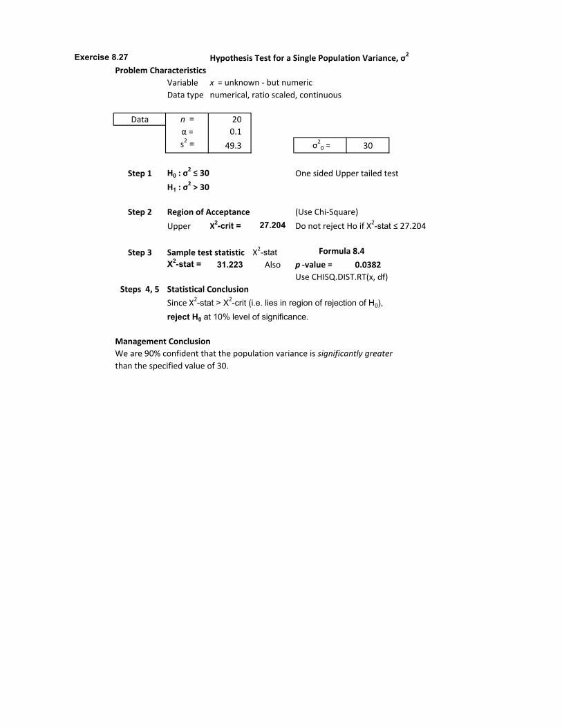
Exercise 8.27 Hypothesis Test for a Single Population Variance, σ2
Problem Characteristics
Variable x = unknown - but numeric
Data type numerical, ratio scaled, continuous
Data n = 20
α = 0.1
s2 = 49.3 σ20 = 30
Step 1 One sided Upper tailed test
Step 2 Region of Acceptance (Use Chi-Square)
Upper Χ2-crit = 27.204 Do not reject Ho if Χ2-stat ≤ 27.204
Step 3 Sample test statistic X2-statX2-stat = 31.223 Also p -value = 0.0382
Use CHISQ.DIST.RT(x, df)
Steps 4, 5 Statistical Conclusion
Since X2-stat > X2-crit (i.e. lies in region of rejection of H0), reject H0 at 10% level of significance.
Management Conclusion
We are 90% confident that the population variance is significantly greater
than the specified value of 30.
H0 : σ2 ≤ 30
H1 : σ2 > 30
Formula 8.4

Exercise 8.28 Hypothesis Test for a Single Population Variance, σ2
Insurance claim values variability analysis
Problem Characteristics
Variable x = claim values (in Rand)
Data type numerical, ratio scaled - implies means and standard deviations
Data n = 32 claims
α = 0.05
s = 84 σ20 = 5625
Step 1 Two-tailed test
Management Question in H0
Step 2 Region of Non-Rejection (Use Chi-Square)
Upper Χ2-crit = 48.232 Lower Χ
2-crit = 17.539Do not reject Ho if 17.539 ≤ Χ2-stat ≤ 48.232
Step 3 Sample test statistic X2-stat
X2-stat = 38.886 Also p -value = 0.1561 Use CHISQ.DIST.RT(x, df)
Steps 4, 5 Statistical Conclusion
Since X2-stat < X2-crit (i.e. lies in region of non-rejection of H0),do not reject H0 at 5% level of significance.
Management Conclusion
The insurance industry can be 95% confident that the variation in claim values is still σ2 = R5625.
---ooOoo---
H0 : σ2 = 5625
H1 : σ2 ≠ 5625
Use Formula 8.4

Exercise 8.29 File: X8.29 - pain relief.xlsx
Problem Characteristics
Variable x = time to pain relief (in minutes)
Data type numerical, ratio scaled, continuous
Data n = 16 patients
α = 0.01
s = 0.9004 σ2
0 = 1.8
Step 1 One sided lower tailed test
Management Question in H0
Step 2 Region of Non-Rejection (Use Chi-Square)
Lower Χ2-crit = 5.229 Do not reject Ho if Χ2-stat ≥ 5.299
Step 3 Sample test statistic X2-statX2-stat = 6.756 Also p -value = 0.0359
Use CHISQ.DIST(x, df)
Steps 4, 5 Statistical Conclusion
Since X2-stat > lower X2-crit (i.e. lies in region of non-rejection of H0), do not reject H0 at 1% level of significance.
Management Conclusion The pharmaceutical company can be 99% confident that
the variation in time to pain relief from the new headache pill is not significantly less than
the current headache pill (of σ2 = 1.8 min).
(i.e. it does not significantly reduce variation in time to pain relief).
H0 : σ2 ≥ 1.8
H1 : σ2 < 1.8
Use Formula 8.4

CHAPTER 9
HYPOTHESIS TESTS
COMPARISON BETWEEN TWO POPULATIONS (MEANS, VARIANCES AND PROPORTIONS)
Exercise 9.1 When the population standard deviations of the two populations are unknown.
Exercise 9.2 Use Formula 9.1
z-stat = [(72 - 66) - 0]/√(202/40+102/50)
z-stat = 1.7321
Exercise 9.3 (a) t-crit (0.05,38) = 2.024 Refer to Appendix 1 Table 2
(b) t-crit (0.05,90) = 1.987 Refer to Appendix 1 Table 3
Exercise 9.4 When the two samples are not independent.
Exercise 9.5 H0: π1 ≥ π2
H1: π1 < π2 One sided lower tailed test.

Exercise 9.6
(a) Test for equality of variances
H0: σ21 = σ2
2 Two tailed test H1: σ²1 ≠ σ²2
F-cri t = F(0.05/2, 23,18) = 2.50 (from Table 4(b), Appendix 1) =F.INV.RT(0.025,23,18)Decision rule: Do not reject H0 if F-stat ≤ 2.50 2.515
F-stat = = 4.14²/3.32² = 1.555 Use rule of larger variance in numerator
Since F-stat (1.555) < F-crit (2.515), do not reject H0 in favour of H1.
Conclude,at α = 0.05, that the two population variances are equal.Therefore, use the pooled-variances t -test to test for differences in means.
(b) Test for difference between two population means
Let population 1 = ManufacturersLet population 2 = Retailers Let μi = population mean earnings yield (%) per sector i .
Use the t test statistic since σi's are unknown (only s1 and s2 are given)
H0: μ1 = μ2 Two tailed test H1: μ1 ≠ μ2
(c) Region of Acceptance Use α = 0.05 with df = (19+24-2) = 41t-crit = t(0.05)(41) = 2.021
Decision rule Do not reject H0 in favour of H1 if -2.021 ≤ t-stat ≤ 2.021
t-stat s² (pooled variance) = ((19-1)3,32²+(24-1)4,14²)/(19+24-2)14.454
std error = √(14.454*(1/19+1/24))1.16747
t-stat = ((8.45-10.22)-(0))/1.16747-1.51609
ConclusionSince t-stat (-1.51609) lies within the region of acceptance, there is insufficient sample evidence at the 5% level of significance to reject H0 in favour of H1. (i.e. Accept H0).Conclude that there is no difference in the mean earnings yield (%) between manufacturing companies and retail companies.

Exercise 9.7
(a) Let population 1 = DIY ConsumersLet population 2 = Non-DIY Consumers Let μi = population mean age of each consumer group i .
Use the t test statistic since σi's are unknown (only s1 and s2 are given)
H0: μ1 ≥ μ2 One sided lower tailed testH1: μ1 < μ2
(b) Region of Acceptance Use α = 0.10 with df = (29+34-2) = 61t-crit = t(0.10)(61) = -1.296
Decision rule Do not reject H0 in favour of H1 if -1.296 ≤ t-stat
t-stat s² (pooled variance) = ((29-1)15.9²+(34-1)16.2²)/(29+34-2)258.0197
std error = √(258.0197*(1/29+1/34))4.060301
t-stat = ((41.8-47.4)-(0))/4.0603-1.379
(c) Statistical conclusionSince t-stat (-1.379) lies outside (below) the region of acceptance,there is sufficient sample evidence at the 10% level of significance to reject H0 in favour of H1. (i.e. Reject H0).Management conclusionConclude that the mean age of DIY consumers is significantly lower thanthe mean age of non-DIY consumers at the 10% level of significance.
(d) Region of Acceptance (new) Use α = 0.05 with df = (29+34-2) = 61t-crit = t(0.05)(61) = -1.671
Decision rule Do not reject H0 in favour of H1 if -1.671 ≤ t-stat
Statistical conclusiont-stat (-1.379) now lies within the (new) region of acceptance. Thus there is insufficient sample evidence at the 5% level of significanceto reject H0 in favour of H1. (i.e. Accept H0).Management conclusionConclude that there is no significant difference in the mean ages betweenDIY consumers and non-DIY consumers.
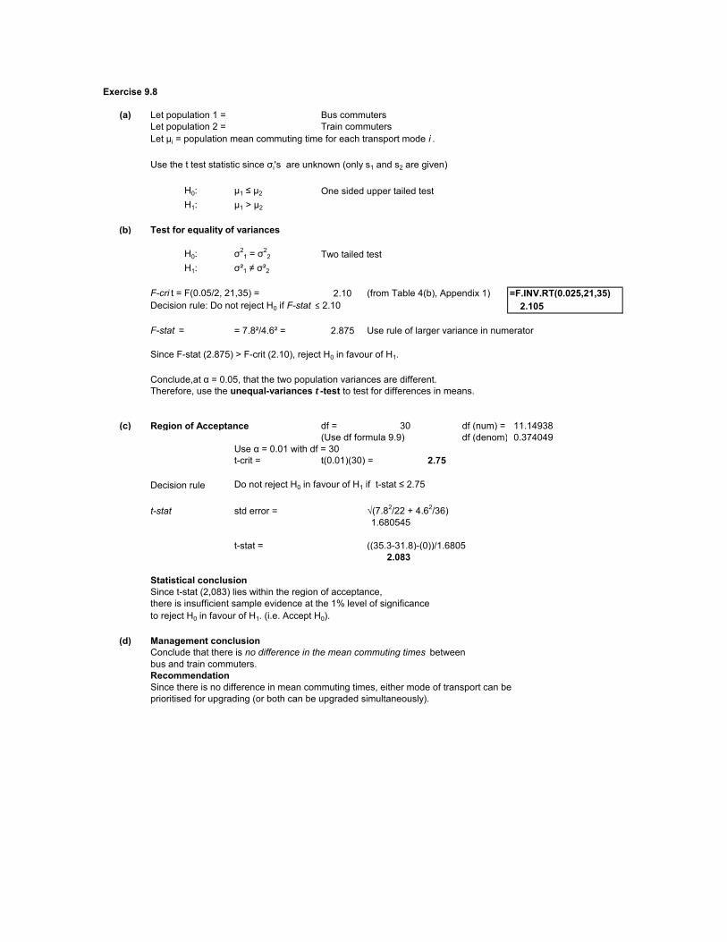
Exercise 9.8
(a) Let population 1 = Bus commutersLet population 2 = Train commutersLet μi = population mean commuting time for each transport mode i .
Use the t test statistic since σi's are unknown (only s1 and s2 are given)
H0: μ1 ≤ μ2 One sided upper tailed testH1: μ1 > μ2
(b) Test for equality of variances
H0: σ21 = σ2
2 Two tailed test H1: σ²1 ≠ σ²2
F-cri t = F(0.05/2, 21,35) = 2.10 (from Table 4(b), Appendix 1) =F.INV.RT(0.025,21,35)Decision rule: Do not reject H0 if F-stat ≤ 2.10 2.105
F-stat = = 7.8²/4.6² = 2.875 Use rule of larger variance in numerator
Since F-stat (2.875) > F-crit (2.10), reject H0 in favour of H1.
Conclude,at α = 0.05, that the two population variances are different. Therefore, use the unequal-variances t -test to test for differences in means.
(c) Region of Acceptance df = 30 df (num) = 11.14938(Use df formula 9.9) df (denom) =0.374049
Use α = 0.01 with df = 30t-crit = t(0.01)(30) = 2.75
Decision rule Do not reject H0 in favour of H1 if t-stat ≤ 2.75
t-stat std error = √(7.82/22 + 4.62/36)1.680545
t-stat = ((35.3-31.8)-(0))/1.68052.083
Statistical conclusionSince t-stat (2,083) lies within the region of acceptance,there is insufficient sample evidence at the 1% level of significanceto reject H0 in favour of H1. (i.e. Accept H0).
(d) Management conclusionConclude that there is no difference in the mean commuting times between bus and train commuters. RecommendationSince there is no difference in mean commuting times, either mode of transport can be prioritised for upgrading (or both can be upgraded simultaneously).

Exercise 9.9
Let population 1 = Mastercard users Let population 2 = Visa Card usersLet μi = population mean month-end credit card balance (in Rands) for each card type i .
Use the z test statistic since σi's are known
H0: μ1 = μ2 Two sided test H1: μ1 ≠ μ2
Region of Acceptance Use α = 0.05z-crit = z(0.05) = 1.96
Decision rule Do not reject H0 in favour of H1 if -1.96 ≤ z-stat ≤ 1.96
z-stat std error = √(294²/45+336²/66)60.26065
z-stat = ((922-828)-(0))/60.260651.5599
Statistical conclusionSince z-stat (1.5599) lies within the region of acceptance, there is insufficient sampleevidence at the 5% significance level to reject H0 in favour of H1. (i.e. Accept H0).
Management conclusionConclude that there is no difference in the mean month-end credit card balances between Mastercard holders and Visa Card holders.

Exercise 9.10
Let population 1 = non-attendees of job enrichment workshopsLet population 2 = attendees of job enrichment workshopsLet μi = population mean job satisfaction rating for each employee category i .
Use the z test statistic since σi's are known
H0: μ1 ≥ μ2 One-sided lower tailed test H1: μ1 < μ2 ← non-attendees have lower job satisfaction than
attendees.
Region of Acceptance Use α = 0.05z-crit = z(0.05) = -1.645
Decision rule Do not reject H0 in favour of H1 if -1.645 ≤ z-stat
z-stat std error = √(1.1²/22+0.8²/25)0.283901
z-stat = ((6.9-7.5)-(0))/0.283901-2.1134
Statistical conclusionSince z-stat (-2.1134) lies outside (below) the region of acceptance, there is sufficientsample evidence at the 5% significance level to reject H0 in favour of H1. (i.e. Reject H0).
Management conclusionConclude that the mean job satisfaction score for non-attendees is significantly lower than the mean job satisfaction score for job enrichment attendees.
Thus, the statistical evidence supports the view that the job enrichment workshops significantly increased job satisfaction levels of sales consultants.
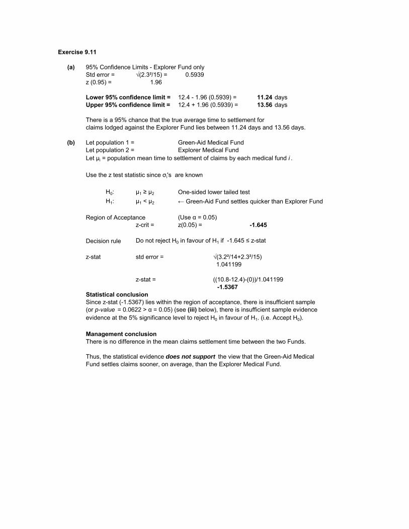
Exercise 9.11
(a) 95% Confidence Limits - Explorer Fund onlyStd error = √(2.3²/15) = 0.5939z (0.95) = 1.96
Lower 95% confidence limit = 12.4 - 1.96 (0.5939) = 11.24 daysUpper 95% confidence limit = 12.4 + 1.96 (0.5939) = 13.56 days
There is a 95% chance that the true average time to settlement for claims lodged against the Explorer Fund lies between 11.24 days and 13.56 days.
(b) Let population 1 = Green-Aid Medical Fund Let population 2 = Explorer Medical Fund Let μi = population mean time to settlement of claims by each medical fund i .
Use the z test statistic since σi's are known
H0: μ1 ≥ μ2 One-sided lower tailed test H1: μ1 < μ2 ← Green-Aid Fund settles quicker than Explorer Fund
Region of Acceptance (Use α = 0.05)z-crit = z(0.05) = -1.645
Decision rule Do not reject H0 in favour of H1 if -1.645 ≤ z-stat
z-stat std error = √(3.2²/14+2.3²/15)1.041199
z-stat = ((10.8-12.4)-(0))/1.041199-1.5367
Statistical conclusionSince z-stat (-1.5367) lies within the region of acceptance, there is insufficient sample(or p-value = 0.0622 > α = 0.05) (see (iii) below), there is insufficient sample evidence evidence at the 5% significance level to reject H0 in favour of H1. (i.e. Accept H0).
Management conclusionThere is no difference in the mean claims settlement time between the two Funds.
Thus, the statistical evidence does not support the view that the Green-Aid Medical Fund settles claims sooner, on average, than the Explorer Medical Fund.

Exercise 9.12
Let population 1 = Gas ovensLet population 2 = Electric ovensLet μi = population mean baking time for each oven type i .
Use the t test statistic since σi's are unknown (only s1 and s2 are given)
H0: μ1 ≥ μ2 One sided lower tailed testH1: μ1 < μ2 ← gas ovens bake faster than electric ovens
Region of Acceptance Use α = 0.05 with df = (5+5-2) = 8t-crit = t(0.05)(8) = -1.86
Decision rule Do not reject H0 in favour of H1 if t-stat ≥ -1.86
t-stat s² (pooled variance) = ((5-1)0.16²+(5-1)0.09²)/(5+5-2)0.01685
std error = √(0.01685*(1/5+1/5))0.08210
t-stat = ((0.75-0.89)-(0))/0.0821-1.705
Statistical conclusionSince t-stat (-1.705) lies within the region of acceptance, there is insufficient sampleevidence at the 5% significance level to reject H0 in favour of H1. (i.e. Accept H0).
Management conclusionConclude that there is no difference in the mean bread baking time between gas and electric ovens, at the 5% significance level. Gas ovens are therefore, not faster, on average, than electric ovens.

Exercise 9.13
(a) Test for equality of variances H0: σ
21 = σ2
2 H1: σ²1 ≠ σ²2
Rule of thumb test: F-stat < 3?F-stat = = 152.2²/121.5² = 1.569Since F-stat (1.569) < 3, do not reject H0 in favour of H1. Conclude that the two population variances are equal.Therefore, use the pooled-variances t -test to test for differences in means.
(b) Let population 1 = Cape Town branchLet population 2 = Durban branchLet μi = population mean size of orders received by each branch i .
Use the t test statistic since σi's are unknown (only s1 and s2 are given)
H0: μ1 ≤ μ2 One sided upper tailed testH1: μ1 > μ2 ← CT branch performing better than Durban branch
Region of Acceptance Use α = 0.10 with df = (18+15-2) = 31t-crit = t(0.10)(31) = 1.309
Decision rule Do not reject H0 in favour of H1 if t-stat ≤ 1.309
t-stat s² (pooled variance) = ((18-1)121.5²+(15-1)152.2²)/(18+15-2)18556.97
std error = √(18556.97*(1/18+1/15))47.6243
t-stat = ((335.2-265.6)-(0))/47.62431.4614
Statistical conclusionSince t-stat (1.4614) lies outside (above) the region of acceptance, there is sufficient sample evidence at the 10% significance level to reject H0 in favour of H1 (i.e. Reject H0).
Management conclusionConclude that the mean size of orders received by the Cape Town branch is significantly larger than the mean size of orders received by the Durban branch.
Thus the Cape Town branch is performing better than the Durban branch in terms of average order size.
(c) Region of Acceptance (new) Use α = 0.05 with df = (18+15-2) = 31t-crit = t(0.05)(31) = 1.696
Decision rule (new) Do not reject H0 in favour of H1 if t-stat ≤ 1.696
Statistical conclusiont-stat (= 1.4614) now lies within the (new) region of acceptance. Thus there is insufficient sample evidence at the 5% level of significance to reject H0 in favour of H1. (i.e. Accept H0).

Management conclusionConclude that there is no significant difference in the mean order sizes between the Cape Town branch and the Durban branch.
Thus there is no evidence to believe that the Cape Town branch is performing better than the Durban branch in terms of average order size.
(d) Findings based on the 5% significance level are more meaningful than those basedon the 10% significance level because it requires stronger (more convincing) sample
evidence before tests conducted at 5% are prepared to reject the null hypothesis.
The operations manager can be more confident that there is no difference in meanperformance between the two branches (conclusion based on (b)).
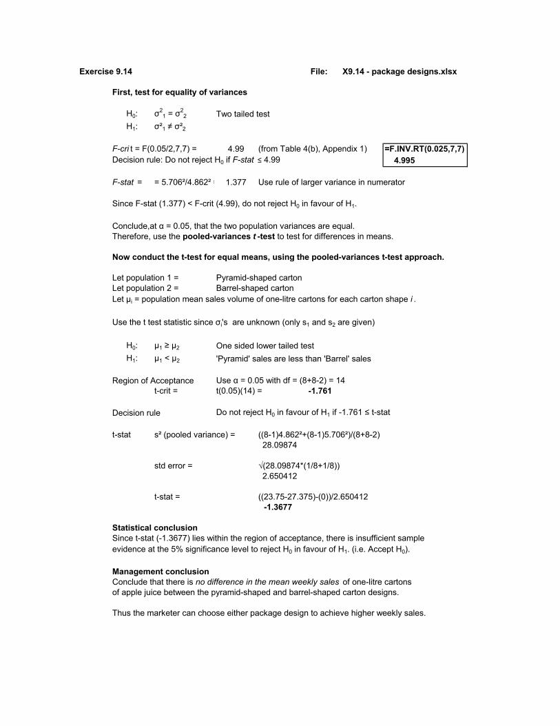
Exercise 9.14 File: X9.14 - package designs.xlsx
First, test for equality of variances
H0: σ21 = σ2
2 Two tailed test H1: σ²1 ≠ σ²2
F-cri t = F(0.05/2,7,7) = 4.99 (from Table 4(b), Appendix 1) =F.INV.RT(0.025,7,7)Decision rule: Do not reject H0 if F-stat ≤ 4.99 4.995
F-stat = = 5.706²/4.862² = 1.377 Use rule of larger variance in numerator
Since F-stat (1.377) < F-crit (4.99), do not reject H0 in favour of H1.
Conclude,at α = 0.05, that the two population variances are equal.Therefore, use the pooled-variances t -test to test for differences in means.
Now conduct the t-test for equal means, using the pooled-variances t-test approach.
Let population 1 = Pyramid-shaped carton Let population 2 = Barrel-shaped cartonLet μi = population mean sales volume of one-litre cartons for each carton shape i .
Use the t test statistic since σi's are unknown (only s1 and s2 are given)
H0: μ1 ≥ μ2 One sided lower tailed testH1: μ1 < μ2 'Pyramid' sales are less than 'Barrel' sales
Region of Acceptance Use α = 0.05 with df = (8+8-2) = 14t-crit = t(0.05)(14) = -1.761
Decision rule Do not reject H0 in favour of H1 if -1.761 ≤ t-stat
t-stat s² (pooled variance) = ((8-1)4.862²+(8-1)5.706²)/(8+8-2)28.09874
std error = √(28.09874*(1/8+1/8))2.650412
t-stat = ((23.75-27.375)-(0))/2.650412-1.3677
Statistical conclusionSince t-stat (-1.3677) lies within the region of acceptance, there is insufficient sampleevidence at the 5% significance level to reject H0 in favour of H1. (i.e. Accept H0).
Management conclusionConclude that there is no difference in the mean weekly sales of one-litre cartons of apple juice between the pyramid-shaped and barrel-shaped carton designs.
Thus the marketer can choose either package design to achieve higher weekly sales.

Exercise 9.15
Let population 1 = Fruit Puffs consumersLet population 2 = Fruity Wheat consumers Let πi = population proportion of consumers who prefer fruit-flavoured wheat cereal i .
Use the z test statistic
H0: π1 ≤ π2 One sided upper tailed testH1: π1 > π2 Fruit Puffs is preferred by more consumers than
Fruity Wheat.
Region of Acceptance Use α = 0.05z-crit = z(0.05) = 1.645
Decision rule Do not reject H0 in favour of H1 if z-stat ≤ 1.645.
Sample data Fruit Puffs Fruity Wheatn 175 150x 54 36pi 0.309 0.240
z-stat π(hat) (pooled proportion) = (54+36)/(175+150) =0.2769
std error = √(0.2769*(1-0.2769)*(1/175+1/150))0.04978949
z-stat = (0.309-0.24)/0.0497891.3858
Statistical conclusionSince z-stat (= 1.3858) lies within the region of acceptance, there is insufficient sampleevidence at the 5% significance level to reject H0 in favour of H1. (i.e. Accept H0).
Management conclusionConclude that there is no difference in the percentage of consumers who prefereach type of fruit-flavoured wheat cereal.
The marketer's view that Fruit Puffs is more preferred than Fruity Wheat cannot be validated based on the statistical evidence at the 5% level of significance. The marketer can therefore choose to launch either fruit flavour of wheat cereal.

Exercise 9.16
(a) Let population 1 = Male respondents Let population 2 = Female respondents Let πi = population proportion who prefer jazz for each gender i .
Use the z test statistic
H0: π1 = π2 Two sided test (equal preference)H1: π1 ≠ π2
Region of Acceptance Use α = 0.05z-crit = 1.96
Decision rule Do not reject H0 in favour of H1 if -1.96 ≤ z-stat ≤ 1.96.
Sample data Male Femalen 140 110x 46 21pi 0.329 0.191
z-stat π(hat) (pooled proportion) = (46+21)/(140+110) =0.268
std error = √(0.268*(1-0.268)*(1/140+1/110))0.056432928
z-stat = (0.329-0.191)/0.0564332.445
Statistical conclusionSince z-stat (2.445) lies outside (above) the region of acceptance, there is sufficient sample evidence at the 5% significance level to reject H0 in favour of H1 (i.e. Reject H0)
Management conclusionConclude that there is a difference in the proportion of males compared to theproportion of females who enjoy listening to jazz.
By inspection , proportionately more males than females enjoy listening to jazz.
(b) p -value = =(1-NORMSDIST(2.445))*2 0.0145
Since the p-value (=0.0145) < α = 0.05, there is strong sample evidence insupport of H1. Hence conclude that there is a difference in the proportion of males compared to the proportion of females who enjoy listening to jazz.

Exercise 9.17
(a) Let population 1 = Status Cheque Account clients Let population 2 = Elite Cheque Account clientsLet πi = population proportion of clients for each account type i who are overdrawn.
Use the z test statistic
H0: π1 ≥ π2 One sided lower tailed testH1: π1 < π2 'Status' proportion less than 'Elite' proportion
Region of Acceptance Use α = 0.05z-crit = -1.645
Decision rule Do not reject H0 in favour of H1 if z-stat ≥ -1.645.
Sample data Status Eliten 300 250x 48 55pi 0.16 0.22
z-stat π(hat) (pooled proportion) = (48+55)/(300+250) =0.1873
std error = √(0.1873*(1-0.1873)*(1/300+1/250))0.0334
z-stat = (0.16-0.22)/0.0334-1.796
Statistical conclusionSince z-stat (= -1.796) lies outside (below) the region of acceptance, there is sufficientsample evidence at the 5% significance level to reject H0 in favour of H1. (i.e. Reject H0).
Management conclusionConclude that proportionately more Elite cheque account clients are overdrawn compared to Status cheque account clients.
(b) p -value = =NORMSDIST(-1.796) 0.0363
Since the p-value (=0.0363) < α = 0.05, there is strong sample evidence insupport of H1. Hence conclude that proportionately more Elite cheque account clients are overdrawn compared to Status cheque account clients.
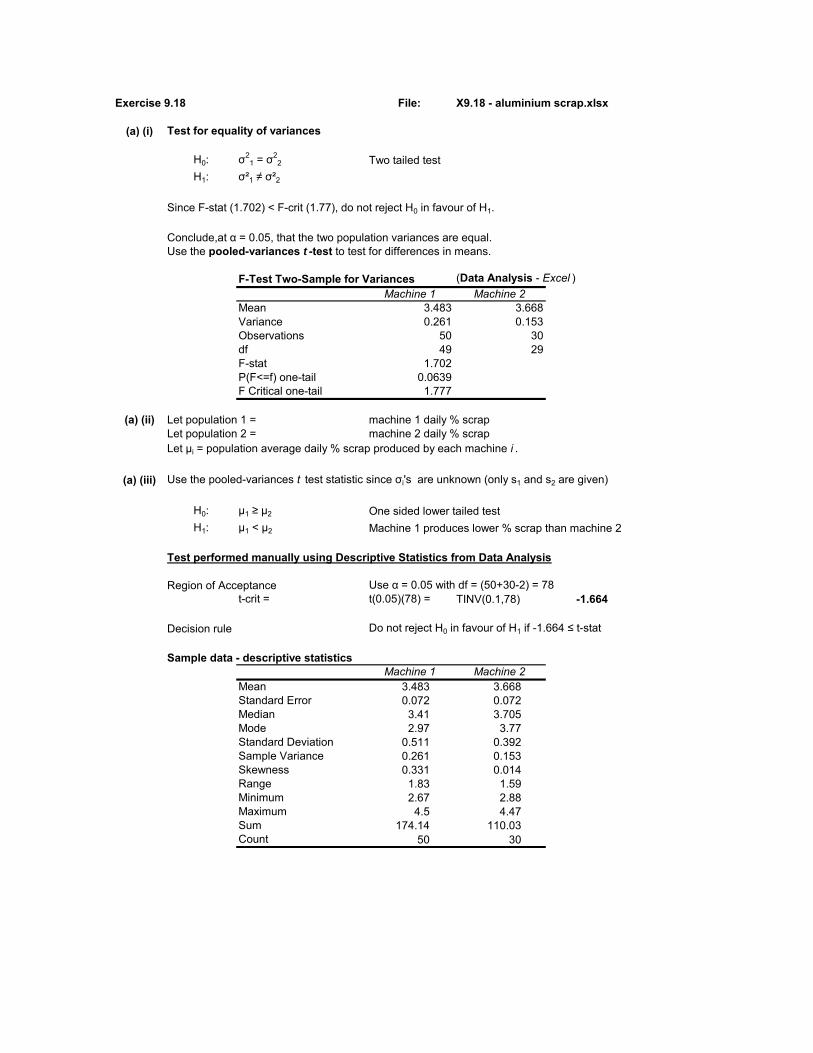
Exercise 9.18 File: X9.18 - aluminium scrap.xlsx
(a) (i) Test for equality of variances
H0: σ21 = σ2
2 Two tailed test H1: σ²1 ≠ σ²2
Since F-stat (1.702) < F-crit (1.77), do not reject H0 in favour of H1.
Conclude,at α = 0.05, that the two population variances are equal.Use the pooled-variances t -test to test for differences in means.
F-Test Two-Sample for Variances (Data Analysis - Excel )Machine 1 Machine 2
Mean 3.483 3.668Variance 0.261 0.153Observations 50 30df 49 29F-stat 1.702P(F<=f) one-tail 0.0639F Critical one-tail 1.777
(a) (ii) Let population 1 = machine 1 daily % scrapLet population 2 = machine 2 daily % scrapLet μi = population average daily % scrap produced by each machine i .
(a) (iii) Use the pooled-variances t test statistic since σi's are unknown (only s1 and s2 are given)
H0: μ1 ≥ μ2 One sided lower tailed testH1: μ1 < μ2 Machine 1 produces lower % scrap than machine 2
Test performed manually using Descriptive Statistics from Data Analysis
Region of Acceptance Use α = 0.05 with df = (50+30-2) = 78t-crit = t(0.05)(78) = TINV(0.1,78) -1.664
Decision rule Do not reject H0 in favour of H1 if -1.664 ≤ t-stat
Sample data - descriptive statisticsMachine 1 Machine 2
Mean 3.483 3.668Standard Error 0.072 0.072Median 3.41 3.705Mode 2.97 3.77Standard Deviation 0.511 0.392Sample Variance 0.261 0.153Skewness 0.331 0.014Range 1.83 1.59Minimum 2.67 2.88Maximum 4.5 4.47Sum 174.14 110.03Count 50 30

t-stat s² (pooled variance) = ((50-1)*0.511²+(30-1)*0.392²)/(50+30-2)0.221169038
std error = √(0.221169*(1/50+1/30))0.108607919
t-stat = ((3.483-3.668)-(0))/0.10861-1.7032
(a) (iii) Test performed using t-Test Assuming Equal Variances in Data Analysis
Using Data Analysis (in Excel )t-Test: Two-Sample Assuming Equal Variances
Machine 1 Machine 2Mean 3.483 3.668Variance 0.261 0.153Observations 50 30Pooled Variance 0.221Hypothesized Mean Difference 0df 78t Stat -1.703P(T<=t) one-tail 0.046t Critical one-tail -1.665P(T<=t) two-tail 0.093t Critical two-tail 1.991
(a) (iv) Statistical conclusionSince t-stat (= -1.7032) lies outside (below) the region of acceptance, there is sufficientor p-value = 0.0463 < α = 0.05 (see below), there is sufficient sample evidence sample evidence at the 5% significance level to reject H0 in favour of H1. (i.e. Reject H0).
Management conclusionConclude that machine 1 has a significantly lower average daily % scrap than machine 2.
(b) p -value = =T.DIST(-(-1.7032),78,1) 0.0463 =T.DIST(-1.7032,78,TRUE)
Since the p-value (=0.046) < α = 0.05, there is strong sample evidence insupport of H1. Conclude that machine 1 produces scrap at a significantly lower average daily rate than machine 2. This conclusion is valid at the 5% significance level.
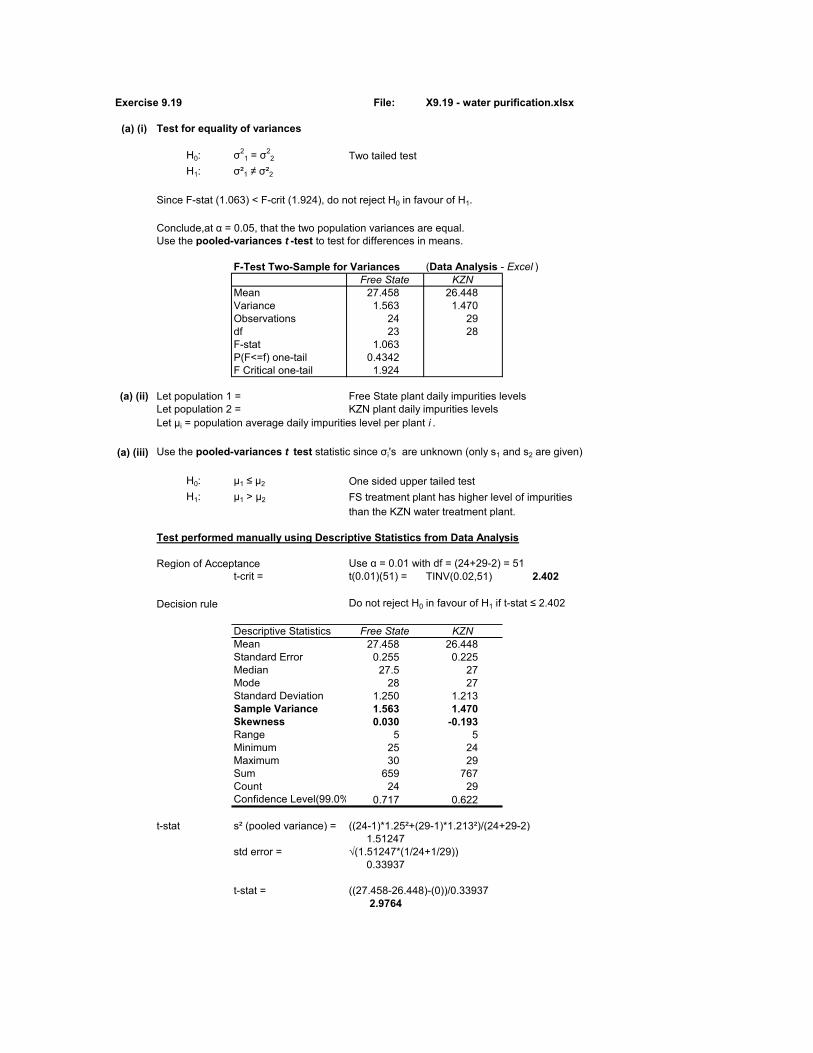
Exercise 9.19 File: X9.19 - water purification.xlsx
(a) (i) Test for equality of variances
H0: σ21 = σ2
2 Two tailed test H1: σ²1 ≠ σ²2
Since F-stat (1.063) < F-crit (1.924), do not reject H0 in favour of H1.
Conclude,at α = 0.05, that the two population variances are equal.Use the pooled-variances t -test to test for differences in means.
F-Test Two-Sample for Variances (Data Analysis - Excel )Free State KZN
Mean 27.458 26.448Variance 1.563 1.470Observations 24 29df 23 28F-stat 1.063P(F<=f) one-tail 0.4342F Critical one-tail 1.924
(a) (ii) Let population 1 = Free State plant daily impurities levels Let population 2 = KZN plant daily impurities levels Let μi = population average daily impurities level per plant i .
(a) (iii) Use the pooled-variances t test statistic since σi's are unknown (only s1 and s2 are given)
H0: μ1 ≤ μ2 One sided upper tailed testH1: μ1 > μ2 FS treatment plant has higher level of impurities
than the KZN water treatment plant.
Test performed manually using Descriptive Statistics from Data Analysis
Region of Acceptance Use α = 0.01 with df = (24+29-2) = 51t-crit = t(0.01)(51) = TINV(0.02,51) 2.402
Decision rule Do not reject H0 in favour of H1 if t-stat ≤ 2.402
Descriptive Statistics Free State KZNMean 27.458 26.448Standard Error 0.255 0.225Median 27.5 27Mode 28 27Standard Deviation 1.250 1.213Sample Variance 1.563 1.470Skewness 0.030 -0.193Range 5 5Minimum 25 24Maximum 30 29Sum 659 767Count 24 29Confidence Level(99.0%) 0.717 0.622
t-stat s² (pooled variance) = ((24-1)*1.25²+(29-1)*1.213²)/(24+29-2)1.51247
std error = √(1.51247*(1/24+1/29))0.33937
t-stat = ((27.458-26.448)-(0))/0.339372.9764

Test performed using t-Test Assuming Equal Variances in Data Analysis
Using Data Analysis (in Excel )t-Test: Two-Sample Assuming Equal Variances
Free State KZNMean 27.458 26.448Variance 1.563 1.470Observations 24 29Pooled Variance 1.512Hypothesized Mean Difference 0df 51t Stat 2.9764P(T<=t) one-tail 0.00223t Critical one-tail 2.402P(T<=t) two-tail 0.004t Critical two-tail 2.676
(a) (iv) Statistical conclusionSince t-stat (2.9764) lies outside (above) the region of acceptance, there is sufficient sample evidence at the 1% significance level to reject H0 in favour of H1. (i.e. Reject H0).
Management conclusionConclude that the KZN plant produces water of a higher quality (fewer impurities, on average)than the Free State plant. Thus the KZN plant manager's claim can be supported statistically at the 1% level of significance.
(b) p -value = =T.DIST(2.9761),51,1) 0.00223 =T.DIST.RT(2.9764,51)
Since the p-value (=0.00223) << α = 0.01, there is overwhelming sample evidence insupport of H1. Same conclusion as in (a) applies.

Exercise 9.20 File: X9.20 - herbal tea.xlsx
(a) Test for equality of variances
H0: σ21 = σ2
2 Two tailed test H1: σ²1 ≠ σ²2
Since F-stat (1.227) < F-crit (2.098), do not reject H0 in favour of H1.
Conclude,at α = 0.05, that the two population variances are equal.Use the pooled-variances t -test to test for differences in means.
F-Test Two-Sample for Variances (Data Analysis - Excel )Freshpak Yellow Label
Mean 7.689 6.917Variance 2.170 1.768Observations 19 23df 18 22F-stat 1.227P(F<=f) one-tail 0.3205F Critical one-tail 2.098
(b) (i) Let population 1 = Freshpak brand Let population 2 = Yellow Label brandLet μi = population mean level of quercetin in mg/kg in each brand i .
Use the t test statistic since σi's are unknown (only s1 and s2 are given)
H0: μ1 = μ2 Two sided test (No difference)H1: μ1 ≠ μ2
Test performed manually using Descriptive Statistics from Data Analysis
Region of Acceptance Use α = 0.05 with df = (19+23-2) = 40t-crit = t(0.05)(40) = 2.021
Decision rule Do not reject H0 in favour of H1 if -2.021 ≤ t-stat ≤ 2.021
Descriptive Statistics Freshpak Yellow LabelMean 7.689 6.917Standard Error 0.3379 0.2772Median 7.9 7.1Mode 7.9 5.7Standard Deviation 1.4731 1.3296Sample Variance 2.1699 1.7679Skewness -0.1752 0.1030Range 5.1 5.3Minimum 5 4.5Maximum 10.1 9.8Sum 146.1 159.1Count 19 23

t-stat s² (pooled variance) = ((19-1)*1.473²+(23-1)*1.3296²)/(19+23-2)1.948688
std error = √(1.948688*(1/19+1/23))0.43277
t-stat = ((7.689-6.917)-(0))/0.432771.784
Test performed using t-Test Assuming Equal Variances in Data Analysis
Using Data Analysis (in Excel )t-Test: Two-Sample Assuming Equal Variances
Freshpak Yellow LabelMean 7.6895 6.9174Variance 2.1699 1.7679Observations 19 23Pooled Variance 1.9488Hypothesized Mean Difference 0df 40t Stat 1.7840P(T<=t) one-tail 0.0410t Critical one-tail 1.6839P(T<=t) two-tail 0.0820t Critical two-tail 2.0211
Statistical conclusionSince t-stat (1.784) lies within the region of acceptance, there is insufficient sampleevidence at the 5% significance level to reject H0 in favour of H1. (i.e. Accept H0).
Management conclusionConclude that there is no difference in the mean quercetin content (in mg/kg)
between the Freshpak and Yellow Labels brands of rooibos tea.

(b) (ii) Let population 1 = Freshpak brand (FP)Let population 2 = Yellow Label brand (YL)
H0: μ1 ≤ μ2 One sided upper tailed testH1: μ1 > μ2 FP contains more quercetin than YL
Using Data Analysis (in Excel )t-Test: Two-Sample Assuming Equal Variances
Freshpak Yellow LabelMean 7.6895 6.9174Variance 2.1699 1.7679Observations 19 23Pooled Variance 1.9488Hypothesized Mean Difference 0df 40t Stat 1.7840P(T<=t) one-tail 0.0410t Critical one-tail 1.6839P(T<=t) two-tail 0.0820t Critical two-tail 2.0211
Statistical conclusionSince t-stat (= 1.784) lies outside (above) the region of acceptance (t-stat ≤ 1.6839), (see table above), there is sufficient sample evidence at the 5% level of significance to reject H0 in favour of H1. (i.e. Reject H0).
Management conclusionConclude that Freshpak's claim that their brand contains more quercetin, on average, than the Yellow Label brand, can be supported statistically at the 5% significance level.

Exercise 9.21 File: X9.21 - meat fat.xlsx
(a) (i) Test for equality of variances
H0: σ21 = σ2
2 Two tailed test H1: σ²1 ≠ σ²2
Since F-stat (1.261) < F-crit (2.066), do not reject H0 in favour of H1.
Conclude,at α = 0.05, that the two population variances are equal.Use the pooled-variances t -test to test for differences in means.
F-Test Two-Sample for Variances (Data Analysis - Excel )Namibia Little Karoo
Mean 27.074 30.333Variance 33.840 26.833Observations 27 21df 26 20F 1.261P(F<=f) one-tail 0.3002F Critical one-tail 2.066
(a) (ii) Let population 1 = Namibian meat producerLet population 2 = Little Karoo meat producerLet μi = population average fat content of meat supplied by each producer i .
Use the t test statistic since σi's are unknown (only s1 and s2 are given)
H0: μ1 ≥ μ2 One sided lower tailed testH1: μ1 < μ2
(a) (iii) Test performed manually using Descriptive Statistics from Data Analysis
Region of Acceptance Use α = 0.01 with df = (27+21-2) = 46t-crit = t(0.01)(46) = =TINV(0.02,46) 2.412
Decision rule Do not reject H0 in favour of H1 if t-stat ≤ 2.412
t-stat s² (pooled variance) =((27-1)*5.8173²+(21-1)*5.1801²)/(27+21-2)30.794
std error = √(30.794*(1/27+1/21))1.61459
t-stat = ((27.0741-30.3333)-(0))/1.61459-2.0186

Test performed using t-Test Assuming Equal Variances in Data Analysis
Using Data Analysis (in Excel )t-Test: Two-Sample Assuming Equal Variances
Namibia Little KarooMean 27.0741 30.3333Variance 33.8405 26.8333Observations 27 21Pooled Variance 30.7939Hypothesized Mean Difference 0df 46t Stat -2.0186P(T<=t) one-tail 0.0247t Critical one-tail -2.4102P(T<=t) two-tail 0.0494t Critical two-tail 2.6870
(a) (iv) Statistical conclusionSince t-stat (-2.0186) lies within the region of acceptance, there is insufficient sample
evidence at the 1% significance level to reject H0 in favour of H1. (i.e. Accept H0).
Management conclusionConclude that the mean fat content of meat between the Namibian producer and theLittle Karoo producer is the same .
There is therefore no statistical justification, at the 1% significance level, to sign anexclusive agreement with the Namibian producer.
(b) p -value = =TDIST(-(-2.0186),46,1) 0.0247 =T.DIST(-2.0186,46,TRUE)This is the same p-value as shown in the Data Analysis output for a one-tailed test.
Since p-value = 0.0247 > α = 0.01 (see Table above), there is insufficient sample evidence to reject H0 in favour of H1 at the 1% level of signficance. Same management conclusion as in (a) (iii) above.

Exercise 9.22 File: X9.22 - disinfectant sales.xlsx
(a) Matched pairs test The same retail outlets were surveyed both before and after the promotional campaign. Thus the two samples are not independent.
(b) Define x1 = Sales per outlet before the promotional campaignx2 = Sales per outlet after the promotional campaign
Let d = (x1 - x2) i.e. " before" - "after" Let μd = population mean difference in sales from before to after the promotional campaign.
Use the matched pairs t test statistic
H0: μd ≥ 0 One sided lower tailed testH1: μd < 0 'before' sales are lower than the 'after' sales
(c) Region of Acceptance Use α = 0.05 with df = (12-1) = 11t-crit = t(0.05)(11) = -1.796
Decision rule Do not reject H0 in favour of H1 if -1.796 ≤ t-stat
Sample data Σxd -8n 12
x(bar)d -0.667sd 1.231
t-stat (-0.667 - 0)/(1.231/√12) =-1.877
Statistical conclusionSince t-stat (-1.877) lies outside (below) the region of acceptance, there is sufficient sample evidence at the 5% significance level to reject H0 in favour of H1. (i.e. Reject H0).
Management conclusionConclude that there has been a significant increase in mean sales of 500ml bottlesof disinfectant liquid from before to after the promotional campaign.
The promotional campaign has therefore been a success at significantly increasing mean sales volume of the product - at the 5% significant level.
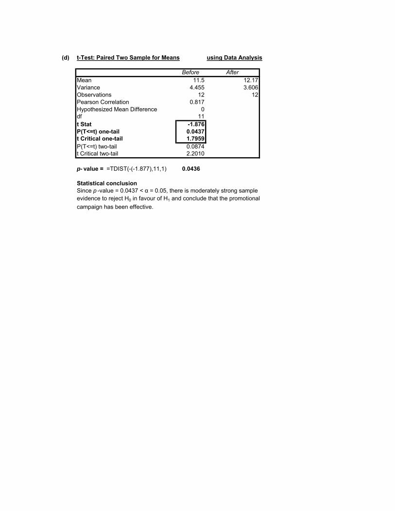
(d) t-Test: Paired Two Sample for Means using Data Analysis
Before AfterMean 11.5 12.17Variance 4.455 3.606Observations 12 12Pearson Correlation 0.817Hypothesized Mean Difference 0df 11t Stat -1.876P(T<=t) one-tail 0.0437t Critical one-tail 1.7959P(T<=t) two-tail 0.0874t Critical two-tail 2.2010
p- value = =TDIST(-(-1.877),11,1) 0.0436
Statistical conclusionSince p -value = 0.0437 < α = 0.05, there is moderately strong sample evidence to reject H0 in favour of H1 and conclude that the promotionalcampaign has been effective.

Exercise 9.23 File: X9.23 - performance ratings.xlsx
(a) The samples are dependent as the same employee is tested both before and after the training sessions.
(b) Matched pairs test x1 = Performance rating before the training sessionsx2 = Performance rating after the training sessions
Let d = (x1 - x2) i.e. " before" - "after" Let μd = population mean difference in performance rating scores from before to after the training sessions.
Use the matched pairs t test statistic
H0: μd ≥ 0 One sided lower tailed testH1: μd < 0 'before rating scores lower than 'after' rating scores.
Test performed manually
Region of Acceptance Use α = 0.05 with df = (18-1) = 17t-crit = t(0.05)(17) = -1.74
Decision rule Do not reject H0 in favour of H1 if -1.74 ≤ t-stat
Sample data Σxd -6.4n 18
x(bar)d -0.356sd 0.7114
t-stat (-0.356 - 0)/(0.7114/√18) =-2.123
Data Analysis: t-Test : Paired Two Sample for Means
Before AfterMean 11.067 11.422Variance 6.024 5.835Observations 18 18Pearson Correlation 0.95743865Hypothesized Mean Difference 0df 17t Stat -2.120P(T<=t) one-tail 0.0245t Critical one-tail 1.740P(T<=t) two-tail 0.04898861t Critical two-tail 2.10981556
Statistical conclusionSince t-stat (-2.123) lies outside (below) the region of acceptance, there is sufficientsample evidence at the 5% significance level to reject H0 in favour of H1 (i.e. Reject H0)

Management conclusionConclude that there has been a significant increase in mean performance ratings scores of employees who attended the series of workshops ans seminars.
The performance enhancement sessions have therefore been effective at increasingmotivation and productivity - at the 5% level of significance.
(c) p -value = =TDIST(-(-2.123),17,1) 0.0244 Also see t-Test Table above.
Since p-value = 0.0244 < α = 0.05, there is strong sample evidence to reject H0in favour of H1 and conclude that the workshops have significantly increased employee motivation and productivity.

Exercise 9.24 File: X9.24 - household debt.xlsx
(a) The samples are dependent as the same household is tested both a year agoand at the current time period .
(b) Matched pairs test x1 = Household debt level a year ago. x2 = Household debt level currently.
Let d = (x1 - x2) i.e. " year ago" - "current" Let μd = population mean difference in household debt levels from a year agoto the current period.
Use the matched pairs t test statistic
H0: μd ≤ 0 One sided upper tailed testH1: μd > 0 Debt higher a year ago than today (current period)
Test performed manually
Region of Acceptance Use α = 0.05 with df = (10-1) = 9t-crit = t(0.05)(9) = 1.833
Decision rule Do not reject H0 in favour of H1 if t-stat ≤ 1.833
Sample data Σxd 12n 10
x(bar)d 1.2sd 1.8135
t-stat (1.2 - 0)/(1.8135/√10) =2.0925
Data Analysis: t-Test : Paired Two Sample for Means
Year ago CurrentMean 40.5 39.3Variance 35.611 36.011Observations 10 10Pearson Correlation 0.9541Hypothesized Mean Difference 0df 9t Stat 2.0925P(T<=t) one-tail 0.0330t Critical one-tail 1.8331P(T<=t) two-tail 0.0659t Critical two-tail 2.2622
Statistical conclusionSince t-stat (2.0925) lies outside (above) the region of acceptance, there is sufficient sample evidence at the 5% significance level to reject H0 in favour of H1. (i.e. Reject H0).

Management conclusionConclude that there has been a significant decrease in the average level of household debt from a year ago.
The increase in prime interest rate (from 6% to 11%) has lead to a significant decline in the average level of household debt from a year ago - at the 5% significance level.
(c) p -value = =TDIST(2.0925,9,1) 0.033 Also see t-Test Table above
Since the p -value (0.033) < α = 0,05, there is strong sample evidence to reject H0 in favour of H1 at the 5% level of significance. Same statistical and management conclusions as (b) above.

Exercise 9.25 Process output variability study
Random variable: Hourly output per process
unit of measure: units produced per hour
H0 σ2(1) = σ2(2) Management question in H0
H1: σ2(1) ≠ σ2(2)
Region of Acceptance (use α = 0.05)
Note: Set up the F-test as an upper tailed test (F-stat = larger s2/smaller s2)
F-crit (upper) = F(0.05,30,24) 1.939
Decision rule: Do not reject H0 if F-stat (the sample evidence) ≤ 1.939
α = 0.05
s12 = 14.6 s2
2 = 23.2
n1 = 25 n2 = 31
F-stat = larger s2/smaller s2F-stat = 23.2/14.6 = 1.589
p -value = 0.1240
Statistical conclusion
Since F-stat = 1.589 < F-crit = 1.939, there is insufficient sample evidence at the
5% level of significance to reject H0 in favour of H1.
Management conclusion
Therefore conclude, with 95% confidence, that the variability of hourly outputs
between the two production processes is the same.
Sample data

Exercise 9.26 File: X9.26 - milk yield.xlsx
Random variable: milk yield (in litres per week) per cow
H0: σ2(f) ≤ σ
2(c)
H1: σ2(f) > σ
2(c) Management question in H1
Region of Acceptance: Use α = 0.05 with df1 = 16-1 = 15 and df2 = 16-1 = 15
F-crit = F(0.05,15,15) = 2.403 (See Excel output)
Decision rule: Do not reject H0 if F-stat ≤ 2.403
F-Test Two-Sample for Variances (Data Analysis in Excel )
Free grazing Controlled Feed
Mean 31.306 35.375
Variance 72.138 43.110
Observations 16 16
df 15 15
F-stat 1.673
P(F<=f) one-tail 0.1647
F Critical one-tail 2.403
F-stat = 1.673 (See Excel output) p -value = 0.1647
Statistical conclusion
Since F-stat = 1.673 < F-crit = 2.403, there is insufficient sample evidence at the
5% level of significance to reject H0 in favour of H1.
Management conclusion
Therefore conclude, with 95% confidence, that there is no signficant difference
in the variability in milk yields of cows between the two feeding practices.
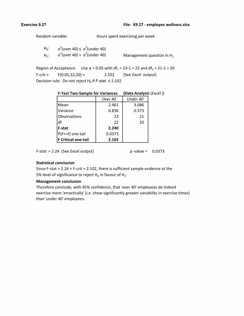
Exercise 9.27 File: X9.27 - employee wellness.xlsx
Random variable: Hours spent exercising per week
H0: σ2(over 40) ≤ σ
2(under 40)
H1: σ2(over 40) > σ
2(under 40) Management question in H1
Region of Acceptance: Use α = 0.05 with df1 = 23-1 = 22 and df2 = 21-1 = 20
F-crit = F(0.05,22,20) = 2.102 (See Excel output)
Decision rule: Do not reject H0 if F-stat ≤ 2.102
F-Test Two-Sample for Variances (Data Analysis (Excel ))
Over 40 Under 40
Mean 2.461 3.086
Variance 0.836 0.373
Observations 23 21
df 22 20
F-stat 2.240
P(F<=f) one-tail 0.0373
F Critical one-tail 2.102
F-stat = 2.24 (See Excel output) p -value = 0.0373
Statistical conclusion
Since F-stat = 2.24 > F-crit = 2.102, there is sufficient sample evidence at the
5% level of significance to reject H0 in favour of H1.
Management conclusion
Therefore conclude, with 95% confidence, that 'over 40' employees do indeed
exercise more 'erractically' (i.e. show significantly greater variability in exercise times)
than 'under 40' employees.

Exercise 9.28 File: X9.28 - attrition rate.xlsx
Random variable Attrition rates (%) per call center per month
H0: σ2(fin) = σ
2(health) Management question in H0
H1: σ2(fin) ≠ σ
2(health)
Region of Acceptance of H0: Find only F-crit (lower) or F-crit (upper)
This depends on whether the smaller or the larger sample variance is in the numerator of F-stat
For an F-crit (upper) only: For an F-crit (lower) only:
F-stat = Larger variance / Smaller variance F-stat = Smaller variance / Larger variance
F-Test Two-Sample for Variances F-Test Two-Sample for Variances
Health Financial Financial Health
Mean 5.46 6.13 Mean 6.13 5.46
Variance 1.1413 0.6653 Variance 0.6653 1.1413
Observations 17 21 Observations 21 17
df 16 20 df 20 16
F-stat 1.715 F-stat 0.583
P(F<=f) one-tail 0.1263 P(F<=f) one-tail 0.1263
F-crit (upper) 2.184 F-crit (lower) 0.458
F-crit (upper) = F(0.05,16,20) =1.1413/0.6653 2.184
OR F-crit (lower) = 1/F(0.05,16,20) =0.6653/1.1413 0.458
(or F(0.95,20,16))
Decision rule: For upper tailed test: Do not reject H0 if F-stat ≤ 2.184
OR For lower tailed test: Do not reject H0 if F-stat ≥ 0.458
Now F-stat = 1.715 (for an upper tailed test); or F-stat = 0.583 (for a lower tailed test)
Conclusion (based on an upper tailed F-test)
Since F-stat = 1.715 > F-crit (upper) = 2.184 (and hence lies within the acceptance region), there
is insufficient sample evidence at the 5% level of significance to reject H0 in favour of H1.
Same Conclusion (based on a lower tailed F-test)
Since F-stat = 0.583 > F-crit (lower) = 0.458 (and hence lies within the acceptance region), there
is insufficient sample evidence at the 5% level of significance to reject H0 in favour of H1.
Management conclusion
With 95% confidence, it can be concluded that there is no significant difference in the variability
in attrition rates between the two sectors (financial and health).

CHAPTER 10
CHI-SQUARE HYPOTHESIS TESTS
Exercise 10.1 Purpose: To test whether there is any statistically significant association between
the outcomes of two categorical variables. Stated differently, are the outcomes
associated with two categorical variables independent of each other or not?
Exercise 10.2 Categorical (nominal or ordinal-scaled) data
Exercise 10.3 H0: There is no statistical association between the two categorical variables
Exercise 10.4 Expected frequencies represent the null hypothesis of no association (or statistical
independence ) between the two categorical variables.
Exercise 10.5 χ²-crit (0.05,6) = 12.592 χ²-crit (0.10,6) = 10.645

Exercise 10.6 File: X10.6 - motivation status.xlsx
(a) Row Percentages
High Moderate Low TotalMale 26.7 26.7 46.7 100Female 47.5 30.0 22.5 100Total 38.6 28.6 32.9 100
Interpretation (by inspection)When compared to the general population profile, males tend to have low levels of motivation, while females tend to be more highly motivated. It appearstherefore that a statistical association exists between gender and motivation level.
(b) H0: There is no association between Gender and Motivation levelH1: There is an association between Gender and Motivation level
Region of Rejection (Use α = 0.10 with degrees of freedom = (2-1)(3-1) = 2)
χ²-crit = χ²(0.10)(2) = 4.605Decision rule
Reject H0 in favour of H1 if χ²-stat ≥ 4.605
χ²-stat Observed frequencies (fo)
High Moderate Low TotalMale 8 8 14 30Female 19 12 9 40Total 27 20 23 70
Expected frequencies (fe)
High Moderate Low TotalMale 11.57 8.57 9.86 30Female 15.43 11.43 13.14 40Total 27 20 23 70
Chi-Squared componentsHigh Moderate Low
Male 1.102 0.038 1.741Female 0.827 0.029 1.306
χ²-stat = 5.0428
ConclusionSince χ²-stat = 5.0428 > χ²-crit = 4.605, there is sufficient sample evidence at the10% significance level to reject H0 in favour of H1. Therefore conclude that there is a
statistical association between the gender of an employee and their level of motivation.The nature of the relationship is described in (a) above.
Motivation level

Exercise 10.7 File: X10.7 - internet shopping.xlsx
(a) Row Percentages
Yes No Totalfull-time 24.3 75.7 100at-home 18.5 81.5 100Total 20.8 79.2 100
Interpretation (by inspection)Since the row percentage profiles (between full-time employed and at-home customers) are very similar to each other and to the general population profile, it can be concluded, by observation, that the two attributes are not associated (i.e. they are statistically independent).
(b) H0: There is no association between Employment Status and Use of Internet ShoppingH1: There is an association between Employment Status and Use of Internet Shopping
Region of Rejection (Use α = 0.05 with degrees of freedom = (2-1)(2-1) = 1)
χ²-crit = χ²(0.05)(1) = 3.843Decision rule
Reject H0 in favour of H1 if χ²-stat ≥ 3.843
χ²-stat Observed frequencies (fo)
Yes No Totalfull-time 35 109 144at-home 40 176 216Total 75 285 360
Expected frequencies (fe)
Yes No Totalfull-time 30 114 144at-home 45 171 216Total 75 285 360
Chi-Squared componentsYes No
full-time 0.8333 0.2193at-home 0.5556 0.1462
χ²-stat = 1.7544
ConclusionSince χ²-stat = 1.7544 < χ²-crit = 3.843, there is insufficient sample evidence at the5% significance level to reject H0 in favour of H1. Therefore conclude that there is
no statistical association between the employment status of a customer and their use of the internet for shopping purposes. These two events are statistically independent.
Internet shopping

Exercise 10.8 File: X10.8 - car size.xlsx
(a) Row Percentages
Small Medium Large TotalUnder 30 15.2 33.3 51.5 10030 - 45 21.1 36.8 42.1 100Over 45 37.5 29.2 33.3 100Total 26.3 33.0 40.7 100
Interpretation (by inspection) With reference to the general population profile (Total row %), under 30's tend to prefer larger cars; 30-45 year age car buyers marginally tendtowards medium to large cars, while over 45's strongly tend to prefer smaller cars.
(b) H0: There is no association between Age of car buyer and Car Size bought.H1: There is an association between Age of car buyer and Car Size bought.
Region of Rejection (Use α = 0.01 with degrees of freedom = (3-1)(3-1) = 4)
χ²-crit = χ²(0.01)(4) = 13.277Decision rule
Reject H0 in favour of H1 if χ²-stat ≥ 13.277
χ²-stat Observed frequencies (fo)
Small Medium Large TotalUnder 30 10 22 34 6630 - 45 24 42 48 114Over 45 45 35 40 120Total 79 99 122 300
Expected frequencies (fe)
Small Medium Large TotalUnder 30 17.38 21.78 26.84 6630 - 45 30.02 37.62 46.36 114Over 45 31.6 39.6 48.8 120Total 79 99 122 300
Chi-Squared componentsSmall Medium Large
Under 30 3.134 0.002 1.91030 - 45 1.207 0.510 0.058Over 45 5.682 0.534 1.587
χ²-stat = 14.6247
ConclusionSince χ²-stat = 14.6247 > χ²-crit = 13.277, there is sufficient sample evidence at the1% significance level to reject H0 in favour of H1. Therefore conclude that there is a
statistical association between the age of a car buyer and the size of car bought.
Car sizes bought

(c) Management ConclusionThe nature of the statistical relationship found in (b) is described in (a) above. Under 30's tend to prefer larger cars; 30-45 year age car buyers marginally tendtowards medium to large cars, while over 45's strongly tend to prefer smaller cars.RecommendationTarget larger cars to the younger market and smaller cars to the older market.

Exercise 10.9 File: X10.9 - sports readership.xlsx
(a) Let πi = proportion of people who read Sports News in each of the i regions.
H0: π1 = π2 = π3
H1: At least one πi is different (i = 1,2,3)
Sample proportions E Cape W Cape KZN0.160 0.104 0.250
(b) Region of Rejection Use α = 0.01 with degrees of freedom = (2-1)(3-1) = 2
χ²-crit = χ²(0.01)(2) = 9.21Decision rule
Reject H0 in favour of H1 if χ²-stat ≥ 9.21
χ²-stat Observed frequencies (fo)
E Cape W Cape KZN TotalNo 84 86 78 248Yes 16 10 26 52Total 100 96 104 300
Expected frequencies (fe)
E Cape W Cape KZN TotalNo 82.67 79.36 85.97 248Yes 17.33 16.64 18.03 52Total 100 96 104 300
Chi-Squared componentsE Cape W Cape KZN
No 0.0215 0.5556 0.7395Yes 0.1026 2.6496 3.5267
χ²-stat = 7.5954
ConclusionSince χ²-stat = 7.5954 < χ²-crit = 9.21, there is insufficient sample evidence at the1% significance level to reject H0 in favour of H1. Therefore conclude that the
proportion of people who read Sports News is the same in each Geographical Region. These two events are statistically independent.
(c) H0: There is no association between the propensity to read Sports News and RegionH1: There is an association between the propensity to read Sports News and Region

Exercise 10.10 File: X10.10 - gym activity.xlsx
(a) Row Percentages
Spinning Swimming Circuit TotalMale 42.35 22.35 35.29 100Female 52.73 29.09 18.18 100Total 46.43 25.00 28.57 100
Interpretation (by inspection) When compared to the general population of gym goers, more females than males tend to prefer spinning and swimming; while more males relative to females tend to prefer mainly doing the circuit. The evidence is however not strongly convincing.
(b) H0: There is no association between Gender and preferred Gym ActivityH1: There is an association between Gender and preferred Gym Activity
Region of Rejection Use α = 0.10 with degrees of freedom = (2-1)(3-1) = 2
χ²-crit = χ²(0.10)(2) = 4.605Decision rule
Reject H0 in favour of H1 if χ²-stat ≥ 4.605
χ²-stat Observed frequencies (fo)
Spinning Swimming Circuit TotalMale 36 19 30 85Female 29 16 10 55Total 65 35 40 140
Expected frequencies (fe)
Spinning Swimming Circuit TotalMale 39.46 21.25 24.29 85Female 25.54 13.75 15.71 55Total 65 35 40 140
Chi-Squared componentsSpinning Swimming Circuit
Male 0.304 0.238 1.345Female 0.470 0.368 2.078
χ²-stat = 4.803
ConclusionSince χ²-stat = 4.803 > χ²-crit = 4.605 (marginally), there is sufficient sample evidence at the 10% significance level to reject H0 in favour of H1. Therefore conclude that
gender and preferred gym activity are associated.The nature of the relationship is described in (a) above.
(c) New rejection region Use α = 0.05 with degrees of freedom = (2-1)(3-1) = 2
χ²-crit = χ²(0.05)(2) = 5.991Decision rule Reject H0 in favour of H1 if χ²-stat ≥ 5.991
New decision Do not reject H0 at the 5% significance level,
Gym activity

since χ²-stat = 4.803 < χ²-crit = 5.991.New conclusion There is no statistical association between gender and gym activity
(i.e. they are statistically independent) at the 5% level of significant.
(d) Let πi = proportion of females who prefer each gym activity i (spinning, swimming, circuit)
H0: π1 = π2 = π3
H1: At least one πi is different (i = 1,2,3)
Sample proportions Spin Swim Circuit0.446 0.457 0.250
Statistical conclusionThe same statistical conclusion applies as in (b) (i.e. a statistical association exists)or stated differently: at least one population proportion is different. Management conclusionBy an inspection of the row percentage table in (a), it can be concluded thatspinning and swimming are the most preferred gym activities of females, while doing the circuit is the least preferred gym activity of females.

Exercise 10.11 File: X10.11 - supermarket visits.xlsx
(a) Categorical Frequency Table - Supermarket Visits
Visits Customers Percent Belief %Daily 36 20.0 253 / 4 times 55 30.6 35Twice 62 34.4 30Once only 27 15.0 10Total 180 100 100
Interpretation (by inspection)Once-a-week visits are the least common shopping behaviour (only 15%). Only one-in-five shoppers (20%) shop daily. The most common shopping pattern is either 3/4 times a week (30.6%) or twice a week (34.4%).These two shopping behaviours represent 65% of all the sampled shoppers.
(b) Goodness-of-fit test for an empirical distribution H0: The frequency of store visits per week is as per the manager's belief.H1: The frequency of store visits per week differs significantly from the manager's belief.
Region of Rejection (Use α = 0.05 with degrees of freedom = (4-1) = 3)
χ²-crit = χ²(0.05)(3) = 7.815Decision rule
Reject H0 in favour of H1 if χ²-stat ≥ 7.815
χ²-stat Visits fo %fe fe χ²-stat
Daily 36 25 45 1.83 / 4 times 55 35 63 1.016Twice 62 30 54 1.185Once only 27 10 18 4.5Total 180 100 180 8.501
ConclusionSince χ²-stat = 8.501 > χ²-crit = 7.815, there is sufficient sample evidence at the 5% significance level to reject H0 in favour of H1. Therefore conclude that
the shopping frequency of customers differs significantly from the manager's belief. The nature of the relationship is described in (a) above.
(c) InterpretationThe manager's belief is that customers shop more frequently during a week. frequently than the manager believes. For example, the survey found that only 51% shop more than 3 times per week, while the manager assumed that thispercentage was 60%. Similarly, more customers prefer to shop only once or twice a week (49%) compared to the manager's belief that this percentage was only 40%).These differences are however not strongly significantly different.
Customers

Exercise 10.12 File: X10.12 - equity portfolio.xlsx
Goodness-of-fit test for an empirical distribution
H0: There is no change in the equity portfolio mix between 2008 and 2012.H1: There is a significant change in the equity portfolio mix between 2008 and 2012.
Region of Rejection (Use α = 0.05 with degrees of freedom = (4-1) = 3)
χ²-crit = χ²(0.05)(3) = 7.815Decision rule
Reject H0 in favour of H1 if χ²-stat ≥ 7.815
χ²-stat Equity fo (2012) Ratio fe fe (2008) χ²-stat
Mining 900 2 900 0Industrial 1400 3 1350 1.852Retail 400 1 450 5.556Financial 1800 4 1800 0Total 4500 10 4500 7.407
ConclusionSince χ²-stat = 7.407 < χ²-crit = 7.815, there is insufficient sample evidence at the 5% significance level to reject H0 in favour of H1. Therefore conclude that
there is no significant change in the equity portfolio mix of the investor between 2008 and 2012. The equity portfolio profile is essentially the same in 2012 as it was in 2008.
Equities
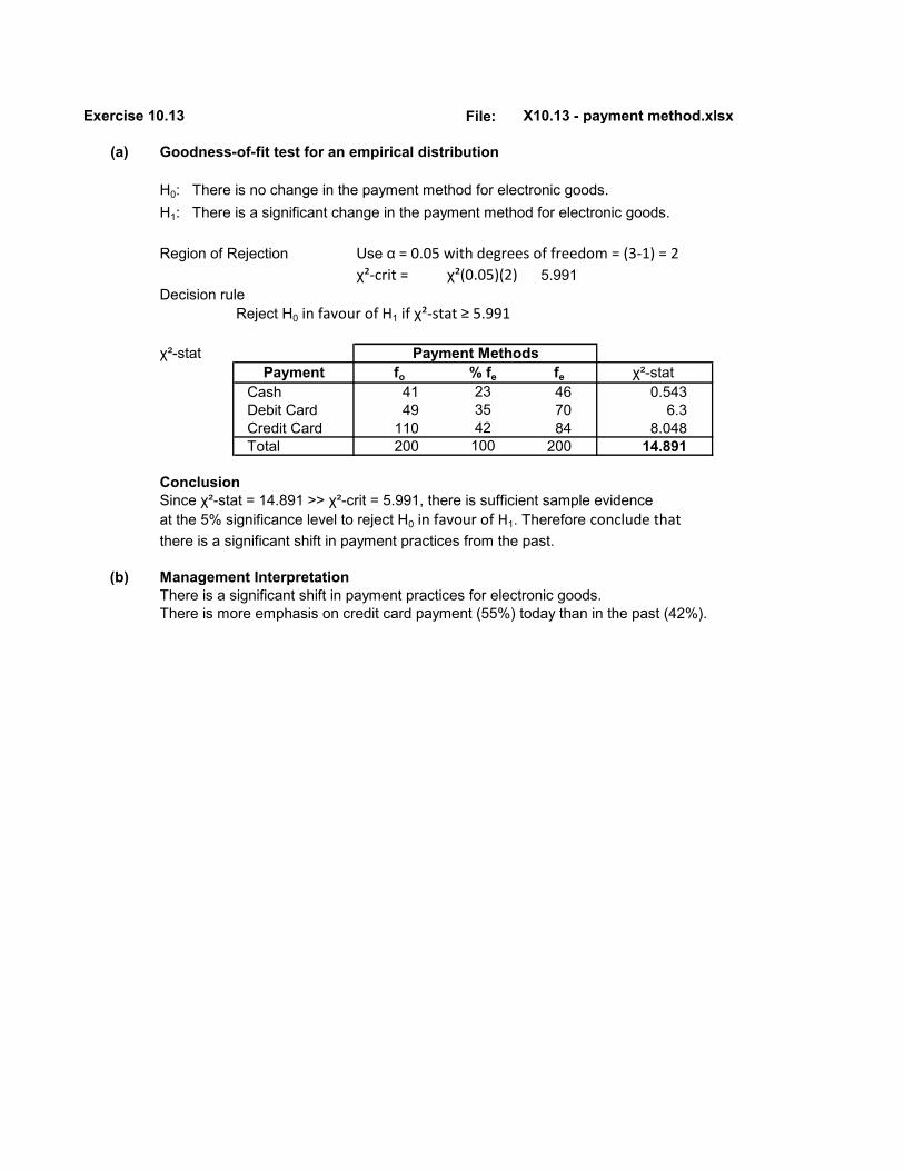
Exercise 10.13 File: X10.13 - payment method.xlsx
(a) Goodness-of-fit test for an empirical distribution
H0: There is no change in the payment method for electronic goods.H1: There is a significant change in the payment method for electronic goods.
Region of Rejection Use α = 0.05 with degrees of freedom = (3-1) = 2
χ²-crit = χ²(0.05)(2) = 5.991Decision rule
Reject H0 in favour of H1 if χ²-stat ≥ 5.991
χ²-stat Payment fo % fe fe χ²-stat
Cash 41 23 46 0.543Debit Card 49 35 70 6.3Credit Card 110 42 84 8.048Total 200 100 200 14.891
ConclusionSince χ²-stat = 14.891 >> χ²-crit = 5.991, there is sufficient sample evidence at the 5% significance level to reject H0 in favour of H1. Therefore conclude that
there is a significant shift in payment practices from the past.
(b) Management InterpretationThere is a significant shift in payment practices for electronic goods. There is more emphasis on credit card payment (55%) today than in the past (42%).
Payment Methods

Exercise 10.14 File: XS10.14 - package sizes.xlsx
(a) Goodness-of-fit test for an empirical distribution
H0: Limpopo sales pattern follows the national sales pattern.H1: Limpopo sales pattern does not follow the national sales pattern.
Region of Rejection (Use α = 0.05 with degrees of freedom = (3-1) = 2)
χ²-crit = χ²(0.05)(2) = 5.991Decision rule
Reject H0 in favour of H1 if χ²-stat ≥ 5.991
χ²-stat Package fo Ratio fe fe χ²-stat Large 190 3 162 4.840Midsize 250 5 270 1.481Small 100 2 108 0.593Total 540 10 540 6.914
ConclusionSince χ²-stat = 6.914 > χ²-crit = 5.991, there is sufficient sample evidence at the 5% significance level to reject H0 in favour of H1. Therefore conclude that
the Limpopo sales pattern of cereal package sizes differs significantly from the national sales pattern of package sizes sold.
(b) Management InterpretationThe Limpopo sales patterns differs significantly from the national sales patternof package sizes sold. By an inspection of the Limpopo sales profile relative to the national pattern, Limpopo tends to sell more large sized packages relative to the national pattern.
Package Size Sales

Exercise 10.15 File: X10.15 - compensation plan.xlsx
(a) Column Percentages
Plan Cape Gauteng Free State KZN TotalPresent 62 75.7 67.1 72.7 70.8New 38 24.3 32.9 27.3 29.2Total 100 100 100 100 100
Interpretation (by inspection) When compared to the national population profile of all employees, the present compensation plan enjoys more support in Gauteng, and the least support in the Cape Province where the new plan is favoured more. The evidence is however not overwhelming (i.e. the profile differences are not large)
(b) Let πi = proportion of sales staff in favour of the present payment plan in each province i .
H0: π1 = π2 = π3 = π4
H1: At least one πi is different (i = 1,2,3,4)
Sample proportions Cape Gauteng Free State KZN0.62 0.757 0.671 0.727
(c) Region of Rejection Use α = 0.10 with degrees of freedom = (2-1)(4-1) = 3
χ²-crit = χ²(0.10)(3) = 6.251Decision rule
Reject H0 in favour of H1 if χ²-stat ≥ 6.251
χ²-stat Observed frequencies (fo)
Plan Cape Gauteng Free State KZN TotalPresent 62 140 47 80 329New 38 45 23 30 136Total 100 185 70 110 465
Expected frequencies (fe)
Plan Cape Gauteng Free State KZN TotalPresent 70.75 130.89 49.53 77.83 329New 29.25 54.11 20.47 32.17 136Total 100 185 70 110 465
Chi-Squared componentsPlan Cape Gauteng Free State KZNPresent 1.0828 0.6337 0.1289 0.0606New 2.6194 1.5330 0.3119 0.1466
χ²-stat = 6.5169
ConclusionSince χ²-stat = 6.5169 > χ²-crit = 6.251 (marginally), there is sufficient sample evidence at the 10% significance level to reject H0 in favour of H1. Therefore conclude that
the support for the present compensation plan is different in at least one of the provinces.The nature of the relationship is described in (a) above.
(d) Formulate as a test for independence of association between payment plan and province.
Regions

H0: There is no association between payment plan preference and province.H1: There is an association between payment plan preference and province.
(e) New rejection region Use α = 0.05 with degrees of freedom = (2-1)(4-1) = 3
χ²-crit = χ²(0.05)(3) = 7.815Decision rule Reject H0 in favour of H1 if χ²-stat ≥ 7.815
New decision Do not reject H0 at the 5% significance level,
since χ²-stat = 6.5169 < χ²-crit = 7.815.
New conclusionThere is no statistical association between payment plan preference and province.(i.e. they are statistically independent) at the 5% level of significant. The sample evidence is not strong enough (i.e. the sample proportion differences are not great enough) to reject H0 in favour of H1 at the 5% level of significance.

Exercise 10.16 File: X10.16 - tyre defects.xlsx
(a) Row Percentages
technical mechanical material TotalMorning 22.1 61.8 16.2 100Afternoon 30.2 46.5 23.3 100Night 42.6 36.8 20.6 100Total 31.5 48.2 20.3 100
Interpretation (by inspection) When compared to the total production of defective tyres (total row %),tyre defects due to mechanical problems tend to be more prevalent during morning shifts.Technical defects however tend to be more prevalent during the night shift. Thus there does appear to be an association between shift and nature of tyre defects.
(b) Formulate as a test for independence of association between nature of defect and shift
H0: There is no association between nature of tyre defect and shift.H1: There is an association between nature of tyre defect and shift.
Region of Rejection Use α = 0.05 with degrees of freedom = (3-1)(3-1) = 4
χ²-crit = χ²(0.05)(4) = 9.488Decision rule
Reject H0 in favour of H1 if χ²-stat ≥ 9.488
χ²-stat Observed frequencies (fo)
technical mechanical material TotalMorning 15 42 11 68Afternoon 26 40 20 86Night 29 25 14 68Total 70 107 45 222
Expected frequencies (fe)
technical mechanical material TotalMorning 21.44 32.77 13.78 68Afternoon 27.12 41.45 17.43 86Night 21.44 32.77 13.78 68Total 70 107 45 222
Chi-Squared componentstechnical mechanical material
Morning 1.9351 2.5967 0.5622Afternoon 0.0460 0.0508 0.3782Night 2.6646 1.8443 0.0034
χ²-stat = 10.0812
(c) ConclusionSince χ²-stat = 10.0812 > χ²-crit = 9.488, there is sufficient sample evidence at the 5% significance level to reject H0 in favour of H1. Therefore conclude that
the nature of tyre defects produced is related to the shift on which the defects occur.The nature of the relationship is described in (a) above.
Nature of defective tyre

(d) Let πi = proportion of defective tyres caused by mechanical factors per shift i .
H0: π1 = π2 = π3
H1: At least one πi is different (i = 1,2,3)
The hypothesis test procedure is identical to (b) above.The sample proportions being compared are: Morning Afternoon Night
0.618 0.465 0.368
ConclusionSince H0 is rejected in favour of H1 at the 5% significance level, it can be concluded that there
is at least one shift that has a different proportion of defective tyres due to mechanical factors. Based on the row percentages table in (a) above, it is clear that the morning shiftproduces a proportionally larger percentage of defective tyres due to mechanical factors than the afternoon or night shifts.

Exercise 10.17 File: X10.17 - flight delays.xlsx
(a) Histogram
Delays(min) Count<5 0
5 - 7.5 87.5 - 10 2810-12.5 2912.5-15 1315-17.5 2
Total 80
Interpretation Flight delay times (in minutes) appear to be normally distributed.
(b) Descriptive Statistics flight delaysMean 10.324Standard Error 0.261Median 10.3Mode 11Standard Deviation 2.333Sample Variance 5.444Kurtosis -0.550Skewness 0.084Range 10.3Minimum 5.3Maximum 15.6Sum 825.9Count 80
Interpretation The low skewness coefficient (0.084) indicates approximate normality.
(c) (i) Goodness-of-fit test for Normality H0: Flight time delays (in minutes) follows a normal distribution with μ = 10.324 min and σ = 2.333 min.
H1: Flight time delays (in minutes) do not follow a normal distribution with μ = 10.324 min and σ = 2.333 min.
Region of Rejection Use α = 0.01 with degrees of freedom = (7-2-1) = 4
χ²-crit = χ²(0.01)(4) = 13.277Decision rule
Reject H0 in favour of H1 if χ²-stat ≥ 13.277
Delay Intervals fo Probability fe χ²-stat -∞ < x < 5 0 P(x < 5) P(z < -2.282) 0.01130 0.90 0.9040
5 < x < 7.5 8 P(5 < x < 7.5) P(-2.282 < z < -1.21) 0.10180 8.14 0.00257.5 < x < 10 28 P(7.5 < x < 10) P(-1.21 < z < -0.139) 0.33120 26.50 0.0854
10 < x < 12.5 29 P(10 < x < 12.5) P(-0.139 < z < 0.933) 0.37950 30.36 0.060912.5 < x < 15 13 P(12.5 < x < 15) P(0.933 < z < 2.004) 0.15400 12.32 0.037515 < x < 17.5 2 P(15 < x < 17.5) P(2.004 < z < 3.076) 0.02117 1.69 0.055417.5 < x < +∞ 0 P(x > 17.5) P(z > 3.076) 0.00103 0.08 0.0824
80 1 80χ²-stat = 1.2282
ConclusionSince χ²-stat = 1.2282 << χ²-crit = 13.277, there is insufficient sample evidence at the 1% significance level to reject H0 in favour of H1. Therefore conclude that
flight delay times (in minutes) follows a Normal distribution with μ = 10.324 min and σ = 2.333 min.
Expected frequencies using x ≡ N(10.324; 2.333) from Z-tableNormal probability intervals (x and z)
0
8
28 29
13
2
0
5
10
15
20
25
30
35
<5 5 - 7.5 7.5 - 10 10-12.5 12.5-15 15-17.5N
o. o
f flig
hts
Delay Intervals (minutes)
Histogram of Flight Delay Times

(c) (ii) NORMDIST() From Z-tableP(x < 5) =NORMDIST(5,10.324,2.333,1) 0.01124 0.01130P(5 < x < 7,5) =NORMDIST(7.5,10.324,2.333,1) - NORMDIST(5,10.324,2.333,1) 0.10181 0.10180P(7,5 < x < 10) =NORMDIST(10,10.324,2.333,1) - NORMDIST(7.5,10.324,2.333,1) 0.33172 0.33120P(10 < x < 12,5) =NORMDIST(12.5,10.324,2.333,1) - NORMDIST(10,10.324,2.333,1) 0.37974 0.37950P(12,5 < x < 15) =NORMDIST(15,10.324,2.333,1) - NORMDIST(12.5,10.324,2.333,1) 0.15297 0.15400P(15 < x < 17,5) =NORMDIST(17.5,10.324,2.333,1) - NORMDIST(15,10.324,2.333,1) 0.02147 0.02117P(x > 17,5) =1-NORMDIST(17.5,10.324,2.333,1) 0.00105 0.00103
1 1

Exercise 10.18 File: newspaper sections.xlsx
(a) Two-way Pivot table of Gender by Newspaper Section Most Preferred to Read.
SectionGender Data Sport Social Business Grand TotalFemale Count 14 28 18 60
Row % 23.3% 46.7% 30.0% 100%Male Count 41 35 44 120
Row % 34.2% 29.2% 36.7% 100%Total Count 55 63 62 180Total Row % 30.6% 35.0% 34.4% 100%
Interpretation (by inspection)Females tend to read the Social section most, with the Sports section read the least.Males, alternatively, are marginally more interested in the Sport and Business sections. These observational conclusions are, however, not overwhelmingly conclusive.
(b)
(c) Formulate as a test for independence of association between gender and section read .
H0: There is no association between gender and the newspaper section most preferred.H1: There is an association between gender and the newspaper section most preferred.
Region of Rejection Use α = 0.10 with degrees of freedom = (2-1)(3-1) = 2
χ²-crit = χ²(0.10)(2) = 4.605Decision rule
Reject H0 in favour of H1 if χ²-stat ≥ 4.605
23.3% 34.2%
46.7% 29.2%
30.0% 36.7%
0%
20%
40%
60%
80%
100%
120%
Female Male
Stacked Bar Chart Newspaper Section Read by Gender
Business
Social
Sport

χ²-stat Observed frequencies (fo)
Sport Social Business Totalfemale 14 28 18 60male 41 35 44 120Total 55 63 62 180
Expected frequencies (fe)
Sport Social Business Totalfemale 18.3 21.0 20.7 60male 36.7 42.0 41.3 120Total 55 63 62 180
Chi-Squared componentsSport Social Business
female 1.0242 2.3333 0.3441male 0.5121 1.1667 0.1720
χ²-stat = 5.5525
ConclusionSince χ²-stat = 5.5525 > χ²-crit = 4.605 (marginal), there is sufficient sample evidence at the 10% significance level to reject H0 in favour of H1. Therefore conclude that
gender and the newspaper section most preferred are statistically associated. The nature of the relationship is described in (a) above.
(d) Let πi = proportion of females who most prefer each newspaper section i .
H0: π1 = π2 = π3
H1: At least one πi is different (i = 1,2,3)
The hypothesis test procedure is identical to (c) above.The sample proportions being compared are:
Sport Social Business0.255 0.444 0.290
ConclusionSince H0 is rejected in favour of H1 at the 10% significance level, it can be concluded that
there is at least one newspaper section that females prefer differently to the other sections. Based on the row percentages table in (a) above, it is clear that females tend to read the Social section most, with the Sports section read the least.

Exercise 10.19 File: X10.19 - vehicle financing.xlsx
(a) One-way Pivot table of Car Loan Sizes
Count of Loan size Count of Loan sizeLoan size Total Loan size Total
Under 100 18 Under 100 6%100 - <150 58 100 - <150 19%150 - <200 110 150 - <200 37%200 - <250 70 200 - <250 23%Above 250 44 Above 250 15%Grand Total 300 Grand Total 100%
Interpretation (by inspection)The most popular car loan size was between R150 000 and R200 000 (37% of allapplications) followed by car loan sizes of between R200 000 and R250 000 (23%).Only 6% of loan applications were for amounts below R100 000.
(b)
(c) Test for Goodness-of-Fit for an empirical distribution.
H0: There is no change in the size of car loan applications from four years ago.H1: There is a significant shift in the size of car loan applications from four years ago.
(d) Region of Rejection Use α = 0.05 with degrees of freedom = (5-1) = 4
χ²-crit = χ²(0.05)(4) = 9.488Decision rule
Reject H0 in favour of H1 if χ²-stat ≥ 9.488
χ²-stat Loan Size fo % fe fe χ²-stat
< R100 18 10 30 4.800R100 - R150 58 20 60 0.067R150 - R200 110 40 120 0.833R200 - R250 70 20 60 1.667> R250 44 10 30 6.533Total 300 100 300 13.900
Payment Methods
0.06
0.19
0.37
0.23
0.15
0
0.05
0.1
0.15
0.2
0.25
0.3
0.35
0.4
Under 100 100 - <150 150 - <200 200 - <250 Above 250Size of Loan Applications (R 1000)
Bar Chart of Car Loan Applications

ConclusionSince χ²-stat = 13.9 > χ²-crit = 9.488, there is sufficient sample evidence at the 5% significance level to reject H0 in favour of H1. Therefore conclude that
there has been a significant shift in the size of car loan applications from 4 years ago. The shift has been towards larger car loan applications.
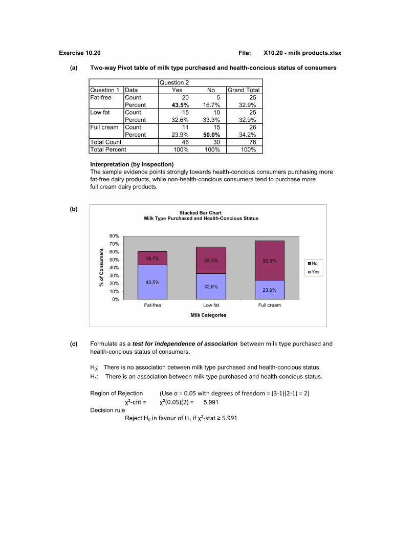
Exercise 10.20 File: X10.20 - milk products.xlsx
(a) Two-way Pivot table of milk type purchased and health-concious status of consumers
Question 2Question 1 Data Yes No Grand TotalFat-free Count 20 5 25
Percent 43.5% 16.7% 32.9%Low fat Count 15 10 25
Percent 32.6% 33.3% 32.9%Full cream Count 11 15 26
Percent 23.9% 50.0% 34.2%Total Count 46 30 76Total Percent 100% 100% 100%
Interpretation (by inspection)The sample evidence points strongly towards health-concious consumers purchasing morefat-free dairy products, while non-health-concious consumers tend to purchase more full cream dairy products.
(b)
(c) Formulate as a test for independence of association between milk type purchased and health-concious status of consumers.
H0: There is no association between milk type purchased and health-concious status.H1: There is an association between milk type purchased and health-concious status.
Region of Rejection (Use α = 0.05 with degrees of freedom = (3-1)(2-1) = 2)
χ²-crit = χ²(0.05)(2) = 5.991Decision rule
Reject H0 in favour of H1 if χ²-stat ≥ 5.991
43.5%32.6%
23.9%
16.7% 33.3% 50.0%
0%10%20%30%40%50%60%70%80%
Fat-free Low fat Full cream
% o
f Con
sum
ers
Milk Categories
Stacked Bar ChartMilk Type Purchased and Health-Concious Status
No
Yes

χ²-stat Observed frequencies (fo)
Yes No Totalfat-free 20 5 25low fat 15 10 25full cream 11 15 26
Total 46 30 76
Expected frequencies (fe)
Yes No Totalfat-free 15.13 9.87 25low fat 15.13 9.87 25full cream 15.74 10.26 26
Total 46 30 76
Chi-Squared componentsYes No
fat-free 1.566 2.402low fat 0.001 0.002full cream 1.426 2.186
χ²-stat = 7.583
ConclusionSince χ²-stat = 7.583 > χ²-crit = 5.991, there is sufficient sample evidence at the 5% significance level to reject H0 in favour of H1. Therefore conclude that
there is a significant statistical association between the health-concious status of a consumer and their preference for certain type of dairy milk products. The nature of the relationship is described in (a) above.
(d) Let πi = proportion of health-concious consumers who prefer each milk type i .
H0: π1 = π2 = π3
H1: At least one πi is different (i = 1,2,3)
The hypothesis test procedure is identical to (c) above.The sample proportions being compared are: fat-free low-fat full cream
0.800 0.600 0.423
ConclusionSince H0 is rejected in favour of H1 at the 5% significance level, it can be concluded that
there is at least one milk type that is purchased by a different proportion of health-conciousconsumers. Based on the row percentages table in (a) above, it is clear that health-concious consumers tend to purchase more fat-free dairy products than full cream products.

CHAPTER 11
ANALYSIS OF VARIANCE
COMPARING MEANS ACROSS MULTIPLE POPULATIONS
Exercise 11.1 The purpose of one-factor Anova is to test for equality of means across
multiple (more than two) populations.
Exercise 11.2 Example: Compare the output performance of five identical machines.
Exercise 11.3 Variation between groups measures how similar or how different
(i.e. how close or how far apart) the sample means are from each other.
It is a measure of the level of influence of the treatment factor on the
response measure. Any differences can be attributed to (or explained by)
the influence of the treatment factor on the numeric response measure.
Exercise 11.4 SST = 25.5
Numerator degrees of freedom = (4 - 1) = 3
SSE = 204.6 - 25.5 = 179.1
Denominator degrees of freedom = (4x10 - 4) = 36
MST = 25.5 / 3 = 8.5
MSE = 179.1 / 36 = 4.975
F-stat = 8.5 / 4.975 = 1.7085
Exercise 11.5 F-crit = F(0.05, 3, 36) = 2.866 In Excel, use =FINV(0.05,3,36)
Exercise 11.6 H0: μ1 = μ2 = μ3 = μ4
H1: At least one μi differs
Decision Rule: Do not reject H0 if F-stat ≤ F-crit .
Since F-stat = 1.7085 < F-crit = 2.866, do not reject H0.
Conclusion: All population means are equal.

Exercise 11.7 File: X11.7 - car fuel efficiency.xlsx
(a) Sample Average Fuel Consumption (l/100km)
Peugot VW FordΣxi 32.4 29.3 34.4ni 5 4 5x(bar)i 6.48 7.325 6.88
Grand mean = 96.1/14 = 6.864
(b) One-Factor Anova Factor = Car Type ( 1 = Peugot; 2 = VW; 3 = Ford)Response measure = Fuel Consumption (l/100km)
H0: μ1 = μ2 = μ3
H1: At least one μi differs (i = 1, 2, 3)
Region of Rejection (Use α = 0.05 with df1 = 3-1 = 2 and df2 = 14-3 = 11)
F-crit = F(0.05)(2,11) = 3.98Decision rule
Reject H0 in favour of H1 if F-stat ≥ 3.98
F-stat SSW = (7-6.48)²+(6.3-6.48)²+(6-6.48)²+(6.4-6.48)²+(6.7-6.48)²+(6.8-7.325)²+(7.4-7.325)²+(7.9-7.325)²+(7.2-7.325)²+(7.6-6.88)²+(6.8-6.88)²+(6-4.88)²+(7-6.88)²+(6.6-6.88)²= 2.0635
SSB = (6.48-6.864)²+(7.325-6.864)²+(6.88-6.864)²= 1.5886
SST = 2.0635 + 1.5886 = 3.6521
Anova Table Source of Variation SS df MS F-stat
Between 1.5886 2 0.79432 4.234Within 2.0635 11 0.18759Total 3.6521 13
Peugot VW FordCar Types 6.48 7.325 6.88
6.487.325 6.88
0123456789
10
litre
s / 1
00 k
m
Bar Chart of Fuel Efficiency Means
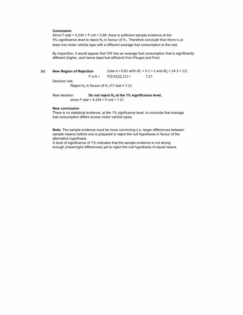
ConclusionSince F-stat = 4.234 > F-crit = 3.98, there is sufficient sample evidence at the5% significance level to reject H0 in favour of H1. Therefore conclude that there is at
least one motor vehicle type with a different average fuel consumption to the rest.
By inspection, it would appear that VW has an average fuel consumption that is significantly different (higher, and hence least fuel efficient) from Peugot and Ford.
(c) New Region of Rejection (Use α = 0.01 with df1 = 3-1 = 2 and df2 = 14-3 = 11)
F-crit = F(0.01)(2,11) = 7.21Decision rule
Reject H0 in favour of H1 if F-stat ≥ 7.21
New decision Do not reject H0 at the 1% significance level, since F-stat = 4.234 < F-crit = 7.21
New conclusionThere is no statistical evidence, at the 1% signficance level, to conclude that averagefuel consumption differs across motor vehicle types.
Note: The sample evidence must be more convincing (i.e. larger differences between sample means) before one is prepared to reject the null hypothesis in favour of the alternative hypothesis. A level of significance of 1% indicates that the sample evidence is not strong enough (meaningful differences) yet to reject the null hypothesis of equal means.

Exercise 11.8 File: X11.8 - package design.xlsx
Assumption 1 Equal population variances. Assumption 2 A normally distribution population for the response variable.
(a) One-Factor Anova Factor = Package designs (1 = A; 2 = B; 3 = C)Response measure = Carton sales (units)
Let μi = population mean sales of a breakfast cereal packaged in design shape i H0: μ1 = μ2 = μ3
H1: At least one μi differs (i = 1, 2, 3)
Region of Rejection (Use α = 0.05 with df1 = 3-1 = 2 and df2 = 21-3 = 18)
F-crit = F(0.05)(2,18) = 3.55Decision rule
Reject H0 in favour of H1 if F-stat ≥ 3.55
F-stat (Refer to formulae in Chapter 11)
Sample evidenceDesign A Design B Design C
Sample means 35.75 32.86 34.17Grand mean 721/21 = 34.33
SSW = (35-35.75)²+(37-35.75)²+(39-35.75)²+(36-35.75)²+(30-35.75)²+(39-35.75)²+(36-35.75)²+(34-35.75)²+(35-32.86)²+(34-32.86)²+(30-32.86)²+(31-32.86)²+(34-32.86)²+(32-32.86)²+(34-32.86)²+(38-34.17)²+(34-34.17)²+(32-34.17)²+(34-34.17)²+(34-34.17)²+(33-34.17)²= 101.1905
SSB = (35.75-34.33)²+(32.86-34.33)²+(34.17-34.33)²= 31.4762
SST = 101.1905+31.4762 = 132.6667
Anova Table Source of Variation SS df MS F-stat
Between 31.4762 2 15.7381 2.7995Within 101.1905 18 5.6217Total 132.6667 20
ConclusionSince F-stat = 2.7995 < F-crit = 3.55, there is insufficient sample evidence at the5% significance level to reject H0 in favour of H1. Therefore conclude that there is
no difference in the mean volume of sales across the 3 package designs.
(b) RecommendationThere is no strong statistical evidence to conclude that sales volumes differ across the three package designs. All are likely to generate the same average sales. Therefore the cereal producer can choose any of the three package designs for their new muesli cereal.

Exercise 11.9 File: X11.9 - bank service.xlsx
(a) One-Factor Anova Factor = Bank (1 = X; 2 = Y; 3 = Z)Response measure = Rating score (1 to 10)
Let μi = population mean service rating score for bank i H0: μ1 = μ2 = μ3
H1: At least one μi differs (i = 1, 2, 3)
Region of Rejection (Use α = 0.10 with df1 = 3-1 = 2 and df2 = 27-3 = 24)
F-crit = F(0.10)(2,24) = 2.538 =FINV(0.1,2,24)Decision rule
Reject H0 in favour of H1 if F-stat ≥ 2.538
F-stat (Refer to the formulae in Chapter 11)
Sample evidenceBank X Bank Y Bank Z
Sample means 6.875 5.778 6.2Grand mean 169/27 = 6.259
SSW = (8-6.875)²+(6-6.875)²+...+(5-5.778)²+(6-5.778)²+…+(8-6.2)²+(7-6.2)²+…+(6-6.2)²= 24.0306
SSB = (6.875-6.259)²+(5.778-6.259)²+(6.2-6.259)²= 5.1546
SST = 24.0306 + 5.1546 = 29.1852
Anova Table
Source of Variation SS df MS F-stat
Between 5.1546 2 2.5773 2.574Within 24.0306 24 1.0013Total 29.1852 26
ConclusionSince F-stat = 2.574 > F-crit = 2.538, there is sufficient sample evidence at the10% significance level to reject H0 in favour of H1. Therefore conclude that there is
at least one bank that has a different mean service rating score to the other banks.
By inspection, it would appear that Bank X has a significantly higher mean service rating score than the other two banks.
(b) New Region of Rejection (Use α = 0.05 with df1 = 3-1 = 2 and df2 = 27-3 = 24)
F-crit = F(0.05)(2,24) = 3.40Decision rule
Reject H0 in favour of H1 if F-stat ≥ 3.40
New decision Do not reject H0 at the 5% significance level,
since F-stat = 2.574 < F-crit = 3.40
New conclusion

There is no statistical evidence, at the 5% signficance level, to conclude that the mean service ratings is different across the three banks.The three banks are perceived similarly by customers in terms of their service levels.
Note: The reason for the change in conclusion between (a) and (b) is that the statistical evidence is only weak (i.e. small differences in sample means) at the 10% significance level, while it the 5% significance level, it is not seen as strong enough (i.e. differences are not large enough) to reject the null hypothesis.

Exercise 11.10 File: X11.10 - shelf height.xlsx
One-Factor Anova Factor = Shelf Height (1 = Bottom; 2 = Waist; 3 = Shoulder; 4 = Top)Response measure = Sales volume (units sold)
Let μi = population mean sales of a drinking chocolate product displayed at shelf height i H0: μ1 = μ2 = μ3 = μ4
H1: At least one μi differs (i = 1, 2, 3, 4)
Region of Rejection (Use α = 0.05 with df1 = 4-1 = 3 and df2 = 30-4 = 26)
F-crit = F(0.05)(3,26) = 2.990Decision rule
Reject H0 in favour of H1 if F-stat ≥ 2,990
F-stat (Refer to the formulae in Chapter 11)
Sample evidenceBottom Waist Shoulder Top
Sample means 76.143 81.375 82.444 74.833Grand mean 2375/30 = 79.167
SSW = (78-76.143)²+….+(78-81.375)²+….+(83-82.444)²+….+(69-74.833)²+…+(75-74.833)²= 727.788
SSB = (76.143-79.167)²+(81.375-79.167)²+(82.444-79.167)²+(74.833-79.167)²= 312.379
SST = 727.788 + 312.379 = 1040.167
Anova Table Source of Variation SS df MS F-stat
Between 312.379 3 104.126 3.720Within 727.788 26 27.992Total 1040.167 29
ConclusionSince F-stat = 3.72 > F-crit = 2.99, there is sufficient sample evidence at the5% significance level to reject H0 in favour of H1. Therefore conclude that there is
at least one shelf height that generates a different mean level of sales to the other shelves.
By inspection, it would appear that shoulder and waist high shelves generate higher averagesales of the drinking chocolate product than bottom or top shelves.
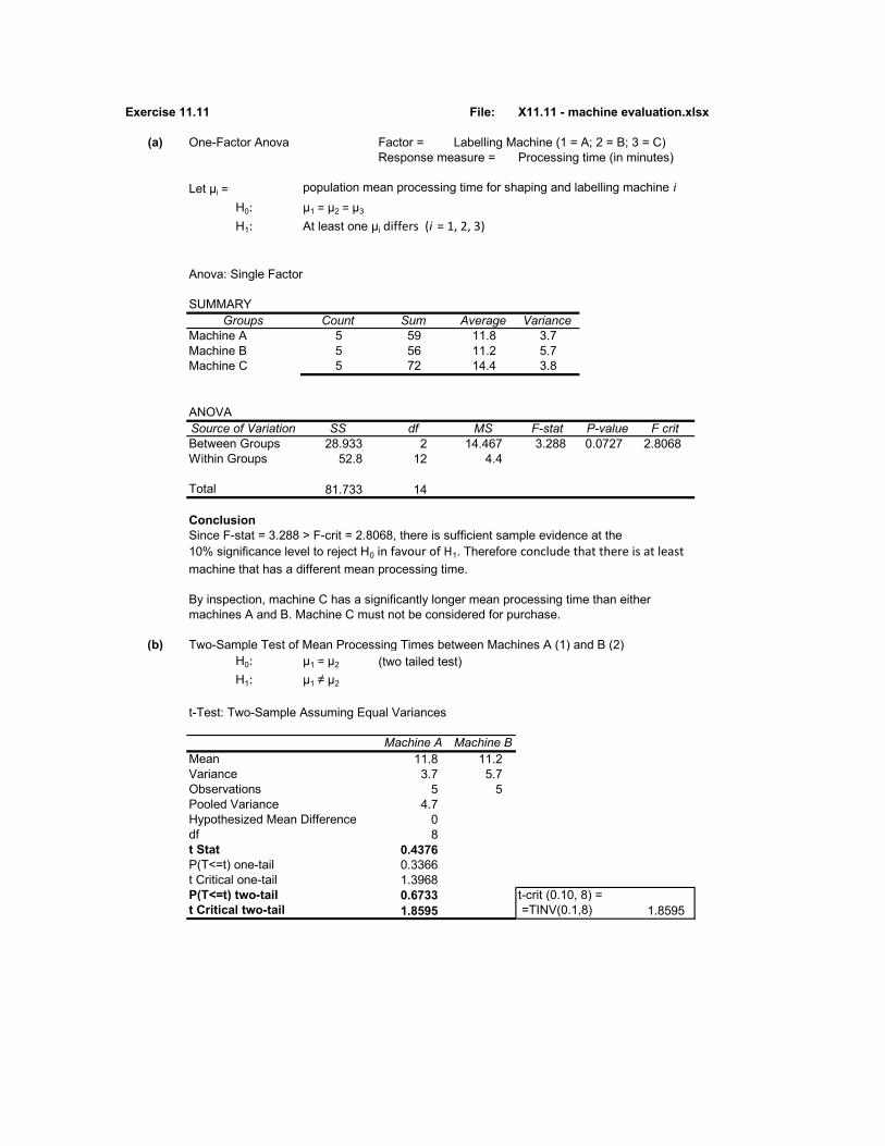
Exercise 11.11 File: X11.11 - machine evaluation.xlsx
(a) One-Factor Anova Factor = Labelling Machine (1 = A; 2 = B; 3 = C)Response measure = Processing time (in minutes)
Let μi = population mean processing time for shaping and labelling machine i H0: μ1 = μ2 = μ3
H1: At least one μi differs (i = 1, 2, 3)
Anova: Single Factor
SUMMARYGroups Count Sum Average Variance
Machine A 5 59 11.8 3.7Machine B 5 56 11.2 5.7Machine C 5 72 14.4 3.8
ANOVASource of Variation SS df MS F-stat P-value F critBetween Groups 28.933 2 14.467 3.288 0.0727 2.8068Within Groups 52.8 12 4.4
Total 81.733 14
ConclusionSince F-stat = 3.288 > F-crit = 2.8068, there is sufficient sample evidence at the10% significance level to reject H0 in favour of H1. Therefore conclude that there is at least
machine that has a different mean processing time.
By inspection, machine C has a significantly longer mean processing time than either machines A and B. Machine C must not be considered for purchase.
(b) Two-Sample Test of Mean Processing Times between Machines A (1) and B (2)H0: μ1 = μ2 (two tailed test)H1: μ1 ≠ μ2
t-Test: Two-Sample Assuming Equal Variances
Machine A Machine BMean 11.8 11.2Variance 3.7 5.7Observations 5 5Pooled Variance 4.7Hypothesized Mean Difference 0df 8t Stat 0.4376P(T<=t) one-tail 0.3366t Critical one-tail 1.3968P(T<=t) two-tail 0.6733 t-crit (0.10, 8) =t Critical two-tail 1.8595 =TINV(0.1,8) 1.8595

ConclusionSince t-stat = 0.4376 lies with the region of non-rejection of H0 (i.e. within ± 1.8595), the sample evidence is not strong enough to reject H0 in favour of H1.The population mean processing times between the two machines A and B are likely to be identical. Thus the company can purchase either machine A or machine B.
(c) RecommendationBased on the statistical evidence in (a) and (b), the company can purchase either machine A or machine B - they are likely to be equally efficient in operation.

Exercise 11.12 File: X11.12 - earnings yield.xlsx
(a) One-Factor Anova Factor = Economic Sector(1 = Financial; 2 = Retail; 3 = Industrial; 4 = Mining)
Response measure = Earnings yield (%)
Let μi = population mean earnings yield per economic sector i H0: μ1 = μ2 = μ3 = μ4
H1: At least one μi differs (i = 1, 2, 3, 4)
(b) Anova: Single Factor
SUMMARYGroups Count Sum Average Variance
Industrial 20 96.1 4.81 1.091Retail 20 94.4 4.72 1.492Financial 20 113.2 5.66 1.588Mining 20 111 5.55 2.067
ANOVASource of Variation SS df MS F-stat P-value F critBetween Groups 14.3894 3 4.7965 3.0757 0.0326 2.7249Within Groups 118.5195 76 1.5595
Total 132.9089 79
ConclusionSince F-stat = 3.076 > F-crit = 2.725, there is sufficient sample evidence at the5% significance level to reject H0 in favour of H1. Therefore conclude that there is
at least one sector with a different mean earnings yield relative to the other sectors.
(c) Interpretation By inspection, the Industrial and Retail sectors each appear to have significantly lower mean earnings yields relative to the Financial and Mining sectors' mean earnings yields.
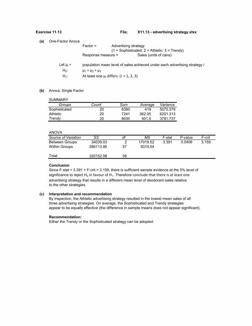
Exercise 11.13 File: X11.13 - advertising strategy.xlsx
(a) One-Factor Anova Factor = Advertising strategy
(1 = Sophisticated; 2 = Athletic; 3 = Trendy)Response measure = Sales (units of cans)
Let μi = population mean level of sales achieved under each advertising strategy i H0: μ1 = μ2 = μ3
H1: At least one μi differs (i = 1, 2, 3)
(b) Anova: Single Factor
SUMMARYGroups Count Sum Average Variance
Sophisticated 20 8380 419 5075.579Athletic 20 7241 362.05 6201.313Trendy 20 8030 401.5 3781.737
ANOVASource of Variation SS df MS F-stat P-value F-critBetween Groups 34039.03 2 17019.52 3.391 0.0406 3.159Within Groups 286113.95 57 5019.54
Total 320152.98 59
ConclusionSince F-stat = 3.391 > F-crit = 3.159, there is sufficient sample evidence at the 5% level of significance to reject H0 in favour of H1. Therefore conclude that there is at least one
advertising strategy that results in a different mean level of deodorant sales relative to the other strategies.
(c) Interpretation and recommendationBy inspection, the Athletic advertising strategy resulted in the lowest mean sales of allthree advertising strategies. On average, the Sophisticated and Trendy strategies appear to be equally effective (the difference in sample means does not appear significant).
Recommendation:Either the Trendy or the Sophisticated strategy can be adopted.

(d) Two-Sample Test of Means between the Sophisticated (1) and Trendy (2) StrategiesH0: μ1 = μ2 (two-tailed test)H1: μ1 ≠ μ2
t-Test: Two-Sample Assuming Equal Variances
Sophisticated Trendy Mean 419 401.5Variance 5075.579 3781.737Observations 20 20Pooled Variance 4428.6579Hypothesized Mean Difference 0df 38t Stat 0.8316P(T<=t) one-tail 0.2054t Critical one-tail 1.6860P(T<=t) two-tail 0.4108 t-crit (0.05,38) =t Critical two-tail 2.0244 =TINV(0.05,38) 2.0244
ConclusionSince t-stat = 0.8316 lies within the region of non-rejection of H0 (i.e. ± 2.0244), there is
insufficient sample evidence to reject H0 in favour of H1. Therefore the population mean sales from each of the two strategies is likely to be identical. The two strategies are therefore equally effective and either can be adopted by the company.
(e) RecommendationThe Athletic strategy can be discarded. It appears the least effective. The remaining two strategies (Sophisticated and Trendy) are equally effective and therefore either can be adopted by the company to promote its new ladies deodorant.

Exercise 11.14 File: X11.14 - leverage ratio.xlsx
(a) Descriptive StatisticsTechnology Construction Banking Manufacturing
Mean 73.83 78.07 69.73 76.37Standard Error 1.697 1.912 2.527 2.347Median 72.5 78.5 68 79.5Mode 60 80 68 81Standard Deviation 9.296 10.471 13.841 12.853Sample Variance 86.420 109.651 191.582 165.206Kurtosis -1.309 -0.546 -0.453 0.495Skewness 0.010 0.051 0.103 -0.857Range 28 40 58 50Minimum 60 58 41 44Maximum 88 98 99 94Sum 2215 2342 2092 2291Count 30 30 30 30Confidence Level(95.0%) 3.471 3.910 5.168 4.799
InterpretationThe mean leverage ratio is lowest for the banking sector and highest for the construction and the manufacturing sectors. These differences do appear to be significant.
(b) One-Factor Anova Factor = Economic Sector(1 = Technology; 2 = Construction; 3 = Banking; 4 = Manufacturing)Response measure = Leverage ratio
Let μi = population mean leverage ratio per economic sector i H0: μ1 = μ2 = μ3 = μ4
H1: At least one μi differs (i = 1, 2, 3, 4)
Anova: Single Factor
SUMMARYGroups Count Sum Average Variance
Technology 30 2215 73.83 86.42Construction 30 2342 78.07 109.65Banking 30 2092 69.73 191.58Manufacturing 30 2291 76.37 165.21
ANOVASource of Variation SS df MS F-stat P-value F crit
Between Groups 1181.13 3 393.711 2.849 0.0406 2.683Within Groups 16032.87 116 138.214
Total 17214 119

ConclusionSince F-stat = 2.849 > F-crit = 2.683 (marginally), there is sufficient sample evidence at the5% significance level to reject H0 in favour of H1. Therefore conclude that there is
at least one sector with a different mean leverage ratio relative to the other sectors.
By inspection, the banking sector has the lowest mean leverage ratio, while constructionand manufacturing appear to have similarly high mean leverage ratios.
Recommendation The investor is advised to consider either the banking sector (with the lowestmean leverage ratio) or the technology sector (with a marginally higher meanleverage ratio). (This difference may not be statistically significant).
(c) Two-Sample Test of Means - Leverage ratios between Technology (1) and Banking (2) sectors.H0: μ1 = μ2 (two-tailed test)H1: μ1 ≠ μ2
t-Test: Two-Sample Assuming Equal Variances
Technology BankingMean 73.833 69.733Variance 86.420 191.582Observations 30 30Pooled Variance 139.001Hypothesized Mean Difference 0df 58t Stat 1.347P(T<=t) one-tail 0.092t Critical one-tail 1.672P(T<=t) two-tail 0.183 t-crit (0.05, 58) =t Critical two-tail 2.002 =TINV(0.05,58) 2.002
ConclusionSince t-stat = 1.347 lies within the region of non-rejection of H0 (i.e. within ±2.002), the sample evidence is
not strong enough to reject H0 in favour of H1. The population mean leverage ratios between the
Technology and the the Banking sector are therefore likely to be equal.
(d) RecommendationBased on the statistical evidence in (c) and (d), an investor is advised to consider either the Technology sector or the Banking sector. Their mean leverage ratios are likely to be equal.Since both sectors offer an investor the same lower risk, either or both can be chosen for investment.
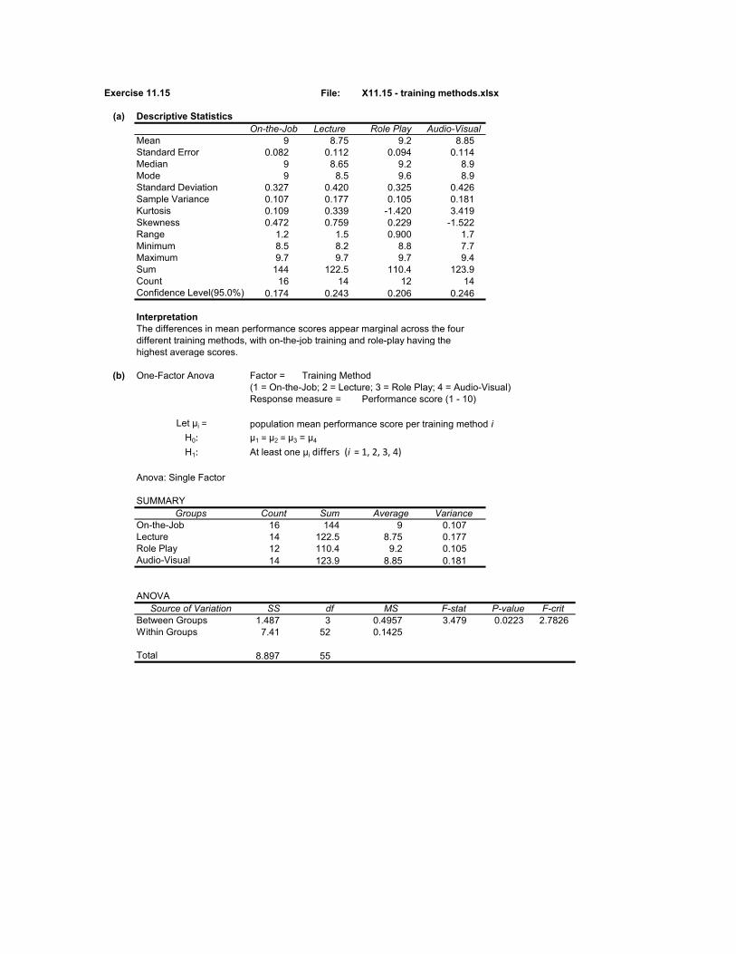
Exercise 11.15 File: X11.15 - training methods.xlsx
(a) Descriptive StatisticsOn-the-Job Lecture Role Play Audio-Visual
Mean 9 8.75 9.2 8.85Standard Error 0.082 0.112 0.094 0.114Median 9 8.65 9.2 8.9Mode 9 8.5 9.6 8.9Standard Deviation 0.327 0.420 0.325 0.426Sample Variance 0.107 0.177 0.105 0.181Kurtosis 0.109 0.339 -1.420 3.419Skewness 0.472 0.759 0.229 -1.522Range 1.2 1.5 0.900 1.7Minimum 8.5 8.2 8.8 7.7Maximum 9.7 9.7 9.7 9.4Sum 144 122.5 110.4 123.9Count 16 14 12 14Confidence Level(95.0%) 0.174 0.243 0.206 0.246
InterpretationThe differences in mean performance scores appear marginal across the fourdifferent training methods, with on-the-job training and role-play having the highest average scores.
(b) One-Factor Anova Factor = Training Method(1 = On-the-Job; 2 = Lecture; 3 = Role Play; 4 = Audio-Visual)Response measure = Performance score (1 - 10)
Let μi = population mean performance score per training method i H0: μ1 = μ2 = μ3 = μ4
H1: At least one μi differs (i = 1, 2, 3, 4)
Anova: Single Factor
SUMMARYGroups Count Sum Average Variance
On-the-Job 16 144 9 0.107Lecture 14 122.5 8.75 0.177Role Play 12 110.4 9.2 0.105Audio-Visual 14 123.9 8.85 0.181
ANOVASource of Variation SS df MS F-stat P-value F-crit
Between Groups 1.487 3 0.4957 3.479 0.0223 2.7826Within Groups 7.41 52 0.1425
Total 8.897 55

ConclusionSince F-stat = 3.479 > F-crit = 2.7826, there is sufficient sample evidence at the5% significance level to reject H0 in favour of H1. Therefore conclude that there is at least one
training method with a different mean performance score relative to the other training methods.
By inspection, the lecture and audio-visual are the least effective (lower mean scores),while on-the-job and the role-play methods are more effective (with higher mean scores).
RecommendationThe training manager is advised to consider either on-the-job training or use role play methods (The difference does not appear to be statistically significant).
(c) Two-Sample Test of MeansPerformance scores between On-the-Job (1) and Role Play (2) methods.
H0: μ1 = μ2 (two-tailed test)H1: μ1 ≠ μ2
t-Test: Two-Sample Assuming Equal Variances
On-the-Job Role PlayMean 9 9.2Variance 0.10666667 0.105454545Observations 16 12Pooled Variance 0.10615385Hypothesized Mean Difference 0df 26t Stat -1.6074361P(T<=t) one-tail 0.06001825t Critical one-tail 1.7056179P(T<=t) two-tail 0.1200365 t-crit (0.05,26) =t Critical two-tail 2.05552942 =TINV(0.05,26) 2.0555
ConclusionSince t-stat = -1.6074 lies within the region of non-rejection of H0, (i.e. within ±2.0555) the sample
evidence is not strong enough to reject H0 in favour of H1. The population mean performance scores
between the two training methods is likely to be the same.
(d) RecommendationBased on the statistical evidence in (b) and (c), the HR manager is advised to select either on-the-job training or role play methods of training. Both are likely to produce similar high mean performance scores.

Exercise 11.16 In one-factor ANOVA, only one categorical factor is used to explain
possible differences between the observed sample means.
In two-factor ANOVA, two categorical factors are used to explain
possible differences between the observed sample means.
Exercise 11.17 Response variable (y) numeric, ratio-scaled
Factor 1 (x1) categorical (nominal / ordinal-scaled)
Factor 2 (x2) categorical (nominal / ordinal-scaled)
Exercise 11.18 Interaction term means that different combinations of the levels from the two factors
can have different influences (effects) on the numeric response variable.
Exercise 11.19 Interaction plot: It visually displays the nature and strength of the interaction
effect of combinations of factor levels on the dependent response variable.
It is constructed from the sample means of the various combinations
of the different factor levels.
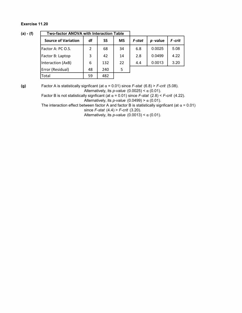
Exercise 11.20
(a) - (f)
Source of Variation df SS MS F-stat p -value F -crit
Factor A: PC O.S. 2 68 34 6.8 0.0025 5.08
Factor B: Laptop 3 42 14 2.8 0.0499 4.22
Interaction (AxB) 6 132 22 4.4 0.0013 3.20
Error (Residual) 48 240 5
Total 59 482
(g) Factor A is statistically signficant (at α = 0.01) since F-stat (6.8) > F-crit (5.08). Alternatively, its p-value (0.0025) < α (0.01).
Factor B is not statistically signficant (at α = 0.01) since F-stat (2.8) < F-crit (4.22). Alternatively, its p-value (0.0499) > α (0.01).
The interaction effect between factor A and factor B is statistically signficant (at α = 0.01)since F-stat (4.4) > F-crit (3.20). Alternatively, its p-value (0.0013) < α (0.01).
Two-factor ANOVA with Interaction Table

XS11.21
Exercise 11.21 File: X11.21 - sales ability.xlsx
(a) (i) Factor: Qualifications Factor: ExperienceH0: μ(b) = μ(a) = μ(s) H0: μ(under 3) = μ(over 3)
H1: At least one μi differs (I = b, a, s) H1: At least one μi differs (i = under 3, over 3)
Factor: InteractionH0: No interaction effectH1: There is an interaction effect
Anova: Two-Factor With Replication (Data Analysis - Excel )
SUMMARY Business Arts Social Science Total
Under 3 years
Count 10 10 10 30
Sum 400.1 376.6 325.9 1102.6
Average 40.01 37.66 32.59 36.7533333
Variance 61.31656 23.07156 14.56766667 40.628092
Over 3 years
Count 10 10 10 30
Sum 446.2 357.6 415.8 1219.6
Average 44.62 35.76 41.58 40.6533333
Variance 28.37956 92.68711 42.13066667 64.626023
Total
Count 20 20 20
Sum 846.3 734.2 741.7
Average 42.315 36.71 37.085
Variance 48.08029 55.78305 48.12555263
ANOVA
Source of Variation SS df MS F-stat p-value F-crit
Sample (Experience) 228.15 1 228.150 5.222 0.0263 4.020
Columns (Qualifications) 392.73 2 196.365 4.494 0.0157 3.168
Interaction (Exper x Qualif) 300.26 2 150.131 3.436 0.0394 3.168
Within 2359.38 54 43.692
Total 3280.52 59
(a) (ii) Factor: Qualifications Since F-stat (4.494) > F-crit (3.168), reject H0 and conclude that qualifications is a statistically significant factor (α = 0.05)Business graduates generate significantly higher average sales (42.32)than graduates with Arts (36.71) or Social Science (37.09) degrees.
(a) (iii) Factor: Experience Since F-stat (5.22) > F-crit (4.02), reject H0 and conclude that experience is a statistically significant factor (α = 0.05)Graduates with over 3 years experience generate significantly higher average sales (40.65)than graduates with less than 3 years experience (36.75).
(a) (iv) Factor: Interaction effect Since F-stat (3.436) > F-crit (3.168), reject H0 and conclude that there is a significant interaction effect between experience and qualifications on graduates' sales performance (α = 0.05)Business graduates with over 3 years experience perform the best (44.62) while social science graduates with with less than 3 years experience perform the worst (32.59).
(b) Summary of Sample Means Table
Business Arts Social Science
Under 3 years 40.01 37.66 32.59
Over 3 years 44.62 35.76 41.58
Page 19

XS11.21
See (a) (iv) for an interpretation of the interaction plot.
(c) Recommendation to HR manager:Recruit predominantly business and social science graduates with over 3 years of work experience. If Arts graduates are employed, they must be given intensive marketing training.
Interaction Plot
30
32
34
36
38
40
42
44
46
Business Arts Social Science
Chart Title
Under 3 years Over 3 years
Page 20

Exercise 11.22 File: X11.22 - dropped calls.xlsx
(a) (i) Random variable: % of daily dropped calls per network switch and transmission type Factor 1 = Switch type (SW1, SW2, SW3, SW4)Factor 2 = Transmission type (Voice, Data bundles)
Management Question: Is the % of daily dropped calls the same across all network switchingdevices and / or transmission types
Factor: Switch type Factor: Transmission typeH0: μ(1) = μ(2) = μ(3) = μ(4) H0: μ(voice) = μ(data)
H1: At least one μi differs (i = 1,2,3,4) H1: At least one μi differs (i = voice, data)
Factor: InteractionH0: No interaction effectH1: There is an interaction effect
Anova: Two-Factor With Replication (Data Analysis - Excel )
SUMMARY SW1 SW2 SW3 SW4 Total
Voice
Count 8 8 8 8 32
Sum 7.76 4.35 4.69 6.39 23.19
Average 0.97 0.54375 0.58625 0.79875 0.724688
Variance 0.098657 0.081884 0.086227 0.071155 0.106645
Data
Count 8 8 8 8 32
Sum 5.83 6.82 8.16 7.1 27.91
Average 0.72875 0.8525 1.02 0.8875 0.872188
Variance 0.047984 0.078707 0.057171 0.067279 0.067818
Total
Count 16 16 16 16
Sum 13.59 11.17 12.85 13.49
Average 0.849375 0.698125 0.803125 0.843125
Variance 0.083953 0.100363 0.11709 0.066703
ANOVA
Source of Variation SS df MS F-stat P-value F-crit
Sample (Transmission) 0.3481 1 0.3481 4.727498 0.033926 4.012973
Columns (Switch) 0.234819 3 0.078273 1.063014 0.372175 2.769431
Interaction (Trans x Switch) 1.050075 3 0.350025 4.753641 0.005055 2.769431
Within 4.12345 56 0.073633
Total 5.756444 63
(a) (ii) Factor: Switching device Since F-stat (1.063) < F-crit (2.769), do not reject H0 and conclude that switch devices are not statisticallysignificant (α = 0.05). Hence all switch devices are likely to have the same average dropped call rate.
(a) (iii) Factor: Transmission Since F-stat (4.73) > F-crit (4.01), reject H0 and conclude that transmission typeis a statistically significant factor (α = 0.05)Data transmission lead to a higher average dropped call rate (0.872) than voice transmission (0.725).
(a) (iv) Factor: Interaction effect Since F-stat (4.75) > F-crit (2.769), reject H0 and conclude that there is a significant interaction effect between switch devices and transmission type. (α = 0.05)SW2 and SW3, transmitting voice (0.544 and 0.586), are likely to have the lowest average dropped call rate, while SW1 transmitting voice (0.97) and SW3 transmitting data (1.02), are likely to have the highest average dropped call rate.

(b) Summary of Sample Means Table
SW1 SW2 SW3 SW4Voice 0.970 0.544 0.586 0.799Data 0.729 0.853 1.020 0.888
See (a) (iv) for an interpretation of the interaction plot.
(c) Recommendation to the chief engineer:For voice transmissions, use switching devices 2 and 3; For data transmission, use only switching device 1. Investigate the high % dropped calls rates of switching device 3 (for data transmission)and switching device 4 for both transmission types.
0.970
0.5440.586
0.7990.729
0.853
1.020
0.888
0.400
0.500
0.600
0.700
0.800
0.900
1.000
1.100
SW1 SW2 SW3 SW4
Chart Title
Voice Data

Exercise 11.23 File: X11.23 - rubber wastage.xlsx
(a) Random variable: % rubber wastage per week
Factor: Machine (TAM) Factor: Tyre H0: μ(1) = μ(2) = μ(3) H0: μ(R) = μ(B)
H1: At least one μi differs (i = 1, 2, 3) H1: At least one μi differs (i = Radial, Bias)
Factor: InteractionH0: No interaction effectH1: There is an interaction effect
Anova: Two-Factor With Replication (Data Analysis - Excel )
SUMMARY TAM1 TAM2 TAM3 Total
Radial
Count 5 5 5 15
Sum 19.71 33.52 19.44 72.67
Average 3.942 6.704 3.888 4.844667
Variance 3.96097 6.56833 3.44237 5.844455
Bias
Count 5 5 5 15
Sum 13.47 38.6 43.77 95.84
Average 2.694 7.72 8.754 6.389333
Variance 1.35283 9.83965 8.96443 13.26548
Total
Count 10 10 10
Sum 33.18 72.12 63.21
Average 3.318 7.212 6.321
Variance 2.794329 7.579173 12.09134
ANOVA
Source of Variation SS df MS F-stat p-value F-crit
Sample (Tyres) 17.89496 1 17.89496 3.146037 0.088802 4.259677
Columns (TAMS) 83.25042 2 41.62521 7.317951 0.003301 3.402826
Interaction (Tyre x TAM) 47.77433 2 23.88716 4.1995 0.0273 3.402826
Within 136.5143 24 5.688097
Total 285.434 29
Statistical and Management ConclusionsFactor: Tyres Since F-stat (3.15) < F-crit (4.26), do not reject H0 and conclude that tyre types is not
a statistically significant factor (α = 0.05)Regardless of TAM used, average rubber wastage is the same across both tyre types produced.
Factor: TAMs Since F-stat (7.318) > F-crit (3.403), reject H0 and conclude that TAM used is a statistically significant factor (α = 0.05)Regardless of tyre type produced, average rubber wastage is likely to be lowest on TAM1 (3.318).compared to TAM2 (7.212) and TAM3 (6.321).
Factor: Interaction effect Since F-stat (4.199) > F-crit (3.403), reject H0 and conclude that there is a significant interaction effect between tyre type produced and TAM used (α = 0.05)Average rubber wastage for bias tyres is lowest on TAM1 (2.694) but highest on TAM3 (8.754). By contrast, average rubber wastage of radial tyres is lowest on TAM3 (3.888) and highest on TAM2 (6.704).
(b) Interaction Plot TAM1 TAM2 TAM3
Radial 3.942 6.704 3.888
Bias 2.694 7.720 8.754
See (a) for an interpretation of the interaction plot.
3.942
6.704
3.888
2.694
7.720
8.754
0.000
1.000
2.000
3.000
4.000
5.000
6.000
7.000
8.000
9.000
10.000
TAM1 TAM2 TAM3
Chart Title
Radial Bias

(c) Recommendation to the production manager:TAM1 machine is the most efficient in minimising wastage for both tyre types (purchase more of TAM1).Allocate Radial tyres manufacturing to TAM3 (it has the minimum % wastage of all three machines on Radial tyres).Investigate the high % wastage of TAM3 for Bias tyres and TAM2 for both tyre types. Possibly replace TAM2 type machines with TAM1 type machines.

CHAPTER 12
SIMPLE LINEAR REGRESSION AND CORRELATION ANALYSIS
Exercise 12.1 Regression analysis defines the structural relationship between two numeric
variables as a mathematical equation (usually a straight line equation).
Its purpose is to use the equation for estimation / prediction purposes.
Correlation analysis measures the strength of the relationship between the
two numeric variables used in the regression equation.
Exercise 12.2 Dependent variable, y
Exercise 12.3 An independent variable, x , is used as a predictor of the dependent variable.
Exercise 12.4 Scatter plot
Exercise 12.5 Method of Least Squares
Exercise 12.6 Strong inverse linear relationship
Exercise 12.7 H0: ρ = 0 H1: ρ ≠ 0
Degrees of freedom = 18 - 2 = 16
t-crit = t(0.05, 16) = 2.12 (Use =TINV(0.05,16) in Excel )
Decision Rule: Accept H0 if -2.12 ≤ t-stat ≤ +2.12
t-stat = (0.42) * √[(18 - 2)/(1 - 0.422)] = 1.851
Conclusion: Do not reject H0. There is no statistically
significant relationship between x and y .

Exercise 12.8 File: X12.8 - training effectiveness.xlsx
(a) Scatter plot - Training hours versus Productivity
InterpretationThere is a strong positive relationship between hours of training and worker output. The more the training received, the higher the output.
(b) Training (x) Output (y) x² xy y²20 40 400 800 160036 70 1296 2520 490020 44 400 880 193638 56 1444 2128 313640 60 1600 2400 360033 48 1089 1584 230432 62 1024 1984 384428 54 784 1512 291640 63 1600 2520 3969
n = 10 24 38 576 912 1444Σ 311 535 10213 17240 29649
Coefficients b1 = (10*17240-(311*535))/(10*10213-(311²))1.112
b0 = (535 - 1.112*311)/1018.917
Thus where 20 ≤ x ≤ 40ŷ = 18.917 + 1.112 x
20
30
40
50
60
70
80
10 15 20 25 30 35 40 45
outp
ut (u
nits
)
hours of training
Scatter Plot - Training hours vs Productivity
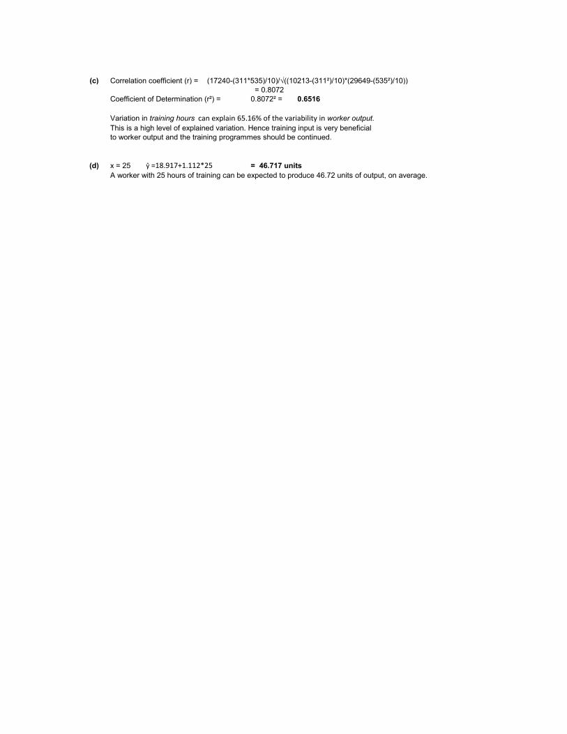
(c) Correlation coefficient (r) = (17240-(311*535)/10)/√((10213-(311²)/10)*(29649-(535²)/10))= 0.8072
Coefficient of Determination (r²) = 0.8072² = 0.6516
Variation in training hours can explain 65.16% of the variability in worker output.This is a high level of explained variation. Hence training input is very beneficialto worker output and the training programmes should be continued.
(d) x = 25 ŷ =18.917+1.112*25 = 46.717 unitsA worker with 25 hours of training can be expected to produce 46.72 units of output, on average.

Exercise 12.9 File: X12.9 - capital utilisation.xlsx
(a) Scatter plot - Earnings Yield versus Inventory Turnover
InterpretationThere is a strong positive relationship between inventory turnover and earnings yield.As inventory turnover increases, earnings yields also increases.
(b) Inv t/o (x) E.Y. (y) x² xy y²3 10 9 30 1005 12 25 60 1444 8 16 32 647 13 49 91 1696 15 36 90 2254 10 16 40 1008 16 64 128 2566 13 36 78 169
n = 9 5 10 25 50 100Σ 48 107 276 599 1327
Coefficients b1 = (9*599-(48*107))/(9*276-(48²))1.4167
b0 = (107-1.4167*48)/94.333
Thus ŷ = 4.333 + 1.4167 x where 3 ≤ x ≤ 8
(c) Correlation coefficient (r) = (599-(48*107)/9)/√((276-(48²)/9)*(1327-(107²)/9))= 0.8552
There is a strong positive linear association between inventory turnover and earnings yield. Thus the business analyst's view is supported by the strong sample evidence.
02468
1012141618
0 1 2 3 4 5 6 7 8 9
earn
ings
yie
ld
inventory turnover
Scatter Plot Earnings Yield vs Inventory Turnover
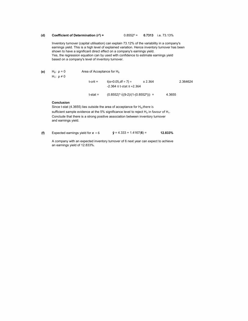
(d) Coefficient of Determination (r²) = 0.8552² = 0.7313 i.e. 73.13%
Inventory turnover (capital utilisation) can explain 73.12% of the variability in a company's earnings yield. This is a high level of explained variation. Hence inventory turnover has been shown to have a significant direct effect on a company's earnings yield. Yes, the regression equation can by used with confidence to estimate earnings yield based on a company's level of inventory turnover.
(e) H0: ρ = 0 Area of Acceptance for H0
H1: ρ ≠ 0t-crit = t(α=0.05,df = 7) = ± 2.364 2.364624
-2.364 ≤ t-stat ≤ +2.364
t-stat = (0.8552)*√((9-2)/(1-(0.8552²))) = 4.3655
ConclusionSince t-stat (4.3655) lies outside the area of acceptance for H0,there is
sufficient sample evidence at the 5% significance level to reject H0 in favour of H1.
Conclude that there is a strong positive association between inventory turnover and earnings yield.
(f) Expected earnings yield for x = 6 ŷ = 4.333 + 1.4167(6) = 12.833%
A company with an expected inventory turnover of 6 next year can expect to achieve an earnings yield of 12.833%.

Exercise 12.10 File: X12.10 - loan applications.xlsx
(a) Dependent variable (y) = No. of Loan applications receivedIndependent variable (x) = interest rate (%) Interest rate (%) is assumed to influence the number of loan applications received.
(b) Scatter plot
InterpretationA moderate to strong negative linear relationship between interest rate and number of loan applications received is observed from the scatter plot.
(c) Correlation coefficient
Int rate % (x) Applications (y) x² y² xy7 18 49 324 126
6.5 22 42.25 484 1435.5 30 30.25 900 165
6 24 36 576 1448 16 64 256 128
8.5 18 72.25 324 1536 28 36 784 168
6.5 27 42.25 729 175.57.5 20 56.25 400 150
8 17 64 289 136n = 11 6 21 36 441 126
Σ 75.5 241 528.25 5507 1614.5
r = (11*1614.5 - 75.5*241)/√((11*528.25-75.5²)*(11*5507-241²))= -0.8302
InterpretationThis correlation shows a strong negative (inverse) assocation between interest rates (%) and the number of loan applications received.
10
15
20
25
30
35
4 5 6 7 8 9 10
no. l
oan
appl
icat
ions
rece
ived
interest rate (%)
Scatter Plot Loan applications Received vs Interest Rate (%)

(d) H0: ρ = 0 Area of Acceptance for H0
H1: ρ ≠ 0t-crit = t(α=0.05,df = 9) = ± 2.262
-2.262 ≤ t-stat ≤ +2.262
t-stat = (-0.8302)*√((11-2)/(1-(-0.8302²))) = '= -4.4677
ConclusionSince t-stat (-4,4677) lies outside the area of acceptance for H0,there is
sufficient sample evidence at the 5% significance level to reject H0 in favour of H1.
Conclude that there is a strong negative relationship between interest rates (%)and the number of loan applications received monthly.
(e) Regression coefficients
b1 = (11*1614.5 - 75.5*241)/(11*528.25-75.5²)-3.9457
b0 = (241 - (-3.9457)*(75.5))/1148.991
Thus ŷ = 48.991 - 3.9457 x where 5.5 ≤ x ≤ 8.5
(f) Interpretation of b1 coefficientFor a 1% increase in interest rate, 3.95 fewer loan applications will be received.
(g) x = 6 ŷ = 48.991 - 3.9457*(6) = 25.32 applications
If the rate of interest is 6%, the bank can expect to receive 25.32 (say, 25) applications.

Exercise 12.11 File: X12.11 - maintenance costs.xlsx
(a) Dependent variable (y) = Annual maintenance cost (Rand)Independent variable (x) = Machine age (years)Machine age is assumed to influence annual maintenance costs.
(b) Scatter plot
InterpretationA strong direct (positive) linear relationship between the ages of machines and their annual maintenance costs (in Rands) is observed in the scatter plot.
(c) Correlation coefficient
Age (yrs) Annual Cost (R) x² y² xy4 45 16 2025 1803 20 9 400 603 38 9 1444 1148 65 64 4225 5206 58 36 3364 3487 50 49 2500 3501 16 1 256 161 22 1 484 225 38 25 1444 1902 26 4 676 524 30 16 900 120
n = 12 6 35 36 1225 210Σ 50 443 266 18943 2182
r = (12*2182 - 50*443)/√((12*266-50²)*(12*18943-443²)) = 0.870028
InterpretationThere is a very strong positive association between the ages ofof machines and their annual maintenance costs (in Rands).
0
10
20
30
40
50
60
70
0 2 4 6 8 10annu
al m
aint
enan
ce c
ost (
R)
machine age (years)
Scatter Plot Annual Maintenance Cost (R) vs Age of Machines
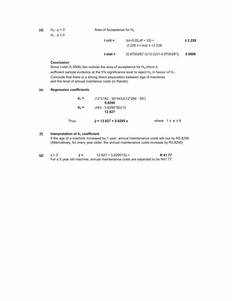
(d) H0: ρ = 0 Area of Acceptance for H0
H1: ρ ≠ 0t crit = t(α=0.05,df = 10) = ± 2.228
-2.228 ≤ t-stat ≤ +2.228
t-stat = (0.870028)*√((12-2)/(1-0.870028²)) 5.5806
ConclusionSince t-stat (5.5806) lies outside the area of acceptance for H0,there is
sufficient sample evidence at the 5% significance level to reject H0 in favour of H1.
Conclude that there is a strong direct association between age of machines and the level of annual maintance costs (in Rands).
(e) Regression coefficients
b1 = (12*2182 - 50*443)/(12*266 - 50²)5.8295
b0 = (443 - 5.8295*50)/1212.627
Thus ŷ = 12.627 + 5.8295 x where 1 ≤ x ≤ 8
(f) Interpretation of b1 coefficientIf the age of a machine increased by 1 year, annual maintenance costs will rise by R5.8295. (Alternatively, for every year older, the annual maintenance costs increase by R5.8295)
(g) x = 5 ŷ = 12.627 + 5.8295*(5) = R 41.77For a 5 year old machine, annual maintenance costs are expected to be R41.77.

Exercise 12.12 File: X12.12 - employee performance.xlsx
(a) Scatter Plot
InterpretationThere appears to be a weak to moderate positive association between an employee's aptitude score and their performance rating.
(b) Correlation coefficient (r)
Aptitude (x) Perf rating (y) x² y² xy7 82 49 6724 5746 74 36 5476 4445 82 25 6724 4104 68 16 4624 2725 75 25 5625 3758 92 64 8464 7367 86 49 7396 6028 69 64 4761 5529 85 81 7225 7656 76 36 5776 4564 72 16 5184 288
n = 12 6 64 36 4096 384Σ 75 925 497 72075 5858
r = (12*5858 - 75*925)/√((12*497-75²)*(12*72075-925²))0.5194
InterpretationThere is a moderate positive association between the aptitude scores ofemployees and their performance scores after one year.
50556065707580859095
2 3 4 5 6 7 8 9 10perf
orm
ance
ratin
g (0
-10
0)
aptitude score (1 - 10)
Scatter PlotPerformance Rating vs Aptitude Score

(c) H0: ρ = 0 Area of Acceptance for H0
H1: ρ ≠ 0t-crit = t(α=0.05,df = 10) = ± 2.228
-2.228 ≤ t-stat ≤ +2.228
t-stat = (0.5194)*√((12-2)/(1-0.5194²)) 1.922
ConclusionSince t-stat (1.922) lies inside the area of acceptance for H0,there is
not sufficient sample evidence at the 5% significance level to reject H0 in favour of H1.
Conclude, at a 5% significance level, that there is no statistically significant association between an employee's aptitude score and their job performance rating score one year later.
(d) Regression coefficients
b1 = (12*5858-75*925)/(12*497-75²) 2.7168
b0 = (925 - 2.7168*75)/12 60.1032
Thus ŷ = 60.1032 + 2.7168 x where 4 ≤ x ≤ 9
Interpretation of b1 coefficientIf an employee's aptitude score increases by one unit, their performance ratingscore will increase by 2,7168 points.
(e) Estimationx = 8 ŷ = 60.1032 + 2.7168*(8) = 81.84
For an employee with an aptitude score of 8, they could expect a job performance rating score of 81.84.
The association between aptitude score and performance rating is not statistically significant. Therefore, the call centre manager should have low confidence in this estimated performance rating score.

Exercise 12.13 File: X12.13 - opinion polls.xlsx
(a) Correlation coefficient (r)
Poll (%) (x) Election (%) (y) x² y² xy42 51 1764 2601 214234 31 1156 961 105459 56 3481 3136 330441 49 1681 2401 200953 68 2809 4624 360440 35 1600 1225 140065 54 4225 2916 351048 52 2304 2704 249659 54 3481 2916 318638 43 1444 1849 1634
n = 11 62 60 3844 3600 3720Σ 541 553 27789 28933 28059
r = (11*28059 - 541*553)/√((11*27789-541²)*(11*2893-553²))0.7448
InterpretationThere is a moderate to strong positive association between opinion poll predictionsand the actual election results.
(b) H0: ρ = 0 Area of Acceptance for H0
H1: ρ ≠ 0t-crit = t(α=0.05,df = 9) = ± 2.262
-2.262 ≤ t-stat ≤ +2.262
t-stat = (0.7448)*√((11-2)/(1-0.7448²)) 3.3484
ConclusionSince t-stat (3.3484) lies outside the area of acceptance for H0,there is
sufficient sample evidence at the 5% significance level to reject H0 in favour of H1.
Conclude, at a 5% significance level, that there is a statistically significant association between opinion poll predictions and the actual election results.
(c) Regression coefficients
b1 = (11*28059 - 541*553)/(11*27789-541²) = 0.729
b0 = (553 - 0.729*541)/11 = 14.4175
Thus ŷ = 14.4175 + 0.729 x where 34 ≤ x ≤ 65
Interpretation of b1 coefficientFor a one percentage point increase in an opinion poll prediction, the actual election percentage is likely to increase by 0.729 percentage points.
(d) Coefficient of Determination r²
r² = 0.7448² = 0.5547
InterpretationOpinion poll predictions can explain 55.47% of variation in actual election results percentages

(e) Predictionx = 58 ŷ = 14.4175 + 0.729*(58) = 56.70%
If an opinion poll predicts support at 58%, the actual election result is likely to be 56.7%.
(f) x = 82 ŷ = 14.4175 + 0.729*(82) = 74.20%If an opinion poll predicts support at 82%, the actual election result is likely to be 74.2%. Because x = 82 is beyond the domain of x (34 ≤ x ≤ 65), this expected actual election resultis unreliable and possibly invalid due to extrapolation being used.
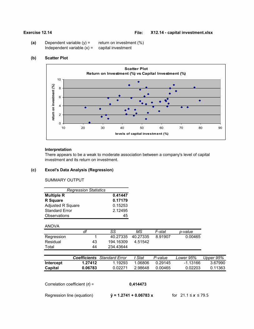
Exercise 12.14 File: X12.14 - capital investment.xlsx
(a) Dependent variable (y) = return on investment (%)Independent variable (x) = capital investment
(b) Scatter Plot
InterpretationThere appears to be a weak to moderate association between a company's level of capitalinvestment and its return on investment.
(c) Excel's Data Analysis (Regression)
SUMMARY OUTPUT
Multiple R 0.41447R Square 0.17179Adjusted R Square 0.15253Standard Error 2.12495Observations 45
ANOVAdf SS MS F-stat p-value
Regression 1 40.27335 40.27335 8.91907 0.00465Residual 43 194.16309 4.51542Total 44 234.43644
Coefficients Standard Error t Stat P-value Lower 95% Upper 95%Intercept 1.27412 1.19293 1.06806 0.29145 -1.13166 3.67990Capital 0.06783 0.02271 2.98648 0.00465 0.02203 0.11363
Correlation coefficient (r) = 0,414473
Regression line (equation) for 21.1 ≤ x ≤ 79.5
Regression Statistics
ŷ = 1.2741 + 0.06783 x
Scatter PlotReturn on Investment (%) vs Capital Investment (%)
0
2
4
6
8
10
10 20 30 40 50 60 70 80 90
levels of capital investment (%)
retu
rn o
n in
vest
men
t (%
)
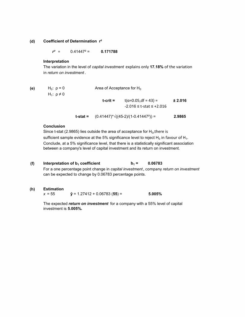
(d) Coefficient of Determination r²
r² = 0.41447² = 0.171788
InterpretationThe variation in the level of capital investment explains only 17.18% of the variation
in return on investment .
(e) H0: ρ = 0 Area of Acceptance for H0
H1: ρ ≠ 0t-crit = t(α=0.05,df = 43) = ± 2.016
-2.016 ≤ t-stat ≤ +2.016
t-stat = (0.41447)*√((45-2)/(1-0.41447²)) = 2.9865
ConclusionSince t-stat (2.9865) lies outside the area of acceptance for H0,there is
sufficient sample evidence at the 5% significance level to reject H0 in favour of H1.
Conclude, at a 5% significance level, that there is a statistically significant association between a company's level of capital investment and its return on investment.
(f) Interpretation of b1 coefficient b1 = 0.06783For a one percentage point change in capital investment , company return on investmentcan be expected to change by 0.06783 percentage points.
(h) Estimationx = 55 ŷ = 1.27412 + 0.06783 (55) = 5.005%
The expected return on investment for a company with a 55% level of capital investment is 5.005%.

Exercise 12.15 File: X12.15 - property valuations.xlsx
(a) Dependent variable (y ) = Market ValuesIndependent variable (x ) = Council Valuations
Council valuations are assumed to have an influence on property market values.
(b) Scatter Plot
InterpretationThere appears to be a strong positive correlation between the council's valuation of a residential property in Bloemfontein and its market value.
(c) Excel's Data Analysis (Regression)
SUMMARY OUTPUT
Regression StatisticsMultiple R 0.78104R Square 0.61002Adjusted R Square 0.59975Standard Error 26.40553Observations 40
ANOVAdf SS MS F-stat p-value
Regression 1 41444.82 41444.82 59.4402 2.7522E-09Residual 38 26495.58 697.2521Total 39 67940.4
Coefficients Standard Error t Stat P-value Lower 95% Upper 95%Intercept 71.3619 14.2370 5.0124 1.28E-05 42.541 100.183Council valuations 1.0151 0.1317 7.7097 2.75E-09 0.749 1.282
Correlation coefficient (r) = 0.78104Regression line (equation) ŷ = 71.3619 + 1.0151 x for 48 ≤ x ≤ 154
(d) Coefficient of Determination r²r ² = 0.78104² = 0.61002
InterpretationVariation in council valuations explain 61.002% of the variation in property market values .
Market Values vs Council Valuations
0
50
100
150
200
250
300
0 50 100 150 200
council valuations (R)
mar
ket v
alue
s (R
)
Market values

(e) H0: ρ = 0 Area of Acceptance for H0
H1: ρ ≠ 0t-crit = t(α=0.05,df = 38) = ± 2.024
-2.024 ≤ t-stat ≤ +2.024
t-stat = (0.78104)*√((40-2)/(1-0.78104²)) = 7.70975
ConclusionSince t-stat (7.70975) lies well outside the area of acceptance for H0,there is
sufficient sample evidence at the 5% significance level to reject H0 in favour of H1.
Conclude, at a 5% significance level, that there is a statistically significant association between the Council's valuation and the resultant property market valuation.
(f) Interpretation of b1 coefficient b1 = 1.0151For a R1 (in R1000) change (up / down) in council valuation , market valuation of aproperty can be expected to change (up / down) by R1.0151 (in R1000) .
(g) Estimation x = 100 ŷ = 71.3619 + 1.0151 (100) = R172.874 (in R1000s)
The expected market value of a property which the council values at R100 (in R1000s) is likely to be R172.874 (in R1000s).

CHAPTER 13
MULTIPLE LINEAR REGRESSION
Exercise 13.1 Simple linear regression has only one independent variable (x1) whereas multiple linear
regression has two or more independent variables (x1, x2, x3, … , xk) that are assumed
to influence the outcome of the dependent variable, y .
Exercise 13.2 ANOVAdf SS MS F-stat p-value F-crit
Regression 5 84 16.8 4.541 0.002261 2.45Residual 40 148 3.7Total 45 232
(a) R2 = 84/232 = 0.362136.2% of total variation in y can be explained by the 5 independent variables.
(b) H0: β1 = β2 = β3 = β4 = β5 = 0 vs H1: At least one βi ≠ 0 (i = 1,2,3,4,5)
or H0: ρ = 0 vs H1: ρ ≠ 0
(c) F-stat = 4.5412 and F-crit = F(0.05,5,40) = 2.45 (See Anova Table)
(d) Reject H0. Conclude that the overall model is statistically significant.
(i.e. at least one x i is statistically significant in estimating y)
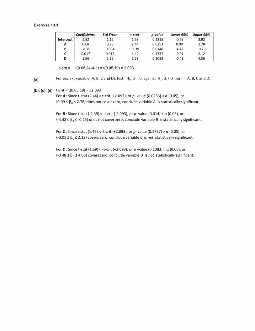
Exercise 13.3
Coefficients Std Error t-stat p-value Lower 95% Upper 95%Intercept 1.82 1.12 1.63 0.1215 -0.53 3.92
A 0.68 0.28 2.44 0.0253 0.09 2.78B -2.35 0.984 -2.39 0.0140 -4.42 -0.25C 0.017 0.012 1.42 0.1737 -0.01 2.12D 1.96 1.16 1.69 0.1083 -0.48 4.06
t-crit = t(0.05,24-4-1) = t(0.05,19) = 2.093
(a) For each x i variable (A, B, C and D), test: H0: βi = 0 against H1: βi ≠ 0 for i = A, B, C and D.
(b), (c), (d) t-crit = t(0.05,19) = ±2.093
For A : Since t-stat (2.44) > t-crit (+2.093); or p -value (0.0253) < α (0.05), or
{0.09 ≤ βA ≤ 2.78} does not cover zero, conclude variable A is statistically significant.
For B : Since t-stat (-2.39) < -t-crit (-2.093); or p -value (0.014) < α (0.05), or
{-4.42 ≤ βB ≤ -0.25} does not cover zero, conclude variable B is statistically significant.
For C : Since t-stat (1.42) < -t-crit (+2.093); or p -value (0.1737) > α (0.05), or
{-0.01 ≤ βC ≤ 2.12} covers zero, conclude variable C is not statistically significant.
For D : Since t-stat (1.69) < -t-crit (+2.093); or p -value (0.1083) > α (0.05), or
{-0.48 ≤ βD ≤ 4.06} covers zero, conclude variable D is not statistically significant.

Exercise 13.4
(a) For x 3 variable, test: H0: β3 = 0 against H1: β3 ≠ 0
(b) t-crit = t(0.05,30) = ±2.042. Hence, do not reject H0 if -2.042 ≤ t-stat ≤ +2.042.
(c ) Since t-stat (2.44) > t-crit (+2.042), hence reject H0 in favour of H1 at α = 0.05.
(d) Conclude that the x 3 variable is statistically significant in estimating y .
Exercise 13.5
(a) Holding all other variables constant, a unit increase in x 2 will result in a 1.6 reduction in y^ .
(b) For x 2 variable, test: H0: β2 = 0 against H1: β2 ≠ 0
Yes, since the 95% confidence interval for β2 does not cover zero.
Exercise 13.6 Binary coding scheme (Choose 'Lean' as the base category)'F1 and F2 are the dummy variable names chosen.
Fuel type F1 F2Leaded 1 0Unleaded 0 1Lean 0 0
Exercise 13.7 Binary coding scheme (Choose 'spring' as the base category)'S1, S2 and S3 are the dummy variable names chosen.
Season S1 S2 S3summer 1 0 0autumn 0 1 0winter 0 0 1spring 0 0 0

Exercise 13.8 File: X13.8 - employee absenteeism.xlsx
Excel's Data Analysis - Regression
SUMMARY OUTPUT
Regression StatisticsMultiple R 0.7384R Square 0.5453Adjusted R Square 0.5012Standard Error 3.7204Observations 35
ANOVAdf SS MS F-stat p-value
Regression 3 514.467 171.489 12.390 0.00001707Residual 31 429.076 13.841Total 34 943.543
Coefficients Standard Error t-stat p-value Lower 95% Upper 95%Intercept 36.411 5.929 6.141 8.22345E-07 24.318 48.504Tenure 0.220 0.065 3.376 0.001997 0.087 0.352Satisfaction -0.184 0.109 -1.692 0.100765 -0.406 0.038Commitment -0.332 0.080 -4.130 0.000254 -0.497 -0.168
(a) R2 = 514.467/943.543 = 54.53%
(b) H0: βT = βS = βC = 0 versus H1: At least one βi ≠ 0
F-crit = F(0.05,3,31) = 2.92 F-stat = 12.39 and p -value = 0.00001707
Reject H0. Conclude the overall model is statistically significant.
(i.e. at least one x i is statistically significant in estimating y)
(c), (d), (e) For each x i variable, test: H0: βi = 0 against H1: βi ≠ 0 with t-crit = t(0.05,31) = ±2.04
Tenure : Since t-stat (3.376) > t-crit (+2.04); or p -value (0.001997) < α (0.05), or
{0.087 ≤ βT ≤ 0.352} does not cover zero, conclude Tenure is statistically significant.
Satisfaction : Since t-stat (-1.692) lies within t-crit (±2.04); or p -value (0.100765) > α (0.05), or
{-0.406 ≤ βS ≤ 0.038} covers zero, conclude Satisfaction is not statistically significant.
Commitment : Since t-stat (-4.13) < t-crit (-2.04); or p -value (0.000254) < α (0.05), or
{-0.497 ≤ βC ≤ -0.168} does not cover zero, conclude Commitment is statistically significant.
(f) (i) No, organisational commitment is the most important explanatory factor because it has a
larger t-stat value (-4.13) and a smaller p- value (0.000254) than job tenure .
(f) (ii) No, job satisfaction is not a statistically signficant explanatory factor of employee
absenteeism (see (c), (d) and (e) above).
Yes, organisational commitment does play a statistically signficant role in explaining
employee absenteeism (see (c), (d) and (e) above).
(g) y(hat) = 36.411 + 0.22 (48) - 0.184 (50) - 0.332 (60) = 17.8008
Using t-crit = t(0.025,31) = ±2.04; standard error = 3.7204; n = 35
giving margin of error = 2.04 (3.7204)/√35 = 1.2826
Lower 95% confidence limit = 17.8008 - 1.2826 16.5182Upper 95% confidence limit = 17.8008 + 1.2827 19.0835{16.52 ≤ y(hat)(estimated) ≤ 19.08}
Management interpretation: We can be 95% confident that the true average number
of days absent per employee per annum is likely to lie between 16.5 days and 19.1 days.

Exercise 13.9 File: X13.9 - plastics wastage.xlsx
Excel's Data Analysis - Regression
SUMMARY OUTPUT
Regression StatisticsMultiple R 0.8061R Square 0.6498Adjusted R Square 0.6109Standard Error 0.5160Observations 31
ANOVAdf SS MS F-stat p-value
Regression 3 13.3384 4.4461 16.6992 2.466E-06Residual 27 7.1887 0.2662Total 30 20.5271
Coefficients Standard Error t-stat p-value Lower 95% Upper 95%Intercept 1.8179 1.2189 1.4914 0.1474 -0.6830 4.3188Dexterity -0.1112 0.0286 -3.8816 0.0006 -0.1700 -0.0524Speed 0.0173 0.0047 3.6770 0.0010 0.0077 0.0270Viscosity 1.9189 1.2581 1.5252 0.1388 -0.6625 4.5004
(a) R2 = 13.3384/20.5271 = 64.98%
(b) H0: βD = βS = βV = 0 versus H1: At least one βi ≠ 0
F-crit = F(0.05,3,27) = 2.99
F-stat = 16.6992 and p-value = 0.000002466
Reject H0. Conclude the overall model is statistically significant.
(i.e. at least one x i is statistically significant in estimating y)
(c), (d), (e) For each x i variable, test: H0: βi = 0 against H1: βi ≠ 0 with t-crit = t(0.05,27) = ±2.052
Dexterity : Since t-stat (-3.886) < t-crit (-2.052); or p -value (0.0006) < α (0.05), or
{-0.17 ≤ βD ≤ -0.0524} does not cover zero, conclude Dexterity is statistically
significant.
Speed : Since t-stat (3.677) > t-crit (+2.052); or p -value (0.001) < α (0.05), or
{0.0077 ≤ βS ≤ 0.027} does not cover zero, conclude Speed is statistically significant.
Viscosity : Since t-stat (1.525) < t-crit (+2.052); or p -value (0.1388) > α (0.05), or
{-0.6625 ≤ βV ≤ 4.5} covers zero, conclude Viscosity is not statistically significant.
(f) The most important factor is operator dexterity (p -value (0.0006)), then machine speed with
p -value = 0.001. Plastic viscosity is not a significant influencing factor (p -value = 0.1388).
(g) y(hat) = 1.8179 - 0.1112 (25) + 0.0173 (200) + 1.9189 (0.25) = 2.9826
Using t-crit = t(0.025,27) = ±2.052; standard error = 0.516; n = 31
giving margin of error = 2.052 (0.516)/√31 = 0.1902
Lower 95% confidence limit = 2.9826 - 0.1902 = 2.7924Upper 95% confidence limit = 2.9826 + 0.1902 = 3.1728{2.79% ≤ y(hat)(estimated) ≤ 3.17%}
Management interpretation: We can be 95% confident that the true average % of plastic
wastage per shift is likely to lie between 2.79% and 3.17%.

Exercise 13.10 File: X13.10 - employee performance.xlsx
(a) Binary coding scheme (Choose 'method C' as the base category)MA and MB are the dummy variable names chosen.
Method Code MA MB
A 1 0
B 0 1
C 0 0
(b) Sample input data for first 6 consultants (showing the binary coded data)
Consultant Productivity Experience MA MB
1 24 9 1 0
2 30 4 0 1
3 26 10 1 0
4 37 12 0 1
5 29 10 0 0
6 28 6 0 0
Excel's Data Analysis - Regression (using the binary coded data as in (a))
SUMMARY OUTPUT
Regression Statistics
Multiple R 0.7894
R Square 0.6231
Adjusted R Square 0.5524
Standard Error 2.3425
Observations 20
ANOVA
df SS MS F-stat p-value
Regression 3 145.151 48.384 8.817 0.001108
Residual 16 87.799 5.487
Total 19 232.95
Coefficients Std error t-stat p-value Lower 95% Upper 95%
Intercept 26.387 1.940 13.601 3.29E-10 22.274 30.499
Experience 0.389 0.167 2.335 0.0329 0.036 0.742
MA -3.659 1.376 -2.659 0.0172 -6.576 -0.742
MB 1.472 1.336 1.102 0.2867 -1.360 4.304
Estimated multiple regression equation:
y^ = 26.387 + 0.389 Experience - 3.659 MA + 1.472 MB (based on data recoded as in (a))
(c) R2 = 145.151/232.95 = 62.31%
(d) H0: βE = βMA = βMB = 0 versus H1: At least one βi ≠ 0
F-crit = F(0.05,3,16) = 3.24
F-stat = 8.817 and p -value = 0.001108
Reject H0. Conclude the overall model is statistically significant.
(i.e. at least one x i is statistically significant in estimating y)
(e) For Experience , test: H0: βE = 0 against H1: βE ≠ 0 with t-crit = t(0.05,16) = ±2.12
Since t-stat (2.335) > t-crit (2.12), conclude work experience is statistically significant at α = 0.05.
(f) For each of MA and MB, test: H0: βi = 0 vs H1: βi ≠ 0 (i = MA, MB), wiith t-crit = t(0.05,16) = ±2.12
MA : Since t-stat (-2.659) < lower t-crit (-2.12), conclude MA is statistically significant (i.e. adopting

marketing method A results in significantly lower consultant productivity levels, on average,
compared to using marketing method C (i.e. the base category).
MB : Since –t-crit (-2.12) < t-stat (1.102) < +t-crit (-2.12), conclude MB is not statistically significant
(i.e. consultant productivity levels, on average, are the same for marketing method B and
and marketing method C (i.e. no difference to the base category average productivity level).
Overall conclusion: the independent variable ‘marketing method’ is statistically significant, but
only for marketing method A (when compared to method C (i.e. the base category).
Marketing methods B and C can be combined as there is no statistically significant difference
between them with regards to their average productivity levels across consultant.
(g), (h) For each x i variable, test: H0: βi = 0 against H1: βi ≠ 0
Experience : Since its p -value (0.0329) < α = 0.05, or {0.036 ≤ βE ≤ 0.742} does not cover zero,
conclude that work experience is statistically significant.
MA : Since its p -value (0.0172) < α = 0.05, or {-6.576 ≤ βMA ≤ -0.742} does not cover zero,
conclude that marketing method A is statistically significantly different from marketing method C
(i.e. the base category) in terms of consultants' average productivity levels.
MB : Since its p -value (0.2867) > α = 0.05, or {-1.36 ≤ βMA ≤ 4.304} covers zero,
conclude marketing method B is not statistically significantly different from marketing method C
(i.e. the base category) in terms of consultants' average productivity levels.
(i) Employ consultants with longer work experience and avoid using marketing method A as it
produces lower productivity levels than either marketing methods B or C.
(j) y^ = 26.387 + 0.389 (8) - 3.659 (0) + 1.472 (1) = 30.9717
Using t-crit = t(0.025,16) = ±2.1199; standard error = 2.3425; n = 20
giving margin of error = 2.1199 (2.3425)/√20 = 1.1104
Lower 95% confidence limit = 30.9717 - 1.1104 = 29.86Upper 95% confidence limit = 30.9717 + 1.1104 = 32.08{29.86 deals ≤ y(hat)(estimated) ≤ 32.08 deals}
Management interpretation: The bank management can be 95% confident that the actual
average number of deals closed per month per consultant is likely to lie between 30 and 32 (rounded).

Exercise 13.11 File: X13.11 - corporate performance.xlsx
(a) Binary coding scheme (Choose region 'KZN' as the base category)R1 and R2 are the dummy variable names chosen.
Region Code R1 R2
Gauteng 1 1 0
Cape 2 0 1
KZN 3 0 0
Binary coding scheme (Choose sector 'Construction' as the base category)S is the dummy variable name chosen.
Sector Code S
Agriculture 1 1
Construction 2 0
(b) Sample input data for first 6 companies (showing the binary coded data)
ROC(%) Sales Margin% Debt ratio(%) R1 R2 S
19.7 7178 18.7 28.5 1 0 0
17.2 1437 18.5 24.3 1 0 1
17.1 3948 16.5 65.6 1 0 1
16.6 1672 16.2 26.4 1 0 1
16.6 2317 16.0 20.1 1 0 1
16.5 4123 15.6 46.4 0 1 0
Excel's Data Analysis - Regression (using the binary coded data as in (a))
SUMMARY OUTPUT Y = f(Sales; Margin %; Debt ratio(%); Region; Sector)
Regression Statistics
Multiple R 0.9125
R Square 0.8327
Adjusted R Square 0.7769
Standard Error 0.9524
Observations 25
ANOVA
df SS MS F-stat p-value
Regression 6 81.2595 13.5433 14.9318 0.000004076
Residual 18 16.3261 0.9070
Total 24 97.5856
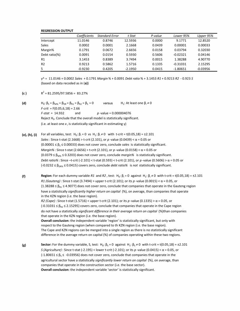
REGRESSION OUTPUT
Coefficients Standard Error t Stat P-value Lower 95% Upper 95%
Intercept 11.0146 0.8746 12.5936 0.0000 9.1771 12.8520
Sales 0.0002 0.0001 2.1668 0.0439 0.00001 0.00033
Margin% 0.1791 0.0672 2.6656 0.0158 0.03794 0.32030
Debt ratio(%) 0.0091 0.0154 0.5930 0.5606 -0.02321 0.04146
R1 3.1453 0.8389 3.7494 0.0015 1.38288 4.90770
R2 0.9213 0.5862 1.5716 0.1335 -0.31031 2.15295
S -0.9230 0.4205 -2.1950 0.0415 -1.80651 -0.03956
y^ = 11.0146 + 0.0002 Sales + 0.1791 Margin % + 0.0091 Debt ratio % + 3.1453 R1 + 0.9213 R2 - 0.923 S
(based on data recoded as in (a))
(c ) R2 = 81.2595/97.5856 = 83.27%
(d) H0: βS = βM% = βDR = βR1 = βR2 = βS = 0 versus H1: At least one βi ≠ 0
F-crit = F(0.05,6,18) = 2.66
F-stat = 14.932 and p -value = 0.000004076
Reject H0. Conclude that the overall model is statistically significant.
(i.e. at least one x i is statistically significant in estimating y)
(e), (h), (i) For all variables, test: H0: βi = 0 vs H1: βi ≠ 0 with t-crit = t(0.05,18) = ±2.101
Sales : Since t-stat (2.1668) > t-crit (2.101), or p -value (0.0439) < α = 0.05 or
{0.00001 ≤ βS ≤ 0.00033} does not cover zero, conclude sales is statistically significant.
Margin% : Since t-stat (2.6656) > t-crit (2.101), or p -value (0.0158) < α = 0.05 or
{0.0379 ≤ βM% ≤ 0.3203} does not cover zero, conclude margin% is statistically significant.
Debt ratio% : Since –t-crit (-2.101) < t-stat (0.593) < t-crit (2.101), or p -value (0.5606) > α = 0.05 or
{-0.0232 ≤ βDR% ≤ 0.0415} covers zero, conclude debt ratio% is not statistically significant.
(f) Region: For each dummy variable R1 and R2 , test: H0: βi = 0 against H1: βi ≠ 0 with t-crit = t(0.05,18) = ±2.101
R1 (Gauteng) : Since t-stat (3.7494) > upper t-crit (2.101); or its p -value (0.0015) < α = 0.05, or
{1.38288 ≤ βR1 ≤ 4.9077} does not cover zero, conclude that companies that operate in the Gauteng region
have a statistically significantly higher return on capital (%), on average, than companies that operate
in the KZN region (i.e. the base region).
R2 (Cape) : Since t-stat (1.5716) < upper t-crit (2.101); or its p -value (0.1335) > α = 0.05, or
{-0.31031 ≤ βR2 ≤ 2.15295} covers zero, conclude that companies that operate in the Cape region
do not have a statistically significant difference in their average return on capital (%)than companies
that operate in the KZN region (i.e. the base region).
Overall conclusion: the independent variable ‘region’ is statistically significant, but only with
respect to the Gauteng region (when compared to th KZN region (i.e. the base region).
The Cape and KZN regions can be merged into a single region as there is no statistically significant
difference in the average return on capital (%) of companies operating within these two regions.
(g) Sector: For the dummy variable, S, test: H0: βS = 0 against H1: βS ≠ 0 with t-crit = t(0.05,18) = ±2.101
S (Agriculture) : Since t-stat (-2.195) < lower t-crit (-2.101); or its p -value (0.0415) < α = 0.05, or
{-1.80651 ≤ βS ≤ -0.03956} does not cover zero, conclude that companies that operate in the
agricultural sector have a statistically significantly lower return on capital (%), on average, than
companies that operate in the construction sector (i.e. the base sector).
Overall conclusion: the independent variable ‘sector’ is statistically significant.

(j) Significant performance measures of ROC% are: Sales, Margin%, but not Debt ratio%.
For region, Gauteng has a significantly positive impact on average ROC% compared to Cape and KZN.
The agricultural sector has a significantly negative impact on average ROC% compared to the construction sector.
(j) y^ = 11.0146 + 0.0002 (8862) + 0.1791 (10) + 0.0091 (22) + 3.1453 (0) + 0.9213 (1) - 0.923 (0) = 15.6995
Using t-crit = t(0.025,18) = ±2.101; standard error = 0.9524; n = 25
giving margin of error = 2.101 (0.9524)/√25 = 0.400198
Lower 95% confidence limit = 15.6995 - 0.400198 = 15.299Upper 95% confidence limit = 15.6995 + 0.400198 = 16.100{15.299% ≤ y(hat)(estimated) ≤ 16.10%}
Management interpretation: The investment analyst can be 95% confident that the actual
average return on capital (%) of companies with the given profile lies between 15.3% and 16.1%.

CHAPTER 14
INDEX NUMBERS
MEASURING BUSINESS ACTIVITY
Exercise 14.1 An index number is a single summary value that measures the overall
change in the level of activity of a single item or a basket of related
items from one time period to the another.
Example: Consumer Price Index (CPI) - the inflation indicator.
Example 14.2 A price index measures changes in price levels over time, holding
quantities constant.
A quantity index measures changes in consumption levels over time, holding
prices constant.
Example 14.3 Items are 'weighted' in a basket to reflect the importance (or value) of each
item in the basket relative to the other items in the basket.
Example 14.4 Laspeyres weighting method and Paasche weighting method
Example 14.5 (i) The purpose (or scope) of the index
(ii) The selection of the basket of items (i.e. the mix of items)
(iii) The choice of item weights
(iv) The choice of a suitable base year
(v) The formulation of a substitution rule
Example 14.6 A link relative is a period-on-period (consecutive) change in level of activity.
A price relative is a change in the level of activity of an item in a given period
relative to a base period.
Example 14.7 Real (constant) values are found by dividing monetary values by an 'inflation' index.
This removes the influence of price increases.
Real (constant) values refer to the actual purchasing power of money / or the
real (actual) change in the level of activity.
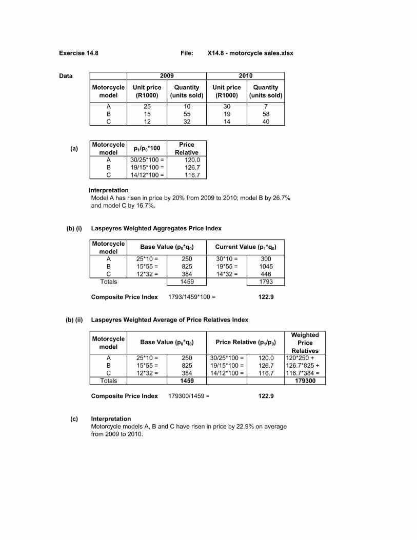
Exercise 14.8 File: X14.8 - motorcycle sales.xlsx
Data
Motorcycle model
Unit price (R1000)
Quantity (units sold)
Unit price (R1000)
Quantity (units sold)
A 25 10 30 7B 15 55 19 58C 12 32 14 40
(a) Motorcycle model p1/p0*100 Price
RelativeA 30/25*100 = 120.0B 19/15*100 = 126.7C 14/12*100 = 116.7
InterpretationModel A has risen in price by 20% from 2009 to 2010; model B by 26.7% and model C by 16.7%.
(b) (i) Laspeyres Weighted Aggregates Price Index
Motorcycle model
A 25*10 = 250 30*10 = 300B 15*55 = 825 19*55 = 1045C 12*32 = 384 14*32 = 448
Totals 1459 1793
Composite Price Index 1793/1459*100 = 122.9
(b) (ii) Laspeyres Weighted Average of Price Relatives Index
Motorcycle model
Weighted Price
RelativesA 25*10 = 250 30/25*100 = 120.0 120*250 +B 15*55 = 825 19/15*100 = 126.7 126.7*825 +C 12*32 = 384 14/12*100 = 116.7 116.7*384 =
Totals 1459 179300
Composite Price Index 179300/1459 = 122.9
(c) InterpretationMotorcycle models A, B and C have risen in price by 22.9% on average from 2009 to 2010.
2009 2010
Base Value (p0*q0) Current Value (p1*q0)
Base Value (p0*q0) Price Relative (p1/p0)
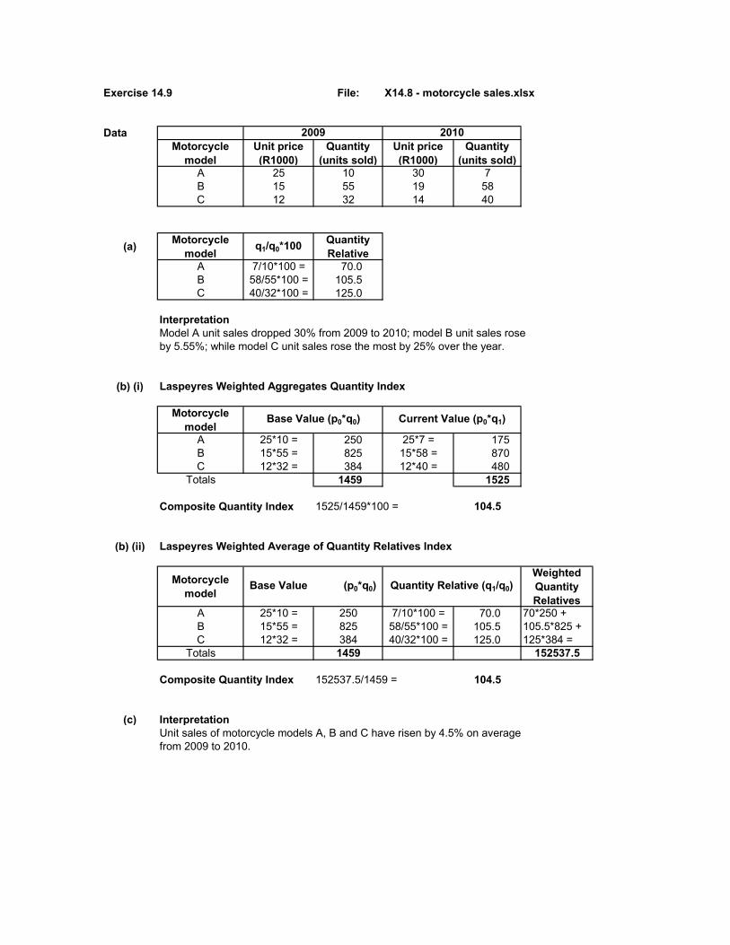
Exercise 14.9 File: X14.8 - motorcycle sales.xlsx
DataMotorcycle
modelUnit price (R1000)
Quantity (units sold)
Unit price (R1000)
Quantity (units sold)
A 25 10 30 7B 15 55 19 58C 12 32 14 40
(a) Motorcycle model q1/q0*100 Quantity
RelativeA 7/10*100 = 70.0B 58/55*100 = 105.5C 40/32*100 = 125.0
InterpretationModel A unit sales dropped 30% from 2009 to 2010; model B unit sales rose by 5.55%; while model C unit sales rose the most by 25% over the year.
(b) (i) Laspeyres Weighted Aggregates Quantity Index
Motorcycle model
A 25*10 = 250 25*7 = 175B 15*55 = 825 15*58 = 870C 12*32 = 384 12*40 = 480
Totals 1459 1525
Composite Quantity Index 1525/1459*100 = 104.5
(b) (ii) Laspeyres Weighted Average of Quantity Relatives Index
Motorcycle model
Weighted Quantity Relatives
A 25*10 = 250 7/10*100 = 70.0 70*250 +B 15*55 = 825 58/55*100 = 105.5 105.5*825 +C 12*32 = 384 40/32*100 = 125.0 125*384 =
Totals 1459 152537.5
Composite Quantity Index 152537.5/1459 = 104.5
(c) InterpretationUnit sales of motorcycle models A, B and C have risen by 4.5% on average from 2009 to 2010.
2009 2010
Base Value (p0*q0) Current Value (p0*q1)
Base Value (p0*q0) Quantity Relative (q1/q0)

Exercise 14.10 File: X14.8 - motorcycle sales.xlsx
DataMotorcycle
modelUnit price (R1000)
Quantity (units sold)
Unit price (R1000)
Quantity (units sold)
A 25 10 30 7B 15 55 19 58C 12 32 14 40
(a) (i) Paasche Weighted Aggregates Quantity Index
Motorcycle model
A 30*10 = 300 30* 7 = 210B 19*55 = 1045 19*58 = 1102C 14*32 = 448 14*40 = 560
Totals 1793 1872
Composite Quantity Index 1872/1793*100 = 104.41
(a) (ii) Paasche Weighted Average of Quantity Relatives Index
Motorcycle model
Weighted Quantity Relatives
A 30*10 = 300 7/10*100 = 70.0 70*300 +B 19*55 = 1045 58/55*100 = 105.5 105.5*1045 +C 14*32 = 448 40/32*100 = 125.0 125*448 =
Totals 1793 187200
Composite Quantity Index 187200/1793 = 104.41
(b) InterpretationUnit sales of motorcycle models A, B and C have risen by 4.41% on average from 2009 to 2010.
2009 2010
Base Value (p1*q0) Current Value (p1*q1)
Base Value (p1*q0) Quantity Relative (q1/q0)

Exercise14.11 File: X14.11 - Telkom services.xlsx
Data
Unit price (cents/call)
Quantity (100's calls)
Unit price (cents/call)
Quantity (100's calls)
Unit price (cents/call)
Quantity (100's calls)
TalkPlus 65 14 70 18 55 17SmartAccess 35 27 40 29 45 24
ISDN 50 16 45 22 40 32
(a) Telkom ServicesTalkPlus 70/65*100 = 107.7 55/65*100 = 84.6SmartAccess 40/35*100 = 114.3 45/35*100 = 128.6ISDN 45/50*100 = 90.0 40/50*100 = 80.0
InterpretationTalkPlus services increased by 7.7% in price from 2009 to 2010, but then dropped by15.4% in price from 2009 to 2011. SmartAccess on the other hand showed an increase in price from 2009 to 2010 of 14.3% and by 28.6% from 2009 to 2011. ISDN showed a decrease in price by 10% in the first year (from 2009 to 2010) and by 20% over the 2 year period from 2009 to 2011.
(b) Laspeyres Weighted Aggregates Price Index
Telkom Services Base Value (p0*q0)
2010 Value (p1*q0)
2011 Value (p1*q0)
TalkPlus 910 980 770SmartAccess 945 1080 1215ISDN 800 720 640
2655 2780 2625
Composite Price Indexes 104.71 98.87
Interpretation (based on the Laspeyres approach)The cost of Telkom services increased, on average, by 4.71% from 2009 to 2010,while there was a net reduction in costs, on average of 1.13% from 2009 to 2011.
(c) Paasche Weighted Aggregates Quantity Index
Telkom Services Base Value (p1*q0)
2010 Value (p1*q1)
Base Value (p1*q0)
2011 Value (p1*q1)
TalkPlus 980 1260 770 935SmartAccess 1080 1160 1215 1080ISDN 720 990 640 1280
2780 3410 2625 3295
Composite Quantity Indexes 122.7 125.5
(d) Interpretation (based on the Paasche approach)
Telkom Services
2009 2010 2011
Price relatives (2010) Price relatives (2011)
2010 Prices 2011 Prices

The printing company's usage of Telkom services has risen by 22.7% over oneyear (from 2009 to 2010) and by 25.5%, on average over two years (from 2009 to 2011).

Exercise 14.12 File: X14.12 - computer personnel.xlsx
Data2008 2011 2008 2011
Systems analyst 42 50 84 107Programmer 29 36 96 82Network manager 24 28 58 64
(a) Laspeyres Weighted Aggregate Salary Index
IT Job Category Base Value 2008 (p0*q0)
Current Value 2011 (p1*q0)
Systems analyst 3528 4200Programmer 2784 3456Network manager 1392 1624
7704 9280
Laspeyres Composite Salary Index 120.46
(b) Interpretation On average, the overall remuneration has increased by 20.46% over the 3 years period from 2008 to 2011.
(c) IT Job Category Price relatives (p1/p0)
Systems analyst 119.05Programmer 124.14Network manager 116.67
Interpretation Programmers have enjoyed the largest percentage increasein remuneration of 24.14% from 2008 to 2011.
Job categories Annual salary (in R10 000) No. of employees

Exercise 14.13 File: X14.12 - computer personnel.xlsx
Data2008 2011 2008 2011
Systems analyst 42 50 84 107Programmer 29 36 96 82Network manager 24 28 58 64
(a) IT Job Category Staff Relatives (q1/q0)
Systems analyst 127.4Programmer 85.4Network manager 110.3
InterpretationThe staff complement of Systems Analysts grew by 27.4% and that of Network managers grew by 10.3% over the period from 2008 to 2011. However, the number of Programmers, on the other hand, reduced by 14.6% over this same period.
(b) (i) Laspeyres Quantity index (Weighted Aggregates approach)
IT Job Category Base Value 2008 (p0*q0)
Current Value 2011 (p0*q1)
Systems analyst 3528 4494Programmer 2784 2378Network manager 1392 1536
7704 8408
Composite Staff Complement (Quantity) Index 109.14
(b) (ii) Laspeyres Quantity index (Weighted Average of Relatives approach)
IT Job Category Base Value 2008 (p0*q0)
Staff Relatives (q1/q0)
Weighted Ave of
Quantity Relatives
Systems analyst 3528 127.38 449400Programmer 2784 85.42 237800Network manager 1392 110.34 153600
7704 840800
Composite Staff Complement (Quantity) Index 109.14
(c) InterpretationThe overall IT staff complement across all job categories has increased by anaverage of 9.14% from 2008 to 2011.
Job categories Annual salary (in R10 000) No. of employees
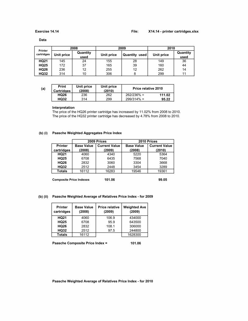
Exercise 14.14 File: X14.14 - printer cartridges.xlsx
Data
Unit price Quantity used Unit price Quantity used Unit price Quantity
usedHQ21 145 24 155 28 149 36HQ25 172 37 165 39 160 44HQ26 236 12 255 12 262 14HQ32 314 10 306 8 299 11
(a) Print Cartridges
Unit price (2008)
Unit price (2010)
HQ26 236 262 262/236% = 111.02HQ32 314 299 299/314% = 95.22
InterpretationThe price of the HQ26 printer cartridge has increased by 11.02% from 2008 to 2010.The price of the HQ32 printer cartridge has decreased by 4.78% from 2008 to 2010.
(b) (i) Paasche Weighted Aggregates Price Index
Printer cartridges
Base Value (2008)
Current Value (2009)
Base Value (2008)
Current Value (2010)
HQ21 4060 4340 5220 5364HQ25 6708 6435 7568 7040HQ26 2832 3060 3304 3668HQ32 2512 2448 3454 3289Totals 16112 16283 19546 19361
Composite Price Indexes 101.06 99.05
(b) (ii) Paasche Weighted Average of Relatives Price Index - for 2009
Printer cartridges
Base Value (2008)
Price relative (2009)
Weighted Ave (2009)
HQ21 4060 106.9 434000HQ25 6708 95.9 643500HQ26 2832 108.1 306000HQ32 2512 97.5 244800Totals 16112 1628300
Paasche Composite Price Index = 101.06
Paasche Weighted Average of Relatives Price Index - for 2010
2009 Prices 2010 Prices
Printer cartridges
2008 2009 2010
Price relative 2010

Printer cartridges
Base Value (2008)
Price relative (2010)
Weighted Ave (2010)
HQ21 5220 102.8 536400HQ25 7568 93.0 704000HQ26 3304 111.0 366800HQ32 3454 95.2 328900Totals 19546 1936100
Paasche Composite Price Index 99.05
(c) InterpretationThe average price of print cartridges increased marginally by 1.06% from 2008 to 2009. However, the average price of print cartridges decreased by 0.95% from 2008 to 2010.
(d) Composite Link Relatives2008 2009 2010
Composite price indexes 100 101.06 99.05Composite link relatives 101.06 98.01
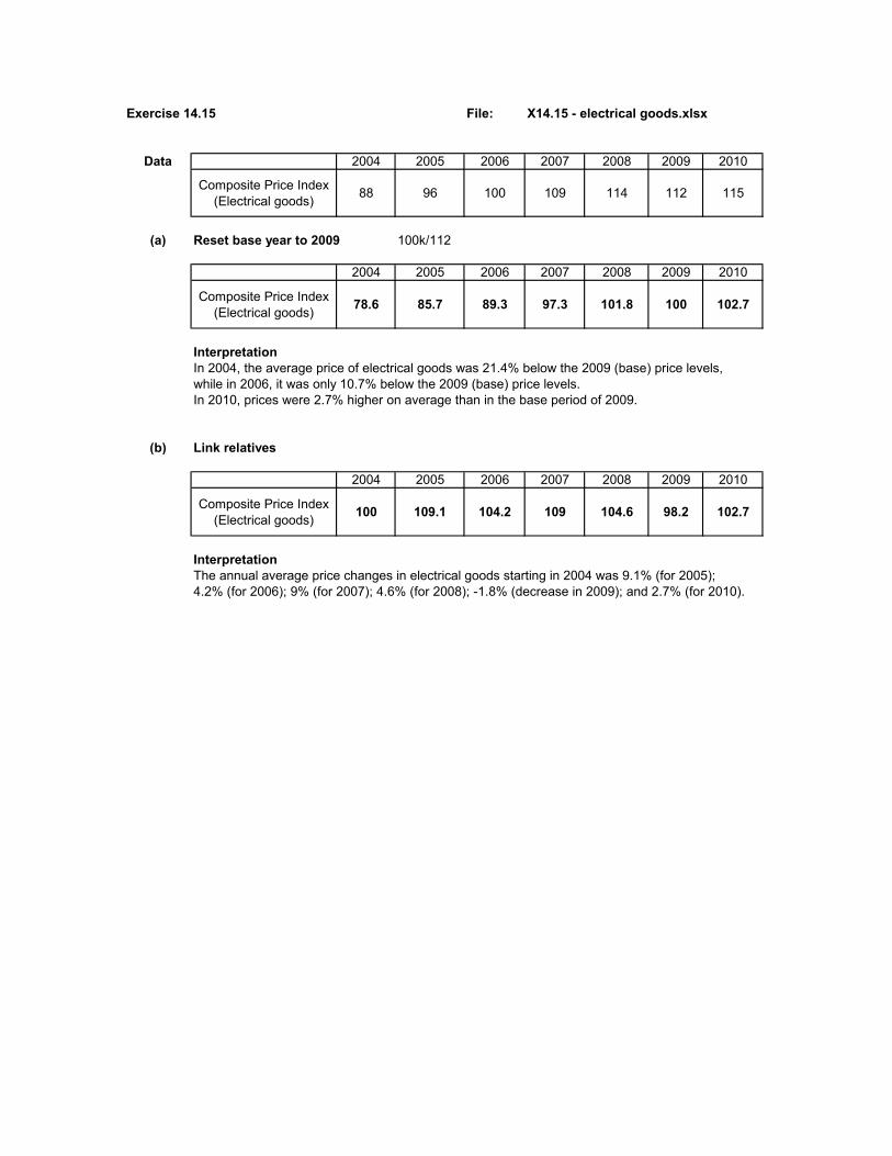
Exercise 14.15 File: X14.15 - electrical goods.xlsx
Data 2004 2005 2006 2007 2008 2009 2010
Composite Price Index (Electrical goods) 88 96 100 109 114 112 115
(a) Reset base year to 2009 100k/112
2004 2005 2006 2007 2008 2009 2010
Composite Price Index (Electrical goods) 78.6 85.7 89.3 97.3 101.8 100 102.7
InterpretationIn 2004, the average price of electrical goods was 21.4% below the 2009 (base) price levels,while in 2006, it was only 10.7% below the 2009 (base) price levels. In 2010, prices were 2.7% higher on average than in the base period of 2009.
(b) Link relatives
2004 2005 2006 2007 2008 2009 2010
Composite Price Index (Electrical goods) 100 109.1 104.2 109 104.6 98.2 102.7
InterpretationThe annual average price changes in electrical goods starting in 2004 was 9.1% (for 2005); 4.2% (for 2006); 9% (for 2007); 4.6% (for 2008); -1.8% (decrease in 2009); and 2.7% (for 2010).
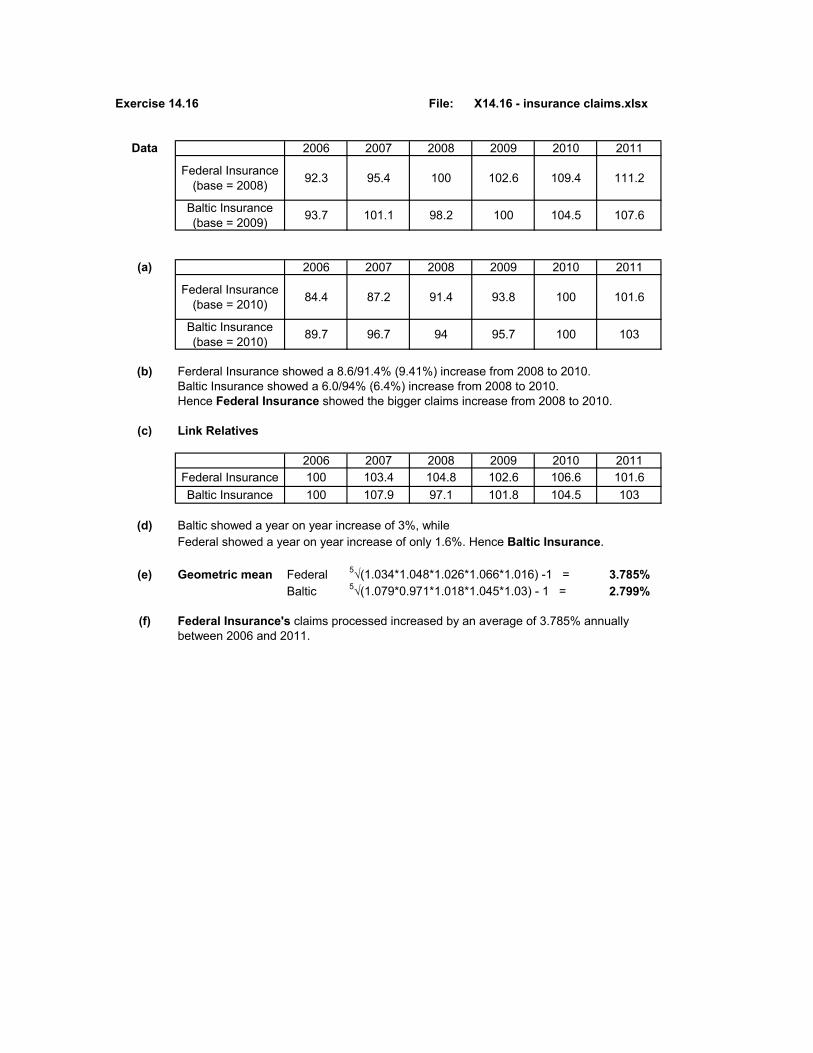
Exercise 14.16 File: X14.16 - insurance claims.xlsx
Data 2006 2007 2008 2009 2010 2011
Federal Insurance (base = 2008) 92.3 95.4 100 102.6 109.4 111.2
Baltic Insurance (base = 2009) 93.7 101.1 98.2 100 104.5 107.6
(a) 2006 2007 2008 2009 2010 2011
Federal Insurance (base = 2010) 84.4 87.2 91.4 93.8 100 101.6
Baltic Insurance (base = 2010) 89.7 96.7 94 95.7 100 103
(b) Ferderal Insurance showed a 8.6/91.4% (9.41%) increase from 2008 to 2010.Baltic Insurance showed a 6.0/94% (6.4%) increase from 2008 to 2010.Hence Federal Insurance showed the bigger claims increase from 2008 to 2010.
(c) Link Relatives
2006 2007 2008 2009 2010 2011Federal Insurance 100 103.4 104.8 102.6 106.6 101.6Baltic Insurance 100 107.9 97.1 101.8 104.5 103
(d) Baltic showed a year on year increase of 3%, while Federal showed a year on year increase of only 1.6%. Hence Baltic Insurance.
(e) Geometric mean Federal 5√(1.034*1.048*1.026*1.066*1.016) -1 = 3.785%Baltic 5√(1.079*0.971*1.018*1.045*1.03) - 1 = 2.799%
(f) Federal Insurance's claims processed increased by an average of 3.785% annually between 2006 and 2011.

Exercise 14.17 File: X14.17 - micro-market basket.xlsx
Data2010 2011 2010 2011
Milk (litres) 7.29 7.89 117 98Bread (loaves) 4.25 4.45 56 64Sugar (kg) 2.19 2.45 28 20Maize meal (kg) 5.25 5.59 58 64
(a) Food items 2010 2011 Price RelativesMilk (litres) 7.29 7.89 108.23Bread (loaves) 4.25 4.45 104.71Sugar (kg) 2.19 2.45 111.87Maize meal (kg) 5.25 5.59 106.48
InterpretationThe price of milk rose by 8.23%; bread by 4.71%; sugar by 11.87% and maize meal by 6.48% per unit of measure from 2010 to 2011. The largerst price change (increase) was sugar with a 11.87% increase.
(b) Paasche Weighted Average of Price Relatives Index
Food items Base Value (p0*q1)
Price Relatives Weighted Average
Milk (litres) 714.42 108.23 77322Bread (loaves) 272 104.71 28480Sugar (kg) 43.8 111.87 4900Maize meal (kg) 336 106.48 35776Total 1366.22 146478
Paasche Composite Price Index 146478/1366.22 = 107.21
On average, the price of the micro-basket of items increased by 7.21% from 2010 to 2011.
(c) Food items 2010 2011 Quantity Relatives
Milk (litres) 117 98 83.8Bread (loaves) 56 64 114.3Sugar (kg) 28 20 71.4Maize meal (kg) 58 64 110.3
InterpretationThe consumption of milk decreased by 16.2%; bread consumption rose by 14.3%;sugar consumption decreased significantly by 28.6% and maize meal consumption rose by 10.3% from 2010 to 2011 respectively. The largest consumption change (decrease) was sugar with a 28.6% decrease. It is interesting to note that sugar showed the largest unit price increase while simultaneously recorded the largest decrease in consumption from 2010 to 2011.
Food items in micro market basket
Unit prices (in Rand) Consumption

(d) Paasche Weighted Average of Quantity (Consumption) Relatives Index
Food items Base Value (p1*q0)
Quantity Relatives Weighted Average
Milk (litres) 923.13 83.8 77322Bread (loaves) 249.20 114.3 28480Sugar (kg) 68.60 71.4 4900Maize meal (kg) 324.22 110.3 35776Total 1565.15 146478
Paasche Composite Quantity Index 146478/1565.15 = 93.6
On average, consumption of the micro-basket items dropped by 6.4% from 2010 to 2011.

Exercise 14.18 File: X14.18 - utilities usage.xlsx
Data2008 2009 2010 2008 2009 2010
Electricity 1.97 2.05 2.09 745 812 977Sewage 0.62 0.68 0.72 68 56 64Water 0.29 0.31 0.35 296 318 378Telephone 1.24 1.18 1.06 1028 1226 1284
(a) Utilities Unit Price 2008
Unit Price 2010
Price relative
2010Electricity 1.97 2.09 106.1Sewage 0.62 0.72 116.1Water 0.29 0.35 120.7Telephone 1.24 1.06 85.5
InterpretationFrom 2008 to 2010, electricity increased by 6.1%; sewage costs by 16.1% water by 20.7%; while telephone costs decreased by 14.5% over this period. Electricity showed the smallest change (increase) of 6.1% from 2008 to 2010.
(b) (i) Laspeyres Weighted Aggregates Price Index
Utilities Base Value (2008)
Current Value (2009)
Current Value (2010)
Electricity 1467.7 1527.3 1557.1Sewage 42.2 46.2 49.0Water 85.8 91.8 103.6Telephone 1274.7 1213.0 1089.7
Totals 2870.4 2878.3 2799.3
Laspeyres Composite Price Indexes 100.3 97.5
(b) (ii) Laspeyres Weighted Average of Price Relatives Index
Utilities Base Value (2008)
Price relative (2009)
Price relative (2010)
Weighted Ave (2009)
Weighted Ave (2010)
Electricity 1467.7 104.1 106.1 152782.4 155717.7Sewage 42.2 109.7 116.1 4625.0 4894.8Water 85.8 106.9 120.7 9176.3 10360.9Telephone 1274.7 95.2 85.5 121353.3 108988.6
Totals 2870.4 287937.0 279961.9
Laspeyres Composite Price Indexes 100.3 97.5
Utilities Prices (in Rand / unit) Consumption (No. of units)

(c) InterpretationThere was virtually no change in the average cost of household utilities between 2008 and 2009. A slight increase of only 0.3% was recorded. From 2008 to 2010, however, the average cost of household utilities actually decreased marginally by 2.5%.
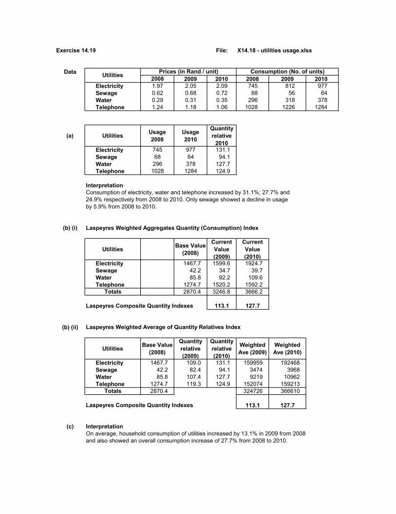
Exercise 14.19 File: X14.18 - utilities usage.xlsx
Data2008 2009 2010 2008 2009 2010
Electricity 1.97 2.05 2.09 745 812 977Sewage 0.62 0.68 0.72 68 56 64Water 0.29 0.31 0.35 296 318 378Telephone 1.24 1.18 1.06 1028 1226 1284
(a) Utilities Usage 2008
Usage 2010
Quantity relative
2010Electricity 745 977 131.1Sewage 68 64 94.1Water 296 378 127.7Telephone 1028 1284 124.9
InterpretationConsumption of electricity, water and telephone increased by 31.1%; 27.7% and24.9% respectively from 2008 to 2010. Only sewage showed a decline in usageby 5.9% from 2008 to 2010.
(b) (i) Laspeyres Weighted Aggregates Quantity (Consumption) Index
Utilities Base Value (2008)
Current Value (2009)
Current Value (2010)
Electricity 1467.7 1599.6 1924.7Sewage 42.2 34.7 39.7Water 85.8 92.2 109.6Telephone 1274.7 1520.2 1592.2
Totals 2870.4 3246.8 3666.2
Laspeyres Composite Quantity Indexes 113.1 127.7
(b) (ii) Laspeyres Weighted Average of Quantity Relatives Index
Utilities Base Value (2008)
Quantity relative (2009)
Quantity relative (2010)
Weighted Ave (2009)
Weighted Ave (2010)
Electricity 1467.7 109.0 131.1 159959 192468Sewage 42.2 82.4 94.1 3474 3968Water 85.8 107.4 127.7 9219 10962Telephone 1274.7 119.3 124.9 152074 159213
Totals 2870.4 324726 366610
Laspeyres Composite Quantity Indexes 113.1 127.7
(c) InterpretationOn average, household consumption of utilities increased by 13.1% in 2009 from 2008 and also showed an overall consumption increase of 27.7% from 2008 to 2010.
Utilities Prices (in Rand / unit) Consumption (No. of units)

Exercise 14.20 File: X14.20 - leather goods.xlsx
Data 2005 2006 2007 2008 2009 2010 2011
Composite cost index 97 92 100 102 107 116 112
(a) Re-base to 2009 Adjustment factor = 100/107 = 0.934579
2005 2006 2007 2008 2009 2010 2011
Composite cost index 90.7 86 93.5 95.3 100 108.4 104.7
(b)
InterpretationPrior to 2009, the average annual cost of leather goods inputs were below the 2009 level, but showed a steady increase towards 2009 prices over this period.Relative to 2009 unit costs, the cost of leathergoods inputs was higher by 8.4% and 4.7% respectively for 2010 and 2011.
(c) The average increase in unit costs of leather goods inputs was only 4.7% between 2009 and 2011.
(d) Link Relatives
2005 2006 2007 2008 2009 2010 2011
Composite cost index 100 94.8 108.7 102.0 104.9 108.4 96.6
The largest year-on-year change in overall unit costs of leather goods inputs was between 2006 and 2007 with an increase of 8.7%.
60
70
80
90
100
110
120
2005 2006 2007 2008 2009 2010 2011
Cost
Inde
x
Composite cost index
Composite cost index

(e) Geometric mean 6√(0.948*1.087*1.02*1.049*1.0841*0.966) 1.024244
(i.e. 2.424% increase on average per year)
=GEOMEAN(0.9485,1.087,1.02,1.049,1.0841,0.9655)= 1.024244

Exercise 14.21 File: X14.21 - accountants' salaries.xlsx
(a) Year Salary CPI Real Salary2005 387 95 407.42006 406 100 406.02007 422 104 405.82008 448 111 403.62009 466 121 385.12010 496 126 393.72011 510 133 383.5
(b) InterpretationThe base real salary is R406 (in R1000s). Since 2006, real salaries have declined relative to 2006 (base) and are continuing to fall further behind inflation (CPI).
(c)Year Salary CPI Salary CPI Diff (Sal - CPI)2005 387 952006 406 100 104.9 105.3 -0.42007 422 104 103.9 104.0 -0.12008 448 111 106.2 106.7 -0.62009 466 121 104.0 109.0 -5.02010 496 126 106.4 104.1 2.32011 510 133 102.8 105.6 -2.7
InterpretationOn a year-on-year basis, salary increases have lagged behind the inflation rate (CPI)in all years except 2010 when salary adjustments exceeded CPI by 2.3%.
Link Relatives
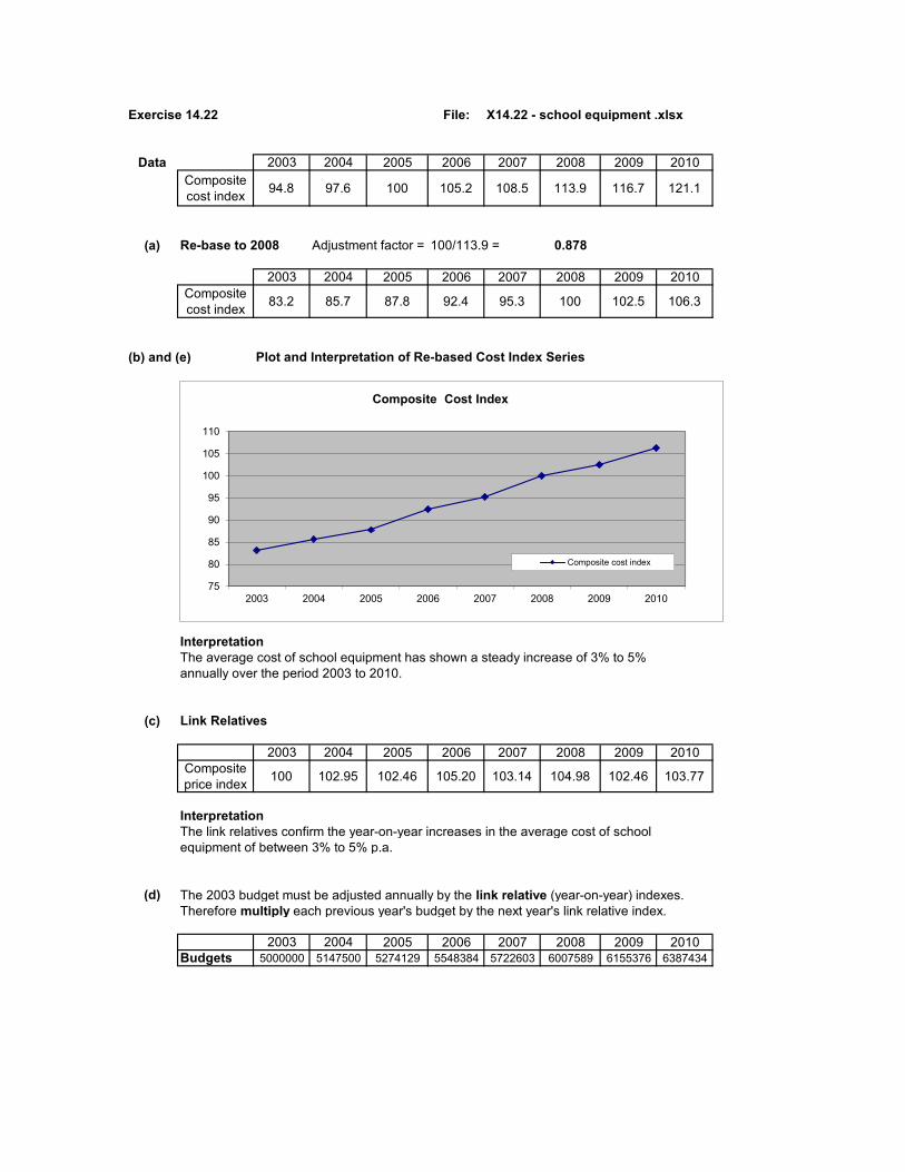
Exercise 14.22 File: X14.22 - school equipment .xlsx
Data 2003 2004 2005 2006 2007 2008 2009 2010Composite cost index 94.8 97.6 100 105.2 108.5 113.9 116.7 121.1
(a) Re-base to 2008 Adjustment factor = 100/113.9 = 0.878
2003 2004 2005 2006 2007 2008 2009 2010Composite cost index 83.2 85.7 87.8 92.4 95.3 100 102.5 106.3
(b) and (e) Plot and Interpretation of Re-based Cost Index Series
InterpretationThe average cost of school equipment has shown a steady increase of 3% to 5% annually over the period 2003 to 2010.
(c) Link Relatives
2003 2004 2005 2006 2007 2008 2009 2010Composite price index 100 102.95 102.46 105.20 103.14 104.98 102.46 103.77
InterpretationThe link relatives confirm the year-on-year increases in the average cost of schoolequipment of between 3% to 5% p.a.
(d) The 2003 budget must be adjusted annually by the link relative (year-on-year) indexes.Therefore multiply each previous year's budget by the next year's link relative index.
2003 2004 2005 2006 2007 2008 2009 2010Budgets 5000000 5147500 5274129 5548384 5722603 6007589 6155376 6387434
75
80
85
90
95
100
105
110
2003 2004 2005 2006 2007 2008 2009 2010
Composite Cost Index
Composite cost index
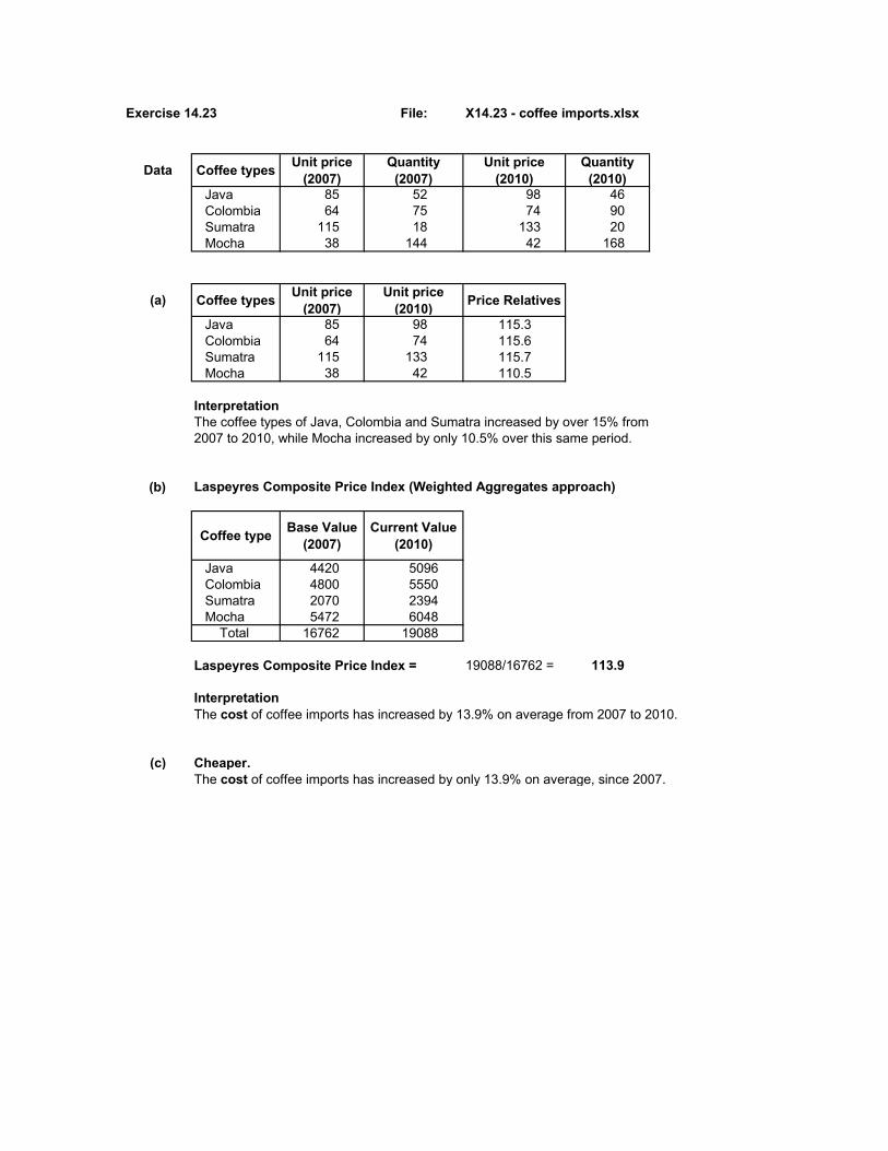
Exercise 14.23 File: X14.23 - coffee imports.xlsx
Data Coffee types Unit price (2007)
Quantity (2007)
Unit price (2010)
Quantity (2010)
Java 85 52 98 46Colombia 64 75 74 90Sumatra 115 18 133 20Mocha 38 144 42 168
(a) Coffee types Unit price (2007)
Unit price (2010) Price Relatives
Java 85 98 115.3Colombia 64 74 115.6Sumatra 115 133 115.7Mocha 38 42 110.5
InterpretationThe coffee types of Java, Colombia and Sumatra increased by over 15% from2007 to 2010, while Mocha increased by only 10.5% over this same period.
(b) Laspeyres Composite Price Index (Weighted Aggregates approach)
Coffee type Base Value (2007)
Current Value (2010)
Java 4420 5096Colombia 4800 5550Sumatra 2070 2394Mocha 5472 6048
Total 16762 19088
Laspeyres Composite Price Index = 19088/16762 = 113.9
InterpretationThe cost of coffee imports has increased by 13.9% on average from 2007 to 2010.
(c) Cheaper.The cost of coffee imports has increased by only 13.9% on average, since 2007.

(d) Laspeyres Composite Quantity Index (Weighted Aggregates approach)
Coffee type Base Value (2007)
Current Value (2010)
Java 4420 3910Colombia 4800 5760Sumatra 2070 2300Mocha 5472 6384
Total 16762 18354
Laspeyres Composite Quantity Index 18354/16762 = 109.5
InterpretationThe quantity of coffee imported has increased by 9.5% on average from 2007 to 2010.
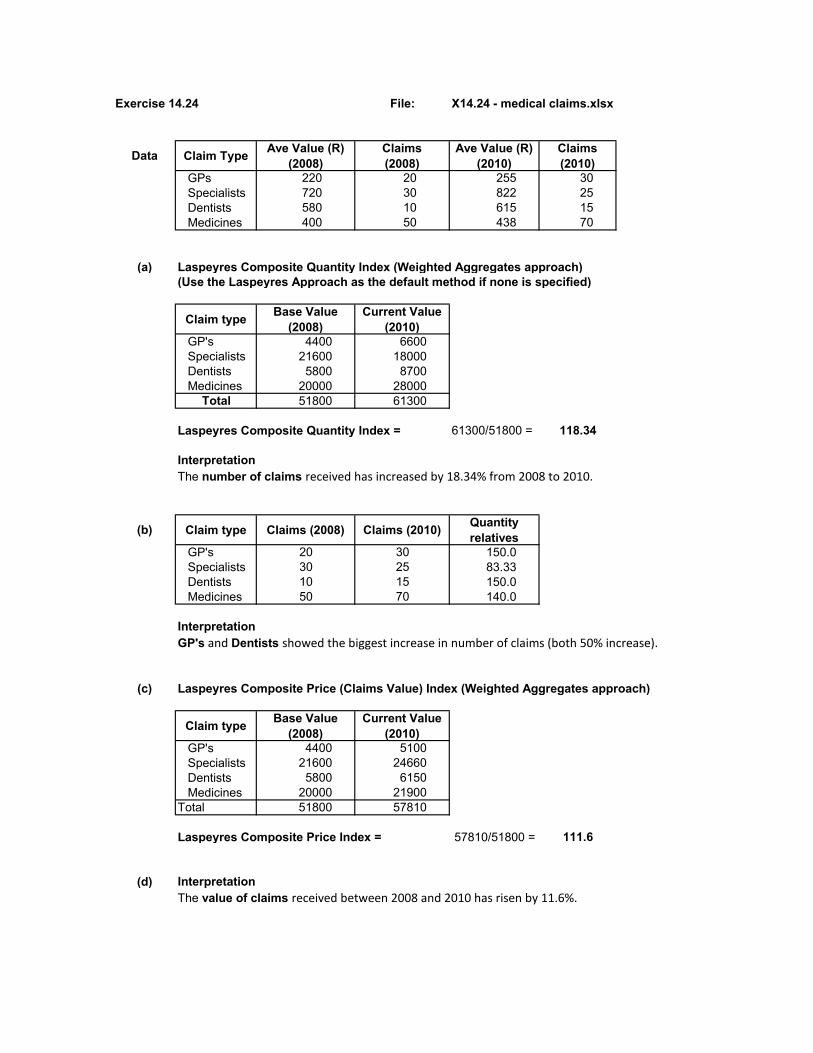
Exercise 14.24 File: X14.24 - medical claims.xlsx
Data Claim Type Ave Value (R) (2008)
Claims (2008)
Ave Value (R) (2010)
Claims (2010)
GPs 220 20 255 30Specialists 720 30 822 25Dentists 580 10 615 15Medicines 400 50 438 70
(a) Laspeyres Composite Quantity Index (Weighted Aggregates approach)(Use the Laspeyres Approach as the default method if none is specified)
Claim type Base Value (2008)
Current Value (2010)
GP's 4400 6600Specialists 21600 18000Dentists 5800 8700Medicines 20000 28000
Total 51800 61300
Laspeyres Composite Quantity Index = 61300/51800 = 118.34
InterpretationThe number of claims received has increased by 18.34% from 2008 to 2010.
(b) Claim type Claims (2008) Claims (2010) Quantity relatives
GP's 20 30 150.0Specialists 30 25 83.33Dentists 10 15 150.0Medicines 50 70 140.0
InterpretationGP's and Dentists showed the biggest increase in number of claims (both 50% increase).
(c) Laspeyres Composite Price (Claims Value) Index (Weighted Aggregates approach)
Claim type Base Value (2008)
Current Value (2010)
GP's 4400 5100Specialists 21600 24660Dentists 5800 6150Medicines 20000 21900
Total 51800 57810
Laspeyres Composite Price Index = 57810/51800 = 111.6
(d) InterpretationThe value of claims received between 2008 and 2010 has risen by 11.6%.

Exercise 14.25 File: X14.25 - tennis shoes.xlsx
Data Shoe Model Unit price (2009)
Pairs Sold (2009)
Unit price (2010)
Pairs Sold (2010)
Trainer 320 96 342 110Balance 445 135 415 162Dura 562 54 595 48
(a) Quantity Relatives
Shoe model Pairs sold (2009)
Pairs sold (2010)
Quantity relatives
Trainer 96 110 114.6Balance 135 162 120.0Dura 54 48 88.9
InterpretationDura's sales volume is down by 11.1% from 2009.
(b) Laspeyres Weighted Aggregates Quantity (Volume) Index
Shoe model Base Value (2009)
Current Value (2010)
Trainer 30720 35200Balance 60075 72090Dura 30348 26976Total 121143 134266
Composite Quantity Index = 134266/121143*100 = 110.83
(c) InterpretationThe average increase in shoes sold from 2009 to 2010 was only 10.83%. Overall, sales volumes do not meet the required growth of at least 12% p.a.
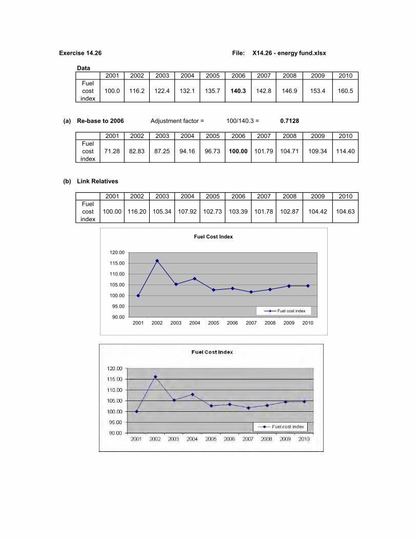
Exercise 14.26 File: X14.26 - energy fund.xlsx
Data2001 2002 2003 2004 2005 2006 2007 2008 2009 2010
Fuel cost index
100.0 116.2 122.4 132.1 135.7 140.3 142.8 146.9 153.4 160.5
(a) Re-base to 2006 Adjustment factor = 100/140.3 = 0.7128
2001 2002 2003 2004 2005 2006 2007 2008 2009 2010Fuel cost index
71.28 82.83 87.25 94.16 96.73 100.00 101.79 104.71 109.34 114.40
(b) Link Relatives
2001 2002 2003 2004 2005 2006 2007 2008 2009 2010Fuel cost index
100.00 116.20 105.34 107.92 102.73 103.39 101.78 102.87 104.42 104.63
90.00
95.00
100.00
105.00
110.00
115.00
120.00
2001 2002 2003 2004 2005 2006 2007 2008 2009 2010
Fuel Cost Index
Fuel cost index

(c) Geometric Mean 9√(1.162*1.0534*1.0792*1.0273*1.0339*1.0178*1.0287*1.0442*1.0463)1.05397
Annual Average Increase = 5.3974% p.a. on average.
Using Excel =GEOMEAN(all link relatives)
(d) InterpretationAnnual fuel cost increases and decreases were high in the period 2001 to 2004.Thereafter, year-on-year increases were moderate and stable at between 3% to 5% p.a.
105.3976
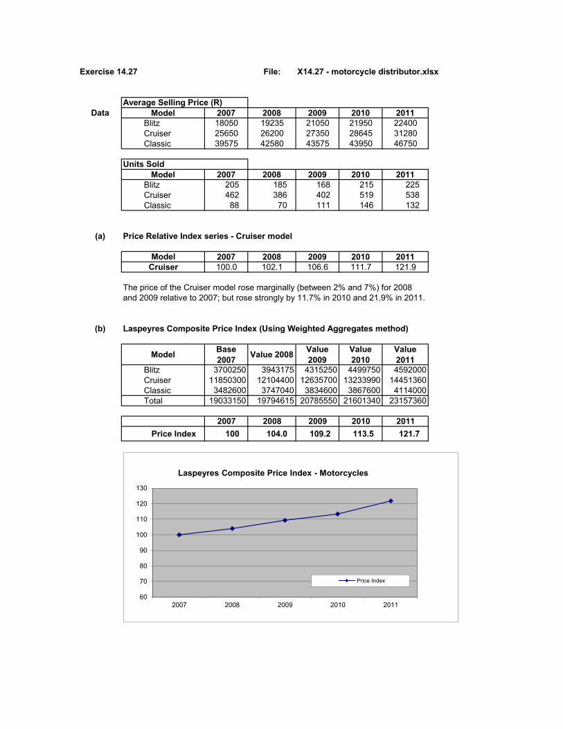
Exercise 14.27 File: X14.27 - motorcycle distributor.xlsx
Data Model 2007 2008 2009 2010 2011Blitz 18050 19235 21050 21950 22400Cruiser 25650 26200 27350 28645 31280Classic 39575 42580 43575 43950 46750
Model 2007 2008 2009 2010 2011Blitz 205 185 168 215 225Cruiser 462 386 402 519 538Classic 88 70 111 146 132
(a) Price Relative Index series - Cruiser model
Model 2007 2008 2009 2010 2011Cruiser 100.0 102.1 106.6 111.7 121.9
The price of the Cruiser model rose marginally (between 2% and 7%) for 2008 and 2009 relative to 2007; but rose strongly by 11.7% in 2010 and 21.9% in 2011.
(b) Laspeyres Composite Price Index (Using Weighted Aggregates method)
Model Base 2007 Value 2008 Value
2009Value 2010
Value 2011
Blitz 3700250 3943175 4315250 4499750 4592000Cruiser 11850300 12104400 12635700 13233990 14451360Classic 3482600 3747040 3834600 3867600 4114000Total 19033150 19794615 20785550 21601340 23157360
2007 2008 2009 2010 2011Price Index 100 104.0 109.2 113.5 121.7
Average Selling Price (R)
Units Sold
60
70
80
90
100
110
120
130
2007 2008 2009 2010 2011
Laspeyres Composite Price Index - Motorcycles
Price Index

(c) InterpretationThere has been a reasonably constant increase in the average price of motorcyclesover the past 5 years. In 2011, motorcycles cost 21.7% more on average than they did in 2007.
(d) Link relative of Selling Prices - Classic Model
2007 2008 2009 2010 2011Classic 100 107.6 102.3 100.9 106.4
InterpretationThe Classic model has shown a very modest year-on-year price increase of between 2.3% and 7.6% between 2007 and 2011. In 2010, the annual(year-on-year) increase was only 0.9% (less than 1%).
(e) Geometric Mean = 4√ (1.076*1.023*1.009*1.064) - 1= 4.263Using Excel = GEOMEAN(link relatives) - 100 = 4.253
Motorcycle prices have risen by an average of 4.263% per annum.
(f) Laspeyres Composite Quantity Index (Using Weighted Aggregates method)
Model Base 2007 Value 2008 Value
2009Value 2010
Value 2011
Blitz 3700250 3339250 3032400 3880750 4061250Cruiser 11850300 9900900 10311300 13312350 13799700Classic 3482600 2770250 4392825 5777950 5223900Total 19033150 16010400 17736525 22971050 23084850
2007 2008 2009 2010 2011Quantity Index 100 84.1 93.2 120.7 121.3
60
70
80
90
100
110
120
130
2007 2008 2009 2010 2011
Laspeyres Composite Quantity Index - Motorcycles
Quantity Index

(g) InterpretationSales of motorcycles dropped for two years after 2007 (i.e. by 15.9% in 2008 andby 6.8% in 2009). Thereafter unit sales, on average per model, increased by 20.7%in 2010 relative to 2007; but performed at the same level in 2011 compared to 2010.
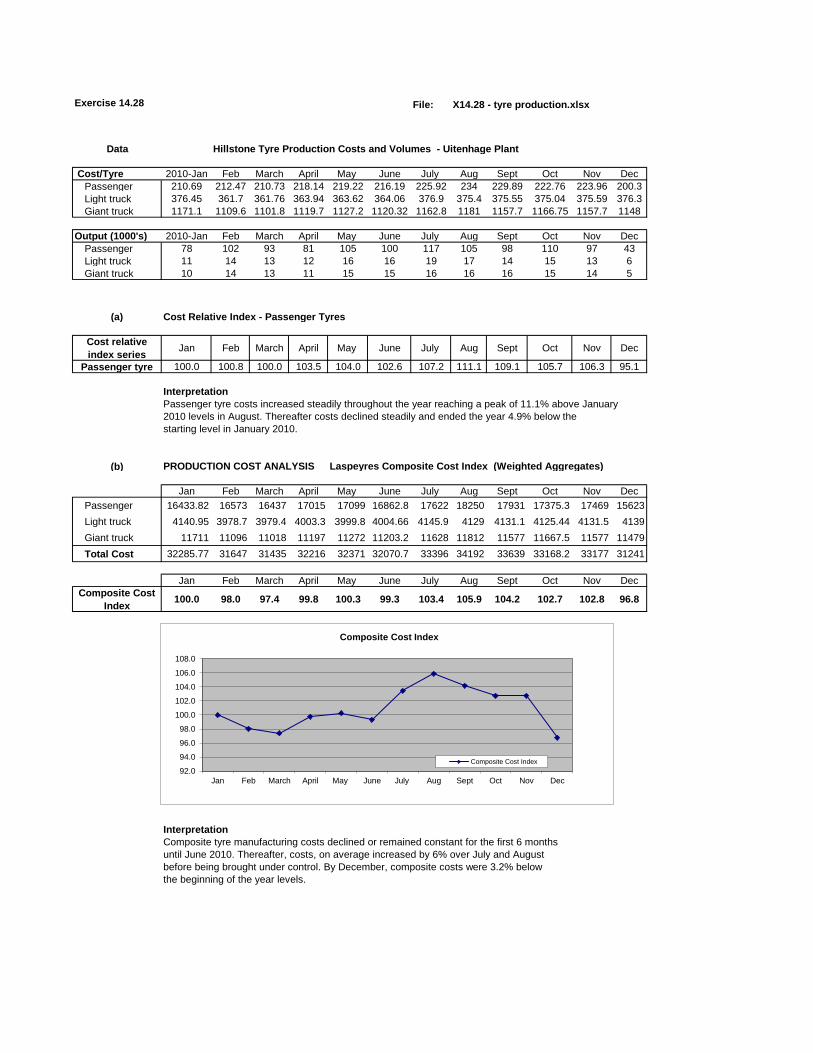
File: X14.28 - tyre production.xlsx
Data Hillstone Tyre Production Costs and Volumes - Uitenhage Plant
Cost/Tyre 2010-Jan Feb March April May June July Aug Sept Oct Nov Dec
Passenger 210.69 212.47 210.73 218.14 219.22 216.19 225.92 234 229.89 222.76 223.96 200.3
Light truck 376.45 361.7 361.76 363.94 363.62 364.06 376.9 375.4 375.55 375.04 375.59 376.3
Giant truck 1171.1 1109.6 1101.8 1119.7 1127.2 1120.32 1162.8 1181 1157.7 1166.75 1157.7 1148
Output (1000's) 2010-Jan Feb March April May June July Aug Sept Oct Nov Dec
Passenger 78 102 93 81 105 100 117 105 98 110 97 43
Light truck 11 14 13 12 16 16 19 17 14 15 13 6
Giant truck 10 14 13 11 15 15 16 16 16 15 14 5
(a) Cost Relative Index - Passenger Tyres
Cost relative
index seriesJan Feb March April May June July Aug Sept Oct Nov Dec
Passenger tyre 100.0 100.8 100.0 103.5 104.0 102.6 107.2 111.1 109.1 105.7 106.3 95.1
Interpretation
Passenger tyre costs increased steadily throughout the year reaching a peak of 11.1% above January
2010 levels in August. Thereafter costs declined steadily and ended the year 4.9% below the
starting level in January 2010.
(b) PRODUCTION COST ANALYSIS Laspeyres Composite Cost Index (Weighted Aggregates)
Jan Feb March April May June July Aug Sept Oct Nov Dec
Passenger 16433.82 16573 16437 17015 17099 16862.8 17622 18250 17931 17375.3 17469 15623
Light truck 4140.95 3978.7 3979.4 4003.3 3999.8 4004.66 4145.9 4129 4131.1 4125.44 4131.5 4139
Giant truck 11711 11096 11018 11197 11272 11203.2 11628 11812 11577 11667.5 11577 11479
Total Cost 32285.77 31647 31435 32216 32371 32070.7 33396 34192 33639 33168.2 33177 31241
Jan Feb March April May June July Aug Sept Oct Nov Dec
Composite Cost
Index100.0 98.0 97.4 99.8 100.3 99.3 103.4 105.9 104.2 102.7 102.8 96.8
Interpretation
Composite tyre manufacturing costs declined or remained constant for the first 6 months
until June 2010. Thereafter, costs, on average increased by 6% over July and August
before being brought under control. By December, composite costs were 3.2% below
the beginning of the year levels.
Exercise 14.28
92.0
94.0
96.0
98.0
100.0
102.0
104.0
106.0
108.0
Jan Feb March April May June July Aug Sept Oct Nov Dec
Composite Cost Index
Composite Cost Index

(c) Link Relatives - Costs - Light Truck Tyres
Jan Feb March April May June July Aug Sept Oct Nov Dec
Light truck 376.45 361.7 361.76 363.94 363.62 364.06 376.9 375.4 375.55 375.04 375.59 376.3
Link Relatives 100.0 96.1 100.0 100.6 99.9 100.1 103.5 99.6 100.0 99.9 100.1 100.2
Interpretation
Light truck radial tyres costs have remained almost constant and unchanged throughout
the year with most adjustments not exceeding 0.5%. Only in Feb (decrease of 3.9%) and
July (increase of 3.5%) did costs fluctuate to any degree.
(d) PRODUCTION VOLUME ANALYSIS Laspeyres Quantity Index (Weighted Aggregates)
Jan Feb March April May June July Aug Sept Oct Nov Dec
Passenger 16433.82 21490 19594 17066 22122 21069 24651 22122 20648 23175.9 20437 9060
Light truck 4140.95 5270.3 4893.9 4517.4 6023.2 6023.2 7152.6 6400 5270.3 5646.75 4893.9 2259
Giant truck 11711 16395 15224 12882 17567 17566.5 18738 18738 18738 17566.5 16395 5856
Total Value 32285.77 43156 39712 34465 45712 44658.7 50541 47260 44656 46389.2 41726 17174
Jan Feb March April May June July Aug Sept Oct Nov Dec
Volume Index 100.0 133.7 123.0 106.8 141.6 138.3 156.5 146.4 138.3 143.7 129.2 53.2
(e) Interpretation
Production volumes of all three makes of tyres showed a steady increase above the January
level by up to nearly 60% over the first half of the year. However output showed a steady
decline in the second half of the year ending at only 53.2% of the beginning of the year levels.
0.0
20.0
40.0
60.0
80.0
100.0
120.0
140.0
160.0
180.0
Jan Feb March April May June July Aug Sept Oct Nov Dec
Laspeyres Composite Production Output (Volume) Index
Volume Index

CHAPTER 15
TIME SERIES ANALYSIS
A FORECASTING TOOL
Exercise 15.1 Cross-sectional data is gathered at one point in time;
Time series data is recorded at fixed intervals over time.
Exercise 15.2 Monthly national new car sales;
Daily maximum temperature for Cape Town.
Exercise 15.3 A line graph
Exercise 15.4 Trend; Cycles; Seasonality; Irregular (random)
Seasonality tends to show the most regularity.
Exercise 15.5 The Moving Average method smooths out short-term
fluctuations in a time series to allow the longer-term
underlying trend and cyclical patterns to be revealed.
Exercise 15.6 Yes, averaging occurs over a longer time period (i.e. five periods)
producing a smoother curve.
Exercise 15.7 A seasonal index of 108 means that seasonal influences stimulate
the time series values by 8% above the trend / cyclical level.
Exercise 15.8 A seasonal index of 88 means that seasonal influences depress
the time series values by 12% below the trend / cyclical level.
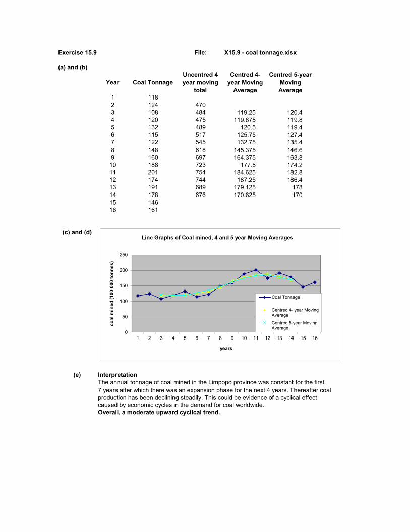
Exercise 15.9 File: X15.9 - coal tonnage.xlsx
(a) and (b)
Year Coal TonnageUncentred 4 year moving
total
Centred 4- year Moving
Average
Centred 5-year Moving Average
1 1182 124 4703 108 484 119.25 120.44 120 475 119.875 119.85 132 489 120.5 119.46 115 517 125.75 127.47 122 545 132.75 135.48 148 618 145.375 146.69 160 697 164.375 163.810 188 723 177.5 174.211 201 754 184.625 182.812 174 744 187.25 186.413 191 689 179.125 17814 178 676 170.625 17015 14616 161
(c) and (d)
(e) InterpretationThe annual tonnage of coal mined in the Limpopo province was constant for the first 7 years after which there was an expansion phase for the next 4 years. Thereafter coal production has been declining steadily. This could be evidence of a cyclical effect caused by economic cycles in the demand for coal worldwide. Overall, a moderate upward cyclical trend.
0
50
100
150
200
250
1 2 3 4 5 6 7 8 9 10 11 12 13 14 15 16
coal
min
ed (1
00 0
00 to
nnes
)
years
Line Graphs of Coal mined, 4 and 5 year Moving Averages
Coal Tonnage
Centred 4- year MovingAverage
Centred 5-year MovingAverage
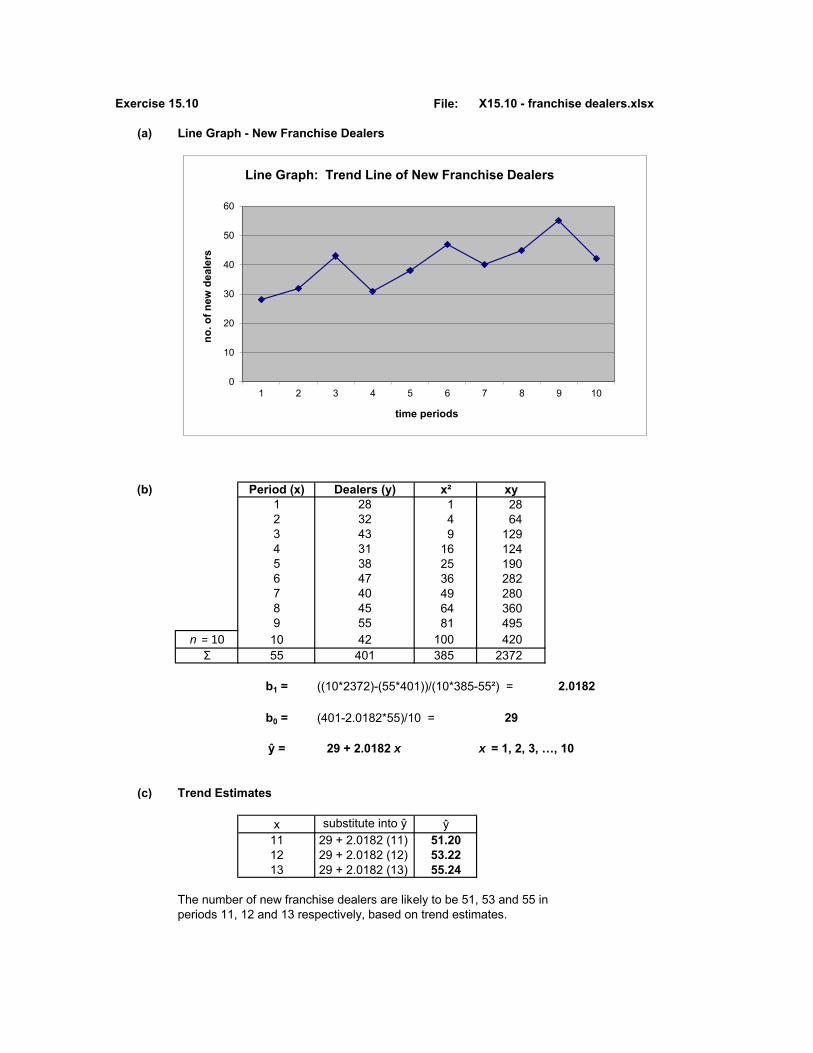
Exercise 15.10 File: X15.10 - franchise dealers.xlsx
(a) Line Graph - New Franchise Dealers
(b) Period (x) Dealers (y) x² xy1 28 1 282 32 4 643 43 9 1294 31 16 1245 38 25 1906 47 36 2827 40 49 2808 45 64 3609 55 81 495
n = 10 10 42 100 420Σ 55 401 385 2372
b1 = ((10*2372)-(55*401))/(10*385-55²) = 2.0182
b0 = (401-2.0182*55)/10 = 29
ŷ = 29 + 2.0182 x x = 1, 2, 3, …, 10
(c) Trend Estimates
x substitute into ŷ ŷ11 29 + 2.0182 (11) 51.2012 29 + 2.0182 (12) 53.2213 29 + 2.0182 (13) 55.24
The number of new franchise dealers are likely to be 51, 53 and 55 in periods 11, 12 and 13 respectively, based on trend estimates.
0
10
20
30
40
50
60
1 2 3 4 5 6 7 8 9 10
no. o
f new
dea
lers
time periods
Line Graph: Trend Line of New Franchise Dealers

Exercise 15.11 File: X15.11 - policy claims.xlsx
(a) Line Graph - Household Policy Claims
(b) Period (x) Claims (y) x² xy1 84 1 842 53 4 1063 60 9 1804 75 16 3005 81 25 4056 57 36 3427 51 49 3578 73 64 5849 69 81 621
10 37 100 37011 40 121 44012 77 144 92413 73 169 94914 46 196 64415 39 225 585
n = 16 16 63 256 1008Σ 136 978 1496 7899
b1 = =[(16)(7899) - (136)(978)]/[(16*1496)-(136)2] -1.21765
b0 = =(978-(-1.21765)*136)/16 71.4751 in Q1 2008
ŷ = 71.475 - 1.21765 x x = 2 in Q2 20083 in Q3 2008
InterpretationThere is a downward trend in household policy claims over the past 4 years.
0102030405060708090
1 2 3 4 5 6 7 8 9 10 11 12 13 14 15 16
no. o
f cla
ims
quarters
Line Graph - Household Policy Claims
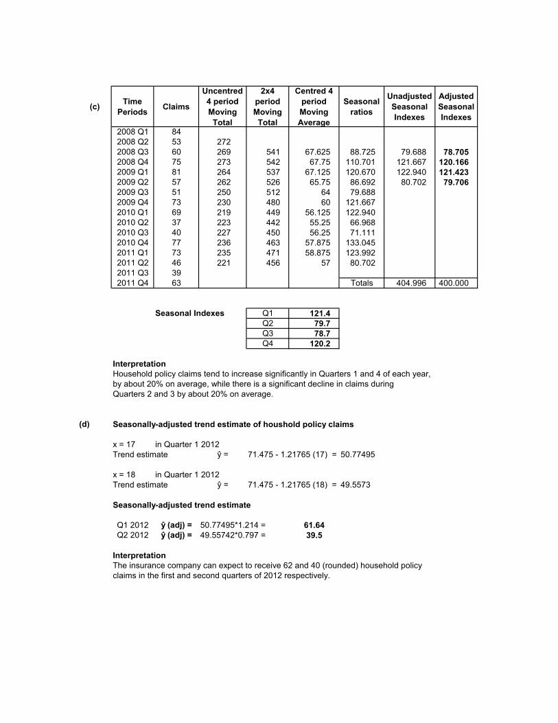
(c) Time Periods Claims
Uncentred 4 period Moving Total
2x4 period Moving
Total
Centred 4 period Moving Average
Seasonal ratios
Unadjusted Seasonal Indexes
Adjusted Seasonal Indexes
2008 Q1 842008 Q2 53 2722008 Q3 60 269 541 67.625 88.725 79.688 78.7052008 Q4 75 273 542 67.75 110.701 121.667 120.1662009 Q1 81 264 537 67.125 120.670 122.940 121.4232009 Q2 57 262 526 65.75 86.692 80.702 79.7062009 Q3 51 250 512 64 79.6882009 Q4 73 230 480 60 121.6672010 Q1 69 219 449 56.125 122.9402010 Q2 37 223 442 55.25 66.9682010 Q3 40 227 450 56.25 71.1112010 Q4 77 236 463 57.875 133.0452011 Q1 73 235 471 58.875 123.9922011 Q2 46 221 456 57 80.7022011 Q3 392011 Q4 63 Totals 404.996 400.000
Seasonal Indexes Q1 121.4Q2 79.7Q3 78.7Q4 120.2
InterpretationHousehold policy claims tend to increase significantly in Quarters 1 and 4 of each year, by about 20% on average, while there is a significant decline in claims during Quarters 2 and 3 by about 20% on average.
(d) Seasonally-adjusted trend estimate of houshold policy claims
x = 17 in Quarter 1 2012Trend estimate ŷ = 71.475 - 1.21765 (17) = 50.77495
x = 18 in Quarter 1 2012Trend estimate ŷ = 71.475 - 1.21765 (18) = 49.5573
Seasonally-adjusted trend estimate
Q1 2012 ŷ (adj) = 50.77495*1.214 = 61.64Q2 2012 ŷ (adj) = 49.55742*0.797 = 39.5
InterpretationThe insurance company can expect to receive 62 and 40 (rounded) household policyclaims in the first and second quarters of 2012 respectively.

Exercise 15.12 File: X15.12 - hotel occupancy.xlsx
(a) Line Graph - Monthly Hotel Occupancy Rate (%)
(b) Month (x) Rate (y) x² xy1 74 1 742 82 4 1643 70 9 2104 90 16 3605 88 25 4406 74 36 4447 64 49 4488 69 64 5529 58 81 522
n = 10 10 65 100 650Σ 55 734 385 3864
b1 = (10*3864 - 55*734)/(10*385 - 55²) = -2.09697
b0 = (734 -(-2.09697)*55)/10 = 84.933
1 in Sept ŷ = 84.933 - 2.09697 x x = 2 in Oct
3 in Nov InterpretationThere is a downward trend in hotel occupancy over the past 10 months since September.
(c) Trend estimate Period x ŷJuly 11 61.87%Aug 12 59.77%
InterpretationThe continued downward trend is reflected in the next 2 month's projections.
40
50
60
70
80
90
100
1 2 3 4 5 6 7 8 9 10
occu
panc
y ra
te (%
)
Months (Sept - June )
Line Graph - Monthly Hotel Occupancy Rate (%)
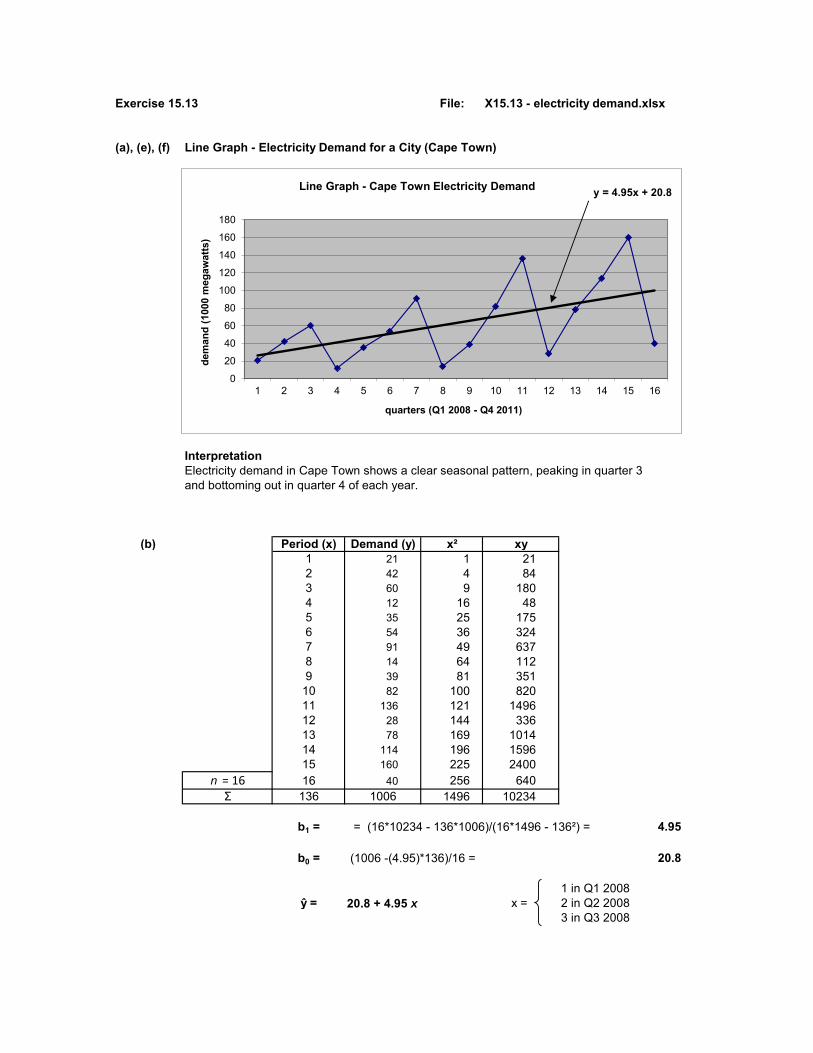
Exercise 15.13 File: X15.13 - electricity demand.xlsx
(a), (e), (f) Line Graph - Electricity Demand for a City (Cape Town)
InterpretationElectricity demand in Cape Town shows a clear seasonal pattern, peaking in quarter 3 and bottoming out in quarter 4 of each year.
(b) Period (x) Demand (y) x² xy1 21 1 212 42 4 843 60 9 1804 12 16 485 35 25 1756 54 36 3247 91 49 6378 14 64 1129 39 81 351
10 82 100 82011 136 121 149612 28 144 33613 78 169 101414 114 196 159615 160 225 2400
n = 16 16 40 256 640Σ 136 1006 1496 10234
b1 = = (16*10234 - 136*1006)/(16*1496 - 136²) = 4.95
b0 = (1006 -(4.95)*136)/16 = 20.8
1 in Q1 2008ŷ = 20.8 + 4.95 x x = 2 in Q2 2008
3 in Q3 2008
y = 4.95x + 20.8
0
20
40
60
80
100
120
140
160
180
1 2 3 4 5 6 7 8 9 10 11 12 13 14 15 16
dem
and
(100
0 m
egaw
atts
)
quarters (Q1 2008 - Q4 2011)
Line Graph - Cape Town Electricity Demand

(c)
Time Periods Demand
Uncentred 4 period Moving Total
2x4 period Moving
Total
Centred 4 period Moving Average
Seasonal ratios
Unadjusted Seasonal Indexes
Adjusted Seasonal Indexes
2008 Q1 212008 Q2 42 1352008 Q3 60 149 284 35.5 169.01 178.65 175.612008 Q4 12 161 310 38.75 30.97 30.97 30.442009 Q1 35 192 353 44.125 79.32 79.32 77.972009 Q2 54 194 386 48.25 111.92 117.99 115.982009 Q3 91 198 392 49 185.712009 Q4 14 226 424 53 26.422010 Q1 39 271 497 62.125 62.782010 Q2 82 285 556 69.5 117.992010 Q3 136 324 609 76.125 178.652010 Q4 28 356 680 85 32.942011 Q1 78 380 736 92 84.782011 Q2 114 392 772 96.5 118.132011 Q3 1602011 Q4 40 Totals 406.927 400.000
Seasonal Indexes Q1 77.97Q2 115.98Q3 175.61Q4 30.44
InterpretationElectricity demand peaks in Q3 by 75% over the trend / cyclical level; and drops to 70% below the trend /cyclical level during Q4.
(d) Seasonally-adjusted trend estimate of Cape Town's electricity demand
Period x Trend ŷ Seasonal Index
Seasonally adjusted
Trend Q3 2012 19 114.85 175.61 201.69Q4 2012 20 119.8 30.44 36.47
InterpretationElectricity demand in Cape Town is likely to peak at 201.69 megawatts inQ3 of 2012 and bottom out at 36.47 megawatts in Q4 of 2012.

Exercise 15.14 File: X15.14 - hotel turnover.xlsx
(a) Actual Seaonal Index
De-seasonalised
568 136 417.6495 112 442.0252 62 406.5315 90 350.0604 136 444.1544 112 485.7270 62 435.5510 90 566.7662 136 486.8605 112 540.2310 62 500.0535 90 594.4
(b) and (e)
(c) Trend line estimate ŷ
Period (x) T/over (y) x² xy1 568 1 5682 495 4 9903 252 9 7564 315 16 12605 604 25 30206 544 36 32647 270 49 18908 510 64 40809 662 81 595810 605 100 605011 310 121 3410
n = 12 12 535 144 6420Σ 78 5670 650 37666
0
100
200
300
400
500
600
700
1 2 3 4 5 6 7 8 9 10 11 12
turn
over
(R m
illio
ns)
quarters (Summer 2008 - Spring 2010)
Hotel Industry Quarterly Turnover
Actual De-seasonalised

b1 = (12*37666 - 78*5670)/(12*650 - 78²) = 5.6713
b0 = (5670 - (5.6713)*78)/12 = 435.64
1 in Summer 2008ŷ = 435.64 + 5.6713 x x = 2 in Autumn 2008
3 in Winter 2008
(d) Seasonally-adjusted trend estimate of Hotel Industry Quarterly Turnover
Period x Trend ŷ Seasonal Index
Seasonally adjusted
Trend Summer 2011 13 509.37 136 692.74Autumn 2011 14 515.04 112 576.84
(f) Trend line estimation using Excel's Chart Wizard
y = 5.6713x + 435.64
100
200
300
400
500
600
700
1 2 3 4 5 6 7 8 9 10 11 12
turn
over
(R m
illio
ns)
quarters
Hotel Industry Quarterly Turnover
Actual Linear (Actual)

Exercise 15.15 File: X15.15 - farming equipment.xlsx
Plot of Farming Equipment Sales (2008 - 2011)
(a) Seasonal Indexes for Farming Equipment Sales
Periods Sales
Uncentred 4 period Moving Total
2x4 period Moving Total
Centred 4 period Moving Average
Seasonal Ratios
Unadjusted Seasonal Indexes
Adjusted Seasonal Indexes
2008 Q1 572008 Q2 51 2142008 Q3 50 217 431 53.88 92.81 92.61 92.632008 Q4 56 222 439 54.88 102.05 102.95 102.972009 Q1 60 225 447 55.88 107.38 107.38 107.402009 Q2 56 230 455 56.88 98.46 96.97 97.002009 Q3 53 235 465 58.13 91.182009 Q4 61 239 474 59.25 102.952010 Q1 65 244 483 60.38 107.662010 Q2 60 251 495 61.88 96.972010 Q3 58 250 501 62.63 92.612010 Q4 68 252 502 62.75 108.372011 Q1 64 252 504 63.00 101.592011 Q2 62 254 506 63.25 98.022011 Q3 582011 Q4 70 Totals 399.92 400
Seasonal Indexes Summer 107.40Autumn 97.00Winter 92.63Spring 102.97
(b) Seasonal InfluencesThe influence of seasonal forces on farming equipment sales is modest. There is a small stimulatory effect during Spring and Summer (no more than 7%) anda small depressing effect (also no more than 7%) during Autumn and Winter.
y = 0.8544x + 52.05
30354045505560657075
1 2 3 4 5 6 7 8 9 10 11 12 13 14 15 16
no. u
nits
sol
d
quarters (2008 - 2011)
Quarterly Farming Implements Sales
Sales
Linear (Sales)

(c) Period (x) Sales (y) x² xy1 57 1 572 51 4 1023 50 9 1504 56 16 2245 60 25 3006 56 36 3367 53 49 3718 61 64 4889 65 81 585
10 60 100 60011 58 121 63812 68 144 81613 64 169 83214 62 196 86815 58 225 870
n = 16 16 70 256 1120Σ 136 949 1496 8357
b1 = (16*8357-136*949)/(16*1496-136²) = 0.8544
b0 = (949 -(0.8544)*136)/16 = 52.05
1 in Summer 2008ŷ = 52.05 + 0.8544 x x = 2 in Autumn 2008
3 in Winter 2008
(d) Seasonally-adjusted trend estimate of Farming Equipment Sales for 2012
Period x Trend ŷ Seasonal Index
Seasonally adjusted
Trend Summer 17 66.57 107.40 71.50Autumn 18 67.43 97.00 65.41Winter 19 68.28 92.63 63.25Spring 20 69.14 102.97 71.19
InterpretationThe company can expect to sell between 63 and 72 farming implements each quarter during 2012 with the higher sales expected in Summer and Spring.

Exercise 15.16 File: X15.16 - energy costs.xlsx
(a), (e) and (f) Line Graph of Office Complex Energy Costs (in R100 000)
(b)
Time Periods Costs
Uncentred 4 period Moving Total
2x4 period Moving Total
Centred 4 period Moving Average
Seasonal ratios
Unadjusted Seasonal Indexes
Adjusted Seasonal Indexes
2009 Q1 2.42009 Q2 3.8 13.32009 Q3 4 13.5 26.80 3.35 119.40 118.27 117.62009 Q4 3.1 13.8 27.30 3.4125 90.84 90.49 90.02010 Q1 2.6 13.9 27.70 3.4625 75.09 73.41 73.02010 Q2 4.1 14.0 27.90 3.4875 117.56 120.21 119.52010 Q3 4.1 14.0 28.00 3.5 117.142010 Q4 3.2 14.4 28.40 3.55 90.142011 Q1 2.6 14.6 29.00 3.625 71.722011 Q2 4.5 14.7 29.30 3.6625 122.872011 Q3 4.32011 Q4 3.3 Totals 402.39 400
Seasonal Indexes Summer 73.0Autumn 119.5Winter 117.6Spring 90.0
InterpretationEnergy costs rise by nearly 20% (19,5% and 17,6%) over the colder months of Autumn and Winter, and decline by between 10% (in Spring) and almost 30% (27%) in Summer.
y = 0.0601x + 3.1091
1
1.5
2
2.5
3
3.5
4
4.5
5
1 2 3 4 5 6 7 8 9 10 11 12
ener
gy c
ost (
R10
0 00
0)
quarters (2009 - 2011)
Office Complex Energy Costs

(c) Period (x) Cost (y) x² xy1 2.4 1 2.42 3.8 4 7.63 4 9 124 3.1 16 12.45 2.6 25 136 4.1 36 24.67 4.1 49 28.78 3.2 64 25.69 2.6 81 23.4
10 4.5 100 4511 4.3 121 47.3
n = 12 12 3.3 144 39.6Σ 78 42 650 281.6
b1 = [(12*281.6)-(78*42)]/[12*650-782] = 0.0601
b0 = (42 - 0.0602*78)/12 = 3.1091
1 in Summer 2009ŷ = 3.1091 + 0.0601 x x = 2 in Autumn 2009
3 in Winter 2009
(d) Seasonally-adjusted trend estimate of Office Complex Energy Costs for 2012
Period x Trend ŷ Seasonal Index
Seasonally adjusted
Trend Summer 13 3.89 72.97 2.84 Autumn 14 3.95 119.50 4.72 Winter 15 4.01 117.57 4.71 Spring 16 4.07 89.95 3.66
InterpretationThe office complex manager must budget between R284 000 and R472 000 each quarter during 2012 with higher costs expected in the Autumn and Winter periods.

Exercise 15.17 File: X15.17 - business registrations.xlsx
(a) Line Graph of New Business Registrations (2007 - 2011)
(b) and (c) 4-Period Moving Average and Quarterly Seasonal Indexes
(b) (c)
Time Periods
New Registrations
Uncentred 4 period Moving
Total
2x4 period Moving
Total
Centred 4 period Moving Average
Seasonal ratios
Unadjusted Seasonal Indexes
Adjusted Seasonal Indexes
2007 Q1 10052007 Q2 1222 47242007 Q3 1298 4892 9616 1202.00 107.99 106.526 106.412007 Q4 1199 5041 9933 1241.63 96.57 98.514 98.412008 Q1 1173 5199 10240 1280.00 91.64 91.820 91.722008 Q2 1371 5376 10575 1321.88 103.72 103.568 103.462008 Q3 1456 5517 10893 1361.63 106.932008 Q4 1376 5677 11194 1399.25 98.342009 Q1 1314 5826 11503 1437.88 91.382009 Q2 1531 5980 11806 1475.75 103.742009 Q3 1605 6125 12105 1513.13 106.072009 Q4 1530 6265 12390 1548.75 98.792010 Q1 1459 6422 12687 1585.88 92.002010 Q2 1671 6569 12991 1623.88 102.902010 Q3 1762 6714 13283 1660.38 106.122010 Q4 1677 6880 13594 1699.25 98.692011 Q1 1604 7034 13914 1739.25 92.222011 Q2 1837 7176 14210 1776.25 103.422011 Q3 19162011 Q4 1819 Totals 400.429 400
Seasonal Indexes Q1 91.72Q2 103.46Q3 106.41Q4 98.41
0
500
1000
1500
2000
2500
1 2 3 4 5 6 7 8 9 10 11 12 13 14 15 16 17 18 19 20
no. o
f new
regi
stra
tions
quarters (2007 - 2011)
Line Graph - New Business Registrations

(d) Interpretation of Seasonal Influences on new business registrationsNew business registrations show a modest seasonal pattern, ranging between8,3% below the annual average in quarter 1 to 6.4% above the annual average in quarter 3.
(b) 4-Period Moving Average Line Graph and Original Data Line Graph
(e) Least Squares trend line (using Add Trendline in Excel )1 in Q1 2007
ŷ = 1078.2 + 39.338 x x = 2 in Q2 20073 in Q3 2007
0
500
1000
1500
2000
2500
no. o
f new
bus
ines
ses
quarters (2007 - 2011)
Line Graph - New Business Registrations
New Registrations
Centred 4 period MovingAverage

(f) Seasonally-adjusted Trend estimates
Periods yAdjusted Seasonal Indexes
Trend Estimate ŷ ŷ (adj)
2007 Q1 1005 91.72 1117.5 1025.02007 Q2 1222 103.46 1156.9 1196.92007 Q3 1298 106.41 1196.2 1272.92007 Q4 1199 98.41 1235.6 1215.92008 Q1 1173 91.72 1274.9 1169.32008 Q2 1371 103.46 1314.2 1359.72008 Q3 1456 106.41 1353.6 1440.32008 Q4 1376 98.41 1392.9 1370.82009 Q1 1314 91.72 1432.2 1313.72009 Q2 1531 103.46 1471.6 1522.52009 Q3 1605 106.41 1510.9 1607.82009 Q4 1530 98.41 1550.3 1525.62010 Q1 1459 91.72 1589.6 1458.02010 Q2 1671 103.46 1628.9 1685.32010 Q3 1762 106.41 1668.3 1775.22010 Q4 1677 98.41 1707.6 1680.52011 Q1 1604 91.72 1746.9 1602.32011 Q2 1837 103.46 1786.3 1848.12011 Q3 1916 106.41 1825.6 1942.62011 Q4 1819 98.41 1865.0 1835.3
(g) Plot of Actual vs Seasonally adjusted Trend estimates (New Business Registrations)
CommentThe seasonally adjusted trend estimates track the actual number of new businessregistrations very closely. It is a good fitting graph.
800
1000
1200
1400
1600
1800
2000
2007
Q1
2007
Q2
2007
Q3
2007
Q4
2008
Q1
2008
Q2
2008
Q3
2008
Q4
2009
Q1
2009
Q2
2009
Q3
2009
Q4
2010
Q1
2010
Q2
2010
Q3
2010
Q4
2011
Q1
2011
Q2
2011
Q3
2011
Q4no
. of n
ew re
gist
ratio
ns
quarters (2007 - 2011)
New Business Registrations (Actual vs Trend Adjusted)
y ŷ (adj)
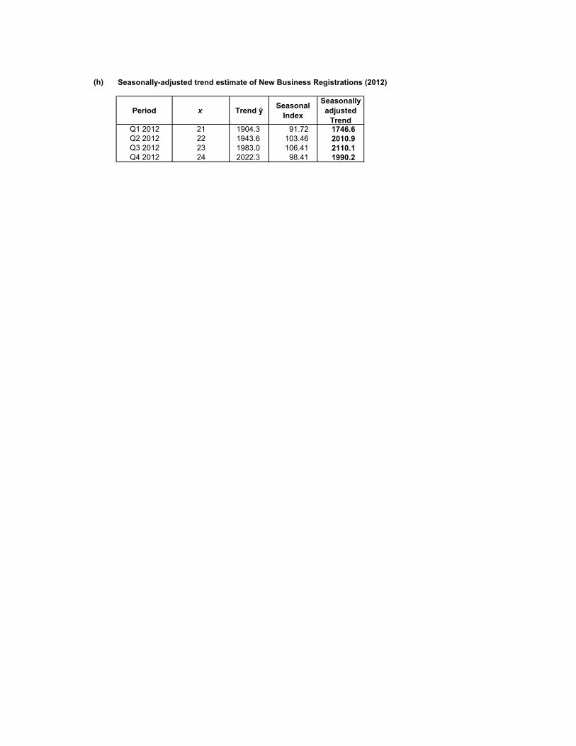
(h) Seasonally-adjusted trend estimate of New Business Registrations (2012)
Period x Trend ŷ Seasonal Index
Seasonally adjusted
Trend Q1 2012 21 1904.3 91.72 1746.6Q2 2012 22 1943.6 103.46 2010.9Q3 2012 23 1983.0 106.41 2110.1Q4 2012 24 2022.3 98.41 1990.2

Exercise 15.18 File: X15.18 - engineering sales.xlsx
Total Sales (Estimate for next year)
Quarter Seasonal Index Trend ŷ
Seasonally Adjusted Trend Estimate ŷ(adj)
1 95 12 11.42 115 12 13.83 110 12 13.24 80 12 9.6
48 48

Exercise 15.19 File: X15.19 - Table Mountain.xlsx
(a) and (b) Period Visitors S Index De-SeasonlisedWi 2009 18.1 62 29.19Sp 2009 26.4 89 29.66Su 2009 41.2 162 25.43Au 2009 31.6 87 36.32Wi 2010 22.4 62 36.13Sp 2010 33.2 89 37.30Su 2010 44.8 162 27.65Au 2010 32.5 87 37.36
CommentThe trend (after de-seasonalising the quarterly data) is only marginally upwards.
(c) Table Mountain Visitors (per quarter for 2011)
Quarter Seasonal Index Trend ŷSeasonally
Adjusted Trend Estimate ŷ(adj)
Winter 62 37.5 23.25Spring 89 37.5 33.375
Summer 162 37.5 60.75Autumn 87 37.5 32.625
150 150
05
101520253035404550
Wi 2009 Sp 2009 Su 2009 Au 2009 Wi 2010 Sp 2010 Su 2010 Au 2010
no. o
f vis
itors
(100
0's)
Quarters (2009 - 2010)
Table Mountain Visitors (Actual vs De-Seasonalised)
Visitors
De-Seasonlised

Exercise 15.20 File: X15.20 - gross domestic product.xlsx
(a) Year GDP (Millions)2001 452002 472003 612004 642005 722006 742007 842008 812009 932010 902011 98
1 in 2001(b) Trend line (see graph in (i)) ŷ = 41.964 + 5.2636 x x = 2 in 2002
3 in 2003
(c) Expected GDP for 2012 and 2013 (in R100 million)
Year Year (x ) Estimate (ŷ)2012 12 105.12013 13 110.4
Trend ŷ41.964 + 5.2636 (12)41.964 + 5.2636 (13)
y = 5.2636x + 41.964
0
20
40
60
80
100
120
1 2 3 4 5 6 7 8 9 10 11
GDP
(in
R100
mill
ions
)
years (2001 - 2011)
African Country Gross Domestic Product
GDP (Millions)
Linear (GDP (Millions))

Exercise 15.21 File: X15.21 - pelagic fish.xlsx
(a) and (c) (a) (c)
Year Months Pelagic fish 3 Period Moving Ave
Seasonal ratio
Unadj Seasonal
Index
Seasonal Index
2007 Jan - Apr 44May - Aug 36 38.00 94.74 96.85 97.79Sept - Dec 34 38.33 88.70 88.70 89.56
2008 Jan - Apr 45 40.33 111.57 111.57 112.65May - Aug 42 40.33 104.13Sept - Dec 34 38.00 89.47
2009 Jan - Apr 38 34.67 109.62May - Aug 32 32.33 98.97Sept - Dec 27 33.00 81.82
2010 Jan - Apr 40 32.67 122.45May - Aug 31 33.00 93.94Sept - Dec 28 Totals 297.12 300
(c) Periods Seasonal Indexes
Jan - Apr 112.65May - Aug 97.79Sept - Dec 89.56
Pelagic fish catches are: - significantly higher (12.65%) than the trend /cyclical volumes in the Jan - April period.- only marginally lower (2.21%) than the trend /cyclical volumes in the May - Aug period.- more than 10% lower than the trend /cyclical volumes in the Sept - Dec period.
(b)
CommentThe trend in pelagic fish catches over the past 4 years is decidedly downwards.
05
101520253035404550
1 2 3 4 5 6 7 8 9 10 11 12
no. o
f ton
nes
2003 - 2006 (4-monthly)
Pelagic Fish Catches (Actual vs 3-Period Moving Average)
Pelagic fish
3 Period Moving Ave
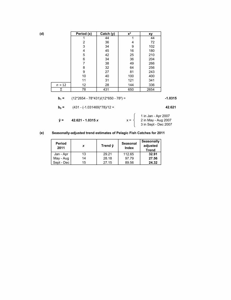
(d) Period (x) Catch (y) x² xy1 44 1 442 36 4 723 34 9 1024 45 16 1805 42 25 2106 34 36 2047 38 49 2668 32 64 2569 27 81 24310 40 100 40011 31 121 341
n = 12 12 28 144 336Σ 78 431 650 2654
b1 = (12*2654 - 78*431)/(12*650 - 78²) = -1.0315
b0 = (431 - (-1.031469)*78)/12 = 42.621
1 in Jan - Apr 2007ŷ = 42.621 - 1.0315 x x = 2 in May - Aug 2007
3 in Sept - Dec 2007
(e) Seasonally-adjusted trend estimates of Pelagic Fish Catches for 2011
Period 2011 x Trend ŷ Seasonal
Index
Seasonally adjusted
Trend Jan - Apr 13 29.21 112.65 32.91May - Aug 14 28.18 97.79 27.56Sept - Dec 15 27.15 89.56 24.32
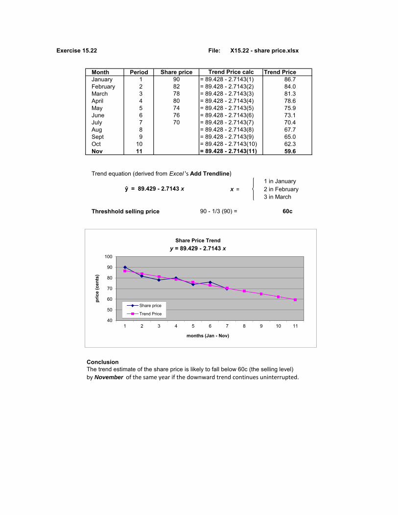
Exercise 15.22 File: X15.22 - share price.xlsx
Month Period Share price Trend PriceJanuary 1 90 = 89.428 - 2.7143(1) 86.7February 2 82 = 89.428 - 2.7143(2) 84.0March 3 78 = 89.428 - 2.7143(3) 81.3April 4 80 = 89.428 - 2.7143(4) 78.6May 5 74 = 89.428 - 2.7143(5) 75.9June 6 76 = 89.428 - 2.7143(6) 73.1July 7 70 = 89.428 - 2.7143(7) 70.4Aug 8 = 89.428 - 2.7143(8) 67.7Sept 9 = 89.428 - 2.7143(9) 65.0Oct 10 = 89.428 - 2.7143(10) 62.3Nov 11 = 89.428 - 2.7143(11) 59.6
Trend equation (derived from Excel 's Add Trendline)1 in January
ŷ = 89.429 - 2.7143 x x = 2 in February3 in March
Threshhold selling price 90 - 1/3 (90) = 60c
ConclusionThe trend estimate of the share price is likely to fall below 60c (the selling level)by November of the same year if the downward trend continues uninterrupted.
Trend Price calc
40
50
60
70
80
90
100
1 2 3 4 5 6 7 8 9 10 11
pric
e (c
ents
)
months (Jan - Nov)
Share Price Trend y = 89.429 - 2.7143 x
Share price
Trend Price

Exercise 15.23 File: X15.23 - Addo park.xlsx
(a) Season Actual Seaonal Index
De-seasonalised
Su 2008 196 112 175.0Au 2008 147 94 156.4Wi 2008 124 88 140.9Sp 2008 177 106 167.0Su 2009 199 112 177.7Au 2009 152 94 161.7Wi 2009 132 88 150.0Sp 2009 190 106 179.2Su 2010 214 112 191.1Au 2010 163 94 173.4Wi 2010 145 88 164.8Sp 2010 198 106 186.8
(b) and (d) Line Plots of Actual and De-Seasonalised Visitor Numbers (by Season)
(c) ConclusionThere is a very slight upward trend in visitors to the Addo National Park. There isalmost no growth in visitors over the past 3 years.
0
50
100
150
200
250
Su2008
Au2008
Wi2008
Sp2008
Su2009
Au2009
Wi2009
Sp2009
Su2010
Au2010
Wi2010
Sp2010
no. o
f vis
itors
(in
1000
s)
quarters (2004 - 2006)
Addo National Park Visitors (Actual vs De-Seasonalised)
Actual
De-seasonalised

Exercise 15.24 File: X15.24 - healthcare claims.xlsx
Value of Healthcare Claims (in R millions)
(a) Seasonal Indexes for Healthcare Claims
Periods Claims
Uncentred 4 period Moving Total
2x4 period Moving Total
Centred 4 period Moving Average
Seasonal Ratios
Unadjusted Seasonal Indexes
Adjusted Seasonal Indexes
2007 Q1 11.82007 Q2 13.2 60.52007 Q3 19.1 59.6 120.1 15.0125 127.23 139.67 136.282007 Q4 16.4 58.8 118.4 14.8 110.81 106.75 104.152008 Q1 10.9 62.1 120.9 15.1125 72.13 72.13 70.372008 Q2 12.4 63.5 125.6 15.7 78.98 91.41 89.192008 Q3 22.4 64.8 128.3 16.0375 139.672008 Q4 17.8 68.6 133.4 16.675 106.75 409.96 4002009 Q1 12.2 70.3 138.9 17.3625 70.272009 Q2 16.2 67.1 137.4 17.175 94.322009 Q3 24.1 67.7 134.8 16.85 143.032009 Q4 14.6 66 133.7 16.7125 87.362010 Q1 12.8 62.7 128.7 16.0875 79.562010 Q2 14.5 64.2 126.9 15.8625 91.412010 Q3 20.82010 Q4 16.1
Seasonal Indexes Q1 70.37Q2 89.19Q3 136.28Q4 104.15
(b) Period (x) Claims (y) x² xy1 11.8 1 11.82 13.2 4 26.43 19.1 9 57.34 16.4 16 65.65 10.9 25 54.56 12.4 36 74.47 22.4 49 156.88 17.8 64 142.49 12.2 81 109.810 16.2 100 16211 24.1 121 265.112 14.6 144 175.213 12.8 169 166.414 14.5 196 20315 20.8 225 312
n = 16 16 16.1 256 257.6Σ 136 255.3 1496 2240.3

b1 = (16*2240.3 - 136*255.3)/(16*1496 - 136²) = 0.2066
b0 = (255.3 -(0.206618)*136)/16 = 14.2
1 in Q1 2007ŷ = 14.2 + 0.2066 x x = 2 in Q2 2007
3 in Q3 2007
(c) Seasonally-adjusted trend estimate of Healthcare Claims for 2011
Period x Trend ŷ Seasonal Index
Seasonally adjusted
Trend Q1 2011 17 17.71 70.37 12.46Q2 2011 18 17.92 89.19 15.98Q3 2011 19 18.13 136.28 24.71Q4 2011 20 18.33 104.15 19.09
InterpretationHealthcare claims are expected to rise during 2011 from a low of R12,46 (mill) in Q1 to R24,71 (mill) in Q3.
(d) Line Plots of Healthcare Claims (Actual vs Seasonally-adjusted trend estimates)
Periods Claims S Index Time Trend (ŷ) Trend (ŷ-adj)2007 Q1 11.8 70.37 1 14.41 10.142007 Q2 13.2 89.19 2 14.61 13.032007 Q3 19.1 136.28 3 14.82 20.202007 Q4 16.4 104.15 4 15.03 15.652008 Q1 10.9 70.37 5 15.23 10.722008 Q2 12.4 89.19 6 15.44 13.772008 Q3 22.4 136.28 7 15.65 21.322008 Q4 17.8 104.15 8 15.85 16.512009 Q1 12.2 70.37 9 16.06 11.302009 Q2 16.2 89.19 10 16.27 14.512009 Q3 24.1 136.28 11 16.47 22.452009 Q4 14.6 104.15 12 16.68 17.372010 Q1 12.8 70.37 13 16.89 11.882010 Q2 14.5 89.19 14 17.09 15.242010 Q3 20.8 136.28 15 17.30 23.582010 Q4 16.1 104.15 16 17.51 18.232011 Q1 70.37 17 17.71 12.462011 Q2 89.19 18 17.92 15.982011 Q3 136.28 19 18.13 24.702011 Q4 104.15 20 18.33 19.09
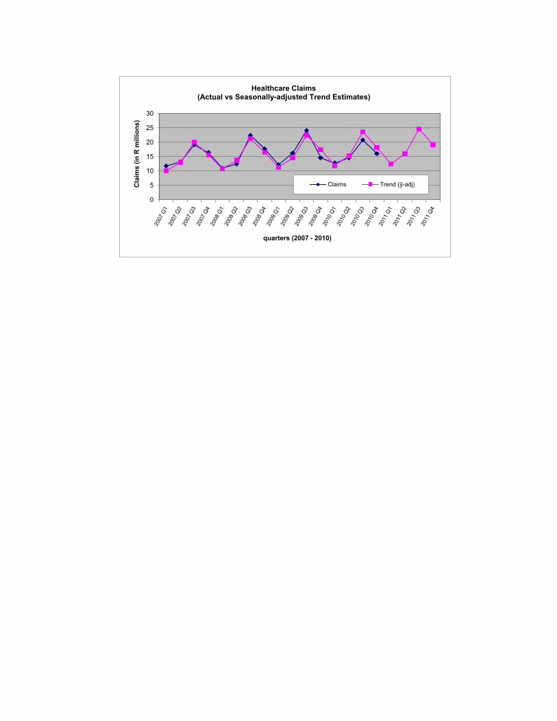
0
5
10
15
20
25
30
Clai
ms
(in R
mill
ions
)
quarters (2007 - 2010)
Healthcare Claims (Actual vs Seasonally-adjusted Trend Estimates)
Claims Trend (ŷ-adj)
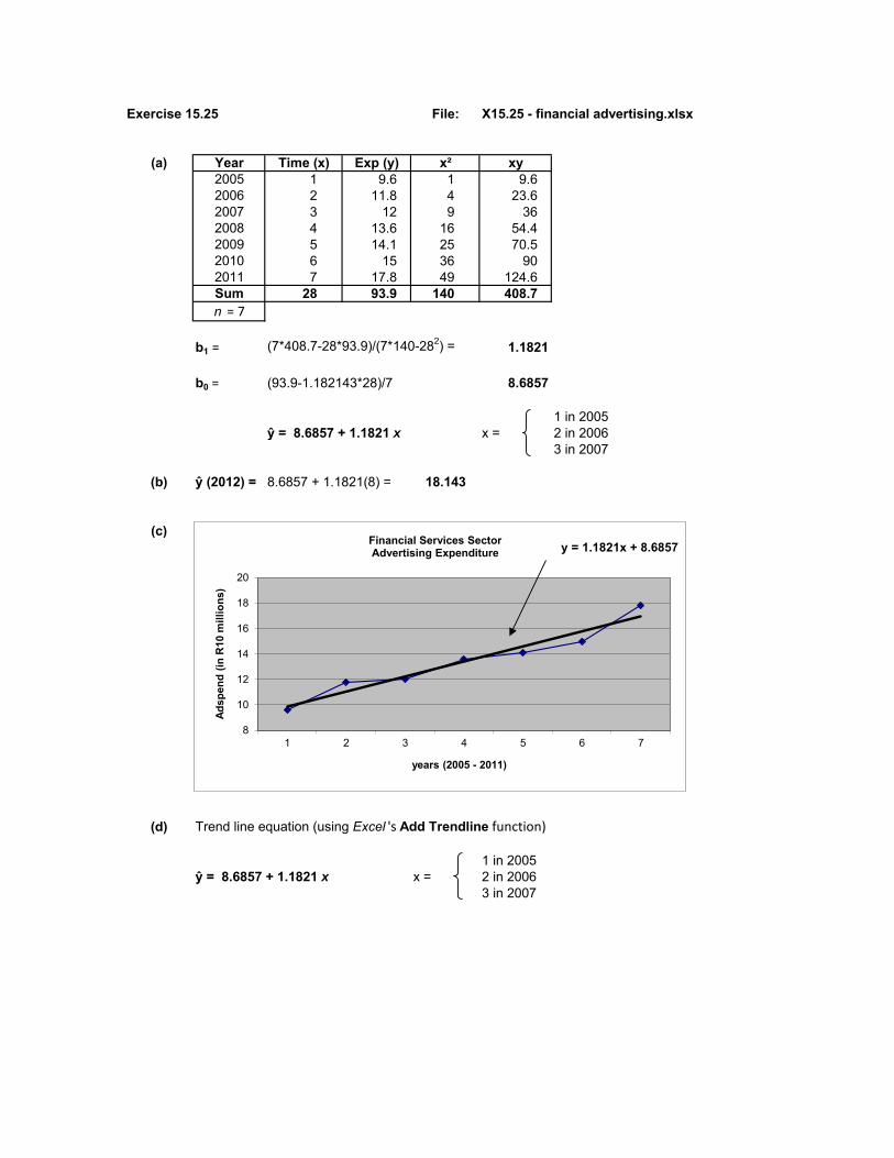
Exercise 15.25 File: X15.25 - financial advertising.xlsx
(a) Year Time (x) Exp (y) x² xy2005 1 9.6 1 9.62006 2 11.8 4 23.62007 3 12 9 362008 4 13.6 16 54.42009 5 14.1 25 70.52010 6 15 36 902011 7 17.8 49 124.6Sum 28 93.9 140 408.7n = 7
b1 = (7*408.7-28*93.9)/(7*140-282) = 1.1821
b0 = (93.9-1.182143*28)/7 8.6857
1 in 2005ŷ = 8.6857 + 1.1821 x x = 2 in 2006
3 in 2007
(b) ŷ (2012) = 8.6857 + 1.1821(8) = 18.143
(c)
(d) Trend line equation (using Excel 's Add Trendline function)
1 in 2005ŷ = 8.6857 + 1.1821 x x = 2 in 2006
3 in 2007
y = 1.1821x + 8.6857
8
10
12
14
16
18
20
1 2 3 4 5 6 7
Adsp
end
(in R
10 m
illio
ns)
years (2005 - 2011)
Financial Services SectorAdvertising Expenditure

(e) Year Time (x) Actual (y) Trend (ŷ)2005 1 9.6 9.872006 2 11.8 11.052007 3 12 12.232008 4 13.6 13.412009 5 14.1 14.602010 6 15 15.782011 7 17.8 16.962012 8 18.14
8
10
12
14
16
18
20
1 2 3 4 5 6 7 8
adsp
end
(in R
10 m
illio
n)
years (2005 - 2011)
Financial Services Adspend
Actual (y)
Trend (ŷ)

Exercise 15.26 File: X15.26 - policy surrenders.xlsx
(a) Line Graph of Surrendered Endowment Policies (2008 - 2010)
InterpretationThere is a distinct moderate downward trend in the number of surrendered policies over the period 2008 - 2010. This reduction could be due to the improved clientcommunication strategy adopted by the company in recent years.
(b)
Time Periods Policies
Uncentred 4 period Moving Total
2x4 period Moving Total
Centred 4 period Moving Average
Seasonal ratios
Unadjusted Seasonal Indexes
Adjusted Seasonal Indexes
2008 Q1 2122008 Q2 186 7952008 Q3 192 769 1564 195.5 98.21 97.84 97.992008 Q4 205 748 1517 189.625 108.11 107.47 107.622009 Q1 186 725 1473 184.125 101.02 100.62 100.772009 Q2 165 702 1427 178.375 92.50 93.49 93.622009 Q3 169 685 1387 173.375 97.482009 Q4 182 678 1363 170.375 106.822010 Q1 169 671 1349 168.625 100.222010 Q2 158 667 1338 167.25 94.472010 Q3 1622010 Q4 178 Totals 399.41 400
Seasonal Indexes Q1 100.77Q2 93.62Q3 97.99Q4 107.62
InterpretationEndowment policy surrenders are highest in Q4 by 7,62% over the quarterly average; and lowest in Q2 by 6,38% below the quarterly average. There is very little - to none - seasonal impact on policy surrenders in Q1 and only 2,01% below the quarterlyaverage in Q3.
100
120
140
160
180
200
220
240
2008Q1
2008Q2
2008Q3
2008Q4
2009Q1
2009Q2
2009Q3
2009Q4
2010Q1
2010Q2
2010Q3
2010Q4
no. o
f pol
icie
s
quarters (2008 - 2010)
Surrendered Endowment Policies
Policies

(c) Period (x) Cost (y) x² xy1 212 1 2122 186 4 3723 192 9 5764 205 16 8205 186 25 9306 165 36 9907 169 49 11838 182 64 14569 169 81 152110 158 100 158011 162 121 1782
n = 12 12 178 144 2136Σ 78 2164 650 13558
b1 = (12*13558 - 78*2164)/(12*650-78²) = -3.55245
b0 = (2164 -(-3.552448)*78)/12 = 203.42
1 in Q1 2008ŷ = 203.42 - 3.5524 x x = 2 in Q2 2008
3 in Q3 2008
(d) Seasonally-adjusted trend estimate of no. of Surrendered Endowment Policies in2011
Period x Trend ŷ Seasonal Index
Seasonally adjusted
Trend (Rounded)
Q1 2011 13 157.24 100.77 158.45 158Q2 2011 14 153.69 93.62 143.88 144Q3 2011 15 150.13 97.99 147.12 147Q4 2011 16 146.58 107.62 157.75 158

Exercise 15.27 File: X15.27 - company liquidations.xlsx
(a)Period Liquidations 3-per M A 5-per M A
1 2462 243 252.73 269 289.7 255.64 357 263.0 237.25 163 224.7 210.46 154 142.0 189.07 109 141.7 162.08 162 164.3 184.09 222 219.0 210.010 273 259.7 249.211 284 287.3 275.412 305 294.0 300.613 293 315.3 330.614 348 354.7 332.015 423 354.0 335.016 291 344.7 327.017 320 288.0 304.218 253 269.0 252.019 234 216.3 241.820 162 212.0 237.421 240 233.3 239.622 298 267.3 243.423 264 271.7 269.624 253 270.0 282.025 293 282.7 260.026 302 261.027 188
(b)
(c) InterpretationThe level of business liquidations shows no actual upward / downward trend over thepast 27 periods. There is a distinct cyclical pattern wih the longest lasting from period 7 to period 20.
050
100150200250300350400450
1 3 5 7 9 11 13 15 17 19 21 23 25 27
no. o
f liq
uida
tions
periods
Company Liquidations (Actual vs 3 and 5 period Moving Averages)
Liquidations 3-per M A 5-per M A

Exercise 15.28 File: X15.28 - passenger tyres.xlsx
Passenger Tyre Sales (Y)
(a) Quarterly Seasonal Ratios and Trend Line Equation
Time Periods Tyre Sales
Uncentred 4 period
Moving Total
2x4 period Moving Total
Centred 4 period Moving Average
Seasonal ratios
Unadjusted Seasonal Indexes
Adjusted Seasonal Indexes
2005 Q1 648762005 Q2 58987 2408292005 Q3 54621 244699 485528 60691.0 90.00 90.64 90.722005 Q4 62345 252285 496984 62123.0 100.36 100.81 100.912006 Q1 68746 258591 510876 63859.5 107.65 107.65 107.762006 Q2 66573 267480 526071 65758.9 101.24 100.51 100.612006 Q3 60927 277522 545002 68125.3 89.432006 Q4 71234 282186 559708 69963.5 101.822007 Q1 78788 289357 571543 71442.9 110.282007 Q2 71237 292567 581924 72740.5 97.932007 Q3 68098 291438 584005 73000.6 93.282007 Q4 74444 296653 588091 73511.4 101.27 399.62 400.002008 Q1 77659 302011 598664 74833.0 103.782008 Q2 76452 306475 608486 76060.8 100.512008 Q3 73456 313379 619854 77481.8 94.802008 Q4 78908 318170 631549 78943.6 99.952009 Q1 84563 319592 637762 79720.3 106.072009 Q2 81243 327440 647032 80879.0 100.452009 Q3 74878 334433 661873 82734.1 90.502009 Q4 86756 338248 672681 84085.1 103.182010 Q1 91556 340405 678653 84831.6 107.932010 Q2 85058 333794 674199 84274.9 100.932010 Q3 77035 345161 678955 84869.4 90.772010 Q4 80145 356559 701720 87715.0 91.372011 Q1 1029232011 Q2 96456
(a) Seasonal Indexes Q1 107.76Q2 100.61Q3 90.72Q4 100.91
Trend line Use Excel 's Add Trendline function

1 in Q1 2005(b) ŷ = 58114 + 1302 x x = 2 in Q2 2005
3 in Q3 2005
(b) Seasonally-adjusted Trend estimates of passenger car tyre sales (in units) for 2012 / 2013.
Time Periods Time Trend (ŷ) Seasonal
Indices
Seasonally Adjusted
Trend Estimate
2012 Q1 29 95872 107.76 1033122012 Q2 30 97174 100.61 977672012 Q3 31 98476 90.72 893372012 Q4 32 99778 100.91 1006862013 Q1 33 101080 107.76 1089242013 Q2 34 102382 100.61 1030072013 Q3 35 103684 90.72 940622013 Q4 36 104986 100.91 105941
(c) InterpretationThe pattern of passenger car tyre sales is very stable. The trend is linear and upward, and seasonal variations are consistent over time. Hence Hillstone management could have high confidence in the estimates.
y = 1302x + 58114
20000
40000
60000
80000
100000
120000
units
sol
d (in
100
0's)
quarters (2000 - 2006)
Passenger Car Tyre Sales
Tyre Sales
Linear (Tyre Sales)

Exercise 15.29 File: X15.29 - outpatient attendances.xlsx
Outpatients Attendances - Butterworth Clinic
(a) Quarterly Seasonal Ratios and Trend Line Equation
Time Periods Visits
Uncentred 4 period Moving Total
2x4 period Moving Total
Centred 4 period Moving Average
Seasonal ratios
Unadjusted Seasonal Indexes
Adjusted Seasonal Indexes
2006 Q1 127672006 Q2 16389 640412006 Q3 19105 65472 129513 16189.1 118.01 117.31 117.462006 Q4 15780 68951 134423 16802.9 93.91 92.62 92.752007 Q1 14198 70745 139696 17462.0 81.31 78.99 79.102007 Q2 19868 73269 144014 18001.8 110.37 110.53 110.692007 Q3 20899 73712 146981 18372.6 113.752007 Q4 18304 74048 147760 18470.0 99.102008 Q1 14641 74227 148275 18534.4 78.992008 Q2 20204 72000 146227 18278.4 110.532008 Q3 21078 71434 143434 17929.3 117.562008 Q4 16077 72489 143923 17990.4 89.36 399.46 400.002009 Q1 14075 72378 144867 18108.4 77.732009 Q2 21259 72484 144862 18107.8 117.402009 Q3 20967 70821 143305 17913.1 117.052009 Q4 16183 71386 142207 17775.9 91.042010 Q1 12412 72569 143955 17994.4 68.982010 Q2 21824 74365 146934 18366.8 118.822010 Q3 22150 79370 153735 19216.9 115.262010 Q4 17979 78114 157484 19685.5 91.332011 Q1 17417 80274 158388 19798.5 87.972011 Q2 20568 85413 165687 20710.9 99.312011 Q3 24310 67996 153409 19176.1 126.772011 Q4 23118 47428 115424 14428.0 160.23
Seasonal Indexes Q1 79.10Q2 110.69Q3 117.46Q4 92.75
Trend line Use Excel 's Add Trendline function

1 in Q1 2006ŷ = 15591 + 224.66 x x = 2 in Q2 2006
3 in Q3 2006
(b) Seasonally-adjusted Trend estimates of Outpatient Visits (Butterworth) for 2012 / 2013 (first half).
Time Periods Time Trend (ŷ) Seasonal
Indices
Seasonally Adjusted
Trend Estimate
2012 Q1 25 21207.5 79.10 167752012 Q2 26 21432.2 110.69 237232012 Q3 27 21656.8 117.46 254382012 Q4 28 21881.5 92.75 202952013 Q1 29 22106.1 79.10 174862013 Q2 30 22330.8 110.69 24718
(c) InterpretationThe pattern of outpatient attendances at the Butterworth Clinic is very stable. It shows a steady upward trend with highly consistent seasonal variations.Demand increases in the winter months ((Q3) and is lowest in the summer months (Q1).
y = 224.66x + 15591
0
5000
10000
15000
20000
25000
30000
1 3 5 7 9 11 13 15 17 19 21 23
no. o
f pat
ient
s
quarters (2006 - 2011)
Outpatient Visits
Visits
Linear (Visits)

Exercise 15.30 File: X15.30 - construction absenteeism.xlsx
Construction Absenteeism
(a) Quarterly Seasonal Ratios and Trend Line Equation
Time Periods Days_lost
Uncentred 4 period Moving Total
2x4 period Moving Total
Centred 4 period Moving Average
Seasonal ratios
Unadjusted Seasonal Indexes
Adjusted Seasonal Indexes
2006 Q1 9332006 Q2 865 35842006 Q3 922 3618 7202 900.3 102.42 102.74 102.882006 Q4 864 3689 7307 913.4 94.59 95.80 95.932007 Q1 967 3698 7387 923.4 104.72 104.07 104.212007 Q2 936 3736 7434 929.3 100.73 96.85 96.982007 Q3 931 3661 7397 924.6 100.692007 Q4 902 3570 7231 903.9 99.792008 Q1 892 3546 7116 889.5 100.282008 Q2 845 3445 6991 873.9 96.702008 Q3 907 3368 6813 851.6 106.502008 Q4 801 3238 6606 825.8 97.00 399.45 400.002009 Q1 815 3110 6348 793.5 102.712009 Q2 715 3020 6130 766.3 93.312009 Q3 779 3027 6047 755.9 103.062009 Q4 711 3168 6195 774.4 91.822010 Q1 822 3151 6319 789.9 104.072010 Q2 856 3162 6313 789.1 108.472010 Q3 762 3125 6287 785.9 96.962010 Q4 722 2984 6109 763.6 94.552011 Q1 785 2962 5946 743.3 105.622011 Q2 715 2944 5906 738.3 96.852011 Q3 740 2159 5103 637.9 116.012011 Q4 704 1444 3603 450.4 156.31
Seasonal Indexes Q1 104.21Q2 96.98Q3 102.88Q4 95.93
Trend line Use Excel 's Add Trendline function
y = -9.917x + 952.75
400
500
600
700
800
900
1000
1 2 3 4 5 6 7 8 9 10 11 12 13 14 15 16 17 18 19 20 21 22 23 24
no. o
f day
s ls
ot
quarters (2006 - 2011)
Construction Industry Days Lost due to Absenteeism
Days_lost
Linear (Days_lost)

1 in Q1 2006ŷ = 952.75 - 9.917 x x = 2 in Q2 2006
3 in Q3 2006
(b) Seasonally-adjusted Trend estimates of Days Lost in Construction Industry for 2012.
Time Periods Time Trend (ŷ) Seasonal
Indices
Seasonally Adjusted
Trend Estimate
2012 Q1 25 704.8 104.21 7342012 Q2 26 694.9 96.98 6742012 Q3 27 685.0 102.88 7052012 Q4 28 675.1 95.93 648
(c) InterpretationThe pattern of days lost due to absenteeism in the Construction industry showsa distinct downward trend but with inconsistent seasonal variations.

CHAPTER 16
FINANCIAL CALCULATIONS
INTEREST, ANNUITIES and NPV
Exercise 16.1 Simple interestInterest is computed on the original lump sum for each period.Compound interestFor each period, interest is computed on the original lump sumplus all accummulated interest of the preceeding periods.
Exercise 16.2 No - a compounded amount will earn more interest than a simple interest investment.
Exercise 16.3 Yes - compounding quarterly will result in interest being capitalised sooner - and therefore earning more interest thanan annual compounded investment.
Exercise 16.4 Nominal interest rate is the quoted per annum interest rate Effective interest rate is the actual interest rate achieved when interest is compounded more than once per year.
Exercise 16.5 Annuity - an annuity is when a constant sum of money is paid (or received) at regular intervals over a period of time.
Exercise 16.6 Ordinary annuity - regular payments begin the first period of the annuity termDeferred annuity - regular payments begin only at some future period intothe term of the annuity.
Exercise 16.7 Ordinary annuity certain - the series of regular payments take place at the end of each payment period.
Ordinary annuity due - the series of regular payments take place at the beginning of each payment period.
Exercise 16.8 NPV is the term used to convert all cash inflows (and outflows) over time into present value terms by dividing by the annual rate of interest It represents future cash flows in current terms.

Exercise 16.9
(a) Fv = 15000*(1+0.08*5) = R21 000.00
(b) Fv = 15000*(1+0.08)5 = R22 039.92
(c) Fv = 15000*(1+0.04)10 = R22 203.66

Exercise 16.10
(a) Pv = 150000/(1+0.12)² = R119 579.10
(b) Pv = 150000/(1+0.06)4 = R118 814
(c) Pv = 150000/(1+0.01)24 = R118 134.90

Exercise 16.11
(a) n = (3/1-1)/0.16 = 12.5 years
(b) n = log(3/1)/log(1+0.16) = 7.402 years
(c) n = log(3/1)/log(1+0.04) = 28.011 quarters(or 7.003 years)

Exercise 16.12
(a) Pv = 10525/(1+0.14/12*30) = R 7,796.30
(b) Pv = 10525/(1+0.14)2.5 R 7,585.08

Exercise 16.13
(a) Effective Rate =(1+0.15/12)12-1 = 16.0755%
(b) =EFFECT(0.15,12) 16.0755%

Exercise 16.14
(a) Effective Rate =(1+0.09/4)4-1 = 9.3083%
(b) =EFFECT(0.09,4) 9.3083%

Exercise 16.15
n = log(58890/25000)/log(1+0.11/2) = 16.00267 half years
n = 8.0013 years

Exercise 16.16
Part 1 - First 3 monthsFv = 2000*(1+0.10/2)0.5 = R 2,049.39
Part 2 - Remaining 21 monthsFv = 2049.39*(1+0.12/12)21 = R 2,525.65
The value of the investment after 2 years is R 2,525.65

Exercise 16.17
Quarterly rate (i ) = (10200/7500)1/(3*4) - 1 = 0.02595% per quarter
Annual rate = (0.02595*4) = 10.3819% p.a.

Exercise 16.18
Monthly rate (i ) = (8000/5000)1/(4*12) - 1 = 0.00984% per month
Annual rate = (0.00984*12) = 11.8078% p.a.

Exercise 16.19
Pv = 25000/(1+0.09/4)11 = R 19,572.37
The investor must deposit R19 572.37 today.

Exercise 16.20
n = log(30000/21353.4)/log(1+0.12) = 3 years

Exercise 16.21
Let Pv = R1 and Fv = R2
Quarterly rate (i ) = (2/1)1/(7*4) - 1 = 0.025064
Annual rate (%) = 0.025064*4 = 10.0257% p.a.
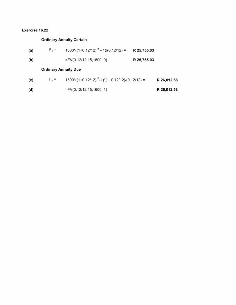
Exercise 16.22
Ordinary Annuity Certain
(a) Fv = 1600*((1+0.12/12)15 - 1)/(0.12/12) = R 25,755.03
(b) =FV(0.12/12,15,1600,,0) R 25,755.03
Ordinary Annuity Due
(c) Fv = 1600*((1+0.12/12)15-1)*(1+0.12/12)/(0.12/12) = R 26,012.58
(d) =FV(0.12/12,15,1600,,1) R 26,012.58

Exercise 16.23
Compound Interest Fv1 = Pv*(1+0.07)9
Simple Interest Fv2 = Pv*(1+0.07*9)
Difference Fv1 - Fv2 = 334.16
Pv*(1+0.07)9 - Pv*(1+0.07*9) = 334.16Pv = 334.16/((1+0.07)9 - (1+0.07*9)) = 1602.999
Captial Sum (Pv) = R 1,603.00
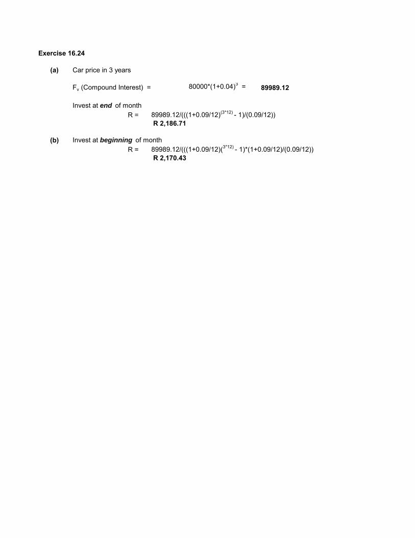
Exercise 16.24
(a) Car price in 3 years
Fv (Compound Interest) = 80000*(1+0.04)3 = 89989.12
Invest at end of monthR = 89989.12/(((1+0.09/12)(3*12) - 1)/(0.09/12))
R 2,186.71
(b) Invest at beginning of monthR = 89989.12/(((1+0.09/12)(3*12) - 1)*(1+0.09/12)/(0.09/12))
R 2,170.43

Exercise 16.25
(a) R = 8500/((1-(1+0.18/12)(-3*12))/(0.18/12)) = R 307.30
(b) Total paid = 11062.8
Interest amt = 11062.8 - 8500 = R 2,562.80
% of debt 2562.8/8500% = 30.15%

Exercise 16.26
Present value of an Ordinary Annuity Certain.
Pv = 8750*((1-(1+0.1/12)^(-(5*12)))/(0.1/12)) = R 411,821.98
The employee will receive a gratuity of R411 821.98.

Exercise 16.27
Ordinary Annuity Due
(a) Fv = 750*((1+0.145/4)(4*15)-1)*(1+0.145/4)/(0.145/4) = R 160,149.71
(b) =FV(0.145/4,60,750,,1) (using Excel function) R 160,149.71

Exercise 16.28
Ordinary annuity certain (OAC) for 2 years with R = 540.
Fv1 (OAC) = 540*((1+0.12/12)(2*12)-1)/(0.12/12) = R14 565.67
Then compute Fv on the capital sum after 2 years until maturity (for 7 years).
Fv1 (CI) = 14565.67*(1+0.12/12)^(7*12) = R33 598.96
Ordinary annuity certain (OAC) for 7 years with R = 750.
Fv2 (OAC) = 750*((1+0.12/12)(7*12)-1)/(0.12/12) = R98 004.21
Total Funds Available Fv1 (CI) + Fv2 (OAC) = R131 603.17

Exercise 16.29
(a) Ordinary Annuity Certain
Fv (monthly) = 1000*((1+0.085/12)^(1*12)-1)/(0.085/12) = R12 478.72
Fv (quarterly) = 3000*((1+0.10/4)^(1*4)-1)/(0.10/4) = R12 457.55
Conclusion It is better to invest monthly .
(b) Ordinary Annuity Certain - Using Excel 's function, FV.
Fv (monthly) = =FV(0.085/12,12,1000,,0) R12 478.72
Fv (quarterly) = =FV(0.10/4,4,3000,,0) R12 457.55
(c) Ordinary Annuity Due - Using Excel 's function, FV.
Fv (monthly) = =FV(0.085/12,12,1000,,1) R12 567.11
Fv (quarterly) = =FV(0.10/4,4,3000,,1) R12 768.99
Conclusion It is now better to invest quarterly .

Exercise 16.30
(a) PV of an Ordinary Annuity Certain
Pv = 2200*(1-(1+0.09/12)^(-(4*12)))/(0.09/12) = R88 406.52Deposit = 20000 R20 000,00Total Purchase Price of Motor Vehicle = R108 406.52
(b) Pv of an Ordinary Annuity Certain - Using Excel 's function, PV
Purchase Price = PV(0.09/12,48,2200,,0) + deposit = R88 406.52 + R20 000= R108 406.52

Exercise 16.31
(a) Using Ordinary Annuity Certain for 2 years
Fv1 (2 years) = 1000*((1+0.08/12)(2*12)-1)/(0.08/12) = R25 933.19
Using Compound Interest on Capital Sum for 1 year.FV1 (1 year) =25933.19*(1+0.1/12)(1*12) = R28 648.73
Using Ordinary Annuity Certain for 1 yearFv2 (1 year) = 1000*((1+0.10/12)(1*12)-1)/(0.10/12) = R12 565.57
12565.56809
Maturity value after 3 years R28 648.73 + R12 565.57 = R41 214.30
(b) Using Excel 's function FV with a compound interest calculation
=FV(0.08/12,24,1000,,0)*(1+0.1/12)12 + FV(0.1/12,12,1000,,0) R41 214.30
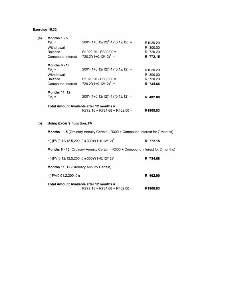
Exercise 16.32
(a) Months 1 - 5FV1 = 200*((1+0.12/12)5-1)/(0.12/12) = R1020.20Withdrawal R 300.00Balance R1020.20 - R300.00 = R 720.20Compound Interest 720.2*(1+0.12/12)7 = R 772.15
Months 6 - 10FV2 = 200*((1+0.12/12)5-1)/(0.12/12) = R1020.20Withdrawal R 300.00Balance R1020.20 - R300.00 = R 720.20Compound Interest 720.2*(1+0.12/12)2 = R 734.68
Months 11, 12FV3 = 200*((1+0.12/12)2-1)/(0.12/12) = R 402.00
Total Amount Available after 12 months =R772.15 + R734.68 + R402.00 = R1908.83
(b) Using Excel 's Function, FV
Months 1 - 5 (Ordinary Annuity Certain - R300 + Compound Interest for 7 months)
=(-(FV(0.12/12,5,200,,0))-300)*(1+0.12/12)7 R 772.15
Months 6 - 10 (Ordinary Annuity Certain - R300 + Compound Interest for 2 months)
=(-(FV(0.12/12,5,200,,0))-300)*(1+0.12/12)2 R 734.68
Months 11, 12 (Ordinary Annuity Certain)
=(-FV(0.01,2,200,,0)) R 402.00
Total Amount Available after 12 months =R772.15 + R734.68 + R402.00 = R1908.83

Exercise 16.33
(a) Option 1 Repayment at the end of every monthR = 26000/((1-(1+0.14/4)(-3*4))/(0.14/4)) = R2 690.58
(b) Option 2 Repayment at the beginning of every monthR = 26000/(((1-(1+0.14/4)(-3*4))*(1+0.14/4))/(0.14/4)) = R2 599.60
(c) The student should select to repay at the beginning of every month. Total repayment will be less than repaying at the end of every month.

Exercise 16.34Present Value (Pv) of a Deferred Annuity
Factor 1 =(1-(1+0.16/12)(-(24+36)))/(0.16/12) 41.12171
Factor 2 =(1-(1+0.16/12)(-(36)))/(0.16/12) 28.44381
Difference 41.12171 - 28.44381 = 12.6779
R = 30000/12.6779 = R2 366.32
The repayment per month is R2 366.32.

Exercise 16.35
Rate (i ) (half yearly) = (40697.7/18000)(1/10)-1 = 0.085
Rate (i ) (nominal % p.a.) = 0.085*2 = 17% p.a.

Exercise 16.36
Re-arrange the Fv formula for an Ordinary Annuity Certain
Factor 1 (103757.98/2000)*(0.12/12)+1 = 1.51879
n = LOG(1.51879)/LOG(1+0.12/12) = 42 months
The house owner will take 3 years and 6 months to save R103 757.98.

Exercise 16.37
Trucking LaundryInitial investment (R) 60000 60000Annual Cash Flow (R)
year 1 32000 0year 2 38500 7500year 3 26000 45000year 4 13000 37500year 5 9500 55500
12% p.a. cost of capital1 28571 02 30692 59793 18506 320304 8262 238325 5391 31492
91422 93333
NPV R31 422 R33 333
Recommend the purchase of the Laundry business.
INVESTMENT OPTIONS


