Journal of Monetary Economics 51 (2004) 257–276

International business cycles: What are the facts?

Steve Amblera,*, Emanuela Cardiab, Christian Zimmermannc

aCentre Interuniversitaire de Recherche sur les Politiques !Economiques et L’emploi (CIRPEE), Universit!e

du Qu!ebec "a Montr!eal, Case Postale, 8888, Succursale Centre-Ville, Montr!eal QC, H3C 3P8, CanadabCentre Interuniversitaire de Recherche en !Economie Quantitative (CIREQ) and D!epartement de Sciences

!Economiques, Universit!e de Montr!eal, Montr!eal QC, CanadacDepartment of Economics, University of Connecticut, Storrs, CT 06269, USA and Centre Interuniversitaire

de Recherche sur les Politiques !Economiques et L’emploi (CIRPEE), Universit!e du Qu!ebec "a Montr!eal,

C.P. 8888, Succ. Centre-ville, Montr!eal QC, H3C 3P8, Canada

Received 26 March 2001; received in revised form 14 June 2002; accepted 14 March 2003

Abstract

Modern business cycle theory involves developing models that explain stylized facts. For

this strategy to be successful, these facts should be well established. In this paper, we focus on

the stylized facts of international business cycles. We use the generalized method of moments

and quarterly data from twenty industrialized countries to estimate and test hypotheses

concerning pairwise cross-country correlations of macroeconomic aggregates. A remarkable

common feature emerges: these correlations are mostly positive, not very high and of a similar

order of magnitude. The most important discrepancy with the theory is the low cross-country

correlation of consumption.

r 2003 Elsevier B.V. All rights reserved.

JEL classification: E32; F41

Keywords: Stylized facts; Business cycles; International comovements

1. Introduction

Dynamic general equilibrium (DGE) models have been quite successful inreplicating a large number of the stylized facts of the business cycle. Progress inbusiness cycle theory has often come from highlighting discrepancies between the

ARTICLE IN PRESS

*Corresponding author. Tel.: +1-514-987-3000ext8372; fax: +1-514-987-8494.

E-mail address: ambler.steven@uqam.ca (S. Ambler).

0304-3932/$ - see front matter r 2003 Elsevier B.V. All rights reserved.

doi:10.1016/j.jmoneco.2003.03.001

predictions of the models and the accepted stylized facts. In an influential surveyarticle, Backus et al. (1995, henceforth BKK) discuss several features of the data oninternational business cycles that are hard for DGE models to capture.1 Theycalculate cross-correlations between U.S. aggregates and their counterparts in theother countries of their sample.2 Using these data they find that the cross-countrycorrelations of output are generally higher than the cross-correlations of aggregateproductivity (as measured by Solow residuals), which are in turn higher than thecross-correlations of consumption and that the cross-correlations of output,investment and employment are generally positive and fairly high.These features have become known as the quantity anomaly because in the baseline

model BKK develop, which is a two-country extension of a standard real businesscycle model, the ordering of the output, Solow residual and consumptioncorrelations is reversed, the cross-correlations of investment and employment arenegative and the cross-correlation of consumption is very high.3 Incentives to useinputs where they are most productive give rise to negative cross-correlations ofoutput, investment and employment. Risk sharing between agents in differentcountries leads instead to cross-country correlations of aggregate consumptionwhich are much higher than in the data.4

These empirical findings have been taken as benchmark stylized facts ofinternational business cycle models in numerous subsequent studies that attemptto develop models which are compatible with the data. The goal of this paper is toexamine whether the empirical findings described in BKK are to be consideredrobust stylized facts. Because the U.S. economy is not representative amongindustrialized economies in terms of both its size and its openness, the cross-countrybusiness cycle features between the U.S. and other countries (nine cross-countrycorrelation coefficients in all) may not be representative of what happens betweenother pairs of individual countries or groups of countries.We extend the BKK sample to consider twenty industrialized countries and

consider all pairwise cross-country correlations. With 190 cross-country correlationswe should be able to assess whether there are common features to internationalbusiness cycle comovements and, if so, what these features are. We use quarterlydata between 1960:1 and 2000:4 and estimate cross-country and within-countrycomovements using the generalized method of moments (GMM)5 to calculatestandard errors and confidence intervals for all of our statistics. This will allow us to

ARTICLE IN PRESS

1See also Baxter (1995) for a broad survey of international business cycle models.2They use quarterly observations from Australia, Austria, Canada, France, Germany, Italy, Japan,

Switzerland, the United Kingdom, the United States, and an aggregate of European countries.3Although BKK do not report standard errors for the predictions of their stochastic simulations, these

predictions are insensitive to the numerical values used to calibrate the baseline model and to sampling

uncertainty in drawing the random shocks.4 In addition DGE models do not generate fluctuations in the terms of trade as large as those observed in

the data. Models which restrict the elasticity of substitution between domestic and foreign goods can

generate volatile terms of trade, but at the cost of a counterfactually low volatility of the trade balance.5Backus and Kehoe (1992) estimate the cross-correlations of output using GMM techniques applied to

annual data on nine different countries. They report standard errors for individual country pairs but do

not derive the implied standard errors for their entire panel of data.

S. Ambler et al. / Journal of Monetary Economics 51 (2004) 257–276258

assess whether the moments generated by international business cycle models differsignificantly from those in the data and whether the quantity anomaly is astatistically significant regularity.The paper is structured as follows. In the next section, we summarize the evidence

from BKK and survey recent articles on international business cycles that take thequantity anomaly as a stylized fact. In Section 3, we describe our econometricmethodology in detail. In Section 4, we describe our data sample and present ourresults, including the results of a series of hypothesis tests. Section 5 concludes.

2. The quantity anomaly in the recent international business cycle literature

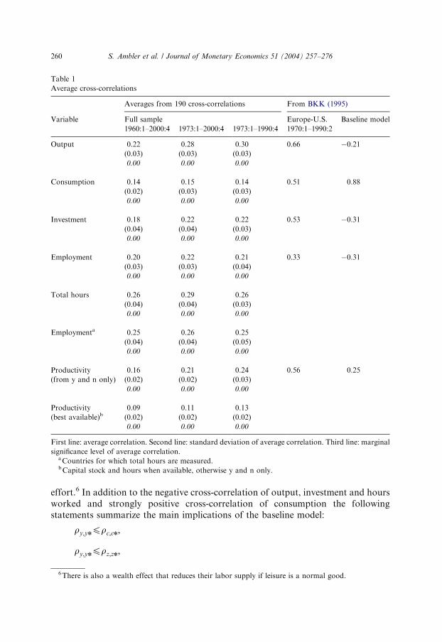
The consensus view concerning the stylized facts of international business cycles islargely based on the seminal contributions of BKK (1992, 1995). They build a two-country DGE model and compare the model’s predictions concerning the cross-correlations of macroeconomic aggregates with the data. BKK (1995) reports thecross-correlations between the same variable in different individual countries andthe U.S., and between the same variable for an aggregate of European countries andthe U.S. These results are reported in Table 1 (fourth column) and in Table 4 (thefigures in square brackets). With two exceptions, the cross-correlations of output arehigher than the cross-correlations of technology shocks as measured by Solowresiduals (see Table 4). Without exception, the cross-correlations of output arehigher than the cross-correlations of consumption. With only three exceptions, thecross-correlations of technology shocks are higher than the cross-correlations ofconsumption. Based on these results, BKK suggest the following relative ordering asa stylized fact of the international business cycle:

ry;yn > rz;zn > rc;cn;

where y; z; and c are respectively output, the Solow residual and consumption,asterisks denote foreign variables, and r denotes a cross-correlation statistic.Tables 1 and 4 also show that the cross-correlations of output, investment andemployment are generally positive. There is just one exception with investment andthere are only two exceptions with employment.The last column of Table 1 brings out the discrepancy between BKK’s baseline

model and their data. The model predicts the opposite ordering of the cross-correlations of output, the Solow residual and consumption and negative cross-correlations of output, investment and labor input. International risk sharing is theexplanation of the high cross-correlation of consumption. In the baseline model,there are strong incentives to use productive inputs more intensively in the countrybenefiting from a positive productivity differential. This leads to negative cross-correlations of output, investment and labor input. The impact of productivity onlabor input arises primarily because of an intertemporal substitution effect on laborsupply. Labor supply increases in the country benefiting from a positive productivityshock. If there are technological spillover effects, agents in the other country expectfuture productivity increases and have an incentive to reduce their current work

ARTICLE IN PRESSS. Ambler et al. / Journal of Monetary Economics 51 (2004) 257–276 259

effort.6 In addition to the negative cross-correlation of output, investment and hoursworked and strongly positive cross-correlation of consumption the followingstatements summarize the main implications of the baseline model:

ry;ynprc;cn;

ry;ynprz;zn;

ARTICLE IN PRESS

Table 1

Average cross-correlations

Averages from 190 cross-correlations From BKK (1995)

Variable Full sample Europe-U.S. Baseline model

1960:1–2000:4 1973:1–2000:4 1973:1–1990:4 1970:1–1990:2

Output 0.22 0.28 0.30 0.66 �0.21(0.03) (0.03) (0.03)

0.00 0.00 0.00

Consumption 0.14 0.15 0.14 0.51 0.88

(0.02) (0.03) (0.03)

0.00 0.00 0.00

Investment 0.18 0.22 0.22 0.53 �0.31(0.04) (0.04) (0.03)

0.00 0.00 0.00

Employment 0.20 0.22 0.21 0.33 �0.31(0.03) (0.03) (0.04)

0.00 0.00 0.00

Total hours 0.26 0.29 0.26

(0.04) (0.04) (0.03)

0.00 0.00 0.00

Employmenta 0.25 0.26 0.25

(0.04) (0.04) (0.05)

0.00 0.00 0.00

Productivity 0.16 0.21 0.24 0.56 0.25

(from y and n only) (0.02) (0.02) (0.03)

0.00 0.00 0.00

Productivity 0.09 0.11 0.13

(best available)b (0.02) (0.02) (0.02)

0.00 0.00 0.00

First line: average correlation. Second line: standard deviation of average correlation. Third line: marginal

significance level of average correlation.aCountries for which total hours are measured.bCapital stock and hours when available, otherwise y and n only.

6There is also a wealth effect that reduces their labor supply if leisure is a normal good.

S. Ambler et al. / Journal of Monetary Economics 51 (2004) 257–276260

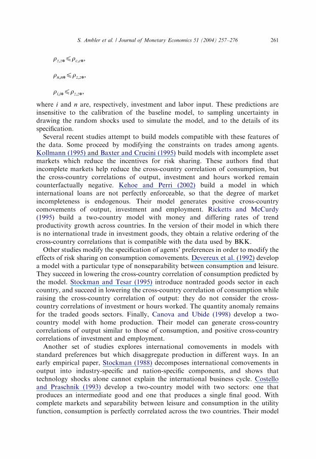
rz;znprc;cn;

rn;nnprz;zn;

ri;inprz;zn;

where i and n are, respectively, investment and labor input. These predictions areinsensitive to the calibration of the baseline model, to sampling uncertainty indrawing the random shocks used to simulate the model, and to the details of itsspecification.Several recent studies attempt to build models compatible with these features of

the data. Some proceed by modifying the constraints on trades among agents.Kollmann (1995) and Baxter and Crucini (1995) build models with incomplete assetmarkets which reduce the incentives for risk sharing. These authors find thatincomplete markets help reduce the cross-country correlation of consumption, butthe cross-country correlations of output, investment and hours worked remaincounterfactually negative. Kehoe and Perri (2002) build a model in whichinternational loans are not perfectly enforceable, so that the degree of marketincompleteness is endogenous. Their model generates positive cross-countrycomovements of output, investment and employment. Ricketts and McCurdy(1995) build a two-country model with money and differing rates of trendproductivity growth across countries. In the version of their model in which thereis no international trade in investment goods, they obtain a relative ordering of thecross-country correlations that is compatible with the data used by BKK.Other studies modify the specification of agents’ preferences in order to modify the

effects of risk sharing on consumption comovements. Devereux et al. (1992) developa model with a particular type of nonseparability between consumption and leisure.They succeed in lowering the cross-country correlation of consumption predicted bythe model. Stockman and Tesar (1995) introduce nontraded goods sector in eachcountry, and succeed in lowering the cross-country correlation of consumption whileraising the cross-country correlation of output: they do not consider the cross-country correlations of investment or hours worked. The quantity anomaly remainsfor the traded goods sectors. Finally, Canova and Ubide (1998) develop a two-country model with home production. Their model can generate cross-countrycorrelations of output similar to those of consumption, and positive cross-countrycorrelations of investment and employment.Another set of studies explores international comovements in models with

standard preferences but which disaggregate production in different ways. In anearly empirical paper, Stockman (1988) decomposes international comovements inoutput into industry-specific and nation-specific components, and shows thattechnology shocks alone cannot explain the international business cycle. Costelloand Praschnik (1993) develop a two-country model with two sectors: one thatproduces an intermediate good and one that produces a single final good. Withcomplete markets and separability between leisure and consumption in the utilityfunction, consumption is perfectly correlated across the two countries. Their model

ARTICLE IN PRESSS. Ambler et al. / Journal of Monetary Economics 51 (2004) 257–276 261

predicts a higher cross correlation of output than the BKK model but does notexamine the cross-country correlations of investment and employment. Head (2001)builds a two-country model with differentiated intermediate goods and monopolisticcompetition. He shows that increasing returns to the variety of intermediate goodscan lead to a positive international transmission of the business cycle.Park (1998) analyzes a model with tradable and nontradable investment and

consumption goods. His model generates positive cross-country correlations ofaggregate output and a cross-country correlation of consumption which is lowerthan that of output. Ambler et al. (2002) build a two-country model with multipletradable goods sectors. The model is relatively successful in matching the cross-country correlations of most aggregates, with the exception of consumption. Bettsand Devereux (1996, 2000) build a model in which firms set prices in advance, eitherin terms of their own currency or in terms of the currency of the market in whichthey are selling. They show that in the latter case, comovements of consumptionacross countries are weaker.These studies suggest that it is necessary to depart from the baseline international

real business cycle model in order to reverse its predictions concerning the relativeordering of cross-correlations of consumption, Solow residuals and output and togenerate positive cross-correlations of output, investment and hours worked. Inaddition, the large number of studies that take the quantity anomaly as a stylizedfact highlights the need to check its robustness and significance.

3. Methodology

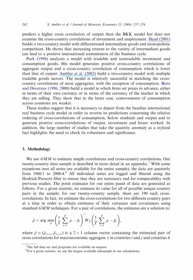
We use GMM to estimate simple correlations and cross-country correlations. Ourtwenty-country data sample is described in more detail in an appendix.7 With someexceptions (not all series are available for the entire sample), the data are quarterlyfrom 1960:1 to 2000:4.8 All individual series are logged and filtered using theHodrick-Prescott filter to ensure that they are stationary and for comparability withprevious studies. The point estimates for our entire panel of data are generated asfollows. For a given statistic, we estimate its value for all of possible unique countrypairs in the sample: for our twenty-country sample, there are 190 such cross-correlations. In fact, we estimate the cross-correlations for two different country pairsat a time in order to obtain estimates of their variances and covariances usingstandard GMM techniques. For a pair of correlations, the estimates are a solution to:

#r ¼ arg minr

1

T

XT

t¼1

r� %rt

!0

WT

1

T

XT

t¼1

r� %rt

!;

where #r � ð #rxi ;xj; #rxk ;xl

Þ is a 2� 1 column vector containing the estimated pair ofcross correlations for macroeconomic aggregate x in countries i and j and countries k

ARTICLE IN PRESS

7The full data set and programs are available on request.8For a given statistic, we use the largest available subsample in our calculations.

S. Ambler et al. / Journal of Monetary Economics 51 (2004) 257–276262

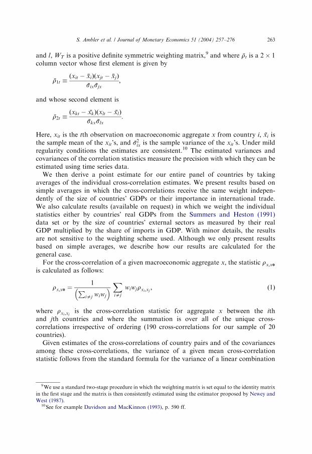
and l; WT is a positive definite symmetric weighting matrix,9 and where %rt is a 2� 1column vector whose first element is given by

%r1t �ðxit � %xiÞðxjt � %xjÞ

%six %sjx

;

and whose second element is

%r2t �ðxkt � %xkÞðxlt � %xlÞ

%skx %slx

:

Here, xit is the tth observation on macroeconomic aggregate x from country i; %xi isthe sample mean of the xit’s, and %s2ix is the sample variance of the xit’s. Under mildregularity conditions the estimates are consistent.10 The estimated variances andcovariances of the correlation statistics measure the precision with which they can beestimated using time series data.We then derive a point estimate for our entire panel of countries by taking

averages of the individual cross-correlation estimates. We present results based onsimple averages in which the cross-correlations receive the same weight indepen-dently of the size of countries’ GDPs or their importance in international trade.We also calculate results (available on request) in which we weight the individualstatistics either by countries’ real GDPs from the Summers and Heston (1991)data set or by the size of countries’ external sectors as measured by their realGDP multiplied by the share of imports in GDP. With minor details, the resultsare not sensitive to the weighting scheme used. Although we only present resultsbased on simple averages, we describe how our results are calculated for thegeneral case.For the cross-correlation of a given macroeconomic aggregate x; the statistic rx;xn

is calculated as follows:

rx;xn ¼1P

iaj wiwj

� � Xiaj

wiwjrxi ;xj; ð1Þ

where rxi ;xjis the cross-correlation statistic for aggregate x between the ith

and jth countries and where the summation is over all of the unique cross-correlations irrespective of ordering (190 cross-correlations for our sample of 20countries).Given estimates of the cross-correlations of country pairs and of the covariances

among these cross-correlations, the variance of a given mean cross-correlationstatistic follows from the standard formula for the variance of a linear combination

ARTICLE IN PRESS

9We use a standard two-stage procedure in which the weighting matrix is set equal to the identity matrix

in the first stage and the matrix is then consistently estimated using the estimator proposed by Newey and

West (1987).10See for example Davidson and MacKinnon (1993), p. 590 ff.

S. Ambler et al. / Journal of Monetary Economics 51 (2004) 257–276 263

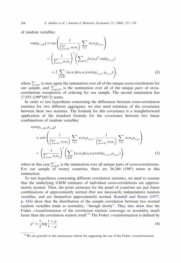
of random variables:

varðrx;xnÞ � var1P

iaj wiwj

� � Xiaj

wiwjrxi ;xj

0@

1A

¼1P

iaj wiwj

!2 Xiaj

ðwiwjÞ2 varðrxi ;xj

Þ

þ 2Xijakl

ðwiwjÞðwkwlÞ covðrxi ;xj; rxk ;xl

Þ

!; ð2Þ

whereP

iaj is once again the summation over all of the unique cross-correlations forour sample, and

Pijakl is the summation over all of the unique pairs of cross-

correlations irrespective of ordering for our sample. The second summation has17,955 ð190n189=2Þ terms.In order to test hypotheses concerning the differences between cross-correlation

statistics for two different aggregates, we also need estimates of the covariancebetween these two statistics. The formula for this covariance is a straightforwardapplication of the standard formula for the covariance between two linearcombinations of random variables:

covðrx;xn; ry;ynÞ

� cov1P

iaj wiwj

� � Xiaj

wiwjrxi ;xj;

1Piaj wiwj

� � Xiaj

wiwjryi ;yj

0@

1A

¼1P

iaj wiwj

!2 Xij;kl

ðwiwjÞðwkwlÞ covðrxi ;xj;ryk ;yl

Þ

!; ð3Þ

where in this caseP

ij;kl is the summation over all unique pairs of cross-correlations.For our sample of twenty countries, there are 36,100 ð1902Þ terms in thissummation.To test hypotheses concerning different correlation statistics, we need to assume

that the underlying GMM estimates of individual cross-correlations are approxi-mately normal. Then, the point estimates for the panel of countries are just linearcombinations of approximately normal (but not necessarily independent) randomvariables, and are themselves approximately normal. Kendall and Stuart (1977,p. 416) show that the distribution of the sample correlation between two normalrandom variables tends to normality, ‘‘though slowly’’. They also show that theFisher z-transformation of the correlation statistic converges to normality muchfaster than the correlation statistic itself.11 The Fisher z-transformation is defined by

rz �1

2log

1þ r1� r

: ð4Þ

ARTICLE IN PRESS

11We are grateful to the anonymous referee for suggesting the use of the Fisher z-transformation.

S. Ambler et al. / Journal of Monetary Economics 51 (2004) 257–276264

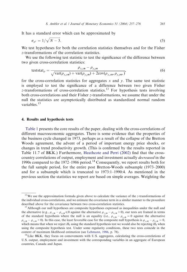
It has a standard error which can be approximated by

srz ¼ 1=ffiffiffiffiffiffiffiffiffiffiffiffiffiN � 3

p: ð5Þ

We test hypotheses for both the correlation statistics themselves and for the Fisherz-transformations of the correlation statistics.We use the following test statistic to test the significance of the difference between

two given cross-correlation statistics:

teststatr ¼rx;xn � ry;ynffiffiffiffiffiffiffiffiffiffiffiffiffiffiffiffiffiffiffiffiffiffiffiffiffiffiffiffiffiffiffiffiffiffiffiffiffiffiffiffiffiffiffiffiffiffiffiffiffiffiffiffiffiffiffiffiffiffiffiffiffiffiffiffiffiffiffiffiffiffiffiffiffiffiffiffiffiffiffiffiffiffiffiffiffi

varðrx;xnÞ þ varðry;ynÞ þ 2covðrx;xn;ry;yn; Þp ; ð6Þ

for the cross-correlation statistics for aggregates x and y: The same test statisticis employed to test the significance of a difference between two given Fisherz-transformations of cross-correlation statistics.12 For hypothesis tests involvingboth cross-correlations and their Fisher z-transformations, we assume that under thenull the statistics are asymptotically distributed as standardized normal randomvariables.13

4. Results and hypothesis tests

Table 1 presents the core results of the paper, dealing with the cross-correlations ofdifferent macroeconomic aggregates. There is some evidence that the properties ofthe business cycle changed in 1973, perhaps as a result of the collapse of the BrettonWoods agreement, the advent of a period of important energy price shocks, orchanges in trend productivity growth. (This is confirmed by the results reported inTable 11.7 of BKK.) Furthermore, Heathcote and Perri (2002) find that the cross-country correlations of output, employment and investment actually decreased in the1990s compared to the 1972–1986 period.14 Consequently, we report results both forthe full sample period, for the entire post Bretton-Woods subsample (1973–2000)and for a subsample which is truncated to 1973:1–1990:4. As mentioned in theprevious section the statistics we report are based on simple averages. Weighting the

ARTICLE IN PRESS

12We use the approximation formula given above to calculate the variance of the z-transformations of

the individual cross-correlations, and we estimate the covariance term in a similar manner to the procedure

described above for the covariance between two cross-correlation statistics.13Although our null hypotheses are composite hypotheses expressed as inequalities under the null and

the alternative (e.g., rz;zn � rc;cnp0 against the alternative rz;zn � rc;cn > 0), our tests are framed in terms

of the standard hypothesis where the null is an equality (i.e., rz;zn � rc;cn ¼ 0 against the alternative

rz;zn � rc;cn > 0). In this case, the least favorable case for the composite null hypothesis is rz;zn � rc;cn ¼ 0;which means that when we reject H0 using the standard hypothesis test we would also be rejecting H0 when

using the composite hypothesis test. Under some regularity conditions, these two tests coincide in the

context of maximum likelihood estimation (see Lehmann, 1986, p. 78).14Like BKK, they focus on comovements with U.S. aggregates, calculating the cross-correlations of

U.S. output, employment and investment with the corresponding variables in an aggregate of European

countries, Canada and Japan.

S. Ambler et al. / Journal of Monetary Economics 51 (2004) 257–276 265

individual statistics either by countries’ real GDPs or by the size of countries’external sectors produced very similar results.For all the samples considered, the average cross-country correlation of output is

much lower than the Europe-U.S. cross-country correlation coefficient reported inBKK (0.22 for the full sample versus 0.66, see Table 1). In all cases the standarderrors are very small. The average cross-country correlation of investment is alsosubstantially lower than the one reported in BKK, though still positive andsignificantly different from zero. Although for both output and investment thedifference between the theory and the data is less striking when looking at a broaderset of countries, the empirical evidence is still not consistent with the negativecoefficient predicted by the standard theoretical model.For both the full sample and the post-1973 subsample, the average cross-country

correlation of consumption is substantially lower than the average cross-countrycorrelation of consumption reported in BKK (0.14 for the full sample versus 0.51).15

Therefore, our results about the cross-country correlation of consumption indicatean even stronger puzzle than suggested in BKK where the baseline internationalbusiness cycle model predicts this cross-correlation coefficient to be 0.88.A remarkable common feature of all the average cross-correlations in Table 1 is

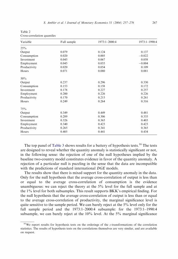
that they are positive, not too high and of a similar order of magnitude (the lowest isequal to 0.09 and the highest is equal to 0.30). For the full sample, the pointestimates of the average cross-correlations of consumption, output and productivityare not too far apart. For the post-1973 subsamples, the point estimates of the cross-correlation of output and productivity increase somewhat. As in the BKK data set,although with different orders of magnitude, the cross-country correlation coefficientof output is higher than for consumption and the cross-country correlation of outputis higher than for productivity when measuring productivity using data on outputand hours worked only. Later (Table 3) we will test whether these results are alsostatistically significant.Table 2 organizes the results in Table 1 in a slightly different way. We start by

ordering the pairwise cross-country correlation statistics. We report the value of thegiven correlation coefficient for the country pair at the 25% quantile level, the 50%quantile level, and the 75% quantile level. This table brings out more clearly thevariability of the correlation coefficients across the countries in the sample. It showsthat within the 25% quantile level most of the correlation statistics are positive (withonly two exceptions for the 1973–1990 sample) and at the 75% quantile level thestatistics are still not too high (the highest is 0.434). Even at the 90% quantile (notreported in the table) the highest correlation is 0.485 (for hours worked). At the 10%quantile (not reported in the table) the correlations vary between 0.00 and �0:177:These results confirm our previous findings that the most striking common feature ofinternational business cycles is the low positive comovements of macroeconomicaggregates.

ARTICLE IN PRESS

15 In our sample the weighted statistics are slightly higher than the unweighted statistics we report (0.21

versus 0.14, for the full sample) but the two coefficients are not statistically significantly different from

each other.

S. Ambler et al. / Journal of Monetary Economics 51 (2004) 257–276266

The top panel of Table 3 shows results for a battery of hypothesis tests.16 The testsare designed to reveal whether the quantity anomaly is statistically significant or not,in the following sense: the rejection of one of the null hypotheses implied by thebaseline two-country model constitutes evidence in favor of the quantity anomaly. Arejection of a particular null is puzzling in the sense that the data are incompatiblewith the predictions of standard international DGE models.The results show that there is mixed support for the quantity anomaly in the data.

Only for the null hypothesis that the average cross-correlation of output is less thanor equal to the average cross-correlation of consumption is the evidenceunambiguous: we can reject the theory at the 5% level for the full sample and atthe 1% level for both subsamples. This result supports BKK’s empirical finding. Forthe null hypothesis that the average cross-correlation of output is less than or equalto the average cross-correlation of productivity, the marginal significance level isquite sensitive to the sample period. We can barely reject at the 5% level only for thefull sample period and the 1973:1–2000:4 subsample: for the 1973:1–1990:4subsample, we can barely reject at the 10% level. At the 5% marginal significance

ARTICLE IN PRESS

Table 2

Cross-correlation quantiles

Variable Full sample 1973:1–2000:4 1973:1–1990:4

25%

Output 0.079 0.124 0.137

Consumption 0.020 0.005 �0.022Investment 0.045 0.067 0.058

Employment 0.045 0.055 �0.004Productivity 0.020 0.054 0.109

Hours 0.071 0.080 0.081

50%

Output 0.237 0.296 0.330

Consumption 0.153 0.158 0.172

Investment 0.178 0.227 0.257

Employment 0.200 0.226 0.226

Productivity 0.170 0.215 0.261

Hours 0.249 0.264 0.316

75%

Output 0.349 0.449 0.481

Consumption 0.289 0.306 0.335

Investment 0.326 0.365 0.403

Employment 0.340 0.423 0.423

Productivity 0.265 0.341 0.365

Hours 0.405 0.441 0.434

16We report results for hypothesis tests on the orderings of the z-transformations of the correlation

statistics. The results of hypothesis tests on the correlations themselves are very similar, and are available

on request.

S. Ambler et al. / Journal of Monetary Economics 51 (2004) 257–276 267

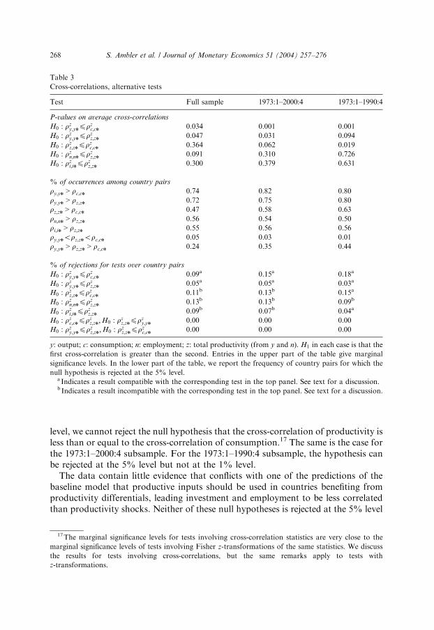
level, we cannot reject the null hypothesis that the cross-correlation of productivity isless than or equal to the cross-correlation of consumption.17 The same is the case forthe 1973:1–2000:4 subsample. For the 1973:1–1990:4 subsample, the hypothesis canbe rejected at the 5% level but not at the 1% level.The data contain little evidence that conflicts with one of the predictions of the

baseline model that productive inputs should be used in countries benefiting fromproductivity differentials, leading investment and employment to be less correlatedthan productivity shocks. Neither of these null hypotheses is rejected at the 5% level

ARTICLE IN PRESS

Table 3

Cross-correlations, alternative tests

Test Full sample 1973:1–2000:4 1973:1–1990:4

P-values on average cross-correlations

H0 : rzy;ynprz

c;cn 0.034 0.001 0.001

H0 : rzy;ynprz

z;zn 0.047 0.031 0.094

H0 : rzz;znprz

c;cn 0.364 0.062 0.019

H0 : rzn;nnprz

z;zn 0.091 0.310 0.726

H0 : rzi;inprz

z;zn 0.300 0.379 0.631

% of occurrences among country pairs

ry;yn > rc;cn 0.74 0.82 0.80

ry;yn > rz;zn 0.72 0.75 0.80

rz;zn > rc;cn 0.47 0.58 0.63

rn;nn > rz;zn 0.56 0.54 0.50

ri;in > rz;zn 0.55 0.56 0.56

ry;ynorz;znorc;cn 0.05 0.03 0.01

ry;yn > rz;zn > rc;cn 0.24 0.35 0.44

% of rejections for tests over country pairs

H0 : rzy;ynprz

c;cn 0.09a 0.15a 0.18a

H0 : rzy;ynprz

z;zn 0.05a 0.05a 0.03a

H0 : rzz;znprz

c;cn 0.11b 0.13b 0.15a

H0 : rzn;nnprz

z;zn 0.13b 0.13b 0.09b

H0 : rzi;inprz

z;zn 0.09b 0.07b 0.04a

H0 : rzc;cnprz

z;zn;H0 : rzz;znprz

y;yn 0.00 0.00 0.00

H0 : rzy;ynprz

z;zn;H0 : rzz;znprz

c;cn 0.00 0.00 0.00

y: output; c: consumption; n: employment; z: total productivity (from y and n). H1 in each case is that the

first cross-correlation is greater than the second. Entries in the upper part of the table give marginal

significance levels. In the lower part of the table, we report the frequency of country pairs for which the

null hypothesis is rejected at the 5% level.a Indicates a result compatible with the corresponding test in the top panel. See text for a discussion.b Indicates a result incompatible with the corresponding test in the top panel. See text for a discussion.

17The marginal significance levels for tests involving cross-correlation statistics are very close to the

marginal significance levels of tests involving Fisher z-transformations of the same statistics. We discuss

the results for tests involving cross-correlations, but the same remarks apply to tests with

z-transformations.

S. Ambler et al. / Journal of Monetary Economics 51 (2004) 257–276268

either for the full sample or for the two subsamples. However, there is still a sense inwhich the output, employment and investment cross-correlations are puzzling. Thebaseline model predicts negative cross-correlations of output, employment andinvestment. The results reported in Table 1 show that these cross-correlations aresignificantly positive (although numerically not very high) for both for the fullsample and for the post-1973 subsample.The middle panel of Table 3 gives an idea of how often the ordering of cross-

correlations in our data set confirms the quantity anomaly. The top rows of the panelindicate the percentage of country pairs that respect at least one of the inequalities ofthe quantity anomaly. The last row of the panel indicates the percentage of countrypairs that simultaneously respect the output-productivity and productivity-consumption ordering of the quantity anomaly. For the full sample, only 24% ofthe country pairs respect the ordering. The percentage does increase to 44% for the1973:1–1990:4 subsample. On the other hand, the second-last row of the panel showsthat only a very small percentage of the country pairs respects the simultaneousordering predicted by the baseline model.The hypothesis tests in the first panel of Table 3 are based on single point estimates

of the cross-correlations based on averaging across country pairs. The last panel inthe table reports results from hypothesis carried out for individual country pairs.Rather than reporting p-values, this panel reports the percentage of country pairs inthe sample for which a particular null hypothesis is rejected at a marginalsignificance level of 5%. These figures should be interpreted with care, since thehypothesis tests are not independent across country pairs. In some cases these resultsconfirm the hypothesis tests carried out by averaging across country pairs. Weindicate a clear agreement between the results in the top and bottom panels byplacing an asterisk next to the relevant percentage in the bottom panel. Thecorrespondence between the results in the top and bottom panels can best beunderstood by an example, the test of H0 : rz

y;ynprzc;cn for the full sample. If the null

hypothesis were true, and if the cross-correlations were independent across countrypairs, we would expect to reject the null for no more than five percent of the countrypairs (taking five percent as our marginal significance level). In fact, we reject fornine percent of the country pairs, which constitutes strong evidence against the nullhypothesis. In the top panel, we note that the p-value for the test based on averagingacross country pairs is 0.019, which therefore agrees with the evidence summarized inthe bottom panel. For the test of H0 : rz

y;ynprzz;zn for both the full sample and for the

1973:1–200:4 subsample, the null is rejected for slightly more than five percent of thecountry pairs, which constitutes weak evidence against the null hypothesis. In the toppanel, we see that in these cases the null is rejected at the five percent level but not atthe one percent level.There are cases of disagreement between the results in the two panels, which we

signify by placing a cross next to the relevant percentage in the bottom panel. Forexample, when we test H0 : rz

z;znprzc;cn using country pairs, we reject for eleven

percent of the pairs. This would seem to constitute strong evidence against the nullhypothesis, but the p-value for the test in the top panel is 0.364. A possibleexplanation of these disagreements between the results in the two panels is simply

ARTICLE IN PRESSS. Ambler et al. / Journal of Monetary Economics 51 (2004) 257–276 269

that the cross-correlations we calculate are not independent across country pairs.18

For this reason, we prefer to give more credence to hypothesis tests based onaveraging across country pairs.The last line of the bottom panel shows that there are no country pairs for which

we reject both the hypothesis that the cross-correlation of output is less than that ofproductivity and that the cross-correlation of productivity is less than that ofconsumption. The second-last line shows that there are no country pairs for whichwe reject these hypotheses with the inequalities reversed. Note that for each countrypair, we test the two hypotheses separately, using a marginal significance level of fivepercent for each test. Once again, these results should be interpreted with care sincethe two test statistics are not independent of one another. Overall, the results fromTable 3 give fairly strong support to one aspect of the quantity anomaly: while thebasic international business cycle model predicts that the consumption correlationsshould exceed the output correlations, the empirical evidence points to the contrary.Our results indicate that cross-country coefficients are somewhat sensitive to the

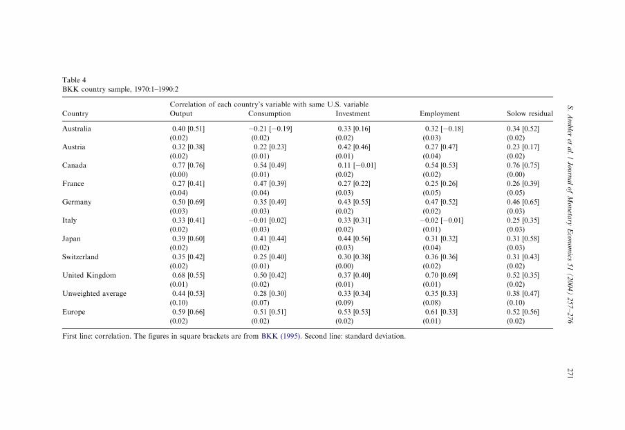
particular sample period chosen. For this reason we use our data set to examinewhether the differences between our results (overall much lower cross-countrycorrelations) and BKKs are due to the fact that the latter study uses a shorter sampleperiod. In Table 4 we use our data for the BKK country set for the same period usedin their study, 1970:1–1990:2. The figures in square brackets are from BKK (1995).Clearly, because the data are not the same, there are some slight differences betweenthe cross-country correlations in BKK and the ones obtained using our data set.However, the results are quite similar.In Table 5 we examine how the cross-country correlations between the nine

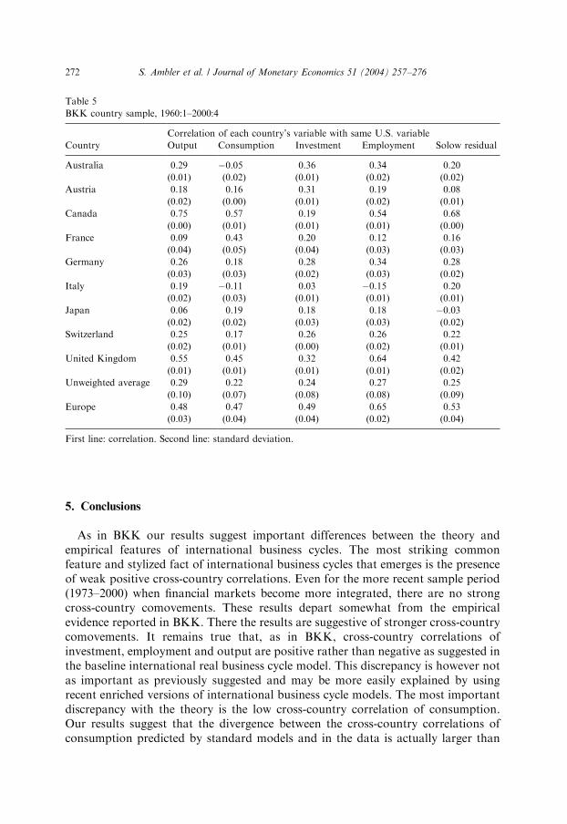
countries included in the BKK sample and the U.S. would fare once we considerour full sample period (1960:1–2000:4). The cross-country correlations reported inTable 5 are, with a few exceptions, lower than the numbers in Table 4. Theunweighted mean cross-country correlation coefficients are between 0.28 and 0.44for the 1970:1–1990:2 sample and between 0.22 and 0.29 for the full sample. Theselast results are very close to the ones we obtained using information from 190 cross-country correlation coefficients. For the particular sample of countries used in theBKK study, there seems to be a stronger sensitivity of the results to the sampleperiod chosen.19 It is to be noted that the Europe-U.S. correlations are always higherthan the unweighted average cross-correlations and, with the exception of twocountries (Canada and U.K.) are also higher than the pairwise country cross-correlations. Canadian and U.K. cross-country correlations with the U.S. areoutliers with respect to the sample of 190 pairwise country combinations consideredhere. Their business cycles seem to be more closely and positively tied to the U.S.business cycle.

ARTICLE IN PRESS

18This is confirmed by inspection of the off-diagonal elements of the estimated covariance matrices of

our GMM estimates.19Similar discrepancies can be found comparing BKK (1992) with BKK (1995). See also Heathcote and

Perri (2002).

S. Ambler et al. / Journal of Monetary Economics 51 (2004) 257–276270

ARTIC

LEIN

PRES

S

Table 4

BKK country sample, 1970:1–1990:2

Correlation of each country’s variable with same U.S. variable

Country Output Consumption Investment Employment Solow residual

Australia 0.40 [0.51] �0.21 [�0.19] 0.33 [0.16] 0.32 [�0.18] 0.34 [0.52]

(0.02) (0.02) (0.02) (0.03) (0.02)

Austria 0.32 [0.38] 0.22 [0.23] 0.42 [0.46] 0.27 [0.47] 0.23 [0.17]

(0.02) (0.01) (0.01) (0.04) (0.02)

Canada 0.77 [0.76] 0.54 [0.49] 0.11 [�0.01] 0.54 [0.53] 0.76 [0.75]

(0.00) (0.01) (0.02) (0.02) (0.00)

France 0.27 [0.41] 0.47 [0.39] 0.27 [0.22] 0.25 [0.26] 0.26 [0.39]

(0.04) (0.04) (0.03) (0.05) (0.05)

Germany 0.50 [0.69] 0.35 [0.49] 0.43 [0.55] 0.47 [0.52] 0.46 [0.65]

(0.03) (0.03) (0.02) (0.02) (0.03)

Italy 0.33 [0.41] �0.01 [0.02] 0.33 [0.31] �0.02 [�0.01] 0.25 [0.35]

(0.02) (0.03) (0.02) (0.01) (0.03)

Japan 0.39 [0.60] 0.41 [0.44] 0.44 [0.56] 0.31 [0.32] 0.31 [0.58]

(0.02) (0.02) (0.03) (0.04) (0.03)

Switzerland 0.35 [0.42] 0.25 [0.40] 0.30 [0.38] 0.36 [0.36] 0.31 [0.43]

(0.02) (0.01) (0.00) (0.02) (0.02)

United Kingdom 0.68 [0.55] 0.50 [0.42] 0.37 [0.40] 0.70 [0.69] 0.52 [0.35]

(0.01) (0.02) (0.01) (0.01) (0.02)

Unweighted average 0.44 [0.53] 0.28 [0.30] 0.33 [0.34] 0.35 [0.33] 0.38 [0.47]

(0.10) (0.07) (0.09) (0.08) (0.10)

Europe 0.59 [0.66] 0.51 [0.51] 0.53 [0.53] 0.61 [0.33] 0.52 [0.56]

(0.02) (0.02) (0.02) (0.01) (0.02)

First line: correlation. The figures in square brackets are from BKK (1995). Second line: standard deviation.

S.

Am

bler

eta

l./

Jo

urn

al

of

Mo

neta

ryE

con

om

ics5

1(

20

04

)2

57

–2

76

271

5. Conclusions

As in BKK our results suggest important differences between the theory andempirical features of international business cycles. The most striking commonfeature and stylized fact of international business cycles that emerges is the presenceof weak positive cross-country correlations. Even for the more recent sample period(1973–2000) when financial markets become more integrated, there are no strongcross-country comovements. These results depart somewhat from the empiricalevidence reported in BKK. There the results are suggestive of stronger cross-countrycomovements. It remains true that, as in BKK, cross-country correlations ofinvestment, employment and output are positive rather than negative as suggested inthe baseline international real business cycle model. This discrepancy is however notas important as previously suggested and may be more easily explained by usingrecent enriched versions of international business cycle models. The most importantdiscrepancy with the theory is the low cross-country correlation of consumption.Our results suggest that the divergence between the cross-country correlations ofconsumption predicted by standard models and in the data is actually larger than

ARTICLE IN PRESS

Table 5

BKK country sample, 1960:1–2000:4

Correlation of each country’s variable with same U.S. variable

Country Output Consumption Investment Employment Solow residual

Australia 0.29 �0.05 0.36 0.34 0.20

(0.01) (0.02) (0.01) (0.02) (0.02)

Austria 0.18 0.16 0.31 0.19 0.08

(0.02) (0.00) (0.01) (0.02) (0.01)

Canada 0.75 0.57 0.19 0.54 0.68

(0.00) (0.01) (0.01) (0.01) (0.00)

France 0.09 0.43 0.20 0.12 0.16

(0.04) (0.05) (0.04) (0.03) (0.03)

Germany 0.26 0.18 0.28 0.34 0.28

(0.03) (0.03) (0.02) (0.03) (0.02)

Italy 0.19 �0.11 0.03 �0.15 0.20

(0.02) (0.03) (0.01) (0.01) (0.01)

Japan 0.06 0.19 0.18 0.18 �0.03(0.02) (0.02) (0.03) (0.03) (0.02)

Switzerland 0.25 0.17 0.26 0.26 0.22

(0.02) (0.01) (0.00) (0.02) (0.01)

United Kingdom 0.55 0.45 0.32 0.64 0.42

(0.01) (0.01) (0.01) (0.01) (0.02)

Unweighted average 0.29 0.22 0.24 0.27 0.25

(0.10) (0.07) (0.08) (0.08) (0.09)

Europe 0.48 0.47 0.49 0.65 0.53

(0.03) (0.04) (0.04) (0.02) (0.04)

First line: correlation. Second line: standard deviation.

S. Ambler et al. / Journal of Monetary Economics 51 (2004) 257–276272

previously thought. Replicating the cross-country correlation of consumption willremain a significant challenge for DGE models as long as a high degree ofinternational risk sharing is possible in the models.As for the quantity anomaly (taken to mean the relative ordering of output, Solow

residual and consumption cross-correlations), our results suggest that it should bereinterpreted and that it should be less central to the analysis of internationalbusiness cycle fluctuations. The anomaly seems more significant for the post 1973period, and most significant for the 1973:1–1990:4 subsample.20 For all the samplesconsidered however we reject the null hypothesis that the average cross-countrycorrelation of output is smaller than or equal to that of consumption, whichsupports this aspect of the quantity anomaly.When we extend the sample used in BKK to include previous and more

recent years we find results that are consistent with the ones described in ourstudy. Even for the U.S. economy the general feature that emerges when consideringthe full sample period 1960–2000 is that comovements are positive but not toostrong.It remains a challenge to develop an international business cycle model

of financially integrated economies that the data show to be so little related.It also remains a challenge to understand why the data so unanimously speak ofsmall positive comovements while the theory suggests these comovements to beeither negative (investment, output and employment) or high and positive(consumption).More generally, our results suggest that researchers should subject ‘‘stylized facts’’

to rigorous hypothesis testing and should test for the stability of relationshipsin the data across countries and across time. Lucas’ (1977) claim that allbusiness cycles are alike may indeed extend to the international transmission ofthe business cycle but unfortunately we do not yet understand the latter with currentmodels.

Acknowledgements

The authors would like to thank the following people for helpful discussions andcomments: Jean-Marie Dufour, Alain Guay, Henrik Hansen, Soren Johansen,Marc-Andr!e Letendre, Nour Meddahi, Kevin Moran, Francisco Ruge-Murcia,seminar participants at the European University Institute, !Ecole des Hautes !EtudesCommerciales, Universit!e de Montr!eal, SUNY Albany, Southern MethodistUniversity, and annual meetings of the Canadian Economic Association, the Soci!et!e!e Canadienne de Science !Economique and the Society for Economic Dynamics, andan anonymous referee. The authors thank the Fonds FCAR and SSHRC forgenerous financial support. The usual caveat applies.

ARTICLE IN PRESS

20This may be due to the change in exchange rate regime, to the greater importance of real shocks since

the first oil price shock, or to increasing capital mobility after 1973. The cause remains an open question.

S. Ambler et al. / Journal of Monetary Economics 51 (2004) 257–276 273

Appendix A. Data sources

The data used here is based on the Quarterly National Accounts and the Main

Economic Indicators of the OECD. To add more quarters of data, data from olderreleases has been added by chaining. Also, we used data from various nationalstatistical offices to add even more quarters or series. All data are quarterly anddetrended with the Hodrick-Prescott filter. In general the sample is 1960:1 to 2000:4,except for some series that start later due to availability constraints, and a smallnumber of series that stop earlier. The twenty countries in the sample are: Australia,Austria, Canada, Denmark, Finland, France, Germany, Greece, Italy, Japan, theNetherlands, New Zealand, Norway, Portugal, South Africa, Spain, Sweden,Switzerland, the United Kingdom and the United States.We have sought to use the most comprehensive employment and hours data

possible with a reasonable sample. For all but France, this is civilian employment.(For France we use manufacturing employment.) Hours per worker are limited tomanufacturing. Hours data were available for all countries except Italy, theNetherlands, New Zealand, Portugal, South Africa and Switzerland. To compute theproductivity measures, we also used capital data where available, that is in allcountries except Australia (data available, but does not look right), New Zealand,Portugal, Spain, and Switzerland. The factor shares are taken from Zimmermann(1994). In almost all cases, yearly capital data has been interpolated to quarterlyfrequencies using the real investment series assuming a constant depreciation ratethrough the year. Occasionally, the average depreciation rate has been used to extendthe capital series forward and/or backward. Note that the consumption seriescontain services, non-durable goods and durable goods. Separate quarterly series fordurable goods are available for only very few countries. Investment is private.Local sources of data were:

* Australia: some hours data have been provided by the Australian Bureau of

Statistics.* Austria: some employment and hours, and all capital data are from the

.Osterreichisches Institut f .ur Wirtschaftsforschung.* Canada: capital data are from Statistics Canada.* Denmark: some data for all series are from the MONA database of the Danmarks

Nationalbank.* Finland: some data for all series are from Suomen Pankki.* France: some data for all series are from the Institut National de la Statistique et

des !Etudes !Economiques (INS !E !E).* Germany: all data pertain to West Germany. Capital and employment data have

been supplied by the Statistisches Bundesamt.* Greece: all data are from Christodoulakis et al. (1995).* Italy: capital data are based on Pagliano and Rossi (1992).* Japan: some data, including capital, have been supplied by the Bank of Japan.* Netherlands: some data for all series are from the Central Planning Bureau.* New Zealand: all data are from the OECD.

ARTICLE IN PRESSS. Ambler et al. / Journal of Monetary Economics 51 (2004) 257–276274

* Norway: all capital data are from the Statistisk Sentralbyr (a.* Portugal: some data for all series have been supplied by the Instituto Nacional de

Estat!ıstica.* South Africa: all data are from the South African Reserve Bank.* Spain: some data for all series are from the Instituto Nacional de Estadistica.* Switzerland: all data are from Office f!ed!eral des statistiques.* United Kingdom: the capital data have been extended from Blackburn and Ravn

(1992).* United States: the capital data are based on Musgrave (1992).

References

Ambler, S., Cardia, E., Zimmermann, C., 2002. International transmission of the business cycle in a multi-

sectoral model. European Economic Review 46, 273–300.

Backus, D., Kehoe, P., 1992. International evidence on the historical properties of business cycles.

American Economic Review 82, 864–888.

Backus, D., Kehoe, P., Kydland, F., 1992. International real business cycles. Journal of Political Economy

101, 745–775.

Backus, D., Kehoe, P., Kydland, F., 1995. International business cycles: theory and evidence.

In: Cooley, T.F. (Ed.), Frontiers of Business Cycle Research. Princeton University Press, Princeton,

NJ, pp. 331–356.

Baxter, M., 1995. International trade and business cycles. In: Grossman, G.M., Rogoff, K. (Eds.),

Handbook of International Economics, Vol. 3. North Holland, Amsterdam, pp. 1801–1864.

Baxter, M., Crucini, M., 1995. Business cycles and the asset structure of foreign trade. International

Economic Review 36, 821–854.

Betts, C., Devereux, M., 1996. The exchange rate in a model of pricing to market. European Economic

Review 40, 1007–1021.

Betts, C., Devereux, M., 2000. Exchange rate dynamics in a model of pricing to market. Journal of

International Economics 50, 215–244.

Blackburn, K., Ravn, M., 1992. Business cycles in the United Kingdom: facts and fiction. Economica 59,

383–401.

Canova, F., Ubide, A., 1998. Household production and international business cycles. Journal of

Economic Dynamics and Control 22, 545–572.

Christodoulakis, N., Dimelis, S., Kollintzas, T., 1995. Comparisons of business cycles in Greece and the

EC: idiosyncrasies and regularities. Economica 62, 1–27.

Costello, D., Praschnik, J., 1993. Intermediate Goods and the Transmission of International Business

Cycles. University of Western Ontario, Mimeo.

Davidson, R., MacKinnon, J., 1993. Estimation and Inference in Econometrics. Oxford University Press,

New York.

Devereux, M., Gregory, A., Smith, G., 1992. Realistic cross-country consumption correlations in a

two-country, equilibrium business cycle model. Journal of International Money and Finance 11, 3–16.

Head, A., 2001. Aggregate fluctuations with national and international returns to scale. International

Economic Review 43, 1101–1125.

Heathcote, J., Perri, F., 2002. Financial globalization and real regionalization, NBER Working Paper

9292.

Kehoe, P., Perri, F., 2002. International business cycles with endogenous incomplete markets.

Econometrica 70, 907–928.

Kendall, M., Stuart, A., 1977. The Advanced Theory of Statistics. Macmillan, New York.

Kollmann, R., 1995. Consumption, real exchange rates, and the structure of international asset markets.

Journal of International Money and Finance 14, 191–211.

Lehmann, E.L., 1986. Testing Statistical Hypotheses. Wiley, New York.

ARTICLE IN PRESSS. Ambler et al. / Journal of Monetary Economics 51 (2004) 257–276 275

Lucas, R., 1977. Understanding business cycles. In: Brunner, K., Meltzer, A. (Eds.), Stabilization of the

Domestic and International Economy. North Holland, Amsterdam.

Musgrave, J., 1992. Fixed reproducible tangible wealth in the United States, revised estimates. Survey of

Current Business January, pp. 106–137.

Newey, W., West, K., 1987. A simple, positive semi-definite heteroskedasticity and autocorrelation

consistent covariance matrix. Econometrica 55, 703–708.

Pagliano, P., Rossi, N., 1992. The Italian saving rate: 1951 to 1990 estimates. Temi di discussione del

Servizio Studi, Banca d’Italia, 169.

Park, H., 1998. International Business Cycle and Transmission Mechanism: Resolving Puzzles and Source

of International Comovement. University of California at Los Angeles, Mimeo.

Ricketts, N., McCurdy, T., 1995. An international economy with country-specific money and productivity

growth processes. Canadian Journal of Economics 28, S141–S162.

Stockman, A., 1988. Sectoral and national aggregate disturbances to industrial output in seven European

countries. Journal of Monetary Economics 21, 387–410.

Stockman, A., Tesar, L., 1995. Tastes and technology in a two-country model of the business cycle:

explaining international comovements. American Economic Review 85, 168–185.

Summers, R., Heston, A., 1991. The Penn world table (mark 5): an expanded set of international

comparisons, 1950–88. Quarterly Journal of Economics 106, 327–368.

Zimmermann, C., 1994. Technology innovations and the volatility of output: an international perspective.

CREF !E (Universit!e du Qu!ebec "a Montr!eal) Working Paper 34.

ARTICLE IN PRESSS. Ambler et al. / Journal of Monetary Economics 51 (2004) 257–276276