INTEGRATED PRODUCTION OF

ALGAL BIOMASS

By Alessandro Marco Lizzul

A thesis submitted in fulfilment of the requirements for graduation of an Engineering

Doctorate (EngD). From the Department of Civil, Environmental and Geomatic Engineering,

Centre for Urban Sustainability and Resilience.

Academic Supervisors:

Dr Luiza Campos, Dr Saul Purton, Dr Frank Baganz

Industrial Supervisor:

Mr Joe McDonald

UNIVERSITY COLLEGE LONDON

SEPTEMBER 2015

2

Declaration of Authorship

I, Alessandro Marco Lizzul declare that this thesis and the work presented within are my

own, generated as the result of original research. Likewise, I can confirm that this work was

done wholly while in candidature for a research degree at University College London. Any

reference or quotation from the published work of others is always clearly attributed. I have

also gone to great lengths to acknowledge all sources of assistance during the project. This

includes contributions from work done in collaboration with others, which are stated in the

contributions section. Due to the industrial relevance of this project care has been taken to

ensure that none of the proprietary intellectual property of the involved parties has been

plagiarised or misrepresented. Some sections within this thesis have already undergone

publication and are declared as such in the publications section.

Signed……………………………………………………

ALESSANDRO MARCO LIZZUL

Date………………………………………………………

3

Publications

A.M. Lizzul, P. Hellier, S. Purton, F. Baganz, N. Ladommatos, L. Campos (2013). Combined

remediation and lipid production using Chlorella sorokiniana grown on wastewater and

exhaust gases. Bioresource Technology. 151:12-18.

K. Koutita, A.M. Lizzul, L. Campos, N. Rai, T. Smith, J. Stegemann (2015). A Theoretical

Fluid Dynamic Model for Estimation of the Hold-up and Liquid Velocity in an External Loop

Airlift Bioreactor. International Journal of Applied Science and Technology, 5, 1-29.

A. M. Lizzul, M. Allen (Article in Press). Book Chapter. Algal Cultivation Technologies.

Biofuels and Bioenergy. Wiley-Blackwell.

Acknowledgements

In the first instance I would like to acknowledge the financial support received from the

engineering and physical sciences research council (EPSRC) in providing provision for the

urban sustainability and resilience (USAR) EngD centre alongside my doctoral project. I

would also like to thank the generous support of University College London, Varicon Aqua

Solutions and the Royal Commission for the Exhibition of 1851, without whom the full scope

of my project would have been largely unrealised.

The considerable support, guidance and financial assistance I have received from my

academic supervisors were of particular importance to the completion of this thesis. I owe a

debt of gratitude to Dr Luiza Campos who has given me considerable academic freedom

during the undertaking of this project, allowing me to better develop my own research ideas

and themes. Secondly, I would like to thank Dr Saul Purton and Dr Frank Baganz who as

second and third supervisors respectively, have provided me with extensive theoretical and

practical insight into the applied aspects of algal cultivation. I would also like to thank my

industrial supervisor Mr Joe McDonald (Varicon Aqua Solutions) for his guidance, both in

4

terms of my personal development and with regards to his significant expertise in applied

phycology and photobioreactor design.

Furthermore, a special thank you goes to my long term collaborators; Dr Paul Hellier, with

whom I undertook considerable work growing algae from waste, as well as co-authoring my

first research paper. I must also take the opportunity to thank Konstantina Koutita whose

considerable expertise in fluid dynamic and biological modelling made for an excellent

collaboration during the course of my research, and allowed for the co-authoring of a second

research paper. Finally, the assistance and collaboration with Richard Beckett of The Bartlett

deserves a particular mention, as it offered a different perspective on my research, as well as

generating some of the technical illustrations used within the thesis.

I must also thank the army of students who have worked on various aspects of the project at

different times, both for the input, headache and joy they generated. In chronological order of

involvement that includes; Gregory Nordberg, Yasmine Nazmy, Hugo Averalo-Bacon, Xin

Jin, Hayder Al Emera, Brendan O’Connor, Matthew Kaczmarczyk, Aitor Lekuona, Eric Dai,

Yidong Chen and Peter Sinner. A very special mention has to go to Aitor Lekuona and Peter

Sinner, who as visiting research students contributed greatly to many aspects of the practical

work during their internships at UCL. This included work with Haematococcus pluvialis at

various scales, microscale platform development, measurements for reactor modelling, as

well as membrane reactor testing. It has to be said that without the involvement of all of these

students the project would have undoubtedly been more constrained in its scope.

Finally, a special thank you has to go to all the other members of Algae@UCL, for their help

with day to day laboratory activities, queries, equipment and the sharing of practical

techniques. I would also like to acknowledge the advice and technical support received by the

Environmental Engineering technicians Ian Sturtevant, Ian Seaton, Catherine Unsworth and

Dr Judith Zho. Furthermore, I would like to thank Dr Cecile Standford (Southern Water) and

Rokiah Yaman (Community By Design) for supplying suitable wastewaters for parts of the

project. Last and most importantly of all, I would like to thank my friends, family and

girlfriend; Stacey Joanne Hemmings. All of whom have put up with me and my algal

obsession over the five years it has taken me to complete my doctorate.

5

Contributions

Chapter 1 - Introduction written by A. M. Lizzul, using some sections of re-worked

material from previous submissions within his MRes and EngD programme.

Chapter 2 - Background written by A. M. Lizzul, using some re-written material from his

MRes report as part of the EngD programme.

Chapter 3 - Written by A M. Lizzul.

Chapter 4 - Microscale work planned and directed by A. M. Lizzul and undertaken with

the assistance of P. Sinner.

Chapter 5 - Growth of Chlorella sorokiniana on waste; Material submitted for

publication in Bioresource Technology (Lizzul et al. 2014). Biological

growth experiments and wastewater quantification undertaken by A. M.

Lizzul, with gas analysis undertaken by Dr P. Hellier, Department of

Mechanical Engineering.

Chapter 6 - Chapter contains several excerpts from the book Chapter ‘Algal Cultivation

Technologies,’ written by A. M. Lizzul and supervised by M. Allen (PML)

(Lizzul and Allen 2015).

Chapter 7 - Experimentation, data collection and original reactor modelling undertaken

by A. M. Lizzul. Further novel model development undertaken by K. Koutita,

and summarised in Appendix 10.1.4.1 and 10.1.5.2 (K. Koutita 2015).

Subsequent validation experiments undertaken by A. M. Lizzul with

assistance from A. Lekuona, P. Sinner and Y. Chen.

Chapter 8 - Cost model developed by A. M. Lizzul in collaboration with E. Dai, under

supervision of S. Balboni (ME, UCL), using literature values and

experimental data from A. M. Lizzul.

Chapter 9 - Written by A. M. Lizzul.

Chapter 10 - Written by A. M. Lizzul.

6

The Engineering Doctorate (EngD)

A Note

The Engineering doctorate (EngD) is a postgraduate qualification scheme initiated in 1992

and is supported by the Engineering and Physical Sciences Research Council (EPSRC). The

programme is split between a Masters of Research (MRes) component in the first year and a

three year doctoral component. It is similar in many respects to a PhD, except for the added

requirement for an industrial sponsor and a component consisting of taught modules. The

fundamental purpose of an EngD is to undertake research that is of PhD standard but with

greater industrial relevance to the sponsoring company. In this respect an EngD may differ

somewhat from a traditional PhD, with the research usually found to be more application

orientated. In practice this means that many EngD projects will give particular consideration

to factors and findings that would add commercial advantage to a sponsoring company.

Industrial Sponsor

The project was initiated by Battle McCarthy (Ltd), an architectural design consultancy based

in London. As a result the original aims of the project were orientated more towards the built

environment, and included the development of a suitable photobioreactor for use as a

building façade. Litigation with UCL resulted in the sponsorship being rescinded, and a new

sponsor was sought out. After a period of undertaking research with no industrial sponsor, the

current industrial partnership with Varicon Aqua Solutions (Ltd) was initiated, with Mr Joe

McDonald (Managing Director) taking the role of industrial supervisor. Varicon Aqua

Solutions is an original equipment manufacturer based in the UK. They have over 20 years'

experience in the design, construction and deployment of algal photobioreactors and

aquaculture production systems. A major part of their business is the supply, installation and

commissioning of both laboratory and industrial platforms for the cultivation of algae to a

broad range of global partners. To date they have deployed over 120 photobioreactor systems

across the world. These installations include horizontal tubular systems such as the

BioFence™ platform, as well as serpentine systems such as the Phyco-Flow™, and an

internally illuminated system, the Phyco-Pyxis™.

7

Abstract

Applied research is increasingly defined within a context of sustainability and ecological

modernisation. Within this remit, recent developments in algal biotechnology are considered

to hold particular promise in integrating aspects of bioremediation and bioproduction.

However, there are still a number of engineering and biological bottlenecks related to large

scale production of algae; including requirements to reduce both capital expenditure

(CAPEX) and operational expenditure (OPEX). One potential avenue to reduce these costs is

via feedstock substitution and resource sharing; often described as industrial symbiosis. Such

an approach has the benefit of providing both environmental and economic benefits as part of

an ‘eco-biorefinery’. This thesis set out to investigate and address how best to approach some

of the cost related bottlenecks within the algal industry, through a process of industrial

integration and novel system design. The doctorate focussed on applications within a

Northern European context and was split into four research topics. The first and second parts

identified a suitable algal strain and were followed by the characterisation of its growth on

wastewater; with the findings showing Chlorella sorokiniana (UTEX1230) capable of robust

growth and rapid inorganic nutrient removal. The third part detailed the design, construction

and validation of a lower cost and fully scalable modular airlift (ALR) photobioreactor,

suitable amongst other applications for use within wastewater treatment. This work

concluded with a pilot scale deployment of a 50 L ALR system. The fourth research section

detailed the costs of ALR construction and operation at a wastewater treatment works, with a

particular focus on the benefits that can be derived by industrial symbiosis. The thesis

concludes with an appraisal of the ALR design and considers the potential for the technology,

particularly within a wastewater treatment role. A final consideration is given to the

practicalities of developing the algal industry within the UK in the short to medium term.

8

Contents

INTEGRATED PRODUCTION OF ALGAL BIOMASS ........................................................ 1

Declaration of Authorship.......................................................................................................... 2

Publications ................................................................................................................................ 3

Acknowledgements .................................................................................................................... 3

Contributions.............................................................................................................................. 5

The Engineering Doctorate (EngD) ........................................................................................... 6

Abstract ...................................................................................................................................... 7

Contents ..................................................................................................................................... 8

List of Figures .......................................................................................................................... 14

List of Tables ........................................................................................................................... 17

Abbreviations ........................................................................................................................... 18

Nomenclature ........................................................................................................................... 21

1. Balancing Industrial and Environmental Requirements ...................................................... 25

1.1. Understanding Environmental Impact .......................................................................... 25

1.2. Sustainable Development .............................................................................................. 26

1.2.1. The Role of Engineering......................................................................................... 26

1.2.2. Ecological Modernisation ....................................................................................... 28

1.2.3. The Growth of the Biobased Economy .................................................................. 29

2. Algal Biology and Biotechnology ....................................................................................... 31

An Introduction to Algal Biology ................................................................................. 31

Algal Growth ................................................................................................................. 33

Requirements for Cultivation ................................................................................. 33

Light Utilisation ...................................................................................................... 34

A Brief History of Applied Phycology ......................................................................... 37

9

Humble Beginnings ................................................................................................ 37

Brave New World ................................................................................................... 38

Microalgal Applications ......................................................................................... 39

Algal Biofuels ......................................................................................................... 41

The Future of Algal Biotechnology .............................................................................. 43

The Role of Algae within a Bio-based Economy ................................................... 43

Biorefineries and Industrial Symbiosis................................................................... 44

Integrating Algal Biorefineries...................................................................................... 46

Combining Bioproduction and Bioremediation ..................................................... 46

Options for Co-location .......................................................................................... 48

3. Thesis Overview and Structure ............................................................................................ 50

3.1. Research Aims and Objectives ...................................................................................... 50

3.1.1. Overview ................................................................................................................ 50

3.1.2. Strain Selection and Growth Kinetics .................................................................... 51

3.1.3. Growing Chlorella sorokiniana on Wastewater ..................................................... 51

3.1.4. Reactor Design, Construction and Validation ........................................................ 51

3.1.5. Cost Model of Tertiary Wastewater Treatment ...................................................... 52

3.1.6. Conclusions and Discussion ................................................................................... 52

4. Strain Selection and Growth Kinetics .................................................................................. 53

4.1. Aims and Objectives ..................................................................................................... 53

4.2. Laboratory Scale Considerations .................................................................................. 53

Production Systems ................................................................................................ 53

Chlorella sorokiniana ............................................................................................. 56

4.3. Experimental Methodology ........................................................................................... 58

4.3.1. Strain List ............................................................................................................... 58

4.3.2. Preliminary Strain Selection Experiments .............................................................. 59

4.3.3. Formulas ................................................................................................................. 59

10

4.3.4. Characterisation of Chlorella sorokiniana ............................................................. 61

4.3.5. Biomass and Lipid Quantification Techniques ...................................................... 64

4.3.6. Determining Nutrient Levels .................................................................................. 64

4.3.7. Data Analysis .......................................................................................................... 65

4.4. Results ........................................................................................................................... 65

4.4.1. Selection of a Suitable Strain .................................................................................. 65

4.4.2. Characterisation of Chlorella sorokiniana ............................................................. 66

4.4.3. Exploration of the Parameter Space ....................................................................... 67

4.4.4. Nutrient Removal ................................................................................................... 69

4.4.5. Optimisation of Feeding Strategy ........................................................................... 71

4.4.6. Comparison of Data between Scales ...................................................................... 72

4.5. Scaled-down Conclusions ............................................................................................. 72

5. Scaled Down Cultivation with Waste .................................................................................. 74

5.1. Aims and Objectives ..................................................................................................... 74

5.2. A Review of Algal Bioremediation ............................................................................... 74

5.2.1. Wastewater Characterisation .................................................................................. 74

5.2.2. Remediation of Industrial Wastewaters .................................................................. 75

5.2.3. Algal Treatment of Agricultural and Municipal Wastewaters ............................... 77

5.2.4. Flue Gas Scrubbing ................................................................................................ 80

5.3. A Detailed look at Municipal Wastewater Treatment ................................................... 81

5.3.1. Preliminary and Primary Wastewater Treatment ................................................... 81

5.3.2. Secondary Wastewater Treatment .......................................................................... 82

5.3.3. Tertiary Wastewater Treatment Processes ............................................................. 83

5.3.4. Priorities for Wastewater Treatment in the UK ...................................................... 85

5.3.5. Integrating Algal Phosphorus Recovery ................................................................. 85

5.3.6. Practical Considerations of Integrated Production ................................................. 87

5.4. Profiling Growth with Wastewater and Flue Gas ......................................................... 91

11

5.4.1. Materials and Methods ........................................................................................... 91

5.5. Results and Discussion .................................................................................................. 94

5.5.1. Preliminary Flue Gas Experiments ......................................................................... 94

5.5.2. Growth on Wastewater and Flue Gas ..................................................................... 96

5.5.3. Effect on pH and Conductivity ............................................................................... 99

5.5.4. Nutrient Uptake and Removal .............................................................................. 102

5.5.5. Flue Gas Scrubbing .............................................................................................. 104

5.5.6. Continuous Flow................................................................................................... 106

5.5.7. Optimisation of Growth and Nutrient Removal ................................................... 107

5.6. Wastewater Conclusions ............................................................................................. 108

6. Reactor Design and Construction ...................................................................................... 111

6.1. Aims and Objectives ................................................................................................... 111

6.2. Overview of Important Considerations ....................................................................... 111

6.2.1. Lighting ................................................................................................................ 112

6.2.2. Mixing .................................................................................................................. 114

6.2.3. Control Systems and Construction Materials ....................................................... 117

6.3. Common Reactor Designs ........................................................................................... 118

6.3.1. Reactor Geometries .............................................................................................. 118

6.3.2. Pond Based Systems ............................................................................................. 119

6.3.3. Membrane Reactors .............................................................................................. 122

6.3.4. Plate or Panel Based Systems ............................................................................... 123

6.3.5. Horizontal Tubular Systems ................................................................................. 125

6.3.6. Bubble Columns ................................................................................................... 128

6.3.7. Airlift Reactors ..................................................................................................... 130

6.4. Evaluation of Photobioreactor Designs ....................................................................... 133

6.4.1. Design Conceptualisation Methodology .............................................................. 133

6.4.2. Vertically Stacked Systems .................................................................................. 135

12

6.5. Airlift and Column Design Principles ......................................................................... 137

6.5.1. Solar Penetration................................................................................................... 138

6.5.2. Algal Growth ........................................................................................................ 139

6.5.3. Liquid Mixing and Circulation in Pneumatic Photobioreactors ........................... 139

6.5.4. Mass Transfer in Pneumatic Photobioreactors ..................................................... 143

6.5.5. Power Consumption ............................................................................................. 144

6.5.6. Heat Transfer in Airlift Reactors .......................................................................... 145

6.5.7. Scale-Up ............................................................................................................... 146

6.6. Airlift Reactor (ALR) Design ..................................................................................... 149

6.6.1. Early Concept ....................................................................................................... 149

6.6.2. Construction Materials and Methods .................................................................... 152

6.7. Summary of the Design Process.................................................................................. 155

7. Reactor Modelling and Scale-up ........................................................................................ 157

Aims and Objectives ................................................................................................... 157

Experimental Methodology ......................................................................................... 157

Reactor Configurations ......................................................................................... 157

Mixing and Mass Transfer .................................................................................... 160

Batch Growth Experiments .................................................................................. 164

Pilot Cultivation .................................................................................................... 165

Reactor Modelling Results .......................................................................................... 167

Gas Hold-Up ......................................................................................................... 167

Liquid Velocity ..................................................................................................... 169

Circulation and Mixing times ............................................................................... 172

Reynolds Number ................................................................................................. 176

Mass Transfer ....................................................................................................... 177

Summary of Engineering Parameters ................................................................... 178

Batch Growth Experiments .................................................................................. 179

13

Summary of Biological Findings .......................................................................... 183

Scale-up and Pilot Production ..................................................................................... 184

Comparison of Biological Performance ............................................................... 184

Summary of ALR at 5, 10 and 50 L Scales .......................................................... 187

Darwin Pilot .......................................................................................................... 187

Reactor Performance Conclusions .............................................................................. 190

8. ALR Performance, Cost Comparison and WWT Model ................................................... 195

Aims and Objectives ................................................................................................... 195

Modelling Methodology .............................................................................................. 196

System Construction and Comparison ................................................................. 196

Phosphorus Removal with the ALR ..................................................................... 198

Results ......................................................................................................................... 201

System Comparison .............................................................................................. 201

ALR Construction Costs ....................................................................................... 207

UK Wastewater Treatment Model ........................................................................ 210

Exploration of Industrial Symbiosis ..................................................................... 217

2.1.1. Comparison to other Tertiary Wastewater Treatment Technologies.................... 221

Modelling Conclusions ............................................................................................... 224

9. Contribution to Field and Further Work ............................................................................ 226

9.1. Overview ..................................................................................................................... 226

9.2. Strain Selection and Growth Kinetics ......................................................................... 227

9.3. Scaled-down Cultivation with Waste .......................................................................... 228

9.4. Reactor Design and Validation ................................................................................... 231

9.5. Operational Costs ........................................................................................................ 236

9.6. Final Conclusions and Summary ................................................................................ 238

9.6.1. Joining the dots within the UK Algal Industry ..................................................... 238

10. References and Appendices ............................................................................................. 242

14

10.1. Appendices ................................................................................................................ 242

10.1.1. Strain Selection and Growth Kinetics ................................................................ 242

10.1.2. Reactor Modelling and Validation ..................................................................... 247

10.1.3. Operational Costs ............................................................................................... 249

10.1.4. Conclusions and Discussion ............................................................................... 256

10.1.5. Published Work .................................................................................................. 257

10.2. References ................................................................................................................. 258

List of Figures

Figure 1.1. Potential system responses to perturbation events. ............................................................................ 28

Figure 2.1. Diagram of a Chlamydomonas cell. ................................................................................................... 32

Figure 2.2. Typical absorption profile and photosynthetic rate at different wavelengths of light (Viridiplantae).35

Figure 2.3. Electron transport chain and associated molecular components required for photosynthesis. ......... 36

Figure 2.4. Light microscopy images of cyanobacterial and algal strains. .......................................................... 40

Figure 2.5. Illustration of biofuel production routes from algal lipids. ................................................................ 42

Figure 2.6. The eco-industrial park at Kalundborg in Denmark. ......................................................................... 45

Figure 2.7. Outline of considerations for an algal biorefinery. ............................................................................ 47

Figure 2.8. Potential options for algal co-location. ............................................................................................. 49

Figure 4.1. Illustration of a flask culture, with single and multiple shaker arrangements. .................................. 54

Figure 4.2. Illustration and photograph of a miniaturised fermenter system. ...................................................... 55

Figure 4.3. Photograph of a microshaker plate reactor, alginate suspend beads, and membrane bioreactor. ..... 56

Figure 4.4. Light microscopy image of C. sorokiniana. ........................................................................................ 57

Figure 4.5. The 1 litre Duran bottle reactor.......................................................................................................... 62

Figure 4.6. Example 6-well microplate arrangement used during experiments testing the optimal concentration

of BBM. ................................................................................................................................................................. 63

Figure 4.7. Growth of C. sorokiniana under phototrophic and mixotrophic conditions. ...................................... 66

Figure 4.8. Maximum specific growth rates and final yields in the 1 litre Duran bottle reactors. ....................... 68

Figure 4.9. Nutrient removal and lipid production profiles in the 1 litre Duran bottle reactor under different

conditions. ............................................................................................................................................................ 70

Figure 4.10. Optimisation of feeding strategy. ..................................................................................................... 71

Figure 5.1. An indication of typical raw municipal wastewater composition. ...................................................... 79

15

Figure 5.2. Overview of a typical municipal wastewater treatment process. ....................................................... 82

Figure 5.3. A HRAP produced by Aqualia and used for wastewater treatment. ................................................... 87

Figure 5.4. Illustration of how an algal treatment platform could be integrated within a wastewater treatment

works. ................................................................................................................................................................... 89

Figure 5.5. The ClearAs process. ......................................................................................................................... 90

Figure 5.6. Growth of C. sorokiniana on 1 x BBM and varying flue gas concentrations. .................................... 95

Figure 5.7. Growth of C. sorokiniana on different wastewaters and commercial media. ..................................... 97

Figure 5.8. Effect of algal growth on pH and conductivity within the different types of media. ......................... 100

Figure 5.9. Level of nutrients in wastewaters and media. .................................................................................. 103

Figure 5.10. Exploration of the scrubbing potential from a culture of centrate grown algae. ........................... 105

Figure 5.11. A 30 day continuous C. sorokiniana growth experiment on final effluent, sparged with 20 cm3min-1

of 12% diesel exhaust gas. .................................................................................................................................. 107

Figure 6.1. Examples of common lighting arrangements. .................................................................................. 114

Figure 6.2. Photographs of different mixing systems. ......................................................................................... 116

Figure 6.3. AlgaeConnect control system and pH probe. ................................................................................... 117

Figure 6.4. Schematic and photograph showing the typical arrangement of a raceway pond. .......................... 120

Figure 6.5. Illustration and photograph of a membrane photobioreactor. ......................................................... 122

Figure 6.6. Diagram shows the potential arrangements of flat panelled reactors. ............................................ 124

Figure 6.7. Schematics and photographs showing potential configurations for tubular reactors. ..................... 126

Figure 6.8. A simplified schematic of a bubble column, alongside an array. ..................................................... 129

Figure 6.9. Different configurations of airlift bioreactors. ................................................................................. 131

Figure 6.10. Diagram shows some of the potential configurations of airlift reactors. ....................................... 132

Figure 6.11. Examples of vertically stacked column configurations. ................................................................. 137

Figure 6.12. Typical light profile within a photobioreactor tube. ....................................................................... 147

Figure 6.13. Early ALR concept sketches. .......................................................................................................... 150

Figure 6.14. Engineering diagram of the two possible mixing modes within the reactor. .................................. 151

Figure 6.15. Technical drawings show the ALR geometry for the 10 L system................................................... 153

Figure 6.16. Photograph of the finished 10 L prototype. .................................................................................... 154

Figure 6.17. The ALR at different scales. ........................................................................................................... 155

Figure 7.1. Experimental ALR arrays and mixing modes. .................................................................................. 158

Figure 7.2. Experimental BC arrays and mixing modes. .................................................................................... 159

Figure 7.3. Diagram showing the arrangement of an inverted u-tube manometer. ............................................ 161

Figure 7.4. Typical response pulse in airlift photobioreactors. .......................................................................... 162

Figure 7.5. The Darwin greenhouse and 50 litre ALR growing C. sorokiniana. ................................................ 166

Figure 7.6. Predicted and experimentally measured gas hold-up within the riser for the 5ALR, 10ALR and

50ALR Systems. .................................................................................................................................................. 167

Figure 7.7. Predicted and experimentally measured gas hold-up within 2.5BC, 5BC, 5CMALR and 10CMALR

systems. ............................................................................................................................................................... 168

Figure 7.8. Modelled and experimentally measured liquid velocities within the 5ALR, 10ALR and 50ALR

systems. ............................................................................................................................................................... 170

16

Figure 7.9. Modelled and experimentally measured liquid velocities within 2.5BC, 5BC, 5CMALR and

10CMALR Systems. ............................................................................................................................................ 171

Figure 7.10. Modelled and experimentally measured circulation times within the 5ALR, 10ALR and 50ALR

systems. ............................................................................................................................................................... 172

Figure 7.11. Modelled and experimentally measured circulation times within the 2.5BC, 5BC, 5CMALR and

10CMALR Systems. ............................................................................................................................................ 173

Figure 7.12. Modelled and experimentally measured mixing times within the 5ALR, 10ALR and 50ALR systems.

............................................................................................................................................................................ 174

Figure 7.13. Modelled and experimentally measured mixing times within the 2.5BC, 5BC, 5CMALR and

10CMALR Systems. ............................................................................................................................................ 175

Figure 7.14. Effect of altering the volumetric gas flow on the Reynolds number of the ALR, BC and CMALR

systems. ............................................................................................................................................................... 176

Figure 7.15. Effect of altering the volumetric airflow upon the mass transfer coefficient within the 5ALR,

10ALR, 50ALR, 2.5BC, 5BC, 5CMALR and 10CMALR Systems. ...................................................................... 178

Figure 7.16. Comparison of growth and pH change within the 5ALR, 5CMALR, 2.5BC, 5BC.......................... 179

Figure 7.17. Comparison of the productivity at 24 h time intervals within the 2.5BC, 5BC, 5ALR and 5CMALR.

............................................................................................................................................................................ 180

Figure 7.18. Dissolved oxygen levels within the 2.5BC, 5BC, 5ALR and 5CMALR systems. ............................. 181

Figure 7.19. Comparison of N-NO3 removal within the 2.5BC, 5BC, 5ALR and 5CMALR systems. ................. 182

Figure 7.20. Comparison of P-PO43- removal within the 2.5BC, 5BC, 5ALR and 5CMALR systems. ............... 183

Figure 7.21. (A) Comparison of maximum and average growth rates. (B) Comparison of productivities and final

yields within the 5, 10 and 50ALR systems over a 96 h time period. .................................................................. 185

Figure 7.22. Dissolved oxygen levels within the 5, 10 and 50ALR systems over a 168 h time period. ............... 186

Figure 7.23. 50ALR performance over different seasons. .................................................................................. 188

Figure 7.24. Comparison of N-NO3- and P-PO4

3- removal between the seasons. ............................................... 190

Figure 8.1. Schematic of ALUP process with key considerations. ...................................................................... 199

Figure 8.2. Illustration of reactor configuration for (A) the base case ALR and (B) the optimised ALR. .......... 203

Figure 8.3. Visualisation of the total ALUP system component costs. ................................................................ 212

Figure 8.4. Visualisation of other capital costs. ................................................................................................. 213

Figure 8.5. Visualisation of annual equipment energy consumption and associated cost. ................................. 214

Figure 8.6. Visualisation of potential energy savings. ........................................................................................ 218

Figure 8.7. The effect on annual costs caused by increased productivity and nutrient uptake. .......................... 221

Figure 10.1. Conversion of optical density at 750 nm and biomass dry weight. ................................................ 244

Figure 10.2. Relationship between triolein concentration and fluorescence intensity........................................ 245

Figure 10.3. Growth curves and pH change of the tested algal strains on BBM. ............................................... 246

Figure 10.3. The bubble rise velocity in water. ................................................................................................... 247

Figure 10.4. Diagram of a A) Vertical reed bed. B) Horizontal reed bed. .......................................................... 252

Figure 10.5. Twin layer membrane bioreactor. ................................................................................................... 253

Figure 10.6. Horizontal algal turf scrubber. ....................................................................................................... 254

17

List of Tables

Table 4-1. Preliminary biological parameters under differing growth conditions. .............................................. 67

Table 4-2. Summary of key parameters. ................................................................................................................ 72

Table 5-1. Indication of common nitrogen to phosphorous molar ratios within wastewaters. ............................. 78

Table 5-2. Table showing the typical nutrient contents of raw municipal wastewaters. ....................................... 79

Table 5-3. Typical composition of combustion gases from differing fossil fuel types. .......................................... 81

Table 5-4. Average composition of gas streams used in the preliminary experiments. ......................................... 94

Table 5-5. Composition of exhaust gas and media. .............................................................................................. 96

Table 5-6. Table of original and optimised parameters for C. sorokiniana grown on final effluent and AD

centrate. .............................................................................................................................................................. 108

Table 6-1. Table outlining the relative merits and disadvantages of major photobioreactor systems. ............... 133

Table 6-2. Common photobioreactor design considerations. ............................................................................. 135

Table 7-1. Reactor characteristics. ..................................................................................................................... 160

Table 7-2. Measured engineering parameters within the tested reactor platforms............................................. 178

Table 7-3. Biological findings from the batch experiments. ................................................................................ 184

Table 7-4. Comparison of biological performance parameters within 5, 10 and 50ALRs.................................. 187

Table 8-1. Original ALR dimensions, sizing and areal footprint. ....................................................................... 201

Table 8-2. Optimised ALR dimensions, sizing and areal footprint. ..................................................................... 202

Table 8-3. Comparison of deployed photobioreactor volume per area............................................................... 204

Table 8-4. Comparison of mixing energy consumption in typical bioprocesses and photobioreactors. ............. 205

Table 8-5. Comparison of volumetric and areal productivities........................................................................... 206

Table 8-6. Cost comparison of different tubular materials. ................................................................................ 207

Table 8-7. Construction costs associated with (A) Original configuration (B) Optimised spatial configuration.

............................................................................................................................................................................ 208

Table 8-8. Wastewater treatment works size. ...................................................................................................... 210

Table 8-9. Wastewater composition and reduction targets for the model. .......................................................... 210

Table 8-10. System performance. ........................................................................................................................ 211

Table 8-11. System components and key operational considerations. ................................................................ 211

Table 8-12. Total ALUP system component costs. .............................................................................................. 212

Table 8-13. Other capital costs. .......................................................................................................................... 213

Table 8-14. Annual equipment energy consumption and associated cost. .......................................................... 214

Table 8-15. Annual consumable costs. ................................................................................................................ 215

Table 8-16. Other annual and recurrent costs. ................................................................................................... 215

Table 8-17. Annual biomass production and projected sale value. ..................................................................... 216

Table 8-18. Annual CAPEX, OPEX and revenue. ............................................................................................... 216

Table 8-19. Electrical energy production from combined heat and power.......................................................... 217

Table 8-20. High grade heat generation. ............................................................................................................ 218

18

Table 8-21. Cumulative energy savings. ............................................................................................................. 219

Table 8-22. Carbon dioxide production and reduction from AD co-location. .................................................... 219

Table 8-23. Total savings to energy consumption and consumable costs using an industrial symbiosis approach.

............................................................................................................................................................................ 220

Table 8-24. Cost comparisons for biological systems and chemical treatment. ................................................. 222

Table 10-1. Composition of Commercial Media. ................................................................................................ 242

Table 10-2. Preliminary biological parameters of the investigated strains. ....................................................... 247

Table 10-2. ALR build costs (Varicon) ................................................................................................................ 249

Abbreviations

Abbreviation Definition

AD Anaerobic digestion

ADC Anaerobic digester centrate

ADP Adenosine diphosphate

Al Aluminium

ALR Airlift reactor

ALUP Algal uptake

ASP Aquatic Species Programme

atm Atmospheres

ATP Adenosine triphosphate

ATS Algal turf scrubber

BBM Bold’s basal medium

BFS BioFuel system

BOD Biological oxygen demand

C Carbon

CAPEX Capital expenditure

CCAP Culture Collection of Algae and Protozoa

CCS Carbon capture and storage

CEGE Department of Civil, Environmental and Geomatic Engineering

CM Column mixed

19

CO Carbon monoxide

Co Cobalt

CO2 Carbon dioxide

COD Chemical oxygen demand

Cd Cadmium

Cr Chromium

Cu Copper

EngD Engineering doctorate

EPSRC Engineering and physical sciences research council

Eq. Equation

ETFE Ethylene tetrafluoroethylene

EU European Union

FA Fatty acid

FAME Fatty acid methyl ester

FAO Food and Agricultural Organisation

FB Fed batch

FP7 Framework Programme 7

GDP Gross domestic product

H2O Water

Hg Mercury

hh Households

HRAP High rate algal pond

IC Ion Chromatography

ID Inner diameter

IPCC International Panel for Climate Change

LCA Lifecycle assessment

LED Light emitting diode

LHC Light harvesting complex

ME Department of Mechanical engineering

MIT Massachusetts Institute of Technology

N Nitrogen

N2 Diatomic nitrogen

NADP(H) Nicotinamide-adenine dinucleotide phosphate (protonated)

20

NH3 Ammonia

NH4+ Ammonium

NO3 Nitrate

NOx Nitrogen oxides

O2 Diatomic Oxygen

OD Outer diameter

OECD Organisation for economic co-operation and development

OPEC Organisation of petroleum exporting countries

OH- Hydroxide

P Phosphorus

PAR Photosynthetically active radiation

PBR Photobioreactor

PE Polythene

PE Population equivalent

PHA Polyhydroxyalkanoate

PML Plymouth marine laboratory

PMMA Poly(methyl methacrylate) or acrylic

PSI,II Photosystem I and II

PUFA Polyunsaturated fatty acids

PVC Polyvinyl chloride

R&D Research and design

rpm Rotations per minute

Rubisco Ribulose-1,5-bisphosphate carboxylase/oxygenase

SCCAP Scandinavian Culture Collection of Algae and Protozoa

SMB Department of Structural and Molecular Biology

SO2 Sulphur dioxide

SOx Sulphur oxides

TAG Triacyl-glycerol

THC Total hydrocarbon

Triose-P Triose-phosphate

UCL University College London

UK United Kingdom

UN United Nations

21

USA United States of America

USAR Centre for Urban Sustainability and Resilience

UTEX University of Texas

UV Ultraviolet

vvm Volume of air per volume of liquid per minute

WTR Water treatment residual

WWT Wastewater treatment

Zn Zinc

Nomenclature

Roman Symbol Description Units

𝐴 Area m2

𝑎𝑑 Cross sectional area, downcomer m2

𝐴𝐻 Area of heat transfer m2

𝑎𝑟 Cross sectional area, riser m2

𝑑ℎ𝑀 Height difference between manometer points m

𝑑𝑝 Pipe diameter m

𝑑𝑡 Tube diameter m

𝐷𝑡 Doubling time h

𝐶𝐴𝐿1,𝐴𝐿2 Oxygen concentrations during re-oxygenation mg L-1

𝐶𝐴𝐿∗ Steady state dissolved oxygen concentration mg L-1

𝐶𝑓 Final tracer concentration mM

𝐶𝑖 Initial tracer concentration mM

𝑓 Scale factor -

𝐹𝐶𝑂2 Molar flow rate of carbon dioxide mol s-1

𝐹𝑂2 Molar flow rate of oxygen mol s-1

𝐹𝑥 Molar flow rate of molecular entity mol s-1

𝑔 Gravitational acceleration m s-2

22

𝐻𝐶𝑂2 Henry’s constant for carbon dioxide mol L-1 Pa-1

ℎ𝐷 Height of dispersion m

ℎ𝑓 Film heat transfer coefficient (m2 K)/W

𝐻𝑂2 Henry’s constant for oxygen mol L-1 Pa-1

hL Height of liquid m

𝐼𝑎𝑣 Average irradiance µ mol m-2 s-1

𝐼𝑘 Strain specific constant -

𝐼𝑜 Irradiance on the culture surface µ mol m-2 s-1

𝐾𝑎 Extinction coefficient m2 mol-1

𝑘𝐵 Friction loss coefficient -

𝑘𝐿𝑎𝐿 Volumetric gas-liquid mass transfer coefficient s

𝐿𝑑 Length of downcomer m

𝐿𝑟 Length of riser m

𝐿𝑡 Lipid concentration at time mg L-1

𝑛 Empirically established exponent -

∅ Diameter m

∅𝑒𝑞 Length of light path m

∅𝐼 Photic fraction -

∅𝐼𝐿 Photic fraction, large scale -

∅𝐼𝑆 Photic fraction, small scale -

𝑃𝐶𝑂2 Carbon dioxide partial pressure Pa

𝑃𝐺 Power input due to gassing W

𝑃𝐿 Lipid productivity mg L-1 d-1

𝑃𝑂2 oxygen partial pressure Pa

𝑃𝑇 Total pressure Pa

𝑃𝑣 Partial pressure Pa

𝑃𝑋 Biomass productivity g L-1 d-1

𝑄𝐻 Heat transfer rate W/(m2K)

𝑄𝐿 Volumetric flow rate of liquid m3 s-1

𝑄𝑅 Volumetric flow rate through dark zone of reactor m3 s-1

𝑅𝑒 Reynolds number -

𝑅𝐻 Heating surface W/(m2K)

23

𝑅𝑠 Specific substrate removal mg L-1 d-1

𝑠 Boundary arc between light and dark zones m

𝑆𝑡 Substrate concentration at time mg L-1

𝑡𝑐 Circulation time s

𝑡𝑐𝑦𝑐𝑙𝑒 Cycling time s

𝑡𝑑 Dark period duration s

𝑡𝑓 Solar collection period duration/flash period s

𝑡𝑚 Mixing time s

𝑡𝑥 Time h

Ub Bubble rise velocity m s-1

UG Gas superficial velocity m s-1

UGr Gas superficial velocity in the riser m s-1

𝑈𝐻 Sum of resistances to heat transfer m2·K/W

𝑈𝐿 Superficial liquid velocity m s-1

�̅�𝐿 Linear liquid velocity m s-1

𝑈𝐿𝑑 Superficial liquid velocity in the downcomer m s-1

𝑈𝐿𝐿 Superficial liquid velocity, large scale m s-1

𝑈𝐿𝑟 Superficial liquid velocity in the riser m s-1

𝑈𝑅 Fluid interchange velocity m s-1

𝑈𝑅𝐿 Fluid interchange velocity, large scale m s-1

𝑈𝑅𝑆 Fluid interchange velocity, small scale m s-1

𝑈𝐿𝑆 Superficial liquid velocity, small scale m s-1

𝑉𝑑 Volume of dark zone m3

𝑉𝑓 Flash volume m3

𝑉𝐿 Volume of liquid m3

𝑉𝐺 Volumetric gas flow m3 s-1

𝑋𝑡 Algal concentration at time g L-1

𝑋𝑌 Yield g L-1

24

Greek Symbol Description Units

𝛼 Ratio between large and small photic fractions

�̇� Shear rate s-1

∆𝑇 Change in temperature K

𝜀𝑑 Gas hold-up in downcomer -

εmean Mean gas hold-up -

𝜀𝑟 Gas hold-up in riser -

𝜃 Solar zenith angle °

𝜇 Viscosity m s-1

𝜇 Specific growth rate h-1

𝜇𝑚𝑎𝑥 Maximum specific growth rate h-1

𝜌 Density Kg m-3

𝜌𝐿 Density of liquid Kg m-3

𝑣 Frequency m s-1

25

1. Balancing Industrial and

Environmental Requirements

1.1. Understanding Environmental Impact

The increasingly interconnected and globalised world of today has changed immeasurably

from that of the pre-industrialised era. Alongside the considerable human progress a growing

understanding of environmental damage and mismanagement has led to calls for better

balancing of industrial and environmental needs (Everett et al. 2010). Despite prescient

warnings of pioneering environmental thinkers such as Malthus, Fourier, Tyndall and

Arrhenius, it was largely not until the latter half of the 20th century that a more

comprehensive understanding of environmental issues developed. This shift in thinking was

driven by a rising societal conscience that had been gaining momentum since the late 1960s

and early 1970s (Günter Brauch 2005). A direct result of this concern is the increasing

number of modern-day scientists and engineers dedicating their research to a better

understanding of human and environmental interactions. The body of work within these

individual fields is too large and varied to outline comprehensively within this thesis; but has

highlighted the considerable losses in habitat and biodiversity caused by human activity (Kerr

and Deguise 2004, Robinson and Hermanutz 2015). Importantly, this work has also raised

awareness of the severity with which current industrial practices are altering both the global

climate and causing rapid depletion of natural resources (Foley et al. 2005). Whilst these

changes present considerable and imminent cause for concern, they also present an

unprecedented opportunity to re-organise the global economy towards greater environmental

and sustainable considerations (Lubchenco 1998).

Perhaps one of the greatest challenges facing our interaction with the environment is the

projected rise in population size and the impact this will have on both economic and

environmental development (Lubchenco 1998, Liddle 2014, Guerin et al. 2015). By 2050

some projections expect a population rise of 2-4 billion people, with almost 70% living

within the urbanised environment (Cohen 2003). Further estimates predict that 70 million

26

hectares of new land will be required to feed this population rise using conventional crop

production methods (FAO 2009). Other types of urban infrastructure will also struggle to

keep up with these demographic changes, in particular drinking water and wastewater

treatment facilities are already found to be overstretched in many areas (Daigger 2007). Other

likely consequences of this population increase will be a growth in the demand for consumer

necessities, creating an upsurge in the need for raw materials and resulting in further

intensification of industrial activity (Cole and Neumayer 2004). This increase in activity will

inevitably incur a considerable and varied environmental burden in locations across the

planet. Perhaps the biggest concern amongst scientists and policy makers alike is the increase

in atmospheric carbon dioxide levels as a result of this industrial activity. The international

panel for climate change (IPCC) projections have shown a rise in carbon dioxide levels

between 25-60% in the years 2000-2050 when compared to a baseline in 1950. This rise

would amount to an atmospheric concentration of carbon dioxide between 400-550 ppm,

which is almost double the pre-industrial levels of 260-280 ppm. This change is expected to

have considerable impact on the planet, potentially altering entire ecosystems, weather

patterns and sea levels, whilst placing greater strain on existing infrastructure and

communities (Houghton et al. 2001, Rahaman et al. 2011).

1.2. Sustainable Development

1.2.1. The Role of Engineering

In response to these environmental challenges scientists and engineers have created

frameworks for sustainable development. These sustainable practices could be described as

being varied and widespread, having no distinct origin or dogma. As a result describing such

activities can be somewhat challenging, but one of the most widely used definitions can be

attributed to the United Nations (UN) Brundtland Commission report from 1987. It describes

sustainable development as, “development that meets the needs of the present without

27

compromising the ability of future generations to meet their own needs,” p. 54 (Brundtand

1987). Within this remit both scientific and engineering solutions have a key role to play

within the sustainable development of industrial practices, and act as major drivers for change

(Bell, Chilvers and Hillier 2011). In practical terms it is the role of the environmental

engineer to liaise with stakeholders to provide sustainable solutions for both industry and the

wider community to lessen their environmental impact. This can occur through the

deployment of step-change technologies or through incremental improvements and

optimisations (Bell et al. 2011). The resultant solutions can range from relatively low-tech

improvements to agricultural practices in the developing world, e.g. through novel tool

design or improved irrigation practices; to more grandiose concepts such as the deployment

of large scale geo-engineering projects, including atmospheric cooling or carbon capture and

storage (CCS) (Wigley 2006, Gibbins and Chalmers 2008).

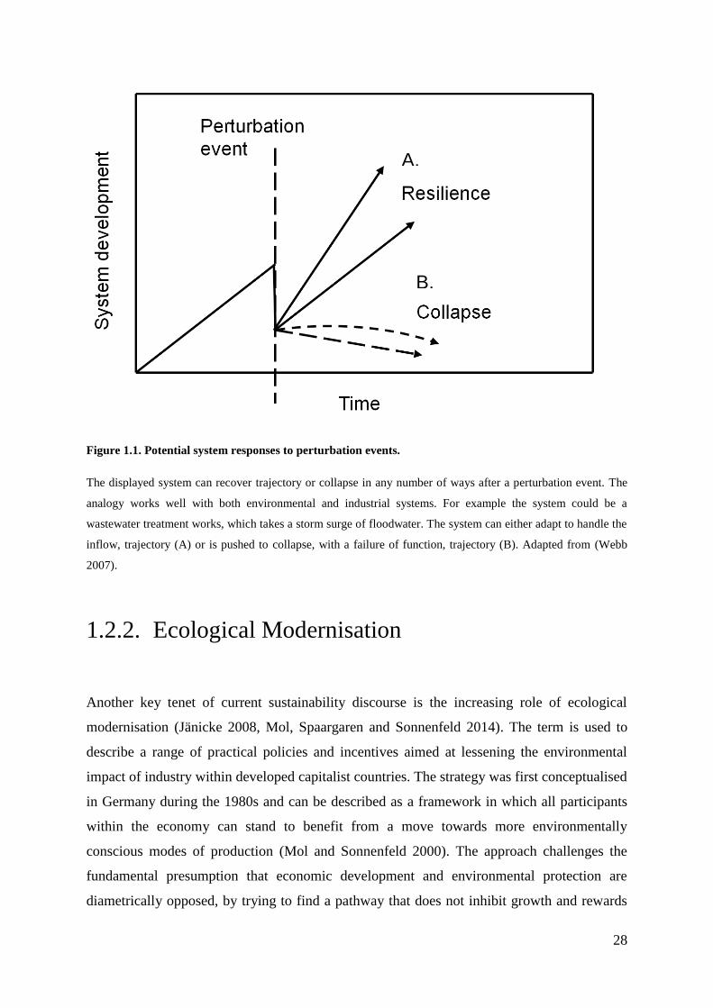
One of the foremost concepts in sustainable engineering today is that of ‘resilience’ which

has gained considerable traction within the discipline (Rahimi and Madni 2014, Righi, Saurin

and Wachs 2015). The term is widely used within many fields (Bahadur, Ibrahim and Tanner

2010), and although its meaning is somewhat nebulous, the ecological definition is widely

accepted; with resilience being “the capacity of a system to respond to perturbations and

changes, by resisting damage, recovering and maintaining function,” p.1 (Webb 2007) (see

Figure 1.1). This differs from the definition of robustness, which can be described as the

“ability of a system to resist change without adapting its initial stable configuration,”

(Wieland and Marcus Wallenburg 2012). The concept of resilience has particular relevance to

how modern economic and industrial activity needs to adapt to a variety of global

uncertainties; including climate change and resource scarcity, whilst concomitantly lessening

its impact on the environment (Ruth and Lin 2006). The role of modern environmental

engineers is twofold, firstly to predict and interpret these future challenges by studying

system dynamics and interactions, and secondly to initiate the creation of more resilient

infrastructure.

28

Figure 1.1. Potential system responses to perturbation events.

The displayed system can recover trajectory or collapse in any number of ways after a perturbation event. The

analogy works well with both environmental and industrial systems. For example the system could be a

wastewater treatment works, which takes a storm surge of floodwater. The system can either adapt to handle the

inflow, trajectory (A) or is pushed to collapse, with a failure of function, trajectory (B). Adapted from (Webb

2007).

1.2.2. Ecological Modernisation

Another key tenet of current sustainability discourse is the increasing role of ecological

modernisation (Jänicke 2008, Mol, Spaargaren and Sonnenfeld 2014). The term is used to

describe a range of practical policies and incentives aimed at lessening the environmental

impact of industry within developed capitalist countries. The strategy was first conceptualised

in Germany during the 1980s and can be described as a framework in which all participants

within the economy can stand to benefit from a move towards more environmentally

conscious modes of production (Mol and Sonnenfeld 2000). The approach challenges the

fundamental presumption that economic development and environmental protection are

diametrically opposed, by trying to find a pathway that does not inhibit growth and rewards

A.

B.

29

firms that are environmentally innovative (Mol et al. 2014). The approach is popular in the

European Union (EU) and practical examples include the incentivising of green innovation

through policy changes, entrepreneurialism or consumer attitude change. Notable instances of

success can be found in the attempts to use eco-labelling and sustainable product re-design in

order to change consumer behaviour; as well as the development of hybrid vehicles and novel

energy initiatives such as solar panel purchasing subsidies (Dryzek and D Schlosberg 2005).

Despite these achievements ecological modernisation is not without its criticisms, having

been described as a supply side solution which fails to tackle issues of excessive consumption

and environmental degradation within modern market economies (Foster 2002). One such

policy failure propagated by ecological modernisation can be seen in the widespread adoption

of bioethanol production in the United States Corn Belt, and the impact this has had on global

food prices (Gallagher 2008, Naik et al. 2010). Another prominent example is the controversy

surrounding palm oil production, which has been driven by global demand for alternatives to

petroleum oils. This has resulted in the deforestation and de-population of large tracts of

rainforest within environmentally vulnerable regions in South East Asia (Gallagher 2008,

Lapola et al. 2010).

1.2.3. The Growth of the Biobased Economy

The exploitation of naturally occurring bioprocesses for human gain is by no means a novel

concept and has long been adapted and refined throughout history. Prominent examples of

well-developed bioprocesses include baking, brewing, wastewater treatment and a range of

pharmaceutical production processes (Sarrouh et al. 2012). There have also been many

notable advances within the biorenewable sectors over recent years. For the most part the

reasons for successful adoption of biological processes within an industrial context can be

attributed to the complex enzymatic conversions that can be achieved via biotransformation.

This is especially the case when the molecule in question is complex (e.g. an enantiomer), of

a protein/macromolecular nature, required for use within the food chain, or is desired to be

biodegradable (Straathof, Panke and Schmid 2002). Commercial examples include the

production of higher value bio-actives, such as antioxidants, pigments (Borowitzka 1992),

immuno-proteins (Petrides, Sapidou and Calandranis 1995) and vaccines (Berndt et al. 2007).

30

Current research and development is focussing on biomolecule production for the bulk

commodity markets, including compounds like the polyhydroxyalkanoates (PHAs) and

polylactones, which can be used in the production of biodegradable plastics (Poirier, Nawrath

and Somerville 1995, Luengo et al. 2003). As well as the development of second generation

biofuels; which include ethanol and butanol from lignocellulose and other unconventional

feedstock (Hamelinck, Hooijdonk and Faaij 2005).

A key part of ecological modernisation policy is the development of less intensive and more

sustainable routes for the production of everyday commodities (Couturier and Thaimai 2013).

In this respect ecological modernisation policy has promoted the development of

biotechnology as a sustainable and high growth industry. This has led to considerable levels

of investment from both the private and state sectors within the Organisation of Economic

Co-operation and Development (OECD) (Oborne 2009, Cantor 2000, Ghatak 2011, Moran

2012). Whilst within the EU 27, the advanced bioeconomy already makes up an average of

6% of the total gross domestic product (GDP) of member states. Future projections for the

OECD grouping show that biotechnology may contribute to some 35% of total chemical

production, 80% of pharmaceutical production and 50% of agricultural output by the year

2030 (Oborne 2009). Currently a majority of this biotechnological output is formed from

parts of the medical or pharma sectors, otherwise known as ‘red biotechnology’. These

companies range in size from small start-ups to specialised divisions of larger pharmaceutical

multinationals. A smaller yet sizable market share within the sector is taken up by ‘green

biotechnology’ companies, which appertain to bio-derived technologies and processes used

within the agricultural sector. The final major contributor is that of ‘white biotechnology,’

which describes more industrialised forms of biotechnology and bio-processing (DaSilva

2004). Looking towards the future it is likely that both the green and white sectors will play a

larger role in the sustainable intensification of agricultural, chemical and environmental

sectors.

31

2. Algal Biology and Biotechnology

An Introduction to Algal Biology

Algae constitute a diverse set of photosynthetic organisms, which can range in size from

single cellular bodies to multicellular seaweeds. Extant specimens display polyphyletic

evolution and can be found in both the eukaryotic and prokaryotic kingdoms. Current

estimates place the number of algal species between 200,000 and 800,000, of which

approximately 35,000 have been classified (Ebenezer, Medlin and Ki 2012). Most algal

species share the common ability to undertake photosynthesis; in which the energy from light

is used to drive the fixation of carbon dioxide into organic compounds. The photosynthetic

efficiency of many algal strains is considered higher than that of land plants; with a range

between 2-6% under practical conditions, compared to the 0.1-2% seen in plants (de la Noue

and de Pauw 1988). This is attributed to their simpler cellular structure and growth within

aqueous media (Sheehan et al. 1998). A testament to this considerable output is that algae

contribute between 40 to 50% of global photosynthetic activity, whilst only comprising 1-2%

of total plant carbon (Parker, Mock and Armbrust 2008, Falkowski 1994).

The green algae are amongst the largest and best understood grouping of these photosynthetic

micro-organisms, and form a separate paraphyletic order within the kingdom Viridiplantae. It

is believed that green algae arose from a primary endosymbiotic event around 1.5 billion

years ago, where the plastid of a cyanobacterium was engulfed by a heterotrophic organism

(Leliaert et al. 2012). Higher plants (embryophytes) which are also contained in the Plantae

group are their direct evolutionary descendants (Palmer, Soltis and Chase 2004). The

Viridiplantae group is split between two clades; the Chlorophyta; which contain the majority

of described algal species; and the Streptophyta from which higher plants can trace their

lineage (Leliaert et al. 2012). In terms of morphology the green algae are a diverse group, and

include unicellular and colonial species, often taking coccoid or filamentous forms as well as

forming macroscopic seaweeds. Some unicellular green algae are motile and in this case

usually display two flagella per cell. To date there are estimated to be over 8,000 species of

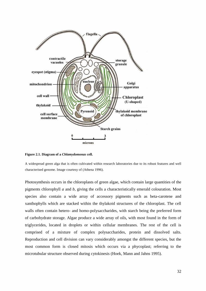
green algae (Guiry 2012), and the structure of a typical cell is shown in Figure 2.1.

32

Figure 2.1. Diagram of a Chlamydomonas cell.

A widespread green alga that is often cultivated within research laboratories due to its robust features and well

characterised genome. Image courtesy of (Athena 1996).

Photosynthesis occurs in the chloroplasts of green algae, which contain large quantities of the

pigments chlorophyll a and b, giving the cells a characteristically emerald colouration. Most

species also contain a wide array of accessory pigments such as beta-carotene and

xanthophylls which are stacked within the thylakoid structures of the chloroplast. The cell

walls often contain hetero- and homo-polysaccharides, with starch being the preferred form

of carbohydrate storage. Algae produce a wide array of oils, with most found in the form of

triglycerides, located in droplets or within cellular membranes. The rest of the cell is

comprised of a mixture of complex polysaccharides, protein and dissolved salts.

Reproduction and cell division can vary considerably amongst the different species, but the

most common form is closed mitosis which occurs via a phycoplast; referring to the

microtubular structure observed during cytokinesis (Hoek, Mann and Jahns 1995).

33

Algal Growth

Requirements for Cultivation

Most species of green algae have a preference for phototrophic growth conditions. They

achieve this by utilising light, water and an inorganic carbon source to drive photosynthesis.

However, some species have been shown to be capable of growth with a source of fixed

carbon and light, often described as mixotrophic growth (Lee et al. 1996); whilst an even

smaller number of species have also been shown to grow without the aid of light in purely

heterotrophic conditions (Cerón-García et al. 2013). Like all organisms, individual algal

species have a preference for certain temperatures, salinities and nutrient levels to grow

productively. Optimal temperature ranges can vary greatly between species and strains, with

organisms generally showing a preference for mesophilic ranges between 15-25°C. However,

there are a number of thermotolerant and thermophilic strains, which grow optimally at

temperatures above 30°C. Likewise, the preference for different salinities can vary greatly

between strains based upon the habitats in which they are normally found; with species

displaying a preference for fresh, brackish or salty water (Singh and Singh 2015).

Algae require carbon, nitrogen, phosphorous, sulphur, trace elements and vitamins to grow.

Although the metabolism of some strains is more flexible than others, the addition of these

substances within a commercial setting is limited by what can be sourced or derived at

reasonable cost. Carbon is usually introduced in the form of inorganic carbon dioxide or

bicarbonates for photoautotrophic growth. For heterotrophic and mixotrophic species fixed

carbon can be added, such as sugar monomers or organic acids. A suitable nitrogen source is

most often found in the form of ammonium, nitrate or urea, with many algal species able to

metabolise all three. Phosphorous is most often found in an inorganic free ion phosphate

form, whilst sulphur is often found in the form of various sulphate species (Hoek et al. 1995).

Trace elements such as metals are most commonly utilised in their oxidised and dissolved

forms, whilst a number of vitamins such as Vitamin B can be important for algal growth,

acting as a co-factor in a number of chemical reactions (de la Noue and de Pauw 1988). Some

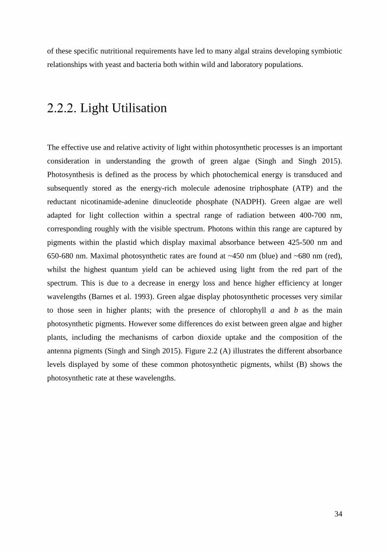
34

of these specific nutritional requirements have led to many algal strains developing symbiotic

relationships with yeast and bacteria both within wild and laboratory populations.

Light Utilisation

The effective use and relative activity of light within photosynthetic processes is an important

consideration in understanding the growth of green algae (Singh and Singh 2015).

Photosynthesis is defined as the process by which photochemical energy is transduced and

subsequently stored as the energy-rich molecule adenosine triphosphate (ATP) and the

reductant nicotinamide-adenine dinucleotide phosphate (NADPH). Green algae are well

adapted for light collection within a spectral range of radiation between 400-700 nm,

corresponding roughly with the visible spectrum. Photons within this range are captured by

pigments within the plastid which display maximal absorbance between 425-500 nm and

650-680 nm. Maximal photosynthetic rates are found at ~450 nm (blue) and ~680 nm (red),

whilst the highest quantum yield can be achieved using light from the red part of the

spectrum. This is due to a decrease in energy loss and hence higher efficiency at longer

wavelengths (Barnes et al. 1993). Green algae display photosynthetic processes very similar

to those seen in higher plants; with the presence of chlorophyll a and b as the main

photosynthetic pigments. However some differences do exist between green algae and higher

plants, including the mechanisms of carbon dioxide uptake and the composition of the

antenna pigments (Singh and Singh 2015). Figure 2.2 (A) illustrates the different absorbance

levels displayed by some of these common photosynthetic pigments, whilst (B) shows the

photosynthetic rate at these wavelengths.

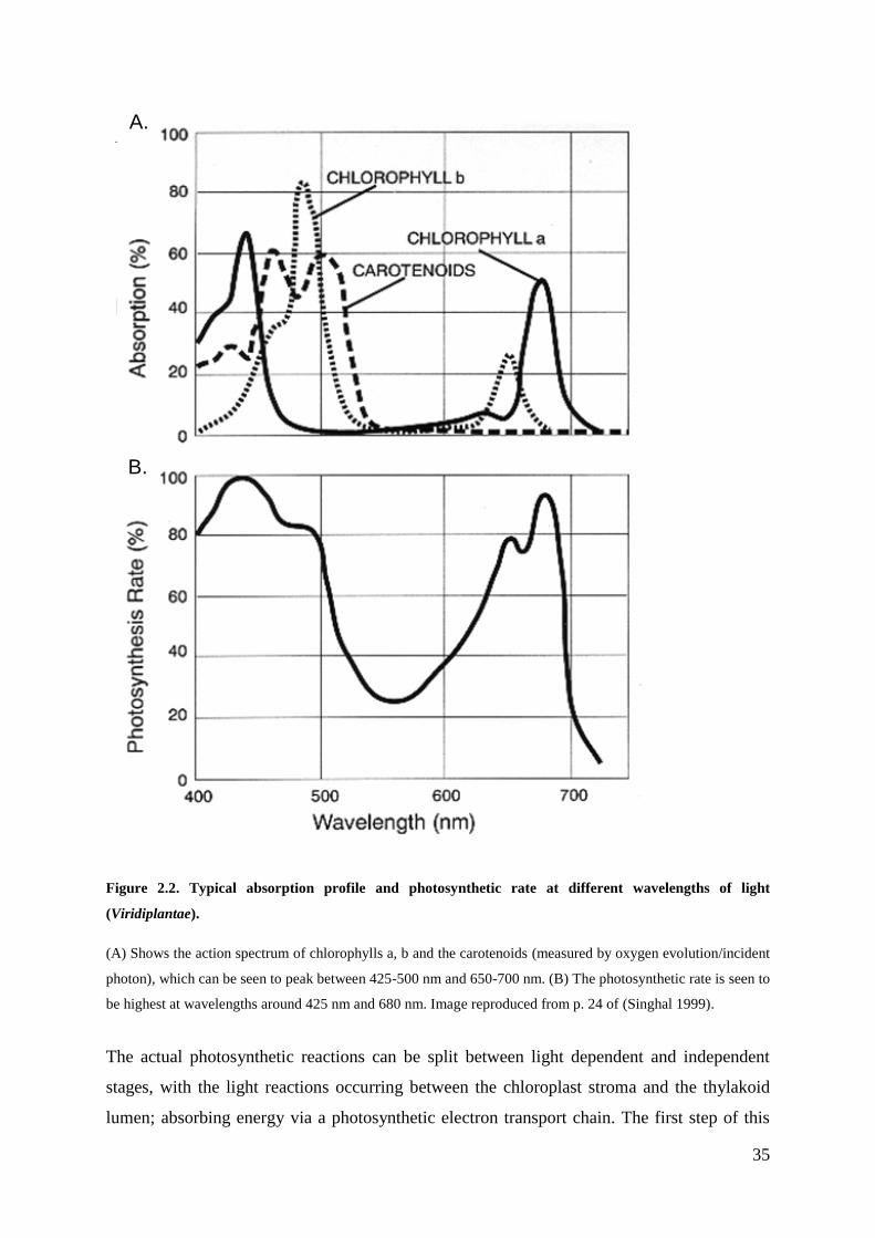
35

Figure 2.2. Typical absorption profile and photosynthetic rate at different wavelengths of light

(Viridiplantae).

(A) Shows the action spectrum of chlorophylls a, b and the carotenoids (measured by oxygen evolution/incident

photon), which can be seen to peak between 425-500 nm and 650-700 nm. (B) The photosynthetic rate is seen to

be highest at wavelengths around 425 nm and 680 nm. Image reproduced from p. 24 of (Singhal 1999).

The actual photosynthetic reactions can be split between light dependent and independent

stages, with the light reactions occurring between the chloroplast stroma and the thylakoid

lumen; absorbing energy via a photosynthetic electron transport chain. The first step of this

A.

B.

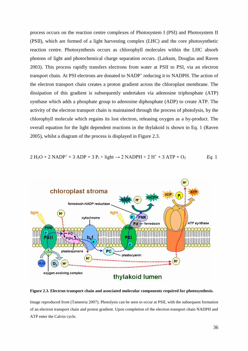
36

process occurs on the reaction centre complexes of Photosystem I (PSI) and Photosystem II

(PSII), which are formed of a light harvesting complex (LHC) and the core photosynthetic

reaction centre. Photosynthesis occurs as chlorophyll molecules within the LHC absorb

photons of light and photochemical charge separation occurs. (Larkum, Douglas and Raven

2003). This process rapidly transfers electrons from water at PSII to PSI, via an electron

transport chain. At PSI electrons are donated to NADP+ reducing it to NADPH. The action of

the electron transport chain creates a proton gradient across the chloroplast membrane. The

dissipation of this gradient is subsequently undertaken via adenosine triphosphate (ATP)

synthase which adds a phosphate group to adenosine diphosphate (ADP) to create ATP. The

activity of the electron transport chain is maintained through the process of photolysis, by the

chlorophyll molecule which regains its lost electron, releasing oxygen as a by-product. The

overall equation for the light dependent reactions in the thylakoid is shown in Eq. 1 (Raven

2005), whilst a diagram of the process is displayed in Figure 2.3.

Figure 2.3. Electron transport chain and associated molecular components required for photosynthesis.

Image reproduced from (Tameeria 2007). Photolysis can be seen to occur at PSII, with the subsequent formation

of an electron transport chain and proton gradient. Upon completion of the electron transport chain NADPH and

ATP enter the Calvin cycle.

2 H2O + 2 NADP+ + 3 ADP + 3 Pi + light → 2 NADPH + 2 H+ + 3 ATP + O2 Eq. 1

37

In the next stage of the process, the Calvin cycle utilises the high energy molecules of ATP

and NADPH to fix carbon dioxide and water into carbohydrates. This process is undertaken

within the chloroplast stroma, via the formation of intermediary molecules like triose-

phosphate (Triose-P) and the action of enzymatic complexes like ribulose-1,5-bisphosphate

carboxylase/oxygenase (Rubisco) (Moroney and Ynalvez 2001). The equation for the

reaction in the stroma is shown in Eq. 2.

A Brief History of Applied Phycology

Humble Beginnings

Mankind has had a longstanding interaction with many types of both macro- and micro-algae.

Historical evidence has shown that hunter gatherers collected washed-up seaweeds as a ready

source of nutrition. In fact fossilised remains of harvested algae have been found alongside

primitive hearths in Chile (Dillehay et al. 2008); and in many places in the world the practice

of harvesting and eating seaweed continues to this day. Other historical examples include

early subsistence societies harvesting Spirulina and Dunaliella species from salt lakes and

pools. Prominent examples continue to this day, and include the harvesting of Spirulina in

areas surrounding Lake Chad in Africa. In this process, Spirulina is filtered through cloth

meshes, collected in pots and sundried before being cut into pieces of cake called Dihe to be

sold at local markets (Ciferri and Tiboni 1985). From these humble beginnings the actual

development of semi-industrialised algal production took off in earnest from the areas

surrounding Tokyo in Japan around the late 1600s. This intensification of production was

driven by the high demand for edible macroalgae in both Japan and China (Borgese 1980).

Far Eastern macro-algal cultivation and harvesting would later develop into an industry

which to this day dwarfs production in other global regions. Prominent examples include the

cultivation of Nori, which alone is estimated to have a market value of around of around $2

3 CO2 + 6 NADPH2 + 9 ATP → C3H6O3-Pi + 6 NADP+ + 3 H2O + 9 ADP + 8 Pi Eq. 2

38

billion (Trono 1990). Despite the considerable size and continuing growth of the macro-algal

industry, it is the more recent developments in microalgal cultivation and processing that

continues to generate the most excitement in biotechnological circles.

Brave New World

As outlined previously, the controlled cultivation of microalgae is a relatively recent

development in biotechnological terms, and the first reported axenic culture was of Chlorella

vulgaris by (Beijerinck 1890). At that time developments were driven by a desire to study

plant physiology and photosynthetic mechanisms (Warburg 1919). From the late 1940’s

much of the research interest was driven by predictions that the rapid post war population

growth would outstrip agricultural production and create conditions for food shortages and

famine later in the century (Hopkins 1966). These predictions of Malthusian catastrophe led

to considerable investigation into alternative sources of nutrition, including research into the

possibility for mass consumption of various micro-organisms. As part of this effort

researchers started to investigate whether nutritional intake could be supplemented with the

consumption of purpose grown single celled microalgae such as Chlorella and Spirulina

(Belasco 1997, Krauss 1962, Terry and Raymond 1985).

Despite some early successes, the first wave of microalgal interest eventually subsided, as it

became clear that many of the species were not particularly suited to mass consumption by

humans (Belasco 1997). In fact, this particular avenue of research was brought to an abrupt

end with the considerable improvements in breeding techniques afforded to conventional

crop plants during the latter phase of the Green Revolution in the 1960s. These genetic

developments rendered large scale algal production for food unnecessarily complicated, and

highlighted many of the problems with algae as a feed product. These included the poor

digestibility of many of the components within the algal cell wall, especially many of the

complex sugar polymers. Other research findings from this early work highlighted the

difficulty in cost effective production, from growth, though to harvesting and cellular

bioprocessing. Despite this set-back, the 1960-1970s saw a boom in the microalgal health

foods market, especially in Asian countries such as Japan (Belasco 1997, Borowitzka 1999).

39

As the applied areas of algal research developed, many proponents saw the potential for

microalgae as a source of fuels and chemicals (Terry and Raymond 1985). This work drove

questions surrounding the feasibility of mass production, and led to advances in technologies

for large scale cultivation which started around 1948 in locations such as Stanford (USA),

Essen (Germany) and Tokyo (Japan) (Burlew 1953). These developments required a

considerable shift in thinking from the conventional mass cultivation techniques previously

deployed for macroalgae, presenting a new and distinct set of challenges. An important

legacy from this era of research was the development of the early algal production platforms,

including the raceway pond and initial attempts at closed photobioreactors (Terry and

Raymond 1985). Looking back at this period it is interesting to see the fascination shown by

both the general public and media with respect to this research, and the concept of algal

‘farming’ in general. In fact it is at around this time we start to find numerous references to

consumption of microalgae within the works of popular science fiction writers such as Isaac

Asimov (Belasco 1997).

Microalgal Applications

The most commonly cultivated microalgal species have a selection of favourable

bioprocessing characteristics. Often these commercially viable strains will have the capacity

to produce higher levels of desirable lipids or valuable secondary metabolites (Borowitzka

1992). Many of these strains also display high growth rates (for algae) in the region of 0.05-

0.1 h-1, and final phototrophic yields in the region of 1-5 g L-1. The productivities of these

industrially relevant strains can vary from 10-30 g m-2 d-1 and 0.15-1.5 g L d-1 on an areal or

volumetric basis, respectively (Brennan and Owende 2010). Another important consideration

for selected strains is that they need to be able to display robustness to the stresses of

mechanical agitation, and therefore have considerable shear tolerance. Likewise, an ability to

withstand any potential contamination that may occur in outdoor cultures is also preferable.

Whilst final yields have been reported to be much higher under heterotrophic growth (in the

region of 20-40 g L-1), most commercial production of microalgae is undertaken under

phototrophic or mixotrophic conditions. To date, some of the most commonly cultivated

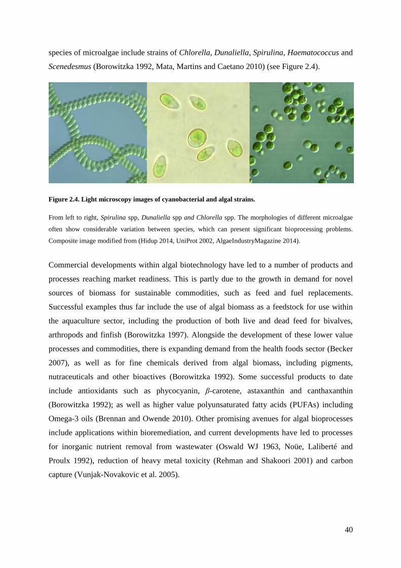
40

species of microalgae include strains of Chlorella, Dunaliella, Spirulina, Haematococcus and

Scenedesmus (Borowitzka 1992, Mata, Martins and Caetano 2010) (see Figure 2.4).

Figure 2.4. Light microscopy images of cyanobacterial and algal strains.

From left to right, Spirulina spp, Dunaliella spp and Chlorella spp. The morphologies of different microalgae

often show considerable variation between species, which can present significant bioprocessing problems.

Composite image modified from (Hidup 2014, UniProt 2002, AlgaeIndustryMagazine 2014).

Commercial developments within algal biotechnology have led to a number of products and

processes reaching market readiness. This is partly due to the growth in demand for novel

sources of biomass for sustainable commodities, such as feed and fuel replacements.

Successful examples thus far include the use of algal biomass as a feedstock for use within

the aquaculture sector, including the production of both live and dead feed for bivalves,

arthropods and finfish (Borowitzka 1997). Alongside the development of these lower value

processes and commodities, there is expanding demand from the health foods sector (Becker

2007), as well as for fine chemicals derived from algal biomass, including pigments,

nutraceuticals and other bioactives (Borowitzka 1992). Some successful products to date

include antioxidants such as phycocyanin, β-carotene, astaxanthin and canthaxanthin

(Borowitzka 1992); as well as higher value polyunsaturated fatty acids (PUFAs) including

Omega-3 oils (Brennan and Owende 2010). Other promising avenues for algal bioprocesses

include applications within bioremediation, and current developments have led to processes

for inorganic nutrient removal from wastewater (Oswald WJ 1963, Noüe, Laliberté and

Proulx 1992), reduction of heavy metal toxicity (Rehman and Shakoori 2001) and carbon

capture (Vunjak-Novakovic et al. 2005).

41

Algal Biofuels

Of all the current and projected algal applications, the one that has generated the most interest

in recent years is that of algal biofuel development (Mata et al. 2010). It is also an area that is

of the utmost importance to understanding both the current status and future potential of algal

biotechnology. Serious research into the field started in the mid-1970s, driven by an

accumulation of economic factors; which became particularly evident after the OPEC oil

embargo. This environment of fuel shortages created an incentive to investigate the potential

of using transesterified microalgal oil as a biofuel replacement for petroleum derived diesel.

Research efforts were boosted by the Carter administration via the creation of the aquatic

species program (ASP) in 1978 (Gao et al. 2012). Despite the closure of the program in 1996,

many of the advances in understanding the potential of algae as a source of biofuel stem from

this work (Sheehan et al. 1998). It was during this period that scientists first recognised

several advantages to producing biofuels from algae in comparison to other oleaginous crops.

One major benefit included the fact that large scale algal production would create less

competition with conventional food and feed production than other 1st and 2nd generation

biofuel sources (Beal et al. 2012). This meant that algal biofuels had the potential to develop

into a comparatively sustainable competitor to the petrochemical industry. Another advantage

against terrestrial plant based fuels was the potential for far greater areal productivity due to

the rapid growth rates displayed by many algal species (Mata et al. 2010). However, the one

property that really aroused the interest of scientists was the relatively high oil content of

many species. Oil levels in productive strains had been shown to range from 20-70% of dry

cell weight, which is considerably higher than the yield of any competing commercial crops.

As a rough comparison, this equates to the theoretical potential for natural oil production

between 20-30 times greater than current commercial oil producing crops per acre (Brennan

and Owende 2010).

The abundant levels of lipid produced by certain strains of microalgae include families of di-

or triglycerides, glycol- and phospholipids, as well as various species of hydrocarbons

(Sharma, Schuhmann and Schenk 2012). These lipid families can be categorised into those

with polar or neutral groups within the molecule. This distinction is important as the

composition of lipids within the cell can affect the efficiency of conversion into secondary

products such as biodiesel. Most existing technology for biodiesel production is optimised for

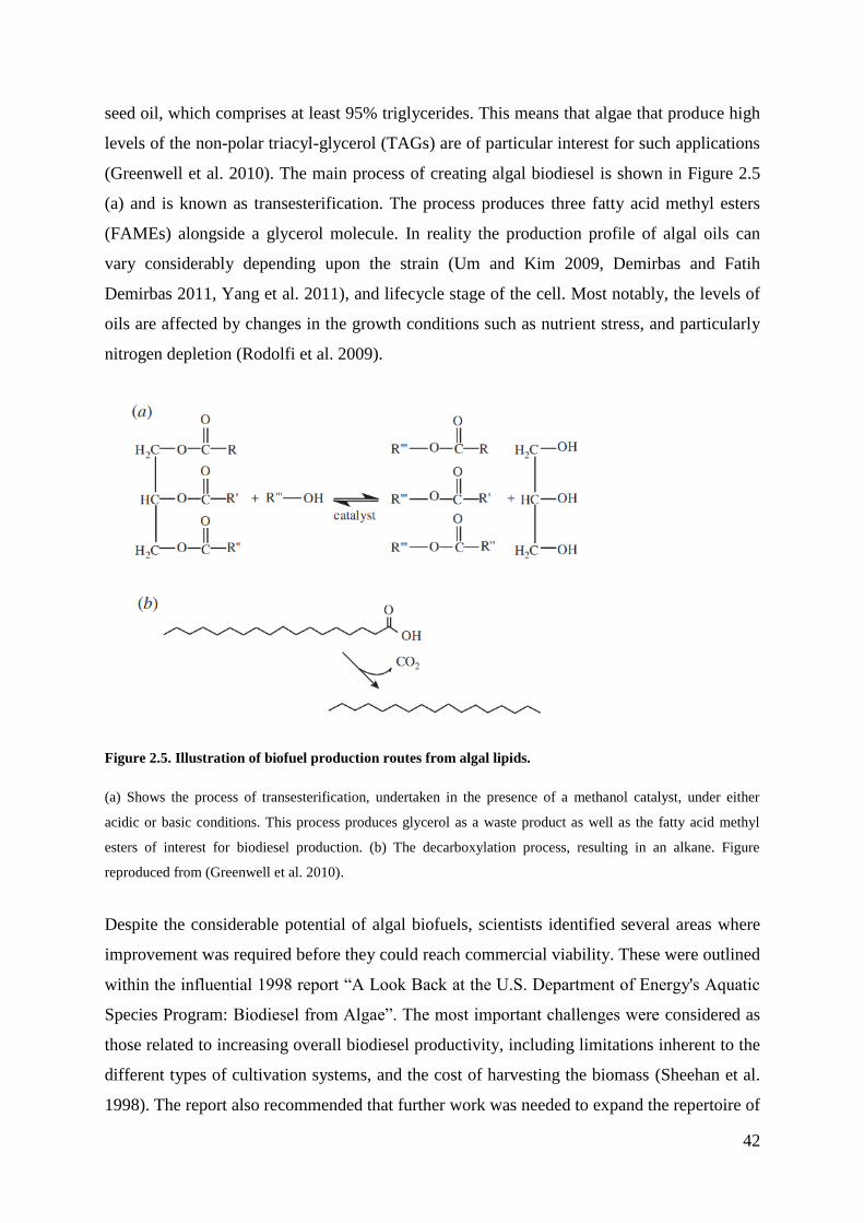
42

seed oil, which comprises at least 95% triglycerides. This means that algae that produce high

levels of the non-polar triacyl-glycerol (TAGs) are of particular interest for such applications

(Greenwell et al. 2010). The main process of creating algal biodiesel is shown in Figure 2.5

(a) and is known as transesterification. The process produces three fatty acid methyl esters

(FAMEs) alongside a glycerol molecule. In reality the production profile of algal oils can

vary considerably depending upon the strain (Um and Kim 2009, Demirbas and Fatih

Demirbas 2011, Yang et al. 2011), and lifecycle stage of the cell. Most notably, the levels of

oils are affected by changes in the growth conditions such as nutrient stress, and particularly

nitrogen depletion (Rodolfi et al. 2009).

Figure 2.5. Illustration of biofuel production routes from algal lipids.

(a) Shows the process of transesterification, undertaken in the presence of a methanol catalyst, under either

acidic or basic conditions. This process produces glycerol as a waste product as well as the fatty acid methyl

esters of interest for biodiesel production. (b) The decarboxylation process, resulting in an alkane. Figure

reproduced from (Greenwell et al. 2010).

Despite the considerable potential of algal biofuels, scientists identified several areas where

improvement was required before they could reach commercial viability. These were outlined

within the influential 1998 report “A Look Back at the U.S. Department of Energy's Aquatic

Species Program: Biodiesel from Algae”. The most important challenges were considered as

those related to increasing overall biodiesel productivity, including limitations inherent to the

different types of cultivation systems, and the cost of harvesting the biomass (Sheehan et al.

1998). The report also recommended that further work was needed to expand the repertoire of

43

robust algal strains; capable both of producing high levels of oil, as well as offering resilience

to a host of biotic and abiotic conditions. Current research is building upon these themes and

exploring the development of less energy intensive biomass harvesting techniques; as well as

improving overall operational costs, through better reactor design, as well as location and

feedstock selection (Greenwell et al. 2010).

The Future of Algal Biotechnology

The Role of Algae within a Bio-based Economy

Algal derived biofuels continue to be a high profile area of research, capable of commanding

a high level of both public and private funding, attested by practical collaborations like the

EnAlgae project in the EU. These developmental drives have led to a considerable increase in

applied understanding, and brought the mass production of algal biomass to the cusp of

commercial feasibility (Borowitzka 1999). Despite these advances, it could be said that

enthusiasm for the algal biofuels sector has started to subside, and both governmental and

private investment has dropped. The reasons for this change are numerous, and can be

described as being primarily driven by events in the United States, where the critical

momentum of many algae biofuel start-ups imploded in the early 2010s. These events were

compounded by a backdrop of wider capital flight from ‘Cleantech’ sectors during the

financial crash. Prominent examples of this changing market dynamic include GreenFuels

which folded despite $70 million of private equity investment, when backers found that

company claims did not match the scientific reality (Voosen 2011). Other notable companies

have re-positioned to survive. This includes Solazyme, who are now producers of both

biofuels and algal derived medium-to-higher value products. Likewise, OriginOil now focus

their business proposition on water separation and remediation technology, having changed

their name to OriginClear (www.originclear.com). Finally, Algenol Biotech LLC have

recently re-structured their business to move away from biofuel production, triggering the

resignation of their CEO and a 25% reduction in staff numbers (Lane 2015).

44

As the algal biotech community readjusts itself to what could be described as a post-biofuel

paradigm it has started to re-diversify research and development priorities accordingly. As

discussed in Chapter 1, the move towards more sustainable processes within chemical

manufacture has led to an increase in the exploration of novel and under-used biomass as a

source of renewable feedstock. This transition to a ‘bio-based’ economy could have

considerable benefits both in terms of reducing environmental impact, as well as bringing

economic prosperity through ‘green job’ creation (Jenkins 2008). Central to the bio-based

economy is the development of a network of biorefineries, capable of processing a wide array

of feedstock inputs. At the lower end of the value chain potential interest is growing for algal

use as an animal feed, as a raw material for bulk chemical production, or feedstock for

pyrolysis or anaerobic digestion (Subhadra and Grinson 2011). At the higher end of the value

chain interest in using algal derived bio-actives for pharmaceutical and nutraceutical purposes

continues to grow (Yaakob et al. 2014). Given the extensive production costs already

identified during the development of algal biofuel research, it is likely that in the short to

medium term these higher value products will offer the most promising immediate routes to

market.

Biorefineries and Industrial Symbiosis

As previously discussed, the production of lower value or ‘bulk’ algal biomass is constrained

in part due to the relatively high production costs and low productivities associated with most

types of cultivation process (Hannon et al. 2010). One potential solution may be to create a

more integrated style of algal production. Such approaches have been used in other industries

and collectively described as ‘industrial symbiosis’. The approach borrows heavily from

systems analysis, integrating mass and material flows between industries, tying individual

partners together through the exchange of waste streams, which act as feedstock for co-

located partners (Chertow 2000, Chertow 2007). The ultimate aim of this type of approach is

to change industrial processes from linear open loop systems to more sustainable closed loop

systems. This philosophy draws inspiration from the fact that many natural systems do not

have waste products, and run as part of an integrated whole (Erkman 1997).Within the

framework of an industrial symbiosis approach, there are considerable drivers to reduce

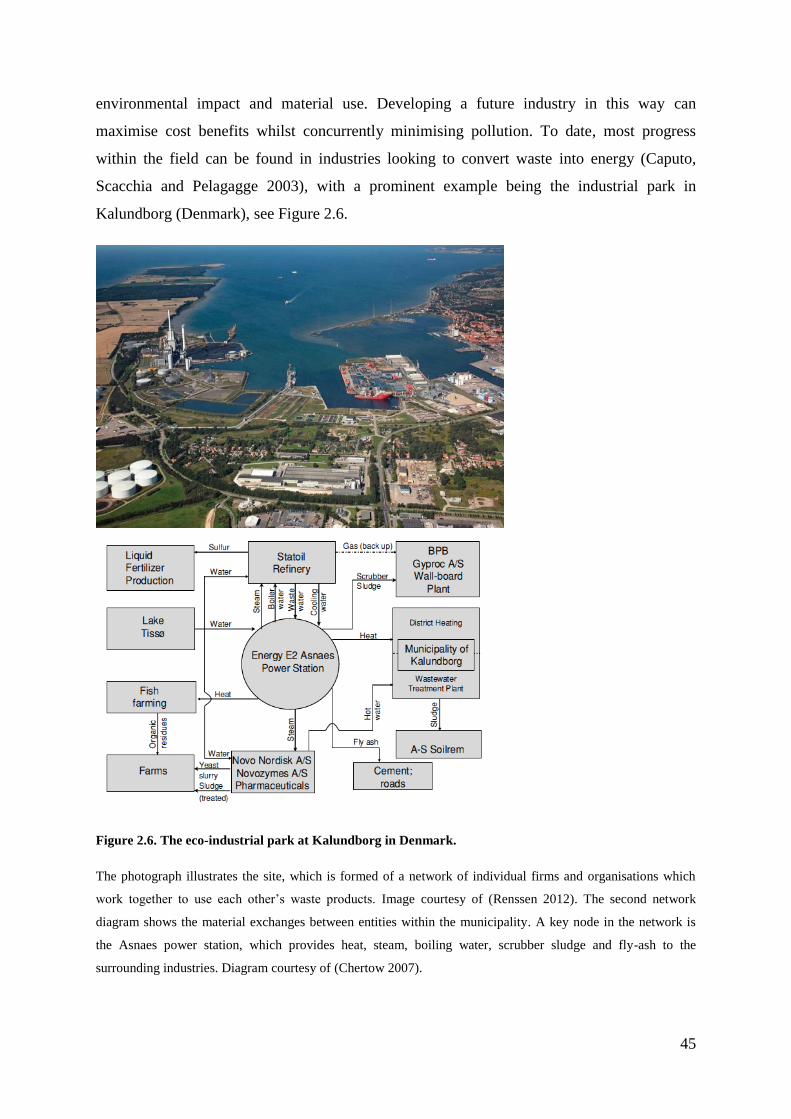
45

environmental impact and material use. Developing a future industry in this way can

maximise cost benefits whilst concurrently minimising pollution. To date, most progress

within the field can be found in industries looking to convert waste into energy (Caputo,

Scacchia and Pelagagge 2003), with a prominent example being the industrial park in

Kalundborg (Denmark), see Figure 2.6.

Figure 2.6. The eco-industrial park at Kalundborg in Denmark.

The photograph illustrates the site, which is formed of a network of individual firms and organisations which

work together to use each other’s waste products. Image courtesy of (Renssen 2012). The second network

diagram shows the material exchanges between entities within the municipality. A key node in the network is

the Asnaes power station, which provides heat, steam, boiling water, scrubber sludge and fly-ash to the

surrounding industries. Diagram courtesy of (Chertow 2007).

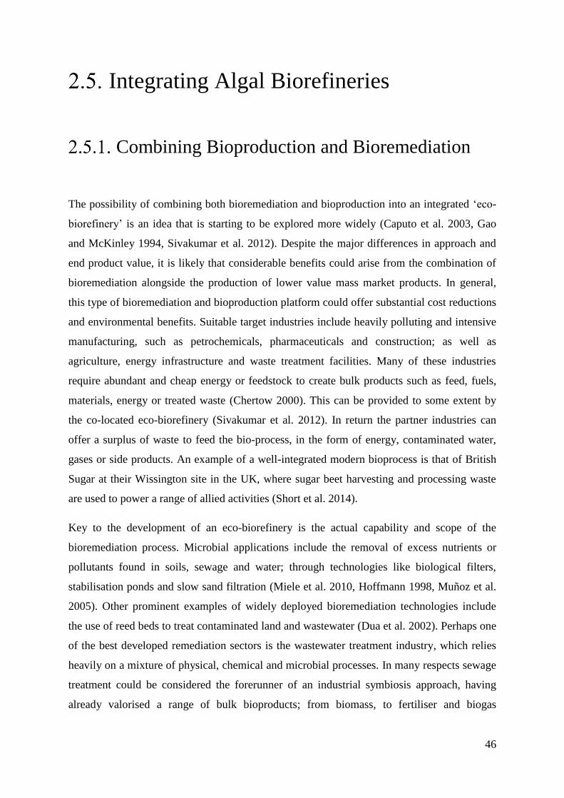
46

Integrating Algal Biorefineries

Combining Bioproduction and Bioremediation

The possibility of combining both bioremediation and bioproduction into an integrated ‘eco-

biorefinery’ is an idea that is starting to be explored more widely (Caputo et al. 2003, Gao

and McKinley 1994, Sivakumar et al. 2012). Despite the major differences in approach and

end product value, it is likely that considerable benefits could arise from the combination of

bioremediation alongside the production of lower value mass market products. In general,

this type of bioremediation and bioproduction platform could offer substantial cost reductions

and environmental benefits. Suitable target industries include heavily polluting and intensive

manufacturing, such as petrochemicals, pharmaceuticals and construction; as well as

agriculture, energy infrastructure and waste treatment facilities. Many of these industries

require abundant and cheap energy or feedstock to create bulk products such as feed, fuels,

materials, energy or treated waste (Chertow 2000). This can be provided to some extent by

the co-located eco-biorefinery (Sivakumar et al. 2012). In return the partner industries can

offer a surplus of waste to feed the bio-process, in the form of energy, contaminated water,

gases or side products. An example of a well-integrated modern bioprocess is that of British

Sugar at their Wissington site in the UK, where sugar beet harvesting and processing waste

are used to power a range of allied activities (Short et al. 2014).

Key to the development of an eco-biorefinery is the actual capability and scope of the

bioremediation process. Microbial applications include the removal of excess nutrients or

pollutants found in soils, sewage and water; through technologies like biological filters,

stabilisation ponds and slow sand filtration (Miele et al. 2010, Hoffmann 1998, Muñoz et al.

2005). Other prominent examples of widely deployed bioremediation technologies include

the use of reed beds to treat contaminated land and wastewater (Dua et al. 2002). Perhaps one

of the best developed remediation sectors is the wastewater treatment industry, which relies

heavily on a mixture of physical, chemical and microbial processes. In many respects sewage

treatment could be considered the forerunner of an industrial symbiosis approach, having

already valorised a range of bulk bioproducts; from biomass, to fertiliser and biogas

47

(Berglund and Börjesson 2006). Whilst the ability to use living organisms in eco-biorefinery

platforms is considerable, there can be a range of performance and cost related problems that

can limit widespread deployment of such an approach. This can include issues of inconsistent

feedstock quality, high treatment costs and unstable process dynamics.

Algal production could have a distinct and major advantage over many other treatment

technologies, in being able to couple both valuable biomass production and useful waste

remediation activities within one consolidated process (Borowitzka 1992). To date, this type

of approach has not been adopted on a holistic scale within algal production facilities

(Soratana and Landis 2011); and could assist a sector in its relative infancy in Europe (Taylor

2008, Greenwell et al. 2010, Hannon et al. 2010). This type of approach could also broaden

the repertoire of bulk products that could be produced profitably from algae (Borowitzka

1992, Chisti 2007, Soratana and Landis 2011). However, to make an algal eco-biorefinery

more feasible it is likely that considerable process improvements still have to be made. Key

areas include increasing productivity, whilst reducing capital and operating costs (CAPEX

and OPEX). This could theoretically be achieved by growing algae from a combination of

common waste streams, using an integrated and simple system design (Greenwell et al. 2010,

Juhasz and Naidu 2000, Gao and McKinley 1994, Muñoz and Guieysse 2006). Some key

considerations for an algal biorefinery are outlined in Figure 2.7.

Figure 2.7. Outline of considerations for an algal biorefinery.

48

Options for Co-location

A consideration of the requirements for algal growth outlined in Section 2.2 would indicate

that the ideal industry for co-location would have access to light for photosynthesis, ample

nutrients for growth, as well as cheap energy for mixing, heating and cooling. To date the

literature has offered several examples of co-located algal production as examples, with many

facilities situated beside power stations. Positioning in this way provides a free and consistent

source of flue gases, with carbon dioxide concentrations within these streams often varying

from 5-15% in concentration, dependent on the source (Vunjak-Novakovic et al. 2005,

Doucha, Straka and Lívanský 2005, Yoshihara et al. 1996). There is also considerable

potential for other environmental benefits to be derived from such a co-location process. For

example, power stations (or any other type of heavy industry) produce considerable levels of

waste heat, which can be used to maintain the temperature within a culture or contribute to

biomass drying. To date, there have been several examples of this type of co-location; with

one particularly notable case coming from the co-location of an airlift photobioreactor

besides the power station at the Massachusetts Institute of Technology (MIT). The results

from this work showed good algal growth and gas scrubbing potential, with reductions in

CO2 and NOx in the region of 80-95% (Vunjak-Novakovic et al. 2005). Despite this success

the project was short lived, and did not consider the combination of additional waste streams

into the production process.

Although power stations would provide the ideal location both for energy provision and

remediation potential, smaller industrial processes could also be utilised. This is because in

reality most power stations would produce energy and carbon dioxide far in excess of

requirements for an algal bioprocess. For example other options could include using diesel

back-up generators, incinerators and biogas production facilities. The literature would also

stipulate that co-location beside a source of nutrients for the algae would be particularly

favourable to the process economics (Noüe et al. 1992, Brennan and Owende 2010).

Conventional examples would include situating besides a wastewater treatment facility. This

allows for the benefits of a free feedstock, whilst also allowing for the algae to remediate the

water, lowering concentrations of nitrates and phosphates. Other interesting examples of co-

location include placing a photobioreactor adjacent to any fishery or farming activity, which

also produce large quantities of nutrient-rich wastewater. Again, the benefits derived from

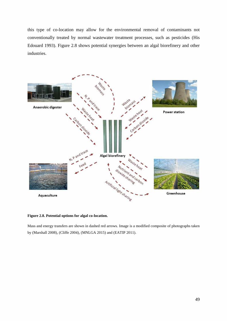
49

this type of co-location may allow for the environmental removal of contaminants not

conventionally treated by normal wastewater treatment processes, such as pesticides (His

Edouard 1993). Figure 2.8 shows potential synergies between an algal biorefinery and other

industries.

Figure 2.8. Potential options for algal co-location.

Mass and energy transfers are shown in dashed red arrows. Image is a modified composite of photographs taken

by (Marshall 2008), (Cliffe 2004), (MNLGA 2015) and (EATIP 2011).

50

3. Thesis Overview and Structure

3.1. Research Aims and Objectives

3.1.1. Overview

The initial literature review undertaken in Chapter 2 indicates that the creation of an

integrated algal eco-biorefinery shows considerable potential; both in terms of introducing

lower value biomass into the market place and undertaking useful remediation services. This

hypothesis is grounded in a current consensus that the production of algae solely for biofuels

and other bulk compounds would prove challenging given current petrochemical prices and

wider economic factors (Chisti 2008, Greenwell et al. 2010). Despite this fact, there are

relatively few direct technological barriers to cultivating algae on a large scale, with problems

instead centring on high CAPEX and OPEX of commercial systems (Darzins 2010, Brennan

and Owende 2010). From a practical perspective, the use of algae as a remediation platform

requires a combination of low cost feedstock inputs to produce cheap algal biomass, whilst

simultaneously generating quantifiable environmental benefits. The project will therefore aim

to profile and select a suitable strain, followed by quantification of appropriate waste

feedstock and treatment processes. As part of designing an integrated eco-biorefinery, the

design and construction of a lower cost and fully scalable photobioreactor would be an

important consideration. Once the prototype is fully functional, quantification of the reactor

performance will be conducted, as will a comprehensive cost assessment. It is hypothesised

that by combining remediation with a novel reactor design numerous commercially relevant

process savings could be implemented.

51

3.1.2. Strain Selection and Growth Kinetics

A key requirement for any bioprocess is to select a suitable species. For this project, this

would mean selecting a robust algal strain capable of rapid growth and remediation. In the

first instance this research will be undertaken through a literature review and consultation

process with Dr Saul Purton’s group (SMB, UCL). The results in this section provide a

detailed experimental exploration of the parameter space for Chlorella sorokiniana

(UTEX1230) at micro and laboratory scale. The research is benchmarked against literature

values to offer insight into the potential for subsequent scale-up. The findings are shown in

Chapter 4.

3.1.3. Growing Chlorella sorokiniana on Wastewater

The specific objectives of this section were to compare the growth characteristics,

productivity and yield of C. sorokiniana on both wastewater and commercial medium, whilst

assessing the influence of flue gas addition on the process. The literature indicates that many

strains of algae are capable of growing and remediating wastewaters (Abeliovich and

Weisman 1978, Muñoz and Guieysse 2006); and this work intends to provide a preliminary

and small scale quantitative evaluation of the potential of coupling biomass production to

remediation at laboratory scale. The research builds from that of Chapter 4, moving onto

testing the suitability of a variety of wastewater types and flue gas concentrations to ascertain

the extent of any effects that these feed inputs have on the growth and productivity of the

selected strain. The results are shown in Chapter 5.

3.1.4. Reactor Design, Construction and Validation

Looking at production issues in more detail, one can ascertain that few photobioreactor

designs within the literature are optimised for both lower value waste remediation activities

and biomass productivity (Noüe et al. 1992, Kumar et al. 2010). Such a reactor would be

52

necessary for a combined biorefinery and remediation process, and this part of the thesis

describes the rationale behind the design and construction of a novel photobioreactor suited

for this purpose. The first step shows a design rationalisation, followed by exploration of the

necessary operational parameters based upon a literature review. Particular consideration is

given to the creation of a fully scalable and economical photobioreactor, which can undertake

bioremediation activities whilst producing high yields of biomass. This is achieved by

validating the reactor through a combination of modelling and experimental approaches,

including a preliminary pilot study. The findings from this work are shown in Chapters 6-7.

3.1.5. Cost Model of Tertiary Wastewater Treatment

The final part of the thesis investigates the costs related to the manufacturing of the

photobioreactor, and benchmarks the system to other platforms within the literature. The next

part of the cost modelling considers phosphorus removal using an integrated algal eco-

biorefinery, and explores the benefits derived from appropriate industrial symbiosis

networking. Finally, the system is compared to other treatment platforms. The results are

shown in Chapter 8.

3.1.6. Conclusions and Discussion

The results from each chapter are summarised in Chapter 9, with a particular focus on the

relevance of the findings to the applied algal biotechnology, as well as proposing interesting

avenues for further research. The thesis then concludes with a discussion of current

technology trends and thoughts on how best to develop the algal sector within the UK.

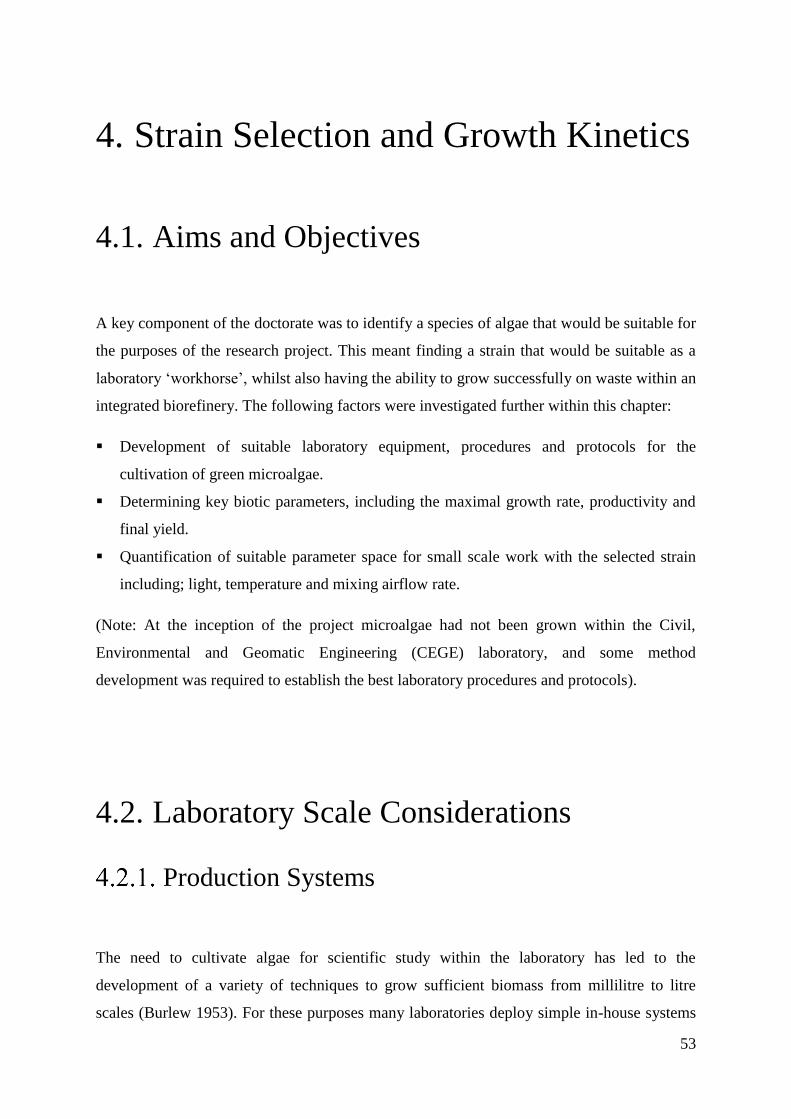
53

4. Strain Selection and Growth Kinetics

4.1. Aims and Objectives

A key component of the doctorate was to identify a species of algae that would be suitable for

the purposes of the research project. This meant finding a strain that would be suitable as a

laboratory ‘workhorse’, whilst also having the ability to grow successfully on waste within an

integrated biorefinery. The following factors were investigated further within this chapter:

Development of suitable laboratory equipment, procedures and protocols for the

cultivation of green microalgae.

Determining key biotic parameters, including the maximal growth rate, productivity and

final yield.

Quantification of suitable parameter space for small scale work with the selected strain

including; light, temperature and mixing airflow rate.

(Note: At the inception of the project microalgae had not been grown within the Civil,

Environmental and Geomatic Engineering (CEGE) laboratory, and some method

development was required to establish the best laboratory procedures and protocols).

4.2. Laboratory Scale Considerations

Production Systems

The need to cultivate algae for scientific study within the laboratory has led to the

development of a variety of techniques to grow sufficient biomass from millilitre to litre

scales (Burlew 1953). For these purposes many laboratories deploy simple in-house systems

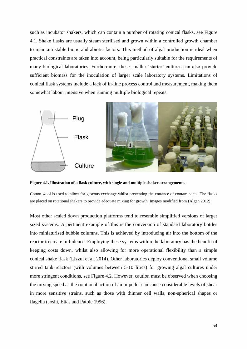
54

such as incubator shakers, which can contain a number of rotating conical flasks, see Figure

4.1. Shake flasks are usually steam sterilised and grown within a controlled growth chamber

to maintain stable biotic and abiotic factors. This method of algal production is ideal when

practical constraints are taken into account, being particularly suitable for the requirements of

many biological laboratories. Furthermore, these smaller ‘starter’ cultures can also provide

sufficient biomass for the inoculation of larger scale laboratory systems. Limitations of

conical flask systems include a lack of in-line process control and measurement, making them

somewhat labour intensive when running multiple biological repeats.

Figure 4.1. Illustration of a flask culture, with single and multiple shaker arrangements.

Cotton wool is used to allow for gaseous exchange whilst preventing the entrance of contaminants. The flasks

are placed on rotational shakers to provide adequate mixing for growth. Images modified from (Algen 2012).

Most other scaled down production platforms tend to resemble simplified versions of larger

sized systems. A pertinent example of this is the conversion of standard laboratory bottles

into miniaturised bubble columns. This is achieved by introducing air into the bottom of the

reactor to create turbulence. Employing these systems within the laboratory has the benefit of

keeping costs down, whilst also allowing for more operational flexibility than a simple

conical shake flask (Lizzul et al. 2014). Other laboratories deploy conventional small volume

stirred tank reactors (with volumes between 5-10 litres) for growing algal cultures under

more stringent conditions, see Figure 4.2. However, caution must be observed when choosing

the mixing speed as the rotational action of an impeller can cause considerable levels of shear

in more sensitive strains, such as those with thinner cell walls, non-spherical shapes or

flagella (Joshi, Elias and Patole 1996).

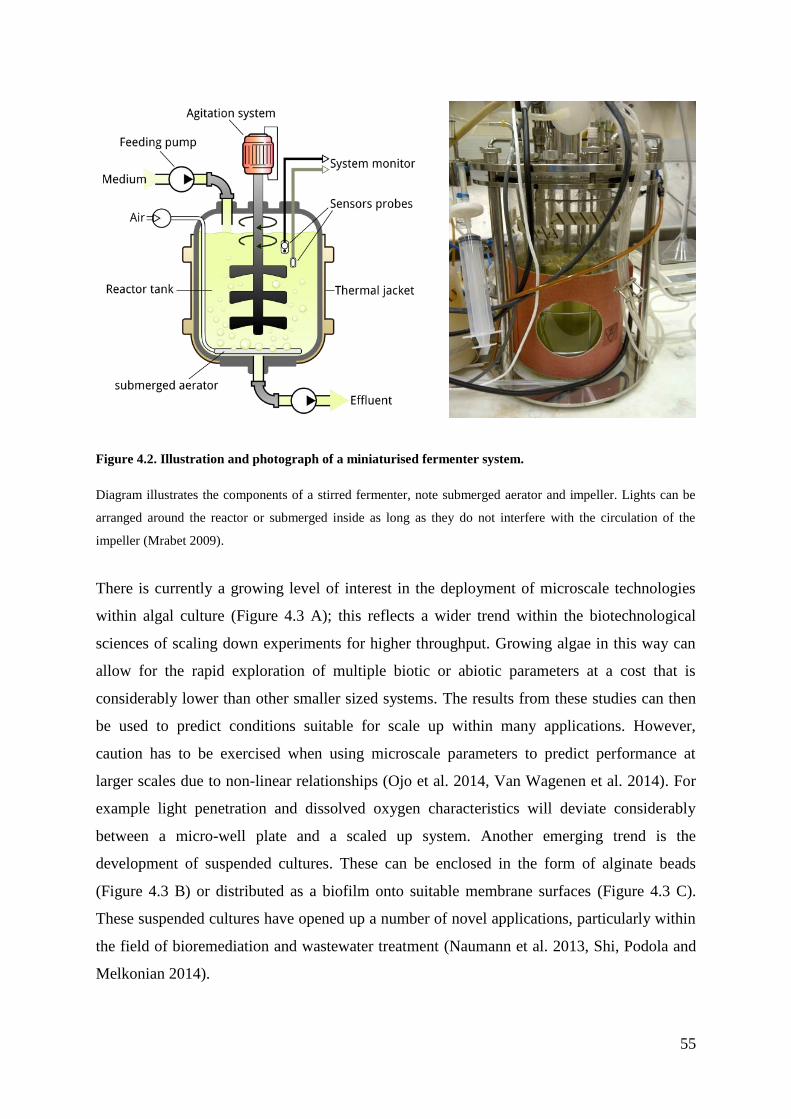
55

Figure 4.2. Illustration and photograph of a miniaturised fermenter system.

Diagram illustrates the components of a stirred fermenter, note submerged aerator and impeller. Lights can be

arranged around the reactor or submerged inside as long as they do not interfere with the circulation of the

impeller (Mrabet 2009).

There is currently a growing level of interest in the deployment of microscale technologies

within algal culture (Figure 4.3 A); this reflects a wider trend within the biotechnological

sciences of scaling down experiments for higher throughput. Growing algae in this way can

allow for the rapid exploration of multiple biotic or abiotic parameters at a cost that is

considerably lower than other smaller sized systems. The results from these studies can then

be used to predict conditions suitable for scale up within many applications. However,

caution has to be exercised when using microscale parameters to predict performance at

larger scales due to non-linear relationships (Ojo et al. 2014, Van Wagenen et al. 2014). For

example light penetration and dissolved oxygen characteristics will deviate considerably

between a micro-well plate and a scaled up system. Another emerging trend is the

development of suspended cultures. These can be enclosed in the form of alginate beads

(Figure 4.3 B) or distributed as a biofilm onto suitable membrane surfaces (Figure 4.3 C).

These suspended cultures have opened up a number of novel applications, particularly within

the field of bioremediation and wastewater treatment (Naumann et al. 2013, Shi, Podola and

Melkonian 2014).

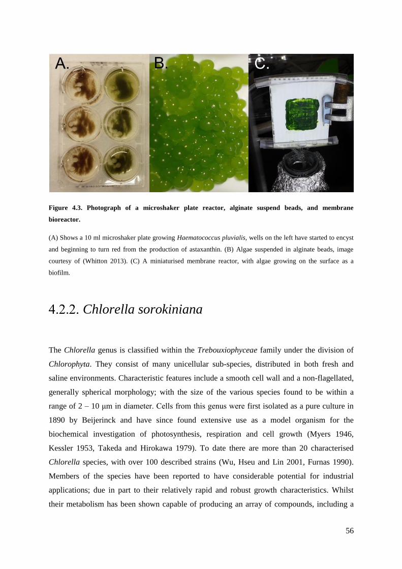
56

Figure 4.3. Photograph of a microshaker plate reactor, alginate suspend beads, and membrane

bioreactor.

(A) Shows a 10 ml microshaker plate growing Haematococcus pluvialis, wells on the left have started to encyst

and beginning to turn red from the production of astaxanthin. (B) Algae suspended in alginate beads, image

courtesy of (Whitton 2013). (C) A miniaturised membrane reactor, with algae growing on the surface as a

biofilm.

Chlorella sorokiniana

The Chlorella genus is classified within the Trebouxiophyceae family under the division of

Chlorophyta. They consist of many unicellular sub-species, distributed in both fresh and

saline environments. Characteristic features include a smooth cell wall and a non-flagellated,

generally spherical morphology; with the size of the various species found to be within a

range of 2 – 10 μm in diameter. Cells from this genus were first isolated as a pure culture in

1890 by Beijerinck and have since found extensive use as a model organism for the

biochemical investigation of photosynthesis, respiration and cell growth (Myers 1946,

Kessler 1953, Takeda and Hirokawa 1979). To date there are more than 20 characterised

Chlorella species, with over 100 described strains (Wu, Hseu and Lin 2001, Furnas 1990).

Members of the species have been reported to have considerable potential for industrial

applications; due in part to their relatively rapid and robust growth characteristics. Whilst

their metabolism has been shown capable of producing an array of compounds, including a

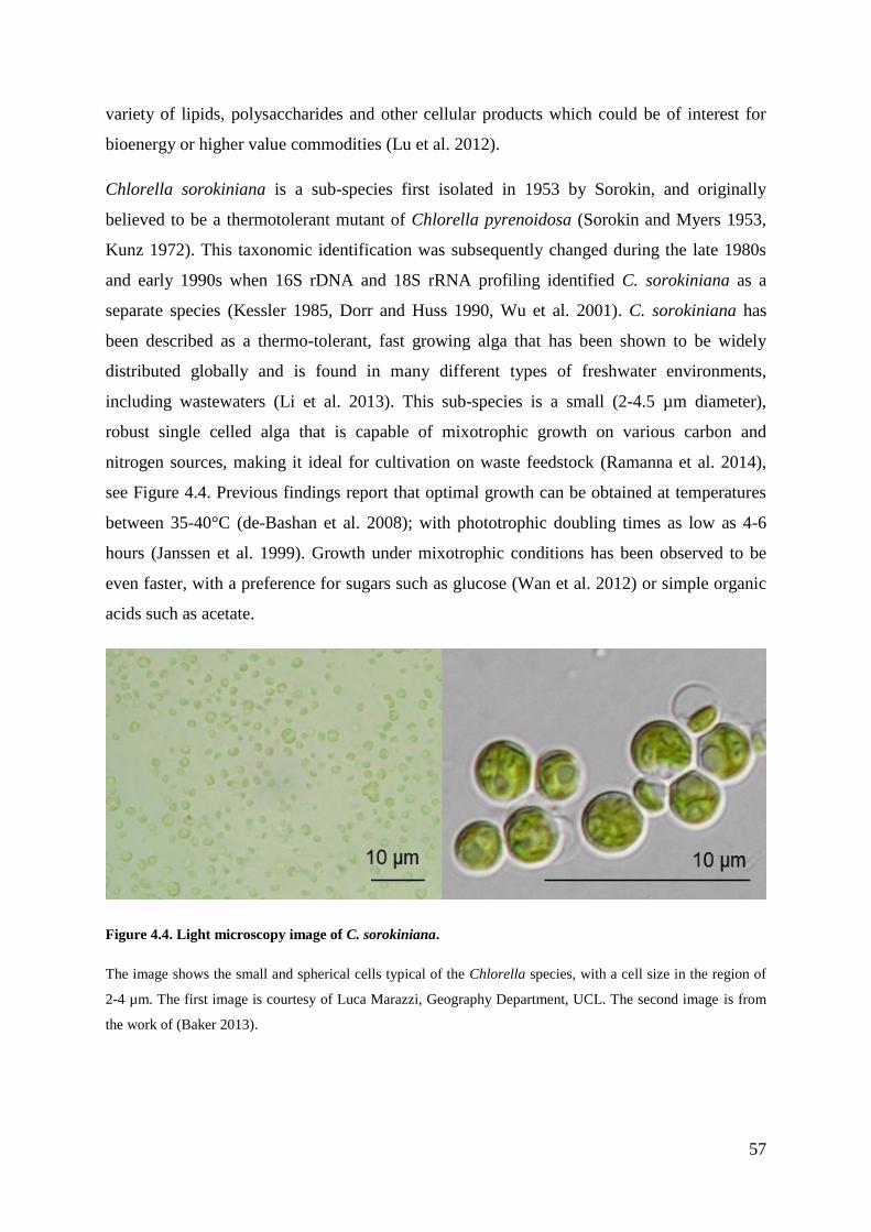
57

variety of lipids, polysaccharides and other cellular products which could be of interest for

bioenergy or higher value commodities (Lu et al. 2012).

Chlorella sorokiniana is a sub-species first isolated in 1953 by Sorokin, and originally

believed to be a thermotolerant mutant of Chlorella pyrenoidosa (Sorokin and Myers 1953,

Kunz 1972). This taxonomic identification was subsequently changed during the late 1980s

and early 1990s when 16S rDNA and 18S rRNA profiling identified C. sorokiniana as a

separate species (Kessler 1985, Dorr and Huss 1990, Wu et al. 2001). C. sorokiniana has

been described as a thermo-tolerant, fast growing alga that has been shown to be widely

distributed globally and is found in many different types of freshwater environments,

including wastewaters (Li et al. 2013). This sub-species is a small (2-4.5 µm diameter),

robust single celled alga that is capable of mixotrophic growth on various carbon and

nitrogen sources, making it ideal for cultivation on waste feedstock (Ramanna et al. 2014),

see Figure 4.4. Previous findings report that optimal growth can be obtained at temperatures

between 35-40°C (de-Bashan et al. 2008); with phototrophic doubling times as low as 4-6

hours (Janssen et al. 1999). Growth under mixotrophic conditions has been observed to be

even faster, with a preference for sugars such as glucose (Wan et al. 2012) or simple organic

acids such as acetate.

Figure 4.4. Light microscopy image of C. sorokiniana.

The image shows the small and spherical cells typical of the Chlorella species, with a cell size in the region of

2-4 µm. The first image is courtesy of Luca Marazzi, Geography Department, UCL. The second image is from

the work of (Baker 2013).

58

The species is widely recognised as having industrial potential, and has been shown to be

sufficiently robust for scale-up in air-mixed (Béchet et al. 2012) or liquid-mixed

photobioreactors (Lee et al. 1996). Previous work has also demonstrated that C. sorokiniana

is able to grow on wastewaters under conditions that would be unfavourable for other algal

species, making it potentially suited to a bioremediation-biorefinery approach (de-Bashan et

al. 2008). In this respect the findings suggest particular suitability for nutrient removal; 0.14

mg h-1 for N-NO3 and 0.03 mg h-1 for P-PO4-3 (Shriwastav et al. 2014). Analysis of C.

sorokiniana dry weight shows that the species is composed on average of 40% protein, 30-

38% carbohydrate and 18-22% lipid (Belkoura, Benider and Dauta 1997, Illman, Scragg and

Shales 2000, Gouveia and Oliveira 2009). Prior research has shown that C. sorokiniana

biomass may be well suited to bulk commodity production, in particular the large scale

production of lipid for biofuel (Kumar et al. 2011, Mizuno et al. 2013). Some other specific

compounds of commercial interest include antioxidants like carotenoids, which make up to

0.69% of dry weight under extremophilic conditions (Matsukawa et al. 2000). Furthermore,

research has shown that genetic transformation of C. sorokiniana is possible, opening up

routes for the expression of a range of transgenic products (Dawson, Burlingame and

Cannons 1997).

4.3. Experimental Methodology

4.3.1. Strain List

Collaboration with Dr Saul Purton’s group at University College London, Department of

Structural and Molecular Biology (UCL, SMB) allowed for access to several algal strains

within the UCL working catalogue. These strains were originally purchased from the

following culture collections; the University of Texas, Austen, US (UTEX -

web.biosci.utexas.edu/utex), the Culture Collection of Algae and Protozoa (CCAP -

http://www.ccap.ac.uk/) and the Scandinavian Culture Collection of Algae and Protozoa

59

(SCCAP- http://www.sccap.dk/). Strains were maintained on Bold’s Basal Medium (BBM),

composition listed in Appendix 10.1.1.1 (Sigma Aldrich). The tested strains included

Chlorella sorokiniana (UTEX1230), Chlamydomonas reinhardtii (CC-1021) and

Scenedesmus dimorphus (CCAP 276/48).

4.3.2. Preliminary Strain Selection Experiments

To investigate the feasibility of growing algae under laboratory conditions, the listed algal

strains were grown at 25°C in 50 ml of BBM (Sigma), under 50 µE m-2 s-1 of artificial light,

provided by one 18 W fluorescent bulb (Gro-Lux). Cultures were continuously shaken at 250

rpm for a 10 day period. Growth was measured by following the increase in optical density,

using the methods outlined in 4.3.5, with light intensity being measured using an Apogee

MQ-100 PAR meter.

4.3.3. Formulas

4.3.3.1. Deriving the Maximal Growth Rate

The maximum specific growth rate (𝜇𝑚𝑎𝑥) was deduced by taking the natural logarithm of

the biomass concentration and plotting against time. The linear portion of the logarithmic plot

was then evaluated to determine the duration of the exponential phase, and the gradient

judged equal to (𝜇𝑚𝑎𝑥 ). This process is represented in Eq. 3, with the terms 𝑋1 and 𝑋0

corresponding to the algal concentration at times 𝑡1 and 𝑡0 respectively (Doran 1995).

𝜇𝑚𝑎𝑥 =ln(𝑋1) − ln (𝑋0)

𝑡1 − 𝑡0

Eq. 3

60

4.3.3.2. Final Yield and Productivity

The final biomass yield (𝑋𝑌) was determined by subtracting the final biomass concentration

from the initial biomass concentration (Eq. 4). Biomass and lipid productivity (𝑃𝑋 and 𝑃𝐿)

were calculated on a batch basis (Eqs. 5 and 6), by dividing the final product yield by the

total number of hours or days within the experiment taken to reach stationary phase. Where

𝑋1 and 𝑋0 or 𝐿1 and 𝐿0 correspond to the algal density and lipid concentration at times 𝑡1

and 𝑡0 respectively (Doran 1995).

𝑋𝑌 = 𝑋𝑡−𝑋0 Eq. 4

𝑃𝑋 =𝑋1−𝑋0𝑡1 − 𝑡0

Eq. 5

𝑃𝐿 =𝐿1−𝐿0𝑡1 − 𝑡0

Eq. 6

4.3.3.3. Doubling Time

The doubling time (𝐷𝑡) was calculated according to the relationship described in Eq. 7, using

an appropriate specific growth rate (𝜇) (Doran 1995).

𝐷𝑡 =ln2

𝜇 Eq. 7

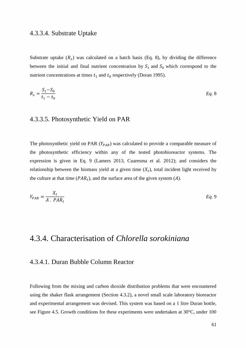
61

4.3.3.4. Substrate Uptake

Substrate uptake (𝑅𝑠) was calculated on a batch basis (Eq. 8), by dividing the difference

between the initial and final nutrient concentration by 𝑆1 and 𝑆0 which correspond to the

nutrient concentrations at times 𝑡1 and 𝑡0 respectively (Doran 1995).

𝑅𝑠 =𝑆1−𝑆0𝑡1 − 𝑡0

Eq. 8

4.3.3.5. Photosynthetic Yield on PAR

The photosynthetic yield on PAR (𝑌𝑃𝐴𝑅) was calculated to provide a comparable measure of

the photosynthetic efficiency within any of the tested photobioreactor systems. The

expression is given in Eq. 9 (Lamers 2013, Cuaresma et al. 2012); and considers the

relationship between the biomass yield at a given time (𝑋𝑡), total incident light received by

the culture at that time (𝑃𝐴𝑅𝑡), and the surface area of the given system (𝐴).

𝑌𝑃𝐴𝑅 =𝑋𝑡

𝐴 . 𝑃𝐴𝑅𝑡 Eq. 9

4.3.4. Characterisation of Chlorella sorokiniana

4.3.4.1. Duran Bubble Column Reactor

Following from the mixing and carbon dioxide distribution problems that were encountered

using the shaker flask arrangement (Section 4.3.2), a novel small scale laboratory bioreactor

and experimental arrangement was devised. This system was based on a 1 litre Duran bottle,

see Figure 4.5. Growth conditions for these experiments were undertaken at 30°C, under 100

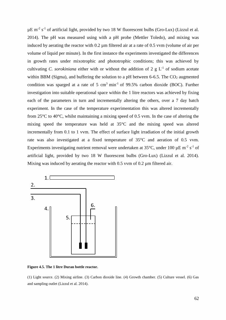
62

µE m-2 s-1 of artificial light, provided by two 18 W fluorescent bulbs (Gro-Lux) (Lizzul et al.

2014). The pH was measured using with a pH probe (Mettler Toledo), and mixing was

induced by aerating the reactor with 0.2 µm filtered air at a rate of 0.5 vvm (volume of air per

volume of liquid per minute). In the first instance the experiments investigated the differences

in growth rates under mixotrophic and phototrophic conditions; this was achieved by

cultivating C. sorokiniana either with or without the addition of 2 g L-1 of sodium acetate

within BBM (Sigma), and buffering the solution to a pH between 6-6.5. The CO2 augmented

condition was sparged at a rate of 5 cm3 min-1 of 99.5% carbon dioxide (BOC). Further

investigation into suitable operational space within the 1 litre reactors was achieved by fixing

each of the parameters in turn and incrementally altering the others, over a 7 day batch

experiment. In the case of the temperature experimentation this was altered incrementally

from 25°C to 40°C, whilst maintaining a mixing speed of 0.5 vvm. In the case of altering the

mixing speed the temperature was held at 35°C and the mixing speed was altered

incrementally from 0.1 to 1 vvm. The effect of surface light irradiation of the initial growth

rate was also investigated at a fixed temperature of 35°C and aeration of 0.5 vvm.

Experiments investigating nutrient removal were undertaken at 35°C, under 100 µE m-2 s-1 of

artificial light, provided by two 18 W fluorescent bulbs (Gro-Lux) (Lizzul et al. 2014).

Mixing was induced by aerating the reactor with 0.5 vvm of 0.2 µm filtered air.

Figure 4.5. The 1 litre Duran bottle reactor.

(1) Light source. (2) Mixing airline. (3) Carbon dioxide line. (4) Growth chamber. (5) Culture vessel. (6) Gas

and sampling outlet (Lizzul et al. 2014).

63

4.3.4.2. Microshaker Platform

As the project developed further it became apparent that the use of the 1 litre Duran bottles

was a cumbersome approach for triplicate experimentation. This was particularly the case for

screening methodologies and parameter space exploration. To undertake these higher

throughput experiments a growth chamber was built in-house around a conventional

Microshaker (SciQuip) with a tray capacity for two microplates. Experiments were

undertaken within 6-well plates, with a total capacity of 10 ml in each well, see Figure 4.6.

Agitation was achieved with a platform rotation of 120 rpm and the wells contained a

circulating glass bead to prevent aggregation on the plate wall and to break up centrifugal

forces. The temperature was maintained between 30-35°C and light was supplied by an array

of full spectrum LEDs (WhitePython) giving a surface irradiance of 100 µE m-2 s-1. Carbon

dioxide levels within the chamber were held at 5%. An example of a typical experimental

array is shown in Figure 4.6. Feeding strategy experiments were undertaken using BBM in

the following concentrations; 1x, 3x and 10x. Fed batch experiments were undertaken with an

initial growth medium concentration of 1x BBM, followed by two feeding injections after 24

and 48h, to give a final nutrient concentration equivalent to 3x BBM.

Figure 4.6. Example 6-well microplate arrangement used during experiments testing the optimal

concentration of BBM.

The shaded colours represent the different concentrations of BBM used for growth condition profiling. FB refers

to the fed batch condition.

64

4.3.5. Biomass and Lipid Quantification Techniques

Further to the promising results from the preliminary strain selection experiments evaluation

of the growth kinetics of C. sorokiniana were undertaken to understand key biological

parameters, as well as to develop a better understanding of its physiology and preferred

growth medium. In this case each experimental condition was undertaken as a set of

biological triplicate repeats, unless otherwise stated. Growth was monitored by measuring the

optical density at 750 nm (CamSpec) (Lizzul et al. 2014) and converting it to a biomass dry

weight. This was achieved by using a previously determined calibration curve, see Appendix

10.1.1.2. Actual dry weights were collected and concentrated by centrifugation (10 minutes at

4,370 g), washed and lyophilised prior to weighing. Care was taken to prevent false readings

by using the appropriate blanks and subtracting from those containing algae. Lipid

accumulation was assessed by fluorescence spectroscopy using the fluorescent dye, Nile Red

(Cooksey et al. 1987). Staining was performed by adding Nile Red to culture samples to a

final concentration of 2 µg/mL, and allowing 150 seconds for the binding to occur.

Fluorescence was measured using a Perkin-Elmer LS-55 Luminescence Spectrometer with

the excitation wavelength set at 510 nm and the emission scanned between 530 and 750 nm,

the emitted fluorescence from Nile Red bound to TAGs was recorded at 575-590 nm.

Comparison to a Triolein standard in aqueous solution (Sigma) was used for estimation of

total lipid levels, see Appendix 10.1.1.3.

4.3.6. Determining Nutrient Levels

Ion chromatography (IC) was undertaken to analyse the nutrient uptake of C. sorokiniana in

relation to reduction of nitrate, phosphate and sulphate levels. The samples were run on a KS-

1100 IC instrument (Dionex), using an AS23 4 x 250 mm carbonate eluent anion-exchange

column (Dionex). Anion mode analysis was carried out according to the manufacturer’s

recommendations, using a mobile phase of 4.5 mM Na2CO3. The flow rate was set at 1 mL

min-1, with a total run time of 30 minutes and temperature held at 30°C. Cation analysis was

undertaken using an IonPac CS16-5µm (5x 250 mm) column with 30 mM methanesulfonic

65

acid as the eluent. The flow rate was set at 1 mL min-1, with a total run time of 25 minutes

and temperature held at 40°C. Detection of ion peaks in both conditions was undertaken by

suppressed conductivity measurements at 25 mA. The spectra were analysed using a set of

standards and software provided by Dionex. The pH of the growth media was monitored over

the course of the experiment with a pH probe (Mettler Toledo).

4.3.7. Data Analysis

Data was analysed and plotted on Windows Microsoft Excel 2010. Triplicate experimental

results display error bars with 2 standard deviations from the mean.

4.4. Results

4.4.1. Selection of a Suitable Strain

Previous results from the Purton laboratory suggested that Chlorella sorokiniana

(UTEX1230) would be a particularly interesting strain due to its robust growth characteristics

and rapid doubling time. These findings included an indication of some resistance towards

antibiotics and herbicides, and the ability for mixotrophic growth (Vonlanthen 2013). To

confirm some of these previous results and in order to compare several of the in-house strains

available at UCL, a series of growth experiments were undertaken, with the results shown in

Appendix 10.1.1.4.

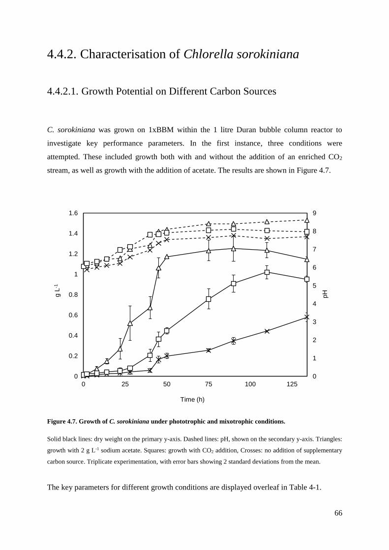
66

4.4.2. Characterisation of Chlorella sorokiniana

4.4.2.1. Growth Potential on Different Carbon Sources

C. sorokiniana was grown on 1xBBM within the 1 litre Duran bubble column reactor to

investigate key performance parameters. In the first instance, three conditions were

attempted. These included growth both with and without the addition of an enriched CO2

stream, as well as growth with the addition of acetate. The results are shown in Figure 4.7.

Figure 4.7. Growth of C. sorokiniana under phototrophic and mixotrophic conditions.

Solid black lines: dry weight on the primary y-axis. Dashed lines: pH, shown on the secondary y-axis. Triangles:

growth with 2 g L-1 sodium acetate. Squares: growth with CO2 addition, Crosses: no addition of supplementary

carbon source. Triplicate experimentation, with error bars showing 2 standard deviations from the mean.

The key parameters for different growth conditions are displayed overleaf in Table 4-1.

0

1

2

3

4

5

6

7

8

9

0

0.2

0.4

0.6

0.8

1

1.2

1.4

1.6

0 25 50 75 100 125

pHg L

-1

Time (h)

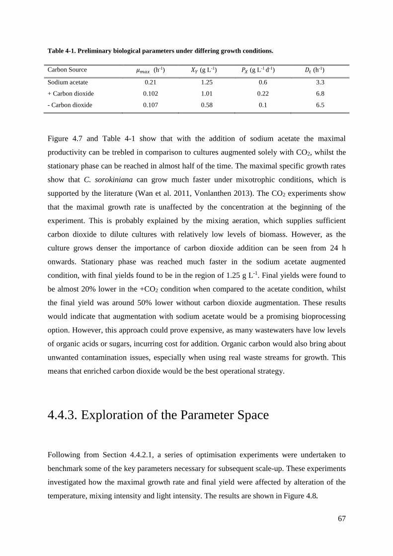
67

Table 4-1. Preliminary biological parameters under differing growth conditions.

Carbon Source 𝜇𝑚𝑎𝑥 (h-1) 𝑋𝑌 (g L-1) 𝑃𝑋 (g L-1 d-1) 𝐷𝑡 (h-1)

Sodium acetate 0.21 1.25 0.6 3.3

+ Carbon dioxide 0.102 1.01 0.22 6.8

- Carbon dioxide 0.107 0.58 0.1 6.5

Figure 4.7 and Table 4-1 show that with the addition of sodium acetate the maximal

productivity can be trebled in comparison to cultures augmented solely with CO2, whilst the

stationary phase can be reached in almost half of the time. The maximal specific growth rates

show that C. sorokiniana can grow much faster under mixotrophic conditions, which is

supported by the literature (Wan et al. 2011, Vonlanthen 2013). The CO2 experiments show

that the maximal growth rate is unaffected by the concentration at the beginning of the

experiment. This is probably explained by the mixing aeration, which supplies sufficient

carbon dioxide to dilute cultures with relatively low levels of biomass. However, as the

culture grows denser the importance of carbon dioxide addition can be seen from 24 h

onwards. Stationary phase was reached much faster in the sodium acetate augmented

condition, with final yields found to be in the region of 1.25 g L-1. Final yields were found to

be almost 20% lower in the +CO2 condition when compared to the acetate condition, whilst

the final yield was around 50% lower without carbon dioxide augmentation. These results

would indicate that augmentation with sodium acetate would be a promising bioprocessing

option. However, this approach could prove expensive, as many wastewaters have low levels

of organic acids or sugars, incurring cost for addition. Organic carbon would also bring about

unwanted contamination issues, especially when using real waste streams for growth. This

means that enriched carbon dioxide would be the best operational strategy.

4.4.3. Exploration of the Parameter Space

Following from Section 4.4.2.1, a series of optimisation experiments were undertaken to

benchmark some of the key parameters necessary for subsequent scale-up. These experiments

investigated how the maximal growth rate and final yield were affected by alteration of the

temperature, mixing intensity and light intensity. The results are shown in Figure 4.8.

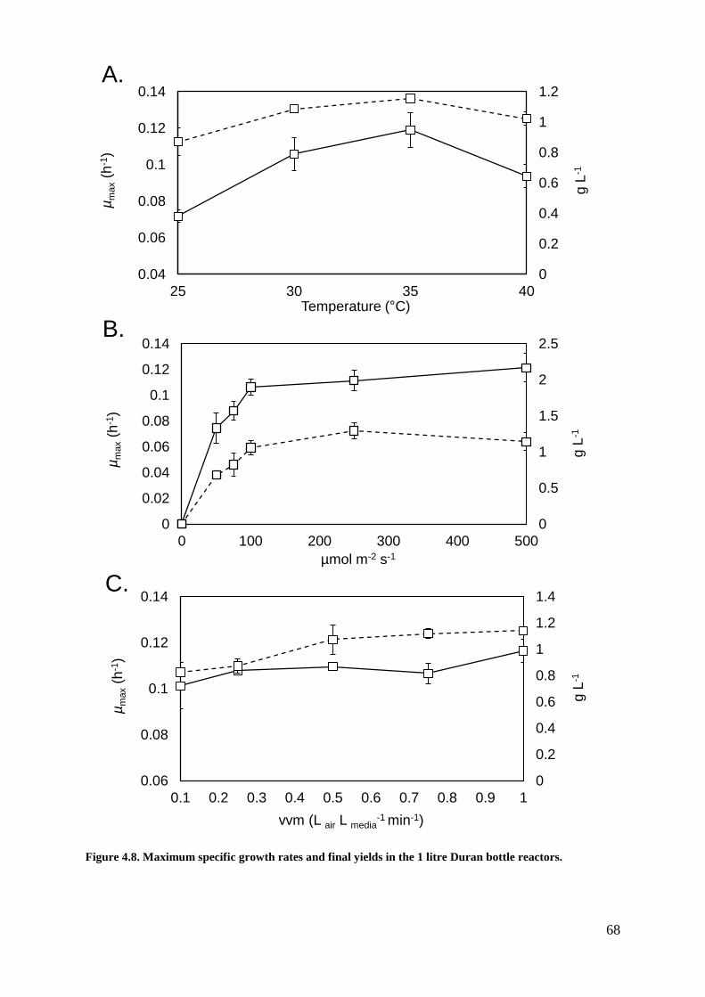
68

Figure 4.8. Maximum specific growth rates and final yields in the 1 litre Duran bottle reactors.

0

0.2

0.4

0.6

0.8

1

1.2

0.04

0.06

0.08

0.1

0.12

0.14

25 30 35 40

g L

-1

µm

ax

(h-1

)

Temperature (°C)

0

0.5

1

1.5

2

2.5

0

0.02

0.04

0.06

0.08

0.1

0.12

0.14

0 100 200 300 400 500

g L

-1

µm

ax

(h-1

)

µmol m-2 s-1

0

0.2

0.4

0.6

0.8

1

1.2

1.4

0.06

0.08

0.1

0.12

0.14

0.1 0.2 0.3 0.4 0.5 0.6 0.7 0.8 0.9 1

g L

-1

µm

ax

(h-1

)

vvm (L air L media-1 min-1)

A.

B.

C.

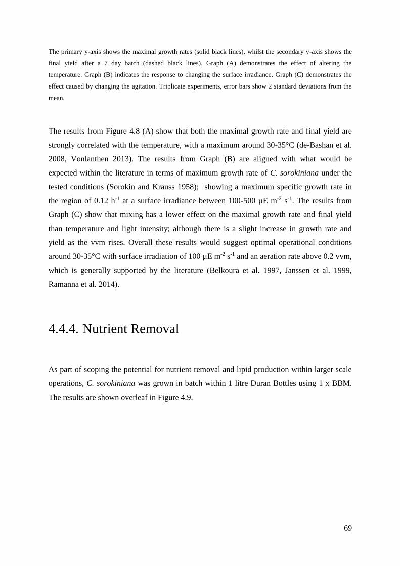
69

The primary y-axis shows the maximal growth rates (solid black lines), whilst the secondary y-axis shows the

final yield after a 7 day batch (dashed black lines). Graph (A) demonstrates the effect of altering the

temperature. Graph (B) indicates the response to changing the surface irradiance. Graph (C) demonstrates the

effect caused by changing the agitation. Triplicate experiments, error bars show 2 standard deviations from the

mean.

The results from Figure 4.8 (A) show that both the maximal growth rate and final yield are

strongly correlated with the temperature, with a maximum around 30-35°C (de-Bashan et al.

2008, Vonlanthen 2013). The results from Graph (B) are aligned with what would be

expected within the literature in terms of maximum growth rate of C. sorokiniana under the

tested conditions (Sorokin and Krauss 1958); showing a maximum specific growth rate in

the region of 0.12 h-1 at a surface irradiance between 100-500 µE m-2 s-1. The results from

Graph (C) show that mixing has a lower effect on the maximal growth rate and final yield

than temperature and light intensity; although there is a slight increase in growth rate and

yield as the vvm rises. Overall these results would suggest optimal operational conditions

around 30-35°C with surface irradiation of 100 µE m-2 s-1 and an aeration rate above 0.2 vvm,

which is generally supported by the literature (Belkoura et al. 1997, Janssen et al. 1999,

Ramanna et al. 2014).

4.4.4. Nutrient Removal

As part of scoping the potential for nutrient removal and lipid production within larger scale

operations, C. sorokiniana was grown in batch within 1 litre Duran Bottles using 1 x BBM.

The results are shown overleaf in Figure 4.9.

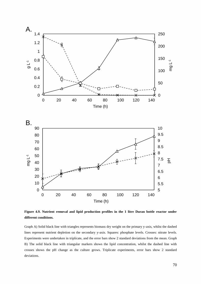
70

Figure 4.9. Nutrient removal and lipid production profiles in the 1 litre Duran bottle reactor under

different conditions.

Graph A) Solid black line with triangles represents biomass dry weight on the primary y-axis, whilst the dashed

lines represent nutrient depletion on the secondary y-axis. Squares: phosphate levels. Crosses: nitrate levels.

Experiments were undertaken in triplicate, and the error bars show 2 standard deviations from the mean. Graph

B) The solid black line with triangular markers shows the lipid concentration, whilst the dashed line with

crosses shows the pH change as the culture grows. Triplicate experiments, error bars show 2 standard

deviations.

0

50

100

150

200

250

0

0.2

0.4

0.6

0.8

1

1.2

1.4

0 20 40 60 80 100 120 140

mg L

-1

g L

-1

Time (h)

5

5.5

6

6.5

7

7.5

8

8.5

9

9.5

10

0

10

20

30

40

50

60

70

80

90

0 20 40 60 80 100 120 140

pH

mg L

-1

Time (h)

A.

B.

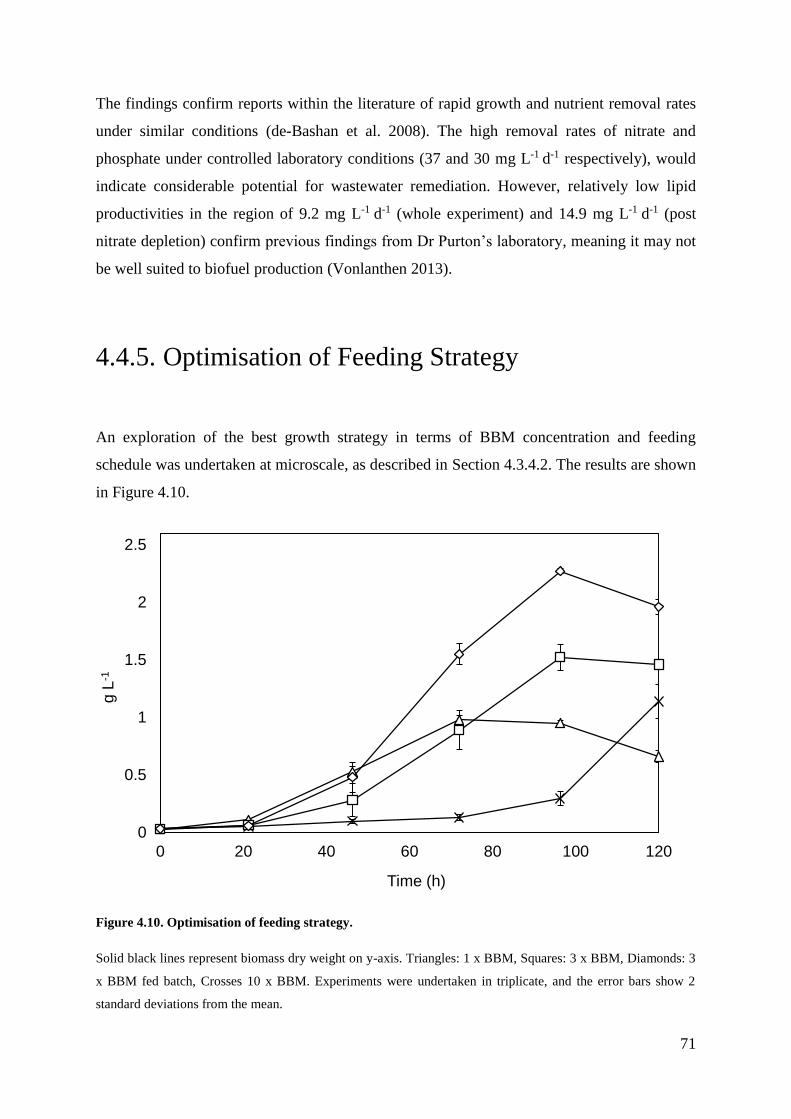
71

The findings confirm reports within the literature of rapid growth and nutrient removal rates

under similar conditions (de-Bashan et al. 2008). The high removal rates of nitrate and

phosphate under controlled laboratory conditions (37 and 30 mg L-1 d-1 respectively), would

indicate considerable potential for wastewater remediation. However, relatively low lipid

productivities in the region of 9.2 mg L-1 d-1 (whole experiment) and 14.9 mg L-1 d-1 (post

nitrate depletion) confirm previous findings from Dr Purton’s laboratory, meaning it may not

be well suited to biofuel production (Vonlanthen 2013).

4.4.5. Optimisation of Feeding Strategy

An exploration of the best growth strategy in terms of BBM concentration and feeding

schedule was undertaken at microscale, as described in Section 4.3.4.2. The results are shown

in Figure 4.10.

Figure 4.10. Optimisation of feeding strategy.

Solid black lines represent biomass dry weight on y-axis. Triangles: 1 x BBM, Squares: 3 x BBM, Diamonds: 3

x BBM fed batch, Crosses 10 x BBM. Experiments were undertaken in triplicate, and the error bars show 2

standard deviations from the mean.

0

0.5

1

1.5

2

2.5

0 20 40 60 80 100 120

g L

-1

Time (h)

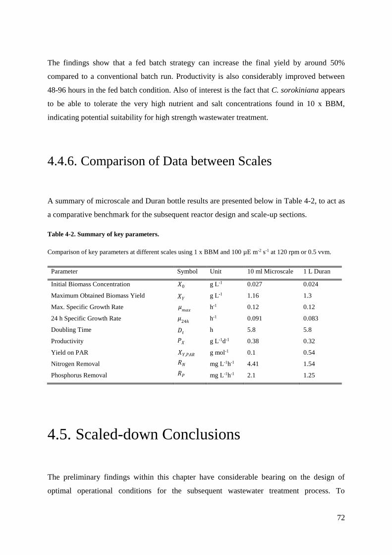
72

The findings show that a fed batch strategy can increase the final yield by around 50%

compared to a conventional batch run. Productivity is also considerably improved between

48-96 hours in the fed batch condition. Also of interest is the fact that C. sorokiniana appears

to be able to tolerate the very high nutrient and salt concentrations found in 10 x BBM,

indicating potential suitability for high strength wastewater treatment.

4.4.6. Comparison of Data between Scales

A summary of microscale and Duran bottle results are presented below in Table 4-2, to act as

a comparative benchmark for the subsequent reactor design and scale-up sections.

Table 4-2. Summary of key parameters.

Comparison of key parameters at different scales using 1 x BBM and 100 µE m-2 s-1 at 120 rpm or 0.5 vvm.

Parameter Symbol Unit 10 ml Microscale 1 L Duran

Initial Biomass Concentration g L-1 0.027 0.024

Maximum Obtained Biomass Yield g L-1 1.16 1.3

Max. Specific Growth Rate h-1 0.12 0.12

24 h Specific Growth Rate h-1 0.091 0.083

Doubling Time h 5.8 5.8

Productivity g L-1d-1 0.38 0.32

Yield on PAR g mol-1 0.1 0.54

Nitrogen Removal mg L-1h-1 4.41 1.54

Phosphorus Removal mg L-1h-1 2.1 1.25

4.5. Scaled-down Conclusions

The preliminary findings within this chapter have considerable bearing on the design of

optimal operational conditions for the subsequent wastewater treatment process. To

𝑋0

𝑋𝑌

𝜇𝑚𝑎𝑥

𝐷𝑡

𝑃𝑋

𝑋𝑌,𝑃𝐴𝑅

𝑅𝑁

𝑅𝑃

𝜇24ℎ

73

summarise the key findings; Chlorella sorokiniana appears to be the most suitable strain

investigated within the study, displaying a maximal growth rate in the region of 0.10-0.12 h-1,

as well as averaged batch productivity under continuous illumination in the region of 0.22-

0.38 g L-1 d-1. These findings are supported by the literature (Sorokin C. 1959) and are at the

higher end of many other phototrophically grown algal strains under these conditions (Ugwu,

Aoyagi and Uchiyama 2008, Molina et al. 2001). In fact a wider review of other studies

shows the maximal growth rate of C. sorokiniana is higher than all other species of Chlorella

(Wang et al. 2010b), and could be expected to be in the range 0.11-0.16 h-1 (Janssen et al.

1999). Other comparable results using C. sorokiniana were reported within 24-well

microplates, with a light intensity of 100 µmol photons m-2 s-1 (maximum specific growth

rate of 0.125 h-1) (Van Wagenen et al. 2014). Further notable findings from Section 4.4.5

found that higher nutrient concentrations decreased the specific growth rates; with maximal

averaged growth rates, productivities and yields being found under batch feeding conditions.

One possible explanation for this is the favourable environment brought on by batch feeding,

which lessens the osmotic stress and hence inhibition of photosynthesis caused by high

nutrient concentrations (Gilmour et al. 1984).

Despite the numerous differences in characteristics shown by each reactor system, many of

the key parameters were reasonably consistent between microscale and Duran bottle

(showing 10-20% variation). In fact, the only notable disparity between the two systems was

the biomass yield on PAR and the nutrient removal rates. The biomass yield on PAR was

found to be considerably lower in the microshaker than the Duran bottle. This could be

attributed to better mixing within the bubble column; as well as the effects of increased

photoinhibition within the micro-well plates (due to the higher surface area to volume ratio),

which would lower the photosynthetic efficiency. With regards to the differences between

nutrient removal rates; these could be attributed to the shorter run time of a microscale

cultivation (72 h versus 96-120 h in a Duran bottle), this would in turn result in a faster

average uptake rate during the course of the cultivation. The relative ease with which C.

sorokiniana grew within the 1 litre Duran bottle reactor is encouraging and indicates that the

strain may be suitable for scale-up using a reactor with bubble column or airlift configuration.

Finally, the findings also show that relatively high nutrient removal rates are achievable,

indicating potential suitability for wastewater treatment. The work undertaken in Chapter 5

seeks to build upon the research from this section and explore the potential of using C.

sorokiniana to treat wastewater and flue gas.

74

5. Scaled Down Cultivation with Waste

5.1. Aims and Objectives

To follow from the scoping work undertaken in Chapter 4, a series of small scale batch

experiments were devised to test the ability of C. sorokiniana to remediate waste effluent

from a conventional municipal wastewater treatment works. This research tested the

following considerations:

Selection of suitable waste effluents for treatment with an algal process, particularly with

a view to the reduction of inorganic nitrogen and phosphorus concentrations.

Ascertaining the most important parameters for the process, including the nutrient uptake

rates that could be achieved.

Identification of any potential pitfalls with the process that may hinder future scale-up.

5.2. A Review of Algal Bioremediation

5.2.1. Wastewater Characterisation

Broadly speaking there are three main types of wastewater; industrial, agricultural and

municipal. Industrial wastewaters can vary considerably in composition, but often contain

high levels of toxins such as metals or petrochemicals. These waters are characterised by

extreme pH values and low levels of organic matter, which in combination can make them a

difficult target for algal bioremediation processes. However, despite these problems there is a

growing body of research that has shown that algae are capable of treating certain types of

75

industrial waste, particularly those with trace metal concentrations (Ahluwalia and Goyal

2007). On the other hand, most types of agricultural wastewaters are derived from animal or

plant matter, and can include manure and fruit processing run-off. These waters contain high

loadings of organic matter, alongside associated bacterial communities, making them better

targets for bioremediation. The final category is comprised of municipal wastewaters, which

include household and urban wastes, often containing a mixture of excrement and suspended

solids, alongside lower concentrations of potentially toxic compounds. Like agricultural

waste there is already a microbial community associated with municipal waste streams, and

treatment processes can be designed accordingly. Previous research and practical application

has shown that algae are generally better suited to the treatment of agricultural or municipal

wastes, due to the favourable characteristics presented within these streams. This includes a

moderate pH range, reasonable levels of light transmission and sufficient inorganic nutrient

loading (Wang et al. 2010a, Pittman, Dean and Osundeko 2011).

5.2.2. Remediation of Industrial Wastewaters

On the whole microalgal metabolism is not as well suited to the breakdown of complex

organic molecules, especially in comparison to bacteria or yeast. However, there are a range

of specific industrial pollutants that can be treated by algae. One interesting approach is to

look at processes in which natural biodegradation of the pollutant in question produces nitrate

(NO3) or ammonia/ammonium (NH3/NH4+). Examples include the breakdown of acetonitrile

by photosynthetic organisms to yield ammonia. Previous research has shown that the uptake

of NH3 produced by this photosynthetically driven degradation pathway is 38-77% higher

when compared to conventional bacterial treatment systems (Muñoz et al. 2005).

Considerable research has also shown the potential for metal absorption by algal species; this

includes the removal of Zn, Cu, Cr, Cd, Co, Al and Hg ions. Algal absorption of these types

of metals has been shown to have 99% removal efficiency, with total metal uptake reported to

be in the region of 15 mg g-1 of algal biomass produced (Muñoz and Guieysse 2006). A range

of other industrial pollutants have also been treated by algal absorption or biodegradation,

including olive oil and paper mill wastewater (both of which are high in phenols and

polyaromatic hydrocarbons) (Abeliovich and Weisman 1978, Narro 1987, Pinto et al. 2002).

76

Other interesting areas for algal treatment include wastewaters from the textile industry,

which can contain high levels of biological oxygen demand (BOD). These can include

synthetic dyes with high carbon and nitrogen content, as well as solvents and heavy metals.

Findings from these studies have shown that some species of Chlorella vulgaris are capable

of breaking azo-dyes down into aromatic amines, thereby reducing the chemical oxygen

demand (COD) within the wastewater (Acuner and Dilek 2004).

As the breakdown of many organic industrial pollutants can be undertaken more easily under

aerobic conditions, algae can play an important role in assisting other micro-organisms to

degrade recalcitrant substances. This photosynthetic production of oxygen by algal species

can reduce processing costs substantially for treatment sites where conventional mechanical

aeration can account for around 50% of all costs (Metcalf et al. 2003). Previous experimental

findings from algal-bacterial consortia indicate faster breakdown rates than solely algal

cultures, with examples including the removal of sodium salicylate at a rate of 87 mg L-1 h-1

(Muñoz et al. 2004), and acetonitrile degradation reaching as much as 2.3 g L-1 d-1 (Dhillon

1999). Another example of the successful use of algal and bacterial consortia includes the

degradation of black oil from wastewaters (Safonova, Dmitrieva and Kvitko 1999, Safonova

et al. 2004). Whilst further studies have shown consortia of Chlorella sorokiniana in

combination with other microorganisms as being able to support the aerobic degradation of

acetonitrile, salicylate, phenol and phenanthrene, without the need for external oxygen

addition (Borde et al. 2003, Guieysse et al. 2002, Muñoz et al. 2005, Muñoz et al. 2004).

Specific findings indicate the potential to remove up to 50 mg L d-1 of p-nitrophenol by a

consortium of Chlorella species (Lima, Castro and Morais 2003). There are however inherent

problems with the use of mixed microbial cultures; namely the fact that it can be hard to

control the actual constitution of the consortia over time. This is particularly the case for any

bacteria within the community, which will generally be both faster growing and more

resistant to any toxic chemicals within the waste stream (Muñoz and Guieysse 2006).

77

5.2.3. Algal Treatment of Agricultural and Municipal

Wastewaters

The activity of algae within the consortia of microorganisms involved in conventional

municipal wastewater treatment is well documented. Many species play an important role in

secondary treatment steps within either maturation ponds or facultative and aerobic ponds

(Abeliovich and Weisman 1978); and are readily able to grow on the dissolved carbon

dioxide and nutrients found within wastewater. As a by-product of their photosynthetic

activity they provide oxygen for aerobic bacteria, thereby allowing for the breakdown of

other more complex organic molecules. The photosynthetic growth of algae on nitrate also

acts to increase the pH of the water, providing a stabilising and sterilising effect (Oswald

1988). Numerous studies have already been undertaken which show that traditional feedstock

for algal cultivation can be replaced with a variety of municipally or agriculturally derived

alternatives (Muñoz and Guieysse 2006). In particular compounds of nitrogen, phosphorous,

trace metals and vitamins can often be sourced directly from secondary or tertiary wastewater

(Greenwell et al. 2010). Unsurprisingly, the composition of the wastewater has a critical

impact on algal cultivation. Nitrogen and phosphorous content and ratios are of particular

importance, as both are a key macronutrient for cell growth, whilst a lack of either can act as

a trigger for lipid accumulation. Previous studies have shown that most algal biomass has a

composition in the range of C106−158N16−18P (Ketchum and Redfield 1949, Sterner and

Hessen 1994) which makes for an attractive benchmark when selecting suitable waste as a

feedstock. Looking at some of the most common waste streams in Table 5-1, many domestic

wastewaters have an appropriate range of N:P ratios, whilst many industries such as mills and

tanneries produce very high nitrogen loadings. Likewise, anaerobic digester centrate (formed

from centrifuged supernatant) contains very high levels nitrogen, often in the form of

ammonia and ammonium ions, making it a particularly favourable feedstock for algal growth

(Wang et al. 2010a, Pittman et al. 2011).

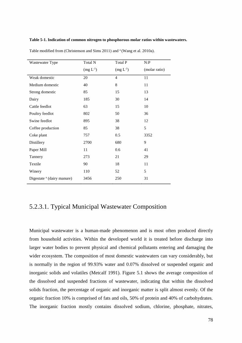
78

Table 5-1. Indication of common nitrogen to phosphorous molar ratios within wastewaters.

Table modified from (Christenson and Sims 2011) and a (Wang et al. 2010a).

Wastewater Type Total N

(mg L-1)

Total P

(mg L-1)

N:P

(molar ratio)

Weak domestic 20 4 11

Medium domestic 40 8 11

Strong domestic 85 15 13

Dairy 185 30 14

Cattle feedlot 63 15 10

Poultry feedlot 802 50 36

Swine feedlot 895 38 12

Coffee production 85 38 5

Coke plant 757 0.5 3352

Distillery 2700 680 9

Paper Mill 11 0.6 41

Tannery 273 21 29

Textile 90 18 11

Winery 110 52 5

Digestate a (dairy manure) 3456 250 31

5.2.3.1. Typical Municipal Wastewater Composition

Municipal wastewater is a human-made phenomenon and is most often produced directly

from household activities. Within the developed world it is treated before discharge into

larger water bodies to prevent physical and chemical pollutants entering and damaging the

wider ecosystem. The composition of most domestic wastewaters can vary considerably, but

is normally in the region of 99.93% water and 0.07% dissolved or suspended organic and

inorganic solids and volatiles (Metcalf 1991). Figure 5.1 shows the average composition of

the dissolved and suspended fractions of wastewater, indicating that within the dissolved

solids fraction, the percentage of organic and inorganic matter is split almost evenly. Of the

organic fraction 10% is comprised of fats and oils, 50% of protein and 40% of carbohydrates.

The inorganic fraction mostly contains dissolved sodium, chlorine, phosphate, nitrates,

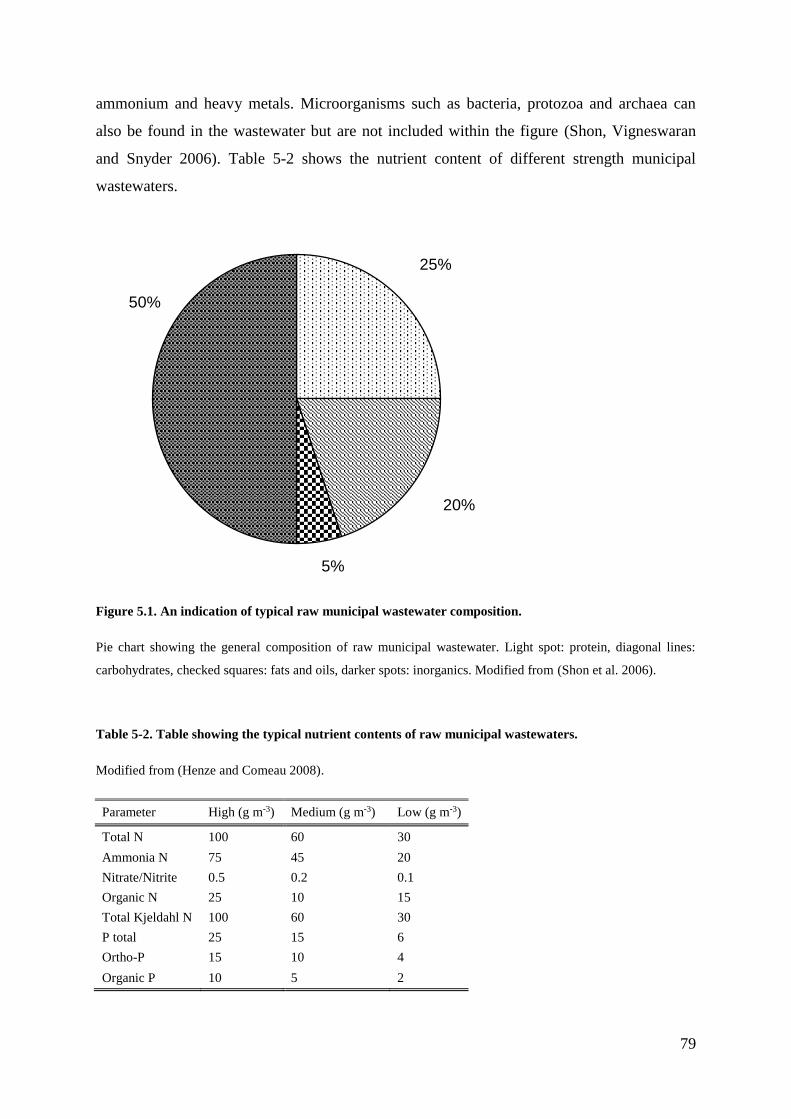
79

ammonium and heavy metals. Microorganisms such as bacteria, protozoa and archaea can

also be found in the wastewater but are not included within the figure (Shon, Vigneswaran

and Snyder 2006). Table 5-2 shows the nutrient content of different strength municipal

wastewaters.

Figure 5.1. An indication of typical raw municipal wastewater composition.

Pie chart showing the general composition of raw municipal wastewater. Light spot: protein, diagonal lines:

carbohydrates, checked squares: fats and oils, darker spots: inorganics. Modified from (Shon et al. 2006).

Table 5-2. Table showing the typical nutrient contents of raw municipal wastewaters.

Modified from (Henze and Comeau 2008).

Parameter High (g m-3) Medium (g m-3) Low (g m-3)

Total N 100 60 30

Ammonia N 75 45 20

Nitrate/Nitrite 0.5 0.2 0.1

Organic N 25 10 15

Total Kjeldahl N 100 60 30

P total 25 15 6

Ortho-P 15 10 4

Organic P 10 5 2

25%

20%

5%

50%

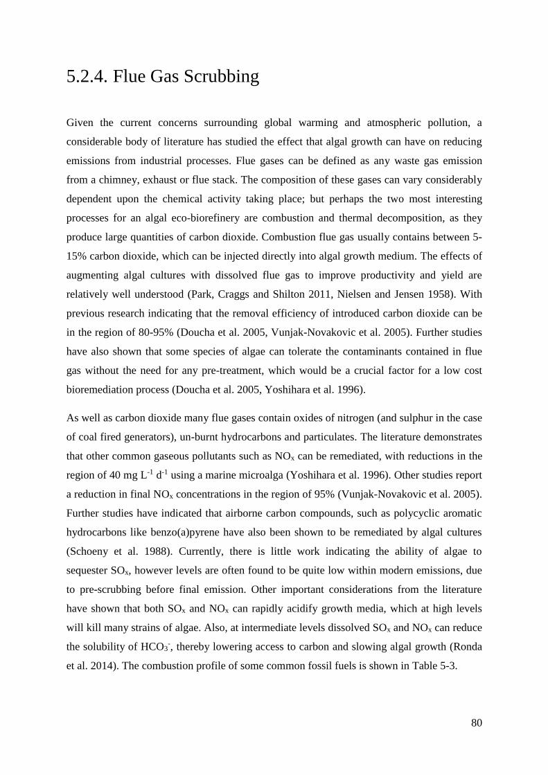
80

5.2.4. Flue Gas Scrubbing

Given the current concerns surrounding global warming and atmospheric pollution, a

considerable body of literature has studied the effect that algal growth can have on reducing

emissions from industrial processes. Flue gases can be defined as any waste gas emission

from a chimney, exhaust or flue stack. The composition of these gases can vary considerably

dependent upon the chemical activity taking place; but perhaps the two most interesting

processes for an algal eco-biorefinery are combustion and thermal decomposition, as they

produce large quantities of carbon dioxide. Combustion flue gas usually contains between 5-

15% carbon dioxide, which can be injected directly into algal growth medium. The effects of

augmenting algal cultures with dissolved flue gas to improve productivity and yield are

relatively well understood (Park, Craggs and Shilton 2011, Nielsen and Jensen 1958). With

previous research indicating that the removal efficiency of introduced carbon dioxide can be

in the region of 80-95% (Doucha et al. 2005, Vunjak-Novakovic et al. 2005). Further studies

have also shown that some species of algae can tolerate the contaminants contained in flue

gas without the need for any pre-treatment, which would be a crucial factor for a low cost

bioremediation process (Doucha et al. 2005, Yoshihara et al. 1996).

As well as carbon dioxide many flue gases contain oxides of nitrogen (and sulphur in the case

of coal fired generators), un-burnt hydrocarbons and particulates. The literature demonstrates

that other common gaseous pollutants such as NOx can be remediated, with reductions in the

region of 40 mg L-1 d-1 using a marine microalga (Yoshihara et al. 1996). Other studies report

a reduction in final NOx concentrations in the region of 95% (Vunjak-Novakovic et al. 2005).

Further studies have indicated that airborne carbon compounds, such as polycyclic aromatic

hydrocarbons like benzo(a)pyrene have also been shown to be remediated by algal cultures

(Schoeny et al. 1988). Currently, there is little work indicating the ability of algae to

sequester SOx, however levels are often found to be quite low within modern emissions, due

to pre-scrubbing before final emission. Other important considerations from the literature

have shown that both SOx and NOx can rapidly acidify growth media, which at high levels

will kill many strains of algae. Also, at intermediate levels dissolved SOx and NOx can reduce

the solubility of HCO3-, thereby lowering access to carbon and slowing algal growth (Ronda

et al. 2014). The combustion profile of some common fossil fuels is shown in Table 5-3.

81

Table 5-3. Typical composition of combustion gases from differing fossil fuel types.

Expressed as % volume or part per million weight (ppm). Table modified from (Zevenhoven and Kilpinen

2001).

Entity Petrol (%) Diesel (%) Gas (%) Coal (%)

N2 71 67 14 66-77

CO2 14 13 7-10 12-15

H2O 12 11 15 6

O2 trace 10 4-5 4.5

CO 1 - 2 < 0.045 300 ppm 50 ppm

NOx < 0.25 < 0.15 70 ppm 420 ppm

SO2 trace < 0.045 nil 420 ppm

5.3. A Detailed look at Municipal Wastewater

Treatment

5.3.1. Preliminary and Primary Wastewater Treatment

The preliminary wastewater treatment process begins with the removal of all larger

contaminants that have entered the treatment stream; including paper, plastic, toiletry and

sanitary items. This is followed by a primary sedimentation process, which allows for most of

the suspended solids to settle out from the flow, whilst the oils and grease can rise to the

surface. Mechanical scraping is then deployed to remove the grease and oils from the water

surface. By the end of this stage in the process the biochemical oxygen demand has been

reduced by 30-40% (DEFRA 2002, DEFRA 2012).

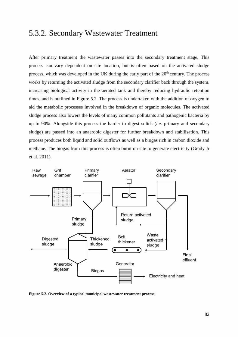
82

5.3.2. Secondary Wastewater Treatment

After primary treatment the wastewater passes into the secondary treatment stage. This

process can vary dependent on site location, but is often based on the activated sludge

process, which was developed in the UK during the early part of the 20th century. The process

works by returning the activated sludge from the secondary clarifier back through the system,

increasing biological activity in the aerated tank and thereby reducing hydraulic retention

times, and is outlined in Figure 5.2. The process is undertaken with the addition of oxygen to

aid the metabolic processes involved in the breakdown of organic molecules. The activated

sludge process also lowers the levels of many common pollutants and pathogenic bacteria by

up to 90%. Alongside this process the harder to digest solids (i.e. primary and secondary

sludge) are passed into an anaerobic digester for further breakdown and stabilisation. This

process produces both liquid and solid outflows as well as a biogas rich in carbon dioxide and

methane. The biogas from this process is often burnt on-site to generate electricity (Grady Jr

et al. 2011).

Figure 5.2. Overview of a typical municipal wastewater treatment process.

83

5.3.3. Tertiary Wastewater Treatment Processes

Whilst the UK Environment Agency has made considerable gains in controlling effluent

levels within waterways since the early part of the last century, there continues to be

considerable concern about the effects of eutrophication within European fresh and saline

waterways. The requirements for improving final effluent quality is codified in the EU Water

Quality Directives under the Water Framework Directive, which stipulates that enhanced

tertiary treatment would be necessary to prevent further eutrophication and pollution of

waterways (CEEP 2007). Many of the standards that control municipal wastewater in the UK

are now dictated by EU regulations, and fall under Wastewater Directives such as the Water

Framework Directive 2000/60/EC; or the Water Quality Directives, which are numerous, but

include the Urban Waste Water Treatment Directive (91/271/EEC), the Nitrates Directive

(91/676/EEC), and the Bathing Water Directive (Directive 2006/7/EC). These regulations

prescribe that the concentration of total phosphorous (P) and nitrogen (N) within wastewater

at discharge should be no more than 2 mg L-1 and 15 mg L-1 respectively, in sites of 10,000-

100,000 population equivalent (PE). The limit is lowered for sites above 100,000 PE to 1 mg

L-1 and 10 mg L-1 for P and N respectively. Despite the extensive legislation most member

countries are still not fully compliant and regularly breach standards, whilst accession

countries have a 10-15 year reprieve before enforcement (CEEP 2007, DEFRA 2012).

Despite the significant progress that has been made since the 1960s, conventional secondary

wastewater treatment at many sites still suffers from a limited ability to reduce the inorganic

N and P content within wastewater below certain levels (Shi et al. 2014). This causes

problems within receiving waterways due to the resultant increase in nutrient levels, which

can encourage the growth of aquatic algae and other fast growing plants (Ferreira et al. 2011).

When these photosynthetic organisms subsequently die they are degraded by bacteria, which

cause an oxygen deficit that leads to eutrophication, killing many of the larger aquatic

organisms. Tertiary treatment is often deployed to prevent further negative impacts within the

environment, and can vary considerably dependent upon local treatment requirements. For

example tertiary processes can reduce suspended solids, levels of inorganic compounds

containing N and P and harmful bacteria. The reason that many of these treatments are not

regularly deployed is due to the high costs that are associated with them (Oswald 1988). In

fact many wastewater treatment facilities operate primary and secondary treatment at overall

84

costs in the region of £0.6 m-3wastewater (Doran 1995), and are under pressure to minimise all

associated costs. Complete tertiary treatment has been shown to cost roughly four times as

much as primary treatment, with a value in the region of £1.20 m-3. Furthermore, quaternary

and quinary treatments are known to have a cost range between 8-16 times more than primary

treatment (Oswald 1988).

There are several effective tertiary treatment options that are in various states of research and

development. For nitrogen removal, the most commonly deployed platform is the biological

oxidation of ammonia to nitrate (nitrification), followed by the reduction of nitrate to nitrogen

gas which is then released into the atmosphere (denitrification). This is a two-step process

undertaken by species of bacteria such as Nitrosomonas spp, Nitrobacter spp and Nitrospira

spp (Grady Jr et al. 2011). Another promising alternative process is direct ammonium

oxidation by the bacteria Brocadia anammoxidans, known as the anammox process (van

Loosdrecht et al. 2004), although the technology is still yet to be widely deployed.

Constructed lagoons and reed beds are also finding increasing usage as a low cost platform

for nitrate and phosphate recovery, functioning via the activity of green plants in conjunction

with mixed microbial communities (Kivaisi 2001, de-Bashan and Bashan 2004).

Phosphate removal can be achieved either via biological or chemical means. One biological

method involves a process known as enhanced biological phosphorous removal, in which

bacteria known as polyphosphate accumulating organisms (PAOs) can hyper-accumulate

phosphorous (Grady Jr et al. 2011). However, the most common method deployed to remove

dissolved phosphorous species is via chemical precipitation with salts such as ferric chloride,

alum or via the addition of Mg, which produces struvite (NH4MgPO4·6H2O). These metals

have high affinity for phosphate and are rapidly flocculated using a polyanionic polymer,

with the resultant material known as water treatment residual (WTR). Though the dose rate

for the metal salts is relatively low at 3-6 mg L-1, this still involves considerable expense in

terms of the salts and polymer, meaning that treatment costs for many WWT sites can run

into £50-300k per annum (Jaffer et al. 2002). Additional costs are subsequently incurred from

to the transportation and gate fees required to take the WTR to landfill. Despite these issues

chemical dosing remains a popular choice for phosphorous removal owing to the large

volumes of water that may be rapidly treated in this way.

85

5.3.4. Priorities for Wastewater Treatment in the UK

By 2015 wastewater companies and businesses which generate effluent across Europe will be

required to comply with the Water Framework Directives (91/271/EEC) and (91/676/EEC).

Failure to comply could result in large fines for both industry and state actors. The EU has

also drafted a list of another 80 priority substances which require increased levels of removal

from effluent streams (2455/2001/EC). Amongst these compounds phosphorous removal is

considered to be of particular importance, with the potential to confer both environmental and

economic benefits. Phosphorus is an essential constituent of all life on Earth and is obtained

from the environment in various mineral forms. Human industrial and agricultural activity

has had a considerable effect upon phosphorus levels and distribution in a number of major

ways. Firstly, the use of phosphorus in fertilisers for arable crop growth has led to

considerable depletion of rock phosphate reserves. Current annual extraction levels are

around 220,000 Mt and are expected to increase by 8 Mt per year in the next 5 years (USGS

2015). This rate of increase has led to the prediction that 'peak phosphorus' may be reached

by the year 2033 (Déry and Anderson 2007). The implementation of wastewater treatment

directives could provide novel incentives to reduce, recover or stabilise phosphorous for

commercial use and will be of particular interest to the waste processing and recovery

industries.

5.3.5. Integrating Algal Phosphorus Recovery

Given the fact that many wastewater treatment facilities are regularly unable to meet EU

emissions standards (CEEP 2007) there has been a concerted drive to improve and diversify

tertiary treatment technologies (TSB 2015). The removal of contamination from tertiary

wastewater using an algal platform has several potentially appealing features. This includes

the ability to reduce the levels of refractory organics, inorganic nutrients like N and P species,

as well as heavy metals (Noüe et al. 1992). Algal remediation can offer several benefits in

comparison to conventional tertiary wastewater treatment. Most prominently is its capacity to

take up various forms of inorganic phosphorous and nitrogen in tandem (Kaya, de la Noüe

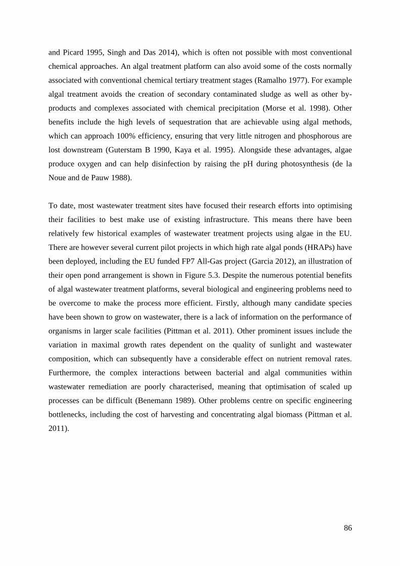
86

and Picard 1995, Singh and Das 2014), which is often not possible with most conventional

chemical approaches. An algal treatment platform can also avoid some of the costs normally

associated with conventional chemical tertiary treatment stages (Ramalho 1977). For example

algal treatment avoids the creation of secondary contaminated sludge as well as other by-

products and complexes associated with chemical precipitation (Morse et al. 1998). Other

benefits include the high levels of sequestration that are achievable using algal methods,

which can approach 100% efficiency, ensuring that very little nitrogen and phosphorous are

lost downstream (Guterstam B 1990, Kaya et al. 1995). Alongside these advantages, algae

produce oxygen and can help disinfection by raising the pH during photosynthesis (de la

Noue and de Pauw 1988).

To date, most wastewater treatment sites have focused their research efforts into optimising

their facilities to best make use of existing infrastructure. This means there have been

relatively few historical examples of wastewater treatment projects using algae in the EU.

There are however several current pilot projects in which high rate algal ponds (HRAPs) have

been deployed, including the EU funded FP7 All-Gas project (Garcia 2012), an illustration of

their open pond arrangement is shown in Figure 5.3. Despite the numerous potential benefits

of algal wastewater treatment platforms, several biological and engineering problems need to

be overcome to make the process more efficient. Firstly, although many candidate species

have been shown to grow on wastewater, there is a lack of information on the performance of

organisms in larger scale facilities (Pittman et al. 2011). Other prominent issues include the

variation in maximal growth rates dependent on the quality of sunlight and wastewater

composition, which can subsequently have a considerable effect on nutrient removal rates.

Furthermore, the complex interactions between bacterial and algal communities within

wastewater remediation are poorly characterised, meaning that optimisation of scaled up

processes can be difficult (Benemann 1989). Other problems centre on specific engineering

bottlenecks, including the cost of harvesting and concentrating algal biomass (Pittman et al.

2011).

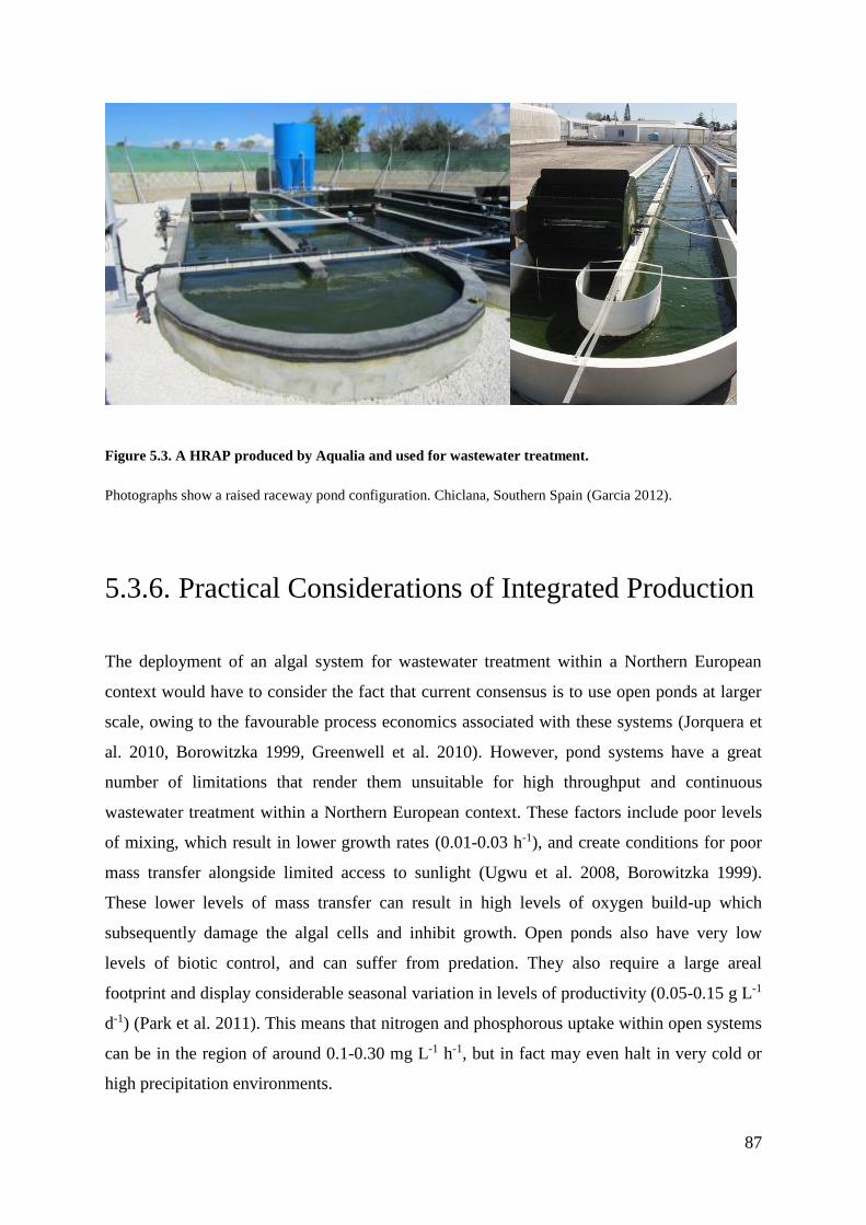
87

Figure 5.3. A HRAP produced by Aqualia and used for wastewater treatment.

Photographs show a raised raceway pond configuration. Chiclana, Southern Spain (Garcia 2012).

5.3.6. Practical Considerations of Integrated Production

The deployment of an algal system for wastewater treatment within a Northern European

context would have to consider the fact that current consensus is to use open ponds at larger

scale, owing to the favourable process economics associated with these systems (Jorquera et

al. 2010, Borowitzka 1999, Greenwell et al. 2010). However, pond systems have a great

number of limitations that render them unsuitable for high throughput and continuous

wastewater treatment within a Northern European context. These factors include poor levels

of mixing, which result in lower growth rates (0.01-0.03 h-1), and create conditions for poor

mass transfer alongside limited access to sunlight (Ugwu et al. 2008, Borowitzka 1999).

These lower levels of mass transfer can result in high levels of oxygen build-up which

subsequently damage the algal cells and inhibit growth. Open ponds also have very low

levels of biotic control, and can suffer from predation. They also require a large areal

footprint and display considerable seasonal variation in levels of productivity (0.05-0.15 g L-1

d-1) (Park et al. 2011). This means that nitrogen and phosphorous uptake within open systems

can be in the region of around 0.1-0.30 mg L-1 h-1, but in fact may even halt in very cold or

high precipitation environments.

88

A key technical challenge for wastewater treatment with algae is that of residence time, as the

phosphorus removal rate has to be matched with the final effluent flow rate from the

treatment site. Any variation in growth conditions, effluent composition or flow rate could

result in washing the algae out from the process. This places physical and cost burdens on

any conventional algal treatment system as they have to be oversized or designed with some

volumetric redundancy, thereby increasing capital expenditure. Other hurdles include

selection of a suitable wastewater growth medium; literature would indicate that typical N-

NO3 and P-PO4 levels within wastewater final effluent are in the region of 5-15 mg L-1 and 1-

5 mg L-1 respectively (Abdel-Raouf, Al-Homaidan and Ibraheem 2012). This makes the final

effluent a comparatively nutrient poor media compared to commercially available media such

as BBM (35 mg L-1 and 50 mg L-1 for N and P respectively). Conversely, N-NH4

concentrations within anaerobic digester centrate can be around 1-3 g L-1 (Voltolina et al.

1999), with P-PO4 in the region of 50–300 mg L-1. This makes anaerobic digester centrate a

couple of orders of magnitude more concentrated than commercial media, and would likely

need dilution for successful cultivation. Likewise, the levels of any potentially inhibiting

substances that are often found in wastewater, such as pesticides and other pollutants need to

be taken into account, as these may limit both growth and downstream options. A further

consideration for any bulk production of algae from waste would also need to consider the

nutrient availability limits within wastewater. This has been identified previously in the

Greenwell review paper (Greenwell et al. 2010), which estimated a 105 kg shortfall in

European waste nutrients, should biodiesel be a desired output (Mueller 2007). However,

many of these problems can be avoided somewhat if the main purpose of the eco-biorefinery

is remediation to EU standards rather than biomass production.

Despite some of these hurdles, it is possible that algae could find a more prominent role

within the conventional wastewater treatment processes of Northern Europe. Previous

research has suggested that an algal platform could be integrated at either secondary or

tertiary treatment stages. In fact, a considerable body of research has shown the potential for

the cost related benefits of integration at the secondary stage, as part of a mixed microbial

community (Oswald 1988, Wang et al. 2010b, Abdel-Raouf et al. 2012). In practical terms

this approach would involve making the conditions within secondary facultative ponds more

favourable for algae within the mixed community. However, this method has some potential

89

limitations due to the high organic loadings which would generally always favour bacterial

populations. This means that the end result would not necessarily be much different to a

conventional secondary wastewater treatment process. Furthermore, this approach would be

unlikely to achieve widespread deployment within a Northern European context due to the

inertial legacy of established methodologies and infrastructure for secondary treatment. Most

treatment sites favour proven and established technologies or those that are able to ‘bolt-on’

to existing infrastructure. This means that algal wastewater treatment in Northern Europe is

more likely to find a role as a tertiary stage ‘super-polisher’, reducing total N and P to trace

levels after a conventional secondary treatment, bringing emissions in line with EU standards

(CEEP 2007, TSB 2015). An illustration of the potential for algal integration is shown in

Figure 5.4.

Figure 5.4. Illustration of how an algal treatment platform could be integrated within a wastewater

treatment works.

One specific example of an algal tertiary treatment technology is the serpentine advanced

biological nutrient recovery (ABNR), produced by ClearAs in the United States. The

platform overcomes the problems associated with having to match an algal growth rate to a

nutrient flow rate through the use of a membrane belt filter. The belt filter assists the process

by separating, concentrating and re-circulating algal biomass to maintain high biomass

densities within the ABNR and hence consistent P removal rates (Robinson et al. 2012).

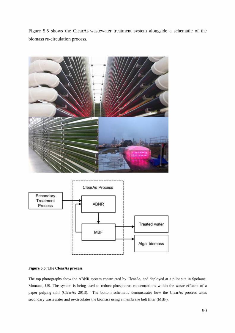
90

Figure 5.5 shows the ClearAs wastewater treatment system alongside a schematic of the

biomass re-circulation process.

Figure 5.5. The ClearAs process.

The top photographs show the ABNR system constructed by ClearAs, and deployed at a pilot site in Spokane,

Montana, US. The system is being used to reduce phosphorus concentrations within the waste effluent of a

paper pulping mill (ClearAs 2013). The bottom schematic demonstrates how the ClearAs process takes

secondary wastewater and re-circulates the biomass using a membrane belt filter (MBF).

91

5.4. Profiling Growth with Wastewater and

Flue Gas

5.4.1. Materials and Methods

5.4.1.1. Batch and Continuous Experiments

Chlorella sorokiniana UTEX1230 was selected for these experiments based on the findings

in Chapter 4. For batch experiments, the bioreactor vessels consisted of 1 litre Duran bottle

reactors, as outlined in Section 4.3.4.1. Media composition is described in 5.4.1.5. Mixing air

was kept consistent throughout the experiments, and introduced into all of the bottles at 0.2

vvm. This was achieved by using an air compressor (Hailea) and a ceramic diffuser. The

lighting was held at 80 µmol m-2 s-1 of artificial light (low light conditions), provided by two

8W Gro-lux lights (Sylvania). Temperature was maintained at 32±2°C (de-Bashan et al.

2008). In the continuous growth experiment the strain was first cultivated under the

aforementioned batch conditions on final effluent for 170 h. After which a continuous

dilution regime (1.92 L d-1 of final effluent) was implemented using a peristaltic pump

(Watson Marlow).

5.4.1.2. Deriving the Maximal Growth Rate

The maximum specific growth rate (𝜇𝑚𝑎𝑥) was calculated as outlined in section 4.3.3.1.

5.4.1.3. Final Yield and Productivity

Each experimental condition was undertaken in triplicate; with final biomass yields,

productivities and lipid yields calculated as in section 4.3.3.2.

92

5.4.1.4. Flue Gas Composition and Analysis

To test whether C. sorokiniana was capable of growing on flue gas, a series of experiments

were conducted in collaboration with Dr Paul Hillier from the Department of Mechanical

Engineering, UCL. These experiments were undertaken by sparging of all cultures with

atmospheric air for mixing, whilst those in the +CO2 group were supplemented with exhaust

gas at a rate of 20 cm3 min-1 (Vunjak-Novakovic et al. 2005). The exhaust gas for these

experiments was produced by a single cylinder diesel engine specially designed for

combustion and fuels research (Ricardo Hydra with Ford Duratorque head). The gas was

stored under 10 bar of pressure in a modified air compressor (Einhell). The engine was

operated on a fossil diesel fuel, with zero fatty acid methyl ester (FAME) content, at a

variable load condition to produce a constant exhaust gas composition of either 6% or 12%

CO2. Exhaust gas sampling took place downstream of the engine using an automotive gas

analyser system (Horiba MEXA9100 HEGR). The composition of the exhaust gas was

determined by the following methods: NOx concentrations were determined by

chemiluminescence; CO and CO2 concentrations by non-dispersive infrared detection, and O2

concentrations with paramagnetic analysis (Hellier and Ladommatos 2011 ).

5.4.1.5. Media Composition

Wastewater was sourced from a UK municipal treatment works processing domestic waste

streams (Southern Water). The tested wastewater included final effluent (FE) generated after

secondary treatment and due for discharge; as well as anaerobic digester centrate (ADC),

which was composed of the liquid fraction (with some suspended material) produced from

the centrifugal separation of anaerobically digested solids. 1x BBM prepared with de-ionised

water was used as a benchmark in the experiments (Sigma). Due to UCL health and safety

policy regarding pathogenic microorganisms, the wastewater samples were autoclaved at

121°C for 15 minutes before bringing them into the Environmental Engineering Laboratory,

and diluted 1:10 with deionised water for the purposes of the experiment.

93

5.4.1.6. Ion chromatography of Wastewater and Commercial Media

Ion chromatography (IC) was undertaken as in Section 4.3.6 to analyse the potential of C.

sorokiniana to reduce ammonium, nitrate, phosphate and sulphate levels.

5.4.1.7. Conductivity and pH of Media

Conductivity and pH were measured to better ascertain some of the key changes in

characteristics within the wastewater. Conductivity was measured using an S230 conductivity

meter (Mettler Toledo), whilst the pH of the media over time was concomitantly monitored

with a probe (Mettler Toledo).

5.4.1.8. Total Dry Weight and Lipid Analysis

The biomass dry weight and lipid concentrations were calculated as in Section 4.3.5.

5.4.1.9. Data Analysis

Data was analysed and plotted on Microsoft Excel 2010. Triplicate results display error bars

with 2 standard deviations from the mean. Significant differences between each treatment

condition (+CO2 and –CO2) were analysed at 96 h by one-way ANOVA with a statistical

significance of p-value of ≤ 0.05.

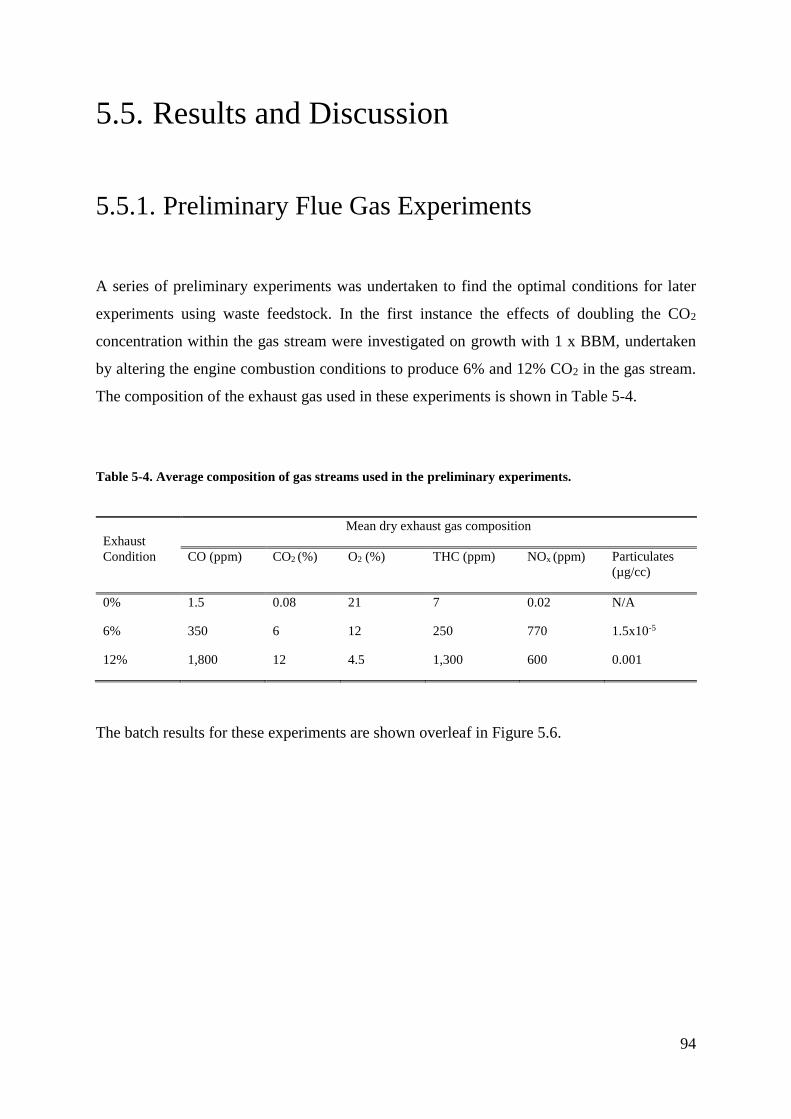
94

5.5. Results and Discussion

5.5.1. Preliminary Flue Gas Experiments

A series of preliminary experiments was undertaken to find the optimal conditions for later

experiments using waste feedstock. In the first instance the effects of doubling the CO2

concentration within the gas stream were investigated on growth with 1 x BBM, undertaken

by altering the engine combustion conditions to produce 6% and 12% CO2 in the gas stream.

The composition of the exhaust gas used in these experiments is shown in Table 5-4.

Table 5-4. Average composition of gas streams used in the preliminary experiments.

The batch results for these experiments are shown overleaf in Figure 5.6.

Exhaust

Condition

Mean dry exhaust gas composition

CO (ppm) CO2 (%) O2 (%) THC (ppm) NOx (ppm) Particulates

(µg/cc)

0% 1.5 0.08 21 7 0.02 N/A

6% 350 6 12 250 770 1.5x10-5

12% 1,800 12 4.5 1,300 600 0.001

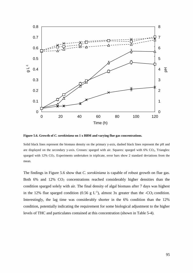
95

Figure 5.6. Growth of C. sorokiniana on 1 x BBM and varying flue gas concentrations.

Solid black lines represent the biomass density on the primary y-axis, dashed black lines represent the pH and

are displayed on the secondary y-axis. Crosses: sparged with air. Squares: sparged with 6% CO2, Triangles:

sparged with 12% CO2. Experiments undertaken in triplicate, error bars show 2 standard deviations from the

mean.

The findings in Figure 5.6 show that C. sorokiniana is capable of robust growth on flue gas.

Both 6% and 12% CO2 concentrations reached considerably higher densities than the

condition sparged solely with air. The final density of algal biomass after 7 days was highest

in the 12% flue sparged condition (0.56 g L-1), almost 3x greater than the -CO2 condition.

Interestingly, the lag time was considerably shorter in the 6% condition than the 12%

condition, potentially indicating the requirement for some biological adjustment to the higher

levels of THC and particulates contained at this concentration (shown in Table 5-4).

0

1

2

3

4

5

6

7

8

0

0.1

0.2

0.3

0.4

0.5

0.6

0.7

0.8

0 20 40 60 80 100 120

pH

g L

-1

Time (h)

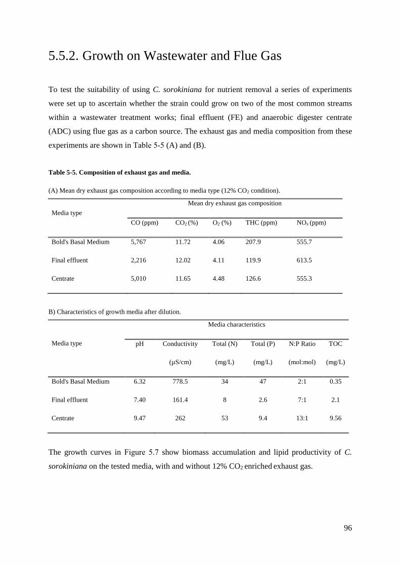
96

5.5.2. Growth on Wastewater and Flue Gas

To test the suitability of using C. sorokiniana for nutrient removal a series of experiments

were set up to ascertain whether the strain could grow on two of the most common streams

within a wastewater treatment works; final effluent (FE) and anaerobic digester centrate

(ADC) using flue gas as a carbon source. The exhaust gas and media composition from these

experiments are shown in Table 5-5 (A) and (B).

Table 5-5. Composition of exhaust gas and media.

(A) Mean dry exhaust gas composition according to media type (12% CO2 condition).

Media type

Mean dry exhaust gas composition

CO (ppm) CO2 (%) O2 (%) THC (ppm) NOx (ppm)

Bold's Basal Medium 5,767 11.72 4.06 207.9 555.7

Final effluent 2,216 12.02 4.11 119.9 613.5

Centrate 5,010 11.65 4.48 126.6 555.3

B) Characteristics of growth media after dilution.

Media type

Media characteristics

pH Conductivity

(µS/cm)

Total (N)

(mg/L)

Total (P)

(mg/L)

N:P Ratio

(mol:mol)

TOC

(mg/L)

Bold's Basal Medium 6.32 778.5 34 47 2:1 0.35

Final effluent 7.40 161.4 8 2.6 7:1 2.1

Centrate 9.47 262 53 9.4 13:1 9.56

The growth curves in Figure 5.7 show biomass accumulation and lipid productivity of C.

sorokiniana on the tested media, with and without 12% CO2 enriched exhaust gas.

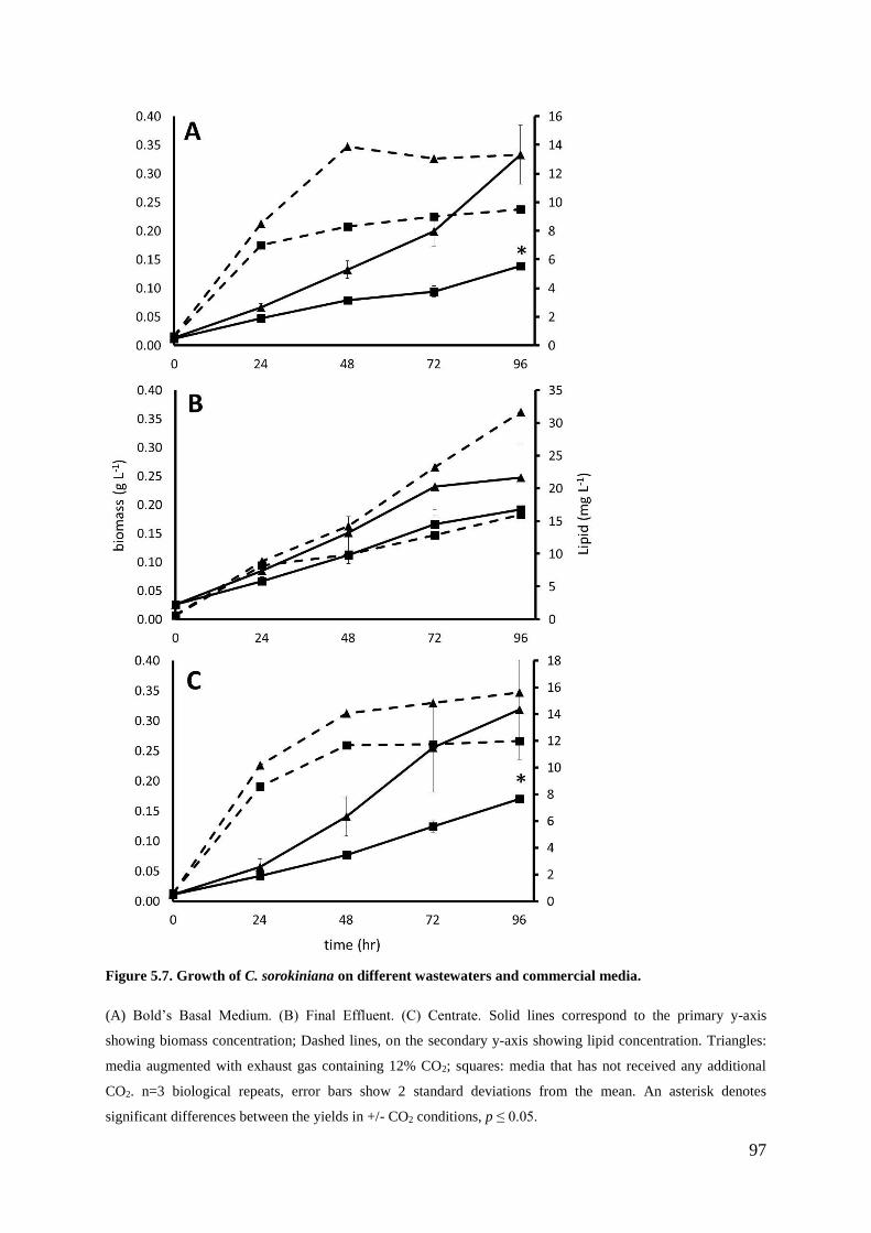
97

Figure 5.7. Growth of C. sorokiniana on different wastewaters and commercial media.

(A) Bold’s Basal Medium. (B) Final Effluent. (C) Centrate. Solid lines correspond to the primary y-axis

showing biomass concentration; Dashed lines, on the secondary y-axis showing lipid concentration. Triangles:

media augmented with exhaust gas containing 12% CO2; squares: media that has not received any additional

CO2. n=3 biological repeats, error bars show 2 standard deviations from the mean. An asterisk denotes

significant differences between the yields in +/- CO2 conditions, p ≤ 0.05.

98

The results of growth on BBM (Figure 5.7 A) indicate there is a significant increase (p ≤

0.05) in biomass productivity under conditions of exhaust gas sparging compared to the non-

enriched condition (82.5 mg L-1 d-1 to 35.5 mg L-1 d-1 respectively). After 96 h growth, the

CO2-supplemented cultures were still growing, and gave an average final biomass yield of

330±50 mg L-1, whilst the control gave a final biomass yield of 140±3 mg L-1. The 24 h µmax

of the CO2 supplemented culture was found to be 0.07 h-1, whilst that of the non-enriched

condition was found to be 0.06 h-1. Neutral lipid concentration increased over the course of

the experiment, with the CO2 augmented condition giving a final yield of 13 mg L-1 against

9.5 mg L-1 in the non-augmented condition (productivity of 3.25 mg L-1 d-1 and 2.38 mg L-1 d-

1 respectively). The final effluent results (Figure 5.7 B) show that after 96 h, a final biomass

yield of 250±56 mg L-1 is obtained, whilst the control showed a final biomass yield of

220±58 mg L-1, (with productivities of 62.5 mg L-1 d-1 and 55 mg L-1 d-1 respectively). The

24 h µmax of the CO2 supplemented culture was 0.05 hr-1, whilst that of the control was 0.04

hr-1. Lipid yield increased after 48 hours, peaking at 32 mg L-1 in the CO2 supplemented

condition and 16 mg L-1 in the non CO2 enriched condition (comparative productivity of 8 mg

L-1 d-1 and 4 mg L-1 d-1 respectively). Growth on anaerobic digester centrate is shown in

(Figure 5.7 C). Again, the results demonstrate a significant increase (p ≤ 0.05) in biomass

yield after 96 h under conditions of exhaust gas sparging when compared to the control. The

CO2 supplemented culture showed a final biomass yield of 320±83 mg L-1, whilst the non

CO2 enriched group showed a final biomass yield of 170±20 mg L-1 (productivities of 80 mg

L-1 d-1 and 42.5 mg L-1 d-1 respectively). The 24 h µmax of the CO2 supplemented culture was

0.07 h-1, whilst that of the control group was 0.05 h-1. Neutral lipid yield showed a similar

trend to the other experiments; with a 16 mg L-1 total in the CO2 enriched condition and 12

mg L-1 in the non-augmented condition (productivity of 4 mg L-1 d-1 and 3 mg L-1 d-1

respectively).

The results from these growth experiments show that the strain can perform in a manner

comparable to commercial media when grown on either autoclaved wastewater final effluent

or centrate under batch conditions. The maximal growth rates and biomass yields were within

a similar range over 96 hours, but BBM and ADC were shown to be marginally superior in

terms of growth rate and yield compared to FE. This could be attributed to the higher nutrient

levels found within these media types. It was also noted that larger productivity differences

were seen between CO2 sparged and non CO2 sparged conditions in these richer media types

99

(BBM and centrate). These results show that growth is augmented considerably with the

addition of 12% CO2 exhaust, especially when nutrient levels are sufficient. The general

effect of increasing the concentration of dissolved carbon dioxide is in good agreement with

previous studies within the literature (Azov, Shelef and Moraine 1982).

Lipid yield and productivity was found to be significantly higher in the cultures bubbled with

12% CO2. It is probable that this extra dissolved carbon had a dual effect in both augmenting

growth, as well as providing excess carbon flux towards lipid production (Widjaja, Chien and

Ju 2009). Despite the noticeable difference, the total lipid productivity was probably

underestimated slightly due to the preference of Nile Red to partition into highly hydrophobic

environments and hence fluoresces to a greater degree in the presence of intracellular neutral

lipid droplets, as opposed to cellular membrane lipids (Greenspan, Mayer and Fowler 1985).

This particular measurement error could be overcome through the use of better quantitative

methods; which could include conventional lipid extraction methods (Bligh and Dyer 1959),

or specific FAME analysis using gas chromatography coupled to mass spectroscopy (GC-

MS) (Vonlanthen 2013). Interestingly, the highest lipid productivity was found in the final

effluent condition, with almost double the yield over 96 h when compared to the other media

types. This could be attributed to the lower concentration of nitrogen within the final effluent;

resulting in rapid starvation over the course of the experiment. The subsequent re-direction of

metabolic carbon and nitrogen flux result in the stress response shown by C. sorokiniana.

This triggers the production of energy storage molecules including lipids, and initiates

chlorosis after 48 hours according to well understood mechanisms (Rodolfi et al. 2009).

5.5.3. Effect on pH and Conductivity

The effect that algal growth has upon the pH and conductivity of the wastewater was

investigated, so as to ascertain any changes in the water chemistry during the experiment. The

results are shown in Figure 5.8.

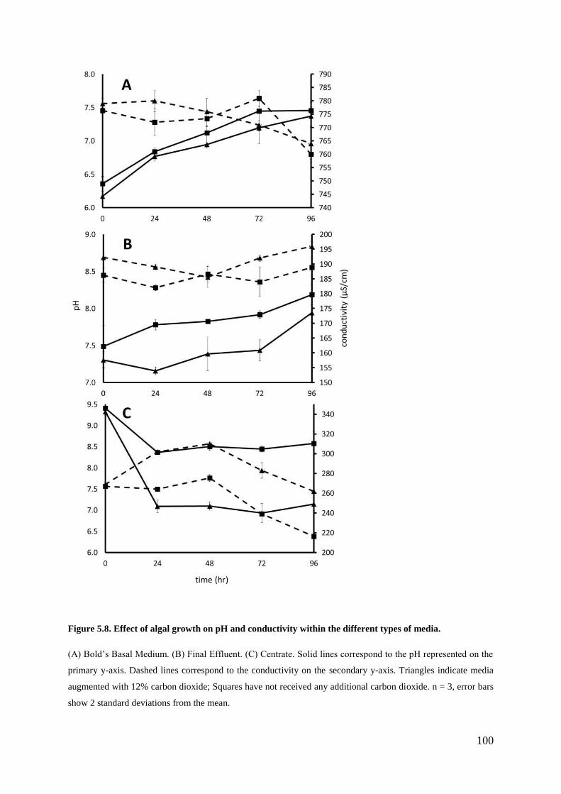
100

Figure 5.8. Effect of algal growth on pH and conductivity within the different types of media.

(A) Bold’s Basal Medium. (B) Final Effluent. (C) Centrate. Solid lines correspond to the pH represented on the

primary y-axis. Dashed lines correspond to the conductivity on the secondary y-axis. Triangles indicate media

augmented with 12% carbon dioxide; Squares have not received any additional carbon dioxide. n = 3, error bars

show 2 standard deviations from the mean.

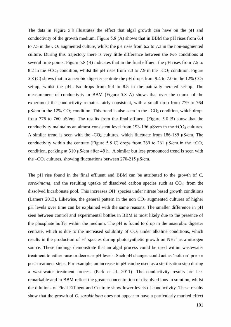
101

The data in Figure 5.8 illustrates the effect that algal growth can have on the pH and

conductivity of the growth medium. Figure 5.8 (A) shows that in BBM the pH rises from 6.4

to 7.5 in the CO2 augmented culture, whilst the pH rises from 6.2 to 7.3 in the non-augmented

culture. During this trajectory there is very little difference between the two conditions at

several time points. Figure 5.8 (B) indicates that in the final effluent the pH rises from 7.5 to

8.2 in the +CO2 condition, whilst the pH rises from 7.3 to 7.9 in the –CO2 condition. Figure

5.8 (C) shows that in anaerobic digester centrate the pH drops from 9.4 to 7.0 in the 12% CO2

set-up, whilst the pH also drops from 9.4 to 8.5 in the naturally aerated set-up. The

measurement of conductivity in BBM (Figure 5.8 A) shows that over the course of the

experiment the conductivity remains fairly consistent, with a small drop from 779 to 764

μS/cm in the 12% CO2 condition. This trend is also seen in the –CO2 condition, which drops

from 776 to 760 μS/cm. The results from the final effluent (Figure 5.8 B) show that the

conductivity maintains an almost consistent level from 193-196 μS/cm in the +CO2 cultures.

A similar trend is seen with the -CO2 cultures, which fluctuate from 186-189 μS/cm. The

conductivity within the centrate (Figure 5.8 C) drops from 269 to 261 μS/cm in the +CO2

condition, peaking at 310 μS/cm after 48 h. A similar but less pronounced trend is seen with

the –CO2 cultures, showing fluctuations between 270-215 μS/cm.

The pH rise found in the final effluent and BBM can be attributed to the growth of C.

sorokiniana, and the resulting uptake of dissolved carbon species such as CO2, from the

dissolved bicarbonate pool. This increases OH- species under nitrate based growth conditions

(Lamers 2013). Likewise, the general pattern in the non CO2 augmented cultures of higher

pH levels over time can be explained with the same reasons. The smaller difference in pH

seen between control and experimental bottles in BBM is most likely due to the presence of

the phosphate buffer within the medium. The pH is found to drop in the anaerobic digester

centrate, which is due to the increased solubility of CO2 under alkaline conditions, which

results in the production of H+ species during photosynthetic growth on NH4+ as a nitrogen

source. These findings demonstrate that an algal process could be used within wastewater

treatment to either raise or decrease pH levels. Such pH changes could act as ‘bolt-on’ pre- or

post-treatment steps. For example, an increase in pH can be used as a sterilisation step during

a wastewater treatment process (Park et al. 2011). The conductivity results are less

remarkable and in BBM reflect the greater concentration of dissolved ions in solution, whilst

the dilutions of Final Effluent and Centrate show lower levels of conductivity. These results

show that the growth of C. sorokiniana does not appear to have a particularly marked effect

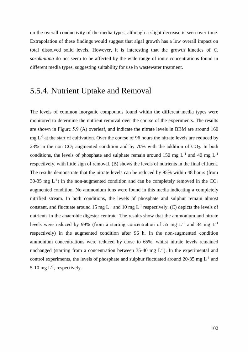
102

on the overall conductivity of the media types, although a slight decrease is seen over time.

Extrapolation of these findings would suggest that algal growth has a low overall impact on

total dissolved solid levels. However, it is interesting that the growth kinetics of C.

sorokiniana do not seem to be affected by the wide range of ionic concentrations found in

different media types, suggesting suitability for use in wastewater treatment.

5.5.4. Nutrient Uptake and Removal

The levels of common inorganic compounds found within the different media types were

monitored to determine the nutrient removal over the course of the experiments. The results

are shown in Figure 5.9 (A) overleaf, and indicate the nitrate levels in BBM are around 160

mg L-1 at the start of cultivation. Over the course of 96 hours the nitrate levels are reduced by

23% in the non CO2 augmented condition and by 70% with the addition of CO2. In both

conditions, the levels of phosphate and sulphate remain around 150 mg L-1 and 40 mg L-1

respectively, with little sign of removal. (B) shows the levels of nutrients in the final effluent.

The results demonstrate that the nitrate levels can be reduced by 95% within 48 hours (from

30-35 mg L-1) in the non-augmented condition and can be completely removed in the CO2

augmented condition. No ammonium ions were found in this media indicating a completely

nitrified stream. In both conditions, the levels of phosphate and sulphur remain almost

constant, and fluctuate around 15 mg L-1 and 10 mg L-1 respectively. (C) depicts the levels of

nutrients in the anaerobic digester centrate. The results show that the ammonium and nitrate

levels were reduced by 99% (from a starting concentration of 55 mg L-1 and 34 mg L-1

respectively) in the augmented condition after 96 h. In the non-augmented condition

ammonium concentrations were reduced by close to 65%, whilst nitrate levels remained

unchanged (starting from a concentration between 35-40 mg L-1). In the experimental and

control experiments, the levels of phosphate and sulphur fluctuated around 20-35 mg L-1 and

5-10 mg L-1, respectively.

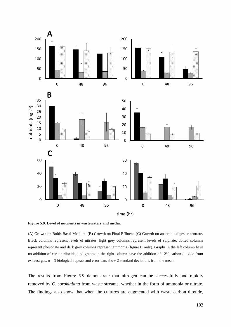
103

Figure 5.9. Level of nutrients in wastewaters and media.

(A) Growth on Bolds Basal Medium. (B) Growth on Final Effluent. (C) Growth on anaerobic digester centrate.

Black columns represent levels of nitrates, light grey columns represent levels of sulphate; dotted columns

represent phosphate and dark grey columns represent ammonia (figure C only). Graphs in the left column have

no addition of carbon dioxide, and graphs in the right column have the addition of 12% carbon dioxide from

exhaust gas. n = 3 biological repeats and error bars show 2 standard deviations from the mean.

The results from Figure 5.9 demonstrate that nitrogen can be successfully and rapidly

removed by C. sorokiniana from waste streams, whether in the form of ammonia or nitrate.

The findings also show that when the cultures are augmented with waste carbon dioxide,

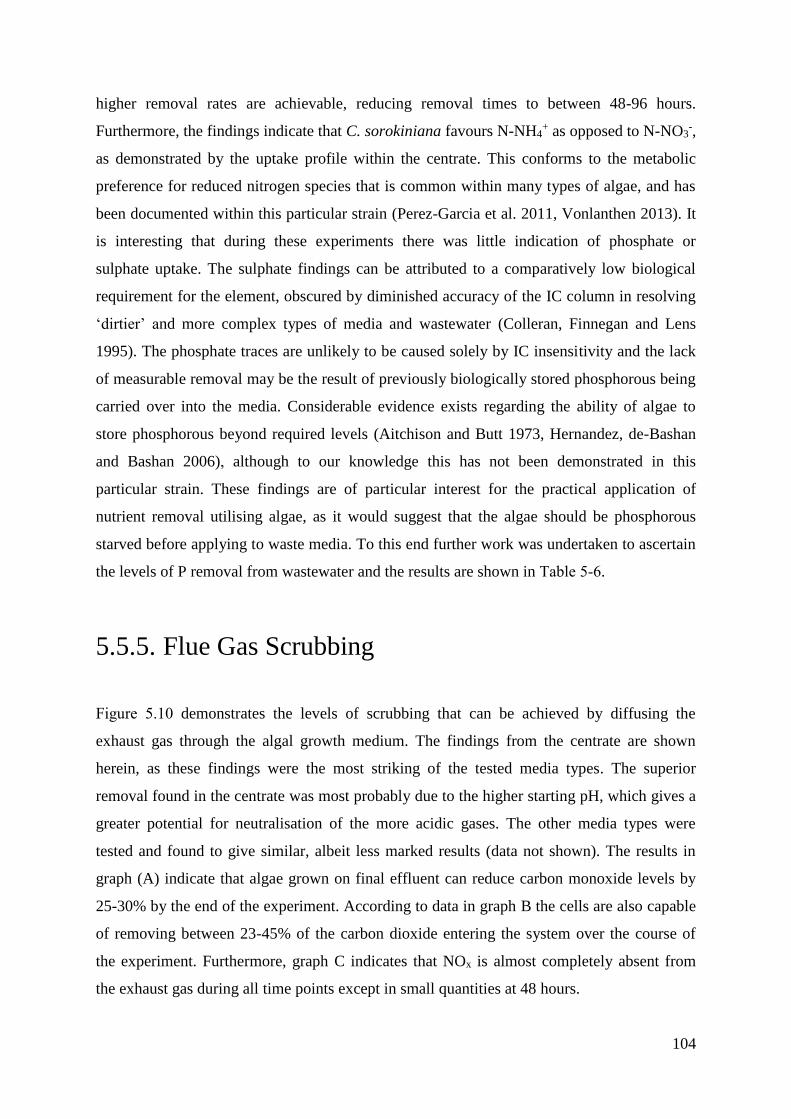
104

higher removal rates are achievable, reducing removal times to between 48-96 hours.

Furthermore, the findings indicate that C. sorokiniana favours N-NH4+ as opposed to N-NO3

-,

as demonstrated by the uptake profile within the centrate. This conforms to the metabolic

preference for reduced nitrogen species that is common within many types of algae, and has

been documented within this particular strain (Perez-Garcia et al. 2011, Vonlanthen 2013). It

is interesting that during these experiments there was little indication of phosphate or

sulphate uptake. The sulphate findings can be attributed to a comparatively low biological

requirement for the element, obscured by diminished accuracy of the IC column in resolving

‘dirtier’ and more complex types of media and wastewater (Colleran, Finnegan and Lens

1995). The phosphate traces are unlikely to be caused solely by IC insensitivity and the lack

of measurable removal may be the result of previously biologically stored phosphorous being

carried over into the media. Considerable evidence exists regarding the ability of algae to

store phosphorous beyond required levels (Aitchison and Butt 1973, Hernandez, de-Bashan

and Bashan 2006), although to our knowledge this has not been demonstrated in this

particular strain. These findings are of particular interest for the practical application of

nutrient removal utilising algae, as it would suggest that the algae should be phosphorous

starved before applying to waste media. To this end further work was undertaken to ascertain

the levels of P removal from wastewater and the results are shown in Table 5-6.

5.5.5. Flue Gas Scrubbing

Figure 5.10 demonstrates the levels of scrubbing that can be achieved by diffusing the

exhaust gas through the algal growth medium. The findings from the centrate are shown

herein, as these findings were the most striking of the tested media types. The superior

removal found in the centrate was most probably due to the higher starting pH, which gives a

greater potential for neutralisation of the more acidic gases. The other media types were

tested and found to give similar, albeit less marked results (data not shown). The results in

graph (A) indicate that algae grown on final effluent can reduce carbon monoxide levels by

25-30% by the end of the experiment. According to data in graph B the cells are also capable

of removing between 23-45% of the carbon dioxide entering the system over the course of

the experiment. Furthermore, graph C indicates that NOx is almost completely absent from

the exhaust gas during all time points except in small quantities at 48 hours.

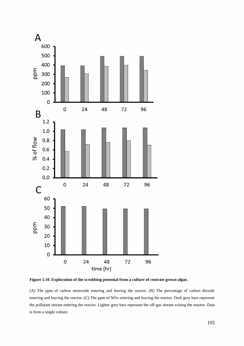
105

Figure 5.10. Exploration of the scrubbing potential from a culture of centrate grown algae.

(A) The ppm of carbon monoxide entering and leaving the reactor. (B) The percentage of carbon dioxide

entering and leaving the reactor. (C) The ppm of NOx entering and leaving the reactor. Dark grey bars represent

the pollutant stream entering the reactor. Lighter grey bars represent the off-gas stream exiting the reactor. Data

is from a single culture.

106

These findings show that a reasonably high level of flue gas scrubbing can be achieved

within a relatively simple system, with a liquid height not too dissimilar from that of an open

pond. Generally speaking, the removal rates of carbon dioxide are in a lower range than some

other findings within the literature (Vunjak-Novakovic et al. 2005, Doucha et al. 2005),

although these researchers appear to have optimised gas flow rate specifically for gaseous

contaminant reduction. This was not the case in this experiment, and the results presented

herein are more likely to reflect realistic removal during a batch operation, especially when

factors such as pH control and variable feed gas composition are taken into account. Removal

of NOx was found to be particularly high, at close to 100%, and was similar to other findings

from within the literature (Vunjak-Novakovic et al. 2005). However, given the low initial

concentrations of gases such as NOx (< 1000 ppm), it was not possible to conclude whether

removal could be attributed in its entirety to the biological or aqueous components of the

system without further experimentation (Svensson, Ljungström and Lindqvist 1987). In this

respect, future experimentation could explore optimising the levels of gas absorption within

the algal culture by adjusting a combination of gas flow rate, algal concentration and ion

concentration within the growth medium. Work could also be undertaken to ascertain

whether NOx is in fact metabolised by C. sorokiniana, by way of cultivation on a medium

lacking in nitrogen.

5.5.6. Continuous Flow

As many wastewater facilities operate with a continuous flow of effluent an experiment was

set up to test the feasibility of growing C. sorokiniana in continuous non axenic culture

conditions. The results are shown in Figure 5.11; and indicate that C. sorokiniana can be

grown continuously on BBM for 30 days in non-sterile conditions at a biomass concentration

of 0.1-0.15 g L-1 with the addition of 12% CO2.

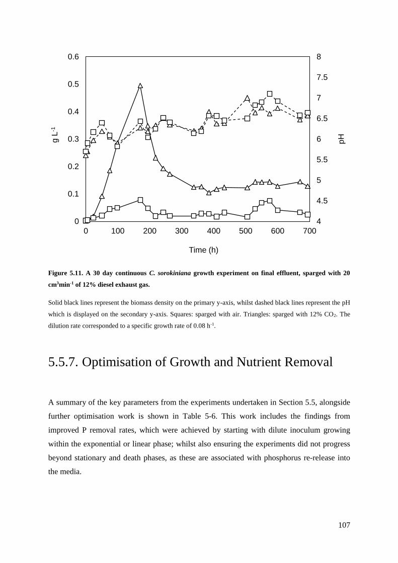
107

Figure 5.11. A 30 day continuous C. sorokiniana growth experiment on final effluent, sparged with 20

cm3min-1 of 12% diesel exhaust gas.

Solid black lines represent the biomass density on the primary y-axis, whilst dashed black lines represent the pH

which is displayed on the secondary y-axis. Squares: sparged with air. Triangles: sparged with 12% CO2. The

dilution rate corresponded to a specific growth rate of 0.08 h-1.

5.5.7. Optimisation of Growth and Nutrient Removal

A summary of the key parameters from the experiments undertaken in Section 5.5, alongside

further optimisation work is shown in Table 5-6. This work includes the findings from

improved P removal rates, which were achieved by starting with dilute inoculum growing

within the exponential or linear phase; whilst also ensuring the experiments did not progress

beyond stationary and death phases, as these are associated with phosphorus re-release into

the media.

4

4.5

5

5.5

6

6.5

7

7.5

8

0

0.1

0.2

0.3

0.4

0.5

0.6

0 100 200 300 400 500 600 700

pHg L

-1

Time (h)

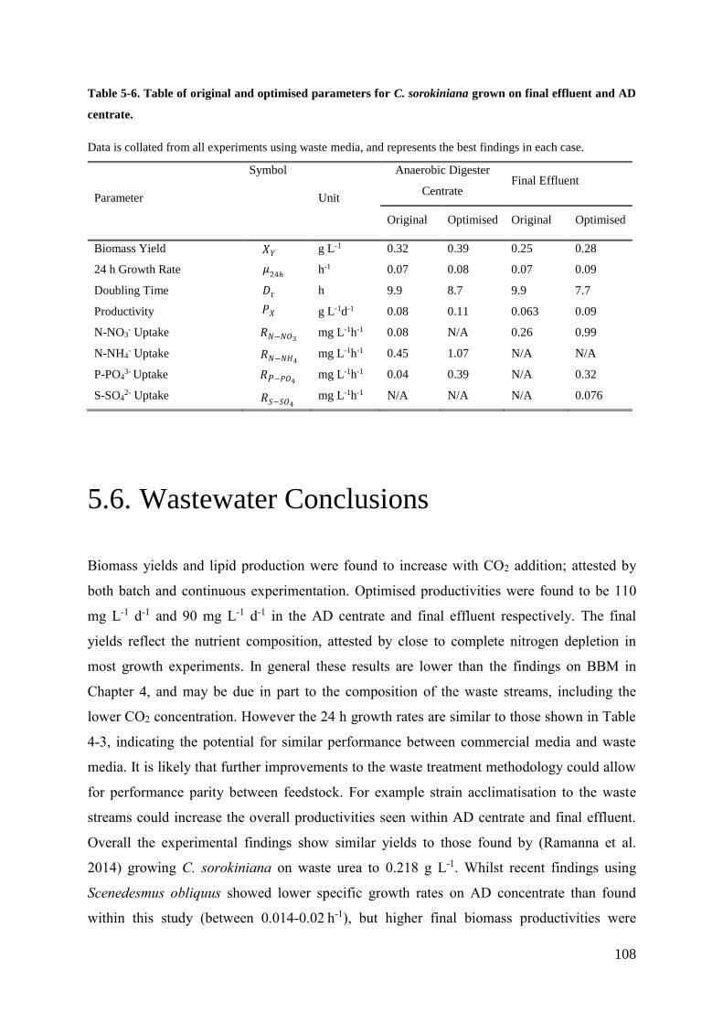
108

Table 5-6. Table of original and optimised parameters for C. sorokiniana grown on final effluent and AD

centrate.

Data is collated from all experiments using waste media, and represents the best findings in each case.

Parameter

Symbol

Unit

Anaerobic Digester

Centrate Final Effluent

Original Optimised Original Optimised

Biomass Yield g L-1 0.32 0.39 0.25 0.28

24 h Growth Rate h-1 0.07 0.08 0.07 0.09

Doubling Time h 9.9 8.7 9.9 7.7

Productivity g L-1d-1 0.08 0.11 0.063 0.09

N-NO3- Uptake mg L-1h-1 0.08 N/A 0.26 0.99

N-NH4- Uptake mg L-1h-1 0.45 1.07 N/A N/A

P-PO43- Uptake mg L-1h-1 0.04 0.39 N/A 0.32

S-SO42- Uptake mg L-1h-1 N/A N/A N/A 0.076

5.6. Wastewater Conclusions

Biomass yields and lipid production were found to increase with CO2 addition; attested by

both batch and continuous experimentation. Optimised productivities were found to be 110

mg L-1 d-1 and 90 mg L-1 d-1 in the AD centrate and final effluent respectively. The final

yields reflect the nutrient composition, attested by close to complete nitrogen depletion in

most growth experiments. In general these results are lower than the findings on BBM in

Chapter 4, and may be due in part to the composition of the waste streams, including the

lower CO2 concentration. However the 24 h growth rates are similar to those shown in Table

4-3, indicating the potential for similar performance between commercial media and waste

media. It is likely that further improvements to the waste treatment methodology could allow

for performance parity between feedstock. For example strain acclimatisation to the waste

streams could increase the overall productivities seen within AD centrate and final effluent.

Overall the experimental findings show similar yields to those found by (Ramanna et al.

2014) growing C. sorokiniana on waste urea to 0.218 g L-1. Whilst recent findings using

Scenedesmus obliquus showed lower specific growth rates on AD concentrate than found

within this study (between 0.014-0.02 h-1), but higher final biomass productivities were

𝜇24ℎ

𝑅𝑁−𝑁𝑂3

𝐷𝑡

𝑃𝑋

𝑅𝑃−𝑃𝑂4

𝑅𝑆−𝑆𝑂4

𝑅𝑁−𝑁𝐻4

𝑋𝑌

109

recorded (up to 0.311 g L-1 d- 1) (Xu et al. 2015).

In terms of nutrient removal, the results from the experiments in Chapter 5 show that both the

centrate and final effluent can be successfully used for algal cultivation. The first set of

experiments showed that nitrogen could be removed by 67-99% within 96 hours in both

wastewaters with the addition of CO2. Further optimisation experiments (Table 5-6) indicated

that N removal rates could reach the region of 1 mg L-1 h-1; whilst maximal P removal was

found to be in the region of 0.4 mg L-1 h-1, and up to 84% removal efficiency. The findings

compare favourably with recent literature reports of wastewater treatment with Chlorella spp;

showing similar findings to research by (Xu et al. 2015), in which N and P removal

efficiencies were shown to be around 74.63% and 88.79% respectively, using a bag based

photobioreactor. The findings are better than those of (Shriwastav et al. 2014) by 4 x for N

removal and 10 x for P removal. Similar removal efficiencies for N and P were found within

AD centrate (Wang et al. 2010a) and municipal wastewater (Hernandez et al. 2006).

Furthermore, the rates of nutrient removal found within this study were seen to be

comparable to the findings shown by (Li et al. 2011), but better for ammonia-N removal than

those reported by (de-Bashan et al. 2008).

Algal growth was achieved despite the diesel exhaust emissions containing high levels of

particulates and un-burnt hydrocarbons, demonstrating the robustness of C. sorokiniana, and

its suitability for growth on flue gases in general. The results from the gas removal

experiments indicate reductions between 23-45% and 25-30% of CO2 and CO, respectively.

Whilst NOx was almost completely absent from the off-gas stream after scrubbing, showing

close to 100% removal. To date, little work had been undertaken within the literature to

investigate the suitability of this particular strain of C. sorokiniana to flue gases, with some

findings reported in the work of (Jeong, Gillis and Hwang 2003). However, the findings are

close to the reported 95% reductions in NOx concentrations reported by (Vunjak-Novakovic

et al. 2005), but lower than those reported for CO2 (50-82% removal efficiency). It is likely

that the CO2 removal efficiencies reported in the study could undergo some optimisation.

However, it is likely that any large scale remediation process would favour high mass transfer

of CO2 as opposed to removal efficiency. This is because lower flue gas volumetric flow rates

may inhibit algal growth by providing insufficient carbon dioxide (Rahaman et al. 2011).

This means any eco-biorefinery process would favour high gas concentrations and flow rates.

110

Overall the results would suggest that C. sorokiniana is sufficiently robust to be grown on

wastewater augmented with flue gas containing 12% CO2. Furthermore, the work indicates

that either FE or ADC are good replacements for conventional media. One interesting

consideration arising from this work is the challenge of optimising both biomass production

and feedstock remediation, which is perhaps one of the greatest problems with deploying an

eco-biorefinery approach at larger scale; due in part to the potential conflicts between the two

processes. This means it is most probably inevitable that one strand will take precedence over

the other, dependent on the principal desired outcome. Chapter 6 builds on the work of

Chapters 4-5 by looking at the requirements for scaling up algal production. This is

undertaken as an extended literature review of the different algal production platforms

alongside their relative advantages and disadvantages.

111

6. Reactor Design and Construction

6.1. Aims and Objectives

The construction of a prototype photobioreactor was undertaken to test the feasibility of

scaling up the growth and nutrient removal processes outlined in Chapters 4 and 5. The novel

reactor design aims to address the following objectives:

Completion of a comprehensive literature review to ensure that all important reactor

design parameters are mapped.

Use a suitable rationale to design a photobioreactor that can scale easily at low cost.

To construct a photobioreactor, using appropriate manufacturing methods and

construction materials.

Explore the potential suitability of the photobioreactor for wastewater treatment.

6.2. Overview of Important Considerations

The design and construction of a novel photobioreactor is a complex multi-parametric

problem, and one in which many different factors have to be considered. In practical terms

this means that most feasible cultivation platforms require a compromise between biotic,

abiotic and economic factors. Most of the more successful designs found both commercially

and within the literature attempt to maximise as many of the parameters as possible within

practical cost limits. The end result is an attempt to construct and operate the photobioreactor

within a multi-parametric ‘sweet-spot’. This philosophy has resulted in numerous small scale

approaches to cultivation; alongside several general blue-prints for larger scale platforms. In

fact most of the photobioreactors in successful operation today can be categorised as having

characteristics that are based on a relatively limited repertoire of basic designs and

112

construction materials. The most common configurations are notable in their external

appearance and include tubular, column, plate, membrane and pond based systems (Ugwu et

al. 2008).

Many of photobioreactor design considerations are relatively well established within the

literature (Acién Fernández et al. 2001, Weissman, Goebel and Benemann 1988, Ugwu et al.

2008, Pulz 2001) (Tredici 2004), and can be simplified into several major categories. Firstly,

a suitable surface for exposure to a source of irradiance is of great importance, as without

adequate light photosynthetic processes cannot occur. The next most important factor is to

ensure suitable provision for the containment of the culture and addition of the nutrients

necessary for algal growth. In practical terms this means that designs should include entry

points for the introduction of an appropriate carbon source; which is usually bubbled into the

culture as carbon dioxide. Within the cultivation medium suitable temperature control is a

very important factor for the maintenance of optimal growth rates and must be kept within set

constraints according to strain preference. Likewise, the ability to remove inhibitory waste

products from the process is imperative, especially when growing the culture to higher

densities. This is particularly true for dissolved oxygen levels, which is a factor known to

inhibit photosynthesis (Ugwu et al. 2008). A final factor of considerable importance is to

ensure these biotic and abiotic factors interface successfully; this is most commonly achieved

by mass transfer under well mixed (or turbulent) conditions within the reactor.

6.2.1. Lighting

Access to sufficient light is imperative for phototrophic algal cultivation, and its

maximisation within biological and economic constraints is desirable at all times. Algal

cultivation can be undertaken using either natural or artificial light; providing they have

sufficient quanta at the correct wavelengths (see Chapter 2, section 2.2.2). Traditional open

ponds often rely solely on natural sunlight and growth within these systems is subject to

seasonal and diurnal cycles (Park et al. 2011). Reliance on natural light has obvious

drawbacks, not least because a sizable proportion of the 24 hour day will have insufficient

light, meaning photosynthesis will stop and respiration will become the predominant

metabolic activity. Another important factor to consider when growing algae under natural

113

conditions is that many strains respond differently to diurnal and seasonal cycles. This has the

combined effect of altering the final biomass composition, and as a result can change the

yield of potential end products (Chen et al. 2011). Given these considerations, algal

production is better suited to latitudes closer to the equator, where irradiation is more

consistent and of a better quality due to decreased seasonal variation. Despite some of the

inherent problems with natural light, the one notable benefit is the significant reduction in

energy costs imparted on the cultivation process when used. This simple fact means that to

date a vast majority of commercially grown algae are produced with natural lighting

(Chaumont 1993, Chen et al. 2011).

Artificially illuminated systems have the benefit of offering a consistent light source, but at

considerable energetic costs. Conventional systems for lighting include fluorescent bulbs,

which are often deployed at laboratory scale due to a favourable wavelength profile and a

reasonable cost per W (see Figure 6.1 A). However, these lights often lack the power output

and penetration required for larger and more densely growing cultures. For these bigger

systems popular choices for irradiance include metal halide lights (see Figure 6.1 B), which

are favoured as they have a spectral output that closely matches natural light making them

ideal for photosynthetic processes. Recent developments in light emitting diode (LED)

technology have made them an attractive alternative to conventional lighting systems, as they

can be manufactured to specific wavelengths at reasonable cost. This means that the

cultivator has the potential to tailor the incident wavelengths to suit the strain or process

requirements. For example, red LEDs with wavelengths between 620-700 nm and blue LEDs

with wavelengths between 455-492 nm can be incorporated in varying proportions (see

Figure 6.1 C). The result is that wavelengths not used during photosynthesis can be excluded,

leading to an increase in quantum efficiency (Lee and Palsson 1996).

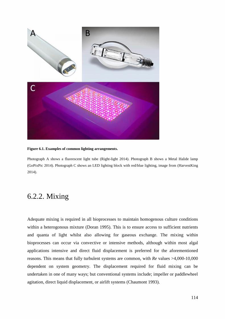
114

Figure 6.1. Examples of common lighting arrangements.

Photograph A shows a fluorescent light tube (Right-light 2014). Photograph B shows a Metal Halide lamp

(GoPixPic 2014). Photograph C shows an LED lighting block with red/blue lighting, image from (HarvestKing

2014).

6.2.2. Mixing

Adequate mixing is required in all bioprocesses to maintain homogenous culture conditions

within a heterogonous mixture (Doran 1995). This is to ensure access to sufficient nutrients

and quanta of light whilst also allowing for gaseous exchange. The mixing within

bioprocesses can occur via convective or intensive methods, although within most algal

applications intensive and direct fluid displacement is preferred for the aforementioned

reasons. This means that fully turbulent systems are common, with Re values >4,000-10,000

dependent on system geometry. The displacement required for fluid mixing can be

undertaken in one of many ways; but conventional systems include; impeller or paddlewheel

agitation, direct liquid displacement, or airlift systems (Chaumont 1993).

115

Impellers and paddle wheels can be used to move an aqueous dispersion around predictable

circulatory patterns by introducing kinetic energy into the fluid. Impellers tend to be used

within smaller laboratory scale systems, or within classical enclosed fermenters (see Figure

6.2 A). This method of mixing has the benefit of transferring a large amount of energy into

the fluid, but can also have some negative attributes, such as high energy consumption and

the creation of considerable shearing effects (Doran 1995). Furthermore, it has been found

that cultivating photosynthetic algae with impellers on a larger scale is challenging due to the

poor light penetration in bigger fermentation vessels (Singh and Sharma 2012). This means

that large scale impeller mixed systems have been deployed solely for heterotrophic

cultivation of algae, with Solazyme producing algal oil in this way in the US (Franklin et al.

2012). Paddlewheel systems differ from impellers in that they are only partially submerged

and positioned in a horizontal plane to the culture, they also run at a much lower rpm (see

Figure 6.2 B). This mode of mixing is preferred for larger scale algal production, due to its

lower running costs and comparative ease of maintenance (Terry and Raymond 1985).

However, the low liquid velocities induced by this type of mixing result in an algal culture

that is sub-optimally mixed, and dead zones are often created within certain areas of the

pond. Some of these problems can be overcome to an extent by introducing baffles and

maintaining certain depth to width and length relationships (Weissman and Goebel 1987,

Hadiyanto et al. 2013).

Other prominent mixing methods deployed within closed systems include liquid or air

pumps. Conventional pumps can be characterised into three main groups, based on how they

create the actual mixing. The first type of pump is the impulse or airlift pump, which creates

a density difference in the fluid circulation pathway, thereby forcing liquid circulation to

occur. These reactors are often described as having a bubble column or airlift configuration,

see Figure 6.2 (C) and (D), and are discussed further in Sections 6.3.6 and 6.3.7 (Chisti

1989). Another prominent category of pumping system is the positive displacement pump,

which creates movement by trapping a fixed volume of fluid and moving it into a discharge

pipe. This is achieved by creating a driving motion through reciprocating or rotary motion.

The final major category of pumps includes velocity driven motors. These operate by adding

kinetic energy into the fluid, increasing the pressure and flow rate around a set pathway (see

Figure 6.2 E). These types of pump form a broad category, which include rotodynamic and

centrifugal motors. Centrifugal pumps are frequently used to move liquids through piping

systems and therefore a popular choice for horizontal tubular reactors (McDonald 2013).

116

These pumps operate by allowing fluid to enter the impeller along or near to the rotating axis.

The liquid is then accelerated by the impeller flowing outward in either radial or axial

directions where it enters a diffuser or volute chamber upon which it can exit towards the

downstream piping system. Centrifugal systems can find particular applications where large

discharge through smaller heads is required.

Figure 6.2. Photographs of different mixing systems.

(A) Rushton impeller, deployed to create radial mixing within stirred tank reactors (Sunkaier 2015). (B)

Paddlewheel, used to create directional fluid mixing in open ponds (Mira 2015). (C) Bubble column reactor,

turbulence is created by direct bubbling of the culture (Allen 2013). (D) Airlift reactor (ALR), where air

injection creates directional liquid circulation. (E) Velocity pump, used in tubular systems, showing the inlet and

outlet (ReefCentral 2013). The red arrows indicate the direction of bulk fluid movement within each of the

mixing configurations.

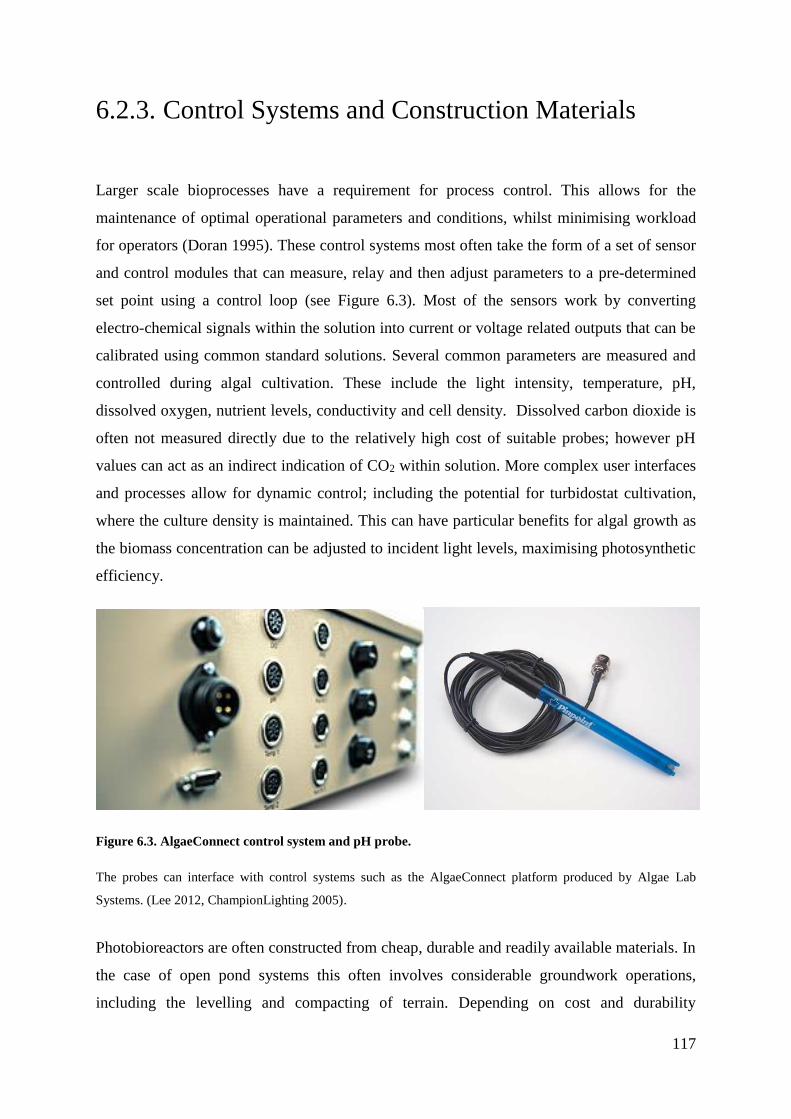
117

6.2.3. Control Systems and Construction Materials

Larger scale bioprocesses have a requirement for process control. This allows for the

maintenance of optimal operational parameters and conditions, whilst minimising workload

for operators (Doran 1995). These control systems most often take the form of a set of sensor

and control modules that can measure, relay and then adjust parameters to a pre-determined

set point using a control loop (see Figure 6.3). Most of the sensors work by converting

electro-chemical signals within the solution into current or voltage related outputs that can be

calibrated using common standard solutions. Several common parameters are measured and

controlled during algal cultivation. These include the light intensity, temperature, pH,

dissolved oxygen, nutrient levels, conductivity and cell density. Dissolved carbon dioxide is

often not measured directly due to the relatively high cost of suitable probes; however pH

values can act as an indirect indication of CO2 within solution. More complex user interfaces

and processes allow for dynamic control; including the potential for turbidostat cultivation,

where the culture density is maintained. This can have particular benefits for algal growth as

the biomass concentration can be adjusted to incident light levels, maximising photosynthetic

efficiency.

Figure 6.3. AlgaeConnect control system and pH probe.

The probes can interface with control systems such as the AlgaeConnect platform produced by Algae Lab

Systems. (Lee 2012, ChampionLighting 2005).

Photobioreactors are often constructed from cheap, durable and readily available materials. In

the case of open pond systems this often involves considerable groundwork operations,

including the levelling and compacting of terrain. Depending on cost and durability

118

requirements this preparatory work is followed by the laying of concrete or plastic under-

lining to contain the culture (Weissman and Goebel 1987, Tredici 2004). In the case of

externally illuminated photobioreactors, the choice of construction material is often decided

by the requirements for transparent materials with high optical clarity and resistance to solar

radiation, such as durable polymers like acrylic or polycarbonate (Tredici 2004). Glass is also

deployed, and can have many lifecycle benefits in comparison to plastics, especially in terms

of overall longevity and ease of cleaning. Other less optically important parts of the reactor

can be constructed from cheaper materials such as polyvinyl chloride (PVC) (Chaumont

1993). The final decision on the choice of material is often driven by a trade-off in lower

upfront expenditure and less durability versus longer lasting and more expensive building

materials. Modern trends in reactor design have started to focus on the environmental impact

of construction materials, achieved via detailed life-cycle assessment (Soratana and Landis

2011).

6.3. Common Reactor Designs

6.3.1. Reactor Geometries

Vessels for algal cultivation are commonly split into two broad categories, often described as

open or closed systems. Open systems usually take the form of high rate algal ponds

(HRAPs), open unmixed ponds or suspended cultures like membrane reactors. These systems

are inherently cheaper than other cultivation methods, but their exposed nature makes biotic

control more challenging. Enclosed vessels are often described as photobioreactors (PBRs).

They are used to culture algal biomass under more stringent and optimised conditions than

open systems (Borowitzka 1999). Although many different photobioreactor configurations

exist, three main geometries dominate; these include horizontal or vertical arrangements with

either tubular, plate or single column configurations. There is still some debate between the

relative merits of horizontally stacked or vertically stacked systems (Mirón et al. 1999),

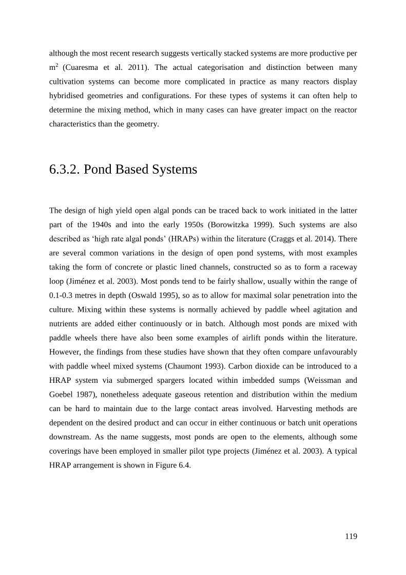
119

although the most recent research suggests vertically stacked systems are more productive per

m2 (Cuaresma et al. 2011). The actual categorisation and distinction between many

cultivation systems can become more complicated in practice as many reactors display

hybridised geometries and configurations. For these types of systems it can often help to

determine the mixing method, which in many cases can have greater impact on the reactor

characteristics than the geometry.

6.3.2. Pond Based Systems

The design of high yield open algal ponds can be traced back to work initiated in the latter

part of the 1940s and into the early 1950s (Borowitzka 1999). Such systems are also

described as ‘high rate algal ponds’ (HRAPs) within the literature (Craggs et al. 2014). There

are several common variations in the design of open pond systems, with most examples

taking the form of concrete or plastic lined channels, constructed so as to form a raceway

loop (Jiménez et al. 2003). Most ponds tend to be fairly shallow, usually within the range of

0.1-0.3 metres in depth (Oswald 1995), so as to allow for maximal solar penetration into the

culture. Mixing within these systems is normally achieved by paddle wheel agitation and

nutrients are added either continuously or in batch. Although most ponds are mixed with

paddle wheels there have also been some examples of airlift ponds within the literature.

However, the findings from these studies have shown that they often compare unfavourably

with paddle wheel mixed systems (Chaumont 1993). Carbon dioxide can be introduced to a

HRAP system via submerged spargers located within imbedded sumps (Weissman and

Goebel 1987), nonetheless adequate gaseous retention and distribution within the medium

can be hard to maintain due to the large contact areas involved. Harvesting methods are

dependent on the desired product and can occur in either continuous or batch unit operations

downstream. As the name suggests, most ponds are open to the elements, although some

coverings have been employed in smaller pilot type projects (Jiménez et al. 2003). A typical

HRAP arrangement is shown in Figure 6.4.

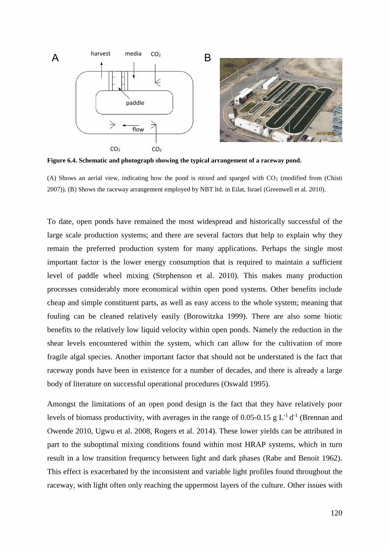
120

Figure 6.4. Schematic and photograph showing the typical arrangement of a raceway pond.

(A) Shows an aerial view, indicating how the pond is mixed and sparged with CO2 (modified from (Chisti

2007)). (B) Shows the raceway arrangement employed by NBT ltd. in Eilat, Israel (Greenwell et al. 2010).

To date, open ponds have remained the most widespread and historically successful of the

large scale production systems; and there are several factors that help to explain why they

remain the preferred production system for many applications. Perhaps the single most

important factor is the lower energy consumption that is required to maintain a sufficient

level of paddle wheel mixing (Stephenson et al. 2010). This makes many production

processes considerably more economical within open pond systems. Other benefits include

cheap and simple constituent parts, as well as easy access to the whole system; meaning that

fouling can be cleaned relatively easily (Borowitzka 1999). There are also some biotic

benefits to the relatively low liquid velocity within open ponds. Namely the reduction in the

shear levels encountered within the system, which can allow for the cultivation of more

fragile algal species. Another important factor that should not be understated is the fact that

raceway ponds have been in existence for a number of decades, and there is already a large

body of literature on successful operational procedures (Oswald 1995).

Amongst the limitations of an open pond design is the fact that they have relatively poor

levels of biomass productivity, with averages in the range of 0.05-0.15 g L-1 d-1 (Brennan and

Owende 2010, Ugwu et al. 2008, Rogers et al. 2014). These lower yields can be attributed in

part to the suboptimal mixing conditions found within most HRAP systems, which in turn

result in a low transition frequency between light and dark phases (Rabe and Benoit 1962).

This effect is exacerbated by the inconsistent and variable light profiles found throughout the

raceway, with light often only reaching the uppermost layers of the culture. Other issues with

A B harvest media CO2

CO2 CO2

flow

paddle

121

the use of open ponds concern their exposed nature, making contamination with competing

organisms or predator species particularly problematic. These problems can be partially

overcome by using growth conditions that favour the cultivated strain. For example the use of

extremophilic or extremotolerant organisms is a preferred option to avoid contamination

(Schenk et al. 2008). Other more generalised problems with open pond systems include the

relatively large areas of land required to establish a production facility, and a vulnerability to

changes in abiotic factors such as temperature, precipitation and fluctuations in light quality.

These criteria would render open ponds largely unsuitable for Central and Northern European

climates. Finally, from an environmental perspective there are also some water conservation

issues regarding the evaporative losses that can occur within hotter climates (Chisti 2007).

Open pond systems are particularly suited to the production of lower and middle value

biomass, including biofuels and feed production (Chaumont 1993). In fact current data

indicates that around 10 times more algal biomass is produced in open pond systems than

within closed reactors (Posten 2009). This data highlights the fact that if the algal

biotechnology industry is to reach its envisaged potential it is somewhat unlikely that closed

reactors will be able to cope with the volume and cost requirements necessary for lower value

bulk products. This means that it is likely that any serious attempt to produce large quantities

of lower value products such as algal biomass for biofuel will require the large scale

deployment of HRAP type systems due to their comparably favourable operational costs.

Currently pond based systems find considerable usage in the production of some higher value

pigments such as astaxanthin and beta-carotene (Borowitzka 1992). In fact several companies

produce algae for this purpose, including Cyanotech, who cultivate Haematococcus pluvialis

to produce astaxanthin in a two stage system; with the initial vegetative stage within closed

photobioreactors and the second maturation stage within outdoor HRAP systems (Borowitzka

1999). Other companies such as Seambiotic produce algae in open ponds grown from flue

gas and wastewater. In fact the integration of algae within wastewater treatment infrastructure

may be a promising avenue for HRAPs, particularly within warmer climates with abundant

unused land (Sheehan et al. 1998, Oswald 1988).

122

6.3.3. Membrane Reactors

The use of membrane technology is increasingly finding its way into the wastewater

treatment sector. This is due to the ability of membrane platforms to increase biological

retention within high flow rate systems, thereby decreasing the hydraulic retention time, and

improving system efficiency (Stephenson et al. 2000). Adaptations of membrane designs are

beginning to be trialled as algal production systems. Common designs vary in the way in

which the culture and media interact, but some form of trickling or rotational contact is

required to keep the algae moist. Perhaps some of the most innovative designs are those that

have a liquid mobile phase separated from the culture with a permeable barrier. An example

of such a configuration is shown in Figure 6.5, where the liquid phase is sandwiched between

two semi-permeable membranes. These membranes allow for the liquid and nutrients to pass

through the specific pore size, but the algae remain attached as a biofilm to the other side of

the membrane (Naumann et al. 2013, Shi et al. 2014). Although much work is still needed to

characterise these systems, the potential advantages are numerous and include a short light

path and little need for downstream de-watering. Foreseeable problems with membrane

reactors include the considerable cost burden associated with harvesting, which would require

considerable manpower. In fact this type of production would resemble agricultural

harvesting practices more closely than modern biotechnology. Other potential problems

centre on the membrane material, its durability and its propensity to foul, all of which could

lead to a considerable performance drop within the system.

Figure 6.5. Illustration and photograph of a membrane photobioreactor.

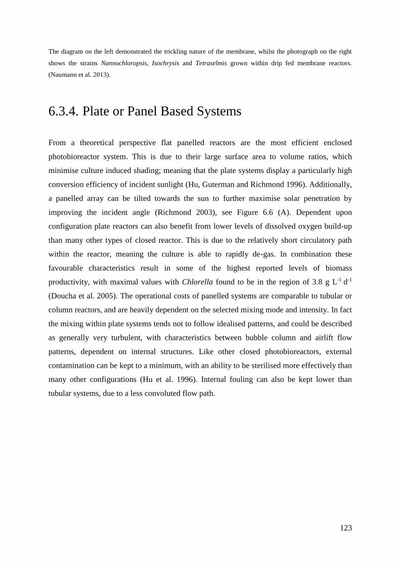
123

The diagram on the left demonstrated the trickling nature of the membrane, whilst the photograph on the right

shows the strains Nannochloropsis, Isochrysis and Tetraselmis grown within drip fed membrane reactors.

(Naumann et al. 2013).

6.3.4. Plate or Panel Based Systems

From a theoretical perspective flat panelled reactors are the most efficient enclosed

photobioreactor system. This is due to their large surface area to volume ratios, which

minimise culture induced shading; meaning that the plate systems display a particularly high

conversion efficiency of incident sunlight (Hu, Guterman and Richmond 1996). Additionally,

a panelled array can be tilted towards the sun to further maximise solar penetration by

improving the incident angle (Richmond 2003), see Figure 6.6 (A). Dependent upon

configuration plate reactors can also benefit from lower levels of dissolved oxygen build-up

than many other types of closed reactor. This is due to the relatively short circulatory path

within the reactor, meaning the culture is able to rapidly de-gas. In combination these

favourable characteristics result in some of the highest reported levels of biomass

productivity, with maximal values with Chlorella found to be in the region of 3.8 g L-1 d-1

(Doucha et al. 2005). The operational costs of panelled systems are comparable to tubular or

column reactors, and are heavily dependent on the selected mixing mode and intensity. In fact

the mixing within plate systems tends not to follow idealised patterns, and could be described

as generally very turbulent, with characteristics between bubble column and airlift flow

patterns, dependent on internal structures. Like other closed photobioreactors, external

contamination can be kept to a minimum, with an ability to be sterilised more effectively than

many other configurations (Hu et al. 1996). Internal fouling can also be kept lower than

tubular systems, due to a less convoluted flow path.

124

Figure 6.6. Diagram shows the potential arrangements of flat panelled reactors.

(A) Gives an indication of the many different tilt angles that are possible to optimise solar penetration. (B)

Shows an array of glass plated panelled reactors at Phoenix, US (NanoVoltaics 2014).

One potential drawback of deploying a flat panelled system is the practical scalability of the

array, as some level of compromise has to be struck between solar collecting surface area,

culture depth and areal considerations, see Figure 6.6 (B). This problem can be overcome to

some extent by connecting a modular array of panels in tandem, although the resultant areal

footprint would be likely to be bigger than the equivalent volume within other types of closed

reactors. Other physical drawbacks to panelled systems include the fact that temperature

control within the reactor can be more energy intensive than other PBR geometries, caused

by the large surface area to volume ratio (Sierra et al. 2008). These larger surface areas and

comparatively short light paths can also create problems with photo-damage if the light levels

are too high; although this damaging effect can be lessened by using turbidostat based

cultivation techniques (Cuaresma et al. 2012). The large surface area to volume ratio also

means that the levels of hydrodynamic stress placed on the algae can be higher than in some

other systems (Brennan and Owende 2010). As with all bioreactors it is also likely that some

degree of wall growth and fouling is unavoidable, especially at the meeting of straight edges,

where the liquid velocity is lower. Another notable point is that the rapid degassing seen in

flat panels could be seen as advantageous in most applications, as it prevents the build-up of

dissolved oxygen. However, the opposite is true if gas use efficiency is sought, as gas

retention is considerably lower in these systems.

Larger scale plate or panel PBRs (Figure 6.6 B) are less commonly deployed than other

closed systems; although one prominent example is the system deployed by Dr Tredici’s

research group in Italy (Rodolfi et al. 2009), with a reactor chassis that can be constructed

from either rigid or flexible plastics. However, there are to date, still numerous manufacturing

A B

125

and cost related issues that need to be overcome before plate systems achieve widespread

deployment. This includes issues with scalability, and problems associated with the sealing

and warping of the planar materials during temperature stress (McDonald 2013). As the

manufacturing problems are overcome it is likely that flat panelled systems will increasingly

find similar applications to those employed by tubular reactors, although with some distinct

process advantages in terms of degassing and solar penetration. At smaller scale the

combination of large surface area and short light path make panelled systems a favourable

option, and systems such as the Labfors 5 Lux photobioreactor (INFORS HT) have found

considerable use in growth modelling and screening (Glaser 2012). In the shorter term it is

likely that higher value indoor algal cultivation may find considerable use for flat panels,

especially if good productivity levels are required. Algenol are one example, using large

modular bag based panels to produce ethanol (Woods et al. 2010). In the UK the company

Algaecytes has developed its own in-house flat panel reactor for the production of omega-3

oils (Bashir 2014).

6.3.5. Horizontal Tubular Systems

Tubular photobioreactors encompass a broad range of designs, and can be arranged either

horizontally or vertically, in serpentine or manifold arrangements (Chisti 2007). They can

also be laid flat on the ground or positioned stacked above one another. Most traditional

commercial and research designs tend to favour a single serpentine or horizontal manifold

arrangement, with the tubes stacked vertically in order to maximise areal productivity

(Cuaresma et al. 2011). Tubular systems have many comparative advantages over open pond

systems. Most importantly they have been shown to achieve higher and more consistent

levels of areal productivity than can be achieved within open ponds (Posten 2009). This is

because horizontal tubular systems have larger illuminated surfaces than open ponds, with

tubes often in the region of 0.03 – 0.1 m in diameter. Productivity is further improved within

tubular systems by the higher liquid velocities found within them which acts to increase the

level of turbulence (Borowitzka 1999). This, in combination with better light penetration

allows for far higher algal growth rates than open ponds; with reports of biomass productivity

reaching 1.9 g L-1 d-1 using a tubular airlift cultivating Phaeodactylum tricornutum (Molina et

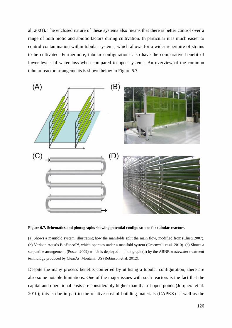
126

al. 2001). The enclosed nature of these systems also means that there is better control over a

range of both biotic and abiotic factors during cultivation. In particular it is much easier to

control contamination within tubular systems, which allows for a wider repertoire of strains

to be cultivated. Furthermore, tubular configurations also have the comparative benefit of

lower levels of water loss when compared to open systems. An overview of the common

tubular reactor arrangements is shown below in Figure 6.7.

Figure 6.7. Schematics and photographs showing potential configurations for tubular reactors.

(a) Shows a manifold system, illustrating how the manifolds split the main flow, modified from (Chisti 2007).

(b) Varicon Aqua’s BioFence™, which operates under a manifold system (Greenwell et al. 2010). (c) Shows a

serpentine arrangement, (Posten 2009) which is deployed in photograph (d) by the ABNR wastewater treatment

technology produced by ClearAs, Montana, US (Robinson et al. 2012).

Despite the many process benefits conferred by utilising a tubular configuration, there are

also some notable limitations. One of the major issues with such reactors is the fact that the

capital and operational costs are considerably higher than that of open ponds (Jorquera et al.

2010); this is due in part to the relative cost of building materials (CAPEX) as well as the

127

considerable energy requirements for operation (OPEX). As with all closed systems it is also

common to find some degree of wall growth and fouling. This can increase the costs

associated with the cleaning and maintenance of such a system, and can become a particular

challenge with larger and more elaborate photobioreactors (McDonald 2013). To overcome

this problem, several companies have devised ingenious methods of keeping the reactor walls

clean, a prominent example being the use of Bio-Beads™ in Varicon Aqua’s BioFence™

(Hulatt and Thomas 2011). In manufacturing terms, the scale-up of tubular reactors can be a

reasonably straight forward process; however larger deployments can suffer from a variety of

biotic and abiotic problems. One major problem with large scale tubular systems is that

considerable gradients of dissolved oxygen, carbon dioxide and pH can develop across the

system, causing inhibition or underperformance of algal growth (Sobczuk et al. 2000). These

considerations can place a practical constraint on the run length of many tubular reactors,

meaning that very large scale systems require interruptions in the run length for degassing. It

is also worth noting that many of these tubular systems are inappropriate for the more fragile

strains of algae, due to the relatively high liquid velocities which cause considerable shear

within the culture (Chisti 2007). Another important consideration when scaling a tubular

system is the multiplication of pumping energy requirements to overcome the frictional

forces of multiple tubes and bends (Borowitzka 1999).

Prominent examples of tubular systems within the literature include the ground based,

horizontal tubular reactor in Cadiz, Spain (Molina et al. 2001) and the vertically stacked

manifold system at the Ben Gurion University, Israel, (Richmond et al. 1993). Mixing within

these tubular reactors is conventionally achieved with a variety of pumping systems,

including centrifugal or diaphragm pumps, as well as airlift driven systems. Many horizontal

tubular reactors are already on the market, and may be purchased in the form of specialised

equipment from a variety of suppliers. One prominent example is Varicon Aqua’s

BioFenceTM (Figure 6.7 B) which has been deployed in over 100 locations worldwide for

both research and industrial activities (McDonald 2013). Currently the system has found

widespread use in the production of higher value nutraceutical and cosmetic compounds. One

example is the deployment of the BioFenceTM in the production of cyanobacterial metabolites

for use in cosmetic products by Blue Lagoon in Iceland (McDonald 2013). Other examples of

commercial production in tubular systems can be found in Ketura, Israel where

Haematococcus pluvialis is grown for the production of astaxanthin in a custom built

manifold system (Richmond et al. 1993). In terms of bulk production, it is more likely in the

128

short term that closed photobioreactors will integrate with open pond systems either as high

rate inoculation platforms or within a two stage production process (Rodolfi et al. 2009).

Looking towards the near future, it is likely that tubular photobioreactors will continue to find

increased usage in the production of higher grade biochemicals, especially where quality

control is of the utmost importance (Pulz 2001).

6.3.6. Bubble Columns

Bubble columns have found widespread use as multiphase reactors in various chemical and

biotechnological processes (Kantarci, Borak and Ulgen 2005). They are used extensively in a

variety of fermentation processes and have proved to be highly adaptable to the cultivation of

many different micro-organisms (see Figure 6.8). Phototrophic bubble columns are typically

smaller in diameter than their heterotrophic counterparts often displaying heights in the range

of 1-2 m, and diameters in the range of 0.1- 0.3 m (Mirón et al. 2000). The mixing regime

within column reactors is created via pneumatic air displacement. At smaller scales mixing in

this way can achieve considerable turbulence, with lower energy consumption than many

other types of liquid displacement pump. However, at larger scales centrifugal pumps tend to

display greater energy efficiency. Other benefits of mixing via aeration are the high mass

transfer coefficients that can be achieved, as well as creating less shear than many other types

of liquid circulation (Mirón et al. 2004). Reports from the literature would indicate that

productivity can reach an average of 0.42 g L-1 d-1 within column systems cultivating

Tetraselmis (Zittelli et al. 2006). Further advantages of column reactors include the fact that

they can be spaced in fairly compact arrangements, allowing for better productivity per m2.

They are also relatively simple to construct in comparison to the larger horizontal tubular

systems that currently dominate the market place, whilst the absence of internal parts can

translate to lower overall maintenance costs (Mirón et al. 2000). Another notable benefit to

using a bubble column configuration is that it can be made from a wider variety of materials

than most other reactors. This includes lower cost plastics like PVC, polyethylene (PE) or

ethylene tetrafluoroethylene (ETFE), which can dramatically lower the CAPEX during the

manufacturing process.

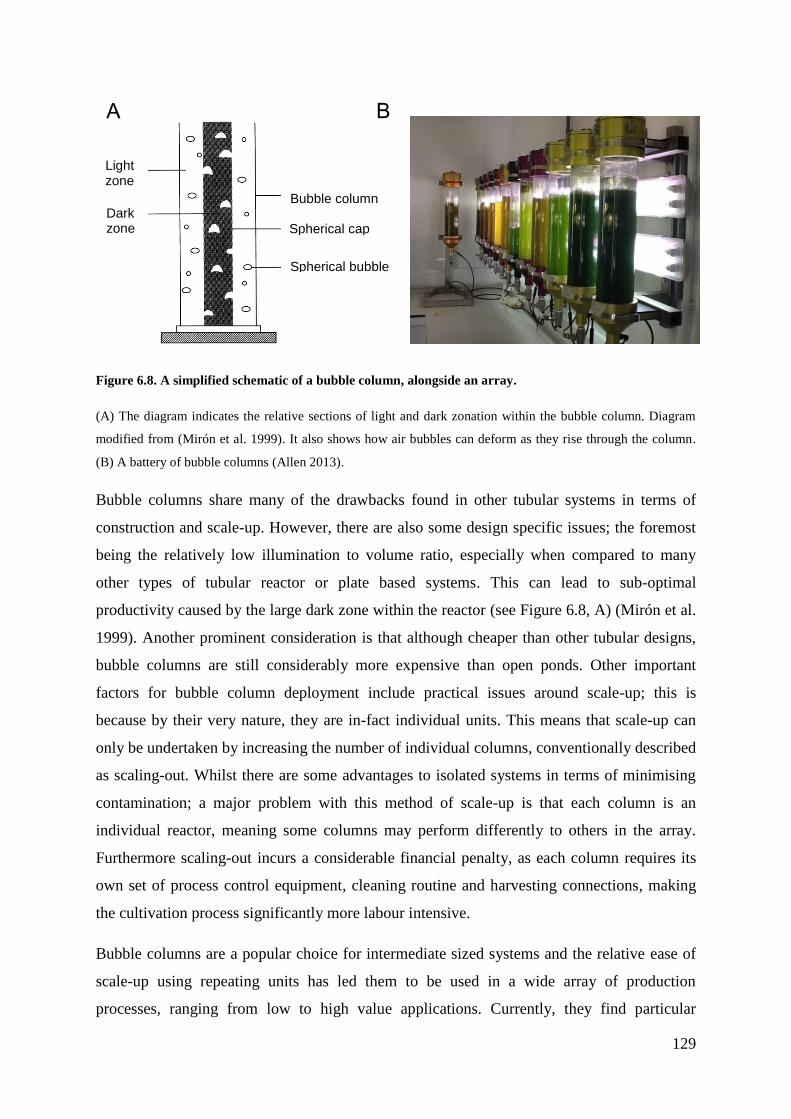
129

Figure 6.8. A simplified schematic of a bubble column, alongside an array.

(A) The diagram indicates the relative sections of light and dark zonation within the bubble column. Diagram

modified from (Mirón et al. 1999). It also shows how air bubbles can deform as they rise through the column.

(B) A battery of bubble columns (Allen 2013).

Bubble columns share many of the drawbacks found in other tubular systems in terms of

construction and scale-up. However, there are also some design specific issues; the foremost

being the relatively low illumination to volume ratio, especially when compared to many

other types of tubular reactor or plate based systems. This can lead to sub-optimal

productivity caused by the large dark zone within the reactor (see Figure 6.8, A) (Mirón et al.

1999). Another prominent consideration is that although cheaper than other tubular designs,

bubble columns are still considerably more expensive than open ponds. Other important

factors for bubble column deployment include practical issues around scale-up; this is

because by their very nature, they are in-fact individual units. This means that scale-up can

only be undertaken by increasing the number of individual columns, conventionally described

as scaling-out. Whilst there are some advantages to isolated systems in terms of minimising

contamination; a major problem with this method of scale-up is that each column is an

individual reactor, meaning some columns may perform differently to others in the array.

Furthermore scaling-out incurs a considerable financial penalty, as each column requires its

own set of process control equipment, cleaning routine and harvesting connections, making

the cultivation process significantly more labour intensive.

Bubble columns are a popular choice for intermediate sized systems and the relative ease of

scale-up using repeating units has led them to be used in a wide array of production

processes, ranging from low to high value applications. Currently, they find particular

Bubble column

Spherical bubble

A

Spherical cap bubble

Light zone

Dark zone

B

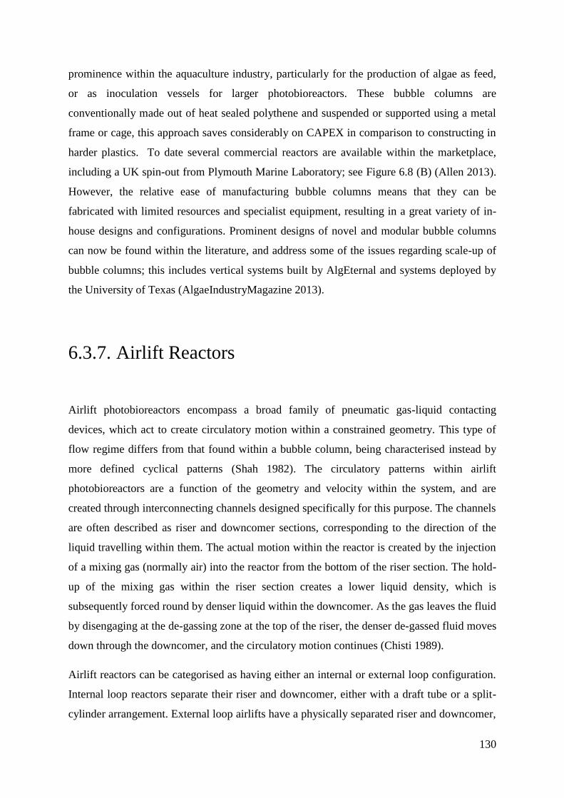
130

prominence within the aquaculture industry, particularly for the production of algae as feed,

or as inoculation vessels for larger photobioreactors. These bubble columns are

conventionally made out of heat sealed polythene and suspended or supported using a metal

frame or cage, this approach saves considerably on CAPEX in comparison to constructing in

harder plastics. To date several commercial reactors are available within the marketplace,

including a UK spin-out from Plymouth Marine Laboratory; see Figure 6.8 (B) (Allen 2013).

However, the relative ease of manufacturing bubble columns means that they can be

fabricated with limited resources and specialist equipment, resulting in a great variety of in-

house designs and configurations. Prominent designs of novel and modular bubble columns

can now be found within the literature, and address some of the issues regarding scale-up of

bubble columns; this includes vertical systems built by AlgEternal and systems deployed by

the University of Texas (AlgaeIndustryMagazine 2013).

6.3.7. Airlift Reactors

Airlift photobioreactors encompass a broad family of pneumatic gas-liquid contacting

devices, which act to create circulatory motion within a constrained geometry. This type of

flow regime differs from that found within a bubble column, being characterised instead by

more defined cyclical patterns (Shah 1982). The circulatory patterns within airlift

photobioreactors are a function of the geometry and velocity within the system, and are

created through interconnecting channels designed specifically for this purpose. The channels

are often described as riser and downcomer sections, corresponding to the direction of the

liquid travelling within them. The actual motion within the reactor is created by the injection

of a mixing gas (normally air) into the reactor from the bottom of the riser section. The hold-

up of the mixing gas within the riser section creates a lower liquid density, which is

subsequently forced round by denser liquid within the downcomer. As the gas leaves the fluid

by disengaging at the de-gassing zone at the top of the riser, the denser de-gassed fluid moves

down through the downcomer, and the circulatory motion continues (Chisti 1989).

Airlift reactors can be categorised as having either an internal or external loop configuration.

Internal loop reactors separate their riser and downcomer, either with a draft tube or a split-

cylinder arrangement. External loop airlifts have a physically separated riser and downcomer,

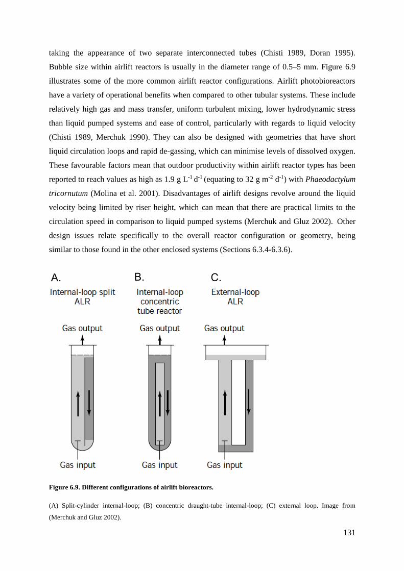
131

taking the appearance of two separate interconnected tubes (Chisti 1989, Doran 1995).

Bubble size within airlift reactors is usually in the diameter range of 0.5–5 mm. Figure 6.9

illustrates some of the more common airlift reactor configurations. Airlift photobioreactors

have a variety of operational benefits when compared to other tubular systems. These include

relatively high gas and mass transfer, uniform turbulent mixing, lower hydrodynamic stress

than liquid pumped systems and ease of control, particularly with regards to liquid velocity

(Chisti 1989, Merchuk 1990). They can also be designed with geometries that have short

liquid circulation loops and rapid de-gassing, which can minimise levels of dissolved oxygen.

These favourable factors mean that outdoor productivity within airlift reactor types has been

reported to reach values as high as 1.9 g L-1 d-1 (equating to 32 g m-2 d-1) with Phaeodactylum

tricornutum (Molina et al. 2001). Disadvantages of airlift designs revolve around the liquid

velocity being limited by riser height, which can mean that there are practical limits to the

circulation speed in comparison to liquid pumped systems (Merchuk and Gluz 2002). Other

design issues relate specifically to the overall reactor configuration or geometry, being

similar to those found in the other enclosed systems (Sections 6.3.4-6.3.6).

Figure 6.9. Different configurations of airlift bioreactors.

(A) Split-cylinder internal-loop; (B) concentric draught-tube internal-loop; (C) external loop. Image from

(Merchuk and Gluz 2002).

A. B. C.

132

Despite the lower levels of commercial uptake than conventional liquid mixed systems, there

are numerous examples of airlift powered photobioreactors in deployment across the globe.

One prominent academic example includes the Massachusetts Institute of Technology (MIT)

airlift reactor, which was deployed to investigate the potential of flue gas scrubbing. This

system takes the form of individual 30 L triangular modules arranged in an array; see Figure

6.10 (A) and (B) (Vunjak-Novakovic et al. 2005). Another prominent reactor within the

literature is the horizontal serpentine airlift system deployed in Almeria, Spain (C) and (D).

This system has provided considerable biological and engineering data from a pilot site

(Molina et al. 2001, Acién Fernandez 2012).

Figure 6.10. Diagram shows some of the potential configurations of airlift reactors.

The MIT reactor in (A) and (B) shows how airlift mixing can be created by directing the flow of air into a

specific vertical riser channel, at the back of the reactor (Vunjak-Novakovic et al. 2005). (C) and (D) shows the

Almeria reactor, which has an individual riser and downcomer section (in the box) and serpentine photo-stage

(Molina Grima et al. 2003, Molina et al. 2001, Acién Fernandez 2012).

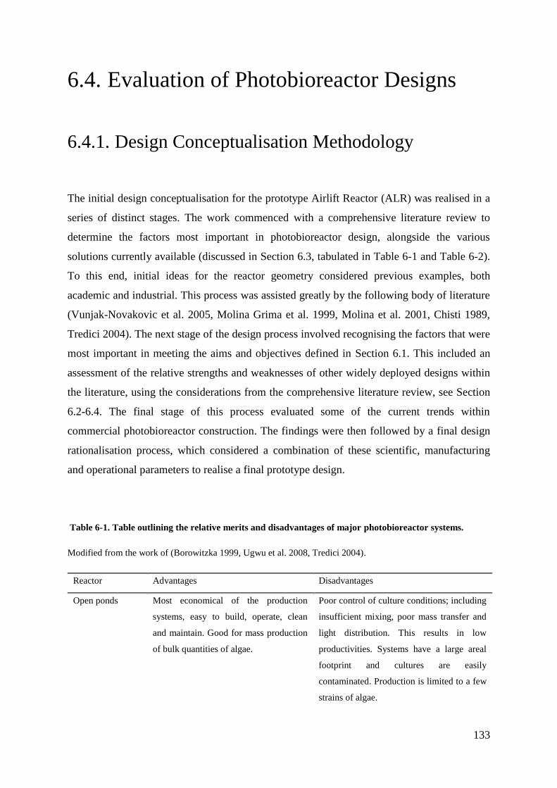
133

6.4. Evaluation of Photobioreactor Designs

6.4.1. Design Conceptualisation Methodology

The initial design conceptualisation for the prototype Airlift Reactor (ALR) was realised in a

series of distinct stages. The work commenced with a comprehensive literature review to

determine the factors most important in photobioreactor design, alongside the various

solutions currently available (discussed in Section 6.3, tabulated in Table 6-1 and Table 6-2).

To this end, initial ideas for the reactor geometry considered previous examples, both

academic and industrial. This process was assisted greatly by the following body of literature

(Vunjak-Novakovic et al. 2005, Molina Grima et al. 1999, Molina et al. 2001, Chisti 1989,

Tredici 2004). The next stage of the design process involved recognising the factors that were

most important in meeting the aims and objectives defined in Section 6.1. This included an

assessment of the relative strengths and weaknesses of other widely deployed designs within

the literature, using the considerations from the comprehensive literature review, see Section

6.2-6.4. The final stage of this process evaluated some of the current trends within

commercial photobioreactor construction. The findings were then followed by a final design

rationalisation process, which considered a combination of these scientific, manufacturing

and operational parameters to realise a final prototype design.

Table 6-1. Table outlining the relative merits and disadvantages of major photobioreactor systems.

Modified from the work of (Borowitzka 1999, Ugwu et al. 2008, Tredici 2004).

Reactor Advantages Disadvantages

Open ponds Most economical of the production

systems, easy to build, operate, clean

and maintain. Good for mass production

of bulk quantities of algae.

Poor control of culture conditions; including

insufficient mixing, poor mass transfer and

light distribution. This results in low

productivities. Systems have a large areal

footprint and cultures are easily

contaminated. Production is limited to a few

strains of algae.

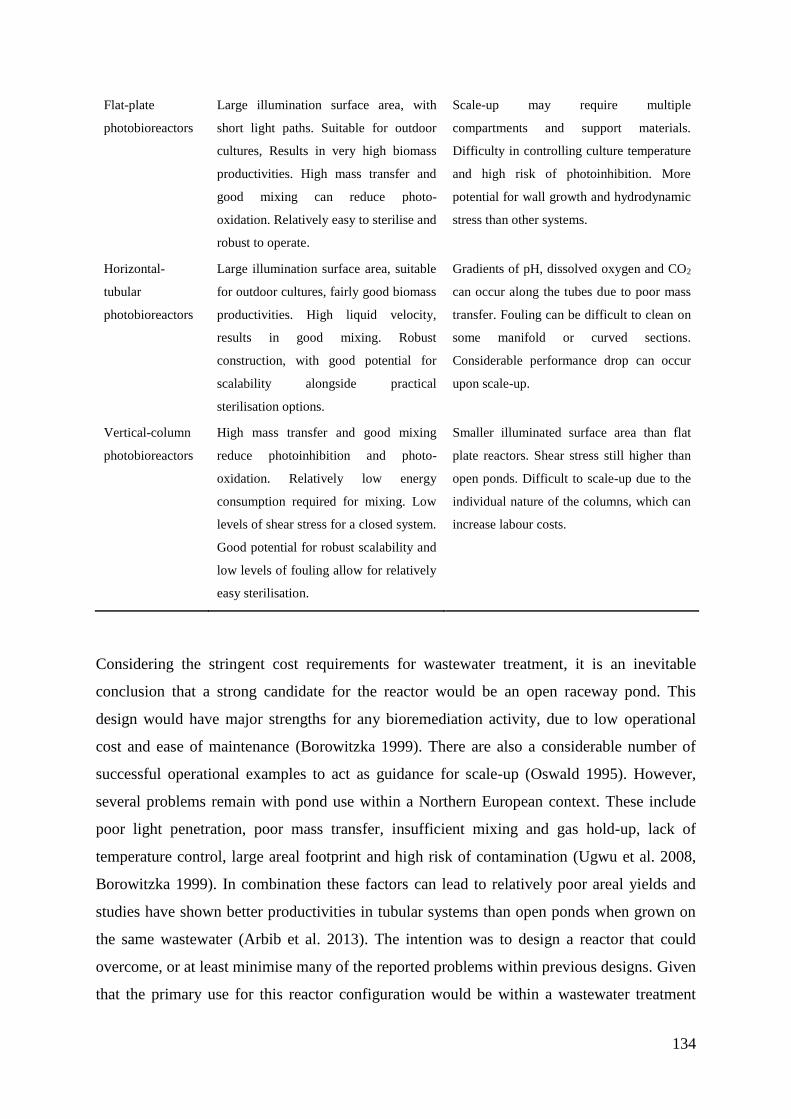
134

Flat-plate

photobioreactors

Large illumination surface area, with

short light paths. Suitable for outdoor

cultures, Results in very high biomass

productivities. High mass transfer and

good mixing can reduce photo-

oxidation. Relatively easy to sterilise and

robust to operate.

Scale-up may require multiple

compartments and support materials.

Difficulty in controlling culture temperature

and high risk of photoinhibition. More

potential for wall growth and hydrodynamic

stress than other systems.

Horizontal-

tubular

photobioreactors

Large illumination surface area, suitable

for outdoor cultures, fairly good biomass

productivities. High liquid velocity,

results in good mixing. Robust

construction, with good potential for

scalability alongside practical

sterilisation options.

Gradients of pH, dissolved oxygen and CO2

can occur along the tubes due to poor mass

transfer. Fouling can be difficult to clean on

some manifold or curved sections.

Considerable performance drop can occur

upon scale-up.

Vertical-column

photobioreactors

High mass transfer and good mixing

reduce photoinhibition and photo-

oxidation. Relatively low energy

consumption required for mixing. Low

levels of shear stress for a closed system.

Good potential for robust scalability and

low levels of fouling allow for relatively

easy sterilisation.

Smaller illuminated surface area than flat

plate reactors. Shear stress still higher than

open ponds. Difficult to scale-up due to the

individual nature of the columns, which can

increase labour costs.

Considering the stringent cost requirements for wastewater treatment, it is an inevitable

conclusion that a strong candidate for the reactor would be an open raceway pond. This

design would have major strengths for any bioremediation activity, due to low operational

cost and ease of maintenance (Borowitzka 1999). There are also a considerable number of

successful operational examples to act as guidance for scale-up (Oswald 1995). However,

several problems remain with pond use within a Northern European context. These include

poor light penetration, poor mass transfer, insufficient mixing and gas hold-up, lack of

temperature control, large areal footprint and high risk of contamination (Ugwu et al. 2008,

Borowitzka 1999). In combination these factors can lead to relatively poor areal yields and

studies have shown better productivities in tubular systems than open ponds when grown on

the same wastewater (Arbib et al. 2013). The intention was to design a reactor that could

overcome, or at least minimise many of the reported problems within previous designs. Given

that the primary use for this reactor configuration would be within a wastewater treatment

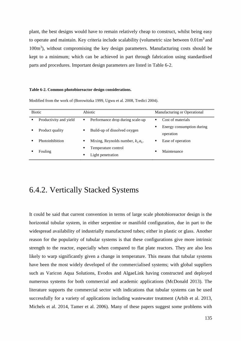
135

plant, the best designs would have to remain relatively cheap to construct, whilst being easy

to operate and maintain. Key criteria include scalability (volumetric size between 0.01m3 and

100m3), without compromising the key design parameters. Manufacturing costs should be

kept to a minimum; which can be achieved in part through fabrication using standardised

parts and procedures. Important design parameters are listed in Table 6-2.

Table 6-2. Common photobioreactor design considerations.

Modified from the work of (Borowitzka 1999, Ugwu et al. 2008, Tredici 2004).

Biotic Abiotic Manufacturing or Operational

Productivity and yield Performance drop during scale-up Cost of materials

Product quality Build-up of dissolved oxygen Energy consumption during

operation

Photoinhibition Mixing, Reynolds number, 𝑘𝐿𝑎𝐿 . Ease of operation

Fouling Temperature control

Light penetration Maintenance

6.4.2. Vertically Stacked Systems

It could be said that current convention in terms of large scale photobioreactor design is the

horizontal tubular system, in either serpentine or manifold configuration, due in part to the

widespread availability of industrially manufactured tubes; either in plastic or glass. Another

reason for the popularity of tubular systems is that these configurations give more intrinsic

strength to the reactor, especially when compared to flat plate reactors. They are also less

likely to warp significantly given a change in temperature. This means that tubular systems

have been the most widely developed of the commercialised systems; with global suppliers

such as Varicon Aqua Solutions, Evodos and AlgaeLink having constructed and deployed

numerous systems for both commercial and academic applications (McDonald 2013). The

literature supports the commercial sector with indications that tubular systems can be used

successfully for a variety of applications including wastewater treatment (Arbib et al. 2013,

Michels et al. 2014, Tamer et al. 2006). Many of these papers suggest some problems with

136

fouling within enclosed systems; which may mean the use of a tubular configuration is

favourable over a plate configuration, as they have higher liquid velocities and are a lot easier

to dissemble and clean (McDonald 2013). The modular nature of the tubes also allows for

easy replacement should one get damaged. In combination these factors would mean that the

deployment of a tubular system would therefore seem preferable to a panel system for

wastewater applications. Especially when considering the likelihood that the system may

encounter tough operational conditions and a degree of damage over its lifespan.

A majority of vertically stacked, vertically orientated systems are based upon bubble column

designs that are arranged as a battery of individual reactors (Mirón et al. 2000). This means

that they display many of the benefits and disadvantages of column based systems previously

discussed in Table 6-1. One particular problem caused by scaling-out non-connected modular

systems by number is the increased requirement for process control systems. For example an

array of un-connected bubble columns would all need their own auxiliary systems, such as

gas and liquid delivery lines, or separate units for temperature control, which can increase

CAPEX considerably. Individual units also multiply operator requirements in terms of

maintenance and process control duties. These issues can be further compounded by both

biotic and abiotic factors, as it can be hard to maintain all of the individual cultures in the

same physiological state. For example some tubes may be exposed to greater extremes of

temperature and light intensity than others based on their positioning, which has an impact on

yield and product quality.

Many of the newer generation of commercial photobioreactors, appear to favour vertically

arranged and orientated tubular systems; this includes the AlgEternal VGM Optimax and the

BFS reactor (BioFuel Systems), both shown in Figure 6.11 (A and B respectively)

(AlgaeIndustryMagazine 2013, BFS 2014). Vertically stacked upright tubes have the ability

to be arranged in a variety of configurations, either as individual columns or on a manifold.

The use of a manifold allows for the individual columns to share the reactor geometry, and

hence help to overcome some of the problems associated with individual column reactors.

These vertical systems are often mixed pneumatically, allowing for superior mass transfer at

equivalent mixing power when compared to conventional liquid pumping in horizontal

serpentine or manifold systems. Additionally, vertically arranged reactors have the benefit of

imparting more intrinsic strength to the reactor than horizontal configurations, hence

requiring less supporting framework and thereby saving on CAPEX. Another benefit of a

vertically stacked system is the considerable body of literature that can be drawn upon to

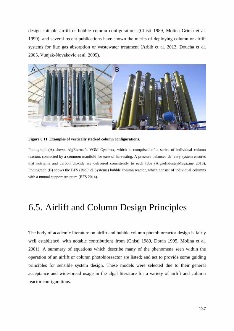
137

design suitable airlift or bubble column configurations (Chisti 1989, Molina Grima et al.

1999); and several recent publications have shown the merits of deploying column or airlift

systems for flue gas absorption or wastewater treatment (Arbib et al. 2013, Doucha et al.

2005, Vunjak-Novakovic et al. 2005).

Figure 6.11. Examples of vertically stacked column configurations.

Photograph (A) shows AlgEternal’s VGM Optimax, which is comprised of a series of individual column

reactors connected by a common manifold for ease of harvesting. A pressure balanced delivery system ensures

that nutrients and carbon dioxide are delivered consistently to each tube (AlgaeIndustryMagazine 2013).

Photograph (B) shows the BFS (BioFuel Systems) bubble column reactor, which consist of individual columns

with a mutual support structure (BFS 2014).

6.5. Airlift and Column Design Principles

The body of academic literature on airlift and bubble column photobioreactor design is fairly

well established, with notable contributions from (Chisti 1989, Doran 1995, Molina et al.

2001). A summary of equations which describe many of the phenomena seen within the

operation of an airlift or column photobioreactor are listed; and act to provide some guiding

principles for sensible system design. These models were selected due to their general

acceptance and widespread usage in the algal literature for a variety of airlift and column

reactor configurations.

A B

138

6.5.1. Solar Penetration

The importance of receiving adequate photosynthetically active radiation (PAR) for biomass

growth is one of the factors of greatest importance for large scale algal cultivation (Molina et

al. 2001). Whilst there are a variety of ways in which PAR can be delivered to a reactor

(outlined in Section 6.2.1), conventional methods often include external or internal lighting

arrays, as well as solar radiation. To estimate the effect that light can have on an algal growth

rate, a number of equations can be used. These relate to the average irradiance received

within the culture, Iav, which can be given by expressions along the lines of those developed

by (Alfano, Romero and Cassano 1986), shown in Eq. 10.

𝐼𝑎𝑣 =𝐼𝑜

∅𝑒𝑞𝐾𝑎𝐶𝑏[1 − exp(−∅𝑒𝑞𝐾𝑎𝑋𝑡)] Eq. 10

Where 𝐼𝑜 is the irradiance on the surface of the culture and 𝐾𝑎 is the extinction coefficient of

the algal biomass, ∅𝑒𝑞 is the length of the light path from the surface of the reactor to any

other point within the bioreactor. Whilst 𝑋𝑡 is the concentration of biomass within the reactor.

For outdoor tubular systems ∅𝑒𝑞 is related to the diameter of the tubing used for cultivation

(Fernández et al. 1997). This relationship can be described in Eq. 11:

∅𝑒𝑞 = 𝑑𝑡

𝑐𝑜𝑠𝜃

Eq. 11

Where 𝑑𝑡 is the tube diameter, and 𝜃 is the solar zenith angle, in degrees.

139

6.5.2. Algal Growth

The ultimate aim of any bioreactor is to maximise biomass productivity by ensuring that the

conditions for growth are optimal. When all other parameters are considered, suboptimal light

is the factor that has the greatest overall limitation on the actual growth rate of the algae.

There are many relationships that describe the relationship of light on algal growth (Molina

Grima et al. 1999). However, for the purposes of this project the expression in Eq. 12 was

selected for this research, due to its simplicity and widespread usage (Grima et al. 1994).

𝜇 = 𝜇𝑚𝑎𝑥𝐼𝑎𝑣

𝑛

𝐼𝑘𝑛 + 𝐼𝑎𝑣

𝑛 Eq. 12

Where 𝜇 is the specific growth rate, 𝜇𝑚𝑎𝑥 is the maximum value of 𝜇, 𝐼𝑎𝑣 is the average

irradiance inside the reactor and 𝐼𝑘 is a constant that is dependent on the algal strain being

cultivated as well as culture conditions, and 𝑛 is an empirically established exponent.

6.5.3. Liquid Mixing and Circulation in Pneumatic

Photobioreactors

6.5.3.1. Reynolds Number

The importance of maintaining a well-mixed and turbulent system within the reactor is

important for mass transfer, shear effects and access to light. The Reynolds number is an

important dimensionless grouping that is often used to determine whether a system is

operating in a turbulent manner, and a simplified expression for Newtonian systems is shown

in Eq. 13;

𝑅𝑒 =𝜌𝑈𝐿𝑑𝑝

𝜇 Eq. 13

140

The terms are expressed as; density 𝜌, superficial liquid velocity 𝑈𝐿, pipe diameter, 𝑑𝑝 and

viscosity, 𝜇. Determining the liquid velocity within airlift reactors can be a complex process,

and will vary greatly upon the chosen system and configuration. Tubular systems with Re

numbers above 4,000 are said to be turbulent (Doran 1995).

6.5.3.2. Liquid Velocity in Airlift Photobioreactors

A generally well accepted expression for the liquid velocity within an external loop airlift

system can be found in the work of (Chisti 1989) and is shown in Eq. 14.

𝑈𝐿 = √

2𝑔ℎ𝐷(𝜀𝑟 − 𝜀𝑑)

𝑘𝐵 (1

(1 − 𝜀𝑟 )2+ (

𝑎𝑟𝑎𝑑)2

. 1

(1 − 𝜀𝑑)2)

Eq. 14

Where the superficial liquid velocity (𝑈𝐿) is equal to the gravitational acceleration (𝑔), the

dispersion height (ℎ𝐷), the gas hold up in the riser (𝜀𝑟) and downcomer (𝜀𝑑), and the friction

loss coefficient (𝑘𝐵). The cross-sectional areas of the riser and downcomer are represented

as 𝑎𝑟 and 𝑎𝑑 respectively. The gas hold-up within the riser 𝜀𝑟 and downcomer 𝜀𝑑 , can be

approximated by Eqs. 15-16.

εr=UG

0.24+1.35(UG+ 𝑈𝐿)0.93

Eq. 15

𝜀𝑑 = 0.79𝜀𝑟 − 0.057 Eq. 16

Where 𝑈𝐺 is the gas superficial velocity; and the dispersion height can be found from the

following Eqs. 17-18.

εmean=𝑎rεr+𝑎dεd𝑎r+𝑎d

Eq. 17

141

hD=hL

(1-εmean)

Eq. 18

Where εmean is the mean gas hold-up in the reactor, ℎ𝐿 is the height of the liquid and ℎ𝐷 the

height of the dispersion. The superficial gas velocity can subsequently be determined from

Eq. 19.

𝑈𝐺 = 𝑉𝐺

𝑎𝑟⁄ Eq. 19

Where 𝑉𝐺 is the volume of gas flowing into the system and 𝑎𝑟 the cross sectional area of the

riser. The actual linear liquid circulation velocity can then be calculated from Eq. 20.

�̅�𝐿=𝑈𝐿

(1- εr)

Eq. 20

6.5.3.3. Liquid Velocity in Column Reactors

Determining the upward liquid velocity within bubble columns under heterogeneous flow can

be described by the expression shown in Eq. 21 (Heijnen and Van't Riet 1984).

𝑈𝐿 = 0.9(𝑔𝑑𝑝𝑈𝐺)0.33

Eq. 21

Where 𝑑𝑝 is the diameter of the bubble column; and the gas superficial velocity is calculated

in a manner identical to Eq. 19. The actual gas hold-up for bubble columns can be

subsequently calculated using the expression in Eq. 22.

𝜀 = 𝑈𝐺

𝑈𝑏⁄ Eq. 22

Where the gas hold-up (𝜀), is defined by the superficial liquid velocity (𝑈𝐺), divided by the

bubble rise velocity (𝑈𝑏).

142

6.5.3.4. Circulation Time in Airlift and Column Photobioreactors

From the superficial liquid velocity it is also possible to describe the mixing times, although

caution should be taken when using these relationships, as they do not always extrapolate

well to individual system configurations (Chisti 1989). One commonly used expression is

shown in Eq. 23.

𝑡𝑐 =𝐿𝑟𝑈𝐿𝑟

+ 𝐿𝑑𝑈𝐿𝑑

Eq. 23

Where 𝑡𝑐 is the circulation time, 𝐿𝑟 the riser length, 𝑈𝐿𝑟 the superficial velocity in the riser,

𝐿𝑑 the length of the downcomer and 𝑈𝐿𝑑 the superficial velocity in the downcomer (Chisti

1989). The mixing time within airlift and bubble column reactors can be approximated using

the expressions outlined in Eqs. 24 and 25 respectively.

𝑡𝑚 = 𝑡𝑐5.2(𝑎𝑟

𝑎𝑑⁄ )0.46 Eq. 24

𝑡𝑚 = 11ℎ𝐷

𝑑𝑡⁄ (𝑔𝑈𝐺𝑑𝑡

−2)−0.33 Eq. 25

6.5.3.5. Shear Rate within Pneumatic Photobioreactors

Another factor that is important for the overall growth of an algal species within a

photobioreactor is the observed shear rate. An approximate estimation of shear within bubble

columns can be described as follows in Eq. 26 (Nishikawa, Kato and Hashimoto 1977).

However it should be noted that the prediction of average shear rates by empirical methods in

pneumatic reactors has been described as being conceptually unsound (Chisti 1989).

�̇� = 5000𝑈𝐺 Eq. 26

143

Where �̇� is the average shear rate, and 𝑈𝐺, the superficial gas velocity is determined from Eq.

19.

6.5.4. Mass Transfer in Pneumatic Photobioreactors

Gas to liquid mass transfer is of considerable importance in all bioprocesses, and good

characterisation allows for optimal aqueous culturing conditions. This is because many

conventional bioprocesses require the addition of air to provide sufficient oxygen for aerobic

respiration, whilst also stripping carbon dioxide from the culture. Conversely, phototrophic

algal cultivation requires the opposite of this process; with a greater requirement for carbon

dioxide input for cellular growth and the removal of excess oxygen which can inhibit

photosynthesis. A general description for the change in the concentration of dissolved

inorganic carbon [𝐶𝑇] in the liquid phase for plug flow is described in Eq. 27, whilst the

equivalent expression for oxygen is shown in Eq. 28 (Rubio et al. 1999);

𝑄𝐿𝐷𝑡[𝐶𝑇] = (𝑘𝐿𝑎𝐿) 𝐶𝑂2([𝐶𝑂2]∗ − [𝐶𝑂2])𝑆𝑑𝑥 + 𝑅𝐶𝑂2

(1 − 𝜀𝐺)𝑆𝑑𝑥 Eq. 27

𝑄𝐿𝐷𝑡[𝑂2] = (𝑘𝐿𝑎𝐿) 𝑂2([𝑂2]∗ − [𝑂2])𝑆𝑑𝑥 + 𝑅𝑂2

(1 − 𝜀𝐺)𝑆𝑑𝑥 Eq. 28

Where 𝑄𝐿 is the volumetric flow rate of liquid through the tube, 𝑑𝑡 is the tube diameter, 𝑘𝐿𝑎𝐿

is the volumetric gas-liquid mass transfer coefficient, 𝑆𝑑𝑥 is the differential volume, 𝜀𝐺 is the

fractional gas holdup, [𝐶𝑂2/𝑂2]∗ is the saturation concentration of carbon dioxide/oxygen

and 𝑅𝐶𝑂2/𝑂2describes the volumetric rate of carbon dioxide/oxygen consumption. For the

liquid phase the component mass balance in Eq. 29 can be established for the molar flow rate

of carbon dioxide (𝐹𝐶𝑂2), and likewise for oxygen (𝐹𝑂2) in Eq. 30 (Molina Grima et al. 1999);

𝑑𝐹𝐶𝑂2 = −(𝑘𝐿𝑎𝐿) 𝐶𝑂2([𝐶𝑂2]∗ − [𝐶𝑂2])𝑆𝑑𝑥 Eq. 29

𝑑𝐹𝑂2 = −(𝑘𝐿𝑎𝐿) 𝑂2([𝑂2]∗ − [𝑂2])𝑆𝑑𝑥 Eq. 30

144

The equilibrium concentrations of carbon dioxide and oxygen can then be determined from

Eqs. 31 and 32, using Henry’s law;

[𝐶𝑂2]∗ = 𝐻𝐶𝑂2𝑃𝐶𝑂2 = 𝐻𝐶𝑂2(𝑃𝑇 − 𝑃𝑣)

𝐹𝐶𝑂2𝐹𝑂2 + 𝐹𝐶𝑂2 + 𝐹𝑁2

+ 𝐹𝐻2𝑂 Eq. 31

[𝑂2]∗ = 𝐻𝑂2𝑃𝑂2 = 𝐻𝑂2(𝑃𝑇 − 𝑃𝑣)

𝐹𝑂2𝐹𝑂2 + 𝐹𝐶𝑂2 + 𝐹𝑁2

+ 𝐹𝐻2𝑂 Eq. 32

Where 𝐻𝐶𝑂2/𝑂2 is Henry’s constant for carbon dioxide/oxygen, and 𝑃𝐶𝑂2/𝑂2 is the carbon

dioxide/oxygen partial pressure in the gas phase (atm), 𝑃𝑇 and 𝑃𝑣 are the total and partial

pressures in the system, and 𝐹𝑥 refers to the molar flow rate of the molecular entities in (mol

s-1). To work out the actual dissolved concentration of carbon dioxide or oxygen within the

reactor the 𝑘𝐿𝑎𝐿 value has to be determined. Within airlift photobioreactors this can be

calculated either in terms of the superficial gas riser velocity or the power input (Bello,

Robinson and Moo-Young 1985), the relationship with gas riser velocity is shown in

Equation 33.

𝑘𝐿𝑎𝐿 = 0.76 [1 + 𝑎𝑑𝑎𝑟]−2

𝑈𝐺𝑟0.8 Eq. 33

Where 𝑈𝐺𝑟 is the superficial gas velocity within the riser section. For column reactors a

number of relationships also exist, but one commonly used expression is presented in Eq. 34

(Doran 1995).

𝑘𝐿𝑎𝐿 = 0.32𝑈𝐺0.7 Eq. 34

6.5.5. Power Consumption

For pneumatically driven reactors, the expressions in Eq. 35 and Eq. 36 can be used to derive

the power input due to gassing (𝑃𝐺) for bubble column and airlift reactors respectively. These

145

expressions hold true based on the assumption that the kinetic energy contribution to power

input can be ignored due to its negligible quantity (Chisti 1989, Pérez et al. 2006).

𝑃𝐺

𝑉𝐿= 𝜌𝐿𝑔𝑈𝐺 Eq. 35

𝑃𝐺

𝑉𝐿=

𝜌𝐿𝑔𝑈𝐺𝑟

1 + 𝐴𝑑

𝐴𝑟

Eq. 36

Where 𝑉𝐿 is the volume of liquid, 𝜌𝐿 is the density of the liquid, 𝑈𝐺 and 𝑈𝐺𝑟 are the total and

riser gas velocities respectively and 𝑎𝑑 and 𝑎𝑟 are the areas of the downcomer and riser

respectively.

6.5.6. Heat Transfer in Airlift Reactors

Heat transfer within photobioreactors is a reasonably well understood phenomenon, and can

present particular problems for outdoor photobioreactors both in terms of overheating or

overcooling; this is particularly the case in systems with large surface area to volume ratios.

Upon establishing the required heat duty, the necessary surface area required for heat transfer

can be calculated from Eq. 37, (Chisti 1989).

𝑄𝐻 = 𝑈𝐻𝐴𝐻∆𝑇 Eq. 37

Where 𝑄𝐻 is the heat transfer rate, 𝑈𝐻 the sum of resistances to heat transfer, 𝐴𝐻 the heat

transfer area and ∆𝑇 the mean temperature difference driving force. The sum of resistances

due to heat transfer can be determined with Eq. 38;

1

𝑈𝐻 =

1

ℎ𝑓 + 𝑅𝐻 Eq. 38

146

Where ℎ𝑓 is the film heat transfer coefficient for the fermentation fluid film in contact with

the heating surface, 𝑅𝐻. The 𝑅𝐻 value can be found in most chemical engineering and heat

transfer data books. However, information on the value for ℎ𝑓 is less prevalent within airlift

literature, but one proposed equation for air and water within concentric draught-tubes is

shown in Eq. 39, and should also be suitable for bubble column systems (Chisti 1989).

ℎ𝑓 = 13.34 (1 + 𝑎𝑟𝑎𝑑)0.7

𝑈𝐺0.275 Eq. 39

Where 𝑎𝑑 and 𝑎𝑟 are the areas of the downcomer and riser respectively, whilst 𝑈𝐺 is the

superficial gas velocity.

6.5.7. Scale-Up

Factors that are considered particularly important for the scale-up of any photobioreactor

include the maintenance of favourable characteristics seen at a smaller scale. As such several

equations have been derived to describe both the importance of maximising the light

intensity, whilst also maintaining the transitional frequency between light and dark zones

during scale-up. An expression used to describe the volumetric rate of fluid movement

through the dark zone of a reactor, 𝑄𝑅 is displayed in Eq. 40 (Molina et al. 2001).

𝑄𝑅 = 𝑉𝑑𝑡𝑑 Eq. 40

Where 𝑡𝑑 is the maximum acceptable duration of dark period between successive light

periods and 𝑉𝑑 is volume of the dark zone. The fluid interchange velocity 𝑈𝑅 can be

described from the 𝑄𝑅 on a unit length basis, as follows in Eq. 41 (Molina et al. 2001).

𝑈𝑅 = 𝑄𝑅

𝑠 Eq. 41

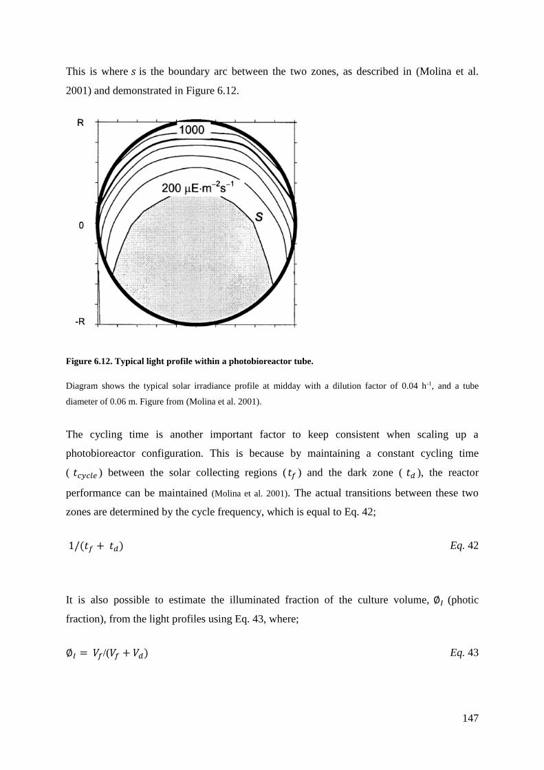
147

This is where 𝑠 is the boundary arc between the two zones, as described in (Molina et al.

2001) and demonstrated in Figure 6.12.

Figure 6.12. Typical light profile within a photobioreactor tube.

Diagram shows the typical solar irradiance profile at midday with a dilution factor of 0.04 h-1, and a tube

diameter of 0.06 m. Figure from (Molina et al. 2001).

The cycling time is another important factor to keep consistent when scaling up a

photobioreactor configuration. This is because by maintaining a constant cycling time

( 𝑡𝑐𝑦𝑐𝑙𝑒 ) between the solar collecting regions ( 𝑡𝑓 ) and the dark zone ( 𝑡𝑑 ), the reactor

performance can be maintained (Molina et al. 2001). The actual transitions between these two

zones are determined by the cycle frequency, which is equal to Eq. 42;

1/(𝑡𝑓 + 𝑡𝑑) Eq. 42

It is also possible to estimate the illuminated fraction of the culture volume, ∅𝐼 (photic

fraction), from the light profiles using Eq. 43, where;

∅𝐼 = 𝑉𝑓/(𝑉𝑓 + 𝑉𝑑) Eq. 43

148

From this expression it can be assumed that the flash volume 𝑉𝑓, is directly proportional to

the flash period ( 𝑡𝑓), and that the dark volume ( 𝑉𝑑), is proportional to the dark period(𝑡𝑑).

This allows the cycling time 𝑡𝑐𝑦𝑐𝑙𝑒 to be expressed in terms of ∅ Eqs. 44 and 45 (Molina et al.

2001):

𝑡𝑐𝑦𝑐𝑙𝑒 = 𝑡𝑑 (1

1 − ∅) Eq. 44

Making the frequency, 𝑣 equal to;

𝑣 = 1 − ∅𝐼

𝑡𝑑 Eq. 45

Using these equations, it can be shown that the light/dark interchange velocity at a large scale

(𝑈𝑅𝐿) and at the small-scale (𝑈𝑅𝑆) may be shown to depend on a scale factor 𝑓, as follows in

Eq. 46 (Molina et al. 2000);

𝑈𝑅𝐿 =𝑓

𝛼 𝑈𝑅𝑆 Eq. 46

The factor 𝑓 is the ratio of tube diameters at the larger and smaller scales, whilst the

parameter 𝛼 depends on the ∅𝐼 values at the two respective scales, described in Eq. 47.

𝛼 = (1 − ∅𝐼𝐿

1 − ∅𝐼𝑆) Eq. 47

The actual velocity of interchange 𝑈𝑅 is then estimated as the fluctuating component of the

steady state velocity in turbulent flow (Molina et al. 2000), shown in Eq. 48.

𝑈𝑅 = 0.2 (𝑈𝐿7𝜇

𝑑𝑡𝜌)

1/8

Eq. 48

149

This gives the radial interchange velocity (𝑈𝑅) within the turbulent core as a function of the

superficial liquid velocity (𝑈𝐿), the tube diameter (𝑑𝑡), the viscosity (𝜇) and the density (𝜌).

To ensure that performance is kept identical during successful scale-up, the linear flow

velocities at the two scales have to conform to Eq. 49 (Molina et al. 2000).

𝑈𝐿𝐿 =𝑓97

𝛼87

𝑈𝐿𝑆 Eq. 49

Where superficial liquid velocity at a large scale is 𝑈𝐿𝐿 and superficial velocity at a small

scale is 𝑈𝐿𝑆.

6.6. Airlift Reactor (ALR) Design

6.6.1. Early Concept

The selection of a simple vertical arrangement favoured by some of the more modern

photobioreactors (shown in Section 6.4.2) allows for high mass transfers, rapid de-gassing,

and a reduction in material costs compared to horizontal systems. The high levels of mass

transfer resulting from the mixing driven by aeration would be particularly suitable for

wastewater treatment as this would allow for the system to reduce any excess BOD, whilst

not over saturating the system with oxygen. Other benefits of using this type of reactor

include the fact that there are no internalised mechanical parts within airlift or bubble column

reactors, meaning that there would be lower levels of equipment ware and fouling; whilst the

constant tube diameter reduces shear within the system. The photobioreactor design outlined

in this thesis seeks to improve on previous work, and overcome some of the limitations

common to scaling out individual units. This was achieved by basing the reactor geometry on

a common manifold along the length of the top and bottom of the system, creating a simple

modular design. Some of the early concept sketches are shown in Figure 6.13.

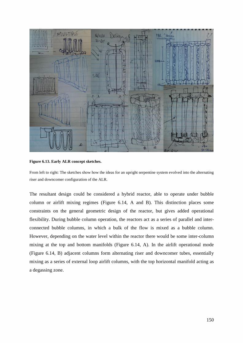
150

Figure 6.13. Early ALR concept sketches.

From left to right: The sketches show how the ideas for an upright serpentine system evolved into the alternating

riser and downcomer configuration of the ALR.

The resultant design could be considered a hybrid reactor, able to operate under bubble

column or airlift mixing regimes (Figure 6.14, A and B). This distinction places some

constraints on the general geometric design of the reactor, but gives added operational

flexibility. During bubble column operation, the reactors act as a series of parallel and inter-

connected bubble columns, in which a bulk of the flow is mixed as a bubble column.

However, depending on the water level within the reactor there would be some inter-column

mixing at the top and bottom manifolds (Figure 6.14, A). In the airlift operational mode

(Figure 6.14, B) adjacent columns form alternating riser and downcomer tubes, essentially

mixing as a series of external loop airlift columns, with the top horizontal manifold acting as

a degassing zone.

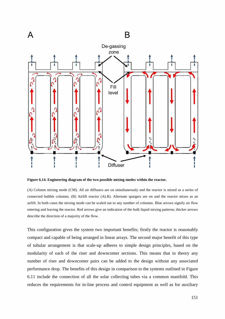
151

Figure 6.14. Engineering diagram of the two possible mixing modes within the reactor.

(A) Column mixing mode (CM). All air diffusers are on simultaneously and the reactor is mixed as a series of

connected bubble columns. (B) Airlift reactor (ALR). Alternate spargers are on and the reactor mixes as an

airlift. In both cases the mixing mode can be scaled out to any number of columns. Blue arrows signify air flow

entering and leaving the reactor. Red arrows give an indication of the bulk liquid mixing patterns; thicker arrows

describe the direction of a majority of the flow.

This configuration gives the system two important benefits; firstly the reactor is reasonably

compact and capable of being arranged in linear arrays. The second major benefit of this type

of tubular arrangement is that scale-up adheres to simple design principles, based on the

modularity of each of the riser and downcomer sections. This means that in theory any

number of riser and downcomer pairs can be added to the design without any associated

performance drop. The benefits of this design in comparison to the systems outlined in Figure

6.11 include the connection of all the solar collecting tubes via a common manifold. This

reduces the requirements for in-line process and control equipment as well as for auxiliary

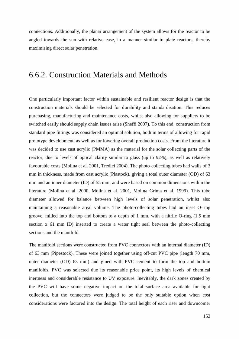
152

connections. Additionally, the planar arrangement of the system allows for the reactor to be

angled towards the sun with relative ease, in a manner similar to plate reactors, thereby

maximising direct solar penetration.

6.6.2. Construction Materials and Methods

One particularly important factor within sustainable and resilient reactor design is that the

construction materials should be selected for durability and standardisation. This reduces

purchasing, manufacturing and maintenance costs, whilst also allowing for suppliers to be

switched easily should supply chain issues arise (Sheffi 2007). To this end, construction from

standard pipe fittings was considered an optimal solution, both in terms of allowing for rapid

prototype development, as well as for lowering overall production costs. From the literature it

was decided to use cast acrylic (PMMA) as the material for the solar collecting parts of the

reactor, due to levels of optical clarity similar to glass (up to 92%), as well as relatively

favourable costs (Molina et al. 2001, Tredici 2004). The photo-collecting tubes had walls of 3

mm in thickness, made from cast acrylic (Plastock), giving a total outer diameter (OD) of 63

mm and an inner diameter (ID) of 55 mm; and were based on common dimensions within the

literature (Molina et al. 2000, Molina et al. 2001, Molina Grima et al. 1999). This tube

diameter allowed for balance between high levels of solar penetration, whilst also

maintaining a reasonable areal volume. The photo-collecting tubes had an inset O-ring

groove, milled into the top and bottom to a depth of 1 mm, with a nitrile O-ring (1.5 mm

section x 61 mm ID) inserted to create a water tight seal between the photo-collecting

sections and the manifold.

The manifold sections were constructed from PVC connectors with an internal diameter (ID)

of 63 mm (Pipestock). These were joined together using off-cut PVC pipe (length 70 mm,

outer diameter (OD) 63 mm) and glued with PVC cement to form the top and bottom

manifolds. PVC was selected due its reasonable price point, its high levels of chemical

inertness and considerable resistance to UV exposure. Inevitably, the dark zones created by

the PVC will have some negative impact on the total surface area available for light

collection, but the connectors were judged to be the only suitable option when cost

considerations were factored into the design. The total height of each riser and downcomer

153

was 1.15 m, with each vertical solar collecting region 1 m in length. The manifold sections

varied in length depending on the reactor configuration and had ¼ bsp brass fittings threaded

at a centre to each vertical riser section at the base, to provide inlets for the introduction of

mixing air. The final working volumes of each system were; 5.5, 11, and 55 L, although the

practical working volumes (due to an increase from aeration) were 5, 10 and 50 L.

Figure 6.15. Technical drawings show the ALR geometry for the 10 L system.

The diagram indicates the dimensions (mm) of the ALR and its main components. The modularity of the reactor

can be clearly seen from the front elevation perspective. (Technical drawing courtesy of Richard Beckett, the

Bartlett School of Architecture).

A frontal profile photo of the finished 10 L prototype is displayed in Figure 6.16 with all the

main constituent parts labelled. The alternating riser and downcomer sections connected by

top and bottom manifolds can be clearly seen in the photograph.

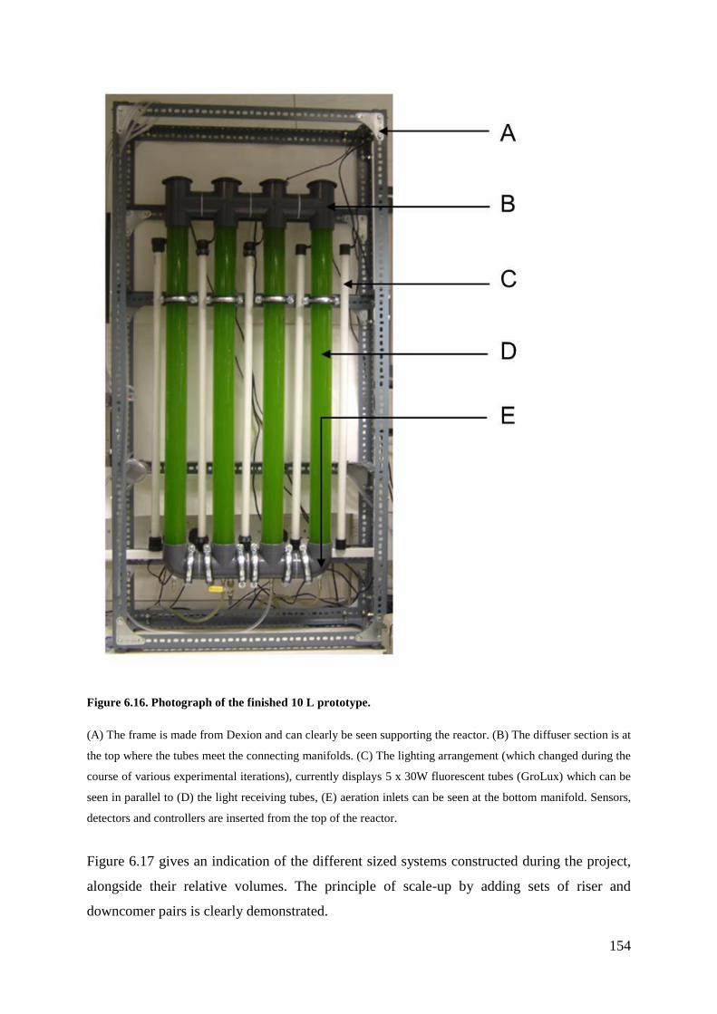
154

Figure 6.16. Photograph of the finished 10 L prototype.

(A) The frame is made from Dexion and can clearly be seen supporting the reactor. (B) The diffuser section is at

the top where the tubes meet the connecting manifolds. (C) The lighting arrangement (which changed during the

course of various experimental iterations), currently displays 5 x 30W fluorescent tubes (GroLux) which can be

seen in parallel to (D) the light receiving tubes, (E) aeration inlets can be seen at the bottom manifold. Sensors,

detectors and controllers are inserted from the top of the reactor.

Figure 6.17 gives an indication of the different sized systems constructed during the project,

alongside their relative volumes. The principle of scale-up by adding sets of riser and

downcomer pairs is clearly demonstrated.

155

Figure 6.17. The ALR at different scales.

The series of photographs demonstrate how the same intrinsic reactor characteristics can be maintained by

scaling out. (A) 5 L system. (B) 10 L system. (C) 50 L system.

6.7. Summary of the Design Process

Overall, the aims and objectives defined in Section 6.1 could be considered as having been

met within this Chapter. The main theoretical considerations have been outlined, and a novel

prototype photobioreactor has been constructed, with specific considerations appertaining to

operation within a wastewater treatment environment. The result is a simple and robust

system that was assembled from relatively cheap and standardised parts. The theoretical

assumptions concerning linear scale-up via the use of a common manifold have been clearly

156

explained; with the belief that this will overcome the performance drop problems that are

often seen when scaling photobioreactor systems. Through its innovative design, the reactor

provides a platform for testing two mixing modes; connected bubble column array, or

connected external loop airlift array. In practical terms, this will allow for greater operational

flexibility and will provide an opportunity to investigate whether bubble column or airlift

mixing modes are superior. This is an important consideration as there are a variety of

conflicting reports regarding the performance of the two mixing modes within the literature

(Chisti 1989, Mirón et al. 2000, Merchuk and Gluz 2002, Kantarci et al. 2005). Chapter 7 will

build upon the work outlined herein and look to characterise the engineering and biological

parameter space of the ALR system, with a view to determine the best operational conditions.

This includes ascertaining the suitability of using the photobioreactor for large scale waste

treatment.

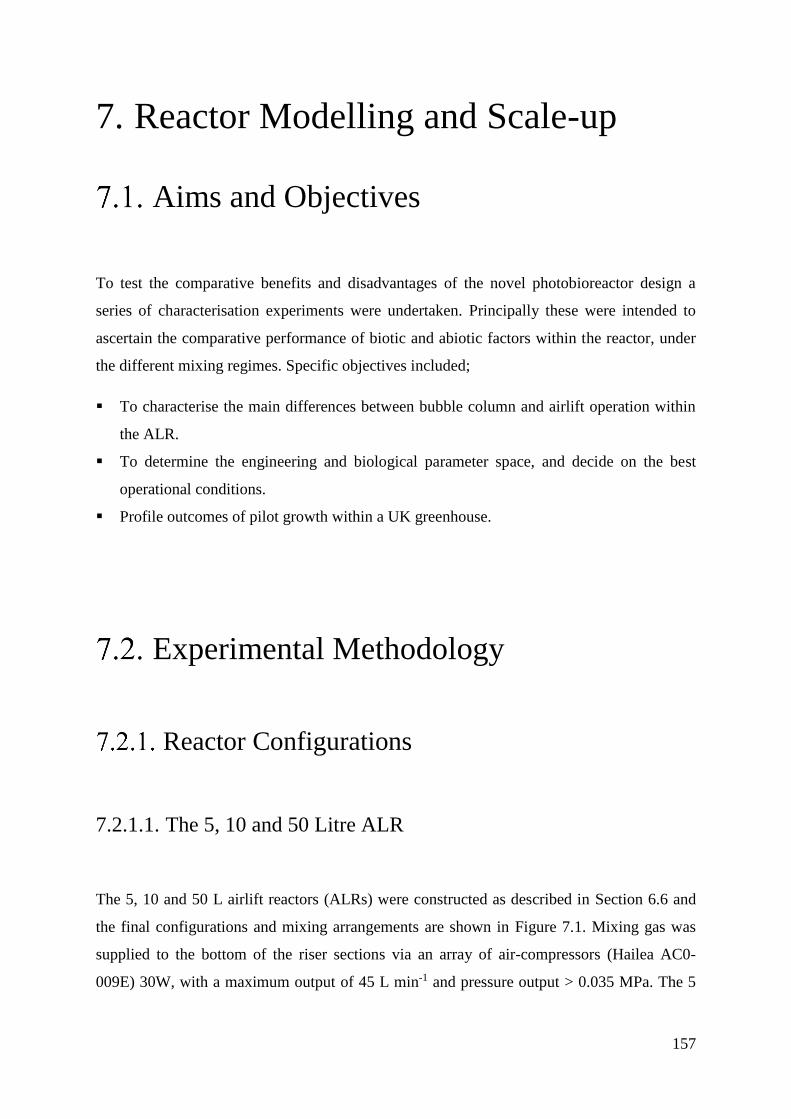
157

7. Reactor Modelling and Scale-up

Aims and Objectives

To test the comparative benefits and disadvantages of the novel photobioreactor design a

series of characterisation experiments were undertaken. Principally these were intended to

ascertain the comparative performance of biotic and abiotic factors within the reactor, under

the different mixing regimes. Specific objectives included;

To characterise the main differences between bubble column and airlift operation within

the ALR.

To determine the engineering and biological parameter space, and decide on the best

operational conditions.

Profile outcomes of pilot growth within a UK greenhouse.

Experimental Methodology

Reactor Configurations

7.2.1.1. The 5, 10 and 50 Litre ALR

The 5, 10 and 50 L airlift reactors (ALRs) were constructed as described in Section 6.6 and

the final configurations and mixing arrangements are shown in Figure 7.1. Mixing gas was

supplied to the bottom of the riser sections via an array of air-compressors (Hailea AC0-

009E) 30W, with a maximum output of 45 L min-1 and pressure output > 0.035 MPa. The 5

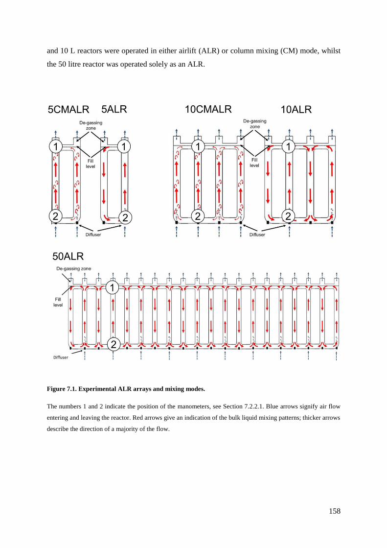
158

and 10 L reactors were operated in either airlift (ALR) or column mixing (CM) mode, whilst

the 50 litre reactor was operated solely as an ALR.

Figure 7.1. Experimental ALR arrays and mixing modes.

The numbers 1 and 2 indicate the position of the manometers, see Section 7.2.2.1. Blue arrows signify air flow

entering and leaving the reactor. Red arrows give an indication of the bulk liquid mixing patterns; thicker arrows

describe the direction of a majority of the flow.

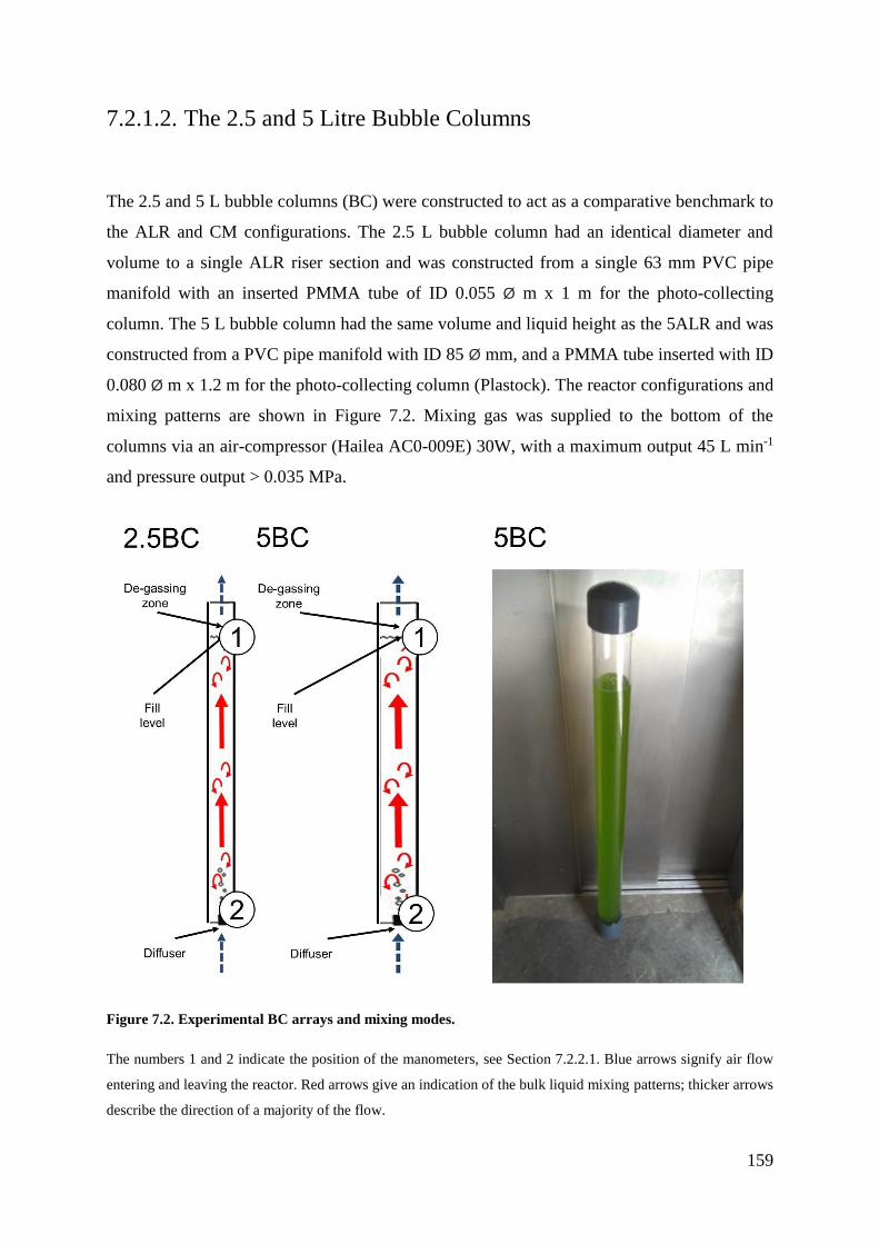
159

7.2.1.2. The 2.5 and 5 Litre Bubble Columns

The 2.5 and 5 L bubble columns (BC) were constructed to act as a comparative benchmark to

the ALR and CM configurations. The 2.5 L bubble column had an identical diameter and

volume to a single ALR riser section and was constructed from a single 63 mm PVC pipe

manifold with an inserted PMMA tube of ID 0.055 Ø m x 1 m for the photo-collecting

column. The 5 L bubble column had the same volume and liquid height as the 5ALR and was

constructed from a PVC pipe manifold with ID 85 Ø mm, and a PMMA tube inserted with ID

0.080 Ø m x 1.2 m for the photo-collecting column (Plastock). The reactor configurations and

mixing patterns are shown in Figure 7.2. Mixing gas was supplied to the bottom of the

columns via an air-compressor (Hailea AC0-009E) 30W, with a maximum output 45 L min-1

and pressure output > 0.035 MPa.

Figure 7.2. Experimental BC arrays and mixing modes.

The numbers 1 and 2 indicate the position of the manometers, see Section 7.2.2.1. Blue arrows signify air flow

entering and leaving the reactor. Red arrows give an indication of the bulk liquid mixing patterns; thicker arrows

describe the direction of a majority of the flow.

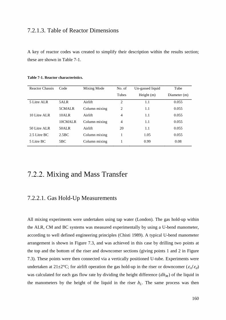
160

7.2.1.3. Table of Reactor Dimensions

A key of reactor codes was created to simplify their description within the results section;

these are shown in Table 7-1.

Table 7-1. Reactor characteristics.

Reactor Chassis Code Mixing Mode No. of

Tubes

Un-gassed liquid

Height (m)

Tube

Diameter (m)

5 Litre ALR 5ALR Airlift 2 1.1 0.055

5CMALR Column mixing 2 1.1 0.055

10 Litre ALR 10ALR Airlift 4 1.1 0.055

10CMALR Column mixing 4 1.1 0.055

50 Litre ALR 50ALR Airlift 20 1.1 0.055

2.5 Litre BC 2.5BC Column mixing 1 1.05 0.055

5 Litre BC 5BC Column mixing 1 0.99 0.08

Mixing and Mass Transfer

7.2.2.1. Gas Hold-Up Measurements

All mixing experiments were undertaken using tap water (London). The gas hold-up within

the ALR, CM and BC systems was measured experimentally by using a U-bend manometer,

according to well defined engineering principles (Chisti 1989). A typical U-bend manometer

arrangement is shown in Figure 7.3, and was achieved in this case by drilling two points at

the top and the bottom of the riser and downcomer sections (giving points 1 and 2 in Figure

7.3). These points were then connected via a vertically positioned U-tube. Experiments were

undertaken at 21±2°C; for airlift operation the gas hold-up in the riser or downcomer (εr/εd)

was calculated for each gas flow rate by dividing the height difference (𝑑ℎ𝑀) of the liquid in

the manometers by the height of the liquid in the riser hL . The same process was then

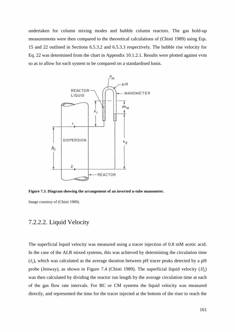
161

undertaken for column mixing modes and bubble column reactors. The gas hold-up

measurements were then compared to the theoretical calculations of (Chisti 1989) using Eqs.

15 and 22 outlined in Sections 6.5.3.2 and 6.5.3.3 respectively. The bubble rise velocity for

Eq. 22 was determined from the chart in Appendix 10.1.2.1. Results were plotted against vvm

so as to allow for each system to be compared on a standardised basis.

Figure 7.3. Diagram showing the arrangement of an inverted u-tube manometer.

Image courtesy of (Chisti 1989).

7.2.2.2. Liquid Velocity

The superficial liquid velocity was measured using a tracer injection of 0.8 mM acetic acid.

In the case of the ALR mixed systems, this was achieved by determining the circulation time

(tc), which was calculated as the average duration between pH tracer peaks detected by a pH

probe (Jenway), as shown in Figure 7.4 (Chisti 1989). The superficial liquid velocity (UL)

was then calculated by dividing the reactor run length by the average circulation time at each

of the gas flow rate intervals. For BC or CM systems the liquid velocity was measured

directly, and represented the time for the tracer injected at the bottom of the riser to reach the

hL

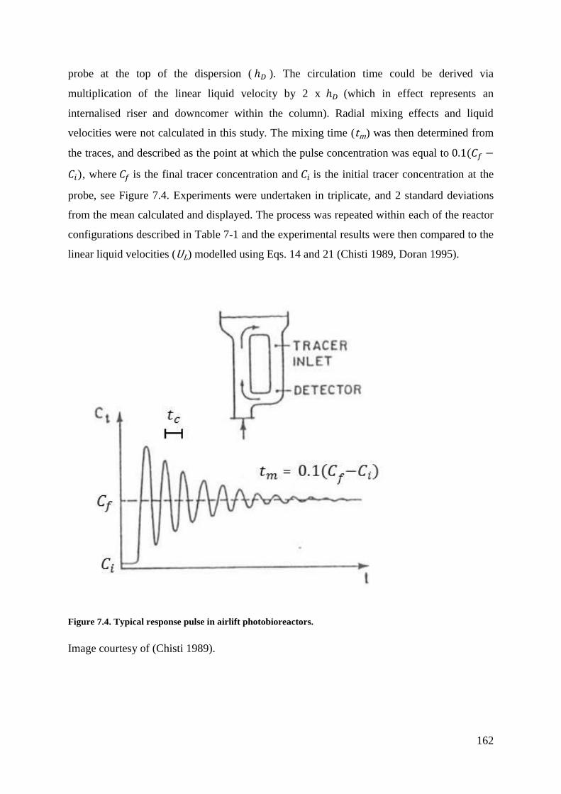
162

probe at the top of the dispersion ( ℎ𝐷 ). The circulation time could be derived via

multiplication of the linear liquid velocity by 2 x ℎ𝐷 (which in effect represents an

internalised riser and downcomer within the column). Radial mixing effects and liquid

velocities were not calculated in this study. The mixing time (tm) was then determined from

the traces, and described as the point at which the pulse concentration was equal to 0.1(𝐶𝑓 −

𝐶𝑖), where 𝐶𝑓 is the final tracer concentration and 𝐶𝑖 is the initial tracer concentration at the

probe, see Figure 7.4. Experiments were undertaken in triplicate, and 2 standard deviations

from the mean calculated and displayed. The process was repeated within each of the reactor

configurations described in Table 7-1 and the experimental results were then compared to the

linear liquid velocities (UL) modelled using Eqs. 14 and 21 (Chisti 1989, Doran 1995).

Figure 7.4. Typical response pulse in airlift photobioreactors.

Image courtesy of (Chisti 1989).

163

7.2.2.3. Reynolds Number

The Reynolds number was determined from Eq. 13, using modelled and experimental 𝑈𝐿

values, and subsequently plotted against the gas flow rate (vvm) in each of the systems.

Assumptions are listed in Appendix 10.1.2.3.

7.2.2.4. Mass Transfer

The mass transfer coefficients within each of the systems were determined using the dynamic

method outlined in (Doran 1995). Each experiment was undertaken by de-oxygenating the

reactor via direct sparging with 100% nitrogen (BOC). The systems were then re-oxygenated

by aeration within the range of commonly used mixing air flow rates (0.1-1 vvm), the

dissolved oxygen concentration would then reach a steady state value based upon its

solubility 𝐶𝐴𝐿∗ . During the process of re-oxygenation, the oxygen concentrations 𝐶𝐴𝐿1 and

𝐶𝐴𝐿2 are measured at times 𝑡1 and 𝑡2 respectively using a dissolved oxygen meter (Jenway).

The 𝑘𝐿𝑎 can then be estimated using two or more time points on during the re-oxygenation.

This is achieved using Eq. 49. and plotting against (𝑡2 − 𝑡1) (Doran 1995).

𝑘𝐿𝑎𝐿 = 𝑙𝑛 ( 𝐶𝐴𝐿

∗ − 𝐶𝐴𝐿1 𝐶𝐴𝐿

∗ − 𝐶𝐴𝐿2) Eq. 49

The results were then compared to the empirical projections from Eqs. 33 and 34, however

due to the poor fit Eqs. 50 and 51 were developed using a linear regression of the 𝑘𝐿𝑎𝐿 data.

𝑘𝐿𝑎𝐿 ALR = 0.2𝑈𝐺 Eq. 50

𝑘𝐿𝑎𝐿 BC = 4𝑈𝐺 Eq. 51

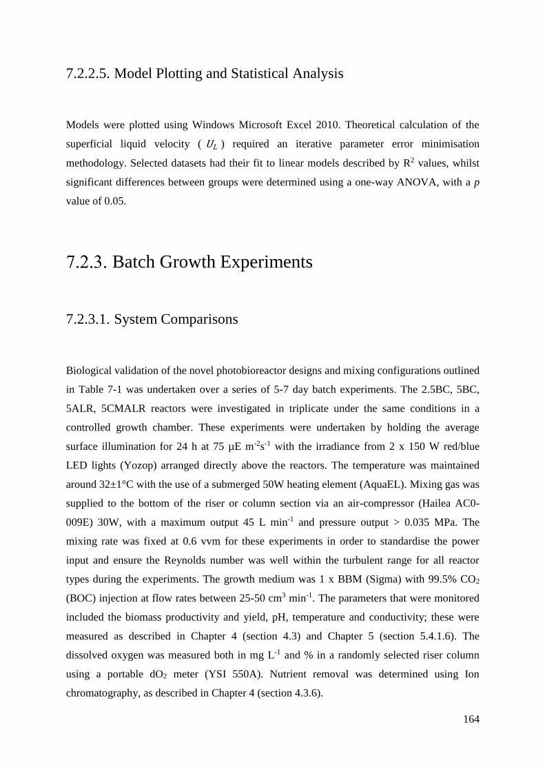
164

7.2.2.5. Model Plotting and Statistical Analysis

Models were plotted using Windows Microsoft Excel 2010. Theoretical calculation of the

superficial liquid velocity ( UL ) required an iterative parameter error minimisation

methodology. Selected datasets had their fit to linear models described by R2 values, whilst

significant differences between groups were determined using a one-way ANOVA, with a p

value of 0.05.

Batch Growth Experiments

7.2.3.1. System Comparisons

Biological validation of the novel photobioreactor designs and mixing configurations outlined

in Table 7-1 was undertaken over a series of 5-7 day batch experiments. The 2.5BC, 5BC,

5ALR, 5CMALR reactors were investigated in triplicate under the same conditions in a

controlled growth chamber. These experiments were undertaken by holding the average

surface illumination for 24 h at 75 µE m-2s-1 with the irradiance from 2 x 150 W red/blue

LED lights (Yozop) arranged directly above the reactors. The temperature was maintained

around 32±1°C with the use of a submerged 50W heating element (AquaEL). Mixing gas was

supplied to the bottom of the riser or column section via an air-compressor (Hailea AC0-

009E) 30W, with a maximum output 45 L min-1 and pressure output > 0.035 MPa. The

mixing rate was fixed at 0.6 vvm for these experiments in order to standardise the power

input and ensure the Reynolds number was well within the turbulent range for all reactor

types during the experiments. The growth medium was 1 x BBM (Sigma) with 99.5% CO2

(BOC) injection at flow rates between 25-50 cm3 min-1. The parameters that were monitored

included the biomass productivity and yield, pH, temperature and conductivity; these were

measured as described in Chapter 4 (section 4.3) and Chapter 5 (section 5.4.1.6). The

dissolved oxygen was measured both in mg L-1 and % in a randomly selected riser column

using a portable dO2 meter (YSI 550A). Nutrient removal was determined using Ion

chromatography, as described in Chapter 4 (section 4.3.6).

165

Further work was undertaken comparing the 5, 10, 50 L ALR systems to each other to ensure

performance was consistent between scales. In the first instance this included testing the

liquid velocity, biomass concentration and dO2 in different tubes and depths along the array.

The liquid velocity was measured as described in Section 7.2.2.2 in randomly selected riser

and downcomer tubes. The biomass was measured by sampling at random positions in the

reactor and measuring the biomass concentration as described in Section 4.3.5. The dissolved

oxygen was measured both in mg L-1 and % in randomly selected riser and downcomer

columns at different heights (0.0, 0.5 and 1 m) using a portable dO2 meter (YSI 550A). The

results from these experiments are summarised in Appendix 10.1.2.4. The second phase of

this work aimed to investigate the conditions necessary for the maximal growth rates and

yields. This was achieved using conditions identical to those described in the previous

paragraph, with the following exceptions; surface irradiance was increased to 500 µE m-2s-1

for 24 h, and achieved through the deployment of a greater number of LED arrays. The

culture was grown using a fed batch strategy as outlined in Chapter 4 (section 4.3.4.2) to a

total concentration of 3 x BBM; whilst CO2 injection was also increased to control the pH,

with flow rates ranging between 25-300 cm3 min-1.

Pilot Cultivation

Pilot testing was undertaken using the 50ALR within the greenhouse on the Darwin Building.

These experiments consisted of a series of 7-10 day batch experiments designed with the

purpose of quantifying performance under an array of natural and artificial conditions. This

included a preliminary investigation of the seasonal variation in algal productivities within a

Northern European greenhouse situated latitude 51.522996, longitude -0.132877, see Figure

7.5. All pilot experiments were undertaken under the following conditions; 1 x BBM with pH

control and feeding with variable addition of 99.5% CO2 (50-300 cm3/min). The mixing was

held at 0.6 vvm, using an array of air-compressors (Hailea AC0-009E) 30W, with a

maximum output 45 L min-1 and pressure output > 0.035 MPa. Naturally illuminated

conditions depended on daily and seasonal light variations. Online measurement of key

parameters was undertaken with the AlgaeConnect data acquisition system (Algae Lab

Systems) alongside an array of sensors. Measured parameters included growth which was

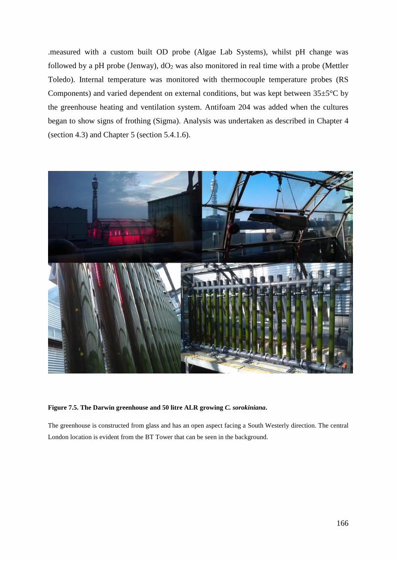
166

.measured with a custom built OD probe (Algae Lab Systems), whilst pH change was

followed by a pH probe (Jenway), dO2 was also monitored in real time with a probe (Mettler

Toledo). Internal temperature was monitored with thermocouple temperature probes (RS

Components) and varied dependent on external conditions, but was kept between 35±5°C by

the greenhouse heating and ventilation system. Antifoam 204 was added when the cultures

began to show signs of frothing (Sigma). Analysis was undertaken as described in Chapter 4

(section 4.3) and Chapter 5 (section 5.4.1.6).

Figure 7.5. The Darwin greenhouse and 50 litre ALR growing C. sorokiniana.

The greenhouse is constructed from glass and has an open aspect facing a South Westerly direction. The central

London location is evident from the BT Tower that can be seen in the background.

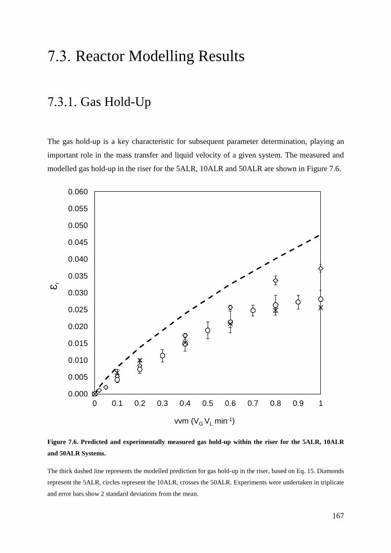
167

Reactor Modelling Results

Gas Hold-Up

The gas hold-up is a key characteristic for subsequent parameter determination, playing an

important role in the mass transfer and liquid velocity of a given system. The measured and

modelled gas hold-up in the riser for the 5ALR, 10ALR and 50ALR are shown in Figure 7.6.

Figure 7.6. Predicted and experimentally measured gas hold-up within the riser for the 5ALR, 10ALR

and 50ALR Systems.

The thick dashed line represents the modelled prediction for gas hold-up in the riser, based on Eq. 15. Diamonds

represent the 5ALR, circles represent the 10ALR, crosses the 50ALR. Experiments were undertaken in triplicate

and error bars show 2 standard deviations from the mean.

0.000

0.005

0.010

0.015

0.020

0.025

0.030

0.035

0.040

0.045

0.050

0.055

0.060

0 0.1 0.2 0.3 0.4 0.5 0.6 0.7 0.8 0.9 1

Ɛr

vvm (VG VL min-1)

168

The results show that in the case of the 5ALR system the percentage deviation between the

model and experimental findings was between 19-42%, and represents the closest fit to the

model. The 10ALR and 50ALR show similar gas hold up levels within the riser, deviating

from the model by between 20-48%. No statistical significance was found between the mean

results of the 10ALR and 50ALR (ANOVA), indicating that scaling by number using the

approach outlined in this thesis minimises performance drop. The greater spread of standard

deviations in the 10ALR was most probably caused by taking average measurements from

the two riser columns. This was deemed necessary at a smaller scale due to the bigger

differences in liquid velocity between central and outlying riser tubes. The gas hold-up for

the 2.5BC, 5BC, 5CMALR, 10CMALR are shown in Figure 7.7.

Figure 7.7. Predicted and experimentally measured gas hold-up within 2.5BC, 5BC, 5CMALR and

10CMALR systems.

The thick lines represent the modelled predictions for bubble column gas hold-up based on Eq. 22. The solid

line is for the 5BC and the dotted and dashed projection for all other configurations. Experimental

measurements are represented by the following shapes; circles: 2.5BC, squares: 5BC, crosses: 5CMALR and

diamonds: 10CMALR. Error bars show 2 standard deviations from the mean.

0.000

0.005

0.010

0.015

0.020

0.025

0.030

0.035

0.040

0.045

0.050

0.055

0.060

0 0.1 0.2 0.3 0.4 0.5 0.6 0.7 0.8 0.9 1

Ɛ(t

ota

l)

vvm (VG VL min-1)

169

The results show that the BC and CM systems deviate from their respective models less than

ALR based systems. The 2.5BC, 5CMALR and 10CMALR all show similar levels of gas

hold-up, which is attributable to their identical column dimensions. Specifically, the 2.5BC

fits the model most closely, with results between 0-20% from the model, whilst the CM

systems deviated by between 5-23%. The 5BC deviates the most considerably from the

model around 0-27% of the projection, for reasons that are unclear at this time. Overall, the

results show that the BC and CM systems have higher gas hold-up than the ALR at

volumetric gas flow rates above 0.1-0.2 vvm.

Liquid Velocity

7.3.2.1. Superficial Liquid Velocity

The liquid velocity was determined to allow for the calculation of key system characteristics,

such as the Reynolds number and circulation times under the different mixing regimes. These

findings were also necessary to validate the assumption that the modular scale up of the

reactor would not have a considerable effect on the liquid velocity found throughout the

system. The experimental findings for the 5ALR, 10ALR and 50ALR are shown in Figure

7.8 and compared to theoretical models in Eqs. 14 and 21.

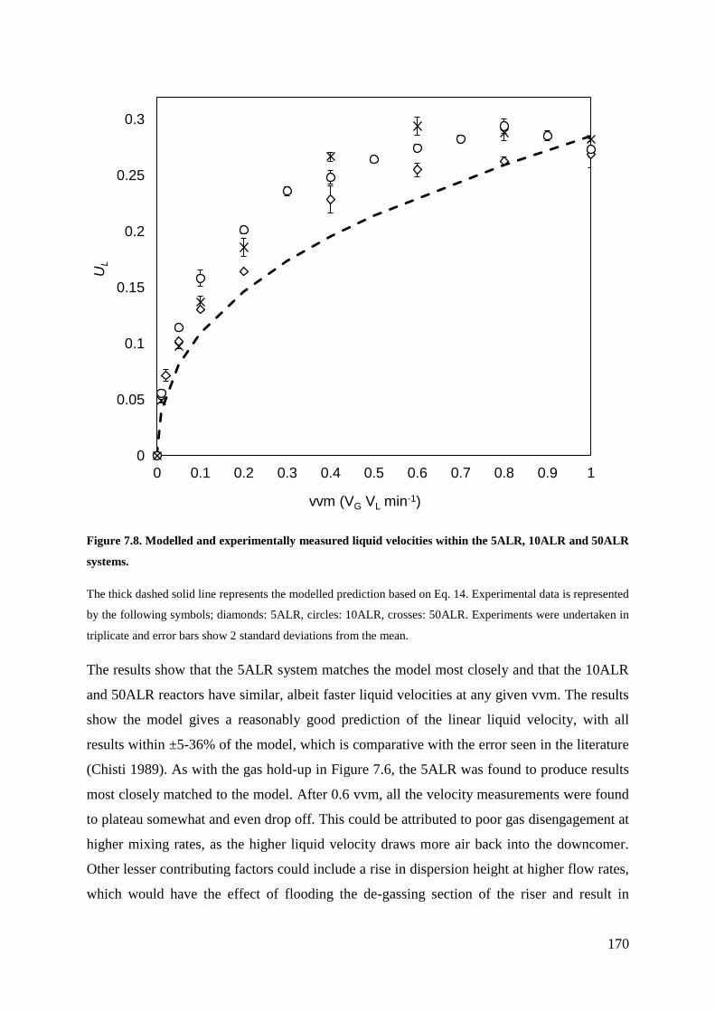
170

Figure 7.8. Modelled and experimentally measured liquid velocities within the 5ALR, 10ALR and 50ALR

systems.

The thick dashed solid line represents the modelled prediction based on Eq. 14. Experimental data is represented

by the following symbols; diamonds: 5ALR, circles: 10ALR, crosses: 50ALR. Experiments were undertaken in

triplicate and error bars show 2 standard deviations from the mean.

The results show that the 5ALR system matches the model most closely and that the 10ALR

and 50ALR reactors have similar, albeit faster liquid velocities at any given vvm. The results

show the model gives a reasonably good prediction of the linear liquid velocity, with all

results within ±5-36% of the model, which is comparative with the error seen in the literature

(Chisti 1989). As with the gas hold-up in Figure 7.6, the 5ALR was found to produce results

most closely matched to the model. After 0.6 vvm, all the velocity measurements were found

to plateau somewhat and even drop off. This could be attributed to poor gas disengagement at

higher mixing rates, as the higher liquid velocity draws more air back into the downcomer.

Other lesser contributing factors could include a rise in dispersion height at higher flow rates,

which would have the effect of flooding the de-gassing section of the riser and result in

0

0.05

0.1

0.15

0.2

0.25

0.3

0 0.1 0.2 0.3 0.4 0.5 0.6 0.7 0.8 0.9 1

UL

vvm (VG VL min-1)

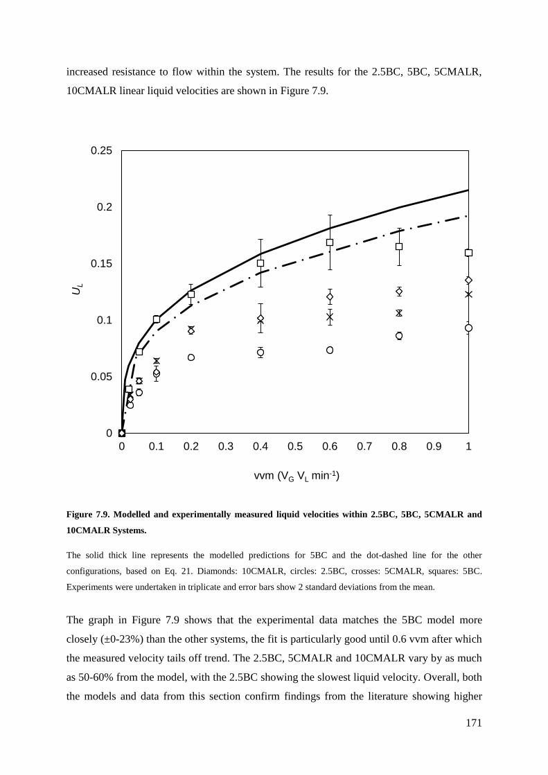
171

increased resistance to flow within the system. The results for the 2.5BC, 5BC, 5CMALR,

10CMALR linear liquid velocities are shown in Figure 7.9.

Figure 7.9. Modelled and experimentally measured liquid velocities within 2.5BC, 5BC, 5CMALR and

10CMALR Systems.

The solid thick line represents the modelled predictions for 5BC and the dot-dashed line for the other

configurations, based on Eq. 21. Diamonds: 10CMALR, circles: 2.5BC, crosses: 5CMALR, squares: 5BC.

Experiments were undertaken in triplicate and error bars show 2 standard deviations from the mean.

The graph in Figure 7.9 shows that the experimental data matches the 5BC model more

closely (±0-23%) than the other systems, the fit is particularly good until 0.6 vvm after which

the measured velocity tails off trend. The 2.5BC, 5CMALR and 10CMALR vary by as much

as 50-60% from the model, with the 2.5BC showing the slowest liquid velocity. Overall, both

the models and data from this section confirm findings from the literature showing higher

0

0.05

0.1

0.15

0.2

0.25

0 0.1 0.2 0.3 0.4 0.5 0.6 0.7 0.8 0.9 1

UL

vvm (VG VL min-1)

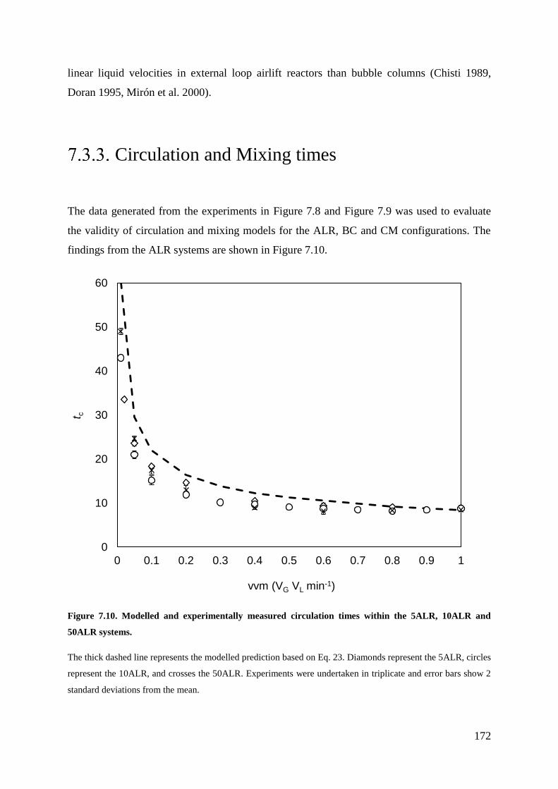
172

linear liquid velocities in external loop airlift reactors than bubble columns (Chisti 1989,

Doran 1995, Mirón et al. 2000).

Circulation and Mixing times

The data generated from the experiments in Figure 7.8 and Figure 7.9 was used to evaluate

the validity of circulation and mixing models for the ALR, BC and CM configurations. The

findings from the ALR systems are shown in Figure 7.10.

Figure 7.10. Modelled and experimentally measured circulation times within the 5ALR, 10ALR and

50ALR systems.

The thick dashed line represents the modelled prediction based on Eq. 23. Diamonds represent the 5ALR, circles

represent the 10ALR, and crosses the 50ALR. Experiments were undertaken in triplicate and error bars show 2

standard deviations from the mean.

0

10

20

30

40

50

60

0 0.1 0.2 0.3 0.4 0.5 0.6 0.7 0.8 0.9 1

t c

vvm (VG VL min-1)

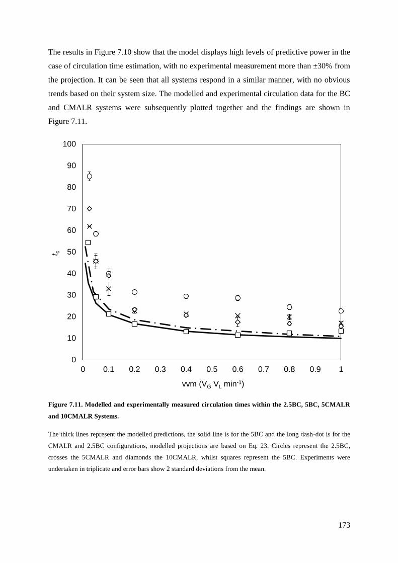
173

The results in Figure 7.10 show that the model displays high levels of predictive power in the

case of circulation time estimation, with no experimental measurement more than ±30% from

the projection. It can be seen that all systems respond in a similar manner, with no obvious

trends based on their system size. The modelled and experimental circulation data for the BC

and CMALR systems were subsequently plotted together and the findings are shown in

Figure 7.11.

Figure 7.11. Modelled and experimentally measured circulation times within the 2.5BC, 5BC, 5CMALR

and 10CMALR Systems.

The thick lines represent the modelled predictions, the solid line is for the 5BC and the long dash-dot is for the

CMALR and 2.5BC configurations, modelled projections are based on Eq. 23. Circles represent the 2.5BC,

crosses the 5CMALR and diamonds the 10CMALR, whilst squares represent the 5BC. Experiments were

undertaken in triplicate and error bars show 2 standard deviations from the mean.

0

10

20

30

40

50

60

70

80

90

100

0 0.1 0.2 0.3 0.4 0.5 0.6 0.7 0.8 0.9 1

t c

vvm (VG VL min-1)

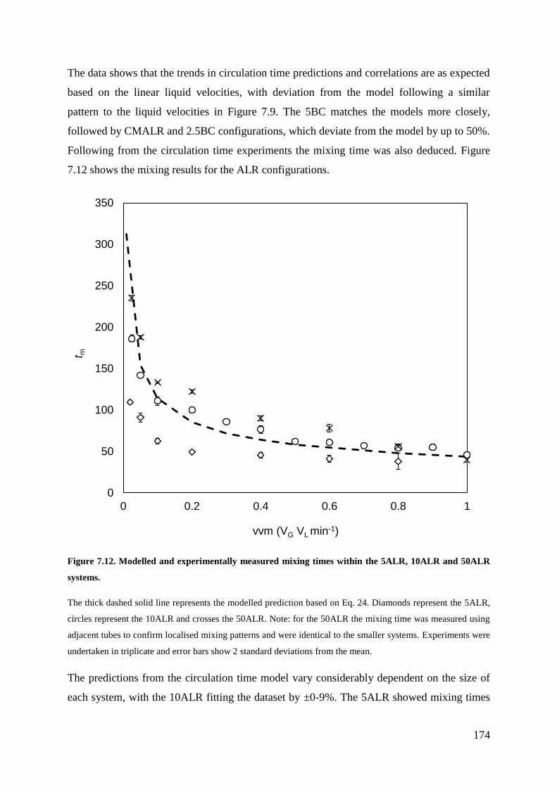
174

The data shows that the trends in circulation time predictions and correlations are as expected

based on the linear liquid velocities, with deviation from the model following a similar

pattern to the liquid velocities in Figure 7.9. The 5BC matches the models more closely,

followed by CMALR and 2.5BC configurations, which deviate from the model by up to 50%.

Following from the circulation time experiments the mixing time was also deduced. Figure

7.12 shows the mixing results for the ALR configurations.

Figure 7.12. Modelled and experimentally measured mixing times within the 5ALR, 10ALR and 50ALR

systems.

The thick dashed solid line represents the modelled prediction based on Eq. 24. Diamonds represent the 5ALR,

circles represent the 10ALR and crosses the 50ALR. Note: for the 50ALR the mixing time was measured using

adjacent tubes to confirm localised mixing patterns and were identical to the smaller systems. Experiments were

undertaken in triplicate and error bars show 2 standard deviations from the mean.

The predictions from the circulation time model vary considerably dependent on the size of

each system, with the 10ALR fitting the dataset by ±0-9%. The 5ALR showed mixing times

0

50

100

150

200

250

300

350

0 0.2 0.4 0.6 0.8 1

t m

vvm (VG VL min-1)

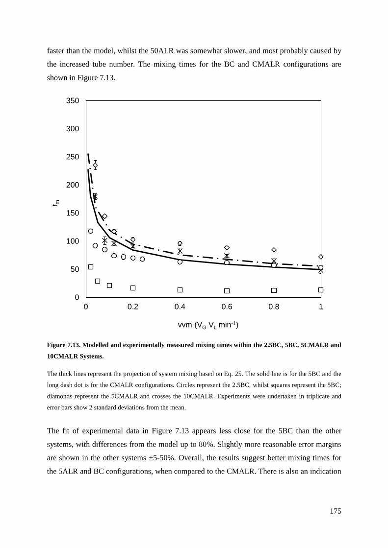
175

faster than the model, whilst the 50ALR was somewhat slower, and most probably caused by

the increased tube number. The mixing times for the BC and CMALR configurations are

shown in Figure 7.13.

Figure 7.13. Modelled and experimentally measured mixing times within the 2.5BC, 5BC, 5CMALR and

10CMALR Systems.

The thick lines represent the projection of system mixing based on Eq. 25. The solid line is for the 5BC and the

long dash dot is for the CMALR configurations. Circles represent the 2.5BC, whilst squares represent the 5BC;

diamonds represent the 5CMALR and crosses the 10CMALR. Experiments were undertaken in triplicate and

error bars show 2 standard deviations from the mean.

The fit of experimental data in Figure 7.13 appears less close for the 5BC than the other

systems, with differences from the model up to 80%. Slightly more reasonable error margins

are shown in the other systems ±5-50%. Overall, the results suggest better mixing times for

the 5ALR and BC configurations, when compared to the CMALR. There is also an indication

0

50

100

150

200

250

300

350

0 0.2 0.4 0.6 0.8 1

t m

vvm (VG VL min-1)

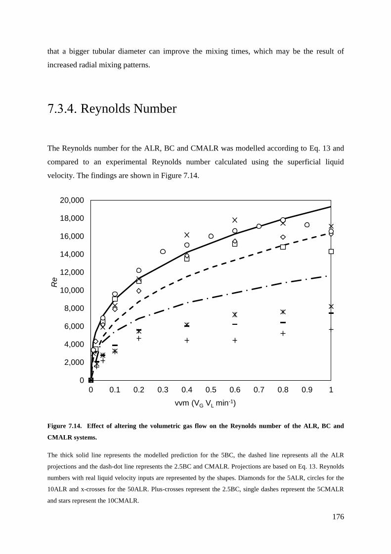
176

that a bigger tubular diameter can improve the mixing times, which may be the result of

increased radial mixing patterns.

Reynolds Number

The Reynolds number for the ALR, BC and CMALR was modelled according to Eq. 13 and

compared to an experimental Reynolds number calculated using the superficial liquid

velocity. The findings are shown in Figure 7.14.

Figure 7.14. Effect of altering the volumetric gas flow on the Reynolds number of the ALR, BC and

CMALR systems.

The thick solid line represents the modelled prediction for the 5BC, the dashed line represents all the ALR

projections and the dash-dot line represents the 2.5BC and CMALR. Projections are based on Eq. 13. Reynolds

numbers with real liquid velocity inputs are represented by the shapes. Diamonds for the 5ALR, circles for the

10ALR and x-crosses for the 50ALR. Plus-crosses represent the 2.5BC, single dashes represent the 5CMALR

and stars represent the 10CMALR.

0

2,000

4,000

6,000

8,000

10,000

12,000

14,000

16,000

18,000

20,000

0 0.1 0.2 0.3 0.4 0.5 0.6 0.7 0.8 0.9 1

Re

vvm (VG VL min-1)

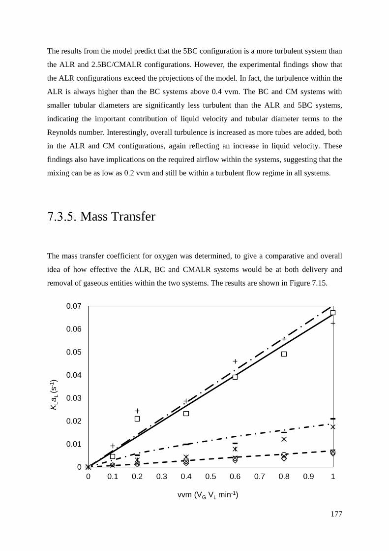
177

The results from the model predict that the 5BC configuration is a more turbulent system than

the ALR and 2.5BC/CMALR configurations. However, the experimental findings show that

the ALR configurations exceed the projections of the model. In fact, the turbulence within the

ALR is always higher than the BC systems above 0.4 vvm. The BC and CM systems with

smaller tubular diameters are significantly less turbulent than the ALR and 5BC systems,

indicating the important contribution of liquid velocity and tubular diameter terms to the

Reynolds number. Interestingly, overall turbulence is increased as more tubes are added, both

in the ALR and CM configurations, again reflecting an increase in liquid velocity. These

findings also have implications on the required airflow within the systems, suggesting that the

mixing can be as low as 0.2 vvm and still be within a turbulent flow regime in all systems.

Mass Transfer

The mass transfer coefficient for oxygen was determined, to give a comparative and overall

idea of how effective the ALR, BC and CMALR systems would be at both delivery and

removal of gaseous entities within the two systems. The results are shown in Figure 7.15.

0

0.01

0.02

0.03

0.04

0.05

0.06

0.07

0 0.1 0.2 0.3 0.4 0.5 0.6 0.7 0.8 0.9 1

KLa

L (s

-1)

vvm (VG VL min-1)

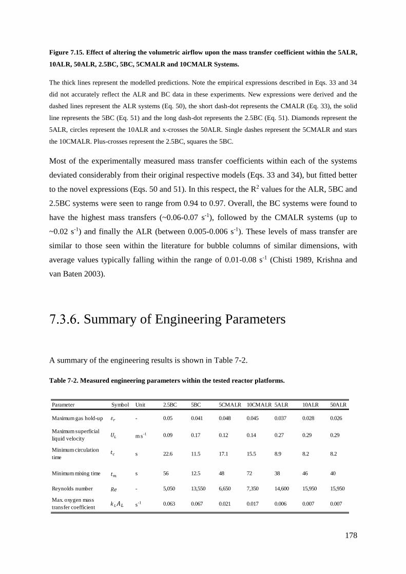
178

Figure 7.15. Effect of altering the volumetric airflow upon the mass transfer coefficient within the 5ALR,

10ALR, 50ALR, 2.5BC, 5BC, 5CMALR and 10CMALR Systems.

The thick lines represent the modelled predictions. Note the empirical expressions described in Eqs. 33 and 34

did not accurately reflect the ALR and BC data in these experiments. New expressions were derived and the

dashed lines represent the ALR systems (Eq. 50), the short dash-dot represents the CMALR (Eq. 33), the solid

line represents the 5BC (Eq. 51) and the long dash-dot represents the 2.5BC (Eq. 51). Diamonds represent the

5ALR, circles represent the 10ALR and x-crosses the 50ALR. Single dashes represent the 5CMALR and stars

the 10CMALR. Plus-crosses represent the 2.5BC, squares the 5BC.

Most of the experimentally measured mass transfer coefficients within each of the systems

deviated considerably from their original respective models (Eqs. 33 and 34), but fitted better

to the novel expressions (Eqs. 50 and 51). In this respect, the R2 values for the ALR, 5BC and

2.5BC systems were seen to range from 0.94 to 0.97. Overall, the BC systems were found to

have the highest mass transfers (~0.06-0.07 s-1), followed by the CMALR systems (up to

~0.02 s-1) and finally the ALR (between 0.005-0.006 s-1). These levels of mass transfer are

similar to those seen within the literature for bubble columns of similar dimensions, with

average values typically falling within the range of 0.01-0.08 s-1 (Chisti 1989, Krishna and

van Baten 2003).

Summary of Engineering Parameters

A summary of the engineering results is shown in Table 7-2.

Table 7-2. Measured engineering parameters within the tested reactor platforms.

Parameter Symbol Unit 2.5BC 5BC 5CMALR 10CMALR 5ALR 10ALR 50ALR

Maximum gas hold-up - 0.05 0.041 0.048 0.045 0.037 0.028 0.026

Maximum superficial

liquid velocitym s

-1 0.09 0.17 0.12 0.14 0.27 0.29 0.29

Minimum circulation

times 22.6 11.5 17.1 15.5 8.9 8.2 8.2

Minimum mixing time s 56 12.5 48 72 38 46 40

Reynolds number - 5,050 13,550 6,650 7,350 14,600 15,950 15,950

Max. oxygen mass

transfer coefficient s

-1 0.063 0.067 0.021 0.017 0.006 0.007 0.007

𝜀𝑟

𝑡𝑐

𝑡𝑚

𝑘𝐿𝐴𝐿

𝑈𝐿

𝑅𝑒

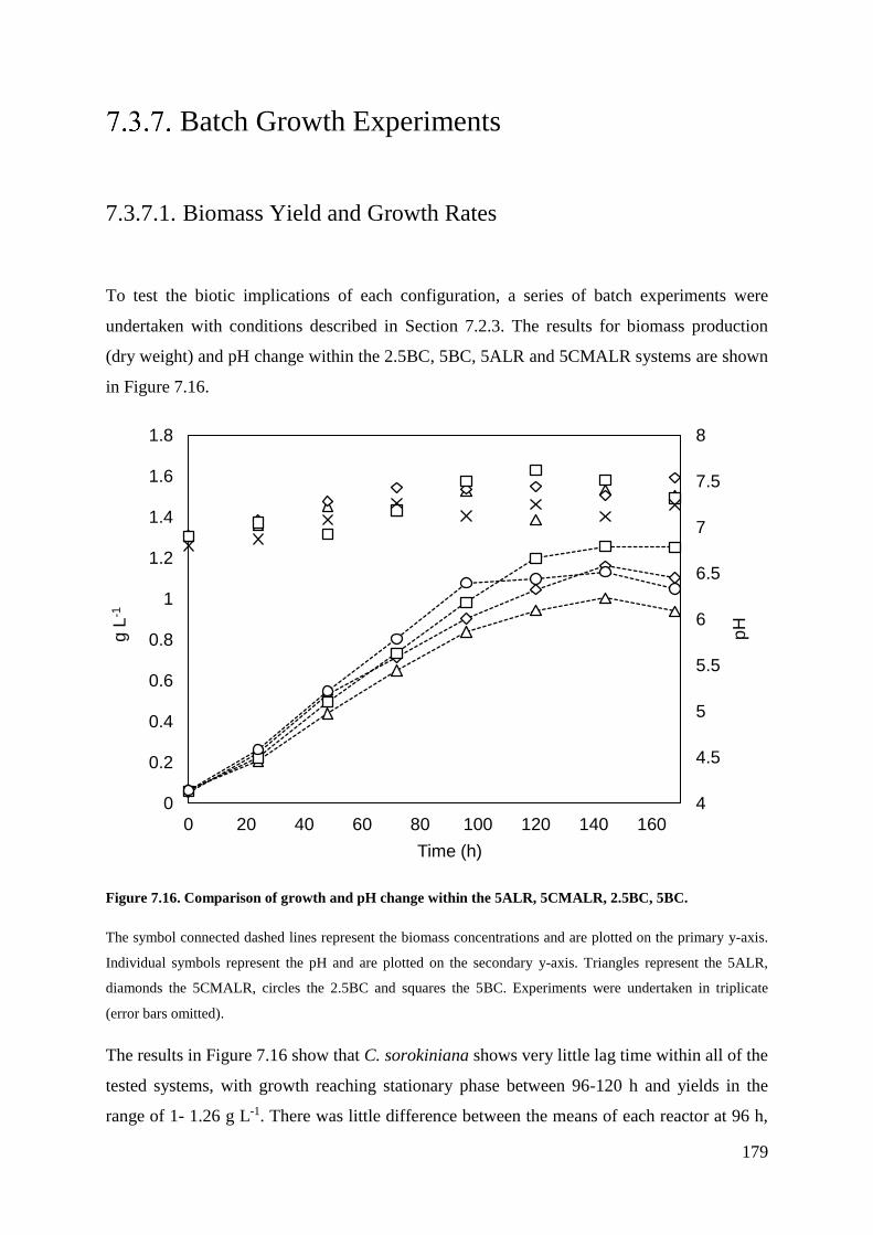
179

Batch Growth Experiments

7.3.7.1. Biomass Yield and Growth Rates

To test the biotic implications of each configuration, a series of batch experiments were

undertaken with conditions described in Section 7.2.3. The results for biomass production

(dry weight) and pH change within the 2.5BC, 5BC, 5ALR and 5CMALR systems are shown

in Figure 7.16.

Figure 7.16. Comparison of growth and pH change within the 5ALR, 5CMALR, 2.5BC, 5BC.

The symbol connected dashed lines represent the biomass concentrations and are plotted on the primary y-axis.

Individual symbols represent the pH and are plotted on the secondary y-axis. Triangles represent the 5ALR,

diamonds the 5CMALR, circles the 2.5BC and squares the 5BC. Experiments were undertaken in triplicate

(error bars omitted).

The results in Figure 7.16 show that C. sorokiniana shows very little lag time within all of the

tested systems, with growth reaching stationary phase between 96-120 h and yields in the

range of 1- 1.26 g L-1. There was little difference between the means of each reactor at 96 h,

4

4.5

5

5.5

6

6.5

7

7.5

8

0

0.2

0.4

0.6

0.8

1

1.2

1.4

1.6

1.8

0 20 40 60 80 100 120 140 160

pH

g L

-1

Time (h)

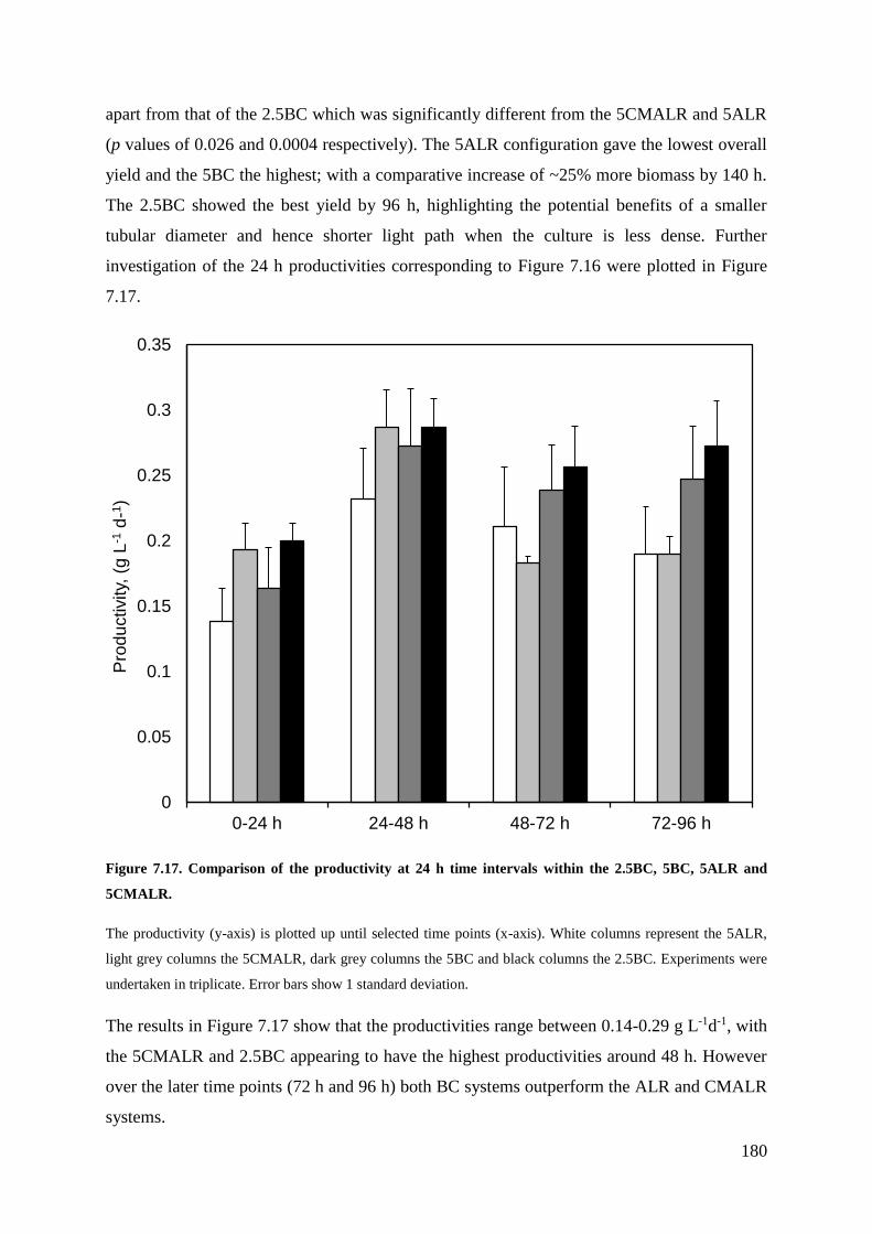
180

apart from that of the 2.5BC which was significantly different from the 5CMALR and 5ALR

(p values of 0.026 and 0.0004 respectively). The 5ALR configuration gave the lowest overall

yield and the 5BC the highest; with a comparative increase of ~25% more biomass by 140 h.

The 2.5BC showed the best yield by 96 h, highlighting the potential benefits of a smaller

tubular diameter and hence shorter light path when the culture is less dense. Further

investigation of the 24 h productivities corresponding to Figure 7.16 were plotted in Figure

7.17.

Figure 7.17. Comparison of the productivity at 24 h time intervals within the 2.5BC, 5BC, 5ALR and

5CMALR.

The productivity (y-axis) is plotted up until selected time points (x-axis). White columns represent the 5ALR,

light grey columns the 5CMALR, dark grey columns the 5BC and black columns the 2.5BC. Experiments were

undertaken in triplicate. Error bars show 1 standard deviation.

The results in Figure 7.17 show that the productivities range between 0.14-0.29 g L-1d-1, with

the 5CMALR and 2.5BC appearing to have the highest productivities around 48 h. However

over the later time points (72 h and 96 h) both BC systems outperform the ALR and CMALR

systems.

0

0.05

0.1

0.15

0.2

0.25

0.3

0.35

0-24 h 24-48 h 48-72 h 72-96 h

Pro

du

ctivity,

(g L

-1d

-1)

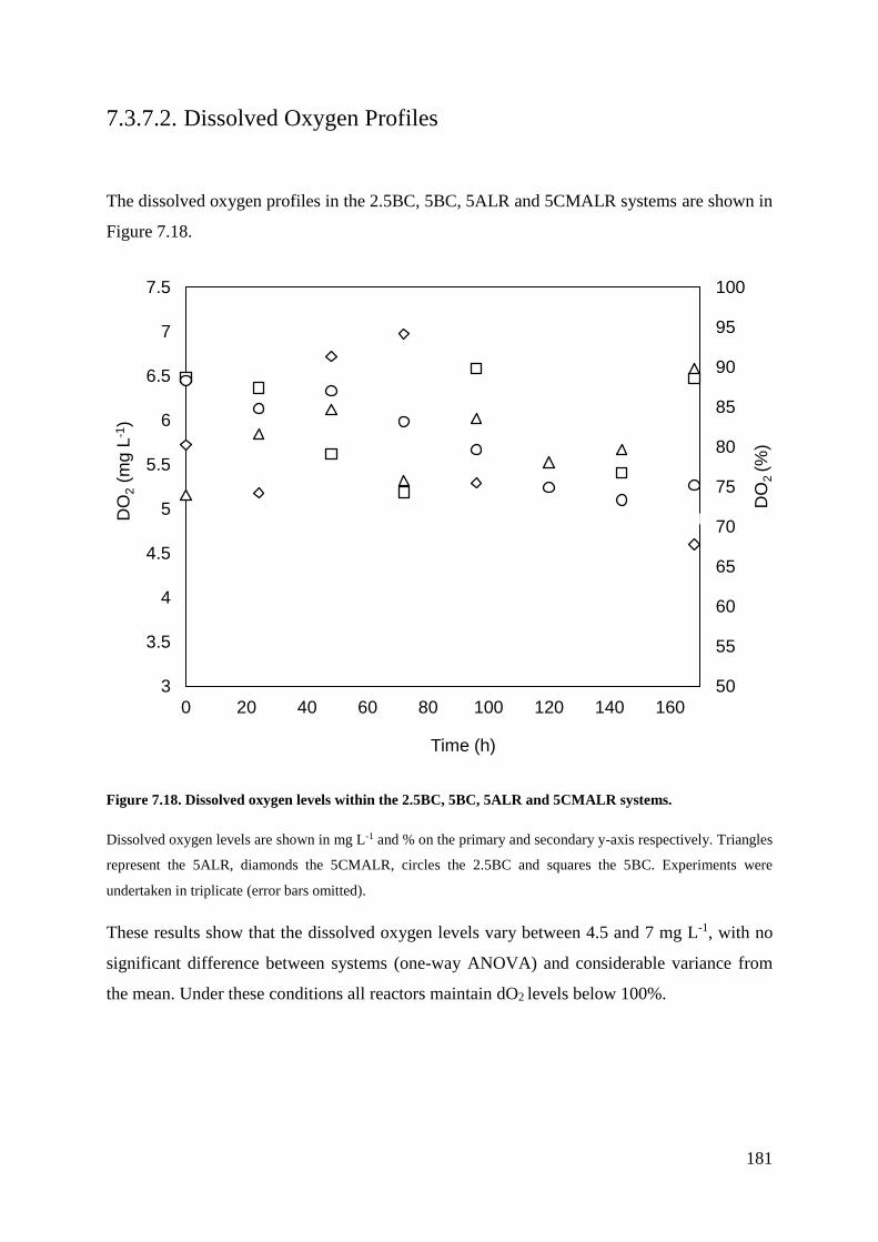
181

7.3.7.2. Dissolved Oxygen Profiles

The dissolved oxygen profiles in the 2.5BC, 5BC, 5ALR and 5CMALR systems are shown in

Figure 7.18.

Figure 7.18. Dissolved oxygen levels within the 2.5BC, 5BC, 5ALR and 5CMALR systems.

Dissolved oxygen levels are shown in mg L-1 and % on the primary and secondary y-axis respectively. Triangles

represent the 5ALR, diamonds the 5CMALR, circles the 2.5BC and squares the 5BC. Experiments were

undertaken in triplicate (error bars omitted).

These results show that the dissolved oxygen levels vary between 4.5 and 7 mg L-1, with no

significant difference between systems (one-way ANOVA) and considerable variance from

the mean. Under these conditions all reactors maintain dO2 levels below 100%.

50

55

60

65

70

75

80

85

90

95

100

3

3.5

4

4.5

5

5.5

6

6.5

7

7.5

0 20 40 60 80 100 120 140 160

DO

2 (%

)

DO

2(m

g L

-1)

Time (h)

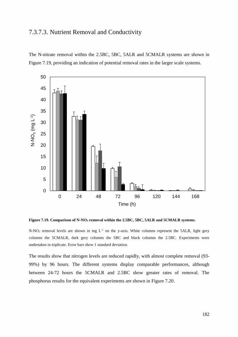
182

7.3.7.3. Nutrient Removal and Conductivity

The N-nitrate removal within the 2.5BC, 5BC, 5ALR and 5CMALR systems are shown in

Figure 7.19, providing an indication of potential removal rates in the larger scale systems.

Figure 7.19. Comparison of N-NO3 removal within the 2.5BC, 5BC, 5ALR and 5CMALR systems.

N-NO3 removal levels are shown in mg L-1 on the y-axis. White columns represent the 5ALR, light grey

columns the 5CMALR, dark grey columns the 5BC and black columns the 2.5BC. Experiments were

undertaken in triplicate. Error bars show 1 standard deviation.

The results show that nitrogen levels are reduced rapidly, with almost complete removal (93-

99%) by 96 hours. The different systems display comparable performances, although

between 24-72 hours the 5CMALR and 2.5BC show greater rates of removal. The

phosphorus results for the equivalent experiments are shown in Figure 7.20.

0

5

10

15

20

25

30

35

40

45

50

0 24 48 72 96 120 144 168

N-N

O3

(mg L

-1)

Time (h)

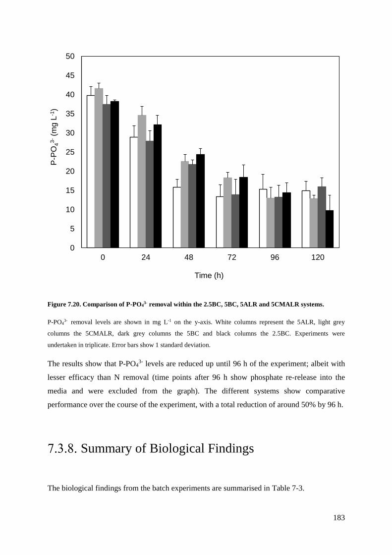
183

Figure 7.20. Comparison of P-PO43- removal within the 2.5BC, 5BC, 5ALR and 5CMALR systems.

P-PO43- removal levels are shown in mg L-1 on the y-axis. White columns represent the 5ALR, light grey

columns the 5CMALR, dark grey columns the 5BC and black columns the 2.5BC. Experiments were

undertaken in triplicate. Error bars show 1 standard deviation.

The results show that P-PO43- levels are reduced up until 96 h of the experiment; albeit with

lesser efficacy than N removal (time points after 96 h show phosphate re-release into the

media and were excluded from the graph). The different systems show comparative

performance over the course of the experiment, with a total reduction of around 50% by 96 h.

Summary of Biological Findings

The biological findings from the batch experiments are summarised in Table 7-3.

0

5

10

15

20

25

30

35

40

45

50

0 24 48 72 96 120

P-P

O43-(m

g L

-1)

Time (h)

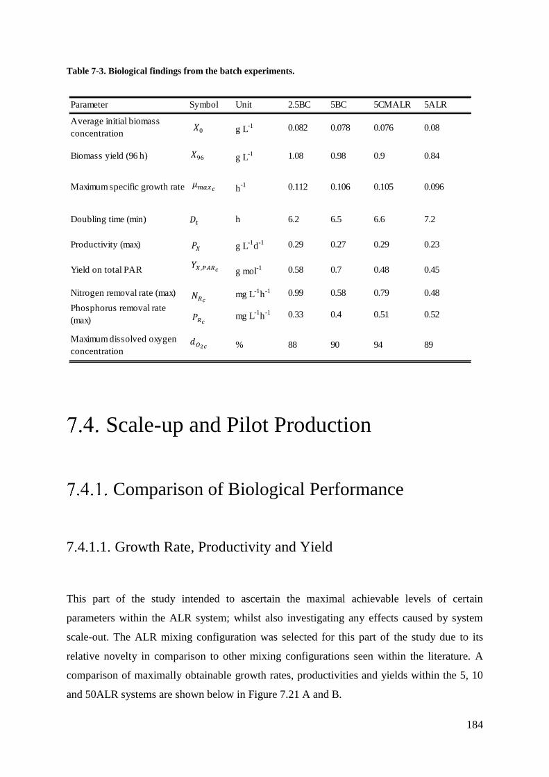
184

Table 7-3. Biological findings from the batch experiments.

Scale-up and Pilot Production

Comparison of Biological Performance

7.4.1.1. Growth Rate, Productivity and Yield

This part of the study intended to ascertain the maximal achievable levels of certain

parameters within the ALR system; whilst also investigating any effects caused by system

scale-out. The ALR mixing configuration was selected for this part of the study due to its

relative novelty in comparison to other mixing configurations seen within the literature. A

comparison of maximally obtainable growth rates, productivities and yields within the 5, 10

and 50ALR systems are shown below in Figure 7.21 A and B.

Parameter Symbol Unit 2.5BC 5BC 5CMALR 5ALR

Average initial biomass

concentrationg L

-1 0.082 0.078 0.076 0.08

Biomass yield (96 h) g L-1 1.08 0.98 0.9 0.84

Maximum specific growth rate h-1 0.112 0.106 0.105 0.096

Doubling time (min) h 6.2 6.5 6.6 7.2

Productivity (max) g L-1

d-1 0.29 0.27 0.29 0.23

Yield on total PAR g mol-1 0.58 0.7 0.48 0.45

Nitrogen removal rate (max) mg L-1

h-1 0.99 0.58 0.79 0.48

Phosphorus removal rate

(max)mg L

-1h

-1 0.33 0.4 0.51 0.52

Maximum dissolved oxygen

concentration% 88 90 94 89

𝑋0

𝑋96

𝜇𝑚𝑎𝑥

𝐷𝑡

𝑃𝑋

𝑌𝑋,𝑃𝐴𝑅

𝑁𝑅

𝑃𝑅

𝑑𝑂2

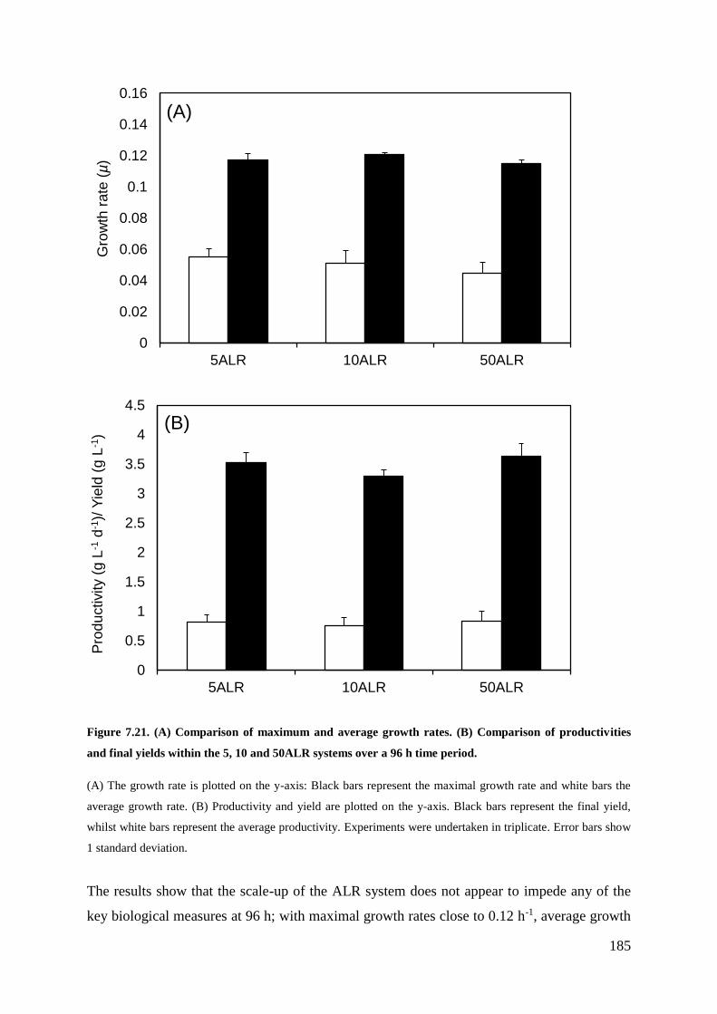
185

Figure 7.21. (A) Comparison of maximum and average growth rates. (B) Comparison of productivities

and final yields within the 5, 10 and 50ALR systems over a 96 h time period.

(A) The growth rate is plotted on the y-axis: Black bars represent the maximal growth rate and white bars the

average growth rate. (B) Productivity and yield are plotted on the y-axis. Black bars represent the final yield,

whilst white bars represent the average productivity. Experiments were undertaken in triplicate. Error bars show

1 standard deviation.

The results show that the scale-up of the ALR system does not appear to impede any of the

key biological measures at 96 h; with maximal growth rates close to 0.12 h-1, average growth

0

0.02

0.04

0.06

0.08

0.1

0.12

0.14

0.16

5ALR 10ALR 50ALR

Gro

wth

ra

te (

µ)

0

0.5

1

1.5

2

2.5

3

3.5

4

4.5

5ALR 10ALR 50ALR

Pro

du

ctivity (

g L

-1d

-1)/

Yie

ld (

g L

-1)

(B)

(A)

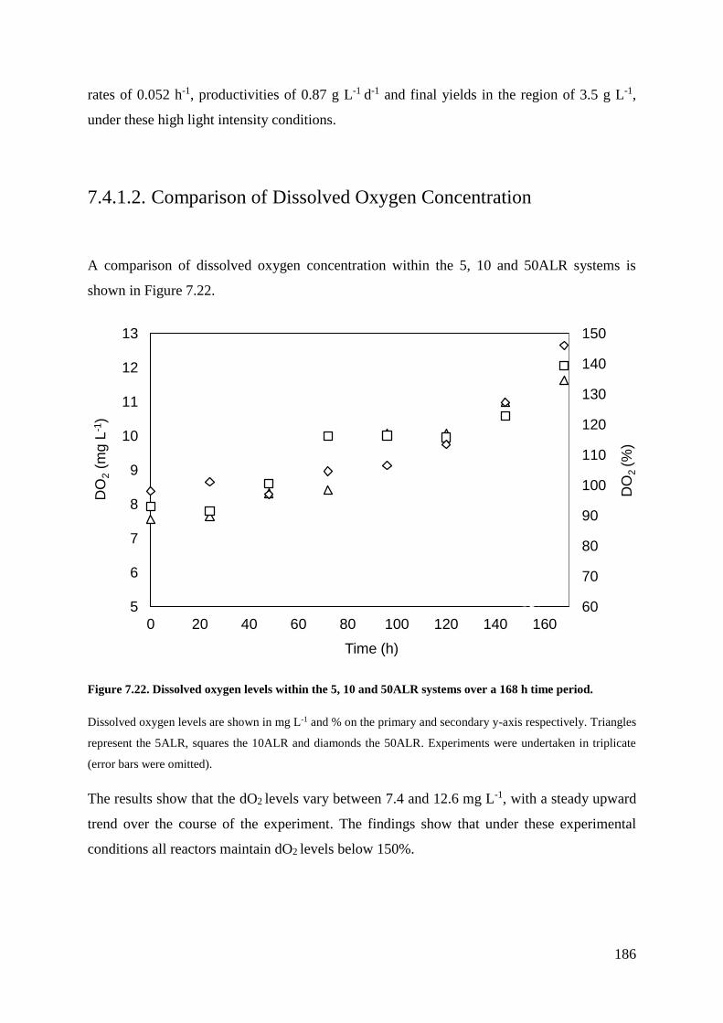
186

rates of 0.052 h-1, productivities of 0.87 g L-1 d-1 and final yields in the region of 3.5 g L-1,

under these high light intensity conditions.

7.4.1.2. Comparison of Dissolved Oxygen Concentration

A comparison of dissolved oxygen concentration within the 5, 10 and 50ALR systems is

shown in Figure 7.22.

Figure 7.22. Dissolved oxygen levels within the 5, 10 and 50ALR systems over a 168 h time period.

Dissolved oxygen levels are shown in mg L-1 and % on the primary and secondary y-axis respectively. Triangles

represent the 5ALR, squares the 10ALR and diamonds the 50ALR. Experiments were undertaken in triplicate

(error bars were omitted).

The results show that the dO2 levels vary between 7.4 and 12.6 mg L-1, with a steady upward

trend over the course of the experiment. The findings show that under these experimental

conditions all reactors maintain dO2 levels below 150%.

60

70

80

90

100

110

120

130

140

150

5

6

7

8

9

10

11

12

13

0 20 40 60 80 100 120 140 160D

O2 (%

)

DO

2(m

g L

-1)

Time (h)

187

Summary of ALR at 5, 10 and 50 L Scales

The biological performance of the ALR at different scales is outlined in Table 7-4.

Table 7-4. Comparison of biological performance parameters within 5, 10 and 50ALRs.

Darwin Pilot

The Darwin pilot set out to provide confirmation that the use of the thermotolerant strain C.

sorokiniana UTEX 1230 was feasible within a Northern European context, particularly with a

view towards wastewater treatment applications under natural lighting conditions. The testing

was undertaken in the 50ALR and the results are shown in Figure 7.23.

Parameter Symbol Unit 5ALR 10ALR 50ALR

Initial Biomass concentration

(high)g L

-1 0.28 0.32 0.35

Maximum obtained biomass

Yield (96 h)g L

-1 3.53 3.3 3.64

Maximum specific growth rate h-1 0.117 0.121 0.115

Doubling time (min) h 5.9 5.7 6

Productivity (max) g L-1

d-1 0.81 0.75 0.83

Yield on total PAR g mol-1 0.26 0.24 0.26

Maximum Dissolved Oxygen

Concentration% 135 139 146

𝑋96

𝑋0

𝜇𝑚𝑎𝑥

𝐷𝑡

𝑃

𝑌𝑋,𝑃𝐴𝑅

𝑑𝑂2

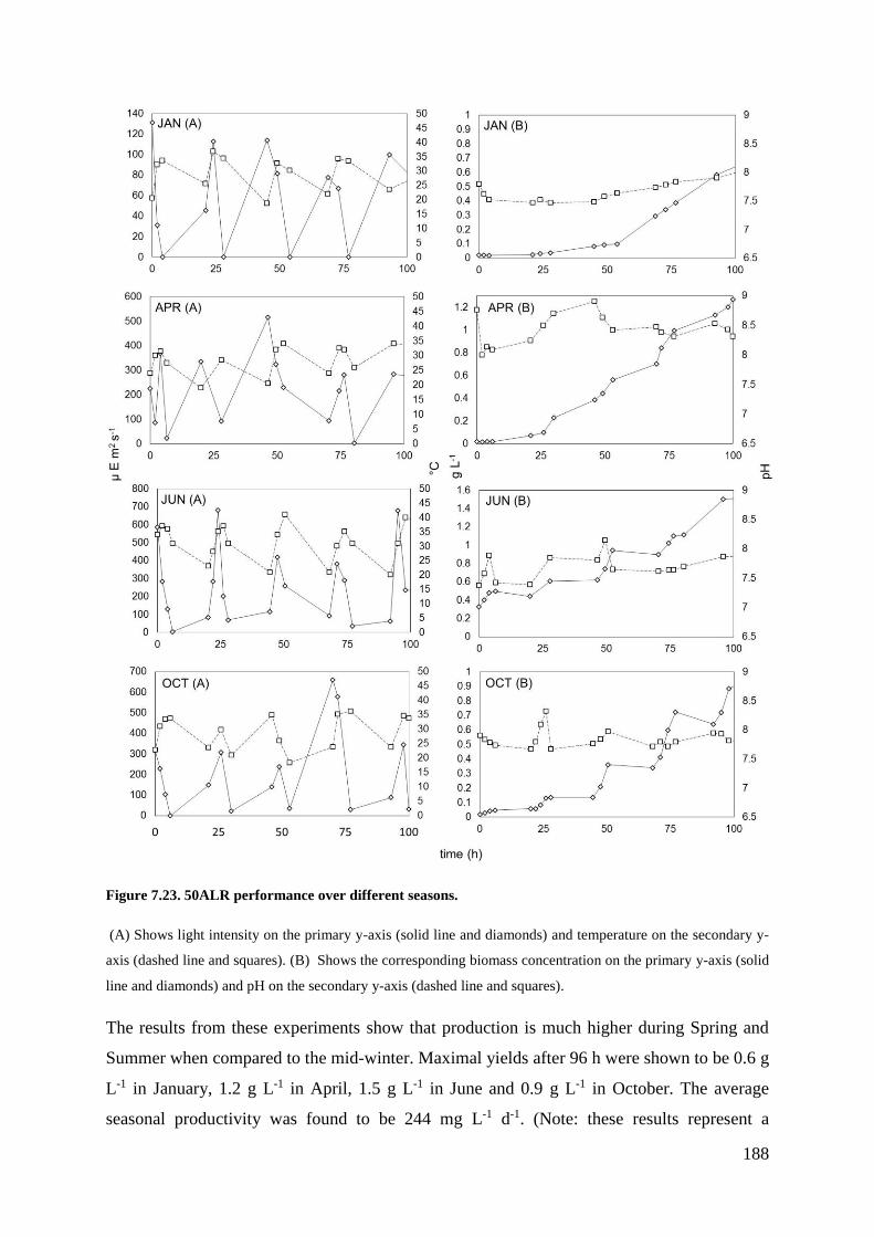
188

Figure 7.23. 50ALR performance over different seasons.

(A) Shows light intensity on the primary y-axis (solid line and diamonds) and temperature on the secondary y-

axis (dashed line and squares). (B) Shows the corresponding biomass concentration on the primary y-axis (solid

line and diamonds) and pH on the secondary y-axis (dashed line and squares).

The results from these experiments show that production is much higher during Spring and

Summer when compared to the mid-winter. Maximal yields after 96 h were shown to be 0.6 g

L-1 in January, 1.2 g L-1 in April, 1.5 g L-1 in June and 0.9 g L-1 in October. The average

seasonal productivity was found to be 244 mg L-1 d-1. (Note: these results represent a

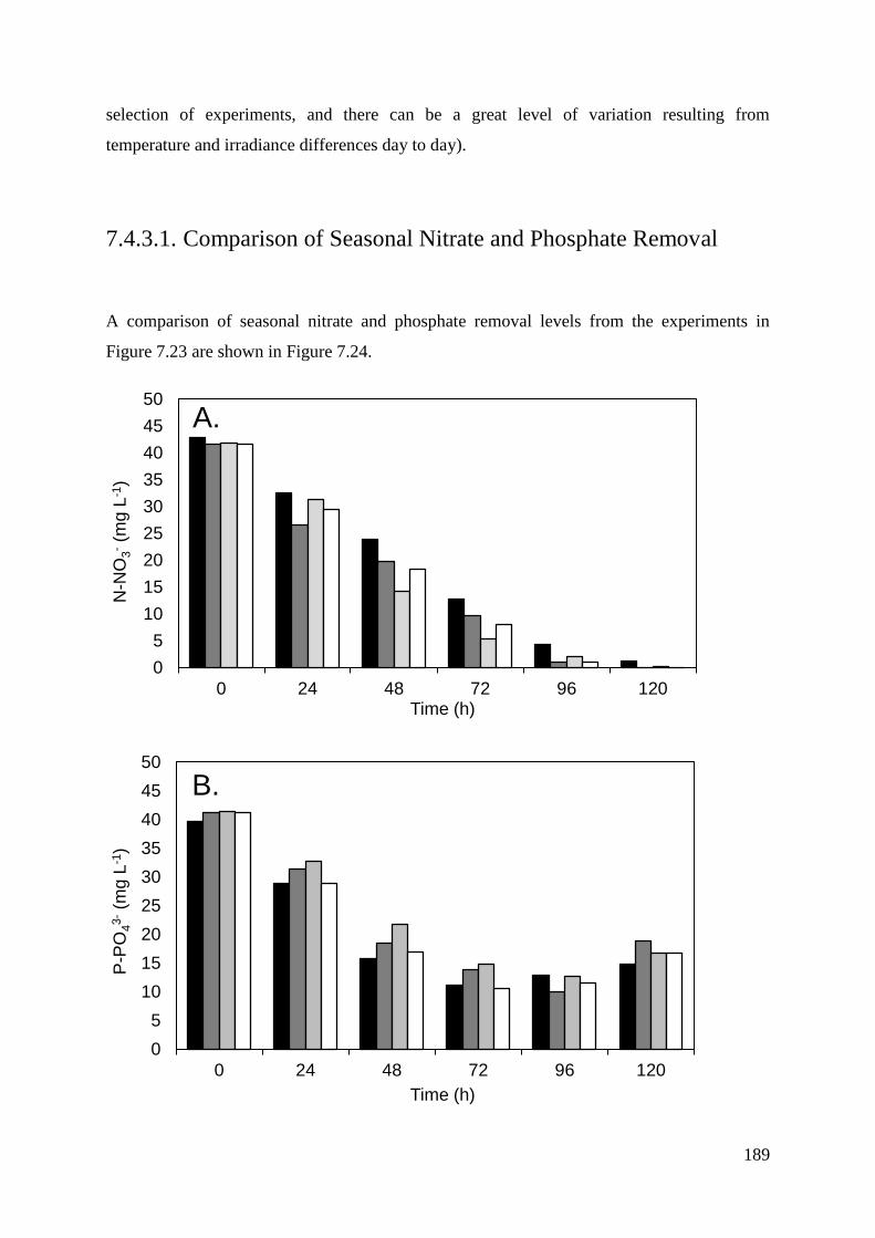
189

selection of experiments, and there can be a great level of variation resulting from

temperature and irradiance differences day to day).

7.4.3.1. Comparison of Seasonal Nitrate and Phosphate Removal

A comparison of seasonal nitrate and phosphate removal levels from the experiments in

Figure 7.23 are shown in Figure 7.24.

0

5

10

15

20

25

30

35

40

45

50

0 24 48 72 96 120

N-N

O3-(m

g L

-1)

Time (h)

0

5

10

15

20

25

30

35

40

45

50

0 24 48 72 96 120

P-P

O43-(m

g L

-1)

Time (h)

A.

B.

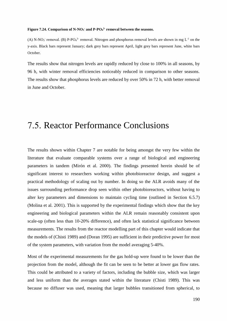
190

Figure 7.24. Comparison of N-NO3- and P-PO4

3- removal between the seasons.

(A) N-NO3- removal. (B) P-PO4

3- removal. Nitrogen and phosphorus removal levels are shown in mg L-1 on the

y-axis. Black bars represent January; dark grey bars represent April, light grey bars represent June, white bars

October.

The results show that nitrogen levels are rapidly reduced by close to 100% in all seasons, by

96 h, with winter removal efficiencies noticeably reduced in comparison to other seasons.

The results show that phosphorus levels are reduced by over 50% in 72 h, with better removal

in June and October.

Reactor Performance Conclusions

The results shown within Chapter 7 are notable for being amongst the very few within the

literature that evaluate comparable systems over a range of biological and engineering

parameters in tandem (Mirón et al. 2000). The findings presented herein should be of

significant interest to researchers working within photobioreactor design, and suggest a

practical methodology of scaling out by number. In doing so the ALR avoids many of the

issues surrounding performance drop seen within other photobioreactors, without having to

alter key parameters and dimensions to maintain cycling time (outlined in Section 6.5.7)

(Molina et al. 2001). This is supported by the experimental findings which show that the key

engineering and biological parameters within the ALR remain reasonably consistent upon

scale-up (often less than 10-20% difference), and often lack statistical significance between

measurements. The results from the reactor modelling part of this chapter would indicate that

the models of (Chisti 1989) and (Doran 1995) are sufficient in their predictive power for most

of the system parameters, with variation from the model averaging 5-40%.

Most of the experimental measurements for the gas hold-up were found to be lower than the

projection from the model, although the fit can be seen to be better at lower gas flow rates.

This could be attributed to a variety of factors, including the bubble size, which was larger

and less uniform than the averages stated within the literature (Chisti 1989). This was

because no diffuser was used, meaning that larger bubbles transitioned from spherical, to

191

elliptical and then cap shapes as they rose through the water column, particularly when they

coalesced at the higher gas flow rates (Chisti 1989, K. Koutita 2015). This larger bubble size

acts to increase the bubble rise velocity and thereby decreases the overall bubble residence

time, lowering gas hold-up. Looking specifically at each set of reactors, it can be seen that the

model fits the experimental data from the 5ALR system the best, which is most probably due

to its simpler ‘textbook’ geometry (one riser, one downcomer). The fit for gas hold-up in the

bubble columns is good up until 0.5 vvm, at which point the mixing could be observed to

transition from imperfect bubbly to churn turbulent and slug flow in the 2.5BC and 5BC

respectively (Deckwer 1992, Kantarci et al. 2005). The column mixed reactors perform

between the 2.5BC and 5 BC, deviating from the model in similar ways. These findings are

important in terms of subsequently predicting the effect that gas hold-up has on mass transfer

and liquid circulation velocity in airlift or column configurations. In this respect, the findings

would suggest that the BC and CM reactors should have higher mass transfer coefficients

than the ALR, which is attested by the experimental findings.

As expected the ALR configurations have superior linear liquid velocities when compared to

BC or CM configurations at equivalent gassing. Looking specifically at each set of reactors, it

can be seen again that the model fits the experimental data for the 5ALR system the best,

most probably due to its idealised geometry (Merchuk and Gluz 2002). Interestingly, the

measured liquid velocity was found to increase slightly in the ALR as the reactor was scaled-

out, indicating that the addition of columns actually increases this particular performance

characteristic. This effect could potentially be attributed to an increase in dispersion height,

decrease in gas hold-up within the downcomer or an effect on the reduction of the friction

loss coefficient. However, due to the absence of similar systems within the literature it is hard

to come to any concrete answer without further experimentation. The modelled fit for the

column reactors deviate more from the experimental data, most probably for reasons of

decreased gas hold-up at increased airflows. The experimental data shows that BC systems

with greater cross sectional pipe diameter match the model most closely, with the 5BC

having the best fit, followed by the 10CMALR, 5CMALR and 2.5BC. This could be

attributed to the empirical nature of Eq. 21, which does not factor the increased frictional

forces in smaller diameter tubes (Heijnen and Van't Riet 1984). As a result of these higher

liquid velocities the ALR systems display improved Reynolds numbers than the BC systems,

particularly those with thinner tube diameters. The higher liquid velocity shown by the ALR

mixed systems translates into faster circulation times; however the BC and CM systems show

192

similar mixing times to the ALR configurations, which can be explained by the radial mixing

characteristics displayed within column reactors (Deckwer 1992, Kantarci et al. 2005). The

maximal linear liquid velocity in ALR operation is comparable to that found within the

literature, with reports of 0.32 m s-1 in a helical photobioreactor (Hall et al. 2003) and 0.35 m

s-1 in a serpentine horizontal airlift, but lower than the 0.7-0.8 m s-1 reported in the manifold

BioFence™ system (McDonald 2013).

The measured gas-liquid mass transfer coefficients for O2 were considerably higher for

bubble-column reactors; this would also be the case for CO2 mass transfer, which can be

estimated by multiplying O2 mass transfer coefficients by a factor 0.91 (Contreras et al.

1998). The higher mass transfer coefficients found in the BC are in accordance with the

secondary and radial mixing patterns that are found within these systems, which act to

increase gas hold-up. These findings are supported within the literature, which report better

mass transfer coefficients within bubble column reactors than airlift systems (Chisti 1989,

Mirón et al. 2000). As mentioned in Section 7.2.2.4 the previous empirical expressions (Eq.

33 and 34) were not suitable for the ALR and BC systems, and the newer expressions (Eq. 50

and 51) displayed much better fit over the range of gas flow rates. This may be due to the

differences in cross sectional areas and ratios between the tested systems and those found

within the literature. For example, the airlift systems tested in this thesis have cross sectional

area ratios (𝑎𝑑

𝑎𝑟⁄ ) that are slightly larger than the ranges stipulated in (Bello et al. 1985).

This is because the ALR system has equal riser and downcomer cross sectional areas.

Likewise, the bubble column systems have cross sectional areas that are slightly smaller than

those stipulated in (Doran 1995). These findings are significant in so much as many tubular

systems suffer from low mass transfer co-efficients, with its importance as a design parameter

under considered both within industry and the literature (Rubio et al. 1999, Ugwu et al. 2008,

McDonald 2013). Overall, the mass transfer coefficients determined during this thesis were

found to be comparable to the literature, both in terms of the BC (Acién Fernández et al.

2001, Krishna and van Baten 2003) and ALR configurations (Loubière et al. 2009). Specific

examples from the literature show maximal mass transfer coefficients of 0.006 s-1 in a helical

airlift (although with a very high power input of 3200 W m-3) (Hall et al. 2003). Whilst

maximal values in flat panelled and airlift tubular reactors (riser column) were found to be as

high as 0.025 s-1 and 0.04 s-1 respectively (Sierra et al. 2008, Acién Fernández et al. 2001).

Interestingly, the findings of (Acién Fernández et al. 2001) also indicate the low levels of

193

mass transfer in a serpentine loop ~0.002 s-1 at superficial gas velocities equivalent to the

experiments within this thesis.

In terms of the biotic performance, it appears from these experiments that the BC

configurations have higher final yields compared to the CM and ALR configurations (up to

28%). Whilst in terms of productivity, both the CM and BC systems outperform the ALR by

between 17% and 26%. These findings conflict with those of (Kumar and Das 2012) that

indicate the growth profile of C. sorokiniana in airlift reactors is better than in bubble-column

reactors. However, as mixing, light path and mass transfer are all important parameters; it

appears that column mixed configurations offer some distinct process benefits in comparison

to ALR configurations. Reasons for this improvement could be due to better mixing and mass

transfer, whilst the radial mixing patterns of bubble columns could increase the frequency and

efficiency of light flashing periods (Camacho Rubio et al. 2004). In the case of the 2.5BC the

improved growth characteristics most probably derive from the short light path and high mass

transfer. Whilst for the 5BC system a greater Reynolds number coupled to high mass transfer

could be major contributing factors. Interestingly, the findings hint at a trade-off between the

light path and other volumetric parameters (e.g. the Reynolds number). This would suggest

that a bigger tubular diameter (up to 0.08) could be selected with minimal detriment to

volumetric productivity, whilst considerably increasing areal productivity. This performance

advantage is borne out by the yield on PAR, which is notably higher in the 5BC than the

other reactors (Table 7-3). Broader analysis of the productivity data under these lower light

conditions would suggest running any of the tested configurations at a density between 0.2-

0.6 g L-1, corresponding to the best daily productivities around 0.23-29 g L-1d-1 (between 24

and 48 h).

The results from the comparative ALR work show that the system is scalable with minimal

performance drop; as outlined by an overview of the parameters shown in Table 7-4, which

generally show performance differences of 5-10%. Likewise the yield on PAR was found to

be similar for each of the tested ALR systems, which was a good indication of consistent

performance despite scale-up. A maximal volumetric yield of 3.64 g L-1 and a daily

productivity of 0.83 g L-1 d-1 were found under high light conditions. These numbers compare

favourably with values from the literature. For example, findings within the review of

Griffiths et al suggest that C. sorokiniana is capable of daily productivities in the region of

0.55-1.1 g L-1 d-1 under similar lighting and temperature conditions (Griffiths and Harrison

2009, Matsukawa et al. 2000). Whilst the findings of Tanaka indicated maximal volumetric

194

yields of 1.5 g L-1 were possible, alongside daily productivities between 0.3-1.2 g L-1 d-1

within airlift reactors (Ugwu CU, Ogbonna J and H. 2002). The findings from the

comparative work also show that levels of dO2 build-up with increased biomass and

photosynthetic activity, but can be kept within acceptable limits (below 150%). This can be

attributed to the short run lengths before de-gassing, coupled to adequate mass transfer

coefficients. These figures compare well to the literature which show dO2 levels reaching

several times air saturation in conventional serpentine tubular systems, often between 300-

500% (Mirón et al. 1999, McDonald 2013, Kiser 2015).

The findings from the Darwin Greenhouse 50ALR pilot study would indicate a similar

biological performance to the less light intensive comparative batch experiments undertaken

in Section 7.3.7; albeit with some seasonal variations, and lower productivities in January. In

this respect nutrient removal was seen to be fairly consistent between the controlled batch and

pilot experiments, with the exception of a notable increase in phosphorus levels in the pilot

experimentation between 96-120 h. This is most probably caused by cell growth slowing

down during the beginning of stationary phase (around 96 h) and the commencement of

various degradation pathways thereafter. For example the beginning of cell death, with the

associated breakdown of cellular components can re-release phosphorus back into the

medium. Unfortunately insufficient experimental data was collected to confirm the

differences in daily and seasonal uptake rates. However, when compared to the ‘intensive’

lighting option outlined in Section 7.4.1 the pilot fell considerably short of what was possible

under higher powered artificial illumination, or better natural illumination. This means that

under lower light (or natural light conditions in the UK) the productivity of C. sorokiniana

within the ALR could be expected to average around 0.244 g L-1 d-1, whilst phosphorus

removal could be expected to be in the region of 0.51 mg L-1 h-1. Chapter 8 will use the

findings from the thesis thus far to construct a realistic cost model for the construction and

operation of an ALR system, using wastewater treatment in UK conditions as a specific case

study.

195

8. ALR Performance, Cost Comparison

and WWT Model

Aims and Objectives

The aim of Chapter 8 is to provide a greater understanding of the costs associated with the

manufacture and operation of an ALR system. This was undertaken at a unit level in

comparison to other photobioreactor systems and also with specific reference to deployment

within the UK as a tertiary wastewater treatment platform. The specific objectives were as

follows:

To benchmark the performance of the ALR in comparison to other photobioreactor

systems.

To provide a bill of materials; including the construction and deployment costs for an

ALR system; in terms of reactor footprint, productivity and volume. This process should

allow the commercial viability of the system to be ascertained, whilst targeting

components and processes for improvement.

To undertake a targeted sensitivity analysis to determine any areas for cost savings within

the manufacturing process.

To determine the feasibility of utilising the ALR alongside a membrane filter to undertake

tertiary treatment of wastewater with a particular focus on nitrogen and phosphorus

removal.

To compare the system to other biological treatment methods as well as to conventional

chemical approaches.

196

Modelling Methodology

System Construction and Comparison

8.2.1.1. Aims and Objectives

This work package intended to demonstrate how changes in construction materials and

operational strategies could affect the capital expenditure (CAPEX) and operational

expenditure (OPEX) of an ALR system. This included quantification of the operational costs,

as well as undertaking sensitivity analysis to assess the effect of changing different reactor

parameters; including configuration, spacing, construction materials, tube diameter and

length.

8.2.1.2. ALR Dimensions, Sizing and Areal Footprint

The original assumptions for characterising the ALR system were based on the reactor design

outlined in Section 6.6. In order to determine a more intensive spatial and volumetric

configuration, several assumptions were then made with regards to the ALR system. In

practice this involved the conversion of volumetric considerations into larger and more

industrially suitable areal footprints, which could be subsequently compared to literature

examples. All modelling within this chapter was undertaken using Excel 2010 (Microsoft),

and the assumptions and changes to the reactor geometry are detailed in Section 8.3.1.

8.2.1.3. Comparison of Mixing Requirements and Productivities

Energy projections for mixing requirements were based upon the manufacturer’s

specifications. The minimum mixing requirements within the ALR (W m-3) were calculated

197

directly using power ratings from lower powered 2W pumps (Hailea). This power rating was

able to provide an airflow rate of at least 0.2 vvm, and benchmarked as being well within the

turbulent range of reactor operation (~Re 4,000). From the design considerations and

validation experiments outlined in Chapters 6 and 7 all comparable ALR parameters were

considered to scale linearly unless otherwise stated. This includes the biomass productivity

and yield, which was considered to not be adversely affected by changes in the tubular

diameter within the ranges of 0.055-0.11 m (supported by discussion in Section 7.5). The

findings were then compared to prominent examples of different reactor configurations found

within the literature, which are described in Appendices 10.1.3.4 and 10.1.3.5.

8.2.1.4. Sensitivity Analysis

A bill of materials was created during the construction of the original ALR prototype, based

on the construction costs in Appendix 10.1.3.1. To reduce the costs associated with the

construction of the ALR, a variety of tubular photo-collecting materials were subsequently

assessed. This investigation was undertaken comparing tubes with diameters ranging from

0.055 m to 0.11 m. The materials selected for this analysis included acrylic (PMMA), both

cast and extruded (~92% transmission); transparent polyvinyl chloride (PVC), which is

capable of reasonable levels of light transmission (~70%), whilst being relatively cheap and

chemically inert. Another chosen material was polycarbonate, which was selected for

favourable properties, including being half the weight of normal glass, as well as having high

clarity (~90%), temperature resistance and impact strength. PETG was also selected due to its

transparency (~90%), inertness and favourable cost profile. Finally, glass tubing was also

selected due to its favourable transmission properties (~91%) and lifecycle (Tunnicliffe

1968). For the analysis all materials were assumed to have negligible differences in light

transmission.

198

Phosphorus Removal with the ALR

8.2.2.1. Aims and Objectives

As has been outlined in Chapter 5 it has become increasingly important to reduce the levels

of phosphorus within tertiary wastewater. One potential solution is to use the ALR coupled to

a membrane belt filter in a wastewater treatment role (Robinson et al. 2012, ClearAs 2013).

8.2.2.2. Sizing the Treatment Process

The wastewater facility modelled in this study was sized using a rationale based on UK

government population statistics and is described with the relevant references in Table 8-8.

This sizing assumption forms the basis upon which the equipment and energy calculations are

based. The model assumes all of the final effluent from the secondary treatment process

passes through the ALR in a continuous flow, and is nutritionally sufficient for the

production of C. sorokiniana. The photobioreactor would have to be operated in a steady

state for 24 hours a day, 365 days a year. After tertiary treatment within the ALR, the

wastewater and algal biomass are separated with a membrane belt filter, and the treated water

is subsequently discharged into a receiving waterway. The biomass from the process is then

either dried by a rotary drying machine or recirculated within the ALR to maintain the

biomass concentration and nutrient uptake rate. In combination, the belt filter and the ALR

are described as being part of an ‘ALUP’ (algal uptake) process, detailed in Figure 8.1, and

based on the system used by ClearAs (USA). The treatment level is based on bringing the

emission standards within the case study plant in line with the most stringent of current EU

emission legislation (from a p.e. of 10,000 to a p.e. of 100,000). In practice, this entails a

reduction of phosphorous within the final effluent from 2mg/L to 1mg/L, and of nitrogen

from 15mg/L to 10mg/L (CEEP 2007, DEFRA 2012).

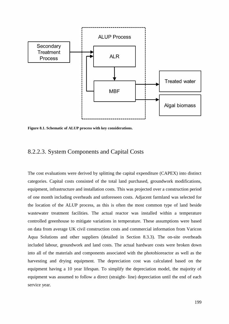
199

Figure 8.1. Schematic of ALUP process with key considerations.

8.2.2.3. System Components and Capital Costs

The cost evaluations were derived by splitting the capital expenditure (CAPEX) into distinct

categories. Capital costs consisted of the total land purchased, groundwork modifications,

equipment, infrastructure and installation costs. This was projected over a construction period

of one month including overheads and unforeseen costs. Adjacent farmland was selected for

the location of the ALUP process, as this is often the most common type of land beside

wastewater treatment facilities. The actual reactor was installed within a temperature

controlled greenhouse to mitigate variations in temperature. These assumptions were based

on data from average UK civil construction costs and commercial information from Varicon

Aqua Solutions and other suppliers (detailed in Section 8.3.3). The on-site overheads

included labour, groundwork and land costs. The actual hardware costs were broken down

into all of the materials and components associated with the photobioreactor as well as the

harvesting and drying equipment. The depreciation cost was calculated based on the

equipment having a 10 year lifespan. To simplify the depreciation model, the majority of

equipment was assumed to follow a direct (straight- line) depreciation until the end of each

service year.

200

8.2.2.4. Annual and Recurrent Costs

Operational and maintenance costs (OPEX) were calculated based upon the ALUP treatment

plant having a lifespan of 10 years (McDonald 2013). The maintenance and cleaning costs

consider a sodium hypochlorite sterilization process and minor repair fees during the

lifecycle. The plant operational costs were categorised into consumable costs, recurrent costs

like energy consumption and other annualised costs such as insurance. The energy costs are

based on summating the relevant equipment ratings and scaling-up from the optimised areal

footprint. The temperature control costs assume an average temperature of 20°C within a

heated greenhouse, with a requirement within the reactor of 35±5oC (de-Bashan et al. 2008).

Carbon dioxide requirements were estimated as being twice the levels of the algal

productivity rate in mass terms (kg/kg) according to well-known stoichiometric principles

(Sayre 2010).

8.2.2.5. Biomass Productivity and Valorisation

As a by-product of the treatment process the algal biomass that was produced was valorised,

with the assumption that C. sorokiniana grown under these conditions with natural irradiance

would have a market price of £6/kg (Shaanxi Jintai Biological Engineering Co). This would

make it suitable for re-sale as a feedstock in an array of low to medium value products.

8.2.2.6. Other Tertiary Treatment Platforms

The costs of operation for competing tertiary wastewater treatment systems were calculated

from the relevant literature sources. This included an open pond with membrane belt filter, a

reed bed, an algal membrane bioreactor, an algal turf scrubber and conventional chemical

precipitation. Detailed descriptions of each system can be found in Appendix 10.1.3.4. The

measured considerations included; the areal footprint, the total cost of deployment by

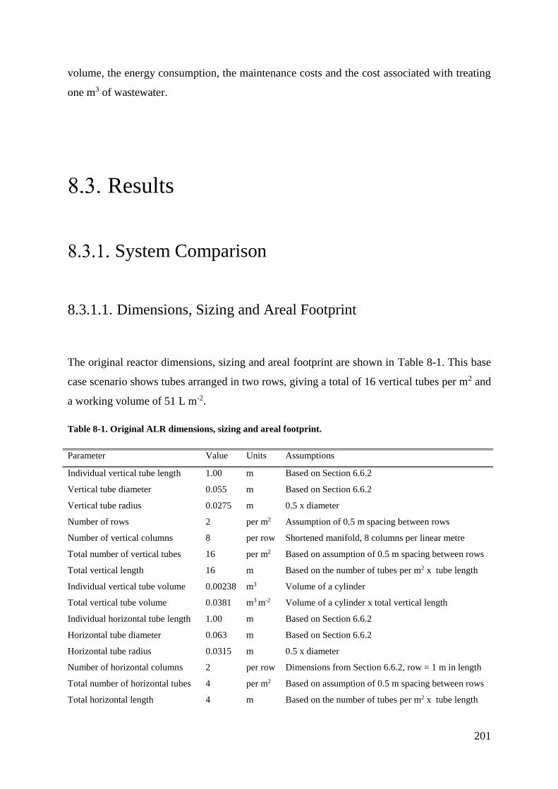
201

volume, the energy consumption, the maintenance costs and the cost associated with treating

one m3 of wastewater.

Results

System Comparison

8.3.1.1. Dimensions, Sizing and Areal Footprint

The original reactor dimensions, sizing and areal footprint are shown in Table 8-1. This base

case scenario shows tubes arranged in two rows, giving a total of 16 vertical tubes per m2 and

a working volume of 51 L m-2.

Table 8-1. Original ALR dimensions, sizing and areal footprint.

Parameter Value Units Assumptions

Individual vertical tube length 1.00 m Based on Section 6.6.2

Vertical tube diameter 0.055 m Based on Section 6.6.2

Vertical tube radius 0.0275 m 0.5 x diameter

Number of rows 2 per m2 Assumption of 0.5 m spacing between rows

Number of vertical columns 8 per row Shortened manifold, 8 columns per linear metre

Total number of vertical tubes 16 per m2 Based on assumption of 0.5 m spacing between rows

Total vertical length 16 m Based on the number of tubes per m2 x tube length

Individual vertical tube volume 0.00238 m3 Volume of a cylinder

Total vertical tube volume 0.0381 m3 m-2 Volume of a cylinder x total vertical length

Individual horizontal tube length 1.00 m Based on Section 6.6.2

Horizontal tube diameter 0.063 m Based on Section 6.6.2

Horizontal tube radius 0.0315 m 0.5 x diameter

Number of horizontal columns 2 per row Dimensions from Section 6.6.2, row = 1 m in length

Total number of horizontal tubes 4 per m2 Based on assumption of 0.5 m spacing between rows

Total horizontal length 4 m Based on the number of tubes per m2 x tube length

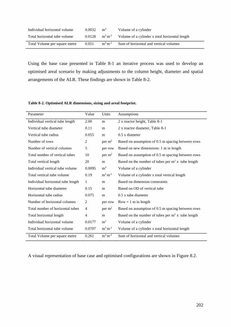
202

Individual horizontal volume 0.0032 m3 Volume of a cylinder

Total horizontal tube volume 0.0128 m3 m-2 Volume of a cylinder x total horizontal length

Total Volume per square metre 0.051 m3 m-2 Sum of horizontal and vertical volumes

Using the base case presented in Table 8-1 an iterative process was used to develop an

optimised areal scenario by making adjustments to the column height, diameter and spatial

arrangements of the ALR. These findings are shown in Table 8-2.

Table 8-2. Optimised ALR dimensions, sizing and areal footprint.

Parameter Value Units Assumptions

Individual vertical tube length 2.00 m 2 x reactor height, Table 8-1

Vertical tube diameter 0.11 m 2 x reactor diameter, Table 8-1

Vertical tube radius 0.055 m 0.5 x diameter

Number of rows 2 per m2 Based on assumption of 0.5 m spacing between rows

Number of vertical columns 5 per row Based on new dimensions: 1 m in length

Total number of vertical tubes 10 per m2 Based on assumption of 0.5 m spacing between rows

Total vertical length 20 m Based on the number of tubes per m2 x tube length

Individual vertical tube volume 0.0095 m3 Volume of a cylinder

Total vertical tube volume 0.19 m3 m-2 Volume of a cylinder x total vertical length

Individual horizontal tube length 1 m Based on dimension constraints

Horizontal tube diameter 0.15 m Based on OD of vertical tube

Horizontal tube radius 0.075 m 0.5 x tube diameter

Number of horizontal columns 2 per row Row = 1 m in length

Total number of horizontal tubes 4 per m2 Based on assumption of 0.5 m spacing between rows

Total horizontal length 4 m Based on the number of tubes per m2 x tube length

Individual horizontal volume 0.0177 m3 Volume of a cylinder

Total horizontal tube volume 0.0707 m3 m-2 Volume of a cylinder x total horizontal length

Total Volume per square metre 0.261 m3 m-2 Sum of horizontal and vertical volumes

A visual representation of base case and optimised configurations are shown in Figure 8.2.

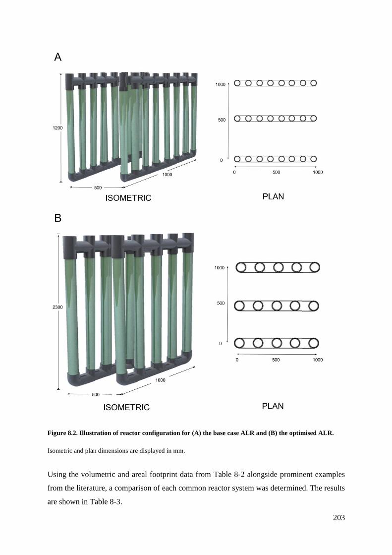
203

Figure 8.2. Illustration of reactor configuration for (A) the base case ALR and (B) the optimised ALR.

Isometric and plan dimensions are displayed in mm.

Using the volumetric and areal footprint data from Table 8-2 alongside prominent examples

from the literature, a comparison of each common reactor system was determined. The results

are shown in Table 8-3.

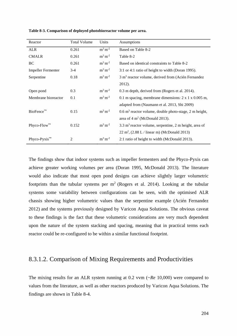
204

Table 8-3. Comparison of deployed photobioreactor volume per area.

Reactor Total Volume Units Assumptions

ALR 0.261 m3 m-2 Based on Table 8-2

CMALR 0.261 m3 m-2 Table 8-2

BC 0.261 m3 m-2 Based on identical constraints to Table 8-2

Impeller Fermenter 3-4 m3 m-2 3:1 or 4:1 ratio of height to width (Doran 1995).

Serpentine 0.18 m3 m-2 3 m3 reactor volume, derived from (Acién Fernandez

2012).

Open pond 0.3 m3 m-2 0.3 m depth, derived from (Rogers et al. 2014).

Membrane bioreactor 0.1 m3 m-2 0.1 m spacing, membrane dimensions: 2 x 1 x 0.005 m,

adapted from (Naumann et al. 2013, Shi 2009)

BioFence™ 0.15 m3 m-2 0.6 m3 reactor volume, double photo-stage, 2 m height,

area of 4 m2 (McDonald 2013).

Phyco-Flow™ 0.152 m3 m-2 3.3 m3 reactor volume, serpentine, 2 m height, area of

22 m2, (2.88 L / linear m) (McDonald 2013)

Phyco-Pyxis™ 2 m3 m-2 2:1 ratio of height to width (McDonald 2013).

The findings show that indoor systems such as impeller fermenters and the Phyco-Pyxis can

achieve greater working volumes per area (Doran 1995, McDonald 2013). The literature

would also indicate that most open pond designs can achieve slightly larger volumetric

footprints than the tubular systems per m2 (Rogers et al. 2014). Looking at the tubular

systems some variability between configurations can be seen, with the optimised ALR

chassis showing higher volumetric values than the serpentine example (Acién Fernandez

2012) and the systems previously designed by Varicon Aqua Solutions. The obvious caveat

to these findings is the fact that these volumetric considerations are very much dependent

upon the nature of the system stacking and spacing, meaning that in practical terms each

reactor could be re-configured to be within a similar functional footprint.

8.3.1.2. Comparison of Mixing Requirements and Productivities

The mixing results for an ALR system running at 0.2 vvm (~Re 10,000) were compared to

values from the literature, as well as other reactors produced by Varicon Aqua Solutions. The

findings are shown in Table 8-4.

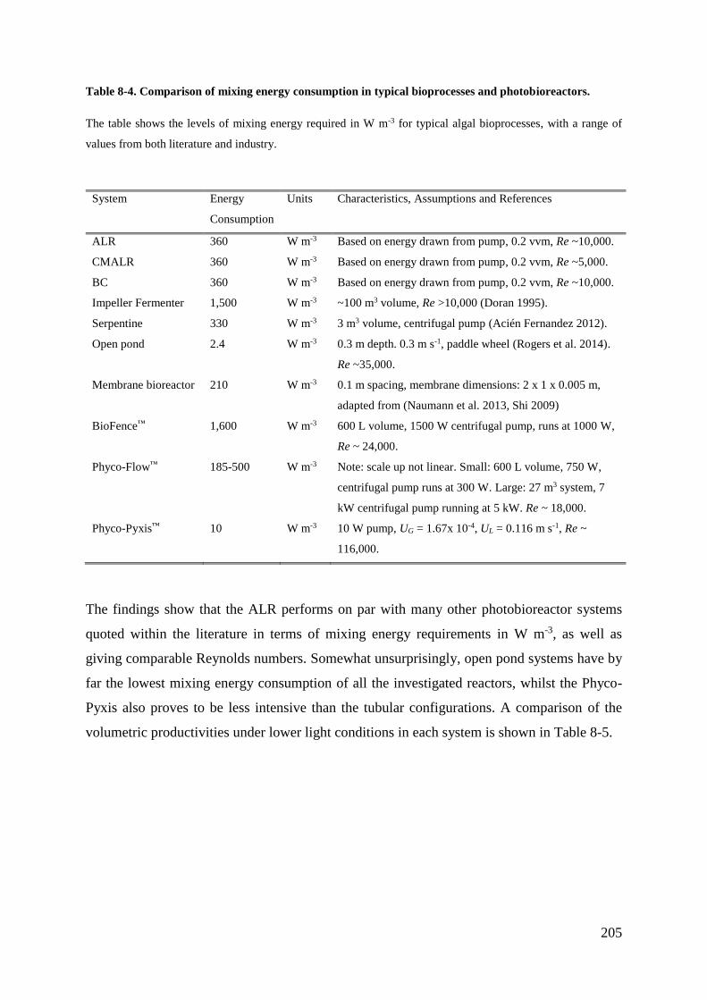
205

Table 8-4. Comparison of mixing energy consumption in typical bioprocesses and photobioreactors.

The table shows the levels of mixing energy required in W m-3 for typical algal bioprocesses, with a range of

values from both literature and industry.

System Energy

Consumption

Units Characteristics, Assumptions and References

ALR 360 W m-3 Based on energy drawn from pump, 0.2 vvm, Re ~10,000.

CMALR 360 W m-3 Based on energy drawn from pump, 0.2 vvm, Re ~5,000.

BC 360 W m-3 Based on energy drawn from pump, 0.2 vvm, Re ~10,000.

Impeller Fermenter 1,500 W m-3 ~100 m3 volume, Re >10,000 (Doran 1995).

Serpentine 330 W m-3 3 m3 volume, centrifugal pump (Acién Fernandez 2012).

Open pond 2.4 W m-3 0.3 m depth. 0.3 m s-1, paddle wheel (Rogers et al. 2014).

Re ~35,000.

Membrane bioreactor 210 W m-3 0.1 m spacing, membrane dimensions: 2 x 1 x 0.005 m,

adapted from (Naumann et al. 2013, Shi 2009)

BioFence™ 1,600 W m-3 600 L volume, 1500 W centrifugal pump, runs at 1000 W,

Re ~ 24,000.

Phyco-Flow™ 185-500 W m-3 Note: scale up not linear. Small: 600 L volume, 750 W,

centrifugal pump runs at 300 W. Large: 27 m3 system, 7

kW centrifugal pump running at 5 kW. Re ~ 18,000.

Phyco-Pyxis™ 10 W m-3 10 W pump, UG = 1.67x 10-4, UL = 0.116 m s-1, Re ~

116,000.

The findings show that the ALR performs on par with many other photobioreactor systems

quoted within the literature in terms of mixing energy requirements in W m-3, as well as

giving comparable Reynolds numbers. Somewhat unsurprisingly, open pond systems have by

far the lowest mixing energy consumption of all the investigated reactors, whilst the Phyco-

Pyxis also proves to be less intensive than the tubular configurations. A comparison of the

volumetric productivities under lower light conditions in each system is shown in Table 8-5.

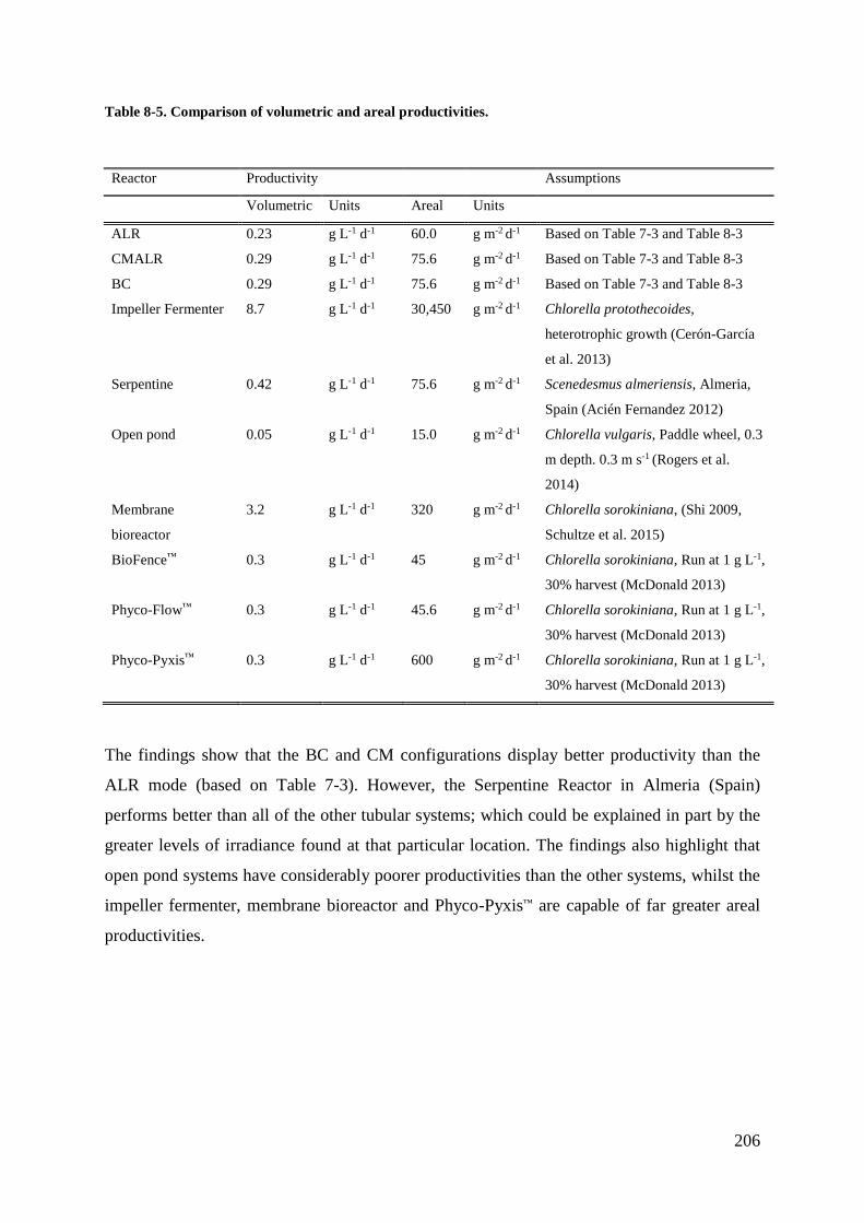
206

Table 8-5. Comparison of volumetric and areal productivities.

Reactor Productivity Assumptions

Volumetric Units Areal Units

ALR 0.23 g L-1 d-1 60.0 g m-2 d-1 Based on Table 7-3 and Table 8-3

CMALR 0.29 g L-1 d-1 75.6 g m-2 d-1 Based on Table 7-3 and Table 8-3

BC 0.29 g L-1 d-1 75.6 g m-2 d-1 Based on Table 7-3 and Table 8-3

Impeller Fermenter 8.7 g L-1 d-1 30,450 g m-2 d-1 Chlorella protothecoides,

heterotrophic growth (Cerón-García

et al. 2013)

Serpentine 0.42 g L-1 d-1 75.6 g m-2 d-1 Scenedesmus almeriensis, Almeria,

Spain (Acién Fernandez 2012)

Open pond 0.05 g L-1 d-1 15.0 g m-2 d-1 Chlorella vulgaris, Paddle wheel, 0.3

m depth. 0.3 m s-1 (Rogers et al.

2014)

Membrane

bioreactor

3.2 g L-1 d-1 320 g m-2 d-1 Chlorella sorokiniana, (Shi 2009,

Schultze et al. 2015)

BioFence™ 0.3 g L-1 d-1 45 g m-2 d-1 Chlorella sorokiniana, Run at 1 g L-1,

30% harvest (McDonald 2013)

Phyco-Flow™ 0.3 g L-1 d-1 45.6 g m-2 d-1 Chlorella sorokiniana, Run at 1 g L-1,

30% harvest (McDonald 2013)

Phyco-Pyxis™ 0.3 g L-1 d-1 600 g m-2 d-1 Chlorella sorokiniana, Run at 1 g L-1,

30% harvest (McDonald 2013)

The findings show that the BC and CM configurations display better productivity than the

ALR mode (based on Table 7-3). However, the Serpentine Reactor in Almeria (Spain)

performs better than all of the other tubular systems; which could be explained in part by the

greater levels of irradiance found at that particular location. The findings also highlight that

open pond systems have considerably poorer productivities than the other systems, whilst the

impeller fermenter, membrane bioreactor and Phyco-Pyxis™ are capable of far greater areal

productivities.

207

ALR Construction Costs

8.3.2.1. Sensitivity Analysis: Construction Material of Solar

Collecting Tubes

Sensitivity analysis would suggest that the construction materials of the photobioreactor have

a disproportionately large cost on the overall CAPEX. This is particularly the case for the

photo-collecting tubes within the system. Table 8-6 shows the results of an investigation into

the effect of altering the materials used for the transparent sections of the photobioreactor.

The finalised results are expressed as a cost per linear metre of tube.

Table 8-6. Cost comparison of different tubular materials.

Materials Cost (£/m) Assumptions

Ø 0.055 Ø 0.11

Acrylic tube (cast) 28.26 50.38 Date: 17/04/15 (http://www.plastock.co.uk/)

Acrylic tube (extruded) 8.36 18.11 Date: 17/04/15 (http://www.plastock.co.uk/)

PETG tube 18.31 30.21 Date: 17/04/15 (http://www.McMaster.com)

Polycarbonate tube 12.55 34.67 Date: 17/04/15 (http://www.plastock.co.uk/)

Transparent PVC tube 21.92 53.68 Date: 17/04/15 (http://www.McMaster.com)

Glass tube 23.6 79.04 Date: 17/04/15 (http://www.glass-solutions.com)

The findings in Table 8-6 show that the reactor tubing material can have considerable impact

upon the costs associated with the photo-collecting region of the ALR. Cast acrylic had been

previously selected for use during the construction of the prototype due to favourable

characteristics and a body of literature supporting its use (Molina et al. 2001, Tredici 2004).

However, its costs are 3.0-3.4 times higher than its extruded counterpart. In fact, the extruded

acrylic tube was by far the cheapest material investigated, offering a clear improvement to the

overall cost profile of the photobioreactor, and was used for all subsequent calculations.

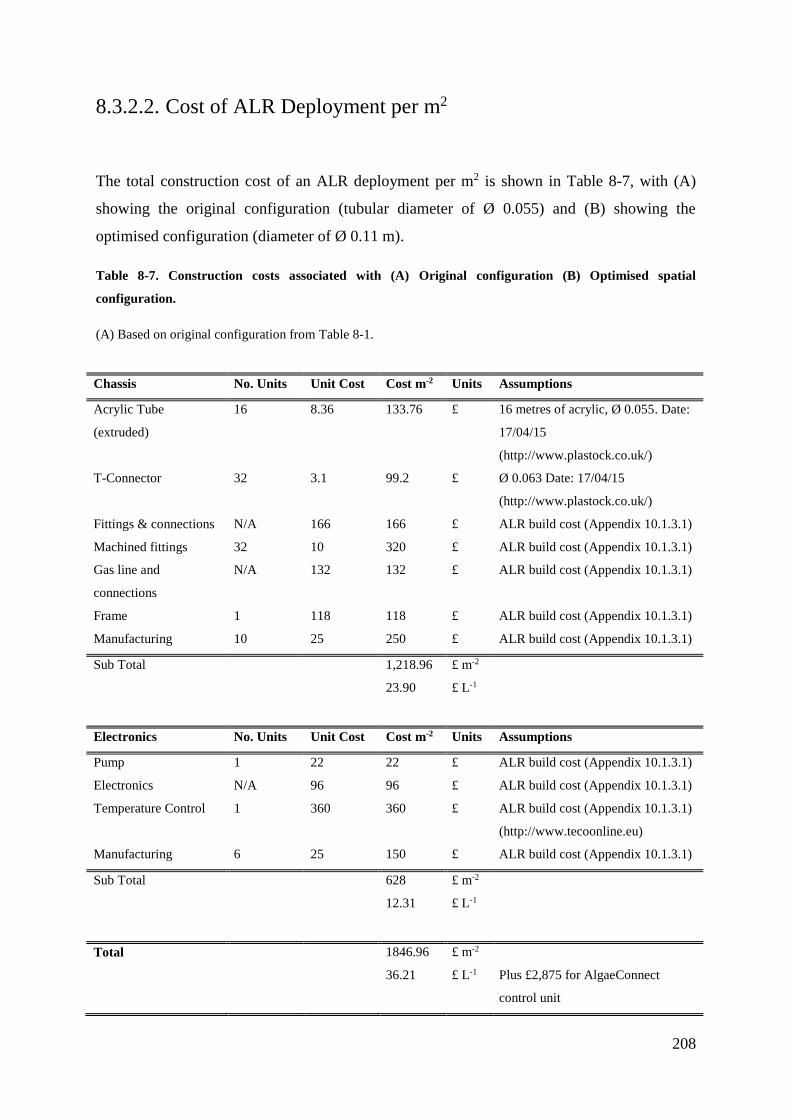
208

8.3.2.2. Cost of ALR Deployment per m2

The total construction cost of an ALR deployment per m2 is shown in Table 8-7, with (A)

showing the original configuration (tubular diameter of Ø 0.055) and (B) showing the

optimised configuration (diameter of Ø 0.11 m).

Table 8-7. Construction costs associated with (A) Original configuration (B) Optimised spatial

configuration.

(A) Based on original configuration from Table 8-1.

Chassis No. Units Unit Cost Cost m-2 Units Assumptions

Acrylic Tube

(extruded)

16 8.36 133.76 £ 16 metres of acrylic, Ø 0.055. Date:

17/04/15

(http://www.plastock.co.uk/)

T-Connector 32 3.1 99.2 £ Ø 0.063 Date: 17/04/15

(http://www.plastock.co.uk/)

Fittings & connections N/A 166 166 £ ALR build cost (Appendix 10.1.3.1)

Machined fittings 32 10 320 £ ALR build cost (Appendix 10.1.3.1)

Gas line and

connections

N/A 132 132 £ ALR build cost (Appendix 10.1.3.1)

Frame 1 118 118 £ ALR build cost (Appendix 10.1.3.1)

Manufacturing 10 25 250 £ ALR build cost (Appendix 10.1.3.1)

Sub Total 1,218.96 £ m-2

23.90 £ L-1

Electronics No. Units Unit Cost Cost m-2 Units Assumptions

Pump 1 22 22 £ ALR build cost (Appendix 10.1.3.1)

Electronics N/A 96 96 £ ALR build cost (Appendix 10.1.3.1)

Temperature Control 1 360 360 £ ALR build cost (Appendix 10.1.3.1)

(http://www.tecoonline.eu)

Manufacturing 6 25 150 £ ALR build cost (Appendix 10.1.3.1)

Sub Total 628 £ m-2

12.31 £ L-1

Total 1846.96 £ m-2

36.21 £ L-1 Plus £2,875 for AlgaeConnect

control unit

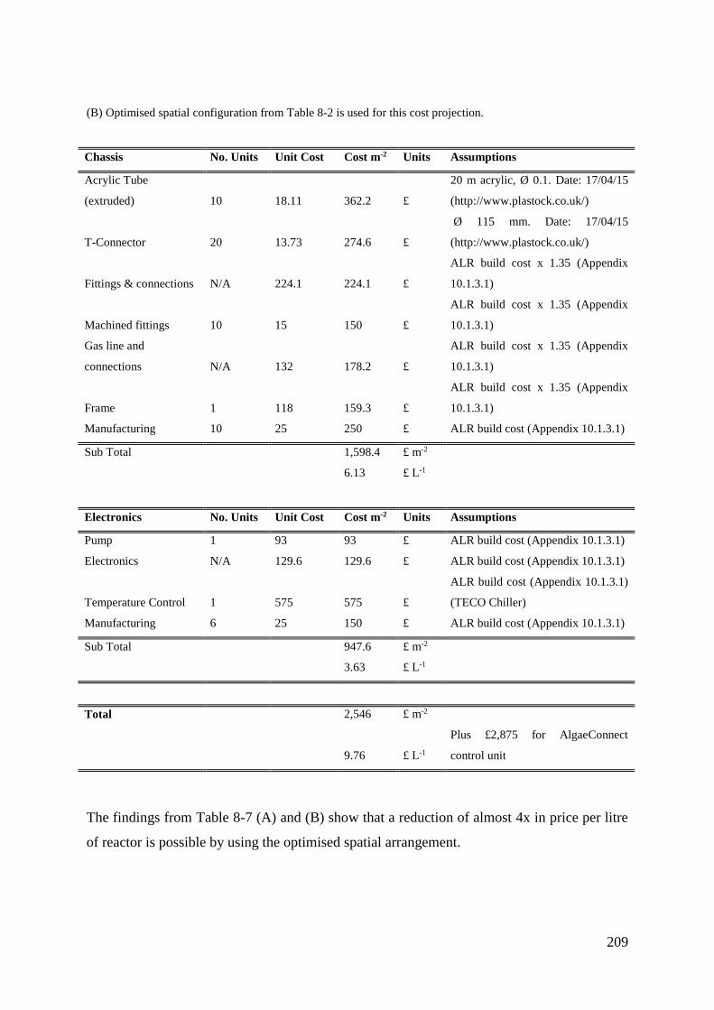
209

(B) Optimised spatial configuration from Table 8-2 is used for this cost projection.

Chassis No. Units Unit Cost Cost m-2 Units Assumptions

Acrylic Tube

(extruded) 10 18.11 362.2 £

20 m acrylic, Ø 0.1. Date: 17/04/15

(http://www.plastock.co.uk/)

T-Connector 20 13.73 274.6 £

Ø 115 mm. Date: 17/04/15

(http://www.plastock.co.uk/)

Fittings & connections N/A 224.1 224.1 £

ALR build cost x 1.35 (Appendix

10.1.3.1)

Machined fittings 10 15 150 £

ALR build cost x 1.35 (Appendix

10.1.3.1)

Gas line and

connections N/A 132 178.2 £

ALR build cost x 1.35 (Appendix

10.1.3.1)

Frame 1 118 159.3 £

ALR build cost x 1.35 (Appendix

10.1.3.1)

Manufacturing 10 25 250 £ ALR build cost (Appendix 10.1.3.1)

Sub Total

1,598.4 £ m-2

6.13 £ L-1

Electronics No. Units Unit Cost Cost m-2 Units Assumptions

Pump 1 93 93 £ ALR build cost (Appendix 10.1.3.1)

Electronics N/A 129.6 129.6 £ ALR build cost (Appendix 10.1.3.1)

Temperature Control 1 575 575 £

ALR build cost (Appendix 10.1.3.1)

(TECO Chiller)

Manufacturing 6 25 150 £ ALR build cost (Appendix 10.1.3.1)

Sub Total

947.6 £ m-2

3.63 £ L-1

Total

2,546 £ m-2

9.76 £ L-1

Plus £2,875 for AlgaeConnect

control unit

The findings from Table 8-7 (A) and (B) show that a reduction of almost 4x in price per litre

of reactor is possible by using the optimised spatial arrangement.

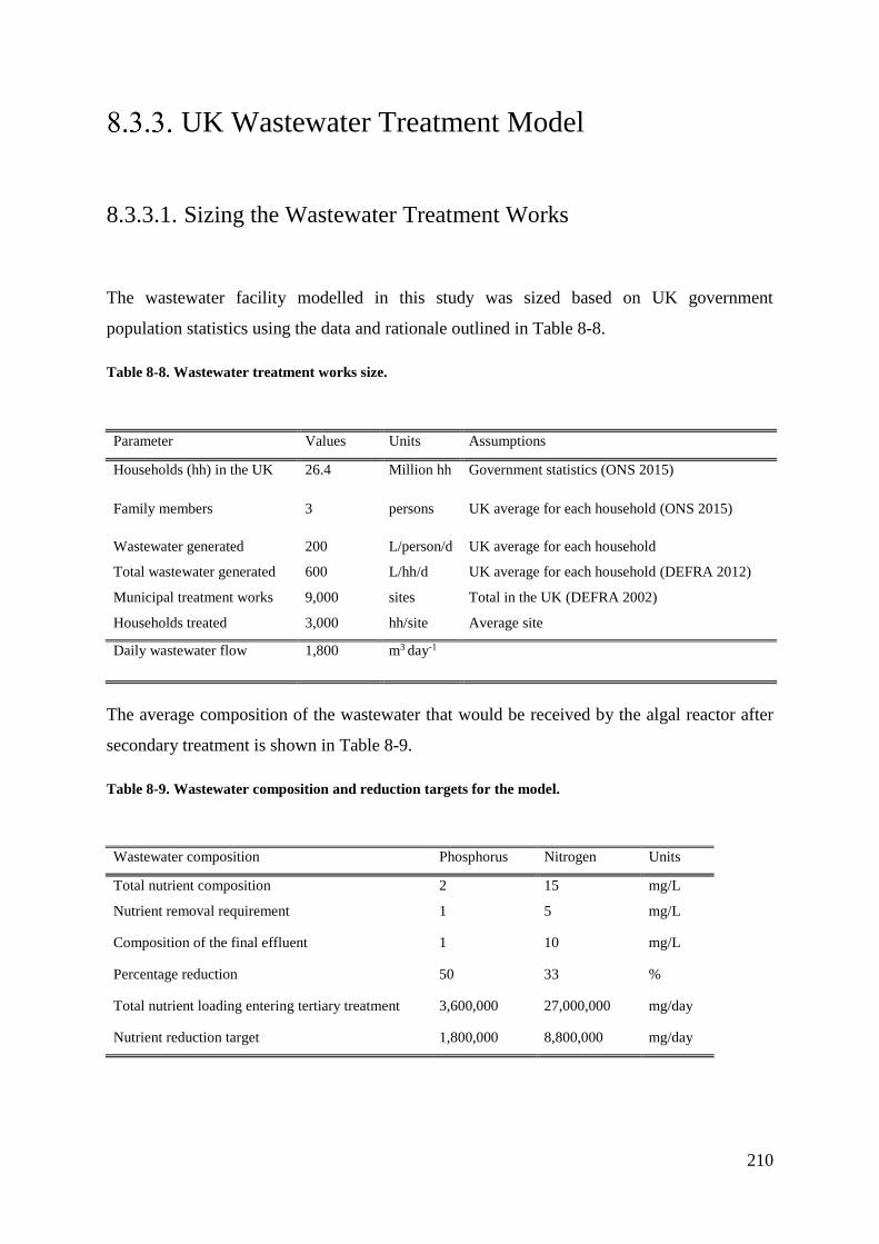
210

UK Wastewater Treatment Model

8.3.3.1. Sizing the Wastewater Treatment Works

The wastewater facility modelled in this study was sized based on UK government

population statistics using the data and rationale outlined in Table 8-8.

Table 8-8. Wastewater treatment works size.

Parameter Values Units Assumptions

Households (hh) in the UK 26.4 Million hh Government statistics (ONS 2015)

Family members 3 persons UK average for each household (ONS 2015)

Wastewater generated 200 L/person/d UK average for each household

Total wastewater generated 600 L/hh/d UK average for each household (DEFRA 2012)

Municipal treatment works 9,000 sites Total in the UK (DEFRA 2002)

Households treated 3,000 hh/site Average site

Daily wastewater flow 1,800 m3 day-1

The average composition of the wastewater that would be received by the algal reactor after

secondary treatment is shown in Table 8-9.

Table 8-9. Wastewater composition and reduction targets for the model.

Wastewater composition Phosphorus Nitrogen Units

Total nutrient composition 2 15 mg/L

Nutrient removal requirement 1 5 mg/L

Composition of the final effluent 1 10 mg/L

Percentage reduction 50 33 %

Total nutrient loading entering tertiary treatment 3,600,000 27,000,000 mg/day

Nutrient reduction target 1,800,000 8,800,000 mg/day

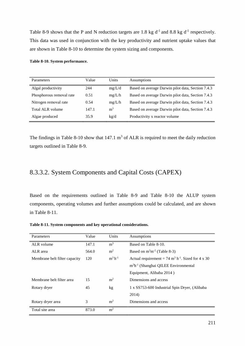
211

Table 8-9 shows that the P and N reduction targets are 1.8 kg d-1 and 8.8 kg d-1 respectively.

This data was used in conjunction with the key productivity and nutrient uptake values that

are shown in Table 8-10 to determine the system sizing and components.

Table 8-10. System performance.

Parameters Value Units Assumptions

Algal productivity 244 mg/L/d Based on average Darwin pilot data, Section 7.4.3

Phosphorous removal rate 0.51 mg/L/h Based on average Darwin pilot data, Section 7.4.3

Nitrogen removal rate 0.54 mg/L/h Based on average Darwin pilot data, Section 7.4.3

Total ALR volume 147.1 m3 Based on average Darwin pilot data, Section 7.4.3

Algae produced 35.9 kg/d Productivity x reactor volume

The findings in Table 8-10 show that 147.1 m3 of ALR is required to meet the daily reduction

targets outlined in Table 8-9.

8.3.3.2. System Components and Capital Costs (CAPEX)

Based on the requirements outlined in Table 8-9 and Table 8-10 the ALUP system

components, operating volumes and further assumptions could be calculated, and are shown

in Table 8-11.

Table 8-11. System components and key operational considerations.

Parameters Value Units Assumptions

ALR volume 147.1 m3 Based on Table 8-10.

ALR area 564.0 m2 Based on m3m-2 (Table 8-3)

Membrane belt filter capacity 120 m3 h-1 Actual requirement = 74 m3 h-1. Sized for 4 x 30

m3h-1 (Shanghai QILEE Environmental

Equipment, Alibaba 2014 )

Membrane belt filter area 15 m2 Dimensions and access

Rotary dryer 45 kg 1 x SS753-600 Industrial Spin Dryer, (Alibaba

2014)

Rotary dryer area 3 m2 Dimensions and access

Total site area 873.0 m2

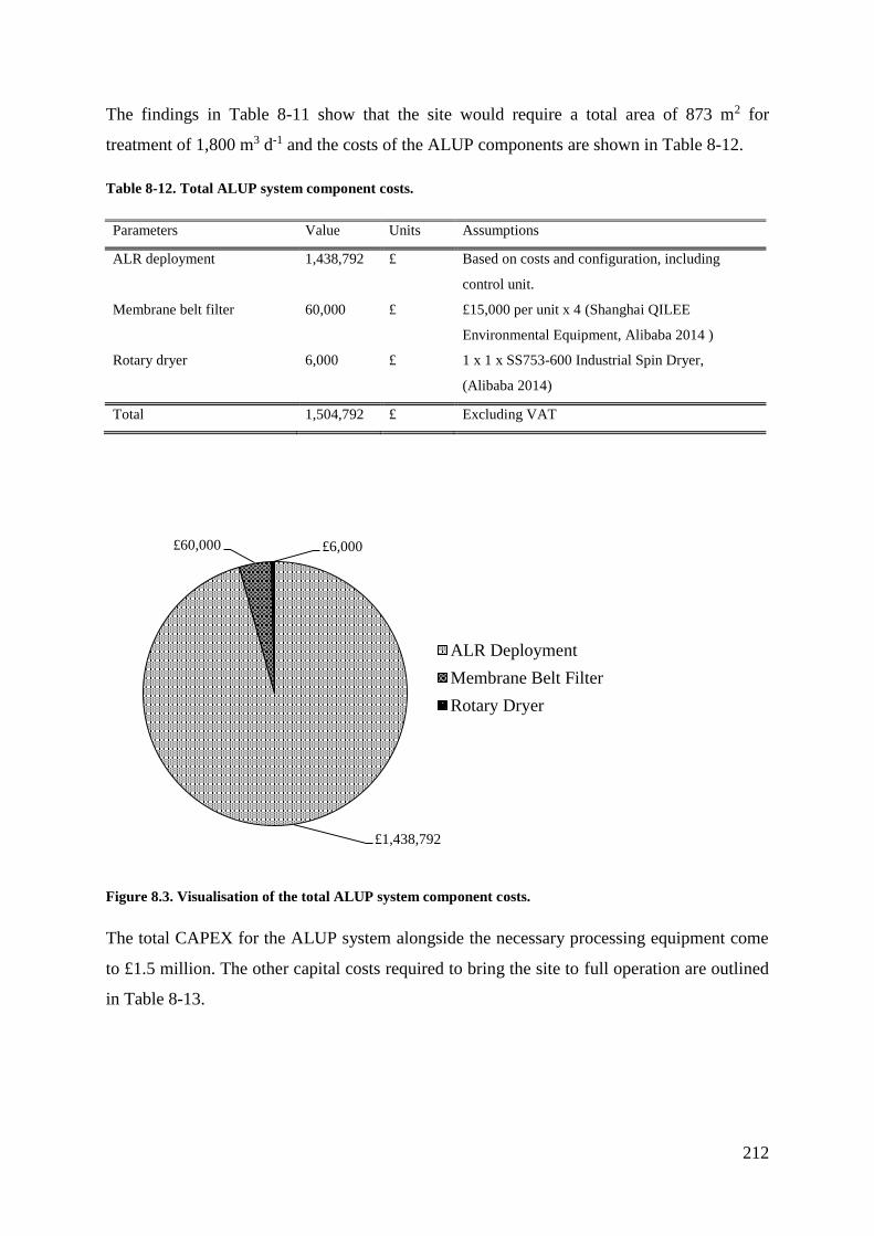
212

The findings in Table 8-11 show that the site would require a total area of 873 m2 for

treatment of 1,800 m3 d-1 and the costs of the ALUP components are shown in Table 8-12.

Table 8-12. Total ALUP system component costs.

Parameters Value Units Assumptions

ALR deployment 1,438,792 £ Based on costs and configuration, including

control unit.

Membrane belt filter 60,000 £ £15,000 per unit x 4 (Shanghai QILEE

Environmental Equipment, Alibaba 2014 )

Rotary dryer 6,000 £ 1 x 1 x SS753-600 Industrial Spin Dryer,

(Alibaba 2014)

Total 1,504,792 £ Excluding VAT

Figure 8.3. Visualisation of the total ALUP system component costs.

The total CAPEX for the ALUP system alongside the necessary processing equipment come

to £1.5 million. The other capital costs required to bring the site to full operation are outlined

in Table 8-13.

£1,438,792

£60,000 £6,000

ALR Deployment

Membrane Belt Filter

Rotary Dryer

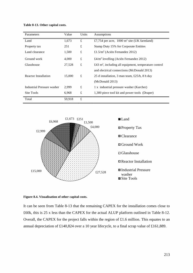
213

Table 8-13. Other capital costs.

Parameters Value Units Assumptions

Land 1,673 £ £7,754 per acre, 1000 m2 site (UK farmland)

Property tax 251 £ Stamp Duty 15% for Corporate Entities

Land clearance 1,500 £ £1.5/m2 (Acién Fernandez 2012)

Ground work 4,000 £ £4/m2 levelling (Acién Fernandez 2012)

Glasshouse 27,528 £ £43 m2, including all equipment, temperature control

and electrical connections (McDonald 2013)

Reactor Installation 15,000 £ 25 d installation, 3 man team, £25/h, 8 h day

(McDonald 2013)

Industrial Pressure washer 2,999 £ 1 x industrial pressure washer (Karcher)

Site Tools 6,968 £ 1,300 piece tool kit and power tools (Draper)

Total 59,918 £

Figure 8.4. Visualisation of other capital costs.

It can be seen from Table 8-13 that the remaining CAPEX for the installation comes close to

£60k, this is 25 x less than the CAPEX for the actual ALUP platform outlined in Table 8-12.

Overall, the CAPEX for the project falls within the region of £1.6 million. This equates to an

annual depreciation of £140,824 over a 10 year lifecycle, to a final scrap value of £161,889.

£1,673 £251£1,500

£4,000

£27,528£15,000

£2,999

£6,968Land

Property Tax

Clearance

Ground Work

Glasshouse

Reactor Installation

Industrial Pressure

washerSite Tools

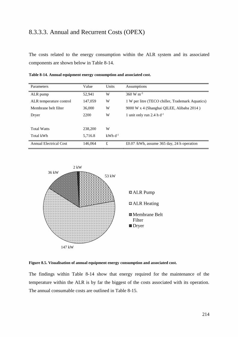
214

8.3.3.3. Annual and Recurrent Costs (OPEX)

The costs related to the energy consumption within the ALR system and its associated

components are shown below in Table 8-14.

Table 8-14. Annual equipment energy consumption and associated cost.

Parameters Value Units Assumptions

ALR pump 52,941 W 360 W m-3

ALR temperature control 147,059 W 1 W per litre (TECO chiller, Trademark Aquatics)

Membrane belt filter 36,000 W 9000 W x 4 (Shanghai QILEE, Alibaba 2014 )

Dryer 2200 W 1 unit only run 2.4 h d-1

Total Watts 238,200 W

Total kWh 5,716.8 kWh d-1

Annual Electrical Cost 146,064 £ £0.07 /kWh, assume 365 day, 24 h operation

Figure 8.5. Visualisation of annual equipment energy consumption and associated cost.

The findings within Table 8-14 show that energy required for the maintenance of the

temperature within the ALR is by far the biggest of the costs associated with its operation.

The annual consumable costs are outlined in Table 8-15.

53 kW

147 kW

36 kW

2 kW

ALR Pump

ALR Heating

Membrane Belt

Filter

Dryer

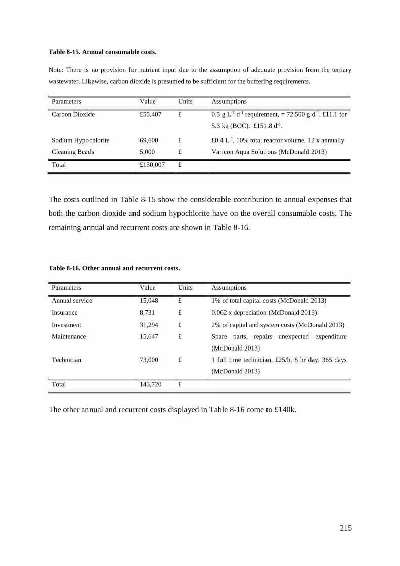
215

Table 8-15. Annual consumable costs.

Note: There is no provision for nutrient input due to the assumption of adequate provision from the tertiary

wastewater. Likewise, carbon dioxide is presumed to be sufficient for the buffering requirements.

Parameters Value Units Assumptions

Carbon Dioxide £55,407 £ 0.5 g L-1 d-1 requirement, = 72,500 g d-1, £11.1 for

5.3 kg (BOC). £151.8 d-1.

Sodium Hypochlorite 69,600 £ £0.4 L-1, 10% total reactor volume, 12 x annually

Cleaning Beads 5,000 £ Varicon Aqua Solutions (McDonald 2013)

Total £130,007 £

The costs outlined in Table 8-15 show the considerable contribution to annual expenses that

both the carbon dioxide and sodium hypochlorite have on the overall consumable costs. The

remaining annual and recurrent costs are shown in Table 8-16.

Table 8-16. Other annual and recurrent costs.

Parameters Value Units Assumptions

Annual service 15,048 £ 1% of total capital costs (McDonald 2013)

Insurance 8,731 £ 0.062 x depreciation (McDonald 2013)

Investment 31,294 £ 2% of capital and system costs (McDonald 2013)

Maintenance 15,647 £ Spare parts, repairs unexpected expenditure

(McDonald 2013)

Technician 73,000 £ 1 full time technician, £25/h, 8 hr day, 365 days

(McDonald 2013)

Total 143,720 £

The other annual and recurrent costs displayed in Table 8-16 come to £140k.

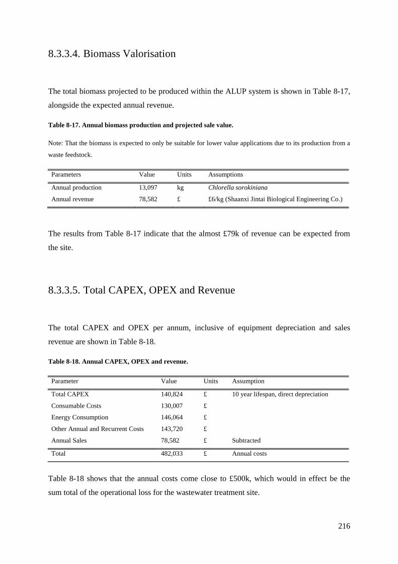
216

8.3.3.4. Biomass Valorisation

The total biomass projected to be produced within the ALUP system is shown in Table 8-17,

alongside the expected annual revenue.

Table 8-17. Annual biomass production and projected sale value.

Note: That the biomass is expected to only be suitable for lower value applications due to its production from a

waste feedstock.

Parameters Value Units Assumptions

Annual production 13,097 kg Chlorella sorokiniana

Annual revenue 78,582 £ £6/kg (Shaanxi Jintai Biological Engineering Co.)

The results from Table 8-17 indicate that the almost £79k of revenue can be expected from

the site.

8.3.3.5. Total CAPEX, OPEX and Revenue

The total CAPEX and OPEX per annum, inclusive of equipment depreciation and sales

revenue are shown in Table 8-18.

Table 8-18. Annual CAPEX, OPEX and revenue.

Parameter Value Units Assumption

Total CAPEX 140,824 £ 10 year lifespan, direct depreciation

Consumable Costs 130,007 £

Energy Consumption 146,064 £

Other Annual and Recurrent Costs 143,720 £

Annual Sales 78,582 £ Subtracted

Total 482,033 £ Annual costs

Table 8-18 shows that the annual costs come close to £500k, which would in effect be the

sum total of the operational loss for the wastewater treatment site.

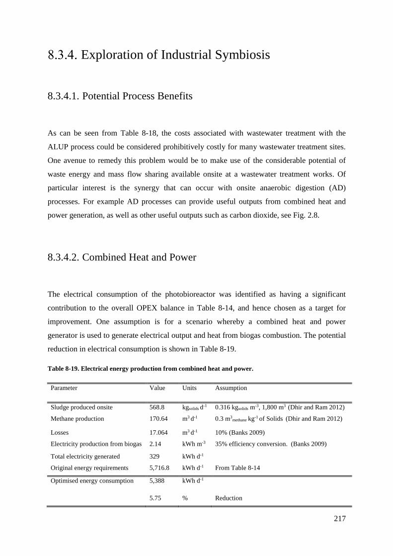
217

Exploration of Industrial Symbiosis

8.3.4.1. Potential Process Benefits

As can be seen from Table 8-18, the costs associated with wastewater treatment with the

ALUP process could be considered prohibitively costly for many wastewater treatment sites.

One avenue to remedy this problem would be to make use of the considerable potential of

waste energy and mass flow sharing available onsite at a wastewater treatment works. Of

particular interest is the synergy that can occur with onsite anaerobic digestion (AD)

processes. For example AD processes can provide useful outputs from combined heat and

power generation, as well as other useful outputs such as carbon dioxide, see Fig. 2.8.

8.3.4.2. Combined Heat and Power

The electrical consumption of the photobioreactor was identified as having a significant

contribution to the overall OPEX balance in Table 8-14, and hence chosen as a target for

improvement. One assumption is for a scenario whereby a combined heat and power

generator is used to generate electrical output and heat from biogas combustion. The potential

reduction in electrical consumption is shown in Table 8-19.

Table 8-19. Electrical energy production from combined heat and power.

Parameter Value Units Assumption

Sludge produced onsite 568.8 kgsolids d-1 0.316 kgsolids m-3, 1,800 m3 (Dhir and Ram 2012)

Methane production 170.64 m3 d-1 0.3 m3methane kg-1 of Solids (Dhir and Ram 2012)

Losses 17.064 m3 d-1 10% (Banks 2009)

Electricity production from biogas 2.14 kWh m-3 35% efficiency conversion. (Banks 2009)

Total electricity generated 329 kWh d-1

Original energy requirements 5,716.8 kWh d-1 From Table 8-14

Optimised energy consumption 5,388 kWh d-1

5.75 % Reduction

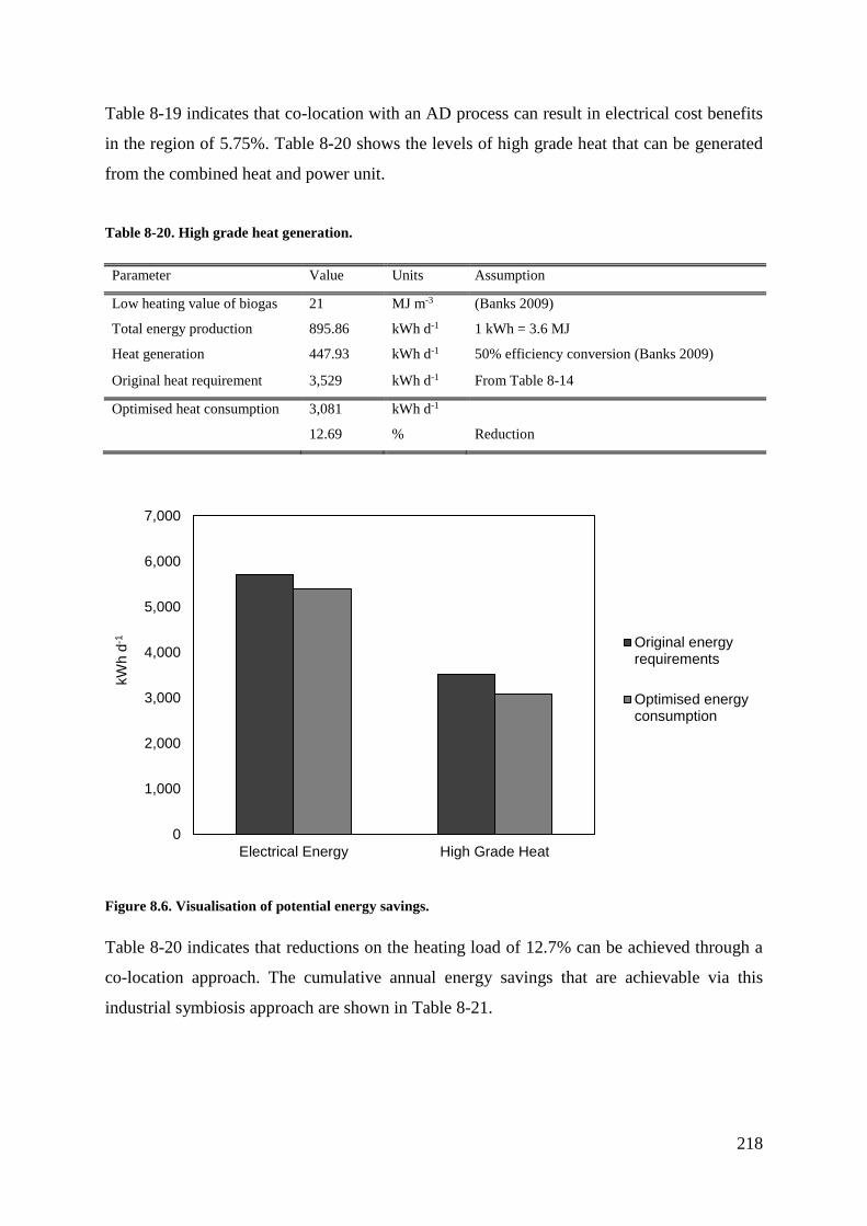
218

Table 8-19 indicates that co-location with an AD process can result in electrical cost benefits

in the region of 5.75%. Table 8-20 shows the levels of high grade heat that can be generated

from the combined heat and power unit.

Table 8-20. High grade heat generation.

Parameter Value Units Assumption

Low heating value of biogas 21 MJ m-3 (Banks 2009)

Total energy production 895.86 kWh d-1 1 kWh = 3.6 MJ

Heat generation 447.93 kWh d-1 50% efficiency conversion (Banks 2009)

Original heat requirement 3,529 kWh d-1 From Table 8-14

Optimised heat consumption 3,081 kWh d-1

12.69 % Reduction

Figure 8.6. Visualisation of potential energy savings.

Table 8-20 indicates that reductions on the heating load of 12.7% can be achieved through a

co-location approach. The cumulative annual energy savings that are achievable via this

industrial symbiosis approach are shown in Table 8-21.

0

1,000

2,000

3,000

4,000

5,000

6,000

7,000

Electrical Energy High Grade Heat

kW

h d

-1 Original energyrequirements

Optimised energyconsumption

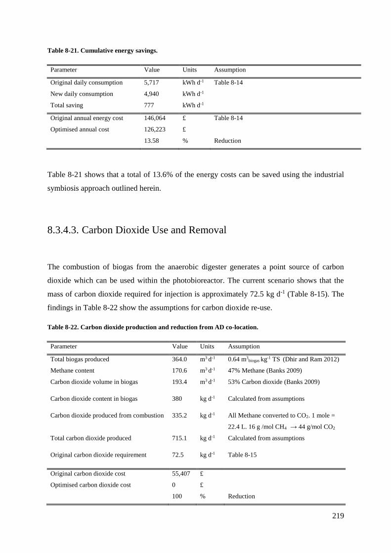
219

Table 8-21. Cumulative energy savings.

Parameter Value Units Assumption

Original daily consumption 5,717 kWh d-1 Table 8-14

New daily consumption 4,940 kWh d-1

Total saving 777 kWh d-1

Original annual energy cost 146,064 £ Table 8-14

Optimised annual cost 126,223 £

13.58 % Reduction

Table 8-21 shows that a total of 13.6% of the energy costs can be saved using the industrial

symbiosis approach outlined herein.

8.3.4.3. Carbon Dioxide Use and Removal

The combustion of biogas from the anaerobic digester generates a point source of carbon

dioxide which can be used within the photobioreactor. The current scenario shows that the

mass of carbon dioxide required for injection is approximately 72.5 kg d-1 (Table 8-15). The

findings in Table 8-22 show the assumptions for carbon dioxide re-use.

Table 8-22. Carbon dioxide production and reduction from AD co-location.

Parameter Value Units Assumption

Total biogas produced 364.0 m3 d-1 0.64 m3biogas kg-1 TS (Dhir and Ram 2012)

Methane content 170.6 m3 d-1 47% Methane (Banks 2009)

Carbon dioxide volume in biogas 193.4 m3 d-1 53% Carbon dioxide (Banks 2009)

Carbon dioxide content in biogas 380 kg d-1 Calculated from assumptions

Carbon dioxide produced from combustion 335.2 kg d-1 All Methane converted to CO2. 1 mole =

22.4 L. 16 g /mol CH4 → 44 g/mol CO2

Total carbon dioxide produced 715.1 kg d-1 Calculated from assumptions

Original carbon dioxide requirement 72.5 kg d-1 Table 8-15

Original carbon dioxide cost 55,407 £

Optimised carbon dioxide cost 0 £

100 % Reduction

220

The findings in Table 8-22 show a 100% reduction in CO2 requirements, with a potential

saving in the region of £55k.

8.1.1.1. Optimised Operational Costs

The comparative savings shown by the use of this industrial symbiosis approach are shown in

Table 8-23.

Table 8-23. Total savings to energy consumption and consumable costs using an industrial symbiosis

approach.

Parameter Value Units Assumption

Original energy and consumable costs 276,071 £ Annualised, Table 8-18

Industrial symbiosis savings 75,249 £ Table 8-19 to Table 8-22

Optimised annual energy and consumable costs 200,823 £

Reduction in costs 27.26 %

Original CAPEX, OPEX and revenue 482,033 £ Table 8-18

Optimised annual costs and revenue 406,785 £

Reduction in costs 15.61 %

8.3.4.4. Improving Algal Productivity

Further improvements to annual costs can be achieved through increased algal productivity

and nutrient uptake (N and P), outlined in Figure 8.7.

221

Figure 8.7. The effect on annual costs caused by increased productivity and nutrient uptake.

Base case is productivity in the region of 0.244 g L-1. Note: Due to the nutrient limitations within the final

effluent this case study would assume nutrient uptake levels of 100% to achieve the 2x productivity, and AD

centrate supplementation to achieve the 4x and 6x conditions.

The findings show that increases in productivity can decrease the annual costs substantially.

It is likely that a 2x improvement target is the most feasible scenario given the unfavourable

cultivation conditions in the UK.

2.1.1. Comparison to other Tertiary Wastewater

Treatment Technologies

As discussed in Chapter 5, many waterways within Europe face severe problems with

nutrient inflow. This has led to stringent EU legislation which may force many facilities to

adopt tertiary wastewater treatment technologies. In this regard biological options may

present a novel cost effective and sustainable strategy for the removal of nitrogen and

phosphorous from within the waterways. A preliminary investigation of these technologies,

0

50,000

100,000

150,000

200,000

250,000

300,000

350,000

400,000

450,000

base case 2x 4x 6x

Annual C

osts

(£'s

)

Productivity and Nutrient Uptake

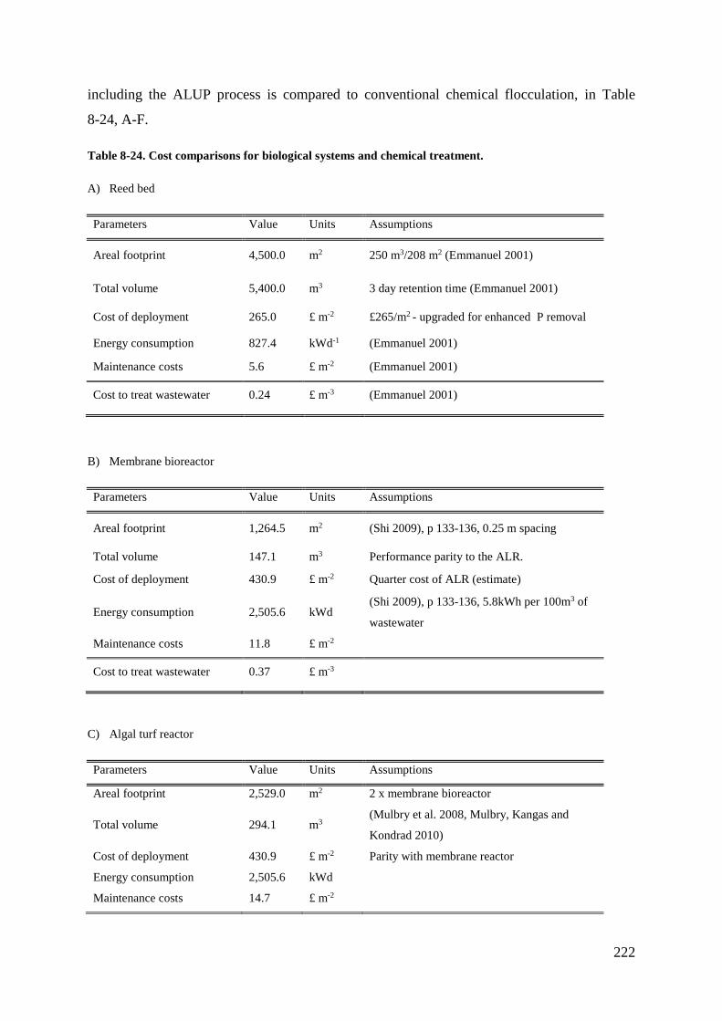
222

including the ALUP process is compared to conventional chemical flocculation, in Table

8-24, A-F.

Table 8-24. Cost comparisons for biological systems and chemical treatment.

A) Reed bed

Parameters Value Units Assumptions

Areal footprint 4,500.0 m2 250 m3/208 m2 (Emmanuel 2001)

Total volume 5,400.0 m3 3 day retention time (Emmanuel 2001)

Cost of deployment 265.0 £ m-2 £265/m2 - upgraded for enhanced P removal

Energy consumption 827.4 kWd-1 (Emmanuel 2001)

Maintenance costs 5.6 £ m-2 (Emmanuel 2001)

Cost to treat wastewater 0.24 £ m-3 (Emmanuel 2001)

B) Membrane bioreactor

Parameters Value Units Assumptions

Areal footprint 1,264.5 m2 (Shi 2009), p 133-136, 0.25 m spacing

Total volume 147.1 m3 Performance parity to the ALR.

Cost of deployment 430.9 £ m-2 Quarter cost of ALR (estimate)

Energy consumption 2,505.6 kWd (Shi 2009), p 133-136, 5.8kWh per 100m3 of

wastewater

Maintenance costs 11.8 £ m-2

Cost to treat wastewater 0.37 £ m-3

C) Algal turf reactor

Parameters Value Units Assumptions

Areal footprint 2,529.0 m2 2 x membrane bioreactor

Total volume 294.1 m3 (Mulbry et al. 2008, Mulbry, Kangas and

Kondrad 2010)

Cost of deployment 430.9 £ m-2 Parity with membrane reactor

Energy consumption 2,505.6 kWd

Maintenance costs 14.7 £ m-2

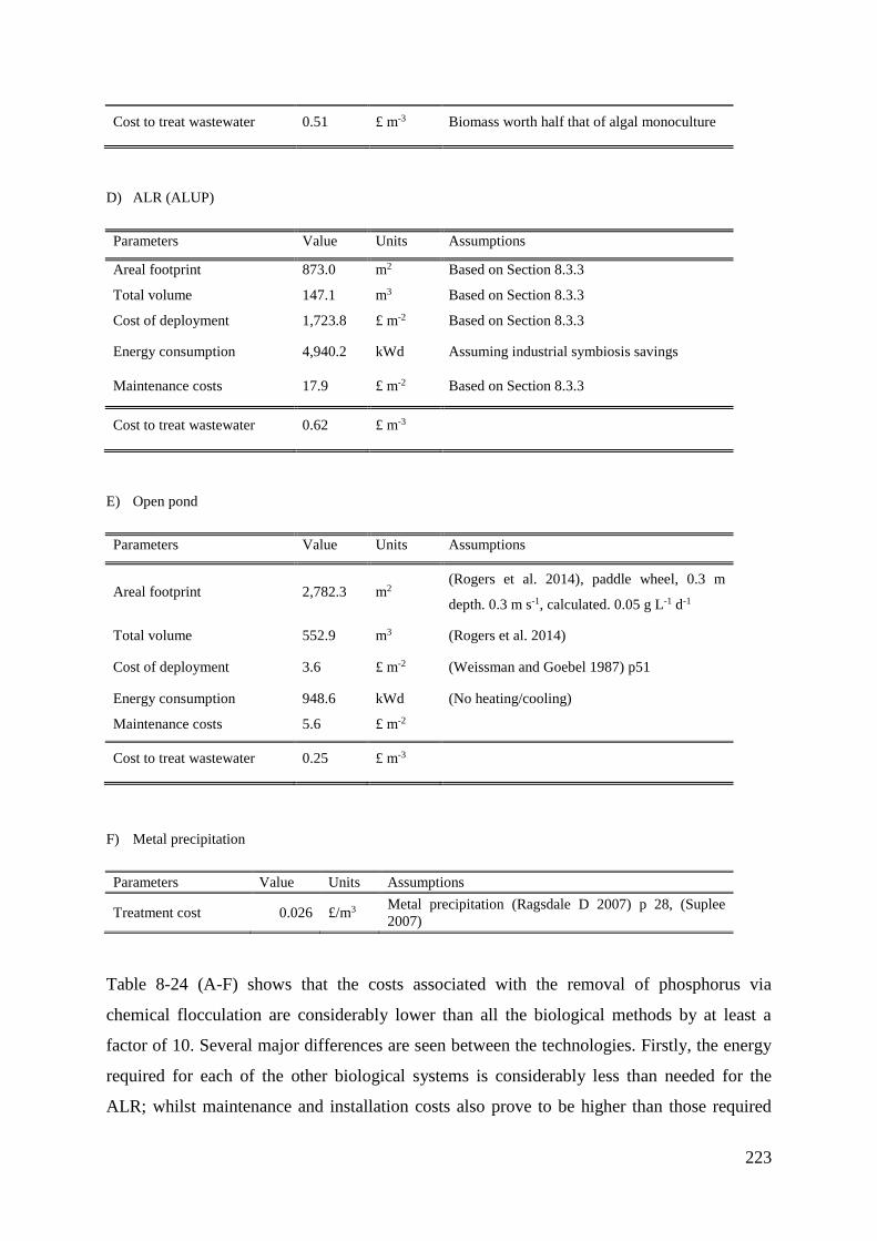
223

Cost to treat wastewater 0.51 £ m-3 Biomass worth half that of algal monoculture

D) ALR (ALUP)

Parameters Value Units Assumptions

Areal footprint 873.0 m2 Based on Section 8.3.3

Total volume 147.1 m3 Based on Section 8.3.3

Cost of deployment 1,723.8 £ m-2 Based on Section 8.3.3

Energy consumption 4,940.2 kWd Assuming industrial symbiosis savings

Maintenance costs 17.9 £ m-2 Based on Section 8.3.3

Cost to treat wastewater 0.62 £ m-3

E) Open pond

Parameters Value Units Assumptions

Areal footprint 2,782.3 m2 (Rogers et al. 2014), paddle wheel, 0.3 m

depth. 0.3 m s-1, calculated. 0.05 g L-1 d-1

Total volume 552.9 m3 (Rogers et al. 2014)

Cost of deployment 3.6 £ m-2 (Weissman and Goebel 1987) p51

Energy consumption 948.6 kWd (No heating/cooling)

Maintenance costs 5.6 £ m-2

Cost to treat wastewater 0.25 £ m-3

F) Metal precipitation

Parameters Value Units Assumptions

Treatment cost 0.026 £/m3 Metal precipitation (Ragsdale D 2007) p 28, (Suplee

2007)

Table 8-24 (A-F) shows that the costs associated with the removal of phosphorus via

chemical flocculation are considerably lower than all the biological methods by at least a

factor of 10. Several major differences are seen between the technologies. Firstly, the energy

required for each of the other biological systems is considerably less than needed for the

ALR; whilst maintenance and installation costs also prove to be higher than those required

224

for the other systems. One aspect in which the photobioreactor excels compared to the other

platforms the relatively low areal footprint that is required. Overall the ALR system results in

a treatment cost of £0.62 m-3 (of wastewater) this is around 2.5 times more expensive than

using a reed bed.

Modelling Conclusions

The findings from the parameter benchmarking exercise show that the ALR compares well to

the other tubular reactor configurations. In this regard, the projections from a reconfigured

spatial arrangement result in better areal volumetric footprints than most of the tubular

examples compared within this study. In terms of energy consumption, the BioFence™ can be

seen to be the most energy intensive system, most probably as a result of the numerous

manifolds and the resultant increase in pressure drop found within the system. The power

requirements between serpentine and air driven photobioreactor systems is fairly consistent at

a smaller scale. However, at a larger scale it can be seen that centrifugal liquid mixing allows

for distinct improvement in economies of scale to be achieved. Previous studies have

suggested the reason for this may be the better efficiency shown by centrifugal pumps (Hall

et al. 2003, Norsker et al. 2011). The overall productivity in the ALR chassis was dependent

on the mixing mode (CM or ALR), but generally found to be comparable to the systems

within the literature, given the light conditions within the UK. Using the findings from Table

8-4 and Table 8-5 the energetic cost of production within the ALR could be derived; and was

found to be 0.027 g W-1. The findings from the sensitivity analysis have shown that extruded

acrylic tubing is the best construction material for the ALR, both in terms of cost and

operational considerations. After spacing and sizing considerations, it was found that a

double length and diameter arrangement had a considerably lower cost profile than the base

case. The optimised manufacturing cost was found to be in the region of £9.76 L-1 of ALR

system, which is similar to many commercially available systems (McDonald 2013).

In terms of the ALUP wastewater treatment model, the total cost of construction and

installation (CAPEX) was found to be in the region of £1.6 million. The annual OPEX costs

225

were also broken down and show the high electricity contribution coming from the mixing

and temperature control requirements (£146k). Using this projection, the optimal annual

operational costs were found to be £482k inclusive of biomass sales, meaning that the plant

would be projected to make a considerable annual loss. Interestingly, it was found that by

using an industrial symbiosis approach, it was possible to reduce the costs by 16%, giving an

annual operational cost of £407k. This would suggest that co-location is a good idea for many

algal production plants, especially those producing low to mid value products. Projections

show that improvements in algal productivity and nutrient uptake could drive the annual costs

of the production plant down to between £250-175k, which would be closer to conventional

chemical costs for P removal. The overall CAPEX and OPEX compare favourably with those

outlined by (Acién Fernandez 2012) for a 3m3 system; (£744k and £96k respectively).

Looking at the production onsite the biomass would have to be sold at £37 kg-1 to break even,

which is similar to values reported within the literature, which range from £50 kg-1 to £9.15

kg-1 depending on scale (Acién Fernandez 2012).

The findings from the analysis of different treatment systems showed that the ALUP process

would be the most expensive way to remove phosphorus from the wastewater (£0.62 m-3).

However, it is somewhat unclear from the literature whether the other systems (particularly

the open pond or reed bed) would be able to maintain the required levels of treatment

throughout the year (Cooper 1999, Green and Upton 1994). Somewhat unsurprisingly, it was

found that chemical flocculation was by far the most cost effective technology, with a total

treatment cost of £0.026 m-3. However, unlike the other biological systems it does not

produce any useable by-product. Furthermore, one of the major advantages highlighted by the

analysis was that the ALR had the smallest areal footprint (873 m2) compared to the other

systems, meaning that the system may well be suited to the limited spatial options in

Northern Europe. Interestingly, the results also highlight that other technologies such as twin

layer membrane reactors or algal turf scrubbers might be more suitable on an operational cost

basis than a photobioreactor. The thesis concludes with Chapter 9, which presents a critique

and discussion of the research undertaken during this doctorate, alongside suggestions and

further work.

226

9. Contribution to Field and Further

Work

9.1. Overview

The results from the thesis are discussed according to the research aims and objectives set out

at the beginning of the report in Chapter 3. To summarise briefly, these describe the selection

of a suitable strain, C. sorokiniana; which scaled down work indicated as being capable of

growth from diesel flue gases, resulting in rapid nutrient removal rates. This laboratory work

indicated the potential for exploitation at larger scales, and was followed by the

conceptualisation of a prototype photobioreactor. The novel ALR system was designed,

constructed, developed and evaluated against a set of engineering and biological criteria.

Experiments were undertaken to determine the optimal operational conditions, and pilot scale

experiments were conducted. Finally, a cost model was developed for the photobioreactor

considering its potential for deployment within a wastewater treatment facility, whilst

indicating possible routes towards marketability. This final chapter discusses the contribution

this thesis has made to the field, whilst exploring some of the unresolved questions. It also

posits potential avenues of research that have arisen from this work. This includes a

discussion of the wider implications of the findings in relation to building a successful algal

industry within the UK, alongside the balancing of wider industrial and environmental

requirements.

227

9.2. Strain Selection and Growth Kinetics

The preliminary strain selection experiments undertaken during this research project showed

that C. sorokiniana was superior to the other strains tested within this work. In particular, the

characterisation found C. sorokiniana well suited to small scale work within the laboratory,

from well plates to 1 litre Duran bottles in the first instance, before moving onto the larger

scale 5, 10 and 50 litre photobioreactors. Overall, the findings indicate that C. sorokiniana

was capable of reaching volumetric productivities and densities comparable to literature

values, see Chapter 7, Section 7.5. In combination, these results mean that the strain could

have a promising future as an industrial ‘workhorse’, although more research would be

required to determine whether it is capable of producing commercial quantities of

biochemicals. Likewise, further work could develop the protocols necessary for stable

transformation of the strain, should a promising target molecule be identified. Given more

time and resources it would be worthwhile to re-open investigation of other fast growing

algal strains to develop a portfolio of potential candidate organisms for growth on

wastewater. For example strains of Scenedesmus have been shown to be fast growing and

robust (Acién Fernandez 2012). This process would be assisted by the improvements in high-

throughput screening afforded by the development of the shaker platform during the EngD

work.

One of the most interesting findings from this initial body of research was the relative ease

with which a microplate shaker could be converted for use in rapid screening processes and

exploration of parameter space. It is likely that the miniaturisation of equipment for higher

throughput work will increase considerably within the field of algal biotechnology, mirroring

developments in other fields. Whilst the microplate shaker proved to be a useful tool for

comparative purposes and rapid screening of feeding strategies, some improvements could

have been made in terms of joining the scaled-down screening to the subsequent scaled-up

reactor work. For example the microplate screening strategy could have been used to profile a

wider range of algal strains directly onto wastewater using UK growth conditions. This would

potentially reduce development times and produce more indicative results for the larger scale

work. Further experiments could also evaluate the large number of poorly quantified

parameters within the shaker plate platform. This would be particularly important for

parameter benchmarking and system standardisation in future design processes. For example,

228

the surface to volume ratio is much higher at mL scale, resulting in a shorter light path length

and higher photosynthetic activity. This means that in the absence of photoinhibition, faster

growth rates are possible (Torzillo and Vonshak 2013) and would lead to poor transferability

of results into larger scale tubular systems. Some of these issues were explored more widely

in the work of (Van Wagenen et al. 2014), including the effect of light path on growth rates in

24-well plates. Furthermore, gas-liquid mass transfer in micro-well plates and bubble-column

or air-lift reactors are not necessarily comparable and would need further investigation (Doig

et al. 2005, Mirón et al. 2000). Some of these transferability problems could perhaps be

overcome to some extent via the deployment of miniaturised mL-scale column

photobioreactors with equal surface to volume ratio than larger scale reactors. Research

investigating these considerations has been undertaken by (Ojo et al. 2015), and demonstrates

the high mass transfers obtained within miniaturised photobioreactors.

9.3. Scaled-down Cultivation with Waste

The ultimate aim of the remediation experiments was to integrate growth on exhaust gas and

wastewater to test the feasibility for scale-up. To this end, the work highlights the

considerable potential for algae in bioremediation, and in particular wastewater treatment;

where better pollutant removal efficiencies are possible when compared to flue gas scrubbing

(Vunjak-Novakovic et al. 2005). The novelty in this work came from combining remediation

of flue gases and wastewater into one integrated laboratory study; and clearly demonstrated

that C. sorokiniana (UTEX1230) could be grown to reasonable yields on either final effluent

or anaerobic digester centrate. The findings suggested that due to the typical volumes,

concentrations and legislation involved in wastewater treatment processes, it is likely that

final effluent would be a most suitable feedstock for an eco-biorefinery.

One aspect within the research that was not fully explored was the optimisation of the

wastewater based growth media. In this regard further research on cultivation with AD

concentrate found that the maximum biomass concentrations were found for 1:2 concentrated

AD medium and also indicated the feasibility of scaling up the process from microplate

shaker to 5ALR (data not shown). However, due to the high turbidity of the AD concentrate,

photosynthetic activity is found to decrease as light penetration is diminished (data not

229

shown) (Molina et al. 2001). The best strategy therefore might be to deploy a final effluent

treatment strategy topped up with digester centrate when biological requirements dictate

necessity. Some further research was undertaken comparing both autoclaved and un-

autoclaved waste media, which showed little difference between the two (data not shown),

however some process optimisation, alongside better quantification of the chemical changes

that this created would be interesting further work. Another interesting area to explore would

be that of improving lipid productivity. Examples from the literature have shown that

changing the carbon, nitrogen and phosphorus ratios within growth media can have a

considerable impact upon the resultant biomass. In particular, changing the C:N ratio can

significantly alter the fatty acid (FA) composition and has been shown to increase lipid

production in C. sorokiniana (Feng and Johns 1991). Furthermore, the same study suggested

that an increased aeration rate can upregulate the synthesis of unsaturated dienoic and trienoic

FAs (Feng and Johns 1991). Other studies show that increasing the temperature closer to the

optimal 35°C can alter the ratio of polyunsaturated to saturated FAs in favour of

polyunsaturated FAs (Belkoura et al. 2000).

One particularly interesting avenue of research would be to investigate the effect that nutrient

starvation would have on algal growth, and subsequent nutrient uptake. Previous research had

shown that phosphate starvation of algae prior to the main cultivation process could improve

phosphate removal (Azad and Borchardt 1970, Hernandez et al. 2006). In practical terms this

could be achieved by starving the inoculation generation and sub-culturing from these starved

parent cultures in future generations. This was investigated in a preliminary capacity during

this doctorate at a laboratory scale, but the results were found to be inconclusive, and so were

omitted from the main body of the work, but may provide an interesting avenue for further

work. Other important considerations for large scale cultivation from waste include dynamic

monitoring of ion compositions, as these can influence buffering capacity and thereby the pH

profile of the culture. Likewise, biofilm development under continuous growth could be a

potential problem during scale-up; and may be a factor that would merit further investigation.

The literature suggests that biofilm formation could be explained to some extent by increased

production of extracellular polymeric substances (Wingender, Neu and Flemming 1999).

This work has also opened up some potentially interesting questions for future research in

terms of optimising both the biological growth of the algae, as well as the absorption of the

gases and nutrients. For example, growth rates could be improved by selecting a point source

with an increased level of CO2 concentration or by increasing the flow rate (indicated in

230

Section 5.5.1). Another interesting direction for future research would be to target SOx and

NOx removal as a means of scale up criteria, as opposed to CO2. This would be favourable at

larger industrial sites, where it would be unfeasible for algal production to remove all of the

carbon dioxide due to the large scales involved. In this case it would be important to retain

dissolved gases within the system, which may require re-design of the photobioreactor.

Another interesting consideration is the rise in pH from ~5.5 to ~8.5 during the course of a

phototrophic fermentation. This natural rise in pH could be seen as an advantageous process

to utilise for the bioremediation of certain substances. It would be worthwhile to investigate

which substances are better remediated at these higher pHs, or over the course of such a pH

transition. For example, there is some evidence that microbial degradation of polyaromatic

hydrocarbons (PAHs) occurs better within neutral soils (Kastner, Breuer-Jammali and Mahro

1998). Another interesting fact is that alkaline solutions are known to allow for higher levels

of CO2 absorption (Hsueh, Chu and Yu 2007).

As the pilot project develops, a major avenue of importance would be the confirmation that it

is possible to grow the strain in a continuous mode from this type of waste feedstock, over the

longer term and without a loss of productivity. This has been identified as important within

the literature (Robinson et al. 2012), and some preliminary work was undertaken during this

project in Chapter 5, Section 5.5.6. The reality of cultivation on waste media in outdoor

conditions would probably result in the complete replacement of any model organism by a

native algal species, inhabiting a natural consortium. This would be especially likely with a

thermotolerant organism like C. sorokiniana growing in a Northern European context, where

both natural competition and the energy costs associated with maintaining temperature could

make culture maintenance a challenge. This would mean that the study of successor

communities and the subsequent impact on removal rates would be of particular interest for

future work. Some indication from the work of ClearAs has shown that stable successor

communities do indeed form during the wastewater cultivation process, and are often

dominated by Scenedesmus spp. Investigation of these mixed microbial communities could

be particularly interesting from the viewpoint of breaking down the more complex chemicals

that are not reported as widely within the literature. Research to date has described this

nascent field as ‘synthetic ecology’ (Pandhal and Noirel 2014), and previous investigations

into the relative merits and disadvantages of photosynthetic or heterotrophic metabolic

pathways have been investigated by (Acuner and Dilek 2004, Muñoz et al. 2005, Muñoz and

Guieysse 2006). To this end, further study of C. sorokiniana metabolism would allow for a

231

greater understanding of the additional benefits this strain could bring to wastewater

treatment. This could open up the possibility to select for algal strains that have better

metabolic characteristics. An example of this would be to mimic conventional carbon capture

(CCS), in which amines are used to dissolve CO2 in an aqueous solution (Gibbins and

Chalmers 2008). Algal, cyanobacterial or bacterial strains could be selected or engineered to

have an amine secretion profile similar to that of carbon capture and storage (CCS) molecules

(Acuner and Dilek 2004).

9.4. Reactor Design and Validation

Within the current literature most photobioreactors have been designed with the

maximisation of areal productivity in mind; whilst particular consideration is also given to

the CAPEX and OPEX of the systems in question (Molina et al. 2001, Acién Fernandez

2012). The completion of this type of multi-parametric problem poses several issues that can

be hard to simultaneously optimise; making the role of the designer one of prioritising the

most important characteristics for the particular application in question. Judging against the

criteria of a novel, lower cost, modular and scalable photobioreactor this part of the research

project could be considered as offering a considerable contribution to the field. Attested by

the low levels of variation seen in many of the key biotic and abiotic parameters at different

scales within the ALR chassis (~0-15%). Furthermore the findings from the system

characterisation experiments were particularly interesting, insomuch as they showed that the

reactor could operate either as an array of connected bubble columns or as an airlift. This

characteristic allows for a range of operational attributes not often achievable in conventional

tubular photobioreactor designs, and provides an adaptable chassis for further research. In

this respect there are still a great many avenues for investigation before the ALR reaches its

full commercial potential.

The overall design methodology proved successful for the initial conceptualisation of the

photobioreactor. However, with the benefit of hindsight it is likely that a more technically

rigorous procedure could have been deployed from the beginning of the design process;

232

rather than the more iterative and creative approach that initiated the design. The finished

ALR prototype was designed to be flexible in terms of its final application, meaning the

concept should be ‘future proof’ for many years to come. As the results from the different

mixing experiments have shown, the ALR chassis should be considered as a modular and

scalable basis upon which differing sparging arrangements, flow rates, remediation or

production activities could be undertaken. The simplicity of the actual vessel geometry

allows for a considerable number of easy variations to be made to the basic design; including

changes in column heights and diameters, as well as the possibility to couple other novel

technologies within the reactor, for example different diffuser types or internalised LED

lighting. The basic ALR configuration could even be extrapolated for use as a flat panel type

system with a channelled flow path. There is also no reason why the reactor could not be used

as a multiphase or even solid state reactor, with algae immobilised within beads or granules

inside the reactor.

The characterisation of fluid properties within the tested systems appears to conform to a

majority of the empirical expressions found within the literature (with a notable exception

being the mass transfer expressions) and therefore could be considered satisfactory for the

initial ALR design and validation process. However, other models in the literature may offer

better predictive capability, and would definitely merit testing in future work; including the

airlift fluid dynamic models outlined within the reviews of (Bitog et al. 2011), (Merchuk and

Siegel 1988) and (Petersen and Margaritis 2001). Of particular importance would be further

modelling of the fluid dynamics using suitable 3D simulation software, which would assist

with the optimisation of the ALR design, and may better elucidate dead zones and other

geometric ratio considerations (Mudde and Van Den Akker 2001). For example, the addition

of extra columns does appear to have a small but quantifiable effect on the flow

characteristics, which may be better elucidated through the use of mesh based problem

solving tools. Another consideration that was not fully explored was the modelling of heat

transfer within the ALR; and further work should determine heating and cooling load

requirements with greater accuracy than the equipment ratings that were used for the reactor

costing. This work may support the observation that temperature control is more energy

intensive given a larger surface area, meaning larger diameter reactors would be more cost

effective to control (Sierra et al. 2008). Likewise, further work could plot and investigate the

projected effects of shear in either airlift or column mixed modes, which were not explored

233

widely in this investigation and may have had an effect on the productivity (Pérez et al.

2006).

One interesting finding regarding the liquid velocity was that there was slight variability

along the length of the reactor (see comment Appendix 10.1.2.4), with the linear liquid

velocity slower at the edges than in the middle, by around 10%. This could be due to an

imbalance in the symmetrically of the flow, caused by increased frictional forces. One

possible solution to this problem may be to have an odd number of tubes within the system,

ensuring that the first and final tubes are always risers. This way drag would be reduced on

what would have been a downcomer tube placed on the edge. Another interesting effect was

the slight increase in liquid velocity within the larger reactors, caused by increasing riser

number. Further testing and mapping of the liquid velocity in each tube would aide in

exploring each of these effects in more detail. Unlike many previous designs described within

the literature, oxygen build-up did not appear to be excessive under the tested conditions; this

is most probably due to the relatively short circulation times before reaching a degassing

zone. However, there were differences in dO2 concentrations between riser and downcomer

tubes (0-14%), especially at higher biomass densities under high irradiance (see Appendix

10.1.2.4), and it would be advisable to gain a better understanding of these phenomena with

further experimentation.

The relative benefit of column mixing over airlift was one of the more interesting findings

from the reactor validation study, and not one that was necessarily obvious from the literature

review at the onset of the investigation (Chisti 1989, Merchuk 1990, Mirón et al. 2000).

Overall these findings suggest the importance of mass transfer considerations in relation to

algal growth, whilst also opening up the possibility that the secondary mixing patterns within

bubble columns (i.e. radial cascades) may offer distinct benefits over the mixing shown

within an airlift reactor (i.e. linear and axial) (Mirón et al. 2004). Furthermore, the higher

liquid velocities seen during airlift mixing may impart greater levels of physiological stress

onto the algae than column mixing. This higher velocity acts to increase shearing effects

within the system; and also creates rapid cycling between zones of high and low gas hold-up,

which in combination may perturb metabolic processes. Other results thus far would suggest

that the reactor design could be improved somewhat by reducing the spacing between

manifolds, as this would shorten the dark phase and circulation time. This would also bring

the overall reactor geometry closer to that of a bubble column, which appears to be a better

configuration for algal growth. Another interesting avenue for experimentation would be to

234

look at the effect of dropping the water level below the manifold, which would result in

mixing even closer to that of a bubble column. In this respect, further study should be

directed towards investigation of column mixing mode within the 50 L ALR, as this would

better elucidate its effect on lateral mixing characteristics within a larger system. Exploration

of the interplay between the aforementioned factors should be continued by investigating

different tubular diameters and heights, and how this in turn would affect algal growth.

Examples from the literature would suggest that increasing the column height of bubble

column systems up to 5 m can improve overall areal production (Mirón et al. 1999); whilst

preliminary work in ALR mixing mode would suggest benefits in increasing the column

height to increase the liquid velocity, and the diameter to increase Reynolds number (see

Appendix 10.1.2.3) {K. Koutita, 2015 #261.

Looking at the wider considerations in terms of the key operational parameters it was found

that the ALR had a performance comparable to that reported within other photobioreactors

from the literature (Chisti 1989, Molina Grima et al. 1999, Molina et al. 2001, Vunjak-

Novakovic et al. 2005). A future avenue of research should build on the work undertaken in

this section by further and more detailed comparisons to reactors found either commercially

or within the literature. These findings should prove useful in comparative terms to the

development of the newer generation of vertically stacked, vertically orientated

photobioreactors; like the AlgEternal (AlgaeIndustryMagazine 2013) system or the new

vertical HCMR serpentine system deployed at Swansea University (Oatley 2013). Evaluation

of the ALR design demonstrated that the simple modular array of repeating units was an

effective method for scale-up, confirmed by findings in Chapter 8. One particularly

interesting finding that would merit further research is the interplay between the two mixing

modes, and the potential for the reactor to alternate between them mid-operation. Such an

approach may be useful for particular organisms, specific mixing requirements or for

cleaning. For example, the reactor could be operated 80% of the time in bubble column mode

and 20% in airlift to ensure high mass transfer with increased levels of lateral mixing.

Variable mixing regimes could also save considerably on the operational costs and should be

explored further; for example night time mixing could use a lower gas flow in airlift mode,

when turbulent mixing is less important.

The impact of solar penetration was not investigated extensively in this thesis, and would

merit further study. One clear finding was that it was possible to create a productivity trade-

off between the tubular diameter and the light penetration, with indications that the diameter

235

can range between certain values (in this case 0.055-0.11 m) without considerable loss in

productivity and hence create considerable areal productivity gain. Obviously, this effect

would only hold true up to a point and is dependent on light considerations, but should merit

further modelling due to the considerable effect this would have on both system CAPEX and

OPEX. In the same respect, it is likely that increasing the incident light levels will have

considerable impact on improving levels of productivity; the 75 µmol m-2 s-1 intensity that

was used in the comparative investigation (Section 7.3.7) is well below saturation of the

maximal growth rate found in Chapter 4 (section 4.4.3 ~250 µmol m-2 s-1), and moreover does

not consider the effects of culture density and light penetration. Future work should create a

suitable biological model for growth in the photobioreactor, considering both light

penetration and nutrient uptake, along the lines of (Molina Grima et al. 1999)(Molina Grima

et al., 2003). Some inroads were made in this direction during the course of the thesis in

collaboration with K. Koutita (data not shown).

Further improvements in reactor performance could be driven by alterations to the actual

sparger design. In particular, the bubble size can have significant effects on the characteristics

within the photobioreactor (K. Koutita 2015), particularly dO2 levels, gas hold-up and mass

transfer (Molina et al. 2001). This makes it an attractive option for further optimisation and

investigation; with attempts to minimise sparger based frictional losses and improvements in

bubble size distribution being important targets. Another line of investigation could assess the

mass transfer during an actual algal cultivation, as the presence of photosynthesing micro-

organisms will have considerable impact on the levels of dissolved oxygen within the system.

Further study of gas diffusion would also be necessary for longer ALR arrays, which may

benefit from pre-mixing the CO2 with atmospheric air before entering the reactor, ensuring a

homogenous distribution of gases. Furthermore, the use of static mixing aids to increase

turbulence within reactor systems has been investigated within other research (Ugwu CU et

al. 2002), and these could easily be incorporated within the ALR chassis from the top of the

system. In the longer term, work should continue to determine the best operational

parameters for different production strategies within the reactor. A summary of the biological

findings would indicate that considerable work could be done in optimising the reactor

performance in terms of seasonality and feeding strategy. The positive results shown with a

fed batch feeding strategy would indicate that there could be other feeding iterations that

would merit testing.

236

9.5. Operational Costs

Overall, the results from this section detail a fully functioning model for both the

manufacture and operation of the ALR. The findings can assist in evaluating differing

treatment technologies, and should provide a useful insight for wastewater treatment facilities

when considering tertiary treatment options. The data is important in so-much as it represents

one of the few studies that bring together design, in-house experimentation and operational

cost modelling within one integrated study. This is especially important, given the fact that

many costing exercises and life cycle analyses (LCA) use data from a variety of sources and

test case scenarios, which can lead to considerable modelling errors (Borowitzka 1992,

Clarens et al. 2010). The findings to date indicate that the operational costs of the platform

are cost competitive with other reactor platforms, and can obtain similar levels of areal

productivity. Furthermore, the results from the sensitivity analysis indicate that considerable

CAPEX savings can be made by altering the construction materials. Overall, the results from

the wastewater treatment model suggest the platform is still cost prohibitive, but that

improvements in productivity and reduced energy consumption can greatly reduce OPEX.

The methodology proved effective for the modelling requirements of this thesis, but further

work may want to expand the excel model with specialist lifecycle assessment (LCA) tools

such as GaBI (thinkstep) (Soratana and Landis 2011). The results from the ALR

configuration and construction suggested that a larger column diameter (0.11 m) and doubled

height (2 m) would be necessary to become cost competitive with other reactor

configurations. Further work could look at even more energy efficient operational strategies

for the ALR system, to bring mixing costs down (preferably by a factor of 10). The results

from the sensitivity analysis highlighted the benefits of altering the manufacturing process;

through the use of thinner extruded PMMA tube, and incorporating the O-ring seal within the

actual reactor manifold. Further factors that could be considered within the sensitivity

analysis include investigation of the manifold array material as this contributes 20% of the

materials CAPEX, and would be a good target for further cost reductions. ALUP modelling

was based on the assumption that volumetric productivity would not be considerably affected

by shading and column diameter changes; however, the literature shows that whilst an

increase in column height could in fact improve areal productivity volumetric productivity

would decrease somewhat (Mirón et al. 1999). These effects are explored further in the

237

research of (Mirón et al. 1999), and give a good example of the further modelling that would

be required to correctly factor in the effects of the change in column diameter and shading.

Alongside the shading effects, a better understanding of seasonality and its impact on nutrient

removal needs to be developed; this would require further experimentation at the 50 L pilot

scale to ascertain any further variability in nutrient removal rates. Other future work should

consider the importance of varying the nitrogen source and the impact this would have on

production (Hulatt et al. 2012), especially if co-feeding with final effluent and AD centrate.

The next logical step for the development of the research would be to gain access to a UK

treatment plant, with a view to constructing a pilot ALUP system and testing practical

operation onsite. This would be important for gauging the range of performance variability

caused by seasonal nutrient flow changes, including the effect of altering N:P ratios; and

would be a pre-requisite before the system could be used for actual wastewater treatment. In

this respect it would be worthwhile to further investigate nitrogen uptake, as removal would

most likely be higher than the stated environmental requirements, this is due to sizing the

system for P removal. Treatment of nitrogen could then be compared to the costs to

conventional and hybrid techniques such as biological carbonaceous conversion-nitrification

(Ngo 1998). Further investigation into carbon dioxide efficiency should also be undertaken as

the range used experimentally during the thesis is much higher (from 10-100 x) than the 2:1

ratio stated in Section 8.2.2.4; it is probable that with optimisation this could be brought

closer to theoretical levels. Pilot operation could also allow for a practical series of

experiments to explore the problems associated with membrane belt filter clogging, as the

wider pitfalls of this method were not fully explored within this thesis.

However, at this current juncture the data from the model would indicate that using the

reactor solely as a remediation platform is challenging due to the considerable CAPEX and

OPEX associated with its use. Given this fact, it may be interesting to investigate whether a

lease model would work better for the sector as a whole. Further work could model reactor

operation under reduced energy consumption, which combined with productivity gains could

lead to break-even operation. Other options include developing an even stronger industrial

symbiosis approach, which could bring increased economic benefits to an algal production

process. For example, a good target for cost savings could be to re-use the metabolic low-

grade heat produced by the AD unit, a factor that was not investigated in this study (Cao

2011). Other auxiliary benefits could also be investigated, these include renewable heating

238

incentives and carbon credits; although their impact on the overall costs may be relatively

small.

The work undertaken comparing the ALR platform to other biological and chemical

treatment systems requires some further optimisation, not least because of the difficulty in

comparing the various literature sources. The general findings show that algae are capable of

removing nitrogen and phosphorus at a rate much higher than conventional reed beds

(Vymazal et al. 2006). However, the findings also show that algal treatment has a relatively

high cost associated with the remediation process, especially in comparison to that of a reed

bed (Green and Upton 1994). All of the biological systems that were profiled were

considerably more expensive than chemical treatment, which could mean that the study of

hybridised systems may be an appropriate way to move forward. This would especially be the

case in combining the space saving advantages of a photobioreactor system with a lower cost

solution like an open pond. For example, an open pond could do a majority of the

remediation, and the photobioreactor could be used afterwards as a final polishing step.

Examples of this kind of hybrid system can be found in the literature from the work of

(Christenson and Sims 2011).

9.6. Final Conclusions and Summary

9.6.1. Joining the dots within the UK Algal Industry

This doctorate has undertaken an interdisciplinary integrated systems approach from the

outset. It was felt that this would create considerable scope to investigate both technical and

scientific problems whilst maintaining a strong focus on practical feasibility. This approach is

somewhat different to a majority of the doctoral algal research within the UK to date, which

is often split between numerous sub-fields and subject to very specific biological or

engineering investigation. This means that most research often commences with a view to

investigate or optimise distinct parts of a process; and whilst undertaking this type of linear

239

problem solving is particularly suitable for investigation in traditional engineering and

theoretical sciences; it can be somewhat inappropriate for the creation and study of integrated

or applied systems. This is often because integrated and applied systems contain many

unforeseen problems that only become apparent upon implementation and operation (Bignell

1984, Emes 2012). Likewise, linear design can also lead to the optimisation of components or

concepts that may become obsolete over the course of time due to unforeseen advances

within allied fields. For these reasons it is the belief of the author that for the algal industry to

flourish in the UK a greater level of interdisciplinary thinking and adaptability to industrial

reality should be fostered, particularly in younger researchers.

Looking back at the algal industry’s recent history, this generation of researchers could be

described as being the ‘biofuel babies’, both in terms of our project and research funding

origins (Steyer 2014). Considerations regarding the overall sustainability of next generation

fuels and feedstock are an important debate and one that is already on-going. In this respect,

the jury is still out on whether algal production will ever reach its full potential in terms of a

global replacement for fossil fuels (Richardson, Outlaw and Allison 2010). It is also

important to stress at this point, that given the current economic conditions the commercial

production of algae for low value biofuels and bioproducts is unfeasible in both Europe and

the UK. With some (possibly optimistic) estimates setting a time scale for the realisation of

mass produced lower cost algal biofuels and bioproducts between 5-20 years, dependent on a

variety of factors (Lamers 2013, Steyer 2014). These ongoing questions over the feasibility of

algal biofuels has left this generation of researchers looking into wider bioeconomy

considerations, and with this diversification has come the exploration and acknowledgement

of many different drivers for the growth of algal biotechnology within the wider bioeconomy

(Subhadra and Grinson 2011).

Despite the positive outlook for integrated algal production there are still several hurdles

before we achieve widespread deployment of the technology. An important consideration is

that within the current economic climate, remediation of waste is often not considered a

means into itself. The successful deployment of this type of eco-biorefinery is only feasible if

backed by a suitable regulatory framework, with demonstrable advantages compared to other

technologies or the result of a more profitable enterprise. This raises some important

questions about the priorities of the plant operator. For example, is the acting driver to meet

sustainability or remediation goals, or is it to produce low value biomass as a feedstock for

the bioeconomy (Stephenson et al. 2010). These two actions are not necessarily aligned in

240

terms of sustainable metrics. Further issues include the considerable problems still associated

with the use of waste feedstock to produce biomass intended for animal or human

consumption. It is possible that the tightening of EU environmental regulation may act in

itself to encourage the deployment of algae solely for remediation, but in the meantime some

legislative change within EU waste disposal frameworks would be crucial to the development

of the sector; or at the very least a case-by-case validation of industrial symbiosis production

processes to ensure compliance (along the lines of PAS110 certification for anaerobic

digestate). Furthermore, the economic analysis undertaken within this project highlights the

bottlenecks in energy requirements for mixing and temperature control, which need to be

targeted for improvement. It is likely that given current technology the only way in which this

balance could be altered more favourably would be in greater volumetric productivities or

through the co-production of higher value products during the remediation process.

The general findings from this thesis would indicate that several cost barriers have to be

overcome before the widespread use of algae for bioremediation in a Northern European

context becomes a reality. Particular areas include the CAPEX and OPEX of a suitable

system and its associated processes. These difficulties in cost effective production of lower

cost biomass mean that in the near term it is likely that developments in algal production

systems will be driven largely by higher value products and the fine chemical sectors

(Borowitzka 1992, Stephenson et al. 2010). One prominent example is the pigment and

antioxidant astaxanthin, produced by the green alga Haematococcus pluvialis. The use of this

red carotenoid is growing rapidly and finding increasing application within the nutraceutical

sector and aquaculture industry, with a retail value in the region of £10,000/kg (Leu and

Boussiba 2014, McDonald 2013). To this end some preliminary work was undertaken

cultivating H. pluvialis within the ALR, and demonstrates the adaptability of the reactor

platform to the cultivation of a variety of strains, whilst showing its potential to exploit

different algal markets. Likewise, further developments within the biotechnology sector, such

as improvements in genetic manipulation and physiological understanding will broaden the

types of cells and pathways that can be used as biorefineries (Ghatak 2011). The ultimate aim

of future research should be to build upon these findings and show that this is indeed a

possibility at larger scales, without overly compromising either of the two processes.

The results presented within this thesis relate closely to resilience in terms of resource

efficiency and re-use, as well as ecological modernisation and the creation of a green

economy. These macro themes were not evaluated in a quantitative manner during this

241

doctorate, and would be an interesting avenue for further research. Metrics for such an

analysis would have to consider the ultimate aim of an eco-biorefinery, which is to generate

an end product of consistent quality, regardless of the type of waste input. To this end, further

research is also needed to investigate strains that are capable of undertaking stable nutrient

recovery alongside valuable product formation. In this regard there are still some legislative

considerations that may need to be overcome to position the final product further up the value

chain. Other important targets for the algal sector include the development of microscale

technologies, which will greatly assist in accelerating process design and development. Of

equal importance is the improvement in photobioreactor technology for lower cost mass

cultivation of algae, as without improvements in production systems the sector will stagnate.

Future photobioreactor design will require a step change in thinking, as all enclosed volume

reactors fundamentally suffer from similar physical constraints, in regards to light

penetration, mixing and biomass separation. Some preliminary work exploring other

production methods was initiated towards the close of the research project (Appendix

10.1.4.2), inspired by the work of (Shi, Podola and Melkonian 2007).

Algae retains its popularity within the minds of the general public, which signals a healthy

future. This, alongside a greater desire for sustainable and resilient infrastructure ensures the

funding situation looks good for the sector as a whole. In the near term the model of research

council funding coupled to private sector investment should assist the industry as a whole.

This includes the development of knowledge transfer networks like Phyconet and AB-SIG

which serve as important ways for academia and industry to pool and exchange technical

expertise and resources. However, it is likely that an increase in governmental subsidies and

support would be required to bring bulk algal products to the market, especially if a truly

green economy is to be established. To this end, and with the conclusion of this doctorate the

author believes that several novel contributions have been made to the understanding of

integrated system design for algal bioprocesses. Alongside these integrated considerations the

research has also generated a practical and adaptable photobioreactor design in the form of

the ALR. Moving forward it is hoped that the findings and design frameworks used within

this thesis will assist future researchers. In particular both academic and industrial

practitioners who wish to combine sustainability and bioprocess design, whilst working

towards greater industrial and environmental harmony.

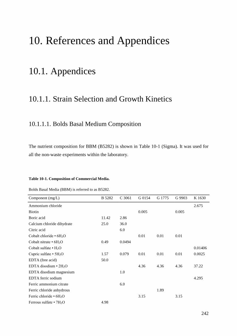
242

10. References and Appendices

10.1. Appendices

10.1.1. Strain Selection and Growth Kinetics

10.1.1.1. Bolds Basal Medium Composition

The nutrient composition for BBM (B5282) is shown in Table 10-1 (Sigma). It was used for

all the non-waste experiments within the laboratory.

Table 10-1. Composition of Commercial Media.

Bolds Basal Media (BBM) is referred to as B5282.

Component (mg/L) B 5282 C 3061 G 0154 G 1775 G 9903 K 1630

Ammonium chloride 2.675

Biotin 0.005 0.005

Boric acid 11.42 2.86

Calcium chloride dihydrate 25.0 36.0

Citric acid 6.0

Cobalt chloride • 6H2O 0.01 0.01 0.01

Cobalt nitrate • 6H2O 0.49 0.0494

Cobalt sulfate • H2O 0.01406

Cupric sulfate • 5H2O 1.57 0.079 0.01 0.01 0.01 0.0025

EDTA (free acid) 50.0

EDTA disodium • 2H2O 4.36 4.36 4.36 37.22

EDTA disodium magnesium 1.0

EDTA ferric sodium 4.295

Ferric ammonium citrate 6.0

Ferric chloride anhydrous 1.89

Ferric chloride • 6H2O 3.15 3.15

Ferrous sulfate • 7H2O 4.98

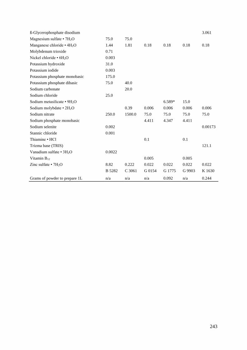
243

ß-Glycerophosphate disodium 3.061

Magnesium sulfate • 7H2O 75.0 75.0

Manganese chloride • 4H2O 1.44 1.81 0.18 0.18 0.18 0.18

Molybdenum trioxide 0.71

Nickel chloride • 6H2O 0.003

Potassium hydroxide 31.0

Potassium iodide 0.003

Potassium phosphate monobasic 175.0

Potassium phosphate dibasic 75.0 40.0

Sodium carbonate 20.0

Sodium chloride 25.0

Sodium metasilicate • 9H2O 6.589* 15.0

Sodium molybdate • 2H2O 0.39 0.006 0.006 0.006 0.006

Sodium nitrate 250.0 1500.0 75.0 75.0 75.0 75.0

Sodium phosphate monobasic 4.411 4.347 4.411

Sodium selenite 0.002 0.00173

Stannic chloride 0.001

Thiamine • HCl 0.1 0.1

Trizma base (TRIS) 121.1

Vanadium sulfate • 3H2O 0.0022

Vitamin B12 0.005 0.005

Zinc sulfate • 7H2O 8.82 0.222 0.022 0.022 0.022 0.022

B 5282 C 3061 G 0154 G 1775 G 9903 K 1630

Grams of powder to prepare 1L n/a n/a n/a 0.092 n/a 0.244

244

10.1.1.2. Biomass Conversion

The biomass conversion relationship used for experimental work is shown in Figure 10.1.

Samples with OD values above 0.8 were diluted to prevent erroneous readings.

Figure 10.1. Conversion of optical density at 750 nm and biomass dry weight.

The gradient of the line was found to be y = 0.2466x.

0

1

2

3

4

5

6

0 5 10 15 20

g L

-1

OD750

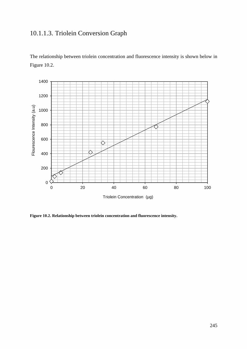
245

10.1.1.3. Triolein Conversion Graph

The relationship between triolein concentration and fluorescence intensity is shown below in

Figure 10.2.

Figure 10.2. Relationship between triolein concentration and fluorescence intensity.

0

200

400

600

800

1000

1200

1400

0 20 40 60 80 100

Flo

ure

scence I

nte

nsity

(a.u

)

Triolein Concentration (µg)

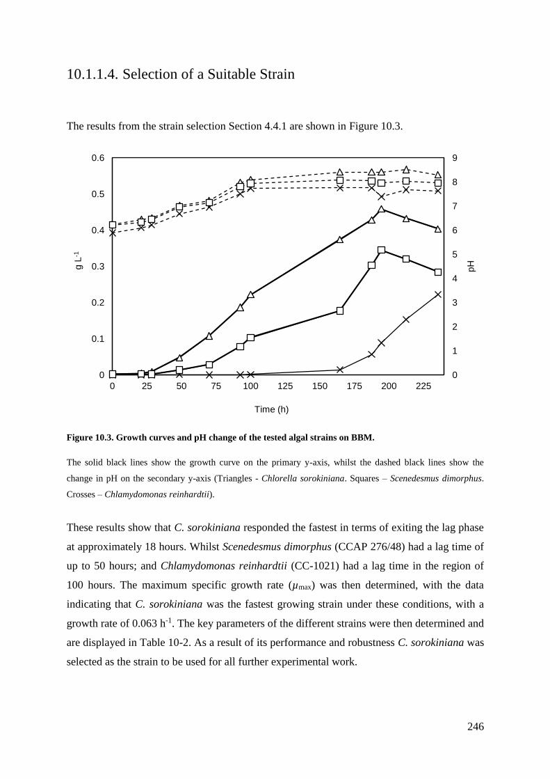
246

10.1.1.4. Selection of a Suitable Strain

The results from the strain selection Section 4.4.1 are shown in Figure 10.3.

Figure 10.3. Growth curves and pH change of the tested algal strains on BBM.

The solid black lines show the growth curve on the primary y-axis, whilst the dashed black lines show the

change in pH on the secondary y-axis (Triangles - Chlorella sorokiniana. Squares – Scenedesmus dimorphus.

Crosses – Chlamydomonas reinhardtii).

These results show that C. sorokiniana responded the fastest in terms of exiting the lag phase

at approximately 18 hours. Whilst Scenedesmus dimorphus (CCAP 276/48) had a lag time of

up to 50 hours; and Chlamydomonas reinhardtii (CC-1021) had a lag time in the region of

100 hours. The maximum specific growth rate (µmax) was then determined, with the data

indicating that C. sorokiniana was the fastest growing strain under these conditions, with a

growth rate of 0.063 h-1. The key parameters of the different strains were then determined and

are displayed in Table 10-2. As a result of its performance and robustness C. sorokiniana was

selected as the strain to be used for all further experimental work.

0

1

2

3

4

5

6

7

8

9

0

0.1

0.2

0.3

0.4

0.5

0.6

0 25 50 75 100 125 150 175 200 225

pHg L

-1

Time (h)

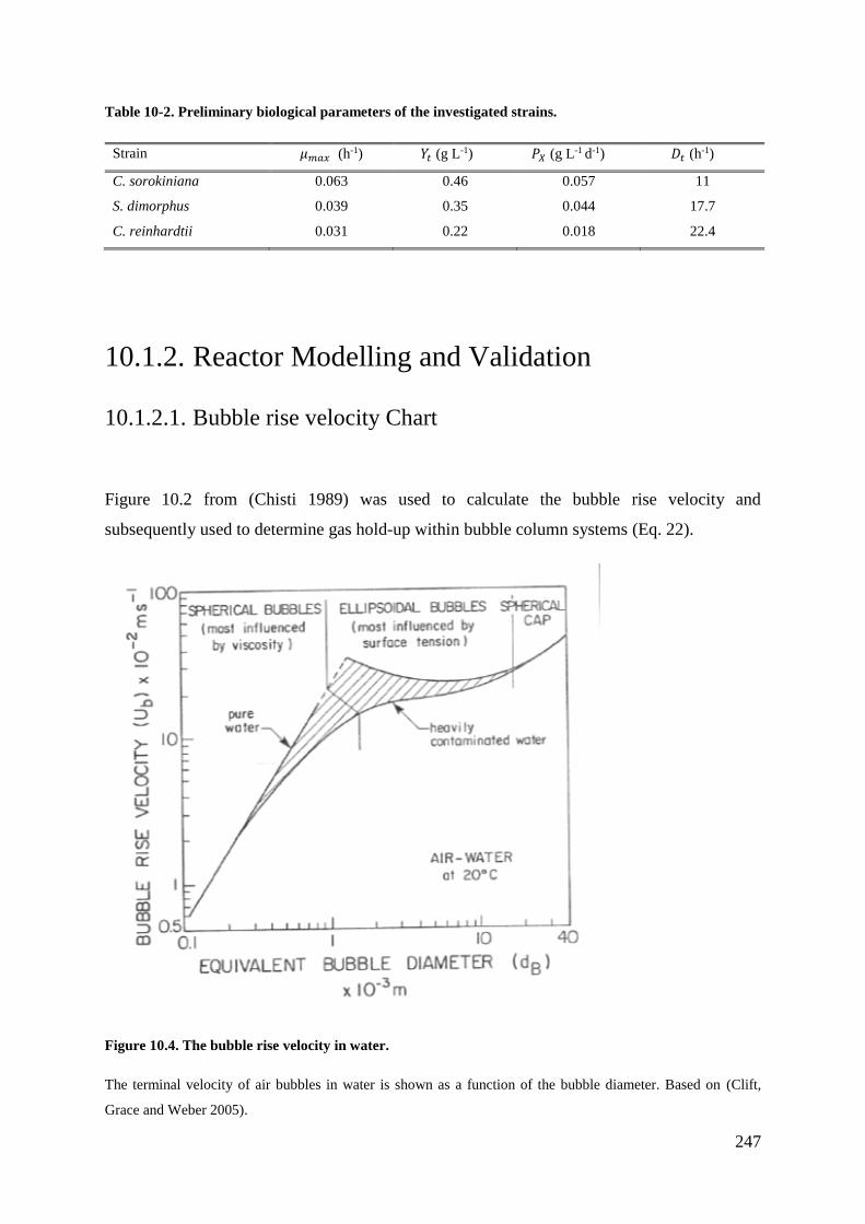
247

Table 10-2. Preliminary biological parameters of the investigated strains.

Strain 𝜇𝑚𝑎𝑥 (h-1) 𝑌𝑡 (g L-1) 𝑃𝑋 (g L-1 d-1) 𝐷𝑡 (h-1)

C. sorokiniana 0.063 0.46 0.057 11

S. dimorphus 0.039 0.35 0.044 17.7

C. reinhardtii 0.031 0.22 0.018 22.4

10.1.2. Reactor Modelling and Validation

10.1.2.1. Bubble rise velocity Chart

Figure 10.2 from (Chisti 1989) was used to calculate the bubble rise velocity and

subsequently used to determine gas hold-up within bubble column systems (Eq. 22).

Figure 10.4. The bubble rise velocity in water.

The terminal velocity of air bubbles in water is shown as a function of the bubble diameter. Based on (Clift,

Grace and Weber 2005).

248

10.1.2.2. Assumptions of linear liquid velocity model

The following assumptions were made from the work of (Heijnen and Van't Riet 1984, Chisti

1989, Doran 1995, K. Koutita 2015).

The gas is incompressible, i.e. there is no change in the gas volume of each bubble during

its propagation along the tube.

Bubbles are spherical; bubbles have been reported to be spherical for a 𝑑𝑏< 1 mm and

ellipsoid for 1 mm < 𝑑𝑏< 1 cm (Clift et al. 2005).

The Reynolds number of the bubbles’ rise in the liquid is always below the threshold

required by Eq.3, based on estimates of 𝑅𝑒𝑏=170 – 2,200 in the experiments.

Bubbles have negligible weight compared to the drag and buoyancy forces.

The gas flow rate is constant.

Flow is at steady state.

Flow is turbulent.

The drag force is uniform over the cross-section of the tube as bubbles are assumed to be

spread evenly after a short distance from their entrance into the bioreactor.

There is negligible bubble recirculation (Chisti 1989).

10.1.2.3. Assumptions for Reynolds number calculations

Liquid density (𝜌𝐿) = 998.2 kg m-3 (water)

Liquid viscosity (𝜇) = 0.0009 kg/(s.m)

249

10.1.2.4. Sampling at different reactor points

Data for the ALR systems not shown, but summarised as follows:

Dissolved oxygen:

Difference between riser and downcomer between 0 - 14%.

Slight increase in dO2 at the bottom of the photo-collecting tube, between 0 - 6%.

Biomass concentration:

Negligible.

Liquid velocity:

Slight decrease towards the edges of the array, no more than 10 % of the velocity

in the centre of the array.

Gas hold-up:

65 - 73% lower in the downcomer than the riser.

10.1.3. Operational Costs

10.1.3.1. ALR Build Cost

Table 10-3 shows the ALR build cost that was used as the basis for the manufacturing costs

in Chapter 8, Section 8.3.2.

Table 10-3. ALR build costs (Varicon)

1 Aluminium frame

1m of 2"x1"x1/4" ALUMINIUM ANGLE 3 5.9 17.7

2.5m of 2"x4"x3mm ALUMINIUM RECTANGULAR BOX 1 29.53 29.53

STAINLESS STEEL FEET 4 4.43 17.72

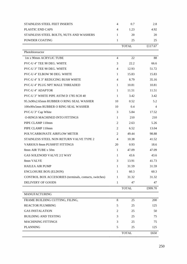
250

STAINLESS STEEL FEET INSERTS 4 0.7 2.8

PLASTIC END CAPS 4 1.23 4.92

STAINLESS STEEL BOLTS, NUTS AND WASHERS 1 20 20

POWDER COATING 1 25 25

TOTAL £117.67

Photobioreactor

1m x 90mm ACRYLIC TUBE 4 22 88

PVC-U 4" TEE 90 DEG. WHITE 3 22.2 66.6

PVC-U 3" TEE 90 DEG. WHITE 4 12.93 51.72

PVC-U 4" ELBOW 90 DEG. WHITE 1 15.83 15.83

PVC-U 4" X 3" REDUCING BUSH WHITE 4 8.79 35.16

PVC-U 4" PLUG NPT MALE THREADED 1 10.81 10.81

PVC-U 4" ADAPTOR 1 11.51 11.51

PVC-U 3" WHITE PIPE ASTM D 1785 SCH 40 1 3.42 3.42

95.3x90x2.65mm RUBBER O RING SEAL WASHER 10 0.52 5.2

100x90x5mm RUBBER O RING SEAL WASHER 10 0.4 4

PVC-U 3" Cap White 3 5.84 17.52

O-RINGS MACHINED INTO FITTINGS 1 210 210

PIPE CLAMP 110mm 2 2.63 5.26

PIPE CLAMP 110mm 2 6.52 13.04

POLYCARBONATE AIRFLOW METER 2 49.44 98.88

STAINLESS STEEL NON RETURN VALVE TYPE 2 4 10.38 41.52

VARIOUS 8mm PUSHFIT FITTINGS 20 0.93 18.6

8mm AIR TUBE x 50m 1 47.09 47.09

GAS SOLENOID VALVE 2/2 WAY 1 43.6 43.6

8mm VALVE 3 13.91 41.73

HAILEA AIR PUMP 1 31.59 31.59

ENCLOSURE BOX (ELDON) 1 60.3 60.3

CONTROL BOX ACCESORIES (terminals, contacts, switches) 1 31.32 31.32

DELIVERY OF GOODS 1 47 47

TOTAL £999.70

MANUFACTURING

FRAME BUILDING CUTTING, FILING, 8 25 200

REACTOR PLUMBING 5 25 125

GAS INSTALATION 2 25 50

BUILDING AND TESTING 3 25 75

MACHINING FITTINGS 3 25 75

PLANNING 5 25 125

TOTAL £650

251

BUILDING COST TOTAL:

£1,767.37

10.1.3.2. Further Cost and Energy Assumptions

Further assumptions that were used include:

Pump costs ~ £1 = 1W of pump capacity.

ALR mixing energy usage = 0.36 W/L.

10.1.3.3. Anaerobic Digestion Principles

Anaerobic digestion is often used on municipal wastewater sites to treat the sludge that is

produced as a by-product of the process. The digestion progresses via hydrolysis,

acidogenesis, acetogenesis and methanogenesis; with the final step producing biogas and

digestate as major by-products. This biogas consists of 55%-75% methane gas (CH4), 25%-

45% carbon dioxide (CO2), as well as traces of other gases like H2O, H2S, H2 and N2. The

biogas produced from anaerobic digestion can be used directly as a biofuel and coupled to a

heat exchanger to convert the energy into electricity.

10.1.3.4. Biological Treatment Systems

10.1.3.4.1. Reed Beds

Reed beds have been a widely deployed wastewater treatment platform for many decades. In

practical terms the process mimics a natural wetland ecosystem, and is conventionally used as

a replacement for primary and secondary treatment when other methods are unfeasible.

However, by increasing the retention time reed based systems can be upgraded for use as a

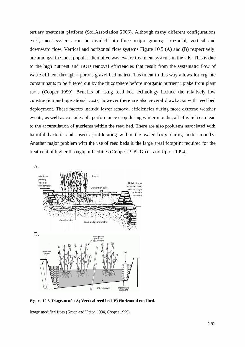
252

tertiary treatment platform (SoilAssociation 2006). Although many different configurations

exist, most systems can be divided into three major groups; horizontal, vertical and

downward flow. Vertical and horizontal flow systems Figure 10.5 (A) and (B) respectively,

are amongst the most popular alternative wastewater treatment systems in the UK. This is due

to the high nutrient and BOD removal efficiencies that result from the systematic flow of

waste effluent through a porous gravel bed matrix. Treatment in this way allows for organic

contaminants to be filtered out by the rhizosphere before inorganic nutrient uptake from plant

roots (Cooper 1999). Benefits of using reed bed technology include the relatively low

construction and operational costs; however there are also several drawbacks with reed bed

deployment. These factors include lower removal efficiencies during more extreme weather

events, as well as considerable performance drop during winter months, all of which can lead

to the accumulation of nutrients within the reed bed. There are also problems associated with

harmful bacteria and insects proliferating within the water body during hotter months.

Another major problem with the use of reed beds is the large areal footprint required for the

treatment of higher throughput facilities (Cooper 1999, Green and Upton 1994).

Figure 10.5. Diagram of a A) Vertical reed bed. B) Horizontal reed bed.

Image modified from (Green and Upton 1994, Cooper 1999).

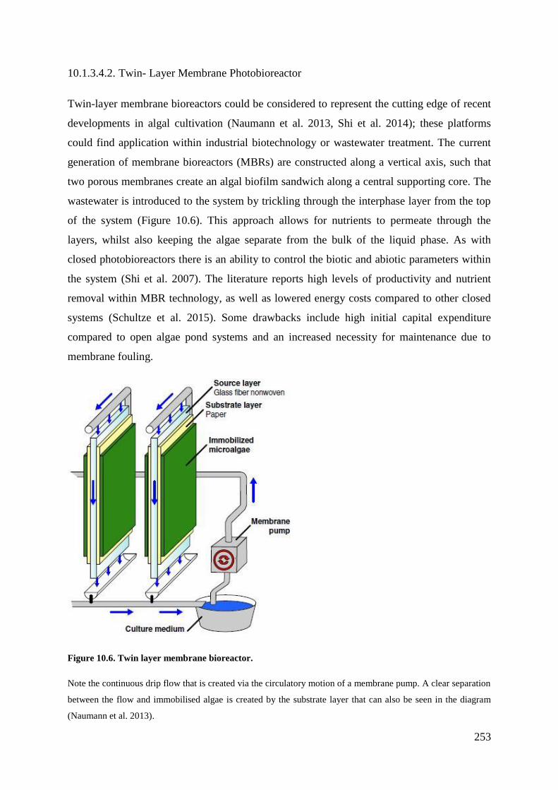
253

10.1.3.4.2. Twin- Layer Membrane Photobioreactor

Twin-layer membrane bioreactors could be considered to represent the cutting edge of recent

developments in algal cultivation (Naumann et al. 2013, Shi et al. 2014); these platforms

could find application within industrial biotechnology or wastewater treatment. The current

generation of membrane bioreactors (MBRs) are constructed along a vertical axis, such that

two porous membranes create an algal biofilm sandwich along a central supporting core. The

wastewater is introduced to the system by trickling through the interphase layer from the top

of the system (Figure 10.6). This approach allows for nutrients to permeate through the

layers, whilst also keeping the algae separate from the bulk of the liquid phase. As with

closed photobioreactors there is an ability to control the biotic and abiotic parameters within

the system (Shi et al. 2007). The literature reports high levels of productivity and nutrient

removal within MBR technology, as well as lowered energy costs compared to other closed

systems (Schultze et al. 2015). Some drawbacks include high initial capital expenditure

compared to open algae pond systems and an increased necessity for maintenance due to

membrane fouling.

Figure 10.6. Twin layer membrane bioreactor.

Note the continuous drip flow that is created via the circulatory motion of a membrane pump. A clear separation

between the flow and immobilised algae is created by the substrate layer that can also be seen in the diagram

(Naumann et al. 2013).

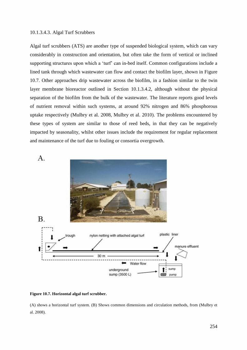
254

10.1.3.4.3. Algal Turf Scrubbers

Algal turf scrubbers (ATS) are another type of suspended biological system, which can vary

considerably in construction and orientation, but often take the form of vertical or inclined

supporting structures upon which a ‘turf’ can in-bed itself. Common configurations include a

lined tank through which wastewater can flow and contact the biofilm layer, shown in Figure

10.7. Other approaches drip wastewater across the biofilm, in a fashion similar to the twin

layer membrane bioreactor outlined in Section 10.1.3.4.2, although without the physical

separation of the biofilm from the bulk of the wastewater. The literature reports good levels

of nutrient removal within such systems, at around 92% nitrogen and 86% phosphorous

uptake respectively (Mulbry et al. 2008, Mulbry et al. 2010). The problems encountered by

these types of system are similar to those of reed beds, in that they can be negatively

impacted by seasonality, whilst other issues include the requirement for regular replacement

and maintenance of the turf due to fouling or consortia overgrowth.

Figure 10.7. Horizontal algal turf scrubber.

(A) shows a horizontal turf system. (B) Shows common dimensions and circulation methods, from (Mulbry et

al. 2008).

255

10.1.3.4.4. Closed Photobioreactors and Open Ponds

A detailed discussion of open and closed algal systems alongside diagrams can be found in

Chapter 6, Section 6.6.3.

10.1.3.5. Varicon Photobioreactor Systems

10.1.3.5.1. BioFence™

The BioFence™ is a highly efficient and reliable system for producing high density

monocultures of marine and freshwater algae, typically operating at densities 2 to 5 times that

of conventional culture methods. The innovative manifold design dramatically reduces the

light path and increases volumetric productivity. Internal tubular diameters typically range

from 25-50 mm, and liquid velocity is in the region of 0.8 m s-1.

10.1.3.5.2. Phyco-Flow™

The Phyco-Flow™ is an innovative serpentine design that scales easily to meet increased

production requirements, whilst dramatically reducing labour and handling problems with a

patented self-cleaning mechanism. The tubes are made from Duran™ grade borosilicate, in

partnership with Schott Glass and result in a highly productive system with a superior

lifespan to many competitors. Liquid velocities are in the range of 0.1 - 0.3 m s-1, with tubular

diameters between 0.05 – 0.11 m.

10.1.3.5.3. Phyco-Pyxis™

The Phyco-Pyxis™ brings a fully controlled enclosed photobioreactor concept to the

marketplace, and is available in a range of incremental sizes from 1m3 to 4m3. The reactor is

internally illuminated with LED technology that can be tailored to specific photosynthetic

requirements; and is mixed by aeration, which significantly reduces the issue of excessive

mechanical shear. Standard fabrication is in glass reinforced plastic, with a top overflow for

harvesting and a bottom outlet for draining, the top of the reactor is removable for

maintenance and cleaning purposes.

256

10.1.4. Conclusions and Discussion

10.1.4.1. Further Work with the ALR

Collaborative work undertaken with K. Koutita demonstrated the effect of changing the

bubble diameter, riser diameter and riser height for a 5 L ALR. For the full paper reference

consult Appendix 10.1.5.2 (K. Koutita 2015). A summary of findings follows:

Gas hold-up:

Smaller bubble diameter increased gas hold-up.

Smaller riser diameter increased gas hold-up.

Shorter risers decrease the gas hold-up, but lengths above 1 m have no apparent

effect on increasing the gas hold-up.

Linear liquid velocity:

No apparent effect of bubble size on liquid velocity within the tested range (1.8-

4.4 mm).

Smaller diameters increase linear liquid velocity.

Longer risers increase linear liquid velocity.

10.1.4.2. Preliminary Membrane Reactor Work

A preliminary investigation into membrane bioreactors was undertaken to investigate the

feasibility of algal production using this platform. A miniaturised reactor was set up as

described in (Naumann et al. 2013), with flow created by a peristaltic pump running at 2 ml

per min. C. sorokiniana was grown at 30°C on 1 x BBM, under 100 µ mol s-1 m-2 of light

provided by white LEDs (White Python). Productivity was found to reach 7.9 g m-2(membrane)

d-1. An image of the membrane can be seen in Chapter 4, Fig. 4.3.

257

10.1.5. Published Work

10.1.5.1. Combined remediation and lipid production using Chlorella

sorokiniana grown on wastewater and exhaust gases.

Complete manuscript was used in Chapter 5, alongside other unpublished data.

A.M. Lizzul, P. Hellier, S. Purton, F. Baganz, N. Ladommatos, L. Campos (2013). Combined

remediation and lipid production using Chlorella sorokiniana grown on wastewater and

exhaust gases. Bioresource Technology. 151:12-18.

10.1.5.2. A Theoretical Fluid Dynamic Model for Estimation of the

Hold-up and Liquid Velocity in an External Loop Airlift

Bioreactor.

Collaborative work undertaken with K. Koutita. Summary of key findings in Appendix

10.1.4.1.

K. Koutita, A.M. Lizzul, L. Campos, N. Rai, T. Smith, J. Stegemann (2015). A Theoretical

Fluid Dynamic Model for Estimation of the Hold-up and Liquid Velocity in an External Loop

Airlift Bioreactor. International Journal of Applied Science and Technology, 5, 1-29.

10.1.5.3. Algal Cultivation Technologies.

Book Chapter written under the supervision of Dr M. Allen (Plymouth Marine

Laboratory). Excerpts used in Chapter 4 and Chapter 6.

A. M. Lizzul, M. Allen (Article in Press). Book Chapter. Algal Cultivation Technologies.

Biofuels and Bioenergy. Wiley-Blackwell.

258

10.2. References

Abdel-Raouf, N., A. A. Al-Homaidan & I. B. M. Ibraheem (2012) Microalgae and

wastewater treatment. Saudi Journal of Biological Sciences, 19, 257-275.

Abeliovich, A. & D. Weisman (1978) Role of heterotrophic nutrition in growth of the alga

Scenedesmus obliquus in high-rate oxidation ponds. Appl. Environ. Microbiol., 35,

32-37.

Acién Fernández, F. G., J. M. Fernández Sevilla, J. A. Sánchez Pérez, E. Molina Grima & Y.

Chisti (2001) Airlift-driven external-loop tubular photobioreactors for outdoor

production of microalgae: assessment of design and performance. Chemical

Engineering Science, 56, 2721-2732.

Acién Fernandez, F. G., J.M. Fernández, J.J. Magán, E. Molina (2012) Production cost of a

real microalgae production plant and strategies to reduce it. Biotechnology Advances,

30, 1344-1353.

Acuner, E. & F. B. Dilek (2004) Treatment of tectilon yellow 2G by Chlorella vulgaris.

Process Biochemistry, 39, 623-631.

Ahluwalia, S. S. & D. Goyal (2007) Microbial and plant derived biomass for removal of

heavy metals from wastewater. Bioresource Technology, 98, 2243-2257.

Aitchison, P. A. & V. S. Butt (1973) The Relation between the Synthesis of Inorganic

Polyphosphate and Phosphate Uptake by Chlorella vulgaris. Journal of Experimental

Botany, 24, 497-510.

Alfano, O. M., R. L. Romero & A. E. Cassano (1986) Radiation field modelling in

photoreactors--I. homogeneous media. Chemical Engineering Science, 41, 421-444.

AlgaeIndustryMagazine. (2013). AlgEternal VGM™ OptiMax photobioreactor matrix.

Retrieved 6th of January, 2014, from

http://www.algaeindustrymagazine.com/algeternal-vgm-optimax-photobioreactor-

matrix/

AlgaeIndustryMagazine. (2014). Chlorella tests effective on reducing chloresterol.

Retrieved 17th August 2015, from http://www.algaeindustrymagazine.com/chlorella-

tests-effective-reducing-cholesterol/

Algen. (2012). Image of Conical Flasks. Retrieved 20th of May, 2015, from

www.biology.mcgill.ca/faculty/fussmann/co2.html

259

Allen, M. (2013). Bubble columns. Retrieved 2nd of March, 2015, from www.bubble-

columns.com

Arbib, Z., J. Ruiz, P. Álvarez-Díaz, C. Garrido-Pérez, J. Barragan & J. A. Perales (2013)

Long term outdoor operation of a tubular airlift pilot photobioreactor and a high rate

algal pond as tertiary treatment of urban wastewater. Ecological Engineering, 52,

143-153.

Athena. (1996). Cell of Chlamydomonas. Retrieved 3rd of February 2015, from

http://www.athenapub.com/17Records-06.htm

Azad, H. S. & J. A. Borchardt (1970) Variations in phosphorus uptake by algae.

Environmental Science & Technology, 4, 737-743.

Azov, Y., G. Shelef & R. Moraine (1982) Carbon limitation of biomass production in high-

rate oxidation ponds. Biotechnology and Bioengineering, 24, 579-594.

Bahadur, A. V., M. Ibrahim & T. Tanner. 2010. The resilience renaissance? Unpacking of

resilience for tackling climate change and disasters. In Strengthening Climate

Resilience, ed. D. f. I. Development, 1-45. UK: Institute of Development Studies.

Baker, A. L. (2013). PhycoKey. Retrieved 23rd of March, 2015, from

http://cfb.unh.edu/phycokey/Choices/Chlorophyceae/unicells/non_flagellated/CHLO

RELLA/Chlorella_Image_page.htm

Banks, C. 2009. Optimising anaerobic digestion. In Evaluating the Potential for Anaerobic

Digestion to provide Energy and Soil amendment, 1-39. University of Reading.

Barnes, C., T. Tibbitts, J. Sager, G. Deitzer, D. Bubenheim, G. Koerner & B. Bugbee (1993)

Accuracy of quantum sensors measuring yield photon flux and photosynthetic photon

flux. HortScience, 28, 1197-1200.

Bashir, N. 2014. From Lab to Scale up: Commercialising high value ingredients from

microalgae: Challenges & Opportunities. In The 4th UK Algae Conference, ed. N.

Bashir. Cranfield University: Algacytes.

Beal, C. M., R. E. Hebner, M. E. Webber, R. S. Ruoff, A. F. Seibert & C. W. King (2012)

Comprehensive evaluation of algal biofuel production: experimental and target

results. Energies, 5, 1943-1981.

Béchet, Q., R. Muñoz, A. Shilton & B. Guieysse (2012) Outdoor cultivation of temperature-

tolerant Chlorella sorokiniana in a column photobioreactor under low power-input.

Biotechnology and Bioengineering, 118-126.

Becker, E. W. (2007) Micro-algae as a source of protein. Biotechnology Advances, 25, 207-

210.

260

Beijerinck, M. (1890) Kulturversuche mit Zoochloren, Lichenengonidien und anderen

niederen Algen. Bot. Ztg, 48, 725–785.

Belasco, W. (1997) Algae Burgers for a Hungry World? The Rise and Fall of Chlorella

Cuisine. Technology and Culture, 38, 608-634.

Belkoura, M., A. Benider & A. Dauta (1997) Effects of temperature, light intensity and

growth phase on the biochemical composition of Chlorella sorokiniana Shihira &

Krauss. Annales De Limnologie-International Journal of Limnology, 33, 3-11.

Belkoura, M., A. Benider, A. El Antari & A. Dauta (2000) Effect of environmental

conditions on the fatty acid composition of the green alga Chlorella sorokiniana

Shihira et Krauss. Archiv fuer Hydrobiologie Supplement, 93-101.

Bell, S., A. Chilvers & J. Hillier (2011) The socio-technology of engineering sustainability.

Proceedings of the ICE - Engineering Sustainability, 164, 177-184.

icevirtuallibrary.com/content/article/10.1680/ensu.900014 (last accessed.

Bello, R. A., C. W. Robinson & M. Moo-Young (1985) Prediction of the volumetric mass

transfer coefficient in pneumatic contactors. Chemical Engineering Science, 40, 53-

58.

Benemann, J. (1989) The future of microalgal biotechnology. Algal and Cyanobacterial

Biotechnology Advances, 317-337.

Berglund, M. & P. Börjesson (2006) Assessment of energy performance in the life-cycle of

biogas production. Biomass and Bioenergy, 30, 254-266.

Berndt, E. R., R. Glennerster, M. R. Kremer, J. Lee, R. Levine, G. Weizsäcker & H. Williams

(2007) Advance market commitments for vaccines against neglected diseases:

estimating costs and effectiveness. Health Economics, 16, 491-511.

BFS. (2014). BFS Biofuel System SL. Retrieved 27th April, 2015, from

http://www.biofuelstp.eu/images/bs-algae-large.jpg

Bignell, V. F., J. 1984. Understanding Systems Failures Manchester University: Manchester

University Press,

Bitog, J., I.-B. Lee, C.-G. Lee, K.-S. Kim, H.-S. Hwang, S.-W. Hong, I.-H. Seo, K.-S. Kwon

& E. Mostafa (2011) Application of computational fluid dynamics for modeling and

designing photobioreactors for microalgae production: A review. Computers and

Electronics in Agriculture, 76, 131-147.

Bligh, E. G. & W. J. Dyer (1959) A Rapid Method of Total Lipid Extraction and Purification.

Canadian Journal of Biochemistry and Physiology, 37, 911-917.

261

Borde, X., B. Guieysse, O. Delgado, R. Muñoz, R. Hatti-Kaul, C. Nugier-Chauvin, H. Patin

& B. Mattiasson (2003) Synergistic relationships in algal-bacterial microcosms for the

treatment of aromatic pollutants. Bioresource Technology, 86, 293-300.

Borgese, E. M. 1980. Seafarm: the story of aquaculture New York: H. N. Abrams.1, 1-236

Borowitzka, M. (1992) Algal biotechnology products and processes — matching science and

economics. Journal of Applied Phycology, 4, 267-279.

Borowitzka, M. (1997) Microalgae for aquaculture: Opportunities and constraints. Journal of

Applied Phycology, 9, 393-401.

Borowitzka, M. (1999) Commercial production of microalgae: ponds, tanks, tubes and

fermenters. Journal of Biotechnology, 70, 313-321.

Brennan, L. & P. Owende (2010) Biofuels from microalgae--A review of technologies for

production, processing, and extractions of biofuels and co-products. Renewable and

Sustainable Energy Reviews, 14, 557-577.

Brundtand, G. H. 1987. Our Common Future. ed. U. Nations, 1-247. United Nations Report

of the World Commission on Environment and Development

Burlew, J. S. 1953. Algae Culture. From Laboratory to Pilot Plant. Washington, DC:

Carnegie Institution of Washington.1, 1-349

Camacho Rubio, F., A. Sánchez Mirón, M. Cerón García, F. García Camacho, E. Molina

Grima & Y. Chisti (2004) Mixing in bubble columns: a new approach for

characterizing dispersion coefficients. Chemical Engineering Science, 59, 4369-4376.

Cantor, C. R. (2000) Biotechnology in the 21st century. Trends in Biotechnology, 18, 6-7.

Cao, Y. S. 2011. Mass flow and energy efficiency of municipal wastewater treatment plants:

IWA Publishing,

Caputo, A. C., F. Scacchia & P. M. Pelagagge (2003) Disposal of by-products in olive oil

industry: waste-to-energy solutions. Applied Thermal Engineering, 23, 197-214.

CEEP. 2007. Phosphates: a good environmental solution for detergents. 1-3. Bruxelles,

Belgium: Centre Europeen d’Etudes des Polyphosphates.

Cerón-García, M. C., M. D. Macías-Sánchez, A. Sánchez-Mirón, F. García-Camacho & E.

Molina-Grima (2013) A process for biodiesel production involving the heterotrophic

fermentation of Chlorella protothecoides with glycerol as the carbon source. Applied

Energy, 103, 341-349.

ChampionLighting. (2005). Pinpoint pH Probe. Retrieved 22nd of April, 2015, from

www.championlighting.com/product.php?productid=17463&cat=1090&bestseller

262

Chaumont, D. (1993) Biotechnology of algal biomass production: a review of systems for

outdoor mass culture. Journal of Applied Phycology, 5, 593-604.

Chen, C.-Y., K.-L. Yeh, R. Aisyah, D.-J. Lee & J.-S. Chang (2011) Cultivation,

photobioreactor design and harvesting of microalgae for biodiesel production: A

critical review. Bioresource Technology, 102, 71-81.

Chertow, M. R. (2000) Industrial Symbiosis: Literature and Taxonomy. Annual Review of

Energy and the Environment, 25, 313-337.

Chertow, M. R. (2007) “Uncovering” Industrial Symbiosis. Journal of Industrial Ecology,

11, 11-30.

Chisti, Y. 1989. Airlift Bioreactors: Elsevier Applied Science.1, 1-353

Chisti, Y. (2007) Biodiesel from microalgae. Biotechnology Advances, 25, 294-306.

Chisti, Y. (2008) Biodiesel from microalgae beats bioethanol. Trends in Biotechnology, 26,

126-131.

Christenson, L. & R. Sims (2011) Production and harvesting of microalgae for wastewater

treatment, biofuels, and bioproducts. Biotechnology Advances, 29, 686-702.

Ciferri, O. & O. Tiboni (1985) The biochemistry and industrial potential of Spirulina. Annual

Reviews in Microbiology, 39, 503-526.

Clarens, A. F., E. P. Resurreccion, M. A. White & L. M. Colosi (2010) Environmental Life

Cycle Comparison of Algae to Other Bioenergy Feedstocks. Environmental Science

& Technology, 44, 1813-1819.

ClearAs. (2013). ClearAs Water Recovery Process. Retrieved 5th September, 2014, from

http://clearaswater.com/

Cliffe, O. 2004. Cooling towers of didcot power station taken from train just outside didcot

parkway.

https://upload.wikimedia.org/wikipedia/commons/e/e7/Didcot_power_station_cooling

_tower_zootalures.jpg: Wikipedia.

Clift, R., J. R. Grace & M. E. Weber. 2005. Bubbles, drops, and particles: Courier

Corporation,

Cohen, J. E. (2003) Human Population: The Next Half Century. Science, 302, 1172-1175.

Cole, M. A. & E. Neumayer (2004) Examining the impact of demographic factors on air

pollution. Population and Environment, 26, 5-21.

Colleran, E., S. Finnegan & P. Lens (1995) Anaerobic treatment of sulphate-containing waste

streams. Antonie van Leeuwenhoek, 67, 29-46.

263

Contreras, A., F. García, E. Molina & J. C. Merchuk (1998) Interaction between CO2-mass

transfer, light availability, and hydrodynamic stress in the growth of Phaeodactylum

tricornutum in a concentric tube airlift photobioreactor. Biotechnology and

Bioengineering, 60, 317-325.

Cooksey, K. E., J. B. Guckert, S. A. Williams & P. R. Callis (1987) Fluorometric

determination of the neutral lipid content of microalgal cells using Nile Red. Journal

of Microbiological Methods, 6, 333-345.

Cooper, P. (1999) A review of the design and performance of vertical-flow and hybrid reed

bed treatment systems. Water Science and Technology, 40, 1-9.

Couturier, A. & K. Thaimai. 2013. Eating the fruit of the poisonous tree? Ecological

modernisation and sustainable consumption in the EU. Working Paper, Institute for

International Political Economy Berlin.

Craggs, R., J. Park, S. Heubeck & D. Sutherland (2014) High rate algal pond systems for

low-energy wastewater treatment, nutrient recovery and energy production. New

Zealand Journal of Botany, 52, 60-73.

Cuaresma, M., M. F. Buffing, M. Janssen, C. Vílchez Lobato & R. H. Wijffels (2012)

Performance of Chlorella sorokiniana under simulated extreme winter conditions.

Journal of Applied Phycology, 24, 693-699.

Cuaresma, M., M. Janssen, C. Vílchez & R. H. Wijffels (2011) Horizontal or vertical

photobioreactors? How to improve microalgae photosynthetic efficiency. Bioresource

Technology, 102, 5129-5137.

Daigger, G. T. (2007) Wastewater Management in the 21st Century. Journal of

Environmental Engineering, 133, 10.

Darzins, A. 2010. Current Status and Potential for Algal Biofuels Production. In IEA

Bioenergy Task 39, 1-146. United States: NREL.

DaSilva, E. J. (2004) The colours of biotechnology: science, development and humankind.

Electronic Journal of Biotechnology, 7, 01-02.

Dawson, H. N., R. Burlingame & A. C. Cannons (1997) Stable Transformation of Chlorella:

Rescue of Nitrate Reductase-Deficient Mutants with the Nitrate Reductase Gene.

Current Microbiology, 35, 356-362.

de-Bashan, L. E. & Y. Bashan (2004) Recent advances in removing phosphorus from

wastewater and its future use as fertilizer (1997–2003). Water Research, 38, 4222-

4246.

264

de-Bashan, L. E., A. Trejo, V. A. R. Huss, J.-P. Hernandez & Y. Bashan (2008) Chlorella

sorokiniana UTEX 2805, a heat and intense, sunlight-tolerant microalga with potential

for removing ammonium from wastewater. Bioresource Technology, 99, 4980-4989.

de la Noue, J. & N. de Pauw (1988) The potential of microalgal biotechnology: A review of

production and uses of microalgae. Biotechnology Advances, 6, 725-770.

Deckwer, W.-D. 1992. Bubble column reactors New York: Wiley New York.1, 1-531

DEFRA. 2002. Sewage Treatment in the UK. ed. F. a. R. A. Department for Environment, 1-

20. gov.uk: Crown Copyright.

DEFRA. 2012. Waste water treatment in the UK ed. F. R. A. Department for Environment, 1-

47. gov.uk: Crown Copyright.

Demirbas, A. & M. Fatih Demirbas (2011) Importance of algae oil as a source of biodiesel.

Energy Conversion and Management, 52, 163-170.

Déry, P. & B. Anderson. 2007. Peak phosphorus. In Energy Bulletin, 1-14.

http://www.greb.ca/.

Dhillon, J. K. S., N (1999) Biodegradation of organic and alkali cyanide compounds in a

trickling filter. Indian Journal of Environmnetal Protection, 19, 805-810.

Dhir, A. & C. Ram (2012) Design of an anaerobic digester for wastewater treatment

Dillehay, T. D., C. Ramírez, M. Pino, M. B. Collins, J. Rossen & J. D. Pino-Navarro (2008)

Monte Verde: Seaweed, Food, Medicine, and the Peopling of South America. Science,

320, 784-786.

Doig, S. D., S. C. Pickering, G. J. Lye & F. Baganz (2005) Modelling surface aeration rates

in shaken microtitre plates using dimensionless groups. Chemical Engineering

Science, 60, 2741-2750.

Doran, P. M. 1995. Bioprocess Engineering Principles UK: Elsevier Academic Press.15, 1-

439

Dorr, R. & V. A. R. Huss (1990) Characterization of nuclear-DNA in 12 species of Chlorella

(Chlorococcales, Chlorophyta) by DNA reassociation. Biosystems, 24, 145-155.

Doucha, J., F. Straka & K. Lívanský (2005) Utilization of flue gas for cultivation of

microalgae, Chlorella sp in an outdoor open thin-layer photobioreactor. Journal of

Applied Phycology, 17, 403-412.

Dryzek, J. S. & D Schlosberg (2005) Debating the Earth. Oxford: Oxford University Press.

Dua, M. D., A. S. Singh, N. S. Sethunathan & A. J. Johri (2002) Biotechnology and

bioremediation: successes and limitations. Applied Microbiology and Biotechnology,

59, 143-152.

265

EATIP. 2011. Fish Farm. http://www.eatip.eu/images/userImages/P1010114.JPG: European

Aquaculture Technology and Innovation Platform.

Ebenezer, V., L. Medlin & J.-S. Ki (2012) Molecular Detection, Quantification, and Diversity

Evaluation of Microalgae. Marine Biotechnology, 14, 129-142.

Emes, M. 2012. Systems Integrity. In Research Methods Lecture, ed. M. Ziebart, 1-34.

University College London.

Emmanuel, K. V. 2001. Reed Beds for the Treatment of Tannery Effluent. 1-49. United

Nations Industrial Development Organisation: United Nations.

Erkman, S. (1997) Industrial ecology: an historical view. Journal of Cleaner Production, 5,

1-10.

Everett, T., M. Ishwaran, G. P. Ansaloni & A. Rubin. 2010. Economic growth and the

environment. 1-52. Defra Evidence and Analysis Series.

Falkowski, P. (1994) The role of phytoplankton photosynthesis in global biogeochemical

cycles. Photosynthesis Research, 39, 235-258.

FAO. 2009. How to Feed the World in 2050. ed. FAO, 1-35. Rome: United Nations.

Feng, C. & M. R. Johns (1991) Effect of C/N ratio and aeration on the fatty-acid composition

of heterotrophic chlorella sorokiniana. Journal of Applied Phycology, 3, 203-209.

Fernández, F. G. A., F. G. Camacho, J. A. S. Pérez, J. M. F. Sevilla & E. M. Grima (1997) A

model for light distribution and average solar irradiance inside outdoor tubular

photobioreactors for the microalgal mass culture. Biotechnology and Bioengineering,

55, 701-714.

Ferreira, J. G., J. H. Andersen, A. Borja, S. B. Bricker, J. Camp, M. Cardoso da Silva, E.

Garcés, A.-S. Heiskanen, C. Humborg & L. Ignatiades (2011) Overview of

eutrophication indicators to assess environmental status within the European Marine

Strategy Framework Directive. Estuarine, Coastal and Shelf Science, 93, 117-131.

Foley, J. A., R. DeFries, G. P. Asner, C. Barford, G. Bonan, S. R. Carpenter, F. S. Chapin, M.

T. Coe, G. C. Daily & H. K. Gibbs (2005) Global consequences of land use. science,

309, 570-574.

Foster, J. B. 2002. Ecology against capitalism New York: NYU Press,

Franklin, S., A. Somanchi, K. Espina, G. Rudenko & P. Chua. (2012). United States of

America Patent No. http://www.google.com/patents/US8435767: USPTO.

Furnas, M. J. (1990) Insitu growth-rates of marine-phytoplankton - approaches to

measurement, community and species growth-rates. Journal of Plankton Research,

12, 1117-1151.

266

Gallagher, E. (2008) The Gallagher review of the indirect effects of biofuels production.

Government Report.

Gao, K. & K. McKinley (1994) Use of macroalgae for marine biomass production and CO2

remediation: a review. Journal of Applied Phycology, 6, 45-60.

Gao, Y., C. Gregor, Y. Liang, D. Tang & C. Tweed (2012) Algae biodiesel—a feasibility

report. Chem. Central J, 6, S1.

Garcia, A. 2012. All-Gas Newsletter. ed. S. F. Programme. all-gas.eu: Aqualia.

Ghatak, H. R. (2011) Biorefineries from the perspective of sustainability: Feedstocks,

products, and processes. Renewable and Sustainable Energy Reviews, 15, 4042-4052.

Gibbins, J. & H. Chalmers (2008) Carbon capture and storage. Energy Policy, 36, 4317-4322.

Gilmour, D., J. Hipkins, M. Boney & D. Arthur (1984) The effect of osmotic and ionic stress

on the primary processes of photosynthesis in Dunaliella tertiolecta. Journal of

experimental botany, 35, 18-27.

Glaser, V. (2012). Bioreactor Market Growth Spurs Innovation. Retrieved 22nd March,

2014, from http://www.genengnews.com/gen-articles/bioreactor-market-growth-

spurs-innovation/4193/

GoPixPic. (2014). Pin Metal Halide. Retrieved 2nd October, 2014, from

www.proprofs.com/quiz-school/user_upload/ckeditor/metal%20halide_lighting.jpg

Gouveia, L. & A. C. Oliveira (2009) Microalgae as a raw material for biofuels production.

Journal of Industrial Microbiology & Biotechnology, 36, 269-274.

Grady Jr, C. L., G. T. Daigger, N. G. Love & C. D. Filipe. 2011. Biological wastewater

treatment: CRC Press,

Green, M. B. & J. Upton (1994) Constructed reed beds: A cost-effective way to polish

wastewater effluents for small communities. Water Environment Research, 66, 188-

192.

Greenspan, P., E. P. Mayer & S. D. Fowler (1985) Nile red: a selective fluorescent stain for

intracellular lipid droplets. The Journal of Cell Biology, 100, 965-973.

Greenwell, H. C., L. M. L. Laurens, R. J. Shields, R. W. Lovitt & K. J. Flynn (2010) Placing

microalgae on the biofuels priority list: a review of the technological challenges.

Journal of The Royal Society Interface, 7, 703-726.

Griffiths, M. & S. Harrison (2009) Lipid productivity as a key characteristic for choosing

algal species for biodiesel production. Journal of Applied Phycology, 21, 493-507.

267

Grima, E. M., F. G. Camacho, J. A. S. Pérez, J. M. F. Sevilla, F. G. A. Fernández & A. C.

Gómez (1994) A mathematical model of microalgal growth in light-limited chemostat

culture. Journal of Chemical Technology & Biotechnology, 61, 167-173.

Guerin, B., S. Hoorens, D. Khodyakov & O. Yaqub. 2015. A growing and ageing population.

In Global societal trends to 2030, 1-55. Rand Europe.

Guieysse, B., X. Borde, R. Muñoz, R. Hatti-Kaul, C. Nugier-Chauvin, H. Patin & B.

Mattiasson (2002) Influence of the initial composition of algal-bacterial microcosms

on the degradation of salicylate in a fed-batch culture. Biotechnology Letters, 24, 531-

538.

Guiry, M. D. (2012) How many species of algae are there? Journal of Phycology, 48, 1057-

1063.

Günter Brauch, H. 2005. Threats, challenges, vulnerabilities and risks in environmental and

human security: UNU-EHS,

Guterstam B, T. J. (1990) Ecological engineering for wastewater treatment and its application

in New England and Sweden. Ambio, 19 173-175.

Hadiyanto, H., S. Elmore, T. Van Gerven & A. Stankiewicz (2013) Hydrodynamic

evaluations in high rate algae pond (HRAP) design. Chemical Engineering Journal,

217, 231-239.

Hall, D. O., F. G. Acién Fernández, E. C. Guerrero, K. K. Rao & E. M. Grima (2003)

Outdoor helical tubular photobioreactors for microalgal production: Modeling of

fluid-dynamics and mass transfer and assessment of biomass productivity.

Biotechnology and Bioengineering, 82, 62-73.

Hamelinck, C. N., G. v. Hooijdonk & A. P. C. Faaij (2005) Ethanol from lignocellulosic

biomass: techno-economic performance in short-, middle- and long-term. Biomass

and Bioenergy, 28, 384-410.

Hannon, M., J. Gimpel, M. Tran, B. Rasala & S. Mayfield (2010) Biofuels from algae:

challenges and potential. Biofuels, 1, 763-784.

HarvestKing. (2014). Professional 300W LED Grow lamp. Retrieved 17th February, 2015,

from www.growledsolutions.com/wp-content/uploads/harvest-king-main.jpg

Heijnen, J. J. & K. Van't Riet (1984) Mass transfer, mixing and heat transfer phenomena in

low viscosity bubble column reactors. The Chemical Engineering Journal, 28, B21-

B42.

Hellier, P. & N. Ladommatos (2011 ) The Impact of Saturated and Unsaturated Fuel

Molecules on Diesel Combustion and Exhaust Emissions. JSAE, 1-17.

268

Henze, M. & Y. Comeau (2008) Wastewater characterization. Biological wastewater

treatment: principles, modelling and design. IWA Publishing, London, 33-52.

Hernandez, J.-P., L. E. de-Bashan & Y. Bashan (2006) Starvation enhances phosphorus

removal from wastewater by the microalga Chlorella spp. co-immobilized with

Azospirillum brasilense. Enzyme and Microbial Technology, 38, 190-198.

Hidup. (2014). Spirulina. Retrieved 5th May, 2015, from

http://isroi.com/2014/04/16/spirulina-alga-micro-yang-bergizi-tinggi/

His Edouard, S. M. (1993) Effects of twelve pesticides on larvae of oysters (Crassostrea

gigas) and on two species of unicellular marine algae (Isochrysis galbana and

Chaetoceros calcitrans). CIEM - Conseil International pour l'Exploration de la Mer.

Hoek, C., D. Mann & H. M. Jahns. 1995. Algae: An Introduction to Phycology Cambridge:

Cambridge University Press, 1-623

Hoffmann, J. P. (1998) Wastewater treatment with suspended and nonsuspended algae.

Journal of Phycology, 34, 757-763.

Hopkins, S. 1966. A Systematic Foray into the Future.513–569: Barker Books,

Houghton, J. T., D. J. Ding, M. Griggs, P. J. Noguer, X. Van der Linden, K. M. Dai & J. C.

A. (eds.). 2001. Climate Change 2001: The Scientific Basis. ed. I. P. o. C. Change, 1-

881. Cambridge, United Kingdom and New York, NY, USA: Cambridge University

Press.

Hsueh, H. T., H. Chu & S. T. Yu (2007) A batch study on the bio-fixation of carbon dioxide

in the absorbed solution from a chemical wet scrubber by hot spring and marine algae.

Chemosphere, 66, 878-886.

Hu, Q., H. Guterman & A. Richmond (1996) A flat inclined modular photobioreactor for

outdoor mass cultivation of photoautotrophs. Biotechnology and Bioengineering, 51,

51-60.

Hulatt, C. J., A.-M. Lakaniemi, J. A. Puhakka & D. N. Thomas (2012) Energy demands of

nitrogen supply in mass cultivation of two commercially important microalgal

species, Chlorella vulgaris and Dunaliella tertiolecta. BioEnergy Research, 5, 669-

684.

Hulatt, C. J. & D. N. Thomas (2011) Energy efficiency of an outdoor microalgal

photobioreactor sited at mid-temperate latitude. Bioresource technology, 102, 6687-

6695.

269

Illman, A. M., A. H. Scragg & S. W. Shales (2000) Increase in Chlorella strains calorific

values when grown in low nitrogen medium. Enzyme and Microbial Technology, 27,

631-635.

Jaffer, Y., T. A. Clark, P. Pearce & S. A. Parsons (2002) Potential phosphorus recovery by

struvite formation. Water Research, 36, 1834-1842.

Jänicke, M. (2008) Ecological modernisation: new perspectives. Journal of Cleaner

Production, 16, 557-565.

Janssen, M., T. C. Kuijpers, B. Veldhoen, M. B. Ternbach, J. Tramper, L. R. Mur & R. H.

Wijffels (1999) Specific growth rate of Chlamydomonas reinhardtii and Chlorella

sorokiniana under medium duration light/dark cycles: 13–87 s. Journal of

Biotechnology, 70, 323-333.

Jenkins, T. (2008) Toward a biobased economy: examples from the UK. Biofuels,

Bioproducts and Biorefining, 2, 133-143.

Jeong, M. L., J. M. Gillis & J.-Y. Hwang (2003) Carbon dioxide mitigation by microalgal

photosynthesis. Bulletin Korean Chemical Society, 24, 1763-1766.

Jiménez, C., B. R. Cossío, D. Labella & F. Xavier Niell (2003) The Feasibility of industrial

production of Spirulina (Arthrospira) in Southern Spain. Aquaculture, 217, 179-190.

Jorquera, O., A. Kiperstok, E. A. Sales, M. Embiruçu & M. L. Ghirardi (2010) Comparative

energy life-cycle analyses of microalgal biomass production in open ponds and

photobioreactors. Bioresource technology, 101, 1406-1413.

Joshi, J. B., C. B. Elias & M. S. Patole (1996) Role of hydrodynamic shear in the cultivation

of animal, plant and microbial cells. The Chemical Engineering Journal and the

Biochemical Engineering Journal, 62, 121-141.

Juhasz, A. L. & R. Naidu (2000) Bioremediation of high molecular weight polycyclic

aromatic hydrocarbons: a review of the microbial degradation of benzo[a]pyrene.

International Biodeterioration & Biodegradation, 45, 57-88.

K. Koutita, A. M. L., L. Campos, N. Rai, T. Smith, J. Stegemann. (2015) A Theoretical Fluid

Dynamic Model for Estimation of the Hold-up and Liquid Velocity in an External

Loop Airlift Bioreactor. International Journal of Applied Science and Technology. , 5,

29.

Kantarci, N., F. Borak & K. O. Ulgen (2005) Bubble column reactors. Process Biochemistry,

40, 2263-2283.

Kastner, M., M. Breuer-Jammali & B. Mahro (1998) Impact of Inoculation Protocols,

Salinity, and pH on the Degradation of Polycyclic Aromatic Hydrocarbons (PAHs)

270

and Survival of PAH-Degrading Bacteria Introduced into Soil. Appl. Environ.

Microbiol., 64, 359-362.

Kaya, V., J. de la Noüe & G. Picard (1995) A comparative study of four systems for tertiary

wastewater treatment by Scenedesmus bicellularis: New technology for

immobilization. Journal of Applied Phycology, 7, 85-95.

Kerr, J. T. & I. Deguise (2004) Habitat loss and the limits to endangered species recovery.

Ecology Letters, 7, 1163-1169.

Kessler, E. (1953) [The mechanism of nitrate reduction by green algae. II. Comparative

physiological studies.]. Archives of Microbiology, 19, 438-57.

Kessler, E. (1985) Upper limits of temperature for growth in Chlorella (Chlorophyceae) Plant

Systematics and Evolution, 151, 67-71.

Ketchum, B. H. & A. C. Redfield (1949) Some physical and chemical characteristics of algae

growth in mass culture. Journal of Cellular and Comparative Physiology, 33, 281-

299.

Kiser, C. (2015). [Oxygen Build Up in Serpentine Systems].

Kivaisi, A. K. (2001) The potential for constructed wetlands for wastewater treatment and

reuse in developing countries: a review. Ecological Engineering, 16, 545-560.

Krauss, R. W. (1962) Mass Culture of Algae for Food and Other Organic Compounds.

American Journal of Botany, 49, 425-435.

Krishna, R. & J. M. van Baten (2003) Mass transfer in bubble columns. Catalysis Today, 79–

80, 67-75.

Kumar, A., X. Yuan, A. K. Sahu, J. Dewulf, S. J. Ergas & H. Van Langenhove (2010) A

hollow fiber membrane photo-bioreactor for CO2 sequestration from combustion gas

coupled with wastewater treatment: a process engineering approach. Journal of

Chemical Technology & Biotechnology, 85, 387-394.

Kumar, K. & D. Das (2012) Growth characteristics of Chlorella sorokiniana in airlift and

bubble column photobioreactors. Bioresource technology, 116, 307-313.

Kumar, K., C. N. Dasgupta, B. Nayak, P. Lindblad & D. Das (2011) Development of suitable

photobioreactors for CO2 sequestration addressing global warming using green algae

and cyanobacteria. Bioresource technology, 102, 4945-4953.

Kunz, W. F. (1972) Response of the alga Chlorella sorokiniana to 60 Co gamma radiation.

Nature, 236, 178-9.

271

Lamers, P. 2013. Algal cultivation conditions and processes. In Microalgae Process Design:

from cells to photobioreactors, 1-20. Wageningen, The Netherlands: Wageningen

University.

Lane, J. (2015). Algenol CEO exits; staff cut by 25%, investors re-up for two years, new

direction tipped. Retrieved 27/11/2015, 2015

Lapola, D. M., R. Schaldach, J. Alcamo, A. Bondeau, J. Koch, C. Koelking & J. A. Priess

(2010) Indirect land-use changes can overcome carbon savings from biofuels in

Brazil. Proceedings of the National Academy of Sciences, 107, 3388-3393.

Larkum, A. W., S. E. Douglas & J. A. Raven. 2003. Photosynthesis in algae: Springer

Netherlands.14, 1-480

Lee, C. (2012). AlgaeConnect. Retrieved 17th October, 2013, from

www.algaelabsystems.com/algaeconnect/

Lee, C. G. & B. Ø. Palsson (1996) Photoacclimation of Chlorella vulgaris to Red Light from

Light-Emitting Diodes Leads to Autospore Release Following Each Cellular Division.

Biotechnology progress, 12, 249-256.

Lee, Y.-K., S.-Y. Ding, C.-H. Hoe & C.-S. Low (1996) Mixotrophic growth of Chlorella

sorokiniana in outdoor enclosed photobioreactor. Journal of Applied Phycology, 8,

163-169.

Leliaert, F., D. R. Smith, H. Moreau, M. D. Herron, H. Verbruggen, C. F. Delwiche & O. De

Clerck (2012) Phylogeny and molecular evolution of the green algae. Critical Reviews

in Plant Sciences, 31, 1-46.

Leu, S. & S. Boussiba (2014) Advances in the production of high-value products by

microalgae. Industrial Biotechnology, 10, 169-183.

Li, T., Y. Zheng, L. Yu & S. Chen (2013) High productivity cultivation of a heat-resistant

microalga Chlorella sorokiniana for biofuel production. Bioresource Technology,

131, 60-67.

Li, Y., Y.-F. Chen, P. Chen, M. Min, W. Zhou, B. Martinez, J. Zhu & R. Ruan (2011)

Characterization of a microalga Chlorella sp. well adapted to highly concentrated

municipal wastewater for nutrient removal and biodiesel production. Bioresource

Technology, 102, 5138-5144.

Liddle, B. (2014) Impact of population, age structure, and urbanization on carbon

emissions/energy consumption: evidence from macro-level, cross-country analyses.

Population and Environment, 35, 286-304.

272

Lima, S. A. C., P. M. L. Castro & R. Morais (2003) Biodegradation of p-nitrophenol by

microalgae. Journal of Applied Phycology, 15, 137-142.

Lizzul, A., P. Hellier, S. Purton, F. Baganz, N. Ladommatos & L. Campos (2014) Combined

remediation and lipid production using Chlorella sorokiniana grown on wastewater

and exhaust gases. Bioresource technology, 151, 12-18.

Lizzul, A. M. & M. Allen. 2015. Algal Cultivation Technologies. In Biofuels and Bioenergy,

ed. J. Love. UK: Wiley-Blackwell.

Loubière, K., E. Olivo, G. Bougaran, J. Pruvost, R. Robert & J. Legrand (2009) A new

photobioreactor for continuous microalgal production in hatcheries based on external-

loop airlift and swirling flow. Biotechnology and Bioengineering, 102, 132-147.

Lu, S., J. Wang, Y. Niu, J. Yang, J. Zhou & Y. Yuan (2012) Metabolic profiling reveals

growth related FAME productivity and quality of Chlorella sorokiniana with different

inoculum sizes. Biotechnology and Bioengineering, 109, 1651-1662.

Lubchenco, J. (1998) Entering the Century of the Environment: A New Social Contract for

Science. Science, 279, 491-497.

Luengo, J. M., B. Garcı́a, A. Sandoval, G. Naharro & E. a. R. Olivera (2003) Bioplastics

from microorganisms. Current Opinion in Microbiology, 6, 251-260.

Marshall, A. (2008). Photograph of anaerobic digesters at the Lübeck Waste Treatment

Facility a mechanical biological treatment plant. Retrieved 3rd September, 2012,

from http://en.wikipedia.org/wiki/Image:Haase_Lubeck_MBT.JPG

Mata, T. M., A. A. Martins & N. S. Caetano (2010) Microalgae for biodiesel production and

other applications: A review. Renewable and Sustainable Energy Reviews, 14, 217-

232.

Matsukawa, R., M. Hotta, Y. Masuda, M. Chihara & I. Karube (2000) Antioxidants from

carbon dioxide fixing Chlorella sorokiniana. Journal of applied phycology, 12, 263-

267.

McDonald, J. (2013). [Varicon Aqua Solutions: Engineering Expertise and Commercial

Projects].

Merchuk, J. (1990) Why use air-lift bioreactors? Trends in Biotechnology, 8, 66-71.

Merchuk, J. C. & M. Gluz. 2002. Bioreactors, Air-lift Reactors. In Encyclopedia of

Bioprocess Technology. John Wiley & Sons, Inc.

Merchuk, J. C. & M. H. Siegel (1988) Air-lift reactors in chemical and biological technology.

Journal of Chemical Technology and Biotechnology, 41, 105-120.

273

Metcalf, Eddy, G. Tchobanoglous, F. L. Burton & H. D. Stensel. 2003. Wastewater

Engineering : Treatment and Reuse. Boston, EUA : McGraw-Hill.

Metcalf, E. 1991. Wastewater Engineering. Treatment Disposal Reuse New York: McGraw-

Hill,

Michels, M. H., M. Vaskoska, M. H. Vermuë & R. H. Wijffels (2014) Growth of Tetraselmis

suecica in a tubular photobioreactor on wastewater from a fish farm. water research,

65, 290-296.

Miele, A., P. Giardina, G. Sannia & V. Faraco (2010) Random mutants of a Pleurotus

ostreatus laccase as new biocatalysts for industrial effluents bioremediation. Journal

of Applied Microbiology, 108, 998-1006.

Mira. 2015. An artifical pond and paddlewheel cultivating Spirulina algae.

cdn.c.photoshelter.com/img-get/I0000DJkiIsnSI9I/s/860/860/0429B654.jpg: Mira.

Mirón, A. S., F. G. Camacho, A. C. Gómez, E. M. Grima & Y. Chisti (2000) Bubble-column

and airlift photobioreactors for algal culture.

Mirón, A. S., M.-C. C. García, F. G. Camacho, E. M. Grima & Y. Chisti (2004) Mixing in

bubble column and airlift reactors. Chemical Engineering Research and Design, 82,

1367-1374.

Mirón, A. S., A. C. Gomez, F. G. Camacho, E. M. Grima & Y. Chisti (1999) Comparative

evaluation of compact photobioreactors for large-scale monoculture of microalgae.

Journal of Biotechnology, 70, 249-270.

Mizuno, Y., A. Sato, K. Watanabe, A. Hirata, T. Takeshita, S. Ota, N. Sato, V. Zachleder, M.

Tsuzuki & S. Kawano (2013) Sequential accumulation of starch and lipid induced by

sulfur deficiency in Chlorella and Parachlorella species. Bioresource technology, 129,

150-155.

MNLGA. (2015). Greenhouse. Retrieved 23rd June, 2015, from

http://www.mnlga.org/slider/rw4Yqd0POkqMUqg.jpg

Mol, A. P. & D. A. Sonnenfeld. 2000. Ecological modernisation around the world:

Perspectives and critical debates: Psychology Press,

Mol, A. P., G. Spaargaren & D. A. Sonnenfeld. 2014. Ecological modernization theory:

taking stock, moving forward. In Routledge International Handbook of Social and

Environmental Change, 15-30. Routledge.

Molina, E., F. G. Acién Fernández, F. García Camacho, F. Camacho Rubio & Y. Chisti

(2000) Scale-up of tubular photobioreactors. Journal of Applied Phycology, 12, 355-

368.

274

Molina, E., J. Fernández, F. G. Acién & Y. Chisti (2001) Tubular photobioreactor design for

algal cultures. Journal of Biotechnology, 92, 113-131.

Molina Grima, E., E. H. Belarbi, F. G. Acién Fernández, A. Robles Medina & Y. Chisti

(2003) Recovery of microalgal biomass and metabolites: process options and

economics. Biotechnology Advances, 20, 491-515.

Molina Grima, E., F. G. A. Fernández, F. García Camacho & Y. Chisti (1999)

Photobioreactors: light regime, mass transfer, and scaleup. Journal of Biotechnology,

70, 231-247.

Moran, N. (2012) UK government unveils innovation booster. Nat Biotech, 30, 125-125.

Moroney, J. V. & R. A. Ynalvez. 2001. Algal Photosynthesis. In eLS. John Wiley & Sons,

Ltd.

Morse, G. K., S. W. Brett, J. A. Guy & J. N. Lester (1998) Review: Phosphorus removal and

recovery technologies. Science of The Total Environment, 212, 69-81.

Mrabet, Y. (2009). General Structure of a Batch Type Bioreactor. Retrieved 27th March,

2014, from www.commons.wikimedia.org/wiki/File:Bioreactor_principle.svg

Mudde, R. F. & H. E. Van Den Akker (2001) 2D and 3D simulations of an internal airlift

loop reactor on the basis of a two-fluid model. Chemical Engineering Science, 56,

6351-6358.

Mueller, J. A. 2007. Western Europe. In Wastewater sludge: a global overview of the current

status and future prospects London, UK: IWA Publishing,

Mulbry, W., P. Kangas & S. Kondrad (2010) Toward scrubbing the bay: Nutrient removal

using small algal turf scrubbers on Chesapeake Bay tributaries. Ecological

Engineering, 36, 536-541.

Mulbry, W., S. Kondrad, C. Pizarro & E. Kebede-Westhead (2008) Treatment of dairy

manure effluent using freshwater algae: Algal productivity and recovery of manure

nutrients using pilot-scale algal turf scrubbers. Bioresource Technology, 99, 8137-

8142.

Muñoz, R. & B. Guieysse (2006) Algal-bacterial processes for the treatment of hazardous

contaminants: A review. Water Research, 40, 2799-2815.

Muñoz, R., M. Jacinto, B. Guieysse & B. Mattiasson (2005) Combined carbon and nitrogen

removal from acetonitrile using algal–bacterial bioreactors. Applied Microbiology and

Biotechnology, 67, 699-707.

275

Muñoz, R., C. Köllner, B. Guieysse & B. Mattiasson (2004) Photosynthetically oxygenated

salicylate biodegradation in a continuous stirred tank photobioreactor. Biotechnology

and Bioengineering, 87, 797-803.

Myers, J. (1946) Oxidative assimilation in relation to photosynthesis in Chlorella American

Journal of Botany, 33, 838-838.

Naik, S. N., V. V. Goud, P. K. Rout & A. K. Dalai (2010) Production of first and second

generation biofuels: A comprehensive review. Renewable and Sustainable Energy

Reviews, 14, 578-597.

NanoVoltaics. (2014). Panel Reactors. Retrieved 27th January, 2015, from

www.nanovoltaics.com/sites/default/files/portfolio_images/pbr_array_0.png:nanovolt

aics.com

Narro, M. L. (1987) Petroleum toxicity and the oxidation of aromatic hydrocarbons. The

Cyanobacteria, 491–511.

Naumann, T., Z. Çebi, B. Podola & M. Melkonian (2013) Growing microalgae as aquaculture

feeds on twin-layers: a novel solid-state photobioreactor. Journal of Applied

Phycology, 25, 1413-1420.

Ngo, V. H. (1998). United States Patent No. US5736047 A.

http://www.google.co.uk/patents/US5736047: USPTO.

Nielsen, E. S. & P. K. Jensen (1958) Concentration of Carbon Dioxide and Rate of

Photosynthesis in Chlorella pyrenoidosa. Physiologia Plantarum, 11, 170-180.

Nishikawa, M., H. Kato & K. Hashimoto (1977) Heat Transfer in Aerated Tower Filled with

Non-Newtonian Liquid. Industrial & Engineering Chemistry Process Design and

Development, 16, 133-137.

Norsker, N.-H., M. J. Barbosa, M. H. Vermuë & R. H. Wijffels (2011) Microalgal production

— A close look at the economics. Biotechnology Advances, 29, 24-27.

Noüe, J., G. Laliberté & D. Proulx (1992) Algae and waste water. Journal of Applied

Phycology, 4, 247-254.

Oatley, D. 2013. Algal Photobioreactor Design Presentation. In BioAlgaeSorb, ed. D. Oatley,

1-35. youtube: Swansea University.

Oborne, M. 2009. The Bioeconomy to 2030: designing a policy agenda. In OECD

International Futures Project 1-322. OECD.

Ojo, E. O., H. Auta, F. Baganz & G. J. Lye (2014) Engineering characterisation of a shaken,

single-use photobioreactor for early stage microalgae cultivation using Chlorella

sorokiniana. Bioresource Technology, 173, 367-375.

276

Ojo, E. O., H. Auta, F. Baganz & G. J. Lye (2015) Design and parallelisation of a miniature

photobioreactor platform for microalgal culture evaluation and optimisation.

Biochemical Engineering Journal, 103, 93-102.

ONS. 2015. Families and Households. ed. O. f. N. Statistics, 1-18. UK: UK Government.

Oswald, W. (1988) Micro-algae and waste-water treatment. . Micro-algal Biotechnology,

305-328.

Oswald, W. J. (1995) Ponds in the twenty-first century. Water Science and Technology, 31,

1-8.

Oswald WJ, G. C., Cooper RC, Gee HK, Bronson JC (1963) Water Reclamation, Algal

Production and Methane Fermentation in Waste Ponds. Air Water Pollution, 7, 627-

648.

Palmer, J. D., D. E. Soltis & M. W. Chase (2004) The plant tree of life: an overview and

some points of view. American Journal of Botany, 91, 1437-1445.

Pandhal, J. & J. Noirel (2014) Synthetic microbial ecosystems for biotechnology.

Biotechnology letters, 36, 1141-1151.

Park, J. B. K., R. J. Craggs & A. N. Shilton (2011) Wastewater treatment high rate algal

ponds for biofuel production. Bioresource Technology, 102, 35-42.

Parker, M. S., T. Mock & E. V. Armbrust (2008) Genomic insights into marine microalgae.

Annual Review of Genetics, 42, 619-645.

Perez-Garcia, O., F. M. E. Escalante, L. E. de-Bashan & Y. Bashan (2011) Heterotrophic

cultures of microalgae: Metabolism and potential products. Water Research, 45, 11-

36.

Pérez, J. S., E. R. Porcel, J. C. López, J. F. Sevilla & Y. Chisti (2006) Shear rate in stirred

tank and bubble column bioreactors. Chemical Engineering Journal, 124, 1-5.

Petersen, E. E. & A. Margaritis (2001) Hydrodynamic and mass transfer characteristics of

three-phase gaslift bioreactor systems. Critical reviews in biotechnology, 21, 233-294.

Petrides, D., E. Sapidou & J. Calandranis (1995) Computer-aided process analysis and

economic evaluation for biosynthetic human insulin production—A case study.

Biotechnology and Bioengineering, 48, 529-541.

Pinto, G., A. Pollio, L. Previtera & F. Temussi (2002) Biodegradation of phenols by

microalgae. Biotechnology Letters, 24, 2047-2051.

Pittman, J. K., A. P. Dean & O. Osundeko (2011) The potential of sustainable algal biofuel

production using wastewater resources. Bioresource Technology, 102, 17-25.

277

Poirier, Y., C. Nawrath & C. Somerville (1995) Production of Polyhydroxyalkanoates, a

Family of Biodegradable Plastics and Elastomers, in Bacteria and Plants. Nat Biotech,

13, 142-150.

Posten, C. (2009) Design principles of photo-bioreactors for cultivation of microalgae.

Engineering in Life Sciences, 9, 165-177.

Pulz, O. (2001) Photobioreactors: production systems for phototrophic microorganisms.

Applied microbiology and biotechnology, 57, 287-293.

Rabe, A. E. & R. J. Benoit (1962) Mean light intensity—a useful concept in correlating

growth rates of dense cultures of microalgae. Biotechnology and Bioengineering, 4,

377-390.

Ragsdale D , P. D. 2007. Advanced Wastewater Treatment to Achieve Low Concentration of

Phosphorus 1-73. Seattle: EPA.

Rahaman, M. S. A., L.-H. Cheng, X.-H. Xu, L. Zhang & H.-L. Chen (2011) A review of

carbon dioxide capture and utilization by membrane integrated microalgal cultivation

processes. Renewable and Sustainable Energy Reviews, 15, 4002-4012.

Rahimi, M. & A. M. Madni (2014) Toward a Resilience Framework for Sustainable

Engineered Systems. Procedia Computer Science, 28, 809-817.

Ramalho, R. S. 1977. Introduction to wastewater treatment processes.17 New York San

Francisco London: Academic press,

Ramanna, L., A. Guldhe, I. Rawat & F. Bux (2014) The optimization of biomass and lipid

yields of Chlorella sorokiniana when using wastewater supplemented with different

nitrogen sources. Bioresource Technology, 168, 127-135.

Raven, P., Eichhorn, SE. 2005. Biology of Plants.pp. 124–127 New York: : W.H. Freeman

and Company Publishers,

ReefCentral. (2013). Velocity Pump. Retrieved 15th September, 2014, from

www.i54.tinypic.com/blkiq.jpg

Rehman, A. & A. R. Shakoori (2001) Heavy Metal Resistance in Chlorella spp., Isolated

from Tannery Effluents, and Their Role in Remediation of Hexavalent Chromium in

Industrial Waste Water. Bulletin of Environmental Contamination and Toxicology, 66,

542-547.

Renssen, S. v. (2012). Waste Not Want Not. Retrieved 9th November, 2013, from

www.nature.com/nclimate/journal/v2/n6/fig_tab/nclimate1541_F1.html

Richardson, J. W., J. L. Outlaw & M. Allison (2010) The Economics of Microalgae Oil.

AgBioForum, 119-130.

278

Richmond, A. 2003. Handbook of Microalgal Culture: Biotechnology and Applied

Phycology: Wiley-Blackwell, 584

Richmond, A., S. Boussiba, A. Vonshak & R. Kopel (1993) A new tubular reactor for mass

production of microalgae outdoors. Journal of Applied Phycology, 5, 327-332.

Righi, A. W., T. A. Saurin & P. Wachs (2015) A systematic literature review of resilience

engineering: Research areas and a research agenda proposal. Reliability Engineering

& System Safety.

Right-light. (2014). 70 Watt T8 Retrieved 30th October, 2014, from www.right-

light.co.uk/media/catalog/product/cache/1/base/700x/9df78eab33525d08d6e5fb8d271

36e95/7/0/70-watt-t8-branded-fluorescent-tube-box-of-25-1800mm-6-foot.jpg

Robinson, J. & L. Hermanutz (2015) Evaluating human-disturbed habitats for recovery

planning of endangered plants. Journal of Environmental Management, 150, 157-163.

Robinson, T. S., K. S. McGraw, J. W. Sylvester & J. D. Weidow. (2012). United States

Patent No. WO/2011/162811 USPTO.

Rodolfi, L., G. Chini Zittelli, N. Bassi, G. Padovani, N. Biondi, G. Bonini & M. R. Tredici

(2009) Microalgae for oil: Strain selection, induction of lipid synthesis and outdoor

mass cultivation in a low-cost photobioreactor. Biotechnology and Bioengineering,

102, 100-112.

Rogers, J. N., J. N. Rosenberg, B. J. Guzman, V. H. Oh, L. E. Mimbela, A. Ghassemi, M. J.

Betenbaugh, G. A. Oyler & M. D. Donohue (2014) A critical analysis of

paddlewheel-driven raceway ponds for algal biofuel production at commercial scales.

Algal Research, 4, 76-88.

Ronda, S. R., C. Kethineni, L. C. P. Parupudi, V. B. S. C. Thunuguntla, S. Vemula, V. S.

Settaluri, P. R. Allu, S. K. Grande, S. Sharma & C. V. Kandala (2014) A growth

inhibitory model with SOx influenced effective growth rate for estimation of algal

biomass concentration under flue gas atmosphere. Bioresource Technology, 152, 283-

291.

Rubio, F. C., F. G. A. Fernández, J. A. S. Pérez, F. G. Camacho & E. M. Grima (1999)

Prediction of dissolved oxygen and carbon dioxide concentration profiles in tubular

photobioreactors for microalgal culture. Biotechnology and Bioengineering, 62, 71-

86.

Ruth, M. & A.-C. Lin (2006) Regional energy demand and adaptations to climate change:

methodology and application to the state of Maryland, USA. Energy policy, 34, 2820-

2833.

279

Safonova, E., K. V. Kvitko, M. I. Iankevitch, L. F. Surgko, I. A. Afti & W. Reisser (2004)

Biotreatment of Industrial Wastewater by Selected Algal-Bacterial Consortia.

Engineering in Life Sciences, 4, 347-353.

Safonova, E. T., I. A. Dmitrieva & K. V. Kvitko (1999) The interaction of algae with

alcanotrophic bacteria in black oil decomposition. Resources, Conservation and

Recycling, 27, 193-201.

Sarrouh, B., T. Santos, A. Miyoshi, R. Dias & V. Azevedo (2012) Up-to-date insight on

industrial enzymes applications and global market. Journal of Bioprocessing &

Biotechniques S, 4, 002.

Sayre, R. (2010) Microalgae: The Potential for Carbon Capture. BioScience, 60, 722-727.

Schenk, P., S. Thomas-Hall, E. Stephens, U. Marx, J. Mussgnug, C. Posten, O. Kruse & B.

Hankamer (2008) Second Generation Biofuels: High-Efficiency Microalgae for

Biodiesel Production. BioEnergy Research, 1, 20-43.

Schoeny, R., T. Cody, D. Warshawsky & M. Radike (1988) Metabolism of mutagenic

polycyclic aromatic hydrocarbons by photosynthetic algal species. Mutation

Research/Fundamental and Molecular Mechanisms of Mutagenesis, 197, 289-302.

Schultze, L. K. P., M.-V. Simon, T. Li, D. Langenbach, B. Podola & M. Melkonian (2015)

High light and carbon dioxide optimize surface productivity in a Twin-Layer biofilm

photobioreactor. Algal Research, 8, 37-44.

Shah, Y. K. B., Godbole S, Deckwer W-D (1982) Design parameters estimations for bubble

column reactors. AIChE J, 28, 353–379.

Sharma, K. K., H. Schuhmann & P. M. Schenk (2012) High Lipid Induction in Microalgae

for Biodiesel Production. Energies, 5, 1532.

Sheehan, J., T. Dunahay, J. Benemann & P. Roessler. 1998. Look Back at the U.S.

Department of Energy's Aquatic Species Program: Biodiesel from Algae; Close-Out

Report. 1-325. United States: US Department of Energy.

Sheffi, Y. 2007. The Resilient Enterprise: Overcoming Vulnerability for Competitive

Advantage: MIT Press Books.1,

Shi, J. 2009. Removal of nitrogen and phosphorus from municipal wastewater using

microalgae immobilised on twin-layer system. In Mathematics and Science Faculty,

174. University of Koln.

Shi, J., B. Podola & M. Melkonian (2007) Removal of nitrogen and phosphorus from

wastewater using microalgae immobilized on twin layers: an experimental study.

Journal of Applied Phycology, 19, 417-423.

280

Shi, J., B. Podola & M. Melkonian (2014) Application of a prototype-scale Twin-Layer

photobioreactor for effective N and P removal from different process stages of

municipal wastewater by immobilized microalgae. Bioresource technology, 154, 260-

266.

Shon, H., S. Vigneswaran & S. Snyder (2006) Effluent organic matter (EfOM) in wastewater:

constituents, effects, and treatment. Critical reviews in environmental science and

technology, 36, 327-374.

Short, S. W., N. M. Bocken, C. Y. Barlow & M. R. Chertow (2014) From Refining Sugar to

Growing Tomatoes. Journal of Industrial Ecology, 18, 603-618.

Shriwastav, A., S. K. Gupta, F. A. Ansari, I. Rawat & F. Bux (2014) Adaptability of growth

and nutrient uptake potential of Chlorella sorokiniana with variable nutrient loading.

Bioresource technology, 174, 60-66.

Sierra, E., F. Acien, J. Fernández, J. García, C. González & E. Molina (2008)

Characterization of a flat plate photobioreactor for the production of microalgae.

Chemical Engineering Journal, 138, 136-147.

Singh, M. & K. C. Das. 2014. Low Cost Nutrients for Algae Cultivation. In Algal

Biorefineries, eds. R. Bajpai, A. Prokop & M. Zappi, 69-82. Springer Netherlands.

Singh, R. N. & S. Sharma (2012) Development of suitable photobioreactor for algae

production – A review. Renewable and Sustainable Energy Reviews, 16, 2347-2353.

Singh, S. & P. Singh (2015) Effect of temperature and light on the growth of algae species: A

review. Renewable and Sustainable Energy Reviews, 50, 431-444.

Singhal, G. 1999. Concepts in photobiology: photosynthesis and photomorphogenesis:

Springer Science & Business Media,

Sivakumar, G., J. Xu, R. W. Thompson, Y. Yang, P. Randol-Smith & P. J. Weathers (2012)

Integrated green algal technology for bioremediation and biofuel. Bioresource

technology, 107, 1-9.

Sobczuk, T. M., F. G. Camacho, F. C. Rubio, F. G. A. Fernández & E. M. Grima (2000)

Carbon dioxide uptake efficiency by outdoor microalgal cultures in tubular airlift

photobioreactors. Biotechnology and Bioengineering, 67, 465-475.

SoilAssociation. (2006). Reed Beds - A Brief Guide. Retrieved 18th November, 2015, from

www.soilassociation.org/LinkClick.aspx?fileticket=e%2FOUEgT%2FUsI%3D&tabid

=151

Soratana, K. & A. E. Landis (2011) Evaluating industrial symbiosis and algae cultivation

from a life cycle perspective. Bioresource technology, 102, 6892-6901.

281

Sorokin, C. & R. W. Krauss (1958) The Effects of Light Intensity on the Growth Rates of

Green Algae. Plant Physiology, 33, 109-113.

Sorokin, C. & J. Myers (1953) A high-temperature strain of Chlorella. Science, 117, 330-1.

Sorokin C., K. R. W. (1959) Maximum growth rates of chlorella in steady-state and in

synchronized cultures. Proc Natl Acad Sci USA, 45, 1740-1744.

Stephenson, A. L., E. Kazamia, J. S. Dennis, C. J. Howe, S. A. Scott & A. G. Smith (2010)

Life-Cycle Assessment of Potential Algal Biodiesel Production in the United

Kingdom: A Comparison of Raceways and Air-Lift Tubular Bioreactors. Energy &

Fuels, 24, 4062-4077.

Stephenson, T., S. Judd, B. Jefferson, K. Brindle & I. W. Association. 2000. Membrane

bioreactors for wastewater treatment: Citeseer,

Sterner, R. W. & D. O. Hessen (1994) Algal Nutrient Limitation and the Nutrition of Aquatic

Herbivores. Annual Review of Ecology and Systematics, 25, 1-29.

Steyer, J.-P. 2014. Microalgae for a green future? In Young Alganeers Symposium.

Montpellier-Narbonne (France).

Straathof, A. J. J., S. Panke & A. Schmid (2002) The production of fine chemicals by

biotransformations. Current Opinion in Biotechnology, 13, 548-556.

Subhadra, B. & G. Grinson (2011) Algal biorefinery-based industry: an approach to address

fuel and food insecurity for a carbon-smart world. Journal of the Science of Food and

Agriculture, 91, 2-13.

Sunkaier. (2015). Rushton Turbine. Retrieved 21st Novemeber, 2015, from

www.directindustry.com/prod/sunkaier-industrial-technology-co-ltd/mixer-impellers-

rushton-turbine-radial-flow-132671-1567049.html

Suplee, M. 2007. Wastewater Treatment Performance And Cost Data to Support An

Affordability Analysis for Water Quality Standards. Helena, Montana: Montana

Department of Environmental Quality.

Svensson, R., E. Ljungström & O. Lindqvist (1987) Kinetics of the reaction between nitrogen

dioxide and water vapour. Atmospheric Environment (1967), 21, 1529-1539.

Takeda, H. & T. Hirokawa (1979) Studies on the cell wall of Chlorella II. Mode of increase

of glucosamine in the cell wall during the synchronous growth of Chlorella

ellipsoidea. Plant and Cell Physiology, 20, 3.

Tameeria. (2007). Light-dependent reactions of photosynthesis at the thylakoid membrane.

Retrieved 25th August, 2015, from

http://commons.wikimedia.org/wiki/File:Thylakoid_membrane.png

282

Tamer, E., M. Amin, E. Ossama, M. Bo & G. Benoit (2006) Biological treatment of industrial

wastes in a photobioreactor. Water Science & Technology, 53, 117-125.

Taylor, G. (2008) Biofuels and the biorefinery concept. Energy Policy, 36, 4406-4409.

Terry, K. L. & L. P. Raymond (1985) System design for the autotrophic production of

microalgae. Enzyme and Microbial Technology, 7, 474-487.

Torzillo, G. & A. Vonshak (2013) Environmental Stress Physiology with Reference to Mass

Cultures. Handbook of Microalgal Culture: Applied Phycology and Biotechnology,

Second Edition, 90-113.

Tredici, M. R. (2004) Mass production of microalgae: photobioreactors. Handbook of

microalgal culture: Biotechnology and applied phycology, 1, 178-214.

Trono, G. C. 1990. Seaweed resources in the developing countries of Asia: production and

socioeconomic implications. Tigbauan, Iloilo, Philippines: Southeast Asia Fisheries

Development Center,

TSB. (2015). Phosphorus and Priority Substances Competition. Retrieved 12th January,

2015, from https://sbri.innovateuk.org/competitions

Tunnicliffe, C. (1968) Comparison of light and heat transmission of horticultural glass and

translucent rigid PVC. New Zealand Journal of Agricultural Research, 11, 219-222.

Ugwu CU, Ogbonna J & T. H. (2002) Improvement of mass transfer characteristics and

productivities of inclined tubular photobioreactors by installation of internal static

mixers. Applied Microbiology and Biotechnology, 58, 600-607.

Ugwu, C. U., H. Aoyagi & H. Uchiyama (2008) Photobioreactors for mass cultivation of

algae. Bioresource Technology, 99, 4021-4028.

Um, B.-H. & Y.-S. Kim (2009) Review: A chance for Korea to advance algal-biodiesel

technology. Journal of Industrial and Engineering Chemistry, 15, 1-7.

UniProt. (2002). Duniela. Retrieved 17th May, 2015, from http://77ingredients.com/wp-

content/uploads/2009/05/dunaliella-salina.jpg

USGS. 2015. Phosphate Rock, Mineral Commodity Summaries. ed. U. S. G. Survey, 1-2.

www.minerals.usgs.gov/minerals/pubs/commodity/phosphate_rock/mcs-2015-

phosp.pdf.

van Loosdrecht, M., X. Hao, M. Jetten & W. Abma (2004) Use of anammox in urban

wastewater treatment. Water Supply, 4, 87-94.

Van Wagenen, J., S. L. Holdt, D. De Francisci, B. Valverde-Pérez, B. G. Plósz & I.

Angelidaki (2014) Microplate-based method for high-throughput screening of

microalgae growth potential. Bioresource Technology, 169, 566-572.

283

Voltolina, D., B. Cordero, M. Nieves & L. P. Soto (1999) Growth of Scenedesmus sp. in

artificial wastewater. Bioresource Technology, 68, 265-268.

Vonlanthen, S. 2013. Analysis and Manipulation of Storage Lipids in Microalgae. In

Structural and Molecular Biology, 278. UK: University College London.

Voosen, P. (2011). As Algae Bloom Fades, Photosynthesis Hopes to Still Shine. The New

York Times.

Vunjak-Novakovic, G., Y. Kim, X. Wu, I. Berzin & J. C. Merchuk (2005) Air-Lift

Bioreactors for Algal Growth on Flue Gas:  Mathematical Modeling and Pilot-Plant

Studies. Industrial & Engineering Chemistry Research, 44, 6154-6163.

Vymazal, J., M. Greenway, K. Tonderski, H. Brix & Ü. Mander. 2006. Constructed Wetlands

for Wastewater Treatment. eds. J. T. A. Verhoeven, B. Beltman, R. Bobbink & D. F.

Whigham, 69-96. Springer Berlin Heidelberg.

Wan, M.-X., R.-M. Wang, J.-L. Xia, J. N. Rosenberg, Z.-Y. Nie, N. Kobayashi, G. A. Oyler

& M. J. Betenbaugh (2012) Physiological evaluation of a new Chlorella sorokiniana

isolate for its biomass production and lipid accumulation in photoautotrophic and

heterotrophic cultures. Biotechnology and Bioengineering, 109, 1958-1964.

Wan, M., P. Liu, J. Xia, J. Rosenberg, G. Oyler, M. Betenbaugh, Z. Nie & G. Qiu (2011) The

effect of mixotrophy on microalgal growth, lipid content, and expression levels of

three pathway genes in Chlorella sorokiniana. Applied Microbiology and

Biotechnology, 91, 835-844.

Wang, L., Y. Li, P. Chen, M. Min, Y. Chen, J. Zhu & R. R. Ruan (2010a) Anaerobic digested

dairy manure as a nutrient supplement for cultivation of oil-rich green microalgae

Chlorella sp. Bioresource Technology, 101, 2623-2628.

Wang, L., M. Min, Y. Li, P. Chen, Y. Chen, Y. Liu, Y. Wang & R. Ruan (2010b) Cultivation

of Green Algae Chlorella sp. in Different Wastewaters from Municipal Wastewater

Treatment Plant. Applied Biochemistry and Biotechnology, 162, 1174-1186.

Warburg, O. (1919) Über die Geschwindigkeit der Kohlensäurezusammensetzung in

lebenden Zellen. Biochemische Zeitschrift, 100, 230–270.

Webb, C. T. (2007) What Is the Role of Ecology in Understanding Ecosystem Resilience?

BioScience, 57, 470-471.

Weissman, J. C. & R. Goebel. 1987. Design and analysis of microalgal open pond systems

for the purpose of producing fuels: a subcontract report. Solar Energy Research Inst.,

Golden, CO (USA).

284

Weissman, J. C., R. P. Goebel & J. R. Benemann (1988) Photobioreactor design: mixing,

carbon utilization, and oxygen accumulation. Biotechnology and bioengineering, 31,

336-344.

Whitton, R. (2013). Algae suspended in alginate Retrieved 21st July, 2015, from

http://www.rachelwhitton.co.uk/blog/micro-algae-macro-potential-wastewater-

remediation-with-microalgae

Widjaja, A., C.-C. Chien & Y.-H. Ju (2009) Study of increasing lipid production from fresh

water microalgae Chlorella vulgaris. Journal of the Taiwan Institute of Chemical

Engineers, 40, 13-20.

Wieland, A. & C. Marcus Wallenburg (2012) Dealing with supply chain risks: Linking risk

management practices and strategies to performance. International Journal of

Physical Distribution & Logistics Management, 42, 887-905.

Wigley, T. M. L. (2006) A Combined Mitigation/Geoengineering Approach to Climate

Stabilization. Science, 314, 452-454.

Wingender, J., T. R. Neu & H.-C. Flemming. 1999. What are bacterial extracellular

polymeric substances? In Microbial extracellular polymeric substances, 1-19.

Springer.

Woods, R. P., E. Legere, B. Moll, C. Unamunzaga & E. Mantecon. (2010). United States

Patent No. US 20100068801 A1. http://www.google.com/patents/US20100068801:

USPTO.

Wu, H. L., R. S. Hseu & L. P. Lin (2001) Identification of Chlorella spp. isolates using

ribosomal DNA sequences. Botanical Bulletin of Academia Sinica, 42, 115-121.

Xu, J., Y. Zhao, G. Zhao & H. Zhang (2015) Nutrient removal and biogas upgrading by

integrating freshwater algae cultivation with piggery anaerobic digestate liquid

treatment. Applied microbiology and biotechnology, 1-9.

Yaakob, Z., E. Ali, A. Zainal, M. Mohamad & M. S. Takriff (2014) An overview:

biomolecules from microalgae for animal feed and aquaculture. Journal of Biological

Research-Thessaloniki, 21, 6.

Yang, J., M. Xu, X. Zhang, Q. Hu, M. Sommerfeld & Y. Chen (2011) Life-cycle analysis on

biodiesel production from microalgae: Water footprint and nutrients balance.

Bioresource Technology, 102, 159-165.

Yoshihara, K.-I., H. Nagase, K. Eguchi, K. Hirata & K. Miyamoto (1996) Biological

elimination of nitric oxide and carbon dioxide from flue gas by marine microalga

285

NOA-113 cultivated in a long tubular photobioreactor. Journal of Fermentation and

Bioengineering, 82, 351-354.

Zevenhoven, R. & P. Kilpinen. 2001. Control of pollutants in flue gases and fuel gases Abo

Akademi University: Helsinki University of Technology Espoo, Finland, 1-6

Zittelli, G. C., L. Rodolfi, N. Biondi & M. R. Tredici (2006) Productivity and photosynthetic

efficiency of outdoor cultures of Tetraselmis suecica in annular columns.

Aquaculture, 261, 932-943.