Instability and Dynamics of Thin Liquid Bilayers

Instability and Dynamics of Thin Liquid Bilayers

Dipankar Bandyopadhyay, Ritesh Gulabani, and Ashutosh Sharma*

Department of Chemical Engineering, Indian Institute of Technology, Kanpur 208016, India

Interfacial instability of two layers of thin (<100-nm) immiscible liquid films on a solid substrateis studied using the long-wave equations. Instability is derived from the van der Waalsinteractions among the substrate and the films. The stability characteristics are classified onthe basis of the different combinations of surface tensions of the liquid layers and the solid.Depending on the surface tensions and the film thicknesses, two distinct modes of instability,namely, squeezing and bending, are manifested. Nonlinear simulations are presented to describethe various modes of initial evolution and film rupture in such systems.

1. Introduction

Theoretical understanding of the stability, dynamics,dewetting, and morphology of thin (<100-nm) films hasattracted much attention1-12 because of their presencein various products and processes ranging from coatings,adhesives, flotation, and biological membranes to a hostof areas in nanotechnology. In addition to their tech-nological content, thin liquid films are model mesoscalesystems for the study of several fundamental scientificissues such as intermolecular forces, self-organization,confinement and finite-size effects, mesoscale dewetting,multilayer adsorption, and phase transitions. Thus,much theoretical and experimental effort has beendevoted to the instability and dewetting of a thin singlelayer by various intermolecular forces, most notably thelong-range van der Waals force.1-12

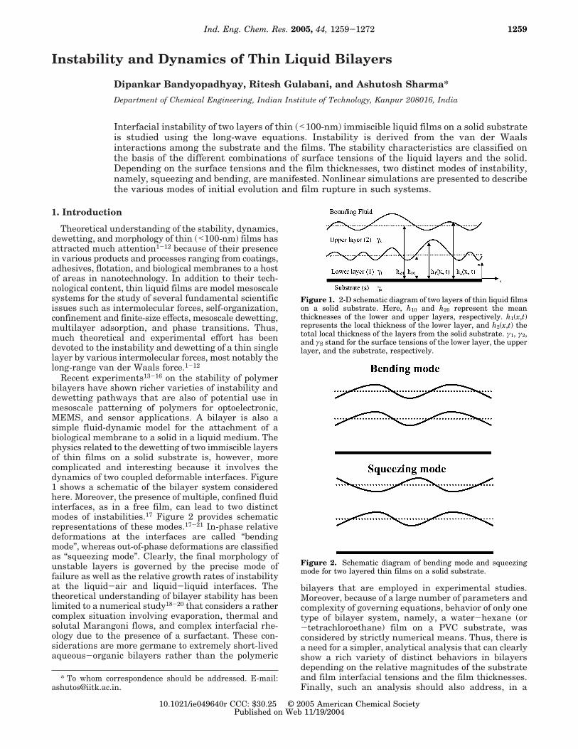
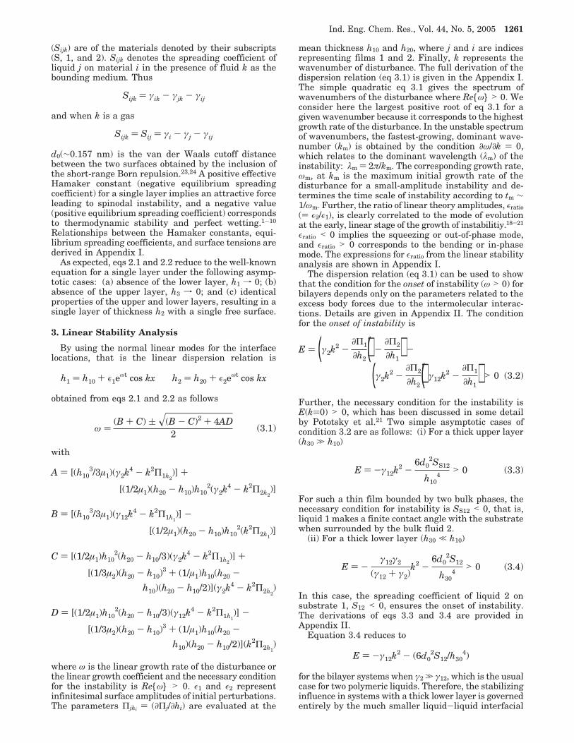
Recent experiments13-16 on the stability of polymerbilayers have shown richer varieties of instability anddewetting pathways that are also of potential use inmesoscale patterning of polymers for optoelectronic,MEMS, and sensor applications. A bilayer is also asimple fluid-dynamic model for the attachment of abiological membrane to a solid in a liquid medium. Thephysics related to the dewetting of two immiscible layersof thin films on a solid substrate is, however, morecomplicated and interesting because it involves thedynamics of two coupled deformable interfaces. Figure1 shows a schematic of the bilayer system consideredhere. Moreover, the presence of multiple, confined fluidinterfaces, as in a free film, can lead to two distinctmodes of instabilities.17 Figure 2 provides schematicrepresentations of these modes.17-21 In-phase relativedeformations at the interfaces are called “bendingmode”, whereas out-of-phase deformations are classifiedas “squeezing mode”. Clearly, the final morphology ofunstable layers is governed by the precise mode offailure as well as the relative growth rates of instabilityat the liquid-air and liquid-liquid interfaces. Thetheoretical understanding of bilayer stability has beenlimited to a numerical study18-20 that considers a rathercomplex situation involving evaporation, thermal andsolutal Marangoni flows, and complex interfacial rhe-ology due to the presence of a surfactant. These con-siderations are more germane to extremely short-livedaqueous-organic bilayers rather than the polymeric

bilayers that are employed in experimental studies.Moreover, because of a large number of parameters andcomplexity of governing equations, behavior of only onetype of bilayer system, namely, a water-hexane (or-tetrachloroethane) film on a PVC substrate, wasconsidered by strictly numerical means. Thus, there isa need for a simpler, analytical analysis that can clearlyshow a rich variety of distinct behaviors in bilayersdepending on the relative magnitudes of the substrateand film interfacial tensions and the film thicknesses.Finally, such an analysis should also address, in a

* To whom correspondence should be addressed. E-mail:[email protected].

Figure 1. 2-D schematic diagram of two layers of thin liquid filmson a solid substrate. Here, h10 and h20 represent the meanthicknesses of the lower and upper layers, respectively. h1(x,t)represents the local thickness of the lower layer, and h2(x,t) thetotal local thickness of the layers from the solid substrate. γ1, γ2,and γS stand for the surface tensions of the lower layer, the upperlayer, and the substrate, respectively.

Figure 2. Schematic diagram of bending mode and squeezingmode for two layered thin films on a solid substrate.

1259Ind. Eng. Chem. Res. 2005, 44, 1259-1272

10.1021/ie049640r CCC: $30.25 © 2005 American Chemical SocietyPublished on Web 11/19/2004

physically transparent way, the problem of mode selec-tion, which can otherwise be obscured by a large numberof coupled phenomena resolved only by numericalanalysis, without any general insights. This study,together with a recent short note of Pototsky et al.,21 isdirected toward these ends. In the note of Pototsky etal.,21 which appeared during the review of this work,basic bilayer equations were independently derived interms of energy variations. These equations can also beshown to transform to the starting equations presentedhere, which were obtained first in the Master’s thesisof one of the authors.22 Thus, although the starting setsof equations are formally identical, we present here aclassification of distinct bilayer systems based on theirinterfacial tensions and their instability characteristics.Detailed results for the linear and nonlinear modeselections are presented. It is shown that, interestingly,the initial linear mode of instability (bending or squeez-ing) can change during the course of nonlinear evolutionnear rupture. In this paper, we present a simple andphysically transparent theory for the onset, dynamics,and modes of instability and relate the results to themacroscopic surface parameters, such as surface ten-sions, that are readily accessible to an experimentalist.In particular, we devise a rational classification schemefor the bilayers based on the relative surface tensionsof the substrate, film1, and film2 and contrast in detailthe instability behavior of each class of bilayers.

2. Nonlinear Long-Wave Dynamics

In this section, x and z are the coordinates paralleland normal to the substrate surface, respectively (asshown in Figure 1), and t represents time. We followthe convention that the subscript i of a variable denotesthe respective fluid layer (i ) 1 denotes the lower layerand i ) 2 denotes the upper layer), S denotes the solidsubstrate, and g denotes bounding fluid (a nonviscousgas). Thus, for layer i, ui is the x component of velocity,wi is the z component of velocity, µi is the viscosity, φiis the excess body force due to intermolecular interac-tions, and Pi ()pi + φi) is the total pressure. γi and γSare the surface tensions of the ith fluid layer and thesolid substrate, respectively. Also, the subscripts t, x,and z in all equations denote differentiation with respectto time and the respective coordinate. Both the notationsh2 - h1 and h3 represent the thickness of the upperlayer. Gravity is neglected in comparison to van derWaals forces because the films are very thin (<100 nm)and thus instability due to density differences is notconsidered.

The long-wave equations of motion for the two layers

the equations of continuity for the two layers

and the kinematic conditions for individual layers

together with the equations of capillarity for the twointerfaces, finally give the equations for the position ofinterfaces, hi ) hi(x,t). The following boundary condi-tions are used

(zero shear)

(continuity of velocity and shear stress at the liquid-liquid interface), and

(no-slip and impermeability at the solid-liquid inter-face). Details of the derivation are given in Appendix I.The evolution equations thus obtained and detailedbelow describe the stability, dynamics, and morphologyof the liquid-air interface (i ) 2) and the liquid-liquidinterface (i ) 1).

In these equations, the total pressures at the liquid-liquid and liquid-air interface are

and

respectively, where p0 denotes the ambient gas pressureand γ12 denotes the interfacial tension at the liquid-liquid interface. The van der Waals disjoining pressures(negative of conjoining pressures)1-5,17 for the twointerfaces are given by

and

As an exception to the indicial notation followed in thispaper, the subscripts of effective Hamaker constants (Ai)are arbitrary and do not represent any fluid layer. Theeffective Hamaker constants (Ai) used in the disjoiningpressure relations above are related to the binaryHamaker constants and also to the macroscopic equi-librium spreading coefficients in the following manner(Appendix I)23,24

and

where the binary Hamaker constants (Aij), interfacialtensions (γij), and equilibrium spreading coefficients

µiuizz ) (pi + φi)x

uix + wiz ) 0

hit + (ui)hihix ) (wi)hi

at z ) h2 µ2u2z ) 0

at z ) h1 u2 ) u1, w2 ) w1, µ2u2z ) µ1u1z

at z ) 0 u1 ) w1 ) 0

∂h1

∂t- 1

3µ1

∂

∂x(h13 ∂P1

∂x ) + 12µ1

∂

∂x[h12(h1 - h2)

∂P2

∂x ] ) 0

(2.1)

∂h2

∂t+ ∂

∂x{[ 13µ2

(h1 - h2)3 + 1

µ1(h1 - h2)h1(h2 -

h1

2 )] ∂P2

∂x } + 12µ1

∂

∂x[h12(h1

3- h2) ∂P1

∂x ] ) 0 (2.2)

P1 ) p0 - γ2h2xx - γ12h1xx - Π1

P2 ) p0 - γ2h2xx - Π2

Π1 ) -A2/6πh13 + A3/6πh2

3

Π2 ) -A1/6π(h2 - h1)3 + A3/6πh2

3

A1 ) A22 - A12 ) -12πd02S12

A2 ) A11 + AS2 - AS1 - A12 ) -12πd02SS12

A3 ) AS2 - A12 ) -12πd02SS12 + 12πd0

2SS1

1260 Ind. Eng. Chem. Res., Vol. 44, No. 5, 2005

(Sijk) are of the materials denoted by their subscripts(S, 1, and 2). Sijk denotes the spreading coefficient ofliquid j on material i in the presence of fluid k as thebounding medium. Thus

and when k is a gas

d0(∼0.157 nm) is the van der Waals cutoff distancebetween the two surfaces obtained by the inclusion ofthe short-range Born repulsion.23,24 A positive effectiveHamaker constant (negative equilibrium spreadingcoefficient) for a single layer implies an attractive forceleading to spinodal instability, and a negative value(positive equilibrium spreading coefficient) correspondsto thermodynamic stability and perfect wetting.1-10

Relationships between the Hamaker constants, equi-librium spreading coefficients, and surface tensions arederived in Appendix I.

As expected, eqs 2.1 and 2.2 reduce to the well-knownequation for a single layer under the following asymp-totic cases: (a) absence of the lower layer, h1 f 0; (b)absence of the upper layer, h3 f 0; and (c) identicalproperties of the upper and lower layers, resulting in asingle layer of thickness h2 with a single free surface.

3. Linear Stability Analysis

By using the normal linear modes for the interfacelocations, that is the linear dispersion relation is

obtained from eqs 2.1 and 2.2 as follows

with

where ω is the linear growth rate of the disturbance orthe linear growth coefficient and the necessary conditionfor the instability is Re{ω} > 0. ε1 and ε2 representinfinitesimal surface amplitudes of initial perturbations.The parameters Πjhi ) (∂Πj/∂hi) are evaluated at the

mean thickness h10 and h20, where j and i are indicesrepresenting films 1 and 2. Finally, k represents thewavenumber of disturbance. The full derivation of thedispersion relation (eq 3.1) is given in the Appendix I.The simple quadratic eq 3.1 gives the spectrum ofwavenumbers of the disturbance where Re{ω} > 0. Weconsider here the largest positive root of eq 3.1 for agiven wavenumber because it corresponds to the highestgrowth rate of the disturbance. In the unstable spectrumof wavenumbers, the fastest-growing, dominant wave-number (km) is obtained by the condition ∂ω/∂k ) 0,which relates to the dominant wavelength (λm) of theinstability: λm ) 2π/km. The corresponding growth rate,ωm, at km is the maximum initial growth rate of thedisturbance for a small-amplitude instability and de-termines the time scale of instability according to tm ∼1/ωm. Further, the ratio of linear theory amplitudes, εratio() ε2/ε1), is clearly correlated to the mode of evolutionat the early, linear stage of the growth of instabilitiy.18-21

εratio < 0 implies the squeezing or out-of-phase mode,and εratio > 0 corresponds to the bending or in-phasemode. The expressions for εratio from the linear stabilityanalysis are shown in Appendix I.

The dispersion relation (eq 3.1) can be used to showthat the condition for the onset of instability (ω > 0) forbilayers depends only on the parameters related to theexcess body forces due to the intermolecular interac-tions. Details are given in Appendix II. The conditionfor the onset of instability is

Further, the necessary condition for the instability isE(k)0) > 0, which has been discussed in some detailby Pototsky et al.21 Two simple asymptotic cases ofcondition 3.2 are as follows: (i) For a thick upper layer(h30 . h10)

For such a thin film bounded by two bulk phases, thenecessary condition for instability is SS12 < 0, that is,liquid 1 makes a finite contact angle with the substratewhen surrounded by the bulk fluid 2.

(ii) For a thick lower layer (h30 , h10)

In this case, the spreading coefficient of liquid 2 onsubstrate 1, S12 < 0, ensures the onset of instability.The derivations of eqs 3.3 and 3.4 are provided inAppendix II.

Equation 3.4 reduces to

for the bilayer systems when γ2 . γ12, which is the usualcase for two polymeric liquids. Therefore, the stabilizinginfluence in systems with a thick lower layer is governedentirely by the much smaller liquid-liquid interfacial

E ) (γ2k2 -

∂Π1

∂h2)(-

∂Π2

∂h1) -

(γ2k2 -

∂Π2

∂h2)(γ12k

2 -∂Π1

∂h1) > 0 (3.2)

E ) -γ12k2 -

6d02SS12

h104

> 0 (3.3)

E ) -γ12γ2

(γ12 + γ2)k2 -

6d02S12

h304

> 0 (3.4)

E ) -γ12k2 - (6d0

2S12/h304)

Sijk ) γik - γjk - γij

Sijk ) Sij ) γi - γj - γij

h1 ) h10 + ε1eωt cos kx h2 ) h20 + ε2e

ωt cos kx

ω )(B + C) ( x(B - C)2 + 4AD

2(3.1)

A ) [(h103/3µ1)(γ2k

4 - k2Π1h2)] +

[(1/2µ1)(h20 - h10)h102(γ2k

4 - k2Π2h2)]

B ) [(h103/3µ1)(γ12k

4 - k2Π1h1)] -

[(1/2µ1)(h20 - h10)h102(k2Π2h1

)]

C ) [(1/2µ1)h102(h20 - h10/3)(γ2k

4 - k2Π1h2)] +

[(1/3µ2)(h20 - h10)3 + (1/µ1)h10(h20 -

h10)(h20 - h10/2)](γ2k4 - k2Π2h2

)

D ) [(1/2µ1)h102(h20 - h10/3)(γ12k

4 - k2Π1h1)] -

[(1/3µ2)(h20 - h10)3 + (1/µ1)h10(h20 -

h10)(h20 - h10/2)](k2Π2h1)

Ind. Eng. Chem. Res., Vol. 44, No. 5, 2005 1261

tension, rather than by the surface tension of the upperthin film. A much smaller stabilizing interfacial tensionforce in this case makes such a bilayer much moreunstable compared to a single thin layer on the sub-strate.

4. Dimensionless Equations

Evolution eqs 2.1 and 2.2 can be made dimensionlessfor a compact representation of numerical results byintroducing the following variables

where

with

where the function sgn is defined as +1 or -1 dependingon the sign of SS12.

The equations were discretized using a central dif-ferencing method in space with half-node interpolation.The resultant set of stiff coupled ordinary differentialequations was solved using Gear’s algorithm (NAGlibrary routine D02EJF) with an initial volume preserv-ing random perturbation and periodic boundary condi-tions. Numerical stiffness of the equations results fromlarge changes in the disjoining pressure terms as thefilm thicknesses decrease locally. Thus, as is well-knownin the context of a single film,6 the growth of instabilityleading to rupture becomes explosive after an initiallinear phase of evolution. This introduces a “fast” timescale in locally thin regions of higher slope.

5. Results and Discussion

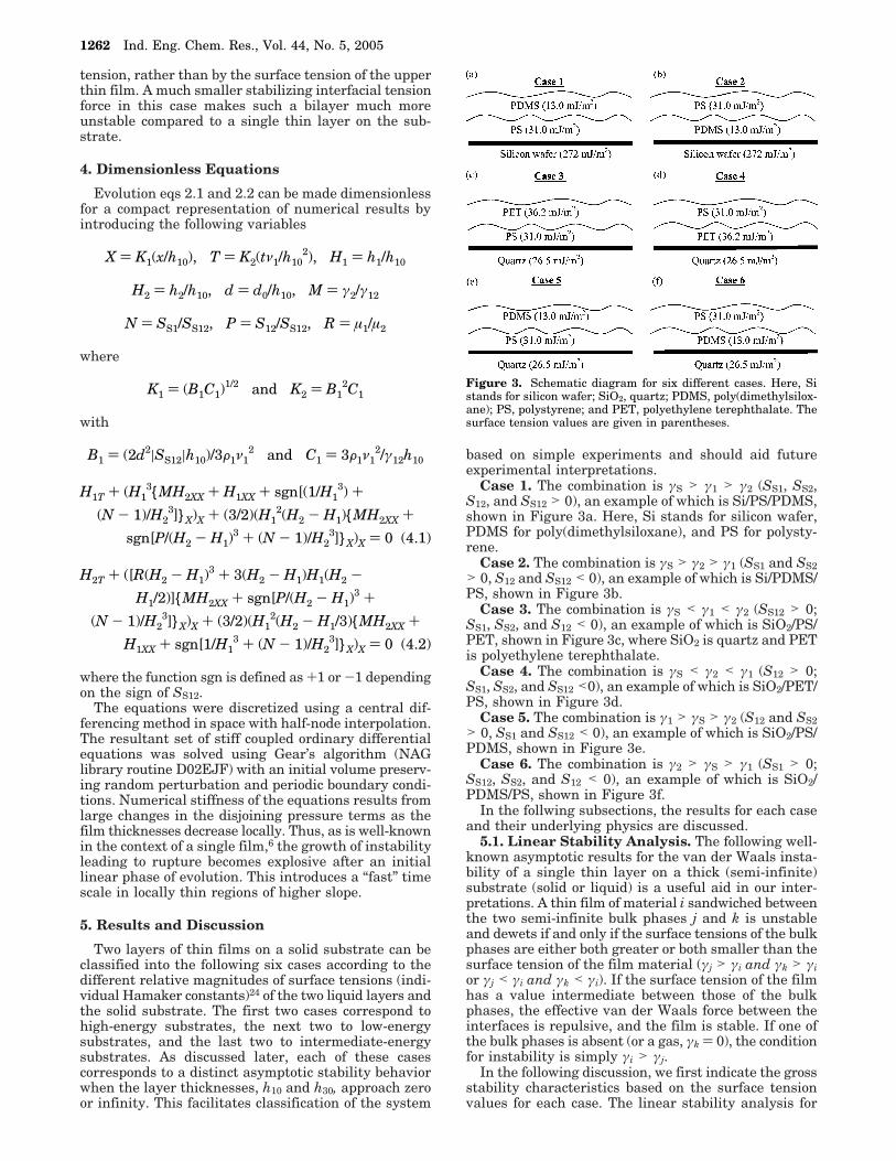
Two layers of thin films on a solid substrate can beclassified into the following six cases according to thedifferent relative magnitudes of surface tensions (indi-vidual Hamaker constants)24 of the two liquid layers andthe solid substrate. The first two cases correspond tohigh-energy substrates, the next two to low-energysubstrates, and the last two to intermediate-energysubstrates. As discussed later, each of these casescorresponds to a distinct asymptotic stability behaviorwhen the layer thicknesses, h10 and h30, approach zeroor infinity. This facilitates classification of the system

based on simple experiments and should aid futureexperimental interpretations.

Case 1. The combination is γS > γ1 > γ2 (SS1, SS2,S12, and SS12 > 0), an example of which is Si/PS/PDMS,shown in Figure 3a. Here, Si stands for silicon wafer,PDMS for poly(dimethylsiloxane), and PS for polysty-rene.

Case 2. The combination is γS > γ2 > γ1 (SS1 and SS2> 0, S12 and SS12 < 0), an example of which is Si/PDMS/PS, shown in Figure 3b.

Case 3. The combination is γS < γ1 < γ2 (SS12 > 0;SS1, SS2, and S12 < 0), an example of which is SiO2/PS/PET, shown in Figure 3c, where SiO2 is quartz and PETis polyethylene terephthalate.

Case 4. The combination is γS < γ2 < γ1 (S12 > 0;SS1, SS2, and SS12 <0), an example of which is SiO2/PET/PS, shown in Figure 3d.

Case 5. The combination is γ1 > γS > γ2 (S12 and SS2> 0, SS1 and SS12 < 0), an example of which is SiO2/PS/PDMS, shown in Figure 3e.

Case 6. The combination is γ2 > γS > γ1 (SS1 > 0;SS12, SS2, and S12 < 0), an example of which is SiO2/PDMS/PS, shown in Figure 3f.

In the follwing subsections, the results for each caseand their underlying physics are discussed.

5.1. Linear Stability Analysis. The following well-known asymptotic results for the van der Waals insta-bility of a single thin layer on a thick (semi-infinite)substrate (solid or liquid) is a useful aid in our inter-pretations. A thin film of material i sandwiched betweenthe two semi-infinite bulk phases j and k is unstableand dewets if and only if the surface tensions of the bulkphases are either both greater or both smaller than thesurface tension of the film material (γj > γi and γk > γior γj < γi and γk < γi). If the surface tension of the filmhas a value intermediate between those of the bulkphases, the effective van der Waals force between theinterfaces is repulsive, and the film is stable. If one ofthe bulk phases is absent (or a gas, γk ) 0), the conditionfor instability is simply γi > γj.

In the following discussion, we first indicate the grossstability characteristics based on the surface tensionvalues for each case. The linear stability analysis for

Figure 3. Schematic diagram for six different cases. Here, Sistands for silicon wafer; SiO2, quartz; PDMS, poly(dimethylsilox-ane); PS, polystyrene; and PET, polyethylene terephthalate. Thesurface tension values are given in parentheses.

X ) K1(x/h10), T ) K2(tν1/h102), H1 ) h1/h10

H2 ) h2/h10, d ) d0/h10, M ) γ2/γ12

N ) SS1/SS12, P ) S12/SS12, R ) µ1/µ2

K1 ) (B1C1)1/2 and K2 ) B1

2C1

B1 ) (2d2|SS12|h10)/3F1ν12 and C1 ) 3F1ν1

2/γ12h10

H1T + (H13{MH2XX + H1XX + sgn[(1/H1

3) +

(N - 1)/H23]}X)X + (3/2)(H1

2(H2 - H1){MH2XX +

sgn[P/(H2 - H1)3 + (N - 1)/H2

3]}X)X ) 0 (4.1)

H2T + ([R(H2 - H1)3 + 3(H2 - H1)H1(H2 -

H1/2)]{MH2XX + sgn[P/(H2 - H1)3 +

(N - 1)/H23]}X)X + (3/2)(H1

2(H2 - H1/3){MH2XX +

H1XX + sgn[1/H13 + (N - 1)/H2

3]}X)X ) 0 (4.2)


each system is then presented to understand thebehavior of unstable systems in detail.

Case 1 (γS > γ1 > γ2). The surface tension valuessuggest that the lower layer is stable in the absence ofany upper layer (SS1 > 0) as well as under a thick upperlayer (SS12 > 0). The upper layer is also stable both whenthe lower layer is absent (SS2 > 0) and when the lowerlayer is thick (S12 > 0). Therefore, this system isunconditionally stable.

Case 2 (γS > γ2 > γ1). In this system, a thin lowerlayer is stable in the absence of the upper layer (SS1 >0), but unstable when a thick upper layer is present(SS12 < 0). Further, the upper layer is stable in theabsence of the lower layer (SS2 > 0), but unstable on athick lower layer (S12 < 0). In view of the aboveconsiderations, it might be anticipated that the overallinstability will be dominated by the instability of theupper layer when it is relatively thin (on a semi-infinitelower layer). In contrast, the instability of the lowerlayer (sandwiched between two semi-infinite media)should drive the system for a relatively thick upperlayer.

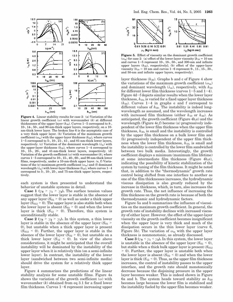
Figure 4 summarizes the predictions of the linearstability analysis for some unstable films. Figure 4ashows the variation of the growth coefficient (ω) withwavenumber (k) obtained from eq 3.1 for a fixed lowerfilm thickness. Curves 1-6 represent increasing upper

layer thickness (h30). Graphs b and c of Figure 4 showthe variations of the maximum growth coefficient (ωm)and dominant wavelength (λm), respectively, with h30for different lower film thickness (curves 1-5 and 1-4).Figure 4d-f depicts similar results when the lower layerthickness, h10, is varied for a fixed upper layer thickness(h30). Curves 1-4 in graphs e and f correspond todifferent values of h30. The instability is indeed long-wavelength as assumed, and the wavelength increaseswith increased film thickness (either h10 or h30). Asanticipated, the growth coefficient (Figure 4b,e) and thewavelength (Figure 4c,f) become (a) progressively inde-pendent of the lower film thickness when the upper filmthickness, h30, is small and the instability is controlledby the upper film thickness on a bulk lower film and(b) progressively independent of the upper film thick-ness when the lower film thickness, h10, is small andthe instability is controlled by the lower film sandwichedbetween two bulk media. Interestingly, the growthcoefficient displays a minimum (maximum film lifetime)at some intermediate film thickness (Figure 4b,e),indicating the possibility of kinetic stabilization of thesystem by tuning of the film thickness. It might be notedthat, in addition to the “thermodynamic” growth ratecontrol being shifted from one interface to another asone of the film thicknesses increases, the hydrodynamicviscous dissipation is also greatly reduced by theincrease in thickness, which, in turn, also increases thegrowth rate. Thus, the net influence of increasing thefilm thickness on the growth rate is because of both thethermodynamic and hydrodynamic factors.

Figure 5a and b summarizes the influence of viscosi-ties on the maximum growth coefficient. In general, thegrowth rate of instability declines with increased viscos-ity of either layer. However, the effect of the upper-layerviscosity on the growth coefficient becomes insignificantwhen the upper layer is very thick and much of thedissipation occurs in the thin lower layer (curve 6,Figure 5b). The variation of ωm with the upper layerthickness is nonmonotonic, as already discussed.

Case 3 (γS < γ1 < γ2). In this system, the lower layeris unstable in the absence of the upper layer (SS1 < 0),but stable when a thick bulk upper layer is present (SS12> 0). Further, the upper layer is unstable both whenthe lower layer is absent (SS2 < 0) and when the lowerlayer is thick (S12 < 0). Thus, as the upper film thicknessincreases, the control of instability passes to the upperinterface, and the growth rate should monotonicallydecrease because the disjoining pressure in the upperlayer becomes weaker. This is indeed shown in Figure6a and b. The system heads toward stability as h30becomes large because the lower film is stabilized andthe instability fueled by the upper film becomes weaker.

Figure 4. Linear stability results for case 2: (a) Variation of thelinear growth coefficient (ω) with wavenumber (k) at differentthicknesses of the upper layer (h30). Curves 1-5 correspond to 8-,10-, 14-, 50-, and 90-nm-thick upper layers, respectively, on a 10-nm-thick lower layer. The broken line 6 is the asymptotic case ofa very thick upper layer. (b) Variation of the maximum growthcoefficient (ωm) with the upper-layer thickness (h30), where curves1-5 correspond to 5-, 10-, 21-, 41-, and 81-nm-thick lower layers,respectively. (c) Variation of the dominant wavelength (λm) withthe upper-layer thickness (h30), where curves 1-4 correspond to10-, 15-, 20-, and 41-nm-thick lower layers, respectively. (d)Variation of the growth coefficient (ω) with wavenumber (k), wherecurves 1-5 correspond to 10-, 15-, 40-, 60-, and 90-nm-thick lowerfilms, respectively, under a 10-nm-thick upper layer. (e, f) Varia-tions of the (e) maximum growth coefficient (ωm) and (f) dominantwavelength (λm) with lower-layer thickness (h10), where curves 1-4correspond to 5-, 10-, 25-, and 75-nm-thick upper layers, respec-tively.

Figure 5. Effect of viscosity on the dominant growth coefficient(ωm) for case 2: (a) effect of the lower-layer viscosity [h10 ) 10 nmand curves 1-5 represent 10-, 18-, 50-, and 300-nm and infiniteupper layers (h30), respectively]; (b) effect of the upper-layerviscosity (h10 ) 10 nm and curves 1-6 represent 9-, 11-, 15-, 30-,and 50-nm and infinite upper layers, respectively).


An interesting aspect of the ω versus k plot (Figure 6a)is the existence of two local maxima in this case. Withincreasing thickness, the maximum at higher wave-number decays much faster than that at lower wave-number, and eventually, the low-wavenumber (higher-wavelength) mode becomes dominant, as shown by anabrupt shift in the dominant wavelength in Figure 6c.The growth rate and the dominant wavelength bothbecome rather independent of the lower-layer thicknessafter the transition, beyond which only the upper-layerthickness controls the instability. The h10-independentregime at relatively lower values of h10 is more clearlyseen in graphs e and f of Figure 6. However, at relativelylarge values of h10 (at fixed h30), the instability growsstronger and approaches the instability characteristicsof the thin upper layer on a thick lower layer. Increasingh10 (at fixed h30) leads to the high-wavenumber (low-wavelength) mode becoming dominant (Figure 6f).

Figure 7a,b shows the expected decrease in thegrowth rate with increased viscosities at different valuesh30 and constant h10. The broken lines correspond to theregime where the low-wavenumber mode is dominant.

Case 4 (γS < γ2 < γ1). In this case, the lower layer isunconditionally unstable, both when the upper layer isabsent (SS1 < 0) and when the upper layer is thick (SS12

< 0). Further, the upper layer is unstable on the solidin the absence of a lower layer (SS2 < 0), but is stableon a thick lower layer (S12 > 0).

Figure 8a-f summarizes the salient features as thefilm thicknesses are varied. The asymptotic values ofωm and λm for thick upper films correspond to theinstability of the lower thin film between two bulkphases and depend solely on the lower film thickness(Figure 8b,c). For small h30, λm (Figure 8c) and ωm(Figure 8b) reach another asymptotic case of a singlelower film, which is also unstable. Because the instabil-ity is largely controlled by the unstable lower layer, it

Figure 6. Linear stability results for case 3: (a) Variation of thegrowth coefficient (ω) with wavenumber (k), where curves 1-4correspond to 15-, 16-, 17-, and 19-nm-thick upper layers, respec-tively, on a 10-nm-thick lower layer. (b) Variation of the maximumgrowth coefficient (ωm) with the upper-layer thickness (h30), wherecurves 1-3 correspond to 10-, 31-, and 61-nm-thick lower layers,respectively. (c) Variation of the dominant wavelength (λm) withthe upper-layer thickness (h30), where curves 1-3 correspond to10-, 15-, and 20-nm-thick lower layers, respectively. Curves 1a-3a correspond to the same thicknesses after the shift of thedominant mode to small wavenumbers. (d) Variation of the growthcoefficient (ω) with wavenumber (k), where curves 1-4 correspondto 5-, 10-, 12-, and 15-nm-thick lower layers, respectively, undera 20-nm-thick upper layer. (e, f) Variations of the (e) maximumgrowth coefficient (ωm) and (f) dominant wavelength (λm) with thelower-layer thickness (h10), where curves 1-3 correspond to 13-,20-, and 25-nm-thick upper layers, respectively. Curves 1a-3a inf correspond to the same thicknesses after the shift to highwavenumbers.

Figure 7. Effect of viscosity on the dominant growth coefficient(ωm) for case 3: (a) effect of the lower-layer viscosity [h10 ) 10 nmand curves 1-4 represent 10-, 15-, 20-, and 40-nm-thick upperlayers (h30), respectively]; (b) effect of the upper-layer viscosity (h10) 10 nm and curves 1-4 represent 10-, 13-, 19-, and 40-nm-thickupper layers, respectively).

Figure 8. Linear stability results for case 4: (a) Variation of thelinear growth coefficient (ω) with wavenumber (k), where curves1-5 correspond to 5-, 10-, 15-, 16-, and 17-nm-thick upper layers,respectively, on a 10-nm-thick lower layer. (b) Variation of themaximum growth coefficient (ωm) with the upper-layer thickness(h30), where curves 1-4 correspond to 5-, 7-, 9-, and 12-nm-thicklower layers, respectively. (c) Variation of the dominant wave-length (λm) with the upper-layer thickness (h30), where curves 1-5correspond to 5-, 7-, 10-, 15-, and 31-nm-thick lower layers,respectively. (d) Variation of the growth coefficient (ω) withwavenumber (k), where curves 1-4 correspond to 10-, 12-, 15-,and 20-nm-thick lower layers, respectively, under a 10-nm-thickupper layer. (e) Variation of the maximum growth coefficient (ωm)with the lower-layer thickness (h10), where curves 1-6 correspondto 5-, 10-, 15-, 25-, 35-, and 55-nm-thick upper layers, respectively.(f) Variation of the dominant wavelength (λm) with the lower-layerthickness (h10), where curves 1-5 correspond to 5-, 10-, 15-, 25-,and 35-nm-thick upper layers, respectively.


grows stronger as h10 decreases for a fixed upper-layerthickness (Figure 8d-f). This is because, as the lowerlayer grows thicker, its intermolecular disjoining pres-sure becomes weaker, and in addition, the instabilityof the upper layer also becomes weaker because theupper layer on a thick lower layer is stable. Figure 9a,bshows the expected effects of viscosities of either layeron the growth rate of instability. Figure 9 also showsthe influence of the lower-layer thickness (Figures 5 and7 earlier showed the influence of the upper-layer thick-ness).

Case 5 (γ1 > γS > γ2). In this case, the lower layer isagain unconditionally unstable, both when the upperlayer is absent (SS1 < 0) and when the upper layer isvery thick (SS12 < 0). However, in contrast to case 4above, the upper layer is unconditionally stable on itssubstrate both when the lower layer is absent (SS2 > 0)and when the lower layer is very thick (S12 > 0). Quiteclearly, the unstable bottom layer (liquid-liquid inter-face) engenders the instability, and the top layer exertsa stabilizing influence.

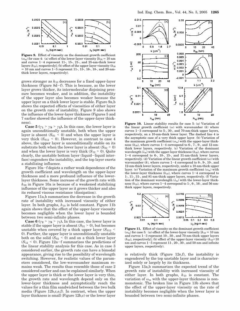
Figure 10a-f depicts a rather weak dependence of thegrowth coefficient and wavelength on the upper-layerthickness and a more profound influence of the lower-layer thickness. Some increase of the growth rate withh30 in Figure 10a is because of a weakened stabilizinginfluence of the upper layer as it grows thicker and alsoits reduced viscous resistance (dissipation).

Figure 11a,b summarizes the decrease in the growthrate of instability with increased viscosity of eitherlayer. In both graphs, h10 is held constant. Figure 11bagain shows that the effect of the upper-layer viscositybecomes negligible when the lower layer is boundedbetween two semi-infinite phases.

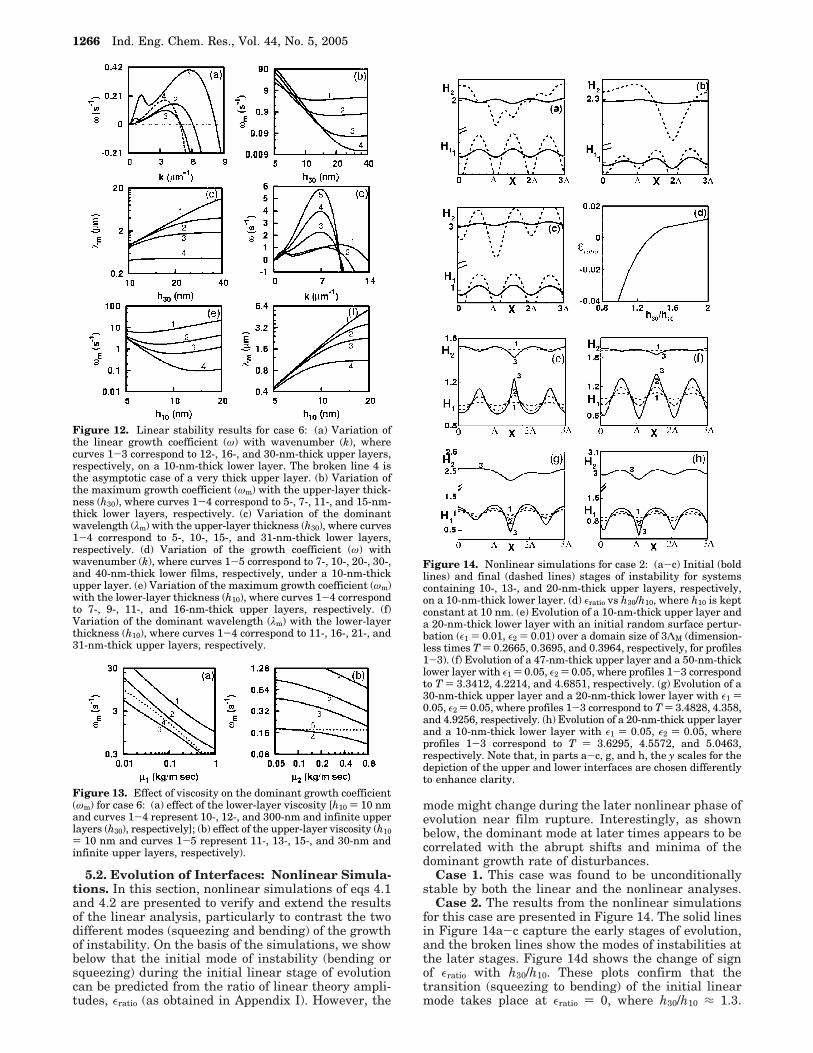
Case 6 (γ2 > γS > γ1). In this case, the lower layer isstable if the upper layer is absent (SS1 > 0), but becomesunstable when covered by a thick upper layer (SS12 <0). Further, the upper layer is unconditionally unstableboth on the solid (SS2 < 0) and on a thick lower layer(S12 < 0). Figure 12a-f summarizes the predictions ofthe linear stability analysis for this case. As in case 3considered earlier, the growth rate can have a bimodalappearance, giving rise to the possibility of wavelengthswitching. However, for realistic values of the param-eters considered, the low-wavenumber maximum re-mains weak. The results thus resemble those of case 2considered earlier and can be explained similarly. Whenthe upper layer is thick or the lower layer is very thin,the growth rate and wavelength depend only on thelower-layer thickness and asymptotically reach thevalues for a thin film sandwiched between the two bulkmedia (Figure 12b,c,e,f). In contrast, when the upperlayer thickness is small (Figure 12b,c) or the lower layer

is relatively thick (Figure 12e,f), the instability isengendered by the top unstable layer and is character-ized solely or largely by its thickness.

Figure 13a,b summarizes the expected trend of thegrowth rate of instability with increased viscosity ofeither layer. In both graphs, h10 is constant. Thevariation of ωm with the upper-layer thickness is non-monotonic. The broken line in Figure 13b shows thatthe effect of the upper-layer viscosity on the rate ofinstability becomes negligible when the lower layer isbounded between two semi-infinite phases.

Figure 9. Effect of viscosity on the dominant growth coefficient(ωm) for case 4: (a) effect of the lower-layer viscosity [h30 ) 10 nmand curves 1-4 represent 11-, 15-, 21-, and 25-nm-thick lowerlayers (h10), respectively]; (b) effect of the upper-layer viscosity (h30) 10 nm and curves 1-5 represent 11-, 13-, 16-, 18-, and 20-nm-thick lower layers, respectively).

Figure 10. Linear stability results for case 5: (a) Variation ofthe linear growth coefficient (ω) with wavenumber (k) wherecurves 1-3 correspond to 5-, 30-, and 70-nm-thick upper layers,respectively, on a 10-nm-thick lower layer. The dashed line 4 isthe asymptotic case of a very thick upper layer. (b) Variation ofthe maximum growth coefficient (ωm) with the upper-layer thick-ness (h30), where curves 1-4 correspond to 6-, 7-, 9-, and 12-nm-thick lower layers, respectively. (c) Variation of the dominantwavelength (λm) with the upper-layer thickness (h30), where curves1-4 correspond to 6-, 10-, 15-, and 31-nm-thick lower layers,respectively. (d) Variation of the linear growth coefficient (ω) withwavenumber (k), where curves 1-4 correspond to 8-, 9-, 10-, and12-nm-thick lower layers, respectively, under a 10-nm-thick upperlayer. (e) Variation of the maximum growth coefficient (ωm) withthe lower-layer thickness (h10), where curves 1-4 correspond to1-, 11-, 31-, and 81-nm-thick upper layers, respectively. (f) Varia-tion of the dominant wavelength (λm) with the lower-layer thick-ness (h10), where curves 1-4 correspond to 1-, 6-, 16-, and 56-nm-thick upper layers, respectively.

Figure 11. Effect of viscosity on the dominant growth coefficient(ωm) for case 5: (a) effect of the lower-layer viscosity [h10 ) 10 nmand curves 1-3 represent 10-, 30-, and 70-nm-thick upper layers(h30), respectively]; (b) effect of the upper-layer viscosity (h10)10nm and curves 1-5 represent 11-, 20-, 30-, and 50-nm and infiniteupper layers, respectively).


5.2. Evolution of Interfaces: Nonlinear Simula-tions. In this section, nonlinear simulations of eqs 4.1and 4.2 are presented to verify and extend the resultsof the linear analysis, particularly to contrast the twodifferent modes (squeezing and bending) of the growthof instability. On the basis of the simulations, we showbelow that the initial mode of instability (bending orsqueezing) during the initial linear stage of evolutioncan be predicted from the ratio of linear theory ampli-tudes, εratio (as obtained in Appendix I). However, the

mode might change during the later nonlinear phase ofevolution near film rupture. Interestingly, as shownbelow, the dominant mode at later times appears to becorrelated with the abrupt shifts and minima of thedominant growth rate of disturbances.

Case 1. This case was found to be unconditionallystable by both the linear and the nonlinear analyses.

Case 2. The results from the nonlinear simulationsfor this case are presented in Figure 14. The solid linesin Figure 14a-c capture the early stages of evolution,and the broken lines show the modes of instabilities atthe later stages. Figure 14d shows the change of signof εratio with h30/h10. These plots confirm that thetransition (squeezing to bending) of the initial linearmode takes place at εratio ) 0, where h30/h10 ≈ 1.3.

Figure 12. Linear stability results for case 6: (a) Variation ofthe linear growth coefficient (ω) with wavenumber (k), wherecurves 1-3 correspond to 12-, 16-, and 30-nm-thick upper layers,respectively, on a 10-nm-thick lower layer. The broken line 4 isthe asymptotic case of a very thick upper layer. (b) Variation ofthe maximum growth coefficient (ωm) with the upper-layer thick-ness (h30), where curves 1-4 correspond to 5-, 7-, 11-, and 15-nm-thick lower layers, respectively. (c) Variation of the dominantwavelength (λm) with the upper-layer thickness (h30), where curves1-4 correspond to 5-, 10-, 15-, and 31-nm-thick lower layers,respectively. (d) Variation of the growth coefficient (ω) withwavenumber (k), where curves 1-5 correspond to 7-, 10-, 20-, 30-,and 40-nm-thick lower films, respectively, under a 10-nm-thickupper layer. (e) Variation of the maximum growth coefficient (ωm)with the lower-layer thickness (h10), where curves 1-4 correspondto 7-, 9-, 11-, and 16-nm-thick upper layers, respectively. (f)Variation of the dominant wavelength (λm) with the lower-layerthickness (h10), where curves 1-4 correspond to 11-, 16-, 21-, and31-nm-thick upper layers, respectively.

Figure 13. Effect of viscosity on the dominant growth coefficient(ωm) for case 6: (a) effect of the lower-layer viscosity [h10 ) 10 nmand curves 1-4 represent 10-, 12-, and 300-nm and infinite upperlayers (h30), respectively]; (b) effect of the upper-layer viscosity (h10) 10 nm and curves 1-5 represent 11-, 13-, 15-, and 30-nm andinfinite upper layers, respectively).

Figure 14. Nonlinear simulations for case 2: (a-c) Initial (boldlines) and final (dashed lines) stages of instability for systemscontaining 10-, 13-, and 20-nm-thick upper layers, respectively,on a 10-nm-thick lower layer. (d) εratio vs h30/h10, where h10 is keptconstant at 10 nm. (e) Evolution of a 10-nm-thick upper layer anda 20-nm-thick lower layer with an initial random surface pertur-bation (ε1 ) 0.01, ε2 ) 0.01) over a domain size of 3ΛM (dimension-less times T ) 0.2665, 0.3695, and 0.3964, respectively, for profiles1-3). (f) Evolution of a 47-nm-thick upper layer and a 50-nm-thicklower layer with ε1 ) 0.05, ε2 ) 0.05, where profiles 1-3 correspondto T ) 3.3412, 4.2214, and 4.6851, respectively. (g) Evolution of a30-nm-thick upper layer and a 20-nm-thick lower layer with ε1 )0.05, ε2 ) 0.05, where profiles 1-3 correspond to T ) 3.4828, 4.358,and 4.9256, respectively. (h) Evolution of a 20-nm-thick upper layerand a 10-nm-thick lower layer with ε1 ) 0.05, ε2 ) 0.05, whereprofiles 1-3 correspond to T ) 3.6295, 4.5572, and 5.0463,respectively. Note that, in parts a-c, g, and h, the y scales for thedepiction of the upper and lower interfaces are chosen differentlyto enhance clarity.


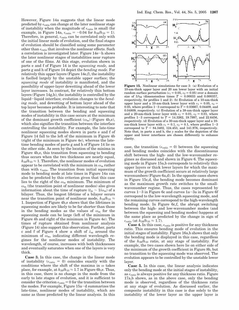
However, Figure 14a suggests that the linear modepredicted by εratio can change at the later nonlinear stageof instability when the magnitude of εratio is small (forexample, in Figure 14a, εratio ) -0.04 for h30/h10 ) 1).Therefore, in general, εratio can be correlated only withthe initial linear mode of evolution, and the final stagesof evolution should be classified using some parameterother than εratio that involves the nonlinear effects. Sucha correlation is investigated later. Figure 14e-h showsthe later nonlinear stages of instabilities near ruptureof one of the films. At this stage, evolution shown inparts e and f of Figure 14 is the squeezing mode, andparts g and h of Figure 14 depict the bending mode. Forrelatively thin upper layers (Figure 14e,f), the instabilityis fuelled largely by the unstable upper surface; thesqueezing mode of instability is manifested, and thepossibility of upper-layer dewetting ahead of the lowerlayer increases. In contrast, for relatively thin bottomlayers (Figure 14g,h), the instability is controlled by theliquid-liquid interface; evolution changes to the bend-ing mode, and dewetting of bottom layer ahead of thetop layer becomes probable. It is interesting to note thatthe transition between the bending and squeezingmodes of instability in this case occurs at the minimumof the dominant growth coefficient (ωm) (Figure 4b,e),which also signifies the transition between the interfacecontrolling the instability. For example, the late-timenonlinear squeezing modes shown in parts e and f ofFigure 14 fall to the left of the minimum in Figure 4b(right of the minimum in Figure 4e), whereas the late-time bending modes of parts g and h of Figure 14 lie onthe other side. As seen by the location of the minima inFigure 4b,e, this transition from squeezing to bendingthus occurs when the two thickness are nearly equal,h30/h10 ≈ 1. Therefore, the nonlinear modes of evolutionappear to be correlated with the minimum in ωm ratherthan with εratio. The transition from initial squeezingmode to bending mode at late times in Figure 14a canalso be predicted by this criterion given that this caselies to the right of the ωm minimum. The minimum ofωm (the transition point of nonlinear modes) also givesinformation about the time of rupture (tm ∼ 1/ωm) of abilayer. Thus, the longest lifetime of a bilayer occursnear the transition point of nonlinear mode, h30/h10 ≈1. Inspection of Figure 4b,e shows that the lifetimes insqueezing modes are likely to be far shorter than thosein the bending modes as the values of ωm for thesqueezing mode can be large (left of the minimum inFigure 4b and right of the minimum in Figure 4e). Thetimes of rupture obtained from nonlinear analysis(Figure 14) also support this observation. Further, partsc and f of Figure 4 show a shift of λm around theminimum of ωm, indicating different wavelength re-gimes for the nonlinear modes of instability. Thewavelength, of course, increases with both thicknessesand eventually saturates when one of the layers is verythick.

Case 3. In this case, the change in the linear modeof instability (εratio ) 0) coincides exactly with theconditions where the shift of the maxima in ω takesplace, for example, at h30/h10 ≈ 1.7 in Figure 6b,e. Thus,in this case, there is no change in the mode from theearly to late stages of evolution, and it is sufficient toconsider the criterion εratio ) 0 for the transition betweenthe modes. For example, Figure 15a-d summarizes thelate-time, nonlinear modes of instability, which aresame as those predicted by the linear analysis. In this

case, the transition (εratio ) 0) between the squeezingand bending modes coincides with the discontinuousshift between the high- and the low-wavenumber re-gimes as discussed and shown in Figure 6. The squeez-ing mode in Figure 15a,b corresponds to relatively thinupper layers or thick lower layers for which the maxi-mum of the growth coefficient occurs at relatively largewavenumbers (Figure 6a,d). In the opposite cases shownin Figure 15c,d, the bending mode becomes dominantas the maximum growth rate switches to the small-wavenumber regime. Thus, the cases represented bycurves 1-3 in Figure 6c and curves 1a-3a in Figure 6fcorrespond to the low-wavelength squeezing mode, andthe remaining curves correspond to the high-wavelengthbending mode. In Figure 6c,f, the abrupt switchingbetween the high- and low-wavenumber modes (andbetween the squeezing and bending modes) happens atthe same place as predicted by the change in sign ofεratio (at h30/h10 ≈ 1.7).

Case 4. In this case, εratio is positive for any thicknessratio. This ensures bending mode of evolution in theinitial stages of instability. Figure 16a,b shows that onlythe bending mode is displayed in this case, regardlessof the h30/h10 ratio, at any stage of instability. Forexample, the two cases shown here lie on either side ofthe minimum of the growth coefficient in Figure 8b, butno transition to the squeezing mode was observed. Theevolution appears to be controlled by the unstable lowerlayer.

Case 5. In this case, the linear analysis indicatesonly the bending mode at the initial stages of instability,as εratio is always positive for any thickness ratio. Figure17a,b shows, as in the above case, only the bendingmode is observed, regardless of the thickness ratioat any stage of evolution. As discussed earlier, thecomposite instability in this case is due solely to theinstability of the lower layer as the upper layer is

Figure 15. Nonlinear simulations for case 3: (a) Evolution of a10-nm-thick upper layer and 20 nm lower layer with an initialrandom surface perturbation (ε1 ) 0.05, ε2 ) 0.05) over a domainsize of 3ΛM (dimensionless times T ) 0.00033 and 0.000357,respectively, for profiles 1 and 2). (b) Evolution of a 10-nm-thickupper layer and a 10-nm-thick lower layer with ε1 ) 0.05, ε2 )0.05, where profiles 1-3 correspond to T ) 0.03667, 0.04409, and0.04809, respectively. (c) Evolution of a 38-nm-thick upper layerand a 20-nm-thick lower layer with ε1 ) 0.01, ε2 ) 0.01, whereprofiles 1-3 correspond to T ) 14.3262, 19.7997, and 22.6456,respectively. (d) Evolution of a 30-nm-thick upper layer and a 10-nm-thick lower layer with ε1 ) 0.1, ε2 ) 0.1, where profiles 1-3correspond to T ) 84.3402, 124.453, and 141.976, respectively.Note that, in parts a and b, the y scales for the depiction of theupper and lower interfaces are chosen differently to enhanceclarity.


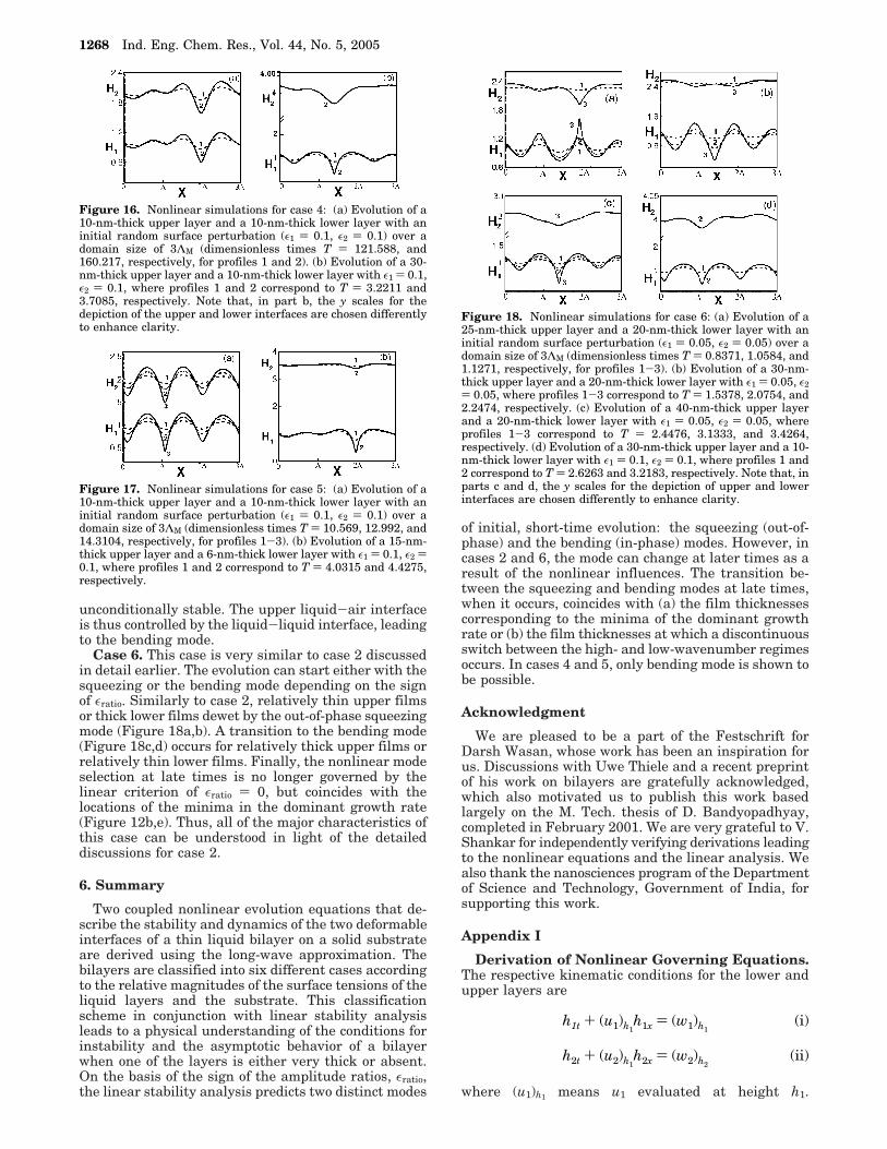
unconditionally stable. The upper liquid-air interfaceis thus controlled by the liquid-liquid interface, leadingto the bending mode.

Case 6. This case is very similar to case 2 discussedin detail earlier. The evolution can start either with thesqueezing or the bending mode depending on the signof εratio. Similarly to case 2, relatively thin upper filmsor thick lower films dewet by the out-of-phase squeezingmode (Figure 18a,b). A transition to the bending mode(Figure 18c,d) occurs for relatively thick upper films orrelatively thin lower films. Finally, the nonlinear modeselection at late times is no longer governed by thelinear criterion of εratio ) 0, but coincides with thelocations of the minima in the dominant growth rate(Figure 12b,e). Thus, all of the major characteristics ofthis case can be understood in light of the detaileddiscussions for case 2.

6. Summary

Two coupled nonlinear evolution equations that de-scribe the stability and dynamics of the two deformableinterfaces of a thin liquid bilayer on a solid substrateare derived using the long-wave approximation. Thebilayers are classified into six different cases accordingto the relative magnitudes of the surface tensions of theliquid layers and the substrate. This classificationscheme in conjunction with linear stability analysisleads to a physical understanding of the conditions forinstability and the asymptotic behavior of a bilayerwhen one of the layers is either very thick or absent.On the basis of the sign of the amplitude ratios, εratio,the linear stability analysis predicts two distinct modes

of initial, short-time evolution: the squeezing (out-of-phase) and the bending (in-phase) modes. However, incases 2 and 6, the mode can change at later times as aresult of the nonlinear influences. The transition be-tween the squeezing and bending modes at late times,when it occurs, coincides with (a) the film thicknessescorresponding to the minima of the dominant growthrate or (b) the film thicknesses at which a discontinuousswitch between the high- and low-wavenumber regimesoccurs. In cases 4 and 5, only bending mode is shown tobe possible.

Acknowledgment

We are pleased to be a part of the Festschrift forDarsh Wasan, whose work has been an inspiration forus. Discussions with Uwe Thiele and a recent preprintof his work on bilayers are gratefully acknowledged,which also motivated us to publish this work basedlargely on the M. Tech. thesis of D. Bandyopadhyay,completed in February 2001. We are very grateful to V.Shankar for independently verifying derivations leadingto the nonlinear equations and the linear analysis. Wealso thank the nanosciences program of the Departmentof Science and Technology, Government of India, forsupporting this work.

Appendix I

Derivation of Nonlinear Governing Equations.The respective kinematic conditions for the lower andupper layers are

where (u1)h1 means u1 evaluated at height h1.

Figure 16. Nonlinear simulations for case 4: (a) Evolution of a10-nm-thick upper layer and a 10-nm-thick lower layer with aninitial random surface perturbation (ε1 ) 0.1, ε2 ) 0.1) over adomain size of 3ΛM (dimensionless times T ) 121.588, and160.217, respectively, for profiles 1 and 2). (b) Evolution of a 30-nm-thick upper layer and a 10-nm-thick lower layer with ε1 ) 0.1,ε2 ) 0.1, where profiles 1 and 2 correspond to T ) 3.2211 and3.7085, respectively. Note that, in part b, the y scales for thedepiction of the upper and lower interfaces are chosen differentlyto enhance clarity.

Figure 17. Nonlinear simulations for case 5: (a) Evolution of a10-nm-thick upper layer and a 10-nm-thick lower layer with aninitial random surface perturbation (ε1 ) 0.1, ε2 ) 0.1) over adomain size of 3ΛM (dimensionless times T ) 10.569, 12.992, and14.3104, respectively, for profiles 1-3). (b) Evolution of a 15-nm-thick upper layer and a 6-nm-thick lower layer with ε1 ) 0.1, ε2 )0.1, where profiles 1 and 2 correspond to T ) 4.0315 and 4.4275,respectively.

Figure 18. Nonlinear simulations for case 6: (a) Evolution of a25-nm-thick upper layer and a 20-nm-thick lower layer with aninitial random surface perturbation (ε1 ) 0.05, ε2 ) 0.05) over adomain size of 3ΛM (dimensionless times T ) 0.8371, 1.0584, and1.1271, respectively, for profiles 1-3). (b) Evolution of a 30-nm-thick upper layer and a 20-nm-thick lower layer with ε1 ) 0.05, ε2) 0.05, where profiles 1-3 correspond to T ) 1.5378, 2.0754, and2.2474, respectively. (c) Evolution of a 40-nm-thick upper layerand a 20-nm-thick lower layer with ε1 ) 0.05, ε2 ) 0.05, whereprofiles 1-3 correspond to T ) 2.4476, 3.1333, and 3.4264,respectively. (d) Evolution of a 30-nm-thick upper layer and a 10-nm-thick lower layer with ε1 ) 0.1, ε2 ) 0.1, where profiles 1 and2 correspond to T ) 2.6263 and 3.2183, respectively. Note that, inparts c and d, the y scales for the depiction of upper and lowerinterfaces are chosen differently to enhance clarity.

h1t + (u1)h1h1x ) (w1)h1

(i)

h2t + (u2)h1h2x ) (w2)h2

(ii)


Integration of the equation of motion of the upperlayer (µ2u2z ) ∫P2x dz) leads to

where P2 is constant in the z direction.At z ) h2, µ2u2z ) 0. Therefore, from eq iii

Thus, eq iii can be modified to

Integration of eq iv [µ2u2 ) ∫(P2xz - P2xh2)dz] leads to

At z ) h1, u2 ) u1. Therefore, from eq v

Integration of the equation of motion of the lower layer[µ1u1z ) ∫P1x dz] leads to

where P1 is constant in the z direction.At z ) h1, µ2u2z ) µ1u1z. Therefore, eqs viii and iv

simplify to

Integration of eq ix {µ1u1 ) ∫[P1xz + (P2x - P1x)h1 -P2xh2] dz} leads to

At z ) 0, u1 ) 0. Therefore, eq x leads to C4 ) 0.Consequently

Differentiation of eq xi with respect to x leads to

The equation of continuity (u1x + w1z ) 0) and eq xiisimplify to

Integrating eq xiii (-µ1w1z ) ∫{P1xx(z2/2) + [(P2x -P1x)h1]xz - (P2xh2)xz} dz] gives

At z ) 0, w1 ) 0. Therefore, eq xiv leads to C5 ) 0 and

At height h1, eqs xi and xv reduce to

Substituting eqs xvi and xvii into eq i gives the finalform of the kinematic condition for the liquid-liquidinterface

Equation vii can be written as follows

Differentiating eq xix with respect to x gives

Replacing u2x from the equation of continuity u2x + w2z) 0 and then integrating eq xx leads to the followingexpression

At z ) h1, w2 ) w1. Therefore, eq xxi gives the expressionfor constant C6

Equation xix is evaluated at height h2

Equations xxii and xxi lead to the following expressionfor w1 at height h2

Substituting eqs xxiii and xxiv into eq ii gives the final

µ2u2z ) P2xz + C1 (iii)

C1 ) -P2xh2

µ2u2z ) P2xz - P2xh2 (iv)

µ2u2 ) P2xz2/2 - P2xh2z + C2 (v)

C2 ) µ2(u1)h1- P2x(h1

2/2) + P2xh2h1 (vi)

µ2u2 ) P2x[(z2 - h1

2)/2] - P2xh2(z - h1) + µ2(u1)h1

(vii)

µ1u1z ) P1xz + C3 (viii)

µ1u1z ) P1xz + (P2x - P1x)h1 - P2xh2 (ix)

µ1u1 ) P1x(z2/2) + (P2x - P1x)h1z - P2xh2z + C4 (x)

µ1u1 ) P1x(z2/2) + (P2x - P1x)h1z - P2xh2z (xi)

µ1u1x ) P1xx(z2/2) + [(P2x - P1x)h1]xz - (P2xh2)xz (xii)

-µ1w1z ) P1xx(z2/2) + [(P2x - P1x)h1]xz - (P2xh2)xz

(xiii)

-µ1w1 ) P1xx(z3/6) + [(P2x - P1x)h1]x(z

2/2) -

(P2xh2)x(z2/2) + C5 (xiv)

-µ1w1 ) P1xx(z3/6) + [(P2x - P1x)h1]x(z

2/2) -

(P2xh2)x(z2/2) (xv)

(u1)h1) (1/µ1)[P1x(h1

2/2) + (P2x - P1x)h12 - P2xh2h1]

(xvi)

(w1)h1 ) (-1/µ1){P1xx(h13/6) +

[(P2x - P1x)h1]x(h12/2) - (P2xh2)x(h1

2/2)} (xvii)

∂h1

∂t- 1

3µ1

∂

∂x(h13 ∂P1

∂x ) + 12µ1

∂

∂x[h12(h1 - h2)

∂P2

∂x ] ) 0

(xviii)

µ2u2 ) P2x[(z2 - h1

2)/2] - P2xh2(z - h1) +

(µ2/µ1)[P1x(h12/2) + (P2x - P1x)h1

2 - P2xh1h2] (xix)

u2x ) (1/µ2)[P2xx(z2/2) - (P2xh1

2/2)x -

(P2xh2)xz + (P2xh2h1)x] + (1/µ1)[(P2xh12)x -

(P2xh2h1)x - (P1xh12/2)x] (xx)

-w2 ) (1/µ2)[P2xx(z3/6) - (P2xh1

2/2)xz -

(P2xh2)x(z2/2) + (P2xh2h1)xz] + (1/µ1)[(P2xh1

2)x -

(P2xh2h1)x - (P1xh12/2)x]z + C6 (xxi)

C6 ) (1/µ1){P1xx(h13/6) + P2xx[(h2h1

2/2) - (h13/2)] +

P2xh1x(h2h1 - 3h12/2) + P1xh1x(h1

2/2) +

P2xh2x(h12/2)} - (1/µ2){P2xx[(- h1

3/3) + (h2h12/2)] +

P2xh1x(h1h2 - h12) + P2xh2x(h1

2/2)} (xxii)

(u2)h2) (1/µ2){P2x[(h2

2 - h12)/2] - P2xh2(h2 - h1)} +

(1/µ1)[-P1x(h12/2) + P2xh1

2 - P2xh1h2] (xxiii)

-(w2)h2 ) (1/µ2){(P2xx/3)(h1 - h2)3 +

P2xh1x(h1 - h2)2 + P2xh2x[h1h2 - (h1

2/2) - (h22/2)]} +

(1/µ1){P2xx[(- h13/2) + (3h1

2h2/2) - h22h1] +

P1xx[(h13/6) - (h1

2h2/2)] + P2xh2x[(h12/2) - h1h2] +

P2xh1x(3h1h2 - h22 - 3h1

2/2) +

P1xh1x[(h12/2) - h1h2]} (xxiv)


form of the kinematic equation for the liquid-airinterface

Linear Stability Analysis. The total pressure (P1) p0 - γ2h2xx - γ12h1xx - Π1) at the liquid-liquidinterface is differentiated with respect to x and linear-ized in the following manner

Therefore

Similarly, the total pressure (P2 ) p0 - γ2h2xx - Π2) atthe liquid-air interface can be differentiated and lin-earized to give

The definitions of disjoining pressures and spreadingcoefficients are as follows

where

and

The binary Hamaker constants and the spreadingcoefficients used here can be obtained from the expres-sions

and when k is a gas

Equations xviii and xxv are linearized with the help ofthe following expressions

which lead to

The following is the list of linearized parameters

Equations xxviii and xxix can be modified by substi-tution of eqs xxvi-xxvii. This leads to

where

The values Πjhi ) (∂Πj/∂hi) are constants determined atmean thickness h10 and h20, where j and i are indicesrepresenting 1 or 2.

Algebraic manipulation of eqs xxx and xxxi gives thedispersion relation

The dispersion relation is used to calculate ωm asmentioned earlier in the paper, and ωm can further beused in eqs xxx and xxxi to calculate the ratio

h1 ) h10 + ε1eωt cos kx

h2 ) h20 + ε2eωt cos kx

h1t - A′P1xx - B′P2xx ) 0 (xxviii)

h2t - C′P2xx - D′P1xx ) 0 (xxix)

h13/3µ1 ≈ h10

3/3µ1 ) A′

(h1 - h2)(h12/2µ1) ≈ (h20 - h10)(h10

2/2µ1) ) B′

(h1 - h2)3/3µ2 + (h2 - h1/2)h1(h2 - h1)/µ1 ≈

(h20 - h10)3/3µ2 + (h20 - h10/2)h10(h20 - h10)/µ1 ) C′

h12(h2 - h1/3)/2µ1 ≈ h10

2(h20 - h10/3)/2µ1 ) D′

ε1ω + ε2A + ε1B ) 0 (xxx)

ε2ω + ε2C + ε1D ) 0 (xxxi)

A ) [(h103/3µ1)(γ2k

4 - k2Π1h2)] +

[(1/2µ1)(h20 - h10)h102(γ2k

4 - k2Π2h2)]

B ) [(h103/3µ1)(γ12k

4 - k2Π1h1)] -

[(1/2µ1)(h20 - h10)h102(k2Π2h1

)]

C ) [(1/2µ1)h102(h20 - h10/3)(γ2k

4 - k2Π1h2)] +

[(1/3µ2)(h20 - h10)3 +

(1/µ1)h10(h20 - h10)(h20 - h10/2)](γ2k4 - k2Π2h2

)

D ) [(1/2µ1)h102(h20 - h10/3)(γ12k

4 - k2Π1h1)] -

[(1/3µ2)(h20 - h10)3 +

(1/µ1)h10(h20 - h10)(h20 - h10/2)](k2Π2h1)

ω )-(B + C) ( x(B - C)2 + 4AD

2(xxxii)

εratio ) ε2/ε1 ) -(ωm + B)/A ) -D/(ωm + C) (xxxiii)

∂h2

∂t+ ∂

∂x{[ 13µ2

(h1 - h2)3 + 1

µ1(h1 - h2)h1(h2 -

h1

2 )]∂P2

∂x } + 12µ1

∂

∂x[h12(h1

3- h2)∂P1

∂x ] ) 0 (xxv)

P1x ) -γ2h2xxx - γ12h1xxx -

(∂Π1

∂h1)

h10,h20

h1x - (∂Π1

∂h2)

h10,h20

h2x

P1xx ) -γ2h2xxxx - γ12h1xxxx -

(∂Π1

∂h1)

h10,h20

h1xx - (∂Π1

∂h2)

h10,h20

h2xx (xxvi)

P2xx ) -γ2h2xxxx - (∂Π2

∂h1)

h10,h20

h1xx - (∂Π2

∂h2)

h10,h20

h2xx

(xxvii)

Π1 ) -A2/6πh13 + A3/6πh2

3

Π2 ) -A1/6π(h2 - h1)3 + A3/6πh2

3

A1 ) A22 - A12 ) -12πd02S12

A2 ) A11 + AS2 - AS1 - A12) -12πd02SS12

A3 ) AS2 - A12 ) (-12πd02SS12 + 12πd0

2SS1)

Aij ) 12πd02(γi + γj - γij)

Sijk ) γik - γjk - γij

Sijk ) Sij ) γi - γj - γij

γij ) (γi + γj - 2xγiγj)


Appendix II

Conditions for Instability. From the linear stabilityanalysis, the condition for instability is ω > 0. Thus,the dispersion relation (eq xxxii from Appendix I)reduces to

The coefficients A-D of Appendix I can be rewrittenas

where

Combining the eqs a and b gives

Because

Equations c and d give the condition for instability, a1a4- a2a3 > 0

The disjoining pressures in terms of Hamaker constantsor equilibrium spreading coefficients in eq e are asfollows

where A1 ) -12πd02S12, A2 ) -12πd0

2SS12, and A3 )-12πd0

2(SS12 - SS1).

The two simple asymptotic cases of eq e are asfollows: (i) For a thick upper layer, h30 . h10

(ii) For a thick lower layer, h30 , h10, which implies

so

Literature Cited

(1) Ruckenstein, E.; Jain, R. K. Spontaneous rupture of thinliquid films. J. Chem. Soc., Faraday Trans. 2 1974, 70, 132-147.

(2) De Gennes, P. G. Wetting: Statics and dynamics. Rev. Mod.Phys. 1985, 57, 827-863.

(3) Brochard-Wyart, F.; Daillant, J. Drying of solids wetted bythin liquid films. Can. J. Phys. 1990, 68, 1084-1088.

(4) Sharma, A. Relationship of thin film stability and morphol-ogy to macroscopic parameters of wetting in the apolar and polarsystems. Langmuir 1993, 9, 861-869.

(5) Reiter, G.; Khanna, R.; Sharma, A. Enhanced Instabilityin Thin Liquid Films by Improved Compatibility. Phys. Rev. Lett.2000, 85, 1432-1435.

(6) Sharma, A.; Jameel, A. T. Nonlinear Stability, Rupture, andMorphological Phase Separation of Thin Fluid Films on Apolarand Polar Substrates. J. Colloid Interface Sci. 1993, 161, 190-208.

(7) Oron, A.; Davis, S. H.; Bankoff, S. G. Long-scale evolutionof thin liquid films. Rev. Mod. Phys. 1997, 69, 931-980.

(8) Sharma, A.; Khanna, R. Pattern Formation in UnstableThin Liquid Films. Phys. Rev. Lett. 1998, 81, 3463-3466.

(9) Sharma, A.; Khanna, R. Pattern formation in unstable thinliquid films under the influence of antagonistic short- and long-range forces. J. Chem. Phys. 1999, 110, 4929-4936.

(10) Oron, A. Three-Dimensional Nonlinear Dynamics of ThinLiquid Films. Phys. Rev. Lett. 2000, 85, 2108-2111.

(11) Konnur, R.; Kargupta, K.; Sharma, A. Instability andMorphology of Thin Liquid Films on Chemically HeterogeneousSubstrates. Phys. Rev. Lett. 2000, 84, 931-934.

(12) Thiele, U.; Velarde, M.; Neuffer, K. Dewetting: FilmRupture by Nucleation in the Spinodal Regime. Phys. Rev. Lett.2001, 87, 016104.

(13) Higgins, A. M.; Jones, R. A. L. Anisotropic spinodaldewetting as a route to self-assembly of patterned surfaces. Nature2000, 404, 476-478.

(14) Lin, Z. Q.; Kerle, T.; Baker, S. M.; Hoagland, D. A.;Schaffer, E.; Steiner, U.; Russell, T. P. Electric field inducedinstabilities at liquid/liquid interfaces. J. Chem. Phys. 2001, 114,2377-2381.

(15) Lin, Z. Q.; Kerle, T.; Russell, T. P.; Schaffer, E.; Steiner,U. Structure formation at the interface of liquid-liquid bilayer inelectric field. Macromolecules 2002, 35, 3971-3976

(16) Lin, Z. Q.; Kerle, T.; Russell, T. P.; Schaffer, E.; Steiner,U. Electric field induced dewetting at polymer/polymer interfaces.Macromolecules 2002, 35, 6255-6262.

(17) Maldarelli, C. H.; Jain, R. K.; Ivanov, I. B.; Ruckenstein,E. Stability of Symmetric and Unsymmetric Thin Liquid Films toShort and Long Wavelength Perturbations. J. Colloid InterfaceSci. 1980, 78, 118-143.

-(B + C) ( x(B - C)2 + 4AD2

> 0,

i.e., (AD - BC) > 0 (a)

A ) A′a1 + B′a2 B ) A′a3 + B′a4

C ) D′a1 + C′a2 D ) D′a3 + C′a4 (b)

A′ ) (h103/3µ1) B′ ) (1/2µ1)(h20 - h10)h10

2

C′ ) [(1/3µ2)(h20 - h10)3 +

(1/µ1)h10(h20 - h10)(h20 - h10/2)]

D′ ) (1/2µ1)h102(h20 - h10/3)

a1 ) γ2k4 - k2Π1h2

a2 ) γ2k4 - k2Π2h2

a3 ) γ12k4 - k2Π1h1

a4 ) -k2Π2h1

(A′C′ - B′D′)(a1a4 - a2a3) > 0 (c)

(A′C′ - B′D′) ) [h103

3µ1

(h20 - h10)3

3µ2 ] +

[h104(h20 - h10)

2

12µ12 ] > 0 (d)

E ) (γ2k2 -

∂Π1

∂h2)(-

∂Π2

∂h1) -

(γ2k2 -

∂Π2

∂h2)(γ12k

2 -∂Π1

∂h1) > 0 (e)

∂Π1

∂h1)

A2

2πh104

∂Π1

∂h2) -

A3

2πh204

∂Π2

∂h1) -

A1

2πh304

∂Π2

∂h2)

A1

2πh304

-A3

2πh204

E ) -(γ12k2 -

∂Π1

∂h1) ) -γ12k

2 +A2

2πh104

)

-γ12k2 -

6d02SS12

h104

> 0 (f)

-∂Π2

∂h1≈ ∂Π2

∂h2

E ) -γ12γ2k

2

γ12 + γ2+

∂Π2

∂h2) -

γ12γ2k2

γ12 + γ2+

A1

2πh304

)

-γ12γ2k

2

γ12 + γ2-

6d02S12

h304

> 0 (g)


(18) Danov, K. D.; Paunov, V. N.; Alleborn, N.; Raszcilier, H.;Durst, F. Stability of evaporating two-layered liquid film in thepresence of surfactantsI. The equations of lubrication approxima-tion. Chem. Eng. Sci., 1998, 53, 2809-2822.

(19) Danov, K. D.; Paunov, V. N.; Stoyanov, S. D.; Alleborn,N.; Raszcilier, H.; Durst, F. Stability of evaporating two-layeredliquid film in the presence of surfactantsII. Linear analysis. Chem.Eng. Sci. 1998, 53, 2823-2837.

(20) Paunov, V. N.; Danov, K. D.; Alleborn, N.; Raszcilier, H.;Durst, F. Stability of evaporating two-layered liquid film in thepresence of surfactantsIII. Nonlinear stability analysis. Chem.Eng. Sci. 1998, 53, 2839-2857.

(21) Pototsky, A.; Bestehorn, M.; Merkt, D.; Thiele, U. Alterna-tive pathways of dewetting for a thin liquid two-layer film. Phys.Rev. E 2004, 70, 025201.

(22) Bandyopadhyay, D. M. Stability and Dynamics of Bilayers.Tech. Thesis, India Institute of Technology, Kanpur, India, 2001.

(23) Israelachvili, J. N. Intermolecular and Surface Forces;Academic Press: London, 1992.

(24) van Oss, C. J.; Chaudhury, M. K.; Good, R. J. InterfacialLifshitz-van der Waals and polar interactions in macroscopicsystems. Chem. Rev. 1988, 88, 927-941.

Received for review May 2, 2004Revised manuscript received August 29, 2004

Accepted September 3, 2004

IE049640R


Documents

Instability and Dynamics of Thin Liquid Bilayers